Dissipative systems: uncontrollability, observability and RLC

realizability

Karikalan Selvaraj, Madhu N. Belur and Rihab Abdulrazak∗

December 30, 2013

Abstract

The theory of dissipativity has been primarily developed for controllable systems/behaviors. For

various reasons, in the context of uncontrollable systems/behaviors, a more appropriate definition of

dissipativity is in terms of the dissipation inequality, namely the existence of a storage function. A

storage function is a function such that along every system trajectory, the rate of increase of the storage

function does not exceed the power supplied. While the power supplied is always expressed in terms of

only the external variables, whether or not the storage function should be allowed to depend on only the

external variables and their derivatives or also unobservable/hidden variables has various consequences

on the notion of dissipativity: this paper thoroughly investigates the key aspects of both cases, and

also proposes another intuitive definition of dissipativity.

We first assume that the storage function can be expressed in terms of the external variables

and their derivatives only and prove our first main result that, assuming the uncontrollable poles are

unmixed, i.e. no pair of uncontrollable poles add to zero, and assuming a strictness of dissipativity

at the infinity frequency, the dissipativities of a system and its controllable part are equivalent; in

other words once the autonomous subsystem satisfies a Lyapunov equation solvability-like condition,

it does not interfere with the dissipativity of the system. We also show that the storage function in

this case is a static state function. This main result proof involves new results about solvability of

the Algebraic Riccati Equation, and uses techniques from Indefinite Linear Algebra and Hamiltonian

matrix properties.

We then investigate the utility of unobservable/hidden variables in the definition of storage function:

we prove that lossless uncontrollable behaviors are ones which require storage function to be expressed

in terms of variables that are unobservable from the external variables.

We next propose another intuitive definition: a behavior is called dissipative if it can be embedded

in a controllable dissipative super-behavior. We show that this definition imposes a constraint on

the number of inputs and thus explains unintuitive examples from the literature in the context of

lossless/orthogonal behaviors. These results are finally related to RLC realizability of passive networks,

specifically to the nonrealizability of the nullator one-port circuit using RLC elements.

1 Introduction

The theory of dissipativity for linear dynamical systems helps in the analysis and design of control systems

for several control problems, for example, LQR/LQG control, H∞, synthesis of passive systems, and

∗The authors are with the Indian Institute of Technology Bombay, Mumbai 400076, India. Corresponding author email:

belur@ee.iitb.ac.in, Fax: +91.22.2572.3707

1

arX

iv:1

110.

2102

v1 [

mat

h.O

C]

10

Oct

201

1

optimal estimation problems. When dealing with LTI systems, it is straightforward to define dissipativity

for controllable systems due to a certain property of such systems that their compactly supported system

trajectories are, loosely speaking, ‘dense’ in the set of all allowed trajectories. However, this is not the

case for uncontrollable systems, and this situation is the central focus of this paper. We elaborate more

on this point when we define dissipativity and review equivalent conditions for controllable systems in

Section 2.

In this paper, we use a less-often-used definition of dissipativity for systems, possibly uncontrollable,

and generalize key results using some techniques from indefinite linear algebra (see [10]) for solving

Algebraic Riccati Inequalities in the context of an uncontrollable state space system. Like in [7, 12], we

define a system as dissipative if there exists a storage function that satisfies the dissipation inequality

for all system trajectories. The existential aspect of this definition raises key issues that this paper deals

with.

The main result we show is that if the uncontrollable poles of an LTI system are such that no two

of them add to zero, and if the controllable subsystem strictly dissipates energy at frequency equal to

infinity, then the dissipativity of the controllable subsystem is equivalent to the system’s dissipativity.

We also show that, using the concatenability axiom of the state, the energy stored in a system is a static

function of the state variables. Further, we also show that this state is ‘observable’ from the external

variables, i.e. the state is a linear combination of the external variables and possibly their derivatives.

This is intuitively expected in view of the fact that energy exchange between the system and its ambience

takes place through the external variables. However, it appears that this may not be the case for lossless

systems, i.e. systems that don’t dissipate any energy, nor contain a source within.

2 Preliminaries

In this section we include various definitions about the behavioral framework for studying dynamical

systems (Subsection 2.1) and then introduce background results about dissipative systems (Subsection

2.2). Subsection 2.3 contains brief notation about indefinite linear algebra from [10]. For this paper,

R denotes the set of all real numbers and R[ξ] the set of polynomials in the indeterminate ξ and real

coefficients; matrices and polynomial matrices are denoted the obvious way. We use • to leave a row

dimension unspecified, for example, R•×w[ξ]. The space of infinitely often differentiable functions from Rto say Rn is denoted by C∞(R,Rn) and D denotes the set of compactly supported functions within this

space.

2.1 The behavioral approach

When dealing with linear differential systems, it is convenient to use polynomial matrices for describing

a differential equation. Suppose R0, R1 . . . RN are constant matrices of the same size such that

R0w +R1ddtw +R2

d2

dt2w . . . RN

dN

dtNw = 0

is a linear constant coefficient ordinary differential equation in the variable w. We define the polynomial

matrix R(ξ) := R0 +R1ξ + . . . RNξN , and represent the above differential equation as R( d

dt )w = 0.

2

A linear differential behavior, denoted by B, is defined as the set of all infinitely often differentiable

trajectories that satisfy a system of ordinary linear differential equations with constant coefficients, i.e.,

B := {w ∈ C∞(R,Rw) | R(d

dt)w = 0},

where R(ξ) is a polynomial matrix having w number of columns, i.e., R(ξ) ∈ R•×w[ξ]. We denote the set

of all such linear differential behaviors with w number of variables by Lw. The linear differential behavior

B ∈ Lw given by the above definition can also be represented by B = kerR( ddt). One views the rows of

R as differential equations that the variable w has to satisfy in order for a trajectory w(t) to be in the

behavior B. The matrix R is not unique and one can use elementary row operations to modify R and

this does not change the set of solutions B: this thus allows assuming without loss of generality that R

has full row rank (see [24]). The number of inputs of B is defined as w− rank (R) and is called the input

cardinality. This integer depends only on B and not on the R used to define it; m(B) denotes the number

of inputs.

An important fundamental concept is controllability of a system. A behavior B = kerR( ddt)w is said

to be controllable, if for every w1 and w2 ∈ B, there exist w3 ∈ B and τ > 0 such that

w3 =

{w1(t) for all t 6 0,

w2(t) for all t > τ .

The set of all controllable behaviors with w variables is denoted as Lwcont. This patchability definition of

controllability is known to have the traditional Kalman state-space definition of controllability as a special

case in [24]. Further, it is shown that B = kerR( ddt)w is controllable if and only if R(λ) has constant

rank for all λ ∈ C. It is also shown in [24] that B is controllable if and only if it can be defined as

B := {w ∈ C∞(R,Rw) | there exists an ` ∈ C∞(R,Rm)

such that w = M( ddt)`},

where M(ξ) ∈ Rw×m [ξ]. This representation of B ∈ Lwcont is known as an image representation. The

variable ` is called a latent variable: these are auxiliary variables used to describe the behavior; we

distinguish the variable w as the manifest variable, the variable of interest. It is known that B ∈ Lwcont

always allows an image representation with M(ξ) such that M(λ) has full column rank for every λ ∈ C.

This kind of image representation is known as an observable image representation. In this paper, unless

otherwise stated explicitly, we assume the image representations are observable. The use of the term

‘observable’ is motivated by the fact that the variable ` is observable from the variable w. This notion is

defined as follows.

For a behavior B with variables w and `, we say ` is observable from w if whenever (w, `1) and (w, `2)

both are in B, we have `1 = `2. Observability of ` from w in a behavior B implies that there exists a

polynomial matrix F (ξ) such that ` = F ( ddt )w for all w and ` in the behavior.

We now define relevant notions in the context of uncontrollable behaviors. For a behavior B, possibly

uncontrollable, the largest controllable behavior contained in B is called the controllable part of B, and

denoted by Bcont. An important fact about the controllable part of B is that m(Bcont) = m(B). The set

of complex numbers λ for which R(λ) loses rank is called the set of uncontrollable modes and is denoted

by Λun. For a detailed exposition on behaviors, controllability and observability we refer the reader to

[24].

3

2.2 Quadratic Differential Forms and dissipativity

The concept of Quadratic Differential Forms (QDF) (see [20]) is central to this paper. Consider a two

variable polynomial matrix with real coefficients, Φ(ζ, η) :=∑

j,k Φjkζjηk ∈ Rw×w [ζ, η], where Φjk ∈ Rw×w,

The QDF QΦ induced by Φ is a map QΦ : C∞(R,Rw) −→ C∞(R,R) defined as

QΦ(w) :=∑j,k

(djw

dtj)TΦjk(

dkw

dtk).

When dealing with quadratic forms in w and its derivatives, we can assume without loss of generality

that Φ(ζ, η) = ΦT (η, ζ): such a Φ is called a symmetric two variable polynomial matrix. A quadratic

form induced by a real symmetric constant matrix S ∈ Rw×w is a special QDF. We frequently need the

number of positive and negative eigenvalues of a nonsingular, symmetric matrix S: they are denoted by

σ+(S) and σ−(S) respectively.

For a two variable polynomial matrix Φ(ζ, η) ∈ Rw×w [ζ, η], we define the single variable polynomial

matrix ∂Φ by ∂Φ(ξ) = Φ(−ξ, ξ).Consider Σ ∈ Rw×w, a symmetric nonsingular matrix. A behavior B ∈ Lw is said to be dissipative

with respect to the supply rate Σ (or Σ-dissipative) if there exists a QDF QΨ such that

ddtQΨ(w) 6 wTΣw for all w ∈ B . (1)

The QDF QΨ is called a storage function: it signifies the energy stored in the system at any time

instant. The above inequality is called the dissipation inequality. A behavior B is called Σ-lossless if the

above inequality is satisfied with an equality for some QDF QΨ. Notice that the storage function plays

the same role as that of Lyapunov functions in the context of autonomous systems; the notion of storage

functions is a generalization to non-autonomous systems of Lyapunov functions, as pointed in [20]. The

following theorem from [20] applies to controllable behaviors.

Proposition 2.1 Consider B ∈ Lwcont and let w = M( d

dt )` be an observable image representation.

Suppose Σ ∈ Rw×w is symmetric and nonsingular. Then, the following are equivalent.

1. There exists a QDF QΨ such that inequality (1) is satisfied for all w ∈ B.

2.∫Rw

TΣwdt > 0 for all w ∈ B ∩D, the compactly supported trajectories in B.

3. MT (−jω)ΣM(jω) > 0 for all ω ∈ R.

The significance of the above theorem is that, for controllable systems, it is possible to verify dissi-

pativity by checking non-negativity of the above integral over all compactly supported trajectories: the

compact support signifying that we calculate the ‘net power’ transferred when the system starts ‘from

rest’ and ‘ends at rest’. The starting and ending ‘at rest’ ensures that for linear systems there is no

internal energy at this time. The absence of internal energy allows ruling out the storage function from

this condition: in fact, this is used as the definition of dissipativity for controllable systems. The same

cannot be done for uncontrollable systems due to the compactly supported trajectories not being dense in

the behavior (see [13]). An extreme case is an autonomous behavior, i.e. a behavior which has m(B) = 0:

while the zero trajectory is the only compactly supported trajectory, the behavior consists of exponentials

corresponding to the uncontrollable poles of B. The issue of existence of storage functions is elaborated

in [20, Remark 5.9] and in text following [12, Proposition 3.3].

4

2.3 States

The state variable is defined as a latent variable that satisfies the property of state, that is, if (w1, x1),

(w2, x2) ∈ Bf and x1(0) = x2(0), then the new trajectory (w, x) formed by concatenating (w1, x1) and

(w2, x2) at t = 0, i.e.,

(w, x)(t) =(w1, x1)(t) for all t 6 0

(w2, x2)(t) for all t > 0,

also satisfies the system equation of Bf in a distributional sense [21]. It is intuitively expected that a

variable x has the state property if and only if w and x satisfy an equation that is at most first order

in x and zeroth order in w: see [15] for precise statement formulation and proof. When w is partitioned

into w = (w1, w2), with w1 as the input and w2 as the output, then Bf admits the more familiar

input/state/output (i/s/o) representation as

d

dtx = Ax+Bw1, w2 = Cx+Dw1. (2)

One can ensure that x is observable from w; this is equivalent to conventional observability of the pair

(C,A). While such a state space representation is admitted by any B, the pair (A,B) is controllable (in

the state space sense) if and only if B is controllable (in the behavioral sense defined above).

2.4 Indefinite linear algebra

In this paper, we use certain properties of matrices that are self-adjoint with respect to an indefinite inner

product. We briefly review self-adjoint matrices and neutral subspaces (see [10]). Let P ∈ Cn×n be an

invertible Hermitian matrix. This defines an indefinite inner product on Cn by (Px, x) := x∗Px, where x∗

is the complex conjugate transpose of the vector x ∈ Cn. For a complex matrix A, the complex conjugate

transpose of A is denoted by A∗.

Consider matrices A and P ∈ Cn×n with P invertible and Hermitian. The P -adjoint of the matrix A,

denoted by A[∗], is defined as A[∗] = P−1A∗P . The matrix A is said to be P -self-adjoint if A = A[∗], i.e.,

A = P−1A∗P .

Since P is not sign-definite in general, the sign of (Px, x) is zero, positive or negative depending on

the vector x. A subspace M ⊆ Cn is said to be P -neutral if the inner product (Px, x) = 0 for all x ∈M.

3 Dissipativity of uncontrollable behaviors

In this paper, we deal with systems which satisfy the dissipativity property, i.e. net energy is directed

inwards along every system trajectory. As elaborated below, the ‘total’ aspect of the energy involves

an integral, thus bringing in the initial and final conditions of the trajectory being integrated. The

convenience of starting-from-rest and ending-at-rest applies to only controllable systems as we will review

soon. The notion of storage function helps in formulating the dissipation property as an inequality to be

satisfied at each time-instant. A central issue in this paper is what variables should the storage function

be allowed to depend on. We explore dependencies on a latent variable `, or on a state variable x, or on

the manifest variable w: this is indicated in the storage function subscript; the following definition has

appeared in several works, see [20, 22, 24], for example.

5

Definition 3.1 Let Σ ∈ Rw×w be a nonsingular symmetric matrix, inducing the supply rate wTΣw.

Consider a behavior B ∈ Lw with manifest variables w and latent variable `, with the corresponding full

behavior B`full. For the behavior B, let x be a state variable with the corresponding full behavior Bx

full.

With respect to the supply rate Σ, the behavior B is said to be dissipative if there exists a quadratic

differential form QΨ such that

ddtQΨ`

(`) 6 wTΣw for all (w, `) ∈ B`full. (3)

1. The function QΨ`, a quadratic function of ` and its derivatives, is called a storage function.

2. A storage function QΨ`is said to be an observable storage function if the latent variable ` is ob-

servable from the manifest variable w. In this case, there exists a storage function QΨw such thatddtQΨw(w) 6 wTΣw for all w ∈ B.

3. A storage function QΨx(x) is said to be a state function if QΨx(x) is equal to xTKx for some

constant matrix K.

In this paper, we study dissipativity with respect to a constant, nonsingular, symmetric Σ ∈ Rw×w.

It is known (see [20, Remark 5.11] and [21, Proposition 2]) that Σ-dissipativity of a behavior B implies

that the input cardinality of B cannot exceed σ+(Σ), i.e., m(B) 6 σ+(Σ). In this context it is helpful

to perform a coordinate transformation in the variables w so that Σ is a diagonal matrix consisting of

only +1’s and −1’s along the diagonal. Moreover, there exists an input/output partition such that all the

inputs correspond to +1’s only and such that the transfer function from these inputs to all other variables

is proper (see [20, Remark 5.11]). In view of these facts and the inequality m(B) 6 σ+(Σ), we assume

without loss of generality

Σ =

Im 0 0

0 Iq 0

0 0 −Ip

and define Jpq =

[Iq 0

0 −Ip

](4)

where m is the number of inputs in B.

3.1 Dissipativity of uncontrollable behaviors: main results

The following theorem assumes an unmixing condition - no pair of uncontrollable poles are symmetric

with respect to the imaginary axis. If this unmixing condition is satisfied for the uncontrollable poles,

then the controllable part of a behavior being dissipative is equivalent to the dissipativity of the whole

behavior.

Theorem 3.2 Consider a behavior B ∈ Lw and a nonsingular, symmetric Σ ∈ Rw×w with the input

cardinality of B at-most the positive signature of Σ, i.e., m(B) 6 σ+(Σ). Assume that the uncontrollable

poles are such that Λun ∩−Λun = ∅. Let B have an observable image representation, B = Image M( ddt),

where M(ξ) is partitioned as

M(ξ) =

[W1(ξ)

W2(ξ)

]; W1 ∈ Rm×m [ξ] ,W2 ∈ R(p+q)×m [ξ] . (5)

Let G(ξ) := W2(ξ)W1(ξ)−1 and D := limω→∞G(jω). Assume Bcont is such that (Im + DTJpqD) > 0.

Then, B is Σ-dissipative if and only if its controllable part Bcont is Σ-dissipative.

6

The above result gives conditions under which the autonomous part of a behavior plays no hindrance

to dissipativity of the behavior after the controllable part is dissipative. One of the conditions for this

is that the uncontrollable poles are not ‘mixed’, meaning no two of the uncontrollable poles add to zero.

For autonomous LTI systems, this condition is a necessary and sufficient condition for solvability of the

Lyapunov equation. Of course, storage functions are just generalizations of Lyapunov functions to non-

autonomous systems. The other condition: (Im + DTJpqD) > 0 on the controllable part is a kind of

strictness of dissipativity ‘at the infinity1 frequency’. While this condition allows the use of Hamiltonian

matrices in the proofs, this condition also rules out consideration of lossless systems from the above result.

More significance of the assumption is noted in the remark below.

Remark: While a behavior B ∈ Lw admits many i/o partitions, and for each i/o partition, admits many i/s/o

representations, the matrix I + DTJq,pD depends only on the behavior, and in particular, only on Bcont the

controllable part. In other words, this matrix can be found from any image representation of Bcont. This matrix

being positive semi-definite is a necessary condition for dissipativity of Bcont, and this denotes dissipativity at very

high frequencies, i.e. as ω →∞. Positive definiteness of I +DTJq,pD may hence be termed as ‘strict dissipativity

at the infinity frequency’. This assumption helps in the existence of a Hamiltonian matrix, our proofs use the

Hamiltonian matrix properties and techniques from indefinite linear algebra (see [10]). Positive definiteness of

this matrix is guaranteed, for example, by strict dissipativity of a behavior; on the other hand, lossless controllable

behaviors have this matrix as zero. Another interpretation of the condition I+DTJq,pD > 0 is that the ‘memoryless’

part of the behavior is strictly dissipative; the memoryless/static part of a behavior was defined in [21], and we

don’t require this notion in this paper.

We now review some existing results and formulate/prove new results about Hamiltonian matrices in

the context of dissipativity of controllable and uncontrollable systems. These are required for the proof

of the main result.

To prove that the behavior B is Σ-dissipative, we use the proposition below and show that the existence

of a symmetric solution to the dissipation LMI is sufficient for Σ-dissipativity. Let the behavior have an

input/output partition w = (w1, w2), w1 ∈ C∞(R,Rm) as the input and w2 ∈ C∞(R,Rp+q) as the output.

Let the input/state/output representation of the behavior B be,

d

dtx = Ax+Bw1, w2 = Cx+Dw1. (6)

with (C,A) observable. The following result is well-known: see [19, 17, 5].

Proposition 3.3 Let a behavior B ∈ Lw have an i/s/o representation for an input/output partition

w = (w1, w2) with A,B,C,D as state space matrices and (A,B) possibly uncontrollable. The behavior B

is Σ-dissipative if there exists a symmetric K ∈ Rn×n which solves the following LMI[(KA+ATK − CTJpqC) (KB − CTJpqD)

(KB − CTJpqD)T −(Im +DTJpqD)

]6 0. (7)

Further, under the condition that (A,B) is controllable, existence of K solving the above LMI is necessary

and sufficient for Σ-disspativity of B.

1The feed-through term D is finite, since the transfer function is proper; see text before Equation (4).

7

As (Im +DTJpqD) is invertible, the Schur complement of (Im +DTJpqD) in the above LMI gives the

Algebraic Riccati Inequality (ARI)

K(A−B(Im +DTJpqD)−1DTJpqC)

+(A−B(Im +DTJpqD)−1DTJpqC)TK

+KB(Im +DTJpqD)−1BTK − CT (Jpq +DDT )−1CA

6 0 (8)

The corresponding equation is the Algebraic Riccati Equation (ARE) and we use properties of this ARE

in proving Theorem 3.2. We rewrite the above ARE as

KA+ ATK +KDK − C = 0 (9)

where

A := (A−B(Im +DTJpqD)−1DTJpqC),

and

D := B(Im +DTJpqD)−1BT , C := CT (Jpq +DDT )−1C.

Also define the Hamiltonian matrix corresponding to the ARE:

H =

[A D

C −A∗

]. (10)

We define the following matrices; they play a crucial role in the results we use from [10] and in our

proofs.

M := j H, P :=

[−C A∗

A D

]and P := j

[0 I

−I 0

]. (11)

It is well-known that a symmetric solution to ARE can be obtained from an n-dimensional, M -

invariant, P -neutral subspace and we state this in the proposition below. Let K ∈ Cn×n be a Hermitian

matrix. The graph subspace corresponding to matrix K is defined as,

G(K) := Im

[I

K

].

Notice that G(K) is an n-dimensional subspace of C2n. The following proposition from [10] states solv-

ability of the ARE in terms of P -neutrality with respect to the above P .

Proposition 3.4 (See [10]) Consider the ARE (9) with (A, D) possibly uncontrollable. Then K ∈ Cn×n

is a Hermitian solution of the ARE if and only if the graph subspace of K is M -invariant and P -neutral.

The proposition below allows use of simplified A and B for all later purposes when dealing with

uncontrollable systems.

Proposition 3.5 (See [25]) Consider the behavior B ∈ Lw with an input/state/output representationddtx = Ax+Bw1, w2 = Cx+Dw1, where w = (w1, w2). Then there exists a nonsingular matrix T ∈ Rn×n

such that

T−1AT =

[Ac Acp

0 Au

], T−1B =

[Bc

0

]and CT =

[Cc Cu

].

8

Further,d

dtx = Acx+Bcw1, w2 = Ccx+Dw1.

gives an i/s/o representation for the controllable part Bcont.

Let Hc and Mc denote the corresponding matrices for the controllable part Bcont as defined in (11)

with Ac, Dc and Cc defined accordingly in (10).

Lemma 3.6 Suppose Bcont ∈ Lwcont satisfies the assumption that (Im + DTJpqD) > 0. If Bcont is Σ-

dissipative, then the partial multiplicities corresponding to the real eigenvalues of Mc, if any, are all even.

In order to prove Lemma 3.6, we use a result from [10] concerning the partial multiplicities of real

eigenvalues of M . Let the generalized eigenspace of a matrix A corresponding to an eigenvalue λ0 be

denoted by Rλ0(A) and the controllable subspace of the pair (A, D) be denoted by CA,D.

Proposition 3.7 (See [10]) Consider the behavior Bcont ∈ Lwcont. Assume Dc ≥ 0 and C∗c = Cc and

there exists a Hermitian solution K ∈ Cn×n to the ARE (9). Suppose

Rλ0(Ac + DcK) ⊆ CAc,Dc

for every purely imaginary eigenvalue λ0 of (Ac + DcK). Then, the partial multiplicities of corresponding

real eigenvalues of Mc are all even and are twice the partial multiplicities of those corresponding to the

purely imaginary eigenvalues of (Ac + DcK).

Proof of the Lemma 3.6: As the controllable part is Σ-dissipative, there exists a symmetric solution

K to the ARE by Proposition 3.3. Since the behavior is controllable, the following is true: CAc,Dc= Cn

and hence Rλ0(Ac + DcK) ⊆ CAc,Dcfor every purely imaginary eigenvalue λ0 of (Ac + DcK). Thus, using

Proposition 3.7, the partial multiplicities of all real eigenvalues of Mc, if any, are all even. This completes

the proof.

We define a set called c-set as in [10]. Such a c-set, if exists, guarantees the existence of a unique

P -neutral, M -invariant subspace N under certain conditions. This is made precise in the proposition

below.

Definition 3.8 (See [10]) Let M ∈ Cn×n and let C be a finite set of non-real complex numbers. C is

called a c-set of M if it satisfies the following properties

1. C ∩ C = ∅

2. C ∪ C = σ(M) \ R, the set of all non-real eigenvalues of M .

Let N be an invariant subspace of M and denote the restriction of A to N as A|N.

Proposition 3.9 (See [10]) Let M ∈ C2n×2n be a P -self-adjoint matrix such that the sizes of the Jordan

blocks of M , say: m1,m2, ...,mr, corresponding to real eigenvalues of M are all even. Then for every

c-set C there exists a unique P -neutral M -invariant subspace N of dimension n and σ(M |N) \R = C, and

the sizes of the Jordan blocks of M |N corresponding to the real eigenvalues are 12 m1,

12 m2, ...,

12 mr.

9

It is easy to verify that M and P satisfy the following relation, PM = M∗P . Hence M is P -self-adjoint

and Proposition 3.9 can be used.

Following proposition, which is a reformulation and combination of Theorems A.6.1, A.6.2 and A.6.3

in [10], states that the partial multiplicities of an eigenvalue are unaffected by pre-multiplying and/or

post-multiplying by an unimodular matrix. This result is used in the proof of the Theorem 3.2.

Proposition 3.10 Consider S1(ξ) and S2(ξ) ∈ Rw×w [ξ] and let p1j (ξ) and p2

j (ξ) ∈ R [ξ] for i = 1, . . . , w

be the invariant polynomials of S1(ξ) and S2(ξ) respectively. Suppose S1(ξ) = T1S2(ξ)T2, for invertible

T1, T2 ∈ Rw×w. Let λ ∈ C and βi1, . . . , βiw be the maximum integers, for j = 1, 2, such that (ξ−λ)β

ij divides

pij(ξ) for j = 1, . . . , w. Then β1j = β2

j for j = 1, . . . , w. In particular, if

S1(ξ) =

[ξI − P 0

0 Q(ξ)

]

and

S2(ξ) =

[ξI − P 0

0 I

]and detQ(λ) 6= 0, then the partial multiplicities of S1(ξ) and S2(ξ) corresponding to λ are equal.

Before proving the main result Theorem 3.2, we state and prove another useful result. The follow-

ing lemma relates the partial multiplicities of purely imaginary eigenvalues of the Hamiltonian matrix

corresponding to the controllable part to that of the uncontrollable behavior.

Lemma 3.11 Consider the behavior B ∈ Lw with the set of uncontrollable modes Λun satisfying Λun ∩−Λun = ∅. Let B have an observable i/s/o representation as d

dtx = Ax + Bw1, w2 = Cx + Dw1,

induced by w = (w1, w2), such that (Im + DTJpqD) > 0. Further, let Bcont = im M( ddt). Define

Φ(ζ, η) = MT (ζ)ΣM(η) and construct the Hamiltonian matrix, H as in (10). Then

1. σ(H) = roots (det ∂Φ(ξ)) ∪ Λun ∪ (−Λun).

2. If the controllable part Bcont is Σ-dissipative, then the partial multiplicities corresponding to the

purely imaginary eigenvalues of H, if any, are all even.

Proof of Lemma 3.11: Statement 1: See [12].

Statement 2: We use the fact that if the controllable part is dissipative, then the partial multiplicities

corresponding to purely imaginary eigenvalues of Hc are even. Without loss of generality the following

i/s/o representation for B is assumed

d

dt

[xc

xu

]=

[Ac Acp

0 Au

][xc

xu

]+

[Bc

0

]w1 (12)

w2 =[Cc Cu

] [ xc

xu

]+ Dw1 (13)

with (Ac, Bc) controllable.

Then, the Hamiltonian matrix gets the following form

10

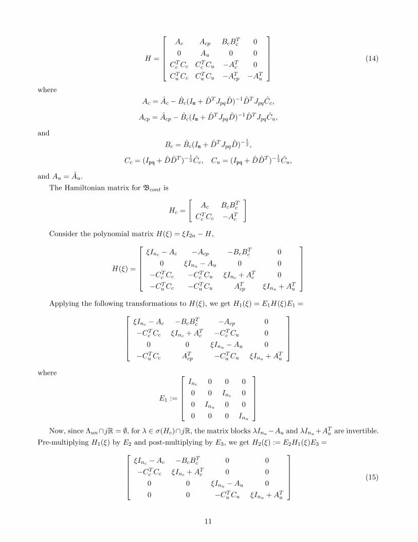
H =

Ac Acp BcB

Tc 0

0 Au 0 0

CTc Cc CTc Cu −ATc 0

CTu Cc CTu Cu −ATcp −ATu

(14)

where

Ac = Ac − Bc(Im + DTJpqD)−1DTJpqCc,

Acp = Acp − Bc(Im + DTJpqD)−1DTJpqCu,

and

Bc = Bc(Im + DTJpqD)−12 ,

Cc = (Ipq + DDT )−12 Cc, Cu = (Ipq + DDT )−

12 Cu,

and Au = Au.

The Hamiltonian matrix for Bcont is

Hc =

[Ac BcB

Tc

CTc Cc −ATc

]

Consider the polynomial matrix H(ξ) = ξI2n −H,

H(ξ) =

ξInc −Ac −Acp −BcBT

c 0

0 ξInu −Au 0 0

−CTc Cc −CTc Cu ξInc +ATc 0

−CTu Cc −CTu Cu ATcp ξInu +ATu

Applying the following transformations to H(ξ), we get H1(ξ) = E1H(ξ)E1 =

ξInc −Ac −BcBTc −Acp 0

−CTc Cc ξInc +ATc −CTc Cu 0

0 0 ξInu −Au 0

−CTu Cc ATcp −CTu Cu ξInu +ATu

where

E1 :=

Inc 0 0 0

0 0 Inc 0

0 Inu 0 0

0 0 0 Inu

Now, since Λun∩jR = ∅, for λ ∈ σ(Hc)∩jR, the matrix blocks λInu−Au and λInu +ATu are invertible.

Pre-multiplying H1(ξ) by E2 and post-multiplying by E3, we get H2(ξ) := E2H1(ξ)E3 =ξInc −Ac −BcBT

c 0 0

−CTc Cc ξInc +ATc 0 0

0 0 ξInu −Au 0

0 0 −CTu Cu ξInu +ATu

(15)

11

where

E2 :=

Inc 0 −T3T

−11 0

0 Inc −T4T−11 0

0 0 Inu 0

0 0 0 Inu

,and

E3 :=

Inc 0 0 0

0 Inc 0 0

0 0 Inu 0

−T−12 T T4 T−1

2 T T3 0 Inu

and T1 := λInu −Au, T2 := λInu +ATu , T3 := −Acp and T4 := −CTc Cu.

Thus

H2(ξ) = E2E1H(ξ)E1E2 =

[ξI2nc −Hc 0

0 Qu(ξ)

]where

Qu =

[T1 0

−CTu Cu T2

]Thus by using Proposition 3.10, the partial multiplicities of purely imaginary eigenvalues of H are

even. This completes the proof of Lemma 3.11.

4 Proof of the main result: Theorem 3.2

Proof : If part: Assume that the controllable part Bcont is Σ-dissipative and the assumption in the

theorem is satisfied. By Propositions 3.3 and 3.4, to prove that the behavior B is dissipative, it suffices

to show the existence of a K ∈ Cn×n such that the corresponding graph subspace is an n-dimensional,

M -invariant, P -neutral subspace. To show the existence of such a K, we use Lemma 3.9 to construct a

c-set such that the corresponding n-dimensional M -invariant, P -neutral subspace is also a graph subspace

of K. This K is the solution to the ARE and storage function for the whole behavior would then be

defined as xTKx, thus completing the proof.

As the unmixing assumption on uncontrollable modes is assumed, λ ∈ jR∩σ(H) means that λ /∈ Λun

and λ ∈ σ(Hc). As we have assumed that the controllable part is Σ-dissipative, from Lemma 3.11, the

partial multiplicities of real eigenvalues of M(:= iH) are all even. Using this fact, Lemma 3.9 can be used

to infer that there exists a unique n-dimensional M -invariant, P -neutral subspace for every c-set.

Now, it remains to show the existence of a c-set such that the corresponding n-dimensional, M -

invariant, P -neutral subspace is also a graph subspace.

We choose a c-set C such that jΛun ⊆ C and show that the corresponding n-dimensional, M -invariant,

P -neutral subspace is a graph subspace. Let L be the n-dimensional, P -neutral, M -invariant subspace of

C2n corresponding to the c-set C and suppose

L = Im

[X1

X2

](16)

12

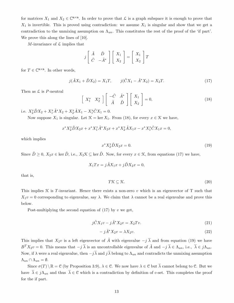
for matrices X1 and X2 ∈ Cn×n. In order to prove that L is a graph subspace it is enough to prove that

X1 is invertible. This is proved using contradiction: we assume X1 is singular and show that we get a

contradiction to the unmixing assumption on Λun. This constitutes the rest of the proof of the ‘if part’.

We prove this along the lines of [10].

M -invariance of L implies that

j

[A D

C −A∗

][X1

X2

]=

[X1

X2

]T

for T ∈ Cn×n. In other words,

j(AX1 + DX2) = X1T, j(CX1 − A∗X2) = X2T. (17)

Then as L is P -neutral [X∗1 X∗2

] [ −C A∗

A D

][X1

X2

]= 0, (18)

i.e. X∗2DX2 +X∗1 A∗X2 +X∗2 AX1 −X∗1 CX1 = 0.

Now suppose X1 is singular. Let K = kerX1. From (18), for every x ∈ K we have,

x∗X∗2DX2x+ x∗X∗1 A∗X2x+ x∗X∗2 AX1x− x∗X∗1 CX1x = 0,

which implies

x∗X∗2DX2x = 0. (19)

Since D ≥ 0, X2x ∈ ker D, i.e., X2K ⊆ ker D. Now, for every x ∈ K, from equations (17) we have,

X1Tx = jAX1x+ jDX2x = 0,

that is,

TK ⊆ K. (20)

This implies K is T -invariant. Hence there exists a non-zero v which is an eigenvector of T such that

X1v = 0 corresponding to eigenvalue, say λ. We claim that λ cannot be a real eigenvalue and prove this

below.

Post-multiplying the second equation of (17) by v we get,

jCX1v − jA∗X2v = X2Tv. (21)

− jA∗X2v = λX2v. (22)

This implies that X2v is a left eigenvector of A with eigenvalue −j λ and from equation (19) we have

BTX2v = 0. This means that −j λ is an uncontrollable eigenvalue of A and −j λ ∈ Λun, i.e., λ ∈ jΛun.

Now, if λ were a real eigenvalue, then −jλ and jλ belong to Λun and contradicts the unmixing assumption

Λun ∩ Λun = ∅.Since σ(T )\R = C (by Proposition 3.9), λ ∈ C. We now have λ ∈ C but λ cannot belong to C. But we

have λ ∈ jΛun and thus λ ∈ C which is a contradiction by definition of c-set. This completes the proof

for the if part.

13

Only if part: Assume B is Σ-dissipative. Then there exists a storage function Qψ(w) such that

d

dtQψ(w) 6 QΣ(w), ∀w ∈ B (23)

Integrating both sides for every w ∈ B ∩D, ∫RQΣ(w)dt > 0 (24)

which implies that Bcont is Σ-dissipative. This completes the proof of Theorem 3.2. �

The above proof is constructive in the sense that if a behavior B ∈ Lw satisfies the three conditions:

• uncontrollable poles are unmixed, i.e. no two of them add to zero

• the controllable part Bcont is dissipative,

• the controllable part Bcont is ‘strictly dissipative’ at infinity, i.e. (Im + DTJpqD) > 0 where D is

the feed-through term of the transfer function,

then we construct a storage function that satisfies the dissipation inequality for the whole behavior B.

Further, the storage function we construct is equal to xTKx where K is a solution to the correspond-

ing Algebraic Riccati Equation. Further, we constructed the storage function by starting with a state

representation in which the state x is observable from the manifest variable w. These facts lead to the

following important corollary.

Corollary 4.1 Let B ∈ Lw be an uncontrollable behavior whose uncontrollable poles Λun are unmixed,

i.e. Λun ∩ −Λun = ∅. Consider Σ partitioned in accordance with the input cardinality of B as

Σ =

Im 0 0

0 Iq 0

0 0 −Ip

.

Suppose Bcont, the controllable part of B, has an observable image representation, w = M( ddt)`, where

M(ξ) is partitioned as

M(ξ) =

[W1(ξ)

W2(ξ)

]; W1 ∈ Rm×m [ξ] ,W2 ∈ R(p+q)×m [ξ] .

Let G(s) := W2(s)W1(s)−1 and D := lims→∞G(s). Assume Bcont is such that (Im + DTJpqD) > 0.

Then, the following are equivalent.

1. Bcont is dissipative.

2. There exists a Ψ ∈ Rw×w[ζ, η] such that QΨ(w) is a storage function, i.e. ddtQψ(w) 6 wTΣw for all

w ∈ B.

3. There exists a matrix K and an observable state variable x such that ddtx

TKx 6 wTΣw for all

w ∈ B.

Statement 2 tells that the storage function can be expressed as a quadratic function of the manifest

variables w and their derivatives. Statement 3 says that the storage function is a ‘state function’, i.e. a

static function of the states, and hence storage of energy requires no more memory of past evolution of

trajectories than required for arbitrary concatenation of any two system trajectories.

14

5 Examples

In this section we discuss two examples of uncontrollable systems that are dissipative. The Riccati

equations encountered in these cases are solvable by the methods proposed in this paper; we also give

solutions to the Riccati equations.

The first example is of an uncontrollable system with uncontrollable modes satisfying the unmixing

assumption, i.e. no two of the uncontrollable poles add to zero. However, the Hamiltonian matrix has

eigenvalues on the imaginary axis.

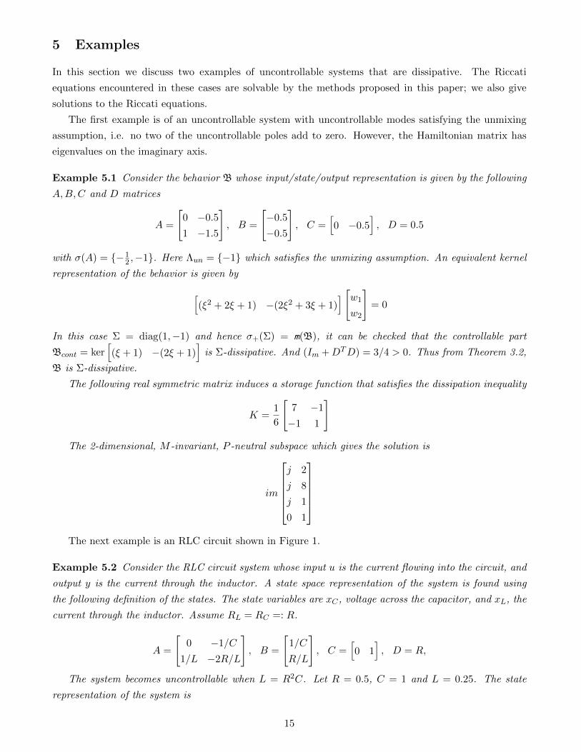
Example 5.1 Consider the behavior B whose input/state/output representation is given by the following

A,B,C and D matrices

A =

[0 −0.5

1 −1.5

], B =

[−0.5

−0.5

], C =

[0 −0.5

], D = 0.5

with σ(A) = {−12 ,−1}. Here Λun = {−1} which satisfies the unmixing assumption. An equivalent kernel

representation of the behavior is given by

[(ξ2 + 2ξ + 1) −(2ξ2 + 3ξ + 1)

] [w1

w2

]= 0

In this case Σ = diag(1,−1) and hence σ+(Σ) = m(B), it can be checked that the controllable part

Bcont = ker[(ξ + 1) −(2ξ + 1)

]is Σ-dissipative. And (Im +DTD) = 3/4 > 0. Thus from Theorem 3.2,

B is Σ-dissipative.

The following real symmetric matrix induces a storage function that satisfies the dissipation inequality

K =1

6

[7 −1

−1 1

]

The 2-dimensional, M -invariant, P -neutral subspace which gives the solution is

im

j 2

j 8

j 1

0 1

The next example is an RLC circuit shown in Figure 1.

Example 5.2 Consider the RLC circuit system whose input u is the current flowing into the circuit, and

output y is the current through the inductor. A state space representation of the system is found using

the following definition of the states. The state variables are xC , voltage across the capacitor, and xL, the

current through the inductor. Assume RL = RC =: R.

A =

[0 −1/C

1/L −2R/L

], B =

[1/C

R/L

], C =

[0 1

], D = R,

The system becomes uncontrollable when L = R2C. Let R = 0.5, C = 1 and L = 0.25. The state

representation of the system is

15

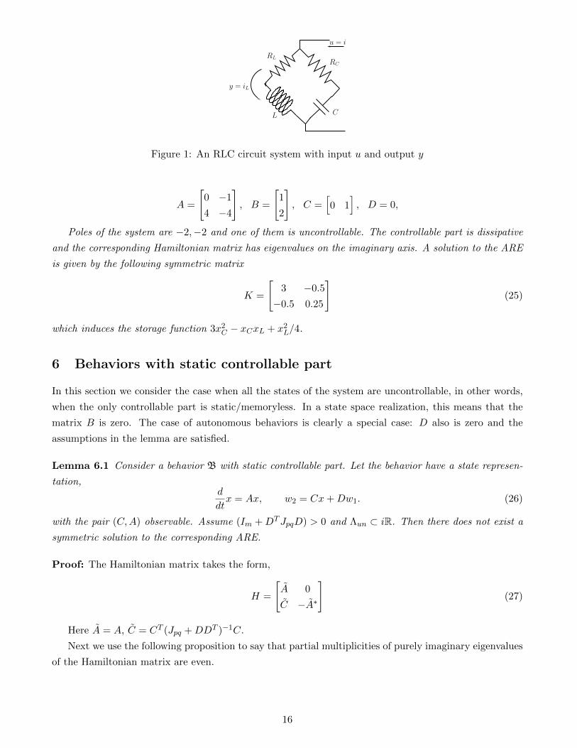
u = i

RC

CL

RL

y = iL

Figure 1: An RLC circuit system with input u and output y

A =

[0 −1

4 −4

], B =

[1

2

], C =

[0 1

], D = 0,

Poles of the system are −2,−2 and one of them is uncontrollable. The controllable part is dissipative

and the corresponding Hamiltonian matrix has eigenvalues on the imaginary axis. A solution to the ARE

is given by the following symmetric matrix

K =

[3 −0.5

−0.5 0.25

](25)

which induces the storage function 3x2C − xCxL + x2

L/4.

6 Behaviors with static controllable part

In this section we consider the case when all the states of the system are uncontrollable, in other words,

when the only controllable part is static/memoryless. In a state space realization, this means that the

matrix B is zero. The case of autonomous behaviors is clearly a special case: D also is zero and the

assumptions in the lemma are satisfied.

Lemma 6.1 Consider a behavior B with static controllable part. Let the behavior have a state represen-

tation,d

dtx = Ax, w2 = Cx+Dw1. (26)

with the pair (C,A) observable. Assume (Im +DTJpqD) > 0 and Λun ⊂ iR. Then there does not exist a

symmetric solution to the corresponding ARE.

Proof: The Hamiltonian matrix takes the form,

H =

[A 0

C −A∗

](27)

Here A = A, C = CT (Jpq +DDT )−1C.

Next we use the following proposition to say that partial multiplicities of purely imaginary eigenvalues

of the Hamiltonian matrix are even.

16

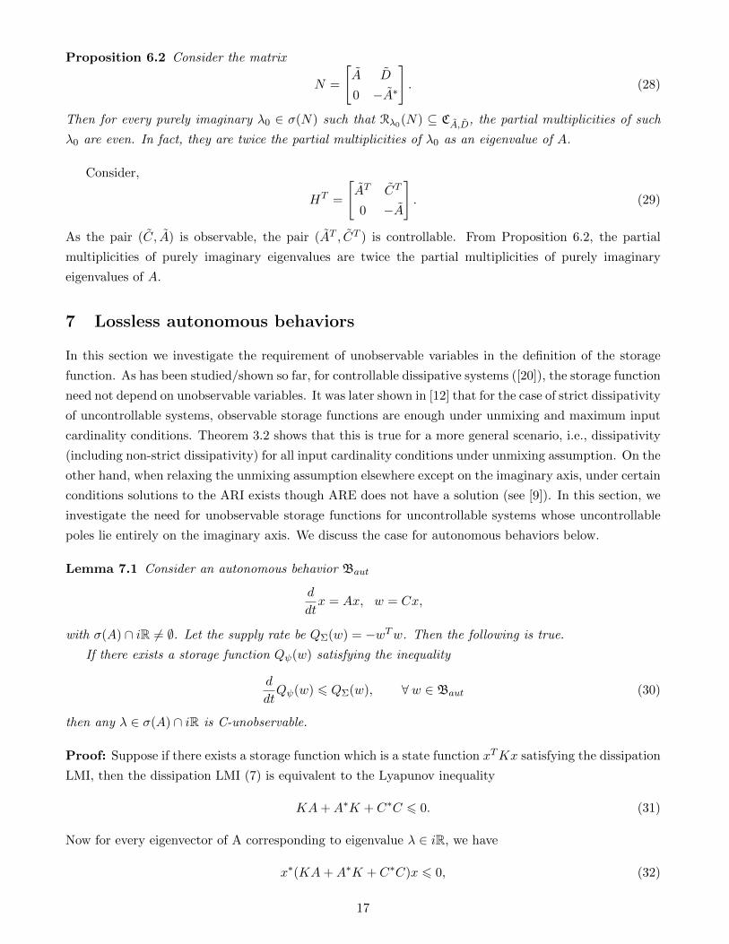
Proposition 6.2 Consider the matrix

N =

[A D

0 −A∗

]. (28)

Then for every purely imaginary λ0 ∈ σ(N) such that Rλ0(N) ⊆ CA,D, the partial multiplicities of such

λ0 are even. In fact, they are twice the partial multiplicities of λ0 as an eigenvalue of A.

Consider,

HT =

[AT CT

0 −A

]. (29)

As the pair (C, A) is observable, the pair (AT , CT ) is controllable. From Proposition 6.2, the partial

multiplicities of purely imaginary eigenvalues are twice the partial multiplicities of purely imaginary

eigenvalues of A.

7 Lossless autonomous behaviors

In this section we investigate the requirement of unobservable variables in the definition of the storage

function. As has been studied/shown so far, for controllable dissipative systems ([20]), the storage function

need not depend on unobservable variables. It was later shown in [12] that for the case of strict dissipativity

of uncontrollable systems, observable storage functions are enough under unmixing and maximum input

cardinality conditions. Theorem 3.2 shows that this is true for a more general scenario, i.e., dissipativity

(including non-strict dissipativity) for all input cardinality conditions under unmixing assumption. On the

other hand, when relaxing the unmixing assumption elsewhere except on the imaginary axis, under certain

conditions solutions to the ARI exists though ARE does not have a solution (see [9]). In this section, we

investigate the need for unobservable storage functions for uncontrollable systems whose uncontrollable

poles lie entirely on the imaginary axis. We discuss the case for autonomous behaviors below.

Lemma 7.1 Consider an autonomous behavior Baut

d

dtx = Ax, w = Cx,

with σ(A) ∩ iR 6= ∅. Let the supply rate be QΣ(w) = −wTw. Then the following is true.

If there exists a storage function Qψ(w) satisfying the inequality

d

dtQψ(w) 6 QΣ(w), ∀ w ∈ Baut (30)

then any λ ∈ σ(A) ∩ iR is C-unobservable.

Proof: Suppose if there exists a storage function which is a state function xTKx satisfying the dissipation

LMI, then the dissipation LMI (7) is equivalent to the Lyapunov inequality

KA+A∗K + C∗C 6 0. (31)

Now for every eigenvector of A corresponding to eigenvalue λ ∈ iR, we have

x∗(KA+A∗K + C∗C)x 6 0, (32)

17

which gives

λx∗Kx+ λx∗Kx+ x∗C∗Cx 6 0 (33)

or

x∗C∗Cx 6 0. (34)

But, as x∗C∗Cx ≥ 0, we have Cx = 0 for every eigenvector of A corresponding to λ ∈ σ(A) ∩ iR. This

implies that the any λ ∈ σ(A) ∩ iR is C-unobservable.

This observation tells that for dissipativity of autonomous systems having eigenvalues on the imaginary

axis, it is necessary to allow storage functions to depend on unobservable variables also.

8 Orthogonality and uncontrollable behaviors

In this section we investigate the property of orthogonality of two behaviors in the absence of controlla-

bility. We propose a definition that is intuitively expected and show that by relating this definition to

lossless uncontrollable behaviors, we encounter a situation that suggests an exploration whether dissipa-

tivity should be defined for behaviors for which the input-cardinality condition is not satisfied. We first

review a result about orthogonality of controllable behaviors.

Proposition 8.1 Let Σ ∈ Rw×w be nonsingular, and suppose B1,B2 ∈ Lwcont. The following are equiv-

alent.

1.∫Rw

T1 Σw2dt = 0 for all w1 ∈ B1 ∩D and for all w2 ∈ B2 ∩D.

2. B1 ×B2 is lossless with respect to

[0 Σ

ΣT 0

].

3. There exists a bilinear differential form LΨ, induced by Ψ ∈ Rw×w[ζ, η] such that ddtLΨ(w1, w2) =

wT1 Σw2.

Statement 1 above is taken as the definition of orthogonality between two controllable behaviors B1

and B2 in [20]. Keeping in line with Definition 3.1 for dissipativity, we could take Statement 3 above as

the definition of orthogonality for behaviors not necessarily controllable. The drawback of this approach

is elaborated later below in this section. We pursue a different direction as follows. Notice that if B1

and B2 satisfy the integral condition in Statement 1, then this integral condition is satisfied for every

respective sub-behaviors B′1 and B′2 also. Of course, restricting to compactly supported trajectories in the

integration implies only controllable parts of respectively B′1 and B′2 satisfy orthogonality. The following

definition builds on this property.

Definition 8.2 Consider a nonsingular Σ ∈ Rw×w and let B1 and B2 ∈ Lw. Behaviors B1 and B2 are

said to be Σ-orthogonal (and denoted by B1 ⊥Σ B2) if there exist Bc1 and Bc

2 ∈ Lwcont such that

• B1 ⊆ Bc1,

• B2 ⊆ Bc2, and

•∫Rw

T1 Σw2dt = 0 for all w1 ∈ Bc

1 ∩D and for all w2 ∈ Bc2 ∩D.

18

While this definition is not existential in the storage function, it is existential in Bc1 and Bc

2, raising

questions about how to check orthogonality. Note that if B is an uncontrollable behavior, then any

controllable Bc ∈ Lwcont such that B ⊆ Bc satisfies m(B) < m(Bc), and B $ Bc.

The question arises as to how much larger a controllable Bc would have to be for it to contain B.

This problem is addressed in the following subsection.

8.1 Smallest controllable superbehavior

Due to its significance for determining whether two uncontrollable behaviors are orthogonal, in this

subsection we study the following problem:

Problem 8.3 Let B1 ∈ Lw. Find B2 ∈ Lw such that

1. B2 ⊇ B1

2. B2 ∈ Lwcont i.e., a controllable behavior

3. B2 is a behavior with the smallest input cardinality satisfying Properties 1 and 2.

The following theorem answers this question.

Theorem 8.4 For B ∈ Lw, the following statements are true.

1. There exists B2 ∈ Lwcont satisfying the requirements in Problem 8.3.

2. The behavior B2 is unique if and only if B1 is controllable, and in that case B1 = B2.

3. Assume B1 is uncontrollable. The input cardinality of B2, m(B2) satisfies m(B2) > m(B1). More

precisely, m(B2) = m(B1)+k where k := maxλ∈C

rank (R1(λ))−minλ∈C

rank (R1(λ)) where R1 is a kernel

representation of B1.

Proof. (1): This is shown by constructing such a B2. Let kerR1(ξ) and kerR2(ξ) be the kernel

representations of B1 and B2 respectively where R1 ∈ Rp1×w, R2 ∈ Rp2×w and there exists an F ∈ Rp2×p1

such that FR1 = R2. Let Λun be the set of uncontrollable modes of B1. Without loss of generality, we

assume R1 to be

R1 =[S 0

](35)

where S is of the form

[I 0

0 D

]such that I ∈ R(p−k)×(p−k) is identity matrix and D ∈ Rk×k[ξ] is a

diagonal matrix with d1, d2 . . . , dk along its diagonal and satisfying the divisibility property: d1|d2, d2|d3,,

. . . and dk−1|dk, with degree of d1 at least one, and with

k = maxλ∈R

rank (R1(λ))−minλ∈R

rank (R1(λ)).

Partitioning F =[F1 F2

]conforming to the row partition of R1, we have

R2 =[F1 F2

] [ I 0 0

0 D 0

](36)

19

This simplifies to

R2 =[F1 F2D 0

](37)

Let B2 be the behaviour defined by the kernel representation of R2. For B2 to be controllable, R2(λ)

needs to have full row rank for all λ ∈ C. As F2P loses rank for λ ∈ Λun, F1 should have full row rank

for every λ ∈ C so that B2 is controllable. This proves the existence of B2 satisfying properties 1 and 2

of 8.3. In order to satisfy property 3 in Problem 8.3, i.e. m(B2) has to be the least, we have to choose a

unimodular F1 and free F2 such that B2 satisfies the three conditions. F2 can be freely chosen because

the choice of F2 does not affect the input cardinality of B2.

(2): Let B1 be controllable. Then, in the above, S = I and D does not exist. This means that F2 does

not exist. Thus the kernel representation matrix of B2 would be given by [F1 0] where F1 is unimodular.

Therefore, B2 is unique. Let B1 be uncontrollable. Then D exists and as shown above, free F2 can be

chosen. This makes the behaviour B2 non-unique.

(3): The input cardinality of B2 is given by

m(B2) = w − p2

= w − (p1 − k)

= m(B1) + k

(38)

Here, k = maxλ∈R

rank (R1(λ))−minλ∈R

rank (R1(λ)) which is determined by the size of the D matrix. �

8.2 Superbehaviors and orthogonality

We saw above in this section that orthogonality of two uncontrollable behaviors is defined by requiring

these uncontrollable behaviors to be sub-behaviors of two orthogonal controllable behaviors. Using the

result on existence of super-behaviors that are controllable, and their non-uniqueness even if the are the

smallest controllable superbehavior, we formulate the question of whether two uncontrollable behaviors

are orthogonal as a question of finding a pair of smallest controllable superbehaviors that are mutually

orthogonal. The requirement of them being smallest is motivated by the fact that orthogonality of two

controllable behaviors imposes an upper bound on their input cardinalities: this is reviewed below. For a

behavior B ∈ Lw and a nonsingular matrix Σ, the set ΣB is defined as follows

ΣB := {w ∈ C∞(R,Rw) | there exists v ∈ B such that w = Σv}.

It is straightforward that ΣB is also a behavior, its controllability is equivalent to that of B, and the

input cardinalities are equal.

Proposition 8.5 Let B1 and B2 ∈ Lwcont and suppose Σ ∈ Rw×w is nonsingular. Then, the following

are true.

1. B1 ⊥Σ B2 ⇔ B1 ⊥ (ΣB2).

2. B1 ⊥ B2 ⇒ m(B1) + m(B2) 6 w.

20

3. B1 ⊥Σ B2 ⇒ m(B1) + m(B2) 6 w.

Due to the above inequality constraint on the input-cardinalities of orthogonal controllable behaviors,

the uncontrollable behaviors too have a necessary condition to satisfy for mutual orthogonality.

Lemma 8.6 Suppose B1 and B2 ∈ Lw with at least one of them uncontrollable and let Σ ∈ Rw×w be

nonsingular. Assume B1 ⊥Σ B2. Then m(B1) + m(B2) < w.

Example 8.7 Consider the pair of ‘seemingly’ orthogonal behaviors studied in [22, page 360]. Define B1

and B2 ∈ Lw byddtx = Ax, w1 = Cx, w2 free, i.e. B2 = C∞(R,Rw)

and the supply rate wT1 w2. Thus B1 is autonomous. Consider the following non-observable latent variable

representation for B2: ddt z = −AT z + CTw2. It can be checked that the ‘storage function’ xT z satisfies

ddtx

T z = wT1 w2. Existence of such a storage function is, in fact, reasonable for a (different) definition

of orthogonality of the two behaviors B1 and B2. In fact, any autonomous behavior B1 ∈ Lw is then

‘orthogonal’ to B2 = C∞(R,Rw)! However, the ‘embeddability’ definition we have used above rules out

this example for an orthogonal pair of behaviors since the necessary condition of the above lemma is not

satisfied. In other words, there doesn’t exist a controllable behavior Bc1 such that Bc

1 contains B1 and

Bc1 ⊥Σ B2. Thus B1 and B2 are not I-orthogonal. �

9 Dissipative sub-behaviors/superbehaviors

In this section we look into the input cardinality condition for dissipative behaviors. Recall that a behavior

B ∈ Lw which is dissipative with respect to the supply rate Σ (constant, symmetric, nonsingular matrix)

satisfies the condition m(B) 6 σ+(Σ). We now look into the possibility of embedding a behavior B in a

controllable superbehavior that is Σ-dissipative, and into the drawback of using this as the definition of

dissipativity, along the lines of orthogonality defined in the previous section.

Problem 9.1 Given a nonsingular, symmetric and indefinite Σ ∈ Rw×w, find conditions for existence of

a behavior B ∈ Lw such that

• there exist B+ and B− ∈ Lwcont with B = B+ ∩B−.

• B+ is strictly Σ dissipative

• B− is strictly −Σ dissipative.

The significance of the above problem is that if a nonzero behavior B satisfying above conditions exists,

then clearly such a behavior would be both strictly Σ and strictly −Σ dissipative, raising concerns about

whether embeddability in a dissipative controllable superbehavior is a reasonable definition of dissipativity

(when dealing with uncontrollable behaviors). The following theorem states that nonzero autonomous

behaviors can indeed exist satisfying above condition.

Theorem 9.2 Let Σ ∈ Rw×w be nonsingular, symmetric and indefinite. Then there exists a nonzero

B ∈ Lw such that requirements in Problem 9.1 are satisfied. Further, any such B satisfies m(B) = 0, i.e.

B is autonomous.

21

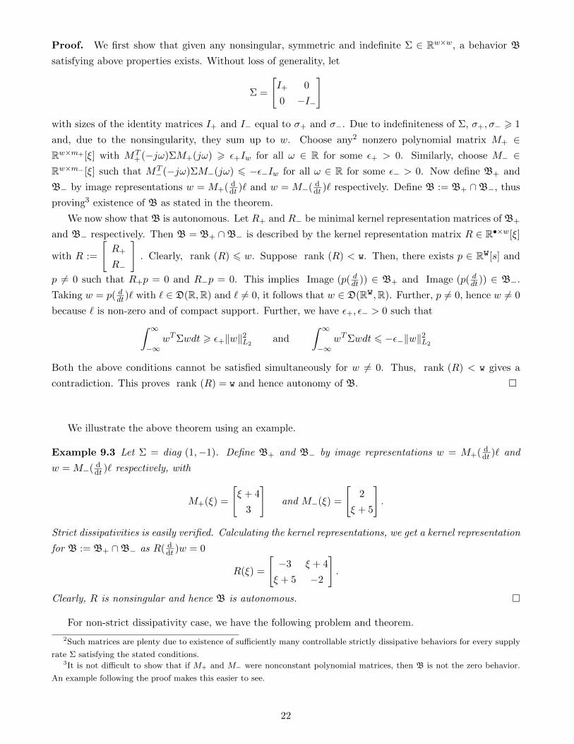
Proof. We first show that given any nonsingular, symmetric and indefinite Σ ∈ Rw×w, a behavior B

satisfying above properties exists. Without loss of generality, let

Σ =

[I+ 0

0 −I−

]

with sizes of the identity matrices I+ and I− equal to σ+ and σ−. Due to indefiniteness of Σ, σ+, σ− > 1

and, due to the nonsingularity, they sum up to w. Choose any2 nonzero polynomial matrix M+ ∈Rw×m+ [ξ] with MT

+(−jω)ΣM+(jω) > ε+Iw for all ω ∈ R for some ε+ > 0. Similarly, choose M− ∈Rw×m− [ξ] such that MT

−(−jω)ΣM−(jω) 6 −ε−Iw for all ω ∈ R for some ε− > 0. Now define B+ and

B− by image representations w = M+( ddt )` and w = M−( d

dt )` respectively. Define B := B+ ∩B−, thus

proving3 existence of B as stated in the theorem.

We now show that B is autonomous. Let R+ and R− be minimal kernel representation matrices of B+

and B− respectively. Then B = B+ ∩B− is described by the kernel representation matrix R ∈ R•×w[ξ]

with R :=

[R+

R−

]. Clearly, rank (R) 6 w. Suppose rank (R) < w. Then, there exists p ∈ Rw[s] and

p 6= 0 such that R+p = 0 and R−p = 0. This implies Image (p( ddt)) ∈ B+ and Image (p( ddt)) ∈ B−.

Taking w = p( ddt)` with ` ∈ D(R,R) and ` 6= 0, it follows that w ∈ D(Rw,R). Further, p 6= 0, hence w 6= 0

because ` is non-zero and of compact support. Further, we have ε+, ε− > 0 such that∫ ∞−∞

wTΣwdt > ε+‖w‖2L2and

∫ ∞−∞

wTΣwdt 6 −ε−‖w‖2L2

Both the above conditions cannot be satisfied simultaneously for w 6= 0. Thus, rank (R) < w gives a

contradiction. This proves rank (R) = w and hence autonomy of B. �

We illustrate the above theorem using an example.

Example 9.3 Let Σ = diag (1,−1). Define B+ and B− by image representations w = M+( ddt )` and

w = M−( ddt )` respectively, with

M+(ξ) =

[ξ + 4

3

]and M−(ξ) =

[2

ξ + 5

].

Strict dissipativities is easily verified. Calculating the kernel representations, we get a kernel representation

for B := B+ ∩B− as R( ddt )w = 0

R(ξ) =

[−3 ξ + 4

ξ + 5 −2

].

Clearly, R is nonsingular and hence B is autonomous. �

For non-strict dissipativity case, we have the following problem and theorem.

2Such matrices are plenty due to existence of sufficiently many controllable strictly dissipative behaviors for every supply

rate Σ satisfying the stated conditions.3It is not difficult to show that if M+ and M− were nonconstant polynomial matrices, then B is not the zero behavior.

An example following the proof makes this easier to see.

22

Problem 9.4 Given a nonsingular, symmetric and indefinite Σ ∈ Rw×w, find conditions for existence of

a behavior B ∈ Lw such that

• there exist B+ and B− ∈ Lwcont such that B = B+ ∩B−.

• B+ is Σ dissipative

• B− is -Σ dissipative.

Theorem 9.5 Let Σ ∈ Rw×w be nonsingular, symmetric and indefinite. Then there exists B ∈ Lw such

that requirements in Problem 9.4 are satisfied. Any such B satisfies m(B) 6 min(σ+(Σ), σ−(Σ)). In case

B is uncontrollable, m(B) < min(σ+(Σ), σ−(Σ))

If m(B) > 1, then neither B+ nor B− can be strictly dissipative.

Proof. The proof proceeds in the same way as the proof for the previous theorem, except for the

strictness of the dissipativities. Construct B+ and B− as in the previous proof, but with ε+ and ε− equal

to zero. We have∫ ∞−∞

wTΣwdt > 0 for all w ∈ B+ ∩D and

∫ ∞−∞

wTΣwdt 6 0 for all w ∈ B− ∩D

The above two equations imply∫∞−∞w

TΣwdt = 0 for all w ∈ B ∩D. Since B = B+ ∩B−, the behavior

B is dissipative with respect to both Σ and −Σ. Dissipativity with respect to Σ implies m(B) 6 σ+(Σ).

Similarly, dissipativity with respect to −Σ implies m(B) 6 σ−(Σ). This implies

m(B) 6 min(σ+, σ−) (39)

If B is uncontrollable, then from Theorem 8.4, then the two inequalities leading to the inequality (39)

are both strict. Hence, the input cardinality of B has to be strictly less than that of B+ and B−. This

implies

m(B) < min(σ+, σ−) (40)

If m(B) > 1, then from Theorem 9.2, B+ and B− cannot be strictly dissipative with respect to Σ

and −Σ respectively. This completes the proof. �

As one of the consequences of the above theorem, if the input cardinality condition is satisfied for an

uncontrollable behavior, i.e. m(B) = σ+(Σ) or m(B) = σ−(Σ), then such a behavior cannot be embedded

into both a Σ-dissipative controllable behavior and a −Σ-dissipative controllable behavior. However, an

observable storage function for such a situation exists when the controllable part is strictly dissipative

at ∞ and when the uncontrollable modes satisfy the unmixing condition (see 3.2 and [16, 12] for this

situation in presence of more assumptions), A situation when m(B) = σ+(Σ) is very familiar: we deal

with RLC circuits in the next section.

6. We use this method of defining orthogonality of two behaviors to explore further the definition of

dissipativity of a behavior. Here we bring out a fundamental significance of the so-called input-cardinality

condition: the condition that the number of inputs to the system is equal to the positive signature of the

matrix that induces the power supply. We show that when this condition is not satisfied, then a behavior

could be both supplying and absorbing net power, and is still not lossless.

23

10 RLC realizability

In this brief section we revisit a classical result: a rational transfer function matrix being positive real is a

necessary and sufficient condition for that transfer matrix to be realizable using only resistors, capacitors

and inductors (see [6] and also [4] for the case with transformers). Note that the transfer matrix captures

only the controllable part of the behavior and positive realness of the transfer matrix is nothing but

dissipativity with respect to the supply rate vT i. This is made precise below.

Consider an n-port electrical network (with each port having two terminals) and the variable w = (v, i),

where v is the vector of voltages across the n-ports and i is the vector of currents through these ports,

with the convention that vT i is the power flowing into the network. Behaviors that are dissipative with

respect to the supply rate vT i are also called4 ‘passive’. Given a controllable behavior B whose transfer

matrix G with respect to a specific input/output partition, say current i is the input and voltage v is

the output, is positive real, one can check that this behavior is passive. G in this case is the impedance

matrix and is square, i.e. the number of inputs is equal to the number of outputs. One can introduce

additional laws that the variables need to satisfy, thus resulting in a sub-behavior Bsub $ B which has

a lesser number of inputs; consider for example these additional laws as putting certain currents equal

to zero: due to opening of certain ports. However, the transfer matrix for Bsub with respect to the

input/output partition: input as currents through the non-open ports and output as the voltages across

all the ports, is clearly not square, and in fact, tall, i.e. has strictly more rows than columns. Let Gsub

denote this transfer function. Since Bsub ⊂ B, the behavior Bsub is also passive. Of course, Bsub need not

be controllable, even if B is assumed to be controllable. As an extreme case, suppose all the currents are

equal to zero, and we obtain an autonomous Bsub. While RLC realization of such transfer matrices which

are tall, and further of autonomous behaviors obtained by, for example, opening all ports, has received

hardly any attention, we remark here one very well-studied sub-behavior of every passive behavior: the

zero behavior.

Consider the single port network with v = 0 and i = 0. This port which is called a nullator (also

nullor, in some literature) behaves as both the open circuit and shorted circuit: see [2, page 75] and [8].

The significant fact about a nullator is that a nullator cannot be realized using only passive elements, and

moreover any realization (necessarily active) leads to the realization of both a nullator and its companion,

the norator; a norator is a two-terminal port that allows both the voltage across it and current through

it to be arbitrary.

11 Concluding remarks

We briefly review the main results in this paper. We first used the existence of an observable storage

function as the definition of a system’s dissipativity and proved that the dissipativities of a behavior and

its controllable part are equivalent assuming the uncontrollable poles are unmixed and the dissipativity

at infinity frequency is strict. This result’s proof involved new results in the solvability of ARE and used

indefinite linear algebra results.

We showed that for lossless autonomous dissipative systems, the storage function cannot be observable,

4It is also common to require the storage function in the context of this dissipativity to satisfy non-negativity. The

sign-definiteness of the storage function is not the focus of this paper, hence we ignore this aspect.

24

thus motivating the need for unobservable storage functions. We then studied orthogonality/lossless

behaviors in the context of using the definition of existence of a controllable dissipative superbehavior

as a definition of dissipativity. In addition to results about the smallest controllable superbehavior, we

showed necessary conditions on the number of inputs for embeddability of lossless/orthogonal behaviors

in larger controllable such behaviors.

In the context of embeddability as a definition of dissipativity, we showed that one can always find

behaviors that can be embedded in both a strictly dissipative behavior and a strictly ‘anti-dissipative’

behavior, thus raising a question on the embeddability definition. We related this question to the well-

known result that the nullator one-port circuit is not realizable using only RLC elements.

References

[1] M. Athans, The role and use of the stochastic Linear-Quadratic-Gaussian problem in control systems

design, IEEE Transactions on Automatic Control, vol. 16, pages 529-552, 1971.

[2] V. Belevitch, Classical Network Theory, Oakland, CA: Holden-Day, 1968.

[3] S. Bittanti, A. J. Laub and J. C. Willems (Eds.), The Riccati Equation, Springer-Verlag, 1991.

[4] R. Bott and R. J. Duffin, Impedance synthesis without transformers, Journal of Applied Physics, vol.

20, page 816, 1949.

[5] S. Boyd, L. E. Ghaoui, E. Feron and V. Balakrishnan, Linear Matrix Inequalities in System and

Control Theory, SIAM, Philadelphia, 1994.

[6] O. Brune, Synthesis of a finite two-terminal network whose driving-point impedance is a prescribed

function of frequency, Journal of Mathematics and Physics, vol. 10, pages 191236, 1931.

[7] M.K. Camlıbel, J. C. Willems and M. N. Belur, On the dissipativity of uncontrollable systems, in

Proceedings of the 42nd IEEE Conference on Decision and Control, Hawaii, USA, December 2003.

[8] H.J. Carlin, “Singular network elements,” IEEE Transactions on Circuit Theory, vol. 11, no. 1, pages

67-72, 1964.

[9] L. E. Faibusovich, Matrix Riccati inequality: existence of solutions, Systems & Control Letters, vol.

9, pages 59-64, January 1987.

[10] I. Gohberg, P Lancaster, and L. Rodman, Indefinite Linear Algebra and Applications, Birkhauser,

Basel, 2005.

[11] A. G. J. MacFarlane, An eigenvector solution of the optimal linear regulator problem, Journal of

Electronics and Control, vol. 14, no. 6, pages 643-654, June 1963.

[12] D. Pal and M. N. Belur. Dissipativity of uncontrollable systems, storage functions, and Lyapunov

functions, SIAM Journal on Control and Optimization, vol. 47, no. 6, pages 2930-2966, 2008.

[13] H.K. Pillai and S. Shankar, A behavioural approach to control of distributed systems, SIAM Journal

on Control and Optimization, vol. 37, pages 388408, 1998.

25

[14] J. E. Potter, Matrix quadratic solutions, SIAM Journal of Applied Mathematics, vol. 14, no. 3, pages

496-501, 1966.

[15] P. Rapisarda and J. C. Willems, State maps for linear systems, SIAM Journal on Control and

Optimization, vol. 35, no. 3, pages 1053-1091, 1997.

[16] S. Karikalan and M.N. Belur, Uncontrollable dissipative dynamical systems, in Proceedings of the

IFAC World Congress, Milan, Italy, 2011.

[17] C.W. Scherer, The Riccati Inequality and State-space H∞-optimal Control, Ph.D. thesis, University

of Wurzburg, Germany, 1990.

[18] H. L. Trentelman and J. C. Willems, Every storage function is a state function, Systems & Control

Letters, vol. 32, pages 249-259, 1997

[19] J. C. Willems, Dissipative dynamical systems - Part I: General theory, Part II: Linear systems with

quadratic supply rates, Archive for Rational Mechanics and Analysis, vol. 45, pages 321351, 352393,

1972,

[20] J. C. Willems and H. L. Trentelman, On quadratic differential forms, SIAM Journal on Control and

Optimization, vol. 36, no. 5, pages 1703-1749, 1998.

[21] J.C. Willems and H.L. Trentelman, Synthesis of dissipative systems using quadratic differential forms,

IEEE Transactions on Automatic Control, vol. 47, pages 53-69, 2002.

[22] J. C. Willems, Hidden variables in dissipative systems, in Proceedings of the 43rd IEEE Conference

on Decision and Control, Bahamas, pages 358-363, 2004.

[23] J. C. Willems, Dissipative dynamical systems, European Journal of Control, vol. 33, pages 134-151,

2007.

[24] J.C. Willems, The behavioral approach to open and interconnected systems, Control Systems Mag-

azine, vol. 27, pages 46-99, 2007.

[25] W. M. Wonham, Linear Multivariable Control: a Geometric Approach, Springer-Verlag, New York,

1979.

26