Dissipative Quantum Systems with Potential Barrier.General Theory and Parabolic BarrierJoachim Ankerhold1, Hermann Grabert1, and Gert-Ludwig Ingold21Fakult�at f�ur Physik der Albert{Ludwigs{Universit�at, Hermann-Herder-Str. 3,D-79104 Freiburg i. Br., Germany2Institut f�ur Physik, Universit�at Augsburg, Memmingerstr. 6,D-86135 Augsburg, Germany(January 20, 1995)AbstractWe study the real time dynamics of a quantum system with potential barriercoupled to a heat-bath environment. Employing the path integral approachan evolution equation for the time dependent density matrix is derived. Thetime evolution is evaluated explicitly near the barrier top in the temperatureregion where quantum e�ects become important. It is shown that there existsa quasi-stationary state with a constant ux across the potential barrier. Thisstate generalizes the Kramers ux solution of the classical Fokker-Planck equa-tion to the quantum regime. In the temperature range explored the quantum ux state depends only on the parabolic approximation of the anharmonicbarrier potential near the top. The parameter range within which the solu-tion is valid is investigated in detail. In particular, by matching the ux stateonto the equilibrium state on one side of the barrier we gain a condition onthe minimal damping strength. For very high temperatures this conditionreduces to a known result from classical rate theory. Within the speci�edparameter range the decay rate out of a metastable state is calculated fromthe ux solution. The rate is shown to coincide with the result of purelythermodynamic methods. The real time approach presented can be extendedto lower temperatures and smaller damping.PACS numbers: 05.40.+j, 82.20.DbTypeset using REVTEX1

I. INTRODUCTIONBarrier penetration phenomena in quantum systems are ubiquitous in physics and chem-istry [1]. Since the reaction coordinates describing the transition across the barrier typicallyinteract with a large number of microscopic degrees of freedom, a useful theory has to startout from a formulation of quantum mechanics which incorporates the e�ects of a heat bathenvironment. In the classical region of thermally activated barrier crossings dissipation isnaturally accounted for by the generalized Langevin equation or related methods. Follow-ing Kramers [2] transition rates can then be calculated from a nonequilibrium steady statesolution describing a constant ux across the potential barrier.Unfortunately, at present a correspondingly well-founded approach to dissipative barriertransmission processes is not available in the quantum regime. Clearly, the descriptionof dissipation within the framework of quantum theory has extensively been discussed inthe literature. For processes involving tunneling Caldeira and Leggett [3] have shown thata path integral formulation is particularly suitable. These studies and extensions thereofto �nite temperatures by Larkin and Ovchinnikov [4] and by Grabert, Weiss, and H�anggi[5] are based on a thermodynamic method for the calculation of transition rates. In thisapproach pioneered by Langer [6] one determines the free energy of an unstable system bymeans of an analytical continuation and extracts the transition rate from the imaginarypart. This technique has developed through the work of Stone [7] and Coleman and Callan[8]. A related approach based on transition state theory has been developed by Miller[9] and extended to dissipative systems by Pollak [10]. However, H�anggi and Hontscha[11] have shown explicitly that the two approaches are in fact equivalent. Analytical andnumerical results on imaginary free energy calculations for dissipative metastable systemsare summarized in an article by Grabert, Olschowski, and Weiss [12]. While the methodwas found to be very successful in explaining experimental data in well-controlled systems[13], its range of validity is not exactly known due to the lack of a �rst principle derivationof the rate formulas.In this and subsequent articles we re-examine the problem of dissipative barrier pene-tration on the basis of a dynamical theory. The general framework is provided by a pathintegral description of the time evolution of the density matrix of dissipative quantum sys-tems introduced by Feynman and Vernon [14] and extended to a wider class of useful initialconditions by Grabert, Schramm, and Ingold [15]. The theory is also presented in a recentbook by Weiss [16] and a brief outline is given in section II. Thereby we also introducethe basic notation. In the remainder of this paper we apply the theory to a system witha potential barrier the height of which is large compared to other relevant energy scales.This allows for a semiclassical evaluation of the path integrals. In sections III and IV thetime dependent semiclassical density matrix is determined explicitly in the high temperatureregion where the nonequilibrium density matrix near the barrier top is only a�ected by theharmonic part of the barrier potential. In section V we then show that the time evolutionof the density matrix allows for a nonequilibrium ux state which is essentially stationarywithin a large time domain and can be shown to be a quantum generalization of the Kramers ux solution. These high temperature results are also part of the thesis by one of us [17].In section VI we use the ux solution to derive the decay rate of a metastable state in theregion of predominantly thermally activated processes. We obtain the well-known formula2

for quantum corrections to the classical Arrhenius rate [1,12], however, supplemented bya de�nite condition for the range of damping parameters within which this result is valid.Thus, the dynamic approach presented here delineates the parameter region where a purelythermodynamic rate calculation su�ces. On the other hand, the ux solution cannot onlybe used to extract transition rates. In fact, it has already been applied to nuclear �ssion.There, the number of evaporated neutrons is related to the time the system needs to get fromthe barrier maximum to the scission point which may be derived from the ux solution [18].In subsequent papers it will be shown that the approach presented here can be extended tolower temperatures where the potential barrier is overcome primarily by tunneling processes.II. PATH INTEGRAL DESCRIPTION OF DISSIPATIVE QUANTUM SYSTEMSIn this section we introduce some key quantities and formulas for quantum Brownianmotion for later use. The notation follows the review by Grabert et al. [15] to which werefer for further details. We also introduce the barrier potential considered in subsequentsections and provide a formulation in terms of dimensionless quantities.A. Model Hamiltonian and barrier potentialWe investigate the dynamics of a system with a relevant degree of freedom that may bevisualized as the coordinate q of a Brownian particle of mass M moving in a potential �eldV (q). The stochastic motion of the particle is due to its interaction with a heat bath. Theentire system is described by the model Hamiltonian [19,3]H = H0 +HR +H0R (1)where H0 = p22M + V (q) (2)is the Hamiltonian of the undamped particle,HR = NXn=1 12 p2nmn +mn!2nx2n! (3)describes the reservoir consisting of N harmonic oscillators, andH0R = �q NXn=1 anxn + q2 NXn=1 a2n2mn!2n (4)introduces the bilinear coupling to the coordinate q of the Brownian particle. The last termin (4) compensates for the coupling induced renormalization of the potential V (q). Thenumber of the bath oscillators N is assumed to be very large. To get a proper heat bathcausing dissipation we will perform later the limitN !1 with a quasi-continuous spectrumof oscillator frequencies. 3

Speci�cally, we shall consider systems where V (q) has a barrier. In this paper we pri-marily investigate the parameter region where the barrier potential can be approximatedby an inverted harmonic oscillator potential. We shall see that at lower temperatures an-harmonicities of the potential �eld are always essential. In subsequent articles we extendthe theory to lower temperatures and investigate systems with arbitrary symmetric barrierpotentials. Assuming that the barrier top is at q = 0 and V (0) = 0, the barrier potentialhas the general form V (q) = �12M!20q2 241 � 1Xk=2 c2kk qqa!2k�235 (5)where the c2k are dimensionless coe�cients and qa is a characteristic length indicating atypical distance from the barrier top at which the anharmonic part of the potential becomesessential. In particular, we assume c4 > 0 so that the barrier potential becomes broaderthan its harmonic approximation at lower energies 1. Also, we restrict ourselves to systemswhere the potential V (q) does not depend on time.A natural quantum mechanical length scale for the system near the barrier top is givenby q0 = �h2M!0!1=2 (6)which is the variance of the coordinate in the ground state of a harmonic oscillator withoscillation frequency !0. We make the assumption that for coordinates of order q0 theharmonic approximation for the potential su�ces. This means that qa is large compared tothe width q0 and � = q0=qa (7)is a small dimensionless parameter which will serve as an expansion parameter in the sequel.B. Path integral representation and in uence functionalThe time evolution of a general initial state W0 of the entire system composed of theBrownian particle and the heat bath readsW (t) = exp(�iHt=�h)W0 exp(iHt=�h): (8)We shall assume that the state W0 is out of thermal equilibrium due to a preparationa�ecting the degrees of freedom of the Brownian particle only. Then1In fact, we may put c4 = 1 thereby �xing the length scale qa. To make the origin of terms insubsequent equations more transparent, we shall keep c4 as a parameter, however.4

W0 =Xj OjW�O0j; (9)where the operators Oj; O0j act in the Hilbert space of the particle, andW� = Z�1� exp(��H) (10)is the equilibrium density matrix of the entire system where the partition function Z� pro-vides the normalization. In an initial state of the form (9) the system and the bath arecorrelated. Hence, the customary assumption that the initial density matrix W0 factorizesinto the density matrix of the particle and the canonical density matrix of the unperturbedheat bath is avoided. Some examples of realistic preparations leading to initial conditions ofthe form (9) are speci�ed in [15]. The simplest case is an initial state which is just the equi-librium density matrix W�. Operators Oj; O0j projecting onto a certain interval in positionspace provide another example.Since we are interested in the dynamics of the particle only, the time evolution of thereduced density matrix �(t) = trRW (t) will be considered, where trR is the trace over thereservoir. To eliminate the environmental degrees of freedom it is convenient to employ thepath integral approach [20,21]. In position representation, the equilibrium density matrixreads W�(�q ; �xn; �q 0; �x0n) = Z�1� Z D�q D�xn exp��1�hSE[�q ; �xn]� (11)where the functional integral is over all paths �q (� ), �xn(� ), 0 � � � �h� with �q (0) =�q 0; �xn(0) = �x0n, and �q (�h�) = �q ; �xn(�h�) = �xn. The Euclidian action is given bySE[�q ; �xn] = SE0 [�q ] + SER[�xn] + SE0R[�q ; �xn] (12)with SE0 [�q ] = Z �h�0 d� �12M _�q 2 + V (�q )�SER[�xn] = NXn=1 Z �h�0 d� �12mn _�x2n + 12mn!2n�x2n�SE0R[�q ; �xn] = NXn=1 Z �h�0 d� �an�q �xn + �q 2 a2n2mn!2n! : (13)The position representation of the time evolution operator K(t) = exp(�iHt=�h) of theentire system is K(qf ; xnf ; t; qi; xni) = Z DqDxn exp� i�hS[q; xn]� : (14)This functional integral sums over all paths q(s); xn(s), 0 � s � t with q(0) = qi, xn(0) = xni,and q(t) = qf , xn(t) = xnf . The action readsS[q; xn] = S0[q] + SR[xn] + S0R[q; xn] (15)5

with S0[q] = Z t0 ds�12M _q2 � V (q)�SR[xn] = NXn=1 Z t0 ds�12mn _x2n � 12mn!2nx2n�S0R[q; xn] = NXn=1 Z t0 ds anqxn � q2 a2n2mn!2n! : (16)Combining the path integral representations of the three real and imaginary time propagatorsin (8) and (9), one obtains for the functional integral representation of the reduced densitymatrix �(qf ; q0f ; t)= 1Z Z dqi dq0i d�q d�q 0 �(qi; �q ; q0i; �q 0)�Z DqDq0D�q exp� i�h (S0[q]� S0[q0])� 1�hSE0 [�q ]� ~F [q; q0; �q ] (17)where the functional integral is over the set of paths q(s); q0(s); �q (� ) withq(0) = qi; q0(0) = q0i; �q (0) = �q 0q(t) = qf ; q0(t) = q0f ; �q (�h�) = �qand where~F [q; q0; �q ] =Z dxnfdxnidx0ni Z�1R Z DxnDx0n D�xn expf i�h(SR[xn] + S0R[q; xn]�SR[x0n]� S0R[q0; x0n])� 1�h (SER[�xn] + SE0R[�q ; �xn])g (18)is the so-called in uence functional, a functional integral over all closed paths xn(s), x0n(s),�xn(� ) of the environment withxn(t) = x0n(t) = xnf ; xn(0) = �xn(�h�) = xni; �xn(0) = x0n(0) = x0ni:ZR normalizes ~F so that ~F = 1 for vanishing interaction, i.e. ZR is the partition function ofthe unperturbed bath. The new normalization factor Z in (17) is given by Z = Z�=ZR. Theposition representations of the preparation operators Oj ; O0j in (9) give rise to a preparationfunction �(q; �q ; q0; �q 0) =Xj hqjOjj�q ih�q 0jO0jjq0i (19)describing the deviation of the initial state W0 from the equilibrium state W�.6

C. Dimensionless formulation and spectral densityBefore we proceed it is convenient to introduce a dimensionless formulation. In the sequelall coordinates are scaled with respect to the quantum mechanical length scale q0 introducedin (6). In particular, the scaled barrier potential then readsV (q) = �12q2 "1� 1Xk=2 c2kk �2k�2q2k�2# : (20)All frequencies are scaled with respect to the barrier frequency !0 and all times with respectto !�10 . The dimensionless imaginary time interval is denoted by� = !0 �h � (21)and the corresponding scaled imaginary time by �, 0 � � � �. Furthermore, we de�ne sumand di�erence coordinates for the real time pathsx = q � q0; r = (q + q0)=2 (22)and for later purposes also �x = �q � �q 0; �r = (�q + �q 0)=2 (23)for the imaginary time path.Finally, we introduce the dimensionless spectral density of the bath oscillatorsI(!) = �M!40 NXn=1 a2n2mn!n �(! � !n) (24)which contains all relevant information on the heat bath. With the help of the spectral den-sity sums over the environmental oscillators may be written as integrals which is convenientwhen performing the limit N !1 with a quasi-continuous spectrum of the environmentaloscillators. In this limit we get a proper heat bath causing dissipation.D. Propagating function, e�ective action, and damping kernelNow, for the harmonic oscillator model of the reservoir, which is equivalent to lineardissipation, the functional integrals occurring in the in uence functional (18) can be evalu-ated exactly. The details of the calculation were given previously [15]. As a result one �ndsthat the in uence of the heat bath is described by an e�ective action containing a nonlocaldamping kernel. The functional integral (17) gives for the dimensionless reduced densitymatrix �(xf ; rf ; t) = Z dxidrid�q d�q 0 J(xf ; rf ; t; xi; ri; �q ; �q 0) �(xi; ri; �q ; �q 0) (25)where the propagating function 7

J(xf ; rf ; t; xi; ri; �q ; �q 0) = Z�1 Z DxDrD�q exp� i2�[x; r; �q ]� (26)depending on the action �[x; r; �q ] given below is a 3-fold path integral over all pathsx(s); r(s); 0 � s � t in real time withx(0) = xi; r(0) = ri; x(t) = xf ; r(t) = rfand over all paths �q (�); 0 � � � � in imaginary time with �q (0) = �q 0, �q (�) = �q . Hence,the trajectories contributing to the propagating function are composed of two paths in realtime and one in imaginary time. An entire path connects rf with xf but is interrupted sinceri 6= �q 0 and xi 6= �q , in general. These intermediate points are connected by the function�(xi; ri; �q ; �q 0). Equation (25) determines the time evolution of the density matrix startingfrom the initial state�(xf ; rf ; 0) = Z d�q d�q 0 �(xf ; rf ; �q ; �q 0)��(�q ; �q 0); (27)where �� = trR(W�) in which W� is the scaled equilibrium density matrix (11) of the entiresystem.The e�ective action in the propagating function (26) is given by [15]�[x; r; �q ] = i Z �0 d� "12 _�q 2 + V (�q ) + 12 Z �0 d�0k(� � �0) �q (�)�q (�0)#+ Z �0 d� Z t0 dsK�(s� i�) �q (�)x(s)+ Z t0 ds [ _x _r � V (r + x=2) + V (r � x=2) � ri (s)x(s)]� Z t0 ds �Z s0 ds0 (s� s0)x(s) _r(s0)� i2 Z t0 ds0K 0(s� s0)x(s)x(s0)� : (28)Here, � denotes complex conjugation. The kernel K(s� i�) may be written asK(s� i�) = K 0(s� i�) + iK 00(s� i�): (29)The real part of K(s� i�) is given byK 0(s� i�) = 1� 1Xn=�1 gn(s) exp (i�n�) (30)with the Fourier coe�cientsgn(s) = 2 Z 10 d!� I(!) !!2 + �2n cos(!s) (31)where the �n = 2n�� (32)8

are dimensionless Matsubara frequencies scaled with !0. The imaginary part of K(s � i�)reads K 00(s� i�) = 1� 1Xn=�1 ifn(s) exp (i�n�) (33)with the Fourier coe�cientsfn(s) = 2 Z 10 d!� I(!) �n!2 + �2n sin(!s): (34)Furthermore, the so-called damping kernel (s) = 2 Z 10 d!� I(!)! cos(!s) (35)determines the imaginary part of the kernel (29) for purely real timesK 00(s) = 12 d (s)ds : (36)For purely imaginary times 0 � � � � the kernel in the Euclidian part of the e�ective action(28) is given by k(�) = �K(�i�) + (0) : �(�) := 2� 1Xn=1 �n cos (�n�) (37)where we have introduced the periodically repeated delta function: �(�) := 1Xn=�1 �(� � n�): (38)The coe�cients �n = 2 Z 10 d!� I(!)! �n!2 + �2n= j�nj (j�nj) (39)are related to the Laplace transform (z) of the damping kernel (s). The kernel k(�)satis�es Z �0 d� k(�) = 0: (40)We note that all quantities describing the e�ect of the heat bath can be expressed in termsof the spectral density I(!) de�ned in (24). 9

III. SEMICLASSICAL APPROXIMATION AND PARABOLIC BARRIERFor an anharmonic potential �eld the 3-fold path integral (26) cannot be evaluated ex-actly. In the following we study the semiclassical approximation which will be seen to su�cefor small � and coordinates near the barrier top. For high temperatures the anharmonicterms in the potential (20) give only small corrections and a simple semiclassical approxi-mation for a parabolic barrier with Gaussian uctuations is appropriate. At the beginningof this section we specify the equations of motion for the minimal action paths of the e�ec-tive action. In subsection IIIB the extremal imaginary time path for high temperatures isdetermined, and in subsection IIIC the extremal real time paths are evaluated using � as anexpansion parameter. The minimal e�ective action and the uctuations around the extremalpaths are then determined in section IV leading to the semiclassical time dependent densitymatrix for high temperatures. A. Minimal action pathsVariation of the e�ective action �[x; r; �q ] introduced in (28) with respect to �q leads tothe equation of motion for the minimal action path in imaginary times��q � Z �0 d�0 k(� � �0)�q (�0)� dV (�q )d�q = �i Z t0 dsK�(s� i�)x(s): (41)The inhomogeneity on the right hand side couples �q (�) to the real time motion. Variationof the e�ective action �[x; r; �q ] with respect to x and r leads to the equations of motion forthe minimal action paths in real time�r + dds Z s0 ds0 (s� s0)r(s0) + 12 ddr fV (r + x=2) + V (r � x=2)g =i Z t0 ds0K 0(s� s0)x(s0) + Z �0 d�K�(s� i�)�q (�): (42)and �x� dds Z ts ds0 (s0 � s)x(s0) + 2 ddx fV (r + x=2) + V (r � x=2)g = 0: (43)The above formulae (25){(28) for the density matrix and the equations of motion (41){(43) for the minimal action paths hold for any potential �eld [15]. In the following we shallconsider explicitly the barrier potential introduced in (5) and (20).B. Extremal imaginary time path for high temperaturesSince we seek a solution of (41) in the �nite time interval 0 � � � �, it is convenient toemploy the Fourier series expansion 10

�q (�) = 1� 1Xn=�1 qn exp (i�n�) : (44)This series for �q (�) continues the path outside the interval 0 � � � � as a periodic pathwith period �. The continuation causes jump singularities in �q (�) and _�q (�) at the endpointswhich must be taken into account when calculating time derivatives of �q (�). In the followingwe shall show selfconsistently that for endpoints �q ; �q 0 of the imaginary time path �q (�) andendpoints xi, xf of the real time path x(s) that are of order 1 or smaller, the qn are of order1 or smaller for high temperatures. Then, the potential (20) may be approximated byV (�q ) = �12 �q 2 +O(�2): (45)Inserting (44) into (41) yields the Fourier representation of the equation of motion(�2n + �n � 1) qn = i�n�x� b+ ifn[x(s)] + ign[x(s)]: (46)The �rst term on the right hand side, i�n�x, corresponds to a : �(�) : singularity of �q (�)according to �q (0�)� �q (0+) = �x. The coe�cient b is related to a :�(�): singularity of _�q (�)b = _�q (0+)� _�q (0�) = _�q (0+)� _�q (��): (47)The functionals fn[x(s)] = Z t0 ds fn(s)x(s) (48)and gn[x(s)] = Z t0 ds gn(s)x(s) (49)describe the coupling to the real time motion. The solution of (46) readsqn = un (i�n �x� b+ ifn[x(s)] + ign[x(s)]) (50)with the abbreviationun = 1=(�2n + �n � 1) = 1=(�2n + j�nj (j�nj)� 1): (51)The coe�cient b must be determined such that the path �q (�) satis�es the boundary condi-tions �q (0+) = �q 0, �q (��) = �q . Due to the discontinuities of the periodically continued pathat the endpoints, care must be taken in performing the limit �! 0. From (50) and (51) weobtain �q (�) = �1� 1Xn=�10 �xi�n exp(i�n�) + 1� 1Xn=�10 �xi�n un(�n � 1) exp(i�n�)� 1� 1Xn=�1 un(b� ifn[x(s)]� ign[x(s)]) exp(i�n�) (52)11

where the prime denotes the sum over all elements except n = 0. The �rst sum gives in thelimit �! 0� lim�!0� 1� 1Xn=�10 �xi�n exp(i�n�) = � �x2 : (53)The second sum in (52) is regular in the limit � ! 0 and vanishes. The third sum is alsoregular and one obtainslim�!0� �q (�) = �b� + i� 1Xn=�1 un gn[x(s)]� �x2 (54)where � = 1� 1Xn=�1 un = �1� + 2� 1Xn=1 un ; (55)and where the relations g�n(s) = gn(s) and f�n(s) = �fn(s) have been used with gn(s),fn(s) given in (31) and (34). We note that for a harmonic oscillator � is related to thevariance of position [15]. For a parabolic barrier, however, � has no obvious physical meaningsince � < 0 for high temperatures. Taking into account the boundary conditions for theperiodically continued path �q (�), we obtain from (54)b = � 1� �r � i� 1Xn=�1 un gn[x(s)]! (56)with �r de�ned in (23). Finally, using (50) and (56), the Fourier coe�cients qn of the imagi-nary time trajectory readqn = un "i�n�x+ ifn[x(s)] + ign[x(s)] + �r� � i�� 1Xm=�1 um gm[x(s)]# (57)which determine the minimal action path �q (�) as a function of the endpoints for high enoughtemperatures. This result depends on the as yet undetermined real time path x(s). Belowwe shall show that x(s) remains of order 1 for all 0 � s � t. Thus, (57) con�rms ourassumption made at the beginning of this subsection that for endcoordinates at most oforder 1 the path �q (�) always remains in the vicinity of the top and is also at most of order1. When the temperature is lowered, i.e. the dimensionless inverse temperature � is in-creased, j�j becomes smaller and vanishes for the �rst time at a critical inverse temperature�c �(�c) = �1� + 2� 1Xn=1 un������=�c = 0: (58)For vanishing damping one has � = �12 cot(�=2) and therefore �c = �, i.e. Tc = �h!0=�kBin dimensional units. As a consequence of (58) the Fourier coe�cients qn in (57) diverge12

for a purely harmonic barrier when �c is approached. This divergence corresponds to theproblem of caustics for a harmonic oscillator [21,22]. Since the harmonic potential is alwaysan approximation, anharmonic terms of the barrier potential must be taken into account fortemperatures near Tc even for coordinates near the barrier top. Hence, the analysis presentedso far is limited to temperatures above the critical temperature Tc. In an earlier work [22]we have investigated the equilibrium density matrix near the top of a weakly anharmonicpotential barrier for vanishing damping down to temperatures slightly below Tc. In thedynamical case with damping the imaginary time part of the propagating function can becalculated in a similiar way [23]. C. Real time pathsLet us �rst consider the equation of motion (42) for the real time path r(s). The inho-mogeneity readsi Z t0 ds0K 0(s� s0)x(s0) + Z �0 d�K�(s� i�)�q (�) = i Z t0 ds0R(s; s0)x(s0) + F (s): (59)Here, we have inserted the result (52) for �q (�) and made use of (57) to obtain the righthand side whereR(s; s0) = K 0(s� s0) + 1� 1Xn=�1 un [gn(s)gn(s0)� fn(s)fn(s0)] (60)and F (s) = 1��rC1(s)� i�xC2(s)� i�C1(s) Z t0 ds0C1(s0)x(s0) (61)with C1(s) = 1� 1Xn=�1 un gn(s)C2(s) = 1� 1Xn=�1 �n un fn(s): (62)In the following we will show that for coordinates �x, �r of the imaginary time path �q (�)and endpoints xi, xf of the real time path x(s) that are at most of order 1, the real timepath r(s) remains for high temperatures also inside this region provided the endpoints ri, rfare also at most of order 1. Anharmonic terms in (42) can then be neglected and we have12 ddr fV (r + x=2) + V (r � x=2)g = �r +O(�2): (63)Hence, the solution for r(s) is straightforward. It has been shown elsewhere [15] that for aharmonic potential it su�ces to solve the equation of motion for r(s) only for the real part.With r(s) = r0(s) + ir00(s) we have from (42)13

�r0 + dds Z s0 ds0 (s� s0)r0(s0)� r0 = F 0 (64)where F 0 denotes the real part of F given in (61). We introduce the propagator G+(s) ofthe homogeneous equation with the initial conditions G+(0) = 0, _G+(0) = 1 which has theLaplace transform G+(z) = �z2 + z (z)� 1��1 : (65)The solution of (64) is then obtained asr0(s) = rfG+(s)G+(t) + ri " _G+(s)� G+(s)G+(t) _G+(t)#� Z s0 ds0G+(s� s0)F 0(s0)� G+(s)G+(t) Z t0 ds0G+(t� s0)F 0(s0): (66)Hence, for endpoints of order 1 or smaller the real time path r(s) is also of order 1 or smallerfor 0 � s � t and high temperatures as assumed above. When the inverse temperatureis increased F 0(s) = �rC1(s)=� grows and diverges at � = �c due to the vanishing of �.Therefore, the solution (66) becomes invalid and anharmonicities in the equation of motion(42) commence to be important for temperatures near Tc.The equation of motion for x(s) is homogeneous and can be shown to be the backwardequation of the equation of motion for r(s) for vanishing inhomogeneity [15]. Correspond-ingly, the solution of (43) readsx(s) = xi G+(t� s)G+(t) + xf _G+(t� s)� G+(t� s)G+(t) _G+(t)! : (67)This con�rms that for endpoints xi, xf of order 1 or smaller x(s) is at most of order 1 asassumed above. Nonlinear terms in the equation of motion (43) are at most of order �2 andcan be neglected. IV. SEMICLASSICAL DENSITY MATRIXHaving evaluated the minimal action paths, we may determine the density matrix in thesemiclassical approximation by expanding the functional integral about the minimal actionpaths. In subsection IVA we �rst calculate the minimal e�ective action and in subsectionIVB we determine the contribution of the uctuations about the minimal action paths. Itwill be seen that above Tc a simple Gaussian approximation for the path integral over the uctuations about the real time and imaginary time paths su�ces.A. Minimal e�ective actionInserting the minimal action path in imaginary time (52) and (57) as well as the mini-mal action paths in real time (66) and (67) into the e�ective action (28), one gains after a14

straightforward but tedious calculation for the minimal e�ective action for inverse temper-atures below �c the result�(xf ; rf ; t; xi; ri; �x; �r) = ��(�x; �r) + �t(xf ; rf ; t; xi; ri; �x; �r): (68)Here, ��(�x; �r) = i �r22� + i2 �x2 (69)is the well-known minimal imaginary-time action of a damped inverted harmonic oscillatorwhere = 1� 1Xn=�1 un (j�nj (j�nj)� 1) : (70)We note that for a harmonic oscillator corresponds to the variance of the momentumwhile for a barrier there is no obvious physical meaning as it is the case with �.Since the time dependence of the minimal action paths in real time is determined essen-tially by the dynamics at a parabolic barrier, it is advantageous to introduce the functionsA(t) = �12 �(t)G+(t) (71)where �(t) denotes the step function andS(t) = � _G+(t) +G+(t)C+1 (t) (72)with C+1 (t) = Z t0 dsC1(s) G+(t� s)G+(t) (73)through which �t(xf ; rf ; t; xi; ri; �x; �r) can be expressed conveniently. We note, that for aharmonic oscillator A(t) is the imaginary part and S(t) the real part of the time dependentposition autocorrelation function [15]. With (71) and (72) one has�t(xf ; rf ; t; xi; ri; �x; �r) =(xfrf + xiri) _A(t)A(t) + xirf 12A(t) � 2xfri �A(t)� _A(t)2A(t) !+�r xi � _A(t)A(t) � S2�A(t)!+ �r xf "2 �A(t)� _A(t)2A(t) !+ _S� � S� _A(t)A(t)#+i�xxi � + _S2A(t)!� i�xxf �S(t)� _A(t)A(t) _S(t)!+ i2x2i "� _SA(t) + �4A(t)2 1� S(t)2�2 !#+ixixf " �S(t)� _A(t)A(t) _S(t)� �2A(t)2 ( _A(t) S(t)2�2 � 1!�A(t)S(t) _S(t)�2 )#+ i2x2f 24 + � _A(t)2A(t)2 � 1� _S(t)� _A(t)A(t)S(t)!235 : (74)15

B. Quantum FluctuationsWith the minimal actions (69) and (74) we have found the leading order term of thepath integral for the propagating function (26). The path integral now reduces to integralsover periodic paths �(0) = �(t) = 0 and �0(0) = �0(t) = 0 in real time and y(0) = y(�) = 0in imaginary time describing the quantum uctuations around the minimal action paths.Firstly, let us consider the real time uctuations. The contribution of the quantum uctuations around the extremal real time paths can be evaluated in the simple semiclassicalapproximation taking into account Gaussian uctuations. In the corresponding second ordervariational operator the anharmonicities of the barrier potential are at most of order �2 andcan therefore be neglected. The linear coupling term with the imaginary time path leads onlyto a shift of the real time uctuations. The second order variational operator is then simplygiven by that of an inverted harmonic oscillator. Using the propagator A(t) introduced in(65), the contribution of the Gaussian uctuations around each of the two real time pathsq(s) and q0(s) reads [15]ZD� exp� i4 Z t0ds�(s)���(s) + Z s0 du (s� u) _�(u)� �(s)�� = 1q8�jA(t)j: (75)For high temperatures for which the harmonic approximation for the potential su�ces,the contribution of the quantum uctuations to the imaginary time path integral can alsobe approximated by the simple semiclassical approximation. Anharmonicities in the secondorder variational operator can then be neglected. Expanding the quantum uctuations intoa Fourier series y(�) = 1� 1Xn=�1 yn exp(i�n�) (76)and taking into account the boundary conditions y(0) = y(�) = 0, one obtains the well-known result [15]ZDy exp��14 Z �0 d�y(�)���y(�) + Z �0 d�0 k(� � �0) y(�0)� y(�)�� =1p�� 1p4��2 1Yn=1 �2n un: (77)When the inverse temperature is increased, the simple semiclassical approximation (77)for the imaginary time path integral diverges for inverse temperatures near �c (� ! 0).This corresponds to the problem of caustics in a harmonic oscillator potential as alreadydiscussed in subsection IIIB. In the harmonic approximation the amplitude of the uctu-ation mode with eigenvalue � of the second order variational operator becomes arbitrarilylarge for temperatures near Tc. As a consequence, the Gaussian approximation breaks downnear Tc and anharmonic terms of the barrier potential must be taken into account for thetemperature region near and below Tc. For vanishing damping we have investigated this indetail in [22]. For nonvanishing damping the corresponding analysis is performed in [23].Combining (69) and (77), the semiclassical equilibrium density matrix for inverse tem-peratures below �c may be written as 16

��(�x; �r) = 1Z 1p�� 1p4��2 1Yn=1 �2n un! exp� i2��(�x; �r)� : (78)Here, Z is a normalization constant and the minimal imaginary time action ��(�x; �r) is givenby (69).Having evaluated the e�ective action and the uctuation integral for small �, we gainthe time dependent semiclassical density matrix for small inverse temperatures up to inversetemperatures somewhat below �c. We �nd�(xf ; rf ; t) = Z dxi dri d�xd�r J(xf ; rf ; t; xi; ri; �x; �r) �(xi; ri; �x; �r) (79)with the propagating functionJ(xf ; rf ; t; xi; ri; �x; �r) =Z�1 18�jA(t)j 1p�� 1p4��2 1Yn=1 �2n un!� exp� i2��(�x; �r) + i2�t(xf ; rf ; t; xi; ri; �x; �r)� : (80)The actions ��(�x; �r) and �t(xf ; rf ; t; xi; ri; �x; �r) are given by (69) and (74), respectively.Within the semiclassical approximation the above formula (79) gives the time evolution ofthe density matrix near the top of a potential barrier starting from an initial state with adeviation from thermal equilibrium described by the preparation function �(xi; ri; �x; �r). Wenote that using the short time expansions of A(t) and S(t) (see [15]) one �nds that (79)indeed reduces to (27) for t! 0.V. STATIONARY FLUX SOLUTIONNow, we consider a system in a metastable state which may decay by crossing a potentialbarrier. We imagine that the system starts out from a potential well to the left of the barrier.Metastability means that the barrier height Vb is much larger than other relevant energyscales of the system such as kBT and �h!0, where �h!0 is the excitation energy in the well ofthe inverted potential. The dynamics of the escape process may therefore be determined viaa semiclassical calculation. In particular, we are interested here in the stationary ux overthe barrier corresponding to a time independent escape rate. Naturally, a stationary uxdoes not exist for all times when the system is prepared at t = 0 in the metastable well. Forshort times preparation e�ects are important leading to a transient behavior. For very largetimes depletion of the state near the well bottom causes a ux decreasing in time. A plateauregion with a quasi-stationary ux over the barrier exists only for intermediate times. Weshall see that for high enough temperatures the ux state depends only on local propertiesof the barrier potential near the barrier top. The time evolution of an initial state in themetastable potential can then be calculated with the propagating function in (79). This willbe done in this section. Firstly, in VA we introduce the inital preparation. Then, in VBwe determine the stationary ux solution for high temperatures from the dynamics of thecorresponding nonequilibrium state. 17

A. Initial PreparationThe initial nonequilibrium state at time t = 0 is described by the preparation function�(xi; ri; �x; �r) = �(xi � �x)�(ri � �r)�(�ri) (81)so that the initial state is a thermal equilibrium state restricted to the left side of the barrieronly. Then, according to (79), the dynamics is given by�(xf ; rf ; t) = Z dxi dri J(xf ; rf ; t; xi; ri; xi; ri) �(�ri): (82)To determine a stationary ux solution we seek for an approximately time independentstate for intermediate times. As already mentioned, the real time dynamics near the barriertop is essentially given in terms of the functions A(t) and S(t) introduced in (71) and(72). Evaluating these functions for times larger than 1=!R one gets to leading order anexponential growth according toA(t) = �12 12!R + (!R) + !R 0(!R) exp(!Rt) (83)and S(t) = �12 cot(!R�2 ) 12!R + (!R) + !R 0(!R) exp(!Rt): (84)These functions describe the unbounded motion at the parabolic barrier. Here, 0(z) denotesthe derivative of (z), and !R is the Grote-Hynes frequency [24] given by the positive solutionof !2R + !R (!R) = 1. The corrections to (83) and (84) are exponentially decaying in time(see [15] for details). In the sequel we consider large times with !Rt � 1 so that theasymptotic behavior (83), (84) holds. We note that then terms in the e�ective action (74)like �A(t)� _A(t)2=A(t) are exponentially small. For !Rt� 1 and �r = ri, �x = xi (74) simpli�esto read ~�t(xf ; rf ; t; xi; ri) = �t(xf ; rf ; t; xi; ri; xi; ri) =(xfrf + xiri) _A(t)A(t) + xirf 12A(t) � ri xi _A(t)A(t) + S(t)2�A(t)!+ i2x2i "� + �4A(t)2 1 � S(t)2�2 !#+ ixixf � _A(t)2A(t)2 + i2x2f + � _A(t)2A(t)2! (85)where we have kept all terms with xi=A(t) since the relevant values of xi will be seen tobecome of order A(t).Hence, the density matrix (82) for times !Rt� 1 may be written as�(xf ; rf ; t) = Z dxi dri ~J(xf ; rf ; t; xi; ri) �(�ri) (86)18

where~J(xf ; rf ; t; xi; ri)=J(xf ; rf ; t; xi; ri; xi; ri) =1Z 18�jA(t)j 1p�� 1p4��2 1Yn=1 �2n un! exp� i2 ~�(xf ; rf ; t; xi; ri)� (87)in which ~�(xf ; rf ; t; xi; ri) = ��(xi; ri) + ~�t(xf ; rf ; t; xi; ri): (88)The two parts of this action are de�ned in (69) and (85).B. Stationary ux solution for high temperaturesWe shall see that for high temperatures anharmonicities of the barrier potential arenot relevant for the ux state. Since then the e�ective action is a bilinear function of thecoordinates, the integrals in (86) are Gaussian and can be evaluated exactly.The extremum of the e�ective action (88) with respect to xi and ri lies atx0i = �2 _A(t)xf + 2iA(t)rf�r0i = i _S(t)xf + S(t)rf� : (89)Introducing the shifted coordinates xi = xi � x0iri = ri � r0i ; (90)the action may be written as~�(xf ; rf ; t; xi; ri) = ~�(xf ; rf ; t; x0i ; r0i ) + �(xi; ri; t): (91)The �rst term is in fact independent of t and coincides with the imaginary time action ofthe equilibrium density matrix, i.e.~�(xf ; rf ; t; x0i ; r0i ) = ��(xf ; rf ) (92)where ��(xf ; rf ) was introduced in (69). For the time dependent second term in (91) oneobtains �(xi; ri; t) = i2� "r2i + iS(t)A(t) rixi � S(t)2 � �24A(t)2 x2i# : (93)With (92) and (93) the time dependent density matrix (82) may now be written as�(xf ; rf ; t) = ��(xf ; rf ) g(xf ; rf ; t) (94)19

where ��(xf ; rf) = 1Z 1p�� 1p4��2 1Yn=1 �2n un! exp� i2��(xf ; rf)� (95)is the equilibrium density matrix (78) for temperatures well above Tc, andg(xf ; rf ; t) = 18�jA(t)j Z dxi dri�(�ri � r0i ) exp� i2�(xi; ri; t)� (96)is a \form factor" describing deviations from equilibrium.To evaluate (96) we �rst perform the Gaussian integral over the xi-coordinate. Complet-ing the square one �ndsg(xf ; rf ; t) = 1p4�vuut j�jS(t)2 � �2 Z dri�(�ri � r0i ) exp 14 �S(t)2 � �2 r2i! : (97)With the transformation ri = S(t)� z � i _S(t)xf (98)the form factor readsg(xf ; rf ; t) = 1q4�j�j vuut S(t)2S(t)2 � �2� Z dz exp8<: 14� S(t)2S(t)2 � �2 z � i� _S(t)S(t)xf!29=; � �S(t)� [z + rf ]! : (99)>From (84) we see that for !R� < � one has S(t) < 0. Now, since � < 0, the � function isnonvanishing only if z < �rf : (100)Furthermore, for large times we have _S(t)=S(t) = !R and S(t)2=(S(t)2��2) = 1 apart fromexponentially small corrections. Thus, for !Rt� 1 the form factor becomes independent oftime and reduces togfl(xf ; rf ) = 1q4�j�j Z �rf�1 dz exp� 14� (z � i�!Rxf )2� : (101)This combines with (94) to yield the stationary ux solution�fl(xf ; rf ) = ��(xf ; rf) 1q4�j�j Z u�1dz exp � z24j�j! (102)20

where u = �rf + ij�j!R xf : (103)To illustrate the result (102) the diagonal part gfl(0; q) of the form factor (101) is shownin Fig. 1 as a function of the scaled coordinate q for ohmic damping with = 3 and threedi�erent values of the inverse temperature �. One sees that with increasing � the width ofthe nonequilibrium state becomes smaller due to the fact that energy uctuations of theBrownian particle decrease for lower temperatures. We note that for = 3 the function �vanishes at the critical inverse temperature �c = 5:79 : : :Finally, let us discuss the range of validity of the time independent ux solution (102).Firstly, in view of (93), the integral over the xi-coordinate in the expression (96) for theform factor is dominated by values of xi of order p�� or smaller. After performing thexi-integration, the relevant coordinate ri=S(t) in the remaining integral (97) becomes of or-der 1=p�� or smaller. For high enough temperatures xi and ri=S(t) are then of order 1 orsmaller which is consistent with the harmonic approximation. However, with increasing in-verse temperature j�j decreases and the relevant values of ri=S(t) become larger. Therefore,the harmonic approximation of the barrier potential which leads to the Gaussian integrals in(96) is valid only for high enough temperatures. We will show in [23] that anharmonicitiesof the potential barrier become essential for temperatures near the critical temperature Tcwhere the �rst caustic in the harmonic potential arises.Secondly, as mentioned above, the ux state (102) was found only for !Rt � 1. Thereis also an upper bound of time due to the fact that the ux solution was obtained bythe harmonic approximation of the potential. To estimate this upper bound we considercoordinates within the width of the diagonal part of the ux solution (102) which is of orderqj�j. Anharmonic terms of the potential (20) are negligible when �2q2 � 1, i.e. qd � qawhere qd is the dimensional coordinate. Hence, inserting the rf -dependent term of the shiftr0i in (89) for values of rf of order qj�j one gains the condition �2S(t)2=j�j � 1. Accordingto (84) for large times S(t) becomes of order (!R=2) cot(!R�=2) exp(!Rt) . Furthermore, asfar as orders of magnitudes are concerned (!R=2) cot(!R�=2) is of same order as j�j for alltemperatures well above Tc. This can be seen by estimating � from (55) in various limits.As a consequence, anharmonic terms in the potential can be neglected only if exp(!Rt) �1=�qj�j. Combining the two bounds we see that a stationary ux solution exists within theplateau region 1 � exp (!Rt) � 1�qj�j � 1�s2 tan(!R�=2)!R : (104)For very high temperatures � � 1, where j�j � 1=�, the upper bound of time reduces toexp (!Rt) � p�=� which can be written as exp (!Rt) � qaq�m!20=2 in dimensional units.For lower temperatures, where j�j is of order 1, one obtains exp (!Rt)� qa=q0 in dimensionalunits. We note that (104) holds only for inverse temperatures � < �c where j�j is �nite. Insummary the ux solution (102) is valid for high enough temperatures and times within therange (104). 21

The result (104) has a simple physical interpretation. The exact propagating functionof the nonlinear potential gives the probability amplitude to reach arbitrary coordinates(xf ; rf ) when starting from coordinates (xi; ri). Now, consider endpoints (xf ; rf ) near thebarrier top. Clearly, the main contribution to the corresponding probability amplitude thencomes from paths with energy of order of the potential energy at the barrier top. Otherpaths either have smaller energy and do not reach the barrier top or much larger energyand are therefore exponentially suppressed. However, a trajectory starting at t = 0 far awayfrom the barrier top in the anharmonic range of the potential with an energy of order of thepotential energy at the barrier top needs at least a time of order ln(qa=�qd) to reach a regionof order �qd about the barrier top. Now, in dimensional units the ux state has a width oforder �qd = q0qj�j. Hence, for times su�ciently smaller than ln(qa=�qd) = ln(1=�qj�j) theprobability to reach endpoints near the barrier top is basically determined by trajectoriesstarting also near the barrier top. The upper bound in (104) gives the timewhere trajectoriesstarting far from the barrier region contribute essentially to the nonstationary state.VI. MATCHING TO EQUILIBRIUM STATE IN THE WELL AND DECAY RATEWith (102) we have found an analytic expression for a stationary ux state of ametastable system for temperatures above Tc. The function �fl(xf ; rf ) describes the re-duced density matrix of the system for coordinates in the barrier region and for timeswithin the plateau region (104). This nonequilibrium state depends on local propertiesof the metastable potential near the barrier top only. On the other hand the metastablesystem is in thermal equilibrium near the well bottom. This means that the ux solutionmust reduce to the thermal equilibrium state for coordinates qf , q0f on the left side of thebarrier su�ciently far from the barrier top but at distances much smaller than ��1 which isthe typical distance from the barrier top to the well bottom. In this section we verify thiscondition for the high temperature nonequilibrium state (102) and use the result to derivethe decay rate of the metastable state in the well.A. Matching of ux solution to equilibrium stateFor coordinates qf , q0f to the left of the barrier the form factor (102) has to approach 1as one moves away from the barrier top. Let us investigate the region of coordinates xf , rfwhere ������1� 1q4�j�j Z u�1dz exp � z24j�j!������ <� exp(�1=��)� 1: (105)Here, u = u(xf ; rf ) is given by (103) and the exponent � is positive. In the semiclassicallimit � can be small. Now, in the halfplane rf < 0 of the xfrf -plane the condition (105)de�nes a region which may be delineated by the relationjxf j<� r2f!2R�2 � 4!2Rj�j��!1=2 : (106)22

On the other hand, the equilibrium density matrix (95) is nonvanishing essentially only forjxf j<� jrf jqj�j : (107)Now, in order that the ux solution matches to the equilibrium state within the region ofcoordinates where (95) and (96) are both valid, (106) and (107) must overlap in the xfrf -plane for su�ciently large rf < 0 but jrf j � ��1. Thereby, one has to take into accountthat due to the de�nitions of rf and xf in (22) one has jxf j � 2jrf j for qf ; q0f < 0. Forhigh temperatures this latter relation is always ful�lled by virtue of (107). Hence, from therelations (106) and (107) one obtainsj�j�2�� � 1� !2R j�j (108)where the �-dependence may be disregarded, since we may choose �� 1.The ux solution (102) describes the density matrix of the metastable system in thebarrier region only when (108) is satis�ed. This condition depends on temperature, anhar-monicity parameter, and damping. We note that in dimensionless units ��2 is the typicalbarrier height with respect to the well bottom.So far, we have written all results in terms of dimensionless quantities according to thede�nitions in subsection IIC, except for a few formulas where the change to dimensionalunits was mentioned explicitly in the text. In order to facilitate a comparison with earlierresults we shall return to dimensional units for the remainder of this section. Then , weobtain from (108) in dimensional units the conditionj�j � Vb�h!20 1� !2R j�j ! : (109)Here, according to (55) and (70) one has in dimensional units� = 1�h� 1Xn=�1 1�2n + j�nj (j�nj)� !20 (110)and = 1�h� 1Xn=�1 j�nj (j�nj)� !20�2n + j�nj (j�nj)� !20 ; (111)where !0 denotes the oscillation frequency at the barrier top, Vb the barrier height withrespect to the well bottom, and the �n = 2�n�h� (112)are the Matsubara frequencies. The dimensional Grote{Hynes frequency is determined bythe largest positive root of the equation!2R + !R (!R)� !20 = 0: (113)23

>From a physical point of view (109) de�nes the region where the in uence of the heatbath on the escape dynamics is strong enough to destroy coherence on a length scale smallerthan the scale where anharmonicities becomes important. Only then are nonequilibriume�ects localized in coordinate space to the barrier region. For very high temperatures,i.e. in the classical region !0�h� � 1, one has j�j � 1=!20�h� and � 1=�h�. Then, oneobtains from (109) for Ohmic dissipation with (!) = the well-known Kramers condition[2] kBT!0=Vb � where we have used 1 � !2R=!20 � =!0 for small damping. When thetemperature is lowered j�j decreases and the range of damping where the ux solution (102)is valid becomes larger.To make the condition (109) more explicit, especially for lower temperatures, one has tospecify the damping mechanism. As an example we consider a Drude model with (t) = !D exp(�!Dt). Clearly, in the limit !D � !0; the Drude model behaves like an Ohmicmodel except for very short times of order 1=!D. The Laplace transform of (t) then reads (z) = !D!D + z : (114)Since the condition (109) is relevant only for small damping strength, it su�ces to evaluate(109) in leading order in . Then, from (113) one gets!R = !0 � 2 !D!D + !0 +O( 2): (115)Expanding � given in (110) up to �rst order in yields�( ) = � 12!0 cot(!0�h�=2) + �0(0) +O( 2) (116)where �0(0) � @�@ ����� =0 = � 1�h� 1Xn=�1 j�nj!D(�2n � !20)2(!D + j�nj) : (117)Correspondingly, for we gain from (111)( ) = !02 cot(!0�h�=2) + 0(0) +O( 2) (118)where 0(0) � @@ ����� =0 = 1�h� 1Xn=�1 j�nj3!D(�2n � !20)2(!D + j�nj) : (119)Combining (115){(119) the condition (109) takes the form � !D + !0!D �h!202Vb tan(!0�h�=2) 11 + 2� tan(!0�h�=2)(!D + !0)=!D (120)where 24

� = 0(0) + !20�0(0) = 1�h� 1Xn=�1 j�nj!D(�2n � !20)(!D + j�nj) : (121)Let us discuss the relation (120) in the limit !D � !0; . For very high temperatures, i.e. inthe classical region !D�h� � 1, the last factor in (120) approaches 1 and (120) reduces to theKramers condition � !0=Vb�. For lower temperatures where !D�h� � 1, but !0�h� < �,the coe�cient � becomes large. In leading order we have [25]� = ln(!D�h�)� : (122)Hence, (120) gives � �h!202Vb tan(!0�h�=2) 11 + 2 ln(!D�h�) tan(!0�h�=2)=� : (123)Clearly, the range of where the result (102) is valid increases for lower temperatures asalready stated above. Finally, we note that the conditions (109) and (120) hold only fortemperatures above Tc where j�j is �nite.B. Decay rate of metastable stateClearly, the ux solution (102) contains all relevant informations about the nonequili-brium state. Speci�cally, the steady-state decay rate � of the metastable state is given bythe momentum expectation value in the ux state at the barrier top. In dimensional unitsone has � = 1Z 12M hp�(q) + �(q)pifl (124)where the expectation value h�ifl is calculated with respect to the dimensional stationary ux solution. Here, the normalization constant Z is determined by the matching of the uxsolution onto the thermal equilibrium state inside the well. From (124) one has in coordinaterepresentation � = JflZ = �hiM @@xf �fl(xf ; 0)!�����xf=0 : (125)Here, Jfl is the total probability ux at the barrier top q = 0. Since the essential contribu-tion to the population in the well comes from the region near the well bottom, Z can beapproximated by the partition function of a damped harmonic oscillator with frequency !wat the well bottom, i.e.Z = 1!w�h� 1Yn=1 �2n�2n + j�nj (j�nj) + !2w! exp(�Vb) : (126)Here, Vb denotes the barrier height with respect to the well bottom in dimensional units.Note that the potential was set to 0 at the barrier top. Inserting (102) for rf = 0 and (126)into (125) gives in dimensional units 25

� = !w2� !R!0 1Yn=1 �2n + j�nj (j�nj) + !2w�2n + j�nj (j�nj)� !20 ! exp(��Vb): (127)We recall that the dimensional Grote-Hynes frequency !R is given by the positive solutionof !2R+!R (!R) = !20. As is apparent from the Arrhenius exponential factor, the rate (127)describes thermally activated transitions across the barrier where the prefactor takes intoaccount quantum corrections. The above decay rate is well-known from imaginary time pathintegral methods [12] and equivalent approaches [1,11,26]. These methods consider staticproperties of the metastable state only. Here, the expression (127) was derived as a result ofa dynamical calculation. This avoids the crucial assumption of the imaginary time methodthat the imaginary part of the analytically continued free energy of the unstable system maybe interpreted as a decay rate. In this sense, we have put the result (127) on �rmer grounds.Moreover, we have obtain the condition (108) on the damping range where (127) is valid.VII. CONCLUSIONSStarting from a path integral representation of the density matrix of a dissipative quan-tum system with a potential barrier we have derived an evolution equation for the densitymatrix in the vicinity of the barrier top. This equation was shown to have a quasi-stationarynonequilibrium solution with a constant ux across the potential barrier. In this paper wehave restricted ourselves to the temperature region where the barrier is crossed primarilyby thermally activated processes. In this region the ux solution was shown to be indepen-dent of anharmonicities of the barrier potential. This nonequilibrium state generalizes thewell{known Kramers solution of the classical Fokker{Planck equation to the region wherequantum corrections are relevant.On one side of the barrier the ux solution approaches an equilibrium state as one movesaway from the barrier top. We have obtained a condition on the damping strength whichensures that the equilibrium state is reached within the range of validity of the harmonicapproximation for the barrier potential. Again this condition can be shown to be a gener-alization of a corresponding condition known from classical rate theory. The ux solutioncan then be matched to the equilibrium state in the metastable well which yields the propernormalization of the ux across the barrier. In particular, we have used the normalized ux state to determine the decay rate of the metastable state. The result was shown to beidentical with the well{known rate formula for thermally activated decay in the presence ofquantum corrections as derived by purely thermodynamic methods. The dynamical theorypresented here gives in addition a criterion for the range of damping parameters where thisresult is valid.A particularly interesting feature of the general approach advanced in this article is thefact that it can be extended both to lower temperatures and smaller damping. This will bethe subject of subsequent work. 26

ACKNOWLEDGMENTSFinancial support was provided by the Deutsche Forschungsgemeinschaft (Bonn) throughSFB237. One of us (G.-L.I.) was also supported additionally through a Heisenberg fellow-ship.

27

REFERENCES[1] P. H�anggi, P. Talkner, and M. Borkovec, Rev. Mod. Phys. 62, 251 (1990).[2] H. A. Kramers, Physica 7, 284 (1948).[3] A. O. Caldeira and A. J. Leggett, Phys. Rev. Lett. 46, 211 (1981); A. O. Caldeira andA. J. Leggett, Ann. Phys. (USA) 149, 374 (1983); 153, 445(E) (1984).[4] A. I. Larkin and Yu. N. Ovchinnikov, Pis'ma Zh. Eksp. Teor. Fiz. 37, 322 (1983) [Sov. Phys.-JETP 37 , 382 (1983)]; A. I. Larkin and Yu. N. Ovchinnikov, Zh. Eksp.Teor. Fiz. 86, 719 (1984) [ Sov. Phys.-JETP 59, 420 (1984)].[5] H. Grabert, U. Weiss, and P. H�anggi, Phys. Rev. Lett. 52, 2193 (1984); H. Grabertand U. Weiss, Phys. Rev. Lett. 53, 1787 (1984).[6] J. S. Langer, Ann. Phys. (N.Y.) 41, 108 (1967).[7] M. Stone, Phys. Lett. 67B, 186 (1977).[8] C. G. Callan and S. Coleman, Phys. Rev. D 16, 1762 (1977). S. Coleman, in: TheWhys of Subnuclear Physics, edited by A. Zichichi (Plenum, New York, 1979).[9] W. H. Miller, J. Chem. Phys. 62, 1899 (1975); W. H. Miller, Adv. Chem. Phys. 25,69 (1974).[10] E. Pollak, Phys. Rev. A 33, 4744 (1986); E. Pollak, Chem. Phys. Lett. 177, 178 (1986).[11] P. H�anggi and W. Hontscha, J. Chem. Phys. 88, 4094 (1988); P. H�anggi and W.Hontscha, Ber. Bunsenges. Phys. Chem. 95, 379 (1991).[12] H. Grabert, P. Olschowski, and U. Weiss, Phys. Rev. B 36, 1931 (1987).[13] M. H. Devoret, D. Esteve, C. Urbina, J. Martinis, A. Cleland, and J. Clarke, in: Quan-tum Tunneling in Solids, edited by Yu. Kagan and A. J. Leggett (Elsevier, New York,1992).[14] R. P. Feynman and F. L. Vernon, Ann. Phys. (N.Y.) 243, 118 (1963).[15] H. Grabert, P. Schramm, and G.-L. Ingold, Phys. Rep. 168, 115 (1988).[16] U. Weiss, Quantum Dissipative Systems (World Scienti�c, Singapore, 1993).[17] G.-L. Ingold, Ph.D. thesis (Stuttgart, 1988).[18] H. Hofmann and G.-L. Ingold, Phys. Lett. B 264, 253 (1991).[19] P. Ullersma, Physica 32, 27, 56, 74, 90 (1966).[20] R. P. Feynman and A. P. Hibbs, QuantumMechanics and Path Integrals (McGraw-Hill,New York, 1965); R. P. Feynman, Statistical Mechanics (Benjamin, New York, 1972).[21] L. S. Schulman, Techniques and Applications of Path Integrals (Wiley, New York,1981).[22] J. Ankerhold and H. Grabert, Physica A188, 568 (1992).[23] J. Ankerhold and H. Grabert, Dissipative Quantum Systems with Potential Barrier. II.Dynamics Near the Barrier Top, to be published.[24] R. F. Grote and J. T. Hynes, J. Chem. Phys. 73, 2715 (1980); P. H�anggi and F.Mojtabai, Phys. Rev. A 26, 1168 (1982).[25] H. Grabert, U. Weiss, and P. Talkner, Z. Phys. B 55, 87 (1984).[26] P. G. Wolynes, Phys. Rev. Lett. 47, 968 (1981).28

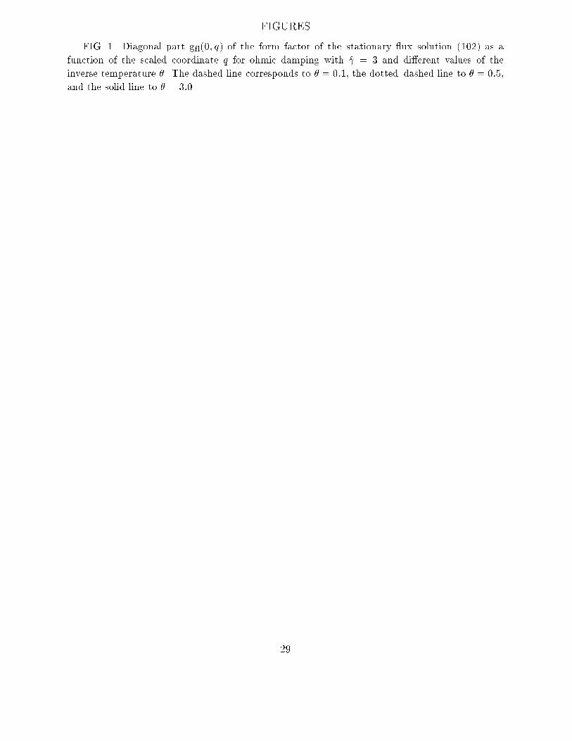
FIGURESFIG. 1. Diagonal part gfl(0; q) of the form factor of the stationary ux solution (102) as afunction of the scaled coordinate q for ohmic damping with = 3 and di�erent values of theinverse temperature �. The dashed line corresponds to � = 0:1, the dotted{dashed line to � = 0:5,and the solid line to � = 3:0.

29