IEEE TRANSACTIONS ON POWER SYSTEMS, VOL. 26, NO. 4, NOVEMBER 2011 1905

Reduced-Order Transfer Matrices From RLCNetwork Descriptor Models of Electric Power Grids

Francisco Damasceno Freitas, Senior Member, IEEE, Nelson Martins, Fellow, IEEE,Sergio Luis Varricchio, Senior Member, IEEE, Joost Rommes, and Franklin C. Véliz

Abstract—This paper compares the computational perfor-mances of four model order reduction methods applied tolarge-scale electric power RLC networks transfer functions withmany resonant peaks. Two of these methods require the state-spaceor descriptor model of the system, while the third requires onlyits frequency response data. The fourth method is proposed inthis paper, being a combination of two of the previous methods.The methods were assessed for their ability to reduce eight testsystems, either of the single-input single-output (SISO) or mul-tiple-input multiple-output (MIMO) type. The results indicatethat the reduced models obtained, of much smaller dimension,reproduce the dynamic behaviors of the original test systems overan ample range of frequencies with high accuracy.

Index Terms—Descriptor systems, dominant poles, domi-nant subspaces, eigenvalues, frequency response, index-2 DAE,large-scale systems, low rank Gramians, passivity, reduced models,resonant peaks, RLC circuits, singular systems, transfer function,vector fitting.

I. INTRODUCTION

M ODEL order reduction (MOR) has been widely used inscalar and multivariable control system applications [1],

vibration analysis of large mechanical structures, and VLSI cir-cuit design [2]. Network equivalents are used in power systemelectromagnetic transient studies [3], as well as in real-time sim-ulators [4] and harmonic distortion analysis [5]. Power systemmodels requiring detailed modeling include those having a largenumber of resonant peaks in their frequency responses, over awide range of frequencies [6]. Detailed representations of everycomponent in a large-scale system yield more accurate resultsbut require excessive CPU time, calling therefore for the furtherdevelopment of model order reduction techniques.

A good reduced-order model (ROM) should have a reducedstate-space vector and be able to reproduce the simulated input-

Manuscript received December 31, 2009; revised January 13, 2010, October05, 2010, and January 12, 2011; accepted March 02, 2011. Date of publicationMay 12, 2011; date of current version October 21, 2011. The work of F. D.Freitas was supported in part by FINATEC. Paper no. TPWRS-01021-2009.

F. D. Freitas is with the Department of Electrical Engineering, University ofBrasilia, Brasilia, DF, CEP:70910-900, Brazil (e-mail: ffreitas@ene.unb.br).

N. Martins and S. L. Varricchio are with CEPEL, Rio de Janeiro, RJ,CEP:20001-970, Brazil (e-mail: nelson@cepel.br; slv@cepel.br).

J. Rommes is with NXP Semiconductors, Central R&D, High Tech Campus46, 5656 AE Eindhoven, The Netherlands (e-mail: joost.rommes@nxp.com).

F. C. Véliz is with the Pontific Catholic University (PUC), Rio de Janeiro,RJ, Brazil (e-mail: franklin@cepel.br).

Color versions of one or more of the figures in this paper are available onlineat http://ieeexplore.ieee.org.

Digital Object Identifier 10.1109/TPWRS.2011.2136442

output response of the original system with the desired accu-racy while requiring a considerably smaller computational ef-fort. Also, the CPU time needed to generate the reduced-ordermodel should not be excessive, so that the whole ROM utiliza-tion process is cost-effective.

The main contributions of this paper are: 1) the performancesof three existing MOR methods are compared for large powersystem RLC models; 2) a combination of two methods isproposed, generating a new MOR method, which is also testedagainst the previous three methods; 3) a simple and effectivechoice for the alternating direction implicit (ADI) parametersof the low-rank Choleski factor (LRCF) method is presented,when applied to RLC circuits; 4) tests including time andfrequency responses as well as spectral (eigenvalue) plots areshown; 5) full data on a 34-bus subtransmission system frompractice, together with eight related descriptor system models,are provided in this paper and online, for data exchange in theelectromagnetic transients as well as the MOR communities.The first method is the LRCF method, described in [7] and [8].The second method is based on the computation of dominantsubspaces (Subspace Accelerated Dominant Pole Algorithmand Subspace Accelerated MIMO Dominant Pole Algorithm(SADPA [9] and SAMDP [10], respectively)). The third methodis vector fitting (VF) [11]–[13], which allows the computationof the reduced model directly from the (finely enough) dis-cretized values of the frequency response of the original system.The fourth method is a new hybrid method, which combinesthe use of the LRCF method with the VF method, yielding bothcomputational and qualitative gains, allowing transformationof nonpassive ROMs obtained by LRCF into passive ROMs.

All transmission lines considered in this paper are modeledby ladder networks, comprised of cascaded RLC PI-circuits,having fixed parameters. Representation of transmission linesby large numbers of RLC PI-circuits results in many resonantpeaks in the system’s frequency response, spread over a largefrequency range.

The formulation and studies of frequency-dependent pa-rameter transmission lines can be found in several classicalreferences [14]–[16] and selected reprints [17]. SISO modalequivalents for -domain models of power systems havinglong transmission lines with frequency-dependent parametersare described in [18]. Multi-port frequency-dependent equiv-alents, involving some approximations but given in terms ofa passive RLC circuit, which are frequently used in practicalEMTP studies, are described in [3]. The terms multi-port andMIMO are used interchangeably in this paper. The frequencydependence of longitudinal parameters is also considered in

0885-8950/$26.00 © 2011 IEEE

1906 IEEE TRANSACTIONS ON POWER SYSTEMS, VOL. 26, NO. 4, NOVEMBER 2011

[19]–[21]. In [19], the frequency dependence is taken intoaccount through the use of synthetic circuits, with a cascade ofPI-circuits for each mode of interest. In [20], rational approx-imation of frequency-dependent admittance matrices has beenproposed. A descriptor system representation is presented in[21]. The frequency responses of these detailed frequency-de-pendent line models can be matched by synthesized RLCcircuits of higher dimension and containing only fixed RLCelements. Therefore, high-fidelity transfer function models offrequency-dependent transmission lines can be described byhigh-dimension linear descriptor systems. This fact is of prac-tical importance and was the major drive for the developmentand testing of MOR techniques, by the authors, for large-scalelinear descriptor systems.

This work is organized as follows. Section II reviews thethree existing MOR methods and the proposed Hybrid method,whose performances are compared in this paper. Section IIIdescribes the test systems, while Sections IV and V presentMOR results for the single-input single-output (SISO) and mul-tiple-input multiple-output (MIMO) test systems, respectively.Section VI concludes.

II. METHODOLOGY

A. RLC Descriptor Systems of Index-2 and Their Reductionto Index-0

The MOR methods compared in this work either make inte-gral use of the descriptor formulations (generalized state-space)of the test systems or are based on the identification of reducedmodels from discretized frequency response data of the test sys-tems. These MOR methods apply to linear, time invariant sys-tems comprising differential and algebraic equations (DAEs) ofthe form

(1)

where is the generalized state vector,is the input vector and is the output vector,

, with a nonzero matrix, , , and.

The generalized state vector com-prises states and algebraic variables ,respectively. With this notation, matrices , , , and canbe written as

(2)

(3)

where , possibly singular, contains at least onenonzero element per line. In this work, we assume that issquare and nonsingular and matrix consists of blocks

, , , and ,

with . The blocks , , , , and havethe structures

Regarding the structure of , the variables in can bewritten as , where and

, with .When modeling the RLC test systems of Section III, as well

as the two-node RLC circuit of Appendix A, with the formu-lation of this paper, matrix is singular, despite beingnonsingular. This means that just part of the algebraic variables,the part, can undergo Gaussian elimination:

(4)

Since is given by (4),algebraic equations can be eliminated. The remaining alge-braic equations and the differential equations are

(5)

where the reduced matrix blocks are given by

and .In the RLC application of this paper, the last equations

in the DAE (1) do not contain any input , which implies in. Also, the network equations in the DAE are organized

such that the products and arezero, although each matrix individually is not necessarily zero(see an example of two-node circuit in Appendix A illustratinghow all matrices are formed). As a result, the matrix blocksand in (5) are both equal to zero.

Considering (5) and the characteristics of and , anindex-2 DAE system [22] can be formed, with states andremaining algebraic variables , as follows:

(6)

In (6), the block is as described in (2) andhas . The equations in (6), therefore, constitute anindex-2 DAE system having generalized states,being states and algebraic variables. If all the algebraic

FREITAS et al.: REDUCED-ORDER TRANSFER MATRICES 1907

equations in (1) could undergo Gaussian elimination, and noredundant states existed in the DAE, then the descriptor systemwould be index-1, allowing the use of the sparse low-rankCholeski factor (SLRCF) algorithm [23]. However, consideringthe index-2 nature of the original systems, and the modestnumber of algebraic equations and variables in (6), these canall be eliminated by employing a symbolic math procedure (seeAppendix C for further details) to form an index-0 (just differ-ential equations) system. This system representation permitsthe use of the LRCF method [7]. The transformation is possiblebecause states in the set of equations can be expressed as alinear combination of states (the effective states).

Appendix C describes the elimination of the algebraic equa-tions, corresponding to the block matrix . Also, the redun-dant differential equations are eliminated, which then allows theuse of LRCF [7]. Eliminations invariably lead to some matrixfill-in, which is however acceptable for the sparse RLC sys-tems being studied here, since is muchsmaller than the rank of . Symbolic math elimination of thealgebraic variables and redundant states in (6) yields the index-0descriptor system model:

(7)

where . Matrices , , , , and have ap-propriate dimensions and is now nonsingular, allowing there-fore the use of LRCF [7], [8].

Frequency response results are obtained by setting ,where is the frequency in over a discretized frequencyinterval, and evaluating

(8)

where is the transfer function matrix, whoseelements are scalar transfer functions (TF). The symbolsand denote the Laplace transforms of variables and

, respectively. As shown in [23], frequency response as wellas SADPA or SAMDP computations can be performed either onthe index-2 descriptor model or on the state-space model in (7).

B. Model Order Reduction

The problem addressed here is to approximate (1) or (7) withanother dynamical system

(9)

where with is the reduced order of the statevector, is the output, and , ,

, and are the reduced model state ma-trices.

In this section, the four methods for model order reductionare briefly described: low-rank Choleski factor (LRCF) ADI[7], [8], Subspace Accelerated Dominant Pole Algorithm(SADPA) [9]/Subspace Accelerated MIMO Dominant PoleAlgorithm (SAMDP) [10], vector fitting [11], and a Hybridmethod that combines vector fitting with LRCF.

1) Low-Rank Choleski Factor (LRCF) ADI: The LRCFmethod has a direct analogy with the conventional state-space

truncated balanced realization (TBR) method [1], beinghowever designed to operate on the sparse, large-dimensionstate-space matrices [7]. This method computes the con-trollability and observability Gramians, both of which aredecomposed into low rank Choleski factors (CF). The productof these low rank CF yields the approximate Hankel matrix,whose singular value decomposition (SVD) will determine theappropriate dimension of the reduced system for a given modelerror tolerance.

The index-2 DAE structure of the test system models doesnot allow the direct use of the SLRCF method to (1), since thismethod, as described in [23], can only be applied to modelswhere the matrix-block is nonsingular (index-1 DAEsystem).

2) Vector Fitting: The VF method identifies the scalartransfer functions from their frequency responses, once someuser-specified parameters such as model order and set of initialestimates for the poles are provided. The VF method requiresthe prior computation of the frequency response [sequenceof numerical values for the scalar transfer function (8)], forsufficiently discretized values of frequency . The levelof discretization can be varied along the frequency range ofinterest, so as to allow the identification of each scalar transferfunction to the user-specified accuracy. Therefore, the samplingrate should be higher along those frequency ranges showinglarge numbers of resonant peaks. In this paper, we use an im-plementation of VF [11] with all the improvements describedin [12] and [13].

3) SADPA and SAMDP: The SADPA method [9] is usedfor the reduction of SISO systems, and directly operates onthe formulation (1), by computing the dominant poles, associ-ated eigenvectors, and transfer function residues. The SAMDPmethod [10], of the same family of methods, is used for the re-duction of MIMO systems.

4) Hybrid Method-VF+LRCF: VF requires initial estimatesfor the poles, and convergence of VF is improved by providinga fairly accurate set of initial estimates. Hence, we propose theHybrid method: VF+LRCF, where initial pole estimates arecomputed from less accurate ROMs obtained by relaxed LRCFsolutions.

III. TEST SYSTEMS

The basic system of this paper is shown in Fig. 1 and relatesto a section of a transmission and distribution network frompractice. Its full RLC data is given in Appendix B, so resultsmay be reproduced. All transmission lines (TL) of this basicsystem were then represented by cascaded PI-circuits and nofrequency-dependent line parameters were modeled, generatingeight large descriptor system models. The performances of fourMOR methods were assessed for these eight test systems.

The DAEs of the eight test systems were built for both SISOand MIMO cases, by varying the number of PI-sections perTL, which are represented by 10 PIs (S10PI, M10PI), 20 PIs(S20PI, M20PI), 40 PIs (S40PI, M40PI), and 80 PIs (S80PI,M80PI). The dimensions of these DAEs and their spectral radii(moduli of their largest eigenvalues) are shown in Table I. Thefour SISO systems (S10PI, S20PI, S40PI, S80PI) have the elec-trical current injected into bus #21 as their input, and the mon-

1908 IEEE TRANSACTIONS ON POWER SYSTEMS, VOL. 26, NO. 4, NOVEMBER 2011

Fig. 1. One-line diagram of the electrical power system.

TABLE INAMES AND STATISTICS OF THE EIGHT TEST SYSTEMS

itored voltage at the same bus as their output. The four MIMOsystems (M10PI, M20PI, M40PI, M80PI) have the electricalcurrents simultaneously injected into buses #18, #21, and #23as their inputs, and the voltages at these same three buses astheir outputs.1

The interest here is to determine the ROMs for these test sys-tems described in Table I, which should adequately reproduce,for all practical purposes, their input-output behavior.

The complete eigensolutions (eigenvalues and associatedright/left eigenvectors) for the test systems can in principle beobtained by either the QR or QZ routines. However, due to the

complexity of these methods, where is the number ofstates, they are not applicable to large-scale systems with manythousands of states. Such large sparse systems can, however, bedealt with by the MOR methods in this paper, that exploit thestructure and sparsity of the system matrices. All results of thispaper were obtained with Matlab, its toolboxes, and M-coderoutines.

The MOR algorithms’ frequency response, time domain, andpole spectra results are compared with those obtained for theoriginal system. The results of these test systems are describedand compared in the next two sections.

The adopted definition for model error was the RMS value ofthe error difference between the frequency response values ofthe original system and that of the ROM [11]:

1The datafiles for these eight descriptor systems are available for direct down-load at: http://sites.google.com/site/rommes/software.

TABLE IIMETHODS’ PERFORMANCES FOR THE SISO TEST SYSTEMS

where is the th frequency response value of the th scalarTF of the original model; is the equivalent element of thereduced model; and are the numbers of scalar TFs andsamples for each one of these TFs, respectively.

IV. RESULTS FOR THE SISO TEST SYSTEMS

A. Vector Fitting Method

This method is widely used in practice for producing linearROMs that match the frequency response plots of the originalsystems [11]. The quality pole-residue results obtained for thefour SISO test systems described in Table I, plus its robust con-vergence fully confirmed the reputation of the method.

The results obtained for the S80PI system are described next.The simulations with the other three SISO test systems requiredsimilar procedures and the choice of system-specific initial pa-rameters: pole estimates, number of iterations, and the dimen-sion of the reduced models. As already mentioned, a systemhaving many resonant peaks in its frequency response requires alarge number of samples. Obviously, when increasing the “res-olution” of the frequency response plots, for more accurate VFresults, there is an associated rise in CPU time. The CPU time,ROM dimensions, ROM errors, and spectral radii are the fourperformance indices used in Table II for comparing the variousmethods. The numbers of DAE equations for the S10PI, S20PI,S40PI, and S80PI systems are given within brackets in this table.All systems have, by construction, the same number of algebraicequations: 119, the remainder being state variables (still con-taining some redundant states). The QR method is not includedin Table II because it is not applicable to large-scale systems ingeneral.

FREITAS et al.: REDUCED-ORDER TRANSFER MATRICES 1909

For the S80PI system, the selected frequency responserange was from 10 Hz to . The initial poleestimates were obtained by distributing the imaginary part of thepole estimates logarithmically spaced on the frequency range[11]. In our application, it is not appropriate to distribute thesepoints linearly over the frequency range since the resonant peaksare spread over several decades.

The scalar TF was represented by a sequence of 800, 1400,1800, and 1800 discrete values of complex frequency, for thetest systems: S10PI, S20PI, S40PI, and S80PI, respectively.

All SISO ROMs were assumed to be strictly propersystem models, among other constraints. As there are no deriva-tive terms in [terms of this nature would exist, if matrixin (5) was nonzero], it was assumed that such term also did notexist in the reduced model. The VF simulations were carried outusing the version 3 of the m-files available at http://www.en-ergy.sintef.no/Produkt/VECTFIT/index.asp. All pole estimateswere constrained to remain on the left half of the complex planefor the SISO systems of this section as well as the MIMO sys-tems of the following section.

The convergence of the VF method, based on a specified RMSerror tolerance, for the four SISO test systems of this paper usu-ally occurred between 7 and 17 iterations. The convergence tol-erance varied from a to a RMS error depending onthe test system. In all computations, the frequency range of in-terest was 10 Hz to 40 kHz.

The descriptor formulation for the S80PI system has 4182equation (4063) states, 119 algebraic variables; the descriptormatrix is highly sparse, with only 10 261 nonzero elements. Thereduced model, computed by VF, the S80PI VF ROM, has 394states, as shown in Table II. Accurate ROMs were obtained forthe systems S10PI, S20PI, and S40PI (of reduced order 152,206, and 297, respectively), as also shown in Table II.

B. LRCF Method

The LRCF-ADI method requires the use of ADI parame-ters [7], [24]. The computation and choice of these parametersare quite challenging for they impact the LRCF convergenceas well as the ROM quality [7], [8]. The LRCF computationswere carried out utilizing multiple ADI parameters, all of whichwere chosen to be real numbers, whose values were equal to thefrequencies of some of the dominant resonant peaks, in rad/s.These peaks can be readily determined from the visual inspec-tion of the frequency response plots of the RLC electric powernetworks.

The number of adopted LRCF iterations for the systemsS10PI, S20PI, S40PI, and S80PI were 300, 300, 450, and 600,respectively. The order of the reduced model is a function ofthe smallest Hankel singular value to be retained. Consideringthat the LRCF is an approximation of the TBR method, it isfair to expect its results to be slightly worse than those of thelatter [23]. This expectation was confirmed in most cases, sincethe obtained reduced models usually had spurious unstablepoles. These spurious poles always have TF residues that areof insignificant magnitude, which makes the task of discardingthem an easy one (one should note that theory points the TBRmethod [1] cannot be directly applied to unstable systems).

Fig. 2. Relevant spectra of S10PI and ROMs obtained by the LRCF and Hybridmethods. The actual S10PI spectrum goes up to , with most polesshowing real parts roughly equal to .

The LRCF method cannot be applied to systems that havepoles which are unstable or very close to zero. However, byusing the spectral shift , as described in [23], thisproblem is circumvented for the test systems.

The chosen ADI parameters for the test systems S10PI,S20PI, S40PI, and S80PI are the elements in vectors , ,

, and , respectively, which are all shown in the following:

where and .In summary, the ROMs were obtained by truncating the bal-

anced realization (computed using the low rank factors) so thatthe Hankel singular values with magnitudes above error toler-ance are preserved.

The LRCF computations were performed on the index-0 de-scriptor (7), derived from the index-2 DAE (1) of the test sys-tems S10PI, S20PI, S40PI, and S80PI, which have 682, 1182,2182, and 4182 variables (states and algebraic), respectively.The number of algebraic variables (119) and redundant states(35) are the same for all systems. The index-0 descriptor ma-trices (cf. (7)) are obtained through the elimination of the re-dundant states and the algebraic variables of the S10PI, S20PI,S40PI, and S80PI systems, and have 528, 1028, 2028, and 4028states, respectively.

The partial spectra of S10PI and of its 158-state ROM ob-tained by LRCF, the S10PI LRCF ROM, are shown in Fig. 2.The poles of this ROM are seen to match many of the systemeigenvalues obtained by the QR eigensolution.

Fig. 4 shows the magnitude plots of S80PI and ROMs com-puted by, amongst others, LRCF and VF, and clearly shows theirexcellent matching, both at low and high frequency ranges. TheRMS errors for both LRCF and VF were smaller than 0.001. Itis clearly seen that up to (as pointed by the arrowtip in the figure), there are some minor resonant peaks.

1910 IEEE TRANSACTIONS ON POWER SYSTEMS, VOL. 26, NO. 4, NOVEMBER 2011

Fig. 3. Relevant spectra of S10PI and ROMs obtained by the SADPA and VFmethods. The actual S10PI spectrum goes up to , with most polesshowing real parts roughly equal to .

Fig. 4. TF magnitude versus frequency of self-impedance of bus #21 for theS80PI system and ROMs, obtained by LRCF, SADPA, VF, and Hybrid methods.

C. SADPA Method

A similar set of ROMs was obtained with SADPA [9], con-sidering the descriptor system in (1). This method requires thatseveral parameters that control the iterative process be specified,but most of these parameters remained fixed for all test systemsof this paper.

The minimum and maximum dimensions of the search spaceswere 5 and 10, respectively, for all test systems. The number ofspecified poles (maximum restarts) were 80 (50), 103 (100), 150(100), and 200 (120) for the S10PI, S20PI, S40PI, and S80PI testsystems, respectively.

The option “turbo deflation” of the SADPA method [25] wasused and allowed a significant computational speed-up. Themodal dominance index was “LM” (largest residue magnitude),since practically all dominant poles are near the imaginary axis,yielding a response with numerous resonant peaks. The initialestimate was , in all runs.

The magnitude plot of the ROM produced by SADPA, theSADPA ROM, was similar to those obtained by the other twomethods; see Fig. 4. The CPU time required by SADPA washowever larger than that of the LRCF method.

Fig. 5. Time simulation plots for the S80PI system and its 394-state ROM ob-tained by the Hybrid method.

The partial spectra of the S10PI and that of its 152-statesROM obtained by SADPA are shown in Fig. 3. The poles com-puted by SADPA perfectly match 152 system eigenvalues ob-tained by the QR eigensolution of the S10PI system.

D. Hybrid Method (LRCF + VF)

This section presents the results obtained with the Hybridmethod, which combines the fast pole estimation of the LRCFwith the quality fitting of the VF, yielding reduced models thatpreserve the passivity and symmetry of the original system. Anadditional motivation for the Hybrid method is the undesirablesensitivity of the VF to poor initial pole estimates and to the dis-cretization level of the frequency response.

The LRCF initializing step for the Hybrid method used 200,206, 297, and 394 iterations, to produce the ROMs for the SISOsystems S10PI, S20PI, S40PI, and S80PI, respectively. Thenumber of iterations used in all cases was about 30% smallerthan the number required when the LRCF method is utilizedalone. Two iterations of the VF method were applied next,improving on the poles and residues, so as to produce a goodmatching between the responses of the original system and thecomputed ROM.

Figs. 2 and 3 show the partial spectra for the full S10PI systemand its 152-state ROMs obtained by Hybrid and VF methods,respectively.

The performance of the MOR methods were also assessedby the quality of the transient time responses from their ROMs.For the SISO case, a step disturbance of electrical current wasinjected into bus #21 and the voltage at this bus was monitored.An integration time step of was used in all simulationsof Section IV. The plot in Fig. 5 shows the good matching be-tween the time simulation results computed for the full systemand for its 394th-order Hybrid ROM. Similar time simulationresults (not shown due to space limitations) were obtained forthe ROMs produced by the other three methods studied in thispaper.

E. Discussion on SISO System Results

Table II shows the CPU times for the methods being com-pared, to obtain the ROMs for the SISO systems. The order of

FREITAS et al.: REDUCED-ORDER TRANSFER MATRICES 1911

these ROMs and their RMS errors are also given in this table.The LRCF method presented the lowest CPU time, regardlessthe test system analyzed. For the test system S10PI the variationin CPU time among the four methods was not significant. TheHybrid method had the second best performance, being fasterthan SADPA and VF for the three largest test systems, as can beverified in Table II.

It should be noted that despite the high number of resonantpeaks of the test systems, the ROMs do not contain much of theirhigher frequency modes, as shown in the pole spectra plots ofFigs. 2 and 3. This can also be seen by comparing the spectralradii of the ROMs obtained by the various methods (in Table II)with those of the test systems (in Table I).

V. RESULTS FOR THE MIMO TEST SYSTEMS

The four test systems considered in this section are M10PI,M20PI, M40PI, and M80PI. The input (output) variables forthese systems are the injected currents (voltages) at buses #18,#21, and #23 (cf. Fig. 1).

Again, the ROMs were produced using the four methods:LRCF, VF, Hybrid, and SAMDP (the MIMO version ofSADPA). The model errors were measured over the entirefrequency range of interest, and simultaneously considered allthe element TFs located in the upper triangular part of the 3 3transfer matrix .

A. MIMO Results Obtained by LRCF

The ADI parameters and eigenvalue shift usedfor systems M10PI, M20PI, M40PI, and M80PI were identicalto those used for the LRCF SISO systems. Systems M10PI,M20PI, and M40PI, required 300 iterations, while 400 iterationswere needed for M80PI. At every LRCF iteration, a new set ofvectors is added to the low-rank Choleski factor of the control-lability matrix [23]. The number of vectors in this set is equal tothe number of system inputs. Similarly, a set of vectors is alsoadded to the low-rank observability matrix. A large number ofinputs and outputs of a MIMO system, therefore, implies a highCPU time as well as large memory requirements for all MORmethods.

The quality of the MIMO ROMs can be assessed from theirSigma plots, a control systems denomination for the plots ofboth the maximum and minimum singular values (SV) of theirtransfer matrices as a function of frequency,and , respectively [10]. Fig. 6 presents theSigma plots for the M80PI system and its ROMs obtainedby all methods. Fig. 7 shows the absolute errors between the

for the full test system and its ROMs.Time domain simulations were computed for the M80PI

system and its LRCF ROM. These simulations involved simul-taneously injecting into buses #18, #21, and #23 the currentsignals:

Fig. 6. Sigma plots for the M80PI system and ROMs, obtained by LRCF,SAMDP, VF, and the Hybrid methods.

Fig. 7. Absolute deviations between of system M80PI andROMs, obtained by LRCF, SAMDP, VF, and Hybrid methods.

where is the step function, ,, and . Values

, , and are time delays associatedwith these input signals. The integration time step used in thenumerical simulations was .

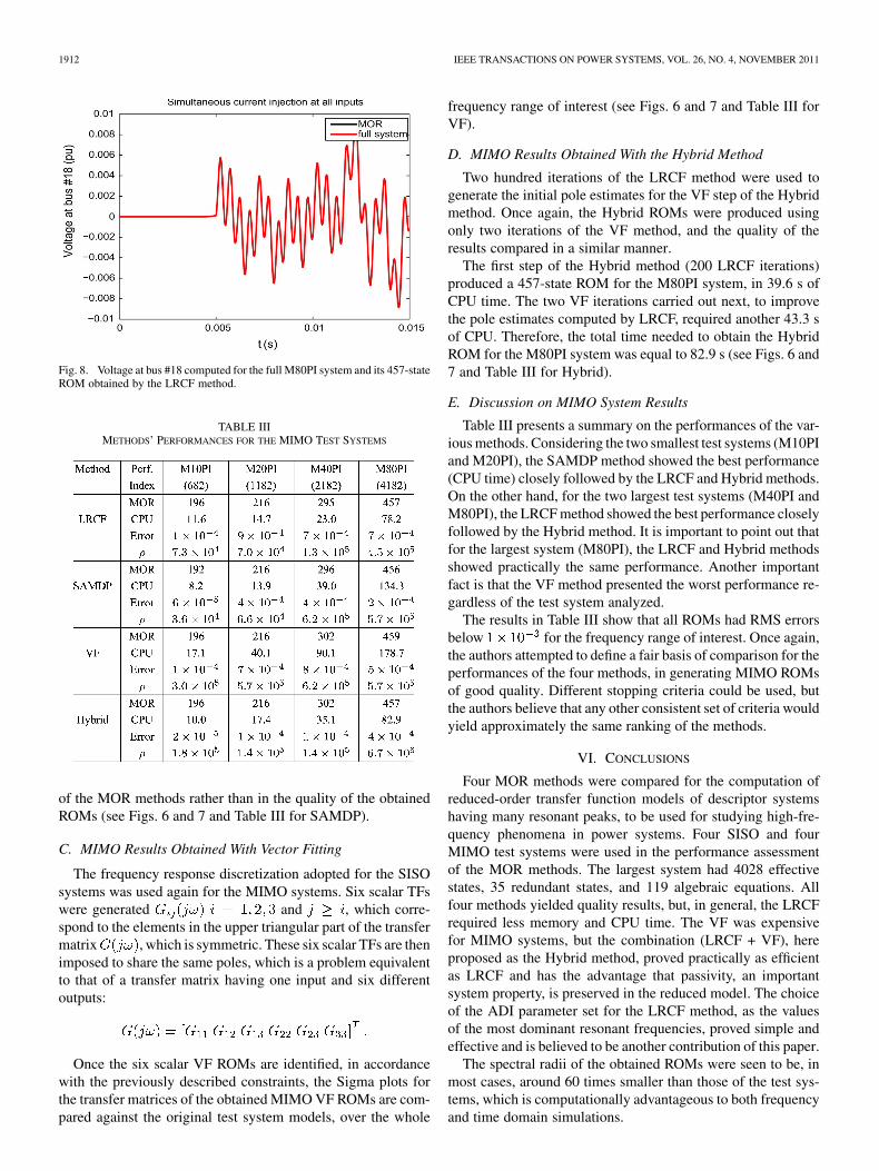
The monitored variables were the voltages at the three buses#18, #21, and #23, but only the voltage at bus #18 is shown.Fig. 8 compares the time simulation plots for the full M80PIsystem and its LRCF ROM, indicating perfect matching forpractical purposes.

B. MIMO Results Obtained With SAMDP

MOR computations similar to those described in Section V-Awere carried out with the SAMDP method. The dimensions ofthe search spaces were kept between 5 and 10 vectors. Thenumber of specified poles (maximum restarts) were 100 (50),110 (100), 150 (100), and 230 (130) for the M10PI, M20PI,M40PI, and M80PI, respectively. The “turbo deflation” optionand the modal dominance index “LM” were adopted. The initialpole estimate was for all test systems.

The computed SAMDP ROMs were of equivalent quality tothose ROMs obtained with LRCF for the MIMO test systems.The difference, once again, was in the computational speeds

1912 IEEE TRANSACTIONS ON POWER SYSTEMS, VOL. 26, NO. 4, NOVEMBER 2011

Fig. 8. Voltage at bus #18 computed for the full M80PI system and its 457-stateROM obtained by the LRCF method.

TABLE IIIMETHODS’ PERFORMANCES FOR THE MIMO TEST SYSTEMS

of the MOR methods rather than in the quality of the obtainedROMs (see Figs. 6 and 7 and Table III for SAMDP).

C. MIMO Results Obtained With Vector Fitting

The frequency response discretization adopted for the SISOsystems was used again for the MIMO systems. Six scalar TFswere generated and , which corre-spond to the elements in the upper triangular part of the transfermatrix , which is symmetric. These six scalar TFs are thenimposed to share the same poles, which is a problem equivalentto that of a transfer matrix having one input and six differentoutputs:

Once the six scalar VF ROMs are identified, in accordancewith the previously described constraints, the Sigma plots forthe transfer matrices of the obtained MIMO VF ROMs are com-pared against the original test system models, over the whole

frequency range of interest (see Figs. 6 and 7 and Table III forVF).

D. MIMO Results Obtained With the Hybrid Method

Two hundred iterations of the LRCF method were used togenerate the initial pole estimates for the VF step of the Hybridmethod. Once again, the Hybrid ROMs were produced usingonly two iterations of the VF method, and the quality of theresults compared in a similar manner.

The first step of the Hybrid method (200 LRCF iterations)produced a 457-state ROM for the M80PI system, in 39.6 s ofCPU time. The two VF iterations carried out next, to improvethe pole estimates computed by LRCF, required another 43.3 sof CPU. Therefore, the total time needed to obtain the HybridROM for the M80PI system was equal to 82.9 s (see Figs. 6 and7 and Table III for Hybrid).

E. Discussion on MIMO System Results

Table III presents a summary on the performances of the var-ious methods. Considering the two smallest test systems (M10PIand M20PI), the SAMDP method showed the best performance(CPU time) closely followed by the LRCF and Hybrid methods.On the other hand, for the two largest test systems (M40PI andM80PI), the LRCF method showed the best performance closelyfollowed by the Hybrid method. It is important to point out thatfor the largest system (M80PI), the LRCF and Hybrid methodsshowed practically the same performance. Another importantfact is that the VF method presented the worst performance re-gardless of the test system analyzed.

The results in Table III show that all ROMs had RMS errorsbelow for the frequency range of interest. Once again,the authors attempted to define a fair basis of comparison for theperformances of the four methods, in generating MIMO ROMsof good quality. Different stopping criteria could be used, butthe authors believe that any other consistent set of criteria wouldyield approximately the same ranking of the methods.

VI. CONCLUSIONS

Four MOR methods were compared for the computation ofreduced-order transfer function models of descriptor systemshaving many resonant peaks, to be used for studying high-fre-quency phenomena in power systems. Four SISO and fourMIMO test systems were used in the performance assessmentof the MOR methods. The largest system had 4028 effectivestates, 35 redundant states, and 119 algebraic equations. Allfour methods yielded quality results, but, in general, the LRCFrequired less memory and CPU time. The VF was expensivefor MIMO systems, but the combination (LRCF + VF), hereproposed as the Hybrid method, proved practically as efficientas LRCF and has the advantage that passivity, an importantsystem property, is preserved in the reduced model. The choiceof the ADI parameter set for the LRCF method, as the valuesof the most dominant resonant frequencies, proved simple andeffective and is believed to be another contribution of this paper.

The spectral radii of the obtained ROMs were seen to be, inmost cases, around 60 times smaller than those of the test sys-tems, which is computationally advantageous to both frequencyand time domain simulations.

FREITAS et al.: REDUCED-ORDER TRANSFER MATRICES 1913

Fig. 9. Two-node RLC circuit with a redundant state and a current source asinput.

In future MOR work, the authors will focus on the preser-vation of system passivity in the ROMs, for example [26]. Theadoption of a quadratic polynomial model and preservation ofpassivity [25] will be investigated, so as to ensure that the ROMswill retain passivity as well as the RLC structure of the originaltest system. Approximating the frequency dependence of trans-mission line parameters by adding RL networks into the orig-inal linear descriptor system models will rise their dimensionby, at least, an order of magnitude. The new descriptor modelscould then easily reach dimensions of about 100 000 but theMOR methods of this paper would be adequate to deal withsuch problems mainly if equipped with robust and reliable stop-ping criteria and adaptive error bounds. With such high orders,these multi-port network equivalents should be automaticallycomputed by powerful MOR algorithms since their computationwould be very laborious if done interactively by the engineer.

APPENDIX AREPRESENTATION OF A SINGLE RLC CIRCUIT

The RLC circuit in Fig. 9 is used to illustrate the descriptorrepresentation of the system as described in Section II-A. Thecircuit is represented by six equations instead of the eight equa-tions in [5].

Using the notation of Section II-A, the following matrices areobtained by applying Kirchhoff’s laws to the circuit:

where ,, . The input variable is

and is the voltage across the

capacitor. The output variables are the voltages at the twonodes and . It follows that

Since and are zero, the term is zero in (5). Simi-larly, as is zero, is null.

This circuit has a redundant state since an inductor is con-nected in series with another inductor. Hence, there are effec-tively two states, one due to the capacitor and the other due tothe two inductors. This physical arrangement, with a redundantstate, is correctly represented by the descriptor system model,since and . The rank of the lattermatrix is equal to the number of redundant states.

The elimination of the algebraic variables and redundantstates produces the system representation

(10)

(11)

where .Numerical values for the elements of the circuit shown in

Fig. 9 are: , , , and. When the QZ method is applied to the descriptor system

(10), the pair of finite eigenvaluesare obtained. The same result was presented in [5]. Moreover, ifthe index-2 representation with three states and three algebraicvariables is used, besides the same finite eigenvalues, four infi-nite eigenvalues are obtained.

APPENDIX BPOWER SYSTEM DATA

This appendix describes the basic data for the power system inFig. 1. Table IV shows the nominal voltage , in kV, for eachbus. Also, load and shunt equipment data are presented. Eachload is modeled by a resistive branch connected to an inductoror a capacitor. For the inductor, the connection is in series andfor the capacitor, the connection is in parallel.

Table V shows the transmission line data for a single PI sec-tion, including the sending-end and receiving-end buses. Theparameters of each TL are the resistance, , the inductance, ,and the capacitance, . The parameters and form the seriesbranch of a PI section circuit. Half of the capacitance is placedat the sending and receiving-ends of the PI-section.

Table VI shows the buses and data related to existing trans-formers in the power system. The parameters are the resistance,

, the reactance, , and the transformer tap. The circuit ele-ments and are in percent of an impedance base which iscalculated considering a 100-MVA power base and the nominal

1914 IEEE TRANSACTIONS ON POWER SYSTEMS, VOL. 26, NO. 4, NOVEMBER 2011

TABLE IVLOAD AND SHUNT EQUIPMENT DATA

voltage of a bus. The frequency of the system is 60 Hz. The datain Tables IV and VI allow to compute the resistance in andthe inductance in H for the transformer equivalent circuit.

APPENDIX CREDUNDANT STATES AND ALGEBRAIC VARIABLES

A procedure for symbolic math elimination of algebraic vari-ables and redundant state variables of an index-2 DAE system[22] is described in this appendix.

Assume that is the operator of the Laplace transform andthat the initial conditions of the system are zero. In the Laplacedomain, system (1) can be written as

(12)

From the structure of matrix and (2), one observesalgebraic equations in (1). If (see, e.g.,[23]), no redundancy exists and the algebraic equations can beused to eliminate algebraic variables. In this paper, however,

TABLE VTRANSMISSION LINE DATA

TABLE VITRANSFORMER DATA

. Hence, the differencegives the number of redundant states.

Equation (12) including the output equation and definitionsfrom (2) and (3) can be written as the augmented system

(13)

where .

FREITAS et al.: REDUCED-ORDER TRANSFER MATRICES 1915

Since , (13) has algebraic variables andredundant states, both of which could be eliminated symboli-cally. As is singular, a Gaussian elimination process canbe carried out through Kron’s reduction technique [27]. In thisprocess, the operator is handled as a symbolic variable. At theend of the Gaussian elimination process, it is used to transformthe model of the resultant system to the time domain.

Assume that a matrix must be submitted toa Kron reduction by using as pivot the element . The newelements of a matrix are

.Since the algebraic equations will be eliminated, each pivot

should be chosen from the matrices and . Let the pivotbe chosen from a nonzero row of this latter matrix. The reduc-tion process must be repeated until the elements in the modifiedmatrix become all equal zero. This transforms the set of(13) into

(14)

where ; and ,, , , , comes from the initial Kron reduction.Note that as the pivot elements were chosen from matrix ,

there was no change in .Without loss of generality, we assumed that , as ex-

plained in (6). Therefore, the equations and variables related tothe system are eliminated next. This processleads to the elimination of redundant states. Choosing the pivotsfrom results in

(15)

The redundant state equations are then eliminated. Thepivots are chosen from and the variables eliminated,yielding

(16)

which in the time domain, assuming that , isgiven by

(17)

ACKNOWLEDGMENT

The authors would like to thank the Brazilian ElectricalEnergy Research Center—CEPEL—for permission to use itspower system software to generate the DAE models.

REFERENCES

[1] A. C. Antoulas, Approximation of Large-Scale Systems. Philadelphia,PA: SIAM, 2005.

[2] W. H. A. Schilders, H. A. van der Vorst, and J. Rommes, Model OrderReduction—Theory, Research Aspects and Applications. New York:Springer, 2008.

[3] A. S. Morched, J. H. Ottevangers, and L. Marti, “Multi-port frequencydependent network equivalents for the EMTP,” IEEE Trans. PowerDel., vol. 8, no. 3, pp. 1402–1412, Jul. 1993.

[4] G. Jackson, U. D. Annakkage, A. M. Gole, D. Lowe, and M. P.McShane, “A real-time platform for teaching power system controldesign,” in Proc. Int. Conf. Power System Transients, Montreal, QC,Canada, Jun. 2005.

[5] S. L. Varricchio, N. Martins, and L. T. G. Lima, “A Newton-Raphsonmethod based on eigenvalue sensitivities to improve harmonic voltageperformance,” IEEE Trans. Power Del., vol. 18, no. 1, pp. 334–342,Jan. 2003.

[6] M. A. Rahman, A. Semlyen, and M. R. Iravani, “Two-layer networkequivalent for electromagnetic transients,” IEEE Trans. Power Del.,vol. 18, no. 4, pp. 1328–1335, Oct. 2003.

[7] T. Penzl, “A cyclic low-rank Smith method for large-scale Lyapunovequations,” SIAM J. Sci. Comput., vol. 2, no. 4, pp. 1401–1418, 2000.

[8] T. Penzl, “Algorithms for model reduction of large dynamical systems,”Lin. Alg. Appl., vol. 415, no. 2–3, pp. 322–3431, Jun. 2006.

[9] J. Rommes and N. Martins, “Efficient computation of transfer functiondominant poles using subspace acceleration,” IEEE Trans. Power Syst.,vol. 21, no. 3, pp. 1216–1226, Aug. 2006.

[10] J. Rommes and N. Martins, “Efficient computation of multivariabletransfer function dominant poles using subspace acceleration,” IEEETrans. Power Syst., vol. 21, no. 4, pp. 1471–1483, Nov. 2006.

[11] B. Gustavsen and A. Semlyen, “Rational approximation of frequencydomain responses by vector fitting,” IEEE Trans. Power Del., vol. 14,no. 3, pp. 1052–1061, Jul. 1999.

[12] B. Gustavsen, “Improving the pole relocating properties of vector fit-ting,” IEEE Trans. Power Del., vol. 21, no. 3, pp. 1587–1592, Jul. 2006.

[13] D. Deschrijver, M. Mrozowski, T. Dhaene, and D. D. Zutter, “Macro-modeling of multiport systems using a fast implementation of thevector fitting method,” IEEE Microw. Wireless Compon. Lett., vol. 18,no. 6, pp. 383–385, Jun. 2008.

[14] W. S. Meyer and H. W. Dommel, “Numerical modelling of fre-quency-dependent transmission line parameters in an electromagnetictransients program,” in Proc. IEEE PES Winter Meeting, New York,Feb. 1, 1974, pp. 1401–1409.

[15] A. Semlyen and A. Dabuleanu, “Fast and accurate switching transientcalculation on transmission lines with ground return using recursiveconvolutions,” IEEE Trans. Power App. Syst., vol. PAS-94, no. 2, pp.361–371, Mar./Apr. 1975.

[16] J. R. Marti, “Accurate modelling of frequency-dependent transmissionlines in electromagnetic transient simulations,” IEEE Trans. PowerApp. Syst., vol. PAS-101, no. 1, pp. 147–157, Jan. 1982.

[17] J. A. Martinez-Velasco, Computer Analysis of Electrical Power SystemTransients. New York: IEEE Press, 1997.

[18] S. Gomes, Jr, N. Martins, and C. Portela, “Sequential computation ofdominant poles of s-domain system models,” IEEE Trans. Power Syst.,vol. 24, no. 2, pp. 776–784, May 2009.

[19] M. C. Tavares, J. Pissolato, and C. M. Portela, “Mode domain multi-phase transmission line model—use in transient studies,” IEEE Trans.Power Del., vol. 14, no. 4, pp. 1533–1544, Oct. 1999.

[20] B. Gustavsen, “Computer code for rational approximation of frequencydependent admittance matrices,” IEEE Trans. Power Del., vol. 17, no.4, pp. 1093–2002, Oct. 2002.

[21] L. T. G. Lima, N. Martins, and S. Carneiro, Jr, “Augmented state-spaceformulation for the study of electrical networks including distributedtransmission line models,” in Proc. Int. Conf. Power Systems Transients(IPST’99), Budapest, Hungary, Jun. 24, 1999, pp. 87–92.

[22] Y. Ren, “The approximate regularization of index-2 differential-al-gebraic problems,” Elsevier, J. Comput. Appl. Math., vol. 78, pp.301–310, 1997.

[23] F. D. Freitas, J. Rommes, and N. Martins, “Gramian-based reductionmethod applied to large sparse power system descriptor models,” IEEETrans. Power Syst., vol. 23, no. 3, pp. 1258–1270, Aug. 2008.

[24] J. R. Li and J. White, “Low-rank solution of Lyapunov equations,”SIAM J. Matrix Anal. Appl., vol. 24, pp. 260–280, 2002.

[25] J. Rommes and N. Martins, “Computing transfer function dominantpoles of large-scale second order dynamical systems,” SIAM J. Sci.Comput., vol. 30, no. 4, pp. 2137–2157, 2008.

[26] B. Porkar, M. Vakilian, R. Iravani, and S. M. Shahrtash, “Passivityenforcement using an unfeasible-interior-point primal-dual method,”IEEE Trans. Power Syst., vol. 23, no. 3, pp. 966–974, Aug. 2008.

[27] J. Arrillaga, B. C. Smith, N. R. Watson, and A. R. Wood, Power SystemHarmonic Analysis. New York: Wiley, 1997.

1916 IEEE TRANSACTIONS ON POWER SYSTEMS, VOL. 26, NO. 4, NOVEMBER 2011

Francisco Damasceno Freitas (SM’08) received the B.Sc. and M.Sc. degreesfrom the University of Brasilia, Brasilia, DF, Brazil, in 1985 and 1987, respec-tively, and the Ph.D. degree from the Federal University of Santa Catarina, Flo-rianopolis, SC, Brazil, in 1995, all in electrical engineering.

Since 1986, he has worked for the University of Brasilia, where he is an As-sistant Professor. His area of interest is power system dynamics.

Nelson Martins (F’98) received the B.Sc. degree from the University ofBrasilia, Brasilia, DF, Brazil, in 1972 and the M.Sc. and Ph.D. degrees from theUniversity of Manchester, Manchester, U. K., in 1974 and 1978, respectively,all in electrical engineering.

He has worked for CEPEL, the Brazilian Electrical Energy Research Center,Rio de Janeiro, Brazil, since 1978, developing methods and tools for powersystem dynamics and control.

Sergio Luis Varricchio (SM’06) received the B.Sc. degree from the CatholicUniversity of Petrópolis (UCP), Petrópolis, Brazil, in 1987 and the M.Sc. degreefrom the Federal University of Rio de Janeiro (UFRJ), Rio de Janeiro, Brazil,in 1994, both in electrical engineering.

Since 1989, he has worked for CEPEL, Rio de Janeiro, in modal analysis,power quality, and electromagnetic transients.

Joost Rommes received the M.Sc. degree in computational science, the M.Sc.degree in computer science, and the Ph.D. degree in mathematics from UtrechtUniversity, Utrecht, The Netherlands, 2002, 2003, and 2007, respectively.

He is currently a researcher at NXP Semiconductors, Eindhoven, The Nether-lands, and works on model reduction, specialized eigenvalue methods, and al-gorithms for problems related to circuit design and simulation.

Franklin C. Véliz received the B.Sc. and M.Sc. degrees in electrical engi-neering from the Federal University of Rio de Janeiro (UFRJ), Rio de Janeiro,Brazil, in 2001 and 2005, respectively.

He works for Pontific Catholic University (PUC), Rio de Janeiro, developingmethods and tools for power system analysis.