IEEE TRANSACTIONS ON AUTOMATIC CONTROL, VOL. XX, NO. Y, MONTH 2010 1

Controllability and stability analysis of planar snakerobot locomotion

Pal Liljeback, Member, IEEE, Kristin Y. Pettersen, Senior Member, IEEE, Øyvind Stavdahl, Member, IEEE,and Jan Tommy Gravdahl, Senior Member, IEEE

Abstract—This paper contributes to the understanding ofsnake robot locomotion by employing nonlinear system analysistools for investigating fundamental properties of snake robotdynamics. The paper has five contributions: 1) A partiallyfeedback linearized model of a planar snake robot influenced byviscous ground friction is developed. 2) A stabilizability analysisis presented proving that any asymptotically stabilizing controllaw for a planar snake robot to an equilibrium point must betime-varying. 3) A controllability analysis is presented provingthat planar snake robots are not controllable when the viscousground friction is isotropic, but that a snake robot becomesstrongly accessible when the viscous ground friction is anisotropic.The analysis also shows that the snake robot does not satisfysufficient conditions for small-time local controllability (STLC). 4)An analysis of snake locomotion is presented that easily explainshow anisotropic viscous ground friction enables snake robots tolocomote forward on a planar surface. The explanation is basedon a simple mapping from link velocities normal to the directionof motion into propulsive forces in the direction of motion. 5)A controller for straight line path following control of snakerobots is proposed and a Poincare map is investigated to provethat the resulting state variables of the snake robot, except forthe position in the forward direction, trace out an exponentiallystable periodic orbit.

Index Terms—Biologically-Inspired Robots, UnderactuatedRobots, Snake Robot, Motion Control, Poincare maps.

I. INTRODUCTION

INSPIRED by biological snake locomotion, snake robotscarry the potential of meeting the growing need for robotic

mobility in unknown and challenging environments. Thesemechanisms typically consist of serially connected joint mod-ules capable of bending in one or more planes. The manydegrees of freedom of snake robots make them difficult to con-trol, but they provide traversability in irregular environmentsthat surpasses the mobility of the more conventional wheeled,tracked and legged forms of robotic mobility. Research onsnake robots has been conducted for several decades. However,our understanding of snake locomotion so far is for the mostpart based on empirical studies of biological snakes andsimulation-based synthesis of relationships between parame-ters of the snake robot. This paper is an attempt to contribute

Manuscript received January 26, 2010.Affiliation of Pal Liljeback is shared between the Dept. of Engineering

Cybernetics at the Norwegian University of Science and Technology (NTNU),NO-7491 Trondheim, Norway, and SINTEF ICT, Dept. of Applied Cybernet-ics, N-7465 Trondheim, Norway. E-mail: Pal.Liljeback@sintef.no.

Kristin Y. Pettersen, Øyvind Stavdahl, and Jan Tommy Gravdahl arewith the Dept. of Engineering Cybernetics at the Norwegian University ofScience and Technology (NTNU), NO-7491 Trondheim, Norway. E-mail:{Kristin.Y.Pettersen, Oyvind.Stavdahl, Tommy.Gravdahl}@itk.ntnu.no.

to the understanding of snake robots by employing nonlinearsystem analysis tools for investigating fundamental propertiesof their dynamics.

There are several reported works aimed at analysing andunderstanding snake locomotion. Gray [1] conducted empiricaland analytical studies of snake locomotion already in the1940s. Hirose [2] studied biological snakes and developedmathematical relationships characterizing their motion, such asthe serpenoid curve. Ostrowski [3] studied the controllabilityproperties of a wheeled snake robot on a purely kinematiclevel. Prautsch et al. [4] modelled the dynamics of a wheeledsnake robot and proposed an asymptotically stable controllerfor the position of the robot. Ma [5] modelled a planar snakerobot without wheels and optimized the motion of the robotbased on computer simulations. Date et al. [6] developedcontrollers for wheeled snake robots aimed at minimizing thelateral constraint forces on the wheels of the robot duringlocomotion. Saito et al. [7] modelled a planar snake robot andoptimized the parameters of Hirose’s serpenoid curve basedon simulations. Hicks [8] investigated general requirementsfor the propulsion of a three-linked snake robot. Nilsson [9]employed energy arguments to analyse planar snake locomo-tion with isotropic friction. Transeth et al. [10] proved that thetranslational and rotational velocity of a planar snake robotis bounded. Li et al. [11] studied the controllability of thejoint motion of a snake robot, but they did not consider theposition and orientation of the robot. Ishikawa [12] proposedfeedback control strategies (on a kinematic level) for a three-linked wheeled snake robot based on Lie bracket calculationsand employed Poincare maps to study the motion of the robot.

Research on control of robotic fish and eel-like mechanismsis relevant to research on snake robots since these mechanismsare very similar. The works in [13]–[15] investigate the con-trollability of various fish-like mechanisms, synthesize gaitsfor translational and rotational motion based on Lie bracketcalculations, and propose controllers for tracking straight andcurved trajectories.

This paper is based on results previously presented bythe authors in [16] and [17], and provides five distinctcontributions. The first contribution is a partially feedbacklinearized model of a planar snake robot that builds on amodel previously presented in [18]. This approach resemblesthe work in [11]. However, the feedback linearized model in[11] does not include the position of the snake robot, whichis a key ingredient in this paper.

The second contribution is a stabilizability analysis for pla-nar snake robots that proves that any asymptotically stabilizing

IEEE TRANSACTIONS ON AUTOMATIC CONTROL, VOL. XX, NO. Y, MONTH 2010 2

control law for a planar snake robot to an equilibrium pointmust be time-varying, i.e. not of pure-state feedback type (seeTheorem 3). This result is valid regardless of which type ofground friction the snake robot is subjected to.

The third contribution is a controllability analysis for planarsnake robots influenced by viscous ground friction forces. Theanalysis shows that a snake robot is not controllable when theviscous ground friction is isotropic (see Theorem 5), but thata snake robot becomes strongly accessible when the viscousground friction is anisotropic (see Theorem 6). The analysisalso shows that the snake robot does not satisfy sufficientconditions for small-time local controllability (see Theorem 8).To the authors’ best knowledge, no formal controllabilityanalysis has previously been reported for the position andlink angles of a wheelless snake robot influenced by groundfriction. Note that the work in [11] studies the controllabilityof the joints of a snake robot under the assumption that onejoint is passive. However, the analysis does not consider theposition of the snake.

The fourth contribution is the development of a simplerelationship between link velocities normal to the directionof motion and propulsive forces in the direction of motion.This relationship explains how snake robots influenced byanisotropic ground friction are able to locomote forward ona planar surface. To the authors’ best knowledge, previouslypublished research on snake robots has not presented anexplicit mathematical description that easily explains how asnake robot achieves forward propulsion.

Finally, the fifth contribution is a path following controllerthat enables snake robots to track a planar straight path, andthe use of a Poincare map to study the stability properties ofthe motion along the path. The method of Poincare maps [19]represents a widely used tool for proving the existence andstability of periodic orbits of dynamical systems (see e.g. [20]).In this paper, a Poincare map is employed to prove that allstate variables of the snake robot, except for the position in theforward direction, trace out an exponentially stable periodicorbit when the proposed controller is applied.

The paper is organized as follows. Section II introducessome selected tools for analyzing controllability of nonlin-ear systems. Section III gives an introduction to Poincaremaps. Section IV presents a mathematical model of a planarsnake robot. Section V converts the model to a simpler formthrough partial feedback linearization. Section VI and SectionVII studies, respectively, the stabilizability and controllabilityproperties of planar snake robots. Section VIII explains howsnake robots are able to move forward. Section IX proposesa controller for the snake robot. Section X investigates thestability of the proposed controller based on a Poincare map.Finally, Section XI presents concluding remarks.

II. INTRODUCTION TO NONLINEAR CONTROLLABILITYANALYSIS

This section presents a brief summary of selected tools foranalyzing the controllability of nonlinear systems. The sum-mary given below is formulated in an intuitive form that aimsto be easily understandable for readers unaccustomed with

nonlinear controllability analysis. For a rigorous presentation,the readers are referred to [21]–[23].

Analyzing the controllability of a linear system is straight-forward and involves a simple test (the Kalman rank condition[21]) on the constant system matrices. However, studying thecontrollability of a nonlinear system is far more complex andconstitutes an active area of research. In the following, wesummarize important controllability concepts for control-affinenonlinear systems, i.e. systems of the form

x = f (x) +m∑j=1

gj (x) vj , x ∈ Rn, v ∈ Rm (1)

where the vector fields of the system are the drift vector field,f (x), and the control vector fields, gj (x), j ∈ {1, ..,m}.

A nonlinear system is said to be controllable if there existadmissible control inputs that will move the system betweentwo arbitrary states in finite time. However, conditions for thiskind of controllability that are both necessary and sufficientdo not exist. Nonlinear controllability is instead typicallyanalyzed by investigating the local behaviour of the systemnear equilibrium points.

The simplest approach to studying controllability of a non-linear system is to linearize the system about an equilibriumpoint, xe. If the linearized system satisfies the Kalman rankcondition at xe, the nonlinear system is controllable in thesense that the set of states that can be reached from xe

contains a neighborhood of xe [21]. Unfortunately, manyunderactuated systems do not have a controllable linearization.Moreover, a nonlinear system can be controllable even thoughits linearization is not.

A necessary (but not sufficient) condition for controllabilityfrom a state x0 (not necessarily an equilibrium) is that thenonlinear system satisfies the Lie algebra rank condition(LARC), also called the accessibility rank condition [21]. Ifthis is the case, the system is said to be locally accessiblefrom x0. This property means that the space that the systemcan reach within any time T > 0 is fully n-dimensional,i.e. the reachable space from x0 has a dimension equal tothe dimension of the state space. A slightly stronger propertyis strong accessibility, which means that the space that thesystem can reach in exactly time T for any T > 0 is fullyn-dimensional.

Accessibility of a nonlinear system is investigated by com-puting the accessibility algebra, here denoted ∆, of the system.Computation of ∆ requires knowledge of the Lie bracket[21], which is now briefly explained. The drift and controlvector fields of the nonlinear system (1) indicate directions inwhich the state x can move. These directions will generallyonly span a subset of the complete state space. However,through combined motion along two or more of these vectorfields, it is possible for the system to move in directions notspanned by the original system vector fields. The Lie bracketbetween two vector fields Y and Z produces a new vector fielddefined as [Y,Z] = ∂Z

∂x Y −∂Y∂x Z. When Y and Z are any of

the system vector fields, the Lie bracket [Y, Z] approximatesthe net motion produced when the system follows these twovector fields in an alternating fashion. The classical exampleis parallel parking with a car, where sideways motion of

IEEE TRANSACTIONS ON AUTOMATIC CONTROL, VOL. XX, NO. Y, MONTH 2010 3

the car may be achieved through an alternating turning andforward/backward motion. Note that Lie brackets can becomputed from other Lie brackets, thereby producing nestedLie brackets. The accessibility algebra, ∆, is a set of vectorfields composed of the system vector fields, f and gj , theLie brackets between the system vector fields, and also higherorder Lie brackets generated by nested Lie brackets. TheLARC is satisfied at x0 if the vector fields in ∆ (x0) spanthe entire n-dimensional state space (dim (span (∆)) = n).The following result is proved in [21]:

Theorem 1: The system (1) is locally accessible from x0

if and only if the LARC is satisfied at x0. The system islocally strongly accessible if the drift field f by itself (i.e.unbracketed) is not included in the accessibility algebra.

Accessibility does not imply controllability since it onlyinfers conclusions on the dimension of the reachable spacefrom x0. Accessibility is, however, a necessary (but not suf-ficient) condition for small-time local controllability (STLC)[22]. STLC is desirable since it is in fact a stronger propertythan controllability. If a system is STLC, then the controlinput can steer the system in any direction in an arbitrarilysmall amount of time. For second-order systems, STLC is onlyconsidered from equilibrium states since it is generally notpossible for a second-order system to instantly move in onedirection if it already has a velocity in the opposite direction.

Sussmann presented sufficient conditions for STLC in [22].These results were later extended by Bianchini and Stefani[23]. We now summarize these conditions. For any Lie bracketterm B generated from the system vector fields, define the θ-degree of B, denoted δθ (B), and the l-degree of B, denotedδl (B), as

δθ (B)=1θδ0 (B)+

m∑j=1

δj (B) , δl (B)=m∑j=0

ljδj (B) (2)

respectively, where δ0 (B) is the number of times the driftvector field f appears in the bracket B, δj (B) is the number oftimes the control vector field gj appears in the bracket B, θ isan arbitrary number satisfying θ ∈ [1,∞), and lj is an arbitrarynumber satisfying lj ≥ l0 ≥ 0, ∀ j ∈ {0, ..,m}. The bracketB is said to be bad if δ0 (B) is odd and δ1 (B) , ..., δm (B) areall even. A bracket is good if it is not bad. As an example, wehave that the bracket [gj , [f, gk]] is bad for j = k and good forj 6= k. This classification is motivated by the fact that a badbracket may have directional constraints. E.g. the drift vectorf is bad because it only allows motion in its positive directionand not in its negative direction, −f . A bad bracket is saidto be θ-neutralized (resp. l-neutralized) if it can be writtenas a linear combination of good brackets of lower θ-degree(resp. l-degree). The Sussmann condition and the Bianchiniand Stefani condition for STLC are now combined in thefollowing theorem:

Theorem 2: The system (1) is small-time locally control-lable (STLC) from an equilibrium point xe ( f (xe) = 0)if the LARC is satisfied at xe and either all bad bracketsare θ-neutralized (Sussmann [22]) or all bad brackets are l-neutralized (Bianchini and Stefani [23]).

Fig. 1. Illustration of the Poincare map corresponding to a Poincare sectionS.

III. INTRODUCTION TO POINCARE MAPS

This section gives a brief presentation of the Poincare mapsince this is used as a stability analysis tool in Section X. Forfurther details on the topic, the reader is referred to [19] and[20].

A. General description of Poincare maps

The Poincare map represents a widely used tool foranalysing the existence and stability of periodic orbits ofdynamical systems. Consider an autonomous (not explicitlydependent on time) n-dimensional dynamical system of theform

x = f (x) , x ∈ Rn (3)

where f (x) is assumed to be continuously differentiable.Assume that the solution of this differential equation for aparticular initial condition is a limit cycle. This means that theflow of x in the n-dimensional state space will return to theinitial condition after a time T , corresponding to the period ofthe limit cycle.

We now define an (n−1)-dimensional hyperplane S (calleda Poincare section) such that the limit cycle intersects andpasses through S at some instant in time. We denote byx ∈ Rn−1 the (n − 1)-dimensional state vector when xis constrained to S. The point on S where the limit cycleintersects S is denoted x ∗ ∈ Rn−1. Assume now that weinitialize (3) on the hyperplane S somewhere close to x∗.Due to the continuity of the solutions of (3) with respect tothe initial condition, the flow of x will, in approximately Tseconds, return to and intersect S somewhere close to x∗. Thisis illustrated in Fig. 1. The mapping from an initial point xon S to the next point where the flow of x intersects S iscalled the Poincare map and is denoted by P (x) ∈ Rn−1.The Poincare map is in other words a function that accepts aninitial point on a Poincare section as input and outputs wherethe Poincare section will be intersected next by the flow of x.This is written more formally as P : S → S . The point x∗ iscalled a fixed point of the Poincare map since the Poincare mapmaps x∗ back to itself. This is also illustrated in Fig. 1. Weonly consider one-sided Poincare maps, i.e. we only considercrossings of S in directions corresponding to the direction ofx when x initially left S.

The Poincare map can be interpreted as a discrete-timesystem with an (n − 1)-dimensional state space that evolveson the Poincare section. This is seen by denoting by x [k] ∈ S

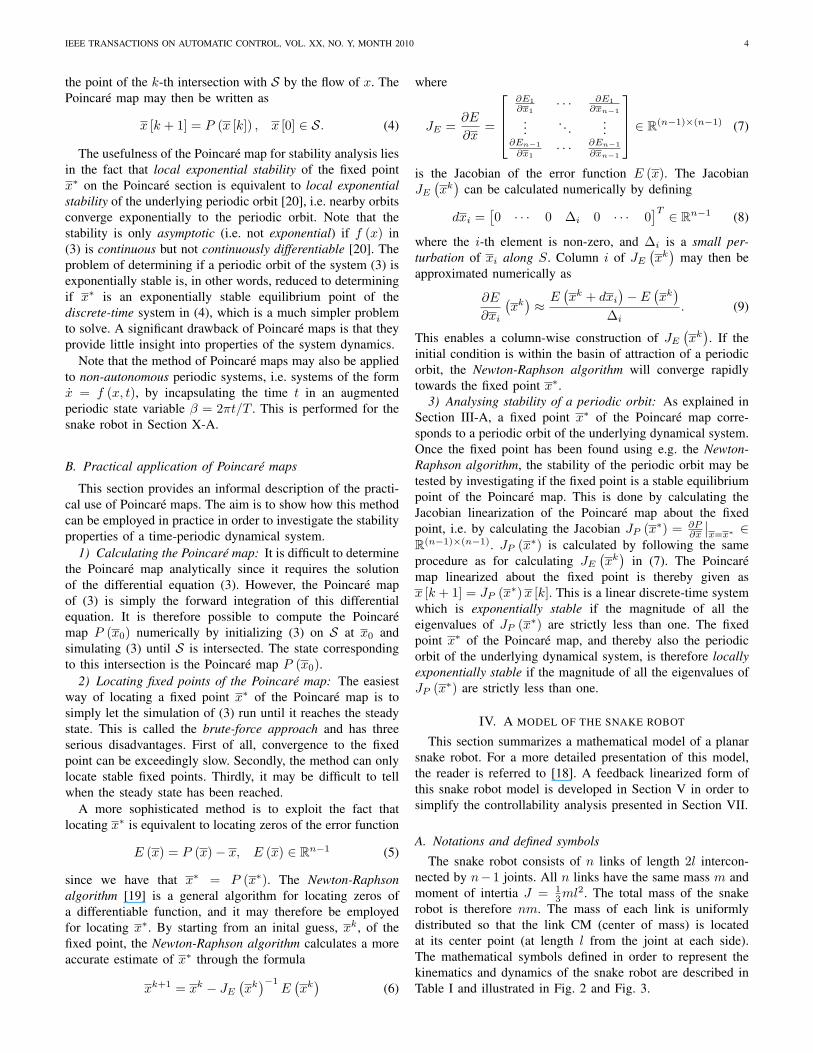
IEEE TRANSACTIONS ON AUTOMATIC CONTROL, VOL. XX, NO. Y, MONTH 2010 4

the point of the k-th intersection with S by the flow of x. ThePoincare map may then be written as

x [k + 1] = P (x [k]) , x [0] ∈ S. (4)

The usefulness of the Poincare map for stability analysis liesin the fact that local exponential stability of the fixed pointx∗ on the Poincare section is equivalent to local exponentialstability of the underlying periodic orbit [20], i.e. nearby orbitsconverge exponentially to the periodic orbit. Note that thestability is only asymptotic (i.e. not exponential) if f (x) in(3) is continuous but not continuously differentiable [20]. Theproblem of determining if a periodic orbit of the system (3) isexponentially stable is, in other words, reduced to determiningif x∗ is an exponentially stable equilibrium point of thediscrete-time system in (4), which is a much simpler problemto solve. A significant drawback of Poincare maps is that theyprovide little insight into properties of the system dynamics.

Note that the method of Poincare maps may also be appliedto non-autonomous periodic systems, i.e. systems of the formx = f (x, t), by incapsulating the time t in an augmentedperiodic state variable β = 2πt/T . This is performed for thesnake robot in Section X-A.

B. Practical application of Poincare maps

This section provides an informal description of the practi-cal use of Poincare maps. The aim is to show how this methodcan be employed in practice in order to investigate the stabilityproperties of a time-periodic dynamical system.

1) Calculating the Poincare map: It is difficult to determinethe Poincare map analytically since it requires the solutionof the differential equation (3). However, the Poincare mapof (3) is simply the forward integration of this differentialequation. It is therefore possible to compute the Poincaremap P (x0) numerically by initializing (3) on S at x0 andsimulating (3) until S is intersected. The state correspondingto this intersection is the Poincare map P (x0).

2) Locating fixed points of the Poincare map: The easiestway of locating a fixed point x∗ of the Poincare map is tosimply let the simulation of (3) run until it reaches the steadystate. This is called the brute-force approach and has threeserious disadvantages. First of all, convergence to the fixedpoint can be exceedingly slow. Secondly, the method can onlylocate stable fixed points. Thirdly, it may be difficult to tellwhen the steady state has been reached.

A more sophisticated method is to exploit the fact thatlocating x∗ is equivalent to locating zeros of the error function

E (x) = P (x)− x, E (x) ∈ Rn−1 (5)

since we have that x∗ = P (x∗). The Newton-Raphsonalgorithm [19] is a general algorithm for locating zeros ofa differentiable function, and it may therefore be employedfor locating x∗. By starting from an inital guess, xk, of thefixed point, the Newton-Raphson algorithm calculates a moreaccurate estimate of x∗ through the formula

xk+1 = xk − JE(xk)−1

E(xk)

(6)

where

JE =∂E

∂x=

∂E1∂x1

· · · ∂E1∂xn−1

.... . .

...∂En−1∂x1

· · · ∂En−1∂xn−1

∈ R(n−1)×(n−1) (7)

is the Jacobian of the error function E (x). The JacobianJE(xk)

can be calculated numerically by defining

dxi =[0 · · · 0 ∆i 0 · · · 0

]T ∈ Rn−1 (8)

where the i-th element is non-zero, and ∆i is a small per-turbation of xi along S. Column i of JE

(xk)

may then beapproximated numerically as

∂E

∂xi

(xk)≈E(xk + dxi

)− E

(xk)

∆i. (9)

This enables a column-wise construction of JE(xk). If the

initial condition is within the basin of attraction of a periodicorbit, the Newton-Raphson algorithm will converge rapidlytowards the fixed point x∗.

3) Analysing stability of a periodic orbit: As explained inSection III-A, a fixed point x∗ of the Poincare map corre-sponds to a periodic orbit of the underlying dynamical system.Once the fixed point has been found using e.g. the Newton-Raphson algorithm, the stability of the periodic orbit may betested by investigating if the fixed point is a stable equilibriumpoint of the Poincare map. This is done by calculating theJacobian linearization of the Poincare map about the fixedpoint, i.e. by calculating the Jacobian JP (x∗) = ∂P

∂x

∣∣x=x∗ ∈

R(n−1)×(n−1). JP (x∗) is calculated by following the sameprocedure as for calculating JE

(xk)

in (7). The Poincaremap linearized about the fixed point is thereby given asx [k + 1] = JP (x∗)x [k]. This is a linear discrete-time systemwhich is exponentially stable if the magnitude of all theeigenvalues of JP (x∗) are strictly less than one. The fixedpoint x∗ of the Poincare map, and thereby also the periodicorbit of the underlying dynamical system, is therefore locallyexponentially stable if the magnitude of all the eigenvalues ofJP (x∗) are strictly less than one.

IV. A MODEL OF THE SNAKE ROBOT

This section summarizes a mathematical model of a planarsnake robot. For a more detailed presentation of this model,the reader is referred to [18]. A feedback linearized form ofthis snake robot model is developed in Section V in order tosimplify the controllability analysis presented in Section VII.

A. Notations and defined symbols

The snake robot consists of n links of length 2l intercon-nected by n−1 joints. All n links have the same mass m andmoment of intertia J = 1

3ml2. The total mass of the snake

robot is therefore nm. The mass of each link is uniformlydistributed so that the link CM (center of mass) is locatedat its center point (at length l from the joint at each side).The mathematical symbols defined in order to represent thekinematics and dynamics of the snake robot are described inTable I and illustrated in Fig. 2 and Fig. 3.

IEEE TRANSACTIONS ON AUTOMATIC CONTROL, VOL. XX, NO. Y, MONTH 2010 5

Fig. 2. Kinematic parameters for the snake robot.

Fig. 3. Forces and torques acting on each link of the snake robot.

Vectors are either expressed in the global coordinate systemor in the local coordinate system of link i. This is indicatedby superscript global or link, i, respectively. If not otherwisespecified, a vector with no superscript is expressed in theglobal coordinate system.

The following vectors and matrices are used in the subse-quent sections:

Symbol Description Associatedvector

n Number of links.l Half the length of a link.m Mass of a link.J Moment of inertia of a link.θi Angle between link i and global x axis. θ ∈ Rn

φi Angle of joint i. φ ∈ Rn−1

(xi, yi) Global coordinates of CM of link i. x, y ∈ Rn

(px, py) Global coordinates of the CM of thesnake robot.

p ∈ R2

ui Actuator torque exerted on link i fromlink i+ 1.

u ∈ Rn−1

ui−1 Actuator torque exerted on link i fromlink i− 1.

u ∈ Rn−1

fR,x,i Friction force on link i in x direction. fR,x ∈ Rn

fR,y,i Friction force on link i in y direction. fR,y ∈ Rn

hx,i Joint constraint force in x direction onlink i from link i+ 1.

hx ∈ Rn−1

hy,i Joint constraint force in y direction onlink i from link i+ 1.

hy ∈ Rn−1

hx,i−1 Joint constraint force in x direction onlink i from link i− 1.

hx ∈ Rn−1

hy,i−1 Joint constraint force in y direction onlink i from link i− 1.

hy ∈ Rn−1

TABLE IDEFINED MATHEMATICAL SYMBOLS.

A =

1 1

. .. .

1 1

, D =

1 −1

. .. .

1 −1

where A ∈ R(n−1)×n and D ∈ R(n−1)×n. Furthermore,

e =[1 . . 1

]T ∈ Rn, E =[

e 0n×1

0n×1 e

]∈ R2n×2,

sin θ=[sin θ1 .. sin θn

]T∈Rn, Sθ = diag(sin θ) ∈ Rn×n,

cos θ=[cos θ1 .. cos θn

]T∈Rn, Cθ = diag(cos θ)∈ Rn×n.

Note that the operator diag (·) produces a diagonal matrixwith the elements of its argument along its diagonal. Notealso that sin (·) and cos (·) are vector operators when theirargument is a vector and scalar operators when their argumentis a scalar value. As shown in Table I, we will use subscript ito denote element i of a vector. When parameters of the linksof the snake robot are assembled into a vector, we associateelement i of this vector with link i.

B. Kinematics

The snake robot moves in the horizontal plane and hasa total of n + 2 degrees of freedom. The absolute angle,θi, of link i is expressed with respect to the global x axiswith counterclockwise positive direction. As seen in Fig. 2,the relative angle between link i and link i + 1 is given byφi = θi − θi+1. The local coordinate system of each link isfixed in the CM (center of mass) of the link with x (tangential)and y (normal) axes oriented such that they are oriented in thedirections of the global x and y axis, respectively, when thelink angle is zero. The rotation matrix from the global frameto the frame of link i is given by

Rgloballink,i =

[cos θi − sin θisin θi cos θi

]. (10)

The position, p, of the CM (center of mass) of the snake robotis given by

p =[pxpy

]=

1nm

n∑i=1

mxi

1nm

n∑i=1

myi

=1n

[eTxeT y

]. (11)

It is shown in [18] that the global frame position of the CMof each link is given by

x =−lNT cos θ + epxy = −lNT sin θ + epy

(12)

whereN = AT

(DDT

)−1D ∈ Rn×n. (13)

The linear velocities of the links are derived by differentiating(12). This gives

x = lNTSθ θ + epxy = −lNTCθ θ + epy.

(14)

An expression for the velocity of a single link may be found byinvestigating the structure of each row in (14). The derivationis not included here due to space restrictions, but it may be

IEEE TRANSACTIONS ON AUTOMATIC CONTROL, VOL. XX, NO. Y, MONTH 2010 6

verified that the linear velocity of the CM of link i in theglobal x and y directions is given by

xi = px − σiSθ θyi = py + σiCθ θ

(15)

where

σi =[a1 a2 ... ai−1

ai+bi

2 bi+1 bi+2 ... bn]∈ Rn

ai = l(2i−1)n

bi = l(2i−1−2n)n .

(16)

C. Viscous friction model

In this paper, we consider snake robots influenced byviscous ground friction forces. In this section, we present theviscous friction model, and in particular we present modelsfor the different cases of isotropic versus anisotropic viscousfriction.

1) Isotropic viscous friction: The friction forces are as-sumed to act on the CM of the links only. The isotropicviscous friction force on link i in the global x and y directionis proportional to the global velocity of the link and is written

fR,x,i = −cxi = −cpx + cσiSθ θ

fR,y,i = −cyi = −cpy − cσiCθ θ(17)

where c is the viscous friction coefficient, and the expressionfor the link velocity is given by (15). The friction forces onall links may be expressed in matrix form as

fR =[fR,xfR,y

]= −c

[xy

]= −c

[lNTSθ θ + epx−lNTCθ θ + epy

](18)

where the expression for the link velocities is given by (14).We disregard the friction torque caused by a link rotating withrespect to the ground since this torque only has a minor impacton the motion.

2) Anisotropic viscous friction: Under anisotropic frictionconditions, a link has two viscous friction coefficients, ct andcn, describing the friction force in the tangential (along linkx axis) and normal (along link y axis) direction of the link,respectively. Using (10), the friction force on link i in theglobal frame as a function of the global link velocity, xi andyi, is given by

fglobalR,i =Rglobal

link,i flink,iR,i =−Rglobal

link,i

[ct 00 cn

]vlink,ii

= −Rgloballink,i

[ct 00 cn

](Rglobal

link,i

)T [xiyi

] (19)

where f link,iR,i and vlink,i

i are, respectively, the friction force andthe link velocity expressed in the local link frame. Performingthe matrix multiplication and assembling the friction forces onall links in matrix form gives

fR=−[ct (Cθ)

2 + cn (Sθ)2 (ct − cn)SθCθ

(ct − cn)SθCθ ct (Sθ)2 + cn (Cθ)

2

][xy

](20)

where fR=[fTR,x fTR,y

]T ∈ R2n. Note that (20) reduces to(18) in the case of isotropic friction (ct = cn = c).

D. Equations of motion

This section presents the equations of motion of the snakerobot in terms of the acceleration of the link angles, θ, and theacceleration of the CM of the snake robot, p. These coordinatesdescribe all n+ 2 DOFs of the snake robot.

The forces and torques acting on link i are visualized inFig. 3. The force balance for link i in global frame coordinatesis given by

mxi = fR,x,i + hx,i − hx,i−1

myi = fR,y,i + hy,i − hy,i−1(21)

while the torque balance for link i is given by

Jθi = ui − ui−1

−l sin θi(hx,i + hx,i−1) + l cos θi(hy,i + hy,i−1).(22)

Through straightforward calculations, it is shown in [18] that(21) and (22) may be rewritten for all links and combined intothe following complete model of the snake robot:

Mθ +Wθ2 − lSθNfR,x + lCθNfR,y = DTu (23)

nmp = nm

[pxpy

]= ET fR =

[eT fR,xeT fR,y

](24)

where θ and p represent the n+ 2 generalized coordinates ofthe system, θ2 = diag(θ)θ, and

M = JIn×n +ml2 (SθV Sθ + CθV Cθ)W = ml2 (SθV Cθ − CθV Sθ)

N = AT(DDT

)−1D

V = AT(DDT

)−1A.

(25)

The model of the snake robot may be written more compactlyas

x =[θT pT θT pT

]T= F (x, t) (26)

where we have introduced the state variablex =

[θT pT θT pT

]T ∈ R2n+4 and also assumedthat u = u (x, t). The elements of F (x, t) are given bysolving (23) and (24) for θ and p, respectively.

V. PARTIAL FEEDBACK LINEARIZATION OF THE MODEL

This section transforms the model (26) to a simpler formthrough partial feedback linearization [24], [25]. This conver-sion greatly simplifies the controllability analysis presented inSection VII. Partial feedback linearization of underactuatedsystems consists of linearizing the dynamics corresponding tothe actuated degrees of freedom of the system. In this section,we show how a change of coordinates makes it possible toemploy this methodology by following the approach presentedin [26].

A. Partitioning the model into an actuated and an unactuatedpart

Before partial feedback linearization can be carried out, themodel of the snake robot in (26) must be partitioned intotwo parts representing the actuated and unactuated degreesof freedom, respectively [26]. The acceleration of the CM ofthe snake robot, p, belongs to the unactuated part since itis not directly influenced by the input, u. The acceleration

IEEE TRANSACTIONS ON AUTOMATIC CONTROL, VOL. XX, NO. Y, MONTH 2010 7

of the link angles, θ, represents one unactuated degree offreedom and n − 1 actuated degrees of freedom since thereare n link accelerations (θ ∈ Rn) and only n − 1 controlinputs (u ∈ Rn−1). However, it is not possible to partitionthe equation for θ in (23) into an actuated and an unactuatedpart since the matrix DT in front of the control input givesa direct influence between u and all the link accelerations.We therefore seek a form of the model where there is adirect influence between u and only n− 1 link accelerations.This is achieved by modifying the choice of generalizedcoordinates from absolute link angles to relative joint angles.The generalized coordinates of the model in (26) are given bythe absolute link angles, θ, and the CM position of the snakerobot, p. We now replace these coordinates with

q =[φp

]∈ Rn+2 (27)

where

φ =[φ1 φ2 · · · φn−1 θn

]T ∈ Rn (28)

contains the n − 1 relative joint angles of the snake robotand the absolute link angle, θn ∈ R, of the head link. Therelative joint angles are defined in Fig. 2. The coordinatetransformation between absolute link angles and relative jointangles is easily shown to be given by

θ = Rφ (29)

R =

1 1 1 · · · 1 10 1 1 · · · 1 1...

...0 0 0 · · · 0 1

∈ Rn×n. (30)

The dynamic model in the new coordinates is found byinserting (29) into (23) and (24). This gives

MRφ+W diag(Rφ)Rφ− lSθNfR,x

+lCθNfR,y = DTunmp = ET fR

(31)

where we have used that θ2 = diag(θ)θ = diag(Rφ)Rφ.

Finally, we premultiply the first matrix equation in (31) withRT in order to achieve the desired form of the input mappingmatrix on the right-hand side by making the last of the nequations independent of the control input. This enables us towrite the complete model of the snake robot as

M (φ) q +W(φ, φ

)+G (φ) fR

(φ, φ, p

)= Bu (32)

where

q =[φp

]∈ Rn+2 (33)

M (φ) =[RTM (φ)R 0n×2

02×n nmI2

](34)

W(φ, φ

)=

[RTW (φ) diag

(Rφ)Rφ

02×1

](35)

G (φ) =

−lRTSRφN lRTCRφN−eT 01×n01×n −eT

(36)

B =[In−1

03×n−1

](37)

and where SRφ = Sθ and CRφ = Cθ. It is interesting tonote that premultiplying the first matrix equation in (31) withRT both causes the input mapping matrix to attain a desirableform and produces a symmetrical inertia matrix. Had we leftthe model in the form of (31), the inertia matrix would nothave been symmetrical.

The first n− 1 equations of (32) represent the dynamics ofthe relative joint angles of the snake robot, i.e. the actuateddegrees of freedom of the snake robot. The last three equationsrepresent the dynamics of the absolute orientation and positionof the snake robot, i.e. the unactuated degrees of freedom. Themodel may therefore be partitioned as

M11qa +M12qu +W 1 +G1fR = u (38)

M21qa +M22qu +W 2 +G2fR = 03×1 (39)

where qa =[φ1 · · · φn−1

]T ∈ Rn−1 represents theactuated degrees of freedom, qu =

[θn px py

]T ∈R3 represents the unactuated degrees of freedom, M11 ∈R(n−1)×(n−1), M12 ∈ R(n−1)×3, M21 ∈ R3×(n−1), M22 ∈R3×3, W 1 ∈ Rn−1, W 2 ∈ R3, G1 ∈ R(n−1)×2n, andG2 ∈ R3×2n. Note that M (φ) only depends on the relativejoint angles of the snake robot and not on the absoluteorientation of the head link, θn. Formally, this is a result of thefact that θn is a cyclic coordinate [27]. Less formally, this isquite obvious since it would not be reasonable that the inertialproperties of a planar snake robot be dependent on how thesnake robot is oriented in the plane. We therefore have thatM = M (qa).

B. Partial feedback linearization

We are now ready to present an input transformation thatlinearizes the dynamics of the actuated degrees of freedomin (38). M22 is an invertible 3 × 3 matrix as a consequenceof the uniform positive definiteness of the complete systeminertia matrix, M (qa). We may therefore solve (39) for qu as

qu = −M−1

22

(M21qa +W 2 +G2fR

). (40)

Inserting (40) into (38) gives(M11 −M12M

−1

22 M21

)qa +W 1 +G1fR

−M12M−1

22

(W 2 +G2fR

)= u.

(41)

IEEE TRANSACTIONS ON AUTOMATIC CONTROL, VOL. XX, NO. Y, MONTH 2010 8

Consequently, the following linearizing controller

u =(M11 −M12M

−1

22 M21

)v +W 1

+G1fR −M12M−1

22

(W 2 +G2fR

) (42)

enables us to rewrite (38) and (39) as

qa = v (43)qu = A (q, q) + B (qa) v (44)

where

A (q, q) = −M−1

22

(W 2 +G2fR

)∈ R3 (45)

B (qa) = −M−1

22 M21 ∈ R3×(n−1). (46)

This model may be written in the standard form of a control-affine system by defining x1 = qa, x2 = qu, x3 = qa, x4 = qu,and x =

[xT1 xT2 xT3 xT4

]T ∈ R2n+4. This gives

x =

x1

x2

x3

x4

=

x3

x4

vA (x) + B (x1) v

= f (x) +

n−1∑j=1

gj (x1) vj

(47)

where

f (x) =

x3

x4

0(n−1)×1

A (x)

, gj (x1) =

0(n−1)×1

03×1

ejBj (x1)

(48)

and where ej denotes the jth standard basis vector in Rn−1

(the jth column of In−1), and Bj (x1) denotes the jth columnof B (x1).

VI. STABILIZABILITY PROPERTIES OF PLANAR SNAKEROBOTS

This section presents a fundamental theorem concerningthe properties of an asymptotically stabilizing control law forsnake robots to any equilibrium point. The equation (47) mapsthe state, x, and the controller input, v, of the robot into theresulting derivative of the state vector, x. For any equilibriumpoint (x1 = xe1, x2 = xe2, x3 = 0, x4 = 0), where (xe1, x

e2) is

the configuration of the system at the equilibrium point, wehave that x = 0.

A well-known result by Brockett [28] states that a neces-sary condition for the existence of a time-invariant (i.e. notexplicitly dependent on time) continuous state feedback law,v = v (x), that makes (xe1, x

e2, 0, 0) asymptotically stable, is

that the image of the mapping (x, v) 7→ x contains someneighbourhood of x = 0. A result by Coron and Rosier[29] states that a control system that can be asymptoticallystabilized (in the Filippov sense [29]) by a time-invariant dis-continuous state feedback law can be asymptotically stabilizedby a continuous time-varying state feedback law. If, moreover,the control system is affine (i.e. linear with respect to thecontrol input), then it can be asymptotically stabilized by atime-invariant continuous state feedback law. We now employ

these results to prove the following fundamental theorem forplanar snake robots:

Theorem 3: An asymptotically stabilizing control law for aplanar snake robot described by (47) to any equilibrium pointmust be time-varying, i.e. of the form v = v (x, t).

Proof: The result by Brockett [28] states that themapping (x1, x2, x3, x4, v) 7→ (x3, x4, v,A (x) + B (x1) v)must map an arbitrary neighbourhood of(x1 = xe1, x2 = xe2, x3 = 0, x4 = 0, v = 0) onto a neigh-bourhood of (x3 = 0, x4 = 0, v = 0,A (x) + B (x1) v = 0).For this to be true, points of the form (x3 = 0, x4 = 0,v = 0,A (x) + B (x1) v = ε) must be contained in thismapping for some arbitrary ε 6= 0 because points of this formare contained in every neighbourhood of x = 0. However,these points do not exist for the system in (47) because x3 = 0,x4 = 0, and v = 0 means that A (x) + B (x1) v = 0 6= ε.Hence, the snake robot cannot be asymptotically stabilizedto (x1 = xe1, x2 = xe2, x3 = 0, x4 = 0) by a time-invariantcontinuous state feedback law. Moreover, since the systemin (47) is affine and cannot be asymptotically stabilized bya time-invariant continuous state feedback law, the result byCoron and Rosier [29] proves that the system can neither beasymptotically stabilized by a time-invariant discontinuousstate feedback law. We can therefore conclude that anasymptotically stabilizing control law for a planar snake robotto any equilibrium point must be time-varying, i.e. of theform v = v (x, t).

Remark 4: Theorem 3 is independent of the choice offriction model and applies to any planar snake robot describedby a friction model with the property that A (xe) = 0 for anyequilibrium point xe.

VII. CONTROLLABILITY ANALYSIS OF PLANAR SNAKEROBOTS

This section studies the controllability of planar snakerobots influenced by viscous ground friction.

A. Controllability with isotropic viscous friction

We begin the controllability analysis of the snake robot byfirst assuming that the viscous ground friction is isotropic. Inthis case, it turns out that the equations of motion take on aparticularly simple form that enables us to study controllabilitythrough pure inspection of the equations of motion. From (24),we have that the acceleration of the CM (center of mass) ofthe snake robot is given by

[pxpy

]=[

1nme

T fR,x1nme

T fR,y

]=

1nm

n∑i=1

fR,x,in∑i=1

fR,y,i

. (49)

Inserting (17) into (49) gives

[pxpy

]=

c

nm

−npx +(

n∑i=1

σi

)Sθ θ

−npy −(

n∑i=1

σi

)Cθ θ

= − c

m

[pxpy

](50)

IEEE TRANSACTIONS ON AUTOMATIC CONTROL, VOL. XX, NO. Y, MONTH 2010 9

because it may be shown thatn∑i=1

σi = 0. This enables us to

state the following theorem:Theorem 5: A planar snake robot influenced by isotropic

viscous ground friction is not controllable.Proof: In order to control the position, the snake robot

must accelerate its CM (center of mass). From (50) it is clearthat the CM acceleration is proportional to the CM velocity.If the snake robot starts from rest (p = 0), it is thereforeimpossible to achieve acceleration of the CM. The position ofthe snake robot is in other words completely uncontrollable inthis case, which renders the snake robot uncontrollable.

B. Controllability with anisotropic viscous friction

The equations of motion of the snake robot in (47) becomefar more complex under anisotropic friction conditions. Wetherefore employ the controllability concepts presented in Sec-tion II and begin by computing the Lie brackets of the systemvector fields. The drift and control vector fields of the snakerobot are given in (48). As explained in Section II, Lie bracketcomputation involves partial derivatives of the componentsof the vector fields. These computations can be carried outwithout dealing with the complex expressions contained inA (x) and B (x1) given by (45) and (46), respectively, sincewe only need to know which variables each row of thevector fields depend on. As an example, consider column jof B (x1). Since we know that it only depends on x1, wemay immediately write ∂Bj(x1)

∂x =[∂Bj(x1)∂x1

03×(n+5)

]. This

methodology enables us to compute the following Lie bracketsof the system vector fields (evaluated at an equilibrium point):

[f, gj ]q=0 =

−ej−Bj

0(n−1)×1

−Cj

, [f, [f, gj ]]q=0 =

0(n−1)×1

Cj0(n−1)×1∂A∂x4Cj

,

[[f, gj ] , [f, gk]]q=0 =

0(n−1)×1

Djk0(n−1)×1

Ejk

(51)

where j, k ∈ {1, ..., n− 1} and

Cj = ∂A∂x3

ej + ∂A∂x4Bj , Djk = ∂Bk

∂x1ej − ∂Bj

∂x1ek,

Ejk= ∂Ck

∂x1ej−∂Cj

∂x1ek+∂Ck

∂x2Bj−∂Cj

∂x2Bk+∂Ck

∂x4Cj−∂Cj

∂x4Ck.

(52)

The Lie brackets have been evaluated at zero velocity (q = 0)since we are interested in controllability from an equilibriumpoint. The above vector fields represent our choice of vectorfields to be contained in the accessibility algebra, ∆, of thesystem. To construct ∆ of full rank, we need to find (2n+ 4)independent vector fields since the snake robot has a (2n+ 4)-dimensional state space. Each of the four types of vector fieldsabove represent (n−1) vector fields. Solving 4(n−1) ≥ 2n+4gives that our analysis is only valid if the snake robot hasn ≥ 4 links. This is a mild requirement, however, since asnake robot generally will have more than four links. In theremainder of this section, we assume that the robot consistsof exactly n = 4 links (and thereby n − 1 = 3 active joints)and argue that the following controllability results will also be

valid for snake robots with more links. In particular, a robotwith n > 4 links can behave as a robot with n = 4 linksby fixing (n − 4) joint angles at zero degrees and allowingthe remaining three joint angles to move. This means thatcontrollability of the robot with n = 4 is a sufficient althoughnot necessary condition for controllability with n > 4.

With n = 4 links, the system has a (2n+ 4) = 12-dimensional state space. The system satisfies the Lie algebrarank condition (LARC) if the above vector fields span a 12-dimensional space. We therefore assemble the 12 vector fieldsinto the following matrix, which represents the accessibilityalgebra of the system evaluated at an equilibrium point xe:

∆ (xe) = [g1, g2, g3, [f, g1] , [f, g2] , [f, g3] ,[f, [f, g1]] , [f, [f, g2]] , [f, [f, g3]] ,

[[f, g1] , [f, g2]] , [[f, g1] , [f, g3]] , [[f, g2] , [f, g3]]]

=

03×3 −I3 03×3 03×3

03×3 −B C DI3 03×3 03×3 03×3

B −C ∂A∂x4C E

∈ R12×12

(53)

where

C = ∂A∂x3

+ ∂A∂x4B ∈ R3×3,

D =[D12 D13 D23

], E =

[E12 E13 E23

].

(54)

We now state the following theorem regarding the accessi-bility of the snake robot:

Theorem 6: A planar snake robot with n ≥ 4 links in-fluenced by anisotropic viscous ground friction (ct 6= cn)is locally strongly accessible from any equilibrium point xe

(q = 0) satisfying det (C) 6= 0 and det(E− ∂A

∂x4D)6= 0,

where det (∗) denotes the determinant evaluated at xe.Proof: By Theorem 1, the system is locally strongly

accessible from xe if ∆ (xe), given by (53), has full rank,i.e. spans a 12-dimensional space. The proof is complete ifwe can show that this is the case as long as det (C) 6= 0 anddet(E− ∂A

∂x4D)6= 0 at xe. The matrix ∆ (xe) has full rank

when all its columns are linearly independent. By investigatingthe particular structure of ∆ (xe), we see that the first and thirdrow contains an identity matrix and then zeros in the remainingelements of these rows. It is therefore impossible to writethe columns containing the two identity matrices as linearcombinations of other columns. We can therefore concludethat any linear dependence between the columns of ∆ (xe)must be caused by linear dependence between the columns ofthe following submatrix of ∆ (xe):

∆ (xe) =[C D

∂A∂x4C E

]∈ R6×6. (55)

Linear dependence between columns of a square matrix causesits determinant to become zero. We therefore calculate thedeterminant of ∆ (xe) by employing the following well-knownmathematical relationship concerning the determinant of ablock matrix (see e.g. [30]):

det([A BC D

])= det (A) det

(D − CA−1B

)(56)

IEEE TRANSACTIONS ON AUTOMATIC CONTROL, VOL. XX, NO. Y, MONTH 2010 10

where A and D are any square matrices and A is non-singular.This gives

det(

∆ (xe))

= det (C) det(E− ∂A

∂x4D). (57)

The determinant of ∆ (xe) is zero when det (C) = 0 orwhen det

(E− ∂A

∂x4D)

= 0. This means that ∆ (xe), andthereby also ∆ (xe), has full rank whenever det (C) 6= 0 anddet(E− ∂A

∂x4D)6= 0. This completes the proof.

The requirement regarding the two determinants in The-orem 6 is not very restrictive, but it implies that the snakerobot can attain configurations that are singular, i.e. certainshapes of the snake robot are obstructive from a controlperspective since the dimension of the reachable space fromthese configurations is not full-dimensional. These singularconfigurations are revealed by the following property:

Property 7: The accessibility algebra ∆ (xe) of the systemdrops rank at equilibrium points where all relative joint anglesare equal (φ1 = φ2 = ... = φn−1).

This property can be shown to hold with a mathematicalsoftware tool such as Matlab Symbolic Math Toolbox sinceit can be verified that det (C)

∣∣φ1=φ2=...=φn−1

= 0, therebyviolating the full rank conditions that are stated in Theorem 6.Property 7 is interesting since it implies that the joint angles ofa snake robot should be out of phase during snake locomotion.This claim has been stated in several previous works [1], [2],[8], [31], but no formal mathematical proof was given.

We now show that the snake robot does not satisfy sufficientconditions for small-time local controllability (STLC).

Theorem 8: At any equilibrium point xe (q = 0), a planarsnake robot with n ≥ 4 links influenced by viscous groundfriction does not satisfy the sufficient conditions for small-timelocal controllability (STLC) stated in Theorem 2.

Proof: The proof is complete if we can show that thereare bad brackets of the system vector fields that cannotbe neither θ-neutralized nor l-neutralized (see Theorem 2).The bad brackets with the lowest θ-degree and the lowestl-degree (except for f , which vanishes at any equilibriumpoint) are [gj , [f, gj ]], j ∈ {1, 2, 3}. Theorem 2 requires thesevectors to be written as linear combinations of good bracketswith either lower θ-degree or lower l-degree. The only suchgood brackets are gj , [f, gj ] , [f, [f, gj ]] , .., [f, [· · · [f, gj ]] · · · ],j ∈ {1, 2, 3}. Brackets of the form [gk, gj ] are not consideredbecause [gk, gj ] = 0, j, k ∈ {1, 2, 3}. For a proper choiceof θ and lj , j ∈ {0, 1, 2, 3}, these brackets have both lowerθ-degree and lower l-degree. It is straightforward to verifythat [gj , [f, gj ]] ∈ R2n+4=12 is a vector of all zeros exceptfor element number 2n + 2 = 10. The only way to writethis vector as a linear combination of the good brackets listedabove is if these good brackets span the entire 12-dimensionalstate space. This is not the case, however, because the vectors[f, [f, gj ]] , .., [f, [· · · [f, gj ]] · · · ] are linearly dependent, as can

be seen by assembling the following matrix:

[[f, [f, gj ]] , [f, [f, [f, gj ]]] , [f, [f, [f, [f, gj ]]]] , · · · ]

=

03×3 03×3 03×3 · · ·

C − ∂A∂x4C

(∂A∂x4

)2

C · · ·03×3 03×3 03×3 · · ·∂A∂x4C −

(∂A∂x4

)2

C(∂A∂x4

)3

C · · ·

(58)

and noting that the fourth row is a multiple of the secondrow. It is therefore not possible to either θ-neutralize nor l-neutralize the bad brackets of the system in (47). The lineardependence in (58) is also present for n > 4 links since thesix non-zero rows of (58) concern the position and head angleof the snake while the 2n − 2 remaining rows will be zeroregardless of n. This completes the proof.

Note that Theorem 8 does not claim that the snake robot isnot STLC. In other words, the snake robot may be STLC eventhough the sufficient conditions of Theorem 2 are violated.Note also that STLC is not a requirement for controllabilitysince, as described in Section II, it is in fact a stronger propertythan controllability. In summary, the above results do notenable us to conclude that a wheelless snake robot influencedby anisotropic ground friction is controllable. However, theabove results are hopefully an important step towards formallyproving that such mechanisms are controllable, which theauthors consider highly likely to be the case.

We end this section with a note on Theorem 6. This theoremclearly shows that anisotropic friction is an important propertyfor a snake robot. In the snake robot literature, it is commonfor snake robots to possess the property cn � ct. The extremecase of this property is realized by installing passive wheelsalong the snake body since this ideally means that ct = 0and cn = ∞. However, from Theorem 6 it is clear that theonly requirement for strong accessibility is that the frictioncoefficients are not equal. The property ct > cn is thereforealso valid. This means that the passive wheels commonlymounted tangential to the snake body may equally well bemounted transversal to the snake body. The resulting motionwill of course be different, but the strong accessibility propertyis still preserved.

VIII. EXPLANATION AND SYNTHESIS OF SNAKELOCOMOTION

This section presents an analysis of snake locomotion thatexplains how anisotropic viscous ground friction enables snakerobots to locomote forward on a planar surface. The analysisis subsequently used to synthesise how the snake robot linksshould be moved in order to propel the snake robot forward.

A. Analysis of propulsive forces during snake locomotion

Anisotropic friction generally means that the friction co-efficients in the tangential and normal direction of the linksare different (ct 6= cn). However, we will only focus on thecommonly assumed property of snake robots that the normaldirection friction is larger than the tangential friction (ct < cn).

We first derive an expression for the total force propellingthe CM (center of mass) of the snake robot forward as a

IEEE TRANSACTIONS ON AUTOMATIC CONTROL, VOL. XX, NO. Y, MONTH 2010 11

function of the linear link velocities. We will call this thepropulsive force on the snake robot and denote it by Fprop.The forward direction of motion is assumed to be along theglobal positive x axis. As described in Section IV-B, the angleθi of link i is expressed with respect to the global x axis withcounterclockwise positive direction. The propulsive force issimply the sum of all external forces on the snake robot in theglobal x direction and is given from (24) as

Fprop = nmpx = eT fR,x. (59)

Inserting fR,x from (20) into (59) gives

Fprop =−eT((ct(Cθ)

2+cn(Sθ)2)x+(ct−cn)SθCθy

). (60)

The purpose of the vector eT is to sum up the friction forcecontributions from all the links. We may therefore write (60)as a summation in order to investigate the force contributionfrom a single link.

Fprop = −∑ni=1

((ct cos2 θi + cn sin2 θi

)xi

+ (ct − cn) sin θi cos θiyi) .(61)

The propulsive force from a single link, Fprop,i, is in otherwords given by

Fprop,i = −Fx (θi) xi − Fy (θi) yi (62)

whereFx (θi) = ct cos2 θi + cn sin2 θiFy (θi) = (ct − cn) sin θi cos θi.

(63)

We see from (62) that Fprop,i consists of two components, i.e.one involving the linear velocity of the link in the forwarddirection of motion, Fx (θi) xi, and one involving the linearvelocity normal to the direction of motion, Fy (θi) yi. Due tothe minus signs in (62), the products Fx (θi) xi and Fy (θi) yiprovide a positive contribution to the propulsive force onlyif they are negative. Since the viscous friction coefficients,ct and cn, are always positive, the expression Fx (θi) isobviously always positive. We assume that the snake robotis not generating waves that involve x direction velocities ofany of the links opposite to the direction of motion. When thesnake robot is moving in the forward direction (px > 0), wetherefore have that xi > 0, which means that the productFx (θi) xi of the propulsive force is always positive. Thisproduct is therefore not contributing to the forward propulsionof the robot, but rather opposing it. This is also expected sincethe snake robot must naturally be subjected to a friction forcein the opposite direction of the motion.

Any maintained propulsive force in the forward directionof motion must therefore be produced by the sideways motionof the links, i.e. the product Fy (θi) yi. A plot of Fy (θi) fordifferent values of the normal friction coefficient cn, whilekeeping the tangential friction coefficient ct fixed, is shownin Fig. 4. For each plot, the angle between the link and theforward direction, θi, is varied from −90◦ to 90◦.

The sideways motion of the links have no effect on thepropulsive force on the snake robot when the friction coeffi-cients are equal since this gives Fy (θi) = 0. However, whencn > ct, Fig. (4) reveals that Fy (θi) is negative as long as θi ispositive, and vice versa. This means that the product Fy (θi) yi

Fig. 4. The mapping from sideways link motion to forward propulsion fordifferent viscous friction coefficients.

is negative as long as sgn (θi) = sgn (yi). The sideways mo-tion of a link is in other words contributing to the propulsion ofthe snake robot as long as θi is positive during leftward motionof the link (left with respect to the direction of motion) andnegative during rightward motion of the link (right with respectto the direction of motion). This fundamental relationship maybe written sgn (Fprop,i) = sgn (sgn (θi) sgn (yi)).

It is straightforward to calculate that the extrema of Fy (θi)occur at θi = ±45◦. This is also seen from Fig. 4. This meansthat, for a given yi, a link produces its highest propulsive forcewhen it forms an angle of ±45◦ with the forward direction ofmotion. It is also evident from (62) that the magnitude ofFy (θi) yi, and thereby the magnitude of the propulsive force,|Fprop,i|, is increased by increasing cn with respect to ct, orby increasing the magnitude of the sideways link velocity, |yi|.

It should now be clear that the function Fy (θi) maps thelink velocities normal to the direction of motion into forcecomponents in the direction of motion. The following simpleanalogy may help understand this result. Imagine a small,hand-held, wheeled wagon of some sort. The direction of thewheels corresponds to the tangential direction of a snake robotlink. Obviously, the friction coefficient of the wagon in thedirection of the wheels is smaller than the friction coefficientnormal to the wheels. Now assume that you push the wagonacross a table in the direction of the wheels. While maintainingconstant direction of motion, assume that you slowly rotate thewagon about the vertical axis, thereby forcing the wheels toslip. The hand that push and rotate the wagon will now feel atendency of the wagon to move sideways in the same directiontowards which the wagon was rotated. This is in accordancewith the results presented above. The above analysis provesthe following propositions:

Proposition 9: A planar snake robot with anisotropicground friction properties achieves forward propulsion throughthe sideways (with respect to the forward direction) velocitycomponents of its links.

Proposition 10: The direction of the propulsive force gen-erated by the sideways motion of link i is given by the fun-damental relationship sgn (Fprop,i) = sgn (sgn (θi) sgn (yi)).

Proposition 11: The function Fy (θi) maps the link veloc-ities normal to the direction of motion into force componentsin the direction of motion.

Proposition 12: The magnitude of the propulsive force gen-

IEEE TRANSACTIONS ON AUTOMATIC CONTROL, VOL. XX, NO. Y, MONTH 2010 12

erated by link i, |Fprop,i|, is increased by increasing cn withrespect to ct, or by increasing the magnitude of the sidewayslink velocity, |yi|.

Proposition 13: For a given yi, a link produces its highestpropulsive force when it forms an angle of θi = ±45◦ withthe forward direction of motion.

Note that these results are general in the sense that noassumptions have been made regarding the actual motionpattern displayed by the snake robot.

B. Synthesis of propulsive motion for the snake robot

The analysis from the previous section enables us to deducehow the snake robot links should be moved in order topropel the snake robot forward along the positive x axis. Thefollowing analysis focuses on manipulating the magnitude,|Fprop,i|, and direction, sgn (Fprop,i), of the propulsive forcefrom each link.

Theorem 3 in Section VI suggests that the angle of eachlink should be time-varying. Furthermore, Proposition 9 showsthat propulsive forces are generated by moving the links inthe normal direction with respect to the desired direction ofmotion. We therefore conclude that the links must have aperiodic velocity component normal to the direction of motion.This suggests that each link should be moved alternatinglyto the left and right with respect to the direction of motion,which can be achieved by letting the trajectory of each linkangle have the form

θi = α sin (ωt) , i ∈ {1, .., n} (64)

where α > 0 is the maximum amplitude of the link anglesduring the locomotion, ω > 0 is the angular frequency of theperiodic motion, and t denotes time. For simplicity, we assumethat α and ω are constant and identical for all links.

In accordance with Property 7 in Subsection VII-B, the jointangles should be out of phase during snake locomotion sincethis improves the controllability properties of the robot. Thissuggests that (64) should be modified to

θi = α sin (ωt+ (i− 1) δ) , i ∈ {1, .., n} (65)

where δ is the phase shift between adjacent links. For sim-plicity, we assume a constant phase shift between the links.

We now investigate how α, ω, and δ affect |Fprop,i| andsgn (Fprop,i) as the snake robot moves along the global xaxis. To simplify the analysis, we assume that the snake robotconsists of only n = 3 links. This is the minimum number oflinks required to achieve propulsion since phase shift betweenjoints requires at least two joints. The below analysis for n = 3links also apply to robots with n > 3 links since a snakerobot can be regarded as a connection of multiple three-linkedsegments. The link angle trajectories are given from (65) as

θ1 = α sin (ωt)θ2 = α sin (ωt+ δ)θ3 = α sin (ωt+ 2δ)

(66)

which, when differentiated with respect to time, gives thefollowing angular link velocities:

θ1 = αω cos (ωt)θ2 = αω cos (ωt+ δ)θ3 = αω cos (ωt+ 2δ) .

(67)

The normal direction velocity of each link is given from (14).We disregard the normal direction velocity of the snake robotby setting py ≈ 0. This approximation is a fairly accurateduring motion along the global x axis, which is the case forthis analysis. Inserting (66) and (67) into (14) gives

y1 = −αωl3 (2 cos (ωt) cos (α sin (ωt)))−αωl3 (3 cos (ωt+ δ) cos (α sin (ωt+ δ)))−αωl3 (cos (ωt+ 2δ) cos (α sin (ωt+ 2δ)))

(68)

y2 = αωl3 (cos (ωt) cos (α sin (ωt)))

−αωl3 (cos (ωt+ 2δ) cos (α sin (ωt+ 2δ)))(69)

y3 = αωl3 (cos (ωt) cos (α sin (ωt)))

+αωl3 (3 cos (ωt+ δ) cos (α sin (ωt+ δ)))

+αωl3 (2 cos (ωt+ 2δ) cos (α sin (ωt+ 2δ))) .

(70)

Proposition 12 tells us that |Fprop,i| is increased by increas-ing |yi|. From (68)-(70), it is therefore clear that |Fprop,i|is increased by increasing α and/or ω. We now determineif δ should be positive or negative in order to achievesgn (Fprop,i) = 1, which is necessary to propel the snakerobot forward along the global x axis. From Proposition 10,we know that sgn (Fprop,i) = 1 requires sgn (θi) = sgn (yi).Considering y2 in (69) (since this expression is easy toanalyze), it is seen through pure inspection that y2 = 0 whenωt = −δ. When ωt = −δ, we see from (66) and (67) thatθ2 = 0 and θ2 = αω > 0. θ2 is in other words aboutto become positive, which means that we also require y2 tobecome positive. This is the case if y2 > 0 when ωt = −δ.Differentiating (69) with respect to time gives

y2

∣∣ωt=−δ = 2α2ω2l

3 cos2 (δ) sin (α sin (δ))+ 2αω2l

3 sin (δ) cos (α sin (δ))(71)

from which it is easily seen that y2 > 0 when δ > 0, i.e.sgn (Fprop,i) = 1 when δ > 0. This indicates that the linksgenerate positive propulsive forces if δ > 0.

In order to verify that forward propulsion requires δ > 0,we have plotted (66) and (68)-(70) together in Fig. 5-7 forα = 70◦, ω = 70◦, and for different positive values of δover a period of ωt from 0 to 2π. The figures show thatsgn (Fprop,i) = sgn (sgn (θi) sgn (yi)) = 1 is always satisfiedfor link 2, but only satisfied over about half the period for links1 and 3 when δ is small. As δ is increased, sgn (Fprop,i) = 1is satisfied over a larger portion of the period. We do notattempt to determine the optimal choice of δ in this analysis,but conclude that positive propulsive forces requires δ > 0.

The above analysis proves the following propositions:Proposition 14: A snake robot with anisotropic friction

properties on a flat surface achieves forward propulsion bymoving its links according to θi = α sin (ωt+ (i− 1) δ)where i ∈ {1, .., n}, α > 0, ω > 0, and δ > 0.

IEEE TRANSACTIONS ON AUTOMATIC CONTROL, VOL. XX, NO. Y, MONTH 2010 13

Fig. 5. The relation between θ1 and y1 for α = 70◦, ω = 70◦, and δ = 10◦

(dotted) , 40◦ (dashed) , 70◦ (solid).

Fig. 6. The relation between θ2 and y2 for α = 70◦, ω = 70◦, and δ = 10◦

(dotted) , 40◦ (dashed) , 70◦ (solid). The plot is zoomed in.

Fig. 7. The relation between θ3 and y3 for α = 70◦, ω = 70◦, and δ = 10◦

(dotted) , 40◦ (dashed) , 70◦ (solid).

Proposition 15: Increasing α and/or ω increases the mag-nitude of the propulsive force generated by link i, |Fprop,i|.

Note that the expression for the link angle trajectories in(65) has previously been deduced by Hirose [2] based onempirical studies of biological snakes. The above study showsthat it is possible to develop logical arguments merely froman analysis of the equations of motion of a snake robot andthereby arrive at similar conclusions as Hirose.

IX. PATH FOLLOWING CONTROL OF SNAKE ROBOTS

Based on the motion pattern developed in the previoussection and summarized in Proposition 14, we propose in thissection a control law for straight line path following controlof snake robots. To this end, we define the global coordinatesystem so that the global x axis is aligned with the desiredstraight path. The position of the snake robot along the globaly axis, py , is then the shortest distance from the robot to thedesired path (i.e. the cross-track error) and the heading of therobot is the angle that the robot forms with the desired path.

Proposition 14 states that forward locomotion is achievedthrough sinusoidal motion of the n absolute link angles ofthe robot while maintaining a positive phase shift δ betweenadjacent links. However, since the snake robot is underactuatedwith only n− 1 control inputs, it is not possible to control alln link angles independently. We therefore choose to controlthe n− 1 relative joint angles (the angle of joint i is denotedby φi as described in Section IV-B) in order to generate aphase shifted sinusoidal motion of the n absolute link angles,and we introduce a joint angle offset in order to control theheading of the robot. The reference motion of φi is thereforegiven by

φi,ref = α sin (ωt+ (i− 1) δ) + φoffset (72)

where α, ω, and δ were defined in Section VIII-B, φoffset

is the joint angle offset, and i ∈ {1, .., n − 1}. The offsetis identical for all joints and affects the direction of themotion by making the link motion asymmetrical with respectto the current heading of the robot. This joint angle referencetrajectory was first introduced in [2].

We denote the heading of the snake by θ and calculate itas the mean of the link angles, i.e. as

θ =1n

n∑i=1

θi. (73)

In order to steer the snake robot towards the desired straightpath (i.e. the global x axis), we employ the Line-of-Sight(LOS) guidance law

θref = − arctan(py

∆

)(74)

where py is the cross-track error, and ∆ > 0 is a designparameter referred to as the look-ahead distance that influ-ences the rate of convergence to the desired path. This LOSguidance law is commonly used during e.g. path followingcontrol of marine surface vessels [32]. As illustrated in Fig. 8,the LOS angle θref corresponds to the orientation of the snakerobot when it is headed towards the point located a distance∆ ahead of itself along the desired path. To steer the heading

IEEE TRANSACTIONS ON AUTOMATIC CONTROL, VOL. XX, NO. Y, MONTH 2010 14

Fig. 8. The Line-of-Sight (LOS) guidance law.

θ according to the LOS angle in (74), we set the joint angleoffset according to

φoffset = kθ(θ − θref

)(75)

where kθ > 0 is a controller gain. To make the joints track thereference angles given by (72), we use a PD-controller and setthe actuator torque of joint i ∈ {1, .., n− 1} as

ui = Kp (φi,ref − φi)−Kdφi (76)

where Kp > 0 and Kd > 0 are controller gains, and wherewe have chosen to set φi,ref = 0 since the purpose of thederivative part is simply to damp the motion if the velocitiesbecome large.

X. STABILITY ANALYSIS OF THE PATH FOLLOWINGCONTROLLER BASED ON THE POINCARE MAP

In this section, we employ the theory of Poincare maps(see Section III) to prove that the controller in (76) generatesa locally exponentially stable periodic orbit in the state spaceof the snake robot as it moves along the global x axis.

A. Converting the snake robot model to a time-periodic au-tonomous system

During locomotion along the global positive x axis, our goalis that the x axis position of the snake robot, px, increases,while all other states of the snake robot in (26) trace out astable limit cycle in the state space. We therefore exclude pxfrom the Poincare map of the snake robot. This correspondsto a partial Poincare map [20]. Exclusion of px has no effecton the other state variables since px is not present in anyof their derivatives in (26). The analysis of snake locomotionin Section VIII, which is the basis of the controller in (76),enables us to argue that forward motion along the x axis(increase of px) is achieved as long as the remaining statevariables trace out a stable periodic orbit.

Stability analysis of the time-periodic state variables of thesnake robot by use of Poincare maps requires the model ofthe snake robot in (26) to represent an autonomous system,i.e. a system not explicitly dependent on time. The controllerin (76), however, makes the system non-autonomous sincetime t is present in the expressions for the joint torque inputs.We therefore follow the approach described in [19] in orderto convert the snake robot model to an autonomous systemby simply augmenting the state vector x with an extra stateβ = 2πt/T , where T = 2π/ω is the period of the cyclic

locomotion generated by the controller in (76). We make βperiodic by enforcing that 0 ≤ β < 2π, i.e. we set β to zeroeach time β = 2π. The model (26) with the controller (76)can therefore be written as the following autonomous system:

x = F(x, T2πβ

), x (t0) = x0,

β = 2πT , β (t0) = 2πt0

T .(77)

We have, in other words, encapsulated time t in the new statevariable β, which is periodic since 0 ≤ β < 2π.

B. Specification of the Poincare section for the snake robot

We choose the global x axis as the Poincare section S ofthe system in (77). Since px is not included in the Poincaremap, we write S =

{(θ, py, θ, p, β

)|py = 0

}. Following the

notation in Section III, the vector of independent time-periodicstates constrained to S is given by

x =[θT θT pT β

]T ∈ R2n+3. (78)

Note that the considered Poincare map is one-sided, i.e. thePoincare section is crossed when py switches from a positiveto a negative value.

C. Stability analysis of the Poincare map

We considered a three-linked snake robot where n = 3, l =0.07 m, m = 1 kg, and J = 0.0016 kgm2. The ground frictioncoefficients were ct = 1 and cn = 10, and the parameters ofthe controller in (76) were α = 70◦, ω = 70◦/s, δ = 70◦,Kp = 20, Kd = 5, kθ = 0.3, and ∆ = 0.42 m.

The Poincare map of the snake robot model in (77) wascalculated as described in Section III-B1 using Matlab R2008bon a laptop running Windows XP. The ode45 solver in Matlabwas used with a relative and absolute error tolerance of 10−6.The Newton-Raphson algorithm described in Section III-B2calculated the fixed point, x∗ ∈ R9, of the Poincare map as

x∗ = [ −15.0◦ −32.6◦ 27.6◦ −72.4◦/s13.7◦/s 66.7◦/s 4.6cm/s −1.2cm/s 182.5◦ ]T . (79)

A plot of the cyclic locomotion of the snake robot over oneperiod is shown in Fig. 9. The initial state of the snake robotwas given by x∗ and the initial position was p = 0. Afterone period of the motion, the state variables returned to theirinitial value, x∗. At this point, however, the position of thesnake robot along the x axis had increased, which was alsoour goal. To clearly illustrate the limit cycle behaviour of theperiodic state variables in (78), a 3D plot of the three absolutelink angles over one period is given in Fig. 10.

The Jacobian linearization of the Poincare map about thefixed point (79) was calculated as described in Section III-B3.The magnitude of the eigenvalues of JP (x∗) ∈ R9×9 was

|eig (JP (x∗))| = [ 0.78 0.78 0.00222.1× 10−4 4.9× 10−5 4.1× 10−5

9.6× 10−6 2.9× 10−6 1.6× 10−6 ].(80)

The magnitude of all the eigenvalues are strictly less thanone. The periodic orbit traced out by the variables in (78)is therefore locally exponentially stable for the given choiceof controller parameters. All initial states inside the basin of

IEEE TRANSACTIONS ON AUTOMATIC CONTROL, VOL. XX, NO. Y, MONTH 2010 15

Fig. 9. The motion of the snake robot over one gait cycle.

Fig. 10. The limit cycle traced out by the link angles of the snake robot.

attraction of this periodic orbit will converge exponentially tothis periodic orbit.

We have now proven that the controller in (76) generates astable periodic orbit comprising all state variables, except theposition px. Based on the analysis in Section VIII, this impliesthat the snake robot is locomoting forward. In particular,Proposition 10 in Section VIII-A states that the direction ofthe propulsive force on the robot from link i is given bysgn (Fprop,i) = sgn (sgn (θi) sgn (yi)). A plot of θi and yi(i = 1, 2, 3) over one period is given in Fig. 11, whichclearly shows that sgn (Fprop,i) = 1 over the majority of theperiod. This means that the net propulsive force on the robotis positive.

XI. CONCLUSIONS

This paper has investigated the controllability and stabilityproperties of planar snake robots influenced by viscous groundfriction forces. The first contribution of the paper has been apartially feedback linearized model of a planar snake robot.The second contribution has been a stabilizability analysisproving that any asymptotically stabilizing control law fora planar snake robot to an equilibrium point must be time-varying. This result is valid regardless of which type of friction

Fig. 11. Plot of θi and yi (i = 1, 2, 3) over one gait cycle.

the robot is subjected to. The third contribution has been acontrollability analysis proving that planar snake robots arenot controllable when the viscous ground friction is isotropic,but that a snake robot becomes strongly accessible when theviscous ground friction is anisotropic. This analysis showedthat the joint angles of a snake robot should be out of phaseduring locomotion. The analysis also showed that the robotdoes not satisfy sufficient conditions for small-time localcontrollability (STLC). The fourth contribution has been anexplanation of how anisotropic viscous ground friction condi-tions enable snake robots to locomote forward on a planarsurface. The explanation was based on a simple mappingfrom link velocities normal to the direction of motion intopropulsive forces in the direction of motion. The fifth and finalcontribution of the paper has been a straight line path followingcontroller and the use of a Poincare map to prove that thestate variables of the robot, except for the position in theforward direction, trace out an exponentially stable periodicorbit during motion along the desired path.

REFERENCES

[1] J. Gray, “The mechanism of locomotion in snakes,” J. Exp. Biol., vol. 23,no. 2, pp. 101–120, 1946.

[2] S. Hirose, Biologically Inspired Robots: Snake-Like Locomotors andManipulators. Oxford: Oxford University Press, 1993.

[3] J. P. Ostrowski, “The mechanics and control of undulatory robotic lo-comotion,” Ph.D. dissertation, California Institute of Technology, 1996.

[4] P. Prautsch and T. Mita, “Control and analysis of the gait of snakerobots,” in Proc. IEEE Int. Conf. Control Applications, Kohala Coast,HI USA, 1999, pp. 502–507.

[5] S. Ma, “Analysis of creeping locomotion of a snake-like robot,” Adv.Robotics, vol. 15, no. 2, pp. 205–224, 2001.

[6] H. Date, M. Sampei, and S. Nakaura, “Control of a snake robot inconsideration of constraint force,” in Proc. IEEE Int. Conf. on ControlApplications, 2001, pp. 966–971.

[7] M. Saito, M. Fukaya, and T. Iwasaki, “Serpentine locomotion withrobotic snakes,” IEEE Contr. Syst. Mag., vol. 22, no. 1, pp. 64–81,February 2002.

[8] G. P. Hicks, “Modeling and control of a snake-like serial-link structure,”Ph.D. dissertation, North Carolina State University, 2003.

[9] M. Nilsson, “Serpentine locomotion on surfaces with uniform friction,”in Proc. IEEE/RSJ Int. Conf. Intelligent Robots and Systems, 2004, pp.1751–1755.

[10] A. A. Transeth, N. van de Wouw, A. Pavlov, J. P. Hespanha, and K. Y.Pettersen, “Tracking control for snake robot joints,” in Proc. IEEE/RSJInt. Conf. Intelligent Robots and Systems, San Diego, CA, USA, Oct-Nov 2007, pp. 3539–3546.

IEEE TRANSACTIONS ON AUTOMATIC CONTROL, VOL. XX, NO. Y, MONTH 2010 16

[11] J. Li and J. Shan, “Passivity control of underactuated snake-like robots,”in Proc. 7th World Congress on Intelligent Control and Automation, June2008, pp. 485–490.

[12] M. Ishikawa, “Iterative feedback control of snake-like robot based onprincipal fiber bundle modeling,” Int. J. Advanced Mechatronic Systems,vol. 1, no. 3, pp. 175–182, 2009.

[13] P. A. Vela, K. A. Morgansen, and J. W. Burdick, “Underwater locomo-tion from oscillatory shape deformations,” in Proc. IEEE Conf. Decisionand Control, vol. 2, Dec. 2002, pp. 2074–2080 vol.2.

[14] K. McIsaac and J. Ostrowski, “Motion planning for anguilliform loco-motion,” IEEE Trans. Rob. Aut., vol. 19, no. 4, pp. 637–625, 2003.

[15] K. Morgansen, B. Triplett, and D. Klein, “Geometric methods for mod-eling and control of free-swimming fin-actuated underwater vehicles,”IEEE Trans. Robotics, vol. 23, no. 6, pp. 1184–1199, Dec 2007.

[16] P. Liljeback, K. Y. Pettersen, Ø. Stavdahl, and J. T. Gravdahl, “Con-trollability analysis of planar snake robots influenced by viscous groundfriction,” in Proc. IEEE/RSJ Int. Conf. Intelligent Robots and Systems,2009, pp. 3615–3622.

[17] ——, “Stability analysis of snake robot locomotion based on Poincaremaps,” in Proc. IEEE/RSJ Int. Conf. Intelligent Robots and Systems,2009, pp. 3623–3630.

[18] P. Liljeback, K. Y. Pettersen, and Ø. Stavdahl, “Modelling and controlof obstacle-aided snake robot locomotion based on jam resolution,” inProc. IEEE Int. Conf. Robotics and Automation, 2009, pp. 3807–3814.

[19] T. S. Parker and L. O. Chua, Practical Numerical Algorithms for ChaoticSystems. Springer-Verlag, 1989.

[20] E. R. Westervelt, J. W. Grizzle, C. Chevallereau, J. H. Choi, andB. Morris, Feedback Control of Dynamic Bipedal Robot Locomotion.CRC Press, 2007.

[21] H. Nijmeijer and A. v. d. Schaft, Nonlinear Dynamical Control Systems.New York: Springer-Verlag, 1990.

[22] H. J. Sussmann, “A general theorem on local controllability,” SIAMJournal on Control and Optimization, vol. 25, no. 1, pp. 158–194, 1987.

[23] R. M. Bianchini and G. Stefani, “Graded approximations and control-lability along a trajectory,” SIAM J. Control and Optimization, vol. 28,no. 4, pp. 903–924, 1990.

[24] Y.-L. Gu and Y. Xu, “A normal form augmentation approach to adaptivecontrol of space robot systems,” in Proc. IEEE Int. Conf. Robotics andAutomation, vol. 2, May 1993, pp. 731–737.

[25] M. W. Spong, “Partial feedback linearization of underactuated mechan-ical systems,” in Proc. IEEE/RSJ/GI Int. Conf. Intelligent Robots andSystems, vol. 1, 1994, pp. 314–321.

[26] M. Reyhanoglu, A. van der Schaft, N. McClamroch, and I. Kol-manovsky, “Dynamics and control of a class of underactuated mechan-ical systems,” IEEE Transactions on Automatic Control, vol. 44, no. 9,pp. 1663–1671, September 1999.

[27] H. Goldstein, C. Poole, and J. Safko, Classical Mechanics - ThirdEdition. Addision Wesley, 2002.

[28] R. Brockett, “Asymptotic stability and feedback stabilization,” Differen-tial Geometric Control Theory, pp. 181–191, 1983.

[29] J.-M. Coron and L. Rosier, “A relation between continuous time-varyingand discontinuous feedback stabilization,” J. of Mathematical Systems,Estimation, and Control, vol. 4, no. 1, pp. 67–84, 1994.

[30] D. A. Harville, Matrix Algebra From a Statistician’s Perspective.Springer, 2000.

[31] T. Kane and D. Lecison, “Locomotion of snakes: A mechanical ‘expla-nation’,” Int. J. Solids Struct., vol. 37, no. 41, pp. 5829–5837, 2000.

[32] T. I. Fossen, Marine Control Systems: Guidance, Navigation and Controlof Ships, Rigs and Underwater Vehicles. Trondheim, Norway: MarineCybernetics, 2002.

Pal Liljeback (M’08) received the MSc degreefrom the Department of Engineering Cybernetics,Norwegian University of Science and Technology(NTNU), Trondheim, Norway, in 2004. He is cur-rently a PhD student at this department at NTNU,and simultaneously works as a research scientist atSINTEF ICT, Department of Applied Cybernetics,Trondheim, Norway, which is a Norwegian researchorganization. His research interests include mod-elling and control of dynamical systems, and designand implementation of mechatronic systems.

Kristin Y. Pettersen (S’93–M’98–SM’04) receivedher MSc and PhD degree in Electrical Engineeringat the Norwegian University of Science and Tech-nology (NTNU), Trondheim, Norway, in 1992 and1996 respectively. In 1996 she became AssociateProfessor, and in 2002 Professor, at the Departmentof Engineering Cybernetics, NTNU. In 1999 she wasa Visiting Fellow at the Department of Mechanicaland Aerospace Engineering, Princeton University,Princeton, NJ and in 2008 Visiting Professor atSection for Automation and Control, University of

Aalborg, Denmark. She has published more than 100 conference and journalpapers. In 2006 she received the IEEE Transactions on Control SystemsTechnology Outstanding Paper Award. She is a senior member of IEEE andAssociate Editor of the IEEE Transactions on Control Systems Technology.She furthermore holds several board positions in industrial and researchcompanies. Her research interests include nonlinear control of mechanicalsystems with applications to robotics, satellites, AUVs and ships.

Øyvind Stavdahl (M’09) was born in Lilleham-mer, Norway, 1967. He received the MSc and PhDfrom the Department of Engineering Cybernetics,Norwegian University of Science and Technology(NTNU), Trondheim, Norway, in 1994 and 2002,respectively. He became a Research Scientist in1998 and in 2004 a Senior Scientist at SINTEFICT, Department of Applied Cybernetics, where hecurrently is a Scientific Advisor. In 2004 he becamea Postdoctoral Fellow, in 2007 Lecturer and in 2008Associate Professor at the Department of Engineer-

ing Cybernetics, NTNU. In 2005 he was a Visiting Fellow at the Instituteof Biomedical engineering, University of New Brunswick, Fredericton, NB,Canada. Dr. Stavdahl is a Board Member of the Norwegian Association ofAutomatic Control. His research interests include rehabilitation engineering,human movement analysis and biomimetic robotics.

Tommy Gravdahl (S’94–M’98–SM’04) graduatedsiv.ing (1994) and dr.ing (1998) in engineering cy-bernetics at the Norwegian University of Science andTechnology (NTNU), Trondheim, Norway. He wasappointed Associate Professor (2001) and Professor(2005) at the Department of Engineering Cybernet-ics, NTNU. In the academic year 2007/08 he wasVisiting Professor with The Centre for ComplexDynamic Systems and Control (CDSC), The Uni-versity of Newcastle, Australia. He has publishedmore than 75 papers at conferences and in journals

and is author of Compressor Surge and Rotating Stall: Modeling and Control(London, Springer, 1999), co-author of Modeling and Simulation for Auto-matic Control (Trondheim, Marine Cybernetics, 2002) and co-editor of GroupCoordination and Cooperative Control (Berlin, Springer, 2006). His researchinterests include mathematical modeling and nonlinear control in general,modeling and control of turbomachinery and control of spacecraft, robots andnanopositioning devices. Professor Gravdahl received the IEEE Transactionson Control Systems Technology Outstanding Paper Award in 2000 and ismember of the editorial board of Simulation Modeling Practice and Theory.