AN APPROXIMATE ANALYTICAL SOLUTION FOR THE BAROCLINICAND VARIABLE EDDY DIFFUSIVITY SEMI-GEOSTROPHIC EKMAN

BOUNDARY LAYER

ZHE-MIN TAN ?

Department of Atmospheric Sciences, Nanjing University, Nanjing 210093, P. R. China

(Received in final form 16 May 2000)

Abstract. The WKB method has been used to develop an approximate solution of the semi-geostrophic Ekman boundary layer with height-dependent eddy viscosity and a baroclinic pressurefield. The approximate solution retains the same simple form as the classical Ekman solution. Be-haviours of the approximate solution are discussed for different eddy viscosity and the pressuresystems. These features show that wind structure in the semi-geostrophic Ekman boundary layerdepends on the interaction between the inertial acceleration, variable eddy viscosity and baroclinicpressure gradient. Anticyclonic shear has an acceleration effect on the air motion in the boundarylayer, while cyclonic shear has a deceleration effect. Decreasing pressure gradient with height resultsin a super-geostrophic peak in the wind speed profile, however the increasing pressure gradient withheight may remove the peak. Anticyclonic shear and decreasing the variable eddy viscosity withheight has an enhanced effect on the peak.

Variable eddy viscosity and inertial acceleration has an important role in the divergence and vorti-city in the boundary layer and the vertical motion at the top of the boundary layer that is called Ekmanpumping. Compared to the constant eddy viscosity case, the variable eddy diffusivity reduces theabsolute value of Ekman pumping, especially in the case of eddy viscosity initially increasing withheight. The difference in the Ekman pumping produced by different eddy diffusivity assumptions isintensified in anticyclonic flow and reduced in cyclonic flow.

Keywords: Baroclinity, Boundary-layer winds, Ekman pumping, Semi-geostrophic dynamics,Variable eddy viscosity.

1. Introduction

The classical Ekman theory shows that the flow in the atmospheric boundary layershould be in a balance between the pressure force, Coriolis force and turbulentfriction (Holton, 1992). The Ekman solution applies only to the situation with aconstant eddy viscosity, barotropic pressure gradient and linear dynamics. Somestudies have been made to improve the Ekman model or Ekman solution thatincluded variable eddy viscosity, baroclinity and advection acceleration. Miles(1994) developed an Ekman model that combined the Ekman layer and the surfacelayer, and included a variable eddy viscosity. For non-rapidly-varying eddy dif-fusivities, Grisogono (1995) found an approximate solution for the Ekman model

? E-mail: zmtan@netra.nju.edu.cn

Boundary-Layer Meteorology98: 361–385, 2001.© 2001Kluwer Academic Publishers. Printed in the Netherlands.

362 ZHE-MIN TAN

in the case of a barotropic pressure gradient using the WKB method (see Benderand Orszag, 1978). The approximate solution retains the form and simplicity of theclassic constant-K Ekman solution.

Bannon and Salem (1995) discussed the dynamic aspects of the baroclinic linearEkman boundary layer and gave the physical explanation of baroclinic effects onthe surface vorticity, divergence and vertical motion in the boundary layer. Ber-ger and Grisogono (1998) extended Grisogono’s solution to the baroclinic Ekmanboundary layer with variable eddy viscosity.

Advection of momentum may significantly alter both the structure of the plan-etary boundary layer and its influence on the overlying free atmosphere. The localand advective acceleration terms are neglected in the classical Ekman model, so theEkman solution is valid only in a linear dynamic framework (Holton, 1992). Wuand Blumen (1982, hereafter WB82) developed a modified Ekman boundary-layermodel with the geostrophic momentum approximation (hereafter GM) (Hoskins,1975) that improved the classic Ekman solution by including the effect of in-ertial terms, and matching to semi-geostrophic flow at the top of the boundarylayer. The semi-geostrophic Ekman boundary-layer model (hereafter SGM) hasbeen applied in some theoretical studies, e.g., baroclinic Eady waves (Blumen andWu, 1983), surface frontal dynamics (Levy, 1989) and analytical boundary-layeranalyses (Panchev and Spassova, 1987; Tan and Farahani, 1998). Similar to theclassical Ekman solution, the semi-geostrophic Ekman boundary-layer solution(see Wu and Blumen, 1982, Equation (23a,b)) also applies only to the case ofconstant eddy viscosity and barotropic pressure fields.

In the present study an approximate solution for the semi-geostrophic Ekmanboundary-layer model is proposed; it includes the effect of variable eddy viscositywith height and a baroclinic pressure field. The approximate solution extends Wuand Blumen’s (1982) solution to include variable eddy viscosity and baroclinity,and Grisogono’s (1995) solution to include the semi-geostrophic boundary-layerdynamics. Therefore, the effect of interaction between inertial acceleration, vari-able eddy viscosity and baroclinic pressure fields on the boundary-layer windstructure are included in this modified semi-geostrophic Ekman boundary-layermodel. Since we have an analytical solution of boundary-layer motion, the physicalfeatures associated with inertial acceleration, baroclinity and eddy viscosity maybe readily displayed and interpreted.

2. Mathematical Model

Following WB82 (see their Equations (18)–(20)), the governing equations of theEkman boundary layer for variable eddy viscosity with the geostrophic momentumapproximation (Hoskins, 1975) are given by(

∂

∂t+ u ∂

∂x+ v ∂

∂y

)ug − f v = −f vg + ∂

∂z

(K(z)

∂u

∂z

), (1)

AN APPROXIMATE ANALYTICAL SOLUTION 363(∂

∂t+ u ∂

∂x+ v ∂

∂y

)vg + f u++f ug + ∂

∂z

(K(z)

∂v

∂z

), (2)

∂u

∂x+ ∂v∂y+ ∂w∂z= 0, (3)

where (u, v,w) are the wind components in the x-, y- and z-direction, respectively.(ug, vg) refers to the geostrophic wind,f is the constant Coriolis parameter,K(z)is the height-dependent eddy viscosity.

In the GM theory, the advected velocity (u, v) is replaced by the geostrophicwind (ug, vg) in the horizontal momentum equations, but the horizontal advectingvelocity component are still retained as the real wind (u, v). The physical featuresof GM and further discussion of the dynamics involved have been provided byHoskins (1975). The barotropic and constant-K SGM dynamics have been dis-cussed in detail by Wu and Blumen (1982) and Panchev and Spassova (1987). Ifthe viscosity is neglected, then Equations (1) and (2) reduce to the set of equationsproposed by Hoskins (1975, see Equation (10)). When a horizontal length scaleL,a vertical depth scaleH , a horizontal velocity scaleV and eddy viscosity scaleKvare introduced in Equations (1) and (2), the following dimensionless parametersthat may be obtained by scaling analysis are

Ro = V

fL,Rossby number, E = 2Kv

fH 2,Ekman number.

The Rossby and Ekman numbers are associated with the inertial acceleration andturbulent friction terms, respectively. The smallness of the Rossby number is ameasure of the validity of the geostrophic approximation. Therefore, in quasi-geostrophic inviscid dynamics or a classical Ekman model,Ro generally is small,e.g.,Ro ≈ 0.1, and the inertial acceleration terms could be neglected compared tothe Coriolis force and pressure gradient force terms. However, in the GM dynamicstheory or the SGM,Ro need not be too small, e.g.,Ro ≈ 0.4, and the inertialacceleration terms under the GM, and thus the ageostrophic velocity componentcould be included (Hoskins, 1975; Wu and Blumen, 1982). Note that (1) and (2)differ from the quasi-geostrophic or classical linear Ekman model, although theadvected momentum is approximated by geostrophic flow (ug, vg), the advectionof momentum is due not only to the geostrophic wind but also to the ageostrophicwind (ua, va). Generally the GM theory is formally valid when the advective timescale becomes comparable to (but somewhat smaller than)f −1 (Snyder et al.,1993).

In the boundary layer the Coriolis and turbulent frictional forces are approx-imately the same order of magnitude, and then the characteristic vertical scale isEkman layer thicknessHb = √2Kv/f , and the Ekman number isO(1) for thevertical Ekman layer depth scale.

364 ZHE-MIN TAN

For the sake of simplicity and convenience, the semi-geostrophic Ekman layerEquations (1) and (2) can be rewritten as

∂

∂z

(K(z)

∂u

∂z

)+ a1u+ b1v = c1,

∂

∂z

(K(z)

∂v

∂z

)+ a2u+ b2v = c2,

(4)

wherea1 = −∂ug

∂x, b1 = f − ∂ug

∂y, c1 = f vg + ∂ug

∂t,

a2 = −(f + ∂vg

∂x

), b2 = −∂vg

∂y, c2 = −f ug + ∂vg

∂t.

(5)

So far the coefficientsai , bi andci (i = 1,2) in (4) are functions ofx, y andz.Neglecting the turbulent stress terms in Equation (4), the wind components in

x-, y-directions with the GM, and called the semi-geostrophic wind, can thus beexpressed as

uT = c1b2− b1c2

D4, vT = c2a1− a2c1

D4, (6)

where

D4 = a1b2− a2b1, (7)

and

ςGM = D4

f= f

[1+ 1

f

(∂vg

∂x− ∂ug∂y

)+ 1

f 2

(∂ug

∂x

∂vg

∂y− ∂vg∂x

∂ug

∂y

)]is the vertical component of the absolute vorticity with the GM derived by Hoskins(1975). With the condition of GM’s validity that the Rossby number is less thanO(1), ςGM andD4 are then positive in the Northern Hemisphere.

The boundary conditions onu andv in (4) require that both horizontal velocitycomponents vanish at the ground and approach the semi-geostrophic wind (6) farfrom the ground:{

z = 0, u = 0, v = 0, w = 0,z→∞, u = uT∞, v = vT∞, (8)

whereuT∞ , vT∞ are the wind components in the x-, y-directions at the top of theboundary layer. Here we denote the value at the top of the boundary layer with thesubscript∞. Note that(ut , vT )→ (uT∞ , vT∞) asz→∞.

AN APPROXIMATE ANALYTICAL SOLUTION 365

3. Approximate Solution

Generally, in studies of baroclinic boundary-layer dynamics, the baroclinic geo-strophic wind was prescribed to be a linear function of heightz (e.g., Bannon andSalem, 1995). Similar to Panchev (1985), the geostrophic wind is assumed to be ofthe form

ug = ug0+ usG(z), (9)

where ug = (ug, vg) is the geostrophic wind,ug0 = (ug0, vg0) is the surface(barotropic) geostrophic wind, whileus = (us, vs) is the thermal wind shear thatdescribes the baroclinity, and is assumed to be constant.G(z) is the vertical func-tion for thermal wind, andus is zero for the barotropic case. For the geostrophicwind, Equation (9), the coefficientsai , bi (i = 1,2) in (4) are independent of theheightz.

A complex variableψ is introduced as follows

ψ = (−a2u− b2v + c2)+ iD2(v − vT ), (10)

whereD2 is real and positive as defined in Equation (7).Substituting Equation (10) into Equation (4) and with Equation (6), Equation

(4) can be rewritten as follows

K∂2ψ

∂z2+ ∂K∂z

∂ψ

∂z− iD2ψ = 9N, (11)

where

9N = ∂

∂z

[K∂

∂z(c2− iD2vT )

], (12)

and9N is associated with the baroclinic forcing and is zero for the barotropic case.With Equations (8) and (10), the boundary conditions for Equation (11) are

given by{z = 0, ψ = ψ0 = c2(0)− iD2vT (0),z→∞, ψ = 0.

(13)

3.1. BAROTROPIC SOLUTION

Equation (11) is a linear inhomogeneous partial differential equation with variablecoefficients if the eddy viscosityK(z) and the pressure fields are specified. It isevident that the heightz is the main independent variable, andx and y can beregarded as extra parameters forψ in Equation (11). Equation (11) can then be

366 ZHE-MIN TAN

solved by ordinary differential equation methods. Similar to Berger and Grisogono(1998), an approximate solution to the inhomogeneous problem (11) can be foundwith the variation of parameters technique, provided that an approximate solutionto the homogeneous problem of Equation (11) exists.

If the homogeneous solutions of Equation (11) are given byψ1,ψ2, the solutionψ of Equation (11) for the barotropic case(9N = 0) is given by

ψ = C1ψ1+ C2ψ2, (14)

whereC1 andC2 are constants.To find the homogeneous solutionψ1 andψ2, similarly to Grisogono (1995) the

WKB method is applied, and we have

ψ ∼ exp(S0+ S1+ · · ·). (15)

The WKB approach can provide a good approximate solution, so long as the prop-erties of the medium vary at least slightly slower then the calculated quantities.In the present work, it requires that the variable eddy viscosity does not vary tooquickly with height,K andD2 does not change their sign and that

|Sn+1(x, y, z)||Sn(x, y, z)| � 1, n = 0,1,2, . . . , (16)

over the intervals. Also, ifSN is the last term used in the series

|SN+1(x, y, z)| � 1. (17)

The first two terms of the expansion are sufficient to give an approximate solution.Solving forS0, S1 yields

S0 = ±(1+ i)(D2

2

)1/2 ∫ z

0K−1/2(ζ ) dζ ; S1 = 1

4ln

(K(0)

K(z)

). (18)

So we have an approximate homogeneous solution of Equation (11)

ψI(x, y, z) = A(z)e(1+i)F (x,y,z), ψ2(x, y, z) = A(z)e−(1+i)F (x,y,z), (19)

where

A(z) =(K(0)

K(z)

)1/4

, F (x, y, z) =(D2

2

)1/2 ∫ z

0K−1/2 dζ. (20)

For the barotropic case,C1 in Equation (14) must be zero by using boundarycondition (13). Then we obtainC2 = ψ0. Therefore, the barotropic solution for theSGM with the variable eddy viscosity is given by

ψ = ψ0A(z)e−(1+i)F (x,y,z). (21)

AN APPROXIMATE ANALYTICAL SOLUTION 367

By using Equations (21) and (13), the generalized solution of the semi-geostrophic Ekman layer with variable eddy viscosity is rewritten as,{u = uT (1− A(z)e−F(x,y,z) cosF(x, y, z)) − c1D

−2A(z)e−F(x,y,z) sinF(x, y, z),v = vT (1− A(z)e−F(x,y,z) cosF(x, y, z)) − c2D

−2A(z)e−F(x,y,z) sinF(x, y, z).

(22)

From Equation (22), we know that the wind structure in the SGM with variableeddy viscosity depends only on the geostrophic wind and features ofQ1(x, y, z)

and Q2(x, y, z). The boundary-layer functionsQ1(x, y, z) and Q2(x, y, z) inEquation (22) that rely on the eddy viscosity for the given geostrophic wind aredefined as{

Q1(x, y, z) = 1− A(z)e−F(x,y,z) cosF(x, y, z),Q2(x, y, z) = A(z)e−F(x,y,z) sinF(x, y, z).

(23)

Note that ifK is constant, thenA(z) = 1 andF(x, y, z) = √D2/2Kz = βz,the solution (22) is thus reduced to{

u = uT (1− e−βz cosβz)− c1D−2e−βz sinβz,

v = vT (1− e−βz cosβz)− c2D−2e−βz sinβz,

(24)

which is the semi-geostrophic Ekman layer solution for the constant-K case (seeWu and Blumen, 1982, Equations (23a, b)).

Furthermore, neglecting the terms in Equation (22) that are associated with theGM, thenD2 = f , (ut , vT ) = (ug, vg), F(x, y, z) = (f/2)1/2

∫ z0 K

−1/2(ς) dς ,and the solution (22) may be reduced to the Ekman-type solution with variableeddy viscosity,{

u = ug(1− A(z)e−F(z) cosF(z))− vgA(z)e−F(z) sinF(z),v = vg(1− A(z)e−F(z) cosF(z))+ ugA(z)e−F(z) sinF(z).

(25)

From Equation (22), it is clear that the barotropic semi-geostrophic Ekmanboundary-layer solution with variable eddy viscosity retains the simple form thatis similar to the constant-K classical Ekman solution.

3.2. BAROCLINIC SOLUTION

With the homogeneous solutionsψ1, ψ2 of Equation (11), the general solutionψof Equation (11) for the baroclinic case is given by

ψ = C1ψ1+ C2ψ2+ C1(x, y, z)ψ1 + C2(x, y, z)ψ2, (26)

whereC1 andC2 are constants.

368 ZHE-MIN TAN

Similar to Berger and Grisogono (1998), the variation of parameters techniqueis utilized here. The coefficientsC1 andC2 are given by

C1(x, y, z) = −∫ z

0

ψ29N(ξ)

ψ1∂ψ2

∂z− ψ2

∂ψ1

∂z

dξ, (27)

and

C2(x, y, z) =∫ z

0

ψ19N(ξ)

ψ1∂ψ2

∂z− ψ2

∂ψ1

∂z

dξ. (28)

Substituting of Equation (21) into Equations (27) and (28), we then have

C1(x, y, z) = 1

2(1+ i)∫ z

0

e−(1+i)F (ξ)9N(ξ)

A(ξ)∂F

∂ξ

dξ, (29)

and

C2(x, y, z) = 1

2(1+ i)∫ z

0

e(1+i)F (ξ)9N(ξ)

A(ξ)∂F

∂ξ

dξ. (30)

The constantsC1, C2 in Equation (26) could be determined by using the boundarycondition (13). For a general problem,C1(0) → 0, C2(0) → 0, ψ1(0) → 1,ψ2(0)→ 1 asz→ 0. So we have{

C1+ C2 = ψ0,

C1ψ1(∞)+ C2ψ2(∞)+ ψp(∞) = 0,(31)

where

ψ1(∞) = A(∞)e(1+i)F (∞), ψ2(∞) = A(∞)e−(1+i)F (∞),ψp(∞) = C1(∞)ψ1(∞)+ C2(∞)ψ2(∞).

The solution of Equation (31) is thenC1 = − C1(∞)+ (ψ0+ C2(∞))e−2(1+i)F (∞)

1− e−2(1+i)F (∞) ,

C2 = −(ψ0+ C1(∞))+ C2(∞))e−2(1+i)F (∞)

1− e−2(1+i)F (∞) .

(32)

AN APPROXIMATE ANALYTICAL SOLUTION 369

TABLE I

The parameter valuesK0, δ and zn in Equation (33) fordifferent eddy viscosity profiles K1, K2, K3 and K4.

Cases K0 (m2 s−1) δ (m−1) zm (m)

Case K1 10.0 0.0 Any constant

Case K2 10.0 0.4/1000 10.0

Case K3 0.1 400.0/1000 1500.0

Case K4 0.3 200.0/1000 500.0

4. Wind Structure in the Boundary Layer

To examine the effects of cyclonic or anticyclonic shear, variable eddy viscosityand baroclinic pressure gradients on the boundary-layer wind structure and verticalvelocity, some examples of shear flow, eddy viscosity profiles and pressure gradientprofiles have been employed.

The height-dependent variable eddy viscosity is assumed to be of the form

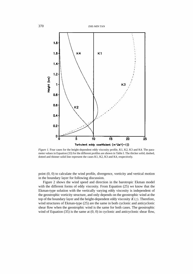
K = K0(1+ δz)e−δz/(1+δzm), (33)

whereK0 is the eddy viscosity at the surface,δ is a constant andzm is the levelwhere∂K/∂z = 0.

Figure 1 shows the four types of eddy viscosity profiles. In Figure 1, case K1represents constant eddy viscosity, in case K2 eddy viscosity decreases with height,while in case K3 it generally increases. Case K4 has a mid-layer peak in the eddyviscosity profile that is similar to that shown by O’Brien (1970). The parametersused in Equation (33) for Figure 1 are presented in Table I.

The baroclinic pressure field is assumed to be of the form

ug = ug0+ usz; vg = vg0+ vsz, (34)

whereus andvs are constants. The surface geostrophic wind is given by

ug0 = u0− αy; vg0 = 0, (35)

where,α is a constant.α > 0 represents cyclonic shear flow, andα < 0 denotesanticyclonic shear flow. Consequently, the surface geostrophic vorticityςg0 = α.In the present work, we assume thatus = ±0.004 s−1, vs = 0. us > 0 denotes thegeostrophic wind increasing with height, whereasus < 0 has the geostrophic winddecreasing with height. We setu0 = 20 m s−1, α = ±0.8f for the cyclonic andanticyclonic shear flow respectively andf = 10−4 s−1. Moreover, we select the

370 ZHE-MIN TAN

Figure 1.Four cases for the height-dependent eddy viscosity profile, K1, K2, K3 and K4. The para-meter values in Equation (33) for the different profiles are shown in Table I. The thicker solid, dashed,dotted and thinner solid line represent the cases K1, K2, K3 and K4, respectively.

point (0, 0) to calculate the wind profile, divergence, vorticity and vertical motionin the boundary layer for following discussion.

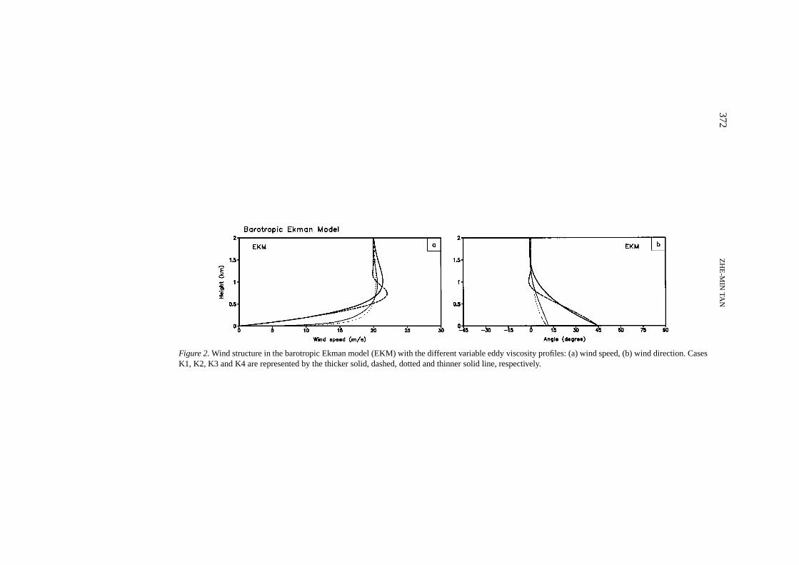
Figure 2 shows the wind speed and direction in the barotropic Ekman modelwith the different forms of eddy viscosity. From Equation (25) we know that theEkman-type solution with the vertically varying eddy viscosity is independent ofthe geostrophic vorticity structure, and only depends on the geostrophic wind at thetop of the boundary layer and the height-dependent eddy viscosityK(z). Therefore,wind structures of Ekman-type (25) are the same in both cyclonic and anticyclonicshear flow when the geostrophic wind is the same for both cases. The geostrophicwind of Equation (35) is the same at (0, 0) in cyclonic and anticyclonic shear flow,

AN APPROXIMATE ANALYTICAL SOLUTION 371

TABLE II

Wind speed (1V800) and direction (1δ800) differences between thecase K2 and the case K3 at the height of 800 m in the barotropicEkman model and the semi-geostrophic Ekman boundary-layer model(SGM).

Ekman model SGM (anticyclonic) SGM (Cyclonic)

1V800 (m/s) 1.60 3.96 1.05

1δ800 (degree) 0.76 19.28 0.63

thus the Ekman-type solution (25) shown in Figure 2 is the same in cyclonic andanticyclonic shear flow at (0, 0) for case (35).

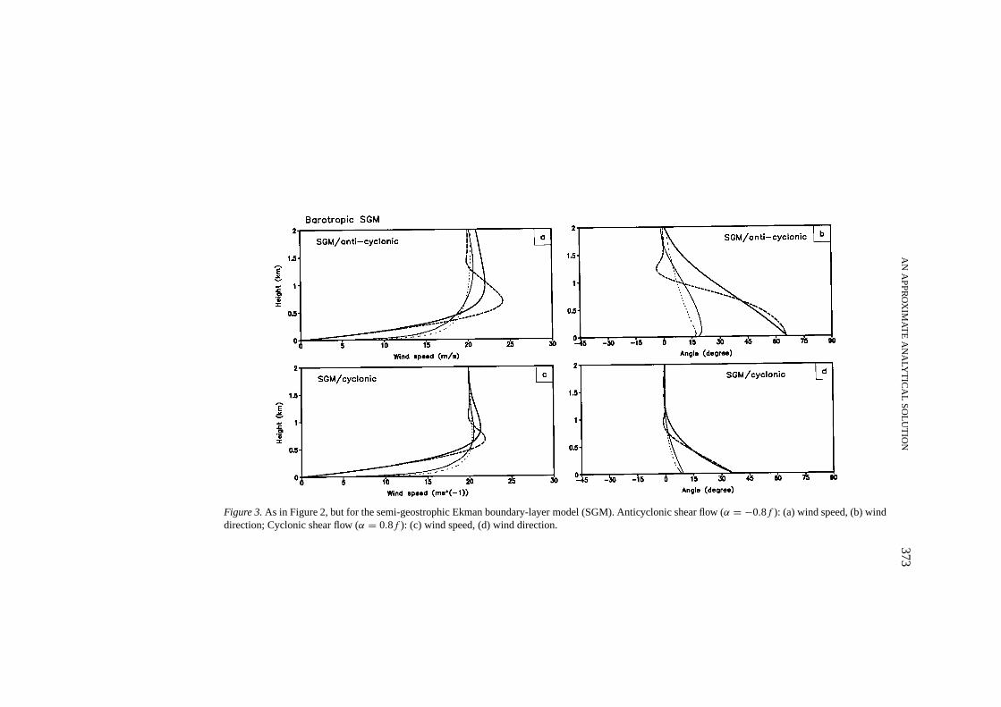
The anticyclonic and cyclonic boundary-layer wind structure in the barotropicsemi-geostrophic Ekman model are shown in Figures 3c–f, respectively. From Fig-ures 3 and 2, we know that the different vertical variable eddy viscosity for a givenbarotropic pressure gradient results in an altered boundary-layer wind structure.However, in all cases in the Ekman dynamics (Figure 2) or in the SGM (Figure 3),the wind speed and direction profiles for the constant eddy viscosity case (case K1)has a similar feature to that in case K2 with K decreasing with height. Moreover,the cases where the eddy viscosity initially increases with height (cases K3 and K4)appear to show similar behavior. From Equations (22) or (25), it is evident that thewind structure in the Ekman model or SGM is primarily dependent on the characterof the eddy viscosity profile for the given geostrophic wind field. Both case K1 andcase K2 have similar boundary-layer functionsQ1(x, y, z) andQ2(x, y, z) thatresult in a similar feature in the wind structure for both cases.

In comparison with Ekman dynamics (Figure 2a), the differences in wind speedcaused by the variable eddy viscosity is enhanced in the anticyclonic shear flow(Figure 3a) and slightly weakened in the cyclonic shear flow (Figure 3c). Table IIshows the wind speed and direction differences between case K2 and K3 at theheight of 800 m, which is near to the maximum wind speed height for these casesin the Ekman model and the SGM.

From Figure 3a, c, it may be noted that the wind speeds in the barotropic SGMdepend on the interaction between the inertial acceleration terms and variable eddyviscosity. Comparison of Figure 3a,c with Figure 2a illustrates that the influence ofvorticity structure on the boundary-layer wind speed for the different eddy viscosityprofiles appears to be similar. The wind speed is larger in the anticyclonic shearflow and smaller in the cyclonic shear flow than that in the Ekman model for a givenvariable eddy viscosity, which is similar to that in the constant-K semi-geostrophicEkman boundary-layer model (Wu and Blumen, 1982).

From Figures 2a, 3a, c, we know that decreasing eddy viscosity with height(case K2) produces a super-geostrophic peak in the wind speed profiles, however

372Z

HE

-MIN

TAN

Figure 2.Wind structure in the barotropic Ekman model (EKM) with the different variable eddy viscosity profiles: (a) wind speed, (b) wind direction. CasesK1, K2, K3 and K4 are represented by the thicker solid, dashed, dotted and thinner solid line, respectively.

AN

AP

PR

OX

IMA

TE

AN

ALY

TIC

AL

SO

LUT

ION

373

Figure 3.As in Figure 2, but for the semi-geostrophic Ekman boundary-layer model (SGM). Anticyclonic shear flow (α = −0.8f ): (a) wind speed, (b) winddirection; Cyclonic shear flow (α = 0.8f ): (c) wind speed, (d) wind direction.

374 ZHE-MIN TAN

the peak is reduced in the cases for eddy viscosity increasing initially with height(Case K3 and K4). In comparison with the Ekman model case (Figure 2a), theanticyclonic shear in the SGM tends to intensify the super-geostrophic peak, andleads to a low-level jet structure (Figure 3a), while the cyclonic shear lessens thepeak (Figure 3c).

Eddy viscosity initially increasing with height (cases K3 and K4) may lead toa smaller angle between the wind direction and x-axis at the surface than that inthe constant or decreasing with the height eddy viscosity cases (cases K1 and K2)(Figures 2b, 3b, d). However, the influence of vorticity structure may produce alarger wind angle in the anticyclonic shear flow (Figure 3b) and a smaller windangle in the cyclonic shear flow (Figure 3d). It is evident that the geostrophicvorticity structure has a dominant effect on the boundary-layer wind structure inthe case of eddy viscosity decreasing with height.

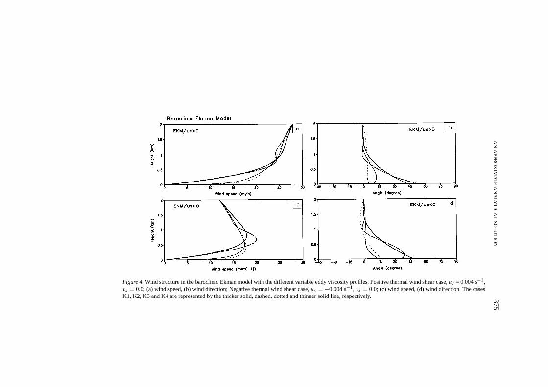
Figures 4a–d, show the wind speed and direction in the baroclinic Ekman layerfor horizontal pressure gradient increasing with height, i.e.,us > 0, and for hori-zontal pressure gradient decreasing with height, i.e.,us < 0, respectively. Figure4a illustrates that the increasing of horizontal pressure gradient with height resultsin a smaller difference in the wind speed profile produced by the different variableeddy viscosity profiles, and removes the super-geostrophic peak in the wind profilethat occurs in the barotropic Ekman model (Figure 2a). However, the decreasing ofhorizontal pressure gradient with height leads to a stronger super-geostrophic peakin the wind speed profile for case K2 (Figure 4c). These features are similar tothose found in Berger and Grisogono (1998). From Figures 4b, d, it is evident thatthe pressure gradient increasing with height produces a surface wind direction de-creasing (increasing) with height for cases K1, K3 and K4, however, an increasing(decreasing) surface wind direction with the height for case K2.

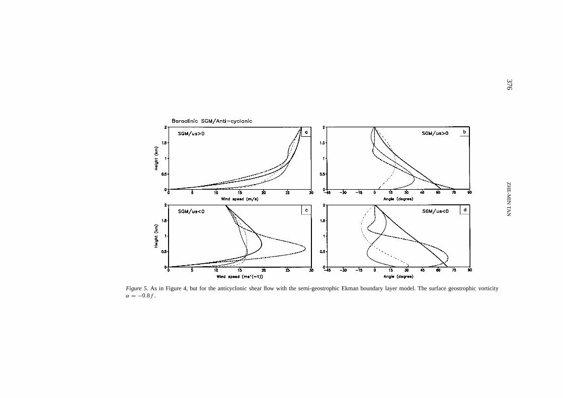
The wind speed profile and direction in the baroclinic SGM for anticyclonicshear flow are shown in Figure 5. Comparison of Figure 5 with Figure 4 shows thatthe effect of inertial acceleration on the wind structure in the baroclinic cases issimilar to that in the barotropic cases. The anticyclonic shear results in an increaseof wind speed and wind angle (Figure 5a, b). In Figure 5c, the super-geostrophicpeak in the wind profiles that occurs in the baroclinic Ekman model (see Figure 4c)may be heightened evidently by the inertial acceleration in the anticyclonic flow,and results in an apparent low-level jet structure. However, the cyclonic shear leadsto a decreasing of wind direction at the surface, especially in K1 and K2 cases, buthas no prominent influence on the wind speed (not shown).

Based on the above analysis, we can conclude that the super-geostrophic peakin the wind profile is most pronounced in the cases of decreasing eddy viscositywith height (case K2), anticyclonic shear flow and geostrophic wind decreasingwith height.

AN

AP

PR

OX

IMA

TE

AN

ALY

TIC

AL

SO

LUT

ION

375

Figure 4.Wind structure in the baroclinic Ekman model with the different variable eddy viscosity profiles. Positive thermal wind shear case,us = 0.004 s−1,νs = 0.0; (a) wind speed, (b) wind direction; Negative thermal wind shear case,us = −0.004 s−1, νs = 0.0; (c) wind speed, (d) wind direction. The casesK1, K2, K3 and K4 are represented by the thicker solid, dashed, dotted and thinner solid line, respectively.

376Z

HE

-MIN

TAN

Figure 5. As in Figure 4, but for the anticyclonic shear flow with the semi-geostrophic Ekman boundary layer model. The surface geostrophic vorticityα = −0.8f .

AN APPROXIMATE ANALYTICAL SOLUTION 377

5. Divergence, Vorticity and Vertical Motion in the Boundary Layer

In this section, the effect of variable eddy diffusivity and inertial acceleration onthe divergence, vorticity and vertical motion in the barotropic boundary layer areexamined. The convergence of ageostrophic boundary-layer flow induces risingmotion at the top of the boundary layer, called Ekman pumping (Holton, 1992), thatproduces an important dynamic coupling of the boundary layer to the large-scaleflow.

With Equation (22), the horizontal divergence (ξ ) and vertical component ofvorticity (ς ) in the barotropic SGM may be expressed as

ξ = ∂u

∂x+ ∂v∂y

= Q1∇h · vT −Q2∇h · cT + R1vT · ∇hD − R2cT · ∇hD,(36)

and

ς = ∂v

∂x− ∂u∂y

= Q1z · ∇ × vT −Q2z · ∇ × cT + R1(z× vT · ∇D)− R2(z× cT · ∇D)(37)

respectively, where

vT = (ut , vT ),cT = (c1D

−2, c2D−2),

∇ = ∇h + z∂

∂z,

∇h = x∂

∂x+ y

∂

∂y,

x, y and z are the unit vectors inx-, y- and z-directions, respectively. ThecoefficientsQ1(x, y, z), Q2(x, y, z) are shown in Equation (23) andR1(x, y, z),R2(x, y, z) are defined as

R1(x, y, z) = A(z)e−F(x,y,z) cos(F(x, y, z) − π

4

) ∫ z

0K−1/2(ς)dς,

R2(x, y, z) = A(z)e−F(x,y,z) cos(F(x, y, z) + π

4

) ∫ z

0K−1/2(ς) dς.

(38)

The vertical motion at the top of the boundary layer may be determined by integ-ration of the continuity Equation (3). Substitution of Equation (22) into Equation(3) yields

wT = −∫ ∞

0

(∂u

∂x+ ∂v∂y

)dz

378 ZHE-MIN TAN

= −∇h · vT

∫ ∞0Q1(x, y, z)dz +∇h · cT

∫ ∞0Q2(x, y, z)dz (39)

− vT · ∇hD∫ ∞

0R1(x, y, z)dz + cT · ∇hD

∫ ∞0R2(x, y, z)dz,

where we have assumed thatw(0) = 0.From Equations (36), (37) and (39) we know that there are four different con-

tributions to the horizontal divergence, vertical vorticity and vertical motion in thebarotropic boundary layer. The first part is the horizontal divergence or verticalvorticity produced by the semi-geostrophic wind at the top of the boundary layervT . The second part is the horizontal divergence or vertical vorticity produced bythe cross isobar windcT that is induced by boundary-layer friction. The third partis the advection of vorticity associated with the windvT , sinceD is related to theGM vertical vorticity ςGM as shown in Section 2. The fourth part is the vorticityadvection associated with the cross isobar windcT .

For Ekman dynamics, the effect of inertial acceleration terms with the GM isneglected, and the horizontal divergenceξ in (36), vertical component of vorticityς in Equation (37) and the vertical motion at the top of the boundary layerwT inEquation (39) can be simplified to

ξE = −ςgA(z)e−FE(z) sinFE(z), (40)

ς = ςg(1− A(z)e−FEz cosFE(z)), (41)

and

wTE = ςg∫ ∞

0A(z)e−FE(z) sinFE(z) dz, (42)

where

ς = ∂vg

∂x− ∂ug∂y

is the geostrophic vorticity, and

FE(x, y, z) =(f

2

)1/2 ∫ z

0K−1/2(ζ ) dζ.

For the specified barotropic case of Equations (35)–(37) may be expressed as

ξs = − ςg0√1+ ςg0

f

A(z)e−F(x,y,z) sinFs(x, y, z) (43)

AN APPROXIMATE ANALYTICAL SOLUTION 379

and

ςs = ςg0[1− A(z)e−Fs(x,y,z) cosFs(x, y, z)], (44)

respectively. where

Fs(x, y, z) =(f

2

)1/2(1+ ςg0

f

)1/4 ∫ z

0K−1/2(ζ ) dζ (45)

andςg0 = α is the surface geostrophic vorticity.The distribution of horizontal divergence with height in the barotropic Ekman

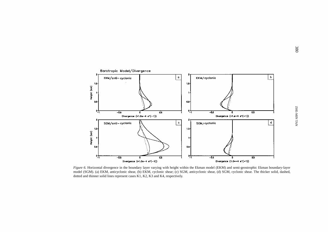
model and SGM are shown in Figure 6. In comparison with the constant eddyviscosity case, case K2 leads to an increasing divergence below 500 m, but a de-creasing divergence above 500 m. Moreover, the initially increasing eddy viscositywith height (case K3 and K4) results in a decreasing horizontal divergence in thewhole boundary layer compared with the constant-K case. Figure 6c indicates thatthe effects of inertial acceleration increase the boundary-layer horizontal diver-gence in the anticyclonic shear flow, and also enhance the difference of horizontaldivergence caused by the different eddy viscosity profiles, although, decreasingthe horizontal divergence and the difference in the cyclonic shear flow (Figure 6d).Comparison of Equation (43) with Equation (40) illustrates that the influence ofinertial acceleration on the horizontal divergence in the SGM relies on the factorof ςg0/f . In the anticyclonic shear flow, the geostrophic vorticityςg0 is negative;this enlarges the absolute value ofςg0/

√1+ ςg0/f and opposes the decrease with

height of the horizontal divergence in Equation (43). Therefore, the magnitude andheight of the maximum horizontal divergence is increased in anticyclonic shearcompared with that in the Ekman model.

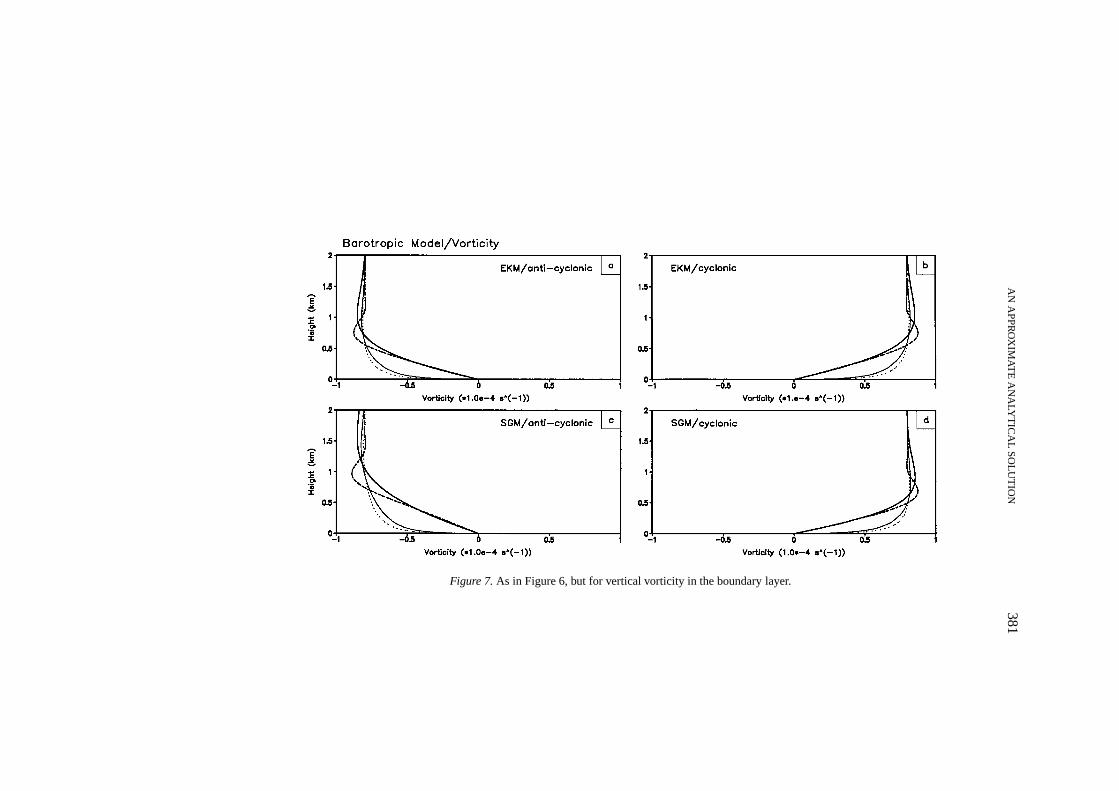
Figure 7 shows the vertical distribution of vertical vorticity in the barotropicEkman and SGM. The initially increasing eddy viscosity (case K3 and K4) resultsin a decreasing vertical vorticity in the whole boundary layer compared with theconstant-K case. The varying of vertical vorticity with height in the boundary layermay be exacerbated in the anticyclonic shear flow (Figure 7c). These features inthe cyclonic shear flow are opposite (Figure 7d).

With Equation (39) for the specified case (35), the vertical motion at the top ofthe boundary layer within the SGM is given as

wT s = ςg0√1+ ςg0

f

∫ ∞0A(z)e−Fs(x,y,z) sinFs(x, y, z)dz. (46)

For the constant-K case, Equation (46) may be simplified further to

wT s =√K

2fςg0

(1+ ςg0

f

)−3/4

. (47)

380Z

HE

-MIN

TAN

Figure 6.Horizontal divergence in the boundary layer varying with height within the Ekman model (EKM) and semi-geostrophic Ekman boundary-layermodel (SGM). (a) EKM, anticyclonic shear, (b) EKM, cyclonic shear; (c) SGM, anticyclonic shear, (d) SGM, cyclonic shear. The thicker solid, dashed,dotted and thinner solid lines represent cases K1, K2, K3 and K4, respectively.

AN

AP

PR

OX

IMA

TE

AN

ALY

TIC

AL

SO

LUT

ION

381

Figure 7.As in Figure 6, but for vertical vorticity in the boundary layer.

382 ZHE-MIN TAN

Similar to the feature of horizontal divergence in the SGM, the vertical motion atthe top of the boundary layer in the SGM for case (35) is also related not only tothe geostrophic vorticityςg0, but also to the factor ofςg0/f . If the effect of inertialaccelerations terms that is associated withσg0/f is neglected, Equation (46) may bereduced to the Ekman dynamic solution (42), and Equation (47) may be simplifiedto classical Ekman pumping (Holton, 1992):

wTE =√K

2fςg0. (48)

Figure 8 shows the vertical velocity at the top of the boundary layer varying withthe geostrophic vorticity for the different height-dependent eddy viscosity profilesin the barotropic Ekman model. In the Ekman dynamics the Ekman pumping, asshown in Equation (42), depends linearly on the geostrophic vorticity and the eddyviscosity. Comparison with the constant-K case (Case K1), the variable eddy vis-cosity with height results from a decreasing absolute value of vertical motion at thetop of the boundary layer. Moreover, the vertical motion at the top of the boundarylayer is larger for the eddy viscosity decreasing with height case (Case K2) thanthat for the eddy viscosity increasing with height (Cases K3 and K4).

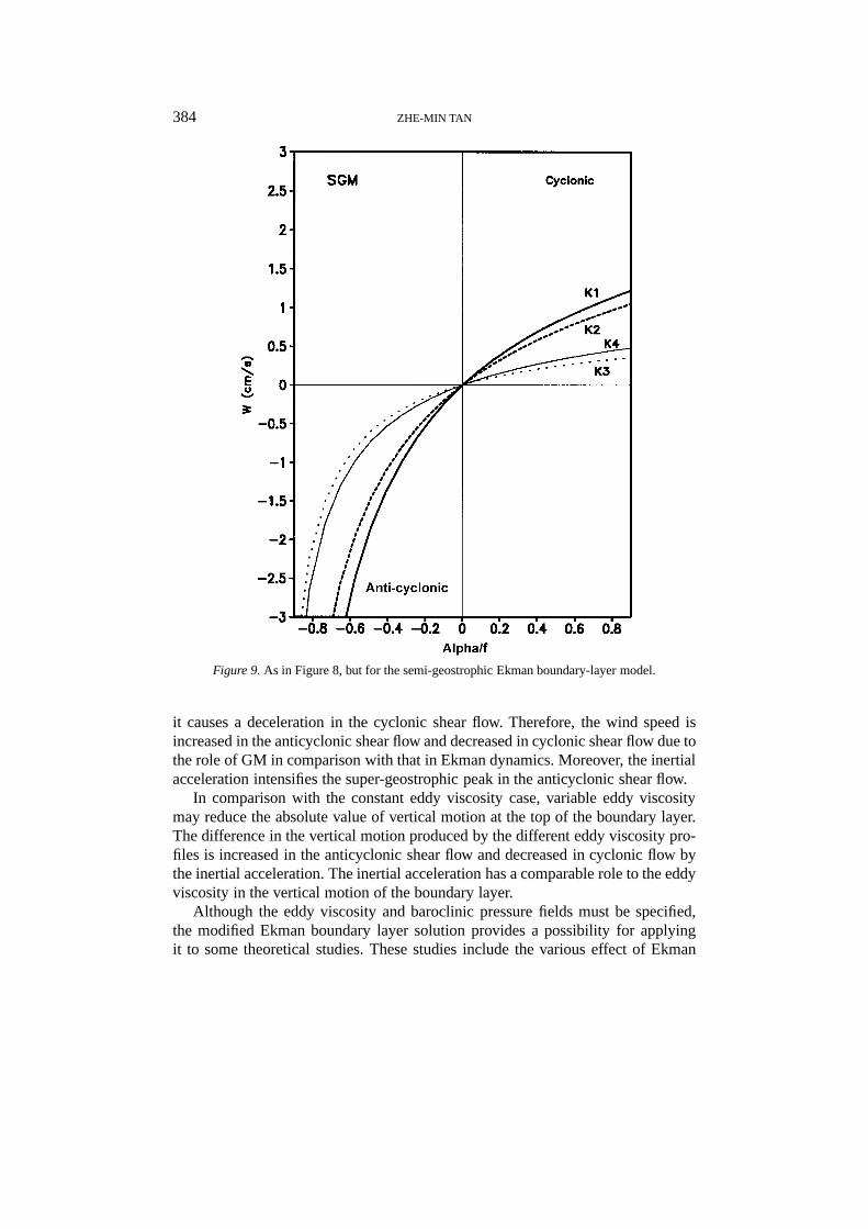
The vertical motions at the top of the boundary layer vary with the geostrophicvorticity in the barotropic SGM are shown in Figure 9. Comparison of Figure 9with Figure 8 shows that the effect of inertial acceleration increases the absolutevalue of Ekman pumping in the anticyclonic shear flow for a given eddy viscosity.However, it decreases the vertical motion in the cyclonic shear flow comparisonwith that in the Ekman model. The feature is similar to the constant-K SGM casein WB82. However, the difference in the vertical motion resulting from the differ-ent variable eddy viscosity is strengthened in the anticyclonic flow, and weakenedin the cyclonic shear flow comparisons with that in the Ekman model. Also thedistinctions between vertical velocity with and without consideration of inertialacceleration are comparable to those caused by different eddy viscosity profiles.We can conclude that the inertial acceleration, the same as the eddy viscosity, hasan important role in the boundary-layer vertical motion.

6. Conclusion

An approximate solution to the semi-geostrophic Ekman boundary layer that in-cludes the effect of variable eddy viscosity, inertial acceleration and a baroclinicpressure field has been developed by using the WKB method. The approximateanalytical solution is an extension of Wu and Blumen’s (1982) solution to includethe variable eddy diffusivity and a baroclinic pressure field, as well as of Griso-gono’s (1995) solution to include the inertial acceleration effect. However, themodified solution retains the simple form that is similar to the classical Ekman

AN APPROXIMATE ANALYTICAL SOLUTION 383

Figure 8. Vertical motion at the top of the boundary layer as a function of the nondimensionalgeostrophic vorticity (α/f ) for the different eddy viscosity in the barotropic Ekman layer model.Cases K1, K2, K3 and K4 represented by the thicker solid, dashed, dotted and thinner solid lines,respectively.

solution, and is also only valid in the slowly varying eddy diffusivity and thesemi-geostrophic dynamic framework.

For a given height-dependent pressure gradient, decreasing eddy viscosity withheight tends to establish a super-geostrophic peak in the wind profile, while eddyviscosity initial increasing with the height reduces the peak. For a given variableeddy diffusivity, increasing horizontal pressure gradient with height tends to re-move the super-geostrophic peak in the wind profile, while decreasing horizontalpressure gradient with height accentuates the peak.

In semi-geostrophic Ekman dynamics, the inertial acceleration has an acceler-ation effect on the boundary-layer wind in the anticyclonic shear flow, whereas

384 ZHE-MIN TAN

Figure 9.As in Figure 8, but for the semi-geostrophic Ekman boundary-layer model.

it causes a deceleration in the cyclonic shear flow. Therefore, the wind speed isincreased in the anticyclonic shear flow and decreased in cyclonic shear flow due tothe role of GM in comparison with that in Ekman dynamics. Moreover, the inertialacceleration intensifies the super-geostrophic peak in the anticyclonic shear flow.

In comparison with the constant eddy viscosity case, variable eddy viscositymay reduce the absolute value of vertical motion at the top of the boundary layer.The difference in the vertical motion produced by the different eddy viscosity pro-files is increased in the anticyclonic shear flow and decreased in cyclonic flow bythe inertial acceleration. The inertial acceleration has a comparable role to the eddyviscosity in the vertical motion of the boundary layer.

Although the eddy viscosity and baroclinic pressure fields must be specified,the modified Ekman boundary layer solution provides a possibility for applyingit to some theoretical studies. These studies include the various effect of Ekman

AN APPROXIMATE ANALYTICAL SOLUTION 385

pumping, baroclinic Eady wave development, low-level frontogenesis, and/or theestimating of boundary-layer wind structure. Also it can be used as a benchmarkfor the numerical solutions of the PBL.

Acknowledgements

This work was supported by the State Key Basic Research Program: Researchon the Formation Mechanism and Predication Theory of Hazardous Weather overChina (CHERES) and the National Natural Science Foundation of China underGrant 49605064 and 49735180. The author benefited from helpful discussions withProfs. Rong-Sheng Wu, Yuan Wang and from anonymous reviews.

References

Bannon, P. R. and Salfm, T. L.: 1995, ’Aspects of Baroclinic Boundary Layer’,J. Atmos. Sci.52,574–596.

Bender, C. M. and Orszag. S. A.: 1970,Advanced Mathematical Methods for Scientists andEngineers, McGraw-Hill, New York, 593 pp.

Berger, B. W. and Grisogono, B.: 1998, ’The Baroclinic, Variable Eddy Viscosity Ekman Layer: AnApproximate Analytical Solution’,Boundary-Layer Meteorol.87, 363–380.

Blumen, W. and Wu, R.: 1983, ’Baroclinic Instability and Frontogenesis with Ekman BoundaryLayer Dynamics Incorporating the Geostrophic Momentum Approximation’,J. Atmos. Sci.40,2630–2637.

Grisogono, B.: 1995, ’A Generalized Ekman Layer Profile with Gradually Varying Eddy Diffusivit-ies’, Quart. J. Roy. Meteorol. Soc.121, 445–453.

Holton, J. R.: 1992,An Introduction to Dynamic Meteorology, Academic Press, San Diego, 570 pp.Hoskins, B. J.: 1975, ’The Geostrophic Momentum Approximation and the Semi-geostrophic

Equations’,J. Atmos. Sci.32, 233–242.Levy, G.: 1989, ’Surface Dynamics of Observed Maritime Fronts’,J. Atmos. Sci.46, 1219–1232.Miles, J.: 1994, ’Analytical Solutions for the Ekman Layer’,Boundary-Layer Meteorol.67, 1–10.O’Brien, J. J.: 1970, ’A Note on the Vertical Structure of the Eddy Exchange Coefficient in the

Planetary Boundary Layer’,J. Atmos. Sci.27, 1213–1215.Panchev, S.: 1985,Dynamic Meteorology, D. Reidel, Dordrecht, 360 pp.Panchev, S. and Spassova, T. S.: 1987, ’A Barotropic Model of the Ekman Planetary Boundary Based

on the Geostrophic Momentum Approximation’,Boundary-Layer Meteorol.40, 339–347.Snyder, C., Skamaroch, W. C., and Rotunno, R.: 1993, ’Frontal Dynamics Near and Following

Frontal Collapse’,J. Atmos. Sci.50, 3194–3211.Tan, Z.-M. and Farahani, M. M.: 1998, ’An Analytical Study of the Diurnal Variations of Wind in a

Semi-Geostrophic Ekman Boundary Layer Model’,Boundary-Layer Meteorol.86, 313–332.Wu, R. and Blumen W.: 1982, ’An Analysis of Ekman Boundary Layer Dynamics Incorporating the

Geostrophic Momentum Approximation’,J. Atmos. Sci.39, 1774–1782.