From Spatial to Subject Marker 1 Oblique Subjects in Urdu/Hindi

J. Fluid Mech. (2003), vol. 487, pp. 91–123. c© 2003 Cambridge University Press
DOI: 10.1017/S0022112003004622 Printed in the United Kingdom91
The onset of thermal convection inEkman–Couette shear flow with oblique rotation
By Y. PONTY1, A. D. GILBERT2 AND A. M. SOWARD2
1Observatoire de la Cote d’Azur – Nice, Laboratoire Cassini – CNRS UMR 6529,BP 4229, 06304 Nice Cedex 4, France
2School of Mathematical Sciences, University of Exeter, Exeter EX4 4QE, UK
(Received 17 June 2002 and in revised form 27 November 2002)
The onset of convection of a Boussinesq fluid in a horizontal plane layer is studied.The system rotates with constant angular velocity ΩΩΩ , which is inclined at an angleϑ to the vertical. The layer is sheared by keeping the upper boundary fixed, whilethe lower boundary moves parallel to itself with constant velocity U0 normal to theplane containing the rotation vector and gravity g (i.e. U0 ‖ g ×ΩΩΩ). The system ischaracterized by five dimensionless parameters: the Rayleigh number Ra, the Taylornumber τ 2, the Reynolds number Re (based on U0), the Prandtl number Pr and theangle ϑ . The basic equilibrium state consists of a linear temperature profile and anEkman–Couette flow, both dependent only on the vertical coordinate z. Our linearstability study involves determining the critical Rayleigh number Rac as a functionof τ and Re for representative values of ϑ and Pr.
Our main results relate to the case of large Reynolds number, for which there isthe possibility of hydrodynamic instability. When the rotation is vertical ϑ = 0 andτ 1, so-called type I and type II Ekman layer instabilities are possible. With theinclusion of buoyancy Ra = 0 mode competition occurs. On increasing τ from zero,with fixed large Re, we identify four types of mode: a convective mode stabilized bythe strong shear for moderate τ , hydrodynamic type I and II modes either assisted(Ra > 0) or suppressed (Ra < 0) by buoyancy forces at numerically large τ , anda convective mode for very large τ that is largely uninfluenced by the thin Ekmanshear layer, except in that it provides a selection mechanism for roll orientation whichwould otherwise be arbitrary. Significantly, in the case of oblique rotation ϑ = 0, thesymmetry associated with U0 ↔ −U0 for the vertical rotation is broken and so thecases of positive and negative Re exhibit distinct stability characteristics, which weconsider separately. Detailed numerical results were obtained for the representativecase ϑ = π/4. Though the overall features of the stability results are broadly similarto the case of vertical rotation, their detailed structure possesses a surprising varietyof subtle differences.
1. IntroductionThermal convection and shear flow instability are pervading themes in fluid dynamic
stability theory. The additional influence of rotation is a key ingredient in the studyof astrophysical and geophysical fluid motion. There has been considerable progressmade in our understanding of both the onset of convection via linear instabilityand the ensuing finite-amplitude convection. Though many of the ingredients

92 Y. Ponty, A. D. Gilbert and A. M. Soward
mentioned – rotation, shear and thermal gradients – have been studied in isolationor in particular combinations, there has been no comprehensive investigation of evenlinear stability with all possible combinations of the many dimensionless parametersthat characterize such a system. Our present linear investigation is motivated by ourdynamo models (Ponty, Gilbert & Soward 2001a, b) which build upon the resultsthat we present here. These dynamo studies relate to magnetic field generation in thetachocline of the Sun and we will expand on the geometry below. It is sufficient tonote here that our work certainly does not encompass all basic configurations butdoes build upon, link and extend extensive earlier results.
We begin by reviewing the basic ideas related to the stability of fluid confinedbetween two parallel planes of infinite horizontal extent. In the absence of shear androtation, static Boussinesq fluid heated from below and subject to a linear adversetemperature gradient becomes unstable to small perturbations when the Rayleighnumber Ra exceeds some critical value Rac0. Onset of convection is characterized bysteady convective rolls. Their orientation is identified by a horizontal wave vector knormal to the roll axis. In view of the rotational symmetry of the system about thevertical, the direction of k is arbitrary. Nevertheless, with the addition of shear orinclined rotation this isotropy is broken and a preferred roll orientation emerges.
In the absence of rotation, a unidirectional shear flow may be generated either bymoving the rigid boundaries parallel to themselves (plane Couette flow with a linearprofile) or by keeping the boundaries fixed and applying a constant pressure gradient(plane Poiseuille flow with a parabolic profile), or a combination of both. Withoutbuoyancy forces plane Couette flow is always stable in the linear approximation,whereas when the Reynolds number Re is sufficiently large, plane Poiseuille flowbecomes unstable to travelling transverse rolls (Tollmien–Schlicting waves) with theirwave vector aligned with the mean flow. With the addition of buoyancy, as describedin the classical Rayleigh–Benard problem above, the preferred mode for Poiseuille flowis purely convective for small Re. It takes the form of longitudinal rolls which do notinteract with the shear and occur when the Rayleigh number takes the critical valueRac0 mentioned above. The anisotropy introduced by the shear only selects the rollorientation for convection. Nevertheless, once Re reaches a value close to the valuefor pure hydrodynamic instability for which Rac = 0, the transverse rolls of Tollmien–Schlicting type take over (see e.g. Gage & Reid 1968). Longitudinal convective rollsare appropriate to the corresponding Couette flow problem at all values of Re (seee.g. Ingersoll 1965; Clever, Busse & Kelly 1977). Various developments of this themeare discussed in the review article of Kelly (1994).
With the addition of rotation, measured by the Taylor number τ 2, the situationbecomes more complicated. Kropp & Busse (1991) considered thermal convection inplane Couette flow with rotation horizontal and transverse to the shear. Two typesof mode can be distinguished. On the one hand, hydrodynamic instability of theplane Couette flow is manifested as Taylor vortices which are longitudinal rolls.On the other, transverse rolls are driven by buoyancy forces as would occur in theabsence of shear. Since they do not vary in the direction of the rotation vector, theyare unaffected by the Coriolis force and so occur when the Rayleigh number takes thecritical value Rac0 mentioned above. Once all these ingredients occur simultaneously,the longitudinal and transverse rolls compete with each other. Which of the two ispreferred is clearly mapped out by Kropp & Busse (1991) in their figure 2. It is alsoimportant to note that the critical Rayleigh number has a complicated dependenceon τ and Re. That work embraces an important special case of the geometry that weinvestigate.
Thermal convection in Ekman–Couette shear flow with oblique rotation 93
We remark briefly on other closely related orientations of the rotation vector ΩΩΩ thatonly loosely impinge on our investigations. Busse & Kropp (1992) considered the caseof aligned horizontal rotation and shear, and found that, paradoxically, buoyantlydriven oblique rolls are sometimes preferred. Matthews & Cox (1997) extended thesestudies by allowing an arbitrary angle between the horizontal rotation vector andthe linear shear flow. They studied the roll orientation as a function of this angleand used arguments based on winding numbers to determine the dominant drivingmechanism for the rolls, shear or convection, in certain parameter ranges.
When the rotation vector has a vertical component ΩΩΩv , a shear flow driven by ahorizontal pressure gradient or by moving rigid boundaries is no longer unidirectional.Indeed in the limit of strong rotation τ 1, the flow is confined to Ekman boundarylayers which are characterized by Ekman spirals. In addition to the pure hydrodynamicinstabilities associated with this spiralling flow, this extra structure also complicatesthe convective instability.
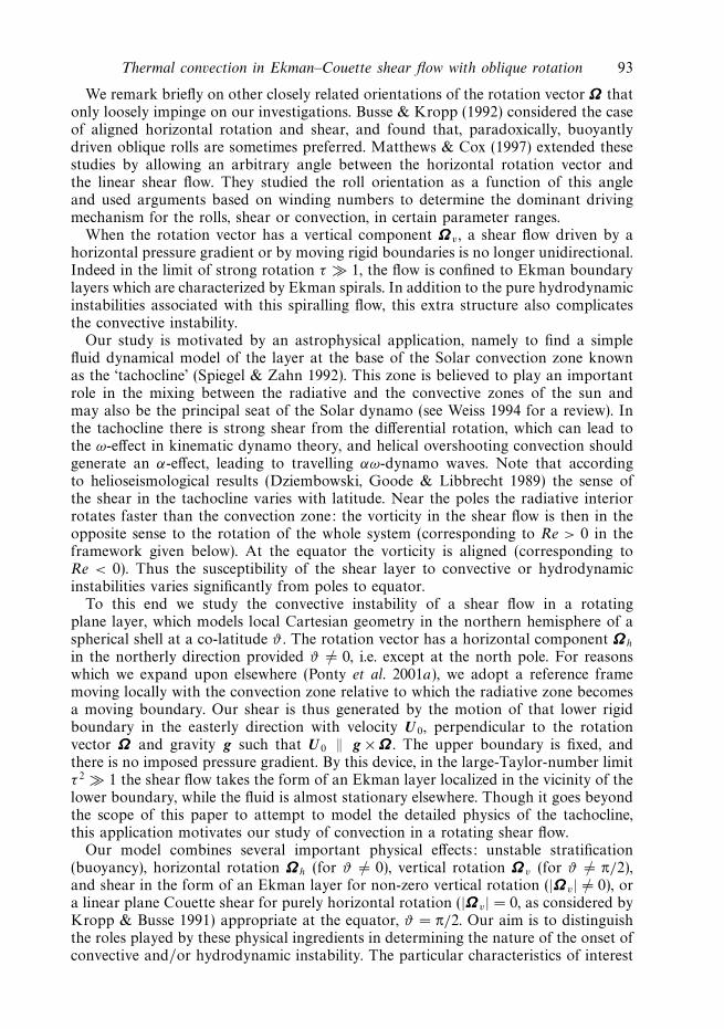
Our study is motivated by an astrophysical application, namely to find a simplefluid dynamical model of the layer at the base of the Solar convection zone knownas the ‘tachocline’ (Spiegel & Zahn 1992). This zone is believed to play an importantrole in the mixing between the radiative and the convective zones of the sun andmay also be the principal seat of the Solar dynamo (see Weiss 1994 for a review). Inthe tachocline there is strong shear from the differential rotation, which can lead tothe ω-effect in kinematic dynamo theory, and helical overshooting convection shouldgenerate an α-effect, leading to travelling αω-dynamo waves. Note that accordingto helioseismological results (Dziembowski, Goode & Libbrecht 1989) the sense ofthe shear in the tachocline varies with latitude. Near the poles the radiative interiorrotates faster than the convection zone: the vorticity in the shear flow is then in theopposite sense to the rotation of the whole system (corresponding to Re > 0 in theframework given below). At the equator the vorticity is aligned (corresponding toRe < 0). Thus the susceptibility of the shear layer to convective or hydrodynamicinstabilities varies significantly from poles to equator.
To this end we study the convective instability of a shear flow in a rotatingplane layer, which models local Cartesian geometry in the northern hemisphere of aspherical shell at a co-latitude ϑ . The rotation vector has a horizontal component ΩΩΩh
in the northerly direction provided ϑ = 0, i.e. except at the north pole. For reasonswhich we expand upon elsewhere (Ponty et al. 2001a), we adopt a reference framemoving locally with the convection zone relative to which the radiative zone becomesa moving boundary. Our shear is thus generated by the motion of that lower rigidboundary in the easterly direction with velocity U0, perpendicular to the rotationvector ΩΩΩ and gravity g such that U0 ‖ g ×ΩΩΩ . The upper boundary is fixed, andthere is no imposed pressure gradient. By this device, in the large-Taylor-number limitτ 2 1 the shear flow takes the form of an Ekman layer localized in the vicinity of thelower boundary, while the fluid is almost stationary elsewhere. Though it goes beyondthe scope of this paper to attempt to model the detailed physics of the tachocline,this application motivates our study of convection in a rotating shear flow.
Our model combines several important physical effects: unstable stratification(buoyancy), horizontal rotation ΩΩΩh (for ϑ = 0), vertical rotation ΩΩΩv (for ϑ = π/2),and shear in the form of an Ekman layer for non-zero vertical rotation (|ΩΩΩv| = 0), ora linear plane Couette shear for purely horizontal rotation (|ΩΩΩv| = 0, as considered byKropp & Busse 1991) appropriate at the equator, ϑ = π/2. Our aim is to distinguishthe roles played by these physical ingredients in determining the nature of the onset ofconvective and/or hydrodynamic instability. The particular characteristics of interest

94 Y. Ponty, A. D. Gilbert and A. M. Soward
are the critical values of wavenumber |kc|, the orientation of the convective roll axisg × kc, the frequency ωc and Rayleigh number Rac for the onset of instability. Thoughwe only explore linear stability, this is a necessary first step before considering theweakly and strongly nonlinear regimes. Indeed the results presented here form thebasis of the kinematic dynamo calculations undertaken by Ponty et al. (2001a).
A study of hydrodynamic instabilities (zero Rayleigh number: Ra = 0) in a rotatinglayer with velocities ∓U0/2 imposed on the top and bottom surfaces was initiatedby Hoffman, Busse & Chen (1998), who considered the case of vertical rotation(|ΩΩΩh| = 0) appropriate at the north pole ϑ = 0. Unlike our problem the basic flowhas an Ekman layer at both the top and bottom boundaries in the large rotationlimit, whereas we have just an Ekman layer at the bottom boundary, which carriesa net Ekman flux. These distinct flows arise because the pressure gradient is notGalilean invariant in a rotating reference frame, as discussed further in Ponty et al.(2001a). Indeed, Hoffmann & Busse (2001) have extended their study by includingan applied constant horizontal pressure gradient perpendicular to the direction ofthe moving boundaries (i.e. −∇p ‖ 2ΩΩΩ × U0). Their problem reduces to ours for thespecial case ∇p = ΩΩΩ × U0, for which their mainstream velocity outside boundarylayers takes the upper boundary value −U0/2 in the large-Taylor-number limit,τ 1. None of the results reported by them are for this case of negative mainstreamvelocity.
Hoffman & Busse (1999) extended the Hoffman et al. (1998) analysis ofhydrodynamic instability to the case of oblique rotation (ϑ = 0), which like ours hasthe shear perpendicular to it: U0 ⊥ ΩΩΩ . That enables them to identify simultaneouslythe so-called type I and type II Ekman layer instabilities associated with verticalrotation (|ΩΩΩv| = 0) as well as the Taylor vortices associated with plane Couetteflow, which occurs when the rotation is horizontal (|ΩΩΩv| = 0) at ϑ = π/2. Prior tothese studies, Cox (1998) investigated convective instabilities in the same geometry,although his rotation vector ΩΩΩ is arbitrarily orientated albeit our case U0 ‖ g × ΩΩΩ
occurs as a special case. Since he employed relatively low values of the Reynoldsnumber Re, he only found convective types of critical modes with Rac > 0, butpursued the numerical simulation of them into the nonlinear regime. In makingdetailed comparisons with the Hoffman et al. (1998) and Hoffman & Busse (1999)studies, it is important to note that Cox (1998) adopts a reversed sign for the top andbottom surfaces, namely ±U0/2. Indeed our lower-boundary velocity U0 is closelylinked to the former convention in the large-Taylor-number limit as we explained inthe paragraph above.
Our paper is organized as follows. In § 2 we formulate the equations governingconvection in the rotating, sheared plane layer, and set up a Cartesian coordinatesystem based on the roll axis of the linearly unstable mode. In § 3 we consider thecase of vertical rotation, ϑ = 0. We focus on values of the Reynolds number Resufficiently large to have the possibility of driving pure hydrodynamic instabilities,which in the large-τ limit are the type I and type II Ekman layer instabilities. Ourprincipal concern is with the competition between these hydrodynamic modes and thepure convective modes. On seeking the critical Rayleigh number Rac for the onset ofinstability, we find that the preferred modes are of convective type for small and largeτ , while for sufficiently large Re and for intermediate values of τ the preferred modesare of Ekman type I or II. In § 4 we consider the case of oblique rotation ϑ = 0. Wefind that the stability characteristics at mid-latitudes resemble the vertical rotationcase. The main differences stem from the fact that there is now no longer a symmetryassociated with changing the direction of the movement of the bottom boundary from
Thermal convection in Ekman–Couette shear flow with oblique rotation 95
(a)
(b)
g
U0
Ω
Z
U0
X (East)
Y (North)
Ω
Y
gT + ∆T
T
yx
X
φ(c)
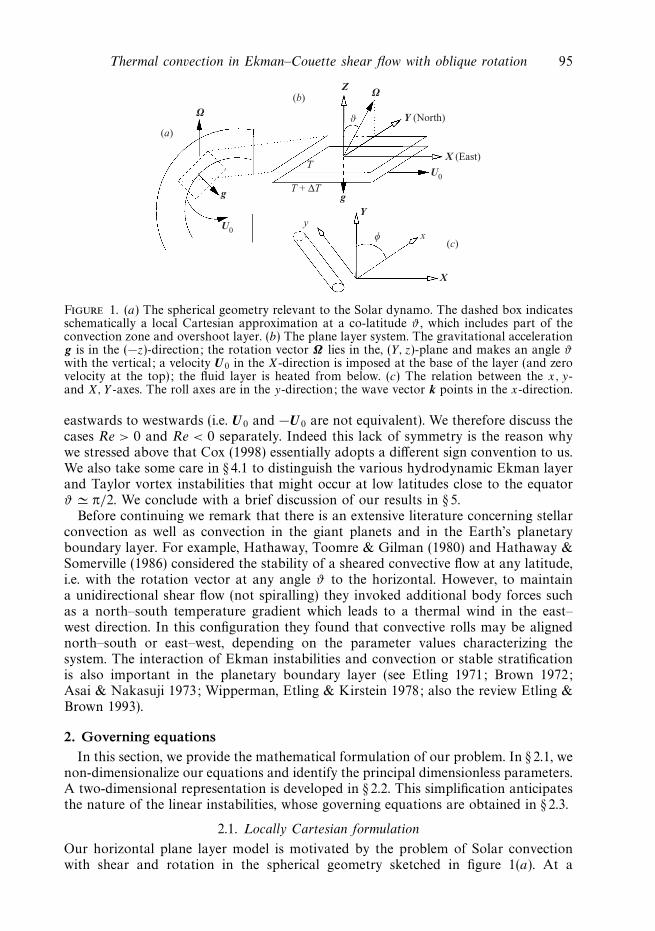
Figure 1. (a) The spherical geometry relevant to the Solar dynamo. The dashed box indicatesschematically a local Cartesian approximation at a co-latitude ϑ , which includes part of theconvection zone and overshoot layer. (b) The plane layer system. The gravitational accelerationg is in the (−z)-direction; the rotation vector Ω lies in the, (Y, z)-plane and makes an angle ϑwith the vertical; a velocity U0 in the X-direction is imposed at the base of the layer (and zerovelocity at the top); the fluid layer is heated from below. (c) The relation between the x, y-and X, Y -axes. The roll axes are in the y-direction; the wave vector k points in the x-direction.
eastwards to westwards (i.e. U0 and −U0 are not equivalent). We therefore discuss thecases Re > 0 and Re < 0 separately. Indeed this lack of symmetry is the reason whywe stressed above that Cox (1998) essentially adopts a different sign convention to us.We also take some care in § 4.1 to distinguish the various hydrodynamic Ekman layerand Taylor vortex instabilities that might occur at low latitudes close to the equatorϑ π/2. We conclude with a brief discussion of our results in § 5.
Before continuing we remark that there is an extensive literature concerning stellarconvection as well as convection in the giant planets and in the Earth’s planetaryboundary layer. For example, Hathaway, Toomre & Gilman (1980) and Hathaway &Somerville (1986) considered the stability of a sheared convective flow at any latitude,i.e. with the rotation vector at any angle ϑ to the horizontal. However, to maintaina unidirectional shear flow (not spiralling) they invoked additional body forces suchas a north–south temperature gradient which leads to a thermal wind in the east–west direction. In this configuration they found that convective rolls may be alignednorth–south or east–west, depending on the parameter values characterizing thesystem. The interaction of Ekman instabilities and convection or stable stratificationis also important in the planetary boundary layer (see Etling 1971; Brown 1972;Asai & Nakasuji 1973; Wipperman, Etling & Kirstein 1978; also the review Etling &Brown 1993).
2. Governing equationsIn this section, we provide the mathematical formulation of our problem. In § 2.1, we
non-dimensionalize our equations and identify the principal dimensionless parameters.A two-dimensional representation is developed in § 2.2. This simplification anticipatesthe nature of the linear instabilities, whose governing equations are obtained in § 2.3.
2.1. Locally Cartesian formulation
Our horizontal plane layer model is motivated by the problem of Solar convectionwith shear and rotation in the spherical geometry sketched in figure 1(a). At a

96 Y. Ponty, A. D. Gilbert and A. M. Soward
co-latitude ϑ , we adopt a local Cartesian approximation with coordinates (X, Y, z) asshown in figure 1(b). The z-axis is vertically upwards, while the associated (constant)gravity g = −g z is downwards (here and below the hat is used to denote unit vectors).The Y -axis points northwards so that the rotation vector ΩΩΩ lies in the (Y, z)-planeand makes an angle ϑ with the vertical. We write
ΩΩΩ (= Ω ΩΩΩ) = Ω cos ϑ z + Ω sinϑ Y ≡ ΩΩΩv + ΩΩΩh, (2.1)
where ΩΩΩv = Ω cosϑ z and ΩΩΩh = Ω sinϑ Y are the vertical and horizontal componentsof the rotation vector respectively.
Our layer is unbounded in the horizontal (X, Y )-plane and is confined verticallybetween rigid boundaries at z = 0 and z = h. At the top of the layer z = h the fluidvelocity vanishes U = 0, while the bottom rigid boundary z = 0 moves parallel to
itself steadily eastwards in the X-direction U = U0 = U0 X , as shown on figure 1(b).In the Solar context, the velocity difference between the base and the top of thelayer is chosen to model the difference in angular velocity between the convectionzone and the radiative interior, as revealed by helioseismological observations. Notethat this geometry requires the velocity U0 to be perpendicular to both ΩΩΩ and g(i.e. U0 ‖ g × ΩΩΩ). This feature distinguishes our study from Matthews & Cox (1997)and Cox (1998), who permit an arbitrary angle between U0 and ΩΩΩh (i.e. ΩΩΩ · U0 = 0in general).
Associated with the form of our rotation vector (2.1), the stability characteristics ofour system are invariant under two distinct simultaneous transformations involvingthe reflection ϑ ↔ π − ϑ in the equatorial plane: they are Ω ↔ Ω , U0 ↔ U0 andΩ ↔ −Ω , U0 ↔ −U0. The triple product T ≡ U0 · (g × ΩΩΩ) is invariant under bothtransformations. Only at the poles ϑ = 0 and π, where the rotation vector is verticaland T = 0, are the stability characteristics invariant to reversing the sign of U0
with all other parameters held fixed. Thus, without loss of generality, we may restrictattention to positive rotation rate Ω 0 in the northern hemisphere 0 ϑ π/2,but we must allow U0 to take either sign (except at ϑ = 0). In the context of theSolar convection zone, for which the differential rotation speed is slower near thepoles than the equator, the lower boundary velocity U0 is eastward (U0 > 0, T > 0)near the north pole and westward (U0 < 0, T < 0) near the equator.
The upper and lower boundaries are maintained at constant temperatures T = T0
and T = T1. We assume that the fluid is incompressible, but make the Boussinesqapproximation. We take the fluid’s kinematic viscosity ν, thermal diffusivity κ , andcoefficient α of expansion to be constant. Under these assumptions the equations ofmotion in the rotating frame are
ρ0
(∂U∂t
+ U · ∇U + 2Ω × U)
= −∇P + ρg + ρ0ν∇2U, (2.2a)
∇ · U = 0, ρ = ρ0[1 − α(T − T0)], (2.2b)
∂T
∂t+ U · ∇T = κ∇2T . (2.2c)
The governing equations possess a steady-state solution U = U eq(z), T = Teq(z),P = Peq(z) dependent only on the vertical coordinate z. Here heat is transportedvia vertical conduction alone, while the fluid motion is of Ekman–Couette type withstructure
U eq = U0 ΛΛΛ(z), ΛΛΛ = Λ1(z) X + Λ2(z) Y . (2.3)
Thermal convection in Ekman–Couette shear flow with oblique rotation 97
The general solution may be expressed in terms of the fluctuations u, θ and Π
about this equilibrium state as follows:
U = U eq(z) + u, T = Teq(z) + θ, P = Peq(z) + Π. (2.4)
We adopt the depth h of our layer as the unit of length and the correspondingdiffusion time h2/κ as the unit of time. Accordingly we introduce dimensionlessvariables (primed) defined by
t = t ′ h2
κ, x = x ′h, u = u′ κ
h, θ = θ ′ νκ
αgh3, Π = Π ′ ρ0κ
2
h2. (2.5)
Upon dropping the primes, the governing equations take the dimensionless form
1
Pr
(∂u∂t
+ u · ∇u)
+ Re
(ΛΛΛ · ∇u + u · z
dΛΛΛ
dz
)+ τ ΩΩΩ × u = −∇ Π
Pr+ θ z + ∇2u,
(2.6a)
∇ · u = 0, (2.6b)
∂θ
∂t+ u · ∇θ + Pr Re ΛΛΛ · ∇θ = Ra u · z + ∇2θ. (2.6c)
Here we have introduced dimensionless parameters, namely the Rayleigh number Ra,the Prandtl number Pr, the Taylor number τ 2 and the Reynolds number Re:
Ra =αgh3(T1 − T0)
νκ, Pr =
ν
κ, τ =
2Ωh2
ν, Re =
U0h
ν. (2.7)
The isothermal and no-slip boundary conditions are
u = 0, θ = 0 at z = 0 and 1. (2.8)
The underlying Ekman–Couette flow may be expressed in terms of a singledimensionless complex function
Λ(z) = Λ1(z) + i Λ2(z) on 0 z 1, (2.9)
which in the absence of a horizontal pressure gradient satisfies
d2Λ
dz2− 2iµ2Λ = 0, where µ =
√τ cos ϑ
2, (2.10a, b)
together with the boundary conditions
Λ(0) = 1, Λ(1) = 0. (2.10c)
The solution
Λ = −sinh[(1 + i)µ(z − 1)]
sinh[(1 + i)µ]for µ = 0 (2.11a)
yields the family of Ekman–Couette flows with components
Λ1 =cosh[µ(z − 2)] cos(µz) − cosh(µz) cos[µ(z − 2)]
cosh(2µ) − cos(2µ), (2.11b)
Λ2 =sinh[µ(z − 2)] sin(µz) − sinh(µz) sin[µ(z − 2)]
cosh(2µ) − cos(2µ); (2.11c)
an example is provided in figure 2. When the vertical component of rotation is small,

98 Y. Ponty, A. D. Gilbert and A. M. Soward
(a) (b)
U0
U0
z
Figure 2. The Ekman spiral. (a) The full line gives a perspective view of the Ekman layervelocity, given by plotting (Λ1(z),Λ2(z), z) as z varies between 0 and 1, for τ = 100. The dottedline represents the velocity U0 of the bottom of the plane layer. (b) The same spiral Ekmanvelocity is projected onto the horizontal (X, Y )-plane.
(2.11b, c) has the power series expansion
Λ1 ∼ 1 − z, Λ2 ∼ − 13µ2z(1 − z)(2 − z) for |µ| 1, (2.12a, b)
which reduces to plane Couette flow in the limit µ = 0. When the vertical rotation isstrong, (2.11b, c) has the asymptotic representation
Λ1 ∼ e−µz cos µz, Λ2 ∼ −e−µz sinµz as µ → ∞, (2.13a, b)
which describes an Ekman boundary layer localized within a distance O(µ−1) from thelower boundary; elsewhere the fluid is essentially stationary. In all cases, a southerly(northerly) mass flux of order τ−1/2 per unit length ensues when U0 > 0 (U0 < 0). Inthe Solar context this small flux is returned by very small velocities, in the convectionzone high above the thin layer. The up–down asymmetry of our Ekman–Couette flow(2.11) results from our assumption of no horizontal pressure gradient. In the large-τlimit (2.13) it ensures that there is no geostrophic motion outside the bottom Ekmanlayer. Of course other choices of uniform geostrophic flow corresponding to finitepressure gradients are possible, as considered by Hoffmann & Busse (2001), but thepresent choice provides the most faithful representation of the Solar tachocline (asingle layer in the boxed region of figure 1a) as Ponty et al. (2001a) explain in somedetail (see also Ponty et al. 2001b). It is important to appreciate that a horizontalpressure gradient is not Galilean invariant in a rotating system. So if we had adoptedcoordinates for which the bottom boundary was at rest with the geostrophic flow−U0 above, there would be a finite pressure gradient in that reference frame.
In our construction, we have implicitly assumed that U0 is positive in defining theReynolds number, while the vector field ΛΛΛ has been normalized via the boundarycondition (2.10c). Since both signs of U0 are relevant in the Sun – positive U0 > 0 nearthe poles and negative U0 < 0 near the equator – we find it convenient to retain theboundary condition Λ(0) = 1 but permit the Reynolds number Re to take positiveand negative values in concert with U0. Interestingly, when |ΩΩΩh| = 0 the stabilitycharacteristics depend on the sign of Re. This is because the absolute vorticity in thenon-rotating inertial frame is different in the two cases, i.e. the vorticity of the sheareither reinforces or weakens the vorticity 2ΩΩΩ of the rotating frame.

Thermal convection in Ekman–Couette shear flow with oblique rotation 99
2.2. Two-dimensional formulation
In the case of purely horizontal rotation (|ΩΩΩv| = 0) at ϑ = π/2 and no shearRe = 0, the axes of the convection rolls at the onset of instability are aligned withthe horizontal rotation vector ΩΩΩh, namely the Y -direction. In contrast, when there isshear Re = 0 but no rotation, τ = 0, the roll axes of the convection are aligned withthe linear shear parallel to U0, namely the X-direction. These trivial results are wellknown. Matthews & Cox (1997) have shown that for the non-trivial extension whenboth horizontal rotation τ = 0 (µ = 0) at ϑ = π/2 and plane Couette shear (Re = 0)are present, the onset of convection continues to be characterized by either X- orY -directed rolls.
When, however, there is a vertical component of rotation (|ΩΩΩv| = 0), the laminarflow loses the uni-directional plane Couette form (2.12) with µ = 0, and insteadtakes on the spiralling Ekman–Couette form (2.11b, c) appropriate to µ = 0. Nowthe convective roll axes at onset are generally oblique and not aligned with eitherthe X- or Y -axes. For this reason, we introduce new horizontal coordinates (x, y)which are related to the roll axes, as shown in figure 1(c). Specifically, since our basicconductive state depends only on the vertical coordinate z, we may seek solutions tothe linear stability problem that are separable in the horizontal coordinates X, Y and
proportional to exp[i(k1X + k2Y )+ (σ +iω)t], where the wave vector k = k1 X + k2Y isconstant and σ + iω is the complex growth rate. To simplify our analysis, we choosenew horizontal axes such that the x-axis is aligned with the wave vector k. As aresult our separable modes are proportional to exp[ikx +(σ +iω)t] (see (2.20)), wherek = |k|, so that now the roll axes are aligned with the y-direction.
We introduce the angle φ between the wave vector k (or x-axis) and the northerlydirection (or Y -axis); in the spherical shell context, the case φ = 0 (k pointsnorthwards) corresponds to doughnut-shaped convection cells, while the case φ = π/2(k points eastwards) defines so-called banana-shaped convection cells. With respectto the new x, y-axes the horizontal component of rotation makes an angle φ with thex-axis, while the bottom velocity U0 subtends an angle φ ∓ π/2 with the x-axis when±U0 > 0 (see figure 1c). Note that the problem may be formulated equivalently undera rotation of 180 with φ ↔ φ + π, provided k ↔ −k, ω ↔ ω. We also have the usualsymmetry φ ↔ φ, k ↔ −k, ω ↔ −ω, corresponding to taking the complex conjugatenormal mode.
In this new framework the governing equations (2.6) continue to hold, but now therotation vector (2.1) becomes
ΩΩΩ = sin ϑ cosφ x + sinϑ sin φ y + cos ϑ z, (2.14)
while the Ekman–Couette flow (2.3) is replaced by
ΛΛΛ = λ1(z) x + λ2(z) y, (2.15a)
where
λ1 = Λ1 sinφ + Λ2 cos φ, λ2 = −Λ1 cosφ + Λ2 sinφ. (2.15b, c)
The advantage of our new coordinates (x, y, z) is that the linear convective modedepends only on the two coordinates x and z, while the angle φ defines the orientationof the rolls. Accordingly, we may introduce the stream function representation forthe velocity in the (x, z)-plane and write
u(x, z, t) = ∇ × (ψ y) + v y ≡ (−∂zψ, v, ∂xψ), (2.16)
100 Y. Ponty, A. D. Gilbert and A. M. Soward
where ∂x ≡ ∂/∂x and ∂z ≡ ∂/∂z. In turn, the vorticity becomes
∇ × u = (−∂zv, −ψ, ∂xv) , where = ∂2x + ∂2
z . (2.17a, b)
We substitute these representations into the y-component of the curl of (2.6a), they-component of (2.6a) itself and (2.6c). In this way we obtain the nonlinear matrixsystem
(∂t + Pr Re λ1∂x)WWWX = BBBX + Re Y ∂xψ − ∂(ψ,WWWX)
∂(x, z), (2.18a)
where
X =
ψ
v
θ
, WWW =
Pr−1 0 0
0 Pr−1 00 0 1
, (2.18b)
Y =
λ′′1
−λ′2
0
, BBB =
2 −τ∂Ω ∂x
τ∂Ω 0Ra ∂x 0
, (2.18c)
the prime denotes the z-derivative d/dz and
∂Ω = ΩΩΩ · ∇ ≡ cosϑ ∂z + sinϑ cosϕ ∂x. (2.18d)
The linear operator BBB is standard and represents convection in a rotating Boussinesqfluid system. The additional shear flow leads to two new terms. The first one,proportional to ∂xWWWX on the left-hand side of the equation, represents the advectionof the fluctuating vorticity, momentum and temperature by the mean shear flow λ1
in the x-direction. The term proportional to Y on the right-hand side is a sourceterm representing the advection of vorticity and momentum associated with the meanshear flow ΛΛΛ by the vertical component of the fluctuating velocity ∂xψ .
For our rigid, isothermal boundary conditions, the fluctuation vector X satisfies
∂zψ = ψ = v = θ = 0 at z = 0 and z = 1. (2.19)
Often, in the absence of shear, stress-free boundary conditions are applied ingeophysical applications at small Ekman number to simplify the analysis. It istherefore significant to appreciate that the underlying shear flow in our system canonly be maintained by the presence of the moving rigid boundary.
2.3. Linear stability problem and numerical methods
We now linearize (2.18a) with respect to the small disturbances and consider separablemodes of the form
X = X exp[ikx + (σ + iω)t] with X = [Ψ (z), V (z), Θ(z)]T , (2.20a, b)
where σ +iω is the complex growth rate. The equation for linear perturbations of thez-dependent equilibrium state becomes
(σ + iω)WWWX = LLLX, (2.21a)
where
WWW =
Pr−1 0 0
0 Pr−1 00 0 1
, (2.21b)
Thermal convection in Ekman–Couette shear flow with oblique rotation 101
LLL =
2 − ik Re λ1 + ik Re λ′′1 −τ ∂Ω ik
τ ∂Ω − ik Re λ′2 − ik Re λ1 0
ik Ra 0 − ik Pr Re λ1
(2.21c)
and
= ∂2z − k2, ∂Ω = cos ϑ ∂z + ik sin ϑ cos ϕ. (2.21d, e)
The marginal modes with σ = 0 determine the neutral Rayleigh number Ra as afunction of the four dimensionless parameters Pr, τ , Re, ϑ of the physical systemtogether with the two mode parameters k and φ. This neutral Ra is then to beminimized over all k and φ to obtain the critical Rayleigh number Rac(Pr, τ, Re, ϑ)which occurs at a particular wavenumber kc, angle φc and frequency ωc.
The system (2.21) is of a generalized eigenvalue form, and was solved in Chebychevspectral space. The tau method was used to implement the rigid boundary conditions.Instead of solving the problem in terms of Ψ , V and Θ as in (2.21) above, weintroduced a fourth variable Ξ = Ψ to avoid spurious eigenvalues (see Gottlieb &Orszag 1977, p. 143). After the calculation of the neutral Rayleigh number for a givenk, φ-mode, the main numerical problem is to find the critical Rayleigh number over the(k, φ)-plane using standard minimization methods. The problem becomes numericallydifficult when two or more minima occur in this plane (see § 3.1), particularly if oneof the minima is very narrow (see e.g. figure 6 below).
We will adopt the convention that k > 0. Accordingly, we need to keep in mindthe rotational symmetry, namely that the interchange φ ↔ φ + π is accompanied byω ↔ −ω, while Ra and k remain unaltered.
3. Vertical rotation ϑ = 0
Throughout this section we restrict attention to the case of vertical rotation (|ΩΩΩh| =0) at ϑ = 0. So in addition to the rotational symmetries already mentioned, ourresults are invariant under interchanging U0 ↔ −U0 (equivalently Re ↔ − Re)simultaneously with φ ↔ φ + π. In § 3.1 we consider only hydrodynamic instabilitywithout buoyancy forces (Ra = 0), while buoyancy related instabilities (Ra = 0) arediscussed in § 3.2. An asymptotic theory valid in the rapid rotation limit is developedin § 3.3 which gives good agreement with the numerical results for sufficiently large τ .
3.1. Ekman layer instability Ra = 0
With rotation vertical (ϑ = 0), the underlying shear flow exhibits the complicatedEkman–Couette profile. When, moreover, the Taylor number τ 2 is large, the shearis localized in a thin Ekman layer of width µ−1 = O(τ−1/2) (see (2.10b)) adjacentto the lower boundary, which is characterized by the well-known Ekman spiral (seefigure 2). Even without any buoyancy forces (Ra = 0), the Ekman layer is prone topure hydrodynamic instabilities at sufficiently large Reynolds number Re. These takethe form of travelling waves, which destroy the laminar Ekman layer flow.
Ekman layer instabilities have been studied experimentally by Faller (1963) andCaldwell & Van Atta (1970), and numerically by Faller & Kaylor (1966) and Lilly(1966). These investigations were concerned with the instability in a semi-infiniteplane layer z 0 of fluid moving steadily with constant velocity U0 as z → ∞, abovea rigid stationary boundary at z = 0. In the absence of a vertical length scale it isnatural to adopt the Ekman boundary layer width D = (ν/Ω)1/2 as the unit of length

102 Y. Ponty, A. D. Gilbert and A. M. Soward
(a)800
600
400
200
Rec
I
II
500 100 150 200
(b)6
5
4
3
2
1
kc
500 100 150 200
(c)
30
20
10
0
–10
–20
φc
50 100 150 200
(d )1200
800
400
ωc
500 100 150 2000ττ
Figure 3. The type I (dotted) and type II (solid) modes of the Ekman layer instability. Thecritical values are plotted against τ : (a) the Reynolds number Rec , (b) the wavenumber kc ,(c) the preferred orientation φc (in degrees), and (d) the frequency ωc .
and D/U0 as the unit of time. The corresponding Reynolds number is
Re∗ =DU0
ν=
U0√νΩ
. (3.1a)
Two different Ekman layer instabilities are distinguished in these studies; they occurwhen the Reynolds number Re∗ exceeds the experimentally measured values of Re∗
c 56.7 and 124.5. The corresponding modes have wavelengths L∗
cD of roughly 22D and11D respectively; they have a similar spatial structure but different orientation withrespect to the mean flow, with positive and negative φc for type II and I respectively.The numerical calculations of Faller & Kaylor (1966) and Lilly (1966) yielded thecritical Reynolds numbers Re∗
c 55 and 110 in good agreement with the experiments;these instabilities are now referred to as type II and type I respectively.
In our geometry the layer has a finite depth h, and so these studies become relevantwhen D h, i.e. for large Taylor number, τ 2 1. In this case the Reynolds numberbased on the Ekman layer thickness may be written as
Re∗ = Re√
2/τ = Re /µ (ϑ = 0), (3.1b)
and in our dimensionless units the distance D becomes µ−1, and the time D/U0
becomes Re−1 Pr−1µ−1. We portray our computed values of the critical values Rec,kc, φc and ωc versus τ for the onset of the Ekman instability in figure 3.
We observe two modes whose critical values cross around τ = 50. For large Taylornumber, the instability is linked to the Ekman layer and in that limit the two modesportrayed in figure 3 evidently correspond to the type II mode (solid) and type I mode(dotted). The curves in figure 3(a, b) have the asymptotic behaviours Rec = Re∗
c µ
and kc = 2πµ/L∗c as τ → ∞. We fitted our numerical results (not only those depicted
but also others at larger values of τ not shown on the figure) to these power laws,

Thermal convection in Ekman–Couette shear flow with oblique rotation 103
1.0
0.5v
0 5 10
(a)
1
0
–1
1.0
0.5ψ
0 5 10
(b) 1
0.5
0
–0.5
Figure 4. Contour plots of the Couette–Ekman layer type II instability in the (x +(ωc/kc)t, z)-frame co-moving with the wave for τ = 100, ϑ = 0. The critical values areRec ≈ 435.32, kc ≈ 2.403, φc ≈ 21.659 and ωc ≈ 214.11. There is no thermal gradient, Ra = 0.(a) The toroidal velocity v, and (b) the stream function ψ .
to obtain the values Re∗c ≈ 54.21 (113.7), L∗
c ≈ 19.9 (11.24), φ∗c ≈ 23.38 (−7.3) and
ω∗c ≈ 0.069 (0.1220) for the solid (dotted) curves, which are clearly correspond well
with type II (type I) values. Our critical value Re∗c ≈ 54.21 for type II instability
is in particularly good agreement with Iooss, Nielsen & True (1978) and Melander(1983).
Hoffman et al. (1998) consider a problem similar to ours. It differs in that theupper boundary moves with equal speed but in the opposite direction. So unlike ourproblem the underlying velocity field is anti-symmetric about the mid-plane, as is alsothe case in Cox (1998). For large τ the numerical results listed in Hoffman et al.’s(1998) table 1 compare favourably with ours after the appropriate rescalings. Formoderate Taylor numbers some differences are evident between the results portrayedin their figure 4 and ours. On the one hand, the complete type II and type I curvesagree qualitatively with our figure 3. On the other, they isolate a steady mode forsmall τ which is not present in our results. The reason is evident from their figure 3(a),which shows that the mode has a reflectional symmetry in the mid-plane which ourgeometry does not admit. Put another way, the type II and I modes are wall modes,while the extra mode of Hoffman et al. (1998) is an interior (centre) mode (called anS-mode by Hoffmann & Busse 2001) linked to the inflection point at the mid-plane.
Figure 4 shows the form of our type II travelling wave instability at large Taylornumber τ = 100 with Rec ≈ 435.32. On it, contours of constant toroidal y-componentof velocity v and poloidal stream function ψ are plotted in the (x, z)-plane in theframe co-moving with the wave at its phase velocity −ωc/kc. They are periodic inthe x-direction with periodicity length 2π/kc. They illustrate the fact that the toroidalvelocity v is activated in the lower Ekman layer and is linked to a poloidal circulationψ having a return flow outside the Ekman layer. The figure compares well with
104 Y. Ponty, A. D. Gilbert and A. M. Soward
(a)
20
10
0
–10
–20
–30
–40
–50
Ra c
/Ra c0
I
II
50 100 150 200
(b)
7
6
5
4
3
2
1
kc
500 100 150 200
(c)
150
100
50
0
φc
50 100 150 200
(d )400
300
200
100
ωc
500 100 150 2000ττ
0
C
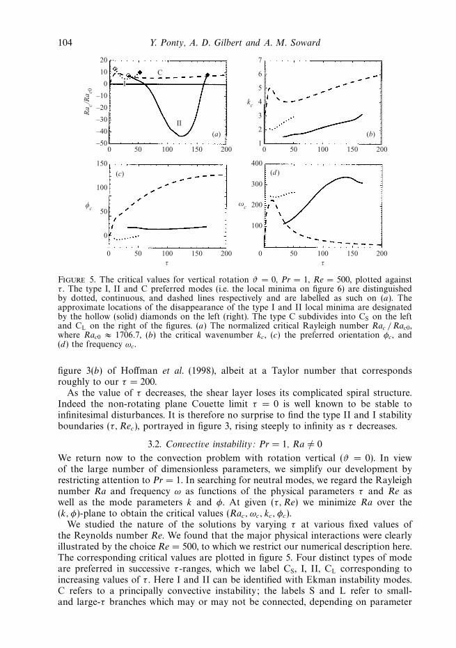
Figure 5. The critical values for vertical rotation ϑ = 0, Pr = 1, Re = 500, plotted againstτ . The type I, II and C preferred modes (i.e. the local minima on figure 6) are distinguishedby dotted, continuous, and dashed lines respectively and are labelled as such on (a). Theapproximate locations of the disappearance of the type I and II local minima are designatedby the hollow (solid) diamonds on the left (right). The type C subdivides into CS on the leftand CL on the right of the figures. (a) The normalized critical Rayleigh number Rac /Rac0,where Rac0 ≈ 1706.7, (b) the critical wavenumber kc , (c) the preferred orientation φc , and(d) the frequency ωc .
figure 3(b) of Hoffman et al. (1998), albeit at a Taylor number that correspondsroughly to our τ = 200.
As the value of τ decreases, the shear layer loses its complicated spiral structure.Indeed the non-rotating plane Couette limit τ = 0 is well known to be stable toinfinitesimal disturbances. It is therefore no surprise to find the type II and I stabilityboundaries (τ, Rec), portrayed in figure 3, rising steeply to infinity as τ decreases.
3.2. Convective instability: Pr = 1, Ra = 0
We return now to the convection problem with rotation vertical (ϑ = 0). In viewof the large number of dimensionless parameters, we simplify our development byrestricting attention to Pr = 1. In searching for neutral modes, we regard the Rayleighnumber Ra and frequency ω as functions of the physical parameters τ and Re aswell as the mode parameters k and φ. At given (τ, Re) we minimize Ra over the(k, φ)-plane to obtain the critical values (Rac, ωc, kc, φc).
We studied the nature of the solutions by varying τ at various fixed values ofthe Reynolds number Re. We found that the major physical interactions were clearlyillustrated by the choice Re = 500, to which we restrict our numerical description here.The corresponding critical values are plotted in figure 5. Four distinct types of modeare preferred in successive τ -ranges, which we label CS, I, II, CL corresponding toincreasing values of τ . Here I and II can be identified with Ekman instability modes.C refers to a principally convective instability; the labels S and L refer to small-and large-τ branches which may or may not be connected, depending on parameter

Thermal convection in Ekman–Couette shear flow with oblique rotation 105
kc
(c)
50
0
–50
φc
2 4 6 71
II
C
3 5 8kc
(d)
50
0
–50
2 4 6 71
II
C
3 5 8
(a)
50
0
–50
φc
2 4 6 71
II
C
3 5 8
(b)
50
0
–50
2 4 6 71
II
C
3 5 8
I
Figure 6. Contours of constant critical Rayleigh number Rac in the wave vector planeparameterized by (kc, φc), for the case of vertical rotation ϑ = 0, Pr = 1, Re = 500. Type I, IIand C minima are labelled. Four different rotation rates are shown: (a) τ = 40, (b) τ = 60,(c) τ = 160, and (d) τ = 170.
values. To understand how these results emerge, we take four representative values ofτ and plot contours of constant neutral Ra in the (k, φ)-plane in figure 6. On each ofthem, we can isolate local minima which include modes I, II and C. Evidently, theselocal minima compete to be the global minimum identified in figure 5. Interestinglythe convective minima CS and CL actually connect with each other as τ is increasedfrom 0 to ∞ and so we can unambiguously label this the convective minimum Cthroughout. This agreeable state of affairs should be contrasted with the obliquerotation cases investigated in § 4.2 below, for which the CS and CL branches aredisconnected. Generally, there is a value of τ at which a local minimum evaporates.The corresponding points, which terminate the curves on figures 5, 11, 14 and 15, aremarked by diamonds.
To understand the nature of the various modes we examine the eigenfunctions,showing v, ψ and perturbation temperature θ in figures 7, 8 and 9. Here we adoptthe frame co-moving with the wave at its phase velocity −ωc/kc, as in figure 4.
3.2.1. Small Taylor number τ 2 1: Re = 500; type CS
When τ = 0, the roll axes are aligned, φc = 0, with the plane Couette shearλ1 = 0, λ2 = −1 + z. Consequently, the Ψ, Θ-equations decouple from the V -equationwithin the system (2.21). As a result, neither the applied shear nor the induced v
interact with the convection, and so the critical Rayleigh number takes the valueRac = Rac0 corresponding to the classical Rayleigh–Benard problem mentioned in

106 Y. Ponty, A. D. Gilbert and A. M. Soward
1.0
0.5v
0 5 10
(a)0.5
0
–0.5
θ
0 5 10
(b)1.0
0.5
1.0
0.5
0 5 10
ψ
0.5
0
–0.5
(c)
2
0
–2
Figure 7. Contour plots describing the onset of convection in the co-moving(x + (ωc/kc)t, z)-frame for the case ϑ = 0, Pr = 1, Re = 500. They illustrate a type CS
mode at τ = 2, for which Rac ≈ 4105.06, kc ≈ 3.271, φc ≈ 1.6 and ωc ≈ 108.75. (a) Thetoroidal velocity v, (b) the stream function ψ , and (c) the heat perturbation θ .
the Introduction. Interestingly, with our choice Pr = 1 the equations governing V andΘ are equivalent except for different constants multiplying the common source termikΨ , and give V = −(Re/Rac0)Θ .
For small Taylor number τ 2 1 the preferred mode CS identified in figure 5 is aperturbation of the τ = 0 solution. It is well known that rotation by itself is stabilizing.Nevertheless, the sharp rise of Rac versus τ suggests that the further interaction withthe shear strengthens that stabilization. Indeed, the situation in the limit Re 1 isquite clear. Though the shear is only weakly modified by the rotation,
λ1 ∼ (1 − z)[φ − 1
3µ2z(2 − z)
], λ2 ∼ −1 + z for |φ| 1, (3.2)
this is the most important effect because of the large value of the Reynolds number.Thus we can neglect rotation except where it modifies ΛΛΛ. Accordingly we need onlyconsider the first and last components of (2.21) for Ψ and Θ , which involve the shearvia λ1 above; here the contribution to the convection made by V is small, because ofthe relatively small size of τ , and can be ignored. The shear associated with λ′
1 tilts theisotherms, shortens the vertical length scale and enhances dissipation. The preferredmode minimizes that shear. For U0 > 0 (< 0), the rolls drift southward (northward)
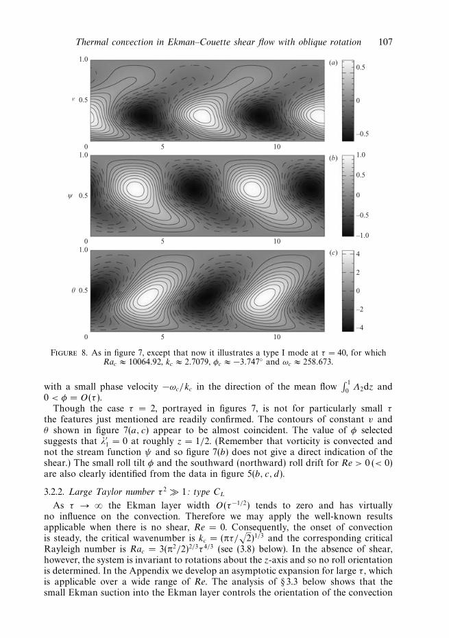
Thermal convection in Ekman–Couette shear flow with oblique rotation 107
1.0
0.5v
0 5 10
(a)0.5
0
–0.5
θ
0 5 10
(b)1.0
0.5
1.0
0.5
0 5 10
ψ
1.0
0.5
0
–0.5
–1.0
(c) 4
2
0
–2
–4
Figure 8. As in figure 7, except that now it illustrates a type I mode at τ = 40, for whichRac ≈ 10064.92, kc ≈ 2.7079, φc ≈ −3.747 and ωc ≈ 258.673.
with a small phase velocity −ωc/kc in the direction of the mean flow∫ 1
0Λ2dz and
0 < φ = O(τ ).Though the case τ = 2, portrayed in figures 7, is not for particularly small τ
the features just mentioned are readily confirmed. The contours of constant v andθ shown in figure 7(a, c) appear to be almost coincident. The value of φ selectedsuggests that λ′
1 = 0 at roughly z = 1/2. (Remember that vorticity is convected andnot the stream function ψ and so figure 7(b) does not give a direct indication of theshear.) The small roll tilt φ and the southward (northward) roll drift for Re > 0 (< 0)are also clearly identified from the data in figure 5(b, c, d).
3.2.2. Large Taylor number τ 2 1: type CL
As τ → ∞ the Ekman layer width O(τ−1/2) tends to zero and has virtuallyno influence on the convection. Therefore we may apply the well-known resultsapplicable when there is no shear, Re = 0. Consequently, the onset of convectionis steady, the critical wavenumber is kc = (πτ/
√2)1/3 and the corresponding critical
Rayleigh number is Rac = 3(π2/2)2/3τ 4/3 (see (3.8) below). In the absence of shear,however, the system is invariant to rotations about the z-axis and so no roll orientationis determined. In the Appendix we develop an asymptotic expansion for large τ , whichis applicable over a wide range of Re. The analysis of § 3.3 below shows that thesmall Ekman suction into the Ekman layer controls the orientation of the convection

108 Y. Ponty, A. D. Gilbert and A. M. Soward
1.0
0.5v
0 5 10
(a) 0.05
0
–0.05
θ
0 5 10
(b)1.0
0.5
1.0
0.5
0 5 10
ψ
0.5
0
–0.5
(c)
2
0
–2
Figure 9. As in figure 7, except that now it illustrates a type CL mode at τ = 200, for whichRac ≈ 13652.27, kc ≈ 6.0025, φc ≈ 154.44 and ωc ≈ 13.73.
rolls, which is found to take the value φc = −27.0451 (or equivalently 152.9548).The corresponding critical frequency is given by (3.11) below.
The large-τ solution retains its character down to moderately large τ , where it isidentified in figure 5 as a mode CL. Indeed, the critical values Rac and kc agree wellwith the asymptotic values; the convection is almost stationary and φc has achievedthe value of 152.95. The mode’s convection characteristics illustrated in figure 9certainly support that point of view. It is also clear that the convection takes placelargely outside the moderately thin Ekman layer. Indeed any overshooting into theEkman layer is rapidly sheared and distorted.
3.2.3. Moderate Taylor numbers: Re = 500; types I and II
From figure 5 we notice that there are two values of τ , roughly 60 and 160, atwhich Rac vanishes. These two values are determined by the intersection of the lineRec = 500 with the (solid) type II curve on figure 3. This means that the modeidentified on figure 5 is essentially a hydrodynamic instability of type II modifiedby the presence of buoyancy forces. Indeed, in the negative-Rac range, where thetype II disturbance is hydrodynamically unstable, the mode is only stabilized by theapplication of a stable stratification. In view of this hydrodynamic identification it isnatural to continue to label it as type II even when the buoyancy force is involved.

Thermal convection in Ekman–Couette shear flow with oblique rotation 109
By examining the stability characteristics of the mode labelled I on figure 5, it isclearly a modification of the type I hydrodynamic mode; compare kc, φc, ωc withthose shown on figure 3(b, c, d). Unlike the type II mode, which exhibits instability atRa = 0, this does not because at Re = 500 the type I mode is hydrodynamically stable(see figure 3a). We exhibit an example of this type I mode in figure 8 for τ = 40,where the minimum values of Ra for the type I and II modes coincide. The dynamicalfeatures of this type I mode, particularly the concentration of the v-velocity insidethe shear layer, are very similar to the type II mode, which occurs at almost the sameRayleigh number. Indeed, this type I mode even bears a striking resemblance to thetype II hydrodynamic mode illustrated in figure 4. One feature that is evident fromfigure 8 is that v is generated high in the Ekman layer. The overall picture suggeststhat energy is being tapped primarily from the shear but the buoyancy force is alsoplaying an essential role in driving the motion.
Just as in the case of the small-τ convective CS modes, φc is small for these typeI modes, suggesting that the roll axis is adjusting its orientation to prevent shearingby the underlying Ekman layer flow from having too strong a stabilizing effect.Despite this tuning, considerable shearing is evident in figure 8. Furthermore, sinceφc is small, these type I convective modes have roll axes which are aligned almosteast–west and travel southwards (northwards) for U0 > 0 (< 0).
The identification of the global minimum is a numerically delicate matter and thatis why we have produced the contour plots of constant neutral Rayleigh numberRa in figure 6. In interpreting these plots it important to appreciate that they areπ (or 180) periodic in the φ-direction, i.e. the top boundary of each contour plotis identical to its bottom boundary. We find that up to three local minima can beidentified at each value of τ . For the case τ = 40 illustrated in figure 6(a) the minimafor type I and II modes have almost identical Ra, while the mode CL minimum isgreater. As τ increases the type I minimum evaporates as illustrated in figure 6(b)for the value τ = 60, shortly after the type II hydrodynamic instability sets in. Withfurther increase in τ the type II mode minimum sharpens as illustrated in figure 6(c)for the value τ = 160 at which the type II hydrodynamic instability is cut off. Indeedwith further increase of τ the type II mode minimum becomes increasingly difficult totrack. By τ = 170, illustrated in figure 6(d), though the local minimum of the type IImode continues to exist, it is very tiny. With further increases of τ it soon evaporatesand we are left with the global minimum associated with the large-τ convective CL
mode.
3.3. Large rotation rate τ 1, τ 2/3 Re
In this subsection (and the Appendix) we sketch the limit of rapid rotation withvertical rotation vector ϑ = 0. For non-zero Reynolds number Re, the solution splitsinto two parts. One part is the mainstream solution valid outside the Ekman layer,where the applied shear is negligible. The other is the boundary layer solution validinside the Ekman layer itself. The structure of this boundary layer determines theorientation of rolls at onset.
With (λ1, λ2) = 0 in the main stream, the governing equations (2.21) have a solutionof the form
Ψ = Ψ sin l(z − z), V = V cos l(z − z), Θ = Θ sin l(z − z), (3.3)
where Ψ , V , Θ , l and z are complex constants, provided that
k2 Ra
k2 + l2 + iω= (k2 + l2 + i Pr−1 ω) (k2 + l2) +
l2τ 2
k2 + l2 + i Pr−1 ω. (3.4)

110 Y. Ponty, A. D. Gilbert and A. M. Soward
We now assume that the Ekman jump conditions take the form
Ψ (1−) = −τ−1/2Γ0V (1−), Ψ (0+) = τ−1/2ΓBV (0+), (3.5a, b)
where Γ0 and ΓB are O(1) complex parameters determined by the boundary layersolution. On the further assumption that k = O(τ 1/3), we see that V ∼ (τ l/k2)Ψ andthen the boundary conditions (3.5) are met by (3.3), when
z ∼ 1 + τ 1/2(Γ0/k2), l ∼ π[−1 + τ 1/2(Γ/k2)
](Γ = Γ0 + ΓB), (3.6a, b)
where the Ekman layer contributions are small, O(τ−1/6). Correct to leading orderthe real and imaginary parts of (3.4) now yield
Ra ∼ τ 2
k2
[π2 +
k6
τ 2− 2π2τ 1/2
k2ReΓ + O
(τ 1/3
)], (3.7a)
Pr−1ω ∼2π2τ 1/2
[ImΓ + O
(τ−1/6
)](Pr −1)π2 + (Pr +1)k6/τ 2
. (3.7b)
From (3.7a), we recover the critical Rayleigh number and wavenumber for rapidlyrotating convection:
Rac ∼ 3(π2/2)2/3τ 4/3, kc ∼ (πτ/√
2)1/3. (3.8a, b)
With (3.7b) they determine the critical frequency:
Pr−1ωc ∼ 4τ 1/2 ImΓ 3 Pr −1
(Pr = 1
3
). (3.9)
To complete the solution, we require the value of Γ as determined by the Ekmanlayer solution. The appropriate boundary layer problem is formulated in the Appendixin terms of the parameter ∆ = ik Re /τ (see (A 3b)), on the basis that Re = O(τ 2/3)(equivalently |∆| = O(1)). Essentially, in that limit, we may ignore buoyancy forcesin the Ekman layer and solve the equations governing Ψ and V alone. In the limit
Re τ 2/3, namely |∆| 1, (3.10)
a series solution is constructed in the Appendix, which determines the real andimaginary parts of ΓB . We also have the standard Ekman layer suction result Γ0 =1/
√2 (see e.g. Greenspan 1968). From (3.7a) it is clear that the critical value of φc is
obtained by maximizing ReΓB with respect to φ. The dependence on φ occurs atO(|∆|2) and maximization determines φc ≈ −27.0451 (see (A 16)). At this angle theimaginary part of ΓB (see (A 17)) determines via (3.9) the critical frequency
Pr−1ωc ∼ 4τ−1/2
3 Pr −1
(π√2
)1/3
Γ1(φc)
(Re
τ 2/3
), where Γ1(φc) ≈ − 0.268652. (3.11)
As a check on the power law behaviour for large τ , figure 10 displays numericalresults for two cases and the asymptotic prediction. The solid lines are for thecomputation for fixed Reynolds number Re = 100, for which || → 0 as τ → ∞.The dotted lines correspond to the variable Reynolds number Re = τ 2/3, for which|| = O(1) as τ → ∞. The dashed lines correspond to the asymptotic analytic values.Certainly Rac and kc shown on figure 10(a, b) approach the asymptotic forms (3.8).Somewhat surprisingly both cases illustrated in figure 10(c) appear to be approachingφ = 152.95 ≡ φc + 180 as predicted by the small-|| theory, which may suggestthat the critical roll angle φc is not sensitive to the value of || (at least when it isO(1)). There is, however, some discrepancy with the critical frequency ωc portrayed in

Thermal convection in Ekman–Couette shear flow with oblique rotation 111
(a)
10
8
6
4
2
0
Ra c
/τ4/
3
(c)
φc
(d )
ττ
102 103 104 105 106 107
2.0
1.5
1.0
0.5
0102 103 104 105 106 107
k c/τ
1/3
(b)
180
160
140
120
100
80102 103 104 105 106 107
1.0
0.8
0.6
0.4
0.2
0102 103 104 105 106 107
ωcτ
1/6 /
Re
Figure 10. The critical values for vertical rotation ϑ = 0, Pr = 1, plotted against τ on alogarithmic scale. The cases illustrated are Re = 100 (solid), Re = τ 2/3 (dotted) and theasymptotic critical values (dashed). (a) The normalized critical Rayleigh number Rac /τ 4/3,(b) the normalized critical wavenumber kc/τ
1/3, (c) the preferred orientation φc , and (d) thenormalized frequency ωcτ
1/6/Re.
figure 10(d), but at any rate the correct power law is evident, which is the most that isto be expected. Note that the 180 rotation of φc between the asymptotic theory andthe numerical results leads to a sign change in ωc. It is associated with the symmetryφ ↔ φ + 180 and ω ↔ −ω at fixed k; the numerical results illustrate a positive ωc,whereas the asymptotic theory (3.11) determines a negative ωc.
4. Oblique rotation 0 < ϑ < π/2
In the previous section we discussed the case of vertical rotation (ϑ = 0), while weexplained in the Introduction that Kropp & Busse (1991) have examined the case ofhorizontal rotation (ϑ = π/2). Here we consider the general case of oblique rotation(0 < ϑ < π/2). In § 4.1 we consider only hydrodynamic instability without buoyancyforces (Ra = 0). In § 4.2 a numerical study of buoyancy-related instabilities (Ra = 0)is undertaken which largely focuses on the representative case ϑ = π/4. In § 4.3 anasymptotic theory is developed for rapid vertical rotation |τ cos ϑ | 1, which like§ 3.3 builds on the analysis of suction in the Ekman boundary layer given in theAppendix.
We emphasize throughout that the character of the Ekman–Couette shear layer forϑ = 0 depends only on the vertical component of rotation ΩΩΩv , whereas the stabilitycharacteristics of the system are sensitive to the sign of the horizontal component ormore precisely the triple product T ≡ U0 · (g × ΩΩΩ), introduced below (2.14), whichhighlights the sign of U0 defining the direction of motion of the lower boundary.Quite simply the U0 ↔ −U0 symmetry appealed to in § 3 in interpreting results is nowbroken by the horizontal component of rotation ΩΩΩh (= 0) and is no longer applicable.

112 Y. Ponty, A. D. Gilbert and A. M. Soward
(e)
ωc
τ
1000
500
0
–500
–1000
–1500
–20000 100 200 300
(c)
kc
8
6
4
2
0 100 200 300
(d )
φc
τ
30
20
10
0
–10
–20
–300 100 200 300
(a)600
400
200
0 100 200 300
(b)
Rec
–400
–600
–800
–1000
–12000 100 200 300
Rec
I
III II
Figure 11. As in figure 3 but now for the case ϑ = π/4, except that positive and negative Reare now shown on separate figures (a) and (b) respectively. Positive (negative) type I modesare distinguished by thick (thin) dotted curves, while type II modes are distinguished by thick(thin) solid curves. The disappearance of the type I and type II local minima are locatedapproximately by the solid and hollow diamonds respectively.
4.1. Ekman layer instability Ra = 0
Let us briefly remark on the limiting plane Couette case (|ΩΩΩv| = 0) at ϑ = π/2.The mathematical formulation of the onset of instability is identical to the classicalRayleigh–Benard problem. From that it is easy to deduce that instability is possibleprovided that Re > 2
√Rac0 (> 0) and then in the Taylor number range (0 <) τ− <
τ < τ+, where τ± = [Re ±√
(Re2 −4 Rac0)]/2. This result illustrates the important factthat the cases of positive and negative U0 are not equivalent, when the rotation hasa horizontal component (|ΩΩΩh| = 0).
When there is a vertical component of rotation (|ΩΩΩv| = 0 for ϑ = 0), the flow is ofEkman–Couette type which becomes an Ekman layer in the limit ϑ fixed, τ → ∞. Infigure 11 we illustrate the characteristics of the critical modes as functions of τ forthe representative inclination ϑ = π/4 of the rotation. The stability curves are plottedfor both signs of the Reynolds number corresponding to the two opposite signs of

Thermal convection in Ekman–Couette shear flow with oblique rotation 113
(c)
φ*c
40
20
0
–20
–40
–600 20 40 60 80
(d )
|ω*c|
0.8
0.6
0.4
0.2
0 20 40 60 80
(a)
|Re*c|
150
100
50
0 20 40 60 80
(b)
L*c
50
40
30
20
10
0 20 40 60 80
Figure 12. Critical values for the Ekman layer instability plotted against the co-latitude ϑof the oblique rotation. The case Re > 0 (< 0) with ω > 0 (< 0) is shown as a solid curveand diamond markers (dashed curve and triangle markers). (a) The magnitude of the criticalReynolds number based on the Ekman layer depth, namely | Re∗
c |, (b) the critical wavelengthof the instability in units of the Ekman layer depth D, namely L∗
c , (c) the critical preferredangle φ∗
c , and (d) the normalized frequency |ω∗c |.
the moving bottom velocity U0; instability occurs when ± Re > ± Rec (>0). Note thatthe two branches for both positive and negative Rec correspond to the type I and IIbranches illustrated in figure 3. In fact what has happened is that the positive andnegative Re stability characteristics are identical for ϑ = 0, namely (Rec, kc, φc, ωc) ↔(−Rec, kc, φc, −ωc). As ϑ increases from zero, an asymmetry develops which is typifiedby our illustrative case ϑ = π/4. Significantly, in view of our remarks about the planeCouette flow case, the positive-Re modes become unstable for smaller |U0| than fornegative Re.
As |τ cosϑ | → ∞ the Ekman layer adjacent to the lower boundary thins indefinitelyand a well-defined Ekman instability is identified as discussed previously by Leibovich& Lele (1985). In this limit the asymptotic behaviours of the curves in figure 11(a–d)have the functional forms
Rec = Re∗c(ϑ)µ, kc = 2πµ/L∗
c(ϑ),
φc = φ∗c (ϑ), ωc = Re Prµω∗
c (ϑ)
on 0 ϑ < π/2, (4.1)
where as usual µ =√
τ (cos ϑ)/2. Here the scaled Reynolds number Re∗c , the
wavelength L∗c and the frequency ω∗
c are based, as in § 3.1, on units of the Ekman layerdepth D =
√ν/(Ω cos ϑ), which is now a function of co-latitude ϑ , and the time scale
D/U0. This latitudinal scaling of the critical quantities is adopted for consistency withthe units adopted by Leibovich & Lele (1985).
Plots of the critical values Re∗c , L∗
c , φ∗c , ω∗
c on 0 ϑ < π/2 are shown on figure 12:all critical values correspond to type II modes. The data points at each fixed ϑ wereobtained in the following way. First, data for the critical values Rec, Lc, φc, ωc were

114 Y. Ponty, A. D. Gilbert and A. M. Soward
obtained for various τ at each ϑ . Secondly, for sufficiently large τ these data werefitted to the asymptotic formulas (4.1) so as to extract the quantities Re∗
c , L∗c , φ∗
c , ω∗c
relevant to the Ekman instability in a semi-infinite region of fluid. At ϑ = 0, we havethe type II minimum Re∗
c 54.21 as noted in § 3.1. On increasing ϑ , while keepingthe magnitude |ΩΩΩv| of the vertical rotation fixed (i.e. constant µ), it is clear fromfigure 12(a) that the effect of increasing the horizontal rotation |ΩΩΩh| is to lower (raise)the magnitude | Re∗
c | of the critical Reynolds number, when Re∗c > 0 (Re∗
c < 0). Thisdestabilization (stabilization) of the Ekman layer flow is consistent with our resultsfor the case ϑ = π/4 portrayed in figure 11(a) (11(b)) at finite τ .
We find that Re∗c(ϑ) is minimized on figure 12(a) at ϑ = ϑmin, where the
corresponding critical values are
Re∗c(ϑmin) ≈ 30.8246, L∗
c(ϑmin) ≈ 6.9741,
φ∗c (ϑmin) ≈ 9.53, ω∗
c (ϑmin) ≈ 0.1943
with ϑmin ≈ 64.02. (4.2)
Leibovich & Lele (1985) considered a more general problem in which the shear
velocity has arbitrary orientation U0 = U0 cos α X + U0 sinα Y outside the boundarylayer and vanishes on the boundary itself. Our studies with Re > 0 and Re < 0correspond to the special cases α = 180 and α = 0 respectively. Though the resultslisted in their table 1 follow a minimization over α, the data of their bottom rowapply to all latitudes less than 26.2. On the co-latitude range 63.8 < ϑ < 90, theirresults correspond to the orientation α = 180 at ϑ = tan−1[2.033/ cos(9)] ≈ 64.08.In turn these values determine Re∗
c = 30.8, L∗c = 2π/0.89 ≈ 7.06, ϕ∗
c = 9 andω∗
c = 0.89 × (0.375 − sin 9) ≈ 0.1945, where we have noted that their phase velocitymust be adjusted to accommodate the fact that their boundary is stationary whereasours moves with velocity U0. These results agree nicely with our results (4.2) obtainedby minimizing over ϑ at α = 0.
For strictly horizontal rotation ϑ = π/2, the critical Reynolds number followsthe Taylor vortex scaling, Rec = O(τ ). For nearly horizontal rotation ϑ π/2, thereis a transition from this scaling to the Ekman type II scaling. More precisely theplane Couette–Taylor vortex limit is applicable when µ 1 (i.e. τ (cos ϑ)−1) andthe Ekman layer limit Rec = O(τ 1/2) is applicable when µ 1 (i.e. τ (cosϑ)−1).We illustrate the transition between the two limiting cases by the thick continuouscurve on figure 13 for the case ϑ = 89.5. The picture is complicated by a new mode,which emerges at τ ≈ 217.5 (i.e. µ ≈ 0.974). It too follows the Taylor vortex scalingat moderate µ. It then behaves in a very different way, tending to line up its rollaxis with the large horizontal component of rotation ΩΩΩh, i.e. φc → π/2 as µ → ∞.This alignment attempts to minimize the inhibiting effect of rotation and leads to alow frequency in much the same way as the large-τ convective CL modes do, whichwe discuss in § 4.3 below. Otherwise the mode appears simply to be yet anotherEkman layer instability, which becomes important at low latitudes. A mode with verysimilar properties was identified by Hoffmann & Busse (1999) at moderate τ and fora significant ϑ range between roughly 40 and 90. They called it a Taylor vortexmode because theirs linked directly with the Taylor vortex solution at ϑ = 90. Ofcourse, our results do not show a direct link and that is why we prefer to call thisa low-latitude Ekman layer mode. It is important to remember that the Hoffmann& Busse (1999) model is different to ours in that their upper and lower boundariesmove with equal magnitudes in opposite directions. The fact that their low-latitudeEkman layer mode links to the Taylor vortices and ours does not may simply be
Thermal convection in Ekman–Couette shear flow with oblique rotation 115
(d )
φc
100
50
0
–50
–100
(a)
Rec
1000
800
600
400
200
01000 2000 3000 4000
1000 2000 3000 4000
(c)
ωc
3000
2000
1000
0
(b)
kc
7
6
5
4
31000 2000 3000 4000
1000 2000 3000 4000ss
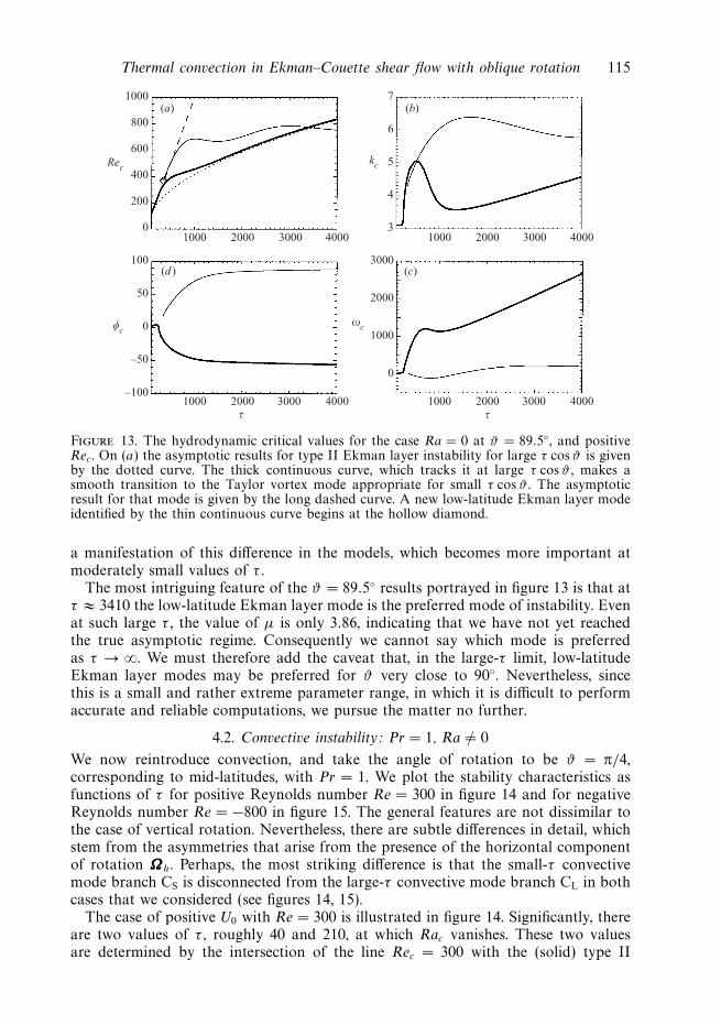
Figure 13. The hydrodynamic critical values for the case Ra = 0 at ϑ = 89.5, and positiveRec . On (a) the asymptotic results for type II Ekman layer instability for large τ cos ϑ is givenby the dotted curve. The thick continuous curve, which tracks it at large τ cos ϑ , makes asmooth transition to the Taylor vortex mode appropriate for small τ cos ϑ . The asymptoticresult for that mode is given by the long dashed curve. A new low-latitude Ekman layer modeidentified by the thin continuous curve begins at the hollow diamond.
a manifestation of this difference in the models, which becomes more important atmoderately small values of τ .
The most intriguing feature of the ϑ = 89.5 results portrayed in figure 13 is that atτ ≈ 3410 the low-latitude Ekman layer mode is the preferred mode of instability. Evenat such large τ , the value of µ is only 3.86, indicating that we have not yet reachedthe true asymptotic regime. Consequently we cannot say which mode is preferredas τ → ∞. We must therefore add the caveat that, in the large-τ limit, low-latitudeEkman layer modes may be preferred for ϑ very close to 90. Nevertheless, sincethis is a small and rather extreme parameter range, in which it is difficult to performaccurate and reliable computations, we pursue the matter no further.
4.2. Convective instability: Pr = 1, Ra = 0
We now reintroduce convection, and take the angle of rotation to be ϑ = π/4,corresponding to mid-latitudes, with Pr = 1. We plot the stability characteristics asfunctions of τ for positive Reynolds number Re = 300 in figure 14 and for negativeReynolds number Re = −800 in figure 15. The general features are not dissimilar tothe case of vertical rotation. Nevertheless, there are subtle differences in detail, whichstem from the asymmetries that arise from the presence of the horizontal componentof rotation ΩΩΩh. Perhaps, the most striking difference is that the small-τ convectivemode branch CS is disconnected from the large-τ convective mode branch CL in bothcases that we considered (see figures 14, 15).
The case of positive U0 with Re = 300 is illustrated in figure 14. Significantly, thereare two values of τ , roughly 40 and 210, at which Rac vanishes. These two valuesare determined by the intersection of the line Rec = 300 with the (solid) type II

116 Y. Ponty, A. D. Gilbert and A. M. Soward
(c)
φc
100
80
60
40
20
(a)
Ra c
/Ra c0
20
10
0
–10
–20100 200 300
50 100 150 200
(d )
ωc
400
300
200
100
(b)
kc
8
7
6
5
4
3
20 100 200 300
0 100 200 3000 250 300τ τ
0
II
CLCS
Figure 14. As in figure 5 but for oblique rotation ϑ = π/4, Pr = 1 and positive Reynoldsnumber Re = 300. The type CS and II modes merge continuously and are identified by thesolid lines. The type CL mode is identified by the dot-dashed lines and its associated localminimum disappears approximately at the location of the hollow diamonds.
curve on figure 11(a) (the type I mode does not appear in figure 14 for the ranges ofRac and τ shown). This scenario is similar to the vertical rotation case illustrated infigure 5. Unlike the vertically rotating case, however, on decreasing τ the minimummerges smoothly with the small-τ convective mode CS, while the large-τ mode CL isdisconnected from it. The change in preference between type II and convective CL
modes occurs at τ 252. The results of the following § 4.3 predict that φc ↓ π/2 andωc ↓ 0 as τ → ∞ (see (4.8a, b)), provided that τ 2/3 Re. These trends are evident infigure 14(c, d) though even at the right of those plots we have not yet achieved theasymptotic limit.
The case of negative U0 with Re = −800 is illustrated in figure 15. Again there aretwo values of τ , now roughly 30 and 80, at which Rac vanishes. These two values aredetermined by the intersection of the line Rec = −800 with the (dotted) type I curveon figure 11(b). On the somewhat wider range roughly 20 τ 80 in figure 15(a),the type I mode is the preferred minimum. Though figure 11(b) suggests that theremight be a τ -range over which the type II mode is the preferred minimum, that isnever the case as figure 15(a) shows. On increasing τ the convective mode minimumCS eventually disappears at τ 307. Before that, however, the preferred minimumchanges to a convective CL mode at τ 220. As τ → ∞, the asymptotic formulae(4.8a, b) again hold for the CL mode. Though the trend ωc ↑ 0 is evident in figure 15(d),the value of φc illustrated in figure 15(c) continues to increase monotonically towardsπ/2, a behaviour which does not conform with the asymptotic prediction φc ↓ π/2.This lack of agreement even at τ = 400 on the right of the figure can be traced tothe large Reynolds number Re = −800, which moves the asymptotic regime to muchlarger values of τ . So to confirm the validity of the large-τ analysis, figure 16 showsthe CL mode branch followed as far as τ = 105. We observe in figure 16(c) that the

Thermal convection in Ekman–Couette shear flow with oblique rotation 117
(c)
φc
150
100
50
0
(a)R
a c/R
a c0
30
20
10
0
–10100 200 300
100 200
(d )
ωc
0
–100
–200
–300
–400
–500
–600
(b)
kc
8
6
4
3
2
0 100 200 300
0 100 200 3000 400300τ τ
0
II
CL
CS
400
400400
I
Figure 15. As in figure 14 but for oblique rotation ϑ = π/4, Pr = 1 and negative Reynoldsnumber Re = −800. The type CS, I, II and CL modes are identified by the dashed, dotted,continuous and dot-dashed lines respectively. The approximate left (right) locations of thedisappearance of the local minima are marked by the hollow (solid) diamonds.
Ra c
/τ4/
3
(c)
φc
τ
k c/τ
1/3
100
95
90
85
80102 103 104 105
ωcτ
1/6 /
Re
(d )
τ
0.5
0.4
0.3
0.2
0.1
0102 103 104 105
(a)10
8
6
4
2
0102 103 104 105
(b)2.0
1.5
1.0
0.5
0102 103 104 105
Figure 16. The critical values for the CL branch with oblique rotation ϑ = π/4, Pr = 1,plotted against τ on a logarithmic scale. The cases illustrated are Re = −800 (solid) and theasymptotic critical values (dashed). (a) The normalized critical Rayleigh number Rac /τ 4/3,(b) the normalized critical wavenumber kc/τ
1/3, (c) the preferred orientation φc , and (d) thenormalized frequency ωc τ 1/6/Re.
118 Y. Ponty, A. D. Gilbert and A. M. Soward
angle φc first overshoots π/2 and then drops back to π/2 in the correct asymptoticmanner (see (4.3), (4.8a)), when τ is about 104. Also shown on figure 16(a, b, d) arethe other parameters Rac, kc and ωc, scaled with powers of Re and τ identified inthe figure caption and chosen to test the asymptotic limits (constants on the figures)predicted by (4.6a, b) and (4.8b). The agreement with theory is very satisfactory.
4.3. Large rotation rate τ 1, τ 2/3 Re
Here we sketch the asymptotic analysis for the case of rapid rotation with obliquerotation ϑ = 0. In this limit, the roll axis attempts to align itself northwards withthe horizontal component of the rotation axis. Nevertheless, the Ekman layer effectstudied in § 3.3 and the Appendix provides a mechanism for non-alignment. Thereforewe write
φ = 12π + Φ, where |Φ| 1, (4.3)
with the objective of determining the small critical angle Φ = Φc, which minimizesRa, and the corresponding small critical frequency ωc.
To that end, we note that in our large-τ , small-Φ limit the main-stream solutionthat replaces (3.3) is
Ψ ∼ Ψ exp[i(tan ϑ)(kΦ)z] sin l(z − z), where k = O(τ 1/3), (4.4)
with similar expressions for V and Θ . In this way the complete solution (2.20)becomes almost independent of the coordinate parallel to the rotation axis evenwhen kΦ itself is large. Accordingly the rolls are inclined to the vertical and so
enhance the dissipation. This is manifested in (2.21c, d) by the approximation ∼−[1 + (tan ϑ)2Φ2]k2 provided that kΦ 1. At very lowest order we ignore boundarylayer effects and solve the main-stream problem subject to the boundary conditionsΨ = 0 on z = 0 and 1. They yield z = 0 and l = π. All these approximations indicatethat the equation which replaces (3.4) at leading order is
k2 Ra ∼[1 + (tan ϑ)2Φ2
]3k6 + (πτ cosϑ)2. (4.5)
Here, the quadratic dependence on Φ illustrates the fact that the critical values of theRayleigh number and wavenumber, namely
Rac ∼ 3(π2/2)2/3(τ cosϑ)4/3, kc ∼ (πτ cos ϑ/√
2)1/3, (4.6a, b)
occur close to Φ = 0.The incorporation of the boundary layer jump conditions requires care but the
upshot of the analysis is that l continues to be given by (3.6b). Consequently equations(3.7a, b) continue to hold with τ replaced by τ cos ϑ and with the additional Φ
dependence identified in (4.5). Specifically, at leading order (3.7a) becomes
Ra ∼ (τ cosϑ)2
k2
π2 +
k6
(τ cos ϑ)2[1 + 3(tan ϑ)2Φ2]− 2π2(τ cos ϑ)1/2
k2ReΓ
. (4.7)
Using (A 3b), (A 7c) and (A 14c), minimization of Ra over small Φ determines thecritical angle
Φc =29
2
(Re
30 tan ϑ
)2 (2
τ cosϑ
)3/2
. (4.8a)

Thermal convection in Ekman–Couette shear flow with oblique rotation 119
The corresponding critical frequency, determined by (3.7b) and (A 11c) on the basisthat φc ≈ π/2, is
Pr−1ωc ∼ 3 Re
10(3 Pr −1)
(4π2
τ cos ϑ
)1/6 (Pr = 1
3
). (4.8b)
It should be emphasized that though we derived (4.5) in the limit kΦ 1, theexpressions (4.5) and (4.7) capture the correct Φ dependence for all values of kΦ ,even as Φ decreases to zero. This fact ensures that (4.8a) holds as τ → ∞. Thusthe remaining requirement Φc 1 is met provided that τ 3/4 Re. Neverthless,that inequality is automatically satisfied when τ 2/3 Re, which is necessary for thevalidity of the boundary layer calculation.
Finally we remark that the symmetries under the interchange Re ↔ − Re (i.e. U0 ↔−U0) implied by (4.8) are simply consequences of our low-order theory and are notexhibited by the actual solution.
5. DiscussionIn our study the nature of the convective instability is affected by three different
physical ingredients. They are the magnitudes of the vertical and horizontalcomponents ΩΩΩv and ΩΩΩh of the rotation vector, and the horizontal shear ΛΛΛ driven bythe bottom boundary velocity U0. Provided that |ΩΩΩv| is sufficiently large an Ekmanlayer forms on the lower boundary. We have explored the ensuing mode competitionbetween hydrodynamic and convective instabilities that occurs in the presence ofbuoyancy forces; in the absence of rotation such competition has been investigatedby Fujimura & Kelly (1988) and Mohamad & Viskanta (1989). Our study has beencomplicated by the fact that the marginal stability surface defined by the neutralRayleigh number Ra = Ra(k, φ) generally has multiple minima. These may includethe type I and II hydrodynamic mode minima as well as the convective minimum.These minima can emerge and disappear in the (k, φ)-plane as figure 6 illustrates.
When there is a horizontal component of rotation (|ΩΩΩh| = 0), the stabilitycharacteristics are sensitive to the sign of U0. For positive Re (U0 pointing westwards)the critical Rayleigh number Rac is generally smaller than for negative Re (U0 pointingeastwards); similar behaviour was identified by Cox (1998). Likewise the magnitude|Rec| of the critical Reynolds numbers in the absence of buoyancy forces at given co-latitude ϑ is generally smaller for positive Re. This feature is also evident in figure 2of Hoffmann & Busse (1999), in which their γ is the co-latitude. The differenceis accentuated as |ΩΩΩv| is reduced to zero. Indeed, in the plane Couette flow limitof horizontal rotation (ϑ = π/2), the pure hydrodynamic Taylor vortex instability(Ra = 0) is only possible for Re > 0. These asymmetries of the stability characteristicsmay have Solar implications, for, according to the interpretation of helioseismologicalresults, the differential rotation of the convection zone is slower (faster) near the pole(equator) than that of the radiative zone below it. So relative to local axes fixed inthe differentially rotating convection zone, the tachocline shear layer is characterizedby Re > 0 (Re < 0) near the pole (equator).
The dynamo properties of the flows described here have been investigated byPonty et al. (2001a, b). Of particular interest are the large-Taylor-number (τ 2 1)convective modes as illustrated for the case τ = 200 in figure 9. Though τ thereis not particularly large, it does illustrate the point that most of the convectiontakes place outside the shear layer with a small part overshooting into it. Since theshear in the layer is quite strong, it opens up the possibility of mixing between
120 Y. Ponty, A. D. Gilbert and A. M. Soward
one cell and its neighbours through horizontal transport in the Ekman layer. Thishas important implications with respect to the question of possible fast dynamomechanisms operating in the tachocline.
Yannick Ponty gratefully acknowledges support from the Leverhulme Trust underResearch Grant F/144/AH. We all acknowledge the support of the CNRS/RoyalSociety cooperation agreement (2002–2003). Andrew Soward thanks the Observatoryof the Cote d’Azur for their kind hospitality during two visits 31 March to 7 April2001 and 13 to 19 April 2002. We have benefited from valuable discussions withProfessors F. H. Busse, C. A. Jones, K. Zhang and Dr P. C. Matthews.
The numerical calculations were performed using the computing facilities of theparallel computer Ceres at the University of Exeter, the computing facilities ofthe laboratory Cassini, Observatory of the Cote d’Azur, provided by the program‘Simulations Interactives et Visualisation en Astronomie et Mecanique (SIVAM)’, andthe computing facilities of IDRIS (Palaiseau, France).
Appendix. The Ekman layerIn the large-τ limit, the buoyancy force in the bottom Ekman layer is negligible.
Thus motion there is governed by the first two components of (2.21a), which reduceunder the boundary layer approximations to
U ′′ + τ (V − V∞) = ik Re (λ1U + λ′1Ψ ), (A 1a)
V ′′ − τU = ik Re (λ1V + λ′2Ψ ), (A 1b)
where V∞ = V (0+) in (3.5) and
Ψ = −∫ z
0
U dz (A 1c)
(cf. (2.16)). The boundary conditions are
U = 0, V = 0 on z = 0. (A 2)
The solution with (U, V ) → (0, V∞) on leaving the Ekman layer leads to the relation
Ψ → τ−1/2ΓBV∞ as τ 1/2z → ∞, (A 3a)
in which we will determine ΓB as a function of φ and
∆ = ik Re
τ. (A 3b)
A compact representation of the solution can be obtained by writing
U + i(V − V∞) = V∞u(ζ ), where ζ = τ 1/2z. (A 4)
Then we have
U = V∞(u + u∗)/2, V = V∞(u − u∗)/(2i) + V∞, (A 5)
where the star denotes the complex conjugate taken when ∆ is real. Accordingly u
satisfies
u,ζζ − β2u = F (∆, ζ ), u(0) = −i(β = eiπ/4
), (A 6a)
where
F (∆, ζ ) = ∆[Reλ(u + i) + λ,ζψ], λ = − i eiφ e−βζ (A 6b, c)

Thermal convection in Ekman–Couette shear flow with oblique rotation 121
and
ψ(ζ ) = −1
2
∫ ζ
0
[u(ξ ) + u∗(ξ )] dξ giving also ΓB = ψ(∞). (A 6d, e)
As an aid to the determination of ΓB , we note that the Green’s function solution
u(ζ ) = −i e−βζ + iβ
[e−βζ
∫ ζ
0
sinhβξ F (∆, ξ ) dξ + sinhβζ
∫ ∞
ζ
e−βξ F (∆, ξ ) dξ
](A 6f)
of (A 6a) may be used to establish the identity∫ ∞
0
u dζ = − β + i
∫ ∞
0
(1 − e−βζ )F (∆, ζ ) dζ. (A 6g)
We emphasize again that the star denotes the complex conjugate taken when ∆ is real;the required results for imaginary ∆ can only be obtained by analytic continuation.
In the small-|∆| limit, we may seek a series expansion
u = u0 + ∆u1 + ∆2u2 + . . . , ψ = ψ0 + ∆ψ1 + ∆2ψ2 + . . . , (A 7a, b)
ΓB = Γ0 + ∆Γ1 + ∆2Γ2 + . . . , F = ∆F1 + ∆2F2 + . . . . (A 7c, d)
Thus at lowest order (A 6d, e, g) determine trivially
Γ0 = 1/√
2, (A 8)
while from (A 6a) u0 satisfies
u0,ζ ζ − iu0 = 0 with u0(0) = −i. (A 9a, b)
The required solution, which tends to zero at infinity, is
u0 = −i e−βζ , ψ0 =Reβ(1 − e−βζ ). (A 10a, b)
At O(|∆|) we have
F1 = Reλ(u0 + i) + λ,ζψ0, (A 11a)
which using (A 10a, b) is
F1 = 12[−i(eiφ + ie−iφ)e−
√2ζ − e−iφe−β∗ζ + ieiφe−βζ ]. (A 11b)
Accordingly (A 6d, e, g) determine
Γ1(φ) =−7 cosφ + 3 sinφ
20√
2. (A 11c)
Furthermore by (A 6a) u1 satisfies
u1,ζ ζ − iu1 = F1 with u1(0) = 0, (A 12)
from which we obtain
u1 =1
20
2(1 − 2i)(eiφ + ie−iφ) e−
√2ζ − 5ie−iφe−β∗ζ
−[5βeiφ ζ + (2(1 − 2i)eiφ + (4 − 3i)e−iφ)]e−βζ
, (A 13a)
ψ1 =1
20Re
−(5 − 2i)βeiφ + 6βe−iφe−
√2ζ
−[5eiφζ − β((9 + 7i)eiφ + (3 + 4i)e−iφ)]e−βζ
. (A 13b)

122 Y. Ponty, A. D. Gilbert and A. M. Soward
At O(|∆|2) we have
F2 = Reλu1 + λ,ζψ1, (A 14a)
which using (A 13a,b) is
F2 =1
40
[−10iβζ + (4 + 3i)e2iφ − (2 − 7i) − (3 + 4i)e−2iφ]e−
√2ζ
− 4(1 + i)(−ie2iφ + 1)e−(β+√
2)ζ + 2(2 + i)(1 + ie−2iφ)e−(β∗+√
2)ζ
− 5(1 + i)e2iφe−2βζ + 5e−2iφe−2β∗ζ + [(5 − 2i)e2iφ + (2 − 5i)]e−βζ. (A 14b)
Accordingly (A 6d, e, g) determine
Γ2(φ) =−21 cos 2φ + 29 sin 2φ
600√
2+ constant, (A 14c)
where the value of the constant is of no interest to us.The main and important point is that
ReΓB ∼ Γ0 −(
k Re
τ
)2
Γ2 (A 15)
is maximized where Γ2 is minimized at
φc = − 12tan−1 29
21≈ − 27.0451. (A 16)
This selects the orientation φc of the rolls which minimizes the Rayleigh number(3.7a), so determining its critical value as a perturbation of (3.8a). The correspondingvalue of
ImΓB ∼ k Re
τΓ1 (A 17a)
is determined by
Γ1(φc) ≈ − 0.268652, (A 17b)
which in turn fixes the critical frequency (3.11).
REFERENCES
Asai, T. & Nakasuji, I. 1973 On the stability of Ekman boundary layer flow with thermally unstablestratification. J. Met. Soc. Japan 51, 29–42.
Brown, R. A. 1972 On the inflexion point instability of a stratified Ekman boundary layer.J. Atmos. Sci. 29, 850–859.
Busse, F. H. & Kropp, M. 1992 Buoyancy driven instabilities in rotating layers with parallel axisof rotation. Z. Angew. Math. Phys. 43, 28–35.
Caldwell, D. R. & Van Atta, C. W. 1970 Characteristics of Ekman boundary layer instabilities.J. Fluid. Mech. 44, 79–95.
Clever, R. M., Busse, F. H. & Kelly, R. E. 1977 Instabilities of longitudinal convection rolls inCouette flow. Z. Angew. Math. Phys. 28, 771–783.
Cox, S. M. 1998 Rotating convection in a shear flow. Proc. R. Soc. Lond. A 454, 1699–1717.
Dziembowski, W., Goode, P. R. & Libbrecht, K. G. 1989 The radial gradient in the Sun’s rotation.Astrophys. J. 337, L53–L57.
Etling, D. 1971 The stability of an Ekman boundary layer flow as influenced by the thermalstratification. Beitr. Phys. Atmosph. 44, 168–186.
Etling, D. & Brown, R. A. 1993 Roll vortices in the planetary boundary: a review. Boundary-LayerMet. 65, 215–248.
Faller, A. J. 1963 An experimental study of the instability of the laminar Ekman boundary layer.J. Fluid Mech. 15, 560–576.

Thermal convection in Ekman–Couette shear flow with oblique rotation 123
Faller, A. J. & Kaylor, R. E. 1966 A numerical study of the instability of laminar Ekmanboundary layer flow. J. Atmos. Sci. 23, 466–480.
Fujimura, K. & Kelly, R. E. 1988 Stability of unstably stratified shear flow between parallel plates.Fluid Dyn. Res. 2, 281–292.
Gage, K. S. & Reid, W. H. 1968 The stability of thermally stratified plane Poiseuille flow. J. FluidMech. 33, 21–32.
Gottlieb, D. & Orszag. S. A. 1977 Numerical Analysis of Spectral Methods: Theory and Applications.SIAM, Philadelphia.
Greenspan, H. P. 1968 The Theory of Rotating Fluids. Cambridge University Press.
Hathaway, D. H. & Somerville, R. C. J. 1986 Nonlinear interactions between convection, rotationand flows with vertical shear. J. Fluid Mech. 164, 91–105.
Hathaway, D. H., Toomre, J. & Gilman, P. A. 1980 Convective instability when the temperaturegradient and rotation vector are oblique to gravity. II. Real fluids with effects of diffusion.Geophys. Astrophys. Fluid Dyn. 15, 7–37.
Hoffman, N. & Busse, F. H. 1999 Instabilities of shear flows between two coaxial differentiallyrotating cones. Phys. Fluids 11, 1676–1678.
Hoffman, N. & Busse, F. H. 2001 Linear instabilities of Poiseuille–Couette–Ekman flows: Localresults for flows between differentially rotating disks with throughflow. Phys. Fluids 13, 2735–2738.
Hoffman, N., Busse, F. H. & Chen, W.-L. 1998 Transition to complex flows in the Ekman–Couettelayer. J. Fluid Mech. 366, 311–331.
Ingersoll, A. P. 1965 Convective instabilities in plane Couette flow. Phys. Fluids 9, 682–689.
Iooss, G., Nielsen, H. B. & True, H. 1978 Bifurcation of the stationary Ekman flow into a stableperiodic flow. Arch. Rat. Mech. Anal. 68, 227–256.
Kelly, R. E. 1994 The onset and development of thermal convection in fully developed shear flows.Adv. Appl. Mech. 31, 35–112.
Kropp, K. & Busse, F. H. 1991 Thermal convection in differentially rotating systems. Geophys.Astrophys. Fluid Dyn. 61, 127–148.
Leibovich, S. & Lele, S. K. 1985 The influence of the horizontal compoment of Earth’s angularvelocity on the instability of the Ekman layer. J. Fluid Mech. 150, 41–87.
Lilly, D. K. 1966 On the instability of Ekman boundary flow. J. Atmos. Sci. 23, 481–494.
Matthews, P. C. & Cox, S. 1997 Linear stability of rotating convection in an imposed shear flow.J. Fluid Mech. 350, 271–293.
Melander, M. V. 1983 An algorithmic approach to the linear stability of the Ekman layer. J. FluidMech. 132, 283–293.
Mohamad, A. A. & Viskanta, R. 1989 Stability of a lid-driven shallow cavity heated from below.Intl J. Heat Mass Transfer 32, 2155–2166.
Ponty, Y., Gilbert, A. D. & Soward, A. M. 2001a Kinematic dynamo action in large magneticReynolds number flows driven by shear and convection. J. Fluid Mech. 435, 261–287.
Ponty, Y., Gilbert, A. D. & Soward, A. M. 2001b Dynamo action due to Ekman layer instability. InDynamo and Dynamics, a Mathematical Challenge (ed. P. Chossat, D. Armbruster & I. Oprea).NATO ASI, pp. 75–82. Kluwer.
Spiegel, E. A. & Zahn, J.-P. 1992 The Solar tachocline. Astron. Astrophys. 265, 106–114.
Weiss, N. O. 1994 Solar and stellar dynamos. In Lectures on Solar and Planetary Dynamos (ed.M. R. E. Proctor & A. D. Gilbert), pp. 59–95. Cambridge University Press.
Wippermann, F. K., Etling, D. & Kirstein, H. J. 1978 On the instability of a planetary boundarylayer with Rossby number similarity. Boundary-Layer Met. 15, 301–321.
Copyright © 2022 FDOKUMEN