Meccanica (2010) 45: 187–198DOI 10.1007/s11012-009-9236-9

Oblique stagnation slip flow of a micropolar fluid

Y.Y. Lok · I. Pop · D.B. Ingham

Received: 11 September 2008 / Accepted: 1 July 2009 / Published online: 21 July 2009© Springer Science+Business Media B.V. 2009

Abstract This paper considers the problem of steadytwo-dimensional boundary layer flow of a micropolarfluid near an oblique stagnation point on a fixed sur-face with Navier’s slip condition. It is shown that thegoverning nonlinear partial differential equations ad-mit similarity solutions. The resulting nonlinear ordi-nary differential equations are solved numerically us-ing the Keller box method for some values of the gov-erning parameters. It is found that the flow character-istics depend strongly on the micropolar and slip para-meters.

Keywords Micropolar fluid · Boundary layer ·Oblique stagnation point · Slip flow

Y.Y. LokFaculty of Manufacturing Engineering, Universiti TeknikalMalaysia Melaka, 76109 Durian Tunggal, Melaka,Malaysia

I. Pop (�)Faculty of Mathematics, University of Cluj, CP 253,3400 Cluj, Romaniae-mail: pop.ioan@yahoo.co.uk

D.B. InghamCentre for Computational Fluid Dynamics, Universityof Leeds, Leeds LS2 9JT, UK

Nomenclature

a Strength of the irrotational stagnation-pointflow

A Constant in (19) and (23)At Slip constantb Strain rate of the uniform shear flowC1,C2 Constants of integrationK Micropolar material parameterl Characteristic lengthn Ratio of the microrotation vector component

and the fluid skin friction at the wall (or wallshear stress)

N Component of the microrotation vectornormal to x–y plane

p PressureU0 Characteristic velocityu,v Velocity components along x- and y-axesxs Point of zero wall shear stressx, y Cartesian coordinates along the plate and

normal to it, respectively

Greek Symbols

α Shear flow parameterγ Velocity slip factorκ Vortex viscosityμ Dynamic viscosityρ Densityυ Kinematic viscosityψ Stream functionτ Wall shear stress

188 Meccanica (2010) 45: 187–198

Superscript

– Dimensional variables

Subscripts

e Far field conditionw Wall condition

1 Introduction

The theory of micropolar fluids, which displays the ef-fects of local rotary inertia and coupled stresses, wasformulated by Eringen [1, 2]. The theory can be usedto explain the flow of colloidal fluids, liquid crystals,low concentration suspensions, animal blood, lubri-cants, turbulent shear flows, etc. In such fluids themicro-elements possess both translational and rota-tional motions. The interaction of the macro-velocityfield and microrotation field can be described throughnew material constants in addition to those of a clas-sical Newtonian fluid. Eringen’s micropolar model in-cludes the classical Navier-Stokes equations as a spe-cial case, but can cover, both in theory and applica-tions, many more phenomena than the classical model.Extensive reviews of the theory and applications of mi-cropolar fluids can be found in the recent books byŁukaszewicz [3] and Eringen [4].

The boundary layer flow of such a micropolar fluidpast a semi-infinite plate was first studied by Ped-dieson and McNitt [5], whereas a similarity solutionfor boundary layer flow near a stagnation point waspresented by Ebert [6]. Hiemenz [7] derived an ex-act solution of the Navier-Stokes equations which de-scribe the steady flow of a viscous and incompress-ible fluid directed perpendicularly (orthogonal) to asemi-infinite wall. Stuart [8], Tamada [9], Dorrepaal[10, 11] and Labropulu et al. [12] have extended theclassical Hiemenz’s flow to oblique stagnation pointflow. In a real situation, this flow results when a uni-form stream approaches a blunt two-dimensional bodyof infinite curvature. The investigation in this areais motivated by the possibility of solving exactly theboundary layer equations at the stagnation point andby their relevance to a wide range of engineering ap-plications. Basic insight into the physical mechanisminvolved at the leading edge and nose regions of bod-ies in high speed flight can be achieved by consider-ing the model of stagnation point flow (Amaouche and

Boukari [13]). We mention also that Tilley and Wei-dman [14] have studied the steady oblique two-fluidstagnation-point flow, while Weidman and Putkaradze[15] have considered the axisymmetric stagnation flowof a viscous and incompressible fluid obliquely im-pinging on a circular cylinder as an exact solution ofthe Navier-Stokes equations. Finally, it is worth men-tioning that the present work is an extension of therecent paper by Lok et al. [16] to the case of the non-orthogonal stagnation-point flow of a micropolar whenthe slip on the boundary is considered. Obliqueness ofthe free stream is believed to have applications to thereattachment zone of certain separated flows and in theproblem of premixed laminar flame extinction.

The slip-flow of a Newtonian fluid past a lin-early stretching sheet has been studied by Andersson[17] and he obtained a closed-form analytical solu-tion. Wang [18–20] obtained the exact similarity so-lutions of the Navier-Stokes equations for the two-dimensional stagnation flow solutions of Hiemenz [7]on a fixed plate [18], on a moving plate in its ownplane [19], and on a cylinder [20] with Navier’s slipcondition. Wang [20] pointed out that partial slip ona solid boundary occurs in many situations. For ex-ample, in rarefied gases, when the Knudsen numberis small, there is a slip regime where the Navier-Stokes equations are valid but slip occurs (Sharipovand Seleznev [21]). On the other hand, the solid sur-face may be rough or porous such that equivalent slipis present (Wang [22]). Some coated surfaces, suchas Teflon, resist adhesion. In these cases the no slipcondition is replaced by Navier’s partial slip condi-tion, where the slip velocity is proportional to the localshear stress. Therefore, the aim of the present paperis, to extend Wang’s [18] problem to the case of mi-cropolar fluid flows. Namely, we consider the steadytwo-dimensional oblique stagnation flow of a microp-olar fluid towards a fixed surface with slip, a prob-lem which has not been considered before. To do itwe shall follow the method suggested by Weidmanand Putkaradze [15] who have corrected the results re-ported earlier by Dorrepaal [10, 11].

2 Basic equations

Consider the steady two-dimensional flow of a mi-cropolar fluid near a non-orthogonal stagnation pointon a fixed flat plate coinciding with the plane y = 0

Meccanica (2010) 45: 187–198 189

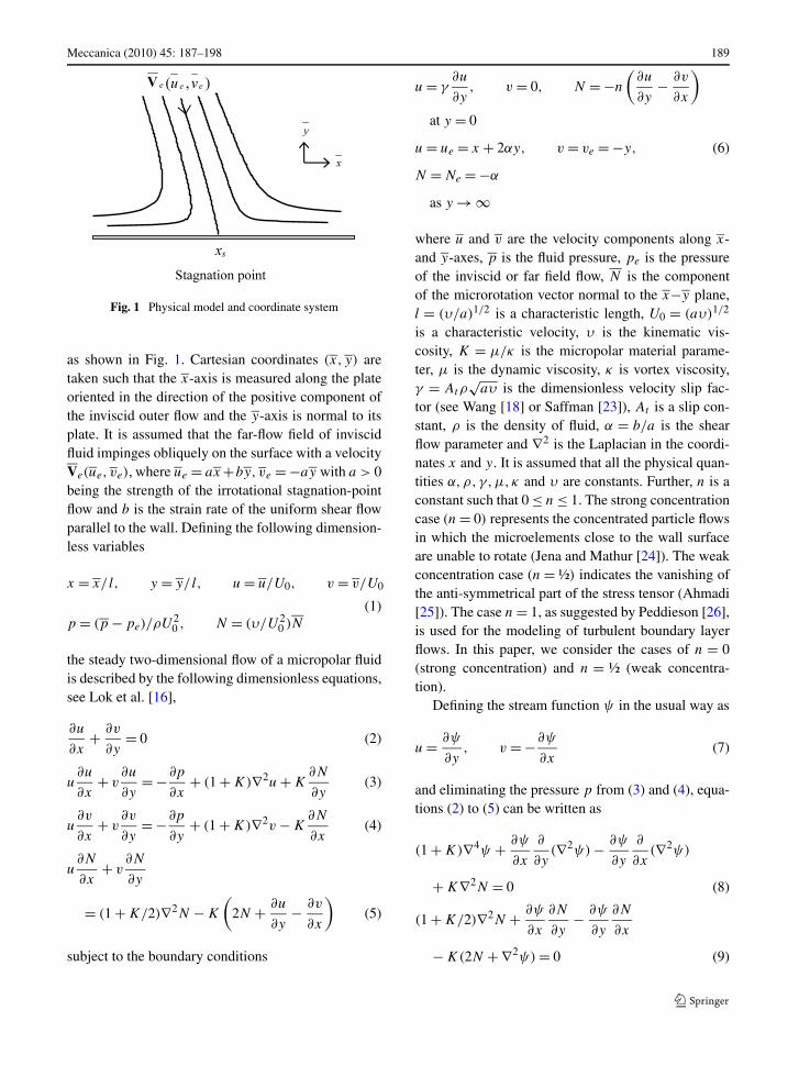
Fig. 1 Physical model and coordinate system

as shown in Fig. 1. Cartesian coordinates (x, y) aretaken such that the x-axis is measured along the plateoriented in the direction of the positive component ofthe inviscid outer flow and the y-axis is normal to itsplate. It is assumed that the far-flow field of inviscidfluid impinges obliquely on the surface with a velocityVe(ue, ve), where ue = ax+by, ve = −ay with a > 0being the strength of the irrotational stagnation-pointflow and b is the strain rate of the uniform shear flowparallel to the wall. Defining the following dimension-less variables

x = x/l, y = y/l, u = u/U0, v = v/U0

(1)p = (p − pe)/ρU2

0 , N = (υ/U20 )N

the steady two-dimensional flow of a micropolar fluidis described by the following dimensionless equations,see Lok et al. [16],

∂u

∂x+ ∂v

∂y= 0 (2)

u∂u

∂x+ v

∂u

∂y= −∂p

∂x+ (1 + K)∇2u + K

∂N

∂y(3)

u∂v

∂x+ v

∂v

∂y= −∂p

∂y+ (1 + K)∇2v − K

∂N

∂x(4)

u∂N

∂x+ v

∂N

∂y

= (1 + K/2)∇2N − K

(2N + ∂u

∂y− ∂v

∂x

)(5)

subject to the boundary conditions

u = γ∂u

∂y, v = 0, N = −n

(∂u

∂y− ∂v

∂x

)

at y = 0

u = ue = x + 2αy, v = ve = −y, (6)

N = Ne = −α

as y → ∞

where u and v are the velocity components along x-and y-axes, p is the fluid pressure, pe is the pressureof the inviscid or far field flow, N is the componentof the microrotation vector normal to the x−y plane,l = (υ/a)1/2 is a characteristic length, U0 = (aυ)1/2

is a characteristic velocity, υ is the kinematic vis-cosity, K = μ/κ is the micropolar material parame-ter, μ is the dynamic viscosity, κ is vortex viscosity,γ = Atρ

√aυ is the dimensionless velocity slip fac-

tor (see Wang [18] or Saffman [23]), At is a slip con-stant, ρ is the density of fluid, α = b/a is the shearflow parameter and ∇2 is the Laplacian in the coordi-nates x and y. It is assumed that all the physical quan-tities α,ρ, γ,μ,κ and υ are constants. Further, n is aconstant such that 0 ≤ n ≤ 1. The strong concentrationcase (n = 0) represents the concentrated particle flowsin which the microelements close to the wall surfaceare unable to rotate (Jena and Mathur [24]). The weakconcentration case (n = ½) indicates the vanishing ofthe anti-symmetrical part of the stress tensor (Ahmadi[25]). The case n = 1, as suggested by Peddieson [26],is used for the modeling of turbulent boundary layerflows. In this paper, we consider the cases of n = 0(strong concentration) and n = ½ (weak concentra-tion).

Defining the stream function ψ in the usual way as

u = ∂ψ

∂y, v = −∂ψ

∂x(7)

and eliminating the pressure p from (3) and (4), equa-tions (2) to (5) can be written as

(1 + K)∇4ψ + ∂ψ

∂x

∂

∂y(∇2ψ) − ∂ψ

∂y

∂

∂x(∇2ψ)

+ K∇2N = 0 (8)

(1 + K/2)∇2N + ∂ψ

∂x

∂N

∂y− ∂ψ

∂y

∂N

∂x

− K(2N + ∇2ψ) = 0 (9)

190 Meccanica (2010) 45: 187–198

and the boundary conditions (6) become

ψ = 0,∂ψ

∂y= γ

∂2ψ

∂y2, N = −n∇2ψ

at y = 0 (10)

ψ = xy + αy2, N = −α as y → ∞It should be mentioned that for the orthogonal stagna-tion point flow, that is when α = 0, from (10) we haveψ = xy and N = 0 as y → ∞.

A physical quantity of interest is the wall shearstress which is given by, see Lok et al. [16],

τw =[(1 + K)

(∂2ψ

∂y2− ∂2ψ

∂x2

)+ KN

]y=0

(11)

We assume that the solutions of (8) and (9) are of theform

ψ(x, y) = xf (y) + g(y),

(12)N(x,y) = xh(y) + t (y)

Substituting expressions (12) into (8) and (9), we ob-tain, after one integration of (8), the following ordinarydifferential equations

(1 + K)f ′′′ + ff ′′ − f ′2 + Kh′ = C1 (13)

(1 + K)g′′′ + fg′′ − f ′g′ + Kt ′ = C2 (14)

(1 + K/2)h′′ + f h′ − f ′h − K(2h + f ′′) = 0 (15)

(1 + K/2)t ′′ + f t ′ − g′h − K(2t + g′′) = 0 (16)

and the boundary conditions (10) now become

f (0) = 0, h(0) = −nf ′′(0), f ′(0) = γf ′′(0)

(17a)f ′(∞) = 1, h(∞) = 0

g(0) = 0, t (0) = −ng′′(0), g′(0) = γg′′(0)

(17b)g′′(∞) = 2α, t (∞) = −α

where C1 and C2 are constants of integration andprimes denote differentiation with respect to y. Us-ing the boundary conditions (17a), we get C1 = −1.In this respect, we have to show that the term ff ′′ →0 as y → ∞ in (13). Thus, the boundary condition(17a) gives ff ′′ − 1 = C1 as y → ∞. Further, iff → y as y → ∞ then ff ′′ gives f ′′ → (C1 + 1)/y

as y → ∞. On integration, this equations gives f ′ =(C1 + 1)(lny) + constant as y → ∞. However, theboundary condition (17a) gives C1 = −1 and the con-stant being unity, i.e. constant = 1. Therefore (13) be-comes

(1 + K)f ′′′ + ff ′′ − f ′2 + Kh′ + 1 = 0 (18)

This equation describes the classical boundary layerflow of a micropolar fluid near a two-dimensional or-thogonal stagnation-point; see Lok et al. [16]. Equa-tion (18) gives

f (y) = y + A as y → ∞ (19)

where A is a constant which depends on K and γ , i.e.A = A(K,γ ). Further, substituting ue, ve and Ne from(6) into (3) and (4), the dimensionless pressure p = pe

of the inviscid or far field flow from the plate can beexpressed as

p = pe = −1

2(x2 + y2) + constant (20)

On the other hand, using (7) and (12) in (2) and (3),we obtain for the viscous flow

−∂p

∂x= x − C2

(21)

−∂p

∂y= (1 + K)f ′′ + ff ′ + Kh

Matching (21) for the viscous flow with the x-pressuregradient for the inviscid or far field flow from (20) re-quires C2 = 0, so that (14) becomes

(1 + K)g′′′ + fg′′ − f ′g′ + Kt ′ = 0 (22)

Then the leading behaviour of g(y) evaluated from(22) using the asymptotic result for f (y) given by(19), takes the form

g(y) ≈ α(y + A)2 + constant as y → ∞ (23)

If we take g′(y) = 2αφ(y) and t (y) = 2α�(y), (22)and (16) then become

(1 + K)φ′′ + f φ′ − f ′φ + K�′ = 0 (24)

(1 + K/2)�′′ + f �′ − φh − K(2� + φ′) = 0 (25)

Meccanica (2010) 45: 187–198 191

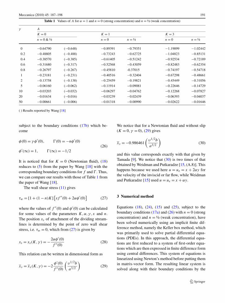
Table 1 Values of A for α = 1 and n = 0 (strong concentration) and n = ½ (weak concentration)

γ A

K = 0 K = 1 K = 3

n = 0 & ½ n = 0 n = ½ n = 0 n = ½

0 −0.64790 (−0.648) −0.89391 −0.79351 −1.19899 −1.02442

0.2 −0.48805 (−0.488) −0.73243 −0.62725 −1.04823 −0.85131

0.4 −0.38570 (−0.385) −0.61405 −0.51242 −0.92534 −0.72189

0.6 −0.31680 (−0.317) −0.52568 −0.43059 −0.82483 −0.62354

0.8 −0.26797 (−0.267) −0.45810 -0.37015 −0.74197 −0.54718

1 −0.23181 (−0.231) −0.40516 −0.32404 −0.67298 −0.48661

2 −0.13758 (−0.138) −0.25459 −0.19821 −0.45449 −0.31056

5 −0.06160 (−0.062) −0.11914 −0.09081 −0.22646 −0.14729

10 −0.03203 (−0.032) −0.06297 −0.04762 −0.12268 −0.07827

20 −0.01634 (−0.016) −0.03239 −0.02439 −0.06393 −0.04037

50 −0.00661 (−0.006) −0.01318 −0.00990 −0.02622 −0.01646

( ) Results reported by Wang [18]

subject to the boundary conditions (17b) which be-come

φ(0) = γφ′(0), �(0) = −nφ′(0)

(26)φ′(∞) = 1, �(∞) = −1/2

It is noticed that for K = 0 (Newtonian fluid), (18)reduces to (5) from the paper by Wang [18] with thecorresponding boundary conditions for f and �. Thus,we can compare our results with those of Table 1 fromthe paper of Wang [18].

The wall shear stress (11) gives

τw = [1 + (1 − n)K] [xf ′′(0) + 2αφ′(0)]

(27)

where the values of f ′′(0) and φ′(0) can be calculatedfor some values of the parameters K,α,γ, x and n.The position xs of attachment of the dividing stream-lines is determined by the point of zero wall shearstress, i.e. τw = 0, which from (27) is given by

xs = xs(K,γ ) = −2αφ′(0)

f ′′(0)(28)

This relation can be written in dimensional form as

xs = xs(K,γ ) = −2φ′(0)

f ′′(0)

(υ1/2b

a3/2

)(29)

We notice that for a Newtonian fluid and without slip(K = 0, γ = 0), (29) gives

xs = −0.986461

(υ1/2b

a3/2

)(30)

and this value corresponds exactly with that given byTamada [9]. We notice that (30) is two times of thatobtained by Weidman and Putkaradze [15, (A.8)]. Thishappens because we used here u = ue = x + 2αy forthe velocity of the inviscid or far flow, while Weidmanand Putkaradze [15] used u = ue = x + αy.

3 Numerical method

Equations (18), (24), (15) and (25), subject to theboundary conditions (17a) and (26) with n = 0 (strongconcentration) and n = ½ (weak concentration), havebeen solved numerically using an implicit finite dif-ference method, namely the Keller box method, whichwas primarily used to solve partial differential equa-tions (PDEs). In this approach, the differential equa-tions are first reduced to a system of first-order equa-tions which are then expressed in finite difference formusing central differences. This system of equations islinearized using Newton’s method before putting themin matrix-vector form. The resulting linear system issolved along with their boundary conditions by the

192 Meccanica (2010) 45: 187–198

Table 2 Initial values for f ′′(0) and φ′(0) as a function of velocity slip factor γ and material parameter K when n = 0 (strongconcentration) and α = 1

γ K = 0 K = 1 K = 3

f ′′(0) φ′(0) f ′′(0) φ′(0) f ′′(0) φ′(0)

0 1.23259 0.60795 0.84107 0.47897 0.55537 0.40000

{1.23259} {0.60795}

(1.2325)

0.2 1.04258(1.0425)

0.58381 0.75238 0.47634 0.51752 0.40267

0.4 0.88635(0.8863)

0.53677 0.67204 0.45872 0.48091 0.39791

0.6 0.76428(0.7642)

0.48731 0.60286 0.43470 0.44684 0.38840

0.8 0.66897(0.6689)

0.44212 0.54432 0.40898 0.41582 0.37618

1 0.59346(0.5934)

0.40266 0.49487 0.38386 0.38787 0.36262

1.4 0.48265 0.33935 0.41711 0.33863 0.34039 0.33464

1.5 0.46095 0.32624 0.40112 0.32852 0.33006 0.32780

2 0.37589(0.3759)

0.27276 0.33602 0.28473 0.28590 0.29579

5 0.17726(0.1773)

0.13561 0.16840 0.15410 0.15575 0.17837

10 0.09404(0.0940)

0.07341 0.09155 0.08643 0.08782 0.10518

20 0.04847(0.0485)

0.03825 0.04781 0.04590 0.04680 0.05747

50 0.01975(0.0198)

0.01569 0.01964 0.01906 0.01947 0.02430

{ } Results reported by Weidman and Putkaradze [15], ( ) Results reported by Wang [18]

block-tridiagonal-elimination method. The details ofthis method can be seen in the books by Cebeci andBradshaw [27] and Cebeci [28].

The computation is started by using a small valueof y∞ and then successively increase the value ofy∞ until a suitably large value of y∞ is obtained.A convergence criterion based on the relative differ-ence between the current and previous iterations hasbeen used. Therefore, in this paper, we use a step sizeof �y = 0.001, y∞ = 10, and convergence criterion1 × 10−7.

4 Results and discussion

The values of A (from (19)) and the initial valuesf ′′(0) and φ′(0) when α = 1 for some values of the

velocity slip factor γ and the material parameter K aregiven in Tables 1 and 2. In order to verify the accuracyof the present results, we have compared the valuesof A and f ′′(0) with some values of γ when K = 0(Newtonian fluid) with those obtained by Wang [18]who used the shooting method. The values of f ′′(0)

and φ′(0) obtained by Weidman and Putkaradze [15]for oblique stagnation-point flow of a Newtonian fluidwith no slip condition are also included in Table 2.These results are shown by parentheses in Tables 1and 2. The results show very good agreement, there-fore we are confident that the present results are accu-rate. From Table 1, it is found that the magnitude ofA decreases as the slip parameter γ increases. How-ever, for a fixed value of γ , the value of A increasesas the micropolar parameter K increases. Further, it isnoticed from Table 2 that the effect of increasing val-

Meccanica (2010) 45: 187–198 193

Fig. 2 Variation of τw with γ for both n = 0 and n = ½ when x = α = 1 and several values of K

Fig. 3 Streamline patterns for γ = α = 1 and n = 0 when K = 0 (Newtonian fluid) and K = 3

ues of K results in a decrease in values of the reducedskin friction f ′′(0) and φ′(0). However, the value ofφ′(0) increases as K increases when γ > 1.5.

Figure 2 shows the variation of wall shear stress,τw with velocity slip factor γ for several values of K

when α = 1 for both strong and weak concentrationmicropolar fluid. It is seen that the shear stress near

the wall decreases as γ increases. This is predictablebecause the velocity slip factor γ is inversely propor-tional to the f ′′(0) (wall shear stress), see the Navier’spartial slip initial condition (17a). On the other hand,the values of wall shear stress for a micropolar fluidare found to be larger than those for a Newtonian fluid,and its values increases as K increases. Therefore, by

194 Meccanica (2010) 45: 187–198

Table 3 Values of xs (zero wall shear stress) for some values of γ and K when n = 0,½ and α = 1

γ xs

K = 0 K = 1 K = 3

n = 0 & ½ n = 0 n = ½ n = 0 n = ½

0 −0.98646 −1.13896 −1.20816 −1.44047 −1.55973

0.2 −1.11992 −1.26622 −1.34611 −1.55616 −1.70238

0.4 −1.21120 −1.36515 −1.44710 −1.65483 −1.81438

0.6 −1.27520 −1.44219 −1.52192 −1.73844 −1.90258

0.8 −1.32181 −1.50274 −1.57869 −1.80935 −1.97289

1 −1.35698 −1.55133 −1.62289 −1.86974 −2.02979

2 −1.45129 −1.69471 −1.74728 −2.06916 −2.20089

5 −1.53009 −1.83021 −1.85183 −2.29038 −2.36707

10 −1.56142 −1.88818 −1.90341 −2.39544 −2.43949

20 −1.57820 −1.92018 −1.92819 −2.45613 −2.47978

50 −1.58864 −1.94044 −1.94375 −2.49553 −2.50542

Fig. 4 Streamline patterns for γ = 0.5, n = 0 and K = 1: (a) α = 0 (orthogonal flow); (b) α = 1; c α = 2

using micropolar fluid as the flow medium, it will helpin increasing the wall shear stress, thus slow down thefluid flow velocity.

The streamline patterns for oblique stagnationflows with slip can be obtained from (12) by solving(18), (22), (15) and (16) subject to the boundary condi-tions (17). For graphing purposes, we take α = γ = 1.Figure 3 shows the streamline patterns for K = 0

and 3 when n = 0 (strong concentration). In addition,the values of xs , i.e. the location of zero wall shearstress, for several values of γ and K are given in Ta-ble 3. It can be seen from Table 3 and Fig. 3 that thepoint of stagnation, or the point of zero wall shearstress, xs is to the left of the origin, and its magnitudeincreases as K increases. Since xs is the ratio of φ′(0)

to f ′′(0) (see (28)), in addition, material parameter

Meccanica (2010) 45: 187–198 195

Fig. 4 (Continued)

K in micropolar fluids enhances φ′(0) while reducingf ′′(0) (see Table 2) when γ increases. Therefore, themagnitude of xs for K = 3 increases faster than forK = 0 and 1. From Table 3, it is also observed thatfor a fixed value of K , the location of the point xs

moves continuously away from the origin with an in-crease in γ . This is because the slip increases with the

slip factor γ , and this results in the slip of the pointof stagnation. Figure 4 shows the streamline patternswhen γ = 0.5, n = 0 and K = 1 for some values of theshear flow parameter α. It is clear that the obliquenessof the oncoming flow increases as α increases, conse-quently the shift in the location of the zero wall shearstress.

196 Meccanica (2010) 45: 187–198

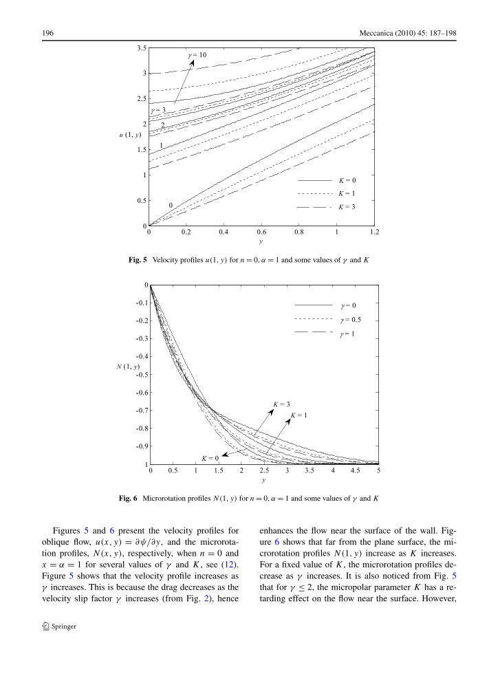
Fig. 5 Velocity profiles u(1, y) for n = 0, α = 1 and some values of γ and K

Fig. 6 Microrotation profiles N(1, y) for n = 0, α = 1 and some values of γ and K

Figures 5 and 6 present the velocity profiles foroblique flow, u(x, y) = ∂ψ/∂y, and the microrota-tion profiles, N(x,y), respectively, when n = 0 andx = α = 1 for several values of γ and K , see (12).Figure 5 shows that the velocity profile increases asγ increases. This is because the drag decreases as thevelocity slip factor γ increases (from Fig. 2), hence

enhances the flow near the surface of the wall. Fig-ure 6 shows that far from the plane surface, the mi-crorotation profiles N(1, y) increase as K increases.For a fixed value of K , the microrotation profiles de-crease as γ increases. It is also noticed from Fig. 5that for γ ≤ 2, the micropolar parameter K has a re-tarding effect on the flow near the surface. However,

Meccanica (2010) 45: 187–198 197

Fig. 7 Velocity at the wall u(1,0) versus the velocity slip factor for n = 0, α = 1 and some values of K

the parameter K enhances the flow near the surfacewhen γ ≥ 3. To investigate this phenomenon, a rela-tionship between the velocities at the wall u(1,0) withthe velocity slip factor γ for K = 0,1 and 3 has beenplotted in Fig 7. It can be seen that for smaller valueof γ , the Newtonian fluid (K = 0) has a higher ve-locity compared to a micropolar fluid (K = 0), how-ever, beyond the critical value γc (2.3 < γc < 2.6),the opposite trend is observed. By looking at the in-dividual values of f ′(0) and g′(0) that contributes tothe velocity u(1,0), we notice that when K increases,f ′(0) and g′(0) decrease, however, g′(0) increases af-ter the critical value γc . This means that for all val-ues of γ , micropolar fluids cause the decrease in thenormalized velocity f ′. When the velocity slip factorγ is large enough, the existence of suspended parti-cles in micropolar fluids enhances the tangential ve-locity g′.

5 Conclusion

The present paper studies the oblique stagnation pointslip flow on a fixed plate in a micropolar fluid. It isfound that the drag decreases as the slip parameterincreases and therefore increases the velocity. This ispossible because when γ is infinity, the flow behaves

as though it were inviscid (Wang [18]). It is interest-ing to note that in [19, 20], for large λ (γ in our case),the author used the perturbation expansion technique,with ε = 1/λ and found that the drag decreases as 1/λ

and the heat transfer increases with λ. It is also foundthat a micropolar fluid causes a higher wall shear stresscompared to a Newtonian fluid. For a fixed value of γ ,the streamlines far from the plane wall shift to the leftof the origin as K increases, and consequently the shiftin the location of the stagnation point or the point ofzero wall shear stress. The results presented in this pa-per should be useful in our understanding of flows nearstagnation regions of blunt bodies.

Acknowledgements The first author (Y.Y. Lok) would like toacknowledge the financial support received from the EU MarieCurie Training Site Grant and the host, the Centre for Compu-tational Fluid Dynamics, University of Leeds, U.K. The secondand third authors (I. Pop and D.B. Ingham) wish to thank theRoyal Society for partial financial support.

References

1. Eringen AC (1966) Theory of micropolar fluids. J MathMech 16:1–18

2. Eringen AC (1972) Theory of thermomicrofluids. J MathAnal Appl 38:480–496

3. Łukaszewicz G (1999) Micropolar fluids: theory and appli-cation. Birkhäuser, Basel

198 Meccanica (2010) 45: 187–198

4. Eringen AC (2001) Microcontinuum field theories. II: Flu-ent media. Springer, New York

5. Peddieson J, McNitt RP (1970) Boundary layer theory fora micropolar fluid. Recent Adv Eng Sci 5:405–426

6. Ebert F (1973) A similarity solution for the boundary layerflow of a polar fluid. Chem Eng J 5:85–92

7. Hiemenz K (1911) Die Grenzschicht an einem in dengleichförmigen Flüssigkeitsstrom eingetauchten geradenKreiszylinder. Dinglers Polytech J 326:321–324

8. Stuart JT (1959) The viscous flow near a stagnation pointwhen the external flow has uniform vorticity. J AerospaceSci 26:124–125

9. Tamada KJ (1979) Two-dimensional stagnation point flowimpinging obliquely on a plane wall. J Phys Soc Jpn46:310–311

10. Dorrepaal JM (1986) An exact solution of the Navier-Stokes equation which describes non-orthogonalstagnation-point flow in two dimensions. J Fluid Mech163:141–147

11. Dorrepaal JM (2000) Is two-dimensional obliquestagnation-point flow unique? Can Appl Math Q 8:61–66

12. Labropulu F, Dorrepaal JM, Chandna OP (1996) Obliqueflow impinging on a wall with suction or blowing. ActaMech 115:15–25

13. Amaouche M, Boukari D (2003) Influence of thermal con-vection on non-orthogonal stagnation point flow. Int JTherm Sci 42:303–310

14. Tilley BS, Weidman PD (1998) Oblique two-fluidstagnation-point flow. Eur J Mech B, Fluids 17:205–217

15. Weidman PD, Putkaradze V (2003) Axisymmetric stagna-tion flow obliquely impinging on a circular cylinder. Eur JMech B, Fluids 22:123–131

16. Lok YY, Pop I, Chamkha Ali J (2007) Non-orthogonalstagnation-point flow of a micropolar fluid. Int J Eng Sci45:173–184

17. Andersson HI (2002) Slip flow past a stretching surface.Acta Mech 158:121–125

18. Wang CY (2003) Stagnation flows with slip: Exact solu-tions of the Navier-Stokes equations. J Appl Math Phys(ZAMP) 54:184–189

19. Wang CY (2006) Stagnation slip flow and heat transfer ona moving plate. Chem Eng Sci 61:7668–7672

20. Wang CY (2007) Stagnation flow on a cylinder with par-tial slip—an exact solution of the Navier-Stokes equations.IMA J Appl Math 72:271–277

21. Sharipov F, Seleznev V (1998) Data on internal rarefied gasflows. J Phys Chem Ref Data 27:657–706

22. Wang CY (2003) Flow over a surface with parallel grooves.Phys Fluids 15(5):1114–1121

23. Saffman PG (1971) On the boundary condition at the sur-face of a porous medium. Stud Appl Math 50:93–101

24. Jena SK, Mathur MN (1981) Similarity solutions for lami-nar free convection flow of a thermomicropolar fluid past anonisothermal flat plate. Int J Eng Sci 19:1431–1439

25. Ahmadi G (1976) Self-similar solution of incompressiblemicropolar boundary layer flow over a semi-infinite plate.Int J Eng Sci 14:639–646

26. Peddieson J (1972) An application of the micropolar fluidmodel to the calculation of turbulent shear flow. Int J EngSci 10:23–32

27. Cebeci T, Bradshaw P (1984) Physical and computationalaspect of convective heat transfer. Springer, New York

28. Cebeci T (2002) Convective heat transfer. Horizon Publish-ing, California