Response of orthotropic micropolar elastic medium due to time harmonic source

Sadhana Vol. 29, Part 1, February 2004, pp. 83–92. © Printed in India

Response of orthotropic micropolar elastic medium due totime harmonic source

RAJNEESH KUMAR and SUMAN CHOUDHARY

Mathematics Department, Kurukshetra University, Kurukshetra 136 119, Indiae-mail:{rajneesh−kuk, sumanmaths}@rediffmail.com

MS received 15 March 2002; revised 13 November 2002

Abstract. The present paper is concerned with the plane strain problem in homo-geneous micropolar orthotropic elastic solids. The disturbance due to time harmonicconcentrated source is investigated by employing eigen-value approach. The inte-gral transforms have been inverted by using a numerical technique to obtain thecomponent of displacement, force stress and couple stress in the physical domain.The results of these quantities are given and illustrated graphically.

Keywords. Micropolar; orthotropic; eigenvalue; time harmonic source.

1. Introduction

In many engineering phenomena, including the response of soils, geological materials andcomposites, the assumptions of an isotropic behaviour may not capture some significant fea-tures of the continuum response. The formulation and solution of anisotropic problems is farmore difficult and cumbersome than its isotropic counterpart. In the last years the elastody-namic response of anisotropic continuum has received the attention of several researchers. Inparticular, transversely isotropic and orthotropic materials, which may not be distinguishedfrom each other in plane strain and plane stress cases, have been more regularly studied.

The theory of micropolar elasticity introduced and developed by Eringen (1966) arousedmuch interest because of its possible utility in investigating the deformation properties ofsolids for which the classical theory is inadequate. The micropolar theory is believed to beparticularly useful in investigating materials consisting of bar-like molecules which exhibitmicrorotation effects and which can support body and surface couples. Recently, Cheng &He (1995,1997), Erbay (2000) and Kumar & Deswal (2000, 2001) have studied differentproblems in micropolar isotropic medium.

A review of literature on micropolar orthotropic continua shows that Iesan (1973, 1974a,1974b) analyzed the static problems of plane micropolar strain of a homogeneous andorthotropic elastic solid, torsion problem of homogeneous and orthotropic cylinders in thelinear theory of micropolar elasticity and bending of orthotropic micropolar elastic beamsby terminals couple. Nakamuraet al (1984) derived finite element method for orthotropicmicropolar elasticity.

Most of the problems studied so far, in micropolar elasticity, involve the use of potentialfunctions. However, the use of the eigen-value approach has the advantage of finding the

83

84 Rajneesh Kumar and Suman Choudhary

solutions of equations in the coupled form directly, in the matrix notations, where as thepotential function approach requires decoupling of equations. Yet, the eigen-value approachhas not been applied in micropolar orthotropic medium. Mahalanabis & Manna (1989) appliedeigen-value approach to linear micropolar elasticity by arranging basic equations of linearmicropolar elasticity in the form of matrix differential equation. Mahalanabis & Manna (1997)discussed the problem of linear micropolar thermoelasticity by using eigen-value approach.Recently Kumaret al (2001) applied the eigen-value approach to micropolar elastic mediumdue to impulsive force at origin.

2. Problem formulation

We consider a homogeneous and orthotropic micropolar medium of infinite extent with Carte-sian co-ordinate system(x, y, z). To analyse displacement and stresses at the interior of themedium due to time harmonic concentrated load, the continuum is divided into two half-spaces defined by:

(i) half-space I|x| < ∞, −∞ < y ≤ 0(ii) half-space II|x| < ∞, 0 ≤ y < ∞.

A time harmonic source is assumed to be acting on the interface of two half-spaces(y = 0)

in the medium. We apply the arbitrary loadFo(x, t) = Fo(x) eιωt .If we restrict our analysis parallel toxy-plane with displacement vectoru = (u1, u2, 0) and

microrotation vectorφ = (0, 0, φ3), the basic equations in the dynamic theory of the planestrain of homogeneous and orthotropic micropolar solids in absence of body forces and bodycouples, given by Eringen (1968), can be recalled as:

tj i,j = ρ∂2ui

∂t2, (1)

mi3,i + εij3tij = ρj∂2φ3

∂t2. (2)

The constitutive relations, given by Iesan (1973), can be written as:

t11 = A11ε11 + A12ε22, t12 = A77ε12 + A78ε21,

t21 = A78ε12 + A88ε21, t22 = A12ε11 + A22ε22,

m13 = B66φ3,1, m23 = B44φ3,2, (3)

where

εij = uj,i + εji3φ3. (4)

In these relations, we have used the following notations:tij – components of the force stresstensor,mij – component of the couple stress tensor,εij – component of micropolar straintensor,ui – components of displacement vector,φ3 – component of microrotation vector,εijk – permutation symbol,A11, A12, A22, A77, A78, A88, B44, B66 – characteristic constantsof the material,ρ – the density andj – the microinertia.

From (1)–(4), we obtain the field equations of the plane strain for orthotropic micropolarsolids in the form:(

A11∂2

∂x2+ A88

∂2

∂y2

)u1 + (A12 + A78)

∂2u2

∂x∂y− K1

∂φ3

∂y= ρ

∂2u1

∂t2,

Response of orthotropic micropolar elastic medium 85

(A12 + A78)∂2u1

∂x∂y+

(A77

∂2

∂x2+ A22

∂2

∂y2

)u2 − K2

∂φ3

∂x= ρ

∂2u2

∂t2,(

B66∂2

∂x2+ B44

∂2

∂y2− χ

)φ3 + K1

∂u1

∂y+ K2

∂u2

∂x= ρj

∂2φ3

∂t2, (5)

where

K1 = A78 − A88, K2 = A77 − A78, χ = K2 − K1. (6)

Assuming time harmonic behaviour as

ui(x, y, t) = ui(x, y)eιωt , ; i = 1, 2,

φ3(x, y, t) = φ3(x, y)eιωt . (7)

Introducing the dimensionless quantities

x∗ = x

h, y∗ = y

h, u∗

i = ui

h,

φ∗3 = A11

K1φ3, t∗ij = tij

A11, t∗ =

√A11

ρh2t

m∗ij = h

B66mij , ω∗2 = ρh2

A11ω2, (8)

whereh is the parameter of dimension of length.Using (7) and (8), the system of equations (5) reduce to (dropping the asterisks for conve-

nience) (A11

∂2

∂x2+ A88

∂2

∂y2

)u1 + (A12 + A78)

∂2u2

∂x∂y− K2

1

A11

∂φ3

∂y= −A11ω

2u1,

(9)

(A12 + A78)∂2u1

∂x∂y+

(A77

∂2

∂x2+ A22

∂2

∂y2

)u2 − K1K2

A11

∂φ3

∂x= −A11ω

2u2,

(10)(B66

∂2

∂x2+ B44

∂2

∂y2− h2χ

) (K1

A11h2

)φ3 + K1

∂u1

∂y+ K2

∂u2

∂x= −jK1

h2ω2φ3.

(11)

Applying Fourier transform w.r.t ‘x’ defined by

{ui(ξ, y, t), φ3(ξ, y, t)} =∫ ∞

−∞{ui(x, y, t), φ3(x, y, t)}eιξxdx, i = 1, 2, (12)

on (9)–(11), we obtain

u′′1 = Q11u1 + Q15u′

2 + Q16φ′3, (13)

u′′2 = Q22u2 + Q23φ3 + Q24u′

1, (14)

φ′′3 = Q32u2 + Q33φ3 + Q34u′

1, (15)


where

Q11 = A11(ξ2 − ω2)

A88, Q15 = ιξ(A12 + A78)

A88, Q16 = K2

1

A11A88,

Q22 = (ξ2A77 − ω2A11)

A22, Q23 = − ιξK1K2

A11A22, Q24 = ιξ(A12 + A78)

A22,

Q32 = ιξh2K2A11

B44K1, Q33 = (ξ2B66 + χ2h2) − jω2A11

B44, Q34 = −h2A11

B44. (16)

The system of equations (13)–(15) can be written as

d

dyW(ξ, y, ω) = A(ξ, ω)W(ξ, y, ω), (17)

where

W =[

U

U ′

], A =

[O I

A2 A1

], U =

u1

u2

φ3

, O =

0 0 0

0 0 00 0 0

,

I = 1 0 0

0 1 00 0 1

, A1 =

0 Q15 Q16

Q24 0 0Q34 0 0

, A2 =

Q11 0 0

0 Q22 Q23

0 Q32 Q33

,

(18)

To solve (17), we take

W(ξ, y, ω) = X(ξ, ω)eqy (19)

so that

A(ξ, ω)W(ξ, y, ω) = qW(ξ, y, ω) (20)

which leads to eigen-value problem. The characteristic equation corresponding to the matrixA is given by

det [A − qI ] = 0, (21)

which on expansion provides us

q6 − λ1q4 + λ2q

2 − λ3 = 0, (22)

where

λ1 = Q15Q24 + Q16Q34 + Q11 + Q22 + Q33,

λ2 = Q15(Q24Q33 − Q23Q34) + Q16(Q22Q34 − Q24Q32)

+ Q11Q22 + Q22Q33 + Q11Q33 − Q23Q32, (23)

λ3 = Q11(Q22Q33 − Q23Q32). (24)

The roots of (22) are±qi, i = 1, 2, 3.


The eigen values of the matrixA are the roots of (22). We assume that real parts ofqi arepositive. The vectorX(ξ) corresponding to the eigen valuesqi can be determined by solvingthe homogeneous equation

[A − qI ]X(ξ, ω) = 0. (25)

The set of eigen vectorsXi(ξ, ω), (i = 1, 2, 3, 4, 5, 6) may be obtained as

Xi(ξ, ω) =[

Xi1(ξ, ω)

Xi2(ξ, ω)

], (26)

where

Xi1(ξ, ω) = aiqi

bi

1

, Xi2(ξ, ω) =

aiq

2i

biqi

qi

, q = qi; i = 1, 2, 3 (27)

Xj1(ξ, ω) = −aiqi

bi

1

, Xj2(ξ, ω) =

aiq

2i

−biqi

−qi

,

j = i + 3, q = −qi; i = 1, 2, 3 (28)

ai = (q2i Q15 + Q16Q32 − Q15Q33)/1i,

bi = [q4i − q2

i (Q16Q34 + Q11 + Q33) + Q11Q33]/1i,

1i = q2i (Q15Q34 + Q32) − Q32Q11. (29)

The solution of (17) is given by

W(ξ, y, ω) =3∑

i=1

[BiXi(ξ, ω)exp(qiy) + Bi+3Xi+3(ξ, ω)exp(−qiy)], (30)

where,Bi(i = 1, 2, 3, 4, 5, 6) are arbitrary constants.Equation (30) represents the solution of the general problem in the plane strain case of

micropolar orthotropic elasticity by employing the eigen-value approach and therefore canbe applied to a broad class of problem in the domain of Fourier transforms.

3. Application

We consider an infinite micropolar orthrotropic space in which a concentrated force of magni-tudeFo(x, t) = Foδ(x)eιωt , acting in the direction of they-axis at the origin of the Cartesianco-ordinate system. The boundary conditions at the interface of two half-spaces(y = 0) aregiven by

u1(x, 0+, t) − u1(x, 0−, t) = 0, u2(x, 0+, t) − u2(x, 0−, t) = 0,

φ3(x, 0+, t) − φ3(x, 0−, t) = 0, m23(x, 0+, t) − m23(x, 0−, t) = 0,

t21(x, 0+, t) − t21(x, 0−, t) = 0,

t22(x, 0+, t) − t22(x, 0−, t) = −Foδ(x)eιωt . (31)


Using (7) and (8) and then applying Fourier transforms from (12) on the system of equations(31), we get

u1(ξ, 0+, ω) − u1(ξ, 0−, ω) = 0, u2(ξ, 0+, ω) − u2(ξ, 0−, ω) = 0,

φ3(ξ, 0+, ω) − φ3(ξ, 0−, ω) = 0, m23(ξ, 0+, ω) − m23(ξ, 0−, ω) = 0,

t21(ξ, 0+, ω) − t21(ξ, 0−, ω) = 0,

t22(ξ, 0+, ω) − t22(ξ, 0−, ω) = −Fo. (32)

The transformed displacement, microrotation and stresses are given fory ≥ 0 as

u1(ξ, y, t) = −(a1q1B4e−q1y + a2q2B5e

−q2y + a3q3B6e−q3y)eιωt , (33)

u2(ξ, y, t) = (b1B4e−q1y + b2B5e

−q2y + b3B6e−q3y)eιωt , (34)

φ2(ξ, y, t) = (B4e−q1y + B5e

−q2y + B6e−q3y)eιωt , (35)

m23(ξ, y, t) = −(B44K1/B66A11)(q1B4e−q1y + q2B5e

−q2y + q3B6e−q3y)eιωt ,

(36)

t21(ξ, y, t) = (M1B4e−q1y + M2B5e

−q2y + M3B6e−q3y)eιωt , (37)

t22(ξ, y, t) = −(N1B4e−q1y + N2B5e

−q2y + N3B6e−q3y)eιωt , (38)

and fory ≤ 0 as

u1(ξ, y, t) = (a1q1B1eq1y + a2q2B2e

q2y + a3q3B3eq3y)eιωt , (39)

u2(ξ, y, t) = (b1B1eq1y + b2B2e

q2y + b3B3eq3y)eιωt , (40)

φ2(ξ, y, t) = (B1eq1y + B2e

q2y + B3eq3y)eιωt , (41)

m23(ξ, y, t) = (B44K1/B66A11)(q1B1eq1y + q2B2e

q2y + q3B3eq3y)eιωt , (42)

t21(ξ, y, t) = (M1B1eq1y + M2B2e

q2y + M3B3eq3y)eιωt , (43)

t22(ξ, y, t) = (N1B1eq1y + N2B2e

q2y + N3B3eq3y)eιωt . (44)

where

Mi = (−ιξA78bi + A88aiq2i )/A11 + K1(A88 − A78)/A

211, (45)

Ni = (A22bi − ιξA12ai)qi/A11 (46)

and

B1 = B4 = Fo(a2 − a3)q2q3/1, (47)

B2 = B5 = Fo(a3 − a1)q1q3/1, (48)

B3 = B6 = Fo(a1 − a2)q1q2/1, (49)

where

1 = 2[q1q2N3(a1 − a2) + q2q3N1(a2 − a3) + q1q3N2(a3 − a1)]. (50)

Thus by (30), the functionsu1, u2, φ3, m23, t21 andt22 can be determined in the transformeddomain and these enable us to find the displacement, microrotation and stresses.


Particular case:Taking

A11 = A22 = λ + 2µ + K, A77 = A88 = µ + K,

A12 = λ, A78 = µ, B44 = B66 = γ,

with

−K1 = K2 = χ/2 = K,

we obtain the corresponding expressions in the micropolar theory of elasticity.

4. Inversion of transforms

The transformed displacements and stresses are functions ofy, the parameters of Fouriertransformsξ , and hence are of the formf (ξ, y, t). To get the functionf (x, y, t) in thephysical domain, first we invert the Fourier transform using

f (x, y, t) = 1

2π

∫ ∞

−∞e−ιξx f (ξ, y, t)dξ,

= 1

π

∫ ∞

0{cos(ξx)fe − ι sin(ξx)fo}dξ, (51)

wherefe andfo are even and odd parts of the functionf (ξ, y, t) respectively. Thus, (51)gives us functionf (x, y, t).

The last step is to evaluate the integral in (51). The method for evaluating this integralby Presset al (1986) , which involves the use of Romberg’s integration with adaptive stepsize. This, also uses the results from successive refinement of the extended trapezoidal rulefollowed by extrapolation of the results to the limit when the step size tends to zero.

5. Numerical results and discussion

For numerical computations, we take the following values of relevant parameters fororthotropic micropolar solid:

A11 = 13·97× 109 N/m2, A22 = 13·75× 109 N/m2,

A77 = 3·0 × 109 N/m2, A88 = 3·2 × 109 N/m2,

A12 = 8·13× 109 N/m2, A78 = 2·2 × 109 N/m2,

B44 = 0·056× 105 N, B66 = 0·057× 105 N,

h = 0·01× 10−2 m.

For comparison with micropolar isotropic solid, following Gauthier (1982), we take the fol-lowing values of relevant parameters for the case of aluminum epoxy composite as

ρ = 2·19× 103 kg/m3, λ = 7·59× 109 N/m2,

µ = 1·89× 109 N/m2, K = 0·0149× 109 N/m2,

γ = 0·0268× 105 N, j = 0·00196× 10−4 m2.


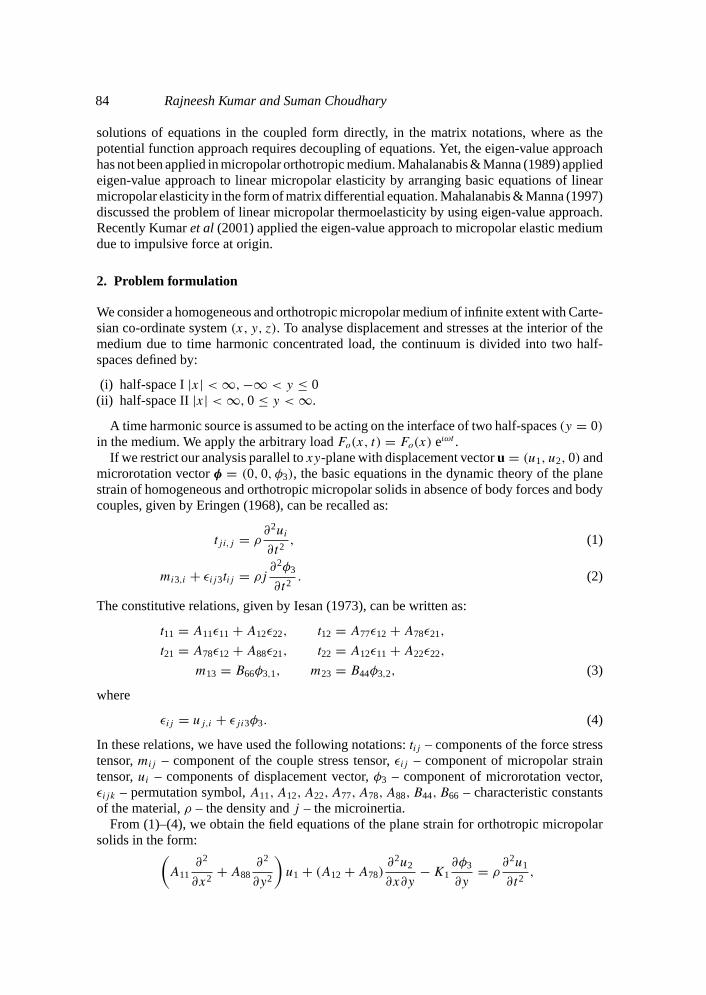
Figure 1. Variation of displacement componentU2(= u2/Fo) with distancex.

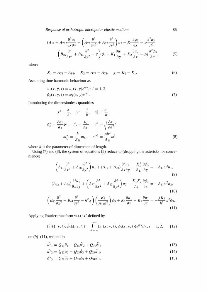
Figure 2. Variation of normal force stressT22(= t22/Fo) with distancex.


The comparison of values of dimensionless displacement componentU2[= u2/Fo], normalforce stressT22[= t22/Fo] and couple stressM23[= m23/Fo], for micropolar orthotropic solid(MOS) and micropolar isotopic solid (MIS) have been studied. The computations were carriedout for three values of dimensionless frequencyω = 0·25, 0·50 andω = 0·75 for t = 1·0 aty = 1·0 in the range 0≤ x ≤ 10. The solid lines either without centre symbol or with centresymbol represent the variations forω = 0·25 whereas the small dashed lines with or withoutcentre symbol represent the variations forω = 0·50 and large dashed lines with or withoutcentre symbol represent variations forω = 0·75 . The curves without centre symbol corre-sponds to the case of MOS whereas those with centre symbol correspond to the case of MIS.

Figure 1 shows the variations of displacement componentU2 with x. For both cases ofMOS and MIS and for all three frequencies, initially the values ofU2 decrease sharply and asfrequencyω increases from 0·25 to 0·75, the values ofU2 increase in the range of 0≤ x ≤ 2·5and 6·5 ≤ x ≤ 10. The behaviour of variations ofU2 for both the cases are same.

Figure 2 shows the variations of normal force stressT22 with x. For all three frequencies, thevalues ofT22 for MOS, are greater than those for MIS at the initial value i.e.,x = 0. Initiallythe values ofT22 start with sharp decrease then follow oscillatory pattern with reference tox. The minimum stress occur at maximum frequencyω = 0·75 in the range 0≤ x ≤ 1 and3·5 ≤ x ≤ 7 in response of concentrated load.

Figure 3 shows the variations of couple stressM23 with x. For case MIS , the values ofM23

have been maximize on multiplying by 10. Initially, for all three values ofω, the values ofM23 are less for MIS than those for MOS in the range 0≤ x ≤ 2·5. In both the cases of MOS

Figure 3. Variation of tangential couple stressM23(= m23/Fo) with distancex.


and MIS, for the maximum value of frequency the value of couple stress is minimum in theranges 0≤ x ≤ 3 and 7≤ x ≤ 10. The behaviour of variations with reference to frequencyare oscillating and same for MOS and MIS cases.

6. Conclusion

Significant anisotropy effect is obtained on displacement component, force stress and couplestress, for all different frequencies. Near the point of application of load, the frequency playsa major role in all the components.

References

Cheng Z-Q, He L-H 1995 Micropolar elastic field due to a spherical inclusion.Int. J. Eng. Sci.33:389–397

Cheng Z-Q, He L-H 1997 Micropolar elastic field due to a circular inclusion.Int. J. Eng. Sci.35:659–668

Erbay H A 2000 An asymptotic theory of thin micropolar plates.Int. J. Eng. Sci.38: 1497–1516Eringen A C 1966 linear theory of micropolar elasticity.J. Math. Mech.15: 909–924Eringen A C 1968Theory of micropolar elasticity in fracture(New York, London: Academic Press)

2: 621–729Gauthier R D 1982 InExperimental investigations on micropolar media, mechanics of micropolar

media(eds) O Brulin, R K T Hsieh. (Singapore: World Scientific)Iesan D 1973 The plane micropolar strain of orthotropic elastic solids.Arch. Mech.25: 547–561Iesan D 1974a Torsion of anisotropic elastic cylinders.ZAMM 54: 773–779Iesan D 1974b Bending of orthotropic micropolar elastic beams by terminal couples.An. St. Uni. Iasi.

20: 411–418Kumar R, Deswal S 2000 Steady-state response of a micropolar generalized thermoelastic half-space

to the moving mechanical/thermal loads.Proc. Indian Acad. (Math. Sci.)119: 449–465Kumar R, Deswal S 2001 Mechanical and thermal source in a micropolar generalized thermoelastic

medium.J. sound and vibrations, 239: 467–488Kumar R, Singh R, Chadha T K 2001 Eigen value approach to micropolar medium due to impulsive

force at the origin.Indian J. Pure Appl. Math.32: 1127–1144Mahalabanabis R K, Manna J 1989 Eigenvalue approach to linear micropolar elasticity.Indian J. Pure

Appl. Math.20: 1237–1250Mahalabanabis R K, Manna J 1997 Eigenvalue approach to the problem of linear micropolar ther-

moelasticity.J. Indian Acad. Math.19: 69–86Nakamura S, Benedict R, Lakes R 1984 Finite elament method for orthotropic micropolar elasticity.

Int. J. Eng. Sci.22: 319–330Press W H, Teukolsky S A, Vellerlig W T, Flannery B P 1986Numerical recipes in Fortran2nd edn

(Cambridge: University Press)

Response of orthotropic micropolar elastic medium due to time harmonic source

Documents

Transcript of Response of orthotropic micropolar elastic medium due to time harmonic source