Stress Analysis and Failure Prediction for Orthotropic Plates ...
194
Master of Science Thesis Stress Analysis and Failure Prediction for Orthotropic Plates with Holes An Analytic Tool for Orthotropic Plates with Loaded/Un- loaded Holes Subjected to Arbitrary In-Plane Loads R.D.B. Sevenois Faculty of Aerospace Engineering · Delft University of Technology
-
Upload
khangminh22 -
Category
Documents
-
view
0 -
download
0
Transcript of Stress Analysis and Failure Prediction for Orthotropic Plates ...

Master of Science Thesis
Stress Analysis and FailurePrediction for Orthotropic Plateswith HolesAn Analytic Tool for Orthotropic Plates with Loaded/Un-loaded Holes Subjected to Arbitrary In-Plane Loads
R.D.B. Sevenois
Faculty of Aerospace Engineering · Delft University of Technology


UNCLASSIFIED
Stress Analysis and Failure Predictionfor Orthotropic Plates with Holes
An Analytic Tool for Orthotropic Plates with Loaded/UnloadedHoles Subjected to Arbitrary In-Plane Loads
Master of Science Thesis
For obtaining the degree of Master of Science in Aerospace Engineeringat Delft University of Technology
R.D.B. Sevenois
December 6, 2013
Faculty of Aerospace Engineering · Delft University of Technology

The work in this thesis was supported by Fokker Aerostructures B.V. Their cooperation isgratefully acknowledged.
Copyright c© R.D.B. SevenoisAll rights reserved.

Delft University of TechnologyFaculty of Aerospace Engineering
Department of Aerospace Structures and MaterialsChair Structural Integrity & Composites
GRADUATION COMMITTEE
Dated: December 6, 2013
Chair holder:Prof.dr.ir. R. Benedictus
Committee members:Dr.ir. S. Koussios
Ing. H. de Frel
Dr. C. Kassapoglou


Abstract
To allow structural designs with lower mass, it is necessary to have access to accurate failureprediction theories for composite plates with holes subjected to arbitrary loading conditions.For design purposes, however, the most accurate failure theories require a considerable amountof computational resources which is often not available. Additionally, current theories allowingless computational resources are unfortunately only valid for a specific load, material, hole orspecimen size and their reliability is still questioned [1].
The purpose of this work is to examine the existing methods to estimate stress and failure incomposite plates with holes and subsequently join or modify them to provide an analytic toolfor a quick and fairly accurate estimation of the static failure load. The plate is representedas a two-dimensional structure containing arbitrary loaded/unloaded holes and edge forceboundary conditions. From a literature study, it is decided that an analytical model basedon the method by Xiong and Poon [2] is used for the determination of the stress field. A newgeneral failure criterion on the basis of Kweon [3] is constructed to determine failure. Thestress and failure theories are implemented in a software package, verified by hand calculationand validated with finite element analysis and experimental data. The performance of the newfailure theory was also compared to the performance of the in-house Point Stress Criterionat the company where the work was performed.
The stress field methodology is able to accurately determine the stress field in two-dimensionalplates with holes. The performance of the new failure criterion is better with respect to thein-house criterion and has a maximum discrepancy of +20% which is acceptable for designpurposes. Unfortunatley, due to issues with the assumption of the stress boundary conditionsfor loaded holes, the method is restricted to laminates with a directionality lower than 1.13.Once these issues are resolved, the method will be generally applicable.
UNCLASSIFIED R.D.B. Sevenois

viii
R.D.B. Sevenois UNCLASSIFIED

Preface
I first contacted Dr. Koussios about this project in January 2012. Being optimistic aboutobtaining the MSc degree in 2 years, I had envisioned to start this project (literature studyand thesis) in July 2012 and graduate in June 2013. An unexpected opportunity, however,forced me to temporarily move to Canada and delay the start to January 2013. Luckilyno additional delays were encountered and with perseverance, regularity and some luck Imanaged to deliver this work to you within the intended timeframe. This project involvestwo reports describing the development, verification and validation of an analytic tool for thedetermination of stress and failure in finite width orthotropic plates with holes subjected toarbitrary in-plane loads. The first report is an extensive literature study in the field of stressanalysis and failure prediction in laminated plates. In the second report, which is this work,the conclusions from the first report are followed to result in the completion of the analytictool. I have put a considerable amount of time and effort in this work and I hope that readingit will give you the same satisfaction as when I finished it.It is expected that you have knowledge of Mathematics, Classical Lamination Theory (CLT),Complex Stress Analysis and Failure Prediction with application to laminated plates to un-derstand the theory explained in this work which is outlined in Chapter 3 and Chapter 4.Contentwise, approximately one third of the pages you are about to read are appendices.They contain the detailed results and workout of some theories which serve as ultimate prooffor the points made and are required to ensure a correct chain of custody. Unless you areextremely interested, you are not expected to read them.This work would not be what it is without the help of my friends, colleagues and supervisors.In this paragraph I would like to thank Dr. ir. S. Koussios and Dr. C. Kassapoglou, MScfor their advice during the execution of the project and being my main supervisors. M.Bakker, MSc for his insights in the stress theories and advice during the construction ofthe computer algorithm. Ing. H.C. de Frel and B. Tijs for their advice and knowledge tomake this work compatible with the designer environment at Fokker Aerostructures B.V. TheTools and Methods team at Fokker Aerostructures B.V. and especially ir. Tim Janssen, R.Hoogendoorn, BSc and F. Gerhardt for providing support, advice, insights and a stimulatingwork environment. And last but not least my friends from Aerospace Structures and Materialsand Aerodynamics for the coffee, fun conversations and movie nights.
UNCLASSIFIED R.D.B. Sevenois

x
R.D.B. Sevenois UNCLASSIFIED

Summary
The more accurate one can predict the failure load of an aircraft component, the lower safetyfactor for the design is required. This results in a lower structural mass and translates into alower fuel consumption which is beneficial for the aircraft operator. Using metals, static failureloads of components can relatively easy be determined by looking at the stress concentrationsin the design. For composites, because of their complexity, determining failure is not sostraightforward. This complexity and the lack of a reliable model [1] led to an abundancein failure criteria for (un)notched laminated plates. Some quite accurate models exist butthey can require a significant amount of computational resources which is often not available.Therefore many design organizations still use the basic, less accurate, criteria. Most of thesecriteria, however, are only valid for a specific load, material, hole or specimen size. Often, formore complicated scenarios, failure can not confidently be estimated.The purpose of this work is to present the development of an analytic tool for the predictionof failure in orthotropic plates with holes subjected to arbitrary loading which can be usedby Fokker Aerostructure B.V. in the design of aircraft components. First the state of theart is determined with a literature survey on existing theories for stress evaluation and staticfailure prediction in composite plates with holes. Next, the theories obtained from the surveyare evaluated for their applicability, joined and/or modified to form the analytic tool. Thetool is then verified by simple hand calculations and validated with finite element analysisand experimental data.The basic problem, which is shown in Figure 1, consists of a two-dimensional flat rectangularorthotropic plate containing m holes. The edges of the plate and holes can be loaded orunloaded as defined by the user. From the literature survey it is determined that, to estimatethe stress field for this type of problem, a complex stress analysis on the basis of Lekhnitskii [4]and Xiong and Poon [2] is best to use. Advantages of this method for the determination ofthe stress field is that it results in a single expression for the entire stress field and thatarbitrary boundary conditions can be used. For failure prediction, it is clear that, for bothnotched and unnotched plates, there is no consensus on which failure criterion is best touse. To predict unnotched ultimate failure in two-dimensional loading conditions, one needsto construct an algorithm on the basis of a progressive failure model. This model consistof an algorithm which takes the degradation of lamina properties due to matrix cracking
UNCLASSIFIED R.D.B. Sevenois

xii
Figure 1: A rectangular plate with multiple holes subjected to arbitrary loading
and the non-linearity of the material into account in conjunction with a failure model topredict onset of failure. To predict failure onset, the phenomenological failure criteria byPuck [5], LaRC03 [6], LaRC04 [7] and the Tsai-Wu [8] are the best criteria with an accuracyof ±10% [1]. An accuracy of ±50% in 85% of the cases has been shown for Puck’s finalfailure progressive model [5] which will be used. From the identified notched failure criteria,the Linear Elastic Fracture Mechanics (LEFM) [9], Average Stress Criterion (ASC) [10] andPoint Stress Criterion (PSC) [10] were selected as most promising when taking into accountthe intended use of the analytic tool. Eventually, because an analytic method to determinethe characteristic length is available from Kweon [3], the PSC [10] was selected to form thebasis for the notched failure criterion.
Following Lekhnitskii [4] an appropriate solution for the stress functions ϕj(zj), j = 1, 2 todetermine the stresses, strains and displacement for arbitrary boundary conditions as shownin Figure 1 is:
ϕj(zj) = C0j +∑Nn=1Cnjz
nj +
∑mk=1
C(k+kN)j
ln(ξmj) +∑Nn=1C(k+kN+n)j
ξ−nmj
j = 1, 2
(1)
In Eq. (1), ξj is the mapping function of the m-th hole to the complex plane, Cnj , j = 1, 2 arecomplex coefficients which must be determined through the problem boundary conditions.These coefficients are determined using the principle of minimum potential energy. Thisprinciple states that the minimum total potential energy of the structure is reached giventhe external loading conditions. Thus, the derivative of the total elastic strain energy inthe problem should be zero. Integrating for the elastic strain energy over the domain andboundaries of the plate and taking its derivative, it is observed that, due to satisfaction ofthe equilibrium equations by Eq. (1), the part related to the domain becomes zero and onlythe boundary terms remain. Working out these boundaries with the stress function (1) andsolving for ∂Π = 0 eventually results in a linear system of equations which can easily besolved.
For an accurate representation of the stress field, one now only has to define valid stressboundary conditions. This is especially important when loaded holes need to be evaluated.Many researchers assume that the pin-load on a hole edge can be represented by a radial cosineshaped compression load on the hole edge [2, 11, 12]. Several studies [13, 14], however, have
R.D.B. Sevenois UNCLASSIFIED

xiii
Figure 2: Definition of the compressive characteristic distance by Kweon [3] and the CPSED
shown that this assumption is essentially wrong because of the effects of pin-hole clearance,flexibility, friction, material orthotropy and magnitude of the total load. In an attempt toresolve some of these issues the pin-hole contact load is replaced by a radial cosine distributionscaled between two contact angles θ1m and θ2m. These angles are subsequently determinedby an iterative procedure which takes into account the size of the pin.
As aforementioned, the PSC is used to predict notched failure in the plate. As input, the PSCrequires a characteristic distance away from the hole and an unnotched failure criterion. Forunnotched failure, because it is one of the recommended theories and the desire was expressedto evaluate this criterion, the Puck criterion as described by Verein Deutsher Enginieure2014(VDI2014) [5, 15] is used. To determine the characteristic distance away from the hole, anovel analytic methodology on the basis of Kweon [3] is constructed. The definition of Kweonfor the compressive characteristic distance in loaded holes is: “The distance from the fronthole edge to a point where the local compressive stress by the arbitrarily applied load is thesame as the mean bearing stress”. This is shown in Figure 2. The original definition for thischaracteristic distance, however, reads [10]: “The distance over which the material around thehole must be critically stressed in order to find a sufficient flaw size to initiate failure.”. Now,this region contains a certain strain energy and, since it is critically stressed, one can call thisenergy the Critical Potential Strain Energy Density (CPSED) for failure of the material. Onecan use this critical energy density to establish a new definition for the characteristic distanced0: “The distance from the hole edge where the strain energy density over this distance equalsthe CPSED.” and given by:
Πcr =∫ d0
0σεdx (2)
Using Kweon’s analytic definition for the compressive characteristic distance, it is possibleto analytically determine the CPSED for compression (Πcr,c). Furthermore, considering thatthe characteristic distances for tension and compression are unequal, it is fair to considerthat the CPSED for the tension and compression cases are unequal. No analytic formulationfor the tensile characteristic distance exists, thus it is chosen to estimate the CPSED fortension by scaling the CPSED for compression with the ratio of the strain energy density ofan unnotched plate subjected to uniaxial tension and compression at failure load respectivelyas shown in Eq. (3)
Πcr,t = Π (σun,t)Π (σun,c)
Πcr,c (3)
In a multiaxial loading condition, however, it is required to have definitions for critical en-
UNCLASSIFIED R.D.B. Sevenois

xiv
ergies which are not only uniaxial tension or uniaxial compression. Therefore, in a similarway as is for the CPSED for tension, the CPSED for transverse tension, transverse compres-sion, tension-tension, tension-compression, compression-tension and compression-compressionloading is defined. The algorithm to predict failure of a notched plate is now given by:
1. Calculate the CPSED for compression by analysis of a pin-loaded joint
2. Calculate the CPSED for tension and the other multiaxial loading conditions
3. Calculate the stress field of the problem
4. Set an initial characteristic distance and determine the minimum Reserve Factor andcritical loading angle around each hole
5. At the critical angle, calculate the Potential Strain Energy Density (PSED) at failurefrom the hole edge to the characteristic distance
6. When the CPSED equals the PSED, the ultimate failure load is obtained. Otherwise,a new characteristic distance is chosen based on whether the PSED is higher or lowerthan the CPSED and the procedure is repeated from step 4.
The algorithm above is implemented in a routine regulated by a Visual Basic Script andcalculated with MathCAD13.1 c©. The functioning of the routing is verified by comparing thestress for several configurations at the hole edge to analytic solutions from Lekhntiskii [4] andsimple hand calculations. The convergence behaviour of the algorithm is determined by inves-tigating the influence of the numerical integration parameter TOL (internal MathCad13.1 c©)and the amount of summations N in the stress function (Eq. (1)). Finally, from this investi-gation it is concluded that good working ranges for N and TOL, when less than 6 holes arepresent, are:
N > 710−3 > TOL > 10−6 ∨ 10−13 > TOL > 10−16 (4)
where ∨ is the OR operator. The performance of the contact angle and stress field method-ology are further investigated by comparing the results from these analysis to Finite ElementAnalysis. More complicated configurations are analyzed and the ability of the tool to take intoaccount the finite size of the plate is determined. From these investigations it is determinedthat, for an accurate representation of the stress field, the ratio of the hole edge distance anddiameter over panel width should be larger than 2.5 and 4 respectively. For design purposes,an E/D > 2.5 + 1.3 [mm] [16] and W/D > 4.7 [17] is advised. These boundaries are thuswell within limits. Unfortunately, the validation of the contact angle algorithm, revealedthat, for the current assumptions for the pin-hole stress boundary condition, the estimationis only conservative for laminates with a directionality lower than 1.13. It is recognized thatthis restriction greatly affects the laminate design space for this tool. This issue was, duringthe construction of this work, addressed by Gerhardt [18] but could unfortunately not beimplemented due to time constraints.
In preparation to validate the notched failure method with experimental data, the hole di-ameter to determine the CPSED is determined by making predictions for a selection of theexperimental data points for multiple hole diameters. The selection of data contains both
R.D.B. Sevenois UNCLASSIFIED

xv
Figure 3: Predicted vs measured failure for unloaded hole configurations, screened
open hole tension and compression as well as pinned hole bearing experiments. Next, the re-quirement that none of the predicted values should overestimate the measured values by 10%and be as close as possible to the measured values, result in a hole diameter of 5[mm]. Finally,by screening a dataset of 151 experimental values to the tool boundaries, a total amount of92 (38 measurement points unloaded and 54 measurement points loaded holes together) areselected and predictions for these data points are made. The results are presented in Figure 3and Figure 4 from which it can be seen that, for the unloaded experimental points, all but afew data points are within ±20% of the measured experimental value. For the loaded data-points, the scatter is much larger but concentrates between −20% and −60%. The predictionfor loaded holes is thus almost always conservative. It is thought that, however no definiteproof can be delivered, the source of this conservatism is due the fact that, in literature, theultimate failure load after occurrence of significant damage is reported and not the onset offailure. For unloaded holes the difference between onset and ultimate failure is often smallwhich is why the same conservatism is not seen in these predictions. For loaded holes, how-ever, as observed by Crews [19], this difference can be significant due to interactions of failuremodes and strengthening effects. The algorithm is not able to take these interactions andstrengthening effects into account and therefore will always predict a lower failure load. It isworthwile to investigate whether this PSC failure criterion actually predicts onset of failureas indicated by the definition from Whitney and Nuismer [10].
Apart from the issues with the loaded hole predictions and the assumption for the pin-hole edge stress distribution, it is emphasized that the new methodology is an improvementover the current in-house failure criterion at Fokker Aerostructures B.V. For loaded holeconfigurations, the majority of the predictions are moderately to highly conservative whilethe unloaded predictions are situated in the ±20% region. It is recognized that, initially, amaximum discrepancy of +10% was set for the method, and although the internal parameters
UNCLASSIFIED R.D.B. Sevenois

xvi
Figure 4: Predicted vs measured failure for loaded holes configurations, screened
were scaled to obtain this result, the finally obtained +20% for the entire dataset is stillremarkably close. This overestimation can easily be eliminated by changing the hole sizefor the determinion of the CPSED to a lower value. Additionally, the pin-hole edge stressdistribution should be improved to eliminate the directionality boundary of 1.13. When theseissues are resolved, the method will be available for design purposes in the entire designenvelope.
R.D.B. Sevenois UNCLASSIFIED

Frequently Used Symbols andAbbreviations
Symbol Explanationα Displacement angleαj Real part of µjβj Imaginary part of µjγxy Shear strain in the xy-planeε In-plane strain vectorεx Normal strain in x-directionεy Normal strain in y-directionθ1m Start contact angle for hole mθ2m End contact angle for hole mθB Contact angleλ Absolute difference between pin size and hole sizeµj Material eigenvalueνij Poissons ratio in ij-planeξmj Mapping function of the m-th hole to the complex planeΠ Total potential strain energyΠcr,c Critical potential strain energy density compressionΠcr,−c Critical potential strain energy density transverse compressionΠcr,cc Critical potential strain energy density biaxial compression-compressionΠcr,ct Critical potential strain energy density biaxial compression-tensionΠcr,t Critical potential strain energy density tensionΠcr,−t Critical potential strain energy density transverse tensionΠcr,tc Critical potential strain energy density biaxial tension-compressionΠcr,tt Critical potential strain energy density biaxial tension-tensionσ In-plane stress vectorσθ Tangential stress on the hole edgeσ12 Normal stress on plate edge 1-2
UNCLASSIFIED R.D.B. Sevenois

xviii
σ23 Normal stress on plate edge 2-3σ34 Normal stress on plate edge 3-4σ41 Normal stress on plate edge 4-1σrm Radial stress on the edge of hole mσun,t/c Unnotched failure stress tension/compressionσb Bearing stressσr Radial stress on the edge of a holeσx Normal stress in x-directionσy Normal stress in y-directionτ Shear stressτ12 Shear stress at plate edge 1-2τ23 Shear stress at plate edge 2-3τ34 Shear stress at plate edge 3-4τ41 Shear stress at plate edge 4-1τrm Shear stress on the edge of hole mτxy Shear stress in the x-y planeϕj Complex stress functionaij Entry i, j in the laminate compliance matrixAij Entry i, j in the laminate stiffness matrixa0 Characteristic length for average stress criterionam Semi major axis of hole maa Material angularitybm Semi minor axis of hole mC Elastic stiffness matrixC−j Complex coefficient of the stress functionD Hole diameterd0c Compressive characteristic distanced0 Characteristic distance for point stress criterionE Hole center edge distanceEi Engineering Young’s modulus in i directionfE Stress exposureGIc Mode I fracture toughnessGIIc Mode II fracture touchnessGij Engineering shear modulus in ij-planeKT Stress concentration factorK infT Stress concentration factor at infinity
L Specimen lengthN Amount of summations in the stress functionpc21 Slope of the fracture curve to the left of σ2 = 0pt21 Slope of the fracture curve to the right of σ2 = 0Pb Total bearing forceRA22 Fracture resistance of the action plane parallel to the fibre directionRmj Coefficient for the m-th hole
R.D.B. Sevenois UNCLASSIFIED
xix
rh Hole radiusrp Pin radiusrr Material directionalityS Elastic complianceS12 In-plane shear strengthS12 Ply shear strengtht Laminate thicknesstmj Coefficient for the m-th holetply Lamina ply thicknessu Displacement in x-directionuα Displacement in x-direction at angle α on the hole edgeu0 Displacement in x-direction at 0 on the hole edgev Displacement in y-directionW Specimen widthXc Longitudinal compressive strengthXt Longitudinal tensile strengthxm Center of hole m with respect to the x-coordinateXn External force component parallel to xY c Transverse compressive strengthY t Transverse tensile strengthym Center of hole m with respect to the y-coordinateYn External force component parallel to yzj Complex coordinate
UNCLASSIFIED R.D.B. Sevenois

xx
Abbreviation ExplanationASC Average Stress CriterionCFRP Carbon Fibre Reinforced PlasticsCID Coordinate IDentifiedCPSED Critical Potential Strain Energy DensityCPU Central Processing UnitDZM Damage Zone ModelESDU Engineering Sciences Data UnitFEA Finite Element AnalysisFEM Finite Element MethodFF Fibre FailureFPF First Ply FailureFRP Fibre Reinforced PlasticsGFRP Glass Fibre Reinforced PlasticsIFF Inter Fibre FailureLaRC Langley Research CenterLEFM Linear Elastic Fracture ModelMCFE Most Conservative Fracture EnvelopePSC Point Stress CriterionPSED Potential Strain Energy DensityQI Quasi-IsotropicRF Reserve FactorSCF Stress Concentration FactorUD Uni-DirectionalUF Ultimate FailureVBScript Visual Basic ScriptVDI Verein Deutscher EnginieureWWFE World Wide Failure ExersiceXFEM eXtended Finite Element Method
R.D.B. Sevenois UNCLASSIFIED

Table of Contents
List of Figures xxvii
List of Tables xxix
Acknowledgments xxix
1 Introduction 1
2 Literature Survey 32.1 Stress Analysis . . . . . . . . . . . . . . . . . . . . . . . . . . . . . . . . . . . . 3
2.1.1 Analytic Stress Analysis . . . . . . . . . . . . . . . . . . . . . . . . . . . 32.1.2 Finite Element Analysis . . . . . . . . . . . . . . . . . . . . . . . . . . . 8
2.2 Strength Prediction . . . . . . . . . . . . . . . . . . . . . . . . . . . . . . . . . 112.2.1 Unnotched Strength . . . . . . . . . . . . . . . . . . . . . . . . . . . . . 112.2.2 Notched Strength . . . . . . . . . . . . . . . . . . . . . . . . . . . . . . 14
3 Determination of the Stress Field 193.1 Expansion of Xiong’s Method . . . . . . . . . . . . . . . . . . . . . . . . . . . . 193.2 Pin Contact Angle . . . . . . . . . . . . . . . . . . . . . . . . . . . . . . . . . . 28
4 Failure Prediction 334.1 Unnotched Failure Prediction . . . . . . . . . . . . . . . . . . . . . . . . . . . . 344.2 Notched Failure . . . . . . . . . . . . . . . . . . . . . . . . . . . . . . . . . . . 384.3 General Program Layout . . . . . . . . . . . . . . . . . . . . . . . . . . . . . . 40
5 Tool Verification 45
UNCLASSIFIED R.D.B. Sevenois

xxii Table of Contents
6 Validation, Comparison to FEA and Experimental Data 516.1 Stress Analysis . . . . . . . . . . . . . . . . . . . . . . . . . . . . . . . . . . . . 52
6.1.1 Influence of accuracy parameters TOL and N . . . . . . . . . . . . . . . 526.1.2 Influence of contact angle estimation . . . . . . . . . . . . . . . . . . . . 576.1.3 Comparison to FEA . . . . . . . . . . . . . . . . . . . . . . . . . . . . . 62
6.2 Failure Prediction - Comparison to Test Results . . . . . . . . . . . . . . . . . . 706.2.1 Unnotched Failure Criterion . . . . . . . . . . . . . . . . . . . . . . . . . 706.2.2 Notched Failure Criterion - Clearance and Hole Size for CPSED . . . . . 746.2.3 Notched Failure Criterion - Comparison to Experimental Data . . . . . . 76
7 Discussion, Conclusions and Recommendations 87
References 91
A Derivation of the Sign Selection Algorithm 105
B Discussion on Kweon’s Tensile Characteristic Length 115
C Flow Charts of Individual Code Segments 117
D Results from Verification 125
E Contact Angle Comparisons FEA 145
F Results from Stress Validation 157
R.D.B. Sevenois UNCLASSIFIED

List of Figures
1 A rectangular plate with multiple holes subjected to arbitrary loading . . . . . . . xii2 Definition of the compressive characteristic distance by Kweon [3] and the CPSED xiii3 Predicted vs measured failure for unloaded hole configurations, screened . . . . . xv4 Predicted vs measured failure for loaded holes configurations, screened . . . . . . xvi
2.1 Evolution of FEA, references can be obtained from [20] . . . . . . . . . . . . . . 92.2 Discretizations of a grain boundary problem for (a) an XFEM/GFEM model with
a structured (Cartesian) mesh and (b) a FEM model [21] . . . . . . . . . . . . . 10
3.1 A rectangular plate with multiple holes subjected to arbitrary loading . . . . . . . 203.2 Two-dimensional anisotropic body with two contours . . . . . . . . . . . . . . . 213.3 Computation algorithm for stress field determination. The subscript j is dropped
for convenience . . . . . . . . . . . . . . . . . . . . . . . . . . . . . . . . . . . 283.4 A hole loaded by a distributed cosine distributed radial load . . . . . . . . . . . . 293.5 Exaggerated view of deformed hole by rigid pin . . . . . . . . . . . . . . . . . . 293.6 Iterative procedure for the determination of the contact angle θB . . . . . . . . . 313.7 Schematic of pin locally deforming the hole shape . . . . . . . . . . . . . . . . . 31
4.1 IFF failure modes [15] . . . . . . . . . . . . . . . . . . . . . . . . . . . . . . . . 344.2 IFF σ2, τ21 fracture plane [15] . . . . . . . . . . . . . . . . . . . . . . . . . . . 354.3 Unnotched failure algorithm, continued in Figure 4.4 . . . . . . . . . . . . . . . 364.4 Unnotched failure algorithm, first part in Figure 4.3 . . . . . . . . . . . . . . . 374.5 Keon definition compressive characteristic distance . . . . . . . . . . . . . . . . 384.6 Main program assembly algorithm . . . . . . . . . . . . . . . . . . . . . . . . . 414.7 Notched failure algorithm, continued in Figure 4.8 . . . . . . . . . . . . . . . . . 424.8 Notched failure algorithm, first part in Figure 4.7 . . . . . . . . . . . . . . . . . 43
UNCLASSIFIED R.D.B. Sevenois

xxiv List of Figures
5.1 Stress concentration factor at hole edge and difference between tool and Lekhnit-skii. 100% UD uniform pressure at hole edge, a = 5 [mm], b = 2 [mm] . . . . . . 47
5.2 Stress concentration factor at hole edge and difference between tool and Lekhnit-skii. 100% ±45 uniform pressure at hole edge, a = 5 [mm], b = 2 [mm] . . . . . 47
5.3 Stress concentration factor at hole edge and difference between tool and Lekhnit-skii. 50% 0, 50% ±90 uniform pressure at hole edge, a = 5 [mm], b = 2 [mm] 47
5.4 Stress concentration factor at hole edge and difference between tool and Lekhnit-skii. 100% UD, uniaxial tension at 0, a = 5 [mm], b = 2 [mm] . . . . . . . . . 48
5.5 Stress concentration factor at hole edge and difference between tool and Lekhnit-skii. 100% ±45, uniaxial tension at 0, a = 5 [mm], b = 2 [mm] . . . . . . . . . 48
5.7 Change of load reserve factor, r and critical energy ratio throughout iterations . 495.8 Configuration 1,2 and 3 (left to right) used for assembly verification. . . . . . . . 50
6.1 Influence of N for a centered single hole subjected to uniaxial tension (left) andmultiaxial tension-tension (right) in a 4D size square plate . . . . . . . . . . . . 53
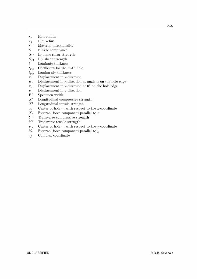
6.2 Influence of N for a centered single hole subjected to uniaxial tension in a 2D sizesquare plate . . . . . . . . . . . . . . . . . . . . . . . . . . . . . . . . . . . . . 54
6.3 Influence of N for a serie of 5 (left) and a rectangular pattern of 4 (right) circularholes in a finite width sheet subjected to uniaxial tension. . . . . . . . . . . . . . 54
6.4 Influence of TOL for a centered single hole subjected to uniaxial tension(left) andmultiaxial tension-tension (right) in a 4D size square plate . . . . . . . . . . . . 55
6.5 Influence of TOL for a centered single hole subjected to uniaxial tension in a 2Dsize square plate . . . . . . . . . . . . . . . . . . . . . . . . . . . . . . . . . . 55
6.6 Influence of TOL for a serie of 5 (left) and a rectangular pattern of 4 (right)circular holes in a finite width sheet subjected to uniaxial tension . . . . . . . . 56
6.7 Influence of TOL for a single elliptical (right) and circular hole in a quasi-infinitesheet . . . . . . . . . . . . . . . . . . . . . . . . . . . . . . . . . . . . . . . . . 56
6.8 Influence of N for a centered single hole subjected multiaxial tension-tension (right)in a 4D size square plate when TOL = 10−6 . . . . . . . . . . . . . . . . . . . . 57
6.9 Schematic representation for the calculation of the CPSED whith a higher or lowercontact angle . . . . . . . . . . . . . . . . . . . . . . . . . . . . . . . . . . . . 58
6.10 Change in contact angle with increasing bearing stress for Tomlinson, FEA andSevenois . . . . . . . . . . . . . . . . . . . . . . . . . . . . . . . . . . . . . . . 59
6.11 Effect of directionality on contact angle prediction (FEA) [18] . . . . . . . . . . 606.12 Effect of clearance on contact angle prediction (FEA) - QI layup [18] . . . . . . . 616.13 Effect of α on contact angle prediction (Sevenois’s model) and comparison to FEA.
Clearance 2% - QI layup in coöperation with [18] . . . . . . . . . . . . . . . . . 616.14 Example of the FEM mesh around a hole . . . . . . . . . . . . . . . . . . . . . 626.15 Boundary condition . . . . . . . . . . . . . . . . . . . . . . . . . . . . . . . . . 646.16 Config. 1, SCF of σθ at the hole edge (left) and SCF of σy at y = 0 (right) when
E/D = 2.5 . . . . . . . . . . . . . . . . . . . . . . . . . . . . . . . . . . . . . 656.17 Config. 1, SCF of σθ at the hole edge (left) and SCF of σy at y = 0 (right) when
E/D = 1 . . . . . . . . . . . . . . . . . . . . . . . . . . . . . . . . . . . . . . 656.18 Config. 2, SCF of σθ at the hole edge (left) and SCF of σx at x = 0 (right) when
W/D = 4 . . . . . . . . . . . . . . . . . . . . . . . . . . . . . . . . . . . . . . 66
R.D.B. Sevenois UNCLASSIFIED

List of Figures xxv
6.19 Config. 2, SCF of σθ at the hole edge (left) and SCF of σx at x = 0 (right) whenW/D = 2 . . . . . . . . . . . . . . . . . . . . . . . . . . . . . . . . . . . . . . 66
6.20 Config. 3, SCF of σθ at the hole edge (left) and SCF of σx at x = xhole (right)when E/D = 2.5 . . . . . . . . . . . . . . . . . . . . . . . . . . . . . . . . . . 67
6.21 Config. 3, SCF of σθ at the hole edge (left) and SCF of σx at x = xhole (right)when E/D = 1.5 . . . . . . . . . . . . . . . . . . . . . . . . . . . . . . . . . . 67
6.22 Difference in SCF between FEM and Tool for a hole in a plate with varying E/Dand W/D . . . . . . . . . . . . . . . . . . . . . . . . . . . . . . . . . . . . . . 69
6.23 Tangential SCF from config. 4 for an unloaded (left) and loaded (right) hole . . 696.24 Biaxial failure envelope for QI AS4-3501 [22] . . . . . . . . . . . . . . . . . . . . 706.25 Biaxial failure envelope for QI IM7-8551 [23,24] . . . . . . . . . . . . . . . . . . 716.26 Biaxial failure envelope for [±15]s IM7-8551 [23,24] . . . . . . . . . . . . . . . . 716.27 Biaxial failure envelope for [±30]s IM7-8551 [23,24] . . . . . . . . . . . . . . . . 726.28 Biaxial failure envelope for [±45]s IM7-8551 [23,24] . . . . . . . . . . . . . . . 726.29 Biaxial failure envelope for [0]8 IM7-9772 [25] . . . . . . . . . . . . . . . . . . . 726.30 Uniaxial-Shear failure envelope for [0]32 IM7-8552 [26] . . . . . . . . . . . . . . 736.31 Uniaxial compressive and tensile test and predictions for material TH5.698/6 for
QI, soft and hard laminate . . . . . . . . . . . . . . . . . . . . . . . . . . . . . 736.32 Discrepancy with experiments from [27] (right) and [28] (left) when the hole size
for the determination of the CPSED is varied. OHT = Open Hole Tension, OHC= Open Hole Compression, PHT = Pinned Hole Tension, S = Soft, H = Hard, QI= Quasi-Isotropic, N = Narrow W/D, W = Wide W/D, L = Large hole . . . . . 75
6.33 Uniaxial tensile (left) and compressive (right) failure for AS4/3501-6 [29], QI CFRPlayup, fixed specimen size . . . . . . . . . . . . . . . . . . . . . . . . . . . . . . 76
6.34 Uniaxial tensile and compressive failure for TH5.698/601 [27], Hard, Soft and QIlayup, hole diameter: normal = 6.35 [mm], Large = 9.52 [mm] . . . . . . . . . . 77
6.35 Uniaxial compressive failure for IM7/8552-1 [30] when changing hole size, fixedspecimen size . . . . . . . . . . . . . . . . . . . . . . . . . . . . . . . . . . . . 77
6.36 Uniaxial compressive failure for T800/924C [31] when changing hole size, fixedspecimen size, part 1 . . . . . . . . . . . . . . . . . . . . . . . . . . . . . . . . 78
6.37 Uniaxial compressive failure for T800/924C [31] when changing hole size, fixedspecimen size, part 2 . . . . . . . . . . . . . . . . . . . . . . . . . . . . . . . . 78
6.38 Biaxial failure strength and prediction [32,33] for SP-286T300 . . . . . . . . . . 796.39 Biaxial failure envelope for QI laminate of IM7/8552 with 10 [mm] hole [34] and
prediction . . . . . . . . . . . . . . . . . . . . . . . . . . . . . . . . . . . . . . 796.40 Failure strength of single hole specimens wrt predictions [35] . . . . . . . . . . . 816.41 Failure strength of holes in series specimens wrt predictions [35] . . . . . . . . . 826.42 Failure strength of holes in parallel specimens wrt predictions [35] . . . . . . . . 836.43 Bearing-bypass envelope for QI graphite epoxy laminate [19] . . . . . . . . . . . 836.44 Prediction vs measurement for unloaded hole experiments, unlimited . . . . . . . 846.45 Prediction vs measurement for loaded hole experiments, unlimited . . . . . . . . 846.46 Prediction vs measurement for unloaded configurations, limited . . . . . . . . . . 856.47 Prediction vs measurement for loaded configurations, limited . . . . . . . . . . . 85
UNCLASSIFIED R.D.B. Sevenois

xxvi List of Figures
R.D.B. Sevenois UNCLASSIFIED

List of Tables
4.1 Recommended values for slope parameters pc21 and pt21 [36] . . . . . . . . . . . . 35
5.1 System test results unnotched failure criterion . . . . . . . . . . . . . . . . . . . 495.2 Verification result of assembly tests . . . . . . . . . . . . . . . . . . . . . . . . . 50
6.1 Analysis parameters for optimal α determination . . . . . . . . . . . . . . . . . . 596.2 Test cases for comparison between FEA and analytic tool . . . . . . . . . . . . . 636.3 Least square error for hole sizes below 6 [mm] based on Figure 6.32 . . . . . . . 75
UNCLASSIFIED R.D.B. Sevenois

xxviii List of Tables
R.D.B. Sevenois UNCLASSIFIED

Acknowledgments
I hereby acknowledge the support of Fokker Aerostructures B.V. and the Department ofAerospace Structures and Materials, Faculty of Aerospace Engineering, Delft University ofTechnology for their support during the writing of this thesis.
Delft, University of Technology R.D.B. SevenoisDecember 6, 2013
UNCLASSIFIED R.D.B. Sevenois

xxx Acknowledgments
R.D.B. Sevenois UNCLASSIFIED

“ Theoretically, a model always matches reality. ”—
“ Assumptions are at the basis of all problems in this world. ”—


Chapter 1
Introduction
When introducing composite structures as a replacement for (metal) components engineersare confronted with many issues. One of these issues is that the standard, isotropic, stressand failure prediction methods for basic structural elements are unusable. To allow compositestructural design, each of these structural elements must therefore be reevaluated. One ofthese structural elements is a rectangular plate with (un)loaded holes subjected to externalloads. Over the years, the complexity of these materials resulted in an abundance of fail-ure prediction methods for this type of structures which often have a limited applicabilityand questionable reliability [1]. In addition, the more accurate failure prediction models canrequire significant computational resources which is often unavailable and renders them lesssuitable for fast prediction of multiple scenarios. There is thus the need for a fast, straight-forward, validated method to predict stress and failure in rectangular composite plates with(un)loaded holes.
In this work the development of an analytic tool and its supporting theories for the determi-nation of the stress and prediction of failure in a rectangular orthotropic plate with multipleelliptical holes subjected to arbitrary in-plane loading conditions is described. The tool isintended to be used by engineers at Fokker Aerostuctures B.V. for the design of aerospacestructural parts. Hence it is imperative that the analytic tool is easy to use, fool proof andwell documented. First, to establish the state-of-the art in stress analysis and failure predic-tion for composite materials, a literature survey is performed. Next, flowing from the survey,the most suitable methods for the purpose of the tool are selected to serve as a basis for thedevelopment of the theory. Finally, the tool is implemented in a software package, verified byhand calculations and validated with experimental data.
The structure of this report is as follows. In Chapter 2 the results of the literature arepresented. Next, the theory used to determine the stress field is given in Chapter 3. InChapter 4 a discussion is provided on the theory for failure prediction followed by verificationand validation of the model in Chapter 5 and 6 respectively. A discussion on the usability andvalidity of the tool is provided in Chapter 7 as well as the conclusions and recommendations.
UNCLASSIFIED R.D.B. Sevenois

2 Introduction
R.D.B. Sevenois UNCLASSIFIED

Chapter 2
Literature Survey
An argumented choice for a suitable stress analysis and failure prediction methodolgy canonly be made if the state-of-the-art about these theories, their expansions, advantages anddisadvantages is known. For this purpose the scientific literature was investigated by theauthor in a previous study [37]. The discussion below is a brief summary of this study.
2.1 Stress Analysis
The mathematical determination of stresses in any structure can be performed using twomethods: analytic analysis or Finite Element Analysis (FEA). In analytic stress analysis theproblem to be solved is reduced to solving a set of equations which represent the stress statewith respect to the boundary conditions. However, due to the complexity of some problems,this process often involves assumptions and simplifications. Fueled by the need for solutionsof problems for which no analytic solution exist, FEA [20, 38] is currently one of the mostpopular methods for the analysis of stress fields. While fairly easy to use, however, it can alsobe dangerous in the hands of an unexperienced engineer/scientist. In the following sectionsboth methods are briefly discussed.
2.1.1 Analytic Stress Analysis
In literature three methods for analytic determination of the stress field exist: “LekhnitskiiFormalism” [4, 39], “Stroh Formalism” [40,41] and approximate analytical methods [42,43].
During the sixties and seventies Lekhnitskii [4] and Savin [39] provided the basis for whatis now called “Lekhnitskii Formalism”. This method essentially generalizes Muskhelivshili’sapproach for solving two-dimensional deformations of isotropic materials [44] with complexstress analysis. Lekhnitskii [4] and Savin [39] obtained solutions for circular, elliptical, tri-angular and square holes in, mainly, infinite orthotropic plates. Lekhnitskii’s approximatesolution for stresses around rectangular and square openings in orthotropic plates was further
UNCLASSIFIED R.D.B. Sevenois

4 Literature Survey
improved by De Jong [45] who used a Cauchy type integral instead of a series to approximatethe boundary conditions. Sufficient accuracy was obtained by using only the first three termsof the series after which numerical values were obtained for six laminates under various loadingconditions. In a similar fashion Rajaiah [46] also obtained the solution for quasi-rectangularholes in an infinite orthotropic plate by using the superposition principle but focused his workon finding the configurations leading to minimum stress concentrations. In the meantime, the“Lekhnitskii Formalism” became well known in the engineering community which led to therelease of ESDU85001 [47] in 1985 by the Engineering Sciences Data Unit (ESDU). This doc-ument contains explicit equations for the stresses around circular holes in infinite orthotropicplates. By 1995 a Fortran computer program (ESDUpac A8501) which performs the calcula-tion automatically was added. Expanding the Formalism continued when Tung [48] providedan approximate solution for the case when the material is close to isotropocy or displaysspecially orthotropic behaviour. This case was initially ignored by Lekhnitskii because hissolution produced a singularity. Tung found that, by letting the roots of the material eigen-values (complex constants which characterize the anisotropocy of a material) differ a smallamount, a solution can be obtained while the discrepancy between the results and actualvalues is within one hundredth of a percent. In 1988, the concept of finite size compositelaminates was introduced in the Formalism by Lin and Ko [49]. They obtained solutions fora single elliptical hole in a rectangular finite width plate by using a Laurent series in con-junction with the least squares boundary collocation method. The hole is mapped using acomplex series and the square boundary is approached using a Taylor series. The stresses inthe doubly connected region are obtained by truncating the series to a finite series after whichsuitable points on the inner and external boundary are chosen. The stresses are imposed atthese points to satisfy the boundary conditions by the “least-squares boundary collocationmethod”.
Some time later Xu [50] recognized that the work provided by Lin and Ko [49] and Gerhardt[51] is good but suffers from computational drawbacks as long CPU time and low accuracy.In order to reduce these drawbacks, Xu used a Faber series for the stress function instead ofa Taylor series. Additionally, his solution allows for the introduction of any plate boundaryshape in contrast to the rectangular shape by Lin and Ko. Again the unknown coefficients aredetermined using the “boundary collocation method” as also used by Lin and Ko [49]. In thecurrent solution the inner boundary can be satisfied accurately (error less than 10−5) whilethe outer boundary can be well satisfied to ensure a relative error within 1%. In the sameyear Xu [52] published an expansion of this work to account for multiple (unloaded) ellipticalholes in finite width plates. Xu claimed that the accuracy of this method is equal to this fromhis previous research and that considerably less computation time is required. No comparisonto FEA was presented and therefore it is not proven that his results are accurate. By furtherdeveloping his work, Xu [12] expanded the formulation of the stress function to incorporatemultiple loaded holes. The stress function is extended with a logarithmic part and the samemethod of solving is used. After the findings by Xu, developments with respect to a finite sizeplate solution have only been presented by Hufenbach [53,54] who incorporated the effects ofhygrothermal loading and a layer by layer analysis for the determination of first ply failure.This is obtained from the average strain by assuming that the strain in every layer is equal,as is often done in classical lamination theory. His work has been validated with results fromFEA.
On the subject of infinite plates Daoust and Hoa [55] investigated the analytical solution
R.D.B. Sevenois UNCLASSIFIED

2.1 Stress Analysis 5
for triangular holes. By introducing a single parameter any shape of triangular hole canbe analysed. On this basis Ukadgaonker [56] investigated the stresses in laminated platessubjected to uniaxial, biaxial and shear stresses. Already it was recognized that a similarmethod can be applied for different hole shapes. In addition, similar to Daoust and Hoa,by introducing a parameter which links tension/compression stress in x and y direction,Gao [57] solved the problem for an infinite plate subjected to biaxial loads with an ellipticalhole without having to use the superposition principle. An explicit expression was obtainedby using an elliptic-hyperbolic coordinate system in contrast to the often used cartesian orcylindrical system. Whitworth [58] used the solution from Lekhnitskii for anisotropic infiniteplates with holes to investigate the effect on the stress field when the fibre orientation ischanged. Early 2000, Ukadgaonker [59] adapted the “Lekhnistkii Formalism” with the aidof the Schwarz-Christoffel formulation to obtain the stresses around arbitrarily shaped holesin an infinite plate subjected to any combination of in-plane loads. Ukadgaonker proposeda mapping function which, if provided with the right coefficients, can map any hole shapeto a unit circle. Subsequently, a very methodical approach to determine the stress functionwas introduced which returns in all of his later work. Due to the superposition principle it ispossible to split the solutions of the stress functions into the sum of the solution for a pristineplate subjected to in-plane loads and the solution of the hole shape when a negative of theload is applied to its boundary. Ukadgaonker obtained the solutions for several hole shapesand loading cases. In the same year Ukadgaonker [60] modified this work to accommodate in-plane moments at infinity. In 2005 the results of the analyses were compared to FEA [61] fromwhich it was concluded that there is an excellent agreement between both. Since Ukadgaonker,few developments for the “Lekhnitskii Formalism” and solving the stress-state problem itselfwere presented. Most recent works focus more on the effect of changing fibre orientationsand looking for configurations which produce minimum stress concentrations in the plates.Nageswara [62] does this for square and rectangular cut-outs while Sharma [63] investigatescircular, elliptical and triangular shapes.
Up to now this discussion mainly concerned problems with finite and infinite symmetricalor orthotropic plates with one or multiple unloaded holes. Progress has also been madewith other configurations. The case of unsymmetric laminates has been investigated byBecker, Chen and Ukadgaonker [64–66]. In these works several hole shapes in an infinite plateare investigated with incorporation of the bending-extension coupling effect. Configurationswhich involve loaded holes have also been investigated. Already mentioned was the workby Xu [12] who derived expressions for finite width orthotropic plates with multiple loadedholes. Xiong [2, 67, 68] derived expressions for multiple pin-loaded holes with biaxial loadingconditions. Using the minimum potential energy principle, Xiong avoids the issues originatingfrom the “least square boundary collocation” method which resulted in a versatile methodfor stress analysis. Gruber [69] analytically performed a layer by layer analysis in conjunctionwith a parameter study to determine the optimal laminate layout for fasteners. Solutions forplates with holes containing a rigid/semi-rigid inclusion have also been obtained. Examplesare Berbinau and Soutis [70], Zheng [71] and Lin [72].
Next to the “Lekhnitskii Formalism” there also exists another method for the analysis of two-dimensional deformation of an anisotropic linear elastic solid. This method is called “StrohFormalism”. The “Stroh Formalism” can be traced back to the work of Eshelby [73] andStroh [74, 75]. Similar to the “Lekhnitskii Formalism”, an Airy stress function is used toobtain the stresses in the plate. By assuming a suitable function which satisfies the boundary
UNCLASSIFIED R.D.B. Sevenois

6 Literature Survey
conditions, the stresses and strains of the problem can be obtained. The major contributorsto this method are Ting and Hwu [40, 41] who both devoted a lot of studies and a book tothe subject. Ting started out by investigating the effect of change of reference coordinates onthe stress analyses of anisotropic elastic materials [76]; this to facilitate his further researchfor the analysis of stress singularities in anisotropic wedges [77, 78]. In later work Tinginvestigated the role of the Barnett-Lothe tensors and the issues when the matrix N in theeigenrelation Nξ = pξ is non-semisimple [79,80]. In 1992 Ting proposed a generalized Strohformalism for generalized boundary conditions [81] which will eventually form the basis forhis book “Anisotropic Elasticity, Theory and Applications” [40] in 1996. In this book, nextto the explanation of basic theory, Ting bundled all his and the existing work from otherauthors to provide a thorough investigation into Stroh Formalism and its defining parameters(Barnett-Lothe tensors, material eigenvalues, etc...). In the book, Ting also presents someapplications of the Formalism for stress analysis. These are mainly applications in infinitespace, half-space, bimaterials, wedges and cracks in plates as well as applications to ellipticholes, inclusions and surface waves. Additionally, an attempt is made to generalize the StrohFormalism for three-dimensional deformations. After publishing his book Ting continued toinvestigate the formalism and provided more insight into the physical meaning of Barnett-Lothe tensors [82]. In 1999 Ting presented a modification to the “Lekhnitskii Formalism”which simplifies the classification of materials [83]. In 2000 Ting provided a summary ofdevelopments since 1996 [84]. It appears that the “Stroh Formalism” is especially popularin the analysis of wedges, cracks, inclusions and the characterization of surface waves andpiezoelectric materials. Some developments were made in the analysis of stresses aroundholes but so far only elliptical holes were investigated. After 2000 the most of Tings workswere on the subject of surface waves [85–87].
Hwu started as a researcher in 1989 by presenting an analysis of the problem of an ellipticinclusion in an anisotropic plate based on the “Stroh Formalism” [88]. In the followingyears Hwu expanded his work to include any type of opening in an infinite plate [89], solvethermal problems [90] and any type of inclusion [91, 92]. In 1994 Hwu developed a specialboundary element for the numerical analysis of multi-hole regions [93]. Later on, besidesother publications, Hwu mainly focuses on the coupled stretching-bending problem [94–97].His most important publication is, obviously, his book: “Anisotropic Elastic Plates” [41]. Thisbook can be seen as an extension to Tings book [40] with a focus on problem solving andmore recent developments. Next to the basic theories subjects as wedges, interfaces, cracks,holes, inclusions, contact problems, piezoelectric materials, thermal stresses and boundaryelement analysis are also discussed. Apart from Ting and Hwu also others have used the“Stroh Formalism” in their research. Gao [98] studied the use of conformal mapping foralmost-circular holes. The topic of (acoustic) surface waves has been especially popular inrecent years [99–102]. Also, behavioural prediction of piezoelectric materials with or withoutholes/inclusions has been reported [103–105]. Although the “Stroh Formalism” has beenapplied to many subjects, no solutions have been presented for the analysis of finite widthanisotropic plates with multiple (un)loaded holes.
Next to the “Lekhnitskii Formalism” and “Stroh Formalism”, several authors have attemptedto find approximate, engineering wise easier, methods for the determination of stresses aroundholes in (finite) width plates. Mostly, these methods are a derivation from the exact analyticalsolutions and are often limited to the determination of stresses in specific problems. In1975 Konish and Whitney [106] recognized that the methods used for isotropic materials to
R.D.B. Sevenois UNCLASSIFIED

2.1 Stress Analysis 7
determine stress concentrations cannot simply be transferred to composites because the stressin the laminate is very dependent on the chosen lay-up which shifts the location of the higheststresses. Additionally, at that time, current techniques to determine the stress field aroundholes in anisotropic plates were cumbersome to be used for engineering purposes. ThereforeKonish and Whitney identified two other approximate methods to determine the criticalstresses. A solution for the stress field can either be obtained by scaling the isotropic solutionwith a measure for the anisotropy or extending the isotropic solution to account for anisotropicmaterials. After comparing both methods to the exact solution it was concluded that scalingthe isotropic solution leads to unsatisfactory results while extending the isotropic solutionproduced good agreement with results in cross-ply dominated laminates. The results are poorwhen unidirectional material is used. The approximate solution of Konish and Whitney isrestricted to problems where uniaxial tensile loading in the x direction is applied in an infiniteplate with a central circular hole. Also, only the stresses in a radial direction perpendicularto the loading can be obtained. For other hole shapes, apart from the exact solution, oneis left with the isotropic solution. For isotropic plates the way to (easily) determine stressconcentrations around holes is documented in Peterson’s Stress Concentration Factors [107].This book contains fast methods to determine stress concentrations for a whole number ofcases. These cases range from isotropic plates with holes, notches, cracks, grooves, fillets,etc..., each of which can be loaded or reinforced. Since the third edition a small section is alsodedicated to elliptical holes in infinite orthotropic plates in which the solutions from Tan [108]are presented. Tan performed research to determine correction factors to incorporate theeffect of a finite width in anisotropic plates. In 1988 [42] this research was started to presenta closed-form solution for anisotropic plates with a central elliptic opening. Two finite widthcorrection factors are proposed for an ellipse size ratio a/b > 1 and a/b 6 4. These correctionfactors are only valid for the problem of uniaxial loading and a centered elliptical hole (theorigin of the hole is the origin of the coordinate system). They were compared to experimentaldata in [109] from which it is concluded that a good comparison with reality is present. Later,these findings have also been published in Tan’s book on stress concentrations [108].
Zhang [110] derived an approximate solution for stresses around pin-loaded holes in symmetriccomposite laminates using the “Reissner variational principle”. In order to be able to use thisprinciple one first has to compute the stress and displacements on the hole edge from the“Lekhnitskii Formalism”. Next, a power and exponential function is employed to estimatethe distribution around the hole. After comparing the results to experimental data it wasconcluded that there is a good agreement between both. In the same year Soutis [111] devisedan improvement for the solution of Konish and Whitney by incorporating biaxial loading. Hissolution has its limitations because it is only valid for infinite plates and only stresses along thetwo principle axes can be obtained. Although in good agreement with the analytical solution,the degree of accuracy of the approximate method is strongly influenced by the laminatelay-up and the biaxiality ratio. For laminates with mainly 45plies the agreement is excellentwhile the analysis of unidirectional laminates can become inaccurate up to 32%. In 2007,Russo [112] published a hybrid theoretical-numerical method for determining stresses in finitewidth laminates containing a circular hole subjected to uniaxial tensile loading. The modelis based on a correction function for the stress distribution in a infinite width plate whichis determined by comparing the infinite analytical results to finite size results from FEA. Acomparison between numerical and experimental data resulted in an accuracy within 2-3% ofthe experimental values.Addiitonally, in contrast to the model from Konish andWhitney [106],
UNCLASSIFIED R.D.B. Sevenois

8 Literature Survey
the model is not restricted to certain laminates and is therefore an improvement.
Although approximate methods greatly simplify the determination of the stress field aroundholes, they are restricted to very specific problems. Because of this none of the existing ap-proximate solutions can efficiently account for the case of a finite width plate with multipleelliptical holes at random locations. The use of approximate methods for the problem athand is therefore excluded. Compared to the “Lekhnitskii Formalism”, “Stroh Formalism”has remained in the background as a method of choice for many researchers which developedsolutions for problems with anisotropic plates. By inspecting both methods the following canbe concluded: solutions exist for the problem at hand which uses the “Lekhnitskii Formal-ism” [2, 50] while, although it is possible, no solution has yet been presented by the “StrohFormalism”. The “Stroh Formalism” is mathematically more elegant because of the use oftensors and matrix notation which simplifies changing coordinate systems. For both meth-ods, however, a mapping to the complex plane is required to be able to solve the problem.Since this is regarded as the most difficult part of the solution algorithm, one can concludethat the difference between the “Lekhnitskii Formalism” and “Stroh Formalism” is minimal.Therefore, and because a solution based on the “Lekhnitskii Formalism” already exists, the“Lekhnitskii Formalism” will be used in the eventual analytic tool.
Within the “Lekhnitskii Formalism” Lin [49] and Xu [50] presented a solution for the case of afinite width plate with multiple (loaded) holes using the “least squares boundary collocationmethod”. Xiong [2,67,68] presented a method for multi-fastener finite width plates using theminimum potential energy principle. It is either one of these methods which will be used inthe analytic tool. The decision is argumented in Chapter 3.
2.1.2 Finite Element Analysis
Since the first use of FEA in 1960 [20] much progress has been made and a standard method-ology for FEA has been formed. First the continuum to be analysed is divided in a finitenumber of parts (elements). The behaviour of each element is defined by a number of pa-rameters. Next the solution of the complete system is obtained by solving the mathematicalrules set for each element for the applied boundary conditions. The evolution of FEA andthe implementation of several methods for analysis is shown in Figure 2.1.
Due to the discretization approximation of the continuum, problems may arise during analysis.First, it is not always easy to ensure that the chosen displacement functions will satisfy therequirement of displacement continuity between adjacent elements. Second, by concentratingthe equivalent forces at nodes, equilibrium conditions are satisfied in the overall sense only.Local violation of equilibrium conditions within each element and on its boundaries will thususually arise. Convergence problems may arise because the assumed element shape functionslimit the infinite degrees of freedom which may result in never reaching the true minimumenergy state of the continuum. In general, accuracy and singularity problems improve as theamount of elements is increased. Other errors may occur due to the computation capabilitiesof the used computer. As the computer uses finite (rounded-off) numbers for computation theaccuracy of the calculation is reduced every time an operation is performed. This reductionof accuracy is mostly quite small as modern computers can carry a large number of significantdigits. Many of these possible errors can be avoided by appropriately modeling the problemin the computer environment. To do this, the choice of element shape and mesh size is crucial.
R.D.B. Sevenois UNCLASSIFIED

2.1 Stress Analysis 9
Figure 2.1: Evolution of FEA, references can be obtained from [20]
UNCLASSIFIED R.D.B. Sevenois

10 Literature Survey
Figure 2.2: Discretizations of a grain boundary problem for (a) an XFEM/GFEM model with astructured (Cartesian) mesh and (b) a FEM model [21]
There exists, however, a multitude of elements and infinite possibilities of meshing. Therefore:“Although the finite element method can make a good engineer better, it can make a poorengineer more dangerous” [38]. It takes skill and knowledge to obtain good results.
Examples of researchers who investigated the stress field around holes in composite laminatesare Gerhardt [51], who proposed a hybrid-finite element approach for stress analysis of notchedanisotropic plates, Shiau [113], who investigated the effect of variable fiber spacing on thestress concentrations by defining a new triangular plane stress element and Ozbay [114] whoused FEA to analyse elastic and elasto-plastic stresses on the cross section of a compositematerial with a circular hole subjected to in-plane loads. FEA has also successfully beenused to investigate (progressive) failure in notched composite laminates. For this the readeris referred to Section 2.2.2.
One of the problems with FEA is that it is required for the elements to follow the physicalboundaries of the problem. This leads, amongst other effects, to the requirement of remeshingthe structure when evolution of damage is investigated. Additionally, at the crack tip, dueto this requirement, a singularity exists at the tip of, e.g. a crack. To avoid this, Belytschkodeveloped the eXtended Finite Element Method (X-FEM) [21,115,116]. X-FEM is a numericalmethod to model internal (or external) boundaries such as holes, inclusions, or cracks, withoutrequiring the mesh to conform to these boundaries. This allows for faster and more reliableanalysis of dynamic stress fields including progressive analysis of damage because it is notnecessary to re-mesh the structure between loading steps which is illustrated in Figure 2.2. Tosimulate the boundaries a method is derived to ’enrich’ the elements based on the Partition-of-Unity Method (PUM). An advantage of X-FEM is that more accurate numerical resultscan be obtained than with FEA. The rate of convergence, however, is not optimal with respectto the mesh parameter “h”. The X-FEM method has mainly been used in the (progressive)analysis of cracks but also in the modeling of solidification problems, fluid mechanics, biofilms,piezoelectric materials and complex industrial structures.
For the purpose of this project, FEA will be used as a validation for the analytic tool. The
R.D.B. Sevenois UNCLASSIFIED

2.2 Strength Prediction 11
choice for FEA has multiple reasons. Firstly, the analysis of a linear elastic stress field aroundholes is well established in the engineering community using FEA methods. Secondly, X-FEMwas mainly developed to provide a better method for the prediction of damage growth. It isrecognized that one could propose not only to validate the stress field, but also validate theultimate failure prediction using finite elements. This would put X-FEM in the advantagebut it would also require to build a significantly complex progressive damage model. Thiswould require additional research and time which is out of the scope of this project. Hencethe ultimate failure prediction has to be validated with test data. At Fokker AerostructuresB.V. the software in use for stress analysis is MSC Patran/Nastran c©. The MSC.LaminateModeler [117] is a readily usable tool to design and analyse composite plates. The solverincludes the use of QUAD4/8 and TRI3/6 laminate shell elements to account for bendingand extension deformation as well as HEX8/20 and WEDGE6/15 elements to model theflexibility of the laminate in all directions.
2.2 Strength Prediction
Next to the determination of the stress field, one has to be able to evaluate the field for theestimation of failure. Several researchers have developed methods to do this such as the PointStress (PSC) and Average Stress Criteria (ASC) from Whitney and Nuismer [10] or the LinearElastic Fracture Model (LEFM) by Waddoups [9]. More advanced methods try to predictthe growth and development of damage which lead to failure in an area called progressivedamage modeling (e.g. [118, 119]). Many, not to mention all, models determine the notchedstrength of laminates by using the unnotched mechanical properties of a lamina or laminatewhich are determined from micromechanics and strength fracture criteria. Therefore first anoverview of the existing strength criteria for an unnotched laminate in Section 2.2.1 is givenfollowed by a discussion on the determination of notched failure strength in Section 2.2.2.
2.2.1 Unnotched Strength
The existing failure criteria for unnotched laminated composites can be categorized in mul-tiple ways. Interactive criteria [120, 121] take into account the stresses and strengths frommultiple directions while non-interactive criteria are composed of multiple requirements foreach loading direction. Some criteria have to be evaluated on the ply level while others areonly valid for the entire laminate. In addition, criteria on a phenomenological [5, 122] basisexist. In the following the author is more interested in the performance and application of theexisting theories rather than their categorization. This has the consequence that the theoriespresented are discussed in a more intuitive way.
The most widely used failure theories are included in composite textbooks as Daniel [123] orKassapoglou [16]. These are the “Maximum Stress or Strain”, “Tsai-Wu”, “Tsai-Hill” and“Hashin-Rotem” criteria. According to the “Maximum Stress” criterion, failure occurs whenat least one stress component along the principal material axis of a lamina inside a laminateexceeds the strength in that direction. The “Tsai-Hill” failure criterion is an energy basedinteractive criterion similar to the Von-Mises criterion for isotropic materials. The “Tsai-Wu”criterion, proposed by Tsai and Wu [120], was one of the first attempts to develop a generaltheory for failure in anisotropic materials. An advantage of the “Tsai-Wu” criterion is that it
UNCLASSIFIED R.D.B. Sevenois

12 Literature Survey
is operationally simple for implementation in a computer environment and is expressed in asingle criterion in which all strengths are incorporated. The “Hashin-Rotem” criterion [122] isa collection of phenomenological criteria, e.g. for each failure mode of the laminate a differentcriterion is used which are evaluated simultaneously. The criterion consists of two separatefailure modes, one for fibre failure and one for interfibre failure. Next to the aforementioned,an enormous amount of other criteria or expansions of existing ones were developed by otherresearchers. Examples are Yamada and Sun [121] who proposed a failure criterion basedon the assumption that, upon ultimate failure, all transverse plies have already failed dueto microcracking which leaves only the plies in the loading direction. Whitworth [124], whoproposed a failure theorem based on the strain energy and Hart-Smith [125,126], who proposedseveral adaptations of the maximum stress theory. By 1991, partly due to this uncontrolledgrowth of failure criteria, it became clear that doubts existed about whether “failure criteriain the current (1991) use were genuinely capable of accurate and meaningful prediction offailure in composite components” [127]. In an effort to resolve this issue, it was decidedto attempt to establish the state-of-the-art of failure prediction in composite laminates bylaunching a project which is now known as the “First World Wide Failure Exercise” (WWFE-I) [1, 128, 129]. In this project, managed by Hinton, Kaddour and Soden, leading researchersin the field were asked to predict failure in a predefined set of test cases [130] of severalcomposite laminates under various in-plane loading conditions. This using their favouritefailure theory. The exercise was divided in two parts: part A [128] in which the theoreticalresults of the contributing theories were compared and part B [129] in which theoretical resultswere compared to experimental results. Ultimately, the exercise was expanded with a partC which included additional failure criteria which were developed during the course of theexercise [131] and a recommendation to designers [1] of composite structures. In the end atotal of 19 different failure theories were evaluated from which it was concluded that 5 theorieshad the most utility for designers. These are the theories provided by Zinoviev [132, 133],Tsai [134, 135],Bogetti [136, 137], Puck [5, 138] and Cuntze [139, 140]. No straightforwardconclusion was given on which theory was best to use. In predicting the final strength ofmultidirectional laminates none of the failure theories were able to predict within ±10% ofthe measured strengths in more than 40% of the cases. Puck and Cuntze performed best beingable to predict within ±50% in 85% of the test cases. For final failure it is recommended touse Puck or Cuntze’s theory.
In an effort to improve the predictions from WWFE-I. Davila [6] proposed a set of six phe-nomenological failure criteria denoted LaRC03. A mix of methods ranging from fracturemechanics to adaptations of the Mohr-Coulomb interaction criterion. Three criteria are pro-posed for matrix cracking and three criteria are proposed for fibre failure. Using these criteriaand the definitions of the non-trivial parameters (e.g. σm2 , τmeff , etc...), which are describedin [6], the following ply properties E1, E2, G12, ν12, XT , XC , Y T , Y C , SL, GIc(L) and GIIc(L)are required to determine failure. The properties α0 and ηL (angle of the fracture plane andlongitudinal coefficient of influence) can be assumed or experimentally obtained (additionalaccuracy). A comparison of the use of these failure criteria with results from WWFE-I ledto the conclusion that LaRC03 is a significant improvement over the commonly used Hashincriteria. This statement should however be approached with caution. Only two test casesfrom WWFE-I are compared and the description of how the results for the laminate finalfailure results are obtained is missing (progressive failure model or first-ply-failure? (FPF)).Nevertheless, LaRC03 must however be quite useful as in later years, Pinho, in cooperation
R.D.B. Sevenois UNCLASSIFIED

2.2 Strength Prediction 13
with Davila, expanded LaRC03 for shear non-linearity and general three-dimensional stressto LaRC04 [7]. Additionally, improvements for some criteria from LaRC03 are presented. Asimilar comparison to test data is provided as in LaRC03. This again adds to the uncertaintyin the correctness of LaRC04 but, as with LaRC03, it can be noted that they were used forthe assessment of the damage tolerance of postbuckled hat-stiffened panels by Bisagni [141]and to develop a continuum damage model by Maimi [142]. Also Vyas [143] (in cooperationwith Pinho) constructed from LaRC04 a constitutive damage model for multidirectional com-posites incorporating the effects of hydrostatic pressure and softening due to matrix crackingby using a finite element formulation. The use of LaRC04 in progressive models indicatesthat the criteria are only capable of predicting the onset of damage. Las [144] attempted toinvestigate the differences in the use of the LaRC04 and Puck criteria for progressive failureanalysis up to final rupture. In his progressive analysis, upon detection of failure, the plystiffnesses associated with a failure mode (matrix or fibre) are immediately reduced to zero.Obviously, since this approach does not take into account the gradual stiffness degradation,the results did not satisfactory match the experiments and no conclusion could be made.Regardless of other theories, most recently, Satheesh [145] decided to return to the simplerfailure criteria (maximum stress, Tsai-Wu and Micromechanism failure) to construct a MostConservative Failure Envelope (MCFE). This most conservative envelope is subsequently usedin a genetic algorithm to construct minimum weight laminates.After the conclusion of WWFE-I in 2004 it was clear that a lot of improvements in failureprediction of composite laminates still had to be made. Additionally, the desire was expressedto perform a similar exercise for laminates under general 3-dimensional loading (e.g. thicklaminates, etc...) and laminates with stress concentrations (e.g. notches, cracks, etc..). Thesedesires were eventually converted in the Second World Wide Failure exercise (WWFE-II) [146]and the Third World Wide Failure exercise (WWFE-III) [147] . Originally it was envisionedto have WWFE-II completed by the end of 2011 [148]. However, as often happens, delaysresulted in the recent release of Part B (March 2013) [149] in which the contributing theoriesare compared to experiments. In WWFE-II a total of 12 models participated, some of whichalso participated in WWFE-I (e.g. Bogetti [150], Chamis [151], Puck [152], etc...). Themodels presented are increasingly complex with three of the twelve participants resolving toFEA-codes for the analysis of the stresses [153]. Furthermore it is concluded that the bettertheories are the ones from Pinho [154], Carrere [155] and Puck [156] producing estimationswithin ±10% of the experimental values in approximately 30% of the cases and estimationsbetween ±10% and ±50% in a further 50% of the cases.From the discussion above it can be concluded that, for two-dimensional loading, the phe-nomenological failure criteria by Puck [5], LaRC03 [6], LaRC04 [7] and the Tsai-Wu [8] are thebest criteria to determine the onset of failure (FPF) with an accuracy of ±10%. To determineultimate failure using semi-analytical means one needs to construct an algorithm on the basisof a progressive failure model in which one takes the degradation of lamina properties dueto matrix cracking and the non-linearity of the material into account. An accuracy of ±50%in 85% of the cases has been shown for Puck’s progressive model [5]. For this progressiveanalysis, however, it should be noted that more test data needs to be available than the linearlamina stiffnesses, strengths and fracture energies. Additionally, it is advised to include theeffect of thermal stresses and moisture absorption due to manufacturing into account. Theprogressive analysis, although more accurate, will also lead to increased computing time.The attentive reader may have noticed that the discussed failure criteria are only applicable
UNCLASSIFIED R.D.B. Sevenois

14 Literature Survey
to laminates constructed from unidirectional (UD) laminae. This has multiple reasons. First,the available knowledge on failure in unidirectional laminae is much greater than for wovenlaminae. Secondly, woven laminae are even more complicated than UD laminae becauseof their three-dimensional internal structure making it difficult for researchers to define arelatively simple description of their behaviour. Thirdly, in the aerospace industry, for plates,shells and pressure vessels, it is preferred to use UD laminae because of their anisotropiccharacteristics. This, however, does not imply that woven laminae are not useful. They areespecially suitable for the absorption of impact damage, crack stopping and improving theresidual strength after occurrence of damage. Examples of some failure models can be foundin [157–159]. For this thesis, it is not of interest to further investigate this topic since theaerospace industry uses mostly UD laminae. Therefore, use of a failure model which includesUD and fabric material will result in unnecessary complexity of the tool.
2.2.2 Notched Strength
In metals, one can reliably use the maximum stress in the structure to predict failure. In lam-inates, this cannot freely be done (it is possible but one has to be careful) because a laminateis a non-homogeneous material. Over the years several researchers have developed and ex-panded several methods to predict failure of a composite laminate with stress concentrations(e.g. notches). Some rely on the Point Stress Criterion (PSC) or Average Stress Criterion(ASC) from Whitney and Nuismer [10]. Others follow a Linear Elastic Fracture Mechanics(LEFM) approach [9] or apply a fictitious crack model [160] in conjunction with a progressivedamage approach. Many of these methods rely on the ability to accurately predict the stressfield around a (growing) damage and use FEA or a simplified analytical solution. Some alsorequire the unnotched strength σun or the critical energy release rate G as input.
One of the earliest methods to predict failure was proposed by Waddoups et al [9]. Waddoupsmodel, which is currently known as the “inherent flaw model”, assumes that a characteristiccrack length a exists away from a notch. When the energy in the region of the “crack” ishigher than the critical energy, the plate is considered failed. The length a and critical energyKIc are obtained from experimental data. Soutis et al [161] used LEFM as a starting pointto predict (progressive) failure in compression loaded open hole specimens. The notch ismodeled as a hole with two cracks with an applied stress on the surface. Then, using thein-plane fracture toughness and remote stress, a model for the stable crack growth is derived.Comparison to experimental data [31] resulted in the conclusion that for UD laminates, theSoutis model is able to accurately predict the compressive strength, damage zone size at failureand compressive strength for UD composites. In later work [111] the model is expanded toaccount for biaxial compression tension load.
As an alternative to the LEFM method, Whitney and Nuismer developed the PSC andASC [10,162]. In the PSC it is assumed that a characteristic distance d0 away from the holeedge exists. When the stress at this distance reaches the unnotched material strength, thenotched plate is considered failed. In the ASC, if the average stress over some characteristicdistance a0 from the edge of the hole reaches the unnotched strength, the notched plate failed.This leads to two two-parameter criteria (σun and a0 or d0) for which the parameters need tobe determined experimentally. The basic models were proposed in 1974. The ASC was furtherelaborated upon by the authors for the uniaxial tension [163], compression and hole bearing
R.D.B. Sevenois UNCLASSIFIED

2.2 Strength Prediction 15
strength [162] cases. Already it was found that the characteristic distances for compressionand tension were no material constants (which was initially proposed). Pipes [164], discoveredthat the characteristic distance is dependent on the size of the hole and developed a three-parameter strength model based on the stress concentration factor, an exponential parameterand notch sensitivity factor which have to be determined experimentally. Using the increasedamounts of curve fitting parameters, it should come to no surprise that this model gave goodresults with experimental data. In 1982 Garbo [165] recognized the power of the PSC as asimple, effective, readily usable method and generalized it for general far field and bearingloading. Garbo’s proposal is to evaluate the stress field in the laminate and evaluate ply-by-plyfailure at a characteristic distance Rc from the hole boundary at all angles using an unnotchedfailure criterion of choice. After FPF one can assume the panel to be broken or perform apost-FPF analysis. Next to investigation of UD materials, Naik and Shembekar [166, 167]used the PSC and ASC to predict the notched strength of fabric laminates. From theirinvestigation, it was concluded that the characteristic dimensions are no material parameters(as was already suspected by earlier authors) and very much dependent on the hole sizeand stacking sequence. In an attempt to solve this issue, Potti [168] proposed a polynomialformulation for the characteristic length. Although Potti is able to work with changingcharacteristic lengths, experimental data is still required for its execution. For the analytictool in this work, however, it is intended to use only the mechanical properties of a single plyas input.
A possible solution for this problem has been proposed by Kweon [3] for the PSC. By assumingnew definitions for the characteristic lengths, Kweon was able to determine the distances forthe compression and tension case based on the stress field around the hole. There is thereforeno need for additional experimental data. Kweon’s definition for the compressive character-istic length is: “The distance from the front hole-edge to a point where the local compressivestress by the arbitrarily applied load is the same as the mean bearing stress when a bearingload is applied to the hole edge”. Kweon’s definition for the tensile characteristic length is:“The distance from the side edge of the fastener hole to a point where the tensile stress bythe failure load of the notched laminate is the same as the tensile strength of the notchedlaminate”. In his work, Kweon shows that the new definition for the compressive characteris-tic length is justified. The definition for the tensile characteristic length, however, is doubtfulsince it implies that the mean stress in the cross-section should equal the unnotched strength.A discussion on this topic is given in Appendix B. Apart from the issues with obtaining exper-imental data and non-constant characteristics lengths, several authors have successfully usedthe PSC and ASC for the prediction of ultimate failure. Xiong [2] used the PSC to (analyti-cally) predict failure in composite joints with multiple fasteners. For tension and compressiontwo separate distances were used which were taken from other research. Xu [169], building onhis earlier work in stress analysis [12, 50], obtained strength predictions for finite width lam-inates with multiple elliptical holes using the PSC, the Yamada-Sun criterion [121] and thecharacteristic distance from Garbo [165]. His results were within 10% accuracy for a range ofQI laminates. More recently, Green [170] re-evaluated the ASC against experimental data andconcluded that the ASC is quite accurate except for configurations which exhibit extensivedelamination prior to failure. Interest in Whitney and Nuismer’s model is also expressed tobe used in braided composite plates. Hwan [171] investigated this possibility and determinednew characteristic lengths for fabric composites with holes. Additionally, a modification forthe variation in strength due to the size of the hole is adapted from [172], which is similar to
UNCLASSIFIED R.D.B. Sevenois

16 Literature Survey
Pipes [164] formulation. A good correlation between experiments and results was shown.Next to the LEFM, PSC and ASC some researchers have proposed other methods to predictultimate failure. Backlund [160] developed the damage zone model (DZM), which is also calledthe fictitious crack model. In this model it is assumed that, in the intense energy region nextto the notch, a fictitious crack forms when the uniaxial tensile strength is exceeded. Whenthe crack forms, cohesive forces try to keep the crack closed until the crack has a certainlength and the crack becomes a real crack. Using the assumptions of a linear decrease instress from the notch edge and a crack opening for stable and unstable crack growth and afinite element analysis, Backlund was able to predict crack growth and notched strength. Inlater work with Carlsson [173], the results from the DZM were validated for graphite-epoxyand graphite-PEEK composite laminates. Furthermore, Aronsson extended the model toaccount for countersunk holes [174] and Hollman [175] used it to predict failure in boltedcomposite joints. Advantages of the DZM over the aforementioned model are the fact thatonly the unnotched strength and fracture energy are required. Therefore there is no need foradditional experiments. Also, the damage growth can be monitored. Downside is that this is atype of progressive failure model which requires FEA to monitor damage growth and ultimatefailure. In an attempt to join the advantages of the PSC (simple to apply) and the DZM(higher accuracy), Eriksson [176] proposed the damage zone criterion (DZC). By assuming acritical length of the damage zone d∗I and using the critical energy release rate Gc Erikssonwas able to obtain a simple relation depending on the plate dimensions and d∗I . His method iseffective and has higher accuracy than PSC but one needs to perform additional experimentsto determine the characteristic length d∗I . A different model is proposed by Liu [177] to moreeasily predict ultimate failure. Using the stress concentration at the edge the “damaged”stress concentration is calculated by using a geometrical factor, stacking sequence factor anda stress concentration factor from FEA.Over the years, with the increase of cheap computing power, more methods have emergedto predict progressive failure in notched composite laminates. One of the earliest were Lo etal. [118] who constructed an analytical model on the basis of the PSC and complex stressanalysis to predict sequential failure in laminate with stress raisers. Chang [178] performs asimilar analysis but uses FEA to analyze the stress field. More recently, Shah [179] createda full size ABAQUS constitutive model which uses the “Tsai-Wu” criterion as a damage ini-tiation criterion to predict failure envelopes for open hole tension and open hole compressionspecimens. The gradual degradation of the material properties is accounted for by using theply-discounting approach developed by Knight [180]. Satyanarayana [181] constructed a pro-gressive failure model where the failure criterion is Hashin-Rotem and the degradation modelis instantaneous complete stress reduction. Flatscher [182] constructed a constitutive modelwhich incorporates material non-linearity (hardening and softening) and the accumulation ofplastic strains. The model is implemented in FEA code and, in subsequent work, comparedto experimental data [183] for open hole tension specimens. An excellent agreement with theexperimental results is shown.In the last few years, a type of damage models called “damage mesomodels” have been givenmore attention. The damage mesomodel is “a continuum mechanics approach which aimsto maintain a complete predictive description of the physics of a composite’s degradationduring the simulation of structural tests” [184]. On the assumptions that the behaviour ofany laminated structure can be reconstructed from the properties of its main constituents,a micromechanical model is constructed which is able to describe the evolution of damage
R.D.B. Sevenois UNCLASSIFIED

2.2 Strength Prediction 17
in a laminated composite. As such, it is able to predict all laminate failure modes andsubsequent growth. The model is incorporated in a finite element formulation. These models(e.g. Abisset [184], Farrokhabadi [185], etc... ) generally have an excellent agreement withexperimental results.
As so much different models exist it would have been strange if no researchers attemptedto compare the prediction of existing models. Curtis [186] evaluated three stress criteria,LEFM, ASC and PSC for Quasi-Isotropic (QI) carbon fibre laminates and concluded that theASC, closely followed however by the PSC and LEFM, performs best in predicting ultimatestrength under various loading conditions. The main deficiency of all methods is that theycannot account for progressive failure and delaminations because they lack a micromechanicsapproach. Toll [187] provided a similar comparison applied to injection moulded compositesand also concluded that the ASC gives most accurate predictions with a maximum error of9%. For PSC the maximum error was 22%. Rao [188] compared and adapted the inherent flawmodel and PSC and ASC for the case of reinforced polyester composites. It was concluded thatall three criteria, when applied to the specific cases they were designed for (uniaxially loadedlaminates), correlate well with test results. Kannan [189] performed a similar evaluationbut also included weft-knitted and pultruded composites. In Kannan’s work a maximumrelative error of 3% and 8% is obtained for UD and QI carbon laminates built from UDplies respectively. The maximum relative error for weft-knitted glass fibre laminates is 10%and for pultruded glass fibre it is 17%. In further work Kannan [190] attempted to use thestress concentration factor from FEA and the unnotched strength for failure prediction whichturned out to be highly conservative. Subsequently, modifications were made in the PSCto incorporate the effect of hole size which resulted in a maximum relative error of 10% forknitted glass fiber composite plates. Su [191] applied the PSC, ASC and DZC to graphitealuminium composite plates with holes. Up to a certain hole size a good agreement withexperimental results was obtained. This is partly due to the fact that no hole size correctionfor the characteristic lengths was used. Wang [192] compared predictions obtained from theinherent flaw model and a continuum damage model. The continuum damage model providedthe best correlation and is most promising for more accurate predictions.
From the discussion above it is clear that numerous methods to predict ultimate (and pro-gressive) failure in notched composite laminates exist and each one has its own advantagesand disadvantages. Keeping the goal of this project (development of an analytic tool for theprediction of failure in anisotropic plates with holes) in mind it can, however, be immediatelydetermined that the methods which rely on some sort of Finite Element code have to be dis-carded. Therefore the continuum damage models and progressive models are eliminated. Thisleaves the choice between LEFM, ASC and PSC. A decision on these models is elaboratedupon in Chapter 4.
UNCLASSIFIED R.D.B. Sevenois

18 Literature Survey
R.D.B. Sevenois UNCLASSIFIED

Chapter 3
Determination of the Stress Field
In Chapter 2 it is concluded that two methods are suitable to analytically determine the stressfield in a finite size plate with holes subjected to in-plane loading conditions. Both methods usethe complex stress analysis principle known as the “Lekhnitskii Formalism”. Their applicationof the boundary conditions, however, is different. The first method, developed by Xiong[2, 67, 68], uses the principle of minimum potential energy while the second, Xu and others( [49, 52, 193]), use the “least squares boundary collocation method”. Both methods are ableto accurately predict the stress field. The “least squares boundary collocation method”,however, involves choosing a number of collocation points on the boundaries of the hole(s)and plate-edge. These points have to be chosen wisely or the solution may become erroneous.Therefore, if this method would be used in the analytic tool, it is required for the user to haveknowledge about choosing collocation points. Consequently, the tool would not be fool proofwhich is one of the initial requirements, Chapter 1. Luckily, the method developed by Xiongdoes not require any user input other than the problem definition and required accuracy ofthe solution. Hence it is evident that Xiong’s method is the best choice for the analytic tool.
In Section 3.1 the theory by Kweon is expanded to account for multiple holes in a rectangularplate with arbitrary boundary conditions. Arbitrary boundary conditions, however, implythat also load boundary conditions can be placed on the edges of the hole. This can be usedto simulate a pin load. For this, it is required to have a good estimate of the stress a pinexerts on the hole edge. This is elaborated upon in Section 3.2.
3.1 Expansion of Xiong’s Method
The basic problem is shown in Figure 3.1. A rectangular plate with m elliptical holes issubjected to distributed loads on the plate as well as the hole edges. These loads can be shearand or normal stresses. The loads on the edges are constant distributed loads while the loadson the holes is a function applied between angle θ1m and θ2m. Consider a two-dimensionalanisotropic medium in a Cartesian coordinate system. Then the three-dimensional equilibrium
UNCLASSIFIED R.D.B. Sevenois

20 Determination of the Stress Field
Figure 3.1: A rectangular plate with multiple holes subjected to arbitrary loading
R.D.B. Sevenois UNCLASSIFIED

3.1 Expansion of Xiong’s Method 21
Figure 3.2: Two-dimensional anisotropic body with two contours
equations can be reduced to:dσxdx + dτxy
dy +X = 0dσy
dy + dτxy
dx + Y = 0
(3.1)
where σx, σy and τxy are the normal and shear stress in the body and X and Y are theexternal force components parallel to the x and y axis. When the body consists of n contourson which forces act as shown in Figure 3.2, the forces on each contour can be expressed as:
Xn = σx cos(n, x) + τxy cos(n, y)Yn = σy cos(n, y) + τxy cos(n, x)
(3.2)
To be able to solve the equilibrium equation, Eq. (3.1), the strain compatibility equation isused:
d2εxdy2 + d2εy
dx2 −d2γxydxdy
= 0 (3.3)
where εx, εy and γxy are the normal and shear strains in the body. The relation between thestresses and strains is given by Hooke’s law:
σ = Cε (3.4)
in which C is the material stiffness matrix, σ is the stress and ε the strain vector. Lekhnitskii[4] derived, on the basis of a complex variational approach, that the solution of the equilibriumand compatibility equation, Eq. (3.1) and Eq. (3.3), in any problem involving anisotropicplates can be reduced to the sum of two stress functions ϕj(zj), j = 1, 2. zj is a complexcoordinate variable given by:
zj = x+ µjy j = 1, 2 (3.5)
With these stress functions the stresses and displacements in the plate can be determinedusing Eq. (3.6) and Eq. (3.7).
σx = 2Re
[µ2
1dϕ1(z1)dz1
+ µ22dϕ2(z2)dz2
](3.6a)
σy = 2Re
[dϕ1(z1)dz1
+ dϕ2(z2)dz2
](3.6b)
UNCLASSIFIED R.D.B. Sevenois

22 Determination of the Stress Field
τxy = −2Re
[µ1dϕ1(z1)dz1
+ µ2dϕ2(z2)dz2
](3.6c)
u = 2Re [p1ϕ1(z1) + p2ϕ2(z2)] (3.7a)
v = 2Re [q1ϕ1(z1) + q2ϕ2(z2)] (3.7b)
In Eq. (3.5) and Eq. (3.6) µj ,j = 1, 2 are complex coefficients called the material eigenvalues.For orthotropic materials, they are defined by:
µ1 =√aa− rr
2 + i
√aa+ rr
2 (3.8a)
µ2 = −√aa− rr
2 + i
√aa+ rr
2 (3.8b)
where:rr =
√a22a11
(3.9a)
aa =(a12 + a33
2
) 1a11
(3.9b)
and aij are the entries in the compliance matrix of the material. For an orthotropic mate-rial, the use of µj in the “Lekhnitskii Formalism” provides no problems. However, when anisotropic material is used µ1 = µ2 = i, the solution cannot be solved due to a singularity.This can be solved by, upon detection of a isotropic material, letting the roots differ a smallamount, see Chapter 2. In this work it is chosen to change to the roots when the layupcontains ±44 plies instead of ±45 degree plies. This results in the following values for µ1and µ2:
µ1 = 1.04i µ2 = 0.98i (3.10)
The complex coefficients pj ,qj , j = 1, 2 in Eq. (3.7) are defined as:
pj = a11µ2j + a12 − a16µj (3.11a)
qj = a12µj + a22µj− a26 (3.11b)
From Hooke’s law, Eq. (3.4), the relation between the in-plane stress and displacementcomponents can be written as:
σx = A11∂u
∂x+A12
∂v
∂y+A16
(∂u
∂y+ ∂v
∂x
)(3.12a)
σy = A12∂u
∂x+A22
∂v
∂y+A26
(∂u
∂y+ ∂v
∂x
)(3.12b)
τxy = A16∂u
∂x+A26
∂v
∂y+A66
(∂u
∂y+ ∂v
∂x
)(3.12c)
in which Aij are the in-plane stiffness coefficients of the material. Following Lekhnitskii [4], anappropriate solution for the stress functions ϕj(zj), j = 1, 2 for arbitrary boundary conditionsis:
ϕj(zj) = C0j +∑Nn=1Cnjz
nj +
∑mk=1
C(k+kN)j
ln(ξmj) +∑Nn=1C(k+kN+n)j
ξ−nmj
j = 1, 2
(3.13)
R.D.B. Sevenois UNCLASSIFIED

3.1 Expansion of Xiong’s Method 23
where Cnj , j = 1, 2 are complex coefficients to be determined through the boundary condi-tions. ξmj is the mapping function of the m-th hole to the complex plane given by:
ξ(x, y)mj =−(zmj − zj(x, y)) + s(x, y, j,m)
√(zmj − zj(x, y))2 − 4R2
mjtmj
2Rmj(3.14)
where zmj is the location of the centre of the m-th hole in the complex plane according toEq. (3.5). Rmj and tmj are given below:
Rmj = am − iµjbm2 (3.15a)
tmj = am + iµjbmam − iµjbm
(3.15b)
in which am and bm are the semi-major and minor axis of the m-the hole. The functions(x, y, j,m) in Eq. (3.14) has either the value +1 or −1 depending on the x, y location inthe plate and the material eigenvalue µj to assure that the hole is mapped correctly tothe complex plane. This value is determined by a sign selection algorithm rather than asimple equation. In this work the algorithm developed by Koussios [194] is used as a basis.Adaptations were made to ensure its validity for unusual layups, such as [±45]4, and for thecase where holes have their centre unequal to the origin of the global coordinate system. Theresulting algorithm is presented below. For convenience, the derivation and adaptations madeare given in Appendix A. First some definitions are set. Since µj is a complex number, it canbe decomposed as:
µj = αj + iβj (3.16)
Next, the imaginary and real part of the expression inside the square root in Eq. (3.14) aredefined as ImR and ReR respectively. Additionally, the function S(x, y,m, j) is defined by :
S(x, y,m, j) = y − ym + x− xmαj
(3.17)
Then, the sign selection algorithm is given by the following (∨ and ∧ stand for OR and ANDrespectively) :
IF αj = 0
s(x, y, j,m) = sign(y − ym) IF x = 0OTHERWISE s(x, y, j,m) = sign(x− xm)
IF βj > |αj |
IF αj > 0IF (y − ym 6 0 ∧ ReR < 0 ∧ ImR < 0 ∧ x− xm > 0)∨(S(x, y,m, j) > 0 ∧ ReR > 0 ∧ x− xm > 0)∨(S(x, y,m, j) > 0 ∧ ImR > 0)∨(S(x, y,m, j) > 0 ∧ ReR < 0 ∧ x− xm > 0)∨(S(x, y,m, j) < 0 ∧ ReR > 0 ∧ x− xm > 0)
UNCLASSIFIED R.D.B. Sevenois

24 Determination of the Stress Field
s(x, y, j,m) = +1OTHERWISE s(x, y, j,m) = −1
IF αj < 0IF (y − ym 6 0 ∧ ReR < 0 ∧ ImR > 0 ∧ x− xm 6 0)∨(S(x, y,m, j) > 0 ∧ ReR > 0 ∧ x− xm 6 0)∨(S(x, y,m, j) > 0 ∧ ImR < 0) ∨ (S(x, y,m, j) > 0 ∧ ReR < 0 ∧ x− xm 6 0)∨(S(x, y,m, j) < 0 ∧ ReR > 0 ∧ x− xm 6 0)
s(x, y, j,m) = −1OTHERWISE s(x, y, j, n) = +1
OTHERWISE
IF αj > 0IF (y − ym 6 0 ∧ ReR < 0 ∧ ImR < 0 ∧ x− xm > 0)∨(S(x, y,m, j) > 0 ∧ ReR > 0 ∧ x− xm > 0)∨(S(x, y,m, j) > 0 ∧ ImR > 0)∨(S(x, y,m, j) > 0 ∧ ReR < 0 ∧ x− xm > 0)
s(x, y, j,m) = +1OTHERWISE s(x, y, j,m) = −1
IF αj < 0IF (y − ym 6 0 ∧ ReR < 0 ∧ ImR > 0 ∧ x− xm 6 0)∨(S(x, y,m, j) > 0 ∧ ReR > 0 ∧ x− xm 6 0) ∨ (S(x, y,m, j) > 0 ∧ ImR < 0)∨(S(x, y,m, j) > 0 ∧ ReR < 0 ∧ x− xm 6 0)
s(x, y, j,m) = −1OTHERWISE s(x, y, j, n) = +1
With Eq. (3.6) through Eq. (3.17) one can find the stress function ϕj , j = 1, 2 and subse-quently the stress and strain distribution by determining the complex coefficients Cnj ,j = 1, 2.First, as the coefficients C(k+kN)j
are multiplied by a “ln” term, the following additionalconstraints are used to ensure single-valued displacements (“ln
(ei)” has infinitely many solu-
tions). In the case when hole k is unloaded:
C(k+kN)j= 0 (3.18)
In the case when hole k is loaded:
Im(p1C(k+kN)1 + p2C(k+kN)2
)= 0 (3.19a)
Im(q1C(k+kN)1 + q2C(k+kN)2
)= 0 (3.19b)
The remaining coefficients are determined by applying the principle of minimum potentialenergy. This fundamental concept asserts that a body will deform in a way such that the
R.D.B. Sevenois UNCLASSIFIED

3.1 Expansion of Xiong’s Method 25
minimum total potential energy of the structure is reached given the external loading condi-tions. The total potential energy in the plate is given by:
Π = 12
∫Ω
A11
(∂u
∂x
)2+ 2A12
(∂u
∂x
∂v
∂y
)+A22
(∂v
∂y
)2
+2(A16
∂u
∂x+A26
∂u
∂x
)(∂u
∂y+ ∂v
∂x
)+A66
(∂u
∂y+ ∂v
∂x
)2dxdy
+Boundary terms
(3.20)
where Ω is the domain of the plate. Using integration by parts, the first order variation ofthe energy with respect to u and v can be written as:
∂Π =∫
Ω
−(∂σx∂x
+ ∂τxy∂y
)∂u−
(∂τxy∂x
+ ∂σy∂y
)∂v
dxdy
+Boundary terms(3.21)
Eq. (3.21) consists of one area integration and boundary terms. The stress functions ϕj ,j = 1, 2 already comply to the equilibrium equations, Eq. (3.1), and therefore the areaintegration in Eq. (3.21) is zero. Thus only the boundary terms remain which are, in expandedform:
∂Π = −∫ −L
2
L2
[σy
(x,W
2
)− σ12
]∂v +
[τxy
(x,W
2
)− τ12
]∂u
dx
+∫ −W
2
W2
[σx
(−L2 , y
)− σ23
]∂u+
[τxy
(−L2 , y
)− τ23
]∂v
dy
−∫ L
2
−L2
[σy
(x,−W2
)− σ34
]∂v +
[τxy
(x,−W2
)− τ34
]∂u
dx
+∫ W
2
−W2
[σx
(L
2 , y)− σ41
]∂u+
[τxy
(L
2 , y)− τ41
]∂v
dy
−m∑k=1
∫ 2π
0
σkr (ak, θ)∂ukr + τkrθ(ak, bk, θ)∂ukθ
√a2k sin2(θ) + b2k cos2(θ)dθ
+∫ θk
2
θk1
[σkr (ak, θ)− σrk(θ)
]∂ukr
+[τkrθ(ak, bk, θ)− τrθk(θ)
]∂ukθ
√a2k sin2(θ) + b2k cos2(θ)dθ
(3.22)
In Eq. (3.22) it is observed that the boundary conditions, which are the loads at the edges,are incorporated in the equation. Hence, satisfaction of the minimal potential energy theoremcan be seen as satisfaction of the boundary conditions of the problem. The minimal potentialenergy theorem requires that:
∂Π = 0 (3.23)
Next, since the stress and displacement resultants σx, σy, τxy, u and v are a linear combinationof the stress functions ϕj , j = 1, 2 (Eq. (3.6)) and the stress functions are a linear combination
UNCLASSIFIED R.D.B. Sevenois

26 Determination of the Stress Field
of the complex coefficients Cnj (Eq. (3.13)) the variational energy formulation can be rewrittenas:
0 =[−∫ −L
2
L2
[σy
(x,W
2
)]∂v
∂Cnj
+[τxy
(x,W
2
)]∂u
∂Cnj
dx
+∫ −W
2
W2
[σx
(−L2 , y
)]∂u
∂Cnj
+[τxy
(−L2 , y
)]∂v
∂Cnj
dy
−∫ L
2
−L2
[σy
(x,−W2
)]∂v
∂Cnj
+[τxy
(x,−W2
)]∂u
∂Cnj
dx
+∫ W
2
−W2
[σx
(L
2 , y)]
∂u
∂Cnj
+[τxy
(L
2 , y)]
∂v
∂Cnj
dy
−m∑k=1
∫ 2π
0
[σkr (ak, θ)
∂ukr∂Cnj
+ τkrθ(ak, bk, θ)∂ukθ∂Cnj
]√a2k sin2(θ) + b2k cos2(θ)
dθ
−∫ −L
2
L2
[−σ12] ∂v
∂Cnj
+ [−τ12] ∂u
∂Cnj
dx+
∫ −W2
W2
[−σ23] ∂u
∂Cnj
+ [−τ23] ∂v
∂Cnj
dy
−∫ L
2
−L2
[−σ34] ∂v
∂Cnj
+ [−τ34] ∂u
∂Cnj
dx+
∫ W2
−W2
[−σ41] ∂u
∂Cnj
+ [−τ41] ∂v
∂Cnj
dy
−m∑k=1
∫ θk2
θk1
[[−σk0(θ)
] ∂ukr∂Cnj
+[−τk0(θ)
]] ∂ukθ∂Cnj
√a2k sin2(θ) + b2k cos2(θ)
dθ
]∂Cnj
k = 1, 2, ...,m n = 1, 2, ..., (m+ 1)(N + 1) j = 1, 2(3.24)
Since Eq. (3.24) should equate to 0, the multiplication by ∂Cnj can be omitted. Additionally,using the following definitions:
anj = −∫ −L
2
L2
[σy
(x,W
2
)]∂v
∂Cnj
+[τxy
(x,W
2
)]∂u
∂Cnj
dx
+∫ −W
2
W2
[σx
(−L2 , y
)]∂u
∂Cnj
+[τxy
(−L2 , y
)]∂v
∂Cnj
dy
−∫ L
2
−L2
[σy
(x,−W2
)]∂v
∂Cnj
+[τxy
(x,−W2
)]∂u
∂Cnj
dx
+∫ W
2
−W2
[σx
(L
2 , y)]
∂u
∂Cnj
+[τxy
(L
2 , y)]
∂v
∂Cnj
dy
−m∑k=1
∫ 2π
0
[σkr (ak, θ)
∂ukr∂Cnj
+ τkrθ(ak, bk, θ)∂ukθ∂Cnj
]√a2k sin2(θ) + b2k cos2(θ)
dθ
(3.25a)
R.D.B. Sevenois UNCLASSIFIED

3.1 Expansion of Xiong’s Method 27
bnj = −∫ −L
2
L2
[−σ12] ∂v
∂Cnj
+ [−τ12] ∂u
∂Cnj
dx+
∫ −W2
W2
[−σ23] ∂u
∂Cnj
+ [−τ23] ∂v
∂Cnj
dy
−∫ L
2
−L2
[−σ34] ∂v
∂Cnj
+ [−τ34] ∂u
∂Cnj
dx+
∫ W2
−W2
[−σ41] ∂u
∂Cnj
+ [−τ41] ∂v
∂Cnj
dy
−m∑k=1
∫ θk2
θk1
[[−σk0(θ)
] ∂ukr∂Cnj
+[−τk0(θ)
]] ∂ukθ∂Cnj
√a2k sin2(θ) + b2k cos2(θ)
dθ
(3.25b)
The variational energy formulation can be rewritten as:
0 = anj + bnj
n = 1, 2, ..., (m+ 1)(N + 1) j = 1, 2 (3.26)
Note that bnj is a function of the boundary stresses only and will therefore result in a complexnumber for each n. anj is a linear function of the complex coefficients Cnj . Since the followingproperty exists between the sum of the product of a constant with a function:
∞∑i=1
aifi =∞∑i=1
∂aifi∂ai
ai (3.27)
anj can be decomposed into the product of two vectors:
anj = anjC (3.28)
where:C =
[C01 C02 C11 C12 ... C(N+1)(m+1)2
]T(3.29a)
anj =[∂anj
∂C01
∂anj
∂C02
∂anj
∂C11
∂anj
∂C12...
∂anj
∂C(N+1)(m+1)2
](3.29b)
Recall that this operation needs to be performed for every coefficient Cnj . Hence one willobtain 2(m+ 1)(N + 1) equations which form a linear system of equations given by:
AC + B = 0 (3.30)
where:A =
[a01 a02 a11 a12 ... a(n+1)(m+1)2
]T(3.31a)
B =[b01 b02 b11 b12 ... b(n+1)(m+1)2
]T(3.31b)
Solving for Eq. (3.30) now results in a solution vector containing all the constants Cnj j = 1, 2.Once these constants are determined, the stress and displacement field are obtained usingEq. (3.6) and Eq. (3.7).The above theory is transformed into an algorithm for MathCAD13.1 c©. The structure ofthe algorithm is as shown in Figure 3.3. The algorithm starts with the definition of the nec-essary input parameters. Most of these input parameters shown in Figure 3.3 do not requireexplanation except for “Summation” and “Tolerance”. “Summation” is the amount of thesummation terms N that are taken in the stress function ϕj , Eq. (3.13). The higher N , thehigher the accuracy of the solution but the higher computation time. “Tolerance”, TOL, rep-resents the accuracy of the numerical integrator provided by MathCAD13.1 c©. Normally thisvalue is between 10−4 and 10−9. The optimal values for these two parameters are determinedin Section 6.1.
UNCLASSIFIED R.D.B. Sevenois

28 Determination of the Stress Field
Figure 3.3: Computation algorithm for stress field determination. The subscript j is dropped forconvenience
3.2 Pin Contact Angle
With the theory provided in the previous section it is possible to determine the stress field inplates with loaded holes provided that the load boundary condition due to the pin is known.Often it is assumed that the pin-load can be represented by a radial cosine shaped compressionload on the hole edge [2, 11,12] represented by Eq. (3.32) and shown in Figure 3.4.
σr = 4PDt cos(θ) −π
2 6 θ 6 π2
σr = 0 π2 6 θ 6 −π
2
(3.32)
Several studies [13,14], however, have shown that this assumption is essentially wrong becauseit neglects the effects of pin-hole clearance, flexibility, friction, material orthotropy and appliedload. Tomlinson [13] attempted to incorporate the effect of clearance by assuming that thehole deforms in an elliptical fashion under the influence of the pin. With this assumptionand the assumption that the pin is rigid, the pin-hole contact angle can be computed usinggoniometry as shown in Figure 3.5 and Eq. (3.33).
0 =
(λ+ u0) cos(θB) +√r2p − (λ+ u0)2 (1− cos2(θB))
2
∗r2h cos2(θB) +
(1− cos2(θB)
)(λ+ u0 + rp)2
− r2
h(λ+ u0 + rp)2(3.33)
where λ = rh − rp is the hole clearance, u0 the horizontal displacement of the hole edge at0, rp is the pin radius, rh is the hole radius and θB is the pin contact angle. The functionfor the applied stress on the hole edge is modified to a cosine distribution between θ1m and
R.D.B. Sevenois UNCLASSIFIED

3.2 Pin Contact Angle 29
Figure 3.4: A hole loaded by a distributed cosine distributed radial load
Figure 3.5: Exaggerated view of deformed hole by rigid pin
UNCLASSIFIED R.D.B. Sevenois

30 Determination of the Stress Field
θ2m, Figure 3.1, and an elliptical hole shape.
σrm(θ) = P
[1
π√a2m cos(θ)2 + b2m sin(θ)2 cos
(θ − θ1mθ2m − θ1m
π + π
2
)] 1Sm
(3.34)
where P is the total load in the direction θ2m+θ1m2 and Sm is defined by:
Sm =∫ θ2m
θ1m
[1
π√a2m cos(θ)2 + b2m sin(θ)2 cos
(θ − θ1mθ2m − θ1m
π + π
2
)∗√a2m cos(θ)2 + b2m sin(θ)2 cos
(θ − θ1m + θ2m
2
)]dθ
(3.35)
The displacement u0 in Eq. (3.34) is not only dependent on the magnitude of the load but alsoon the contact angles θ1m and θ2m. Therefore, the contact angles for a certain load can only bedetermined with an iterative procedure. This procedure is shown schematically in Figure 3.6.Normally, convergence is obtained within approximately 5 iterations. Sometimes, however, itoccurs that using the new contact angle results in the contact angle of the previous iterationwhich leads to a never converging state. Fortunately, when this happens, both the old andnew contact angle are close (in the order of 0.1 [deg]) and using the one or the other doesnot significantly change the final solution. To avoid this state, in the procedure, a counterX is embedded which breaks the loop as soon as more than 20 iterations have been executedwithout reaching convergence.
At first, having confidence in Tomlinson’s model, his model was used to estimate the contactangle of pin-loaded holes. However, during validation, Section 6.1.2, it was discovered thatthis model does not perform well when compared to FEA simulations. Eventually, in thesearch for a better model to estimate pin-hole contact angle it was found that, instead ofassuming that the hole deforms in an elliptical fashion, it is better to assume that the pinlocally deforms the hole as shown in Figure 3.7. In the Figure, angle θB is the contact angleof the pin and the hole while uα is the horizontal displacement of the hole at an angle αwith respect to the x-axis. Using the horizontal displacement at an angle instead of 0 ismore advantageous than using the horizontal displacement at 0 since it allows, by varyingthis angle, “tuning” of the results. Again assuming a rigid pin, the hole and pin can berepresented by Eq. (3.36) and Eq. (3.37).
x2 + y2 = r2h (3.36)
(x− (λ+ uα))2 + y2 = r2p (3.37)
Solving for the intersection of both functions results in the following for the x-coordinate:
xα =r2h − r2
p + (λ+ uα)2(λ+ uα) (3.38)
From which θB is determined using Eq. (3.39).
θB = arccos(xαrh
)(3.39)
One now only has to determine the horizontal displacement angle α to be able to solve forθB. The optimal value for this angle is determined in Section 6.1.2.
R.D.B. Sevenois UNCLASSIFIED

3.2 Pin Contact Angle 31
Figure 3.6: Iterative procedure for the determination of the contact angle θB
Figure 3.7: Schematic of pin locally deforming the hole shape
UNCLASSIFIED R.D.B. Sevenois

32 Determination of the Stress Field
Together, the estimation of the contact angle, pin-hole edge stress distribution and stressdetermination method allow the determination of the stress field in a rectangular orthotropicplate with multiple (un)loaded holes subjected to arbitrary in-plane loads. The methoddescribed here is verified in Chapter 5 and its performance assessed in Section 6.1. To beable to predict failure, a failure criterion on the basis of this stress method is required whichis discussed in the next Chapter.
R.D.B. Sevenois UNCLASSIFIED

Chapter 4
Failure Prediction
From Chapter 2, it is evident that currently, there is no consensus on which failure criterion isbest to use for the determination of unnotched/notched laminate failure. None of the existing,engineering wise feasible, criteria perform well in all quadrants of the failure envelope andtherefore it is as choosing between the lesser of evils. Nevertheless, an attempt is made foran argumented choice.
In Section 2.2.2 the choice is left between LEFM, ASC and PSC for the prediction of notchedstrength of a laminated plate. A major disadvantage of all three techniques is that one has toexperimentally determine a characteristic distance for accurate predictions. For the analytictool, however, as a more general approach is required, this experimental information is notavailable . Therefore this characteristic distance will either have to be assumed or, in someway, analytically determined. Because of the diversity of composites, however, a consequenceof assuming a characteristic distance is that the use of the tool would be limited to a particulartype of composite laminate configuration (e.g. graphite-epoxy, glass fibre-epoxy, etc..) andloading conditions (uniaxial, biaxial, etc..) . This is, however, not desired and therefore itis required to analytically estimate the characteristic distance. An analytic expression forthe characteristic distance has been identified for only one method, the PSC, by Kweon [3].Thus, use of the PSC in conjunction with an analytic expression for the characteristic lengthsis preferred. Caution is expressed since Kweons formulation for the characteristic lengths isproven to be flawed for the tensile case (Appendix B). In Section 4.2 this issue is furtheraddressed.
For the PSC, an unnotched strength criterion is also required. In Section 2.2.1 the progressivephenomenological failure criterion as Puck [5] is one of the favourites. At Fokker Aerostruc-tures B.V., a Puck-like failure criterion is currently in use. The desire exists, however, toreplace this criterion with a more recent version of Puck described in VDI2014 [15]. VDI2014is a guideline for engineering purposes of fibre-reinforced plastics (FRP) by the German As-sociation of Engineers (Verein Deutscher Ingenieure) which is essentially a contraption of thephenomenological theories by Puck, Flemming, Schürmann and Knops [195–198]. The cri-terion is meant for FRP’s with thermoset matrices and UD laminae but can restrictedly beextended to thermoplastic matrix and woven reinforcements. In this work, it is chosen to use
UNCLASSIFIED R.D.B. Sevenois

34 Failure Prediction
Figure 4.1: IFF failure modes [15]
the VDI2014 [15] to predict unnotched failure as it is expected to give better predictions thanthe current Fokker criterion. Whether this expectations are true is shown in Section 6.2. Thecriterion is explained in Section 4.1.
4.1 Unnotched Failure Prediction
When one desires to follow VDI2014 [15] to the letter, it is necessary to perform a non-linear analysis which requires detailed knowledge about the stress-strain behaviour of theused material (complete stress-strain curves in all quadrants of the in-plane loading). Otherparameters, like the slopes of the (σ2, τ21) fracture curve at several locations, also need tobe known. At Fokker Aerostructures B.V., however, for basic analysis, no other materialparameters than the standard strengths and stiffnesses of the lamina are known renderingthese advanced analysis methods virtually unusable. Thus, the method in VDI2014 needsto be adapted for efficient use at the company. Therefore it is chosen to neglect non-linearmaterial behaviour, 3D effects such as interlaminar stresses, residual stress in the laminatedue to manufacturing process and the effect of high σ1 on IFF criteria. Not neglected are thematerial properties when a ply is loaded in tension or compression.
The determination of failure is based on a layer by layer analysis of the laminate. Fromthe laminate loads, the strains and stresses for every ply are determined and passed throughseveral failure criteria to assess failure. VDI2014 distinguishes between two types of failure:Fibre Failure (FF) and Inter Fibre Failure (IFF). FF occurs in a ply when:
σ1Xt
= 1 if σ1 > 0 (4.1a)
σ1−Xc
= 1 if σ1 < 0 (4.1b)
in Eq. (4.1), Xt and Xc (values have to be positive) are the tensile and compressive laminastrength in the direction parallel to the fibres. IFF can occur in three ways due to the possiblefracture planes on the load as shown in Figure 4.1. They are defined as Mode A, B and C. Foreach mode there is a separate criterion based on the so-called action-plane related fracturecriteria. For Mode A (σ2 ≥ 0) the stress exposure fE is calculated using:
fE |θfp=0 deg = 1S12
√(S12Y t− pt21
)2σ2
2 + τ221 + pt21σ2
(4.2)
R.D.B. Sevenois UNCLASSIFIED

4.1 Unnotched Failure Prediction 35
Figure 4.2: IFF σ2, τ21 fracture plane [15]
Whether failure Mode B or Mode C (σ2 < 0) occurs is dependent on the ratio (τ21, σ2) denotedby point C in Figure 4.2. For Mode B the stress exposure fE is:
fE |θfp=0 deg = 1S12
(√τ2
21 + (pc21σ2)2 + pc21σ2
)(4.3)
and for Mode C:fE |θfp=crit. = τ2
21
4(S12 + pc21R
A22)2 −Y c
σ2+ σ2−Y c
(4.4)
In Equation (4.2) through Eq. (4.4) S12, Y t and Y c are the lamina shear, transverse tensileand transverse compressive strength respectively. RA22 is the fracture resistance of an actionplane parallel to the fibre direction against fracture due to τ22. This is calculated using:
RA22 = S122pc21
(√1 + 2pc21
Y c
S12− 1
)(4.5)
pt21 and pc21 are the slopes of the (σ2, τ21) fracture curve (Figure 4.2) at the location σ2 = 0.Ideally, these values must be obtained from material tests. If no experimentally determinedvalue is available, the values shown in Table 4.1 can be used for Glass Fibre Reinforce Plastics(GFRP) and Carbon Fibre Reinforced Plastics (CFRP).
Table 4.1: Recommended values for slope parameters pc21 and pt21 [36]
pc21 pt21GFRP 0.25 0.30CFRP 0.30 0.35
Since VDI2014 is a progressive criterion, there is a roadmap for the determination of finalfailure. First, when given an initial load vector, the minimum Reserve Factor (RF) for allplies of the laminate for FF and IFF is calculated. When the minimum RF is coincidentwith IFF, that ply is considered as IFF failed but the laminate is still able to carry load.When Mode A occurs the secant modulus of that ply, the shear modulus and the Poisson’sratio are reduced to 1/10th of their original value. When mode B or C occur no reduction in
UNCLASSIFIED R.D.B. Sevenois

36 Failure Prediction
modulus is applied because matrix failure due to compression is expected to have no effecton the compressive properties of the ply. After marking a ply as IFF and/or performing thenecessary reduction in properties, the minimum RF is again determined until it is coincidentwith FF or, in the case of UD or angle plied laminates, when all plies have IFF. Then thelaminate is considered failed. The aforementioned procedure translates into the algorithmshown in Figure 4.3 and Figure 4.4.
Figure 4.3: Unnotched failure algorithm, continued in Figure 4.4
R.D.B. Sevenois UNCLASSIFIED

4.1 Unnotched Failure Prediction 37
Figure 4.4: Unnotched failure algorithm, first part in Figure 4.3
UNCLASSIFIED R.D.B. Sevenois

38 Failure Prediction
Figure 4.5: Keon definition compressive characteristic distance
4.2 Notched Failure
As determined in the introduction of this chapter, it is chosen to use the PSC as a basis topredict notched failure. The PSC, originally formulated by Whitney and Nuismer, assumesthat failure occurs when the stress over some distance away from the hole is equal to orgreater than the strength of the unnotched material. This distance, d0, represents “thedistance over which the material around the hole must be critically stressed in order tofind a sufficient flaw size to initiate failure” [10]. Initially it was assumed that d0 would bea material constant but this was quickly proven wrong [164]. Nonetheless, with sufficientreliable test data, the PSC is still in use as a good method to quickly estimate failure innotched plates. Ideally, d0 is determined with experimental data which is expensive andresults in characteristic lengths only valid for uniaxially loaded specimens. Therefore, in thiswork, a new definition of the characteristic length is proposed which allows for an analyticestimate. It is recognized that the new formulation for characteristic distances has not beentried in other research. The only alternative however is to assume a constant characteristicdistance, which was already proven wrong [164,165], or use one of the empirically calibratedexpansions by other researchers [164, 165, 168] . Hence, attempting to analytically formulatea characteristic distance in an effort to get rid of empirical calibration is not a waste ofresources. To evaluate the new formulation, its performance will be compared to the constantcharacteristic distance approach, which is currently in use at Fokker Aerostructures B.V., andexperimental data in Section 6.2.3.
A possible solution to analytically determining d0 is provided by Kweon [3] who proposedtwo analytic definitions for the tensile and compressive characteristic length in pinned lugs.Kweon’s definition for the compressive characteristic length is: “The distance from the fronthole edge to a point where the local compressive stress by the arbitrarily applied load is thesame as the mean bearing stress”, Figure 4.5. The definition for the tensile characteristiclength is: “The distance from the side edge of the fastener hole to a point where the tensilestress by the failure load of the notched laminate is the same as the tensile strength of the
R.D.B. Sevenois UNCLASSIFIED

4.2 Notched Failure 39
notched laminate”. Upon inspection of Kweon’s method for the compressive characteristicdistance, it was noticed that the presented results are reproducible. The definition of thetensile characteristic distance, however, results in different values than for the standard char-acteristic distance approach. Taking a closer look, it is discovered that it actually impliesthat the mean stress in the cross section can be used as the failure stress, Appendix B. Thisis, obviously, nonsense and the tensile definition should be discarded.
The establishment of an analytical method to determine the compressive characteristic lengthfor pin-loaded lugs grew a curiosity. Would it be possible to use this analytical definition todetermine characteristic lengths for general loading conditions? Consider the aforementioneddefinition of Whitney and Nuismer [10] for d0: “The distance over which the material aroundthe hole must be critically stressed in order to find a sufficient flaw size to initiate failure”.Assuming a linear material behaviour, one can compute the potential strain energy densityin this region. Since the material in this region is critically stressed, one can call this strainenergy the Critical Potential Strain Energy Density (Πcr,c) (CPSED) for the failure of thematerial due to the compressive bearing load of the pin. The definition of the CPSED forcompression is given by Eq. (4.6) and shown in Figure 4.5.
Πcr,c =∫ d0c
0σεdx (4.6)
This critical energy density can now be used to establish a new definition for the characteristicdistance d0. This distance is then defined as: “The distance from the hole edge where thestrain energy density over this distance equals the CPSED”. Furthermore, considering thatthe characteristic distances for tension and compression are unequal, it is fair to consider thatthe CPSED for the tension and compression case are unequal. A CPSED for compression isalready obtained but what is the CPSED for tension? As no analytic solution for the tensilecharacteristic distance exists, it is chosen to estimate the CPSED for tension by scaling theCPSED for compression with the ratio of the strain energy density of an unnotched platesubjected to uniaxial tension and compression at failure load respectively. This is given byEq. (4.7).
Πcr,t = Π (σun,t)Π (σun,c)
Πcr,c (4.7)
In a multiaxial loading condition, however, it can be required to have definitions for criticalenergies which are not only uniaxial tension or uniaxial compression. Therefore, in a similarway as for the CPSED for tension, the CPSED for transverse tension, transverse compres-sion, tension-tension, tension-compression, compression-tension and compression-compressionloading are defined as:
Πcr,−t = Π (σun,t)Π (σun,c)
Πcr,c (4.8a)
Πcr,−c = Π (σun,c)Π (σun,c)
Πcr,c (4.8b)
Πcr,tt = Π (σun,tt)Π (σun,c)
Πcr,c (4.8c)
Πcr,tc = Π (σun,tc)Π (σun,c)
Πcr,c (4.8d)
UNCLASSIFIED R.D.B. Sevenois

40 Failure Prediction
Πcr,cc = Π (σun,cc)Π (σun,c)
Πcr,c (4.8e)
Πcr,ct = Π (σun,ct)Π (σun,c)
Πcr,c (4.8f)
Note that a CPSED for shear is not defined. This is not necessary as no shear load will bepresent on the hole edge since the pin is assumed to be frictionless.Having established the new definitions for the tensile and compressive characteristic distances,the following method is used to determine failure of a laminate with stress concentrations.First, the stress field in a uniaxial joint is used to determine the CPSED for uniaxial com-pression. Next, using the unnotched failure criterion, Eq. (4.7) and Eq. (4.8), the CPSED’sfor tensile, transverse tensile, transverse compression and biaxial tension-tension, tension-compression, compression-tension and compression-compression loading are obtained. Third,an initial characteristic distance is chosen and for every location around the shape of the holesin the stress field of the actual problem (this stress field is obtained earlier) a minimum RFand critical angle are obtained. At that critical angle, the Potential Strain Energy Density(PSED) from the hole edge to the characteristic distance is calculated and compared to theCPSED at that angle. When the CPSED equals the PSED, the ultimate failure load is found.Otherwise, a new characteristic distance is chosen based on whether the PSED is higher orlower than the CPSED and the procedure is repeated. The procedure is schematically shownin Figure 4.7 and Figure 4.8. Note that, in this procedure, as with the contact angle algo-rithm, an iteration counter X is present to protect against infinite loops (although this hasnever been encountered during validation).
4.3 General Program Layout
Having determined a methodology for stress analysis and failure prediction of notched plateswith general stress boundary conditions, the layout of the complete analytic tool is con-structed. Eventually, the code consists of one VBScript and 7 MathCAD13.1 c©calculationsheets. Each calculation sheet calculates a specific part of the complete solution. Their tasksare:
• Sanity Check: symmetric and balanced laminate, input loads are static equilibrium
• Calculate CPSED’s
• Calculate unnotched failure RF
• Calculate pin contact angle
• Calculate the plate stress field coefficients
• Show the plate stress field for approval by user
• Calculate plate ultimate failure
The VBScript interprets a problem input file, handles input and output from each calculationsheet and writes the results file. By only requiring an input file and providing a results file,the analytic tool can be used by Fokker Engineers to estimate failure of a notched plate witharbitrary stress boundary conditions. The assembly is shown in Figure 4.6.
R.D.B. Sevenois UNCLASSIFIED

4.3 General Program Layout 41
Figure 4.6: Main program assembly algorithm
UNCLASSIFIED R.D.B. Sevenois

42 Failure Prediction
Figure 4.7: Notched failure algorithm, continued in Figure 4.8
R.D.B. Sevenois UNCLASSIFIED

4.3 General Program Layout 43
Figure 4.8: Notched failure algorithm, first part in Figure 4.7
UNCLASSIFIED R.D.B. Sevenois

44 Failure Prediction
R.D.B. Sevenois UNCLASSIFIED

Chapter 5
Tool Verification
Although verifying whether the analytic tool functions as intended does not contribute to thescientific value of this report, it is required for use in a design environment. For verification,every code block in the analytic tool was tested individually by providing a suitable input,calculating the expected output by hand and comparing this to the value from the tool. Thetested code blocks are listed below. For convenience, the numerical results are not shown herebut located in Appendix D.
Stress Algorithm:
• Sanity check
• Laminate compliance-matrix
• Material eigenvalues
• Complex parameters pj , qj Rj , tj
• zkj , ξkj and their derivatives
• Sign selection
• Matrices B and A
• Contact angle
Failure Algorithm:
• Ply property selection compresson/ten-sion
• Laminate strains
• Ply stresses
• FF and IFF exposures
• Change of material properties upon IFF
• Calculation and selection of CPSED
From the unit tests it is concluded that there is a maximum difference in the order of 0.1%between the hand calculation and analytic tool. This difference is attributed to round-offerrors. Next to unit tests, system tests were performed to assure overall functionality ofthe analytic tool. The system tests are divided into tests for stress determination, failureprediction and a general tool test. For stress determination, the results from the tool arecompared to the analytical, infinite plate, solution obtained by Lekhntiskii [4]. The followingconfigurations are used:
UNCLASSIFIED R.D.B. Sevenois

46 Tool Verification
• Infinite plate with elliptical hole and uniform pressure at the opening contour
• Infinite plate with elliptical hole and uniaxial tension at the plate edge
When a uniform pressure q is applied at the edge of an elliptical hole, the closed form solutionfor the tangential stress around the hole is [4]:
σθ = q
l2Re
ie−iθ
(a sin θ − µ1b cos θ) (a sin θ − µ2b cos θ)
×[(µ1µ2a− iµ1b− iµ2b) a3 sin3 θ + i (µ1µ2 − 2) a2b2 sin2 θ cos θ
+ (2µ1µ2 − 1) a2b2 sin θ cos2 θ + (µ1a+ µ2a− ib) b3 cos3 θ] (5.1)
where a is the semi major axis and b is the semi minor axis of the hole. l is defined as:
l2 = a2 sin2 θ + b2 cos2 θ (5.2)
In the case where a uniaxial load p is present at the plate edges and the hole is unloaded theclosed form solution for the tangential stress around the hole is given by [4]:
σθ = pa2
l2sin2(θ) + pb
l2Re
e−iθ
(a sin θ − µ1b cos θ) (a sin θ − µ2b cos θ)[(µ1 + µ2) a3 sin3 θ
+ (2− µ1µ2) a2b sin2 θ cos θ + b3 cos3 θ] (5.3)
The closed form solutions for infinite plates cannot simply be reproduced by the analytictool. This because the analytic tool has, as input, finite size plate edges and holes. Assuch, to simulate infinite boundary conditions, a large plate (1m by 1m) with small hole(a = 5 [mm], b = 2 [mm]) is modeled. The material for the plate is a layup of UD carbon-epoxy laminates with a symmetric layup and varying amounts of 0, 45 and 90 plies. Thepresence of each of these three angles is varied between 0% and 100% which resulted in atotal of 10 configurations. For precision parameters; N = 6 and TOL = 10−12 are used. Toillustrate the results from both comparisons, the tangential stress concentration factor whena UD, ±45 and [0/90]s layup is used are shown in Figure 5.1 to Figure 5.3 for the caseof uniform pressure at the hole edge and Figure 5.4 and Figure 5.6 for the case of uniformtension. The complete results of the comparisons between the tangential stress concentrationfactor around the hole with different materials is given in Appendix D. From the comparisonsit is concluded that a maximum discrepancy of ±0.5% exists between the analytic tool andtheoretical solution which is attributed to round-off errors in the computation and errors dueto numerical integration. The discrepancy is small enough to conclude that the algorithm forstress determination is verified.
For failure prediction, the system tests are divided into one for unnotched failure and onefor notched failure. The system test for the unnotched failure criterion is done by supplyinguniaxial loading conditions in compression, tension and shear to some laminates. By hand,the failure load is estimated by considering only the fibres in the direction of the load andtheir respective strengths. The result from the tool should be in the same order of magnitude.
R.D.B. Sevenois UNCLASSIFIED

47
Figure 5.1: Stress concentration factor at hole edge and difference between tool and Lekhnitskii.100% UD uniform pressure at hole edge, a = 5 [mm], b = 2 [mm]
Figure 5.2: Stress concentration factor at hole edge and difference between tool and Lekhnitskii.100% ±45 uniform pressure at hole edge, a = 5 [mm], b = 2 [mm]
Figure 5.3: Stress concentration factor at hole edge and difference between tool and Lekhnitskii.50% 0, 50% ±90 uniform pressure at hole edge, a = 5 [mm], b = 2 [mm]
UNCLASSIFIED R.D.B. Sevenois

48 Tool Verification
Figure 5.4: Stress concentration factor at hole edge and difference between tool and Lekhnitskii.100% UD, uniaxial tension at 0, a = 5 [mm], b = 2 [mm]
Figure 5.5: Stress concentration factor at hole edge and difference between tool and Lekhnitskii.100% ±45, uniaxial tension at 0, a = 5 [mm], b = 2 [mm]
Figure 5.6: Stress concentration factor at hole edge and difference between tool and Lekhnitskii.50% 0, 50% 90 uniaxial tension at 0, a = 5 [mm], b = 2 [mm]
R.D.B. Sevenois UNCLASSIFIED

49
Table 5.1: System test results unnotched failure criterion
Layup Load Vector Tool (MPa) Hand (MPa)42% 0, 42% ±45, 16% 90 (1,0,0) 816 82642% 0, 42% ±45, 16% 90 (-1,0,0) -629 -629100% 0 (1,0,0) 1575 1575100% 0 (0,1,0) 60 60100% 0 (0,0,1) 113 11350% 0, 50% 90 (1,0,0) 792 787.550% 0, 50% 90 (0,1,0) 792 787.5
They are shown in Table 5.1 where it can be seen that they are as expected. The algorithmfor unnotched failure prediction is considered verified.
For notched failure prediction, the algorithm is verified by looking at the change in character-istic distance d, Reserve factor and CPSED ratio with every new iteration. This is illustratedin Figure 5.7 where it can be seen that, after a few iterations, all values converge to a steadyvalue which is as expected. The notched failure algorithm is considered verified.
Figure 5.7: Change of load reserve factor, r and critical energy ratio throughout iterations
Verification of the stress analysis and failure prediction assembly is done using three config-urations. In configuration one, a uniaxial load in the longitudinal direction is applied to arectangular plate with an open circular hole in a quasi-isotropic sheet. The expected angle offailure is ±90.The failure load must, at least, be higher than one third of, and lower than,the unnotched failure strength since a stress concentration factor of three is present at thehole edge. In the second configuration, a uniaxial load in transverse direction is applied tothe same setup. Since the layup is quasi-isotropic, the expected failure load is equal to thefailure load of configuration 1 while the failure angle should either be 0 or 180. In the thirdconfiguration, the hole is loaded with a cosine distributed radial load between ±90. Theload is balanced by a distributed edge load on the opposite edge. In this case it is expectedto have (bearing) failure at 0 at a load which is lower than the compressive strength of the
UNCLASSIFIED R.D.B. Sevenois

50 Tool Verification
Figure 5.8: Configuration 1,2 and 3 (left to right) used for assembly verification.
Table 5.2: Verification result of assembly tests
Angle of failure (deg) Failure Load (MPa)Case Tool Hand Tool Hand1 270 90 ∨ 270 610 372 ≤ X ≤ 11152 0 0 ∨ 180 611 372 ≤ X ≤ 11153 358 0 834 0 ≤ X ≤ 905
laminate. The configurations are shown in Figure 5.8. The results from the analysis aregiven in Table 5.2 where it can be seen that all three test cases produce results which arewithin expected bounds. Note, however, that the failure load for case one and two differsslightly while it is expected to be equal since, virtually, the same case is investigated twice(only rotated by 90). This discrepancy is attributed to round-off errors in the calculation.Additionally, it is observed that a failure angle of 358 was predicted for case three while itis expected to have a failure angle of 0. This does not raise any concern as it is sufficientlyclose to 0. It only indicates that failure occurs at a different angle than expected because ofthe complex two-dimensional stress state in front of the pin.
By passing the units, systems and assembly verification tests it is confirmed that the analytictool produces results as intended. The tool can now be used to compare against experimentaldata for validation which is done in Chapter 6.
R.D.B. Sevenois UNCLASSIFIED

Chapter 6
Validation, Comparison to FEA andExperimental Data
Before the tool is ready to be used in a design environment, it’s performance and operationalboundaries must be assessed. First, however, optimal values for the remaining “free” pa-rameters need to be determined. These “free” parameters are required for the algorithm butnot directly related to the problem configuration. Since they are not directly related to theproblem, the future user of the tool will have no physical connection to these parameters andwill, if inexperienced, not be able to choose suitable values. Hence it is necessary to providea guideline for these parameters. For stress analysis, the “free” parameters are:
• MathCAD13.1 c©integration tolerance TOL
• The summation parameter N
• The horizontal displacement angle α
For failure prediction these parameters are:
• The pin-hole clearance λ
• The hole size for determination of the CPSED
In this chapter, the optimal values for these parameters are determined by investigating theirinfluence on the results. Next, the results from the stress field analysis and failure predictionare compared to, respectively, FEA and experimental data to validate the analytic tool anddetermine the operational boundaries and performance of the new criterion.
UNCLASSIFIED R.D.B. Sevenois

52 Validation, Comparison to FEA and Experimental Data
6.1 Stress Analysis
Since FEA is also a model instead of reality itself, it can be argued that it should not beused for validation. Over the years, however, FEA, when well constructed, has been generallyaccepted to provide an accurate representation of reality. Additionally, data from experimentswhere the entire stress field is measured are very hard to get by and limited to specific casesonly. For this reason and the fact that FEA can provide an accurate representation of thestress field, FEA is used as validation for the stress field method. Before a comparison toFEA can be made, the “free” parameters: MathCAD13.1 c©integration tolerance TOL, thesummation parameter N and the the pin-hole contact angle α; need to be determined. Thisis done in Section 6.1.1 and Section 6.1.2. Next, in Section 6.1.3 the comparison to FEA isprovided.
6.1.1 Influence of accuracy parameters TOL and N
It is difficult to determine the exact influence of TOL and N because they interact withthe specific configuration of a problem. For example, the impact of these parameters willbe different for problems with one hole or multiple holes. Also the type and amount ofloading as well as the size and material of the plate has an influence. For this work it is notintended, nor required to perform a complete parametric study on the influence of TOL andN . Therefore, five configurations, representative for the intended use of the tool are chosenfor this evaluation. The configurations are:
1. Circular hole, diameter D, in square sheet size 4D subjected to uniaxial tension
2. Circular hole, diameter D, in a square sheet size 4D subjected to multiaxial tension-tension
3. Circular hole, diameter D, in a square sheet 2D subjected to uniaxial tension
4. Serie of 5 circular holes, diameter D, in a quasi-infinite length sheet with width 4Dsubjected to uniaxial tension
5. 4 circular holes, diameter D, in a rectangular pattern subjected to uniaxial tension
In the configurations, circular holes are chosen because these are the most common in aircraftstructures. Configuration 1 is used as baseline. To provide an indication on whether anincrease in boundary conditions influences the behaviour of the algorithm, an additionaltension load is added which results in configuration 2. Next, to test whether the size ofthe plate has an influence, the plate size is halved (increasing edge effects) which results inconfiguration 3. The effect of multiple holes and their location is investigated by addingmore holes and changing patterns which results in configuration 4 and 5. The material usedis representative for a carbon fibre reinforced lamina (material 2, Table D.1) with layup[−45/45/ − 45/45/90/0/0/0]s. From practical experience with the tool it is noticed that Nhas the largest influence on the results. Therefore this parameter is investigated first.
N represents the amount of summations, thus the accuracy, of the solution given by Eq.(3.13). By increasing N , it is expected that the solution will converge to a steady value.
R.D.B. Sevenois UNCLASSIFIED

6.1 Stress Analysis 53
Figure 6.1: Influence of N for a centered single hole subjected to uniaxial tension (left) andmultiaxial tension-tension (right) in a 4D size square plate
If the solution converges to a steady value, increasing N might return the same stress fieldbecause convergence is reached. Increasing N , however, will always result in an increase incomputation time because the size of the solution vector increases. To minimize computationaltime, it thus needs to be determined which minimum value ofN results in a converged solution.
For the five aforementioned configurations, the difference between the maximum stress con-centration factor with the current solution (N) and the first solution (N = 1), the differencebetween the maximum stress concentration factor with the current solution (N) and the pre-vious solution (N = N − 1) and the increase in computation time is plotted while varyingN from 1 to 10. The value of TOL is set to 10−12. The results are shown in Figure 6.1to Figure 6.3. Note that in the figures only relative calculation time is given because itwill differ depending on the performance capabilities of the computer used. For convenience,computation time for a single hole in a rectangular sheet 4D, N = 1 and TOL = 10−12 isapproximately 7 seconds.
The configurations with a single hole in a rectangular sheet subjected to uniaxial tensionand the same configuration with multiaxial tension-tension are shown in Figure 6.1. Fromthe Figure it is observed that, as expected, computation time increases exponentially whenincreasing the accuracy of the solution. Additionally, one can see that, for both cases, thesolution does not change significantly when the amount of summations is larger than or equalthan 5. Increasing the amount of boundary conditions thus does not have a significant effecton the convergence behaviour of the algorithm. To investigate whether the size of the plateinfluences this behaviour, the same uniaxial problem is taken but the size of the plate isreduced to 2D which induces significant edge effects. The results are shown in Figure 6.2.Comparing both figures one can see an increase in required summations (N > 6) before astable solution is obtained.
The results from a serie of 5 circular holes in a quasi-infinite length sheet with width 4Dand 4 holes in a rectangular pattern subjected to uniaxial tension is shown in Figure 6.3.Comparing Figure 6.3 with Figure 6.1 it is observed that, because more holes are present,the amount of summations required for a convergent solution is higher (N > 7). Again, thecomputational time increases exponentially with each increase in summations. It is concludedthat, providing that the amount of holes is lower than 6, it is sufficient to use N = 7 for aconvergent solution of the stress field.
UNCLASSIFIED R.D.B. Sevenois
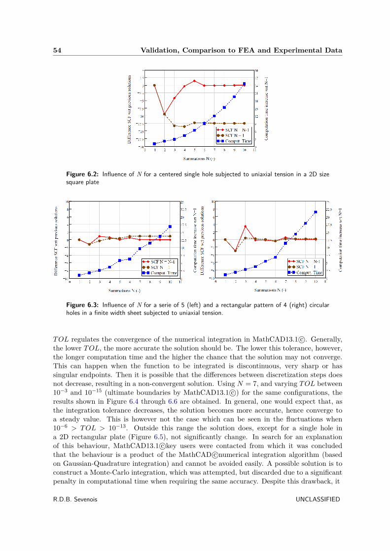
54 Validation, Comparison to FEA and Experimental Data
Figure 6.2: Influence of N for a centered single hole subjected to uniaxial tension in a 2D sizesquare plate
Figure 6.3: Influence of N for a serie of 5 (left) and a rectangular pattern of 4 (right) circularholes in a finite width sheet subjected to uniaxial tension.
TOL regulates the convergence of the numerical integration in MathCAD13.1 c©. Generally,the lower TOL, the more accurate the solution should be. The lower this tolerance, however,the longer computation time and the higher the chance that the solution may not converge.This can happen when the function to be integrated is discontinuous, very sharp or hassingular endpoints. Then it is possible that the differences between discretization steps doesnot decrease, resulting in a non-convergent solution. Using N = 7, and varying TOL between10−3 and 10−15 (ultimate boundaries by MathCAD13.1 c©) for the same configurations, theresults shown in Figure 6.4 through 6.6 are obtained. In general, one would expect that, asthe integration tolerance decreases, the solution becomes more accurate, hence converge toa steady value. This is however not the case which can be seen in the fluctuations when10−6 > TOL > 10−13. Outside this range the solution does, except for a single hole ina 2D rectangular plate (Figure 6.5), not significantly change. In search for an explanationof this behaviour, MathCAD13.1 c©key users were contacted from which it was concludedthat the behaviour is a product of the MathCAD c©numerical integration algorithm (basedon Gaussian-Quadrature integration) and cannot be avoided easily. A possible solution is toconstruct a Monte-Carlo integration, which was attempted, but discarded due to a significantpenalty in computational time when requiring the same accuracy. Despite this drawback, it
R.D.B. Sevenois UNCLASSIFIED

6.1 Stress Analysis 55
Figure 6.4: Influence of TOL for a centered single hole subjected to uniaxial tension(left) andmultiaxial tension-tension (right) in a 4D size square plate
Figure 6.5: Influence of TOL for a centered single hole subjected to uniaxial tension in a 2Dsize square plate
is concluded that a safe working range for the analysis of a general problem is 10−3 > TOL >10−6 ∨ 10−13 > TOL > 10−16.
The attentive reader might have noticed that, due to this conclusion, the investigations per-formed for stress verification, Chapter 5, and to determine a good value for N are invalidbecause a value TOL = 10−12 was used for the analysis. Contradictory, despite that this “un-reliable” value was used for stress verification, the difference between Lekthnitskii’s solutionswere negligible which points towards a correct solution. Both statements can only be true if,for the case of a quasi-infinite plate, the influence of TOL on the results is negligible. This isshown in Figure 6.7 where additional results are presented for a single elliptical and circularhole in a quasi-infinite sheet with N = 7. One can see that in these cases the solution, whenvarying TOL, does not differ significantly. Also, these experiments differ only from the previ-ous experiments in the size of the plate. Hence the plate size plays a role in the convergenceof the solution. Consequently, one might conclude that the results obtained to determine Nhave to be recalculated using a proper value of TOL because, in the used configurations, there
UNCLASSIFIED R.D.B. Sevenois

56 Validation, Comparison to FEA and Experimental Data
Figure 6.6: Influence of TOL for a serie of 5 (left) and a rectangular pattern of 4 (right) circularholes in a finite width sheet subjected to uniaxial tension
Figure 6.7: Influence of TOL for a single elliptical (right) and circular hole in a quasi-infinitesheet
is a significant edge effect. This, however, does not necessarily need to be true if it can beshown that the same behaviour for changing N exists when using another value for TOL. Thereason being that, if one does a calculation with an initial error (e.g. using “unreliable” valuefor TOL), and compares the outcome to an outcome where the same error is incorporated,the errors will cancel each other out. This is illustrated by Figure 6.8 where the configurationwith a single hole subjected to multiaxial tension-tension is recalculated for TOL = 10−6.Comparing the outcome to the earlier results in Figure 6.1 (TOL = 10−12) shows that thebehaviour of both graphs is the same. Thus, the earlier obtained results are valid.
Finally, from this investigation on the effect of the accuracy parameters TOL and N on theobtained solution, it is concluded that good working ranges for N and TOL, when maximum6 holes are present, are:
N = 710−3 > TOL > 10−6 ∨ 10−13 > TOL > 10−16 (6.1)
R.D.B. Sevenois UNCLASSIFIED

6.1 Stress Analysis 57
Figure 6.8: Influence of N for a centered single hole subjected multiaxial tension-tension (right)in a 4D size square plate when TOL = 10−6
6.1.2 Influence of contact angle estimation
A satisfactory estimation of the contact angle for a pin-loaded hole is essential for a reliableestimation of the stress field. In Section 3.2 two models based on an iterative process wereexplained. A model developed by Tomlinson [13] and a model developed by the author. Inthis section the performance of both models is compared to results from FEA after whichthe most suitable model is chosen. FEA for this subsection were performed by Gerhardt [18]and comprise of a two-dimensional simulation of a rigid pin in a circular hole. Friction ofthe pin and hole edge is neglected. The results from the FEA analysis were validated withresults obtained from an earlier study on bearing bypass loads in pin loaded composite jointsby Crews [14].
Before proceeding to the discussion of the configurations and results, an explanation on resultsbeing (not) conservative is required. The graphs produced in this subsection are constructedby applying a bearing load σb = Pb/(Dt) on a pinned hole and letting the algorithm determinethe accompanying contact angle. Therefore, if for a given load σb, the contact angle is smallerthan in the real (FEA) case, the stress concentration factor at the hole edge will be largerthan in reality. Since the opposite is true when the contact angle is larger than the realcase, one might say that the smaller contact angle estimation is more conservative as it willresult in a lower ultimate failure load. This is true when one is focussing on the stressconcentration factor on the hole edge. However, the model described in this work does notuse the highest stress concentration factor at the hole edge but uses the CPSED to determinea characteristic distance away from the hole at which failure is evaluated, Section 4.1. TheCPSED is calculated using a pinned hole configuration and Kweon’s definition of compressivecharacteristic distance. Recall the aforementioned definition: “The distance from the fronthole-edge to a point where the local compressive stress by the arbitrarily applied load is thesame as the mean bearing stress when a bearing load is applied to the hole edge”. When asmall contact angle is used, the location where the local compressive stress is the same as themean bearing stress will be further away from the hole edge compared to a larger contactangle due to the higher stresses, Figure 6.9. The CPSED is calculated as the sum of thestrain energy density along d. Hence for the smaller contact angle a higher CPSED will beobtained than for the larger contact angle. In turn, the CPSED is a measure for the ability
UNCLASSIFIED R.D.B. Sevenois

58 Validation, Comparison to FEA and Experimental Data
Figure 6.9: Schematic representation for the calculation of the CPSED whith a higher or lowercontact angle
of the material to absorb energy. Therefore, if the material is able to absorb more energy, theestimated failure load of the plate will be higher with respect to a lower CPSED. Since thelower CPSED is associated with a higher contact angle, in this work, a higher contact angleis considered conservative as it results in a lower predicted failure load.
An initial comparison between the model by Tomlinson and Sevenois model (author) is shownin Figure 6.10. In the Figure the contact angle associated with a fixed bearing load σb is shown.The configuration used is a rectangular plate size 125 [mm] x25 [mm] containing one circularhole with a diameter of 5 [mm] and a QI layup. Clearance between the pin and the hole is1.5% and α, Figure 3.7, equals half of the contact angle. In the Figure it is observed that thecontact angle from Tomlinson’s model remains 0 at low bearing stress levels. At higher stresslevels the model converges rapidly towards FEA data but stays in the non-conservative region(smaller contact angle than expected). The contact angle being zero at low bearing stresslevels has to do with the assumption of an elliptical deformation of the hole. At a lower loadlevel, thus lower horizontal displacement, the elliptical curve, Eq. (3.33), only intersects thepin shape at 0. Therefore the result is also 0. Compared to Tomlinsons model, Sevenois’model approaches the curve from FEA much better and the contact angle is, in all cases,conservative. Furthermore no unexpected behaviour is observed. From this first investigationit is clear that the performance of Sevenois’s model is better, therefore it chosen to be usedin the analytic tool.
To produce the results in Figure 6.10, a value for the displacement angle α was chosen tobe half of the contact angle. Noting that there is a discrepancy with respect to FEA, it isfurther investigated if changing α would be beneficial for the prediction. Additionally, differentlaminate directionalities (=
√Exx/Eyy) and pin hole clearances might also have an influence
on the predictions and this should also be investigated. For this purpose a parametric studyis set up where a total of 10 different layups with 6 different clearances for a typical CFRPlaminate are investigated resulting in 24 analysis. Graphs of bearing load vs contact angleare produced from FEA and Sevenois’ model. For Sevenois’ model a value for α equal to thecontact angle, half the contact angle and 0 is investigated. The ply properties, layups andclearances are shown in Table 6.1.
R.D.B. Sevenois UNCLASSIFIED

6.1 Stress Analysis 59
Figure 6.10: Change in contact angle with increasing bearing stress for Tomlinson, FEA andSevenois
Table 6.1: Analysis parameters for optimal α determination
Layups - in % 0/± 45/90 degrees20/70/10 25/50/2550/40/10 30/40/3020/20/60 60/20/2020/60/20 40/30/300/0/100 100/0/0
Clearances (%)2.0,1.5,1.0,0.5,0.1,0.01
Material Properties DimensionsE11(GPa): 133.5 Laminate thickness: 1 [mm]E22(GPa): 8.3 Plate length: 125 [mm]G12(GPa): 40.5 Plate width: 25 [mm]v12(GPa): 0.3 Hole diameter: 5 [mm]
UNCLASSIFIED R.D.B. Sevenois

60 Validation, Comparison to FEA and Experimental Data
Figure 6.11: Effect of directionality on contact angle prediction (FEA) [18]
The directionality of each laminate was computed and associated with the results. For conve-nience, in this subsection only the most important result of the analyses are shown. All resultsare given in Appendix E. First the effects of laminate directionality and pin-hole clearanceare investigated. As is illustrated in Figure 6.11 the higher the directionality, the higher thecontact angle given a certain bearing load. Furthermore, from Figure 6.12 it is concludedthat a lower pin-hole clearance results in a higher contact angle. This is as expected sincea smaller clearance implies a bigger pin for the same hole size. Thus the contact angle willautomatically increase. A comparison between FEA and Sevenois’s model for different valuesof α (equal to the contact angle, half the contact angle and 0 denoted by 1.0, 0.5 and 0.0respectively) is shown in Figure 6.13. In the figure results for a QI layup and a clearance of2.0% are presented. From the figure it is observed that increasing α results in a lower contactangle when given a certain load. This results in non-conservative predictions when α is equalto the contact angle. Therefore this value for α is excluded for analysis. Furthermore it canbe seen that when α is equal to half the contact angle, the prediction is conservative but lessconservative than when α is taken equal to 0. This conclusion is valid for the tested layupswhere the directionality is smaller than 1.11. For directionalities between 1.11 and 1.13, theprediction is within 5% of the value from FEA. For higher directionalities the contact angleprediction is conservative for α = 0 up to a directionality of 1.13.
It is recognized that a better approximation of the pin-hole contact problem might be achievedwhen using displacement boundary conditions. Time constraints however did not allow foradaptation of the model and therefore the validity of the tool has to be restricted to laminateswith a directionality lower than 1.13. As to which value of α should be used, it is recommendedto use α equal to half the contact angle because it results in the least discrepancy with respectto FEA.
R.D.B. Sevenois UNCLASSIFIED

6.1 Stress Analysis 61
Figure 6.12: Effect of clearance on contact angle prediction (FEA) - QI layup [18]
Figure 6.13: Effect of α on contact angle prediction (Sevenois’s model) and comparison to FEA.Clearance 2% - QI layup in coöperation with [18]
UNCLASSIFIED R.D.B. Sevenois

62 Validation, Comparison to FEA and Experimental Data
Figure 6.14: Example of the FEM mesh around a hole
6.1.3 Comparison to FEA
In Section 6.1.1 and Section 6.1.2 optimal parameters for TOL, N and α are established. InChapter 5 it was demonstrated that the model can accurately produce stress distributions forinfinite plates and a single hole. Now, it remains to determine how well the tool is capable ofincorporating the effect of edges and multiple holes. For this purpose one needs to know theaccuracy of the stress field when:
• a hole is close to a plate edge
• a hole is loaded in the presence of edges
• multiple (loaded/unloaded) holes are present
From these goals suitable test cases are derived which are shown in Table 6.2. In the tableit can be seen that, to determine the accuracy of the tool when the hole is close to a plateedge, the configuration of a single hole in a plate subjected to uniaxial tension is used. Inconfiguration 1 the distance to the loaded edge (E/D) and in configuration 2 the diameterto width ratio (W/D) is varied. To determine the accuracy when a hole is loaded, a holewith a radial cos-distributed load, Eq. (3.32) , at its edge is modeled in a finite size plate asshown in configuration 3. Lastly, with configuration 4, the ability of the tool to account for acombination of loaded and unloaded holes close to each other is investigated. Four holes withdiameter D are placed 3D apart in a square pattern. The holes to the right(2) are loadedwith a radial cos-distributed load, Eq. (3.32). The remaining holes are unloaded. The loadsare balanced with an edge load to one side of the plate.
The configurations in Table 6.2 are modeled in a FEA environment using MSC PATRAN/-NASTRAN c©. Since the tool is only capable of calculating the stress field for a 2D-plate useof CQUAD4 shell elements is justified. A mesh refinement is applied around the holes tocapture stress concentrations which resulted in 240 elements around each hole. Additionally,in accordance with the Fokker FEM manual [199], it is made certain that the aspect ratio ofthe elements is lower than 4, the skew is higher than 60 degrees and taper lower than 0.5 inthe vicinity of the hole. An example of the mesh is shown in Figure 6.14. A 2D orthotropic
R.D.B. Sevenois UNCLASSIFIED

6.1 Stress Analysis 63
Table 6.2: Test cases for comparison between FEA and analytic tool
1.
Layup: [0/+ 45/− 45/+ 45/− 45]sCases: E/D = 1.0, 1.5, 2.0, 2.5Hole diameter: 10 [mm]Plate length: 90 [mm]Plate width: 100 [mm]
2.
Layup: [0/+ 45/− 45/+ 45/− 45]sCases: W/D = 2.0, 2.5, 3.0, 4.0Hole diameter: 10 [mm]Plate length: 100 [mm]
3.
Layup: [0/+ 45/− 45/+ 45/− 45]sCases: E/D = 1.5, 2.5Hole loaded with edge pressure load radially distributedHole diameter: 10 [mm]Plate length: 100 [mm]Plate width: 100 [mm]
4.
Layup: [0/+ 45/− 45/+ 45/− 45]sCases: two holes unloaded, two holes loadedHole diameter: 10 [mm]Plate length: 200 [mm]Plate width: 200 [mm]
UNCLASSIFIED R.D.B. Sevenois

64 Validation, Comparison to FEA and Experimental Data
Figure 6.15: Boundary condition
homogeneous material type is used. The engineering properties of the layup are calculatedbeforehand and inserted as scalars.
Load and boundary conditions are handled in different ways depending on the configuration.For configuration 1 and 2, the load on the plate edge furthest away from the hole is replaced bya displacement restriction in the direction of the load. Additionally, to avoid unnecessary pivotratios (out-of-plane movements), the central node on that edge is restricted to move or rotate.This is illustrated in Figure 6.15. For configuration 3 and 4 the hole edge load is representedby a CID distributed radial edge load while the edge is replaced by the same displacementboundary condition as described for configuration 1 and 2. Modelling the configurations in theanalytic tool is much simpler. The software tool takes edge loads, material properties, plateand hole(s) dimensions as direct input. Therefore it is completely parametric and providesworry-free (no need to check the validity of the mesh) batch processing which is one of themajor strengths of this tool. One however does need to check whether the solution is stablewith respect to the amount of summations (N) used for the solution. However, as has beenshown in Section 6.1.1, using N = 7 suffices for problems up to 5 holes where no excessive edgeor hole to hole effects are present. Therefore, for all problem cases N = 7 and TOL = 10−6
is used as accuracy parameters.
The comparison between FEA and the tool is performed by qualitatively and quantitativelyassessing the SCF of the tangential stress around each hole. Furthermore, the change of max-imum SCF along the length or width of the plate is assessed qualitatively. For convenience,only the most important results from the analyses are shown in this section. All results arepresented in Appendix F. The analyses of configuration 1 when E/D = 2.5 and E/D = 1 areshown in Figure 6.16 and Figure 6.17 respectively. In both figures it is observed that thegeneral behaviour of the SCF when revolving around the hole is the same for FEA and theanalytic tool. Four stress peaks in a symmetric fashion are present of which two are higherthan the other. For E/D = 2.5 there is no apparent difference between both solutions. ForE/D = 1.0, however, a discrepancy is present between the higher stress peaks. Looking at thechange of σy/σ0 along x while y = 0 reveals that in the vicinity of the hole the SCF followsthe same trend. At the plate edges a discrepancy is also present. The tool predicts a stressvalue of approximately zero while FEA, especially when E/D = 1, expects much higher stress
R.D.B. Sevenois UNCLASSIFIED

6.1 Stress Analysis 65
Figure 6.16: Config. 1, SCF of σθ at the hole edge (left) and SCF of σy at y = 0 (right) whenE/D = 2.5
Figure 6.17: Config. 1, SCF of σθ at the hole edge (left) and SCF of σy at y = 0 (right) whenE/D = 1
in σy.
The analyses of configuration 2 for W/D = 4 and W/D = 2 are shown in Figure 6.18 andFigure 6.19 respectively. Comparing both figures to the figures from configuration 1 it isobserved that a similar conclusion can be drawn. For the case where W/D = 4, there is anegligible discrepancy between FEA and results from the analytic tool. For W/D = 2 thereis a larger, but with respect to configuration 1 smaller, discrepancy between both. Theanalyses for configuration 3, a loaded hole with E/D = 2.5 and E/D = 1.5 are shown inFigure 6.20 and Figure 6.21 respectively. Just as with configuration 1 and 2 it is seen herethat, for the configuration with the hole furthest from the edge, the difference between bothmethods is smaller compared to the configuration where the hole is closer to the edge.
UNCLASSIFIED R.D.B. Sevenois

66 Validation, Comparison to FEA and Experimental Data
Figure 6.18: Config. 2, SCF of σθ at the hole edge (left) and SCF of σx at x = 0 (right) whenW/D = 4
Figure 6.19: Config. 2, SCF of σθ at the hole edge (left) and SCF of σx at x = 0 (right) whenW/D = 2
R.D.B. Sevenois UNCLASSIFIED

6.1 Stress Analysis 67
Figure 6.20: Config. 3, SCF of σθ at the hole edge (left) and SCF of σx at x = xhole (right)when E/D = 2.5
Figure 6.21: Config. 3, SCF of σθ at the hole edge (left) and SCF of σx at x = xhole (right)when E/D = 1.5
UNCLASSIFIED R.D.B. Sevenois

68 Validation, Comparison to FEA and Experimental Data
As from all three configurations a similar conclusion is drawn, it can be investigated howa different E/D or W/D affects the magnitude of the discrepancy between FEA and theanalytic tool.From all three configurations the discrepancy in maximum tangential stressconcentration factor was calculated and plotted in Figure 6.22. In the figure the generaltrend, a closer hole distance means a higher discrepancy, can quite clearly be observed. Inthe search of why these discrepancies exist the following are noted. Investigating the FEAmodels themselves did not result in convergence errors. All elements were small enoughto lead to stable results. Investigating the parameters used for the analytic analysis itselfrevealed the following. For all analyses a summation parameter N = 7 and integrationtolerance parameter TOL = 10−6 are used. Since N controls the accuracy of the solution, it isexpected that increasing this parameter would result in a better approximation of the problem.However, upon increasing this parameter it was found that the analytic solutions were alreadyconverged. This brought the attention to the integration tolerance parameter TOL. Since thisparameter controls the accuracy of the numerical integration it is suspected that, for settingswith close edges, the convergence criterium for the numerical integration is too high and thusit was attempted whether decreasing this parameter improved the results. Ultimately, thisalso prove unsuccessful since here also convergence was found. Further testing whether thenumerical integration routine could be at the basis of the discrepancies at close hole edgesconfiguration 3 for E/D = 1.5 was analyzed with a Mathematica c©algorithm developed byBakker [200]. This algorithm is founded on the same theory but constructed as applicationfor single lap joints. It was expected that the results from the Mathematica c©algorithm arecloser to FEA because of the better numerical integration procedures in Mathematica c©. Theopposite turned out to be true for which the cause was found in the initial assumption that:
σx = 2Re
[µ2
1dϕ1(z1)dz1
− µ22dϕ2(z2)dz2
](6.2a)
σy = 2Re
[dϕ1(z1)dz1
− dϕ2(z2)dz2
](6.2b)
τxy = −2Re
[µ1dϕ1(z1)dz1
− µ2dϕ2(z2)dz2
](6.2c)
where it can be seen that the initial summation between the stress functions is replacedby substraction. One cause for the discrepancies between FEA and the tool remain. Theinitial assumed shape function, Eq. (3.13), is less suitable of accurately representing thestress field when holes are very close to the edge leading to a less accurate minimum energysolution. Solving this requires trying the assumption of a different shape function which wasnot attempted due to time constraints.
Nevertheless this drawback, the discrepancy between FEA and the analytic tool vanishes whenE/D > 2.5 and W/D > 4. Since, for design purposes, an E/D > 2.5 + 1.3 [mm] [16] andW/D > 4.7 [17] is advised, the analytic tool can confidently be used for common engineeringpractice. Finally, the ability of the tool to account for multiple holes which are loaded orunloaded is tested using configuration 4. A rectangular plate size 20D is modeled with 4holes, each 3D apart. Two holes are loaded while the other two are unloaded. The total loadis balanced with an equivalent edge load. For comparison, the tangential stress concentrationfactor with respect to the hole angle for the FEA model and the analytic tool is plotted inFigure 6.23. It is observed that there is an excellent agreement between both.
R.D.B. Sevenois UNCLASSIFIED

6.1 Stress Analysis 69
Figure 6.22: Difference in SCF between FEM and Tool for a hole in a plate with varying E/Dand W/D
Figure 6.23: Tangential SCF from config. 4 for an unloaded (left) and loaded (right) hole
UNCLASSIFIED R.D.B. Sevenois

70 Validation, Comparison to FEA and Experimental Data
Figure 6.24: Biaxial failure envelope for QI AS4-3501 [22]
6.2 Failure Prediction - Comparison to Test Results
Having determined the validity of the stress field method, the performance of the failureprediction method can be assessed. This is done by comparing the unnotched and notchedfailure prediction to experimental data from literature. Comparison of the unnotched failureprediction can be done without any adaptations to the algorithm. For notched failure pre-diction, however, as mentioned in the beginning of this Chapter, the optimal values for the“free” parameters; the pin-hole clearance λ and hole size for determination of the CPSEDneed to be determined first.
6.2.1 Unnotched Failure Criterion
Using the unnotched failure criterion described in Section 4.1, uniaxial, biaxial and uniaxial-shear failure envelopes are produced to compare to experimental data from various researchers[22–26] and Fokker Aerostructures B.V. [201].Biaxial failure experimental data and predicted failure envelopes for CFRP material AS4-3501 [22], IM7-8551 [23, 24] and IM7-9772 [25] are shown in Figure 6.24 to Figure 6.29. InFigure 6.24 and Figure 6.25 it can be seen that, for QI layups, the Fokker criterion has abetter correlation with experimental data than the modified Puck criterion. This is espe-cially true in the second and third quadrant of the failure envelope where the modified Puckcriterion significantly overestimates the strength of the laminate. The Fokker criterion alsooverestimates the laminate strength in the compression compression quadrant. In the firstquadrant both criteria have a good agreement with experimental data. The fourth quadrant isnot investigated since an orthotropic laminate results in a symmetric failure envelope aroundthe axis σx = σy. Biaxial failure envelopes for compression-compression loaded angle plied[±α]s laminates are shown in Figure 6.26 to Figure 6.28. Observe that the performance of theFokker criterion in the compression-compression quadrant is better than the Modified Puckcriterion but nonetheless significantly overestimates the laminate strength. In the remainingquadrants, no experimental data was obtained but note the apparent infinite strengths pre-dicted by the current Fokker criterion in Figure 6.27 and Figure 6.28. Because the modified
R.D.B. Sevenois UNCLASSIFIED
6.2 Failure Prediction - Comparison to Test Results 71
Figure 6.25: Biaxial failure envelope for QI IM7-8551 [23,24]
Figure 6.26: Biaxial failure envelope for [±15]s IM7-8551 [23,24]
Puck criterion does not contain this region, it is concluded that its performance is betterthan the Fokker criterion. A biaxial failure envelope for a [0]8 IM7-977-2 laminate is shownin Figure 6.29. Comparing the performance of both failure criteria it is observed that themodified Puck criterion provides a better fit to the test data than the Fokker criterion. Thisespecially in the first quadrant where the experimental data in the upper right corner matchesexceptionally well. Furthermore the Fokker criterion is more conservative. Different from thebiaxial failure envelopes, a uniaxial-shear failure envelope for a [0]32 IM7-8552 laminate isshown in Figure 6.30. Here the Modified Puck criterion has a better fit than the Fokkercriterion.
Both criteria were also used to provide a comparison to experimental data from FokkerAerostructures B.V. [201] Predictions for the uniaxial compressive and tensile strength ofa soft, hard and QI laminate made from material TH5.698/6 are shown in Figure 6.31. Inthe Figure it can be seen that there is virtually no difference between both criteria. A verygood correlation with the experimental data is obtained.
UNCLASSIFIED R.D.B. Sevenois

72 Validation, Comparison to FEA and Experimental Data
Figure 6.27: Biaxial failure envelope for [±30]s IM7-8551 [23,24]
Figure 6.28: Biaxial failure envelope for [±45]s IM7-8551 [23,24]
Figure 6.29: Biaxial failure envelope for [0]8 IM7-9772 [25]
R.D.B. Sevenois UNCLASSIFIED

6.2 Failure Prediction - Comparison to Test Results 73
Figure 6.30: Uniaxial-Shear failure envelope for [0]32 IM7-8552 [26]
Figure 6.31: Uniaxial compressive and tensile test and predictions for material TH5.698/6 forQI, soft and hard laminate
UNCLASSIFIED R.D.B. Sevenois

74 Validation, Comparison to FEA and Experimental Data
From the comparisons between the experimental data and both criteria it is difficult to pointout which criterion performs best. The Fokker criterion performs better (although not dras-tical) for QI laminates subjected to biaxial loads while the modified puck criterion is superiorin the case of a UD laminate. For angle plied laminates performance of both criteria is ques-tionable because of the apparent lack of test data. Sometimes the Fokker criterion predictsapparent infinite strengths in the first quadrant. It is clear that in this investigation the con-clusion from the literature survey, Section 2.2, is encountered again. The current (unnotched)failure models for composite laminates are all but perfect and still require much development.As such the question which criterion in this investigation performs better seems redundant.Both criteria have their advantages and disadvantages and therefore they perform equallygood (or bad for the pessimists). In the remainder of this thesis it is decided to use theModified Puck criterion as a basis for the unnotched laminate strength because the Fokkercriterion contains curve fitting elements while in this work a universally applicable failurecriterion is sought. Thus, the less curve fitting elements present, the better.
6.2.2 Notched Failure Criterion - Clearance and Hole Size for CPSED
Before the performance of the notched failure criterion can be determined, optimal values forthe remaining “free” parameters need to be determined. As aforementioned, these parametersare the pin-hole clearance λ and hole size for determination of the CPSED. The pin-holeclearance is the percentage difference between the size of the pin and the size of the holewith respect to the hole. Usually, there is a measurable clearance between the pin and ahole, however, this is only so for loaded hole experiments where, in the documentation, thepin-hole clearance is reported. Therefore, to be able to estimate hole strengths when pin-holeclearance is unknown, it is necessary to have a recommended value for the pin-hole clearance.By inspection of datasheets with clearance fit allowables [202] it is noted that a hole clearancecan be as small as 0.5% for a hole diameter of 10 [mm] (the largest most occuring hole diameterin the experimental dataset) while it can be as large as 11.3% for a hole diameter of 3 [mm]. Itis recognised that this is a large range. However, since conservative predictions are preferred,and a smaller clearance results in more conservative predictions ,a hole clearance of 0.5% isused as recommended value.
Since the compressive characteristic distance, used to calculate the CPSED (Kweon’s def-inition Section 4.2), is dependent on the stress field around the hole and the stress fieldaround the hole is dependent on the hole size, the hole size for determination of the CPSEDis crucial for the prediction of notched failure. In his research, Kweon [3] uses a hole di-ameter of 6.35 [mm]. However, since the hole size for CPSED has such a significant effecton the predicted failure strength, it is decided to determine an optimal value by calibrationwith experimental data. For this purpose, using the aformentioned clearance value of 0.5%,predictions are made using several hole diameters ranging between 2 [mm] to 10 [mm] forexperimental configurations from [27, 28]. [27] describes open (small and large) hole uniaxialcompression and tension experiments on CFRP-epoxy laminates with a soft, hard and quasi-isotropic layup. [28] outlines both open hole and pinned-hole tensile tests on the same typeof laminates. Together, both datasets contain 12 experiments which are considered represen-tative for the other experimental data used in Section 6.2.3. Therefore, if conclusions fromthese limited number of configuratons for the hole size for CPSED are drawn, the conclusionsshould be applicable to the other experimental data. Plotting the discrepancy in percent be-
R.D.B. Sevenois UNCLASSIFIED

6.2 Failure Prediction - Comparison to Test Results 75
Figure 6.32: Discrepancy with experiments from [27] (right) and [28] (left) when the hole sizefor the determination of the CPSED is varied. OHT = Open Hole Tension, OHC = Open HoleCompression, PHT = Pinned Hole Tension, S = Soft, H = Hard, QI = Quasi-Isotropic, N =Narrow W/D, W = Wide W/D, L = Large hole
Table 6.3: Least square error for hole sizes below 6 [mm] based on Figure 6.32
Hole diameter for CPSED (mm) Least square error2 106943 84814 73525 5918
tween the predicted failure and measured failure for every hole size for CPSED against everyconfiguration results in Figure 6.32. In the figure it can be seen that there exists a generaltrend in prediction vs hole size. Namely, the predictions from larger hole sizes lie above thepredictions from lower hole sizes. This is expected since a higher hole size for CPSED resultsin a higher CPSED which in turn results in a higher failure load. Additionally, it is observedthat the discrepancy for pin-loaded holes is highly conservative.
The recommended value for the hole size of the CPSED is now determined in the followingmanner. From discussions with supervisors at Fokker Aerostructures B.V., it is concludedthat, for the new criterion to be immediately applicable in industry, the discrepancy be-tween predicted and measured value should be lower than +10%. When this restriction isrespected, the discrepancy should be as close to 0% as possible. The +10% threshold is drawnin Figure 6.32 from which it is concluded that the hole sizes above 5 [mm] are excluded forconsideration. Next, the sum of the least square errors of the remaining hole sizes are cal-culated to assess which curve is closest to 0% discrepancy. The calculated values are shownin Table 6.3 from which it can be seen that the lowest value, thus the graph closest to 0%,occurs when a hole diameter for CPSED of 5 [mm] is used.
UNCLASSIFIED R.D.B. Sevenois

76 Validation, Comparison to FEA and Experimental Data
Figure 6.33: Uniaxial tensile (left) and compressive (right) failure for AS4/3501-6 [29], QI CFRPlayup, fixed specimen size
Concluding, the recommended values for the remaining free parameters, pin-hole clearanceand hole diameter for CPSED are 0.5% and 5 [mm] respectively. The value for the pin-holeclearance is determined based on a logical reasoning while the value for the hole diameter isdetermined by calibration with a representative selection of test data.
6.2.3 Notched Failure Criterion - Comparison to Experimental Data
With the determination of all “free” parameters, the performance of the notched failure cri-terion can be assessed. Experimental results from 9 sources [19, 27, 29–35] are obtained andcompared to predicted failure loads from the analytic tool and the current criterion in use atFokker Aerostructures B.V. In the first paragraphs, no distinction is made between configu-rations which comply and configurations which violate the tool directionality boundary (lessthen 1.13) determined in Section 6.1.2. This is done on purpose such that a quantitative dis-cussion on results with and without this distinction is possible at a later stage. All predictionsin this section are calculated using the “optimal” settings for the “free” parameters.
The obtained datasets are divided in four categories: uniaxial, biaxial, bearing and bearing-bypass tests. In the uniaxial category Wang [29] and Bos [27] performed tensile and compres-sive failure tests on laminates from UD AS4/3501-6 and TH5.698/601 respectively. Wangused a QI layup and varied the hole size while keeping a fixed specimen size. Bos tested a QI,soft and hard layup while keeping a fixed hole size. The results from both investigations areshown in Figure 6.33 and Figure 6.34 respectively. From the Figures, it is observed that hereis a good, although sometimes unconservative, agreement between prediction and experimentin the tensile configurations for both the Fokker and Sevenois criterion. Additionally, it ap-pears that, for hole sizes larger than 3 [mm], Sevenois’ criterion is more conservative than theFokker criterion. For lower hole sizes the opposite is true. In the compression experiments, itis observed that the Fokker method has a better fit for Wang’s experiments while it overesti-mates three of the four (compressive)experimental failure loads by Bos. The Sevenois modelis always conservative but in one datapoint from Wang.
Two other datasets for uniaxial compressive failure where obtained from Hodge [30] andSoutis [31]. Both authors investigated the effect of increasing the hole size on the compressive
R.D.B. Sevenois UNCLASSIFIED

6.2 Failure Prediction - Comparison to Test Results 77
Figure 6.34: Uniaxial tensile and compressive failure for TH5.698/601 [27], Hard, Soft and QIlayup, hole diameter: normal = 6.35 [mm], Large = 9.52 [mm]
Figure 6.35: Uniaxial compressive failure for IM7/8552-1 [30] when changing hole size, fixedspecimen size
failure strength. Hodge used IM7/8552-1 UD prepreg while Soutis used T800/924C prepregand investigated multiple layups. The results are shown in Figure 6.35, Figure 6.36 andFigure 6.37 where it can be seen that, in contrast to the conclusions from the previous results,the discrepancies between prediction and measurement are much larger. This for layup nr.1 in Figure 6.35, and nr. 1,3,4, 5 in Figure 6.36 and Figure 6.37. In 60% of the cases theSevenois criterion predicts a lower failure load than the Fokker criterion. Both criteria dofollow the trend (decreasing strength with increasing hole size) of the data .
Experimental data from biaxial load experiments is obtained from 3 sources. Daniel, [32, 33]performed biaxial tension-tension experiments on QI and [02/± 45]s laminates from UD SP-286T300 CFRP. For all experiments Daniel tested several hole sizes for the same loadingratio. For the QI layup, the loading σx − σy was 1/1 while for the [02/ ± 45]s laminatethe loading ratio was 2/1. In contrast to other researchers, the hole sizes from Daniel wererather large, in to order of some [cm]’s rather than the more common [mm] size. The results,shown in Figure 6.38, indicate that their is only a minor difference between the new criterionand the Fokker criterion where the Fokker criterion in all but one case predicts a higher
UNCLASSIFIED R.D.B. Sevenois

78 Validation, Comparison to FEA and Experimental Data
Figure 6.36: Uniaxial compressive failure for T800/924C [31] when changing hole size, fixedspecimen size, part 1
Figure 6.37: Uniaxial compressive failure for T800/924C [31] when changing hole size, fixedspecimen size, part 2
R.D.B. Sevenois UNCLASSIFIED

6.2 Failure Prediction - Comparison to Test Results 79
Figure 6.38: Biaxial failure strength and prediction [32,33] for SP-286T300
Figure 6.39: Biaxial failure envelope for QI laminate of IM7/8552 with 10 [mm] hole [34] andprediction
failure strength with regard to the Sevenois criterion. Furthermore, the discrepancies withthe measurements are small with the QI-layup while they are rather high (but conservative)in case of the [02/±45]s layup. Huang [34] used a QI layup of IM7/8552 to construct a biaxialfailure envelope. This is shown in Figure 6.39 where it can be seen that, here too, both criteriaproduce conservative predictions where the Fokker criterion is closer to the experimental data.
Chang [35] performed an extensive experimental investigation on the pinned strength ofT300/1034C laminates. Three basic specimen designs: single hole, two holes in paralleland two holes in series, were tested up to failure with 7 different layups (Figure 6.41). Ad-ditionally, the basic dimensions of the specimens were varied to investigate edge effects. Themeasured strengths and the predictions are shown in Figure 6.40 to Figure 6.42. In eachfigure, the specimen dimensions are indicated. For almost all layups and configurations boththe Fokker and Sevenois criterion underestimate the strength of the joint. Furthermore, withthe single hole specimens the magnitude of the discrepancy between measurement and pre-
UNCLASSIFIED R.D.B. Sevenois

80 Validation, Comparison to FEA and Experimental Data
diction seems to be dependent on the specimen size. Compare, for example Figure 6.40(a)with Figure 6.40(c) and (d) where it is observed that, overall, the disrepancy with (d) ismuch smaller with regard to the other two cases. With the two hole series this observationcan not be made with confidence. It seems, however, that the predictions for the two holespecimens in series are closer to the measured failure strengths. Especially, when comparingFigure 6.40(a), Figure 6.41(b) and Figure 6.40(b), Figure 6.41(c).Crews [19] performed bearing bypass experiments on QI graphite epoxy laminates in anattempt to generate the complete bearing bypass curve. Crews measured both initial failureand final failure of the specimens. The comparison to Sevenois and Fokker is shown inFigure 6.43 where it can be seen that both criteria underestimate the ultimate failure strengthsignificantly. Instead, the predicted failure loads seems to coincide with the onset of failurewith the Sevenois criterion being the most conservative. Additionally, it is noted that thecurve does not coincide well in the compressive bearing bypass region. This is attributed tothe contact angle algorithm which was not designed for this purpose.Qualitatively, it seems that the performance of the new criterion is an improvement over thecurrent Fokker criterion since it provides better predictions which are almost always conser-vative or close to the measured values for open hole configurations. Qualitative observations,however, are somewhat sensitive to subjectivity and in the following an attempt is made toquantify the predictions. Two graphs, one for unloaded and one for loaded configurations,are constructed where prediction is set out against measurement for all 151 datapoints. Theboundaries for 60%, 40%, 20% and 0% discrepancy are indicated in the graphs which areshown in Figure 6.44 and Figure 6.45. In Figure 6.44 it immediately stands out that thereis more compressive than tensile data. In the tensile case, all predicted values are within+20% and −40% of the measured failure load. In the compressive case, however, scatter ismuch larger. Here the Fokker criterion overestimates some experiments by over 40% whilethe Sevenois criterion produces predictions between +20% and −40% of the measured value.Most predictions, however are located in the boundary −20%, +20%. Looking at the graphfor the loaded experiments, Figure 6.45, scatter is much larger. Most predictions are conserva-tive concentrating in the −20% to −60% region. A great deal are, more Sevenois than Fokker,overestimations. This is quite worrying since, this way, it appears that one cannot determineconfidence bounds for the loaded hole experiments. Up to now, the boundaries of the tool,determined in the previous sections, were not taking into account. Applying these boundariesand eliminating the measurements where [0/90]s laminates (early microbuckling occured [31]which is not taken into account by te failure criterion) are used, resulted in the exclusionof 39% of the datapoints to a total amount of 92 (38 measurement points unloaded and 54measurement points loaded holes together). Replotting the graphs results in Figure 6.46 andFigure 6.47.As expected, one can see that now, with the inclusion of the tool boundaries, the resultshave significantly improved. For the Sevenois criterion in the unloaded configurations allpredictions are within +20% and −40% of the measured value. The Fokker criterion hassome overestimations in the +20%, +40% region. For unloaded holes, the Sevenois criterionperforms thus better than the Fokker criterion. In the loaded case, Figure 6.47, the great dealof conservative predictions between −20% and −60% is still present. The overestimations bythe Sevenois criterion, however, have reduced to lower than +20% while the Fokker criterionstill has some predictions above +20% discrepancy. Remarkable is that there are 5 datapointswhere the prediction is lower than 60% of the measured value. Also, for these datapoints, the
R.D.B. Sevenois UNCLASSIFIED

6.2 Failure Prediction - Comparison to Test Results 81
(a) (b)
(c) (d)
(e)
Figure 6.40: Failure strength of single hole specimens wrt predictions [35]
UNCLASSIFIED R.D.B. Sevenois

82 Validation, Comparison to FEA and Experimental Data
(a) (b)
(c) (d)
Figure 6.41: Failure strength of holes in series specimens wrt predictions [35]
R.D.B. Sevenois UNCLASSIFIED

6.2 Failure Prediction - Comparison to Test Results 83
(a) (b)
(c)
Figure 6.42: Failure strength of holes in parallel specimens wrt predictions [35]
Figure 6.43: Bearing-bypass envelope for QI graphite epoxy laminate [19]
UNCLASSIFIED R.D.B. Sevenois

84 Validation, Comparison to FEA and Experimental Data
Figure 6.44: Prediction vs measurement for unloaded hole experiments, unlimited
Figure 6.45: Prediction vs measurement for loaded hole experiments, unlimited
R.D.B. Sevenois UNCLASSIFIED

6.2 Failure Prediction - Comparison to Test Results 85
Figure 6.46: Prediction vs measurement for unloaded configurations, limited
Figure 6.47: Prediction vs measurement for loaded configurations, limited
UNCLASSIFIED R.D.B. Sevenois

86 Validation, Comparison to FEA and Experimental Data
predicted failure value from the Fokker and Sevenois criterion is almost equal. Upon detailedinspection of these specific configurations, it was found out that, in these cases, the stressalgorithm was unable to converge to a steady solution resulting in an unrealistic stress fieldwhich again resulted in an unrealistic failure load. They should thus be neglected.
One cannot say that the performance of the current criterion for notched holes at Fokker,which is based on a constant characteristic distance approach, is unusable. In most of thecases it predicts a value which is within ±40% of the measured value which is acceptableconsidering the rudimentary approach taken. However, in the discussion above it is shownthat the new criterion, with an equally fast and simple set-up, provides a better estimationof the failure strength of notched laminated plates. Additionally, it is able to cope withmultiaxial stress conditions which the Fokker criterion was never designed for and providesfast linear stress field analysis. For unloaded holes, all predictions are within +20% and -40%of the measured value. For loaded holes the predictions are within +20% and -60%.
R.D.B. Sevenois UNCLASSIFIED

Chapter 7
Discussion, Conclusions andRecommendations
The determination of the stress field and evaluation of failure in orthotropic plates with holessubjected to arbitrary boundary conditions is one of the key challenges during the design ofcomposite structures. Up to now, no relatively simple methodology for general configurationsexisted but has now been resolved.
The goal of this project was to construct an analytic tool for the determination of the stressfield and prediction of failure of rectangular orthotropic plates with holes subjected to arbi-trary boundary conditions. Initially, it was envisioned to validate the tool only for unloadedholes but during the construction of the new criterion it was recognized that also loaded holescould be analyzed. Hence, the criterion was also validated for this type of holes. Because theanalytic tool will be used in a design environment by a general engineer, the tool had to befast, simple to use and its functioning easy enough to understand. Additionally, the failurecriterion had to be valid for multiaxial load scenarios.
First it was investigated which theories already existed for the analysis of stresses in or-thotropic notched plates and the prediction of failure based on these stress fields. From thisinvestigation it was concluded that simplicity had to go to the wall for a performant stressanalysis and a complex stress analysis on the basis of Lekhnitskii [4] in conjunction with thetheory from Xiong and Poon [2] was constructed. Their research was expanded to accountfor multiple (loaded) holes and shear loading on the hole and plate edges. The sign selectionmethod by Koussios [194] was also expanded to account for all types of orthotropic laminates.For failure prediction no definite conclusion on which failure criterion would be best to usecould be drawn. Considerations on the basis of the intended use and required speed of thetool led to the birth of the modified critical energy point-stress criterion for failure prediction.A novel criterion which has its roots in the PSC by Whitney and Nuismer [10] in conjunctionwith Kweon [3].
Both stress and failure prediction algorithms were verified thoroughly to ensure a correctfunctioning of the tool. Comparisons to analytic stress fields from other authors resulted
UNCLASSIFIED R.D.B. Sevenois

88 Discussion, Conclusions and Recommendations
in a very good agreement. The effects of changing the amount of summations N and theintegration tolerance TOL were investigated from which it followed that the recommendedminimum values for these parameters are:
• N > 7
• 10−3 > TOL > 10−6 ∨ 10−13 > TOL > 10−16
Validation of the stress field methodology with FEA revealed that, when the holes are veryclose to a plate edge, the solution becomes less accurate. Therefore the following restrictionswith regard to the location of holes and plate edges are identified:
• E/D > 2.5
• W/D > 4
Additionally, validation of the method to determine the contact angle in pin-loaded holesrestricted the tool usage for a laminate directionality lower than 1.13. Optimal values forthe load displacement angle α and hole diameter for the computation of the CPSED weredetermined to be:
• α = half the contact angle
• Hole diameter for computation of the CPSED = 5 [mm]
Validation of the failure prediction methodology was done by comparing the predictions fromthe tool to experimental data and the current failure prediction methods at Fokker Aerostruc-tures B.V. A total of 151 experimental datapoints, mainly from single hole compression, tensileand bearing tests, were used of which 87 were for unloaded and 64 for loaded hole config-urations with biaxial and bearing bypass loading configurations. Eventually, 59 of theseexperimental points were neglected due to the tool boundaries and preliminary ply buckling.92 experimental datapoints remained from which it was concluded that, for unloaded holes,the prediction lies between +20% and −40% of the measured value with all but a few in the±20% region. For loaded holes this is between +20% and −60%. The new criterion is animprovement over the current design methodology.
Strikingly, the unloaded hole predictions are better than the loaded hole predictions. Thiswhile it was expected that the loaded hole predictions would be better than the unloaded holepredictions because Kweon’s failure criterion is based on a failure for loaded holes. During thecourse of validation, several causes for this phenomenon were put forward. It is known, forexample, that the assumed stress distribution of the pin on the hole edge does not adequatelyrepresent the actual contact problem at other angles than 0 and the contact angle. Thiscauses a high tangential stress at the location of the contact angle which sometimes causesthe prediction of early failure. Another possible reason is the use of a fixed hole size todetermine the CPSED. It is true that, using the actual hole size to determine the CPSEDis beneficial for the prediction of loaded holes (it increases the failure load between 0% and10%). Using a fixed hole size, however, is one of the cornerstones of the criterion and changingthis would negatively affect the unloaded hole predictions. Because of the entanglement of
R.D.B. Sevenois UNCLASSIFIED

89
unnotched and notched failure it is impossible to find a cause related to the tool which doesnot affect the unloaded hole predictions. Since these predictions are acceptable, and in fact,quite good, the cause of the discrepancy is sought elsewere. Namely, the test data itself. Asalready indicated in Section 6.2.3, Figure 6.43, it is possible that the notched failure criterionactually predicts the onset of failure instead of final failure. For unloaded holes this shouldnot be of significant concern as onset is usually quite close to final failure. For loaded holes,however, final failure and onset can be far apart due to several strengthening and interlockingmechnisms in the joint. Unfortunately, no details on the failure mechanisms leading up tofailure was found from the literature. It is thus quite hard to determine whether this statementis true. It is however, the most plausible cause.
Unfortunately, due to the directionality boundary condition, the design space where the toolcan confidently be used does not cover all possible laminates. To allow usage in the com-plete design space, the directionality restriction due to the contact angle estimation procedureneeds to be resolved. This ultimately means that the contact angle and pin-hole stress distri-bution need to be improved which can be done using Gerhardt’s model [18]. This model wasdeveloped during the construction of this thesis but was, when finalizing this work, not yetready for implementation. Other recommended improvements to the tool are:
• Include compression bearing-bypass loading in the pin-hole boundary condition
• Include additional effects in the unnotched failure method such as ply buckling anddelamination
• Investigate other/better numerical integration routines for the determination of thestress field
When these challenges are resolved and validated, the tool can easily be used in the Fokkerdesign environment.
Apart from these issues with the loaded predictions, it is emphasized that the majority of thepredictions are moderately to highly conservative while the unloaded predictions are situatedin the +20%, −40% region. Although it was mentioned in Section 6.2.2 that a maximumdiscrepancy of +10% is viable for industry, and the “free” parameters were scaled to obtain thisresult, the finally obtained +20% for the entire dataset is a remarkably close value. It proofsthat, with a select number of experimental measurements, the basic conclusions from a failurecriterion can be made when one is careful with experimental data. The structural element:orthotropic rectangular plate with multiple (un)loaded holes subjected to arbitrary boundaryconditions can be evaluated with confidence when keeping to the determined boundaries.
UNCLASSIFIED R.D.B. Sevenois

90 Discussion, Conclusions and Recommendations
R.D.B. Sevenois UNCLASSIFIED

References
[1] P.D. Soden, A.S. Kaddour, and M.J. Hinton. Recommendations for designers and re-searchers resulting from the world-wide failure exercise. Composites Science and Tech-nology, 64(3-4):589–604, March 2004.
[2] Y. Xiong. An analytical method for failure prediction of multi-fastener composite joints.International Journal of Solids and Structures, 33(29):4395–4409, December 1996.
[3] J.-H. Kweon, H.-S. Ahn, and J.-H. Choi. A new method to determine the characteristiclengths of composite joints without testing. Composite Structures, 66(1-4):305–315,October 2004.
[4] S. Lekhnitskii. Anisotropic Plates. Routledge, 1968.
[5] A. Puck and H. Schürmann. Failure Analysis of FRP Laminates by Means of Physicallybased Phenomenological Models. Composites Science and Technology, 58(7):1045–1067,July 1998.
[6] C.G. Dávila, P.P. Camanho, and C.A. Rose. Failure criteria for FRP laminates. Journalof Composite Materials, 39(4):323–345, 2005.
[7] S.T. Pinho, C.G. Dàvila, and P.P. Camanho. Failure models and criteria for FRPunder in-plane or three-dimensional stress states including shear non-linearity. TechnicalReport February, NASA, 2005.
[8] S.W. Tsai. Theory of Composites Design. Think Composites, Palo Alto, 1992.
[9] M.E. Waddoups, J.R. Eisenmann, and B.E. Kaminski. Macroscopic Fracture Mechan-ics of Advanced Composite Materials. Journal of Composite Materials, 5(4):446–454,January 1971.
[10] J.M. Whitney and R.J. Nuismer. Stress Fracture Criteria for Laminated CompositesContaining Stress Concentrations. Journal of Composite Materials, 8(3):253–265, Jan-uary 1974.
UNCLASSIFIED R.D.B. Sevenois

92 References
[11] T. de Jong. On the calculation of stresses in pin-loaded anisotropic plates. PhD thesis,Delft University of Technology, 1987.
[12] X.W. Xu, T.M. Yue, and H.C. Man. Stress analysis of finite composite laminate withmultiple loaded holes. International Journal of Solids and Structures, 36(6):919–931,1999.
[13] N.A. Tomlinson. Determination of Contact Stress Distribution in Pin Loaded Or-thotropic Plates. PhD thesis, Howard University, 2006.
[14] Jr. Crews, J.H. and R.A. Naik. Bearing-Bypass Loading on Bolted Composite Joints.Technical Report NASA-TM89153, NASA, 1987.
[15] VDI. VDI 2014, Development of Fibre-Reinforced Plastics components Analysis. Tech-nical report, Düsseldorf, 2006.
[16] C. Kassapoglou. Design and Analysis of Composite Structures. John Wiley & Sons,Ltd, Chichester, UK, September 2010.
[17] B.H.A.H. Tijs. Th3.331 - determination of open hole strength of carbon-epoxy lami-nates. Technical report, Fokker Aerostructures B.V., 2012.
[18] F. Gerhardt. Internship report fokker aerostructures. Report, Fokker AerostructuresBV, 2013.
[19] J.H. Crews Jr and R.A. Naik. Combined bearing and bypass loading on a graphite/e-poxy laminate. Composite Structures, 6(1-3):21 – 40, 1986. Special Issue Joining andRepair of Fibre-Reinforced Plastics.
[20] O.C. Zienkiewicz and R.L. Taylor. The Finite Element Method. Buterworth-Heinemann,Oxford, fifth edition, 2000.
[21] T. Belytschko, R. Gracie, and G. Ventura. A review of extended/generalized finiteelement methods for material modeling. Modelling and Simulation in Materials Scienceand Engineering, 17(4):043001, June 2009.
[22] P.D. Soden, M.J. Hinton, and A.S. Kaddour. Biaxial test results for strength anddeformation of a range of E-glass and carbon fibre reinforced composite laminates:failure exercise benchmark data. Composites Science and Technology, 62(12-13):1489–1514, September 2002.
[23] X. Chen. Mechanism-based Failure Laws for Biaxially Compressed IM7/8551-7Graphite-Epoxy Laminates. Journal of Composite Materials, 40(10):899–923, July 2005.
[24] G.E. Colvin and S.R. Swanson. Mechanical Characterization of IM7/8551-7 Carbon/E-poxy Under Biaxial Stress. Journal of Engineering Materials and Technology, 112(1):61,1990.
[25] J.S. Welsh, A.C. Biskner, and E.E. Nelson. Experimental and Numerical Failure Pre-dictions of Biaxially-Loaded Unidirectional Carbon Composite Laminates. In 17th In-ternational Conference on Composite Materials, Edinburghm UK, 2009. ICCM.
R.D.B. Sevenois UNCLASSIFIED

93
[26] H. Koerber, J. Xavier, and P.P. Camanho. High strain rate characterisation of uni-directional carbon-epoxy IM7-8552 in transverse compression and in-plane shear usingdigital image correlation. Mechanics of Materials, 42(11):1004–1019, November 2010.
[27] G. Bos. Test results notched strength test program, 2007. COMPANY CONFIDEN-TIAL.
[28] P. Lamaris, J.; Minderhoud. The static strength of mechanically fastened carbon-epoxyjoints without bending. Technical Publication TP89019L, National Aerospace Labora-tory NLR, 1989.
[29] J. Wang, P.J. Callus, and M.K. Bannister. Experimental and numerical investigation ofthe tension and compression strength of un-notched and notched quasi-isotropic lami-nates. Composite Structures, 64(3-4):297–306, June 2004.
[30] A.J. Hodge, A.T. Nettles, and J.R. Jackson. Comparison of Open-Hole CompressionStrength and Compression After Impact Strength on Carbon Fiber / Epoxy Laminatesfor the Ares I Composite Interstage. Technical Report March, National Aeronautis andSpace Administration, Alabama, 2011.
[31] C. Soutis, P.. Curtis, and N. Fleck. Compressive Failure of Notched Carbon-FiberComposites. In Mathematical and Physical Sciences, page 15. The Royal Society, 1993.
[32] I.M. Daniel. Behavior of graphite/epoxy plates with holes under biaxial loading. Ex-perimental Mechanics, 20(1):1–8, January 1980.
[33] I.M. Daniel. Biaxial Testing of [ 0/+-_ 45]_S Graphite / Epoxy Plates with Holes.Experimental Mechanics, 22(5):188–195, 1982.
[34] Y. Huang, S.K. Ha, J. Koyanagi, J.D.D. Melo, H. Kumazawa, and I. Susuki. Effects ofan Open Hole on the Biaxial Strengths of Composite Laminates. Journal of CompositeMaterials, 44(20):2429–2445, June 2010.
[35] Fu-Kuo Chang, Richard A. Scott, and George S. Springer. Failure of composite lami-nates containing pin loaded holesâĂŤmethod of solution. Journal of Composite Mate-rials, 18(3):255–278, 1984.
[36] A. Puck, J. Kopp, and M. Knops. Guidelines for the Determination of the Parameters InPuck’s Action Plane Strength Criterion. Composites Science and Technology, 62(3):371–387, 2002.
[37] R.D.B. Sevenois. Review of stress analysis and failure criteria for orthotropic plateswith holes. Report, Delft University of Technology.
[38] R.D. Cook, D.S. Malkus, and M.E. Plesha. Concepts and Applicatons of Finite ElementAnalysis. Number October. John Wiley & Sons Inc., Wisconsin, third edition, 1989.
[39] G.N. Savin. Stress Concentration Around Holes. Pergamon Press, London, 1961.
[40] T.C.T. Ting. Anisotropic Elasticity: Theory and Applications. Oxford University Press,Oxford, 1996.
UNCLASSIFIED R.D.B. Sevenois

94 References
[41] C. Hwu. Anisotropic Elastic Plates. Springer US, Boston, MA, 2010.
[42] S.C. Tan. Finite-Width Correction Factors for Anisotropic Plate Containing a CentralOpening. Journal of Composite Materials, 22(11):1080–1097, November 1988.
[43] J. Schijve. Fatigue of Structures and Materials. Springer Science + Business Media,B.V., Delft, second edition, 2009.
[44] N.I. Muskhelishvili. Some Basic Problems of the Mathematical Theory of Elasticity.Springer, April 1953.
[45] T. de Jong. Stresses around Rectangular Holes in Orthotropic Plates. Journal ofComposite Materials, 15:311–328, 1981.
[46] K. Rajaiah and N.K. Naik. Quasi-Rectangular Holes with Minimum Stress Concentra-tion in Orthotropic Plates. Journal of Reinforced Plastics and Composites, 2(3):164–177,July 1983.
[47] M.E. Grayley. Elastic Stress and Strain Distributions Around Circular Holes In InfinitePlates Of Orthotropic Material (Applicable to Fibre Reinforced Composites). Technicalreport, ESDU, 1985.
[48] T.K. Tung. On Computation of Stresses Around Holes in Anisotropic Plates. Journalof Composite Materials, 21(2):100–104, February 1987.
[49] C.C. Lin and C.-C. Ko. Stress and Strength Analysis of Finite Composite Laminateswith Elliptical Holes. Journal of Composite Materials, 22(4):373–385, January 1988.
[50] X. Xu, L. Sun, and X. Fan. Stress concentration of finite composite laminates withelliptical hole. Computers & Structures, 57(1):29–34, 1995.
[51] T.D. Gerhardt. A Hybrid/Finite Element Approach for Stress Analysis of NotchedAnisotropic Materials. Journal of Applied Mechanics, 51(4):804–810, December 1984.
[52] X. Xu, L. Sun, and X. Fan. Stress concentration of finite composite laminates weakenedby multiple elliptical holes. International Journal of Solids and Structures, 32(20):3001–3014, October 1995.
[53] W. Hufenbach and L. Kroll. Stress analysis of notched anisotropic finite plates undermechanical and hygrothermal loads. Archive of Applied Mechanics, 69(June 1998), 1999.
[54] W. Hufenbach, B. Gruber, R. Gottwald, M. Lepper, and B. Zhou. Analytical andExperimental Analysis of Stress Concentration in Notched Multilayered Compositeswith Finite Outer Boundaries. Mechanics of Composite Materials, 46(5):531–538, 2010.
[55] J. Daoust and S.V. Hoa. An analytical solution for anisotropic plates containing trian-gular holes. Composite Structures, 19(2):107–130, 1991.
[56] V.G. Ukadgaonker and D.K.N. Rao. Stress distribution around triangular holes inanisotropic plates. Composite Structures, 45(3):171–183, June 1999.
R.D.B. Sevenois UNCLASSIFIED

95
[57] X.-L. Gao. A general solution of an infinite elastic plate with an elliptic hole underbiaxial loading. International Journal of Pressure Vessels and Piping, 67(1):95–104,June 1996.
[58] H.A. Whitworth and H. Mahase. Stress concentration in graphite/epoxy laminatescontaining a circular hole. Journal of Advanced Materials, 31(4):45–51, 1999.
[59] V.G. Ukadgaonker and D.K.N. Rao. A general solution for stresses around holes insymmetric laminates under inplane loading. Composite Structures, 49(3):339–354, July2000.
[60] V.G. Ukadgaonker and D.K.N Rao. A general solution for moments around holes insymmetric laminates. Composite Structures, 49(1):41–54, 2000.
[61] V.G. Ukadgaonker and V. Kakhandki. Stress analysis for an orthotropic plate withan irregular shaped hole for different in-plane loading conditionsâĂŤPart 1. CompositeStructures, 70(3):255–274, September 2005.
[62] D.K.N. Rao, M.R. Babu, K.R.N. Reddy, and D. Sunil. Stress around square and rectan-gular cutouts in symmetric laminates. Composite Structures, 92(12):2845–2859, Novem-ber 2010.
[63] D.S. Sharma. Stress Concentration around Circular/Elliptical/Triangular Cutouts inInfinite Composite Plate. Lecture Notes in Engineering and Computer Science, III:6–11,2011.
[64] W. Becker. Complex method for the elliptical hole in an unsymmetric laminate. Archiveof Applied Mechanics, 63(3):159–169, 1993.
[65] V.G. Ukadgaonker and D.K.N. Rao. A general solution for stress resultants and mo-ments around holes in unsymmetric laminates. Composite Structures, 49(1):27–39, 2000.
[66] P. Chen and Z. Shen. Stress resultants and moments around holes in unsymmetricalcomposite laminates subjected to remote uniform loading. Mechanics Research Com-munications, 30(1):79–86, January 2003.
[67] Y. Xiong and C. Poon. Stresses around a biaxially loaded fastener hole in a laminate offinite geometry. Journal of Thermoplastic Composite Materials, 11(3):261–271, 1998.
[68] Y. Xiong. A Complex Variational Approach for Single Loaded/Unloaded Hole in FiniteLaminated Plate Under General In-Plane Loads. Science and Engineering of CompositeMaterials, 8(5), January 1999.
[69] B. Grüber, W. Hufenbach, L. Kroll, M. Lepper, and B. Zhou. Stress concentrationanalysis of fibre-reinforced multilayered composites with pin-loaded holes. CompositesScience and Technology, 67(7-8):1439–1450, 2007.
[70] P Berbinau, C Filiou, and C Soutis. Stress and Failure Analysis of Composite Laminateswith an Inclusion under Multiaxial Compression-Tension Loading. Applied CompositeMaterials, (8):307–326, 2001.
UNCLASSIFIED R.D.B. Sevenois

96 References
[71] Xi. Zheng and X. Xu. Stress Analysis of Finite Composite Laminates with EllipticalInclusion. Computers & structures, 70(3):0–4, 1999.
[72] Z.Y. Lin and X.W. Xu. Stress concentration analysis of stiffened composite laminateswith multiple elliptical holes or inclusions. Jisuan Lixue Xuebao/Chinese Journal ofComputational Mechanics, 25(3):379–384+391, 2008.
[73] J D Eshelby, W T Read, and W Shockley. Anisotropic elasticity with applications todislocation theory. Acta Metallurgica, 1(3):251–259, May 1953.
[74] A.N. Stroh. Dislocations and Cracks in Anisotropic Elasticity. Philosophical Magazine,3(30):625–646, June 1958.
[75] A.N. Stroh. Steady State Problems in Anisotropic Elasticity. Journal of Mathematicsand Physics, 41(2):77–&, 1962.
[76] T.C.T. Ting. Effects of change of reference coordinates on the stress analyses ofanisotropic elastic materials. International Journal of Solids and Structures, 18(2):139–152, 1982.
[77] T.C.T. Ting. The wedge subjected to tractions: a paradox re-examined. Journal ofElasticity, 14(3):235–247, 1984.
[78] T.C.T. Ting. Elastic wedge subjected to antiplane shear tractions-a paradox explained.Quarterly Journal of Mechanics and Applied Mathematics, 38(2):245–255, 1985.
[79] T.C.T. Ting and C. Hwu. Sextic formalism in anisotropic elasticity for almost non-semisimple matrix N. International Journal of Solids and Structures, 24(1):65–76, 1988.
[80] T.C.T. Ting. Barnett-Lothe tensors and their associated tensors for monoclinic mate-rials with the symmetry plane at x3=0. Journal of Elasticity, 27(2):143–165, 1992.
[81] T.C.T. Ting and W. Minzhong. Generalized stroh formalism for anisotropic elasticityfor general boundary conditions. Acta Mechanica Sinica, 8(3):193–207, 1992.
[82] T.C.T. Ting. Symmetric Representation of Stress and Strain in the Stroh Formalism andPhysical Meaning of the Tensors L, S, L (θ) and S(θ). Journal of Elasticity, 50(1):91–96,1998.
[83] T.C.T. Ting. A modified Lekhnitskii formalism à la Stroh for anisotropic elasticity andclassifications of the 6 by 6 matrix N. Proceedings of the Royal Society A: Mathematical,Physical and Engineering Sciences, 455(1981):69–89, 1999.
[84] T.C.T. Ting. Recent developments in anisotropic elasticity. International Journal ofSolids and Structures, 37(1-2):401–409, 2000.
[85] T.C.T. Ting. Transverse waves in anisotropic elastic materials. Wave Motion, 44(2):107–119, 2006.
[86] T.C.T. Ting. Existence of one-component Rayleigh waves, Stoneley waves, love waves,slip waves and one-component waves in a plate or layered plate. Journal of Mechanicsof Materials and Structures, 4(4):631–647, 2009.
R.D.B. Sevenois UNCLASSIFIED

97
[87] T.C.T. Ting. Surface waves in an exponentially graded, general anisotropic elasticmaterial under the influence of gravity. Wave Motion, 48(4):335–344, 2011.
[88] C. Hwu and T.C.T. Ting. Two-dimensional problems of the anisotropic elastic solidwith an elliptic inclusion. Quarterly Journal of Mechanics and Applied Mathematics,42(4):553–572, 1989.
[89] C. Hwu. Anisotropic plates with various openings under uniform loading or pure bend-ing. Journal of Applied Mechanics, Transactions ASME, 57(3):700–706, 1990.
[90] C. Hwu. Thermal stresses in an anisotropic plate disturbed by an insulated elliptic holeor crack. In American Society of Mechanical Engineers (Paper), 1990.
[91] C. Hwu and W.-Y. Wang. Various rigid inclusions in anisotropic media. Journal ofthe Chinese Society of Mechanical Engineers, Transactions of the Chinese Instituteof Engineers, Series C/Chung-Kuo Chi Hsueh Kung Ch’eng Hsuebo Pao, 13(1):10–16,1992.
[92] C. Hwu and W.J. Yen. On the anisotropic elastic inclusions in plane elastostatics.Journal of Applied Mechanics, Transactions ASME, 60(3):626–632, 1993.
[93] C. Hwu and C.Y. Liao. A special boundary element for the problems of multi-holes,cracks and inclusions. Computers and Structures, 51(1):23–31, 1994.
[94] C. Hwu. Stroh-like formalism for the coupled stretching-bending analysis of compositelaminates. International Journal of Solids and Structures, 40(13-14):3681–3705, 2003.
[95] C. Hwu. Stroh-like complex variable formalism for the bending theory of anisotropicplates. Journal of Applied Mechanics, Transactions ASME, 70(5):696–707, 2003.
[96] C. Hwu. Stroh formalism and its extensions to coupled inplane-bending problems.Journal of Mechanics, 19(1):41–53, 2003.
[97] C. Hwu. Boundary element formulation for the coupled stretching-bending analysis ofthin laminated plates. Engineering Analysis with Boundary Elements, 36(6):1027–1039,2012.
[98] H. Gao. Stress analysis of holes in anisotropic elastic solids: Conformal mapping andboundary perturbation. Quarterly Journal of Mechanics and Applied Mathematics,45(2):149–168, 1992.
[99] G. Caviglia and A. Morro. Wave propagation in multilayered anisotropic solids. Inter-national Journal of Engineering Science, 38(8):847–863, 2000.
[100] L. Wang. Space of degeneracy in the Stroh eigensystem and surface waves in transverselyisotropic elastic media. Wave Motion, 40(2):173–190, 2004.
[101] X.-F. Wu and Y.A. Dzenis. Antiplane surface acoustic waves propagating in elastichalf-space coated with an anisotropic laminate. Composites Science and Technology,65(11-12):1761–1768, 2005.
[102] K. Tanuma and C.-S. Man. Perturbation of Rayleigh waves in anisotropic media. Jour-nal of Physics: Conference Series, 73(1), 2007.
UNCLASSIFIED R.D.B. Sevenois

98 References
[103] M.Y. Chung and T.C.T. Ting. Piezoelectric solid with an elliptic inclusion or hole.International Journal of Solids and Structures, 33(23):3343–3361, 1996.
[104] J.Y. Liou and J.C. Sung. On the generalized Barnett-Lothe tensors for monoclinicpiezoelectric materials. International Journal of Solids and Structures, 44(16):5208–5221, 2007.
[105] T. Ikeda, H. Hirai, M. Abe, M. Chiba, and N. Miyazaki. Stress intensity factor analysisof an interfacial corner between piezoelectric bimaterials in a two dimensional structureusing the H-integral method. In ASME 2011 Pacific Rim Technical Conference and Ex-hibition on Packaging and Integration of Electronic and Photonic Systems, InterPACK2011, volume 1, pages 463–471, 2011.
[106] H.J. Konish and J.M. Whitney. Approximate Stresses in an Orthotropic Plate Contain-ing a Circular Hole. Journal of Composite Materials, 9(2):157–166, January 1975.
[107] W.D. Pilkey and D.F. Pilkey. Petersons’s Stress Concentration Factors. John Wiley &Sons Inc., Hoboken, third edition, 2008.
[108] S.C. Tan. Stress Concentrations in Laminated Composite. Technomic, 1994.
[109] S.C. Tan and R.Y. Kim. Strain and stress concentrations in composite laminates con-taining a hole. Experimental Mechanics, 30(4):345–351, 1990.
[110] C. Zhang, S.V. Hoa, and R. Ganesan. Approximate Solutions for Stresses around Pin-Loaded Holes in Symmetric Composite Laminates. Journal of Reinforced Plastics andComposites, 17(9):800–818, June 1998.
[111] C. Soutis and C. Filiou. Stress Distributions around Holes in Composite LaminatesSubjected to Biaxial Loading. Applied Composite Materials, 5(365-378):365–378, 1998.
[112] A. Russo and B. Zuccarello. An accurate method to predict the stress concentration incomposite laminates with a circular hole under tensile loading. Mechanics of CompositeMaterials, 43(4):359–376, 2007.
[113] L.-C. Shiau and G.C. Lee. Stress concentration around holes in composite laminateswith variable fiber spacing. Composite Structures, 24(2):107–115, January 1993.
[114] M. Ozbay and D. Ozer. The Analysis of Elasto-plastic Stresses in the Composite Lam-inate with a Circular Hole Subjected to In-plane Loads by Means of Finite ElementMethod. Journal of Reinforced Plastics and Composites, 24(6):621–631, April 2005.
[115] Y. Abdelaziz and A. Hamouine. A survey of the extended finite element. Computers &Structures, 86(11-12):1141–1151, June 2008.
[116] A. Yazid, N. Abdelkader, and H. Abdelmadjid. A state-of-the-art review of the X-FEMfor computational fracture mechanics. Applied Mathematical Modelling, 33(12):4269–4282, December 2009.
[117] MSC Software. MSC Laminate Modeler User’s Guide, 2013.
[118] H. Lo, E. Wu, and D.Y. Konishi. Failure Strength of Notched Composite Laminates.Journal of Composite Materials, 17(5), 1983.
R.D.B. Sevenois UNCLASSIFIED

99
[119] T. Flatscher, C. Schuecker, and H.E. Pettermann. Prediction of plastic strain accumula-tion in continuous fiber reinforced laminates by a constitutive ply model. InternationalJournal of Fracture, 158(2):145–156, May 2009.
[120] S.W. Tsai and E.M. Wu. A General Theory of Strength for Anisotropic Materials.Journal of Composite Materials, 5(1):58–80, January 1971.
[121] S.E. Yamada and C.T. Sun. Analysis of Laminate Strength and Its Distribution. Journalof Composite Materials, 12(3):275–284, January 1978.
[122] A. Rotem. Prediction of Laminate Failure with the Rotem Failure Criterion. CompositesScience and Technology, 58(7):1083–1094, July 1998.
[123] I.M. Daniel and O. Ishai. Engineering mechanics of composite materials. Oxford Uni-versity Press, New York, second edition, 2006.
[124] H.A. Whitworth and S.W. Yin. A failure criterion for laminated fiber-reinforced com-posites. Composites Engineering, 1(2):61–67, 1991.
[125] L.J. Hart-Smith. Predictions of the original and truncated maximum-strain failuremodels for certain fibrous composite laminates. Composites Science and Technology,58(7):1151–1178, July 1998.
[126] L.J. Hart-Smith. Predictions of a generalized maximum-shear-stress failure criterion forcertain fibrous composite laminates. Composites Science and Technology, 58(7):1179–1208, July 1998.
[127] Failure criteria for composite laminates. Composites Science and Technology, 45(3):283–284, 1992.
[128] M.J. Hinton and P.D. Soden. Predicting failure in composite laminates: the backgroundto the exercise. Composites Science and Technology, 58(7):1001–1010, July 1998.
[129] M.J. Hinton, A.S. Kaddour, and P.D. Soden. Evaluation of failure prediction in compos-ite laminates: background to part B of the exercise. Composites Science and Technology,62(12-13):1481–1488, September 2002.
[130] P.D. Soden, M.J. Hinton, and A.S. Kaddour. Lamina properties, lay-up configurationsand loading conditions for a range of fibre-reinforced composite laminates. CompositesScience and Technology, 58(7):1011–1022, July 1998.
[131] A.S. Kaddour, M.J. Hinton, and P.D. Soden. A comparison of the predictive capabilitiesof current failure theories for composite laminates: additional contributions. CompositesScience and Technology, 64(3-4):449–476, March 2004.
[132] P.A. Zinoviev, S.V. Grigoriev, O.V. Lebedeva, and L.P. Tairova. The strength of mul-tilayered composites under a plane-stress state. Composites Science and Technology,58(7):1209–1223, July 1998.
[133] P.A. Zinoviev, O.V. Lebedeva, and L.P. Tairova. A coupled analysis of experimental andtheoretical results on the deformation and failure of composite laminates under a stateof plane stress. Composites Science and Technology, 62(12-13):1711–1723, September2002.
UNCLASSIFIED R.D.B. Sevenois

100 References
[134] K.-D. Liu and S.W. Tsai. A Progressive Quadratic Failure Criterion for a Laminate.Composites Science and Technology, 58(7):1023–1032, July 1998.
[135] A. Kuraishi, S.W. Tsai, and Kevin K.S. Liu. A progressive quadratic failure criterion,part B. Composites Science and Technology, 62(12-13):1683–1695, September 2002.
[136] T.A. Bogetti, C.P.R. Hoppel, V.M. Harik, J.F. Newill, and B.P. Burns. Predicting thenonlinear response and progressive failure of composite laminates. Composites Scienceand Technology, 64(3-4):329–342, March 2004.
[137] T.A. Bogetti, C.P.R. Hoppel, V.M. Harik, J.F. Newill, and B.P. Burns. Predicting thenonlinear response and failure of composite laminates: correlation with experimentalresults. Composites Science and Technology, 64(3-4):477–485, March 2004.
[138] A. Puck and H. Schürmann. Failure analysis of FRP laminates by means of physicallybased phenomenological models. Composites Science and Technology, 62(12-13):1633–1662, September 2002.
[139] R.G. Cuntze and A. Freund. The predictive capability of failure mode concept-basedstrength criteria for multidirectional laminates. Composites Science and Technology,64(3-4):343–377, March 2004.
[140] R.G. Cuntze. The predictive capability of failure mode concept-based strength criteriafor multi-directional laminates part B. Composites Science and Technology, 64(3-4):487–516, March 2004.
[141] C. Bisagni and R. Vescovini. Assessment of the Damage Tolerance of PostbuckledHat-Stiffened Panels using Single-Stringer Specimens. Technical report, National Aero-nautical and Space Agency, Hampton, Virginia, 2010.
[142] P. Maimí, P.P. Camanho, J.A. Mayugo, and C.G. Dávila. A Thermodynamically Con-sistent Damage Model for Advanced Composites. Technical Report March, NationalAeronautics And Space Administration, 2006.
[143] G.M. Vyas and S.T. Pinho. Computational implementation of a novel constitutivemodel for multidirectional composites. Computational Materials Science, 51(1):217–224, January 2012.
[144] V. Las, R. Zemcík, T. Kroupa, and R. Kottner. Failure prediction of composite mate-rials. Bulletin of Applied Mechanics, 4(14):81–87, 2008.
[145] R. Satheesh, G.N. Naik, and R. Ganguli. Conservative Failure Criteria for Optimal De-sign of Composite Structures Including Effect of Shear Loading. Mechanics of AdvancedMaterials and Structures, 19(8):625–640, December 2012.
[146] M.J. Hinton and A.S. Kaddour. The background to the Second World-Wide FailureExercise. Journal of Composite Materials, 46(19-20):2283–2294, June 2012.
[147] A.S. Kaddour, M.J. Hinton, S. Li, and P. Smith. Damage theories for fibre-reinforcedpolymer composites: the third world-wide failure exercise (WWFE-III). In Proceedingsof the 16th International Conference on Composite Materials, Kyoto, 2007. QinetiQLimited.
R.D.B. Sevenois UNCLASSIFIED

101
[148] M.J. Hinton. Failure Criteria in Fibre Reinforced Polymer Composites : Can any of thePredictive Theories be Trusted ? In NAFEMS World Congress, number May, Boston,2011. QinetiQ Limited.
[149] AS Kaddour and MJ Hinton. Maturity of 3d failure criteria for fibre-reinforced com-posites: Comparison between theories and experiments: Part b of wwfe-ii. Journal ofComposite Materials, 47(6-7):925–966, 2013.
[150] T.A. Bogetti, J. Staniszewski, B.P. Burns, C.P. Hoppel, J.W. Gillespie, and J. Tierney.Predicting the nonlinear response and progressive failure of composite laminates undertri-axial loading. Journal of Composite Materials, 46(19-20):2443–2459, June 2012.
[151] C.C. Chamis and L. Minnetyan. Multiscale Multifunctional Progressive Fracture ofComposite Structures. Technical Report September, National Aeronautics and SpaceAdministration, Ohio, 2012.
[152] M.H. Deuschle and B.-H. Kroplin. Finite element implementation of Puck’s failure the-ory for fibre-reinforced composites under three-dimensional stress. Journal of CompositeMaterials, 46(19-20):2485–2513, October 2012.
[153] A.S. Kaddour and M.J. Hinton. Benchmarking of triaxial failure criteria for compositelaminates: Comparison between models of ’Part (A)’ of ’WWFE-II’, volume 46. June2012.
[154] ST Pinho, GM Vyas, and P Robinson. Material and structural response of polymer-matrix fibre-reinforced composites: Part b. Journal of Composite Materials, 47(6-7):679–696, 2013.
[155] N Carrere, F Laurin, and J-F Maire. Micromechanical-based hybrid mesoscopic three-dimensional approach for non-linear progressive failure analysis of composite structures-part b: Comparison with experimental data. Journal of Composite Materials, 47(6-7):743–762, 2013.
[156] H Matthias Deuschle and Alfred Puck. Application of the puck failure theory for fibre-reinforced composites under three-dimensional stress: Comparison with experimentalresults. Journal of Composite Materials, 47(6-7):827–846, 2013.
[157] N.K. Naik, S.I. Tiwari, and R.S. Kumar. An analytical model for compressive strengthof plain weave fabric composites. Composites Science and Technology, 63(5):609–625,April 2003.
[158] M. Nasr, M. N. Abouelwafa, a. Gomaa, a. Hamdy, and E. Morsi. A New Failure Criterionfor Woven-Roving Fibrous Composites Subjected to Tension-Compression Local PlaneStresses With Different Stress Ratios. Journal of Engineering Materials and Technology,127(1):130, 2005.
[159] C. Hochard, J. Payan, and C. Bordreuil. A progressive first ply failure model for wovenply CFRP laminates under static and fatigue loads. International Journal of Fatigue,28(10):1270–1276, October 2006.
[160] J. Backlund. Fracture analysis of notched composites. Computers & Structures, 13(1-3):145–154, June 1981.
UNCLASSIFIED R.D.B. Sevenois

102 References
[161] C. Soutis, N.A. Fleck, and P.A. Smith. Failure prediction technique for compressionloaded carbon fibre-epoxy laminate with open holes. Journal of Composite Materials,25(11):1476, 1991.
[162] R.J. Nuismer and J.D. Labor. Applications of the Average Stress Failure Criterion:Part II – Compression. Journal of Composite Materials, 13(1):49–60, January 1979.
[163] R.J. Nuismer and J.D. Labor. Applications of the Average Stress Failure Criterion:Part I – Tension. Journal of Composite Materials, 12(3):238–249, January 1978.
[164] R.B. Pipes, R.C. Wetherhold, and J.W. Gillespie. Notched Strength of CompositeMaterials. Journal of Composite Materials, 13(2):148–160, April 1979.
[165] S.P. Garbo. Design and Analysis of Composite Structures with stress concentratios,1982.
[166] N.K. Naik and P. Shembekar. Notched strength of fabric laminates I: Prediction. Com-posites Science and Technology, 44(1):1–12, 1992.
[167] P. Shembekar and N. Naik. Notched strength of fabric laminates. II: Effect of stackingsequence. Composites Science and Technology, 44(1):13–20, 1992.
[168] P.G. Potti, N.B. Rao, and V. Srivastava. Notched strength of carbon fibre/epoxy com-posite laminates with a circular hole. Forschung im Ingenieurwesen, 65(7):295–300,1999.
[169] X.W. Xu, H.C. Man, and T.M. Yue. Strength prediction of composite laminates withmultiple elliptical holes. International Journal of Solids and Structures, 37(21):2887–2900, May 2000.
[170] B.G. Green, M.R. Wisnom, and S.R. Hallett. An experimental investigation into thetensile strength scaling of notched composites. Composites Part A: Applied Science andManufacturing, 38(3):867–878, March 2007.
[171] C.-L. Hwan, K.-H. Tsai, W.-L. Chen, C.-H. Chiu, and C. M. Wu. Strength predic-tion of braided composite plates with a center hole. Journal of Composite Materials,45(19):1991–2002, March 2011.
[172] S.-Y. Kim, J.-M. Koo, D. Kim, and C.-S. Seok. Prediction of the static fracture strengthof hole notched plain weave CFRP composites. Composites Science and Technology,71(14):1671–1676, September 2011.
[173] L.A. Carlsson, C.G. Aronsson, and J. Backlund. Notch Sensitivity of Thermoset andThermoplastic Laminates Loaded in Tension. Journal of Materials Science, 24(5):1670–1682, 1989.
[174] C.G. Aronsson. Strength of carbon/epoxy laminates with countersunk hole. CompositeStructures, 24(4):283–289, January 1993.
[175] K. Hollmann. Failure Analysis of Bolted Composite Joints Exhibiting In-Plane FailureModes. Journal of Composite Materials, 30(3):358–383, February 1996.
R.D.B. Sevenois UNCLASSIFIED

103
[176] I. Eriksson and C.-G. Aronsson. Strength of Tensile Loaded Graphite/Epoxy LaminatesContaining Cracks, Open and Filled Holes. Journal of Composite Materials, 24(5):456–482, May 1990.
[177] C.J. Liu, A.H.J. Nijhof, L.J. Ernst, and R0 Marissen. A new ultimate strength modelof notched composite laminates -Including the effects of matrix failure. Journal ofComposite Materials, 44(11):1335–1349, 2010.
[178] K.-Y. Chang, S. Liu, and F.-K. Chang. Damage tolerance of laminated composites con-taining an open hole and subjected to tensile loadings. Journal of Composite Materials,25(3):274–301, 1991.
[179] P.D. Shah, J.D.D. Melo, C.A. Cimini, and M. Ridha. Evaluation of Notched Strengthof Composite Laminates for Structural Design. Journal of Composite Materials,44(20):2381–2392, May 2010.
[180] N.F.Jr. Knight. User-Defined Material Model for Progressive Failure Analysis. TechnicalReport December, Viginia, 2006.
[181] A. Satyanarayana and A. Przekop. Predicting Failure Progression and Failure Loadsin Composite Open-Hole Tension Coupons. Technical Report May, ATK Space SysemsInc., Virginia, 2010.
[182] T. Flatscher and H.E. Pettermann. A constitutive model for fiber-reinforced polymerplies accounting for plasticity and brittle damage including softening - Implementationfor implicit FEM. Composite Structures, 93(9):2241–2249, August 2011.
[183] T. Flatscher, M. Wolfahrt, G. Pinter, and H.E. Pettermann. Simulations and exper-iments of open hole tension tests - Assessment of intra-ply plasticity, damage, andlocalization. Composites Science and Technology, 72(10):1090–1095, June 2012.
[184] E. Abisset, F. Daghia, and P. Ladevèze. On the validation of a damage mesomodel forlaminated composites by means of open-hole tensile tests on quasi-isotropic laminates.Composites Part A: Applied Science and Manufacturing, 42(10):1515–1524, October2011.
[185] A. Farrokhabadi, H. Hosseini-Toudeshky, and B. Mohammadi. Development of a Dam-age Analysis Method in Laminated Composites Using Finite Fracture Toughness ofSingle Lamina. Mechanics of Advanced Materials and Structures, 20(3):177–188, March2013.
[186] A.R. Curtis and P. Grant. The Strength of Carbon-Fiber Composite Plates with Loadedand Unloaded Holes. Composite Structures, 2(3):201–221, 1984.
[187] S. Toll and C.G. Aronsson. Notched Strength of Long-Fiber and Short-Fiber ReinforcedPolyamide. Composites Science and Technology, 45(1):43–54, 1992.
[188] A.S. Rao, Y. Krishna, and B.N. Rao. Comparison of fracture models to assess thenotched strength of composite/solid propellant tensile specimens. Materials Scienceand Engineering: A, 385(1-2):429–439, November 2004.
UNCLASSIFIED R.D.B. Sevenois

104 References
[189] V.K. Kannan, V. Murali, A. Rajadurai, and B.N. Rao. Tension and CompressionStrength Evaluation of Composite Plates with Circular Holes. Journal of ReinforcedPlastics and Composites, 29(10):1500–1514, 2010.
[190] V.K. Kannan, V. Murali, A. Rajadurai, and B.N. Rao. Finite element analysis andnotched tensile strength evaluation of center-hole 2D carbon/carbon laminates. Ad-vanced Composite Materials, 20(3):289–300, 2011.
[191] J. Su, H. Gou, Y. Li, G. Wu, and G. Chen. Strength prediction of tensile loaded graphitefiber-reinforced aluminum composites containing circular holes. Journal of ReinforcedPlastics and Composites, 30(7):601–607, June 2011.
[192] C.H. Wang, A.J. Gunnion, A.C. Orifici, and A. Rider. Residual strength of compos-ite laminates containing scarfed and straight-sided holes. Composites Part A: AppliedScience and Manufacturing, 42(12):1951–1961, December 2011.
[193] W. Fan and J.-G Wu. Stress concentration of a laminate weakened by multiple holes.Composite structures, 10:303–319, 1988.
[194] S. Koussios. Continuity of the solutions obtained by Lekhnitskii’s theory for anisotropicplates: Sign selection strategies. In American Society for Composites - 23rd TechnicalConference of the American Society for Composites 2008, volume 1, pages 289–307,2008.
[195] A. Puck. Festigkeitsanalyse von Faser-Matrix-Laminaten - Modelle für die Praxis. CarlHanser Verlag, 1996.
[196] M. Flemming and S. Roth. Faserverbundbaueisen, Eigenshaften, mechangische, kon-struktive, thermische, elektrische, ökologisch, wirtschaftliche Aspecte. Springer, 2003.
[197] H. Schürmann. Konstruieren mit Faser-KunststoffenVerbunden. Springer, 2005.
[198] M. Knops. The Puck Theory of Failure in fiber Polymer Laminates: Fundamentals,Verification and Application. Springer, 2007.
[199] Stork AESP B.V. FEM Modeling Handbook, 2010.
[200] M. Bakker. Analytic stress field and failure prediction of mechanically fastened com-posite joints. Master’s thesis, Deft University of Technology, Faculty of AerospaceEngineering, Aerospace Structures and Materials, 2012.
[201] G. Bos. Test results undisturbed laminates test program. COMPANY CONFIDEN-TIAL.
[202] A. Abdoella. Handboek omrekengegevens. Technical report, Fokker-VFW B.V., 1994.
R.D.B. Sevenois UNCLASSIFIED

Appendix A
Derivation of the Sign SelectionAlgorithm
In this Chapter the derivation of the sign selection algorithm is given. For this algorithm thealgorithm provided by Koussios [194] was taken as a basis. This algorithm is given by:
IF α = 0
s = sign(y − ym) IF x = 0s = sign(x− xm) OTHERWISE
IF α > 0
IF (y − ym 6 0 ∧ R < 0 ∧M < 0) ∨ (S > 0 ∧ R > 0) ∨ (S > 0 ∧M > 0)s = +1
OTHERWISE s = −1
IF α < 0
IF (y − ym 6 0 ∧ R < 0 ∧M > 0) ∨ (S > 0 ∧ R > 0) ∨ (S > 0 ∧M < 0)s = −1
OTHERWISE s = +1
and is based on the fact that the sign s before the square root of Eq. (A.1) should changewhen the sign of the imaginary part inside the square root changes sign.
ξ(x, y)mj =zj(x, y) + s
√zj(x, y)2 − 4R2
mjtmj
2Rmj(A.1)
UNCLASSIFIED R.D.B. Sevenois

106 Derivation of the Sign Selection Algorithm
Figure A.1: Basis of the algorithm by Koussios [194]
R and M are the real respectively imaginary part of the equation inside the square root. S isthe asymptote of the region bounded by M = 0. They can be represented in equation formusing:
R = ((x− xm)2 − a2) + ((y − ym)2 −H2)(α2 − β2)(α2 − β2) + 2α(x− xm)(y − ym) (A.2a)
M = 2β(α((y − ym)2 − b2
)+ (x− xm)(y − ym)
)(A.2b)
S = (y − ym) + x− xmα
(A.2c)
where a and b are the ellipse semi major and minor axes. α is the real and β the imaginarypart of the material eigenvalue µ. A sign plot of these three functions which is shown inFigure A.1 is used. For each region in this plot it was identified which parameters shouldresult in a positive or negative sign and on this basis the algorithm was constructed. The plot,however, is not valid for every combination of α and β. More specifically, the region R < 0does not always consist of two parts but sometimes also forms one region. This happens whenβ < |α|. As shown in Figure A.2 this induces additional regions which are not captured bythe algorithm. Also when β u 2|α| additional regions are invoked as shown in Figure A.3. Toincorporate these regions in the sign selection algorithm an additional distinction is made forthe case when β < |α| and the original requirements for "+"or "-" sign adapted. This resultsin the algorithm below:
R.D.B. Sevenois UNCLASSIFIED

107
Figure A.2: Sign regions for β < |α|
Figure A.3: Sign regions for β u 2|α|
UNCLASSIFIED R.D.B. Sevenois

108 Derivation of the Sign Selection Algorithm
IF α = 0
s(x, y, j,m) = sign(y − ym) IF x = 0s(x, y, j,m) = sign(x− xm) OTHERWISE
IF β > |α|
IF α > 0IF (y − ym 6 0 ∧ R < 0 ∧M < 0 ∧ −xm > 0)∨(S > 0 ∧ R > 0 ∧ x− xm > 0)∨(S > 0 ∧M > 0)∨(S > 0 ∧ R < 0 ∧ x− xm > 0)∨(S < 0 ∧ R > 0 ∧ x− xm > 0)
s = +1OTHERWISE s = −1
IF α < 0IF (y − ym 6 0 ∧ R < 0 ∧M > 0 ∧ x− xm 6 0)∨(S > 0 ∧ R > 0 ∧ x− xm 6 0)∨(S > 0 ∧M < 0) ∨ (S > 0 ∧ R < 0 ∧ x− xm 6 0)∨(S < 0 ∧ R > 0 ∧ x− xm 6 0)
s(x, y, j,m) = −1OTHERWISE s(x, y, j, n) = +1
OTHERWISE
IF α > 0IF (y − ym 6 0 ∧ R < 0 ∧M < 0 ∧ x− xm > 0)∨(S > 0 ∧ R > 0 ∧ x− xm > 0)∨(S > 0 ∧M > 0)∨(S > 0 ∧ R < 0 ∧ x− xm > 0)
s(x, y, j,m) = +1OTHERWISE s(x, y, j,m) = −1
IF α < 0IF (y − ym 6 0 ∧ R < 0 ∧M > 0x− xm 6 0)∨(S > 0 ∧ R > 0x− xm 6 0) ∨ (S > 0 ∧M < 0)∨(S > 0 ∧ R < 0 ∧ x− xm 6 0)
s = −1OTHERWISE s = +1
The algorithm above is tested for multiple layups and hole shapes as shown in Figure A.4 toFigure A.19 from which it is concluded that the algorithm now does choose the correct signfor all possible cases (the red line is the line where the sign changes from + to -).
R.D.B. Sevenois UNCLASSIFIED

109
Figure A.4: Layup: [0]s
Figure A.5: Layup: [90]s
UNCLASSIFIED R.D.B. Sevenois

110 Derivation of the Sign Selection Algorithm
Figure A.6: Layup: [±45]s
Figure A.7: Layup: [±15]s
Figure A.8: Layup: [±30]sR.D.B. Sevenois UNCLASSIFIED

111
Figure A.9: Layup: [±60]s
Figure A.10: Layup: [±75]s
Figure A.11: Layup: 0%0, 50%± 45, 50%90UNCLASSIFIED R.D.B. Sevenois

112 Derivation of the Sign Selection Algorithm
Figure A.12: Layup: 20%0, 40%± 45, 40%90
Figure A.13: Layup: 25%0, 25%± 45, 50%90
Figure A.14: Layup: 25%0, 50%± 45, 25%90
R.D.B. Sevenois UNCLASSIFIED

113
Figure A.15: Layup: 33%0, 33%± 45, 33%90
Figure A.16: Layup: 40%0, 40%± 45, 20%90
Figure A.17: Layup: 50%0, 0%± 45, 50%90
UNCLASSIFIED R.D.B. Sevenois

114 Derivation of the Sign Selection Algorithm
Figure A.18: Layup: 50%0, 25%± 45, 25%90
Figure A.19: Layup: 50%0, 50%± 45, 0%90
R.D.B. Sevenois UNCLASSIFIED

Appendix B
Discussion on Kweon’s TensileCharacteristic Length
In this chapter a discussion is provided on the definition of the tensile characteristic lengthfor the PSC by Kweon [3]. This definition is: "The distance from the side edge of the fastenerhole to a point where the tensile stress by the failure load of the notched laminate is the sameas the tensile strength of the notched laminate" and it implies that when the mean stress inthe cross-section equals the unnotched strength, the plate is considered failed.Following the derivation by Kweon [3], to determine the tensile characteristic length accordingto his definition, one applies an arbitrary far-field load σ∞ as shown in Figure B.1. Next, themean stress in the cross section is calculated with:
σm = σ∞
(1− 2a
w
)(B.1)
Subsequently, from the analysis of the stress field, the distance from the edge to the pointwhere the stress equals σm is determined and taken as the characteristic distance. Now,
Figure B.1: Specimen with center hole and uniaxial tensile load
UNCLASSIFIED R.D.B. Sevenois

116 Discussion on Kweon’s Tensile Characteristic Length
when the stress at this characteristic distance equals the unnotched strength, the specimenis considered failed. However, since the stress at this point equals the mean stress in thespecimen due to the far-field load, this is the same as evaluating the mean stress due tothe cross-section against the unnotched strength. Any composite strength engineer, whenpresented with this conclusion, will judge that this approach is incorrect. Hence Kweon’sdefinition of the tensile characteristic length is incorrect.
R.D.B. Sevenois UNCLASSIFIED

Appendix C
Flow Charts of Individual CodeSegments
Figure C.1: Main program assembly algorithm
UNCLASSIFIED R.D.B. Sevenois

118 Flow Charts of Individual Code Segments
Figure C.2: Critical Energies algorithm, part1
R.D.B. Sevenois UNCLASSIFIED

119
Figure C.3: Critical Energies algorithm, part 2UNCLASSIFIED R.D.B. Sevenois

120 Flow Charts of Individual Code Segments
Figure C.4: Unnotched failure algorithm, part 1
R.D.B. Sevenois UNCLASSIFIED

121
Figure C.5: Unnotched failure algorithm, part 2
UNCLASSIFIED R.D.B. Sevenois

122 Flow Charts of Individual Code Segments
Figure C.6: Notched failure algorithm, part 1
R.D.B. Sevenois UNCLASSIFIED

123
Figure C.7: Notched failure algorithm, part 2
UNCLASSIFIED R.D.B. Sevenois

124 Flow Charts of Individual Code Segments
Figure C.8: Contact angle determination algorithm
R.D.B. Sevenois UNCLASSIFIED

Appendix D
Results from Verification
In this chapter the results from the verification process of the stress field algorithm and failureprediction algorithm is presented. For every verification step the input to the (sub)part of thealgorithm is provided and the output is given. Also the expected output by hand calculationis provided for comparison.
abd-matrix
Table D.1: Material properties used for verification. Stiffnesses (GPa), strengths (MPa)
Nr. E11 E22 G12 ν12(−) Xt Xc Y t Y c S tply(mm)0 151.0 10.6 6.6 0.31 1401 1132 54 211 72 0.131 148.0 8.6 5.9 0.27 2760 1620 75 185 85 0.132 142.0 10.3 7.2 0.27 2280 1440 57 228 71 0.13
Table D.2: Verification input abd-matrix
Input 1 2Layup [90/0/0/90/0/0/90/0/0/90/0/0/90/0/0/90] [90/45 /-45/90 /0 /0/90/-45/45/90]Material All Material 2 [0/2/2/2/2/2/2/2/2/0]
Result tool input 1:
abd =
5.0895 ∗ 10−9 −2.3714 ∗ 10−10 0 0 0 0−2.3714 ∗ 10−10 7.8971 ∗ 10−9 0 0 0 0
0 0 6.5722 ∗ 10−8 0 0 00 0 0 1.5628 ∗ 10−2 −6.0988 ∗ 10−4 00 0 0 −6.0988 ∗ 10−4 1.7772 ∗ 10−2 00 0 0 0 0 1.7659 ∗ 10−1
N,m
(D.1)
UNCLASSIFIED R.D.B. Sevenois

126 Results from Verification
Result KolibriV2 c©input 1:
abd =
5.0888 ∗ 10−9 −2.3710 ∗ 10−10 0 0 0 0−2.3710 ∗ 10−10 7.8959 ∗ 10−9 0 0 0 0
0 0 6.5712 ∗ 10−8 0 0 00 0 0 1.5621 ∗ 10−2 −6.0960 ∗ 10−4 00 0 0 −6.0960 ∗ 10−4 1.7764 ∗ 10−2 00 0 0 0 0 1.7651 ∗ 10−1
N,m
(D.2)
Result tool with input 2:
abd =
1.5538 ∗ 10−8 −2.8921 ∗ 10−9 0 0 0 0−2.8921 ∗ 10−9 1.0086 ∗ 10−8 0 0 0 0
0 0 3.9993 ∗ 10−8 0 0 00 0 0 2.1333 ∗ 10−1 −3.2164 ∗ 10−2 4.2873 ∗ 10−2
0 0 0 −3.2164 ∗ 10−2 5.6564 ∗ 10−2 5.7742 ∗ 10−3
0 0 0 4.2873 ∗ 10−2 5.7742 ∗ 10−3 2.7008 ∗ 10−1
N,m
(D.3)
Result KolibriV2 c©with input 2:
abd =
1.5536 ∗ 10−8 −2.8919 ∗ 10−9 0 0 0 0−2.8919 ∗ 10−9 1.0085 ∗ 10−8 0 0 0 0
0 0 3.9988 ∗ 10−8 0 0 00 0 0 2.1325 ∗ 10−1 −3.2155 ∗ 10−2 4.2856 ∗ 10−2
0 0 0 −3.2155 ∗ 10−2 5.6547 ∗ 10−2 5.7725 ∗ 10−3
0 0 0 4.2856 ∗ 10−2 5.7725 ∗ 10−3 2.6997 ∗ 10−1
N,m
(D.4)
material eigenvalues
Input 1:
abd =
1.5538 ∗ 10−8 −2.8921 ∗ 10−9 0 0 0 0−2.8921 ∗ 10−9 1.0086 ∗ 10−8 0 0 0 0
0 0 3.9993 ∗ 10−8 0 0 00 0 0 2.1333 ∗ 10−1 −3.2164 ∗ 10−2 4.2873 ∗ 10−2
0 0 0 −3.2164 ∗ 10−2 5.6564 ∗ 10−2 5.7742 ∗ 10−3
0 0 0 4.2873 ∗ 10−2 5.7742 ∗ 10−3 2.7008 ∗ 10−1
N,m
(D.5)
Input 2:
R.D.B. Sevenois UNCLASSIFIED

127
abd =
1.5538 ∗ 10−8 −2.8921 ∗ 10−9 0 0 0 0−2.8921 ∗ 10−9 1.5538 ∗ 10−8 0 0 0 0
0 0 3.9993 ∗ 10−8 0 0 00 0 0 2.1333 ∗ 10−1 −3.2164 ∗ 10−2 4.2873 ∗ 10−2
0 0 0 −3.2164 ∗ 10−2 5.6564 ∗ 10−2 5.7742 ∗ 10−3
0 0 0 4.2873 ∗ 10−2 5.7742 ∗ 10−3 2.7008 ∗ 10−1
N,m
(D.6)
Result from Input 1:
Table D.3: Hand calculation and tool result material eigenvalues from input 1
Hand Tool Difference (%)µ1 0 + 1.361i 0 + 1.361i 0µ2 0 + 0.5921i 0 + 0.592i 0
Result from Input 2:
Table D.4: Hand calculation and tool result material eigenvalues from input 2
Hand Tool Difference (%)µ1 0 + 1.04i 0 + 1.04i 0µ2 0 + 0.98i 0 + 0.98i 0
Complex parameters pj and qj
Input:
a =
1.1274 ∗ 10−8 −6.9481 ∗ 10−9 0−6.9481 ∗ 10−9 3.7359 ∗ 10−8 0
0 0 4.294 ∗ 10−8
N,m (D.7a)
µ =(
0.5158 + 1.2467i−0.5158 + 1.2467i
)(D.7b)
Result:
Table D.5: Results from hand calculation and tool for pj and qj
Hand Tool Difference (%)p1 −2.147 ∗ 10−8 + 1.45 ∗ 10−8i −2.147 ∗ 10−8 + 1.45 ∗ 10−8i 0p2 −2.147 ∗ 10−8 − 1.45 ∗ 10−8i −2.147 ∗ 10−8 − 1.45 ∗ 10−8i 0q1 7.002 ∗ 10−9 − 3.43 ∗ 10−8i 7.002 ∗ 10−9 − 3.43 ∗ 10−8i 0q2 −7.002 ∗ 10−9 − 3.43 ∗ 10−8i −7.002 ∗ 10−9 − 3.43 ∗ 10−8i 0
UNCLASSIFIED R.D.B. Sevenois

128 Results from Verification
Complex parameters Rj, tj
Input:
Table D.6: Input for verification of Rj and tj
Hole x(m) y(m) a(m) b(m)0 −0.03 0.00 5 ∗ 10−3 5 ∗ 10−3
1 0.03 0.01 2 ∗ 10−3 3 ∗ 10−3
µ =(
0.5158 + 1.2467i−0.5158 + 1.2467i
)(D.8)
Results:
Table D.7: Results from hand calculation and tool for Rmj and tmj
Hand Tool Difference (%)R01 5.62 ∗ 10−3 − 1.29 ∗ 10−3i 5.62 ∗ 10−3 − 1.29 ∗ 10−3i 0R02 5.62 ∗ 10−3 + 1.29 ∗ 10−3i 5.62 ∗ 10−3 + 1.29 ∗ 10−3i 0t01 −0.154 + 0.194i −0.154 + 0.194i 0t02 −0.154− 0.194i −0.154− 0.194i 0R11 2.87 ∗ 10−3 − 7.738 ∗ 10−4i 2.87 ∗ 10−3 − 7.738 ∗ 10−4i 0R12 2.87 ∗ 10−3 + 7.738 ∗ 10−4i 2.87 ∗ 10−3 + 7.738 ∗ 10−4i 0t11 −0.35 + 0.175i −0.35 + 0.175i 0t12 −0.35− 0.175i −0.35− 0.175i 0
Sign Selection Algorithm
See Appendix A
Verification of zkj , ξkj and their derivatives
Verification of zj and ξj , input:
Table D.8: Input values for verification of zj and ξj
x(m) y(m) µj Rmj tmj zmj Sign0.5 0.02 1.23− 2.54i 2.56− 0.25i 2.35 + 5i 0.2 + 0.3i +1
Output:
R.D.B. Sevenois UNCLASSIFIED

129
Table D.9: Results from tool and hand calculation for zj and ξj
Hand Toolzj 0.5246− 0.0508i 0.5246− 0.0508iξj 2.0499− 1.3213i 2.0549− 1.3231i
Verification of coefficient matrix ξj , input:
Table D.10: Input for verification of ξ matrix
Hole x(m) y(m) a(m) b(m)0 −0.03 0.00 5 ∗ 10−3 5 ∗ 10−3
1 0.03 0.01 2 ∗ 10−3 3 ∗ 10−3
n 2 x(m) -0.02z −0.02 + 1.247-4i y(m) 0.0001ξ1 1.7627 + 0.2901i ξ2 −16.8311− 8.8180i
Result:
Table D.11: Results from verification of ξ matrix
Hand Tool1 1 1z −0.0199 + 1.2467 ∗ 10−4i −0.0199 + 1.2467 ∗ 10−4i
z2 3.9792 ∗ 10−4 − 4.9739 ∗ 10−6i 3.9792 ∗ 10−4 − 4.9739 ∗ 10−6i
ln(ξ1) 0.5802 + 0.1631i 0.5802 + 0.1631iξ−1
1 0.5524− 0.0909i 0.5523− 0.0909iξ−2
1 0.2968− 0.1004i 0.2968− 0.1004iln(ξ2) 2.9445− 2.6590i 2.9445− 2.659iξ−1
2 −0.0466 + 0.0244i −0.0466 + 0.0244iξ−2
2 0.0016− 0.0023i 1.5767 ∗ 10−3 − 2.2772 ∗ 10−3i
i i i
1 −1.2467 ∗ 10−4 − 0.0199i −1.2467 ∗ 10−4 − 0.0199iiz 4.9739 ∗ 10−6 + 3.9792 ∗ 10−4i 4.9739 ∗ 10−6 + 3.9792 ∗ 10−4i
iz2 4.9739 ∗ 10−6 + 3.9792 ∗ 10−4i 4.9739 ∗ 10−6 + 3.9792 ∗ 10−4i
i ln(ξ1) −0.1631 + 0.5802i −0.1631 + 0.5802iiξ−1
1 0.0909 + 0.5524i 0.0909 + 0.5524iiξ−2
1 0.1004 + 0.2968i 0.1004 + 0.2968ii ln(ξ2) 2.6590 + 2.9445i 2.659 + 2.9445iiξ−1
2 −0.0244 + 0.0466i −0.0244− 0.0466iiξ−2
2 0.0023 + 0.0016i 2.2772 ∗ 10−3 + 1.5767 ∗ 10−3i
UNCLASSIFIED R.D.B. Sevenois

130 Results from Verification
A similar calculation as performed for the coefficientmatrix of the derivative of zj and ξj . Thesame input was used (Table D.10). The result is:
Table D.12: Results from verification of derivate ξ matrix
Hand Tool0 0 0dzdz 1 1dz2
dz −0.0399 + 2.493 ∗ 10−4i −0.0399 + 2.4934 ∗ 10−4id ln(ξ1)dz 93.5623 + 12.5865i 93.5604 + 12.5838i
dξ−11dz −52.8234 + 1.5531i −52.8205 + 1.5548idξ−2
1dz −58.0717 + 11.3194i −58.0664 + 11.321id ln(ξ2)dz −17.2829 + 3.8318i 17.2828 + 3.8318i
dξ−12dz −0.7121 + 0.6007i −0.7121 + 0.6007idξ−2
2dz 0.0370− 0.0908i 0.0370− 0.0908i
0 0 0dizdz i idiz2
dz −2.4934 ∗ 10−4 − 0.0399i −2.4934 ∗ 10−4 − 0.0399idi ln(ξ1)dz −12.5838 + 93.5604i −12.5838 + 93.5604i
diξ−11dz −1.553− 52.8234i −1.5548− 52.8205i
diξ−21dz −11.3194 + 58.0717i −11.321− 58.0664i
di ln(ξ2)dz −3.8318− 17.2829i −3.8318− 17.2828i
diξ−12dz −0.6007− 0.7121i −0.6007− 0.7121i
diξ−22dz 0.0908 + 0.0370i 0.0908 + 0.037i
Stress System Test
Input:
Material used: material 2Layups used:33/33/33100/0/00/100/00/0/10050/50/00/50/5050/0/5050/25/2525/50/2525/25/50
Hole x(m) y(m) a(m) b(m)0 0.00 0.00 5 ∗ 10−3 2 ∗ 10−3
Width Length1.00 1.00
n TOL6 10−12
R.D.B. Sevenois UNCLASSIFIED

131
Uniform uniaxial tension at the plate edge
Figure D.1: Stress concentration factor at hole edge and difference between tool and Lekhnitskii.33% ±0, 33% ±45,33% ±90 uniaxial tension at 0,a = 5 [mm], b = 2 [mm]
Figure D.2: Stress concentration factor at hole edge and difference between tool and Lekhnitskii.100% UD, uniaxial tension at 0, a = 5 [mm], b = 2 [mm]
UNCLASSIFIED R.D.B. Sevenois

132 Results from Verification
Figure D.3: Stress concentration factor at hole edge and difference between tool and Lekhnitskii.100% ±45, uniaxial tension at 0,a = 5 [mm], b = 2 [mm]
Figure D.4: Stress concentration factor at hole edge and difference between tool and Lekhnitskii.100% 90, uniaxial tension at 0,a = 5 [mm], b = 2 [mm]
Figure D.5: Stress concentration factor at hole edge and difference between tool and Lekhnitskii.50% 0, 50% ±45 uniaxial tension at 0,a = 5 [mm], b = 2 [mm]
R.D.B. Sevenois UNCLASSIFIED

133
Figure D.6: Stress concentration factor at hole edge and difference between tool and Lekhnitskii.50% 90, 50% ±45 uniaxial tension at 0,a = 5 [mm], b = 2 [mm]
Figure D.7: Stress concentration factor at hole edge and difference between tool and Lekhnitskii.50% 0, 50% 90 uniaxial tension at 0,a = 5 [mm], b = 2 [mm]
Figure D.8: Stress concentration factor at hole edge and difference between tool and Lekhnitskii.50% ±0, 25% ±45,25% ±90 uniaxial tension at 0,a = 5 [mm], b = 2 [mm]
UNCLASSIFIED R.D.B. Sevenois

134 Results from Verification
Figure D.9: Stress concentration factor at hole edge and difference between tool and Lekhnitskii.25% ±0, 50% ±45,25% ±90 uniaxial tension at 0,a = 5 [mm], b = 2 [mm]
Figure D.10: Stress concentration factor at hole edge and difference between tool and Lekhnitskii.25% ±0, 25% ±45,50% ±90 uniaxial tension at 0,a = 5 [mm], b = 2 [mm]
R.D.B. Sevenois UNCLASSIFIED

135
System test, uniform pressure at the hole edge
Figure D.11: Stress concentration factor at hole edge and difference between tool and Lekhnitskii.33% ±0, 33% ±45,33% ±90 uniform pressure at hole edge,a = 5 [mm], b = 2 [mm]
Figure D.12: Stress concentration factor at hole edge and difference between tool and Lekhnitskii.100% UD uniform pressure at hole edge,a = 5 [mm], b = 2 [mm]
UNCLASSIFIED R.D.B. Sevenois

136 Results from Verification
Figure D.13: Stress concentration factor at hole edge and difference between tool and Lekhnitskii.100% ±45 uniform pressure at hole edge,a = 5mm, b = 2 [mm]
Figure D.14: Stress concentration factor at hole edge and difference between tool and Lekhnitskii.100% ±90 uniform pressure at hole edge,a = 5 [mm], b = 2 [mm]
Figure D.15: Stress concentration factor at hole edge and difference between tool and Lekhnitskii.50% 0, 50% ±45 uniform pressure at hole edge,a = 5 [mm], b = 2 [mm]
R.D.B. Sevenois UNCLASSIFIED
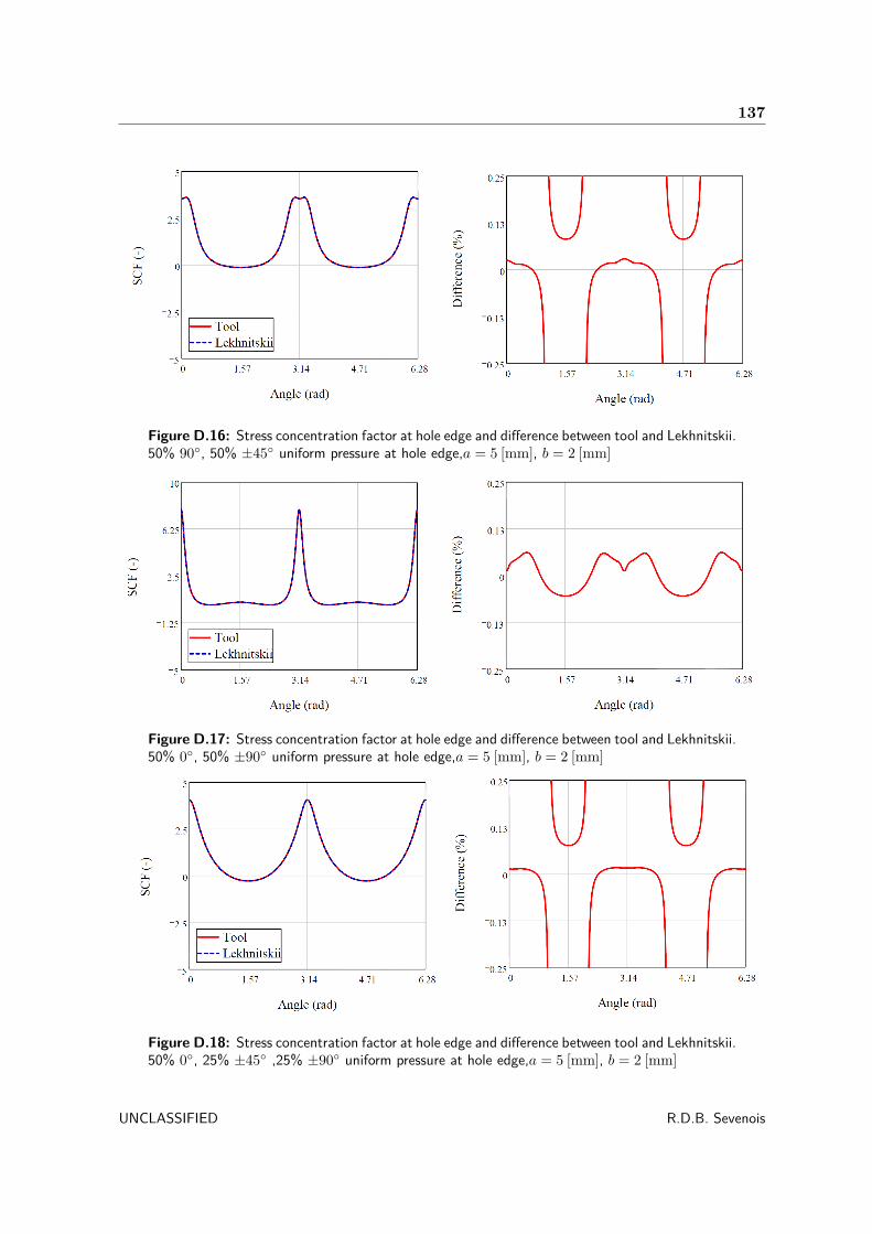
137
Figure D.16: Stress concentration factor at hole edge and difference between tool and Lekhnitskii.50% 90, 50% ±45 uniform pressure at hole edge,a = 5 [mm], b = 2 [mm]
Figure D.17: Stress concentration factor at hole edge and difference between tool and Lekhnitskii.50% 0, 50% ±90 uniform pressure at hole edge,a = 5 [mm], b = 2 [mm]
Figure D.18: Stress concentration factor at hole edge and difference between tool and Lekhnitskii.50% 0, 25% ±45 ,25% ±90 uniform pressure at hole edge,a = 5 [mm], b = 2 [mm]
UNCLASSIFIED R.D.B. Sevenois

138 Results from Verification
Figure D.19: Stress concentration factor at hole edge and difference between tool and Lekhnitskii.25% 0, 50% ±45 ,25% ±90 uniform pressure at hole edge,a = 5 [mm], b = 2 [mm]
Figure D.20: Stress concentration factor at hole edge and difference between tool and Lekhnitskii.25% 0, 25% ±45 ,50% ±90 uniform pressure at hole edge,a = 5 [mm], b = 2 [mm]
R.D.B. Sevenois UNCLASSIFIED

139
Unnotched Failure Algorithm
Table D.13: Verification of ply strain calculation
Laminate Strain 0 deg 90 degTool Hand Tool Hand
εx 5.562e-009 5.562e-009 5.562e-009 -1.96e-009 -1.96e-009εy -1.96e-009 -1.96e-009 -1.96e-009 5.562e-009 5.562e-009γxy 7.307e-025 7.307e-025 7.307e-025 -1.652e-024 -1.652e-24
Laminate Strain 45 degTool Hand
εx 5.562e-009 1.801e-009 1.801e-009εy -1.96e-009 1.801e-009 1.801e-009γxy 7.307e-025 -7.522e-009 -7.522e-009
Table D.14: Laminate properties used for unnotched failure verification
Type E11 E22 G12 ν12(−) Xt Xc Y t Y c S tply(mm)Tens. 142.0 8.1 4.5 0.3 2335 1635 80 215 120 0.184Comp. 125.0 8.5 4.5 0.3 2335 1635 80 215 120 0.184
Table D.15: Laminate properties selected for unnotched failure verification. Stiffnesses (GPa),Strengths (MPa)
Ply E11 E22 G12 ν12(−) Xt Xc Y t Y c S tply(mm)0 142.0 8.5 4.5 0.3 2335 1635 80 215 120 0.18445 142.0 8.1 4.5 0.3 2335 1635 80 215 120 0.18490 125.0 8.1 4.5 0.3 2335 1635 80 215 120 0.184
UNCLASSIFIED R.D.B. Sevenois

140 Results from Verification
Table D.16: Verification of the ply stress calculation. Stiffnesses (GPa), Strengths (MPa)
Direction Strain (-) Stress (Pa)Tool Hand
longitudinal 4.25E-09 603.2 6.03E+02transverse -1.42E-09 -1.24 -1.24E+00shear 1.02E-25 4.60E-16 4.60E-16
Table D.17: Verification of FF and IFF exposure
Ply RFF (-) FF (-)Tool Hand Tool Hand
0 2.02e6 2.02e6 9.60e7 9.616e745 6.11e6 6.11e6 2.106e6 2.106e690 4.57e6 4.57e6 1.5e6 1.5e6
Table D.18: Changing of material properties upon IFF failure
Failure mode Initial properties Mode A Mode B Mode CE11 (Pa) 140.0e9 140.0e9 140.0e9 140.0e9E22 (Pa) 8.0e8 8.0e7 8.0e8 8.0e8G12 (Pa) 5.0e8 5.0e7 5.0e8 5.0e8ν12 (-) 0.03 0.02 0.03 0.03tply (m) 1.29e-4 1.29e-4 1.29e-4 1.29e-4
Table D.19: System test results unnotched failure criterion
Layup Load Vector Tool (MPa) Hand (MPa)42% 0, 42% ±45, 16% 90 (1,0,0) 816 82642% 0, 42% ±45, 16% 90 (-1,0,0) -629 -629100% 0 (1,0,0) 1575 1575100% 0 (0,1,0) 60 60100% 0 (0,0,1) 113 11350% 0, 50% 90 (1,0,0) 792 787.550% 0, 50% 90 (0,1,0) 792 787.5
R.D.B. Sevenois UNCLASSIFIED

141
Contact Angle Calculation
Table D.20: Verification of contact angle calculation.
Tool HandClearance (%) 1.0 1.0uα (m) 2.457e-5 2.457e-5rh(m) 3.175e-3 3.175e-3rp(m) 3.143e-3 3.143e-3Contact Angle () 55.265 55.265
Critical Potential Strain Energy Density Calculation and Selection
Table D.21: Verification of CPSED
Scalefactor(-) CPSED (Pa/m2)Tool Hand Tool Hand
Long. Compr. 1.00 1.00 26.7156 26.7156Long. Tens. 1.542 1.542 41.1914 41.1914Biax Tens. 0.678 0.678 18.122 18.122Biax Compr. 0.633 0.633 16.9168 16.9168Biax Tens.-Comp. 0.518 0.518 13.8367 13.8367Biax Compr.-Tens. 0.518 0.518 13.8367 13.8367Trans. Compr. 0.411 0.411 10.9873 10.9873Trans. Tens. 0.432 0.432 11.5395 11.5395
Table D.22: Verification of the calculation of the critical energy ratio
Inputd(m) Load Reserve Factor at r Energy from edge to d (Pa/m2) (Pa/m2)0.001 293363 9.53e-12 214.10
OutputEnergy at failure (Pa/m2) CPSED ratio (-)
Tool Hand Tool Hand82.04 82.04 2.61 2.61
In Figure D.21 the selection of the CPSED around a hole subjected to uniaxial tension isgiven. As explained in the thesis, the CPSED at a certain hole angle is chosen depending onthe loading condition at that location. In the Figure it is shown that this is done correctlybecause of the transverse compression region around 0 and 180 and the longitudinal tensileregion at 90 and 270.
UNCLASSIFIED R.D.B. Sevenois

142 Results from Verification
Figure D.21: Selection of the CPSED on a unit circle subjected to uniaxial tension in thehorizontal direction
R.D.B. Sevenois UNCLASSIFIED

143
Notched Failure Algorithm
The behaviour of the notched failure algorithm is verified by looking at the change in char-acteristic distance, reserve factor and critical energy ratio over the amount of iteration steps.As one can see, they all converge to a steady value.
Figure D.22: Change of load reserve factor, r and critical energy ratio throughout the iterationprocess
Assembly Verification
Table D.23: Verification result of assembly tests
Angle of failure (deg) Failure Load (MPa)Case Tool Hand Tool Hand1 270 90 ∨ 270 610 372 ≤ X ≤ 11152 0 0 ∨ 180 611 372 ≤ X ≤ 11153 358 0 834 0 ≤ X ≤ 905
UNCLASSIFIED R.D.B. Sevenois

144 Results from Verification
R.D.B. Sevenois UNCLASSIFIED

Appendix E
Contact Angle Comparisons FEA
In this Chapter, the results of the comparison of the contact angle algorithm to FEA are shownhere. The figures show the result when the hole contact angle α is varied in the analytic tooland the result from FEA analysis. The title of each figure give the clearance used. In thefigure legends, “S” denotes, Sevenois, “FEA” denotes Finite Element Analysis. The layupand corresponding directionality is also given according to the coding system below.
UNCLASSIFIED R.D.B. Sevenois

146 Contact Angle Comparisons FEA
Figure E.1: Clearance = 2.0%
Figure E.2: Clearance = 1.0%
Figure E.3: Clearance = 0.1%
Figure E.4: Clearance = 1.5%
Figure E.5: Clearance = 0.5%
Figure E.6: Clearance = 0.01%
R.D.B. Sevenois UNCLASSIFIED

147
Figure E.7: Clearance = 2.0%
Figure E.8: Clearance = 1.0%
Figure E.9: Clearance = 0.1%
Figure E.10: Clearance = 1.5%
Figure E.11: Clearance = 0.5%
Figure E.12: Clearance = 0.01%
UNCLASSIFIED R.D.B. Sevenois

148 Contact Angle Comparisons FEA
Figure E.13: Clearance = 2.0%
Figure E.14: Clearance = 1.0%
Figure E.15: Clearance = 0.1%
Figure E.16: Clearance = 1.5%
Figure E.17: Clearance = 0.5%
Figure E.18: Clearance = 0.01%
R.D.B. Sevenois UNCLASSIFIED

149
Figure E.19: Clearance = 2.0%
Figure E.20: Clearance = 1.0%
Figure E.21: Clearance = 0.1%
Figure E.22: Clearance = 1.5%
Figure E.23: Clearance = 0.5%
Figure E.24: Clearance = 0.01%
UNCLASSIFIED R.D.B. Sevenois

150 Contact Angle Comparisons FEA
Figure E.25: Clearance = 2.0%
Figure E.26: Clearance = 1.0%
Figure E.27: Clearance = 0.1%
Figure E.28: Clearance = 1.5%
Figure E.29: Clearance = 0.5%
Figure E.30: Clearance = 0.01%
R.D.B. Sevenois UNCLASSIFIED

151
Figure E.31: Clearance = 2.0%
Figure E.32: Clearance = 1.0%
Figure E.33: Clearance = 0.1%
Figure E.34: Clearance = 1.5%
Figure E.35: Clearance = 0.5%
Figure E.36: Clearance = 0.01%
UNCLASSIFIED R.D.B. Sevenois

152 Contact Angle Comparisons FEA
Figure E.37: Clearance = 2.0%
Figure E.38: Clearance = 1.0%
Figure E.39: Clearance = 0.1%
Figure E.40: Clearance = 1.5%
Figure E.41: Clearance = 0.5%
Figure E.42: Clearance = 0.01%
R.D.B. Sevenois UNCLASSIFIED

153
Figure E.43: Clearance = 2.0%
Figure E.44: Clearance = 1.0%
Figure E.45: Clearance = 0.1%
Figure E.46: Clearance = 1.5%
Figure E.47: Clearance = 0.5%
Figure E.48: Clearance = 0.01%
UNCLASSIFIED R.D.B. Sevenois

154 Contact Angle Comparisons FEA
Figure E.49: Clearance = 2.0%
Figure E.50: Clearance = 1.0%
Figure E.51: Clearance = 0.1%
Figure E.52: Clearance = 1.5%
Figure E.53: Clearance = 0.5%
Figure E.54: Clearance = 0.01%
R.D.B. Sevenois UNCLASSIFIED

155
Figure E.55: Clearance = 2.0%
Figure E.56: Clearance = 1.0%
Figure E.57: Clearance = 0.1%
Figure E.58: Clearance = 1.5%
Figure E.59: Clearance = 0.5%
Figure E.60: Clearance = 0.01%
UNCLASSIFIED R.D.B. Sevenois

156 Contact Angle Comparisons FEA
R.D.B. Sevenois UNCLASSIFIED

Appendix F
Results from Stress Validation
In this chapter, the results from the validation of the stress field theory by comparing themto FEA are presented.
The effect of varying E/D for an unloaded hole
Figure F.1: SCF of σθ at the hole edge (left) and SCF of σy at y = 0 (right) when E/D = 2.5
UNCLASSIFIED R.D.B. Sevenois

158 Results from Stress Validation
Figure F.2: SCF of σθ at the hole edge (left) and SCF of σy at y = 0 (right) when E/D = 2.0
Figure F.3: SCF of σθ at the hole edge (left) and SCF of σy at y = 0 (right) when E/D = 1.5
Figure F.4: SCF of σθ at the hole edge (left) and SCF of σy at y = 0 (right) when E/D = 1
R.D.B. Sevenois UNCLASSIFIED

159
The effect of varying W/D for an unloaded hole
Figure F.5: SCF of σθ at the hole edge (left) and SCF of σx at x = 0 (right) when W/D = 4
Figure F.6: SCF of σθ at the hole edge (left) and SCF of σx at x = 0 (right) when W/D = 3
UNCLASSIFIED R.D.B. Sevenois

160 Results from Stress Validation
Figure F.7: SCF of σθ at the hole edge (left) and SCF of σx at x = 0 (right) when W/D = 2.5
Figure F.8: SCF of σθ at the hole edge (left) and SCF of σx at x = 0 (right) when W/D = 2
R.D.B. Sevenois UNCLASSIFIED

161
The effect of varying E/D for a loaded hole
Figure F.9: SCF of σθ at the hole edge (left) and SCF of σx at x = xhole (right) when E/D = 2.5
Figure F.10: SCF of σθ at the hole edge (left) and SCF of σx at x = xhole (right) whenE/D = 1.5
UNCLASSIFIED R.D.B. Sevenois

162 Results from Stress Validation
The effects of having multiple loaded/unloaded holes
Figure F.11: multihole 1 and 2 unloaded
Figure F.12: multihole 3 and 4 loaded
R.D.B. Sevenois UNCLASSIFIED