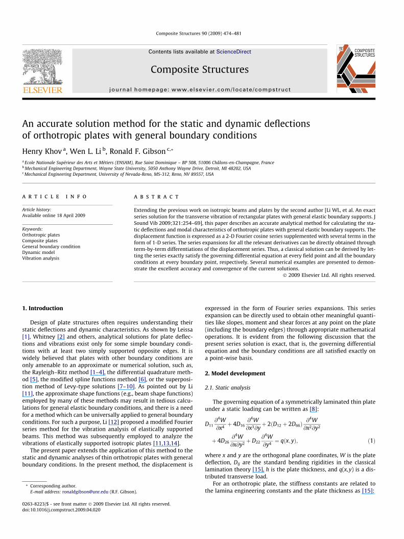
Composite Structures 90 (2009) 474–481

Contents lists available at ScienceDirect

Composite Structures

journal homepage: www.elsevier .com/locate /compstruct

An accurate solution method for the static and dynamic deflectionsof orthotropic plates with general boundary conditions

Henry Khov a, Wen L. Li b, Ronald F. Gibson c,*

a Ecole Nationale Supérieur des Arts et Métiers (ENSAM), Rue Saint Dominique – BP 508, 51006 Châlons-en-Champagne, Franceb Mechanical Engineering Department, Wayne State University, 5050 Anthony Wayne Drive, Detroit, MI 48202, USAc Mechanical Engineering Department, University of Nevada-Reno, MS-312, Reno, NV 89557, USA

a r t i c l e i n f o a b s t r a c t

Article history:Available online 18 April 2009

Keywords:Orthotropic platesComposite platesGeneral boundary conditionDynamic modelVibration analysis

0263-8223/$ - see front matter � 2009 Elsevier Ltd. Adoi:10.1016/j.compstruct.2009.04.020

* Corresponding author.E-mail address: ronaldgibson@unr.edu (R.F. Gibson

Extending the previous work on isotropic beams and plates by the second author [Li WL, et al. An exactseries solution for the transverse vibration of rectangular plates with general elastic boundary supports. JSound Vib 2009;321:254–69], this paper describes an accurate analytical method for calculating the sta-tic deflections and modal characteristics of orthotropic plates with general elastic boundary supports. Thedisplacement function is expressed as a 2-D Fourier cosine series supplemented with several terms in theform of 1-D series. The series expansions for all the relevant derivatives can be directly obtained throughterm-by-term differentiations of the displacement series. Thus, a classical solution can be derived by let-ting the series exactly satisfy the governing differential equation at every field point and all the boundaryconditions at every boundary point, respectively. Several numerical examples are presented to demon-strate the excellent accuracy and convergence of the current solutions.

� 2009 Elsevier Ltd. All rights reserved.

1. Introduction

Design of plate structures often requires understanding theirstatic deflections and dynamic characteristics. As shown by Leissa[1], Whitney [2] and others, analytical solutions for plate deflec-tions and vibrations exist only for some simple boundary condi-tions with at least two simply supported opposite edges. It iswidely believed that plates with other boundary conditions areonly amenable to an approximate or numerical solution, such as,the Rayleigh–Ritz method [1–4], the differential quadrature meth-od [5], the modified spline functions method [6], or the superposi-tion method of Levy-type solutions [7–10]. As pointed out by Li[11], the approximate shape functions (e.g., beam shape functions)employed by many of these methods may result in tedious calcu-lations for general elastic boundary conditions, and there is a needfor a method which can be universally applied to general boundaryconditions. For such a purpose, Li [12] proposed a modified Fourierseries method for the vibration analysis of elastically supportedbeams. This method was subsequently employed to analyze thevibrations of elastically supported isotropic plates [11,13,14].

The present paper extends the application of this method to thestatic and dynamic analyses of thin orthotropic plates with generalboundary conditions. In the present method, the displacement is

ll rights reserved.

).

expressed in the form of Fourier series expansions. This seriesexpansion can be directly used to obtain other meaningful quanti-ties like slopes, moment and shear forces at any point on the plate(including the boundary edges) through appropriate mathematicaloperations. It is evident from the following discussion that thepresent series solution is exact, that is, the governing differentialequation and the boundary conditions are all satisfied exactly ona point-wise basis.

2. Model development

2.1. Static analysis

The governing equation of a symmetrically laminated thin plateunder a static loading can be written as [8]:

D11@4W@x4 þ 4D16

@4W@x3@y

þ 2ðD12 þ 2D66Þ@4W@x2@y2

þ 4D26@4W@x@y2 þ D22

@4W@y4 ¼ qðx; yÞ; ð1Þ

where x and y are the orthogonal plane coordinates, W is the platedeflection, Dij are the standard bending rigidities in the classicallamination theory [15], h is the plate thickness, and q(x,y) is a dis-tributed transverse load.

For an orthotropic plate, the stiffness constants are related tothe lamina engineering constants and the plate thickness as [15]:

Nomenclature

a plate dimension in x directionb plate dimension in y directionh plate thicknessq mass densityE1, E2 Young’s modulus in 1- and 2-directionG12 shear modulus associated with 1–2 planem12 major Poisson’s ratiom21 minor Poisson’s ratioDij standard bending rigiditiesW(x,y) flexural displacementM, N Fourier series truncation numbers in 1- and 2-direc-

tions, respectivelym 0,1, . . .,M � 1, Fourier series indices in 1-directionn 0,1, . . .,N � 1, Fourier series indices in 2-directionp n �M + m rearranged index numbersl 1,2,3,4 index in the special functions and single Fourier

seriesR a

b aspect ratio

kam mp/akbn np/bx angular frequencyK stiffness matrixM mass matrixA double Fourier series coefficients matrixp single Fourier series coefficients matrixAmn double Fourier series coefficientscl

m; dln single Fourier series coefficients

kx0, kxa translational stiffnesses at x = 0 and x = a, respectivelyky0, kyb translational stiffnesses at y = 0 and y = b, respectivelyKx0, Kxa rotational stiffnesses at x = 0 and x = a, respectivelyKy0, Kyb rotational stiffnesses at y = 0 and y = b, respectivelyMx, My bending momentsMxy twisting momentQx, Qy shear forces

H. Khov et al. / Composite Structures 90 (2009) 474–481 475

D11 ¼E1h3

12ð1� v12v21Þ; D22 ¼

E2h3

12ð1� v12v21Þ; D12 ¼ v12D22;

ð2—4Þ

D66 ¼G12h3

12and D16 ¼ D26 ¼ 0: ð5;6Þ

In terms of the flexural displacement, the bending and twistingmoment and transverse shearing forces can be expressed as

Mx ¼ �D11@2W@x2 � D12

@2W@y2 ; ð7Þ

My ¼ �D22@2W@y2 � D12

@2W@x2 ; ð8Þ

Mxy ¼ �2D66@2W@x@y

; ð9Þ

Q x ¼ �D11@3W@x3 � ðD12 þ 4D66Þ

@3W@x@y2 ; ð10Þ

Q y ¼ �D22@3W@y3 � ðD12 þ 4D66Þ

@3W@x2@y

: ð11Þ

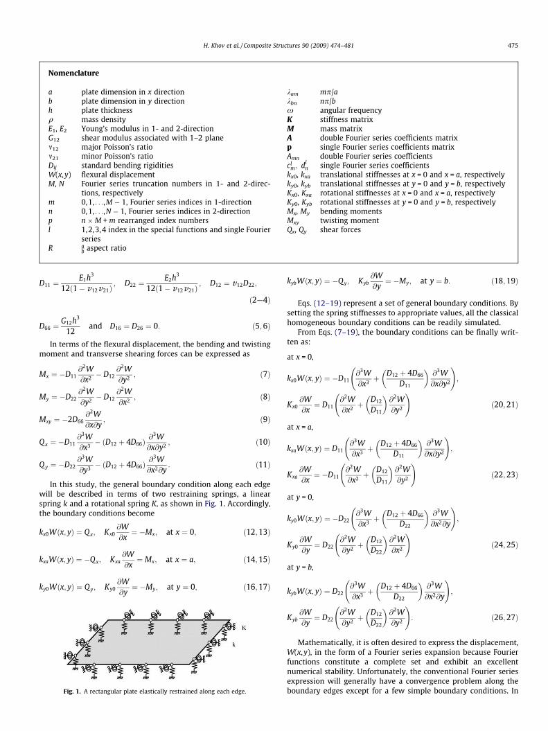
In this study, the general boundary condition along each edgewill be described in terms of two restraining springs, a linearspring k and a rotational spring K, as shown in Fig. 1. Accordingly,the boundary conditions become

kx0Wðx; yÞ ¼ Q x; Kx0@W@x¼ �Mx; at x ¼ 0; ð12;13Þ

kxaWðx; yÞ ¼ �Q x; Kxa@W@x¼ Mx; at x ¼ a; ð14;15Þ

ky0Wðx; yÞ ¼ Q y; Ky0@W@y¼ �My; at y ¼ 0; ð16;17Þ

Fig. 1. A rectangular plate elastically restrained along each edge.

kybWðx; yÞ ¼ �Q y; Kyb@W@y¼ �My; at y ¼ b: ð18;19Þ

Eqs. (12–19) represent a set of general boundary conditions. Bysetting the spring stiffnesses to appropriate values, all the classicalhomogeneous boundary conditions can be readily simulated.

From Eqs. (7–19), the boundary conditions can be finally writ-ten as:

at x = 0,

kx0Wðx; yÞ ¼ �D11@3W@x3 þ

D12 þ 4D66

D11

� �@3W@x@y2

!;

Kx0@W@x¼ D11

@2W@x2 þ

D12

D11

� �@2W@y2

!ð20;21Þ

at x = a,

kxaWðx; yÞ ¼ D11@3W@x3 þ

D12 þ 4D66

D11

� �@3W@x@y2

!;

Kxa@W@x¼ �D11

@2W@x2 þ

D12

D11

� �@2W@y2

!ð22;23Þ

at y = 0,

ky0Wðx; yÞ ¼ �D22@3W@x3 þ

D12 þ 4D66

D22

� �@3W@x2@y

!;

Ky0@W@y¼ D22

@2W@y2 þ

D12

D22

� �@2W@x2

!ð24;25Þ

at y = b,

kybWðx; yÞ ¼ D22@3W@x3 þ

D12 þ 4D66

D22

� �@3W@x2@y

!;

Kyb@W@y¼ D22

@2W@y2 þ

D12

D22

� �@2W@y2

!: ð26;27Þ

Mathematically, it is often desired to express the displacement,W(x,y), in the form of a Fourier series expansion because Fourierfunctions constitute a complete set and exhibit an excellentnumerical stability. Unfortunately, the conventional Fourier seriesexpression will generally have a convergence problem along theboundary edges except for a few simple boundary conditions. In

476 H. Khov et al. / Composite Structures 90 (2009) 474–481

addition, without being uniformly convergent, the derivatives of aFourier series cannot be obtained simply through term-by-termdifferentiation. To overcome these problems, the displacementfunction will be here expressed as a more robust form of Fourierseries expansion

Wðx; yÞ ¼X1m¼0

X1n¼0

Amn cosðkamxÞ cosðkbnyÞ

þX4

l¼1

nlbðyÞ

X1m¼0

clm cosðkamxÞ þ nl

aðxÞX1n¼0

dln cosðkbnyÞ

!;

ð28Þ

where the eight supplementary terms are introduced to deal withany possible discontinuities or jumps at the boundaries which arepotentially associated with the displacement function and its deriv-atives when they are periodically extended onto the entire x–yplane. It should be noted that these discontinuities are not inher-ently related to the displacement function over the solution do-main; instead they are the artifact resulting from the Fourierseries representation of the displacement solution. To illustrate thispoint, take a slice of W(x,y) along y = y0, for example. Mathemati-cally, expanding W(x,y0) into a Fourier series implies that it isviewed as a periodic function (of period a) defined over the entirex axis. Consequently, if the plate is not fully fixed at x = 0 andx = a as in a general boundary condition, the displacement values,W(0,y0) and W(a,y0), are typically not equal and the Fourier series(of the displacement) will hence only converge to the mean value,[W(0,y0) + W(a,y0)]/2, at x = 0,±a, ±2a, . . . This deems the unsuitabil-ity of the conventional Fourier series method since the series solu-tion clearly fails to satisfy the correct boundary values at x = 0 andx = a. This problem, however, can be easily avoided by viewingW(x,y0) as a part of an even function defined over [�a,a]. The Fourierexpansion of this even function will then only contain the cosineterms, and be able to correctly converge to W(x,y0) at any point over[0,a]. This treatment alone, however, still cannot revive the conven-tional Fourier series method because the satisfaction of boundaryconditions in a plate problem means that each of the first three deriv-atives has to be correctly produced by the series representationalong each and every edge. Notice that the first (also, the third)derivative of W(x,y0) is an odd function over [�a,a], its (sine) seriesexpansion will thus invariantly converge to zero at x = 0 and x = a,regardless of the actual slope values. To overcome this problem,we will append to the original displacement function four suffi-ciently smooth functions so that the first and third derivatives (withrespect to x) of the resulting (or residual) displacement function allvanish at x = 0 and x = a. Similarly, four additional functions are alsoused to deal with the same problems related to the series expansionin y-direction. The ‘‘physical” impact of these mathematical treat-ments is that the arbitrary boundary conditions in the original plateproblem are reconfigured into a guided support along each edge(that is, zero slope and zero restraining force in the transverse direc-tion) for the residual displacement solution which is almost auto-matically sought in the form of a cosine expansion or modalsuperposition.

The four n-functions in the x direction in Eq. (28) are here cho-sen as

n1aðxÞ ¼

9a4p

sinpx2a

� �� a

12psin

3px2a

� �;

n2aðxÞ ¼ �

9a4p

cospx2a

� �� a

12pcos

3px2a

� �;

n3aðxÞ ¼

a3

p3 sinpx2a

� �� a3

3p3 sin3px2a

� �;

n4aðxÞ ¼

a3

p3 cospx2a

� �� a3

3p3 cos3px2a

� �:

ð29Þ

It is easy to verify that their first and third derivatives aremostly equal to zero along the boundary edges except forn10

a ð0Þ ¼ n20a ðaÞ ¼ n3000

a ð0Þ ¼ n4000a ðaÞ ¼ 1. The n-functions in the y direc-

tion can be readily obtained from Eq. (29) by replacing x and a withy and b, respectively.

It can be proven mathematically that the series expression inEq. (28) is able to expand and uniformly converge to any functionf(x,y) 2 C3 for "(x,y) 2 D: ([0,a] � [0,b]). Also, this series can besimply differentiated, through term-by-term, to obtain the uni-formly convergent series expansions for up to the fourth-orderderivatives. Mathematically, an exact displacement (or classical)solution is a particular function w(x,y) 2 C3 for "(x,y) 2 D whichsatisfies the governing equation at every field point and the bound-ary conditions at every boundary point. Thus, the remaining taskfor seeking an exact displacement solution will simply involvefinding a set of expansion coefficients to ensure the governingequation and the boundary conditions to be satisfied by the currentseries solution exactly on a point-wise basis.

By substituting the displacement expression (28) into theboundary condition at x = 0, Eq. (20), one has

kx0

X1m¼0

X1n¼0

Amn cosðkbnyÞ þX4

l¼1

nlbðyÞ

X1m¼0

clm þ nl

aðxÞX1n¼0

dln cosðkbnyÞ

! !

¼ �D11

X1n¼0

d3n cosðkbnyÞÞ þ D12 þ 4D66

D11

� �X1n¼0

ð�k2bnÞd

ln cosðkbnyÞ

!:

ð30Þ

Expanding all the n-functions into Fourier cosine series andcomparing the similar terms will result in the following equations:

kx0

D11

X4

l¼1

bln

X1m¼0

clm þ nl

að0Þdln

!þ D12 þ 4D66

D11

� ��k2

bn

� �d1

n þ d3n

¼ � kx0

D11

X1m¼0

Amn ðn ¼ 0;1; . . . ;1; x ¼ 0Þ: ð31Þ

Substitution of Eq. (28) into the remaining boundary conditions,Eqs. (21–23), will lead to three similar equations:

X4

l¼1

X1m¼0

�kambln þ

D12

D11bl

n

� cl

m þX4

i¼1

n00la ð0Þ �D12

D11k2

bnnlað0Þ

� dl

n �Kx0

D11d1

n

¼X1m¼0

k2am þ

D12

D11k2

bn

� �Amn ðn ¼ 0;1 . . .1; x ¼ 0Þ; ð32Þ

kxa

D11

X4

l¼1

bln

X1m¼0

ð�1Þmclm þ nl

aðaÞdln

!þ D12 þ 4D66

D11

� ��k2

bn

� �d2

n þ d4n

¼ � kxa

D11

X1m¼0

ð�1Þmþ1Amn ðn ¼ 0;1; . . .1; x ¼ 0Þ; ð33Þ

X4

l¼1

X1m¼0

ð�1Þm D12

D11

�bln � k2

ambln

� �cl

m

þX4

l¼1

n00la ðaÞ �D12

D11k2

bnnlaðaÞ

� dl

n �Kxa

D11d2

n

¼X1m¼0

ð�1Þm k2am þ

D12

D11k2

bn

� �Amn ðn ¼ 0;1 . . .1; x ¼ 0Þ: ð34Þ

The four corresponding boundary condition equations in the y-direction can be derived in the same way, and will not be pre-sented here. In numerical calculations, the series expansions mustbe truncated, such as, to m = M and n = N. Thus, the boundary con-dition equations can be expressed in a matrix form as:

HP ¼ QA; ð35Þ

d

c

a

b

x

y

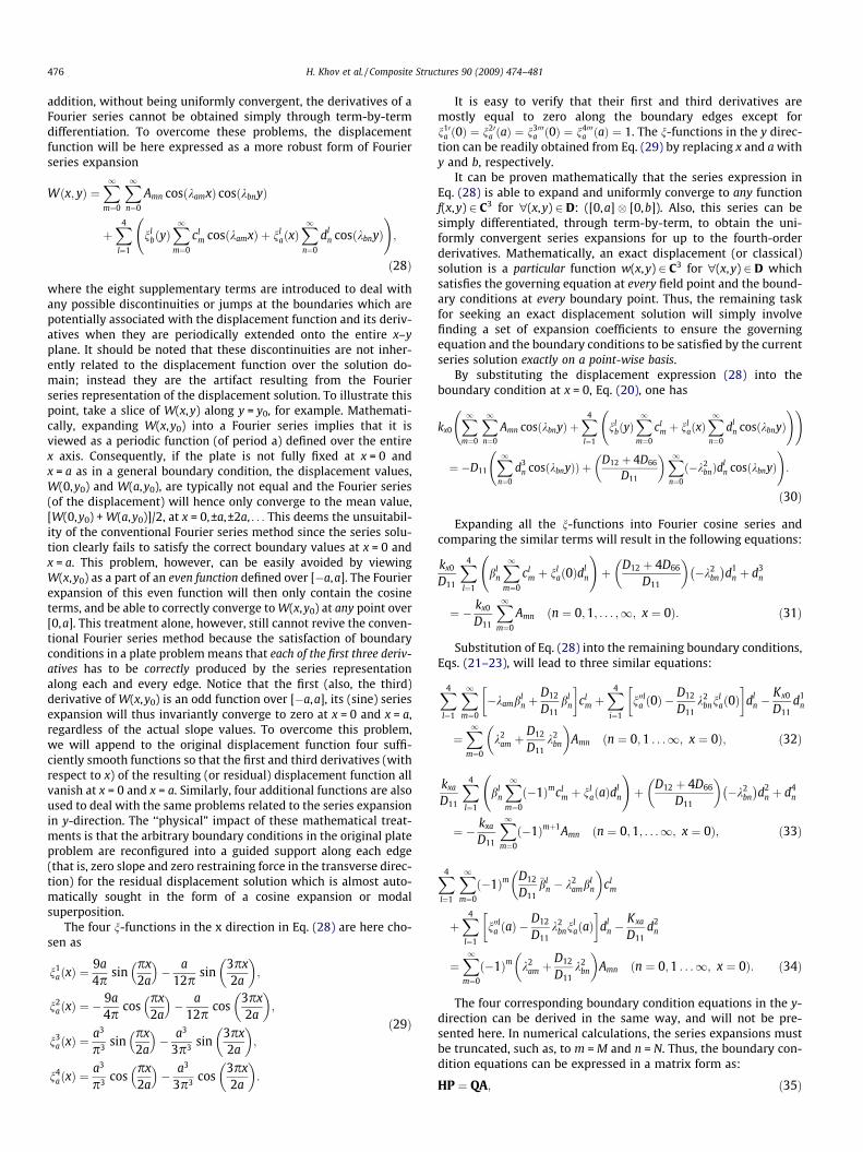
Fig. 2. An illustration of the loading area.

H. Khov et al. / Composite Structures 90 (2009) 474–481 477

where P ¼ c10; c

11; c

12; . . . ; c1

M ; c20; c

21; c

22; . . . ; c2

M ; . . . ; c40; c

41; c

42; . . . ; c4

M ;d10;

hd1

1;d12; . . . ; d1

M ;d20;d

21; d

22; . . . ;d2

M ; . . . ;d40;d

41;d

42; . . . ;d4

M� and A = [A01,A11, . . . ,AM1, . . . ,A02,A12, . . . ,AM2, . . . ,A0N,A1N, . . . ,AMN]T, and H and Qrepresent the coefficient matrices which can be determined fromEqs. (31)–(34).

Eq. (35) essentially states that the expansion coefficients in Eq.(28) are not completely independent; the coefficients in the 1-Dseries expansions can be considered dependent upon those in the2-D Fourier series. Consequently, there is only a total of(M + 1) � (N + 1) independent Fourier coefficients which, as de-scribed in the following section, can be directly solved from thegoverning differential equations.

In determining the static deflection, the load function should beexpressed as a Fourier cosine series

qðx; yÞ ¼X1m¼0

X1n¼0

qmn cosmpx

acos

npyb

; ð36Þ

where the Fourier coefficients are determined from the relationship

qmn ¼4ab

Z b

0

Z a

0qðx; yÞ cos

mpxa

cosnpy

bdxdy: ð37Þ

Consider a special case when a uniform pressure q = q0 is ap-plied to the plate, the Fourier coefficients are simply

q00 ¼ q0 and qm0 ¼ qon ¼ qmn ¼ 0: ð38Þ

Another interesting case, as illustrated in Fig. 2, involves a uni-form pressure q = q0 acting on a smaller rectangular area. For thiscase the Fourier coefficients can be obtained as

q00 ¼q0cdab

; ð39—42Þ

qm0 ¼4q0dbmp

cosmpn

asin

mpc2a

;

q0n ¼4q0canp cos

npgb

sinnpd2b

;

qmn ¼16q0

p2mncos

mpna

cosnpg

bsin

mpc2a

sinnpd2b

;

where c and d are the dimensions of the rectangle in the x- and y-directions, respectively, and n and g are the coordinates of itscenter.

The Fourier coefficients for a concentrated load q0 at x = n andy = g can be readily written out as

q00 ¼q0

ab; ð43—46Þ

qm0 ¼2q0

abcos

mpna

;

q0n ¼4q0

abcos

npgb

;

qmn ¼4q0

abcos

mpna

cosnpg

b:

2.2. Dynamic analysis

The inertial effect will have to be considered in a dynamic anal-ysis. By assuming a harmonic excitation, the equation of motion foran orthotropic plate can be written as

D11@4W@x4 þ 4D16

@4W@x3@y

þ 2ðD12 þ 2D66Þ@4W@x2@y2 þ 4D26

@4W@x@y3

þ D22@4W@y4 � qhx2Wðx; yÞ ¼ qðx; x; yÞ; ð47Þ

where q is the mass density of the plate, and x is the frequency ofthe harmonic motion.

By substituting Eq. (28) into Eq. (47), one yieldsX1m¼0

X1n¼0

D11k4am þ D22k

4bn þ 2ðD12 þ 2D66Þk2

amk2bn

� �� Amn cosðkamxÞ cosðkbnyÞ

þX4

l¼1

X1m¼0

D11nlbðyÞk

4am � 2ðD12 þ 2D66Þk2

amn00lb ðyÞ�

þ D22nð4Þlb ðyÞ

�cl

m cosðkamxÞ

þX4

l¼1

X1n¼0

D22nlaðxÞk

4bn � 2ðD12 þ 2D66Þk2

bn00la ðxÞ þ D11n

ð4Þla ðxÞ

� �dl

n

� cosðkbnyÞ � qhx2X1m¼0

X1n¼0

Amn cosðkamxÞ cosðkbnyÞ"

þXl¼1

nlbðyÞ

X1m¼0

clm cosðkamxÞ þ nl

aðxÞX1n¼0

dln cosðkbnyÞ

!#¼ qðx; x; yÞ: ð48Þ

Again, after all the non-cosine functions in the above equationare expanded into Fourier cosine series, a system of equationscan be derived by comparing the like terms on both sides

D11k4am þ D22k

4bn þ 2ðD12 þ 2D66Þk2

amk2bn

� �Amn

þX4

l¼1

D11blnk

4am � 2ðD12 þ 2D66Þk2

am�bl

n þ D22bln

� �cl

m

þX4

l¼1

D22almk4

bn � 2ðD12 þ 2D66Þk2bn

�alm þ D11al

m

� �dl

n

� qhx2 Amn þX4

l¼1

blncl

m þ almdl

n

� � !¼ qmn: ð49Þ

The governing equations can be written in matrix form as

ðeKAþ BPÞ � qhx2ðfMAþ FPÞ ¼ q; ð50Þ

where the definitions of the four coefficient matrices are kind ofobvious from Eq. (49).

Making use of Eq. (35), the system equation simplifies to

ðK� qhx2MÞA ¼ q; ð51Þ

where K ¼ eK þ BH�1Q and M ¼fM þ FH�1Q .In a static analysis, the Fourier coefficients, A, will be first solved

from Eq. (51) by setting x=0 and Eq. (35) will be used to calculatethe remaining Fourier coefficients. The actual displacement func-tion can then be easily determined from Eq. (28). The calculationof the load vector q in Eq. (51) has already been demonstrated inthe previous section for some simple loading conditions. The dy-namic load vector is essentially the same as the static one exceptthat it may be frequency-dependent. The modal properties for anorthotropic plate can be readily obtained from solving a standardmatrix characteristic equation, Eq. (51) with q = 0. In this study,the eigenvector A for a given eigenvalue x2 actually contains theFourier coefficients for the corresponding mode shape.

Table 4Maximum deflection under a point load, p0 = 106 N, applied at different locations.

Boundarycondition

Forcelocation

FEM ABAQUS(mm)

Analytical solution[2] (mm)

Current method(mm)

S-S-S-S n = g = a/2 698 692 691n = g = a/3 582 581 580n = g = a/5 317 316 316

C-F-F-F n = g = a/2 1550 – 1550n = g = a/3 851 – 852n = g = a/5 454 – 454

C-C-F-C n = g = a/2 1010 – 1010n = g = a/3 395 – 396n = g = a/5 128 – 127

478 H. Khov et al. / Composite Structures 90 (2009) 474–481

It is evident from the above derivations that the present seriessolution is exact in the sense that the governing differential equa-tion and the boundary conditions are all satisfied exactly on apoint-wise basis. However, since the series solution will have tobe truncated in an actual calculation, the term ‘‘exact solution”should be better understood as a solution with arbitrary precision.

3. Results

To demonstrate the use of the method, the deformations andmodal properties of square graphite/epoxy plates will be consid-ered below for several different boundary conditions (free edges,clamped edges, and simply supported edges). The correspondingstiffnesses for the restraining springs are specified in Table 1. Inthe numerical calculations, the value k = 5E07 N/m, K = 5E07 N m/rad were found to be sufficiently large to simulate the infinite stiff-ness. The material properties and dimensions of the plates arelisted in Table 2.

3.1. Static deflections

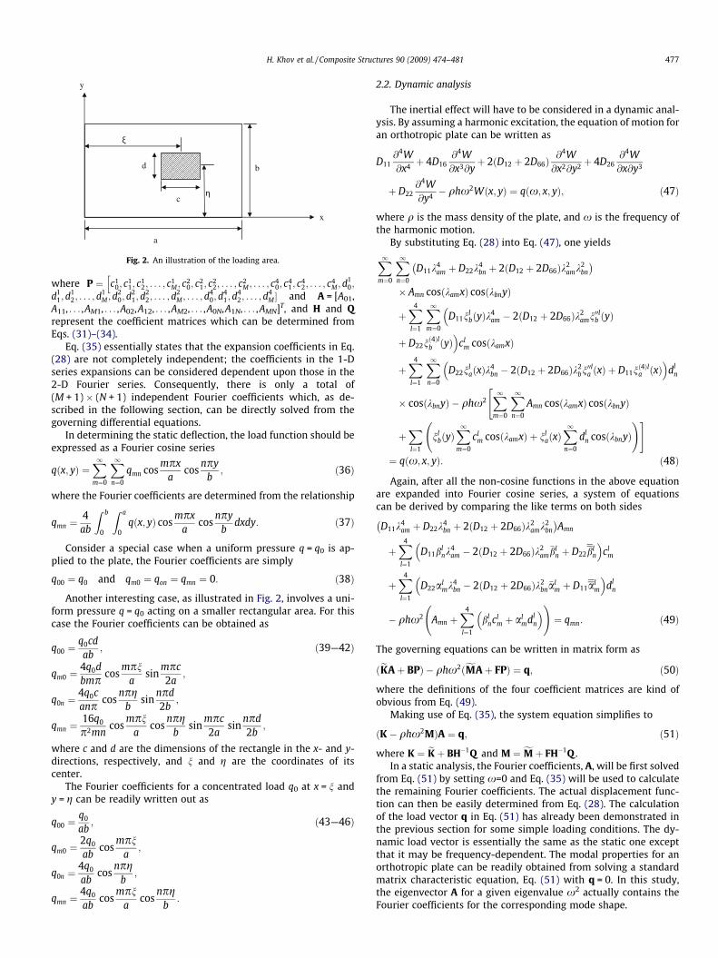
First consider the deformations of the plates under the action ofa uniform pressure p0=10 MPa. The maximum deflections pre-dicted by the current method are compared with those from theABAQUS finite element method (FEM) in Table 3 for three differentboundary conditions. The locations for the maximum deflectionsare obviously dependent upon the boundary conditions; whilethe maximum deflection obviously occurs at the center of the sim-ply supported plate, its locations will not be so clear for otherboundary conditions. It should be noted that the geometrical andmaterial properties of the plates in these cases are kept the sameexcept for their thicknesses (refer to Table 2). The analytical solu-tion [2] in the form of Fourier sine series is only available for the all

Table 3Maximum deflection under a uniform pressure, p0 = 106 Pa.

Boundarycondition

FEM ABAQUS(mm)

Analytical solution [2](mm)

Current method(mm)

S-S-S-S 14.1 14.1 14.1C-F-F-F 101 – 101.4C-C-F-C 43.4 – 43.4

Table 2Geometrical and material properties of Graphite epoxy platesa.

Boundarycondition

a, b(cm)

h(mm)

q (g/cm3)

E1

(GPa)E2

(GPa)G12

(GPa)V12 V21

F-F-F-Fb 1.483C-F-F-F 1.688C-C-F-C 25.4c 1.379 1.584c 127.9c 10.27c 7.312c 0.22c 0.0177c

S-S-S-S 1.483

a Graphite/epoxy consisting of 12 plies oriented at 0� and fabricated from FiberiteHy-E1034C prepreg; properties are taken from Ref. [17].

b Boundary condition convention: (x = 0)–(y = b)–(x = a)–(y = 0); C, clamped; F,free; S, simply supported.

c Indicating this value is the same for each row.

Table 1Spring stiffnesses.

Free (F) Clamped (C) Simply supported (S)

K (N m/rad) 0 5E07 0k (N/m) 0 5E07 5E07

Fig. 3. Static deflection of an anisotropic S-S-S-S plate under a uniform pressure: (a)finite element (ABAQUS); (b) closed-form solution; and (c) current solution.

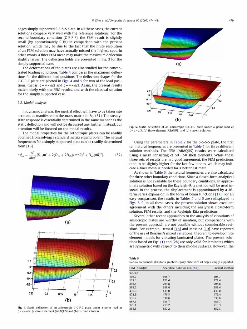
Fig. 5. Static deflection of an anisotropic C-C-F-C plate under a point load atn = g = a/3: (a) finite element (ABAQUS) and (b) current solution.

H. Khov et al. / Composite Structures 90 (2009) 474–481 479

edges simply supported S-S-S-S plate. In all these cases, the currentsolutions compare very well with the reference solutions. For thesecond boundary condition (C-F-F-F), the FEM result is slightlysmall (by approximately 0.3%) in comparison with the presentsolution, which may be due to the fact that the finite resolutionof an FEM solution may have actually missed the highest spot. Inother words, a finer FEM mesh may make the maximum deflectionslightly larger. The deflection fields are presented in Fig. 3 for thesimply supported case.

The deformations of the plates are also studied for the concen-trated loading conditions. Table 4 compares the maximum deflec-tions for the different load positions. The deflection shapes for theC-C-F-C plate are plotted in Figs. 4 and 5 for two of the load posi-tions, that is, n = g = a/2 and n = g = a/3. Again, the present resultsmatch nicely with the FEM results, and with the classical solutionfor the simply supported case.

3.2. Modal analysis

In dynamic analysis, the inertial effect will have to be taken intoaccount, as manifested in the mass matrix in Eq. (51). The steady-state response is essentially determined in the same manner as thestatic deflection and will not be discussed any further. Instead, ourattention will be focused on the modal results.

The modal properties for the orthotropic plates can be readilyobtained from solving a standard matrix eigenproblem. The naturalfrequencies for a simply supported plate can be readily determinedfrom [16]

x2mn ¼

p4

qha4 ½D11m4 þ 2ðD12 þ 2D66ÞðmnRÞ2 þ D22ðnRÞ4�: ð52Þ

Fig. 4. Static deflection of an anisotropic C-C-F-C plate under a point load atn = g = a/2: (a) finite element (ABAQUS) and (b) current solution.

Using the parameters in Table 2 for the S-S-S-S plate, the firstten natural frequencies are presented in Table 5 for three differentsolution methods. The FEM (ABAQUS) results were calculatedusing a mesh consisting of 50 � 50 shell elements. While thesethree sets of results are in a good agreement, the FEM predictionstend to be slightly higher for the last few modes, which may indi-cate a finer mesh is needed for a better estimate.

As shown in Table 6, the natural frequencies are also calculatedfor three other boundary conditions. Since a closed-form analyticalsolution is not available for these boundary conditions, an approx-imate solution based on the Rayleigh–Ritz method will be used in-stead. In the process, the displacement is approximated by a 36-term series expansion in the form of beam functions [17]. For aneasy comparison, the results in Tables 5 and 6 are redisplayed inFigs. 6–9. In all these cases, the present solution shows excellentagreement with the others including the analytical closed-formsolution, FEM results, and the Rayleigh–Ritz predictions.

Several other recent approaches to the analysis of vibrations ofanisotropic plates are worthy of mention, but comparisons withthe present approach are not possible without considerable revi-sions. For example, Demasi [18] and Messina [19] have reportedon the use of Reissner’s mixed variational theorem to develop finiteelement models for vibrating laminated plates. The present solu-tions based on Eqs. (1) and (28) are only valid for laminates whichare symmetric with respect to their middle surfaces. However, the

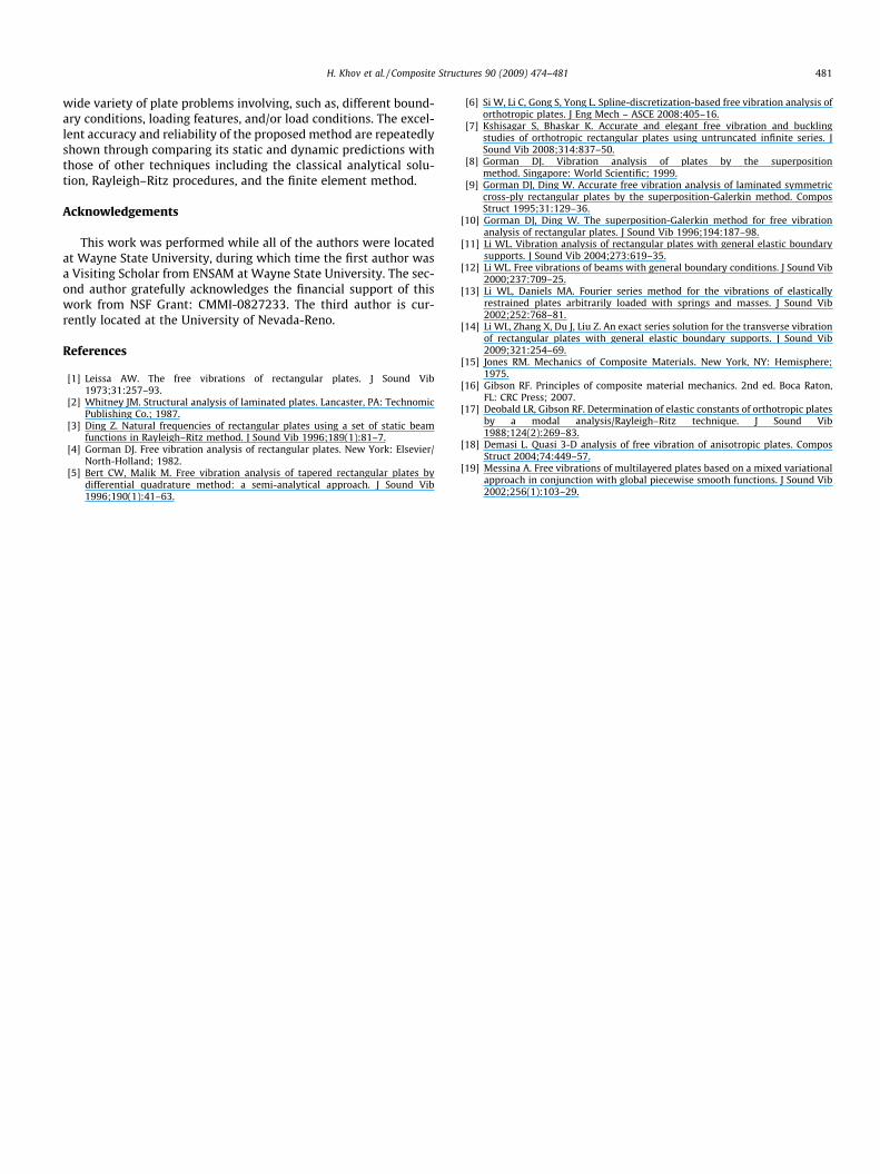
Table 5Natural frequencies (Hz) for a graphite–epoxy plate with all edges simply supported.

FEM (ABAQUS) Analytical solution (Eq. (52)) Present method

S-S-S-S108.7 108.7 108.7171.3 171.4 171.4295.4 294.8 294.8388.5 388.4 388.4435.0 435.0 435.0478.9 476.3 476.4530.7 530.6 530.6687.1 685.7 685.7720.1 713.2 713.3858.5 857.2 857.3

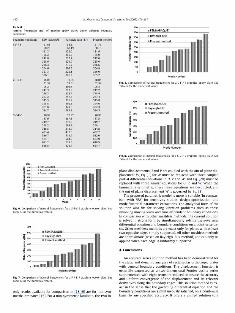
Table 6Natural frequencies (Hz) of graphite–epoxy plates under different boundaryconditions.

Boundary condition FEM (ABAQUS) Rayleigh–Ritz [17] Present method

F-F-F-F 51.68 51.81 51.7660.20 60.19 60.18

121.2 122.0 121.4166.2 165.9 165.9212.6 212.7 212.6228.6 229.0 228.6236.4 236.7 236.6304.6 306.5 304.9327.3 326.1 326.0386.1 386.2 385.2

C-F-F-F 38.03 38.05 38.0452.52 52.61 52.58

105.2 105.5 105.3217.3 217.3 217.2238.3 238.5 238.4257.2 257.5 257.4315.3 316.9 315.8395.8 394.8 394.6421.8 423.6 422.3584.7 589.9 584.5

C-C-F-C 70.99 70.97 70.96167.9 167.5 167.5219.7 219.8 219.7298.2 298.2 298.1316.5 314.9 314.8433.4 432.5 432.2516.7 511.9 512.0564.1 564.0 563.9621.2 618.0 618.9626.5 624.7 624.7

Fig. 6. Comparison of natural frequencies for a S-S-S-S graphite–epoxy plate. SeeTable 5 for the numerical values.

Fig. 7. Comparison of natural frequencies for a F-F-F-F graphite–epoxy plate. SeeTable 6 for the numerical values.

Fig. 8. Comparison of natural frequencies for a C-F-F-F graphite–epoxy plate. SeeTable 6 for the numerical values.

Fig. 9. Comparison of natural frequencies for a C-C-F-C graphite–epoxy plate. SeeTable 6 for the numerical values.

480 H. Khov et al. / Composite Structures 90 (2009) 474–481

only results available for comparison in [18,19] are for non-sym-metric laminates [16]. For a non-symmetric laminate, the two in-

plane displacements U and V are coupled with the out of plane dis-placement W, Eq. (1) for W must be replaced with three coupledpartial differential equations in U, V and W, and Eq. (28) must bereplaced with three similar equations for U, V, and W. When thelaminate is symmetric, these three equations are decoupled, andthe out of plane displacement W is governed by Eq. (1).

The proposed parametric model is more is suitable (in compar-ison with FEA) for sensitivity studies, design optimization, andmodel/material parameter extractions. The analytical form of thesolution also fits for solving vibration problems such as thoseinvolving moving loads and time-dependent boundary conditions.In comparison with other meshless methods, the current solutionis solved in strong form by simultaneously solving the governingdifferential equation and boundary conditions on a point-wise ba-sis. Other meshless methods are exact only for plates with at leasttwo opposite edges simply supported. All other meshless methodsare approximate (based on Rayleigh–Ritz method) and can only beapplied when each edge is uniformly supported.

4. Conclusions

An accurate series solution method has been demonstrated forthe static and dynamic analyses of rectangular orthotropic plateswith general boundary conditions. The displacement function isgenerally expressed as a two-dimensional Fourier cosine seriessupplemented with eight terms introduced to ensure the accuracyand uniform convergence of the displacement and its relevantderivatives along the boundary edges. This solution method is ex-act in the sense that the governing differential equation and theboundary conditions are simultaneously satisfied, on a point-wisebasis, to any specified accuracy. It offers a unified solution to a

H. Khov et al. / Composite Structures 90 (2009) 474–481 481

wide variety of plate problems involving, such as, different bound-ary conditions, loading features, and/or load conditions. The excel-lent accuracy and reliability of the proposed method are repeatedlyshown through comparing its static and dynamic predictions withthose of other techniques including the classical analytical solu-tion, Rayleigh–Ritz procedures, and the finite element method.

Acknowledgements

This work was performed while all of the authors were locatedat Wayne State University, during which time the first author wasa Visiting Scholar from ENSAM at Wayne State University. The sec-ond author gratefully acknowledges the financial support of thiswork from NSF Grant: CMMI-0827233. The third author is cur-rently located at the University of Nevada-Reno.

References

[1] Leissa AW. The free vibrations of rectangular plates. J Sound Vib1973;31:257–93.

[2] Whitney JM. Structural analysis of laminated plates. Lancaster, PA: TechnomicPublishing Co.; 1987.

[3] Ding Z. Natural frequencies of rectangular plates using a set of static beamfunctions in Rayleigh–Ritz method. J Sound Vib 1996;189(1):81–7.

[4] Gorman DJ. Free vibration analysis of rectangular plates. New York: Elsevier/North-Holland; 1982.

[5] Bert CW, Malik M. Free vibration analysis of tapered rectangular plates bydifferential quadrature method: a semi-analytical approach. J Sound Vib1996;190(1):41–63.

[6] Si W, Li C, Gong S, Yong L. Spline-discretization-based free vibration analysis oforthotropic plates. J Eng Mech – ASCE 2008:405–16.

[7] Kshisagar S, Bhaskar K. Accurate and elegant free vibration and bucklingstudies of orthotropic rectangular plates using untruncated infinite series. JSound Vib 2008;314:837–50.

[8] Gorman DJ. Vibration analysis of plates by the superpositionmethod. Singapore: World Scientific; 1999.

[9] Gorman DJ, Ding W. Accurate free vibration analysis of laminated symmetriccross-ply rectangular plates by the superposition-Galerkin method. ComposStruct 1995;31:129–36.

[10] Gorman DJ, Ding W. The superposition-Galerkin method for free vibrationanalysis of rectangular plates. J Sound Vib 1996;194:187–98.

[11] Li WL. Vibration analysis of rectangular plates with general elastic boundarysupports. J Sound Vib 2004;273:619–35.

[12] Li WL. Free vibrations of beams with general boundary conditions. J Sound Vib2000;237:709–25.

[13] Li WL, Daniels MA. Fourier series method for the vibrations of elasticallyrestrained plates arbitrarily loaded with springs and masses. J Sound Vib2002;252:768–81.

[14] Li WL, Zhang X, Du J, Liu Z. An exact series solution for the transverse vibrationof rectangular plates with general elastic boundary supports. J Sound Vib2009;321:254–69.

[15] Jones RM. Mechanics of Composite Materials. New York, NY: Hemisphere;1975.

[16] Gibson RF. Principles of composite material mechanics. 2nd ed. Boca Raton,FL: CRC Press; 2007.

[17] Deobald LR, Gibson RF. Determination of elastic constants of orthotropic platesby a modal analysis/Rayleigh–Ritz technique. J Sound Vib1988;124(2):269–83.

[18] Demasi L. Quasi 3-D analysis of free vibration of anisotropic plates. ComposStruct 2004;74:449–57.

[19] Messina A. Free vibrations of multilayered plates based on a mixed variationalapproach in conjunction with global piecewise smooth functions. J Sound Vib2002;256(1):103–29.