Sound radiation from perforated plates
278
University of Southampton Research Repository ePrints Soton Copyright © and Moral Rights for this thesis are retained by the author and/or other copyright owners. A copy can be downloaded for personal non-commercial research or study, without prior permission or charge. This thesis cannot be reproduced or quoted extensively from without first obtaining permission in writing from the copyright holder/s. The content must not be changed in any way or sold commercially in any format or medium without the formal permission of the copyright holders. When referring to this work, full bibliographic details including the author, title, awarding institution and date of the thesis must be given e.g. AUTHOR (year of submission) "Full thesis title", University of Southampton, name of the University School or Department, PhD Thesis, pagination http://eprints.soton.ac.uk
-
Upload
independent -
Category
Documents
-
view
1 -
download
0
Transcript of Sound radiation from perforated plates

University of Southampton Research Repository
ePrints Soton
Copyright © and Moral Rights for this thesis are retained by the author and/or other copyright owners. A copy can be downloaded for personal non-commercial research or study, without prior permission or charge. This thesis cannot be reproduced or quoted extensively from without first obtaining permission in writing from the copyright holder/s. The content must not be changed in any way or sold commercially in any format or medium without the formal permission of the copyright holders.
When referring to this work, full bibliographic details including the author, title, awarding institution and date of the thesis must be given e.g.
AUTHOR (year of submission) "Full thesis title", University of Southampton, name of the University School or Department, PhD Thesis, pagination
http://eprints.soton.ac.uk

UNIVERSITY OF SOUTHAMPTON
Sound Radiation from
Perforated Plates
by
Azma Putra
Thesis submitted for the degree of
Doctor of Philosophy
Faculty of Engineering, Science and Mathematics
Institute of Sound and Vibration Research
June 2008

UNIVERSITY OF SOUTHAMPTON
ABSTRACT
FACULTY OF ENGINEERING, SCIENCE AND MATHEMATICS
INSTITUTE OF SOUND AND VIBRATION RESEARCH
Doctor of Philosophy
SOUND RADIATION FROM PERFORATED PLATES
by Azma Putra
Perforated plates are quite often used as a means of engineering noise control to reducethe sound radiated by structures. However, there appears to be a lack of representativemodels to determine the sound radiation from a perforated plate. The aim of this thesis isto develop such a model that can be used to give quantitative guidance corresponding to thedesign and effectiveness of this noise control measure.
Following an assessment of various models for the radiation efficiency of an unbaffledplate, Laulagnet’s model is implemented. Results are calculated and compared with thosefor baffled plates. From this, simple empirical formulae are developed and give a very goodagreement with the analytical result. Laulagnet’s model is then modified to include theeffect of perforation in terms of a continuously distributed surface impedance to representthe holes. This produces a model for the sound radiation from a perforated unbaffled plate.It is found that the radiation efficiency reduces as the perforation ratio increases or as thehole size reduces. An approximate formula for the effect of perforation is proposed whichshows a good agreement with the analytical calculation up to half the critical frequency. Thiscould be used for an engineering application to predict the noise reduction due to perforation.
The calculation for guided-guided boundary conditions shows that the radiation efficiencyof an unbaffled plate is not sensitive to the edge conditions. It is also shown that perforationchanges the plate bending stiffness and mass and hence increases the plate vibration.
The situation is also considered in which a perforated unbaffled plate is located closeto a reflecting rigid surface. This is established by modifying the Green’s function in theperforated unbaffled model to include an imaginary source to represent the reflected sound.The result shows that the presence of the rigid surface reduces the radiation efficiency at lowfrequencies.
The limitation of the assumption of a continuous acoustic impedance is investigatedusing a model of discrete sources. The perforated plate is discretised into elementary sourcesrepresenting the plate and also the holes. It is found that the uniform surface impedance isonly valid if the hole distance is less than an acoustic wavelength for a vibrating rectangularpiston and less than half an acoustic wavelength for a rectangular plate in bending vibration.Otherwise, the array of holes is no longer effective to reduce the sound radiation.
Experimental validation is conducted using a reciprocity technique. A good agreement isachieved between the measured results and the theoretical calculation for both the unbaffledperforated plate and the perforated plate near a rigid surface.

Acknowledgements
In the Name of God, The Beneficent, The Merciful
First and foremost, I would like to give sincere tribute to my supervisor, Prof. David
Thompson for his guidance and excellent supervision in this research. He provided
me motivation and optimism throughout the three years. And also for the generous
funding for my first year, which was a first entrance door to my Ph.D study.
I would like also to thank Prof. Frank Fahy for his input to improve the thesis.
My work was also made easier with the help from Dr. Anand Thite throughout my
experimental work for useful discussions and particularly for teaching me to use the
Laser vibrometer.
My appreciation is also addressed to Institute of Sound and Vibration Research (ISVR)
for its Rayleigh Scholarship for the second and third year funding. I am proud to be
in the ISVR for its excellent environment of study and research. My colleagues in the
Dynamics Group also gave a great atmosphere. My Malaysian and Indonesian friends
for their warmth of friendship and kindness during my life in the UK of which their
names are too numerous to mention.
I wish to express my gratitude to my parents, Abdul Aziz and Maymunah Yatim, for
their unlimited love. It is because of their prayer that I have become of what I am.
Also for my parents in law, Irawan Yunus and Adawiyah, for their sincere kindness.
Finally but most importantly, for my beloved wife, Amelia, to whom this work is
lovingly dedicated. Her unconditional love, support, encouragement and sacrifices
have given me a peaceful heart during my study. And also for her gifts from heaven,
Faiz Ahmad and Zaid Umar Durrani, who have cheered up my days.
Read! And your Lord is the Most Bounteous.Who teaches by the pen, Teaches man that which he knew not (Al-Quran: 96, v.3−5).
ii

Contents
Acknowledgements ii
Abbreviations vi
Nomenclature vii
1 Introduction 1
1.1 Background . . . . . . . . . . . . . . . . . . . . . . . . . . . . . . . . . 1
1.2 Literature review . . . . . . . . . . . . . . . . . . . . . . . . . . . . . . 3
1.2.1 Analytical models . . . . . . . . . . . . . . . . . . . . . . . . . . 3
1.2.1.1 Baffled plate models . . . . . . . . . . . . . . . . . . . 3
1.2.1.2 Unbaffled plate models . . . . . . . . . . . . . . . . . . 7
1.2.2 Numerical models . . . . . . . . . . . . . . . . . . . . . . . . . . 9
1.2.3 Experimental work and methods . . . . . . . . . . . . . . . . . 10
1.2.4 Perforated plate models . . . . . . . . . . . . . . . . . . . . . . 12
1.3 Objectives and scope of the thesis . . . . . . . . . . . . . . . . . . . . . 15
1.4 Thesis outline . . . . . . . . . . . . . . . . . . . . . . . . . . . . . . . . 15
1.5 Thesis contributions . . . . . . . . . . . . . . . . . . . . . . . . . . . . 17
2 Radiation efficiency of a baffled plate 19
2.1 Spatial domain approach . . . . . . . . . . . . . . . . . . . . . . . . . . 19
2.1.1 Power radiated in terms of plate modes . . . . . . . . . . . . . . 19
2.1.2 Average over forcing points . . . . . . . . . . . . . . . . . . . . 23
2.2 Wavenumber domain approach . . . . . . . . . . . . . . . . . . . . . . . 28
2.2.1 Governing equations . . . . . . . . . . . . . . . . . . . . . . . . 28
2.2.2 Singularity solution . . . . . . . . . . . . . . . . . . . . . . . . . 33
2.3 The Fast Fourier Transform (FFT) approach . . . . . . . . . . . . . . . 34
2.3.1 Steps of calculation and bias error . . . . . . . . . . . . . . . . . 34
2.3.2 Modified Green’s function . . . . . . . . . . . . . . . . . . . . . 37
2.4 Comparison of the methods for a baffled plate . . . . . . . . . . . . . . 40
2.4.1 Example results . . . . . . . . . . . . . . . . . . . . . . . . . . . 40
2.4.2 Mode regions . . . . . . . . . . . . . . . . . . . . . . . . . . . . 43
2.4.3 Effect of damping . . . . . . . . . . . . . . . . . . . . . . . . . . 45
2.4.4 Calculation time . . . . . . . . . . . . . . . . . . . . . . . . . . 47
2.5 Variability in radiation efficiency due to forcing position . . . . . . . . 49
2.5.1 Method . . . . . . . . . . . . . . . . . . . . . . . . . . . . . . . 49
2.5.2 Results . . . . . . . . . . . . . . . . . . . . . . . . . . . . . . . . 50
2.6 Conventional modal-average radiation efficiency . . . . . . . . . . . . . 57
iii

CONTENTS iv
2.7 Summary . . . . . . . . . . . . . . . . . . . . . . . . . . . . . . . . . . 59
3 Radiation efficiency of an unbaffled plate 61
3.1 Iterative scheme using the FFT . . . . . . . . . . . . . . . . . . . . . . 61
3.1.1 Algorithm . . . . . . . . . . . . . . . . . . . . . . . . . . . . . . 61
3.1.2 Convergence problem . . . . . . . . . . . . . . . . . . . . . . . . 63
3.2 Wavenumber domain using modal basis . . . . . . . . . . . . . . . . . . 65
3.2.1 Derivation of equations . . . . . . . . . . . . . . . . . . . . . . . 65
3.2.2 Integral solution using modal summation . . . . . . . . . . . . . 68
3.3 Results and comparison with baffled plate . . . . . . . . . . . . . . . . 76
3.4 Empirical formulae for radiation efficiency of an unbaffled plate . . . . 80
3.5 Summary . . . . . . . . . . . . . . . . . . . . . . . . . . . . . . . . . . 83
4 Radiation efficiency of a guided-guided plate 86
4.1 Introduction . . . . . . . . . . . . . . . . . . . . . . . . . . . . . . . . . 86
4.2 Baffled plate . . . . . . . . . . . . . . . . . . . . . . . . . . . . . . . . . 87
4.3 Unbaffled plate . . . . . . . . . . . . . . . . . . . . . . . . . . . . . . . 95
4.4 Summary . . . . . . . . . . . . . . . . . . . . . . . . . . . . . . . . . . 101
5 Radiation efficiency of a perforated plate 102
5.1 Acoustic impedance of the perforated plate . . . . . . . . . . . . . . . . 102
5.1.1 The effect of fluid viscosity and end correction . . . . . . . . . . 104
5.1.2 The effect of interaction between holes . . . . . . . . . . . . . . 106
5.1.3 Condition for use of uniform acoustic impedance . . . . . . . . . 111
5.1.4 Uniform acoustic impedance . . . . . . . . . . . . . . . . . . . . 111
5.2 Radiation by modes of a perforated plate in a perforated baffle . . . . . 113
5.2.1 Wave in an infinite plate . . . . . . . . . . . . . . . . . . . . . . 113
5.2.2 Finite plate in a perforated baffle . . . . . . . . . . . . . . . . . 116
5.2.3 Results . . . . . . . . . . . . . . . . . . . . . . . . . . . . . . . . 118
5.2.4 Approximate formula for EoP . . . . . . . . . . . . . . . . . . . 122
5.3 Radiation by modes of a perforated, unbaffled plate . . . . . . . . . . . 123
5.3.1 Extended equations . . . . . . . . . . . . . . . . . . . . . . . . . 123
5.3.2 Results . . . . . . . . . . . . . . . . . . . . . . . . . . . . . . . . 128
5.3.3 Approximate formula for EoP . . . . . . . . . . . . . . . . . . . 133
5.4 Perforated plate near a rigid surface . . . . . . . . . . . . . . . . . . . . 138
5.4.1 Modifying the Green’s function . . . . . . . . . . . . . . . . . . 138
5.4.2 Results for solid plates . . . . . . . . . . . . . . . . . . . . . . . 141
5.4.3 Results for perforated plates . . . . . . . . . . . . . . . . . . . . 145
5.5 Effect of perforation on plate dynamicproperties . . . . . . . . . . . . . . . . . . . . . . . . . . . . . . . . . . 151
5.5.1 Effect on bending stiffness and mass . . . . . . . . . . . . . . . 151
5.6 Summary . . . . . . . . . . . . . . . . . . . . . . . . . . . . . . . . . . 155
6 Sound Radiation from a Plate Modelled by Discrete Sources 157
6.1 Discrete version of Rayleigh integral . . . . . . . . . . . . . . . . . . . . 158
6.2 Impedance matrix including perforation . . . . . . . . . . . . . . . . . . 160
6.3 Results . . . . . . . . . . . . . . . . . . . . . . . . . . . . . . . . . . . . 164
6.3.1 Radiation by a vibrating piston . . . . . . . . . . . . . . . . . . 164

CONTENTS v
6.3.2 Radiation by bending vibration . . . . . . . . . . . . . . . . . . 168
6.4 Frequency limit of continuous impedance . . . . . . . . . . . . . . . . 171
6.4.1 Frequency limit for vibrating piston . . . . . . . . . . . . . . . . 172
6.4.2 Frequency limit for bending vibration . . . . . . . . . . . . . . . 173
6.5 Summary . . . . . . . . . . . . . . . . . . . . . . . . . . . . . . . . . . 174
7 Experimental Validation 178
7.1 Plate parameters . . . . . . . . . . . . . . . . . . . . . . . . . . . . . . 178
7.2 Mobility measurements . . . . . . . . . . . . . . . . . . . . . . . . . . . 180
7.2.1 Experimental setup and procedure . . . . . . . . . . . . . . . . 182
7.2.2 Simply supported boundary condition . . . . . . . . . . . . . . . 186
7.2.2.1 Mobility results for 1.5 mm thick plates . . . . . . . . 186
7.2.2.2 Mobility results for 3 mm thick plates . . . . . . . . . 192
7.2.2.3 Effect of perforation on mobility . . . . . . . . . . . . 199
7.2.3 Free-free boundary conditions . . . . . . . . . . . . . . . . . . . 204
7.2.3.1 Mobility results for 1.5 mm thick plates . . . . . . . . 205
7.2.3.2 Mobility results for 3 mm thick plates . . . . . . . . . 208
7.2.3.3 Mobility results for 12 mm thick plates . . . . . . . . . 208
7.2.4 Structural damping . . . . . . . . . . . . . . . . . . . . . . . . . 211
7.3 Sound power measurements using reciprocal technique . . . . . . . . . 213
7.3.1 Theory . . . . . . . . . . . . . . . . . . . . . . . . . . . . . . . . 214
7.3.2 Experimental setup and procedure . . . . . . . . . . . . . . . . 216
7.3.3 Sound power results . . . . . . . . . . . . . . . . . . . . . . . . 221
7.4 Radiation efficiency results . . . . . . . . . . . . . . . . . . . . . . . . . 221
7.4.1 Radiation efficiency results for simply supported plates . . . . . 221
7.4.2 Radiation efficiency results for free-free plates . . . . . . . . . . 228
7.4.3 Comparison with existing measured data . . . . . . . . . . . . . 233
7.5 Radiation efficiency results for plates near a rigid surface . . . . . . . . 235
7.6 Summary . . . . . . . . . . . . . . . . . . . . . . . . . . . . . . . . . . 241
8 Conclusions 245
8.1 Baffled plates . . . . . . . . . . . . . . . . . . . . . . . . . . . . . . . . 245
8.2 Unbaffled plates . . . . . . . . . . . . . . . . . . . . . . . . . . . . . . . 246
8.3 Perforated plates . . . . . . . . . . . . . . . . . . . . . . . . . . . . . . 247
8.4 Recommendations for further work . . . . . . . . . . . . . . . . . . . . 249
References 250
A Sound Radiation by a Uniformly Vibrating Perforated Strip 259
B Mobility of a Simply Supported Rectangular Plate 262
C Fourier transform of mode shape functions 264

Abbreviations
EoP Effect of perforation
DFT Discrete Fourier Transform
FFT Fast Fourier Transform
MOF Modal overlap factor
RMSE Root mean square error
SPL Sound pressure level
XLE Perpendicular ligament efficiency
YLE Parallel ligament efficiency
vi

Nomenclature
a Length of plate
aQ Acceleration due to acoustic excitation from volume velocity Q
b Width of plate
bx Distance between holes
B Bending stiffness
c Speed of sound
cL Longitudinal wave speed of plate
cp Transverse wave speed of plate
Cpqmn Acoustic cross-modal coupling terms
do Diameter of hole
dmn Modal displacement amplitude
D Distance of plate from a rigid surface
E Young’s modulus
E∗ Effective Young’s modulus of perforated plate
f Frequency
fc Critical frequency
fe Starting frequency for edge mode region
fs Schroeder cross-over frequency
F Excitation force
Fmn Modal excitation force
F−1 Inverse Fourier transform
F 2 Mean-square force
G Green’s function
G Fourier transform of Green’s function
h Non-dimensional specific acoustic reactance
hc Non-dimensional specific acoustic reactance at critical frequency
vii

NOMENCLATURE viii
j =√−1 Imaginary unit
k Acoustic wavenumber
kmn Modal wavenumber or bending wavenumber
kx, ky, kz Wavenumber vector components in x,y,z directions
mp Mass per unit area of plate
(m,n) Index of mode order; m,n = 1, 2, 3, ...
Mmn Modal mass of plate
M Mass of plate
[M] Matrix of acoustic impedance
n(ω) Modal density
No Number of holes
p, pa, pc Acoustic pressure⟨p2⟩
Spatially averaged mean-square pressure
P Fourier transform of acoustic pressure
Ps Perimeter of plate
Q Volume velocity
ro Radius of hole
Rr Radiation resistance
R Distance from origin to observation point
R′ Distance from source to observation point
S, Sp Area of plate surface
t Time
tp Thickness of plate
T60 Reverberation time
umn Complex modal velocity amplitude
Un, Uo, Uf , Up Uniform velocity (piston motion)
v Normal velocity of plate
vf Velocity of fluid through hole
VR Volume of reverberant room
〈|v|2〉 Spatially averaged squared velocity
V Fourier transform of velocity
w Normal displacement of plate
W Sound power

NOMENCLATURE ix
Wmn Modal sound power
Yt Transfer mobility
Yp Point mobility
〈|Yt|2〉 Spatially averaged squared modulus of transfer mobility
za Specific acoustic impedance of air
zh Specific acoustic impedance of hole
Zh Acoustic impedance of hole
Zh,R Real part of the acoustic impedance of hole
Zh,I Imaginary part of the acoustic impedance of hole
α, β Non-dimensional wavenumber vector components in (x, y) directions
ρ Density of air
ρp Density of plate material
ρ∗p Effective density of perforated plate
η Damping loss factor
ω Angular frequency
ωmn Natural frequency of mode (m,n)
ω∗mn Natural frequency of mode (m,n) for effective material properties
σ Radiation efficiency
σmn Modal radiation efficiency
τ Perforation ratio
ν Poisson’s ratio
ν∗ Effective Poisson’s ratio of perforated plate
νa Viscosity of air
λ Acoustic wavelength
λs Schroeder cross-over wavelength
ϕmn Mode shape function

Chapter 1
Introduction
1.1 Background
Noise exposure of workers, particularly in industry, is one of the major health and
safety problems which must be taken seriously. Long-term exposure at certain noise
levels, can lead to hearing impairment, hypertension, ischemic heart disease, annoyance
and sleep disturbance [1]. For example, a person who is exposed to noise exceeding 85
dB(A) in an average over a working day of 8 hours (LAeq,8h) for a long period of time
can suffer a permanent hearing loss [2]. Noise exposure can also create stress, increase
workplace accident rates, and stimulate aggression and other anti-social behaviour [3].
Due to these serious effects, the management and control of noise levels, especially in
the workplace is the subject of legislation.
The majority of industrial noise sources come from vibrating structures. The accurate
prediction of sound radiation from such structures remains a challenging problem.
Many structures can be presented in terms of an assemblage of flat plates, for example
machinery casings, car body shells, hulls of ships, walls and floors. By reducing the
complexity of such structures by approximating them as simple structures like plates,
the mechanism of sound radiation can then be modelled considerably more easily by
using analytical or numerical approaches. The study of an isolated plate provides the
basic understanding of the interaction between the flexural vibration behaviour of a
structure and its sound radiation. From this, in many cases, the determination of sound
radiation from more complex structures can be estimated reasonably accurately [4].
1

Chapter 1 Introduction 2
The sound radiation from a structure is often defined in a dimensionless form known
as the radiation efficiency or radiation ratio. Because of its importance throughout the
thesis, this is introduced here. The radiation efficiency is the ratio of the acoustic power
radiated by a vibrating surface to that produced in an equivalent idealised situation
as a function of frequency. This idealised situation can be visualised as follows. When
an infinite flat surface vibrates at harmonic frequency ω with a uniform amplitude and
phase where the surface wave speed cp is greater than the speed of sound in the fluid c,
it produces plane waves in the acoustic medium. In such a situation, the sound power
Wo radiated per unit area is
Wo
S=
1
2ρc |v|2 (1.1)
where ρ is the density of medium enclosing the structure, S is the surface area of the
structure and v is the surface velocity amplitude.
The radiation efficiency indicates how much sound power W a given structure radiates
compared with the vibrating infinite flat surface for the same area. The radiation
efficiency is thus given by [4, 5, 6, 7, 8]
σ =W
Wo
=W
12ρcS
⟨|v|2⟩ (1.2)
where 〈· · · 〉 denotes a spatial average and v is the amplitude of the velocity normal to
the surface of the structure. The radiation resistance Rr can be defined as
Rr = ρcSσ =W
12
⟨|v|2⟩ (1.3)
These definitions are often written in terms of the ’mean-square’ velocity (over time)
in a frequency band in place of 12|v|2.
The radiation efficiency depends on the size and shape of the structure and on the
distribution of vibration over the surface. Usually at low frequencies the radiation effi-
ciency is very small (σ ≪ 1) but at high frequencies it tends to unity [4]. For relatively
simple sources, the radiation efficiency can be determined by analytical models while
for more complex structures numerical approaches can be used. In the next section,
literature on sound radiation, particularly from plates, is reviewed.

Chapter 1 Introduction 3
1.2 Literature review
1.2.1 Analytical models
1.2.1.1 Baffled plate models
A simplified model of the sound radiation from a plate can be made by assuming the
source is flat and set in an infinite rigid baffle. If the velocity distribution of the plate
is known, and the velocity is assumed to be zero on the baffle, the radiated sound field
can be calculated by a Rayleigh integral approach [9]. The sound power can be found
either by integrating the far field acoustic intensity over a hemisphere enclosing the
plate or by integrating the normal component of the acoustic intensity over the surface
of the vibrating plate. A detailed knowledge of the magnitude and phase distribution
at each frequency of the vibration velocity is required in both approaches. Since
the modes of a plate with simply supported boundaries can readily be determined
analytically, such boundaries are often assumed in order to simplify the velocity field.
Many papers have been produced concerning the sound radiation from a baffled plate.
Maidanik [5] determined the radiation resistance of a baffled plate for a broadband ex-
citation in terms of a frequency band average. It was assumed that the resonant modes
within a frequency band have equal vibrational energies. Several approximate formu-
lae were proposed for calculating the radiation resistance over the whole frequency
range. Figure 1.1 from [10] shows a graph based on Maidanik’s formulae.
The curve begins with the slope of 6 dB/octave or 20 dB/decade at very low frequency
known as the fundamental mode region of the plate. The flat region followed by the
increasing trend in the curve up to the critical frequency fc are the short circuit
cancellation regions which will be explained in more detail in Chapter 2. The critical
frequency is the frequency at which the speed of sound in the fluid is equal to the wave
speed of flexural waves in the plate. Above this frequency is the supersonic region
where the plate wave speed is greater than the speed of sound.
Leppington et al. [11] found that near the critical frequency, Maidanik’s prediction
overestimates the radiation resistance by a factor of about 2, for a large plate as-
pect ratio. An alternative asymptotic formula at the critical frequency was therefore

Chapter 1 Introduction 4
c
P
Figure 1.1: Theoretical modal average radiation efficiency of a baffled rectangularplate [10].
proposed.
Wallace [6] studied the radiation efficiency of a finite, simply supported rectangular
plate in an infinite baffle. The radiation efficiency was determined for individual
modes using a Rayleigh integral to calculate the total energy radiated to the farfield.
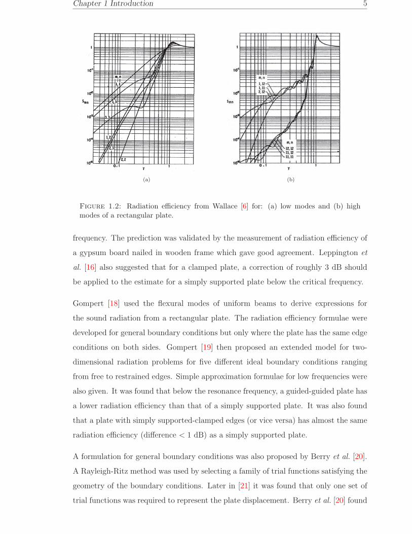
Asymptotic solutions for low frequencies were also presented. Figure 1.2 shows example
radiation efficiency results from Wallace [6] for several low and high order modes.
For each mode (m,n) results are plotted against γ = k/kmn where k is the acoustic
wavenumber and kmn is the plate bending wavenumber. The results from Wallace
were used by Xie et al. [12] to form a summation over the contributions of individual
modes. This was used to obtain the radiation efficiency in forced vibration. It was
found that using an average over many uncorrelated force point locations, the cross-
modal coupling terms average to zero.
Bonilha and Fahy [13] also proposed a model of sound radiation from a baffled flat plate
in multi-modal response. It was assumed that the modal density of a plate is sufficiently
large for there to be a considerable number of resonant modes of vibration within a
frequency band of analysis. The model gave a good agreement with Leppington’s
numerical estimate [14] except at low frequencies.
A restrained edge plate, e.g. clamped plate, was also studied by several authors [15,
16, 17]. Maidanik [15] found that the radiation efficiency of a clamped plate is 3 dB
greater than that of a simply supported plate for frequencies up to half the critical
Chapter 1 Introduction 5
(a) (b)
Figure 1.2: Radiation efficiency from Wallace [6] for: (a) low modes and (b) highmodes of a rectangular plate.
frequency. The prediction was validated by the measurement of radiation efficiency of
a gypsum board nailed in wooden frame which gave good agreement. Leppington et
al. [16] also suggested that for a clamped plate, a correction of roughly 3 dB should
be applied to the estimate for a simply supported plate below the critical frequency.
Gompert [18] used the flexural modes of uniform beams to derive expressions for
the sound radiation from a rectangular plate. The radiation efficiency formulae were
developed for general boundary conditions but only where the plate has the same edge
conditions on both sides. Gompert [19] then proposed an extended model for two-
dimensional radiation problems for five different ideal boundary conditions ranging
from free to restrained edges. Simple approximation formulae for low frequencies were
also given. It was found that below the resonance frequency, a guided-guided plate has
a lower radiation efficiency than that of a simply supported plate. It was also found
that a plate with simply supported-clamped edges (or vice versa) has almost the same
radiation efficiency (difference < 1 dB) as a simply supported plate.
A formulation for general boundary conditions was also proposed by Berry et al. [20].
A Rayleigh-Ritz method was used by selecting a family of trial functions satisfying the
geometry of the boundary conditions. Later in [21] it was found that only one set of
trial functions was required to represent the plate displacement. Berry et al. [20] found

Chapter 1 Introduction 6
that in low-order modes up to the mode (2,2), the simply supported plate has a slightly
higher radiation efficiency than that of the clamped plate. For all other modes, the
opposite situation applies with a maximum factor of 2.5 (4 dB). The radiation efficiency
for multi-modal responses for a single forcing location was also calculated up to 3 kHz.
In an average sense, the radiation efficiency level was found to be almost equal for
the clamped and simply supported plates, apart from the antisymmetric resonances
appearing for the two cases. The same phenomenon was also found between the cases
of guided-guided and free-free edges.
Williams and Maynard [22] used a scheme based on the Fast Fourier transform (FFT)
to calculate the radiation from a baffled plate. Rayleigh’s integral formula was eval-
uated numerically for baffled planar radiators, with specified velocity in the source
plane using the FFT algorithm. Bias errors appearing using this technique were also
described. Williams [23] also proposed a series expansion technique of the acoustic
power radiated from planar sources. A Maclaurin expansion of the Fourier transform
of the velocity was used to calculate the first few terms of the acoustic power. This
was later used by Li [24] to solve the Green’s function to derive analytical solutions
for the self and mutual radiation resistances of a rectangular plate.
Vitiello et al. [25], Cunefare and Koopmann [26], Elliott and Johnson [27] and Gardonio
et al. [28] used an approach based on elementary radiators. The plate was divided into
rectangular sources, where for each source, the normal time-harmonic velocity was
defined at its centre position. The interaction among the elementary sources, i.e. the
pressure at one source position as a result of contributions from the remaining sources,
was expressed by a radiation resistance matrix. The power radiated by the plate can
be found from the contributions of these sources provided that the elementary source
dimensions are small compared with both structural and acoustic wavelengths [4].
As described above, models for the sound radiation from a baffled plate are well es-
tablished. They began in the 1960s when Maidanik [5] proposed formulae for the
frequency band average due to the modal response of a lightly damped plate. In the
1970s, Wallace [6] presented the radiation efficiency of a baffled plate for single modes.
Later on in the 1990s and more recently, the averaged radiation efficiency was calcu-
lated by summation over these individual modes [4, 12]. This method is still being
expanded to fulfil many practical situations. However, the baffle in the model is used

Chapter 1 Introduction 7
for mathematical convenience rather than picturing the practical case. Often, plates
are mounted without a baffle. The model for this unbaffled condition is more compli-
cated as account has to be taken of the interaction of sound between the two sides of
the plate.
1.2.1.2 Unbaffled plate models
The infinite rigid baffle frequently used as an approximation never exists in practical
cases. A more practical situation for flat plates is often an unbaffled plate. The
problem of the radiation from an unbaffled flat plate is more difficult as the velocity is
known over the plate surface whereas elsewhere in the plane of the plate the pressure
is known (zero) due to anti-symmetry but the velocity is unknown. This creates a
mixed boundary condition which has to be overcome. However, several methods have
been developed to solve the problem.
Williams [29] applied an FFT based iterative technique to evaluate numerically the
acoustic pressure and particle velocity on and near unbaffled thin plates vibrating in
air. However, this technique suffers from convergence problems at low frequencies
which is the region where the sound radiation of baffled and unbaffled plates shows
significant differences.
Atalla et al. [30] gave a numerical solution for the sound radiation of an unbaffled
plate with general boundary conditions. The Kirchhoff-Helmholtz equation allows
the pressure to be defined anywhere within the volume enclosing the plate. Apply-
ing Euler’s equation, the plate displacement solution was obtained, which involved
a surface integral of the Green’s function. The plate displacement was then solved
using a variational approach [31]. From this, the pressure jump was neglected when
calculating the velocity of the plate, allowing any boundary conditions to be derived
analytically at the plate edges. The simulation was compared with a measurement
result from [32] and showed good agreement. However, the numerical implementation
was found to be incorrect at high frequencies due to convergence problems. The model
implied that the radiation efficiency of an unbaffled plate started to exceed that of the
equivalent baffled plate at frequencies below the critical frequency.

Chapter 1 Introduction 8
Laulagnet [33] gave an alternative solution by also using the Kirchhoff-Helmholtz equa-
tion to represent the acoustic pressure. The surface integral for the Green’s function
was solved analytically by implementing a two-dimensional spatial Fourier transform.
Both the pressure jump and the plate displacement were developed in terms of a series
of the simply supported plate modes. The matrix of modal coupling coefficients was
calculated numerically and later was used to define the accuracy of the radiation effi-
ciency. In the paper, the author used the normalized cross-modal radiation impedance
rather than the radiation efficiency. The real and imaginary parts of the radiation im-
pedance were plotted for certain modes and were compared with those of the baffled
plate.
Nelisse et al. [34] proposed a study on the radiation of both baffled and unbaffled
plates. A Rayleigh-Ritz approach was used to develop the plate displacement in the
baffled case, as well as the pressure jump in the unbaffled case. The plate mode
shape function was defined by applying a set of trigonometric functions for arbitrary
boundary conditions [35]. As in Laulagnet’s model [33], the pressure jump was also
expanded in terms of a series of modes. The radiation efficiency was obtained by first
determining sets of matrices, namely radiation impedance, mass and stiffness matrices.
Intended for general boundary conditions, the calculation is more complicated than
Laulagnet’s model. In the paper, the radiation efficiency of an unbaffled clamped plate
in water was presented against frequency up to moderate frequencies and compared
with that of the baffled plate.
Oppenheimer and Dubowsky [36] introduced heuristic correction factors in the formula
for a baffled plate and then used curve-fitting based on measured results to determine
the various coefficients. This method is not sufficiently rigorous to be considered
further here but it is practical from an engineering point of view.
More recently, Fahy and Thompson [37] developed a wavenumber domain scheme
involving inversion of a matrix equation. However, the model was only applied to
a one-dimensional strip piston. Intended for perforated strips, this method can also
be applied to an unbaffled strip although the results were found to be poor in this
case due to a singular matrix produced (see Appendix A). In terms of its concept, the
model provides a useful insight to a case of mixed boundary conditions. The acoustic
pressure was defined as a function of the acoustic impedance which could be different

Chapter 1 Introduction 9
in the region above the strip and beyond it, creating the mixed boundary conditions.
The acoustic power was then calculated in the wavenumber domain.
Models for the radiation from an unbaffled plate are much less widely considered than
for the baffled plate. From the existing methods, particularly in [29] and [33], the
results presented were only focused on single modes. The radiation efficiency due to
vibration in multiple modes was calculated in [30, 33, 34] but only up to relatively low
frequency. However, this is not still adequate to give a thorough analysis, particularly
to provide a complete investigation into the difference between the radiation from the
baffled and unbaffled plate.
1.2.2 Numerical models
Alternative approaches are available using numerical methods such as the finite element
method (FEM) or boundary element method (BEM). The FEM is used to obtain
solutions to the differential equations that describe, or approximately describe a wide
variety of physical (and non-physical) problems [38, 39]. The BEM is basically derived
through the discretisation of an integral equation that is mathematically equivalent
to the original partial differential equation [40]. The FEM and BEM allow arbitrary
geometry to be considered but do not provide the same physical insight as analytical
methods. The FEM is usually first used for analysing the vibration of a structure.
Once motion of the vibrating structure is obtained, the BEM is employed to solve
the equation of motion of the acoustic medium [41]. Several studies relating to the
sound radiation have been proposed based on these methods. For heavy fluid loading,
FEM/BEM can also be used in fully a coupled mode to allow for the effect of the fluid
on the structure.
Nolte and Gaul [42] investigated the sound radiation from a vibrating structure in
water. The pressure field in the fluid domain and the velocity field were determined
by using BEM with input data of surface velocities obtained from a FEM calculation
of modal analysis. The sound radiation can be identified by determining the intensity
vector in the acoustic near field. For a comparison, the sound radiation calculated by
using BEM was compared with the results obtained by a superposition of monopole
sources (pulsating spheres). Mattei [43] presented a formulation and a numerical

Chapter 1 Introduction 10
solution using a simple BEM model of a boundary integral equation for a baffled
plate, and also developed an analytical method for the constrained plate.
Zhao et al. [44] proposed a method to calculate the radiation efficiency of arbitrary
structures by combining BEM and general eigenvalue decomposition. The surface
pressure of the structure was calculated using BEM and as the impedance matrix
is positive definite and the mean square velocity is real symmetric and also positive
definite, the sound radiation can be decoupled using general eigenvalue decomposition.
The method was validated with the prediction for radiation efficiencies of a pulsating
sphere and a radiating cube.
Although FEM can also be used for acoustic fields, it cannot be used directly for
open problems such as sound radiation from structures. However, it is possible to use
the scheme called the ’infinite element method’ to simulate non-reflecting boundaries.
This can be implemented to solve an unbounded acoustical problems [45, 46] as an
alternative to the BEM.
1.2.3 Experimental work and methods
Many experimental investigations using various methods have also been carried out to
validate models for the sound radiation from a vibrating structure. To determine the
radiation efficiency, the experimental work requires two sets of measurement i.e. the
acoustical measurement for the sound power and the mechanical measurement for the
squared surface velocity. Mostly, the methods only differ in the means of measuring
the sound power. This can be obtained in several ways:
1. by measuring the nearfield, sound intensity using the sound intensity probe [47,
48]
2. by measuring the direct field far from the plate [49]. This can be done accurately
in an anechoic chamber, a special room having walls with high absorption to
suppress the reflected sound. For a sound source with high directivity, the sound
pressure must be taken at many measurement positions.
3. by measuring the diffuse field in a reverberant chamber [50, 51, 52]. At a certain
distance from the sound source where the direct field is negligible compared

Chapter 1 Introduction 11
with the reverberant field, the sound pressure is approximately uniform across
the room. A smaller number of measurement locations than for the anechoic
chamber is therefore sufficient.
To prevent unwanted noise from the mechanical exciter, such as a shaker, the reci-
procity technique can be applied to obtain the radiated power for a given squared
input force [50, 51, 53]. Instead of exciting the structure mechanically, the structure
is now excited acoustically by a broadband sound. The sound pressure over the room
and the surface velocity or acceleration of the structure are measured. This tech-
nique, in many cases of practical application in noise control engineering, can provide
information in a simpler, faster and cheaper than by direct test methods [54].
Ramachandran and Narayanan [52] implemented experimental statistical energy analy-
sis (SEA) to determine the radiation efficiency of a stiffened cylindrical shell. The es-
timated modal density was obtained from the measured point mobility of the cylinder.
The cylinder was then excited by a diffuse sound field in a reverberant chamber. From
this, experimental SEA was employed to obtain the coupling loss factors (CLFs) and
the damping loss factors (DLFs). The radiation efficiency is proportional to the CLF
between the cylinder and the acoustic subsystem. A correction factor, as in [36], was
applied below the critical frequency as the experiment was conducted in unbaffled con-
dition. The results showed a good agreement between the experiment and predictions
for stiffened and unstiffened cylinders.
Hashimoto [55] proposed a combination between theoretical calculation and measure-
ment for obtaining the radiation efficiency using both vibration measurements and
calculations of self and mutual radiation impedances. The plate was divided into rec-
tangular elements smaller than the acoustic wavelength at the critical frequency. To
have a simple formula to calculate the radiation impedance, each element was approxi-
mated as a circular piston. The sound power was then obtained by using the measured
surface velocity of the structure at the centre of each element in combination with the
calculated radiation impedance. The radiation efficiency calculated from this method
was validated by comparison with Rayleigh’s integral [9] for uniform vibration of the
plate surface and with Maidanik’s formulae [5] for diffuse vibration, the latter being
obtained from FEM. The results showed a reasonably good agreement. This method
offers an advantage that the acoustic (sound power) measurement is not required.

Chapter 1 Introduction 12
Figure 1.3: Measured radiation efficiencies of some unbaffled perforated plates [56].
However, the paper does not provide results comparing measured data with the the-
oretical results to demonstrate that the method could be a good alternative for the
conventional method. Furthermore, the method is applicable only for a flat baffled
plate.
1.2.4 Perforated plate models
The main aim in studying the sound radiated by vibrating plates is usually to de-
termine how to reduce the sound radiation. For this purpose, several schemes have
been developed, one of which is to introduce perforation over the area of the plate.
Although not applicable in every situation, this technique is known to be very effec-
tive [4]. Figure 1.3 shows measured data [56] of radiation efficiencies from 1 mm thick
perforated unbaffled steel plates with various perforation ratios. It can be seen that
the perforated plates produce less sound radiation than the solid plate does.
Perforated plates can be seen in many practical applications, for example safety guard
enclosures, such as the protective cover over flywheels and belt drives as seen in Fig-
ure 1.4(a), and product collection hoppers as shown in Figure 1.4(b). They are also

Chapter 1 Introduction 13
(a)
(b)
Figure 1.4: Applications of perforated plates for reducing the sound radiation [62]: (a)cover of a belt drive and (b) product collection hopper.
widely used in sound absorption applications, as flexible panels covering a porous ma-
terial [57] or backed by an air cavity [58, 59, 60]. In such applications, it has been
shown that the vibration of the perforated plate has the effect of increasing the absorp-
tion coefficient [58]. In developing models for the sound absorption from a perforated
plate, the acoustic impedance of a hole was approximated by the analytical solution
for wave propagation in a small tube having a circular cross section, as proposed by
Maa [61].
Very few models have been proposed to calculate the sound radiation from a perfo-
rated plate. Janssens and van Vliet [63] studied the sound radiation from a vibrating
steel railway bridge, and investigated the potential effect of perforating various bridge
components. Measurements were carried out on a set of perforated plates by varying
the perforation ratio, the hole density and the hole diameter. An empirical formula
was then derived for the effect of perforation on the radiation efficiency.
Fahy and Thompson [37] started with a model of radiation by plane bending waves

Chapter 1 Introduction 14
propagating in an unbounded plate with uniform perforation to calculate the radiation
efficiency of a simply supported rectangular perforated plate. The assumptions imply
that the plate is effectively mounted in a similarly perforated rigid baffle, which would
not be found in practice. This model replaces the perforations by an equivalent con-
tinuous impedance, based on an assumption that the hole size is much smaller than
the acoustic wavelength.
The model was then extended to the situation where the plate and the baffle have
different specific acoustic impedances. The relation between velocities and pressures
was derived in the wavenumber domain as a matrix problem and then solved by matrix
inversion. As a preliminary case, this was applied to the radiation by a perforated strip
piston, in one dimension, vibrating in an infinite baffle. Good results were obtained
for the case of a perforated strip piston in a perforated baffle and in a rigid baffle.
However, problems were found with this model at low frequencies for an unbaffled
perforated strip. A very low acoustic impedance of the boundary (relative to the
acoustic impedance of the hole) led to a singular or nearly singular matrix which
reduced the quality of the results from the inverted matrix. In addition, expanding
this model into the two-dimensional case is found to require intensive computational
effort. Results from this model have been reproduced and are given in Appendix A.
A somewhat different study was carried out by Toyoda and Takahashi [59] who pro-
posed a model for the sound radiation from an infinite, thin elastic plate under a single
normal point force excitation in the presence of a perforated plate used as an absorp-
tive facing to the vibrating plate. The analysis was carried out under the assumption
that the perforated board was rigidly attached to the vibrating plate via a honeycomb
structure so that both plates have an identical motion. The problem was examined
as a one-dimensional situation. The basic model for the sound power radiated by the
flexural vibration of a perforated plate was adopted from [57]. In [60], the problem
was extended to three-dimensions but still using a normal point force excitation at a
particular location on the plate. A large reduction in sound radiation due to perfora-
tion on the facing was found around a narrow frequency of the Helmholtz resonator
formed by the air cavity inside the honeycomb structure and the perforated plate.
In terms of the effect of perforation in reducing the radiated sound over a wider
frequency range, which can be achieved by perforating the vibrating main structure,

Chapter 1 Introduction 15
if possible, there is still a lack of quantitative models that can accurately determine
the level of sound reduction due to the perforation.
1.3 Objectives and scope of the thesis
The main objective of this thesis is to develop models for the sound radiation from
vibrating perforated plates, with or without a baffle. These should be applicable in
practical cases and be usable to give quantitative guidance especially relating to the
noise reduction potential. The emphasis is therefore placed on a vibrating rectangular
plate rather than simpler case of a strip. Extensive measurements are presented to
validate these models.
Most emphasis is placed on simply supported boundary conditions although the model
can in principle be extended to other edge conditions. A guided-guided boundary
condition is highlighted as a comparison for perforated baffled and unbaffled plates.
The plate is also assumed to be immersed in air so that the effect of fluid loading can
be neglected.
Perforation introduced to a solid plate will also change the dynamic properties of the
plate, i.e. the effective Young’s modulus, the Poisson’s ratio and the density, depending
on the ratio of the perforation [64, 65]. This will thus change the resonance frequencies
of the plate. The models proposed assume that the perforation does not affect these
properties significantly, although it will be shown later from the experimental results
that this also affects the radiation efficiency particularly for thin, light plates. In
addition, the model proposed is based on regular evenly spaced holes so that the mode
shapes are unchanged.
1.4 Thesis outline
The structure of the thesis is as follows:
Chapter 2 reviews several existing models for calculating the radiation efficiency of a
plate set in an infinite baffle. The accuracy and computational efficiency of methods

Chapter 1 Introduction 16
from Xie et al. [12], Fahy [4] and Williams [22] are compared and their advantages
and disadvantages are discussed. The radiation efficiency is calculated for multi modal
responses and averaged over force positions. The variability of the radiation efficiencies
due to the location of a single point force is also investigated.
In Chapter 3 models for the unbaffled plate are reviewed. Similar to the baffled
plate in Chapter 2, the accuracy and computational efficiency of the existing models
are discussed. Methods from Williams [23] and Laulagnet [33] are implemented to
calculate the radiation efficiency of an unbaffled plate. The results are plotted and
also compared with those of the baffled plate. From this, simple empirical formulae,
equivalent to Maidanik’s formulae for the baffled plate, will be derived.
In Chapter 4 the effect of the plate edge condition on the radiation efficiency is sought.
This is calculated in particular for the combination of simply supported and guided-
guided boundary conditions both for baffled and unbaffled plates.
Chapter 5 extends the problem to consider the sound radiation from a perforated
plate. The impedance of the hole and its approximations in terms of fluid viscosity
and near field effects are described. The model from Fahy and Thompson [37] for
the perforated plate in an infinite perforated baffle is implemented. Some results are
plotted including the effect of perforation. For the latter, an approximate formula is
developed. The sound radiation from a perforated unbaffled plate is then modelled by
extending Laulagnet’s model [33]. The result is compared with the model of a perfo-
rated plate in an infinite perforated baffle. An approximate formula is also developed
for the effect of perforation at low frequency. The unbaffled perforated plate model is
also extended further to consider the case where the plate is close to a reflecting rigid
surface.
In Chapter 6 a model is developed for a perforated plate in a rigid baffle based on
discretisation of the Rayleigh integral to simulate a distribution of discrete monopole
sources. The concept is similar to [25, 26] where the plate is divided into small ele-
mentary radiators. This allows an investigation of the limitation of using a uniform
specific acoustic impedance to represent the holes.
Chapter 7 presents experimental work to validate the model for the sound radiation
from an unbaffled plate. The experiments are conducted with two types of boundary

Chapter 1 Introduction 17
conditions, namely simply supported and free-free. A validation experiment is also
made for the radiation from a plate close to a rigid surface.
Chapter 8 summarises the main findings of the thesis and proposes further work.
1.5 Thesis contributions
The main contributions from this thesis can be summarised as follows:
(a) An assessment is made of existing methods for calculating the averaged radiation
efficiency of baffled plates. The variability of the radiation efficiency due to the
forcing location has been established. It is shown that the highest variability lies
in the corner mode frequency region. The variability depends on plate thickness
whereas it is largely independent of damping and plate dimensions.
(b) Existing models of the sound radiation from unbaffled plates have been imple-
mented and assessed. It is shown that Laulagnet’s model is the most powerful
and reliable model to calculate the results up to high frequency. Simple empirical
formulae for calculating the radiation efficiency of an unbaffled plate have been
introduced. For engineering purposes, these are found to be very useful in terms
of calculation time.
(c) The effect of plate boundary conditions on the radiation from multi-modal re-
sponses have been determined by comparing results for simply supported and
guided-guided boundaries both for baffled and unbaffled plates. For the unbaf-
fled case, the plate boundary conditions are found to have less influence on the
radiation efficiency than for the baffled case.
(d) By modifying Laulagnet’s model, a model for sound radiation from an unbaffled
perforated plate is proposed. It is found that the radiated sound can be reduced
by increasing the perforation ratio or by introducing a smaller hole size for a
constant perforation ratio.
(e) A model for sound radiation from a baffled perforated plate is developed by using
a discrete sources approach. This model demonstrates that the assumption of a
continuous impedance is only valid when the distance between holes is less than

Chapter 1 Introduction 18
an acoustic wavelength for a rectangular piston and less than half an acoustic
wavelength for a plate in bending vibration.
(f) The unbaffled perforated plate model is extended to consider the case where the
plate is close to a rigid surface. It is found that at low frequency, the effect of
perforation on the sound radiation is greater than that when the rigid surface is
absence.
(g) Experimental validation of the models is provided which gives good agreement
between measured results and the predictions. It also confirms point (c) above
because a good agreement is achieved for the prediction calculated using simply
supported edges while the experiment is actually conducted with free-free edges.

Chapter 2
Radiation efficiency of a baffled
plate
The purpose of this chapter is to compare different methods of calculating the radiation
efficiency of a rectangular plate set in an infinite baffle, for a case of a point force
excitation. Since plate vibrations generally involve many superimposed modes, the
radiation efficiency of a plate, in principle, can be obtained by summing over all the
modes that contribute significantly in the frequency range under consideration [12].
Methods described in this chapter and in Chapter 3 apply this theory to obtain the
radiation efficiency of baffled and unbaffled plates respectively. In each case an average
over possible point force locations is taken. Simply supported plate boundaries will
be considered for simplicity. The methods are described in detail as they form a basis
for later sections on perforated plates.
2.1 Spatial domain approach
2.1.1 Power radiated in terms of plate modes
Figure 2.1 shows a rectangular plate of length a and width b set in an infinite rigid
baffle. Harmonic motion at frequency ω is assumed. The complex acoustic pressure
amplitude p(r) at position r can be written in terms of the plate surface velocity using
the Rayleigh integral [9] evaluated over the plate surface S, since the velocity is zero
19

Chapter 2 Radiation efficiency of a baffled plate 20
+
_
+
_
+
_
q
f
z
R R’
y
x
x= x,y( )
a
b/n
a/m
b
r= R,( q, f)
Figure 2.1: Co-ordinate system of a vibrating plate.
elsewhere on the baffle
p(r) =jkρc
2π
∫
s
v(x)e−jkR′
R′ dx (2.1)
where v(x) is the complex velocity amplitude normal to the surface at location x =
(x, y), k is the acoustic wavenumber (k = ω/c), ρ is the density of air, c is the speed of
sound and R′ = |r−x| is the distance from the location on the plate to the observation
point. The term e−jkR′
/2πR′ is the half space Green’s function [4]. A time dependence
of ejωt is assumed, where t is time.
Following the method of Xie et al. [12], by integrating the far field acoustic intensity
over a hemisphere of radius R, the total radiated acoustic power can be written as
W =
∫ 2π
0
∫ π/2
0
|p(r)|22ρc
R2 sin θ dθ dφ (2.2)
where the location r is expressed in spherical co-ordinates as r = (R, θ, φ).
The radiated power can also be calculated by integrating the acoustic intensity over
the surface of the vibrating plate. This calculation is not developed further here as
there are singularities when R′ = 0, hence more effort would be needed to overcome
the problems in the Rayleigh integral. One approach is to use series expansions. For
a further description of this approach, one can refer to reference [66] or [67].

Chapter 2 Radiation efficiency of a baffled plate 21
The velocity v(x) at any location x on the plate can be found by summing over all
the modes of structural vibration of the plate,
v(x) =∞∑
m=1
∞∑
n=1
umnϕmn(x) (2.3)
where umn is the complex velocity amplitude of mode (m,n), which depends on the
form of excitation and on frequency, and ϕmn(x) is the value of the associated mode
shape function at x.
For a plate with simply supported edges, the mode shape function ϕmn(x) is the
product of two sinusoidal functions along the x and y directions (see Appendix B)
ϕmn(x, y) = sin(mπx
a
)sin(nπy
b
)(2.4)
From Cremer et al. [7], the modal velocity amplitude due to a point force applied at
a location (x0, y0) is given by
umn =jωFϕmn(x0, y0)
[ω2mn(1 + jη) − ω2]Mmn
(2.5)
where F is the force amplitude, ωmn is the natural frequency, η is the damping loss
factor, and Mmn is the modal mass which, for the simply supported boundaries, is
given by
Mmn =
∫
s
ρptpϕ2mn(x, y)dS =
1
4ρptpab =
M
4(2.6)
where ρp, tp and M are the density, thickness and mass of the plate respectively.
The natural frequencies ωmn are given by
ωmn =
(B
ρptp
)1/2 [(mπa
)2
+(nπb
)2]
(2.7)
where B = Et3p/[12(1 − ν2)] is the bending stiffness of the plate, in which E is the
Young’s modulus and ν is the Poisson’s ratio.

Chapter 2 Radiation efficiency of a baffled plate 22
By substituting Eq.(2.3) into Eq.(2.1), the sound pressure is thus given by
p(r) =∞∑
m=1
∞∑
n=1
umn
jkρc
2π
∫
s
ϕmn(x)e−jkR′
R′ dx
(2.8)
or it can also be expressed as
p(r) =∞∑
m=1
∞∑
n=1
umnAmn(r) (2.9)
where Amn(r) is the term in the brackets in Eq.(2.8).
Wallace [6] has produced an analytical solution for Amn(r), which is given by
Amn(r) =jkρc
2π
(e−jkR
R
)Φ (2.10)
where
Φ =ab
π2mn
[(−1)mejµ − 1
(µ/(mπ))2 − 1
] [(−1)nejχ − 1
(χ/(nπ))2 − 1
]
µ = ka sin θ cosφ, χ = kb sin θ sinφ and r = |r|
Since p.p∗ = |p|2, substituting Eq.(2.9) into Eq.(2.2) gives the total radiated power as
W =∞∑
m=1
∞∑
n=1
∞∑
m′=1
∞∑
n′=1
umnu
∗m′n′
∫ 2π
0
∫ π/2
0
Amn(r)A∗m′n′(r)
2ρcR2 sin θ dθ dφ
(2.11)
where m and n′ denote the values of m and n in the conjugate form. This equation
shows that the total radiated power depends on the contributions of combinations of
modes. The contribution is usually referred to as the self-modal radiation for m = m′
and n = n′, and cross-modal radiation for either m 6= m′ or n 6= n′. According to
Snyder and Tanaka [66], the cross-modal coupling can only occur (non-zero value)
between a pair of modes with the same parity, i.e. both odd or both even in each of
the x and y directions. Li and Gibeling [67] have shown that the cross-modal coupling
could have a significant impact on the radiated power, depending upon frequency and
load condition. In particular it is found that the effect is significant between pairs

Chapter 2 Radiation efficiency of a baffled plate 23
of low order modes. Without taking the cross-modal contribution into account, the
sound power may be over- or under-estimated. However, Xie et al. [12] arrive at the
conclusion that the contribution of the cross-modal coupling can be neglected when
the plate is excited with uncorrelated point forces averaged over all positions on the
plate. This is explained in the next section.
2.1.2 Average over forcing points
Following the procedure of [12], consider a point force applied on the plate at location
(x0, y0) producing a radiated power W (x0, y0). It is possible to average the radi-
ated power for all possible locations of uncorrelated point forces on the plate. Such
excitation, known as ”rain on the roof”, is often used in statistical energy analysis
(SEA) [68] where geometrical details of a system are neglected. It can be considered
as an ensemble average. This average is written as
W =1
ab
∫ a
0
∫ b
0
W (x0, y0) dx0 dy0 (2.12)
Substituting Eq.(2.11) into Eq.(2.12) gives
W =∞∑
m=1
∞∑
n=1
∞∑
m′=1
∞∑
n′=1
1
ab
∫ a
0
∫ b
0
umnu∗m′n′dx0dx0
∫ 2π
0
∫ π/2
0
Amn(r)A∗m′n′(r)
2ρcR2 sin θ dθ dφ
(2.13)
where
∫ a
0
∫ b
0
umnu∗m′n′dx0 dy0 =
∫ a
0
∫ b
0
(jωFϕmn(x0, y0)
[ω2mn(1 + jη) − ω2]Mmn
)( −jωFϕm′n′(x0, y0)
[ω2m′n′(1 − jη) − ω2]Mm′n′
)dx0 dy0
For a uniform structure with a constant mass per unit area, due to the orthogonality
of the eigenfunctions, Eq.(2.13) can be simplified to [12]

Chapter 2 Radiation efficiency of a baffled plate 24
W =∞∑
m=1
∞∑
n=1
1
ab
∫ a
0
∫ b
0
umnu∗mn dx0 dy0
∫ 2π
0
∫ π/2
0
Amn(r)A∗mn(r)
2ρcR2 sin θ dθ dφ
(2.14)
This verifies that the total radiated power averaged over forcing locations is a summa-
tion of the power radiated by each single mode. The cross-modal coupling terms have
now been eliminated.
Eq.(2.14) can also be expressed as
W =∞∑
m=1
∞∑
n=1
Wmn (2.15)
where Wmn is given by
Wmn = |umn|2∫ 2π
0
∫ π/2
0
Amn(r)A∗mn(r)
2ρcR2 dθ dφ (2.16)
and |umn|2 is the squared modal velocity amplitude umn, averaged over all forcing
positions.
From Eq.(2.5), for simply supported boundaries |umn|2 can be calculated as
|umn|2 =1
ab
∫ a
0
∫ b
0
umnu∗mn dx0 dy0 =
4ω2|F |2[(ω2
mn − ω2)2 + η2ω4mn]M2
(2.17)
Recalling Eq.(1.2), the modal radiation efficiency σmn can be given by
σmn =Wmn
12ρcab
⟨|vmn|2
⟩ (2.18)
where⟨|vmn|2
⟩is the spatially averaged squared velocity amplitude of a single mode
at one forcing location given by
⟨|vmn|2
⟩=
1
ab
∫ a
0
∫ b
0
|umn|2ϕ2mn(x, y) dx dy =
|umn|24
(2.19)
Averaging⟨|vmn|2
⟩over all possible forcing positions gives

Chapter 2 Radiation efficiency of a baffled plate 25
⟨|vmn|2
⟩=
1
ab
∫ a
0
∫ b
0
⟨|vmn|2
⟩dx0 dy0
=1
ab
∫ a
0
∫ b
0
1
4|umn|2 dx0 dy0 =
|umn|24
(2.20)
Therefore by substituting Eq.(2.16) and (2.20) into (2.18) yields the modal radiation
efficiency averaged over all forcing positions
σmn = 4
∫ 2π
0
∫ π/2
0
Amn(r)A∗mn(r)
(ρc)2abR2 dθ dφ (2.21)
After algebraic manipulation, Eq.(2.21) can be expressed as
σmn =64abk2
π6m2n2
∫ π/2
0
∫ π/2
0
Θ sin θ dθ dφ (2.22)
where
Θ =
cos(ξ/2) cos(/2)
sin(ξ/2) sin(/2)
[(ξ/mπ)2 − 1][(/nπ)2 − 1]
2
in which cos(ξ/2) and sin(ξ/2) are used when m is an odd or even integer respectively.
Similarly, cos(/2) and sin(/2) are used when n is an odd or even integer respectively.
Since sin(ξ/2 + pπ/2) = ± cos(ξ/2) and sin(ξ/2 + qπ/2) = ± sin(ξ/2) where p is odd
and q is even, Θ can be expressed more efficiently as
Θ =
sin(ξ/2 +mπ/2) sin(/2 + nπ/2)
[(ξ/mπ)2 − 1][(/nπ)2 − 1]
2
(2.23)
As an example, Figure 2.2 plots the radiation efficiency of modes (1,1) and (10,1) of a
rectangular plate having dimensions 0.65×0.5×0.003 m (details given in Section 2.4)
in terms of normalised frequencies k/kmn, where kmn =√
(mπ/a)2 + (nπ/b)2. The
frequency resolution used is 40 points per decade spaced logarithmically to ensure a
good resolution at the resonance.

Chapter 2 Radiation efficiency of a baffled plate 26
10−1
100
101
10−3
10−2
10−1
100
k/kmn
radia
tion
effici
ency
,σ
(a)
10−1
100
10−3
10−2
10−1
100
k/kmn
radia
tion
effici
ency
,σ
(b)
Figure 2.2: Radiation efficiency of (a) mode (1,1) and (b) mode (10,1) of a simplysupported baffled plate using the spatial domain approach: e = −−10−3, − · −10−5,· · · 10−7, —10−9.

Chapter 2 Radiation efficiency of a baffled plate 27
The double integral in Eq.(2.22) is evaluated using a built-in function in MATLAB
implementing the two-dimensional Simpson quadrature with various error tolerances,
e. The results show that the radiation efficiency increases as the frequency increases
and then converges to unity above the maximum peak at k ≈ kmn. As e is reduced,
the curve converges.
Finally, the general average radiation efficiency σ is given by
σ =
∑∞m=1
∑∞n=1Wmn
12ρcab
⟨|v|2⟩ =
∑∞m=1
∑∞n=1 σmn
⟨|vmn|2
⟩⟨|v|2⟩ (2.24)
where according to Cremer et al. [7],⟨|v|2⟩
is the result of summation of the spatially
averaged modal squared velocity⟨|vmn|2
⟩, averaged over forcing locations, i.e.
⟨|v|2⟩
=ω2|F |22M2
∞∑
m=1
∞∑
n=1
1
[(ω2mn − ω2)2 + η2ω4
mn]=
∞∑
m=1
∞∑
n=1
⟨|vmn|2
⟩(2.25)
Eq.(2.25) indicates that, as the cross-modal contributions vanish due to averaging over
forcing locations, the modal responses are uncorrelated. In other words, the modes
act individually, and are all excited with the same input power.
Therefore by substituting Eq.(2.20) and Eq.(2.17) gives
σ =
∑∞m=1
∑∞n=1 σmn
⟨|vmn|2
⟩
∑∞m=1
∑∞n=1
⟨|vmn|2
⟩
(2.26)
=
∑∞m=1
∑∞n=1 σmn[(ω2
mn − ω2)2 + η2ω4mn]−1
∑∞m=1
∑∞n=1[(ω
2mn − ω2)2 + η2ω4
mn]−1
Example results of σ will be given in Section 2.4 below.

Chapter 2 Radiation efficiency of a baffled plate 28
2.2 Wavenumber domain approach
2.2.1 Governing equations
The sound radiation from a mode of vibration of a finite plate set in an infinite baffle
can also be determined by wavenumber decomposition of the spatial distribution of
velocity in the mode [4].
Consider first a one-dimensional infinite vibrating plate, having velocity v(x), which is
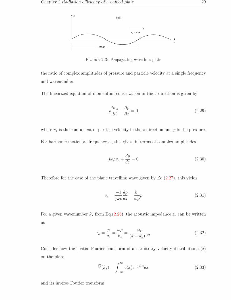
in contact with a fluid in the semi-infinite space z > 0 as shown in Figure 2.3. A plane
transverse wave is travelling in the plate with arbitrary frequency ω and wavenumber
κ in the x direction. Sound is radiated by the plate into the fluid with the same
wavenumber component in the x direction.
As the propagation of a plane wave in a two-dimensional space is expressed by
p(x, z, t) = p e−j(κx+kzz)ejωt (2.27)
the condition must be satisfied that κ < k, i.e. the plate wave speed cp is greater than
the speed of sound c in the fluid, to allow the wave to propagate away from the plate
surface. Also to fulfil this distinct condition, the positive sign must be chosen for kz,
whereas the negative sign is disallowed as no wave can propagate towards the surface
of the plate.
Assuming a light fluid (for example air), the dependence of the acoustic field in the
fluid in the x direction must be the same as that of the plate, i.e. kx = κ so that the
wavenumber relationship is given by
kz = ±(k2 − k2x)
1/2 (2.28)
where k is the acoustic wavenumber, k = ω/c.
The radiated pressure field can be related to the surface normal velocity distribution
through the specific acoustic impedance. The specific acoustic impedance is defined as
Chapter 2 Radiation efficiency of a baffled plate 29
z
x
2 /p k
fluid
c = /p w k
Figure 2.3: Propagating wave in a plate
the ratio of complex amplitudes of pressure and particle velocity at a single frequency
and wavenumber.
The linearized equation of momentum conservation in the z direction is given by
ρ∂vz
∂t+∂p
∂z= 0 (2.29)
where vz is the component of particle velocity in the z direction and p is the pressure.
For harmonic motion at frequency ω, this gives, in terms of complex amplitudes
jωρvz +dp
dz= 0 (2.30)
Therefore for the case of the plane travelling wave given by Eq.(2.27), this yields
vz =−1
jωρ
dp
dz=kz
ωρp (2.31)
For a given wavenumber kx from Eq.(2.28), the acoustic impedance za can be written
as
za =p
vz
=ωρ
kz
=ωρ
(k − k2x)
1/2(2.32)
Consider now the spatial Fourier transform of an arbitrary velocity distribution v(x)
on the plate
V (kx) =
∫ ∞
−∞v(x)e−jkxxdx (2.33)
and its inverse Fourier transform
Chapter 2 Radiation efficiency of a baffled plate 30
v(x) =1
2π
∫ ∞
−∞V (kx)e
jkxxdkx (2.34)
For a finite plate in a rigid baffle, if v(x ) represents the plate velocity, or zero on the
baffle, the velocity distribution of the plate can also be expressed as an integral over
wavenumber. Similarly the pressure at z = 0 can be Fourier transformed with respect
to kx.
Thus in terms of the wavenumber transforms, Eq.(2.32) can be written as
[P (kx)
]z=0
= V (kx)za(kx) =
(ωρ
(k2 − k2x)
1/2
)V (kx) (2.35)
Considering now a plane wave travelling in the plate surface with a component in the
x and y directions, having wavenumber components kx and ky, k2x is then replaced by
k2x + k2
y. The direction of travel is at an angle θ = tan−1(ky/kx) to the x-axis. Thus
from Eq.(2.35), the surface pressure wavenumber component is related to the velocity
wavenumber component by
[P (kx, ky)
]z=0
=ωρ
(k2 − k2x − k2
y)1/2
V (kx, ky) (2.36)
Referring to Eq.(2.34) for a two-dimensional case, the surface pressure field and the
surface normal velocity are
[p(x, y)]z=0 =1
4π2
∫ ∞
−∞
∫ ∞
−∞[P (kx, ky)]z=0 e
j(kxx+kyy) dkx dky (2.37)
vn(x, y) =1
4π2
∫ ∞
−∞
∫ ∞
−∞V (kx, ky) e
j(kxx+kyy) dkx dky (2.38)
The radiated power per unit area is calculated by
W =1
2ℜ∫
S
p(x, y) v∗n(x, y) dx dy
(2.39)
where ℜ denotes the real part.

Chapter 2 Radiation efficiency of a baffled plate 31
Therefore by substituting Eq.(2.37) and (2.38) into (2.39) this gives
W =1
32π4ℜ∫
S
[∫ ∞
−∞
∫ ∞
−∞[P (kx, ky)]z=0 e
j(kxx+kyy) dkx dky
(2.40)
×∫ ∞
−∞
∫ ∞
−∞V ∗(k′x, k
′y) e
−j(k′
xx+k′
yy) dk′x dk′y
]dxdy
The range of double integration over the surface S can be extended to −∞ to ∞because the particle velocity v is ensured to be zero outside the plate boundary.
Thus substituting Eq.(2.36) into (2.40) gives
W =1
32π4ℜ∫ ∞
−∞
∫ ∞
−∞
[∫ ∞
−∞
∫ ∞
−∞
ωρ
(k2 − k2x − k2
y)1/2
V (kx, ky) ej(kxx+kyy) dkx dky
(2.41)
×∫ ∞
−∞
∫ ∞
−∞V ∗(k′x, k
′y) e
−j(k′
xx+k′
yy) dk′x dk′y
]dx dy
If the integration is first performed over x and y, by changing the order of integration,
the Dirac delta functions are obtained i.e.
∫ ∞
−∞
∫ ∞
−∞e−j(kx−k′
x)xe−j(ky−k′
y)ydx dy = 4π2δ(kx − k′x)δ(ky − k′y) (2.42)
Hence Eq.(2.41) can be simplified as
W =1
8π2ℜ∫ ∞
−∞
∫ ∞
−∞
ωρ
(k2 − k2x − k2
y)1/2
|V (kx, ky)|2 dkx dky (2.43)
In addition only wavenumber components satisfying the condition k2x + k2
y ≤ k2 con-
tribute to sound power radiation; elsewhere the term (k2 − k2x − k2
y)1/2 is imaginary.
The range of integration can therefore be limited to give
W =ρc
8π2
∫ k
−k
∫ √k2−k2
y
−√
k2−k2y
k
(k2 − k2x − k2
y)1/2
|V (kx, ky)|2 dkx dky (2.44)
In the two-dimensional spatial Fourier transform, the velocity distribution of an indi-
vidual mode (m,n) is decomposed into a continuous spectrum of spatially harmonic,

Chapter 2 Radiation efficiency of a baffled plate 32
travelling plane wave components, each having a certain wavenumber vector which is
given by
Vmn(kx, ky) =
∫ a
0
∫ b
0
umn ϕmne−j(kxx+kyy) dx dy (2.45)
where Vmn(kx, ky) is the complex amplitude of the wavenumber component. Integra-
tion yields
Vmn(α, β) = umnΛk−2(ε+ jϑ)(γ + jς) (2.46)
where
Λ =
(mπka
)(nπkb
)
[α2 −
(mπka
)2] [β2 −
(nπkb
)2]
ε = (−1)m cos (αka) − 1, ϑ = (−1)m+1 sin (αka)
γ = (−1)n cos (βkb) − 1, ς = (−1)n+1 sin (βkb)
in which α = kx/k and β = ky/k are the non-dimensional wavenumbers and a and b
are the plate dimensions. The derivation of Eq.(2.46) is given in Appendix C.
Referring to the co-ordinates in Figure 2.1 for wavenumber components, it is found
that kx = k sin θ cosφ and ky = k sin θ sinφ.
Thus by relating Eq.(2.46) to Eq.(2.10), it can also be found that
Vmn(k, θ, φ) = umnΦ
(ka)(kb)(2.47)
Substituting Eq.(2.46) into Eq.(2.44), the sound power radiated by a single mode is
thus
Wmn =ρc|umn|28π2k2
∫ 1
−1
∫ √1−α2
−√
1−α2
Λ2 (Γ2 + Π2)
(1 − α2 − β2)1/2dβ dα (2.48)
where Γ = (εγ − ϑς) and Π = (ϑγ + ες). Note that the integrand in Eq.(2.48) forms
an even function, so that the limit of integration can be simplified
Wmn =ρc|umn|22π2k2
∫ 1
0
∫ √1−α2
0
Λ2 (Γ2 + Π2)
(1 − α2 − β2)1/2dβ dα (2.49)

Chapter 2 Radiation efficiency of a baffled plate 33
Because only spectral components of Vmn with α2 + β2 ≤ 1 can radiate sound to the
far field, the integrands over α and β are calculated for the area of non-dimensional
wavenumber space enclosed by a quarter of a circle of unit radius centred on the origin
(see Figure 2.4(a)).
The bar above the squared modal velocity amplitude |umn|2 indicates the excitation
force averaged over all possible positions (x0, y0), i.e.
|umn|2 =1
ab
∫ a
0
∫ b
0
|umn|2 dx0 dy0 (2.50)
From Eq.(2.18), as⟨|vmn|2
⟩equals |umn|2/4 (see Eq.(2.20)), the modal radiation effi-
ciency averaged over forcing positions is
σmn =4
π2(ka)(kb)
∫ 1
0
∫ √1−α2
0
Λ2 (Γ2 + Π2)
(1 − α2 − β2)1/2dβ dα (2.51)
2.2.2 Singularity solution
A singularity problem occurs in evaluating the integrals when the values of sample
points over α and β coincide with the radiation circle α2 + β2 = 1 or k2x + k2
y = k2.
Although not rigorous, the following approach is found to give reasonable results. If
k2p = k2
x + k2y, the infinity when kp = k can be avoided by taking the sample points in
the middle of rectangular integration segments of length dkp (see Figure 2.4). Thus
the calculation of the double integral in Eq.(2.51) is implemented by selecting suitable
sample spacing dα and dβ.
Of course, the sample spacing must be chosen to be sufficiently small to obtain such
a smooth result, especially to ensure that the radiation efficiency converges to unity
above the critical frequency. Figure 2.5 shows the results for the same plate dimensions
as those in the previous section with different values of dα or dβ. It shows that the
radiation efficiency converges as the sampling precision increases. For dα = dβ = 0.05,
the curve converges to unity above the bending wavenumber kmn. It can also be seen
that using the wavenumber domain approach, the results are exactly the same as
the results of the spatial domain approach, given in Figure 2.2. To find the average

Chapter 2 Radiation efficiency of a baffled plate 34
ky
kx
k= k +k( )x y
2 2 1/2
(a)
s( )kp
kp
dkp
k =kp
(b)
Figure 2.4: (a) Radiation circle and (b) Integration performed as a series of rectanglesdefining the area under the graph. The sample points are taken at the middle of therectangles.
radiation efficiency over all modes, Eq.(2.26) can be applied. Example results are given
in Section 2.4 below.
2.3 The Fast Fourier Transform (FFT) approach
The Fourier transform of the velocity in the calculation, as defined in Eq.(2.33), can
be solved much faster by using the Fast Fourier Transform (FFT). Compared with
numerical integration of the conventional Fourier transform, the FFT can reduce the
number of computations needed for N points from 2N2 to 2N log2N [69]. In addition,
as many programming languages, such as MATLAB, provide a built-in FFT function,
the task of programming it is much reduced.
2.3.1 Steps of calculation and bias error
Williams [22] first implemented the numerical evaluation of the radiation efficiency
using the FFT method. Using Figure 2.1 for the plate co-ordinates, Rayleigh’s formula
as expressed in Eq.(2.1) is rewritten in convolution form
p(x, y, d) = v(x, y) ⊗ hg(x, y, d) (2.52)

Chapter 2 Radiation efficiency of a baffled plate 35
10−1
100
101
10−3
10−2
10−1
100
k/kmn
radia
tion
effici
ency
,σ
(a)
10−1
100
10−3
10−2
10−1
100
k/kmn
radia
tion
effici
ency
,σ
(b)
Figure 2.5: Radiation efficiency of (a) mode (1,1) and (b) mode (10,1) of a simplysupported baffled plate using the wavenumber domain approach: dα = dβ = −−0.20,− · −0.15, · · · 0.09, —0.05 m.

Chapter 2 Radiation efficiency of a baffled plate 36
where hg is given by1
hg(x, y, d) = jωρG(x, y, d) =jωρ
2π
(e−jk(x2+y2+d2)1/2
(x2 + y2 + d2)1/2
)(2.53)
where G(x, y, d) is the half-space Green’s function evaluated at z = d.
Thus by applying the convolution theorem, one can obtain
p(x, y, d) = F−1[V (kx, ky)Hg(kx, ky, d)
](2.54)
where F−1 denotes the inverse Fourier transform, V is the Fourier transform of v and
Hg is the Fourier transform of hg, given by
Hg(kx, ky, d) = jωρG(kx, ky, d) = ωρe−jkzd
kz
(2.55)
where
kz =
(k2 − k2x − k2
y)1/2, k2 ≥ k2
x + k2y
i(k2x + k2
y − k2)1/2, k2 ≤ k2x + k2
y
From a knowledge of v(x, y), a process of calculating p(x, y, d) using the FFT can be
performed as follows:
1. Calculate the discrete Fourier transform (DFT) of v(x, y) using the two-dimensional
FFT algorithm to obtain VD(kx, ky).
2. Calculate Hg(kx, ky, d) from Eq.(2.55).
3. Multiply results of 1 and 2.
4. Calculate the inverse DFT of result 3.
The velocity v(x, y) is defined on every point of a baffle having dimensions of L × L.
The points are sampled with the sample spacing of as. The plate itself occupies a
region in the centre of this baffle as can be seen in Figure 2.6. The velocity on the rest
of the baffle is zero. However due to the truncation of the FFT, the region beyond that
1Note that Williams [22] uses the time dependence of e−jωt instead of ejωt. This has been changedhere for consistency with the remainder of this thesis.

Chapter 2 Radiation efficiency of a baffled plate 37
L
L
aS x
y
( , )x y0 0 ( + , )x a y0 0
( + , + )x a y b0 0( , + )x y b0 0
(0,0)
Figure 2.6: Diagram of a plate in a sampled baffle for sound radiation calculation usingthe FFT.
shown in Figure 2.6 is effectively periodic. This produces so-called replicated sources.
Thus L must be chosen to be sufficiently large to prevent overlapping the pressure field
p(x, y) with that from the replicated sources causing a bias error in the analysis.
The two-dimensional DFT of v(x, y) can be written as
VD(r∆k, s∆k) =1
N2
N/2−1∑
p=−N/2
N/2−1∑
q=−N/2
v(pas, qas)e−j2π(rp+sq)/N (2.56)
where N = L/as and ∆k = 2π/L.
2.3.2 Modified Green’s function
From Eq.(2.55) it can be seen that the Green’s function G(kx, ky, d) becomes infinite
when kz = 0, although the integral is finite. To avoid another bias error in the resulting
integral, the averaged Green’s function G over an annulus k1 ≤ k0 ≤ k2 in wavenumber
space is introduced [22]. For d = 0, this yields2
2In Williams [22], a typing mistake is made on the operator of the denominator in the second
term, i.e. k2
2+ k2
1. The fourth term has been added here as another important condition of G.

Chapter 2 Radiation efficiency of a baffled plate 38
G =
−2j[(k2 − k21)
1/2 − (k2 − k22)
1/2]
(k22 − k2
1), k2 ≤ k
−2j(k2 − k21)
1/2 + 2(k2 − k22)
1/2
(k22 − k2
1), k1 ≤ k ≤ k2
2[(k2 − k21)
1/2 − (k2 − k22)
1/2]
(k22 − k2
1), k ≤ k1
−jk, k0 = 0
(2.57)
where k1 = k0 − ∆k/2, k2 = k0 + ∆k/2 and k0 = (p2 + q2)1/2∆k.
Therefore G from Eq.(2.55) is now replaced with G from Eq.(2.57). Substituting this
into Eq.(2.54), the acoustic pressure on the source plane (d = 0) is now
p(x, y, 0) = jωρF−1[VD(kx, ky)G(kx, ky, d)
](2.58)
Finally, the radiated power from the plate can be calculated in the spatial domain,
given by
W =1
2
∫ L
0
∫ L
0
ℜ [p(x, y, 0)] v(x, y) dx dy (2.59)
since v(x, y) is real. Alternatively, in the wavenumber domain, the radiated sound
power is given by
W = 2
∫ k
0
∫ √k2−k2
y
0
ℜ[P ∗(kx, ky)VD(kx, ky)
]dkx dky (2.60)
where kx = r∆k and ky = s∆k and * denotes the complex conjugate. The wavenum-
bers are filtered so that only those satisfying k2x+k
2y < k2 are retained in the calculation,
and again use has been made of symmetry of the integrand. The radiation efficiency
can be found by applying Eq.(1.2).
Figure 2.7 presents the results for modes (1,1) and (10,1) using various numbers of
points in the FFT, i.e. using different baffle lengths L and sample spacing as. From
Figure 2.7(a), using L = 6.4 m and as = 0.1 m, a bias error appears at low frequency.
It can be seen that the error is then reduced by using larger values of L (larger baffle).

Chapter 2 Radiation efficiency of a baffled plate 39
10−1
100
10−3
10−2
10−1
100
101
k/kmn
radia
tion
effici
ency
,σ
(a)
10−1
100
10−3
10−2
10−1
100
101
k/kmn
radia
tion
effici
ency
,σ
(b)
Figure 2.7: Radiation efficiency of a simply supported baffled plate using FFT method.(a) mode (1,1): −−L = 6.4 m, as = 0.1 m; —L = 12.8 m, as = 0.1 m and (b) mode(10,1): L = 6.4 m; · · · as = 0.1 m, − · −as = 0.05 m, −−as = 0.04 m, —as = 0.03 m.

Chapter 2 Radiation efficiency of a baffled plate 40
For the higher order mode, the bias error is very small at low frequency and is not
shown in the plot. However, without changing the baffle length, a finer resolution of
sample points is required to obtain the true result of the radiation efficiency. This can
be explained as follows. In mode (10,1), there are 5 structural wavelengths in the plate
length a. In this case a = 0.65 m is used, therefore λ = 0.65/5 = 0.13 m. Meanwhile
more than two points are required to represent one wavelength digitally. Therefore
the sample spacings needed are as ≪ 0.13/2 = 0.065 m. Figure 2.7(b) presents the
radiation efficiency using L = 6.4 m and different values of as. It is clear that for
as = 0.1 m, the result does not capture the interference due to the modal pattern.
For as < 0.065 m, the results converge to the true value of radiation efficiency as
the resolution of the sample spacing gets finer. It appears that 3 or more points per
wavelength are required to obtain a good accuracy of result.
2.4 Comparison of the methods for a baffled plate
2.4.1 Example results
Three different methods have been described for determining the radiation efficiency
of a baffled plate. A comparison is made of the above methods by applying them
to calculate the average radiation efficiency of a rectangular aluminium plate having
dimensions of 0.65 × 0.5 × 0.003 m, density ρp = 2700 kg/m3, Young’s modulus E =
7× 10¹⁰ N/m2, and damping loss factor η = 0.1. The frequency resolution is 40 points
per decade, spaced logarithmically. For these parameters, the first plate mode occurs
at 48 Hz and the critical frequency is 4022 Hz. The critical frequency fc is given by
fc =c2
2π
(ρptpB
)1/2
(2.61)
Figure 2.8 presents the modal and average radiation efficiencies calculated using the
wavenumber domain approach. The spatial domain approach gives identical results,
hence these are not presented here. The calculation is made up to 10 kHz for 20× 20
modes. However, the modal resonance frequency for mode (21,1) is 7.6 kHz, which is
much lower than the resonance frequency for mode (20,20), i.e. 18.6 kHz. This means

Chapter 2 Radiation efficiency of a baffled plate 41
101
102
103
104
10−4
10−3
10−2
10−1
100
frequency [Hz]
radia
tion
effici
ency
,σ
Figure 2.8: Modal and average radiation efficiency of a simply supported rectangularbaffled plate (0.65 × 0.5 × 0.003 m aluminium plate with η = 0.1) using wavenumberdecomposition: —modal radiation efficiency; −average radiation efficiency.
101
102
103
104
10−10
10−9
10−8
10−7
10−6
10−5
10−4
10−3
frequency [Hz]
mea
nsq
uare
velo
city
(m2/s2
)
Figure 2.9: Contibution of modal mean square velocity (—) to total mean squarevelocity (−) of a rectangular plate (0.65 × 0.5 × 0.003 m aluminium plate with η = 0.1).
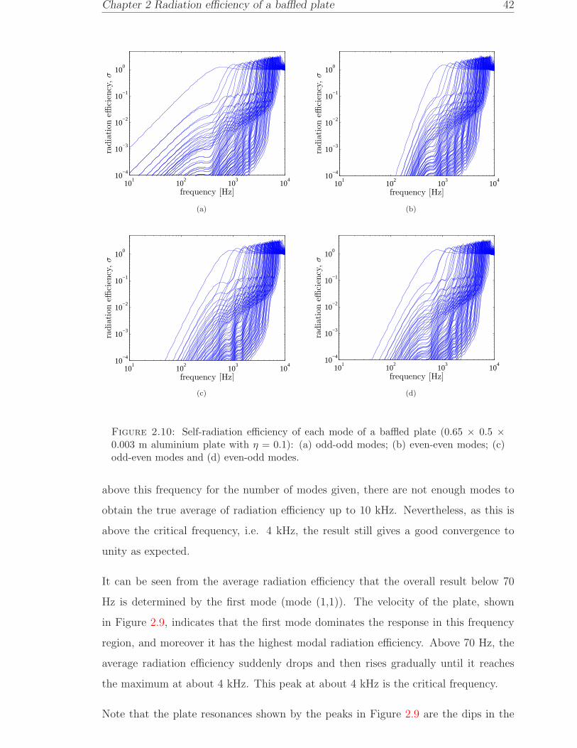
Chapter 2 Radiation efficiency of a baffled plate 42
101
102
103
104
10−4
10−3
10−2
10−1
100
frequency [Hz]
radia
tion
effici
ency
,σ
(a)
101
102
103
104
10−4
10−3
10−2
10−1
100
frequency [Hz]
radia
tion
effici
ency
,σ
(b)
101
102
103
104
10−4
10−3
10−2
10−1
100
frequency [Hz]
radia
tion
effici
ency
,σ
(c)
101
102
103
104
10−4
10−3
10−2
10−1
100
frequency [Hz]
radia
tion
effici
ency
,σ
(d)
Figure 2.10: Self-radiation efficiency of each mode of a baffled plate (0.65 × 0.5 ×0.003 m aluminium plate with η = 0.1): (a) odd-odd modes; (b) even-even modes; (c)odd-even modes and (d) even-odd modes.
above this frequency for the number of modes given, there are not enough modes to
obtain the true average of radiation efficiency up to 10 kHz. Nevertheless, as this is
above the critical frequency, i.e. 4 kHz, the result still gives a good convergence to
unity as expected.
It can be seen from the average radiation efficiency that the overall result below 70
Hz is determined by the first mode (mode (1,1)). The velocity of the plate, shown
in Figure 2.9, indicates that the first mode dominates the response in this frequency
region, and moreover it has the highest modal radiation efficiency. Above 70 Hz, the
average radiation efficiency suddenly drops and then rises gradually until it reaches
the maximum at about 4 kHz. This peak at about 4 kHz is the critical frequency.
Note that the plate resonances shown by the peaks in Figure 2.9 are the dips in the

Chapter 2 Radiation efficiency of a baffled plate 43
radiation efficiency plot as seen in Figure 2.8. This is because the radiation efficiency
is inversely proportional to the mean-square velocity (see Eq.(1.2)).
Figure 2.10 shows the modal radiation efficiencies of the various modes, separated into
odd-odd, even-even, odd-even and even-odd modes. From Figure 2.8, the slope of
the average radiation efficiency at frequencies below 70 Hz is 20 dB/decade (σ ∝ k2).
It can be seen that this corresponds to the slope for the odd-odd modes, where the
first mode (1,1) is dominant. Acting like monopole sources below 250 Hz, the odd-
odd modes make the highest contributions to the sound radiation, see Figure 2.10(a).
The odd-even in Figure 2.10(c) and the even-odd modes in Figure 2.10(d), with 40
dB/decade slope below 250 Hz, act like dipole sources (σ ∝ k4). They radiate sound
less effectively than the odd-odd modes. Meanwhile the even-even modes resemble
a quadrupole source behaviour. They have the lowest contributions to the sound
radiation, with a slope of 60 dB/decade (σ ∝ k6) below 250 Hz, see Figure 2.10(b).
It is interesting to note that these slopes apply at low frequencies up to around 250
Hz. Above 250 Hz, where the greatest width of the plate (0.65 m) is more than half an
acoustic wavelength, the curves are more complex, due to interference effect between
the travelling waves that leads to a spatial variation in amplitude, before each rising
to a peak at a frequency where the acoustic wavenumber equals the plate wavenumber
in their mode.
2.4.2 Mode regions
From Figure 2.8, the fluctuation seen in the radiation efficiency between the first
peak at low frequency (70 Hz) and the critical frequency is dominated by the ’corner’
modes (mπ/a > k and nπ/b > k) and ’edge’ modes (mπ/a > k, nπ/b < k or
mπ/a < k, nπ/b > k). For corner modes the sound is radiated effectively from the
plate corners, while the edge modes radiate sound from along the two plate edges
on opposite sides. Close to the critical frequency where the radiation efficiency rises
dramatically, all four edges of the plate effectively become a good radiator (mπ/a <
k, nπ/b < k; but ((mπ/a)2 + (nπ/b)2)1
2 > k) [4, 11]. Above the critical frequency, the
whole plate surface effectively radiates sound into the air. Figure 2.11(a) illustrates
the classification of mode regions in wavenumber space and Figure 2.11(b) shows the

Chapter 2 Radiation efficiency of a baffled plate 44
kx
ky
k
(m /a)
A
B
C
D
E
A: corner modes
B: x-edge modes
C: y-edge modes
D: xy-edge modes
E: surface modes
(n /b)
(a)
monopole
characteristic corner mode edge mode
supersonic
1 2 3
(b)
Figure 2.11: (a) classification of modes in wavenumber space relative to the acousticwavenumber k and (b) example of mode regions in the radiation efficiency curve.
regions in the radiation efficiency curve for the example of the plate given above,
but now plotted against the normalised frequency Ω = f/fc. Note that the curve
in Figure 2.11(b) is only applicable for thin plates with a moderate aspect ratio,
0.1 ≤ γ ≤ 1 (γ = a/b, a ≤ b). For a smaller plate dimensions with a greater thickness,
the corner and edge mode regions will be narrower. The radiation efficiency curve for
the case of a strip type plate (γ ≤ 0.1) can be seen in [12].

Chapter 2 Radiation efficiency of a baffled plate 45
The boundaries 1,2, and 3 in Figure 2.11(b) in terms of non-dimensional frequency Ω
are given by [4, 10]
Ω1 =π2B
c2ρptp
(1
a2+
1
b2
)
Ω2 =6π
cPs
(B
ρptp
)1/2
(2.62)
Ω3 = 0.5
where Ps is the perimeter of the plate. In terms of frequency f , Eq.(2.62) can be
written as
f1 =π
2
√B
ρptp
(1
a2+
1
b2
)
f2 =3c
Ps
(2.63)
f3 =fc
2
It can be seen from Eq.(2.63) that the boundary between corner and edge mode regions
(f2) depends only on the plate dimensions and not on the plate thickness.
In this thesis, the terminology ”fundamental mode”, ”corner mode” and ”edge mode”
regions will be used to denote the frequency region in the radiation efficiency. In
the remainder of the thesis, all results will be plotted as a function of dimensional
frequency (Eq.(2.63)). This is chosen because, although non-dimensional frequency
can eliminate the critical frequency, it does not eliminate the influence of bending
stiffness, mass or thickness, as seen in Eq.(2.62).
2.4.3 Effect of damping
Figure 2.12 presents the average radiation efficiency for various values of the damping
loss factor. This shows that the significant effect of damping on the sound radiation
lies in the corner and edge mode regions. It can also be seen that the radiation from the
first mode, which has the form of a monopole source, is not affected by the damping.
The radiation efficiency is also independent of the damping above the critical frequency.
However, the greatest damping effect can be seen between around 450 Hz and 4 kHz,
i.e. in the edge mode region.
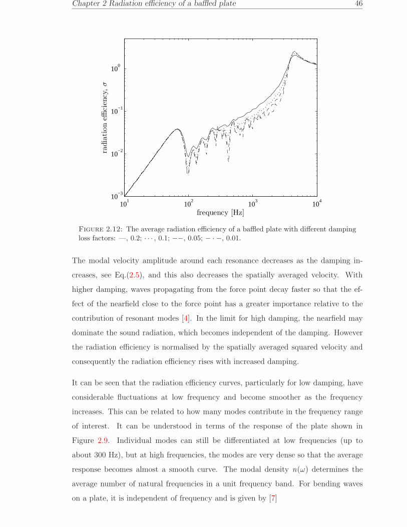
Chapter 2 Radiation efficiency of a baffled plate 46
101
102
103
104
10−3
10−2
10−1
100
frequency [Hz]
radia
tion
effici
ency
,σ
Figure 2.12: The average radiation efficiency of a baffled plate with different dampingloss factors: —, 0.2; · · · , 0.1; −−, 0.05; − · −, 0.01.
The modal velocity amplitude around each resonance decreases as the damping in-
creases, see Eq.(2.5), and this also decreases the spatially averaged velocity. With
higher damping, waves propagating from the force point decay faster so that the ef-
fect of the nearfield close to the force point has a greater importance relative to the
contribution of resonant modes [4]. In the limit for high damping, the nearfield may
dominate the sound radiation, which becomes independent of the damping. However
the radiation efficiency is normalised by the spatially averaged squared velocity and
consequently the radiation efficiency rises with increased damping.
It can be seen that the radiation efficiency curves, particularly for low damping, have
considerable fluctuations at low frequency and become smoother as the frequency
increases. This can be related to how many modes contribute in the frequency range
of interest. It can be understood in terms of the response of the plate shown in
Figure 2.9. Individual modes can still be differentiated at low frequencies (up to
about 300 Hz), but at high frequencies, the modes are very dense so that the average
response becomes almost a smooth curve. The modal density n(ω) determines the
average number of natural frequencies in a unit frequency band. For bending waves
on a plate, it is independent of frequency and is given by [7]

Chapter 2 Radiation efficiency of a baffled plate 47
101
102
103
104
10−2
10−1
100
101
102
frequency [Hz]
MO
F
Figure 2.13: Modal overlap factor of the plate (0.65 × 0.5 × 0.003 m aluminium platewith η = 0.1).
n(ω) = 0.276S
tpcL(2.64)
where S is the plate area, tp is the plate thickness and cL =√E/ρp(1 − ν2) is the
longitudinal wavespeed in the plate. The modal overlap factor is given by
MOF = n(ω)ωη (2.65)
where η is the damping loss factor. This is shown in Figure 2.13 for η = 0.1. This
indicates that MOF = 1 occurs at around 300 Hz. For a flat plate at high frequency,
where MOF ≫ 1, the contribution of single modes is of less interest than the average
over several modes. In Figure 2.12 it can be seen that in this example the radiation
efficiency curves become smoother above 300 Hz for η = 0.2, 600 Hz for η = 0.1 and
1200 Hz for η = 0.05, i.e. for MOF > 2.
2.4.4 Calculation time
Considering Eq.(2.22) in the spatial domain approach, the modal radiation efficiency is
calculated by integrating over a hemisphere of farfield positions. Using the wavenumber
domain scheme, the radiation efficiency is found directly for each wavenumber, but

Chapter 2 Radiation efficiency of a baffled plate 48
integration is then performed over wavenumber components which contribute to the
radiated sound. This method can also be used to plot the spectrum of the plate
velocity [4] as a function of wavenumber. This gives a better insight into the mechanism
of sound radiation.
Both methods involve double integrals. However in the spatial approach, the calcula-
tion has to deal with integrating factors of the form of sin(sin(A) cos(B)) as expressed
in Eq.(2.10), Eq.(2.22) and (2.23). To obtain a good accuracy of result, this form
must be solved with a good resolution of integration segments. Consequently, this in-
creases the calculation time. On the other hand in the wavenumber domain approach,
the calculation can be performed more efficiently as the integration only employs the
multiplication of the form of sin(A) or sin(B) (see Eq.(2.51)). Using a sufficient reso-
lution, not necessarily as fine as that used in the spatial domain, this method can save
a significant amount of calculation time.
Using MATLAB on a personal computer with the specification as in Table 2.1, the
calculation using the wavenumber domain approach with dα = dβ = 0.03 based on
400 modes takes approximately 8 minutes. For the spatial domain approach to have
a good convergence for frequencies up to 10 kHz, the error tolerance needed is 10−9.
With the same number of modes, the calculation of the radiation efficiency takes more
than 4 hours.
Despite the advantages of the FFT algorithm, the FFT approach is not found to
be an efficient method to calculate the radiation efficiency. It is time consuming as
the averaged Green’s function G needs to be constructed first before implementing
the inverse FFT of the plate velocity for each frequency, and later calculating the
acoustic power. As described in section 2.3, an accurate result needs a good resolution
of sample points and a larger baffle is required to overcome the bias error at low
frequency, especially in the first mode. The calculation of a single modal radiation
efficiency for a 64 × 64 points FFT takes 11 seconds. The equivalent calculation is
estimated to take more than 15 hours for the average over 400 modes. Therefore, the
calculation of the average radiation efficiency using this method has not been pursued
further here.

Chapter 2 Radiation efficiency of a baffled plate 49
Table 2.1: Computer specification used for calculation
Processor Pentium IVProcessor speed 3 GHz
Memory 0.99 GByte
2.5 Variability in radiation efficiency due to forcing
position
In the previous sections, the average radiation efficiency of a simply supported plate
was obtained from the summation over vibration modes. This method has the advan-
tage that information is provided about the contribution of the various modes to the
sound radiation. Moreover, no account is needed of the cross-modal radiation. How-
ever, often in practice the plate will be excited at a particular location and the sound
radiation may differ from the result averaged over all possible point force positions.
In this section the distribution of the radiation efficiencies from several discrete point
force positions is studied for a baffled plate. Despite the limitations of the FFT method
noted above, it is found to be efficient to use the FFT approach for this investigation
since it implicitly takes account of cross-modal radiation.
2.5.1 Method
The velocity of the plate v(x, y) due to a single point force position at a location
(x0, y0) can be calculated as a sum of modes. Recalling Eq.(2.3), the expression is
given by
v(x, y) =∞∑
m=1
∞∑
n=1
umnϕmn(x, y) (2.66)
where ϕmn is the mode shape function from Eq.(2.4) and umn is the complex velocity
amplitude of the mode from Eq.(2.5).
The velocity in the wavenumber domain V (kx, ky) can then be obtained by applying
the two-dimensional FFT to v(x,y). Therefore, for each frequency, the FFT method
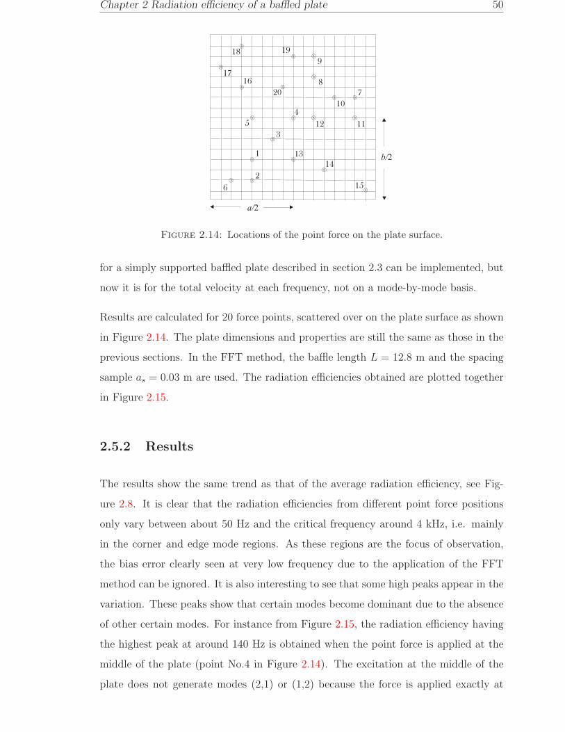
Chapter 2 Radiation efficiency of a baffled plate 50
b/2
a/2
1
6
2
3
15
5
7
8
9
10
1112
13
14
4
16
20
1918
17
Figure 2.14: Locations of the point force on the plate surface.
for a simply supported baffled plate described in section 2.3 can be implemented, but
now it is for the total velocity at each frequency, not on a mode-by-mode basis.
Results are calculated for 20 force points, scattered over on the plate surface as shown
in Figure 2.14. The plate dimensions and properties are still the same as those in the
previous sections. In the FFT method, the baffle length L = 12.8 m and the spacing
sample as = 0.03 m are used. The radiation efficiencies obtained are plotted together
in Figure 2.15.
2.5.2 Results
The results show the same trend as that of the average radiation efficiency, see Fig-
ure 2.8. It is clear that the radiation efficiencies from different point force positions
only vary between about 50 Hz and the critical frequency around 4 kHz, i.e. mainly
in the corner and edge mode regions. As these regions are the focus of observation,
the bias error clearly seen at very low frequency due to the application of the FFT
method can be ignored. It is also interesting to see that some high peaks appear in the
variation. These peaks show that certain modes become dominant due to the absence
of other certain modes. For instance from Figure 2.15, the radiation efficiency having
the highest peak at around 140 Hz is obtained when the point force is applied at the
middle of the plate (point No.4 in Figure 2.14). The excitation at the middle of the
plate does not generate modes (2,1) or (1,2) because the force is applied exactly at

Chapter 2 Radiation efficiency of a baffled plate 51
101
102
103
104
10−3
10−2
10−1
100
frequency [Hz]
radia
tion
effici
ency
,σ
Figure 2.15: Distribution of radiation efficiency over 20 point force positions on theplate (0.65 × 0.5 × 0.003 m aluminium plate with η = 0.1).
_
+
F
a
b
a
F
Figure 2.16: Excitation at the node point of mode (2,1).
the nodal point of these modes. This is illustrated in Figure 2.16. Mode (1,1) then
becomes dominant in the response over a wider frequency range, leading to a higher
overall radiation efficiency. That is why the knowledge of modes of vibration is useful
at low frequencies especially when structural sensors and actuators are embedded in a
structure in active control systems to reduce the sound radiation [4].
Figure 2.17 shows the range of the variation from the results such as Figure 2.15
corresponding to the 10% and 90% bands at each frequency in narrow bands and
also in 13
octave bands. These are arranged with increasing damping (η = 0.05, η =
0.1, η = 0.2) from top to bottom to investigate the variation with damping loss factor.
As seen in the figure, the average radiation efficiency (calculated directly using the

Chapter 2 Radiation efficiency of a baffled plate 52
wavenumber domain method) lies among the variations. It can also be seen that there
is no significant change due to damping in the extent of the variation, except at a few
specific frequencies.
Figure 2.18 shows the averaged and 10/90 percentile curves of the radiation efficiency
for three different plate dimensions. These are calculated for different plate areas and
aspect ratios. On average, this also shows that the variation of the radiation efficiency
does not change significantly with the plate dimensions, although for a larger plate area
as in Figure 2.18(a)-(b), the corner mode region has a slightly greater range of radiation
efficiency compared with the same region in Figure 2.18(c)-(d) and Figure 2.18(e)-(f).
However, a clear change of variation can be seen in Figure 2.19. This maintains the
plate dimensions but changes the thickness of the plate. It can be seen that the range
of variation, especially in corner mode region, reduces as the thickness increases. This
is due to the increasing of the plate bending stiffness as the thickness increases. For
the same input power, a stiffer plate has less modes which then produces a smaller
variation in the radiation efficiency.
Figure 2.20 shows the variability of the radiation efficiency for each case in narrow and
13
octave bands plotted in decibels (dB) given by
variability = 10 log10
(σ10
σ90
). (2.67)
where σ10 and σ90 denotes the radiation efficiency from 10 and 90 percentiles, respec-
tively. It can be seen that all cases produce similar pattern of variability where it is
high in corner mode region and then it declines in the edge mode region with increasing
frequency.
In Figure 2.20(a)-(b), no consistent effect of damping can be clearly observed, except
around the peaks at 160 Hz and 230 Hz where the variation increases with reduced
damping.
The same phenomenon can also be seen in In Figure 2.20(c)-(d). The variation is
similar except that the curves are shifted due to different location of the corner mode
region in frequency with differing plate dimensions (perimeter), see Eq.(2.63). From
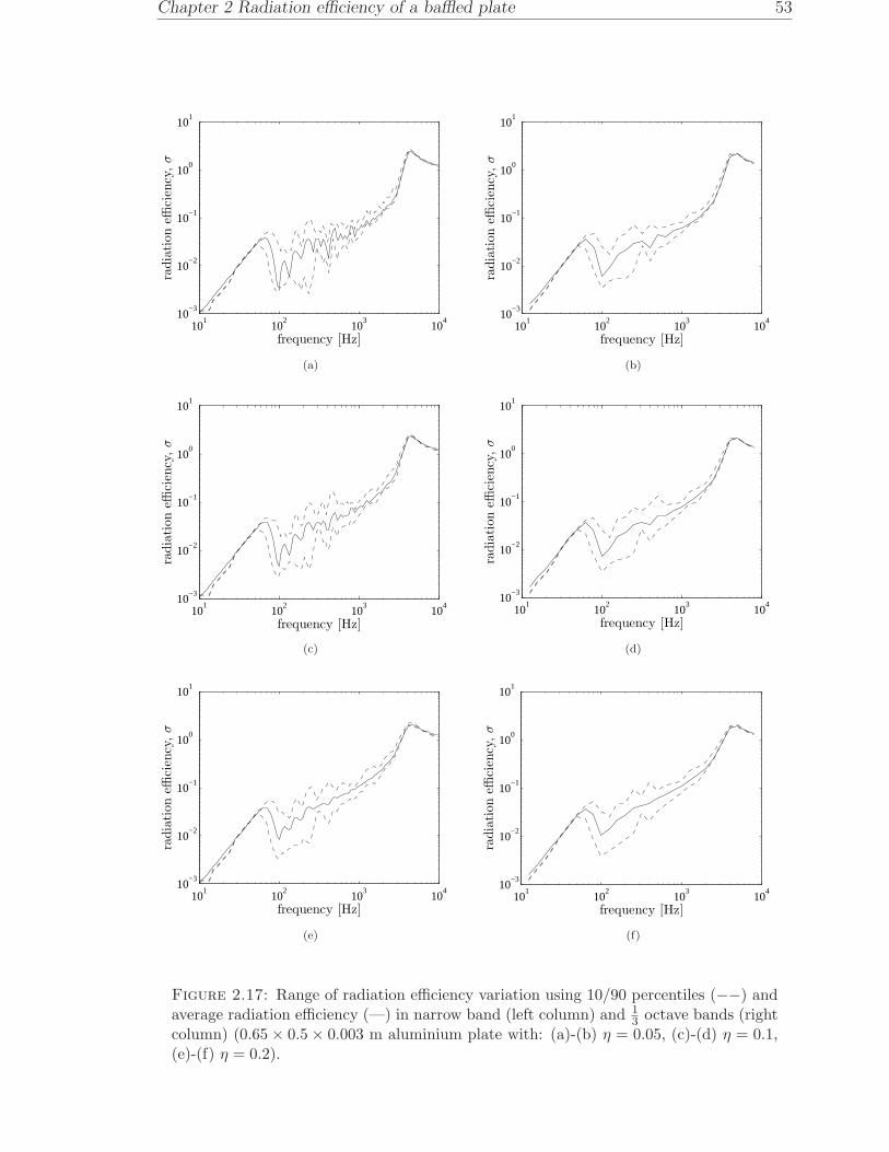
Chapter 2 Radiation efficiency of a baffled plate 53
101
102
103
104
10−3
10−2
10−1
100
101
frequency [Hz]
radia
tion
effici
ency
,σ
(a)
101
102
103
104
10−3
10−2
10−1
100
101
frequency [Hz]
radia
tion
effici
ency
,σ
(b)
101
102
103
104
10−3
10−2
10−1
100
101
frequency [Hz]
radia
tion
effici
ency
,σ
(c)
101
102
103
104
10−3
10−2
10−1
100
101
frequency [Hz]
radia
tion
effici
ency
,σ
(d)
101
102
103
104
10−3
10−2
10−1
100
101
frequency [Hz]
radia
tion
effici
ency
,σ
(e)
101
102
103
104
10−3
10−2
10−1
100
101
frequency [Hz]
radia
tion
effici
ency
,σ
(f)
Figure 2.17: Range of radiation efficiency variation using 10/90 percentiles (−−) andaverage radiation efficiency (—) in narrow band (left column) and 1
3 octave bands (rightcolumn) (0.65 × 0.5 × 0.003 m aluminium plate with: (a)-(b) η = 0.05, (c)-(d) η = 0.1,(e)-(f) η = 0.2).
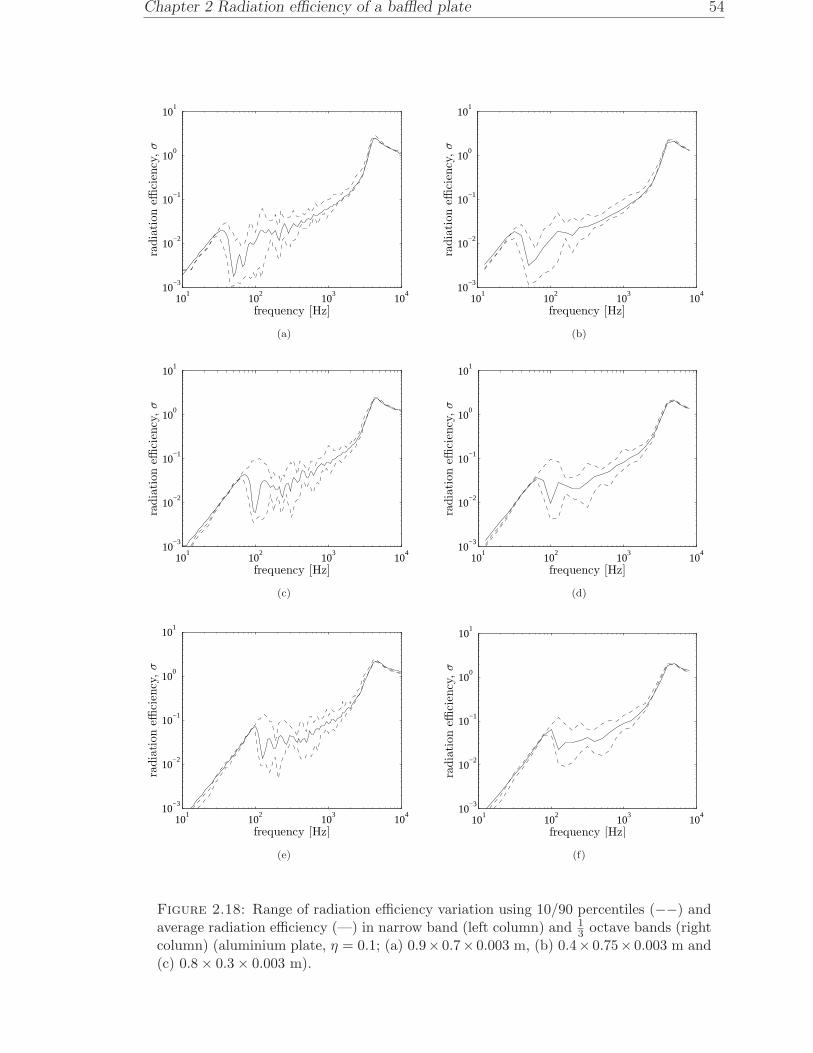
Chapter 2 Radiation efficiency of a baffled plate 54
101
102
103
104
10−3
10−2
10−1
100
101
frequency [Hz]
radia
tion
effici
ency
,σ
(a)
101
102
103
104
10−3
10−2
10−1
100
101
frequency [Hz]
radia
tion
effici
ency
,σ
(b)
101
102
103
104
10−3
10−2
10−1
100
101
frequency [Hz]
radia
tion
effici
ency
,σ
(c)
101
102
103
104
10−3
10−2
10−1
100
101
frequency [Hz]
radia
tion
effici
ency
,σ
(d)
101
102
103
104
10−3
10−2
10−1
100
101
frequency [Hz]
radia
tion
effici
ency
,σ
(e)
101
102
103
104
10−3
10−2
10−1
100
101
frequency [Hz]
radia
tion
effici
ency
,σ
(f)
Figure 2.18: Range of radiation efficiency variation using 10/90 percentiles (−−) andaverage radiation efficiency (—) in narrow band (left column) and 1
3 octave bands (rightcolumn) (aluminium plate, η = 0.1; (a) 0.9× 0.7× 0.003 m, (b) 0.4× 0.75× 0.003 m and(c) 0.8 × 0.3 × 0.003 m).

Chapter 2 Radiation efficiency of a baffled plate 55
101
102
103
104
10−3
10−2
10−1
100
101
frequency [Hz]
radia
tion
effici
ency
,σ
(a)
101
102
103
104
10−3
10−2
10−1
100
101
frequency [Hz]
radia
tion
effici
ency
,σ
(b)
101
102
103
104
10−3
10−2
10−1
100
101
frequency [Hz]
radia
tion
effici
ency
,σ
(c)
101
102
103
104
10−3
10−2
10−1
100
101
frequency [Hz]
radia
tion
effici
ency
,σ
(d)
101
102
103
104
10−3
10−2
10−1
100
101
frequency [Hz]
radia
tion
effici
ency
,σ
(e)
101
102
103
104
10−3
10−2
10−1
100
101
frequency [Hz]
radia
tion
effici
ency
,σ
(f)
Figure 2.19: Range of radiation efficiency variation using 10/90 percentiles (−−) andaverage radiation efficiency (—) in narrow band (left column) and 1
3 octave bands (rightcolumn) (aluminium plate, η = 0.1; (a) 0.65 × 0.5 × 0.003 m, (b) 0.65 × 0.5 × 0.005 mand (c) 0.65 × 0.5 × 0.008 m).

Chapter 2 Radiation efficiency of a baffled plate 56
101
102
103
104
0
5
10
15
20
frequency [Hz]
vari
ability
[dB
re1]
(a)
101
102
103
104
0
5
10
15
20
frequency [Hz]
vari
ability
[dB
re1]
(b)
101
102
103
104
0
5
10
15
20
frequency [Hz]
vari
ability
[dB
re1]
(c)
102
103
104
0
5
10
15
20
frequency [Hz]
vari
ability
[dB
re1]
(d)
101
102
103
104
0
5
10
15
20
frequency [Hz]
vari
ability
[dB
re1]
(e)
102
103
104
0
5
10
15
20
frequency [Hz]
vari
ability
[dB
re1]
(f)
Figure 2.20: Variability of radiation efficiency of an aluminium rectangular plate from10/90 percentiles in narrow band (left column) and 1
3 octave bands (right column):(a)-(b) 0.65 × 0.5 × 0.003 m; · · · η = 0.01, —η = 0.05, − − η = 0.1, (c)-(d) η = 0.1;—0.9× 0.7× 0.003 m, −− 0.4× 0.75× 0.003 m, · · · 0.8× 0.3× 0.003 m, (e)-(f) η = 0.1;—0.65 × 0.5 × 0.003 m, −− 0.65 × 0.5 × 0.005 m, · · · 0.65 × 0.5 × 0.008 m.

Chapter 2 Radiation efficiency of a baffled plate 57
Figure 2.20(b) and Figure 2.20(d), it is shown that for a 3 mm thick plate, the variation
of the radiation efficiency in 13
octave bands is around ±5 dB in the corner mode region.
Figure 2.20(e)-(f) shows the effect of the plate thickness on the variability. It is clearly
shown that the variability reduces as the plate thickness increases.
Another interesting phenomenon is that the variability is lower at the plate resonances.
From Figure 2.20(a), one can note that the dips in the variability, for example around
140 Hz and 190 Hz, correspond to peaks in the mean-square velocity of the plate,
i.e. the resonances, as seen in Figure 2.9. Conversely, one can see that the peaks in
the variability correspond to the dips in the mean-square velocity of the plate, not to
resonances. A similar phenomenon occurs in each case in Figure 2.18 and Figure 2.19.
2.6 Conventional modal-average radiation efficiency
Besides the analytical method described in the previous sections, predictions of the
sound radiation from a rectangular plate set in an infinite baffle are widely used,
particularly using the simple modal-average formulae of Maidanik [5]. This approach
is more efficient although more restricted in its assumptions. This model was based on
the assumption of equal modal vibration energy in a number of modes in a frequency
band (requiring a high modal density and an average over force locations) for a lightly
damped plate. The formulae have been summarized in [70] as follows

Chapter 2 Radiation efficiency of a baffled plate 58
σ =
4S
c2f 2 , f < f1,1, f1,1 =
π
2
√B
ρptp
(1
a2+
1
b2
)
4π2
c2S
B
ρptp, f1,1 < f < fe, fe =
3c
Ps
Psc
4π2Sfc
×(1 − α2) ln
(1 + α
1 − α
)+ 2α
(1 − α2)3/2, fe < f < fc, α =
√f
fc
0.45
√Psfc
c, f = fc
(1 − fc
f
)−1/2
, f > fc
(2.68)
where Ps is the perimeter of the plate, f1,1 is the fundamental frequency of the plate,
B is the bending stiffness, ρptp is the mass per unit area of the plate and fc is the
critical frequency.
The first term is the monopole characteristic of the fundamental mode. This has also
been derived by Wallace [6] for the radiation efficiency below the fundamental natural
frequency
σ1,1 =32k2S
π5=
128
π3c2Sf 2 ≈ 4S
c2f 2 (2.69)
The second term is the approximation for the corner mode region. However, according
to Leppington et al. [11] and Xie et al. [12], the first and second terms are only valid
for moderate aspect ratio, 0.1 ≤ γ ≤ 1 (γ = a/b, a ≤ b). For the case of a strip
(γ ≤ 0.1), the edge modes will dominate the corner mode region.
The third term in Eq.(2.68) is the edge mode region. For this region, a second term is
presented in [70] but this is often neglected and is not presented here.
For a point-excited plate with a higher damping loss factor η, the effect of damping
can be included into the formulae by introducing an equivalent radiation efficiency to
account for the near-field of a point force [4, 7] i.e.

Chapter 2 Radiation efficiency of a baffled plate 59
σn =4f
πfc
η, f < fc (2.70)
As explained in Section 2.4, when the damping increases, the plate displacement be-
comes concentrated only in the vicinity of the driving force. Therefore for a plate with
high damping, it can be misleading to average the plate surface velocity when the
velocity which is relatively far from the excitation point is much less than that near
the excitation point. Thus according to Eq.(1.2) the radiation efficiency increases as
the spatially averaged mean-square velocity decreases due to the increased damping,
assuming that the sound power from the near-field is unchanged. Eq.(2.70) supports
this assumption. Therefore it is less appropriate to judge the radiated noise from a
plate having a high damping by its ’radiation efficiency’ rather than by its radiated
’sound power’ per unit mean square force. In other words, the definition of ’radiation
efficiency’ is less useful if a plate has a high damping.
The prediction of the radiation efficiency including the effect of damping can be written
as
σ = σ0 + σn (2.71)
where σ0 is the radiation efficiency for a very lightly damped plate. This technique
has been implemented by Xie et al. [12] and has been compared with the prediction
results from the modal summation approach. Figure 2.21 reproduces the results for
the plate geometry considered here for various damping loss factors. This shows a
good agreement over a wide range of frequency. The prediction from Eq.(2.68, 2.70,
2.71) overestimates the dips in the corner mode region and also underestimates the
result at around 100 Hz which is dominated by the first mode.
2.7 Summary
Several analytical and numerical methods for calculating the radiation efficiency of a
vibrating plate set in an infinite baffle have been implemented and evaluated. It was
found that the wavenumber domain approach is the most effective method to calculate
the radiation efficiency, particularly in terms of the summation of the modal responses.

Chapter 2 Radiation efficiency of a baffled plate 60
101
102
103
104
10−3
10−2
10−1
100
frequency [Hz]
radia
tion
effici
ency
,σ
Figure 2.21: The average radiation efficiency of a simply supported baffled plate fromEq.(2.71) (thin line, blue) and the modal summation approach (thick line) : —η = 0.05,− · −η = 0.1, −−η = 0.3, · · · η = 0.5.
The spatial domain approach needs a higher resolution of integration segments to
obtain a result with a good accuracy, which increases the calculation time considerably.
The FFT method is also not effective where more integration segments are needed to
define the baffle. At low frequency, this requires a larger baffle and hence more sample
points to overcome the bias error due to the overlapped pressure. Moreover, a finer
resolution is needed to give a good accuracy for higher modes which are important at
high frequencies.
The variability in radiation efficiency of a typical plate due to variations in the location
of a single forcing point is found to be higher in the corner mode region. For 3 mm thick
plate, the variation relative to the average radiation efficiency is around a factor of
three (± 5 dB). This variation reduces as the plate thickness increases. It is important
to consider this variation in practice, for example in experimental statistical energy
analysis (SEA) where ’acoustic’ power is injected to a subsystem by an impact hammer
excitation at several locations on the plate [68].

Chapter 3
Radiation efficiency of an unbaffled
plate
In practice, vibrating plates are not set in a baffle and the opposite extreme of an
unbaffled plate is also important. As long as the sound field from one side can interact
with that from the other side of the plate, the plate condition can be categorised as
unbaffled. Unlike the baffled plate, where the velocity is known to be zero on the rigid
baffle, for the unbaffled plate the particle velocity is not known outside the plate region.
However, it is known that the pressure is zero beyond the plate in its plane. This makes
the task of solving the sound radiation from an unbaffled plate more complicated than
that from the baffled plate. This chapter discusses existing methods for calculating the
radiation efficiency from an unbaffled plate. Simply supported boundary conditions of
the plate are again used for simplicity.
3.1 Iterative scheme using the FFT
3.1.1 Algorithm
Continuing the FFT method for calculating the sound radiation for baffled plates,
Williams [29] also developed this method for application to unbaffled, finite plates.
This involves using an iterative scheme based on the Rayleigh integral and its inverse
61

Chapter 3 Radiation efficiency of an unbaffled plate 62
expressed in the wavenumber domain. The FFT algorithm is then implemented to
evaluate them.
Applying the averaged Green’s function used in the baffled plate calculation in section
2.3, Eq.(2.58) gives the Rayleigh integral formula as
p(x, y, 0) = jωρF−1[V (kx, ky)G(kx, ky, 0)
](3.1)
Inverting Eq.(3.1) gives
v(x, y) = −(j/ωρ)F−1[P (kx, ky)/G(kx, ky, 0)
](3.2)
In the case of a baffled plate, the velocity is defined on the plate and is zero on
the baffle. This velocity is then used to determine the pressure everywhere. For an
unbaffled plate, neither the velocity nor the pressure are fully known and therefore
an iterative procedure is employed. The velocity is used to estimate the pressure on
the plate, and then the pressure is used to calculate the velocity beyond the plate.
Eq.(3.1) and (3.2) are the basic formulae used in the iteration process, as explained
below.
Assuming P is the plate region and E is the exterior region in the plane of the plate,
the mixed boundary condition for the unbaffled plate is v(x, y) = vi(x, y) on P and
p(x, y, 0) = 0 on E, where vi(x, y) is the given velocity. Note that in the FFT method,
E is only defined over an aperture of dimensions L× L.
The following iteration algorithm is used:
1. Start with the boundary condition for the baffled plate, i.e. v(x, y) = vi(x, y)
on P and v(x, y) = 0 on E on the plane at z = 0. For a simply supported
plate, Eq.(2.3) is used for vi(x, y). Implement the two dimensional FFT to find
V (kx, ky) (see section 2.3).
2. Use Eq.(3.1) to obtain p(x, y, 0). Retain this solution for P but set p(x, y, 0) = 0
on E.

Chapter 3 Radiation efficiency of an unbaffled plate 63
3. Find P (kx, ky) using the FFT and calculate the new v(x, y) for the whole plane
at z = 0 from Eq.(3.2).
4. Check the root mean square error (RMSE) of the reconstructed velocity field on
P from
ǫ =
√√√√ 1
N
N∑
0
| [v(x, y) − vi(x, y)] |2 (3.3)
where N is the total number of points considered on the plate region P.
5. If the RMSE is more than a certain tolerance, the iteration is repeated from the
first step by setting v(x, y) = vi(x, y) on P and leaving v(x, y) unchanged on E.
When the iteration is stopped, the boundary condition in the exterior region E,
p(x, y, 0) = 0 should also be closely achieved. Williams [29] found that for RMSE
less than 0.005, for a unit maximum amplitude of vi(x, y), the pressure magnitude on
E was generally three orders of magnitude below its maximum value on P.
Equivalent approaches for calculating the radiated power as those used for the baffled
plates can be employed, either by integrating over the spatial domain or over the
wavenumber domain using Eq.(2.59) or Eq.(2.60) respectively.
3.1.2 Convergence problem
Figure 3.1 plots the radiation efficiency of mode (1,1) using both approaches (spatial
or wavenumber domains) to calculate the radiated power (Eq.(2.59) and Eq.(2.60))
for a plate having the same dimensions and properties as in the previous sections.
From Figure 3.1(a) and (c), it can be seen that using the spatial domain integration,
the calculation results in a discontinuity below 100 Hz. Some results are actually
negative. This limitation of using the spatial domain could be because the calculation
includes all the wavenumbers; those outside the radiation circle that contribute to the
non-propagating waves may not cancel each other at low frequencies due to numerical
inaccuracies. Meanwhile, positive results are obtained over the whole frequency range
using the wavenumber domain integration for as = 0.1 m, but the slope of the graph
deviates below 50 Hz for L = 6.4 m. This is due to a bias error from the replicated

Chapter 3 Radiation efficiency of an unbaffled plate 64
101
102
103
104
10−8
10−6
10−4
10−2
100
frequency [Hz]
radia
tion
effici
ency
,σ
(a)
101
102
103
104
10−8
10−6
10−4
10−2
100
frequency [Hz]
radia
tion
effici
ency
,σ
(b)
101
102
103
104
10−8
10−6
10−4
10−2
100
frequency [Hz]
radia
tion
effici
ency
,σ
(c)
101
102
103
104
10−8
10−6
10−4
10−2
100
frequency [Hz]
radia
tion
effici
ency
,σ
(d)
Figure 3.1: Radiation efficiency of mode (1,1) of a simply supported unbaffled plateusing the FFT method: (a) L = 6.4 m, as = 0.1 m, (b) L = 6.4 m, as = 0.05 m, (c)L = 12.8 m, as = 0.1 m and (d) L = 12.8 m, as = 0.05 m. −−, spatial domain; —,wavenumber domain (aluminium plate: 0.65 × 0.5 × 0.003 m, η = 0.1).
sources (outside the window L×L) as explained in section 2.3.1. This can be overcome
by using a larger aperture, i.e. in this case L is increased to 12.8 m, see Figure 3.1(c).
Convergence problems appear due to the sample spacing used, as. It is found that
using as ≤ 0.05 m, the results for both values of L fail to converge below 200 Hz as
seen in Figure 3.1(b) and (d). This might be due to the pressure discontinuity at the
plate edge. It is interesting to note that, for an unbaffled disc of radius a, Williams [29]
found that the mean square error did not converge for ka < 1.7. The results shown
here suggest that this is connected with the sample spacing as rather than the size of
the radiating plate. Unfortunately finer resolution is required to represent higher order
modes so that it appears that this iterative FFT method cannot cope satisfactorily
with higher order plate modes.
Chapter 3 Radiation efficiency of an unbaffled plate 65
3.2 Wavenumber domain using modal basis
Laulagnet [33] has proposed a numerical evaluation for calculating the sound radia-
tion from a simply supported unbaffled plate, where the pressure jump and the plate
displacement are developed as a sum over the plate modes. This method is explained
in this section.
3.2.1 Derivation of equations
Consider a flat thin unbaffled plate with a surface area Sp located in an infinite medium,
excited by a harmonic force distribution F (x, y) of angular frequency ω. ∆p(x, y) is
the difference of the acoustic surface pressure on the two side of the plate. Thus the
pressure jump across the plate due to the transverse motion is given by
∆p(x, y) = p−(x, y) − p+(x, y) (3.4)
where p−(x, y) and p+(x, y) are the surface pressure at z = 0− and z = 0+ respectively.
By symmetry p− = −p+.
The force distribution is assumed to act normal to the plate. One can apply the
equation of motion expressed as
B∇4w(x, y) −mpω2w(x, y) = F (x, y) + ∆p(x, y) (3.5)
where B is the bending stiffness, mp is the mass per unit area, w(x,y) is the transverse
displacement of the plate and ∇4 is given by
∇4 =∂4
∂x4+
2∂4
∂x2 ∂y2+
∂4
∂y4(3.6)
The pressure anywhere in the volume encompassing the plate can be found by using
the Green’s function, see Figure 3.2. Applying the Kirchhoff-Helmholtz (K-H) integral
theorem, the pressure in the surrounding fluid can be expressed by [4, 71]

Chapter 3 Radiation efficiency of an unbaffled plate 66
x
y
z
Q
M
F x,y( )
Sp
Sv
nQ
V
Figure 3.2: A simply supported plate enclosed by a volume V in the medium with itsbounding surface Sv.
p(M) =
∫
Sv
(p(Q)
∂G(Q,M)
∂nQ
−G(Q,M)∂p
∂nQ
)dSv (3.7)
where M denotes a point in the medium, nQ is the normal to the surface taken at
point Q on the plate, G(Q,M) = e−jkR/4πR is the free-field Green’s function with R
the distance between points Q and M . The surface Sv covers both sides of the plate
plus a surface at infinity.
Considering that only outgoing waves from the plate are allowed in the calculation,
the surface integral in Eq.(3.7) can be reduced to Sp, i.e. the whole surface of the
plate, Sp+ and Sp−. The surface at infinity is neglected since it is assumed that there
is no wave reflected back to the plate.
To help visualise this equation, the plate can be considered as consisting of discrete
elementary sources. The first term in the K-H equation is the dipole term representing
the presence of a body in obstructing the free passage of sound, both that generated by
its own normal motion (monopole source) and that incident upon it due to any other
sources [71]. As the sound pressure appears both in the left and right hand sides of the
equation, the sound pressure on the surface is a dependent variable. The elementary
sources cannot be treated as isolated monopole sources because they are operating
in the presence of other elementary sources from the remainder of the body [4]. The
second term represents the monopole contribution which is proportional to the nor-
mal acceleration of the plate surface. From the linearized equation of momentum

Chapter 3 Radiation efficiency of an unbaffled plate 67
conservation
∂p
∂nQ
= −ρ∂vn
∂t(3.8)
where vn is the normal plate velocity at Q.
The free field Green’s function G must satisfy
∇2G(Q,M) + k2G(Q,M) = δ(x− x0)δ(y − y0)δ(z − z0) (3.9)
where δ is the Dirac delta distribution; Q is at (x, y, z ) and M is at (x0, y0, z0). By
using the two dimensional spatial Fourier transform of Eq.(3.9), the Green’s function
can be expressed as [72]
G =j
8π2
∫ ∞
−∞
∫ ∞
−∞
ejkx(x−x0)ejky(y−y0)ejkz |z−z0|
kz
dkx dky (3.10)
where kz =√k2 − k2
x − k2y.
Restricting attention to the pressure at a point M above the plate (in the half space
V +, z0 ≥ 0), by considering the normal vector n parallel to the z -axis and pointing into
the fluid as illustrated in Figure 3.3, the K-H integral in Eq.(3.7) can be decomposed
as
p(M) =
∫
Sp+
p+(Q)∂G(Q,M)
∂zQ
dSp+ −∫
Sp−
p−(Q)∂G(Q,M)
∂zQ
dSp−
(3.11)
−∫
Sp+
G(Q,M)∂p+
∂zQ
dSp+ +
∫
Sp−
G(Q,M)∂p−
∂zQ
dSp−
where M ∈ V +.
Since the plate thickness is assumed to be very small compared with its length and
width, the normal velocity can be assumed equal on Sp+ and Sp−. From Eq.(3.8)
therefore ∂p/∂zQ is equal on both side of plate. Thus from Eq.(3.11), it is obtained
that∫
Sp
G(Q,M)
(∂p−
∂zQ
− ∂p+
∂zQ
)dSp = 0 , Q ∈ Sp (3.12)

Chapter 3 Radiation efficiency of an unbaffled plate 68
z
x n n
Sp+
Sp
Figure 3.3: Agreement of normal vector n on the plate
Therefore the monopole term vanishes, leaving only the dipole term, which is related
the discontinuity of the acoustic surface pressure
p(M) = −∫
Sp
∆p∂G(Q,M)
∂zQ
dSp (3.13)
Substituting Eq.(3.5) for ∆p into Eq.(3.13) yields
p(M) =
∫
Sp
[F (x, y) +mpω
2w(x, y) −B∇4w(x, y)] ∂G(Q,M)
∂zQ
dSp (3.14)
where Q ∈ Sp, M ∈ V +.
The two unknown fields, i.e. the acoustic field p(M) and the vibration of the plate
w(Q) in Eq.(3.14) can be related using Eq.(3.8). Since vn = jωw ejωt, in the plane of
the plate at z=0
∂p
∂z(M)
∣∣∣z=0
= ρ ω2w(M)
(3.15)
=
∫
Sp
[F (Q) +mpω
2w(Q) −B∇4w(Q)] ∂2G(Q,M)
∂zQ∂zM
dSp
where ∂/∂zQ and ∂/∂zM are the derivatives in the z direction at Q and M respectively.
Eq.(3.15) can be solved to find the displacement w.
3.2.2 Integral solution using modal summation
The displacement can be considered as the summation of a series of plate modes.
Similar to Eq.(2.3) for the velocity, the displacement can be expressed as

Chapter 3 Radiation efficiency of an unbaffled plate 69
w(x, y) =∞∑
m=1
∞∑
n=1
dmnϕmn(x, y) (3.16)
where dmn is the modal displacement amplitude and ϕmn is the associated mode shape
function as in Eq.(2.4).
The same form of modal series can also be applied for the excitation force,
F (x, y) =∞∑
m=1
∞∑
n=1
Fmnϕmn(x, y) (3.17)
where Fmn is the generalized force density for mode (m,n). This can be recovered by
multiplying by mpϕpq(x, y) and integrating over the plate area Sp
Fpq =mp
Mpq
∫
Sp
F (x, y)ϕpq(x, y) dx dy (3.18)
where Mpq is the modal mass as in Eq.(2.6) i.e.
Mpq =
∫
Sp
mp ϕ2pq dSp (3.19)
while∫
Spmp ϕmnϕpq dSp = 0 for m 6= p or n 6= q by orthogonality of the mode shapes.
Substituting Eq.(3.16) and Eq.(3.17) into Eq.(3.15), this can then be written as
ρω2
∞∑
m=1
∞∑
n=1
dmnϕmn(x0, y0) =
∫
Sp
∞∑
m=1
∞∑
n=1
[Fmnϕmn(x, y) +mpω
2dmnϕmn(x, y) −Bdmn∇4ϕmn(x, y)]
× ∂2G
∂z∂z0
(x, x0, y, y0, z = z0 = 0) dx dy (3.20)
By multiplying both sides by ϕpq and then integrating over the plate area, this yields

Chapter 3 Radiation efficiency of an unbaffled plate 70
ρω2
mp
dpqMpq =
∫
Sp
∫
Sp
∞∑
m=1
∞∑
n=1
[Fmnϕmn(x, y) +mpω
2dmnϕmn(x, y) −Bdmn∇4ϕmn(x, y)]
× ϕpq(x0, y0)∂2G
∂z∂z0
(x, x0, y, y0, z = z0 = 0) dx dy dx0 dy0 (3.21)
The mode shape ϕmn must satisfy
∇4ϕmn(x, y) = k4mnϕmn(x, y) =
(mpω
2mn
B
)ϕmn(x, y) (3.22)
where ωmn is the modal natural frequency. Substituting Eq.(3.22) into Eq.(3.21) yields
ρω2
mp
dpqMpq =∞∑
m=1
∞∑
n=1
[Fmn −mp(ω
2mn − ω2)dmn
]Cpqmn (3.23)
where Cpqmn is the acoustical cross-modal coupling term expressed by
Cpqmn =
∫
Sp
∫
Sp
ϕpq(x0, y0)∂2G
∂z∂z0
(x, x0, y, y0, z = z0 = 0)ϕmn(x, y)dxdydx0dy0 (3.24)
Substituting Eq.(3.10) into Eq.(3.24) and performing the two integrals over Sp yields
Cpqmn =j
8π2
∫ ∞
−∞
∫ ∞
−∞kz ϕ
∗pq(kx, ky)ϕmn(kx, ky) dkx dky (3.25)
where ϕmn(kx, ky) is the Fourier transform of the mode shape ϕmn(x, y) which is ex-
pressed by
ϕmn(kx, ky) =
∫ a
0
∫ b
0
ϕmn(x, y)e−j(kxx+kyy) dx dy (3.26)
For a simply supported plate, by substituting Eq.(2.4) into Eq.(3.19), the modal mass
Mpq gives
Mmn = mpSp
4(3.27)
Substituting Eq.(3.27) into Eq.(3.23) gives

Chapter 3 Radiation efficiency of an unbaffled plate 71
ρω2Sp
4dpq =
∞∑
m=1
∞∑
n=1
[Fmn −mp(ω
2mn − ω2)dmn
]Cpqmn (3.28)
where the modal natural frequency ωmn for a simply supported plate is given in
Eq.(2.7).
Evaluating analytically Eq.(3.26) for the simply supported mode shape gives
ϕmn(kx, ky) =ab
π2mn
[(−1)me−jµ − 1
(µ/(mπ))2 − 1
] [(−1)ne−jχ − 1
(χ/(nπ))2 − 1
](3.29)
where µ = kxa and χ = kyb. Note that this is identical with Φ in the spatial domain
as in Eq.(2.10). The derivation of Eq.(3.29) can be found in Appendix C.
For the conjugate form of the mode shape ϕ∗pq(x, y), the result is identical except that
the sign of the exponentials is changed from negative to positive, i.e.
ϕ∗pq(kx, ky) =
ab
π2pq
[(−1)pejµ − 1
(µ/(pπ))2 − 1
] [(−1)qejχ − 1
(χ/(qπ))2 − 1
](3.30)
From Eq.(3.26), it can be found that the integrand, with respect to kx, is an even
function when the mode orders (p,m) are of the same parity. Also, with respect to ky,
it is an even function when the mode orders (q, n) are of the same parity.
Therefore Eq.(3.25) can be simplified as
Cpqmn =j
2π2
∫ ∞
0
∫ ∞
0
kz ϕ∗pq(kx, ky)ϕmn(kx, ky) dkx dky (3.31)
when p and m are of the same parity and q and n are also of the same parity. The
remaining cases will have Cpqmn = 0.
Finally after substituting Eq.(3.29) and Eq.(3.30) into Eq.(3.31), it is found that
Cpqmn = Cmnpq =2j
pqmn
(ab
π3
)2 ∫ ∞
0
∫ ∞
0
kzΥ Ω dkx dky (3.32)
where Υ =1 − (−1)p cosµ
((µ/pπ)2 − 1)((µ/mπ)2 − 1), Ω =
1 − (−1)q cosχ
((χ/qπ)2 − 1)((χ/nπ)2 − 1).

Chapter 3 Radiation efficiency of an unbaffled plate 72
In practice, the infinite limits of the double layer integrals over kx and ky can be
limited, as in [33], to
kmaxx = (1 +K)
pπ
a, kmax
y = (1 +K)qπ
b(3.33)
for some K ≥ 1.
To avoid the singularities in the integration, the method used in the wavenumber
domain method in Section 2.2.2 can be applied.
From Eq.(3.28), after numerically evaluating Cmnpq, the displacement modal amplitude
dpq can be found by solving the linear matrix equation
[Cmnpq]mp(ω2pq − ω2)dpq + ρω2Sp
4[I] dpq = [Cmnpq]Fpq (3.34)
where [Cmnpq] is the complex cross coupling matrix, [I] is the identity matrix of size
N ×N and indicates a column vector.
After inverting Cmnpq this gives
mp(ω2pq − ω2)dpq + ρω2Sp
4[Cmnpq]
−1 dpq = Fpq (3.35)
Here, the matrix [Cmnpq] has to be inverted first. Thus the solution strongly depends
not only on the accuracy of the calculated [Cmnpq] but also on the size of the matrix
[Cmnpq] to be inverted. In order to simplify the calculation and avoid the matrix
inversion, an approximation can be applied in which the off-diagonal terms in Cmnpq
are neglected. In other words, as in the baffled plate case in section 2.1.2, only the
self-modal radiation contributions are taken into account in the calculation. The effect
of the cross-modal coupling is eliminated. Laulagnet [33] showed that, compared with
the exact solution, this gives a very good approximation in light fluid such as air. This
approach is still consistent with the objective of this thesis where the study is limited
only for the radiation into the air. However, it was found that for a plate with a heavy
fluid loading such as water, the off-diagonal terms become important, particularly for
the radiated sound power [33].

Chapter 3 Radiation efficiency of an unbaffled plate 73
Therefore Eq.(3.35) can written as
mp(ω2pq − ω2)dpq + ρω2Sp
4
(1
Cpqpq
)dpq = Fpq (3.36)
Multiplying by Sp/4 gives
Mpq(ω2pq − ω2)dpq + ρω2
(Sp
4
)2(1
Cpqpq
)dpq = Fpq (3.37)
where Mpq = mp(Sp/4) and Fpq = Fpq(Sp/4) are the generalized mass and the gener-
alized force for the simply supported plate. Fpq now has units of Newtons.
Eq.(3.37) can be solved to find the complex displacement amplitude of mode (p, q),
dpq. The plate velocity for each mode is given by
vpq(x, y) =∂w
∂t= jωdpqϕpq(x, y) (3.38)
where ϕpq is the value of the corresponding mode shape function.
The spatially average squared velocity of a mode can be expressed as
⟨|vpq|2
⟩=
1
Sp
∫
Sp
|vpq(x, y)|2 dx dy (3.39)
Substituting Eq.(3.38) for the case of a simply supported plate gives
⟨|vpq|2
⟩=ω2
4|dpq|2 (3.40)
For a plate immersed in light fluid, the fluid loading has a negligible effect on the
vibrational behaviour of the plate. The second term in Eq.(3.37) i.e. the fluid loading
part is very small compared with the first term. The displacement dpq can therefore
be calculated by neglecting this term.
Referring to Figure 3.3, the total radiated sound power from both sides of the plate
can be defined as

Chapter 3 Radiation efficiency of an unbaffled plate 74
W =1
2
∫
Sp
ℜ ∞∑
p=1
∞∑
q=1
p+(x, y)v∗pq(x, y) · n dSp+ + p−(x, y)v∗
pq(x, y) · n dSp−
=1
2
∫
Sp
ℜ ∞∑
p=1
∞∑
q=1
(p+(x, y) − p−(x, y))v∗pq(x, y)
dSp
= −1
2
∫
Sp
ℜ ∞∑
p=1
∞∑
q=1
∆p(x, y)v∗pq(x, y)
dSp (3.41)
As in Eq.(3.4), the acoustic pressure is determined from the pressure difference ∆p(x, y)
between the two sides of the plate surface. To obtain a convenient calculation, the
pressure difference ∆p(x, y) can also be written as a sum of plate mode shapes
∆p(x, y) =∞∑
m=1
∞∑
n=1
pmnϕmn(x, y) (3.42)
where pmn are the corresponding amplitudes.
Therefore by using the orthogonality relationship for the simply supported conditions,
the radiated sound power can be written as
W = −1
2
∫
Sp
ℜ ∞∑
m=1
∞∑
n=1
pmnϕmn × (jω)∞∑
p=1
∞∑
q=1
d∗pqϕpq
dSp
(3.43)
= −ω2
(Sp
4
)ℜj
∞∑
p=1
∞∑
q=1
ppqd∗pq
Substituting Eq.(3.42), Eq.(3.5) can then be written as
∞∑
m=1
∞∑
n=1
mp(ω2mn − ω2)dmnϕmn(x, y)
=∞∑
m=1
∞∑
n=1
Fmnϕmn(x, y) +∞∑
m=1
∞∑
n=1
pmnϕmn(x, y) (3.44)
Again, applying the orthogonality relationship yields
mp(ω2pq − ω2)dpq = Fpq + ppq (3.45)

Chapter 3 Radiation efficiency of an unbaffled plate 75
Eliminating ppq in Eq.(3.43) using Eq.(3.45)
W =ωSp
8ℜj
∞∑
p=1
∞∑
q=1
(Fpq −mp(ω
2pq − ω2)dpq
)d∗pq
(3.46)
In terms of the acoustic cross-modal coupling Cpqpq, from Eq.(3.37) the sound power
W can also be written as
W =ωSp
8ℜj
∞∑
p=1
∞∑
q=1
[ρω2
(Sp
4
)2(1
Cpqpq
)dpq
]d∗pq
(3.47)
The total radiation efficiency σ can be found from this using
σ =W
12ρcSp
∑∞p=1
∑∞q=1
⟨|vpq|2
⟩ (3.48)
where⟨|vpq|2
⟩is the spatially averaged squared velocity, averaged over all possible
forcing locations (x0, y0). As in Eq.(2.20), it is given by
⟨|vpq|2
⟩=
1
ab
∫ a
0
∫ b
0
⟨|vpq|2
⟩dx0 dy0 (3.49)
Eq.(3.48) is the average radiation efficiency which is defined as a summation over the
contributions of modes (modal summation approach). As in Eq.(2.25) in the baffled
plate case, here it is also assumed that the individual modes are uniformly excited si-
multaneously and each mode acts as an independent energy reservoir (uncorrelated) [7].
The same assumption should also be applied to the modal force Fpq in Eq.(3.18) where
all modes produce equal excitation energy.
The modal radiation efficiency σpq can be calculated from
σpq =Wpq
12ρcSp
⟨|vpq|2
⟩ (3.50)
where Wpq is the modal radiated sound power given by one term in Eq.(3.47)

Chapter 3 Radiation efficiency of an unbaffled plate 76
Wpq =ωSp
8ℜj
[ρω2
(Sp
4
)2(1
Cpqpq
)dpq
]d∗pq
(3.51)
The radiation efficiency of the unbaffled plate takes into account the fluid loading on
both sides of the plate but has been normalised only by the area of one side. To have
an equivalency to the radiation efficiency of the baffled plate, as a consequence, it has
to be further divided by two.
3.3 Results and comparison with baffled plate
Figure 3.4 shows example results for different mode orders, i.e. odd-odd, even-odd,
odd-even and even-even. The results for the baffled plate are also plotted for compar-
ison. The plate is a rectangular plate having the same dimensions and properties as
the baffled plate described in section 2.4. It can be seen that the radiation efficiency
is much reduced for the unbaffled plate at low frequencies. For mode (1,1) in Fig-
ure 3.4(a), the slope below the modal coincidence frequency is 40 dB/decade (σ ∝ k4)
instead of 20 dB/decade found for the baffled plate. This is a dipole type radiation.
A similar phenomenon can be seen for other types of modes where the slope at very
low frequency in the unbaffled plate is 20 dB/decade steeper than that of the baffled
plate. From Figure 3.4(b) and (c), the even-odd modes and the odd-even modes have
a dependency of 60 dB/decade (σ ∝ k6) at low frequencies. As in the baffled plate
case, the lowest radiation is found for the even-even mode as in Figure 3.4(d) where
the slope is 80 dB/decade (σ ∝ k8).
The difference between the radiation efficiency of the unbaffled plate and the baffled
plate can also be noted from the mathematical point of view. Eq.(3.32) for the acousti-
cal cross-modal coupling term in the unbaffled case is identical with Eq.(2.10) in the
baffled case. However, the former becomes the denominator due to the matrix inver-
sion in the equation of motion (Eq.(3.37)), while the latter becomes the numerator in
the radiation efficiency equation (Eq.(2.51)).
Figure 3.5 shows a result for the averaged radiation efficiency obtained using the modal
summation approach as in Eq.(3.48). The radiation efficiencies of individual modes
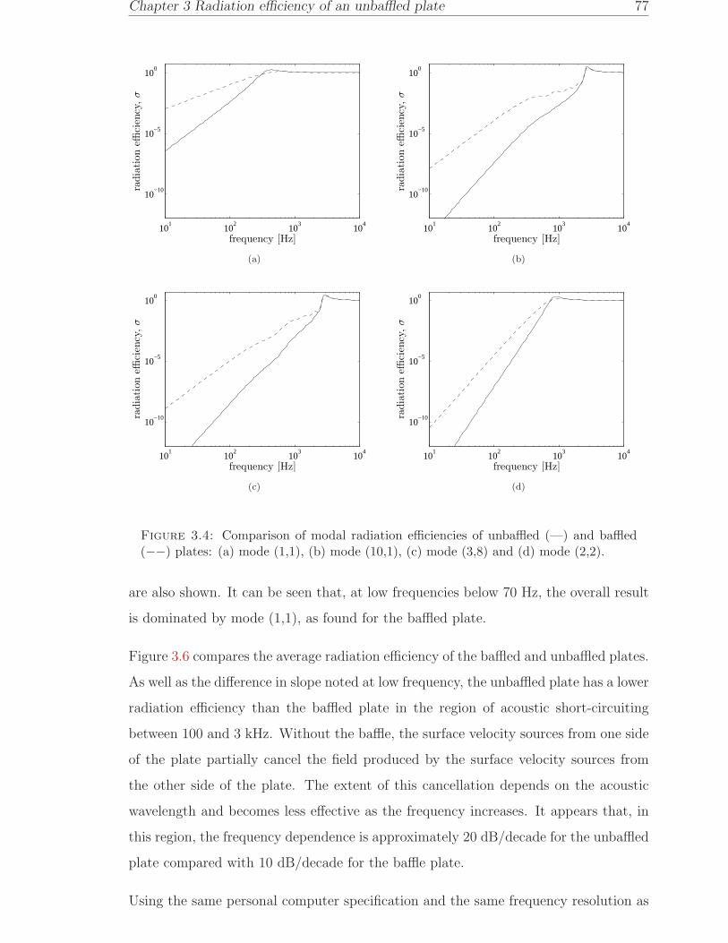
Chapter 3 Radiation efficiency of an unbaffled plate 77
101
102
103
104
10−10
10−5
100
frequency [Hz]
radia
tion
effici
ency
,σ
(a)
101
102
103
104
10−10
10−5
100
frequency [Hz]
radia
tion
effici
ency
,σ
(b)
101
102
103
104
10−10
10−5
100
frequency [Hz]
radia
tion
effici
ency
,σ
(c)
101
102
103
104
10−10
10−5
100
frequency [Hz]
radia
tion
effici
ency
,σ
(d)
Figure 3.4: Comparison of modal radiation efficiencies of unbaffled (—) and baffled(−−) plates: (a) mode (1,1), (b) mode (10,1), (c) mode (3,8) and (d) mode (2,2).
are also shown. It can be seen that, at low frequencies below 70 Hz, the overall result
is dominated by mode (1,1), as found for the baffled plate.
Figure 3.6 compares the average radiation efficiency of the baffled and unbaffled plates.
As well as the difference in slope noted at low frequency, the unbaffled plate has a lower
radiation efficiency than the baffled plate in the region of acoustic short-circuiting
between 100 and 3 kHz. Without the baffle, the surface velocity sources from one side
of the plate partially cancel the field produced by the surface velocity sources from
the other side of the plate. The extent of this cancellation depends on the acoustic
wavelength and becomes less effective as the frequency increases. It appears that, in
this region, the frequency dependence is approximately 20 dB/decade for the unbaffled
plate compared with 10 dB/decade for the baffle plate.
Using the same personal computer specification and the same frequency resolution as

Chapter 3 Radiation efficiency of an unbaffled plate 78
101
102
103
104
10−6
10−4
10−2
100
frequency [Hz]
radia
tion
effici
ency
,σ
Figure 3.5: Modal and average radiation efficiency of a simply supported unbaffledplate (0.65× 0.5× 0.003 m aluminium plate with η = 0.1): —modal radiation efficiency;
−average radiation efficiency.
101
102
103
104
10−6
10−4
10−2
100
frequency [Hz]
radia
tion
effici
ency
,σ
Figure 3.6: Comparison of average radiation efficiency between unbaffled (—) andbaffled (−−) plates (0.65 × 0.5 × 0.003 m aluminium plate with η = 0.1).
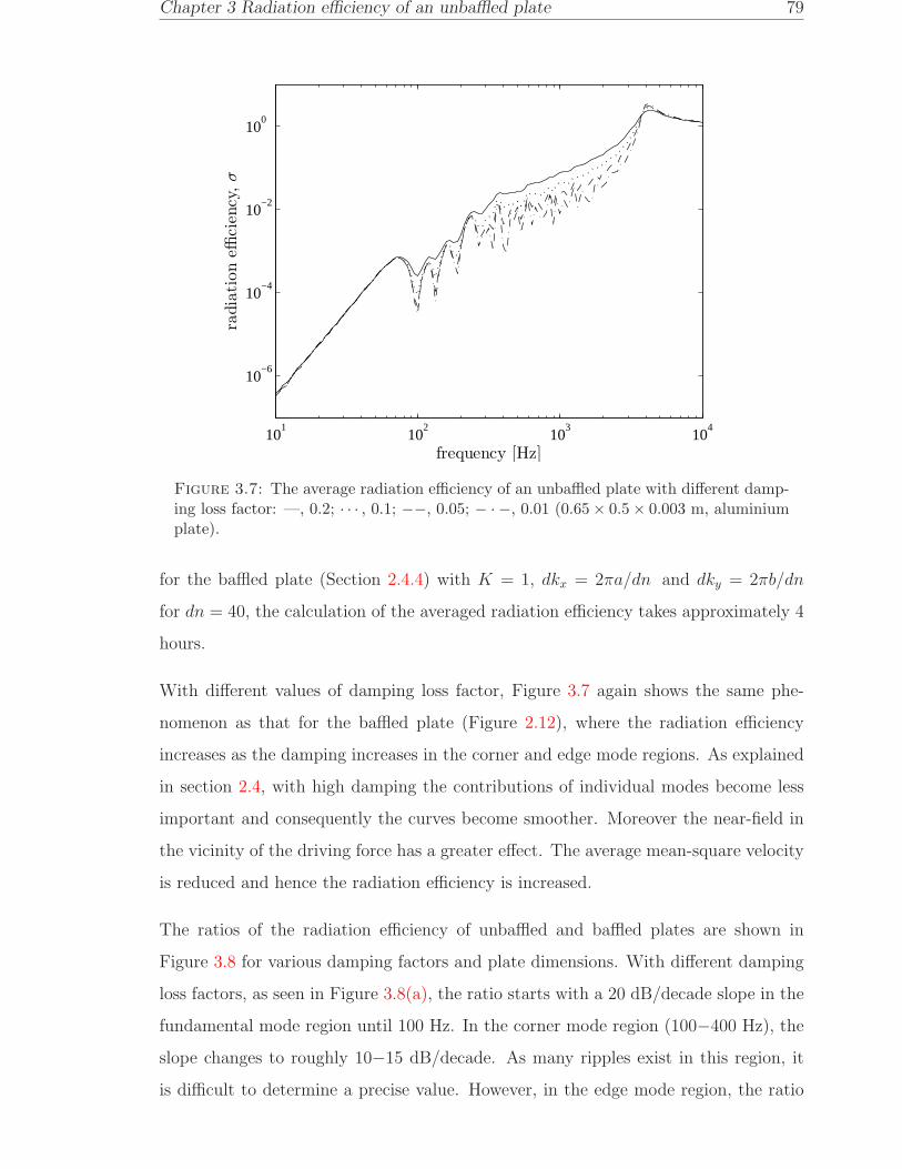
Chapter 3 Radiation efficiency of an unbaffled plate 79
101
102
103
104
10−6
10−4
10−2
100
frequency [Hz]
radia
tion
effici
ency
,σ
Figure 3.7: The average radiation efficiency of an unbaffled plate with different damp-ing loss factor: —, 0.2; · · · , 0.1; −−, 0.05; − · −, 0.01 (0.65 × 0.5 × 0.003 m, aluminiumplate).
for the baffled plate (Section 2.4.4) with K = 1, dkx = 2πa/dn and dky = 2πb/dn
for dn = 40, the calculation of the averaged radiation efficiency takes approximately 4
hours.
With different values of damping loss factor, Figure 3.7 again shows the same phe-
nomenon as that for the baffled plate (Figure 2.12), where the radiation efficiency
increases as the damping increases in the corner and edge mode regions. As explained
in section 2.4, with high damping the contributions of individual modes become less
important and consequently the curves become smoother. Moreover the near-field in
the vicinity of the driving force has a greater effect. The average mean-square velocity
is reduced and hence the radiation efficiency is increased.
The ratios of the radiation efficiency of unbaffled and baffled plates are shown in
Figure 3.8 for various damping factors and plate dimensions. With different damping
loss factors, as seen in Figure 3.8(a), the ratio starts with a 20 dB/decade slope in the
fundamental mode region until 100 Hz. In the corner mode region (100−400 Hz), the
slope changes to roughly 10−15 dB/decade. As many ripples exist in this region, it
is difficult to determine a precise value. However, in the edge mode region, the ratio

Chapter 3 Radiation efficiency of an unbaffled plate 80
starts with a slope of 4.7 dB/decade from 400 Hz up to about 3 kHz. Each curve then
has a different slope as it rises up to the critical frequency (4 kHz) depending on the
damping loss factor. It can also be seen that at the critical frequency, the ratio is more
than 0 dB. It means that the peak at the critical frequency is higher for an unbaffled
plate than for a baffled plate (see also Figure 3.6).
With constant plate damping and different plate dimensions, a roughly constant slope
can be seen in the results in the edge mode region, see Figure 3.8(b). Above the critical
frequency, the baffled and unbaffled results are identical.
3.4 Empirical formulae for radiation efficiency of
an unbaffled plate
The average radiation efficiency of an unbaffled plate obtained with a summation over
individual modes, presented in the previous section, is not efficient from a practical
point of view, considering the calculation time required. One solution is to develop
an empirical formula for the region below the critical frequency, based on the results
of the ratio of the radiation efficiencies of unbaffled and baffled plates. Considering
different frequency regions, as for the baffled plate, the empirical formulae for a simply
supported unbaffled plate are therefore derived below. In the proposed formula, σb
equals the radiation efficiency of a baffled plate in Eq.(2.71) in the corresponding
frequency region.
1. Below the fundamental mode, the monopole radiation in the baffled plate case
now becomes dipole radiation in the unbaffled plate case. By analogy with a
sphere of radius a, where a monopole has σ = (ka)2 and a dipole has σ =
(ka)4/4 [73], the formula can be expressed as
σub =4S2f 4
c4= σb
f 2S
c2, f < f1,1 (3.52)
2. In the corner mode region, the radiation efficiency of the unbaffled plate is found
to increase with approximately 20 dB/decade, see Figure 3.6. The second term

Chapter 3 Radiation efficiency of an unbaffled plate 81
101
102
103
104
−35
−30
−25
−20
−15
−10
−5
0
frequency [Hz]
σu
b/σ
b[d
Bre
1]
(a)
101
102
103
104
−35
−30
−25
−20
−15
−10
−5
0
frequency [Hz]
σub/σ
b[d
Bre
1]
(b)
Figure 3.8: Ratio between radiation efficiency of simply supported unbaffled and baf-fled plates: (a) 0.65 × 0.5 × 0.003 m; —η = 0.05, · · · η = 0.1, −−η = 0.2 and(b) η = 0.1; —0.65 × 0.5 × 0.003 m, −−0.325 × 0.5 × 0.003 m, − · −0.25 × 0.5 × 0.003m, · · · 0.9 × 0.2 × 0.003 m.
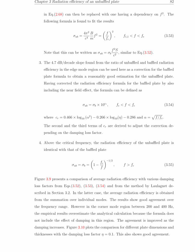
Chapter 3 Radiation efficiency of an unbaffled plate 82
in Eq.(2.68) can then be replaced with one having a dependency on f 2. The
following formula is found to fit the results
σub =4π2
c4B
mf 2 =
(f
fc
)2
, f1,1 < f < fe (3.53)
Note that this can be written as σub = σbf 2S
c2, similar to Eq.(3.52).
3. The 4.7 dB/decade slope found from the ratio of unbaffled and baffled radiation
efficiency in the edge mode region can be used here as a correction for the baffled
plate formula to obtain a reasonably good estimation for the unbaffled plate.
Having corrected the radiation efficiency formula for the baffled plate by also
including the near field effect, the formula can be defined as
σub = σb × 10cr , fe < f < fc (3.54)
where cr = 0.466 × log10 (α2) − 0.266 × log10(η) − 0.286 and α =√f/fc.
The second and the third terms of cr are derived to adjust the correction de-
pending on the damping loss factor.
4. Above the critical frequency, the radiation efficiency of the unbaffled plate is
identical with that of the baffled plate
σub = σb =
(1 − fc
f
)−1/2
, f > fc (3.55)
Figure 3.9 presents a comparison of average radiation efficiency with various damping
loss factors from Eqs.(3.52), (3.53), (3.54) and from the method by Laulagnet de-
scribed in Section 3.2. In the latter case, the average radiation efficiency is obtained
from the summation over individual modes. The results show good agreement over
the frequency range. However in the corner mode region between 200 and 400 Hz,
the empirical results overestimate the analytical calculation because the formula does
not include the effect of damping in this region. The agreement is improved as the
damping increases. Figure 3.10 plots the comparison for different plate dimensions and
thicknesses with the damping loss factor η = 0.1. This also shows good agreement.

Chapter 3 Radiation efficiency of an unbaffled plate 83
101
102
103
104
10−6
10−4
10−2
100
frequency [Hz]
radia
tion
effici
ency
,σ
Figure 3.9: The average radiation efficiency of a simply supported unbaffled plate fromEqs. (3.52), (3.53), (3.54) (thin line, blue) and the method by Laulagnet (thick line)(0.65 × 0.5 × 0.003 m: —η = 0.01, − · −η = 0.05, −− η = 0.1 and · · · η = 0.2).
For the purpose of presentation, for all the plotted graphs here, Maidanik’s formula is
used at the critical frequency.
3.5 Summary
Williams’ and Lauglagnet’s models for the sound radiation from an unbaffled rectan-
gular plate have been implemented and assessed. It has been shown that Williams’
iterative scheme has problems with convergence at low frequency. The model fails
to converge when a small sample spacing (finer resolution) is used. However such a
spacing would be required in order to calculate the radiation from higher order modes
of vibration. Therefore, this model is not considered suitable to calculate the radiation
efficiency of an unbaffled plate, especially for the multi-modal response.
Laulagnet’s model gives a good result for radiation efficiency even up to very high
frequency. The most important finding concerns a comparison of these results with
the radiation efficiency of a baffled plate up to the critical frequency. It has been
shown that below the critical frequency, due to the partial cancellation of the sound

Chapter 3 Radiation efficiency of an unbaffled plate 84
101
102
103
104
10−6
10−4
10−2
100
frequency [Hz]
radia
tion
effici
ency
,σ
(a)
101
102
103
104
10−6
10−4
10−2
100
frequency [Hz]
radia
tion
effici
ency
,σ
(b)
101
102
103
104
10−6
10−4
10−2
100
frequency [Hz]
radia
tion
effici
ency
,σ
(c)
101
102
103
104
10−6
10−4
10−2
100
frequency [Hz]
radia
tion
effici
ency
,σ
(d)
Figure 3.10: The average radiation efficiency of a simply supported unbaffled platefrom Eqs. (3.52), (3.53), (3.54) (−−) and the method by Laulagnet (—), η = 0.01:(a) 0.65 × 0.5 × 0.002 m, (b) 0.65 × 0.5 × 0.005 m, (c) 0.325 × 0.5 × 0.003 m and (d)1.3 × 0.5 × 0.003 m.
field between the two sides of the plate, the unbaffled plate radiates less sound than the
baffled plate. The difference is greater as the frequency reduces. Above the critical
frequency, there is no difference between the radiation from baffled and unbaffled
plates.
From the ratio between the radiation efficiency of baffled and unbaffled plates, em-
pirical formulae have been developed which have been shown to give good agreement
for the whole frequency range. The proposed empirical formulae are summarised as
follows.

Chapter 3 Radiation efficiency of an unbaffled plate 85
σub =
4S2
c4f 4 , f < f1,1,
f1,1 =π
2
√B
ρptp
(1
a2+
1
b2
)
(f
fc
)2
, f1,1 < f < fe, fe =3c
Ps
σb × 10cr , fe < f < fc, α =
√f
fc
cr = 0.466 log10 (α2) − 0.266 log10(η) − 0.286
(1 − fc
f
)−1/2
, f > fc
(3.56)

Chapter 4
Radiation efficiency of a
guided-guided plate
4.1 Introduction
In Chapters 2 and 3 results have been presented for simply supported plate boundaries.
It has been noted in Chapter 1 that some authors [15, 16, 17] suggest that 3 dB should
be added to the radiation efficiency for clamped boundaries. In this chapter, the
effect of changing boundary conditions is studied. However, rather than consider a
clamped (or free) edge for which the plate modes are more complicated [18] a guided
boundary is introduced. While a simply supported boundary has zero displacement
but unconstrained rotation, the guided boundary has zero rotation and unconstrained
displacement.
Thus the mode shapes consist of cosine functions given by
ϕmn(x, y) = cos(mπx
a
)cos(nπy
b
)(4.1)
The corresponding modal natural frequency is given by
ωmn =
(B
ρptp
)1/2 [(mπa
)2
+(nπb
)2]
(4.2)
86

Chapter 4 Radiation efficiency of a guided-guided plate 87
(a) (b)
Figure 4.1: Edge conditions: (a) Simply supported and (b) guided-guided.
as for the simply supported plate (Eq.(2.7)). However, modes also exist with m = 0
or n = 0.
Figure 4.1 illustrates both simply supported and guided-guided boundary conditions.
The aim of this chapter is to determine the effect of these boundary conditions on
the radiation efficiency, particularly for multi-modal responses, both for baffled and
unbaffled plates.
4.2 Baffled plate
The wavenumber decomposition approach as in Section 2.2 can be used to calculate
the radiation efficiency for the baffled plate case. For a guided-guided plate having
dimensions a × b, the spatial Fourier transform of the velocity distribution of mode
(m,n) in terms of the non-dimensional wavenumber α = kx/k and β = ky/k, as in
Eq.(2.45), yields
Vg−g(α, β) = umnΛg−gk−2(ε+ jϑ)(γ + jς) (4.3)
where
Λg−g =αβ[
α2 −(mπka
)2] [β2 −
(nπkb
)2]
and ε, ϑ, γ and ς are the same as in Section 2.2.
A further configuration can be considered in which the boundaries along the x -axes
of the plate are simply supported and those along the y-axes are guided. In this case,
the mode shape is
ϕmn(x, y) = sin(mπx
a
)cos(nπy
b
)(4.4)

Chapter 4 Radiation efficiency of a guided-guided plate 88
101
102
103
104
10−6
10−4
10−2
100
frequency [Hz]
radia
tion
effici
ency
,σ 1
2
1
1
2
2
3 33
(a)
101
102
103
104
10−6
10−4
10−2
100
frequency [Hz]
radia
tion
effici
ency
,σ
1 2
31
1
22
3
3
(b)
101
102
103
104
10−6
10−4
10−2
100
frequency [Hz]
radia
tion
effici
ency
,σ
1
2 3
1
1
2
2
3
3
(c)
101
102
103
104
10−6
10−4
10−2
100
frequency [Hz]
radia
tion
effici
ency
,σ
1
2
3
1
1
2
2
3
3
(d)
Figure 4.2: Modal radiation efficiencies of baffled plates. (a). 1:(1,1), 2:(3,3), 3:(9,9);(b). 1:(2,2), 2:(8,8), 3:(10,10); (c). 1:(1,2), 2:(2,3), 3:(2,9); (d). 1:(1,10), 2:(7,9), 3:(8,10)(0.65 × 0.5 × 0.003 m aluminium plate). —(ss−ss), −−(ss−g), − · −(g−g).
and the Fourier transform of the velocity in mode (m,n) is
Vss−g(α, β) = umnΛss−gk−2(ε+ jϑ)(γ + jς) (4.5)
where
Λss−g =jβ(mπka
)
[α2 −
(mπka
)2] [β2 −
(nπkb
)2]
Results for several modes are presented in Figure 4.2, some of which have also been
produced by Gompert [19]. It is shown that the guided-guided (g−g) plate has a
lower radiation efficiency than those from the simply supported-guided (ss−g) and
simply supported (ss−ss) plates for a given mode order. However, equal radiation

Chapter 4 Radiation efficiency of a guided-guided plate 89
efficiency is obtained for all three cases at and above the modal coincidence frequency,
i.e. fmn = (c/2π)√
(mπ/a)2 + (nπ/b)2.
The g−g plate also has a (0,0) mode i.e. a rigid body motion where all the plate
surface moves in the same phase (piston). In addition it has modes (m, 0) and (n, 0)
while the ss−g plate also has modes of zero index, i.e. (m, 0). For the rigid body
motion, the Fourier transform of the velocity is
V00(α, β) = umnΛ00k−2(εo + jϑo)(γo + jςo) (4.6)
where
Λ00 =1
αβ
εo = cos (αka) − 1, ϑo = sin (αka)
γo = cos (βkb) − 1, ςo = sin (βkb)
Similar expressions can be found for (m, 0) and (0, n) modes.
Recalling Eq.(3.19) for the modal mass
Mmn =
∫
Sp
mp ϕ2mn dSp (4.7)
the modal mass for the guided-guided plate is given by
Mmn =
mpSp = M, m = 0; n = 0
mpSp
2=M
2, m = 0; n 6= 0 and m 6= 0; n = 0
mpSp
4=M
4, m 6= 0; n 6= 0
(4.8)
where Sp is the plate area, mp is the mass per unit area and M is the plate mass. For
the simply supported-guided boundary conditions, the modal mass Mmn is similar to
Eq.(4.8) for m 6= 0, n = 0 and m 6= 0, n 6= 0. The remaining procedures to calculate
the radiation efficiency are the same as in Section 3.2.2.

Chapter 4 Radiation efficiency of a guided-guided plate 90
101
102
103
104
10−8
10−6
10−4
10−2
100
frequency [Hz]
radia
tion
effici
ency
,σ
1
23
10
5
4
6
8
79
Figure 4.3: Modal radiation efficiencies of baffled plates. 1:(1,1), 2 and 9:(1,0), 3:(0,0),4:(3,1), 5-6:(3,0), 7:(2,1), 8 and 10:(2,0) (0.65×0.5×0.003 m aluminium plate). —(ss−ss),−−(ss−g), − · −(g−g).
Results for some of the low modes are shown in Figure 4.3. This shows that the rigid
body motion is the most effective radiator dominating the sound radiation, with a
similar characteristic to the (1,1) mode of the ss−ss plate and mode (1,0) for the ss−g
plate. Additionally it is found that modes (1,0) of a g−g plate, (2,0) of a ss−g plate
and (2,1) of a ss−ss plate all have similar radiation characteristics.
Table 4.1: Mode order and its type of radiation
simply supported
mode order radiation type(odd,odd) 1 monopole
(odd,even) or (even,odd) 2 dipole(even,even) 3 quadrupole
guided-guided
mode order radiation type(0,0) 1 monopole
(0,odd) or (odd,0) 2 dipole(0,even), (even,0) or (odd,odd) 3 quadrupole
(odd,even) or (even,odd) 4 2×quadrupole(even,even) 5 4×quadrupole

Chapter 4 Radiation efficiency of a guided-guided plate 91
+
-
+ + +
-
+
-+ +
-
+
+
- -
+++
- -
simply supported guided-guided
odd mode
even mode
-
++
-
zero mode
odd mode
even mode
Figure 4.4: Illustration of positive and negative inter-cells for vibrating simply sup-ported and guided-guided plates (−−steady state condition).
Table 4.1 lists the mode order corresponding to its type of radiation for baffled plates.
The slope of the radiation efficiency at low frequency is proportional to f q where
q is the order listed. For example from Figure 4.3, mode (2,1) for the ss−ss plate
has the slope of 40 dB/decade (10 log10 f4) and mode (2,0) for the g−g plate has 60
dB/decade (10 log10 f6). It can be seen that apart from the zero order modes, the
g−g plate produces a higher order type of radiation. This is a very much less effective
radiator than a quadrupole source, as seen in Figure 4.2.
For the g−g plate, other than its fundamental mode, all modes have no net volume
velocity, that is the positive and negative regions are equal in area. For the ss−ss plate
this is only the case for even-even modes as illustrated in Figure 4.4. This makes the
g-g plate radiate less sound than the ss-ss plate except at very low frequency where
the (0,0) mode is dominant. This can be clearly observed in the multimodal responses.
For that reason, it is also interesting to consider the effect of multimodal radiation due
to force excitation. Calculating the averaged radiation efficiencies for 20 × 20 modes
(frequency resolution of 40 points per decade spaced logarithmically), Figure 4.5 shows
the radiation index (10 log10 σ) of a 3 mm thick plate with dimensions of 0.65× 0.5m.
It can be seen that the g-g plate has the lowest radiation efficiency, particularly in
corner and edge mode regions. In this frequency range, the ss−g plate has a radiation
efficiency between that of the ss−ss and g−g plates. At very low frequencies, in this
case < 10 Hz, the g−g plate has the largest radiation efficiency due to the rigid body

Chapter 4 Radiation efficiency of a guided-guided plate 92
motion. At < 40 Hz, the ss−g plate has a higher radiation efficiency than that of the
ss−ss plate due to the first zero index mode (1,0).
The first non-rigid mode of the g−g plate, mode (1,0), occurs at 17 Hz as seen in
Figure 4.6 which shows the modal mean square velocity. This is responsible for the
dip in the radiation efficiency between 10 Hz and 20 Hz. The subsequent modes also
correspond to the dips appearing in the radiation efficiency result, for example at 29
Hz and 47 Hz.
The radiation efficiency of the g−g plate is around 10 dB lower than that of the ss−ss
plate in the corner mode region between 100 and 400 Hz. This discrepancy reduces as
the frequency increases. The radiation efficiencies for the three boundary conditions
are similar above the critical frequency (4 kHz).
Figure 4.7 shows the averaged radiation efficiency for a rectangular plate having dif-
ferent dimensions, i.e. 0.4 × 0.3 × 0.0015 m. Similar phenomena can be seen as in
Figure 4.5. From these results, it can be concluded that for a baffled plate, the edge
conditions have a significant effect on the radiation efficiency.
Figure 4.8 shows the results for lower damping loss factors for only ss−ss and g−g
plates, plotted in 13
octave bands for clarity. It can be seen that the difference between
the radiation efficiency of ss−ss and g−g plates for damping loss factor η = 0.05
increases by around 1 dB and by roughly by 2 dB for η = 0.01 in corner and edge
mode regions compared to the results for η = 0.1 in Figure 4.5. This indicates that
the nearfield has more effect in increasing the radiation efficiency for the g−g plate
than for the ss−ss plate. For the guided-guided boundary conditions, the plate edges
can move freely compared to the simply supported edges. As the damping decreases,
the mean-square velocity around the guided plate edges increases more than that of
the simply supported plate. For the same radiated sound power for different damping
loss factors, this therefore also reduces the radiation efficiency in a greater amount for
a guided-guided plate than for a simply supported plate.

Chapter 4 Radiation efficiency of a guided-guided plate 93
101
102
103
104
−50
−45
−40
−35
−30
−25
−20
−15
−10
−5
0
5
frequency [Hz]
radia
tion
index
[dB
re1]
Figure 4.5: Average radiation efficiencies of baffled plates for different boundary con-ditions: —(ss−ss), −−(ss−g), − · −(g−g) (0.65 × 0.5 × 0.003 m aluminium plate withη = 0.1).
101
102
103
104
10−10
10−8
10−6
10−4
frequency [Hz]
mea
nsq
uare
velo
city
(m2/s2
)
Figure 4.6: Contibution of modal mean square velocity (—) to total mean squarevelocity (−) of a rectangular guided-guided plate (0.65 × 0.5 × 0.003 m aluminium
plate with η = 0.1).

Chapter 4 Radiation efficiency of a guided-guided plate 94
101
102
103
104
−50
−45
−40
−35
−30
−25
−20
−15
−10
−5
0
5
frequency [Hz]
radia
tion
index
[dB
re1]
Figure 4.7: Average radiation efficiencies of baffled plates for different boundary con-ditions: —(ss−ss), −−(ss−g), − · −(g−g) (0.4 × 0.3 × 0.0015 m aluminium plate withη = 0.1).
101
102
103
104
−50
−40
−30
−20
−10
0
frequency [Hz]
radia
tion
index
[dB
re1]
(a)
101
102
103
104
−50
−40
−30
−20
−10
0
frequency [Hz]
radia
tion
index
[dB
re1]
(b)
Figure 4.8: Average radiation efficiencies of baffled plates for different boundary con-ditions: —(ss−ss), − · −(g−g) (0.65 × 0.5 × 0.003 m aluminium plate with (a) η = 0.05and (b) η = 0.01).

Chapter 4 Radiation efficiency of a guided-guided plate 95
4.3 Unbaffled plate
As in the baffled plate case, the radiation efficiency of an unbaffled guided-guided plate
and of a simply supported-guided plate can be easily investigated by performing the
Fourier transform of the appropriate mode shape function.
Recalling Eq.(3.26), the Fourier transform of the mode shape function is given by
ϕmn(kx, ky) =
∫ a
0
∫ b
0
ϕmn(x, y)e−j(kxx+kyy) dx dy (4.9)
For the guided-guided unbaffled plate, by substituting Eq.(4.1) into Eq.(4.9) yields
ϕpq(kx, ky) = −µχ ab
π4p2q2
[(−1)pe−jµ − 1
(µ/(pπ))2 − 1
] [(−1)qe−jχ − 1
(χ/(qπ))2 − 1
](4.10)
where µ = kxa and χ = kyb. The derivation can be found in Appendix C.
For the rigid body motion, Eq.(4.9) is written as
ϕ00(kx, ky) =
∫ a
0
∫ b
0
e−j(kxx+kyy) dx dy
=
∫ a
0
e−jkxx dx
∫ b
0
e−jkyy dy
= − 1
kxky
(e−jkxa − 1)(e−jkyb − 1)
= − ab
µχ(e−jµ − 1)(e−jχ − 1) (4.11)
As in Chapter 3, the radiation efficiency is calculated only for the self-modal radia-
tion, i.e. taking only the diagonal terms of the acoustic cross-modal coupling (Cpqpq).
Eq.(3.25) is now written as
Cpqpq =j
8π2
∫ ∞
−∞
∫ ∞
−∞kz ϕ
∗pq(kx, ky)ϕpq(kx, ky) dkx dky (4.12)
where kz =√k2 − k2
x − k2y.
Due to the presence of the zero mode index in the guided boundary condition, i.e.
(0, q) or (p, 0), Cpqpq is given separately for four conditions

Chapter 4 Radiation efficiency of a guided-guided plate 96
Cpqpq =
j
8π2
∫ ∞
0
∫ ∞
0
kz
(ab
µχ
)2 [sin2
(µ2
)] [sin2
(χ2
)]dkx dky,
p = 0; q = 0
j2b4
q4π6
∫ ∞
0
∫ ∞
0
kz
(aχ
bµ
)2[1 − cosµ] [1 − (−1)q cosχ]
[(χ
qπ
)2
− 1
]2 dkx dky,
p = 0; q 6= 0
j2a4
p4π6
∫ ∞
0
∫ ∞
0
kz
(bµ
aχ
)2[1 − cosχ] [1 − (−1)p cosµ]
[(µ
pπ
)2
− 1
]2 dkx dky,
p 6= 0; q = 0
2ja4b4
p4q4π10
∫ ∞
0
∫ ∞
0
kz
(µχab
)2 [1 − (−1)p cosµ] [1 − (−1)q cosχ][(µ
pπ
)2
− 1
][(χ
qπ
)2
− 1
] dkx dky,
p 6= 0; q 6= 0
(4.13)
For the case of simply supported boundary conditions along the edges x = 0, a and
guided boundary conditions along the edges y = 0, b the modal coupling Cpqpq is given
by
Cpqpq =
j2a2
p2π4
∫ ∞
0
∫ ∞
0
kz
(b
χ
)2[1 − (−1)p cosµ] [1 − cosχ]
[(µ
pπ
)2
− 1
]2 dkx dky,
p 6= 0; q = 0
2ja2b2
p2q4π8
∫ ∞
0
∫ ∞
0
χ2 [1 − (−1)p cosµ] [1 − (−1)q cosχ][(µ
pπ
)2
− 1
][(χ
qπ
)2
− 1
] dkx dky,
p 6= 0; q 6= 0
(4.14)

Chapter 4 Radiation efficiency of a guided-guided plate 97
The Fourier transform of the sinusoidal component is the same as in Section 2.2, see
also Appendix C. The modal mass is the same as in Eq.(4.8).
Figure 4.9 presents the radiation efficiencies for various modes of vibration. The results
show the same pattern as those for the baffled plate in Figure 4.2, although the present
curves have a steeper slope. Figure 4.10 shows the radiation efficiency for some low
order modes of vibration. As for the baffled plate, mode (0,0) of the g−g plate has
a similar characteristic to mode (1,1) of the ss−ss plate. Compared with the baffled
plate, the unbaffled plate becomes a less effective radiator. The slope of the radiation
efficiency at low frequency for the unbaffled case is now proportional to f 2q+2, where
q is the order listed in Table 4.1. The corresponding radiation characteristics are
increased, for example, the rigid mode (0,0) of the g−g unbaffled plate now exhibits a
dipole rather than a monopole radiation.
Figure 4.11 shows the radiation index for a 3 mm thick plate determined from the
multimodal responses (400 modes) averaged over forcing points. This reveals an inter-
esting phenomenon. Although the modal radiation efficiencies for the non-rigid modes
show large differences for the simply supported and guided boundary conditions (see
Figure 4.9), the radiation efficiencies are very similar in the corner and edge mode
regions above 100 Hz. Whereas for the baffled plate case, there were large differences.
The difference here between the simply supported plate and the guided-guided plate is
less than 2 dB. Figure 4.12 presents equivalent results for a 1.5 mm thick plate showing
the same phenomenon.
As for the baffled plate, Figure 4.13 shows the results for lower damping loss factors
for ss−ss and g−g plates. It can also be seen that the difference between the radiation
efficiency of ss−ss and g−g plates for damping loss factor for η = 0.01 increases to
be up to 3−4 dB on average in the edge mode region. In the corner mode regions,
the radiation efficiency for both edge conditions is still similar. The same as the
baffled plate, the nearfield at the plate edges has more effect in increasing the radiation
efficiency for the g−g plate.
However, the difference is still not significant compared with that for the baffled plate.
Figure 4.9 shows that the modal radiation efficiencies of the ss−ss plate are closer to
those of the ss−g and g−g plates compared to the baffled plate in Figure 4.2 in the
same frequency range. Compare for example Figure 4.9(b), (d) and Figure 4.2(b),

Chapter 4 Radiation efficiency of a guided-guided plate 98
101
102
103
104
10−6
10−4
10−2
100
frequency [Hz]
radia
tion
effici
ency
,σ
12 3
11
2
2
3 3
(a)
101
102
103
104
10−6
10−4
10−2
100
frequency [Hz]
radia
tion
effici
ency
,σ
1
2
3
1
1
2
233
(b)
101
102
103
104
10−6
10−4
10−2
100
frequency [Hz]
radia
tion
effici
ency
,σ
1
2
3
3
31
1
2
2
(c)
101
102
103
104
10−6
10−4
10−2
100
frequency [Hz]
radia
tion
effici
ency
,σ
1
3
2
1
1
2
2
3
3
(d)
Figure 4.9: Modal radiation efficiencies of unbaffled plates. (a). 1:(1,1), 2:(3,3), 3:(9,9);(b). 1:(2,2), 2:(8,8), 3:(10,10); (c). 1:(1,2), 2:(2,3), 3:(2,9); (d). 1:(1,10), 2:(7,9), 3:(8,10)(0.65 × 0.5 × 0.03 m aluminium plate). —(ss−ss), −−(ss−g), − · −(g−g).
(d). The unbaffled plate results will have the same difference with the baffled plate at
lower frequency. The same phenomena can also be observed for the zero mode orders
in Figure 4.10 and Figure 4.3. Furthermore, the zero mode orders of the ss−g and g−g
plates have higher radiation efficiencies than the identical non-rigid modes of the ss−ss
plate which then increase their radiation efficiencies in the multimodal responses.
As already mentioned in Chapter 3, due to the absence of the baffle, the cancellation
of sound radiation from the two sides of the plate around the plate edges reduces the
radiated sound significantly at low frequencies compared with that from the baffled
plate. It appears that this cancellation is less sensitive to the edge conditions of the
plate modes for the unbaffled plate. On the other hand for the baffled plate case, the
baffle appears to have an effect of increasing the sound radiation.

Chapter 4 Radiation efficiency of a guided-guided plate 99
101
102
103
104
10−8
10−6
10−4
10−2
100
frequency [Hz]
radia
tion
effici
ency
,σ
10
7
8
9
4
5
1
23
6
Figure 4.10: Modal radiation efficiencies of unbaffled plates. 1:(1,1), 2 and 9:(1,0),3:(0,0), 4:(3,1), 5-6:(3,0), 7:(2,1), 8 and 10:(2,0) (0.65× 0.5× 0.003 m aluminium plate).—(ss−ss), −−(ss−g), − · −(g−g).
101
102
103
104
−80
−70
−60
−50
−40
−30
−20
−10
0
frequency [Hz]
radia
tion
index
[dB
re1]
Figure 4.11: Average radiation efficiencies of unbaffled plates for different boundaryconditions: —(ss−ss), −−(ss−g), −·−(g−g) (0.65×0.5×0.003 m aluminium plate withη = 0.1).

Chapter 4 Radiation efficiency of a guided-guided plate 100
101
102
103
104
−80
−70
−60
−50
−40
−30
−20
−10
0
frequency [Hz]
radia
tion
index
[dB
re1]
Figure 4.12: Average radiation efficiencies of unbaffled plates for different boundaryconditions: —(ss−ss), −−(ss−g), −·−(g−g) (0.4×0.3×0.0015 m aluminium plate withη = 0.1).
101
102
103
104
−70
−60
−50
−40
−30
−20
−10
0
frequency [Hz]
radia
tion
index
[dB
re1]
(a)
101
102
103
104
−70
−60
−50
−40
−30
−20
−10
0
frequency [Hz]
radia
tion
index
[dB
re1]
(b)
Figure 4.13: Average radiation efficiencies of unbaffled plates for different boundaryconditions: —(ss−ss), −·−(g−g) (0.65×0.5×0.003 m aluminium plate with (a) η = 0.05and (b) η = 0.01).

Chapter 4 Radiation efficiency of a guided-guided plate 101
4.4 Summary
The radiation efficiency of a plate with the guided-guided boundary conditions and
also a combination of the simply supported and guided edges has been calculated for
baffled and unbaffled cases. It has been shown that the guided-guided plate gives less
sound radiation for the baffled case. However, it is found that the boundary condition
does not have a significant effect on the radiation efficiency for the unbaffled case.

Chapter 5
Radiation efficiency of a perforated
plate
The radiation efficiency of solid plates, both for baffled and unbaffled conditions has
been discussed in the previous chapters. However, although the applications of a
perforated plate to reduce the sound radiation are frequently found in practice, models
to calculate its radiated sound are lacking. This chapter now focuses on the radiation
efficiency of perforated plates. After derivation of the acoustic impedance associated
with perforation, two approaches are used. The first follows Fahy and Thompson [37]
in studying a perforated plate in a perforated baffle. The second extends the model of
Laulagnet [33] to include perforation for an unbaffled plate.
5.1 Acoustic impedance of the perforated plate
One of the most important parameters of a perforated plate is the perforation ratio.
The perforation ratio τ is defined as the ratio of the total area of the holes to the total
area of the plate S (including the holes), i.e.
τ =Noπr
2o
S(5.1)
where ro is the radius of each hole (assumed circular) and No is the number of holes.
102

Chapter 5 Radiation efficiency of a perforated plate 103
As a result of a pressure difference between the two sides of the plate when the plate is
vibrating, the fluid in the hole is forced to move in the opposite direction relative to the
plate motion. The fluid driven through the holes reduces the strength of the volume
velocity sources, which then causes a reduction in the sound radiation. Therefore, the
amplitude of the fluid motion in the holes will play an important role. This is related
to its physical property, namely its impedance.
For a circular hole in a plate of finite thickness tp, its acoustic impedance (ratio between
pressure and velocity) can be approximated by that of a static (non-moving) short tube
(ktp ≪ 1). The specific acoustic impedance of a short tube has been studied by various
authors [9], [74], [75]. Maa [61] gives the following approximate formula
Zh = Zh,R + Zh,I =∆p
vf
(5.2)
where
Zh,R =32νatpd2
o
[(1 +
X2o
32
)1/2
+
√2
32Xo
do
tp
]
Zh,I = jρωtp
[1 +
(9 +
X2o
2
)−1/2
+
(8
3π
)do
tp
]
Xo =do
2
√ωρ
νa
∆p is the sound pressure difference between the two sides of the plate, vf is the fluid
velocity in the tube, ρ is the density of the fluid, do is the hole diameter and νa is the
viscosity, which for air is 1.8 × 10⁻⁵ N.s/m2.
The real part Zh,R is called the acoustic resistance and is associated with energy
radiation and viscous losses. It includes the distortion of the acoustic flow around the
hole edges at the plate surface. The imaginary part is termed the acoustic reactance
which is inertial in nature [4]. It corresponds to the mass of the air moving inside
the hole, including a part beyond the plate thickness (end correction). This is shown
in the diagram in Figure 5.1 [76]. The combination of reactive and resistive motion
comprises a region of uniform motion on the centre of the hole, and a boundary layer
close to the edges, which reduces in size as frequency increases.

Chapter 5 Radiation efficiency of a perforated plate 104
ro
t
inner viscous
effect
viscous correction
lengths accounting
for distorted flow
surface viscous
effect
distorted flow
mass of air
participating to
the motion
end correction,
RESISTIVE REACTIVE
velocity profile
Figure 5.1: Physical explanation for the resistive and reactive parts of impedance(re-drawn from [76]).
The above formula was developed for use in the case of a micro-perforated plate (MPP)
for an acoustic absorber. For effective absorption, it is suggested that the MPP should
have a hole diameter do between 0.05 and 1 mm and a perforation ratio τ between 0.5
and 1.5% [57], [61], [77]. In order to use the formula for larger perforations, as here,
some of the terms can be neglected, as will be discussed below.
5.1.1 The effect of fluid viscosity and end correction
The effect of the fluid viscosity ν must be taken into account in modelling microperfo-
rations. Xo in Eq.(5.2) is called the perforation constant [61] that includes the effect
of friction between the air and the plate interface in the hole due to the viscosity.
Figure 5.2 plots the real and imaginary parts of the acoustic impedance of a 3 mm
tube length for certain frequencies as a function of hole diameter. This shows that,
for a small hole diameter, the reactance component is almost independent of do. For
do < 0.1 mm, the resistive component has a higher contribution to the acoustic im-
pedance. However, the resistive component contribution decreases as the hole diameter
increases. For a larger hole diameter (do > 1 mm), the contribution of the reactive
component becomes more significant than that of the resistive component. Moreover,
its contribution becomes more important as the frequency increases. Therefore for the
purpose of the present study, where the hole diameters are generally larger than 1 mm,
it can be assumed that the fluid reaction in the holes is purely inertial (behaves like a
mass). Hence the resistive component Zh,R will be neglected, leaving only the reactive
component Zh,I .

Chapter 5 Radiation efficiency of a perforated plate 105
10−4
10−3
10−2
10−1
100
101
102
103
hole diameter, do [m]
aco
ust
icim
ped
ance
,|Z
h|[
Pa.s
/m
]
Figure 5.2: The magnitude of the real (thin line) and imaginary (thick line) part ofthe acoustic impedance of a circular hole for particular frequencies (· · · 100 Hz, −−1 kHzand —5 kHz; 3 mm tube length).
As ν for air is small, for larger do the term ()−1/2 in the reactive component is also
small. It becomes much smaller than unity as the frequency increases. Hence it can
also be omitted from the equation and Eq.(5.2) reduces to
Zh = jρωtp
[1 +
2ǫetp
](5.3)
This corresponds to the impedance of the mass of the fluid in the hole plus an end
correction (correction length) ǫe for each end of the tube. For a hole in a thin plate
where tp ≪ ro; where ro is the radius of the hole (do/2) and tp is the plate thickness,
Rayleigh [9] proposed the end corrections to be between (π/4)ro and (8/3π)ro. The first
term is proportional to an added mass that corresponds to the excess kinetic energy
of fluid motion due to the open end of the hole [73]. In Eq.(5.2), Maa used (8/3π)ro.
This end correction is proportional to an added mass in the proximity of a moving
rigid piston [4, 73]. This can be used assuming that the velocity in the hole is uniform.
Another end correction has also been proposed by King [78] i.e. 0.82ro. However,
quantitatively these values are very similar (0.79ro, 0.85ro and 0.82ro respectively). In
the remainder of this thesis the form (π/4)ro will be used as in [9].

Chapter 5 Radiation efficiency of a perforated plate 106
Atalla and Sgard [76] applied an equivalent, effective tortuosity following the Johnson-
Allard [79] approach for the case of rigid porous media. This effective tortuosity was
shown to depend on the end correction due to radiation from the fluid at the end of the
hole and also the dynamic tortuosity of the media interfacing with it. Tortuosity is a
geometrical parameter related to the kinetic energy of an ideal incompressible potential
fluid flow through the material [80]. The end correction used was ǫe = ǫo(1− 1.14√τ)
for√τ < 0.4, where ǫo = 0.85ro from Rayleigh’s end correction [9]. Here, the presence
of τ indicates the effect of adjacent holes on the end correction and hence on the
individual impedance of the hole.
An incident sound pressure causes a jet flow through holes and also a grazing flow
can reduce the air mass oscillating in the holes and hence change the hole impedance.
From this, for low sound pressure levels and no grazing flow, Mechel and Ver [81]
proposed a rather similar end correction derived from empirical data i.e. ǫe = ǫo(1 −1.47
√τ + 0.47
√τ 3); ǫo = 0.85ro.
Figure 5.3 compares the hole impedance using three different end correction models,
from Rayleigh [9], Atalla and Sgard [76] and Mechel and Ver [81], against the perfo-
ration ratio τ . It can be seen that the impedance is similar for all the models at very
low perforation (τ < 0.4%) as expected. The Rayleigh model does not completely
converge with the other two models as it uses ǫe = (π/4)ro rather than 0.85ro. The
impedance from the Mechel-Ver model is lower than the Atalla-Sgard model and both
decrease as the perforation ratio increases. At 40% perforation the impedance is likely
to be reduced by roughly by 30−40% relative to the simple model. However, both
Atalla and Sgard [76] and Mechel and Ver [81] models are for the case of a sound field
impinging on a perforated panel. This could differ from the case of sound radiation
from a vibrating perforated plate. It is unclear whether these end correction models
can be used in the different context. Further discussion will be presented in the next
section.
5.1.2 The effect of interaction between holes
In order to see whether the model of the hole impedance proposed (Rayleigh’s end
correction) for sound radiation from a perforated plate is valid, one consideration is to

Chapter 5 Radiation efficiency of a perforated plate 107
10−3
10−2
10−1
100
10
15
20
25
τ
Im(Z
h)
[Pa.s
/m
]
Figure 5.3: The magnitude of the acoustic impedance of a circular hole against theperforation ratio τ at 100 Hz for different models (—Rayleigh, −−Atalla-Sgard and− · −Mechel-Ver; do = 15 mm, t = 1.5 mm).
assess the effect of the acoustic field from one hole on the adjacent holes. From this it
should be possible to say whether the acoustic impedance of an array of holes can be
derived simply from that of a single hole.
The idea is to calculate the acoustic pressure on the surface of the plate as a function
of distance from the centre of the hole and to compare it with the acoustic pressure at
the centre of the hole. It is assumed that if the hole is large enough to ignore viscous
effects at the edges, but small compared with the acoustic wavelength, the motion of
fluid inside the holes can be treated as uniform across the hole area. The fluid motion
at the hole can then be represented by a piston mounted in an infinite rigid baffle,
see Figure 5.4. Assuming a piston of radius ro moves harmonically with a uniform
velocity amplitude Uo, the acoustic pressure p can be obtained by using the Rayleigh
integral [9]
p(R, φ, θ) =jkρcUo
2π
∫
S
e−jkR′
R′ dS (5.4)
where R′ is the distance between the point (r, θ) on the piston and the field point
(R, φ, θ).

Chapter 5 Radiation efficiency of a perforated plate 108
z
x
y
p(R,¸)
RR’
r¸
(a)
(b)
UoUo
Figure 5.4: (a) Fluid motion inside the holes acting like a moving piston with velocityUo and (b) co-ordinate system of a flat piston.
Following Kinsler and Frey [82], along the z axis (φ = 0), the pressure can be written
as
p(R, φ)∣∣∣φ=0
=jkρcUo
2π
∫ ro
0
e−jk√
R2+r2
√R2 + r2
2πrdr (5.5)
The integral can be solved readily since
r√R2 + r2
e−jk√
R2+r2
= − d
dr
(e−jk
√R2+r2
jk
)
Then the complex acoustic pressure is
p(R, φ)∣∣∣φ=0
= ρcUo
[e−jkR − e−jk
√R2+r2
o
](5.6)
The pressure at the centre pc of the piston (R = 0) is thus
pc = p(R, φ)∣∣∣R=0,φ=0
= ρcUo
(1 − e−jkro
)= ρcUoe
−jkro/2(ejkro/2 − e−jkro/2
)(5.7)
This has magnitude
|pc| = 2ρcUo
∣∣∣∣sin(kro
2
)∣∣∣∣ (5.8)
For a point in the plane of the piston at distance R from the centre, see Figure 5.5,
the distance R′ from the small element dS of the piston to the observer point can be

Chapter 5 Radiation efficiency of a perforated plate 109
R
R’r
r cos
rsi
n
rd
dr
p(R, )
x
y
ro
Figure 5.5: Co-ordinate system of a piston in xy axes plane.
written as
R′ =√
(R− r cos θ)2 + (r sin θ)2 =√R2 − 2Rr cos θ + r2 (5.9)
Eq.(5.4) can now be written as
p(R, φ, θ)∣∣∣φ=π/2
=jkρcUo
2π
∫ 2π
0
∫ ro
0
e−jk√
R2−2Rr cos θ+r2
√R2 − 2Rr cos θ + r2
r dr dθ (5.10)
The double integral in Eq.(5.10) is more difficult to solve analytically so a numerical
calculation has been used.
Figure 5.6 plots the ratio of the acoustic pressure on the plate surface to the pressure at
the centre of the piston for kro ≪ 1. This is found to be independent of the frequency.
The pressure falls very steeply around R = ro. For values of R > 2ro, the pressure
ratio becomes less than 0.25 corresponding to a significant sound pressure level (SPL)
difference (10 log10 p21/p
22) of more than 12 dB. The SPL difference increases as the
distance increases. Relating this to an array of holes, if R = 2ro, R corresponds to the
centre of a second hole whose edge is just touching the first, which is quite an extreme
form of perforation. Thus for practical situations where R ≫ 2ro, the pressure due to
one hole can be ignored at the next. Therefore, it can be concluded that the acoustic
field of one hole does not have a significant effect on the pressure at the adjacent holes.
Considering a perforated plate with a rectangular array of circular holes, the perfora-
tion ratio can be expressed as

Chapter 5 Radiation efficiency of a perforated plate 110
0 5 10 15 200
0.2
0.4
0.6
0.8
1
1.2
1.4
R/ro
|(p(R
,φ=
π/2,θ
)/p
c|
Figure 5.6: Pressure on plate surface due to a circular piston of radius ro relative tothe pressure at the centre of the piston (kro ≪ 1).
0 0.1 0.2 0.3 0.4 0.5 0.6 0.7−35
−30
−25
−20
−15
−10
τ
|(p(R
,φ=
π/2,θ
)/p
c|2
[dB
re1]
Figure 5.7: Pressure on plate surface due to a circular piston of radius ro relative tothe pressure at the centre of the piston plotted against the perforation ratio (kro ≪ 1).

Chapter 5 Radiation efficiency of a perforated plate 111
τ =πr2
o
R2(5.11)
where R is the distance between adjacent hole centres.
Figure 5.7 presents the pressure ratio on a dB scale (10log10 |p/pc|2) for p at the centre
of an adjacent hole, plotted against perforation ratio. This shows that a plate can
have a very high perforation ratio yet still the influence of one hole on another is
small. Even for the maximum theoretical perforation of π/4, the pressure difference is
more than 10 dB.
5.1.3 Condition for use of uniform acoustic impedance
Another factor that has to be considered to have a simple model of the sound radiation
from a perforated plate is the assumption that the array of holes can be replaced by
a uniform distributed acoustic impedance at the surface of the plate. For this to be
valid, the distance between the holes must be small enough compared with the acoustic
wavelength.
Figure 5.8(a) presents the real part of the ratio between the pressure at some distance
R and the pressure at the piston centre. The real part is plotted as this corresponds
to radiated part of the sound field. Results are shown for different frequencies. It can
be seen that the curves intersect roughly around kR = π/2. Figure 5.8(b) also shows
that at kR = π/2 the phase is −90o. This suggests that the distance between holes to
achieve a uniform acoustic impedance must satisfy
R <π
2k=λ
4(5.12)
where λ is the acoustic wavelength. However this condition will be considered in more
detail in Chapter 6 using a different approach.
5.1.4 Uniform acoustic impedance
Consider a plate with a uniform array of holes as shown in Figure 5.9. If the hole
distance bo is much smaller than the acoustic wavelength such that kbo ≪ 1, the
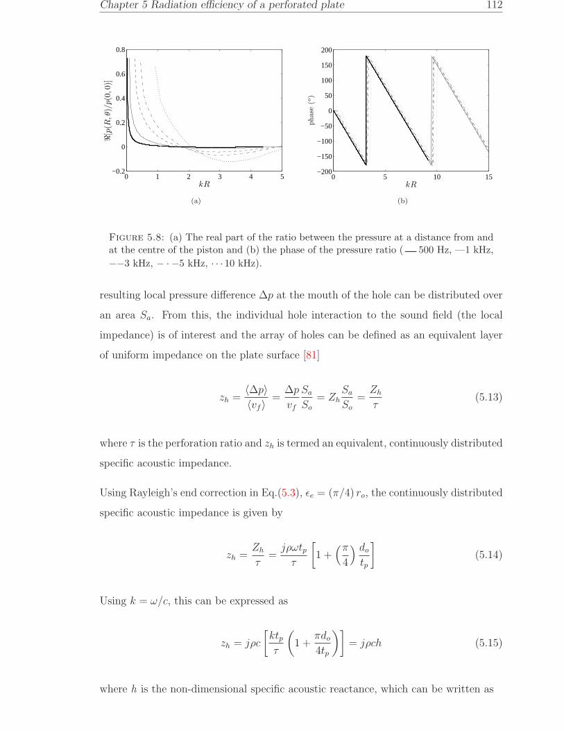
Chapter 5 Radiation efficiency of a perforated plate 112
0 1 2 3 4 5−0.2
0
0.2
0.4
0.6
0.8
kR
ℜ[p(R
,θ)/
p(0,
0)]
(a)
0 5 10 15−200
−150
−100
−50
0
50
100
150
200
kR
phase
(o)
(b)
Figure 5.8: (a) The real part of the ratio between the pressure at a distance from andat the centre of the piston and (b) the phase of the pressure ratio (−500 Hz, —1 kHz,
−−3 kHz, − · −5 kHz, · · · 10 kHz).
resulting local pressure difference ∆p at the mouth of the hole can be distributed over
an area Sa. From this, the individual hole interaction to the sound field (the local
impedance) is of interest and the array of holes can be defined as an equivalent layer
of uniform impedance on the plate surface [81]
zh =〈∆p〉〈vf〉
=∆p
vf
Sa
So
= ZhSa
So
=Zh
τ(5.13)
where τ is the perforation ratio and zh is termed an equivalent, continuously distributed
specific acoustic impedance.
Using Rayleigh’s end correction in Eq.(5.3), ǫe = (π/4) ro, the continuously distributed
specific acoustic impedance is given by
zh =Zh
τ=jρωtpτ
[1 +
(π4
) do
tp
](5.14)
Using k = ω/c, this can be expressed as
zh = jρc
[ktpτ
(1 +
πdo
4tp
)]= jρch (5.15)
where h is the non-dimensional specific acoustic reactance, which can be written as

Chapter 5 Radiation efficiency of a perforated plate 113
bo
do
Sa
So
Figure 5.9: An array of holes in a plate.
h =k
τ
(tp +
πdo
4
)(5.16)
In Chapter 6, the plate and the holes are modelled with discrete sources, i.e. an array
of monopole sources that contribute to the sound radiation. This allows the frequency
limit of the uniform acoustic impedance to be verified in terms of distance between
holes.
All the results throughout the remainder of this thesis will be based on using the
impedance as in Eq.(5.15).
5.2 Radiation by modes of a perforated plate in a
perforated baffle
5.2.1 Wave in an infinite plate
For a plane, harmonic, bending wave of frequency ω and wavenumber kx propagating
in the x -direction in an infinite plate (see Figure 2.3), the specific acoustic impedance
presented to the upper surface of the plate by the fluid (z > 0), za(kx), is given by [4]
za(kx) =P (kx)
V (kx)=
ωρ
(k2 − k2x)
1/2, kx < k (5.17)
where P (kx) and V (kx) are the complex acoustic pressure and the plate velocity am-
plitudes respectively (see Eq.(2.32)). For kx > k, za(kx) is imaginary (reactive). Only

Chapter 5 Radiation efficiency of a perforated plate 114
v xf( )
v x( )
x
p xa( )
—p xa( )
Figure 5.10: Analytical model of a perforated plate
the real part of za(kx) is required here to calculate the propagating waves producing
sound radiation. The imaginary part produces a near field.
In the case of a perforated plate, as shown in Figure 5.10, following the method of [37]
the difference between the local pressures on the upper and lower surfaces of the plate
drives fluid through the individual holes. In turn, these pressures are modified by
the flow through the holes. Considering the holes as a continuous distribution, an
equivalent fluid particle velocity vf (x), due to the flow through the holes relative to
the plate, can be given by
vf (x) =−2pa(x)
zh
(5.18)
where pa is the upper surface pressure (the pressure on the lower surface is −pa) result-
ing from the combination of the plate velocity v(x) and the equivalent continuously
distributed fluid velocity through the holes vf (x) and zh is the distributed hole im-
pedance given by Eq.(5.15) (the actual flow through the holes is vf/τ). Therefore for
the perforated plate, the net particle velocity vp formed by the combination of the
normal velocity of plate v and the continuously distributed average fluid motion vf is
given by
vp(x) = v(x) + vf (x) = v(x) − 2pa(x)
zh
(5.19)
Since the plate is assumed infinite and the bending wave has a unique wavenumber
kx, the plate and the equivalent fluid particle velocity also have the same unique
wavenumber in the x direction. Eq.(5.19) can be expressed as
Vp(kx) = V (kx) + Vf (kx) = V (kx) −2Pa(kx)
zh
(5.20)

Chapter 5 Radiation efficiency of a perforated plate 115
From Eq.(5.17), this generates the pressure Pa
Pa(kx) = Vp(kx)za(kx) =
(V (kx) −
2Pa(kx)
zh
)za(kx) (5.21)
Rearranging yields
Pa(kx) =zh za(kx)
zh + 2za(kx)V (kx) (5.22)
Finally substituting Eq.(5.22) into Eq.(5.20) yields the ratio of the complex amplitudes
of the combined normal velocity of plate and fluid flow through the holes to that of
the plate alone
Vp(kx)
V (kx)=
1
1 + 2za(kx)/zh
(5.23)
Eq.(5.23) confirms that the sound radiation from the plate is reduced by introducing
perforation to the plate. As |za(kx)/zh| → ∞, i.e. open area condition (absence of the
plate), the ratio tends to zero so that flow through the holes completely compensates
the plate motion, while as za(kx)/zh → 0, i.e. the unperforated plate (absence of the
holes), the ratio tends to unity.
The sound power radiated per unit area of the perforated plate can be calculated from
Wp(kx) =1
2ℜP (kx)V
∗p (kx)
(5.24)
By using the relation from Eq.(5.17)
Wp(kx) =1
2ℜza(kx)Vp(kx)V
∗p (kx)
=
1
2
∣∣∣Vp(kx)∣∣∣2
ℜza(kx) (5.25)
The ratio of sound power per unit area of the perforated plate to that of the unperfo-
rated plate is therefore given by
Wp(kx)
W (kx)=
∣∣∣∣∣Vp(kx)
V (kx)
∣∣∣∣∣
2
=1
1 + 4(za(kx)/ |zh|)2, kx < k (5.26)
since zh is imaginary and za is real.

Chapter 5 Radiation efficiency of a perforated plate 116
In terms of the non-dimensional specific acoustic reactance h, the ratio za(kx)/ |zh| can
be expressed as
za(kx)
|zh|=
1
h(1 − k2x/k
2)1/2=
1
h(1 − α2)1/2, α < 1 (5.27)
where α = kx/k.
For a plane wave travelling with components in the x and y directions, k2x can be
replaced by the square of the resultant k2x + k2
y. It follows that Eq.(5.27) can be
written as
za(kx, ky)
|zh|=
1
h(1 − α2 − β2)1/2, α2 + β2 < 1 (5.28)
where β = ky/k.
5.2.2 Finite plate in a perforated baffle
From the infinite plate case, the situation can be extended to the case of modes of
vibration in a finite baffled plate which can be decomposed into a spectrum of travelling
waves.
Consider a rectangular plate set in an infinite baffle. For convenience at this stage, the
baffle is assumed to be similarly perforated to the plate so that the previous analysis
can be used, i.e. the plate and the equivalent fluid particle velocity through the holes
share the same wavenumber. If the baffle is rigid, a mixed boundary impedance would
exist and Eq.(5.20) would not be valid and would have to be modified.
Suppose the plate is vibrating in mode (m,n). The plate vibration can be defined by
its non-dimensional wavenumber spectrum over (α, β). From Eq.(5.26), the ratio of
the squared amplitudes of the total normal velocity of plate and fluid flow through the
holes to that of the unperforated plate velocity, for the mode (m,n) at non-dimensional
wavenumber (α, β) is given by
|X(α, β)|2 =
∣∣∣∣∣Vp,mn(α, β)
Vmn(α, β)
∣∣∣∣∣
2
=h2(1 − α2 − β2)
4 + h2(1 − α2 − β2), α2 + β2 < 1 (5.29)
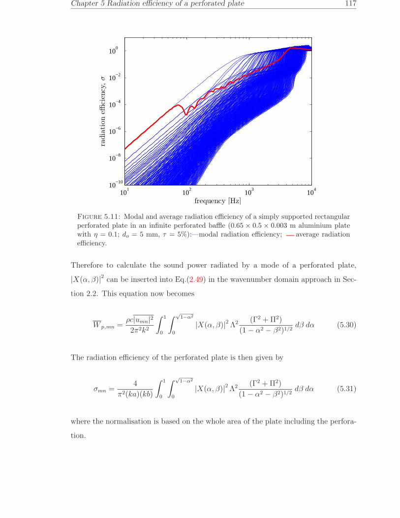
Chapter 5 Radiation efficiency of a perforated plate 117
101
102
103
104
10−10
10−8
10−6
10−4
10−2
100
frequency [Hz]
radia
tion
effici
ency
,σ
Figure 5.11: Modal and average radiation efficiency of a simply supported rectangularperforated plate in an infinite perforated baffle (0.65 × 0.5 × 0.003 m aluminium platewith η = 0.1; do = 5 mm, τ = 5%):—modal radiation efficiency; −average radiationefficiency.
Therefore to calculate the sound power radiated by a mode of a perforated plate,
|X(α, β)|2 can be inserted into Eq.(2.49) in the wavenumber domain approach in Sec-
tion 2.2. This equation now becomes
W p,mn =ρc|umn|22π2k2
∫ 1
0
∫ √1−α2
0
|X(α, β)|2 Λ2 (Γ2 + Π2)
(1 − α2 − β2)1/2dβ dα (5.30)
The radiation efficiency of the perforated plate is then given by
σmn =4
π2(ka)(kb)
∫ 1
0
∫ √1−α2
0
|X(α, β)|2 Λ2 (Γ2 + Π2)
(1 − α2 − β2)1/2dβ dα (5.31)
where the normalisation is based on the whole area of the plate including the perfora-
tion.
Chapter 5 Radiation efficiency of a perforated plate 118
5.2.3 Results
With the same plate dimensions and properties as in the previous chapters, Figure 5.11
shows the results of the modal and average radiation efficiencies of an example plate
having a 5% perforation ratio with 5 mm diameter holes. As seen from the figure, at
very low frequencies, at the fundamental mode (< 70 Hz), instead of increasing at 20
dB/decade as the unperforated plate does, the slope of the average radiation efficiency
of the perforated plate now becomes 40 dB/decade, where the additional 20 dB/decade
is due to the effect of the holes. The motion of the fluid in the holes is in the opposite
direction to that of the plate, i.e. 180 out of phase. The field produced by the surface
sources of the plate in the vicinity of the holes is largely suppressed by the opposite
fluid motion through the holes. Hence below the natural frequency of the fundamental
mode, the motion of the plate and the fluid in the holes can be associated with the
motion of two monopole sources acting in opposite directions which now constitute a
dipole source. In the region from 100 Hz to 1 kHz, the average radiation efficiency has
a frequency dependence of approximately 20 dB/decade.
Figure 5.12 plots the average radiation efficiencies obtained with various perforation
ratios τ and constant hole diameter do and also the radiation efficiency of the unperfo-
rated plate for comparison. It can be seen that, as the perforation ratio increases, the
radiation efficiency is simply reduced by an amount that is approximately constant
over the frequency range.
In order to show the effect of the perforation on the sound radiation, the results are
presented in terms of the sound radiation of a perforated plate relative to that of the
equivalent unperforated plate. The effect of perforation (EoP) is defined in decibels
(dB) by
EoP = 10 log10
(Wp
W
)(5.32)
where Wp and W are the overall radiated power of the perforated and unperforated
plates respectively. This is related to the insertion loss (IL) commonly used in noise
control where EoP = −IL. As the perforation is assumed to have no effect on the
average mean square velocity of the plate 〈v2〉, the EoP can also be written as
EoP = 10 log10
(σp
σ
)(5.33)

Chapter 5 Radiation efficiency of a perforated plate 119
101
102
103
104
10−10
10−8
10−6
10−4
10−2
100
frequency [Hz]
radia
tion
effici
ency
,σ
Figure 5.12: Average radiation efficiency of a simply supported rectangular perforatedplate in an infinite perforated baffle (0.65× 0.5× 0.003 m aluminium plate with η = 0.1;do = 5 mm: −unperforated, τ= — 5%, −− 10%, · · · 20% and − · − 40%).
where σp is the radiation efficiency of the perforated plate and σ is for the unperforated
plate. However, the validity of this assumption will be considered in Section 5.5.
Figure 5.13 plots the effect of perforation (EoP) for a constant hole diameter of 10 mm
and varying perforation ratio. It can be seen the EoP has a trend of 20 dB/decade
slope before converging to 0 dB at high frequency. The 0 dB value in the EoP curve
means that the perforation no longer has an effect on the radiated sound. A slight dip
occurs at the critical frequency (4 kHz).
Figure 5.14 show results with a constant perforation ratio and various hole diameters.
This shows that the sound radiation can be further reduced by reducing the hole
diameter, i.e. increasing the number of holes per unit area of the plate (hole density)
for a given perforation ratio. From Eq.(5.16), for a thin plate where the plate thickness
is much smaller than the hole radius, tp ≪ do, the non-dimensional specific acoustic
reactance is dominated by the end correction and can be expressed as h = kπdo/(4τ).
Consequently, the effect of perforation is controlled by a factor of do/τ . As seen from
Figure 5.13 and Figure 5.14, with the same values of do/τ , the effect of the perforation
is almost equal. For example do = 10 mm, τ = 10% and do = 20 mm, τ = 20% give

Chapter 5 Radiation efficiency of a perforated plate 120
101
102
103
104
−60
−50
−40
−30
−20
−10
0
frequency [Hz]
EoP
[dB
re1]
Figure 5.13: Effect of perforation (EoP) on sound power radiation of a simply sup-ported rectangular perforated plate in an infinite perforated baffle (0.65 × 0.5 × 0.003m aluminium plate, η = 0.1, do = 10 mm; · · · τ = 10%, − · −τ = 20%, −−τ = 40%,—τ = 60%).
101
102
103
104
−60
−50
−40
−30
−20
−10
0
frequency [Hz]
EoP
[dB
re1]
Figure 5.14: Effect of perforation (EoP) on sound power radiation of a simply sup-ported rectangular perforated plate in an infinite perforated baffle (0.65× 0.5× 0.003 maluminium plate, η = 0.1, τ = 20%; —do = 5 mm, − · −do = 10 mm, · · · do = 20 mm,−− do = 50 mm).

Chapter 5 Radiation efficiency of a perforated plate 121
101
102
103
104
−60
−50
−40
−30
−20
−10
0
frequency [Hz]
EoP
[dB
re1]
(a)
101
102
103
104
−60
−50
−40
−30
−20
−10
0
frequency [Hz]
EoP
[dB
re1]
(b)
101
102
103
104
−60
−50
−40
−30
−20
−10
0
frequency [Hz]
EoP
[dB
re1]
(c)
101
102
103
104
−60
−50
−40
−30
−20
−10
0
frequency [Hz]
EoP
[dB
re1]
(d)
Figure 5.15: Effect of perforation (EoP) on sound power radiation of a simply sup-ported rectangular perforated plate in a perforated baffle for different thicknesses; (a)0.65× 0.5× 0.006 m, (b) 0.65× 0.5× 0.008 m and dimensions; (c) 0.75× 0.4× 0.003 m,(d) 0.9 × 0.3 × 0.003 m (aluminium plate, η = 0.1; do = 10 mm, τ = — 20%, −− 40%,· · · 60%).
very similar results.
Figure 5.15 presents the results for different thicknesses and dimensions of the plate.
For different thicknesses, Figure 5.15(a) and (b) show similar results apart from the
region of the critical frequency (2 kHz for 6 mm and 1.5 kHz for 8 mm thickness). The
thickness also has an effect on h (Eq.(5.16)).
Figure 5.15(c) and Figure 5.15(d) show clearly that, for this model, the effect of per-
foration does not depend on the plate dimensions, see also Figure 5.13. The effect of
perforation is affected only by the perforation ratio and the hole size (see Eq.(5.16))
and to a lesser extent by the plate thickness.

Chapter 5 Radiation efficiency of a perforated plate 122
10−3
10−2
10−1
100
101
102
−70
−60
−50
−40
−30
−20
−10
0
h
EoP
[dB
re1]
Figure 5.16: Effect of perforation (EoP) on sound power radiation of a simply sup-ported rectangular perforated plate in an infinite perforated baffle plotted against non-dimensional reactance h (0.65× 0.5× 0.003 m (blue line), 0.65× 0.5× 0.006 m (red line)and 0.75 × 0.4 × 0.003 m (black line); aluminium plate with η = 0.1, do = 10 mm; τ =— 20%, −− 40%, · · · 60%).
The results can also be plotted against the non-dimensional acoustic reactance h. It
can be seen from Figure 5.16 that for different dimensions and thicknesses, all the
results collapse to a single line apart from small differences among the results that
occur close to the critical frequency. Because the effect of perforation is independent
of the plate dimensions, the curves are identical for similar plate thickness (see blue
and black curves).
5.2.4 Approximate formula for EoP
The differences in the effect of perforation at high frequencies are due to the results
around and above the critical frequency as each curve converges to 0 dB. Neglecting
this, an approximation can be made, at least up to the edge mode region of the sound
radiation by fitting a straight line to the results in Figure 5.16. The approximate
formula for the effect of perforation for a perforated plate in an infinite perforated

Chapter 5 Radiation efficiency of a perforated plate 123
baffle can be written as
EoPaprx = 20 log10 (h) − 10.5 , f < fc/2 (5.34)
Figure 5.17 plots the results comparing the analytical (EoP) and approximated (EoPaprx)
effect of perforation. Good agreement is found between the results up to hc/2, where
hc is the non-dimensional acoustic reactance at the critical frequency, fc.
5.3 Radiation by modes of a perforated, unbaffled
plate
Although mathematically convenient, a perforated plate set in a similarly perforated
baffle is not of direct practical relevance, as such a situation is rarely found in practice.
The more interesting case is where the baffle has a different acoustic impedance, such
as a perforated plate mounted in a rigid baffle or an unbaffled perforated plate. The
latter especially is frequently found in real applications and is discussed in this section.
5.3.1 Extended equations
The method of Laulagnet [33] for the sound radiation of an unbaffled plate discussed
in Section 3.2 can be extended to introduce perforation on the plate.
Recalling Eq.(3.5), the flexural wave equation of a perforated plate excited by a point
force is written as
B∇4w(x, y) −mpω2w(x, y) = F (x, y) + (1 − τ)∆p(x, y) (5.35)
where τ is the perforation ratio.
The motion of the fluid inside the holes depends on the pressure difference ∆p(x, y)
between the two sides of the plate surface as in Eq.(3.4) (positive for larger pressure
at z < 0 than at z > 0). The specific acoustic impedance of the distribution of holes
can then be expressed as

Chapter 5 Radiation efficiency of a perforated plate 124
10−2
100
102
−60
−50
−40
−30
−20
−10
0
10
h
EoP
[dB
re1]
hc/2
(a)
10−2
100
102
−60
−50
−40
−30
−20
−10
0
10
h
EoP
[dB
re1]
hc/2
(b)
10−2
100
102
−60
−50
−40
−30
−20
−10
0
10
h
EoP
[dB
re1]
hc/2
(c)
10−2
100
102
−60
−50
−40
−30
−20
−10
0
10
h
EoP
[dB
re1]
hc/2
(d)
10−2
100
102
−60
−50
−40
−30
−20
−10
0
10
h
EoP
[dB
re1]
hc/2
(e)
10−2
100
102
−60
−50
−40
−30
−20
−10
0
10
h
EoP
[dB
re1]
hc/2
(f)
Figure 5.17: Comparison of exact (−−) and approximated (—) effect of perforation(EoP) of a simply supported plate in an infinite perforated baffle.(a) and (b) 0.65×0.5×0.003 m, (c) and (d) 0.65 × 0.5 × 0.006 m, (e) and (f) 0.75 × 0.4 × 0.003 m; (a),(c), (e):τ = 20% and (b),(d), (f): τ = 60% (aluminium plate with η = 0.1; do = 10 mm).

Chapter 5 Radiation efficiency of a perforated plate 125
zh =∆p(x, y)
vf (x, y)(5.36)
where vf (x, y) is the velocity of the fluid.
With the same coordinate system of the plate as in Figure 3.2 in Chapter 3, by using
Eq.(3.8) on the plate surface at z = 0 and substituting Eq.(5.36), the pressure gradient
at the plate surface can be written as
∂p
∂z(M)|z=0 = ρ ω2(w(M) − wf (M)) = ρ ω2w(M) + jρ ω vf (M)
(5.37)
= ρ ω2w(M) +jρω
zh
∆p(M)
where M is a point in the medium above the plate, wf is the fluid displacement relative
to the plane z = 0 and vf = jωwf .
Substituting for ∆p from Eq.(5.35) gives
∂p
∂z(M)|z=0 = ρ ω2w(M) +
jρω
zh
(B∇4w(M) −mpω2w(M) − F (M))
1
(1 − τ)(5.38)
Following the same procedure as in Section 3.2, this is inserted into the Kirchhoff-
Helmholtz integral of Eq.(3.13) to give
(1 − τ)ρ ω2w(M) +jρω
zh
(B∇4w(M) −mpω2w(M) − F (M))
(5.39)
= −∫
Sp
(B∇4w(Q) −mpω2w(Q) − F (Q))
∂2G(Q,M)
∂zQ∂zM
dSp
where Q is a point on the plate surface. Compared with Eq.(3.15) the second term on
the left-hand side has been added by the perforation.
Writing the displacement w (Eq.(3.16)) and the excitation force F (Eq.(3.17)) in terms
of modal series gives

Chapter 5 Radiation efficiency of a perforated plate 126
(1 − τ)ρ ω2
∞∑
m=1
∞∑
n=1
dmnϕmn(x0, y0)
+jρω
zh
∞∑
m=1
∞∑
n=1
(Bdmn∇4ϕmn(x0, y0) −mpω2dmnϕmn(x0, y0) − Fmnϕmn(x0, y0))
(5.40)
= −∫
Sp
(Bdmn∇4ϕmn(x, y) −mpω2dmnϕmn(x, y) − Fmnϕmn(x, y))
∂2G(Q,M)
∂zQ∂zM
dSp
where dmn is the modal complex displacement amplitude and Fmn is the generalized
force density.
Substituting Eq.(3.22) to eliminate the terms ∇4ϕmn yields
(1 − τ)ρ ω2
∞∑
m=1
∞∑
n=1
dmnϕmn(x0, y0) +jρω
zh
∞∑
m=1
∞∑
n=1
(mp(ω2mn − ω2)dmn − Fmn)ϕmn(x0, y0)
(5.41)
= −∫
Sp
∞∑
m=1
∞∑
n=1
(mp(ω2mn − ω2)dmn − Fmn)ϕmn(x, y)
∂2G(Q,M)
∂zQ∂zM
dSp
Multiplying by ϕpq and integrating over the plate area gives
(1 − τ)ρ ω2
mp
dpqMpq +jρω
zhmp
(mp(ω2pq − ω2)dpq − Fpq)Mpq
(5.42)
=∞∑
m=1
∞∑
n=1
(Fmn −mp(ω2mn − ω2)dmn) Cpqmn
where Cpqmn = Cmnpq are the acoustical cross-modal coupling terms as defined in
Eq.(3.24).
For the case of a simply supported plate, using the modal mass as in Eq.(3.27) yields
(1 − τ)ρω2Sp
4dpq +
jωρ
zh
Sp
4(mp(ω
2pq − ω2)dpq − Fpq)
(5.43)
=∞∑
m=1
∞∑
n=1
(Fmn −mp(ω2mn − ω2)dmn)Cpqmn

Chapter 5 Radiation efficiency of a perforated plate 127
To include the effect of damping into the sound radiation calculation, the plate natural
frequency ω2mn is replaced by ω2
mn(1 + jη).
After re-arranging Eq.(5.43), its solution can be written in terms of vectors and ma-
trices as
[Cmnpq] mp(ω2mn − ω2)dmn + (1 − τ)ρω2Sp
4[I] dmn +
jωρ
zh
Sp
4[I] mp(ω
2mn − ω2)dmn
(5.44)
= [Cmnpq] Fmn + [I]jωρ
zh
Sp
4Fmn
where [I] is the mn×mn identity matrix and denotes a column vector.
Multiplying by [Cmnpq]−1 yields
[I] mp(ω2mn − ω2)dmn+
+ ρω2Sp
4[Cmnpq]
−1
((1 − τ) [I] dmn +
jmp
ωzh
[I](ω2
mn − ω2)dmn
)
=
([I] +
jωρ
zh
Sp
4[Cpqmn]−1
)Fmn (5.45)
By neglecting the cross-modal coupling contributions in the sound radiation as in
Chapter 3 ([33]) i.e. only the self-modal coupling terms are considered, this can be
approximated by
Mpq(ω2pq − ω2)dpq + ρω2
(Sp
4
)21
Cpqpq
(1 − τ +
4jMpq
Spωzh
(ω2pq − ω2)
)dpq
(5.46)
=
(1 +
jωρ
zh
Sp
4
1
Cpqpq
)Fpq
where Mpq = mp(Sp/4) and Fpq = Fpq(Sp/4) are the generalized mass and the gener-
alized force respectively for the simply supported plate. The case of the unperforated,
unbaffled plate (Eq.(3.34)) can be recovered by introducing very large zh and setting
τ = 0.
The remaining procedure to calculate the sound power W is similar to that for the
unperforated unbaffled plate in Chapter 3.

Chapter 5 Radiation efficiency of a perforated plate 128
101
102
103
104
10−10
10−5
100
frequency [Hz]
radia
tion
effici
ency
,σ
(a)
101
102
103
104
10−10
10−5
100
frequency [Hz]
radia
tion
effici
ency
,σ
(b)
101
102
103
104
10−10
10−5
100
frequency [Hz]
radia
tion
effici
ency
,σ
(c)
101
102
103
104
10−10
10−5
100
frequency [Hz]
radia
tion
effici
ency
,σ
(d)
Figure 5.18: Comparison of modal radiation efficiency including the cross-modal terms(—) and only the self-modal terms (· · · ): (a) mode (1,1), (b) mode (1,2), (c) mode (2,4)and (d) mode (3,3) (0.65 × 0.5 × 0.003 m aluminium plate with η = 0.1; do = 10 mm,τ = 40%).
5.3.2 Results
Figure 5.18 shows a comparison between the calculation of the radiation efficiency for
modes (1,1),(1,2),(2,4) and (3,3) using Eq.(5.45) involving the full matrix [Cpqmn] and
the one using Eq.(5.46), based on neglecting cross-modal terms. For calculating the
results using the full matrix of Cpqmn (Eq.(5.45)), a total of 49×49 modes are included
in each calculation. In each case only modes of the same parity are included as other
terms are zero.
For modes (1,1) and (1,2), both results appear to have a perfect agreement. Differences
occur for modes (2,4) and (3,3) below the modal coincidence frequency of each mode.

Chapter 5 Radiation efficiency of a perforated plate 129
101
102
103
104
10−8
10−6
10−4
10−2
100
frequency [Hz]
radia
tion
effici
ency
,σ
Figure 5.19: Modal and average radiation efficiency of a simply supported rectangularunbaffled perforated plate (0.65× 0.5× 0.003 m aluminium plate, η = 0.1; do = 10 mm,τ = 40%): —modal radiation efficiency; −average radiation efficiency.
This is the effect of the cross-modal coupling which is greater in the higher modes.
In the unbaffled plate case, the cross-modal terms do not completely converge to zero
as they do for the baffled plate case, even though all possible force positions have
been averaged. However, the self-modal radiation is still considered to give quite
good agreement with the result where the cross-modal terms are included, especially
when the full modal summation is considered. Over the whole frequency range, the
average differences are less than 1 dB, which thus can be neglected, except at certain
frequencies where the discrepancy is a bit higher. For example at 700 Hz for mode
(2,4) in Figure 5.18(c) the difference is around 4−5 dB. Therefore, in the remainder of
this section, the calculation of the radiation efficiency is carried out by using Eq.(5.46),
i.e. neglecting the cross-modal coupling distribution.
Figure 5.19 presents the results of the modal and average radiation efficiencies of an
unbaffled perforated plate with 40% perforation ratio and 10 mm diameter holes. The
results show a curve which has the same trend of slope as obtained from the case
of a perforated plate in an infinite perforated baffle, see Figure 5.11, particularly for
the region below the first mode (40 dB/decade) and the corner mode region (about
20 dB/decade). However, the unbaffled plate has a lower radiation efficiency than

Chapter 5 Radiation efficiency of a perforated plate 130
101
102
103
104
10−6
10−4
10−2
100
frequency [Hz]
radia
tion
effici
ency
,σ
(a)
101
102
103
104
10−6
10−4
10−2
100
frequency [Hz]
radia
tion
effici
ency
,σ
(b)
101
102
103
104
10−6
10−4
10−2
100
frequency [Hz]
radia
tion
effici
ency
,σ
(c)
101
102
103
104
10−6
10−4
10−2
100
frequency [Hz]
radia
tion
effici
ency
,σ
(d)
Figure 5.20: Average radiation efficiency of simply supported rectangular perforatedplates in a perforated baffle (−−) and unbaffled (—) (0.65 × 0.5 × 0.003 m aluminiumplate with η = 0.1; do = 10 mm): (a) τ = 10%, (b) τ = 20%, (c) τ = 40% mm, (d)τ = 60%.
that of the plate in the perforated baffle for most of the frequency range as shown in
Figure 5.20.
It can be seen that the difference is almost constant for the increasing perforation
ratio from 10% to 40%. For very high perforation at 60%, the difference increases in
about 1-2 dB. This can be seen clearly in Figure 5.21 which shows the differences of
the radiation efficiencies ∆σ for no baffle and with a perforated baffle on a dB scale.
It is found that there is no consistent trend on the difference level between both cases
that can be related to the perforation ratio.
Figure 5.22 compares the results with those for the unperforated unbaffled plate from
Section 3.2. Perforation yields a constant reduction at low frequencies including the
corner mode region (up to 450 Hz in this case). The effect then reduces as frequency

Chapter 5 Radiation efficiency of a perforated plate 131
101
102
103
104
−10
−9
−8
−7
−6
−5
−4
−3
−2
−1
0
1
frequency [Hz]
∆σ
[dB
re1]
Figure 5.21: Radiation efficiency difference of a perforated plate in a perforated baffleand an unbaffled plate) (0.65 × 0.5 × 0.003 m aluminium plate, η = 0.1; do = 10 mm):×—τ = 3%, —τ = 10%, −−τ = 20%, · · · τ = 40% mm, − · −τ = 60%.
increases. This can be explained as the impedance of the hole is proportional to
frequency. Therefore at high frequency, the fluid in the holes has very high mass-like
impedance. This mass does not move sufficiently to compensate for the volume sources
adjacent to the hole. The cancellation of radiated sound thus becomes ineffective.
As in the previous section, the level difference between the perforated and unperforated
results can be expressed as the ’effect of perforation’, EoP, see Eq.(5.32). Figure 5.23
and Figure 5.24 present the effect of perforation for a constant hole diameter and a
constant perforation ratio, respectively. These show that, for the case of the unbaffled
perforated plate, the effect of perforation is almost independent of frequency at low
frequencies and the effect reduces in the edge mode region as the frequency increases.
Results for different thicknesses and dimensions are presented in Figure 5.25. Unlike
the case of a perforated baffle (Fig.5.15), the results show that the effect of perforation
in the unbaffled case depends on both the plate thickness (see Figure 5.25(a), 5.25(b))
and on the plate dimensions (see Figure 5.25(c), 5.25(d)).
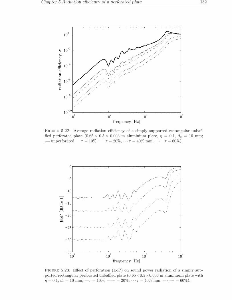
Chapter 5 Radiation efficiency of a perforated plate 132
101
102
103
104
10−10
10−8
10−6
10−4
10−2
100
frequency [Hz]
radia
tion
effici
ency
,σ
Figure 5.22: Average radiation efficiency of a simply supported rectangular unbaf-fled perforated plate (0.65 × 0.5 × 0.003 m aluminium plate, η = 0.1, do = 10 mm;
−unperforated, —τ = 10%, −−τ = 20%, · · · τ = 40% mm, − · −τ = 60%).
101
102
103
104
−35
−30
−25
−20
−15
−10
−5
0
frequency [Hz]
EoP
[dB
re1]
Figure 5.23: Effect of perforation (EoP) on sound power radiation of a simply sup-ported rectangular perforated unbaffled plate (0.65×0.5×0.003 m aluminium plate withη = 0.1, do = 10 mm; —τ = 10%, −−τ = 20%, · · · τ = 40% mm, − · −τ = 60%).

Chapter 5 Radiation efficiency of a perforated plate 133
101
102
103
104
−30
−25
−20
−15
−10
−5
0
frequency [Hz]
EoP
[dB
re1]
Figure 5.24: Effect of perforation (EoP) on sound power radiation of a simply sup-ported rectangular perforated unbaffled plate (0.65×0.5×0.003 m aluminium plate withη = 0.1; τ = 20%: do = — 50 mm, −− 20 mm, − · − 5 mm, · · · 2 mm).
5.3.3 Approximate formula for EoP
Figure 5.26 plots the effect of perforation against non-dimensional specific acoustic
reactance h for different plate thicknesses. It can be seen that the curves collapse
together with the same slope of 15 dB/decade in the edge mode region. Below the
edge mode region, the results are independent of h but vary with plate dimensions and
perforation ratio.
In the edge mode region, up to half the critical frequency (fc/2), the effect of perfora-
tion (EoP) can be written as
EoPub,edge = 15 log10 [h(1 − τ)] − 11, fe < f < fc/2 (5.47)
where fe is as in Eq.(2.68).
As the effect of perforation ratio for the unbaffled perforated plate shows constant
values at low frequency, at least up to end of the corner mode region, an approximate
formula can be developed to determine the EoP ratio in this frequency range.

Chapter 5 Radiation efficiency of a perforated plate 134
101
102
103
104
−35
−30
−25
−20
−15
−10
−5
0
frequency [Hz]
EoP
[dB
re1]
(a)
101
102
103
104
−35
−30
−25
−20
−15
−10
−5
0
frequency [Hz]
EoP
[dB
re1]
(b)
101
102
103
104
−35
−30
−25
−20
−15
−10
−5
0
frequency [Hz]
EoP
[dB
re1]
(c)
101
102
103
104
−35
−30
−25
−20
−15
−10
−5
0
frequency [Hz]
EoP
[dB
re1]
(d)
Figure 5.25: Effect of perforation (EoP) on sound power radiation of a simply sup-ported rectangular perforated unbaffled plate for different thicknesses; (a) 0.65 × 0.5 ×0.006 m, (b) 0.65 × 0.5 × 0.008 m and different dimensions; (c) 0.8 × 0.4 × 0.003 m, (d)0.9 × 0.2 × 0.003 m (aluminium plate with η = 0.1; do = 10 mm, τ = — 20%, −− 40%,− · − 60%).
Figure 5.27 plots the effect of perforation at low frequency for plates with the same
dimensions but different thickness and perforation ratio to show the increment in the
EoP curve as the plate thickness increases. This is plotted against h(1− τ)/k which is
independent of frequency. The constant values over the corner mode region are taken
from the average value between 30 Hz and 60 Hz.
It is seen that the perforation of thinner plates has a greater effect of reducing the sound
radiation. The result also shows that the trend has a dependency of 15 dB/decade.
Therefore a simple curve fit can be obtained as a function of the non-dimensional
acoustic reactance h

Chapter 5 Radiation efficiency of a perforated plate 135
10−3
10−2
10−1
100
101
−35
−30
−25
−20
−15
−10
−5
0
h(1-τ)
EoP
[dB
re1]
Figure 5.26: Effect of perforation (EoP) on sound power radiation of a simply sup-ported rectangular perforated, unbaffled plate plotted against h (0.65 × 0.5 × 0.003 m(black line), 0.65 × 0.5 × 0.006 m (blue line) ); aluminium plate, η = 0.1, do = 10 mm;τ = — 20%, −− 40%, − · − 60%).
EoPubf,corner = 15 log10
[h(1 − τ)
k
]+ 2.3, f < fe (5.48)
where EoPub,corner is the effect of perforation of the unbaffled perforated plate at very
low frequency, i.e. in the dipole and the corner mode regions, as a function of h (which
include thickness, perforation ratio and hole diameter).
The EoP at low frequency for different dimensions with the same plate thickness is
shown in Figure 5.28 for perforation ratios of 20% and 40%. For the 20% perforation
ratio, the dependence on the plate dimensions a and b can be written as
EoPub,a×b = −8.46 log10
(1
1/a2 + 1/b2 + 1/2ab
)− 25, f < fe (5.49)
where a × b is the plate area1 and the unit length should be in metre (m). The EoP
in Fig. 5.28 is calculated for different plate areas and plate ratios. It can be seen that
the 40% perforation has similar gradient to that of the 20%.
1The results were also plotted against ab, a/b, ab/(a + b) and a + b but these did not yield aconsistent relationship as here.

Chapter 5 Radiation efficiency of a perforated plate 136
10−3
10−2
10−1
−40
−35
−30
−25
−20
−15
−10
h(1-τ)/k
EoP
[dB
re1]
Figure 5.27: Effect of perforation (EoP) on sound power radiation of a simply sup-ported rectangular perforated unbaffled plate at low frequency asymptote for differentthickness (: 0.65 × 0.5 × 0.003 m, ♦: 0.65 × 0.5 × 0.004 m, : 0.65 × 0.5 × 0.006 m,: 0.65 × 0.5 × 0.008 m aluminium plate with η = 0.1; τ = 20% (blue), τ = 40% (red),τ = 60% (green)).
10−2
10−1
100
−35
−30
−25
−20
−15
−10
−5
1
(1/a2 + 1/b2 + 1/2ab)
EoP
[dB
re1]
Figure 5.28: Effect of perforation (EoP) on sound power radiation of a simply sup-ported rectangular perforated unbaffled plate at low frequency asymptote for variousplate dimensions (t = 3 mm, aluminium plate with η = 0.1; +=20%, =40%).

Chapter 5 Radiation efficiency of a perforated plate 137
10−2
100
102
−35
−30
−25
−20
−15
−10
−5
0
5
10
h
EoP
[dB
re1]
hc/2
(a)
10−2
100
102
−35
−30
−25
−20
−15
−10
−5
0
5
10
h
EoP
[dB
re1]
hc/2
(b)
10−2
100
102
−35
−30
−25
−20
−15
−10
−5
0
5
10
h
EoP
[dB
re1]
hc/2
(c)
10−2
100
102
−35
−30
−25
−20
−15
−10
−5
0
5
10
h
EoP
[dB
re1]
hc/2
(d)
Figure 5.29: Comparison of exact (−−) and approximated (—) effect of perforation(EoP) on sound power radiation of a simply supported rectangular perforated unbaffledplate: 0.65 × 0.5 × 0.003 m; (a) τ = 10%, (b) τ = 20%, (c) τ = 40%, (d) τ = 60%(aluminium plate with η = 0.1, do = 10 mm).
These two equations (Eq.(5.48) and Eq.(5.49)) can be combined to give a general
equation for the effect of perforation at low frequency. For the sake of clarity, the
coefficients are rounded to give the form
EoPub = −8.5 log10
(1
1/a2 + 1/b2 + 1/2ab
)+ 15 log10
[h(1 − τ)
k
]− 5.5, f < fe
(5.50)
Figures 5.29 and 5.30 show a comparison of the effect of perforation to test the va-
lidity of Eq.(5.50) and Eq.(5.47) for different perforation ratios, plate dimensions and
thicknesses. The results show good agreement over the frequency range up to half the
critical frequency. However in the corner mode region, the approximate model does
not give such a good estimation. This is due to high fluctuations in this region both

Chapter 5 Radiation efficiency of a perforated plate 138
from the radiation efficiency of the perforated plate and that of the solid plate, which
then also lead to high fluctuations in the effect of perforation curve. Nevertheless the
differences in this region are only 2−4 dB at most.
5.4 Perforated plate near a rigid surface
Another consideration for sound radiation from a plate is its radiation characteristic
when it is placed near a reflecting, rigid surface. Such an application can be found,
for example, when a plate is used as a dynamic vibration absorber [56]. The vibration
of the structure under treatment is suppressed while its vibration energy is transfered
to the absorber. This plate absorber will then radiate sound into the air.
This section will first evaluate the radiation efficiency of a solid unbaffled plate located
close to an infinite rigid surface before considering the effect due to perforation.
5.4.1 Modifying the Green’s function
Consider the situation in Figure 5.31 where an unbaffled plate is located at a distance
D above an infinite rigid, reflecting surface lying in the xy-plane. The boundary
condition on the rigid surface is that the normal fluid velocity is zero, or from Eq.(3.8)
that the normal gradient of the pressure is zero. This boundary condition is equivalent
to the situation in which an imaginary plate, vibrating in the opposite direction, is
located at a distance 2D below the real vibrating plate, in the absence of the infinite
reflecting surface. The sound field below the rigid surface, of course, has no physical
meaning. However, the corresponding sound field above the rigid surface (z ≥ 0)
includes the reflected wave from this surface.
The Green’s function can now be modified to include the contribution of the image
source Q′ at (x, y,−z) to the pressure at the observation point M at (x0, y0, z0). The
appropriate Green’s function is given by
G(Q,M) =e−jkR
4πR+e−jkR′
4πR′ (5.51)

Chapter 5 Radiation efficiency of a perforated plate 139
10−2
100
102
−35
−30
−25
−20
−15
−10
−5
0
5
10
h
EoP
[dB
re1]
hc/2
(a)
10−2
100
102
−35
−30
−25
−20
−15
−10
−5
0
5
10
h
EoP
[dB
re1]
hc/2
(b)
10−2
100
102
−35
−30
−25
−20
−15
−10
−5
0
5
10
h
EoP
[dB
re1]
hc/2
(c)
10−2
100
102
−35
−30
−25
−20
−15
−10
−5
0
5
10
h
EoP
[dB
re1]
hc/2
(d)
10−2
100
102
−30
−25
−20
−15
−10
−5
0
5
10
h
EoP
[dB
re1]
hc/2
(e)
10−2
100
102
−35
−30
−25
−20
−15
−10
−5
0
5
10
h
EoP
[dB
re1]
hc/2
(f)
Figure 5.30: Comparison of exact (−−) and approximated (—) effect of perforation(EoP) on sound power radiation of a simply supported rectangular perforated unbaffledplate: τ = 20%; (a) 0.8×0.4×0.003 m, (b) 0.65×0.4×0.002 m, (c) 0.52×0.4×0.006 m,(d) 0.7× 0.45× 0.004 m, (e) 0.39× 0.3× 0.005 m and (f) 0.9× 0.3× 0.003 m (aluminiumplate with η = 0.1, do = 10 mm).

Chapter 5 Radiation efficiency of a perforated plate 140
D
D x
z
y
Q’
Q
M
R’
R
rigid surface
Figure 5.31: Perforated, unbaffled plate near a reflecting rigid surface
where
R =√
(x0 − x)2 + (y0 − y)2 + (z0 − z)2
R′ =√
(x0 − x)2 + (y0 − y)2 + (z0 + z)2
As in Eq.(3.9), the Green’s function must now satisfy
∇2G(Q,M) + k2G(Q,M) =
δ(x0 − x)δ(y0 − y)δ(z0 − z) + δ(x0 − x)δ(y0 − y)δ(z0 + z) (5.52)
Taking the two dimensional Fourier transform of Eq.(5.52), the Green’s function can
be expressed as [72]
G =j
8π2
∫ ∞
−∞
∫ ∞
−∞
1
kz
ejkz |z−z0| + ejkz(z+z0)
ejkx(x−x0)ejky(y−y0) dkx dky (5.53)
where kz =√k2 − k2
x − k2y.
The additional term in the bracket (compare Eq.(3.10)) is the image source contribu-
tion.
For z0 ≥ z, the term in the bracket can be expressed as
ejkz(z0−z) + ejkz(z+z0) = ejkzz0(e−jkzz + ejkzz) = 2ejkzz0 cos(kzz)

Chapter 5 Radiation efficiency of a perforated plate 141
For z0 ≤ z the terms in z0 and z should be exchanged.
Following the method of Laulagnet [33] in Section 3.2, the acoustical cross-modal
coupling terms in Eq.(3.25) thus become
Cpqmn =1
4π2
∫ ∞
−∞
∫ ∞
−∞kz e
jkzz0 sin(kzz) ϕ∗pq(kx, ky)ϕmn(kx, ky) dkx dky
(5.54)
=1
π2
∫ ∞
0
∫ ∞
0
kz ejkzz0 sin(kzz) ϕ
∗pq(kx, ky)ϕmn(kx, ky) dkx dky
For z = z0 = D, Eq.(3.32) becomes
Cpqmn = Cmnpq =4
pqmn
(ab
π3
)2 ∫ ∞
0
∫ ∞
0
kz ejkzD sin(kzD) Υ Ω dkx dky (5.55)
The remaining steps to obtain the radiation efficiency are the same as in Section 3.2
for a solid plate or in Section 5.3 for perforated plate.
5.4.2 Results for solid plates
Figure 5.32 plots the modal radiation efficiencies and the average radiation efficiency
for the unbaffled plate (dimensions as before) located 2 and 4 cm above the rigid
surface. At very low frequency (< 100 Hz), the average radiation efficiency has a
frequency dependence of 60 dB/decade. This shows that the vibrating plate behaves
like a quadrupole source, a very inefficient radiator. At very low frequency the un-
baffled plate itself behaves like a dipole source; the rigid surface provides its image
with opposite phase hence constructing a quadrupole source. However, this requires
that the distance from the rigid surface is much smaller than the acoustic wavelength
(kD ≪ 1).
For each mode the modal radiation efficiency has a sharp peak which occurs around
a frequency when k2 = (mπ/a)2 + (nπ/b)2, i.e. the modal coincidence frequency.
Figure 5.33 shows the modal radiation efficiencies for modes (1,1) and (6,6) together
with those for the plate without the rigid surface. The peak can be seen to occur at
the same frequency for different values of D. This sharp peak is due to the standing

Chapter 5 Radiation efficiency of a perforated plate 142
101
102
103
104
10−5
100
frequency [Hz]
radia
tion
effici
ency
,σ
(a)
101
102
103
104
10−6
10−4
10−2
100
102
frequency [Hz]
radia
tion
effici
ency
,σ
(b)
Figure 5.32: —Modal radiation efficiency and −average radiation efficiency of an
unbaffled plate near rigid surface: (a) D = 0.02 m and (b) D = 0.04 m (aluminiumplate, 0.65 × 0.5 × 0.003 m, η = 0.1).
101
102
103
104
10−6
10−4
10−2
100
102
frequency [Hz]
radia
tion
effici
ency
,σ
Figure 5.33: Radiation efficiency of an unbaffled plate near rigid surface for mode(1,1)(black) and mode (6,6)(blue): −absence of rigid surface, −−D = 0.04 m, · · ·D =
0.02 m, − · −D = 0.01 m (0.65 × 0.5 × 0.003 m, η = 0.1).
wave between the plate and the rigid surface. At higher frequencies for higher modes,
peaks are built up above the modal coincidence frequency as seen in mode (6,6).
In Figure 5.32, very high peaks also can be seen at high frequencies. This causes the
average radiation efficiency to increase instead of converging to unity. This appears
to be due to an interference effect of the incident and reflected waves when the plate

Chapter 5 Radiation efficiency of a perforated plate 143
101
102
103
104
10−6
10−4
10−2
100
frequency [Hz]
radia
tion
effici
ency
,σ
Figure 5.34: Radiation efficiency of an unbaffled plate near rigid, reflecting surface:
−absence of rigid surface, −−D = 0.04 m, · · ·D = 0.02 m, − · −D = 0.01 m (0.65 ×0.5 × 0.003 m, η = 0.1).
distance above the rigid surface is a multiple of half of the acoustic wavelength (kD =
nπ, n =interger). Thus it can be seen from Figure 5.32 the very high peak starts at
8.5 kHz for D = 2 cm and at 4.2 kHz for D = 4 cm and is repeated at 8.5 kHz.
Figure 5.34 shows the average results for the unperforated unbaffled plate located at
various distances from a reflecting rigid surface compared with the result without a
rigid surface. This shows that, as the plate is placed closer to the rigid surface, the point
at which the radiation efficiency intersects that of the plate without the rigid surface
shifts to a higher frequency. Above this intersection frequency, the radiation efficiency
in the presence of the rigid surface becomes larger than that without the rigid surface.
The sound radiation reflected from the rigid surface contributes to and increases the
radiated sound above the vibrating plate. It appears that it is independent of the
distance D particularly in the edge mode region just before the critical frequency
(above 1 kHz in the given case). Figure 5.35 shows similar phenomena in the corner
and edge mode regions for a plate with different dimensions and thickness.
Figure 5.36 shows the effect of the presence of a rigid surface on the radiated sound
power from the plate in Figure 5.34. This is also the same as the insertion loss (IL) of

Chapter 5 Radiation efficiency of a perforated plate 144
101
102
103
104
10−6
10−4
10−2
100
frequency [Hz]
radia
tion
effici
ency
,σ
Figure 5.35: Radiation efficiency of an unbaffled plate near rigid, reflecting surface(0.325 × 0.25 × 0.006 m, η = 0.1): −absence of rigid surface, −−D = 0.04 m, · · ·D =0.02 m, − · −D = 0.01 m.
101
102
103
104
−40
−30
−20
−10
0
10
20
frequency [Hz]
effec
tofri
gid
surf
ace
[dB
re1]
Figure 5.36: The effect of rigid surface on sound radiation of an unbaffled plate (0.65×0.5 × 0.003 m, η = 0.1): −−D = 0.04 m, · · ·D = 0.02 m, − · −D = 0.01 m.

Chapter 5 Radiation efficiency of a perforated plate 145
a rigid surface. However, in this thesis, this is presented as -IL, i.e. the ratio between
sound radiation with the presence of a rigid surface and with no rigid surface in place.
5.4.3 Results for perforated plates
Figure 5.37 plots the modal radiation efficiencies and the average radiation efficiency
for a perforated unbaffled plate having hole diameter of 10 mm and 10% perforation
ratio. The plate is located 2 or 4 cm above the rigid surface. As in the previous result
for the unperforated plate in Figure 5.32, the interference effect also appears at high
frequency (> 4.2 kHz) when the plate distance D is more than half of the acoustic
wavelength. The sharp peak for each mode, as seen in Figure 5.32 around 400 Hz and
above, vanishes as there is no longer a standing wave between the vibrating plate and
the rigid surface because the sound can now easily ’escape’ through the holes.
Figure 5.38 presents the average results for the same perforated plate but at various
distances above the rigid surface. It shows similar phenomenon as for the unperforated
plate except that the radiation efficiency of the plate close to the rigid surface is much
lower in this case and does not very much exceed that of the perforated plate without
the rigid surface even in the edge mode region (1−4 kHz). Figure 5.39 plots the effect
of the rigid surface on the sound radiation from the perforated plate. It can be seen
that as the vibrating perforated plate is brought closer to the rigid wall, a sound
reduction is obtained over a broader frequency range.
Figure 5.40 compares results for perforated and unperforated plates at various dis-
tances from the rigid surface. It can be seen here that peaks in corner and edge mode
regions occurring for the solid plate vanish in the radiation efficiency of the perforated
plate. Results are also included for another plate dimensions i.e. 0.325× 0.25× 0.006
m. In both cases the reduction due to perforation is effective over a wide range of
frequency, up to the critical frequency (4 kHz and 2 kHz respectively).
The effect of perforation (EoP) is plotted in Figures 5.41 and 5.42 for both plates
including the case with no rigid surface. In the fundamental mode and edge mode
regions, the effect of perforation becomes greater as the plate is located closer to the
rigid surface. However, in the corner mode region, there is no consistent effect in terms
of the plate distance from the surface. The effect of perforation is greater than for

Chapter 5 Radiation efficiency of a perforated plate 146
101
102
103
104
10−5
100
frequency [Hz]
radia
tion
effici
ency
,σ
(a)
101
102
103
104
10−5
100
frequency [Hz]
radia
tion
effici
ency
,σ
(b)
Figure 5.37: —Modal radiation efficiency and −average radiation efficiency of a
perforated unbaffled plate near rigid surface: (a) D = 0.02 m and (b) D = 0.04 m(aluminium plate, 0.65 × 0.5 × 0.003 m, η = 0.1, do = 0.01 m, τ = 10%).
101
102
103
104
10−8
10−6
10−4
10−2
100
frequency [Hz]
radia
tion
effici
ency
,σ
Figure 5.38: Radiation efficiency of perforated unbaffled plate near rigid, reflectingsurface: —absence of rigid surface, −−D = 0.04 m, · · ·D = 0.02 m, − · −D = 0.01 m(aluminium plate, 0.65 × 0.5 × 0.003 m, η = 0.1, do = 0.01 m, τ = 10%).

Chapter 5 Radiation efficiency of a perforated plate 147
101
102
103
104
−30
−25
−20
−15
−10
−5
0
5
10
frequency [Hz]
effec
tofri
gid
surf
ace
[dB
re1]
Figure 5.39: The effect of rigid surface on sound radiation of a perforated unbaffledplate: −−D = 0.04 m, · · ·D = 0.02 m, −·−D = 0.01 m (0.65×0.5×0.003 m aluminiumplate, η = 0.1, do = 0.01 m, τ = 10%).
the plate without the rigid surface in all cases below the critical frequency, as in all
previous results.
Figures 5.43 and 5.44 shows the EoP for a fixed plate distance with varying perforation
ratio. The effect of perforation is almost constant with frequency in each case in the
corner mode region. The effect of perforation is increased as the perforation increases.

Chapter 5 Radiation efficiency of a perforated plate 148
101
102
103
104
10−6
10−4
10−2
100
frequency [Hz]
radia
tion
effici
ency
,σ
(a)
101
102
103
104
10−6
10−4
10−2
100
frequency [Hz]
radia
tion
effici
ency
,σ
(b)
101
102
103
104
10−6
10−4
10−2
100
frequency [Hz]
radia
tion
effici
ency
,σ
(c)
101
102
103
104
10−6
10−4
10−2
100
frequency [Hz]
radia
tion
effici
ency
,σ
(d)
101
102
103
104
10−6
10−4
10−2
100
frequency [Hz]
radia
tion
effici
ency
,σ
(e)
101
102
103
104
10−6
10−4
10−2
100
frequency [Hz]
radia
tion
effici
ency
,σ
(f)
Figure 5.40: Radiation efficiency of a perforated unbaffled plate near a reflecting rigidsurface: —unperforated, −−perforated; (a)-(b) D = 0.01 m, (c)-(d) D = 0.02 m and(e)-(f) D = 0.04 m (do = 0.01 m, τ = 10%, η = 0.1; first column: 0.65 × 0.5 × 0.003 m,second column: 0.325 × 0.25 × 0.006 m).

Chapter 5 Radiation efficiency of a perforated plate 149
102
103
104
−45
−40
−35
−30
−25
−20
−15
−10
−5
0
5
10
frequency [Hz]
EoP
[dB
re1]
Figure 5.41: The effect of perforation on sound radiation of a perforated unbaffled platenear a reflecting rigid surface: —absence of rigid surface, τ = 10%: −−D = 0.01 m,· · ·D = 0.02 m, − · −D = 0.04 m (0.65 × 0.5 × 0.003 m; η = 0.1, do = 0.01 m).
102
103
104
−45
−40
−35
−30
−25
−20
−15
−10
−5
0
5
10
frequency [Hz]
EoP
[dB
re1]
Figure 5.42: The effect of perforation on sound radiation of a perforated unbaffledplate near a rigid surface: —absence of rigid surface, τ = 10%: −−D = 0.01 m,· · ·D = 0.02 m, − · −D = 0.04 m (0.325 × 0.25 × 0.006 m; η = 0.1, do = 0.01 m).
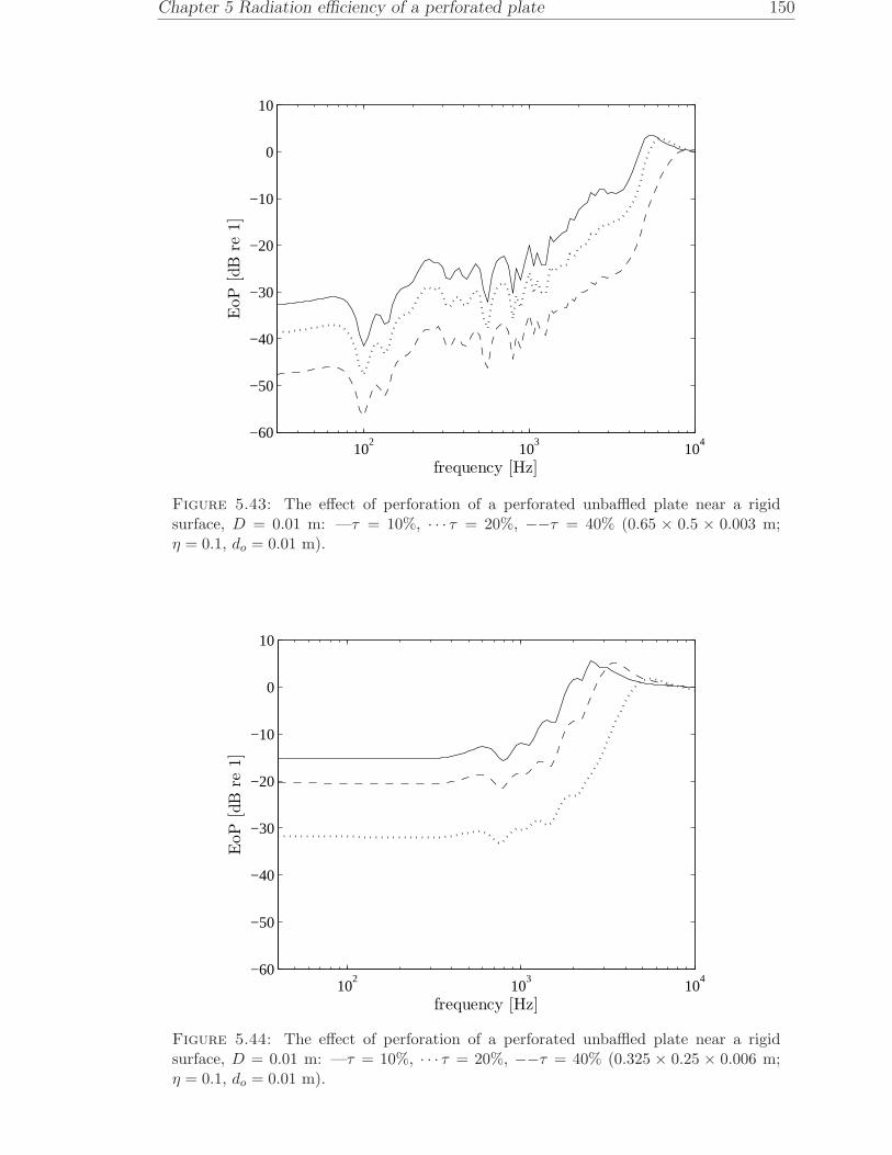
Chapter 5 Radiation efficiency of a perforated plate 150
102
103
104
−60
−50
−40
−30
−20
−10
0
10
frequency [Hz]
EoP
[dB
re1]
Figure 5.43: The effect of perforation of a perforated unbaffled plate near a rigidsurface, D = 0.01 m: —τ = 10%, · · · τ = 20%, −−τ = 40% (0.65 × 0.5 × 0.003 m;η = 0.1, do = 0.01 m).
102
103
104
−60
−50
−40
−30
−20
−10
0
10
frequency [Hz]
EoP
[dB
re1]
Figure 5.44: The effect of perforation of a perforated unbaffled plate near a rigidsurface, D = 0.01 m: —τ = 10%, · · · τ = 20%, −−τ = 40% (0.325 × 0.25 × 0.006 m;η = 0.1, do = 0.01 m).

Chapter 5 Radiation efficiency of a perforated plate 151
5.5 Effect of perforation on plate dynamic
properties
5.5.1 Effect on bending stiffness and mass
In the results in this chapter the effect of perforation on the dynamic properties of the
plate have been neglected. However in practice perforation will reduce both bending
stiffness and mass of a plate. This effect is discussed in this section.
The investigation of the effect of perforation on dynamic properties of plates began
in the early 1960s in order to determine an accurate stress analysis of perforated
panels used to support the tubes in a heat exchanger [83, 84, 85]. To obtain an
equivalence with the actual properties corresponding to a solid plate, the effective
material properties were defined, namely the effective Young’s modulus (E∗), Poisson’s
ratio (ν∗) and density (ρ∗p).
To allow different spacing between holes in an array of perforation, Forskitt et al. [65]
introduced a perpendicular and parallel ligament efficiency given by
XLE =bx − 2do
bx, YLE =
by − 2do
by(5.56)
where bx is perpendicular pitch and by is parallel pitch as shown in Figure 5.45 for a
triangular or rectangular array of perforation. Forskitt et al. [65] then used a Finite
Element Method (FEM) to determine E∗ and ν∗ for a perforation plate with circular
holes.
Perforation also reduces the mass of a plate. Based on the solid plate, this effect is
quantified by introducing the effective density ρ∗p. The effective density ρ∗p according
to [65] can be obtained based on the fraction of the solid plate i.e.
ρ∗pρp
= 1 −[π8(1 − XLE)(1 − YLE)
](5.57)
This is only for a regular triangular array of holes. For a rectangular array, it can be
written as

Chapter 5 Radiation efficiency of a perforated plate 152
ρ∗pρp
= 1 −[ π16
(1 − XLE)(1 − YLE)]
(5.58)
In terms of perforation ratio τ , both Eq.(5.57) and Eq.(5.58) are equivalent to 1 − τ .
It was then proposed that the effective resonance frequency of a simply supported
plate is given as in Eq.(2.7), but introducing the effective material properties
ω∗mn =
(E∗t2p
12ρ∗p(1 − ν∗2)
) 1
2[(mπ
a
)2
+(nπb
)2]
(5.59)
According to Burgemeister and Hansen [64], this equation does not provide correct
resonance frequencies when using the effective material properties. The FEM was then
implemented to model the modal response of range of plates with varying perforation
geometries. From this, the resonance frequency f ∗ was compared with that from the
FEM model for the solid plate f . The results of these comparisons (f ∗/f) were then
fitted to a cubic expression as a general equation for other perforation geometries in
terms of XLE and YLE which is independent of the mode order (m,n). The cubic
function is given by
f ∗
f= ac × XLE3 + bc × XLE2 + cc × XLE + ... (5.60)
+ dc × YLE3 + ec × YLE2 + fc × YLE + gc
where the coefficients are listed in Table 5.1.
This formula was validated by comparison with the measured resonance frequencies of
two perforated plates. The results using Eq.(5.59) (with the material properties data
from [65]) underestimated the measured results. However, the experimental validation
was carried out on plates having similar geometries from among the models which gave
a good agreement. It should also be made with different plate dimensions, thicknesses
and hole geometries to ensure a stronger validation of the proposed formula.
Figure 5.46 shows a comparison between the results of the resonance frequency ratio
f ∗/f from [64] with those using the effective material properties obtained from [65].
A large difference can be seen, particularly for small XLE and YLE (large τ). Fig-
ure 5.46(a) is obviously non-linear. In [64], the graph was constructed from available

Chapter 5 Radiation efficiency of a perforated plate 153
bx
by do
(a)
bx
by
do
(b)
Figure 5.45: Array of holes: (a) triangular and (b) rectangular.
Table 5.1: Coefficient for the cubic function in Eq.(5.60)
Coefficient Valueac 0.0399bc −0.0727cc 0.1161dc −0.1295ec 0.1013fc 0.1096gc 0.8395
data in [65]. The graph is only applicable for XLE > 0, YLE > 0. Meanwhile Fig-
ure 5.46(b) produces almost a smooth plane surface. The graph can also be expanded
to include XLE < 0 and or YLE < 0.
Patil et al. [86] also used a curve fitting technique to develop an effective resonance
frequency formula from simulation data of resonance frequencies for five perforated
plates using FEM. The formula was a function of the so-called mass remnant ratio
(MR) i.e. the ratio of surface area of a perforated plate to that of the solid plate for
the same dimension. This is equivalent to 1− τ . The formula was then expressed as a
seventh order polynomial function of MR. However, the formula was applicable only
for the first three modes of vibration.
Soler and Hill [87] proposed a formula for calculating the effective bending stiffness B∗.
For a regular array of circular holes in a very thin plate (tp ≪ bx) where XLE ≈ YLE,
the effective modal resonance frequency is given by
ω∗mn =
(B∗
ρptp
) 1
2[(mπ
a
)2
+(nπb
)2]
(5.61)

Chapter 5 Radiation efficiency of a perforated plate 154
(a) (b)
Figure 5.46: The ratio of the effective resonance frequency of a perforated plate tothe resonance frequency of a solid plate: (a) using effective material properties datafrom [65] and (b) using FEM [64].
where
B∗ =B
(1 − πd2o/√
3b2x)
(1 − π
2√
3
(1 − bx − do
bx
)2)(2bx−do)/0.8bx
and B = Et3p/12(1 − ν2). The true density ρp is used in this equation because the
correction factor has been implicitly included in the effective bending stiffness B∗. It
was shown that this formula agrees well with the results from Figure 5.46(a) [65].
Table 5.2 lists the changes in resonance frequency predicted for different perforation
geometries and plate thicknesses considered in the experiments in Chapter 7. Results
are given for the ratio f ∗/f using Eq.(5.60) and Eq.(5.61). The hole distance is made
similar (bx = by) to be able to apply Eq.(5.61). Using Eq.(5.60) for 1.5 mm plate
thickness, it can be seen the ratio f ∗/f is reduced as the hole diameter is increased.
The reduced resonance frequency is due to a reduction in the bending stiffness of the
plate due to the perforation, which basically makes the plate more flexible. For the
3 mm thick plate, all the plates with 20% perforation ratio give the same effective
resonance frequency ratio. This is because the hole diameter and the hole separation
distance increase with the same factor.
The results using Eq.(5.61) give a frequency ratio which is sometimes greater than
unity. This is due to the plate thicknesses given which is not small enough to apply this
equation. Eq.(5.61) also has another limitation. It can be observed from the formula
that in order to avoid a negative bending stiffness, it requires that d2o < (
√3/π)b2x. In
other words, the holes cannot be very closely spaced. The results in Table 5.2, i.e. for

Chapter 5 Radiation efficiency of a perforated plate 155
1.5 mm plates with 19% and 44% and 3 mm plates for 20% perforation ratios, suggest
that Eq.(5.61) is being used outside its range of validity.
Table 5.2: Comparison of effective resonance frequencies
Dimensions (m) do (m) bx (m) τ (%)f ∗/f
Eq.(5.60) Eq.(5.61)
0.4 × 0.3 × 0.0015
0.005 0.027 5 0.9706 0.99630.008 0.027 12 0.9301 0.99840.010 0.027 19 0.8984 1.00780.015 0.027 44 0.8149 1.1206
0.4 × 0.3 × 0.003
0.005 0.010 20 0.8395 1.06290.010 0.020 20 0.8395 1.06290.015 0.050 7 0.9286 0.99860.025 0.050 20 0.8395 1.0629
As Eq.(5.61) is limited in its perforation geometry and plate thickness, therefore for
the purpose of this study, only Eq.(5.60) will be implemented.
The critical frequency will also be altered. In this case a reduction in bending stiffness
leads to an increase in critical frequency
f ∗c
fc
=f
f ∗ (5.62)
5.6 Summary
The sound radiation from a perforated plate set in an equally infinite perforated baffle
has been calculated using an approach from Fahy and Thompson [37]. It has been
shown that the radiation efficiency of a baffled plate is reduced drastically at low
frequency because of the perforation in the plate and the baffle. The effect of perfora-
tion (EoP) curve also shows that the reduction follows a 20 dB/decade trend against
the frequency. From this, an approximate formula for determining the EoP has been
proposed that gives a good agreement up to half the critical frequency. It is also
found that the EoP is independent of the plate dimensions, depending only on the
non-dimensional reactance of the perforation, h.
A model for sound radiation from an unbaffled plate has been developed by modifying
Laulagnet’s model for the radiation efficiency of an unbaffled solid plate [33]. For

Chapter 5 Radiation efficiency of a perforated plate 156
the thin plates (tp ≪ do), similar to the case of a perforated plate set in an infinite
perforated baffle, the EoP is proportional to τ/do. The EoP increases as the perforation
ratio increases and as the hole size reduces for a given perforation ratio. However,
unlike the former case, the EoP for an unbaffled plate depends on the plate thickness
and dimensions. An approximate formula has also been proposed for this case which
gives a good agreement up to half the critical frequency.
The model has then been extended to consider a plate located near a rigid, reflecting
surface. Depending on the distance between the plate and the rigid surface, the radi-
ation efficiency is considerably reduced at low frequencies. More sound reduction can
be gained by introducing perforation to the plate. However, at higher frequencies, the
radiation efficiency is similar than or greater than that for the plate in absence of the
rigid surface.
It has also been shown that the perforation changes the bending stiffness of the plate
which causes a slight reduction of the resonance frequencies and corresponding increase
in the critical frequency.
The proposed approximate formulae for the EoP can be used as an engineering design
guide for noise control measures. The results show that for only 10% perforation
ratio, the sound radiation can be reduced by 10 − 15 dB at low frequencies which
shows the effectiveness of perforation as a noise control measure. However, it should
be remembered that in certain structures, the stiffness reduction due to perforation
also has to be considered. In other words, the structural strength must be taken into
account when the perforation is introduced. Consequently, a trade-off may be required
between reducing the sound radiation and maintaining the strength of the structure.

Chapter 6
Sound Radiation from a Plate
Modelled by Discrete Sources
In Chapter 5, the assumption was made that the array of holes can be replaced by
a uniform acoustic impedance at the suface of the plate. For this to be valid, the
distance between the holes must be short enough compared with the acoustic wave-
length. However, the effect is not obvious in the models because the perforation ratio
is a parameter defined without necessarily knowing the hole position or the distance
between holes. As already mentioned in Section 5.1.3, a frequency limit should exist
where the continuous impedance assumption is breached when the hole distance is
large compared with the acoustic wavelength.
In this chapter, a discrete source approach is taken. A continuous baffled source can be
modelled by replacing it with an array of point sources. In the same way a perforated
plate can also be modelled by an array of sources, some representing the plate and
others the holes. The acoustic pressure at each source due to the motion of the other
sources is calculated numerically. This discrete source model is attractive as the hole
configuration can be set arbitrarily and the hole distance is known. This approach
also provides a model for the case of a perforated plate set in an infinite rigid baffle
which has not been covered in Chapter 5. In principle, the concept is similar to the
models of Vitiello et al. [25], Cunefare and Koopman [26], Elliott and Johnson [27] and
Gardonio et al. [28] which used discrete elementary radiators to replace a continuous
157

Chapter 6 Sound Radiation from a Plate Modelled by Discrete Sources 158
radiator. However, as will be shown later, the self-radiation impedance used in the
proposed model is slightly different.
6.1 Discrete version of Rayleigh integral
The well-known Rayleigh integral [9] can be used to calculate the sound pressure at
any point of observation due to a vibrating plate set in an infinite rigid baffle. The
equation can be written as
p(x) = −2
∫
s
G(x|xo)
(∂p(x)
∂n
)
S
dS (6.1)
where x = (x, y, z) and S denotes the surface area of the plate (assumed to lie in the
xy-plane). The first term of the integrand is the free-field Green’s function, which is
the sound pressure contribution at x due to the radiation from a unit point monopole
source at xo. Since ∂p/∂n = −jρck Up and G = e−jkR/4πR, this equation can be
written as
p(x) =jρck
2π
∫
s
Up(xo)e−jkR
RdS (6.2)
where R = |x − xo| and Up is the normal velocity amplitude of the plate.
The Rayleigh integral requires that the normal velocity Up is known over the whole
plate surface area. For the simple case of a moving piston, the normal velocity is
uniform across the surface
Up(xo) = Un (6.3)
where Un is constant. For bending of a rectangular plate with dimensions a × b and
assuming simply supported edges, the velocity can be written as the sum of modal
contributions given by
Up(xs) =∞∑
m=1
∞∑
n=1
umn sin(mπx
a
)sin(nπy
b
)(6.4)

Chapter 6 Sound Radiation from a Plate Modelled by Discrete Sources 159
where umn is the complex velocity amplitude of mode (m,n). For a point force excita-
tion at (x0, y0), it can be defined as in Eq.(2.5)
umn =4jωF
[ω2mn(1 + jη) − ω2]M
sin(mπx0
a
)sin(nπy0
b
)(6.5)
where F is the force amplitude, ωmn is the natural frequency, η is the damping loss
factor and M is the plate mass.
The Rayleigh integral can next be written in discrete form as a sum over discrete source
regions. For a rectangular plate in the xy coordinate plane, the sources are defined
by dividing the plate into a set of grid points. The spacings between points are dx in
the x direction and dy in the y direction. The small element of the plate dS = dxdy
thus becomes a discrete monopole source. This requires that the size of the elemental
source must be much smaller than the acoustic wavelength (k dx≪ 1, k dy ≪ 1).
Discretizing the Rayleigh integral yields
p(x) =jρck
2π
∑
s
Up(xs)e−jkR
Rdxdy (6.6)
where R = |x − xs|. However for positions x on the surface (x = xr) the integrand
is singular for r = s. To solve the integral for element r, another approximation
corresponding to the pressure distribution on the plate surface is needed. Morse and
Ingard [75] give the total force per unit area (pressure) acting on a rectangular (almost
square) piston moving with uniform velocity Un. For a plate of dimensions a×b, where
b ∼= a, the radiation impedance is given by
p
Un
=ρck2
16(a2 + b2
)+j8ρck
9π
(a2 + ab+ b2
a+ b
), ka≪ 1 (6.7)
Applying this to the elemental source dS and assuming a square piston, i.e. a = dx =
b = dy, this reduces to
p
Un
= ρc
(k2dx2
8+j4k dx
3π
), k dx≪ 1 (6.8)

Chapter 6 Sound Radiation from a Plate Modelled by Discrete Sources 160
do
t
Up
1 2 3 4 5 6 7
bafflebaffle baffle
Ufplate hole
Figure 6.1: Analytical model of an array of discrete (monopole) sources for calculatingthe sound radiation of a perforated plate
Therefore the Rayleigh integral can be written in the form
pr = Mrs Us (6.9)
where
Mrs =
jρck
2π
(e−jkRrs
Rrs
)dx2, r 6= s
ρc
(k2dx2
8+j4k dx
3π
), r = s
(6.10)
The matrix M is actually an impedance matrix since the acoustic impedance expresses
the ratio of complex pressure to the associated particle velocity. In the models of Elliott
and Johnson [27] and Gardonio et al. [28], the impedance of the elementary radiator
is defined by
ℜ (Mrs) =ρck2d2
x
2π
(sin kRrs
kRrs
)(6.11)
wheresin kRrs
kRrs
= 1 for kRrs → 0.
For the real part of the self-radiation impedance (Mrr), the difference between the two
models is 27%.
6.2 Impedance matrix including perforation
Consider an array of circular holes on a plate, as shown in Figure 6.1. Each hole can
be considered to be an acoustic source with volume velocity πd2oUh/4 where Uh is the
fluid velocity in the hole and do is the diameter of the hole.

Chapter 6 Sound Radiation from a Plate Modelled by Discrete Sources 161
The pressure at any point on the plate surface can be written as a sum of the pressure
contributions from all sources representing the plate and the holes. The pressure at
source position r due to source s can be written as
pr =∑
s
MrsUs (6.12)
where Us is the velocity of source s which may represent the plate surface or the holes.
Using the example in Figure 6.1, Mrs can be written as a matrix, for example
Mrs =
M11 · M13 · M15 · M17
· · M23 · M25 · ·M31 M32 M33 M34 M35 M36 M37
· · M43 · M45 · ·M51 M52 M53 M54 M55 M56 M57
· · M63 · M65 · ·M71 · M73 · M75 · M77
(6.13)
In the present example, sources 3 and 5 correspond to the holes. The elements inside
the dashed lines correspond to the pressure at the hole locations due to the sources
at the plate or the holes; or the pressure at the plate location due to the holes. The
matrix Mrs can be partitioned to give
M =
Mp−p Mp−h
Mh−p Mh−h
(6.14)
where p− p refers to the pressure at a plate location due to plate sources, p− h refers
to the pressure at plate locations due to hole sources, etc.
The pressure and velocity can be partitioned into components corresponding to the
plate and the holes giving
pp
ph
= M
Up
Uh
(6.15)
where denotes a column vector.

Chapter 6 Sound Radiation from a Plate Modelled by Discrete Sources 162
The fluid velocity in the hole is defined from the acoustic impedance of the hole Zh
Uf = −2ph
Zh
(6.16)
where Zh = τzh is given in Eq (5.14) and 2ph is the difference between the pressure
on both sides of the plate.
The model is developed for discrete, independent holes on the plate. Therefore, the
acoustic impedance is no longer treated as a uniform specific acoustic impedance zh
across the plate surface.
As the fluid velocity in each hole may be represented by ne monopole sources, where
ne may be greater than one, the fluid velocity through the hole area must be averaged
to the corresponding element area dS of the monopole sources to maintain the correct
source strength. Thus
Ufa = Ufcf (6.17)
where Ufa is the corrected fluid velocity and cf is the correction factor given by
cf =1
nedS
(πd2
o
4
)(6.18)
Since Uf represents the motion of the fluid relative to the plate, the source velocity
from the hole Uh is the combination of the velocity of the plate and the fluid. It can
be expressed as
Uh = U ′p + Ufa = U ′
p −2ph
Zh
cf (6.19)
where U ′p is the (interpolated) plate velocity for a solid plate at the hole locations.1
The pressure at the plate location and at the holes can then be written as
pp = [Mp−p] Up + [Mp−h] Uh (6.20)
1Without any viscous effect, the impedance of the hole is inertial. It may be appropriate for theabsolute velocity in the hole to depend on the pressure difference rather than the relative velocity asgiven. However, this has not been investigated here.

Chapter 6 Sound Radiation from a Plate Modelled by Discrete Sources 163
ph = [Mh−p] Up + [Mh−h] Uh (6.21)
Substituting Eq.(6.19) into Eq.(6.21) and rearranging yields
[I +
2Mh−h cfZh
]ph = ([Mh−p Mh−h]) Up (6.22)
where Up is a vector containing the plate velocity at all locations including the plate
(Up) and the holes (U ′p) and I is the identity matrix of dimension equal to the number
of holes.
Inverting the matrix on the left-hand side of Eq.(6.22) gives
ph =
[I +
2Mh−h cfZh
]−1
([Mh−p Mh−h]) Up (6.23)
The pressure at the plate locations pp can be obtained by substituting Eq.(6.23) into
Eq.(6.19) to give Uh and then substituting into Eq.(6.20).
The total sound power radiated by the plate can be expressed as the summation over
the power contributions from all discrete sources. The sound power can thus be given
by
W =1
2ℜ(∑
ppU∗p +
∑phU
∗h
)dS (6.24)
where dS is the elemental source area.
Finally, recalling Eq.(1.2), the radiation efficiency of the perforated plate can be writ-
ten as
σ =W
12ρcab
⟨∣∣U2p
∣∣⟩ (6.25)
where⟨∣∣U2
p
∣∣⟩ is the spatially averaged squared surface velocity of the plate.

Chapter 6 Sound Radiation from a Plate Modelled by Discrete Sources 164
6.3 Results
6.3.1 Radiation by a vibrating piston
The model is examined first for a uniform plate velocity or vibrating piston. The
sound radiated by a perforated vibrating piston is calculated by using Eq.(6.3) to
represent the plate velocity. The accuracy of the results depends on the source spacing
dx. Figure 6.2 shows the results for different source spacings. It can be seen that
the smaller the spacing, i.e. the larger the number of sources, the better the result
converges. The blue curve is plotted as a reference and calculated analytically using
Rayleigh’s integral from Eq.(2.1) where the velocity v is set to be unity. The results
show that the spacing must be less than 0.01 m to ensure that the result (black, solid
line) converges to unity up to at least 4 kHz. However, as dx is reduced the calculation
time becomes more intensive and the impedance matrices representing this number of
sources become large requiring greater computer memory. With the elemental source
spacing of dx = dy = 0.01 m, the number of elemental sources is 3250. As from
1 kHz the radiation efficiency for a vibrating piston is close to unity, the remaining
calculations in this section are performed only up to 3 kHz and using dx = 0.01 m.
The calculation is carried out for the same plate dimensions 0.65× 0.5× 0.003 m and
parameters as in previous chapters. For a rigid piston the thickness is only relevant for
the definition of the hole impedance. Figure 6.3 shows the plate with the grid points
and the locations of the holes for one example in which, 20 holes are chosen with each
hole represent by 16 monopole sources. The hole distance in the x or y directions is
0.13 m.
Figure 6.4 plots the results for the rectangular piston with various perforation ratios
(different numbers of holes) with the hole diameter do = 4 cm. It can be seen that
the radiation efficiency reduces as the perforation ratio increases. The curves all have
a 20 dB/decade slope until they converge to unity. This proportionality to f 2 shows
the characteristic of a monopole source radiation. For the present case, the calculation
of radiation efficiency up to 3 kHz (frequency resolution of 20 points per decade,
spaced logarithmically) using MATLAB takes about 11 minutes. See Table 2.1 for the
computer specification.

Chapter 6 Sound Radiation from a Plate Modelled by Discrete Sources 165
101
102
103
104
10−3
10−2
10−1
100
101
frequency [Hz]
radia
tion
effici
ency
,σ
Figure 6.2: Radiation efficiency of a solid baffled plate (rectangular piston) fromdiscrete monopole sources: 0.65 × 0.5 × 0.003 m (— analytical, − · −dx = 0.04 m,−−dx = 0.02 m and —dx = 0.01 m).
−0.3 −0.2 −0.1 0 0.1 0.2 0.3−0.25
−0.2
−0.15
−0.1
−0.05
0
0.05
0.1
0.15
0.2
0.25
a
b
Figure 6.3: Example of the grid points (+) and the locations of 5×4 holes from groupsof monopole sources () on the plate (0.65 × 0.5 m).

Chapter 6 Sound Radiation from a Plate Modelled by Discrete Sources 166
101
102
103
10−3
10−2
10−1
100
frequency [Hz]
radia
tion
effici
ency
,σ
Figure 6.4: Radiation efficiency of a perforated baffled plate (rectangular piston)from discrete monopole sources: 0.65 × 0.5 × 0.003 m, do = 0.04 m, dx = 0.01 m(−unperforated, —τ = 6%, −−τ = 12%, · · · τ = 22%, − · −τ = 31% ).
As the spacing between holes is also defined by the elemental sources, the perforation
ratio (number of holes and their diameter) thus affects the number of sources required,
particularly for the plate with a large number of holes. For example consider a perfo-
rated plate of similar dimensions having 40×30 holes with 5 mm diameter (τ = 20%).
Assuming in each direction, one monopole source is set to represent the hole and the
plate parts, the number of sources required is 81 × 61 = 4941. Consequently, the
larger the number of holes, the more sources are required and the more intensive the
calculation time. This limits the capability of the model to calculate the radiation
efficiency of a perforated plate only for a moderate number of holes.
Figure 6.5 plots the results for various hole diameters with constant perforation ratio.
It can be seen that the radiation efficiency can be further reduced by reducing the
hole size, as also seen for the case of a perforated plate set in a perforated baffle and
a perforated unbaffled plate (see Section 5.2.3).
Figure 6.6 plots the effect of perforation (EoP) corresponding to the results in Fig-
ure 6.4. It shows that the trend is similar to that for the perforated unbaffled case (see
Figure 5.23) where the EoP curve is constant at low frequencies until it rises toward

Chapter 6 Sound Radiation from a Plate Modelled by Discrete Sources 167
101
102
103
10−3
10−2
10−1
100
frequency [Hz]
radia
tion
effici
ency
,σ
Figure 6.5: Radiation efficiency of a perforated baffled plate (rectangular piston) fromdiscrete monopole sources: 0.65×0.5×0.003 m, τ = 4%, dx = 0.01 m (−unperforated,
—do = 43, −−do = 33, · · · do = 26, − · −do = 13 mm ).
101
102
103
−20
−15
−10
−5
0
5
frequency [Hz]
EoP
[dB
re1]
Figure 6.6: Effect of perforation (EoP) on sound power radiation of a perforatedbaffled plate (rectangular piston) from discrete monopole sources: 0.65 × 0.5 × 0.003 m,do = 0.04 m, dx = 0.01 m (—τ = 6%, −−τ = 12%, · · · τ = 22%, − · −τ = 31% ).

Chapter 6 Sound Radiation from a Plate Modelled by Discrete Sources 168
101
102
103
104
10−3
10−2
10−1
100
101
frequency [Hz]
radia
tion
effici
ency
,σ
Figure 6.7: Radiation efficiency from modal response of a perforated baffled platefrom discrete monopole sources: 0.65 × 0.5 × 0.003 m with η = 0.1 (· · · dx = 0.04 m,−−dx = 0.02 m, − · −dx = 0.015 m and —dx = 0.01 m).
0 dB.
6.3.2 Radiation by bending vibration
The model is next applied to calculate the sound radiation due to the forced vibration
of a simply supported, perforated baffled plate. Eq.(6.4) is now implemented for the
plate vibration.
Figure 6.7 plots the radiation efficiency for the same plate specifications as in the
previous section. The force is applied at (−0.13a,−0.1b) where the origin (0,0) is at
the plate centre as in Figure 6.3. The results are presented for different source spacings
dx. As also expected from Figure 6.2, the choice of dx defines the discrepancy at high
frequency. It can be seen that the convergence of the curves to the true value of
radiation efficiency needs a small value of dx. For 20 × 20 modes and dx = 0.01 m,
which involves 3250 sources for the present case, the calculation time is 38 minutes.
The frequency resolution is 40 points per decade (spaced logarithmically) to ensure 3
points within the half-power bandwith of resonances.

Chapter 6 Sound Radiation from a Plate Modelled by Discrete Sources 169
101
102
103
104
10−5
10−4
10−3
10−2
10−1
100
frequency [Hz]
radia
tion
effici
ency
,σ
Figure 6.8: Radiation efficiency from bending vibration of a perforated baffled platefrom discrete monopole sources: 0.65×0.5×0.003 m, do = 0.04 m, dx = 0.01 m, η = 0.1(−unperforated, —τ = 6%, −−τ = 12%, · · · τ = 22%, − · −τ = 31% ).
Figure 6.8 plots the radiation efficiency of a perforated baffled plate for constant hole
diameter of 4 cm with different perforation ratios. The radiation efficiency reduces as
the perforation ratio increases. The effect of hole density (number of holes per unit
area) on the radiation efficiency is shown in Figure 6.9. For the same perforation ratio,
the sound radiation can again be seen to be reduced by increasing the hole density
(reducing the size).
The effect of perforation (EoP) corresponding to the results in Figure 6.8 is shown in
Figure 6.10. This shows that the sound reduction due to perforation is constant at
the fundamental mode (< 70 Hz). The effect is also almost constant in the edge mode
region up to the critical frequency, i.e. between 1.5 kHz and 4 kHz.
Figure 6.11 compares these results with the EoP for the baffled piston from Section
6.3.1 and also for an unbaffled perforated plate from Chapter 5. It can be seen that
these three sets of results diverge as the perforation ratio increases. In the fundamental
mode region, the perforated baffled plate has the greatest effect (−EoP), while in the
edge mode region between 400 Hz and 4 kHz, the perforated unbaffled plate has the
largest effect. However, in the corner mode region between 100 Hz and 400 Hz, the

Chapter 6 Sound Radiation from a Plate Modelled by Discrete Sources 170
101
102
103
104
10−4
10−3
10−2
10−1
100
frequency [Hz]
radia
tion
effici
ency
,σ
Figure 6.9: Radiation efficiency from bending vibration of a perforated baffled platefrom discrete monopole sources: 0.65 × 0.5 × 0.003 m, τ = 4%, dx = 0.01 m(−unperforated, —do = 43, −−do = 33, · · · do = 26, − · −do = 13 mm ).
101
102
103
104
−20
−15
−10
−5
0
5
frequency [Hz]
EoP
[dB
re1]
Figure 6.10: Effect of perforation (EoP) on sound power radiation of a perforatedbaffled plate in bending vibration from discrete monopole sources: 0.65× 0.5× 0.003 m,do = 0.04 m, dx = 0.01 m (—τ = 6%, −−τ = 12%, · · · τ = 22%, − · −τ = 31% ).

Chapter 6 Sound Radiation from a Plate Modelled by Discrete Sources 171
101
102
103
104
−20
−15
−10
−5
0
5
frequency [Hz]
EoP
[dB
re1]
(a)
101
102
103
104
−20
−15
−10
−5
0
5
frequency [Hz]
EoP
[dB
re1]
(b)
101
102
103
104
−20
−15
−10
−5
0
5
frequency [Hz]
EoP
[dB
re1]
(c)
101
102
103
104
−20
−15
−10
−5
0
5
frequency [Hz]
EoP
[dB
re1]
(d)
Figure 6.11: Comparison of the effect of perforation (EoP) on sound power radiation:perforated baffled plate (—), perforated unbaffled plate (−−) and baffled piston (−·−);0.65 × 0.5 × 0.003 m, do = 0.04 m, dx = 0.02 m, η = 0.1; (a) τ = 6%, (b) τ = 12%, (c)τ = 22%, (d) τ = 31%.
three results are similar.
6.4 Frequency limit of continuous impedance
All the models developed in Chapter 5 are based on the assumption that the distribu-
tion of holes can be represented by a continuous impedance on the plate surface. This
implies that the hole distance must be much smaller than the acoustic wavelength.
The effect of perforation is expected to be limited in frequency depending on the dis-
tance between holes. However, the models cannot predict the frequency limit because
the perforation ratio is defined only as a function of hole size and number, not as a

Chapter 6 Sound Radiation from a Plate Modelled by Discrete Sources 172
Table 6.1: Distance between holes.
No. number of holes, No distance (m)
1 5 × 5 0.122 3 × 3 0.203 2 × 2 0.32
function of hole distance. This section investigates the frequency limit above which
the sound reduction no longer occurs due to the excessive hole distance.
6.4.1 Frequency limit for vibrating piston
Figure 6.12 presents the the radiation efficiency of a perforated plate having a uniform
velocity (rectangular piston) with a small number of holes in order to have a large hole
separation. The hole distances are listed in Table 6.1.
An interesting phenomenon is found at a certain frequency where the radiation effi-
ciency from the perforated plates exceeds or becomes similar to that of the unperfo-
rated plate. This is marked in Figure 6.12 at 1100, 1700 and 2700 Hz for Figure 6.12(a),
(b) and (c), respectively. If these intersection frequencies (limit frequencies) fl are ex-
amined for each case, it is found that the hole spacing equals one acoustic wavelength
at fl: λ = c/1100 ≈ 0.32 m (Figure 6.12(a)), λ = c/1700 = 0.20 m (Figure 6.12(b))
and λ = c/2700 ≈ 0.12 m (Figure 6.12(c)) where λ is the acoustic wavelength and
c = 343 m/s is the speed of sound.
The phenomenon is more obvious when the results are plotted in terms of the effect
of perforation, as seen in Figure 6.13. The limit frequencies are denoted by fl1, fl2
and fl3. It can be seen that above these limit frequencies, the perforation no longer
reduces the sound radiation, i.e. EoP ∼= 0 dB.
However, the case of a vibrating piston is rarely found in practice. A more practical
problem is to observed this effect in the bending vibration case.

Chapter 6 Sound Radiation from a Plate Modelled by Discrete Sources 173
100 1000 30000.5
1
2
frequency [Hz]
radia
tion
effici
ency
,σ
fl
(a)
100 1000 30000.5
1
2
frequency [Hz]
radia
tion
effici
ency
,σ
fl
(b)
100 1000 30000.5
1
2
frequency [Hz]
radia
tion
effici
ency
,σ
fl
(c)
Figure 6.12: Radiation efficiency of a perforated baffled plate (rectangular piston)from discrete monopole sources showing the frequency limit of continuous impedanceassumption: 0.65 × 0.5 × 0.003 m, dx = 0.01 m (—unperforated, −−perforated; (a)do = 0.05 m: No = 2× 2, (b) do = 0.06 m: No = 3× 3 and (c) do = 0.02 m: No = 5× 5).
6.4.2 Frequency limit for bending vibration
Figure 6.14 plots the the radiation efficiency of perforated plates with similar number
and distance of holes as in Table 6.1. The unit force is applied at (−0.315a,−0.3b)
from the origin (0, 0) at the plate centre. It can be seen from Figure 6.14, that in this
case, the intersection frequencies between the perforated and unperforated results are
half those for the vibration piston. The frequencies are 530, 850 and 1400 Hz. At
these frequencies, the hole distance is equal to half the acoustic wavelength. At these
frequencies, well below fc, the wavelength in the panel is much shorter than that in
air, whereas for the piston the structural wavelength is effectively infinite.
Figure 6.15 plots the EoP for the same results which clearly shows the limit frequencies

Chapter 6 Sound Radiation from a Plate Modelled by Discrete Sources 174
1000 2000 3000−0.5
−0.4
−0.3
−0.2
−0.1
0
0.1
0.2
0.3
0.4
0.5
frequency [Hz]
EoP
[dB
re1]
fl1fl3fl2
Figure 6.13: Effect of perforation (EoP) from a perforated baffled plate (rectangularpiston) from discrete monopole sources showing the frequency limit of continuous im-pedance assumption: 0.65× 0.5× 0.003 m, dx = 0.01 m ((a) —do = 0.06 m; No = 2× 2,(b) −−do = 0.075 m; No = 3 × 3 and (c) − · −do = 0.03 m; No = 5 × 5).
fl. Figure 6.16 shows corresponding results for a different hole radius but with the
same hole separation. This gives a similar result and confirms that the limit frequency
fl depends only on the hole separation, regardless of the hole radius.
Therefore it has been shown that in order for the perforation of the vibrating plate
still to have an effect in reducing the radiated sound, the distance between holes must
be less than half the acoustic wavelength. If this condition is satisfied, the holes can
effectively suppress part of the adjacent volume sources resulting in a reduction of the
radiated sound. However when the the holes are further apart than half a wavelength,
this process is no longer effective and the sound is radiated as from the solid plate.
6.5 Summary
A model of sound radiation from a perforated baffled plate has been proposed. The
model is developed by dividing the plate and the holes into discrete monopole sources.
The contribution of the sound sources to each other is assembled into an impedance
matrix. The pressure due to the holes is obtained by inverting the impedance matrix.

Chapter 6 Sound Radiation from a Plate Modelled by Discrete Sources 175
101
102
103
104
10−3
10−2
10−1
100
frequency [Hz]
radia
tion
effici
ency
,σ
fl
(a)
101
102
103
104
10−3
10−2
10−1
100
frequency [Hz]
radia
tion
effici
ency
,σ fl
(b)
101
102
103
104
10−3
10−2
10−1
100
frequency [Hz]
radia
tion
effici
ency
,σ
fl
(c)
Figure 6.14: Radiation efficiency from bending vibration of a perforated baffled platefrom discrete monopole sources showing the frequency limit of continuous impedanceassumption: 0.65× 0.5× 0.003 m, dx = 0.01 m, η = 0.1 (—unperforated, −−perforated;(a) do = 0.05 m: No = 2 × 2, (b) do = 0.06 m: No = 3 × 3 and (c) do = 0.02 m:No = 5 × 5).
This avoids assuming a layer of continuous impedance (Section 5.1.4) as the interaction
of the holes with the sound field is analysed individually. The holes are now arranged
at a known separation distance. The major important finding from this model is that
the holes can effectively suppress the adjacent volume sources which hence reduce the
radiated sound from a plate surface, when the hole distance is less than an acoustic
wavelength for a rectangular vibrating piston and less than half the acoustic wavelength
for a rectangular plate in bending vibration below its critical frequency.
This frequency limit should be taken into account depending on the desired frequency
range of noise reduction. Of course, the shorter the hole distance, the wider the
frequency range of sound reduction. This means introducing large perforation to the

Chapter 6 Sound Radiation from a Plate Modelled by Discrete Sources 176
101
102
103
104
−7
−6
−5
−4
−3
−2
−1
0
1
2
frequency [Hz]
EoP
[dB
re1]
fl1
fl2 f
l3
Figure 6.15: Effect of perforation (EoP) from bending vibration of a perforated baf-fled plate from discrete monopole sources showing the frequency limit of continuousimpedance assumption: 0.65 × 0.5 × 0.003 m, dx = 0.01 m, η = 0.1 ((a) —do = 0.05 m;No = 2 × 2, (b) −−do = 0.06 m; No = 3 × 3 and (c) − · −do = 0.02 m; No = 5 × 5).
101
102
103
104
−7
−6
−5
−4
−3
−2
−1
0
1
2
frequency [Hz]
EoP
[dB
re1]
fl1
fl2 f
l3
Figure 6.16: Effect of perforation (EoP) from bending vibration of a perforated baf-fled plate from discrete monopole sources showing the frequency limit of continuousimpedance assumption: 0.65 × 0.5 × 0.003 m, dx = 0.01 m, η = 0.1 ((a) —do = 0.06 m;No = 2 × 2, (b) −−do = 0.075 m; No = 3 × 3 and (c) − · −do = 0.03 m; No = 5 × 5).

Chapter 6 Sound Radiation from a Plate Modelled by Discrete Sources 177
plate or increasing the number of holes. However, large perforation can reduce the
stiffness of the plate which then increases the plate vibration, particularly for point
force or rain on the roof excitations. This will be discussed in Chapter 7 in the context
of experimental validation.
Unfortunately it was not possible to compare results from the discrete sources model
with equivalent results from the previous chapter, based on a continuous impedance
assumption, as the boundary conditions differ. In particular in the current chapter
results are for a rigid baffle whereas the previous chapter has results for a perforated
baffle and an unbaffled plate.
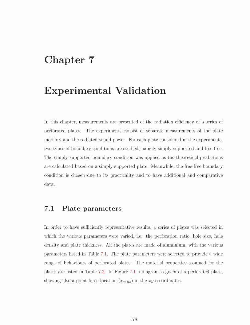
Chapter 7
Experimental Validation
In this chapter, measurements are presented of the radiation efficiency of a series of
perforated plates. The experiments consist of separate measurements of the plate
mobility and the radiated sound power. For each plate considered in the experiments,
two types of boundary conditions are studied, namely simply supported and free-free.
The simply supported boundary condition was applied as the theoretical predictions
are calculated based on a simply supported plate. Meanwhile, the free-free boundary
condition is chosen due to its practicality and to have additional and comparative
data.
7.1 Plate parameters
In order to have sufficiently representative results, a series of plates was selected in
which the various parameters were varied, i.e. the perforation ratio, hole size, hole
density and plate thickness. All the plates are made of aluminium, with the various
parameters listed in Table 7.1. The plate parameters were selected to provide a wide
range of behaviours of perforated plates. The material properties assumed for the
plates are listed in Table 7.2. In Figure 7.1 a diagram is given of a perforated plate,
showing also a point force location (xo, yo) in the xy co-ordinates.
178
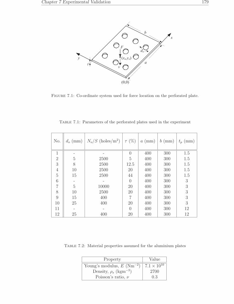
Chapter 7 Experimental Validation 179
F
v
(0,0)
a
b
t
x
y
do
(xo,yo)
Figure 7.1: Co-ordinate system used for force location on the perforated plate.
Table 7.1: Parameters of the perforated plates used in the experiment
No. do (mm) No/S (holes/m2) τ (%) a (mm) b (mm) tp (mm)
1 - - 0 400 300 1.52 5 2500 5 400 300 1.53 8 2500 12.5 400 300 1.54 10 2500 20 400 300 1.55 15 2500 44 400 300 1.56 - - 0 400 300 37 5 10000 20 400 300 38 10 2500 20 400 300 39 15 400 7 400 300 310 25 400 20 400 300 311 - - 0 400 300 1212 25 400 20 400 300 12
Table 7.2: Material properties assumed for the aluminium plates
Property Value
Young’s modulus, E (Nm−2) 7.1 × 10¹⁰
Density, ρs (kgm−3) 2700Poisson’s ratio, ν 0.3

Chapter 7 Experimental Validation 180
The plate dimensions 0.4 × 0.3 m were kept constant so that all plates could be sup-
ported in a single frame, constructed to represent the simply supported boundary con-
dition. Plates 6−12 were already available from a previous undergraduate project [88]
at ISVR. The configurations of plates 7, 8 and 10 were aimed to investigate the effect
of the hole size on the radiated sound for constant perforation ratio. Plates 1−5 were
obtained as commercial products to see the effect of the perforation area; plates 2−5
have a constant hole geometry but varying hole size. Three different thicknesses are
included and should be sufficient to see the effect of the plate thickness. As the plates
were very lightly damped, adhesive damping patches, made of a rubber material, were
attached to parts of one side of the plates to increase their damping. The damping
loss factors of the plates have been measured.
The perforated plates used in the experiment are shown in Figure 7.2. For the 1.5
mm thick plates (2−5), the hole configuration is triangular, while for the 3 mm thick
plates (7−10) it is rectangular. The 12 mm perforated plate (plate 12) has the same
configuration as plate 10 and is not shown in the figure.
7.2 Mobility measurements
Recalling Eq.(1.2)
σ =W
12ρcS 〈|v2|〉 (7.1)
determination of the radiation efficiency requires knowledge of the spatially averaged
square surface velocity, 〈|v2|〉, of the plate and also the radiated sound powerW . These
two unknown quantities can be normalised by the mean-square force F 2 = 12|F |2.
Assuming that the system is linear, this normalisation allows a convenient comparison
of different plates for which the input force spectrum may differ. For the normalised
sound power, Eq.(7.1) then reads
W
F 2= ρcS
⟨|Yt|2
⟩σ (7.2)
where 〈|Yt|2〉 =〈|v2|〉|F 2| is the spatially averaged squared transfer mobility.

Chapter 7 Experimental Validation 181
(a) (b)
(c) (d)
(e) (f)
(g) (h)
Figure 7.2: Samples of perforated plates used in the experiment: (a) plate 2, (b) plate3, (c) plate 4, (d) plate 5, (e) plate 7, (f) plate 8, (g) plate 9 and (h) plate 10.

Chapter 7 Experimental Validation 182
It is important to note that, for the unbaffled plate, the sound is radiated from both
sides of the plate. Therefore the surface area S should equal 2ab.
From now on, Yt and Yp are used to denote the transfer mobility and the point mobility
respectively. The transfer mobility Yt is the response at one point due to an excitation
at another point and the point mobility Yp is the response at the same location as that
of the excitation. Comprehensive formulae for theoretical predictions of the mobility
of a plate are summarised in [89].
7.2.1 Experimental setup and procedure
The experimental setup used for measuring the spatially averaged mobility is shown
in Figure 7.3. The plate was excited by a broadband pseudo-random signal, using
an LDS V201 shaker attached at a point. The point force locations on the plate
(xo, yo) are listed in Table 7.3 (see also Figure 7.1). The input force was measured by
a PCB force gauge, type 208C01. A stud was tightly bolted on the transducer surface
and then glued to the plate surface using an epoxy glue. To minimise the effect of
moments transmitted from the shaker, a 25 mm long stinger was used to connect the
force gauge and the shaker. Figure 7.4 shows the arrangement of the shaker and the
force transducer attached to the plate, as used in the experiment. It also shows the
damping patches attached on the plate surface. All other equipment used for the
mobility measurements can be seen in Figure 7.5.
To improve the coherence of the input and output results, the excitation frequency
range was divided into 0−3.2 kHz and 3.2−6.4 kHz. The division is aimed to concen-
trate the force within these frequency ranges and increase the frequency resolution. In
processing the measured data, these two frequency ranges were combined using MAT-
LAB. It was intended to include frequencies up to 10 kHz so that the measurements
would cover the critical frequency of the 1.5 mm plate, i.e. 8 kHz. However it was
found that the coherence was very poor for frequencies above 6.4 kHz. For the 12 mm
plate, as its critical frequency is 1 kHz, only the lower frequency range of excitation
(0−3.2 kHz) was used.
The plate surface velocity was measured by using a Polytec OFV 056 laser vibrometer.
The vibrometer scanning head, in conjunction with the analyser through the PSV

Chapter 7 Experimental Validation 183
Shaker
Laser vibrometer
Signal conditioner
Analyser
Amplifier
Amperemeter
Computer
Force gauge
Plate
POWER
Figure 7.3: Experimental setup for mobility measurement using laser vibrometer.
Figure 7.4: The shaker used to give random excitation and the force transducer at-tached to the plate.

Chapter 7 Experimental Validation 184
Table 7.3: Force location on the plate
tp (mm) do (mm) τ (%)(xo, yo)
simply supported free-free
1.5
5 5 (0.47a, 0.37b) (0.32a, 0.46b)8 12 (0.68a, 0.57b) (0.68a, 0.56b)10 19 (0.61a, 0.38b) (0.71a, 0.52b)15 44 (0.40a, 0.40b) (0.35a, 0.38b)- 0 (0.60a, 0.48b) (0.61a, 0.47b)
3
5 20 (0.50a, 0.40b) (0.60a, 0.60b)10 20 (0.35a, 0.38b) (0.65a, 0.45b)15 7 (0.33a, 0.62b) (0.63a, 0.67b)25 20 (0.38a, 0.37b) (0.38a, 0.38b)- 0 (0.38a, 0.57b) (0.38a, 0.57b)
1225 20 (0.60a, 0.40b)- 0 (0.50a, 0.30b)
software, was used to measure at 81 points on the plate surface to give a reliable surface
average. It was ensured that the measurement points avoided the holes but also varied
in location, e.g. at the plate corners and edges, between two holes, at the hole edge,
etc. For free-free conditions the plate was hung vertically and the laser vibrometer
positioned horizontally as indicated in Figure 7.3. For simply supported conditions
the arrangement was as shown in Figure 7.5 with the laser pointing downwards. In
each case, the scanning head was positioned at a distance of about 1.5 m perpendicular
(90o) to the plate surface. The scanning head then scanned each measurement point
performing 30 FFT averages for each point. The results (mobility, coherence, etc)
were calculated using the Polytec software. For all results it was ensured that the
signal-to-noise ratio was sufficient (at least 10 dB).
The responses at all 81 measurement points were averaged to give the mean-square
mobility of the plate 〈|Yt|2〉. Using the laser vibrometer, the focus of the laser beam
to the plate surface is critical to obtain a good coherence of the data. Therefore, in
the measurement, some points resulted in poor coherence due to instability of the
beam focus, particularly when the plate was vibrating. Roughly 20% of points were
found to have poor coherence with values less than 0.5. These points were omitted
from the calculation of spatially averaged mobility to ensure good measurement data.
The remaining 80% of points still represent the spatial average of the plate surface
vibration.

Chapter 7 Experimental Validation 185
Figure 7.5: Equipment used for mobility measurement.
accelerometer
hammer
analyser
Computer
Figure 7.6: Experimental setup for mobility measurement using impact hammer.
For the 1.5 mm thick plates, mass loading occurred due to the force gauge used in the
shaker excitation (as will be shown, for the thicker plates this had much less effect).
Therefore measurements of the point mobility were also taken using impact excitation,
as shown in Figure 7.6. A PCB 086D80 hammer was used to strike the plate at the
same location as used with the shaker. At the same position on the other side of the
plate, a PCB accelerometer was attached to the plate to measure the plate acceleration.
The mobility and the coherence were then calculated using the analyser software (the
Data Physics DP240 analyser was used).

Chapter 7 Experimental Validation 186
7.2.2 Simply supported boundary condition
For an ideal simply supported boundary condition, the displacement is blocked at
the plate edges but the rotation is free. Thus the realisation of such a boundary
condition in practice is not easy. However, several attempts have been made in previous
measurements involving this type of boundary condition [90, 91, 92]. Similar to the
method used in [91], a 460× 362 mm frame was constructed to support the plate. As
shown in Figure 7.7, the frame was made with a very stiff aluminium section having a
width of 31 mm. The frame height of 44 mm was designed to be greater than the width
to minimise any transverse vibration induced by the vibrating plate. Furthermore, the
mass was also large to prevent the frame moving together with the plate, particularly
at low frequency (rigid body modes). The frame was then mounted on a rigid stand,
using 1 cm thick pieces of soft foam between the frame corners and the stand to isolate
the frame from the stand.
Along the plate perimeter, a 0.2 mm thick aluminium shim was glued in part under
the plate and the other part was clamped by 3 mm thick aluminium beams using
screws along the plate perimeter. A small gap was left between the plate and the
frame to allow space for edge rotation. The frame used in the experiments is shown
in Figure 7.8.
7.2.2.1 Mobility results for 1.5 mm thick plates
Figure 7.9 plots the point mobility of various 1.5 mm thick plates, compared with
the theoretical predictions for a solid plate, (see also [89]). The mobility formula for
the simply supported plate is given in Appendix B. As already mentioned, the point
mobilities were measured using an impact hammer. The results show that, in general,
the measured mobilities have a good agreement with the predictions, even for the
first four modes. This confirms that the realisation of the simply supported boundary
condition has been very well achieved. By way of illustration, the first two mode
shapes obtained from the Polytec software are also shown in Figure 7.10 for the 1.5
mm thick plate having 5 mm hole diameter.
The perforation of the plate also has an effect on the effective plate material proper-
ties, namely the Young’s modulus (E), Poisson’s ratio (ν) and density (ρp) and hence
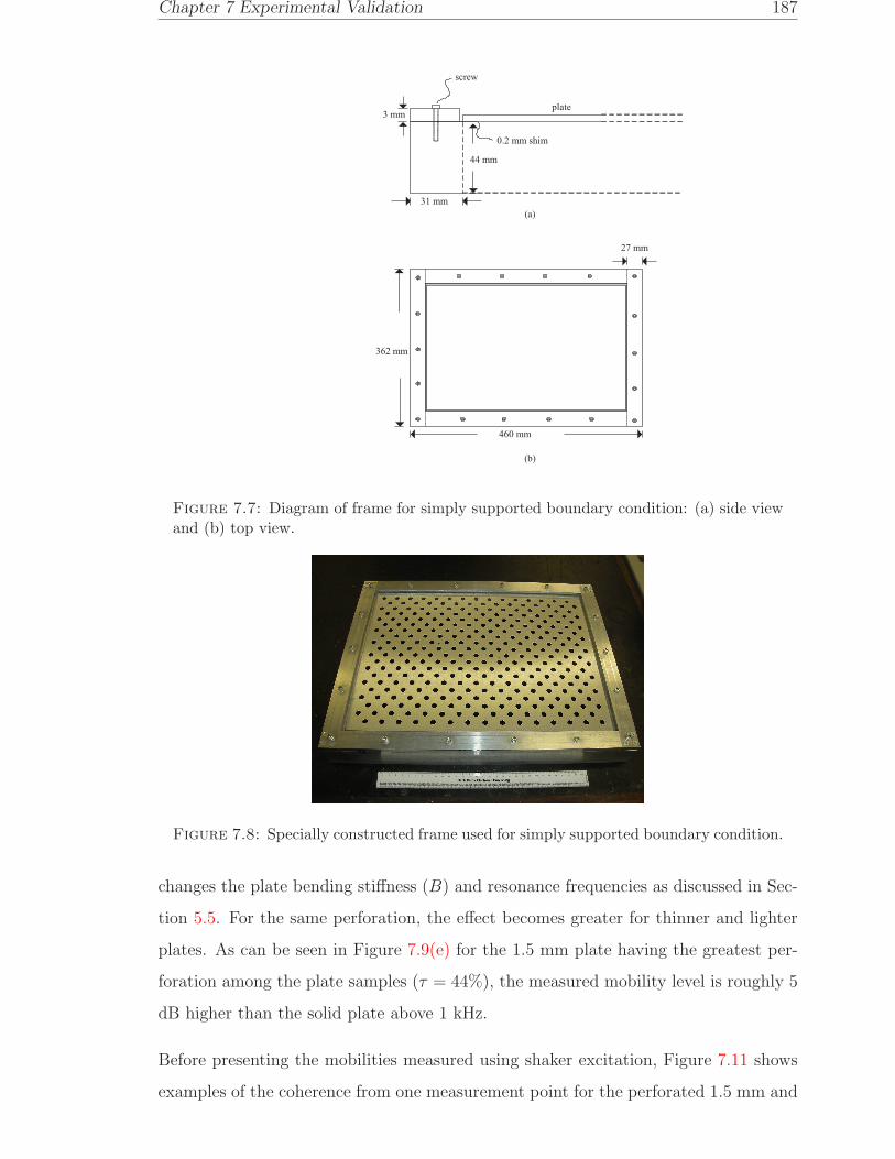
Chapter 7 Experimental Validation 187
31 mm
44 mm
3 mm
0.2 mm shim
plate
460 mm
27 mm
362 mm
(a)
(b)
screw
Figure 7.7: Diagram of frame for simply supported boundary condition: (a) side viewand (b) top view.
Figure 7.8: Specially constructed frame used for simply supported boundary condition.
changes the plate bending stiffness (B) and resonance frequencies as discussed in Sec-
tion 5.5. For the same perforation, the effect becomes greater for thinner and lighter
plates. As can be seen in Figure 7.9(e) for the 1.5 mm plate having the greatest per-
foration among the plate samples (τ = 44%), the measured mobility level is roughly 5
dB higher than the solid plate above 1 kHz.
Before presenting the mobilities measured using shaker excitation, Figure 7.11 shows
examples of the coherence from one measurement point for the perforated 1.5 mm and

Chapter 7 Experimental Validation 188
101
102
103
104
−80
−70
−60
−50
−40
−30
−20
−10
0
frequency[Hz]|Y
p|[
dB
re1
ms−
1/N
]
(a)
101
102
103
104
−80
−70
−60
−50
−40
−30
−20
−10
0
frequency[Hz]
|Yp|[
dB
re1
ms−
1/N
]
(b)
101
102
103
104
−80
−70
−60
−50
−40
−30
−20
−10
0
frequency[Hz]
|Yp|[
dB
re1
ms−
1/N
]
(c)
101
102
103
104
−80
−70
−60
−50
−40
−30
−20
−10
0
frequency[Hz]
|Yp|[
dB
re1
ms−
1/N
]
(d)
101
102
103
104
−80
−70
−60
−50
−40
−30
−20
−10
0
frequency[Hz]
|Yp|[
dB
re1
ms−
1/N
]
(e)
Figure 7.9: Comparison of measured point mobility and the theoretical predictionfor 1.5 mm plates (20 log10 |Yp|): −−experiment, —theoretical; (a) unperforated, (b)do = 5 mm, τ = 5%, (c) do = 8 mm, τ = 12%, (d) do = 10 mm, τ = 19% and (e)do = 15 mm, τ = 44%.

Chapter 7 Experimental Validation 189
(a) (b)
Figure 7.10: Diagram from scanning vibrometer software. Mode shape of simplysupported plates from the experiment: (a) mode (1,1) and (b) mode (2,1).
101
102
103
104
0
0.2
0.4
0.6
0.8
1
frequency [Hz]
coher
ence
(a)
101
102
103
104
0
0.2
0.4
0.6
0.8
1
frequency [Hz]
coher
ence
(b)
Figure 7.11: Typical coherence for simply supported plates: (a) 1.5 mm and (b) 3mm.
3 mm simply supported plates measured using shaker excitation. In an average sense,
these are also typical of the coherence for all other plates including the solid plates.
For the 1.5 mm plate, it is poor below 30 Hz but up to 4 kHz the coherence can be
seen to be approximately unity apart from dips at anti resonances. Above 4 kHz, the
coherence has a magnitude around 0.9. Thus for the whole frequency range, it can
be judged to be acceptable. For the 3 mm plate, it can be seen that the coherence
roughly has the same quality as that of the 1.5 mm plates. However, for the plate with
5 mm hole diameter, the coherence was very poor below 200 Hz where the coherence
was less than 0.5. This was because this plate was not quite flat in one corner, so that
the plate edge was not well attached to the shim on the frame. Its coherence is not
presented here.
Figure 7.12 compares the point mobilities of the 1.5 mm plates obtained by using the

Chapter 7 Experimental Validation 190
shaker and the force gauge transducer with the results obtained by impact excitation
using the instrumented hammer. It is clear that the results obtained using the shaker
roll off above 1 kHz, which indicates the effect of mass loading over that frequency
range. The phase also tends to −90o above 1 kHz corresponding to a purely imaginary
mobility (mass-like), i.e. Y = −j/mω. By comparing the mobilities from the shaker
and impact hammer, it can be seen that the mass loading has started to take effect
from around 600 Hz.
In order determine the loading effect of the transducer mass mt over the frequency
range, the transducer mobility, i.e. 1/(jmtω) is plotted together with the point mo-
bility Yp of the plate. The active transducer mass itself was obtained by measuring
the transfer function of its acceleration at and the excitation force F (1/mt = at/F ).
This was done by pointing the laser beam at the transducer surface (stud) without
attaching the transducer to the plate. It was found that the active mass is 9.8 grams,
see Figure 7.13(a), compared with a total mass of 25.5 grams. As the mean magnitude
of the point mobility of a finite plate is equivalent to the point mobility of an infinite
plate, given by 1/8√Bρptp [4], this can then be used to represent the point mobility
of the finite plate. The graph is plotted in Figure 7.13(b).
For 1.5 mm plates, it can be confirmed again from Figure 7.13(b) that the mass loading
effect ideally starts from around 1 kHz. Above the intersection, as the frequency
increases, the impedance of the force transducer Z = 1/Y seen by the shaker becomes
greater than that of the plate. Hence the shaker no longer gives sufficient force to
the plate. The effect starts below the intersection frequency as seen in the combined
mobility curves.
Therefore the measured transfer mobility Yt for the 1.5 mm plates obtained with the
shaker and the force transducer has to be corrected to eliminate the effect of mass
loading. The correction factor can be derived using the point mobility measured using
the saker Yshaker and that obtained using impact excitation Yimpact. The correction
factor CY for each frequency ω can be written as
CY (ω) =
∣∣∣∣Yimpact(ω)
Yshaker(ω)
∣∣∣∣ (7.3)
This correction factor represents the ratio of the total force to the force acting on the

Chapter 7 Experimental Validation 191
101
102
103
104
−500
50
frequency [Hz]
phas
e[o
]
101
102
103
104
−80
−60
−40
−20
0
|Yp|[
dB
re1
ms−
1/N
]
(a)
101
102
103
104
−80
−60
−40
−20
0
|Yp|[
dB
re1
ms−
1/N
]
101
102
103
104
−500
50
frequency [Hz]
phas
e[o
]
(b)
101
102
103
104
−500
50
frequency [Hz]
phas
e[o
]
101
102
103
104
−80
−60
−40
−20
0
|Yp|[
dB
re1
ms−
1/N
]
(c)
101
102
103
104
−500
50
frequency [Hz]
phas
e[o
]
101
102
103
104
−80
−60
−40
−20
0
|Yp|[
dB
re1
ms−
1/N
]
(d)
101
102
103
104
−500
50
frequency [Hz]
phas
e[o
]
101
102
103
104
−80
−60
−40
−20
0
|Yp|[
dB
re1
ms−
1/N
]
(e)
Figure 7.12: Measured point mobility and phase of 1.5 mm simply supported perfo-rated plates (20 log10 |Yp|): −−impact hammer, —shaker and force gauge transducer;(a) unperforated, (b) do = 5 mm, τ = 5%, (c) do = 8 mm, τ = 12%, (d) do = 10 mm,τ = 19% and (e) do = 15 mm, τ = 44%.

Chapter 7 Experimental Validation 192
102
103
10−3
10−2
10−1
frequency [Hz]
mt
(F/a
t)
[kg]
(a)
101
102
103
104
−60
−50
−40
−30
−20
−10
0
10
frequency[Hz]
|Y|[
dB
re1
ms−
1/N
]
(b)
Figure 7.13: (a) Measured force gauge transducer mass and (b) Comparison of trans-ducer mass mobility (—) with infinite plate mobilities of 1.5 mm (−−) and 3 mm (−·−)plates and combination between mobility of infinite plate and mass transducer (blueline) (20 log10 |Yi|).
plate alone. Thus the corrected transfer mobility Yct can be obtained by multiplying
Yt by CY for each response point, the excitation point being fixed. Since the phase of
the transfer mobility is not required, it can be written as
|Yct| = |Yt| × CY (7.4)
Based on the measurement results, the correction is applied from 600 Hz. Below 600
Hz, the correction is found to be unreliable as it is affected by the small shifting
of individual resonances. However, from Figure 7.13(b) it is seen that no significant
correction should be required below 600 Hz. The corrected spatially averaged squared-
transfer mobilities 〈|Yct|2〉 are shown in Figure 7.14 in 13
octave bands along with the
uncorrected results. It can be seen that the squared transfer mobilities can be reduced
by up to roughly 15 dB at 5 kHz due to the mass loading effect.
7.2.2.2 Mobility results for 3 mm thick plates
Figure 7.15 shows the measured point mobility for 3 mm plates along with the theoret-
ical predictions for a simply supported solid plate. The results show good agreement
with the predictions, although some resonance frequencies are found to be slightly
shifted, as was the case for the 1.5 mm plates. A rigid body mode also appears at

Chapter 7 Experimental Validation 193
101
102
103
104
−60
−50
−40
−30
−20
−10
0
frequency [Hz]<
|Yt|2
>[d
Bre
1m
2s−
2/N
2]
(a)
101
102
103
104
−60
−50
−40
−30
−20
−10
0
frequency [Hz]
<|Y
t|2
>[d
Bre
1m
2s−
2/N
2]
(b)
101
102
103
104
−60
−50
−40
−30
−20
−10
0
frequency [Hz]
<|Y
t|2
>[d
Bre
1m
2s−
2/N
2]
(c)
101
102
103
104
−60
−50
−40
−30
−20
−10
0
frequency [Hz]
<|Y
t|2
>[d
Bre
1m
2s−
2/N
2]
(d)
101
102
103
104
−60
−50
−40
−30
−20
−10
0
frequency [Hz]
<|Y
t|2
>[d
Bre
1m
2s−
2/N
2]
(e)
Figure 7.14: Experimental results of spatially averaged squared transfer mobilities of1.5 mm simply supported perforated plates (10 log10
⟨|Yt|2
⟩): -o- before correction, --
corrected; (a) unperforated, (b) do = 5 mm, τ = 5%, (c) do = 8 mm, τ = 12%, (d)do = 10 mm, τ = 19% and (e) do = 15 mm, τ = 44%.

Chapter 7 Experimental Validation 194
very low frequency around 20 Hz. At this mode, the plate and the frame are coupled
and hence move together in phase with each other. Noise from electrical interference
is also found at 50 Hz as shown in Figure 7.15(b).
The point mobility for these 3 mm plates was measured using broadband noise exci-
tation (using shaker and force transducer). From Figure 7.15, it is difficult to observe
the mass loading effect as the results show the same average level of mobility between
the measured data and the prediction at high frequencies. However, the phase shows a
slight tendency to be biased towards −90o above 2.5 kHz. Therefore the mass loading
correction has been applied from this frequency, seen from Figure 7.13(b).
The point mobility data from the hammer excitation is not available for the 3 mm
plates. However, the mass loading correction can also be made by subtracting the mass
loading effect from the measured point mobility data. Consider Figure 7.16 where a
shaker gives a harmonic force excitation F through a stinger connected to a force
transducer attached to a plate. Assuming that the plate has an impedance Zp, the net
force on the transducer with mass mt can be given by
F − Zpvp = Zmtvt = jωmtvt (7.5)
The combined system (transducer and plate) ’seen through’ the force is
Zmt+p = F/v (7.6)
As the transducer is rigidly attached to the plate, both have identical velocity (vp = vt).
Therefore
Zmt+p − Zp = jωmt (7.7)
In terms of mobility (Y = 1/Z), Eq.(7.7) can written as
1
Ymt+p
− 1
Yp
= jωmt (7.8)
where Ymt+p is the measured mobility having the mass loading effect and Yp the desired
mobility. Therefore the corrected mobility can be obtained by

Chapter 7 Experimental Validation 195
101
102
103
104
−80
−60
−40
−20
0
|Yp|[
dB
re1
ms−
1/N
]10
110
210
310
4
−500
50
frequency [Hz]
phas
e[o
]
(a)
101
102
103
104
−80
−60
−40
−20
0
|Yp|[
dB
re1
ms−
1/N
]
101
102
103
104
−500
50
frequency[Hz]
phas
e[o
]
(b)
101
102
103
104
−80
−60
−40
−20
0
|Yp|[
dB
re1
ms−
1/N
]
frequency[Hz]
101
102
103
104
−500
50
frequency [Hz]
phas
e[o
]
(c)
101
102
103
104
−500
50
frequency [Hz]
phas
e[o
]
101
102
103
104
−80
−60
−40
−20
0
|Yp|[
dB
re1
ms−
1/N
]
(d)
101
102
103
104
−500
50
frequency[Hz]
phas
e[o
]
101
102
103
104
−80
−60
−40
−20
0
|Yp|[
dB
re1
ms−
1/N
]
(e)
Figure 7.15: Comparison of measured point mobility and the theoretical prediction andphase for 3 mm simply supported plates (20 log10 |Yp|): −−experiment, —theoretical;(a) unperforated, (b) do = 5 mm, τ = 20%, (c) do = 10 mm, τ = 20%, (d) do = 15 mm,τ = 7% and (e) do = 25 mm, τ = 20%.

Chapter 7 Experimental Validation 196
Fmt M
vt
vp
shaker
stinger
force
transducer
plate
Zpvp
Figure 7.16: Digram of a dynamic force from a shaker acting between a transducerand a plate.
Yp =1
1
Ymt+p
− jωmt
(7.9)
This correction can be applied provided that ωmt is not much greater than 1/Ymt+p.
Eq.(7.9) is applied to the measured point mobility Yp for the 3 mm thick plates. The
ratio between the corrected mobility Yp and the measured mobility Yp+mt will be the
correction factor CY to the transfer mobility as in Eq.7.3, i.e.
CY (ω) =
∣∣∣∣Yp
Ymt+p
∣∣∣∣ =1
|1 − jωmtYmt+p|(7.10)
Figure 7.17 shows the measured and the corrected point mobilities in 13
octave bands.
The results show a correction by up to 5 dB from 2.5 kHz to 5 kHz. The spatially
averaged squared transfer mobility for the 3 mm plates is shown in Figure 7.18.
For the 12 mm thick plates, it was difficult to mount them on the frame due to their
heavy weight. Hence they were only measured under the free-free boundary conditions.

Chapter 7 Experimental Validation 197
101
102
103
104
−80
−70
−60
−50
−40
−30
−20
−10
0
frequency [Hz]|Y
p|[
dB
re1
ms−
1/N
]
(a)
101
102
103
104
−80
−70
−60
−50
−40
−30
−20
−10
0
frequency [Hz]
|Yp|[
dB
re1
ms−
1/N
]
(b)
101
102
103
104
−80
−70
−60
−50
−40
−30
−20
−10
0
frequency [Hz]
|Yp|[
dB
re1
ms−
1/N
]
(c)
101
102
103
104
−80
−70
−60
−50
−40
−30
−20
−10
0
frequency [Hz]
|Yp|[
dB
re1
ms−
1/N
]
(d)
101
102
103
104
−80
−70
−60
−50
−40
−30
−20
−10
0
frequency [Hz]
|Yp|[
dB
re1
ms−
1/N
]
(e)
Figure 7.17: Experimental results of point mobility of 3 mm simply supported perfo-rated plates (20 log10 |Yp|) in 1
3 octave bands: (a) unperforated, (b) do = 5 mm,τ = 20%, (c) do = 10 mm, τ = 20%, (d) do = 15 mm, τ = 7%, (e) do = 25 mm,τ = 20% (--before correction, --corrected).

Chapter 7 Experimental Validation 198
101
102
103
104
−70
−60
−50
−40
−30
−20
−10
0
frequency [Hz]<
|Yt|2
>[d
Bre
1m
2s−
2/N
2]
(a)
101
102
103
104
−70
−60
−50
−40
−30
−20
−10
0
frequency [Hz]
<|Y
t|2
>[d
Bre
1m
2s−
2/N
2]
(b)
101
102
103
104
−70
−60
−50
−40
−30
−20
−10
0
frequency [Hz]
<|Y
t|2
>[d
Bre
1m
2s−
2/N
2]
(c)
101
102
103
104
−70
−60
−50
−40
−30
−20
−10
0
frequency [Hz]
<|Y
t|2
>[d
Bre
1m
2s−
2/N
2]
(d)
101
102
103
104
−70
−60
−50
−40
−30
−20
−10
0
frequency [Hz]
<|Y
t|2
>[d
Bre
1m
2s−
2/N
2]
(e)
Figure 7.18: Experimental results of spatially averaged squared transfer mobilityof 3 mm simply supported perforated plates (10 log10
⟨|Yt|2
⟩) in 1
3 octave bands: (a)unperforated, (b) do = 5 mm, τ = 20%, (c) do = 10 mm, τ = 20%, (d) do = 15 mm,τ = 7% and (e) do = 25 mm, τ = 20% (--before correction, --corrected).

Chapter 7 Experimental Validation 199
7.2.2.3 Effect of perforation on mobility
The effect of perforation on the material dynamic properties of a plate has been dis-
cussed in Section 5.5. The perforation introduced to a plate reduces its bending
stiffness B and density ρp. It has also been shown that these effects, as a result, shift
the resonance frequencies to a lower frequency. Since the mobility depends on the
resonance frequencies and the plate density (mass), this section will discuss the effect
of perforation on the plate mobility.
Table 7.4: Effective density and bending stiffness of perforated 1.5 mm and 3 mmsimply supported plates.
Dimensions (m) do (m) bx (m) by (m) τ (%) ρ∗p/ρp B∗/B
0.4 × 0.3 × 0.0015
0.005 0.026 0.028 5 0.95 0.89590.008 0.026 0.028 12 0.88 0.75790.010 0.026 0.028 19 0.81 0.80200.015 0.026 0.028 44 0.56 0.3685
0.4 × 0.3 × 0.003
0.005 0.010 0.010 20 0.80 0.56380.010 0.020 0.020 20 0.80 0.56380.015 0.050 0.050 7 0.93 0.80200.025 0.050 0.050 20 0.80 0.5638
Table 7.4 lists all the parameters for the plate samples as in Table 7.1 together with
effective plate density ρ∗p and bending stiffness B∗. The hole arrays of all 1.5 mm
plates are triangular and 3 mm plates are rectangular (see Figure 7.2). For 3 mm
plates, the hole distances (bx and by) are similar for each plate, but the hole diameter
varies. The effective plate density ρ∗p is calculated using Eq.(5.57) and Eq.(5.58).
The effective bending stiffness B∗ can be calculated by (f ∗/f)2(1 − τ), where f ∗/f is
predicted using Eq.(5.60) for a common forcing point position. The results show that
the density and the bending stiffness are reduced as the perforation ratio is increased.
Figure 7.19 shows the predicted plate point mobility Yp for the 1.5 mm simply sup-
ported plates based on the corrected bending stiffness and density. The results show
that the level of the mobility increases as the perforation ratio increases as well as
the natural frequencies being shifted to lower frequencies. Note that the average point
mobility at high frequency is given by 1/8√Bρptp. Hence as ρp and B are reduced due
to perforation, the mobility increases. Based on an infinite plate, the average increase
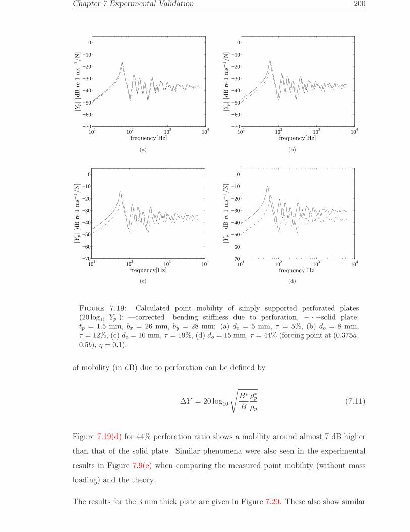
Chapter 7 Experimental Validation 200
101
102
103
104
−70
−60
−50
−40
−30
−20
−10
0
frequency[Hz]
|Yp|[
dB
re1
ms−
1/N
]
(a)
101
102
103
104
−70
−60
−50
−40
−30
−20
−10
0
frequency[Hz]
|Yp|[
dB
re1
ms−
1/N
]
(b)
101
102
103
104
−70
−60
−50
−40
−30
−20
−10
0
frequency[Hz]
|Yp|[
dB
re1
ms−
1/N
]
(c)
101
102
103
104
−70
−60
−50
−40
−30
−20
−10
0
frequency[Hz]
|Yp|[
dB
re1
ms−
1/N
]
(d)
Figure 7.19: Calculated point mobility of simply supported perforated plates(20 log10 |Yp|): —corrected bending stiffness due to perforation, − · −solid plate;tp = 1.5 mm, bx = 26 mm, by = 28 mm: (a) do = 5 mm, τ = 5%, (b) do = 8 mm,τ = 12%, (c) do = 10 mm, τ = 19%, (d) do = 15 mm, τ = 44% (forcing point at (0.375a,0.5b), η = 0.1).
of mobility (in dB) due to perforation can be defined by
∆Y = 20 log10
√B∗
B
ρ∗pρp
(7.11)
Figure 7.19(d) for 44% perforation ratio shows a mobility around almost 7 dB higher
than that of the solid plate. Similar phenomena were also seen in the experimental
results in Figure 7.9(e) when comparing the measured point mobility (without mass
loading) and the theory.
The results for the 3 mm thick plate are given in Figure 7.20. These also show similar

Chapter 7 Experimental Validation 201
101
102
103
104
−70
−60
−50
−40
−30
−20
−10
0
frequency[Hz]
|Yp|[
dB
re1
ms−
1/N
]
(a)
101
102
103
104
−70
−60
−50
−40
−30
−20
−10
0
frequency[Hz]
|Yp|[
dB
re1
ms−
1/N
]
(b)
101
102
103
104
−70
−60
−50
−40
−30
−20
−10
0
frequency[Hz]
|Yp|[
dB
re1
ms−
1/N
]
(c)
101
102
103
104
−70
−60
−50
−40
−30
−20
−10
0
frequency[Hz]
|Yp|[
dB
re1
ms−
1/N
]
(d)
Figure 7.20: Calculated point mobility of simply supported perforated plates(20 log10 |Yp|): —corrected bending stiffness due to perforation, − · −solid plate;tp = 3 mm: (a) do = 5 mm, τ = 20%, bx = by = 10 mm, (b) do = 10 mm, τ = 20%,bx = by = 20 mm, (c) do = 15 mm, τ = 7%, bx = by = 50 mm, (d) do = 25 mm,τ = 20%, bx = by = 50 mm (forcing point at (0.375a, 0.5b), η = 0.1).
effects. These plate samples have a different hole distance bx for each plate and hence
do not show an orderly increment of mobility level as for the 1.5 mm plate samples.
Figure 7.20(a), (b) and (c) show similar results with 3.5 dB higher mobility level
than that of the solid plate as they have equal perpendicular and parallel ligament
efficiencies, i.e. XLE = YLE = 0.
For all the perforated plate samples given (tp = 1.5 mm and 3 mm), it can be seen
that the modal resonance frequencies, which are the peaks in the mobility, shift to
lower frequencies, as also found in Section 5.5.
Figure 7.21 compares the point mobility of the 1.5 mm thick plates calculated using

Chapter 7 Experimental Validation 202
101
102
103
104
−70
−60
−50
−40
−30
−20
−10
0
frequency[Hz]
|Yp|[
dB
re1
ms−
1/N
]
(a)
101
102
103
104
−70
−60
−50
−40
−30
−20
−10
0
frequency[Hz]
|Yp|[
dB
re1
ms−
1/N
]
(b)
101
102
103
104
−70
−60
−50
−40
−30
−20
−10
0
frequency[Hz]
|Yp|[
dB
re1
ms−
1/N
]
(c)
101
102
103
104
−70
−60
−50
−40
−30
−20
−10
0
frequency[Hz]
|Yp|[
dB
re1
ms−
1/N
]
(d)
Figure 7.21: Point mobility of simply supported perforated plates (20 log10 |Yp|):—corrected bending stiffness due to perforation, −−measurement; tp = 1.5 mm, px =27 mm: (a) do = 5 mm, τ = 5%, (b) do = 8 mm, τ = 12%, (c) do = 10 mm, τ = 19%,(d) do = 15 mm, τ = 44%.
the corrected plate bending stiffness and density with the measured data from hammer
transducer (the point excitation is listed in Table 7.3 and the damping loss factor is in
Table 7.7). The results are plotted in 13
octave bands for clarity. Compared with the
results of Figure 7.9 it can be seen that the mobility is closer to the measurement when
the corrected bending stiffness and density is used, especially for frequencies above 1
kHz.
Figure 7.22 shows the corresponding results for the 3 mm plates. A good agreement
is found between the corrected mobility level and the measured data in this case.
For the purpose of investigating the effect of material properties change due to per-
foration on the radiation efficiency, the focus is not paid in detail on the resonance

Chapter 7 Experimental Validation 203
101
102
103
104
−80
−70
−60
−50
−40
−30
−20
−10
0
frequency[Hz]
|Yp|[
dB
re1
ms−
1/N
]
(a)
101
102
103
104
−80
−70
−60
−50
−40
−30
−20
−10
0
frequency[Hz]
|Yp|[
dB
re1
ms−
1/N
]
(b)
101
102
103
104
−80
−70
−60
−50
−40
−30
−20
−10
0
frequency[Hz]
|Yp|[
dB
re1
ms−
1/N
]
(c)
101
102
103
104
−80
−70
−60
−50
−40
−30
−20
−10
0
frequency[Hz]
|Yp|[
dB
re1
ms−
1/N
]
(d)
Figure 7.22: Point mobility of simply supported perforated plates (20 log10 |Yp|):—corrected bending stiffness due to perforation, −−measurement; tp = 3 mm: (a)do = 5 mm, τ = 20%, px = 10 mm, (b) do = 10 mm, τ = 20%, px = 20 mm, (c)do = 15 mm, τ = 7%, px = 50 mm, (d) do = 25 mm, τ = 20%, px = 50 mm.
frequencies, but to the level of mobility. Nevertheless, it can be seen from Figure 7.19
and Figure 7.20, that the resonance frequencies are reduced in the same way as in
the measured data. Tables 7.5 and 7.6 compare the measured resonance frequencies
for first four modes with those from the cubic function (Eq.(5.60)). It can be seen
that the measured resonance frequency is reduced by perforation and has a reasonable
agreement with the cubic function.
This investigation has only been made for the simply supported boundary conditions
as the effective resonance frequency (Eq.5.60) applies to the simply supported plate.
Moreover, the theoretical model of the radiation efficiency has only been implemented
for the simply supported and guided boundary conditions.

Chapter 7 Experimental Validation 204
Table 7.5: Measured effective resonance frequencies for 1.5 mm thick plates
Mode fmn (Hz)do = 8 mm, τ = 12% do = 10 mm, τ = 19%
f ∗mn(Hz) f ∗
mn/fmn Eq.(5.60) f ∗mn(Hz) f ∗
mn/fmn Eq.(5.60)
(1,1) 69 63 0.913 0.9311 67 0.971 0.8995(2,1) 142 142 1.000 0.9311 119 0.838 0.8995(1,2) 188 183 0.973 0.9311 159 0.846 0.8995(2,2) 256 241 0.941 0.9311 203 0.793 0.8995
Table 7.6: Measured effective resonance frequencies for 3 mm thick plates
Mode fmn (Hz)do = 10 mm, τ = 20% do = 15 mm, τ = 7%
f ∗mn (Hz) f ∗
mn/fmn Eq.(5.60) f ∗mn (Hz) f ∗
mn/fmn Eq.(5.60)
(1,1) 140 131 0.936 0.8395 137 0.979 0.9286(2,1) 279 254 0.910 0.8395 266 0.953 0.9286(1,2) 372 329 0.884 0.8395 362 0.973 0.9286(2,2) 495 438 0.885 0.8395 471 0.952 0.9286
7.2.3 Free-free boundary conditions
Although less common in practice, the free-free boundary condition is frequently used
in experiments as it is easy to setup without special treatment of the plate edges. In
order to measure the plates in free-free boundary conditions, they were hung from
a frame with light ropes through the holes. The same measurement procedure was
applied as in the simply supported boundary condition experiment.
Figure 7.23 shows typical examples of the coherence from one measurement point of
1.5 mm, 3 mm and 12 mm free-free plates. It can be seen that the coherence for the 1.5
mm plates is unity for the whole frequency range apart from some isolated frequencies
above 1 kHz (anti resonances of the plate). For the 3 mm plates, the coherence is
poor around 3.2 kHz. However generally, it can be judged to be satisfactory. For the
12 mm plate, the coherence is poor especially between 400 Hz and 1 kHz and above
3 kHz. This is because the plate thickness and its high stiffness made it difficult to
obtain a good signal-to-noise ratio.

Chapter 7 Experimental Validation 205
101
102
103
104
0
0.2
0.4
0.6
0.8
1
frequency [Hz]
coher
ence
(a)
101
102
103
104
0
0.2
0.4
0.6
0.8
1
frequency [Hz]
coher
ence
(b)
101
102
103
104
0
0.2
0.4
0.6
0.8
1
frequency [Hz]
coher
ence
(c)
Figure 7.23: Typical coherence for free-free plates: (a) 1.5 mm, (b) 3 mm and (c)12 mm
7.2.3.1 Mobility results for 1.5 mm thick plates
Figure 7.24 shows the measured point mobility from both impact and shaker excitation
for the 1.5 mm thick plates, which again shows the mass loading effect. As for the
simply supported plate, the effect of mass loading begins at roughly 600 Hz. Also, as a
result of this effect, it can be noted that the signal quality reduces at high frequencies
as the plate responds less to the input force.
Using the same correction technique as in Section 7.2.2.1 for the 1.5 mm simply sup-
ported plate, Figure 7.25 shows corrected and uncorrected squared mobilities in 13
octave bands. Similar to the simply supported plates, the difference between the
curves, i.e. the effect of mass loading, becomes greater as the frequency increases.
The first two high peaks at 46 and 84 Hz seen in Figure 7.24(a), (b) and (c) are

Chapter 7 Experimental Validation 206
101
102
103
104
−500
50
frequency [Hz]
phase
[o]
101
102
103
104
−80
−60
−40
−20
0
|Yp|[
dB
re1
ms−
1/N
]
(a)
101
102
103
104
−500
50
frequency [Hz]
phas
e[o
]
101
102
103
104
−80
−60
−40
−20
0
|Yp|[
dB
re1
ms−
1/N
]
(b)
101
102
103
104
−500
50
frequency [Hz]
phas
e[o
]
101
102
103
104
−80
−60
−40
−20
0
|Yp|[
dB
re1
ms−
1/N
]
(c)
101
102
103
104
−500
50
frequency [Hz]
phas
e[o
]
101
102
103
104
−80
−60
−40
−20
0
|Yp|[
dB
re1
ms−
1/N
]
(d)
101
102
103
104
−500
50
frequency [Hz]
phas
e[o
]
101
102
103
104
−80
−60
−40
−20
0
|Yp|[
dB
re1
ms−
1/N
]
(e)
Figure 7.24: Measured point mobility and phase of 1.5 mm free-free perforated plates(20 log10 |Yp|): −−impact hammer, —shaker and force gauge transducer; (a) unperfo-rated, (b) do = 5 mm, τ = 5%, (b) do = 8 mm, τ = 12%, (c) do = 10 mm, τ = 19%, (d)do = 15 mm, τ = 44%.

Chapter 7 Experimental Validation 207
101
102
103
104
−60
−50
−40
−30
−20
−10
0
frequency [Hz]<
|Yt|2
>[d
Bre
1m
2s−
2/N
2]
(a)
101
102
103
104
−60
−50
−40
−30
−20
−10
0
frequency [Hz]
<|Y
t|2
>[d
Bre
1m
2s−
2/N
2]
(b)
101
102
103
104
−60
−50
−40
−30
−20
−10
0
frequency [Hz]
<|Y
t|2
>[d
Bre
1m
2s−
2/N
2]
(c)
101
102
103
104
−60
−50
−40
−30
−20
−10
0
frequency [Hz]
<|Y
t|2
>[d
Bre
1m
2s−
2/N
2]
(d)
101
102
103
104
−60
−50
−40
−30
−20
−10
0
frequency [Hz]
<|Y
t|2
>[d
Bre
1m
2s−
2/N
2]
(e)
Figure 7.25: Experimental results of spatially average square-transfer mobilities of1.5 mm free-free perforated plates (10 log10
⟨|Yt|2
⟩): (a) unperforated, (b) do = 5 mm,
τ = 5%, (c) do = 8 mm, τ = 12%, (d) do = 10 mm, τ = 19% and (d) do = 15 mm,τ = 44% (-- before correction, --corrected).

Chapter 7 Experimental Validation 208
(a) (b)
Figure 7.26: Operating deflections from scanning vibrometer software. Bending modesof 1.5 mm free-free plates from the experiment: (a) 46 Hz and (b) 84 Hz.
bending modes from the free-free boundary condition. These modes correspond to
half a structural wavelength in one direction in the plate. The mode shapes calculated
using the Polytec vibrometer software are illustrated in Figure 7.26.
7.2.3.2 Mobility results for 3 mm thick plates
Figure 7.27 shows the point mobility for the 3 mm free-free plates in 13
octave bands.
The corrected point mobility is obtained by applying the same technique as for the 3
mm simply supported plates in Section 7.2.2.2, also from 3 kHz. It can be seen that
the corrected mobility increases by roughly 5 dB. The corrected spatially averaged
squared mobility is shown in Figure 7.28.
7.2.3.3 Mobility results for 12 mm thick plates
The spatially averaged squared mobility for the 12 mm plates is plotted in Figure 7.29.
It can be seen that it is dominated by a few individual modes especially below the
critical frequency, i.e. 1 kHz.

Chapter 7 Experimental Validation 209
101
102
103
104
−70
−60
−50
−40
−30
−20
−10
frequency[Hz]|Y
p|[
dB
re1
ms−
1/N
]
(a)
101
102
103
104
−70
−60
−50
−40
−30
−20
−10
frequency[Hz]
|Yp|[
dB
re1
ms−
1/N
]
(b)
101
102
103
104
−70
−60
−50
−40
−30
−20
−10
frequency [Hz]
|Yp|[
dB
re1
ms−
1/N
]
(c)
101
102
103
104
−70
−60
−50
−40
−30
−20
−10
frequency [Hz]
|Yp|[
dB
re1
ms−
1/N
]
(d)
101
102
103
104
−70
−60
−50
−40
−30
−20
−10
frequency [Hz]
|Yp|[
dB
re1
ms−
1/N
]
(e)
Figure 7.27: Experimental results of point mobility of 3 mm free-free plates(20 log10 |Yp|) in 1
3 octave bands: (a) unperforated, (b) do = 5 mm, τ = 20%, (c)do = 10 mm, τ = 20%, (d) do = 15 mm, τ = 7%, (e) do = 25 mm, τ = 20% (--before correction, --corrected).

Chapter 7 Experimental Validation 210
101
102
103
104
−70
−60
−50
−40
−30
−20
−10
0
frequency [Hz]<
|Yt|2
>[d
Bre
1m
2s−
2/N
2]
(a)
101
102
103
104
−70
−60
−50
−40
−30
−20
−10
0
frequency [Hz]
<|Y
t|2
>[d
Bre
1m
2s−
2/N
2]
(b)
101
102
103
104
−70
−60
−50
−40
−30
−20
−10
0
frequency [Hz]
<|Y
t|2
>[d
Bre
1m
2s−
2/N
2]
(c)
101
102
103
104
−70
−60
−50
−40
−30
−20
−10
0
frequency [Hz]
<|Y
t|2
>[d
Bre
1m
2s−
2/N
2]
(d)
101
102
103
104
−70
−60
−50
−40
−30
−20
−10
0
frequency [Hz]
<|Y
t|2
>[d
Bre
1m
2s−
2/N
2]
(e)
Figure 7.28: Experimental results of spatially averaged squared-transfer mobilityof 3 mm free-free perforated plates (10 log10
⟨|Yt|2
⟩) in 1
3 octave bands: (a) unperforated,(b) do = 5 mm, τ = 20%, (c) do = 10 mm, τ = 20%, (d) do = 15 mm, τ = 7% and (e)do = 25 mm, τ = 20% (-- before correction, --corrected).

Chapter 7 Experimental Validation 211
101
102
103
104
−90
−80
−70
−60
−50
−40
−30
−20
frequency [Hz]
<|Y
t|2
>[d
Bre
1m
2s−
2/N
2]
(a)
101
102
103
104
−90
−80
−70
−60
−50
−40
−30
−20
frequency [Hz]
<|Y
t|2
>[d
Bre
1m
2s−
2/N
2]
(b)
Figure 7.29: Experimental results of spatially averaged squared-transfer mobility of12 mm free-free perforated plates (20 log10 |Yp|); · ⋄ · 1
3 octave bands: (a) unperforatedand (b) do = 25 mm, τ = 20%.
7.2.4 Structural damping
The damping loss factor η usually has to be determined from measurements because
it is difficult to predict. One method to determine η is through the measurement of
the input power Win and spatially averaged squared velocity of the plate 〈|v2|〉. Under
steady state conditions, the power injected to the plate is equal to the power dissipated
by the plate. The input power Win is given by
Win =1
2ℜYp |F |2 (7.12)
where Yp is the input mobility and |F |2 is the squared input force amplitude. The
dissipated power Wdiss is proportional to the vibrational kinetic energy Ek and can be
expressed as
Wdiss = ωηEk =1
2ωηM
⟨∣∣v2∣∣⟩ (7.13)
where ω is the circular frequency and M is the total plate mass.
Therefore, as Win = Wdiss in steady state, the damping loss factor η can be written as
η =ℜYpωM
(|F |2〈|v2|〉
)=
ℜYpωM 〈|Yt|2〉
(7.14)
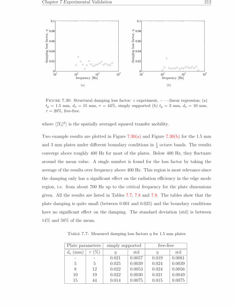
Chapter 7 Experimental Validation 212
101
102
103
104
0
0.02
0.04
0.06
0.08
0.1
frequency [Hz]
dam
pin
glo
ssfa
ctor,
η
(a)
101
102
103
104
0
0.02
0.04
0.06
0.08
0.1
frequency [Hz]
dam
pin
glo
ssfa
ctor,
η
(b)
Figure 7.30: Structural damping loss factor: experiment, − · −linear regression; (a)tp = 1.5 mm, do = 15 mm, τ = 44%, simply supported (b) tp = 3 mm, do = 10 mm,τ = 20%, free-free.
where 〈|Yt|2〉 is the spatially averaged squared transfer mobility.
Two example results are plotted in Figure 7.30(a) and Figure 7.30(b) for the 1.5 mm
and 3 mm plates under different boundary conditions in 13
octave bands. The results
converge above roughly 400 Hz for most of the plates. Below 400 Hz, they fluctuate
around the mean value. A single number is found for the loss factor by taking the
average of the results over frequency above 400 Hz. This region is most relevance since
the damping only has a significant effect on the radiation efficiency in the edge mode
region, i.e. from about 700 Hz up to the critical frequency for the plate dimensions
given. All the results are listed in Tables 7.7, 7.8 and 7.9. The tables show that the
plate damping is quite small (between 0.001 and 0.025) and the boundary conditions
have no significant effect on the damping. The standard deviation (std) is between
14% and 58% of the mean.
Table 7.7: Measured damping loss factors η for 1.5 mm plates
Plate parameters simply supported free-free
do (mm) τ (%) η std η std- - 0.021 0.0057 0.019 0.00815 5 0.025 0.0039 0.024 0.00398 12 0.022 0.0053 0.024 0.005610 19 0.022 0.0030 0.021 0.004915 44 0.014 0.0075 0.015 0.0075

Chapter 7 Experimental Validation 213
Table 7.8: Measured damping loss factors η for 3 mm plates
Plate parameters simply supported free-free
do (mm) τ (%) η std η std- - 0.015 0.0055 0.015 0.00645 20 0.008 0.0027 0.008 0.004310 20 0.007 0.0040 0.006 0.002015 7 0.010 0.0037 0.011 0.004125 20 0.010 0.0057 0.008 0.0034
Table 7.9: Measured damping loss factors η for 12 mm plates
Plate parameters free-free
do (mm) τ (%) η std- - 0.001 0.001325 20 0.003 0.0025
7.3 Sound power measurements using reciprocal tech-
nique
To measure the radiation efficiency, in addition to the spatially averaged squared
mobility, a measurement is required of the sound power for a unit squared input
force. Although this can be measured directly by attaching a shaker to the plate and
measuring the radiated sound, here a reciprocal technique is used.
Reciprocal measurement techniques have been used in many practical cases of sound
radiation from vibrating structures, structural response to incident sound and sound
transmission through partitions e.g. in vehicles for both airborne and structure borne
transmission. These techniques are often less costly, less time consuming, more con-
venient and sometimes more accurate than the equivalent direct measurement [54].
They may also be less labour intensive, if for example, vibration sources are involved
which would have to be replaced by vibration generators in a direct method.
In the case of the present experiments, particular attention has to be paid to the noise
from the shaker if using the direct method. Although it has been shown that the
shaker noise is negligible compared with the radiated sound of an aluminium 3 mm
solid plate in the room [88], it is believed that the shaker alone produces a different
Chapter 7 Experimental Validation 214
( )op r
( )sv r
( )oQ r
sr
oror
sr O O
( )oF r
A A
BB
Figure 7.31: Basic concept of reciprocal measurement of an elastic structure excitedby a point force.
noise level than when it is attached to the plate. In addition, as the perforated plate
has a much lower radiation efficiency, especially at low frequency, the shaker noise
may contaminate the measured sound power. The measurement also requires careful
attention to other background noise from in and outside the room which could add
errors in the measurement. Therefore, in this experiment, the reciprocal technique is
chosen as an alternative method with less significant effect from background noise to
the accuracy of the measurement.
7.3.1 Theory
Lyamshev [93] proposed that the transfer function between a point force F exciting a
linear elastic structure and the resulting sound pressure p at a particular observation
point is equivalent to the transfer function between a volume velocity Q of a point
monopole located at the former observation point and the resulting vibration velocity
v produced at the former excitation point, in the same direction as the excitation force.
As shown in Figure 7.31, this gives
p(ro)
F (rs)≡ − v(rs)
Q(ro)(7.15)
where ro and rs are the position vectors of the observation point and of the excitation
point on the structure respectively. This should be equally true if the structure is
perforated.
If the direct method experiment is conducted in a reverberant chamber, the radiated
power Wrad normalised by the mean-square force F 2 at point B in Figure 7.31 is given

Chapter 7 Experimental Validation 215
by
Wrad
F 2=Sα
4ρc
⟨p2
F 2
⟩(7.16)
where Sα is the room absorption, ρ is the air density, c is the sound speed and⟨p2⟩
is
the spatially-averaged mean square pressure in the room due to radiation by the plate.
In a reverberant field the sound pressure is approximately the same at any location A,
so Eq.(7.16) can be approximated by
Wrad
F 2=Sα
4ρc
p2
F 2(7.17)
Using the principle of reciprocity from Eq.(7.15), Eq.(7.17) can then be written as
Wrad
F 2=Sα
4ρc
v2Q
Q2(7.18)
where v2Q is the mean-square plate velocity at point B due to the sound excitation
from a monopole source of mean-square volume velocity Q2 at point A.
The source volume velocity Q in the reciprocal measurement can itself be determined
from a sound power measurement. In the diffuse field, the radiated sound power WQ
of a compact source is given by [94]
WQ = ρcQ2k2
4π(7.19)
where k is the wavenumber. If the source is operated in the reverberant chamber, the
sound power WQ can be obtained by measuring the spatially averaged mean-square
pressure⟨p2⟩
in the room. It can be written as
WQ =Sα
4ρc
⟨p2
Q
⟩(7.20)
After rearranging Eq.(7.19) and Eq.(7.20), the mean-square volume velocity Q2 is
given by
Chapter 7 Experimental Validation 216
Q2 =Sαπ
ρ2c2k2
⟨p2
Q
⟩=Sαπ
ρ2ω2
⟨p2
Q
⟩(7.21)
since k = ω/c. Hence, substituting this into Eq.(7.18) gives
Wrad
F 2=Sα
4ρc
v2Q ρ
2ω2
Sα π⟨p2
Q
⟩ =a2
Q⟨p2
Q
⟩ ρ
4πc(7.22)
where aQ = jωvQ is the plate acceleration and⟨p2
Q
⟩is averaged over microphone
positions. The acceleration could also be averaged over source positions in the room
equivalent to the averaging in Eq.(7.16). However it is not very critical to average for
different source positions since the sound is assumed to be diffuse irrespective of the
source position in the room. Note that the absorption of the room Sα cancels out in
Eq.(7.22). The radiation efficiency is finally obtained by using Eq.(7.22) together with
the spatially averaged transfer mobility 〈|Yt|2〉 in Eq.(7.2).
7.3.2 Experimental setup and procedure
Figure 7.32 shows the experimental setup of the reciprocal measurement which was
carried out in the large reverberation chamber at the ISVR. The room has average
dimensions 9.15 × 6.25 × 6.10 m, giving a volume of 348 m3 and a surface area of
302 m2. The room is constructed with non-parallel walls to give a good diffuse field
and the internal surfaces are finished with a hard gloss paint to give a high reflection
coefficient. The diffuse field is a situation where the room has many overlapping
acoustic modes instead of distinct individual modes (direct field). The ’Schroeder
frequency’ determines the transition frequency (cross-over frequency) above which the
diffuse field applies. It is given by [95]
fs = 2000
√T60
VR
(7.23)
For a minimum reverberation time of the room, i.e. 3 s, and for the given room volume,
the Schroeder frequency is fs = 185 Hz. The diffuse field cannot be assumed below
this frequency.

Chapter 7 Experimental Validation 217
Loudspeaker
Accelerometer
CONTROL ROOM
Signal conditioner
Microphone
Microphone
boom
REVERBERATION ROOM
Signal conditioner
Analyser
Computer
Figure 7.32: Experimental setup for reciprocity measurement.
Figure 7.33 shows the interior of the room and the equipment used in the measurement.
The loudspeaker was located close to one corner of the room, about 2 m from the
wall. It was fed with random broadband noise up to 10 kHz. Before starting the
sound power measurement, the microphone was calibrated using Bruel & Kjær piston
calibrator type 4231. This was done for each plate sample. The microphone used
to measure the sound pressure was a Bruel & Kjær pressure microphone type 40AG.
The spatial averaging of the sound pressure across the room was achieved by using a
Bruel & Kjær rotating microphone boom type 3923. The signal from the microphone
was first conditioned (converted and amplified) by Bruel & Kjær Nexus conditioning
amplifier Type 2690 before it was processed in a Data Physics analyser DP240.
The nearest microphone position to the loudspeaker was ensured to be more than
2 m. This fulfills the standard given by ANSI S1.21-1972 [96] that the minimum
distance dmin between the microphone and the sound source shall not be less than
dmin = 0.08(VR/T60)1/2, where VR is the room volume and T60 is the reverberation

Chapter 7 Experimental Validation 218
Figure 7.33: Equipment setup in the reverberation chamber.
time. This is half of the cross-over wavelength (λs = c/2fs) from the ’Schroeder
frequency’, fs in Eq.(7.23). Assuming T60 ≥ 1 s (it is actually in the range 3−14 s),
the minimum microphone distance required is dmin ≤ 1.49 m.
Figure 7.34 plots the averaged sound pressure level (SPL) spectrum in 13
octave bands
used as the acoustic excitation as well as the noise floor in the room (i.e. measured
when the loudspeaker was switched off). The SPL falls below 80 Hz, but between 80
and 2.5 kHz the spectrum is almost flat; it slowly decreases at high frequency. Above
40 Hz, the background noise can be considered negligible (signal-to-noise ratio greater
than 10 dB).
For the free-free boundary condition, the plates were hung using soft ropes from a stiff
frame, as for the mobility measurement (see Figure 7.33). For the simply supported
boundary condition, the plate (and the frame) was mounted horizontally on a rigid
frame. Soft foam was placed under each corner of the frame to prevent vibration being
transfered from the base. The plate was located away from the centre of the room,
but more than 2 m from the walls. For the simply supported boundary conditions, the
plate (and the frame) was placed horizontally 0.65 m from the floor. For the free-free
boundary conditions, hung vertically, the centre of the plate was roughly 0.9 m from

Chapter 7 Experimental Validation 219
101
102
103
104
30
40
50
60
70
80
90
100
frequency [Hz]
SP
L[d
Bre
2×
10−
5P
a]
Figure 7.34: Sound pressure level in the chamber (—) and its noise floor (− · −) in13 octave bands.
the floor.
The distance between the plate and the loudspeaker was about 5 m. This ensures
that the direct field from the sound source is negligible and the plate was excited
predominantly by the diffuse field. This requires that the distance to the plate must
be greater than the reverberation radius, rR = 0.056√VR/T60 [95]. Assuming again
that T60 ≥ 1 s, this gives rR ≤ 1 m.
At the same location as used for the force gauge transducer in the mobility measure-
ment, a PCB accelerometer was attached to the plate to measure its acceleration. The
mass of the accelerometer 0.8 gram has negligible effect on the response. Figure 7.35
plots the mean square acceleration of the various plates in 13
octave bands together
with the corresponding noise floor i.e. when there was no sound excitation. For each
boundary condition, the plate acceleration at low frequency has a similar level to the
noise floor. This is due to the low level of sound excitation at very low frequencies as
seen in Figure 7.34, combined with the small values of radiation efficiency expected.
Thus, the data at these frequencies are rejected. The free-free plates have much lower
vibration than the simply supported plates, as seen in Figure 7.35(a), (c) and (e). For
some plates, the squared acceleration is still within 3 dB of the noise floor up to 300
Hz. However, for each boundary condition, the results will be plotted from 100 Hz
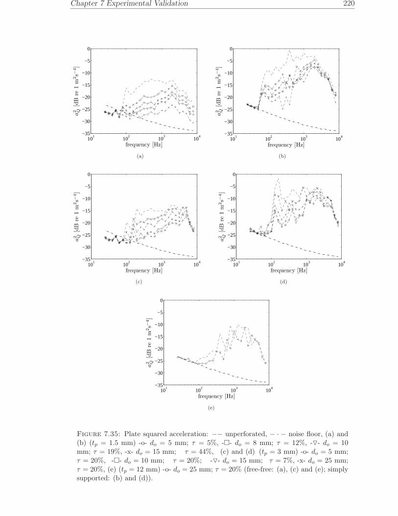
Chapter 7 Experimental Validation 220
101
102
103
104
−35
−30
−25
−20
−15
−10
−5
0
frequency [Hz]
a2 Q
[dB
re1
m2s−
4]
(a)
101
102
103
104
−35
−30
−25
−20
−15
−10
−5
0
frequency [Hz]
a2 Q
[dB
re1
m2s−
4]
(b)
101
102
103
104
−35
−30
−25
−20
−15
−10
−5
0
frequency [Hz]
a2 Q
[dB
re1
m2s−
4]
(c)
101
102
103
104
−35
−30
−25
−20
−15
−10
−5
0
frequency [Hz]
a2 Q
[dB
re1
m2s−
4]
(d)
101
102
103
104
−35
−30
−25
−20
−15
−10
−5
0
frequency [Hz]
a2 Q
[dB
re1
m2s−
4]
(e)
Figure 7.35: Plate squared acceleration: −− unperforated, − · − noise floor, (a) and(b) (tp = 1.5 mm) -o- do = 5 mm; τ = 5%, -- do = 8 mm; τ = 12%, -- do = 10mm; τ = 19%, -x- do = 15 mm; τ = 44%, (c) and (d) (tp = 3 mm) -o- do = 5 mm;τ = 20%, -- do = 10 mm; τ = 20%; -- do = 15 mm; τ = 7%, -x- do = 25 mm;τ = 20%, (e) (tp = 12 mm) -o- do = 25 mm; τ = 20% (free-free: (a), (c) and (e); simplysupported: (b) and (d)).
Chapter 7 Experimental Validation 221
although care should be taken for some of the free-free plates as the data up to 300
Hz might be influenced by the noise floor of the accelerometer.
7.3.3 Sound power results
The normalised sound power of the plates determined from Eq.(7.22) is displayed in
Figure 7.36 in 13
octave bands. It can be seen that the plate sound power shows different
levels according to the diameter of the holes and perforation ratio of the plates. Similar
to the radiation efficiency trend, according to the theory, the sound power also reduces
as the perforation ratio increases and as the hole size reduces. This can be seen clearly
for the free-free plates in Figure 7.36(a) and (c) and also for the simply supported
plates in Figure 7.36(b) and (d), although there are some fluctuations below 1 kHz.
For the free-free plates, the trend also shows the sound power increases toward the
critical frequency.
7.4 Radiation efficiency results
7.4.1 Radiation efficiency results for simply supported plates
Figure 7.37 presents the radiation efficiency in dB (radiation index, 10 log10 σ) for the
1.5 mm simply supported plates along with corresponding predictions. Although the
measured and predicted results show similar trends, it can be seen that the measured
radiation efficiencies exceed the theoretical predictions by about 5−10 dB. Figure 7.38
shows the radiation efficiency for the 3 mm simply supported plates. Again the exper-
imental results are considerably higher than the predictions.
The measured results cover the range 100 Hz−5 kHz. The upper limit is determined
by the mobility measurements which had a maximum frequency of 6.4 kHz, meaning
that the highest 13
octave band covered is 5 kHz.
Regarding the sound radiation from a vibrating plate in an unbaffled condition, the
radiated sound from one side can ’communicate’ with the radiated sound from the
other side of the plate. This communication, particularly at the plate edges for a solid

Chapter 7 Experimental Validation 222
102
103
104
−65
−60
−55
−50
−45
−40
−35
−30
−25
frequency [Hz]
Wrad/F
2[d
Bre
1W
att/
N2]
(a)
102
103
104
−65
−60
−55
−50
−45
−40
−35
−30
−25
frequency [Hz]
Wrad/F
2[d
Bre
1W
att/
N2]
(b)
102
103
104
−65
−60
−55
−50
−45
−40
−35
−30
−25
frequency [Hz]
Wrad/F
2[d
Bre
1W
att/
N2]
(c)
102
103
104
−65
−60
−55
−50
−45
−40
−35
−30
−25
frequency [Hz]
Wrad/F
2[d
Bre
1W
att/
N2]
(d)
102
103
104
−65
−60
−55
−50
−45
−40
−35
−30
−25
frequency [Hz]
Wrad/F
2[d
Bre
1W
att/
N2]
(e)
Figure 7.36: Plate normalised sound power: −− unperforated, (a) and (b) (tp = 1.5mm) -o- do = 5 mm; τ = 5%, -- do = 8 mm; τ = 12%, -- do = 10 mm; τ = 19%,-x- do = 15 mm; τ = 44%, (c) and (d) (tp = 3 mm) -o- do = 5 mm; τ = 20%, --do = 10 mm; τ = 20%; -- do = 15 mm; τ = 7%, -x- do = 25 mm; τ = 20%, (e)(tp = 12 mm) -o- do = 25 mm; τ = 20% (free-free: (a), (c) and (e); simply supported:(b) and (d)).

Chapter 7 Experimental Validation 223
plate, creates cancellation of the sound radiation. The effectiveness of this cancellation
depends on the acoustic wavelength. The longer the wavelength, the more effective
the cancellation, as explained in Chapter 3. Conversely, in the baffled condition this
sort of communication is not possible. Therefore, a baffled plate has a higher radiation
efficiency, as already shown in Figure 3.6.
Figure 7.39 shows a diagram of one side of the plate edges. This illustrates that
the path length for the sound to propagate from one side of the plate to the other is
approximately 110 mm. In order for the plate to be considered as unbaffled, this has to
be less than about half an acoustic wavelength. It means that the frequency should be
less than f = 343/(2×0.11) ≈ 1.5 kHz. Above this frequency, the radiated sound from
the back of the plate is blocked by the frame and the plate becomes effectively baffled.
This may explain the disagreement in the results at least above 1 kHz. Moreover, the
nature of the radiated sound from the back of the plate is also modified by the frame.
So the sound radiation from the back will be more directional than that from the front.
This could also reduce the effectiveness of the cancellation process. Hence the plate
may also be effectively baffled at lower frequencies than 1.5 kHz.
Figure 7.40 compares some of the results with predictions for both baffled and unbaffled
conditions. The results of the perforated baffled plate were calculated using the discrete
sources model from Chapter 6. They could only be calculated for the 3 mm plate with
small hole density, i.e. plates numbered 9 and 10 in Table 7.1. For greater hole
densities, the model needs more sources which then results in excessive calculation
times. The results for the unperforated plates are calculated by the wavenumber
approach of Section 2.2. It can be seen that above around 1 kHz the measured results
follow the trend of the baffled plate results rather than the unbaffled results. Thus
the frame used for the simply supported boundary conditions does not allow unbaffled
results to be obtained.
Figure 7.41 displays the measured and predicted effect of perforation (EoP) for 1.5
mm simply supported plates. This shows the level difference between the curves in
Figure 7.37(a) and those in (b)−(e). Above 500 Hz, the measured results follow the
trend of the predictions although at some frequencies the measured effect is about
2 − 5 dB less than the predictions. Below 500 Hz, high fluctuations occur due to the
disagreement, particularly in the corner mode region, between the measured radiation

Chapter 7 Experimental Validation 224
101
102
103
104
−70
−60
−50
−40
−30
−20
−10
0
10
frequency [Hz]
radia
tion
index
[dB
re1]
(a)
101
102
103
104
−70
−60
−50
−40
−30
−20
−10
0
10
frequency [Hz]
radia
tion
index
[dB
re1]
(b)
101
102
103
104
−70
−60
−50
−40
−30
−20
−10
0
10
frequency [Hz]
radia
tion
index
[dB
re1]
(c)
101
102
103
104
−70
−60
−50
−40
−30
−20
−10
0
10
frequency [Hz]
radia
tion
index
[dB
re1]
(d)
101
102
103
104
−70
−60
−50
−40
−30
−20
−10
0
10
frequency [Hz]
radia
tion
index
[dB
re1]
(e)
Figure 7.37: Radiation efficiency of unbaffled 1.5 mm simply supported perforatedplates: — theoretical, -- experiment; (a) unperforated, (b) do = 5 mm; τ = 5%, (c)do = 8 mm; τ = 12%, (d) do = 10 mm; τ = 19% and (e) do = 15 mm; τ = 44%.

Chapter 7 Experimental Validation 225
101
102
103
104
−70
−60
−50
−40
−30
−20
−10
0
10
frequency [Hz]
radia
tion
index
[dB
re1]
(a)
101
102
103
104
−70
−60
−50
−40
−30
−20
−10
0
10
frequency [Hz]
radia
tion
index
[dB
re1]
(b)
101
102
103
104
−70
−60
−50
−40
−30
−20
−10
0
10
frequency [Hz]
radia
tion
index
[dB
re1]
(c)
101
102
103
104
−70
−60
−50
−40
−30
−20
−10
0
10
frequency [Hz]
radia
tion
index
[dB
re1]
(d)
101
102
103
104
−70
−60
−50
−40
−30
−20
−10
0
10
frequency [Hz]
radia
tion
index
[dB
re1]
(e)
Figure 7.38: Radiation efficiency of unbaffled 3 mm simply supported perforated plates:— theoretical, -- experiment; (a) unperforated, (b) do = 5 mm; τ = 20%, (c)do = 10 mm; τ = 20%, (d) do = 15 mm; τ = 7% and (e) do = 25 mm; τ = 20%.
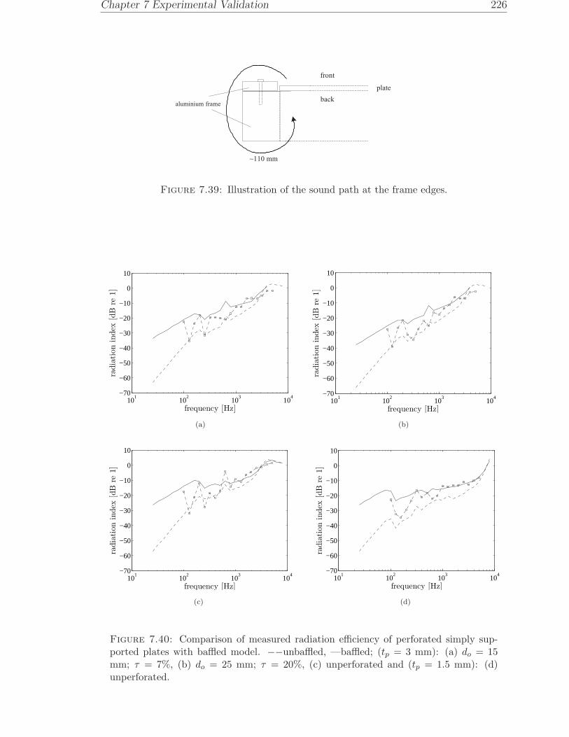
Chapter 7 Experimental Validation 226
~110 mm
front
backaluminium frame
plate
Figure 7.39: Illustration of the sound path at the frame edges.
101
102
103
104
−70
−60
−50
−40
−30
−20
−10
0
10
frequency [Hz]
radia
tion
index
[dB
re1]
(a)
101
102
103
104
−70
−60
−50
−40
−30
−20
−10
0
10
frequency [Hz]
radia
tion
index
[dB
re1]
(b)
101
102
103
104
−70
−60
−50
−40
−30
−20
−10
0
10
frequency [Hz]
radia
tion
index
[dB
re1]
(c)
101
102
103
104
−70
−60
−50
−40
−30
−20
−10
0
10
frequency [Hz]
radia
tion
index
[dB
re1]
(d)
Figure 7.40: Comparison of measured radiation efficiency of perforated simply sup-ported plates with baffled model. −−unbaffled, —baffled; (tp = 3 mm): (a) do = 15mm; τ = 7%, (b) do = 25 mm; τ = 20%, (c) unperforated and (tp = 1.5 mm): (d)unperforated.
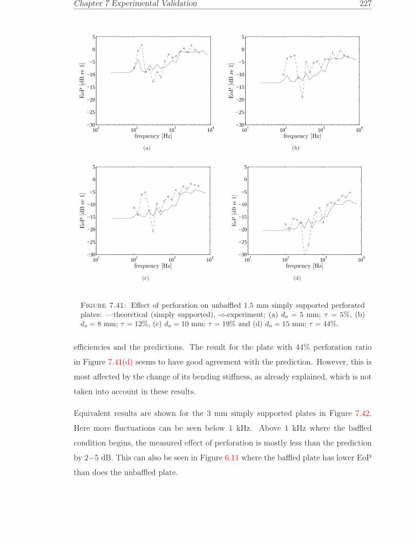
Chapter 7 Experimental Validation 227
101
102
103
104
−30
−25
−20
−15
−10
−5
0
5
frequency [Hz]
EoP
[dB
re1]
(a)
101
102
103
104
−30
−25
−20
−15
−10
−5
0
5
frequency [Hz]
EoP
[dB
re1]
(b)
101
102
103
104
−30
−25
−20
−15
−10
−5
0
5
frequency [Hz]
EoP
[dB
re1]
(c)
101
102
103
104
−30
−25
−20
−15
−10
−5
0
5
frequency [Hz]
EoP
[dB
re1]
(d)
Figure 7.41: Effect of perforation on unbaffled 1.5 mm simply supported perforatedplates: —theoretical (simply supported), --experiment; (a) do = 5 mm; τ = 5%, (b)do = 8 mm; τ = 12%, (c) do = 10 mm; τ = 19% and (d) do = 15 mm; τ = 44%.
efficiencies and the predictions. The result for the plate with 44% perforation ratio
in Figure 7.41(d) seems to have good agreement with the prediction. However, this is
most affected by the change of its bending stiffness, as already explained, which is not
taken into account in these results.
Equivalent results are shown for the 3 mm simply supported plates in Figure 7.42.
Here more fluctuations can be seen below 1 kHz. Above 1 kHz where the baffled
condition begins, the measured effect of perforation is mostly less than the prediction
by 2−5 dB. This can also be seen in Figure 6.11 where the baffled plate has lower EoP
than does the unbaffled plate.

Chapter 7 Experimental Validation 228
101
102
103
104
−30
−25
−20
−15
−10
−5
0
5
frequency [Hz]
EoP
[dB
re1]
(a)
101
102
103
104
−30
−25
−20
−15
−10
−5
0
5
frequency [Hz]
EoP
[dB
re1]
(b)
101
102
103
104
−30
−25
−20
−15
−10
−5
0
5
frequency [Hz]
EoP
[dB
re1]
(c)
101
102
103
104
−30
−25
−20
−15
−10
−5
0
5
frequency [Hz]
EoP
[dB
re1]
(d)
Figure 7.42: Effect of perforation on unbaffled 3 mm simply supported perforatedplates: —theoretical (simply supported), − −experiment; (a) do = 5 mm; τ =20%, (b) do = 10 mm; τ = 20%, (c) do = 15 mm; τ = 7% and (d) do = 25 mm;τ = 20%.
7.4.2 Radiation efficiency results for free-free plates
The measured radiation efficiencies for free-free boundary conditions are shown in
Figure 7.43 for 1.5 mm plates and in Figure 7.44 for 3 mm plates. These show good
agreement with the predictions, although the latter are for simply supported boundary
conditions.
For the 12 mm plates, the results are plotted in Figure 7.45. It can be seen that the
measured radiation efficiencies show high fluctuations relative to the predictions. This
is due the low modal density especially below the critical frequency (1 kHz).
For the 1.5 mm plates the measured results are greater than the predictions in the

Chapter 7 Experimental Validation 229
101
102
103
104
−70
−60
−50
−40
−30
−20
−10
0
10
frequency [Hz]
radia
tion
index
[dB
re1]
(a)
101
102
103
104
−70
−60
−50
−40
−30
−20
−10
0
10
frequency [Hz]
radia
tion
index
[dB
re1]
(b)
101
102
103
104
−70
−60
−50
−40
−30
−20
−10
0
10
frequency [Hz]
radia
tion
index
[dB
re1]
(c)
101
102
103
104
−70
−60
−50
−40
−30
−20
−10
0
10
frequency [Hz]
radia
tion
index
[dB
re1]
(d)
101
102
103
104
−70
−60
−50
−40
−30
−20
−10
0
10
frequency [Hz]
radia
tion
index
[dB
re1]
(e)
Figure 7.43: Radiation efficiency of unbaffled 1.5 mm free-free perforated plates: —theoretical (simply supported), --experiment; (a) unperforated, (b) do = 5 mm; τ =5%, (c) do = 8 mm; τ = 12%, (d) do = 10 mm; τ = 19% and (e) do = 15 mm; τ = 44%.

Chapter 7 Experimental Validation 230
101
102
103
104
−70
−60
−50
−40
−30
−20
−10
0
10
frequency [Hz]ra
dia
tion
index
[dB
re1]
(a)
101
102
103
104
−70
−60
−50
−40
−30
−20
−10
0
10
frequency [Hz]
radia
tion
index
[dB
re1]
(b)
101
102
103
104
−70
−60
−50
−40
−30
−20
−10
0
10
frequency [Hz]
radia
tion
index
[dB
re1]
(c)
101
102
103
104
−70
−60
−50
−40
−30
−20
−10
0
10
frequency [Hz]
radia
tion
index
[dB
re1]
(d)
101
102
103
104
−70
−60
−50
−40
−30
−20
−10
0
10
frequency [Hz]
radia
tion
index
[dB
re1]
(e)
Figure 7.44: Radiation efficiency of unbaffled 3 mm free-free perforated plates: —theoretical (simply supported), --experiment; (a) unperforated, (b) do = 5 mm;τ = 20%, (c) do = 10 mm; τ = 20%, (d) do = 15 mm; τ = 7% and (e) do = 25 mm;τ = 20%.

Chapter 7 Experimental Validation 231
101
102
103
104
−70
−60
−50
−40
−30
−20
−10
0
10
frequency [Hz]
radia
tion
index
[dB
re1]
(a)
101
102
103
104
−70
−60
−50
−40
−30
−20
−10
0
10
frequency [Hz]
radia
tion
index
[dB
re1]
(b)
Figure 7.45: Radiation efficiency of unbaffled 12 mm free-free perforated plates: —theoretical (simply supported), --experiment; (a) unperforated and (b) do = 25 mm;τ = 20%.
region 100−300 Hz. Below 200 Hz (i.e. for centre frequency band 100,125 and 160
Hz), this could be due to errors from the measured spatially mean-square sound pres-
sure⟨p2
Q
⟩as the field is not diffuse below this frequency (the cross-over frequency is
185 Hz). This could also be due to unreliable measured data, as they are still very
close to the noise floor (within 5 dB, see Figure 7.35(a)) particularly for the plates in
Figure 7.43(c), (d) and (e). This could be improved by trying to increase the acoustic
excitation level or using an accelerometer which is more sensitive at low frequency.
However this has not been done.
The 3 mm plates show a similar effect for 100−300 Hz where high fluctuations appear.
Especially for 100−200 Hz, these are again likely to be because the measured data is
below the cross-over frequency of the room. In addition, it should be noted that in the
experiments only one mechanical force excitation position was applied. This could be
possible source of discrepancies between measurement and prediction below 300 Hz.
As explained in Chapter 2, the variability of the radiation efficiency due to the use
of a single force position could lead to up to around ±5 dB differences in the corner
mode region for a 3 mm thick plate compared with the result for an average over
force positions. This variability then converges in the edge mode region and above the
critical frequency.
Above 3 kHz the measured radiation efficiency of the 3 mm plates, particularly for
the perforated plates, is lower than the measurements. The trend suggests that the

Chapter 7 Experimental Validation 232
measured result tends toward a higher critical frequency. This can be explained as in
Section 5.5 that because of the perforation, the bending stiffness and the plate mass
are changed, resulting to the resonance frequency shift. For the plate samples with
20% perforation ratio and all have similar XLE and YLE, the critical frequency is
expected to be 4.8 kHz.
The good agreement found between the measured results for free-free boundary con-
ditions and the theoretical result for the simply supported boundary conditions also
raises an interesting finding. The hypothesis has been made in Chapter 4 that for
an unbaffled plate, the boundary condition has less effect on the radiation efficiency
than for a baffled plate because the process of cancellation can still happen through
the plate edges effectively. Moreover, the cancellation becomes more effective if the
plate is perforated, particularly along the plate edges for the higher hole density. This
may explain the satisfactory agreement between the results of the free-free boundary
condition in the experiment and the theoretical predictions of the simply supported
boundary condition. As already shown in Figure 4.11 and Figure 4.12 in Chapter 4,
the results for a simply supported plate and a guided-guided plate show the almost
same radiation efficiency even in the corner mode region. Meanwhile for the same case,
differences up to 10 dB in the corner mode region and 5 dB in the edge mode region
are found for the baffled plates in Figure 4.5 and Figure 4.7. This at least shows that,
for the unbaffled case, the condition of the plate edges does not give a significant effect
to the sound radiation. However, to validate this hypothesis more fully, a model for
the unbaffled free-free plate would be required.
The effect of perforation (EoP) for 1.5 mm free-free plates is shown in Figure 7.46. In
an average sense, this has good agreement with the predictions, particularly above 400
Hz. For the plate with the highest perforation ratio (44%) in Figure 7.46(d), again,
the effect of perforation on material properties should be taken into account.
A satisfactory agreement between the measured EoP and the prediction can also be
seen in Figure 7.47 for the 3 mm free-free plates above 400 Hz. The measured results
follow the trend of the prediction up to frequencies above the critical frequency (4
kHz). For each 3 mm perforated plate, a peak appears at 1.6 kHz, which is roughly
3 dB greater than the prediction. This comes from the measured radiation efficiency
for the solid plate (see Figure 7.44(a)) where at 1.6 kHz, the measured result is 3 dB

Chapter 7 Experimental Validation 233
101
102
103
104
−30
−25
−20
−15
−10
−5
0
5
frequency [Hz]
EoP
[dB
re1]
(a)
101
102
103
104
−30
−25
−20
−15
−10
−5
0
5
frequency [Hz]
EoP
[dB
re1]
(b)
101
102
103
104
−30
−25
−20
−15
−10
−5
0
5
frequency [Hz]
EoP
[dB
re1]
(c)
101
102
103
104
−30
−25
−20
−15
−10
−5
0
5
frequency [Hz]
EoP
[dB
re1]
(d)
Figure 7.46: Effect of perforation on unbaffled 1.5 mm free-free perforated plates:—theoretical (simply supported), − −experiment; (a) do = 5 mm; τ = 5%, (b)do = 8 mm; τ = 12%, (c) do = 10 mm; τ = 19% and (d) do = 15 mm; τ = 44%.
lower than the prediction. This illustrates that it is not easy to obtain a reliable result
of the EoP because one has to deal with four input errors, i.e. from the sound power
and the mobility measurements on the perforated and the unperforated plates.
For the 12 mm plate, a poor agreement of the effect of perforation with the prediction
can be seen in Figure 7.48. This is obviously due to poor agreement of the results from
the radiation efficiency, accentuated by taking the ratio of two measurements.
7.4.3 Comparison with existing measured data
To complement the validation of the model, comparison is made with existing measured
data. The data was the experiment made by Pierri [56] in 1977 at ISVR for 1.22 mm

Chapter 7 Experimental Validation 234
101
102
103
104
−30
−25
−20
−15
−10
−5
0
5
frequency [Hz]
EoP
[dB
re1]
(a)
101
102
103
104
−30
−25
−20
−15
−10
−5
0
5
frequency [Hz]
EoP
[dB
re1]
(b)
101
102
103
104
−30
−25
−20
−15
−10
−5
0
5
frequency [Hz]
EoP
[dB
re1]
(c)
101
102
103
104
−30
−25
−20
−15
−10
−5
0
5
frequency [Hz]
EoP
[dB
re1]
(d)
Figure 7.47: Effect of perforation on unbaffled 3 mm free-free perforated plates: —theoretical (simply supported), − −experiment; (a) do = 5 mm; τ = 20%, (b)do = 10 mm; τ = 20%, (c) do = 15 mm; τ = 7% and (d) do = 25 mm; τ = 20%.
101
102
103
104
−40
−30
−20
−10
0
10
20
30
frequency [Hz]
EoP
[dB
re1]
Figure 7.48: Effect of perforation on unbaffled 12 mm free-free perforated plate:—theoretical (simply supported), -o-experiment; do = 25 mm; τ = 20%.

Chapter 7 Experimental Validation 235
thick perforated steel plates having dimensions of 0.3×0.3 m. The results can be seen
in Figure 1.3 in Chapter 1.
The measurement of the radiation efficiency was conducted using the direct method,
where the plate was excited by a broadband force from a shaker and the radiated sound
pressure was measured across the reverberant room. The plate sample was supported
by the edges with very soft foam rubber so that free-free boundary conditions could
be assumed.
Figure 7.49 shows a comparison of the radiation index from the model with that
from the established measured data. The damping loss factor is not known. In the
calculation it is assumed to be very low, i.e. η = 0.001. It can be seen that a good
agreement is achieved with these results, including the unperforated plate. For the
plate having 41.5% perforation ratio, the measured data is greater than the prediction
by roughly 10 dB. This could be due to the effect of noise from the shaker. As the
radiated sound was very low from this plate, the shaker noise might have a significant
contribution to the measured data.
7.5 Radiation efficiency results for plates near a
rigid surface
This section describes experimental results for the radiation efficiency for a plate lo-
cated close to a rigid surface. For this, the measurement setup was similar to the
previous case. The only difference was the arrangement of the plate. The plate was
supported on a soft pieces of foam placed under each corner of the plate on the floor
of the reverberant chamber. This still produced the free-free boundary conditions as
the plate edges can move freely on the very soft foam. The thicknesses of the foam
used were 1, 2 and 4 cm. This thickness thus becomes the distance of the plate from
the rigid surface D. The arrangement is shown in Figure 7.50.
The radiation efficiency of a plate located close to a rigid surface is very small at
low frequency, particularly for the perforated plates. This causes problems in mea-
suring such a small acceleration. Figure 7.51 plots the plate squared acceleration for
unperforated and perforated plates. It can be seen that, for the perforated plate in

Chapter 7 Experimental Validation 236
101
102
103
104
−60
−50
−40
−30
−20
−10
0
frequency [Hz]ra
diat
ion
inde
x [d
B r
e 1]
(a)
101
102
103
104
−60
−50
−40
−30
−20
−10
0
frequency [Hz]
radia
tion
index
[dB
re1]
(b)
101
102
103
104
−60
−50
−40
−30
−20
−10
0
frequency [Hz]
radia
tion
index
[dB
re1]
(c)
101
102
103
104
−60
−50
−40
−30
−20
−10
0
frequency [Hz]
radia
tion
index
[dB
re1]
(d)
101
102
103
104
−60
−50
−40
−30
−20
−10
0
frequency [Hz]
radia
tion
index
[dB
re1]
(e)
Figure 7.49: Comparison of the radiation index from analytical calculation (—) withthat from existing measured data (--); (a) unperforated, (b) do = 5.6 mm; τ = 5.7%,(c) do = 7.1 mm; τ = 9.4%, (d) do = 8.8 mm; τ = 14.1% and (e) do = 15 mm; τ = 41.5%(mild steel; 0.3 × 0.3 × 0.0012 m, η = 0.001).

Chapter 7 Experimental Validation 237
Figure 7.50: A perforated plate placed close to a rigid surface.
101
102
103
104
−35
−30
−25
−20
−15
−10
−5
frequency [Hz]
a2 Q
[dB
re1
m2s−
4]
(a)
101
102
103
104
−35
−30
−25
−20
−15
−10
−5
frequency [Hz]
a2 Q
[dB
re1
m2s−
4]
(b)
Figure 7.51: Squared acceleration of plates near rigid surface (tp = 3 mm): (a) unper-forated and (b) do = 5 mm, τ = 20% (—D = 1 cm, − − D = 2 cm, − · −D = 4 cm,· · ·noise floor).
Figure 7.51(b), the noise floor contaminates the data up to 400 Hz for D = 1 cm.
Meanwhile for the solid plate in Figure 7.51(a), the contamination appears to be only
up to 160 Hz. However to ensure a signal-to-noise of 10 dB would limit the frequency
range to 400 Hz and above for the unperforated plate and to 2 kHz and above for the
perforated plate in Figure 7.51(b).
Figure 7.52 shows these results in the form of the measured normalised sound power
for the unperforated 3 mm plate. It can be seen that, below 630 Hz, the plate radiates
less sound as it is moved closer to the rigid surface. Above 2 kHz, the plate radiates
almost the same power for the three different distances. The radiation efficiency is

Chapter 7 Experimental Validation 238
102
103
104
−55
−50
−45
−40
−35
−30
−25
frequency [Hz]
Wrad/F
2[d
Bre
1W
att
/N
2]
Figure 7.52: Measured normalised sound power of a plate near a rigid surface (unper-forated, tp = 3 mm): —D = 1 cm, −− D = 2 cm, − · −D = 4 cm.
shown in Figure 7.53, along with the results without the rigid surface. This shows
that the effect of the rigid surface occurs below about 600 Hz where the results are
less than the measured result without the rigid surface. Above 600 Hz, the measured
radiation efficiency from the plate close to the rigid surface starts to exceed that of
the plate in the absence of the rigid surface by 5−6 dB on average. These results are
consistent with the theory in Chapter 5 for the unperforated plate (see Figure 5.34),
although there is less difference between the predictions for different distances than
between the corresponding measurements.
The measured radiation efficiency for the 3 mm unperforated plates is plotted together
with the predictions in Figure 7.54 for different distances from the rigid surface. In
an average sense, a good agreement can be seen between the measured result and
the prediction. The data below 200 Hz is contaminated by the noise floor from the
accelerometer so that the low frequency trend of 60 dB/decade could not be validated.
The effect of the rigid surface is shown in Figure 7.55, comparing the data from mea-
surement and theoretical calculation. A good agreement is found above 700 Hz.
Figure 7.56 plots the radiation index for the perforated 3 mm plates having 5 mm

Chapter 7 Experimental Validation 239
102
103
104
−50
−40
−30
−20
−10
0
10
frequency [Hz]
radia
tion
index
[dB
re1]
Figure 7.53: Measured radiation index of a plate near a rigid surface (tp = 3 mm,unperforated): —absence of rigid surface, —D = 1 cm, −−D = 2 cm, − · −D = 4 cm.
diameter holes. This shows generally good agreement between predictions and mea-
surements. At high frequencies the measured data deviates toward a higher critical
frequency, as already seen in Figure 7.44 for the case without the rigid surface. At low
frequencies discrepancies occur due to contamination by the measurement noise of the
accelerometer particularly for the smaller distances (see Figure 7.51).
Figure 7.57 shows some measured results compared with the predictions for the 1.5 mm
perforated plates with various hole diameters and plate distances. The fluctuations
at low frequency are again due to noise contamination, but otherwise generally good
agreement is seen.
Figure 7.58 presents one example of the effect of the rigid surface from the measured
data together with the theory. As expected from the latter, the perforated plate located
close to a rigid surface will radiated less sound than that without the reflecting rigid
surface, below a certain frequency. The plate at a closer distance will produce a
lower sound radiation over a wider frequency range. At higher frequency, the sound
radiation exceeds that from the plate in the absence of the surface by up to 5 dB (see
Figure 5.39). A reasonably good agreement between the experiment and the theory
can be seen in this region.

Chapter 7 Experimental Validation 240
101
102
103
104
−70
−60
−50
−40
−30
−20
−10
0
10
frequency [Hz]
radia
tion
index
[dB
re1]
(a)
101
102
103
104
−70
−60
−50
−40
−30
−20
−10
0
10
frequency [Hz]
radia
tion
index
[dB
re1]
(b)
101
102
103
104
−70
−60
−50
−40
−30
−20
−10
0
10
frequency [Hz]
radia
tion
index
[dB
re1]
(c)
Figure 7.54: Radiation efficiency of 3 mm solid plates near a rigid surface: — theo-retical, -- experiment; (a) D = 1 cm, (b) D = 2 cm and (c) D = 4 cm.
Generally, the measured data has a reasonably good agreement with the model. As
for the case of the stand-alone plate in the previous section, the experiment was con-
ducted in free-free conditions, while the model is for a simply supported plate. This
experiment again confirms that the edge conditions is less sensitive for the unbaffled
case.
The foam placed at the corners to support the plate (see Figure 7.50) may affect
the sound radiation, particularly in the corner mode region, as the foam is a sound
absorption material. However, the measured results for the solid 3 mm thick plate in
Figure 7.54 seem to be well predicted even in the corner mode region below 700 Hz.
For the perforated plates, the measured data are affected by the accelerometer noise
below this frequency.

Chapter 7 Experimental Validation 241
102
103
104
−20
−15
−10
−5
0
5
10
15
20
frequency [Hz]
effec
tofri
gid
surf
ace
[dB
re1]
Figure 7.55: Measured effect of rigid surface on sound radiation of an unbaffled plate(unperforated, tp = 3 mm): ()—D = 1 cm, ()− − D = 2 cm, (♦)− · −D = 4 cm(experiment: marked line, theoretical: unmarked line).
7.6 Summary
The theoretical predictions of radiation efficiency of perforated plates have been suc-
cessfully validated through experiments. The measurements included the spatially
averaged mobility and the sound power per unit mean-square force, the latter being
obtained using a reciprocity technique.
In terms of the mechanical measurement, i.e. the mobility, the application of simply
supported boundary conditions has been very well achieved; a good agreement was
obtained against the prediction. However, for the acoustic measurement, it was found
that the constructed frame did not allow the unbaffled condition to be fully obtained.
Above around 1 kHz, the condition changed to be effectively baffled due to the blocking
of the radiated sound field by the frame. In this frequency range the measurements
showed good agreement with predictions for a baffled perforated plate.
For free-free boundary conditions, a very good agreement was obtained with the pre-
diction for the radiation efficiency of the perforated plates even though the predictions
are based on simply supported boundaries. It is believed that, for the unbaffled case,

Chapter 7 Experimental Validation 242
101
102
103
104
−70
−60
−50
−40
−30
−20
−10
0
10
frequency [Hz]
radia
tion
index
[dB
re1]
(a)
101
102
103
104
−70
−60
−50
−40
−30
−20
−10
0
10
frequency [Hz]
radia
tion
index
[dB
re1]
(b)
101
102
103
104
−70
−60
−50
−40
−30
−20
−10
0
10
frequency [Hz]
radia
tion
index
[dB
re1]
(c)
Figure 7.56: Radiation efficiency of 3 mm perforated plates near a rigid surface(do = 5 mm, τ = 20%): — theoretical, -- experiment; (a) D = 1 cm, (b) D = 2 cmand (c) D = 4 cm.
the sound radiation is less sensitive to the conditions at the plate edges, as demon-
strated in Chapter 4 using guided boundaries.
For a plate close to a rigid surface, problems occurred in the validation at low fre-
quencies where the data is contaminated by the accelerometer noise due to a very
small response and very low radiation efficiency. Apart from this, a reasonably good
agreement is also achieved between the model and the measured data.

Chapter 7 Experimental Validation 243
101
102
103
104
−70
−60
−50
−40
−30
−20
−10
0
10
frequency [Hz]
radia
tion
index
[dB
re1]
(a)
101
102
103
104
−70
−60
−50
−40
−30
−20
−10
0
10
frequency [Hz]
radia
tion
index
[dB
re1]
(b)
101
102
103
104
−70
−60
−50
−40
−30
−20
−10
0
10
frequency [Hz]
radia
tion
index
[dB
re1]
(c)
101
102
103
104
−70
−60
−50
−40
−30
−20
−10
0
10
frequency [Hz]
radia
tion
index
[dB
re1]
(d)
101
102
103
104
−70
−60
−50
−40
−30
−20
−10
0
10
frequency [Hz]
radia
tion
index
[dB
re1]
(e)
101
102
103
104
−70
−60
−50
−40
−30
−20
−10
0
10
frequency [Hz]
radia
tion
index
[dB
re1]
(f)
Figure 7.57: Radiation efficiency of perforated 1.5 mm plates near a rigid surface:—theoretical , --experiment; D = 1 cm: (a) do = 5 mm, τ = 5%, (b) do = 8 mm,τ = 12%; D = 2 cm: (c) do = 8 mm, τ = 12%, (d) do = 10 mm, τ = 19%; D = 4 cm:(e) do = 5 mm, τ = 5%, (f) do = 10 mm, τ = 19%.

Chapter 7 Experimental Validation 244
101
102
103
104
−15
−10
−5
0
5
10
frequency [Hz]
effec
tofri
gid
surf
ace
[dB
re1]
Figure 7.58: Measured effect of rigid surface on sound radiation of an unbaffled per-forated plate (tp = 1.5 mm, do = 10 mm, τ = 19%): ()—D = 1 cm, ()−−D = 2 cm,(♦)− · −D = 4 cm (experiment: marked line, theoretical: unmarked line).

Chapter 8
Conclusions
The primary work of this thesis relates to the sound radiation from a perforated plate.
Models have been investigated for baffled and unbaffled plates, before introducing the
effect of perforation. This chapter summarises the main conclusions of this thesis and
makes recommendations for further work.
8.1 Baffled plates
Several methods for calculating the radiation efficiency of a baffled plate have been
investigated. The emphasis is placed on methods which calculate the sound radiation
for a point force excitation averaged over all possible locations on the plate. The
average radiation efficiency is obtained using a summation over all modes of vibration.
The wavenumber domain approach to determine the sound power has been found to
be more efficient than the spatial domain approach. Due to the oscillatory nature
of its integrand, the latter needs a high resolution of integration segments to obtain
an accurate result. Apart from this, both methods give the same results. Although
appearing attractive, the FFT method does not provide an efficient way for calculating
the average radiation efficiency. Although the FFT itself is fast, the need to calculate
the modified Green’s function to avoid the singularity increases the calculation time.
The FFT method is also not efficient for calculations on a mode-by-mode basis. How-
ever, it has been used successfully to calculate the radiation efficiency from a baffled
245

Chapter 8 Conclusions 246
plate for a single forcing position. Selecting 20 points scattered over the surface of
the plate, the variation of radiation efficiency due to the location of a single point
force position has been determined. The largest variations occur in the corner mode
regions where a range of roughly ±5 dB is found in 13
octave band results for a 3 mm
thick plate. It is also found that this variability does not depend strongly on the plate
damping or the plate dimensions, but increases as the plate thickness is reduced.
The effect of boundary conditions on the radiation efficiency of a baffled plate has
been considered by comparing the results for simply supported and guided-guided
plates and also combinations of these boundary conditions. It has been shown that
the guided-guided plate has a radiation efficiency which is up to about 10 dB lower in
the corner mode regions and up to 5 dB lower in the edge mode regions than that of a
simply supported plate. This confirms that, for the baffled plate, the sound radiation
is sensitive to the condition of the plate edges.
8.2 Unbaffled plates
Two methods for calculating the radiation efficiency of an unbaffled plate have been
implemented. The iterative method using the FFT appears to have convergence prob-
lems at low frequencies. It is also found that it cannot cope with higher order plate
modes. The method proposed by Laulagnet gives a much better result. This gives
results directly in the form of the radiation from the forced response and can be stud-
ied in terms of modal contributions, in the same way as for the baffled plate. The
calculation can be performed up to very high frequency. It is found that, below the
critical frequency, the radiation efficiency of an unbaffled plate is lower than that of
a baffled plate. The difference reduces as the frequency increases. Above the critical
frequency the results are identical.
The ratio between the average radiation efficiency of unbaffled and baffled plates has
been used to develop an empirical formula. This gives a very good agreement with the
analytical calculations for unbaffled plates over a wide range of frequency.
The effect of boundary conditions on the radiation efficiency is found to be much less
significant for the unbaffled plate than for the baffled case, even in the corner mode

Chapter 8 Conclusions 247
region. The difference between the radiation efficiency of a simply supported plate
and a guided-guided plate is found to be less than 2 dB for frequencies above the
fundamental mode of the simply supported plate for damping loss factor η = 0.1. As
the damping is reduced to be very small (η = 0.01), the difference increases to be 3−4
dB, while for the baffled plate it is around 10 dB. Good agreement is found between
predicted radiation efficiencies for simply supported plates and measured results for
free-free boundaries.
8.3 Perforated plates
To calculate sound radiation from a perforated plate, three methods have been im-
plemented. For a perforated plate in an equally perforated baffle a method by Fahy
and Thompson has been implemented. The results are presented particularly in terms
of the effect of perforation (EoP). From this, a simple approximate formula for the
EoP with a 20 dB dependency has been proposed which gives a good agreement up
to half the critical frequency. It is also shown that the EoP for a perforated plate in
a perforated baffle does not depend on the plate dimensions.
By extending Laulagnet’s model for an unbaffled plate, a model of a perforated un-
baffled plate has been developed. In this case, the EoP is found to depend on the
plate thickness and dimensions. A proposed approximate formula for the EoP gives
a good agreement with the theory up to half the critical frequency. This formula can
be used for the purpose of an engineering design guide in considering perforation for
noise control.
A perforated baffled plate model has been developed by discretising the plate and the
holes into discrete elementary sources. Due to practical limitations on the number
of elements that can be used, this could only be used for plates with a moderate
number of holes. Using this model, it was found that the assumption of a continuous
impedance on the plate surface is only valid when the distance between holes is less
than an acoustic wavelength for a plate moving with uniform velocity (rectangular
piston) and less than half an acoustic wavelength when a plate is in bending vibration
below its critical frequency.

Chapter 8 Conclusions 248
It is shown using each model that the radiation efficiency can be reduced by increasing
the perforation ratio or by increasing the hole density (reducing the hole size for the
same perforation ratio).
Experimental results for free-free plate boundary conditions give a good agreement
with the theory, although the latter is for simply supported edges. This is consistent
with the finding that the boundary conditions have a less significant effect on the
radiation efficiency for the unbaffled case.
The realisation of simply supported boundary conditions experimentally has been sat-
isfactorily achieved from a mechanical point of view. In the acoustical measurements,
however, the frame designed to support the plate prevents the condition from being
unbaffled. The frame blocks the radiated sound from interacting with the other side of
the plate. It appears that above approximately 1.5 kHz, the condition becomes baffled
rather than unbaffled.
The model for the perforated unbaffled plate has also been extended to consider the
situation where the plate is located close to a reflecting rigid surface. It is found
that, at low frequencies, the radiation efficiency is less than that of the unbaffled
plate without the presence of the rigid surface. As the frequency increases, the sound
radiation becomes more than (for a solid plate) or almost similar to (for a perforated
plate) the radiation from the plate without the rigid surface. Experiments also give a
satisfactory agreement between the measured data and the theory for this situation.
The changes in the mass and bending stiffness due to perforation have also been
considered. The natural frequencies are reduced slightly and the frequency average
mobility is increased. The critical frequency is also increased slightly by these changes,
as confirmed in the measurements. As a result, for the lighter plate sample (1.5 mm
thick) with a large perforation (44% perforation ratio), the level of measured radiation
efficiency is found to be up to 5 dB less than the theory neglecting this effect.
It has been shown that perforation of a vibrating plate has a good potential as a noise
control measure. For a 20% perforation ratio, the radiated sound power can be reduced
by a substantial amount, in the range of 10−20 dB. However, allowance should also
be made for the increase of the plate vibration due to perforation.

Chapter 8 Conclusions 249
8.4 Recommendations for further work
Models have been developed for the sound radiation from a plate with simply supported
and guided-guided boundary conditions. Further work is required to develop models
for other plate boundary conditions, such as clamped or free. An efficient analytical or
numerical model is desirable in order to calculate results for the multi-modal responses.
For this it is necessary to solve the Fourier transform of mode shape functions for these
edge conditions.
To improve the experimental validation for the radiation efficiency of a simply sup-
ported plate, it is necessary to reduce the frame height and width as much as possible
while still providing a sufficient restraint. In practice this may not be feasible. An
alternative would be to construct a more ’open’ supporting structure by using a per-
forated beam.
It has been shown that introducing perforation into a plate can change the resonance
frequencies and critical frequency. This needs a further, more rigorous investigation,
as the existing models still have some limitations. The proposed prediction model
should be tested for various plate dimensions and thicknesses; it should take account
of the perforation array and geometry. Its effect on the radiation efficiency also has
to be modelled. This can be extended to develop formulae to allow the trade-off to be
investigated between the effect on stiffness or structural integrity and sound radiation.
The empirical formulae for the unbaffled plate need improvement particularly in the
edge mode region and around the critical frequency. An analytical approach is pre-
ferred which involves the understanding of the physical phenomena.
Finally, the models involving the effect of the array of holes, especially on the end
corrections of the hole impedance, need further investigation. The end corrections for
holes due to a vibrating, instead of a static plate also need to be investigated.

References
[1] B. Berglund, T. Lindvall, and D. H. Schwela. Guidelines for com-
munity noise. Technical report, World Health Organization, 1999.
[http://www.who.int/docstore/peh/noise/guidelines2.html].
[2] I. H. Findell. Fundamentals of human response to sound, chapter 3 in Fundamen-
tals of Noise and Vibration (Eds. F. J. Fahy and J. G. Walker). E & FN Spon,
1998.
[3] K. D. Kryter. The handbook of hearing and the effects of noise: physiology,
psychology, and public health. Academic Press, Boston, 1994.
[4] F. J. Fahy and P. Gardonio. Sound and Structural Vibration: Radiation, Trans-
mission and Response. Academic Press, London, 2nd edition, 2006.
[5] G. Maidanik. Response of ribbed panels to reverberant acoustic fields. Journal
of the Acoustical Society of America, 34:809–826, 1962.
[6] C. E. Wallace. Radiation resistance of a rectangular panel. Journal of the Acousti-
cal Society of America, 51:946–952, 1972.
[7] L. Cremer, M. Heckl, and B. A. T. Petersson. Structure-borne sound. Springer,
Berlin, 3rd edition, 2005.
[8] E. G. Williams. Fourier Acoustics: Sound Radiation and Nearfield Acoustical
Holography. Academic Press, London, 1999.
[9] L. Rayleigh. The Theory of Sound. 2nd edition, 1896.
[10] I. L. Ver and C. I. Holmer. Interaction of sound waves with solid structures,
chapter 11 in Noise and Vibration Control (Ed. L. L. Beranek). McGraw-Hill,
1971.
250

REFERENCES 251
[11] F. G. Leppington, E. G. Broadbent F. R. S, and K. H. Heron. The acoustic
radiation efficiency of rectangular panels. Proceedings of the Royal Society London,
A 382:245–271, 1982.
[12] G. Xie, D. J. Thompson, and C. J. C. Jones. The radiation efficiency of baffled
plates and strips. Journal of Sound and Vibration, 280:181–209, 2005.
[13] M. Bonilha and F. J. Fahy. An approximation to the frequency-average radiation
efficiency of flat plates. Acoustical Society of America, 138th meeting, Colombus,
Ohio, 1999.
[14] F. G. Leppington, E. G. Broadbent F. R. S, and S. M. Mead. Resonant and
non-resonant acoustic properties of elastic panels. I. The radiation problem. Pro-
ceedings of the Royal Society London, A 406:139–171, 1986.
[15] G. Maidanik. Radiation efficiency of panels. Journal of the Acoustical Society of
America, 35:115, 1963.
[16] F. G. Leppington, E. G. Broadbent F. R. S, and K. H. Heron. Acoustic radiation
from rectangular panels with constrained edges. Proceedings of the Royal Society
London, A 393:67–84, 1984.
[17] W. L. Li. Vibroacoustic analysis of rectangular plates with elastic rotational edge
restraints. Journal of the Acoustical Society of America, 120(2):769–779, 2006.
[18] M. C. Gomperts. Radiation from rigid baffled, rectangular plates with general
boundary conditions. Acustica, 30:320–327, 1974.
[19] M. C. Gomperts. Sound radiation from baffled, thin, rectangular plates. Acustica,
37:93–102, 1977.
[20] A. Berry, J. L. Guyader, and J. Nicolas. A general formulation for the sound
radiation from rectangular, baffled plates with arbitrary boundary conditions.
Journal of the Acoustical Society of America, 88(6):2792–2802, 1990.
[21] A. Berry. A new formulation for sound radiation of fluid loaded plates. Journal
of the Acoustical Society of America, 96(2):2792–2802, 1994.

REFERENCES 252
[22] E. G. Williams and J. D. Maynard. Numerical evaluation of the rayleigh integral
for planar radiators using the FFT. Journal of the Acoustical Society of America,
72(6):2020–2030, 1982.
[23] E. G. Williams. A series expansion of the acoustic power radiated from planar
sources. Journal of the Acoustical Society of America, 73(5):1520–1524, 1983.
[24] W. L. Li. An analytical solution for the self and mutual radiation resistances of
a rectangular plate. Journal of Sound and Vibration, 245(1):1–16, 2001.
[25] P. Vitiello, P. A. Nelson, and M. Petyt. Numerical studies of the active control of
sound transmission through double partitions. Technical report, ISVR Technical
Report 183, University of Southampton, 1989.
[26] K. A. Cunefare and G. H. Koopmann. Global optimum active noise control:
surface and far field effects. Journal of the Acoustical Society of America, 90:365,
1991.
[27] S. J. Elliott and M. E. Johnson. Radiation modes and the active control of sound
power. Journal of the Acoustical Society of America, 94:2194–2204, 1993.
[28] P. Gardonio, E. Bianchi, and S. J. Elliott. Smart panel with multiple decentral-
ized units for the control of sound transmission. Part I: Theoretical predictions.
Journal of Sound and Vibration, pages 163–192, 2004.
[29] E. G. Williams. Numerical evaluation of the radiation from unbaffled, finite plates
using the FFT. Journal of the Acoustical Society of America, 74(1):343–347, 1983.
[30] N. Atalla, J. Nicolas, and C. Gauthier. Acoustic radiation of an unbaffled vibrating
plate with general elastic boundary conditions. Journal of the Acoustical Society
of America, 99(3):1484–1494, 1996.
[31] A. D. Pierce. Variational formulations in acoustic radiation and scattering. Phys-
ical Acoustics, XXII, 1993.
[32] P. Labrecque, D. Couture, and Y. Champoux. Experimental investigation of the
vibroacoustic behavior of structures for validation purposes. Applied Acoustics,
46:197–210, 1995.

REFERENCES 253
[33] B. Laulagnet. Sound radiation by a simply supported unbaffled plate. Journal of
the Acoustical Society of America, 103(5):2451–2462, 1998.
[34] H. Nelisse, O. Beslin, and J. Nicolas. A generalized approach for the acoustic
radiation from a baffled or unbaffled plate with arbitrary boundary conditions,
immersed in a light or heavy fluid. Journal of Sound and Vibration, 211(2):207–
225, 1998.
[35] O. Beslin and J. Nicolas. A hierarchical functions set for predicting very high
order plate bending modes with any boundary conditions. Journal of Sound and
Vibration, 202(5):633–655, 1997.
[36] C. H. Oppenheimer and S. Dubowsky. A radiation efficiency for unbaffled plates
with experimental validation. Journal of Sound and Vibration, 199(3):473–489,
1997.
[37] F. J. Fahy and D. J. Thompson. The effect of perforation on the radiation effi-
ciency of vibrating plates. Proceedings of the Institute of Acoustics, 26, 2004.
[38] C. S. Desai and J. F. Abei. Introduction to the Finite Element Method. Van
Nostrand Reinhold, 1972.
[39] M. Petyt. Finite Element Techniques for acoustics, chapter 11 in Noise and
Vibration (Ed. R. G. White and J. G. Walker). Ellis Horwood Ltd, 1982.
[40] S. M. Kirkup. The Boundary Element Method in Acoustics. Integrated Sound
Software, 2007.
[41] M. Petyt and C. J. C. Jones. Advanced Applications in Acoustics, Noise and
Vibration, chapter numerical methods in acoustics (Eds. F. J. Fahy and J. G.
Walker). Spon Press, 2004.
[42] B. Nolte and L. Gaul. Sound energy flow in the acoustic near field of a vibrating
plate. Mechanical Systems and Signal Processing, 10(3):351–364, 1996.
[43] P. O. Mattei. Sound energy by baffled and constrained plates. Journal of Sound
and Vibration, 179(1):63–77, 1995.

REFERENCES 254
[44] Z. G. Zhao, Q. B. Huang, and Z. He. Calculation of sound radiant efficiency and
sound radiant modes of arbitrary shape structures by BEM and general eigenvalue
decomposition. Applied Acoustics, doi:10.1016/j.apacoust.2007.04.003.
[45] R. J. Astley, G. J. Macaulay, J−P. Coyotte, and L. Cremers. Three-dimensional
wave-envelope elements of variable order for acoustic radiation and scattering.
Part I. Formulation in the frequency domain. Journal of the Acoustical Society
of America, 1:49–63, 1998.
[46] R. J. Astley, J−P. Coyotte, and L. Cremers. Three-dimensional wave-envelope
elements of variable order for acoustic radiation and scattering. Part II. Formu-
lation in the time domain. Journal of the Acoustical Society of America, 1:64–72,
1998.
[47] P. Cordonnier-Cloarec, S. Pauzin, and D. Biron. Contribution to the study of
sound transmission and radiation of corrugated steel structure. Journal of Sound
and Vibration, 157(3):515–530, 1992.
[48] C. H. Hansen and D. A. Bies. Near field determination of the complex radiation
efficiency and acoustic intensity distribution for a resonality vibrating surface.
Journal of Sound and Vibration, 62(1):93–110, 1979.
[49] C. C. Sung and J. T. Jan. The response of and sound power radiated by a clamped
rectangular plate. Journal of Sound and Vibration, 207(3):301–317, 1997.
[50] G. Xie, D. J. Thompson, and C. J. C. Jones. A modelling approach for the
vibroacoustic behaviour of aluminium extrusions used in railway vehicles. Journal
of Sound and Vibration, 293:921–932, 2006.
[51] D. J. Thompson, I. Back, and A. N. Thite. Measurement of sound radiation by a
steel valve cover. Technical report, ISVR, University of Southampton, 2002.
[52] P. Ramachandran and S. Narayanan. Evaluation of modal density, radiation effi-
ciency and acoustic response of longitudinally stiffened cylindrical shell. Journal
of Sound and Vibration, pages 154–174, 2007.
[53] J. Zheng, F. J. Fahy, and D. Anderton. Application of vibro-acoustic reciprocity
technique to the prediction of sound radiated by a motored I.C. engine. Applied
Acoustics, 42:333–346, 1994.

REFERENCES 255
[54] F. J. Fahy. The vibro-acoustic reciprocity principle and applications to noise
control. Acustica, 81:544–558, 1995.
[55] N. Hashimoto. Measurement of sound radiation efficiency by the discrete calcu-
lation method. Applied Acoustics, 62:429–446, 2001.
[56] R. A. Pierri. Study of a dynamic absorber for reducing the vibration and noise
radiation of plate-like structures. Master’s thesis, Institute of Sound and Vibration
Reseach, University of Southampton, 1977.
[57] D. Takahashi and M. Tanaka. Flexural vibration of perforated plates and porous
elastic materials under acoustic loading. Journal of the Acoustical Society of
America, 112(4):1456–1464, 2002.
[58] Y. Y. Lee, E. W. M. Lee, and C. F. Ng. Sound absorption of a finite flexible
micro-perforated panel backed by an air cavity. Journal of Sound and Vibration,
287:227–243, 2005.
[59] M. Toyoda and D. Takahashi. Reduction of acoustic radiation by impedance con-
trol with a perforated absorber system. Journal of Sound and Vibration, 286:601–
614, 2005.
[60] M. Toyoda, M. Tanaka, and D. Takahashi. Reduction of acoustic radiation by
perforated board and honeycomb layer systems. Applied Acoustics, 68:71–85,
2007.
[61] D. Y. Maa. Microperforated panel wideband absorber. Noise Control Engineering
Journal, pages 77–84, November-December 1987.
[62] Noise Control: Principles and Practice. Bruel & Kjær, 1986.
[63] M. H. A. Janssens and W. J. van Vliet. Noise from steel bridges: research into
the effect of perforations of bridge components (in dutch). Technical report, TNO
report TPD-HAG-RPT-960057, 1996.
[64] K. A. Burgemeister and C. H. Hansen. Calculating resonance frequencies of per-
forated panels. Journal of Sound and Vibration, 196(4):387–399, 1996.
[65] Forskitt, J. R. Moon, and P. A. Brook. Elastic properties of plates perforated by
elliptical holes. Applied Mathematical Modelling, 15:182–190, 1991.

REFERENCES 256
[66] S. D. Snyder and N. Tanaka. Calculating total acoustic power output using modal
radiation efficiencies. Journal of the Acoustical Society of America, 97(3):1702–
1709, 1995.
[67] W. L. Li and H. J. Gibeling. Determination of the mutual radiation resistances
of a rectangular plate and their impact on the radiated sound power. Journal of
Sound and Vibration, 229(5):1213–1233, 2000.
[68] A. J. Keane and W. G. Price. Statistical Energy Analysis: An Overview, with
Applications in Structural Dynamics. Cambridge University Press, 1997.
[69] E. W. Weisstein. Fast fourier transform. From MathWorld−−A Wolfram Web
Resource. http://mathworld.wolfram.com/FastFourierTransform.html.
[70] L. L. Beranek. Noise and Vibration Control. McGraw-Hill, 1971.
[71] F. J. Fahy. Foundation of Engineering Acoustics. Elsevier Academic Press, 2005.
[72] M. C. M. Wright. Mathematics of Acoustics. Imperial College Press, 2005.
[73] A. D. Pierce. Acoustics. Acoustical Society of America, 1989.
[74] I. B. Crandall. Theory of Vibration System and Sound. Van Nostrand, New York,
1926.
[75] P. M. Morse and U. Ingard. Theoretical Acoustics. McGraw-Hill, New York, 1968.
[76] N. Atalla and F. Sgard. Modelling of perforated plates and screens using rigid
frame porous models. Journal of Sound and Vibration, 303:195–208, 2007.
[77] D. Y. Maa. Potential of microperforated panel absorber. Journal of the Acoustical
Society of America, 104(4):2861–2866, 1998.
[78] L. V. King. On the electrical and acoustic conductivities of cylindrical tubes
bounded by infinite flanges. Philosophical Magazine, 21(7):128–144, 1936.
[79] J. F. Allard. Propagation of Sound in Porous Media. Elsevier, London, 1993.
[80] C. L. Morfey. Dictionary of Acoustics. Academic Press, 2001.

REFERENCES 257
[81] F. P. Mechel and I. L. Ver. Sound-absorbing Materials and Sound Absorbers,
chapter 8 in Noise and Vibration Control Engineering: Principles and Applica-
tions (Eds. L. L. Beranek and I. L. Ver). John Wiley and Sons, Inc., 1992.
[82] L. E. Kinsler, A. R. Frey, A. B. Coppens, and J. V. Sanders. Fundamentals of
Acoustics. John Wiley and Sons, 3rd edition, 1982.
[83] R. Bailey and R. Hicks. Behavior of perforated plates under plane stress. Journal
of Mechanical Engineering Science, 2:143–161, 1960.
[84] W. J. O’Donnel and B. F. Langer. Design of perforated plates. Journal of Engi-
neering for Industry, 84:307–320, 1962.
[85] J. P. Duncan and R. W. Uphold. Equivalent elastic of perforated bars and plates.
Journal of Mechanical Engineering Science, 5:53–65, 1963.
[86] D. C. Patil, Gawade. S. S, and Mali. K. D. Dynamic response analysis of rectan-
gular perforated plates with varying sizes of circular perforation holes. In. Proc.
ICSV 14 Cairns Australia, 9-12 July 2007.
[87] A. I. Soler and W. S. Hill. Effective bending properties for stress analysis of
rectangular tubesheets. Journal of Engineering for Power, 2:143–161, 1960.
[88] L. Robertson. Determination of the radiation efficiency of perforated plates. Tech-
nical report, ISVR BEng Project Dissertation, University of Southampton, 2003.
[89] P. Gardonio and M. J. Brennan. Moblity and Impedance Methods in Structural
Dynamics, chapter 9 in Advanced Applications in Acoustics, Noise and Vibration
(Eds. F. J. Fahy and J. G. Walker). Spon Press, 2004.
[90] J. B. Ochs and J. C. Snowdown. Transmissibility across simply supported thin
plates. I. rectangular and square plates with and without damping layers. Journal
of the Acoustical Society of America, 58:832–840, 1975.
[91] O. Lacour, M. A. Galland, and D. Thenail. Preliminary experiments on noise
reduction in cavities using active impedance changes. Journal of Sound and Vi-
bration, 230:69–99, 2000.
[92] J. P. Maillard and C. R. Fuller. Advanced time domain wave-number sensing for
structural acoustic systems. Part III. Experiments on active broadband radiation

REFERENCES 258
control of a simply supported plate. Journal of the Acoustical Society of America,
98(5):2613–2621, 1995.
[93] L. M. Lyamshev. A method for solving the problem of sound radiation by thin
elastic shells and plates. Soviet Physics Acoustics, 5:122–124, 1959.
[94] A. C. Geerlings, D. J. Thompson, and J. W. Verheij. Model-based acoustic sub-
stitution source methods for assesing shielding measures applied trains. Applied
Acoustics, 62:979–1000, 2001.
[95] M. R. Schroeder. The schroeder frequency revisited. Journal of the Acoustical
Society of America, 99:3240–3241, 1996.
[96] ANSI S1-1972. Methods for Determination of Sound Power Level of Small Sources
in Reverberation Rooms. Acoustical Society of America, Standards Secretariat,
New York, 1972.

Appendix A
Sound Radiation by a Uniformly
Vibrating Perforated Strip
Fahy and Thompson [37] developed a model of radiation of a uniformly vibrating
perforated strip set in an infinite baffle which may have a different impedance from
the plate (i.e. different perforation). For a strip set in a rigid infinite baffle, the specific
acoustic impedance associated with the baffle zh2 is set to be very large compared with
that associated with the perforation of the plate zh1 (|zh1/zh2| → 0). Conversely for
an unbaffled perforated strip, the specific acoustic impedance zh2 should be very low
(|zh1/zh2| → ∞). The complete mathematical derivation of the method can be found
in reference [37].
Figure A.1 presents the radiation efficiency of a perforated strip with width L plotted
against the non-dimensional parameter kL. Results are given for the case of a perfo-
rated strip set in a similarly perforated baffle (zh2 = zh1) and in a rigid baffle. For the
rigid baffle, the results are proportional to kL at low kL, i.e. they have a frequency
dependence of 10 dB/decade. The perforation of the baffle drastically changes the
frequency dependence of the radiation efficiency to 30 dB/decade. The results are
proportional to (kL)3 and the radiation efficiency for the perforated baffled is lower
than that for the rigid baffle.
As mentioned in the Chapter 1, for an unbaffled strip, it is found that the matrix to
be inverted is singular or nearly singular, which affects the quality of the solution.
Figure A.2 shows the radiation efficiency of the unbaffled perforated strip compared
259

Appendix A Sound Radiation by a Uniformly Vibrating Perforated Strip 260
10−1
100
101
102
10−3
10−2
10−1
100
kL
radia
tion
effici
ency
,σ
Figure A.1: Radiation efficiency of a strip-piston in a perforated baffle (thick line)and in a rigid baffle (thin line): —h/kL = 0.44, −−h/kL = 0.22, · · ·h/kL = 0.11,− · −h/kL = 0.055.
10−1
100
101
102
10−4
10−3
10−2
10−1
100
kL
radia
tion
effici
ency
,σ
Figure A.2: Radiation efficiency of a strip-piston in a perforated baffle (thick line) andin a low impedance baffle (zh1 = 0.1zh2, thin line): —h/kL = 0.44, −−h/kL = 0.22,· · ·h/kL = 0.11, − · −h/kL = 0.055.

Appendix A Sound Radiation by a Uniformly Vibrating Perforated Strip 261
with that of the perforated strip set in the rigid perforated baffle. The results for the
unbaffled perforated strip are expected to be lower than those for the perforated baffle
but have the same frequency dependence at low kL. As seen in the figure, the inverted
near-singular matrix gives poor quality results.
In both Figure A.1 and Figure A.2 results are presented for different h/kL where h is
the non-dimensional specific acoustic impedance as defined in Section 5.1.4. The strip
itself has implicitly an infinite length. Consequently, an arbitrary number of holes can
be introduced even though they are limited in the strip width direction.

Appendix B
Mobility of a Simply Supported
Rectangular Plate
For a rectangular plate having dimensions a× b× tp, its mobility Y for each frequency
ω is defined by
Y (ω) = jω
∞∑
m=1
∞∑
m=1
ψmn(x2, y2)ψmn(x1, y1)
Mmn [ω2mn(1 + jη) − ω2]
(B.1)
where Mmn is the modal mass, η is the damping loss factor, (x1, y1) and (x2, y2) are
the excitation point and response point co-ordinates respectively.
The (m,n) natural frequency ωmn is given by [89]
ωmn =
√Et2p
12ρp(1 − ν2)
(πa
)2
qmn (B.2)
where E is the Young’s modulus, ν is the Poisson’s ratio, ρp is the plate density and
qmn =
√G4
x(m) +G4y(n)
(ab
)4
+ 2(ab
)2
[νHx(m)Hy(n) + (1 − ν)Jx(m)Jy(n)]
For a simply supported boundary condition, Gx = m,Gy = n andHx = Jx = m2, Hy =
Jy = n2, which gives
qmn =1
b2[(mb)2 + (na)2
]
262

Appendix B Mobility of a Simply Supported Rectangular Plate 263
The mode shape function ψmn(x, y) can be approximated as the product of the char-
acteristic beam function φm(x) and φn(y) that gives
ψmn(x, y) = φm(x)φn(y) (B.3)
The mode shape function of a simply supported beam for mode m is written as
φm = sin(mπx
a
)(B.4)
in which case the mode shape ψmn(x, y) is exact.
The modal mass is defined as
Mmn =
∫
S
ρptpψmn(x, y)dxdy (B.5)
For simply supported edges, the modal mass Mmn is given by
Mmn =1
4ρpabtp (B.6)

Appendix C
Fourier transform of mode shape
functions
For a simply supported plate with dimensions a × b lying in the xy plane, the mode
shape function ϕmn is given by
ϕmn(x, y) = sin(mπx
a
)sin(nπy
b
)(C.1)
The Fourier transform of ϕmn in the wavenumber domain is given by
ϕmn(kx, ky) =
∫ a
0
∫ b
0
ϕmne−j(kxx+kyy) dx dy (C.2)
Substituting Eq.(C.2)
ϕmn(kx, ky) =
∫ a
0
sin(mπx
a
)e−jkxx dx
︸ ︷︷ ︸X
Y︷ ︸︸ ︷∫ b
0
sin(nπy
b
)ϕmne
−jkyy dy (C.3)
For convenience, only the first part (for x direction) is derived. The technique is similar
for the y direction.
X =
∫ a
0
sin(mπx
a
)e−jkxx dx (C.4)
264

Appendix C Fourier transform of mode shape functions 265
Integrating by parts, X can be written as
X =
∫ a
0
udv
dxdx = uv −
∫ a
0
vdu
dxdx (C.5)
where from Eq.(C.5) the integrand is defined as
u = sin(mπx
a
)
du
dx=mπ
acos(mπx
a
)
dv
dx= e−jkxx (C.6)
v = − 1
jkx
e−jkxx
This gives
X = − 1
jkx
sin(mπx
a
)e−jkxx +
mπ
jkxa
∫ a
0
cos(mπx
a
)e−jkxx dx
︸ ︷︷ ︸Z
(C.7)
Solving the integral Z using Eq.(C.5), the integrand is
u = cos(mπx
a
)
du
dx= −mπ
asin(mπx
a
)
dv
dx= e−jkxx (C.8)
v = − 1
jkx
e−jkxx

Appendix C Fourier transform of mode shape functions 266
Eq.(C.7) is now written as
X = − 1
jkx
sin(mπx
a
)e−jkxx+
+mπ
jkxa
[− 1
jkx
cos(mπx
a
)e−jkxx − mπ
jkxa
∫ a
0
sin(mπx
a
)e−jkxx dx
]
= − 1
jkx
sin(mπx
a
)e−jkxx +
(mπ
k2xa
)cos(mπx
a
)e−jkxx+
+
(mπ
kxa
)2 ∫ a
0
sin(mπx
a
)e−jkxx dx (C.9)
Rearranging Eq.(C.9) yields
[1 −
(mπ
kxa
)2] ∫ a
0
sin(mπx
a
)e−jkxx dx =
= − 1
jkx
sin(mπx
a
)e−jkxx +
(mπ
k2xa
)cos(mπx
a
)e−jkxx
∣∣∣a
0
=
(− 1
jkx
sin (mπ) e−jkxa +
(mπ
k2xa
)cos (mπ) e−jkxa
)+
(0 +
mπ
k2xa
)
(C.10)
For m = 0, 1, 2, ...; sin(mπ) = 0 and cos(mπ) = (−1)m. Hence Eq.(C.10) yields
[1 −
(mπ
kxa
)2]∫ a
0
sin(mπx
a
)e−jkxx dx =
mπ
k2xa
[(−1)me−jkxa − 1
](C.11)
Therefore
∫ a
0
sin(mπx
a
)e−jkxx dx =
mπ
k2xa
[(−1)me−jkxa − 1
]
[1 −
(mπ
kxa
)2] (C.12)
Multiplying both the numerator and denominator on the right side of Eq.(C.12), by(kxa
mπ
)2
gives
∫ a
0
sin(mπx
a
)e−jkxx dx =
a
mπ
[(−1)me−jkxa − 1
]
[(kxa
mπ
)2
− 1
] (C.13)

Appendix C Fourier transform of mode shape functions 267
By including the Fourier transform of the sinusoidal wave function for the y-direction
(Y in Eq.(C.3)), the Fourier transform of the mode shape function for the simply
supported plate can be expressed as
ϕmn(kx, ky) =
ab
mnπ2
[(−1)me−jkxa − 1
] [(−1)ne−jkyb − 1
]
[(kxa
mπ
)2
− 1
][(kyb
nπ
)2
− 1
] (C.14)
In terms of non-dimensional wavenumber (α, β) where α = kx/k and β = ky/k and
by expanding the exponential component where e±jz = cos z ± j sin z gives
ϕmn(kx, ky) =k−2
(mπka
)(nπkb
)(ε+ jϑ)(γ + jς)
[α2 −
(mπka
)2] [β2 −
(nπkb
)2] (C.15)
where
ε = (−1)m cos (αka) − 1, ϑ = (−1)m+1 sin (αka)
γ = (−1)n cos (βkb) − 1, ς = (−1)n+1 sin (βkb)
A similar procedure can be applied to the Fourier transform of the cosine functions
for the guided-guided boundary conditions.