SOUND SYNTHESIS OF GONGS OBTAINED FROM NONLINEAR THINPLATES VIBRATIONS: COMPARISON BETWEEN A MODAL APPROACH

AND A FINITE DIFFERENCE SCHEME.

Michele DucceschiUME - ENSTA Paristechducceschi@ensta.fr

Cyril TouzeUME - ENSTA Paristech

Stefan BilbaoUniversity Of Edinburgh

ABSTRACT

The sound of a gong is simulated through the vibrationsof thin elastic plates. The dynamical equations are nec-essarily nonlinear, crashing and shimmering being typicalnonlinear effects. In this work two methods are used tosimulate the nonlinear plates: a finite difference schemeand a modal approach. The striking force is approximatedto the first order by a raised cosine of varying amplitudeand contact duration acting on one point of the surface. Itwill be seen that for linear and moderately nonlinear vibra-tions the modal approach is particularly appealing as it al-lows the implementation of a rich damping mechanism byintroducing a damping coefficient for each mode. In thisway, the frequency-dependent decay rates can be tuned toget a very realistic sound. However, in many cases cymbalvibrations are found in strongly nonlinear regimes, wherean energy cascade through lengthscales brings energy upto high-frequency modes. Hence, the number of modesretained in the truncation becomes a crucial parameter ofthe simulation. In this sense the finite difference scheme isusually better suited for reproducing crash and gong-likesounds, because this scheme retains all the modes up to(almost) Nyquist. However, the modal equations will beshown to have useful symmetry properties that can be usedto speed up the off-line calculation process, leading to largememory and time savings and thus giving the possibility tosimulate higher frequency ranges using modes.

1. INTRODUCTION

Thin plates are common mechanical elements found in sev-eral contexts in physics and engineering, from fluid-structureinteraction, to aeronautics, civil engineering, wave turbu-lence [1–3], and others. The context of musical acousticsdoes not represent an exception, including linear and non-linear examples. Plates are constitutive parts of several mu-sical instruments: the soundboards of pianos and guitarsare thin plates vibrating usually in a linear regime. Plateshave been used in the past as reverberation units in musicperformances before the advent of digital software. Large

Copyright: c©2013 Michele Ducceschi et al. This is

an open-access article distributed under the terms of the

Creative Commons Attribution 3.0 Unported License, which permits unre-

stricted use, distribution, and reproduction in any medium, provided the original

author and source are credited.

metallic plates were found at times in theatres as they canreproduce quite conveniently the sound of a storm whenshaken.

When a thin plate is struck with a mallet or a hammerat large amplitudes, it produces a gong-like sound [4, 5].Nonlinear effects caused by the large amplitudes of vibra-tion are responsible for the crashing and shimmering soundsimilar to that of a gong [6]. These effects are reproducedby the von Karman equations, who have proved to be an ef-fective model for weakly nonlinear vibrations despite theintroduction of a single second-order correction in the in-plane strain tensor with respect to the linear plate equa-tions [7, 8].

Here the focus is on the resolution of the von Karmanequations in the context of sound synthesis obtained throughphysical modelling. A finite difference code developed byBilbao [9, 10] is used as a benchmark for testing a codebased on modal projection. The finite difference schemeis energy conserving and was used before in the analysisof thin plates in chaotic and turbulent regimes [1]. Al-though modal schemes have been employed several timesin physical modelling of linear instruments, examples oftheir use for the production of sounds in a nonlinear con-text are rare. This is explained by the fact that the nonlin-ear modal equations can be quite involved, and thereforerequire a lot of memory and computational time, consid-ering that the number of modes to be kept for synthesis istypically a few hundred.

In this work, some symmetries of the modal nonlinearplate equations are shown to help achieve memory andcomputational savings: in turn, this can help in the cre-ation of faster synthesis algorithms. The most appealingfeature of modal synthesis is the possibility of adding arich damping mechanism with practically no extra effort:it is sufficient to add a damping term to each mode. Thedamping terms can be tuned at will, and they can be esti-mated in a real experiment, at least in a first approxima-tion. In a finite difference code, on the contrary, dampingcan only be introduced in the time domain, thus limitingthe implementation of a rich mechanism.

2. MODEL EQUATIONS

Consider a rectangular domain S of lengths Lx, Ly withboundary ∂S. Cartesian coordinates x ≡ (x, y) will beused to identify a point over S. Weakly nonlinear vibra-tions w(x, t) of the order of the plate thickness h are de-

scribed by the von Karman equations. These are:

ρhw = −D∆∆w − 2σ0w + L(w,F ) + P (x, t); (1a)

∆∆F = −Eh2L(w,w). (1b)

The function F (x, t) is an auxiliary function that describesthe in-plane motion; it is usually referred to as Airy’s stressfunction. The symbol ∆ is the Laplacian; therefore inCartesian coordinates ∆∆w ≡ (w,xx + w,yy)2. D =Eh3

12(1−ν2) is the rigidity of the plate, where E is Young’smodulus and ν is Poisson’s ratio; ρ is the volume den-sity. P (x, t) is a forcing term of some kind acting per-pendicularly to the plate surface, and σ0 is a damping co-efficient. L(·, ·) is the nonlinear coupling term known asvon Karman operator, who reads:

L(w,F ) = w,xxF,yy + w,yyF,xx − 2w,xyF,xy. (2)

The system must be provided with boundary conditionsalong ∂S. In this work, simply supported boundary condi-tions with movable in-plane edges are chosen, i.e.

w = w,nn = 0 ∀x ∈ ∂S, (3a)

F = F,n = 0 ∀x ∈ ∂S, (3b)

where n is the direction normal to the boundary. Theseconditions describe edges fixed in the transverse direction,but free to rotate. In the in-plane direction the plate is freeof loads.

2.1 Linear Modes and Modal Projection

A solution to system (1) can be obtained by projecting thefunctions w and F onto their linear modes. These are de-fined as:

w = Sw

Nw∑i=1

Φi(x)

‖Φi‖qi(t); (4a)

∆∆Φi(x) =ρh

Dω2iΦi(x). (4b)

F = SF

NF∑i=1

Ψi(x)

‖Ψi‖ηi(t); (4c)

∆∆Ψi(x) = ζ4i Ψi(x). (4d)

(4b) and (4d) are completed, respectively, by their bound-ary conditions (3a) and (3b). Note that Nw and NF are, intheory, infinite. However they must be truncated to finitenumbers for obvious computational reasons. As usual forlinear problems, the modes are orthogonal with respect toa suitable scalar product. The scalar product between twomodes Φi, Φj can be defined as

〈Φi,Φj〉S =

∫S

dx Φi Φj , (5)

and the orthogonality condition imposes

〈Φi,Φj〉S = ‖Φi‖2δij , (6)

with δ being Kronecker’s delta. The norm of each mode isthus imposed by the scalar product. However, the constantSw appearing in (4a) can be chosen so that the norm of themode SwΦi/‖Φi‖ becomes, precisely, Sw. The same istrue for the modes Ψi and the constant SF .

To obtain the modal equations, (4) is inserted into (1).Then one takes inner products of (1a) and (1b) with, re-spectively, Φs(x) and Ψk(x) to get:

qs + 2χsωsqs + ω2sqs =

−ES2w

2ρ

∞∑n,p,q,r=1

Hnq,rE

sp,n

ζ4n

qpqqqr+〈Φs, P (x, t)〉S‖Φs‖ρhSw

. (7)

Note that the original σ0 coefficient is replaced here bysuitable χs coefficients, which are the modal damping co-efficients. Regarding the forcing, one usually chooses apointwise impulsion at the point x0, therefore

P (x, t) = δ(x− x0)p(t). (8)

The form of p(t) can be chosen as a raised cosine of theform

p(t) =

{p02 (1 + cos(π(t− t0)/∆t)), |t− t0| ≤ ∆t

0 otherwise.(9)

This creates a raised cosine of maximum amplitude p0 cen-tered around t0 and of length ∆t. This is a first approxi-mation to a striking impulsion on the plate. Typically, for atimpani mallet one may choose p0 ≈ 5−35 N and ∆t ≈ 5ms; for drum sticks p0 ≈ 17− 200 N and ∆t ≈ 0.15− 0.3ms. Examples are given in fig. 1(a).

Note that, with the current choice for P (x, t) one gets

〈Φs, P (x, t)〉S = Φs(x0)p(t). (10)

Moreover, two third order tensors appear in (7). These are:

Hnq,r =

〈Ψn, L(Φq,Φr)〉S‖Ψn‖‖Φq‖‖Φr‖

; (11a)

Esp,n =〈Φs, L(Φp,Ψn)〉S‖Φp‖‖Φs‖‖Ψn‖

. (11b)

The two tensors can be combined to give

Γsp,r,q ≡NF∑n=1

Hnq,rE

sp,n

ζ4n

; (12)

this tensor is the tensor of coupling coefficients for themodal equations. It is fourth order because the modal equa-tions are cubic with respect to the modal coordinates qs(t).

2.1.1 Solutions to The Eigenvalue Problems

A solution to (4b) with boundary conditions (3a) is ob-tained immediately by considering

Φi(x) = sin

(i1πx

Lx

)sin

(i2πy

Ly

), (13)

for integers i1, i2. This gives the following eigenfrequen-cies of vibration:

ω2i =

D

ρh

[(i1π

Lx

)2

+

(i2π

Ly

)2]2

. (14)

On the other hand, for the Airy stress function modes thereis no analytical solution. It is worth noticing that the eigen-value problem (4d) with boundary conditions (3b) corre-sponds mathematically to the problem of a clamped Kirch-hoff plate, even though it describes the physical situationof in-plane motion free of loads at the boundary. The ques-tion is then how to find the modes of a Kirchhoff plate withclamped edges. A possible strategy is to construct an ap-propriate algebraic eigenvalue problem starting from en-ergy considerations. This is known as Galerkin’s method.This method is based on the assumption that the genericeigenfunction Ψk can be written as a weighted sum of cho-sen expansion functions, hence:

Ψk(x) =

Nc∑n=1

ankΛn(x). (15)

The rate of convergence and accuracy of such a methodrelies heavily on the expansion functions used to approx-imate the sought solution, as well as on the total numberof functions, Nc. Obviously the expansion functions mustform a complete set over the domain of interest; in addi-tion they need to satisfy all the geometric boundary con-ditions. The case of the clamped plate presents two suchconditions, namely zero displacement and zero slope at theboundary. Usually one resorts to modification of Fourierseries, for which completeness follows directly from theFourier theorem. In addition, satisfaction of the boundaryconditions can be achieved by adding a fourth order poly-nomial to the Fourier series, as explained in [11]. Hencefor the clamped plate problem one may use

Λn(x) = Xn1(x)Yn2

(y), (16)

where

Xn1(x) = cos

(n1πx

Lx

)+

15(1 + (−1)n1)

L4x

x4

− 4(8 + 7(−1)n1)

L3x

x3 +6(3 + 2(−1)n1)

L2x

x2 − 1, (17)

and similarly for Yn2(y). The eigenvalue problem may bewritten in the form

Ka = ζ4Ma; (18)

this gives the expansion coefficients ank along with the eigen-values ζk. The stiffness and mass matrices are obtainedfrom energy considerations [11], and they read:

Kij = 〈∆Λi,∆Λj〉S −∫S

dx L(Λi,Λj), (19a)

Mij = 〈Λi,Λj〉S . (19b)

2.2 The Finite Difference Approximation

Time and space are discretised so that the continuous vari-ables (x, y, t) are approximated by their discrete counter-parts (lhx,mhy, nht), where (l,m, n) are integer indicesand (hx, hy, ht) are the steps. Boundedness of the domainimplies that (l,m) ∈ [0, Nx]× [0, Ny] so that the grid size

is given by (Nx+1)× (Ny +1). The continuous variablesw(x, t), F (x, t) are then approximated by wnl,m, Fnl,m atthe discrete time n for the grid point (l,m). Time shiftingoperators are introduces as

et+wnl,m = wn+1

l,m , et−wnl,m = wn−1

l,m . (20)

Time derivatives can then by approximated by:

δt· =1

2ht(et+ − et−), δt+ =

1

ht(et+ − 1),

δt− =1

ht(1− et+), δtt = δt+δt−. (21)

Time averaging operators are introduced as:

µt+ =1

2(et+ + 1), µt− =

1

2(1 + et−),

µt· =1

2(et+ + et−), µtt = µt+µt−. (22)

Similar definitions hold for the space operators. Hence, theLaplacian ∆ and the double Laplacian ∆∆ are given by:

δ∆ = δxx + δyy, δ∆∆ = δ∆δ∆. (23)

The von Karman operator at interior points L(w,F ) canthen be discretised as:

l(w,F ) = δxxwδyyF + δyywδxxF

− 2µx−µy−(δx+y+wδx+y+F ). (24)

Thus the discrete counterpart of (1) is:

Dδ∆∆w+ρhδttw = l(w, µt·F )−2σ0δt·w+Pnl,m; (25a)

µt−Dδ∆∆F = −Eh2l(w, et−w). (25b)

Such a scheme is energy conserving, where the discrete en-ergy is positive definite and yields a stability condition, asproved in [9, 10]. Implementation of boundary conditionsis explained thoroughly in [10]. For the sound synthesis ofa struck plate, however, the constraint of energy conserva-tion may be relaxed: if the initial amplitude of vibration isnot too large (typically less than 10

√LxLy), the damping

effects will make sure that the time series will not becomeunstable. A faster scheme than can then be implemented,and this is:

Dδ∆∆w + ρhδttw = l(w,F )− 2σ0δt·w + Pnl,m; (26a)

Dδ∆∆F = −Eh2l(w,w). (26b)

2.3 Convergence of Γ coefficients

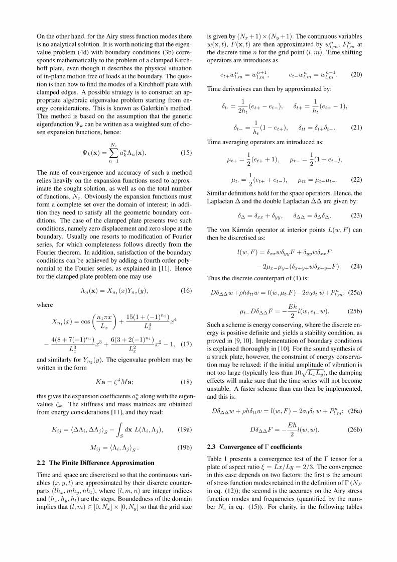
Table 1 presents a convergence test of the Γ tensor for aplate of aspect ratio ξ = Lx/Ly = 2/3. The convergencein this case depends on two factors: the first is the amountof stress function modes retained in the definition of Γ (NFin eq. (12)); the second is the accuracy on the Airy stressfunction modes and frequencies (quantified by the num-ber Nc in eq. (15)). For clarity, in the following tables

NF

k 100 144 2251 20.033 20.034 20.034

20 7.5605·103 9.4893·103 9.4960·103

50 1.3928·104 1.3929·104 1.3937·104

100 1.4847·104 2.7360·104 1.2413·105

400 484 6251 20.034 20.034 20.034

20 9.4970·103 9.4975·103 9.4977·103

50 1.3937·104 1.3937·104 1.3937·104

100 1.3334·105 2.2100·105 2.2108·105

Table 1. Convergence of coupling coefficients,Γkk,k,k(LxLy)3, ξ = 2/3.

Grid Points

k 51× 76 161× 241 280× 4191 20.728 20.381 20.189

20 9.7935·103 9.6413·103 9.5567·103

50 1.4440·104 1.4234·104 1.4080·104

100 2.0223·105 2.0246·105 2.0286·105

Table 2. Convergence of coupling coefficients, FDscheme, Γkk,k,k(LxLy)3, ξ = 2/3, NF = 225

NF is always the same as Nc. It is seen that a four-digitconvergence up to the Γ100

100,100,100 coefficient is obtainedwhen NF = 484. The same coefficients can be calculatedusing the finite difference code. Results are summarisedin table 2. It is seen that the coupling coefficients canbe calculated to very high precision when using the modaldescription. The major drawback of the modal approach isthe limited number of modes that one can keep for the sim-ulations (≈ 200). On the other hand, the finite differencescheme produces simulations including a vast number ofmodes (≈ 10000), at the expense of numerical precision.Comparing tables 1 and 2 suggests that a four-digit conver-gence is out of reach for the finite difference scheme withtypical grid sizes. The question is then which one of thetwo methods is better suited for sound synthesis.

3. EXAMPLE: A STRUCK PLATE

In this section an example is investigated to compare thetwo methods. The reference plate is a steel plate of di-mensions Lx × Ly = 0.4 × 0.6 m2, Young’s modulusE = 2 · 1011 Pa, density ρ = 7860 kg/m3, Poisson’sratio ν = 0.3 and thickness h = 1 mm. The plate isexcited with a temporal raised cosine at one point, with∆t = 0.1 ms and varying amplitude p0. The damping fac-tor is ωsχs = 0.75 s−1, resulting in σ0 = 0.75ρh kg/m2.

The finite difference scheme is run at 100 kHz, resultingin a grid size of 51×76 points. Scheme (25) takes abouttwo hours of calculation per second of simulation, on amachine running MATLAB equipped with Intel Core i5CPU 650 @ 3.20GHz. However, the simpler scheme (26)

0.095 0.1 0.1050

10

20

30

40

Time (s)

For

ce (

N)

0 1 2 3−1

−0.5

0

0.5

1

Am

p

Time (s)

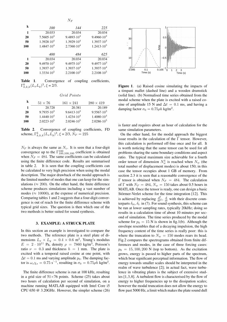
Figure 1. (a) Raised cosine simulating the impacts ofa timpani mallet (dashed line) and a wooden drumstick(solid line). (b) Normalised time series obtained from themodal scheme when the plate is excited with a raised co-sine of amplitude 15 N and ∆t = 0.1 ms, and having adamping factor σ0 = 0.75ρh kg/m2.

is faster and requires about an hour of calculation for thesame simulation parameters.

On the other hand, for the modal approach the biggestissue results in the calculation of the Γ tensor. However,this calculation is performed off-line once and for all. Itis worth noticing that the same tensor can be used for allproblems sharing the same boundary conditions and aspectratio. The typical maximum size achievable for a fourthorder tensor of dimension N4

w is reached when Nw (thetotal number of displacement modes) is about 150; in thiscase the tensor occupies about 1 GB of memory. Fromsection 2.3 it is seen that a reasonable convergence of theΓ tensor is obtained when NF = 484. The calculationof Γ with NF = 484, Nw = 150 takes about 0.5 hours inMATLAB. Once the tensor is ready, one can design a basicStormer-Verlet scheme for the time integration [12]. Thisis achieved by replacing d2

dt2 , ddt with their discrete coun-

terparts δtt, δt· in (7). For sound synthesis, this scheme canbe run at lower sampling rates, typically 20kHz; doing soresults in a calculation time of about 10 minutes per sec-ond of simulation. The time series produced by the modalscheme for p0 = 15 N is shown in fig.1(b). Although theenvelope resembles that of a decaying impulsion, the highfrequency content of the time series is really poor: this iswhere the truncation to Nw = 150 modes rears its head.Fig.2 compares the spectrograms obtained from finite dif-ferences and modes, in the case of three forcing cases:p0 = 15, 100, 200 N (top to bottom). As the excitationgrows, energy is passed to higher parts of the spectrum,which bear significant perceptual information. The flow ofenergy towards smaller scales should be interpreted in therealm of wave turbulence [2]; in actual fact, wave turbu-lence in vibrating plates is the subject of extensive stud-ies [1,3,8]. A turbulent flow is characterised by the flow ofenergy to higher frequencies up to the dissipation scales;however the modal truncation does not allow the energy toflow past 5000 Hz, a limit which makes the plate sound dull

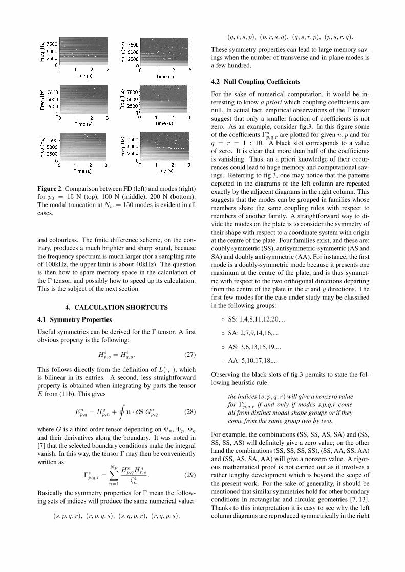
Figure 2. Comparison between FD (left) and modes (right)for p0 = 15 N (top), 100 N (middle), 200 N (bottom).The modal truncation at Nw = 150 modes is evident in allcases.

and colourless. The finite difference scheme, on the con-trary, produces a much brighter and sharp sound, becausethe frequency spectrum is much larger (for a sampling rateof 100kHz, the upper limit is about 40kHz). The questionis then how to spare memory space in the calculation ofthe Γ tensor, and possibly how to speed up its calculation.This is the subject of the next section.

4. CALCULATION SHORTCUTS

4.1 Symmetry Properties

Useful symmetries can be derived for the Γ tensor. A firstobvious property is the following:

Hip,q = Hi

q,p. (27)

This follows directly from the definition of L(·, ·), whichis bilinear in its entries. A second, less straightforwardproperty is obtained when integrating by parts the tensorE from (11b). This gives

Enp,q = Hqp,n +

∮n · δS Gnp,q (28)

where G is a third order tensor depending on Ψn, Φp, Φqand their derivatives along the boundary. It was noted in[7] that the selected boundary conditions make the integralvanish. In this way, the tensor Γ may then be convenientlywritten as

Γsp,q,r =

NF∑n=1

Hnp,qH

nr,s

ζ4n

. (29)

Basically the symmetry properties for Γ mean the follow-ing sets of indices will produce the same numerical value:

(s, p, q, r), (r, p, q, s), (s, q, p, r), (r, q, p, s),

(q, r, s, p), (p, r, s, q), (q, s, r, p), (p, s, r, q).

These symmetry properties can lead to large memory sav-ings when the number of transverse and in-plane modes isa few hundred.

4.2 Null Coupling Coefficients

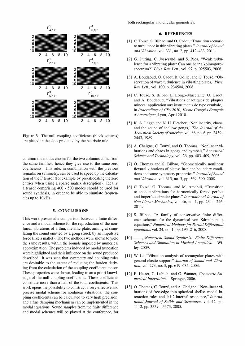
For the sake of numerical computation, it would be in-teresting to know a priori which coupling coefficients arenull. In actual fact, empirical observations of the Γ tensorsuggest that only a smaller fraction of coefficients is notzero. As an example, consider fig.3. In this figure someof the coefficients Γnp,q,r are plotted for given n, p and forq = r = 1 : 10. A black slot corresponds to a valueof zero. It is clear that more than half of the coefficientsis vanishing. Thus, an a priori knowledge of their occur-rences could lead to huge memory and computational sav-ings. Referring to fig.3, one may notice that the patternsdepicted in the diagrams of the left column are repeatedexactly by the adjacent diagrams in the right column. Thissuggests that the modes can be grouped in families whosemembers share the same coupling rules with respect tomembers of another family. A straightforward way to di-vide the modes on the plate is to consider the symmetry oftheir shape with respect to a coordinate system with originat the centre of the plate. Four families exist, and these are:doubly symmetric (SS), antisymmetric-symmetric (AS andSA) and doubly antisymmetric (AA). For instance, the firstmode is a doubly-symmetric mode because it presents onemaximum at the centre of the plate, and is thus symmet-ric with respect to the two orthogonal directions departingfrom the centre of the plate in the x and y directions. Thefirst few modes for the case under study may be classifiedin the following groups:

◦ SS: 1,4,8,11,12,20,...

◦ SA: 2,7,9,14,16,...

◦ AS: 3,6,13,15,19,...

◦ AA: 5,10,17,18,...

Observing the black slots of fig.3 permits to state the fol-lowing heuristic rule:

the indices (s, p, q, r) will give a nonzero valuefor Γsp,q,r if and only if modes s,p,q,r comeall from distinct modal shape groups or if theycome from the same group two by two.

For example, the combinations (SS, SS, AS, SA) and (SS,SS, SS, AS) will definitely give a zero value; on the otherhand the combinations (SS, SS, SS, SS), (SS, AA, SS, AA)and (SS, AS, SA, AA) will give a nonzero value. A rigor-ous mathematical proof is not carried out as it involves arather lengthy development which is beyond the scope ofthe present work. For the sake of generality, it should bementioned that similar symmetries hold for other boundaryconditions in rectangular and circular geometries [7, 13].Thanks to this interpretation it is easy to see why the leftcolumn diagrams are reproduced symmetrically in the right

Γ14,q,r

2 4 6 8 10

2468

10

Γ48,q,r

2 4 6 8 10

2468

10

Γ12,q,r

2 4 6 8 10

2468

10

Γ47,q,r

2 4 6 8 10

2468

10

Γ35,q,r

2 4 6 8 10

2468

10

Γ610,q,r

2 4 6 8 10

2468

10

Figure 3. The null coupling coefficients (black squares)are placed in the slots predicted by the heuristic rule.

column: the modes chosen for the two columns come fromthe same families, hence they give rise to the same zerocoefficients. This rule, in combination with the previousremarks on symmetry, can be used to speed up the calcula-tion of the Γ tensor (for example by pre-allocating the zeroentries when using a sparse matrix description). Ideally,a tensor comprising 400 - 500 modes should be used forsound synthesis, in order to be able to simulate frequen-cies up to 10kHz.

5. CONCLUSIONS

This work presented a comparison between a finite differ-ence and a modal scheme for the reproduction of the non-linear vibrations of a thin, metallic plate, aiming at simu-lating the sound emitted by a gong struck by an impulsiveforce (like a mallet). The two methods were shown to yieldthe same results, within the bounds imposed by numericalapproximation. The problems induced by modal truncationwere highlighted and their influence on the sound produceddescribed. It was seen that symmetry and coupling rulesare desirable to the extent of reducing the burden deriv-ing from the calculation of the coupling coefficient tensor.These properties were shown, leading to an a priori knowl-edge of the null coupling coefficients. These coefficientsconstitute more than a half of the total coefficients. Thiswork opens the possibility to construct a very effective andprecise modal scheme for nonlinear vibrations: the cou-pling coefficients can be calculated to very high precision,and a fine damping mechanism can be implemented in themodal equations. Sound samples from the finite differenceand modal schemes will be played at the conference, for

both rectangular and circular geometries.

6. REFERENCES

[1] C. Touze, S. Bilbao, and O. Cadot, “Transition scenarioto turbulence in thin vibrating plates,” Journal of Soundand Vibration, vol. 331, no. 2, pp. 412–433, 2011.

[2] G. During, C. Josserand, and S. Rica, “Weak turbu-lence for a vibrating plate: Can one hear a kolmogorovspectrum?” Phys. Rev. Lett., vol. 97, p. 025503, 2006.

[3] A. Boudaoud, O. Cadot, B. Odille, and C. Touze, “Ob-servation of wave turbulence in vibrating plates,” Phys.Rev. Lett., vol. 100, p. 234504, 2008.

[4] C. Touze, S. Bilbao, L. Longo-Mucciante, O. Cadot,and A. Boudaoud, “Vibrations chaotiques de plaquesminces: application aux instruments de type cymbale,”in Proceedings of CFA 2010, 10eme Congres Francaisd’Acoustique, Lyon, April 2010.

[5] K. A. Legge and N. H. Fletcher, “Nonlinearity, chaos,and the sound of shallow gongs,” The Journal of theAcoustical Society of America, vol. 86, no. 6, pp. 2439–2443, 1989.

[6] A. Chaigne, C. Touze, and O. Thomas, “Nonlinear vi-brations and chaos in gongs and cymbals,” AcousticalScience and Technology, vol. 26, pp. 403–409, 2005.

[7] O. Thomas and S. Bilbao, “Geometrically nonlinearflexural vibrations of plates: In-plane boundary condi-tions and some symmetry properties,” Journal of Soundand Vibration, vol. 315, no. 3, pp. 569–590, 2008.

[8] C. Touze, O. Thomas, and M. Amabili, “Transitionto chaotic vibrations for harmonically forced perfectand imperfect circular plates,” International Journal ofNon-Linear Mechanics, vol. 46, no. 1, pp. 234 – 246,2011.

[9] S. Bilbao, “A family of conservative finite differ-ence schemes for the dynamical von Karman plateequations,” Numerical Methods for Partial Differentialequations, vol. 24, no. 1, pp. 193–216, 2008.

[10] ——, Numerical Sound Synthesis: Finite DifferenceSchemes and Simulation in Musical Acoustics. Wi-ley, 2009.

[11] W. Li, “Vibration analysis of rectangular plates withgeneral elastic support,” Journal of Sound and Vibra-tion, vol. 273, no. 3, pp. 619–635, 2003.

[12] E. Hairer, C. Lubich, and G. Wanner, Geometric Nu-merical Integration. Springer, 2006.

[13] O. Thomas, C. Touze, and A. Chaigne, “Non-linear vi-brations of free-edge thin spherical shells: modal in-teraction rules and 1:1:2 internal resonance,” Interna-tional Journal of Solids and Structures, vol. 42, no.1112, pp. 3339 – 3373, 2005.