Flow-Induced Vibrations Classifications and Lessons from ...
311
-
Upload
khangminh22 -
Category
Documents
-
view
0 -
download
0
Transcript of Flow-Induced Vibrations Classifications and Lessons from ...

Flow-Induced Vibrations

This page intentionally left blank
Flow-Induced Vibrations Classifications and Lessons from
Practical Experiences
Editors
Shigehiko Kaneko Tomomichi Nakamura
Fumio Inada Minoru Kato
Technical Section on Flow-Induced VibrationsJSME DMC Division
English Translation Editor
Njuki W. Mureithi
AMSTERDAM • BOSTON • HEIDELBERG • LONDON • NEW YORK • OXFORDPARIS • SAN DIEGO • SAN FRANCISCO • SINGAPORE • SYDNEY • TOKYO

Elsevier The Boulevard, Langford Lane, Kidlington, Oxford OX5 1GB, UK Radarweg 29, PO Box 211, 1000 AE Amsterdam, The Netherlands
First edition 2008
Copyright © 2008 Elsevier Ltd. All rights reserved
No part of this publication may be reproduced, stored in a retrieval system or transmitted in any form or by any means electronic, mechanical, photocopying, recording or otherwise without the prior written permission of the publisher.
Permissions may be sought directly from Elsevier ’ s Science & Technology Rights Department in Oxford, UK: phone (+44) (0) 1865 843830; fax (+44) (0) 1865 853333; email: [email protected]. Alternatively, you can submit your request online by visiting the Elsevier web site at http://elsevier.com/locate/permissions , and selecting Obtaining permission to use Elsevier material
Notice: No responsibility is assumed by the publisher for any injury and/or damage to persons or property as a matter of products liability, negligence or otherwise, or from any use or operation of any methods,products, instructions or ideas contained in the material herein. Because of rapid advances in the medical sciences, in particular, independent verification of diagnoses and drug dosages should be made.
British Library Cataloguing-in-Publication Data A catalogue record for this book is available from the British Library
Library of Congress Cataloging-in-Publication Data A catalog record for this book is available from the Library of Congress
ISBN: 978-0-08-044954-8
For information on all Elsevier publications visit our web site at books.elsevier.com
Typeset by Charon Tec Ltd., A Macmillan Company. (www.macmillansolutions.com)
Printed and bound in Hungary
08 09 10 11 12 10 9 8 7 6 5 4 3 2 1
Contents
Preface ix
Foreword xi
List of Figures xiii
List of Tables xxi
List of Contributors xxiii
Nomenclature xxv
Chapter 1 Introduction 1
1.1 General overview 1 1.1.1 History of FIV research 1 1.1.2 Origin of this book 3
1.2 Modeling approaches 4 1.2.1 The importance of modeling 4 1.2.2 Classification of FIV and modeling 6 1.2.3 Modeling procedure 7 1.2.4 Analytical approach 11 1.2.5 Experimental approach 13
1.3 Fundamental mechanisms of FIV 15 1.3.1 Self-induced oscillation mechanisms 16 1.3.2 Forced vibration and added mass and damping 22
Chapter 2 Vibration Induced by Cross-Flow 29
2.1 Single circular cylinder 29 2.1.1 Structures under evaluation 29 2.1.2 Vibration mechanisms and historical review 29 2.1.3 Evaluation methods 36 2.1.4 Examples of component failures due to vortex-induced vibration 42
2.2 Two circular cylinders in cross-flow 44 2.2.1 Outline of structures of interest 44 2.2.2 Historical background 44 2.2.3 Evaluation methodology 50 2.2.4 Examples of practical problems 53
2.3 Multiple circular cylinders 54 2.3.1 Outline of targeted structures 54 2.3.2 Vibration evaluation history 54 2.3.3 Estimation method 57 2.3.4 Examples of component failures 66
v
2.4 Bodies of rectangular and other cross-section shapes 66 2.4.1 General description of cross-section shapes 67 2.4.2 FIV of rectangular-cross-section structures and historical review 68 2.4.3 Evaluation methods 71 2.4.4 Example of structural failures and suggestions for countermeasures 80
2.5 Acoustic resonance in tube bundles 81 2.5.1 Relevant industrial products and brief description of the phenomenon 81 2.5.2 Historical background 83 2.5.3 Resonance prediction method at the design stage 89 2.5.4 Examples of acoustic resonance problems and hints for
anti-resonance design 95 2.6 Prevention of FIV 97
Chapter 3 Vibration Induced by External Axial Flow 107
3.1 Single cylinder/multiple cylinders 107 3.1.1 Summary of objectives 107 3.1.2 Random vibration due to flow turbulence 107 3.1.3 Flutter and divergence 117 3.1.4 Examples of reported component-vibration problems and hints
for countermeasures 119 3.2 Vibration of elastic plates and shells 120
3.2.1 Bending–torsion flutter 120 3.2.2 Panel flutter 123 3.2.3 Shell flutter 124 3.2.4 Turbulence-induced vibration 126 3.2.5 Hints for countermeasures 127
3.3 Vibration induced by leakage flow 128 3.3.1 General description of the problem 128 3.3.2 Evaluation method for single-degree-of-freedom translational system 129 3.3.3 Analysis method for single-degree-of-freedom translational system
with leakage-flow passage of arbitrary shape 132 3.3.4 Mechanism of self-excited vibration 134 3.3.5 Self-excited vibrations in other cases 137 3.3.6 Hints for countermeasures 140 3.3.7 Examples of leakage-flow-induced vibration 142
Chapter 4 Vibrations Induced by Internal Fluid Flow 145
4.1 Vibration of straight and curved pipes conveying fluid 145 4.1.1 Vibration of pipes conveying fluid 145 4.1.2 Vibration of pipes excited by oscillating and two-phase fluid flow 152 4.1.3 Piping vibration caused by gas–liquid two-phase flow 155
4.2 Vibration related to bellows 160 4.2.1 Vibration of bellows 160 4.2.2 Hints for countermeasures and examples of flow-induced vibrations 169
vi Contents
4.3 Collapsible tubes 171 4.3.1 Summary 171 4.3.2 Self-excited vibration of collapsible tubes 171 4.3.3 Key to prevention 173
Chapter 5 Vibration Induced by Pressure Waves in Piping 177
5.1 Pressure pulsation in piping caused by compressors 177 5.1.1 Summary 177 5.1.2 Explanation of the phenomenon, and the history of
research/evaluation 178 5.1.3 Calculation and evaluation methods 179 5.1.4 Hints for countermeasures 187 5.1.5 Case studies 190
5.2 Pressure pulsations in piping caused by pumps and hydraulic turbines 194 5.2.1 Outline 194 5.2.2 Explanation of phenomena 195 5.2.3 Vibration problems and suggested solutions 206
5.3 Pressure surge or water hammer in piping system 209 5.3.1 Water hammer 209 5.3.2 Synopsis of investigation 209 5.3.3 Solution methods 210 5.3.4 Countermeasures 213 5.3.5 Examples of component failures 213
5.4 Valve-related vibration 217 5.4.1 Valve vibration 217 5.4.2 Coupled vibrations between valve and fluid in the piping 219 5.4.3 Problem cases 226 5.4.4 Hints for countermeasures against valve vibration 229
5.5 Self-excited acoustic noise due to flow separation 231 5.5.1 Summary 231 5.5.2 Outline of excitation mechanisms 232 5.5.3 Case studies and hints for countermeasures 238
Chapter 6 Acoustic Vibration and Noise Caused by Heat 247
6.1 Acoustic vibration and noise caused by combustion 247 6.1.1 Introduction 247 6.1.2 Combustion driven oscillations 248 6.1.3 Combustion roar 259
6.2 Oscillations due to steam condensation 262 6.2.1 Introduction 262 6.2.2 Characteristics and prevention 263 6.2.3 Examples of practical problems 263
Contents vii

6.3 Flow induced vibrations related to boiling 266 6.3.1 Introduction/background 266 6.3.2 Vibration mechanisms 266 6.3.3 Analytical approach 266 6.3.4 Vibration/oscillation problems and solutions 271
Index 279
viii Contents
ix
Preface
The soundness of the energy plant system and its peripheral equipment is attracting strong interest not only from people in industry engaged in nuclear power generation, thermal power generation, hydroelectric power generation and chemical plant operation, but also from ordinary citizens. In addition, abnormal vibrations and noise, that arise in aircraft and automobiles for example, are also important problems related to reliability.
One of the key factors inhibiting the soundness of the energy plant system and reli-ability of equipment is flow induced vibration (FIV), which arises via flow and structural system coupling or flow and acoustic system coupling. Research on FIV, ranging from basic research in laboratories to practical research at the prototypical industrial scale in various research institutes around the world, has been widely carried out.
However, the number of incidents due to flow induced vibration or noise generation leading to structural failure do not show any signs of significant decline. Indeed, there is an increase in the number of incidents which might lead to loss of confidence from soci-ety as well as economic loss. Problems in nuclear power stations are a case in point.
The reason why such phenomena arise is because a network for the purpose of trans-mission of knowledge and information on flow induced vibration between researchers, designers, builders and operation managers has not been constituted.
Once a vibration problem arises, it must be solved in a short time. To achieve this, investigation of similar past cases is energetically carried out. However, the number of well documented previous cases with useful information is very limited due to the veil of business secrecy.
It is against this background that the researchers who gathered at the Japan Society of Mechanical Engineers FIV workshops undertook the task of extracting the most useful information from the literature reviewed at the series of workshops over the past 20 years. The information has been put together in the form of a database in which fundamental knowledge on flow induced vibration is explained in detail and the information vital for the designer is conveniently compiled and consolidated.
We hope this volume will be useful to engineers and students both for the systematic evaluation and understanding of flow induced vibration and in contributing to the creation of new research topics based on knowledge acquired in the field.
Representatives of the technical section on FIV, Japan Society of Mechanical Engineers
Shigehiko Kaneko (The University of Tokyo)Fumio Inada (Central Research Institute of Electric Power Industry)Tomomichi Nakamura (Osaka Sangyo University)Minoru Kato (Kobelco Research Institute, Inc.)

This page intentionally left blank
xi
Foreword
The operative words for this book are “ pragmatic ” “ practical ” and “ useful ” for anyone who is interested in solving a problem involving Flow-Induced Vibration (FIV). It brings to the reader two invaluable assets: (i) the formidable, accumulated decades-long experi-ence of many researcher-engineers specializing in different aspects of FIV; (ii) the hitherto unavailable rich Japanese literature on the subject.
The scope of the book is formidable: FIV related to cross-flow or parallel flow around solitary cylinders or prisms, internal-flow-induced vibrations, vibrations related to pres-sure waves in piping and acoustical vibration associated with combustion. In each case, the phenomenology of the vibration is identified, so that the user of this book may iden-tify which kind of problem he/she is faced with, the background theory and/or experi-mental data available, and finally practical guidance as to what to do about the problem (see, e.g., Table 2.18).
The book is amply illustrated and provides the references which will help the reader get a wider view of each of the subtopics and further technical details on which the recommended course of action is based.
Although the book offers understanding of the mechanisms involved in each subtopic, it goes very much further than any other book on the “ how to ” aspect of solving one’s problem. It is for this reason that it is useful for researchers and invaluable for engineers faced with Flow-Induced Vibration problems.
Michael P. PaïdoussisThomas Workman Emeritus ProfessorDepartment of Mechanical EngineeringMcGill University, Montreal, QC, Canada

This page intentionally left blank
List of Figures
1.1 Design support system for FIV. 3 1.2 How will this half cylinder respond to wind flow? 5 1.3 Route to solution. 5 1.4 Mechanism of oscillation. 6 1.5 Classification of FIV and the corresponding sections. 7 1.6 Examples of models and mechanisms. 8 1.7 Vibration problems in design of feed water heater. 8 1.8 Vibration of tube array caused by cross-flow. 9 1.9 Decision based on importance. 10 1.10 Flowchart of simplified treatment. 10 1.11 Separate and distinct modeling of structure and flow. 11 1.12 Example of flow analysis and vibration model. 12 1.13 Dimensionless vortex shedding frequency dependence on Reynolds number. 15 1.14 Instability mechanism of elastic force coupled system. 18 1.15 Feedback forces. 20 2.1 Vortex-induced synchronization. 32 2.2 Tip-vortex shedding. 33 2.3 Cylinder motion and vortex shedding in oscillating flow. 33 2.4 Evaluation for vibration of a circular cylinder in cross-flow. 37 2.5 Range of avoidance and suppression of synchronization. 38 2.6 Suppression of in-line synchronization. 38 2.7 Lock-in in two-phase flow. 41 2.8 Suppression of synchronization by spiral strake. 42 2.9 In-line vibration of marine pile at Immingham. 43 2.10 Rain-induced vibration in Japan. 43 2.11 Example of coupling of a pipe and a thermo well. 44 2.12 Possible configurations of cylinder pairs in cross-flow: (a) two cylinders in
tandem, (b) staggered arrangement of two cylinders, (c) two cylinders in parallel, (d) two staggered cylinders with different diameters, (e) two cylinders in criss-crossed configuration, and (f) intersecting cylinders. 45
2.13 Cylinder interaction regimes based on in-flow and transverse spacings. 48 2.14 Region within which control can be achieved for different diameter
ratios D/d. 48 2.15 Pressure coefficient Cp variation and dependence on Z/D. 49 2.16 Experiments on upstream cylinder dynamics in the case where the
downstream cylinder is fixed. 51
xiii
2.17 Cylinder configuration and coordinates. 53 2.18 Tube array patterns: (a) tube row, (b) tube column, (c) square tube array,
and (d) triangular tube array. 55 2.19 Strouhal numbers for tube arrays related to pitch/diameter ratio:
(a) in-line array, and (b) staggered array. 58 2.20 Example of stability boundary for fluidelastic instability. 60 2.21 Example of measured random force acting on array of circular tubes. 61 2.22 Example of measured damping ratio for tubes in two-phase flow. 64 2.23 Example of proposed random force liquid–gas two-phase flow. 65 2.24 Vibration modes for various types of structures: (a) parallel vibration,
(b) rotational vibration, (c) in plane vibration, and (d) out of plane vibration. 68 2.25 Strouhal numbers for rectangular-cross-section bodies for various
aspect ratios, attack angles, and rounded corners. 72 2.26 Effect of attack angle on Strouhal number for large aspect ratio ( e/d � 10). 73 2.27 Effect of aspect ratio on possible vortex-induced vibration modes with
zero attack angle: (a) ranges of possible FIV for lightly damped rectangular prisms in low-turbulence cross-flow (α � 0), cross-hatched and dotted regions represent prisms with transverse and streamwise degree-of-freedom, respectively, and (b) effects of aspect ratio on the mode of vortex formation. 74
2.28 Effects of attack angle on possible vortex-induced vibration modes for large aspect ratio ( e/d � 10): (a) effects of attack angle on possible transverse vibration of rectangular cross-section body in cross-flow (lightly damped, low-turbulence flow, zero attack angle), and (b) effects of attack angle on the mode of vortex formation. 74
2.29 Galloping vibration amplitude of a square-cross-section body in the transverse degree-of-freedom. 79
2.30 Structures of guide vane and elbow splitter. 81 2.31 Overview of acoustic resonance in tube bundle. 82 2.32 Classification of acoustic resonance by mode shape: (a) transverse mode,
and (b) longitudinal mode. 83 2.33 Resonance map for tube bundles, based on pitch-to-diameter ratio:
(a) in-line, and (b) staggered array. 85 2.34 Examples of baffle placement for countermeasures against
transverse acoustic modes: (a) irregular pitch, and (b) regular pitch. 85 2.35 Resonance suppression effect of cavity baffle: (a) baffle structure,
and (b) sound pressure level. 86 2.36 View showing vortex–acoustic interaction: (a) stable, and (b) resonance. 86 2.37 Feed back mechanism between flow and acoustic field. 87 2.38 Experimental setup for stability evaluation by forced water-flow fluctuation. 87 2.39 Resonance occurrence in boiler scale model apparatus. 88 2.40 Mode shapes in boiler scale model apparatus: (a) transverse
mode – 805 Hz, and (b) longitudinal mode – 990 Hz. 89 2.41 Typical experimental results of longitudinal mode suppression:
(a) without bell-mouth, and (b) with bell-mouth. 90 2.42 Finned tubes: (a) serrated fin, and (b) solid fin. 91
xiv List of figures
2.43 Experimental validation of estimated Strouhal number using equivalent diameter and Fitz-Hugh Strouhal number. 91
2.44 Prediction of resonance based on Eisinger ’ s method: (a) parameter definition for staggered array, (b) setting of critical region, and (c) example of application. 94
2.45 Flow chart of Eisinger ’ s resonance suppression design. 94 2.46 Example of countermeasure by cavity baffle: (a) side view of boiler,
(b) standing wave data, and (c) countermeasure (top view). 96 2.47 Example of countermeasure in shell and tube type heat exchanger:
(a) structure of air cooler, and (b) relation between resonance frequency and flow. 96
2.48 Example of countermeasure with acoustic absorbers for coal fired boiler. 97 2.49 Region of occurrence of vortex shedding and maximum
response of square cylinder as functions of Scruton number. (Solid line: boundary of occurrence; Broken line: maximum response.) 100
3.1 Schematic of: (a) BWR fuel bundle and (b) steam generator. 108 3.2 Circular cylinder subject to turbulent pressure fluctuations. 109 3.3 Turbulent wall pressure spectra. 110 3.4 Magnitude of cross-spectral density of turbulent wall pressure
(longitudinal). 110 3.5 Magnitude of cross-spectral density of turbulent wall pressure (lateral). 111 3.6 Dependence of convection velocity on dimensionless frequency. 111 3.7 Mid-span rms displacement of fixed-fixed cylinders. 113 3.8 Parameters used for random vibration correlation: (a) parameter � , and
(b) parameter b . 116 3.9 Parameters for spatial correlation in air–water flow condition:
(a) parameter �, and (b) parameter Vc. 116 3.10 Relationship between measured and predicted amplitudes of
vibration according to Païdoussis ’ empirical formula. 117 3.11 A two-dimensional airfoil. 121 3.12 Coupling between the bending and torsional motion. 121 3.13 Spring-supported rigid wing section in two-dimensional flow. 121 3.14 Dimensionless flutter speed versus frequency ratio. 122 3.15 Panel flutter. 123 3.16 Simply-supported plate of infinite width subjected to fluid flow
over one side. 123 3.17 Dimensionless critical flow velocity versus mass ratio. 124 3.18 Jet engine after-burner. 125 3.19 Coupled sloshing and cylindrical weir shell vibration. 125 3.20 Sound spectrum for 90 degree elbow duct. 126 3.21 Examples of leakage-flow-induced vibration events: (a) PWR
core barrel, and (b) feed-water sparger. 128 3.22 One-dimensional leakage passage under study and coordinate system:
(a) tapered leakage-flow passage, and (b) arbitrary-shaped leakage-flow passage. 130
List of figures xv
3.23 Region where added damping and stiffness coefficients become positive or negative when the one-dimensional tapered passagewall oscillates as a single-degree-of-freedom translating system. 132
3.24 The distribution of variation of the flow resistance and the inertia force when the flow rate varies in the leakage passage. 136
3.25 Region where added damping and stiffness coefficients become positive or negative for a one-dimensional tapered passage wall oscillating as a single-degree-of-freedom rotational system: (a) lf � 0 (the pivot point is at the entrance), (b) lf � 0.5 (the pivot point is at the center of the passage), and (c) lf � 0.7 (the pivot point is slightly closer to the outlet from the mid-point of the passage). 138
3.26 Critical velocity of two-degree-of-freedom translational and rotational system. 139
3.27 Plate motion during one cycle of self-excited vibration. 139 3.28 Critical velocity of cantilevered plate clamped at the upstream end. 140 3.29 Examples of leakage-flow-induced vibrations. 141 4.1 Flexible pipe conveying fluid and coordinate system. 146 4.2 Forces and moments acting on elements of (a) the fluid, and (b) the pipe,
respectively. 147 4.3 Root loci of pinned-pinned pipes with increasing flow velocity
for � � � � � � 0, and (a) � � 0.1 or (b) � � 0.5. 149 4.4 Root loci of fixed-free pipes with increasing flow velocity for
� � � � � � 0 and � � 0.5. 150 4.5 Variation of critical velocity of fixed-free pipes versus � for
progressively higher values of the viscoelastic dissipation constant � . 150 4.6 Variation of natural frequencies of fixed-fixed curved pipes with flow
velocity u for �α π= and � � 0, 0.5, 1.0. 151 4.7 Root locus of fixed-fixed curved pipes with flow velocity u for
�α π= , � � 0.75. 152 4.8 Pipes with harmonically oscillating fluid flow and coordinate system. 153 4.9 Bent pipe and coordinate system. 153 4.10 Frequency response of pipe with harmonically oscillating fluid flow
for �b � 90 degrees. 154 4.11 Flow patterns in vertical piping: (a) bubble flow, (b) slug flow, (c) froth
flow, (d) annular mist flow, (e) mist flow, and (f) inverse annular flow. 155 4.12 Flow patterns in horizontal piping: (a) bubbly flow, (b) stratified flow,
(c) wavy flow, (d) plug flow, (e) slug flow, (f) froth flow, (g) annular mist flow, and (h) mist flow. 156
4.13 Flow pattern map for horizontal piping. 157 4.14 Flow pattern map for vertical piping. 158 4.15 Test equipment for piping vibration caused by gas–liquid two-phase flow. 159 4.16 Piping vibration due to gas–liquid two-phase flow. 159 4.17 Typical sketch of single bellows and double bellows. 161 4.18 Free share layer created by bellows. 161 4.19 Details of bellows geometry. 162 4.20 Dimensions of double bellows. 163
xvi List of figures
4.21 Vibration modes of single bellows. 164 4.22 Half-convolution added mass coefficient for axial vibration. 164 4.23 Half-convolution added mass coefficient for transverse vibration. 166 4.24 Vibration modes of double bellows. 167 4.25 Coefficients for second lateral mode; no lateral support. 168 4.26 Coefficients for third lateral mode; no lateral support. 168 4.27 Coefficients for first rocking mode; no lateral support. 169 4.28 Coefficients for second rocking mode; no lateral support. 169 4.29 Coefficients for second rocking mode; no lateral support. 170 4.30 Coefficients for first rocking mode with lateral support. 170 4.31 Typical collapsible tube experimental system. 172 4.32 Flow rate–pressure characteristic curve. 173 4.33 Tube law. 174 4.34 Unstable region in the characteristic curve. 174 5.1 Suction/discharge flow and pressure pulsation in reciprocating compressors. 178 5.2 Suction/discharge flow waveform in reciprocating compressors. 183 5.3 Piping sections excited by pressure pulsations. 185 5.4 Selection criteria for API design approach number. 186 5.5 SwRI ’ s evaluation criteria for piping vibration. 187 5.6 Reciprocating compressor: schematic diagram of plant. 188 5.7 Comparison between measured and calculated pressure at each point. 190 5.8 Root blower: schematic diagram of plant. 190 5.9 Result of vibration field data (effect of countermeasure). 191 5.10 Turbine: schematic diagram of plant. 194 5.11 Result of piping vibration field data (before [ ● ] and after [❍]
countermeasure). 195 5.12 Influence of void fraction on pressure wave velocity in water pipes. 196 5.13 Illustration of pulsation reduction by means of parallel operation
of multiple pumps. 197 5.14 An example of the frequency spectrum of pulsations caused by a pump. 198 5.15 Pipe element model equivalent to a pump. 199 5.16 Pipeline system including a pump and a tank. 201 5.17 Example of a pressure head versus flow rate curve for a pump having
a negative resistance characteristic. 201 5.18 Relation between pump resistance and rotational speed. 203 5.19 Suppression of intake vortex. 204 5.20 Influence of trailing edge on vibrations (case of plane
blade in parallel flow). 206 5.21 Synchronous and asynchronous guide vane positioning at partial load. 207 5.22 Vibration of an axial flow turbine with fixed guide vanes. 207 5.23 Wave propagation due to instantaneous valve closure. 209 5.24 Characteristic line of MOC on x�t plane. 211 5.25 Flow chart of valve stroking analysis. 216 5.26 Support damage due to negative pressure wave. 216 5.27 Pipe dislocation due to operational change in pump station. 217 5.28 Unexpected blow-out from safety valve caused by re-start operation. 217
List of figures xvii
5.29 Schematic view of butterfly valve. 218 5.30 Self-excited vibration of a valve having an annular clearance. 218 5.31 Frequency spectrum of valve vibration caused by cavitation. 219 5.32 Examples of valves to be discussed. 220 5.33 Examples of valve position relative to piping: (a) valve located at
exit of piping, (b) valve located at middle of piping, (c) valve located at inlet of piping, and (d) valve and adjacent volume. 220
5.34 Valve that closes as flow increases. 221 5.35 Condition for self-excited vibration for check valve. 222 5.36 Hysteresis caused by fluid inertia. 222 5.37 System consisting of piping, valve, and constant pressure tank. 223 5.38 Boundary condition and equilibrium position. 223 5.39 Auto-valve in pipeline system: (a) valve which closes at high
pressure, and (b) corresponding pressure-flow characteristic. 224 5.40 Valve model. 225 5.41 Automatic response type decompression valve. 227 5.42 Schematic view of power steering system. 227 5.43 Examples of coupled vibration of pipe structural modes high-order
acoustic modes. 228 5.44 Cavity tone at relief valve and preventive countermeasure. 229 5.45 (a) Flow in the high-pressure bypass control valve, and (b) vibration
countermeasure. 230 5.46 Flow and countermeasure in turbine control valve. 230 5.47 Basic configurations of shear-layer and impingement-edge
geometries that produce self-sustained oscillations. 231 5.48 Flow over a two-dimensional cavity. 232 5.49 Variation of organized-oscillation Strouhal number with cavity
length for fluid-dynamic oscillations in a two-dimensional cavity. 233 5.50 Matrix categorization of fluid-dynamic, fluid-resonant, and
fluid-elastic types of cavity oscillations. 234 5.51 Configurations of closed side branches: (a) single branch, (b) tandem
branches, and (c) coaxial branches. 234 5.52 Variations of Strouhal numbers with Reynolds number for the
hole-tone system. 235 5.53 Frequencies and amplitudes of pressure fluctuation for different
perforated plate thickness. 236 5.54 Examples of diametral acoustic modes and corresponding
circumferential structural modes with matching wave numbers: (a) acoustic modes, and (b) structural modes. 237
5.55 Fatigue diagram, for piping systems subjected to internal acoustic loading, relating acoustic input energy parameter to pipe geometry parameter. 238
5.56 Pathlines in the symmetry plane of a standard plug at 100% stroke. 239 6.1 Spectrum of combustion driven oscillations. 247 6.2 Generation of heat driven oscillations. 247 6.3 Spectrum of combustion roar: (a) open flame, and
(b) flame in a chamber. 248
xviii List of figures
6.4 Higgins’ experiment. 249 6.5 Rijke tube heated by (a) burner and, (b) heater. 249 6.6 Heater positions susceptible to vibrations for different pressure modes. 250 6.7 The mechanism of heat driven air column vibration. 250 6.8 Acoustic vibration test apparatus. 251 6.9 Vibration occurrence zone. 251 6.10 Mechanism of thermo-acoustic vibration. 252 6.11 Feed back system. 252 6.12 Time lag by fuel transportation. 253 6.13 Transfer functions G � q/q1. 254 6.14 Mid-size furnace used in experiments. 255 6.15 Sondhauss and Rijke tubes. 256 6.16 Stability criterion chart. 257 6.17 Blast furnace: (a) furnace configuration, and (b) pressure amplitude
versus fuel flow rate. 258 6.18 Water tube type boiler. 259 6.19 Turbulent flame. 260 6.20 Low noise burner. 261 6.21 Home use boiler: (a) structure of the boiler, and (b) a slant plate
for countermeasure. 262 6.22 Schematics of chugging and steam hammer: (a) chugging, and
(b) steam hammer. 264 6.23 Steam hammer in feed water piping. 265 6.24 Steam hammer at emergency cooling system. 265 6.25 Feed water piping in boiler. 266 6.26 Single boiling piping system. 268 6.27 Characteristic curves of mass flow rate m in the heating tube versus
the pressure difference P between the inlet and outlet . The conditions for generation of density-wave type oscillations (heat flow rate q0 = 2931 W), and pressure drop type oscillations are also shown. 268
6.28 Relations between flow rate and pressure drop for pressure drop type oscillations. Limit cycle is formed. 269
6.29 Wave form of flow rate Q2 for pressure drop type oscillations. Experimental results and analytical results obtained by solution of van der Pol ’ s equation ( � 34.2, � � � 0.263) are compared. � is the period of oscillations. 270
6.30 Geysering in thermosyphone side reboiler. 271 6.31 Flow rate fluctuation and pressure difference observed in the column
due to geysering. 272 6.32 LNG tank bottom feed system. 273 6.33 LNG tank top feed system. 273 6.34 Geysering suppression by the use of cross-feed recirculation in the
liquid fuel feed system. 274 6.35 Geysering suppression by the use of concentric inner tube in the
liquid fuel feed system. 274
List of figures xix

This page intentionally left blank
List of Tables
1.1 Examples of numerical codes 11 1.2 Non-dimensional parameters and their physical meaning 14 2.1 Classification of products in this chapter 30 2.2 Classsification of flow in this chapter 31 2.3 Classification of vibration in Section 2.1 31 2.4 Studies on vortex-induced vibration 36 2.5 Studies on ovalling vibration of a cylindrical shell 36 2.6 Conditions for avoidance or suppression of synchronization 39 2.7 Semi-empirical formulae for resonant amplitude 39 2.8 Classification of interference flow induced oscillations 47 2.9 Evaluation and classification in steady flow 53 2.10 Evaluation and classification for sinusoidal flow 54 2.11 History of research on FIV of tube arrays 56 2.12 Natural frequency and average damping ratio of circular structures 61 2.13 Examples of tube failures within tube banks 66 2.14 Types of vortex-induced vibration of a rectangular cross-section
body in cross-flow 73 2.15 Values of partial derivative of Cy with respect to angle of attack
for several cross-section bodies in steady flow 77 2.16 Polynomial approximation expressions of Cy for several
cross-section bodies 78 2.17 Values of partial derivative of CM with respect to angle of attack for
several bodies of different cross-sections, in steady flow 80 2.18 Hints on prevention of FIV 98 2.19 The conditions of occurrence of wing flutter/divergence, depending
on the relative positions of the gravity center: ( G ), the elastic axis: ( E ), and the total fluid force on the wing: and ( F ), along the fluid flow direction (case of small attack angle) 100
3.1 Formulae for vibration amplitude 118 3.2 Tube support conditions and instability phenomena 119 3.3 Condition for prevention of instability induced by external parallel flow 120 3.4 Definition of parameters in Eq. (3.28) 131 3.5 Transfer matrices for steady flow component 133 3.6 Transfer matrices for unsteady flow component 135 4.1 Conversion coefficients of flow pattern map 158 4.2 Nomenclature 163 4.3 Aik constants for transverse modes 166 4.4 Aik constants for lateral modes 167 4.5 Aik constants for rocking modes 168
xxi

5.1 Classification of compressors and blowers 177 5.2 Calculation/analysis methods for pressure pulsations 180 5.3 Transfer matrices for piping elements 181 5.4 Equivalent damping coefficient 182 5.5 Maximum allowable level of pulsation specified in APl Standard 618 186 5.6 Acoustic resonance frequencies 188 5.7 Methods to reduce pressure pulsation 189 5.8 Methods to reduce piping vibration 191 5.9 Example cases 192 5.10 Characteristics of noise generation mechanisms in centrifugal pumps 200 5.11 Effect of pump design on pressure pulsation 200 5.12 Examples of problem cases for pumps and hydraulic turbines 208 5.13 Typical examples of pressure surge 214 5.14 Necessary data for pressure surge analysis 214 5.15 Typical countermeasures and cautions 215 6.1 Dissipation ratio for each mode 255 6.2 Condensation induced oscillations 263 6.3 Classification and physical mechanisms of flow induced vibrations
related to boiling 267
xxii List of tables

xxiii
List of Contributors
Editors
Fumio InadaCentral Research Institute of Electric Power Industry, Komae, Tokyo, Japan
Minoru KatoKabelco Research, Inc., Kobe, Hyogo, Japan
Shigehiko KanekoProfessor, Department of Mechanical Engineering, The University of Tokyo, Hongo, Tokyo, Japan
Tomomichi NakamuraProfessor, Department of Mechanical Engineering, Osaka Sangyo University, Daito, Osaka, Japan
English Translation Editor
Njuki W. MureithiProfessor, Department of Mechanical Engineering, Ecole Polytechnique de Montreal,Quebec, Canada
Authors
Takeshi FujikawaProfessor, Department of Business Administration Education, Ashiya University, Ashiya, Hyogo, Japan
Tsuyoshi HagiwaraToshiba Corporation, Yokohama, Kanagawa, Japan
Itsuro HayashiChiyoda Advanced Solutions Corporation, Yokohama, Kanagawa, Japan
Kazuo HirotaMitsubishi Heavy Industries, Ltd., Takasago, Hyogo, Japan
Toru IijimaProfessor, Organization for Education and Research, Muroran Institute of Technology, Muroran, Hokkaido, Japan
Fumio InadaCentral Research Institute of Electric Power Industry, Komae, Tokyo, Japan
Shigehiko KanekoProfessor, Department of Mechanical Engineering, The University of Tokyo, Hongo, Tokyo, Japan

Minoru KatoKobelco Reseach Institute, Inc., Kobe, Hyogo, Japan
Tatsuhiko KiuchiToyo Engineering Corporation, Narashino, Chiba, Japan
Hiroyuki MatsudaChiyoda Advanced Solutions Corporation, Yokohama, Kanagawa, Japan
Ryo MoritaCentral Research Institute of Electric Power Industry, Komae, Tokyo, Japan
Hisayuki MotoiIHI Corporation, Yokohama, Kanagawa, Japan
Hiroshi NagakuraMitsubishi Heavy Industries, Ltd., Fukabori, Nagasaki, Japan
Tomomichi NakamuraProfessor, Department of Mechanical Engineering, Osaka Sangyo University, Daito, Osaka, Japan
Akira NemotoToshiba Corporation, Yokohama, Kanagawa, Japan
Eiichi Nishida Professor, Department of Mechanical System Engineering, Shonan Institute of Technology, Fujisawa, Kanagawa, Japan
Toru OkadaKobe Steel Ltd., Kobe, Hyogo, Japan
Noboru SaitoToshiba Corporation, Shibaura, Tokyo, Japan
Masashi SanoProfessor, Department of Mechanical Engineering, Shizuoka Institute of Science and Technology, Fukuroi, Shizuoka, Japan
Yoshihiko UrataProfessor, Department of Mechanical Engineering, Shizuoka Institute of Science and Technology, Fukuroi, Shizuoka, Japan
Masahiro Watanabe Associate Professor, Department of Mechanical Engineering, Aoyama Gakuin University, Sagamihara, Kanagawa, Japan
Kazuaki YabeToyo Engineering Corporation, Narashino, Chiba, Japan
Akira YasuoCentral Research Institute of Electric Power Industry, Komae, Tokyo, Japan
Kimitoshi YonedaCentral Research Institute of Electric Power Industry, Komae, Tokyo, Japan
xxiv List of contributors
xxv
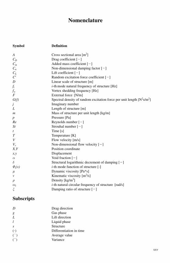
Nomenclature
Symbol Definition
A Cross sectional area [m2]CD Drag coefficient [�]Cm Added mass coefficient [�]Cn Non-dimensional damping factor [�]CL Lift coefficient [�]C� Random excitation force coefficient [�]D Linear scale of structure [m]fi i-th mode natural frequency of structure [Hz]fw Vortex shedding frequency [Hz]F External force [N/m]G(f) Spectral density of random excitation force per unit length [N2s/m2]j Imaginary numberL Length of structure [m]m Mass of structure per unit length [kg/m]p Pressure [Pa]Re Reynolds number [�]St Strouhal number [�]t Time [s]T Temperature [K]V Flow velocity [m/s]Vr Non-dimensional flow velocity [�]X,Y Position coordinatex,y Displacementα Void fraction [�]δ Structural logarithmic decrement of damping [�]Φi(x) i-th mode function of structure [-]� Dynamic viscosity [Pa*s] Kinematic viscosity [m2/s]� Density [kg/m3]�i i-th natural circular frequency of structure [rad/s]� Damping ratio of structure [�]
Subscripts
D Drag directiong Gas phaseL Lift directionl Liquid phases Structure(�) Differentiation in time(� ) Average value(�) Variance

This page intentionally left blank
1
1 Introduction
1.1 General overview
Vibration and noise problems due to fluid flow occur in many industrial plants. This obstructs smooth plant operation. These flow-related phenomena are known as “ Flow-Induced Vibrations ” (FIV). The term “ Flow-Induced Vibration and Noise ” (FIVN) is used when flow-induced noise is present.
It can be easily understood that the fluid force acting on an obstacle in flow, will vary due to the flow unsteadiness and that the force, in turn, may cause vibration of the obsta-cle. In the case of piping connected to reciprocating fluid machines, it is well known that the oscillating (fluctuating) flow in the piping generates excitation forces causing piping vibration.
However, even for steady flow conditions, vibration problems may be caused by vor-tex shedding behind obstacles or by other phenomena. The drag direction vibration of the thermocouple well in the fast breeder reactor at “ Monju ” in Japan is an example of a vibration problem caused by the symmetric vortex shedding behind the well. This kind of self-excited FIV occurs even in steady flow, making it much more difficult to determine the underlying mechanism and thus one of the most difficult problems to deal with at the design stage or during trouble shooting. Flow-induced acoustic noise is also an important problem in industry.
1.1.1 History of FIV research
Two conferences (Naudascher [1] ; Naudascher and Rockwell [2] ) on fluid-related vibration were held in 1972 and 1979, with the initiative of Prof. Naudascher of University of Karlsruhe, Germany. At the 1979 conference, many practical problems related to flow-induced vibration and noise in a wide variety of industrial fields, such as mechanical systems, civil engineering, aircrafts, ships, and nuclear power plants, were presented. The conference included many interesting results that are still, pertinent today.
In 1977, Dr. Robert Blevins wrote the first textbook [3] in this field. The term “ Flow-Induced Vibration ” became popular after he used it for the book title. In the book and probably for the first time, FIV phenomena were classified based on the two basic flow types: steady flow induced and unsteady flow related. Blevins [4] went on to publish a handbook focused on the frequency and the eigen modes of structural systems and fluid systems related to FIV. A second handbook (Blevins [5] ), aimed at designers, gave sys-tematic information for pipe flows, open water channels, separated flow, flow resistance,

2 Flow induced vibrations: classifications and lessons from practical experiences
shear flow, etc. These handbooks contain valuable information on FIV-related problems and the underlying phenomena. The second edition of the book “ Flow-Induced Vibration ” (Blevins [6] ) was published in 1990.
On the other side of the Atlantic, Prof. Naudascher in Germany wrote a book [7] on the hydraulic forces acting on dams and gates mainly from the civil engineering and hydrau-lics point of view. He and Prof. Rockwell co-authored a textbook [8] for designers where the vibration classifications are based on excitation mechanisms. The text is useful for the design of mechanical systems.
Several books focusing on specific phenomena have been written. These include the book [9] on cylindrical structures by Dr. S.S. Chen, the book [10] on the fluid–structure interaction (FSI) of pressure vessels by Dr. Morand and Dr. Ohayon, and two volumes [11] by Prof. Païdoussis dealing extensively with the subject of axial FIV. Païdoussis and Li [12] have written an important paper discussing pipes conveying fluids and the fundamental mechanisms behind the coupled fluid–structure oscillations. In the paper, the pipe conveying fluid problem was introduced as a “ model problem ” or paradigm use-ful for the understanding of the excitation mechanisms underlying FIV.
In Japan, a chapter [13] containing a detailed introduction on FIV was published in 1976. However, this was only a part of a large handbook on vibration of fluid machines (e.g. piping vibration and surging in reciprocating compressors). In 1980, a Japanese Society of Mechanical Engineers (JSME) committee on FIV, under the leadership of Prof. Tajima, reviewed the state of the art in FIV, producing a report [14] including many examples of experiences with flow-induced phenomena in Japanese industry. In 1989, another report [15] focusing on piping system pressure pulsations caused by reciprocat-ing compressors was published under the leadership of Prof. Hayama. Other important papers have also been published on the excitation mechanisms underlying FIV (Iwatsubo [16] ) or introducing examples from industrial experience (Fujita [17] ).
Specifically on the topic of nuclear power plants, the “ Yayoi research seminar ” has been held since 1990 at the nuclear test facility of the University of Tokyo to introduce research studies and disseminate information (Madarame [18] ). The leader, Prof. Madarame, indi-cated at the first meeting that a design support system such as depicted in Fig. 1.1 was required. The system incorporates analytical tools and a database on FIV. Such systems are already used in other fields. His idea appeared in the form of published guidelines of the JSME, such as the guidelines [19] motivated by the steam generator tube failure in the “ Mihama ” power plant of the Kansai Electric Power Corporation or the guidelines [20] developed following the thermocouple well failure in the “ Monju ” Fast Breeder Reactor.
With regard to flow-induced noise, an international conference was held in 1979 (Muller [21] ), and a book was written by Blake [22] in 1986. In Japan, a book on “ Examples of Noise & Vibration Resistance Systems ” was published in 1990 by the Japanese Noise Control Academy [23] . The book includes many examples on flow-induced noise, mak-ing it very useful for designers. A paper (Maruta [24] ) introducing the subject of FIV and including a review of recent research papers on noise was also published.
As for major meetings of the American Society of Mechanical Engineers (ASME), the “ International Symposium on Fluid–Structure Interactions (FSI), Aeroelasticity and Flow-Induced Vibration & Noise ” is held every 4 years, while an FIV symposium is held at almost every conference of the Pressure Vessel and Piping Division. In Europe, the “ International Conference on Flow-Induced Vibrations ” is also held every 4 years. This

Chapter 1. Introduction 3
conference is related to the 1973 Keswick conference in England. The conference has since expanded to many fields. In Japan, a FIV session is held yearly, during every JSME conference.
1.1.2 Origin of this book
The FIV seminar, which is held by the JSME, began in 1984 under the leadership of Profs. Hara (Science University of Tokyo) and Iwatsubo 1 (Kobe University). The aim of the seminar is to collect and analyze worldwide information on FIV in the field of mechanical engineering, and to communicate this information to participants and Japanese researchers. About 100 young researchers have attended this seminar. Its first phase activi-ties ended in February 1999. From April of 1999, Prof. Kaneko took up the leadership of the second phase, to study and come up with the best method to use the information accumulated over more than 10 years of activities. The most important objective was to develop collaboration techniques for creative work using the technical information.
The main activity of the first phase was to gather information from around the world and present it to Japanese engineers and researchers. Reports on FIV problems and research papers from outside Japan were organized and translated into Japanese language
Development ofcomputer code
Knowledge-basedengineering
Development ofcomputing technology
Development ofcomputer hardware
Development ofcomputational fluid
dynamics (CFD)
Design supportsystem for FIV
Development and new design
New informationon FIV
FIV database
Fig. 1.1 Design support system for FIV.
1 Presently at Kansai University.

4 Flow induced vibrations: classifications and lessons from practical experiences
summaries, which presently number more than 400. These organized files are considered to be of high quality because almost all Japanese specialists and researchers in FIV were involved. However, the information has, to date, not been compiled into a comprehensive document. This book is therefore intended to be an adequate database documenting the present worldwide activities on FIV, useful not only for transferring knowledge, but also for creating new knowledge.
FIV can be roughly divided into five fields. The FIV seminar therefore had five work-ing groups who wrote this book:
1. Vibration induced by cross-flow (Leader: Tomomichi Nakamura). 2. Vibration induced by parallel flow (Leader: Fumio Inada). 3. Vibration of piping conveying fluid, pressure fluctuation, and thermal excitation
(Leader: Minoru Kato). 4. Fluid–structure interactions. 5. Vibration of rotating structures in flow.
This book presents, as the first step, the results of work on the first three fields (1–3). An effort was made to include examples from actual practical experience to the extent possi-ble. The description of a practical problem is followed by presentation of the evaluation method, the vibration mechanisms, and, finally, practical hints for vibration prevention.
As outlined above, depending on the FIV problem, different evaluation methods are required. The different types of FIV problems are presented and explained in detail begin-ning in Chapter 2. It is recommended, however, to start by reading Sections 1.2 and 1.3 of the book where information on modeling and general basic mathematical methods that can be used are first presented.
1.2 Modeling approaches
1.2.1 The importance of modeling
Figure 1.2 shows a semi-circular pillar. The pillar is only lightly supported in the verti-cal and horizontal directions. How will the pillar respond when subjected to (wind) flow from left to right as depicted in the figure?
A designer or technician with sufficient engineering knowledge would likely answer that the pillar will vibrate. We guess that the majority of engineers would answer that the pillar would vibrate in the direction transverse to the wind direction. Most people, when asked to explain the cause of the vibration, are likely to suggest that vortex shed-ding behind the pillar is the source of the additional energy responsible for the vibrations.
When we consider vortex-induced vibration (VIV), we need to take measures as depicted in Fig. 1.3 . This means proceeding as follows:
1. Determine the frequency of vortex shedding responsible for the vibration excitation. 2. Measure the resonant frequency of the pillar. 3. Separate the structural frequency from the vortex shedding frequency.
Changing the structural resonance frequency by changing the support conditions is more easily achievable than changing the vortex shedding frequency.

Chapter 1. Introduction 5
For the present problem though, the vortex excitation counter measures presented in Fig. 1.3 would not work at all. It turns out that the pillar vibrates at a frequency far above the vortex shedding frequency. Thus, counter measures based on the premise of VIV would be inappropriate. This is an example of a diagnosis and solution failure. The failure is caused by mistakes in the assumed vibration mechanism or in the assumed vibration model.
Figure 1.4 depicts schematically the mechanism underlying the vibrations. When the pillar moves upward ( Fig. 1.4(a) ), the relative flow is oriented diagonally downward. The lift force therefore amplifies the motion. Since the pillar is elastically supported, the direc-tion of motion reverses in the next half cycle ( Fig. 1.4(b) ). The relative flow direction is now diagonally upward. Thus, a downward lift force acts on the semi-circular pillar. As a result, the pillar vibrates transverse to the upstream flow. The vibration itself is amplified and the vibration amplitude grows in time. This type of FIV is known as galloping. Vortex formation in the semi-circular cylinder wake is irrelevant to the vibration phenomenon. It is clear then that any measurement on vortex shedding would be of little use.
Thus, other than analysis or experiments, modeling should also involve ascertaining the underlying mechanism in order to correctly determine the physical quantities involved.
Fig. 1.2 How will this half cylinder respond to wind flow?
Assumed vortexinduced vibration (VIV)
Check the vortex frequency
Try to detune frequencies
No solution
Was
te o
f tim
e
Solved
Root cause is “galloping”
Fig. 1.3 Route to solution.

6 Flow induced vibrations: classifications and lessons from practical experiences
As will be demonstrated in the next section many phenomena responsible for FIV have already been identified and classified. Many of the associated mechanisms are also well understood. For this reason, many problems usually encountered in FIV fall within one or more of the existing classifications. When difficulty is encountered solving a problem, it is likely that an incorrect modeling approach has been taken.
Modeling is the most important tool to investigate the causes of observed FIV phenomena, solve problems, confirm designs, and point to the shortest route to a solution.
1.2.2 Classification of FIV and modeling
Figure 1.5 classifies FIV according to the type of flow involved. Here, the types of FIV that have already been confirmed are classified based on the following flow types: steady flow, unsteady flow, and two-phase flow. For vibration in steady flow, the mutual inter-action between fluid and structure leading to increasingly large vibration amplitudes is the most commonly observed scenario. In unsteady flow, turbulence forces are the domi-nant source of structural vibration excitation. Since two-phase flow consists of a mix-ture of two fluids of different densities flowing together, the time variation of the flow momentum acts as a source of excitation for the structure. Furthermore, the variation of the momentum and the pressure variation also contribute the structural vibration.
Consider the example classified by: steady flow → external flow → VIV caused by steady flow. As we saw earlier ( Fig. 1.4 ), there is often a tendency to associate flow-induced excita-tion to vortex shedding. 2 One must be careful to keep in mind that vortex shedding is but one of several mechanisms that may be responsible for the observed vibration phenomenon.
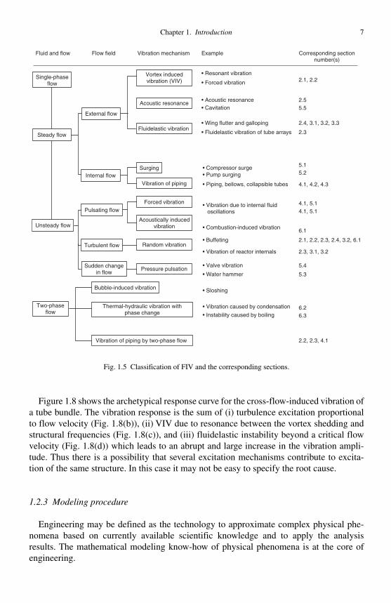
Figure 1.6 shows examples of FIV mechanisms as well as the corresponding models. The vibration mechanism depicted in Fig. 1.6(a) , is governed by turbulent random pressure fluctuations. Flow instability underlies the (VIV) mechanism of Fig. 1.6(b). The FIV mech-anism associated with the structure displacement induced boundary condition and tempo-ral flow variations is shown in Fig. 1.6(c) . In reality, these mechanisms will often interact resulting in complex flow and vibration phenomena [25].
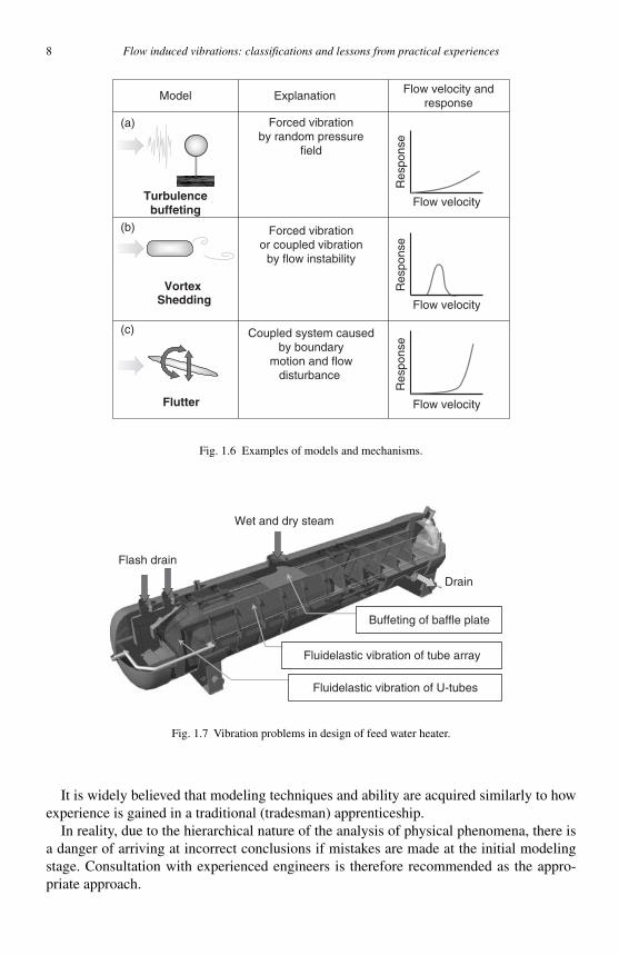
For example, Fig. 1.7 shows a feed-water heater. The fluid components in the heater are steam (the heat source), heated water, and two-phase steam-water flow mixture tra-versing the U-bend tube bank. Several factors must therefore be considered even for such a single piece of equipment.
(a) (b)
Motion
Motion
Liftforce
Liftforce
Fig. 1.4 Mechanism of oscillation.
2 The classical example is the Tacoma-Narrows bridge failure in Washington State, USA.
Chapter 1. Introduction 7
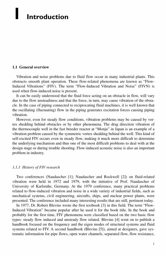
Fluid and flow Flow field Vibration mechanism Example Corresponding sectionnumber(s)
Single-phaseflow
2.1, 2.2
• Acoustic resonance• Cavitation
2.55.5
• Wing flutter and galloping
• Fluidelastic vibration of tube arrays
2.4, 3.1, 3.2, 3.3
2.3
5.15.2
4.1, 4.2, 4.3
4.1, 5.14.1, 5.1
6.1
2.1, 2.2, 2.3, 2.4, 3.2, 6.1
2.3, 3.1, 3.2
5.4
5.3
6.26.3
Steady flow
External flow
• Resonant vibration
• Forced vibration
• Compressor surge• Pump surging
• Piping, bellows, collapsible tubes
• Vibration due to internal fluid oscillations
• Combustion-induced vibration
• Buffeting
• Vibration of reactor internals
• Valve vibration
• Water hammer
• Sloshing
• Vibration caused by condensation
• Instability caused by boiling
Pulsating flow
Turbulent flow
Sudden changein flow
2.2, 2.3, 4.1
Unsteady flow
Internal flow
Fluidelastic vibration
Vibration of piping
Random vibration
Pressure pulsation
Bubble-induced vibration
Vibration of piping by two-phase flow
Forced vibration
Acoustically inducedvibration
Thermal-hydraulic vibration withphase change
Two-phaseflow
Surging
Acoustic resonance
Vortex inducedvibration (VIV)
Fig. 1.5 Classification of FIV and the corresponding sections.
Figure 1.8 shows the archetypical response curve for the cross-flow-induced vibration of a tube bundle. The vibration response is the sum of (i) turbulence excitation proportional to flow velocity ( Fig. 1.8(b) ), (ii) VIV due to resonance between the vortex shedding and structural frequencies ( Fig. 1.8(c) ), and (iii) fluidelastic instability beyond a critical flow velocity (Fig. 1.8(d)) which leads to an abrupt and large increase in the vibration ampli-tude. Thus there is a possibility that several excitation mechanisms contribute to excita-tion of the same structure. In this case it may not be easy to specify the root cause.
1.2.3 Modeling procedure
Engineering may be defined as the technology to approximate complex physical phe-nomena based on currently available scientific knowledge and to apply the analysis results. The mathematical modeling know-how of physical phenomena is at the core of engineering.
8 Flow induced vibrations: classifications and lessons from practical experiences
VortexShedding
Turbulencebuffeting
Flutter
(a)
(b)
(c)
Model Explanation
Forced vibrationby random pressure
field
Forced vibrationor coupled vibration
by flow instability
Coupled system causedby boundary
motion and flowdisturbance
Flow velocity andresponse
Flow velocity
Res
pons
e
Flow velocity
Res
pons
eFlow velocity
Res
pons
e
Fig. 1.6 Examples of models and mechanisms.
Flash drain
Wet and dry steam
Drain
Fluidelastic vibration of tube array
Fluidelastic vibration of U-tubes
Buffeting of baffle plate
Fig. 1.7 Vibration problems in design of feed water heater.
It is widely believed that modeling techniques and ability are acquired similarly to how experience is gained in a traditional (tradesman) apprenticeship.
In reality, due to the hierarchical nature of the analysis of physical phenomena, there is a danger of arriving at incorrect conclusions if mistakes are made at the initial modeling stage. Consultation with experienced engineers is therefore recommended as the appro-priate approach.

Chapter 1. Introduction 9
The modeling procedure when dealing with a concrete physical FIV problem consists of the following two steps:
1. Identification of the underlying physical phenomenon or mechanism. 2. Choice of evaluation approach.
There are two different approaches with regard to identification of the physical mecha-nism. The approaches are based on two opposing philosophies.
In the first, the problem at hand is simplified as much as possible and conclusions are drawn based on a basic analysis of the simplified problem. We shall refer to this approach as the “ simplified treatment. ” In the second approach, the exact opposite is done. The problem is modeled as accurately as possible. The resulting model will normally be much more complex. We shall refer to this procedure, and the associated interpretation of results, as the “ detailed treatment. ”
Which approach one should take depends on the importance of the problem. Thus, before modeling, there is the need to classify the importance of the problem. The deci-sion regarding the choice of approach may be made following a flow chart such as Fig.1.9 . In what follows below, assuming this decision has been made, we introduce a prob-lem analysis approach depending on which of these two different positions is valid.
1.2.3.1 Simplified treatment In order to simplify the problem, the essence of the associated physical phenomenon
must be understood to the extent possible. Lack of understanding can lead to incorrect results, possibly contrary to the facts. Clearly this could lead to eventual problems in new designs while problems in existing designs would remain unresolved.
Simplifying the problem means, in general, extracting only the essential complexity of the fluid and the structure. Note, however, that without a good understanding of the physi-cal phenomenon, any mathematical modeling is bound to lead to incorrect results and, hence, is doomed to fail.
In order to correctly perform a simplified assessment, it is vitally important to base the analysis on existing knowledge of the phenomenon under investigation. Furthermore, it is important to distinguish those aspects of the problem that can be analyzed theoretically or numerically from those that cannot.
In concrete terms, one must decide whether the decision procedure shown in Fig. 1.10 is applicable. If the answer is negative, then either a more detailed analysis or experimen-tal investigation is called for.
� � �
(a)
Res
pons
e
Flow velocity
(b)
Randomvibration
(c)
Vortex inducedvibration
(d)
Fluidelasticvibration
Fig. 1.8 Vibration of tube array caused by cross-flow.

10 Flow induced vibrations: classifications and lessons from practical experiences
1.2.3.2 Detailed treatment This procedure is required either when the problem is very important or when it cannot
be evaluated from previous knowledge. In both cases this ‘ detailed treatment ’ can be con-ducted by the following two methods: ‘ analytical approach ’ or ‘ experimental approach ’ . The former approach is adopted in general but the latter approach should be considered when the analytical method is not reliable.
Yes
Yes
No
No
Knowledge
Experimental study
Published data or experience
Judgement on adaptability to the present problem
Simplified modeling tobe able to apply theestimation method
Experimentaltests possible?
Precise analysis
Fig. 1.10 Flowchart of simplified treatment.
Yes
Yes
No
No
Problem
Important?
Enough time and fundsavailable?
Simplified treatment Detailed treatment
Fig. 1.9 Decision based on importance.
Chapter 1. Introduction 11
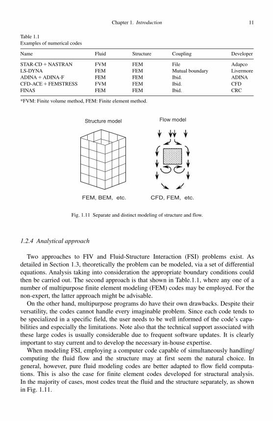
1.2.4 Analytical approach
Two approaches to FIV and Fluid-Structure Interaction (FSI) problems exist. As detailed in Section 1.3, theoretically the problem can be modeled, via a set of differential equations. Analysis taking into consideration the appropriate boundary conditions could then be carried out. The second approach is that shown in Table.1.1 , where any one of a number of multipurpose finite element modeling (FEM) codes may be employed. For the non-expert, the latter approach might be advisable.
On the other hand, multipurpose programs do have their own drawbacks. Despite their versatility, the codes cannot handle every imaginable problem. Since each code tends to be specialized in a specific field, the user needs to be well informed of the code ’ s capa-bilities and especially the limitations. Note also that the technical support associated with these large codes is usually considerable due to frequent software updates. It is clearly important to stay current and to develop the necessary in-house expertise.
When modeling FSI, employing a computer code capable of simultaneously handling/computing the fluid flow and the structure may at first seem the natural choice. In general, however, pure fluid modeling codes are better adapted to flow field computa-tions. This is also the case for finite element codes developed for structural analysis. In the majority of cases, most codes treat the fluid and the structure separately, as shown in Fig. 1.11 .
FEM, BEM, etc. CFD, FEM, etc.
Structure model Flow model
Fig. 1.11 Separate and distinct modeling of structure and flow.
Table 1.1 Examples of numerical codes
Name Fluid Structure Coupling Developer
STAR-CD � NASTRAN FVM FEM File Adapco LS-DYNA FEM FEM Mutual boundary Livermore ADINA � ADINA-F FEM FEM Ibid. ADINA CFD-ACE � FEMSTRESS FVM FEM Ibid. CFD FINAS FEM FEM Ibid. CRC
*FVM: Finite volume method, FEM: Finite element method.
12 Flow induced vibrations: classifications and lessons from practical experiences
It is important to understand the computational fluid dynamics and FEM theory under-lying the multipurpose codes. In particular, computational fluid dynamics turbulence modeling ranges from the k-� model to Large Eddy Simulation (LES). The more accurate Direct Numerical Simulation (DNS) requires no turbulence model. For coupled fluid–structure computations, some codes employ moving boundary elements while others do not, thus leading to difficulty when dealing with moving geometries. Careful considera-tion must therefore be made in the choice of numerical code.
Besides the considerations above, one must keep in mind that time domain simulations based on a computed flow field will be subjective; their accuracy depending on the accu-racy of the computed flow field.
In the case of time history analysis, it is often difficult to perform parametric studies to investigate the influence of different parameters. Since general conclusions cannot be derived from limited analysis, the numerical computations should be viewed as desktop numerical experiments rather than definitive physical results.
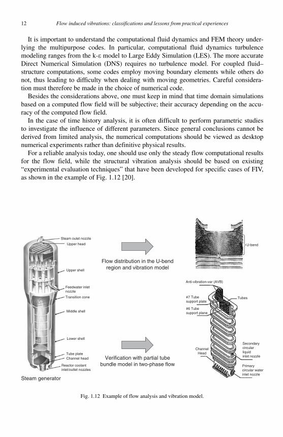
For a reliable analysis today, one should use only the steady flow computational results for the flow field, while the structural vibration analysis should be based on existing “ experimental evaluation techniques ” that have been developed for specific cases of FIV, as shown in the example of Fig. 1.12 [20] .
Steam generator
Flow distribution in the U-bendregion and vibration model
Anti-vibration-var (AVB)
Tubes#7 Tubesupport plate
#6 Tubesupport plane
ChannelHead
Secondarycircularliquidinlet nozzle
Primarycircular waterinlet nozzle
Verification with partial tubebundle model in two-phase flow
U-bend
Steam oulet nozzle
Upper head
Upper shell
Feedwater inletnozzle
Transition cone
Middle shell
Lower shell
Tube plateChannel head
Reactor coolantinlet/outlet nozzles
Fig. 1.12 Example of flow analysis and vibration model.
Chapter 1. Introduction 13
1.2.5 Experimental approach
The experimental approach is the only remaining option when the underlying phenom-enon cannot be identified via numerical analysis or when such analysis is not considered reliable. In principle, experimental testing should be carried out on the prototype compo-nent itself; very often though this is not possible. The remaining option is to build a test model to recreate the observed phenomenon.
1.2.5.1 Test facility The first important decision is with regard to the test facility. As long as a large-scale
project is not intended, effort should be made to use existing test facilities rather than building new ones from scratch. The search for appropriate equipment can be extended from the organization to institutions (engineering schools are often equipped with basic test apparatus) or public research organizations if need be. The possibility of joint research can also be considered.
1.2.5.2 Similarity laws It is rarely possible to recreate the prototypical operating conditions in a test appara-
tus. It often happens that physical quantities such as temperature, pressure, and even the fluid itself are different for the test conditions. Test conditions are therefore set to match dimensionless quantities, such as Reynolds number, Froude number, Strouhal number, etc. in order to reproduce the observed phenomenon as accurately as possible.
The foregoing is the well-known similarity law-based approach [26]. Note that not only the fluid similarity law should be considered; structural similarity must also be modeled.
Structural model Once the test facility has been determined, a test model matching the test facility must
be designed. The following points should be carefully considered at this stage:
1. With regard to the flow field–structure interaction problem, the flow field should approximate the prototype flow field as closely as possible. This means that the form of the test model should match the actual structure as closely as possible. It is usually not necessary to model the complete structure; only the structural components perti-nent to the phenomenon under investigation need be modeled.
2. When thermal effects are not of importance, only three independent physical param-eters control FIV phenomena. These are characteristic length ( L ), time ( T ), and force (F ) or mass ( M ). All other physical quantities are functions of these three parameters. Thus, once the scales or ranges of these three parameters are chosen (each one inde-pendently of the other two), the corresponding values of the other physical quantities are automatically determined by the underlying similarity laws. The existence of con-straints associated with the similarity laws means that it may not be possible to match every dimensionless physical quantity of interest. Decisions must be made regarding the relative importance of the different dimensionless quantities that need to be matched
14 Flow induced vibrations: classifications and lessons from practical experiences
between prototype and experiment. One could attempt to “ forcibly ” match the quanti-ties or, alternatively, quantities deemed to be of “ less importance ” can be ignored.
For the latter modeling procedure, the so-called Buckingham-Pi theorem is generally used.
Fluid model In reality, it is impossible to achieve perfect similarity for the physical quantities (flow
speed, pressure, etc.) that characterize the flow field while at the same time accurately matching the important structural quantities such as vibration frequencies, stresses, etc. The goal should therefore be to create a model that satisfies only the most important quantities based on “ engineering judgment. ”
In general, the important quantities referred to above are the normal dimensionless parameters that govern the physical phenomenon. Table 1.2 lists examples of the dimen-sionless quantities encountered in FSI problems.
As an example, Fig. 1.13 shows the problem of the Karman wake flow behind a sta-tionary circular cylinder. The relation between the associated physical quantities is dem-onstrated in the figure. The frequency f is a function of the steady flow velocity V , the cylinder diameter D , the fluid density � , and fluid viscosity � . Based on these five physi-cal quantities, a dimensionless analysis yields the relations for the dimensionless Strouhal number (S) and Reynolds number (Re). Furthermore, combining the latter two relations, it can be shown that the Strouhal number is a function of the Reynolds number.
Table 1.2 Non-dimensional parameters and their physical meaning
Non-dimensional parameterand corresponding person Definition Physical meaning
Corresponding phenomena
Euler numberLeonard Euler (1707–1783)* (Switzerland)Mathematician & Physicist
Eu �p
V� ⋅ 2
Pressure
Inertia for ec
CavitationFluid machines
Reynolds number Osborne Reynolds (1842–1912)* (England) Physicist
Re �V D
v
⋅
Inertia force
Viscous force
Fluid motion
Froude number William Froude (1810–1879)* (England) Naval engineer
Fr �V
g D
2
⋅
Inertia force
Gravity force
Motion under gravity
Strouhal number Vincenz Strouhal (1850–1925)* (Czech Republic) Physicist
St �f D
Vw ⋅ Local flow velocity
Average flow velocity
Periodic vortex shedding (Karman vortex)
Scruton number(mass-damping parameter) Cristopher Scruton (1911–1990)* (England) Physicist
m
D
�� 2
Mass of structure
Mass of fluid⋅ Damping
Instability
* Person (years), country of origin, and title.

Chapter 1. Introduction 15
D
f
f � F(V, D, r, m)
r · v · Dm
V
r
m
p1V
f · D
St � F(Re)
St � Strouhal number��
p2 � Re � Reynolds number
107106105104103102100.1
0.2
0.3St
Re
0.4
0.5
�
Fig. 1.13 Dimensionless vortex shedding frequency dependence on Reynolds number.
1.3 Fundamental mechanisms of FIV
In FIV, which couples fluid mechanics and vibration engineering, explaining the phenomena is of primary importance. For this reason, first a model to express the phenom-enon is proposed. Next the model is expressed as a set of differential equations and finally solved taking into consideration the appropriate boundary conditions. In the modeling pro-cedure, the equation of continuity, momentum equations (fluid flow governing equations), structural equations and the corresponding boundary conditions are described in a proper coordinate system. The equations are then expressed in non-dimensional form to obtain the ratios between the forces in the equations. Based on these ratios, a proper approxi-mation is introduced to express the phenomenon. An analysis based on the approximateequations is then carried out.
Linear analysis may be performed employing one of several techniques including Fourier analysis, Laplace transform, and traditional modal analysis. On the other hand, non-linear analysis is used to obtain the vibration response. The representative methods for the analysis of weak non-linear systems are the averaging method, the perturbation method, and the multiple scales method, as well as other analytical methods. The finite element method, the boundary element method, and the finite volume method are the standard numerical analysis approaches. From the linear analysis, the natural frequency, the vibration mode, the amplitude growth rate, the frequency response spectra, the tran-sient response, etc. are obtained. The non-linear analysis yields the stability boundary, the post-instability limit cycle amplitude, and the time–history response.
16 Flow induced vibrations: classifications and lessons from practical experiences
In the following section, in order to understand the fundamental mechanisms of FIV, the basic mathematical treatment of the most important problem of self-excited oscillations is first presented.
1.3.1 Self-induced oscillation mechanisms
A system that oscillates under the influence of its own energy source due to its inter-nal physical mechanisms is said to undergo “ self-excited vibration. ” Examples of energy sources are:
• Steady fluid flow. • A system rotating at constant speed. • Mechanical system forced by “external” load.
In the sections that follow, cases of a one-degree-of-freedom system, a two-degrees-of-freedom system, and a multi-degrees-of-freedom system are explained.
1.3.1.1 One-degree-of-freedom system In the case of the one-degree-of-freedom system, self-induced vibration occurs when
the total damping of the combined fluid–structural system vanishes and then becomes negative. The vibration amplitude increases exponentially in time. For this system, the governing equation of motion is:
mx cx kx f x x x�� � � ��� � � ( , , ) (1.1)
Here the right hand term is the excitation force while the three left hand terms correspond to the inertia force, the structural damping force, and the restoring force, respectively. The forces are linearly proportional to the acceleration, the velocity, and the displacement, respectively.
If f x x x c x( , , )� �� �� � 0 is assumed, the excitation force has a linear relation to the veloc-ity. In this case, Eq. (1.1) can be re-written in the form:
mx c c x kx�� �� � � �( )0 0 (1.2)
If c + c0 � 0, the vibration amplitude increases with time. The condition for self-excited vibration may thus be recast in terms of c0 as follows. A negative value of c0 leads to self-excited vibrations when | c0 | � c . This case is referred to as negative-damping-induced self-excited vibration.
The foregoing phenomenon can be understood from an energy viewpoint. In Eq. (1.1), the energy variation is integrated for one period T as follows:
mxx t cx t kxx t fx tT T T T
��� � � �d d d d0
2
0 0 0∫ ∫ ∫ ∫� � � (1.3)
Here, the damped period T is given by:
Tk
m
c
mk
� �
�
2 2
12
2
��
�
⋅⎛
⎝⎜⎜⎜⎜
⎞
⎠⎟⎟⎟⎟
(1.4)
Chapter 1. Introduction 17
Re-arranging Eq. (1.3) yields,
d
dd
tmx kx t fx cx
T T1
2
1
22 2
0
2
0
� � �� � �⎛
⎝⎜⎜⎜
⎞
⎠⎟⎟⎟⎟
⎧⎨⎪⎪⎩⎪⎪
⎫⎬⎪⎪⎭⎪⎪
∫ ( )∫∫ dt (1.5)
The left hand term is the integral of the total energy variation during one period. Then, if the right hand term is positive, the total energy increases during the cycle. In the case of f c x� � 0 �, the right hand term of Eq. (1.5) is:
Right hand term d� � �( )c c x tT
02
0
�∫ (1.6)
Since the integral value is either zero or positive, the total energy increases when the coefficient of the integral is positive. When the condition c0 � c 0 is satisfied, self-excited vibrations occur. The latter condition physically means that the net damping of the fluid–structure system is negative.
1.3.1.2 Two-degrees-of-freedom system In the case of the two-degrees-of-freedom system [27], coupled-mode self-excited
vibration can occur in addition to the single-degree-of-freedom type instability described above. The equations of motion of the two-degrees-of-freedom system may be expressed in the following matrix form:
[ ]{ } [ ]{ } [ ]{ } { }M C K F�� �x x x� � � (1.7)
where [ ] , [ ] , [ ]M m mm m C c c
c c K k� � �11 12
21 22
11 12
21 22
1⎡
⎣⎢⎢
⎤
⎦⎥⎥
⎡
⎣⎢⎢
⎤
⎦⎥⎥
11 12
21 22
kk k⎡
⎣⎢⎢
⎤
⎦⎥⎥, and
{ } [ ] , { } [ ]x F� �x x F F1 2 1 2T T (and m12 � m21; symmetrical mass matrix)
In this equation, the excitation force is of the form { ( , , )}F x x x� �� as in Eq. (1.1). The force term in the right hand term of the above equation can be moved to the left hand side, and incorporated into the matrices [ M ], [ C ], [ K ].
The excitation energy in this two-degrees-of-freedom system increases when the initial two natural frequencies of the system are close and the phase delay of the vibration is 90 degrees relative to the excitation force while the energy is mutually transferred between the two degrees-of-freedom.
mm
xx
cc
xx
k k11
22
1
2
11
22
1
2
11 1200
00
⎡
⎣⎢⎢
⎤
⎦⎥⎥ { } ⎡
⎣⎢⎢
⎤
⎦⎥⎥ { }��
����� � kk k
xx21 22
1
20
⎡
⎣⎢⎢
⎤
⎦⎥⎥ { }� (1.8)
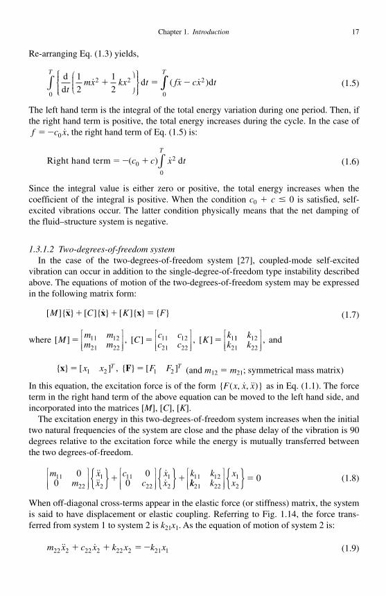
When off-diagonal cross-terms appear in the elastic force (or stiffness) matrix, the system is said to have displacement or elastic coupling. Referring to Fig. 1.14 , the force trans-ferred from system 1 to system 2 is k21x1 . As the equation of motion of system 2 is:
m x c x k x k x22 2 22 2 22 2 21 1�� �� � � � (1.9)
18 Flow induced vibrations: classifications and lessons from practical experiences
the “ input force ” is �k21x1 . If this system is close to resonance, x2 leads x1 by 90 degrees in phase.
Recall the equation of motion for the one-degree-of-freedom system excited by an external force. The displacement response lags 90 degrees behind the excitation force at resonance. Since �k21x1 is considered to be the excitation force, x2 lags 90 degrees behind the excitation force. This is equivalent to x2 leading x1 in phase by 90 degrees.
The equation of motion of system 1 is:
m x c x k x k x11 1 11 1 11 1 12 2�� �� � � � (1.10)
Based on a similar argument as above, system 1 ( x1 ) now leads system 2 (x2) by 90 degrees at resonance. When k12 and k21 have opposite signs, the phase angle becomes zero and the amplitude increases after each cycle around the system. This means that the two-degrees-of-freedom system can become unstable due to purely elastic coupling.
The same result can be obtained from energy considerations for the two-degrees-of-freedomsystem. At first, assuming a periodic solution of Eq. (1.8), the energy integrals satisfy:
{ }[ ]{ } { }[ ]{ } { }[ ]{ }� �� � � �x x x x x xM t C t K tT T T
d d d0 0 0
0∫ ∫ ∫� � � (1.11)
Here, the first term corresponds to the kinetic energy, the second to the dissipation energy, and the third to the potential energy.
The two matrices [ M ] and [ C ] are assumed to be diagonal. The matrix [ K ] on the other hand is generally not. It can, however, be expressed as the sum of a symmetric matrix and a skew-symmetric matrix. Thus,
[ ]K k kk k
k kk k
kk� � �
�11 12
21 22
11 0
0 22
00
⎡
⎣⎢⎢
⎤
⎦⎥⎥⎡
⎣⎢⎢
⎤
⎦⎥⎥⎡⎣⎢⎢
⎤⎦⎥
⎥⎥� �[ ] [ ]K K0 (1.12)
Inversesign
System 2
System 1
Noise
k12
k12x2
k 21x1
x2
x1
k21
Fig. 1.14 Instability mechanism of elastic force coupled system.
Chapter 1. Introduction 19
where
k k k k k k0 12 21 12 211
2
1
2� � � �( ), ( ) (1.13)
From the fact that the symmetric matrix components do not contribute to the integrated energy, the total energy change is obtained only from the skew-symmetric matrix compo-nents in the restoring force term.
E K t k x x x x tTT T
� � �{ }[ ]{ } ( )� � � �x x 0
1 2 1 20
∫ ∫d d (1.14)
When the displacements are expressed in the form:
xx
u tu t
1
2
1 1
2 2{ } { }�
��
sin( )sin( )
��
φφ
(1.15)
the total energy becomes:
E k k u u� � � �( ) sin( )12 21 1 2 1 2φ φ (1.16)
This equation indicates that the signs of k12� k21 and φ1� φ2 determine the sign of the energy E , which, in turn, means that the stability condition is determined by these terms.
For example, the case of k12 � 0, k21 � 0 under the condition of φ2 � φ1 � � /2 gives negative total energy change, which means negative energy dissipation or energy accumu-lation. This therefore leads to self-excited vibration of the two-degrees-of-freedom system.
It can therefore be concluded that self-excited vibration occurs when the non-diago-nal components have opposite signs in the case of the elastic force coupling. Similarly, the possibility of self-excited vibration also exists in the case of damping force cross-coupling as well as inertia (mass) term cross-coupling. These possibilities are explained inthe next section where the more general multi-degrees-of-freedom systems are considered.
1.3.1.3 Multi-degrees-of-freedom system For the multi-degrees-of-freedom system [28], variables representing the motion of the
structure or of the fluid are defined as a vector { } [ , , , ]x x x xn� 1 2 … … . With the iner-tia, damping, and rigidity terms represented by the matrices [ Ms ], [ Cs ], [ Ks ] and the fluid force acting on the structure by { F }, the equation of motion becomes:
[ ]{ } [ ]{ } [ ]{ } { }M x C x K x Fs s s�� �� � � (1.17)
The fluid force can be approximated as a linear function of the structural motion as follows:
{ } [ ]{ } [ ]{ } [ ]{ } { }F M x C x K x G� � � � �f f f�� � (1.18)
[ Mf ], [ Cf ], and [ Kf ] are the added mass, fluid damping, and fluid rigidity matrix, respect-ively. { G } is an external (time-dependent) force vector. Figure 1.15 shows a block diagram representation of Eqs. (1.17) and (1.18). The first three terms on the r.h.s. of Eq. (1.18) express the feedback fluid force.
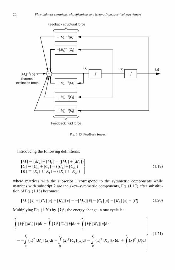
20 Flow induced vibrations: classifications and lessons from practical experiences
Introducing the following definitions:
[ ] [ ] [ ] ([ ] [ ])[ ] [ ] [ ] ([ ] [ ])[ ] [ ]
M M M M MC C C C CK K
���
s f
s f
s
� � �� � �
1 2
1 2�� � �[ ] ([ ] [ ])K K Kf 1 2
⎫⎬⎪⎪⎪
⎭⎪⎪⎪
(1.19)
where matrices with the subscript 1 correspond to the symmetric components while matrices with subscript 2 are the skew-symmetric components, Eq. (1.17) after substitu-tion of Eq. (1.18) becomes:
[ ]{ } [ ]{ } [ ]{ } [ ]{ } [ ]{ } [ ]{ } { }M x C x K x M x C x K x G1 2 1 2 1 2�� � �� �� � � � � � � (1.20)
Multiplying Eq. (1.20) by { }�x T , the energy change in one cycle is:
{ } [ ]{ } { } [ ]{ } { } [ ]{ }� �� � � �x M x t x C x t x K x tT TTT
TT
1 200
10
d d d� �
� �
∫∫ ∫
{{ } [ ]{ } { } [ ]{ } { } [ ]{ } { } { }� �� � � � �x M x t x C x t x K x t x GT T T T2 1 2d d d d� � � tt
TTTT
0000∫∫∫∫
⎫
⎬
⎪⎪⎪⎪⎪⎪⎪⎪⎪
⎭
⎪⎪⎪⎪⎪⎪⎪⎪⎪
(1.21)
Feedback fluid force
Externalexcitation force
[Ms]�1{G}
�[Ms]�1[Ks]
�[Ms]�1[Cs]
�[Ms]�1[Mf]
� � �
�[Ms]�1[Cf]
�[Ms]�1[Kf]
Feedback structural force
{x} {x}{x}
Fig. 1.15 Feedback forces.
Chapter 1. Introduction 21
The first and the third terms on the left hand side above express the increase of the kinetic energy and potential energies. The sum of these terms corresponds to the net increase in the system energy E . The second term on the left hand side is zero since [ C2 ] is a skew-symmetric matrix. The right hand side term of Eq. (1.21) equals the sum of the increase of the following energies:
E x M x t M MTT
M d : Work by in � � { } [ ]{ } [ ] [ ]� ��20
2∫ (1.22)
E x C x t C CTT
C d : Work by in � � { } [ ]{ } [ ] [ ]� �10
1∫ (1.23)
E x K x t K KTT
K d : Work by in � � { } [ ]{ } [ ] [ ]� 20
2∫ (1.24)
E x G tTT
G d : Work by the external force� � { } { }�0∫ (1.25)
This means that the energy increase E :
E E E E E� � � �M C K G (1.26)
must be positive for fluid-force-induced oscillations to occur. When the structure oscillates as a one-degree-of-freedom system, the increase of the
system energy E is:
E E E� �C G (1.27)
When no external forces act on the structure, in the case of the negative fluid damping, C1� 0,
E E� �C 0 (1.28)
and self-excited vibration occurs. This case is called “ excitation by negative damping feedback. ”
On the other hand, when the system has two or more degrees-of-freedom, there is the case where EK contributes to the increase of the kinetic energy E rather than the other components. The case where the matrix [ K2 ] derives from fluid forces is called “ the exci-tation by fluidelastic feedback. ”
Finally, vibration where [ EG ] mostly contributes to the increase of the system energy Ecorresponds to basic forced vibration.
22 Flow induced vibrations: classifications and lessons from practical experiences
1.3.2 Forced vibration and added mass and damping
1.3.2.1 Forced vibration system [16] Eq. (1.18) expresses only the work done by the external force if the first three feedback
fluid force terms are neglected. In this case the equation of motion, Eq. (1.17), can be solved as a forced vibration system because the forcing is independent of the structural motion.
However, even in the presence of the first three terms of Eq. (1.18), the system may still be viewed as a forced vibration system, when the sum of the energies by Eqs. (1.22)–(1.24), E E EM C K� � , is negative and hence no self-excited vibration occurs.
The forced vibration system appears as shown below in the case of turbulent flow, or when the mutual interaction between the structure and the fluid motion is neglected in the case of vortex shedding.
([ ] [ ]){ } ([ ] [ ]){ } [ ]{ } { }M M x C C x K x Fs f s f s� � � � ��� � (1.29)
Both responses of the one-degree-of-freedom system and the multi-degrees-of-freedom system can be obtained by solving Eq. (1.29) analytically or numerically.
In the case of continuous structures such as beams in flow, the excitation force is usu-ally given by the summation of local fluid forces coupled with the correlation along the beam axis. After expanding the equation of motion with the undamped structural vibra-tion modes, the continuous system can be decoupled into independent equations of motion, based on the orthogonal characteristics of the modes when the correlation effects between modes are negligible. The equation of motion for the j -th mode is:
�� �q h q qm
Fj j j j jj
j ii
i� � ��
212
1
� � φ∑ � (1.30)
Here { }qj is the generalized time function (or generalized coordinate) of the j -th mode
( )x qi j ij
� φi∑ , �j is the natural circular frequency of the j -th mode ( � 2� f j ), and hj the cor-
responding damping ratio. The modal mass is m mj i j ii
��
φ 2
1∑ , where jφi is the value of the
j -th mode at position i and mi and F�i express the distributed mass and fluid forces.
In many practical cases, where the interaction with the surrounding structures can be assumed to be negligible, the diagonal terms of the added mass and the added damping matrices [ Mf ] and [ Cf ] are dominant, thus leading to Eq. (1.30).
When the right hand term of Eq. (1.30) is due to excitation forces that are random (both in time and in space), the equation can be solved using statistical theory. When mode coupling terms are neglected, the following integral solution for the square average of the displacement response of the structure Xd
2 is obtained:
X x x L Hd jj
j j2 ( ) ( ) d( ) ( )�
�
φ1
2 2
0
∑ ∫∞
� � � (1.31)
Chapter 1. Introduction 23
In Eq. (1.31) Hj ( � ) is the transfer function of the j -th mode:
H ihjj
jj
(���
��
)2
� � �
�
1 22
1⎛
⎝
⎜⎜⎜⎜⎜
⎞
⎠
⎟⎟⎟⎟⎟
⎡
⎣
⎢⎢⎢
⎤
⎦
⎥⎥⎥
(1.32)
And the correlation term Lj ( � ), which is defined as the joint acceptance of the j -th mode, is given by:
Lm
R x x x x x xjj j L
j j( ) ( , , ) ( ) ( )��
�� � � �12 4 ∫∫ φ φ d d (1.33)
where R ( x , x� , � ) is the correlation function of the excitation force:
R x x S Rxx xx( , , ) ( ) ( ) cos ( )� � � ���
� � � �1
F2� (1.34)
which is frequency and space dependent. In the equation above, SF ( � ) is the power spec-tral density of the excitation force while �Rxx�( )� and θxx� ( � ) are the correlation function and phase difference between the positions x and x ’ .
The joint acceptance Lj ( � ) in Eq. (1.33) expresses the correlation of the fluid force along the beam axis. Empirical values of this quantity, for example, have been determined experi-mentally both for an isolated cylinder in cross-flow and tubes and tube arrays in cross-flow.
Finally, Eq. 1.30 can be solved by similar methods when the excitation force is not random. An example being the case of periodic vortex shedding induced excitation.
1.3.2.2 Added mass In many cases of flow-induced forced vibration, the response estimation can be divided
into independent equations of motion for each mode such as Eq. (1.30). However, the added mass and the added damping greatly affect the characteristics of the structures and therefore must be considered. In this section, the determination of the added mass for the case of a circular cylinder in still fluid is outlined.
The added mass [9] is basically obtained using potential flow theory for perfect fluids. When a circular cylinder is fully immersed in still fluid, the motion of the cylinder is coupled to that of the surrounding fluid. The continuity equation of the two-dimensional flow, assuming a perfect fluid, is:
�2 0φ θ( , , )r t � (1.35)
where φ is the velocity potential and �2 is the Laplacian operator. The flow velocity and the associated pressure field are related to the velocity
potential by:
U→
� �φ (1.36)
pt
� ����φ
(1.37)

24 Flow induced vibrations: classifications and lessons from practical experiences
On the boundary between the circular cylinder and the fluid, the velocity of the fluid is equal to that of the cylinder. Thus,
uu
tr Rr � �
��
�cos ( ) (1.38)
while at infinity:
u rr � �0 ( )∞ (1.39)
The following forms for the velocity and velocity potential, respectively, are assumed:
u aei tr � � (1.40)
φ( , , ) ( ) ( )r t F r F ei t� ���� r (1.41)
Substituting Eq. (1.41) into Eq. (1.35), and employing separation of variables, the follow-ing ordinary differential equations are derived:
1 10
2r rr
F
r rF
d
d
d
dr
r
⎛
⎝⎜⎜⎜
⎞
⎠⎟⎟⎟⎟
⎧⎨⎪⎪⎩⎪⎪
⎫⎬⎪⎪⎭⎪⎪
� � (1.42)
d
d
2
20
FF�
��� � (1.43)
Applying the boundary conditions (1.38) and (1.39) to the general solutions of Eqs. (1.42) and (1.43) yields the solution:
φ( , , ) cosr ti R a
rei t�
�� �� �
2(1.44)
Since the fluid force, g , acting on the cylinder in its direction of motion is;
g P r t Rr R� � �( ) d, , cos� � ��
0
2
∫ (1.45)
this force can be re-written in the form:
g Mu
tM R� � �f f
d
d,
2
22�� (1.46)
“Mf ” in this equation is the cylinder “ added mass ” per unit length. The added mass is also called the “ virtual mass. ” Practically, the added mass is expressed as the mass of fluid having the same volume as that of the immersed cylinder multiplied by the added mass coef ficient Cm . For the circular cylinder in unconfined flow, Cm is unity. Note, however, that this is generally not the case for other configurations.
The added mass decreases the natural frequency of the structure. If the fluid is perfect, there is no fluid damping and only the change of the natural frequency characterizes the kinetic effect of the fluid on the structure.
Chapter 1. Introduction 25
1.3.2.3 Fluid damping The fluid damping can be divided into two categories: damping in still fluid and damp-
ing induced by fluid flow. The latter damping depends on many mechanisms. Their detailed explanation is therefore given in later sections. Here, only the damping in still fluid is explained.
Damping in still fluid can be divided into two components: damping caused by fluid viscosity and energy dissipation by sound.
Fluid viscous damping may be obtained by the following method. The drag force by the surrounding fluid FD , when the structure moves with velocity �x , is given by the following equation based on the characteristic length D and the non-dimensional drag coefficient CD :
F C x xDD D f | |�1
2� � � (1.47)
Assuming sinusoidal motion with the circular frequency � , and taking only the first term of the Fourier expansion:
| | d d� � �x x X t X x��
� ��
�8
3
8
32 2 cos( ) � � (1.48)
the damping ratio hf (= Cf /2 m�n) in still fluid becomes:
hD
m
X
DC
nf �
2
3
2
�� �
�f d
D (1.49)
where � n is the undamped natural frequency. This damping can therefore be estimated when the non-dimensional drag coefficient
CD is known. However, CD does not take a simple form in FSI systems such as a cylinder in a narrow path or tubes in a tube array. Additional detailed information on the damping in still fluid is therefore presented later in Sections 3.3.2 � 3.3.4 and 4.1.1.
The damping by energy dissipation through sound radiation cannot be ignored for light structures such as panels. The following estimation for this type of damping is proposed:
ha b
M aff�
1
4
2
�� �
� (1.50)
��
� �
�� � ��
��2
0 2
1 0 2
22 2
⎛
⎝⎜⎜⎜⎞
⎠⎟⎟⎟⎟
⎧
⎨⎪⎪⎪⎪
⎩⎪
( ) , .
, .
a b for a
for a
/ /
/⎪⎪⎪⎪
(1.51)
Here, the panel having dimensions a by b and mass M radiates sound waves at the fre-quency � n having wavelength � � 2 � c /� n where c is the sound speed.
26 Flow induced vibrations: classifications and lessons from practical experiences
References
[1] Naudascher , E. , Flow-Induced Structural Vibrations , Springer-Verlag , Berlin , 1972 . [2] Naudascher , E. and Rockwell , D., Practical Experiences with Flow-Induced
Vibrations , Springer-Verlag , Berlin , 1979 . [3] Blevins , R.D., Flow-Induced Vibration , Van Nostrand Reinhold , New York , 1977 . [4] Blevins , R.D. , Formulas for Natural Frequency and Mode Shape , Van Nostrand
Reinhold , New York , 1979 . [5] Blevins , R.D., Applied Fluid Dynamics Handbook , Van Nostrand Reinhold ,
New York , 1984 . [6] Blevins , R.D., Flow-Induced Vibration , Second Edition , Krieger, Malabar, 1990 . [7] Naudascher , E. , Hydrodynamic Forces , A.A. Balkema , Rotterdam , 1991 . [8] Naudascher , E. and Rockwell , D., Flow-Induced Vibrations, An Engineering Guide ,
A.A. Balkema , Rotterdam , 1993 . [9] Chen , S.S., Flow-Induced Vibration of Circular Cylindrical Structures , Springer-
Verlag , Berlin , 1987 . [10] Morand , H.J.P. and Ohayon , R., Fluid Structure Interaction , Wiley , New Jersey ,
1995 . [11] Païdoussis , M.P., Fluid–Structure Interactions. Vol. 1 , 2, Academic Press , London ,
1998, 2004 . [12] Païdoussis , M.P. and Li , G.X. , Pipes Conveying Fluid: A Model Dynamical Problem
J. Fluid. Struct. , Vol. 7 , 1993 , pp. 137 – 204 . [13] Hayama , S., Vibration Engineering Handbook (in Japanese), Chapter 23 , Yokendo
Publication , Tokyo , 1976 . [14] JSME, Flow-Induced Vibration in Mechanical Engineering – Its Status and the
Prevention , P-SC10 Report of Flow-Induced Vibration Organization Group, 1980. [15] JSME, Pressure Pulsation in Piping Induced by Reciprocating Compressors (in
Japanese), P-SC105 Report of Organization Group on Pressure Pulsation in Piping and Reciprocating Compressors, 1989.
[16] Iwatsubo, T., “ Flow-Induced Vibration ” (in Japanese), Proceedings of 63rd Annual Meeting of Kansai Branch in JSME , 884-2, 1988, p. 125.
[17] Fujita, K., “ Topic on Flow-Induced Vibration in Industry ” (in Japanese), Proceedings of the Annual Meeting of Kansai Branch in JSME , 884-2, 1988, p. 133.
[18] Madarame, H., Recent Flow-Induced Vibration in Nuclear Power Industry (in Japanese), Report of Organization Group on Nuclear Power Industry, Nuclear Engineering Facility in University of Tokyo, 1990, pp. 1–20.
[19] JSME, “Guideline for Evaluation of Flow-Induced Vibration of a Cylindrical Structure in a Pipe ” , JSME S012, 1998.
[20] JSME , “ Guideline for Fluid-Elastic Vibration Evaluation of U-bend Tubes in Steam Generators ” (in Japanese), JSME S016, 2002.
[21] Muller , E.A., Mechanics of Sound Generation in Flows , Springer-Verlag , Berlin , 1979 .
[22] Blake , W.K., Mechanics of Flow-Induced Sound and Vibration , Academic Press , Orland , 1986 .
[23] Examples of Prevention of Noise & Vibration , Japan Noise Control Society, 1990.

Chapter 1. Introduction 27
[24] Maruta, Y., Seminar on Flow-Induced Noise , Ebara Tech. Report, No. 181, 1998; No. 182, 1999; No. 183, 1999; No. 184, 1999; No. 185, 1999.
[25] Naudascher, E. and Rockwell, D., “ Flow-Induced Vibrations, An Engineering Guide, ” Hydraulic Design Considerations , IAHRAIRH (Hydraulic Structures Design Manual 7).
[26] Emori, I., “ Theory and Application of Model Test ” (in Japanese), Gihodo Pub. [27] Iwatsubo, T., “ Flow-Induced Vibration ” (in Japanese), Proceedings of #63 Annual
Meeting of Kansai Branch of JSME , No. 884-2, 1988, p. 125. [28] Hara, F., Dynamics Handbook (in Japanese), Asakura Syoten, 1993, p. 608.

This page intentionally left blank
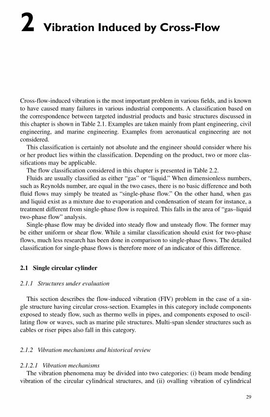
29
2 Vibration Induced by Cross-Flow
Cross-flow-induced vibration is the most important problem in various fields, and is known to have caused many failures in various industrial components. A classification based on the correspondence between targeted industrial products and basic structures discussed in this chapter is shown in Table 2.1 . Examples are taken mainly from plant engineering, civil engineering, and marine engineering. Examples from aeronautical engineering are not considered.
This classification is certainly not absolute and the engineer should consider where his or her product lies within the classification. Depending on the product, two or more clas-sifications may be applicable.
The flow classification considered in this chapter is presented in Table 2.2 . Fluids are usually classified as either “ gas ” or “ liquid. ” When dimensionless numbers,
such as Reynolds number, are equal in the two cases, there is no basic difference and both fluid flows may simply be treated as “ single-phase flow. ” On the other hand, when gas and liquid exist as a mixture due to evaporation and condensation of steam for instance, a treatment different from single-phase flow is required. This falls in the area of “ gas–liquid two-phase flow ” analysis.
Single-phase flow may be divided into steady flow and unsteady flow. The former may be either uniform or shear flow. While a similar classification should exist for two-phase flows, much less research has been done in comparison to single-phase flows. The detailed classification for single-phase flows is therefore more of an indicator of this difference.
2.1 Single circular cylinder
2.1.1 Structures under evaluation
This section describes the flow-induced vibration (FIV) problem in the case of a sin-gle structure having circular cross-section. Examples in this category include components exposed to steady flow, such as thermo wells in pipes, and components exposed to oscil-lating flow or waves, such as marine pile structures. Multi-span slender structures such as cables or riser pipes also fall in this category.
2.1.2 Vibration mechanisms and historical review
2.1.2.1 Vibration mechanisms The vibration phenomena may be divided into two categories: (i) beam mode bending
vibration of the circular cylindrical structures, and (ii) ovalling vibration of cylindrical
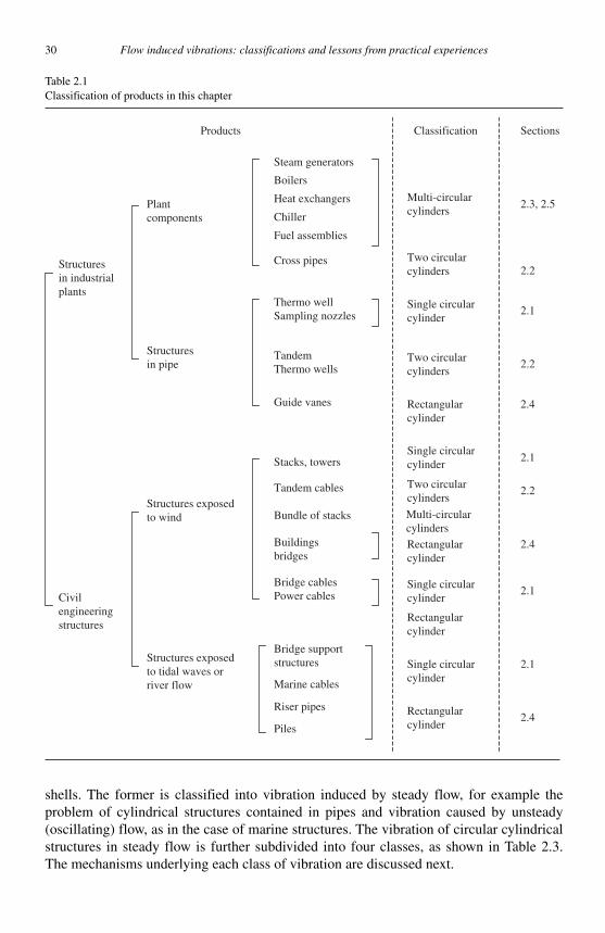
30 Flow induced vibrations: classifications and lessons from practical experiences
shells. The former is classified into vibration induced by steady flow, for example the problem of cylindrical structures contained in pipes and vibration caused by unsteady (oscillating) flow, as in the case of marine structures. The vibration of circular cylindrical structures in steady flow is further subdivided into four classes, as shown in Table 2.3 . The mechanisms underlying each class of vibration are discussed next.
Products
Structuresin industrialplants
Civilengineeringstructures
Plantcomponents
Structuresin pipe
Structures exposedto wind
Structures exposedto tidal waves orriver flow
Steam generators
Boilers
Heat exchangers
Chiller
Fuel assemblies
Cross pipes
Thermo well
TandemThermo wells
Guide vanes
Stacks, towers
Tandem cables
Bundle of stacks
Buildingsbridges
Bridge cablesPower cables
Bridge supportstructures
Marine cables
Riser pipes
Piles
Classification Sections
Multi-circularcylinders
Two circularcylinders
Single circularcylinder
Two circularcylinders
Rectangularcylinder
Rectangularcylinder
Single circularcylinder
Two circularcylinders
Single circularcylinder
Single circularcylinder
Rectangularcylinder
Rectangularcylinder
2.3, 2.5
2.2
2.1
2.2
2.4
2.2
2.1
2.1
2.1
2.4
2.4
Multi-circularcylinders
Sampling nozzles
Table 2.1 Classification of products in this chapter
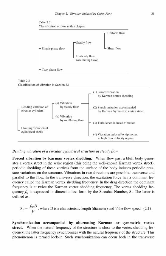
Chapter 2. Vibration Induced by Cross-Flow 31
Bending vibration of a circular cylindrical structure in steady flow
Forced vibration by Karman vortex shedding. When flow past a bluff body gener-ates a vortex street in the wake region (this being the well-known Karman vortex street), periodic shedding of these vortices from the surface of the body induces periodic pres-sure variations on the structure. Vibrations in two directions are possible, transverse and parallel to the flow. In the transverse direction, the excitation force has a dominant fre-quency called the Karman vortex shedding frequency. In the drag direction the dominant frequency is at twice the Karman vortex shedding frequency. The vortex shedding fre-quency fw is expressed in dimensionless form by the Strouhal Number, St. The latter is defined as:
St W�f D
V, where D is a characteristic length (diameter) and V the flow speed. (2.1)
Synchronization accompanied by alternating Karman or symmetric vortex street. When the natural frequency of the structure is close to the vortex shedding fre-quency, the latter frequency synchronizes with the natural frequency of the structure. This phenomenon is termed lock-in. Such synchronization can occur both in the transverse
Single-phase flow
Two-phase flow
Steady flow
Unsteady flow(oscillating flow)
Uniform flow
Shear flow
Table 2.2 Classification of flow in this chapter
Bending vibration ofcircular cylinders
Ovalling vibration ofcylindrical shells
(a) Vibration by steady flow
(b) Vibration by oscillating flow
(1) Forced vibration by Karman vortex shedding
(2) Synchronization accompanied by Karman /symmetric vortex street
(3) Turbulence-induced vibration
(4) Vibration induced by tip vortex in high flow velocity regime
Table 2.3 Classification of vibration in Section 2.1
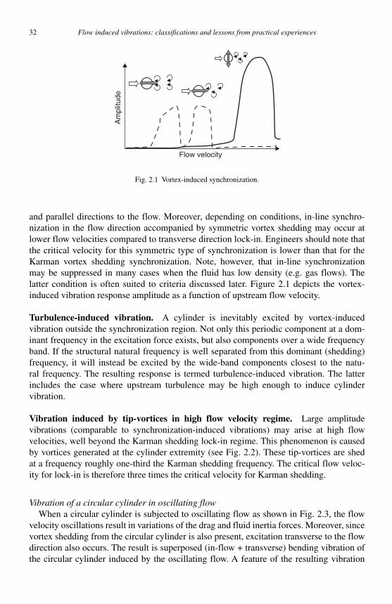
32 Flow induced vibrations: classifications and lessons from practical experiences
and parallel directions to the flow. Moreover, depending on conditions, in-line synchro-nization in the flow direction accompanied by symmetric vortex shedding may occur at lower flow velocities compared to transverse direction lock-in. Engineers should note that the critical velocity for this symmetric type of synchronization is lower than that for the Karman vortex shedding synchronization. Note, however, that in-line synchronization may be suppressed in many cases when the fluid has low density (e.g. gas flows). The latter condition is often suited to criteria discussed later. Figure 2.1 depicts the vortex-induced vibration response amplitude as a function of upstream flow velocity.
Turbulence-induced vibration. A cylinder is inevitably excited by vortex-induced vibration outside the synchronization region. Not only this periodic component at a dom-inant frequency in the excitation force exists, but also components over a wide frequency band. If the structural natural frequency is well separated from this dominant (shedding) frequency, it will instead be excited by the wide-band components closest to the natu-ral frequency. The resulting response is termed turbulence-induced vibration. The latter includes the case where upstream turbulence may be high enough to induce cylinder vibration.
Vibration induced by tip-vortices in high flow velocity regime. Large amplitude vibrations (comparable to synchronization-induced vibrations) may arise at high flow velocities, well beyond the Karman shedding lock-in regime. This phenomenon is caused by vortices generated at the cylinder extremity (see Fig. 2.2 ). These tip-vortices are shed at a frequency roughly one-third the Karman shedding frequency. The critical flow veloc-ity for lock-in is therefore three times the critical velocity for Karman shedding.
Vibration of a circular cylinder in oscillating flow When a circular cylinder is subjected to oscillating flow as shown in Fig. 2.3 , the flow
velocity oscillations result in variations of the drag and fluid inertia forces. Moreover, since vortex shedding from the circular cylinder is also present, excitation transverse to the flow direction also occurs. The result is superposed (in-flow + transverse) bending vibration of the circular cylinder induced by the oscillating flow. A feature of the resulting vibration
Flow velocity
Am
plitu
de
Fig. 2.1 Vortex-induced synchronization.
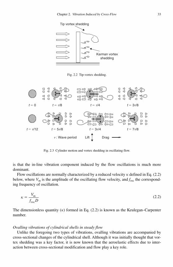
Chapter 2. Vibration Induced by Cross-Flow 33
is that the in-line vibration component induced by the flow oscillations is much more dominant.
Flow oscillations are normally characterized by a reduced velocity � defined in Eq. (2.2) below, where Vm is the amplitude of the oscillating flow velocity, and fosc the correspond-ing frequency of oscillation.
� �V
f Dm
osc
(2.2)
The dimensionless quantity ( � ) formed in Eq. (2.2) is known as the Keulegan–Carpenter number.
Ovalling vibrations of cylindrical shells in steady flow Unlike the foregoing two types of vibrations, ovalling vibrations are accompanied by
cross-sectional changes of the cylindrical shell. Although it was initially thought that vor-tex shedding was a key factor, it is now known that the aeroelastic effects due to inter-action between cross-sectional modification and flow play a key role.
Lift Drag
t � 0 t � t/8 t � t/4 t � 3t/8
t � 3t/4t � 5t/8t � t/12 t � 7t/8
t : Wave period
Fig. 2.3 Cylinder motion and vortex shedding in oscillating flow.
Karman vortexshedding
Tip vortex shedding
Fig. 2.2 Tip-vortex shedding.
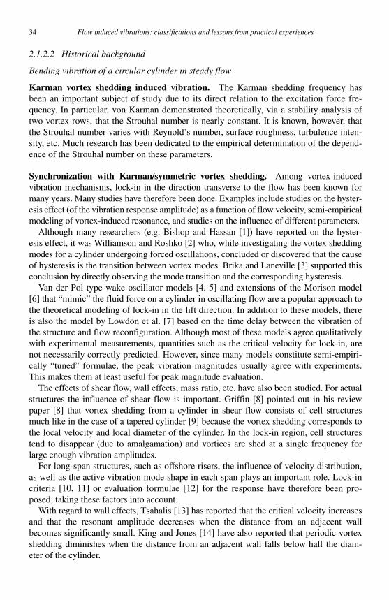
34 Flow induced vibrations: classifications and lessons from practical experiences
2.1.2.2 Historical background
Bending vibration of a circular cylinder in steady flow
Karman vortex shedding induced vibration. The Karman shedding frequency has been an important subject of study due to its direct relation to the excitation force fre-quency. In particular, von Karman demonstrated theoretically, via a stability analysis of two vortex rows, that the Strouhal number is nearly constant. It is known, however, that the Strouhal number varies with Reynold ’ s number, surface roughness, turbulence inten-sity, etc. Much research has been dedicated to the empirical determination of the depend-ence of the Strouhal number on these parameters.
Synchronization with Karman/symmetric vortex shedding. Among vortex-induced vibration mechanisms, lock-in in the direction transverse to the flow has been known for many years. Many studies have therefore been done. Examples include studies on the hyster-esis effect (of the vibration response amplitude) as a function of flow velocity, semi-empirical modeling of vortex-induced resonance, and studies on the influence of different parameters.
Although many researchers (e.g. Bishop and Hassan [1] ) have reported on the hyster-esis effect, it was Williamson and Roshko [2] who, while investigating the vortex shedding modes for a cylinder undergoing forced oscillations, concluded or discovered that the cause of hysteresis is the transition between vortex modes. Brika and Laneville [3] supported this conclusion by directly observing the mode transition and the corresponding hysteresis.
Van der Pol type wake oscillator models [4, 5] and extensions of the Morison model [6] that “ mimic ” the fluid force on a cylinder in oscillating flow are a popular approach to the theoretical modeling of lock-in in the lift direction. In addition to these models, there is also the model by Lowdon et al. [7] based on the time delay between the vibration of the structure and flow reconfiguration. Although most of these models agree qualitatively with experimental measurements, quantities such as the critical velocity for lock-in, are not necessarily correctly predicted. However, since many models constitute semi-empiri-cally “ tuned ” formulae, the peak vibration magnitudes usually agree with experiments. This makes them at least useful for peak magnitude evaluation.
The effects of shear flow, wall effects, mass ratio, etc. have also been studied. For actual structures the influence of shear flow is important. Griffin [8] pointed out in his review paper [8] that vortex shedding from a cylinder in shear flow consists of cell structures much like in the case of a tapered cylinder [9] because the vortex shedding corresponds to the local velocity and local diameter of the cylinder. In the lock-in region, cell structures tend to disappear (due to amalgamation) and vortices are shed at a single frequency for large enough vibration amplitudes.
For long-span structures, such as offshore risers, the influence of velocity distribution, as well as the active vibration mode shape in each span plays an important role. Lock-in criteria [10, 11] or evaluation formulae [12] for the response have therefore been pro-posed, taking these factors into account.
With regard to wall effects, Tsahalis [13] has reported that the critical velocity increases and that the resonant amplitude decreases when the distance from an adjacent wall becomes significantly small. King and Jones [14] have also reported that periodic vortex shedding diminishes when the distance from an adjacent wall falls below half the diam-eter of the cylinder.
Chapter 2. Vibration Induced by Cross-Flow 35
Khalak and Williamson [15] have reported that the cylinder mass ratio and damping have independent effects for very small mass-damping parameter values.
Standards or codes on vortex-induced vibration, including symmetric vortex shedding excitation, include “ Code Sec. III, Div. 1, Appendix N, 1300 Series ” by the American Society of Mechanical Engineers (ASME) [16] and the “ Guideline for Evaluation of Flow-Induced Vibration of a Cylindrical Structure in a Pipe” by the Japanese Society of Mechanical Engineers (JSME) [17] . The latter was created in response to the thermo well failure acci-dent in the Monju Fast Breeder Reactor. The latest knowledge is reflected in this code.
Turbulence-induced vibration. Many researcher frequency have measured the power spectral density (PSD) of the excitation force in the broad frequency range outside of the periodic vortex shedding region. In particular, Mulcahy summarized the measured fluctu-ating fluid force coefficient results by many researchers as a function of Reynolds number [17] . Unlike vortex-induced vibration, the response to turbulence excitation is usually estimated from calculations based on empirical functions derived from measured PSDs.However, many studies [18–20] have recently appeared in the field of numerical analysis (computational fluid dynamics [CFD]) reflecting recent advances in computer technology.
Vibration induced by tip-vortices in high flow velocity regime. Fox and Apelt [21] have reported that the tip-vortex shedding frequency is about one-third the natural shed-ding frequency along the cylinder span. The tip region spans roughly two diameters at the cylinder extremity. Kitagawa et al. [22] reported that vibration induced by tip-vortex shed-ding occurs at far higher flow velocities relative to the range in which lock-in by Karman vortex shedding occurs. Although it is known that the resonant region is determined by reduced velocity calculations similar to the type of vibration discussed in “ Synchronization with Karman/symmetric vortex shedding ” above, this knowledge is not reflected in either the ASME or the JSME design guidelines.
Vibration of a circular cylinder in oscillating flow Studies on the vibration of circular cylinders in oscillating flow began with research
on structures exposed to ocean waves in marine engineering. In the 1950s, Morison et al. [23] proposed a modeling method where the force on the structure in oscillating flow is expressed as the sum of inertia and drag forces. Most researchers still use this method. Besides Morison ’ s approach, Longoria et al. [24] proposed a method where the wave-motion-induced force is expressed in the form of a random force PSD. This method yields a good approximation of the excitation force in the low frequency range. Vibration control methods based on the Morison model have also been reported [25, 26] .
There are also numerous CFD-based vortex-induced vibration studies [27–29] . The latter are usually for comparatively low reduced velocities. In Zhang ’ s study [27] , the predicted added mass and drag coefficients are in good agreement with experimental data ( Table 2.4 ).
Ovalling vibrations of cylindrical shells in steady flow For ovalling vibration of a cylindrical shell in cross-flow, aeroelastic flutter theory is gener-
ally considered valid although there is a dispute between two opinions (a vortex-induced vibration theory [28–32] and aeroelastic flutter theory [33–37] ), shown in Table 2.5 . These discussions are explained in full detail in the review paper by Païdoussis et al. [38] .

36 Flow induced vibrations: classifications and lessons from practical experiences
2.1.3 Evaluation methods
2.1.3.1 Bending vibrations of a circular cylinder in steady flow Although a flow chart of the evaluation procedure for bending vibrations of a circular
cylinder is given in Fig. 2.4 , the engineer need not perform all evaluations according to this chart. For example, in the JSME guidelines, the evaluation of forced vibration by Karman vortex shedding is not included because of the mechanism ’ s low contribution to the vibration amplitude. The resonant amplitude is not evaluated because the design criteria avoids the resonance region. In a similar manner, the designer must make judgment calls
Table 2.4 Studies on vortex-induced vibration
Year Studies (Researchers)
1970 Van der Pol type lock-in model using fluctuating lift coefficient and displacement of cylinder as variables (Hartlen and Currie)
1972 Observation of cell structures in wake behind tapered cylinder (Vickery and Clark) 1974 Van der Pol type lock-in model using displacements of cylinder and fluid as variables (Iwan and
Blevins) 1980 Vortex-induced vibration of a cylinder near a wall (King) 1982 Extension of Morison models to lock-in (Sarpkaya) 1984 Wall effect on lock-in (Tsahalis) 1985 Review paper on vortex-induced vibration in shear flow (Griffin) 1986 Modified lock-in model for vibration in shear flow (Wang) 1988 Observation of vortex mode transition in lock-in (Williamson and Roshko) 1991 Time-delay model of fluid force at lock-in model of unsteady boundary layer (Lowdon) 1993 Lock-in criteria for marine structures (Vandiver) Vortex mode transition and hysteresis (Brika and Laneville) 1995 Revision of ASME Code Sec. III, Div. 1, Appendix N, 1300 Series (ASME) Response estimation method for vortex-induced vibration of multi-span circular structure (Bokaian) 1996 Lock-in for low mass ratio and low damping ratio (Khalak and Williamson) 1998 Publication of JSME Guideline for Evaluation of Flow-Induced Vibration of a Cylindrical Structure
in a Pipe (JSME)
Table 2.5 Studies on ovalling vibration of a cylindrical shell
Year Studies (Researchers)
1956 Observation of ovalling vibration at half the frequency of vortex shedding frequency (Dockstader) 1974 Observation of ovalling vibration with frequency ratio 1:6 (a vortex-induced vibration theory is
asserted) (Johns) 1979 Observation of vibration with non-integral frequency ratio (Païdoussis) Discovery of non suppression effect of a splitter plate for ovalling vibration (Païdoussis) Discussion on splitter plate in journals (Johns) 1982 Refutal of the vortex-induced vibration theory by detailed measurement of vortex shedding
(Païdoussis) Proposal of an aeroelastic flutter theory (Païdoussis) 1985 Measurement of aeroelastic damping (backing an aeroelastic flutter theory) (Katsura)

Chapter 2. Vibration Induced by Cross-Flow 37
on parameters that must be considered in design and their appropriate values. This deter-mination is directly linked to the problem at hand.
Vibration induced by single-phase flow
Forced vibration induced by Karman vortex shedding. The fluid excitation force on a cylinder subjected to cross-flow is periodic, and its frequency fW is expressed by the Eq. (2.3):
fV
DW St� (2.3)
Eq. (2.3) gives the frequency of the excitation force in the lift direction. In the drag direc-tion, the excitation frequency is twice that in the lift direction. Unless these frequencies approach the cylinder natural frequency, no significant vibration occurs. Conversely, when either forcing frequency approaches the cylinder frequency, synchronous vibrations can usually be expected.
Synchronization with Karman/symmetric vortex shedding. The condition for avoid-ance or suppression of synchronization for a single circular cylinder is expressed in terms of reduced velocity Vr and reduced damping Cn defined in Eqs. (2.4) and (2.5) where f0 is the fundamental natural frequency of the circular cylinder. The avoidance or suppression region for synchronization is shown in Fig. 2.5 .
Estimation of reduced velocity/reduced damping
Start
Judgement onsynchronization
Estimation of amplitude in non- synchronization case
Estimation of amplitude in synchronization
Amplitude estimation of forced vibration by Karman
vortex shedding
Amplitude estimation of turbulence-induced
vibration
Amplitude estimation in synchronization
Comparison with allowable limits
Fatigue curve, limitation for displacement, acceleration, etc.
Fig. 2.4 Evaluation for vibration of a circular cylinder in cross-flow.

38 Flow induced vibrations: classifications and lessons from practical experiences
VV
f Dr �0
(2.4)
C mm
D
m
Dn*� 2
2 42 2
��
�� ��
� � (2.5)
The threshold reduced damping for in-line synchronization in Fig. 2.5 is based on the study and guidelines of JSME [17] . The results are presented in Fig. 2.6 . The param-eter bounds for vibration avoidance in the JSME guideline are presented together with
0
0.02
0.04
0.06
0.08
0.5 1 1.5 2 2.5 3 3.5 4
Cn � 0.80
Cn � 0.99
Cn � 1.27
Cn � 2.65
Cn � 2.82
Reduced velocity: Vr
Nor
mal
ized
am
plitu
de
Synchronization by Karmanvortex shedding
Synchronization bysymmetric vortex shedding
Reduced damping
Fig. 2.6 Suppression of in-line synchronization [17] .
Vr
Cn
All synchronizationis suppressed
Synchronizationin life direction
is avoided
Synchronizationin drag directionis suppressed
Allsynchronization
is avoided
64
2.5
1.0 3.3
Fig. 2.5 Range of avoidance and suppression of synchronization.
Chapter 2. Vibration Induced by Cross-Flow 39
the equivalent ASME guideline bounds in Table 2.6 . The JSME bounds correspond to Fig. 2.5 .
Next, the vibration amplitude evaluation method during synchronization (lock-in) is described. Here the model by Iwan and Blevins [5] is presented as an example of a typical modeling method. In the model, the system is expressed by the following set of simultaneous equations for the cylinder displacement y and the hidden fluid parameter zcorresponding to the center of gravity of the fluid.
� � � � � � �02
1 22 2D z DV
D
Vz z z F�� � �� � � � �
⎧⎨⎪⎪⎩⎪⎪
⎫⎬⎪⎪⎭⎪⎪
W (2.6)
my cy ky F�� �� �+ (2.7)
F D z y DV z y� � � �� � � �32
4( ) ( )�� �� � � (2.8)
Here �0 , �1 , �2 , �3 , �4 are empirical constants. Using such a model, the resonant vibra-tion amplitude can be estimated. In addition to the semi-empirical formula by Iwan and Blevins [5] , other formulae exist such as those by Griffin ’ s [39] and Sarpkaya ’ s [40] . These formulae are presented in Table 2.7 .
Turbulence-induced vibration. The response to turbulence excitation is treated as fol-lows in the JSME S 012 guideline [17] . Random vibration theory is used for response
Table 2.6 Conditions for avoidance or suppression of synchronization
JSME Guidelines ASME Guidelines
Satisfaction of some requirements is needed 1 Vr � 1 Vr � 1 Avoidance 2 Cn � 64 Cn � 64 Suppression 3 Vr � 3.3 and Cn � 2.5 Vr � 3.3 and Cn � 1.2 Avoidance of lift oscillation
Suppression of drag oscillation 4 f0 / fw � 0.7 or f0 / fw � 1.3 Avoidance of only lift oscillations
Table 2.7 Semi-empirical formulae for resonant amplitude
Semi-empirical formulae
Griffin 3.35
20 n
1.29
1 0.43 (2 St )
y
d C⎡ ⎤⎢ ⎥⎣ ⎦
��
�
�
Gives conservative amplitude in low Cn region
Blevins 1 / 2
20 n n
0.07 0.720.3
( 1.9)St ( 1.9)St
y
d C C
⎡ ⎤⎢ ⎥⎢ ⎥⎢ ⎥⎣ ⎦
� �� �
�
Sarpkaya 1 / 2
2 20 n
0.32
0.06 (2 St )
y
d C⎡ ⎤⎢ ⎥⎣ ⎦
�� �
Mode factor not included
40 Flow induced vibrations: classifications and lessons from practical experiences
estimation. The spatial dependence of the excitation force is taken into consideration by introducing a turbulence fluctuation fluid force coefficient that incorporates the influence of the spatial correlation length. The resulting root-mean-square (rms) value of the turbu-lence-induced vibration amplitude is given by:
wG f
m fzmean
( )( )2 0 0
3 20
3 02
64�
�� �
φ (2.9a)
where
�0
0
�
φ
φ
( )d
( )d0
z z
z zLe
2
L
∫
∫(2.9b)
is the participation factor of the fundamental mode f0 ( z ). The PSD per unit length of the turbulence excitation force G ( f ) is expressed in terms of the normalized PSD � and the turbulence excitation force coefficient C� as shown in Eqs. (2.10)–(2.12).
G f C V D fD
V( ) ( )r� �
1
22
2
� �⎛
⎝⎜⎜⎜
⎞
⎠⎟⎟⎟⎟ (2.10)
� �( ) /( ) ( : )r r r rf f V f� � � 4 1 4 3 3 0 32 2 . . (2.11)
�( ) ( : )r r r rf f V f� � � � � ��7 979 10 3 3 5 0 0 2 0 33 4. . . . . (2.12)
In the equations above, fr is the reduced frequency defined as fr � fD / V . � ( fr ) is a function enveloping most of the existing experimental data. A value of C�
approximately 0.13 is adopted based on Fung ’ s data. In the case where turbulence is gen-erated upstream, or in the regime beyond the critical Reynolds number, PSD measure-ments in model experiments are required.
Vibration induced by tip-vortices in the high flow velocity regime. Research on this type of vibration [22] is relatively new and has yet to find its way into the ASME or JSME design guidelines. Tip-vortex-induced vibration occurs starting near the reduced velocity Vr � 10. The resulting vibration amplitude attains a maximum value at Vr � 15. Thus it is a phenomenon manifested in the region beyond about 3 times the critical velocity for clas-sical lock-in in the lift direction due to Karman vortex shedding. Usually a cylinder under-goes Karman shedding lock-in before the onset of tip-vortex-induced vibration as the flow velocity is increased. The tip-vortex-induced vibration depends on tip shape. According to Kitagawa [22] , vibration can be suppressed by attaching, at the cylinder extremity, a cir-cular plate of diameter Dp � 1.6 D where D is the circular cylinder diameter.
Vibration induced by two-phase flow Although Karman vortex shedding has not been clearly observed in most two-phase flow
regimes, Hara and Ohtani [41] reported that Karman vortices are formed for void fractions below 15%, much like in single-phase flow. The critical void fraction for Karman vortex

Chapter 2. Vibration Induced by Cross-Flow 41
shedding depends on the ratio of the average bubble diameter to the cylinder diameter, and increases with decreasing bubble diameter. In addition, Hara [42] measured the fluctuating lift and drag forces for various void fraction values. He reported that these forces increase dramatically beyond a certain void fraction. This feature is seen in the frequency character-istics of the flow, which takes on a random character for high void fractions.
As for synchronization in two-phase flow, lock-in in the lift direction tends to be sup-pressed when compared with the same phenomenon in single-phase flow. On the other hand, at high void fractions in-line vibration amplitudes are more significant in comparison to sin-gle-phase flow in-line excitation (see Fig. 2.7 ) [43] . Besides Hara and Ogawa’s data, little else has been reported on vibration in two-phase flow. For this reason, an established method for the analysis of two-phase flow induced vibration of a solitary circular cylinder does not presently exist.
2.1.3.2 Vibration of a circular cylinder in oscillating flow Morison ’ s model [23] is well known as an estimation method of the fluid force act-
ing on a circular cylinder in oscillating flow. In this model, the fluid inertia force FI is expressed as the sum of buoyancy and added mass components as follows:
F AV C A V xI m ( )� � �� �� � �� (2.13)
The fluctuating drag force FD derived from flow velocity oscillation is expressed as:
F V x V x DCD D ( )� � � �1
2�� �� � (2.14)
The cylinder governing equation of motion therefore becomes:
( ) ( )m I Dm AC x m x kx AC V V x V x DCi� � � � � � �� �� � �� ��� � � � �21
2 (2.15)
Here the inertia coefficient is defined as CI � 1 + Cm . Because this equation is non-linear, simplified methods employing linearization have
been proposed. Using the simplified methods, the estimated amplitudes tend to be larger than those obtained by solving the non-linear equations.
0
0.1
0.2
0.3
0.4
0.5
2.0 3.0 4.0 5.0 6.0
Reduced velocity: Vr
rms
of a
ccel
arat
ion
(G) 0%
1.5%5%10%20%
Void fraction
Fig. 2.7 Lock-in in two-phase flow [43] .

42 Flow induced vibrations: classifications and lessons from practical experiences
2.1.3.3 Ovalling vibrations of cylindrical shells in steady flow The ovalling vibration of a cylindrical shell is considered to be caused by aeroelas-
tic flutter. However, in the “ Recommendations for Loads on Buildings ” published (in Japanese) by the Architectural Institute of Japan [44] , designers are required to ensure that the design flow velocity falls below the following two critical velocities. The first is the critical flow velocity for vortex-induced vibration, Ur , as shown in Eq. (2.16). The second is the aeroelastic flutter critical velocity, Uthr , by Uematsu et al. [45] given in Eq. (2.17).
Uf D
ji
r St� (2.16)
In Eq. (2.16) above, fi is natural frequency of the i -th ovalling mode and j is a positive integer ( j � 2 when i � 3).
Uf D
ii
thr � 1 03. � (2.17)
Eq. (2.17) is based on experimental results. A theoretical method [35] for estimating the critical velocity based on aeroelastic flutter theory also exists. Unfortunately, this model cannot accurately estimate the critical velocity due to the influence of pressure fluc-tuations in the wake region [46] . Modified models [47] have also been proposed.
2.1.4 Examples of component failures due to vortex-induced vibration
Since lock-in in the lift direction is well known among designers, there have been few failures attributable to this mechanism in the recent past. Although a slit or spiral strake [48, 49] on the surface of a cylinder is often mentioned as a countermeasure for vortex-induced vibration, these cannot completely eliminate vortex-induced vibration. In fact, these countermeasures only shift the resonant velocity regime (see Fig. 2.8 ).
Few well-documented examples of failures due to in-line shedding synchroniza-tion exist [50, 51] . Engineers are likely to overlook this type of vibration at the design
4
5
6
7
8
9
0 20 40 60 80
Reduced damping: Cn
Red
uced
vel
ocity
: Vr Without strake
t � 0.029D
t � 0.059D
t � 0.088D
t � 0.118DStable
UnstableUnstable
Flow
D
Fig. 2.8 Suppression of synchronization by spiral strake [49] .
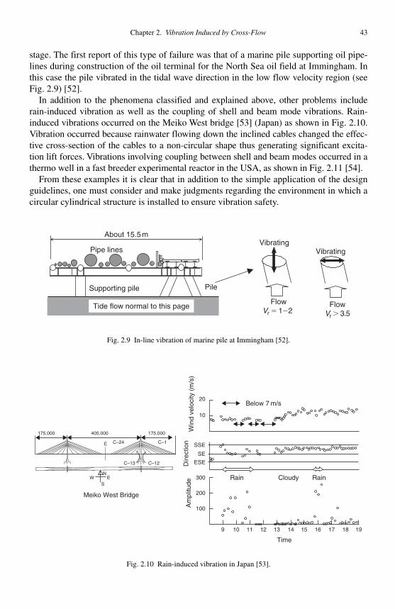
Chapter 2. Vibration Induced by Cross-Flow 43
stage. The first report of this type of failure was that of a marine pile supporting oil pipe-lines during construction of the oil terminal for the North Sea oil field at Immingham. In this case the pile vibrated in the tidal wave direction in the low flow velocity region (see Fig. 2.9 ) [52] .
In addition to the phenomena classified and explained above, other problems include rain-induced vibration as well as the coupling of shell and beam mode vibrations. Rain-induced vibrations occurred on the Meiko West bridge [53] (Japan) as shown in Fig. 2.10 . Vibration occurred because rainwater flowing down the inclined cables changed the effec-tive cross-section of the cables to a non-circular shape thus generating significant excita-tion lift forces. Vibrations involving coupling between shell and beam modes occurred in a thermo well in a fast breeder experimental reactor in the USA, as shown in Fig. 2.11 [54] .
From these examples it is clear that in addition to the simple application of the design guidelines, one must consider and make judgments regarding the environment in which a circular cylindrical structure is installed to ensure vibration safety.
Supporting pile
Pipe lines
Pile
About 15.5 mVibrating
Vibrating
FlowVr � 1�2
FlowVr � 3.5
Tide flow normal to this page
Fig. 2.9 In-line vibration of marine pile at Immingham [52] .
SE
SSE
ESE
200
300
100
9 10 11 12 15 16 17 18 1913 14
20
10
175.000405.000175.000
N
SE
C–13 C–12
C–1C–24E
W
Meiko West Bridge
Below 7 m/s
RainRain Cloudy
Win
d ve
loci
ty (
m/s
)A
mpl
itude
Dire
ctio
n
Time
Fig. 2.10 Rain-induced vibration in Japan [53] .
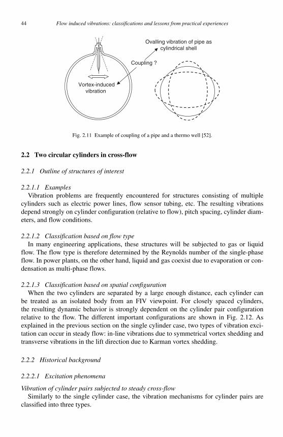
44 Flow induced vibrations: classifications and lessons from practical experiences
2.2 Two circular cylinders in cross-flow
2.2.1 Outline of structures of interest
2.2.1.1 Examples Vibration problems are frequently encountered for structures consisting of multiple
cylinders such as electric power lines, flow sensor tubing, etc. The resulting vibrations depend strongly on cylinder configuration (relative to flow), pitch spacing, cylinder diam-eters, and flow conditions.
2.2.1.2 Classification based on flow type In many engineering applications, these structures will be subjected to gas or liquid
flow. The flow type is therefore determined by the Reynolds number of the single-phase flow. In power plants, on the other hand, liquid and gas coexist due to evaporation or con-densation as multi-phase flows.
2.2.1.3 Classification based on spatial configuration When the two cylinders are separated by a large enough distance, each cylinder can
be treated as an isolated body from an FIV viewpoint. For closely spaced cylinders, the resulting dynamic behavior is strongly dependent on the cylinder pair configuration relative to the flow. The different important configurations are shown in Fig. 2.12 . As explained in the previous section on the single cylinder case, two types of vibration exci-tation can occur in steady flow: in-line vibrations due to symmetrical vortex shedding and transverse vibrations in the lift direction due to Karman vortex shedding.
2.2.2 Historical background
2.2.2.1 Excitation phenomena
Vibration of cylinder pairs subjected to steady cross-flow Similarly to the single cylinder case, the vibration mechanisms for cylinder pairs are
classified into three types.
Vortex-inducedvibration
Ovalling vibration of pipe ascylindrical shell
Coupling ?
Fig. 2.11 Example of coupling of a pipe and a thermo well [52] .
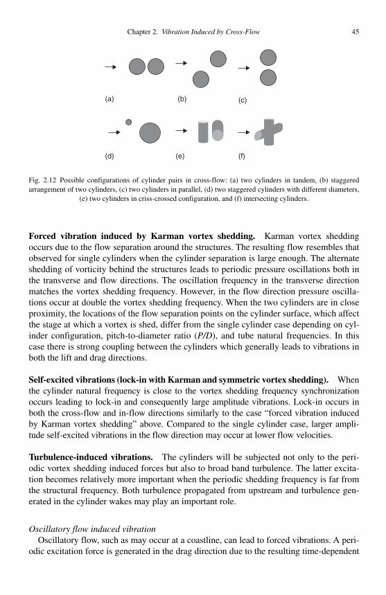
Chapter 2. Vibration Induced by Cross-Flow 45
Forced vibration induced by Karman vortex shedding. Karman vortex shedding occurs due to the flow separation around the structures. The resulting flow resembles that observed for single cylinders when the cylinder separation is large enough. The alternate shedding of vorticity behind the structures leads to periodic pressure oscillations both in the transverse and flow directions. The oscillation frequency in the transverse direction matches the vortex shedding frequency. However, in the flow direction pressure oscilla-tions occur at double the vortex shedding frequency. When the two cylinders are in close proximity, the locations of the flow separation points on the cylinder surface, which affect the stage at which a vortex is shed, differ from the single cylinder case depending on cyl-inder configuration, pitch-to-diameter ratio ( P/D ), and tube natural frequencies. In this case there is strong coupling between the cylinders which generally leads to vibrations in both the lift and drag directions.
Self-excited vibrations (lock-in with Karman and symmetric vortex shedding). When the cylinder natural frequency is close to the vortex shedding frequency synchronization occurs leading to lock-in and consequently large amplitude vibrations. Lock-in occurs in both the cross-flow and in-flow directions similarly to the case “ forced vibration induced by Karman vortex shedding ” above. Compared to the single cylinder case, larger ampli-tude self-excited vibrations in the flow direction may occur at lower flow velocities.
Turbulence-induced vibrations. The cylinders will be subjected not only to the peri-odic vortex shedding induced forces but also to broad band turbulence. The latter excita-tion becomes relatively more important when the periodic shedding frequency is far from the structural frequency. Both turbulence propagated from upstream and turbulence gen-erated in the cylinder wakes may play an important role.
Oscillatory flow induced vibration Oscillatory flow, such as may occur at a coastline, can lead to forced vibrations. A peri-
odic excitation force is generated in the drag direction due to the resulting time-dependent
(d)
(b)(a) (c)
(e) (f)
Fig. 2.12 Possible configurations of cylinder pairs in cross-flow: (a) two cylinders in tandem, (b) staggered arrangement of two cylinders, (c) two cylinders in parallel, (d) two staggered cylinders with different diameters,
(e) two cylinders in criss-crossed configuration, and (f) intersecting cylinders.
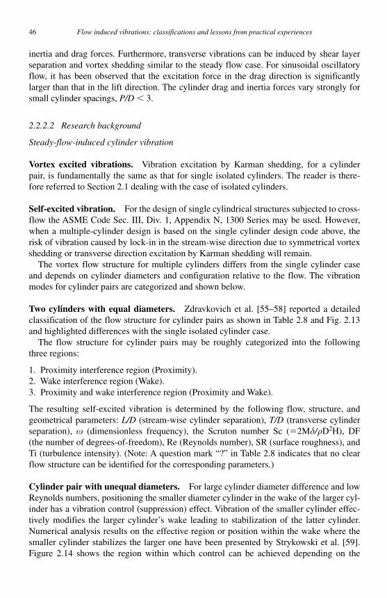
46 Flow induced vibrations: classifications and lessons from practical experiences
inertia and drag forces. Furthermore, transverse vibrations can be induced by shear layer separation and vortex shedding similar to the steady flow case. For sinusoidal oscillatory flow, it has been observed that the excitation force in the drag direction is significantly larger than that in the lift direction. The cylinder drag and inertia forces vary strongly for small cylinder spacings, P/D � 3.
2.2.2.2 Research background
Steady-flow-induced cylinder vibration
Vortex excited vibrations. Vibration excitation by Karman shedding, for a cylinder pair, is fundamentally the same as that for single isolated cylinders. The reader is there-fore referred to Section 2.1 dealing with the case of isolated cylinders.
Self-excited vibration. For the design of single cylindrical structures subjected to cross-flow the ASME Code Sec. III, Div. 1, Appendix N, 1300 Series may be used. However, when a multiple-cylinder design is based on the single cylinder design code above, the risk of vibration caused by lock-in in the stream-wise direction due to symmetrical vortex shedding or transverse direction excitation by Karman shedding will remain.
The vortex flow structure for multiple cylinders differs from the single cylinder case and depends on cylinder diameters and configuration relative to the flow. The vibration modes for cylinder pairs are categorized and shown below.
Two cylinders with equal diameters. Zdravkovich et al. [55–58] reported a detailed classification of the flow structure for cylinder pairs as shown in Table 2.8 and Fig. 2.13 and highlighted differences with the single isolated cylinder case.
The flow structure for cylinder pairs may be roughly categorized into the following three regions:
1. Proximity interference region (Proximity). 2. Wake interference region (Wake). 3. Proximity and wake interference region (Proximity and Wake).
The resulting self-excited vibration is determined by the following flow, structure, and geometrical parameters: L/D (stream-wise cylinder separation), T/D (transverse cylinder separation), � (dimensionless frequency), the Scruton number Sc (�2 M� / �D2 H ), DF (the number of degrees-of-freedom), Re (Reynolds number), SR (surface roughness), and Ti (turbulence intensity). (Note: A question mark “ ? ” in Table 2.8 indicates that no clear flow structure can be identified for the corresponding parameters.)
Cylinder pair with unequal diameters. For large cylinder diameter difference and low Reynolds numbers, positioning the smaller diameter cylinder in the wake of the larger cyl-inder has a vibration control (suppression) effect. Vibration of the smaller cylinder effec-tively modifies the larger cylinder ’ s wake leading to stabilization of the latter cylinder. Numerical analysis results on the effective region or position within the wake where the smaller cylinder stabilizes the larger one have been presented by Strykowski et al. [59] . Figure 2.14 shows the region within which control can be achieved depending on the

C
hapter 2.Vibration Induced by C
ross-Flow
47
Table 2.8 Classification of interference flow induced oscillations
0
0
0
1.1
1.5
3.8
1.1
3.2
�3.8
�8
�3.2
�8
0
�CLmax
0
0.3
0.2
0
01.5
�IB
�IB
�3.8
2.0
4.0
2.2
1.1Biased jet
Coupledvortex streets
Gap flow
Quasi-steadyreattachment
Disturbedvortex street
Displaced wake
Outsidewake boundary
No InterferenceWake
galloping
Coupledvortex streets
Synchronizedreattachment
1.2
1.0 Singlevortex street
Jet switching
max
maxmax
max
max
max
max
None
Gap flowswitching
Wakedisplacement
Low Vr
?
;
?
? ?
??
? ?
?
?
?
High VrMedium Vr
Flow regimesfor stationary
cylinders
Transversespacing T/D
Type of excitation
Sideby
side(parallel)
Staggered
Staggered
Staggered
Tandem
Tandem
Cylinderconfiguration
Streamwisespacing L /D
Category
Wake
proxi
mity
Wake
and
;
Interference
Interference
Proxi
mity
Interference
IB: Interference boundary.
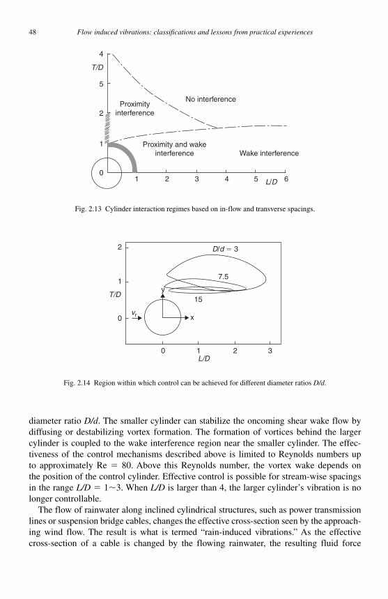
48 Flow induced vibrations: classifications and lessons from practical experiences
diameter ratio D/d . The smaller cylinder can stabilize the oncoming shear wake flow by diffusing or destabilizing vortex formation. The formation of vortices behind the larger cylinder is coupled to the wake interference region near the smaller cylinder. The effec-tiveness of the control mechanisms described above is limited to Reynolds numbers up to approximately Re � 80. Above this Reynolds number, the vortex wake depends on the position of the control cylinder. Effective control is possible for stream-wise spacings in the range L/D � 1�3. When L/D is larger than 4, the larger cylinder ’ s vibration is no longer controllable.
The flow of rainwater along inclined cylindrical structures, such as power transmission lines or suspension bridge cables, changes the effective cross-section seen by the approach-ing wind flow. The result is what is termed “ rain-induced vibrations. ” As the effective cross-section of a cable is changed by the flowing rainwater, the resulting fluid force
0 1 2
7.5
15
xvr
y
L/D3
T/D
0
1
2 D/d � 3
Fig. 2.14 Region within which control can be achieved for different diameter ratios D/d .
No interferenceProximity
interference
T/D
4
5
2
1
01 2 3 4 5 6L/D
Proximity and wakeinterference Wake interference
Fig. 2.13 Cylinder interaction regimes based on in-flow and transverse spacings.
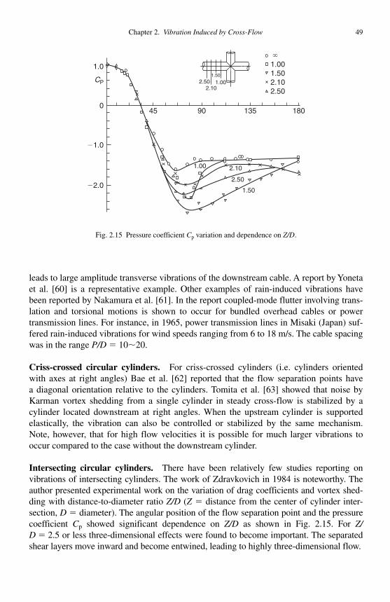
Chapter 2. Vibration Induced by Cross-Flow 49
leads to large amplitude transverse vibrations of the downstream cable. A report by Yoneta et al. [60] is a representative example. Other examples of rain-induced vibrations have been reported by Nakamura et al. [61] . In the report coupled-mode flutter involving trans-lation and torsional motions is shown to occur for bundled overhead cables or power transmission lines. For instance, in 1965, power transmission lines in Misaki (Japan) suf-fered rain-induced vibrations for wind speeds ranging from 6 to 18 m/s. The cable spacing was in the range P/D � 10�20.
Criss-crossed circular cylinders. For criss-crossed cylinders (i.e. cylinders oriented with axes at right angles) Bae et al. [62] reported that the flow separation points have a diagonal orientation relative to the cylinders. Tomita et al. [63] showed that noise by Karman vortex shedding from a single cylinder in steady cross-flow is stabilized by a cylinder located downstream at right angles. When the upstream cylinder is supported elastically, the vibration can also be controlled or stabilized by the same mechanism. Note, however, that for high flow velocities it is possible for much larger vibrations to occur compared to the case without the downstream cylinder.
Intersecting circular cylinders. There have been relatively few studies reporting on vibrations of intersecting cylinders. The work of Zdravkovich in 1984 is noteworthy. The author presented experimental work on the variation of drag coefficients and vortex shed-ding with distance-to-diameter ratio Z/D ( Z � distance from the center of cylinder inter-section, D � diameter). The angular position of the flow separation point and the pressure coefficient Cp showed significant dependence on Z/D as shown in Fig. 2.15 . For Z/D � 2.5 or less three-dimensional effects were found to become important. The separated shear layers move inward and become entwined, leading to highly three-dimensional flow.
1.00 2.10
2.50
1.50
2.502.10
1.50
1.00
1.001.502.102.50
1.0
0
CP
�1.0
�2.0
45 90 135 180
Fig. 2.15 Pressure coefficient Cp variation and dependence on Z/D .
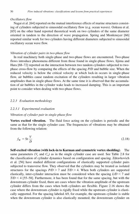
50 Flow induced vibrations: classifications and lessons from practical experiences
Oscillatory flow Nagai et al. [64] reported on the mutual interference effects of marine structures consist-
ing of cylinders subjected to sinusoidal oscillatory flow (e.g. ocean waves). Ookusu et al. [65] on the other hand reported theoretical work on two cylinders of the same diameter oriented in tandem to the direction of wave propagation. Spring and Monkmeyer [66]reported similar work for two cylinders having different diameters subjected to sinusoidal oscillatory ocean wave flow.
Vibration of cylinder pairs in two-phase flow In real machinery both single-phase and two-phase flows are encountered. Two-phase
flows introduce phenomena different from those found in single-phase flows. Iijima and Hara [68–72] reported on the interaction between two tandem cylinders subjected to two-phase cross-flow by comparing the effects of the spacing P/D and bubble size. When the reduced velocity is below the critical velocity at which lock-in occurs in single-phase flow, air bubbles cause random excitation of the cylinders resulting in larger vibration amplitudes than in single-phase flows. At the same time it is observed that the accumula-tion of air bubbles in the cylinder wake leads to increased damping. This is an important point to consider when dealing with two-phase flows.
2.2.3 Evaluation methodology
2.2.3.1 Experimental evaluation
Vibration of cylinder pair in single-phase flow
Vortex excited vibration. The fluid force acting on the cylinders is periodic and the same as that for the single cylinder case. The frequencies of vibrations may be obtained from the following relation:
fV
DW St� (2.18)
Self-excited vibration (with lock-in to Karman and symmetric vortex shedding). The same parameters ( Vr and Cn ) as in the single cylinder case are used. See Table 2.8 for the classification of cylinder dynamics based on configuration and spacing. Zdravkovich et al. [56] have studied different configurations of elastically supported cylinder pairs subjected to transverse flow. They observed that the cylinders may be treated as isolated structures for the spacings P/D � 7 and T/D � 4. When both cylinders are supported elastically, inter-cylinder interaction must be considered when the spacing L/D � 7 and T/D � 4 [55–58] . Furthermore, it has been found that for the same spacing, but with the downstream cylinder fixed, there are cases where the vibration amplitude of the upstream cylinder differs from the cases when both cylinders are flexible. Figure 2.16 shows the case where the downstream cylinder is rigidly fixed while the upstream cylinder is elasti-cally supported. For the spacing labeled A9, for example, the upstream cylinder is stable when the downstream cylinder is also elastically mounted; the downstream cylinder on
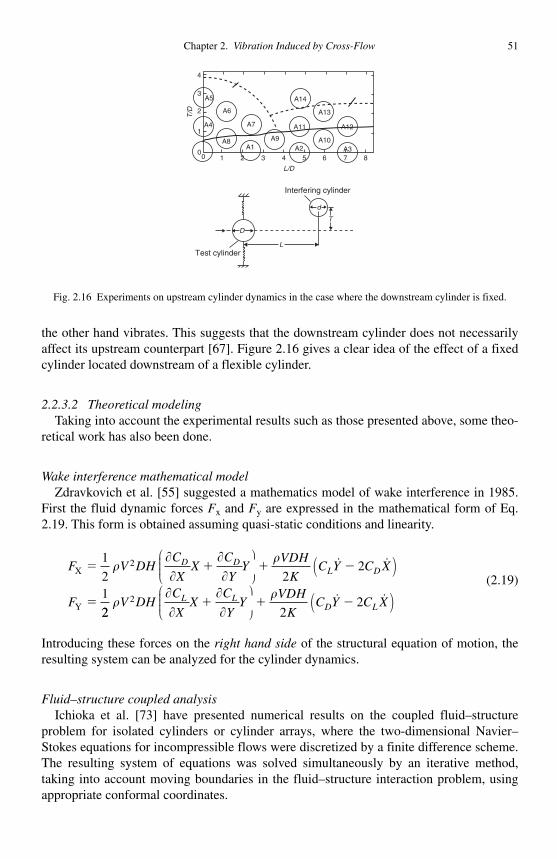
Chapter 2. Vibration Induced by Cross-Flow 51
the other hand vibrates. This suggests that the downstream cylinder does not necessarily affect its upstream counterpart [67]. Figure 2.16 gives a clear idea of the effect of a fixed cylinder located downstream of a flexible cylinder.
2.2.3.2 Theoretical modeling Taking into account the experimental results such as those presented above, some theo-
retical work has also been done.
Wake interference mathematical model Zdravkovich et al. [55] suggested a mathematics model of wake interference in 1985.
First the fluid dynamic forces Fx and Fy are expressed in the mathematical form of Eq. 2.19. This form is obtained assuming quasi-static conditions and linearity.
F V DHC
XX
C
YY
VDH
KC Y C X
F
D DL DX
Y
� � � �
�
1
2 22
1
2���
��
�⎛
⎝⎜⎜⎜
⎞
⎠⎟⎟⎟⎟ ( )� �
22 222�
��
��
�V DH
C
XX
C
YY
VDH
KC Y C XL L
D L� � �⎛
⎝⎜⎜⎜
⎞
⎠⎟⎟⎟⎟ ( )� �
(2.19)
Introducing these forces on the right hand side of the structural equation of motion, the resulting system can be analyzed for the cylinder dynamics.
Fluid–structure coupled analysis Ichioka et al. [73] have presented numerical results on the coupled fluid–structure
problem for isolated cylinders or cylinder arrays, where the two-dimensional Navier–Stokes equations for incompressible flows were discretized by a finite difference scheme. The resulting system of equations was solved simultaneously by an iterative method, taking into account moving boundaries in the fluid–structure interaction problem, using appropriate conformal coordinates.
A5 A14
A13
A12
A3A10
A1
A7A4
A8
A6
A11
A9A2
0 1 2 3 4 5 6 87
4
3
2
1
0
T/D
L/D
d
D
L
Interfering cylinder
Test cylinder
T
Fig. 2.16 Experiments on upstream cylinder dynamics in the case where the downstream cylinder is fixed.
52 Flow induced vibrations: classifications and lessons from practical experiences
Determination of instability boundary by unsteady fluid force models Theoretical models based on inter-cylinder coupling unsteady fluid forces have been
developed by Tanaka et al. [71] and Chen [75] . The unsteady fluid forces are measured experimentally. In the measurements, the rigid reference cylinder is oscillated periodically at a known frequency and small amplitude. The resulting force amplitude and phase on the neighboring cylinder is determined. The force magnitude and phase determine the net work done during a cycle of oscillation. Instability occurs when the net work done is posi-tive and large enough to overcome damping. In the model by Chen, the drag force hj and lift force gj acting on a fixed cylinder are given, respectively, by:
g U DC U DC t g
h U DC U
j j j j j j
j j
� � � �
� �
� �1
2
1
21
2
1
2
2 2
2
� � � �
� �
D D D D
L
sin( )
22 1 2DC t h jj j j jL L Lsin )� �� � �( ,� �(2.20)
The first terms are the steady drag and lift forces while the second terms are the unsteady periodic fluid force components. The third terms represent the random turbulence-induced forces. When the cylinders are supported elastically, hence free to vibrate, the following inter-cylinder coupling forces must be added:
gu
t
v
t
u
t
v
tu vj jk
kjk
kjk
kjk
kjk k jk k� � � � � �� � � ��
��
���
��
���
� �2
2
2
2
�⎛⎛
⎝⎜⎜⎜⎜
⎞
⎠⎟⎟⎟⎟∑
k
j jkk
jkk
jkk
jkhu
t
v
t
u
t
�
� �� � � �
1
2
2
2
2
2�
��
���
���
��vv
tu vk
jk k jk kk �
� �� �� �
�
⎛
⎝⎜⎜⎜⎜
⎞
⎠⎟⎟⎟⎟∑
1
2(2.21)
The wake-induced flutter of a cylinder in the wake of a fixed upstream cylinder ( Fig. 2.17 ) may be analyzed by the unsteady theory above. Assuming the downstream cylinder lift and drag coefficients CL and CD are functions of position only, the stability boundary for the downstream cylinder for small P/D spacings is given by:
U
fD
P D
C
m
DL
=− ∂ ∂
⎛
⎝⎜⎜⎜⎜
⎞
⎠⎟⎟⎟⎟⎛
⎝⎜⎜⎜⎜
⎞
⎠⎟⎟⎟3 54
2
2
0 5
2.
( ) sin
./
/ β θπζρ ⎟⎟
0 5.
(2.22)
For the general problem, however, where cylinder dynamical behavior has been classified based on in-line and transverse spacing ( Fig. 2.12 ) much work remains to be done.
Quasi-steady theory Price et al. [76] have proposed the quasi-steady model in which the relative velocity
vector between the moving cylinder and the flow is taken into consideration when deter-mining the fluid forces acting on the cylinder. The underlying quasi-static assumption is valid for high reduced velocities but may lead to significant error at low reduced veloci-ties. The force coefficients in the effective lift and drag directions are given by:
C V V C CC V V C C
x r D L
y r L D
( / ){ }( / ){ }
� �
� �
2 2
2 2cos sincos sin
� �� �
(2.23)
Chapter 2. Vibration Induced by Cross-Flow 53
where Vr is the magnitude of the flow velocity relative to the cylinder. Blevins [77] sug-gests that a reasonable limit value of the reduced velocity for design based on the quasi-static assumption is Vr � 10. However, this latter value does not take into account the changes in the fluid force orientation during cylinder motion. The suggested limit is therefore presently not recommended by the authors.
Cylinder pair dynamics in steady and oscillating flows have been presented in the fore-going. The key results are summarized in Tables 2.9 and 2.10 , respectively.
2.2.4 Examples of practical problems
1. The majority of cases reporting on vibrations due to steady flow have been for cable stayed bridges and power transmission lines. These may, however, be treated as iso-lated structures in most cases and are therefore not presented here. Few problems caused by oscillating flow have been reported. However, there are cases where large added mass values have been found depending on cylinder diameter ratio ( Table 2.10 ).In such cases it is prudent to increase the structural strength by 50% relative to the isolated cylinder case. Vibrations have also been reported in the case of criss-crossed pipes. As a countermeasure, S/D � 1 is recommended for design. In single-phase flow,
Table 2.9 Evaluation and classification in steady flow
Two cylinders in parallel Two cylinders in tandem
For L/D � 1.5, added mass is 20% higher than that for an isolated cylinder
For 2 � L/D � 3 the added mass is slightly lower than isolated cylinder case
For 3 � L/D � 4 proximity interference between the cylinders is negligible; each cylinder may be treated as an isolated body
For 3 � L/D � 4 proximity interference between the cylinders can be neglected as a first approximation; however, added mass and drag forces, which increase by 20–50%, must be considered
U
D
L
T
Y
� Lift
Drag
Fig. 2.17 Cylinder configuration and coordinates.
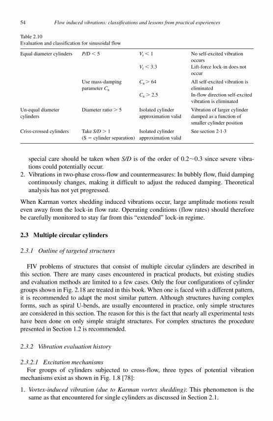
54 Flow induced vibrations: classifications and lessons from practical experiences
special care should be taken when S/D is of the order of 0.2�0.3 since severe vibra-tions could potentially occur.
2. Vibrations in two-phase cross-flow and countermeasures: In bubbly flow, fluid damping continuously changes, making it difficult to adjust the reduced damping. Theoretical analysis has not yet progressed.
When Karman vortex shedding induced vibrations occur, large amplitude motions result even away from the lock-in flow rate. Operating conditions (flow rates) should therefore be carefully monitored to stay far from this “ extended ” lock-in regime.
2.3 Multiple circular cylinders
2.3.1 Outline of targeted structures
FIV problems of structures that consist of multiple circular cylinders are described in this section. There are many cases encountered in practical products, but existing studies and evaluation methods are limited to a few cases. Only the four configurations of cylinder groups shown in Fig. 2.18 are treated in this book. When one is faced with a different pattern, it is recommended to adapt the most similar pattern. Although structures having complex forms, such as spiral U-bends, are usually encountered in practice, only simple structures are considered in this section. The reason for this is the fact that nearly all experimental tests have been done on only simple straight structures. For complex structures the procedurepresented in Section 1.2 is recommended.
2.3.2 Vibration evaluation history
2.3.2.1 Excitation mechanisms For groups of cylinders subjected to cross-flow, three types of potential vibration
mechanisms exist as shown in Fig. 1.8 [78] :
1. Vortex-induced vibration (due to Karman vortex shedding) : This phenomenon is the same as that encountered for single cylinders as discussed in Section 2.1.
Table 2.10 Evaluation and classification for sinusoidal flow
Equal diameter cylinders P/D � 5 Vr � 1 No self-excited vibration occurs
Vr � 3.3 Lift-force lock-in does not occur
Use mass-damping parameter Cn
Cn � 64 All self-excited vibration is eliminated
Cn � 2.5 In-flow direction self-excited vibration is eliminated
Un-equal diameter cylinders
Diameter ratio � 5 Isolated cylinder approximation valid
Vibration of larger cylinder damped as a function of smaller cylinder position
Criss-crossed cylinders Take S/D � 1 (S � cylinder separation)
Isolated cylinder approximation valid
See section 2 · 1 · 3
Chapter 2. Vibration Induced by Cross-Flow 55
2. Self-induced oscillations (fluidelastic vibration) : Arrays which consist of multiple cylinders can oscillate with large amplitudes when they are exposed to high velocity fluid flow. This phenomenon is not observed for a single cylinder. This is the most dangerous vibration mechanism and the root cause of many problems in industry.
3. Random vibration : Vibration is considered random when it does not correspond to either of the two phenomena above. This therefore includes the excitation by vorticity generated by upstream structures. In the latter case, the random force excitation spec-tra will contain periodic components related to upstream vorticity shedding.
2.3.2.2 Historical background In many heat exchangers, heat transfer tubes are designed to work in cross-flow. The
FIV problem of circular cylindrical structures is strongly associated with FIV problems for heat exchanger tubes. Numerous problems, including tube rupture and tube surface wear, have been encountered for many years. Therefore, the design procedure includes some experience based knowledge, such as keeping span lengths short, to avoid severe accidents [79] . However, this knowledge has been kept as closely guarded corporate know-how.
Vortex shedding, as explained in Section 2.1, not only occurs for single cylinders, but is also observed in cylinder arrays. In 1970, Y.N. Chen [80] proposed a map of the non-dimensional vortex flow periodicity frequency based on the cylinder array geometry pitch spacing. This map has become an important reference for designers.
Flow
Flow
Flow
Flow(a) (b) (c)
Flow
Flow
(d)
Fig. 2.18 Tube array patterns: (a) tube row, (b) tube column, (c) square tube array, and (d) triangular tube array.
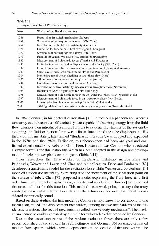
56 Flow induced vibrations: classifications and lessons from practical experiences
In 1969 Connors, in his doctoral dissertation [81] , introduced a phenomenon where a tube array could become a self-excited system capable of absorbing energy from the fluid flow. Connors then introduced a simple formula to evaluate the stability of the system by assuming the fluid excitation force was a linear function of the tube displacement. His theory on this instability, later named “ fluidelastic vibration ” , was adopted and expanded in the 1970s and the 1980s. Earlier on, this phenomenon had been analyzed and con-firmed experimentally by Roberts [82] in 1966. However, it was Connors who introduced a simple formula for this instability, which has been adopted in the design and develop-ment of nuclear power plants over the years ( Table 2.11 ).
Other researchers that have worked on fluidelastic instability include Price and Païdoussis, Weaver and Lever, and Chen and his colleagues. Price and Païdoussis [83]developed a quasi-static model for the excitation force while Weaver and co-workers [84] modeled fluidelastic instability by relating it to the movement of the separation point on the surface of tubes. Chen [78] proposed a model expressing the fluid force as a first order function of the tube displacement , velocity, and acceleration. Tanaka [85] presented the measured data for this function. This method has a weak point, that any tube array needs the measured excitation force data for the estimation, however, the model is con-sidered theoretically sound.
Based on these studies, the first model by Connors is now known to correspond to one mechanism, called “ the displacement mechanism, ” among the two mechanisms of the flu-idelastic vibration. The second mechanism is called “ the velocity mechanism ” . The mech-anism cannot be easily expressed by a simple formula such as that proposed by Connors.
Due to the lesser importance of the random excitation forces there are only a few papers published on the subject. In 1973, Pettigrew and Gorman [86] presented estimated random force spectra, which showed dependence on the location of the tube within tube
Table 2.11 History of research on FIV of tube arrays
Year Works and studies (Lead author)
1966 Proposal of jet switch mechanism (Roberts) 1968 Strouhal number map for tube arrays (Y.N. Chen) 1969 Introduction of fluidelastic instability (Connors) 1970 Guideline for tube wear in heat exchangers (Thorngren) 1972 Strouhal number map for tube arrays (Fitz-Hugh) 1973 Random force and two-phase flow estimation (Pettigrew) 1980 Measurement of fluidelastic forces (Tanaka and Takahara) 1981 Fluidelastic model related to displacement and velocity (S.S. Chen) 1982 Fluidelastic model due to movement of separation point (Lever and Weaver) 1983 Quasi-static fluidelastic force model (Price and Païdoussis) 1984 Non-existence of vortex shedding in two-phase flow (Hara) 1987 Vibration test in steam–water two-phase flow (Axisa) 1988 Correlation estimation of random force (Au-Yang) 1992 Introduction of two instability mechanisms in two-phase flow (Nakamura) 1994 Revision of ASME ’ s guideline for FIV (Au-Yang) 1996 Measurement of fluidelastic force in steam–water two-phase flow (Mureithi et al.) 1997 Measurement of fluidelastic force in air–water two-phase flow (Inada) 2000 U-bend tube bundle model test using freon fluid (Takai et al.) 2001 JSME guideline for fluidelastic vibration in steam generators (Iwatsubo et al.)
Chapter 2. Vibration Induced by Cross-Flow 57
array. This data is incorporated in the ASME design guideline. Although the correlation evaluation of the excitation force along the tube axis is required for the random vibration analysis, there had been no work reported on this subject until Au-Yang [87] published his study in 1999. To date, available data on the subject remains very limited.
Studies cited above pertain to vibration in single-phase flow. However, many tube arrays in heat exchangers are subjected to gas–liquid two-phase flow. Faced with this reality, Pettigrew and co-workers [88] started to study the two-phase FIV problem in 1973. They focused primarily on fluidelastic vibration and random vibration; vortex-induced vibration was not considered since two-phase flow in many heat exchangers does not produce stable periodic vortex shedding. Their approach was based on similar meth-ods as employed for single-phase flow. However, the idea that the vibration induced by two-phase flow could be treated with this method was original. When the void fraction of the two-phase flow is low enough, vortex shedding can be observed. However, in this case the flow can be estimated as single phase as shown by Hara and Ohtani [89] .
Initial studies in the 1970s were based on air–water two-phase flow tests at atmospheric conditions. However, many heat exchangers operate at high temperature and high pressure conditions. Axisa et al. [90] have measured the two-phase flow damping in steam–water two-phase flow tests. Nakamura et al. [91] proposed an original estimation method for the two-phase flow instability velocity based on measured data by tests in steam–water two-phase flow. This theory proposes a unique estimation method for the fluidelastic instability boundary, and for the random excitation force caused by gas–liq-uid two-phase flow. Two possible instability boundaries for “ the absolute instability ” and “ the intermittent instability, ” are predicted.
In the 1990s, freon two-phase mixtures were used to simulate the steam–water flow, because they are easier to handle due to low temperature and pressure operating condi-tions. A large scale vibration test [92] of the partial model of a practical steam generator has been performed using freon.
On the other hand, the measurement of the fluidelastic forces, which has successfully been achieved in single-phase flow, has been attempted by several researchers, Inada et al. [93] and Mureithi et al. [94] . However, the measurement of fluidelastic forces in two-phase flow remains a difficult challenge.
2.3.3 Estimation method
2.3.3.1 Vibration in single-phase flow
Steady flow
Vortex-induced vibration. When vortex shedding occurs in the flow, a periodic exci-tation force acts on the cylinder. The force frequency, fW , can be expressed in the form of Eq. (2.1). The non-dimensional number, St, in this equation, has been experimen-tally determined for tube arrays and is shown in Fig. 2.19(a) and (b) [95] . The Strouhal number is known to be a function of the tube pitch ratio.
For isolated cylinders the Strouhal number, St, is known to be a function of the Reynolds number, Re. However, for tube arrays, no work has been reported on the variation of the Strouhal number with Reynolds number. Eq. 2.1 corresponds to the case of lift
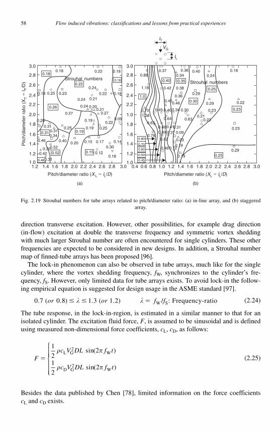
58 Flow induced vibrations: classifications and lessons from practical experiences
direction transverse excitation. However, other possibilities, for example drag direction (in-flow) excitation at double the transverse frequency and symmetric vortex shedding with much larger Strouhal number are often encountered for single cylinders. These other frequencies are expected to be considered in new designs. In addition, a Strouhal number map of finned-tube arrays has been proposed [96] .
The lock-in phenomenon can also be observed in tube arrays, much like for the single cylinder, where the vortex shedding frequency, fW , synchronizes to the cylinder ’ s fre-quency, fS . However, only limited data for tube arrays exists. To avoid lock-in the follow-ing empirical equation is suggested for design usage in the ASME standard [97] .
0 7 0 8 1 3 1 2. . . ( .( ) ) / : Frequency-ratioW Sor or f f� � �� � (2.24)
The tube response, in the lock-in-region, is estimated in a similar manner to that for an isolated cylinder. The excitation fluid force, F , is assumed to be sinusoidal and is defined using measured non-dimensional force coefficients, cL , cD , as follows:
Fc V DL f t
c V DL f t�
1
22
1
22
2
2
� �
� �
L G W
D G W
( )
( )
sin
sin
⎧
⎨
⎪⎪⎪⎪⎪
⎩
⎪⎪⎪⎪⎪
(2.25)
Besides the data published by Chen [78] , limited information on the force coefficients cL and cD exists.
2.8
2.6
2.4
2.2
2.0
1.8
1.6
1.4
1.2
3.0
1.01.4 1.6 1.8 2.0 2.2 2.4 2.6 2.81.2 3.0
0.180.120.15
0.300.170.150.200.40
0.52
0.460.31
0.420.300.52
0.14
0.190.25 0.19 0.25
0.22
0.270.21
0.200.24
0.27
0.26
0.20
0.310.310.310.34
0.46
0.25 0.230.210.24
0.240.22
0.22 0.18
0.18
0.183.0
lL
2.8
2.6
2.4
2.2
1.0
1.8
1.6
1.4
1.2
1.00.4 0.6 0.8 1.0 1.2 1.4 1.6 1.8 2.0 2.2 2.4 2.6 2.8 3.0
0.250.29
0.23
0.230.21
0.22
0.230.23
0.290.30
0.63
0.090.310.410.48
0.630.64
0.300.340.400.451.380.70
0.460.46
0.36
0.380.42
0.40 0.35
0.250.29
0.400.24
0.180.34
0.360.37
VG
lT
0.88
1.18
1.0
0.230.19
0.19
0.720.46
0.420.78
0.49 0.37
0.80
0.70
0.60
0.50
0.45
0.09
0.220.18
0.18
0.18Strouhal numbers
Strouhal numbers
0.19
Pitch/diameter ratio (X L � lL/D) Pitch/diameter ratio (XL � lL/D)
(a) (b)
Pitc
h/di
amet
er r
atio
(X
T�
l T/D
)
Fig. 2.19 Strouhal numbers for tube arrays related to pitch/diameter ratio: (a) in-line array, and (b) staggered array.

Chapter 2. Vibration Induced by Cross-Flow 59
When the excitation force is assumed to be independent of cylinder motion, the response of the tube can be obtained by direct solution of the equation of motion. The analysis is generally quite complex thus requiring numerical computation. The simple case of a simply supported tube is estimated with the following equation:
X x H X xd s( ) ( )� � ( ) (2.26)
where Xd ( x ) is the root-mean-square-response at the position x , Xs ( x ) is the deformation when the excitation force statically acts on the tube, and H ( � ) is the transfer function
of the tube given by H( )( ) ( )
./
�� ��
�� �
1
1 22 2 2
1 2⎡
⎣⎢⎢
⎤
⎦⎥⎥
⎛
⎝
⎜⎜⎜⎜⎜
⎞
⎠
⎟⎟⎟⎟⎟⎟
Fluidelastic vibration (self-excited vibration). The self-excited vibration of tube arrays due to cross-flow was named “ fluid-elastic vibration ” by Connors [81] . He proposed a simple criterion for the occurrence of this instability by introducing a non-dimensional factorK as shown in the following Eq. (2.27) and Fig. 2.20 .
V
f DK
m
Dc
S
/
��
� 2
1 2⎡
⎣⎢⎢
⎤
⎦⎥⎥
(2.27)
Here Vc is the critical flow velocity. The gap flow velocity is usually used. There are two major estimation methods for fluidelastic instability:
1. Method based on measured fluid force data:
The fluid forces are measured experimentally [85] or determined by numerical sim-ulations [73] using CFD. Assuming the fluid forces to be function of cylinder dis-placement, velocity, and acceleration, the measured forces are estimated in terms the coefficients of Eq. (2.21). This method is considered the most accurate.
2. Simplified estimation method for designers:
Chen [78] proposed the criterion below for the occurrence of fluidelastic instability based on many experimental data. Since he used the lowest flow velocity among the available data, this formula gives a conservative value for the critical velocity.
V
f Da
m
D
bc
S
� V V�� 2
⎡
⎣⎢⎢
⎤
⎦⎥⎥
(2.28)
The constants a and b are given in the table below. Here T is the array pitch, and �V
the non-dimensional mass-damping parameter, given by:
�
��s
V V�m
D2.
The subscript “ V ” indicates the value in vacuum. There is ongoing debate on which val-ues should be used for the criterion, values in vacuum or those in practical conditions.
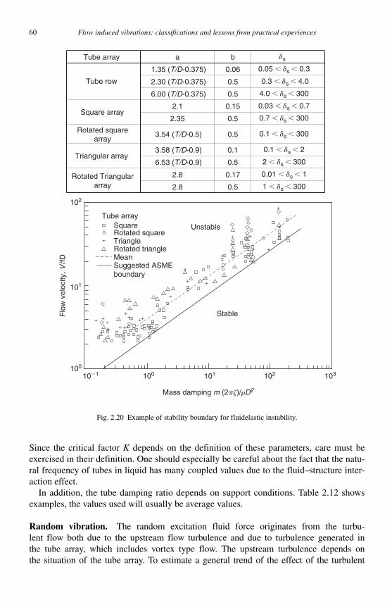
60 Flow induced vibrations: classifications and lessons from practical experiences
Since the critical factor K depends on the definition of these parameters, care must be exercised in their definition. One should especially be careful about the fact that the natu-ral frequency of tubes in liquid has many coupled values due to the fluid–structure inter-action effect.
In addition, the tube damping ratio depends on support conditions. Table 2.12 shows examples, the values used will usually be average values.
Random vibration. The random excitation fluid force originates from the turbu-lent flow both due to the upstream flow turbulence and due to turbulence generated in the tube array, which includes vortex type flow. The upstream turbulence depends on the situation of the tube array. To estimate a general trend of the effect of the turbulent
Tube array
102
101
10�1 100 101 102 103
Mass damping m (2pz)/rD2
100
Square
Triangle
MeanSuggested ASMEboundary
Flo
w v
eloc
ity, V
/fD
Unstable
Stable
Rotated triangle
Rotated square
Tube array a b ds
1.35 (T/D-0.375) 0.06 0.05 � ds � 0.3
2.30 (T/D-0.375) 0.5 0.3 � ds � 4.0
6.00 (T/D-0.375) 0.5 4.0 � ds � 300
2.1 0.15 0.03 � ds � 0.7
2.35 0.5 0.7 � ds � 300
Rotated squarearray
3.54 (T/D-0.5) 0.5 0.1 � ds � 300
3.58 (T/D-0.9) 0.1 0.1 � ds � 2
6.53 (T/D-0.9) 0.5 2 � ds � 300
2.8 0.17 0.01 � ds � 1
2.8 0.5 1 � ds � 300
Tube row
Square array
Triangular array
Rotated Triangulararray
Fig. 2.20 Example of stability boundary for fluidelastic instability.
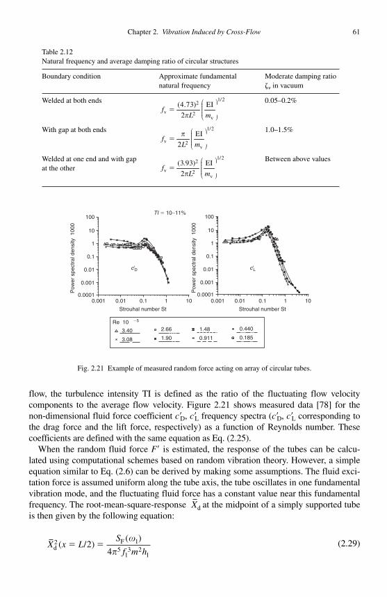
Chapter 2. Vibration Induced by Cross-Flow 61
flow, the turbulence intensity TI is defined as the ratio of the fluctuating flow velocity components to the average flow velocity. Figure 2.21 shows measured data [78] for the non-dimensional fluid force coefficient c� D , c� L frequency spectra ( c� D , c� L corresponding to the drag force and the lift force, respectively) as a function of Reynolds number. These coefficients are defined with the same equation as Eq. (2.25).
When the random fluid force F� is estimated, the response of the tubes can be calcu-lated using computational schemes based on random vibration theory. However, a simple equation similar to Eq. (2.6) can be derived by making some assumptions. The fluid exci-tation force is assumed uniform along the tube axis, the tube oscillates in one fundamental vibration mode, and the fluctuating fluid force has a constant value near this fundamental frequency. The root-mean-square-response Xd at the midpoint of a simply supported tube is then given by the following equation:
X x LS
f m hdF( / )
(2 15
13 2
1
24
� ��
�)
(2.29)
Fig. 2.21 Example of measured random force acting on array of circular tubes.
Table 2.12 Natural frequency and average damping ratio of circular structures
Boundary condition Approximate fundamental natural frequency
Moderate damping ratio �� in vacuum
Welded at both ends 1/22
v 2v
(4.73) EI
2f
L m
⎛ ⎞⎟⎜ ⎟⎜ ⎟⎜ ⎟⎟⎜⎝ ⎠�
�
0.05–0.2%
With gap at both ends 1/2
v 2v
EI
2f
L m
⎛ ⎞⎟⎜ ⎟⎜ ⎟⎜ ⎟⎟⎜⎝ ⎠�
� 1.0–1.5%
Welded at one end and with gap at the other
1/22
v 2v
(3.93) EI
2f
L m
⎛ ⎞⎟⎜ ⎟⎜ ⎟⎜ ⎟⎟⎜⎝ ⎠�
�
Between above values
100
10
TI � 10∼11%
1
0.1
0.01
Pow
er s
pect
ral d
ensi
ty
100
0
Pow
er s
pect
ral d
ensi
ty
100
0
0.001
0.0001
100
10
c�D c�L
1
0.1
0.01
0.001
0.00010.001 0.01 0.1
Re 10�5
3.40
3.08
2.66
1.90
1.48
0.911
0.440
0.185
1 100.001 0.01 0.1 1 10
Strouhal number StStrouhal number St
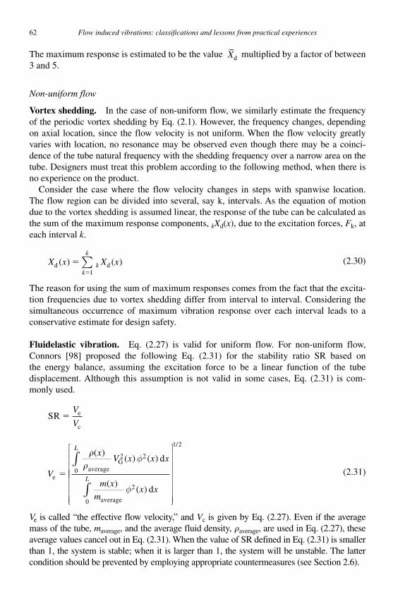
62 Flow induced vibrations: classifications and lessons from practical experiences
The maximum response is estimated to be the value Xd multiplied by a factor of between 3 and 5.
Non-uniform flow
Vortex shedding. In the case of non-uniform flow, we similarly estimate the frequency of the periodic vortex shedding by Eq. (2.1). However, the frequency changes, depending on axial location, since the flow velocity is not uniform. When the flow velocity greatly varies with location, no resonance may be observed even though there may be a coinci-dence of the tube natural frequency with the shedding frequency over a narrow area on the tube. Designers must treat this problem according to the following method, when there is no experience on the product.
Consider the case where the flow velocity changes in steps with spanwise location. The flow region can be divided into several, say k, intervals. As the equation of motion due to the vortex shedding is assumed linear, the response of the tube can be calculated as the sum of the maximum response components, k Xd ( x ), due to the excitation forces, Fk , at each interval k .
X x X xkk
k
d d( ) ( )��1∑ (2.30)
The reason for using the sum of maximum responses comes from the fact that the excita-tion frequencies due to vortex shedding differ from interval to interval. Considering the simultaneous occurrence of maximum vibration response over each interval leads to a conservative estimate for design safety.
Fluidelastic vibration. Eq. (2.27) is valid for uniform flow. For non-uniform flow, Connors [98] proposed the following Eq. (2.31) for the stability ratio SR based on the energy balance, assuming the excitation force to be a linear function of the tube displacement. Although this assumption is not valid in some cases, Eq. (2.31) is com-monly used.
SR e
c
�V
V
V
xV x x x
m x
mx x
L
Leaverage
G2
average
( )( ) ( ) d
( )( ) d
�
��
φ
φ
2
0
2
0
∫
∫
⎡
⎣
⎢⎢⎢⎢⎢⎢⎢⎢⎢
⎤
⎦
⎥⎥⎥⎥⎥⎥⎥⎥
1 2/
(2.31)
Ve is called “ the effective flow velocity, ” and Vc is given by Eq. (2.27). Even if the average mass of the tube, maverage , and the average fluid density, �average , are used in Eq. (2.27), these average values cancel out in Eq. (2.31). When the value of SR defined in Eq. (2.31) is smaller than 1, the system is stable; when it is larger than 1, the system will be unstable. The latter condition should be prevented by employing appropriate countermeasures (see Section 2.6).
Chapter 2. Vibration Induced by Cross-Flow 63
Random vibration. Eq. (2.29) is not mathematically valid in the case of non-uniform flow because the power spectral density (PSD) of the excitation force, SF ( � )(�2G ( � )) depends on the axial location along the tube. To avoid this problem, the following two approximate methods are applied.
1. The frequency composition of the excitation force is considered to be constant even if the flow velocity changes with location. Thus, only the magnitude of the excitation force is considered in the response calculation using the following equation:
S x c V x SF G F) ( ) ( )( , � � �� �1
22
2⎛
⎝⎜⎜⎜
⎞
⎠⎟⎟⎟⎟ (2.32)
Here, SF ( )� is the non-dimensional PSD of the excitation force.
2. Dividing the span into intervals, k � 1, 2 … , along the cylinder where the PSD of the excitation force is considered uniform, the average square of the response, k X xd
2 ( ) in each interval k , is calculated. Finally the total response is obtained by summation, thus:
X x X xkk
d d( ) ( )2 2
1
��∑ (2.33)
2.3.3.2 Vibration induced by two-phase flow The vibration phenomenon in two-phase flow depends on the so-called “ flow regime. ”
Detailed explanation on the flow regime will not be given here, since the two-phase flow regimes are well known in the field of thermal-hydraulics. Although it is not an easy task to determine the flow regime. Grant [99] and Baker [100] have proposed flow regime maps for cross-flow in tube arrays. Void fraction (the volume fraction of gas in the mixture) is one of the quantities used to identify the flow regime. Air–water two-phase flow shows the following regimes as the void fraction is progressively increased from low values:
• Bubbly flow (mainly liquid flow mixed with bubbles). • Intermittent flow (strongly unsteady flow, slug flow, froth flow, or annular flow). • Mist flow (mainly gas flow mixed with liquid mist).
Vortex shedding Hara and Ohtani [89] reported that periodic vortex shedding is observed in the low
void fraction regime, below 15%, as in the case of single-phase flow. However, no peri-odic vortex shedding has been observed at higher void fractions. Although there is no data in the extremely high void fraction range, the possibility of periodic vortex shedding should be considered in the mist flow regime.
Vortex shedding can therefore be neglected in the void fraction range of 15–95%, but its effect must be estimated otherwise, even in two-phase flow conditions. The estimation
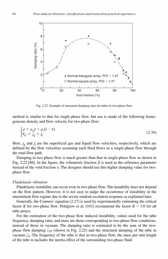
64 Flow induced vibrations: classifications and lessons from practical experiences
method is similar to that for single-phase flow, but use is made of the following homo-geneous density and flow velocity for two-phase flow:
� � � � �� � �� �
g l
G g l
( )1V j j⎧⎨⎪⎪⎩⎪⎪
(2.34)
Here, jg and jl are the superficial gas and liquid flow velocities, respectively, which are defined by the flow velocities assuming each fluid flows as a single-phase flow through the total flow path.
Damping in two-phase flow is much greater than that in single-phase flow as shown in Fig. 2.22 [86] . In the figure, the volumetric fraction � is used as the reference parameter instead of the void fraction � . The designer should use this higher damping value for two-phase flow.
Fluidelastic vibration Fluidelastic instability can occur even in two-phase flow. The instability does not depend
on the flow pattern. However, it is not easy to judge the occurrence of instability in the intermittent flow regime due to the severe random excitation response as explained later.
Generally, the Connors ’ equation (2.27) is used by experimentally estimating the critical factor K for two-phase flow. Pettigrew et al. [101] recommend the factor K � 3.0 for all tube arrays.
For the estimation of the two-phase flow induced instability, values used for the tube frequency, damping ratio, and mass are those corresponding to two-phase flow conditions, instead of those in vacuum. The damping ratio is estimated to be the sum of the two-phase flow damping �TP (shown in Fig. 2.22 ) and the structural damping of the tube in vacuum �V . The frequency of the tube is that in two-phase flow, the mass per unit length of the tube m includes the inertia effect of the surrounding two-phase fluid.
10
8
6
4
Dam
ping
rat
io (
%)
2
00 20
Normal-triangular array, P/D � 1.47
Normal-square array, P/D � 1.47
40
Void fraction (%)
60 80 100
Fig. 2.22 Example of measured damping ratio for tubes in two-phase flow.

Chapter 2. Vibration Induced by Cross-Flow 65
In addition, a design criterion using the critical factor K � 7.3 in Connors ’ equation for U-bend tubes is proposed by the JSME [102] , based on the experimental data of a large scale test. The details in this guideline should be reviewed.
Random vibration The most important difference between two-phase flow and single-phase flow is the
random buffeting force in the two-phase intermittent flow regime. When not in the inter-mittent flow regime (e.g. in bubbly flow or mist flow), the vibration estimation is similar to that for single-phase flow except for the fluid density. A smaller response may be obtained due to the larger damping ratio in two-phase flow. However, the large excitation force must be considered in the intermittent flow regime.
There are two excitation forces proposed by researchers:
General power spectral density (PSD) . A non-dimensional PSD [103] of the two-phase flow excitation force is proposed as the following equation. This equation was determined empirically considering numerous experimental data ( Fig. 2.23 ). It is there-fore valid for the majority of cases.
ΦΦ
E r r r
E r r r
for )for )
( ) ( .( ) ( .
.
.f f ff f f
�
�
10 0 062 10 0 06
0 5
3 3 5
−
− −
� �
⎧⎧⎨⎪⎪⎩⎪⎪
(2.35)
Here, fr is the non-dimensional frequency, defined as fdB / VG , based on the bubble diameter dB .
PSD in the intermittent flow regime . For the intermittent flow regime [91] only, where the excitation force is large, the equation below is proposed, based on the practi-cal flow velocity in this regime. From the experimental fact that the excitation force has a linear relation with the liquid slug velocity VS , the PSD of the excitation force is approxi-mated by a shot noise due to the liquid slugs.
10
Freon tests
1
Steam–watertests
Air–watertests
10�3
10�6
10�2 102
fdB
VG� 2 · 10�3�E
fdB
VG
–
–�E
Fig. 2.23 Example of proposed random force for liquid–gas two-phase flow [103].
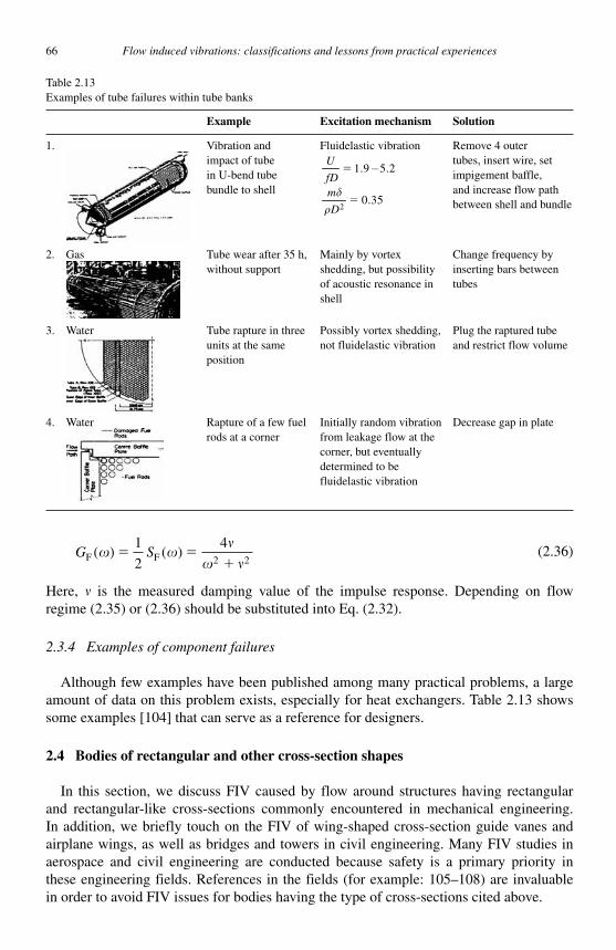
66 Flow induced vibrations: classifications and lessons from practical experiences
G SF F( ) ( )� �
� � �
�
1
2
42 2
(2.36)
Here, is the measured damping value of the impulse response. Depending on flow regime (2.35) or (2.36) should be substituted into Eq. (2.32).
2.3.4 Examples of component failures
Although few examples have been published among many practical problems, a large amount of data on this problem exists, especially for heat exchangers. Table 2.13 shows some examples [104] that can serve as a reference for designers.
2.4 Bodies of rectangular and other cross-section shapes
In this section, we discuss FIV caused by flow around structures having rectangular and rectangular-like cross-sections commonly encountered in mechanical engineering. In addition, we briefly touch on the FIV of wing-shaped cross-section guide vanes and airplane wings, as well as bridges and towers in civil engineering. Many FIV studies in aerospace and civil engineering are conducted because safety is a primary priority in these engineering fields. References in the fields (for example: 105–108) are invaluable in order to avoid FIV issues for bodies having the type of cross-sections cited above.
Table 2.13 Examples of tube failures within tube banks
Example Excitation mechanism Solution
1. Vibration and impact of tube in U-bend tube bundle to shell
Fluidelastic vibration
−
2
1.9 5.2
0.35
U
fDm
D
�
��
�
Remove 4 outer tubes, insert wire, set impigement baffle, and increase flow path between shell and bundle
2. Gas Tube wear after 35 h, without support
Mainly by vortex shedding, but possibility of acoustic resonance in shell
Change frequency by inserting bars between tubes
3. Water Tube rapture in three units at the same position
Possibly vortex shedding, not fluidelastic vibration
Plug the raptured tube and restrict flow volume
4. Water Rapture of a few fuel rods at a corner
Initially random vibration from leakage flow at the corner, but eventually determined to be fluidelastic vibration
Decrease gap in plate

Chapter 2. Vibration Induced by Cross-Flow 67
2.4.1 General description of cross-section shapes
At first, several examples of products treated in this section are given, for a better understanding of the objective of the study. Next, the flow conditions and cross-section shapes are presented in order to identify the different FIV mechanisms.
2.4.1.1 Products focused on In this section, we focus on mechanical engineering structures subjected to flow in
power plants and civil engineering structures subjected to wind, river flow, and tides. Furthermore, we limit ourselves to components having simple rectangular geometry or structures common in mechanical engineering.
2.4.1.2 Classification based on fluid flow Single-phase flow is ubiquitous. Whether the fluid is gas or liquid, the flow behaves
similarly if all non-dimensional numbers, such as Reynolds number, are nearly equal. On the other hand, gas–liquid two-phase flow in power plants has different characteris-
tics from a single-phase flow and must be treated in a special way. There are few studies on two-phase FIV for bodies having the type of cross-sections discussed in this section. The effect of two-phase flow is therefore not discussed here.
Broadly, two types of single-phase flow conditions may be considered. The first con-dition is steady flow. The second is unsteady flow where the flow varies (oscillates) sinu-soidally in the flow direction.
There are only a few studies on FIV in oscillating flows. Such flows may not be impor-tant in actual applications for the bodies treated here; hence, they are not considered.
It may also be necessary to consider the influence of sheared flows. Significant research has been done on such flows in marine engineering. These flows are, however, of less importance in mechanical engineering. FIV specifically related to shear flows is therefore not discussed.
2.4.1.3 Classification by vibration mode of structure In classifying the vibration of rectangular-cross-section structures, two types of vibra-
tion are focused on, Fig. 2.24 . The first type involves the vibration modes restricted “ within ” the cross-section plane. In the second type, vibration is not restricted to the cross-section plane. Vibration modes normal to the cross-section (e.g. airplane wing beam modes) are excited. The former vibration, within the rectangular-cross-section plane, includes lateral vibration, rotational vibration, and combined lateral–rotational vibration.
Two-dimensional vibration within the cross-section plane When the rotational stiffness is comparatively large, as is often the case for mechanical
components and civil engineering structures such as chimneys and buildings, the rota-tional vibration caused by fluid dynamic rotational moments may be small and therefore negligible. In this case, only vibrations transverse to the flow and in the in-flow direction are of importance.
On the other hand, for civil engineering structures such as bridges, or aircraft wings in aeronautical engineering, the mass per unit length is typically not large. In this case the rotational stiffness is not significantly larger than the lateral stiffness. The rotational moment induced by fluid flow is then no longer negligible. In addition to lateral vibra-tions, rotational and coupled lateral–rotation vibrations can also occur.
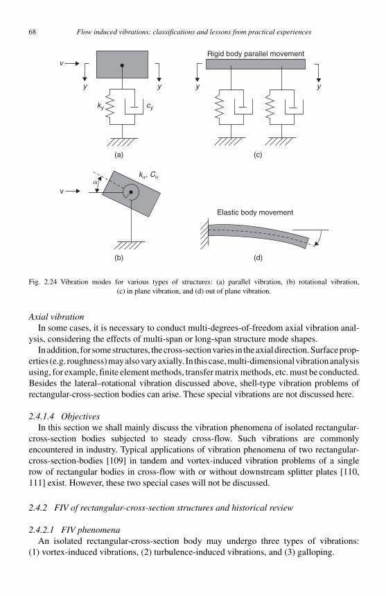
68 Flow induced vibrations: classifications and lessons from practical experiences
Axial vibration In some cases, it is necessary to conduct multi-degrees-of-freedom axial vibration anal-
ysis, considering the effects of multi-span or long-span structure mode shapes. In addition, for some structures, the cross-section varies in the axial direction. Surface prop-
erties (e.g. roughness) may also vary axially. In this case, multi-dimensional vibration analysisusing, for example, finite element methods, transfer matrix methods, etc. must be conducted.Besides the lateral–rotational vibration discussed above, shell-type vibration problems of rectangular-cross-section bodies can arise. These special vibrations are not discussed here.
2.4.1.4 Objectives In this section we shall mainly discuss the vibration phenomena of isolated rectangular-
cross-section bodies subjected to steady cross-flow. Such vibrations are commonly encountered in industry. Typical applications of vibration phenomena of two rectangular-cross-section-bodies [109] in tandem and vortex-induced vibration problems of a single row of rectangular bodies in cross-flow with or without downstream splitter plates [110, 111] exist. However, these two special cases will not be discussed.
2.4.2 FIV of rectangular-cross-section structures and historical review
2.4.2.1 FIV phenomena An isolated rectangular-cross-section body may undergo three types of vibrations:
(1) vortex-induced vibrations, (2) turbulence-induced vibrations, and (3) galloping.
(a) (c)
v
y
cyky
y y y
Rigid body parallel movement
(d)
Elastic body movement
(b)
v
ka, Caa
Fig. 2.24 Vibration modes for various types of structures: (a) parallel vibration, (b) rotational vibration, (c) in plane vibration, and (d) out of plane vibration .

Chapter 2. Vibration Induced by Cross-Flow 69
Vortex-induced vibration Around a rectangular-cross-section body, vortices are shed at the corners and flow down-
stream. The behavior of the vortices is similar to that observed in the case of a circular cylinder. The frequency of Karman vortex shedding behind a rectangular-cross-section body is affected by the body ’ s aspect ratio and the flow attack angle.
When the natural frequency of the body is close to the vortex shedding frequency, lock-in of the shedding frequency to the structural frequency may occur. Lock-in is pos-sible transverse to the flow direction as well as in the flow direction.
Careful examination is needed for transverse vibration since the vibration can be large enough to cause structural failure. Various kinds of vibration can be observed depending on the aspect ratio of the cross-section, the angle of attack, and the vibration direction (parallel/normal to the flow [109] ). There is a lack of comprehensive and systematic knowledge on the effects of large parameter changes, and variations in configuration and flow conditions.
Turbulence-induced vibration Similarly to a circular cylinder, a rectangular-cross-section structure vibrates mainly due
to turbulence when the structure natural frequency is well separated from the dominant vortex shedding frequencies. Turbulence-induced vibration amplitudes are generally larger than amplitudes for a circular cylinder. In addition, the vibration varies with the strength of upstream flow turbulence.
Galloping Suppose that an elastically supported rectangular-cross-sectional body subjected to cross-
flow has an attack angle to the cross-flow. The body, subjected to a static lift force, drag force, and torsional moment in cross-flow, will normally vibrate only slightly in the lift, drag, and/or torsional directions. However, under certain conditions, the vibratory motion itself induces negative dynamic damping leading to dynamic instability. The resulting vibra-tion is also known as galloping. Galloping can arise in the lift and drag directions as well as in torsion. Furthermore, coupled-mode galloping involving a combination of modes is also possible. We adopt the terms “ flutter ” and “ galloping ” to suit the engineering field. The term “ galloping ” is used mainly in civil engineering where the focus is primarily on the single-degree-of-freedom self-excited vibrations of bluff body subjected to wind or ocean tides. On the other hand, the term “ flutter ” is used mainly in the aerospace engineering field, where bending-torsional coupled self-excited vibrations of a streamlined wing subjected to airflow are mainly focused on. Galloping occurs usually far above the critical flow velocity for self-excited vibration by Karman vortex shedding. If the Scruton number, S c , is small, the flow velocity range for Karman vortex vibration and that for galloping vibration may coincide. In this case, the phenomenon becomes complicated and evaluation becomes difficult [112] .
2.4.2.2 Historical background
Vortex-induced vibration The Strouhal number is defined by:
St W�f d
V (2.37)
70 Flow induced vibrations: classifications and lessons from practical experiences
fW being the vortex shedding frequency, V the approach flow velocity, and d the projected width normal to the flow direction.
The Strouhal number, St, for a rectangular body is affected by the aspect ratio, attack angle, as well as the radius of curvature of the corners. It is also affected by flow condi-tions (Reynolds number) and turbulence intensity in the main stream. Strouhal numbers for rectangular bodies, obtained experimentally by many researchers, seem to fit within the range 0.1 � St � 0.2 [109] , with the exception of bodies rounded off at the corners. The Strouhal number, St, for the latter falls within the range 0.2 � St � 0.3.
Little data exists on Strouhal numbers for high Reynolds number flows commonly encountered in actual industrial processes. Clearly much more work is needed for these flows.
Many researchers have attempted to theoretically predict the maximum vibration amplitude for circular cylinders at lock-in. There are, however, few investigations on rec-tangular-cross-section bodies.
According to the study of Naudascher [109] , a rectangular-cross-section body can vibrate in various vibration modes. The vibration depends on: (i) cross-section shape (aspect ratio, attack angle, and the corner radius of curvature), (ii) characteristics of the body (mass, damping, and elastic characteristics in the flow direction, direction orthogonal to the flow, and rotational direction), and (iii) flow characteristics such as Reynolds number, turbulence intensity. Thus far a systematic database, which is needed for evaluating vortex-induced vibration, has not been established. Therefore if one wishes to evaluate the vibration of a rectangular-cross-section body, a search through past studies on the vibration behavior of similar bodies must be done to determine the expected vibration characteristics. It is espe-cially difficult to predict vibration characteristics in high Reynolds number flow regimes; little is known about Strouhal number characteristics here.
Turbulence-induced vibration To analyze the turbulence-induced vibration of bluff bodies, the PSD of the turbulence-
induced forces acting on the body is measured experimentally and expressed in normal-ized form. The response of the body is computed using the normalized PSD.
Recently, in the architectural and civil engineering fields, experimental PSD data for flexible structures (tall buildings, etc.), which vibrate fairly easily when subjected to wind turbulence, have been actively accumulated. PSD data for rectangular-cross-section bodies, however, depend on many parameters, such as the cross-section shape (aspect ratio, attack angle, and the radius of curvature of corners of the body), and flow charac-teristics (Reynolds number, turbulence intensity). This is much like the case of a circular cylinder. The existing database is still quite limited, especially for high Reynolds number flows. To evaluate the turbulence-induced vibration of a rectangular body, past studies must be searched to find PSDs as closely relevant as possible to the body under study.
With the continuing increase of computational power, CFD methods for the determina-tion of turbulence-induced PSDs for rectangular-cross-section bodies are under develop-ment. The methods numerically evaluate PSDs for very complicated cross-section bodies without experimental input. Practical application may be expected in the near future.
Galloping When ice builds up on power transmission lines (thus changing the effective cross-
sectional geometry) large amplitude vibrations can arise. The phenomenon is named
Chapter 2. Vibration Induced by Cross-Flow 71
galloping, due to the similarity of the power line vibration to a galloping horse. Galloping, which was likely the cause of the Tacoma narrows bridge collapse in 1940, was explained theoretically by Den Hartog [113] . Thereafter, researchers such as Novak [114, 115] ,Nakamura [108, 110, 111] , and Naudascher and Rockwell [104, 117] investigated the gal-loping of bodies of various cross-section shapes for a wide range of flow conditions. This work was done in the four-decade period from the 1950s to the 1980s. Regions of self-excited vibrations such as galloping can be evaluated to examine the negative damping condition using the lift and drag coefficients obtained experimentally or theoretically. The vibration amplitude during galloping can also be evaluated analytically/quantitatively, with reasonable accuracy, using non-linear differential equation analysis methods based on the assumption of slowly varying amplitude and phase. It is extremely important to accurately determine the flow condition for the onset of bending-torsion coupled-mode flutter for air-plane wings. The critical speed for flutter and prevention of airplane flutter have been inves-tigated actively from the 1950s to the 1980s. Evaluation methods are now well established for many types of airfoils.
2.4.3 Evaluation methods
The ASME Code Sec. III, Div. 1, Appendix N, 1300 Series are the first standards of evaluation methods concerning vortex- and turbulence-induced vibration of circular cyl-inders in steady cross-flow. The same evaluation methods can be applied to the evalu-ation of vortex- and turbulence-induced vibrations of a rectangular-cross-section body. However, the standard contains only data (e.g. Strouhal numbers) for the evaluation of circular cylinder vibration. One may therefore either perform approximate analysis based on circular cylinder data or conduct experiments to obtain data for non-circular cross-sec-tion bodies.
There is no detailed description of galloping in the ASME Code. Refs. [23, 77, 117] may serve as useful sources of information.
2.4.3.1 Vortex-induced vibration The frequency fW at which vortices induce a periodic force on a rectangular body is
given by:
fV
dW St� (2.38)
where V is the upstream flow velocity, and d a characteristic length dimension (e.g. cross-section width transverse to the flow).
The Strouhal number, St, which is an important non-dimensional coefficient, is obtained experimentally. Generally, large amplitude vortex-induced vibrations of a rectangular-cross-section body will not be observed and the integrity of the structure will be maintained, unless the frequency of vortex shedding is locked into a frequency of the body. If the fre-quency of vortex shedding coincides with a structural natural frequency, the lock-in phe-nomenon discussed above can occur, resulting in resonant vibration. Evaluation methods for self-excited resonant vibrations are discussed below.
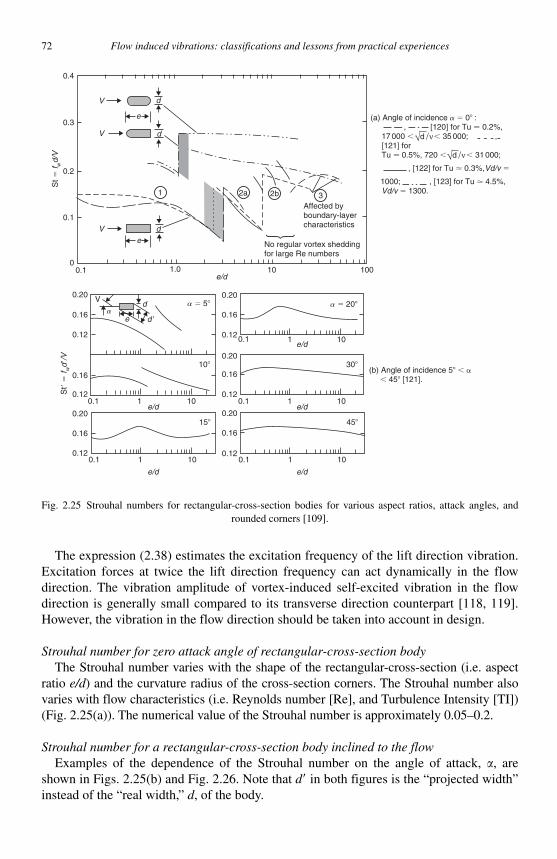
72 Flow induced vibrations: classifications and lessons from practical experiences
The expression (2.38) estimates the excitation frequency of the lift direction vibration. Excitation forces at twice the lift direction frequency can act dynamically in the flow direction. The vibration amplitude of vortex-induced self-excited vibration in the flow direction is generally small compared to its transverse direction counterpart [118, 119]. However, the vibration in the flow direction should be taken into account in design.
Strouhal number for zero attack angle of rectangular-cross-section body The Strouhal number varies with the shape of the rectangular-cross-section (i.e. aspect
ratio e/d ) and the curvature radius of the cross-section corners. The Strouhal number also varies with flow characteristics (i.e. Reynolds number [Re], and Turbulence Intensity [TI]) ( Fig. 2.25(a) ). The numerical value of the Strouhal number is approximately 0.05–0.2.
Strouhal number for a rectangular-cross-section body inclined to the flow Examples of the dependence of the Strouhal number on the angle of attack, � , are
shown in Figs. 2.25(b) and Fig. 2.26 . Note that d� in both figures is the “ projected width ” instead of the “ real width, ” d , of the body.
0.20
0.16
0.12
0.16
0.12
0.20
0.16
0.1210 0.1
0.12
0.16
0.20
0.12
0.16
0.20
0.12
0.16
0.20
1 100.1 1
e
Vd
d �
St�
� f w
d�/V
e/d
0.1 1 10e/d
0.1 1 10e/d
e/d
10
10� 30�
45�15�
a � 5� a � 20�
0.1 1e/d
a
V
V
V
0.2
0.3
0.4
0.1
00.1 1.0
de
1 2a 2b 3Affected byboundary-layercharacteristics
e
d
d
St�
f wd/
V
10
No regular vortex sheddingfor large Re numbers
100e/d
(a) Angle of incidence a � 0� : , [120] for Tu � 0.2%, 17 000 � � 35 000; , [121] for Tu � 0.5%, 720 � � 31 000;
, [122] for Tu � 0.3%,Vd/v �
1000; , [123] for Tu � 4.5%,Vd/v � 1300.
(b) Angle of incidence 5� � � � 45� [121].
√d ν/
√d ν/
Fig. 2.25 Strouhal numbers for rectangular-cross-section bodies for various aspect ratios, attack angles, and rounded corners [109] .

Chapter 2. Vibration Induced by Cross-Flow 73
Flow speed range of vortex-induced vibrations for a rectangular-cross-section body When the non-dimensional flow speed, Vr , is increased from a low value, the four dif-
ferent vibration mechanisms in Table 2.14 are possible depending on the angle of attack, � , and the aspect ratio, e/d (see also Figs. 2.27 and 2.28 ).
0.30
0.20
0.10
e
a
d
d�V (a) Data for square-edged prism:—, [124] for Tu � 0.8%,
Vd/v � 1500, aspect ratio L/e � 10;- - -, [121] for
Tu�0.5%, � 2000,
L/e � 3.2;— –, [125] for Tu � 2.4%, 1000 � � 2500, L/e � 8.
V
V
e/d � 10
e/d � 10
0
0.25
0.20
St�
� f w
d�/V
St�
� f w
d�/V
0.15
0.100� 10� 20� 50�
a30� 40�
0� 10� 20� 50�30� 40�
(b) Data for prism with square and rounded edges [124], for � 1500, L/e � 10: , , Tu � 0.8%; Tu � 2.1%.,
Vd
Vd
νVd
ν
ν
Fig. 2.26 Effect of attack angle on Strouhal number for large aspect ratio ( e/d � 10) [109] .
Table 2.14 Types of vortex-induced vibration of a rectangular cross-section body in cross-flow [109]
Aspect ratio: e/d
Attack angle: � Kinds of vortex shedding Possible vibration
0 � e/d � 2 – LEVS: Leading-edge vortex shedding (separation bubble at leading edge of the body [ Fig. 2.27 ])
• Karman vortex-induced vibration in the transverse direction
• Galloping caused by negative damping with the body movement
2 � e/d � 16 – ILEV: Impinging leading-edge vortex shedding (vortices detached from leading edge attach again on the body before passing trailing-edge [ Fig. 2.27] )
Karman vortex-induced vibration in the transverse flow direction as well as the rotational direction
16 � e/d – TEVS: Trailing-edge vortex shedding (vortices detach from the trailing edge of the body [ Fig. 2.27] )
The vibration characteristics are similar to that of a flat board, but the amplitude might not be large
10 � e/d 10 ° � � AEVS: Alternate-edge vortex-shedding (vortex shedding in turn from leading/trailing edges is observed [ Fig. 2.28 ])
When both attack angle and aspect ratio are large, vortex shedding in the condition of IEVS/TEVS causes vibrations in the flow direction or in the chord direction
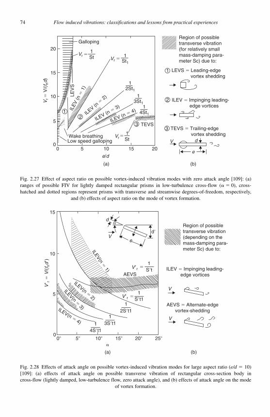
74 Flow induced vibrations: classifications and lessons from practical experiences
15
10
ILEV(n�
1)
ILEV(n�
2)
ILEV(n�
3)ILEV(n � 4)
V� r
� V
/(f n
d�)
d
d�V
V�r
V�r
e
1S�t
1
AEVS
1S�t1
2S�t11
3S�t114S�t1
�
5
00� 5� 10� 15� 20� 25�
�
�
�
V
V
ILEV � Impinging leading-edge vortices
AEVS � Alternate-edgevortex-shedding
Region of possibletransverse vibration(depending on themass-damping para-meter Sc) due to:
(a) (b)
Fig. 2.28 Effects of attack angle on possible vortex-induced vibration modes for large aspect ratio ( e/d � 10) [109] : (a) effects of attack angle on possible transverse vibration of rectangular cross-section body in cross-flow (lightly damped, low-turbulence flow, zero attack angle), and (b) effects of attack angle on the mode
of vortex formation.
20
Galloping
LEV
SLEVS � Leading-edge vortex shedding
ILEV � Impinging leading- edge vortices
TEVS � Trailing-edge vortex shedding
Region of possibletransverse vibration(for relatively smallmass-damping para-meter Sc) due to:
Wake breathingLow speed galloping
15
10
5
00 5 10
VrV
e
d
15 20
e/d
1St
Vr1St Vr
1�
�
St1
14St1
12St1
TEVS3
21
1
2
3
Vr�
V/(
f nd)
13St1
ILE
V (n
� 1
)
ILEV (n �
2)
ILEV (n � 3)
ILEV (n � 4)
�
(a) (b)
Fig. 2.27 Effect of aspect ratio on possible vortex-induced vibration modes with zero attack angle [109] : (a) ranges of possible FIV for lightly damped rectangular prisms in low-turbulence cross-flow (� � 0), cross-hatched and dotted regions represent prisms with transverse and streamwise degrees-of-freedom, respectively,
and (b) effects of aspect ratio on the mode of vortex formation.
Chapter 2. Vibration Induced by Cross-Flow 75
Vibration amplitude of vortex-induced vibrations for a rectangular-cross-section body The amplitude of vortex-induced vibrations for a rectangular-cross-section body may be
predicted using the evaluation methods developed for a circular cross-section body. However, there seems to be only a few studies, including work by Naudascher and Wang [109] . The latter discuss the effect of aspect ratio, attack angle, corner radius of curvature, and vibration direction in the flow on vibration amplitudes measured experimentally.
2.4.3.2 Turbulence-induced vibration The turbulence-induced vibration response of a rectangular-cross-section body can also be
evaluated with the method presented in the Japanese JSME S 012 guideline. The method has already been detailed in Section 2.1.3 of this book. However, for the reader ’ s convenience, the essence of the method, applied to rectangular-cross-section bodies, is outlined below.
The turbulence-induced vibration response is obtained based on random vibration the-ory. The root-mean-square-value, wmean , of the turbulence-induced vibration amplitude is evaluated using the following expression:
wG f
m fz2 0 0
3 20
364meanF
02( )( )�
�� �
φ (2.39)
where
�0
0
0
�
φ
φ
( )d
( )d2
z z
z z
Le
L
∫
∫
m is the mass per unit length and � is the damping ratio of the structure. After introducing the conversion coefficient C0 , the peak-value of the turbulence-
induced vibration is evaluated using Eq. (2.39).
w z CG f
m fzR
F( )( )
( )� 00 0
3 20
3 064
�� �
φ (2.40)
where C0 is approximately 3–5. Using the standardized PSD, � , and unsteady fluid force coefficient, C� , the PSD GF ( f )
of the random excitation force per unit length is given by:
G f C V d fF ( ) ( ) ( )� �1
22 2� �
� �( ) ( )C V d fd
V
1
22 2� � (2.41)
where � is the fluid density and ffd
V� is a non-dimensional frequency.
General expressions for the standardized PSD � ( f ) in Eq. (2.41) are generally unknown for rectangular-cross-section structures. It is thus necessary to estimate � ( f ) based on results of similar past experimental studies, or to conduct model tests to determine � ( f ).
76 Flow induced vibrations: classifications and lessons from practical experiences
2.4.3.3 Galloping Consider the galloping phenomenon in the lift (transverse) direction. The transverse
motion of the body at the velocity �y relative to an upstream velocity V induces a relative angle of attack given by:
���y
V (2.42)
The resultant fluid force in the lift direction is then:
F V dC V dC
CLyd
LD
2 )� � � � �� �
1
2
1
202
0
2
0
� ���
� ��
�⎛
⎝⎜⎜⎜
⎞
⎠⎟⎟⎟⎟ ( (2.43)
In the Eq. (2.43), �Cy/�� � � �CL/�� � CD is an important coefficient of the fluid force, where Cy is the vertical force coefficient [77]. A positive value of the vertical force coef-ficient derivative ( �Cy/�� � 0) indicates that the fluid force acts in the direction of motion of the body. The fluid force thus amplifies the body ’ s vibration in the lift direction if �CL/�� is negative and the absolute value of �CL/�� is larger than the drag coefficient (i.e. �CL/�� � CD � 0). Self-excited vibrations finally occur when the negative fluid force overcomes the internal damping of the structure. The critical velocity is given by:
Vm
dC
C
� �
��
4
0
��
����
�
LD
⎛
⎝⎜⎜⎜
⎞
⎠⎟⎟⎟⎟
(2.44)
Table 2.15 [77] shows values of �Cy/�� � ��CL/���CD for various cross-section shapes. This data may be useful to the reader wishing to determine the critical velocity for galloping.
The vibration amplitude of galloping in the lift direction can be evaluated assuming that the amplitude and phase of the non-linear vibrations vary slowly. The equation of motion in the lift direction is:
my m y k y V dC�� �� � �21
22� � �y y y y (2.45)
Expanding the force coefficient Cy in a Taylor series of the angle of attack � defined in Eq. (2.42).
C a a a a
a ay
Va
y
V
y( )� � � �� � � � �
� � �
0 1 22
33
0 1 2
�� �⎛
⎝⎜⎜⎜⎞
⎠⎟⎟⎟⎟
⎛
⎝⎜⎜⎜⎞
⎠⎟⎟⎟⎟⎟
⎛
⎝⎜⎜⎜⎞
⎠⎟⎟⎟⎟
2
3
3
� �ay
V
��
(2.46)
Several examples of the Taylor approximation are presented in Table 2.16 . An approxi-mate solution of the limit cycle amplitude of the non-linear equation (2.45) is obtained based on Eq. (2.46) with the assumption that both the amplitude and phase are slowly varying. Novak [114] derived the following simple expression for the vibration amplitude
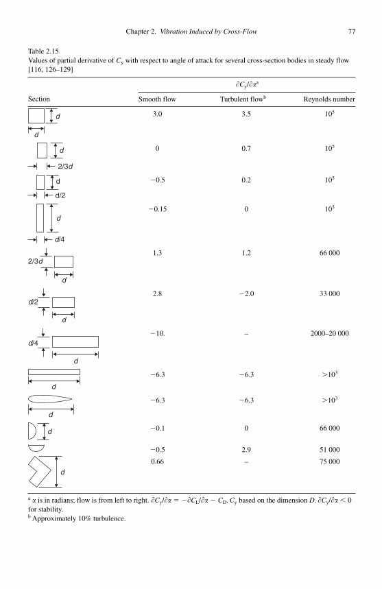
Chapter 2. Vibration Induced by Cross-Flow 77
Table 2.15 Values of partial derivative of Cy with respect to angle of attack for several cross-section bodies in steady flow [116, 126–129]
� Cy / ��a
Section Smooth flow Turbulent flow b Reynolds number
d
d 3.0 3.5 10 5
2/3d
d 0 0.7 10 5
d/2
d � 0.5 0.2 10 5
d/4
d� 0.15 0 10 5
d
2/3d 1.3 1.2 66 000
d
d/2 2.8 � 2.0 33 000
d
d/4� 10. – 2000–20 000
d
� 6.3 � 6.3 � 10 3
d
� 6.3 � 6.3 � 10 3
d � 0.1 0 66 000
� 0.5 2.9 51 000
d
0.66 – 75 000
a � is in radians; flow is from left to right. �Cy / �� � ��CL / �� � CD. Cy based on the dimension D. �Cy/�� � 0 for stability.b Approximately 10% turbulence.
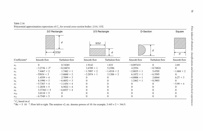
78F
low induced vibrations: classifications and lessons from
practical experiences
Table 2.16 Polynomial approximation expressions of Cy for several cross-section bodies [114, 115]
3/2 Rectangle
d
2/3d
2/3 Rectangle
d
3/2d
D-Section
d
Square
d
Coefficients a Smooth flow Turbulent flow Smooth flow Turbulent flow Smooth flow Turbulent flow Smooth flow
a1 0 0.74285 1.9142 1.833 � 0.097431 0 2.69 a2 � 3.2736 � 1 b � 0.24874 3.4789 � 1 5.2396 4.2554 � 0.74824 0 a3 7.4467 � 2 1.7482 � 1 � 1.7097 � 2 � 1.4518 � 2 � 2.8835 � 1 5.4705 � 1.684 � 2 a4 � 55834 � 3 � 3.6060 � 2 � 2.2074 � 1 3.1206 � 2 6.1072 � 1 � 6.3595 0. a5 1.4559 � 4 2.7099 � 3 0 0 � 4.8006 � 1 2.6844 6.27 � 3 a6 8.1990 � 3 � 6.4052 � 3 0 0 1.2462 � 1 � 0.3903 0 a7 � 5.7367 � 4 � 1.1454 � 4 0 0 0 0 � 5.99 � 4 a8 � 1.2038 � 5 6.5022 � 4 0 0 0 0 0 a9 3.37363 � 5 � 6.6937 � 4 0 0 0 0 0 a10 2.0118 � 5 0 0 0 0 0 0 a11 � 6.7549 � 5 0 0 0 0 0 0
a Cy based on d.b Re � 5 10 4 . Flow left to right. The notation +2, etc. denotes powers of 10: for example, 3.445 + 2 � 344.5.
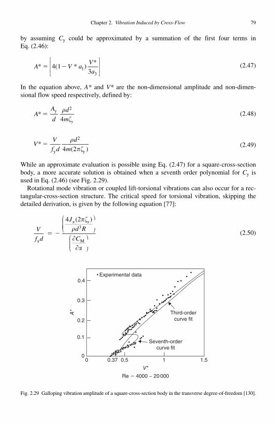
Chapter 2. Vibration Induced by Cross-Flow 79
by assuming Cy could be approximated by a summation of the first four terms in Eq. (2.46):
A V aV
a* (1 )
*� �4
313
*⎡
⎣⎢⎢
⎤
⎦⎥⎥ (2.47)
In the equation above, A* and V* are the non-dimensional amplitude and non-dimen-sional flow speed respectively, defined by:
AA
d
d
m y
* �y �
�
2
4 (2.48)
VV
f d
d
m* �
y y(2 )
���
2
4 (2.49)
While an approximate evaluation is possible using Eq. (2.47) for a square-cross-section body, a more accurate solution is obtained when a seventh order polynomial for Cy is used in Eq. (2.46) (see Fig. 2.29 ).
Rotational mode vibration or coupled lift-torsional vibrations can also occur for a rec-tangular-cross-section structure. The critical speed for torsional vibration, skipping the detailed derivation, is given by the following equation [77] :
V
f d
J
d R
C�
� �������
( )
M
� �
4 23
⎛
⎝⎜⎜⎜⎜
⎞
⎠⎟⎟⎟⎟
⎛
⎝⎜⎜⎜
⎞
⎠⎟⎟⎟⎟
(2.50)
0.4
0.3
0.2
0.1
00 0.37 0.5
Re � 4000 ~ 20 000
V*
A*
1
Seventh-ordercurve fit
1.5
Third-ordercurve fit
Experimental data
Fig. 2.29 Galloping vibration amplitude of a square-cross-section body in the transverse degree-of-freedom [130] .
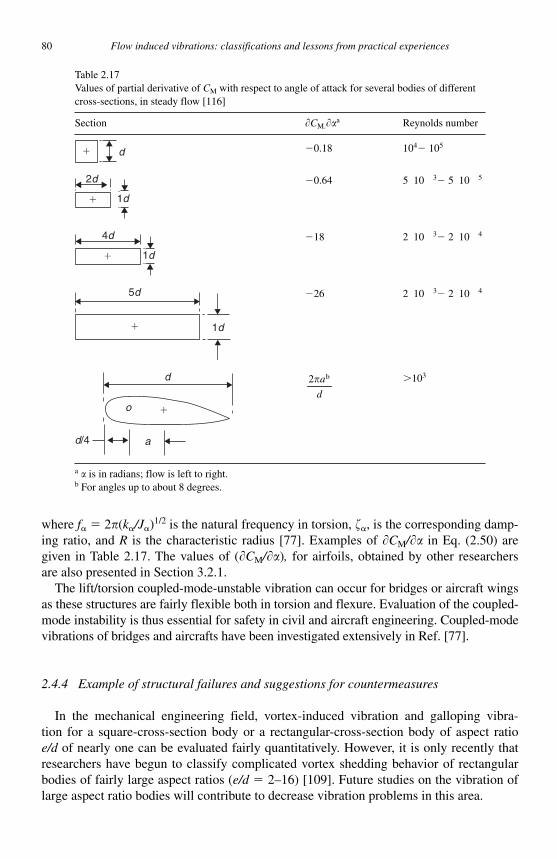
80 Flow induced vibrations: classifications and lessons from practical experiences
where f� � 2 � ( k� /J � ) 1/2 is the natural frequency in torsion, �� , is the corresponding damp-ing ratio, and R is the characteristic radius [77] . Examples of �CM/�� in Eq. (2.50) are given in Table 2.17 . The values of ( �CM/�� ) , for airfoils, obtained by other researchers are also presented in Section 3.2.1.
The lift/torsion coupled-mode-unstable vibration can occur for bridges or aircraft wings as these structures are fairly flexible both in torsion and flexure. Evaluation of the coupled-mode instability is thus essential for safety in civil and aircraft engineering. Coupled-mode vibrations of bridges and aircrafts have been investigated extensively in Ref. [77] .
2.4.4 Example of structural failures and suggestions for countermeasures
In the mechanical engineering field, vortex-induced vibration and galloping vibra-tion for a square-cross-section body or a rectangular-cross-section body of aspect ratio e/d of nearly one can be evaluated fairly quantitatively. However, it is only recently that researchers have begun to classify complicated vortex shedding behavior of rectangular bodies of fairly large aspect ratios ( e/d � 2–16) [109] . Future studies on the vibration of large aspect ratio bodies will contribute to decrease vibration problems in this area.
Table 2.17 Values of partial derivative of CM with respect to angle of attack for several bodies of different cross-sections, in steady flow [116]
Section �CM.��a Reynolds number
d� � 0.18 10 4� 10 5
1d
2d
�
� 0.64 5 10 3� 5 10 5
4d
� 1d
� 18 2 10 3� 2 10 4
5d
� 1d
� 26 2 10 3� 2 10 4
d
o �
ad/4
b2 a
d
� � 10 3
a � is in radians; flow is left to right.b For angles up to about 8 degrees.
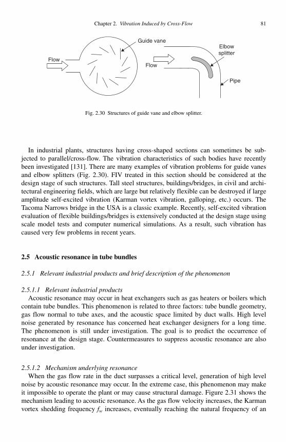
Chapter 2. Vibration Induced by Cross-Flow 81
In industrial plants, structures having cross-shaped sections can sometimes be sub-jected to parallel/cross-flow. The vibration characteristics of such bodies have recently been investigated [131] . There are many examples of vibration problems for guide vanes and elbow splitters ( Fig. 2.30 ). FIV treated in this section should be considered at the design stage of such structures. Tall steel structures, buildings/bridges, in civil and archi-tectural engineering fields, which are large but relatively flexible can be destroyed if large amplitude self-excited vibration (Karman vortex vibration, galloping, etc.) occurs. The Tacoma Narrows bridge in the USA is a classic example. Recently, self-excited vibration evaluation of flexible buildings/bridges is extensively conducted at the design stage using scale model tests and computer numerical simulations. As a result, such vibration has caused very few problems in recent years.
2.5 Acoustic resonance in tube bundles
2.5.1 Relevant industrial products and brief description of the phenomenon
2.5.1.1 Relevant industrial products Acoustic resonance may occur in heat exchangers such as gas heaters or boilers which
contain tube bundles. This phenomenon is related to three factors: tube bundle geometry, gas flow normal to tube axes, and the acoustic space limited by duct walls. High level noise generated by resonance has concerned heat exchanger designers for a long time. The phenomenon is still under investigation. The goal is to predict the occurrence of resonance at the design stage. Countermeasures to suppress acoustic resonance are also under investigation.
2.5.1.2 Mechanism underlying resonance When the gas flow rate in the duct surpasses a critical level, generation of high level
noise by acoustic resonance may occur. In the extreme case, this phenomenon may make it impossible to operate the plant or may cause structural damage. Figure 2.31 shows the mechanism leading to acoustic resonance. As the gas flow velocity increases, the Karman vortex shedding frequency fw increases, eventually reaching the natural frequency of an
Guide vane
Flow
Pipe
Flow
Elbowsplitter
Fig. 2.30 Structures of guide vane and elbow splitter.
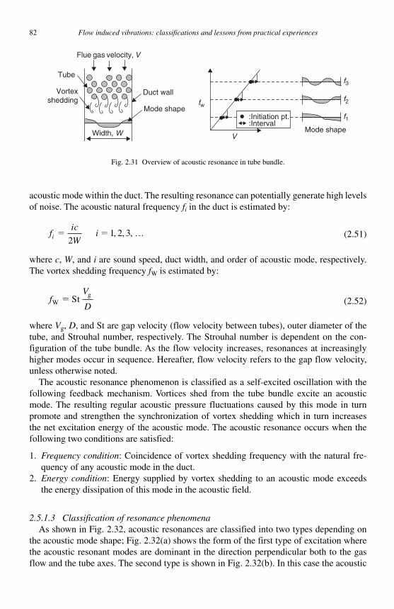
82 Flow induced vibrations: classifications and lessons from practical experiences
acoustic mode within the duct. The resulting resonance can potentially generate high levelsof noise. The acoustic natural frequency fi in the duct is estimated by:
fic
Wii � �
21 2 3, , ,… (2.51)
where c , W , and i are sound speed, duct width, and order of acoustic mode, respectively. The vortex shedding frequency fW is estimated by:
fV
DWgSt� (2.52)
where Vg , D , and St are gap velocity (flow velocity between tubes), outer diameter of the tube, and Strouhal number, respectively. The Strouhal number is dependent on the con-figuration of the tube bundle. As the flow velocity increases, resonances at increasingly higher modes occur in sequence. Hereafter, flow velocity refers to the gap flow velocity, unless otherwise noted.
The acoustic resonance phenomenon is classified as a self-excited oscillation with the following feedback mechanism. Vortices shed from the tube bundle excite an acoustic mode. The resulting regular acoustic pressure fluctuations caused by this mode in turn promote and strengthen the synchronization of vortex shedding which in turn increases the net excitation energy of the acoustic mode. The acoustic resonance occurs when the following two conditions are satisfied:
1. Frequency condition : Coincidence of vortex shedding frequency with the natural fre-quency of any acoustic mode in the duct.
2. Energy condition : Energy supplied by vortex shedding to an acoustic mode exceeds the energy dissipation of this mode in the acoustic field.
2.5.1.3 Classification of resonance phenomena As shown in Fig. 2.32 , acoustic resonances are classified into two types depending on
the acoustic mode shape; Fig. 2.32(a) shows the form of the first type of excitation where the acoustic resonant modes are dominant in the direction perpendicular both to the gas flow and the tube axes. The second type is shown in Fig. 2.32(b) . In this case the acoustic
Vortexshedding
Duct wall
Mode shape
:Initiation pt.:Interval
Flue gas velocity, V
Tube
Width, W Mode shapeV
fw
f3
f2
f1:Initiation pt.:Interval
Mode shape
Fig. 2.31 Overview of acoustic resonance in tube bundle.

Chapter 2. Vibration Induced by Cross-Flow 83
modes parallel to the gas flow direction are dominant. Hereafter, the first type is referred to as the transverse mode resonance while the second type is referred to as the longitudi-nal mode resonance.
The transverse mode resonance is more commonly encountered than its longitudinal counterpart. It is further classified into two types depending on the location of resonance in the tube bundle; the type where the main part of the resonance exists within the tube bun-dle and the other where the resonance occurs mainly in the cavity between upstream and downstream tube bundles. To eliminate these types of acoustic resonances, baffle plates are introduced. Subdivision of the acoustic space effectively increases the resonant frequencies of the acoustic modes separating them from the vortex shedding frequency. For the sec-ond type of resonance which occurs in the cavity, baffle plates must be located within the cavity, or within the cavity and tube bundle itself. Therefore, when countermeasures are required, it is recommended to measure the acoustic pressure distribution in the duct.
For the longitudinal mode resonance, the foregoing baffle plate method is generally not regarded as an effective countermeasure. Countermeasures will be presented later in Section 2.5.2.2. Resonance with both types of acoustic modes involves “ lock-in. ” Once resonance occurs, the vortex shedding frequency is captured by the acoustic natural fre-quency over a range of gas flow velocities. As a reference, in Section 2.1.2, a similar phe-nomenon was discussed where lock-in occurred between the vortex shedding frequencies and the structural natural frequencies.
2.5.2 Historical background
Key research issues include prediction of resonance and estimation of the critical gas flow velocity for a given tube bundle configuration and acoustic space geometry in ducts. Many studies have attempted to clarify the relation between the occurrence of resonance and the two foregoing frequency and energy conditions.
Since the early 1950s there have been many research articles on resonance phenom-ena in heat exchangers [132] . The work of Y.N. Chen [133] in 1968 is well known as a breakthrough in this field. Chen was the first to identify the relationship between reso-nant noise and Karman vortex shedding. To study this relationship hot-wire measure-ments, coupled with excitation force measurements, using strain gauges mounted on a tube were conducted. The tests revealed that the vortex shedding was synchronized with
(a) (b)
Baffle plate
Mode shape(pressure)
Tube bundleV
V
Fig. 2.32 Classification of acoustic resonance by mode shape: (a) transverse mode, and (b) longitudinal mode.
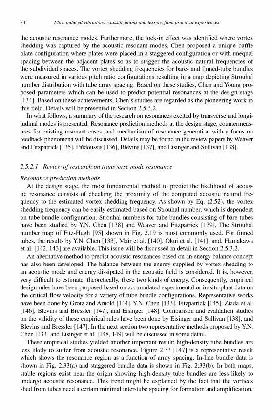
84 Flow induced vibrations: classifications and lessons from practical experiences
the acoustic resonance modes. Furthermore, the lock-in effect was identified where vortex shedding was captured by the acoustic resonant modes. Chen proposed a unique baffle plate configuration where plates were placed in a staggered configuration or with unequal spacing between the adjacent plates so as to stagger the acoustic natural frequencies of the subdivided spaces. The vortex shedding frequencies for bare- and finned-tube bundles were measured in various pitch ratio configurations resulting in a map depicting Strouhal number distribution with tube array spacing. Based on these studies, Chen and Young pro-posed parameters which can be used to predict potential resonances at the design stage [134] . Based on these achievements, Chen’s studies are regarded as the pioneering work in this field. Details will be presented in Section 2.5.3.2.
In what follows, a summary of the research on resonances excited by transverse and longi-tudinal modes is presented. Resonance prediction methods at the design stage, countermeas-ures for existing resonant cases, and mechanism of resonance generation with a focus on feedback phenomena will be discussed. Details may be found in the review papers by Weaver and Fitzpatrick [135] , Païdoussis [136] , Blevins [137] , and Eisinger and Sullivan [138] .
2.5.2.1 Review of research on transverse mode resonance
Resonance prediction methods At the design stage, the most fundamental method to predict the likelihood of acous-
tic resonance consists of checking the proximity of the computed acoustic natural fre-quency to the estimated vortex shedding frequency. As shown by Eq. (2.52), the vortex shedding frequency can be easily estimated based on Strouhal number, which is dependent on tube bundle configuration. Strouhal numbers for tube bundles consisting of bare tubes have been studied by Y.N. Chen [138] and Weaver and Fitzpatrick [139] . The Strouhal number map of Fitz-Hugh [95] shown in Fig. 2.19 is most commonly used. For finned tubes, the results by Y.N. Chen [133] , Mair et al. [140] , Okui et al. [141] , and, Hamakawa et al. [142, 143] are available. This issue will be discussed in detail in Section 2.5.3.2.
An alternative method to predict acoustic resonances based on an energy balance concept has also been developed. The balance between the energy supplied by vortex shedding to an acoustic mode and energy dissipated in the acoustic field is considered. It is, however, very difficult to estimate, theoretically, these two kinds of energy. Consequently, empirical design rules have been proposed based on accumulated experimental or in-situ plant data on the crit ical flow velocity for a variety of tube bundle configurations. Representative works have been done by Grotz and Arnold [144] , Y.N. Chen [133] , Fitzpatrick [145] , Ziada et al. [146] , Blevins and Bressler [147] , and Eisinger [148] . Comparison and evaluation studies on the validity of these empirical rules have been done by Eisinger and Sullivan [138] , and Blevins and Bressler [147] . In the next section two representative methods proposed by Y.N. Chen [133] and Eisinger et al. [148, 149] will be discussed in some detail.
These empirical studies yielded another important result: high-density tube bundles are less likely to suffer from acoustic resonance. Figure 2.33 [147] is a representative result which shows the resonance region as a function of array spacing. In-line bundle data is shown in Fig. 2.33(a) and staggered bundle data is shown in Fig. 2.33(b) . In both maps, stable regions exist near the origin showing high-density tube bundles are less likely to undergo acoustic resonance. This trend might be explained by the fact that the vortices shed from tubes need a certain minimal inter-tube spacing for formation and amplification.
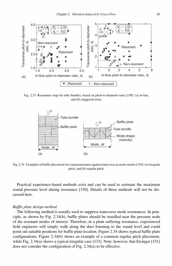
Chapter 2. Vibration Induced by Cross-Flow 85
Practical experience-based methods exist and can be used to estimate the maximum sound pressure level during resonance [150] . Details of these methods will not be dis-cussed here.
Baffle plate design method The following method is usually used to suppress transverse mode resonances. In prin-
ciple, as shown by Fig. 2.34(b) , baffle plates should be installed near the pressure node of the resonant modes of interest. Therefore, in a plant suffering resonance, experienced field engineers will simply walk along the duct listening to the sound level and could point out suitable positions for baffle plate location. Figure 2.34 shows typical baffle plate configurations. Figure 2.34(b) shows an example of a common regular pitch placement, while Fig. 2.34(a) shows a typical irregular case [133] . Note, however, that Eisinger [151]does not consider the configuration of Fig. 2.34(a) to be effective.
: Resonant : Non-resonant
5
4
3
2
143 52 81
4.0
3.0D
V LV
L
T
DT
X1 � L/DXt � T/D
X1 � L/DXt � T/D
2.0
1.01.0 2.0 3.0 4.0
In-flow pitch-to-diameter ratio, Xl In-flow pitch-to-diameter ratio, Xl
Resonant
ResonantNon-resonant
Non-resonant
Tra
nsve
rse
pitc
h-to
-dia
met
erra
tio,X
t
Tra
nsve
rse
pitc
h-to
-dia
met
erra
tio,X
t
(a) (b)
Fig. 2.33 Resonance map for tube bundles, based on pitch-to-diameter ratio [150] : (a) in-line, and (b) staggered array.
(a) (b)
Tube bundle
Mode shape(velocity)
Baffle plateV
Width, W
Tube bundle
Baffle plate
V
Width, W
Fig. 2.34 Examples of baffle placement for countermeasures against transverse acoustic modes [154] : (a) irregular pitch, and (b) regular pitch.
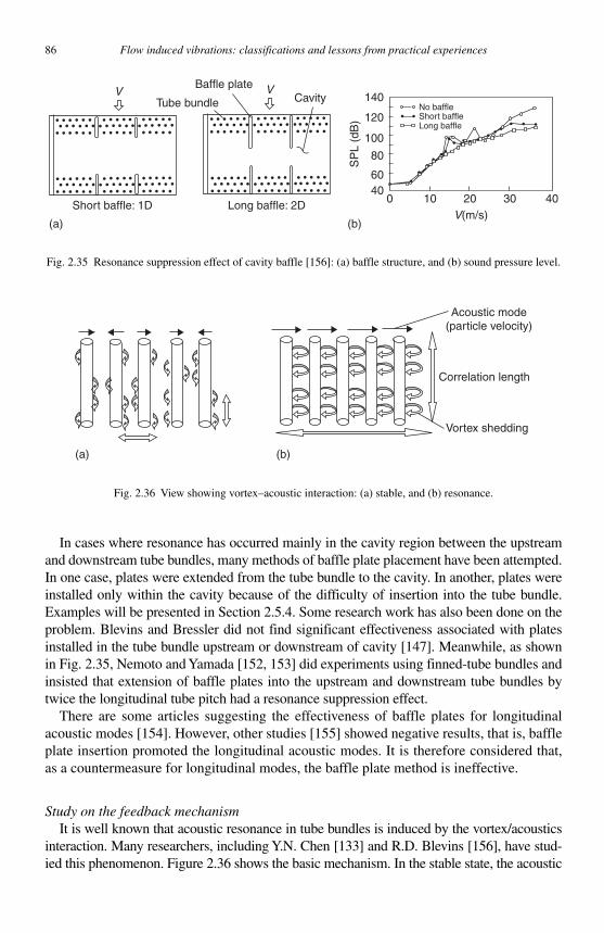
86 Flow induced vibrations: classifications and lessons from practical experiences
In cases where resonance has occurred mainly in the cavity region between the upstream and downstream tube bundles, many methods of baffle plate placement have been attempted. In one case, plates were extended from the tube bundle to the cavity. In another, plates were installed only within the cavity because of the difficulty of insertion into the tube bundle. Examples will be presented in Section 2.5.4. Some research work has also been done on the problem. Blevins and Bressler did not find significant effectiveness associated with plates installed in the tube bundle upstream or downstream of cavity [147] . Meanwhile, as shown in Fig. 2.35 , Nemoto and Yamada [152, 153] did experiments using finned-tube bundles and insisted that extension of baffle plates into the upstream and downstream tube bundles by twice the longitudinal tube pitch had a resonance suppression effect.
There are some articles suggesting the effectiveness of baffle plates for longitudinal acoustic modes [154] . However, other studies [155] showed negative results, that is, baffle plate insertion promoted the longitudinal acoustic modes. It is therefore considered that, as a countermeasure for longitudinal modes, the baffle plate method is ineffective.
Study on the feedback mechanism It is well known that acoustic resonance in tube bundles is induced by the vortex/acoustics
interaction. Many researchers, including Y.N. Chen [133] and R.D. Blevins [156], have stud-ied this phenomenon. Figure 2.36 shows the basic mechanism. In the stable state, the acoustic
(a) (b)
Tube bundle
Baffle plateCavity
Long baffle: 2DShort baffle: 1D
VV 140
120
100
80
6040
0 10 20 30 40V(m/s)
No baffleShort baffleLong baffle
SP
L (d
B)
Fig. 2.35 Resonance suppression effect of cavity baffle [156] : (a) baffle structure, and (b) sound pressure level.
(b)(a)
Acoustic mode(particle velocity)
Correlation length
Vortex shedding
Fig. 2.36 View showing vortex–acoustic interaction: (a) stable, and (b) resonance.
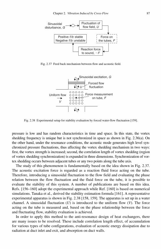
Chapter 2. Vibration Induced by Cross-Flow 87
pressure is low and has random characteristics in time and space. In this state, the vortex shedding frequency is unique but is not synchronized in space as shown in Fig. 2.36(a) . On the other hand, under the resonance conditions, the acoustic mode generates high level syn-chronized pressure fluctuations, thus affecting the vortex shedding mechanism in two ways: first, the vortex strength is increased; second, the correlation length of vortex shedding (region of vortex shedding synchronization) is expanded in three dimensions. Synchronization of vor-tex shedding occurs between adjacent tubes or any two points along the tube axis.
The study of this phenomenon is fundamentally based on the idea shown in Fig. 2.37 . The acoustic excitation force is regarded as a reaction fluid force acting on the tube. Therefore, introducing a sinusoidal fluctuation to the flow field and evaluating the phase relation between the flow fluctuation and the fluid force on the tube, it is possible to evaluate the stability of this system. A number of publications are based on this idea. Refs. [156–160] adopt the experimental approach while Ref. [160] is based on numerical simulations. Tanaka et al., derived the stability estimation formula [161] . A representative experimental apparatus is shown in Fig. 2.38 [158, 159] . The apparatus is set up in a water channel. A sinusoidal fluctuation ( U ) is introduced to the uniform flow ( V ). The force acting on the tube is measured and, based on the phase relationship between the force and fluctuating flow, stability evaluation is achieved.
In order to apply this method to the anti-resonance design of heat exchangers, there are many issues to be resolved. These include correlation length effect, of accumulation for various types of tube configurations, evaluation of acoustic energy dissipation due to radiation at duct inlet and exit, and absorption on duct walls.
Fluctuation offlow field, U
Sinusoidaldisturbance, G
Reaction forceto sound, �F
Positive f /b: stableNegative f /b: unstable
Force onthe tubes, F
Fig. 2.37 Feed back mechanism between flow and acoustic field.
Sinusoidal excitation, G
Uniform flow
V
U
Force measurementon tube, F
Forced flowfluctuation
Fig. 2.38 Experimental setup for stability evaluation by forced water-flow fluctuation [159] .
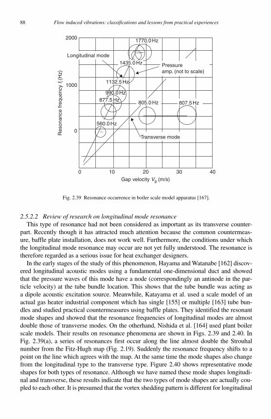
88 Flow induced vibrations: classifications and lessons from practical experiences
2.5.2.2 Review of research on longitudinal mode resonance This type of resonance had not been considered as important as its transverse counter-
part. Recently though it has attracted much attention because the common countermeas-ure, baffle plate installation, does not work well. Furthermore, the conditions under which the longitudinal mode resonance may occur are not yet fully understood. The resonance is therefore regarded as a serious issue for heat exchanger designers.
In the early stages of the study of this phenomenon, Hayama and Watanabe [162] discov-ered longitudinal acoustic modes using a fundamental one-dimensional duct and showed that the pressure waves of this mode have a node (correspondingly an antinode in the par-ticle velocity) at the tube bundle location. This shows that the tube bundle was acting as a dipole acoustic excitation source. Meanwhile, Katayama et al. used a scale model of an actual gas heater industrial component which has single [155] or multiple [163] tube bun-dles and studied practical countermeasures using baffle plates. They identified the resonant mode shapes and showed that the resonance frequencies of longitudinal modes are almost double those of transverse modes. On the otherhand, Nishida et al. [164] used plant boiler scale models. Their results on resonance phenomena are shown in Figs. 2.39 and 2.40 . In Fig. 2.39(a) , a series of resonances first occur along the line almost double the Strouhal number from the Fitz-Hugh map (Fig. 2.19) . Suddenly the resonance frequency shifts to a point on the line which agrees with the map. At the same time the mode shapes also change from the longitudinal type to the transverse type. Figure 2.40 shows representative mode shapes for both types of resonance. Although we have named these mode shapes longitudi-nal and transverse, these results indicate that the two types of mode shapes are actually cou-pled to each other. It is presumed that the vortex shedding pattern is different for longitudinal
1770.0 Hz2000
1000
Res
onan
ce fr
eque
ncy
f i(H
z)
0 �
0 10 20 30 40
Gap velocity Vg (m/s)
Longitudinal mode1435.0 Hz
1132.5 Hz
990.0 Hz877.5 Hz
560.0 Hz
805.0 Hz 807.5 Hz
Transverse mode
Pressureamp. (not to scale)
Fig. 2.39 Resonance occurrence in boiler scale model apparatus [167] .
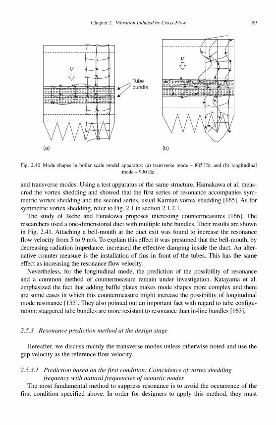
Chapter 2. Vibration Induced by Cross-Flow 89
and transverse modes. Using a test apparatus of the same structure, Hamakawa et al. meas-ured the vortex shedding and showed that the first series of resonance accompanies sym-metric vortex shedding and the second series, usual Karman vortex shedding [165]. As for symmetric vortex shedding, refer to Fig. 2.1 in section 2.1.2.1.
The study of Ikebe and Funakawa proposes interesting countermeasures [166] . The researchers used a one-dimensional duct with multiple tube bundles. Their results are shown in Fig. 2.41 . Attaching a bell-mouth at the duct exit was found to increase the resonance flow velocity from 5 to 9 m/s. To explain this effect it was presumed that the bell-mouth, by decreasing radiation impedance, increased the effective damping inside the duct. An alter-native counter-measure is the installation of fins in front of the tubes. This has the same effect as increasing the resonance flow velocity.
Nevertheless, for the longitudinal mode, the prediction of the possibility of reson ance and a common method of countermeasure remain under investigation. Katayama et al. emphasized the fact that adding baffle plates makes mode shapes more complex and there are some cases in which this countermeasure might increase the possibility of longitudinal mode resonance [155] . They also pointed out an important fact with regard to tube configu-ration: staggered tube bundles are more resistant to resonance than in-line bundles [163] .
2.5.3 Resonance prediction method at the design stage
Hereafter, we discuss mainly the transverse modes unless otherwise noted and use the gap velocity as the reference flow velocity.
2.5.3.1 Prediction based on the first condition: Coincidence of vortex shedding frequency with natural frequencies of acoustic modes
The most fundamental method to suppress resonance is to avoid the occurrence of the first condition specified above. In order for designers to apply this method, they must
(a) (b)
Tubebundle
V
V
Fig. 2.40 Mode shapes in boiler scale model apparatus: (a) transverse mode – 805 Hz, and (b) longitudinal mode – 990 Hz.
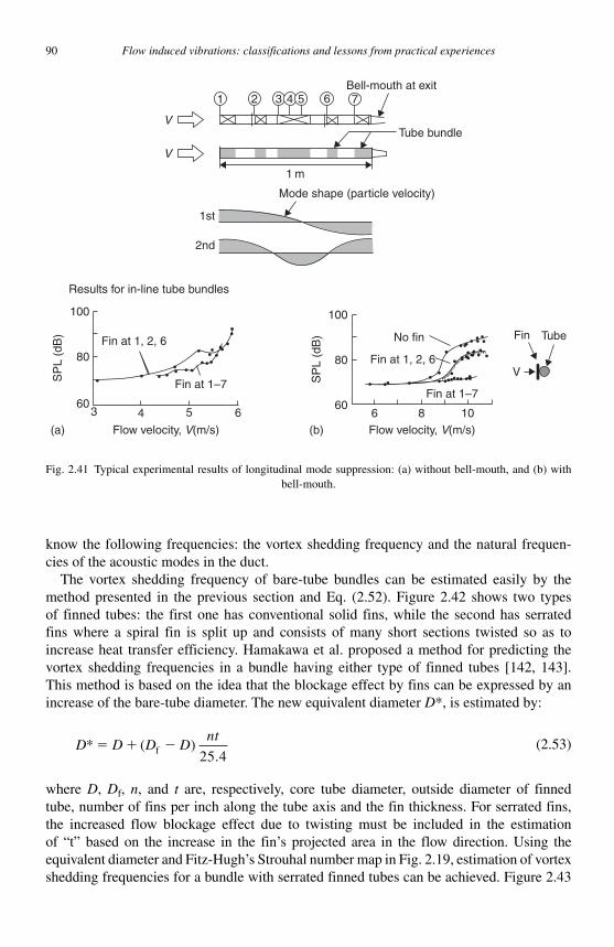
90 Flow induced vibrations: classifications and lessons from practical experiences
know the following frequencies: the vortex shedding frequency and the natural frequen-cies of the acoustic modes in the duct.
The vortex shedding frequency of bare-tube bundles can be estimated easily by the method presented in the previous section and Eq. (2.52). Figure 2.42 shows two types of finned tubes: the first one has conventional solid fins, while the second has serrated fins where a spiral fin is split up and consists of many short sections twisted so as to increase heat transfer efficiency. Hamakawa et al. proposed a method for predicting the vortex shedding frequencies in a bundle having either type of finned tubes [142, 143] .This method is based on the idea that the blockage effect by fins can be expressed by an increase of the bare-tube diameter. The new equivalent diameter D *, is estimated by:
D D D Dnt
* ( )f� � �25 4.
(2.53)
where D , Df , n, and t are, respectively, core tube diameter, outside diameter of finned tube, number of fins per inch along the tube axis and the fin thickness. For serrated fins, the increased flow blockage effect due to twisting must be included in the estimation of “ t ” based on the increase in the fin ’ s projected area in the flow direction. Using the equivalent diameter and Fitz-Hugh ’ s Strouhal number map in Fig. 2.19 , estimation of vortex shedding frequencies for a bundle with serrated finned tubes can be achieved. Figure 2.43
1 m
1st
2nd
100
80
603 4
Flow velocity, V(m/s)
5 6
Fin at 1, 2, 6
Fin at 1–7
(a) (b)
SP
L (d
B)
Results for in-line tube bundles
100
80
606 8 10
No fin
Fin at 1, 2, 6
Fin at 1–7
Fin Tube
V
Flow velocity, V(m/s)
SP
L (d
B)
Bell-mouth at exit
Tube bundle
Mode shape (particle velocity)
V
V
6 754321
Fig. 2.41 Typical experimental results of longitudinal mode suppression: (a) without bell-mouth, and (b) with bell-mouth.
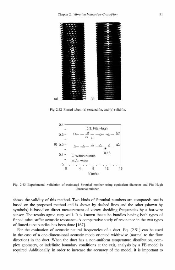
Chapter 2. Vibration Induced by Cross-Flow 91
shows the validity of this method. Two kinds of Strouhal numbers are compared: one is based on the proposed method and is shown by dashed lines and the other (shown by symbols) is based on direct measurement of vortex shedding frequencies by a hot-wire sensor. The results agree very well. It is known that tube bundles having both types of finned tubes suffer acoustic resonance. A comparative study of resonance in the two types of finned-tube bundles has been done [167] .
For the evaluation of acoustic natural frequencies of a duct, Eq. (2.51) can be used in the case of a one-dimensional acoustic mode oriented widthwise (normal to the flow direction) in the duct. When the duct has a non-uniform temperature distribution, com-plex geometry, or indefinite boundary conditions at the exit, analysis by a FE model is required. Additionally, in order to increase the accuracy of the model, it is important to
Fig. 2.42 Finned tubes: (a) serrated fin, and (b) solid fin.
At wake
0.4
0.3
0.2
0.1
00 4
St
8 12
V (m/s)
16
0.18
0.3: Fitz-Hugh
Within bundle
Fig. 2.43 Experimental validation of estimated Strouhal number using equivalent diameter and Fitz-Hugh Strouhal number.
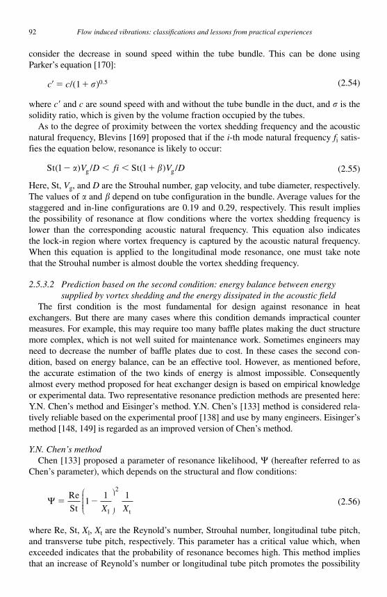
92 Flow induced vibrations: classifications and lessons from practical experiences
consider the decrease in sound speed within the tube bundle. This can be done using Parker ’ s equation [170]:
c c� � �/(1 )� 0 5. (2.54)
where c� and c are sound speed with and without the tube bundle in the duct, and � is the solidity ratio, which is given by the volume fraction occupied by the tubes.
As to the degree of proximity between the vortex shedding frequency and the acoustic natural frequency, Blevins [169] proposed that if the i -th mode natural frequency fi satis-fies the equation below, resonance is likely to occur:
St( ) / St( ) /g g1 1� � � �� �V D fi V D (2.55)
Here, St, Vg , and D are the Strouhal number, gap velocity, and tube diameter, respectively. The values of � and � depend on tube configuration in the bundle. Average values for the staggered and in-line configurations are 0.19 and 0.29, respectively. This result implies the possibility of resonance at flow conditions where the vortex shedding frequency is lower than the corresponding acoustic natural frequency. This equation also indicates the lock-in region where vortex frequency is captured by the acoustic natural frequency. When this equation is applied to the longitudinal mode resonance, one must take note that the Strouhal number is almost double the vortex shedding frequency.
2.5.3.2 Prediction based on the second condition: energy balance between energy supplied by vortex shedding and the energy dissipated in the acoustic field
The first condition is the most fundamental for design against resonance in heat exchangers. But there are many cases where this condition demands impractical counter measures. For example, this may require too many baffle plates making the duct structure more complex, which is not well suited for maintenance work. Sometimes engineers may need to decrease the number of baffle plates due to cost. In these cases the second con-dition, based on energy balance, can be an effective tool. However, as mentioned before, the accurate estimation of the two kinds of energy is almost impossible. Consequently almost every method proposed for heat exchanger design is based on empirical knowledge or experimental data. Two representative resonance prediction methods are presented here: Y.N. Chen ’ s method and Eisinger ’ s method. Y.N. Chen ’ s [133] method is considered rela-tively reliable based on the experimental proof [138] and use by many engineers. Eisinger ’ s method [148, 149] is regarded as an improved version of Chen ’ s method.
Y.N. Chen ’ s method Chen [133] proposed a parameter of resonance likelihood, � (hereafter referred to as
Chen ’ s parameter), which depends on the structural and flow conditions:
� � �Re
St l t
11 1
2
X X
⎛
⎝⎜⎜⎜⎜
⎞
⎠⎟⎟⎟⎟ (2.56)
where Re, St, Xl , Xt are the Reynold ’ s number, Strouhal number, longitudinal tube pitch, and transverse tube pitch, respectively. This parameter has a critical value which, when exceeded indicates that the probability of resonance becomes high. This method implies that an increase of Reynold ’ s number or longitudinal tube pitch promotes the possibility
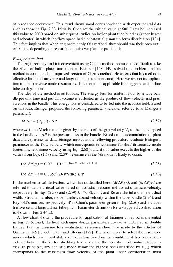
Chapter 2. Vibration Induced by Cross-Flow 93
of resonance occurrence. This trend shows good correspondence with experimental data such as those in Fig. 2.33 . Initially, Chen set the critical value at 600. Later he increased this value to 2000 based on subsequent studies on boiler plant tube bundles (super heater and reheater) in which the flow speed had a substantially non-uniform distribution [134] . This fact implies that when engineers apply this method, they should use their own criti-cal values depending on research on their own plant or product data.
Eisinger ’ s method The engineer may find it inconvenient using Chen ’ s method because it is difficult to take
the effect of baffle plates into account. Eisinger [148, 149] solved this problem and his method is considered an improved version of Chen ’ s method. He asserts that his method is effective for both transverse and longitudinal mode resonances. Here we restrict its applica-tion to the transverse mode resonances. This method is applicable for staggered and in-line tube configurations.
The idea of the method is as follows. The energy loss for uniform flow by a tube bun-dle per unit time and per unit volume is evaluated as the product of flow velocity and pres-sure loss in the bundle. This energy loss is considered to be fed into the acoustic field. Based on this idea, Eisinger proposed the following parameter (hereafter referred to as Eisinger ’ s parameter):
M P V c P � � �( / )g (2.57)
where M is the Mach number given by the ratio of the gap velocity Vg to the sound speed in the bundle, c� . P is the pressure loss in the bundle. Based on the accumulation of plant data and experimental data, Eisinger arrived at the following procedure: evaluate Eisinger ’ s parameter at the flow velocity which corresponds to resonance for the i -th acoustic mode (determine resonance velocity using Eq. [2.60]), and if this value exceeds the higher of the values from Eqs. (2.58) and (2.59), resonance in the i -th mode is likely to occur.
( ) , / St)/ ]M P p i D W i � � �0 07 100 4375 0 0172 1. . [( . (2.58)
( ) , ( / St) /M P v i c D W i �� �0 035. Re (2.59)
In the mathematical derivation, which is not detailed here, ( MP ) p , i , and ( MP ) v , i are referred to as the critical value based on acoustic pressure and acoustic particle velocity, respectively. In Eqs. (2.58) and (2.59) D , W , St, i , c� , and Re are the tube diameter, duct width, Strouhal number, mode number, sound velocity within the tube bundle (2.54), and Reynold ’ s number, respectively. � is Chen ’ s parameter given in Eq. (2.56) and includes transverse and longitudinal tube pitch. Parameter definition for a staggered configuration is shown in Fig. 2.44(a) .
A flow chart showing the procedure for application of Eisinger ’ s method is presented in Fig. 2.45 . First, the heat exchanger design parameters are set as indicated in double frames. For the pressure loss evaluation, reference should be made to the articles of Grimison [169] , Jacob [171] , and Blevins [172] . The next step is to select the resonance modes which have a probability of excitation based on the condition of frequency coin-cidence between the vortex shedding frequency and the acoustic mode natural frequen-cies. In principle, any acoustic mode below the highest one (identified by imax) which corresponds to the maximum flow velocity of the plant under consideration must
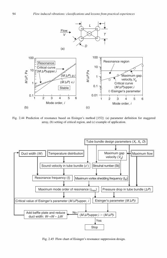
94 Flow induced vibrations: classifications and lessons from practical experiences
(a)
FlowV
D
T
L
100
10
1
0.1
100
10
1
0.1
0.011 2 3 4 5 61 2 3 4 5 6
M�
P, P
a
M�
P,P
a
Maximum gap.velocity,Vg
Resonance region
Critical curve(M �P)upper,i
Mode order, i Mode order, i
Eisinger’s parameter
Critical curve(M �P)upper,i
Resonance
Stable
(M �P) p,i
(M �P) v,i
(b) (c)
Fig. 2.44 Prediction of resonance based on Eisinger ’ s method [152] : (a) parameter definition for staggered array, (b) setting of critical region, and (c) example of application.
Tube bundle design parameters (Xl, Xt, D)
Maximum flow
Sound velocity in tube bundle (c�)
Maximum gapvelocity (Vg)
Temperature distributionDuct width (W )
Strouhal number (St)
Maximum vortex shedding frequency (fW)
Maximum mode order of resonance (imax)
Eisinger’s parameter (M �P)iCritical value of Eisinger’s parameter (M �P)upper, i
(M �P)upper,i � (M �P)iAdd baffle plate and reduce
duct width: W→W – �W
Stop
Resonance frequency (fi)
Pressure drop in tube bundle (�P)
Yes
No
Fig. 2.45 Flow chart of Eisinger ’ s resonance suppression design.
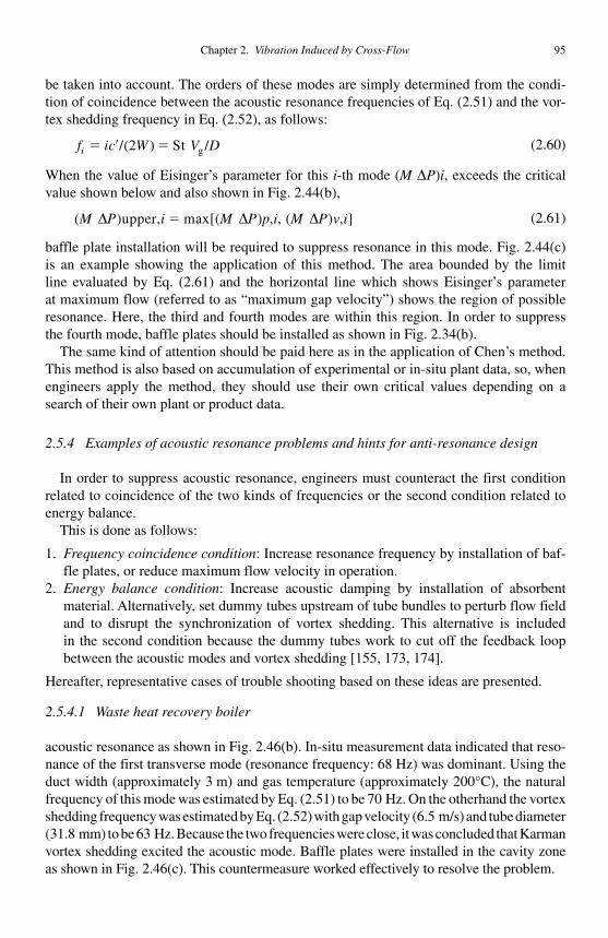
Chapter 2. Vibration Induced by Cross-Flow 95
be taken into account. The orders of these modes are simply determined from the condi-tion of coincidence between the acoustic resonance frequencies of Eq. (2.51) and the vor-tex shedding frequency in Eq. (2.52), as follows:
f ic W V Di � � �/( ) St /g2 (2.60)
When the value of Eisinger ’ s parameter for this i -th mode ( M P ) i , exceeds the critical value shown below and also shown in Fig. 2.44(b) ,
( )upper, max[( ) , , ( ) , ]M P i M P p i M P v i � (2.61)
baffle plate installation will be required to suppress resonance in this mode. Fig. 2.44(c) is an example showing the application of this method. The area bounded by the limit line evaluated by Eq. (2.61) and the horizontal line which shows Eisinger ’ s parameter at maximum flow (referred to as “ maximum gap velocity ” ) shows the region of possible resonance. Here, the third and fourth modes are within this region. In order to suppress the fourth mode, baffle plates should be installed as shown in Fig. 2.34(b) .
The same kind of attention should be paid here as in the application of Chen ’ s method. This method is also based on accumulation of experimental or in-situ plant data, so, when engineers apply the method, they should use their own critical values depending on a search of their own plant or product data.
2.5.4 Examples of acoustic resonance problems and hints for anti-resonance design
In order to suppress acoustic resonance, engineers must counteract the first condition related to coincidence of the two kinds of frequencies or the second condition related to energy balance.
This is done as follows:
1. Frequency coincidence condition : Increase resonance frequency by installation of baf-fle plates, or reduce maximum flow velocity in operation.
2. Energy balance condition : Increase acoustic damping by installation of absorbent material. Alternatively, set dummy tubes upstream of tube bundles to perturb flow field and to disrupt the synchronization of vortex shedding. This alternative is included in the second condition because the dummy tubes work to cut off the feedback loop between the acoustic modes and vortex shedding [155, 173, 174] .
Hereafter, representative cases of trouble shooting based on these ideas are presented.
2.5.4.1 Waste heat recovery boiler The structure of the boiler is shown in Fig. 2.46(a) [175]. The boiler suffered a strong
acoustic resonance as shown in Fig. 2.46(b) . In-situ measurement data indicated that reso-nance of the first transverse mode (resonance frequency: 68 Hz) was dominant. Using the duct width (approximately 3 m) and gas temperature (approximately 200°C), the natural frequency of this mode was estimated by Eq. (2.51) to be 70 Hz. On the otherhand the vortex shedding frequency was estimated by Eq. (2.52) with gap velocity (6.5 m/s) and tube diameter (31.8 mm) to be 63 Hz. Because the two frequencies were close, it was concluded that Karman vortex shedding excited the acoustic mode. Baffle plates were installed in the cavity zone as shown in Fig. 2.46(c) . This countermeasure worked effectively to resolve the problem.
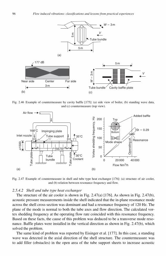
96 Flow induced vibrations: classifications and lessons from practical experiences
2.5.4.2 Shell and tube type heat exchanger The structure of the air cooler is shown in Fig. 2.47(a) [176]. As shown in Fig. 2.47(b) ,
acoustic pressure measurements inside the shell indicated that the in-plane resonance mode across the shell cross-section was dominant and had a resonance frequency of 120 Hz. The plane of the mode is normal to both the tube axes and flow direction. The calculated vor-tex shedding frequency at the operating flow rate coincided with this resonance frequency. Based on these facts, the cause of this problem was deduced to be a transverse mode reso-nance. Baffle plates were installed in the vertical direction as shown in Fig. 2.47(b) , which solved the problem.
The same kind of problem was reported by Eisinger et al. [177] . In this case, a standing wave was detected in the axial direction of the shell structure. The countermeasure was to add filler (obstacles) in the open area of the tube support sheets to increase acoustic
(a) (b)
200
150
100
50
00 20 000 40 000
Vor
tex
shed
ding
freq
uenc
y, H
z
Ope
ratin
g pt
.
Resonance
Added baffle
St � 0.29
Mode shape
Top
Bottom
Flow Nm3/h
Air flow
Impinging plate
Tube supportInlet nozzle
5675
Tub
e pl
ate
Tub
e pl
ate
Coolant
35�C
30�CTubebundle
f15
00
168�C
Fig. 2.47 Example of countermeasure in shell and tube type heat exchanger [176] : (a) structure of air cooler, and (b) relation between resonance frequency and flow.
(a)
Tube bundle
5m
5 m
W � 3 m
V
(c)
5 m
W�
3m V
Cavity baffle plateTube bundle(b)
3 m
Near side
177 dB
Center Far side
Fig. 2.46 Example of countermeasure by cavity baffle [175] : (a) side view of boiler, (b) standing wave data, and (c) countermeasure (top view).
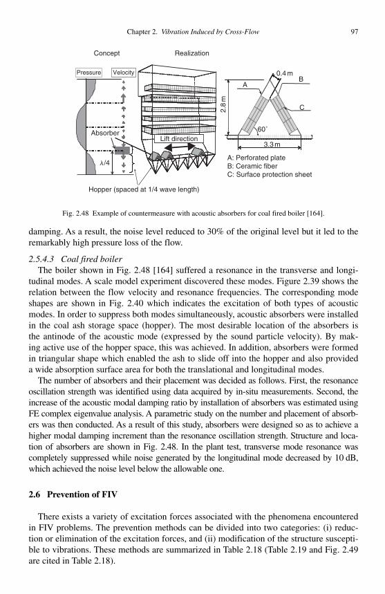
Chapter 2. Vibration Induced by Cross-Flow 97
damping. As a result, the noise level reduced to 30% of the original level but it led to the remarkably high pressure loss of the flow.
2.5.4.3 Coal fired boiler The boiler shown in Fig. 2.48 [164] suffered a resonance in the transverse and longi-
tudinal modes. A scale model experiment discovered these modes. Figure 2.39 shows the relation between the flow velocity and resonance frequencies. The corresponding mode shapes are shown in Fig. 2.40 which indicates the excitation of both types of acoustic modes. In order to suppress both modes simultaneously, acoustic absorbers were installed in the coal ash storage space (hopper). The most desirable location of the absorbers is the antinode of the acoustic mode (expressed by the sound particle velocity). By mak-ing active use of the hopper space, this was achieved. In addition, absorbers were formed in triangular shape which enabled the ash to slide off into the hopper and also provideda wide absorption surface area for both the translational and longitudinal modes.
The number of absorbers and their placement was decided as follows. First, the resonance oscillation strength was identified using data acquired by in-situ measurements. Second, the increase of the acoustic modal damping ratio by installation of absorbers was estimated using FE complex eigenvalue analysis. A parametric study on the number and placement of absorb-ers was then conducted. As a result of this study, absorbers were designed so as to achieve a higher modal damping increment than the resonance oscillation strength. Structure and loca-tion of absorbers are shown in Fig. 2.48. In the plant test, transverse mode resonance was completely suppressed while noise generated by the longitudinal mode decreased by 10 dB, which achieved the noise level below the allowable one.
2.6 Prevention of FIV
There exists a variety of excitation forces associated with the phenomena encountered in FIV problems. The prevention methods can be divided into two categories: (i) reduc-tion or elimination of the excitation forces, and (ii) modification of the structure suscepti-ble to vibrations. These methods are summarized in Table 2.18 ( Table 2.19 and Fig. 2.49 are cited in Table 2.18 ).
A
3.3 m
0.4 mB
C2.8
m
A: Perforated plateB: Ceramic fiberC: Surface protection sheet
Absorber
Hopper (spaced at 1/4 wave length)
Pressure Velocity
l/4
Concept Realization
Lift direction60˚
Fig. 2.48 Example of countermeasure with acoustic absorbers for coal fired boiler [164] .
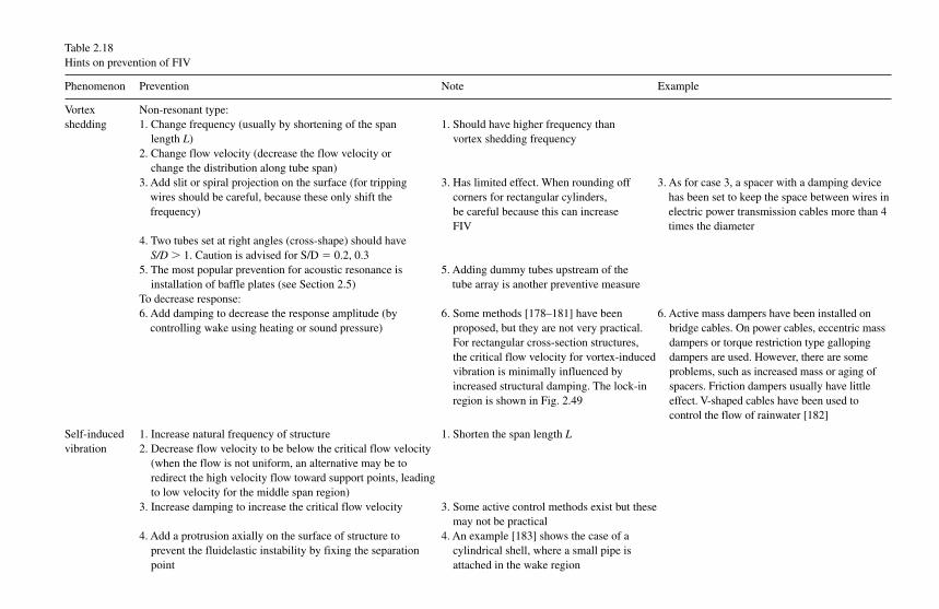
Table 2.18 Hints on prevention of FIV
Phenomenon Prevention Note Example
Vortex shedding
Non-resonant type:1. Change frequency (usually by shortening of the span
length L ) 1. Should have higher frequency than
vortex shedding frequency 2. Change flow velocity (decrease the flow velocity or
change the distribution along tube span) 3. Add slit or spiral projection on the surface (for tripping
wires should be careful, because these only shift the frequency)
3. Has limited effect. When rounding off corners for rectangular cylinders, be careful because this can increase FIV
3. As for case 3, a spacer with a damping device has been set to keep the space between wires in electric power transmission cables more than 4 times the diameter
4. Two tubes set at right angles (cross-shape) should have S/D � 1. Caution is advised for S/D � 0.2, 0.3
5. The most popular prevention for acoustic resonance is installation of baffle plates (see Section 2.5)
5. Adding dummy tubes upstream of the tube array is another preventive measure
To decrease response:6. Add damping to decrease the response amplitude (by
controlling wake using heating or sound pressure) 6. Some methods [178–181] have been
proposed, but they are not very practical. For rectangular cross-section structures, the critical flow velocity for vortex-induced vibration is minimally influenced by increased structural damping. The lock-in region is shown in Fig. 2.49
6. Active mass dampers have been installed on bridge cables. On power cables, eccentric mass dampers or torque restriction type galloping dampers are used. However, there are some problems, such as increased mass or aging of spacers. Friction dampers usually have little effect. V-shaped cables have been used to control the flow of rainwater [182]
Self-induced vibration
1. Increase natural frequency of structure 1. Shorten the span length L 2. Decrease flow velocity to be below the critical flow velocity
(when the flow is not uniform, an alternative may be to redirect the high velocity flow toward support points, leading to low velocity for the middle span region)
3. Increase damping to increase the critical flow velocity 3. Some active control methods exist but these may not be practical
4. Add a protrusion axially on the surface of structure to prevent the fluidelastic instability by fixing the separation point
4. An example [183] shows the case of a cylindrical shell, where a small pipe is attached in the wake region
Table 2.18 (Continued) Hints on prevention of FIV
Phenomenon Prevention Note Example
5. Based on the critical flow velocity conditions (2.44), (2.50) for bending and twisting, the critical flow velocity for galloping can be estimated knowing the mass m and rigidity k as follows:
V m kcr/ 1/� 1 2 2
(2.59) This equation is valid even in the case of coupled bending
and twisting [77] . Prevention methods include increasing the equivalent mass m and equivalent rigidity k in order to raise the critical flow velocity. By adding some attachment on the rectangular cylinder, the negative gradient of lift force can be reduced. Note also that if the modification of section properties increases the drag coefficient, this will introduce a damping effect
5. Table 2.19 shows the relation between the relative positions of the gravity center, elastic axis, and the total fluid force from the upstream edge of the wing considered to design for the prevention of a/c wing bending-twisting coupled flutter and static divergence. The wing is stable when the elastic axis is downstream of the gravity center, and is upstream of the total fluid force
Random vibration
While these vibrations cannot be completely eliminated, it is possible to decrease the vibration level:
1. Generally shortening the span length is effective
1. Increase natural frequency of structures
2. Decrease flow velocity. Redistributing the flow such that high-flow velocity is closer to the support points and lowvelocity closer to the middle of the spans is especially effective
2. An alternative method involves setting an impingement baffle to restrict the flow
Acoustic resonance
Two methods are available: (i) changing the vortex shedding or (ii) changing the acoustic field
To modify the acoustic field, the following approaches exist: 1. Insert plates into the duct to change the acoustic natural
frequency 1. Sometimes higher modes appear
2. Install acoustic absorbers in the duct to increase the field damping
2. Includes perforated plate
3. Change the flow condition (temperature, etc.) to change the frequency of the acoustic field
3. Can be achieved by changing operating conditions

100 Flow induced vibrations: classifications and lessons from practical experiences
Table 2.19 The conditions of occurrence of wing flutter/divergence, depending on the relative positions of the gravity center: ( G ), the elastic axis: ( E ), and the total fluid force on the wing: and ( F ), along the fluid flow direction (case of small attack angle [77] )
Case of Case of
[Leading edge] → ( F ) → ( E ) → ( G ) →[Trailing edge]
[Leading edge] → ( F ) → ( G ) → ( E ) → [Trailing edge] Or
[Leading edge] → ( G ) → ( F ) → E ) → [Trailing edge] ( Note : Arrow “ → ” indicates flow direction)
Then Then • Flutter: Bad • No flutter: Good • Divergence: Bad • Divergence: Bad
Case of Case of [Leading edge] → ( E ) → ( G ) → ( F ) →[Trailing edge]
[Leading edge] → ( G ) → ( E ) → ( F ) → [Trailing edge]
Or [Leading edge] → ( E ) → ( F ) → ( G ) →[Trailing edge] Then Then • Flutter: Bad • No flutter: Good • No divergence: Good • No divergence: Good
40
30
20
10
00 20 40 60 80 90
0
0.05
0.10
:
Maximumamplitudeby vortex
(V/f D � 6.6)
Unstable(galopping)
Unstable(Vortex)N
on-d
imen
sion
al fl
ow v
eloc
ity V
/fd
Non
-dim
ensi
onal
am
plitu
de h
max
Scruton number Sc
Fig. 2.49 Region of occurrence of vortex shedding and maximum response of square cylinder as functions of Scrutonnumber [112] . (Solid line: boundary of occurrence; Broken line: maximum response.)
References
[1] Bishop , R.E.D. and Hassan , A.Y. , Proc. Roy. Soc. A. , Vol. 277 , 1964 , pp. 51 – 75 . [2] Williamson , C.H. and Roshko , A.J. , Fluid. Struct. , Vol. 2 , No. 4 , 1988 , pp.
355 – 381 .
Chapter 2. Vibration Induced by Cross-Flow 101
[3] Brika , D. and Laneville , A.J. , Fluid. Mech. , Vol. 250 , 1993 , pp. 481 – 508 . [4] Hartlen , R.T. and Currie , I.G. , ASCE J. Eng. Mech. Div. , Vol. 96 , 1970 . [5] Iwan , W.D. and Blevins , R.D. , J. Appl. Mech. , Vol. 40 , 1974 , pp. 518 – 586 . [6] Sarpkaya , T. , Proceedings of the International Conference on FIV in Fluids
Engineering , 1982 , pp. 131 – 139 . [7] Lowdon, A. et al., C416/041, IMechE, 1991, p. 283. [8] Griffin , O.M. , J. Fluid. Eng. , Vol. 107 , 1985 , pp. 298 – 306 . [9] Vickery , B.J. and Clark , A.W. , ASCE J. Struct. Div. , Vol. 98 , No. ST1 , 1972 , p. 1 . [10] Wang, E. et al., Proceedings of OMAE/Tokyo , ASME, Vol. III, 1986, pp. 393–401. [11] Vandiver , J.K. , J. Fluid. Struct. , Vol. 7 , 1993 , pp. 423 – 455 . [12] Bokaian , A. , J. Sound Vib. , Vol. 175 , No. 5 , 1994 , pp. 607 – 623 . [13] Tsahalis , D.T. , J. Energ. Resour. ASME , Vol. 106 , 1984 , pp. 206 – 213 . [14] King, R. and Jones, R., “Practical Experiences with Flow-Induced Vibrations, ”
E. Naudacsher & D. Rockwell (eds.), Springer-Verlag, Berlin, 1980. [15] Khalak , A. and Williamson , C.H. , J. Fluid. Struct. , Vol. 10 , 1996 , pp. 455 – 472 . [16] ASME, “ Boiler and Pressure Vessel Code Section III, Division I Appendix N,
Article N-1300, ” 1995, pp. 370–397. [17] JSME Standard, “ Guideline for Evaluation of Flow-Induced Vibration of a
Cylindrical Structure in a Pipe” (in Japanese), JSME S 012, 1998. [18] Newman, D.J. and Karniadakis, G., “ Flow-Induced Vibration, ” Bearman (ed.),
Balkema, Rotterdam, 1995. [19] Massih, A.R. and Forsberg, K., FSI,AE,FIV+N Vol. I ASME, AD-Vol. 53-1,
1997. [20] Anagnostopoulos , P. et al., J. Fluid. Struct. , Vol. 12 , No. 3 , 1998 , pp. 225 – 258 . [21] Fox , T.A. and Apelt , C.J. , J. Fluid. Struct. , Vol. 7 , 1993 , pp. 375 – 386 . [22] Kitagawa , J. et al., J. Fluid. Struct. , Vol. 13 , 1999 , pp. 499 – 518 . [23] Morison , J.R. et al., AIME Petrol. Trans , Vol. 189 , 1950 , pp. 149 – 154 . [24] Longoria , R.G. et al., J. Offshore Mech. Arct. , Vol. 115 , 1993 , pp. 23 – 30 . [25] Yoshida , K. et al., J. Offshore Mech. Arct. , Vol. 112 , 1990 , pp. 14 – 20 . [26] Hall, M.S. and Griffin. O.M., J. Fluid. Eng ., Vol. 115, 1993, pp. 283–291. [27] Zhang , J. et al., J. Fluid. Struct. , Vol. 7 , 1993 , pp. 39 – 56 . [28] Meneghini , J.R. and Bearman , P.W. , J. Fluid. Struct. , Vol. 9 , 1995 , pp. 435 – 455 . [29] Badr , H.M. et al., J. Fluid. Mech. , Vol. 303 , No. 6 , 1995 , pp. 215 – 232 . [30] Dockstader , et al., Trans. ASCE , Vol. 121 , 1956 , pp. 1088 – 1112 . [31] Johns, D.J. and Sharma, C.B., In “ Flow-Induced Structural Vibrations. ”
Naudascher (ed.), 1974, pp. 650–662. [32] Johns , D.J. , J. Sound Vib. , Vol. 67 , 1979 , pp. 432 – 435 . [33] Païdoussis , M.P. and Helleur , C. , J. Sound Vib. , Vol. 63 , 1979 , pp. 527 – 542 . [34] Païdoussis , M.P. , J. Sound Vib. , Vol. 103 , 1985 , pp. 201 – 209 . [35] Païdoussis , M.P. , J. Sound Vib. , Vol. 83 , 1982 , pp. 533 – 553 . [36] Païdoussis , M.P. and M-Wong , D.T. , J. Fluid. Mech. , Vol. 115 , 1982 , pp. 411 – 426 . [37] Katsura , S. , J. Sound Vib. , Vol. 100 , 1985 , pp. 527 – 550 . [38] Païdoussis , M.P. et al., Int. Conf. FIV , 1987 , pp. 377 – 392 . [39] Griffin, O.M. et al., Paper No. OTC-2319 , Offshore Technology Conference, 1975. [40] Sarpkaya, T., J., WWPC & Ocean Div. 104, ASCE, 1978, pp. 275–290. [41] Hara , and Ohtani , J. Jpn. Soc. Mech. Eng. (in Japanese) , Vol. 48 , No. 431 , 1982 C ,
pp. 962 – 971 .

102 Flow induced vibrations: classifications and lessons from practical experiences
[42] Hara, J. Jpn. Soc. Mech. Eng. (in Japanese) , Vol. 48 , No. 433 , 1982 C , pp. 1371 – 1379 . [43] Hara , and Ogawa , J. Jpn. Soc. Mech. Eng. (in Japanese) , Vol. 49 , No. 445 , 1983
C , pp. 1624 – 1629 . [44] Architectural Institute of Japan, “ Recommendations for Loads on Buildings ” (in
Japanese), Maruzen, 2000, pp. 323–325. [45] Uematsu , Y. et al., J. Fluid. Struct. , Vol. 2 , 1988 . [46] Païdoussis , M.P. , J. Sound Vib. , Vol. 83 , 1982 , pp. 555 – 572 . [47] Mazouzi , A. et al., J. Fluid. Struct. , Vol. 5 , 1991 , pp. 605 – 626 . [48] Wong , H.Y. and Cox , R.N. Colloq. Indus. Aerodyn. , Third Edition , Vol. 2,
Fachhochschule Aachen , Germany , 1978 . [49] Scruton, C. and Walshe, D.E.J., “ NPL, UK, Aero Report No. 335 ” , 1957. [50] Oarai Engineering Center, Power reactor and nuclear fuel development corpora-
tion, Report “ Cause identification of sodium leakage accident in Monju; Vibration of thermo well by fluid force ” (in Japanese), 1997.
[51] King , R. et al., J. Sound Vib. , Vol. 29 , No. 2 , 1973 , p. 169 . [52] Sainsbury , R.N. and King , D. , Proceedings of the Institution of Civil Engineers ,
Vol. 49 , 1971 . [53] Hikami , Wind Engineers (in Japanese) , Vol. 11 , No. 27 , 1986 , pp. 17 – 28 . [54] Halle, H. and Lawrence, W.P., “ Practical Experiences with Flow-Induced Vibrations, ”
Naudascher, E. & Rockwell, D. (eds.), Springer-Verlag, Berlin, 1980. [55] Zdravkovich , M.M., et al., J. Sound Vib. , Vol. 101 , No. 4 , 1985 , pp. 511 – 521 . [56] Zdravkovich , M.M., et al., J. Fluid. Eng. , Vol. 1 , No. 107 , 1985 , pp. 507 – 511 . [57] Zdravkovich , M.M., et al., Proceedings of ASME Winter Meeting , Vol. 2 , 1984 , pp. 1 – 18 . [58] Zdravkovich , M.M., et al., J. Sound Vib. , Vol. 101 , No. 4 , 1985 , pp. 511 – 521 . [59] Strykowski , P.J. et al., J. Fluid. Mech. , Vol. 71 , 1990 , p. 107 . [60] Yoneta, M. et al., Bridge Engineering (in Japanese), 1992, pp. 54–62. [61] Nakamura , T. et al., J. Wind Eng. , No. 20 , 1984 , pp. 129 – 140 . [62] Bae , K. et al., J. JSME (in Japanese) , Vol. 55 , No. 519 , 1989 , pp. 3328 – 3332 . [63] Tomita , Y. et al., J. JSME (in Japanese) , Vol. 51 , No. 468 , 1987 , pp. 2571 – 2580 . [64] Nagai , S. et al., J. JCCE (in Japanese) , Vol. 24 , 1997 , pp. 352 – 356 . [65] Ookusu , M. et al., J. JASNAOE (in Japanese) , Vol. 131 , 1972 , pp. 53 – 64 . [66] Spring B.H. and Monkmeyer, P.L. Proceedings of 14th International Conference
on Costal Engineering , 1974, 1828–1847. [67] Lakshmana , B.H. et al., JSV , Vol. 122 , 1988 , pp. 497 – 514 . [68] Hara, F. , et al., ASME FIVN , Vol. 2 , 1988 , pp. 63 – 78 . [69] Iijima, T . and Hara, F., JSME (in Japanese) , Vol. 54 , No. 497 , 1988 , pp. 80 – 86 . [70] Iijima, T. and Hara, F. , JSME (in Japanese) , Vol. 56 , No. 525 , 1990 , pp. 1087 – 1093 . [71] Nojima, T. et al. , JSME (in Japanese) , Vol. 56 , No. 527 , 1990 , pp. 1665 – 1672 . [72] Iijima, T , et al., JSME (in Japanese) , Vol. 57 , No. 537 , 1991 , pp. 1469 – 1476 . [73] Ichioka , T. et al., Proceedings of Fluid Mechanics of JSME , 1993 , pp. 370 – 372 . [74] Tanaka , H. et al., JSV , Vol. 77 , 1981 , pp. 19 – 37 . [75] Chen , S.S. ASME J. PVP , Vol. 108 , 1986 , pp. 382 – 393 . [76] Price, S.J. , et al., FIVN , Vol. 1 , 1998 , pp. 91 – 111 . [77] Blevins , R.D., Flow-induced vibration , Second Edition , Krieger Publishing Co. ,
Malabar, FL , 1990 .
Chapter 2. Vibration Induced by Cross-Flow 103
[78] Chen , S.S. , Flow-Induced Vibration of Circular Cylindrical Structures , Hemishere Publishing Corporation , 1987, Washington.
[79] Thorngren, J.T., Hydrocarb. Process ., 1970. [80] Chen , Y.N. , Trans. ASME , Vol. 2 , 1970 , pp. 134 – 146 . [81] Connors, H.J., “ An Experimental Investigation of the Flow-Induced Vibration of
Tube Arrays in Cross Flow ” “ Ph.D. Report ” , University of Pittsburg, 1969. [82] Roberts, B.W., Mechanical Engineering Science, Monograph No. 4, 1966. [83] Price , S.J. and Païdoussis , M.P. , J. Sound Vib. , Vol. 97 , No. 4 , 1984 , pp. 615 – 640 . [84] Lever , J.H. and Weaver , D.S. , ASME J. Pressure Technol. , Vol. 104 , 1982 ,
pp. 147 – 158 . [85] Tanaka , H. , JSME J. , Vol. 46 , No. 408 , 1980 , pp. 1398 – 1407 . [86] Pettigrew, M.J. and Gorman, D.J., Proceedings of International Symposium
Vibration Problems in Industry, No. 424 Part I, 1973. [87] Au-Yang , M.K. , ASME PVP , Vol. 389 , 1999 , pp. 17 – 33 . [88] Pettigrew , M.J. et al., Nucl. Eng. Des. , Vol. 48 , 1978 , pp. 97 – 115 . [89] Hara , F. and Ohtani , I. , JSME J. , Vol. 48 , No. 431 , 1984 , pp. 962 – 969 . [90] Axisa , F. et al., ASME PVP , Vol. 133 , 1988 . [91] Nakamura , T. et al., ASME J. Pressure Vessel Technol. , Vol. 114 , 1992 ,
pp. 472 – 485 . [92] Takai, M. et al., Proceedings of 8th International Conference on Nuclear Engineering ,
ICONE-8090, 2000. [93] Inada , F. et al., ASME AD , Vol. 53 , No. 2 , 1997 , pp. 357 – 364 . [94] Mureithi , N.W. et al., ASME PVP , Vol. 328 , 1996 , pp. 111 – 121 . [95] Fitz-Hugh, J.S. Proceedings of UKAEA/NPL International Symposium on
Vibration Problem in Industry, Keswick, England, Paper 427, 1973, pp. 1–17 . [96] Chen , Y.N. , Transactions of the ASME journal of engineering for industry , 1968 ,
pp. 134 – 146 . [97] ASME, ASME Boiler and Pressure Vessel Code – Section III Rules for Construction
of Nuclear Power Plant Components Division 1 – Appendices, 1995, pp. 370–397. [98] Connors , H.J. , ASME J. Mech. Des. , Vol. 100 , 1978 , pp. 347 – 353 . [99] Grant, I.D.R., NEL Report No. 590, 1975, pp. 1–22. [100] Baker , O. , Oil Gas J , Vol. 53 , 1954 , p. 185 . [101] Pettigrew, M.J. et al., ASME J. PVP, Vol. 111, 1989, pp. 478–587 . [102] JSME, “ Guideline for Fluidelastic Vibration Evaluation of U-bend Tubes in Steam
Generators ” , JSME S016, 2002. [103] de Langre, E. and Villard, B., Proceedings in EAHA Conference , 1994. [104] Naudascher, E. and Rockwell, D. (eds.), “Practical experiences with flow induced
vibrations, ” Springer-Verlag, New York, 1980. [105] Japanese Society of Steel Construction, “Wind-Resistant Engineering of
Structures ” (in Japanese), Tokyo Electric University Publication Station, 1997. [106] Architectural Institute of Japan, “Building Load Standard/Guidance ” (in Japanese),
Maruzen, 1993. [107] Balendra , T., Vibration of building to wind and earthquake loads , Springer-Verlag ,
New York , 1995 .

104 Flow induced vibrations: classifications and lessons from practical experiences
[108] Nakamura, Y. et al., “ The Aerodynamic Forces and Moment Characteristics of Rectangular and H-shaped Cylinders ” (in Japanese), Reports of Research Institute for Applied Mechanics, No. 40, Kyushu University, 1982.
[109] Naudascher , E. and Wang , Y. , J. Fluid. Struct. , Vol. 7 , 1993 , pp. 341 – 373 . [110] Nakamura , Y. , Hirata , K. and Urabe , T. , J. Fluid. Struct. , Vol. 5 , 1991 ,
pp. 521 – 549 . [111] Nakamura , Y. , J. Fluid. Struct. , Vol. 10 , 1996 , pp. 147 – 158 . [112] Scruton, C., “ On the Wind Excited Oscillations of Stacks, Towers, and Masts, ”
Proceedings of the International Conference of Wind Effects on Buildings and Structures , Teddington, Her Majesty ’ s stationary office, 1963.
[113] Den Hartog , J.P. Mechanical Vibrations , Fourth Edition , McGraw-Hill , New York , 1984 . Reprinted by Dover, New York.
[114] Novak , M. , ASCE J. Eng. Mech. Div. , Vol. 96 , 1969 , pp. 115 – 142 . [115] Novak , M. and Tanaka , H. , ASCE J. Eng. Mech. Div. , Vol. 100 , 1974 , pp. 27 – 47 . [116] Nakamura , Y. and Mizota , T. , ASCE J. Eng. Mech. Div. , Vol. 101 , No. 2, 1975 ,
pp. 125 – 142 . [117] Naudascher, E. and Rockwell, D., Flow Induced Vibrations – An Engineering
Guide , A.A. Balkema, Rotterdam, 1994. [118] Okajima, A. et al., Trans. Jpn. Soc. Mech. Eng. (in Japanese), Series B, Vol. 65,
No. 635, 1999, pp. 2196–2222. [119] Okajima , A. , Trans. Jpn. Soc. Mech. Eng. (in Japanese), Series B , Vol. 65 , No. 635 ,
1999 , pp. 2190 – 2195 . [120] Parker, R. and Welsh, M.C., The Effect of Sound on Flow Over Bluff Bodies ,
University of Wales, Swansea, Mechanical Engineering Report MR/87/81, 1981. (Also in Int. J. Heat Fluid Flow, Vol. 4, 1983, pp. 113–127.)
[121] Knisely, C.W., Strouhal Number of Rectangular Cylinders at Incidence , Report SFB 210/E/13. Sonderforschungs-bereich 210, Universitat Karlsruhe, Karlsruhe, Germany, 1985.
[122] Nakamura, Y., Ohya, Y. and Tsuruya, H., J. Fluid. Mech ., Vol. 222, 1991, pp. 437–447. [123] Nguyen, D.T. and Naudasher, K., J. Hydraulic Eng ., Vol. 117, 1991, pp. 1056–1076. [124] Wang, Y., “ Transverse and Plunging Vibrations of Trashrack Bars in Inclined
Flow ” (in German), Report SFB 210/E/74, Sonderforschungsbereich 210, Universitat Karlsruhe, Karlsruhe, Germany, 1992.
[125] Novak, J., Acta Technica CSAV, 1972, pp. 372–386. [126] Richardson, A.S. et al., Proceedings of the 1st International Conference on Wind
Effects on Buildings and Structures , 2, 1965, pp. 612–686. [127] Parkinson , G.V. , Brooks , N.P.H. and Smith , J.D. , J. Appl. Math. , Vol. 28 , 1961 ,
pp. 252 – 258 . [128] Salter, J.E., “ Aero-elastic Instability of Structural Angle Section, ” Ph.D. Thesis,
University of British Columbia, 1969. [129] Nakamura , Y. and Tomonari , Y. , J. Sound Vib. , Vol. 52 , 1977 , pp. 233 – 241 . [130] Parkinson , G.V. and Smith , J.D. , Quart. J. Math. Appl. Math. , Vol. 17 , 1964 ,
pp. 225 – 239 . [131] Nishihara, T., Eguchi, Y., Inada, F. and Yasuo, A., Proceedings of the 12th Asia-
Pacific Vibration Conference , Paper No. 10, Sapporo, Japan, August, 2007. [132] Baird , R.C. , Combustion , Vol. 25 , No. 10 , 1954 , pp. 38 – 44 .
Chapter 2. Vibration Induced by Cross-Flow 105
[133] Chen , Y.N. , Trans. ASME J. Eng. Ind. , 1968 , pp. 134 – 146 . [134] Chen , Y.N. and Young , W.C. , Trans ASME , 1974 , pp. 1072 – 1075 . [135] Weaver , D.S. and Fitzpatrick , J.H. , International Conference on Flow Induced
Vibration, Paper A1. BHRA. , 1987 , pp. 1 – 17 . [136] Païdoussis , M.P. , Nucl. Eng. Des. , Vol. 74 , No. 1 , 1983 , pp. 31 – 60 . [137] Blevins , R.D. , J. Sound Vib. , Vol. 92 , No. 4 , 1984 , pp. 455 – 470 . [138] Eisinger , F.L. and Sullivan , R.E. , J. Pressure Vessel Technol. , Vol. 166 , 1994 ,
pp. 17 – 23 . [139] Weaver , D.S. and Fitzpatrick , J.A. , ASME J. Pressure Vessel Technol. , Vol. 109 ,
1987 , pp. 219 – 223 . [140] Mair , W.A. , Jones , P.D.F. and Palmer , R.K.W. , J. Sound Vib. , Vol. 39 , No. 3 , 1975 ,
pp. 293 – 296 . [141] Okui , K., Iwabuchi , M., Oda , H., and Shimada , K., Proceedings of JSME VS
Tech ’ 95 (in Japanese) , Vol. 22 , 1995 , pp. 132 – 135 . [142] Hamakawa , H. , Fukano , T. , Aragaki , M. and Nishida , E. , JSME J. (in Japanese) ,
Vol. 65(B) , No. 635 , 1997 , pp. 18 – 25 . [143] Hamakawa , H. , Fukano , T. , Nishida , E. , Ikuta , Y. and Morooka , T. , JSME J.
(in Japanese) , Vol. 66(B) , No. 646 , 2000 , pp. 1301 – 1308 . [144] Grotz, B.J. and Arnold, F.R., Technical Report, No. 31, Mechanical Engineering
Department, Stanford University, Stanford, CA., 1956. [145] Fitzpatrick , J.A. , J. Sound Vib. , Vol. 99 , No. 3 , 1985 , pp. 425 – 435 . [146] Ziada, S., Oengoren, A. and Buhlmann, E.T., International Symposium on Flow
Induced Vibration and Noise , Winter Annual Meeting Chicago, ASME, 3, 1988, pp. 245– 254.
[147] Blevins , R.D. and Bressler , M.M. , Trans. ASME , Vol. 109 , 1987 , pp. 282 – 288 . [148] Eisinger, F.L., Flow-Induced Vibration , ASME PVP, 298, 1995, pp. 111–120. [149] Sullivan, R.E., Francis, J.T. and Eisinger, F.L., ASME PVP, 363, 1998, pp. 1–9. [150] Blevins, R.D. and Bressler, M.M., Symposium on Flow-Induced Vibration and
Noise , ASME, 4, Vol. 243, 1992, pp. 59–79. [151] Eisinger , F.L. , ASME J. Pressure Vessel Technol. , Vol. 102 , 1980 , pp. 138 – 145 . [152] Nemoto, A. and Yamada, M., Flow-Induced Vibration , ASME, PVP, 273, 1994,
pp. 273–282. [153] Nemoto, A. and Yamada, M., Symposium on Flow-Induced Vibration and Noise ,
ASME, PVP, Vol. 243, No. 4, 1992, pp. 137–152. [154] Eisinger , F.L. and Sullivan , R.E. , J. Fluid. Struct. , Vol. 10 , 1996 , pp. 99 – 107 . [155] Katayama , K., Tsuboi , M., Kawaoka , T., Ohta , K., and Sato , Y., JSME J. (in
Japanese), Vol. 65(C) , No. 640 , 1999 , pp. 4633 – 4639 . [156] Blevins , R.D. , J. Fluid. Mech. , Vol. 161 , 1985 , pp. 217 – 237 . [157] Yamanaka , G., and Adachi , T., J. Acoust. Soc. Jpn. (in Japanese) , Vol. 27 , No. 5 ,
1971 , pp. 246 – 256 . [158] Tanaka , H., Imayama , Y., Koga , K., and Katayama , K., JSME J. (in Japanese),
Vol. 55(B) , No. 509 , 1989 , pp. 120 – 125 . [159] Sato , T., Imayama , Y., and Katayama , K., JSME J. (in Japanese) , Vol. 61(C) , No.
585 , 1995 , pp. 1763 – 1768 . [160] Sato , T., Imayama , Y., and Nakajima , F., JSME J. (in Japanese) , Vol. 61(C) , No.
585 , 1995 , pp. 1769 – 1775 .
106 Flow induced vibrations: classifications and lessons from practical experiences
[161] Tanaka , H., Tanaka , K., Shimizu , F., and Iijima , T., JSME J. (in Japanese) , Vol. 64(C) , No. 626 , 1998 , pp. 3293 – 3298 .
[162] Hayama, S., Watanabe, T., Proceedings of the 73rd JSME ’ s Annual Meeting (in Japanese), V, 1995, pp. 155–156.
[163] Katayama , K., Morii , S., Tsuboi , M., Kawaoka , T., Sato , Y., and Imayama , Y., JSME J. (in Japanese) , Vol. 66(C) , No. 641 , 2001 , pp. 60 – 66 .
[164] Nishida, E., Miki, M., Sadaoka, N., Fukano, T. and Hamakawa, H., ASME IMECE, 2002, 2002-33405, pp. 17–22.
[165] Hamakawa, H., Fukano, T., Nishida, E., and Fujimura, N., CDROM Proceedings of Dynamics and Design Conference 2005 , No. 117, JSME, 2005 (in CD ROM).
[166] Ikebe, H., Funakawa, M., Proceedings of JSME ’ s DMCD (in Japanese). Vol. A, No. 930-42, 1993, pp. 370–375.
[167] Nemoto, A., Takakuwa, A. and Tsutsui, M., AD-Vol. 53-2, Fluid–Structure Interaction, Aeroelasticity, Flow-Induced Vibration and Noise , Vol. 11, ASME, 1997, pp. 311–320.
[168] Parker , R. , J. Sound Vib. , Vol. 57 , 1978 , pp. 245 – 260 . [169] Blevins , R.D. and Bressler , M.M. , J. Pressure Vessel Technol. , Vol. 190 , 1987 ,
pp. 275 – 281 . [170] Grimison , E.D. , Trans. ASME , Vol. 59 , 1937 , pp. 583 – 594 . [171] J acob , M. , Trans. ASEM , Vol. 60 , No. 4 , 1938 , pp. 384 – 386 . [172] Blevins , R.D., Applied Fluid Dynamics Handbook. , Van Nostrand Reinhold, New
York , 1984 . [173] Rolsma, B. and Nagamatsu, B., Design Engineering Technical Conference ,
Hartford, Connecticut, 1981, pp. 20–23. [174] Strykowski, P.J., Ph.D. Thesis Engineering and Applied Science , Yale University,
1986. [175] Proceedings of [v-BASE] Forum, JSME, [No. 920-55], 1997, pp. 22–23. [176] Proceedings of [v-BASE] Forum, JSME, [No. 920-65], 1992, pp. 9–10. [177] Eisinger, F.L., Symposium on Flow-Induced Vibration and Noise, ASME PVP,
Vol. 243, No. 4, 1992, pp. 27–43. [178] Monkewitz, P.A., IUTAM Symposium , Gottingen, Bluff-Body Wakes Dynamics
and Instabilities, 1992, pp. 227–240. [179] Williams , J.E.F. and Zhao , B.C. , Flow-Induced Vibration and Noise , Vol. 1 , 1988 ,
p. 51 . [180] Baz , A. and Kim , M. , ASME PVP. , Vol. 206 , 1991 , p. 75 . [181] Roussopoulos , K. , J. Fluid. Mech. , Vol. 248 , 1993 , pp. 267 – 296 . [182] Miyazaki , T. , Proceedings of Symposium on Wind Direction , 1988 , pp. 145 – 150 . [183] Païdoussis , M.P. , Price , S.J. and Ang , S.Y. , International Conference on Flow
Induced Vibrations , Vol. XXX , 1987 , pp. 377 – 392.
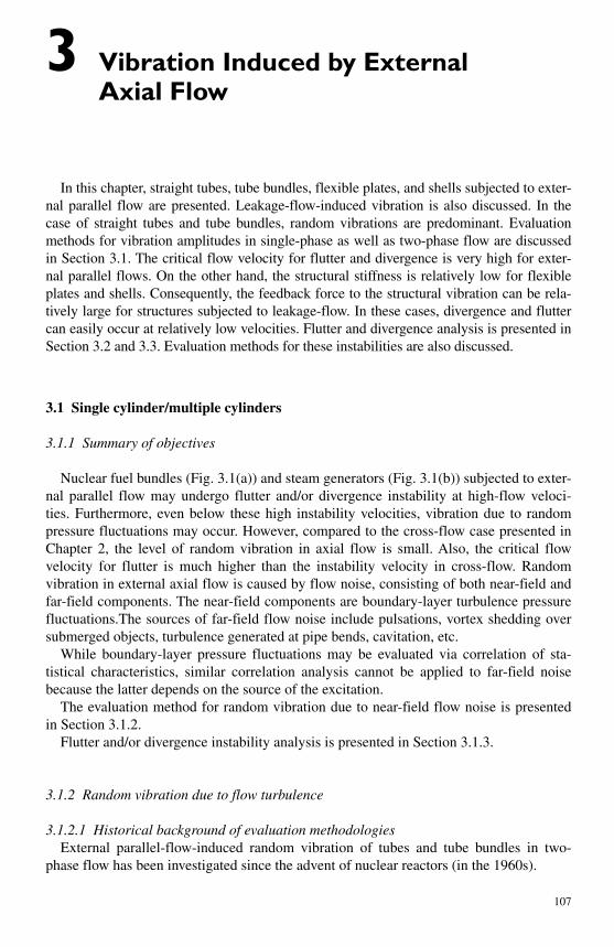
107
3 Vibration Induced by External Axial Flow
In this chapter, straight tubes, tube bundles, flexible plates, and shells subjected to exter-nal parallel flow are presented. Leakage-flow-induced vibration is also discussed. In the case of straight tubes and tube bundles, random vibrations are predominant. Evaluation methods for vibration amplitudes in single-phase as well as two-phase flow are discussed in Section 3.1. The critical flow velocity for flutter and divergence is very high for exter-nal parallel flows. On the other hand, the structural stiffness is relatively low for flexible plates and shells. Consequently, the feedback force to the structural vibration can be rela-tively large for structures subjected to leakage-flow. In these cases, divergence and flutter can easily occur at relatively low velocities. Flutter and divergence analysis is presented in Section 3.2 and 3.3. Evaluation methods for these instabilities are also discussed.
3.1 Single cylinder/multiple cylinders
3.1.1 Summary of objectives
Nuclear fuel bundles ( Fig. 3.1(a) ) and steam generators ( Fig. 3.1(b) ) subjected to exter-nal parallel flow may undergo flutter and/or divergence instability at high-flow veloci-ties. Furthermore, even below these high instability velocities, vibration due to random pressure fluctuations may occur. However, compared to the cross-flow case presented in Chapter 2, the level of random vibration in axial flow is small. Also, the critical flow velocity for flutter is much higher than the instability velocity in cross-flow. Random vibration in external axial flow is caused by flow noise, consisting of both near-field and far-field components. The near-field components are boundary-layer turbulence pressure fluctuations. The sources of far-field flow noise include pulsations, vortex shedding over submerged objects, turbulence generated at pipe bends, cavitation, etc.
While boundary-layer pressure fluctuations may be evaluated via correlation of sta-tistical characteristics, similar correlation analysis cannot be applied to far-field noise because the latter depends on the source of the excitation.
The evaluation method for random vibration due to near-field flow noise is presented in Section 3.1.2.
Flutter and/or divergence instability analysis is presented in Section 3.1.3.
3.1.2 Random vibration due to flow turbulence
3.1.2.1 Historical background of evaluation methodologies External parallel-flow-induced random vibration of tubes and tube bundles in two-
phase flow has been investigated since the advent of nuclear reactors (in the 1960s).

108 Flow induced vibrations: classifications and lessons from practical experiences
Tests simulating boiling water reactor (BWR) fuel bundles by steam-water flow were performed. Quinn [1] found the relationship between the natural frequencies of fuel rods and the maximum amplitude of vibration in the early 1960s.
In the 1970s, Gorman [2] , Pettigrew [3] and others studied vibration in air–water and steam–water two-phase flows.
In 1987, Chen et al. [4] proposed a semi-theoretical method to determine tube random vibration in single-phase flow. The method employs random vibration theory and mea-sured pressure fluctuation data.
In the 1980s Païdoussis and Curling [5] developed a method for random vibration anal-ysis of tube bundles in which inter-tube coupling was taken into consideration.
3.1.2.2 Evaluation of random vibration in single-phase flow The evaluation of random vibration due to near-field flow noise is described in this
section. The evaluation method for the vibration of a cylinder in axial single-phase flow is
described quoting the papers of Chen and Wambsganss [6] and others cited in the work of Chen [4] . Random vibration theory is employed by Chen and co-workers. The spatial correlation of the fluid excitation in the axial and circumferential directions forces is
Channel box
Water rod
Range of modelU-Tube
Tube support plateFlow distributionbaffle plateTube sheet
Fuel rod
Spacer
(a) (b)
Fig. 3.1 Schematic of: (a) BWR fuel bundle and (b) steam generator.

Chapter 3. Vibration induced by external axial flow 109
taken into consideration. A phenomenological model, of the cross-correlation function of the wall surface pressure field, by Corcos [7] , is usually used (see Fig. 3.2 ). Mathematically, this model is expressed as follows:
� � � � � ��� � � �� � �
pp ppc
( , , , , ) ( )z z Az z
VB
D1 2 1 2
2 1 2 1�� �⎛
⎝⎜⎜⎜⎜
⎞
⎠⎟⎟⎟⎟ 22
2 1
V
i z z
Vc c
exp⎛
⎝⎜⎜⎜⎜
⎞
⎠⎟⎟⎟⎟
⎛
⎝⎜⎜⎜⎜
⎞
⎠⎟⎟⎟⎟
�� ��(3.1)
Here, �pp is the cross-spectral density of the wall pressure field, �pp ( � ) is the wall pres-sure power spectral density at a point, A and B are spatial functions describing the axial and circumferential decay of the correlation, respectively, and Vc is the convection velocity.
Chen and Wambsganss proposed the functional forms for A , B , and Vc in Eq. (3.1) and compared their results with experimental measurements.
The wall pressure power spectral density from experimental measurements is shown in Fig. 3.3 , and is given by:
��
��
pp rpp
h
r.
r
r
( )( )
. /
. /
ff
V
V
df f
f f
�
�
�
�
2 4
5 0 25
5 3
0 272 10 5
22 75 10 rr 5
(3.2)
y
x
y
z
d
2
q(x, t )
p(x, θ, t )θ
Fig. 3.2 Circular cylinder subject to turbulent pressure fluctuations.

110 Flow induced vibrations: classifications and lessons from practical experiences
Here, dh is the hydraulic diameter and fr is the reduced frequency defined by fr � fdh / V , where f � � /2 .
The decay functions A and B are given by:
Az z
V
z z
V
BD
�� � �
�
2 1 2 10 1�
� ��
c c
exp .( )⎛
⎝⎜⎜⎜⎜
⎞
⎠⎟⎟⎟⎟
⎛
⎝⎜⎜⎜⎜⎜
⎞
⎠
⎟⎟⎟⎟⎟
��� � � � � �2 1 2 1
20 55
2
�� �
�
V
D
Vc c
exp .( )⎛
⎝⎜⎜⎜⎜
⎞
⎠⎟⎟⎟⎟
⎛
⎝⎜⎜⎜⎜⎜
⎞
⎠
⎟⎟⎟⎟⎟
(3.3)
Fig 3.3 Turbulent wall pressure spectra [6].
10�3
10�4
10�5
10�6
10�7
10�8
0.01 0.1 1 10
Willmarth andWooldridge (1962)
Clinch (1969)
Bakewell (1968)
Reduced frequency f�*/V
Pow
er s
pect
rum
�pp
(f)/
�2 V
3 d*
Fig. 3.4 Magnitude of cross-spectral density of turbulent wall pressure (longitudinal) [6].
Bakewell
Willmarth and Wooldridge
Eq. (3.3)
1.0
0.2
0.4
0.6
0.8
0 5 10 15 20 25
Reduced circular frequency v|z2 � z1|/Vc
Long
itudi
nal c
ross
-spe
ctra
l den
sity
AV
c
��z
2�
z 1�
Chapter 3. Vibration induced by external axial flow 111
Comparisons with the experimental results of Willmarth and Wooldridge [8] and Clinch [9] are shown in Figs. 3.4 and 3.5 .
The average convection velocity of the boundary layer is given by:
V
V Vc . . exp .� � �0 6 0 4 2 2
��*⎛
⎝⎜⎜⎜
⎞
⎠⎟⎟⎟⎟ (3.4)
This empirical relation is compared with the experimental results of Bakewell [10] and Schloemer [11] in Fig. 3.6.
Bakewell
Willmarth and Wooldridge
Eq. (3.3)
1.0
0.2
0.4
0.6
0.8
0 1 2 3 4 5 6 7Reduced circular frequency vD|u2 � u1|/2Vc
Late
ral c
ross
-spe
ctra
l den
sity
B��
D|u
2�
u1|�
2Vc
Fig. 3.5 Magnitude of cross-spectral density of turbulent wall pressure (lateral) [8] [9].
1.0
0.9
0.8
0.7
0.6
0.5
0.40
Reduced circular frequency v�*/V
1 2 3 4 5
Bakewell
Eq. (3.4)
Schloemer
Rat
io o
f con
vect
ion
velo
city
to fr
eest
ream
vel
ocity
V/V
c
Fig. 3.6 Dependence of convection velocity on dimensionless frequency [10] [11].
112 Flow induced vibrations: classifications and lessons from practical experiences
Here, � * is the displacement thickness of the boundary layer, given by
�*( )
(for large pipe or flow channel)h��
d
n2 1
where
n m m m� � � �0 125 0 181 0 625 5 8513 2. . . .
and
m � �log (Re)10 3
The cross-spectral density of the wall pressure field of Eq. (3.1) is derived based on Eqs. (3.2), (3.3), and (3.4). The root-mean-square (rms) vibration amplitude and tube displace-ment power spectral density can be calculated using random vibration theory via this equation.
From the mathematical model and the pressure field characteristics, the following con-clusions can be drawn:
1. The response of the first mode is dominant in comparison with the higher modes. In practice, a one mode approximation is therefore sufficiently accurate.
2. Since the magnitude of the power spectral density of the pressure field is approxi-mately proportional to the mean axial flow velocity, the root-mean-square (rms) cylin-der vibration amplitude value is proportional to V1.5 � V3.0 .
The rms response can be expressed approximately, depending on the reduced natural frequency of the cylinder, as follows:
y V fy V fy V f
rms.
r
rms.
r
rms.
r
.. .
���
1 5
2 0
3 0
0 20 2 3 53 5
�� ��.
(3.5)
An example of the comparison between random vibration theory prediction and experi-mental data is shown in Fig. 3.7 where the rms response at the mid-point of a clamped-clamped cylinder is compared with the predicted value [12]. The empirical model underestimates the experimental data at low-flow velocity. This may be due to far-field flow noise, which is not considered in the model.
As the flow velocity increases, the pressure fluctuations in the turbulent boundary layer become dominant and the predicted values are in better agreement with the experiment values. However, the predicted values overestimate the experimental values in TEST 1-C in comparison with other conditions. The reason for this is that the pressure power spectral density of Eq. (3.2) used in the evaluation is based on measurements on a single cylindri-cal rod with a hydraulic diameter of 25.4 mm while a cylindrical rod with a hydraulic diameter of 12.7 mm is used in TEST 1-C.

Chapter 3. Vibration induced by external axial flow 113
As the hydraulic diameter decreases, the turbulence intensity also decreases, result-ing in lower vibration amplitudes. It is clear that the hydraulic diameter is an important parameter in the prediction of the vibration amplitude.
In the case of multiple cylinders, the influence of the interaction with the adjacent cylinders is evaluated by Païdoussis and Curling [5] . The authors also make comparisons between theory and experiments.
3.1.2.3 Random vibration evaluation in two-phase flow The following experimental research has been done on the vibration of cylinders in
axial two-phase flow. Quinn [1] performed fundamental experiments on single and multiple pipes in steam-
water under average thermal-hydraulic conditions of 7.0 MPa pressure and a temperature of 260 ° C. The two-phase flow quality (ratio of gas-phase mass flow rate to total mass flow rate) was kept below 0.15 to simulate BWR fuel rod vibration. A schematic of the BWR fuel bundle is shown in Fig. 3.1(a) . The amplitude of fuel rod vibration was meas-ured by strain gauges mounted on the inner surface of the instrumented rod, which con-tained lead pellets to simulate an actual fuel rod. This instrumented rod was used for both single-rod and multi-rod tests.
The maximum vibration amplitude and the dominant frequency of the rod were mea-sured changing flow velocity as a parameter under single-phase flow conditions for single-rod tests. Test model parameters were: outer diameter of the rod, 10 mm; inner diameter of the flow channel, 32 mm; and distance between end supports, 1875 mm.
The experiments on the 6 6 multi-rod bundle were performed in single-phase and steam-water two-phase flow with prototypical flow velocity of about 2.1 m/s, for three dominant frequencies, 3.2 Hz, 11.0 Hz, and 27.5 Hz. By varying the distance between the end supports the relationship between the maximum amplitude and dominant frequency was determined.
2.0
1.00.90.80.70.60.50.4
0.3
0.2
0.14 5 10 20 30 5 10 20 30 40
TEST 1-ARm
s di
spla
cem
ent {
Yrm
s/D
}
500
TEST 1-B
5 10 20
Mean axial flow velocity V (m/sec)
30 40 50
TEST 1-C
TheoryExperiment
Fig. 3.7 Mid-span rms displacement of fixed-fixed cylinders [12].
114 Flow induced vibrations: classifications and lessons from practical experiences
Gorman [2] performed fundamental experiments with a single rod in air–water two-phase flow to evaluate BWR fuel rod vibration. These tests were carried out in two-phase flow under the following conditions: 0.28 MPa average pressure, a quality range between 0.04 and 0.44, and constant mass flow rate. The test rod had an outer diameter of 19 mm and a span of 520 mm between supports. The vibration response was measured by strain gauges mounted on the inner surface of the rod similarly to Quinn ’ s experi-ments. The excitation force was determined indirectly by differential pressure measure-ments in between the opposite inner surfaces of the flow channel (inner diameter, 32 mm) rather than directly on the outer surfaces of the rod.
Pressure fluctuation correlations in the axial and circumferential directions were derived from the measurement results of the differential pressure. It was shown that the pressure fluctuations are more highly correlated in the circumferential direction for two-phase flow than for single-phase flow. The rms value of the differential pressure fluc-tuations attained a maximum value in the quality range of 0.1 � 0.2. The rms vibration amplitude at the rod mid-span also attained a maximum value in the same quality range. The damping ratio of the rod was measured by tapping tests. It was found to be rela-tively independent of quality but was approximately four times the damping in single-phase flow.
Pettigrew and Gorman [3] performed fundamental experiments with a single heated rod having an outer diameter of 20 mm. The inner diameter of the flow channel was 29 mm, and the distance between the end supports was 1700 mm. Tests were done in boiling water two-phase flow at an average pressure of 2.8 � 5.5 MPa, a maximum mass flow rate of 1760 kg/m 2 s, and a maximum quality of 0.65. They selected these conditions in order to evaluate heat exchanger pipes used in CANDU-type nuclear reactors.
The maximum rod vibration amplitude was found to be approximately proportional to the mass flux, but decreased with increasing average pressure. The quality at which the maximum amplitude occurs decreased as mass flux increased and/or average pressure decreased.
The vibration amplitude versus quality graph was found to have two peaks near 0.1 � 0.25 and 0.4 � 0.5 quality for low-mass flux, suggesting an important effect of the two phase flow regime on the vibration amplitude.
In a recent study, Pettigrew and Taylor [13] concluded that nucleate boiling on the sur-face of a heated rod had no effect on vibration. The authors performed experiments under BWR fuel operating conditions of 2.8 MPa to 9.0 MPa average pressure, up to 1000 kW/m2 heat flux, up to 25% quality, and a mass flux up to 4600 kg/m 2 s.
The results of their steam-water experiment may be summarized as follows: the excita-tion force power spectral density is proportional to V1.56 � V2.7 while the vibration ampli-tude is in proportion to V0.78 � V1.35 .
Pettigrew and Taylor noted that the single-phase flow turbulence spectrum for which the vibration amplitude of the fuel rod is nearly proportional to the square of the flow velocity cannot be applied for two-phase flow where the maximum vibration amplitude is approximately proportional to mass flux.
In 2002, Saito et al. [14] performed tests on BWR fuel bundles. The fundamental experiment of the 2 2 bundle and actual scale experiments on 8 8 and 9 9 bundles were performed in this study under the following BWR fuel conditions: up to 7.2 MPa in average pressure, 270 ° C temperature, 25% quality, and up to 2110 kg/m 2 s mass flux.

Chapter 3. Vibration induced by external axial flow 115
The vibration of the fuel rod was measured with an instrumented rod in which biaxial accelerometers were installed at several axial positions. Moreover, pressure fluctuations on the adjacent inner surface of the flow channel wall were simultaneously measured.
The experimental results showed that the fuel rod vibration was caused by boiling water/two-phase flow turbulence. The rms value of the wall pressure fluctuations was found to be proportional to the mass flux with the constant of proportionality being dependent on two-phase quality. The fuel rod rms vibration amplitude varied in proportion to the magnitude of the wall pressure fluctuations. This same vibration amplitude was found to decrease with increasing average pressure in the bundle.
Kawamura et al. [15] performed steam-water flow-induced vibration tests on full-scale steam-generator tubes and supports under prototypical PWR thermal-hydraulic condi-tions. Employing random vibration theory, they expressed their test results in the form of general excitation force spectra. The resulting computed rms vibration is given by
yz
m ffn
n sn
nrms2
s2 e
( )( )�
φ2
3 364 ��∑ (3.6)
The excitation force spectrum �e in Eq. (3.6) is determined from the experimentally measured model response. The local pressure power spectral density �pp ( f ) associated with �e (see Eq. [3.1]) was found to be expressible in the following empirical form:
� �e ( )/L ( )f b� �1 (3.7)
Here, b and � depend on the pressure and the vibration frequency as shown in Fig.3.8 (a) and (b) respectively. From Fig. 3.8 , it is seen that the vibration amplitude shows a decreasing trend with increasing frequency and increasing average pressure.
Although the analysis above is based on generalized excitation force spectra, it is nec-essary to obtain the spatial correlation in order to evaluate vibration amplitudes in cases which have different mode shapes from those measured by Kawamura et al. Gorman [2] and Inada et al. [16] have measured the spatial correlation in air–water flow. Inada et al. [16] suggested that the spatial correlation of the fluid force acting on the pipe per unit length has a form similar to that of Eq. (3.1) thus arriving at the following formula :
� � �
FFc
exp exp� � � ��F
fz z j
f z z
V
2
02 1
2 12�( )
( )⎛
⎝⎜⎜⎜⎜
⎞
⎠
⎟⎟⎟⎟⎟(3.8)
Here, F2 is the mean square of the liquid force acting at a local location in the frequency range below 20 Hz while f0 is the frequency bound (20 Hz in this case). The parameters �and Vc were obtained experimentally, as shown in Fig. 3.9 .
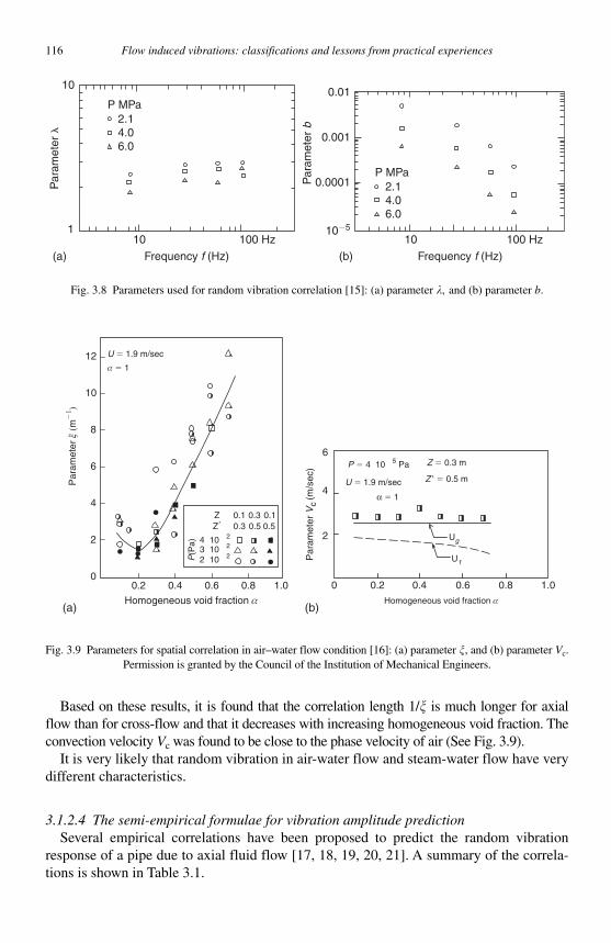
116 Flow induced vibrations: classifications and lessons from practical experiences
Based on these results, it is found that the correlation length 1/ � is much longer for axial flow than for cross-flow and that it decreases with increasing homogeneous void fraction. The convection velocity Vc was found to be close to the phase velocity of air (See Fig. 3.9 ).
It is very likely that random vibration in air-water flow and steam-water flow have very different characteristics.
3.1.2.4 The semi-empirical formulae for vibration amplitude prediction Several empirical correlations have been proposed to predict the random vibration
response of a pipe due to axial fluid flow [17, 18, 19, 20, 21]. A summary of the correla-tions is shown in Table 3.1 .
10
10 100 Hz
Par
amet
er �
1
P MPa2.14.06.0
Frequency f (Hz)(a)
Par
amet
er b
100 Hz10
0.01
0.001
0.0001
10�5
P MPa2.14.06.0
(b) Frequency f (Hz)
Fig. 3.8 Parameters used for random vibration correlation [15]: (a) parameter � , and (b) parameter b .
U � 1.9 m/sec
α � 112
10
8
6
4
2
00.2 0.4 0.6 0.8 1.0
Homogeneous void fraction α
P(P
a)
Par
amet
erξ
(m�
1 )
ZZ�
4 102
3 102
2 102
0.1 0.10.3 0.5 0.5
0.3
(a) (b)
U � 1.9 m/sec
α � 1
6
4
2
Par
amet
erV
c(m
/sec
) P � 4 105 Pa Z � 0.3 m
Z ' � 0.5 m
Ug
U1
0 0.2 0.4 0.6 0.8 1.0
Homogeneous void fraction α
Fig. 3.9 Parameters for spatial correlation in air–water flow condition [16]: (a) parameter �, and (b) parameter Vc.Permission is granted by the Council of the Institution of Mechanical Engineers.

Chapter 3. Vibration induced by external axial flow 117
Burgreen et al.QuinnSogreahRoström & AndersonPaïdoussis & Sharp
Empir
ical e
xpre
ssion
10�410�4
10�3
10�2
10�1
1
10�3 10�2 10�1 1
Predicted amplitude
Exp
erim
enta
l am
plitu
de
Fig. 3.10 Relationship between measured and predicted amplitudes of vibration according to Païdoussis ’ empir-ical formula [4].
These correlation models have generally been developed using dimensional analy-sis and experimental results. The formulae are useful for predicting approximate pipe response. However, due to the significant scatter in the reported data, correlation factors have inevitably been incorporated into the models. Before employing these correlations, one must take into consideration the uncertainty inherent in the actual problem analyzed (See Fig. 3.10).
3.1.3 Flutter and divergence
3.1.3.1 Historical background Studies on the stability of fluid conveying pipes were conducted in the 1950s and
1960s by Païdoussis and co-workers. This work will be described in Section 4.1. On the other hand, regarding instability due to external parallel flow, Hawthorne [22]
was the first to demonstrate the occurrence of the divergence-type instability. Païdoussis et al. [23–26] derived the basic equations for the first time, and investigated the criti-cal velocity for flutter and divergence analytically. He also verified his analytical evalua-tion with experiments. Until the 1980s [27] , many studies were conducted in which more detailed analytical models were developed and the mechanisms of instability further investigated. The response of the fluid force to structural vibration and the dynamic char-acteristics of the pipe in external parallel flow have similar basic characteristics to those found for fluid conveying pipe systems.
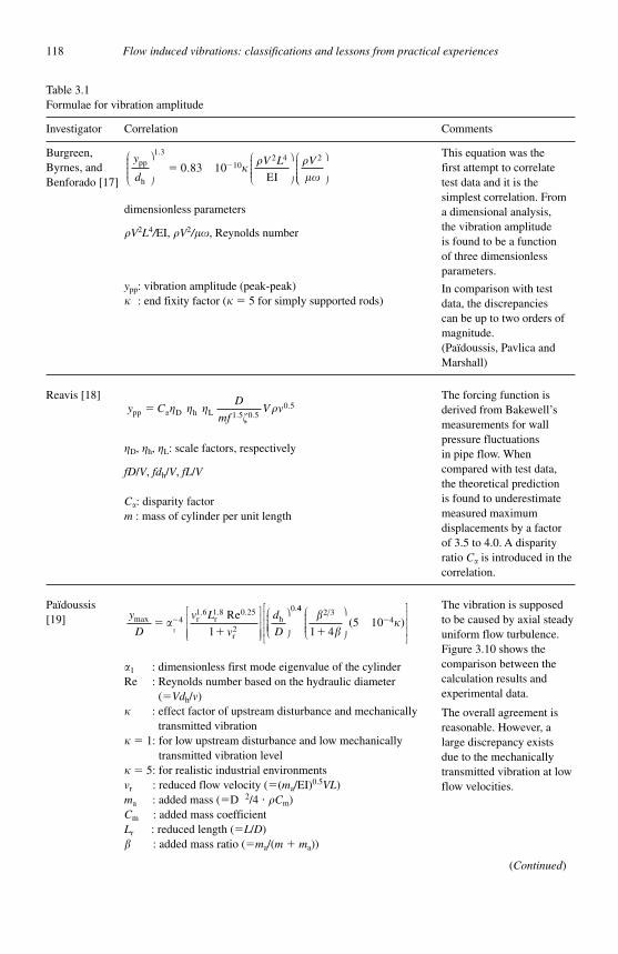
118 Flow induced vibrations: classifications and lessons from practical experiences
Table 3.1 Formulae for vibration amplitude
Investigator Correlation Comments
Burgreen, Byrnes, and Benforado [17]
y
d
V L Vpp
h
102 4 2
0.83 10EI
⎛
⎝⎜⎜⎜⎜
⎞
⎠⎟⎟⎟⎟⎟
⎛
⎝⎜⎜⎜⎜
⎞
⎠⎟⎟⎟⎟⎛1 3.
� � �� �
��⎝⎝⎜⎜⎜⎜
⎞
⎠⎟⎟⎟⎟⎟
dimensionless parameters
� V2L4/ EI, � V2/�� , Reynolds number
ypp : vibration amplitude (peak-peak) � : end fixity factor ( � � 5 for simply supported rods)
This equation was the first attempt to correlate test data and it is the simplest correlation. From a dimensional analysis, the vibration amplitude is found to be a function of three dimensionless parameters.
In comparison with test data, the discrepancies can be up to two orders of magnitude. (Païdoussis, Pavlica and Marshall)
Reavis [18] y C
D
mfV vpp D h L 1.5 0.5
0.5� � � ��
�
�D, �h, �L : scale factors, respectively
fD / V , fdh / V , fL / V
C : disparity factor m : mass of cylinder per unit length
The forcing function is derived from Bakewell ’ s measurements for wall pressure fluctuations in pipe flow. When compared with test data, the theoretical prediction is found to underestimate measured maximum displacements by a factor of 3.5 to 4.0. A disparity ratio C is introduced in the correlation.
Païdoussis [19] y
D
v L
v
d
Dmax
. Re�
�� 1
r1.6
r0.25
r
h0.
14
1 8
2
⎡
⎣⎢⎢⎢
⎤
⎦⎥⎥⎥
⎛
⎝⎜⎜⎜⎜⎞
⎠⎟⎟⎟⎟
44 2 34
1 45 10
��
��
�⎛
⎝⎜⎜⎜⎜
⎞
⎠⎟⎟⎟⎟⎟
⎡
⎣
⎢⎢⎢
⎤
⎦
⎥⎥⎥
( )
1 : dimensionless first mode eigenvalue of the cylinder Re : Reynolds number based on the hydraulic diameter
(�Vdh / v ) � : effect factor of upstream disturbance and mechanically
transmitted vibration � � 1: for low upstream disturbance and low mechanically
transmitted vibration level � � 5: for realistic industrial environments vr : reduced flow velocity ( � ( ma /EI) 0.5VL ) ma : added mass ( � D 2 /4 � � Cm )Cm : added mass coefficient Lr : reduced length ( �L / D ) � : added mass ratio ( �ma /( m � ma ))
The vibration is supposed to be caused by axial steady uniform flow turbulence. Figure 3.10 shows the comparison between the calculation results andexperimental data.
The overall agreement is reasonable. However, a large discrepancy exists due to the mechanically transmitted vibration at low flow velocities.
(Continued)

Chapter 3. Vibration induced by external axial flow 119
3.1.3.2 Evaluation methods and countermeasures against instability In general, divergence instability for supported tubes occurs when the flow velocity
surpasses a critical value. When the flow velocity is increased further, various types of instabilities can occur depending on the flow field surrounding the tube, and the tube sup-port conditions (See Table 3.2) [24, 28] .
Friction on the tube surface can introduce tension and stabilize the system when the downstream end is free. Lee [29] and Triantafyllou and Chryssostomidis [30] reported that the system became stable when either of requirements shown in Table 3.3 is satisfied.
3.1.4 Examples of reported component-vibration problems andhints for countermeasures
Axial flow-induced random vibration in nuclear plant components has been reported. Examples include the vibration of in-core neutron flux monitoring tube causing neutron
Table 3.1 (Continued)
Investigator Correlation Comments
Chen andWever [20] y
d
V
V
V
Vh cr
21
cr
2
1� �
�
⎛
⎝⎜⎜⎜⎜
⎞
⎠⎟⎟⎟⎟⎟
⎡
⎣
⎢⎢⎢⎢
⎤
⎦
⎥⎥⎥⎥
⎛
⎝⎜⎜⎜⎜
⎞
⎠⎟⎟⎟⎟⎟
�
� : initial turbulence factor ranging from 0.5 for ideally quiet flow to 2.0 for practical flow conditions
VL
C LD mcr
2 2
4 f a
0.5EI
��
( )�
⎡
⎣
⎢⎢⎢
⎤
⎦
⎥⎥⎥
Cf : surface drag coefficient
The vibration is supposed to be caused by parametric excitation. Introducing a sinusoidally varying velocity fluctuation into the equation, the critical buckling velocity Vcr is determined.
Chen and Wambsganss [21]
y z VD d V z
L f m mrms
1.5h
2
0.5 1.5a
0.5
0.018( , )
( )
( )
.�
�
��
1 5 φ
� : constant derived from experiment � ( z ): modal function of the cylinder
This equation is derived from a theoretical relationship for calculating the rms displacement of a cylinder in nominally axial flow.
Table 3.2 Tube support conditions and instability phenomena
Support condition Instability phenomena
Pinned-pinned tube Coupled-mode flutter.
Cantilevered tube Single-degree-of-freedom flutter: critical velocity depends on the shape of the downstream end. The critical velocity with smooth tapered end is lower than that without it.
Flexible tube bundle Critical velocity decreases because of the tube-coupling through fluid.

120 Flow induced vibrations: classifications and lessons from practical experiences
flux fluctuation, fretting wear of BWR fuel cladding, CANDU reactor fuel rod vibration, and tube fretting wear at tube supports caused by vibration in heat exchangers and steam generators. Note however, that there is no reported case of tube failure.
As mentioned above, the random vibration response due to near field turbulence noise in external axial flow varies in proportion to V1.50 � V3.0 in single-phase flow and to V0.75 � V1.35 in two-phase flow. The excitation force is such that the amplitude decreases with increasing frequency. Research findings show that decreasing the flow velocity and increasing the natural frequency of the tube or tubes are effective measures in decreasing the amplitude of random vibration.
It is reported that both the divergence-type and flutter-type instabilities can be elimi-nated when tension develops in the pipe, and when the length of the pipe is increased. If the conditions given in Table 3.3 are satisfied, stabilization can be achieved. In addition, considering that the instability occurs above a certain non-dimensional critical velocity, increasing the natural frequency by thickening the tube walls or by reinforcement and decreasing the flow velocity are effective measures to control instability phenomena.
3.2 Vibration of elastic plates and shells
In this section, self-excited vibration and turbulence-induced vibration of elastic plates and shells subjected to parallel flow are described.
3.2.1 Bending–torsion flutter
3.2.1.1 Historical background Bending–torsion flutter is a dynamic instability which results from coupling between the
bending and torsional modes of a flexible structure, such as shown in Fig. 3.11 . It occurs if the flow velocity exceeds a critical velocity, and the bending and torsional modes have a phase and amplitude combination that extracts energy from the flow [31], as shown in Fig. 3.12 .
Theories on aerodynamic forces acting on two-dimensional airfoil sections were devel-oped mostly in the mid-1940s. These theories are reviewed by Bisplinghoff et al. [32]and Fung [33] . Recently, intensive studies have been carried out on aero-elastic tailoring techniques [34] , computations of unsteady aerodynamic loads [35] , active flutter control [36] , etc.
3.2.1.2 Evaluation method Consider the spring-supported wing section in incompressible flow of velocity U ,
shown in Fig. 3.13 . Let the bending and pitching displacements be resisted by springsat the elastic axis with spring constants Kh and K , respectively. The restoring force
Table 3.3 Condition for prevention of instability induced by external parallel flow
When either of the conditions below is satisfied, the system is stabilized
Tension force at the downstream end � � AU2 L / D � /(2 Cf )
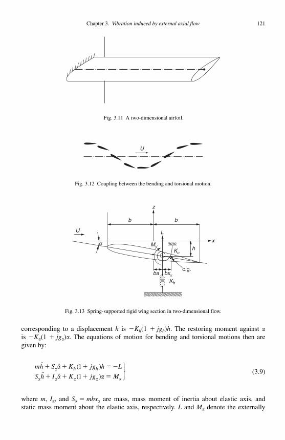
Chapter 3. Vibration induced by external axial flow 121
corresponding to a displacement h is �Kh (1 � jgh ) h . The restoring moment against is �K (1 � jg ) . The equations of motion for bending and torsional motions then are given by:
mh S K jg h L
S h I K jg Mh h
�� ���� ��
� � � � �
� � � �
( )
( )
1
1
⎫⎬⎪⎪⎭⎪⎪
(3.9)
where m , I , and S � mbx are mass, mass moment of inertia about elastic axis, and static mass moment about the elastic axis, respectively. L and M denote the externally
U
b b
hx
c.g.ba bxα
L
MyKα
Kh
z
α
Fig. 3.13 Spring-supported rigid wing section in two-dimensional flow.
Fig. 3.11 A two-dimensional airfoil.
U
Fig. 3.12 Coupling between the bending and torsional motion.
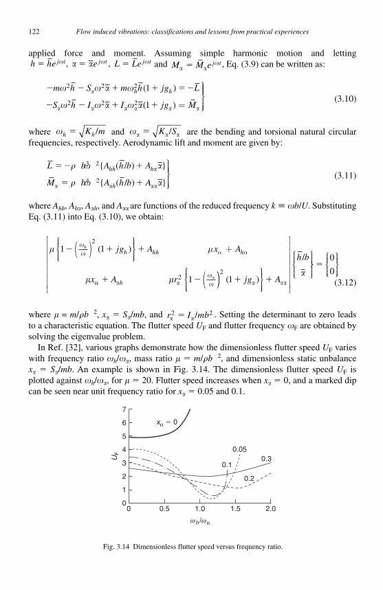
122 Flow induced vibrations: classifications and lessons from practical experiences
applied force and moment. Assuming simple harmonic motion and letting h he e L Lej t j t j t� � �� � � , , and M M e j t
�� , Eq. (3.9) can be written as:
� � � � � �
� � � �
m h S m h jg L
S h I I jg M
h h� � �
� � �
2 2 2
2 2 2
1
1
( )
( ) =
⎫⎬⎪⎪⎪⎪
⎭⎪⎪⎪
(3.10)
where �h hK m� / and � � K S/ are the bending and torsional natural circular frequencies, respectively. Aerodynamic lift and moment are given by:
L b A h b A
M b A h b A
hh h
h
� � �
� �
� �
� �
3 2
4 2
{ ( / ) }
{ ( / ) }
⎫⎬⎪⎪⎪
⎭⎪⎪⎪
(3.11)
where Ahh , Ah , A h , and A are functions of the reduced frequency k � � b / U . Substituting Eq. (3.11) into Eq. (3.10), we obtain:
�
� �
��
��
1 1
1
2
2
� � �
� ��
h jg A x A
x A r
h hh h
h
( )⎧⎨⎪⎪⎩⎪⎪
⎫⎬⎪⎪⎭⎪⎪
+
(
( ) μ α α
))⎧⎨⎪⎪⎩⎪⎪
⎫⎬⎪⎪⎭⎪⎪
⎡
⎣
⎢⎢⎢⎢⎢⎢⎢
⎤
⎦
⎥⎥⎥⎥⎥⎥⎥
⎧⎨⎪⎪
⎩⎪⎪
⎫
21( )
/
� �jg A
h b
⎬⎬⎪⎪
⎭⎪⎪
⎧⎨⎪⎪⎩⎪⎪
⎫⎬⎪⎪⎭⎪⎪
�0
0(3.12)
where � = m / � b2 , x � S / mb , and r I mb 2 2� / . Setting the determinant to zero leads
to a characteristic equation. The flutter speed UF and flutter frequency �F are obtained by solving the eigenvalue problem.
In Ref. [32] , various graphs demonstrate how the dimensionless flutter speed UF varies with frequency ratio �h / � , mass ratio � � m / � b2 , and dimensionless static unbalance x � S / mb . An example is shown in Fig. 3.14 . The dimensionless flutter speed UF is plotted against �h / � , for � � 20. Flutter speed increases when x � 0, and a marked dip can be seen near unit frequency ratio for x � 0.05 and 0.1.
0.1
0.05
xα � 0
0.3
0.2
2.01.51.00.500
1
2
UF
3
4
5
6
7
ωh /ωα
Fig. 3.14 Dimensionless flutter speed versus frequency ratio.
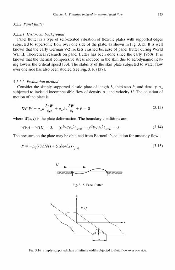
Chapter 3. Vibration induced by external axial flow 123
3.2.2 Panel flutter
3.2.2.1 Historical background Panel flutter is a type of self-excited vibration of flexible plates with supported edges
subjected to supersonic flow over one side of the plate, as shown in Fig. 3.15 . It is well known that the early German V-2 rockets crashed because of panel flutter during World War II. Theoretical research on panel flutter has been done since the early 1950s. It is known that the thermal compressive stress induced in the skin due to aerodynamic heat-ing lowers the critical speed [33] . The stability of the skin plate subjected to water flow over one side has also been studied (see Fig. 3.16 ) [37].
3.2.2.2 Evaluation method Consider the simply supported elastic plate of length L , thickness h , and density �m
subjected to inviscid incompressible flow of density �0 , and velocity U . The equation of motion of the plate is:
D W hW
th
W
tPm m�4
2
20� � � ��
��
� ���
(3.13)
where W ( x , t ) is the plate deformation. The boundary conditions are:
W W L W x W xx x L( ) ( ) , ( ) ( )0 0 02 20
2 2� � � �� �� � � �/ / (3.14)
The pressure on the plate may be obtained from Bernoulli ’ s equation for unsteady flow:
P t U xz
� � ��
� � � � �0 0( ) ( )φ φ/ /{ } (3.15)
U
Fig. 3.15 Panel flutter.
U
z
x
y
h
L
Fig. 3.16 Simply-supported plate of infinite width subjected to fluid flow over one side.
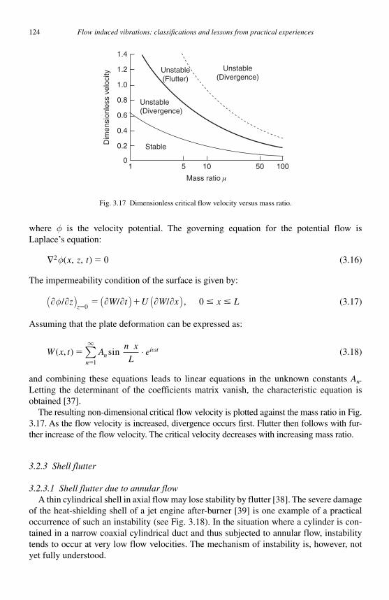
124 Flow induced vibrations: classifications and lessons from practical experiences
where φ is the velocity potential. The governing equation for the potential flow is Laplace ’ s equation:
�2 0φ( , , )x z t � (3.16)
The impermeability condition of the surface is given by:
� � � � � �φ/ / /z W t U W x x Lz
( ) ( ) ( )�
� � � �0
0, (3.17)
Assuming that the plate deformation can be expressed as:
W x t An x
Len
i t
n
( , ) ��
sin �⋅
∞
∑1
(3.18)
and combining these equations leads to linear equations in the unknown constants An . Letting the determinant of the coefficients matrix vanish, the characteristic equation is obtained [37].
The resulting non-dimensional critical flow velocity is plotted against the mass ratio in Fig. 3.17 . As the flow velocity is increased, divergence occurs first. Flutter then follows with fur-ther increase of the flow velocity. The critical velocity decreases with increasing mass ratio.
3.2.3 Shell flutter
3.2.3.1 Shell flutter due to annular flow A thin cylindrical shell in axial flow may lose stability by flutter [38] . The severe damage
of the heat-shielding shell of a jet engine after-burner [39] is one example of a practical occurrence of such an instability (see Fig. 3.18) . In the situation where a cylinder is con-tained in a narrow coaxial cylindrical duct and thus subjected to annular flow, instability tends to occur at very low flow velocities. The mechanism of instability is, however, not yet fully understood.
Unstable(Divergence)
Unstable(Divergence)
Stable
Mass ratio μ
Dim
ensi
onle
ss v
eloc
ity
1.4
1.2
1.0
0.8
0.6
0.4
0.2
01 5 10 50 100
Unstable(Flutter)
Fig. 3.17 Dimensionless critical flow velocity versus mass ratio.
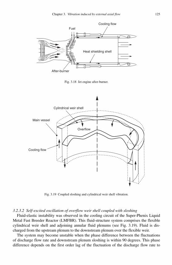
Chapter 3. Vibration induced by external axial flow 125
3.2.3.2 Self-excited oscillation of overflow weir shell coupled with sloshing Fluid-elastic instability was observed in the cooling circuit of the Super-Phenix Liquid
Metal Fast Breeder Reactor (LMFBR). This fluid-structure system comprises the flexible cylindrical weir shell and adjoining annular fluid plenums (see Fig. 3.19 ) . Fluid is dis-charged from the upstream plenum to the downstream plenum over the flexible weir.
The system may become unstable when the phase difference between the fluctuations of discharge flow rate and downstream plenum sloshing is within 90 degrees . This phase difference depends on the first order lag of the fluctuation of the discharge flow rate to
FuelCooling flow
Heat shielding shell
After-burner
Fig. 3.18 Jet engine after-burner.
Overflow
Main vessel
Cylindrical weir shell
Cooling flow
Fig. 3.19 Coupled sloshing and cylindrical weir shell vibration.
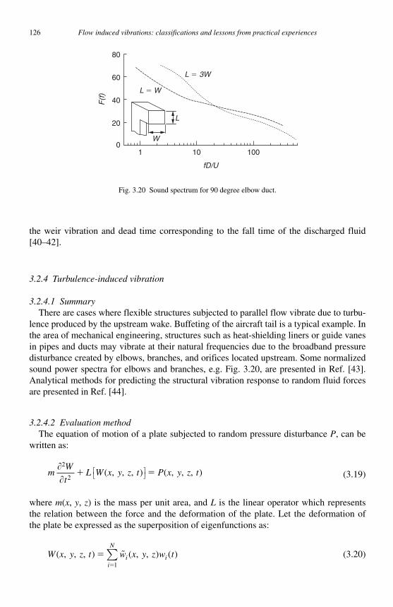
126 Flow induced vibrations: classifications and lessons from practical experiences
the weir vibration and dead time corresponding to the fall time of the discharged fluid [40–42] .
3.2.4 Turbulence-induced vibration
3.2.4.1 Summary There are cases where flexible structures subjected to parallel flow vibrate due to turbu-
lence produced by the upstream wake. Buffeting of the aircraft tail is a typical example. In the area of mechanical engineering, structures such as heat-shielding liners or guide vanes in pipes and ducts may vibrate at their natural frequencies due to the broadband pressure disturbance created by elbows, branches, and orifices located upstream. Some normalized sound power spectra for elbows and branches, e.g. Fig. 3.20 , are presented in Ref. [43] . Analytical methods for predicting the structural vibration response to random fluid forces are presented in Ref. [44] .
3.2.4.2 Evaluation method The equation of motion of a plate subjected to random pressure disturbance P , can be
written as:
mW
tL W x y z t P x y z t
��
2
2� �( , , , ) ( , , , )⎡⎣ ⎤⎦ (3.19)
where m ( x , y , z ) is the mass per unit area, and L is the linear operator which represents the relation between the force and the deformation of the plate. Let the deformation of the plate be expressed as the superposition of eigenfunctions as:
W x y z t w x y z w ti ii
N
( , , , ) ( , , ) ( )��
�1∑ (3.20)
80
60
40
20
01 10
fD/U
L � W
L � 3W
L
W
F(f
)
100
Fig. 3.20 Sound spectrum for 90 degree elbow duct.
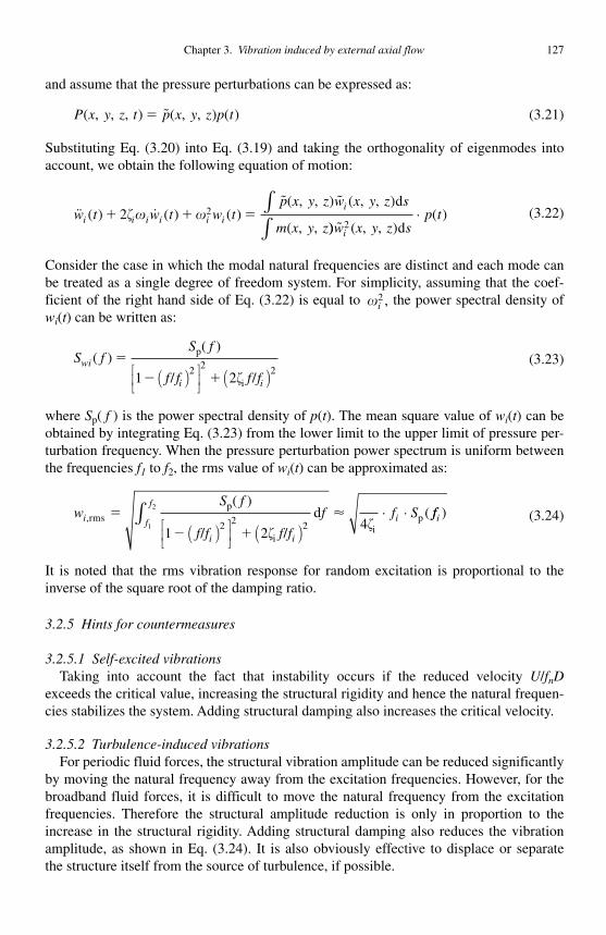
Chapter 3. Vibration induced by external axial flow 127
and assume that the pressure perturbations can be expressed as:
P x y z t p x y z p t( , , , ) ( , , ) ( )� � (3.21)
Substituting Eq. (3.20) into Eq. (3.19) and taking the orthogonality of eigenmodes into account, we obtain the following equation of motion:
�� �� �
w t w t w tp x y z w x y z s
m x y zi i i i i i
i( ) ( ) ( )
( , , ) ( , , )
( , ,� � �2 2�� �
d∫)) ( , , )
( )�w x y z s
p ti2 d∫
⋅ (3.22)
Consider the case in which the modal natural frequencies are distinct and each mode can be treated as a single degree of freedom system. For simplicity, assuming that the coef-ficient of the right hand side of Eq. (3.22) is equal to �i
2 , the power spectral density of wi ( t ) can be written as:
S fS f
f f f fwi
i i
( )( )
/ /
p
i
�
� �1 22 2 2( )⎡
⎣⎢⎤⎦⎥( )�
(3.23)
where Sp ( f ) is the power spectral density of p ( t ). The mean square value of wi ( t ) can be obtained by integrating Eq. (3.23) from the lower limit to the upper limit of pressure per-turbation frequency. When the pressure perturbation power spectrum is uniform between the frequencies f1 to f2 , the rms value of wi ( t ) can be approximated as:
wS f
f f f f
f f Si
i i
f
f
i,rmsp
ii
p
( )
/ /
d (�
� �1 242 2 21
2
( )⎡⎣⎢
⎤⎦⎥( )
⋅ ⋅∫�
�
� ffi ) (3.24)
It is noted that the rms vibration response for random excitation is proportional to the inverse of the square root of the damping ratio.
3.2.5 Hints for countermeasures
3.2.5.1 Self-excited vibrations Taking into account the fact that instability occurs if the reduced velocity U / fn D
exceeds the critical value, increasing the structural rigidity and hence the natural frequen-cies stabilizes the system. Adding structural damping also increases the critical velocity.
3.2.5.2 Turbulence-induced vibrations For periodic fluid forces, the structural vibration amplitude can be reduced significantly
by moving the natural frequency away from the excitation frequencies. However, for the broadband fluid forces, it is difficult to move the natural frequency from the excitation frequencies. Therefore the structural amplitude reduction is only in proportion to the increase in the structural rigidity. Adding structural damping also reduces the vibration amplitude, as shown in Eq. (3.24). It is also obviously effective to displace or separate the structure itself from the source of turbulence, if possible.

128 Flow induced vibrations: classifications and lessons from practical experiences
3.3 Vibration induced by leakage flow
3.3.1 General description of the problem
Large amplitude self-excited vibrations can occur in structures forming leakage-flow passages. One of the major features of leakage-flow-induced vibration is that the sensitivityof the pressure loss can be very high compared to the displacement of the structures forming the leakage-flow passage. This can induce the vibration of huge structures such as the core barrel of a PWR, feed-water spargers in BWRs (see Fig. 3.21 [45] ), and so on.
3.3.1.1 Single degree-of-freedom translational systems In this section, we assume incompressibility of the gas or liquid, when the Mach
number is less than 0.3. One-dimensional tapered- as well as arbitrary-shaped passages
Inlet nozzle
Reactor pressure vessel
Core barrelThermal shield
Sparger
Reactor pressure vessel
Reactor pressurevessel
Water supply nozzle
Thermalsleeve
(a)
(b)
Fig. 3.21 Examples of leakage-flow-induced vibration events [45]: (a) PWR core barrel, and (b) feed-water sparger.
Chapter 3. Vibration induced by external axial flow 129
are considered. The structure forming the leakage passage is assumed to vibrate as a single-degree-of-freedom translational system.
3.3.1.2 Other cases We will consider other cases such as single-degree-of-freedom rotational systems, two-
degrees-of-freedom translational and rotational systems, and continuous systems. The results are compared with the case of single-degree-of-freedom translational systems. At the end of this section, an explanation is given for the case of the annular gap, where nei-ther the inner tube nor the outer tube rotates.
3.3.2 Evaluation method for single-degree-of-freedom translational system
In this section, a method is described to model the fluid dynamic forces acting on the wall of a tapered passage of area increment ratio ( ( ) ( )} ( )� �{ / ;H L H H0 0 over-bars – indicate a steady state condition). Using this method, the characteristics of the sys-tem are considered [46].
3.3.2.1 Basic equations of leakage flow As shown in Fig. 3.22(a) , the upper wall of the tapered passage is assumed to be vibrat-
ing in the normal direction relative to the lower wall with a circular frequency � . When Qis the flow rate per unit width of the passage, the continuity and momentum equations of the leakage flow can be written as:
��
��
Q
Y
H
t
Q
t Y
Q
H
H P
Y
Q
H� � � � � �
��
�� �
��
�01
4
2 2
2,
⎛
⎝⎜⎜⎜⎜⎞
⎠⎟⎟⎟⎟ (3.25[a])
The boundary conditions at the entrance and the exit of the passage are expressed as:
P PQ
HP L P
Q L
H L( ) ,in in ex ex0
1
2
0
0
1
2
2
2
2
2� � � �� � � �
( )
( )( )
( )
( )(3.25[b])
where �in and �ex denote the entrance and the exit pressure loss factors, and � denotes the friction factor of the passage. The values for pipes can be used for �in and �ex for qualita-tive evaluation; the loss factor �in � 1.5 for entrance into a passage mounted flush with the wall, �in � 1.0 for circular bellmouth entrance, and �ex � 0 for outlet from a passage mounted flush with the wall. � is the friction factor of the passage and given as a function of the Reynolds number, Re; � � 48/Re(Re � 1000) for laminar flow, and � � 0.266 Re� 0.25 (Re � 1000) for turbulent flow where Re � Q / � .
3.3.2.2 Relation between steady flow rate and pressure difference across the passage The relationship between the steady flow rate and the steady pressure difference across
the leakage-flow passage is expressed as:
Q
H
P P
I h0 321 2 2 1
��
� � �
in ex
in ex/ /{� � � �( ) ( ) ( )}{ }(3.26)

130 Flow induced vibrations: classifications and lessons from practical experiences
where H0 is the steady inlet gap of the passage, and the effective pressure loss factor of the passage � , non-dimensional axial location y , and the function In ( y ), ( n � 3 inEq. [3.26]), are defined as:
� � � � � �
��
��
�
L H y Y L h H H y
I yn h yn n
/( , / , /4 11
11
10 0
1
)
( )( ) ( )
⎡
⎣⎢⎢
⎤
⎦⎥⎥⎥ ( ) ( )) ( )n h y n� 1 1ln( / �
(3.27)
3.3.2.3 Unsteady fluid forces of a tapered passage The basic equations are linearized with respect to the unsteady components. The
unsteady pressure distribution is determined and integrated from the entrance to the out-let. The unsteady fluid dynamic force, �F , acting on the wall of unit width is obtained assuming that wall vibrates with infinitesimally small amplitude, �H . Defining the non-dimensional frequency � �� H L Q0 / , the dynamic force becomes:
�FQ L
Hi m c
c
i Ti k
k
i T� � � �
�� �
�
��
��
�
2
02 1
21
2
1 1
⎛
⎝⎜⎜⎜
⎞
⎠⎟⎟⎟⎟
⎛
⎝⎜⎜⎜
⎞
⎠⎟⎟⎟⎟⎟
⎧⎨⎪⎪
⎩⎪⎪
⎫⎬⎪⎪
⎭⎪⎪
�H
H0
(3.28)
Fig. 3.22 One-dimensional leakage passage under study and coordinate system: (a) tapered leakage-flow passage, and (b) arbitrary-shaped leakage-flow passage.
Q0 Q1
l1
1
lj�1 ljQj
j
Qj�1
j�1
lNQN QN�1
N
(N � 1)�
PN�1Pj
j�
hj
P2
2�
h2
P1
1�
h1 hN�1
Z
H
�H • exp(i � t )
Q
0 L
YPin Pex
Z
H
�H • exp(i � t )
Q
0(a)
(b)
L Y
Pin Pex
Chapter 3. Vibration induced by external axial flow 131
The parameters m , c1 , c2 , k1 , k2 are defined in Table 3.4 . The first term in the braces inEq. (3.28) corresponds to the squeeze-film effect, in which the fluid force can be gen-erated by oscillation of the relatively large axial velocity induced by the wall oscilla-tion of the leakage passage. The second term is the fluid force due to oscillations of the axial velocity induced by the flow resistance variation of the fluid flow. Equation (3.28) includes a first order delay term due to fluid inertia. When we estimate stability, i� is replaced by the Laplace transform parameter s , and �F is substituted into the basic equa-tion of the structure forming the leakage-flow passage. If the equation of the structureis expressed in terms of a second order system, the characteristic equation is expressed by a third order polynomial.
Equation (3.28) is rearranged as:
� � � �F M H C C H K H� � � � �a w e a�� �( ){ } (3.29)
Table 3.4 Definition of parameters in Eq. (3.28)
Parameters in Eq (3.28)
m J N I N
cN J
I
N J
I
J N I
IN
� �
� � � � �
1 1 1 1
11 3
1
3 1
1
1 1 3
12 32
/
( )
*
*�� ⎛
⎝⎜⎜⎜⎜
⎞
⎠⎟⎟⎟⎟⎟⎟
⎛
⎝⎜⎜⎜⎜
⎞
⎠⎟⎟⎟⎟⎟
⎛
⎝⎜⎜⎜⎜
⎞
⎠⎟⎟⎟⎟⎟
� � � �
�
2 12 1
12
1
1
1
1
I N
IN
J
I
N
I�in
��ex
( )
( / ) ( / )
h
N
I
J
I
c J N I B B r
k
21
1
1
1
2 1 1 12
1 3
1
11
3
�
�
�
⎛
⎝⎜⎜⎜⎜
⎞
⎠⎟⎟⎟⎟⎟
(( )(inex� �
�� � � � �
N I
IN
N
I h1 4
14
1
13
1⎛
⎝⎜⎜⎜⎜
⎞
⎠⎟⎟⎟⎟⎟
⎛
⎝⎜⎜⎜⎜
⎞
⎠⎟⎟⎟⎟⎟ 11
1
12
1
1
2 3 1
), ,
N
Ik
N
I
B B
rT
I
r� �
definition of symbols in the above equations
J y I y I y I I J J N I J
N
n n n n n n n n n n
n*
( ) ( ( ) ( ))/ , ( ), ,� � � � � � �
��
�1 1 1
2
2
( )
��
�
2 3 2 3
11 1
2
2 1
11 3
12
��
� ��
�� �
� �
ln( ) ( ), ln( )( )n n
Q
( )+
d
ddQ
BI J
JI
I I
J
⎛
⎝⎜⎜⎜⎜
⎞
⎠⎟⎟⎟⎟
⎛
⎝⎜⎜⎜⎜
⎞
⎠⎟⎟⎟⎟⎟
0
11 3
13
1 2
1
2 2� � � � �( )�� �iinex
inex
( )
( )( )
� �
� � � �
�
�
� ��
h
I
J
B Ih
B
21
1
2 4 3
3
11
31
⎛
⎝⎜⎜⎜⎜
⎞
⎠⎟⎟⎟⎟⎟
22 11 3
13
1
1
( )�� ��
� � � � �I N
NI
I
N h
⎛
⎝⎜⎜⎜⎜
⎞
⎠⎟⎟⎟⎟⎟
⎛
⎝⎜⎜⎜⎜
⎞
⎠⎟⎟⎟⎟⎟in
ex22
3 2
1
21
( )
( )inexr I
h� � � �( )�� �
�
132 Flow induced vibrations: classifications and lessons from practical experiences
where a dot denotes differentiation with respect to time. Ma , ( Cw + Ce ), and Ka are added mass, added damping, and added stiffness coefficients defined as functions of � :
ML
Hm
c T
TC
QL
Hc
c
Ta w,� ��
� ��
��
��
3
0
22 2
2
02 1
22 21 1
⎛
⎝⎜⎜⎜
⎞
⎠⎟⎟⎟⎟
⎛
⎝⎜⎜⎜
⎞
⎠⎠⎟⎟⎟⎟
⎛
⎝⎜⎜⎜
⎞
⎠⎟⎟
, e
a
CQL
H
k T
T
KQ L
Hk
k
T
� ��
� ��
��
��
2
02
22 2
2
03 1
22 2
1
1
,
⎟⎟⎟ ( . )3 30
Cw , the damping component due to squeeze-film effects is generally positive. Ce , the damping coefficient due to the flow resistance variations, can be negative in the case of divergent passages. The negative damping can generate self-excited vibrations. In the case of divergent passages, the added stiffness coefficient can be negative, which can induce divergence-type (buckling-type) instability. Figure 3.23 shows the ranges where Cw � Ce
and Ka become positive or negative on the ( , � ) plane. It is recommended that the area increment ratio be set to zero or negative, the latter corresponding to the leakage-flow passage being changed to a convergent passage to control the self-excited vibration.
3.3.3 Analysis method for single-degree-of-freedom translational system withleakage-flow passage of arbitrary shape
3.3.3.1 Steady fluid force In the case of one-dimensional leakage-flow passage, steady and unsteady fluid
forces can be easily analyzed for arbitrary-shaped passages, such as Fig. 3.22(b), using the transfer matrix method. When steady flow rate Q is assumed, the transfer matrix of the element connected to the entrance can be obtained. The elements outlet pressure can
102
101
10�1
10�2
10�1 1011
1 � �
1b
Cw�Ce � 0
Ka � 0
Ka � 0
jin � 1.5jex � 0
vT
vT
0
vT 0
vT
� 1
}
}
Cw�Ce�0
Ka � 0
vT
0
vT
� 1
Fig. 3.23 Region where added damping and stiffness coefficients become positive or negative when the one-dimensional tapered passage wall oscillates as a single-degree-of-freedom translating system [46].
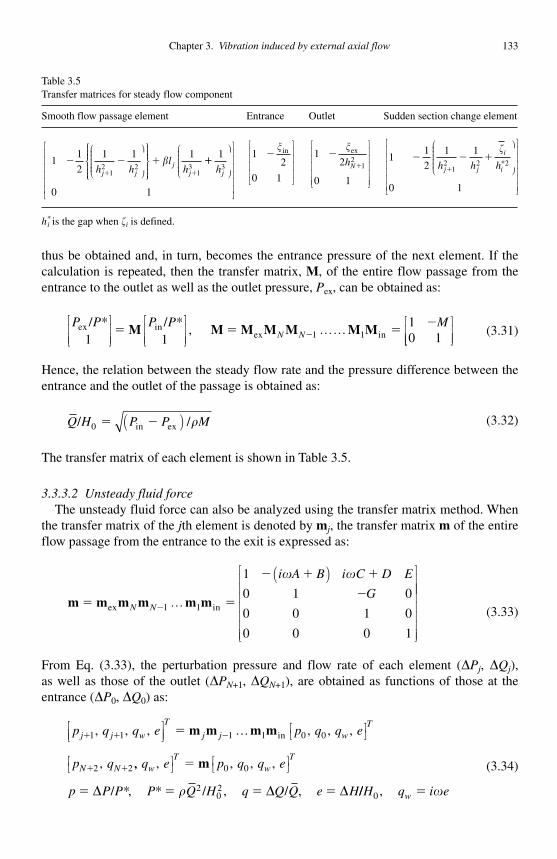
Chapter 3. Vibration induced by external axial flow 133
thus be obtained and, in turn, becomes the entrance pressure of the next element. If the calculation is repeated, then the transfer matrix, M , of the entire flow passage from the entrance to the outlet as well as the outlet pressure, Pex , can be obtained as:
P P P P MN N
ex inex in
/ /,
* *1 1
10 11 1
⎡
⎣⎢⎢
⎤
⎦⎥⎥
⎡
⎣⎢⎢
⎤
⎦⎥⎥
…… ⎡� � �
��M M M M M M M
⎣⎣⎢⎢
⎤⎦⎥⎥
(3.31)
Hence, the relation between the steady flow rate and the pressure difference between the entrance and the outlet of the passage is obtained as:
Q H P P M/ /in ex0 � �( ) � (3.32)
The transfer matrix of each element is shown in Table 3.5 .
3.3.3.2 Unsteady fluid force The unsteady fluid force can also be analyzed using the transfer matrix method. When
the transfer matrix of the j th element is denoted by mj, the transfer matrix m of the entire flow passage from the entrance to the exit is expressed as:
m m m m m m� �
� � �
��ex inN N
i A B i C D E
G1 1
1
0 1 0
0 0 1 0
0 0 0 1
…
( )⎡
⎣
⎢⎢⎢⎢⎢⎢⎢
⎤
⎦
⎥� �⎥⎥⎥⎥⎥⎥⎥
(3.33)
From Eq. (3.33), the perturbation pressure and flow rate of each element ( �Pj , �Qj ), as well as those of the outlet ( �PN+1 , �QN+1 ), are obtained as functions of those at the entrance ( �P0 , �Q0 ) as:
p q q e p q q e
p q
j j w
T
j j wT
N N
� � �
� �
�1 1, , , , , ,
,
⎡⎣⎢
⎤⎦⎥
⎡⎣ ⎤⎦m m m m1 1 0 0
2 2
… in
,, , , , ,
/ , / , / ,
q e p q q e
p P P P Q H q Q Q e H
wT
wT⎡⎣ ⎤⎦ ⎡⎣ ⎤⎦�
� � � �
m 0 0
202� � �* * � // ,H q i ew0 � �
(3.34)
Table 3.5 Transfer matrices for steady flow component
Smooth flow passage element Entrance Outlet Sudden section change element
11
2
1 1 1
12 2
13
� � �� �h h
lhj j
jj
⎛
⎝
⎜⎜⎜⎜⎜
⎞
⎠
⎟⎟⎟⎟⎟⎟
⎧⎨⎪⎪⎪
⎩⎪⎪⎪
⎫⎬⎪⎪⎪
⎭⎪⎪⎪
� ��1
0 1
3hj
⎛
⎝
⎜⎜⎜⎜⎜
⎞
⎠
⎟⎟⎟⎟⎟⎟
⎡
⎣
⎢⎢⎢⎢⎢⎢
⎤
⎦
⎥⎥⎥⎥⎥⎥
12
0 1
��in
⎡
⎣
⎢⎢⎢⎢
⎤
⎦
⎥⎥⎥⎥
12
0 1
12
��
�ex
hN
⎡
⎣
⎢⎢⎢⎢⎢
⎤
⎦
⎥⎥⎥⎥⎥
11
2
1 1
0 1
12 2 2
� � ��h h hj j
i
i
�*
⎛
⎝
⎜⎜⎜⎜⎜
⎞
⎠
⎟⎟⎟⎟⎟⎟
⎡
⎣
⎢⎢⎢⎢⎢⎢
⎤
⎦
⎥⎥⎥⎥⎥⎥
h*i is the gap when �i is defined.

134 Flow induced vibrations: classifications and lessons from practical experiences
where [] T indicates the matrix transpose. The transfer matrices of the different elements are shown in Table 3.6 . The perturbation pressures just before the entrance and just after the exit p0 , pN+1 are zero. Considering the second equation of Eq. (3.34), q 0 can be obtained as a function of qw and e as:
qi C D
i A Bq
E
i A Bew0 �
�
��
�
�� � (3.35)
Substituting Eq. (3.35) into the first equation of Eq. (3.34), the non-dimensional pertur-bation pressure distribution pj can be obtained as a function of qw and e . Finally, when the non-dimensional perturbation pressure is integrated numerically, the unsteady fluid force acting on the wall can be obtained as a function of qw and e as:
�F P L f q f ew/ w e* � �� � (3.36)
The added mass coefficient Ma , added damping coefficients Cw , Ce , and added stiffness coefficient Ka are defined as:
ML
H
Im fC
QL
Hf C
QL
H
Im f
K
aw
w w ee
a
, , ,� � � � � �
� �
��
� ��
3
0
2
02
2
02
( )Re( )
( )
��Q L
Hf
2
03
Re( )e (3.37)
With �F given by Eq. (3.36), an equation of motion for the structure similar to Eq. (3.29) can be written. The conditions of negative damping and negative stiffness can similarly be evaluated as done above [47].
3.3.4 Mechanism of self-excited vibration [48]
The wall oscillation of the leakage-flow passage can induce flow resistance variation, which in turn induces oscillations of the leakage-flow velocity. In this section, the reason why a negative damping force can be easily generated is given in the case of a divergent passage [48]. This is done by considering how the flow velocity oscillations or variations affect the pressure variations in the leakage-flow passage. The second equation of Eq. (3.25) is linearized as follows:
d
d
d
d
p
y
i
h hq
h
q
y he� � �
�� �
�� �� � 2 2 33 2 4
( ) ( )⎧⎨⎪⎪⎩⎪⎪
⎫⎬⎪⎪⎭⎪⎪
(3.38)
The second term in the bracket of Eq. (3.38) expresses the variation of pressure due to the flow resistance variation associated with variations in the flow rate q , while the first
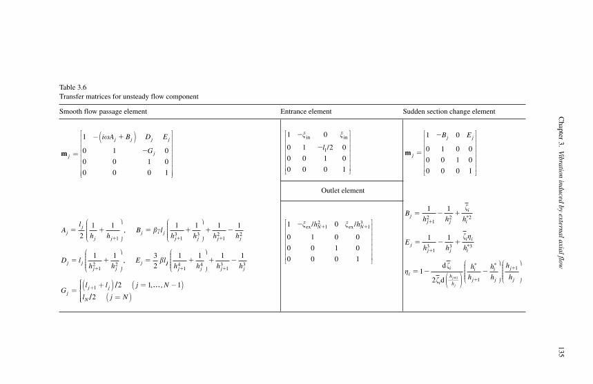
C
hapter 3. Vibration induced by external axial flow
135
Table 3.6 Transfer matrices for unsteady flow component
Smooth flow passage element Entrance element Sudden section change element
m j
j j j j
j
i A B D E
G=
−( )⎡
⎣
⎢⎢⎢⎢⎢⎢⎢⎢
⎤
⎦
⎥⎥⎥⎥⎥⎥⎥⎥
1
0 1 0
0 0 1 0
0 0 0 1
� �
�
1 0
0 1 2 0
0 0 1 0
0 0 0 1
1
�
�
� �in in
/l
⎡
⎣
⎢⎢⎢⎢⎢⎢⎢
⎤
⎦
⎥⎥⎥⎥⎥⎥⎥
m j
j jB E
�
�1 0
0 1 0 0
0 0 1 0
0 0 0 1
⎡
⎣
⎢⎢⎢⎢⎢⎢⎢
⎤
⎦
⎥⎥⎥⎥⎥⎥⎥
Outlet element
Al
h hB l
h hjj
j jj j
j j
� � � �� �2
1 1 1 1
1 13 3
⎛
⎝
⎜⎜⎜⎜⎜
⎞
⎠
⎟⎟⎟⎟⎟⎟
⎛
⎝
⎜⎜⎜⎜⎜
⎞
⎠, ��
⎟⎟⎟⎟⎟⎟⎟
⎛
⎝
⎜⎜⎜⎜⎜
⎞
⎠
⎟⎟⎟⎟⎟⎟
� �
� � �
�
�
1 1
1 1 3
2
12 2
12 2
h h
D lh h
E l
j j
j jj j
j, � jjj j j j
jj j
h h h h
Gl l j
1 1 1 1
2 1
14 4
13 3
1
� �
� � �⎛
⎝
⎜⎜⎜⎜⎜
⎞
⎠
⎟⎟⎟⎟⎟⎟
=+( ) =+ / ,�� , N
l j NN
−( )=( )
⎧⎨⎪⎪⎪
⎩⎪⎪⎪
1
2/
1 0
0 1 0 0
0 0 1 0
0 0 0 1
12
13� � �� �ex ex/ /h hN N
⎡
⎣
⎢⎢⎢⎢⎢⎢⎢
⎤
⎦
⎥⎥⎥⎥⎥⎥⎥
Bh h h
Eh h h
jj j
i
i
jj j
i i
i
ii
ihj
� � �
� � �
� �
�
�
1 1
1 1
2
12 2 2
13 3 3
�
� �
��
�
*
*
1d
d �� �
��
1 1
1
h
i
j
i
j
j
jj
h
h
h
h
h
h( )⎛
⎝
⎜⎜⎜⎜⎜
⎞
⎠
⎟⎟⎟⎟⎟⎟
⎛
⎝
⎜⎜⎜⎜⎜
⎞
⎠
⎟⎟⎟⎟⎟⎟
* *
136 Flow induced vibrations: classifications and lessons from practical experiences
term expresses the pressure variation due to fluid inertia. From Eq. (3.38) we note the following regarding the various contributions to pressure variations:
1. Pressure variation due to inertia effects is proportional to 1/ h. 2. Pressure variation due to flow resistance is proportional to 1/ h3 within the leakage-
flow passage and proportional to 1/ h2 for the entrance and the exit.
Therefore, though in the divergent passage the variation of the flow resistance and inertia force decreases with y , the inertia force can be dominant in the downstream region compared to the flow resistant related force (see Fig. 3.24 ).
Now, let us consider the process when the gap width increases (as passage walls move away from each other) for the divergent passage. The flow rate increases since the flow resistance of the leakage passage decreases. Near the outlet, the influence of the iner-tia force is dominant compared with that of the flow resistance, and the flow rate can-not increase easily. That is, pressure in the channel increases due to an effect similar to attempting to close the outlet while pumping fluid into the channel at the entrance. On the other hand, when the gap width decreases (as passage walls approach), though the flow rate decreases, the flow rate does not decrease easily near the outlet since the influ-ence of the inertia force can be dominant. That is, pressure in the channel decreases due to an effect similar to trying to close the entrance while sucking out fluid at the outlet. Pressure increases as the gap width increases, and decreases with decreasing gap width. The increased pressure as the gap width increases acts to push the walls further apart while the suction effect as the gap width decreases acts to bring the walls even closer. The net effect then is that pressure acts as a negative damping (destabilizing) force.
In the case of the convergent passage, the inertia force is dominant over the flow resist-ant variation induced force near the entrance. Consequently, the resulting pressure variations
0 0.2 0.4 0.6 0.8 1
Axial location, Y/L
Pressure variation due to flow passage resistance
Convergent passage
Pressure variation due to fluid intertia
Pressure variation due to fluid inertia
Pressure variation due to flow passage resistance
Divergent passage
Fig. 3.24 The distribution of variation of the flow resistance and the inertia force when the flow rate varies in the leakage passage [48].
Chapter 3. Vibration induced by external axial flow 137
lead to a positive damping force generated via the same effects causing the negative damping in a divergent passage. Note that in this case the force directions are reversed.
The foregoing is now explained using a more mathematical approach. The added damping coefficient Ce can be rewritten as follows:
CH
QL
k T
T
B y y T
T
yh y
y y
e02
2 m r
r
d
� � ��
� ��
�
�
�
� � �
��
2 2 22
2 2
3
1 1
2
( ),
( )
( )��
� �
�
�
���
�
�ex
inex
m
d
dh
h yy
h
yi
h yy y
20
1
3 20
1
012
1
1( )
( ) ( )
,( )∫
∫−( )α
11
0
1 1
∫
∫ih y
y�( )
d
(3.39)
where yr and ym are first order moments of the inertia force and the variation of the flow resistance, respectively.
Equation (3.39) also shows that the sign (positive or negative) of Ce depends on the inter-relation between the first order moments of inertia and flow resistance forces. In addition, the condition where Ce becomes negative in the case of arbitrary-shaped pas-sages can also be obtained from Eq. (3.39).
3.3.5 Self-excited vibrations in other cases
3.3.5.1 Rotational vibration of one-dimensional tapered passage wall In the case of rotational motion of the flow-passage wall, the moment around the pivot
point can be calculated, from which we can obtain the added moment coefficients [46]. Though the mechanism of the self-excited vibration is similar to the mechanism in the case of translational vibration, the condition of negative damping depends on the location of the pivot point.
Figure 3.25(a)–(c) shows the ranges where added damping and added stiffness coef-ficients become positive or negative on the ( , � )-plane in the case of laminar flow, �in � 1.0, �ex � 0, and the non-dimensional pivot location lf (�Lf / L , Lf is the pivot loca-tion) is selected to be 0, 0.5, and 0.7. The figure shows that divergence-type instability can occur in the case of the divergent passage as well as the convergent passage. The self-excited vibration can easily occur in the case of the divergence passage, however, it can also occur in the case of the convergent passage when the pivot point is upstream of the center of the passage. When the pivot point is at the entrance ( lf � 0), the region where divergent-type instability and self-induced vibration occur becomes limited, and the gen-eration of divergent-type instability and self-induced vibration tends to be controlled.
3.3.5.2 Two-degrees-of-freedom translational and rotational systems andcontinuous systems [46, 49, 50]
In the cases of a two-degrees-of-freedom translational and rotational system and a con-tinuous system, the self-excited vibration of the same mechanism as the single-degree-of-freedom system, as well as the self-excited vibration due to the modal coupling where two or more vibration modes are coupled through the fluid, can occur. Figure 3.26 shows

138 Flow induced vibrations: classifications and lessons from practical experiences
102
101
10�1
10�2
10�1 1011
1 � �
10�1 1011
1 � �
10�1 10111��
1b
102
101
10�1
10�2
1b
102
101
10�1
10�2
1b
Cw � Ce � 0
Ka � 0
Cw � Ce � 0
Cw
�C
e�0
Cw �C
e �0
Ka � 0
Cw�Ce�0
Cw�Ce�0
Cw
�C
e�0
Ka�0
Cw � Ce � 0
Cw � Ce � 0
Ka � 0
Ka � 0
Ka�
0
Ka�
0
Ka�
0
Ka�
0
Ka�0
jin � 1.0jex � 0.0lf � 0.0
jin�1.0
jin�1.0
jex�0.0
jex�0.0
lf�0.5
lf�0.7
vT
vT
vT
0
vT0vT
0
vT
0
vT0
vT
0
vT
0
vT
�1
vT
0
vT
�1
vT�1
vT
�1
vT
�1
vT�1
vT�1
vT
�1
vT
�1
Cw
�C
e�0
Ka�0
(a)
(b)
(c)
Fig. 3.25 Region where added damping and stiffness coefficients become positive or negative for a one-dimensional tapered passage wall oscillating as a single-degree-of-freedom rotational system [46]: (a) lf � 0 (the pivot point is at the entrance), (b) lf � 0.5 (the pivot point is at the center of the passage), and (c) lf � 0.7
(the pivot point is slightly closer to the outlet from the mid-point of the passage).
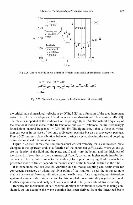
Chapter 3. Vibration induced by external axial flow 139
the critical non-dimensional velocity qr ( )=Q H L/( 0 � ) as a function of the area increment ratio 1 � for a two-degree-of-freedom translational–rotational plate system [46, 49]. The plate is supported at the mid-point of the passage ( lf � 0.5). The natural frequency of the rotational mode is close to the translational one ( �r � [rotational natural frequency]/[translational natural frequency] � 0.9) [46, 49] . The figure shows that self-excited vibra-tion can occur in the case of not only a divergent passage but also a convergent passage. Figure 3.27 presents plate vibration behavior during a cycle, showing the modal coupling of translational and rotational motions.
Figure 3.28 [50] shows the non-dimensional critical velocity for a cantilevered plate clamped at the upstream end, as a function of the parameter �fL
2 / �s wH0 where �f and �s
are the density of the fluid and the plate, and L and w are the length and the thickness of the plate. It is seen that as the parameter �fL
2 / �swH0 increases, higher mode instabilities can occur. This is quite similar to the tendency for a pipe conveying fluid, in which the generated mode of flutter depends on the mass ratio of the tube and the fluid in the tube.
It is concluded that self-excited vibration due to modal coupling can occur even for convergent passages, or where the pivot point of the rotation is near the entrance; note that in this case self-excited vibration cannot easily occur for a single-degree-of- freedom system. A simple stabilization method for this coupled mode instability is yet to be found. Further experimental and analytical work is needed to fully understand this instability.
Recently the mechanism of self-excited vibration for continuous systems is being con-sidered. As an example the wave equation has been derived from the linearized basic
0.60
0.45
0.30
0.15
0.0 0
500 Re
q r
l f � 0.5 1000
10�1 1011
1 � �
vr � 0.90
Two-degree-of -freedomFlutter
Analysis
Experimentunstablestable Stable
Unstable
Fig. 3.26 Critical velocity of two-degree-of-freedom translational and rotational system [49].
� � �0.2 qr � 0.39
t
Fig. 3.27 Plate motion during one cycle of self-excited vibration [49].
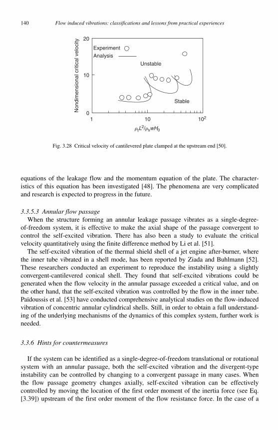
140 Flow induced vibrations: classifications and lessons from practical experiences
equations of the leakage flow and the momentum equation of the plate. The character-istics of this equation has been investigated [48] . The phenomena are very complicated and research is expected to progress in the future.
3.3.5.3 Annular flow passage When the structure forming an annular leakage passage vibrates as a single-degree-
of-freedom system, it is effective to make the axial shape of the passage convergent to control the self-excited vibration. There has also been a study to evaluate the critical velocity quantitatively using the finite difference method by Li et al. [51] .
The self-excited vibration of the thermal shield shell of a jet engine after-burner, where the inner tube vibrated in a shell mode, has been reported by Ziada and Buhlmann [52] . These researchers conducted an experiment to reproduce the instability using a slightly convergent-cantilevered conical shell. They found that self-excited vibrations could be generated when the flow velocity in the annular passage exceeded a critical value, and on the other hand, that the self-excited vibration was controlled by the flow in the inner tube. Païdoussis et al. [53] have conducted comprehensive analytical studies on the flow-induced vibration of concentric annular cylindrical shells. Still, in order to obtain a full understand-ing of the underlying mechanisms of the dynamics of this complex system, further work is needed.
3.3.6 Hints for countermeasures
If the system can be identified as a single-degree-of-freedom translational or rotationalsystem with an annular passage, both the self-excited vibration and the divergent-type instability can be controlled by changing to a convergent passage in many cases. When the flow passage geometry changes axially, self-excited vibration can be effectively controlled by moving the location of the first order moment of the inertia force (see Eq. [3.39]) upstream of the first order moment of the flow resistance force. In the case of a
Experiment
Analysis
Unstable
20
01 10
rfL2/rswH0
102
10
Stable
Non
dim
ensi
onal
crit
ical
vel
ocity
Fig. 3.28 Critical velocity of cantilevered plate clamped at the upstream end [50].
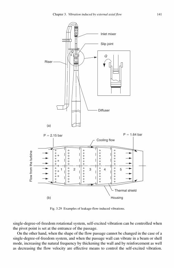
Chapter 3. Vibration induced by external axial flow 141
single-degree-of-freedom rotational system, self-excited vibration can be controlled when the pivot point is set at the entrance of the passage.
On the other hand, when the shape of the flow passage cannot be changed in the case of a single-degree-of-freedom system, and when the passage wall can vibrate in a beam or shell mode, increasing the natural frequency by thickening the wall and by reinforcement as well as decreasing the flow velocity are effective means to control the self-excited vibration.
Q
Inlet mixer
Slip joint
Riser
Diffuser
(a)
(b)
Q
1 2 3 4 5
Thermal shield
Housing
Flo
w fr
om th
e tu
rbin
e
P � 2.15 bar P � 1.64 bar
Cooling flow
Fig. 3.29 Examples of leakage-flow-induced vibrations.
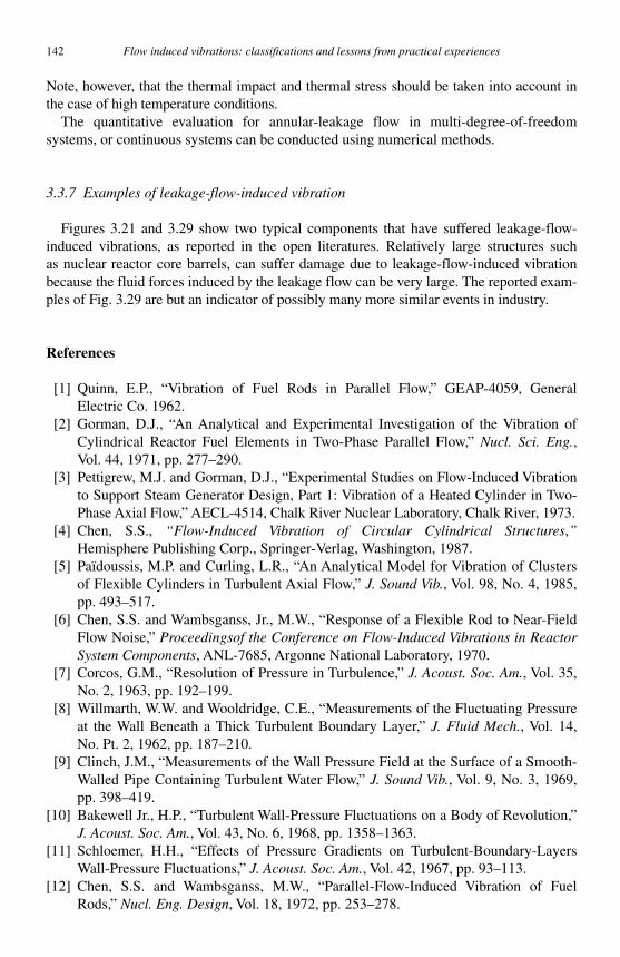
142 Flow induced vibrations: classifications and lessons from practical experiences
Note, however, that the thermal impact and thermal stress should be taken into account in the case of high temperature conditions.
The quantitative evaluation for annular-leakage flow in multi-degree-of-freedom systems, or continuous systems can be conducted using numerical methods.
3.3.7 Examples of leakage-flow-induced vibration
Figures 3.21 and 3.29 show two typical components that have suffered leakage-flow- induced vibrations, as reported in the open literatures. Relatively large structures such as nuclear reactor core barrels, can suffer damage due to leakage-flow-induced vibration because the fluid forces induced by the leakage flow can be very large. The reported exam-ples of Fig. 3.29 are but an indicator of possibly many more similar events in industry.
References
[1] Quinn, E.P., “ Vibration of Fuel Rods in Parallel Flow, ” GEAP-4059, General Electric Co. 1962.
[2] Gorman , D.J. , “ An Analytical and Experimental Investigation of the Vibration of Cylindrical Reactor Fuel Elements in Two-Phase Parallel Flow, ” Nucl. Sci. Eng. , Vol. 44 , 1971 , pp. 277 – 290 .
[3] Pettigrew, M.J. and Gorman, D.J., “ Experimental Studies on Flow-Induced Vibration to Support Steam Generator Design, Part 1: Vibration of a Heated Cylinder in Two-Phase Axial Flow, ” AECL-4514, Chalk River Nuclear Laboratory, Chalk River, 1973.
[4] Chen , S.S., “ Flow-Induced Vibration of Circular Cylindrical Structures, ” Hemisphere Publishing Corp. , Springer-Verlag , Washington, 1987 .
[5] Païdoussis , M.P. and Curling , L.R. , “ An Analytical Model for Vibration of Clusters of Flexible Cylinders in Turbulent Axial Flow, ” J. Sound Vib. , Vol. 98 , No. 4 , 1985 , pp. 493 – 517 .
[6] Chen, S.S. and Wambsganss, Jr., M.W., “ Response of a Flexible Rod to Near-Field Flow Noise, ” Proceedingsof the Conference on Flow-Induced Vibrations in Reactor System Components , ANL-7685, Argonne National Laboratory, 1970.
[7] Corcos , G.M. , “ Resolution of Pressure in Turbulence, ” J. Acoust. Soc. Am. , Vol. 35 , No. 2 , 1963 , pp. 192 – 199 .
[8] Willmarth , W.W. and Wooldridge , C.E. , “ Measurements of the Fluctuating Pressure at the Wall Beneath a Thick Turbulent Boundary Layer, ” J. Fluid Mech. , Vol. 14 , No. Pt. 2 , 1962 , pp. 187 – 210 .
[9] Clinch , J.M. , “ Measurements of the Wall Pressure Field at the Surface of a Smooth-Walled Pipe Containing Turbulent Water Flow, ” J. Sound Vib. , Vol. 9 , No. 3 , 1969 , pp. 398 – 419 .
[10] Bakewell Jr. , H.P. , “ Turbulent Wall-Pressure Fluctuations on a Body of Revolution, ” J. Acoust. Soc. Am. , Vol. 43 , No. 6 , 1968 , pp. 1358 – 1363 .
[11] Schloemer , H.H. , “ Effects of Pressure Gradients on Turbulent-Boundary-Layers Wall-Pressure Fluctuations, ” J. Acoust. Soc. Am. , Vol. 42 , 1967 , pp. 93 – 113 .
[12] Chen , S.S. and Wambsganss , M.W. , “ Parallel-Flow-Induced Vibration of Fuel Rods, ” Nucl. Eng. Design , Vol. 18 , 1972 , pp. 253 – 278 .
Chapter 3. Vibration induced by external axial flow 143
[13] Pettigrew , M.J. and Taylor , C.E. , “ Two-Phase Flow-Induced Vibration: An Overview, ” J. Press. Vessel Technol. , Vol. 116 , 1994 , pp. 233 – 253 .
[14] Saito, N., Tsukuda, Y. et al., “ BWR 9 9 Type Rod Assembly Thermal Hydraulic Tests (2) –Hydraulic Vibration Test–, ” 10th International Conference on Nuclear Engineering , ICONE10-22557, 2002.
[15] Kawamura, K., Yasuo, A. and Inada, F., “ Turbulence-Induced Tube Vibration in a Parallel Steam-Water Two-Phase Flow, ” 4th International Conference on Fluid-Structure Interactions , Aeroelasticity, Flow-Induced Vibration and Noise, Vol. 2, ASME AD-Vol. 53, No. 2, 1997, pp. 83–92.
[16] Inada, F., Kawamura, K. and Yasuo, A., “ A Study on Random Fluid Force Acting on a Tube in Parallel Two-Phase Flow, ” Symposium on Flow-Induced Vibrations , IMechE , 1991, pp. 379–384.
[17] Burgreen , D. , Byrnes , J.J. and Benforado , D.M. , “ Vibration of Rods Induced by Water in Parallel Flow, ” Trans. ASME , Vol. 80 , No. 5 , 1958 , pp. 991 – 1003 .
[18] Reavis , J.R. , “ Vibration Correlation for Maximum Fuel-Element Displacement in Parallel Turbulent Flow, ” Nucl. Sci. Eng. , Vol. 38 , No. 1 , 1969 , pp. 63 – 69 .
[19] Païdoussis , M.P. , “ An Experimental Study of Vibration of Flexible Cylinders Induced by Nominally Axially Flow, ” Nucl. Sci. Eng. , Vol. 35 , No. 1 , 1969 , pp. 127 – 138 .
[20] Chen, Y.N. and Wever, M., “ Flow-Induced Vibration in Tube Bundle Heat Exchangers with Cross and Parallel Flow, ” ASME Symposium on Flow-Induced Vibration in Heat Exchangers, New York, December 1970, pp. 57–77.
[21] Chen, S.S. and Wambsganss, M.W., “ Tentative Design Guide for Calculation the Vibration Response of Flexible Cylindrical Elements in Axial Flow, ” ANL-ETD-71-07, Argonne National Laboratory, 1971.
[22] Hawthorne, W.R., Proceeding of the Institution of Mechanical Engineers, Vol. 175,1961, pp. 52.
[23] Païdoussis , M.P. , “ Dynamics of Flexible Slender Cylinders in Axial Flow, Part 1. Theory, ” J. Fluid Mech. , Vol. 26 , No. 4 , 1966 , pp. 717 – 736 .
[24] Païdoussis , M.P. , “ Dynamics of Flexible Slender Cylinders in Axial Flow, Part 2. Experiments, ” J. Fluid Mech. , Vol. 26 , No. 4 , 1966 , pp. 737 – 751 .
[25] Païdoussis , M.P. , “ Dynamics of Cylindrical Structures Subjected to Axial Flow, ” J. Sound Vib. , Vol. 29 , No. 3 , 1973 , pp. 365 – 385 .
[26] Païdoussis , M.P. and Ostoja-Starzewski , M. , “ Dynamics of a Flexible Cylinder in Subsonic Axial Flow, ” AIAA J. , Vol. 19 , 1981 , pp. 1467 – 1475 .
[27] Païdoussis , M.P. , Appl. Mech. Rev. , Vol. 40 , No. 2 , 1987 , pp. 163 – 175 . [28] Païdoussis, M.P., Trans. ASME , J. Press. Vess. Tech. , Vol. 115, 1993, pp. 2–14. [29] Lee , T.S. , J. Fluid Mech. , Vol. 110 , 1981 , pp. 293 – 295 . [30] Triantafyllou , G.S. and Chryssostomidis , C. , “ Stability of a String in Axial Flow, ”
J. Energy Res. Technol. , Vol. 107 , 1985 , pp. 421 – 425 . [31] Washizu, K. Aeroelasticity (in Japanese) , Kyoritsu Publishing Co. Ltd., 1957. [32] Bisplinghoff , R.L. , Ashley , H. and Halfman , R.L. Aeroelasticity , Addison-Wesley
Publishing Co. Inc. , Cambridge, MA , 1955 . [33] Fung , Y.C. An Introduction to the Theory of Aeroelasticity , John Wiley & Sons, Inc. ,
New York , 1955 . [34] Isogai, K. et al., “ Experimental Study on Transonic Flutter Characteristics of
Sweptback Wing with Core Composite Plates having different Fiber Orientations, ” NAL-TR-827 (in Japanese), 1984.
144 Flow induced vibrations: classifications and lessons from practical experiences
[35] Nakamichi , J. , “ Unsteady Aerodynamics Analyses around Oscillating Airfoils, ” J. Japan Soc. Aeronaut. Space Sci. (in Japanese) , Vol. 43 , No. 501 , 1995 , pp. 549 – 556 .
[36] Matsushita , H. , “ Active Control of Flutter, ” J. Architect. Building Sci. (in Japanese) , Vol. 109 , No. 1351 , 1994 .
[37] Weaver , D.S. and Unny , T.E. , “ The Hydroelastic Stability of a Flat Plate, ” Trans. ASME, J. Appl. Mech. , Vol. 37 , 1970 , pp. 823 – 827 .
[38] Païdoussis , M.P. , Chan , S.P. and Misra , A.K. , “ Dynamics and Stability of Coaxial Cylindrical Shells containing Flowing Fluid, ” J. Sound Vib. , Vol. 97 , No. 2 , 1984 , pp. 201 – 235 .
[39] Ziada , S. and Buhlmann , E.T. , “ Model Tests on Shell Flutter due to Flow on BothSides, ” J. Fluid Str. , Vol. 2 , No. 2 , 1988 , pp. 177 – 196 .
[40] Nagakura , H. and Kaneko , S. , “ Self-Excited Sloshing due to the Fluid Discharge over a Flexible Cylindrical Weir, ” Trans. ASME, J. Press. Vess. Tech. , Vol. 122 , 2000 , pp. 33 – 39 .
[41] Tanaka , S. , Kaneko , S. and Watanabe , T. , “ Self-Excited Oscillations of Dual Cylindrical Flexible Weir Shells due to Overflow Liquid, ” J. Vib. Contr. , Vol. 6 , No. 3 , 2000 , pp. 351 – 373 .
[42] Hirota, K. et al. “ Flow Induced Vibration of a Thin Cylindrical Weir due to Fluid Discharge, ” Proceedings of JSME D & D (in Japanese), 1995.
[43] Blake , W.K. Mechanics of Flow-Induced Sound and Vibration , Academic Press INC. , Orlando, FL , 1986 .
[44] Blevins , R.D. Flow-Induced Vibration , Second Edition , Van Nostrand Reinhold , New York , 1990 .
[45] Naudascher , E. and Rockwell , D., Practical Experiences with Flow Induced Vibrations , Springer-Verlag , Berlin , 1980 , 1–81.
[46] Inada, F. and Hayama, S., J. Fluid Str. , Vol. 4, 1990, pp. 395–412. [47] Inada, F. and Hayama, S., JSME Int. J. , Vol. 31-1, 1988, pp. 39–47. [48] Inada, F. and Hayama, S., Proceedings of the 7th International Conference on Flow
Induced Vibration , 2000, pp. 837–844. [49] Inada, F. and Hayama, S., J. Fluid. Str. , Vol. 4, 1990, pp. 413–428. [50] Nagakura, H. and Kaneko, S., Symposium on Flow-Induced Vibrations in
Engineering Systems , Asia-Pacific Vibration Conference Vol. 1, 1993, pp. 248–253. [51] Li, D.W., Kaneko, S. and Hayama, S., J. Fluid Str. , Vol. 16, 2002, pp. 909–930. [52] Ziada, S. and Buhlmann, E.T., J. Fluid Str. , Vol. 2, 1988, pp. 177–196. [53] Païdoussis, M.P. et al., ASME Symposium on FIV-90 . PVP-Vol. 189, 1990,
pp. 207–226.
145
4 Vibrations Induced by Internal Fluid Flow
Piping systems are widely utilized to convey fluids in many industrial fields, ranging from chemical plants to biological engineering systems. The instability problem of flexible pipes conveying fluid provides a paradigm for the modeling and analysis of the instabilitymechanisms of fluid-structure interaction systems. Consequently, significant research on the dynamics of flexible pipes conveying fluid has been conducted.
In this chapter, the research history on dynamics of the instability phenomenon of pipes conveying fluid is presented. Evaluation methods for the vibration of pipes excited by oscil-lating fluid flow and two-phase fluid flow are discussed in Section 4.1. The vibration of bel-lows and corrugate tubes, which are major piping elements, are introduced in Section 4.2. Unstable vibrations of collapsible tubes, which have recently become important in biologi-cal engineering, are introduced in Section 4.3. Countermeasures against the different types of vibration are presented at the end of each section.
4.1 Vibration of straight and curved pipes conveying fluid
4.1.1 Vibration of pipes conveying fluid
Pipes conveying fluids are found in many industrial systems. Examples include fuel pipes in engine systems, heat transfer pipes in power generation plants, chemical plant piping, and so forth. Piping vibration problems are therefore very important in industry. The instability phenomenon of flexible pipes conveying fluid has been studied by many researchers. The stability and dynamic characteristics are now well understood. The dynamics are known to be sensitively dependent on flow velocity and support/boundary conditions.
With regard to the instability mechanism of flexible pipes conveying fluid there are two different cases: (i) unstable vibration caused by the fluid flow when the flow velocity surpasses a critical value, and (ii) vibration due to oscillating fluid flow.
4.1.1.1 Research history Major research on the regarding stability and vibration of flexible pipes conveying fluid
started in the 1950s in relation to the design of pipelines conveying oil. Thereafter, these studies were enhanced by the work of Benjamin [1, 2] , Gregory and Païdoussis [3, 4] , and Païdoussis et al. [5–13] . Many other detailed studies on the stability and dynamic behavior of flexible pipes conveying fluid have since been conducted and reported. The effects of an attached mass, damper or spring, for example, were investigated by Sugiyama et al. [14] .
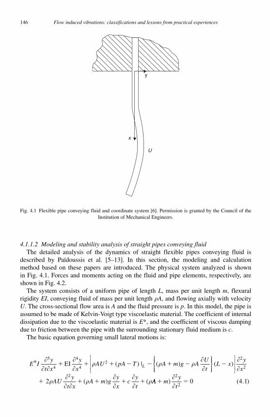
146 Flow induced vibrations: classifications and lessons from practical experiences
4.1.1.2 Modeling and stability analysis of straight pipes conveying fluid The detailed analysis of the dynamics of straight flexible pipes conveying fluid is
described by Païdoussis et al. [5–13] . In this section, the modeling and calculation method based on these papers are introduced. The physical system analyzed is shown in Fig. 4.1 . Forces and moments acting on the fluid and pipe elements, respectively, are shown in Fig. 4.2 .
The system consists of a uniform pipe of length L , mass per unit length m , flexural rigidity EI , conveying fluid of mass per unit length � A , and flowing axially with velocity U . The cross-sectional flow area is A and the fluid pressure is p . In this model, the pipe is assumed to be made of Kelvin-Voigt type viscoelastic material. The coefficient of internal dissipation due to the viscoelastic material is E* , and the coefficient of viscous damping due to friction between the pipe with the surrounding stationary fluid medium is c .
The basic equation governing small lateral motions is:
E Iy
t x
y
xAU pA T A m g A
U
tL* EI
�� �
��
� � ���
5
4
4
42� � � � � � �( ) | ( )
⎧⎨⎪⎪⎩⎪⎪
⎫⎬⎪⎪⎪⎭⎪⎪
⎡
⎣⎢⎢
⎤
⎦⎥⎥( )
( ) (
L xy
x
AUy
t xA m g
y
xc
y
t
�
� � � � �
��
��� �
���
��
�
2
2
22 AA m
y
t� �) ( . )
��
2
20 4 1
y
U
x
Fig. 4.1 Flexible pipe conveying fluid and coordinate system [6]. Permission is granted by the Council of the Institution of Mechanical Engineers.

Chapter 4. Vibrations excited by internal fluid flow 147
This equation can be expressed in dimensionless form by defining the following dimensionless parameters:
� � �
��
��
�
��
� � ��
��
��
�
x L y LI
E A m
E
L
A
A m
A mL g
cL
A
/ , / ,( )
*, , ,
(
23
2
EI
EI ��� �
�mu
AUL
m A
t
L), ,
��
�EI
EI2
(4.2)
Substituting Eqs. (4.2) into Eq. (4.1), the following dimensionless equation of motion is obtained:
� ���
�����
�� �����
� �
�����
����
����
�
2
2
2 5
4
2
2� � � �
� � �
u
uu⎧
⎨⎪⎪⎩⎪⎪
⎫⎬⎬⎪⎪⎭⎪⎪
⎡
⎣⎢⎢
⎤
⎦⎥⎥( )1 0
2
2
4
4� � ��
� ���
� ���
(4.3)
For a constant flow velocity, the equation of motion becomes:
� ��
�����
�� �����
�
�����
����
� �� ���
2
2
2 5
4
22
2
2
1
τη
� � � �
� � � �
u
u ( ){ } �� ���
4
40� (4.4)
M( )2ydx
Fdx
Mgdx
qSdx
mgdx
qSdxFdx
m dx
pA
Q
T
(a) (b)
M
ddt
ddx�U
d2ydt 2
T � dxdTdx
Q � dxdQdxA(p � dx)dp
dx
~
dxdMdx
M �
~~
Fig. 4.2 Forces and moments acting on elements of (a) the fluid, and (b) the pipe, respectively [6]. Permission is granted by the Council of the Institution of Mechanical Engineers.
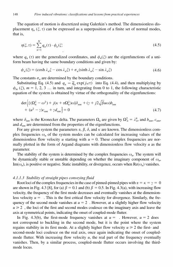
148 Flow induced vibrations: classifications and lessons from practical experiences
The equation of motion is discretized using Galerkin ’ s method. The dimensionless dis-placement �n ( � , � ) can be expressed as a superposition of a finite set of normal modes, that is,
� � � � �( , ) ( ) ( )��
qn nn
N
⋅∑ �1 .
(4.5)
where qn ( � ) are the generalized coordinates, and �n ( � ) are the eigenfunctions of a uni-form beam having the same boundary conditions and given by:
�n n n n n n( ) ( cos ) ( sin )� � � � � � � � � �� � � �cosh sinh (4.6)
The constants �n are determined by the boundary conditions. Substituting Eq. (4.5) and q q jn n= exp( )ω� into Eq. (4.4), and then multiplying by
� m ( � ), m � 1, 2, 3 … in turn, and integrating from 0 to 1, the following characteristic equation of the system is obtained by virtue of the orthogonality of the eigenfunctions:
det {( ) ( ) } ( )
( )
� � � � � � � � �
� �n n nm nm
nm nm
j j u b
u c d
2 2 2
2
2� � � � �
� � �
⎡⎣⎢
⎤⎤⎦⎥ � 0 (4.7)
where �nm is the Kronecker delta. The parameters �n are given by �2n � �4
n , and bnm , cnm , and dnm are determined from the properties of the eigenfunctions.
For any given system the parameters , � , � , and � are known. The dimensionless com-plex frequencies �n of the system modes can be calculated for increasing values of the dimensionless flow velocity u starting with u � 0. These complex frequencies are nor-mally plotted in the form of Argand diagrams with dimensionless flow velocity u as the parameter.
The stability of the system is determined by the complex frequencies �n . The system will be dynamically stable or unstable depending on whether the imaginary component of �n , Im(�n ), is positive or negative. Static instability, or divergence, occurs when Re( �n ) vanishes.
4.1.1.3 Stability of straight pipes conveying fluid Root loci of the complex frequencies in the case of pinned-pinned pipes with � � � � � 0
are shown in Fig. 4.3 [8] , for (a) � � 0.1 and (b) � � 0.5. In Fig. 4.3(a) , with increasing flow velocity, the frequency of the first mode decreases and eventually vanishes at the dimension-less velocity u � . This is the first critical flow velocity for divergence. Similarly, the fre-quency of the second mode vanishes at u � 2 . However, at a slightly higher flow velocity u � 2 , the loci of the first and second modes coalesce on the imaginary axis and leave the axis at symmetrical points, indicating the onset of coupled-mode flutter.
In Fig. 4.3(b) , the first-mode frequency vanishes at u � . However, u � 2 does not correspond to buckling in the second mode, but it is the point where the system regains stability in its first mode. At a slightly higher flow velocity u � 2 the first- and second-mode loci coalesce on the real axis, once again indicating the onset of coupled-mode flutter. With increasing flow velocity u , the real part of the frequency eventually vanishes. Then, by a similar process, coupled-mode flutter occurs involving the third-mode locus.
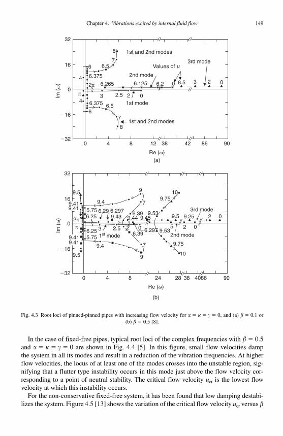
Chapter 4. Vibrations excited by internal fluid flow 149
In the case of fixed-free pipes, typical root loci of the complex frequencies with � � 0.5 and � � � � � 0 are shown in Fig. 4.4 [5] . In this figure, small flow velocities damp the system in all its modes and result in a reduction of the vibration frequencies. At higher flow velocities, the locus of at least one of the modes crosses into the unstable region, sig-nifying that a flutter type instability occurs in this mode just above the flow velocity cor-responding to a point of neutral stability. The critical flow velocity ucr is the lowest flow velocity at which this instability occurs.
For the non-conservative fixed-free system, it has been found that low damping destabi-lizes the system. Figure 4.5 [13] shows the variation of the critical flow velocity ucr versus �
32
16
8
76.5
6.375
6.2652π
6
4
4π
6
6.375 6.5
7
8
022.53
6.125
1st and 2nd modes
1st and 2nd modes
1st mode
3rd mode
2nd mode
6.2 8.5 3 2 00
Values of u
0
�16
�324 8 12 38
(a)
Im (
v)
42 860 90
Re (v)
32
16
0
�16
�324 8 24 28 38 40860 90
9
79.75
10
9.5 9.25 2 0
025
9.75
10
9.53
7
9
9.4
6.396.29702.5 2
9.4
5.75
9.5
9.5
2ππ
6.2976.296.25 9.43 9.44
6.399.45
9.533rd mode
2nd mode5.756.25 3
1st mode
Im (
v)
(b)
Re (v)
9.419.41
9.419.41
Fig. 4.3 Root loci of pinned-pinned pipes with increasing flow velocity for � � � � � 0, and (a) � � 0.1 or (b) � � 0.5 [8].

150 Flow induced vibrations: classifications and lessons from practical experiences
for progressively higher values of the viscoelastic dissipation constant . It can be seen that, in the case of large � , the flow velocity decreases with the viscoelastic dissipation constant.
4.1.1.4 Stability of curved pipes conveying fluid The stability of curved pipes conveying fluid can be also studied using the approach
outlined above. Detailed calculation methods and evaluation for curved flexible pipes were presented by Chen [15] . In this section, typical results obtained by Chen are discussed.
Figure 4.6 [15] shows the frequencies of a fixed-fixed curved pipe forming a 90 degree curve, as functions of the flow velocity. As the flow velocity increases, the frequencies
15
a � 0
a � 10�2
a � 10�3
a � 5 10�3
10
5
0.0
Crit
ical
vel
ocity
, ucr
0.2 0.4 0.6 0.8 10
b
Fig. 4.5 Variation of critical velocity of fixed-free pipes versus � for progressively higher values of the visco-elastic dissipation constant [8].
11.251111.75
11.511
10.75
10.75
5.5
5.55
4
4
10
20
010
Im (
v)
0 10 20 30 40
1112
10
9
8.758.5 7
86
11.5
12
54
32
110
234
87
6 5 8.75
8.8125
9
10
108
7911
11
5.56
4
535.5
24
1st mode
3rd mode
2nd mode
4th modeValues of u
50 60
Re (v)
�10
5
Fig. 4.4 Root loci of fixed-free pipes with increasing flow velocity for � � � � � 0 and � � 0.5 [5].
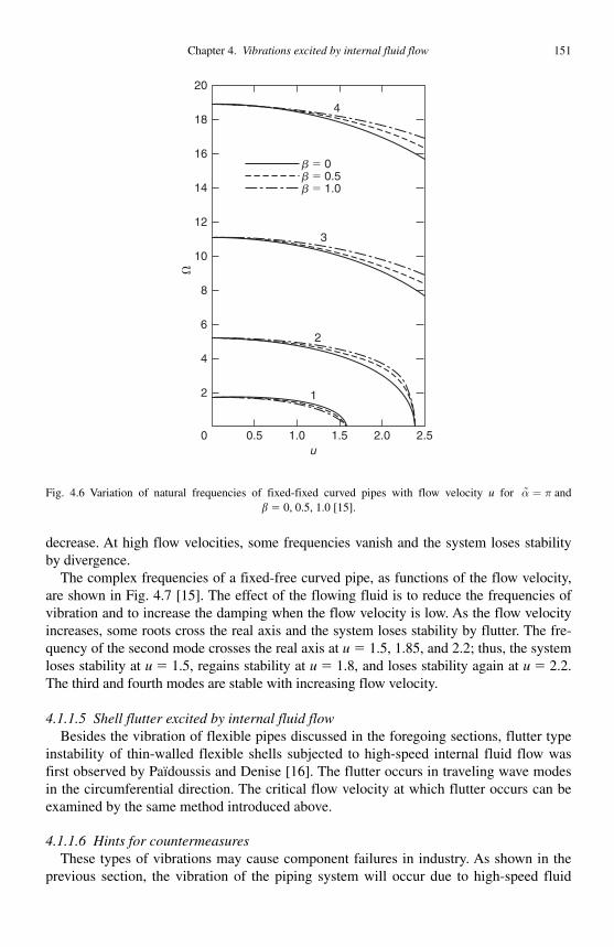
Chapter 4. Vibrations excited by internal fluid flow 151
decrease. At high flow velocities, some frequencies vanish and the system loses stability by divergence.
The complex frequencies of a fixed-free curved pipe, as functions of the flow velocity, are shown in Fig. 4.7 [15] . The effect of the flowing fluid is to reduce the frequencies of vibration and to increase the damping when the flow velocity is low. As the flow velocity increases, some roots cross the real axis and the system loses stability by flutter. The fre-quency of the second mode crosses the real axis at u � 1.5, 1.85, and 2.2; thus, the system loses stability at u � 1.5, regains stability at u � 1.8, and loses stability again at u � 2.2. The third and fourth modes are stable with increasing flow velocity.
4.1.1.5 Shell flutter excited by internal fluid flow Besides the vibration of flexible pipes discussed in the foregoing sections, flutter type
instability of thin-walled flexible shells subjected to high-speed internal fluid flow was first observed by Païdoussis and Denise [16] . The flutter occurs in traveling wave modes in the circumferential direction. The critical flow velocity at which flutter occurs can be examined by the same method introduced above.
4.1.1.6 Hints for countermeasures These types of vibrations may cause component failures in industry. As shown in the
previous section, the vibration of the piping system will occur due to high-speed fluid
b � 0
4
3
2
1
0
4
2
6
8
10
12
�14
16
18
20
0.5 1.0u
1.5 2.0 2.5
b � 0.5b � 1.0
Fig. 4.6 Variation of natural frequencies of fixed-fixed curved pipes with flow velocity u for �α π= and� � 0, 0.5, 1.0 [15].
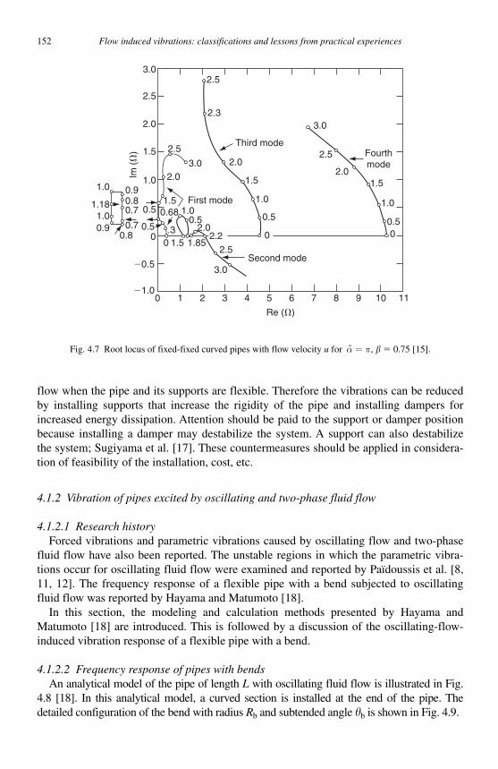
152 Flow induced vibrations: classifications and lessons from practical experiences
flow when the pipe and its supports are flexible. Therefore the vibrations can be reduced by installing supports that increase the rigidity of the pipe and installing dampers for increased energy dissipation. Attention should be paid to the support or damper position because installing a damper may destabilize the system. A support can also destabilize the system; Sugiyama et al. [17]. These countermea sures should be applied in considera-tion of feasibility of the installation, cost, etc.
4.1.2 Vibration of pipes excited by oscillating and two-phase fluid flow
4.1.2.1 Research history Forced vibrations and parametric vibrations caused by oscillating flow and two-phase
fluid flow have also been reported. The unstable regions in which the parametric vibra-tions occur for oscillating fluid flow were examined and reported by Païdoussis et al. [8,11, 12] . The frequency response of a flexible pipe with a bend subjected to oscillating fluid flow was reported by Hayama and Matumoto [18] .
In this section, the modeling and calculation methods presented by Hayama and Matumoto [18] are introduced. This is followed by a discussion of the oscillating-flow-induced vibration response of a flexible pipe with a bend.
4.1.2.2 Frequency response of pipes with bends An analytical model of the pipe of length L with oscillating fluid flow is illustrated in Fig.
4.8 [18] . In this analytical model, a curved section is installed at the end of the pipe. The detailed configuration of the bend with radius Rb and subtended angle �b is shown in Fig. 4.9 .
0�1.0
�0.5
0.80.91.0
1.18
1.0 0.90.80.7
0.70
0.5
0.5
1.0
1.5
lm (
�)
Re (�)
2.5
3.02.0
1.51.0
First mode
0.52.0
2.22.5
3.0
1.851.50.3
0.68
2.0
3.0
2.5
2.5
2.3
2.0
1.5
1.0
0.5
0
Second mode
Third modeFourthmode
3.0
2.5
1.5
1.0
0.50
2.0
1 2 3 4 5 6 7 9 10 118
Fig. 4.7 Root locus of fixed-fixed curved pipes with flow velocity u for �α π= , � � 0.75 [15].
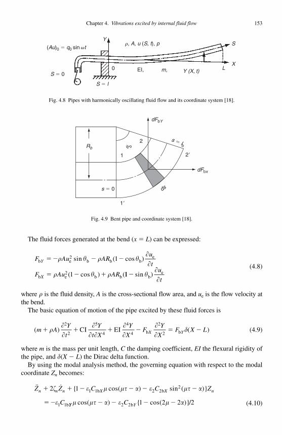
Chapter 4. Vibrations excited by internal fluid flow 153
The fluid forces generated at the bend ( x � L ) can be expressed:
F Au ARu
t
F Au AR
Y
X
b e2
b b be
b e2
b b
� � � �
� � �
� � � ���
� � �
sin ( cos )
( cos ) (
1
1 11� sin )���b
eu
t
(4.8)
where � is the fluid density, A is the cross-sectional flow area, and ue is the flow velocity at the bend.
The basic equation of motion of the pipe excited by these fluid forces is
( ) ( )m AY
t
Y
t X
Y
XF
Y
XF X LX Y� � � � � ��
��
�� �
��
��
�2
2
5
4
4
4
2
2CI EI b b (4.9)
where m is the mass per unit length, C the damping coefficient, EI the flexural rigidity of the pipe, and � ( X � L ) the Dirac delta function.
By using the modal analysis method, the governing equation with respect to the modal coordinate Zn becomes:
�� �Z Z C C Z
C
n n n X X n� � � � � �
� �
2 1 1 1 2 22
1 1
� � � �� � ��
�
{ cos( ) sin ( )}b b
bYY YC� �� � � cos( ) { cos( )}/� � � �2 2 1 2 2 2b (4.10)
S � 0
S � l
0
Y
EI,
r, A, u (S, t), p
m, LX
S
Y (X, t)
(Au)0 � q0 sin vt
Fig. 4.8 Pipes with harmonically oscillating fluid flow and its coordinate system [18].
Rb
s � 0
1�
1
2
dFbx
ds
2�
u b
s � lb
dFbY
Fig. 4.9 Bent pipe and coordinate system [18].
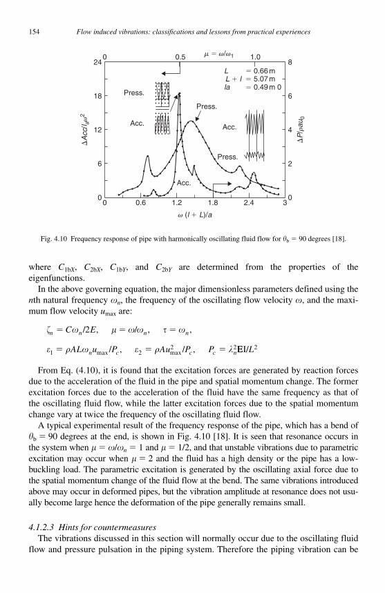
154 Flow induced vibrations: classifications and lessons from practical experiences
where C1bX , C2bX , C1bY , and C2bY are determined from the properties of the eigenfunctions.
In the above governing equation, the major dimensionless parameters defined using the n th natural frequency �n , the frequency of the oscillating flow velocity � , and the maxi-mum flow velocity umax are:
� � � � � � �
� � � � � �
n n n n
n c c c n
C E
AL u P Au P P
� � �
� � �
/ , / , ,
/ , / ,
2
1 22 2
max max EEI/L2
From Eq. (4.10), it is found that the excitation forces are generated by reaction forces due to the acceleration of the fluid in the pipe and spatial momentum change. The former excitation forces due to the acceleration of the fluid have the same frequency as that of the oscillating fluid flow, while the latter excitation forces due to the spatial momentum change vary at twice the frequency of the oscillating fluid flow.
A typical experimental result of the frequency response of the pipe, which has a bend of �b � 90 degrees at the end, is shown in Fig. 4.10 [18] . It is seen that resonance occurs in the system when � � � / �n � 1 and � � 1/2, and that unstable vibrations due to parametric excitation may occur when � � 2 and the fluid has a high density or the pipe has a low-buckling load. The parametric excitation is generated by the oscillating axial force due to the spatial momentum change of the fluid flow at the bend. The same vibrations introduced above may occur in deformed pipes, but the vibration amplitude at resonance does not usu-ally become large hence the deformation of the pipe generally remains small.
4.1.2.3 Hints for countermeasures The vibrations discussed in this section will normally occur due to the oscillating fluid
flow and pressure pulsation in the piping system. Therefore the piping vibration can be
Press.
Press.
L � 0.66 m� 5.07 m� 0.49 m 0la
L � l
Press.
Acc.
0.5024
18
12
6
00 0.6 1.2 1.8
v (l � L)/a
m � v/v1
�A
cc/l a
v2
�P
/rau
0
2.4 30
2
4
6
81.0
Acc.
Acc.
Fig. 4.10 Frequency response of pipe with harmonically oscillating fluid flow for � b � 90 degrees [18].
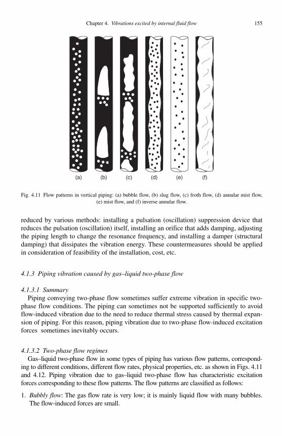
Chapter 4. Vibrations excited by internal fluid flow 155
reduced by various methods: installing a pulsation (oscillation) suppression device that reduces the pulsation (oscillation) itself, installing an orifice that adds damping, adjusting the piping length to change the resonance frequency, and installing a damper (structural damping) that dissipates the vibration energy. These countermeasures should be applied in consideration of feasibility of the installation, cost, etc.
4.1.3 Piping vibration caused by gas–liquid two-phase flow
4.1.3.1 Summary Piping conveying two-phase flow sometimes suffer extreme vibration in specific two-
phase flow conditions. The piping can sometimes not be supported sufficiently to avoid flow-induced vibration due to the need to reduce thermal stress caused by thermal expan-sion of piping. For this reason, piping vibration due to two-phase flow-induced excitation forces sometimes inevitably occurs.
4.1.3.2 Two-phase flow regimes Gas–liquid two-phase flow in some types of piping has various flow patterns, correspond-
ing to different conditions, different flow rates, physical properties, etc. as shown in Figs. 4.11 and 4.12. Piping vibration due to gas–liquid two-phase flow has characteristic excitation forces corresponding to these flow patterns. The flow patterns are classified as follows:
1. Bubbly flow : The gas flow rate is very low; it is mainly liquid flow with many bubbles. The flow-induced forces are small.
(a) (b) (c) (d) (e) (f)
Fig. 4.11 Flow patterns in vertical piping: (a) bubble flow, (b) slug flow, (c) froth flow, (d) annular mist flow, (e) mist flow, and (f) inverse annular flow.

156 Flow induced vibrations: classifications and lessons from practical experiences
2. Plug flow and slug flow : Large bubbles move in the piping intermittently in the case of plug flow. For slug flow, large bubbles, having the shape of artillery shells and with which the piping is almost filled, and liquid slugs flow alternately. Two-phase flow tur-bulence is low for both flow patterns. When a liquid slug, which has a high density, passes through the elbow portion of the piping, excitation forces are generated. These forces can cause piping vibration.
3. Froth flow : Liquid slugs contain many bubbles in the case of froth flow. The shape of the gas bubble is distorted and the flow is highly turbulent. Flow-induced forces are also large because of high turbulence.
4. Mist flow : The main flow is gas flow in the case of mist flow. Liquid droplets flow in the piping like mist. This flow is basically the “ opposite ” of the bubbly flow. Flow induced forces are therefore small.
5. Annular flow : This flow consists of liquid film flow adhering to the inner wall of the piping, and gas flow in the center of the piping. The liquid film flow is not completely stable. Piping vibration sometimes occurs due to turbulence in the liquid film flow.
6. Stratified flow and wavy flow : Gas–liquid two-phase flow is stratified into the upper side gas and the lower side liquid in the case of horizontal piping. If the interfacial
(a)
(b)
(c)
(d)
(e)
(f)
(g)
(h)
Fig. 4.12 Flow patterns in horizontal piping: (a) bubbly flow, (b) stratified flow, (c) wavy flow, (d) plug flow, (e) slug flow, (f) froth flow, (g) annular mist flow, and (h) mist flow.
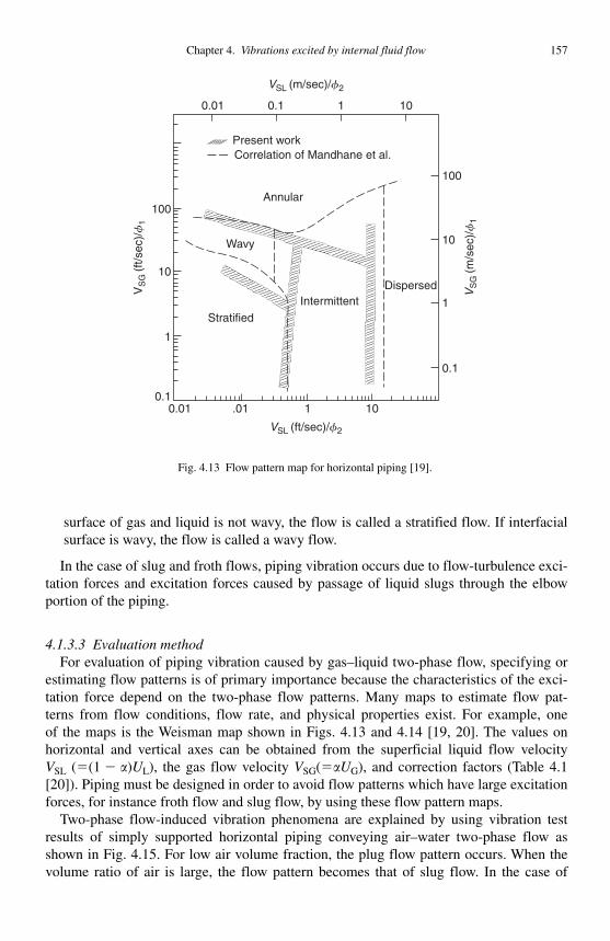
Chapter 4. Vibrations excited by internal fluid flow 157
surface of gas and liquid is not wavy, the flow is called a stratified flow. If interfacial surface is wavy, the flow is called a wavy flow.
In the case of slug and froth flows, piping vibration occurs due to flow-turbulence exci-tation forces and excitation forces caused by passage of liquid slugs through the elbow portion of the piping.
4.1.3.3 Evaluation method For evaluation of piping vibration caused by gas–liquid two-phase flow, specifying or
estimating flow patterns is of primary importance because the characteristics of the exci-tation force depend on the two-phase flow patterns. Many maps to estimate flow pat-terns from flow conditions, flow rate, and physical properties exist. For example, one of the maps is the Weisman map shown in Figs. 4.13 and 4.14 [19, 20] . The values on horizontal and vertical axes can be obtained from the superficial liquid flow velocity VSL ( � (1 � ) UL ), the gas flow velocity VSG ( � UG ), and correction factors ( Table 4.1 [20] ). Piping must be designed in order to avoid flow patterns which have large excitation forces, for instance froth flow and slug flow, by using these flow pattern maps.
Two-phase flow-induced vibration phenomena are explained by using vibration test results of simply supported horizontal piping conveying air–water two-phase flow as shown in Fig. 4.15 . For low air volume fraction, the plug flow pattern occurs. When the volume ratio of air is large, the flow pattern becomes that of slug flow. In the case of
Stratified
Wavy
Annular
Present work
VSL (m/sec)/f2
VS
G(f
t/sec
)/f
1
VSL (ft/sec)/f2
VS
G(m
/sec
)/f
1
Correlation of Mandhane et al.
IntermittentDispersed
10
100
10
1
0.1
101.010.010.1
1
10
100
10.10.01
Fig. 4.13 Flow pattern map for horizontal piping [19].
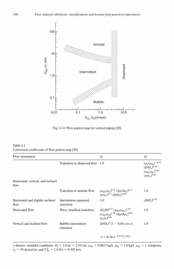
158 Flow induced vibrations: classifications and lessons from practical experiences
Annular
Intermittent
Dis
pers
ed
Bubble
0.01
0.1
1.0
10
100
0.1 1.0 10.0
VS
G/f
1m
/s
VGL /f2(m/sec)
Fig. 4.14 Flow pattern map for vertical piping [20].
Table 4.1 Conversion coefficients of flow pattern map [20]
Flow orientation �1 �2
Transition to dispersed flow 1.0 ( �L / �SL ) � 0.33
(D / Ds ) 0.16
(�SL / �L ) 0.09
(� / �s )0.24
Horizontal, vertical, and inclined flow
Transition to annular flow ( �SG / �G ) 0.23 ( �� / ��s ) 0.11
(� / �s ) 0.11 ( D / Ds )
0.415 1.0
Horizontal and slightly inclined flow
Intermittent-separated transition
1.0 ( D / Ds ) 0.45
Horizontal flow Wavy-stratified transition ( Ds / D ) 0.17 ( �SG / �SG ) 1.55
(�SG / �G ) 1.55 ( �� / ��s ) 0.69
(�s / � ) 0.69
1.0
Vertical and inclined flow Bubble-intermittent transition
( D / Ds ) n (1 � 0.65 cos ) 1.0
n V V� �0 26 0 17. . ( / )e SL SLS
s denotes standard conditions. Ds � 1.0 in. � 2.54 cm, �SG � 0.0013 kg/l, �SL � 1.0 kg/l, �SL � 1 centipoise, �s � 70 dynes/cm, and V S
SL � 1.0 ft/s � 0.305 m/s.
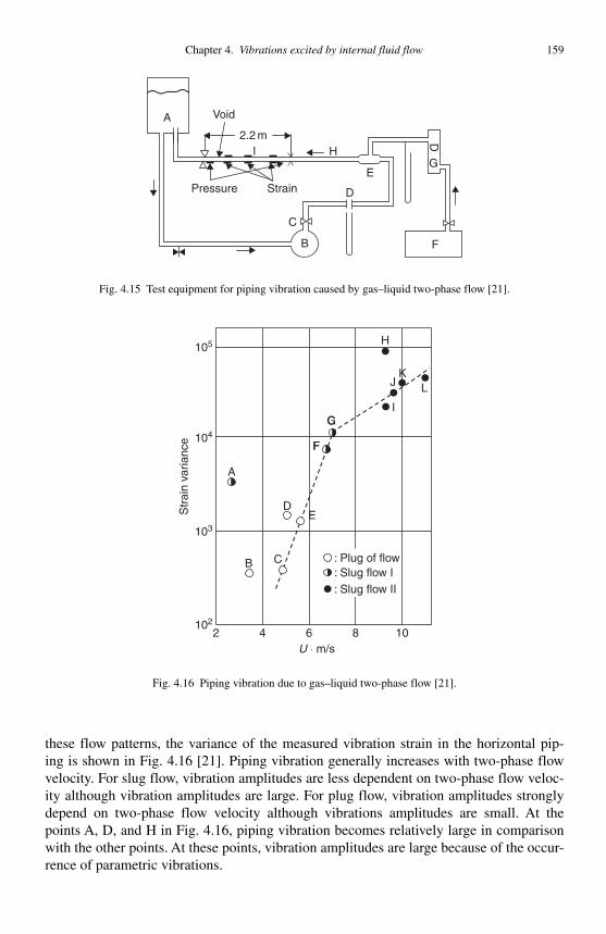
Chapter 4. Vibrations excited by internal fluid flow 159
these flow patterns, the variance of the measured vibration strain in the horizontal pip-ing is shown in Fig. 4.16 [21] . Piping vibration generally increases with two-phase flow velocity. For slug flow, vibration amplitudes are less dependent on two-phase flow veloc-ity although vibration amplitudes are large. For plug flow, vibration amplitudes strongly depend on two-phase flow velocity although vibrations amplitudes are small. At the points A, D, and H in Fig. 4.16 , piping vibration becomes relatively large in comparison with the other points. At these points, vibration amplitudes are large because of the occur-rence of parametric vibrations.
A
2.2 m
B
C
D
H
StrainPressure
Void
I
EG
D
F
Fig. 4.15 Test equipment for piping vibration caused by gas–liquid two-phase flow [21].
H
KJ
IC
F
L
2102
103
104
A
D
B C
E
F
Str
ain
varia
nce
G
105
4 6U ⋅ m/s
8 10
: Plug of flow: Slug flow I: Slug flow II
Fig. 4.16 Piping vibration due to gas–liquid two-phase flow [21].
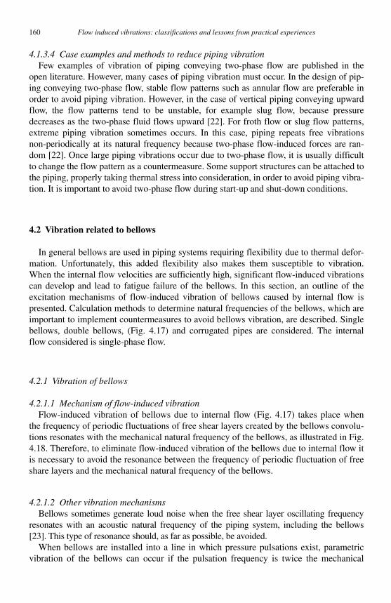
160 Flow induced vibrations: classifications and lessons from practical experiences
4.1.3.4 Case examples and methods to reduce piping vibration Few examples of vibration of piping conveying two-phase flow are published in the
open literature. However, many cases of piping vibration must occur. In the design of pip-ing conveying two-phase flow, stable flow patterns such as annular flow are preferable in order to avoid piping vibration. However, in the case of vertical piping conveying upward flow, the flow patterns tend to be unstable, for example slug flow, because pressure decreases as the two-phase fluid flows upward [22] . For froth flow or slug flow patterns, extreme piping vibration sometimes occurs. In this case, piping repeats free vibrations non-periodically at its natural frequency because two-phase flow-induced forces are ran-dom [22] . Once large piping vibrations occur due to two-phase flow, it is usually difficult to change the flow pattern as a countermeasure. Some support structures can be attached to the piping, properly taking thermal stress into consideration, in order to avoid piping vibra-tion. It is important to avoid two-phase flow during start-up and shut-down conditions.
4.2 Vibration related to bellows
In general bellows are used in piping systems requiring flexibility due to thermal defor-mation. Unfortunately, this added flexibility also makes them susceptible to vibration. When the internal flow velocities are sufficiently high, significant flow-induced vibrations can develop and lead to fatigue failure of the bellows. In this section, an outline of the excitation mechanisms of flow-induced vibration of bellows caused by internal flow is presented. Calculation methods to determine natural frequencies of the bellows, which are important to implement countermeasures to avoid bellows vibration, are described. Single bellows, double bellows, (Fig. 4.17) and corrugated pipes are considered. The internal flow considered is single-phase flow.
4.2.1 Vibration of bellows
4.2.1.1 Mechanism of flow-induced vibration Flow-induced vibration of bellows due to internal flow (Fig. 4.17) takes place when
the frequency of periodic fluctuations of free shear layers created by the bellows convolu-tions resonates with the mechanical natural frequency of the bellows, as illustrated in Fig.4.18 . Therefore, to eliminate flow-induced vibration of the bellows due to internal flow it is necessary to avoid the resonance between the frequency of periodic fluctuation of free share layers and the mechanical natural frequency of the bellows.
4.2.1.2 Other vibration mechanisms Bellows sometimes generate loud noise when the free shear layer oscillating frequency
resonates with an acoustic natural frequency of the piping system, including the bellows [23]. This type of resonance should, as far as possible, be avoided.
When bellows are installed into a line in which pressure pulsations exist, parametric vibration of the bellows can occur if the pulsation frequency is twice the mechanical
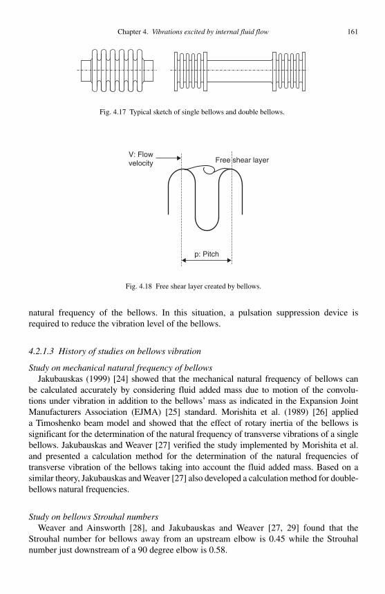
Chapter 4. Vibrations excited by internal fluid flow 161
natural frequency of the bellows. In this situation, a pulsation suppression device is required to reduce the vibration level of the bellows.
4.2.1.3 History of studies on bellows vibration
Study on mechanical natural frequency of bellows Jakubauskas (1999) [24] showed that the mechanical natural frequency of bellows can
be calculated accurately by considering fluid added mass due to motion of the convolu-tions under vibration in addition to the bellows ’ mass as indicated in the Expansion Joint Manufacturers Association (EJMA) [25] standard. Morishita et al. (1989) [26] applied a Timoshenko beam model and showed that the effect of rotary inertia of the bellows is signi ficant for the determination of the natural frequency of transverse vibrations of a single bellows. Jakubauskas and Weaver [27] verified the study implemented by Morishita et al. and presented a calculation method for the determination of the natural frequencies of transverse vibration of the bellows taking into account the fluid added mass. Based on a similar theory, Jakubauskas and Weaver [27] also developed a calculation method for double-bellows natural frequencies.
Study on bellows Strouhal numbers Weaver and Ainsworth [28] , and Jakubauskas and Weaver [27, 29] found that the
Strouhal number for bellows away from an upstream elbow is 0.45 while the Strouhal number just downstream of a 90 degree elbow is 0.58.
Fig. 4.17 Typical sketch of single bellows and double bellows.
V: Flow velocity
p: Pitch
Free shear layer
Fig. 4.18 Free shear layer created by bellows.
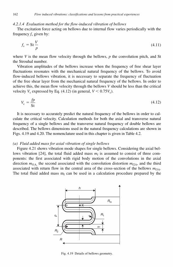
162 Flow induced vibrations: classifications and lessons from practical experiences
4.2.1.4 Evaluation method for the flow-induced vibration of bellows The excitation force acting on bellows due to internal flow varies periodically with the
frequency fv given by:
fV
pv St� (4.11)
where V is the mean flow velocity through the bellows, p the convolution pitch, and St the Strouhal number.
Vibration amplitudes of the bellows increase when the frequency of free shear layer fluctuations resonates with the mechanical natural frequency of the bellows. To avoid flow-induced bellows vibration, it is necessary to separate the frequency of fluctuation of the free shear layer from the mechanical natural frequency of the bellows. In order to achieve this, the mean flow velocity through the bellows V should be less than the critical velocity Vc expressed by Eq. (4.12) (in general, V � 0.75 Vc ).
Vfp
c St� (4.12)
It is necessary to accurately predict the natural frequency of the bellows in order to cal-culate the critical velocity. Calculation methods for both the axial and transverse natural frequency of a single bellows and the transverse natural frequency of double bellows are described. The bellows dimensions used in the natural frequency calculations are shown in Figs. 4.19 and 4.20 . The nomenclature used in this chapter is given in Table 4.2 .
(a) Fluid added mass for axial vibration of single bellows Figure 4.21 shows vibration mode shapes for single bellows. Considering the axial bel-
lows vibration [24], the total fluid added mass mf is assumed to consist of three com-ponents: the first associated with rigid body motion of the convolutions in the axial direction mf1A, the second associated with the convolution distortion mf2A , and the third associated with return flow in the central area of the cross-section of the bellows mf3A . The total fluid added mass m f can be used in a calculation procedure prepared by the
Rm
R1
R2
h
δ
p
R
X
Fig. 4.19 Details of bellows geometry.
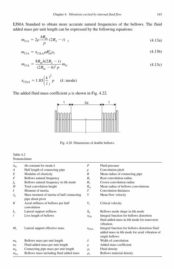
Chapter 4. Vibrations excited by internal fluid flow 163
EJMA Standard to obtain more accurate natural frequencies of the bellows. The fluid added mass per unit length can be expressed by the following equations:
mhR
pR tf1A
mf� �2 2 2 �( ) (4.13a)
m Rf A f kA m3
f2 2� � � (4.13b)
mR h R t
R h pmf A
m
mf3
22 1
8 2
2�
�
�
( )
( ) (4.13c)
f kA :mode2
2
1 85� . ( )k
lp k
⎛
⎝⎜⎜⎜⎞
⎠⎟⎟⎟⎟
The added fluid mass coefficient � is shown in Fig. 4.22.
1 12a
Fig. 4.20 Dimensions of double bellows.
Table 4.2 Nomenclature
Aik i th constant for mode k P Fluid pressure A Half length of connecting pipe p Convolution pitch E Modulus of elasticity R Mean radius of connecting pipe F Bellows natural frequency R1 Root convolution radius fk Bellows natural frequency in k th mode R2 Crown convolution radius H Total convolution height Rm Mean radius of bellows convolutions I Moment of inertia T Convolution thickness Jp Mass moment of inertia of half connecting
pipe about pivot V Mean flow velocity
K Axial stiffness of bellows per half convolution
Vc Critical velocity
ks Lateral support stiffness Xk Bellows mode shape in k th mode l Live length of bellows f2k Integral function for bellows distortion
fluid added mass in k th mode for transverse vibration.
Ms Lateral support effective mass f2kA Integral function for bellows distortion fluid added mass in k th mode for axial vibration of single bellows
mb Bellows mass per unit length � Width of convolution mf Fluid added mass per unit length � Added mass coefficient mp Connecting pipe mass per unit length �f Fluid density mtot Bellows mass including fluid added mass �b Bellows material density
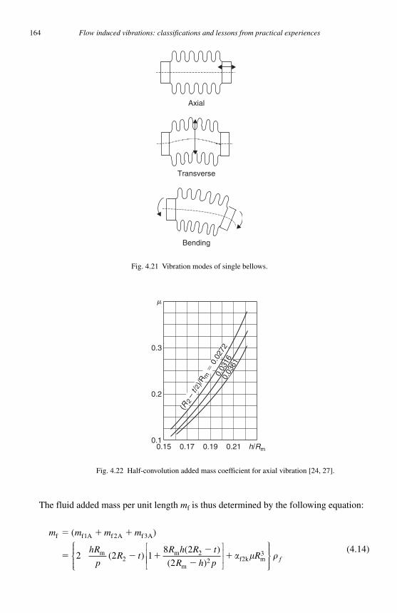
164 Flow induced vibrations: classifications and lessons from practical experiences
The fluid added mass per unit length mf is thus determined by the following equation:
m m m m
hR
pR t
R h R t
R h p
f f A f A f A
m2
m 2
m2
2(2 )
( )
� � �
� � ��
�
( )
( )
1 2 3
2 18
2
⎡
⎣⎢⎢⎢
⎤
⎦⎥⎥
⎧⎨⎪⎪
⎩⎪⎪
⎫⎬⎪⎪
⎭⎪⎪� � �f2k mR f
3 (4.14)
Bending
Axial
Transverse
Fig. 4.21 Vibration modes of single bellows.
m
0.3
0.2
0.10.15 0.17 0.19 0.21 h/Rm
(R2
–t /2
)/Rm
� 0
.027
20.
0316
0.03
61
Fig. 4.22 Half-convolution added mass coefficient for axial vibration [24, 27].
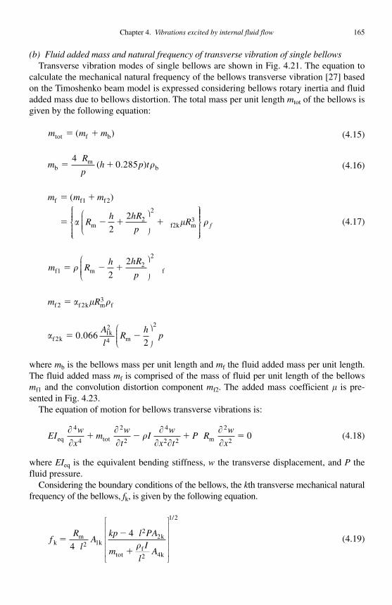
Chapter 4. Vibrations excited by internal fluid flow 165
(b) Fluid added mass and natural frequency of transverse vibration of single bellows Transverse vibration modes of single bellows are shown in Fig. 4.21 . The equation to
calculate the mechanical natural frequency of the bellows transverse vibration [27] based on the Timoshenko beam model is expressed considering bellows rotary inertia and fluid added mass due to bellows distortion. The total mass per unit length mtot of the bellows is given by the following equation:
m m mtot f b� �( ) (4.15)
mR
ph p tb
mb� �
40 285
�( . ) (4.16)
m m m
Rh hR
pR
f f f
m2
f2k m2
� �
� � � �
( )1 2
2
32 �⎛
⎝⎜⎜⎜⎜
⎞
⎠⎟⎟⎟⎟
⎧⎨⎪⎪⎪
⎩⎪⎪⎪
⎫⎬⎪⎪⎪⎪
⎭⎪⎪⎪� f (4.17)
m Rh hR
pf m f2
21
22
� � � �⎛
⎝⎜⎜⎜⎜
⎞
⎠⎟⎟⎟⎟
m Rf f k m f2 23� � �
f kk
m212
4
2
0 0662
� �.A
lR
hp
⎛
⎝⎜⎜⎜
⎞
⎠⎟⎟⎟⎟
where mb is the bellows mass per unit length and mf the fluid added mass per unit length. The fluid added mass mf is comprised of the mass of fluid per unit length of the bellows mf1 and the convolution distortion component mf2 . The added mass coefficient � is pre-sented in Fig. 4.23 .
The equation of motion for bellows transverse vibrations is:
EIw
xm
w
tI
w
x tP R
w
xeq 4 tot m��
��
��
� �
��
4 2
2
4
2 2
2
20� � � � (4.18)
where EIeq is the equivalent bending stiffness, w the transverse displacement, and P the fluid pressure.
Considering the boundary conditions of the bellows, the k th transverse mechanical natural frequency of the bellows, fk , is given by the following equation.
fR
lA
k l PA
mI
lA
km
k
2k
totf
4k
/
��
�4
42 1
2
2
1 2
�
p⎡
⎣
⎢⎢⎢⎢⎢
⎤
⎦
⎥⎥⎥⎥⎥
(4.19)
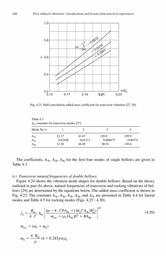
166 Flow induced vibrations: classifications and lessons from practical experiences
The coefficients, A1k , A2k , A4k for the first four modes of single bellows are given in Table 4.3 .
(c) Transverse natural frequencies of double bellows Figure 4.24 shows the vibration mode shapes for double bellows. Based on the theory
outlined in part (b) above, natural frequencies of transverse and rocking vibrations of bel-lows [29] are determined by the equations below. The added mass coefficient is shown in Fig. 4.23 . The constants A1k , A2k , A3k , A4k , and A5k are presented in Table 4.4 for lateral modes and Table 4.5 for rocking modes ( Figs. 4.25 � 4.30 ).
fR
lA
kp l PA k l A R
m IA l BAkm
2 k
22k s
33k m
tot f 4k2
54�
� �
� �
�1
24 4( / )
( )/ kk
⎡
⎣⎢⎢
⎤
⎦⎥⎥
1 2/
(4.20)
m m mtot f b( )� �
mR
ph p tb
mb� �
40 285
�( . )
0.19 0.21 0.230.150.2
0.4
0.6
0.8m
1.0
0.17 0.21h/Rm
� 0.0361� 0.0316t
� 0.0272
R mR 2
� 12
Fig. 4.23 Half-convolution added mass coefficient for transverse vibration [27, 29].
Table 4.3 Aik constants for transverse modes [27]
Mode No. k 1 2 3 4
A1k 22.37 61.67 120.9 199.9 A2k 0.02458 0.01211 0.006677 0.00374 A4k 12.30 46.05 98.91 149.4

Chapter 4. Vibrations excited by internal fluid flow 167
Rocking
Axial
Transverse
Fig. 4.24 Vibration modes of double bellows.
Table 4.4 Aik constants for lateral modes [29]
Mode # Without transverse support
With transverse supports
Aik 1 2 3 1
A1k 5.650 Fig. 4.25 Fig. 4.26 5.62 A2k 0.10 0.0249 0.0119 0.0998 A3k 0 0 0 0.0826 A4k 3.193 Fig. 4.25 Fig. 4.26 3.152 A5k 2.656 Fig. 4.25 Fig. 4.26 2.611
m Rh hR
pRf m
2f2k m f2
� � � � � �2
2
3⎛
⎝⎜⎜⎜⎜
⎞
⎠⎟⎟⎟⎟
⎧⎨⎪⎪⎪
⎩⎪⎪⎪
⎫⎬⎪⎪⎪
⎭⎪⎪⎪
f kk
4 m 2212 2
0 066� �.A
lR
hp
⎛
⎝⎜⎜⎜
⎞
⎠⎟⎟⎟⎟
B M m m a l
B J a l
� � �
�
[ ( ) ]/
( ) :
s p f
p2
: for transverse modes
for rockingg modes
Jm m a m m aR
M app f p f
s
( ) 2�
��
��
3 22
3 4
( )
� � �I Rh
pt
h
pR t� � � �m b 2 f
3 20 571 2. ( )
⎛
⎝⎜⎜⎜⎜
⎞
⎠⎟⎟⎟⎟
⎛
⎝⎜⎜⎜⎜
⎞
⎠⎟⎟⎟⎟⎟

168 Flow induced vibrations: classifications and lessons from practical experiences
1.00
1
2
3
4
5
1.5
a/l
A42
A12
A12
1
0�1 ,
A42
1
0�1 ,
A52
1
0
A52
2.0
Fig. 4.25 Coefficients for second lateral mode; no lateral support [29].
1.5a/l
1.00
5
A13
1
0�1 ,
A43
1
0�1 ,
A53
1
02
10
A53
A43
A13
2.0
Fig. 4.26 Coefficients for third lateral mode; no lateral support [29].
Table 4.5 Aik constants for rocking modes [28]
Mode # Without transverse support
With transverse supports
Aik 1 2 3 1
A1k Fig. 4.27 Fig. 4.28 Fig. 4.29 Fig. 4.30 A2k Fig. 4.27 Fig. 4.28 Fig. 4.29 Fig. 4.30 A3k 0 0 0 Fig. 4.30 A4k 3.08 Fig. 4.28 Fig. 4.29 3.073 A5k Fig. 4.27 Fig. 4.28 Fig. 4.29 Fig. 4.30
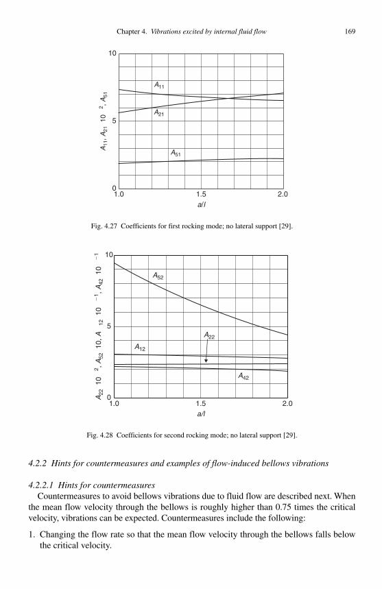
Chapter 4. Vibrations excited by internal fluid flow 169
4.2.2 Hints for countermeasures and examples of flow-induced bellows vibrations
4.2.2.1 Hints for countermeasures Countermeasures to avoid bellows vibrations due to fluid flow are described next. When
the mean flow velocity through the bellows is roughly higher than 0.75 times the critical velocity, vibrations can be expected. Countermeasures include the following:
1. Changing the flow rate so that the mean flow velocity through the bellows falls below the critical velocity.
A11
A21
A51
1.00
5
A11
,A21
1
02 ,A
51
10
1.5a/l
2.0
Fig. 4.27 Coefficients for first rocking mode; no lateral support [29].
A12
A22
1
02 ,A
52
10,
A12
1
0�1 ,
A42
1
0�1
A52
A22
A42
5
10
01.0 1.5
a/l2.0
Fig. 4.28 Coefficients for second rocking mode; no lateral support [29].
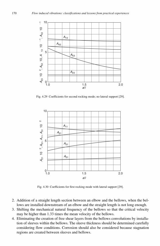
170 Flow induced vibrations: classifications and lessons from practical experiences
2. Addition of a straight length section between an elbow and the bellows, when the bel-lows are installed downstream of an elbow and the straight length is not long enough.
3. Shifting the mechanical natural frequency of the bellows so that the critical velocity may be higher than 1.33 times the mean velocity of the bellows.
4. Eliminating the creation of free shear layers from the bellows convolutions by installa-tion of sleeves within the bellows. The sleeve thickness should be determined carefully considering flow conditions. Corrosion should also be considered because stagnation regions are created between sleeves and bellows.
1.0 1.5a/l
2.0
10
A13
A43
A53
A23
5
A23
1
02 ,A
53
10,
A13
1
0�1 ,
A43
1
0�1
0
Fig. 4.29 Coefficients for second rocking mode; no lateral support [29].
1.0 1.5
a/l
2.0
10
A11
A21
A31
A51
5
A21
1
02 ,A
51,A
11,A
31
102
0
Fig. 4.30 Coefficients for first rocking mode with lateral support [29].
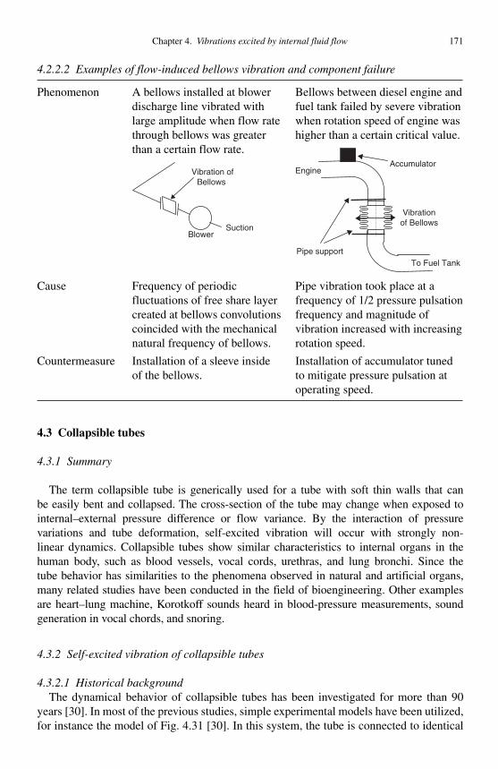
Chapter 4. Vibrations excited by internal fluid flow 171
4.2.2.2 Examples of flow-induced bellows vibration and component failure
Phenomenon A bellows installed at blower discharge line vibrated with large amplitude when flow rate through bellows was greater than a certain flow rate.
Vibration of Bellows
BlowerSuction
Bellows between diesel engine and fuel tank failed by severe vibration when rotation speed of engine was higher than a certain critical value.
Accumulator
Vibrationof Bellows
Pipe support To Fuel Tank
Engine
Cause Frequency of periodic fluctuations of free share layer created at bellows convolutions coincided with the mechanical natural frequency of bellows.
Pipe vibration took place at a frequency of 1/2 pressure pulsation frequency and magnitude of vibration increased with increasing rotation speed.
Countermeasure Installation of a sleeve inside of the bellows.
Installation of accumulator tuned to mitigate pressure pulsation at operating speed.
4.3 Collapsible tubes
4.3.1 Summary
The term collapsible tube is generically used for a tube with soft thin walls that can be easily bent and collapsed. The cross-section of the tube may change when exposed to internal–external pressure difference or flow variance. By the interaction of pressure variations and tube deformation, self-excited vibration will occur with strongly non-linear dynamics. Collapsible tubes show similar characteristics to internal organs in the human body, such as blood vessels, vocal cords, urethras, and lung bronchi. Since the tube behavior has similarities to the phenomena observed in natural and artificial organs, many related studies have been conducted in the field of bioengineering. Other examples are heart–lung machine, Korotkoff sounds heard in blood-pressure measurements, sound generation in vocal chords, and snoring.
4.3.2 Self-excited vibration of collapsible tubes
4.3.2.1 Historical background The dynamical behavior of collapsible tubes has been investigated for more than 90
years [30]. In most of the previous studies, simple experimental models have been utilized, for instance the model of Fig. 4.31 [30]. In this system, the tube is connected to identical
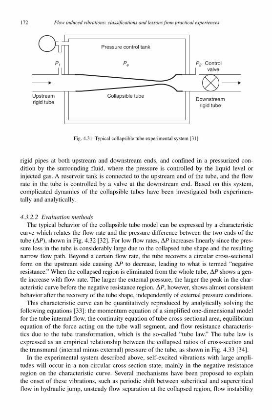
172 Flow induced vibrations: classifications and lessons from practical experiences
rigid pipes at both upstream and downstream ends, and confined in a pressurized con-dition by the surrounding fluid, where the pressure is controlled by the liquid level or injected gas. A reservoir tank is connected to the upstream end of the tube, and the flow rate in the tube is controlled by a valve at the downstream end. Based on this system, complicated dynamics of the collapsible tubes have been investigated both experimen-tally and analytically.
4.3.2.2 Evaluation methods The typical behavior of the collapsible tube model can be expressed by a characteristic
curve which relates the flow rate and the pressure difference between the two ends of the tube ( �P ), shown in Fig. 4.32 [32]. For low flow rates, �P increases linearly since the pres-sure loss in the tube is considerably large due to the collapsed tube shape and the resulting narrow flow path. Beyond a certain flow rate, the tube recovers a circular cross-sectional form on the upstream side causing �P to decrease, leading to what is termed “ negative resistance. ” When the collapsed region is eliminated from the whole tube, �P shows a gen-tle increase with flow rate. The larger the external pressure, the larger the peak in the char-acteristic curve before the negative resistance region. �P , however, shows almost consistent behavior after the recovery of the tube shape, independently of external pressure conditions.
This characteristic curve can be quantitatively reproduced by analytically solving the following equations [33]: the momentum equation of a simplified one-dimensional model for the tube internal flow, the continuity equation of tube cross-sectional area, equilibrium equation of the force acting on the tube wall segment, and flow resistance characteris-tics due to the tube transformation, which is the so-called “ tube law. ” The tube law is expressed as an empirical relationship between the collapsed ratios of cross-section and the transmural (internal minus external) pressure of the tube, as shown in Fig. 4.33 [34] .
In the experimental system described above, self-excited vibrations with large ampli-tudes will occur in a non-circular cross-section state, mainly in the negative resistance region on the characteristic curve. Several mechanisms have been proposed to explain the onset of these vibrations, such as periodic shift between subcritical and supercritical flow in hydraulic jump, unsteady flow separation at the collapsed region, flow instability
Pressure control tank
Controlvalve
Downstreamrigid tube
Collapsible tube
Pe P2P1
Upstreamrigid tube
Fig. 4.31 Typical collapsible tube experimental system [31].
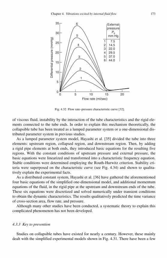
Chapter 4. Vibrations excited by internal fluid flow 173
of viscous fluid, instability by the interaction of the tube characteristics and the rigid ele-ments connected to the tube ends. In order to explain this mechanism theoretically, the collapsible tube has been treated as a lumped parameter system or a one-dimensional dis-tributed parameter system in previous studies.
As a lumped parameter system model, Hayashi et al. [35] divided the tube into three elements: upstream region, collapsed region, and downstream region. Then, by adding a rigid pipe elements at both ends, they introduced basic equations for the resulting five regions. With the constant conditions of upstream pressure and external pressure, the basic equations were linearized and transformed into a characteristic frequency equation. Stable conditions were determined employing the Routh-Hurwitz criterion. Stability cri-teria were superposed on the characteristic curve (see Fig. 4.34 ) and shown to qualita-tively explain the experimental facts.
As a distributed constant system, Hayashi et al. [36] have gathered the aforementioned four basic equations of the simplified one-dimensional model, and additional momentum equations of the fluid, in the rigid pipe at the upstream and downstream ends of the tube. These six equations were discretized and solved numerically under transient conditions to obtain the dynamic characteristics. The results qualitatively predicted the time variance of cross-section area, flow rate, and pressure.
Although many other studies have been conducted, a systematic theory to explain this complicated phenomenon has not been developed.
4.3.3 Key to prevention
Studies on collapsible tubes have existed for nearly a century. However, these mainly dealt with the simplified experimental models shown in Fig. 4.31 . There have been a few
1 7.5
Externalpressure
Pemm Hg
2 14.53 22.04 29.55 37.06
00 5 10
Flow rate (ml/sec)15 20
5
10
15
Diff
eren
tial p
ress
ure
(mm
Hg)
20
25
30
35
44.0
6
5
4
3
2
1
Fig. 4.32 Flow rate–pressure characteristic curve [32].
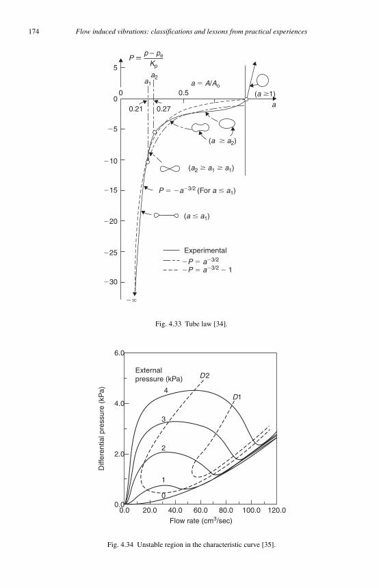
174 Flow induced vibrations: classifications and lessons from practical experiences
0
1
2
3
4
D2
D1
Externalpressure (kPa)
0.00.0
2.0
4.0
Diff
eren
tial p
ress
ure
(kP
a)
6.0
20.0 40.0 60.0 80.0 100.0 120.0
Flow rate (cm3/sec)
Fig. 4.34 Unstable region in the characteristic curve [35].
�
00 0.5
a � A/Ao
(a 1)
a
(a a2)
(a2 a1 a1)
(a � a1)
P � �a�3/2 (For a � a1)
a1
a2
5Kp
p – peP �
�5
�10
�15
�20
�25
�30
0.21 0.27
Experimental
�P � a�3/2
�P � a�3/2 � 1
Fig. 4.33 Tube law [34].

Chapter 4. Vibrations excited by internal fluid flow 175
investigations which modified or analyzed the phenomena in actual internal organs and artificial organs. Although stability analysis methods may be applied to avoid self-excited vibrations in a simplified experimental system, the methods are not developed enough to evaluate actual practical engineering or biological systems. Concrete preventive measures depend on future work.
References
[1] Benjamin , T.B. , Proc. Roy. Soc. , Vol. A 206 , 1961 , pp. 457 – 486 . [2] Benjamin , T.B. , Proc. Roy. Soc. , Vol. A 206 , 1961 , pp. 487 – 499 . [3] Gregory , R.W. and Païdoussis , M.P. , Proc. Roy. Soc. , Vol. A 293 , 1966 , pp. 512 – 527 . [4] Gregory , R.W. and Païdoussis , M.P. , Proc. Roy. Soc. , Vol. A 293 , 1966 , pp. 528 – 542 . [5] Païdoussis, M.P., Mechanical Engineering Research Laboratories Report MERL 69-3 ,
Department of Mechanical Engineering, McGill University, Montreal, Quebec, Canada, 1969.
[6] Païdoussis , M.P. , J. Mech. Eng. Sci. , Vol. 12 , No. 2 , 1970 , pp. 85 – 103 . [7] Païdoussis , M.P. , J. Mech. Eng. Sci. , Vol. 12 , No. 4 , 1970 , pp. 288 – 300 . [8] Païdoussis , M.P. and Issid , N.T. , J. Sound Vib. , Vol. 33 , No. 3 , 1974 , pp. 267 – 294 . [9] Païdoussis , M.P. , J. Mech. Eng. Sci. , Vol. 17 , No. 1 , 1975 , pp. 19 – 25 . [10] Païdoussis , M.P. and Li , G.X. , J. Fluids Struct. , Vol. 7 , 1993 , pp. 137 – 204 . [11] Païdoussis , M.P. and Sundararajan , C. , J. Appl. Mech. , Vol. 42 , 1975 , pp. 780 – 784 . [12] Païdoussis , M.P. and Issid , N.T. , J. Appl. Mech. , Vol. 43 , 1976 , pp. 198 – 202 . [13] Semler, C., Alighanbari, H. and Païdoussis. M.P., J. Appl. Mech. Vol. 65, 1998,
pp. 642–648. [14] Sugiyama, Y. et al., Trans. JSME (in Japanese) , Vol. 54, No. 498, C, 1988, pp. 353–356. [15] Chen , S.S. , J. Appl. Mech. , Vol. 40 , No. 2 , 1973 , pp. 362 – 368 . [16] Païdoussis , M.P. and Denise , J.P. , J. Sound Vib. , Vol. 20 , No. 1 , 1972 , pp. 9 – 26 . [17] Sugiyama, Tanaka, Kishi and Kanagoe, J. Sound Vib. , Vol. 100, No. 2, 1985,
pp. 257–270. [18] Hayama, S. and Matumoto, M., Trans. JSME (in Japanese) , Vol. 52, No. 476, C,
1986, pp. 1192–1197. [19] Weisman , J. et al. , Int. J. Multiphas. Flow , Vol. 5 , No. 6 , 1979 , pp. 437 – 462 . [20] Weisman , J. and Kang , S.Y. , Int. J. Multiphas. Flow , Vol. 7 , No. 3 , 1981 , pp.
271 – 291 . [21] Hara , F. , Trans. JSME (in Japanese) , Vol. 42 , No. 360 , C, 1976 , pp. 2400 – 2411 . [22] Matsuda , H. , Piping Technol. (in Japanese) , Vol. 40 , No. 6 , 1998 , pp. 28 – 35 . [23] Nakamura , Y. and Fukamachi , N. , “ Sound generation in corrugated tubes, ” Fluid
Dynamic Research , Vol. 7 , Japan Society for Fluid Mechanics, 1991 , pp. 255 – 261 . [24] Jakubauskas , V.F. , “ Added Fluid Mass for Bellows Expansion Joints in Axial
Vibrations, ” Trans ASME, J. Press. Vess. Technol. , Vol. 121 , 1999 , pp. 216 – 219 . [25] Standards of the Expansion Joint Manufacturers Association, Inc., Seventh Edition,
EJMA, 1998. [26] Morishita, M., Ikahata, N. and Kitamura, S., “ Dynamic Analysis Methods of
Bellows Including Fluid-Structure Interaction, ” Metallic Bellows and Expansion Joints-1989 , ASME PVP-Vol.168, 1989, pp. 149–157.
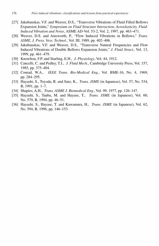
176 Flow induced vibrations: classifications and lessons from practical experiences
[27] Jakubauskas, V.F. and Weaver, D.S., “ Transverse Vibrations of Fluid Filled Bellows Expansion Joints, ” Symposium on Fluid Structure Interaction, Aeroelasticity, Fluid-Induced Vibration and Noise , ASME AD-Vol. 53-2, Vol. 2, 1997, pp. 463–471.
[28] Weaver, D.S. and Ainsworth, P., “Flow Induced Vibrations in Bellows,” Trans. ASME, J. Press. Vess. Technol., Vol. III, 1989, pp. 402–406.
[29] Jakubauskas, V.F. and Weaver, D.S., “Transverse Natural Frequencies and Flow Induced Vibrations of Double Bellows Expansion Joints,” J. Fluid Struct., Vol. 13, 1999, pp. 461–479.
[30] Knowlton , F.P. and Starling , E.H. , J. Physiology , Vol. 44 , 1912 . [31] Cancelli , C. and Pedley , T.J. , J. Fluid Mech. , Cambridge University Press, Vol. 157 ,
1985 , pp. 375 – 404 . [32] Conrad , W.A. , IEEE Trans. Bio-Medical Eng. , Vol. BME-16 , No. 4 , 1969 ,
pp. 284 – 295 . [33] Hayashi , S. , Toyoda , R. and Sato , K. , Trans. JSME (in Japanese) , Vol. 57 , No. 534,
B , 1991 , pp. 1 – 7 . [34] Shapiro , A.H. , Trans. ASME J. Biomedical Eng. , Vol. 99 , 1977 , pp. 126 – 147 . [35] Hayashi , S. , Tanba , M. and Hayase , T. , Trans. JSME (in Japanese) , Vol. 60 ,
No. 579, B , 1994 , pp. 46 – 51 . [36] Hayashi , S. , Hayase , T. and Kawamura , H. , Trans. JSME (in Japanese) , Vol. 62 ,
No. 594, B , 1996 , pp. 146 – 153 .
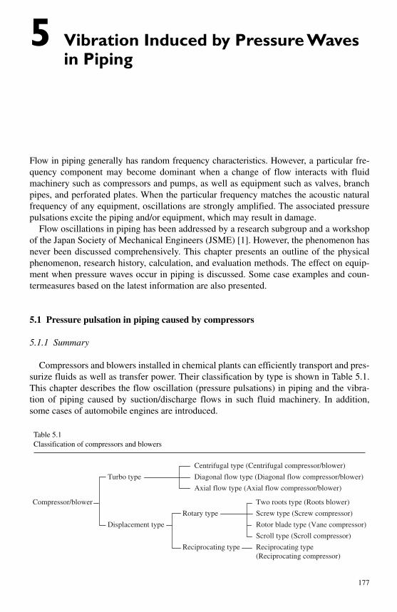
177
5 Vibration Induced by Pressure Waves in Piping
Flow in piping generally has random frequency characteristics. However, a particular fre-quency component may become dominant when a change of flow interacts with fluid machinery such as compressors and pumps, as well as equipment such as valves, branch pipes, and perforated plates. When the particular frequency matches the acoustic natural frequency of any equipment, oscillations are strongly amplified. The associated pressure pulsations excite the piping and/or equipment, which may result in damage.
Flow oscillations in piping has been addressed by a research subgroup and a workshop of the Japan Society of Mechanical Engineers (JSME) [1] . However, the phenomenon has never been discussed comprehensively. This chapter presents an outline of the physical phenomenon, research history, calculation, and evaluation methods. The effect on equip-ment when pressure waves occur in piping is discussed. Some case examples and coun-termeasures based on the latest information are also presented.
5.1 Pressure pulsation in piping caused by compressors
5.1.1 Summary
Compressors and blowers installed in chemical plants can efficiently transport and pres-surize fluids as well as transfer power. Their classification by type is shown in Table 5.1 . This chapter describes the flow oscillation (pressure pulsations) in piping and the vibra-tion of piping caused by suction/discharge flows in such fluid machinery. In addition,some cases of automobile engines are introduced.
Table 5.1 Classification of compressors and blowers
Centrifugal type (Centrifugal compressor/blower)
Turbo type Diagonal flow type (Diagonal flow compressor/blower)
Axial flow type (Axial flow compressor/blower)
Compressor/blower Two roots type (Roots blower)
Rotary type Screw type (Screw compressor)
Displacement type Rotor blade type (Vane compressor)
Scroll type (Scroll compressor)
Reciprocating type Reciprocating type(Reciprocating compressor)
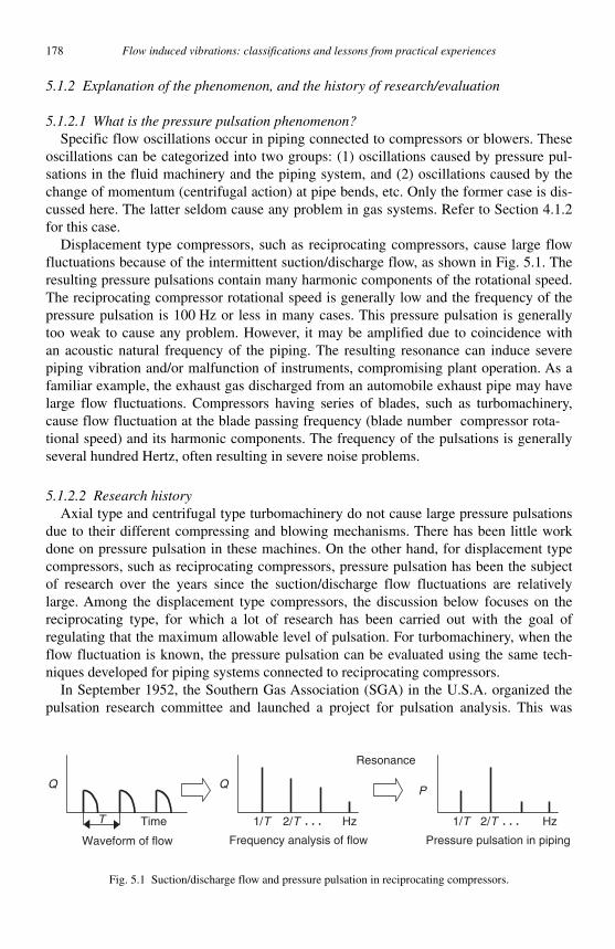
178 Flow induced vibrations: classifications and lessons from practical experiences
5.1.2 Explanation of the phenomenon, and the history of research/evaluation
5.1.2.1 What is the pressure pulsation phenomenon? Specific flow oscillations occur in piping connected to compressors or blowers. These
oscillations can be categorized into two groups: (1) oscillations caused by pressure pul-sations in the fluid machinery and the piping system, and (2) oscillations caused by the change of momentum (centrifugal action) at pipe bends, etc. Only the former case is dis-cussed here. The latter seldom cause any problem in gas systems. Refer to Section 4.1.2 for this case.
Displacement type compressors, such as reciprocating compressors, cause large flow fluctuations because of the intermittent suction/discharge flow, as shown in Fig. 5.1 . The resulting pressure pulsations contain many harmonic components of the rotational speed. The reciprocating compressor rotational speed is generally low and the frequency of the pressure pulsation is 100 Hz or less in many cases. This pressure pulsation is generally too weak to cause any problem. However, it may be amplified due to coincidence with an acoustic natural frequency of the piping. The resulting resonance can induce severe piping vibration and/or malfunction of instruments, compromising plant operation. As a familiar example, the exhaust gas discharged from an automobile exhaust pipe may have large flow fluctuations. Compressors having series of blades, such as turbomachinery, cause flow fluctuation at the blade passing frequency (blade number compressor rota-tional speed) and its harmonic components. The frequency of the pulsations is generally several hundred Hertz, often resulting in severe noise problems.
5.1.2.2 Research history Axial type and centrifugal type turbomachinery do not cause large pressure pulsations
due to their different compressing and blowing mechanisms. There has been little work done on pressure pulsation in these machines. On the other hand, for displacement type compressors, such as reciprocating compressors, pressure pulsation has been the subject of research over the years since the suction/discharge flow fluctuations are relatively large. Among the displacement type compressors, the discussion below focuses on the reciprocating type, for which a lot of research has been carried out with the goal of regulat ing that the maximum allowable level of pulsation. For turbomachinery, when the flow fluctuation is known, the pressure pulsation can be evaluated using the same tech-niques developed for piping systems connected to reciprocating compressors.
In September 1952, the Southern Gas Association (SGA) in the U.S.A. organized the pulsation research committee and launched a project for pulsation analysis. This was
1/T 1/TT Hz
Q Q
Hz
P
Time
Waveform of flow
Resonance
Frequency analysis of flow Pressure pulsation in piping
2/T 2/T
Fig. 5.1 Suction/discharge flow and pressure pulsation in reciprocating compressors.
Chapter 5. Vibration excited by pressure waves in piping 179
the beginning of systematic research on pulsation in piping connected to reciprocat-ing compressors. The Southwest Research Institute (SwRI) was selected as an external research agency and achieved good results in pulsation analysis using an analog computer for the first time in autumn of 1954. They started calculations for practical use in the summer of 1955 and have undertaken pulsation analysis on a commercial basis around the world.
Then, in the 1960s, the American Petroleum Institute Standard 618 (API Standard 618) imposed the requirement that pulsation analysis be done at the design stage of process plants in order to control pulsations to an appropriate level. The API Standard 618 had specified that pulsation analysis be done using analog simulation until the third edition revised the standard in February 1986. This was based on the background that the digital computer at the time had difficulty performing pulsation analysis considering the interac-tion between reciprocating compressors and piping which is a requirement of the API Standard 618. Based on an analogy between equations for fluid flow and those for an electric circuit, the analog simulation method [2, 3] evaluates the pulsation in piping by simulating the fluid characteristic with an L-C-R circuit on the assumption that pressure and flow in the fluid system are equivalent to voltage and current in the electric circuit. However, the third edition of API Standard 618, revised in 1986, removed the restriction on the kind of computer to be used and allowed the use of digital computers for pulsa-tion analysis. In addition to this revision of the API Standard, along with the remarkable progress in the performance of digital computers and achievements in research efforts on pulsation in piping in the late 1960s, the mainstream of the pulsation analysis in piping in Japan moved to digital simulations and today pressure pulsation in piping can be calcu-lated with sufficient accuracy for design purposes.
5.1.3 Calculation and evaluation methods
5.1.3.1 Calculation method
Calculation method for pressure pulsations in piping Generally, the transfer matrix method, developed and employed in the field of mechan-
ical vibration and acoustics, is extensively used in pulsation analysis. This method has been used since the beginning because the acoustic natural frequency in piping can be obtained theoretically. However, the analysis may be difficult when the piping system is complicated due to bypass-lines or in the presence of a piping network. In this case, alternative calculation/analysis methods, such as the stiffness matrix method, the modal analysis method, and the finite element method, have been developed and used in compu-tations for practical use. The internal fluid is considered as a one-dimensional flow when the pipe diameter is less than 1/5 of the pulsation wavelength [4] in the above analy-sis methods. When such an assumption is not applicable, the boundary element method, which is used in the field of acoustics, can be employed effectively. Table 5.2 shows the calculation/analysis methods that are currently used in calculations for practical use. The impedance method [5] that uses the ratio of the pressure fluctuation to the flow fluctua-tion and the pressure pulsation analysis method [6] that applies the nodal analysis method for an electric circuit network are not listed. These methods are rarely used in pulsation analysis today. The transfer matrix method is described below.

180 Flow induced vibrations: classifications and lessons from practical experiences
Table 5.2 Calculation/analysis methods for pressure pulsations
Calculationmethod Outlines, etc. Key equation
Transfer matrix method References [7–16]
● This is the most extensively used method to calculate the pressure pulsation response in piping in the frequency domain.
⎧ ⎫ ⎧ ⎫⎪ ⎪ ⎪ ⎪⎪ ⎪ ⎪ ⎪⎨ ⎬ ⎨ ⎬⎪ ⎪ ⎪ ⎪⎪ ⎪⎪ ⎪ ⎩ ⎭⎩ ⎭�out in
out in[ ]
p pM
q q
● The acoustic natural frequency in piping can be calculated theoretically.
● This analysis may be difficult when the piping system is complicated with bypass lines and/or piping network.
Stiffness matrix method Reference [17]
● This is a frequency domain method, which improved onthe transfer matrix method so that complicated piping systems can be analyzed.
in in
out out[ ]
q pA
q p
⎧ ⎫ ⎧ ⎫⎪ ⎪ ⎪ ⎪⎪ ⎪ ⎪ ⎪⎨ ⎬ ⎨ ⎬⎪ ⎪ ⎪ ⎪⎪ ⎪ ⎪ ⎪⎩ ⎭ ⎩ ⎭�
● It is named after the methodology where the relation between flow and pressure is formulated similarly to the stiffness matrix in structural analysis.
Modal analysis method References [18–23]
● This method applies modal superposition, often used invibration analysis, to the pressure pulsation analysis related to a complicated piping system. 1
1
( ) ( )
( ) ( )
i ii
i ii
q x y t
p x z tφ
∑
∑�
�
� �
� �
��
�● The natural frequencies and the modal functions are
calculated using the transfer matrix method. The pressure pulsation is calculated by the time history analysis. The computation time of this method is shorter compared with direct numerical integration
Finite element method
● This was developed as the pulsation analysis method for complicated piping systems. ∫� � ��[ ] [ ] [ ] dM q C q K q t p
References [24–27]
● The method models the fluid as a one-dimensional problem similarly to longitudinal vibration analysis, formulates a whole system matrix similarly to the structural analysis, and calculates the pressure pulsation. Both frequency and time domain analyses can be performed.
Boundary element method
● This is a frequency domain method that is applied in cases where the internal fluid cannot be analyzed as a one-dimensional flow. Example applications include large tanks and silencers.
�[ ]{ } [ ]{ }H p G q
References [28–32]
● Computation time can be reduced when the system under analysis is sufficiently large compared with the pulsation wavelength.
p : Pressure fluctuation, q : Flow fluctuation.
Transfer matrix method The transfer matrix method [7–16] is the most extensively used method in pulsation
analysis. In the method, the piping system is divided into several piping elements such as a pipe, a side branch, a volume (vessel), and resistance (orifice or valve). The 2 2 transfer matrix M is then formulated to relate the pressure fluctuation p and the flow fluc-tuation q between the inlet and outlet of each piping element, as expressed in Eq. (5.1).
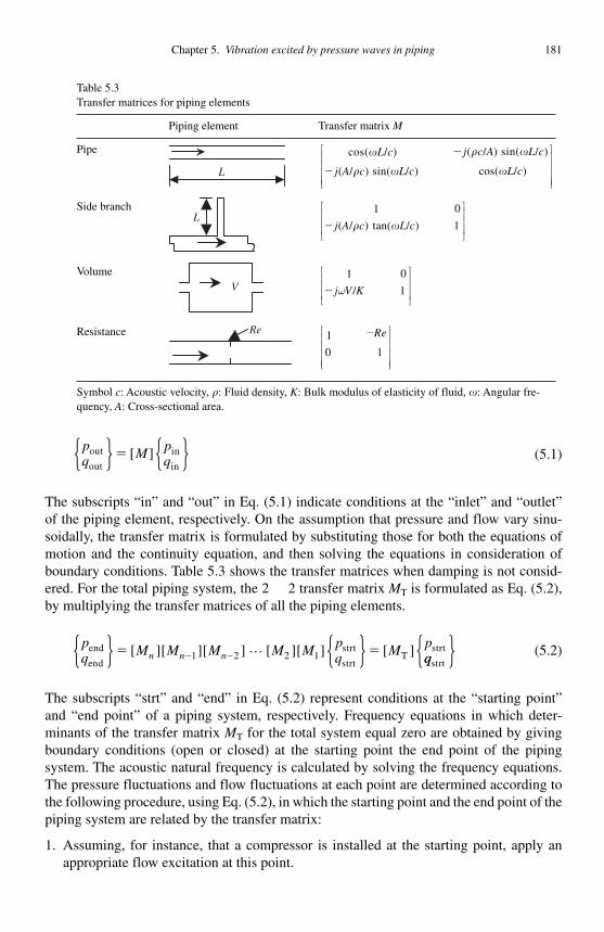
Chapter 5. Vibration excited by pressure waves in piping 181
pq M p
qout
out
in
in{ } { }� [ ] (5.1)
The subscripts “ in ” and “ out ” in Eq. (5.1) indicate conditions at the “ inlet ” and “ outlet ”of the piping element, respectively. On the assumption that pressure and flow vary sinu-soidally, the transfer matrix is formulated by substituting those for both the equations of motion and the continuity equation, and then solving the equations in consideration of boundary conditions. Table 5.3 shows the transfer matrices when damping is not consid-ered. For the total piping system, the 2 2 transfer matrix MT is formulated as Eq. (5.2), by multiplying the transfer matrices of all the piping elements.
pq M M M M M p
q M pn n n
end
end
strt
strtT
strt{ } { }� �� �[ ][ ][ ] [ ][ ] [ ]1 2 2 1� qqstrt{ } (5.2)
The subscripts “ strt ” and “ end ” in Eq. (5.2) represent conditions at the “ starting point ” and “ end point ” of a piping system, respectively. Frequency equations in which deter-minants of the transfer matrix MT for the total system equal zero are obtained by giving boundary conditions (open or closed) at the starting point the end point of the piping system. The acoustic natural frequency is calculated by solving the frequency equations. The pressure fluctuations and flow fluctuations at each point are determined according to the following procedure, using Eq. (5.2), in which the starting point and the end point of the piping system are related by the transfer matrix:
1. Assuming, for instance, that a compressor is installed at the starting point, apply an appropriate flow excitation at this point.
Table 5.3 Transfer matrices for piping elements
Piping element Transfer matrix M
Pipe
L
( / ) sin( / )cos( / )
cos( / )( / ) sin( / )
j c A L cL c
L cj A c L c
⎡ ⎤⎢ ⎥⎢ ⎥⎢ ⎥⎢ ⎥⎣ ⎦
�
�
� ��
�� �
Side branch L
⎡ ⎤⎢ ⎥⎢ ⎥⎢ ⎥⎣ ⎦� � �
01
( / ) tan( / ) 1j A c L c
Volume V
01
/ 1j V Kω
⎡ ⎤⎢ ⎥⎢ ⎥⎢ ⎥⎣ ⎦�
Resistance Re ⎡ ⎤⎢ ⎥⎢ ⎥⎢ ⎥⎢ ⎥⎣ ⎦
�1
0 1
Re
Symbol c : Acoustic velocity, � : Fluid density, K : Bulk modulus of elasticity of fluid, � : Angular fre-quency, A : Cross-sectional area.
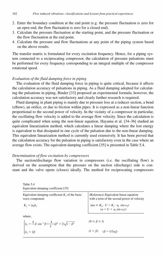
182 Flow induced vibrations: classifications and lessons from practical experiences
2. Enter the boundary condition at the end point (e.g. the pressure fluctuation is zero for an open end, the flow fluctuation is zero for a closed end).
3. Calculate the pressure fluctuation at the starting point, and the pressure fluctuation or the flow fluctuation at the end point.
4. Calculate the pressure and flow fluctuations at any point of the piping system based on the above results.
The transfer matrix is formulated for every excitation frequency. Hence, for a piping sys-tem connected to a reciprocating compressor, the calculation of pressure pulsations must be performed for every frequency corresponding to an integral multiple of the compressor rotational speed.
Evaluation of the fluid damping force in piping The evaluation of the fluid damping force in piping is quite critical, because it affects
the calculation accuracy of pulsations in piping. As a fluid damping adopted for calculat-ing the pulsations in piping, Binder [33] proposed an experimental formula; however, the calculation accuracy was not satisfactory and clearly further research is required.
Fluid damping in plant piping is mainly due to pressure loss at a reducer section, a bend (elbow), an orifice, or due to friction within pipes. It is expressed as a non-linear function proportional to the second power of velocity. In the vicinity of a compressor in particular, the oscillating flow velocity is added to the average flow velocity. Since the calculation is quite complicated when using the non-linear equation, Hayama et al. [34–36] studied an equivalent linearization method, which calculates a linear damping where the lost energy is equivalent to that dissipated in one cycle of the pulsation due to the non-linear damping. This equivalent linearization method is currently used extensively. It has been proved that the calculation accuracy for the pulsation in piping is satisfactory even in the case where an average flow exists. The equivalent damping coefficient [35] is presented in Table 5.4 .
Determination of flow excitation by compressors The suction/discharge flow variation in compressors (i.e. the oscillating flow) is
derived on the assumption that the pressure on the suction (discharge) side is con-stant and the valve opens (closes) ideally. The method for reciprocating compressors
Table 5.4 Equivalent damping coefficient [35]
Equivalent damping coefficient K1 of the basic wave component
(Reference) Equivalent linear equation with a term of the second power of velocity
� � �1 1 1K u k 0 1 1 1
1 1
sin( sin )
u u K U K u tu U u t� � �
� �
� � ��
where,
1 2 21
1
4 4sin ( 2) 1
3
2
k
k
⎧⎪⎪⎪⎪⎨⎪⎪⎪⎪⎩
�� � � �
�
� � � �
�
� ��(0 1)
� �(1 )1( / )U u�� � �
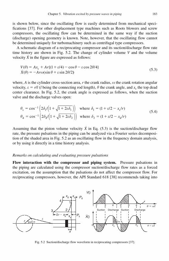
Chapter 5. Vibration excited by pressure waves in piping 183
is shown below, since the oscillating flow is easily determined from mechanical speci-fications [37] . For other displacement type machines such as Roots blowers and screw compressors, the oscillating flow can be determined in the same way if the suction (discharge) opening geometry is known. Note, however, that the oscillating flow cannot be determined uniquely for turbomachinery such as centrifugal type compressors.
A schematic diagram of a reciprocating compressor and its suction/discharge flow rate time history are shown in Fig. 5.2 . The change of cylinder volume V and the volume velocity X
. in the figure are expressed as follows:
V Ax ArX Ar
( ) {( )� � � � �� � � � �
� � � � �
� � �c ( / ) cos cos / }
(sin sin /1 4 2 4
2 2� ))(5.3)
where, A is the cylinder cross-section area, r the crank radius, � the crank rotation angularvelocity, � � r / l ( l being the connecting rod length), � the crank angle, and xc the top dead center clearance. In Fig. 5.2 , the crank angle is expressed as follows, when the suction valve and the discharge valves open:
� � �� � �
� �
s1
s
d1
cos where / /
cos
� � � � � �
�
�
�
2 1 1 2 1 2
2
1 1 1/ ( )( )( ) x r
22 2 21 1 2 1 2/ ( )� � � � ��� � �( )( ) where / /dx r(5.4)
Assuming that the piston volume velocity X. in Eq. (5.3) is the suction/discharge flow
rate, the pressure pulsations in the piping can be analyzed via a Fourier series decomposi-tion of the shaded area in Fig. 5.2 as an oscillating flow in the frequency domain analysis, or by using it directly in a time history analysis.
Remarks on calculating and evaluating pressure pulsations
Flow interaction with the compressor and piping system. Pressure pulsations in the piping are calculated using the compressor suction/discharge flow rates as a forced excitation, on the assumption that the pulsations do not affect the compressor flow. For reciprocating compressors, however, the API Standard 618 [38] recommends taking into
r vt = θ
3
4 1
2
Ps
Pd
2r � xs
xd
x
xs
xc
Suction Discharge Suction Discharge
V(θ)
X(θ)
1
0us 2!
!us
udud
2 3 4 3 41 2
u � vt
u � vt
Fig. 5.2 Suction/discharge flow waveform in reciprocating compressors [37].
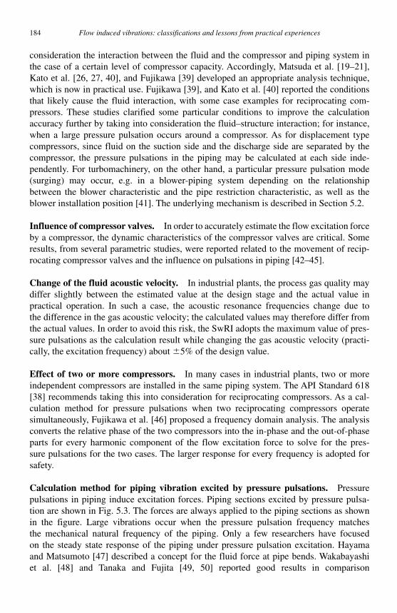
184 Flow induced vibrations: classifications and lessons from practical experiences
consideration the interaction between the fluid and the compressor and piping system in the case of a certain level of compressor capacity. Accordingly, Matsuda et al. [19 – 21] , Kato et al. [26, 27, 40] , and Fujikawa [39] developed an appropriate analysis technique, which is now in practical use. Fujikawa [39] , and Kato et al. [40] reported the conditions that likely cause the fluid interaction, with some case examples for reciprocating com-pressors. These studies clarified some particular conditions to improve the calculation accuracy further by taking into consideration the fluid–structure interaction; for instance, when a large pressure pulsation occurs around a compressor. As for displacement type compressors, since fluid on the suction side and the discharge side are separated by the compressor, the pressure pulsations in the piping may be calculated at each side inde-pendently. For turbomachinery, on the other hand, a particular pressure pulsation mode (surging) may occur, e.g. in a blower-piping system depending on the relationship between the blower characteristic and the pipe restriction characteristic, as well as the blower installation position [41] . The underlying mechanism is described in Section 5.2.
Influence of compressor valves. In order to accurately estimate the flow excitation force by a compressor, the dynamic characteristics of the compressor valves are critical. Some results, from several parametric studies, were reported related to the movement of recip-rocating compressor valves and the influence on pulsations in piping [42–45] .
Change of the fluid acoustic velocity. In industrial plants, the process gas quality may differ slightly between the estimated value at the design stage and the actual value in practical operation. In such a case, the acoustic resonance frequencies change due to the difference in the gas acoustic velocity; the calculated values may therefore differ from the actual values. In order to avoid this risk, the SwRI adopts the maximum value of pres-sure pulsations as the calculation result while changing the gas acoustic velocity (practi-cally, the excitation frequency) about " 5% of the design value.
Effect of two or more compressors. In many cases in industrial plants, two or more independent compressors are installed in the same piping system. The API Standard 618 [38] recommends taking this into consideration for reciprocating compressors. As a cal-culation method for pressure pulsations when two reciprocating compressors operate simultaneously, Fujikawa et al. [46] proposed a frequency domain analysis. The analysis converts the relative phase of the two compressors into the in-phase and the out-of-phase parts for every harmonic component of the flow excitation force to solve for the pres-sure pulsations for the two cases. The larger response for every frequency is adopted for safety.
Calculation method for piping vibration excited by pressure pulsations. Pressure pulsations in piping induce excitation forces. Piping sections excited by pressure pulsa-tion are shown in Fig. 5.3 . The forces are always applied to the piping sections as shown in the figure . Large vibrations occur when the pressure pulsation frequency matches the mechanical natural frequency of the piping. Only a few researchers have focused on the steady state response of the piping under pressure pulsation excitation. Hayama and Matsumoto [47] described a concept for the fluid force at pipe bends. Wakabayashi et al. [48] and Tanaka and Fujita [49, 50] reported good results in comparison
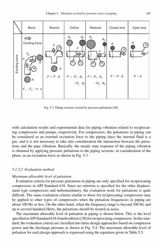
Chapter 5. Vibration excited by pressure waves in piping 185
with calculation results and experimental data for piping vibration related to reciprocat-ing compressors and pumps, respectively. For compressors, the pulsations in piping can be considered as an external excitation force to the piping since the internal fluid is a gas, and it is not necessary to take into consideration the interaction between the pulsa-tions and the pipe vibration. Basically, the steady state response of the piping vibration is obtained by applying pressure pulsations to the piping sections, in consideration of the phase, as an excitation force as shown in Fig. 5.3 .
5.1.3.2 Evaluation method
Maximum allowable level of pulsation Evaluation criteria for pressure pulsations in piping are only specified for reciprocating
compressors in API Standard 618. Since no criterion is specified for the other displace-ment type compressors and turbomachinery, the evaluation work for pulsations is quite difficult. The same evaluation criteria similar to those for reciprocating compressors may be applied to other types of compressors when the pulsation frequencies in piping are about 100 Hz or less. On the other hand, when the frequency range is beyond 200 Hz and up to several hundred Hertz, the pulsations should be treated as noise.
The maximum allowable level of pulsation in piping is shown below. This is the level specified in API Standard 618 (fourth edition) [38] for reciprocating compressors. In this stan-dard, the evaluation criteria are classified into three design approaches based on compressorpower and the discharge pressure as shown in Fig. 5.4 . The maximum allowable level of pulsation for each design approach is expressed using the equations given in Table 5.5 .
Bend Branch Orifice Reducer Closed end Open end
Exc
iting
forc
e
Exciting force
F2
F
A
P
F1A
A1 A2 A1
P1 P2P1 P2
A2
A
P
A
FF
FP
A
P
F1 � F2 � P · A
F � P · A F � P · A F � 0F � P1 · A1
�P2 · A2
F � P1 · A1
�P2 · A2
Fig. 5.3 Piping sections excited by pressure pulsations [49].
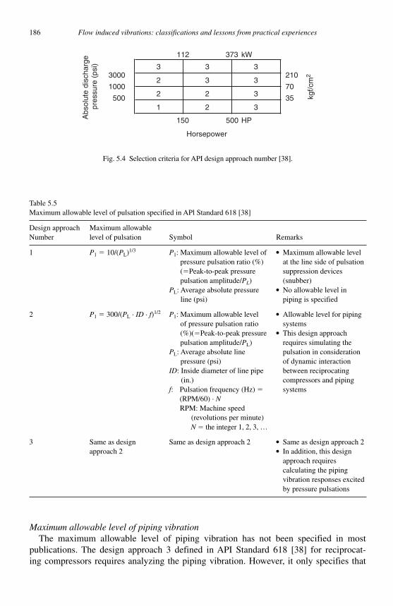
186 Flow induced vibrations: classifications and lessons from practical experiences
3 3 3
2 3 3
2 2 3
1 2 3
Horsepower
kgf/c
m2
kW
3000
1000
500
210
70
35
Abs
olut
e di
scha
rge
pre
ssur
e (p
si)
112 373
HP150 500
Fig. 5.4 Selection criteria for API design approach number [38].
Table 5.5 Maximum allowable level of pulsation specified in APl Standard 618 [38]
Design approach Number
Maximum allowable level of pulsation Symbol Remarks
1 P1 � 10/( PL ) 1/3 P1 : Maximum allowable level of pressure pulsation ratio (%) (�Peak-to-peak pressure pulsation amplitude/ PL )
● Maximum allowable level at the line side of pulsation suppression devices (snubber)
PL : Average absolute pressure line (psi)
● No allowable level in piping is specified
2 P1 � 300/( PL · ID · f ) 1/2 P1 : Maximum allowable level of pressure pulsation ratio (%)(�Peak-to-peak pressure pulsation amplitude/ PL )
● Allowable level for piping systems
● This design approach requires simulating the pulsation in consideration of dynamic interaction between reciprocating compressors and piping systems
PL: Average absolute line pressure (psi)
ID: Inside diameter of line pipe (in.)
f : Pulsation frequency (Hz) �(RPM/60) · NRPM: Machine speed (revolutions per minute) N � the integer 1, 2, 3, …
3 Same as designapproach 2
Same as design approach 2 ● Same as design approach 2 ● In addition, this design
approach requires calculating the piping vibration responses excited by pressure pulsations
Maximum allowable level of piping vibration The maximum allowable level of piping vibration has not been specified in most
publications. The design approach 3 defined in API Standard 618 [38] for reciprocat-ing compressors requires analyzing the piping vibration. However, it only specifies that
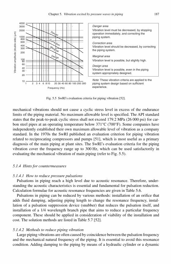
Chapter 5. Vibration excited by pressure waves in piping 187
mechanical vibrations should not cause a cyclic stress level in excess of the endurance limits of the piping material. No maximum allowable level is specified. The API standard states that the peak-to-peak cyclic stress shall not exceed 179.2 MPa (26 000 psi) for car-bon steel pipes at an operating temperature below 371°C (700°F). Some companies have independently established their own maximum allowable level of vibration as a company standard. In the 1970s the SwRI published an evaluation criterion for piping vibration related to reciprocating compressors and pumps [51] , which is most useful as a primary diagnosis of the main piping at plant sites. The SwRI ’ s evaluation criteria for the piping vibration cover the frequency range up to 300 Hz, which can be used satisfactorily in evaluating the mechanical vibration of main piping (refer to Fig. 5.5 ).
5.1.4 Hints for countermeasures
5.1.4.1 How to reduce pressure pulsations Pulsations in piping reach a high level due to acoustic resonance. Therefore, under-
standing the acoustic characteristics is essential and fundamental for pulsation reduction. Calculation formulae for acoustic resonance frequencies are given in Table 5.6 .
Pulsations in piping can be reduced by various methods: installation of an orifice that adds fluid damping, adjusting piping length to change the resonance frequency, instal-lation of a pulsation suppression device (snubber) that reduces the pulsation itself, and installation of a 1/4 wavelength branch pipe that aims to reduce a particular frequency component. These should be applied in consideration of viability of the installation and cost. The solution methods are listed in Table 5.7 [52] .
5.1.4.2 Methods to reduce piping vibration Large piping vibrations are often caused by coincidence between the pulsation frequency
and the mechanical natural frequency of the piping. It is essential to avoid this resonance condition. Adding damping to the piping by means of a hydraulic cylinder or a dynamic
Note: These vibration criteria are applied to thepiping system design based on sufficientexperience.
Danger areaVibration level must be decreased, by stoppingoperation immediately, and correcting thepiping system.
Correction areaVibration level should be decreased, by correctingthe piping system.
Marginal area
Vibration level is possible, but slightly high.
Design areaVibration level is possible, even in the pipingsystem appropriately designed.
Frequency (Hz)
Vib
ratio
n am
plitu
de (
doub
le s
ide)
(μm
)
10
20
3040
60
100
200
300400
600800
1000
2000
30004000
80
1 2 3 4 6 8 10 20 30 40 60 80 100 200 300
Design
Marginal
Correction
Danger
Fig. 5.5 SwRI ’ s evaluation criteria for piping vibration [52].
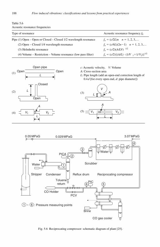
188 Flow induced vibrations: classifications and lessons from practical experiences
Water
Water
3
2
1
1
6
6
5
PICA
0.05 MPaG 0.029 MPaG 3.07 MPaG
Scrubber
Stripper Condenser Reflux drum Reciprocating compressor
Toluenereturn
CO Holder
4
PIC
Brine
CO gas cooler
: Pressure measuring points
PCV
Fig. 5.6 Reciprocating compressor: schematic diagram of plant [25].
Table 5.6 Acoustic resonance frequencies
Type of resonance Acoustic resonance frequency f0
Pipe (1) Open – Open or Closed – Closed 1/2 wavelength resonance fo � ( c/ 2 L ) n n � 1, 2, 3, …
(2) Open – Closed 1/4 wavelength resonance fo � ( c/ 4 L )(2 n� 1) n � 1, 2, 3, …
(3) Helmholtz resonance fo � ( c/ 2 )( A/LV ) 1/2
(4) Volume – Restriction – Volume resonance (low pass filter) fo � ( c/ 2 ){( A/L ) · (1 /V1� 1 / V2 )} 1/2
(1)Open
Open pipe
LOpen
c : Acoustic velocity, V : Volume A : Cross-section area L : Pipe length (add an open-end correction length of
0.4d [for every open end, d : pipe diameter])
(2) L
Open
Closed
(3) L
VA
(4)L
V1 V2
A
(5)
L
V1 V2
A

Chapter 5. Vibration excited by pressure waves in piping 189
Table 5.7Methods to reduce pressure pulsation
Measures Description/feature Remarks
1. Installing an orifice[53, 54]
● Adds damping to reduce pressurepulsation
● Install at the location where flowfluctuation is large
● This is the simplest countermeasure to reduce pulsation with minimum change of piping
● Installing at the inlet or outlet of a large volume is most effective (inlet/outlet of snubber)
● Note that the pressure loss is quite large. Usually, an opening area ratio of 1/4 is adopted
● Installing at an appropriate location is effective also for the change of acoustic velocity in a broad range
2. Adjusting piping length
● In order to avoid acousticresonance, adjust piping lengthto change the acoustic naturalfrequency
● Pay attention when the acoustic velocity changes over a wide range
● Pay attention to piping flexibility
● The 1/4 wavelength resonance ina safety valve piping or a closedbranch with a gate block valvecan be avoided effectively
3. Changing pipingdiameter
● For reducing pressure pulsation,use a piping of larger diameter at the location where pressure pulsation is large, in order to increase the acoustic volume/ capacitance
● For the location where size increase ofpiping is predicted, consider required space at design stage
● Pay attention to piping flexibility
4. Installing a side branch(1/4 wavelength pipe)and a resonator
● Installing the dynamic damper that aims at a particular frequency is sometime considered
● Breaking the resonance mode in main piping reduces the pressure pulsation
● Install at the antinode ofpressure pulsation
● Pay attention to the effect when the acoustic velocity changes on a wide range
● Adding damping is also effective [55]● Pay attention to the supports to prevent
vibration since pulsations may be large in a branch pipe
5. Increasing surge drum size(snubber) volume
● Theoretically, a larger volume reduces pressure pulsations more
● This can be the most effectivemeasure to reduce pressurepulsation
● Install as close to compressor as possible
● It is important to consider a snubber having a large enough volume in the planning stage (refer to API Standard 618 [38])
6. Installing second(additional) drum
● Install the second drum tocomplement the snubber volume
● Delivery period may be a problem in emergency case
● Use as a low pass filter, combining with snubber
● It may be quite expensive
7. Installing a pulsationdamper and a snubberinternal
● It works as a low pass filter● Use as a low pass filter by
installing an internal to a snubber
● Pay attention to material selection when the fluid is corrosive gas
● Maintenance is required. ExpensiveGenerally, pressure loss is large
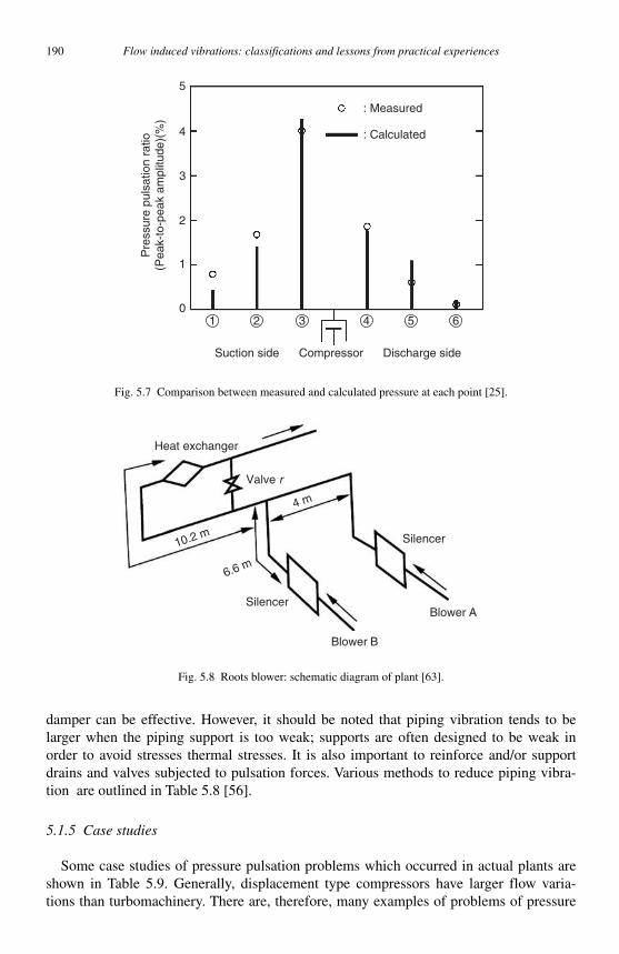
190 Flow induced vibrations: classifications and lessons from practical experiences
damper can be effective. However, it should be noted that piping vibration tends to be larger when the piping support is too weak; supports are often designed to be weak in order to avoid stresses thermal stresses. It is also important to reinforce and/or support drains and valves subjected to pulsation forces. Various methods to reduce piping vibra-tion are outlined in Table 5.8 [56] .
5.1.5 Case studies
Some case studies of pressure pulsation problems which occurred in actual plants are shown in Table 5.9 . Generally, displacement type compressors have larger flow varia-tions than turbomachinery. There are, therefore, many examples of problems of pressure
Pre
ssur
e pu
lsat
ion
ratio
(Pea
k-to
-pea
k am
plitu
de)(
%)
Suction side Compressor Discharge side
: Measured
: Calculated
1 2 3 4 5 6
5
4
3
2
1
0
Fig. 5.7 Comparison between measured and calculated pressure at each point [25].
Heat exchanger
Valve r
Silencer
SilencerBlower A
Blower B
6.6 m
10.2 m
4 m
Fig. 5.8 Roots blower: schematic diagram of plant [63].
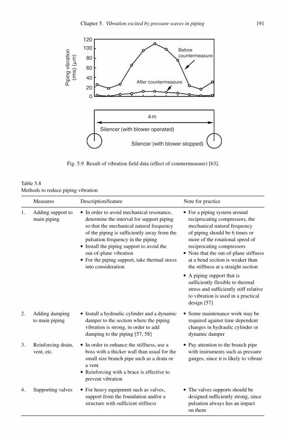
Chapter 5. Vibration excited by pressure waves in piping 191
Beforecountermeasure
After countermeasure
Silencer (with blower operated)
Silencer (with blower stopped)
Pip
ing
vibr
atio
n(r
ms)
(#
m)
4 m
0
20
40
60
80
100
120
Fig. 5.9 Result of vibration field data (effect of countermeasure) [63].
Table 5.8 Methods to reduce piping vibration
Measures Description/feature Note for practice
1. Adding support to main piping
● In order to avoid mechanical resonance, determine the interval for support piping so that the mechanical natural frequency of the piping is sufficiently away from the pulsation frequency in the piping
● Install the piping support to avoid the out-of-plane vibration
● For the piping support, take thermal stress into consideration
● For a piping system around reciprocating compressors, the mechanical natural frequency of piping should be 6 times or more of the rotational speed of reciprocating compressors
● Note that the out-of-plane stiffness at a bend section is weaker than the stiffness at a straight section
● A piping support that is sufficiently flexible to thermal stress and sufficiently stiff relative to vibration is used in a practical design [57]
2. Adding damping to main piping
● Install a hydraulic cylinder and a dynamic damper to the section where the piping vibration is strong, in order to add damping to the piping [57, 58]
● Some maintenance work may be required against time dependent changes in hydraulic cylinder or dynamic damper
3. Reinforcing drain, vent, etc.
● In order to enhance the stiffness, use a boss with a thicker wall than usual for the small size branch pipe such as a drain or a vent
● Pay attention to the branch pipe with instruments such as pressure gauges, since it is likely to vibrate
● Reinforcing with a brace is effective to prevent vibration
4. Supporting valves ● For heavy equipment such as valves, support from the foundation and/or a structure with sufficient stiffness
● The valves supports should be designed sufficiently strong, since pulsation always has an impact on them

192F
low induced vibrations: classifications and lessons from
practical experiences
Table 5.9Example cases
Machinery type Vibration/pulsation problems Possible causes Measures
1. Reciprocating compressor: gas recovery plant in an ironworks [25]. Refer to Figs. 5.6 and 5.7
● Malfunction of instruments (pressure gauges)
● Acoustic resonance with a frequency of 2 times the compressor rotational speed
● The maximum allowable level of pulsation to the pressure gauge is as severe as 3%
● The possible problem was avoided by changing the pressure gauge location
2. Reciprocating compressor: petroleum refinery [59]
● Bending vibration of piping● The piping vibrated 900 �m with a
frequency of 2 times the reciprocating compressor rotational speed
● A large pulsation (17 Hz) at a frequency 2 times the reciprocating compressor rotational speed occurred
● 18 orifices were installed. Their diameter ratio to the pipe diameter was 1/2
● The piping vibration was decreased from about 900 to 350 �m
3. Reciprocating compressor: reactor [60]
● Vibration of the reactor and the structure● The pressure pulsation in the piping
connected to the reactor was 0.92 psi, and the vertical vibration amplitude of the structure was 261 �m
● The gas blown into the bottom of the reactor from a reciprocating compressor flowed intermittently due to pressure pulsation; the forced excitation affected the reactor vertically
● An orifice was installed, and the structure was reinforced
● The pressure pulsation was decreased from 0.92 to 0.19 psi, and the piping vibration was decreased from 261 to 86�m
4. Reciprocating compressor: drains and vents in a piping system [61, 62]
● High harmonics pulsations occurred when measuring pressure fluctuation using the drain and/or the vent
● A 1/4 wavelength resonance in a branch pipe such as a drain
● An orifice was installed at the inlet of the drain, which area ratio was 1/4. Note that installing an orifice may decrease theexpected pressure fluctuation in the measurements
5. Roots blower: direct reduction steel plant [31]
● Pressure pulsations with a component of 4 times (the fundamental 29 Hz) and 12 times (third order, 87 Hz) the rotational speed occurred
● Intermittent discharge flow from the Roots blower
● A large-sized silencer (2.2 m diameter, 6 m height) was installed
C
hapter 5. Vibration excited by pressure waves in piping
193
6. Root blower: chemical plant [63]. Refer to Figs. 5.8 and 5.9
● Radial (shell mode) vibration of piping● The blower outlet piping vibrated 100 #m
radially peak-peak
● The piping was excited by the acoustic resonance in piping
● A 1/4 wavelength pipe (side branch) was installed between the root blower and the silencer, which was tuned at 55 Hz (pulsation frequency)
7. Expansion turbine: chemical plant [64]. Refer to Figs. 5.10 and 5.11
● Bending vibration of piping● Piping vibration occurred at the partial load
operation (80%) of the turbine● The piping vibrated with the fourth acoustic
natural frequency of 31 Hz, and amplitude of 200 �m or more
● Possibly caused by an unstable flow due to interference of the swirling flow at the turbine outlet with the secondary flow at a piping bend section
● Installing a honeycomb (discharge angle coefficient: 0.25) at the turbine outlet eliminated the vibration
8. Automobile diesel engine [65] ● A bellows supplying fuel to the engine vibrated several centimeters when the engine was operated above a certain rotational frequency
● Parametric vibration caused by a periodic variation of the bellows stiffness due to internal pressure pulsations
● An accumulator that was tuned to the pressure pulsation frequency at the driving rotational speed range was installed
● The pressure pulsation was decreased to about l/20 of the original level
9. Truck engine [66] ● In the driver’s compartment of a 4 ton truck, a noise around 100, 250, and 400 Hz occurred when the engine was operated at 2000 rpm or more
● The peak components of the noise spectrum at the air intake were at the same as frequencies
● The design change of the air cleaner and an air intake duct caused the elimination of insertion loss of the air intake system
● The insertion losses of the target frequency was improved about 20 dB by installing a resonator to both the air intake duct and the air cleaner

194 Flow induced vibrations: classifications and lessons from practical experiences
4782
10B
12 B
12B
12B 10B
A
B
C
D
P1
P2
V1
Turbine
North
East3720
1550
300 8001600
2470
1301
1500
10B 10
B
10B
10B
Condenser
Evaporator
Unit : mm
204
1
Fig. 5.10 Turbine: schematic diagram of plant [64].
pulsations in piping due to these compressors. For turbomachinery, on the other hand, there are few examples because fundamentally the compression mechanism in turboma-chinery does not cause any pressure pulsation. Noise [67] , swirling stall, and surging are, however, often experienced in turbomachinery. These problems will be discussed in a subsequent section .
5.2 Pressure pulsations in piping caused by pumps and hydraulic turbines
5.2.1 Outline
In this section, the phenomena related to steady pressure pulsations that occur in pipe-line systems including pumps and hydraulic turbines are discussed. The first discussion is focused on positive displacement pumps and turbo-pumps, which are used to transport, supply, and pressurize liquids, particularly water in various plants. Discussion on Francis and Kaplan turbines for hydroelectric power plants follow. Furthermore, pipelines, tanks, and other equipment, which accompany pumps or turbines, are examined. The causes of pulsation are divided roughly into two kinds, namely forced vibrations and self-excited vibrations. In either case, pulsations will do damage to machines or plants directly and

Chapter 5. Vibration excited by pressure waves in piping 195
may be the cause of secondary damage by propagation of vibrations and noise to the sur-roundings. However, since solution methods vary depending on the cause of pulsations, it is important to first identify the cause.
Pulsations in simple pipelines that do not include pumps or hydraulic turbines were discussed in Section 4.1, while pulsations caused by flow velocity fluctuations were pre-sented in Section 5.1.
5.2.2 Explanation of phenomena
5.2.2.1 Piping portion As a method for the numerical simulation of steady pulsation in a piping portion, the
transfer matrix method is most commonly used. Amplitudes of pressure P and flow rate Q are taken as components of the state vector. Neglecting damping effects, the following equation relates quantities at two arbitrary points:
P x
Q x
x c j c A x c
j A c
( )
( )
cos( / ) ( / ) sin( / )
( / ) sin(
⎡
⎣⎢⎢⎢
⎤
⎦⎥⎥⎥
−
−=
ω ρ ω
ρ ωxx c x c
P
Q/ ) cos( / )
( )
( )ω
⎡
⎣
⎢⎢⎢
⎤
⎦
⎥⎥⎥
⎡
⎣⎢⎢⎢
⎤
⎦⎥⎥⎥
0
0 (5.5)
Gas flow rate (kg/s)
100
50
10
5
0.25
13.9 27.8 41.7
0.5
0.6
0.70.8
0.9
Pip
ing
vibr
atio
n am
plitu
de(#
m)
Fig. 5.11 Result of piping vibration field data (before [ • ] and after [❍] countermeasure) [64].
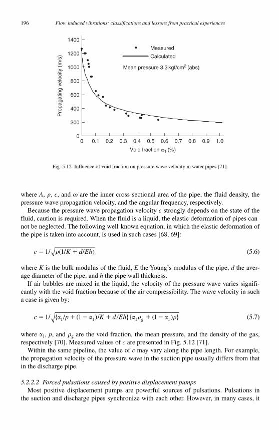
196 Flow induced vibrations: classifications and lessons from practical experiences
where A , � , c , and � are the inner cross-sectional area of the pipe, the fluid density, the pressure wave propagation velocity, and the angular frequency, respectively.
Because the pressure wave propagation velocity c strongly depends on the state of the fluid, caution is required. When the fluid is a liquid, the elastic deformation of pipes can-not be neglected. The following well-known equation, in which the elastic deformation of the pipe is taken into account, is used in such cases [68, 69] :
c K d Eh� �1/ / /�( )1 (5.6)
where K is the bulk modulus of the fluid, E the Young ’ s modulus of the pipe, d the aver-age diameter of the pipe, and h the pipe wall thickness.
If air bubbles are mixed in the liquid, the velocity of the pressure wave varies signifi-cantly with the void fraction because of the air compressibility. The wave velocity in such a case is given by:
c p K d Eh� � � � � � �1/ / g{ ( )/ }{ ( ) } � �1 1 1 11 1 (5.7)
where 1 , p , and �g are the void fraction, the mean pressure, and the density of the gas, respectively [70] . Measured values of c are presented in Fig. 5.12 [71] .
Within the same pipeline, the value of c may vary along the pipe length. For example, the propagation velocity of the pressure wave in the suction pipe usually differs from that in the discharge pipe.
5.2.2.2 Forced pulsations caused by positive displacement pumps Most positive displacement pumps are powerful sources of pulsations. Pulsations in
the suction and discharge pipes synchronize with each other. However, in many cases, it
Pro
paga
ting
velo
city
(m
/s)
Void fraction �1 (%)
Calculated
Mean pressure 3.3 kgf/cm2 (abs)
Measured
200
400
600
800
1000
1200
1400
00 0.1 1.00.2 0.3 0.4 0.5 0.6 0.7 0.8 0.9
Fig. 5.12 Influence of void fraction on pressure wave velocity in water pipes [71].
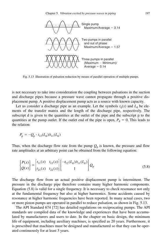
Chapter 5. Vibration excited by pressure waves in piping 197
is not necessary to take into consideration the coupling between pulsations in the suction and discharge pipes because a pressure wave cannot propagate through a positive dis-placement pump. A positive displacement pump acts as a source with known capacity.
Let us consider a discharge pipe as an example. Let the symbols tij ( x ) and Ld be ele-ments of the transfer matrix and the length of the discharge pipe, respectively. The subscript d is given to the quantities at the outlet of the pipe and the subscript p to the quantities at the pump outlet. If the outlet end of the pipe is open, Pd � 0. This leads to the relation:
P Q t L t Lp p d d� � � 12 11( )/ ( )
Thus, when the discharge flow rate from the pump Qp is known, the pressure and flow rate amplitudes at an arbitrary point can be obtained from the following equation:
P x
Q x
t x t x
t x t x
( )
( )
( ) ( )
( ) ( )
⎧⎨⎪⎪⎩⎪⎪
⎫⎬⎪⎪⎭⎪⎪
⎡
⎣
⎢⎢⎢
⎤
⎦
⎥⎥⎥
−�
11 12
21 22
tt L t LQ
12 11
1
( )/ ( )d dp
⎧⎨⎪⎪
⎩⎪⎪
⎫⎬⎪⎪
⎭⎪⎪(5.8)
The discharge flow from an actual positive displacement pump is intermittent. The pressure in the discharge pipe therefore contains many higher harmonic components. Equation (5.8) is valid for a single frequency. It is necessary to check resonance not only at the fundamental frequency but also at higher harmonics. Some accidents caused by resonance at higher harmonic frequencies have been reported. In many actual cases, two or more piston pumps are operated in parallel to reduce pulsation, as shown in Fig. 5.13 .
The API Standard 674 [72] has detailed regulations on reciprocating pumps. The API standards are compiled data of the knowledge and experiences that have been accumu-lated by manufacturers and users to date. In the chapter on basic design, the minimum life of equipment, including auxiliary machines, is specified as 20 years. Furthermore, it is prescribed that machines must be designed and manufactured so that they can be oper-ated continuously for at least 3 years.
Two pumps in parallel and out of phase Maximum/Average � 1.57
Three pumps in parallel (Maximum � Minimum)/ Average � 0.14
Single pump Maximum/Average � 3.14
Fig. 5.13 Illustration of pulsation reduction by means of parallel operation of multiple pumps.
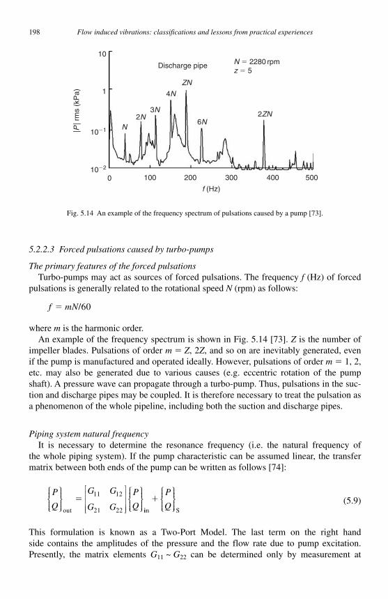
198 Flow induced vibrations: classifications and lessons from practical experiences
5.2.2.3 Forced pulsations caused by turbo-pumps
The primary features of the forced pulsations Turbo-pumps may act as sources of forced pulsations. The frequency f (Hz) of forced
pulsations is generally related to the rotational speed N (rpm) as follows:
f mN� /60
where m is the harmonic order. An example of the frequency spectrum is shown in Fig. 5.14 [73] . Z is the number of
impeller blades. Pulsations of order m � Z , 2 Z , and so on are inevitably generated, even if the pump is manufactured and operated ideally. However, pulsations of order m � 1, 2,etc. may also be generated due to various causes (e.g. eccentric rotation of the pump shaft). A pressure wave can propagate through a turbo-pump. Thus, pulsations in the suc-tion and discharge pipes may be coupled. It is therefore necessary to treat the pulsation as a phenomenon of the whole pipeline, including both the suction and discharge pipes.
Piping system natural frequency It is necessary to determine the resonance frequency (i.e. the natural frequency of
the whole piping system). If the pump characteristic can be assumed linear, the transfer matrix between both ends of the pump can be written as follows [74] :
P
Q
G G
G G
P
Q
⎧⎨⎪⎪⎩⎪⎪
⎫⎬⎪⎪⎭⎪⎪
⎡
⎣
⎢⎢⎢
⎤
⎦
⎥⎥⎥
⎧⎨⎪⎪⎩⎪⎪
⎫⎬⎪⎪⎭⎪⎪out
�11 12
21 22 iin S
�P
Q
⎧⎨⎪⎪⎩⎪⎪
⎫⎬⎪⎪⎭⎪⎪
(5.9)
This formulation is known as a Two-Port Model. The last term on the right hand side contains the amplitudes of the pressure and the flow rate due to pump excitation. Presently, the matrix elements G11 ~ G22 can be determined only by measurement at
0 100 200 300 400 500
f (Hz)
10�2
10�1
1
10
Discharge pipe
N2N
3N
4N
6N2ZN
ZN|P
| rm
s (k
Pa)
N � 2280 rpmz � 5
Fig. 5.14 An example of the frequency spectrum of pulsations caused by a pump [73].
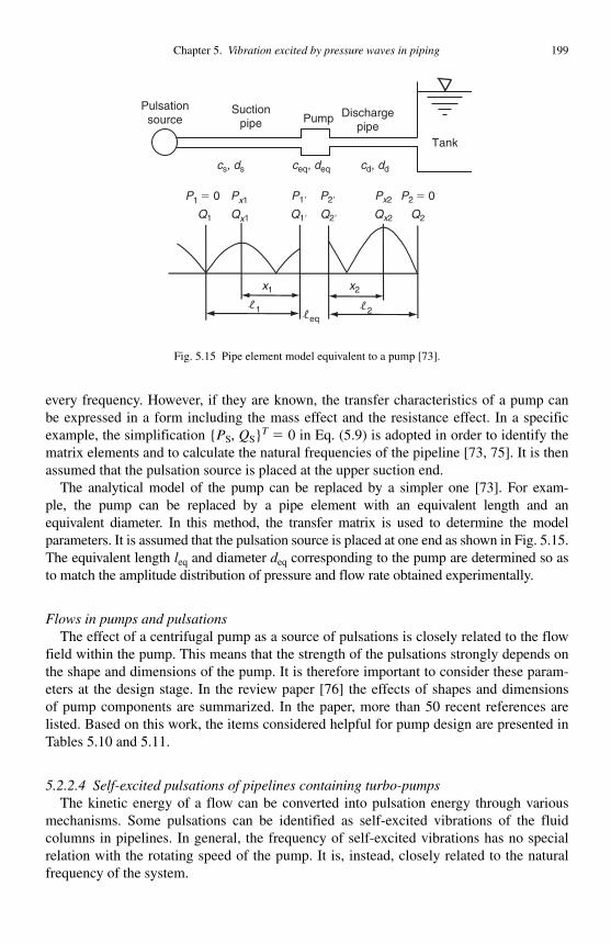
Chapter 5. Vibration excited by pressure waves in piping 199
every frequency. However, if they are known, the transfer characteristics of a pump can be expressed in a form including the mass effect and the resistance effect. In a specific example, the simplification { PS , QS } T � 0 in Eq. (5.9) is adopted in order to identify the matrix elements and to calculate the natural frequencies of the pipeline [73, 75]. It is then assumed that the pulsation source is placed at the upper suction end.
The analytical model of the pump can be replaced by a simpler one [73]. For exam-ple, the pump can be replaced by a pipe element with an equivalent length and an equivalent diameter. In this method, the transfer matrix is used to determine the model parameters. It is assumed that the pulsation source is placed at one end as shown in Fig. 5.15 .The equivalent length leq and diameter deq corresponding to the pump are determined so as to match the amplitude distribution of pressure and flow rate obtained experimentally.
Flows in pumps and pulsations The effect of a centrifugal pump as a source of pulsations is closely related to the flow
field within the pump. This means that the strength of the pulsations strongly depends on the shape and dimensions of the pump. It is therefore important to consider these param-eters at the design stage. In the review paper [76] the effects of shapes and dimensions of pump components are summarized. In the paper, more than 50 recent references are listed. Based on this work, the items considered helpful for pump design are presented in Tables 5.10 and 5.11 .
5.2.2.4 Self-excited pulsations of pipelines containing turbo-pumps The kinetic energy of a flow can be converted into pulsation energy through various
mechanisms. Some pulsations can be identified as self-excited vibrations of the fluid columns in pipelines. In general, the frequency of self-excited vibrations has no special relation with the rotating speed of the pump. It is, instead, closely related to the natural frequency of the system.
Qx1 Qx2
x1 x2
Pulsationsource Pump
Suctionpipe
Dischargepipe
Q1�Q1 Q2� Q2
Px2P1 � 0 P1�
eq
cs, ds cd, ddceq, deq
Tank
P2 � 0P2�Px1
21
Fig. 5.15 Pipe element model equivalent to a pump [73].
200 Flow induced vibrations: classifications and lessons from practical experiences
Table 5.10 Characteristics of noise generation mechanisms in centrifugal pumps [76]
Mechanism of noise generation Flow/pressure field characteristics Parameters controlling design
Impeller blade and volute tongueinteraction
Impingement of wake flow on volute tongue
Lip clearance, impeller blade trailing edge, and volute tongue geometry
Oscillation in stagnation pressure near volute tongue
Lip clearance, blade and volute tongue geometry
Unsteady flow recirculation and separation at tongue surface
Lip clearance, volute tongue geometry (tip radius)
Impeller blade and flow interaction
Discontinuity in pressure field between discharge and suction sides of impeller blade
Impeller blade trailing edge geometry
Local flow separation on impeller blade surface
Smooth surface finish
Non-uniform outflow from impeller
Flow and stagnation pressure oscillation at pump discharge
Impeller blade geometry
Jet flow impingement on volute tongue
Lip clearance, impeller blade, and volute tongue geometry
Vortex interaction with flow Extended trains of vortex structures near volute tongue and blade (may coincide)
Impeller blade trailing edge, impeller blade, and volute tongue geometry
Table 5.11 Effect of pump design on pressure pulsation [76]
Recommendations
Design parameter Hydraulic design Pulsation control Comments
Lip clearance (in percent of impeller radius)
5–10% ~ 10% Large clearance may lead to excessive flow circulation and strong pulsation
May have significant impact on pump performance
Volute tongue geometry Tip radius 6.3–25 mm Large tip radius Inclined cutwater
edge (3D design)
Elimination of the effect of flow separation
Prolong the time of blade/cutwater passage
Number of impeller blades
High number of impeller blade
Select number of blades to avoid system acoustic resonance
Twisting and staggeringof impeller blades
Twist angle 15–22º Prolong the time of blade/cutwater passage
Impeller blade trailing edge
Thickness must be sufficient to sustain
Profile to reduce wake width
Marginal effect on pump performance
hydraulic load
Pump volute geometry Uniform and smooth flow passage
Increase internal impedance
High impedance pump must be placed near pressure node
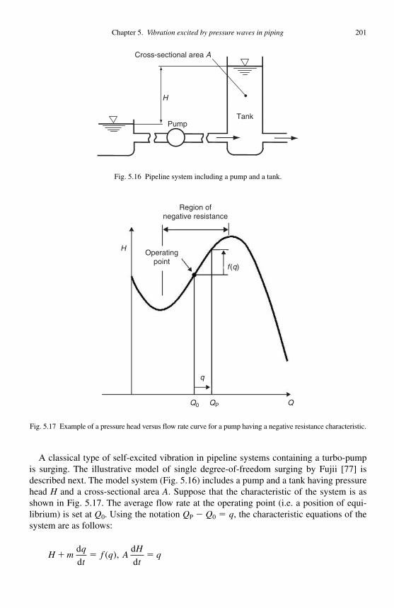
Chapter 5. Vibration excited by pressure waves in piping 201
A classical type of self-excited vibration in pipeline systems containing a turbo-pump is surging. The illustrative model of single degree-of-freedom surging by Fujii [77] is described next. The model system ( Fig. 5.16 ) includes a pump and a tank having pressure head H and a cross-sectional area A . Suppose that the characteristic of the system is as shown in Fig. 5.17 . The average flow rate at the operating point (i.e. a position of equi-librium) is set at Q0 . Using the notation QP � Q0 � q , the characteristic equations of the system are as follows:
H mq
tf q A
H
tq� � �
d
d
d
d( ),
PumpTank
H
Cross-sectional area A
Fig. 5.16 Pipeline system including a pump and a tank.
Region ofnegative resistance
Operatingpoint
H
f (q)
q
Q0 QP Q
Fig. 5.17 Example of a pressure head versus flow rate curve for a pump having a negative resistance characteristic.
202 Flow induced vibrations: classifications and lessons from practical experiences
where the coefficient m is related to the inertia of the system, and f ( q ) is the characteristic of the pump near the operating point. Eliminating H from these two equations, the fol-lowing equation is obtained:
mq
ta q
q
t Aq
d
d
d
d
2
2
10� � �( ) (5.10)
where a ( q ) � d f ( q )/d q . Small oscillations expressed by the solution of the differential equation (5.10) around the point of q � 0 grow if a ( q ) � 0 and decay if a ( q ) � 0. In other words, if the operating point of the system is located in a positive slope region to the right of the Q–H curve, the operating point is unstable. In such a case, large self-excited oscillations can occur. If pulsation occurs, L , the energy per cycle, will be accu-mulated in the system. L can be estimated by the following equation:
L a qq
tq� ( )
d
dd�∫
Depending on whether L is positive or negative, pulsations grow or are attenuated. IfL � 0, the pulsation reaches a stationary state and a limit cycle is traced on the Q – H plane.
Whether pulsations are due to surging is judged by whether the operating point of the system is in the positive slope region of the Q–H curve. However, even if the operating point is within this region, surging may not necessarily occur. Surging may occur easily in a pipeline in which a tank or an accumulator is located downstream of the pump and a resistive component, such as a flow-regulating valve, is located further on downstream. This means that surging requires a potential energy accumulating element corresponding to the term q/A in Eq. (5.10). When the fluid contains many air bubbles, the bubbles can play the same role as installed accumulators. More detailed research has been done on surging [78] .
Self-excited vibrations other than surging can also occur. For example, it has been reported that self-excited pulsations occurred in the low flow rate region of a high-pressuremulti-stage pump [79, 80]. Since the operating point of the system was located in the portion of the Q – H curve having a negative slope, it was determined to be a type of self-excited vibration different from surging. This case may be analyzed as follows. A pipe-line is divided into several pipe elements. A model for analysis is developed using the transfer matrix. Laplace transformation of the transfer matrix is carried out next. Thus, the elements of the matrix contain the operator s . A frequency equation is obtained from the boundary conditions at both ends of the pipeline. Values of s which satisfy the fre-quency equation are obtained by a numerical calculation. s represents a complex natural frequency and has the form s � � j� . The system is unstable when � 0. The imagi-nary part of s , that is � , is the angular natural frequency.
In the low-frequency region in which the wavelength of the pressure wave is much longer than the pump size, Eq. (5.9), which expresses the transfer characteristics of the pump portion, can be simplified as follows:
P
Q
Z P
Q
⎧⎨⎪⎪⎩⎪⎪
⎫⎬⎪⎪⎭⎪⎪
⎡
⎣⎢⎢
⎤
⎦⎥⎥⎧⎨⎪⎪⎩⎪⎪
⎫⎬⎪⎪⎭⎪⎪out
p
in
�1
0 1 (5.11)
Chapter 5. Vibration excited by pressure waves in piping 203
In this equation, it is assumed that { PS , QS } T � 0. ZP is called the pump impedance. It is identified by vibration tests and the transfer matrix of the line system. The real and imag-inary parts of ZP , Re( ZP ) and Im( ZP ) are the pump resistance and the pump inertance, respectively. It has become clear through numerical experiments that the stability of the system is governed mainly by the pump resistance Re( ZP ). The system is usually stable since the pipeline has positive resistance. However, if Re( ZP ) surpasses the pipeline resist-ance and if the value of becomes positive, pulsations will arise. Figure 5.18 shows an example of the measured relationship between the pump resistance and the rotating speed [79] . Detailed information on measurement methods for pump characteristics, including Z P , can be found in the Refs. [75, 80, 81] .
5.2.2.5 Vibrations and pulsations caused by suction of vortices into turbo-pumps When the suction pipe entrance of a centrifugal pump is placed in a tank with a free
surface, a whirlpool or vortex in the tank may be sucked into the pipe [82, 83]. A whirl-pool is accompanied by a core of air extending from the free surface; air is inhaled by the pump when the core is deep. Even in the case where only an underwater vortex arises, low pressure in the vortex core causes a kind of cavitation by dissociating dissolved air from water. Dissociated air may be inhaled into the pipe. The vibration or pulsation prob-lems below are caused by this phenomenon (refer to Fig. 5.19 ):
1. Swirling flow which arises in a suction pipe and contains many air bubbles causes an unbalanced torque to the pipe. This can be a cause of structural vibrations and noise.
Rotational speed of pump
Uns
tabl
eS
tabl
e
1500 rpm
2000 rpm2500 rpm3000 rpm
Q/QN � 0.1
500
�500
0
0 2 4 6f (Hz)
Re(
ZP)
(s/m
2 )
Fig. 5.18 Relation between pump resistance and rotational speed [79].

204 Flow induced vibrations: classifications and lessons from practical experiences
2. An air column is interrupted by the turbo-pump impeller. This causes a change of the fluid force acting on the impeller. Resulting vibrations and pressure pulsations may damage the impeller and piping [84, 85].
3. In some cases flow may vary significantly and seem almost intermittent [83, 84, 86].
The countermeasure to the foregoing problems is to prevent whirlpools and air inhalation. To achieve this, the following proposals have been put forward:
1. The clearances surrounding the suction pipe should be small. 2. Installation of a cross-shaped guide vane at the front or the inside of the suction pipe
is recommended. 3. A free surface near the suction port in a tank should be avoided. For this purpose, a
roof inclined on the water surface is effective. 4. A raft-like floating structure installed around the pipe is effective to prevent the for-
mation of a whirlpool.
5.2.2.6 Other types of pump vibrations When a loss of coolant accident occurs in the pump and pipeline system for heat trans-
port in a nuclear reactor, the void fraction will rise because of reduction of suction pres-sure. This introduces two-phase flow instability. It is believed that the observed pump instabil ity, intermittence of the flow due to separation of air bubbles, density wave, and acoustic sound resonance are factors related to this phenomenon. There is continuing research on the interactions of these factors [87]. A method of analyzing a primary cooling
Vortex formed behindsuction pipe
Suppression of intake vortex byinclined roof and cross vanes
Intake of a deep air core
Damping vortex formationby means of a raft
Pump
Cross vanes
Raft
Fig. 5.19 Suppression of intake vortex.
Chapter 5. Vibration excited by pressure waves in piping 205
water loop system that contains a pressurized water reactor, a steam generator, and a pri-mary cooling water pump by the transfer matrices has also been reported [88]. It is sup-posed in the analysis that the flow in the cooling water loop system is almost single-phase flow but partially two-phase. The transfer matrices used in the analysis are different from those described thus far .
If cavitation occurs in the flow through a pump, strong vibrations will occur in the pump and, in the worst case, may result in breakage. Cavitation is strongly dependent on the properties of the fluid conveyed through the pump. It may be mentioned that the cause of the Japanese H-II rocket launch failure in November, 1999 was cavitation-induced fail-ure of a fuel system pump.
5.2.2.7 Hydraulic turbines In Francis and Kaplan turbines, strong vibrations can occur in the main parts of the
turbine and the draft tube.
The blade passing frequency The wakes behind the guide vanes produce a non-steady flow in Francis turbine run-
ners [89] . This unsteady flow causes pressure pulsations and stress fluctuations in the runner blades of all Francis type turbines. Stress concentration may result depending on the shape of each part of the turbine rotor; the result may be fatigue failure and cracking. The dominant frequency is the rotational frequency multiplied by the number of guide vanes. Higher frequencies caused by shedding of Karman vortices are also observed. The latter depends strongly on the cross-sectional shape of the trailing edge of the guide vane. The results of examination show that the trailing edge must not be cut off at right angles to the flow direction; ideally the angle should be about 45 degrees. It should also be noted that a semicircle shape is perhaps the worst geometry of the trailing edge from the view-point of prevention of vibrations (see Fig. 5.20 ).
Vibrations and pulsations in hydraulic turbine draft tubes Vibrations and pressure pulsations in hydraulic turbine draft tubes may arise under
partial load operation [90] . In general, the central and circumferential parts of the flow that enters a draft tube from a runner are swirling as a forced vortex and a free vortex, respectively. The vortex core has very low pressure; thus, air cavities appear. On the other hand, the draft tube acts as a diffuser by causing downstream pressure recovery. Since the pressure rise is large in the core when a swirling flow enters the draft tube, a dead water core appears. As a result, cavities coil around the perimeter of the dead water core. Thus a spiral-formed cavitation appears. When the swirling flow accompanied by cavitation rotates, associated pressure fluctuations may also cause structural vibration. This is the so-called draft tube surging.
The cavity cores may grow along the axis of the draft tube downstream, and they may disappear rapidly near the elbow portion of the draft tube because of increasing pres-sure. This causes intense pressure fluctuations. As a cure, the taper angle of the draft tube entrance portion is enlarged so that the static pressure in the vortex core may rise quickly downstream. This is effective in eliminating cavitation and suppressing pressure pulsations.
206 Flow induced vibrations: classifications and lessons from practical experiences
Self-excited pulsations There are cases where pressure pulsations in pipelines containing a hydraulic turbine
may be regarded as a self-excited vibration. An example is given in [91] where fluc-tuations of pressure and electric power output were observed in low output states of a hydraulic turbine–electric generator system. When the guide vane opening is small, the circumferential component of the flow into the runner becomes large in comparison with the radial component. The flow alternately separates and re-attaches to the runner blades. As a cure, the guide vanes were opened and closed asynchronously. In the low output state, only a certain guide vane was opened and all the others closed. The direction of the flow into the runner can then be stabilized (see Fig. 5.21 ).
It has also been reported that another kind of self-excited pulsation based on the char-acteristic of the check valve with a flexible diaphragm occurred in a hydraulic turbine – pump – pipeline system for irrigation [92] ( Fig. 5.22 ).
5.2.3 Vibration problems and suggested solutions
If pulsations are due to forced vibrations, the first option is to avoid resonance. If possible, the operation condition such as the rotation speed of the pump should be
Trailing edge Trailing edge
The frequency may be calculated by the following approximate formula:
υ � water velocity (m/s), t � plate thickness in mm
B � constant depending on geometry (see table).
90°
60°
90°
60°
45°
30°
2t
1.2t
t
60°
45°
45°
45°
30°
R � 2t
R � 3t
R � 4t
A B A B
100 (100)
(48)
38 (20)
3 (0)
0
0
(260)
100
131
149
112
181
(0)
(0)
190 (230)
380 (360)
43
0 159
117
83
96
f � 0.19B
100y
(t � 0.56)(Hz)
Fig. 5.20 Influence of trailing edge on vibrations (case of plane blade in parallel flow) [90].
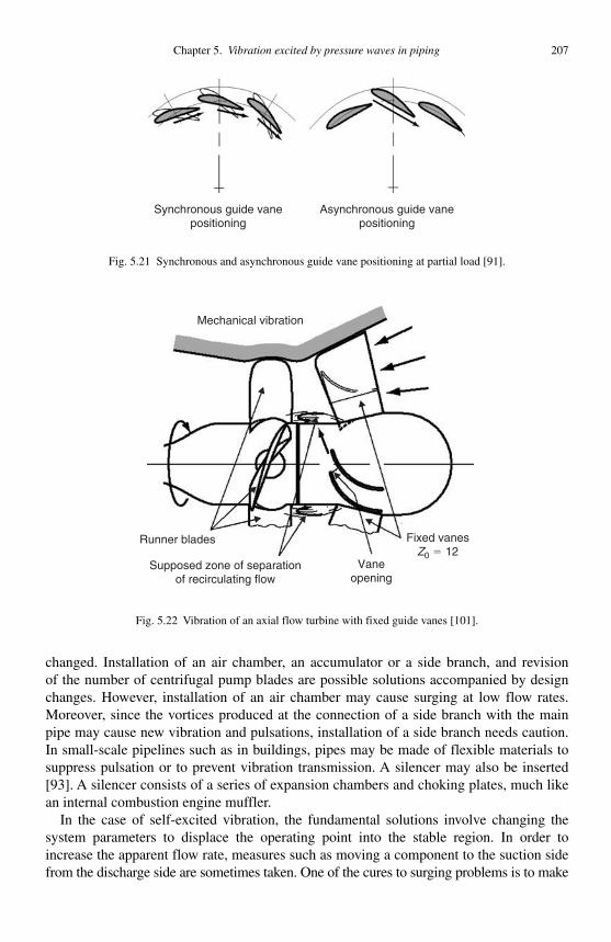
Chapter 5. Vibration excited by pressure waves in piping 207
changed. Installation of an air chamber, an accumulator or a side branch, and revision of the number of centrifugal pump blades are possible solutions accompanied by design changes. However, installation of an air chamber may cause surging at low flow rates. Moreover, since the vortices produced at the connection of a side branch with the main pipe may cause new vibration and pulsations, installation of a side branch needs caution. In small-scale pipelines such as in buildings, pipes may be made of flexible materials to suppress pulsation or to prevent vibration transmission. A silencer may also be inserted [93]. A silencer consists of a series of expansion chambers and choking plates, much like an internal combustion engine muffler.
In the case of self-excited vibration, the fundamental solutions involve changing the system parameters to displace the operating point into the stable region. In order to increase the apparent flow rate, measures such as moving a component to the suction side from the discharge side are sometimes taken. One of the cures to surging problems is to make
Supposed zone of separationof recirculating flow
Vaneopening
Runner blades
Mechanical vibration
Fixed vanesZ0 � 12
Fig. 5.22 Vibration of an axial flow turbine with fixed guide vanes [101].
Synchronous guide vanepositioning
Asynchronous guide vanepositioning
Fig. 5.21 Synchronous and asynchronous guide vane positioning at partial load [91].

208 Flow induced vibrations: classifications and lessons from practical experiences
the Q–H curve slant downward to the right. Another solution is to install resistance com-ponents such as valves downstream of the pump. The latter cure prevents the occurrence of a negative resistance domain in the system.
Other examples of problems and solutions, in addition to the cases illustrated so far, are summarized in Table 5.12 .
Table 5.12Examples of problem cases for pumps and hydraulic turbines
Machine Phenomenon Causes Cure
1. Three reciprocating pumps in parallel operation [94]
When the temperature in the suction pipe reached 200°C or more, unusual vibrations occurred
Pressure fluctuation by rapid collapse of steam bubbles and of gas bubbles which are separated from water and resonance
Accumulator was formed by enclosing nitrogen gas in upper part of the volume bottle
2. Swash plate axial piston pump for hydraulic excavator [95]
Rapid increase of pressure pulsations near 2000 rpm
Simulations indicated resonance
Installation of a side branch
3. Vertical mixed flow sewer pump [96]
Large pulsations accompanied by a water column separation in piping
Resonance of the pulsations with torsional vibrations of the shaft connecting motor and pump
In some cases piping length was changed, in others the radius of the shaft was increased
4. Centrifugal pump for waste treatment facility [97]
Vibration accompanied by unusual noise occurred in the tank installed on suction-side
Resonance of liquid column in the tank with pulsations
The number of impeller blades was changed
5. Multi-stage centrifugal pump feeding water to boiler [98]
Vibration in which the ZN component is dominant
Forced vibration by the fluid force generated in interference of the impeller blade and the guide vanes
The angle of the fourth stage guide vanes was changed by 20 degrees in the anti-rotation direction from the third stage guide vanes
6. Multi-stage centrifugal pump [99]
Vibration at 80% of shaft speed
Force on an impeller caused by swirling flow
Reduction of the eccentricity between diffuser/blower and impeller.Installation of a swirl breaker
7. Vertical mixed flow pump [100]
Vibration with a broad-band spectrum
Cavitation at the valve placed downstream of the pump
A perforated-plate orifice was installed downstream of the valve so that the pressure at the valve increased
8. Axial-flow hydraulic turbine [101].(see Fig. 5.12)
Vibration of housing and noise with irregular frequency of 140–176 Hz
It was presumed that flow separates in downstream portion of the guide vanes
The guide vanes were shortened
9. Francis turbine [102] Large pressure fluctuations
A cavitation core grows towards the elbow where it disappears
The taper suction pipe entrance was increased
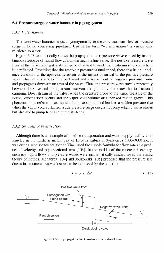
Chapter 5. Vibration excited by pressure waves in piping 209
5.3 Pressure surge or water hammer in piping system
5.3.1 Water hammer
The term water hammer is used synonymously to describe transient flow or pressure surge in liquid conveying pipelines. Use of the term “ water hammer ” is customarily restricted to water.
Figure 5.23 schematically shows the propagation of a pressure wave caused by instan-taneous stoppage of liquid flow at a downstream inline valve. The positive pressure wave front at the valve propagates at the speed of sound towards the upstream reservoir where it is reflected. Providing that the reservoir pressure is unchanged, there results an unbal-ance condition at the upstream reservoir at the instant of arrival of the positive pressure wave. The liquid starts to flow backward and a wave front of negative pressure forms and propagates downstream toward the valve. Thus, the pressure wave travels repeatedly between the valve and the upstream reservoir and gradually attenuates due to frictional damping. Downstream of the valve, when the pressure drops to the vapor pressure of the liquid, vaporization occurs and the vapor void volume or vaporized region grows. This phenomenon is referred to as liquid column separation and leads to a sudden pressure rise when the vapor void collapses. Such pressure surge occurs not only when a valve closes but also due to pump trips and pump start-ups.
5.3.2 Synopsis of investigation
Although there is an example of pipeline transportation and water supply facility con-structed in the northern ancient city of Habuba Kabira in Syria circa 3500–3000 B.C , it was during renaissance era that da Vinci used the simple formula for flow rate as a prod-uct of velocity and pipe sectional area [103] . In the middle of the nineteenth century, unsteady liquid flows and pressure waves were mathematically studied using the elastic theory of liquids. Menabrea [104] and Joukowski [105] proposed that the pressure rise due to instanta neous valve closure can be expressed by the equation:
J c V� � �� � (5.12)
Flow direction
Quick closing valve
Positive wave front
Propagation withsound speed
Negative wave front
Fig. 5.23 Wave propagation due to instantaneous valve closure.

210 Flow induced vibrations: classifications and lessons from practical experiences
where J is the pressure rise due to the change of fluid velocity �V ; � is the fluid density, and c the wave speed. Until the early 1930s, the mathematical model derived by integra-tion of Joukowsky’s equation neglecting pipe friction was used. Allievi [106] applied the method for the problem of slow valve closure to render the assumption of linear change of flow at the valve. From the early 1930s to the early 1960s a graphical method taking account of pipe friction iteratively with the model above was utilized by plotting on the head-velocity diagram [106, 107] . With the development of high-performance computers, these methods are no longer used but they are useful for understanding the mechanism of water hammer.
There are several numerical computation methods, including the method of characteristics (MOC), the semi-implicit two-step Lax–Wendroff method (2-LW) [108] , the fully implicit method [109] , and the finite element method [110, 111] . MOC is the most commonly used method for fluid transient analysis, especially for liquid or water hammer analysis. The advantage of MOC is the ease of handling complex boundary conditions such as pumps and compressors. Also, MOC guarantees a numerically stable solution providing that the Courant condition is satisfied [108]. Depending on the nature of the problem, other methods may be used. For example, 2-LW can be applied to solve impulsive shock wave problems and column separation problems [112] . A fully implicit method is advantageous when solv-ing slow transient problems that may occur in a gas pipeline [113] .
5.3.3 Solution methods
5.3.3.1 Method of characteristics (MOC) This paragraph describes MOC [114, 115, 116] as a calculation method for transient
flow in liquid pipelines, its application to column separation problems, and practical aspects of frequency-dependent friction.
The equations governing unsteady fluid flow in pipelines consist of two partial differ-ential equations of momentum and continuity. A general solution to the partial differential equations is not available. However, these hyperbolic type partial differential equations can be mathematically transformed by MOC into two ordinary differential equations that are valid along particular characteristic lines C� and C� in time and space [117] . These two ordinary differential equations can be recast into the following finite differ-ence equations:
C c u u g h h g u tf u u
Dc t� � � � � � � � � � �
� �
�� � �: ( ) ( ) sinP R P R R
P R� �2
0 (5.13)
C c u u g h h g u tf u u
Dc t� � � � � � � � � � �
� �
�� � �: ( ) ( ) sinP S P S S
P S� �2
0 (5.14)
where f is the Darcy–Weisbach friction factor, g the gravitational acceleration, c thewave speed, the pipe slope and u the fluid velocity. The piezometric head h is defined by h � p / � � z , where � is the unit weight of the fluid, z the elevation of the pipe above a reference datum, D the pipe diameter, and �t time step.
Figure 5.24 shows a schematic visualization of the characteristic lines C� and C � along which the corresponding finite difference equations are valid. Each characteristic line
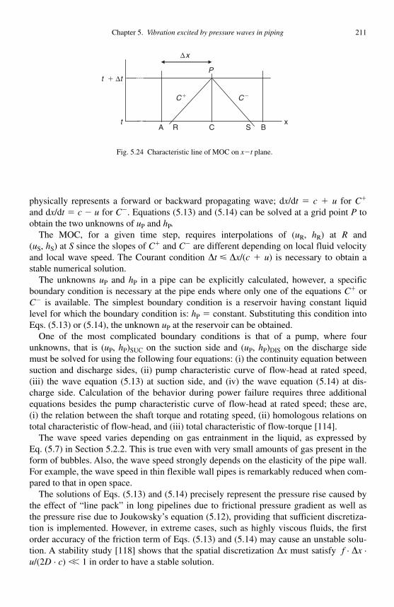
Chapter 5. Vibration excited by pressure waves in piping 211
physically represents a forward or backward propagating wave; d x /d t � c � u for C�
and d x /d t � c � u for C� . Equations (5.13) and (5.14) can be solved at a grid point P to obtain the two unknowns of uP and hP .
The MOC, for a given time step, requires interpolations of ( uR , hR ) at R and(uS , hS ) at S since the slopes of C� and C� are different depending on local fluid velocity and local wave speed. The Courant condition �t $ �x /( c � u ) is necessary to obtain a stable numerical solution.
The unknowns uP and hP in a pipe can be explicitly calculated, however, a specific boundary condition is necessary at the pipe ends where only one of the equations C� or C� is available. The simplest boundary condition is a reservoir having constant liquid level for which the boundary condition is: hP � constant. Substituting this condition into Eqs. (5.13) or (5.14), the unknown uP at the reservoir can be obtained.
One of the most complicated boundary conditions is that of a pump, where four unknowns, that is ( uP , hP ) SUC on the suction side and ( uP , hP ) DIS on the discharge side must be solved for using the following four equations: (i) the continuity equation between suction and discharge sides, (ii) pump characteristic curve of flow-head at rated speed, (iii) the wave equation (5.13) at suction side, and (iv) the wave equation (5.14) at dis-charge side. Calculation of the behavior during power failure requires three additional equations besides the pump characteristic curve of flow-head at rated speed; these are, (i) the relation between the shaft torque and rotating speed, (ii) homologous relations on total characteristic of flow-head, and (iii) total characteristic of flow-torque [114] .
The wave speed varies depending on gas entrainment in the liquid, as expressed by Eq. (5.7) in Section 5.2.2. This is true even with very small amounts of gas present in the form of bubbles. Also, the wave speed strongly depends on the elasticity of the pipe wall. For example, the wave speed in thin flexible wall pipes is remarkably reduced when com-pared to that in open space.
The solutions of Eqs. (5.13) and (5.14) precisely represent the pressure rise caused by the effect of “ line pack ” in long pipelines due to frictional pressure gradient as well as the pressure rise due to Joukowsky’s equation (5.12), providing that sufficient discretiza-tion is implemented. However, in extreme cases, such as highly viscous fluids, the first order accuracy of the friction term of Eqs. (5.13) and (5.14) may cause an unstable solu-tion. A stability study [118] shows that the spatial discretization �x must satisfy f · �x · u /(2 D · c ) �� 1 in order to have a stable solution.
SC Bx
C� C�
P
Δx
A R
t � Δt
t
Fig. 5.24 Characteristic line of MOC on x�t plane.
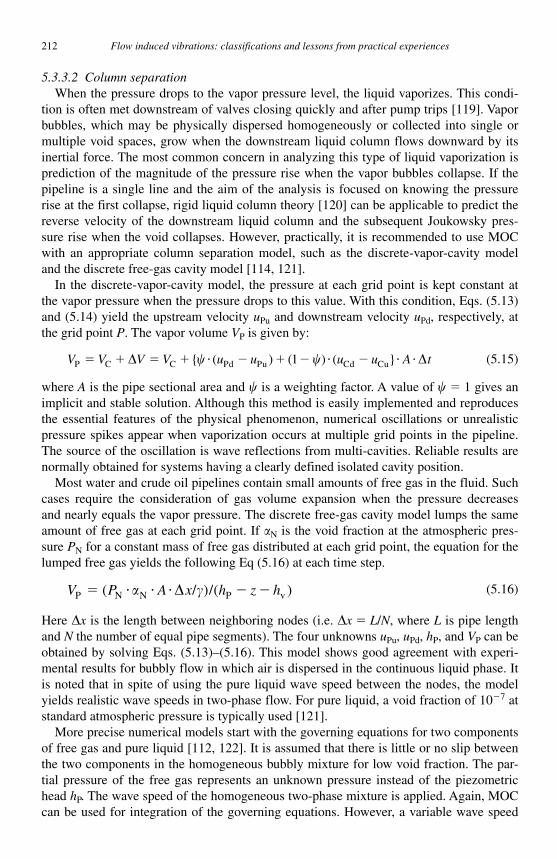
212 Flow induced vibrations: classifications and lessons from practical experiences
5.3.3.2 Column separation When the pressure drops to the vapor pressure level, the liquid vaporizes. This condi-
tion is often met downstream of valves closing quickly and after pump trips [119] . Vapor bubbles, which may be physically dispersed homogeneously or collected into single or multiple void spaces, grow when the downstream liquid column flows downward by its inertial force. The most common concern in analyzing this type of liquid vaporization is prediction of the magnitude of the pressure rise when the vapor bubbles collapse. If the pipeline is a single line and the aim of the analysis is focused on knowing the pressure rise at the first collapse, rigid liquid column theory [120] can be applicable to predict the reverse velocity of the downstream liquid column and the subsequent Joukowsky pres-sure rise when the void collapses. However, practically, it is recommended to use MOC with an appropriate column separation model, such as the discrete-vapor-cavity model and the discrete free-gas cavity model [114, 121] .
In the discrete-vapor-cavity model, the pressure at each grid point is kept constant at the vapor pressure when the pressure drops to this value. With this condition, Eqs. (5.13) and (5.14) yield the upstream velocity uPu and downstream velocity uPd , respectively, at the grid point P . The vapor volume VP is given by:
V V V V u u u u A tP C C Pd Pu Cd Cu� � � � � � � � � � � �� � � �{ ( ) ( ) ( }1 (5.15)
where A is the pipe sectional area and � is a weighting factor. A value of � � 1 gives an implicit and stable solution. Although this method is easily implemented and reproduces the essential features of the physical phenomenon, numerical oscillations or unrealistic pressure spikes appear when vaporization occurs at multiple grid points in the pipeline. The source of the oscillation is wave reflections from multi-cavities. Reliable results are normally obtained for systems having a clearly defined isolated cavity position.
Most water and crude oil pipelines contain small amounts of free gas in the fluid. Such cases require the consideration of gas volume expansion when the pressure decreases and nearly equals the vapor pressure. The discrete free-gas cavity model lumps the same amount of free gas at each grid point. If N is the void fraction at the atmospheric pres-sure PN for a constant mass of free gas distributed at each grid point, the equation for the lumped free gas yields the following Eq (5.16) at each time step.
V P A x h z hP N N P v/� � � � � �( )/( ) � � (5.16)
Here �x is the length between neighboring nodes (i.e. �x � L / N , where L is pipe length and N the number of equal pipe segments). The four unknowns uPu , uPd , hP , and VP can be obtained by solving Eqs. (5.13)–(5.16). This model shows good agreement with experi-mental results for bubbly flow in which air is dispersed in the continuous liquid phase. It is noted that in spite of using the pure liquid wave speed between the nodes, the model yields realistic wave speeds in two-phase flow. For pure liquid, a void fraction of 10 � 7 at standard atmospheric pressure is typically used [121] .
More precise numerical models start with the governing equations for two components of free gas and pure liquid [112, 122] . It is assumed that there is little or no slip between the two components in the homogeneous bubbly mixture for low void fraction. The par-tial pressure of the free gas represents an unknown pressure instead of the piezometric head hP . The wave speed of the homogeneous two-phase mixture is applied. Again, MOC can be used for integration of the governing equations. However, a variable wave speed

Chapter 5. Vibration excited by pressure waves in piping 213
depending on void fraction may affect the accuracy of interpolation. In this case, the two-step Lax–Wendroff method is recommended [112] .
5.3.3.3 Frequency-dependent friction The mechanism of shear stress generation in pipe walls in transient flow is quite differ-
ent from that in steady flow. The velocity near the wall responds in phase with the pres-sure gradient since the frictional force dominates relative to the inertia force, whereas the acceleration is in phase with the pressure gradient in the central portion of the pipe since the inertial force is dominant here. This means that the friction term of Eqs. (5.13) and (5.14) based on velocity squared will not accurately model transient losses [123–127] .
Uchida [128] derived a solution of the frequency-dependent friction factor for sine-wave pulsation in laminar flow, and Zielke [123] used a weighting function applied to the time history of unsteady laminar flow. Kagawa et al. [126] developed a fast computation method to calculate the weighting function. Extensive efforts have been made to develop sophisticated methods for turbulent flow [129, 130] . Fortunately, however, quasi-steady modeling is normally sufficiently accurate during the early phase of a transient. The fre-quency-dependent friction is important for high-frequency pulsative flows and laminar flows often observed in highly viscous fluids.
5.3.3.4 Design practice and criteria The basic design of a liquid piping system requires consideration and study of pressure
surge. Typical examples are summarized in Table 5.13 . Various design codes and standards specify the limitation on surge pressure in a piping
system. Since pressure surge is categorized as an occasional load, the allowable surge pressure is normally greater than the design pressure of the system. For example, ASME/ANSI B31.3 for the chemical and petrochemical plant piping systems specifies a maxi-mum allowable surge pressure of 1.33 times the design pressure of the system. For long distance pipelines, ASME/ANSI B31.4 specifies 1.1 times the design pressure. It should be noted that each code and standard has a unique definition of the allowable stress, which leads to different definitions of the allowable surge pressure.
Table 5.14 shows typical data necessary for surge analysis of a piping system. Initial pressure and flow balance are first determined based on the boundary conditions before transient analysis can be implemented.
5.3.4 Countermeasures
Table 5.15 summarizes typical countermeasures for water hammer or pressure surge. Numerical computations are necessary for the detailed design of the countermeasures.
Figure 5.25 shows a flow chart for valve stroking analysis most frequently encountered by engineers.
5.3.5 Examples of component failures
Numerous examples of surge-related problems including structural coupling problems [131, 132] have been reported in the literature. The following examples are typical cases.
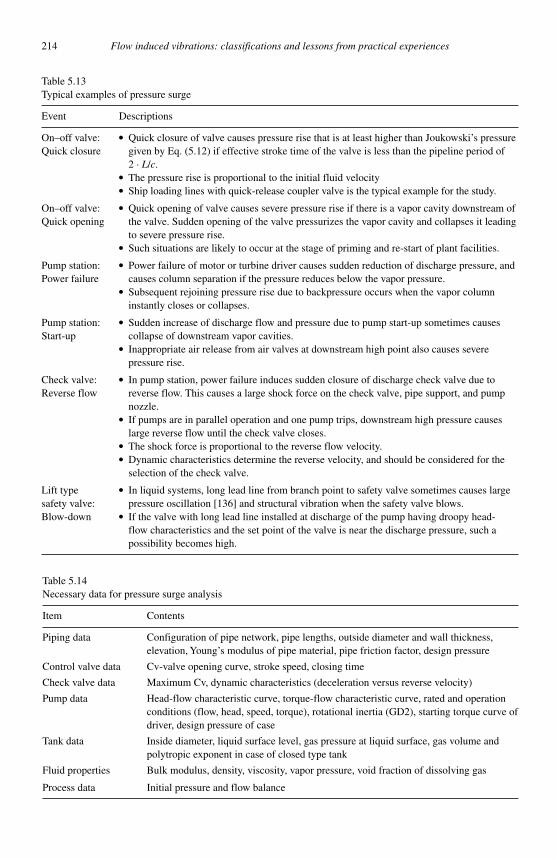
214 Flow induced vibrations: classifications and lessons from practical experiences
Table 5.13Typical examples of pressure surge
Event Descriptions
On–off valve: Quick closure
● Quick closure of valve causes pressure rise that is at least higher than Joukowski’s pressure given by Eq. (5.12) if effective stroke time of the valve is less than the pipeline period of 2 · L/c.
● The pressure rise is proportional to the initial fluid velocity● Ship loading lines with quick-release coupler valve is the typical example for the study.
On–off valve: Quick opening
● Quick opening of valve causes severe pressure rise if there is a vapor cavity downstream of the valve. Sudden opening of the valve pressurizes the vapor cavity and collapses it leading to severe pressure rise.
● Such situations are likely to occur at the stage of priming and re-start of plant facilities.
Pump station: Power failure
● Power failure of motor or turbine driver causes sudden reduction of discharge pressure, and causes column separation if the pressure reduces below the vapor pressure.
● Subsequent rejoining pressure rise due to backpressure occurs when the vapor column instantly closes or collapses.
Pump station: Start-up
● Sudden increase of discharge flow and pressure due to pump start-up sometimes causes collapse of downstream vapor cavities.
● Inappropriate air release from air valves at downstream high point also causes severe pressure rise.
Check valve: Reverse flow
● In pump station, power failure induces sudden closure of discharge check valve due to reverse flow. This causes a large shock force on the check valve, pipe support, and pump nozzle.
● If pumps are in parallel operation and one pump trips, downstream high pressure causes large reverse flow until the check valve closes.
● The shock force is proportional to the reverse flow velocity.● Dynamic characteristics determine the reverse velocity, and should be considered for the
selection of the check valve.
Lift type safety valve: Blow-down
● In liquid systems, long lead line from branch point to safety valve sometimes causes large pressure oscillation [136] and structural vibration when the safety valve blows.
● If the valve with long lead line installed at discharge of the pump having droopy head-flow characteristics and the set point of the valve is near the discharge pressure, such a possibility becomes high.
Table 5.14 Necessary data for pressure surge analysis
Item Contents
Piping data Configuration of pipe network, pipe lengths, outside diameter and wall thickness, elevation, Young’s modulus of pipe material, pipe friction factor, design pressure
Control valve data Cv-valve opening curve, stroke speed, closing time
Check valve data Maximum Cv, dynamic characteristics (deceleration versus reverse velocity)
Pump data Head-flow characteristic curve, torque-flow characteristic curve, rated and operation conditions (flow, head, speed, torque), rotational inertia (GD2), starting torque curve of driver, design pressure of case
Tank data Inside diameter, liquid surface level, gas pressure at liquid surface, gas volume and polytropic exponent in case of closed type tank
Fluid properties Bulk modulus, density, viscosity, vapor pressure, void fraction of dissolving gas
Process data Initial pressure and flow balance
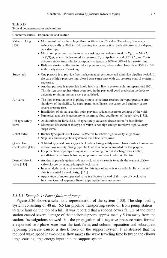
Chapter 5. Vibration excited by pressure waves in piping 215
Table 5.15Typical countermeasures and cautions
Countermeasures Explanation and caution
Valve stroking [137]
● Most on–off valves have large flow coefficient or Cv value. Therefore, flow starts to reduce typically at 30% to 10% opening in closure action. Such effective stroke depends on valve type.
● Maximum pressure rise due to valve stroking can be determined by PSurge � Min(J,J · Tp/Teff), where J is Joukowski’s pressure; Tp is pipeline period of 2 · L/c, and Teff is effective stroke time which corresponds to typically 10% to 30% of full stroke time.
● Bi-linear stroke is effective to reduce pressure rise, where valve closes from 30% to 10% in the early stages of stroking.
Surge tank ● One purpose is to provide free surface near surge source and minimize pipeline period. In the case of high-pressure line, closed type surge tank with gas pressure control system is necessary.
● Another purpose is to provide liquid into main line to prevent column separation [106]. This design concept has often been used in the past until good prediction methods to calculate rejoining pressure were established.
Air valve ● The high elevation point in piping system sometimes reaches the vapor pressure after shutdown of the facility. Re-start operation collapses the vapor void and may cause severe pressure rise.
● Installation of air valve at this point prevents sudden closure or collapse of the void.● Numerical analysis is necessary to determine flow coefficient of the air valve [138].
Lift type safety valve
● As described in Table 5.13, lift type safety valve requires caution for installation.● Moreover, lift speed of this type of valve is not high enough to relieve high-velocity
surge wave.
Relief valve ● Rubber type quick relief valve is effective to relieve high-velocity surge wave.● Slop tank and re-injection system to main line is required.
Quick close check valve [139]
● Split disk type and nozzle type check valves have good dynamic characteristics to minimize reverse flow velocity. Swing type check valve is not recommended for this purpose.
● For protection of pump casing against slamming force at discharge check valve, installation of bellows between pump nozzle and check valve is effective.
Damped check valve [115]
● Another approach against sudden check valve closure is to apply the concept of slow valve closure by using a damped check valve.
● In general, dynamic characteristic for this type of valve is not available. Experimental data is essential for real design [131].
● Application of motor operated valve is effective instead of this type of check valve function. Control sequence linked to pump failure is necessary.
5.3.5.1 Example-1: Power failure of pump Figure 5.26 shows a schematic representation of the system [133]. The ship loading
system consisting of 48 in. 6.5 km pipeline transporting crude oil from pump station to tank farm on the top of a hill. It was reported that a sudden power failure of the pump station caused severe damage of the anchor supports approximately 5 km away from the station. Investigations showed that the propagation of a negative pressure wave formed a vaporized two-phase zone near the tank farm, and column separation and subsequent rejoining pressure caused a shock force on the support system. It is stressed that the reduced wave speed in two-phase flow makes the wave traveling time between the elbows large, causing large energy input into the support system.
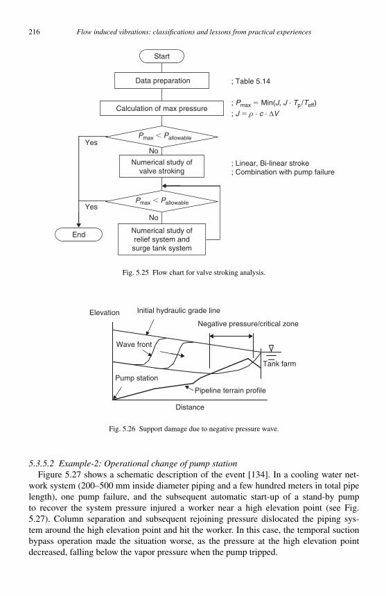
216 Flow induced vibrations: classifications and lessons from practical experiences
5.3.5.2 Example-2: Operational change of pump station Figure 5.27 shows a schematic description of the event [134]. In a cooling water net-
work system (200–500 mm inside diameter piping and a few hundred meters in total pipe length), one pump failure, and the subsequent automatic start-up of a stand-by pump to recover the system pressure injured a worker near a high elevation point (see Fig. 5.27). Column separation and subsequent rejoining pressure dislocated the piping sys-tem around the high elevation point and hit the worker. In this case, the temporal suction bypass operation made the situation worse, as the pressure at the high elevation point decreased, falling below the vapor pressure when the pump tripped.
; Pmax � Min(J, J · Tp /Teff)
; J � ρ · c · ΔV
Data preparation
Calculation of max pressure
Pmax � Pallowable
Numerical study ofvalve stroking
; Linear, Bi-linear stroke; Combination with pump failure
Numerical study ofrelief system andsurge tank system
End
; Table 5.14
No
No
Yes
Yes
Start
Pmax � Pallowable
Fig. 5.25 Flow chart for valve stroking analysis.
Elevation
Distance
Pump station
Tank farm
Initial hydraulic grade line
Negative pressure/critical zone
Wave front
Pipeline terrain profile
Fig. 5.26 Support damage due to negative pressure wave.
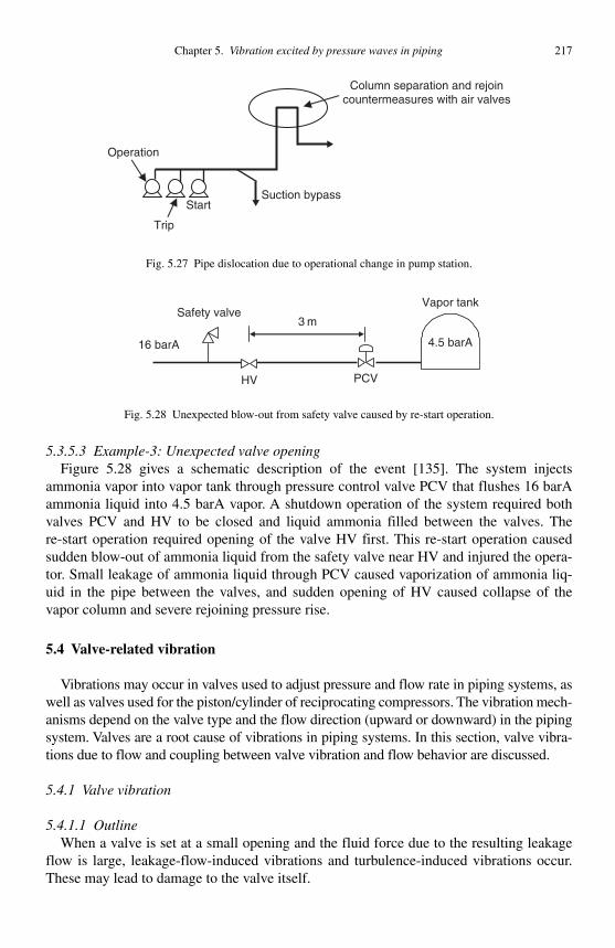
Chapter 5. Vibration excited by pressure waves in piping 217
5.3.5.3 Example-3: Unexpected valve opening Figure 5.28 gives a schematic description of the event [135]. The system injects
ammonia vapor into vapor tank through pressure control valve PCV that flushes 16 barA ammonia liquid into 4.5 barA vapor. A shutdown operation of the system required both valves PCV and HV to be closed and liquid ammonia filled between the valves. The re-start operation required opening of the valve HV first. This re-start operation caused sudden blow-out of ammonia liquid from the safety valve near HV and injured the opera-tor. Small leakage of ammonia liquid through PCV caused vaporization of ammonia liq-uid in the pipe between the valves, and sudden opening of HV caused collapse of the vapor column and severe rejoining pressure rise.
5.4 Valve-related vibration
Vibrations may occur in valves used to adjust pressure and flow rate in piping systems, as well as valves used for the piston/cylinder of reciprocating compressors. The vibration mech-anisms depend on the valve type and the flow direction (upward or downward) in the pipingsystem. Valves are a root cause of vibrations in piping systems. In this section, valve vibra-tions due to flow and coupling between valve vibration and flow behavior are discussed.
5.4.1 Valve vibration
5.4.1.1 Outline When a valve is set at a small opening and the fluid force due to the resulting leakage
flow is large, leakage-flow-induced vibrations and turbulence-induced vibrations occur. These may lead to damage to the valve itself.
HV PCV
3 m
16 barA
Safety valveVapor tank
4.5 barA
Fig. 5.28 Unexpected blow-out from safety valve caused by re-start operation.
Column separation and rejoincountermeasures with air valves
Trip
Operation
Suction bypassStart
Fig. 5.27 Pipe dislocation due to operational change in pump station.

218 Flow induced vibrations: classifications and lessons from practical experiences
5.4.1.2 Self-excited valve flutter Flutter, similar to that encountered for aircraft wings, can occur with butterfly valves
( Fig. 5.29 ) for some valve opening conditions (refer Section 3.2.2). Increasing the stiff-ness of the valve can generally raise the critical flow velocity. Flutter can also be avoided by operating with a large opening. An additional valve or introduction of an orifice can also suppress flutter.
5.4.1.3 Leakage-flow-induced vibration
Outline Consider the valve shown in Fig. 5.30 . Displacement of the gag bomb changes the
leakage-flow rate through the orifice. The change in flow rate in turn modifies the fluid force acting on the gag bomb at the orifice into a feedback loop, resulting in vibration. In the case of divergent channel geometries, or inlet local pressure loss geometries, the resultant negative fluid damping force can lead to the self-excited vibrations [140].
E valuation method Flutter type or divergence type instability can often be avoided by employing conver-
gent channel geometries. Divergent geometries, in addition to being destabilizing, have the added disadvantage of increased turbulence excitation forces. These geometries should therefore be avoided.
Piping
FlowButterfly valve
Fig. 5.29 Schematic view of butterfly valve.
OrificeFins
Bias ports
Gag bomb
Outlet ports
Drive shaft
Fig. 5.30 Self-excited vibration of a valve having an annular clearance [143].
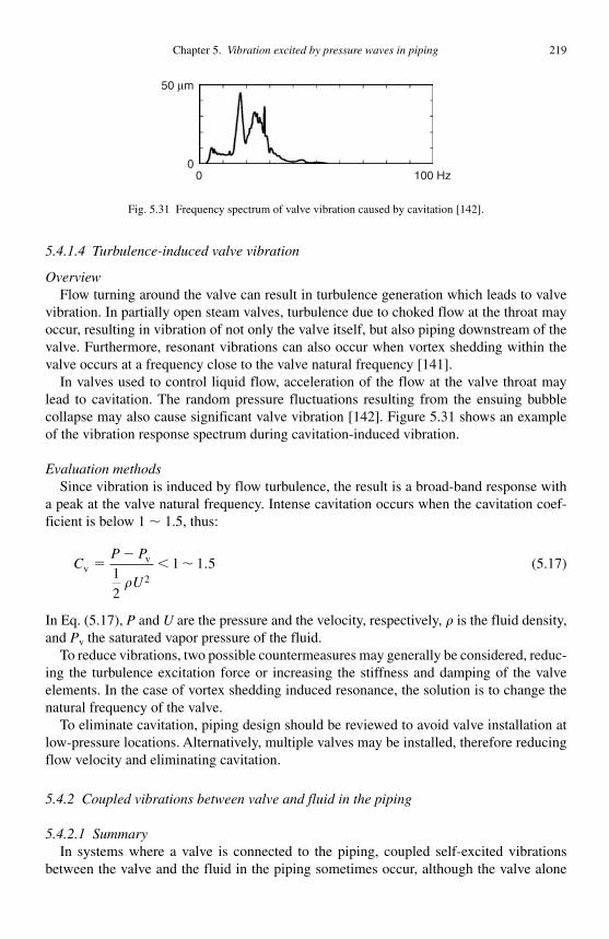
Chapter 5. Vibration excited by pressure waves in piping 219
5.4.1.4 Turbulence-induced valve vibration
Overview Flow turning around the valve can result in turbulence generation which leads to valve
vibration. In partially open steam valves, turbulence due to choked flow at the throat may occur, resulting in vibration of not only the valve itself, but also piping downstream of the valve. Furthermore, resonant vibrations can also occur when vortex shedding within the valve occurs at a frequency close to the valve natural frequency [141] .
In valves used to control liquid flow, acceleration of the flow at the valve throat may lead to cavitation. The random pressure fluctuations resulting from the ensuing bubble collapse may also cause significant valve vibration [142] . Figure 5.31 shows an example of the vibration response spectrum during cavitation-induced vibration.
Evaluation methods Since vibration is induced by flow turbulence, the result is a broad-band response with
a peak at the valve natural frequency. Intense cavitation occurs when the cavitation coef-ficient is below 1 � 1.5, thus:
CP P
Uv
v��
�12
1 1 52�
� . (5.17)
In Eq. (5.17), P and U are the pressure and the velocity, respectively, � is the fluid density, and Pv the saturated vapor pressure of the fluid.
To reduce vibrations, two possible countermeasures may generally be considered, reduc-ing the turbulence excitation force or increasing the stiffness and damping of the valve elements. In the case of vortex shedding induced resonance, the solution is to change the natural frequency of the valve.
To eliminate cavitation, piping design should be reviewed to avoid valve installation at low-pressure locations. Alternatively, multiple valves may be installed, therefore reducing flow velocity and eliminating cavitation.
5.4.2 Coupled vibrations between valve and fluid in the piping
5.4.2.1 Summary In systems where a valve is connected to the piping, coupled self-excited vibrations
between the valve and the fluid in the piping sometimes occur, although the valve alone
50 μm
00 100 Hz
Fig. 5.31 Frequency spectrum of valve vibration caused by cavitation [142].

220 Flow induced vibrations: classifications and lessons from practical experiences
is stable against self-excited vibrations. These types of coupled vibrations often occur in plants, hydraulic structures, and high-pressure oil hydraulic piping systems. Many kinds ofvalve-piping coupled systems with spool valves and poppet valves have been studied as shown in Figs. 5.32 and 5.33 .
5.4.2.2 Vibration phenomena and history of research and evaluation Weaver [143] showed that self-excited vibration occurs due to the delay of pressure
pulsations in the piping relative to the valve vibration when the valve, which closes as the fluid starts to flow, is connected to the piping systems. Fujii et al. [144] showed that coupled valve-piping self-excited vibration occurs if the natural frequency of the piping
Oiling Return
Load
L1L � L1 � L2L2
Damping length
Fig. 5.32 Examples of valves to be discussed.
(a) (b)
(c) (d)
Tank
TankTank
Tank
Piping
Piping
Piping
Piping
Volume
Valve
Valve
Valve
Valve
Fig. 5.33 Examples of valve position relative to piping: (a) valve located at exit of piping, (b) valve located at middle of piping, (c) valve located at inlet of piping, and (d) valve and adjacent volume.
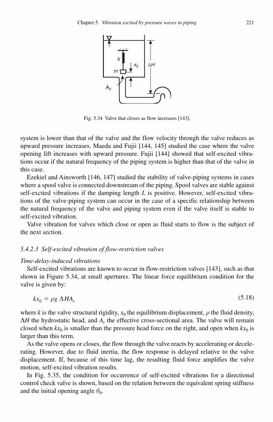
Chapter 5. Vibration excited by pressure waves in piping 221
system is lower than that of the valve and the flow velocity through the valve reduces as upward pressure increases. Maeda and Fujii [144, 145] studied the case where the valve opening lift increases with upward pressure . Fujii [144] showed that self-excited vibra-tions occur if the natural frequency of the piping system is higher than that of the valve in this case.
Ezekiel and Ainsworth [146, 147] studied the stability of valve-piping systems in cases where a spool valve is connected downstream of the piping. Spool valves are stable against self-excited vibrations if the damping length L is positive. However, self-excited vibra-tions of the valve-piping system can occur in the case of a specific relationship between the natural frequency of the valve and piping system even if the valve itself is stable to self-excited vibration.
Valve vibration for valves which close or open as fluid starts to flow is the subject of the next section.
5.4.2.3 Self-excited vibration of flow-restriction valves
Time-delay-induced vibrations Self-excited vibrations are known to occur in flow-restriction valves [143], such as that
shown in Figure 5.34 , at small apertures. The linear force equilibrium condition for the valve is given by:
kx g HA0 � � � v(5.18)
where k is the valve structural rigidity, x0 the equilibrium displacement, � the fluid density, �H the hydrostatic head, and Av the effective cross-sectional area. The valve will remain closed when kx0 is smaller than the pressure head force on the right, and open when kx0 is larger than this term.
As the valve opens or closes, the flow through the valve reacts by accelerating or decele-rating. However, due to fluid inertia, the flow response is delayed relative to the valve displacement. If, because of this time lag, the resulting fluid force amplifies the valvemotion, self-excited vibration results.
In Fig. 5.35 , the condition for occurrence of self-excited vibrations for a directional control check valve is shown, based on the relation between the equivalent spring stiffness and the initial opening angle �0 .
k
mx0
AV
ΔH
Fig. 5.34 Valve that closes as flow increases [143].
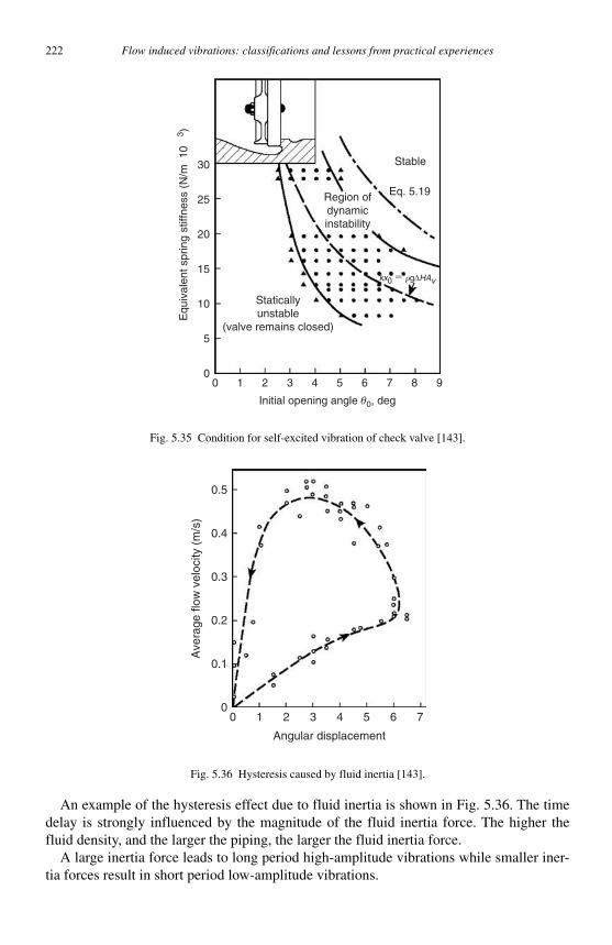
222 Flow induced vibrations: classifications and lessons from practical experiences
An example of the hysteresis effect due to fluid inertia is shown in Fig. 5.36 . The time delay is strongly influenced by the magnitude of the fluid inertia force. The higher the fluid density, and the larger the piping, the larger the fluid inertia force.
A large inertia force leads to long period high-amplitude vibrations while smaller iner-tia forces result in short period low-amplitude vibrations.
00
5
10
15
20
25
30
1 2 3 4 5 6 7 8 9
Stable
Region ofdynamicinstability
Initial opening angle θ0, deg
Equ
ival
ent s
prin
g st
iffne
ss (
N/m
1
03 )
Staticallyunstable
(valve remains closed)
Eq. 5.19
kx0 � rgΔHAv
Fig. 5.35 Condition for self-excited vibration of check valve [143].
0
0.1
0.2
0.3
0.4
0.5
0 1 2 3 4 5 6 7
Ave
rage
flow
vel
ocity
(m
/s)
Angular displacement
Fig. 5.36 Hysteresis caused by fluid inertia [143].
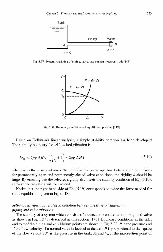
Chapter 5. Vibration excited by pressure waves in piping 223
Based on Kolkman ’ s linear analysis, a simple stability criterion has been developed The stability boundary for self-excited vibration is:
kx g HAm
ALg HA0 2 1 2� �� �
�� �
⎛
⎝⎜⎜⎜⎜
⎞
⎠⎟⎟⎟⎟
� (5.19)
where m is the structural mass. To minimize the valve aperture between the boundaries for permanently open and permanently closed valve conditions, the rigidity k should be large. By ensuring that the selected rigidity also meets the stability condition of Eq. (5.19), self-excited vibration will be avoided.
Notice that the right hand side of Eq. (5.19) corresponds to twice the force needed for static equilibrium given in Eq. (5.18).
Self-excited vibration related to coupling between pressure pulsations inpiping and valve vibration
The stability of a system which consists of a constant pressure tank, piping, and valve as shown in Fig. 5.37 is described in this section [148]. Boundary conditions at the inlet and exit of the piping and equilibrium points are shown in Fig. 5.38 . P is the pressure and V the flow velocity. If a normal valve is located at the exit, P is proportional to the square of the flow velocity. Ps is the pressure in the tank; P0 and V0 at the intersection point of
x � 0x �
Piping
Tank
Valve
A B
Fig. 5.37 System consisting of piping, valve, and constant pressure tank [148].
00
P � B2(V )
P � B1(V )
P
Ps
P0
V0 V
Fig. 5.38 Boundary condition and equilibrium position [148].

224 Flow induced vibrations: classifications and lessons from practical experiences
the two curves are the pressure and flow velocity in the piping at the stable condition. When the pressure in the piping becomes P0 � p and the velocity V0 � v , the fluctuations p and v can be expressed as follows:
p F t x a f t x a� � � �( ) ( )/ / (5.20)
v a F t x a f t x a� � � �( ) ( ) ( )1/ / /� { } (5.21)
where � is the fluid density, and a the wave propagation velocity. The pressure boundary conditions near the equilibrium point ( V0 , P0 ) are linearized as follows:
P b v b� � �1 1 0( , Inlet end) (5.22)
P b v b� �2 2 0( , Outlet end) (5.23)
The following equations are obtained by taking the reflection condition of the wave at the inlet end and the exit end into consideration:
F t R R F t aR b a b aR b a b
( ) ( )( )( ) (
� �� � �� � �
1 2
1 1 1
2 2 2
21 11 1
�// /( / )/ /� �� //�a)
⎫⎬⎪⎪⎪
⎭⎪⎪⎪
(5.24)
| R1R2 | is the growth rate when the wave makes a “ round trip ” in the piping. If | R1R2 | � 1, the system is stable. In the case of the equilibrium condition shown in Fig. 5.38 , the sys-tem is stable because b1 � 0, b2 � 0, | R1 | � 1, and | R2 | � 1. Instability of a valve which closes as the pressure increases, as shown in Fig. 5.39(a), may be explained as follows. The clearance h between the valve and the valve seat is given by:
h h A P k� �m b / (5.25)
hm
Pm
0
31 Pm
Qm
(ii) Unstable
(i) StableAb
P
Q
k
h
(a) (b)
Q
Fig. 5.39 Auto-valve in pipeline system [148]: (a) valve which closes at high pressure, and (b) correspondingpressure-flow characteristic.
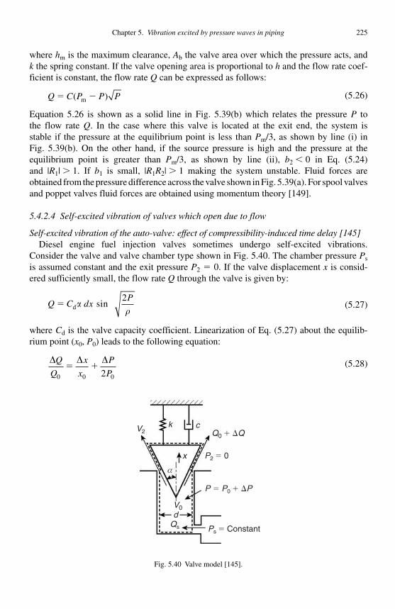
Chapter 5. Vibration excited by pressure waves in piping 225
where hm is the maximum clearance, Ab the valve area over which the pressure acts, and k the spring constant. If the valve opening area is proportional to h and the flow rate coef-ficient is constant, the flow rate Q can be expressed as follows:
Q C P P P� �( )m (5.26)
Equation 5.26 is shown as a solid line in Fig. 5.39(b) which relates the pressure P to the flow rate Q . In the case where this valve is located at the exit end, the system is stable if the pressure at the equilibrium point is less than Pm /3, as shown by line (i) in Fig. 5.39(b) . On the other hand, if the source pressure is high and the pressure at the equilibrium point is greater than Pm /3, as shown by line (ii), b2 � 0 in Eq. (5.24) and | R1 | � 1. If b1 is small, | R1R2 | � 1 making the system unstable. Fluid forces are obtained from the pressure difference across the valve shown in Fig. 5.39(a) . For spool valves and poppet valves fluid forces are obtained using momentum theory [149] .
5.4.2.4 Self-excited vibration of valves which open due to flow
Self-excited vibration of the auto-valve: effect of compressibility-induced time delay [145] Diesel engine fuel injection valves sometimes undergo self-excited vibrations.
Consider the valve and valve chamber type shown in Fig. 5.40 . The chamber pressure Ps
is assumed constant and the exit pressure P2 � 0. If the valve displacement x is consid-ered sufficiently small, the flow rate Q through the valve is given by:
Q C dxP
� d sin �
2(5.27)
where Cd is the valve capacity coefficient. Linearization of Eq. (5.27) about the equilib-rium point ( x0 , P0 ) leads to the following equation:
� � �Q
Q
x
x
P
P0 0 02� � (5.28)
k
d
c
x
α
Q0 � �Q
P2 � 0
P � P0 � �P
Ps � Constant
V2
V0
Qs
Fig. 5.40 Valve model [145].
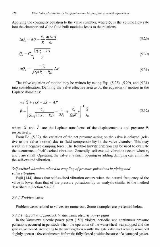
226 Flow induced vibrations: classifications and lessons from practical experiences
Applying the continuity equation to the valve chamber, where Qs is the volume flow rate into the chamber and K the fluid bulk modulus leads to the relations:
� ��
Q QV
K
P
ts0 d
d� �
( ) (5.29)
Q CP P
s ss( )
��2
�(5.30)
��
�QC
P PPs
s
s
��
�2 0( ) (5.31)
The valve equation of motion may be written by taking Eqs. (5.28), (5.29), and (5.31) into consideration. Defining the valve effective area as A , the equation of motion in the Laplace domain is:
ms X csX kX AP
PC
Q P P P
V
Q Ks
2
0 0 0
0
02
1
2
� � � �
�
� � �
��
�� �
�
s
s�( )
⎡
⎣
⎢⎢⎢
⎤
⎦
⎥⎥⎥
11
0
�Xx
(5.32)
where �X and �P are the Laplace transforms of the displacement x and pressure P , respectively.
From Eq. (5.32), the variation of the net pressure acting on the valve is delayed (rela-tive to the valve motion) due to fluid compressibility in the valve chamber. This may result in a negative damping force. The Routh–Hurwitz criterion can be used to evaluate the occurrence of self-excited vibration. Generally, self-excited vibration occurs when x0
and c are small. Operating the valve at a small opening or adding damping can eliminate the self-excited vibration.
Self-excited vibration related to coupling of pressure pulsations in piping and valve vibration
Fujii [144] shows that self-excited vibration occurs when the natural frequency of the valve is lower than that of the pressure pulsations by an analysis similar to the method described in Section 5.4.2.3.
5.4.3 Problem cases
Problem cases related to valves are numerous. Some examples are presented below.
5.4.3.1 Vibration of penstock in Yatsusawa electric power plant In the Yatsusawa electric power plant [150], violent, periodic, and continuous pressure
pulsations occurred in penstock when the operation of the waterwheel was stopped and the gate valve closed. According to the investigation results, the gate valve had actually remained slightly open at a few centimeters before the fully closed position because of a damaged gasket.
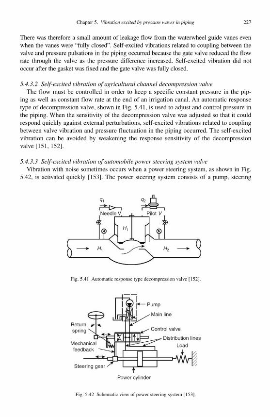
Chapter 5. Vibration excited by pressure waves in piping 227
There was therefore a small amount of leakage flow from the waterwheel guide vanes even when the vanes were “ fully closed ” . Self-excited vibrations related to coupling between the valve and pressure pulsations in the piping occurred because the gate valve reduced the flow rate through the valve as the pressure difference increased. Self-excited vibration did not occur after the gasket was fixed and the gate valve was fully closed.
5.4.3.2 Self-excited vibration of agricultural channel decompression valve The flow must be controlled in order to keep a specific constant pressure in the pip-
ing as well as constant flow rate at the end of an irrigation canal. An automatic response type of decompression valve, shown in Fig. 5.41 , is used to adjust and control pressure in the piping. When the sensitivity of the decompression valve was adjusted so that it could respond quickly against external perturbations, self-excited vibrations related to coupling between valve vibration and pressure fluctuation in the piping occurred. The self-excited vibration can be avoided by weakening the response sensitivity of the decompression valve [151, 152].
5.4.3.3 Self-excited vibration of automobile power steering system valve Vibration with noise sometimes occurs when a power steering system, as shown in Fig.
5.42, is activated quickly [153]. The power steering system consists of a pump, steering
Pilot VNeedle V
H1
H1 H2
q1 q2
Fig. 5.41 Automatic response type decompression valve [152].
Pump
Main line
Control valve
Distribution linesLoad
Returnspring
Steering gear
Power cylinder
Mechanicalfeedback
Fig. 5.42 Schematic view of power steering system [153].
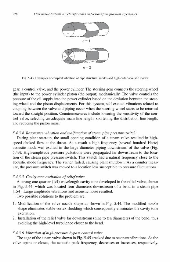
228 Flow induced vibrations: classifications and lessons from practical experiences
gear, a control valve, and the power cylinder. The steering gear connects the steering wheel (the input) to the power cylinder piston (the output) mechanically. The valve controls the pressure of the oil supply into the power cylinder based on the deviation between the steer-ing wheel and the piston displacements. For this system, self-excited vibrations related to coupling between the valve and piping occur when the steering wheel starts to be returned toward the straight position. Countermeasures include lowering the sensitivity of the con-trol valve, selecting an adequate main line length, shortening the distribution line length, and reducing the piston mass.
5.4.3.4 Resonance vibration and malfunction of steam pipe pressure switch During plant start-up, the small opening condition of a steam valve resulted in high-
speed choked flow at the throat. As a result a high-frequency (several hundred Hertz) acoustic mode was excited in the large diameter piping downstream of the valve ( Fig. 5.43 ). High-amplitude pressure pulsations were propagated far downstream to the loca-tion of the steam pipe pressure switch. This switch had a natural frequency close to the acoustic mode frequency. The switch failed, causing plant shutdown. As a counter meas-ure, the pressure switch was moved to a location less susceptible to pressure fluctuations.
5.4.3.5 Cavity tone excitation of relief valve A strong one-quarter (1/4) wavelength cavity tone developed in the relief valve, shown
in Fig. 5.44 , which was located four diameters downstream of a bend in a steam pipe [154]. Large amplitude vibrations and acoustic noise resulted.
Two possible solutions to the problem are:
1. Modification of the valve nozzle shape as shown in Fig. 5.44 . The modified nozzle shape eliminates stable vortex shedding which consequently eliminates the cavity tone excitation.
2. Installation of the relief valve far downstream (nine to ten diameters) of the bend, thus avoiding the high-level turbulence closer to the bend.
5.4.3.6 Vibration of high-pressure bypass control valve The cage of the steam valve shown in Fig. 5.45 cracked due to resonant vibrations. As the
valve opens or closes, the acoustic peak frequency, decreases or increases, respectively.
�
��
�
�
�
n � 1
n � 2
Fig. 5.43 Examples of coupled vibration of pipe structural modes and high-order acoustic modes.
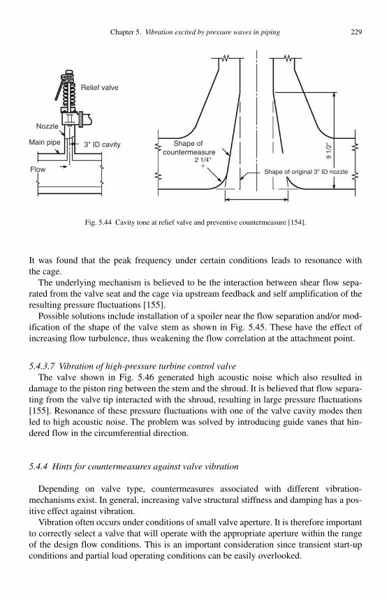
Chapter 5. Vibration excited by pressure waves in piping 229
It was found that the peak frequency under certain conditions leads to resonance with the cage.
The underlying mechanism is believed to be the interaction between shear flow sepa-rated from the valve seat and the cage via upstream feedback and self amplification of the resulting pressure fluctuations [155].
Possible solutions include installation of a spoiler near the flow separation and/or mod-ification of the shape of the valve stem as shown in Fig. 5.45 . These have the effect of increasing flow turbulence, thus weakening the flow correlation at the attachment point.
5.4.3.7 Vibration of high-pressure turbine control valve The valve shown in Fig. 5.46 generated high acoustic noise which also resulted in
damage to the piston ring between the stem and the shroud. It is believed that flow separa-ting from the valve tip interacted with the shroud, resulting in large pressure fluctuations [155]. Resonance of these pressure fluctuations with one of the valve cavity modes then led to high acoustic noise. The problem was solved by introducing guide vanes that hin-dered flow in the circumferential direction.
5.4.4 Hints for countermeasures against valve vibration
Depending on valve type, countermeasures associated with different vibration-mechanisms exist. In general, increasing valve structural stiffness and damping has a pos-itive effect against vibration.
Vibration often occurs under conditions of small valve aperture. It is therefore importantto correctly select a valve that will operate with the appropriate aperture within the range of the design flow conditions. This is an important consideration since transient start-up conditions and partial load operating conditions can be easily overlooked.
Shape of original 3" ID nozzle
Shape of countermeasure
2 1/4" 9 1/
2"
�
Relief valve
Nozzle
Main pipe
Flow
3" ID cavity
Fig. 5.44 Cavity tone at relief valve and preventive countermeasure [154].

230 Flow induced vibrations: classifications and lessons from practical experiences
1: Stem
5
2
2
11 44
33
6
t
v
2: Cage
3: Body
4: Steam inlet
5: Valve exit
6: Water injection
(a)
(b)
Stem shape change
Spoiler
Fig. 5.45 (a) Flow in the high-pressure bypass control valve and, (b) vibration countermeasure [155].
Guide vanes
L
t
v
Fig. 5.46 Flow and countermeasure in turbine control valve [155].

Chapter 5. Vibration excited by pressure waves in piping 231
In the case of vibration problems with a single stage valve, the installation of an orifice or additional valves can resolve the problem by reducing the pressure drop per stage.
5.5 Self-excited acoustic noise due to flow separation
5.5.1 Summary
When an obstacle or acoustic reflector is placed downstream of a free shear layer, discretevortices are formed, giving rise to flow noise and structural vibration. This phenomenon, which is well known as cavity tone, hole tone, or self-excited vibration of orifice plates, is frequently observed in power and process plant piping systems. Figure 5.47 illustrates impinging jet configurations which produce self-sustained flow oscillations [156] .
Large-scale boundary-layer separation at the pipe inlet or flow control valves cause low-frequency vibrations. High-rate pressure reducing devices generate high-frequency
Planarjets
Axisymmetricjets
Planar andaxisymmetricmixing layers
L
u(y )
U
X
y
d
Jet-edge(Edge-tone)
Jet-ring(Ring-tone)
uδ0
Mixing layer-edge(Shear-tone)
Jet-slotJet-hole
(Hole-tone)Rectangular
cavity
Jet-cylinder Jet-plateAxisymmetric
cavity
Jet-surface Jet-flapSpecial cavity(Gate with lip)
w
g
Fig. 5.47 Basic configurations of shear-layer and impingement-edge geometries that produce self-sustained oscillations [156].
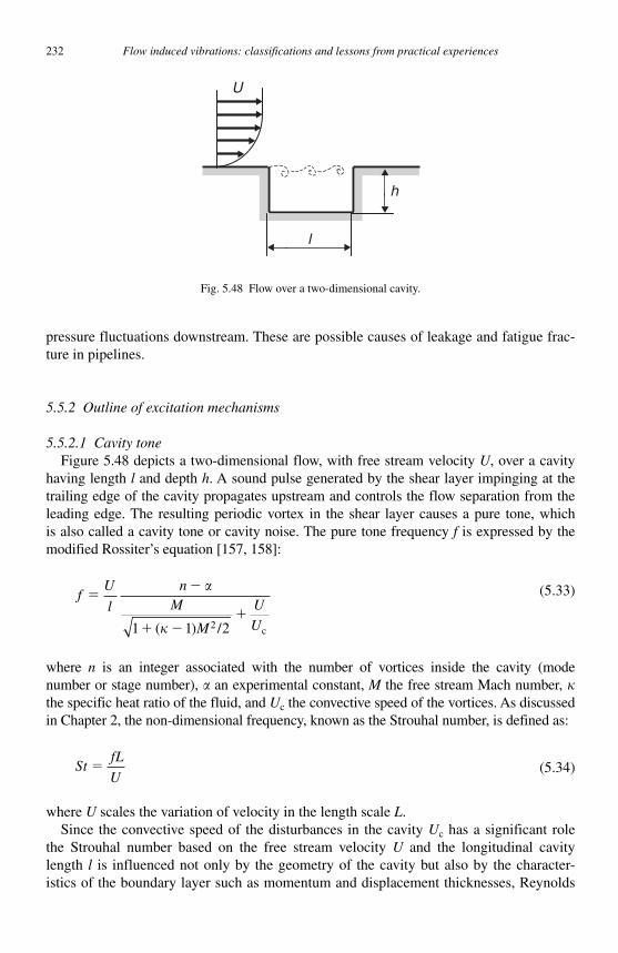
232 Flow induced vibrations: classifications and lessons from practical experiences
pressure fluctuations downstream. These are possible causes of leakage and fatigue frac-ture in pipelines.
5.5.2 Outline of excitation mechanisms
5.5.2.1 Cavity tone Figure 5.48 depicts a two-dimensional flow, with free stream velocity U , over a cavity
having length l and depth h . A sound pulse generated by the shear layer impinging at the trailing edge of the cavity propagates upstream and controls the flow separation from the leading edge. The resulting periodic vortex in the shear layer causes a pure tone, which is also called a cavity tone or cavity noise. The pure tone frequency f is expressed by the modified Rossiter ’ s equation [157, 158] :
fU
l
nM
M
U
U
��
� ��
1 1 22( )� / c
(5.33)
where n is an integer associated with the number of vortices inside the cavity (mode number or stage number), an experimental constant, M the free stream Mach number, �the specific heat ratio of the fluid, and Uc the convective speed of the vortices. As discussed in Chapter 2, the non-dimensional frequency, known as the Strouhal number, is defined as:
StfL
U� (5.34)
where U scales the variation of velocity in the length scale L . Since the convective speed of the disturbances in the cavity Uc has a significant role
the Strouhal number based on the free stream velocity U and the longitudinal cavity length l is influenced not only by the geometry of the cavity but also by the character-istics of the boundary layer such as momentum and displacement thicknesses, Reynolds
U
l
h
Fig. 5.48 Flow over a two-dimensional cavity.
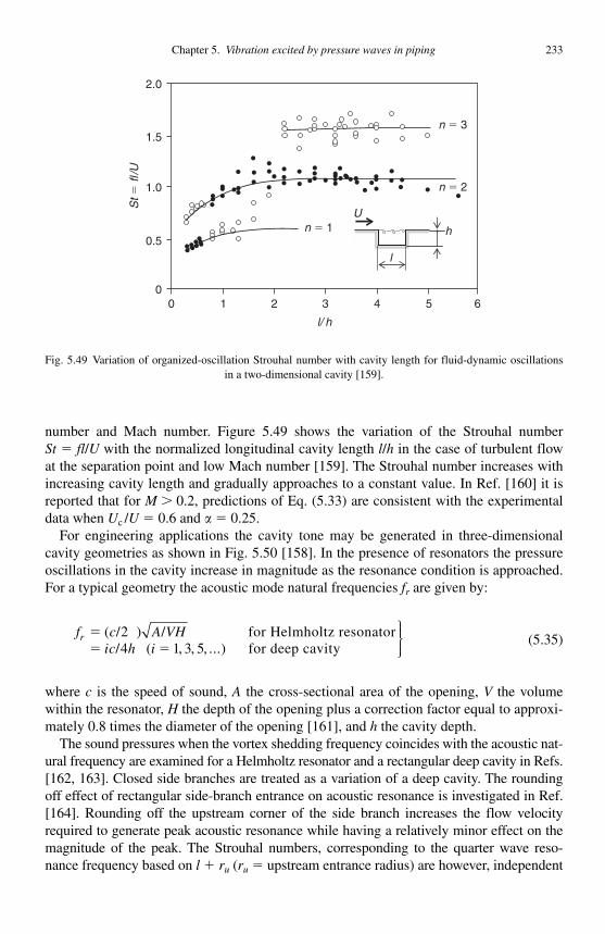
Chapter 5. Vibration excited by pressure waves in piping 233
number and Mach number. Figure 5.49 shows the variation of the Strouhal number St � fl / U with the normalized longitudinal cavity length l / h in the case of turbulent flow at the separation point and low Mach number [159] . The Strouhal number increases with increasing cavity length and gradually approaches to a constant value. In Ref. [160] it is reported that for M � 0.2, predictions of Eq. (5.33) are consistent with the experimental data when Uc / U � 0.6 and � 0.25.
For engineering applications the cavity tone may be generated in three-dimensional cavity geometries as shown in Fig. 5.50 [158] . In the presence of resonators the pressure oscillations in the cavity increase in magnitude as the resonance condition is approached. For a typical geometry the acoustic mode natural frequencies fr are given by:
f c A VHic h i
r �� �
( )( , , , ...)
/ / for Helmholtz resonator/ for24 1 3 5
deep cavity
⎫⎬⎪⎪⎭⎪⎪
(5.35)
where c is the speed of sound, A the cross-sectional area of the opening, V the volume within the resonator, H the depth of the opening plus a correction factor equal to approxi-mately 0.8 times the diameter of the opening [161] , and h the cavity depth.
The sound pressures when the vortex shedding frequency coincides with the acoustic nat-ural frequency are examined for a Helmholtz resonator and a rectangular deep cavity in Refs. [162, 163] . Closed side branches are treated as a variation of a deep cavity. The rounding off effect of rectangular side-branch entrance on acoustic resonance is investigated in Ref. [164] . Rounding off the upstream corner of the side branch increases the flow velocity required to generate peak acoustic resonance while having a relatively minor effect on the magnitude of the peak. The Strouhal numbers, corresponding to the quarter wave reso-nance frequency based on l � ru ( ru � upstream entrance radius) are however, independent
St�
fl/U
l/ h
h
l
Un � 1
n � 2
n � 3
0 1 2 3 4 5 6
2.0
1.5
1.0
0.5
0
Fig. 5.49 Variation of organized-oscillation Strouhal number with cavity length for fluid-dynamic oscillations in a two-dimensional cavity [159].
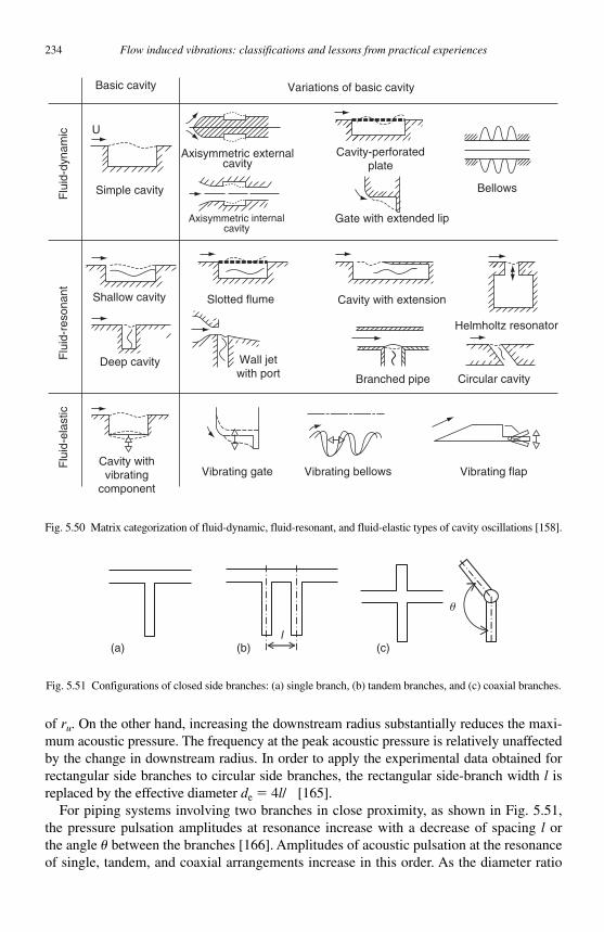
234 Flow induced vibrations: classifications and lessons from practical experiences
of ru . On the other hand, increasing the downstream radius substantially reduces the maxi-mum acoustic pressure. The frequency at the peak acoustic pressure is relatively unaffected by the change in downstream radius. In order to apply the experimental data obtained for rectangular side branches to circular side branches, the rectangular side-branch width l is replaced by the effective diameter de � 4 l / [165] .
For piping systems involving two branches in close proximity, as shown in Fig. 5.51 , the pressure pulsation amplitudes at resonance increase with a decrease of spacing l or the angle u between the branches [166] . Amplitudes of acoustic pulsation at the resonanceof single, tandem, and coaxial arrangements increase in this order. As the diameter ratio
Basic cavity Variations of basic cavity
Axisymmetric externalcavity
Cavity-perforatedplate
Axisymmetric internalcavity
Simple cavity
Shallow cavity
Deep cavity
Slotted flume
Wall jetwith port
Cavity with extension
Branched pipe
Helmholtz resonator
Circular cavity
Vibrating flapVibrating bellowsVibrating gate
Flu
id-e
last
icF
luid
-res
onan
tF
luid
-dyn
amic
Cavity withvibrating
component
Gate with extended lip
Bellows
U
Fig. 5.50 Matrix categorization of fluid-dynamic, fluid-resonant, and fluid-elastic types of cavity oscillations [158].
(a) (b) (c)
θ
l
Fig. 5.51 Configurations of closed side branches: (a) single branch, (b) tandem branches, and (c) coaxial branches.
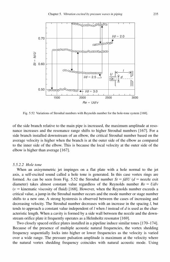
Chapter 5. Vibration excited by pressure waves in piping 235
of the side branch relative to the main pipe is increased, the maximum amplitude at reso-nance increases and the resonance range shifts to higher Strouhal numbers [167] . For a side branch installed downstream of an elbow, the critical Strouhal number based on the average velocity is higher when the branch is at the outer side of the elbow as compared to the inner side of the elbow. This is because the local velocity at the outer side of the elbow is higher than average [167] .
5.5.2.2 Hole tone When an axisymmetric jet impinges on a flat plate with a hole normal to the jet
axis, a self-excited sound called a hole tone is generated. In this case vortex rings are formed. As can be seen from Fig. 5.52 the Strouhal number St � fd / U ( d � nozzle exit diameter) takes almost constant value regardless of the Reynolds number Re � Ud / v(v � kinematic viscosity of fluid) [168] . However, when the Reynolds number exceeds a critical value, a jump in the Strouhal number occurs and the mode number or stage number shifts to a new one. A strong hysteresis is observed between the cases of increasing and decreasing velocity. The Strouhal number decreases with an increase in the spacing l , but tends to approach a constant value independent of l when l instead of d is used as the char-acteristic length. When a cavity is formed by a side wall between the nozzle and the down-stream orifice plate it frequently operates as a Helmholtz resonator [169] .
Two closely spaced orifice plates installed in a pipeline induce similar tones [170–174] . Because of the presence of multiple acoustic natural frequencies, the vortex shedding frequency sequentially locks into higher or lower frequencies as the velocity is varied over a wide range. The pressure pulsation amplitude is maximum at the velocity where the natural vortex shedding frequency coincides with natural acoustic mode. Using
St�
fd/U
l/d � 3.0
l/d � 2.0
l/d � 2.5
Re � Ud /v
3000250020001500
l
dU
0.50
0.60
0.70
Fig. 5.52 Variations of Strouhal numbers with Reynolds number for the hole-tone system [168].
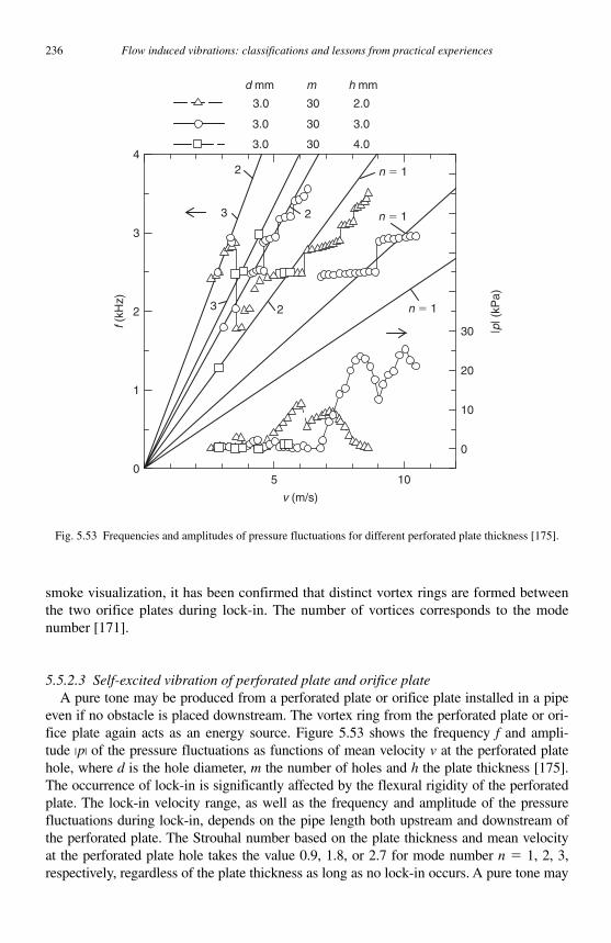
236 Flow induced vibrations: classifications and lessons from practical experiences
smoke visualization, it has been confirmed that distinct vortex rings are formed between the two orifice plates during lock-in. The number of vortices corresponds to the mode number [171] .
5.5.2.3 Self-excited vibration of perforated plate and orifice plate A pure tone may be produced from a perforated plate or orifice plate installed in a pipe
even if no obstacle is placed downstream. The vortex ring from the perforated plate or ori-fice plate again acts as an energy source. Figure 5.53 shows the frequency f and ampli-tude |p| of the pressure fluctuations as functions of mean velocity v at the perforated plate hole, where d is the hole diameter, m the number of holes and h the plate thickness [175] . The occurrence of lock-in is significantly affected by the flexural rigidity of the perforated plate. The lock-in velocity range, as well as the frequency and amplitude of the pressure fluctuations during lock-in, depends on the pipe length both upstream and downstream of the perforated plate. The Strouhal number based on the plate thickness and mean velocity at the perforated plate hole takes the value 0.9, 1.8, or 2.7 for mode number n � 1, 2, 3, respect ively, regardless of the plate thickness as long as no lock-in occurs. A pure tone may
24
3
2
1
0
3 2
2
n � 1
n � 1
n � 1
30
20
10
105
0
3
f (kH
z)
d mm h mmm
|p| (
kPa)
v (m/s)
3.0 30 2.0
3.0
4.0
30
30
3.0
3.0
Fig. 5.53 Frequencies and amplitudes of pressure fluctuations for different perforated plate thickness [175].

Chapter 5. Vibration excited by pressure waves in piping 237
also be generated at an orifice plate with a single hole [176] . Flow visualization shows that the vortex ring spacing approximately equals the plate thickness, one half the plate thick-ness and one-third the plate thickness for n � 1, 2, 3, respectively [177] .
5.5.2.4 Low-frequency vibration due to flow separation A recirculation cell, due to large-scale flow separation at a pipe inlet or inside a flow
control valve, frequently causes low-frequency vibrations. This phenomenon seems to be associated with instability of the pressure inside the cell due to volumetric flow change, but the excitation mechanism remains unclarified.
5.5.2.5 Acoustic fatigue of piping systems Steam or gas flow through high-rate pressure reducing devices such as safety valves,
depressurizing valves and restriction orifices frequently produces severe acoustic vibra-tion causing piping system fatigue failure. The broad-banded random excitation differs from the single frequency self-excited excitations discussed above. Since the pipe wall thickness is relatively thin, the risk of acoustic fatigue generally increases with increasing pipe diameter.
As shown in Fig. 5.54, the diametral acoustic modes and corresponding circumferen-tial structural modes must be focused on if the frequency is higher than about 500 Hz. Guidelines for designing piping systems against acoustic fatigue have been proposed, based on the data of practical pipes [178, 179] . Recently, numerical analysis of resonant stress amplitudes in pipe walls during coincidence with the acoustic diametral modes has also
n � 1 n � 2 n � 3
(p, q) � (1, 0) (p, q) � (2, 0) (p, q) � (3, 0)
(a)
(b)
Fig. 5.54 Examples of diametral acoustic modes and corresponding circumferential structural modes with matching wave numbers: (a) acoustic modes, and (b) structural modes.
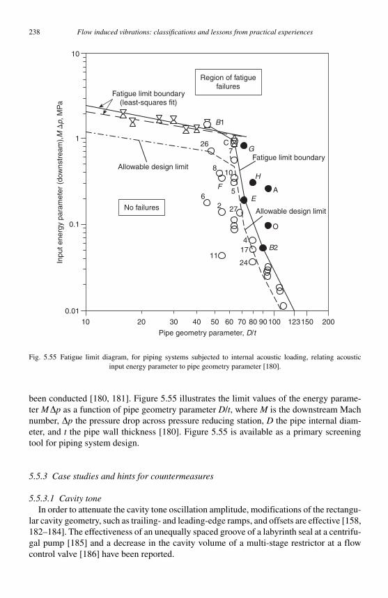
238 Flow induced vibrations: classifications and lessons from practical experiences
been conducted [180, 181] . Figure 5.55 illustrates the limit values of the energy parame-ter M�p as a function of pipe geometry parameter D / t , where M is the downstream Mach number, �p the pressure drop across pressure reducing station, D the pipe internal diam-eter, and t the pipe wall thickness [180] . Figure 5.55 is available as a primary screening tool for piping system design.
5.5.3 Case studies and hints for countermeasures
5.5.3.1 Cavity tone In order to attenuate the cavity tone oscillation amplitude, modifications of the rectangu-
lar cavity geometry, such as trailing- and leading-edge ramps, and offsets are effective [158,182–184] . The effectiveness of an unequally spaced groove of a labyrinth seal at a centrifu-gal pump [185] and a decrease in the cavity volume of a multi-stage restrictor at a flow control valve [186] have been reported.
Region of fatiguefailures
Fatigue limit boundary(least-squares fit)
Fatigue limit boundary
Allowable design limit
Allowable design limit
No failures
1124
B2174
O
2726
5
810
726
B1
GC
H
E
F A
10
0.01
0.1
1
10
20 30 40 50 60 70 80 90100 123150 200
Pipe geometry parameter, D/t
Inpu
t ene
rgy
para
met
er (
dow
nstr
eam
),M
�p,
MP
a
Fig. 5.55 Fatigue limit diagram, for piping systems subjected to internal acoustic loading, relating acoustic input energy parameter to pipe geometry parameter [180].
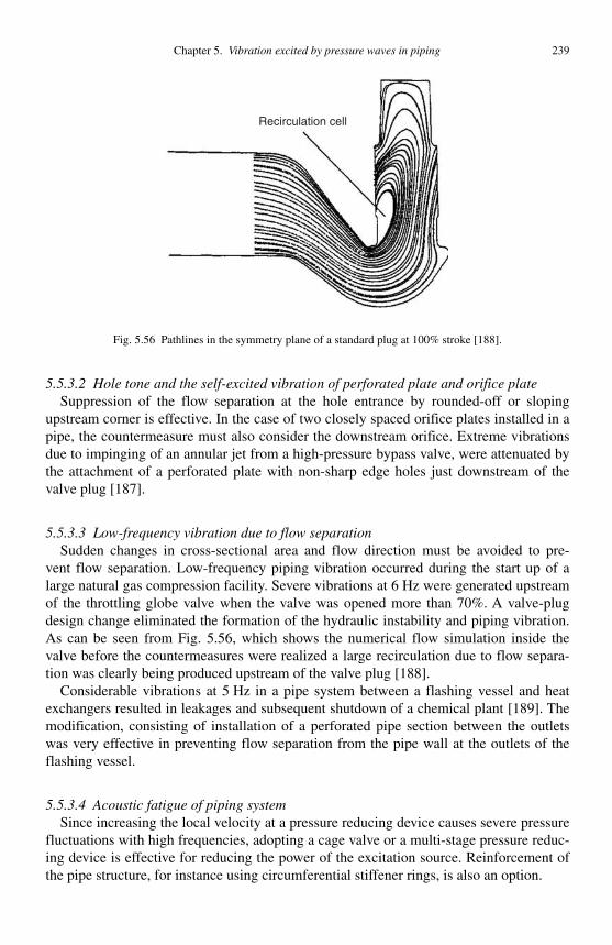
Chapter 5. Vibration excited by pressure waves in piping 239
5.5.3.2 Hole tone and the self-excited vibration of perforated plate and orifice plate Suppression of the flow separation at the hole entrance by rounded-off or sloping
upstream corner is effective. In the case of two closely spaced orifice plates installed in a pipe, the countermeasure must also consider the downstream orifice. Extreme vibrations due to impinging of an annular jet from a high-pressure bypass valve, were attenuated by the attachment of a perforated plate with non-sharp edge holes just downstream of the valve plug [187] .
5.5.3.3 Low-frequency vibration due to flow separation Sudden changes in cross-sectional area and flow direction must be avoided to pre-
vent flow separation. Low-frequency piping vibration occurred during the start up of a large natural gas compression facility. Severe vibrations at 6 Hz were generated upstream of the throttling globe valve when the valve was opened more than 70%. A valve-plug design change eliminated the formation of the hydraulic instability and piping vibration. As can be seen from Fig. 5.56, which shows the numerical flow simulation inside the valve before the countermeasures were realized a large recirculation due to flow separa-tion was clearly being produced upstream of the valve plug [188] .
Considerable vibrations at 5 Hz in a pipe system between a flashing vessel and heat exchangers resulted in leakages and subsequent shutdown of a chemical plant [189] . The modification, consisting of installation of a perforated pipe section between the outlets was very effective in preventing flow separation from the pipe wall at the outlets of the flashing vessel.
5.5.3.4 Acoustic fatigue of piping system Since increasing the local velocity at a pressure reducing device causes severe pressure
fluctuations with high frequencies, adopting a cage valve or a multi-stage pressure reduc-ing device is effective for reducing the power of the excitation source. Reinforcement of the pipe structure, for instance using circumferential stiffener rings, is also an option.
Recirculation cell
Fig. 5.56 Pathlines in the symmetry plane of a standard plug at 100% stroke [188].
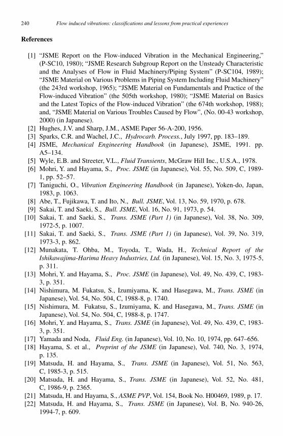
240 Flow induced vibrations: classifications and lessons from practical experiences
References
[1] “ JSME Report on the Flow-induced Vibration in the Mechanical Engineering, ” (P-SC10, 1980); “ JSME Research Subgroup Report on the Unsteady Characteristic and the Analyses of Flow in Fluid Machinery/Piping System ” (P-SC104, 1989); “ JSME Material on Various Problems in Piping System Including Fluid Machinery ”(the 243rd workshop, 1965); “ JSME Material on Fundamentals and Practice of the Flow-induced Vibration ” (the 505th workshop, 1980); “ JSME Material on Basics and the Latest Topics of the Flow-induced Vibration ” (the 674th workshop, 1988); and, “ JSME Material on Various Troubles Caused by Flow ” , (No. 00-43 workshop, 2000) (in Japanese).
[2] Hughes, J.V. and Sharp, J.M., ASME Paper 56-A-200, 1956. [3] Sparks , C.R. and Wachel , J.C. , Hydrocarb. Process. , July 1997 , pp. 183 – 189 . [4] JSME, Mechanical Engineering Handbook (in Japanese) , JSME , 1991 . pp.
A5–134. [5] Wyle , E.B. and Streeter , V.L., Fluid Transients , McGraw Hill Inc. , U.S.A. , 1978 . [6] Mohri , Y. and Hayama , S. , Proc. JSME (in Japanese) , Vol. 55 , No. 509 , C, 1989-
1 , pp. 52 – 57 . [7] Taniguchi , O., Vibration Engineering Handbook (in Japanese) , Yoken-do , Japan ,
1983 , p. 1063. [8] Abe , T. , Fujikawa , T. and Ito , N. , Bull. JSME , Vol. 13 , No. 59 , 1970 , p. 678 . [9] Sakai , T. and Saeki , S. , Bull. JSME , Vol. 16 , No. 91 , 1973 , p. 54 . [10] Sakai , T. and Saeki , S. , Trans. JSME (Part 1) (in Japanese) , Vol. 38 , No. 309 ,
1972-5 , p. 1007 . [11] Sakai , T. and Saeki , S. , Trans . JSME (Part 1) (in Japanese) , Vol. 39 , No. 319 ,
1973-3 , p. 862 . [12] Munakata , T. Ohba, M ., Toyoda, T., Wada, H., Technical Report of the
Ishikawajima-Harima Heavy Industries, Ltd. (in Japanese) , Vol. 15 , No. 3 , 1975-5 , p. 311 .
[13] Mohri , Y. and Hayama , S. , Proc. JSME (in Japanese) , Vol. 49 , No. 439 , C, 1983-3 , p. 351 .
[14] Nishimura , M. Fukatsu, S., Izumiyama, K. and Hasegawa, M., Trans. JSME (inJapanese) , Vol. 54 , No. 504 , C, 1988-8 , p. 1740 .
[15] Nishimura , M. Fukatsu, S., Izumiyama, K. and Hasegawa, M., Trans. JSME (inJapanese) , Vol. 54 , No. 504 , C, 1988-8 , p. 1747 .
[16] Mohri , Y. and Hayama , S. , Trans. JSME (in Japanese) , Vol. 49 , No. 439 , C, 1983-3 , p. 351 .
[17] Yamada and Noda, Fluid Eng. (in Japanese) , Vol. 10 , No. 10 , 1974 , pp. 647 – 656 . [18] Hayama , S. et al. , Preprint of the JSME (in Japanese) , Vol. 740 , No. 3 , 1974 ,
p. 135 . [19] Matsuda , H. and Hayama , S. , Trans. JSME (in Japanese) , Vol. 51 , No. 563 ,
C, 1985-3 , p. 515 . [20] Matsuda , H. and Hayama , S. , Trans . JSME (in Japanese) , Vol. 52 , No. 481 ,
C, 1986-9 , p. 2365 . [21] Matsuda, H. and Hayama, S., ASME PVP, Vol. 154, Book No. H00469, 1989, p. 17. [22] Matsuda , H. and Hayama , S. , Trans . JSME (in Japanese) , Vol. B , No. 940-26 ,
1994-7 , p. 609 .
Chapter 5. Vibration excited by pressure waves in piping 241
[23] Matsuda, H. and Hayama, S., ASME PVP, Vol. 310, Book No. H00973, 1995, p. 117. [24] Hayama , S. , Preprint of the JSME (in Japanese) , Vol. 730 , No. 14 , 1973-10 ,
pp. 113 – 116 . [25] Fujikawa , T. Kurohashi , M. Kato , M. Aoshima, M. and Yamamura , H.,
KOBELCO Technol. Rev. , Vol. 37 , No. 1 , 1987 , p. 59 . [26] Kato , Inoue , Fujikawa and Aoshima , Proc. JSME (in Japanese) , Vol. 52 , No. 481 ,
C, 1986-1 , pp. 2375 – 2381 . [27] Kato , M. Hirooka , E. Inoue Y. and Sato , S. Trans . JSME (in Japanese) , Vol. 58 , No. 554 ,
C, 1992-10 , pp. 2907 – 2911 . [28] Brebbia, C.A. and Wa1ker, S., Boundary Element Techniques in Engineering ,
Newness-Butterworths, London, 1980. (Translated jointly by Kamitani, N., Tanaka, M. and Tanaka, K., Fundamentals and Application of Boundary Element Method , Baihukan, 1981.)
[29] Tanaka , T. Fujikawa , T. Abe T. and Utsuno , H. Trans. JSME (in Japanese) , Vol. 50 , No. 453 , C, 1984-5 , pp. 848 – 856 .
[30] Tanaka , T. Fujikawa , T. Abe T. and Utsuno , H. Trans . JSME (in Japanese) , Vol. 50 , No. 460 , C, 1984-12 , pp. 2356 – 2363 .
[31] Tanaka , T. Utsuno , H. Masuda T. and Kanzaki , N. Trans . JSME (in Japanese) , Vol. 53 , No. 491 , C, 1987-7 , pp. 1443 – 1449 .
[32] Suzuki , S. Imai M. and Ishiyama , S. Trans. JSME (in Japanese) , Vol. 52 , No. 473 , C, 1986 , pp. 310 – 317 .
[33] Binder , R.C. , J. Acoust. Soc. Am. , Vol. 15 , No. 1 , 1943 , pp. 41 – 43 . [34] Hayama , S. et al ., Bull. JSME , Vol. 20 , No. 146 , 1977 , p. 955 . [35] Hayama , S. et al. , Proc. JSME (in Japanese) , Vol. 45 , No. 392 , 1979-4 , p. 422 . [36] Mori , Y. and Hayama , S. , Proc. JSME (in Japanese) , Vol. 52 , No. 481 , 1986-9 ,
p. 59 . [37] JSME, Research Subgroup Report on Pressure Pulsations in Piping Systems
caused by Reciprocating Compressors, P-SC105, 1989. [38] API (American Petroleum Institute) Standard 618, 4th edition, June 1995. [39] Fujikawa , T. , Proc. JSME (in Japanese) , Vol. 57 , No. 533 , C 1991-1 , pp. 148 – 153 . [40] Kato, M., Hirooka, E., Murai, K. and Fujikawa, T., Symposium on Flow-Induced
Vibration and Noise, ASME Winter Annual Meeting , Vol. 6, 1992, pp. 237–244. [41] Taniguchi , O., Vibration Engineering Handbook (in Japanese) , Yoken-do , Japan ,
1976 , p. 1033. [42] Costagliola , M. , Trans. ASME, J. Appl. Mech. , Vol. 14 , No. 4 , 1950 , p. 415 . [43] Maclaren, J.F.T. et al., Inst. Mech. Engrs., Conference Publication 4, 1974,
pp. 9–17. [44] Kato , M. Kurohashi, M., Fujikawa, T. and Aoshima, M. , Trans. JSME (in
Japanese) , Vol. 54 , No. 505 , C, 1988-9 , p. 2148 . [45] Matsuda , H. and Hayama , S. , Trans . JSME (in Japanese) , Vol. 54 , No. 506 ,
C, 1988-10 , p. 2465 . [46] Fujikawa , T. Kato , M. Ito M. and Nomura , H. Trans . JSME (in Japanese) , Vol. 55 ,
No. 512 , C, 1989-4 , pp. 904 – 909 . [47] Hayama , S. and Matsumoto , M. , Trans. JSME (in Japanese) , Vol. 52 , No. 476 ,
C, 1986-4 , p. 1192 . [48] Wakabayashi , Arai and Yamada , Trans. JSME (in Japanese) , Vol. 63 , No. 605 ,
B, 1997-1 , pp. 231 – 236 .
242 Flow induced vibrations: classifications and lessons from practical experiences
[49] Tanaka , M. and Fujita , K. , Trans. JSME (in Japanese) , Vol. 53 , No. 487 , C, 1987-3 , p. 591 .
[50] Tanaka , M. and Fujita , K. , Trans . JSME (in Japanese) , Vol. 53 , No. 491 , C, 1987-7 , p. 1363 .
[51] Wachel , J.C. and Bates , C.L. , Hydrocarb. Process. , October 1976 , p. 152 . [52] Matsuda , H. , Safety Engineering (in Japanese) , Vol. 34 , No. 3 , 1995 , p. 197 . [53] Abe , T. , Preprint of the JSME (in Japanese) , No. 200 , 1968-9 , p. 73 . [54] Mitsuhashi , K. and Kodera , Y. , Preprint of the JSME (in Japanese) , Vol. 750 ,
No. 14 , 1975-10 , p. 13 . [55] Kanda , T. , Trans. JSME (in Japanese) , Vol. 55 , No. 512 , C, 1989-4 , pp. 910 – 915 . [56] Matsuda , H. and Yamaguchi , T. , Piping Technology (in Japanese) , Vol. 347-27 ,
No. 8 , 1985-7 , p. 66 . [57] Ohashi , H., Fluid Machinery Handbook (in Japanese) , Asakura-Shoten , Japan ,
1998 , p. 535. [58] The JSME, Vibration Damping Technology (in Japanese) , Yoken-do , Japan , 1998 ,
p. 220. [59] The JSME D & D 98, V_BASE forum (in Japanese), No. 98-8 (II), 1998-8, pp. 32–34. [60] The JSME D & D 98, V_BASE forum (in Japanese), No. 98-8 (II), 1998-8, pp. 35–36. [61] Matsuda , H. and Hayama , S. , Trans . JSME (in Japanese) , Vol. 53 , No. 496 ,
C, 1987-12 , p. 2510 . [62] Matsuda, H. and Hayama, S., Asia-Pacific Vibration Conference, 93/Symposium
on FIVES, Proceeding , Vol. 1, 1993-11, p. 213. [63] The JSME V_BASE forum (in Japanese), No. 920-65, 1992, pp. 22–23. [64] Kato , M. Sakamoto Y. and Nosaka , Y. R & D Technical Report of Kobe Steel (in
Japanese) , Vol. 42 , No. 4 , 1992 , pp. 55 – 58 . [65] The JSME D & D 96, V_BASE forum (in Japanese), No. 96-5 (II), 1996-8,
pp. 86–87. [66] The JSME D & D 97, V_BASE forum (in Japanese), No. 97-10-3, 1997-7, pp. 14–15. [67] The JSME material on Today ’ s Vibration and Noise in Fluid Machinery (the 636th
workshop) (in Japanese), 1986, pp. 65–70. [68] Korteweg , D.J. , Annalen der Physik und Chemie , Vol. 5 , 1878 , pp. 525 – 542 . [69] Simin , O. , Proc. Water Works Ass , 1904 , p. 35 . [70] Mori , Y. et al. , Trans. JSME (in Japanese), Vol. 39 , No. 317 , 1973 , p. 305 . [71] Kobori , T. et al. , Hitachi Hyouron (in Japanese) , Vol. 37 , No. 10 , 1955 , p. 33 . [72] API STANDARD 674, Second Edition, American Petroleum Institute, 1995. [73] Sano , M. , Trans. JSME (in Japanese), Vol. 49 , No. 440B , 1983 , p. 828 . [74] Rzentkowski , G. and Zbrojia , S. , J. Fluid. Struct. , Vol. 14 , 2000 , pp. 529 – 558 . [75] Kawata , H. et al. , Trans. JSME (in Japanese), Vol. 55 , No. 514 , 1989 , p. 1584. [76] Rzentkowski, G., Flow Induced Vibration, ASME PVP, Vol. 328, 1996, pp. 439–454. [77] Fujii , S. , Trans. JSME (in Japanese) , Vol. 13 , No. 44 , 1947 , p. 184 . [78] Kusama , H. et al. , Trans. JSME (in Japanese), Vol. 20 , No. 89 , 1954 , p. 15 . [79] Kawata , H. et al. , Trans. JSME (in Japanese), Vol. 52 , No. 480 , 1986 , p. 2947 . [80] Kawata, H., “ A study on the pulsating phenomena in centrifugal pumps and pipe-
lines ” , Doctoral dissertation (in Japanese), The University of Tokyo. [81] Kawata , H. et al. , Trans. JSME (in Japanese), Vol. 55 , No. 514 , 1986 , p. 1590 . [82] Chen, Y.N, IAHR/UTAM Symposium , Karlsruhe, 1979, pp. 265–278.
Chapter 5. Vibration excited by pressure waves in piping 243
[83] Elder, R.E., IAHR/UTAM Symposium , Karlsruhe, 1979, pp. 285–286. [84] Wang, J.C. et al., IAHR/UTAM Symposium , Karlsruhe, 1979, pp. 333–335. [85] Wei-Yih Chou and Rudavsky, A.B., IAHR/UTAM Symposium , Karlsruhe, 1979,
pp. 337–339. [86] Ohashi , H., The Fluid-Machinery Handbook (in Japanese) , Asakura Publishing ,
1998 . 147. [87] Rzentkowski, G., EAM, pp. 525–537. [88] Benedek , S. , J. Sound Vib. , Vol. 177 , No. 3 , 1994 , pp. 337 – 348 . [89] Brekke, H., 7th International Conference Pressure Surge , BHC Group, 1996,
pp. 399–415. [90] See p. 241 of Ref [87]. [91] Glattfelder, A.H. et al., IAHR/UTAM Symposium, Karlsruhe, 1979, pp. 293–297. [92] Brekke, H., 8th International Conference Pressure Surge , BHR Group 2000,
pp. 599–610. [93] Bihhadi, A. and Edge K.A., “ Flow Induced Vibration, ” Ziada & Staubi (eds.),
Balkema, Rotterdam, 2000, pp. 607, 613. [94] JSME, “ The collection of the draft papers presented in the 69th National
Conference of the JSME ” (in Japanese), No. 910-62, Vol. D, 1991, p. 16. [95] JSME, “ The collection of data of the vibration and noise problems presented in the
v_BASE forum of the JSME ” (in Japanese), No.99-7 III, 1999, p. 29. [96] JSME, “ The collection of the draft papers presented in the ordinary general meet-
ing of JSME, ” No. 920-17, 1992, Vol. D, p. 664. [97] JSME, “ The collection of the draft papers presented in the 69th National
Conference of the JSME ” (in Japanese), No. 930-63, 1993, Vol. G, p. 156. [98] JSME, “ The collection of data of the vibration and noise problems presented in the
v_BASE forum of the JSME ” (in Japanese), 1997, p. 57. [99] JSME, “ The collection of the draft papers presented in the 69th National
Conference of the JSME ” (in Japanese), No. 920-17, 1992, Vol. D, p. 642. [100] JSME, “ The collection of data of the vibration and noise problems presented in the
v_BASE forum of the JSME, ” (in Japanese) 1992, p. 11. [101] Eichler, O., IAHR/UTAM Symposium, Karlsruhe, 1979, pp. 240–249. [102] Kubota, T. and Aoki, H., IAHR/U Symposium, Kahrsruhe, 1979, pp. 279–284. [103] Garbrecht, G., 5th International Conference on Pressure Surges , BHRA, 1986,
pp. ix–xx. [104] Menabrea , L.F. , Note sur les effects de choc de l ’ eau dans les conduits C. R. Acad.
Sci. (Paris) , Vol. 47 , 1858 , pp. 221 – 224 . [105] Joukowsky , N. , Waterhammer, Procs. AWWA , Vol. 24 , 1904 , pp. 341 – 424 . [106] Parmakian , J., Waterhammer Analysis , Dover , 1963 . [107] Akimoto, T., Water Hammer and Pulsation, Nikkan Kougyo Shinbunshya (in
Japanese), 1977. [108] Rorche , P.J., Computational Fluid Dynamics , Hermosa , 1985 , p. 250. [109] Amein, M. et al., J. Hydraul. Div ., ASCE, Vol. 101, No. HY6, June 1975,
pp. 717–731. [110] Katopodes, N.D. and Wylie, E.B., Symposium on Multi-dimensional Fluid
Transients, ASME, New Orleans, LA., December 1984, pp. 9–16. [111] Rachford, H.H. and Ramsy, E.L., SPE 5663, ASME, Dallas, September 1975.
244 Flow induced vibrations: classifications and lessons from practical experiences
[112] Kranenburg, C., J., Hydraul. Div ., ASCE, Vol. 100, No. HY10, October 1974,pp. 1383–1398.
[113] Kiuchi , T. , Int. J. Heat Fluid Flow , Vol. 15 , No. 5 , October 1994 . [114] Wylie , B.E. and Streeter , V.L., Fluid Transients in Systems , Prentice-Hall ,
Englewood Cliffs, NJ. 07632 , 1993 . [115] Thorley , A.R.D. , Fluid Transients in Pipeline System, D. & L. George Ltd. ,
1991 , p. 242 . [116] Yokoyama, J., Suigeki Nyuumon, Nishin Syuppan (in Japanese), 1980. [117] Shapiro , A.H. , The Dynamics and Thermodynamics of Compressible Fluid Flow,
Vol. 2, Krieger , Florida , 1983, p. 972. [118] O ’ Brien , G.G. et al. , J. Math. Phys. , Vol. 29 , 1951 . [119] Kephart , J.T. , Trans. ASME , Series D, Vol. 83, No. 3 , September 1961 ,
pp. 456 – 460 . [120] Tanahashi , T. et al. , Trans. JSME (in Japanese) , Vol. 35-2 , No. 279 , 1969 ,
pp. 2217 – 2226 . [121] Provoost, G.A. and Wylie, E.B., 5th International Symposium on Column
Separation , Germany, September 1981. [122] Wylie, E.B., 3rd. International Conference on Pressure Surges , BHRA, March
1980, pp. 27–42. [123] Zielke , W. , J. Basic Eng., ASME, Ser. D , Vol. 90 , No. 1 , 1968 , pp. 109 – 115 . [124] Trikha , A.K. , J. Fluid Eng., ASME , Vol. 97 , March 1975 , pp. 97 – 105 . [125] Achard , J.L. and Lespinard , G.M. , J. Fluid Mech. , Vol. 113 , 1981 , pp. 283 – 298 . [126] Kagawa , T. et al. , JSME Proc. (in Japanese) , Vol. 921 , No. 83-0063 , 1983 . [127] Oomi , S. et al. , Trans. JSME (in Japanese) , Vol. 47-424-B , 1981 , p. 2282 . [128] Uchida , S. , ZAMP , Vol. 7 , 1956 , pp. 403 – 422 . [129] Oomi , S. et al. , Trans. JSME (in Japanese) , Vol. 50-457-B , 1984 , pp. 1995 – 2003 . [130] Hayama , S. et al. , Trans. JSME (in Japanese) , Vol. 45 , 1979 , pp. 422 – 432 . [131] Botros , K.K. , Jones , B.J. and Roorda , O. , “ Fluid Structure Interaction ” , ASME
PVP , Vol. 337 , No. 27-1, 27-2 , 1996 , pp. 241 – 264 . [132] Wiggert , D.C. and Tijsseling , A.S. , Appl. Mech. Rev. , ASME, Vol. 54 , 2002 ,
pp. 455 – 481 . [133] Almeida, A.B.D., 5th International Conference Pressure Surge , BHRA, 1986,
pp. 27–34. [134] Locher, F.A. and Wang, J.S., 7th International Conference Pressure Surge , BHRA,
1996, pp. 211–223. [135] Hamilton, M. and Taylor, G., 7th International Conference Pressure Surge , BHRA,
1996, pp. 15–27. [136] Taylor, G., 7th International Conference Pressure Surge , BHRA, 1996,
pp. 343–362. [137] Nakata , N. et al. , Ebara Jihou (in Japanese) , Vol. 114 , 1980 , pp. 39 – 43 . [138] Kruisbrink, A.C.H., Proceedings of the 3rd International Conference on Valves
and Actuators , 1990, pp. 137–150. [139] Thorley, A.R.D., Proceedings of the 4th International Conference on Pressure
Surges , BHRA, 1983, pp. 231–242. [140] Inada and Hayama , Proc. JSME C (in Japanese) , Vol. 53 , 1986 , pp. 933 – 939 . [141] JSME D & D Conf. /V-BASE No.139.
Chapter 5. Vibration excited by pressure waves in piping 245
[142] JSME D & D Conf. /V-BASE No.76. [143] Weaver , D.S., Practical Experiences with Flow-Induced Vibrations . In
Naudascher , E. and Rockwell , D. (eds.), Springer-Verlag , 1980 , pp. 305 – 319 . [144] Fujii , S. Proc. JSME (in Japanese) , Vol. 18 , No. 73 , 1952 , pp. 182 – 184 . [145] Maeda , T. Proc. JSME (in Japanese) , Vol. 35 , No. 274 , 1969 , pp. 1285 – 1292 . [146] Ainsworth , F.W. , Trans. ASME , Vol. 78 , No. 4 , 1956 , pp. 773 – 778 . [147] Ezekiel , F.D. , Trans. ASME , Vol. 80 , No. 4 , 1958 , pp. 904 – 908 . [148] Taniguchi , O., Vibration Engineering Handbook (in Japanese) , Yoken-do , Japan,
pp. 1068–1071 , 1976 . [149] Takenaka T. and Urata , E. Proc. JSME (in Japanese) , Vol. 71 , No. 599 , 1968-12 , p.
1684 . [150] Fujii , S. Science of Machine (in Japanese) , Vol. 1 , No. 11 , 1949 . [151] Cho, K. et al. , Transactions of the Japanese Society of Irrigation, Drainage and
Reclamation Engineering (in Japanese) , Vol. 135 , 1988-6 , p. 91 . [152] Cho, K. Transactions of the Faculty of Agriculture of Kagoshima University ,
Vol. 39 , 1989 , pp. 273 – 286 . [153] Matsunaga, T. et al., Proceedings of Symposium on Fluid Power , Japan Society of
Fluid Power System, 1991, pp. 125–128. [154] Berstein , M.D. et al. , “ Flow-Induced Vibration ” , ASME PVP , Vol. 154 , 1989 ,
p. 155 . [155] Ziada , S. et al. , J. Fluid. Struct. , Vol. 3 , 1989 , pp. 529 – 549 . [156] Rockwell , D. and Naudascher , E. , Ann. Rev. Fluid Mech. , Vol. 11 , 1979 ,
pp. 67 – 94 . [157] Rossiter, J.E., RAE Tech. Rep. No. 64037 (1964) and Reports and Memoranda
No. 3438, 1964. [158] Rockwell , D. and Naudascher , E. , Trans. ASME, J. Fluid. Eng. , Vol. 100 , 1978 ,
pp. 152 – 165 . [159] Rockwell , D. , Trans. ASME, J. Fluid. Eng. , Vol. 99 , 1977 , pp. 294 – 300 . [160] Ahuja, K.K. and Mendoza, J., NASA Contractor Report, Final Report Contract
NAS1-19061, Task 13, 1995. [161] Rayleigh , J.S.W. , The Theory of Sound , Vol. II , Dover, 1945 , pp. 180 – 183 . [162] DeMetz, F.C. and Farabee, T.M., AIAA Paper 77-1293, 1977. [163] Elder , S.A. , Farabee , T.M. and DeMetz , F.C. , J. Acoust. Soc. Am. , Vol. 72 , No. 2 ,
1982 , pp. 532 – 549 . [164] Weaver , D.S. and Macleod , G.O. , “ Proc. Symp. on Flow-Induced-Vibration ” ,
ASME, PVP , Vol. 389 , 1999 , pp. 291 – 297 . [165] Bruggeman, J.C., Doctoral Dissertation, Technische Universität Eindhoven,
Eindhoven, The Netherlands, 1987. [166] Ziada, S. and Bühlmann, E.T., IMechE, C416/009, 1991, pp. 435–444. [167] Ziada , S. and Shine , S. , J. Fluid. Struct. , Vol. 13 , No. 1 , 1999 , pp. 127 – 142 . [168] Chanaud , R.C. and Powell , A. , J. Acoust. Soc. Am. , Vol. 37 , No. 5 , 1965 ,
pp. 902 – 911 . [169] Morel , T. , Trans. ASME, J. Fluid. Eng. , Vol. 101 , 1979 , pp. 383 – 390 . [170] Culick , F.E.C. and Magiawala , K. , J. Sound Vib. , Vol. 64 , No. 3 , 1979 ,
pp. 455 – 457 . [171] Nomoto , H. and Culick , F.E.C. , J. Sound Vib. , Vol. 84 , No. 2 , 1982 , pp. 247 – 252 .
246 Flow induced vibrations: classifications and lessons from practical experiences
[172] Harris, R.E., Weaver, D.S. and Dokainish, M.A., Proceedings of the International Conference on Flow Induced Vibrations , 1987, pp. 35–59.
[173] Ramoureux, P.N. and Weaver, D.S., IMechE, C416/093, 1991, pp. 303–312. [174] JSME, The JSME D & D 96, v_BASE forum (in Japanese), No. 96-5 (II), 1996,
pp. 82–83. [175] Sano , M. , JSME Int. J. C , Vol. 41 , No. 1 , 1998 , pp. 30 – 36 . [176] Okui , K. , Yamane , R. , Mikami , F. and Takekoshi , E. , Turbomachinery (in
Japanese) , Vol. 20 , No. 10 , 1992 , pp. 636 – 641 . [177] Okui , K. , Yamane , R. , Mikami , F. and Takekoshi , E. , Turbomachinery (in
Japanese) , Vol. 21 , No. 2 , 1993 , pp. 87 – 91 . [178] Carucci, V.A. and Mueller, R.T., ASME Paper, No. 82-WA/PVP-8, 1982. [179] Marsh, K.J., van de Loo, P.J., Spallanzani, G. and Temple, R.W., Concawe Report,
No. 85/52, 1985. [180] Eisinger , F.L. and Francis , J.T. , “ Proc. Symp. on Flow-Induced Vibration, ” ASME
PVP , Vol. 389 , 1999 , pp. 393 – 399 . [181] Hayashi, I., Hioki, T. and Isobe, H., Preprint of JSME Conf. (in Japanese), No. 01-12,
2001, pp. 116–119. [182] Ethembabaoglu, S., Division of Hydraulic Engineering, University of Trondheim,
Norwegian Institute of Technology, 1973. [183] Franke, M.E. and Carr, D.L., AIAA Paper 75-492, 1975. [184] Zhang , X. , Chen , X.X. , Rona , A. and Edwards , J.A. , J. Sound Vib. , Vol. 221 , No. 1 ,
1999 , pp. 23 – 47 . [185] Handa , Y. and Toyonaga , K. , Turbomachinery (in Japanese) , Vol. 18 , No. 4 , 1990 ,
pp. 220 – 224 . [186] JSME, The JSME D & D 96, v_BASE forum (in Japanese), No. 96-5 (II), 1996,
pp. 80–81. [187] JSME, The JSME Conf., v_BASE forum (in Japanese), No. 024-1, 2002,
pp. v11–v12. [188] Schafbuch , P.J. , McMahon , T. and Kiuchi , T. , “ Proc. Symp. on Fluid–Structure
Interaction, Aeroelasticity, Flow-Induced Vibration and Noise, ” ASME, AD , Vol. 53 ,No. 2 , 1997 , pp. 507 – 516 .
[189] van Bokhorst , E. , Goos , F. , Korst , H.J. and Bruggeman , J.C. , “ Proc. Symp. on Fluid–Structure Interaction, Aeroelasticity, Flow-Induced Vibration and Noise, ” ASME, AD , Vol. 53 , No. 2 , 1997 , pp. 533 – 541 .
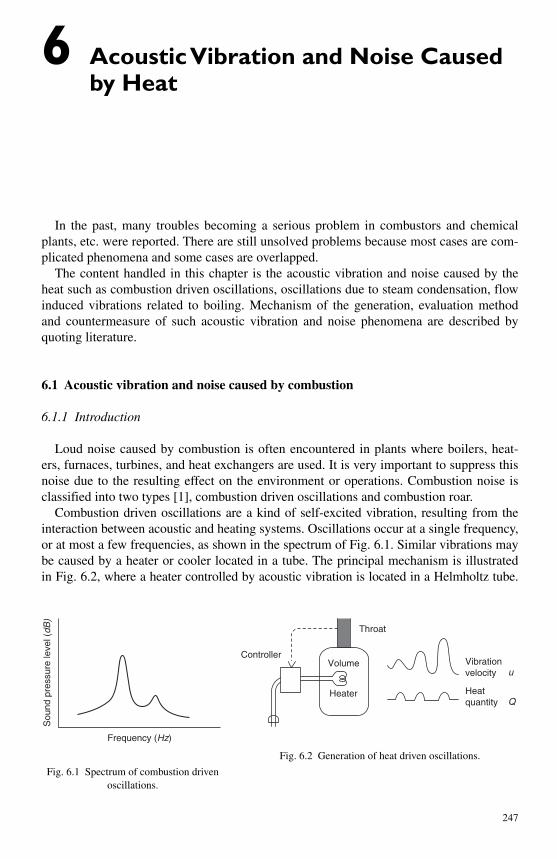
247
6 Acoustic Vibration and Noise Caused by Heat
In the past, many troubles becoming a serious problem in combustors and chemical plants, etc. were reported. There are still unsolved problems because most cases are com-plicated phenomena and some cases are overlapped.
The content handled in this chapter is the acoustic vibration and noise caused by the heat such as combustion driven oscillations, oscillations due to steam condensation, flow induced vibrations related to boiling. Mechanism of the generation, evaluation method and countermeasure of such acoustic vibration and noise phenomena are described by quoting literature.
6.1 Acoustic vibration and noise caused by combustion
6.1.1 Introduction
Loud noise caused by combustion is often encountered in plants where boilers, heat-ers, furnaces, turbines, and heat exchangers are used. It is very important to suppress this noise due to the resulting effect on the environment or operations. Combustion noise is classified into two types [1] , combustion driven oscillations and combustion roar.
Combustion driven oscillations are a kind of self-excited vibration, resulting from the interaction between acoustic and heating systems. Oscillations occur at a single frequency, or at most a few frequencies, as shown in the spectrum of Fig. 6.1 . Similar vibrations may be caused by a heater or cooler located in a tube. The principal mechanism is illustrated in Fig. 6.2 , where a heater controlled by acoustic vibration is located in a Helmholtz tube.
Fig. 6.1 Spectrum of combustion driven oscillations.
Sou
nd p
ress
ure
leve
l (dB
)
Frequency (Hz)
Fig. 6.2 Generation of heat driven oscillations.
Vibrationvelocity
Heatquantity
u
Q
Throat
Volume
Heater
Controller
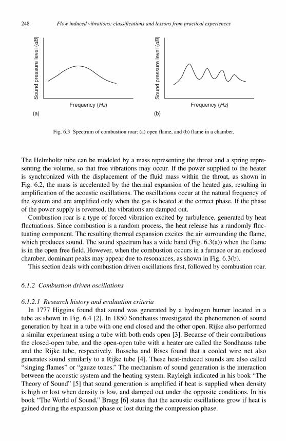
248 Flow induced vibrations: classifications and lessons from practical experiences
The Helmholtz tube can be modeled by a mass representing the throat and a spring repre-senting the volume, so that free vibrations may occur. If the power supplied to the heater is synchronized with the displacement of the fluid mass within the throat, as shown in Fig. 6.2, the mass is accelerated by the thermal expansion of the heated gas, resulting in amplification of the acoustic oscillations. The oscillations occur at the natural frequency of the system and are amplified only when the gas is heated at the correct phase. If the phase of the power supply is reversed, the vibrations are damped out.
Combustion roar is a type of forced vibration excited by turbulence, generated by heat fluctuations. Since combustion is a random process, the heat release has a randomly fluc-tuating component. The resulting thermal expansion excites the air surrounding the flame, which produces sound. The sound spectrum has a wide band ( Fig. 6.3(a) ) when the flame is in the open free field. However, when the combustion occurs in a furnace or an enclosed chamber, dominant peaks may appear due to resonances, as shown in Fig. 6.3(b) .
This section deals with combustion driven oscillations first, followed by combustion roar.
6.1.2 Combustion driven oscillations
6.1.2.1 Research history and evaluation criteria In 1777 Higgins found that sound was generated by a hydrogen burner located in a
tube as shown in Fig. 6.4 [2] . In 1850 Sondhauss investigated the phenomenon of sound generation by heat in a tube with one end closed and the other open. Rijke also performed a similar experiment using a tube with both ends open [3] . Because of their contributions the closed-open tube, and the open-open tube with a heater are called the Sondhauss tube and the Rijke tube, respectively. Bosscha and Rises found that a cooled wire net also generates sound similarly to a Rijke tube [4] . These heat-induced sounds are also called “ singing flames ” or “ gauze tones. ” The mechanism of sound generation is the interaction between the acoustic system and the heating system. Rayleigh indicated in his book “ The Theory of Sound ” [5] that sound generation is amplified if heat is supplied when density is high or lost when density is low, and damped out under the opposite conditions. In his book “ The World of Sound, ” Bragg [6] states that the acoustic oscillations grow if heat is gained during the expansion phase or lost during the compression phase.
Sou
nd p
ress
ure
leve
l (dB
)
Sou
nd p
ress
ure
leve
l (dB
)
Frequency (Hz) Frequency (Hz)
(a) (b)
Fig. 6.3 Spectrum of combustion roar: (a) open flame, and (b) flame in a chamber.
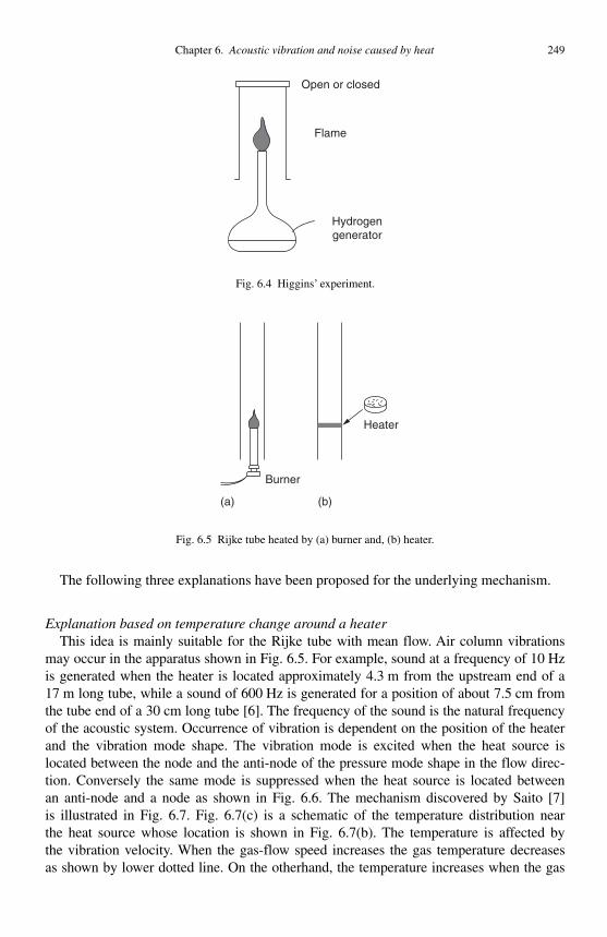
Chapter 6. Acoustic vibration and noise caused by heat 249
The following three explanations have been proposed for the underlying mechanism.
Explanation based on temperature change around a heater This idea is mainly suitable for the Rijke tube with mean flow. Air column vibrations
may occur in the apparatus shown in Fig. 6.5 . For example, sound at a frequency of 10 Hz is generated when the heater is located approximately 4.3 m from the upstream end of a 17 m long tube, while a sound of 600 Hz is generated for a position of about 7.5 cm from the tube end of a 30 cm long tube [6] . The frequency of the sound is the natural frequency of the acoustic system. Occurrence of vibration is dependent on the position of the heater and the vibration mode shape. The vibration mode is excited when the heat source is located between the node and the anti-node of the pressure mode shape in the flow direc-tion. Conversely the same mode is suppressed when the heat source is located between an anti-node and a node as shown in Fig. 6.6 . T he mechanism discovered by Saito [7] is illustrated in Fig. 6.7. Fig. 6.7(c) is a schematic of the temperature distribution near the heat source whose location is shown in Fig. 6.7(b) . The temperature is affected by the vibration velocity. When the gas-flow speed increases the gas temperature decreases as shown by lower dotted line. On the otherhand, the temperature increases when the gas
Burner
Heater
(a) (b)
Fig. 6.5 Rijke tube heated by (a) burner and, (b) heater.
Open or closed
Flame
Hydrogengenerator
Fig. 6.4 Higgins’ experiment.
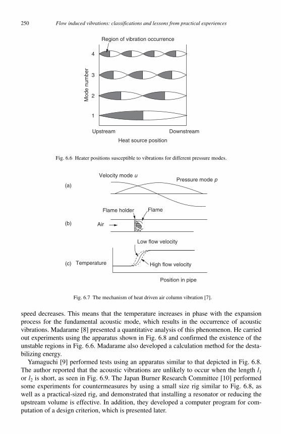
250 Flow induced vibrations: classifications and lessons from practical experiences
speed decreases. This means that the temperature increases in phase with the expansion process for the fundamental acoustic mode, which results in the occurrence of acoustic vibrations. Madarame [8] presented a quantitative analysis of this phenomenon. He carried out experiments using the apparatus shown in Fig. 6.8 and confirmed the existence of the unstable regions in Fig. 6.6 . Madarame also developed a calculation method for the desta-bilizing energy.
Yamaguchi [9] performed tests using an apparatus similar to that depicted in Fig. 6.8 .The author reported that the acoustic vibrations are unlikely to occur when the length l1or l2 is short, as seen in Fig. 6.9 . The Japan Burner Research Committee [10] performed some experiments for countermeasures by using a small size rig similar to Fig. 6.8 , as well as a practical-sized rig, and demonstrated that installing a resonator or reducing the upstream volume is effective. In addition, they developed a computer program for com-putation of a design criterion, which is presented later.
Velocity mode uPressure mode p
FlameFlame holder
Air
High flow velocity
Low flow velocity
Position in pipe
Temperature(c)
(b)
(a)
Fig. 6.7 The mechanism of heat driven air column vibration [7].
Region of vibration occurrence
Mod
e nu
mbe
r
Upstream
Heat source position
Downstream
1
2
3
4
Fig. 6.6 Heater positions susceptible to vibrations for different pressure modes.

Chapter 6. Acoustic vibration and noise caused by heat 251
Explanation by thermo-acoustic theory Katto et al. [11] performed experiments using a Sondhauss tube to examine the heat
excited vibration. The mechanism of vibration in a Sondhauss tube may be explained by thermo-acoustic theory. This approach was introduced by Swift [12] based on results by
Flame holder
Town gasPressure sensor
Combustion tube
l 2l 1
Air
Flow meter
Blower
Fig. 6.8 Acoustic vibration test apparatus [8, 9].
0 600
Large noise
l1, mm
l 2, m
m
Silent
0
600
Fig. 6.9 Vibration occurrence zone [9].
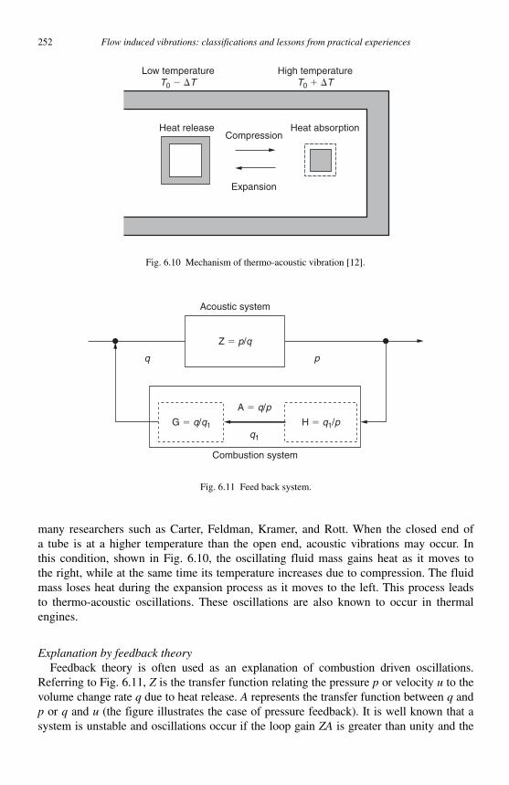
252 Flow induced vibrations: classifications and lessons from practical experiences
many researchers such as Carter, Feldman, Kramer, and Rott. When the closed end of a tube is at a higher temperature than the open end, acoustic vibrations may occur. In this condition, shown in Fig. 6.10, the oscillating fluid mass gains heat as it moves to the right, while at the same time its temperature increases due to compression. The fluid mass loses heat during the expansion process as it moves to the left. This process leads to thermo-acoustic oscillations. These oscillations are also known to occur in thermal engines.
Explanation by feedback theory Feedback theory is often used as an explanation of combustion driven oscillations.
Referring to Fig. 6.11, Z is the transfer function relating the pressure p or velocity u to the volume change rate q due to heat release. A represents the transfer function between q and p or q and u (the figure illustrates the case of pressure feedback). It is well known that a system is unstable and oscillations occur if the loop gain ZA is greater than unity and the
Low temperatureT0 � �T
High temperatureT0 � �T
Heat release Heat absorption
Expansion
Compression
Fig. 6.10 Mechanism of thermo-acoustic vibration [12].
G � q/q1
Z � p/q
H � q1/p
A � q/p
q1
Combustion system
q p
Acoustic system
Fig. 6.11 Feed back system.
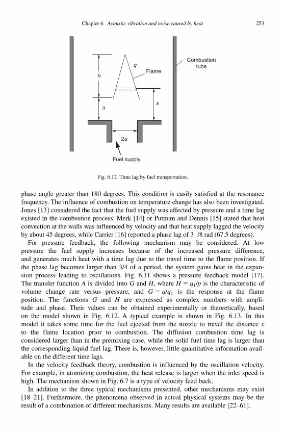
Chapter 6. Acoustic vibration and noise caused by heat 253
phase angle greater than 180 degrees. This condition is easily satisfied at the resonance frequency. The influence of combustion on temperature change has also been investigated. Jones [13] considered the fact that the fuel supply was affected by pressure and a time lag existed in the combustion process. Merk [14] or Putnum and Dennis [15] stated that heat convection at the walls was influenced by velocity and that heat supply lagged the velocity by about 45 degrees, while Carrier [16] reported a phase lag of 3 /8 rad (67.5 degrees).
For pressure feedback, the following mechanism may be considered. At low pressure the fuel supply increases because of the increased pressure difference, and generates much heat with a time lag due to the travel time to the flame position. If the phase lag becomes larger than 3/4 of a period, the system gains heat in the expan-sion process leading to oscillations. Fig. 6.11 shows a pressure feedback model [17] . The transfer function A is divided into G and H , where H � q1/p is the characteristic of volume change rate versus pressure, and G � q / q1 is the response at the flame position. The functions G and H are expressed as complex numbers with ampli-tude and phase. Their values can be obtained experimentally or theoretically, based on the model shown in Fig. 6.12 . A typical example is shown in Fig. 6.13 . In this model it takes some time for the fuel ejected from the nozzle to travel the distance xto the flame location prior to combustion. The diffusion combustion time lag is con sidered larger than in the premixing case, while the solid fuel time lag is larger than the corresponding liquid fuel lag. There is, however, little quantitative information avail-able on the different time lags.
In the velocity feedback theory, combustion is influenced by the oscillation velocity. For example, in atomizing combustion, the heat release is larger when the inlet speed is high. The mechanism shown in Fig. 6.7 is a type of velocity feed back.
In addition to the three typical mechanisms presented, other mechanisms may exist [18 – 21] . Furthermore, the phenomena observed in actual physical systems may be the result of a combination of different mechanisms. Many results are available [22–61] .
q
x
h
δ
Flame
2a
Fuel supply
Combustiontube
Fig. 6.12 Time lag by fuel transportation.
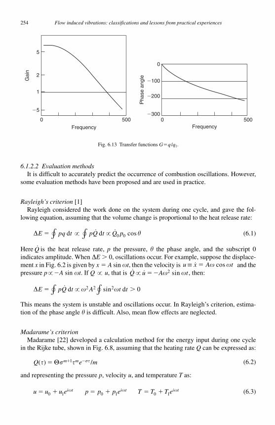
254 Flow induced vibrations: classifications and lessons from practical experiences
6.1.2.2 Evaluation methods It is difficult to accurately predict the occurrence of combustion oscillations. However,
some evaluation methods have been proposed and are used in practice.
Rayleigh ’ s criterion [1] Rayleigh considered the work done on the system during one cycle, and gave the fol-
lowing equation, assuming that the volume change is proportional to the heat release rate:
� �E pq t pQ t Q p� d d � � � �∫ ∫� � 0 0 cos (6.1)
Here �Q is the heat release rate, p the pressure, � the phase angle, and the subscript 0 indicates amplitude. When �E � 0, oscillations occur. For example, suppose the displace-ment x in Fig. 6.2 is given by x � A sin � t , then the velocity is u x A t� � � � �cos and the pressure p��A sin � t . If Q � u , that is � �Q u A t� � � � �2 sin , then:
� � �E pQ t A t t� ��� �d d∫ ∫� 2 2 2 0sin
This means the system is unstable and oscillations occur. In Rayleigh ’ s criterion, estima-tion of the phase angle � is difficult. Also, mean flow effects are neglected.
Madarame ’ s criterion Madarame [22] developed a calculation method for the energy input during one cycle
in the Rijke tube, shown in Fig. 6.8 , assuming that the heating rate Q can be expressed as:
Q mm m( ) /� � � ��� � �� 1 e (6.2)
and representing the pressure p , velocity u , and temperature T as:
u u u p p p T T Ti t i t i t� � � � � �0 1 0 1 0 1e e e� � � (6.3)
Frequency
5000
�5
1
2
5
Gai
n
Pha
se a
ngle
500�300
�200
�100
0
0Frequency
Fig. 6.13 Transfer functions G�q /q1.
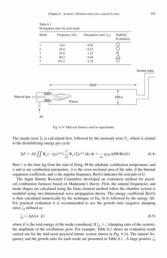
Chapter 6. Acoustic vibration and noise caused by heat 255
The steady term T0 is calculated first, followed by the unsteady term T1 , which is related to the destabilizing energy per cycle
� ���
�
��� �E A ip et
T e x t p u A G� � �R ( ) R ( )d d Re( )e e∫∫ 1 1 1 1i t i t (6.4)
Here � is the time lag from the start of firing, � the adiabatic combustion temperature, and � and m are combustion parameters. A is the cross-sectional area of the tube, � the thermal expansion coefficient, and � the angular frequency. Re( G ) indicates the real part of G .
The Japan Burner Research Committee developed an evaluation method for practi-cal combustion furnaces based on Madarame ’ s theory. First, the natural frequencies and mode shapes are calculated using the finite element method where the chamber system is modeled using one-dimensional wave propagation theory. The energy coefficient Re(G)is then calculated numerically by the technique of Eq. (6.4) followed by the energy � E .For practical evaluation it is recommended to use the growth ratio (negative damping ratio) �h defined as:
� � h � E E/( )4 (6.5)
where E is the total energy of the mode considered. If �h � � (damping ratio of the system), the amplitude of the oscillations grow. For example, Table 6.1 shows an evaluation result carried out for the mid-sized practical burner system shown in Fig. 6.14 . The natural fre-quency and the growth ratio for each mode are presented in Table 6.1 . A large positive �h
2009
Smoke tube
Natural gas
Flame
Air
296 φ
Fig. 6.14 Mid-size furnace used in experiments.
Table 6.1 Dissipation ratio for each mode
Mode Frequency ( Hz ) Dissipation ratio ( �h ) Stability Evaluation
1 19.8 � 5.02 2 45.8 � 0.23 3 65.8 1.22 4 80.2 0.04 5 167.2 � 2.38
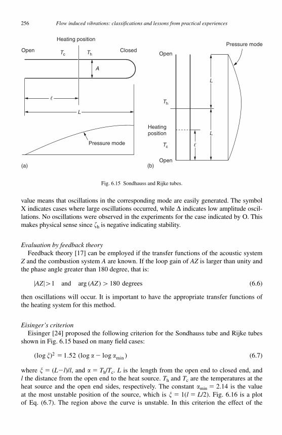
256 Flow induced vibrations: classifications and lessons from practical experiences
value means that oscillations in the corresponding mode are easily generated. The symbol X indicates cases where large oscillations occurred, while � indicates low amplitude oscil-lations. No oscillations were observed in the experiments for the case indicated by O. This makes physical sense since �h is negative indicating stability.
Evaluation by feedback theory Feedback theory [17] can be employed if the transfer functions of the acoustic system
Z and the combustion system A are known. If the loop gain of AZ is larger than unity and the phase angle greater than 180 degree, that is:
� �AZ AZ 1 180 and arg ( ) degrees (6.6)
then oscillations will occur. It is important to have the appropriate transfer functions of the heating system for this method.
Eisinger ’ s criterion Eisinger [24] proposed the following criterion for the Sondhauss tube and Rijke tubes
shown in Fig. 6.15 based on many field cases:
( ) . ( )log log log min� 2 1 52� � (6.7)
where � � ( L�l )/ l , and � Th / Tc . L is the length from the open end to closed end, and l the distance from the open end to the heat source. Th and Tc are the temperatures at the heat source and the open end sides, respectively. The constant min � 2.14 is the value at the most unstable position of the source, which is � � 1(l � L /2). Fig. 6.16 is a plot of Eq. (6.7). The region above the curve is unstable. In this criterion the effect of the
Heating position
Heatingposition
Tc
Tc
Th
Th
A
L
�
Pressure mode
Closed
Open(a) (b)
OpenOpen
L
L
�
Pressure mode
Fig. 6.15 Sondhauss and Rijke tubes.
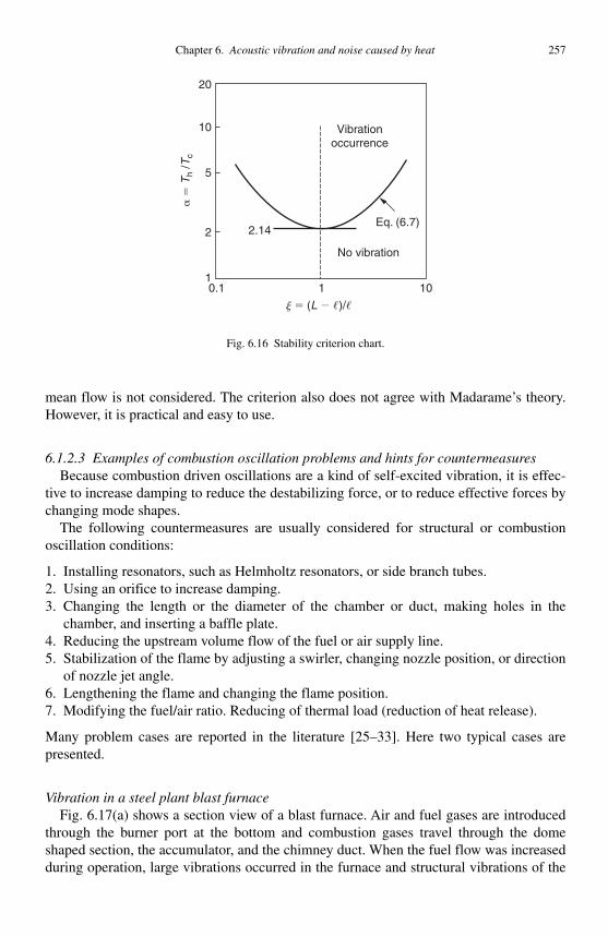
Chapter 6. Acoustic vibration and noise caused by heat 257
mean flow is not considered. The criterion also does not agree with Madarame ’ s theory. However, it is practical and easy to use.
6.1.2.3 Examples of combustion oscillation problems and hints for countermeasures Because combustion driven oscillations are a kind of self-excited vibration, it is effec-
tive to increase damping to reduce the destabilizing force, or to reduce effective forces by changing mode shapes.
The following countermeasures are usually considered for structural or combustion oscillation conditions:
1. Installing resonators, such as Helmholtz resonators, or side branch tubes. 2. Using an orifice to increase damping. 3. Changing the length or the diameter of the chamber or duct, making holes in the
chamber, and inserting a baffle plate. 4. Reducing the upstream volume flow of the fuel or air supply line. 5. Stabilization of the flame by adjusting a swirler, changing nozzle position, or direction
of nozzle jet angle. 6. Lengthening the flame and changing the flame position. 7. Modifying the fuel/air ratio. Reducing of thermal load (reduction of heat release).
Many problem cases are reported in the literature [25–33] . Here two typical cases are presented.
Vibration in a steel plant blast furnace Fig. 6.17(a) shows a section view of a blast furnace. Air and fuel gases are introduced
through the burner port at the bottom and combustion gases travel through the dome shaped section, the accumulator, and the chimney duct. When the fuel flow was increased during operation, large vibrations occurred in the furnace and structural vibrations of the
20
10
5
2
10.1 1 10
Vibrationoccurrence
Eq. (6.7)
No vibration
2.14
j � (L � �)/�
��
Th
/Tc
Fig. 6.16 Stability criterion chart.
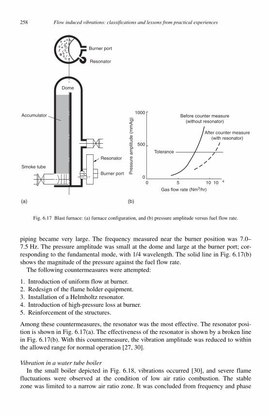
258 Flow induced vibrations: classifications and lessons from practical experiences
piping became very large. The frequency measured near the burner position was 7.0–7.5 Hz. The pressure amplitude was small at the dome and large at the burner port; cor-responding to the fundamental mode, with 1/4 wavelength. The solid line in Fig. 6.17(b) shows the magnitude of the pressure against the fuel flow rate.
The following countermeasures were attempted:
1. Introduction of uniform flow at burner. 2. Redesign of the flame holder equipment. 3. Installation of a Helmholtz resonator. 4. Introduction of high-pressure loss at burner. 5. Reinforcement of the structures.
Among these countermeasures, the resonator was the most effective. The resonator posi-tion is shown in Fig. 6.17(a) . The effectiveness of the resonator is shown by a broken line in Fig. 6.17(b) . With this countermeasure, the vibration amplitude was reduced to within the allowed range for normal operation [27, 30].
Vibration in a water tube boiler In the small boiler depicted in Fig. 6.18 , vibrations occurred [30], and severe flame
fluctuations were observed at the condition of low air ratio combustion. The stable zone was limited to a narrow air ratio zone. It was concluded from frequency and phase
Fig. 6.17 Blast furnace: (a) furnace configuration, and (b) pressure amplitude versus fuel flow rate.
Dome
Resonator
Burner port
Accumulator
Resonator
Burner port
Smoke tube
(a)
1000Before counter measure
(without resonator)
After counter measure(with resonator)
Tolerance
Pre
ssur
e am
plitu
de (
mm
Ag)
500
00 5 10 104
Gas flow rate (Nm3/hr)
(b)
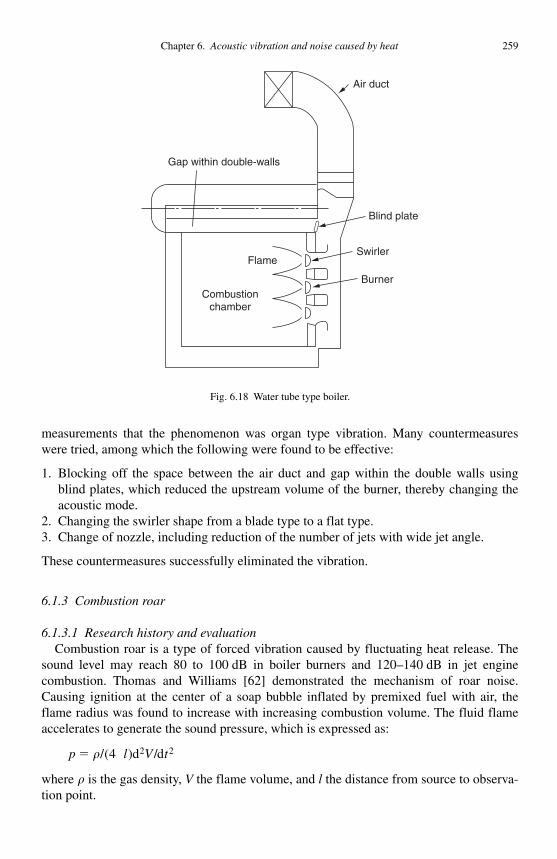
Chapter 6. Acoustic vibration and noise caused by heat 259
measurements that the phenomenon was organ type vibration. Many countermeasures were tried, among which the following were found to be effective:
1. Blocking off the space between the air duct and gap within the double walls using blind plates, which reduced the upstream volume of the burner, thereby changing the acoustic mode.
2. Changing the swirler shape from a blade type to a flat type. 3. Change of nozzle, including reduction of the number of jets with wide jet angle.
These countermeasures successfully eliminated the vibration.
6.1.3 Combustion roar
6.1.3.1 Research history and evaluation Combustion roar is a type of forced vibration caused by fluctuating heat release. The
sound level may reach 80 to 100 dB in boiler burners and 120–140 dB in jet engine combustion. Thomas and Williams [62] demonstrated the mechanism of roar noise. Causing ignition at the center of a soap bubble inflated by premixed fuel with air, the flame radius was found to increase with increasing combustion volume. The fluid flame accelerates to generate the sound pressure, which is expressed as:
p l V t� � / d /d( )4 2 2
where � is the gas density, V the flame volume, and l the distance from source to observa-tion point.
Blind plate
Swirler
Burner
Flame
Combustionchamber
Gap within double-walls
Air duct
Fig. 6.18 Water tube type boiler.

260 Flow induced vibrations: classifications and lessons from practical experiences
The work of many researchers on combustion roar, for example, Smith and Kilham [63] , Hurle [64] , Strahe [65] , Shivashankara [66] , and others, has been discussed by Suzuki [67] . In Japan, Kotake [68] , Irie [69] , Kazuki et al. [70] , as well as the JSME research committee [1] have studied and reported on combustion roar. Other work is also reported in references [71–94].
Flow in a flame normally becomes turbulent in practical burners, resulting in ran-domly fluctuating combustion. This non-uniform combustion becomes a monopole sound source. Kazuki et al. [70] state that roar consists of local roar, tip combustion roar, and jet sound, based on observation of a turbulent Bunsen burner. In a flame such as shown in Fig. 6.19, turbulence generated by the instability of the shear layer around the burner is amplified by combustion when it goes through the flame zone and propagates upward accompanying the local roar. On the other hand, the flow at the central part is ignited at random by turbulence from the flame tip, causing tip roar. In addition, gas flow is accel-erated by thermal expansion, producing noise by shear action.
6.1.3.2 Evaluation methods The combustion roar sound power has been estimated by many researchers. Generally,
the power P is dependent on the velocity U , the burner size D , the combustion speed S , and can be expressed in the form:
P U S D� � �
For the various types of flames the following relations have been proposed:
Thomas (cubic flame) : P S D� 2
Smith (premixed flame) : P U S D� 2 2 2
Strahe (spreading flame) : P U S D� 3 3 2
Strahe (wrinkle flame) : P U S D� 3 3 3
Kotake, Hatta (diffusion flame) : P U D� 4 3
Shivashankara (premixed flame) : P U S D� 2 68 1 35 2 84. . .
Muthukrishnan (flame holder) : P U S D� 2083 1 89 2 77. .
Jet noise
Flame tip roar
Localcombustion roar
Mixture
Fig. 6.19 Turbulent flame.
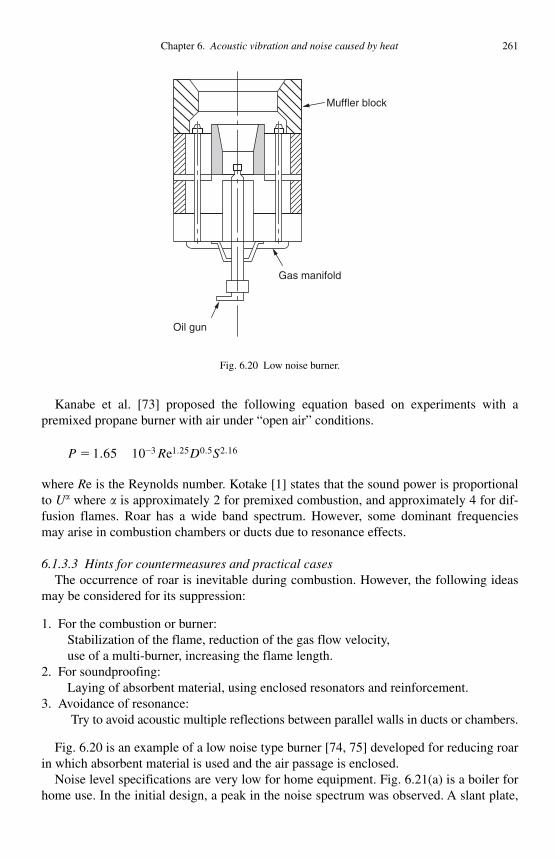
Chapter 6. Acoustic vibration and noise caused by heat 261
Kanabe et al. [73] proposed the following equation based on experiments with a premixed propane burner with air under “ open air ” conditions.
P R D S� �1 65 10 3 1 25 0 5 2 16. . . .e
where Re is the Reynolds number. Kotake [1] states that the sound power is proportional to U where is approximately 2 for premixed combustion, and approximately 4 for dif-fusion flames. Roar has a wide band spectrum. However, some dominant frequencies may arise in combustion chambers or ducts due to resonance effects.
6.1.3.3 Hints for countermeasures and practical cases The occurrence of roar is inevitable during combustion. However, the following ideas
may be considered for its suppression:
1. For the combustion or burner: Stabilization of the flame, reduction of the gas flow velocity, use of a multi-burner, increasing the flame length.
2. For soundproofing: Laying of absorbent material, using enclosed resonators and reinforcement.
3. Avoidance of resonance: Try to avoid acoustic multiple reflections between parallel walls in ducts or chambers.
Fig. 6.20 is an example of a low noise type burner [74, 75] developed for reducing roar in which absorbent material is used and the air passage is enclosed.
Noise level specifications are very low for home equipment. Fig. 6.21(a) is a boiler for home use. In the initial design, a peak in the noise spectrum was observed. A slant plate,
Oil gun
Gas manifold
Muffler block
Fig. 6.20 Low noise burner.
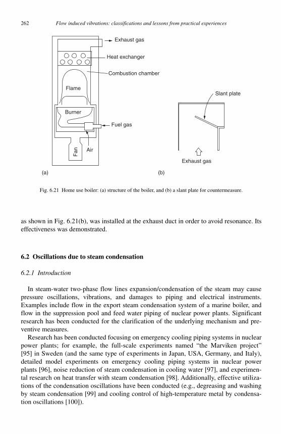
262 Flow induced vibrations: classifications and lessons from practical experiences
as shown in Fig. 6.21(b), was installed at the exhaust duct in order to avoid resonance. Its effectiveness was demonstrated.
6.2 Oscillations due to steam condensation
6.2.1 Introduction
In steam-water two-phase flow lines expansion/condensation of the steam may cause pressure oscillations, vibrations, and damages to piping and electrical instruments. Examples include flow in the export steam condensation system of a marine boiler, and flow in the suppression pool and feed water piping of nuclear power plants. Significant research has been conducted for the clarification of the underlying mechanism and pre-ventive measures.
R esearch has been conducted focusing on emergency cooling piping systems in nuclear power plants; for example, the full-scale experiments named “ the Marviken project ” [95] in Sweden (and the same type of experiments in Japan, USA, Germany, and Italy), detailed model experiments on emergency cooling piping systems in nuclear power plants [96] , noise reduction of steam condensation in cooling water [97] , and experimen-tal research on heat transfer with steam condensation [98] . Additionally, effective utiliza-tions of the condensation oscillations have been conducted (e.g., degreasing and washing by steam condensation [99] and cooling control of high-temperature metal by condensa-tion oscillations [100] ).
Heat exchanger
Combustion chamber
Exhaust gas
Fuel gas
Air
Fan
Burner
FlameSlant plate
(a) (b)
Exhaust gas
Fig. 6.21 Home use boiler: (a) structure of the boiler, and (b) a slant plate for countermeasure.
Chapter 6. Acoustic vibration and noise caused by heat 263
6.2.2 Characteristics and prevention
Pressure oscillations caused by condensation (condensation oscillations) can be clas-sified into “ chugging, ” “ two-phase flow oscillations in piping, ” and “ steam hammer ” [101,102] . Table 6.2 and Fig. 6.22 show the characteristics of condensation oscillations, affected systems, and preventive methods. Chugging and steam hammer result in large amplitude pressure oscillations. Although two-phase flow in piping generally results in relatively small amplitudes, sustained large amplitude system oscillations may occur in the case of a sudden increase of the cooling water flow rate.
6.2.3 Examples of practical problems
1. Experiment on feed water piping system for nuclear power plant [103] : In 1989, at the LOUVIISA nuclear power plant (Russia), a steam hammer experiment at the
Table 6.2 Condensation induced oscillations
Class Chugging Two-phase flow oscillationsin piping
Steam hammer
Cause 1. Inflow of steam to cooling water.
Water/steam two-phase flow in piping system.
Trapping of steam in cooling water.
2. Inflow of cooling water to steam flow.
Characteristics 1. Flow oscillation by time-lag between steam inflow rate and condensation rate.
2. Flow oscillation by relation among the inertia, condensation rate and pressure fluctuation.
Flow oscillation by sudden change in condensation rate caused by sudden change of cooling water flow rate.
Water hammer by sudden condensation of trapped steam.
Affected system 1. Boiler export steam condensation system.
Water/steam two-phase piping system.
Boiler and nuclear power plant feed water line.
2. Nuclear power plant suppression pool.
Preventive method
1. Raise cooling water temperature.
Enlarge piping diameter.
Avoid sudden increase of the cooling water flow rate.
Enlarge piping diameter.
Avoid accumulation in piping.
Introduce slope in piping system.
Install drain trap at lower elevation of piping system.
Mix air to reduce condensation speed.
Suppress condensation by mixing noncondensable gas.
Make outflow pattern random using many different diameter holes.
2. Raise cooling water temperature.
Increase steam flow rate.
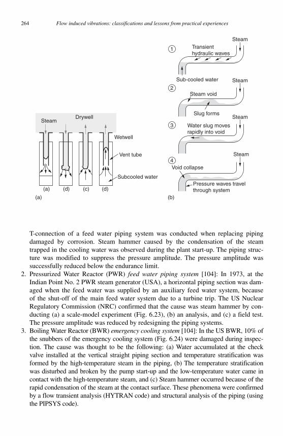
264 Flow induced vibrations: classifications and lessons from practical experiences
T-connection of a feed water piping system was conducted when replacing pipingdamaged by corrosion. Steam hammer caused by the condensation of the steam trapped in the cooling water was observed during the plant start-up. The piping struc-ture was modified to suppress the pressure amplitude. The pressure amplitude was successfully reduced below the endurance limit.
2. Pressurized Water Reactor (PWR) feed water piping system [104] : In 1973, at the Indian Point No. 2 PWR steam generator (USA), a horizontal piping section was dam-aged when the feed water was supplied by an auxiliary feed water system, because of the shut-off of the main feed water system due to a turbine trip. The US Nuclear Regulatory Commission (NRC) confirmed that the cause was steam hammer by con-ducting (a) a scale-model experiment ( Fig. 6.23 ), (b) an analysis, and (c) a field test. The pressure amplitude was reduced by redesigning the piping systems.
3. Boiling Water Reactor (BWR) emergency cooling system [104] : In the US BWR, 10% of the snubbers of the emergency cooling system ( Fig. 6.24 ) were damaged during inspec-tion. The cause was thought to be the following: (a) Water accumulated at the check valve installed at the vertical straight piping section and temperature stratification was formed by the high-temperature steam in the piping, (b) The temperature stratification was disturbed and broken by the pump start-up and the low-temperature water came in contact with the high- temperature steam, and (c) Steam hammer occurred because of the rapid condensation of the steam at the contact surface. These phenomena were confirmed by a flow transient analysis (HYTRAN code) and structural analysis of the piping (using the PIPSYS code).
SteamDrywell
Wetwell
Transienthydraulic waves
Sub-cooled water
Steam
Steam
SteamSlug forms
Steam void
Water slug movesrapidly into void
Steam
Void collapse
Pressure waves travelthrough system
Vent tube
(a)
(a) (b)
(d) (c) (d)
Subcooled water
1
2
3
4
Fig. 6.22 Schematics of chugging and steam hammer: (a) chugging, and (b) steam hammer [104].
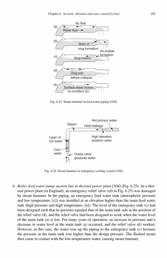
Chapter 6. Acoustic vibration and noise caused by heat 265
4. Boiler feed water pump suction line in thermal power plant [104] ( Fig. 6.25 ): At a ther-mal power plant (in England), an emergency relief valve ((d) in Fig. 6.25 ) was damaged by steam hammer. In the piping, an emergency feed water tank (atmospheric pressure and low temperature, [c]) was installed at an elevation higher than the main feed water tank (high pressure and high temperature, [a]). The level of the emergency tank (c) had been designed such that its pressure equaled that of the main tank side at the position of the relief valve (d), and the relief valve had been designed to work when the water level of the main tank (a) is low. For many years of operation, an increase in pressure and a decrease in water level at the main tank (a) occurred, and the relief valve (d) worked. However, in this case, the water rose up the piping to the emergency tank (c) because the pressure at the main tank was higher than the design pressure. The flushed steam then came in contact with the low-temperature water, causing steam hammer.
Air flow(a)
(b)
(c)
(d)
(e)
Water flow
Start of
slug formation
Slug motion
Slug just
before collapse
Surface wave motionto condition (b)
Air bubbleformation
Fig. 6.23 Steam hammer in feed water piping [104] .
Check valvegradually leaks
Coolwater
Layer ofhot water
SteamHot primary water
Heat leakage
High elevationisolation valve
Fig. 6.24 Steam hammer at emergency cooling system [104] .

266 Flow induced vibrations: classifications and lessons from practical experiences
6.3 Flow induced vibrations related to boiling
6.3.1 Introduction/background
Flow-induced vibrations in boiling systems may cause structural fatigue failure. Furthermore, such vibrations may compromise the ability to control system pressure, temperature, and flow rate. Other possible outcomes include temperature increase in pipe walls due to the decrease in burnout heat flux, and thermal fatigue failure due to tempera-ture fluctuations on the pipe wall. In order to avoid vibrations in boiling systems, a thor-ough study to evaluate potential vibration mechanisms is required at the design stage.
A study by Ledinegg [105] on pulsations in a boiler header represents the first research work in the field of boiling two-phase flow. Thereafter, research on a Fast Breeder Reactor (FBR) steam generator, a Liquefied Natural Gas (LNG) plant vaporizer, and a reboiler in a heat recovery system was conducted [106] . The review papers [107–110]present a historical background of this research.
6.3.2 Vibration mechanisms
The generation mechanisms of flow-induced vibrations related to boiling are varied. In many cases vibration is often caused by more than one mechanism. A classification based on the basic mechanisms is presented in Table 6.3 [111–112] .
6.3.3 Analytical approach
Only a few estimation methods have been developed for the analysis of vibration in boiling systems. One of these methods, an analytical model for pressure drop type
(d) Emergency valve
(a) Hot feed tank (250�F)
(c) Reserve feed tank (70�F)
(b) Boiler feed pump
Fig. 6.25 Feed water piping in boiler [104] .
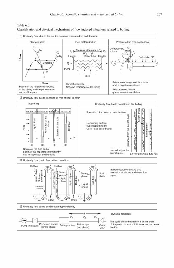
Chapter 6. Acoustic vibration and noise caused by heat 267
Table 6.3Classification and physical mechanisms of flow induced vibrations related to boiling
1
1
2
3
4
B
DP
Pressure difference �P
Unstable
Q1 P1
Q
Q2
AD
Based on the negative resistanceof the piping and the performancecurve of the pump
C
2 (P1 – P2)P2
Header Header Boiler tube �P
Compressiblevolume
Existence of compressible volumeand a negative resistance
Relaxation oscillation, quasi-harmonic oscillation
Unsteady flow due to transition of film boiling
Parallel channels
Heat
Pump
Negative resistance of the piping
Boiler tube
Unsteady flow due to the relation between pressure drop and flow rate
Flow excursion Flow maldistribution Pressure drop type-oscillations
P
Av
Vg
APg
Lv
Lr
LA
Le
Uv
ui
Pi
uo
Unsteady flow due to transition of type of heat transfer
Geysering
Liqu
id fi
lled
(a)
(a)
(b) (c) (d)
Hea
t
Spouts of the fluid and abackflow are repeated intermittentlydue to superheat and bumping
Unsteady flow due to flow pattern transition
Unsteady flow due to density wave type instability
Outflow Outflow
Steamphase
Steamphase
Bubble coalescence and slugformation at elbows and down flowpipes
Liquidphase
Inflow Inflow
Liquidphase
Liqu
id p
hase
Liqu
id p
hase
Bac
kflo
w
Bac
kflo
w
Sta
tiona
ryst
eam
pha
se
Ups
trea
m b
ound
ary
For
mat
ion
of th
e b
ubbl
e
Spo
uts
of th
e flu
id
Bac
kflo
w
Formation of an inverted annular flow
Generating surface –superheated steamCore – sub cooled water
Inlet velocity at thequench point 0.17 m/s 0.57 m/s 1.43 m/s
Dis
tanc
e fr
om th
e qu
ench
poi
nt
Ste
am p
hase
Liqu
id p
hase
Pump Inlet valvePreheated section
(single phase)Boiling section
The cycle of flow fluctuation is of the orderof the period in which fluid traverses the heatedsection
Outletvalve
Dynamic feedback
Raiser pipe(two phase)
θ
θ θ θ
θ
PB Ug
LPe
θ
Downstreamboundary
Liquidphase

268 Flow induced vibrations: classifications and lessons from practical experiences
oscillations [113] , is explained in this section as an example of a non-linear analysis. A single boiling piping system, which is fitted with a surge tank between the supply tank and the heating tube, is shown in Fig. 6.26 . The relation between flow rate Q2 and the pressure difference �P2 � P2�Pe between the surge tank and the exit of the heating tube is shown in Fig. 6.27 . The relation between the flow rate Q1 at the valve upstream of the surge tank and the pressure drop �P1 � P1�P2 corresponds to line No. 1 in Fig. 6.28 . Onthe other hand, the relation between the flow rate to the heating tube Q2 and the pressure
D
�P
(105
Pa)
E
3
2
1
0 0.5 1.0
m (kg/s)
1.5
C
B
AGeneration of density-wave type oscillationsGeneration of pressure droptype oscillations
heat flow rateA 2 q0B 1.5C 1.2D 0.9E 0
Fig. 6.27 Characteristic curves of mass flow rate m in the heating tube versus the pressure difference �P between the inlet and outlet. The conditions for generation of density-wave type oscillations (heat flow rate q0 � 2931 W),
and pressure drop type oscillations are also shown.
P1 (Constant)
Supply tank
Heating tube
Pe (Constant)
P2, Vs
Q1Qs
Q2P
Fig. 6.26 Single boiling piping system.

Chapter 6. Acoustic vibration and noise caused by heat 269
drop �P2 � P2� Pe corresponds to line No. 2 in the same figure. To simplify the analysis, the pressure P1 in the supply tank and the pressure Pe at the heating tube exit are assumed constant. Consider now the case where the condition of the system is somewhere between point B and D on line No. 2 in Fig. 6.28 . Perturbation of the pressure P2 causes the flow rate Q2 to decrease along the line BD thereby increasing the pressure P2 . Since the flow rate Q1 becomes higher than the flow rate Q2 , the water level in the surge tank increases, resulting in an increase of the pressure P2 to the point B. As the pressure for line No. 1 corresponding to the flow rate at point B is different from that for line No. 2, point B cannot be stable. The operating point of the system consequently jumps from point B to point C, causing a sudden increase of the flow rate Q2 . At point C, since the flow rate Q2
is higher than the flow rate Q1 , the water level in the surge tank decreases. This causes the pressure P2 to decrease to point D. Similarly to point B, the system is unstable at point D. The operating point therefore jumps from point D to point A with a sudden decrease of the flow rate Q2 . The flow rate Q2 is, however, lower than the flow rate Q1 at point A. The pressure in the surge tank P2 increases to point B and the cycle is repeated, resulting in the generation of vibration.
Hence, for a pressure drop type oscillation, the existence of a compressible volume, such as a surge tank, and a negative resistance element in the system are dominant fac-tors. Other than these factors, the following characteristics of pressure drop type oscilla-tions are worth noting:
1. An increase of the negative gradient of the pressure versus flow rate characteristic, an increase of a heat duty, or an increase of the pressure drop at the exit all have a desta-bilizing effect.
2. A horizontal boiling piping system is more stable than a vertical one.
A numerical model for pressure drop type oscillation taking into consideration the charac-teristics of the foregoing destabilization mechanism was proposed by Nakanishi et al. [113] .
Pre
ssur
e dr
op
Flow rate
Unstable
B
AD
C
DP2
DP1
1
2
Fig. 6.28 Relation between flow rate and pressure drop for pressure drop type oscillations. Limit cycle is formed.
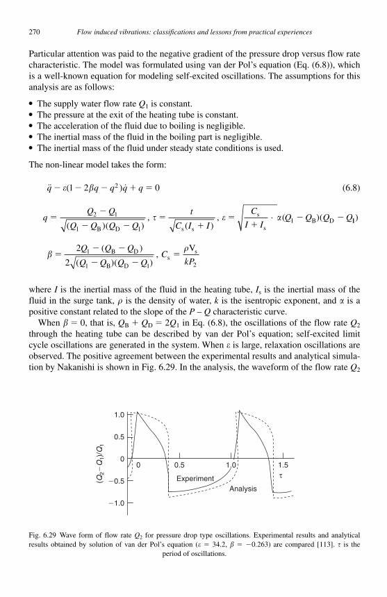
270 Flow induced vibrations: classifications and lessons from practical experiences
Particular attention was paid to the negative gradient of the pressure drop versus flow rate characteristic. The model was formulated using van der Pol ’ s equation (Eq. (6.8)), which is a well-known equation for modeling self-excited oscillations. The assumptions for this analysis are as follows:
● The supply water flow rate Q1 is constant. ● The pressure at the exit of the heating tube is constant. ● The acceleration of the fluid due to boiling is negligible. ● The inertial mass of the fluid in the boiling part is negligible. ● The inertial mass of the fluid under steady state conditions is used.
The non-linear model takes the form:
�� �q q q q q� � � � �� �( )1 2 02 (6.8)
q ��
� ��
��
�� �
Q Q
Q Q Q Q
t
C I I
C
I IQ Q Q Q2 1
1 11
( )( ),
( ), ( )(
s s
s
sB D
B D
� � ⋅ 11)
��
�� �
� ��
2
21
1 1 2
Q Q Q
Q Q Q QC
kP
( )
( )( ),
VB D
B Ds
s
where I is the inertial mass of the fluid in the heating tube, Is is the inertial mass of the fluid in the surge tank, � is the density of water, k is the isentropic exponent, and is a positive constant related to the slope of the P – Q characteristic curve.
When � � 0, that is, QB � QD � 2 Q1 in Eq. (6.8), the oscillations of the flow rate Q2
through the heating tube can be described by van der Pol ’ s equation; self-excited limit cycle oscillations are generated in the system. When � is large, relaxation oscillations are observed. The positive agreement between the experimental results and analytical simula-tion by Nakanishi is shown in Fig. 6.29 . In the analysis, the waveform of the flow rate Q2
1.0
0.5
00
(Q2�
Q1)
/Q1
0.5
ExperimentAnalysis
1.0 1.5τ
�0.5
�1.0
Fig. 6.29 Wave form of flow rate Q2 for pressure drop type oscillations. Experimental results and analytical results obtained by solution of van der Pol ’ s equation ( � � 34.2, � � � 0.263) are compared [113] . � is the
period of oscillations.

Chapter 6. Acoustic vibration and noise caused by heat 271
was obtained by use of Eq. (6.8), using values of � and � corresponding to experimental conditions. A cycle of the pressure drop type oscillation corresponds to a complete cycle about the limit cycle.
6.3.4 Vibration/oscillation problems and solutions
Boilers, nuclear steam generators, and BWRs are examples of facilities that may suffer flow-induced vibrations related to boiling [114] . In the 1960s oscillations of the sodium exit temperature were observed in a FBR and, consequently, research on these systems has been performed in many countries [106] . Since numerous references for these prob-lems may be found in [106] and [114] , they will not be considered here. Instead, exam-ples of problems experienced in other industries will be presented in what follows.
6.3.4.1 Thermosyphone reboiler
Geysering Geysering is an unsteady two-phase flow phenomenon observed in systems such as
those shown in Table 6.3 . Spouts of gas and liquid, as well as reverse liquid flow, are repeated intermittently. The basic mechanism is the same as that of geysers observed in natural hot springs.
In oil refineries, gas and chemical plants, geysering can occur in the exit piping of ther-mosyphone side reboilers if the elevation of the reboiler is sufficiently low [115]. Referring to Fig. 6.30 in the case of a low load, bubbly flow or slug flow is formed in the exit pip-ing. Consequently, only the gas flows up the column while the liquid level in the piping
Column
Return pipe
Side reboiler
Fig. 6.30 Geysering in thermosyphone side reboiler [115] .

272 Flow induced vibrations: classifications and lessons from practical experiences
increases gradually. As the boiling point increases in the piping due to the increase of static pressure, heat is accumulated in the liquid. When liquid flow into the column com-mences, the static pressure and the boiling point decrease, resulting in evaporation in the spout. The liquid level decreases due to liquid outflow caused by the foregoing combina-tion of a static pressure decrease and evaporation effects, and the system returns to the previous low liquid level. A cycle of flow fluctuation by geysering may last between 1 and 3 minutes ( Fig. 6.31 ).
The effects of geysering on equipment include:
● Piping vibration due to sudden fluctuations in the internal flow momentum. ● Damage of internals in columns due to intermittent influx of two-phase flow.
As countermeasures, the following points should be considered in the design:
● Shortening length of return piping. ● Appropriate determination of pipe size to maintain high flow rates thereby avoiding
unstable flow conditions.
Density-wave type oscillations Fatigue failure and leakage caused by thermal stress fluctuations induced by den-
sity-wave type oscillations in a reboiler were experienced as reported in Ref. [116] . The pressure pulsation period at the exit of the reboiler was about 25 s; thus, it is a very low frequency phenomenon. Increasing the pressure drop in the inlet piping by installing a valve was effective in reducing the pressure pulsations.
The following measures may be effective against flow oscillations in thermosyphone reboilers.
Pre
ssur
e di
ffere
nce
in th
e co
lum
nG
as fl
ow r
ate
at th
eto
p of
the
colu
mn
Time
Time
Fig. 6.31 Flow rate fluctuation and pressure difference observed in the column due to geysering.
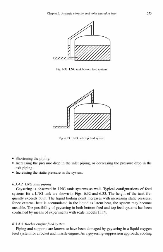
Chapter 6. Acoustic vibration and noise caused by heat 273
● Shortening the piping. ● Increasing the pressure drop in the inlet piping, or decreasing the pressure drop in the
exit piping. ● Increasing the static pressure in the system.
6.3.4.2 LNG tank piping Geysering is observed in LNG tank systems as well. Typical configurations of feed
systems for a LNG tank are shown in Figs. 6.32 and 6.33 . The height of the tank fre-quently exceeds 30 m. The liquid boiling point increases with increasing static pressure. Since external heat is accumulated in the liquid as latent heat, the system may become unstable. The possibility of geysering in both bottom feed and top feed systems has been confirmed by means of experiments with scale models [117] .
6.3.4.3 Rocket engine feed system Piping and supports are known to have been damaged by geysering in a liquid oxygen
feed system for a rocket and missile engine. As a geysering-suppression approach, cooling
Fig. 6.32 LNG tank bottom feed system.
Fig. 6.33 LNG tank top feed system.
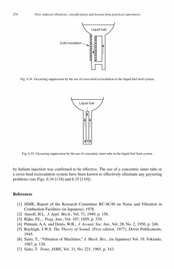
274 Flow induced vibrations: classifications and lessons from practical experiences
by helium injection was confirmed to be effective. The use of a concentric inner tube or a cross-feed recirculation system have been known to effectively eliminate any geysering problems (see Figs. 6.34 [118] and 6.35 [119] ).
References
[1] JSME, Report of the Research Committee RC-SC40 on Noise and Vibration in Combustion Facilities (in Japanese), 1978.
[2] Ansoff , H.I. , J. Appl. Mech. , Vol. 71 , 1949 , p. 158 . [3] Rijke , P.L. , Pogg. Ann. , Vol. 107 , 1859 , p. 339 . [4] Putnum , A.A. and Denis , W.R. , J. Acoust. Soc. Am. , Vol. 28 , No. 2 , 1956 , p. 246 . [5] Rayleigh , J.W.S. The Theory of Sound, (First edition, 1877) , Dover Publications ,
1945 . [6] Saito , T. , “ Vibration of Machines, ” J. Mach. Res. , (in Japanese) Vol. 19 , Yokendo,
1967 , p. 120 . [7] Saito , T. Trans. JSME , Vol. 31 , No. 221 , 1965 , p. 143 .
Liquid fuel
Fig. 6.35 Geysering suppression by the use of concentric inner tube in the liquid fuel feed system.
Liquid fuel
Cold insulation
Fig. 6.34 Geysering suppression by the use of cross-feed recirculation in the liquid fuel feed system.
Chapter 6. Acoustic vibration and noise caused by heat 275
[8] Madarame, H. Trans. JSME (in Japanese), C47-413, 10 (1st report, 1981), C47-416, 434 (2nd, 1981),C48-432, 1157 (3rd, 1982).
[9] Yamaguti, T. Kansai University (in Japanese), Dissertation, 1996. [10] Yamamoto, H. Report of Tanigawa Thermal Engineering Promotion Fund (in
Japanese), 1995. [11] Katto , Y. et al ., Trans. JSME (in Japanese), Vol. 43 , No. 365 , 1977 , p. 203 . [12] Swift , G.W. , J. Acoust. Soc. Am. , Vol. 84 , No. 4 , 1988 , p. 1145 . [13] Jones , A.T. , J. Acoust. Soc. Am. , Vol. 16 , No. 4 , 1945 , p. 254 . [14] Merk, H.J., 6th Symposium on Combustion , the Combustion Institute, 1956, p. 500. [15] Putnum , A.A. and Dennis , W.R. , J. Acoust. Soc. Am. , Vol. 25 , No. 5 , 1954 , p. 716 . [16] Carrier , G.F. , Quart. Appl. Math. , Vol. 12 , 1955 , p. 383 . [17] Baade , P.K. , ASHRAE Trans. , Vol. 78 , No. 2 , 1978 , p. 449 . [18] Nagahiro, T. et al., JSME Paper (in Japanese), No. 760-4, 1976, p. 21. [19] Mizutani, Y. et al., JSME Paper (in Japanese), No. 954-4, 1995, 84. [20] Suga , T. et al. , J. Mach. Res. (in Japanese), Vol. 47 , No. 12 , 1995 , p. 44 . [21] Kadowaki, S. Trans. JSME (in Japanese), B56-527, 1990, p. 2104. [22] Madarame, H. Trans. JSME (in Japanese), C48-432, p. 1157. [23] Fujikawa, T. et al., JSME Paper (in Japanese), No. 981-2, 1998, 41, No. 98-7, 1998. [24] Eisinger , F.L. , J. Trans. ASME , Vol. 121 , 1999 , p. 444 . [25] JSME, Report of Research Committee RC-SC40 (in Japanese), 1978, p. 10. [26] Putnum , A.A., Combustion Driven Oscillations in Industry , American Elsevier
Publishers, New York, NY , 1971 . [27] Kameda , J. Therm. Contr. (in Japanese), Vol. 23 , No. 5 , 1970 , p. 14 . [28] Kobayashi, S. JSME Kansai 173th Seminar Material (in Japanese), 1990, p. 79. [29] Japan Burner Research Committee, J. JBRC (in Japanese), No. 33, 25, No. 35, p. 1. [30] Aoki and Saima, A.K. Report of Nihon Daigaku Science and Engineering Institute
(in Japanese), 1987, p. 496. [31] Akiyama, I. “ Combustion Driven Oscillation on Multi-spad Burner, ” Hiroshima
University Dissertation (in Japanese), 1995. [32] Tabata , S. A. et al ., Tech. Rep. Tokyo Gas (in Japanese), Vol. 24 , 1949 , p. 225 . [33] Kaneko, S. JSME D & D00 Forum (in Japanese), No. 00-6, 2000, p. 25. [34] Yamamoto, T. Tech. Rep. Mitsubishi Heavy Indust. (in Japanese), Vol. 5 , No. 5 , 1968 . [35] Hiruta , T. et al ., Trans. JSME (in Japanese), Vol. B45 , No. 398 , 1979 , p. 1557 . [36] Ikugoe , H. et al. , Trans. JSME (in Japanese), Vol. B48 , No. 426 , 1982 , p. 373 . [37] Ono, M. et al., JSME Paper (in Japanese), No. 940-261, 1994, p. 597. [38] Ishii, T. et al., JSME Paper (in Japanese), No. 940-261, 1994, p. 93. [39] Ishii , X. T. et al. , Trans. JSME (in Japanese), Vol. B 50 , No. 449 , 1984 , p. 151 . [40] Akiyama , I. Indust. Heating (in Japanese), Vol. 28 , No. 4 , 1991 , p. 65 . [41] Akiyama , I. Trans. JSME (in Japanese), Vol. B61 , No. 588 , 1995 , p. 3082 . [42] Segawa , Y. Trans. JSME (in Japanese), Vol. B53 , No. 486 , 1987 , p. 642 . [43] Tabata , A. Tech. Rep. Tokyo Gas (in Japanese), Vol. 24 , 1979 , p. 225 . [44] Katayama, K. Acoustic Research Meeting in Hiroshima (in Japanese), 1978. [45] Sato , S. , Trans. JSME (in Japanese), Vol. 33 , No. 252 , 1967 , p. 1260 . [46] Sato, M. The 29th Combustion Symposium (in Japanese), in Kyoto, 1991, p. 400. [47] Sato, M. Sugimoto, T. 30th Symposium on Combustion (in Japanese), in Nagoya,
1992, p. 73.
276 Flow induced vibrations: classifications and lessons from practical experiences
[48] Madarame, H. Material of Non-linear Vibration Research Meeting (in Japanese), 1992, p. D1.
[49] Sato, M. 31th Symposium on Combustion (in Japanese), in Yokohama, 1993, p. 108. [50] Saito, T. Preprint of the 2nd Japan Heat Transfer Symposium (in Japanese), 1970,
p. 8. [51] Nakamoto, M. et al., Energy and Resources Society, 13th Conference Paper, 1994,
p. 153. [52] Ochi, T. JSME Paper (in Japanese), No. 964-1, 1996, p. 611. [53] Nakamoto, M. et al., JSME Paper (in Japanese), No. 964, 1996, p. 613. [54] Becker, R. and Gunter, R., 13th International Symposium , the Combustion Institute,
1971, p. 517. [55] Wolfbrandt , G. et al. , ASHRAE Trans. , Vol. 78 , No. 2 , 1978 , p. 466 . [56] Matsui , Y. , Combust. Flame , Vol. 43 , 1981 , p. 199 . [57] Sugimoto, T. and Matsui, Y., 19th International Symposium on Combustion , the
Combustion Institute, 1982, p. 245. [58] Segawa , Y. , JSME Int. J. , Vol. 30 , No. 267 , 1987 , p. 1443 . [59] Carvalo, J.A. et al., Combustion & Flame 76, 17-27, 1989, p. 17. [60] Friker , N. and Roberts , A. , Gas Warme , Vol. 28 , 1979 , p. 13 . [61] Seebold, J.G., ASME Paper , 72-PET-19, 1972, p. 1. [62] Thomas , A. and Wiliam , G. , Proc. Roy. Soc. (London) , Vol. A294 , 1966 , p. 449 . [63] Smith , T.J. and Kilham , J.K. , J. Acoust. Soc. Am. , Vol. 35 , No. 5 , 1963 , p. 715 . [64] Hurle , I.R. , Proc. Roy. Soc. (London) , Vol. A303 , 1968 , p. 409 . [65] Strahe , W.C. , J. Sound Vib. , Vol. 23 , No. 1 , 1972 , p. I13 . [66] Shivashankara, B.N. et al., AIAA Paper , No. 73-1025, 1973. [67] Suzuki , K. J. JSME (in Japanese), Vol. 80 , No. 708 , 1977 , p. 1188 . [68] Kotake , S. J. Fuel. Soc. (in Japanese), Vol. 50 , No. 535 , 1971 , p. 832 . [69] Urie, T. and Sato, K. Report of Osaka Prefecture Engineering Institute (in
Japanese), 1974, 63. [70] Kazuki , M. et al ., J. High Temp. Soc. (in Japanese), Vol. 15 , No. 3 , 1985 , p. 117 . [71] Kishimoto, K. Combustion Research (in Japanese), 100 (1955), 35–44 and 101
(1955), 35. [72] Putnum, A.A., ASME Paper , 81-WA/Fu-8, 1982, p. 1. [73] Kanabe T. et al., JSME Paper (in Japanese), 770-14, 1977, p. 22. [74] Bitterlich , G. , Noise Cont. Eng. , Vol. 14 , No. 1 , 1980 , p. 1 . [75] Okuzono, T. Piping Technol. (in Japanese), 1775, p. I15. [76] Watanabe, S. et al., 27th Symposium on Combustion (in Japanese), 1989, p. 101. [77] Saito , T. , Indust. Heating , Vol. 17 (in Japanese), No. 3 , 1980 , p. 11 . [78] Ogisu, Y. JSME Paper (in Japanese), No. 760-4, 1976, p. 17. [79] Azuma , T. et al. , Report of Osaka Prefecture Engineering Institute (in Japanese),
Vol. 75 , 1979 , p. l . [80] Azuma , T. Pollution (in Japanese), Vol. 15 , No. 2 , 1980 , p. 15 . [81] Nishimura , M. Trans. JSME (in Japanese), Vol. 29 , No. 207 , 1963 , p. 1844 . [82] Mizutani , Y. J. Mach. Res. , Vol. 40 , No. 7 , 1988 , p. 777 . [83] Oiwa , Y. et al. , Trans. JSME (in Japanese), Vol. B55 , No. 517 , 1989 , p. 2824 . [84] Nakamoto, M. 31th Symposium on Combustion (in Japanese), in Yokohama, 1993,
p. I17.

Chapter 6. Acoustic vibration and noise caused by heat 277
[85] Sugimoto, J. JSME Paper (in Japanese), No. 964. 1, 1996, p. 609. [86] Kazuki, M. et al., JSME Paper (in Japanese), No. 964-1, 1966, p. 585. [87] Kagiya, S. and Hase, K. JSME Paper (in Japanese), No. 964-1, 1996, p. 615. [88] Kotake , S. and Takamoto , K. , J. Sound Vib. (in Japanese), Vol. 112 , No. 2 , 1987 . [89] Chiu , H.H. and Summerfield , M. , Acta Astonica , Vol. 1 , 1973 , p. 967 . [90] Shivashankara , B.N. , Acta Astonica , Vol. 1 , 1974 , p. 985 . [91] Shivashankara, B.N., AIAA Paper , 76-586, 1976, p. 1. [92] Hassan , H.A. , J. Fluid Mech. , Vol. 66 , No. 3 , 1974 , p. 445 . [93] Methews, D.C. and Rekos, N.F., AIAA Paper , 76-579, 1976, p. 1. [94] Okada, K. Sound Environment and Control Engineering (in Japanese),
Fujitechnosystem, p. 281, 2000. [95] MXA-1-301, Aktiebolaget Atomenergi, Sweden, 1974. [96] Aya , I. and Nariai , H. , JSME Int. J. , Series II. Vol. 31 , No. 3 , 1988 , pp. 461 – 468 . [97] Kamei , S. and Hirata , M. , Trans. JSME (in Japanese) , Vol. 49 , No. 438 , 1983 , p. 483 . [98] Fukuda , S. and Saitoh , S. , J. AESJ (in Japanese) , Vol. 24 , No. 5 , 1982 , p. 372 . [99] Taira, E., Kasashima, H. et al., Rep. Indust. Res. Inst. Miyazaki (in Japanese),
No. 39, 1994, 65–68. [100] Narasaki, M. et al., Proceedings of ASME-JSME, Thermal Engineering Joint
Conference , 1987, 381–388. [101] Handbook of Gas/Liquid Two-Phase Flow (in Japanese) , CORONA Publishing
Co., 1989. [102] Fujii , T. , Akagawa , K. and Itoh , Y., Dynamic Piping Design of Gas/Liquid Two-
Phase Flow (in Japanese) , Nikkan Kogyo Shinbun, Ltd. , 1999 . [103] Katajara, S., Nurkkala, et al., ICONE 6th-6485 , 1998. [104] Wallis, G.B., Rothe, P.H. and Izenson, M.G., NRC Report NUREG-5220 , Vol. 1–2,
1988. [105] Ledinegg , M. , Die Warme , Vol. 61 , No. 8 , 1938 , pp. 891 – 898 . [106] The JSME research subgroup report on the dynamics of the two-phase flow (in
Japanese), 2P-SC26, 1977. [107] Boure , J.A. et al ., Nucl. Eng. Des. , Vol. 25 , 1973 , p. 165 . [108] Akagawa , K. , Turbomachinery (in Japanese) , Vol. 3 , No. 6 , 1975 , p. 13 . [109] Arinobu , M. et al. , J. JSME (in Japanese) , Vol. 82 , No. 728 , 1979 , p. 391 . [110] Lahey , Jr. , R.T. , Nucl. Eng. Des. , Vol. 95 , 1986 , pp. 5 – 34 . [111] Fujii, T. et al., “ Piping Plan for Gas-Liquid Two-Phase Line ” (in Japanese), The
Nikkan Kogyo Shimbun Ltd., 1999. [112] “ Handbook of Gas-Liquid Two-Phase Flow Technology ” (in Japanese), edited by
the USME, Corona Publishing Co., Ltd, 1989. [113] Nakanishi , S. et al ., Transactions of the JSME (in Japanese) , Vol. 44 , No. 388 ,
1978 , p. 4252 . [114] State of the Art Report in Boiling Water Reactor Stability, OECD-NEA, 1996. [115] Kaneko, S. and Matsuda, H., “ Diagnosis and Countermeasures for the Plant Equipment
and Piping Systems ” (in Japanese), The JSME, No. 99–20, 1999, pp. 57–77. [116] The JSME 69th Plenary Meeting, V_BASE forum (in Japanese), No. 24, 1991. [117] Morioka, M. et al., LNG8 Los Angeles, USA, Session III, Paper 13, 1986. [118] Morgan , S.K. and Brady , H.F. , Adv. Cryo. Eng. , Vol. 7 , 1962 , pp. 206 – 213 . [119] Howard , H.S. , Adv. Cryo. Eng. , Vol. 18 , 1972 , pp. 162 – 169 .

This page intentionally left blank

279
Index
Acoustic fatigue , 239–40 countermeasures , 241
Acoustic resonance in tube bundles , 81–97 baffl e plate design , 85–6 classifi cation , 82–3 coal fi red boiler , 97 feedback mechanism , 86–7 historical background , 83–9
longitudinal mode resonance , 88–9 transverse mode resonance , 84–7
industrial products , 81 mechanism , 81–2 prediction , 84–5 , 89–95
based on energy condition , 92–5 based on frequency condition , 89–92 , 93
shell and tube type heat exchanger , 96–7 waste heat recovery boiler , 95
Acoustic vibration , See Noise Added mass , 23–4
bellows , 164–8 axial vibration , 164–6 transverse vibration , 167–8
Agricultural channel decompression valve , 229
Annular fl ow , 142 , 158 Automobile power steering system valve ,
229–30 Axial vibration , 68
bellows , 164–6
Baffl e plate design , 85–6 Bellows , 162–73
evaluation methods for fl ow-induced vibrations , 164–8
axial vibration , 164–6 double bellows , 168 transverse vibration , 167–8
history of vibration studies , 163 vibration countermeasures , 171–3 vibration mechanisms , 162–3
Bending–torsion fl utter , 122–4
evaluation method , 122–4 historical background , 122
Blast furnace vibration , 259–60 Blowers , 179 Boiler noise , 95 , 97 , 260–1
See also Combustion noise Boiling water reactor (BWR) , 109 , 115–16 , 266 Boiling-related fl ow induced vibrations , 268–76
analytical approach , 268–73 density-wave type oscillations , 274–5 geysering , 273–4 , 275–6 LNG tank piping , 275 rocket engine feed system , 275–6 vibration mechanisms , 268
Bubbly fl ow , 63 , 157 Buckingham-Pi theorem , 14 Butterfl y valves , See Valve-related vibration
Cavity tone , 230 , 234–7 countermeasures , 240
Chugging , 265 Circular cylinders , See Multiple circular
cylinders; Single circular cylinder; Two circular cylinders
Classifi cation of FIV , 6–7 Coal fi red boiler , 97 Collapsible tubes , 173–7
self-excited vibration , 173–7 evaluation methods , 174–5 historical background , 173–4 prevention , 175–7
See also Internal fl uid fl ow in pipes Column separation , 214–15 Combustion noise , 249–63
combustion driven oscillations , 250–61 countermeasures , 259–61 evaluation methods , 256–9 examples , 259–61 feed back theory , 254–5 temperature change around a heater , 251–2 thermo-acoustic theory , 253–4
280 Index
Combustion noise (continued) combustion roar , 261–3
countermeasures , 263 evaluation methods , 262–3 research history , 261–2
Compressors , 179 , 180 derivation method of excitation fl ow , 184–5 displacement type , 180 fl uid interaction between compressor and
piping system , 185–6 reciprocating , 180 , 184–5 valve characteristics , 186 See also Pressure waves in pipes
Computational fl uid dynamics modeling , 11–12 Condensation induced oscillations , 264–7
characteristics , 265 examples , 265–7
Cross-fl ow-induced vibration , 29 See also Multiple circular cylinders ;
Rectangular-cross-section structures ; Single circular cylinder ; Two circular cylinders
Damping , 25 adding damping to piping , 192 fl uid damping force in piping , 184 two-phase fl ow , 64
Direct Numerical Simulation (DNS) , 12 Divergence instability:
countermeasures , 121 evaluation , 121 historical background , 119
Draft tube surging , 207
Eisinger’s criterion, combustion noise , 258–9 Elastic plates and shells:
bending–torsion fl utter , 122–4 panel fl utter , 125–6 shell fl utter , 126–8 turbulence-induced vibration , 128–9
Feed back theory of combustion noise , 254–5 , 258
Feed water heater , 6 Finite element modeling (FEM) codes , 11–12 Flow separation , 214–15 , 233
low-frequency vibration , 239 countermeasures , 241
Flow-induced noise , See Noise
Flow-induced vibrations (FIV): classifi cation , 6–7 mechanisms , 15–25 modeling , 4–15 prevention , 97–9 research history , 1–3 See also Boiling-related fl ow induced
vibrations; Specifi c systems Fluid damping , 25
evaluation in piping , 184 Fluid-Structure Interaction (FSI) modeling ,
11–12 , 51 Fluidelastic vibration , 55 , 56 , 59–60 , 62 , 64–5
displacement mechanism , 56 velocity mechanism , 56
Flutter , 69 , 71 , 109 bending–torsion fl utter , 122–4 historical background , 119 panel fl utter , 125–6 shell fl utter , 126–8
pipes conveying fl uid , 153 valve fl utter , 220
Forced pulsations , 200–1 Forced vibration system , 22–3
added mass , 23–4 fl uid damping , 25 pumps , 198–201
Frequency-dependent friction , 215 Froth fl ow , 158 , 159 , 162
Galloping , 5 rectangular-cross-section structures , 69 ,
70–1 , 76–80 Gas–liquid two-phase fl ow , See Two-phase fl ow Geysering , 273–4 , 275–6
Heat exchanger , 96–7 Hole tone , 237–8
countermeasures , 241 Hydraulic turbines , 207–10
blade passing frequency , 207 pulsation countermeasures , 208–10 pulsations in draft tubes , 207 self-excited pulsations , 208
Hysteresis effect , 34
Instability boundary , 52 , 57 See also Divergence instability ; Stability
Intermittent fl ow , 63 power spectral density (PSD) , 65–6

Index 281
Internal fl uid fl ow in pipes , 147 acoustic velocity changes , 186 fl utter , 153 modeling , 148–50 oscillating fl ow , 154–6 pressure pulsations and , 186–7 research history , 147 , 154 stability , 148–53
curved pipes , 152–3 straight pipes , 148–52
two-phase fl ow , 154 , 157–62 evaluation method , 159–61 examples , 162 explanation of phenomena , 157–9
vibration countermeasures , 153–4 , 156–7 , 162 , 189–92
See also Bellows ; Collapsible tubes ; Pressure waves in pipes
Karman vortex shedding , 31 , 34 , 37 acoustic resonance and , 81–2 multiple circular cylinders , 54 rectangular-cross-section structures , 69 two circular cylinders , 45 , 46 two-phase fl ow , 40–1 See also Synchronization with Karman/
symmetric vortex shedding Keulegan–Carpenter number , 33
Large Eddy Simulation (LES) , 12 Leakage fl ow-induced vibration , 130–44
annular fl ow passage , 142 evaluation , 131–6
hints , 142–4 mechanism , 136–9 rotational vibration of wall , 139 single-degree-of-freedom system , 131–6 trouble events , 144 two-degrees-of-freedom systems , 139–42 valve vibration , 220
Liquefi ed Natural Gas (LNG) tank piping , 275 Lock-in , 31–2 , 34
acoustic resonance and , 84 multiple circular cylinders , 58 rectangular-cross-section structures , 69 two circular cylinders , 45 two-phase fl ow , 41 See also Synchronization with Karman/
symmetric vortex shedding
Madarame’s criterion, combustion noise , 256–8 Method of characteristics (MOC) , 212–13 Mist fl ow , 63 , 158 Modeling , 4–15
analytical approach , 11–12 detailed treatment , 10 experimental approach , 13–14 FIV classifi cation and , 6–7 importance of , 4–6 internal fl uid fl ow in pipes , 148–50 simplifi ed treatment , 9–10 two circular cylinders , 51–3
Multiple circular cylinders , 54–66 component failures , 66 estimation method , 57–66 excitation mechanisms , 54–5 historical background , 55–7
Neutron fl ux fl uctuation , 121–2 Noise , 2
combustion and , 249–63 combustion driven oscillations , 250–61 combustion roar , 261–3
self-excited vibration in piping systems , 233–41
acoustic fatigue , 239–40 cavity tone , 234–7 countermeasures , 240–1 hole tone , 237–8 perforated/orifi ce plate vibration , 238–9
See also Acoustic resonance in tube bundles Nuclear power plants , 2 , 115–16 , 266
fuel bundles , 109 neutron fl ux fl uctuation , 121–2 pump vibrations , 206–7 steam hammer , 265–6
Orifi ce plate vibration , 238–9 countermeasures , 241
Oscillatory fl ow induced vibration: inside pipes , 154–6 single circular cylinder , 32–3 , 35 , 41 two circular cylinders , 45–6 , 50
Panel fl utter , 125–6 evaluation method , 125–6 historical background , 125
Penstock vibration , 228–9 Perforated plate vibration , 238–9
countermeasures , 241
282 Index
Pipes , See Internal fl uid fl ow in pipes; Pressure waves in pipes
Plates , See Elastic plates and shells Plug fl ow , 158 , 161 Positive displacement pumps , 198–9
See also Pressure waves in pipes Power spectral density (PSD) , 35 , 65 , 70
intermittent fl ow , 65–6 Power steering system valve , 229–30 Pressure waves in pipes , 179
compressors and , 179–96 calculation method , 181–7 case studies , 192–6 countermeasures , 189–92 evaluation method , 187–9 pressure pulsation phenomenon , 180 research history , 180–1
hydraulic turbines and , 207–10 blade passing frequency , 207 countermeasures , 208–10 pulsations in draft tubes , 207 self-excited pulsations , 208
pressure surge/water hammer , 211–19 component failures , 215–19 countermeasures , 215 investigation , 211–12 solution methods , 212–15
pumps and , 196–210 countermeasures , 206 forced displacement pumps , 198–200 forced pulsations , 198–201 in a piping portion , 197–8 self-excited pulsations , 201–5 turbo-pumps , 200–6
self-excited acoustic noise , 233–41 acoustic fatigue , 239–40 cavity tone , 234–7 countermeasures , 240–1 hole tone , 237–8 low-frequency vibration due to fl ow
separation , 239 vibration of perforated/orifi ce plate , 238–9
See also Internal fl uid fl ow in pipes ; Valve-related vibration
Pumps: operational change of pump station , 218 positive displacement , 198–9 power failure , 217 turbo , 200–6
forced pulsations , 200–1
pulsations caused by suction of vortices , 205–6
self-excited pulsations , 201–5 See also Pressure waves in pipes
Quasi-steady theory , 52–3
Rain-induced vibration: single circular cylinder , 43 two circular cylinders , 48–9
Random vibration , 55 , 56–7 , 60–2 , 63 , 65–6 , 109–19
historical background , 109–10 evaluation in single-phase fl ow , 110–15 evaluation in two-phase fl ow , 115–18
See also Turbulence-induced vibration Rayleigh’s criterion, combustion noise , 256 Rectangular-cross-section structures , 66–81
classifi cation , 67 evaluation methods , 71–80 historical background , 69–71 structural failures , 80–1 vibration phenomena , 68–9
Research history , 1–3 Resonance , 230
pipeline resonance frequency , 200–1 See also Acoustic resonance in tube bundles
Reynolds number , 14 Rocket engine feed system , 275–6
Self-induced vibration: acoustic noise in piping systems , 233–41
cavity tone , 234–7 hole tone , 237–8
agricultural channel decompression valve , 229
automobile power steering system valve , 229–30
collapsible tubes , 173–7 evaluation methods , 174–5 prevention , 175–7
elastic plates and shells , 122–8 , 129 hydraulic turbines , 208 leakage fl ow-induced vibration , 136–42 mechanisms , 16–21
multi-degrees-of-freedom system , 19–21 one-degree-of-freedom system , 16–17 two-degrees-of-freedom system , 17–19
multiple circular cylinders , 55 , 59–60

Index 283
pipelines containing turbo-pumps , 201–5 two circular cylinders , 45 , 46 , 50–1 valve vibration , 220 , 222–8
fl ow-restriction valves , 223–7 time-delay induced , 223–5 valves which open due to fl ow , 227–8
See also Lock-in ; Synchronization with Karman/symmetric vortex shedding
Shear fl ow , 34 Shell fl utter , 126–8
pipes conveying fl uid , 153 See also Elastic plates and shells
Similarity law , 13–15 fl uid model , 14–15 structural model , 13–14
Single circular cylinder , 29–43 bending vibrations in steady fl ow , 31–2 ,
34–5 , 36–41 component failures , 42–3 evaluation methods , 36–42 historical background , 34–6 mechanisms , 29–33 oscillating fl ow , 32–3 , 35 , 41 ovalling vibrations in steady fl ow , 33 , 35 , 42
Single-phase fl ow , 29 random vibration evaluation , 110–15
Slug fl ow , 158 , 159–61 , 162 Stability:
curved pipes conveying fl uid , 152–3 straight pipes conveying fl uid , 148–52 See also Instability
Steady fl ow analysis , 12 bending vibrations of a circular cylinder ,
31–2 , 34–5 , 36–41 multiple circular cylinders , 57–62 ovalling vibrations of cylindrical shells , 33 ,
35 , 42 two circular cylinders , 44–5 , 46–9
Steam condensation oscillations , See Condensation induced oscillations
Steam generator , 109 Steam hammer , 265–7 Stratifi ed fl ow , 158–9 Strouhal number (St) , 14 , 31 , 34 , 57–8 , 69–70 ,
234–5 acoustic resonance prediction , 90–2 bellows , 163 rectangular body , 70 , 71
body inclined to the fl ow , 72 zero attack angle , 72
Symmetric vortex shedding: single cylinder , 31–2 , 34–5 two circular cylinders , 45 See also Synchronization with Karman/
symmetric vortex shedding Synchronization with Karman/symmetric
vortex shedding: acoustic resonance and , 83–4 , 89–92 single circular cylinder , 31–2 , 34–5 , 37–9 , 41 two circular cylinders , 45 , 46 See also Lock-in ; Self-induced vibration
Test loop , 13 Thermo-acoustic theory of combustion noise ,
253–4 Thermosyphone reboiler , 273–5 Time-delay induced vibrations , 223–5
compressibility induced time delay , 227–8 Tip-vortex-induced vibration , 32 , 35 , 40 Transfer matrix method for pulsation analysis ,
181 , 182–4 , 197–8 Tube law , 174
See also Collapsible tubes Turbo-pumps , 200–6
forced pulsations , 200–1 pulsations caused by suction of vortices ,
205–6 self-excited pulsations , 201–5 See also Pressure waves in pipes
Turbulence-induced vibration: elastic plates and shells , 128–9 multiple circular cylinders , 60–1 rectangular-cross-section structures , 69 , 70 ,
75 single cylinder , 32 , 35 , 39–40 two circular cylinders , 45 valve vibration , 221 See also Random vibration
Two circular cylinders , 44–54 classifi cation , 44 criss-crossed circular cylinders , 49 cylinders with equal diameters , 46 cylinders with unequal diameters , 46–9 evaluation methodology , 50–3 excitation phenomena , 44–6 intersecting circular cylinders , 49 oscillating fl ow , 45–6 , 50 practical problems , 53–4 research background , 46–50

284 Index
Two-phase fl ow , 29 , 31 inside pipes , 154 , 157–62 , 265
evaluation method , 159–61 examples , 162 explanation of vibration phenomena ,
157–9 multiple circular cylinders , 57 , 63–6 random vibration evaluation , 115–18 single circular cylinder , 40–1 two circular cylinders , 50
Two-Port Model , 200
Unsteady fl uid force models , 52
Valve-related vibration , 219–33 countermeasures , 231–3 coupling vibration between valve and fl uid in
piping , 221–8 fl ow-restriction valves , 223–7 time-delay induced vibrations , 223–5 valves which open due to fl ow , 227–8
evaluation method , 220 , 221 problem cases , 228–31
agricultural channel decompression valve , 229
automobile power steering system valve , 229–30
cavity tone excitation of relief valve , 230 high-pressure bypass control valve , 230–1
high-pressure turbine control valve , 231 penstock vibration , 228–9 steam pipe pressure switch , 230
research history , 222–3 Vortex-induced vibration (VIV) , 4–5
multiple circular cylinders , 54 , 57–9 , 62 , 63–4 rectangular-cross-section structures , 69–70 ,
71–5 fl ow speed range , 73 vibration amplitude , 75
two circular cylinders , 46 , 50 See also Karman vortex shedding
Wake interference mathematics model , 51 Wall effects , 34 Waste heat recovery boiler , 95 Water hammer , 211–19
component failures , 215–19 countermeasures , 215 investigation , 211–12 solution methods , 212–15
column separation , 214–15 design practice and criteria , 215 frequency-dependent friction , 215 method of characteristics (MOC) , 212–13
Wavy fl ow , 158–9 Weisman map , 159
Yatsusawa electric power plant , 228–9