
Suppressing Flow-Induced Vibrations by Parametric Excitation
Upload
khangminh22Category
view
0download
0
Reduction of torsional vibrations due to
electromechanical interaction in aircraft
systems
Constanza Ahumada Sanhueza
Thesis submitted to the University of Nottingham
for the degree of Doctor of Philosophy
May 2018
Abstract
With the growth of electrical power onboard aircraft, the interaction between the
electrical systems and the engine will become significant. Moreover, since the
drivetrain has a flexible shaft, higher load connections can excite torsional
vibrations on the aircraft drivetrain. These vibrations can break the shaft if the
torque induced is higher than the designed value, or reduce its lifespan if the
excitation is constant. To avoid these problems, the electromechanical interaction
between the electrical power system and the drivetrain must be evaluated. Past
studies have identified the electromechanical interaction and introduced
experimental setups that allow its study. However, strategies to reduce the
excitation of the torsional vibrations have not been presented.
This thesis aims to analyse the electromechanical interaction in aircraft systems and
develop an advanced electrical power management system (PMS) to mitigate its
effects. The PMS introduces strategies based on the load timing requirements,
which are built on the open loop Posicast compensator. The strategies referred as
Single Level Multi-edge Switching Loads (SLME), Multilevel Loading (MLL),
and Multi-load Single Level Multi-edge Switching Loads (MSLME) are applied to
different loads, such as pulsating loads, ice protection system, and time-critical
loads, such as the control surfaces.
The Posicast based strategies, eliminate the torsional vibrations after a switching
event, by the addition of zeros that cancel the poles of the system. For this reason,
the knowledge of the natural frequencies of the mechanical system is necessary.
Experimentally, the system parameters are obtained through Fourier analysis of the
step response and the strategies are applied. A robust analysis of the strategies
allows the establishment of the range of uncertainty on the frequencies that allow
the proper operation of the strategies. Simulation and experimental results show
that the torsional vibrations can be reduced to values close to zero by the application
of the strategy. Therefore, the PMS mitigates the electromechanical interaction
between the electrical power system and the aircraft drivetrain.

Acknowledgements
First, I wish to thank my supervisor Prof Seamus Garvey for his continuous
guidance and support during my PhD. The discussions with him allowed me to
learn, get ideas, and enjoy the research. I would also like to thank my supervisors
Prof Patrick Wheeler for giving me this opportunity and Dr Tao Yang for his advice
during the thesis.
Also, I would like to thank Dr Ponggorn Kulsangcharoen for his guidance in the
building of the experimental rig and Dr Michele Degano for offering the universal
motor machine and its information.
Next, I wish to thank Prof Doris Sáez and Prof Roberto Cárdenas for encouraging
me to pursue this PhD and for supporting me all this time. I wouldn’t be here if you
haven’t been my supervisors during my master and taught me about control and
research.
I would also like to thank my friends and colleagues in the University of
Nottingham for the discussions and the fun. Chiara, Adrian, Luca, Savvas, Stefano,
Sharmila, Matias, Tim, Lalo, ATC lunch breaks group, and so many others in the
PEMC group, you have made this a wonderful experience.
As well, I wish to thank my parents for teaching me to think, to be independent,
and to laugh about myself. A special thanks to Bea for challenging me and not
wanting to play Barbies with me.
Finally, I wish to thank my partner Dr Luca Tarisciotti, for his infinite patience, for
listening to me, complain and celebrate, and for believing in me even when I did
not.
Contents
1 Introduction ....................................................................................................... 1
1.1 Background ............................................................................................... 1
1.2 Aims and Objectives ................................................................................. 4
1.3 Contributions ............................................................................................ 4
1.4 Thesis Structure ........................................................................................ 5
2 Aircraft Systems ............................................................................................... 8
2.1 Introduction ............................................................................................... 8
2.2 Conventional Aircraft ............................................................................. 10
2.2.1 Mechanical Power ........................................................................... 11
2.2.2 Hydraulic Power .............................................................................. 11
2.2.3 Pneumatic Power ............................................................................. 12
2.2.4 Electrical Power .............................................................................. 13
2.3 More Electric Aircraft ............................................................................. 14
2.3.1 Aircraft Engines .............................................................................. 16
2.3.2 Electrical Generation Strategies ...................................................... 18
2.3.3 Emerging New Loads ...................................................................... 19
2.3.4 Electrical Power System .................................................................. 23
2.3.5 Cases of MEA ................................................................................. 24
2.4 Aero Gas Turbine ................................................................................... 26
2.5 Torsional Vibrations on Aircraft Drivetrain ........................................... 28
2.6 Summary ................................................................................................. 31
3 Electromechanical Interaction ........................................................................ 32
3.1 Introduction ............................................................................................. 32
3.2 Sources of Torsional Vibrations due to Electromechanical Interaction . 33
3.2.1 Step Load ......................................................................................... 34
3.2.2 Grid Faults ....................................................................................... 35
3.2.3 Pulsating Load ................................................................................. 35
3.2.4 Sub-synchronous Currents .............................................................. 36
3.2.5 Control Systems .............................................................................. 37
3.3 Effect of Electromechanical Interaction ................................................. 38
3.4 Electromechanical Interaction in Applications ....................................... 39
CONTENTS
iv
3.4.1 Ground Systems .............................................................................. 40
3.4.2 Transport Systems ........................................................................... 41
3.5 Solutions ................................................................................................. 42
3.5.1 System Analysis .............................................................................. 43
3.5.2 System Design ................................................................................. 44
3.5.3 Controller Design ............................................................................ 45
3.6 Summary ................................................................................................. 49
4 Analysis of Electromechanical Interaction ..................................................... 50
4.1 Introduction ............................................................................................. 50
4.2 System Modelling ................................................................................... 50
4.2.1 Mechanical System Modelling ........................................................ 51
4.2.2 Electrical System Modelling ........................................................... 54
4.3 Functional Modelling of Electromechanical Systems ............................ 55
4.3.1 Modelling of the Drivetrain ............................................................. 56
4.3.2 Modelling of the Engine .................................................................. 59
4.3.3 Modelling of the Generator and Electrical Power System .............. 60
4.3.4 Integrated Model ............................................................................. 63
4.4 Stability of the System ............................................................................ 65
4.4.1 Torsional Vibration Modes of the System ...................................... 66
4.4.2 Poles of the System ......................................................................... 68
4.5 Load Connections ................................................................................... 70
4.5.1 Step Connection .............................................................................. 70
4.5.2 Pulsating Load Connections ............................................................ 75
4.6 GCU Controller Effect ............................................................................ 80
4.6.1 GCU Operation ................................................................................ 80
4.6.2 GCU Impact on Stability ................................................................. 83
4.7 Summary ................................................................................................. 87
5 Power Management System ........................................................................... 89
5.1 Introduction ............................................................................................. 89
5.2 Power Load Classification ...................................................................... 90
5.3 Vibration Analysis .................................................................................. 91
5.3.1 Posicast Method .............................................................................. 95

CONTENTS
v
5.4 Step Load ................................................................................................ 97
5.4.1 Time Non-Critical Load Strategies ................................................. 97
5.4.2 Time Critical Load Strategy .......................................................... 111
5.4.3 Frequency Analysis ....................................................................... 118
5.5 Pulsating Load ...................................................................................... 120
5.5.1 Low-Frequency Strategy ............................................................... 121
5.5.2 High-Frequency Strategy .............................................................. 122
5.6 Real Application ................................................................................... 123
5.7 Summary ............................................................................................... 124
6 Design of Test Rig ........................................................................................ 125
6.1 Introduction ........................................................................................... 125
6.2 Mechanical System Components .......................................................... 127
6.2.1 Generator ....................................................................................... 128
6.2.2 Motor ............................................................................................. 130
6.2.3 Drivetrain ....................................................................................... 131
6.3 Torsional Vibrations Modes ................................................................. 132
6.4 Electrical Power System Components .................................................. 135
6.4.1 Resistance Banks ........................................................................... 136
6.4.2 IGBT and Gate driver .................................................................... 137
6.4.3 Microcontroller .............................................................................. 138
6.4.4 Motor Drive ................................................................................... 139
6.4.5 Power Supplies .............................................................................. 140
6.5 Control System ..................................................................................... 141
6.5.1 Drive Control ................................................................................. 141
6.5.2 Load Control .................................................................................. 143
6.6 Sensors .................................................................................................. 145
6.6.1 LEM Transducer ............................................................................ 145
6.6.2 Tachometer .................................................................................... 148
6.6.3 Resolver ......................................................................................... 149
6.6.4 Position Sensor .............................................................................. 150
6.7 Safety System ....................................................................................... 151
6.8 Summary ............................................................................................... 152
CONTENTS
vi
7 Results Experimental Test Rig ..................................................................... 154
7.1 Introduction ........................................................................................... 154
7.2 Drivetrain Characterisations ................................................................. 154
7.2.1 Critical Speeds ............................................................................... 154
7.2.2 Torsional Modes ............................................................................ 155
7.3 Torque and Vibrations Measurement ................................................... 160
7.3.1 Direct Speed Measurement ........................................................... 162
7.3.2 Sensorless Measurement ............................................................... 168
7.4 Electromechanical Interaction .............................................................. 177
7.5 Power Management System Operation ................................................ 179
7.5.1 Single Level Multi-edge Switching Load ..................................... 180
7.5.2 Multilevel Loading Switching ....................................................... 184
7.5.3 Multi-load Single Level Multi-edge Switching Loads .................. 188
7.5.4 Summary ....................................................................................... 193
7.6 Summary ............................................................................................... 195
8 Power Management System Robustness Analysis ....................................... 197
8.1 Introduction ........................................................................................... 197
8.2 Sensitivity Analysis .............................................................................. 197
8.2.1 Experimental Results ..................................................................... 198
8.2.2 Operation Limits ............................................................................ 202
8.2.3 Summary ....................................................................................... 209
8.3 Electrical Load with Inductance ........................................................... 209
8.3.1 Change of Time Constant .............................................................. 212
8.3.2 Delay SLME .................................................................................. 212
8.3.3 Exponential SLME ........................................................................ 215
8.3.4 Summary ....................................................................................... 218
8.4 Comparison with Alternative Methods ................................................. 221
8.5 Summary ............................................................................................... 224
9 Conclusions and Future Work ...................................................................... 226
9.1 Summary ............................................................................................... 226
9.2 Conclusions........................................................................................... 228
9.3 Future Work .......................................................................................... 229
CONTENTS
vii
9.4 Publications ........................................................................................... 231
Appendix I - Universal Motor ............................................................................. 233
A I -1 Windings Resistance ......................................................................... 234
A I -2 Generator Magnetization Curve ........................................................ 234
A I -3 Maximum Current Test ..................................................................... 236
A I -4 Brush Voltage Drop .......................................................................... 239
A I -5 Inertia Determination ........................................................................ 241
A I -6 Summary ........................................................................................... 246
Appendix II - Vibration absorber ........................................................................ 247
References ........................................................................................................... 249
List of Figures
Figure 1.1: Increment of electric power system in civil aircraft (Data from [1], [14],
[15]). ........................................................................................................................ 2
Figure 1.2: System diagram. .................................................................................... 3
Figure 2.1: Aircraft time line. (Data from [3], [6]–[8], [10]–[13], [19], [26]). ....... 8
Figure 2.2: Conventional aircraft power (Data from [3], [15], [27], [28]). ........... 11
Figure 2.3: Electrical system. ................................................................................ 13
Figure 2.4: CSD configuration. ............................................................................. 14
Figure 2.5: More electric aircraft power. .............................................................. 15
Figure 2.6: VSCF configuration. ........................................................................... 18
Figure 2.7: VF configuration. ................................................................................ 19
Figure 2.8: Electro-hydraulic actuator. .................................................................. 21
Figure 2.9: Electromechanical actuator. ................................................................ 21
Figure 2.10: Possible electrical power system of and hybrid MEA. ..................... 24
Figure 2.11: Three spool turbine system. .............................................................. 27
Figure 2.12: Drivetrain vibrations. ........................................................................ 28
Figure 2.13: Engine mechanical system. ............................................................... 30
Figure 3.1: Electromechanical interaction through the years. ............................... 33
Figure 3.2: General electromechanical interaction system layout. ....................... 34
Figure 3.3: Sub-synchronous system ..................................................................... 36
Figure 3.4: Damping plot. ..................................................................................... 44
Figure 3.5: Closed-loop diagram. .......................................................................... 45
Figure 3.6: Closed-loop diagram with ramp torque. ............................................. 46
Figure 3.7: Closed-loop diagram torque feedback. ............................................... 47
Figure 3.8: Closed-loop diagram with filter. ......................................................... 47

LIST OF FIGURES
ix
Figure 4.1: Lumped mass system. ......................................................................... 51
Figure 4.2: Multilevel modelling of electrical systems (Data from [47]). ............ 54
Figure 4.3: Electromechanical interaction system. ............................................... 55
Figure 4.4: Mechanical layout. .............................................................................. 56
Figure 4.5: Linear behaviour engine. .................................................................... 60
Figure 4.6: Electrical power system. ..................................................................... 61
Figure 4.7: Torsional mode shapes. ....................................................................... 67
Figure 4.8: Poles of the system. ............................................................................ 68
Figure 4.9: Settling time diagram. ......................................................................... 69
Figure 4.10: Electrical step response of the system. ............................................. 72
Figure 4.11: Mechanical step response of the system. .......................................... 73
Figure 4.12: Generator 2 shaft torque for different damping. ............................... 74
Figure 4.13: Pulsating load. ................................................................................... 75
Figure 4.14. Generator 2 shaft torque versus time. ............................................... 77
Figure 4.15: Peak shaft torque as a function of the frequency and duty cycle. ..... 78
Figure 4.16: Peak shaft torque as a function of the frequency. ............................. 79
Figure 4.17: Simplified open loop GCU. .............................................................. 80
Figure 4.18: Electrical system with GCU. ............................................................ 82
Figure 4.19: Mechanical system with GCU. ......................................................... 82
Figure 4.20: Normalised torque with and without GCU. ...................................... 83
Figure 4.21: Poles movement of the electromechanical interaction system. ........ 86
Figure 4.22: GCU stability. ................................................................................... 87
Figure 5.1: PMS layout. ........................................................................................ 89
Figure 5.2: System diagram with and without Posicast compensator. .................. 96
Figure 5.3: Posicast compensator steps. ................................................................ 96
LIST OF FIGURES
x
Figure 5.4: Time non-critical load strategies. ........................................................ 99
Figure 5.5: Residuals of MLL. ............................................................................ 101
Figure 5.6: Solutions for MLL. ........................................................................... 102
Figure 5.7: MLL time connection and pulse size as a function of 𝜉. .................. 102
Figure 5.8: MLL torque response for a 1 natural frequency system. .................. 103
Figure 5.9: Torque shaft response with MLL signal. .......................................... 105
Figure 5.10: Residuals of SLME. ........................................................................ 107
Figure 5.11: Solutions for SLME. ....................................................................... 108
Figure 5.12: SLME time connection as a function of 𝜉. ..................................... 108
Figure 5.13: SLME torque response for a 1 natural frequency system. .............. 109
Figure 5.14: Torque shaft response with SLME signal. ...................................... 110
Figure 5.15: Time critical load. ........................................................................... 112
Figure 5.16: Residuals of MSLME. .................................................................... 113
Figure 5.17: Solutions for MSLME. ................................................................... 114
Figure 5.18: Solution spectrum for MSLME with 𝜉 ∈ 0,1. ................................ 114
Figure 5.19: MSLME torque response for a 1 natural frequency system. .......... 115
Figure 5.20: Torque shaft response with MSLME signal. .................................. 117
Figure 5.21: Poles (shown by x) and zeros (shown by o) of the system. ............ 119
Figure 5.22: Fourier analysis of the system. ....................................................... 120
Figure 5.23: Low-frequency SLME. ................................................................... 121
Figure 5.24: High-frequency SLME. .................................................................. 122
Figure 6.1: Rig schematic. ................................................................................... 126
Figure 6.2: Mechanical rig assembly. ................................................................. 127
Figure 6.3: Universal motor circuit. .................................................................... 128
Figure 6.4: Generator. ......................................................................................... 129
LIST OF FIGURES
xi
Figure 6.5: Generator curve. Power generated vs speed vs current. ................... 130
Figure 6.6: Motor. ............................................................................................... 130
Figure 6.7: Gearbox connection. ......................................................................... 131
Figure 6.8: Mechanical layout. ............................................................................ 132
Figure 6.9: Mode shapes. .................................................................................... 134
Figure 6.10: Electrical power system connection diagram. ................................ 135
Figure 6.11: IGBT and gate driver. ..................................................................... 137
Figure 6.12: IGBT circuit. ................................................................................... 137
Figure 6.13: Microcontroller board ..................................................................... 138
Figure 6.14: Drive. .............................................................................................. 139
Figure 6.15: Power supplies. ............................................................................... 140
Figure 6.16: Drive communication diagram. ...................................................... 141
Figure 6.17: Drive adaptor board diagram. ......................................................... 142
Figure 6.18: Real drive adaptor board. ................................................................ 143
Figure 6.19: Load control communication diagram. ........................................... 143
Figure 6.20: Load control adaptor board diagram. .............................................. 144
Figure 6.21: Load control adaptor board. ............................................................ 144
Figure 6.22: LEM sensors. .................................................................................. 145
Figure 6.23: Current LEM circuit. ....................................................................... 146
Figure 6.24: Voltage LEM circuit. ...................................................................... 147
Figure 6.25: Tachometer. .................................................................................... 149
Figure 6.26: Resolver circuit. .............................................................................. 149
Figure 6.27: Resolver. ......................................................................................... 150
Figure 6.28: Emergency button. .......................................................................... 152
Figure 6.29: Rig protection. ................................................................................ 152

LIST OF FIGURES
xii
Figure 6.30: Whole rig picture. ........................................................................... 153
Figure 7.1: Critical speed identification. ............................................................. 155
Figure 7.2: Fourier analysis at different speed. ................................................... 156
Figure 7.3: Filtered Fourier analysis. .................................................................. 156
Figure 7.4: Filtered Fourier for different data. .................................................... 158
Figure 7.5: Mode decomposition. ........................................................................ 159
Figure 7.6: Hilbert curves. ................................................................................... 160
Figure 7.7: Electrical data for step connection. ................................................... 162
Figure 7.8: Tachometer voltage measure. ........................................................... 163
Figure 7.9: Tachometer filtered speed. ................................................................ 165
Figure 7.10: Tachometer torque. ......................................................................... 165
Figure 7.11: Resolver angle. ................................................................................ 166
Figure 7.12: Resolver filtered speed. ................................................................... 167
Figure 7.13: Resolver torque. .............................................................................. 167
Figure 7.14: Sensorless strategy methodology. ................................................... 169
Figure 7.15: Original simulation data. ................................................................. 170
Figure 7.16: Noisy simulation signals. ................................................................ 171
Figure 7.17: FFT Simulation system. .................................................................. 172
Figure 7.18: Filtered simulation data .................................................................. 173
Figure 7.19: Step resonant filter response. .......................................................... 173
Figure 7.20: Final simulation filtered data. ......................................................... 174
Figure 7.21: Speed of the system by simulation. ................................................ 175
Figure 7.22: Sensorless simulation torque measurement. ................................... 175
Figure 7.23: FFT sensorless simulation data. ...................................................... 176
Figure 7.24: Sensorless speed and torque. .......................................................... 177

LIST OF FIGURES
xiii
Figure 7.25: Speed and torque for step connection. ............................................ 178
Figure 7.26: FFT for step connection. ................................................................. 179
Figure 7.27: Switching SLME. ............................................................................ 181
Figure 7.28: Electrical data for SLME connection. ............................................. 181
Figure 7.29: Resolver and tachometer speed for SLME connection. .................. 182
Figure 7.30: Speed and torque for the SLME connection. .................................. 183
Figure 7.31: FFT SLME connection. .................................................................. 184
Figure 7.32: Switching MLL. .............................................................................. 185
Figure 7.33: Electrical data for MLL connection. ............................................... 186
Figure 7.34: Resolver and tachometer speed for MLL connection. .................... 186
Figure 7.35: Speed and torque for MLL connection. .......................................... 187
Figure 7.36: FFT for MLL connection. ............................................................... 188
Figure 7.37: Switching MSLME. ........................................................................ 190
Figure 7.38: Electrical data for MSLME connection. ......................................... 190
Figure 7.39: Resolver and tachometer speed for MSLME connection. .............. 191
Figure 7.40: Speed and torque for MSLME connection. .................................... 192
Figure 7.41: FFT for MSLME connection. ......................................................... 193
Figure 7.42: Summary PMS strategies. ............................................................... 194
Figure 8.1: Torque with different natural frequencies. ....................................... 199
Figure 8.2: Torque with 1 natural frequency. ...................................................... 200
Figure 8.3: Sensitivity to changes in 𝑓1. ............................................................. 203
Figure 8.4: SLME response sensitivity in 𝑓1. ..................................................... 203
Figure 8.5: Sensitivity to changes in 𝜉1. ............................................................. 204
Figure 8.6: SLME response sensitivity in 𝜉1. ..................................................... 204
Figure 8.7: Sensitivity to changes in 𝑓2. ............................................................. 205
LIST OF FIGURES
xiv
Figure 8.8: SLME response sensitivity in 𝑓2. ..................................................... 205
Figure 8.9: Sensitivity to changes in 𝜉2. ............................................................. 206
Figure 8.10: SLME response sensitivity in 𝜉2. ................................................... 206
Figure 8.11: Sensitivity to changes in 𝜉1 and missing one frequency. ............... 207
Figure 8.12: SLME response sensitivity in 𝜉1 and missing one frequency. ....... 207
Figure 8.13: Sensitivity to changes in 𝑓1 missing one frequency. ...................... 208
Figure 8.14: SLME response sensitivity in 𝑓1 and missing one frequency. ....... 208
Figure 8.15: Torque shaft response with Step and SLME. ................................. 210
Figure 8.16: Torque shaft response in a 2 inertia system with Step and SLME. 211
Figure 8.17: Torque shaft response in a 2 inertia system for delay SLME. ........ 214
Figure 8.18: Torque shaft response for delay SLME. ......................................... 215
Figure 8.19: Torque shaft response in a 2 inertia system for exponential SLME.
............................................................................................................................. 217
Figure 8.20: Torque shaft response for exponential SLME. ............................... 218
Figure 8.21: Summary solutions of system with inductance. .............................. 219
Figure 8.22: Summary torque in system with inductance. .................................. 220
Figure 8.23: Torsional vibration solutions for electromechanical systems. ........ 222
List of Tables
Table 4.1. Parameters of the engine and the drivetrain. ........................................ 65
Table 4.2. Generator parameters. .......................................................................... 66
Table 4.3: Steady state values. .............................................................................. 71
Table 4.4: Performance of the system for different damping. ............................... 74
Table 5.1: Classification of loads on aircraft system. ........................................... 90
Table 5.2: Parameter of the two inertia system. .................................................. 103
Table 6.1: Generator parameters. ........................................................................ 129
Table 6.2: Motor parameters. .............................................................................. 131
Table 6.3: Gearbox parameters. .......................................................................... 132
Table 6.4: Mechanical values. ............................................................................. 133
Table 6.5: Current LEM parameters. ................................................................... 146
Table 6.6: Voltage LEM parameters. .................................................................. 148
Table 6.7: Resolver parameters. .......................................................................... 150
Table 6.8: Position sensor parameters. ................................................................ 151
Table 7.1. PMS strategies performance. .............................................................. 195
Table 8.1: Connection times. ............................................................................... 198
Table 8.2. PMS strategies performance. .............................................................. 201
Acronyms
MEA: More Electric Aircraft
AEA: All Electric Aircraft
EMD: Empirical Mode Decomposition
SLME: Single Level Multi-edge Switching
MLL: Multilevel Loading Switching
MSLME: Multiload Single Level Multi-edge Switching
FFT: Fast Fourier Transform
ECS: Environmental Control System
IPS: Ice Protection System
FBW: Fly by Wire
PBW: Power by Wire
GCU: Generator Control Unit
EMF: Electromotive Force
PMS: Power Management System
Chapter 1
1 Introduction
1.1 Background
Civil air traffic has increased 9% each year since 1960, and it is expected to keep
growing at a rate between 5 and 7% [1], [2]. Likewise, cargo traffic has grown at a
mean value of 8.3% [3]. However, aircraft systems already produce 2% of the
worlds CO2 emissions [4], and with the ongoing rise in passengers, it is estimated
that the emissions will be 3% by 2050. To decrease the effect on the environment,
the Advisory Council for Aviation Research and Innovation in Europe (ACARE)
has set the challenge of reducing by 2020 and 2050 the CO2 emissions in 50% and
75% respectively, the NOx in 80% in 90% respectively, and the noise in 50% and
65% respectively [4], [5]. To achieve these goals and reduce cost of air travel, fuel
efficiency must be improved [3], [4], [6], [7].
To meet these requirements, the following approaches can be taken:
Lighter aircraft: reduced weight and hence the fuel consumption.
More aerodynamically shaped aircraft: reduced drag and hence the fuel
consumption.
Improved efficiency: reduce the wasteful use of energy sources.
Conventional aircraft have a mechanical, hydraulic, pneumatic and electric power
system [8], which are described in detail in chapter 2. To obtain lighter aircraft and
improve the efficiency, the All Electric Aircraft (AEA), in which the propulsion
and auxiliary systems are electrical, and the More Electric Aircraft (MEA), in
which only the auxiliary systems are electrical, are introduced [8]–[10]. Thus, there
is no need for hydraulic and pneumatic systems. The use of an electrical system
allows the elimination of expensive and cumbersome hydraulics. Consequently, the
weight of the aircraft can be reduced, by up to 10% and the fuel consumption by
9% according to [11]. Moreover, the design, development, and testing costs are
CHAPTER 1. INTRODUCTION
2
reduced, and advanced diagnostics methods are easier to apply. Overall, the
efficiency increases and the maintenance decreases [12] [3], [6]–[8]. The MEA and
its systems are described in chapter 2.
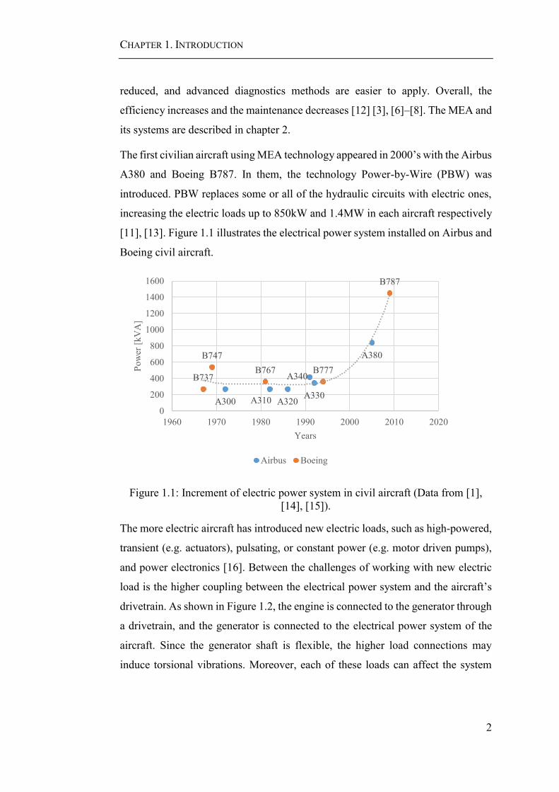
The first civilian aircraft using MEA technology appeared in 2000’s with the Airbus
A380 and Boeing B787. In them, the technology Power-by-Wire (PBW) was
introduced. PBW replaces some or all of the hydraulic circuits with electric ones,
increasing the electric loads up to 850kW and 1.4MW in each aircraft respectively
[11], [13]. Figure 1.1 illustrates the electrical power system installed on Airbus and
Boeing civil aircraft.
Figure 1.1: Increment of electric power system in civil aircraft (Data from [1],
[14], [15]).
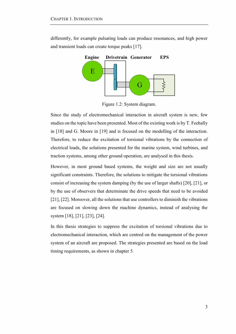
The more electric aircraft has introduced new electric loads, such as high-powered,
transient (e.g. actuators), pulsating, or constant power (e.g. motor driven pumps),
and power electronics [16]. Between the challenges of working with new electric
load is the higher coupling between the electrical power system and the aircraft’s
drivetrain. As shown in Figure 1.2, the engine is connected to the generator through
a drivetrain, and the generator is connected to the electrical power system of the
aircraft. Since the generator shaft is flexible, the higher load connections may
induce torsional vibrations. Moreover, each of these loads can affect the system
A300 A310 A320A330
A340
A380
B737
B747
B767 B777
B787
0
200
400
600
800
1000
1200
1400
1600
1960 1970 1980 1990 2000 2010 2020
Po
wer
[kV
A]
Years
Airbus Boeing
CHAPTER 1. INTRODUCTION
3
differently, for example pulsating loads can produce resonances, and high power
and transient loads can create torque peaks [17].
GeneratorEngine Drivetrain
G
E
EPS
Figure 1.2: System diagram.
Since the study of electromechanical interaction in aircraft system is new, few
studies on the topic have been presented. Most of the existing work is by T. Feehally
in [18] and G. Moore in [19] and is focused on the modelling of the interaction.
Therefore, to reduce the excitation of torsional vibrations by the connection of
electrical loads, the solutions presented for the marine system, wind turbines, and
traction systems, among other ground operation, are analysed in this thesis.
However, in most ground based systems, the weight and size are not usually
significant constraints. Therefore, the solutions to mitigate the torsional vibrations
consist of increasing the system damping (by the use of larger shafts) [20], [21], or
by the use of observers that determinate the drive speeds that need to be avoided
[21], [22]. Moreover, all the solutions that use controllers to diminish the vibrations
are focused on slowing down the machine dynamics, instead of analysing the
system [18], [21], [23], [24].
In this thesis strategies to suppress the excitation of torsional vibrations due to
electromechanical interaction, which are centred on the management of the power
system of an aircraft are proposed. The strategies presented are based on the load
timing requirements, as shown in chapter 5.

CHAPTER 1. INTRODUCTION
4
1.2 Aims and Objectives
This thesis aims to analyse the electromechanical interaction in aircraft electrical
power system and develop strategies to suppress the excitation of torsional
vibrations. The specific objectives to achieve the aim are:
Show the electromechanical interaction in an aircraft system, identifying
the effects of different sources. Propose mitigation strategies for them.
A theoretical understanding of the dynamic interaction between load
connections and the system response. Understand the importance of the
timing in the connection and introduced strategies based on it to minimise
the effects of torque impacts.
Develop a power management system (PMS) that minimises the drivetrain
torsional vibrations produced by the connection of electrical loads with
different characteristics and requirements.
Build an experimental setup to test the electromechanical interaction and
the strategies that suppress the excitation of torsional vibrations.
1.3 Contributions
The contributions of this thesis are:
A study of the state of the art, which describes the current state of aircraft
systems and electromechanical interaction, is presented.
Different sources of electromechanical interaction in aircraft system are
presented and analysed. Past studies have shown the effect of electrical load
step connection. In this thesis, electrical load step and pulsating loads are
analysed. Moreover, the effects of the Generator Control Unit (GCU) on the
electromechanical interaction is shown.
A strategy to supress the excitation of the drivetrain torsional vibrations
centred on the electrical loads connected is developed. This strategy is based
CHAPTER 1. INTRODUCTION
5
on the Posicast compensator and the analysis of the electrical load
switching.
A PMS that can be applied to different electrical loads present in an aircraft
is proposed. The PMS applies different switching strategies according to
the electrical load being connected and hence eliminates the excitation of
torsional vibrations.
A reduced model to study the electromechanical interaction in aircraft
systems is presented. In the past it has been shown that the mechanical
system can be reduced to one with two natural frequencies. In this thesis, to
that reduction is added that to study the electromechanical interaction, the
electrical system can be represented by a DC system. This reduction allows
the reduction of the experimental setup cost.
A validation methodology for sensorless systems is proposed. This
methodology allows the obtention of experimental results which are
comparable with the theory.
A sensibility analysis that shows the relationship between the strategies
behaviour and the tuning accuracy is carried out.
Finally, an improved method to apply the strategies to inductive loads, and
which can be extended to capacitive loads is proposed.
1.4 Thesis Structure
The rest of the thesis is organised as follows:
In chapter 2 and chapter 3 the literature review is presented. Chapter 2 provides an
overview of aircraft systems and its development. For this purpose, the evolution
of aircraft from traditional models and to the adoption of More Electric Aircraft
technology is analysed. The changes in power distribution technologies and the
increase in the electrical system power is presented. Finally, a gas turbine and a
typical drivetrain for aircraft systems are described.
In chapter 3 a review about electromechanical system interaction is presented. First,
the reasons why torsional vibrations are excited in the mechanical drivetrain are

CHAPTER 1. INTRODUCTION
6
presented including step and pulsating load connections, grid faults, sub-
synchronous currents, and machine control systems. The effects of the torsional
vibrations on the mechanical system are described, and the applications in which
electromechanical interaction is found presented. Finally, the solutions traditionally
used in the literature to mitigate the effects of the interaction are considered.
Chapter 4, introduces a functional model of the aircraft system used in this study.
Using this model the stability of the system is analysed; the poles are identified,
and the torsional vibrations modes are shown. Later, the electromechanical
interaction is considerd. The cases of load connection (step and pulsating) and
machine control systems are analysed. Techniques to minimise the effect of
pulsating load connections and the machine control are presented.
In chapter 5, a PMS that eliminates the drivetrain torsional vibrations excited by
the connection of electrical loads is described. The strategies used by the PMS are
based on the Posicast method that suppresses vibrations using a compensator. This
compensator introduces a series of step delays that depend on the frequency that is
being cancelled. A detailed description of the method equations and its
implementation are presented. Finally, strategies based on this approach are
introduced and applied to some of the different electrical loads found in an aircraft,
such as ailerons, ice protection systems, and a radar.
The experimental setup to test the effectiveness of the PMS strategies is described
in chapter 6. The components used and the design torsional vibrations are
presented. The theoretical vibrations models associated with each frequency are
studied.
In chapter 7, the experimental results are presented. To test the Posicast strategies
described in chapter 5, the torsional vibrations are identified using a combined
method of Fourier analysis, Empirical Mode Decomposition (EMD) and Hilbert
Transform. Moreover, the methods employed to measure the torque of the
mechanical system are introduced. The results obtained by each method are
compared. Finally, the electromechanical interaction due to the connection of
resistive loads is shown, and the PMS is tested.

CHAPTER 1. INTRODUCTION
7
An analysis of the robustness of the Posicast based strategies is presented in chapter
8. In this chapter, improvements to the method are introduced. The effect of
inductance on the machine is considered, and sensitivity is studied.
Finally, in chapter 9 the conclusions and summary of this thesis are presented. Also,
further areas for future research are discussed.
Chapter 2
2 Aircraft Systems
2.1 Introduction
Since the beginning of aircraft systems, innovation has been its main characteristic.
These changes have been transversal to every area of study: engines, airframes,
controls, airline business models, materials, and electrical power system among
others [25]. Now, the changes in aircraft technologies are centred on meeting the
market needs, protecting the environment by reducing the emissions, and ensuring
safety and security [4]. To decrease the effect on the environment, the FlightPath
2050 has set the target that the CO2 emissions should reduce 50% by 2020, the NOx
and noise should reduce in 80%, and 50% respectively [4].
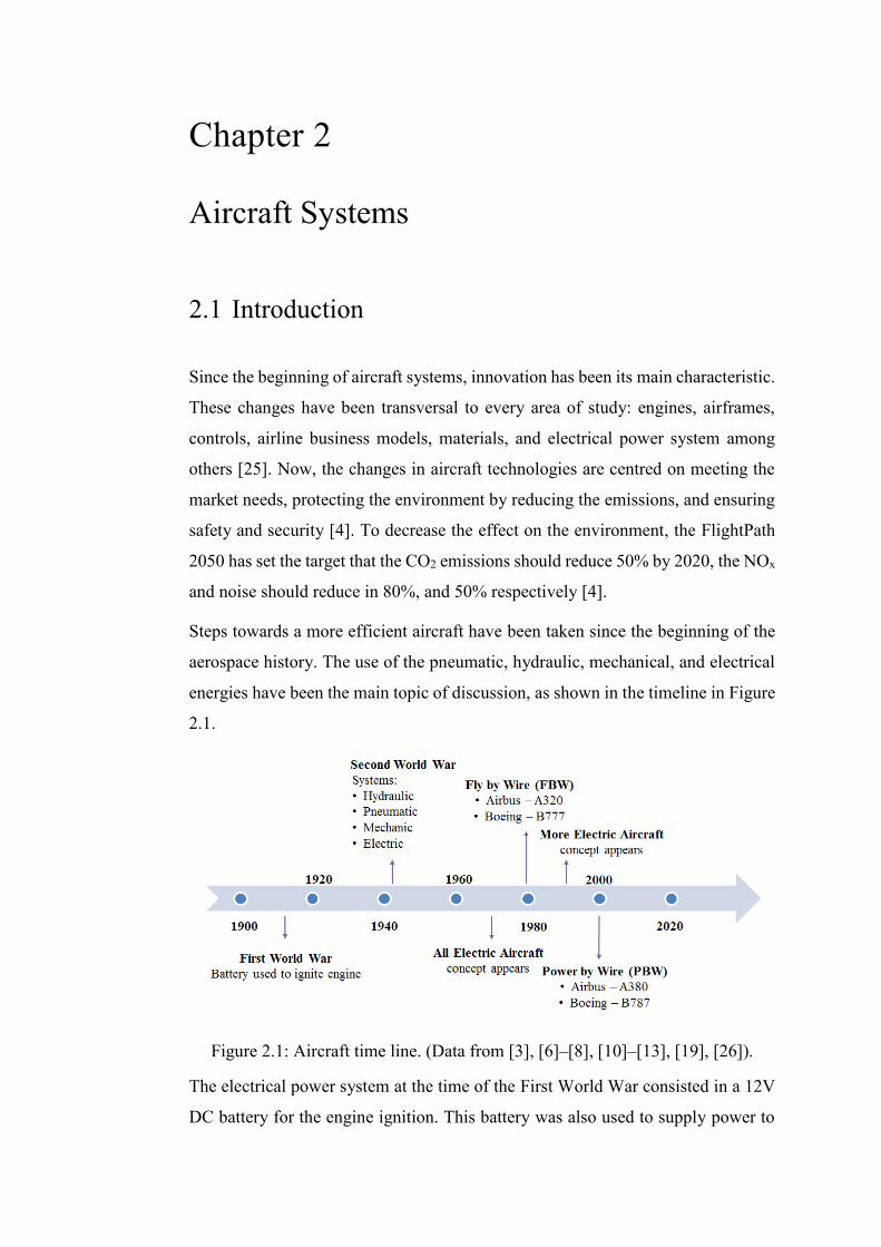
Steps towards a more efficient aircraft have been taken since the beginning of the
aerospace history. The use of the pneumatic, hydraulic, mechanical, and electrical
energies have been the main topic of discussion, as shown in the timeline in Figure
2.1.
Figure 2.1: Aircraft time line. (Data from [3], [6]–[8], [10]–[13], [19], [26]).
The electrical power system at the time of the First World War consisted in a 12V
DC battery for the engine ignition. This battery was also used to supply power to

CHAPTER 2. AIRCRAFT SYSTEMS
9
instruments, landing lights, radio receivers and transmitters [10]. However, with
the expansion of the size of civil aircraft and accordingly an increase in passengers,
a need of faster flights, and better radio equipment, the battery power became
insufficient. As a consequence, an electrical power system was incorporated in
aircraft systems. The transmission (AC or DC), voltage and frequency of the
electrical power system were not agreed.
By the time of the Second World War, the aircraft had electrical, hydraulic and
pneumatic systems, but their functions varied between models even of the same
characteristics. For this reason, in the 1940s the systems were standardised [8]:
Hydraulic System: For applications operating with high torque and short
time intervals as undercarriages and ailerons.
Pneumatic System: For air conditioning and pressurisation.
Electrical System: For avionics and airframe utilities.
The use of a single power system to reduce the complexity was discussed in the
1970’s, and the All Electric Aircraft (AEA) concept was introduced [8], [10]. In
[12], the AEA is defined as an aircraft with only electrical power off-take, with
only electrical loads and electric propulsion. Additionally, in the 1990s the More
Electric Aircraft (MEA) concept was introduced [3], [6]–[8]. The MEA, described
in section 2.3, aims to change the pneumatic, hydraulic, and mechanical systems to
electrical systems while keeping the actual propulsion system. Thus, there is no
need for hydraulic and pneumatic systems. The use of an electrical system allows
the elimination of expensive and cumbersome hydraulics. Moreover, the design,
development, and testing costs are reduced, and advanced diagnostics technology
is easier applied. Overall, the efficiency increases and the maintenance decreases
[12].
The first step towards the AEA and MEA were taken in the decade of 1980 when
Fly-by-Wire (FBW) systems were introduced and used in Airbus A320 and Boeing
B777. FBW uses electrical control systems to regulate the flight control surfaces,
such as aileron, elevator, rudder, and spoiler; replacing the mechanical and hydro-

CHAPTER 2. AIRCRAFT SYSTEMS
10
mechanical ones used before. Thus, the aircraft have less weight, improved
reliability, and an easier and safer control system [13].
The first MEA appeared with the introduction of Power-by-Wire (PBW) systems
in 2000’s in Airbus A380 and Boeing B787. PBW replaces the hydraulic circuits
by electric ones, increasing the electric loads up to 850kW and 1.4MW in each
aircraft respectively [11], [13]. As a consequence of the MEA and AEA concept,
the electric demand in aircraft has increased drastically in 20 years [26].
In next sections, the conventional aircraft power systems and the More Electric
Aircraft (MEA) are discussed. Later the aero gas turbine and the drivetrain torsional
vibrations are described. Finally, the chapter summary is presented.
2.2 Conventional Aircraft
For a conventional aircraft, engines are mainly used to produce the propulsion
thrust of the plane (about 40MW for propulsion). Another 1.7MW of the generated
power is consumed by the pneumatic, hydraulic, mechanic and electrical power
system as shown in Figure 2.2 [1], [9].

CHAPTER 2. AIRCRAFT SYSTEMS
11
Figure 2.2: Conventional aircraft power (Data from [3], [15], [27], [28]).
2.2.1 Mechanical Power
On a conventional aircraft, the mechanical power is derived from a gearbox
connected to the engine and is used to drive the hydraulic pumps, oil pumps as well
as the electrical generators. The main disadvantage of this the gearbox is that it is
normally very heavy and requires regular maintenance [1], [12].
2.2.2 Hydraulic Power
The hydraulic system has been used in the aircraft from the 1930s when a
retractable undercarriage was introduced. Since then, the hydraulic system has been

CHAPTER 2. AIRCRAFT SYSTEMS
12
used to manage the flight actuators, including the rudders, the elevators the ailerons,
and the landing gear, among others [1].
The hydraulic system consists of two pressurised circuits supplied by hydraulic
pumps which are driven by a gearbox, as shown in green lines in Figure 2.2.
Through these pipes, the fluid is distributed to all the actuators for aircraft flight
control actuators.
The main advantages of hydraulic systems include high reliability, robustness, and
high power density. However, the hydraulic system has a abundant weight and
requires regular maintenance [1].
2.2.3 Pneumatic Power
The pneumatic power is the highest one after the thrust, as can be seen in Figure
2.2. This type of power is derived by bleeding air from the engine core. In reality,
about 2- 8% of the air flux is bled from the engine. The air bled from the engine is
mainly used for the environmental control system and the ice protection system [1],
[12]:
Environmental Control System (ECS): its functions are the pressurisation
and the thermal regulation of the cabin. The air bled from the engine is
regulated by pressure valves in a heat exchanger and is cooled down by
ambient air. The fans, valves and monitoring and control are electrical.
Ice Protection System (IPS): its function is to heat the engine intake and
aircraft wings, protecting from the ice and rain. The bleed air is used to heat
the wings, while its control is electric.
The advantages are its simple design and high reliability. However, as the
pressurised air of the bleed system comes from the engine, its temperature and
pressure are high. To be able to use the bleed air, it must be cooled down, causing
a significant waste of energy [12], [14].

CHAPTER 2. AIRCRAFT SYSTEMS
13
2.2.4 Electrical Power
The electrical power in a conventional aircraft is used for the avionics, cabin and
aircraft lighting, monitoring and control of ECS, etc. [1]. As shown in purple in
Figure 2.2 and in Figure 2.3, the electrical system consists of two identical
subsystems: the left side power system and the right side power system. Each
subsystem has an electrical generator which generates an AC 115Vrms three-phase
electrical power operating at 400Hz constant frequency [6], [29], [30].
GCU GCU
Avionics, Cabin Electronics, Batteries
115V 400Hz
28V DC 28V DC
AC Loads,
Hydraulic Pumps,
Lights
GeneratorGenerator
APU
TRUTRU
AC Loads,
Hydraulic Pumps,
Lights
Left Side
Power System
Right Side
Power System
Figure 2.3: Electrical system.
To achieve a constant frequency, the generator speed needs to be constant. This is
achieved through a Constant Speed Drive (CSD) which transforms a variable
engine shaft speed to a constant one. The CSD, shown in Figure 2.4, is essentially

CHAPTER 2. AIRCRAFT SYSTEMS
14
a hydro-mechanical automatic gearbox. The CSD is mechanically complex and
needs oil and maintenance [9].
Figure 2.4: CSD configuration.
Each generator has its own Generator Control Unit (GCU) to keep the voltage
amplitude of the generator at a desired value (115Vrms). Electrical loads such as
lighting, entertainment system and auxiliary hydraulic pumps are directly fed by
the HVAC bus [1], [12]. The avionics, cabin electronics and backup batteries are
connected to a 28V DC bus. As shown in Figure 2.3, a Transformer Rectifier Unit
(TRU) is used to change from AC to DC voltage [10].
The advantages of using electrical systems are its high efficiency and low
maintenance. For these two reasons, in MEA aircraft, the hydraulic and pneumatic
systems are replaced by electrical ones to improve the overall system efficiency.
2.3 More Electric Aircraft
The More Electric Aircraft (MEA) aims to replace the pneumatic, hydraulic and
mechanical system by electrical ones [6], [29]–[32]. For this reason, the MEA’s
engine would only require fuel, a control interface, and electrical power
connections as presented in section 2.3.1 [3].
To reduce the mechanical system, the fuel and oil pump systems can be driven by
electrically powered pumps [7], [31]. In the same way, the drivetrain will need to
be removed, and hence the speed of the generator will not be constant. For this
reason, new drive strategies are necessary as presented in section 2.3.2.
CHAPTER 2. AIRCRAFT SYSTEMS
15
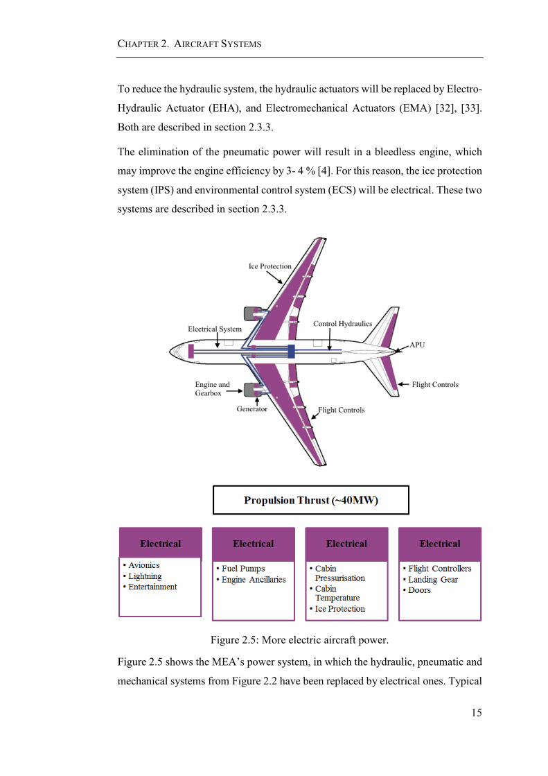
To reduce the hydraulic system, the hydraulic actuators will be replaced by Electro-
Hydraulic Actuator (EHA), and Electromechanical Actuators (EMA) [32], [33].
Both are described in section 2.3.3.
The elimination of the pneumatic power will result in a bleedless engine, which
may improve the engine efficiency by 3- 4 % [4]. For this reason, the ice protection
system (IPS) and environmental control system (ECS) will be electrical. These two
systems are described in section 2.3.3.
Figure 2.5: More electric aircraft power.
Figure 2.5 shows the MEA’s power system, in which the hydraulic, pneumatic and
mechanical systems from Figure 2.2 have been replaced by electrical ones. Typical

CHAPTER 2. AIRCRAFT SYSTEMS
16
load values on a large MEA according to [9] are fuel pumps (10kW), flight controls
(2-35kW), environmental control system (4*70kW), ice protection system
(250kW), landing gear (5-70kW), and the starting of the engine (200kW). A higher
electrical power system will require new electrical network configurations.
Furthermore, in a higher power system, high power disturbances are now passed
on to the drivetrain, and electromechanical interaction needs to be studied. Chapter
3 presents the reasons and effects for electromechanical interaction, and in the rest
of this thesis, solutions are proposed.
In the following sections, the aircraft engines, electrical power generation
strategies, the new electrical loads (such as EHAs, EMAs, IPS, and ECS), the
electrical power system, and cases of the MEA will be introduced.
2.3.1 Aircraft Engines
To have a more electric system, new technologies for the engine has also been
proposed. The main ones are the Bleedless Engine, and the More Electric Engine
(MEE).
2.3.1.1 Bleedless Engine
In a conventional aircraft, the ECS and IPS use pneumatic power. This power
comes from air bled from the HP spool in the gas turbine [34]. However, the bleed
air temperature is much higher than the one required normally, up to 350℉ in the
LP spool and 1200℉ in the HP spool at a pressure of up to 500psig. For this reason,
the air must be cool down to around 150℉ and the pressure reduced to
approximately 30 psig before it is used in the ECS and IPS. Therefore, pressure
regulating valves and a pre-cooler arrangement are used [34].
Because the process of heat exchange has a lower thermal and energy efficiency,
the use of bleed air reduces the efficiency of the engine. Furthermore, the bleed air
is responsible for higher aeroplane drag and the noise production [35].
For Boeing B787, the bleed air has been drastically reduced and is only used as
anti-icing at the engine cowl. For the ECS and IPS, bleed air is not used anymore.
Instead, these systems operate electrically [14].

CHAPTER 2. AIRCRAFT SYSTEMS
17
The advantages are [35]:
Improved fuel consumption (1 to 2% in cruise and 3% overall)
Reduced maintenance cost, because the bleed system has been eliminated.
Reduce weight, since the bleed system has been removed. Consequently,
the fuel consumption reduces and the operation range expands.
2.3.1.2 More Electric Engine
The More Electric Engine (MEE) is directly related to the MEA, as it aims to reduce
the hydraulic, pneumatic, and mechanical system in the aircraft engine to reduce
the weight, the required thrust, and the fuel burn [3], [36]. Also, the interface
between the engine and the aircraft would be simplified, as the system has been
reduced to electric power and fuel only [3].
With this objective, the following components will be eliminated in the MEE [3]:
Lubrication system: It will be replaced by Active Magnetic Bearings
(AMB).
Gearbox and associated shaft: A motor/generator, combined with an AMB,
will be embedded into the IP and HP spools. In this way, the inter-shaft
power transfer would improve the operability of the engine, and the
compressors and valves will be reduced. These changes will allow the
removal of the radial driveshaft, internal and external drivebox, and
lubrication systems.
Hydraulic system: Electric power from the generator will be used to power
an electric motor hydraulic pump, allowing the replacement of the hydraulic
system with a fan shaft generator.
Pneumatic engine starting system: Gas turbine engines have traditionally
been started with an air motor applying torque to the accessory drivetrain to
turn the GT spools. In the MEE an HP motor/generator will be used to
launch the engine electrically.
Bleed air offtake: As mentioned before, the system will be bleedless.
CHAPTER 2. AIRCRAFT SYSTEMS
18
The first steps towards an MEE have been taken in the B787, in which the bleed air
has been removed, and the engine is started electrically [37].
2.3.2 Electrical Generation Strategies
In section 2.2.4 was mentioned that most electrical loads need to operate at a
constant frequency and that normally a CSD is used. Since the CSD is a complex
mechanical system, which needs regular maintenance, in this section, two new
strategies to keep the load's frequency constant are presented: Variable Speed
Constant Frequency (VSCF), and Variable Frequency (VF) operation.
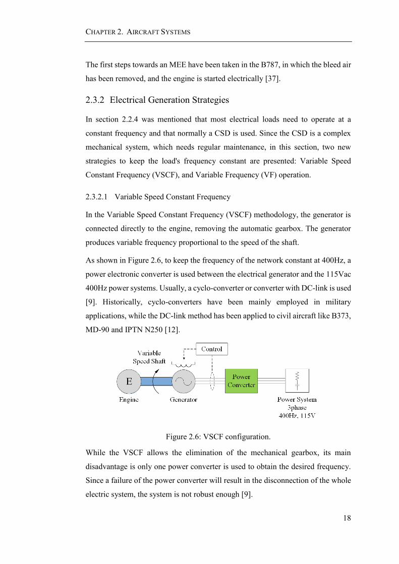
2.3.2.1 Variable Speed Constant Frequency
In the Variable Speed Constant Frequency (VSCF) methodology, the generator is
connected directly to the engine, removing the automatic gearbox. The generator
produces variable frequency proportional to the speed of the shaft.
As shown in Figure 2.6, to keep the frequency of the network constant at 400Hz, a
power electronic converter is used between the electrical generator and the 115Vac
400Hz power systems. Usually, a cyclo-converter or converter with DC-link is used
[9]. Historically, cyclo-converters have been mainly employed in military
applications, while the DC-link method has been applied to civil aircraft like B373,
MD-90 and IPTN N250 [12].
Figure 2.6: VSCF configuration.
While the VSCF allows the elimination of the mechanical gearbox, its main
disadvantage is only one power converter is used to obtain the desired frequency.
Since a failure of the power converter will result in the disconnection of the whole
electric system, the system is not robust enough [9].

CHAPTER 2. AIRCRAFT SYSTEMS
19
2.3.2.2 Variable Frequency
To overcome the problem of the VSCF strategy, the operation of the electrical
network with a Variable Frequency (VF) is used [9], [27]. In the VF strategy, the
generator is connected directly to the engine and the frequency of the grid changes
between 320 and 720Hz, as shown in Figure 2.7. To each load operating at constant
speed, a power converter is connected if necessary. In this way, a single failure
point is removed, and each connection can be fixed independently [9], [12], [31].
Figure 2.7: VF configuration.
The advantage of this method is the elimination of the mechanical CSD and that
there is no single connection point failure problem as in the VSCF strategy.
However, the number of power converters required is high, since nearly all aircraft
loads required constant frequency [9], [31]. For this reasons, the VF strategy is used
in Boeing B787 and Airbus A380.
2.3.3 Emerging New Loads
In the MEA, a variety of power loads with different requirements and effects on the
system can be found [14], [38], [39], for example:
Pulsating Loads: Can be solid-state radars and digital loads.
Constant Power Loads: Motor driven pump can operate as constant power
loads.
High Power Loads: The ECS and undercarriage are high power loads which
are connected to the DC bus to avoid additional AC-DC converter. As the
ECS consumes high electrical energy, it might add harmonics to the system
if connected through AC-DC-AC converters.
CHAPTER 2. AIRCRAFT SYSTEMS
20
Transient Loads: EHA and EMA loads are transient. They are fed from the
essential buses which can be powered by backup batteries under emergency.
In general, they are connected to the essential AC bus, but the need of AC-
DC converters suggests the use of an essential DC bus instead.
In the next sections, different loads on board MEA such as the actuators,
environmental control system and ice-protection systems will be described.
2.3.3.1 Actuators
For the MEA operation, two actuators are considered: Electro-Hydraulic Actuator
(EHA) and Electromechanical Actuator (EMA). The main advantages of electric
actuators compared to the hydraulic ones are the decrease in the weight and an
increased efficiency. The weight is reduced because the use of electric actuators
allows the removal of the hydraulic pipes, replacing them with a lighter electrical
network. The use of a PBW connection makes the installation and replacement of
actuators more accessible as they are line-replaceable [40].
Secondly, electric actuators are more efficient because they consume power only
when the control surface moves or overcomes a load, instead of being continuously
active like the hydraulic system.
Electro-hydraulic Actuator
Electro-hydraulic actuators (EHA) are employed to localize the hydraulic system
used on the flight control surfaces, such as rudders, elevators and ailerons. The use
of EHA allows the elimination of the central hydraulic pumps (driven by the engine
gearbox) and the replacement of hydraulic distribution pipes by electrical cables
thus reduce the weight and maintenance cost. As shown in Figure 2.8, EHA consists
of an electrically driven pump which pressurises a local hydraulic system. The fixed
displacement pump is connected to a motor, and the position of the actuator moves
a fixed amount per revolution [9].

CHAPTER 2. AIRCRAFT SYSTEMS
21
Motor
Hydraulic
Ram
Ram
Power
Converter
3phase
Supply
Fixed
Displacement
Pump
Control Surface
Figure 2.8: Electro-hydraulic actuator.
There are several advantages of EHA. First, because there is no direct mechanical
connection between the motor and actuator, the failure possibility of the system is
reduced. Second, the technology is more similar to hydraulic actuators [9].
Currently, EHA is used as backup systems of Boeing B787 and Airbus 380, where
is connected in parallel to conventional hydraulic systems [9].
Electromechanical Actuator
An alternative to the EHA, is the Electromechanical Actuator (EMA). As shown in
Figure 2.9, in an EMA, an electric motor is connected to a gearbox which drives a
ball screw to amplify the machine’s torque and provide linear actuation force. The
linear force allows the movement of the flight surface. With the use of the gearbox
and the ball screw, the local hydraulic system is removed [9].
The EMA can be used for surface control, landing gear and undercarriage with
reduced cost, less complexity and maintenance cost, and increased reliability [9],
[32]. However, due to the mechanical connection on the ball-screw, jamming may
occur. This limits the EMA to be used only for secondary control actuation (flaps
and slats) [9].
Motor Reduction
Gearbox
Ball Screw
Ram
Power
Converter
3phase
Supply
Control Surface
Figure 2.9: Electromechanical actuator.

CHAPTER 2. AIRCRAFT SYSTEMS
22
2.3.3.2 Environmental Control System
The Environmental Control System (ECS), is used to control the temperature and
air of the cabin. Conventionally, it consists of one or two stages compressor
connected to the main engine. However, to reduce the bleed air, an electric ECS is
used [15].
In the electric ECS, instead of pneumatic power, electric motors and converters are
used to drive a compressor which provides air for the pressurisation. To adjust the
temperature of the pressurised air, an electrical heating/cooling plant is used [7],
[9], [15], [31], [35].
The advantage of this method is the elimination of the bleeding air from the engine,
which will improve the efficiency of the aircraft. The main challenge is sizing the
overall system and calculating the required electrical power for every phase of the
flight [15].
2.3.3.3 Ice-Protection System
Traditionally, the Ice-Protection System (IPS) uses the bleed air to heat the wings
[1], [12]. Instead, in the MEA, the IPS is achieved using electrical power with
thermal mats embedded in the wing leading edges. These thermal mats, formed by
resistive materials will generate heat for de-icing or anti-icing functions when
powered on. For anti-icing protection, the thermal mats can be energised
simultaneously, while for de-icing protection in the wing leading edge, the mats
can be connected sequentially [35].
Compared with conventional ways, these electrical IPS solutions are more
controllable and have a more flexible and lighter interface than pressure pipes [7],
[31]. Moreover, since no excess energy is used, the system is more efficient [35].
This kind of IPS is used in the Boeing 787.
The electrical loads described can make the system unstable. For instance, after a
perturbation or load connection, currents are induced in the machine circuits. The
velocity with which these currents decay depends on the components of the system
CHAPTER 2. AIRCRAFT SYSTEMS
23
[41]. As a result, the modelling of the load's behaviour and the system stability
analysis are fundamental. In [33], [39], [42], [43] the stability of the electric power
system is studied with pole analysis through small-signal model analysis. In [44] a
stability analysis for a hybrid AC-DC system has been studied, in [45] the impact
of pulsating loads over the electrical power system is evaluated considering a
storage system, and in [46] a secondary control for voltage restoration is presented.
In [18], the effect of the electrical load connection over the mechanical drivetrain
has been studied. However, no studies to minimise the effects of the
electromechanical interaction have been presented.
The disturbances in the electrical system can pass to the mechanical one, generating
electromechanical interaction. For example, high electrical transients can produce
mechanical transients, or pulsating electrical loads can resonate with the
mechanical system. Although the electromechanical interaction has been
acknowledged in [17], [18], no solution has been proposed to attenuate these
electromechanical interactions.
2.3.4 Electrical Power System
The electrical power on board has increased from 100-200kW to over 1MW in a
large civilian aircraft such as the Boeing B787 during last few decades [9].
Electrical power systems with higher capabilities imply new challenges that need
to be assessed. This makes the study and design of the electrical power system
fundamental.
In general, an electrical power system can be DC, AC, or hybrid with a variable
voltages or variable frequencies. Most systems operate with an AC distribution
because it is easier to implement. On the other hand, DC systems are more reliable
for high transient systems because the DC-link capacitors can help in maintaining
the voltage. Since no agreement has been reached in the advantages of the different
electrical systems, the MEA can operate with a DC, AC, or hybrid architecture [11].
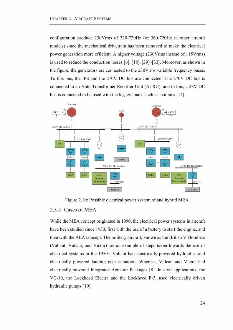
A possible hybrid configuration is presented in Figure 2.10. In that case, 230Vrms
VF is used for generation, 270V DC for distribution, and 28V DC for lower loads
as shown in Figure 2.10 [11], [14], [47]. The generators of the proposed
CHAPTER 2. AIRCRAFT SYSTEMS
24
configuration produce 230Vrms of 320-720Hz (or 360-720Hz in other aircraft
models) since the mechanical drivetrain has been removed to make the electrical
power generation more efficient. A higher voltage (230Vrms instead of 115Vrms)
is used to reduce the conduction losses [6], [18], [29]–[32]. Moreover, as shown in
the figure, the generators are connected to the 230Vrms variable frequency buses.
To this bus, the IPS and the 270V DC bus are connected. The 270V DC bus is
connected to an Auto-Transformer Rectifier Unit (ATRU), and to this, a 28V DC
bus is connected to be used with the legacy loads, such as avionics [14].
GCU GCU
230V 320-720Hz
270V DC Distribution
GeneratorGenerator
APU
ECS
Inverter
Driven Loads
IPS
Avionics
Battery
EMA EMA
...
AC ESS 230V
28V DC
230V 320-720Hz
270V DC Distribution
ECS
Inverter
Driven Loads
IPS
Avionics
EMA EMA
...
AC ESS 230V
28V DC
Figure 2.10: Possible electrical power system of and hybrid MEA.
2.3.5 Cases of MEA
While the MEA concept originated in 1990, the electrical power systems in aircraft
have been studied since 1930, first with the use of a battery to start the engine, and
then with the AEA concept. The military aircraft, known as the British V-Bombers
(Valiant, Vulcan, and Victor) are an example of steps taken towards the use of
electrical systems in the 1950s. Valiant had electrically powered hydraulics and
electrically powered landing gear actuation. Whereas, Vulcan and Victor had
electrically powered Integrated Actuator Packages [8]. In civil applications, the
VC-10, the Lockheed Electra and the Lockheed P-3, used electrically driven
hydraulic pumps [10].
CHAPTER 2. AIRCRAFT SYSTEMS
25
In modern aircraft, the Airbus A380 and A350, and Boeing B787 are examples of
MEA. In them, the number of centralised hydraulic system has been reduced,
connecting EHA backup systems [9]. In the A380 a more electric flight control is
used. Instead in B787 maintains centralised hydraulic systems, but the ECS and IPS
are done electrically [37].
Next, the functions of the pneumatic, hydraulic, and electrical systems in the B787
and A380 are described.
2.3.5.1 Boeing B787
The case of the Boeing B787 is the one with more MEA features. The characteristic
of its power systems are:
Pneumatic system: is only used for the anti-icing of the engine cowl, and
the ECS and IPS are both electrical. In the first, the air is pressurised and
warmed electrically using 280kW. While in the second, a thermal mat
protects the wing of the ice consuming 250kW. Moreover, the engine,
Rolls-Royce Trent 1000, is the first large commercial aircraft to be equipped
with electric engine starter [37].
Hydraulic system: a conventional hydraulic system is combined with EHA
to decrease the hydraulic and keep redundancy at the same time [9].
Electrical system: its power network is hybrid, combining AC and DC
buses. It has four 250kVA Hamilton-Sundstrand variable frequency
generators (2 per engine) connected to a 230V AC voltage bus. The variable
frequency generator allows a more efficient energy conversion so that the
fuel can be reduced. On the other hand, the operation at a higher voltage
than the conventional aircraft (115V AC) decreases the losses in the
transmission lines. Hence, less wiring is required on the plane, and the
weight is reduced [19].

CHAPTER 2. AIRCRAFT SYSTEMS
26
2.3.5.2 Airbus A380
The power systems characteristics of Airbus A380 are:
Pneumatic system: the ECS is conventional, and hence the pneumatic
system has been retained.
Hydraulic system: uses EHAs. In conventional aircraft, the actuators are
connected in pairs to give redundancy to the network. In the A380, one
hydraulic actuator has been replaced with two EHA. In other control
surfaces (as the rudders), backup EHAs have been implemented parallel to
the traditional hydraulic ones. This connection also used in the V-bombers,
allows the choosing which actuator to use: hydraulic or EHA [40].
Electrical system: has four engines, and to each of them, an Aerolec
150kVA variable frequency (370-770Hz) generators are connected [37].
Also, there are two 120kVA 400Hz auxiliary power unit (APU) generators,
each of which is driven by the APU. Each generator is connected to VF bus.
These buses cannot be paralleled.
2.4 Aero Gas Turbine
The Gas Turbine (GT) introduced in the 1940s is one of the best methods to produce
mechanical power [34], [37], [48]. It involves the compression and heating of a
fluid at high temperatures. Later this fluid is expanded, generating power. The main
three stages of the GT are:
Compressor: The air entering the turbine is compressed.
Combustion chamber: Fuel combustion is used to rise the temperature of
the fluid before the expansion to increase the produced power.
Turbine: The hot fluid expands generating power.
The advantage of the GT is that it has high power to weight ratio and high thrust
speeds [37]. Because of this reason, the GT replaced other engines for all aircraft
but the light ones [48].

CHAPTER 2. AIRCRAFT SYSTEMS
27
In the case of the Aero Gas Turbine, the behaviour is equivalent as shown in Figure
2.11. The fluid, air, enters the turbine through an intake; it goes through the
compressor, combustion chamber and turbine; and finally, it is expelled through
the nozzle propelling the jet at a high velocity [48].
Fan
Low-pressure
compressor
High-pressure
compressor
Low-pressure
shaftHigh-pressure
shaft
Low-pressure
turbine
Nozzle
Combustion
Chamber
Intake
Figure 2.11: Three spool turbine system.
A turbofan is connected to obtain a higher efficiency. It consists of connecting
further turbines to drive a larger diameter fan after the first gas exhaustion [17],
[34], [37], [48]. Thus, the exhaust gas can be used to drive one or more additional
spools. These spools are not attached to each other, but their operation is coupled
through the air flow, and their speed is related to the level of pressure and the thrust
generated. In general two and three spool shaft are used. The spools will be referred
as High Pressure (HP), Intermediate Pressure (IP), and Low Pressure (LP) spool
according to their position. Three-spool systems are preferred for a long-haul flight,
where fuel burn is a higher fraction of the cost. Two spool systems are preferred
for short haul operation [37]. The turbine from Figure 2.11 has three spool turbine,
like the one from Rolls-Royce Trent 1000 [18]. The three spools are represented in
purple (HP), blue (IP), and green (LP). In this configuration, the generator is
connected to the IP shaft through the drivetrain. For a two spool system, the
generator is connected to the HP shaft. The studies presented in this thesis can be
applied to the two and three spool configurations.
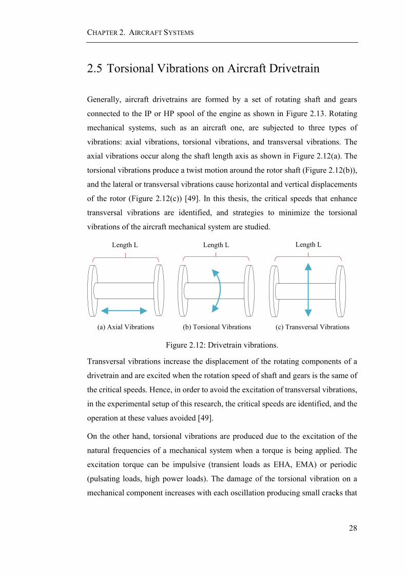
CHAPTER 2. AIRCRAFT SYSTEMS
28
2.5 Torsional Vibrations on Aircraft Drivetrain
Generally, aircraft drivetrains are formed by a set of rotating shaft and gears
connected to the IP or HP spool of the engine as shown in Figure 2.13. Rotating
mechanical systems, such as an aircraft one, are subjected to three types of
vibrations: axial vibrations, torsional vibrations, and transversal vibrations. The
axial vibrations occur along the shaft length axis as shown in Figure 2.12(a). The
torsional vibrations produce a twist motion around the rotor shaft (Figure 2.12(b)),
and the lateral or transversal vibrations cause horizontal and vertical displacements
of the rotor (Figure 2.12(c)) [49]. In this thesis, the critical speeds that enhance
transversal vibrations are identified, and strategies to minimize the torsional
vibrations of the aircraft mechanical system are studied.
(a) Axial Vibrations (b) Torsional Vibrations (c) Transversal Vibrations
Length L Length L Length L
Figure 2.12: Drivetrain vibrations.
Transversal vibrations increase the displacement of the rotating components of a
drivetrain and are excited when the rotation speed of shaft and gears is the same of
the critical speeds. Hence, in order to avoid the excitation of transversal vibrations,
in the experimental setup of this research, the critical speeds are identified, and the
operation at these values avoided [49].
On the other hand, torsional vibrations are produced due to the excitation of the
natural frequencies of a mechanical system when a torque is being applied. The
excitation torque can be impulsive (transient loads as EHA, EMA) or periodic
(pulsating loads, high power loads). The damage of the torsional vibration on a
mechanical component increases with each oscillation producing small cracks that
CHAPTER 2. AIRCRAFT SYSTEMS
29
propagate along the material. Fatigue of the material occurs when the cross-section
of the material is lower than the required for the torque applied [49]–[51].
In general, systems with large inertias have low natural frequencies. Instead, the
natural frequencies of systems with small inertial values and stiff mechanical
components are high [50]. In aircraft systems, due to the large engine inertia and
the flexible shaft used to reduce weight, two vibrations modes below 100Hz can be
found [18], [19]. When the electrical network share of loads is weak, and there are
dynamic loads, the likelihood of electromechanical interaction increases [18]. In
[18] it was shown that the torsional torques produced by the electrical system could
affect the mechanical one, and hence the electromechanical interaction studies must
be carried out.
The maximum torsional vibration allowed depends on the duration and the
amplitude of the stress. For higher amplitude stresses, the number of times the stress
can occur reduces. The life of the component can be predicted studying its fatigue.
To analyse the torsional vibrations, the rotating system must be reduced to a model.
The complexity of the model depends on the system and the purpose of the study.
When a model aims to identify potential problems, it can be represented by a simple
motor, couplings and a driven load. Instead, to predict the component life and the
exact torsional oscillations complex models with gearboxes and multiple inputs or
loads are used [50].
Moreover, a conventional aircraft drivetrain, connecting the gas turbine to the
generator is shown in Figure 2.13 [18]. The drivetrain consists of three subsystems:
the spool coupling, the transmission, and the accessory load gearbox [18], [37].
The drivetrain is connected to a spool in the engine, the IP spool in the case of a
three pressure spool, and the HP in the case of a two spool system [18], [35]. The
spool operates at a variable speed, and a fixed ratio bevel gear is used for the
coupling. Since the engine inertia is much higher than the rest of the drivetrain,
when the aircraft is not in idle, the speed of the system is fixed by the gas turbine
that acts as the ground of the system [18], [37].
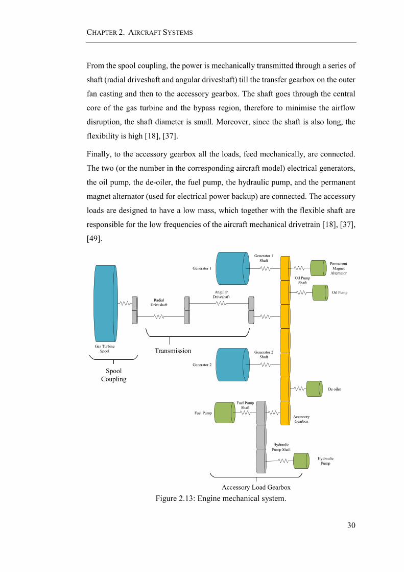
CHAPTER 2. AIRCRAFT SYSTEMS
30
From the spool coupling, the power is mechanically transmitted through a series of
shaft (radial driveshaft and angular driveshaft) till the transfer gearbox on the outer
fan casting and then to the accessory gearbox. The shaft goes through the central
core of the gas turbine and the bypass region, therefore to minimise the airflow
disruption, the shaft diameter is small. Moreover, since the shaft is also long, the
flexibility is high [18], [37].
Finally, to the accessory gearbox all the loads, feed mechanically, are connected.
The two (or the number in the corresponding aircraft model) electrical generators,
the oil pump, the de-oiler, the fuel pump, the hydraulic pump, and the permanent
magnet alternator (used for electrical power backup) are connected. The accessory
loads are designed to have a low mass, which together with the flexible shaft are
responsible for the low frequencies of the aircraft mechanical drivetrain [18], [37],
[49].
Gas Turbine
Spool
Oil Pump
Hydraulic
Pump
Generator 1
Generator 2
Fuel Pump
Radial
Driveshaft
Angular
Driveshaft
Generator 1
Shaft
Generator 2
Shaft
Accessory
Gearbox
Hydraulic
Pump Shaft
Fuel Pump
Shaft
Oil Pump
Shaft
Permanent
Magnet
Alternator
De oiler
Spool
Coupling
Transmission
Accessory Load Gearbox
Figure 2.13: Engine mechanical system.
CHAPTER 2. AIRCRAFT SYSTEMS
31
In [18], was shown that the drivetrain system presented in Figure 2.13 could be
reduced from 9 to 2 natural frequencies and keep the firsts two vibration modes
within 5% of the original ones. These two vibrations modes are the lower ones,
which are responsible for the system torsional vibrations. Hence, a simple system
can be used to analyse the electromechanical interaction in an aircraft. Chapter 4
presents the reduced mechanical model used for the electromechanical interaction
studies in this thesis.
2.6 Summary
In this chapter, the aircraft systems and the migration towards an MEA have been
presented. The MEA comprises the development of a whole new set of
technologies, such as the MEE, the EHA and EMA actuators, new generation
strategies such as VF, and a whole new design of the aircraft electrical power
system.
Moreover, the electrical and the mechanical system of a plane have been described.
To understand the interaction between these two systems, in next chapter a review
on electromechanical interactions and its solutions is presented. Then, in chapter 4
the electromechanical system in the study is modelled. In chapter 5 a power
management system (PMS) to suppress the excitation of the drivetrain torsional
vibrations is proposed.

Chapter 3
3 Electromechanical Interaction
3.1 Introduction
Studies on mechanical and electrical stabilities have been carried out from as early
as 1937. However, the first study on electromechanical interaction started after a
shaft failure at the Mohave Generating Station in Southern Nevada in the early
1970s [52]. A similar case was discussed in [53] where two motor shafts, driving a
compressor, failed, one after 3400 hours of operation and the other after 7000 hours
of operation.
These two incidences were due to electromechanical interaction as only the
electrical natural frequencies were considered in the design and not the mechanical
ones. The electrical natural frequencies are dependent on its controllers, resistances
and other components, while the mechanical natural frequencies are dependent on
the inertias and stiffness of the components on the drivetrain. Since the machines
are the interface between the electrical and mechanical systems, some disturbances
can pass from one to the other, and resonant modes can be excited [18], [54].
However, frequently when studying machines and drives, the mechanical system is
simplified, and the torsional elements are not considered. Because of the lack of
electromechanical studies, transient torque can be produced at various points on the
drive during a fault or switching event [55], [56].
The evolution of the electromechanical interaction studies is shown in Figure 3.1.
As can be seen, the first cases analysed in the 1970s are associated with traction
systems [23], [53] and ground generation (for example the Mohave case) [52].
However, during this period, the studies of electromechanical interaction were
mainly associated with the modelling of the systems and the identification of
vibration modes. It was at the beginning of this century, with the ongoing growth
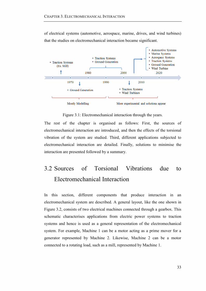
CHAPTER 3. ELECTROMECHANICAL INTERACTION
33
of electrical systems (automotive, aerospace, marine, drives, and wind turbines)
that the studies on electromechanical interaction became significant.
Figure 3.1: Electromechanical interaction through the years.
The rest of the chapter is organised as follows: First, the sources of
electromechanical interaction are introduced, and then the effects of the torsional
vibration of the system are studied. Third, different applications subjected to
electromechanical interaction are detailed. Finally, solutions to minimise the
interaction are presented followed by a summary.
3.2 Sources of Torsional Vibrations due to
Electromechanical Interaction
In this section, different components that produce interaction in an
electromechanical system are described. A general layout, like the one shown in
Figure 3.2, consists of two electrical machines connected through a gearbox. This
schematic characterises applications from electric power systems to traction
systems and hence is used as a general representation of the electromechanical
system. For example, Machine 1 can be a motor acting as a prime mover for a
generator represented by Machine 2. Likewise, Machine 2 can be a motor
connected to a rotating load, such as a mill, represented by Machine 1.

CHAPTER 3. ELECTROMECHANICAL INTERACTION
34
Independently of the operation case, the electromechanical system has a controller
and loads connected. The controller (or drive), electrical power system connected
to the generator, and flywheels can produce or be affected by torsional vibrations
excited by electromechanical interaction. Next, the sources of this interaction are
described: step and pulsating load connections, grid faults, sub-synchronous
currents, and control systems.
Figure 3.2: General electromechanical interaction system layout.
3.2.1 Step Load
The transient of the electrical load will produce a short-time disturbance in the
mechanical system through the generator. This induced torque disturbance may
result in mechanical vibrations and produce speed fluctuations. Furthermore,
mechanical torque variations can change the speed and produce vibrations which
are transmitted to the electrical system [18]. In general, higher load connections
produce higher disturbance, and thus the magnitude of the connection is limited
[57].
The load changes are especially relevant in isolated electrical systems, such as
aerospace and marine, in which the effect of the connection and disconnection of
an electrical load affects the generators [8] directly. In contrast, in most ground
power systems the effect of a load connection is shared among the whole grid and
thus the generator, and consequently, the mechanical system is not affected.
However, breakers operation in power systems is equivalent to load connections in
isolated systems, and the connection and disconnection of grid buses and faults can
produce transient torques [57].

CHAPTER 3. ELECTROMECHANICAL INTERACTION
35
3.2.2 Grid Faults
As step connections in isolated power systems, grid faults can also produce
torsional vibrations [58], [59]. Faults and instabilities of a power system can
generate oscillations on the shaft due to the resultant high electromagnetic torque
at the generator [58], [59]. For this reason, it is essential to have a good voltage
control on circuit breaker and relays to avoid peak torques being produced [57],
[58].
In [60], a zone of vulnerability of a power plant is defined. This zone is shaped by
the regions in which an electrical disturbance damages a critical shaft due to
torsional stress. These characteristics (fault location, type, clearing time, load of the
line and generating unit, the effect of series capacitors, and distance of the fault)
define the magnitude and set time of the torque applied to the generator, and which
are the ones that excite the mechanical system [57], [60].
3.2.3 Pulsating Load
Pulsating loads can be found in mechanical and electrical systems, and in both
cases, their effects have to be taken into account to avoid resonance [54]. Regarding
electrical loads, many applications use pulsating loads, such as radars [18], [61].
These electrical loads can create resonance in mechanical systems if their period is
close to the natural frequency of the mechanical system. Therefore the effect of the
pulsating load over the mechanical system depends on its period [23], [62], [63].
In the case of mechanical loads, the pulsating loads can be found as cyclic rotational
disturbance caused by eccentric or unbalanced rolls, bent shafts, seams in felts or
wires, and mechanical misalignment. Their principal effect is imposing a periodic
load change on the machine electrical drive [23].
Some systems have mechanical pulsating loads, like in [64] where its effect on an
induction motor is studied. While in other cases mechanical and electric pulsating
loads are present. For example, in marine systems, the pulsating loads can be of
both origins, mechanical, such as the vibrations produced by the waves, and
electrical, such as the radar connected to the system. The torsional vibrations can
affect the mechanical system and the drive [65].

CHAPTER 3. ELECTROMECHANICAL INTERACTION
36
3.2.4 Sub-synchronous Currents
The AC current in an electrical system is composed of two components, the
fundamental (𝑖𝐹(𝑡)) and the harmonics (𝑖𝐻(𝑡)), as shown in equation (3.1). The
fundamental, shown in equation (3.2), has an amplitude 𝐴 and oscillates at a
frequency 𝑓0, normally 50 or 60Hz. On the other hand, the harmonics, shown in
equation (3.3), have an amplitude 𝐵𝑖 and oscillate at the electrical system natural
frequencies 𝑓𝑖 with an exponential decay given by the damping ratio 𝜉𝑖 [66].
𝑖(𝑡) = 𝑖𝐹(𝑡) + 𝑖𝐻(𝑡) (3.1)
𝑖𝐹(𝑡) = 𝐴 sin(2𝜋𝑓0 𝑡 + 𝜙0) (3.2)
𝑖𝐻(𝑡) =∑𝐵𝑖 exp(−2𝜋𝑓𝑖𝜉𝑖𝑡) sin (2𝜋𝑓𝑖√1 − 𝜉2𝑡 + 𝜙𝑖)
𝑖
(3.3)
Figure 3.3 shows a simplified electromechanical system with one mechanical
natural frequency and one electrical natural frequency. The mechanical frequencies
are given by the inertia 𝐽, the stiffness 𝐾, and the damping 𝐷, while the electrical
ones are given by the resistance 𝑅, the inductance 𝐿, and the capacitance 𝐶.
Transmission
Line
Capacitor
Grid BusMachineShaft
Machine
R L C
JJK D
Figure 3.3: Sub-synchronous system.
Equations (3.4) and (3.5) show the electrical natural frequencies of the system with
and without capacitance connected respectively. As given in equation (3.5), if there
is no capacitance connected, the damping ratio is unitary thus there is no oscillation
due to the current harmonic after an excitation to the system. However, as shown
in equation (3.4), when the capacitances are connected close to the generator, the
damping ratio is not unitary, and thus the oscillatory component of equation (3.1)
is present after an excitation to the system.
CHAPTER 3. ELECTROMECHANICAL INTERACTION
37
𝑓1 =1
2𝜋
1
√𝐿𝐶 and 𝜉 =
𝑅
2√𝐶
𝐿 (3.4)
𝑓1 =1
2𝜋
𝑅
𝐿 and 𝜉 = 1 (3.5)
When a capacitance is connected, the current harmonics are present. The current
harmonic with frequency 𝑓1 flowing into the generator’s armature produce a
rotating magnetic field in the machine, which induces currents on the rotor at
frequencies 𝑓0 ∓ 𝑓1 . The current produced by 𝑓𝑟 = 𝑓0 − 𝑓1 is called sub-
synchronous current because its value is below the power system frequency and
can generate shaft torques [51], [57], [66], [67]. For this reason, a capacitor can
produce steady state or transient currents at sub-synchronous frequencies [67]. If
the induced rotor current frequency 𝑓𝑟 is close to the mechanical natural frequency
𝑓𝑚, the system oscillates producing resonance. This is known as sub-synchronous
resonance [51], [52], [57], [66], [67].
An example of this is the Mohave case, in which the plant shaft failed because the
second torsional mode was excited by sub-synchronous currents, which in general
cause no harm to the electrical system [52]. Sub-synchronous currents also produce
these problems in wind turbines which generally use capacitors next to the
generators.
Another effect of the sub-synchronous currents is the self-excitation of the
induction machine. The rotor resistance of an induction machine viewed from the
armature terminals depends on the system frequency by the factor 𝑓𝑟/(𝑓𝑟 − 𝑓0 ), its
value produced by sub-synchronous currents is negative as 𝑓𝑟 < 𝑓0. For this reason,
if the rotor resistance referred to the armature is higher than the armature and
network resistance the electrical system is self-excited [68], [69]. This self-
excitation is passed to the mechanical system, producing higher and increasing
torque vibrations.
3.2.5 Control Systems
Control systems or drives regulating electrical machines speed or voltage are found
in every application. Among them, variable speed drives are increasing in use, due

CHAPTER 3. ELECTROMECHANICAL INTERACTION
38
to their performance and low cost. These drives can potentially produce vibrations
because their bandwidth can get close to the vibration modes of mechanical systems
[22], [50] and since their control system can produce negative damping over the
mechanical vibrations.
The effect of the drive bandwidth is accentuated when there is a backlash on the
system, and the shaft is not stiff enough [60]. To avoid the excitation of the
vibration modes, the drives and controllers must be designed with a bandwidth far
from the natural frequencies of the vibration modes [18], [22], [70]. For this,
electromechanical interaction analysis must be executed.
Alternatively, large drive or controller gains, which are used to improve transient
responses, can produce negative damping over the mechanical system. Negative
damping produces a continuous rise in the torsional vibrations, making the system
unstable [71]. In general, adjustable frequency controllers can be found in aircraft
actuators, marine systems, wind turbines or robot servo systems [18], [22], [63].
3.3 Effect of Electromechanical Interaction
The effect of the electromechanical interaction on the mechanical system is the
generation of torsional vibrations. Depending on the source, these vibrations can
make the system unstable if they are generated due to negative damping or
resonance, or break the shaft or reduce its lifespan if the oscillations have a high
amplitude (load connection or electrical fault) or are constant (pulsating loads) [50],
[59].
In general, the effect of stresses on the shaft depends on their magnitude and
duration, and the maximum that can be withstood by a material depends on the
following two properties [72].
Ultimate stress: Peak magnitude of oscillation.
Endurance stress: Duration of oscillation.
Subsequently, the shaft of a system sustains damage if the torque applied is more
than the maximum it can stand, or if the maximum amount of vibrations that it can

CHAPTER 3. ELECTROMECHANICAL INTERACTION
39
hold has been reached, producing fatigue. For example, pulsating loads can
generate vibrations under the maximum allowed but sustained on time. In this case,
the lifespan of the shaft is reduced [53]. Likewise, the presence of backlash can
produce extended vibrations after a speed change in the system [23], [24], [73],
[74]. On the other hand, if the peak of torque is too high, the material can break
[50], [75], as it happened in the Mohave Generation Plant in [52].
In particular, for induction machines, overload, fatigue, and corrosion are a
common reason for shaft failure [76].
3.4 Electromechanical Interaction in Applications
Electromechanical interaction is a transversal problem that can be found in different
applications. In general, every system with drivetrains with multiple stages has
electromechanical interaction. In this thesis, the applications susceptible to
electromechanical interaction are separated into two categories: Ground Systems,
and Transport Systems. In ground systems, the applications of wind turbines,
generation and power systems, and traction systems like paper machines and mills
are studied. While in transport systems, three subgroups are distinguished,
automotive, marine, and aerospace.
The timeline in Figure 3.1 showed the evolution of electromechanical interaction
studies. The first cases presented were traction systems, like a paper machine,
followed by generation and power systems. Later, wind turbines started to be
analysed, and finally, the case of automotive, marine, and aircraft became relevant.
Other areas in which the electromechanical interaction has been investigated is
devices and robotics, but they are not discussed for being out of the scope of this
thesis. The only exception is the study presented in [77], in which to suppress the
electromechanical interaction on devices such as MEMS (RF switches) the method
of input shaping was used. This case is relevant because of its similitude to the
solution to eliminate torsional vibrations due to electromechanical interaction
developed in thesis and presented in chapter 5. Next, the ground and transport cases
studied are presented.
CHAPTER 3. ELECTROMECHANICAL INTERACTION
40
3.4.1 Ground Systems
Ground systems are the primary area of research in which electromechanical
interaction has been analysed, and can be divided into three: traction systems, and
generation – power systems, wind turbines.
3.4.1.1 Traction Systems
Usually, traction systems such as rolling mill, and paper machines have low natural
frequencies or vibrations modes (10-20Hz) because their shafts are long and
henceforth have low stiffness [23], [24], [55], [78]. As the natural frequencies are
low, they can be of the same order of the drive ones, and so these systems are
susceptible to electromechanical interaction like vibrations or resonances. As most
traction systems have reducers is usual to find backlash, which makes the duration
of the vibrations longer [24].
Moreover, these systems work with servo drives [76], [79], which are affected by
the torsional vibrations produced by disturbances due to misalignment, unbalance,
or mechanical pulsating loads [23].
3.4.1.2 Generation – Power Systems
In the case of power systems, load connections, such as step load and pulsating
loads do not produce electromechanical interaction because the whole power
system controls their switching and not only one generator. However, grid faults,
sub-synchronous currents, and machine controllers are known to excite torsional
modes since early 1970 when the shaft of the Mohave Station broke due to
electromechanical interaction [52].
To minimise the effect of grid faults or electrical system disturbances, such as
breakers, the mechanical systems are designed to have high damping or frequencies
far from the electrical ones [51], [57], [59], [80]. Instead, to avoid the effect of sub-
synchronous currents, the connection of capacitances close to the machines is
studied, and observers strategies used [18], [81], [82].
CHAPTER 3. ELECTROMECHANICAL INTERACTION
41
3.4.1.3 Wind Turbines
In wind turbines, which operate with variable speed controllers, the control
systems, and the grid faults can be sources of electromechanical interaction. The
power system disturbances or faults can produce vibrations on the mechanical
components of the generator [83], [84] and the gearbox can extend its duration due
to backlash [18]. Moreover, the control system can induce negative damping on the
shaft, and resonance must be avoided [21]. Also, in some configurations, flywheels,
which are susceptible to the vibrations, are used to store energy [21].
3.4.2 Transport Systems
3.4.2.1 Automotive Systems
Internal combustion engines are being replaced by electric and hybrid vehicles,
which reduce the emission and the fuel consumption. These vehicles use integrated
powertrains to reduce size, weight, and cost. However, integrated powertrains have
no mechanical dampers, such as the clutch, flying wheel, and flexible joints, which
were present in internal combustion engines. Therefore, the electric motor is
directly coupled to the mechanical system, and perturbations in the electrical
system can be passed into the mechanical one, increasing the wear [37], [85], [86].
Strategies to eliminate the mechanical vibrations through the power system control
are being studied in [85], [86].
3.4.2.2 Marine Systems
Marine systems have increased their power system considerably in the last decades
since their mechanical and hydraulic power systems are being replaced with
electrical ones. A higher electric system increases the design flexibility, optimises
the power management, reduces the fuel consumption and the maintenance, and
increases operational flexibility [65], [87].
In the more electric marine systems, auxiliary loads as cargo handling equipment,
sensor and navigation systems, and passenger and crew amenities have been
integrated using variable speed propulsion drives [63]. Consequently, resonance
and negative damping must be analysed [63]. Likewise, marine systems have
instability due to waves, which can produce pulsating torques and hence torsional
CHAPTER 3. ELECTROMECHANICAL INTERACTION
42
vibrations on the mechanical system [18], [65]. These effects have to be accounted
for on the drive, to avoid further problems.
A particular research case on marine systems is the one from the AMEPS project
[87] in which different universities have come together to study and integrate
different parts of the marine system.
3.4.2.3 Aerospace Systems
Electromechanical interaction on aerospace systems has been known since its
beginning, but most studies on the topic are new and have been presented in [18],
[19], [88] by T. Feehally and G. Moore.
As with marine systems, new aircraft have higher power demands as their hydraulic
and mechanical systems are being replaced by electrical ones. Higher electrical
power demand implies that larger disturbances pass to the mechanical system.
Nowadays different electrical loads can be found: high powered, transient (e.g.
actuators), pulsating, or constant power (e.g. motor driven pumps). Each of these
loads can affect the system in a different way, for example, pulsating loads can
produce resonances, and high power and transient loads can create torque peaks.
Moreover, the aircraft systems have variable speed, which makes the study of its
control necessary to review to avoid negative damping and resonance [17].
3.5 Solutions
The solutions found in the literature to minimise the effects of electromechanical
interaction in the different applications can be separated into three groups: System
Analysis, System Design and Controller Design. In the first case, the system has
been analysed to know which are the natural frequencies of the mechanical system
and avoid them. In the second, the applications are being designed to prevent the
cases in which electromechanical interaction are found. Finally, on the third case,
the control systems are being adapted to minimise the effect of electromechanical
interaction.
CHAPTER 3. ELECTROMECHANICAL INTERACTION
43
3.5.1 System Analysis
In most electromechanical interaction studies to avoid torsional vibrations and
resonance, the electromechanical system has been analysed. Once the system is
known, the vibration modes or natural frequencies of the mechanical system can be
identified and avoided [18], [56], [57], [67], [81].
To analyse the vibration modes, the system must be modelled. Since the modelling
of the electrical and mechanical system has high computational requirements
(computer time, program size and data space), reduction techniques must be used
[57]. For example, on the first electromechanical interaction studies, due to
computational processing limitations, the electrical system was modelled
independently [57], and then only its torque was applied to a model of the
mechanical system.
Likewise, in most models, the non-linearity of the mechanical system, such as
backlash and torsional coupling, are simplified [56]. However, as studies have
shown that in ground applications, such as a mill, the backlash is a source of
torsional vibrations that can affect the electrical drive, its effects have been
modelled in [74].
More improvements on the modelling have been made in [54], in which a new
modelling approach for pulsating torques that helps with the integration of the
overall model has been proposed. In [59], [76] the fatigue of the system has been
modelled. In [65], [87] the electromechanical interaction of a marine system is
modelled, and in the study of wind turbines typically the mechanical model FAST
is used [83].
Despite the frequent use of this methodology to avoid torsional vibrations, in [59]
is mentioned that predicting the values of the frequencies has not been enough to
predict the vibrations produced by electromechanical interaction in cases such as
the sub-synchronous currents. For this reason, the solutions of the next sections are
studied.

CHAPTER 3. ELECTROMECHANICAL INTERACTION
44
3.5.2 System Design
As presented in the last case, most initial studies consisted of modelling the system
and then identifying the natural frequencies to avoid them. One approach is to
design the controllers to operate at different bandwidth, which is presented in
section 3.5.3. The other method, which was initially used, was to design the
mechanical components, such as shaft and inertias to move the vibration modes far
from possible resonances [18], [23].
Two methods are used to avoid vibrations: increase the damping of the mechanical
system, or change the stiffness to move the natural frequencies values.
3.5.2.1 Damping
A higher damping ratio produces less vibration on a system as shown in Figure 3.4.
For this reason, when possible it is desired to increase the damping of the system.
However, higher damping requires higher weight and size, which is not desired in
aircraft applications [21], [24].
Figure 3.4: Damping plot.
3.5.2.2 Stiffness
From the mechanical point of view, there are two possible cases for electrical
machines, to have rigid or flexible shaft:
Rigid shaft: the lowest frequency (critical speed) is 130% or more than the
maximum operating speed. They have no problem in operating at a wide
range of speeds.
Flexible shaft: is the case in which the critical speed is under 130% of the
maximum speed. The flexible shaft is recommended for machines that

CHAPTER 3. ELECTROMECHANICAL INTERACTION
45
operate at constant speed, but not for adjustable speed operations, as at some
speeds there may be high vibrations [89].
Most torsional vibrations are due to systems with a flexible shaft and hence low
stiffness. For this reason, increasing the stiffness of the mechanical system, mainly
of the shaft has been a traditional solution to avoid interaction and resonance [21],
[23]. Higher stiffness can be obtained using a shaft with larger diameters, but this
is not always sought as also the weight increases. For this reason, in [24] is
presented the use of hollow shafts to increase stiffness and not weight. Nonetheless,
this method can be expensive in a system with space restrictions as marine and
aircraft ones [78].
3.5.3 Controller Design
A standard closed-loop control is shown in Figure 3.5. In it, a signal is being
controlled, in general, the speed or the voltage of the machine. Due to this control,
a step or pulsating torque is being applied to a mechanical system 𝐺𝑝(𝑠), and this
generates vibrations on the shaft.
System Gp(s) Shaft Torque
Tsh(t)
Controller
Gc(s)
Torque Applied
Tg(t)Ref Signal
Output Signal
Figure 3.5: Closed-loop diagram.
To avoid extreme vibrations, like resonance, the first step is to design the controller
operating at a different bandwidth without overlapping the natural frequency of the
shaft [21], [22]. However as this does not eliminate all the vibrations, other
strategies are desired. To minimise the torsional vibrations in the drivetrain, many
strategies have been developed recently and can be categorized into three groups:
Ramp torque control, torque feedback in the control loop, use of anti-resonant
filters in the control loop.

CHAPTER 3. ELECTROMECHANICAL INTERACTION
46
3.5.3.1 Ramp Torque Control
The use of electrical drives that apply a ramp torque (or similar) to the mechanical
system, as shown in Figure 3.6., has been proposed in [20], [78], [90] [62], [78],
[90]. The application of a ramp torque to the mechanical system instead of a step,
can eliminate the excitation of torsional vibrations or reduce them. When the proper
slope is chosen, the torque does not excite the mechanical natural frequencies [20].
On the other hand, slope values different from the optimal, reduce the vibrations on
the drivetrain because the dynamic response of a ramp is slower than a step [19],
[62], [78], [90]. However, this solution is not always desirable, since a ramp
connection can take a long time, extending the duration of the transient response
and slowing down the system dynamics.
System Gp(s) Shaft Torque
Tsh(t)
Controller
Gc(s)
Torque Applied
Tg(t)Ref Signal Output Signal
Figure 3.6: Closed-loop diagram with ramp torque.
3.5.3.2 Torque Feedback
Another method to suppress the torsional vibrations is to feedback the measured
torque to the output of the controller as shown in Figure 3.7. The feedback will
compensate the disturbance in the torque. Since not every system has torque
measurements, observers have been used in [22], [55], [82]. The observers estimate
the torque on the system based on the system models and thus depend on the
knowledge of the stiffness 𝐾 , inertia 𝐽 , and the damping 𝐷 of the mechanical
system.
Since these parameters are not always easy to derive [78], others method to obtain
the torque have been proposed. In [91], the shaft torque is estimated as the
difference of angles at both ends. Another alternative, presented in [64], [92], is the
use of a repetitive controller instead of an observer. The repetitive controller can

CHAPTER 3. ELECTROMECHANICAL INTERACTION
47
reduce the torsional vibration of the 𝑉/𝑓 controller of an induction motor with
pulsating torque load.
System Gp(s)
Shaft Torque
Tsh(t)
Controller
Gc(s)
Torque Applied
Tg(t)
Observer C(s)
Output SignalRef Signal
Figure 3.7: Closed-loop diagram torque feedback.
Like in the case of the ramp connection, the main problem of this type of strategy
is that the controller reduces torque applied to the system at once, slowing down
the connection. Since the response of the mechanical system is not directly
analysed, the strategies do not give an optimal solution and slow down the
dynamics of the overall system.
3.5.3.3 Anti-resonant Filter
Another approach to reduce the vibrations is to use a filter in the closed loop as
shown in Figure 3.8. Contrary to the last case, the filter connected in line with the
controller reduces the torsional vibrations by studying the mechanical system and
filtering the frequencies that produce the excitation. The most common filters used
are low pass, notch, and input shaping [77], [79].
System Gp(s)Ref Signal
Shaft Torque
Tsh(t)
Torque Applied
Tg(t)
Filter F(s)
Output SignalController
Gc(s)
Figure 3.8: Closed-loop diagram with filter.
The low pass and phase-lead compensation filters are used to reduce the gain of the
resonance frequency. These filters are easy to apply, but are not efficient for low

CHAPTER 3. ELECTROMECHANICAL INTERACTION
48
resonant frequencies, since they filter a wide range of frequencies and not the
resonant frequency alone [55], [78], [79].
To overcome this problem, notch filters are used. A notch filter is a filter designed
to use the numerator roots or zeros to cancel each resonant poles. However, while
these filters can be designed to cancel more than one frequency, they work better
filtering one natural frequency at the time. In practice, they are used to cancel one
natural frequency in traction systems such as rolling mill drives, paper machines,
and machining centres [24], [55], [60], [78], [79].
A different approach was taken in [77], were input shaping was used for micro-
electromechanical system (MEMS) devices used in the computer storage and
automobile industry. Input shaping consists in modelling the shape of a load or
torque applied such that the excitation of the mechanical natural frequencies is
cancelled [93]. The input shaping strategy and its derivative the Posicast
compensator are further explained in chapter 5.
Since anti-resonant filters, such as the input shaping, are designed considering the
drivetrain torsional vibrations, the response of the system is faster than the one
using torque feedback and applying directly a ramp connection. For this reason, the
strategies proposed in this thesis are centred on this solution.
Moreover, in general the solutions to reduce or eliminate the excitation of torsional
vibrations have been centred in the control of the machine. This thesis proposes to
apply the input shaping strategies directly to the loads being connected. This
approach is taken since the load connection following patterns, which can be given
by input shaping (or Posicast compensator), is already present in aircraft systems.
For example, the switches used to connect loads present a rebound in their
connection which can be seen as a short pulse. Thus, the application of these
strategies does not disrupt the dynamics of the electrical system.

CHAPTER 3. ELECTROMECHANICAL INTERACTION
49
3.6 Summary
In this chapter, the sources, effects, applications and solutions of electromechanical
interaction have been presented. It has been shown that the problem is transversal
to diverse engineering fields and that due to the development of more electric
systems, the studies on electromechanical interaction are increasing.
However, as most of the electromechanical interaction studies are associated with
the modelling of the system and simulation, there is a lack of feasible solutions to
eliminate the torsional vibrations produced. Moreover, all the solutions that use
controllers to diminish the vibrations are focused on adapting the controller of the
machine, and do not consider the dynamics of the mechanical system. Furthermore,
these control strategies do not take into consideration the load or timings
requirements. Contrary, the use of anti-resonant filters, such as the strategies given
by input-shaping, allow the obtention of an optimal response. Since their
application is focused on the mechanical system model, the time connections are
faster than the one obtained in torque feedback cases.
In the case of aircraft systems, which is studied in this thesis, few studies have been
carried out, and no solutions have been presented. For this reason, in this thesis
strategies to eliminate the electromechanical interaction centred on input shaping
strategies are going to be proposed. Next chapters present a study on the sources of
electromechanical interaction in aircraft system and a power management system
(PMS) to eliminate these effects.
Chapter 4
4 Analysis of Electromechanical Interaction
4.1 Introduction
In this chapter, the electromechanical interaction in aircraft systems is introduced.
The effects of step load connections, pulsating loads, and the negative damping of
a generator controller are studied. To analyse this interaction, the electromechanical
interaction system is modelled using reduction techniques for the drivetrain and the
electrical system.
The rest of the chapter is organised as follows. First model reductions are described.
Then, the electromechanical system model is presented. Thirdly, the stability of the
system and the vibration modes are assessed. Fourthly, the effect of electrical load
connections over the mechanical system is shown. After, the effect of a Generator
Control Unit (GCU) on the mechanical system is analysed. Finally, the chapter
summary is presented.
4.2 System Modelling
As presented in chapter 3, for the studies of electromechanical interaction the
simplification of the systems has always been relevant. The presence of low and
high natural frequencies of the mechanical and electrical system implies that
simulations take a high time to run. To decrease the complexity of systems, and
hence reduce the number of equations and simulation time, systems are reduced
[94], [95]. In the electrical system, the reductions are presented in terms of
modelling precision levels, while in the mechanical system, reduction strategies
that allow the maintaining of the desired accuracy are going to be shown. Next, the

CHAPTER 4. ANALYSIS OF ELECTROMECHANICAL INTERACTION
51
mechanical and electrical system modelling and their reduction strategies are
presented.
4.2.1 Mechanical System Modelling
When working with mechanical models, the prediction of the exact torsional
oscillations and component life are complex and time-consuming. However, the
identification of torsional vibrations and the potential problems associated use
simplified systems [50]. Because of this, the systems can be reduced to model only
the lower vibration modes or natural frequencies, which allows the analysis of
electromechanical interaction as shown in [18], [88]. Therefore, as shown in [18],
[88], [96], a turbine drivetrain can be represented as a lumped mass model as the
one from Figure 4.1. The system is modelled by equation (4.1), which is formed by
the inertias ( 𝐽 ), stiffness (𝐾 ) and damping (𝐷 ) matrices, and the angular
displacements 𝜃, speeds �̇�, accelerations �̈� vectors. 𝑢 is the vector of externally
applied torques. Rotating parts, such as machines, flywheels, and gears are
represented as inertias, while the connections, such as shafts and couplings, are
represented in terms of stiffness and damping.
𝐽�̈� + 𝐷�̇� + 𝐾𝜃 = 𝑢 (4.1)
J1
k1
d1
J2
θ1 θ2
T1 T2
Figure 4.1: Lumped mass system.
Next, the modelling of the components of the lumped mass system is presented.
After, reduction methods to decrease the computational power needed are
presented.
4.2.1.1 Modelling
In this section, the modelling of the inertia, stiffness, and damping, along with its
equations are presented.

CHAPTER 4. ANALYSIS OF ELECTROMECHANICAL INTERACTION
52
Inertia
The mass moment of inertia 𝐽1 is described as the object’s opposition to an absolute
angular acceleration �̈�1 measured in an inertial frame of reference, which produces
a reaction torque 𝑇1 as shown in equation (4.2).
𝑇1 = 𝐽1�̈�1 (4.2)
The inertia value depends on the axis of rotation. Therefore, each flywheel or gear
used in this thesis is modelled as a rotating cylinder, with inner radius 𝑟𝑖, outer
radius 𝑟𝑜, mass 𝑀, or density 𝜌 and length 𝐿 its value is given by equation (4.3)
[37].
𝐽 =𝜋𝜌𝐿
2(𝑟𝑜4 − 𝑟𝑖
4) =1
2𝑀(𝑟𝑖
2 + 𝑟𝑜2) (4.3)
Torsional Stiffness
The stiffness 𝑘 of a component is the opposition to a relative angular displacement
between two points (𝜃1 and 𝜃2) which results in a reaction torque 𝑇𝑠 as shown in
equation (4.4) [37].
𝑇𝑆 = 𝑘(𝜃1 − 𝜃2) (4.4)
The stiffness of a solid shaft is calculated by equation (4.5), with 𝐺 the material
shear modulus, 𝑟 the shaft radius, and 𝐿 the shaft length.
𝑘 =𝐺𝜋𝑟4
2𝐿 (4.5)
Damping
The damping of an element 𝑑 is any effect that tends to reduce the vibrations, for
example the internal friction. It is described by equation (4.6), in which �̇�1 and �̇�2
are the speed at both ends of the shaft and 𝑇𝑑 is the produced torque [37].
𝑇𝑑 = 𝑑(�̇�1 − �̇�2) (4.6)

CHAPTER 4. ANALYSIS OF ELECTROMECHANICAL INTERACTION
53
4.2.1.2 Reduction Methods
To simplify the number of equations of a mechanical system and add constraints to
the system, the equation system are reduced using methods such as Direct
Reduction, Guyan Reduction, and Balance Reduction [94], [95], [97]–[99].
In all of these methods, a reduction matrix 𝑇, which obeys equation (4.7), is used.
The methodology to obtain 𝑇 changes in each method. In the Direct Reduction,
equations that relate the states to reduce to the remaining states must be found using
the characteristics of the system. For the Guyan Reduction, the states of the system
are divided into masters and slaves. The slaves are written as a function of the
master and reduced [100]. The Balance Reduction method is applied to the state
space system and is able to reduce the order of a large-scale system independently
if all the variables are decoupled or not. This method, was originally developed by
Enns in [101], and consists in selecting the states that are less observable or
controllable for elimination, previous balancing the system, as explained by Moore
in [102].
As a result, of the Direct, Guyan, and Balanced reduction, the reduction matrix 𝑇
is replaced on the lumped mass system as shown in equations (4.8) and (4.9), and
the reduced system from equation (4.10) is obtained.
𝑇′𝑇 = 𝐼 (4.7)
𝜃𝑅 = 𝑇′𝜃
𝑢𝑅 = 𝑇′𝑢
(4.8)
𝐽𝑅 = 𝑇′𝐽𝑇
𝐷𝑅 = 𝑇′𝐷𝑇
𝐾𝑅 = 𝑇′𝐾𝑇
(4.9)
𝐽𝑅�̈�𝑅 +𝐷𝑅�̇�𝑅 + 𝐾𝑅𝑞𝑅 = 𝑢𝑅 (4.10)
In this thesis, the lumped mass system of equation (4.1), which is a model reduction
representation of the system, is used. Moreover, to add constraints on the gearbox
speed, Direct Reduction is applied as shown in section 4.3.

CHAPTER 4. ANALYSIS OF ELECTROMECHANICAL INTERACTION
54
4.2.2 Electrical System Modelling
In the case of the electrical system modelling, to maximise the computational
efficiency, while keeping the required accuracy, the multilevel paradigm, presented
in [47], is used. As shown in Figure 4.2, four modelling levels with different
complexities can be identified: Architectural, Functional, Behavioural, and
Component. The lower in the pyramid, the more detail is needed.
Figure 4.2: Multilevel modelling of electrical systems (Data from [47]).
The Component Level models the behaviour of each element up to the region of
MHz, such as solid-state switches. Still, as high-frequency switching makes the
system slower, the Behaviour Level models the system up to kHz, including
converter switching and harmonics and non-linearity. In the Functional Level, the
components are modelled up to hundreds of Hz (200-300Hz) with a time waveform
accuracy of 5% respect to the Behaviour Level. Its primary focus is the power
system performance, stability, and transient response. The switching of the
converters is not modelled. Finally, Architecture Level computes the steady state
of a system and is typically used to calculate weight, and cost of systems [103].
The transients of each component are not necessary to study the electromechanical
interaction. Therefore, in this thesis, the Functional Level modelling is used, and
the following simplifications are assumed:
Reduced systems of the mechanical and electrical systems are used. The
drivetrain reduction is based on the studies presented by Gareth Moore and
Thomas Feehally in [18], [19]. While for the electrical case, the system is
DC because from a control point of view its behaviour is equivalent.

CHAPTER 4. ANALYSIS OF ELECTROMECHANICAL INTERACTION
55
Only the connection of resistive loads is studied. Non-linear loads are
proposed for further research. Moreover, the electrical loads are connected
through IGBTs to the generator. No converter is used to avoid the modelling
of the switching.
The effect of the machine over the transversal vibrations is not studied. Only
the critical speeds are identified.
No grid instabilities are considered (no negative impedance due to
converters, or three phase).
4.3 Functional Modelling of Electromechanical
Systems
In this section, the system used to show the electromechanical interaction is
presented. As shown in Figure 4.3, the electromechanical interaction system is
composed of the engine, drivetrain (shafts and gearbox), generators and the
electrical loads. Next, the modelling of each part of the system is presented.
Figure 4.3: Electromechanical interaction system.
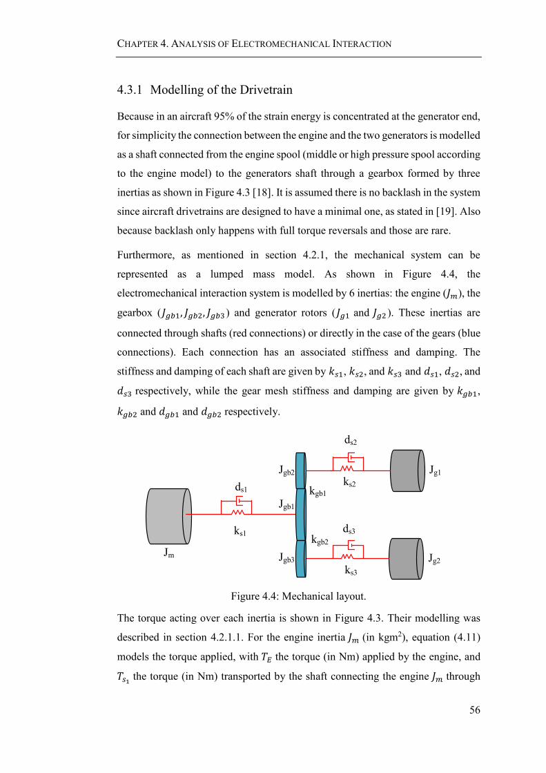
CHAPTER 4. ANALYSIS OF ELECTROMECHANICAL INTERACTION
56
4.3.1 Modelling of the Drivetrain
Because in an aircraft 95% of the strain energy is concentrated at the generator end,
for simplicity the connection between the engine and the two generators is modelled
as a shaft connected from the engine spool (middle or high pressure spool according
to the engine model) to the generators shaft through a gearbox formed by three
inertias as shown in Figure 4.3 [18]. It is assumed there is no backlash in the system
since aircraft drivetrains are designed to have a minimal one, as stated in [19]. Also
because backlash only happens with full torque reversals and those are rare.
Furthermore, as mentioned in section 4.2.1, the mechanical system can be
represented as a lumped mass model. As shown in Figure 4.4, the
electromechanical interaction system is modelled by 6 inertias: the engine (𝐽𝑚), the
gearbox (𝐽𝑔𝑏1, 𝐽𝑔𝑏2, 𝐽𝑔𝑏3) and generator rotors (𝐽𝑔1 and 𝐽𝑔2 ). These inertias are
connected through shafts (red connections) or directly in the case of the gears (blue
connections). Each connection has an associated stiffness and damping. The
stiffness and damping of each shaft are given by 𝑘𝑠1, 𝑘𝑠2, and 𝑘𝑠3 and 𝑑𝑠1, 𝑑𝑠2, and
𝑑𝑠3 respectively, while the gear mesh stiffness and damping are given by 𝑘𝑔𝑏1,
𝑘𝑔𝑏2 and 𝑑𝑔𝑏1 and 𝑑𝑔𝑏2 respectively.
Jm
Jgb1
ks1
Jg1
Jg2
Jgb2
Jgb3
ks2
ks3
ds1
ds2
ds3
kgb1
kgb2
Figure 4.4: Mechanical layout.
The torque acting over each inertia is shown in Figure 4.3. Their modelling was
described in section 4.2.1.1. For the engine inertia 𝐽𝑚 (in kgm2), equation (4.11)
models the torque applied, with 𝑇𝐸 the torque (in Nm) applied by the engine, and
𝑇𝑠1 the torque (in Nm) transported by the shaft connecting the engine 𝐽𝑚 through

CHAPTER 4. ANALYSIS OF ELECTROMECHANICAL INTERACTION
57
the gearbox 𝐽𝑔𝑏1. 𝑇𝑠1 can be calculated by equation (4.12), with 𝜃𝑚, �̇�𝑚, and �̈�𝑚,
the position (in rad), speed (in rad/s), and acceleration (in rad/s2) of the engine
inertia, and 𝜃𝑔𝑏1, �̇�𝑔𝑏1, and �̈�𝑔𝑏1 the values associated with the gear.
𝐽𝑚�̈�𝑚 = 𝑇𝐸 − 𝑇𝑠1 (4.11)
𝑇𝑠1 = 𝑘𝑠1(𝜃𝑚 − 𝜃𝑔𝑏1) + 𝑑𝑠1(�̇�𝑚 − �̇�𝑔𝑏1) (4.12)
The equations for the rest of the system are obtained repeating the same
methodology used for the engine inertia and are shown in equations (4.13) and
(4.14). With 𝑇𝑠1, 𝑇𝑠2 and 𝑇𝑠3 the shafts torque, 𝑇𝑔𝑏1 and 𝑇𝑔𝑏2 the gearshaft torque,
and 𝜃𝑔𝑏1 , 𝜃𝑔𝑏2, 𝜃𝑔𝑏3, 𝜃𝑔1, 𝜃𝑔2 the angles associated with each inertia as shown in
Figure 4.3 and Figure 4.4.
𝐽𝑔𝑏1�̈�𝑔𝑏1 = 𝑇𝑠1 − 𝑇𝑔𝑏1 − 𝑇𝑔𝑏2𝐽𝑔𝑏2�̈�𝑔𝑏2 = 𝑇𝑔𝑏1 − 𝑇𝑠2𝐽𝑔𝑏3�̈�𝑔𝑏3 = 𝑇𝑔𝑏2 − 𝑇𝑠3𝐽𝑔1�̈�𝑔1 = 𝑇𝑠2 − 𝑇𝑔1𝐽𝑔2�̈�𝑔2 = 𝑇𝑠3 − 𝑇𝑔2
}
(4.13)
𝑇𝑠2 = 𝑘𝑠2(𝜃𝑔𝑏2 − 𝜃𝑔1) + 𝑑𝑠2(�̇�𝑔𝑏2 − �̇�𝑔1)
𝑇𝑠3 = 𝑘𝑠3(𝜃𝑔𝑏3 − 𝜃𝑔2) + 𝑑𝑠3(�̇�𝑔𝑏3 − �̇�𝑔2)
𝑇𝑔𝑏1 = 𝑘𝑔𝑏1(𝜃𝑔𝑏1 − 𝜃𝑔𝑏2) + 𝑑𝑔𝑏1(�̇�𝑔𝑏1 − �̇�𝑔𝑏2)
𝑇𝑔𝑏2 = 𝑘𝑔𝑏2(𝜃𝑔𝑏1 − 𝜃𝑔𝑏3) + 𝑑𝑔𝑏2(�̇�𝑔𝑏1 − �̇�𝑔𝑏3)
}
(4.14)
Sorting out equations (4.11)-(4.14), the lumped mass system of equation (4.15) is
obtained. The inertia matrix 𝐽, the stiffness matrix 𝐾, the damping matrix 𝐷, the
input vector 𝑢, and the variables vector of the second order system 𝜃 are given in
equation (4.16).
𝐽�̈� + 𝐷�̇� + 𝐾𝜃 = 𝑢 (4.15)
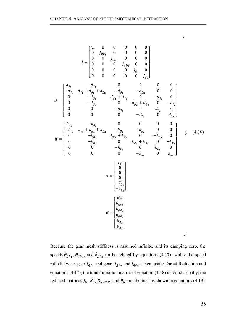
CHAPTER 4. ANALYSIS OF ELECTROMECHANICAL INTERACTION
58
𝐽 =
[ 𝐽𝑚 0 0 0 0 00 𝐽𝑔𝑏1 0 0 0 0
0 0 𝐽𝑔𝑏2 0 0 0
0 0 0 𝐽𝑔𝑏3 0 0
0 0 0 0 𝐽𝑔1 0
0 0 0 0 0 𝐽𝑔2]
𝐷 =
[ 𝑑𝑠1 −𝑑𝑠1 0 0 0 0
−𝑑𝑠1 𝑑𝑠1 + 𝑑𝑔1 + 𝑑𝑔2 −𝑑𝑔1 −𝑑𝑔2 0 0
0 −𝑑𝑔1 𝑑𝑔1 + 𝑑𝑠2 0 −𝑑𝑠2 0
0 −𝑑𝑔2 0 𝑑𝑔2 + 𝑑𝑔3 0 −𝑑𝑠30 0 −𝑑𝑠2 0 𝑑𝑠2 0
0 0 0 −𝑑𝑠3 0 𝑑𝑠3 ]
𝐾 =
[ 𝑘𝑠1 −𝑘𝑠1 0 0 0 0
−𝑘𝑠1 𝑘𝑠1 + 𝑘𝑔1 + 𝑘𝑔2 −𝑘𝑔1 −𝑘𝑔2 0 0
0 −𝑘𝑔1 𝑘𝑔1 + 𝑘𝑠2 0 −𝑘𝑠2 0
0 −𝑘𝑔2 0 𝑘𝑔2 + 𝑘𝑔3 0 −𝑘𝑠30 0 −𝑘𝑠2 0 𝑘𝑠2 0
0 0 0 −𝑘𝑠3 0 𝑘𝑠3 ]
𝑢 =
[ 𝑇𝐸000
−𝑇𝑔1−𝑇𝑔2]
𝜃 =
[ 𝜃𝑚𝜃𝑔𝑏1𝜃𝑔𝑏2𝜃𝑔𝑏3𝜃𝑔1𝜃𝑔2 ]
(4.16)
Because the gear mesh stiffness is assumed infinite, and its damping zero, the
speeds �̇�𝑔𝑏1 , �̇�𝑔𝑏2 , and �̇�𝑔𝑏3can be related by equations (4.17), with 𝑟 the speed
ratio between gear 𝐽𝑔𝑏1 and gears 𝐽𝑔𝑏2 and 𝐽𝑔𝑏3. Then, using Direct Reduction and
equations (4.17), the transformation matrix of equation (4.18) is found. Finally, the
reduced matrices 𝐽𝑅, 𝐾𝑟, 𝐷𝑅, 𝑢𝑅, and 𝜃𝑅 are obtained as shown in equations (4.19).

CHAPTER 4. ANALYSIS OF ELECTROMECHANICAL INTERACTION
59
�̇�𝑔𝑏1 = 𝑟�̇�𝑔𝑏2
�̇�𝑔𝑏1 = 𝑟�̇�𝑔𝑏3
(4.17)
𝑇 =
[ 𝑟1 0 0 00 𝑟1 0 00 1 0 00 1 0 00 0 1 00 0 0 1]
(4.18)
𝐽𝑅 = 𝑇′𝐽𝑇
𝐾𝑅 = 𝑇′𝐾𝑇
𝐷𝑅 = 𝑇′𝐷𝑇
𝑢𝑅 = 𝑇′𝑢 =
[ 𝑇𝐸0
−𝑇𝑔1−𝑇𝑔2]
𝜃𝑅 = 𝑇′𝜃 =
[ 𝜃𝑚𝜃𝑔𝑏𝜃𝑔1𝜃𝑔2 ]
(4.19)
The drivetrain is related to the rest of the system through the torque applied, 𝑇𝐸, 𝑇𝑔1
and 𝑇𝑔2. In the next section the engine and the electrical system are modelled in
order to obtain these values.
4.3.2 Modelling of the Engine
As shown in equation (4.19), the engine applies a torque 𝑇𝐸 on the drivetrain. In
this thesis the modelling of the engine is not in study, hence it can be considered as
a big inertia that keeps the speed constant. Consequently, the torque 𝑇𝐸 is going to
be modelled as a linear equation depending on the engine speed (�̇�𝑚 = 𝜔𝑚) as
shown in (4.20), in which 𝐴𝑇𝑒 and 𝐵𝑇𝑒 are the slope and the position constant.
𝑇𝐸 = 𝐴𝑇𝑒𝜔𝑚 + 𝐵𝑇𝑒 (4.20)
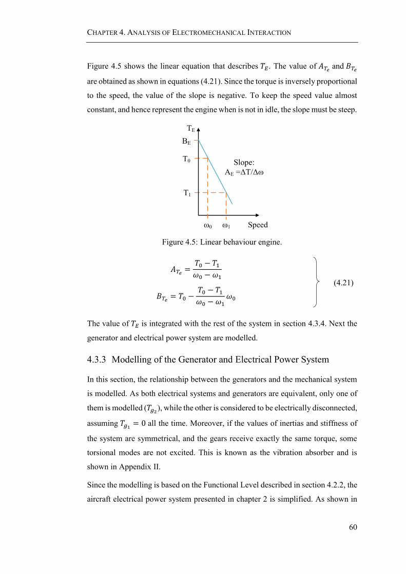
CHAPTER 4. ANALYSIS OF ELECTROMECHANICAL INTERACTION
60
Figure 4.5 shows the linear equation that describes 𝑇𝐸. The value of 𝐴𝑇𝑒 and 𝐵𝑇𝑒
are obtained as shown in equations (4.21). Since the torque is inversely proportional
to the speed, the value of the slope is negative. To keep the speed value almost
constant, and hence represent the engine when is not in idle, the slope must be steep.
TE
Speed
T1
T0
ω0
Slope:
AE =ΔT/Δω
ω1
BE
Figure 4.5: Linear behaviour engine.
𝐴𝑇𝑒 =𝑇0 − 𝑇1𝜔0 − 𝜔1
𝐵𝑇𝑒 = 𝑇0 −𝑇0 − 𝑇1𝜔0 − 𝜔1
𝜔0
(4.21)
The value of 𝑇𝐸 is integrated with the rest of the system in section 4.3.4. Next the
generator and electrical power system are modelled.
4.3.3 Modelling of the Generator and Electrical Power System
In this section, the relationship between the generators and the mechanical system
is modelled. As both electrical systems and generators are equivalent, only one of
them is modelled (𝑇𝑔2), while the other is considered to be electrically disconnected,
assuming 𝑇𝑔1 = 0 all the time. Moreover, if the values of inertias and stiffness of
the system are symmetrical, and the gears receive exactly the same torque, some
torsional modes are not excited. This is known as the vibration absorber and is
shown in Appendix II.
Since the modelling is based on the Functional Level described in section 4.2.2, the
aircraft electrical power system presented in chapter 2 is simplified. As shown in

CHAPTER 4. ANALYSIS OF ELECTROMECHANICAL INTERACTION
61
Figure 4.3 and Figure 4.6, the electrical power system is represented by resistive
banks (𝑅𝐿1 , 𝑅𝐿2 , … , 𝑅𝐿𝑛) connected to the generator through IGBTs. The IGBTs are
switched on and off only to connect and disconnect the loads. Moreover, the
generator is modelled as a DC machine as from a control point of view, the control
of a DC and AC system are the same.
Figure 4.6: Electrical power system.
The generator is modelled as a single phase DC machine operating with
independent field connection. Its equations are given by (4.22) and (4.23), in which
𝑘 is the rotational inductance, 𝑖𝑓 is the field current, 𝑖𝑎 is the armature current, 𝐸 is
the induced voltage, 𝑣𝑎 is the armature voltage at the terminals of the machine, 𝑅𝑎
and 𝐿𝑎 are the armature resistance and inductance respectively, and 𝑉0 is the
voltage drop in the machine brushes.
𝐸 = 𝑅𝑎𝑖𝑎 + 𝐿𝑎𝑑𝑖𝑎𝑑𝑡
+ 𝑣𝑎 + 𝑉0 (4.22)
𝐸 = 𝑘𝑖𝑓�̇�𝑔2 (4.23)

CHAPTER 4. ANALYSIS OF ELECTROMECHANICAL INTERACTION
62
The generator armature voltage 𝑣𝑎 can be kept reasonably constant using a
Generator Control Unit (GCU), which is shown in section 4.6. However, in most
of this thesis the system operates without a GCU, and the field current 𝑖𝑓 is kept
constant instead.
The electrical power system is modelled as a resistive load 𝑅𝑃 always connected in
parallel to the machine terminal, and resistive loads 𝑅𝐿1 , 𝑅𝐿2 , … , 𝑅𝐿𝑛 , connected
through IGBTs to the machine as shown in Figure 4.6. The IGBT allows the
switching of the electrical loads according to different connection patterns which
are studied in this thesis and presented in chapter 5. The resistance 𝑅𝑃 is a
protection resistance to guard the machine of the inductance current when the loads
𝑅𝐿𝑛 are disconnected. To protect the IGBTs during the disconnection, diodes are
connected parallel to the load resistances.
The electrical loads are related to the generator through equation (4.24), in which
𝑅𝑒𝑞 is the equivalent resistance of the parallel connection of 𝑅𝑃 and the load
resistances 𝑅𝐿.
𝑣𝑎 = 𝑅𝑒𝑞𝑖𝑎 (4.24)
Combining equations (4.22) - (4.24), the state variable of the electrical power
system, 𝑖𝑎, is obtained and given by equation (4.25).
𝑑𝑖𝑎𝑑𝑡
=1
𝐿𝑎(𝑘𝑖𝑓�̇�𝑔2 − (𝑅𝑎 + 𝑅𝑒𝑞)𝑖𝑎 − 𝑉0) (4.25)
The torque applied to the mechanical system is given by equation (4.26), in which
𝑇𝑒 is the torque producing the electromotive force and 𝑇𝑤𝑖𝑛𝑑𝑎𝑔𝑒 is the torque
consumed by the windage of the machine. In Appendix I was shown that the
windage torque of the machine is small, therefore, the torque applied to the
mechanical system is modelled as the torque that produces the electromagnetic
force 𝑇𝑒 and shown in equation (4.27). When operating with constant field current,
the torque applied to the mechanical system depends only on the armature current.
𝑇𝑔2 = 𝑇𝑒 + 𝑇𝑤𝑖𝑛𝑑𝑎𝑔𝑒 (4.26)

CHAPTER 4. ANALYSIS OF ELECTROMECHANICAL INTERACTION
63
𝑇𝑔2 = 𝑇𝑒 = 𝑘𝑖𝑓𝑖𝑎 (4.27)
Finally, equation (4.25) and (4.27) are integrated to the drivetrain model as shown
in the next section.
4.3.4 Integrated Model
The equations (4.19)-(4.27) can be modelled in Simulink and PLECS, which allows
the simulation of the electromechanical interaction system. To study the stability
of the integrated electromechanical system, the state system must be obtained.
Consequently, the torques 𝑇𝐸 , 𝑇𝑔1 , and 𝑇𝑔2 , along with the state 𝑖𝑎 must be
connected to the system of equation (4.19).
In the case of the engine, the engine’s torque is modelled linearly by equation (4.20)
and depends on the speed �̇�𝑚. Hence, only the damping matrix 𝐷𝑅 and the input 𝑢𝑅
changes as shown in equations (4.28). The new damping matrix includes the slope
of the engine linear equation 𝐴𝑇𝑒, while the input of the system have the equation
constant value 𝐵𝑇𝑒. Keeping the matrices 𝐽𝑅 and 𝐾𝑅 presented in section 4.3.1, the
lumped mass system equation (4.29) is obtained.
𝐷𝐸𝑛𝑔𝑖𝑛𝑒 = 𝐷𝑅 + [−𝐴𝑇𝑒 03𝑥101x3 03𝑥3
]
𝑢𝐸𝑛𝑔𝑖𝑛𝑒 =
[ 𝐵𝑇𝑒0
−𝑇𝑔1−𝑇𝑔2]
(4.28)
𝐽𝑅�̈�𝑅 + 𝐷𝐸𝑛𝑔𝑖𝑛𝑒�̇�𝑅 + 𝐾𝑅𝜃𝑅 = 𝑢𝐸𝑛𝑔𝑖𝑛𝑒 (4.29)
The state space system, given by equation (4.30) can be obtained from the second
order lumped mass system as shown in equations (4.31) - (4.32) [95]. The states
are given by the angle 𝜃𝑅 and speed �̇�𝑅 of each inertia, while the input of the system
remains the same.
�̇�𝐸𝑛𝑔𝑖𝑛𝑒 = 𝐴𝐸𝑛𝑔𝑖𝑛𝑒𝑥𝐸𝑛𝑔𝑖𝑛𝑒 + 𝐵𝐸𝑛𝑔𝑖𝑛𝑒𝑢𝐸𝑛𝑔𝑖𝑛𝑒 (4.30)

CHAPTER 4. ANALYSIS OF ELECTROMECHANICAL INTERACTION
64
𝑥𝐸𝑛𝑔𝑖𝑛𝑒 = [𝜃𝑅�̇�𝑅] (4.31)
𝐴𝐸𝑛𝑔𝑖𝑛𝑒 = [0 𝐼
−𝐽𝑅−1𝐾𝑅 −𝐽𝑅
−1𝐷𝐸𝑛𝑔𝑖𝑛𝑒]
𝐵𝐸𝑛𝑔𝑖𝑛𝑒 = [0𝐽𝑅−1]
(4.32)
After obtaining the state system of the engine and drivetrain, the effects of the
electrical system can be added. The values of 𝑇𝑔1 = 0 and 𝑇𝑔2 given by equation
(4.27) are used. Moreover, the state equation for 𝑖𝑎 given by equation (4.25) is
added to the system. Since the field current 𝑖𝑓 is constant, the equations do not need
to be linearized.
The state system of the electromechanical interaction, which allows the study of
the stability, is shown in equation (4.33) with the matrices and vector given by
equations (4.34) and (4.35). In next section, the stability of the described system is
analysed, and in sections 4.5 and 4.6 the electromechanical interaction is shown.
�̇�𝑇 = 𝐴𝑇𝑥𝑇 + 𝐵𝑇𝑢𝑇 (4.33)
𝐴𝑇 = [𝐴𝐸𝑛𝑔𝑖𝑛𝑒 08𝑥1
[01x7𝑘𝑖𝑓
𝐿𝑎] −
1
𝐿𝑎(𝑅𝑎 + 𝑅𝑒𝑞)
]
𝐵𝑇 = [
𝐵𝐸𝑛𝑔𝑖𝑛𝑒
−1
𝐿𝑎
]
(4.34)
𝑥𝑇 = [𝑥𝐸𝑛𝑔𝑖𝑛𝑒𝑖𝑎
]
𝑢𝑇 = [𝑢𝐸𝑛𝑔𝑖𝑛𝑒𝑉0
]
(4.35)
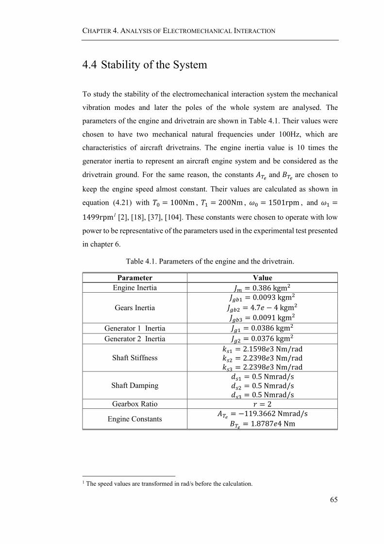
CHAPTER 4. ANALYSIS OF ELECTROMECHANICAL INTERACTION
65
4.4 Stability of the System
To study the stability of the electromechanical interaction system the mechanical
vibration modes and later the poles of the whole system are analysed. The
parameters of the engine and drivetrain are shown in Table 4.1. Their values were
chosen to have two mechanical natural frequencies under 100Hz, which are
characteristics of aircraft drivetrains. The engine inertia value is 10 times the
generator inertia to represent an aircraft engine system and be considered as the
drivetrain ground. For the same reason, the constants 𝐴𝑇𝑒 and 𝐵𝑇𝑒 are chosen to
keep the engine speed almost constant. Their values are calculated as shown in
equation (4.21) with 𝑇0 = 100Nm , 𝑇1 = 200Nm , 𝜔0 = 1501rpm , and 𝜔1 =
1499rpm1 [2], [18], [37], [104]. These constants were chosen to operate with low
power to be representative of the parameters used in the experimental test presented
in chapter 6.
Table 4.1. Parameters of the engine and the drivetrain.
Parameter Value
Engine Inertia 𝐽𝑚 = 0.386 kgm2
Gears Inertia
𝐽𝑔𝑏1 = 0.0093 kgm2
𝐽𝑔𝑏2 = 4.7𝑒 − 4 kgm2
𝐽𝑔𝑏3 = 0.0091 kgm2
Generator 1 Inertia 𝐽𝑔1 = 0.0386 kgm2
Generator 2 Inertia 𝐽𝑔2 = 0.0376 kgm2
Shaft Stiffness 𝑘𝑠1 = 2.1598𝑒3 Nm/rad
𝑘𝑠2 = 2.2398𝑒3 Nm/rad
𝑘𝑠3 = 2.2398𝑒3 Nm/rad
Shaft Damping
𝑑𝑠1 = 0.5 Nmrad/s 𝑑𝑠2 = 0.5 Nmrad/s 𝑑𝑠3 = 0.5 Nmrad/s
Gearbox Ratio 𝑟 = 2
Engine Constants 𝐴𝑇𝑒 = −119.3662 Nmrad/s
𝐵𝑇𝑒 = 1.8787𝑒4 Nm
1 The speed values are transformed in rad/s before the calculation.

CHAPTER 4. ANALYSIS OF ELECTROMECHANICAL INTERACTION
66
The generator parameters are presented in Table 4.2. Their values are the same as
those of the experimental generator which are used for the experimental test in
chapter 6 and chapter 7.
Table 4.2. Generator parameters.
Parameter Value
Armature resistance 𝑅𝑎 = 4.025 Ω
Field resistance 𝑅𝑓 = 2 Ω
Armature Inductance 𝐿𝑎 = 0.019H
Field Inductance 𝐿𝑓 = 0.02H
Rotational inductance 𝑘 = 0.0713 ln − in/A
Drop Voltage Brushes 𝑉0 = 12.247 V
4.4.1 Torsional Vibration Modes of the System
The vibration modes of the drivetrain are analysed to prove that the reduced
electromechanical interaction model in the study is representative of an aircraft
drivetrain. For this, the electromechanical interaction of Figure 4.4 is modelled in
TorTrans, a Matlab Toolbox written by Seamus Garvey, which allows the analysis
of the torsional vibrations of a lumped mass system.
The torsional mode shapes obtained are presented in Figure 4.7. The circles
symbolise the inertias, while the red and blue connections denote the shafts and
gearbox respectively. The vertical green lines represent the inertias referred angles
in each operation mode. It is observed that the system has four modes, a rigid mode
at 0Hz (Figure 4.7 (a)), and three vibration modes at 11.98Hz (Figure 4.7 (a)),
38.59Hz (Figure 4.7 (b)), and 109.7Hz (Figure 4.7 (c)).
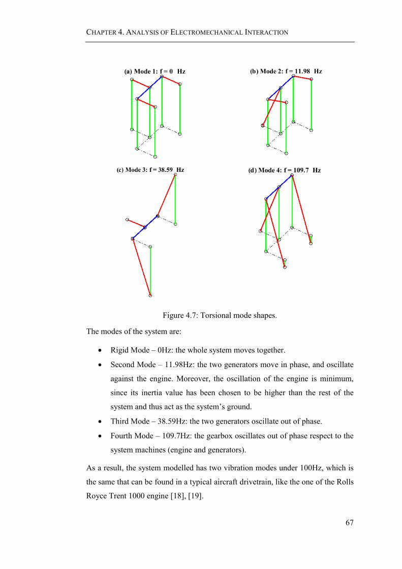
CHAPTER 4. ANALYSIS OF ELECTROMECHANICAL INTERACTION
67
Figure 4.7: Torsional mode shapes.
The modes of the system are:
Rigid Mode – 0Hz: the whole system moves together.
Second Mode – 11.98Hz: the two generators move in phase, and oscillate
against the engine. Moreover, the oscillation of the engine is minimum,
since its inertia value has been chosen to be higher than the rest of the
system and thus act as the system’s ground.
Third Mode – 38.59Hz: the two generators oscillate out of phase.
Fourth Mode – 109.7Hz: the gearbox oscillates out of phase respect to the
system machines (engine and generators).
As a result, the system modelled has two vibration modes under 100Hz, which is
the same that can be found in a typical aircraft drivetrain, like the one of the Rolls
Royce Trent 1000 engine [18], [19].

CHAPTER 4. ANALYSIS OF ELECTROMECHANICAL INTERACTION
68
4.4.2 Poles of the System
The state system presented in section 4.3.4 is used to analyse the stability through
poles analyses. Figure 4.8 shows the poles of the electromechanical interaction
system. Since all the poles are in the left hemisphere the system in study is stable.
Moreover, through participation factor analysis the states with a higher correlation
to each pole are found. These are circled in red in the figure, observing that the
poles associated with the engine and the electrical power system are further from
the origin than the ones related to the mechanical system or drivetrain as was
expected.
Figure 4.8: Poles of the system.
The natural frequencies and damping ratio are obtained using equation (4.36), in
which 𝑎 and 𝑏 are the real and imaginary part of the eigenvalue respectively, and
𝜉 , 𝜔𝑛 , and 𝑓𝑛 are the damping ratio, natural frequency in rad/s and natural
frequency in Hz.
𝑠 = −𝑎 ± 𝑗𝑏 = −𝜉𝜔𝑛 ± 𝜔𝑛√1 − 𝜉2
𝑓𝑛 =𝜔𝑛2𝜋
(4.36)
The obtained natural frequencies and damping ratios are:
𝑓0 = 0Hz, 𝜉0 = 1
𝑓1 = 11.9443Hz, 𝜉1 = 0.0362

CHAPTER 4. ANALYSIS OF ELECTROMECHANICAL INTERACTION
69
𝑓2 = 38.5982Hz, 𝜉2 = 0.0276
𝑓3 = 109.7207Hz, 𝜉3 = 0.0774
𝑓4 = 137.4276Hz, 𝜉4 = 1
𝑓5 = 196.3611Hz, 𝜉5 = 1
The participation analysis of the poles shows that the first four frequencies are
predominantly associated with the mechanical system. This is the same that was
obtained through the vibration mode analysis, proving that the poles closer to the
origin are the drivetrain vibration modes.
Furthermore, the poles allow finding the settling time of the electromechanical
interaction to a step connection. This is the time that the system’s response takes to
reach a set range of the steady-state value. To obtain this, the envelope of the system
response given by equation (4.37) is used.
𝑦𝑒𝑛𝑣𝑒𝑙𝑜𝑝𝑒(𝑡) = 1 ±exp(−𝜉𝜔𝑛𝑡)
√1 − 𝜉2 (4.37)
For 𝜉 = 1 the settling time is given by the time constant of the system. Instead, for
𝜉 < 1, the settling time is obtained by calculating the value at which the signal
envelope has the desired value, as shown in equation (4.38) and Figure 4.9. 𝑆 is the
settling value to be used. For 𝑆 = 1%, equation (4.39) can be used to obtain the
settling time associated with each natural frequency [105].
Figure 4.9: Settling time diagram.
𝑦𝑒𝑛𝑣𝑒𝑙𝑜𝑝𝑒(𝑡) ≤ (1 ± 𝑆) (4.38)
CHAPTER 4. ANALYSIS OF ELECTROMECHANICAL INTERACTION
70
exp(−𝜉𝜔𝑛𝑡𝑠)
√1 − 𝜉2= 0.01 ⇒ 𝑡𝑠 = −
log(0.01√1 − 𝜉2 )
𝜉𝜔𝑛 (4.39)
The settling times are:
𝑓1 = 11.9443Hz 𝑡𝑠1 = 1.6953s
𝑓2 = 38.5982Hz 𝑡𝑠2 = 0.6881s
𝑓3 = 109.7207Hz 𝑡𝑠3 = 0.0864s
𝑓4 = 137.4276Hz 𝑡𝑠4 = 0.0073s
𝑓5 = 196.3611Hz 𝑡𝑠5 = 0.0051s
Finally, the settling times of the mechanical system are higher than the ones of the
electrical system. This difference in timing allows the modelling of the power
system as torque step connections.
4.5 Load Connections
Until now, the modelling of the electromechanical interaction has been presented,
and its stability has been assessed. In this section, the effects of step load
connections and pulsating load connections are shown.
4.5.1 Step Connection
To test the step connection, a 5Ω resistive load is connected to the system operating
in steady state with a field current 𝑖𝑓 = 6.2A and only the protection resistance
𝑅𝑃 = 60Ω connected. Table 4.3 shows the steady state operation values before and
after the connection. It is observed that as the speed of the system is controlled by
the engine, the step only produces a low drop on its value, regardless of the 2.5Nm
change in torque.

CHAPTER 4. ANALYSIS OF ELECTROMECHANICAL INTERACTION
71
Table 4.3: Steady state values.
Parameter Value
Before Connection After Connection
Armature Current 𝑖𝑎 0.8947 A 2.307 A
Armature Voltage 𝑣𝑎 53.68 V 30.59 V
Field Current 𝑖𝑓 6.2 A 6.2 A
Field Voltage 𝑣𝑓 11.16 V 11.16 V
Electrical Power 𝑃𝐸 48.03 W 202.8 W
Electrical Torque 𝑇𝑔2 0.3952 Nm 2.928 Nm
Shaft Torque 𝑇𝑠3 0.3952 Nm 2.928 Nm
Generator Speed 𝜔𝑔2 1503 rpm 1502.8 rpm
The electrical results of the step connection are shown in Figure 4.10. Since the
field current is externally given, its value and the field voltage value do not change
as a result of the connection. However, the armature current is higher because a
higher load must be fed. The armature voltage drops, due to the higher current
consumption in the machine windings. As the electromotive voltage, given by 𝐸 =
𝑘𝑖𝑓𝜔, depends only on the speed its value is virtually constant since the speed is
fixed by the engine, and hence is practically constant as shown in Table 4.3.
Therefore, the change in armature voltage is only due to the higher current
consumption on the armature windings.
The consumed power and the torque needed at the machine are higher after the load
connection. The temporary drop in power after the load connection is due to the
drop in voltage, produced by the presence of inductances in the system. Moreover,
it is observed that the transient lasts 7ms (for a settling time of 1%), which agrees
with the 7.3ms time constant obtained for 137Hz. Small vibrations can be observed
after 7ms , which are due to the lower natural frequencies associated with the
drivetrain of the system. The maximum load connection depends on the electrical
characteristics and the value of the voltage overshoot according to [106].

CHAPTER 4. ANALYSIS OF ELECTROMECHANICAL INTERACTION
72
Figure 4.10: Electrical step response of the system.
The mechanical response of the system: the speed (a), acceleration (b) of each
inertia in the drivetrain, along with the torque in the generator shaft (c) are shown
in Figure 4.11. It is observed that the connection of the electrical load produces
vibrations in these variables along the whole drivetrain. Hence, a change in the
electrical load produces a transient in all the components of the system. In (a), and
(b) the vibrations of the engine shaft are observed in blue. These vibrations are
considerably lower than the ones of the rest of the system due to the higher damping
and inertia of the engine, which acts as the ground of the mechanical system. This
behaviour is consistent with an aircraft drivetrain in which the size of the engine is
much higher than the one of the electrical system as its power is used to move the
plane and not only power the electrical power system.

CHAPTER 4. ANALYSIS OF ELECTROMECHANICAL INTERACTION
73
Moreover, it can be seen that the transients are longer than the one presented on the
electrical system, with values of the order of 1.3s. This is consistent with having
lower natural frequencies with lower damping and between the theory settling times
obtained for 𝑓1 and 𝑓2.
Figure 4.11: Mechanical step response of the system.
In Figure 4.11 (c), the changes in electrical torque (in red) and shaft torque (in blue)
are observed. 𝑇𝑔2 can be approximated by a step, with a settling time much lower
than the one of the mechanical system, as was already mentioned. This connection
is reduced and modelled as a perfect step connection for simplification from chapter
5 to 7.
Since the effect of an electrical step connection is the production of vibrations on
the shaft of the system, electromechanical interaction has been demonstrated. As
presented in chapter 3, the torsional vibrations can reduce the lifespan of the
mechanical components and produce fatigue. To decrease the effect of the
electromechanical interaction, and consequently, reduce the torsional vibrations,
vibration suppression methods must be analysed.
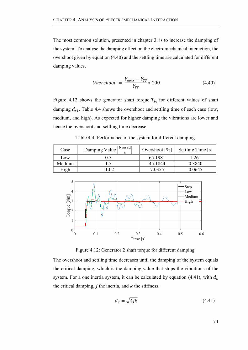
CHAPTER 4. ANALYSIS OF ELECTROMECHANICAL INTERACTION
74
The most common solution, presented in chapter 3, is to increase the damping of
the system. To analyse the damping effect on the electromechanical interaction, the
overshoot given by equation (4.40) and the settling time are calculated for different
damping values.
𝑂𝑣𝑒𝑟𝑠ℎ𝑜𝑜𝑡 = 𝑌𝑚𝑎𝑥 − 𝑌𝑆𝑆
𝑌𝑆𝑆∗ 100 (4.40)
Figure 4.12 shows the generator shaft torque 𝑇𝑠3 for different values of shaft
damping 𝑑𝑠1. Table 4.4 shows the overshoot and settling time of each case (low,
medium, and high). As expected for higher damping the vibrations are lower and
hence the overshoot and settling time decrease.
Table 4.4: Performance of the system for different damping.
Case Damping Value [Nmrad
s] Overshoot [%] Settling Time [s]
Low 0.5 65.1981 1.261
Medium 1.5 45.1844 0.3840
High 11.02 7.0355 0.0645
Figure 4.12: Generator 2 shaft torque for different damping.
The overshoot and settling time decreases until the damping of the system equals
the critical damping, which is the damping value that stops the vibrations of the
system. For a one inertia system, it can be calculated by equation (4.41), with 𝑑𝑐
the critical damping, 𝑗 the inertia, and 𝑘 the stiffness.
𝑑𝑐 = √4𝑗𝑘 (4.41)
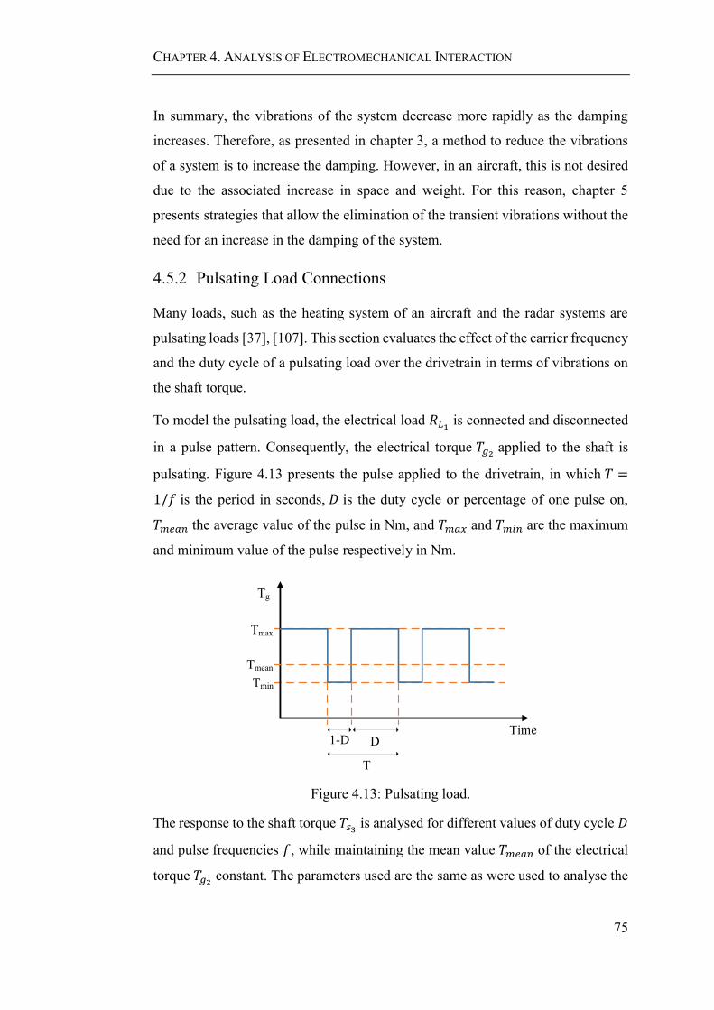
CHAPTER 4. ANALYSIS OF ELECTROMECHANICAL INTERACTION
75
In summary, the vibrations of the system decrease more rapidly as the damping
increases. Therefore, as presented in chapter 3, a method to reduce the vibrations
of a system is to increase the damping. However, in an aircraft, this is not desired
due to the associated increase in space and weight. For this reason, chapter 5
presents strategies that allow the elimination of the transient vibrations without the
need for an increase in the damping of the system.
4.5.2 Pulsating Load Connections
Many loads, such as the heating system of an aircraft and the radar systems are
pulsating loads [37], [107]. This section evaluates the effect of the carrier frequency
and the duty cycle of a pulsating load over the drivetrain in terms of vibrations on
the shaft torque.
To model the pulsating load, the electrical load 𝑅𝐿1 is connected and disconnected
in a pulse pattern. Consequently, the electrical torque 𝑇𝑔2 applied to the shaft is
pulsating. Figure 4.13 presents the pulse applied to the drivetrain, in which 𝑇 =
1/𝑓 is the period in seconds, 𝐷 is the duty cycle or percentage of one pulse on,
𝑇𝑚𝑒𝑎𝑛 the average value of the pulse in Nm, and 𝑇𝑚𝑎𝑥 and 𝑇𝑚𝑖𝑛 are the maximum
and minimum value of the pulse respectively in Nm.
Tg
Time
Tmin
Tmax
Tmean
1-D D
T
Figure 4.13: Pulsating load.
The response to the shaft torque 𝑇𝑠3 is analysed for different values of duty cycle 𝐷
and pulse frequencies 𝑓, while maintaining the mean value 𝑇𝑚𝑒𝑎𝑛 of the electrical
torque 𝑇𝑔2 constant. The parameters used are the same as were used to analyse the

CHAPTER 4. ANALYSIS OF ELECTROMECHANICAL INTERACTION
76
stability and the step load connection. The shaft damping is 𝑑𝑠1 = 0.5Nmrad/s
and 𝑑𝑠2 = 𝑑𝑠3 = 0.5Nmrad/s . The minimum value of the electrical torque is
𝑇𝑚𝑖𝑛 = 0.3952Nm , which is the torque obtained when only 𝑅𝑃 = 60Ω is
connected. The maximum torque 𝑇𝑚𝑎𝑥 is calculated from equation (4.42), in which
𝑇𝑚𝑒𝑎𝑛 is the mean torque applied to the system, and its value is 2.928Nm,
corresponding to the torque obtained when a resistance 𝑅𝐿1is connected.
𝑇𝑚𝑎𝑥 =𝑇𝑚𝑒𝑎𝑛 − 𝑇𝑚𝑖𝑛(1 − 𝐷)
𝐷 (4.42)
Figure 4.14 presents the results obtained when a pulse with a duty cycle 𝐷 = 75%
and frequencies of 1Hz (a), 11.94Hz (b), and 200Hz (c) are connected. In the three
cases the generator torque 𝑇𝑔2 applied is shown in red, while the shaft torque 𝑇𝑠3 is
presented in blue.
When a 1Hz pulse is used as shown in Figure 4.14 (a), each connection presents a
transient response, due to the long time between the pulses. This case, which is
observed in aircraft heating systems, can be considered as a series of step load
connections and thus apply the same strategies to eliminate the vibrations. These
strategies are presented in chapter 5. In the second case, shown in Figure 4.14 (b),
a frequency equals to the natural frequency of the drivetrain 11Hz is used. This
generates resonance, and thus a high amplitude sustained vibration on the shaft.
Therefore, the operation at the natural frequency values must be avoided. Finally,
when a high-frequency pulse is applied, as in Figure 4.14 (c), the system reaches
steady state as if the load applied would be equal to a single step connection.
Therefore, only an initial overshoot and settling time are observed. Now, low
frequencies are going to be defined as those under the lower resonance value, while
higher frequencies are the ones over.
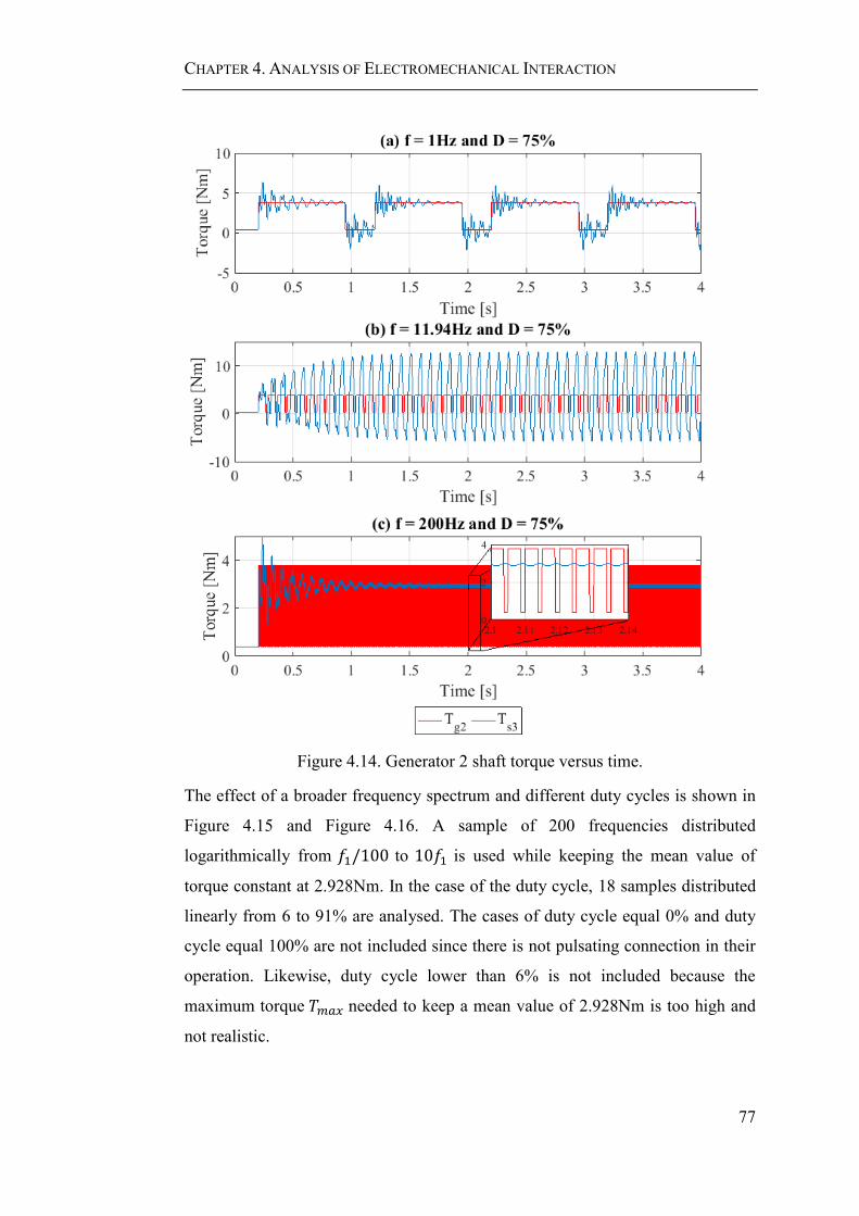
CHAPTER 4. ANALYSIS OF ELECTROMECHANICAL INTERACTION
77
Figure 4.14. Generator 2 shaft torque versus time.
The effect of a broader frequency spectrum and different duty cycles is shown in
Figure 4.15 and Figure 4.16. A sample of 200 frequencies distributed
logarithmically from 𝑓1/100 to 10𝑓1 is used while keeping the mean value of
torque constant at 2.928Nm. In the case of the duty cycle, 18 samples distributed
linearly from 6 to 91% are analysed. The cases of duty cycle equal 0% and duty
cycle equal 100% are not included since there is not pulsating connection in their
operation. Likewise, duty cycle lower than 6% is not included because the
maximum torque 𝑇𝑚𝑎𝑥 needed to keep a mean value of 2.928Nm is too high and
not realistic.
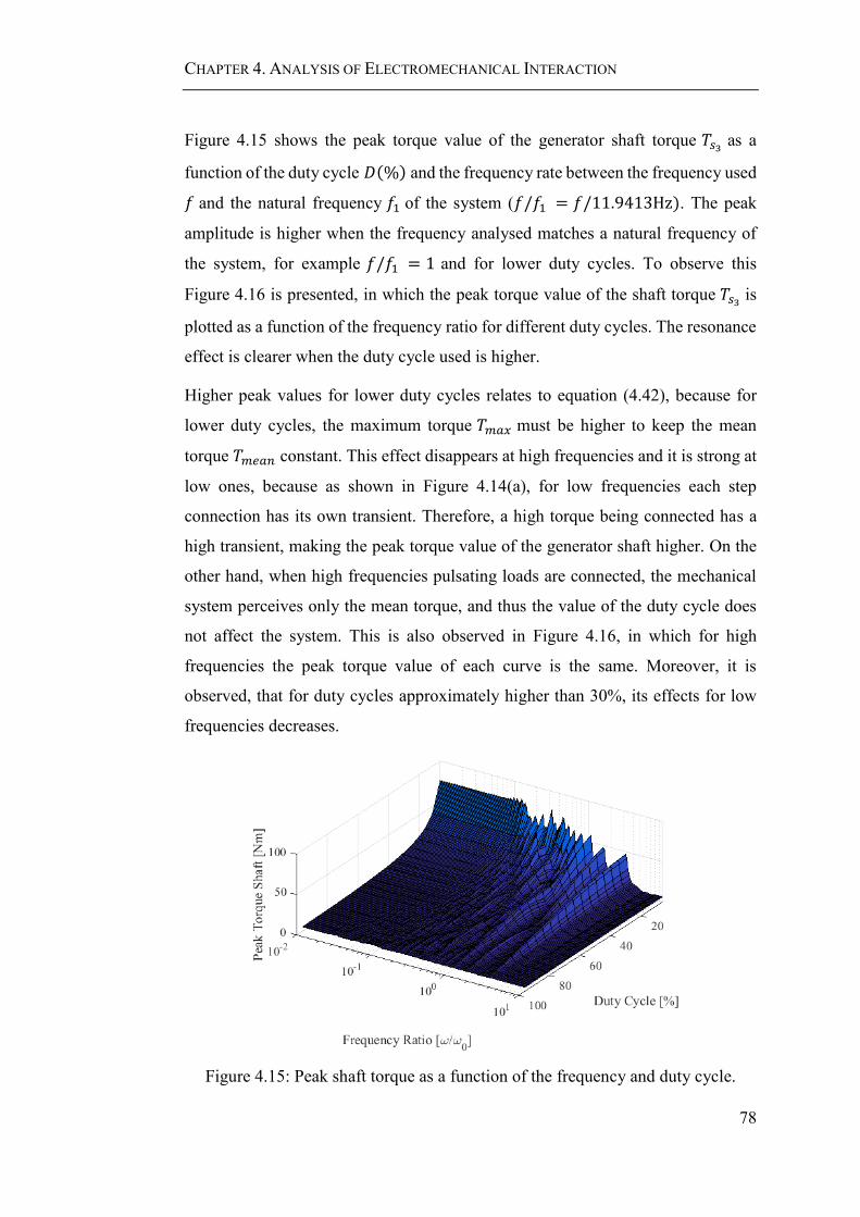
CHAPTER 4. ANALYSIS OF ELECTROMECHANICAL INTERACTION
78
Figure 4.15 shows the peak torque value of the generator shaft torque 𝑇𝑠3 as a
function of the duty cycle 𝐷(%) and the frequency rate between the frequency used
𝑓 and the natural frequency 𝑓1 of the system (𝑓/𝑓1 = 𝑓/11.9413Hz). The peak
amplitude is higher when the frequency analysed matches a natural frequency of
the system, for example 𝑓/𝑓1 = 1 and for lower duty cycles. To observe this
Figure 4.16 is presented, in which the peak torque value of the shaft torque 𝑇𝑠3 is
plotted as a function of the frequency ratio for different duty cycles. The resonance
effect is clearer when the duty cycle used is higher.
Higher peak values for lower duty cycles relates to equation (4.42), because for
lower duty cycles, the maximum torque 𝑇𝑚𝑎𝑥 must be higher to keep the mean
torque 𝑇𝑚𝑒𝑎𝑛 constant. This effect disappears at high frequencies and it is strong at
low ones, because as shown in Figure 4.14(a), for low frequencies each step
connection has its own transient. Therefore, a high torque being connected has a
high transient, making the peak torque value of the generator shaft higher. On the
other hand, when high frequencies pulsating loads are connected, the mechanical
system perceives only the mean torque, and thus the value of the duty cycle does
not affect the system. This is also observed in Figure 4.16, in which for high
frequencies the peak torque value of each curve is the same. Moreover, it is
observed, that for duty cycles approximately higher than 30%, its effects for low
frequencies decreases.
Figure 4.15: Peak shaft torque as a function of the frequency and duty cycle.
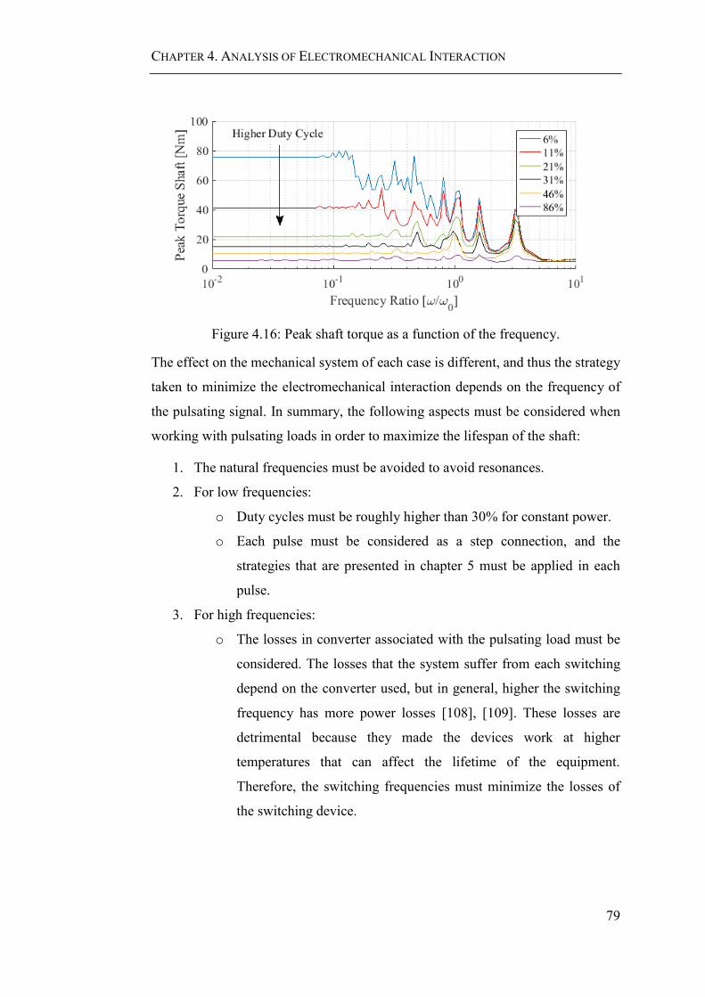
CHAPTER 4. ANALYSIS OF ELECTROMECHANICAL INTERACTION
79
Figure 4.16: Peak shaft torque as a function of the frequency.
The effect on the mechanical system of each case is different, and thus the strategy
taken to minimize the electromechanical interaction depends on the frequency of
the pulsating signal. In summary, the following aspects must be considered when
working with pulsating loads in order to maximize the lifespan of the shaft:
1. The natural frequencies must be avoided to avoid resonances.
2. For low frequencies:
o Duty cycles must be roughly higher than 30% for constant power.
o Each pulse must be considered as a step connection, and the
strategies that are presented in chapter 5 must be applied in each
pulse.
3. For high frequencies:
o The losses in converter associated with the pulsating load must be
considered. The losses that the system suffer from each switching
depend on the converter used, but in general, higher the switching
frequency has more power losses [108], [109]. These losses are
detrimental because they made the devices work at higher
temperatures that can affect the lifetime of the equipment.
Therefore, the switching frequencies must minimize the losses of
the switching device.

CHAPTER 4. ANALYSIS OF ELECTROMECHANICAL INTERACTION
80
4.6 GCU Controller Effect
The previous section showed that an electrical load connection could have
repercussions in the mechanical system, producing vibrations that decrease the
shaft lifespan. However, as mentioned in chapter 3, the control systems can also be
a source of electromechanical interaction. In [21] it is said that the electrical
machine control can produce negative damping on the shaft. And in [63] it has been
shown by simulation that the GCU produces an interaction on marine systems. To
avoid these problems, the system must be designed appropriately.
Now, a case in which the Generator Control Unit (GCU) of the generator can
produce instabilities in the mechanical system if its design is oversimplified is
presented. For this reason, a GCU controller, which keeps the armature voltage 𝑣𝑎
constant, is connected to the generator of the system modelled in section 4.3.
4.6.1 GCU Operation
As shown in Figure 4.17, a 𝑉/𝑓 open loop control is used to keep the armature
voltage of the generator 𝑣𝑎(𝑡) constant at 𝑉𝑛𝑜𝑚 by regulating the field current
𝑖𝑓(𝑡).
System Gp(s)Controller
Gc(s)
Field Current
if (t)Vnom
Output Signal
va(t)
Figure 4.17: Simplified open loop GCU.
The field current 𝑖𝑓 determines the back-EMF through equation (4.23), in which
𝐸 = 𝑘𝑖𝑓𝜔𝑔2 . Then, as shown in equation (4.43) the field current applied to the
machine depends on the speed of the system, which regulates the armature voltage.
Replacing the value of the torque constant 𝑘𝑡 = 𝑘𝑖𝑓 in the electrical torque equation
(4.26) and the back-EMF equation (4.23), the control values of these variables,
given by equations (4.44) and (4.45) are found.

CHAPTER 4. ANALYSIS OF ELECTROMECHANICAL INTERACTION
81
𝑘𝑡 = 𝑘𝑖𝑓 =𝑉𝑛𝑜𝑚𝜔𝑔2
⇒ 𝑖𝑓 =𝑉𝑛𝑜𝑚𝑘𝜔𝑔2
(4.43)
𝐸 = 𝑘𝑖𝑓𝜔𝑔2 = 𝑘𝑡𝜔𝑔2 = 𝑉𝑛𝑜𝑚 (4.44)
𝑇𝑔2 = 𝑘𝑖𝑓𝑖𝑎 = 𝑘𝑡𝑖𝑎 =𝑉𝑛𝑜𝑚𝜔𝑔2
𝑖𝑎 (4.45)
The system is tested using the parameters of Table 4.1 and Table 4.2. To eliminate
the change in power consumed in the windings 𝑅𝑎 = 0Ω. The nominal voltage
𝑉𝑛𝑜𝑚 is given by equation (4.46), in which 𝑉0 is the voltage drop across the brushes
(shown in Table 4.2), and 𝑉𝑎∗ = 40V the desired output voltage.
𝑉𝑛𝑜𝑚 = 𝑉𝑎∗ + 𝑉0 (4.46)
Figure 4.18 and Figure 4.19 show the results obtained for the electrical and
mechanical systems after a step load connection. The protection resistance used is
𝑅𝑃 = 60Ω and the load connected is 𝑅𝐿1 = 5Ω . It is observed that with the
exception of having a constant armature voltage (Figure 4.18 (b)), and thus, a higher
power consumption and torque, the response of the rest of the system (electrical
and mechanical) is equivalent to the one of a step connection with no GCU. The
higher power and torque is due to the having a higher armature voltage since the
GCU is keeping it constant. Figure 4.20 shows that when the torque is normalised,
the behaviour of the system is the same with and without GCU.

CHAPTER 4. ANALYSIS OF ELECTROMECHANICAL INTERACTION
82
Figure 4.18: Electrical system with GCU.
Figure 4.19: Mechanical system with GCU.
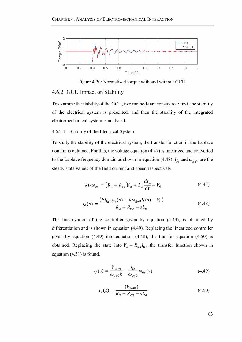
CHAPTER 4. ANALYSIS OF ELECTROMECHANICAL INTERACTION
83
Figure 4.20: Normalised torque with and without GCU.
4.6.2 GCU Impact on Stability
To examine the stability of the GCU, two methods are considered: first, the stability
of the electrical system is presented, and then the stability of the integrated
electromechanical system is analysed.
4.6.2.1 Stability of the Electrical System
To study the stability of the electrical system, the transfer function in the Laplace
domain is obtained. For this, the voltage equation (4.47) is linearized and converted
to the Laplace frequency domain as shown in equation (4.48). 𝐼𝑓0 and 𝜔𝑔20 are the
steady state values of the field current and speed respectively.
𝑘𝑖𝑓𝜔𝑔2 = (𝑅𝑎 + 𝑅𝑒𝑞)𝑖𝑎 + 𝐿𝑎𝑑𝑖𝑎𝑑𝑡
+ 𝑉0 (4.47)
𝐼𝑎(𝑠) =(𝑘𝐼𝑓0𝜔𝑔2(𝑠) + 𝑘𝜔𝑔20𝐼𝑓(s) − 𝑉0)
𝑅𝑎 + 𝑅𝑒𝑞 + 𝑠𝐿𝑎 (4.48)
The linearization of the controller given by equation (4.43), is obtained by
differentiation and is shown in equation (4.49). Replacing the linearized controller
given by equation (4.49) into equation (4.48), the transfer equation (4.50) is
obtained. Replacing the state into 𝑉𝑎 = 𝑅𝑒𝑞𝐼𝑎 , the transfer function shown in
equation (4.51) is found.
𝐼𝑓(s) =𝑉𝑛𝑜𝑚𝜔𝑔20𝑘
−𝐼𝑓0𝜔𝑔20
𝜔𝑔2(𝑠) (4.49)
𝐼𝑎(𝑠) =(𝑉𝑛𝑜𝑚)
𝑅𝑎 + 𝑅𝑒𝑞 + 𝑠𝐿𝑎 (4.50)

CHAPTER 4. ANALYSIS OF ELECTROMECHANICAL INTERACTION
84
𝑉𝑎(𝑠)
𝑉𝑛𝑜𝑚=
𝑅𝑒𝑞
𝑅𝑎 + 𝑅𝑒𝑞 + 𝑠𝐿𝑎 (4.51)
From the transfer function (4.51), the pole of the electrical system 𝑠 = −(𝑅𝑎 +
𝑅𝑒𝑞)/𝐿𝑎 is obtained. As the resistances and inductances are always positive, the
stability analysis of the electrical system shows that regardless of the GCU value,
the system is stable.
4.6.2.2 Stability of the Electromechanical System
It has been demonstrated that when the electrical power system is analysed in
isolation, the system is always stable. Now, the stability of the same system is
studied, through state systems, including the mechanical drivetrain. For this,
considering the electrical system in steady state, the stability is tested in the
presence of a mechanical perturbation.
Equation (4.45) shows that when the GCU is connected, the electrical torque
applied on the mechanical system depends on the armature current 𝑖𝑎 and speed of
the system 𝜔𝑔2. Because for a stable electrical system 𝑖𝑎 = 𝑐𝑜𝑛𝑠𝑡𝑎𝑛𝑡, since the
armature current 𝑣𝑎 and the power are constant, a new constant 𝐾𝑔 = 𝑉𝑛𝑜𝑚𝑖𝑎 can
be defined and replaced into (4.45) obtaining equation (4.52).
𝑇𝑔2 =𝑉𝑛𝑜𝑚𝜔𝑔2
𝑖𝑎 =𝐾𝑔
𝜔𝑔2 (4.52)
To obtain the state system, equation (4.52) must be linearized and equation (4.53)
is obtained. The slope of the equation, given by −𝐾𝑔/𝜔𝑔202 shows that GCU has a
negative damping effect proportional to the nominal voltage 𝑉𝑛𝑜𝑚. Therefore, there
is a value in the system, in which the system becomes unstable.
𝑇𝑔2 = −𝐾𝑔
𝜔𝑔202 𝜔𝑔2 +
2𝐾𝑔
𝜔𝑔20 (4.53)
Equation (4.53) is replaced in the engine-drivetrain steady state system found in
section 4.3.4 and given by equation (4.30), as shown in equation (4.54).

CHAPTER 4. ANALYSIS OF ELECTROMECHANICAL INTERACTION
85
[�̇�𝑅�̈�𝑅] = 𝐴𝐷𝐸 [
𝜃𝑅�̇�𝑅] + 𝐵𝐷𝐸 [
𝐵𝐸𝑛𝑔𝑖𝑛𝑒00
−𝑇𝑔2
]
[�̇�𝑅�̈�𝑅] = 𝐴𝐷𝐸 [
𝜃𝑅�̇�𝑅] + 𝐵𝐷𝐸
[
𝐵𝐸𝑛𝑔𝑖𝑛𝑒00
𝐾𝑔
𝜔𝑔20�̇�𝑔2 −
2𝐾𝑔
𝜔𝑔20]
[�̇�𝑅�̈�𝑅] =
(
𝐴𝐷𝐸 + 𝐵𝐷𝐸
[ 000𝐾𝑔
𝜔𝑔202 ]
[01𝑥7 1]
)
[𝜃𝑅�̇�𝑅] + 𝐵𝐷𝐸
[ 𝐵𝐸𝑛𝑔𝑖𝑛𝑒00
−2𝐾𝑔
𝜔𝑔20 ]
[�̇�𝑅�̈�𝑅] = 𝐴𝐺𝐶𝑈 [
𝜃𝑅�̇�𝑅] + 𝐵𝐷𝐸
[ 𝐵𝐸𝑛𝑔𝑖𝑛𝑒00
−2𝐾𝑔
𝜔𝑔20 ]
(4.54)
Rewriting the GCU constant as shown in equation (4.55), the nominal voltage value
to be controlled is given by equation (4.56).
�̃� =𝐾𝑔
𝜔𝑔202 (4.55)
𝑉𝑛𝑜𝑚 =�̃�𝜔𝑔20
2
𝐼𝑎0 (4.56)
For the system parameters of Table 4.1, Figure 4.21 shows the movement of the
poles while �̃� increases. Hence, when the stability of the whole system is analysed,
there is a maximum 𝑉𝑛𝑜𝑚 that can be controlled by the GCU which turns the system
unstable.
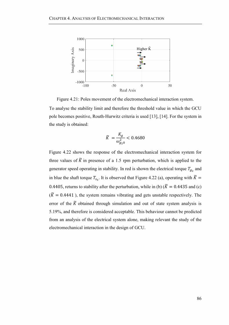
CHAPTER 4. ANALYSIS OF ELECTROMECHANICAL INTERACTION
86
Figure 4.21: Poles movement of the electromechanical interaction system.
To analyse the stability limit and therefore the threshold value in which the GCU
pole becomes positive, Routh-Hurwitz criteria is used [13], [14]. For the system in
the study is obtained:
�̃� =𝐾𝑔
𝜔𝑔202 < 0.4680
Figure 4.22 shows the response of the electromechanical interaction system for
three values of �̃� in presence of a 1.5 rpm perturbation, which is applied to the
generator speed operating in stability. In red is shown the electrical torque 𝑇𝑔2 and
in blue the shaft torque 𝑇𝑠3. It is observed that Figure 4.22 (a), operating with �̃� =
0.4405, returns to stability after the perturbation, while in (b) (�̃� = 0.4435 and (c)
(�̃� = 0.4441 ), the system remains vibrating and gets unstable respectively. The
error of the �̃� obtained through simulation and out of state system analysis is
5.19%, and therefore is considered acceptable. This behaviour cannot be predicted
from an analysis of the electrical system alone, making relevant the study of the
electromechanical interaction in the design of GCU.

CHAPTER 4. ANALYSIS OF ELECTROMECHANICAL INTERACTION
87
Figure 4.22: GCU stability.
4.7 Summary
In this chapter, the reduced electromechanical system representative of an aircraft
drivetrain and electrical power system was presented and modelled. Its stability was
studied, and its natural frequencies were analysed, proving that the model is
representative of an aeroplane system since the main natural frequencies are found
in a real plane.
Furthermore, the coupling between both systems (electrical and mechanical) was
demonstrated through analysis of the effect of load connections and the GCU
stability. These allowed the testing of the sources of electromechanical interaction
presented in chapter 3: Control System, Step Load, and Pulsating Load. The effects
CHAPTER 4. ANALYSIS OF ELECTROMECHANICAL INTERACTION
88
of a Grid Fault are equivalent to the ones of a high step load, while the
electromechanical interaction due to sub-synchronous currents is out of the scope
of this thesis.
Moreover, the strategy to eliminate the vibrations due to electromechanical
interaction depends on the reason for the torsional vibrations excitation. For
example, to avoid instability due to the control system, the GCU needs to be
designed considering the whole system. In the case of load connections, the strategy
used to eliminate the transients depend on the load characteristics.
For pulsating loads, the operation at frequencies equal to the natural frequency is
avoided. The transients produced due to each pulse connection at low frequencies
are treated as a step connection, while for high frequencies, the overall torque
applied over the mechanical shaft can be considered as a step.
To reduce the vibrations due to step connections, it was shown that the damping
could be increased. However, as this is not desired in aircraft systems, the next
chapter presents a power management system (PMS) that allows the suppression of
the torsional vibrations due to electrical load connections.

Chapter 5
5 Power Management System
5.1 Introduction
In this chapter, a power management system (PMS) that reduces the excitation of
torsional vibrations in the drivetrain due to electrical load connections is presented.
Due to the different loads in an aircraft, in section 5.2 a classification of them is
established: time non-critical, time critical, low frequency pulsating load, and high
frequency pulsating load. Thus, the PMS must apply different strategies according
to the electrical load connected, as shown in Figure 5.1. These strategies are based
on the open loop Posicast method [110] and are called Single Level Multi-edge
Switching (SLME), Multilevel Loading (MLL), and Multi-load Single Level Multi-
edge Switching (MSLME). These strategies are presented in section 5.4 and 5.5.
Figure 5.1: PMS layout.
Since this thesis studies the effect of resistive loads, the effects of inductance and
capacitance are ignored in the strategies defined in this chapter. Thus, the torque
steps applied by the generator are perfectly square. For this reason, the machine
inductances of the system presented in chapter 4 are zero: 𝐿𝑎 = 0H. The effects of

CHAPTER 5. POWER MANAGEMENT SYSTEM
90
the inductances are shown in the experimental results presented in chapter 7 and
studied in chapter 8.
The rest of the chapter is organised as follows. First, the classification of aircraft
power loads is presented. Second, the relationship between the excitation of natural
frequencies and the force applied is analysed. As a solution, the Posicast method is
studied. Third, PMS strategies for step load connections are proposed and analysed.
Later, the strategies to be applied in pulsating loads are introduced, and the
requirements to apply the strategies in a real aircraft presented. Finally, the chapter
summary is given.
5.2 Power Load Classification
Since not every load has the same requirements, the PMS applies different
strategies according to the load connected to the system (shown in Figure 5.1).
Table 5.1 classifies the MEA aircraft loads given in [9], into step loads with time
critical and time non-critical requirements, and pulsating loads with low and high
frequency.
Table 5.1: Classification of loads on aircraft system.
Step Load Pulsating Load
Time Critical Time Non-critical Low Frequency High Frequency
Flight Control
Surfaces
(2-35kW)
Fuel Pumps
(10kW)
De-Icing (20kW)
Cabin Air
(4*70kW)
Landing Gear
(5-70kW)
Engine starting
(200kW)
De-Icing
(20kW)
Radar
Step load connections can be either Time Critical or Time Non-critical. Time
Critical Loads are those in which the connection time represents a crucial factor for
its operation. For these loads, a precise connection time is essential. An example is
the case of the flight control surfaces or the landing gear, which cannot have a delay
in their connection.

CHAPTER 5. POWER MANAGEMENT SYSTEM
91
On the other hand, Time Non-critical Loads are the ones for which an exact time
connection is not a crucial factor for its operation. For example, the de-icing system
and the air cabin can be connected and disconnected at any stage during the flight.
In particular, it was stated in [111], that the de-icing system has a low-frequency
pulsating behaviour. This characteristic is the one that makes the de-icing system
the perfect load to use on the PMS strategies, as it is shown in section 5.4.
Pulsating loads can have high or low frequencies. In chapter 4 the low frequency
pulsating loads were defined as those with frequencies below the natural
frequencies of the mechanical system. By contrast, high frequencies pulsating loads
are the ones with a switching over the resonance values.
Section 5.4 presents the strategies applied for step load connection and section 5.5
the ones for pulsating loads. Next, the relationship of the excitation of vibrations
with the load applied is studied.
5.3 Vibration Analysis
The lumped mass system, presented in chapter 4, and modelled by equation (5.1)
is a linear, time-invariant, viscously damped and multiple degrees of freedom
system. In which, 𝐽 is the inertia matrix, 𝐷 the damping matrix, and 𝐾 the stiffness
matrix; 𝑥 is the angle of each element in the system, and 𝑓(𝑡) is the excitation
applied.
𝐽�̈� + 𝐷�̇� + 𝐾𝑥 = 𝑓(𝑡) (5.1)
If the system (5.1) is initially at rest at its equilibrium position, the response of 𝑥(𝑡)
to the external excitation 𝑓(𝑡) is given by the Duhamel integral as shown in
equation (5.2). Here, 𝑔(𝑡) is the system impulse response function [49], [112].
Rewriting equation (5.2), to model a system in discrete time, equation (5.3) is
obtained. Here, 𝜏𝐷 is the discrete time.
𝑥(𝑡) = ∫ 𝑓(𝜏)𝑔(𝑡 − 𝜏)𝑑𝜏𝜏=𝑡
𝜏=0
(5.2)

CHAPTER 5. POWER MANAGEMENT SYSTEM
92
𝑥(𝑡) = ∑ 𝑓(𝜏𝐷)𝑔(𝑡 − 𝜏𝐷)
𝑡
𝜏𝐷=0
= ∑ 𝑓(𝑡 − 𝜏𝐷)𝑔(𝜏𝐷)
𝑡
𝜏𝐷=0
(5.3)
If 𝑓(𝑡) is a unit step 𝑏(𝑡) at time 𝑇𝑘, the excitation can be modelled by equation
(5.4). Defining the step response ℎ(𝑡 − 𝑇𝑘) to a system in steady state by equation
(5.5), the response of the linear, time-invariant and viscously damped system 𝑥(𝑡)
can be written as shown in equation (5.6).
𝑏(𝑡) = {0 𝑡 < 𝑇𝑘1 𝑡 ≥ 𝑇𝑘
(5.4)
ℎ(𝑡 − 𝑇𝑘): = ∑ 𝑔(𝑡 − 𝜏𝐷)
𝑡
𝜏𝐷=𝑇𝑘
(5.5)
𝑥(𝑡) = ℎ(𝑡 − 𝑇𝐾) (5.6)
For a system that has been subjected to 𝑚 steps with sizes {𝑝1, 𝑝2, 𝑝3, 𝑝4, …, 𝑝𝑚}
at the ordered time set {𝑇1, 𝑇2, 𝑇3, 𝑇4, …, 𝑇𝑚}, the excitation function 𝑓(𝑡) can be
written by equation (5.7). Combining equation (5.6) and equation (5.7), the
response of 𝑥(𝑡) is obtained as shown in equation (5.8).
𝑓(𝑡) =∑ 𝑝𝑘𝑏(𝑡)𝑘=𝑚
𝑘=1 (5.7)
𝑥(𝑡) =∑ 𝑝𝑘ℎ(𝑡 − 𝑇𝑘)𝑘=𝑚
𝑘=1 (5.8)
The step response of equation (5.5) can be written as a function of system response
modes, which is known as the modal approach [113]. Equation (5.9) is obtained,
where 𝜆𝑗 represents the jth eigenvalue and ℎ𝑗 represents the corresponding
coefficient.
ℎ(𝑡 − 𝑇𝑘) = ∑ℎ𝑗𝑒𝜆𝑗(𝑡−𝑇𝑘)
𝑛
𝑗=0
(5.9)

CHAPTER 5. POWER MANAGEMENT SYSTEM
93
Since this thesis studies the undamped and underdamped cases, the eigenvalues 𝜆𝑗
are complex conjugate pairs as shown in equation (5.10). Each eigenvalue defines
a mode of the system response, as was shown in chapter 4. For the undamped case
(𝐷 = 0 or 𝜉𝑗 = 0), 𝜔𝑛𝑗 represents the frequency at which the system vibrates
without the application of an external excitation. This frequency is called the
natural frequency of the system [49].
𝜆𝑗 = 𝜔𝑛𝑗 (−𝜉𝑗 ± 𝑗√1 − 𝜉𝑗2) = −𝜉𝑗𝜔𝑛𝑗 ± 𝑗𝜔𝑑𝑗 (5.10)
When the system is underdamped (𝜉𝑗 < 1), the vibrations of the system decay
exponentially by 𝑒−𝜉𝑗𝜔𝑛𝑗 . The vibration frequency of the damped model is defined
by the imaginary part of the eigenvalue and is called the damped natural frequency
𝜔𝑑𝑗. The ratio between the real damping and the minimum damping required to
stop the vibrations is represented by the damping ratio 𝜉𝑗. When the damping ratio
is small, the damped natural frequency is comparable to the natural frequency [49].
To ensure that the response ℎ(𝑡 − 𝑇𝑘) is real, the coefficients ℎ𝑗 are also complex
conjugate pairs in an undamped and underdamped system [49]. Also, a single step
function excites all modes of the system, both vibrating modes and decay modes.
Substituting equation (5.9) into equation (5.8), the response of the system given by
equation (5.11) is found [49]. Also, since the first natural frequency of mechanical
system is the rigid mode 𝜆0 = 0, equation (5.11) can be rewritten by equation
(5.12).
𝑥(𝑡) = ∑ 𝑝𝑘∑ ℎ𝑗𝑗=𝑛
𝑗=0𝑒𝜆𝑗(𝑡−𝑇𝑘)
𝑘=𝑚
𝑘=1 (5.11)
𝑥(𝑡) = ℎ0∑ 𝑝𝑘𝑘=𝑚
𝑘=1+∑ 𝑝𝑘∑ ℎ𝑗
𝑗=𝑛
𝑗=1𝑒𝜆𝑗(𝑡−𝑇𝑘)
𝑘=𝑚
𝑘=1 (5.12)
Now, due to ∑𝑝𝑘 not having an oscillatory component, it can be defined by
equation (5.13). Then, the response of the linear system is given by equation (5.14),
in which ℎ0𝑝0 represent the steady state response of the system.

CHAPTER 5. POWER MANAGEMENT SYSTEM
94
∑ 𝑝𝑘𝑘=𝑚
𝑘=1= 𝑝0 (5.13)
𝑥(𝑡) = ℎ0𝑝0 +∑ ℎ𝑗∑ 𝑝𝑘𝑒𝜆𝑗(𝑡−𝑇𝑘)
𝑘=𝑚
𝑘=1
𝑗=𝑛
𝑗=1 (5.14)
Separating the eigenvalues and the step response in their conjugate terms, 𝜆𝑗 , 𝜆𝑗∗,
and ℎ𝑗 , ℎ𝑗∗ respectively:
𝑥(𝑡) = 𝑝0ℎ0 +∑[ℎ𝑗 ∑ 𝑝𝑘𝑒𝜆𝑗(𝑡−𝑇𝑘)
𝑘=𝑚
𝑘=1
+ ℎ𝑗∗ ∑ 𝑝𝑘𝑒
𝜆𝑗∗(𝑡−𝑇𝑘)
𝑘=𝑚
𝑘=1
]
𝑛
𝑗=1
(5.15)
Separating the real and imaginary part of ℎ𝑗 = ℎ𝑗𝑟 + 𝑗ℎ𝑗𝑐 and 𝜆𝑗 = −𝜉𝑗𝜔𝑛𝑗 ±
𝑗𝜔𝑛𝑗√1 − 𝜉𝑗2 = −𝜉𝑗𝜔𝑛𝑗 ± 𝑗𝜔𝑑𝑗, equation (5.16) is obtained.
𝑥(𝑡) = 𝑝0ℎ0 +∑[ℎ𝑗𝑟∑𝑝𝑘𝑒(−𝜉𝑗𝜔𝑛𝑗+𝑗𝜔𝑑𝑗)(𝑡−𝑇𝑘)
𝑚
𝑘=1
𝑛
𝑗=1
+ 𝑗ℎ𝑗𝑐∑𝑝𝑘𝑒(−𝜉𝑗𝜔𝑛𝑗+𝑗𝜔𝑑𝑗)(𝑡−𝑇𝑘)
𝑚
𝑘=1
+ ℎ𝑗𝑟∑𝑝𝑘𝑒(−𝜉𝑗𝜔𝑛𝑗−𝑗𝜔𝑑𝑗)(𝑡−𝑇𝑘)
𝑚
𝑘=1
− 𝑗ℎ𝑗𝑐∑𝑝𝑘𝑒(−𝜉𝑗𝜔𝑛𝑗−𝑗𝜔𝑑𝑗)(𝑡−𝑇𝑘)
𝑚
𝑘=1
]
(5.16)
Writing the complex factor of the exponential as a function of sine and cosine, and
reordering the algebraic, the following equation (5.17) is found:
𝑥(𝑡) = 𝑝0ℎ0 +∑[2ℎ𝑗𝑟∑𝑝𝑘𝑒−𝜉𝑗𝜔𝑛𝑗(𝑡−𝑇𝑘) cos (𝜔𝑑𝑗(𝑡 − 𝑇𝑘))
𝑚
𝑘=1
𝑛
𝑗=1
+ 2ℎ𝑗𝑐∑𝑝𝑘𝑒−𝜉𝑗𝜔𝑛𝑗(𝑡−𝑇𝑘) sin (𝜔𝑑𝑗(𝑡 − 𝑇𝑘))
𝑚
𝑘=1
]
(5.17)

CHAPTER 5. POWER MANAGEMENT SYSTEM
95
The vibrations produced by the torsional mode associated with the natural
frequency 𝜔𝑛𝑗 are zero when the set of steps is orthogonal to the vibration mode.
This condition is met when equations (5.18) are satisfied.
∑𝑝𝑘𝑒−𝜉𝑗𝜔𝑛𝑗𝑇𝑘 cos(𝜔𝑑𝑗𝑇𝑘)
𝑚
𝑘=1
= 0
∑𝑝𝑘𝑒−𝜉𝑗𝜔𝑛𝑗𝑇𝑘 sin(𝜔𝑑𝑗𝑇𝑘)
𝑚
𝑘=1
= 0
}
∀ 𝜆𝑗 (5.18)
This thesis proposes electrical load connection configurations that solve the
equation system (5.18). The method that studies excitation function configurations
is called Posicast or input shaping.
5.3.1 Posicast Method
The Posicast method was introduced in [110], [114] by Otto J. M. Smith. It is
defined as an open loop compensator that connects an excitation 𝑓(𝑡) in segments.
In most studies, systems with one frequency are analysed. In them, the load is split
in two and the second half is connected half a period after the first one. The step
size 𝑝𝑘 and timing 𝑇𝑘 of the load connection allows the elimination of the
overshoot for systems with one or more natural frequencies, as given by equation
(5.18).
Figure 5.2 shows the transient response of a system after a step response is shown.
While, in Figure 5.2 (a), the load is applied as a step, in Figure 5.2 (b) the open loop
Posicast compensator is used, which allows the elimination of the vibrations. By
carefully choosing the excitation time and amplitude, the vibrations can be
suppressed.
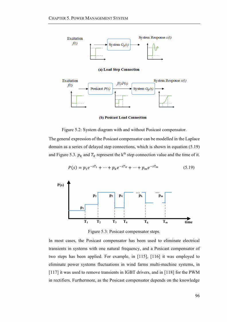
CHAPTER 5. POWER MANAGEMENT SYSTEM
96
Figure 5.2: System diagram with and without Posicast compensator.
The general expression of the Posicast compensator can be modelled in the Laplace
domain as a series of delayed step connections, which is shown in equation (5.19)
and Figure 5.3. 𝑝𝑘 and 𝑇𝑘 represent the kth step connection value and the time of it.
𝑃(𝑠) = 𝑝1𝑒−𝑠𝑇1 +⋯+ 𝑝𝑘𝑒
−𝑠𝑇𝑘 +⋯+ 𝑝𝑚𝑒−𝑠𝑇𝑚 (5.19)
P(s)
timeT1 T2
p1
p2
... ...
T3 T4 Tk Tm
p3 p4 pk pm
Figure 5.3: Posicast compensator steps.
In most cases, the Posicast compensator has been used to eliminate electrical
transients in systems with one natural frequency, and a Posicast compensator of
two steps has been applied. For example, in [115], [116] it was employed to
eliminate power systems fluctuations in wind farms multi-machine systems, in
[117] it was used to remove transients in IGBT drivers, and in [118] for the PWM
in rectifiers. Furthermore, as the Posicast compensator depends on the knowledge

CHAPTER 5. POWER MANAGEMENT SYSTEM
97
of the natural frequencies of the system, to improve its response to perturbations,
in [93], [119] a modified closed-loop Posicast is studied for second-order systems.
Also, when an optimal signal that eliminates the transient vibrations is analysed,
the method is referred as input-shaping [120], [121]. In general, studies that
eliminate transient vibrations for electrical systems speak about the Posicast
method, while mechanical engineers call it input-shaping methods.
This chapter presents a PMS that applies open-loop strategies based on the Posicast
method for the connection of step and pulsating loads.
5.4 Step Load
In this section, strategies to eliminate the torsional vibrations due to the connection
of time non-critical and time-critical loads are developed using the theory presented.
5.4.1 Time Non-Critical Load Strategies
In section 5.2 time non-critical loads were described as those for which an exact
time connection is not crucial, such as the de-icing system and the air cabin. For
that reason, the PMS can apply the open loop Posicast compensator directly to the
load connection.
To obtain the size of the steps 𝑝𝑘 and connection times 𝑇𝑘 the equation system from
equation (5.18) is solved for each natural frequency in the system. For a system
with 𝑛 natural frequencies, the non-linear equation system (5.20) must be solved.

CHAPTER 5. POWER MANAGEMENT SYSTEM
98
[ ∑𝑝𝑘𝑒
−𝜉1𝜔𝑛1𝑇𝑘 cos(𝜔𝑑1𝑇𝑘)
𝑚
𝑘=1
∑𝑝𝑘𝑒−𝜉1𝜔𝑛1𝑇𝑘 sin(𝜔𝑑1𝑇𝑘)
𝑚
𝑘=1
∑𝑝𝑘𝑒−𝜉2𝜔𝑛2𝑇𝑘 cos(𝜔𝑑2𝑇𝑘)
𝑚
𝑘=1
∑𝑝𝑘𝑒−𝜉2𝜔𝑛2𝑇𝑘 sin(𝜔𝑑2𝑇𝑘)
𝑚
𝑘=1
⋮
∑𝑝𝑘𝑒−𝜉𝑛𝜔𝑛𝑛𝑇𝑘 cos(𝜔𝑑𝑛𝑇𝑘)
𝑚
𝑘=1
∑𝑝𝑘𝑒−𝜉𝑛𝜔𝑛𝑛𝑇𝑘 sin(𝜔𝑑𝑛𝑇𝑘)
𝑚
𝑘=1 ]
= 0 (5.20)
The connection patterns used to connect electrical loads are based on the concepts
of edges and levels. An edge refers to the number of pulses before arriving at the
final value. Instead, the level denotes the number of consecutive additive steps
taken before reaching the final value.
Based on the edges and levels, Figure 5.4 presents two different types of excitation
pattern. Figure 5.4(a) shows a signal with two consecutive positive steps,
corresponding to two levels. This excitation is called Multilevel Loading (MLL).
Instead, Figure 5.4(b) shows a waveform in which there is a pulse composed of two
edges and one level. This excitation is called Single Level Multi-edge Switching
Loading (SLME). In both signals, MLL and SLME, the load goes from a load 1,
𝐿1, to a load 2, 𝐿2, but the connection pattern used is different. Next, the operation
of the MLL and SLME is shown.
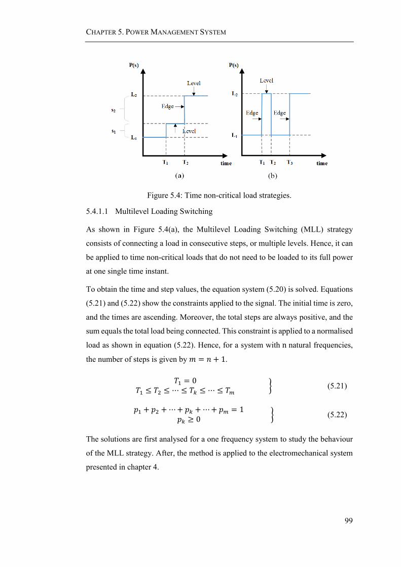
CHAPTER 5. POWER MANAGEMENT SYSTEM
99
Figure 5.4: Time non-critical load strategies.
5.4.1.1 Multilevel Loading Switching
As shown in Figure 5.4(a), the Multilevel Loading Switching (MLL) strategy
consists of connecting a load in consecutive steps, or multiple levels. Hence, it can
be applied to time non-critical loads that do not need to be loaded to its full power
at one single time instant.
To obtain the time and step values, the equation system (5.20) is solved. Equations
(5.21) and (5.22) show the constraints applied to the signal. The initial time is zero,
and the times are ascending. Moreover, the total steps are always positive, and the
sum equals the total load being connected. This constraint is applied to a normalised
load as shown in equation (5.22). Hence, for a system with n natural frequencies,
the number of steps is given by 𝑚 = 𝑛 + 1.
𝑇1 = 0𝑇1 ≤ 𝑇2 ≤ ⋯ ≤ 𝑇𝑘 ≤ ⋯ ≤ 𝑇𝑚
} (5.21)
𝑝1 + 𝑝2 +⋯+ 𝑝𝑘 +⋯+ 𝑝𝑚 = 1𝑝𝑘 ≥ 0
} (5.22)
The solutions are first analysed for a one frequency system to study the behaviour
of the MLL strategy. After, the method is applied to the electromechanical system
presented in chapter 4.

CHAPTER 5. POWER MANAGEMENT SYSTEM
100
For a one frequency system, 𝑛 = 1 and 𝑚 = 2. Thus, applying the equation system
(5.20), the equation system (5.23) is obtained. From equation (5.21) and (5.22),
𝑇1 = 0 and 𝑝2 = 1 − 𝑝1 respectively, hence the values of 𝑝1 and 𝑇2 must be found.
[𝑝1 + 𝑝2𝑒
−𝜉1𝜔𝑛1𝑇2 cos(𝜔𝑑1𝑇2)
𝑝2𝑒−𝜉1𝜔𝑛1𝑇2 sin(𝜔𝑑1𝑇2)
] = 0 (5.23)
The frequencies are rewritten as a function of the period to analyse the response of
the one frequency system as a function of the damping ratio. Equation (5.24) shows
the period equation and (5.25) the transient response as a function of it. Now the
connection times can be analysed as a function of the period 𝑇𝑝 and the damping
ratio 𝜉 ∈ [0,1].
𝑇𝑝 =2𝜋
𝜔𝑛√1 − 𝜉𝑛2=2𝜋
𝜔𝑑⇒
{
𝜔𝑑 =
2𝜋
𝑇𝑝
𝜔𝑛 =2𝜋
𝑇𝑝√1 − 𝜉2
(5.24)
[ 𝑝1 + 𝑝2𝑒
−2π𝜉1
√1−𝜉12 (𝑇2𝑇𝑝)
cos (2𝜋𝑇2𝑇𝑝)
𝑝2𝑒
−2π𝜉1
√1−𝜉12 (𝑇2𝑇𝑝)
sin (2𝜋𝑇2𝑇𝑝)
]
= 0 (5.25)
To simplify the notation, the following variable changes are defined: Γ2: = T2/𝑇𝑝
and 𝛿1: = 𝜉1/√1 − 𝜉12 . Replacing into equation (5.25), equation (5.26) is obtained.
[𝑝1 + 𝑝2𝑒
−2π𝛿Γ2 cos(2𝜋Γ2)
𝑝2𝑒−2π𝛿Γ2 sin(2𝜋Γ2)
] = 0 (5.26)
Figure 5.5 shows the sine and cosine curves or residuals as a function of Γ2 for
ascending values of 𝜉 ((a) 𝜉 = 0, (b) 𝜉 = 0.1, (c) 𝜉 = 0.3, and (d) 𝜉 = 0.65). The
curves show that at higher values the oscillations of the sine and cosine decrease,
proving that higher damping reduces the overshoot and settling time of a system.
Additionally, for each damping ratio, the step 𝑝1 has been chosen such that the sine
(in blue) and cosine (in red) curves intersect at zero, obtaining the system’s

CHAPTER 5. POWER MANAGEMENT SYSTEM
101
solution. It is observed than independently of the damping ratio, the curves intersect
at Γ2 = 0.5, and that for higher damping ratio the step 𝑝1 tends to 1.
Figure 5.5: Residuals of MLL.
Further details on the solutions of the system are shown in Figure 5.6, in which the
contour at zero of the sine and cosine curves is presented. The intersection of this
curves, marked by *, represent the solutions of the system for Γ2 ∈ [0,3]. The
system has more than one solution, of which one is equal to half a period of the
system, which is the solution presented in Figure 5.5. Moreover, the step connection
tends to unity as the damping ratio increases, showing that when damping ratio
reaches the critical value (𝜉 = 1) the compensator is not needed.

CHAPTER 5. POWER MANAGEMENT SYSTEM
102
Figure 5.6: Solutions for MLL.
The solutions for the whole damping ratio spectrum in the one frequency system
are presented in Figure 5.7. Again, it is observed that the connection time is 0.5
independent of the damping ratio value, while the step increases until the unity for
a critically damped (𝜉 = 1) system. Hence, the MLL connection has always a
solution inside half a period, and the step size tends to the unity for critically
damped systems. This last statement confirms that the critical damping is the value
at which the system stops vibrating.
Figure 5.7: MLL time connection and pulse size as a function of 𝜉.

CHAPTER 5. POWER MANAGEMENT SYSTEM
103
Since the MLL switching takes place in half a period of the system, for the natural
frequencies of the aircraft drivetrain, the connection is made in milliseconds.
Additionally, equation (5.24) shows that 𝑇𝑝 increases for higher 𝜉. Thus the time
connection 𝑇2 also increases for higher 𝜉, while keeping the proportion Γ2 constant.
For a simplified two inertia drivetrain with the parameters shown in Table 5.2, the
frequency and damping ratio of the system are 𝑓 = 19.09Hz and 𝜉 = 0.0327
respectively. Hence, 𝑇𝑝 = 52.4115 ms , 𝑝1 = 0.5257 , and Γ2 = 0.5 (or 𝑇2 =
26.2057ms).
Table 5.2: Parameter of the two inertia system.
Parameter Value
Engine Inertia 𝐽𝑚 = 0.0965 kgm2
Generator Inertia 𝐽𝑔 = 0.0376 kgm2
Shaft Stiffness 𝑘𝑠 = 5.3995 ∗ 102 Nm/rad
Shaft Damping 𝑑𝑠 = 0.125 Nmrad/s
Figure 5.8 shows the shaft response for a torque connection equal to the one used
for the step connection in chapter 4: from 0.3952Nm to 2.9282Nm, which is
obtained by an electrical load connection of 5Ω when 60Ω are connected with a
constant field of 6.2A. In red the generator torque 𝑇𝑔2 is shown, while in blue the
shaft torque for the one frequency system is observed. The solution obtained,
eliminates the torsional vibrations due to the torque connection. Furthermore, the
switching occurs in half a period of the system (𝑇𝑝/2 = 26.2ms), and as the
damping ratio is higher than zero, the step size is greater than 0.5.
Figure 5.8: MLL torque response for a 1 natural frequency system.
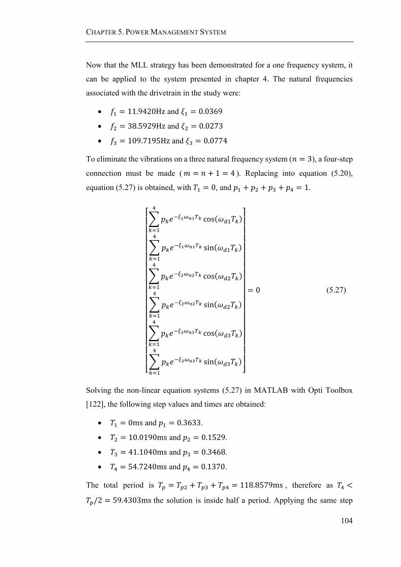
CHAPTER 5. POWER MANAGEMENT SYSTEM
104
Now that the MLL strategy has been demonstrated for a one frequency system, it
can be applied to the system presented in chapter 4. The natural frequencies
associated with the drivetrain in the study were:
𝑓1 = 11.9420Hz and 𝜉1 = 0.0369
𝑓2 = 38.5929Hz and 𝜉2 = 0.0273
𝑓3 = 109.7195Hz and 𝜉3 = 0.0774
To eliminate the vibrations on a three natural frequency system (𝑛 = 3), a four-step
connection must be made (𝑚 = 𝑛 + 1 = 4 ). Replacing into equation (5.20),
equation (5.27) is obtained, with 𝑇1 = 0, and 𝑝1 + 𝑝2 + 𝑝3 + 𝑝4 = 1.
[ ∑𝑝𝑘𝑒
−𝜉1𝜔𝑛1𝑇𝑘 cos(𝜔𝑑1𝑇𝑘)
4
𝑘=1
∑𝑝𝑘𝑒−𝜉1𝜔𝑛1𝑇𝑘 sin(𝜔𝑑1𝑇𝑘)
4
𝑘=1
∑𝑝𝑘𝑒−𝜉2𝜔𝑛2𝑇𝑘 cos(𝜔𝑑2𝑇𝑘)
4
𝑘=1
∑𝑝𝑘𝑒−𝜉2𝜔𝑛2𝑇𝑘 sin(𝜔𝑑2𝑇𝑘)
4
𝑘=1
∑𝑝𝑘𝑒−𝜉3𝜔𝑛3𝑇𝑘 cos(𝜔𝑑3𝑇𝑘)
4
𝑘=1
∑𝑝𝑘𝑒−𝜉3𝜔𝑛3𝑇𝑘 sin(𝜔𝑑3𝑇𝑘)
4
𝑘=1 ]
= 0 (5.27)
Solving the non-linear equation systems (5.27) in MATLAB with Opti Toolbox
[122], the following step values and times are obtained:
𝑇1 = 0ms and 𝑝1 = 0.3633.
𝑇2 = 10.0190ms and 𝑝2 = 0.1529.
𝑇3 = 41.1040ms and 𝑝3 = 0.3468.
𝑇4 = 54.7240ms and 𝑝4 = 0.1370.
The total period is 𝑇𝑝 = 𝑇𝑝2 + 𝑇𝑝3 + 𝑇𝑝4 = 118.8579ms , therefore as 𝑇4 <
𝑇𝑝/2 = 59.4303ms the solution is inside half a period. Applying the same step

CHAPTER 5. POWER MANAGEMENT SYSTEM
105
connection used before (from 0.3952Nm to 2.9282Nm) to the system modelled in
Simulink in chapter 4, Figure 5.9 is obtained. In (a) a step connection is shown, and
in (b) the MLL strategy is applied. The torque applied to the drivetrain by the
generator 𝑇𝑔2 is shown in red. It is composed of the series of steps defined by the
MLL strategy instead of a step connection. The shaft response 𝑇𝑠3 is observed in
blue. Comparing with the step connection in (a), the Posicast compensator in (b)
has eliminated the transient vibrations on the generator shaft. Hence, the use of the
MLL allows suppression of the shaft vibrations due to electrical load connections.
Figure 5.9: Torque shaft response with MLL signal.
In practice, this solution can be applied by using multilevel converters for loads
that can be connected by steps, such as the ice protection systems. For loads that
cannot be connected by multiple steps, the SLME connection strategy is proposed.
5.4.1.2 Single Level Multi-edge Switching Load
An alternative connection arrangement to eliminate the torsional vibrations due to
electromechanical interaction is the Single Level Multi-edge Switching Loads
(SLME) method showed in Figure 5.4(b). It consists of connecting the load as a
series of on/off pulses. Therefore, the step applied to the system takes values ±1
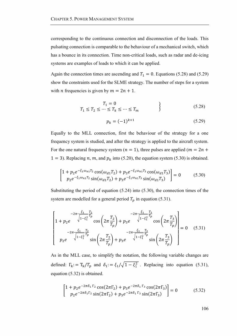
CHAPTER 5. POWER MANAGEMENT SYSTEM
106
corresponding to the continuous connection and disconnection of the loads. This
pulsating connection is comparable to the behaviour of a mechanical switch, which
has a bounce in its connection. Time non-critical loads, such as radar and de-icing
systems are examples of loads to which it can be applied.
Again the connection times are ascending and 𝑇1 = 0. Equations (5.28) and (5.29)
show the constraints used for the SLME strategy. The number of steps for a system
with 𝑛 frequencies is given by 𝑚 = 2𝑛 + 1.
𝑇1 = 0𝑇1 ≤ 𝑇2 ≤ ⋯ ≤ 𝑇𝑘 ≤ ⋯ ≤ 𝑇𝑚
} (5.28)
𝑝𝑘 = (−1)𝑘+1 (5.29)
Equally to the MLL connection, first the behaviour of the strategy for a one
frequency system is studied, and after the strategy is applied to the aircraft system.
For the one natural frequency system (𝑛 = 1), three pulses are applied (𝑚 = 2𝑛 +
1 = 3). Replacing 𝑛, 𝑚, and 𝑝𝑘 into (5.20), the equation system (5.30) is obtained.
[1 + 𝑝2𝑒
−𝜉1𝜔𝑛1𝑇2 cos(𝜔𝑑1𝑇2) + 𝑝3𝑒−𝜉1𝜔𝑛1𝑇3 cos(𝜔𝑑1𝑇3)
𝑝2𝑒−𝜉1𝜔𝑛1𝑇2 sin(𝜔𝑑1𝑇2) + 𝑝3𝑒
−𝜉1𝜔𝑛1𝑇3 sin(𝜔𝑑1𝑇3)] = 0 (5.30)
Substituting the period of equation (5.24) into (5.30), the connection times of the
system are modelled for a general period 𝑇𝑝 in equation (5.31).
[ 1 + 𝑝2𝑒
−2𝜋𝜉1
√1−𝜉12 𝑇2𝑇𝑝
cos (2𝜋𝑇2𝑇𝑝) + 𝑝3𝑒
−2𝜋𝜉1
√1−𝜉12 𝑇3𝑇𝑝
cos (2𝜋𝑇3𝑇𝑝)
𝑝2𝑒
−2𝜋𝜉1
√1−𝜉12 𝑇2𝑇𝑝
sin (2𝜋𝑇2𝑇𝑝) + 𝑝3𝑒
−2𝜋𝜉1
√1−𝜉12 𝑇3𝑇𝑝
sin (2𝜋𝑇3𝑇𝑝)
]
= 0 (5.31)
As in the MLL case, to simplify the notation, the following variable changes are
defined: Γk: = Tk/𝑇𝑝 and 𝛿1: = 𝜉1/√1 − 𝜉12 . Replacing into equation (5.31),
equation (5.32) is obtained.
[1 + 𝑝2𝑒
−2𝜋𝛿1 Γ2 cos(2𝜋Γ2) + 𝑝3𝑒−2𝜋𝛿1 Γ3 cos(2𝜋Γ3)
𝑝2𝑒−2𝜋𝛿1Γ2 sin(2𝜋Γ2) + 𝑝3𝑒
−2𝜋𝛿1 Γ3 sin(2𝜋Γ3)] = 0 (5.32)

CHAPTER 5. POWER MANAGEMENT SYSTEM
107
To analyse the connection times as a function of the period 𝑇𝑝 and the damping
ratio (𝜉 ∈ [0,1]), Figure 5.10, Figure 5.11, and Figure 5.12 are obtained. The sine
and cosine curves as a function of Γ3 are shown in Figure 5.10. At higher damping
ratio, the vibrations decrease.
In Figure 5.11 the sine and cosine contour at zero for different damping ratio in a
range of time Γ3 ∈ [0,3] are presented. Their intersections (marked by *) show that
the system has multiple solutions, of which one is inside half a period of the system,
independently of the damping value.
Lastly, Figure 5.12 illustrates the first solution of Γ2 and Γ3 that eliminates the
vibrations for the underdamped spectrum. Like in the MLL solution, the time
connections are inside half a period of the system. Moreover, while the damping
ratio increases, the connection times Γ2 and Γ3 get closer. At the critical damping
(𝜉 = 1) their values are the same, indicating again, that no compensator is needed
for the connection of load in systems with high damping.
Figure 5.10: Residuals of SLME.

CHAPTER 5. POWER MANAGEMENT SYSTEM
108
Figure 5.11: Solutions for SLME.
Figure 5.12: SLME time connection as a function of 𝜉.
Solving for the same one natural frequency system used in the MLL method and
the same step connection from 0.3952Nm to 2.9282Nm, Figure 5.13 is obtained.
In red, the pulsating generator torque applied to the mechanical system is shown,
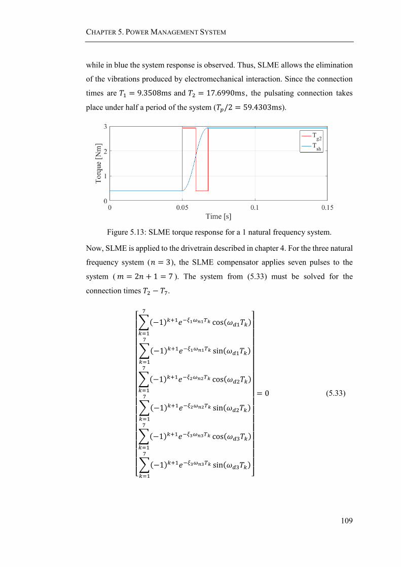
CHAPTER 5. POWER MANAGEMENT SYSTEM
109
while in blue the system response is observed. Thus, SLME allows the elimination
of the vibrations produced by electromechanical interaction. Since the connection
times are 𝑇1 = 9.3508ms and 𝑇2 = 17.6990ms, the pulsating connection takes
place under half a period of the system (𝑇𝑝/2 = 59.4303ms).
Figure 5.13: SLME torque response for a 1 natural frequency system.
Now, SLME is applied to the drivetrain described in chapter 4. For the three natural
frequency system (𝑛 = 3), the SLME compensator applies seven pulses to the
system (𝑚 = 2𝑛 + 1 = 7 ). The system from (5.33) must be solved for the
connection times 𝑇2 − 𝑇7.
[ ∑(−1)𝑘+1𝑒−𝜉1𝜔𝑛1𝑇𝑘 cos(𝜔𝑑1𝑇𝑘)
7
𝑘=1
∑(−1)𝑘+1𝑒−𝜉1𝜔𝑛1𝑇𝑘 sin(𝜔𝑑1𝑇𝑘)
7
𝑘=1
∑(−1)𝑘+1𝑒−𝜉2𝜔𝑛2𝑇𝑘 cos(𝜔𝑑2𝑇𝑘)
7
𝑘=1
∑(−1)𝑘+1𝑒−𝜉2𝜔𝑛2𝑇𝑘 sin(𝜔𝑑2𝑇𝑘)
7
𝑘=1
∑(−1)𝑘+1𝑒−𝜉3𝜔𝑛3𝑇𝑘 cos(𝜔𝑑3𝑇𝑘)
7
𝑘=1
∑(−1)𝑘+1𝑒−𝜉3𝜔𝑛3𝑇𝑘 sin(𝜔𝑑3𝑇𝑘)
7
𝑘=1 ]
= 0 (5.33)

CHAPTER 5. POWER MANAGEMENT SYSTEM
110
Solving the non-linear system in Matlab with Opti Toolbox [122], the following
connection values are obtained:
𝑇1 = 0ms and 𝑝1 = 1.
𝑇2 = 5.7595ms and 𝑝2 = −1.
𝑇3 = 8.6953ms and 𝑝3 = 1.
𝑇4 = 14.1730ms and 𝑝4 = −1.
𝑇5 = 20.3020ms and 𝑝5 = 1.
𝑇6 = 26.8580ms and 𝑝6 = −1.
𝑇7 = 33.7580ms and 𝑝7 = 1.
Modelling the system in Simulink, Figure 5.14 is obtained. In (a) and (b) the step
connection and the SLME strategy are respectively shown. The generator torque
𝑇𝑔2 applied is shown in red, while the shaft torque 𝑇𝑠3 is illustrated in blue. The
parameters are the same that were used for the step connection in chapter 4 and the
MLL strategy. Again, the vibrations produced by the connection have been
eliminated.
Figure 5.14: Torque shaft response with SLME signal.

CHAPTER 5. POWER MANAGEMENT SYSTEM
111
Until now, two strategies to connect time non-critical loads have been shown. The
MLL and SLME strategies can be applied to loads that allow the connection of
multiple segments or under a pulsating pattern respectively. Moreover, the duration
of the connection is in the order of milliseconds, which makes it faster than with
other control strategies and virtually instantaneous for loads such as the de-icing
system that remains connected for a longer time.
However, to find the timing and step values, the natural frequencies and damping
ratio of the system must be known. In chapter 7, the identification of these
parameters is studied, and in chapter 8, the robustness of the methods is analysed.
Next, the case of time-critical loads is analysed.
5.4.2 Time Critical Load Strategy
So far strategies for time non-critical loads have been proposed. This section studies
the case of time-critical loads, like flight control surfaces, to which a delay in their
connection cannot be applied.
For this reason, to avoid the vibrations produced by a step connection the PMS uses
an Auxiliary Load, while the time-critical load is connected as a step. Auxiliary
loads are time non-critical loads already in the system (or that also need to be
connected), to which a Posicast based strategy is applied. The electrical power of
the time non-critical load must be higher than the one of the time-critical load being
connected. An example of an auxiliary load is the ice protection system, which, as
shown in [111], has an on/off/on operation pattern, making possible the connection
and disconnection by short times.
It follows that the equation system that needs to be solved must include both loads,
the auxiliary load 𝐿𝑎𝑢𝑥 and the critical load 𝐿𝐶 . Thus, equation (5.18) has two
components, one associated with the auxiliary load (𝑝𝑎𝑢𝑥 , 𝑇𝑎𝑢𝑥) and one to the
critical load (𝑝𝑐, 𝑇𝑐) as shown in (5.34). The step of the critical load is 𝑝𝑐 = 1.

CHAPTER 5. POWER MANAGEMENT SYSTEM
112
𝑝𝑐𝑒−𝜉𝑗𝜔𝑛𝑗𝑇𝑘 cos(𝜔𝑑𝑗𝑇𝑐) +∑𝑝𝑎𝑢𝑥 𝑘𝑒
−𝜉𝑗𝜔𝑛𝑗𝑇𝑘 cos(𝜔𝑑𝑗𝑇𝑎𝑢𝑥 𝑘)
𝑚
𝑘=1
= 0
𝑝𝑐𝑒−𝜉𝑗𝜔𝑛𝑗𝑇𝑘 sin(𝜔𝑑𝑗𝑇𝑐) +∑𝑝𝑎𝑢𝑥 𝑘𝑒
−𝜉𝑗𝜔𝑛𝑗𝑇𝑘 sin(𝜔𝑑𝑗𝑇𝑎𝑢𝑥 𝑘)
𝑚
𝑘=1
= 0
}
∀ λ (5.34)
The strategy used is presented in Figure 5.15. While the time-critical load (𝐿𝐶 in
yellow line) is connected as a step, the auxiliary load (𝐿𝑎𝑢𝑥 in purple line) is
disconnected and reconnected using the SLME method. Thus, the total load applied
to the generator (𝐿 = 𝐿𝐶 + 𝐿𝑎𝑢𝑥) is not a single step. This strategy is called Multi-
load Single Level Multi-edge Switching Loads (MSLME).
Figure 5.15: Time critical load.
For a system with 𝑛 natural frequencies, the number of steps is given by 𝑚 = 2𝑛.
Moreover, the equation’s constraints are given by (5.35) and (5.36).
𝑇1 = 0𝑇1 ≤ 𝑇2 ≤ ⋯ ≤ 𝑇𝑘 ≤ ⋯ ≤ 𝑇𝑚
} (5.35)
𝑝𝑎𝑢𝑥 𝑘 = (−1)𝑘𝑝 (5.36)
As was done for the time non-critical loads, the system is analysed for one
frequency system first, and afterwards for the drivetrain in the study. It follows that
the solution for the one frequency system, shown in equation (5.37), is obtained by
substituting 𝑛 = 1, and 𝑚 = 2𝑛 = 2 into equation (5.34). The connection time 𝑇2
and step value 𝑝 that must be disconnected from the auxiliary load are the variables
to obtain. In the case of one natural frequency, the MSLME strategy is equivalent
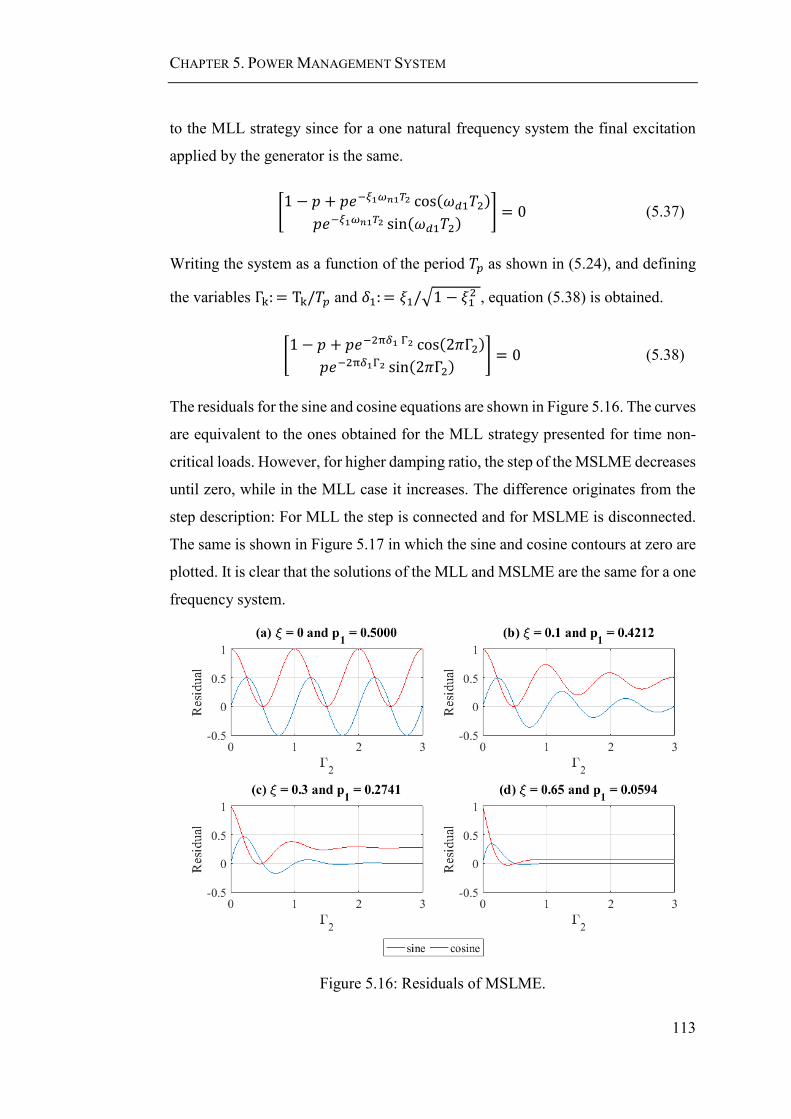
CHAPTER 5. POWER MANAGEMENT SYSTEM
113
to the MLL strategy since for a one natural frequency system the final excitation
applied by the generator is the same.
[1 − 𝑝 + 𝑝𝑒−𝜉1𝜔𝑛1𝑇2 cos(𝜔𝑑1𝑇2)
𝑝𝑒−𝜉1𝜔𝑛1𝑇2 sin(𝜔𝑑1𝑇2)] = 0 (5.37)
Writing the system as a function of the period 𝑇𝑝 as shown in (5.24), and defining
the variables Γk: = Tk/𝑇𝑝 and 𝛿1: = 𝜉1/√1 − 𝜉12 , equation (5.38) is obtained.
[1 − 𝑝 + 𝑝𝑒−2π𝛿1 Γ2 cos(2𝜋Γ2)
𝑝𝑒−2π𝛿1Γ2 sin(2𝜋Γ2)] = 0 (5.38)
The residuals for the sine and cosine equations are shown in Figure 5.16. The curves
are equivalent to the ones obtained for the MLL strategy presented for time non-
critical loads. However, for higher damping ratio, the step of the MSLME decreases
until zero, while in the MLL case it increases. The difference originates from the
step description: For MLL the step is connected and for MSLME is disconnected.
The same is shown in Figure 5.17 in which the sine and cosine contours at zero are
plotted. It is clear that the solutions of the MLL and MSLME are the same for a one
frequency system.
Figure 5.16: Residuals of MSLME.

CHAPTER 5. POWER MANAGEMENT SYSTEM
114
Figure 5.17: Solutions for MSLME.
In Figure 5.18 the solutions for the underdamped system are presented. While the
time Γ2 remains constant at half a period, the auxiliary load that must be
disconnected decreases. When the damping ratio is high, there is no need to
disconnect the auxiliary load.
Figure 5.18: Solution spectrum for MSLME with 𝜉 ∈ [0,1].
Solving the one frequency system presented in section 5.4.1.1 Figure 5.19 is
obtained. The initial torque is 0.3952Nm, the same initial torque of the other cases.
Instead, the final torque is 1.0532Nm , the torque obtained when 30Ω are
connected with a field current of 6.2A. The value of the load connected is lower
than the one used for the MLL and SLME case because of the auxiliary load value,

CHAPTER 5. POWER MANAGEMENT SYSTEM
115
already connected to the system, is approximately half of the load being connected.
In Figure 5.19(a) the auxiliary load (𝑇𝑎𝑢𝑥 in purple), critical load (𝑇𝑐 in yellow),
and total load (𝑇𝑔2 in red) are shown. The resulting load 𝑇𝑔2 applied by the
generator to the mechanical system is shown in Figure 5.19(b). As shown in the
previous analysis for a one frequency system, the total torque is the same obtained
for the MLL method. The torque shaft is shown in blue, and as expected the
vibrations are eliminated after the final switching event.
Figure 5.19: MSLME torque response for a 1 natural frequency system.
Now, the MSLME method is solved for the aircraft system composed of three
natural frequencies. Replacing 𝑛 = 3, the auxiliary load must be disconnected and
connected six times (𝑚 = 2𝑛 = 6). The system from equation (5.39) must be
solved.
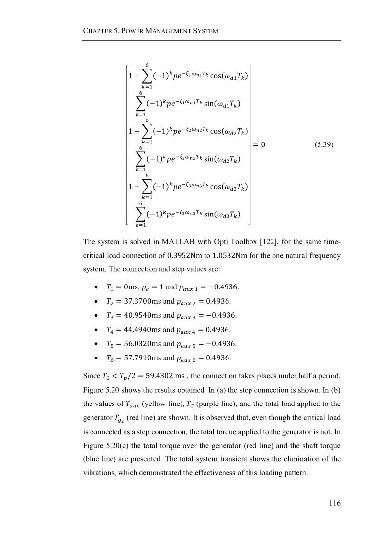
CHAPTER 5. POWER MANAGEMENT SYSTEM
116
[ 1 +∑(−1)𝑘𝑝𝑒−𝜉1𝜔𝑛1𝑇𝑘 cos(𝜔𝑑1𝑇𝑘)
6
𝑘=1
∑(−1)𝑘𝑝𝑒−𝜉1𝜔𝑛1𝑇𝑘 sin(𝜔𝑑1𝑇𝑘)
6
𝑘=1
1 +∑(−1)𝑘𝑝𝑒−𝜉2𝜔𝑛2𝑇𝑘 cos(𝜔𝑑2𝑇𝑘)
6
𝑘−1
∑(−1)𝑘𝑝𝑒−𝜉2𝜔𝑛2𝑇𝑘 sin(𝜔𝑑2𝑇𝑘)
6
𝑘=1
1 +∑(−1)𝑘𝑝𝑒−𝜉3𝜔𝑛3𝑇𝑘 cos(𝜔𝑑3𝑇𝑘)
6
𝑘=1
∑(−1)𝑘𝑝𝑒−𝜉3𝜔𝑛3𝑇𝑘 sin(𝜔𝑑3𝑇𝑘)
6
𝑘=1 ]
= 0 (5.39)
The system is solved in MATLAB with Opti Toolbox [122], for the same time-
critical load connection of 0.3952Nm to 1.0532Nm for the one natural frequency
system. The connection and step values are:
𝑇1 = 0ms, 𝑝𝑐 = 1 and 𝑝𝑎𝑢𝑥 1 = −0.4936.
𝑇2 = 37.3700ms and 𝑝𝑎𝑢𝑥 2 = 0.4936.
𝑇3 = 40.9540ms and 𝑝𝑎𝑢𝑥 3 = −0.4936.
𝑇4 = 44.4940ms and 𝑝𝑎𝑢𝑥 4 = 0.4936.
𝑇5 = 56.0320ms and 𝑝𝑎𝑢𝑥 5 = −0.4936.
𝑇6 = 57.7910ms and 𝑝𝑎𝑢𝑥 6 = 0.4936.
Since 𝑇6 < 𝑇𝑝/2 = 59.4302 ms , the connection takes places under half a period.
Figure 5.20 shows the results obtained. In (a) the step connection is shown. In (b)
the values of 𝑇𝑎𝑢𝑥 (yellow line), 𝑇𝐶 (purple line), and the total load applied to the
generator 𝑇𝑔2 (red line) are shown. It is observed that, even though the critical load
is connected as a step connection, the total torque applied to the generator is not. In
Figure 5.20(c) the total torque over the generator (red line) and the shaft torque
(blue line) are presented. The total system transient shows the elimination of the
vibrations, which demonstrated the effectiveness of this loading pattern.
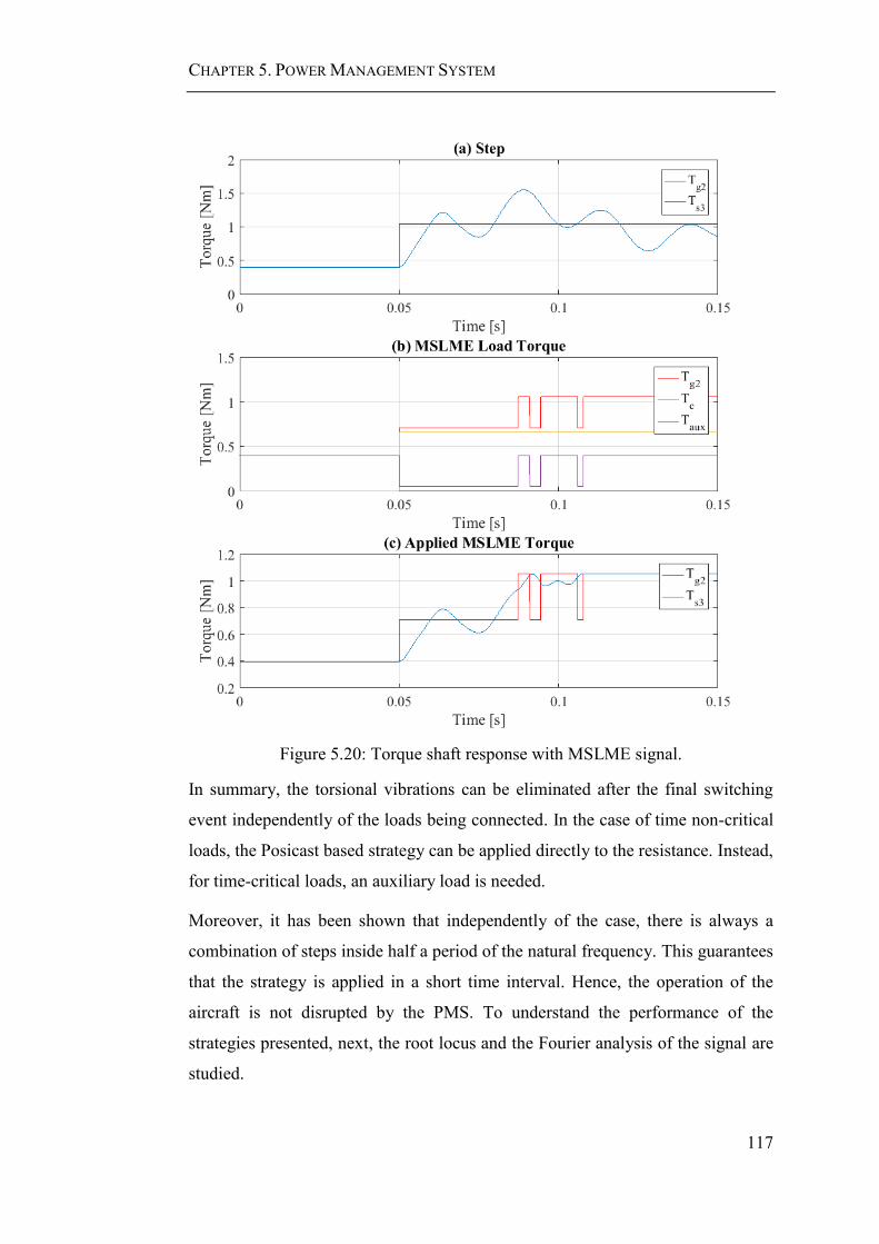
CHAPTER 5. POWER MANAGEMENT SYSTEM
117
Figure 5.20: Torque shaft response with MSLME signal.
In summary, the torsional vibrations can be eliminated after the final switching
event independently of the loads being connected. In the case of time non-critical
loads, the Posicast based strategy can be applied directly to the resistance. Instead,
for time-critical loads, an auxiliary load is needed.
Moreover, it has been shown that independently of the case, there is always a
combination of steps inside half a period of the natural frequency. This guarantees
that the strategy is applied in a short time interval. Hence, the operation of the
aircraft is not disrupted by the PMS. To understand the performance of the
strategies presented, next, the root locus and the Fourier analysis of the signal are
studied.
CHAPTER 5. POWER MANAGEMENT SYSTEM
118
5.4.3 Frequency Analysis
In this section, the effect of the Posicast based strategies is considered in terms of
frequency. For this, the root locus analysis of the system and the Fourier analysis
are studied.
5.4.3.1 Root Locus Analysis
To understand the effect of the strategies used by the PMS on the overall system,
the zero-pole root locus technique is analysed for the system without and with the
strategies MLL, SLME, and MSLME.
To analyse the root locus the transfer function of the system is calculated in the
Laplace domain. For the base case (step connection), the transfer function
𝐻𝑝𝑙𝑎𝑛𝑡(𝑠) is obtained from the drivetrain system presented in chapter 4 in equation
(4.30)2.
The transfer function of the system with the compensator is given by equation
(5.40). In which, 𝐻𝑝𝑙𝑎𝑛𝑡 is the drivetrain transfer function used for the step
connection, and 𝐻𝑃𝑜𝑠𝑖𝑐𝑎𝑠𝑡 is the compensator applied to the system, MLL, SLME,
or MSLME. The transfer function 𝐻𝑃𝑜𝑠𝑖𝑐𝑎𝑠𝑡 is given by equation (5.19), in which
𝑝𝑘 represents the height of the kth step at a time 𝑇𝑘. Representing the time delays
of the step connections by Padé approximation, the transfer function is obtained.
𝐻𝑆𝑦𝑠𝑡𝑒𝑚(𝑠) = 𝐻𝑃𝑜𝑠𝑖𝑐𝑎𝑠𝑡(𝑠)𝐻𝑃𝑙𝑎𝑛𝑡(𝑠) (5.40)
Figure 5.21 shows the poles of the system with the zeros added by the PMS
strategies. Figure 5.21(a) presents the poles (represented by x) of the drivetrain
while Figure 5.21(b), (c) and (d) show the poles and zeros (represented by o) when
the strategies are applied. In every case, the Posicast compensator adds zeros to the
system at the poles values. For this reason, the poles cannot be excited by input
signals, and the mechanical vibrations are suppressed. The extra poles added are
due to the use of high order Padé approximations, which is a frequency domain
expansion of a time domain delay.
2 The command ss2tf from Matlab is used

CHAPTER 5. POWER MANAGEMENT SYSTEM
119
Figure 5.21: Poles (shown by x) and zeros (shown by o) of the system.
The cancellations of poles are similar to the use of a notch filter, in which the use
of a filter cancels the resonant frequencies [123]. This method has been used for
electromechanical systems as discussed in chapter 3.
5.4.3.2 Fourier Analysis
To analyse the frequencies excited by the load connection, the shaft torque 𝑇𝑠ℎ is
analysed through Fourier Transform. Figure 5.22 shows the frequency spectrum
obtained for the loads connected as a step. In (a) the step connection presented in
chapter 4 is shown, while in (b), (c), and (d) the results obtained with MLL, SMLE,
and MSLME are analysed.
In the step case (a), the frequencies of the system are observed. This shows that
after a step connection the torsional vibrations are excited. Instead when the
strategies are applied no frequency is recognised, which corroborates that the
Posicast methods do not excite the mechanical natural frequencies.
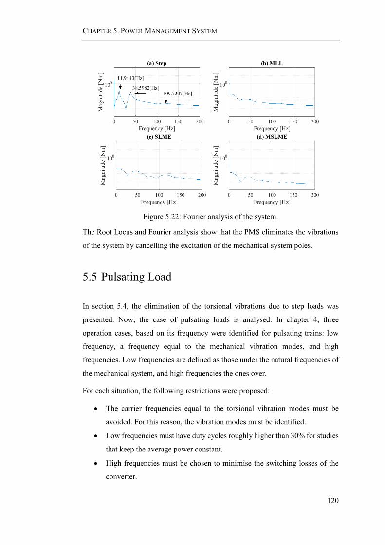
CHAPTER 5. POWER MANAGEMENT SYSTEM
120
Figure 5.22: Fourier analysis of the system.
The Root Locus and Fourier analysis show that the PMS eliminates the vibrations
of the system by cancelling the excitation of the mechanical system poles.
5.5 Pulsating Load
In section 5.4, the elimination of the torsional vibrations due to step loads was
presented. Now, the case of pulsating loads is analysed. In chapter 4, three
operation cases, based on its frequency were identified for pulsating trains: low
frequency, a frequency equal to the mechanical vibration modes, and high
frequencies. Low frequencies are defined as those under the natural frequencies of
the mechanical system, and high frequencies the ones over.
For each situation, the following restrictions were proposed:
The carrier frequencies equal to the torsional vibration modes must be
avoided. For this reason, the vibration modes must be identified.
Low frequencies must have duty cycles roughly higher than 30% for studies
that keep the average power constant.
High frequencies must be chosen to minimise the switching losses of the
converter.

CHAPTER 5. POWER MANAGEMENT SYSTEM
121
Now, the elimination of the transient vibrations due to the pulsating load's
connection is analysed. Thus, strategies for the system operating at low and high
frequencies are presented.
5.5.1 Low-Frequency Strategy
A pulsating load operating at a low frequency produces a complete transient
response for each load pulse, as shown in Figure 5.23(a). In it, a pulsating load with
an average torque equal to the load connected in the step connection (2.9282Nm),
60% duty cycle, and a frequency of 0.2Hz is applied to the system described in
chapter 4.
The strategies presented in section 5.4 eliminate the system vibrations by applying
a series of pulses in under half a period. Since the times between low-frequency
pulses are higher than half a period of the mechanical system, to each pulse the
Posicast compensator is applied. As well, low-frequency loads, such as the heating
system, can act as an auxiliary load for the critical load connections. For the low
frequencies pulsating train of Figure 5.23(a), the SLME strategy is implemented as
shown in Figure 5.23(b). The transient vibrations are eliminated.
Figure 5.23: Low-frequency SLME.

CHAPTER 5. POWER MANAGEMENT SYSTEM
122
5.5.2 High-Frequency Strategy
In the case of high frequencies, which switching time is higher than the natural
frequencies of the drivetrain, the Posicast based strategies cannot be applied to each
switching event. Moreover, Figure 5.24(a) shows that the connection of a high
frequency pulsating load (𝑇𝑔2 in red) is perceived as a step load connection by the
mechanical system ( 𝑇𝑠3 in blue). The signal applied 𝑇𝑔2 has a frequency of
2000Hz, 60% duty cycle and the same mean torque of the low frequency case and
the step connection (2.9282Nm).
Therefore, the Posicast based strategies are applied at the beginning of the
switching load connection as if it were a regular step connection. The final load
applied 𝑇𝑔2 is obtained by convolution of the pulsating load 𝑇𝑝𝑙 and the Posicast
method 𝑃 as shown in equation (5.41).
𝑇𝑔2(𝑡) =∑𝑇𝑝𝑙(𝑘)
𝑘
𝑃(𝑡 − 𝑘 + 1) (5.41)
Figure 5.24(b) shows the response of the system when the SLME strategy is applied
to the pulsating load. As if the load was a step connection, the strategy eliminates
the transient vibrations of the mechanical system.
Figure 5.24: High-frequency SLME.

CHAPTER 5. POWER MANAGEMENT SYSTEM
123
5.6 Real Application
In the last section a PMS for aircraft systems that allows the suppression of the
excitation of torsional vibrations when electrical loads are connected has been
presented. Now, the requirements of the electrical power system of the aircraft that
allow the implementation of this PMS are presented:
Solid State switches to control the loads: the electrical loads should be
connected through solid state switches or converters to the grid. In present
aircraft systems, electrical loads connected through mechanical switches
can still be found. This switches have to be changed to be able to apply the
connection patterns in study.
Ratio of load types: to be able to apply the strategies for time critical loads,
the time non-critical load installed on the system must be equal or higher
than the time critical loads, 𝐿𝑁𝑜𝑛 𝐶𝑟𝑖𝑡𝑖𝑐𝑎𝑙 ≥ 𝐿𝐶𝑟𝑖𝑡𝑖𝑐𝑎𝑙.
Minimum inner loop bandwidth in converter: the control loop in which
the current of the converter is given must be fast enough to allow the
switching given by the PMS strategies. Therefore, the converters will
operate with a minimum bandwidth for their control.
High bandwidth communication/sensing/control link: for the
application of the strategies for time critical loads, the signals must be sent
simultaneously to both loads: critical and auxiliary. For this reason, the
electrical power system must have a high bandwidth communication
system, in order to avoid delays. Alternatively, high bandwidth
communication control links between time critical and auxiliary loads or
sensing strategies can be implemented.
CHAPTER 5. POWER MANAGEMENT SYSTEM
124
5.7 Summary
This chapter introduced a PMS that allows the elimination of torsional shaft
vibrations excited by the connection of electrical loads. The strategies, based on the
Posicast compensator, can be applied to different purely resistive loads: time
critical loads, time non-critical loads, and pulsating loads. The effect of inductance
over the strategies implemented is shown in chapter 7 and analysed in chapter 8.
Moreover, the switching patterns defined by the PMS are applied inside half a
period of the natural frequencies. Thus, for mechanical natural frequencies below
200Hz, the connection takes place in milliseconds, which is lower than the settling
time of a step connection, and faster than the control strategies used in other
applications.
Since the Posicast based strategies depend on the frequency and damping ratio of
the system, in an experimental setup these values must be known. Chapter 7
presents a methodology for its identification and the experimental results, while in
chapter 8 the robustness of the method for frequencies uncertainties is studied. In
next chapter, the experimental setup to test the PMS is developed.

Chapter 6
6 Design of Test Rig
6.1 Introduction
In this chapter, the experimental rig used to study the electromechanical interaction
on the system is designed. The aim of this test rig is to validate the
electromechanical system model, verify the electromechanical interaction, and
analyse the solutions presented in chapter 5.
The test rig design allows the testing of multiple aircraft systems: an in-line
starter/generators, an air-riding seals, and the study of electromechanical
interaction. The first two experiments were undertaken using the test rig aimed to
minimise the transversal vibrations and analyse the fluid dynamic characteristics.
Their study is out of the scope of this thesis, and more information can be found in
[124]. This thesis considers the study of electromechanical interaction and the
minimisation of the torsional vibrations due to electrical load connections. For this
reason, in the rest of the chapter, only the components associated with the
electromechanical interaction are discussed.
As presented in [18] and discussed in chapters 4 and 5, a reduced aircraft drivetrain
can be used to study electromechanical interactions. As shown in Figure 6.1 the
motor or prime mover is connected to a generator through a drivetrain. The
drivetrain is composed of a shaft and a gearbox. The generator is coupled to a DC
power system since from a control point of view the behaviour is the same. Only
one generator is used in the test rig, instead of two. This simplification removes one
torsional vibration mode of the system, while still allowing the analysis of the
electromechanical interaction and the test of the power management system (PMS).
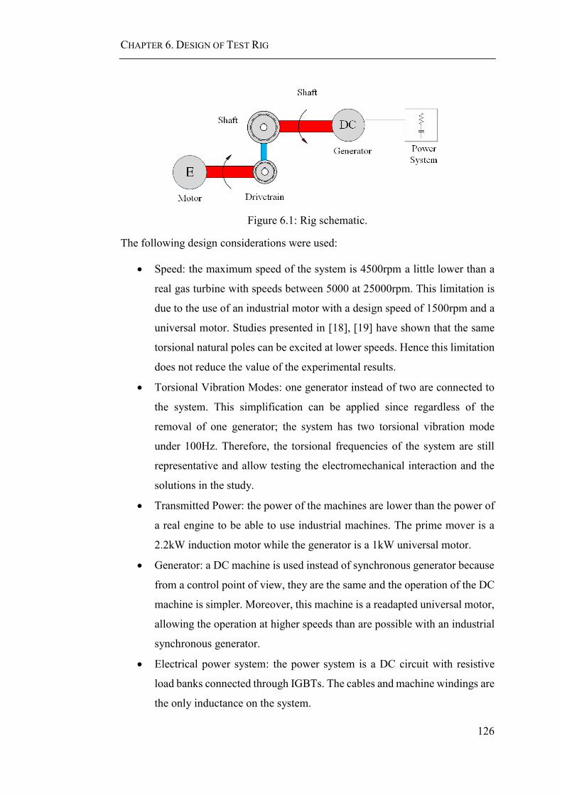
CHAPTER 6. DESIGN OF TEST RIG
126
Figure 6.1: Rig schematic.
The following design considerations were used:
Speed: the maximum speed of the system is 4500rpm a little lower than a
real gas turbine with speeds between 5000 at 25000rpm. This limitation is
due to the use of an industrial motor with a design speed of 1500rpm and a
universal motor. Studies presented in [18], [19] have shown that the same
torsional natural poles can be excited at lower speeds. Hence this limitation
does not reduce the value of the experimental results.
Torsional Vibration Modes: one generator instead of two are connected to
the system. This simplification can be applied since regardless of the
removal of one generator; the system has two torsional vibration mode
under 100Hz. Therefore, the torsional frequencies of the system are still
representative and allow testing the electromechanical interaction and the
solutions in the study.
Transmitted Power: the power of the machines are lower than the power of
a real engine to be able to use industrial machines. The prime mover is a
2.2kW induction motor while the generator is a 1kW universal motor.
Generator: a DC machine is used instead of synchronous generator because
from a control point of view, they are the same and the operation of the DC
machine is simpler. Moreover, this machine is a readapted universal motor,
allowing the operation at higher speeds than are possible with an industrial
synchronous generator.
Electrical power system: the power system is a DC circuit with resistive
load banks connected through IGBTs. The cables and machine windings are
the only inductance on the system.

CHAPTER 6. DESIGN OF TEST RIG
127
The rest of this chapter is organised as follows. First, the mechanical components
are designed in section 6.2, and the torsional vibration modes are studied in section
6.3. In sections 6.4 and 6.5, the electrical system and control system are defined. In
section 6.6 the sensors used are described, and finally, in section 6.7 and 6.8 the
safety system and summary are introduced.
6.2 Mechanical System Components
Figure 6.2 shows the mechanical rig assembly. The system is composed of the
motor, the generator, the drive train, and the air-riding seal. The drivetrain consists
of three shafts rotating at different speeds, one connected to the prime mover, one
to the seal, and one to the generator. The flywheels, depicted in blue, are used to
obtain two torsional vibrations under 100Hz and hence obtain values close to the
ones of an aircraft engine.
In other electromechanical interaction aircraft studies [18], [19], and in the studies
presented in chapter 4 and 5 a flywheel is connected to the system to emulate the
second generator connected to the engine. In this case, only one generator is used,
and hence one vibration mode is removed. This does not affect the aim of the thesis
because for the purpose of studying the electromechanical interaction and the
Posicast solutions only one torsional mode is needed.
Figure 6.2: Mechanical rig assembly.

CHAPTER 6. DESIGN OF TEST RIG
128
6.2.1 Generator
From a control point of view, a DC load and an AC load are equivalent. Therefore
for simplification, a DC machine is used. Readily available Universal Motors can
operate at speeds up to 15000rpm instead of 1500rpm for a typical industrial
induction motor. For these reasons, the generator in the test rig is a washing
machine universal motor, which windings have been reconnected to operate as a
DC generator.
Figure 6.3 shows the winding connections and its terminals number for the machine
working as Universal Motor in (a) and as DC generator in (b). The terminals 1, 2
and 5 are the field connectors, with 1 an alternative field connection; and terminals
3 and 4 are the armature connectors. A Universal Motor has the armature and field
connected in series. To be able to use the machine as a generator, the windings must
be disconnected. Then, the field is supplied by a DC power source instead of an AC
one, and the output of the armature is connected to the loads on the system as shown
in Figure 6.3 (b). The generator is coupled to a prime mover, which is used to apply
a torque to the shaft.
Figure 6.3: Universal motor circuit.

CHAPTER 6. DESIGN OF TEST RIG
129
The machine used, shown in Figure 6.4, is a 1kW Nidec Universal Motor, which
was supplied by Michele Degano and the Università degli studi di Trieste. The
machine characteristics and parameters, shown in Table 6.1, were determined
experimentally using the tests described in Appendix I.
Figure 6.4: Generator.
Table 6.1: Generator parameters.
Parameter Value
Armature resistance 𝑅𝑎 = 4.025 Ω
Field resistance 𝑅𝑓 = 2 Ω
Armature Inductance 𝐿𝑎 = 0.019 H
Field Inductance 𝐿𝑓 = 0.02 H
Rotational inductance 𝑘0 = 0.1274 ln − in/A
Rotational inductance constant 𝑏 = 0.1271 1/A
Drop Voltage Brushes 𝑉0 = 12.247 V
Rotational inertia 𝐽𝑔 = 0.0005 kgm2
Max speed 𝜔𝑚𝑎𝑥 = 15000 rpm
Max current continuous 𝐼𝑚𝑎𝑥 = 6 A
Max current / 5 min 𝐼𝑚𝑎𝑥/5𝑚𝑖𝑛 = 10 A
As presented in Appendix I, the machine saturates at 3A. Because the saturation
current is lower than the field current used in the rig, to model the rotational
inductance equation (6.1), proposed in [125], is used. This equation has the
advantage of modelling the basic features of saturation using one constant 𝑏 and
the magnetization value 𝑘0 at the origin.
𝑘 =𝑘0
1 + 𝑏𝑖𝑓 (6.1)
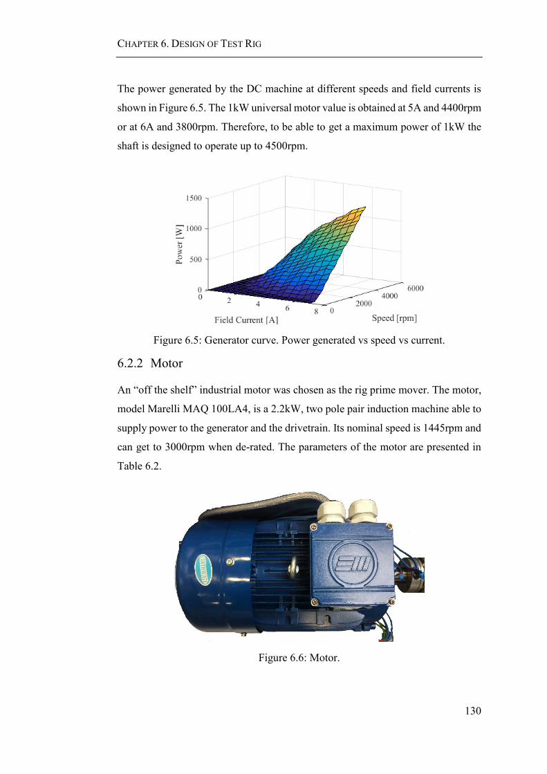
CHAPTER 6. DESIGN OF TEST RIG
130
The power generated by the DC machine at different speeds and field currents is
shown in Figure 6.5. The 1kW universal motor value is obtained at 5A and 4400rpm
or at 6A and 3800rpm. Therefore, to be able to get a maximum power of 1kW the
shaft is designed to operate up to 4500rpm.
Figure 6.5: Generator curve. Power generated vs speed vs current.
6.2.2 Motor
An “off the shelf” industrial motor was chosen as the rig prime mover. The motor,
model Marelli MAQ 100LA4, is a 2.2kW, two pole pair induction machine able to
supply power to the generator and the drivetrain. Its nominal speed is 1445rpm and
can get to 3000rpm when de-rated. The parameters of the motor are presented in
Table 6.2.
Figure 6.6: Motor.
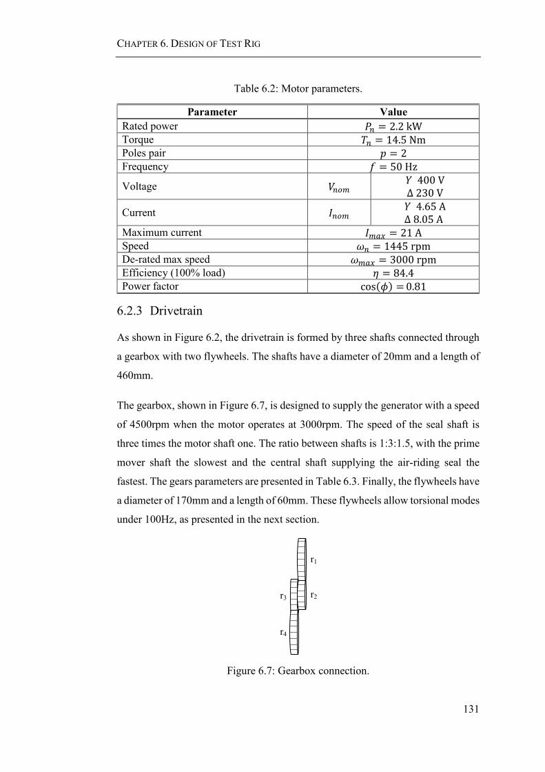
CHAPTER 6. DESIGN OF TEST RIG
131
Table 6.2: Motor parameters.
Parameter Value
Rated power 𝑃𝑛 = 2.2 kW
Torque 𝑇𝑛 = 14.5 Nm
Poles pair 𝑝 = 2
Frequency 𝑓 = 50 Hz
Voltage 𝑉𝑛𝑜𝑚 𝑌 400 V Δ 230 V
Current 𝐼𝑛𝑜𝑚 𝑌 4.65 A Δ 8.05 A
Maximum current 𝐼𝑚𝑎𝑥 = 21 A
Speed 𝜔𝑛 = 1445 rpm
De-rated max speed 𝜔𝑚𝑎𝑥 = 3000 rpm
Efficiency (100% load) 𝜂 = 84.4
Power factor cos(𝜙) =0.81
6.2.3 Drivetrain
As shown in Figure 6.2, the drivetrain is formed by three shafts connected through
a gearbox with two flywheels. The shafts have a diameter of 20mm and a length of
460mm.
The gearbox, shown in Figure 6.7, is designed to supply the generator with a speed
of 4500rpm when the motor operates at 3000rpm. The speed of the seal shaft is
three times the motor shaft one. The ratio between shafts is 1:3:1.5, with the prime
mover shaft the slowest and the central shaft supplying the air-riding seal the
fastest. The gears parameters are presented in Table 6.3. Finally, the flywheels have
a diameter of 170mm and a length of 60mm. These flywheels allow torsional modes
under 100Hz, as presented in the next section.
r1
r2r3
r4
Figure 6.7: Gearbox connection.

CHAPTER 6. DESIGN OF TEST RIG
132
Table 6.3: Gearbox parameters.
Gear Model Number of Teeth Diameter [mm]
𝑟1 YG275 75 150
𝑟2 YG2 25 25 50
𝑟3 YG2 35 35 70
𝑟4 YG2 70 70 140
6.3 Torsional Vibrations Modes
In this section, the torsional vibrations modes of the rig are designed. These
vibration modes allow the analysis of electromechanical interaction, and hence the
selection of their value is fundamental for the objectives of this thesis. The torsional
modes are determined by the flywheel connected next to the motor and generator
as shown in Figure 6.2.
Jm
Jg
Jfg
ksm
Jfm
Jg1
Jg2
Jg3
kc2
kc1
ksg
FlywheelsMachines GearsShaft
Figure 6.8: Mechanical layout.
Figure 4.4 illustrates the components of the mechanical system in terms of inertias,
stiffness and damping, with 𝐽𝑚 the inertia of the motor, 𝐽𝑓𝑚 the inertia of the
flywheel connected to the motor shaft, 𝐽𝑔1 the inertia of the motor shaft gear, 𝐽𝑔2
the inertia of both gears in the central shaft, 𝐽𝑔3, the inertias of generator shaft gear,
𝐽𝑓𝑔 the inertia of the flywheel connected in the generator shaft, and 𝐽𝑔 the generator

CHAPTER 6. DESIGN OF TEST RIG
133
inertia. 𝑘𝑐1 and 𝑘𝑐2 are the stiffness on the couplings of the motor and generator
respectively, and 𝑘𝑠𝑚 and 𝑘𝑠𝑔 are the stiffness of the shaft.
The inertias and stiffness values are shown in Table 6.4. The flywheels and gears
inertia in kgm2 were calculated using equation (6.2), with 𝜌 the material density in
kg/m3 , 𝐿 the length of the flywheel in m , and 𝑟𝑒𝑥𝑡 and 𝑟𝑖𝑛𝑡 the external and
internal flywheel radios in m . The motor inertia was given by the machine
datasheet, and the generator inertia was obtained experimentally as shown in
Appendix I. The shafts stiffness were calculated by equation (6.3), with 𝐺 the shear
modulus in GPa, 𝑟 the shaft radios in m, and 𝐿 the shaft length in m. The couplings
stiffness was obtained from the datasheet.
𝐽 = 𝜌𝜋𝐿 ∗(𝑟𝑒𝑥𝑡4 − 𝑟𝑖𝑛𝑡
4 )
2 (6.2)
𝑘 =𝐺𝜋𝑟
2𝐿 (6.3)
Table 6.4: Mechanical values.
Component Value
Motor Inertia 𝐽𝑚 = 0.0058 kgm2
Generator Inertia 𝐽𝑔 = 0.0005 kgm2
Flywheel Inertia 𝐽𝑓𝑚 = 0.0386 kgm2
𝐽𝑓𝑔 = 0.0386 kgm2
Gears Inertia
𝐽𝑔𝑏1 = 0.0093 kgm2
𝐽𝑔𝑏2 = 4.7 ∗ 10−3 kgm2
𝐽𝑔𝑏3 = 0.0091 kgm2
Coupling Stiffness 𝑘𝑐1 = 113406 Nm/rad
𝑘𝑐2 = 113406 Nm/rad
Shaft Stiffness 𝑘𝑠𝑚 = 2.1598 ∗ 103 Nm/rad
𝑘𝑠𝑔 = 2.2398 ∗ 103 Nm/rad
The mechanical natural frequencies obtained are 0Hz, 35.99Hz, and 82.15Hz. The
torsional vibration modes, obtained with TorTrans, a Matlab Toolbox written by
Seamus Garvey, and associated with each natural frequency, are shown in Figure
6.9. The circles symbolise the inertias, the shafts are modelled in red, and the
gearbox in blue. The vertical green lines represent the inertias referred angles in
each operation mode. In the first mode or rigid mode, the system moves together.

CHAPTER 6. DESIGN OF TEST RIG
134
In the second mode, the generator and motor are moving out of phase as was
observed in chapter 4. In the third mode, the generator and motor move together
while the gearbox moves in opposite direction. Comparing with the modes obtained
in chapter 4, only the mode in which both generators move out of phase, and
therefore, associated with the second generator has been eliminated. In chapter 7,
mode 2 and 3 are suppressed through the strategies proposed in chapter 5.
Figure 6.9: Mode shapes.

CHAPTER 6. DESIGN OF TEST RIG
135
6.4 Electrical Power System Components
As already mentioned, the electrical power system is a DC system with three
resistive loads 𝑅𝐿 that can be switched on/off. As shown in Figure 6.10, the
resistances are connected through an IGBT which allows its connection and
disconnection. The resistances switching allows the application of the connection
patterns in study: step connection, SLME connection, MLL connection, and
MSLME connection.
Figure 6.10: Electrical power system connection diagram.

CHAPTER 6. DESIGN OF TEST RIG
136
As shown in Figure 6.10, the IGBT switching is controlled through the PC. The
computer sends a signal to a microcontroller, which is connected to an adaptor
board that sends a signal to the IGBT gate driver to open and close the switch. To
control the speed of the motor, an industrial drive is used.
To guard the machines and IGBT of the currents produced by the inductances when
the resistance is disconnected the following protections are used:
To protect the generator and dissipate the current when the switches turn
off, there is a high resistance 𝑅𝑃 connected in parallel to the IGBT system.
To protect the IGBT when the switches are off, a diode has been connected
in parallel to each load.
In this section, the resistance, IGBT, microcontroller, drive, and power supplies are
described. The control system, including the load connection and the motor drive,
are presented in section 6.5.
6.4.1 Resistance Banks
The maximum current at which the generator can operate is 6A and 10A/15 min in
overload. Thus, the resistances are chosen to stand these values.
The resistance 𝑅𝑃, used to protect the machine when the IGBT opens, is a fixed
value resistance bank with enclosure, brand HVR Pentagon. It is composed by three
resistance BX375 of 20Ω, each of a maximum of 1kW. Hence the total resistance
connected in series is 60Ω and can stand a maximum of 3kW.
The load resistance 𝑅𝐿 are three variable wire resistance, brand Arcol, model
VRH320. One of the resistances can change its value between 1 and 10Ω, with a
maximum current of 5.7A and 8A/15 min in overload. While the other two
resistance are 33Ω with a maximum current of 3.1A and 4.4A/15 min in overload.
Both operate at maximum 320V and 640V/15 min in overload. For the cases in
which higher resistances need to be connected, as in the MLL strategy, a spare
resistance bank with the same characteristics of the resistance 𝑅𝑃 is connected in
series to the variable resistances.

CHAPTER 6. DESIGN OF TEST RIG
137
6.4.2 IGBT and Gate driver
The IGBT used to connect the resistive loads are dual switch high power IGBT,
model CM225DX-24S1 that can stand a maximum of 225A and 1200V. This IGBT
model was chosen because of the existence of a gate driver designed to operate with
it. The gate driver used with this IGBT is a Powerex VLA536-01R, which is fed by
a 15V and maximum 1.58A power supply. To dissipate the heat produced by the
IGBT a heatsink is used. Figure 6.11 shows the IGBT, and the gate driver
connected.
Figure 6.11: IGBT and gate driver.
The IGBT and gate driver are designed to operate with dual switches (half bridge),
which are intended to be used in an inverter leg. In this experimental setup, only
one IGBT is used for the switching and the second IGBT is kept open. Of the second
IGBT, its diode is utilised for the protection of the system as shown in Figure 6.12.
The diode permits the dissipation of the current stored in the resistance winding
when the switch opens. For this operation, the two IGBT must operate
independently, and thus the signals sent by the gate driver must be decoupled.
RL
IGBT
Gatedrive
+
Va
-
Always 0Switching
0/1
Figure 6.12: IGBT circuit.

CHAPTER 6. DESIGN OF TEST RIG
138
To turn on the IGBT, the difference of voltage between the gate driver terminals
Vin-IN1 must be 5V, while the current must be 13mA. Since the microcontroller
cannot supply these values of current, an adaptor board is used. The control and
adaptor board are presented in section 6.5.2. To keep the second IGBT open, and
hence used only the protection diode, the terminals Vin-IN2 are directly connected,
and its voltage is maintained in 0V.
6.4.3 Microcontroller
The microcontrollers used in the system are two Infineon Easy Kit XE164FM. This
model was chosen due to the availability to control through the PC, and the
compatibility with the software DAvE.exe that helps in its programming. Figure
6.13 shows the microcontroller. In red the main components of the board are
highlighted: Pin Connectors, State Lights, USB Connection, and Power Supply.
Figure 6.13: Microcontroller board.
The pin connectors allow the connection of the microcontroller and the adaptor
board and have been soldered into the board to supply the requirements of this
experimental rig. Each of them can generate a voltage difference of 5V. The state
lights, internally connected to the board pin, can be programmed to turn on and off.
The USB connection can be used to supply the board electrically, to load the code,
or/and to send signals from the PC. For this reason, the USB is a dual USB to
UART/JTAG interface. To control the microcontroller from the PC, an RS232
serial interface is available via the USB port, which converts TTL-UART-signals
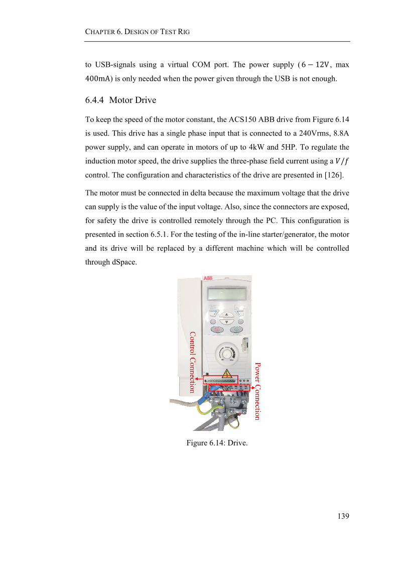
CHAPTER 6. DESIGN OF TEST RIG
139
to USB-signals using a virtual COM port. The power supply (6 − 12V , max
400mA) is only needed when the power given through the USB is not enough.
6.4.4 Motor Drive
To keep the speed of the motor constant, the ACS150 ABB drive from Figure 6.14
is used. This drive has a single phase input that is connected to a 240Vrms, 8.8A
power supply, and can operate in motors of up to 4kW and 5HP. To regulate the
induction motor speed, the drive supplies the three-phase field current using a 𝑉/𝑓
control. The configuration and characteristics of the drive are presented in [126].
The motor must be connected in delta because the maximum voltage that the drive
can supply is the value of the input voltage. Also, since the connectors are exposed,
for safety the drive is controlled remotely through the PC. This configuration is
presented in section 6.5.1. For the testing of the in-line starter/generator, the motor
and its drive will be replaced by a different machine which will be controlled
through dSpace.
Figure 6.14: Drive.
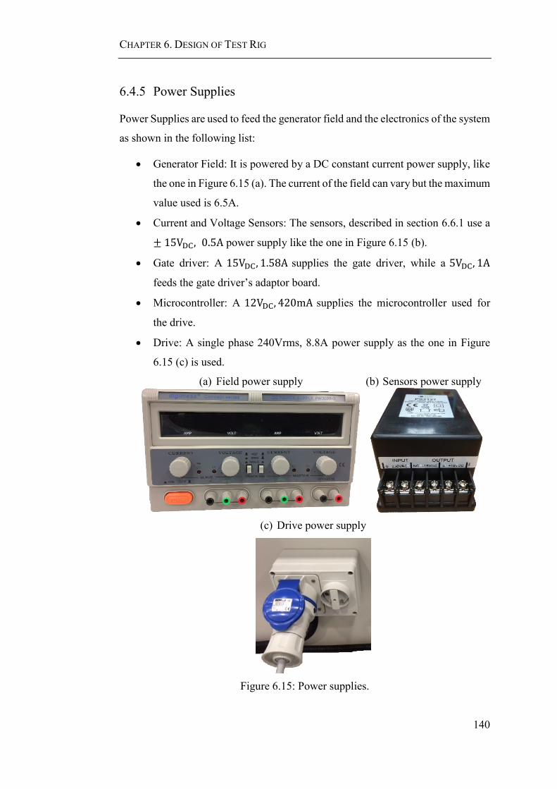
CHAPTER 6. DESIGN OF TEST RIG
140
6.4.5 Power Supplies
Power Supplies are used to feed the generator field and the electronics of the system
as shown in the following list:
Generator Field: It is powered by a DC constant current power supply, like
the one in Figure 6.15 (a). The current of the field can vary but the maximum
value used is 6.5A.
Current and Voltage Sensors: The sensors, described in section 6.6.1 use a
± 15VDC, 0.5A power supply like the one in Figure 6.15 (b).
Gate driver: A 15VDC, 1.58A supplies the gate driver, while a 5VDC, 1A
feeds the gate driver’s adaptor board.
Microcontroller: A 12VDC, 420mA supplies the microcontroller used for
the drive.
Drive: A single phase 240Vrms, 8.8A power supply as the one in Figure
6.15 (c) is used.
(a) Field power supply (b) Sensors power supply
(c) Drive power supply
Figure 6.15: Power supplies.
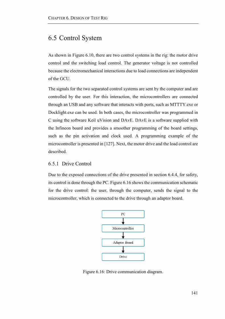
CHAPTER 6. DESIGN OF TEST RIG
141
6.5 Control System
As shown in Figure 6.10, there are two control systems in the rig: the motor drive
control and the switching load control. The generator voltage is not controlled
because the electromechanical interactions due to load connections are independent
of the GCU.
The signals for the two separated control systems are sent by the computer and are
controlled by the user. For this interaction, the microcontrollers are connected
through an USB and any software that interacts with ports, such as MTTTY.exe or
Docklight.exe can be used. In both cases, the microcontroller was programmed in
C using the software Keil uVision and DAvE. DAvE is a software supplied with
the Infineon board and provides a smoother programming of the board settings,
such as the pin activation and clock used. A programming example of the
microcontroller is presented in [127]. Next, the motor drive and the load control are
described.
6.5.1 Drive Control
Due to the exposed connections of the drive presented in section 6.4.4, for safety,
its control is done through the PC. Figure 6.16 shows the communication schematic
for the drive control: the user, through the computer, sends the signal to the
microcontroller, which is connected to the drive through an adaptor board.
Figure 6.16: Drive communication diagram.

CHAPTER 6. DESIGN OF TEST RIG
142
As shown in [126], five 24V signals are needed to control the drive remotely. These
signals, that take binary values (0/1), control the turning on/off of the drive (DI1),
the direction of rotation (DI2), the increase of the speed (DI3), the decrease of the
speed (DI4), or the use of a fixed speed set on the drive for operation (DI5). Thus,
to fix the operation speed of the drive two strategies can be taken: the designated
fixed speed can be chosen turning on the pin DI5, or the speed can be controlled in
a potentiometer basis using the signals DI3 and DI4. When DI3 and DI4 are
simultaneously on or off the speed is constant, and when only one of them is on the
value increases or decreases.
Since the microcontroller only generates 5V signals, to send the signals to the drive,
an adaptor board is used. The schematic is shown in Figure 6.17. The board consists
of five optocouplers connected to the drive 24V drive output, which turns on when
the microcontroller sends the signals. The adaptor board is shown in Figure 6.18.
DI5
DI4
DI3
DI2
DI1
COM
GND
+24V
Drive Input
MC 1
MC 2
MC 3
MC 4
MC 5
GND
Microcontroller
Signal
Figure 6.17: Drive adaptor board diagram.
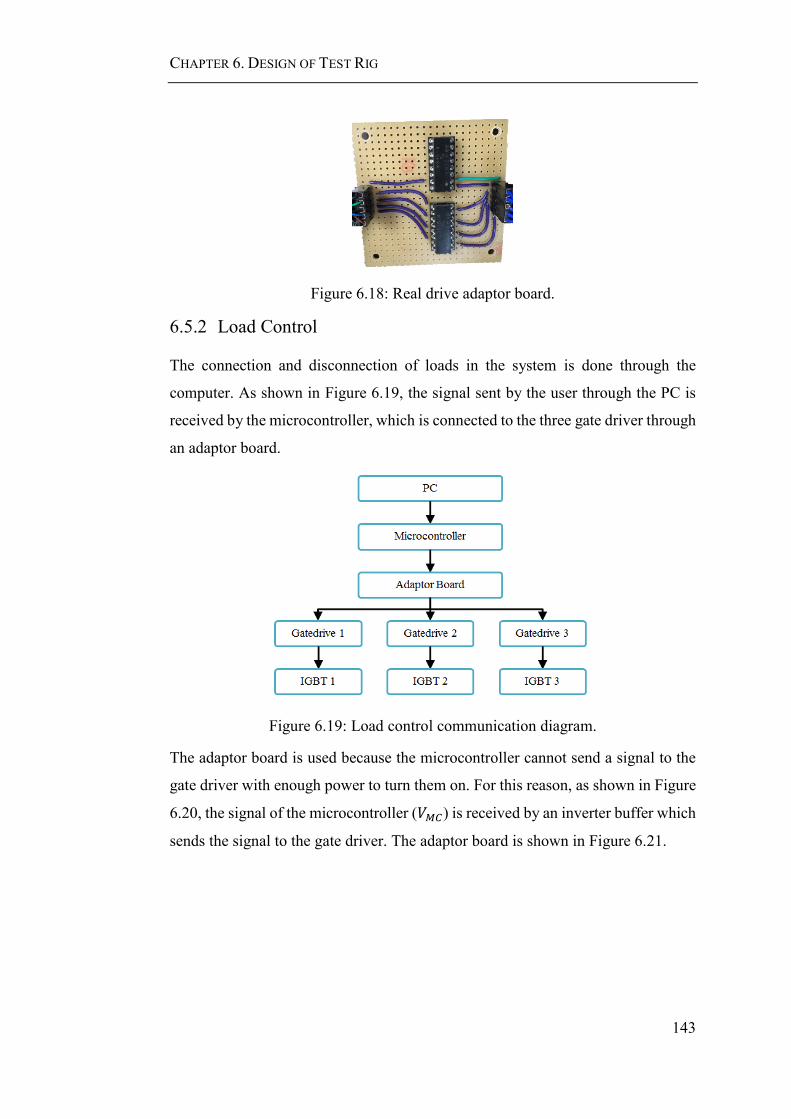
CHAPTER 6. DESIGN OF TEST RIG
143
Figure 6.18: Real drive adaptor board.
6.5.2 Load Control
The connection and disconnection of loads in the system is done through the
computer. As shown in Figure 6.19, the signal sent by the user through the PC is
received by the microcontroller, which is connected to the three gate driver through
an adaptor board.
Figure 6.19: Load control communication diagram.
The adaptor board is used because the microcontroller cannot send a signal to the
gate driver with enough power to turn them on. For this reason, as shown in Figure
6.20, the signal of the microcontroller (𝑉𝑀𝐶) is received by an inverter buffer which
sends the signal to the gate driver. The adaptor board is shown in Figure 6.21.

CHAPTER 6. DESIGN OF TEST RIG
144
VMC1 ING1 VMC2 ING2 VMC3 ING3
5V
R
Figure 6.20: Load control adaptor board diagram.
Figure 6.21: Load control adaptor board.
Finally, to switch on and off the loads using the different PMS strategies the user
can choose between the following options which are given to the microcontroller
trough MTTTY.exe or Docklight.exe:
0 – Disconnect the loads at the same time.
1 – Step connection of one resistance.
2 – SLME connection applied to one natural frequency.
3 – MLL and MSLME connection applied to one frequency.
4 – SLME connection applied to two natural frequencies.
5 – MLL connection applied to two natural frequencies.
6 – MSLME connection applied to two natural frequencies.

CHAPTER 6. DESIGN OF TEST RIG
145
6.6 Sensors
To measure the electrical signals, the speed and the transversal position of the motor
shaft, sensors are used. The electrical signals, armature current, armature voltage,
and field current, are measured with LEM transducers. The speed is measured with
a tachometer and a resolver connected at both ends of the generator shaft. The
position of the motor shaft is measured with a position sensor. Figure 6.2 shows the
position of the tachometer, resolver, and position sensor.
To visualise the sensor signals dSpace is used. dSpace is chosen for the control of
the in-line starter/generator, out of the scope of this thesis, and the signals
associated with this, such as the position sensor. To have the rest of the signals on
the same platform, the tachometer, resolver, and LEM transducer are also
connected to dSpace, using an acquisition frequency of 10kHz or 10−5s. Next, the
LEM transducer, tachometer, resolver, and position sensor are described.
6.6.1 LEM Transducer
To improve the resolution obtained with the probes available at the laboratory and
to read the signals with dSpace, LEM transducers are used. Their operation is based
on the Hall Effect, in which the current in a coil produces a magnetic field that
induces a proportional voltage across an electrical conductor. In this thesis, two
current LEM transducer and one voltage LEM transducer are used. Figure 6.22
shows the board with the LEM sensors. Next, the transducers used are described.
Figure 6.22: LEM sensors.

CHAPTER 6. DESIGN OF TEST RIG
146
6.6.1.1 Current LEM
The current LEM transducer model LA100-P of Figure 6.23 is used to sense the
armature and field current of the generator. To measure the current, the cable 𝐼𝑃
must cross the transducer, which induces a secondary current 𝐼𝑆. To obtain the value
of 𝐼𝑆, a measuring resistance 𝑅𝑀 is connected at the output as shown in Figure 6.23.
The parameters of the LEM LA100-P are given in Table 6.5.
IP
IS
RM
+
-
M
+VC
-VC
GNDVT
RS
Figure 6.23: Current LEM circuit.
Table 6.5: Current LEM parameters.
Parameter Value
Primary nominal current 𝐼𝑃𝑁 = 100 A
Secondary nominal current 𝐼𝑆𝑁 = 100 mA
Measuring resistance 𝑅𝑀 = 40… 95 Ω
Conversion ratio 𝑁𝑃/𝑁𝑆 = 1/1000
Supply voltage 𝑉𝐶 = ±15 V
Secondary coil resistance 25 Ω
Current consumption 𝐼𝐶 𝑅𝑆 = 10 + 𝐼𝑠 mA
Accuracy at 𝐼𝑃𝑁 and 25°𝐶 ±0.45%
Linearity error < 0.15%
The nominal values of the transducer are significantly higher than the operational
ones, in which the maximum current is 10A. For this reason, to increase the
precision of the measurement, the number of turns of the measurement cable is
increased to five (𝑁𝑃 = 5) and the measuring resistance 𝑅𝑀 range is recalculated
for these values.
The minimum value of the measuring resistance depends on 𝑉𝐶, and hence its value
remains the same. Instead, the maximum value of the resistance can be obtained

CHAPTER 6. DESIGN OF TEST RIG
147
from the equations (6.4) and (6.5), in which 𝑉𝑇 is the voltage before the coil
resistance as shown in Figure 6.23.
𝑁𝑃𝐼𝑃 = 𝑁𝑆𝐼𝑆 (6.4)
𝑉𝑇 = (𝑅𝑆 + 𝑅𝑀)𝐼𝑆 (6.5)
Using the LA100-P datasheet data, it is obtained that 𝑉𝑇 = 12V. Designing the
transducer for a nominal current 𝐼𝑃 = 6A and 𝑁𝑃 = 5, it is obtained that 𝐼𝑆𝑁 =
30mA and that the maximum measuring resistance value is 𝑅𝑀 = 375Ω. Finally,
the value of 𝑅𝑀 is chosen using equation (6.6). To have a nominal output voltage
𝑉𝑀 = 6V when the current is 6A, the measuring resistance is 𝑅𝑀 = 200Ω.
𝑉𝑀 = 𝑅𝑀𝐼𝑆 (6.6)
6.6.1.2 Voltage LEM
A voltage transducer LV25-P is used to measure the armature voltage. As shown
in Figure 6.24, the measured voltage is connected to the terminals +HV and –HV.
For this reason, besides the measuring resistance 𝑅𝑀 , the resistance 𝑅1 used to
obtain the current proportional to the measuring voltage, must be also calculated.
Table 6.6 shows the main parameters of the voltage transducer.
IP
IS
RM
+
-
M
+VC
-VC
GNDVT
RSR1
+HV
-HV
Figure 6.24: Voltage LEM circuit.
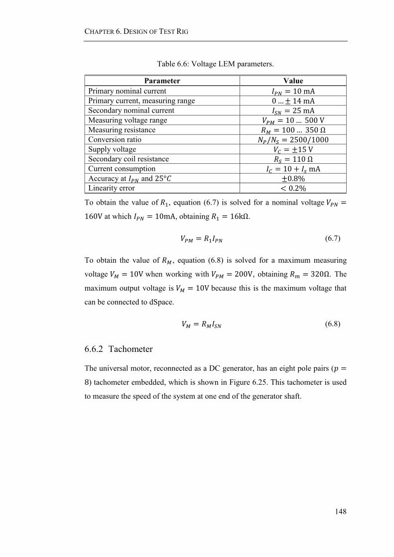
CHAPTER 6. DESIGN OF TEST RIG
148
Table 6.6: Voltage LEM parameters.
Parameter Value
Primary nominal current 𝐼𝑃𝑁 = 10 mA
Primary current, measuring range 0…± 14 mA
Secondary nominal current 𝐼𝑆𝑁 = 25 mA
Measuring voltage range 𝑉𝑃𝑀 = 10… 500 V
Measuring resistance 𝑅𝑀 = 100… 350 Ω
Conversion ratio 𝑁𝑃/𝑁𝑆 = 2500/1000
Supply voltage 𝑉𝐶 = ±15 V
Secondary coil resistance 𝑅𝑆 = 110 Ω
Current consumption 𝐼𝐶 = 10 + 𝐼𝑠 mA
Accuracy at 𝐼𝑃𝑁 and 25°𝐶 ±0.8%
Linearity error < 0.2%
To obtain the value of 𝑅1, equation (6.7) is solved for a nominal voltage 𝑉𝑃𝑁 =
160V at which 𝐼𝑃𝑁 = 10mA, obtaining 𝑅1 = 16kΩ.
𝑉𝑃𝑀 = 𝑅1𝐼𝑃𝑁 (6.7)
To obtain the value of 𝑅𝑀 , equation (6.8) is solved for a maximum measuring
voltage 𝑉𝑀 = 10V when working with 𝑉𝑃𝑀 = 200V, obtaining 𝑅𝑚 = 320Ω. The
maximum output voltage is 𝑉𝑀 = 10V because this is the maximum voltage that
can be connected to dSpace.
𝑉𝑀 = 𝑅𝑀𝐼𝑆𝑁 (6.8)
6.6.2 Tachometer
The universal motor, reconnected as a DC generator, has an eight pole pairs (𝑝 =
8) tachometer embedded, which is shown in Figure 6.25. This tachometer is used
to measure the speed of the system at one end of the generator shaft.

CHAPTER 6. DESIGN OF TEST RIG
149
Figure 6.25: Tachometer.
The tachometer generates a sinusoidal voltage with frequency (𝑓𝑉) proportional to
the speed of the machine shaft (𝜔𝑠ℎ𝑎𝑓𝑡). To obtain the speed of the shaft in rpm,
equation (6.9) is used.
𝜔𝑠ℎ𝑎𝑓𝑡 [rpm] = 𝑓𝑉 [Hz] ∗60
8= 𝑓𝑉 [Hz] ∗ 7.5 (6.9)
6.6.3 Resolver
The resolver is connected opposite to the tachometer as shown in Figure 6.2. The
aim is to provide higher resolution for the speed measurement than the one obtained
with the tachometer. As presented in Figure 6.26, the operation of the resolver
consists in inducing a sinusoidal current into two coils shifted by 90° (shown in
blue), by exciting a rotating coil (shown in red).
Rotor
R1
R2
Stator
cosφ
sinφ
S1
S2
S3
S4
φ
Figure 6.26: Resolver circuit.

CHAPTER 6. DESIGN OF TEST RIG
150
The angle of the system is obtained from equation (6.10), in which 𝜙 is the
rotational angle, 𝐸 is the excitation voltage, 𝐾 is the transformation ratio, and 𝑅1 −
𝑅2, 𝑆1 − 𝑆3, and 𝑆2 − 𝑆4 are the voltage difference between the resolver terminals.
𝐸(𝑆1 − 𝑆3) = 𝐾𝐸(𝑅1 − 𝑅2) cos(𝜙)
𝐸(𝑆2 − 𝑆4) = 𝐾𝐸(𝑅1 − 𝑅2) sin(𝜙) (6.10)
The resolver connected is a brushless frameless Harowe resolver, model
21BRX709 as the one in Figure 6.27. Table 6.7 presents the resolver parameters.
The resolver is connected to the resolver input/output on dSpace, which sends the
excitation field and measures the output angle.
Figure 6.27: Resolver.
Table 6.7: Resolver parameters.
Parameter Value
Excitation parameters 𝑓𝐸 = 10 kHz Input voltage 𝐸𝑅 = 7 V
Input current max28 mA
Input power 0.065 W
Transformation ratio 𝐾 = 0.31
Inner shaft diameter 20 mm
Maximum continuous speed 20000 rpm
6.6.4 Position Sensor
The position sensor measures the motor shaft movements along the x and y-axis,
which is fundamental for the in-line starter/generator as presented in [124]. In this
thesis, the position sensor is only used to identify the critical speeds of the system.

CHAPTER 6. DESIGN OF TEST RIG
151
The position sensor is a non-contact sensor, brand Lion Precision, and model U5C.
Table 6.8 presents its parameters. The resolutions depend on the material being
measured (ferrous and non-ferrous) and the frequency used (from 250Hz to 15kHz).
Table 6.8: Position sensor parameters.
Parameter Value
Dimension 𝑋 = 3.4 mm
Dimension 𝑌 = 3.0 mm
Dimension 𝑍 = 4.90 +/− .025 mm
Range 0.25 − 1.5 mm
Minimum resolution 75 nm
Maximum resolution 260 nm
6.7 Safety System
To protect the people working on the rig of unexpected hazards, the following
safety precautions have been taken.
Risk Assessment: A risk assessment, revised and certified by qualified
university personnel has been carried out.
Emergency button: A button as the one in Figure 6.28 allows the quick
disconnection of all electric equipment.
Remote operation: To avoid contact with electronics, the drive handling,
and the connection and disconnection of loads is done through the PC.
Covered rotating parts: As shown in Figure 6.29, the rotating shaft and
machines of the rig are covered. They cannot be accessed while the system
is in operation.
Covered electronics: As shown in Figure 6.30(b), all the electronics are
covered. The switches are covered by Plexiglas, while the drive is enclosed
in a metal case.
Isolated electronics: The electronics are isolated through the use of Paxolin.
Grounded electronics: The electric components are grounded.

CHAPTER 6. DESIGN OF TEST RIG
152
Figure 6.28: Emergency button.
Figure 6.29: Rig protection.
6.8 Summary
The test rig developed is a multidisciplinary experiment that allows the analysis of
different aircraft applications such as an air-riding seal, in-line starter/generator,
and electromechanical interactions. In this chapter, the design of the
electromechanical interaction capacity of the test rig has been presented. To test the
electromechanical interaction, the system is equipped with IGBTs that switch
on/off resistance banks and that are controlled through the PC with the use of
Infineon microcontrollers. Figure 6.30 shows the whole rig, in (a) the mechanical
components are shown while in (b) the electronics are presented. In the next
chapter, the results obtained with the test rig are given.

CHAPTER 6. DESIGN OF TEST RIG
153
(a) Mechanical components
(b) Electrical components
Figure 6.30: Whole rig picture.

Chapter 7
7 Results Experimental Test Rig
7.1 Introduction
In this chapter, the experimental system presented in chapter 6 is used to test the
electromechanical interaction and the power management system (PMS) solutions
presented in chapter 5. The rest of the chapter is organised as follows: First, the
drivetrain is parametrised. After, the approach to obtain the vibrations of the system
and the torque is defined. In section 7.4 the electromechanical interaction produced
by an electrical load connection is shown. In section 7.5 Posicast strategies are
experimentally tested. Finally, the chapter summary is given.
7.2 Drivetrain Characterisations
To apply the PMS strategies and avoid resonance with the mechanical system, the
drivetrain is characterised in terms of its critical speeds or transversal frequencies
and its torsional frequencies.
7.2.1 Critical Speeds
To prevent excessive vibration on the experimental rig, the critical speeds or
transversal vibrations of the system are identified. For this purpose, the motor shaft
displacement is measured for increasing speed. The movement of the shaft is
measured through a position sensor as described in chapter 6, while the speed is
obtained from the resolver. The resolver, connected to dSpace, gives the rotational
angle of the shaft attached to the generator. Therefore, to get the motor shaft speed,
the angle is differentiated and divided by 1.5, the speed factor between shafts. Both
signals are recorded through dSpace.

CHAPTER 7. RESULTS EXPERIMENTAL TEST RIG
155
Figure 7.1 shows the displacement of the shaft connected to the motor for ascending
speed. Higher displacements show higher vibrations. Therefore, the critical speeds
are those at which the vibrations are higher: 733rpm , 1497rpm , 1669rpm ,
2170rpm, and 2631rpm. To avoid reducing the rig lifespan, the experimental
system is not operated at these speeds.
Figure 7.1: Critical speed identification.
7.2.2 Torsional Modes
To test the load connection strategies presented in chapter 5, the torsional modes of
the rig must be determined. The natural frequencies are obtained using FFT
analysis, while for the damping ratio a method based on the Hilbert Transform is
employed.
7.2.2.1 Frequency Identification
The FFT is measured after applying a step connection to the system, which excites
the torsional modes. The information recorded consists of 10 seconds of data with
a sampling time 𝑡𝑠 = 10−5s. The FFT is applied to the armature current 𝑖𝑎, and the
magnitude is normalised by the steady state value 𝑖𝑎/𝑖𝑎𝑠𝑡𝑒𝑎𝑑𝑦. Figure 7.2 shows
the Fourier response of the system operating at 1500rpm and 2000rpm.
The frequencies 𝑓1 = 35Hz and 𝑓2 = 73.1Hz are shown in both plots encircled in
red. However, in black, a second set of frequencies is marked. These frequencies
are associated with the speed frequencies since 1500rpm = 25Hz and
2000rpm = 33Hz . Likewise, 50Hz and 67Hz are the first speed harmonics,
which are associated to the speeds in the middle shaft.

CHAPTER 7. RESULTS EXPERIMENTAL TEST RIG
156
Figure 7.2: Fourier analysis at different speed.
Because the frequencies associated with the speed are not part of the torsional
vibrations modes, they are filtered. Using a band stop IIR filter for each speed
frequency, 25Hz and 50Hz, or 33Hz and 67Hz, with a bandwidth of 2Hz and 1Hz
for the first and second frequency respectively, Figure 7.3 is obtained. Now, the
frequencies obtained at both speeds are the same: 35Hz and 73.1Hz.
Figure 7.3: Filtered Fourier analysis.

CHAPTER 7. RESULTS EXPERIMENTAL TEST RIG
157
Small frequency variations are detected between the two results. For example, the
frequencies are less excited when the system is operating at 2000rpm. This is
because the signal was taken when the system was closer to the steady-state than in
the case of 1500rpm. Data closer to the load connection was not used, due to a
high change in speed. This speed change generates many frequency peaks
associated with the speed which difficults the FFT analysis.
Moreover, 𝑓1 obtained at 2000rpm is higher than the one obtained at 1500rpm
(37Hz instead of 35Hz). To understand this difference, further data sets have been
used for the FFT recognition. Figure 7.4 shows the FFT obtained for a step load
connection of the system operating at 1500rpm with 6.2A field current. Two
seconds of data measured with an oscilloscope and a sampling time 𝑡𝑠 = 10−5s
was used. The frequencies obtained are 𝑓1 = 35.5Hz and 𝑓2 = 77.1Hz . These
frequencies are close to the ones presented in Figure 7.3 but not the same. The
differences are due to small changes in the experimental rig between the
measurements, such as movement of the flywheels and gears, and due to the noise
of signals. The results obtained through different dataset show that the torsional
frequencies of the system are in the following ranges:
𝑓1 ∈ [35 − 37] Hz
𝑓2 ∈ [73 − 77.1] Hz
Since the relative difference between the measurements is small (5.4% for 𝑓1 and
5.1% for 𝑓2), the values are considered acceptable. Also, the frequencies are close
to the design values presented in chapter 6: 35.99Hz and 82.15Hz. Thus, the
experimental system is close to its design.

CHAPTER 7. RESULTS EXPERIMENTAL TEST RIG
158
Figure 7.4: Filtered Fourier for different data.
Additionally, writing the frequencies in rpm is obtained that 35.5Hz equals
2130rpm. This value is one of the critical speeds found in section 7.2.1, showing
that because of the gears the torsional vibrations produce transversal ones.
In this section, it has been demonstrated that the Fourier analysis allows the
identification of torsional vibrations with an error of 5%. Since the difference is
also affected by external changes, such as small movements of the components of
the rig, the FFT method is a suitable identification method for torsional vibrations
in real systems. However, for simulation cases, in which the system in the study
can be symmetric, the FFT can fail to identify one or more natural frequencies due
to the system acting as a vibration absorber configuration [49]. This is not a
problem experimentally because small differences in the inertias and stiffness of
the system are always present. The vibration absorber example is shown in
Appendix II.
7.2.2.2 Damping Ratio Identification
In most cases, to determine the damping ratio associated with a frequency, the
logarithmic decrement method is used. However, this approach presents high error
in systems with high noise as this one [3]. For this reason, to identify the damping
ratio, the Hilbert Transform Method combined with empirical mode decomposition
(EMD) presented in [128], [129] is used.
The first step in this method is to separate the frequencies with EMD. For this, as
shown in [128], the armature current signal is filtered using a passband filter around

CHAPTER 7. RESULTS EXPERIMENTAL TEST RIG
159
each frequency 𝑓1 and 𝑓2 with a bandwidth of 4Hz. To the filtered signals, the
EMD method is applied to obtain the free response of a single mode. The central
frequencies used for the filter are 𝑓1 = 35.5Hz and 𝑓2 = 77.1Hz, since these are
the frequencies that are used for the Posicast based methods in section 7.5. Figure
7.5 shows the vibration modes obtained.
Figure 7.5: Mode decomposition.
After getting the response of the vibration modes, the Hilbert Transform is applied.
The real and imaginary parts are expressed in terms of the amplitude and phase as
shown in equations (7.1) and (7.2). Where 𝜉 is damping ratio, 𝜔(𝑡) is the
instantaneous frequency, 𝜔𝑑 and 𝜔𝑛 are the natural damped and natural
frequencies, and 𝐴0 and 𝜃0 are constants.
To obtain the damping ratio and the frequency associated with it, logarithm is
applied to equation (7.1). The slope of this equation is – 𝜉𝜔𝑛 . The damped
frequency is obtained by differentiating the angle as shown in equation (7.2).
𝐴(𝑡) = 𝐴0𝑒−𝜉𝜔𝑛𝑡 → log(𝐴(𝑡)) = log(𝐴0) − 𝜉𝜔𝑛𝑡 (7.1)
𝜃(𝑡) = 𝜔𝑑𝑡 + 𝜃0 → 𝜔(𝑡) = 𝜔𝑑 = 𝜔𝑛√1 − 𝜉2 (7.2)
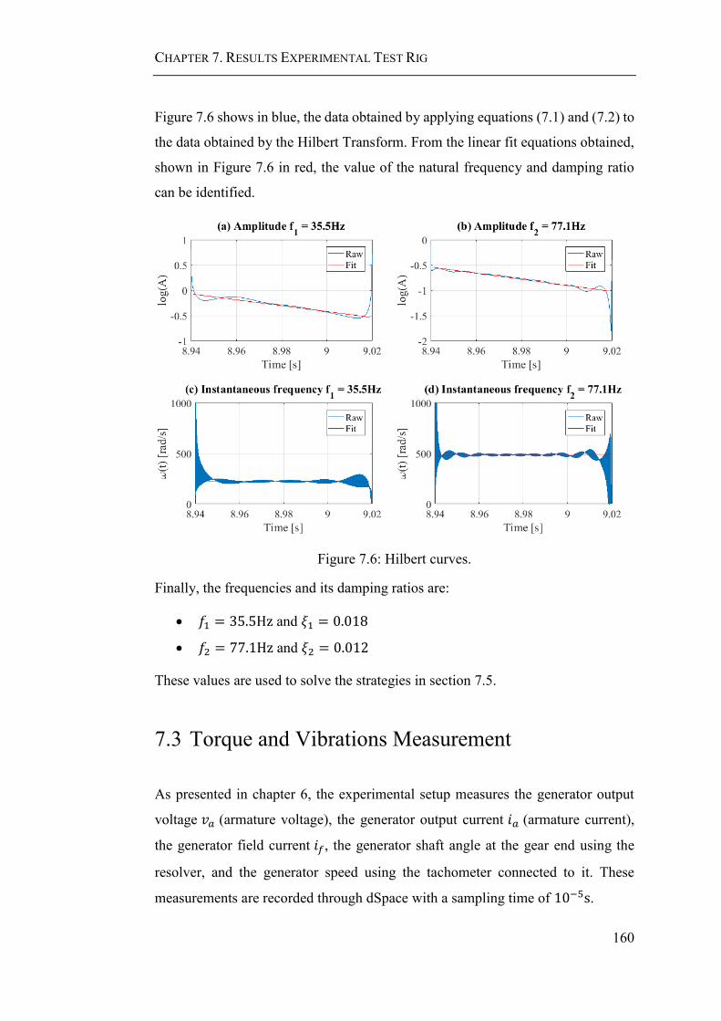
CHAPTER 7. RESULTS EXPERIMENTAL TEST RIG
160
Figure 7.6 shows in blue, the data obtained by applying equations (7.1) and (7.2) to
the data obtained by the Hilbert Transform. From the linear fit equations obtained,
shown in Figure 7.6 in red, the value of the natural frequency and damping ratio
can be identified.
Figure 7.6: Hilbert curves.
Finally, the frequencies and its damping ratios are:
𝑓1 = 35.5Hz and 𝜉1 = 0.018
𝑓2 = 77.1Hz and 𝜉2 = 0.012
These values are used to solve the strategies in section 7.5.
7.3 Torque and Vibrations Measurement
As presented in chapter 6, the experimental setup measures the generator output
voltage 𝑣𝑎 (armature voltage), the generator output current 𝑖𝑎 (armature current),
the generator field current 𝑖𝑓, the generator shaft angle at the gear end using the
resolver, and the generator speed using the tachometer connected to it. These
measurements are recorded through dSpace with a sampling time of 10−5s.

CHAPTER 7. RESULTS EXPERIMENTAL TEST RIG
161
The torsional vibrations are analysed by obtaining the torque of the system. Since
the torque is not being measured, its value is calculated by equation (7.3). The
electrical torque 𝑇𝑔, gives the steady-state value and is obtained by equation (7.4),
where 𝑃 is the power generated by the machine and 𝜔 is the speed of it. Moreover,
due to the use of a DC machine the electrical torque can also be obtained from
𝑘𝑖𝑓𝑖𝑎 , in which k is the machine constant, 𝑖𝑓 is the field current, and 𝑖𝑎 is the
armature current. This second method is used in this thesis. The transient torque
𝑇𝑚𝑒𝑐, produces the vibrations of the system and is proportional to the acceleration
(𝑑𝜔/𝑑𝑡) as shown in equation (7.5). 𝐽 is the inertia where the torque is being
measured. In this case, since the higher torque is next to the flywheel 𝐽𝑓𝑔, its inertia
value is used. The value of 𝑇𝑔 can be ignored to study the vibrations of the system
if the steady-state value is not desired.
𝑇𝑠ℎ = 𝑇𝑚𝑒𝑐 + 𝑇𝑔 (7.3)
𝑇𝑔 =𝑃
𝜔= 𝑘𝑖𝑓𝑖𝑎 (7.4)
𝑇𝑚𝑒𝑐 = 𝐽𝑑𝜔
𝑑𝑡 (7.5)
To obtain the torque of the system, the speed must be known. Two methods are
going to be used to get the shaft speed: direct measurement and sensorless
measurement. For the first one, the resolver and tachometer installed on the system
are used. For the second, the speed and torque are obtained from the electrical
signals: armature current, armature voltage, and field current.
To analyse the transient behaviour, the speed is analysed after an electrical load of
5Ω is connected to the system at 0.5s. The system operates at 1550rpm with a
constant field current of 6.2A. The electrical parameters obtained are shown in
Figure 7.7. In (a) the armature (in blue) and field (in red) current are presented and
in (b) the armature voltage is shown. Plot (c) illustrates the consumed power 𝑃𝐿𝑜𝑎𝑑
given by equation (7.6). The resistance connected in the system 𝑅𝐶𝑜𝑛𝑛𝑒𝑐𝑡𝑒𝑑 can be

CHAPTER 7. RESULTS EXPERIMENTAL TEST RIG
162
obtained by equation (7.7), in which 𝑅𝑃 and 𝑅𝐿 are the protection resistance and
the resistance of the load respectively.
𝑃𝐿𝑜𝑎𝑑 = 𝑣𝑎𝑖𝑎 (7.6)
𝑅𝐶𝑜𝑛𝑛𝑒𝑐𝑡𝑒𝑑 =𝑅𝑃𝑅𝐿𝑅𝑝 + 𝑅𝐿
=𝑣𝑎𝑖𝑎
(7.7)
Figure 7.7: Electrical data for step connection.
7.3.1 Direct Speed Measurement
In this section, the steps to obtain the speed using the installed tachometer and
resolver are shown.
7.3.1.1 Tachometer
As mentioned in chapter 6, the tachometer generates a sinusoidal voltage with
frequency (𝑓𝑉) proportional to the speed of the machine shaft measured by the
tachometer 𝑣𝑡. To obtain the speed of the shaft in rpm, the frequency is detected
through zero crossing, and its value is multiplied by 7.5 as shown in equation (6.9).
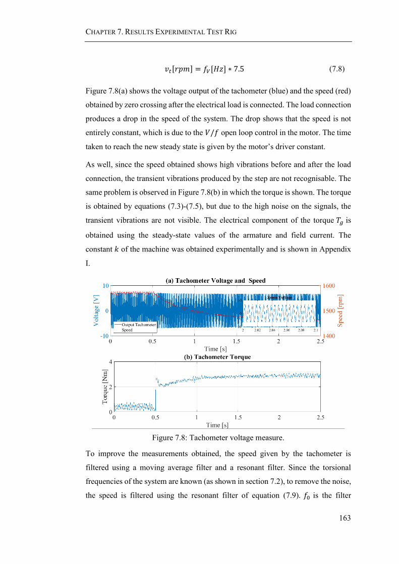
CHAPTER 7. RESULTS EXPERIMENTAL TEST RIG
163
𝑣𝑡[𝑟𝑝𝑚] = 𝑓𝑉[𝐻𝑧] ∗ 7.5 (7.8)
Figure 7.8(a) shows the voltage output of the tachometer (blue) and the speed (red)
obtained by zero crossing after the electrical load is connected. The load connection
produces a drop in the speed of the system. The drop shows that the speed is not
entirely constant, which is due to the 𝑉/𝑓 open loop control in the motor. The time
taken to reach the new steady state is given by the motor’s driver constant.
As well, since the speed obtained shows high vibrations before and after the load
connection, the transient vibrations produced by the step are not recognisable. The
same problem is observed in Figure 7.8(b) in which the torque is shown. The torque
is obtained by equations (7.3)-(7.5), but due to the high noise on the signals, the
transient vibrations are not visible. The electrical component of the torque 𝑇𝑔 is
obtained using the steady-state values of the armature and field current. The
constant 𝑘 of the machine was obtained experimentally and is shown in Appendix
I.
Figure 7.8: Tachometer voltage measure.
To improve the measurements obtained, the speed given by the tachometer is
filtered using a moving average filter and a resonant filter. Since the torsional
frequencies of the system are known (as shown in section 7.2), to remove the noise,
the speed is filtered using the resonant filter of equation (7.9). 𝑓0 is the filter
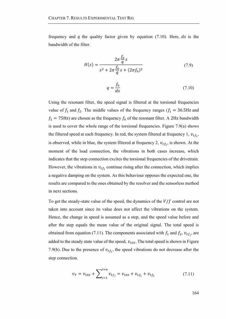
CHAPTER 7. RESULTS EXPERIMENTAL TEST RIG
164
frequency and 𝑞 the quality factor given by equation (7.10). Here, 𝑑𝑠 is the
bandwidth of the filter.
𝐻(𝑠) =2𝜋𝑓0𝑞 𝑠
𝑠2 + 2𝜋𝑓0𝑞 𝑠 +
(2𝜋𝑓0)2 (7.9)
𝑞 =𝑓0𝑑𝑠
(7.10)
Using the resonant filter, the speed signal is filtered at the torsional frequencies
value of 𝑓1 and 𝑓2. The middle values of the frequency ranges (𝑓1 = 36.5Hz and
𝑓2 = 75Hz) are chosen as the frequency 𝑓0 of the resonant filter. A 2Hz bandwidth
is used to cover the whole range of the torsional frequencies. Figure 7.9(a) shows
the filtered speed at each frequency. In red, the system filtered at frequency 1, 𝑣𝑡𝑓1,
is observed, while in blue, the system filtered at frequency 2, 𝑣𝑡𝑓2, is shown. At the
moment of the load connection, the vibrations in both cases increase, which
indicates that the step connection excites the torsional frequencies of the drivetrain.
However, the vibrations in 𝑣𝑡𝑓1 continue rising after the connection, which implies
a negative damping on the system. As this behaviour opposes the expected one, the
results are compared to the ones obtained by the resolver and the sensorless method
in next sections.
To get the steady-state value of the speed, the dynamics of the 𝑉/𝑓 control are not
taken into account since its value does not affect the vibrations on the system.
Hence, the change in speed is assumed as a step, and the speed value before and
after the step equals the mean value of the original signal. The total speed is
obtained from equation (7.11). The components associated with 𝑓1 and 𝑓2, 𝑣𝑡𝑓𝑖, are
added to the steady state value of the speed, 𝑣𝑡𝑆𝑆. The total speed is shown in Figure
7.9(b). Due to the presence of 𝑣𝑡𝑓1, the speed vibrations do not decrease after the
step connection.
𝑣𝑇 = 𝑣𝑡𝑆𝑆 +∑ 𝑣𝑡𝑓𝑖
𝑖=𝑛
𝑖=1= 𝑣𝑡𝑆𝑆 + 𝑣𝑡𝑓1 + 𝑣𝑡𝑓2 (7.11)
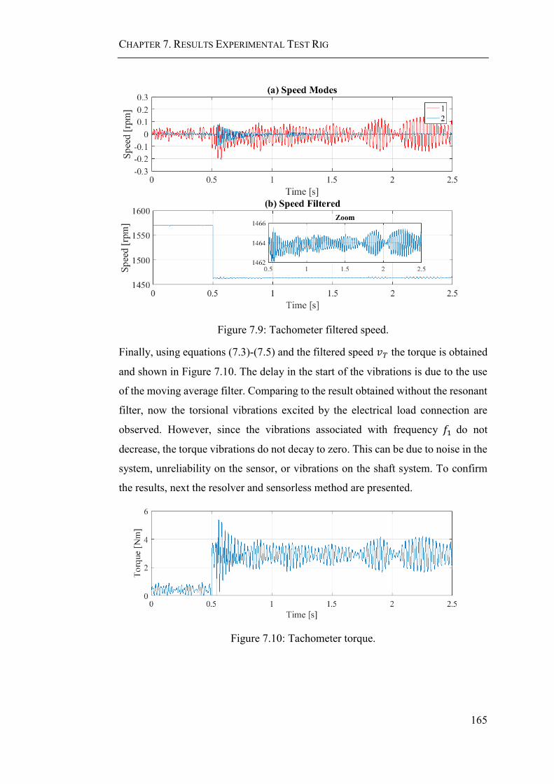
CHAPTER 7. RESULTS EXPERIMENTAL TEST RIG
165
Figure 7.9: Tachometer filtered speed.
Finally, using equations (7.3)-(7.5) and the filtered speed 𝑣𝑇 the torque is obtained
and shown in Figure 7.10. The delay in the start of the vibrations is due to the use
of the moving average filter. Comparing to the result obtained without the resonant
filter, now the torsional vibrations excited by the electrical load connection are
observed. However, since the vibrations associated with frequency 𝑓1 do not
decrease, the torque vibrations do not decay to zero. This can be due to noise in the
system, unreliability on the sensor, or vibrations on the shaft system. To confirm
the results, next the resolver and sensorless method are presented.
Figure 7.10: Tachometer torque.

CHAPTER 7. RESULTS EXPERIMENTAL TEST RIG
166
7.3.1.2 Resolver
As presented in chapter 6, the output of the resolver connected to dSpace is the
shaft angle. To obtain the speed, the angle must be differentiated. Since
differentiating add high-frequency noise, a moving average filter is also used.
Figure 7.11(a) shows resolver angle in rad and the speed obtained in rpm. The
torque, obtained from equations (7.3)-(7.5) is shown in Figure 7.11(b). Like in the
tachometer case, the speed and the torque show constant vibrations before and after
the load connection. Therefore, the same filtering method presented for the
tachometer signal is used for the resolver.
Figure 7.11: Resolver angle.
Using the same resonant filters that were described for the tachometer signal, the
vibrations modes associated with each frequency 𝑣𝑟𝑓1 and 𝑣𝑟𝑓2 are obtained and
shown in Figure 7.12(a). It is observed, that the speed vibrations rise for both
frequencies 𝑓1 and 𝑓2 after the load connection. However, for 𝑓1 the vibrations
increase before the connection, while for 𝑓2 the rise is after. The second case, as in
the tachometer case is due to the moving average filter. Moreover, contrary to the
tachometer case, the vibrations associated with both speed decrease with time. This
shows that in the tachometer case, the increase in the frequency associated with 𝑓1
is due to the sensor, and does not indicate that the vibrations in the system remain.

CHAPTER 7. RESULTS EXPERIMENTAL TEST RIG
167
The total speed is obtained by equation (7.12). The steady state is the same of the
tachometer. Figure 7.12(b) shows the total filtered speed.
𝑣𝑅 = 𝑣𝑟𝑆𝑆 +∑ 𝑣𝑟𝑓𝑖
𝑖=𝑛
𝑖=1= 𝑣𝑟𝑆𝑆 + 𝑣𝑟𝑓1 + 𝑣𝑟𝑓2 (7.12)
Figure 7.12: Resolver filtered speed.
Finally, the torque obtained is shown in Figure 7.13. Now it is observed that the
load connection produces vibrations which decrease in time. However, the start of
the vibrations before the load connection reduces the measurement reliability.
Figure 7.13: Resolver torque.
This section has shown that the torque of a system, and its transient value, can be
obtained using speed measurements. However, since the torque vibrations are low,

CHAPTER 7. RESULTS EXPERIMENTAL TEST RIG
168
and the sensors have noise, if the signal is not filtered correctly, the transient
response is not appreciated. Moreover, due to the high noise, the filters can
recognise vibrations before the load has been connected as in the case of the
resolver, or show higher vibrations after they have decreased as in the tachometer.
For this reason, in next section, a sensorless torque measurement method is
presented.
7.3.2 Sensorless Measurement
In most cases, it is possible but undesirable to install a torque sensor on a drivetrain.
These sensors are expensive and require large installations [130]–[132]. Moreover,
as shown in the tachometer and resolver analysis, sensors reduce the reliability
because they are affected by vibrations and dust. Therefore the sensor can reduce
transients and not show the electromechanical interaction response. The accuracy
of the sensor is necessary for the transient analysis. The use of sensorless
measurement overcomes these problems and allows the reduction of hardware
complexity, cost and size [132].
The sensorless strategy depends on the machine used. In [19], methods for
synchronous machines are presented, in [133], [134] DC machines are studied, and
in [135] the induction case is investigated. Despite the use of diverse sensor
strategies for different machines, in general, first sensorless measurements were
open-loop. However, as parameters uncertainty and noise are not accounted for, the
convergence of open-loop methods is low. For this reason, closed-loop strategies
were introduced. Closed-loop estimators have better disturbance rejection and
better robustness against parameters inaccuracy. An example is model reference
adaptive system (MRAS) observers, which are used for speed estimation in cage
induction machine [135].
Moreover, most sensorless measuring methods are based on estimation techniques
or mathematical models. Mathematical model methods, such as the back-
Electromotive Force (EMF) strategy are the standard industrial solution. They
obtain the angle and speed of the system by estimating the back-EMF and are
typically used for medium and high-speed systems [132], [136]. However, when

CHAPTER 7. RESULTS EXPERIMENTAL TEST RIG
169
operating at low speeds, the back-EMF presents large errors, because the voltage
drop in the stator resistance is high compared to the EMF. For this reason,
estimation methods are used for low-speed systems. Some studies estimate the
resistance to reduce the errors. In [8], steady state and online methods to estimate
the resistance are presented. In [132], [136], anisotropy-based techniques are
studied. These strategies inject high-frequency signals into the machine to obtain
the angle. However, this method can produce losses and larger torque ripple.
Another angle estimation technique is presented in [135], in which a slip angle
estimator for doubly fed induction generator is obtained from the stator inductance.
For DC machines, in [137] a method to improve the commutation performance of
sensorless brushless dc motors is proposed. This method is robust to parameter
variations, as well as to non-ideal back-EMF. In [134] a strategy based on the
symmetrical characteristic of the phase back-EMF is suggested.
In general, it is not desired to work with systems that require high knowledge of its
components. However, for the DC machine in the study, since the operation speed
is high and its parameters are known, a model based back-EMF method is used. To
eliminate the noise of the signals, the back-EMF method is combined with signal
filtering.
Figure 7.14: Sensorless strategy methodology.
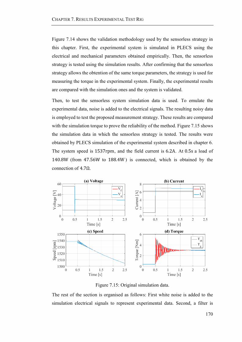
CHAPTER 7. RESULTS EXPERIMENTAL TEST RIG
170
Figure 7.14 shows the validation methodology used by the sensorless strategy in
this chapter. First, the experimental system is simulated in PLECS using the
electrical and mechanical parameters obtained empirically. Then, the sensorless
strategy is tested using the simulation results. After confirming that the sensorless
strategy allows the obtention of the same torque parameters, the strategy is used for
measuring the torque in the experimental system. Finally, the experimental results
are compared with the simulation ones and the system is validated.
Then, to test the sensorless system simulation data is used. To emulate the
experimental data, noise is added to the electrical signals. The resulting noisy data
is employed to test the proposed measurement strategy. These results are compared
with the simulation torque to prove the reliability of the method. Figure 7.15 shows
the simulation data in which the sensorless strategy is tested. The results were
obtained by PLECS simulation of the experimental system described in chapter 6.
The system speed is 1537rpm, and the field current is 6.2A. At 0.5s a load of
140.8W (from 47.56W to 188.4W ) is connected, which is obtained by the
connection of 4.7Ω.
Figure 7.15: Original simulation data.
The rest of the section is organised as follows: First white noise is added to the
simulation electrical signals to represent experimental data. Second, a filter is

CHAPTER 7. RESULTS EXPERIMENTAL TEST RIG
171
presented to eliminate the noise of the signals. Third, the speed of the system is
calculated. Finally, the torque is obtained.
7.3.2.1 Noisy Data
It has been shown that a problem of the experimental data is the amount of noise,
making it difficult to get torque measurements. Thus, to emulate the real results,
white noise3 is added to the armature voltage and current obtained by simulation.
Since the field current is constant, noise is not needed to be added. Figure 7.16
shows a comparison of the signals before (in red) and after the noise has been added
(in blue).
Figure 7.16: Noisy simulation signals.
7.3.2.2 Filtering of the Data
Like it was done with the resolver and tachometer data, to identify the vibrations
associated with the torsional vibrations, the FFT of the armature current is obtained
and shown in Figure 7.17. The magnitude is normalised by the steady-state value
of the signal, and the natural frequencies at 36.73Hz and 83.67Hz are found.
3 Matlab command: awgn(signal,40,’measured’)
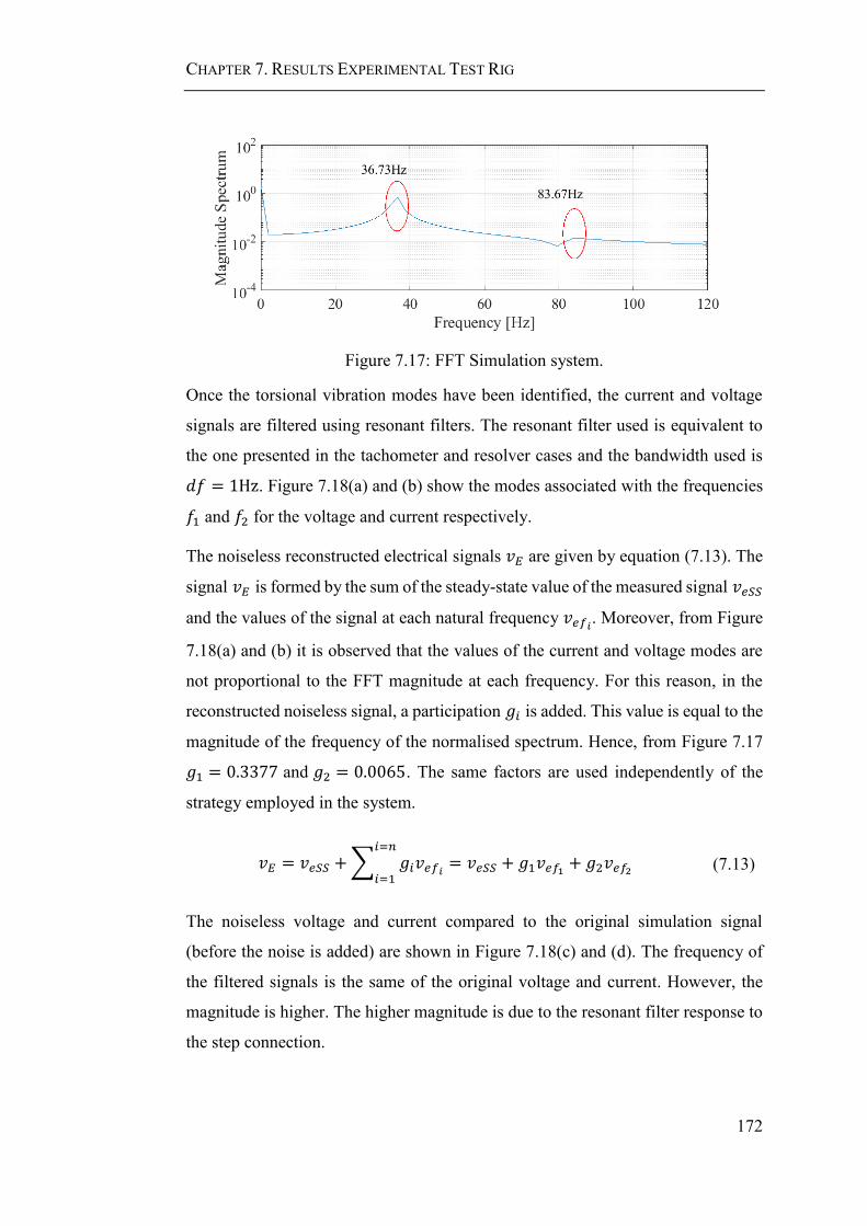
CHAPTER 7. RESULTS EXPERIMENTAL TEST RIG
172
Figure 7.17: FFT Simulation system.
Once the torsional vibration modes have been identified, the current and voltage
signals are filtered using resonant filters. The resonant filter used is equivalent to
the one presented in the tachometer and resolver cases and the bandwidth used is
𝑑𝑓 = 1Hz. Figure 7.18(a) and (b) show the modes associated with the frequencies
𝑓1 and 𝑓2 for the voltage and current respectively.
The noiseless reconstructed electrical signals 𝑣𝐸 are given by equation (7.13). The
signal 𝑣𝐸 is formed by the sum of the steady-state value of the measured signal 𝑣𝑒𝑆𝑆
and the values of the signal at each natural frequency 𝑣𝑒𝑓𝑖. Moreover, from Figure
7.18(a) and (b) it is observed that the values of the current and voltage modes are
not proportional to the FFT magnitude at each frequency. For this reason, in the
reconstructed noiseless signal, a participation 𝑔𝑖 is added. This value is equal to the
magnitude of the frequency of the normalised spectrum. Hence, from Figure 7.17
𝑔1 = 0.3377 and 𝑔2 = 0.0065. The same factors are used independently of the
strategy employed in the system.
𝑣𝐸 = 𝑣𝑒𝑆𝑆 +∑ 𝑔𝑖𝑣𝑒𝑓𝑖
𝑖=𝑛
𝑖=1= 𝑣𝑒𝑆𝑆 + 𝑔1𝑣𝑒𝑓1 + 𝑔2𝑣𝑒𝑓2 (7.13)
The noiseless voltage and current compared to the original simulation signal
(before the noise is added) are shown in Figure 7.18(c) and (d). The frequency of
the filtered signals is the same of the original voltage and current. However, the
magnitude is higher. The higher magnitude is due to the resonant filter response to
the step connection.
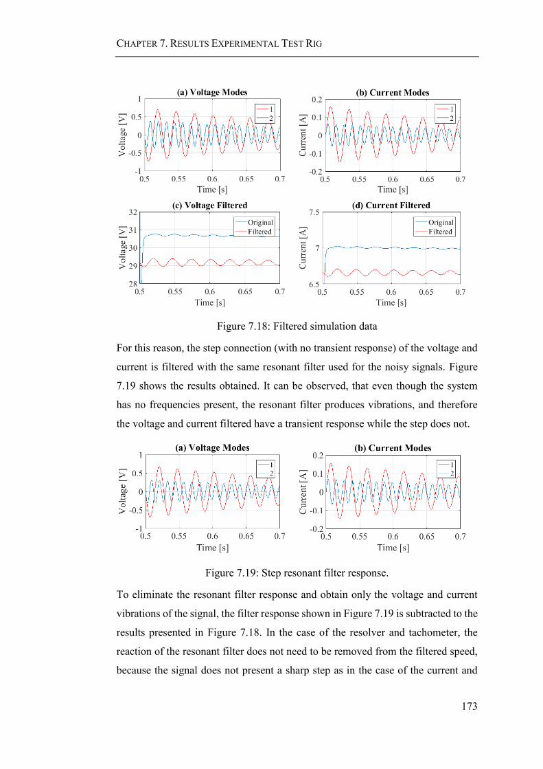
CHAPTER 7. RESULTS EXPERIMENTAL TEST RIG
173
Figure 7.18: Filtered simulation data
For this reason, the step connection (with no transient response) of the voltage and
current is filtered with the same resonant filter used for the noisy signals. Figure
7.19 shows the results obtained. It can be observed, that even though the system
has no frequencies present, the resonant filter produces vibrations, and therefore
the voltage and current filtered have a transient response while the step does not.
Figure 7.19: Step resonant filter response.
To eliminate the resonant filter response and obtain only the voltage and current
vibrations of the signal, the filter response shown in Figure 7.19 is subtracted to the
results presented in Figure 7.18. In the case of the resolver and tachometer, the
reaction of the resonant filter does not need to be removed from the filtered speed,
because the signal does not present a sharp step as in the case of the current and

CHAPTER 7. RESULTS EXPERIMENTAL TEST RIG
174
voltage. The resulting modes and results are shown in Figure 7.20. It is observed
that after removing the filter response, the values of voltage and current obtained
after the noise signal has been filtered are equal to the ones obtained initially by
simulation. The difference in the voltage and current mean value are due to
neglecting the motor drive dynamics. This approximation is applied since in this
study only the vibrations are relevant.
Figure 7.20: Final simulation filtered data.
7.3.2.3 Speed Determination
To get the torque, the speed must be found. For a single phase DC machine, its
value in rad/s can be obtained using equation (7.14), which is based on the back-
EMF method. The values of 𝑘 and 𝑖𝑓 are constant and the induced voltage (or back-
EMF) 𝐸, depends on the filtered armature voltage and current as given by equation
(7.15). The effect of the inductance has been simplified. The values of 𝑅𝑎, 𝑉0, and
𝑘 have been determined experimentally for the DC machine as presented in
Appendix I. In the case of working with a synchronous generator, as in most
aircraft, the steps are equivalent. The speed is proportional to the machine
frequency, and the electrical torque can be obtained as a function of the electrical
power and the speed.

CHAPTER 7. RESULTS EXPERIMENTAL TEST RIG
175
𝜔𝑔 =𝐸
𝑘𝑖𝑓 (7.14)
𝐸 = 𝑅𝑎𝑖𝑎 + 𝑣𝑎 + 𝑉0 (7.15)
Figure 7.21 shows the speed obtained in the simulation (in blue) and sensorless (in
red). It is observed that the frequency and amplitude of the vibrations are the same.
However, like for the voltage and current, the average value of the estimated signal
is lower than the original one. As already explained, this is due to the simplification
of the motor dynamics.
Figure 7.21: Speed of the system by simulation.
7.3.2.4 Torque Determination
After finding the speed, the torque can be obtained following the same equations
(7.3)-(7.5) used for the resolver and tachometer sensors. Figure 7.22 shows the
torque obtained from the simulation software PLECS (in blue), and the torque
obtained with the described sensorless procedure (in red). The results reached are
the same for the transient response, and therefore the estimated torque is not
affected by the simplification of the motor dynamics.
Figure 7.22: Sensorless simulation torque measurement.
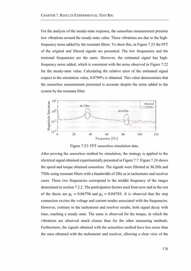
CHAPTER 7. RESULTS EXPERIMENTAL TEST RIG
176
For the analysis of the steady-state response, the sensorless measurement presents
low vibrations around the steady-state value. These vibrations are due to the high-
frequency noise added by the resonant filters. To show this, in Figure 7.23 the FFT
of the original and filtered signals are presented. The low frequencies and the
torsional frequencies are the same. However, the estimated signal has high-
frequency noise added, which is consistent with the noise observed in Figure 7.22
for the steady-state value. Calculating the relative error of the estimated signal
respect to the simulation value, 0.0799% is obtained. This value demonstrates that
the sensorless measurement presented is accurate despite the noise added to the
system by the resonant filter.
Figure 7.23: FFT sensorless simulation data.
After proving the sensorless method by simulation, the strategy is applied to the
electrical signal obtained experimentally presented in Figure 7.7. Figure 7.24 shows
the speed and torque obtained sensorless. The signals were filtrated at 36.5Hz and
75Hz using resonant filters with a bandwidth of 2Hz as in tachometer and resolver
cases. These two frequencies correspond to the middle frequency of the ranges
determined in section 7.2.2. The participation factors used from now and in the rest
of the thesis are 𝑔1 = 0.06796 and 𝑔2 = 0.04703. It is observed that the step
connection excites the voltage and current modes associated with the frequencies.
However, contrary to the tachometer and resolver results, both signal decay with
time, reaching a steady state. The same is observed for the torque, in which the
vibrations are observed much clearer than for the other measuring methods.
Furthermore, the signals obtained with the sensorless method have less noise than
the ones obtained with the tachometer and resolver, allowing a clear view of the

CHAPTER 7. RESULTS EXPERIMENTAL TEST RIG
177
torque step produced by the load connection. Moreover, the results are close to the
ones obtained through simulation and shown in Figure 7.22 in which the same
system was modelled. This indicates that the simulation is accurate and that the
results obtained experimentally are reliable.
Figure 7.24: Sensorless speed and torque.
In next sections, the electromechanical interaction due to load step connection and
the application of the PMS strategies is shown. The resolver, tachometer and
sensorless method are used and compared.
7.4 Electromechanical Interaction
In sections 7.2 and 7.3 the electromechanical interaction due to electrical load
connections has been indirectly shown. In this section, the results obtained are
analysed. The electrical signals of the step connection (current and voltage) and the
calculated power and resistance are shown in section 7.3 in Figure 7.7. The system
operates with a field current of 6.2A and at a speed of 1550rpm approximately.
After the load is connected, the speed decreases to under 1500rpm. The load
initially attached to the system is 50.82W, given by the protection resistance of

CHAPTER 7. RESULTS EXPERIMENTAL TEST RIG
178
60Ω. The final load in the system is 210W. The same parameters are used to test
the PMS strategies in section 7.5.
The filtered speed and torque were shown in the sensor analysis, and it is
summarised in Figure 7.25. The torsional vibrations due to the load connection can
be observed. This shows the electromechanical interaction due to the connection of
electrical loads. Moreover, as mentioned in the last section, the result obtained by
the resolver and tachometer sensor strategies have a higher presence of noise than
the sensorless method. This noise produces problems in the visualization of the
results when the PMS strategies are applied, as shown in the next section.
The steady state torque obtained is 2.92Nm. The peak torque obtained by the
resolver, tachometer and sensorless method are 3.5Nm , 5.4Nm , and 5.3Nm
respectively. The results obtained with the Posicast compensators are compared
with these values in next section.
Figure 7.25: Speed and torque for step connection.

CHAPTER 7. RESULTS EXPERIMENTAL TEST RIG
179
The FFT analysis of the armature current uses 10 seconds of data after the load is
connected. Figure 7.26 shows the results obtained. The presence of the peak at 𝑓1
and 𝑓2 shows the excitation of the vibrations. Thus, the torque results can be
confirmed.
Figure 7.26: FFT for step connection.
In the next section, the results obtained by the Posicast based strategies are
presented. In each case, the torque found by the tachometer, resolver, and sensorless
method are analysed.
7.5 Power Management System Operation
Until now, the electromechanical interaction due to electrical step connection has
been tested experimentally. In this section, the PMS strategies, based on the
Posicast compensator are verified.
The strategies for time non-critical loads (MLL and SLME) and time-critical loads
(MSLME) described in chapter 5 are solved for the two frequency system found in
section 7.2:
𝑓1 = 35.5Hz and 𝜉1 = 0.018
𝑓2 = 77.1Hz and 𝜉2 = 0.012
The vibrations of the system are measured using the methods presented in section
7.3. For the sensorless measuring method, the participation factors are the same
used in the step connection: 𝑔1 = 0.06796, and 𝑔2 = 0.04703.

CHAPTER 7. RESULTS EXPERIMENTAL TEST RIG
180
The loads switching is executed by the three IGBT connected in parallel as shown
in Figure 6.12 in chapter 6. Moreover, in the three cases, the initial and final
operation parameters are the same used for the step connection. The generator field
current is 6.2A, and the speed is 1550rpm. The protection resistance is 60Ω, and
the initial power and torque are 50.82W and 0.41Nm respectively. The final load
connected is approximately 210.52W and 2.93Nm.
7.5.1 Single Level Multi-edge Switching Load
The first strategy to be tested is the Single Level Multi-edge Switching Load or
SLME. For a two natural frequency system (𝑛 = 2), the SLME method consists of
five pulses (𝑚 = 2𝑛 + 1 = 5). Solving the equation system (5.33) in Matlab with
Opti Toolbox [122], the following switching times are obtained:
𝑇1 = 0s
𝑇2 = 2.5ms
𝑇3 = 6.7ms
𝑇4 = 11.1ms
𝑇5 = 13.4ms
[ ∑(−1)𝑘+1𝑒−𝜉1𝜔𝑛1𝑇𝑘 cos(𝜔𝑑1𝑇𝑘)
5
𝑘=1
∑(−1)𝑘+1𝑒−𝜉1𝜔𝑛1𝑇𝑘 sin(𝜔𝑑1𝑇𝑘)
5
𝑘=1
∑(−1)𝑘+1𝑒−𝜉2𝜔𝑛2𝑇𝑘 cos(𝜔𝑑2𝑇𝑘)
5
𝑘=1
∑(−1)𝑘+1𝑒−𝜉2𝜔𝑛2𝑇𝑘 sin(𝜔𝑑2𝑇𝑘)
5
𝑘=1 ]
= 0 (7.16)
Figure 7.27 shows the switching signals sent by the microcontroller to IGBT 1. The
resistance being connected and disconnected by the IGBT is 4.95Ω.

CHAPTER 7. RESULTS EXPERIMENTAL TEST RIG
181
Figure 7.27: Switching SLME.
Figure 7.28 shows the measured current and voltage of the system, along with the
power obtained. From (c) is observed that the final power is close to 210.51W,
which makes the results comparable with ones obtained for the step connection.
Moreover, from the zoom presented in each subplot, the switching of the load is
appreciated. Observing the current in Figure 7.28(a), it is appreciated that the step
has an exponential component which stops the whole load from being applied at
once in each connection. This delay is due to the inductance of the system, which
is mostly given by the DC machine.
Figure 7.28: Electrical data for SLME connection.

CHAPTER 7. RESULTS EXPERIMENTAL TEST RIG
182
Figure 7.29(b) shows the speed obtained from the resolver and tachometer before
the application of the resonant filter. Comparing with the results obtained by a step
connection, presented in Figure 7.29(a), the system is operating at the same speed.
Figure 7.29: Resolver and tachometer speed for SLME connection.
The filtered speed and torque obtained through the sensors and sensorless method
are shown in Figure 7.30. In (d), (e), and (f) the torque obtained through the
resolver, tachometer and sensorless method is shown. In red the electrical torque
connection, in blue the resulting shaft torque, and in yellow the shaft torque in the
step case are shown. The steady state value of the SLME connection torque is the
same of the step connection: 2.93Nm. Comparing the transient response with the
step connection results, the measurements given by the tachometer and sensorless
method show considerably lower peak torque vibrations. In both cases, for the step
connection, the peak vibration was 5.5Nm and 5.3Nm respectively. With the
SLME connection, the peaks are 3.9Nm and 3.8Nm respectively. This shows that
the SLME strategy reduces the vibrations comparing with the step connection.
However, the vibrations are not completely eliminated after the load switching as
was presented by simulation. This difference is because the steps applied to the
mechanical system are not perfect square step, but exponential. Moreover, the

CHAPTER 7. RESULTS EXPERIMENTAL TEST RIG
183
frequencies for which the strategy was solved is not precise since in section 7.2.2 a
range for each torsional frequency was identified instead of a single value. Since
the strategy was solved for a specific value, a level of uncertainty is present in the
response. This situation and the robustness of the strategies is analysed in chapter
8.
On the other hand, since the resolver results are similar to the step connection, and
the tachometer has high vibrations after the steady state has been reached, the
sensors are not reliable for the transient analysis of the system. For further analysis
of the resolver and tachometer performances, the results obtained through the MLL
and MSLME are analysed in the next section.
Figure 7.30: Speed and torque for the SLME connection.
The FFT of the step and SLME connection, calculated for 10s of armature current
data after the load connection are shown in Figure 7.31(a) and (b) respectively.
Comparing the SLME results with the results obtained for the step connection, it is

CHAPTER 7. RESULTS EXPERIMENTAL TEST RIG
184
observed that the vibrations are slightly reduced. This confirms the torque
performance.
Figure 7.31: FFT SLME connection.
7.5.2 Multilevel Loading Switching
Now, the Multilevel Loading Switching (MLL) is tested. For a two natural
frequency system (𝑛 = 2), the MLL method is formed by three steps (𝑚 = 𝑛 +
1 = 3). Thus, the three IGBT connected on the system are used. Each IGBT is
connected to a load, which value and connection time is given by equation system
(7.17). Solving in Matlab with Opti Toolbox [122], the following switching times
and step values are obtained:
𝑇1 = 0s and 𝑝1 = 0.37
𝑇2 = 8.9ms and 𝑝2 = 0.29
𝑇3 = 17.7ms and 𝑝3 = 0.33

CHAPTER 7. RESULTS EXPERIMENTAL TEST RIG
185
[ ∑𝑝𝑘𝑒
−𝜉1𝜔𝑛1𝑇𝑘 cos(𝜔𝑑1𝑇𝑘)
3
𝑘=1
∑𝑝𝑘𝑒−𝜉1𝜔𝑛1𝑇𝑘 sin(𝜔𝑑1𝑇𝑘)
3
𝑘=1
∑𝑝𝑘𝑒−𝜉2𝜔𝑛2𝑇𝑘 cos(𝜔𝑑2𝑇𝑘)
3
𝑘=1
∑𝑝𝑘𝑒−𝜉2𝜔𝑛2𝑇𝑘 sin(𝜔𝑑2𝑇𝑘)
3
𝑘=1 ]
= 0 (7.17)
Figure 7.32 shows the switching signals sent by the microcontroller to IGBT 1,
IGBT 2 and IGBT 3. Each IGBT is turned on, at the times obtained. The resistances
connected to each of them that allow having the torque step sizes required are
𝑅𝐿1 = 30.53Ω, 𝑅𝐿2 = 18.29Ω, and 𝑅𝐿3 = 10.23Ω.
Figure 7.32: Switching MLL.
The electrical signals obtained are shown in Figure 7.33. From (c), it can be seen
that the final load connected to the system is close to 210W. Therefore the data can
be compared to the step connection. Moreover, the current signal in (a) shows the
effect of the machine inductances, which produces exponential load connections
instead of step load connections. However, contrary to the SLME connection, in
this case, the loads are completely connected before the next IGBT is switched on,
making the connection closer to the theory.
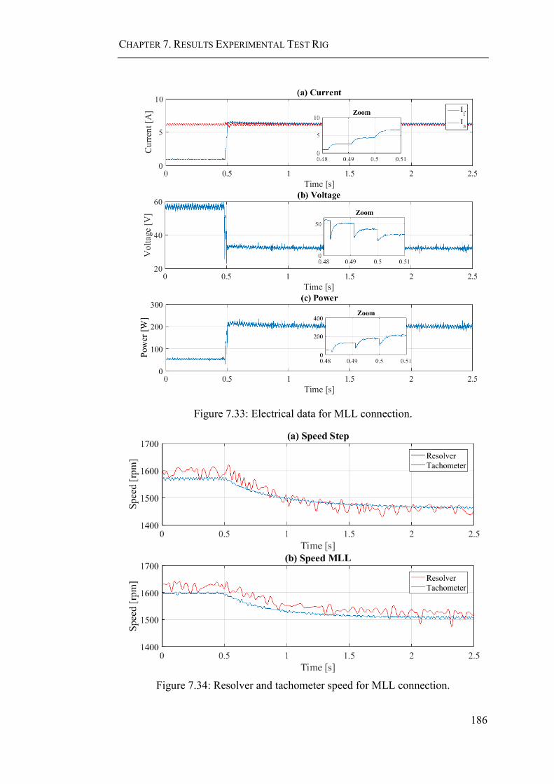
CHAPTER 7. RESULTS EXPERIMENTAL TEST RIG
186
Figure 7.33: Electrical data for MLL connection.
Figure 7.34: Resolver and tachometer speed for MLL connection.
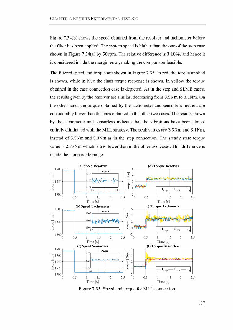
CHAPTER 7. RESULTS EXPERIMENTAL TEST RIG
187
Figure 7.34(b) shows the speed obtained from the resolver and tachometer before
the filter has been applied. The system speed is higher than the one of the step case
shown in Figure 7.34(a) by 50rpm. The relative difference is 3.18%, and hence it
is considered inside the margin error, making the comparison feasible.
The filtered speed and torque are shown in Figure 7.35. In red, the torque applied
is shown, while in blue the shaft torque response is shown. In yellow the torque
obtained in the case connection case is depicted. As in the step and SLME cases,
the results given by the resolver are similar, decreasing from 3.5Nm to 3.1Nm. On
the other hand, the torque obtained by the tachometer and sensorless method are
considerably lower than the ones obtained in the other two cases. The results shown
by the tachometer and sensorless indicate that the vibrations have been almost
entirely eliminated with the MLL strategy. The peak values are 3.3Nm and 3.1Nm,
instead of 5.5Nm and 5.3Nm as in the step connection. The steady state torque
value is 2.77Nm which is 5% lower than in the other two cases. This difference is
inside the comparable range.
Figure 7.35: Speed and torque for MLL connection.

CHAPTER 7. RESULTS EXPERIMENTAL TEST RIG
188
The same behaviour is confirmed by the FFT analysis of Figure 7.36. In (a) the
frequencies excited by the step connection are shown, while in (b) it can be seen
that for the MLL connection, the frequencies associated with the torsional modes
are not excited. Therefore, the MLL method tested allows almost the complete
elimination of the vibrations after the switching event, although the load applied is
exponential and the frequency used has a level of uncertainty. This result implies
that the main reason for the remaining vibrations in the SLME connection are the
inductances.
Figure 7.36: FFT for MLL connection.
Moreover, the low change in the resolver measurements, and the remaining noise
in the tachometer support that these sensors are reliable for the torque measurement
in this experimental setup.
7.5.3 Multi-load Single Level Multi-edge Switching Loads
Finally, for the case of working with Time Critical loads, the strategy Multi-load
Single Level Multi-edge Switching Load (MSLME) was presented in chapter 5. It
consisted in connecting the time-critical load as a step connection, and apply a
pulsating pattern to a time non-critical load. In chapter 5, the time non-critical load

CHAPTER 7. RESULTS EXPERIMENTAL TEST RIG
189
was disconnected and connected following the desired pattern. In this case, to work
with the same final load of the other three connection strategies, the auxiliary load
is a secondary load being connected as shown in red in Figure 7.37. The equations
to solve are the same of the disconnection case since the overall effect in the
drivetrain is equal. Then, for a two natural frequency system (𝑛 = 2), the MSLME
method is formed by four load connections (𝑚 = 2𝑛 = 4). Solving the equation
system (7.18) in Matlab with Opti Toolbox [122], the following switching times
are obtained:
𝑇1 = 0s
𝑇2 = 10.7ms
𝑇3 = 13.2ms
𝑇4 = 16.3ms
The auxiliary load value is 60% of the time-critical load connected.
[ 1 +∑(−1)𝑘𝑝𝑒−𝜉1𝜔𝑛1𝑇𝑘 cos(𝜔𝑑1𝑇𝑘)
4
𝑘=1
∑(−1)𝑘𝑝𝑒−𝜉1𝜔𝑛1𝑇𝑘 sin(𝜔𝑑1𝑇𝑘)
4
𝑘=1
1 +∑(−1)𝑘𝑝𝑒−𝜉2𝜔𝑛2𝑇𝑘 cos(𝜔𝑑2𝑇𝑘)
4
𝑘−1
∑(−1)𝑘𝑝𝑒−𝜉2𝜔𝑛2𝑇𝑘 sin(𝜔𝑑2𝑇𝑘)
4
𝑘=1 ]
= 0 (7.18)
Figure 7.37 shows the switching signals sent by the microcontroller to IGBT 1 and
IGBT 2. The critical load, connected to IGBT 1, and which value is 13.34Ω is
connected as a step. The auxiliary load, coupled to IGBT 2 is connected as a pulse
at time 𝑇2. Its value is 9.07Ω.

CHAPTER 7. RESULTS EXPERIMENTAL TEST RIG
190
Figure 7.37: Switching MSLME.
Figure 7.38 shows the electrical data obtained. In (c), the final electrical load
connected to the system is 207W, which is close to the values presented in the other
three cases. From the current in (a) is observed that due to the closeness between
steps, the inductance has a high effect on the connections. Therefore, as in the
SLME case, some transient vibrations are obtained.
Figure 7.38: Electrical data for MSLME connection.

CHAPTER 7. RESULTS EXPERIMENTAL TEST RIG
191
From Figure 7.39(b) it is observed that as in the MLL case, the speed of the system
is 50rpm higher than in the step case shown in Figure 7.39(a). Since the values are
close, the results obtained are comparable.
Figure 7.39: Resolver and tachometer speed for MSLME connection.
The filtered speed and torque obtained through the different methods are shown in
Figure 7.40. In red, the torque applied is shown, while in blue the shaft torque
response is shown. In yellow the torque obtained in the case connection case is
depicted. The steady state torque is 2.723Nm which is close to the one in the step
connection, and thus comparable with the ones of the other cases. The vibrations
obtained by the sensorless method are lower than in the SLME and step cases, but
higher than the MLL. This was expectable since the steps are affected by the system
inductance less than in the SLME connection but more than in the MLL. This shows
the correlation between the time between steps and the inductance in the system.
Further analysis is presented in chapter 8.

CHAPTER 7. RESULTS EXPERIMENTAL TEST RIG
192
Figure 7.40: Speed and torque for MSLME connection.
The FFT of the system analysed is shown in Figure 7.41. In (a) the results obtained
for the step connection are shown, while in (b) the results obtained using the
MSLME strategy are presented. Using the MSLME strategy, the excitation of 𝑓1
has almost entirely been cancelled, while 𝑓2 is not. This can be explained by the
connection curve. The steps associated with higher frequencies are closer. From
Figure 7.38(a), the closer the steps, the higher the effect of the inductance in the
system. Therefore, the inductances in the system are mostly affecting the
cancellation of the second frequency.

CHAPTER 7. RESULTS EXPERIMENTAL TEST RIG
193
Figure 7.41: FFT for MSLME connection.
Moreover, the results obtained by the tachometer and resolver show, again, that the
sensorless method is less affected by the noise. The resolver shows slightly lower
vibrations than the ones obtained in the step connection, and higher than the MLL
case. However, the delay in the start of the vibrations could be due to the filter used,
or because the vibrations have noise. Similarly, the results obtained by the
tachometer show lower vibrations than the ones achieved by the MLL strategy.
These vibration increase after. Both situations are contrary to what is expected by
theory and obtained with the sensorless method. Therefore, the results obtained by
the tachometer and resolver, are highly affected by the noise and not reliable. On
the other hand, the sensorless method has shown results close to the theory and the
Fourier analysis of the armature current. For this reason, from now, only the results
obtained by the sensorless method are studied.
7.5.4 Summary
The results obtained in each case, Step, MLL, SLME, and MSLME connections
with the sensorless torque measuring are shown in Figure 7.42. In red the load
applied is shown, while in blue and yellow the shaft torque vibrations obtained
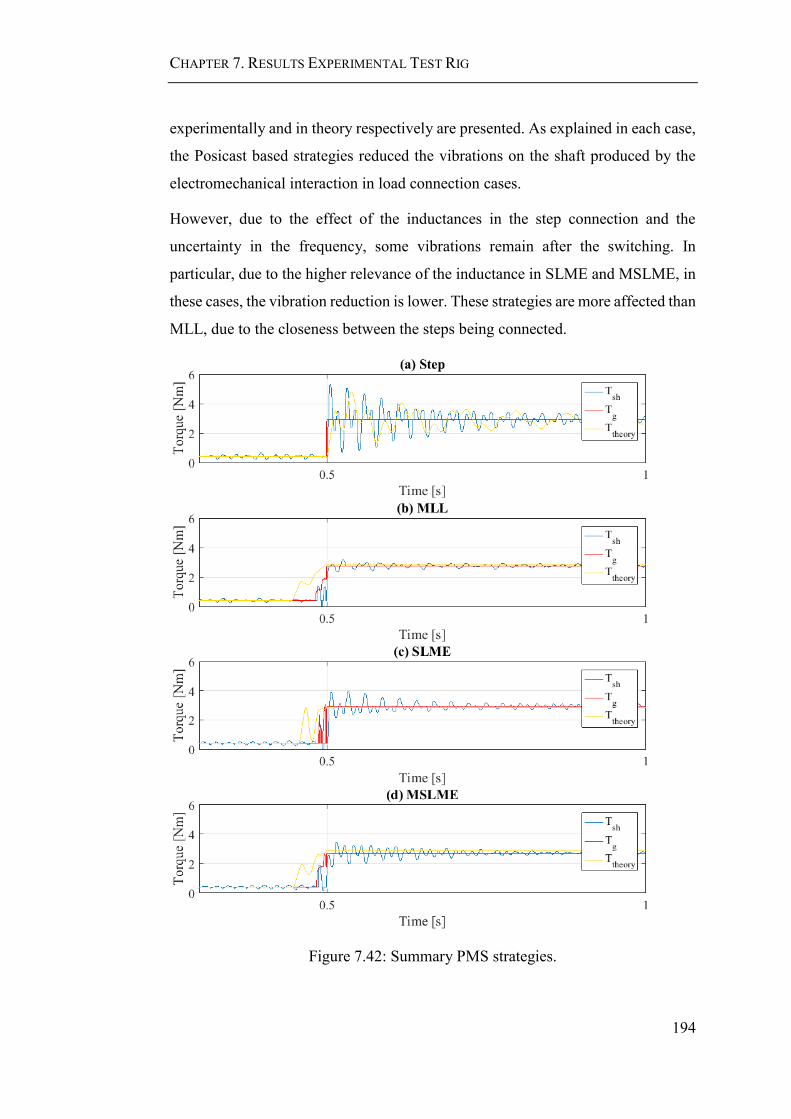
CHAPTER 7. RESULTS EXPERIMENTAL TEST RIG
194
experimentally and in theory respectively are presented. As explained in each case,
the Posicast based strategies reduced the vibrations on the shaft produced by the
electromechanical interaction in load connection cases.
However, due to the effect of the inductances in the step connection and the
uncertainty in the frequency, some vibrations remain after the switching. In
particular, due to the higher relevance of the inductance in SLME and MSLME, in
these cases, the vibration reduction is lower. These strategies are more affected than
MLL, due to the closeness between the steps being connected.
Figure 7.42: Summary PMS strategies.

CHAPTER 7. RESULTS EXPERIMENTAL TEST RIG
195
Analysing the strategies in terms of the overshoot and the settling time of the
transient, the same behaviour is observed. Table 7.1 shows the results. The settling
time was calculated for a torque value of 5% of the steady-state value, while the
overshoot was obtained with equation (4.40) presented in chapter 4. The overshoot
and settling time of every strategy is lower than the one in the step connection case.
Even in the SLME and MSLME cases, which are highly affected by the inductance,
the performance has improved in 50% . These results show that the Posicast
strategies allow the reduction of the torsional vibrations produced by the connection
of electrical loads. Chapter 8, presents the robust analysis of the strategy.
Table 7.1. PMS strategies performance.
Connection Overshoot [%] Settling Time [s]
Step 80.85 0.64
SLME 33.90 0.44
MLL 13.63 0.39
MSLME 26.22 0.49
7.6 Summary
In this chapter, the electromechanical interaction due to electrical loads connection
presented in chapter 4 has been experimentally tested. The case of a pulsating load
has not been studied because as shown in chapter 4 and 5, its behaviour is equal to
a step load.
The analysis of the experimental system has identified a range of frequencies close
to the design ones presented in chapter 6. To find these parameters the method of
Fourier analysis combined with Hilbert Transform and EMD has been used. This
has allowed the verification of the designed system.
Moreover, three torque measuring methods have been compared: tachometer
sensor, resolver sensor, and sensorless. The results obtained in each strategy applied
have shown that the sensor-based methods are highly affected by the system noise
for low power systems. The same does not happen for the sensorless strategy. A
methodology to validate the experimental results using the back-EMF and resonant

CHAPTER 7. RESULTS EXPERIMENTAL TEST RIG
196
filter sensorless method has been presented. This method has shown results that are
validated by the FFT analysis and the simulation results.
Likewise, the PMS based on the Posicast method presented in chapter 5 has been
experimentally tested. The results have shown that the strategies allow the
reduction of the torsional vibrations due to electrical load connections. However,
due to the machine inductances and the uncertainty in the torsional frequencies
values the vibrations are not completely eliminated after the load switching.
Respect the first aspect; the load connections applied are not perfect steps, which
reduces the efficacy of the strategies. The inductances affect mostly the SLME and
MSLME due to the closeness of their pulses.
Regarding the frequency uncertainty, a range of the torsional values has been
identified. Therefore, the Posicast based strategies have not been solved for the
exact value. FFT post analysis shows that at the moment of the test the frequencies
of the system were 35Hz and 73Hz instead of 35.5Hz and 77.1Hz. The changes in
frequency may be due to movements of the gears and flywheels. This difference is
responsible for the remaining vibrations.
Nonetheless, even in the connection strategies most affected by the uncertainty and
inductances, the overshoot has been reduced by more than 50%. Even more, for
the MLL connection, in which the effect of the inductance is lower, the overshoot
has been reduced to an eighth of the step connection. For this reason, despite the
uncertainties, the strategies are able to reduce of vibrations. Chapter 8 presents a
robust analysis to approach the uncertainty in the system parameters and the effect
of the inductance.

Chapter 8
8 Power Management System Robustness
Analysis
8.1 Introduction
In chapter 7 the power management system (PMS) was experimentally tested. It
was shown that the strategies presented in chapter 5 allow the reduction of the
torsional vibrations. However, due to the uncertainty in the natural frequencies
values and the presence of inductance in the system, the vibrations were not fully
suppressed after the electrical load switching. Additionally, the MLL strategy
proved to be more robust to uncertainty and the presence of inductances. To further
analyse the sensitivity of the three methods (SLME, MLL, and MSLME), in this
chapter the PMS robustness and the effect of the inductances are studied.
The rest of the chapter is organised as follow. First, the sensitivity of the system is
studied, and the effects of uncertainty in frequency and damping ratio for each
method are established. After, strategies to minimise the effect of the inductance in
the system are studied. Later, the strategies presented are compared with alternative
methods used in the literature. Finally, the summary is presented.
8.2 Sensitivity Analysis
Two approaches are taken to study the sensitivity of the system. First, experimental
results obtained for the strategies with different connection values are shown.
Second, a theoretical analysis of the strategies robustness for frequency and
damping ratio uncertainty is carried out. Finally, a summary is presented.

CHAPTER 8. POWER MANAGEMENT SYSTEM ROBUSTNESS ANALYSIS
198
8.2.1 Experimental Results
In this section, the experimental system was tested for SLME, MLL, and MSLME
connections solved for three different natural frequencies and damping ratio. Three
cases are compared: The first case or base case are the results presented in chapter
7 and is solved for the frequencies 𝑓1𝐵 = 35.5Hz and 𝑓2𝐵 = 77.1Hz and the
respective damping ratio 𝜉1𝐵 = 0.018 and 𝜉2𝐵 = 0.012. The second case is solved
for different natural frequencies and damping ratio than the ones used in chapter 7.
This case is solved for 𝑓1𝐶 = 36.4Hz and 𝑓2𝐶 = 77Hz and the respective damping
ratio 𝜉1𝐶 = 0.0219 and 𝜉2𝐶 = 0.0096. These frequencies are inside the frequency
range defined in chapter 7 ( 𝑓1 ∈ [35 − 37]Hz and 𝑓2 ∈ [73 − 77.1]Hz). Lastly,
the third case, consists in solving the strategies for one natural frequency instead of
two. The natural frequency and damping ratio used, corresponds to the lower
natural frequency of the base case 𝑓1𝐵 = 35.5Hz and 𝜉1𝐵 = 0.018, omitting the
value of 𝑓2𝐵 and 𝜉2𝐵. The results obtained by each strategy and case are compared
in terms of overshoot and settling time. The connection times and step values of
each case studied are shown in Table 8.1.
Table 8.1: Connection times.
Case SLME MLL MSLME
Time
[ms] Step Size Time
[ms] Step Size Time
[ms] Step Size
𝑓1𝐵
𝑓2𝐵
𝑇1 = 0
𝑇2 = 2.5
𝑇3 = 6.7
𝑇4 = 11.1
𝑇5 = 13.4
𝑝1 = 1
𝑝2 = −1
𝑝3 = 1
𝑝4 = −1
𝑝5 = 1
𝑇1 = 0
𝑇2 = 8.9
𝑇3 = 17.7
𝑝1 = 0.37
𝑝2 = 0.29
𝑝3 = 0.33
𝑇1 = 0
𝑇2 = 10.7
𝑇3 = 13.2
𝑇4 = 16.3
𝑝1 = 0.40
𝑝2 = 0.60
𝑝3 = −0.60
𝑝4 = 0.60
𝑓1𝐶
𝑓2𝐶
𝑇1 = 0
𝑇2 = 2.4
𝑇3 = 6.6
𝑇4 = 11.1
𝑇5 = 13.3
𝑝1 = 1
𝑝2 = −1
𝑝3 = 1
𝑝4 = −1
𝑝5 = 1
𝑇1 = 0
𝑇2 = 8.8
𝑇3 = 17.6
𝑝1 = 0.37
𝑝2 = 0.29
𝑝3 = 0.33
𝑇1 = 0
𝑇2 = 10.5
𝑇3 = 13.2
𝑇4 = 16.2
𝑝1 = 0.39
𝑝2 = 0.61
𝑝3 = −0.61
𝑝4 = 0.61
𝑓1𝐵 𝑇1 = 0
𝑇2 = 4.8
𝑇3 = 9.4
𝑝1 = 1
𝑝2 = −1
𝑝3 = 1
𝑇1 = 0
𝑇2 = 14.1
𝑝1 = 0.51
𝑝2 = 0.49
𝑇1 = 0
𝑇2 = 14.1
𝑝1 = 0.51
𝑝2 = 0.49
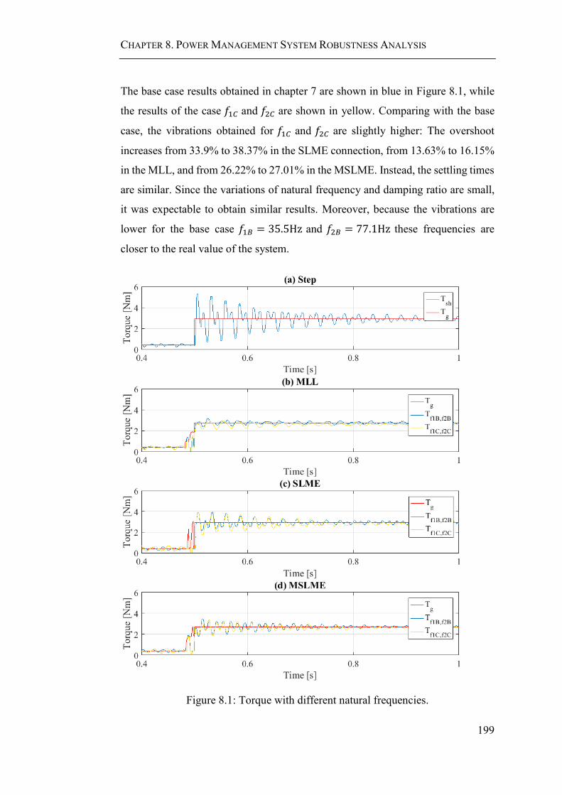
CHAPTER 8. POWER MANAGEMENT SYSTEM ROBUSTNESS ANALYSIS
199
The base case results obtained in chapter 7 are shown in blue in Figure 8.1, while
the results of the case 𝑓1𝐶 and 𝑓2𝐶 are shown in yellow. Comparing with the base
case, the vibrations obtained for 𝑓1𝐶 and 𝑓2𝐶 are slightly higher: The overshoot
increases from 33.9% to 38.37% in the SLME connection, from 13.63% to 16.15%
in the MLL, and from 26.22% to 27.01% in the MSLME. Instead, the settling times
are similar. Since the variations of natural frequency and damping ratio are small,
it was expectable to obtain similar results. Moreover, because the vibrations are
lower for the base case 𝑓1𝐵 = 35.5Hz and 𝑓2𝐵 = 77.1Hz these frequencies are
closer to the real value of the system.
Figure 8.1: Torque with different natural frequencies.
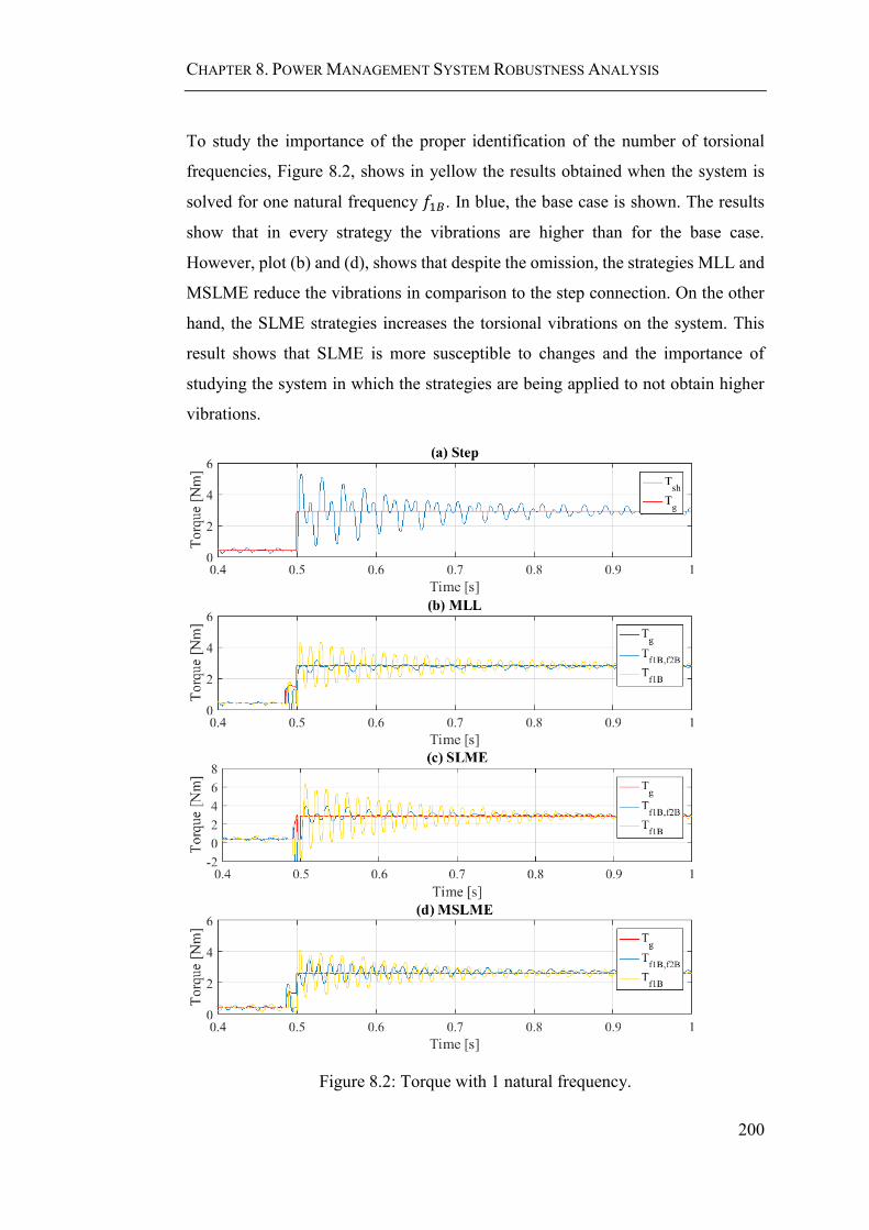
CHAPTER 8. POWER MANAGEMENT SYSTEM ROBUSTNESS ANALYSIS
200
To study the importance of the proper identification of the number of torsional
frequencies, Figure 8.2, shows in yellow the results obtained when the system is
solved for one natural frequency 𝑓1𝐵. In blue, the base case is shown. The results
show that in every strategy the vibrations are higher than for the base case.
However, plot (b) and (d), shows that despite the omission, the strategies MLL and
MSLME reduce the vibrations in comparison to the step connection. On the other
hand, the SLME strategies increases the torsional vibrations on the system. This
result shows that SLME is more susceptible to changes and the importance of
studying the system in which the strategies are being applied to not obtain higher
vibrations.
Figure 8.2: Torque with 1 natural frequency.
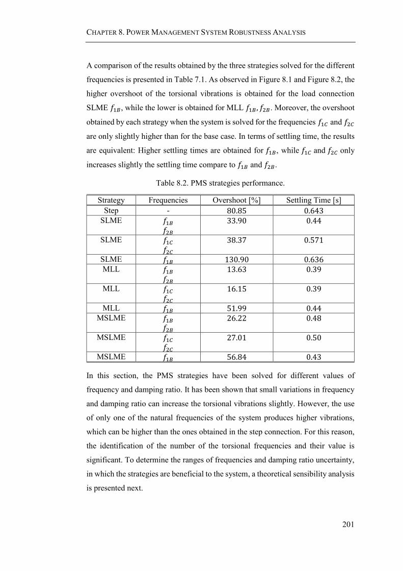
CHAPTER 8. POWER MANAGEMENT SYSTEM ROBUSTNESS ANALYSIS
201
A comparison of the results obtained by the three strategies solved for the different
frequencies is presented in Table 7.1. As observed in Figure 8.1 and Figure 8.2, the
higher overshoot of the torsional vibrations is obtained for the load connection
SLME 𝑓1𝐵, while the lower is obtained for MLL 𝑓1𝐵, 𝑓2𝐵. Moreover, the overshoot
obtained by each strategy when the system is solved for the frequencies 𝑓1𝐶 and 𝑓2𝐶
are only slightly higher than for the base case. In terms of settling time, the results
are equivalent: Higher settling times are obtained for 𝑓1𝐵, while 𝑓1𝐶 and 𝑓2𝐶 only
increases slightly the settling time compare to 𝑓1𝐵 and 𝑓2𝐵.
Table 8.2. PMS strategies performance.
Strategy Frequencies Overshoot [%] Settling Time [s]
Step - 80.85 0.643 SLME 𝑓1𝐵
𝑓2𝐵
33.90 0.44
SLME 𝑓1𝐶
𝑓2𝐶
38.37 0.571
SLME 𝑓1𝐵 130.90 0.636 MLL 𝑓1𝐵
𝑓2𝐵
13.63 0.39
MLL 𝑓1𝐶
𝑓2𝐶
16.15 0.39
MLL 𝑓1𝐵 51.99 0.44 MSLME 𝑓1𝐵
𝑓2𝐵
26.22 0.48
MSLME 𝑓1𝐶
𝑓2𝐶
27.01 0.50
MSLME 𝑓1𝐵 56.84 0.43
In this section, the PMS strategies have been solved for different values of
frequency and damping ratio. It has been shown that small variations in frequency
and damping ratio can increase the torsional vibrations slightly. However, the use
of only one of the natural frequencies of the system produces higher vibrations,
which can be higher than the ones obtained in the step connection. For this reason,
the identification of the number of the torsional frequencies and their value is
significant. To determine the ranges of frequencies and damping ratio uncertainty,
in which the strategies are beneficial to the system, a theoretical sensibility analysis
is presented next.
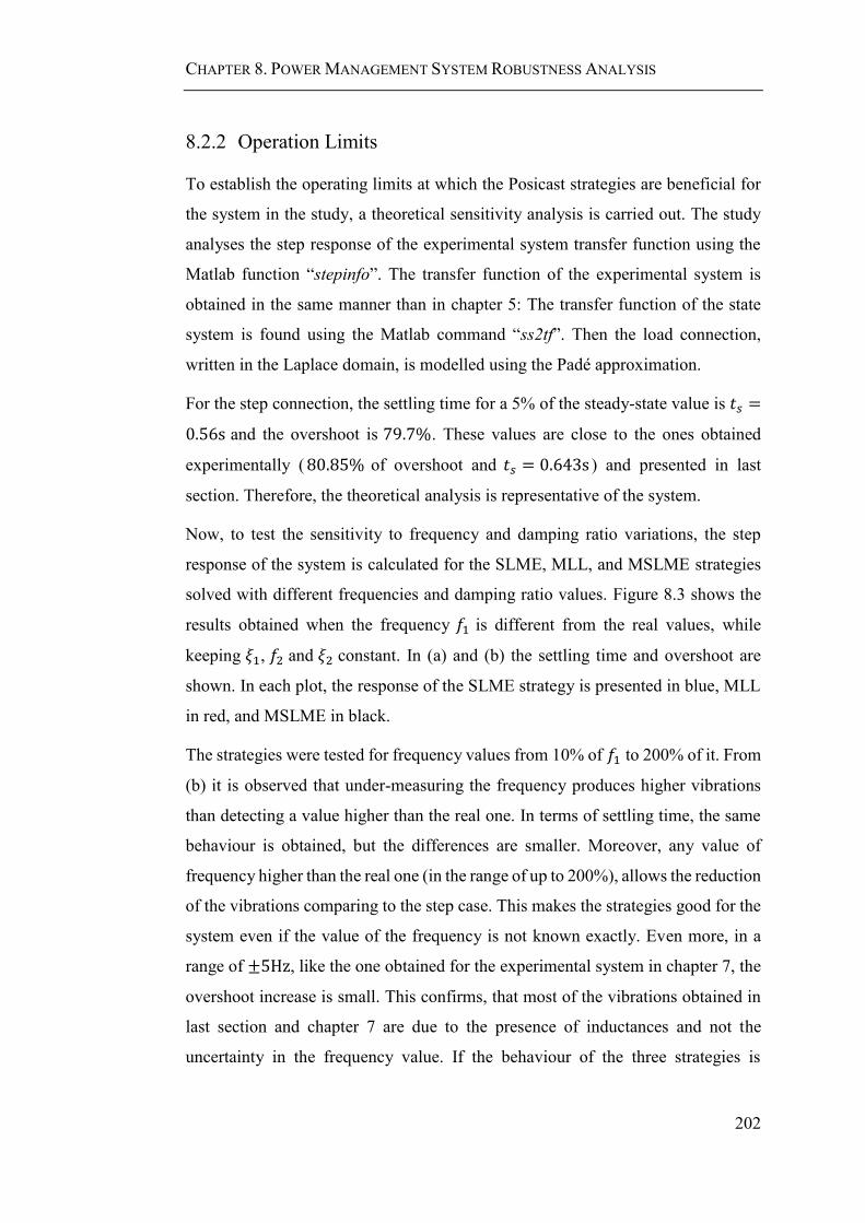
CHAPTER 8. POWER MANAGEMENT SYSTEM ROBUSTNESS ANALYSIS
202
8.2.2 Operation Limits
To establish the operating limits at which the Posicast strategies are beneficial for
the system in the study, a theoretical sensitivity analysis is carried out. The study
analyses the step response of the experimental system transfer function using the
Matlab function “stepinfo”. The transfer function of the experimental system is
obtained in the same manner than in chapter 5: The transfer function of the state
system is found using the Matlab command “ss2tf”. Then the load connection,
written in the Laplace domain, is modelled using the Padé approximation.
For the step connection, the settling time for a 5% of the steady-state value is 𝑡𝑠 =
0.56s and the overshoot is 79.7%. These values are close to the ones obtained
experimentally (80.85% of overshoot and 𝑡𝑠 = 0.643s ) and presented in last
section. Therefore, the theoretical analysis is representative of the system.
Now, to test the sensitivity to frequency and damping ratio variations, the step
response of the system is calculated for the SLME, MLL, and MSLME strategies
solved with different frequencies and damping ratio values. Figure 8.3 shows the
results obtained when the frequency 𝑓1 is different from the real values, while
keeping 𝜉1, 𝑓2 and 𝜉2 constant. In (a) and (b) the settling time and overshoot are
shown. In each plot, the response of the SLME strategy is presented in blue, MLL
in red, and MSLME in black.
The strategies were tested for frequency values from 10% of 𝑓1 to 200% of it. From
(b) it is observed that under-measuring the frequency produces higher vibrations
than detecting a value higher than the real one. In terms of settling time, the same
behaviour is obtained, but the differences are smaller. Moreover, any value of
frequency higher than the real one (in the range of up to 200%), allows the reduction
of the vibrations comparing to the step case. This makes the strategies good for the
system even if the value of the frequency is not known exactly. Even more, in a
range of ±5Hz, like the one obtained for the experimental system in chapter 7, the
overshoot increase is small. This confirms, that most of the vibrations obtained in
last section and chapter 7 are due to the presence of inductances and not the
uncertainty in the frequency value. If the behaviour of the three strategies is
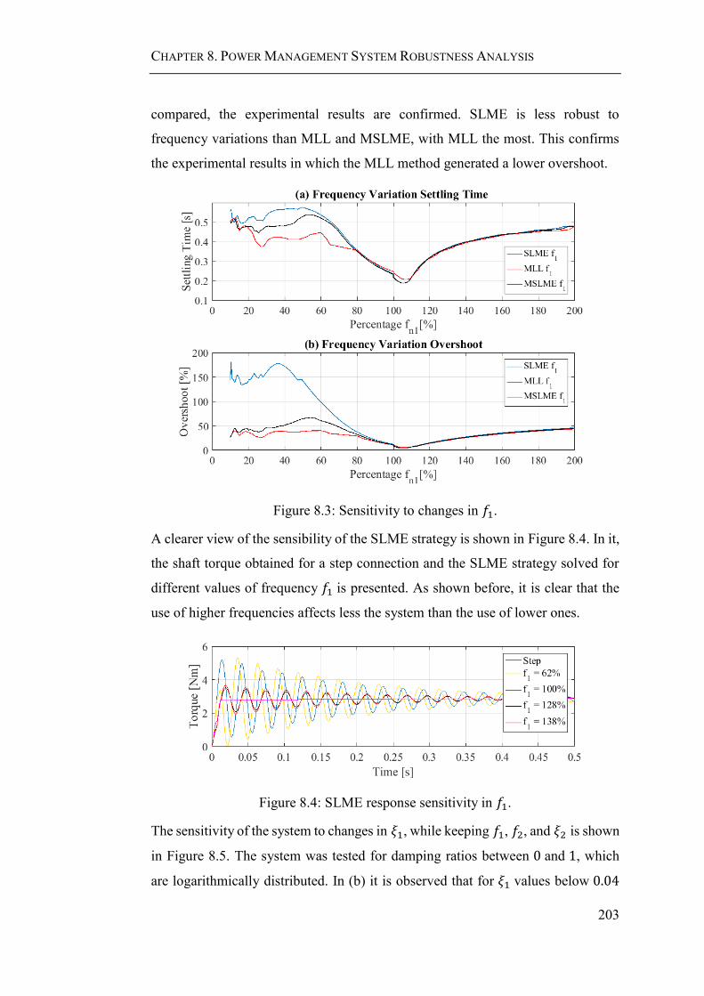
CHAPTER 8. POWER MANAGEMENT SYSTEM ROBUSTNESS ANALYSIS
203
compared, the experimental results are confirmed. SLME is less robust to
frequency variations than MLL and MSLME, with MLL the most. This confirms
the experimental results in which the MLL method generated a lower overshoot.
Figure 8.3: Sensitivity to changes in 𝑓1.
A clearer view of the sensibility of the SLME strategy is shown in Figure 8.4. In it,
the shaft torque obtained for a step connection and the SLME strategy solved for
different values of frequency 𝑓1 is presented. As shown before, it is clear that the
use of higher frequencies affects less the system than the use of lower ones.
Figure 8.4: SLME response sensitivity in 𝑓1.
The sensitivity of the system to changes in 𝜉1, while keeping 𝑓1, 𝑓2, and 𝜉2 is shown
in Figure 8.5. The system was tested for damping ratios between 0 and 1, which
are logarithmically distributed. In (b) it is observed that for 𝜉1 values below 0.04

CHAPTER 8. POWER MANAGEMENT SYSTEM ROBUSTNESS ANALYSIS
204
the overshoot is zero. For the same range, in (a) it is seen that the settling time
remains below 0.1s, though the time increases for damping ratio different than the
one associated with the system. Since the damping ratio of the system is inside this
range, it is consider that the damping ratio does not affect the Posicast strategies in
study. The same is shown in Figure 8.6, in which the effect of solving the SLME
strategy for different damping is shown. Damping below 0.05 produce no
difference, while damping below 0.1 produce only small vibrations.
Figure 8.5: Sensitivity to changes in 𝜉1.
Figure 8.6: SLME response sensitivity in 𝜉1.
Examining the robustness of the methods to variation in 𝑓2, while keeping 𝑓1, 𝜉1,
and 𝜉2 constant, Figure 8.7 is obtained. The results are equivalent in terms of
strategy robustness to the ones obtained for changes in 𝑓1. SLME is more affected
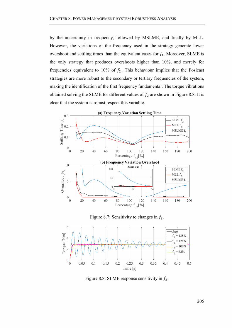
CHAPTER 8. POWER MANAGEMENT SYSTEM ROBUSTNESS ANALYSIS
205
by the uncertainty in frequency, followed by MSLME, and finally by MLL.
However, the variations of the frequency used in the strategy generate lower
overshoot and settling times than the equivalent cases for 𝑓1. Moreover, SLME is
the only strategy that produces overshoots higher than 10%, and merely for
frequencies equivalent to 10% of 𝑓2 . This behaviour implies that the Posicast
strategies are more robust to the secondary or tertiary frequencies of the system,
making the identification of the first frequency fundamental. The torque vibrations
obtained solving the SLME for different values of 𝑓2 are shown in Figure 8.8. It is
clear that the system is robust respect this variable.
Figure 8.7: Sensitivity to changes in 𝑓2.
Figure 8.8: SLME response sensitivity in 𝑓2.

CHAPTER 8. POWER MANAGEMENT SYSTEM ROBUSTNESS ANALYSIS
206
The robustness of the strategies to variations in the damping ratio 𝜉2, while keeping
the frequencies and the damping ratio 𝜉1 constant, is shown in Figure 8.9. It is
observed that for damping ratio values below 0.1, the overshoot is 0.1%, while the
settling time remains constant for values below 0.04. This shows that as in the case
of variations in 𝜉1, the strategies are robust to changes in the damping ratio of the
second natural frequency. The same is shown in Figure 8.10, where the vibrations
obtained when solving the SLME strategy for different values of 𝜉2 are presented.
Therefore, the studies must be focused in the frequency identification and not in the
identification of the damping ratio.
Figure 8.9: Sensitivity to changes in 𝜉2.
Figure 8.10: SLME response sensitivity in 𝜉2.
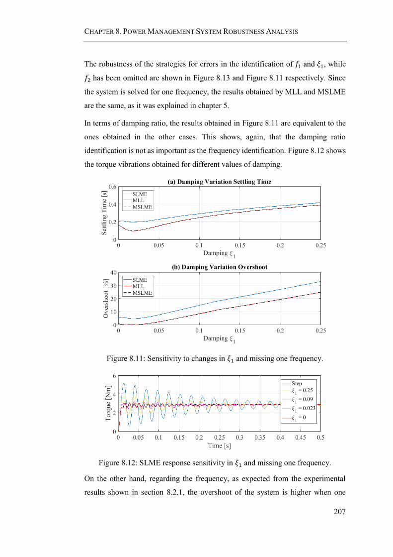
CHAPTER 8. POWER MANAGEMENT SYSTEM ROBUSTNESS ANALYSIS
207
The robustness of the strategies for errors in the identification of 𝑓1 and 𝜉1, while
𝑓2 has been omitted are shown in Figure 8.13 and Figure 8.11 respectively. Since
the system is solved for one frequency, the results obtained by MLL and MSLME
are the same, as it was explained in chapter 5.
In terms of damping ratio, the results obtained in Figure 8.11 are equivalent to the
ones obtained in the other cases. This shows, again, that the damping ratio
identification is not as important as the frequency identification. Figure 8.12 shows
the torque vibrations obtained for different values of damping.
Figure 8.11: Sensitivity to changes in 𝜉1 and missing one frequency.
Figure 8.12: SLME response sensitivity in 𝜉1 and missing one frequency.
On the other hand, regarding the frequency, as expected from the experimental
results shown in section 8.2.1, the overshoot of the system is higher when one

CHAPTER 8. POWER MANAGEMENT SYSTEM ROBUSTNESS ANALYSIS
208
frequency is missing, especially for the SLME connection. In the experimental
SLME solved for one frequency, the overshoot was 130%, which is higher than the
80% obtained for the step connection. Comparing with the results of Figure 8.13(b),
SLME has 130% of overshoot when the system has been solved for a frequency
equal to 50% of the real value. The same is observed from Figure 8.14 where the
torque obtained after applying the SLME solved for different values of 𝑓1 is shown.
Since the frequencies of the experimental system have a ±2Hz of uncertainty, the
higher overshoot obtained experimentally is associated with the presence of
inductances. For this reason, in section 8.3, strategies that include the inductances
are presented.
Figure 8.13: Sensitivity to changes in 𝑓1 missing one frequency.
Figure 8.14: SLME response sensitivity in 𝑓1 and missing one frequency.
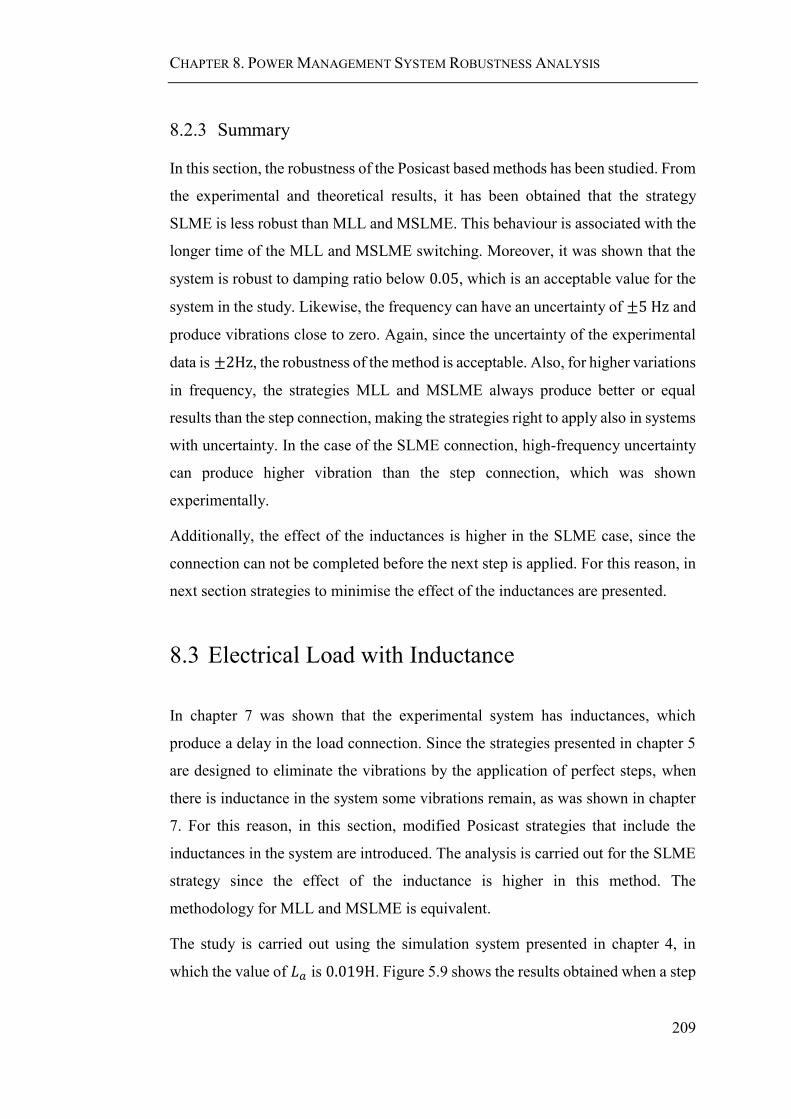
CHAPTER 8. POWER MANAGEMENT SYSTEM ROBUSTNESS ANALYSIS
209
8.2.3 Summary
In this section, the robustness of the Posicast based methods has been studied. From
the experimental and theoretical results, it has been obtained that the strategy
SLME is less robust than MLL and MSLME. This behaviour is associated with the
longer time of the MLL and MSLME switching. Moreover, it was shown that the
system is robust to damping ratio below 0.05, which is an acceptable value for the
system in the study. Likewise, the frequency can have an uncertainty of ±5 Hz and
produce vibrations close to zero. Again, since the uncertainty of the experimental
data is ±2Hz, the robustness of the method is acceptable. Also, for higher variations
in frequency, the strategies MLL and MSLME always produce better or equal
results than the step connection, making the strategies right to apply also in systems
with uncertainty. In the case of the SLME connection, high-frequency uncertainty
can produce higher vibration than the step connection, which was shown
experimentally.
Additionally, the effect of the inductances is higher in the SLME case, since the
connection can not be completed before the next step is applied. For this reason, in
next section strategies to minimise the effect of the inductances are presented.
8.3 Electrical Load with Inductance
In chapter 7 was shown that the experimental system has inductances, which
produce a delay in the load connection. Since the strategies presented in chapter 5
are designed to eliminate the vibrations by the application of perfect steps, when
there is inductance in the system some vibrations remain, as was shown in chapter
7. For this reason, in this section, modified Posicast strategies that include the
inductances in the system are introduced. The analysis is carried out for the SLME
strategy since the effect of the inductance is higher in this method. The
methodology for MLL and MSLME is equivalent.
The study is carried out using the simulation system presented in chapter 4, in
which the value of 𝐿𝑎 is 0.019H. Figure 5.9 shows the results obtained when a step

CHAPTER 8. POWER MANAGEMENT SYSTEM ROBUSTNESS ANALYSIS
210
connection and the SLME connection presented in chapter 5 are applied to the
system. In red the electrical torque applied over the drivetrain is shown, in blue the
shaft response is depicted, and in black, the desired rectangular step is presented. It
is observed that now the steps applied are not rectangular and that the SLME
strategy does not eliminate the vibrations but reduced them. Moreover, the delay in
the step does not allow the connection of the whole switching event in the SLME
strategy before the next step has been applied. Therefore, the time delay should be
at least smaller than the time between steps connections. This problem is
accentuated for systems with higher frequencies in which the steps are closer in
time. The results for the two inertia system used to analyse the strategies in chapter
5 are equivalent and shown in Figure 8.16.
Figure 8.15: Torque shaft response with Step and SLME.

CHAPTER 8. POWER MANAGEMENT SYSTEM ROBUSTNESS ANALYSIS
211
Figure 8.16: Torque shaft response in a 2 inertia system with Step and SLME.
The delay of the system is given by equation (8.1) in which 𝐿 is the inductance and
𝑅 is the resistance. Replacing the armature inductance 𝐿𝑎 = 0.019H and the
resistances connected to the system 𝑅𝑒𝑞1 = 4.55Ω when the electrical load is
connected, and 𝑅𝑒𝑞2 = 60.5Ω when the electrical load is disconnected, the delays
are:
𝜏1 = 4.1ms
𝜏2 = 0.3ms
The same results can be obtained from Figure 5.9 (b).
𝜏 =𝐿
𝑅 (8.1)
Next, three methodologies to minimise the effect of the inductance in the Posicast
strategies are presented. First the time constant value is studied, second, the delay
of the connection is included in the SLME solver, and thirdly, the real step is
modelled in the SLME solver.

CHAPTER 8. POWER MANAGEMENT SYSTEM ROBUSTNESS ANALYSIS
212
8.3.1 Change of Time Constant
The most straightforward strategy to minimise the effect of the inductance is to
reduce the time delay in the system. In equation (8.1) was shown that the delay in
the step connection depends on the inductance and the resistance. Therefore, for
systems in which the inductance is fixed, working with high resistances which can
reduce the delay in the connection considerably, allows the elimination of the
vibrations.
However, this method is not feasible for every system. For example, in the
experimental setup, the resistances needed to reduce the time delay would not allow
the analysis of the electromechanical interaction, since the load connected would
be too small. Therefore, two strategies that include the delay in the solver are
studied next.
8.3.2 Delay SLME
A solution to decrease the effect of the delay in the step connection due to the
inductances in the electrical system is its inclusion in the solver. For this reason, in
the equations presented in chapter 5 to solve the SLME connection, the term 𝑇𝑘 is
replaced by (𝑇𝑘 + 𝜏𝑘) as shown in the equation system (5.20). 𝜏𝑘 represents the
delay for the kth step. For the SLME connection in study, 𝜏𝑘 = 𝜏1 for odd
connections and 𝜏𝑘 = 𝜏2 for even connections. Moreover, as presented in chapter
5, 𝑝𝑘 = (−1)𝑘+1. This method is applied in the same manner to the strategies MLL
and MSLME.

CHAPTER 8. POWER MANAGEMENT SYSTEM ROBUSTNESS ANALYSIS
213
[ ∑𝑝𝑘𝑒
−𝜉1𝜔𝑛1(𝑇𝑘+𝜏𝑘) cos(𝜔𝑑1(𝑇𝑘 + 𝜏𝑘))
𝑚
𝑘=1
∑𝑝𝑘𝑒−𝜉1𝜔𝑛1(𝑇𝑘+𝜏𝑘) sin(𝜔𝑑1(𝑇𝑘 + 𝜏𝑘))
𝑚
𝑘=1
∑𝑝𝑘𝑒−𝜉2𝜔𝑛2(𝑇𝑘+𝜏𝑘) cos(𝜔𝑑2(𝑇𝑘 + 𝜏𝑘))
𝑚
𝑘=1
∑𝑝𝑘𝑒−𝜉2𝜔𝑛2(𝑇𝑘+𝜏𝑘) sin(𝜔𝑑2(𝑇𝑘 + 𝜏𝑘))
𝑚
𝑘=1
⋮
∑𝑝𝑘𝑒−𝜉𝑛𝜔𝑛𝑛(𝑇𝑘+𝜏𝑘) cos(𝜔𝑑𝑛(𝑇𝑘 + 𝜏𝑘))
𝑚
𝑘=1
∑𝑝𝑘𝑒−𝜉𝑛𝜔𝑛𝑛(𝑇𝑘+𝜏𝑘) sin(𝜔𝑑𝑛(𝑇𝑘 + 𝜏𝑘))
𝑚
𝑘=1 ]
= 0 (8.2)
Following the steps of chapter 5, first the solutions for the 2 inertia system with one
natural frequency 𝑓𝑛1 = 19.09Hz and 𝜉1 = 0.0327 are presented. Solving the
system with the time delays 𝜏1 and 𝜏2 calculated before, the times of the step
connections are 𝑇1 = 0ms, 𝑇2 = 11.4ms, 𝑇3 = 17.7ms. The load connected is the
same that has been used in the other cases, from 0.3952Nm to 2.9282Nm ,
corresponding to the connection of a resistance of 5Ω. The simulation results are
shown in Figure 8.17. It is observed that the vibrations have been almost completely
eliminated, showing that the strategy works.

CHAPTER 8. POWER MANAGEMENT SYSTEM ROBUSTNESS ANALYSIS
214
Figure 8.17: Torque shaft response in a 2 inertia system for delay SLME.
Now, the system is solved for the 3 natural frequency system in the study. The
parameters were presented in chapter 4 and used in chapter 5 (𝑓1 = 11.9443Hz,
𝜉1 = 0.0362 , 𝑓2 = 38.5982Hz , 𝜉2 = 0.0276 , 𝑓3 = 109.7207Hz , 𝜉3 = 0.0774).
The time delays are 𝜏1 = 4.1ms and 𝜏2 = 0.3ms. The connection times and step
values are:
𝑇1 = 0ms and 𝑝1 = 1.
𝑇2 = 7.7578ms and 𝑝2 = −1.
𝑇3 = 8.6957ms and 𝑝3 = 1.
𝑇4 = 16.1720ms and 𝑝4 = −1.
𝑇5 = 20.3030ms and 𝑝5 = 1.
𝑇6 = 28.5560ms and 𝑝6 = −1.
𝑇7 = 33.7590ms and 𝑝7 = 1.
The results obtained are shown in Figure 8.18. It is observed, that like for the two
inertia system, comparing with the normal SLME case in (a), the vibrations have
been reduced almost to zero.
CHAPTER 8. POWER MANAGEMENT SYSTEM ROBUSTNESS ANALYSIS
215
Figure 8.18: Torque shaft response for delay SLME.
To further study strategies that allow the elimination of the torsional vibrations after
the switching event in systems with inductances, next section presents an
Exponential SLME strategy.
8.3.3 Exponential SLME
It has been presented that including the delay in the solver allows further reductions
of the vibrations when the system has inductances. In this section, another strategy
to achieve the same aim is presented.
The exponential SLME consists in modelling the real step connection in the
equation system that allows the elimination of the vibration after the switching
connection. For this reason, the load connection 𝑝𝑘 is modelled as a series of
infinite steps in time 𝑝𝑘𝑡(𝑡𝑝) as shown in equation (8.3). The value of each step is
given by equation (8.4), in which 𝑡𝑝 is the time of the step, 𝜏𝑘 is the delay produced
by the inductance, 𝑝𝑘(𝑡−1) is the value of the step in the previous instant, and 𝑇𝐾 is
the connection time of each exponential step. By subtracting 𝑝𝑘(𝑡−1), the equation
system takes into account that the step connection may not have finished before the
next step is applied. Replacing into the standard SLME equation, the equation
system to solve is given by (8.5).

CHAPTER 8. POWER MANAGEMENT SYSTEM ROBUSTNESS ANALYSIS
216
𝑝𝑘 = ∑ 𝑝𝑘𝑡(𝑡𝑝)
𝑇𝑘+1
𝑡𝑝=0
(8.3)
𝑝𝑘𝑡 = (−1)𝑘 + (−1)𝑘+1𝑒−𝑡𝑝𝜏𝑘 − 𝑝𝑘(𝑡−1)
(8.4)
[ ∑ ∑ 𝑝𝑘𝑡𝑒
−𝜉1𝜔𝑛1(𝑇𝑘+𝑡𝑝) cos (𝜔𝑑1(𝑇𝑘 + 𝑡𝑝))
𝑇𝑘+1
𝑡𝑝=0
𝑚
𝑘=1
∑ ∑ 𝑝𝑘𝑡𝑒−𝜉1𝜔𝑛1(𝑇𝑘+𝑡𝑝) sin (𝜔𝑑1(𝑇𝑘 + 𝑡𝑝))
𝑇𝑘+1
𝑡𝑝=0
𝑚
𝑘=1
∑ ∑ 𝑝𝑘𝑡𝑒−𝜉2𝜔𝑛2(𝑇𝑘+𝑡𝑝) cos (𝜔𝑑2(𝑇𝑘 + 𝑡𝑝))
𝑇𝑘+1
𝑡𝑝=0
𝑚
𝑘=1
∑ ∑ 𝑝𝑘𝑡𝑒−𝜉2𝜔𝑛2(𝑇𝑘+𝑡𝑝) sin (𝜔𝑑2(𝑇𝑘 + 𝑡𝑝))
𝑇𝑘+1
𝑡𝑝=0
𝑚
𝑘=1
⋮
∑ ∑ 𝑝𝑘𝑡𝑒−𝜉𝑛𝜔𝑛𝑛(𝑇𝑘+𝑡𝑝) cos (𝜔𝑑𝑛(𝑇𝑘 + 𝑡𝑝))
𝑇𝑘+1
𝑡𝑝=0
𝑚
𝑘=1
∑ ∑ 𝑝𝑘𝑡𝑒−𝜉𝑛𝜔𝑛𝑛(𝑇𝑘+𝑡𝑝) sin (𝜔𝑑𝑛(𝑇𝑘 + 𝑡𝑝))
𝑇𝑘+1
𝑡𝑝=0
𝑚
𝑘=1 ]
= 0 (8.5)
Solving the equation system for the one natural frequency system used in the other
cases (with 𝑛 = 1 and 𝑚 = 3 ), Figure 8.19 is obtained. The times of the
connections are: 𝑇1 = 0ms , 𝑇1 = 11.0ms and 𝑇3 = 17.3ms . Comparing to the
results given by the methods SLME and Delay SLME, the vibrations have been
completely eliminated after the switching load connection. This shows that the
modelling of the load connections as a series of steps allows the elimination of the
vibrations.

CHAPTER 8. POWER MANAGEMENT SYSTEM ROBUSTNESS ANALYSIS
217
Figure 8.19: Torque shaft response in a 2 inertia system for exponential SLME.
Solving the equations for the 3 natural frequencies system in the study, with 𝑛 = 3
and 𝑚 = 7, the following connection times are obtained:
𝑇1 = 0ms and 𝑝1 = 1.
𝑇2 = 7.4696ms and 𝑝2 = −1.
𝑇3 = 13.8950ms and 𝑝3 = 1.
𝑇4 = 23.2620ms and 𝑝4 = −1.
𝑇5 = 30.3730ms and 𝑝5 = 1.
𝑇6 = 40.4690ms and 𝑝6 = −1.
𝑇7 = 41.5040ms and 𝑝7 = 1.
Figure 8.20 shows the torque obtained when the same load connection of the past
cases is applied. Contrary to what was expected, the remaining vibrations are
slightly higher than the ones obtained by the Delay SLME strategy. This behaviour
is due to solver inaccuracies since the system is more complicated than the one
from the past cases. Since the addition of infinite steps adds a new level of difficulty
to the solver, the accuracy required to obtain the result has to be decreased. This
was not a problem for the one natural frequency system since the solution was
obtained graphically, through the sine and cosine residual curves.

CHAPTER 8. POWER MANAGEMENT SYSTEM ROBUSTNESS ANALYSIS
218
Figure 8.20: Torque shaft response for exponential SLME.
Therefore, the exponential SLME allows the elimination of the torsional vibrations
in systems with inductances, but the complexity of the equation system implies that
new solver strategies must be used. Next, the advantages and disadvantages of each
method are discussed.
8.3.4 Summary
In this section strategies that take into account the effect of the inductance in the
system were presented. Now, comparisons between the SLME, Delay SLME, and
Exponential SLME methods are discussed. The change in the time constant by
increasing the resistance is not further analysed since its application is not applied
to the system in the study.
To compare the strategies, first, the sine and cosine residual curves for the 2 inertia
system are presented in Figure 8.21. The curves, like in chapter 5, were obtained as
a function of the period Γ𝑘 = 𝑇𝑘/𝑇𝑝, and hence their values are normalised. The
delay values used are the one used in the past sections. In (a), (c), and (e) the
solutions for a system with no damping ratio are shown, while in (b), (d), and (f),
the case in which the damping ratio is 𝜉 = 0.3 is presented. From the zero damping
ratio situations is observed that the curves obtained by delay SLME and exponential
SLME are almost the same, which shows the similitude between the results
obtained. Likewise, it can be seen that the effect of the delay changes considerably

CHAPTER 8. POWER MANAGEMENT SYSTEM ROBUSTNESS ANALYSIS
219
the curves associated with the cosine. From the plots obtained for 𝜉 = 0.3, it is
observed that for higher damping ratio the curves and results tend to the same value.
However, in the case of the exponential SLME, only the first solution of the system
remains, since the rest of the curves do not cross.
Figure 8.21: Summary solutions of system with inductance.

CHAPTER 8. POWER MANAGEMENT SYSTEM ROBUSTNESS ANALYSIS
220
A summary of the results obtained for the 3 natural frequencies system is shown in
Figure 8.22. As previously described, the presence of inductance reduces the
effectivity of the SLME connection. While SLME method still reduces the
vibrations considerably, as was shown experimentally in chapter 7, some vibrations
remain after the switching connection. From (c) and (d) the response of the systems
solved with delay SLME and exponential SLME are presented. While in theory,
exponential SLME should produce better results, eliminating all the vibrations after
the switching, the complexity in its solving makes delay SLME an easy method to
apply in practice.
Figure 8.22: Summary torque in system with inductance.

CHAPTER 8. POWER MANAGEMENT SYSTEM ROBUSTNESS ANALYSIS
221
The advantage of exponential SLME is that by modelling the load connection as a
series of steps, the methodology can be expanded to any curve shape. For example,
a ramp connection, presented as a solution in chapter 3, eliminates the vibrations
because an adequate slope solves the Posicast equation system, which can be shown
by the modelling of the connection as a series of infinite steps.
Moreover, the results presented by the delay SLME and exponential SLME show
that the inductance in a system is not an impediment to eliminate the vibrations
produced by electromechanical interaction. In future work these methodologies can
be expanded for different loads (capacitive for example) and for the MLL and
MSLME strategies.
8.4 Comparison with Alternative Methods
In this section the strategies proposed in this thesis are compared with the methods
used in the literature and which have been presented in chapter 3. A summary of
them is shown in Figure 8.23. The strategies can be divided in three approaches.
System analysis, which consists in analysing the natural frequencies or vibration
modes of the mechanical system to avoid the operation of the electrical system at
those values. System design, which designs the mechanical system with higher
damping or stiffness to reduce the vibrations. And finally, controller design, in
which different control methods are used. One method is to control the torque
applied by the machine and apply a ramp. The ramp reduces the vibrations since
the torque applied at a given time is lower. Otherwise, torque strategies with closed-
loop torque are used. When using this system, the torque applied by the machine is
controlled by the value of the torsional torque vibrations. Finally, anti-resonant
filters which cancel the excitation of frequencies can be used to avoid reduce the
torsional vibrations. In addition, all the strategies found in the literature have been
applied to the machine connected to the mechanical system.

CHAPTER 8. POWER MANAGEMENT SYSTEM ROBUSTNESS ANALYSIS
222
Figure 8.23: Torsional vibration solutions for electromechanical systems.
Of the strategies presented, the system analysis does not reduce the vibrations when
electrical loads are being connected. On the other hand, the design of the system
with higher damping or stiffness, makes the system heavier and larger. For this
reason, the solutions for the reduction of the torsional vibrations excited by the
connection of electrical loads are based in controller design.
In general, the controller design strategies used consist in slowing down the system.
For example, the ramp and the closed-loop torque strategies are effective but slow.
Moreover, these strategies reduce the vibration but do not consider the reason for
their excitation. For this reason, in this thesis, strategies based on the Posicast
Compensator, a filter that stops the excitation of the resonance frequencies was
studied. This method allows the elimination of the torsional vibrations in a time
lower than half the period of the torsional frequency, making it much faster than
the other methods commonly used.
However, the Posicast compensator and the methods used in the literature review
are not independent, but complementary. First, it was mentioned that the Posicast
compensator is part of the Anti-resonant filter subsection, since it consists in
eliminating the excitation of the torsional vibrations. Second, as was shown in the

CHAPTER 8. POWER MANAGEMENT SYSTEM ROBUSTNESS ANALYSIS
223
last section, the step connection of loads can be used to model any load shape. For
this reason, the use of a ramp connection can be a solution of the same problem.
The difference with the ramp connection used nowadays would be the time of the
connection. There is one ramp slope that allows the elimination of the vibrations in
half a period. Finally, the use of closed-loop torque feedback can be integrated in
the strategies presented to increase the robustness of the system.
The main difference between the strategies typically used and the ones presented
in this work is where they are being applied. Most studies apply the strategies
directly on the machine since the studies on machines and electrical power system
are independent. However, in this thesis the control to reduce the torsional
vibrations is applied to the electrical loads. The main reason for this is to reduce
the effect on the stability of the electrical power system, since in current aircraft
electrical power system, the loads are already being connected in a pulsing pattern
by the use of mechanical switches.
Still, as presented in chapter 5 to be able to apply the control in the electrical power
system, the following requirements must be fulfilled:
Solid State switches to control the loads.
A given ratio of load types.
Minimum inner loop bandwidth in converter.
High bandwidth communication/sensing/control link.
If the requirements cannot be satisfied, a combination between the traditional
methods and the methods presented in this thesis can be used. The strategies
presented in this thesis have been applied on the loads but they can be applied in
the machine too. For example, for the connection of loads in which solid state
switches are not available yet, the strategy can be applied directly to the machine.
The same can done if the amount of critical loads connected is higher than the
quantity of non-critical loads.
CHAPTER 8. POWER MANAGEMENT SYSTEM ROBUSTNESS ANALYSIS
224
8.5 Summary
This chapter presented a robust analysis of the Posicast based strategies and
modifications to include the effect of the inductances in the system. The study of
the sensitivity of the strategies allowed the identification of the parameters that
affect the robustness of the methods. It was obtained, that for damping ratio below
0.05 , which are the normal values obtained, its identification is not critical.
Likewise, it was obtained that the identification of the correct number of torsional
frequencies in the system is essential, since solving the strategies for fewer
frequencies reduce the effectivity and can produce vibrations higher than for the
step connection. Also, it was shown that the identification of a correct first
frequency is more important than the second. Finally, for uncertainties of ±5Hz,
the results of the strategies are similar.
Regarding the inductances of the system, it was shown that their value must be
considered in the strategies because the delay produced by them affects the strategy
as much as the frequency uncertainty. The combined effect of inductance and
frequency uncertainty can produce vibrations higher than the ones obtained for the
step connection. For this reason, two strategies that remove the effect of the
inductances were presented: delay SLME and exponential SLME. It was shown
that while delay SLME has some vibrations after the switching event, exponential
SLME allows the elimination of them. However, exponential SLME has high
computational requirements which reduce the solver effectivity. For this reason, if
the complete elimination of the vibrations is desired, new solver strategies for the
non-linear equation system must be studied.
Summing up, this chapter has shown the importance of identifying the overall
system parameters. In an aircraft system, the drivetrain torsional vibrations are
given by the machine and gears inertias and the shaft stiffness. Since these values
do not present considerable variations during its operation, a first identification
through the FFT method is enough for the application of the strategies. Moreover,
since the torsional frequencies must be known regardless of the Posicast strategies,

CHAPTER 8. POWER MANAGEMENT SYSTEM ROBUSTNESS ANALYSIS
225
to avoid resonance between the drivetrain and the generator control, the PMS
presented is a feasible solution to reduce the torsional vibrations.

Chapter 9
9 Conclusions and Future Work
9.1 Summary
This thesis presented a study of the electromechanical interaction in aircraft
systems. The importance of studying the excitation of the drivetrain torsional
vibration modes by the connection of electrical loads has been shown. For this, a
reduced aircraft drivetrain has been analysed.
To reduce the vibrations produced by the excitation of the drivetrain natural
frequencies, a power management system (PMS) has been developed. The PMS
proposes the use of strategies based on the Posicast compensator to suppress the
excitation of vibrations when different electrical loads are connected.
In the ideal case (known frequency and no inductance or capacitance), the torsional
vibrations can be eliminated after the switching connection by the application of a
switching event. Experimentally, the system parameters are not known, and thus
they must be estimated. Therefore, the frequencies used have an error respect to the
real system values. Likewise, the experimental system has inductance, which was
omitted by simulation, and which generates logarithmic load connections instead
of steps. For these two reasons, experimentally the PMS strategies reduce the
torsional vibrations to values close to zero instead of eliminating them. To study
these effects a sensitivity analysis was carried on, and strategies based on
logarithmic load connections were proposed to improve the system response.
Therefore, the presence of inductance in the system does not affect the elimination
of the torsional vibrations produced by electromechanical interaction.
In chapter 2 and 3, the literature review was presented. Chapter 2 described the
evolution of aircraft systems, while chapter 3 presented a review of the
electromechanical interaction across diverse electrical applications. The study

CHAPTER 9. CONCLUSIONS AND FUTURE WORK
227
shows the importance this subject has gained in every area that involves interchange
of electrical and mechanical power. Sources and solutions applied in each field of
study have been presented.
In chapter 4, the electromechanical interaction in aircraft systems has been studied.
Simulation results have been presented to show the effect of the connection of step
and pulsating electrical loads on the mechanical drivetrain. Furthermore, the
importance of designing the machine control system considering the electrical and
mechanical system has been shown.
In chapter 5, a PMS that eliminates the torsional vibrations due to the connection
of electrical loads has been designed. The PMS can be applied to pulsating loads
and step electrical loads with or without a critical time connection. Each of the
strategies is based on the Posicast method, which cancels the vibrations by the
connection of a series of switching events. The switching is determined as a
function of the natural frequencies and damping ratio of the drivetrain. Further
understanding of the strategies has been given by studying the solution range as a
function of the system’s damping ratio. Graphically, it has been shown that the
Posicast strategies eliminate the vibrations by adding zeros at the poles value.
To experimentally test the PMS, in chapter 6 the experimental setup was designed.
The rig presented allows the testing of different aircraft related studies, such as an
in-line starter/generator, an air-riding seal, and the electromechanical interactions.
Of them, this thesis only studies the electromechanical interactions. Furthermore,
it was shown that a domestic appliance universal motor could be readapted to
operate as a generator in the experimental setup. The use of this machine allows the
simplification of the system and the reduction of the cost.
In chapter 7 the PMS strategies have been tested experimentally. To prove the
strategies SLME, MLL and MSLME, the frequencies were identified and torque
measuring strategies presented. For the frequency and damping ratio identification,
a method based on the FFT, the empirical mode decomposition and Hilbert
Transform were used. To measure the shaft torque, sensor and sensorless methods
were presented. It was shown, that for the low load and high noise application the

CHAPTER 9. CONCLUSIONS AND FUTURE WORK
228
sensorless method provides the best results. The sensorless torque measurement
methodology can be expanded to synchronous generators like the ones used in
aircraft. Moreover, the results of the PMS have demonstrated that the torsional
vibrations are reduced when the strategies are applied. The effect of the inductance
and the frequency uncertainty over the SLME, MLL, and MSLME strategies have
been shown. For closer steps, such as the steps associated with 77.1Hz in the SLME
connection, the inductances affect the step shape, reducing the effectivity of the
method.
Finally, in chapter 8 the robustness of the Posicast strategies was studied, and future
enhancements to the method presented. Regarding the robustness, a comparison of
the three strategies presented (SLME, MLL, and MSLME) show that MLL is less
affected by the uncertainty of the system and by the presence of inductance. The
reason behind this behaviour is that the MLL strategy is slower than the other two.
A slower strategy allows the step connection to finish, regardless of the inductance,
before the next switching takes place, and at the same time makes the system more
robust to frequency uncertainty. To include a wider range of loads, the modelling
of any connection pattern as a series of steps has been proposed. In particular, for
the case of inductive and resistive loads, the solving of the equation system for load
connections has been introduced.
9.2 Conclusions
This thesis showed that the electromechanical interaction is a relevant problem for
aircraft systems since it reduced the life of the mechanical drivetrain and creates
instability. For the case in which the interaction is due to the connection of electrical
loads, the solutions in the literature review are not optimal. Since the behaviour of
the vibrations is not considered, the time it takes to eliminate the torsional
vibrations is high. For this reason, this thesis presented strategies to cancel the
excitation of torsional vibrations which are based on the characteristics of the
mechanical system. The connection is carried out in half a period of the drivetrain
natural frequency, which is in the order of milliseconds.
CHAPTER 9. CONCLUSIONS AND FUTURE WORK
229
The method presented is not necessarily independent from the ones already in use
but can be complementary. In this study, the Posicast compensator has been applied
to the electrical loads being connected to the system, but it can also be applied to
the machine control and can be expanded to ramp connections and closed loop.
Moreover, the strategies were demonstrated by simulation and experimentally. It
was also shown that the methods are robust respect to the damping and the second
(or higher) frequencies and that its response depends more on the shape of the
connection than the frequency identification. Therefore, the robust studies should
focus on the identification of the lower natural frequency and the shape of the
connection.
Finally, it is concluded that the PMS presented in this thesis is a valid alternative to
the suppression of torsional vibrations in aircraft electromechanical systems. The
strategies presented can be applied as presented here or partially, and they can also
be adapted to systems with similar problems, like the interconnection of electrical
power system and wind turbines applications.
9.3 Future Work
Future works that can be developed from the work presented in this thesis are listed
below:
Posicast with uncertainty and non-linear loads: In this thesis open-loop
Posicast strategies have been applied to systems with known frequencies
and damping ratio and operating with resistive loads. To extend the method
to a wider range of systems, the effect of uncertainty and non-linear loads
must be studied.
o Respect to the system uncertainty, Posicast strategies with closed-
loop can be developed. For example, a PI can improve the results
for systems in which the value of the frequencies is not exact. These
results can be further extended to comprise systems in which the

CHAPTER 9. CONCLUSIONS AND FUTURE WORK
230
frequencies are unknown or change in time by the use of adaptive
controllers.
o In consideration of systems with non-resistive loads, chapter 7 show
that the presence of inductance can affect the Posicast method. For
this problem, chapter 8 proposed the solving of the Posicast
strategies for inductive loads. By the modelling of any connection
pattern as a series of infinite steps, the strategy can be adapted to
different loads. Therefore, further work can include inductive and
capacitive loads, which are common in aircraft systems. The same
strategy can also be used to obtain the optimal ramp which allows
the connection of the load in half a period of the drivetrain natural
frequency. Moreover, combining the connection patterns with
closed-loop methods, the Posicast based method can be extended to
non-linear loads with frequencies uncertainty.
Implementation of the Posicast strategies in other applications: The
Posicast strategies can be applied to cancel the vibrations produced on other
electrical and mechanical systems. For example, in wind turbines in which
there is electromechanical interaction due to changes in the turbine rotation
speed. Alternatively, the Posicast methods can be applied on the
synchronisation of systems, such as microgrids, which can see their
interconnection stopped due to the presence of high transients. Furthermore,
the use of Posicast compensator can be beneficial for the interconnection of
electrical systems. For example, in aircraft systems, when one generator
fails, the two power networks are connected. This connection can be seen
as the connection of a high load and therefore it will produce torsional
vibrations on the shaft of the remaining generator. To avoid these vibration
the Posicast compensator can be used.
Moreover, the Posicast strategies can be studied to reduce the transients in
electrical systems. In general, the use of these strategies to reduce transient
vibrations in electrical systems require high switching, since the connection
is made in half a period. However in chapter 5 was shown that each equation
CHAPTER 9. CONCLUSIONS AND FUTURE WORK
231
system has more than one solution. Therefore, to avoid the use of high
switching devices, to apply the Posicast strategies to electrical systems,
connection times greater than half a period are desired. This work can also
be combined with closed-loop Posicast strategies, allowing the reduction of
the vibrations in a system with uncertainty.
Experimental rig integration with in-line starter/generator: In chapter
6 was mentioned that the experimental rig allows the testing of three aircraft
aspects: the electromechanical interaction presented in this thesis, an in-line
starter/generator, and an air-riding seal. The starter/generator allows the
reduction of the transversal vibrations, while the seal is benefited by the
decrease. Since the PMS strategies reduce the torsional vibrations produced
by electromechanical interaction, further analysis can be done by
integrating these strategies into the starter/generator. This will allow the
presentation of a system that reduces transversal and torsional vibrations
simultaneously.
Study of electrical power system requirements: In chapter 5, the
requirement of the electrical power system for the application of the
proposed PMS were stated. Future work should study:
o The implementation of the strategies on the power electronics of the
system.
o The effect of the communication system on the strategy presented.
For example, the delay in the communication should be considered
and strategies to minimise its effect proposed.
o The power quality of the electrical power system after applying the
proposed PMS.
9.4 Publications
C. Ahumada, S. Garvey, T. Yang, P. Wheeler, "Electromechanical
Interaction Analysis through Sensorless Torque Measurement," 2017 IEEE

CHAPTER 9. CONCLUSIONS AND FUTURE WORK
232
Southern Power Electronics Conference (SPEC), Puerto Varas, Chile, 2017,
pp. 1-6., doi: 10.1109/SPEC.2017.8333597.
C. Ahumada, S. Garvey, T. Yang, P. Kulsangcharoen, P. Wheeler and H.
Morvan, "Minimization of electro-mechanical interaction with posicast
strategies for more-electric aircraft applications," IECON 2016 - 42nd
Annual Conference of the IEEE Industrial Electronics Society, Florence,
2016, pp. 4423-4428, doi: 10.1109/IECON.2016.7794134.
Ahumada Sanhueza, C., Bristot, A., Kumar, S., Schneider, N. et al., "An
Integrated System’s Approach Towards Aero Engine Subsystems Design,"
SAE Technical Paper 2016-01-2020, 2016, doi:10.4271/2016-01-2020.
S. C. Ahumada, S. Garvey, T. Yang, P. Wheeler and H. Morvan, "The
importance of load pulse timing in aircraft generation," 2015 18th
International Conference on Electrical Machines and Systems (ICEMS),
Pattaya, 2015, pp. 1339-1345, doi: 10.1109/ICEMS.2015.7385247.
Ahumada S., C., Garvey, S., Yang, T., Wheeler, P. et al., "Impact of Electric
Loads on Engine Shaft Dynamics within More Electric Aircraft," SAE
Technical Paper 2015-01-2409, 2015, doi:10.4271/2015-01-2409.

Appendix I - Universal Motor
This appendix presents the universal motor parameters and its connection to operate
as a single phase DC generator. The plate characteristics of the machine are
presented in Table A I - 1. Figure AI - 1 shows the winding connection for its
operation as a universal motor (in (a)) and as a DC generator (in (b)).
Table A I - 1: Machine plate parameters.
Characteristic Value
Brand Nidec
Speed 480 − 15000 rpm
Frequency 50 − 60 Hz
Voltage 230 − 240 V
Figure AI - 1: Universal motor circuit.
In the following sections, the resistance of the windings, the rotational inductance,
the maximum operating current, and the inertia are determined. The values of the
armature and field inductance are 𝐿𝑎 = 0.19H and 𝐿𝑓 = 0.2H respectively and
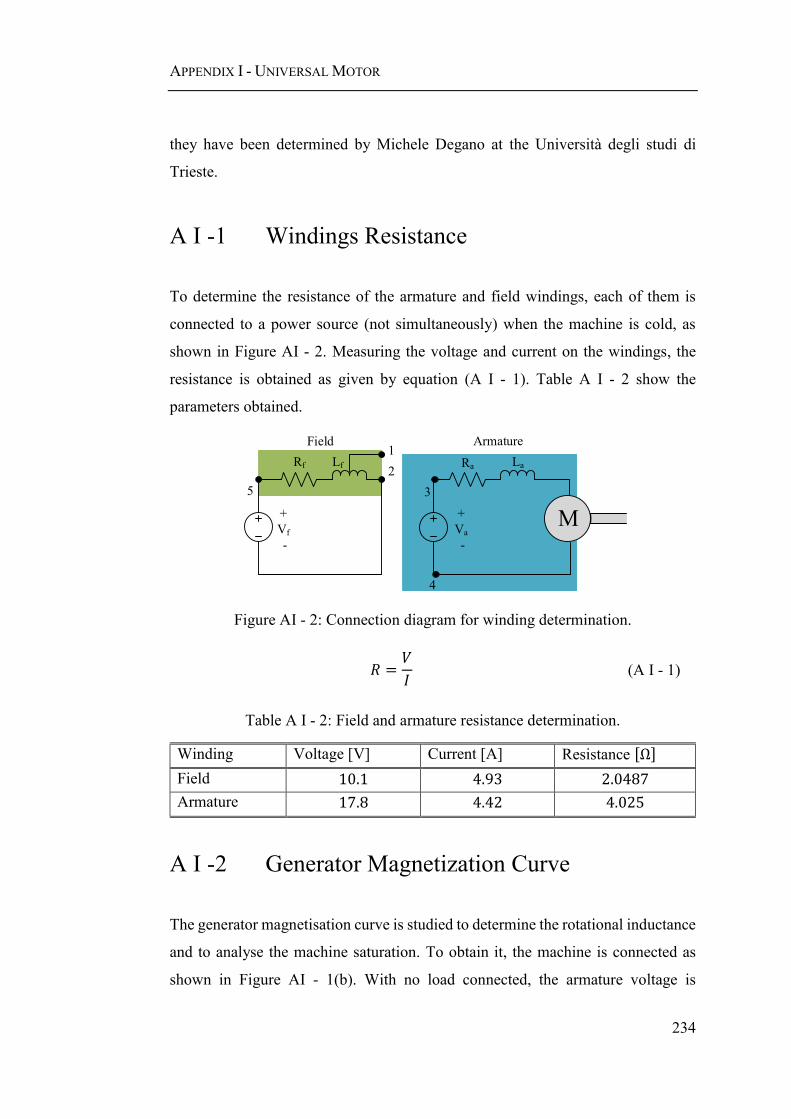
APPENDIX I - UNIVERSAL MOTOR
234
they have been determined by Michele Degano at the Università degli studi di
Trieste.
A I -1 Windings Resistance
To determine the resistance of the armature and field windings, each of them is
connected to a power source (not simultaneously) when the machine is cold, as
shown in Figure AI - 2. Measuring the voltage and current on the windings, the
resistance is obtained as given by equation (A I - 1). Table A I - 2 show the
parameters obtained.
M
Rf RaLf La
1
2
3
4
5
Field Armature
+
Va
-
+
Vf
-
Figure AI - 2: Connection diagram for winding determination.
𝑅 =𝑉
𝐼 (A I - 1)
Table A I - 2: Field and armature resistance determination.
Winding Voltage [V] Current [A] Resistance [Ω]
Field 10.1 4.93 2.0487
Armature 17.8 4.42 4.025
A I -2 Generator Magnetization Curve
The generator magnetisation curve is studied to determine the rotational inductance
and to analyse the machine saturation. To obtain it, the machine is connected as
shown in Figure AI - 1(b). With no load connected, the armature voltage is

APPENDIX I - UNIVERSAL MOTOR
235
measured for different values of field current, while keeping the speed constant.
The test is repeated increasing the current, and decreasing it for two different speed
values. Figure AI - 3 show the results obtained. In blue, the magnetisation curve for
an increasing field current is shown, while in red the curve obtained when the
current decrease is depicted.
Figure AI - 3: Results magnetization curve of the generator.
It is observed that the machine saturates slightly after 3A. Because the saturation
current is lower than the field current that is used in the rig, to model the rotational
inductance 𝑘(𝑖𝑓) equation (A I - 2), proposed in [125], is used. This equation has
the advantage of modelling the basic features of saturation using one constant 𝑏
and the magnetization value 𝑘0 at the origin, with 𝑖𝑓 the field current. The value of
the rotational inductance as a function of 𝑖𝑓 is found from equation (A I - 3).
APPENDIX I - UNIVERSAL MOTOR
236
𝑘(𝑖𝑓) =𝑘0
1 + 𝑏𝑖𝑓 (A I - 2)
𝑣𝑎 = 𝐸 = 𝑘(𝑖𝑓)𝑖𝑓𝜔 (A I - 3)
Fitting the data from the figures the following values are obtained:
𝑘0 = 0.1274
𝑏 = 0.1221
A I -3 Maximum Current Test
In last section was shown that the machine starts saturating at 3A. This section
studies the maximum current at which the machine can operate. For this test, the
machine is connected as a generator with no load and no speed. Then, the field
voltage was measured during 5 minutes (or 300 seconds) while supplying a constant
current. The test was repeated for currents from 4A to 10A. Between each test, the
machine must cool down to obtain correct results. Figure AI - 4(a) shows the results
obtained. It is observed that for lower currents the voltage changes less than at
higher values.
The change in voltage is associated with a rise in the field resistance as shown in
Figure AI - 4(b). The field resistance was obtained from equation (A I - 1). The
results show that the generator can run up to a current of 6A without increasing the
machine resistance considerably. Also, it is observed that for a field current of 4, 6,
and 9A, the resistance at the start of the measurement 𝑅0 has the same value of
1.8Ω, while in the other two cases the resistance is higher. This behaviour shows
that the two measurements at 8 and 10A were done when the machine was warm,
while for the other three, the measurements started with the machine cold.

APPENDIX I - UNIVERSAL MOTOR
237
Figure AI - 4: Maximum machine current.
Now that the field resistance has been obtained, its behaviour can be modelled as a
function of the field current and the time. The resistance has a common initial value
𝑅0, which changes exponentially with the time. Therefore, it can be modelled by
an exponential curve as shown in equation (A I - 4). With, 𝑅0 the resistance at the
origin, 𝑅𝑡, the resistance variation, and 𝜏 the time constant of the resistance change.
𝑅(𝑡, 𝑖𝑓) = 𝑅0 + 𝑅𝑡 (1 − exp (−1
𝜏𝑡)) (A I - 4)
Fitting the five resistance curves of Figure AI - 4(b), the parameters from Table A
I - 3 are obtained for each current. As mentioned before, the value of 𝑅0 is the same
for currents of 4, 6 and 9A, while in the other two cases higher results are obtained.
Since the higher values of 𝑅0 indicate that the machine was warm when the test
was done, from now on, the value of 𝑅0 = 1.79Ω is assumed real.

APPENDIX I - UNIVERSAL MOTOR
238
Table A I - 3: Resistance parametrization constant.
Current 𝑖𝑓 [𝐴] 𝑅0 [Ω] 𝑅𝑡 [Ω] 𝜏 [𝑠]
4 1.792 0.1702 176.3
6 1.788 0.435 215.1
8 1.908 0.8905 268.4
9 1.783 1.385 312.1
10 1.937 1.675 284.4
On the other hand, the parameters 𝑅𝑡 and 𝜏 are not constant, and therefore an
approximation must be found. Since 𝑅𝑡 and 𝜏 depend on the current of the system,
applying curve fitting is obtained that their behaviour can me modelled by
equations (A I - 5) and (A I - 6), with 𝑅𝑡0 = 0.01599Ω/A2, 𝜏0 = 103.5s, and 𝜏1 =
18.91s/A.
𝑅𝑡(𝑖𝑓) = 𝑅𝑡0𝑖𝑓2 (A I - 5)
𝜏(𝑖𝑓) = 𝜏0 + 𝜏1𝑖𝑓 (A I - 6)
Replacing the values of 𝑅0, and equations (A I - 5) and (A I - 6) into equation (A I
- 4), the following equation to represent the field resistance as a function of current
and time is obtained:
𝑅(𝑡, 𝑖) = 1.79 + 0.01599𝑖2 (1 − exp (−1
103.5 + 18.91𝑖𝑡)) (A I - 7)
The resistance values found by equation (A I - 7) are compared with the real values
in Figure AI - 5. It is obtained that the model is representative of the system.
Therefore, calculating the field resistance as a function of time and current Figure
AI - 6 is obtained. From here it is gotten that the maximum current at which the
machine can operate is 6A continuous or 10A for 5min, which warranties that the
resistance has not increased to the double of its value. Moreover, since the machine
operates for periods longer than 5 minutes, the field resistance is assumed as 𝑅𝑓 =
2Ω, which is the value obtained in section A I -1.

APPENDIX I - UNIVERSAL MOTOR
239
Figure AI - 5: Comparison of estimation and real field resistance.
Figure AI - 6: Estimated field resistance as a function of time and field current.
A I -4 Brush Voltage Drop
As mentioned in [96] there is a voltage drop in the brushes of the universal motor.
To determine its value equations (A I - 8) and (A I - 9) are used. With 𝐸 the back-
EMF in V, 𝑅𝑎 the armature resistance in Ω, 𝐿𝑎 the armature inductance in H, 𝑖𝑎 and
𝑖𝑓 the armature and field current in A, 𝑣𝑎 the armature voltage in V, 𝑉0 the voltage
drop in the brushes in V, 𝑘 the rotational inductance obtained in section A I -2, and
𝜔 the speed in rad/s.

APPENDIX I - UNIVERSAL MOTOR
240
𝐸 = 𝑅𝑎𝑖𝑎 + 𝐿𝑎𝑑𝑖𝑎𝑑𝑡
+ 𝑣𝑎 + 𝑉0 (A I - 8)
𝐸 = 𝑘𝑖𝑓𝜔 (A I - 9)
When the system is in steady state 𝑑𝑖𝑎/𝑑𝑡 = 0. Replacing its value and (A I - 9)
into (A I - 8), equation (A I - 10) is obtained.
𝑉0 = 𝑘𝑖𝑓𝜔 − 𝑅𝑎𝑖𝑎 − 𝑣𝑎 (A I - 10)
To find the value of the brushes voltage drop, the steady state date of Figure AI - 7
is used.
Figure AI - 7: Experimental steady state data.
Finally it is obtained that the voltage drop in the brushes is:
𝑉0 = 12.247 V

APPENDIX I - UNIVERSAL MOTOR
241
A I -5 Inertia Determination
To determine the inertia of the machine the acceleration must be measured. For this
test, the machine is connected as an independent field motor, as shown in Figure
AI - 8. Connecting a resistance in parallel to the armature voltage, the speed is
measured after the armature voltage has been disconnected while keeping the field
current constant. The test is repeated for three initial armature currents (20, 25, and
30V) and two values of 𝑅𝐿, 30 and 59Ω, and for the case in which no resistance is
connected. Figure AI - 9 shows the speed obtained in each case. Differentiating the
speed, the results of Figure AI - 10 are obtained.
M
Rf RaLf La
1
2
3
4
5
Field Armature
RL
+
Va
-
+
Vf
-
Figure AI - 8: Diagram for J determination.

APPENDIX I - UNIVERSAL MOTOR
242
Figure AI - 9: Speed of the machine.
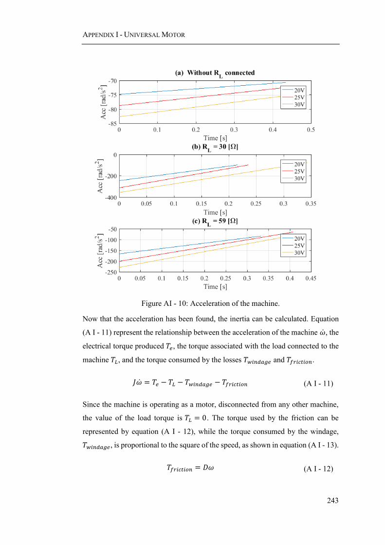
APPENDIX I - UNIVERSAL MOTOR
243
Figure AI - 10: Acceleration of the machine.
Now that the acceleration has been found, the inertia can be calculated. Equation
(A I - 11) represent the relationship between the acceleration of the machine �̇�, the
electrical torque produced 𝑇𝑒, the torque associated with the load connected to the
machine 𝑇𝐿, and the torque consumed by the losses 𝑇𝑤𝑖𝑛𝑑𝑎𝑔𝑒 and 𝑇𝑓𝑟𝑖𝑐𝑡𝑖𝑜𝑛.
𝐽�̇� = 𝑇𝑒 − 𝑇𝐿 − 𝑇𝑤𝑖𝑛𝑑𝑎𝑔𝑒 − 𝑇𝑓𝑟𝑖𝑐𝑡𝑖𝑜𝑛 (A I - 11)
Since the machine is operating as a motor, disconnected from any other machine,
the value of the load torque is 𝑇𝐿 = 0. The torque used by the friction can be
represented by equation (A I - 12), while the torque consumed by the windage,
𝑇𝑤𝑖𝑛𝑑𝑎𝑔𝑒, is proportional to the square of the speed, as shown in equation (A I - 13).
𝑇𝑓𝑟𝑖𝑐𝑡𝑖𝑜𝑛 = 𝐷𝜔 (A I - 12)

APPENDIX I - UNIVERSAL MOTOR
244
𝑇𝑤𝑖𝑛𝑑𝑎𝑔𝑒 ∝ 𝜔2 (A I - 13)
The value of the electrical torque 𝑇𝑒 produced by the machine depends on the
connection of the resistance 𝑅𝐿. Each case is explained next.
Case with resistance 𝑹𝑳
When there is a resistance 𝑅𝐿 connected parallel to the armature voltage, the
armature current and therefore the airgap torque of the machine does not become
automatically zero after disconnecting the voltage. Therefore, there is a torque 𝑇𝑒
which for a given load is proportional to the speed, as shown in equation (A I - 14)
[96].
𝑇𝑒 = 𝑓(𝜔) = 𝐴𝜔 (A I - 14)
Replacing the values of 𝑇𝑒 , 𝑇𝑓𝑟𝑖𝑐𝑡𝑖𝑜𝑛 , and 𝑇𝑤𝑖𝑛𝑑𝑎𝑔𝑒 into equation (A I - 11),
equation (A I - 15) is obtained. Since the data can be fitted by equation (A I - 16),
the relationships from equations (A I - 17) and (A I - 18) are found.
�̇� =𝐴𝜔 − 𝐷𝜔 − 𝑇𝑤𝑖𝑛𝑑𝑎𝑔𝑒
𝐽 (A I - 15)
�̇� = 𝑘1𝜔2 + 𝑘2𝜔 + 𝑘3 (A I - 16)
𝐴 − 𝐷 = 𝐽𝑘2 (A I - 17)
−𝑇𝑤𝑖𝑛𝑑𝑎𝑔𝑒
𝐽= 𝑘1𝜔
2 + 𝑘3 (A I - 18)
Case without resistance 𝑹𝑳
When there is not a resistance 𝑅𝐿 connected to the system, the armature current and
therefore the electrical torque 𝑇𝑒 become automatically zero after disconnecting the
voltage. Consequently, the equation that describes the system can be modelled by
(A I - 19), while the data of the system can be fitted using equation (A I - 20). From
these two equations, the relationships from equations (A I - 21) and (A I - 22) are
found.

APPENDIX I - UNIVERSAL MOTOR
245
�̇� =−𝐷𝜔 − 𝑇𝑤𝑖𝑛𝑑𝑎𝑔𝑒
𝐽 (A I - 19)
�̇� = 𝑘′1𝜔2 + 𝑘′2𝜔 + 𝑘′3 (A I - 20)
𝐷 = −𝐽𝑘′2 (A I - 21)
−𝑇𝑤𝑖𝑛𝑑𝑎𝑔𝑒
𝐽= 𝑘′1𝜔
2 + 𝑘′3 (A I - 22)
Then, fitting the experimental data with the equations described, the parameters
presented in Table A I - 4 and Table A I - 5 are obtained for each case.
Table A I - 4: Parametrization variables for data with load.
Voltage 𝑉𝑎 [V] Load Resistance
𝑅𝐿 [Ω] 𝑘1 𝑘2 𝑘3
20 59 0.0159 -2.8510 -63.1070
25 59 0.0230 -4.0452 -33.4146
30 59 0.0164 -3.7411 -35.2987
20 30 0.0464 -6.6667 -26.0642
25 30 0.0474 -7.9945 11.8159
30 30 0.0310 -6.3704 -28.9132
Table A I - 5: Parametrization variables for data with no load.
Voltage 𝑉𝑎 [V] 𝑘′1 𝑘′2 𝑘′3
20 1.1958e-4 -0.1401 -67.9584
25 2.5081e-4 -0.2170 -66.0593
30 2.9762e-4 -0.2506 -65.2397
Now, the equation system given by (A I - 17), (A I - 18), (A I - 21), and (A I - 22)
is solved for the resistance 𝑅𝐿 = 30Ω and 𝑅𝐿 = 59Ω compared to the no resistance
case. The inertias 𝐽 and damping 𝐷 obtained in each case are shown in Table A I -
6. It is observed that the values obtained are relatively constant, and from now on,
the inertia of the machine is approximated by 𝐽 = 5𝑒 − 4kgm2.

APPENDIX I - UNIVERSAL MOTOR
246
Table A I - 6: Inertia and damping.
Voltage 𝑉𝑎 [V] Load
Resistance
𝑅𝐿 [Ω]
Inertia 𝐽[𝐾𝑔𝑚2] Damping 𝐷 [𝑁𝑚𝑠
𝑟𝑎𝑑]
20 30 5.2095e-4 7.2985e-5
25 30 4.3716e-4 9.4864e-5
30 30 5.5557e-4 1.3923e-4
20 59 6.6399e-4 9.3025e-5
25 59 4.7019e-4 1.0203e-4
30 59 5.1569e-4 1.2923e-4
A I -6 Summary
The parameters of the universal motor used as a generator are shown in Table A I
- 7.
Table A I - 7: Generator parameters.
Parameter Value
Armature resistance 𝑅𝑎 = 4.025 Ω
Field resistance 𝑅𝑓 = 2 Ω
Armature Inductance 𝐿𝑎 = 0.019 H
Field Inductance 𝐿𝑓 = 0.02 H
Rotational inductance 𝑘0 = 0.1274 ln − in/A
Rotational inductance constant 𝑏 = 0.1271 1/A
Rotational inertia 𝐽𝑔 = 0.0005 kgm2
Max speed 𝜔𝑚𝑎𝑥 = 15000 rpm
Max current continuous 𝐼𝑚𝑎𝑥 = 6 A
Max current / 5 min 𝐼𝑚𝑎𝑥/5𝑚𝑖𝑛 = 10 A
Brush Voltage Drop 𝑉0 = 12.247 V
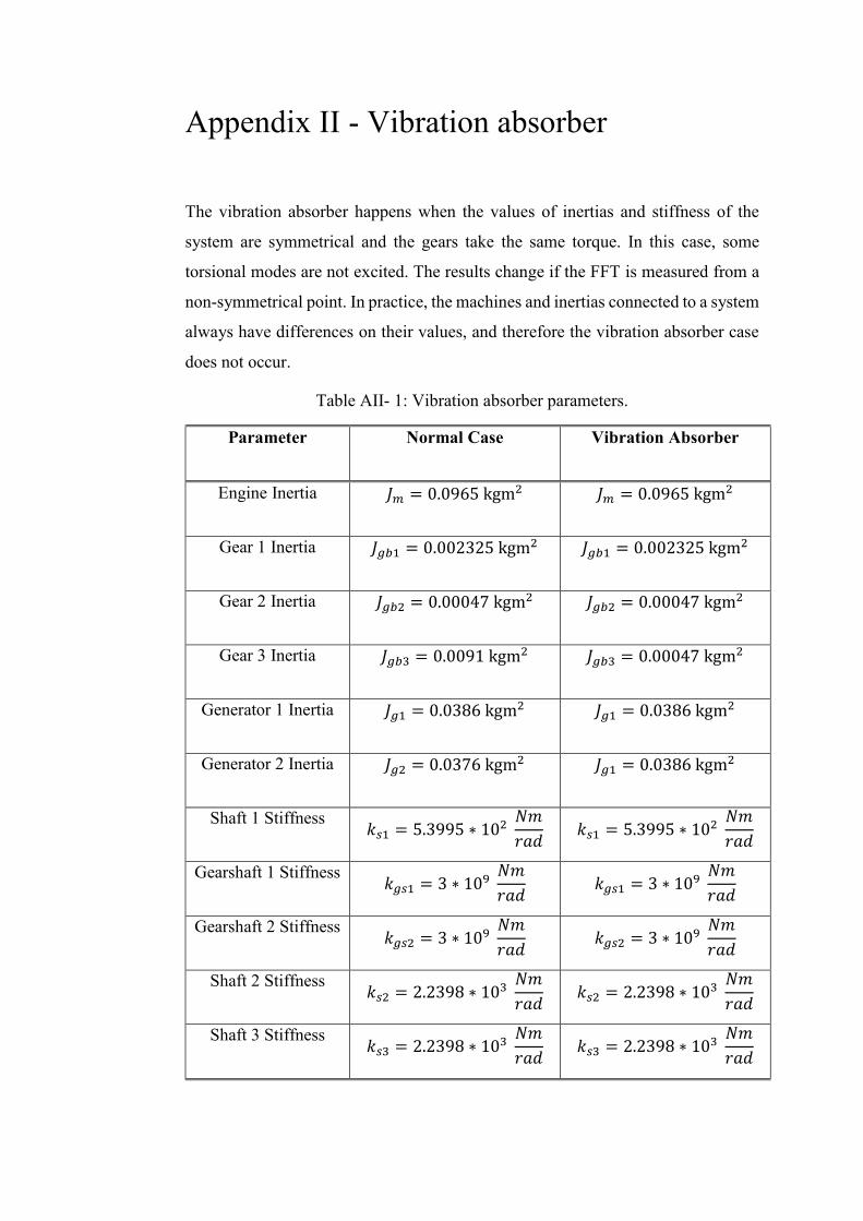
Appendix II - Vibration absorber
The vibration absorber happens when the values of inertias and stiffness of the
system are symmetrical and the gears take the same torque. In this case, some
torsional modes are not excited. The results change if the FFT is measured from a
non-symmetrical point. In practice, the machines and inertias connected to a system
always have differences on their values, and therefore the vibration absorber case
does not occur.
Table AII- 1: Vibration absorber parameters.
Parameter Normal Case Vibration Absorber
Engine Inertia 𝐽𝑚 = 0.0965 kgm2 𝐽𝑚 = 0.0965 kgm2
Gear 1 Inertia 𝐽𝑔𝑏1 = 0.002325 kgm2 𝐽𝑔𝑏1 = 0.002325 kgm
2
Gear 2 Inertia 𝐽𝑔𝑏2 = 0.00047 kgm2 𝐽𝑔𝑏2 = 0.00047 kgm2
Gear 3 Inertia 𝐽𝑔𝑏3 = 0.0091 kgm2 𝐽𝑔𝑏3 = 0.00047 kgm2
Generator 1 Inertia 𝐽𝑔1 = 0.0386 kgm2 𝐽𝑔1 = 0.0386 kgm
2
Generator 2 Inertia 𝐽𝑔2 = 0.0376 kgm2 𝐽𝑔1 = 0.0386 kgm
2
Shaft 1 Stiffness 𝑘𝑠1 = 5.3995 ∗ 102
𝑁𝑚
𝑟𝑎𝑑 𝑘𝑠1 = 5.3995 ∗ 102
𝑁𝑚
𝑟𝑎𝑑
Gearshaft 1 Stiffness 𝑘𝑔𝑠1 = 3 ∗ 10
9 𝑁𝑚
𝑟𝑎𝑑 𝑘𝑔𝑠1 = 3 ∗ 10
9 𝑁𝑚
𝑟𝑎𝑑
Gearshaft 2 Stiffness 𝑘𝑔𝑠2 = 3 ∗ 10
9 𝑁𝑚
𝑟𝑎𝑑 𝑘𝑔𝑠2 = 3 ∗ 10
9 𝑁𝑚
𝑟𝑎𝑑
Shaft 2 Stiffness 𝑘𝑠2 = 2.2398 ∗ 103
𝑁𝑚
𝑟𝑎𝑑 𝑘𝑠2 = 2.2398 ∗ 103
𝑁𝑚
𝑟𝑎𝑑
Shaft 3 Stiffness 𝑘𝑠3 = 2.2398 ∗ 103
𝑁𝑚
𝑟𝑎𝑑 𝑘𝑠3 = 2.2398 ∗ 103
𝑁𝑚
𝑟𝑎𝑑

APPENDIX II - VIBRATION ABSORBER
248
To show its effects, the aircraft model presented in chapter 4 and the data from
Table AII- 1 are used. Table AII- 1 presents two cases: symmetrical and non-
symmetrical parameters. To both data cases, a step torque connection is applied in
generator 2. Measuring the torque in the second generator shaft, and calculating the
FFT, Figure AII- 1 is obtained. Comparing (a) and (b), it is observed that in the
case of applying a step connection to a system with symmetrical parameters, the
third vibration mode is not excited. For this reason, it is important to not use
symmetrical parameters in simulation analysis.
Figure AII- 1: Vibration absorber FFT.

References
[1] R. Seresinhe and C. Lawson, “Electrical load-sizing methodology to aid
conceptual and preliminary design of large commercial aircraft,” Proc. Inst.
Mech. Eng. Part G J. Aerosp. Eng., vol. 229, no. 3, pp. 445–466, Mar. 2015.
[2] A. Boglietti, A. Cavagnino, A. Tenconi, S. Vaschetto, and P. di Torino, “The
safety critical electric machines and drives in the more electric aircraft: A
survey,” in 2009 35th Annual Conference of IEEE Industrial Electronics,
2009, pp. 2587–2594.
[3] M. J. Provost, “The More Electric Aero-engine: a general overview from an
engine manufacturer,” in International Conference on Power Electronics
Machines and Drives, 2002, vol. 2002, pp. 246–251.
[4] Acare, “Strategic Research & Innovation Agenda,” Brussels, Belgium, 2017.
[5] J. Chen, C. Wang, and J. Chen, “Investigation on the Selection of Electric
Power System Architecture for Future More Electric Aircraft,” IEEE Trans.
Transp. Electrif., vol. PP, no. 99, p. 1, 2018.
[6] J. A. Rosero, J. A. Ortega, E. Aldabas, and L. Romeral, “Moving towards a
more electric aircraft,” IEEE Aerosp. Electron. Syst. Mag., vol. 22, no. 3, pp.
3–9, Mar. 2007.
[7] J. A. Weimer, “Electrical power technology for the more electric aircraft,”
in [1993 Proceedings] AIAA/IEEE Digital Avionics Systems Conference,
1993, pp. 445–450.
[8] R. I. Jones, “The More Electric Aircraft: the past and the future?,” in IEE
Colloquium. Electrical Machines and Systems for the More Electric Aircraft,
1999, vol. 1999, pp. 1–1.
[9] P. W. Wheeler, J. C. Clare, A. Trentin, and S. Bozhko, “An overview of the
more electrical aircraft,” Proc. Inst. Mech. Eng. Part G J. Aerosp. Eng., vol.
227, no. 4, pp. 578–585, Apr. 2013.
[10] M. J. J. Cronin, “The all-electric aircraft,” IEE Rev., vol. 36, no. 8, p. 309,
1990.

REFERENCES
250
[11] R. T. Naayagi, “A review of more electric aircraft technology,” Energy
Efficient Technologies for Sustainability (ICEETS), 2013 International
Conference on. pp. 750–753, 2013.
[12] I. Moir, “The all-electric aircraft - major challenges,” in IEE Colloquium on
All Electric Aircraft, 1998, vol. 1998, pp. 2–2.
[13] L. J. Feiner, “Power-by-wire aircraft secondary power systems,” in [1993
Proceedings] AIAA/IEEE Digital Avionics Systems Conference, 1993, pp.
439–444.
[14] T. Yang, “Development of Dynamic Phasors for the Modelling of Aircraft
Electrical Power Systems By,” Phd Thesis University of Nottingham, 2013.
[15] B. Sarlioglu and C. T. Morris, “More Electric Aircraft: Review, Challenges,
and Opportunities for Commercial Transport Aircraft,” IEEE Trans. Transp.
Electrif., vol. 1, no. 1, pp. 54–64, Jun. 2015.
[16] P. J. Norman, S. J. Galloway, G. M. Burt, D. R. Trainer, and M. Hirst,
“Transient analysis of the more-electric engine electrical power distribution
network,” Power Electronics, Machines and Drives, 2008. PEMD 2008. 4th
IET Conference on. pp. 681–685, 2008.
[17] P. J. J. Norman, S. J. J. Galloway, G. M. M. Burt, J. E. E. Hill, and D. R. R.
Trainer, Evaluation of the dynamic interactions between aircraft gas turbine
engine and electrical system. York: IET, 2008, pp. 671–675.
[18] T. Feehally, I. E. Damian, and J. M. Apsley, “Analysis of Electromechanical
Interaction in Aircraft Generator Systems,” IEEE Trans. Ind. Appl., vol. 52,
no. 5, pp. 4327–4336, Sep. 2016.
[19] G. Moore, “Electro-Mechanical Interactions in Aerospace Gas Turbines,”
University of Nottingham, 2012.
[20] M. A. Valenzuela, J. M. Bentley, and R. D. Lorenz, “Evaluation of Torsional
Oscillations in Paper Machine Sections,” IEEE Trans. Ind. Appl., vol. 41,
no. 2, pp. 493–501, Mar. 2005.
REFERENCES
251
[21] Li Ran, Dawei Xiang, and J. L. Kirtley, “Analysis of Electromechanical
Interactions in a Flywheel System With a Doubly Fed Induction Machine,”
IEEE Trans. Ind. Appl., vol. 47, no. 3, pp. 1498–1506, May 2011.
[22] M. Yang, C. Wang, D. Xu, W. Zheng, and X. Lang, “Shaft Torque Limiting
Control Using Shaft Torque Compensator for Two-Inertia Elastic System
With Backlash,” IEEE/ASME Trans. Mechatronics, vol. 21, no. 6, pp. 2902–
2911, Dec. 2016.
[23] W. C. Carter, “Mechanical Factors Affecting Electrical Drive Performance,”
IEEE Trans. Ind. Gen. Appl., vol. IGA-5, no. 3, pp. 282–290, May 1969.
[24] M. A. Valenzuela, J. M. Bentley, and R. D. Lorenz, “Evaluation of torsional
oscillations in paper machine sections,” in Conference Record of 2004
Annual Pulp and Paper Industry Technical Conference (IEEE Cat.
No.04CH37523), 2004, pp. 15–22.
[25] R. Muller, D. Schmitt, and J. Kimber, “Create - Creating innovative air
transport technologies for Europe,” Brussels, Belgium, 2010.
[26] M. Bailey, “Distributed electrical power management architecture,” in IEE
Colloquium. Electrical Machines and Systems for the More Electric Aircraft,
1999, vol. 1999, pp. 7–7.
[27] I. Moir and A. Seabridge, Aircraft Systems. Chichester, UK: John Wiley &
Sons, Ltd, 2008.
[28] Wenping Cao, B. C. Mecrow, G. J. Atkinson, J. W. Bennett, and D. J.
Atkinson, “Overview of Electric Motor Technologies Used for More
Electric Aircraft (MEA),” IEEE Trans. Ind. Electron., vol. 59, no. 9, pp.
3523–3531, Sep. 2012.
[29] M. E. Elbuluk and M. D. Kankam, “Potential starter/generator technologies
for future aerospace applications,” IEEE Aerosp. Electron. Syst. Mag., vol.
12, no. 5, pp. 24–31, May 1997.
[30] Jie Chang and Anhua Wang, “New VF-power system architecture and
evaluation for future aircraft,” IEEE Trans. Aerosp. Electron. Syst., vol. 42,

REFERENCES
252
no. 2, pp. 527–539, Apr. 2006.
[31] K. Emadi and M. Ehsani, “Aircraft power systems: technology, state of the
art, and future trends,” IEEE Aerosp. Electron. Syst. Mag., vol. 15, no. 1, pp.
28–32, 2000.
[32] A. Garcia, J. Cusido, J. A. Rosero, J. A. Ortega, and L. Romeral, “Reliable
electro-mechanical actuators in aircraft,” IEEE Aerosp. Electron. Syst. Mag.,
vol. 23, no. 8, pp. 19–25, Aug. 2008.
[33] L. Han, J. Wang, and D. Howe, “Stability assessment of distributed Dc
power systems for ‘more- electric’ aircraft,” in 4th IET International
Conference on Power Electronics, Machines and Drives (PEMD 2008),
2008, pp. 661–665.
[34] B. MacIsaac and R. Langton, Gas Turbine Propulsion Systems. Chichester,
UK: John Wiley & Sons, Ltd, 2011.
[35] S. J. Khalid, “Mitigating Impact of Bleed and Power Extraction with More
Electric Architectures,” in SAE Technical Paper, 2016.
[36] R. Newman, “The more electric engine concept,” SAE Tech. Pap., no. 2004–
013128.
[37] T. Feehally, “Electro-mechanical Interaction in Gas Turbine-generator
Systems for More-electric Aircraft,” PhD Thesis University of Manchester,
2012.
[38] A. Griffo and J. Wang, “Stability assessment of electric power systems for
more electric aircraft,” Power Electronics and Applications, 2009. EPE ’09.
13th European Conference on. pp. 1–10, 2009.
[39] L. Han, J. Wang, and D. Howe, “Small-signal stability studies of a 270V DC
more-electric aircraft power system,” in IET Internation Conference on
Power Electronics Machines and Drives, 2006, pp. 162–166.
[40] I. Chakraborty, D. N. Mavris, M. Emeneth, and A. Schneegans, “A
methodology for vehicle and mission level comparison of More Electric
REFERENCES
253
Aircraft subsystem solutions: Application to the flight control actuation
system,” Proc. Inst. Mech. Eng. Part G J. Aerosp. Eng., vol. 229, no. 6, pp.
1088–1102, May 2015.
[41] P. Kundur, Power System Stability and Control, 1st ed. New York: McGraw-
Hill Professional Publishing, 1994.
[42] L. Han, J. Wang, A. Griffo, and D. Howe, “Stability assessment of AC
hybrid power systems for more electric aircraft,” in 2008 IEEE Vehicle
Power and Propulsion Conference, 2008, pp. 1–6.
[43] F. Barruel, N. Retiere, and J. L. Schanen, “Stability analysis for aircraft on-
board system,” in 3rd IET International Conference on Power Electronics,
Machines and Drives (PEMD 2006), 2006, vol. 2006, no. 33, pp. 361–367.
[44] K.-N. Areerak, T. Wu, S. V. Bozhko, G. M. Asher, and D. W. P. Thomas,
“Aircraft Power System Stability Study Including Effect of Voltage Control
and Actuators Dynamic,” IEEE Trans. Aerosp. Electron. Syst., vol. 47, no.
4, pp. 2574–2589, 2011.
[45] L. C. Herrera and B.-H. Tsao, “Analysis and Control of Energy Storage in
Aircraft Power Systems with Pulsed Power Loads,” SAE Int. J. Aerosp., vol.
9, no. 1, pp. 2016-01–1981, Sep. 2016.
[46] F. Gao, S. Bozhko, and P. Wheeler, “An Enhanced Secondary Control
Approach for Voltage Restoration in the DC Distribution System,” in SAE
Technical Papers, 2016.
[47] T. Wu, “Integrative System Modelling of Aircraft Electrical Power
Systems,” Phd Thesis University of Nottingham, 2010.
[48] H. Cohen and G. Rogers, Gas turbine theory, 4th ed. Essex, 1996.
[49] M. I. Friswell, J. E. T. Penny, S. D. Garvey, and A. W. Lees, Dynamics of
Rotating Machines. Cambridge University Press, 2010.
[50] D. J. Sheppard, “Torsional vibration resulting from adjustable-frequency AC
drives,” IEEE Trans. Ind. Appl., vol. 24, no. 5, pp. 812–817, 1988.

REFERENCES
254
[51] IEEE, “Proposed Terms and Definitions for Subsynchronous Oscillations,”
IEEE Trans. Power Appar. Syst., vol. PAS-99, no. 2, pp. 506–511, 1980.
[52] D. N. Walker, C. E. J. Bowler, R. L. Jackson, and D. A. Hodges, “Results of
subsynchronous resonance test at Mohave,” IEEE Trans. Power Appar.
Syst., vol. 94, no. 5, pp. 1878–1889, Sep. 1975.
[53] J. H. Holdrege, W. Subler, and W. E. Frasier, “AC Induction Motor
Torsional Vibration Consideration - A Case Study,” IEEE Trans. Ind. Appl.,
vol. IA-19, no. 1, pp. 68–73, Jan. 1983.
[54] J. Song-Manguelle, J.-M. Nyobe-Yome, and G. Ekemb, “Pulsating Torques
in PWM Multi-Megawatt Drives for Torsional Analysis of Large Shafts,”
IEEE Trans. Ind. Appl., vol. 46, no. 1, pp. 130–138, 2010.
[55] S. N. Vukosavic and M. R. Stojic, “Suppression of torsional oscillations in
a high-performance speed servo drive,” IEEE Trans. Ind. Electron., vol. 45,
no. 1, pp. 108–117, 1998.
[56] G. W. Buckley, “The effects of torsional elements on the transient
performance of large induction motor drives,” Electr. Mach. Power Syst.,
vol. 5, no. 1, pp. 53–64, Jan. 1980.
[57] D. Ramey, A. Sismour, and G. Kung, “Important Parameters in Considering
Transient Torques on Turbine-Generator Shaft Systems,” IEEE Trans.
Power Appar. Syst., vol. PAS-99, no. 1, pp. 311–317, Jan. 1980.
[58] A. Gaikwad and P. Rajarapollu, “Analysis of mechanical stresses developed
on T-G shaft during faults,” Information and Communication Technology in
Electrical Sciences (ICTES 2007), 2007. ICTES. IET-UK International
Conference on. pp. 126–131, 2007.
[59] D. N. Walker, S. L. Adams, and R. J. Placek, “Torsional Vibration and
Fatigue of Turbine-Generator shafts,” IEEE Trans. Power Appar. Syst., vol.
PAS-100, no. 11, pp. 4373–4380, Nov. 1981.
[60] P. Pourbeik, D. G. Ramey, N. Abi-Samra, D. Brooks, and A. Gaikwad,
“Vulnerability of Large Steam Turbine Generators to Torsional Interactions
REFERENCES
255
During Electrical Grid Disturbances,” Power Systems, IEEE Transactions
on, vol. 22, no. 3. pp. 1250–1258, 2007.
[61] R. L. Steigerwald, G. W. Ludwig, and R. Kollman, “Investigation of power
distribution architectures for distributed avionics loads,” in Proceedings of
PESC ’95 - Power Electronics Specialist Conference, 1995, vol. 1, pp. 231–
237.
[62] A. A. Shaltout, “Analysis of torsional torques in starting of large squirrel
cage induction motors,” IEEE Trans. Energy Convers., vol. 9, no. 1, pp.
135–142, Mar. 1994.
[63] I. M. Elders, P. J. Norman, J. D. Schuddebeurs, C. D. Booth, G. M. Burt, J.
R. McDonald, J. Apsley, M. Barnes, A. Smith, S. Williamson, S. Loddick,
and I. Myers, “Modelling and Analysis of Electro-Mechanical Interactions
between Prime-Mover and Load in a Marine IFEP System,” in 2007 IEEE
Electric Ship Technologies Symposium, 2007, pp. 77–84.
[64] S. Higuchi, M. Ishida, and T. Hori, “Reduction of mechanical vibration of
an induction motor with pulsating torque load by feedforward control
utilizing an acceleration sensor and a timing sensor,” in Proceedings of 4th
IEEE International Workshop on Advanced Motion Control - AMC ’96 -
MIE, vol. 1, pp. 316–320.
[65] J. K. Kambrath, A. A. Ayu, Y. Wang, Y.-J. Yoon, X. Liu, C. J. Gajanayake,
and A. K. Gupta, “Dynamic study of electromechanical interaction in marine
propulsion,” in 2016 IEEE Energy Conversion Congress and Exposition
(ECCE), 2016, pp. 1–8.
[66] X. Lei, B. Buchholz, and D. Povh, “Analysing subsynchronous resonance
phenomena in the time- and frequency domain,” Eur. Trans. Electr. Power,
vol. 10, no. 4, pp. 203–211, Sep. 2007.
[67] S. Goldberg and W. Schmus, “Subsynchronous Resonance and Torsional
Stresses in Turbine-Generator Shafts,” IEEE Trans. Power Appar. Syst., vol.
PAS-98, no. 4, pp. 1233–1237, Jul. 1979.
REFERENCES
256
[68] C. Concordia and G. K. Carter, “Negative Damping of Electrical
Machinery,” Trans. Am. Inst. Electr. Eng., vol. 60, no. 3, pp. 116–119, Mar.
1941.
[69] “Reader’s guide to subsynchronous resonance,” IEEE Trans. Power Syst.,
vol. 7, no. 1, pp. 150–157, 1992.
[70] P. Kumar Ȧ, U. K. Agarwal Ḃ, and V. Kumar Sharma Ȧ, “Design of
Controller for Chopper Fed DC Drive with Pulsating Load and Elastic
Coupling under Resonance,” Int. J. Curr. Eng. Technol., vol. 44, no. 44,
2450.
[71] D. Sen Gupta, Ce. N. MIEE Narahari ME I Boyd, and B. Hogg CEng, “An
adaptive power-system stabiliser which cancels the negative damping torque
of a synchronous generator List of symbols.”
[72] J. S. Joyce, T. Kulig, and D. Lambrecht, “Torsional Fatigue of Turbine-
Generator Shafts Caused by Different Electrical System Faults and
Switching Operations,” Power Apparatus and Systems, IEEE Transactions
on, vol. PAS-97, no. 5. pp. 1965–1977, 1978.
[73] R. Dhaouadi, K. Kubo, and M. Tobise, “Analysis and compensation of speed
drive systems with torsional loads,” IEEE Trans. Ind. Appl., vol. 30, no. 3,
pp. 760–766, 1994.
[74] B. A. Leishman, S. J. Drew, and B. J. Stone, “Torsional vibration of a back-
to-back gearbox rig Part 1: frequency domain modal analysis,” Proc. Inst.
Mech. Eng. Part K J. Multi-body Dyn., vol. 214, no. 3, pp. 143–162, Jan.
2000.
[75] D. Melot de Beauregard, A. Conradi, B. Benthaus, and L. Golebiowski,
“Electromechanical roller conveyor model with enhanced consideration of
roller-belt interaction,” in 2012 IEEE International Conference on
Automation and Logistics, 2012, pp. 7–12.
[76] S. H. Kia, H. Henao, and G.-A. Capolino, “Torsional Vibration Effects on
Induction Machine Current and Torque Signatures in Gearbox-Based

REFERENCES
257
Electromechanical System,” IEEE Trans. Ind. Electron., vol. 56, no. 11, pp.
4689–4699, Nov. 2009.
[77] K.-S. Ou and K.-S. Chen, “Developing Electromechanical Coupling Macro
Models for Dynamic Responses of MEMS Structures With Command
Shaping Techniques,” IEEE Trans. Device Mater. Reliab., vol. 16, no. 2, pp.
123–131, Jun. 2016.
[78] P. Schmidt and T. Rehm, “(2)Notch Filter Tuning for Resonant Frequency
Reduction in Dual Inertia Systems,” Transform, vol. 3, no. 1, pp. 1730–1734,
1999.
[79] G. Ellis and R. D. Lorenz, “Resonant load control methods for industrial
servo drives,” Conf. Rec. 2000 IEEE Ind. Appl. Conf., vol. 3, pp. 1438–1445,
2000.
[80] T. J. Hammons and L. Chanal, “Measurement of torque in steam turbine-
generator shafts following severe disturbances on the electrical supply
system-analysis and implementation,” IEEE Transactions on Energy
Conversion, vol. 6, no. 1. pp. 193–203, 1991.
[81] V. Atarod, P. L. Dandeno, and M. R. Iravani, “Impact of synchronous
machine constants and models on the analysis of torsional dynamics,” IEEE
Trans. Power Syst., vol. 7, no. 4, pp. 1456–1463, 1992.
[82] L. Feng, W. Gao, C. Tan, H. Qin, B. Xie, and Z. Hao, “Observer-Based
Active Control of Torsional Vibration for Large Turbine-Generator Shaft
System,” in 2010 Asia-Pacific Power and Energy Engineering Conference,
2010, pp. 1–5.
[83] R. Fadaeinedjad, M. Moallem, and G. Moschopoulos, “Simulation of a Wind
Turbine With Doubly Fed Induction Generator by FAST and Simulink,”
IEEE Trans. Energy Convers., vol. 23, no. 2, pp. 690–700, Jun. 2008.
[84] D. S. Ochs, R. D. Miller, and W. N. White, “Simulation of electromechanical
interactions of permanent-magnet direct-drive wind turbines using the fast
aeroelastic simulator,” IEEE Trans. Sustain. Energy, vol. 5, no. 1, pp. 2–9,
REFERENCES
258
2014.
[85] Hong Fu, Chao Feng, and Shan Xue, “Vibration suppression control of an
integrated powertrain of electric and hybrid vehicles using LQR controller
and reduced-order observer,” in 2014 IEEE Conference and Expo
Transportation Electrification Asia-Pacific (ITEC Asia-Pacific), 2014, pp.
1–6.
[86] Q. Wang, K. Rajashekara, Y. Jia, and J. Sun, “A Real-time Vibration
Suppression Strategy in Electric Vehicles,” IEEE Trans. Veh. Technol., pp.
1–1, 2017.
[87] P. J. Norman, C. D. Booth, J. D. Schuddebeurs, G. M. Burt, J. R. McDonald,
J. M. Apsley, M. Barnes, A. C. Smith, S. Williamson, E. Tsoudis, P. Pilidis,
and R. Singh, “Integrated Electrical and Mechanical Modelling of
Integrated-Full-Electric-Propulsion Systems,” Power Electronics, Machines
and Drives, 2006. The 3rd IET International Conference on. pp. 101–105,
2006.
[88] T. Feehally and J. M. Apsley, “The Doubly Fed Induction Machine as an
Aero Generator,” IEEE Trans. Ind. Appl., vol. 51, no. 4, pp. 3462–3471, Jul.
2015.
[89] E. L. Owen, “Flexible shaft versus rigid shaft electric machines for
petroleum and chemical plants,” IEEE Trans. Ind. Appl., vol. 27, no. 2, pp.
245–253, 1991.
[90] S. M. M. Rahman, “A novel variable impedance compact compliant series
elastic actuator for human-friendly soft robotics applications,” in 2012 IEEE
RO-MAN: The 21st IEEE International Symposium on Robot and Human
Interactive Communication, 2012, pp. 19–24.
[91] T. Kakinoki, R. Yokoyama, G. Fujita, T. Nakano, K. Koyanagi, T.
Funabashi, and H. Nara, “Estimation of turbine shaft torques using
observer,” in 2001 IEEE Porto Power Tech Proceedings, 2001, vol. 2, pp.
81–84.

REFERENCES
259
[92] S. Higuchi, M. Ishida, and T. Hori, “Reduction of mechanical vibration of
an induction motor with pulsating torque load by feedforward control
utilizing an acceleration sensor and a timing sensor,” Advanced Motion
Control, 1996. AMC ’96-MIE. Proceedings., 1996 4th International
Workshop on, vol. 1. pp. 316–320 vol.1, 1996.
[93] D. Vrančić and P. M. Oliveira, “Design of feedback control for underdamped
systems,” 2012.
[94] S. Garvey, Z. Chen, M. I. Friswell, and U. Prells, “Model reduction using
structure-preserving transformations,” in Proceedings of the International
Modal Analysis Conference IMAC XXI, 2003, no. 3, pp. 361–377.
[95] M. Friswell, J. E. T. Penny, and S. D. Garvey, “Model reduction for
structures with damping and gyroscopic effects,” in Proceedings of ISMA-
25, 2000, pp. 1151–1158.
[96] C.-M. Ong, Dynamic Simulation of Electric Machinery: Using
MATLAB/SIMULINK. Prentice Hall PTR, 1998.
[97] S. D. Garvey, M. I. Friswell, and U. Prells, “Co-Ordinate Transformations
for Second Order Systems. Part Ii: Elementary Structure-Preserving
Transformations,” J. Sound Vib., vol. 258, no. 5, pp. 885–909, Dec. 2002.
[98] Y. Chahlaoui, D. Lemonnier, K. Meerbergen, A. Vandendorpe, P. Van
Dooren, and K. Gallivan, “Model reduction of second-order systems,”
Dimens. Reduct. …, vol. 1, no. 2, pp. 1–23, 2005.
[99] R. Colgren, “Efficient Model Reduction for the Control of Large-Scale
Systems,” in Efficient Modeling and Control of Large-Scale Systems SE -
2, J. Mohammadpour and K. M. Grigoriadis, Eds. Springer US, 2010, pp.
59–72.
[100] R. Guyan, “Reduction of stiffness and mass matrices,” AIAA J., vol. 3, no.
2, p. 380, 1965.
[101] D. F. Enns, “Model reduction with balanced realizations: An error bound
and a frequency weighted generalization,” Decision and Control, 1984. The

REFERENCES
260
23rd IEEE Conference on, vol. 23. pp. 127–132, 1984.
[102] B. Moore, “Principal component analysis in linear systems: Controllability,
observability, and model reduction,” IEEE Trans. Automat. Contr., vol. 26,
no. 1, pp. 17–32, Feb. 1981.
[103] T. Wu, S. Bozhko, G. Asher, P. Wheeler, and D. Thomas, “Fast Reduced
Functional Models of Electromechanical Actuators for More-Electric
Aircraft Power System Study,” in SAE Power Systems Conference, 2008, p.
12.
[104] C. Gan, R. Todd, and J. Apsley, “HIL emulation for future aerospace
propulsion systems,” Power Electronics, Machines and Drives (PEMD
2014), 7th IET International Conference on. pp. 1–6, 2014.
[105] K. Ogata, Modern control engineering. Prentice-Hall, 2010.
[106] Department of Defense Armed Forced Supply Support, “MIL-STD-704
Military standard characteristics,” 1959.
[107] A. Shenkman, Y. Berkovich, and B. Axelrod, “Pulse converter for induction-
heating applications,” Electric Power Applications, IEE Proceedings -, vol.
153, no. 6. pp. 864–872, 2006.
[108] F. Blaabjerg and S. Munk-Nielsen, “Power losses in PWM-VSI inverter
using NPT or PT IGBT devices,” Power Electronics, IEEE Transactions on,
vol. 10, no. 3. pp. 358–367, 1995.
[109] Gaoyu Zou and Zhengming Zhao, “Research on impacts of different
parameters on transient power loss of IGBT,” in 2013 International
Conference on Electrical Machines and Systems (ICEMS), 2013, pp. 490–
495.
[110] O. J. M. Smith, “Posicast Control of Damped Oscillatory Systems,”
Proceedings of the IRE, vol. 45, no. 9. pp. 1249–1255, 1957.
[111] E. W. Giloy, “An electric deicing system for aircraft,” Transactions of the
American Institute of Electrical Engineers, vol. 69, no. 2. pp. 1051–1057,
REFERENCES
261
1949.
[112] K. Veselić, Damped Oscillations of Linear Systems, 1st ed., vol. 2023.
Berlin, Heidelberg: Springer-Verlag Berlin Heidelberg, 2011.
[113] C. W. de Silva, Vibration: Fundamentals and Practice, Second Edition.
CRC Press, 2011.
[114] G. Tallman and O. Smith, “Analog study of dead-beat posicast control,” IRE
Trans. Autom. Control, vol. 4, no. 1, pp. 14–21, Mar. 1958.
[115] H. Ghorbani, J. I. Candela, A. Luna, and P. Rodriguez, “Posicast control A
novel approach to mitigate multi-machine power system oscillations in
presence of wind farm,” in 2014 IEEE PES General Meeting | Conference
& Exposition, 2014, pp. 1–5.
[116] M. R. Aghamohammadi, A. Ghorbani, and S. Pourmohammad, “Enhancing
transient and small signal stability in power systems using a posicast
excitation controller,” in 2008 43rd International Universities Power
Engineering Conference, 2008, pp. 1–5.
[117] L. Michel, X. Boucher, A. Cheriti, P. Sicard, and F. Sirois, “FPGA
Implementation of an Optimal IGBT Gate Driver Based on Posicast
Control,” IEEE Trans. Power Electron., vol. 28, no. 5, pp. 2569–2575, May
2013.
[118] Y. w. Li, B. Wu, N. Zargari, J. Wiseman, and D. Xu, “An Effective Method
to Suppress Resonance in Input LC Filter of a PWM Current-Source
Rectifier,” in 2006 5th International Power Electronics and Motion Control
Conference, 2006, vol. 2, pp. 1–6.
[119] P. B. M. Oliveira and D. Vrančić, “Underdamped Second-Order Systems
Overshoot Control,” IFAC Proc. Vol., vol. 45, no. 3, pp. 518–523, 2012.
[120] P. H. Meckl, “Control of Vibration in Mechanical Systems Using Shaped
Reference Inputs,” MIT Artificial Intelligence Laboratory, 1988.
[121] T. Singh and W. Singhose, “Input shaping/time delay control of
REFERENCES
262
maneuvering flexible structures,” in Proceedings of the 2002 American
Control Conference (IEEE Cat. No.CH37301), 2002, pp. 1717–1731 vol.3.
[122] J. Currie and D. I. Wilson, “OPTI: Lowering the Barrier Between Open
Source Optimizers and the Industrial MATLAB User,” in Foundations of
Computer-Aided Process Operations, 2012.
[123] Huijun Wang, Dong-Hee Lee, Zhen-Guo Lee, and Jin-Woo Ahn, “Vibration
Rejection Scheme of Servo Drive System with Adaptive Notch Filter,” in
37th IEEE Power Electronics Specialists Conference, 2006, pp. 1–6.
[124] C. Ahumada Sanhueza, A. Bristot, S. Kumar, N. Schneider, S. Garvey, and
H. Morvan, “An Integrated System’s Approach Towards Aero Engine
Subsystems Design,” 2016.
[125] F. M. Atay, “Magnetic saturation and steady-state analysis of electrical
motors,” Appl. Math. Model., vol. 24, no. 11, pp. 827–842, 2000.
[126] ABB, User’s manual ACS150 drives. ABB, 2016.
[127] Infineon, “AP16133 XE166 ‘Cookery-Book.’” pp. 1–130, 2008.
[128] W. Lu, X. Du, J. Ding, and X. Wang, “Modal parameter identification based
on fast fourier transform and Hilbert Huang transform,” in 2012 2nd
International Conference on Consumer Electronics, Communications and
Networks (CECNet), 2012, pp. 2703–2706.
[129] C. B. Smith and N. M. Wereley, “Transient analysis for damping
identification in rotating composite beams with integral damping layers,”
Smart Mater. Struct., vol. 5, no. 5, pp. 540–550, Oct. 1996.
[130] M. S. Arefeen, M. Ehsani, and A. Lipo, “Sensorless position measurement
in synchronous reluctance motor,” IEEE Trans. Power Electron., vol. 9, no.
6, pp. 624–630, 1994.
[131] P. Phumiphak and C. Chat-uthai, “Induction motor speed measurement
using motor current signature analysis technique,” in 2009 International
Conference on Electrical Machines and Systems, 2009, pp. 1–5.
REFERENCES
263
[132] D. Kumar and P. Radcliffe, “Sensorless speed measurement for brushed DC
motors,” IET Power Electron., vol. 8, no. 11, pp. 2223–2228, Nov. 2015.
[133] A.-C. Lee, C.-J. Fan, and G.-H. Chen, “Current Integral Method for Fine
Commutation Tuning of Sensorless Brushless DC Motor,” IEEE Trans.
Power Electron., vol. 32, no. 12, pp. 9249–9266, Dec. 2017.
[134] H. Li, S. Zheng, and H. Ren, “Self-Correction of Commutation Point for
High-Speed Sensorless BLDC Motor With Low Inductance and Nonideal
Back EMF,” IEEE Trans. Power Electron., vol. 32, no. 1, pp. 642–651, Jan.
2017.
[135] A. B. Ataji, Y. Miura, T. Ise, and H. Tanaka, “A Rotor-Current-Based Slip
Angle Estimator for Grid-Connected Doubly Fed Induction Generator
Requiring the Stator Inductance Only,” IEEE Trans. Power Electron., vol.
32, no. 6, pp. 4827–4838, Jun. 2017.
[136] D. Liang, J. Li, and R. Qu, “Sensorless Control of Permanent Magnet
Synchronous Machine Based on Second-Order Sliding-Mode Observer With
Online Resistance Estimation,” IEEE Trans. Ind. Appl., vol. 53, no. 4, pp.
3672–3682, Jul. 2017.
[137] A.-C. Lee, C.-J. Fan, and G.-H. Chen, “Current Integral Method for Fine
Commutation Tuning of Sensorless Brushless DC Motor,” IEEE Trans.
Power Electron., vol. 32, no. 12, pp. 9249–9266, Dec. 2017.
Copyright © 2022 FDOKUMEN