1

Abstract— In power systems are normally localized linear controllers placed at several subsystems located in different geographical zones. In addition, there have been introduced new technologies of non-linear control, with applied methodologies of feedback linearization, where all the system is transformed to a linear system. Nevertheless, the decentralized scheme is not possible because all the information of the entire system is required when that transformation is done. That is why it must be developed a controller that maintains the decentralization at the same time as the robustness.

The procedure detailed in this paper consists of the utilization of reduced dynamical models computed at each FACTS device useful for the computation of supplementary controls. So, a decentralized model is done from a linear model, where there are the local controls for each device and a central control that gives the reference. The paper also describes the methodology used for computing optimal LQG/LTR decentralized controls for FACTS and, previously, it is outlined the problem to locate the FACTS devices and know its dimensions.

Index Terms— Decentralized control, Electromechanical oscillations, LQG/LTR, Modal analysis, Power system stability, SVC, TCSC.

I INTRODUCTION 

n power systems (PS) are normally localized controllers, such as the PSS at generators and supplementary controllers

at FACTS. In addition, a PS has many subsystems that are located in different geographical zones.

For each one of these subsystems, there is a control that is localized and has the information of the state variables of the system, events that happened and in general, many of the possible operating conditions. That is the reason of designing simple behavior analysis in the affected zone or small-signal models. Besides, the solely presence of the FACTS does not totally improve the stability. That is why there is also required a type of supplementary control for these devices.

The electromechanical oscillations can be damped with different control devices. In the objectives of damping, there is the voltage support and load flow stabilization. The controllers allow that the open-loop can be closed-loop. So, in PSS (the Power System Stabilizers are the controllers of the generators) as in FACTS, the feedback signals are the generator velocities, the active power of generators, mechanical power, etc. [1]. Although FACTS are in the transmission systems, local

D. Cerón has obtained his M.Sc degree in electrical engineering at

Universidad de los Andes (e-mail d.ceron144@egresados.uniandes.edu.co) M.A. Ríos is an Associate Professor at the Dept. of Electrical Engineering

and Electronics at Universidad de los Andes, Bogotá, Colombia. (e-mail: mrios@uniandes.edu.co).

signals are preferred, such as the power deviation ∆P in the line, bus voltages or nodal currents [2].

The damping helps to increase the power transfer through the system. For the SVC, the control is made over its susceptance. For the TCSC, the control is made over the line reactance or over the thyristor firing angle α. The control over α produces a variable capacitance that compensates the line inductance and it so controls the flow. However, the application of these controllers to damp the interarea oscillations and also local oscillations over a wide range of different operating conditions is difficult to achieve [3]. Besides, when installing multiple controllers, the dynamic behavior may not be improved and the tuning of the controllers affects the others and the system is lead to instability conditions [4].

For the PSS tuning with the supplementary controllers of the FACTS, there may be different approaches to the problem: the conventional and the modern ones. The conventional [5], [6] is based on the modal analysis, determining the residue for the location of the PSS and the supplementary controllers of the FACTS. Next, there are calculated the controller parameters in different operating conditions and finally, some time-domain simulations are done in critical conditions, such as ground faults or line outages [5].

The modern approaches explore techniques of optimization to decrease the oscillations damping in a direct way [7] or indirect of the SVC [8] or of the TCSC [9], or use fuzzy modeling techniques [5], [10]. In these techniques it is also used the residue method to know the allocation of the FACTS and of the PSS, as so the feedback signal.

So, there have been introduced new technologies of non-linear control, with applied methodologies of feedback linearization, where all the system is transformed to a linear system. Nevertheless, the decentralized scheme is not possible because all the information of the entire system is required when that transformation is done. That is why it must be developed a controller that maintains the decentralization at the same time as the robustness.

The procedure detailed in this paper consists of the utilization of reduced dynamical models computed at each FACTS device useful for the computation of supplementary controls. In consequence, a decentralized model is done from a linear model, where there are the local controls for each device and a central control that gives the reference.

Section II presents the basic idea of modeling the power system by reduced models, placement of FACTS devices and computation of LQG/LTR decentralized control for FACTS.

Section III describes in detail the characteristics of the test system to be analyzed, and Section IV presents simulations and results.

D. Ceron, M. A. Rios, IEEE Member d.ceron144@egresados.uniandes.edu.co, mrios@uniandes.edu.co

Combining Voltage Stability Margin and Electromechanical Damping for FACTS

I

2

II POWER SYSTEMS MODELING 

A. Modal Analysis

The power system is represented by the small-signal analysis as a set of differential-algebraic equations [11]:

),(0

),(

yxg

BuxAyxfx S

(1)

where x is the state variables vector and y the algebraic variables vector that are the voltage amplitudes V and phases θ.

The state matrix AS can be calculated by means of the jacobian matrix AC, which is defined by means of the linearization of this set of equations, as:

y

xA

y

x

GG

FF

y

x

gg

ffxC

yx

yx

yx

yx

0

(2)

xyyxS GGFFA 1 (3)

In the same way, for obtaining the realization of this system through the Jacobian matrix, the following calculations are made:

FACTSuyFACTS GGD ,1 (4)

FACTSyFACTS DFB (5)

Xyy GGC 1 (6)

The modal analysis technique allows the computation of Eigenvalues λ and left (w) and right (v) Eigenvectors of matrix AS, where

iii j (7) Some important parameters can be calculated from each

complex mode; such as: the oscillation frequency fi and the damping factor ζi:

2i

iw

f (8)

22

i

i (9)

In addition, the modal analysis technique allows the computation of participation factors; which defines an association measure of modes and state variables, which measure the relative participation of the state variable i with the mode j [12]. In general, the participation factors are computed as:

n

kkjjk

jiijij

vw

vwp

1

(10)

B. Placement of FACTS

So, using a classical approach, if the system realization is:

DsGDBAsICsG r )()( 1 (11)

where A is the state matrix, B the controllability matrix, C the observability matrix, and D the direct relationship between the input-output matrix, it can be found an important term that relates the observability and controllability, called residue.

The residue method is used to allocate FACTS for damping electromechanical modes and for selection of feedback signals.

The residue is a sensitivity index of the mode to the feedback signal of the input u to the output y. The matrix D is excluded from the modal analysis, since its direct influence does not affect the mode [13]:

n

i i

ir s

RBAsICsG

1

1)(

(12)

BwCvR iii (13)where Ri is the associated residue to the mode λi, Cvi is the modal observability and wiB is the modal controllability.

The singular values of a matrix are determined in a unique way, and for the case of square matrixes for which all singular values are different, the singular vectors are also unique. The number of nonzero singular values in a matrix corresponds to its rank. In general, the singular values are calculated as the squared root of the Eigenvalue of the matrix AHA:

AAA Hii (14)

In addition a combined loadability criteria computed by the Continuation Power Flow (CPF) with power transfer capacity between interconnected areas is used to place the FACTS (SVC and TCSC).

C. Order Reduction

It is useful for some cases to reduce the system to lower orders with the same relevance of information. In this particular case, it is necessary for using the H∞ or the LQG controllers, because these controllers are as least as high as the same order of the open-loop system [14].

The main advantage of this model is that all the parameters of all the machines in the grid are not required to be known, to model the dynamic behavior of the generator in interest, without losing much precision. Besides, the model does not need any computing power and simulation time. On the other hand, as not all of the machines are included, the dynamic parameters of the machines which have not been simulated are kept uncertain.

The main idea of this problem is to design a plant approximation in such way that the difference of its infinity norm is sufficiently small, for example less than 1%. The guaranteed bound for a reasonable reduction is [13]:

n

kiiR HSVjGjG

1

2 (15)

D. LQG Control

The problem of the LQG (linear quadratic Gaussian regulator) consists in the problem solving of the LQR (linear quadratic regulator) with the state estimation problem, with the Kalman filter. The problem of minimization is similar to the LQR to find an optimal controller u(t) which minimizes [15]:

TTTT

TdtRuuzQzEJ

0min (16)

whmalin

y

x

TnoGaV, pro

T

x̂

whKaex

K

whobtha

P

Tadj

u

HLQimthethemalocdetheide

AnoSybu50cribeTh

T[1jacEigCP

Awhhafivthains

here Q is a weatrix for the inear combinatio

vCxy

BuAxx

The vectors w oise, respectiveaussian white n

respectively. ocess.

The Kalman fil

KBuxAx ˆˆ

here the state alman filter g

xpected value sh1 VCPK T

ff

xxE Tk ˆ

here V is a pbservable and Pat solves:

fT

f PAPAP

The matrixes Qdjusted until an

xKu c ˆ

Here the LQGQG) is used, w

mproved, as thee system robuse observation argins, obtainecal feedback sicentralized LQe product of Centity matrix an

As test system odes system (Fiystem and the Nut close to volt0 and a TCSC iterion that usetween areas an

hen, a LQG/LTThe simulation1]. The first cobian matrix genvalues, prePF for this systAs it is shown,hich indicates and, the dynamve, which indicat the system stability. This i

eighting matrixnputs and z con, and states aw

and v are theely, assuming noise process, wThe matrix Γ

lter structure is

xCyK f ˆ

variables aregain shown inhown in (20).

xx ˆ

positive definiPf is the only s

1 f

Tf CPVCP

Q, R, W and Vacceptable des

G/LTR (loop where the LQGe state estimatistness, as the c

(Kalman filted by the LQRignals as in theQG/LTR contrC times CT. Tnd Γ as Q time

III TES

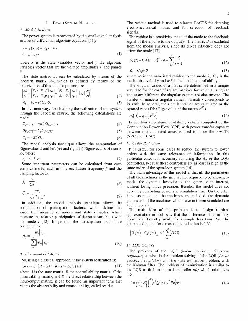
has been used ig. 1). It is a co

New York Powetage and transiat line 41-42

es: power systend the residue

TR supplementns were done

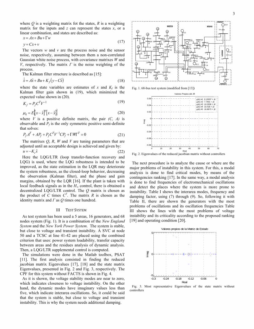
analysis conEigenvalues [

esented in Fig. tem without FA, the voltage scloseness to v

mic modes hacate interarea ois stable, but

is why the syst

x fot the states,can represent tare described a

e process noisbetween themwith covariancΓ is the noise

described as [

e estimates of n (19), which

ite matrix, thymmetric posi

0 TW

V are tuning pasign is achieve

transfer-functiG robustness ion in the LQRlosed-loop behter), and the

R [16]. If the pe H∞ control, throl. The Q maThe matrix R es one hundred

ST SYSTEM 

a 5 areas, 16 gombination of er System. Theient instabilityare placed usi

em loadability,es analysis of dal control is coin the Matlab

sisted in find[17], [18] and2 and Fig. 3,

ACTS is showntability modes

voltage instabilave imaginary oscillations. So

close to voltatem needs addi

, R is a weightthe states x, oas:

(

se and the senm a non-correlace matrixes W weighting of

[15]:

(

f x and Kf is h minimized

(

(

e pair (C, A)itive semi-defin

(

arameters that ed and given by

(on recovery ais intended toR may deteriorhavior, decreas

phase and glant is taken where is obtaineatrix is chosenis chosen as

d.

generators, andthe New Engla

e system is staby. A SVC at ning the combin, transfer capacdynamic analyomputed. b toolbox, PSding the redud the state ma

respectively. Tn in Fig. 4. s are near to zelity. On the otvalues less th

o, it could be sage and transiitional damping

ting or a

(17)

nsor ated and the

(18)

the the

(19)

(20)

) is nite

(21)

are y: (22) and be rate sing gain with ed a n as

the

d 68 and ble, ode ned city

ysis.

SAT uced atrix The

ero, ther han said ient g.

Fig. 1. 6

Fig. 2. E

The ne

major panalysiscontingeis done and detinstabilidampingTable IproblemIII showinstabili[19] and

Fig. 3. controller

68-bus test system

Eigenvalues of the

ext procedure roblems of ins

s is done to encies rankingto find frequ

tect the placeity. Table I shg factor, usingII, there are

ms of oscillatiows the lines ity and its critid operating con

Most representars

0 10

-0.08

-0.06

-0.04

-0.02

0

0.02

0.04

0.06

Imag

-0.3 -0.2-5

0

5

Imag

Valo

(modified from [1

reduced jacobian

is to analyze tstability in thisfind critical m [17]. In the saencies of elecs where the sows the interag (7) through shown the g

ons and its oscwith the mo

icality accordinndition [20].

ative Eigenvalues

20 30 40Real

Valores Propios d

24 -0.18 -0Real

ores propios de la Ma

13])

matrix without co

the cause or ws system. For thmodes, by meame way, a motromechanical system is mo

area modes, fre(9). So, follow

generators withcillation frequeost problems ng to the propo

s of the state m

0 50 60

del JR

µ(A) #1 0.13037 + jµ(A) #2 7.7401 + j0µ(A) #3 10.2936 + jµ(A) #4 10.426 + j0µ(A) #5 16.8673 + j

0.12 -0.06

atriz de Estado

3

ontrollers

where are the his, a modal eans of the odal analysis

oscillations re prone to equency and wing it with h the most encies Table

of voltage osed ranking

matrix without

70

j00j0

0j0

0

4

Fig. 4. CPF of the system without FACTS

TABLE I INTERAREA MODES

Mode States Real part Imaginary part

f (Hz) ζ

1 'ωsyn13, δsyn13' -0,20 4,48 0,71 0,045 'ωsyn13, δsyn13' -0,20 -4,48 0,71 0,045 2 'ωsyn16, δsyn16' -0,14 3,45 0,55 0,041 'ωsyn16, δsyn16' -0,14 -3,45 0,55 0,041 3 'ωsyn13, δsyn13' -0,13 2,35 0,37 0,055 'ωsyn13, δsyn13' -0,13 -2,35 0,37 0,055 4 'ωsyn15, δsyn15' -0,28 5,18 0,82 0,054 'ωsyn15, δsyn15' -0,28 5,18 0,82 0,054

A. Allocation and Dimensioning SVC and TCSC

Depending on the objective that it is required to achieve, there are several techniques to locate a FACTS device. The location is also required, depending on the realized analysis to the problem and to the given solution. For instance, if the load flow needs to be improved or the power losses need to be kept under acceptable levels, the analysis is static. If the interarea oscillations need to be damped, the analysis is dynamical [21].

For the location of SVC there have been presented several techniques [8], [21], [22]. For this specific case, it was used the methodology explained in [22], along with the method outlined above in [19]. To validate this technique, the residue method is used. Here, it is use an index to establish the lines that have stability problems, which in this case are the ones presented in Table III. Next, a continuous power flow (CPF) is run to calculate the maximum loadability in these buses. For the dimensioning, it is followed the methodology presented in [22]. For the TCSC, the best location is where the residue of the transfer-function associated to its terminal voltages and its reactance is the largest.

TABLE II ELECTROMECHANICAL OSCILLATIONS

Type of Oscillation Number of generator

f (Hz)

Intraplant 4 2,02 11 2,16

Local 2 1,29 3 1,64 5 1,37 7 1,88 8 1,82 9 1,18 10 1,54 12 1,68

Interarea 13 0,37 15 0,82 16 0,55

TABLE III LINES WITH VOLTAGE INSTABILITY PROBLEMS

Line Criticality 50-51 Extreme Emergency 45-51 Emergency 36-17 Emergency 18-16 Emergency 41-14 Emergency 17-13 Alert

The compensation percentage of a TCSC is what is to be controlled (although in some operation modes the firing angle can be also controlled). This percentage is given as the ratio of the fixed reactance of the capacitor XC to the total reactance of the line or the inductive reactance XL. A compensation percentage of 40-80% is only a typical data used for this kind of operation in which the reactance is controlled. The capacitance value is fixed and the inductance must be taken in such way that does not coincide with any harmonic value of the fundamental frequency [23]. In general, the operation limit of the TCSC must be limited between -0.8 and 0.2 times that of the line [24] in the case that it operates in reactance mode. If the operation mode is the firing angle, this is limited between 90 and 180° [25].

IV ANALYSES AND RESULTS 

A. Allocation and dimensioning of FACTS

Table IV and Table V show the residues calculated for locating the TCSC and SVC. The first choice is to install the SVC in bus 50. In the second choice, the TCSC should be located in line 50-51 and the SVC in the second best location that would be the bus 51. But there would be the same trouble. So, there should be installed in a third best location which is bus 36. This SVC would not give an important improvement in stability to the system. As a conclusion, the best choice would be the first one, because it gives the best values of the residue.

In Table VI it is observed how much the voltage stability is improved as the FACTS are installed with respect to the CPF shown in Appendix A when the system does not have FACTS. Table VII shows how the system moves away from the voltage instability when these devices are installed. In the same way, Table VIII shows how the interarea modes increase their damping with the installation of these devices.

TABLE IV NORMALIZED RESIDUE FOR THE SVC

Bus Mode 1 Mode 2 Mode 3 Mode 4 17 0,0003 0,0040 0,0569 0,0044 36 0,0543 0,2001 0,0550 0,0330 45 0,1220 0,0154 0,0565 0,0433 50 1,0000 0,8922 1,0000 0,4503 51 0,6053 1,0000 0,0856 1,0000

TABLE V NORMALIZED RESIDUE FOR THE TCSC

Line Mode 1 Mode 2 Mode 3 Mode 4 18-42 0,0560 0,0118 0,0166 0,0339 42-41 0,0210 1,0000 0,9577 0,9786 53-54 0,0176 0,0010 0,0003 0,0008 53-27 0,1310 0,0030 0,0303 0,5674 17-36 0,0076 0,0042 0,0020 0,0220 45-51 0,0380 0,0190 0,0322 0,0045 60-61 0,1310 0,0589 0,0093 1,0000 50-51 1,0000 0,6856 1,0000 0,5060

0 0.2 0.4 0.6 0.8 1 1.20.4

0.5

0.6

0.7

0.8

0.9

1

1.1

X: 1.369Y: 0.7767

Loading Parameter (p.u.)

VBus 50

EEEEEE

'ω'ω'ω'ω

B.

TshThis to sinmostareaobit i

F

F

M

II

EIGENVALUES OF

Eigenvalue WitEig Jlfr #1 Eig Jlfr #2 Eig Jlfr #3 Eig Jlfr #4 Eig Jlfr #5

MODE DA

States Wωsyn13, δsyn13' ωsyn16, δsyn16' ωsyn13, δsyn13' ωsyn15, δsyn15'

Initial Reduce

The Hankel Siown in Fig. 5

hese values mestored in the smake the bal

ngle TCSC. In odel, having a ates, for an eralized for the

bserved that theis not the same

Fig. 5. HSV of the

Fig. 6. Reduced tra

TAB

MAXIMUM LOADAB

Case Installed SVC nstalled TCSC Both installed

TAB

THE REDUCED JAC

thout FACTS W0,1304 7,7401 110,2936 110,4260 116,8673 2

TAB

AMPING IN PERCEN

Without FACTS 4,5737 4,0343 5,1211 5,4134

ed Order Syste

ngular Valuesand those cal

ean that the mostates 1 to 30. Alanced realizatFig. 6 it is desystem with 2

rror of 1% inTCSC and thie phase is shifte, because this

test system

ansfer function at th

BLE VI BILITY WITH FACT

λ 1,552 1,389 1,446

BLE VII COBIAN WITHOUTH

With SVC With 9,0621 9,011,7556 11,313,6090 12,214,0223 14,421,4532 21,5

BLE VIII NTAGE FOR DIFFERE

With SVC Wit4,6536 54,0144 46,1529 65,4183 5

ems

s (HSV) of thelculated as infost significant pAlong with thition with a siepicted the orig214 outputs, o

n (15). The sais is shown in fted, but this doshifting is of 3

he SVC - error of

TS

H AND WITH FACTTCSC With bot299 8,7683077 11,6692611 13,3574229 13,8725033 21,434

ENT CASES th TCSC With b5,2149 5,024,3792 4,576,0956 6,065,5735 5,93

e test system,finity are omittpart of the eneis, the next stepingle SVC anginal and redu

one input and ame procedure

Fig. 7. It canoes not imply t360°.

1%

TS th 5 95 73 27 41

both 218 734 680 366

are ted.

ergy p is d a

uced 108 e is n be that

Fig. 7. R

The implememargin that witalong wthe sysindicateincreaseboth maprovide

For chincreasesecondsgeneratois shownto 1000become

Fig. 8. A

Fig. 9. S

Reduced transfer fu

Bode diagrentation is pris infinity and

th this controllwith significant

tem to be stes that, in theed indefinitely argins are nega

stability to thehecking this ce in load of 2s a fault in buors 13 and 2 an that the 42-st

00 gives a signs unstable.

Active power in ge

Singular values wit

unction at the TCS

am of theresented in Fid the phase mler, the adequat gain and phastable in openeory, the gainwithout leadin

ative in closed-e system in opeontrol, it is si

20% in bus 61us 60 is simulaare shown in Fitates controllernal damping, a

enerator 16 withou

thout and with LQ

SC – error 1%

e LQG/LTR ig. 9. The ob

margin is -93°. ate robustness se margin valu

n-loop. This gn of the systng itself to inloop, this conten-loop. imulated an in1 at 2 secondsated. The activig. 10 and Figr LQG/LTR wand without it,

ut and with H∞ con

QG/LTR control

5

controller btained gain This means is achieved

ues, to allow gain margin tem can be stability. As troller would

nstantaneous s, and at 20 ve power of . 11. Here it ith a q equal , the system

ntrol

F

F

Aloaintcopre

Tcoof LQ

[1]

[2]

[3]

[4]

[5]

[6]

Fig. 10. Active pow

Fig. 11. Active pow

V

A combined cradability of tterconnected antrollability aesented.

The selected plntrols to be ap

f electromechanQG controllers

Mekki, K.; HaF. F., (Jun. Oscillations aSession 39, Pahttp://www.ps

Sadikovic, R.Damping of PEngineering S

Snyder, A. FStabilizers anVirginia, USA1997.

Mithulananthaand interactionSociety Summ2002.

Cai, L., RobuPower SystemDuisburg-Esse

Ilea, V.; BerizFACTS DevicPower EngineSep. 2009.

wer in generator 13

wer in generator 2

CONCLUSIONS A

riteria of placethe system areas and, at thaspects to se

lace allows thepplied to FACTnical oscillationbased on redu

VI REF

adjsaid, N.; Georg2002). "Wide-Ar

and FACTS Inteaper 1, Sevilla, Spscc-central.org/upl; Korba, P.; And

Power System OscSociety General Me., Inter-Area Osc

nd Synchronized A: Virginia Polyt

an, N.; Canizares, ns of PSS and FA

mer Meeting, 2002

ust Coordinated ms, Doctoral disseen, Feb. 2004. zzi, A.; Eremia, Mces", Proceedingseering Conference

3 without and with

without and with L

AND FURTHER W

ement of FACand transfer che same time, telect the allo

e computation TS in order to ns. This is sho

uced order dyna

FERENCES 

ges, D.; Feuillet, Rrea Measurementseractions", Presenpain, Jun. 24-28, 2oads/tx_ethpublica

dersson, G., "Self-cillations with FACeeting, IEEE, pp. 1cillation DampingPhasor Measuremtechnic Institute a

C. A.; Reeve, J., ACTS controllers,2 IEEE, vol.2, pp

Control of FACTertation, Berlín, A

M., "Damping Intes of the 44th Intere UPEC, pp. 1-5

h LQG/LTR contro

LQG/LTR control

WORK 

TS that improcapacity betwtakes into accoocation place

of supplementimprove damp

own by computamic models.

R.; Phadke, A. G.; s for Power Sys

nted in: 14th PS2002. [pdf]. Availaations/s39p01.pdf.-tuning ControllerCTS Devices", Po1-6, Oct. 2006 g with Power Sysments, Master thand State Univer

"Tuning, performa," Power Engineep.981-987, 25-25

TS Devices in LaAlemania: Univer

er-area Oscillationrnational Univers

5, Glasgow, Scotl

ol

l

oves ween ount

is

tary ping ting

Wu, stem SCC, able: f. r for ower

stem esis,

rsity,

ance ering

Jul.

arge rsität

ns by sities land,

[7] CaiFAIEE

[8] MuComEng200

[9] MaDamSci

[10] MoLocStaIns

[11] Mil[on

[12] KunEPR

[13] PalEd.

[14] RíoreaBog

[15] MaMuJ. P

[16] RodSpaUn

[17] Gaousinno.

[18] Ja’fCon200166

[19] CerundAssEur

[20] RepAppFin

[21] MadamCon134

[22] MaPowthe

[23] YedResEng

[24] GerTypAlg60,

[25] AmangELS85,

Daniel engineerinColombiaMario Aelectrical Colombia(1998), FrAndes (1Electrical mrios@un

i, L.; Erlich, I., ACTS damping conEE Transactions oustafa, M. W.; Mmpensator Devicgineering and Ap09. agaji, N.; Mustafamping Oscillationences, vol.4, no.3,

ohagheghi, S., Adcal and Wide Area

atic Compensator,titute of Technololano, F., “Power

nline]. Available: hndur, P., Power syRI Power System l, B.; Chaudhuri, B. Springer, 2005. os, M. A., Modellactive power compgotá, Colombia: U

aciejowski, J. Multivariable FeedbPress, 1989, pp. 22dríguez, N. F.; Lanish), Sevilla, iversidad de Sevilo, B.; Morison, Gng modal analysi4, pp. 1529-1542, fari, M.; Afsharntingency Conditi07 The Internatio61-1665, Sep. 9-12rón, D.; Ríos, M. der contingenciessociation of ScienroPES 2009, Palmpo, S., Online Voproach of Black-

nland: Tampere Unagaji, N.; Mustafa,mping oscillationnference, 2008. P44, 1-3 Dec. 2008.artínez, G. M., Ower Compensatorsis, Bogotá, Colomdidi V. K.; Johnssearch Applicationgineering Society rbex, S.; Cherkaoupe FACTS Devicgorithms," Power Aug. 2001.

mbriz-Pérez, H.; Agle model for optimSEVIER Electrica Oct. 2006.

V

Cerón He is an ng (2009) both a.(e-mail d.ceron14

A. Ríos (M’89) Hengineering (1992

a. He has a PhD Drance; and Doctor998). Currently, Engineering at U

niandes.edu.co).

"Simultaneous cntrollers in large pn, vol.20, no.1, ppMagaji, N., "Op

ce for Damping pplied Sciences, v

, M. W., "Optimans", ARPN Journ, pp. 28-34, May. 2

daptive Critic Desa Control of a Mu, Doctoral dissergy, Ago. 2006. system analysis

http://thunderbox.uystem stability anEngineering SerieB., Robust Contro

ling for dynamicapensators –SVC- (iUniversidad de los

M., “Multivariableack Design. Padst

22-264. López, M. J., AdSpain: Secretarila, Serie: IngenierG. K.; Kundur, Ps" Power SystemsNov. 1992. rnia, S., “Voltaions Using Shunt

onal Conference o2. A.; Sánchez, J. L.s: A Fuzzy Infnce and Technolo

ma de Mallorca, Spoltage Stability As-box Modelling, niversity of Techn, M. W., "Optima

ns using residuePECon 2008. IEE

Optimal Location rs (SVC) in Tranmbia: Universidadson, B. K., "Designs on an AnalogGeneral Meeting, ui, R.; Germond, ces in a Power Engineering Revi

Acha, E.; Fuerte-mal power flow sol Power and Ener

VII BIOGRAPH

electrical engineefrom Universid

44@egresados.uniHe is an electrica

2) both from UniDegree in electricr Degree in Enginhe is Associate PUniversidad de L

coordinated tuningpower systems," P

p. 294-300, Feb. 20ptimal Location

Oscillations", Avol.4, no.3, pp.

al Location of TCnal of Engineering2009. sign based Neuroultimachine Powerrtation, Georgia,

toolbox. PSAT duwaterloo.ca/~fmild control, New Y

es McGraw-Hill, 1ol in Power Syste

al analyses of elecin French), DoctorAndes, 1998.

e Design: LQG tow, Cornwall, Gr

daptive and Robuiado de Publicaría, No. 9, 1996. P., "Voltage stabis, IEEE Transact

age Stability Ent FACTS Deviceson “Computer as

., “Prediction of Sference System”,ogy for Developm

pain, Sep. 2009. ssesment of PoweDoctoral dissertat

nology Publicational location of FACe factor," PowerEE 2nd Internatio

and Dimensioninnsmission Systemsd de Los Andes, Jungn of TCSC for

g Model Power SIEEE, pp. 1-8, JunA., "Optimal LocSystem by Mea

iew, IEEE, vol.21

-Esquivel, C. R.,olutions using Newrgy Systems, vol.2

HIES 

er (2008) and M.Sdad de Los Aandes.edu.co). l engineer (1991)versidad de Los A

cal engineering froneering from UnivProfessor at the

Los Andes (Colom

6

g of PSS and Power Systems, 005. of Static Var merican J. of 353-359, May.

CSC Device for g and Applied

ocontrollers for r System with a USA: Georgia

documentation”, lano.

York, USA: The 994.

ems, NY, USA:

ctric grids with ral dissertation,

Methods”. In ran Bretaña: T.

ust Control (in aciones de la

ility evaluation tions on, vol.7,

nhancement in s”, EUROCON s a Tool”, pp.

Security Margin , International ment (IASTED)

er System – An tion, Tampere,

ns 344, 2001. CTS devices for r and Energy onal, pp. 1339-

ng of Reactive s (in Spanish), n. 2009. Classroom and ystem", Power n. 2006. cation of Multi-ans of Genetic 1, no.8, pp. 59-

, "TCSC-firing wton's method", 8, no.2, pp. 77-

Sc in electrical Andes, Bogotá,

) and M.Sc in Andes, Bogotá, om INPG-LEG

versidad de Los Department of mbia). (e-mail: