modeling and simulation of vibrations of a tractor

MODELING AND SIMULATION OF VIBRATIONS OF A TRACTOR

GEARBOX

JAMES KURIA KIMOTHO

MASTER OF SCIENCE

(Mechanical Engineering)

JOMO KENYATTA UNIVERSITY OF

AGRICULTURE AND TECHNOLOGY

2008

Modeling and Simulation of Vibrations of a Tractor Gearbox

James Kuria Kimotho

A thesis submitted in partial fulfilment for the Degree of Master of Science in

Mechanical Engineering in the Jomo Kenyatta University of Agriculture and

Technology

2008

DECLARATION

This thesis is my original work and has not been presented for a degree in any other

University.

Signature................................................... Date................................................

James Kuria Kimotho

This thesis has been submitted for examination with my approval as the University

Supervisor.

Signature................................................... Date................................................

Eng. Prof. J. M. Kihiu

JKUAT, Kenya

i

DEDICATION

Dedicated to my loving wife Janet, for being the wind beneath my wings and to our

daughter Njeri, for being the source of joy in my life.

ii

ACKNOWLEDGEMENTS

I would like to thank my research supervisor, Dr. J. M. Kihiu for his support and

instructions that were important in this study. His ingenious ideas and allowing me

free reign in my investigation enabled me to discover and learn many new things.

I also express my appreciation to the Chairman of the Department of Mechanical

Engineering, Dr. P. K. Kibicho for ensuring that the facilities needed for the re-

search were available and for ensuring that our proposals were processed in good

time. Special thanks go to the Chief Technician of the Department of Mechanical

Engineering, Mr. E. Kibiro for his assistance in the computer laboratory and for

providing essential softwares and materials.

The willingness of fellow graduate students, O. Mutuku, Z. Kithinji and C. Adenya

to share research and programming experiences has been instrumental in the com-

pletion of my work. I also thank H. Ndiritu, A. Gitahi and M. Njuguna for their

valuable support and encouragement in using Latex. I am also thankful to the en-

tire staff members of the Department of Mechanical Engineering for their direct and

indirect support and cooperation.

I am highly indebted to my wife, Janet Mutheu who has been consistently giving

me support and encouragement. The countless sacrifices that she made for me to

be able to accomplish this work are too numerous to list.

This work was entirely sponsored by Jomo Kenyatta University of Agriculture and

Technology for which I am very grateful.

iii

TABLE OF CONTENTS

DECLARATION . . . . . . . . . . . . . . . . . . . . . . . . . . . . . . i

DEDICATION . . . . . . . . . . . . . . . . . . . . . . . . . . . . . . . ii

ACKNOWLEDGEMENTS . . . . . . . . . . . . . . . . . . . . . . . . iii

TABLE OF CONTENTS . . . . . . . . . . . . . . . . . . . . . . . . . iv

LIST OF TABLES . . . . . . . . . . . . . . . . . . . . . . . . . . . . . viii

LIST OF FIGURES . . . . . . . . . . . . . . . . . . . . . . . . . . . . xi

LIST OF APPENDICES . . . . . . . . . . . . . . . . . . . . . . . . . xvi

ABBREVIATIONS . . . . . . . . . . . . . . . . . . . . . . . . . . . . xvii

LIST OF SYMBOLS . . . . . . . . . . . . . . . . . . . . . . . . . . . xviii

ABSTRACT . . . . . . . . . . . . . . . . . . . . . . . . . . . . . . . . xx

CHAPTER 1 . . . . . . . . . . . . . . . . . . . . . . . . . . . . . . . 1

INTRODUCTION . . . . . . . . . . . . . . . . . . . . . . . . . . . 1

1.1 Overview . . . . . . . . . . . . . . . . . . . . . . . . . . . . . . . . . . 1

1.2 Problem Statement . . . . . . . . . . . . . . . . . . . . . . . . . . . . 3

1.3 Research Objectives . . . . . . . . . . . . . . . . . . . . . . . . . . . . 4

1.4 Thesis Outline . . . . . . . . . . . . . . . . . . . . . . . . . . . . . . . 5

CHAPTER 2 . . . . . . . . . . . . . . . . . . . . . . . . . . . . . . . 7

LITERATURE REVIEW . . . . . . . . . . . . . . . . . . . . . . . 7

iv

2.1 Overview . . . . . . . . . . . . . . . . . . . . . . . . . . . . . . . . . . 7

2.2 Gear Dynamics Modeling . . . . . . . . . . . . . . . . . . . . . . . . . 8

2.2.1 Modeling of a Spur Gear Pair . . . . . . . . . . . . . . . . . . 8

2.2.2 Single Stage Gear Models . . . . . . . . . . . . . . . . . . . . 13

2.2.3 Multi-stage Gear Train Models . . . . . . . . . . . . . . . . . 16

2.3 Gear Stress Analysis . . . . . . . . . . . . . . . . . . . . . . . . . . . 19

2.4 Efficiency Prediction of Geared Systems . . . . . . . . . . . . . . . . 22

2.5 Optimal Design of Gear Sets . . . . . . . . . . . . . . . . . . . . . . . 22

2.5.1 High Contact Ratio Gears . . . . . . . . . . . . . . . . . . . . 23

2.5.2 Tooth Profile Modification . . . . . . . . . . . . . . . . . . . . 26

2.6 Conclusion . . . . . . . . . . . . . . . . . . . . . . . . . . . . . . . . . 27

CHAPTER 3 . . . . . . . . . . . . . . . . . . . . . . . . . . . . . . . 29

THEORETICAL BACKGROUND . . . . . . . . . . . . . . . . . 29

3.1 Introduction . . . . . . . . . . . . . . . . . . . . . . . . . . . . . . . . 29

3.2 Mesh Stiffness Estimation . . . . . . . . . . . . . . . . . . . . . . . . 29

3.2.1 Elastic Deflection of a Tooth . . . . . . . . . . . . . . . . . . . 30

3.2.2 Bending Deflection . . . . . . . . . . . . . . . . . . . . . . . . 32

3.2.3 Shear Deformation . . . . . . . . . . . . . . . . . . . . . . . . 33

3.2.4 Deformation Due to Axial Compression . . . . . . . . . . . . . 34

3.2.5 Deflection Due to Rim Flexibility . . . . . . . . . . . . . . . . 34

3.2.6 Hertzian Contact Deflection . . . . . . . . . . . . . . . . . . . 35

3.2.7 The Individual Tooth Stiffness . . . . . . . . . . . . . . . . . . 38

3.2.8 Combined Mesh Stiffness . . . . . . . . . . . . . . . . . . . . . 39

v

3.3 Modeling Friction in Spur Gears . . . . . . . . . . . . . . . . . . . . . 40

3.3.1 Frictional Torque . . . . . . . . . . . . . . . . . . . . . . . . . 41

3.3.2 Instantaneous Friction Coefficient . . . . . . . . . . . . . . . . 42

3.4 Natural Frequencies of the System . . . . . . . . . . . . . . . . . . . . 47

3.5 Dynamic Stress Analysis . . . . . . . . . . . . . . . . . . . . . . . . . 51

CHAPTER 4 . . . . . . . . . . . . . . . . . . . . . . . . . . . . . . . 53

MODEL DEVELOPMENT . . . . . . . . . . . . . . . . . . . . . . 53

4.1 Model Description . . . . . . . . . . . . . . . . . . . . . . . . . . . . 53

4.1.1 Damping Coefficients . . . . . . . . . . . . . . . . . . . . . . . 60

4.1.2 Gear Shaft Torsion . . . . . . . . . . . . . . . . . . . . . . . . 61

4.2 Numerical Simulation . . . . . . . . . . . . . . . . . . . . . . . . . . . 62

CHAPTER 5 . . . . . . . . . . . . . . . . . . . . . . . . . . . . . . . 65

RESULTS AND DISCUSSIONS . . . . . . . . . . . . . . . . . . . 65

5.1 Introduction . . . . . . . . . . . . . . . . . . . . . . . . . . . . . . . . 65

5.2 Mesh Stiffness . . . . . . . . . . . . . . . . . . . . . . . . . . . . . . . 65

5.3 Frictional Torque . . . . . . . . . . . . . . . . . . . . . . . . . . . . . 68

5.4 Code Validation . . . . . . . . . . . . . . . . . . . . . . . . . . . . . . 71

5.5 Multistage Gear Train Results . . . . . . . . . . . . . . . . . . . . . . 77

5.5.1 Bottom Gear Ratio Configuration . . . . . . . . . . . . . . . . 77

5.5.2 Top Gear Ratio Configuration . . . . . . . . . . . . . . . . . . 97

5.6 Effect of Gear Design Parameters . . . . . . . . . . . . . . . . . . . . 110

5.6.1 Effect of Module on Gear Vibrations . . . . . . . . . . . . . . 110

5.6.2 Effect of Pressure Angle on Gear Vibrations . . . . . . . . . . 116

vi

5.6.3 Effect of Contact Ratio on Gear vibrations . . . . . . . . . . . 119

CHAPTER 6 . . . . . . . . . . . . . . . . . . . . . . . . . . . . . . . 129

CONCLUSIONS AND RECOMMENDATIONS . . . . . . . . . 129

6.1 Conclusions . . . . . . . . . . . . . . . . . . . . . . . . . . . . . . . . 129

6.2 Recommendations for Future Work . . . . . . . . . . . . . . . . . . . 131

REFERENCES . . . . . . . . . . . . . . . . . . . . . . . . . . . . . . . 133

APPENDICES . . . . . . . . . . . . . . . . . . . . . . . . . . . . . . 143

vii

LIST OF TABLES

Table 2.1 Minimum numbers of teeth to avoid undercutting for stan-

dard gears . . . . . . . . . . . . . . . . . . . . . . . . . . . 24

Table 3.1 Commonly cited formulas for µ . . . . . . . . . . . . . . . . 44

Table 3.2 Parameters and operating conditions used in the analysis

of coefficient of friction . . . . . . . . . . . . . . . . . . . . 45

Table 5.1 Gear set data and operating conditions for stiffness prediction 66

Table 5.2 Test rig parameters . . . . . . . . . . . . . . . . . . . . . . 73

Table 5.3 Rotor properties for gear train 1 . . . . . . . . . . . . . . . 78

Table 5.4 Operating conditions and gear parameters for gear train 1 . 78

Table 5.5 Mesh frequencies for gear train 1 . . . . . . . . . . . . . . . 83

Table 5.6 Percentage difference between peak dynamic load and max-

imum static load for gear train 1 . . . . . . . . . . . . . . . 85

Table 5.7 Values of allowable stress . . . . . . . . . . . . . . . . . . . 89

Table 5.8 Allowable root bending stress based on AGMA equation . . 90

Table 5.9 Factors used to compute the bending stress using Lewis

equation . . . . . . . . . . . . . . . . . . . . . . . . . . . . 90

Table 5.10 Comparison of the dynamic stress, Lewis stress and AGMA

allowable stress . . . . . . . . . . . . . . . . . . . . . . . . . 91

Table 5.11 System Natural Frequencies corresponding to gear train 1 . 92

Table 5.12 Predicted natural frequencies with modified system properties 96

Table 5.13 Rotor properties for gear train 2 . . . . . . . . . . . . . . . 98

Table 5.14 Operating conditions and gear parameters for gear train 2 . 98

Table 5.15 Fundamental mesh frequencies for gear train 2 . . . . . . . 101

viii

Table 5.16 Percentage difference between peak dynamic load and max-

imum static load for gear train 2 . . . . . . . . . . . . . . . 103

Table 5.17 Recommended and maximum dynamic tooth stresses for

gear train 2 . . . . . . . . . . . . . . . . . . . . . . . . . . . 105

Table 5.18 System Natural Frequencies corresponding to gear train 2 . 106

Table 5.19 Corresponding numbers of teeth for different modules on

gear train 1 (bottom gear ratio) . . . . . . . . . . . . . . . 111

Table 5.20 Corresponding numbers of teeth for different modules on

gear train 2 (top gear ratio) . . . . . . . . . . . . . . . . . . 111

Table 5.21 Maximum possible contact ratio for a gear pair with module

3.0 . . . . . . . . . . . . . . . . . . . . . . . . . . . . . . . 120


2.5 . . . . . . . . . . . . . . . . . . . . . . . . . . . . . . . 120


2.0 . . . . . . . . . . . . . . . . . . . . . . . . . . . . . . . 121

Table A.1 Speed ratios and corresponding maximum road speed for

each speed . . . . . . . . . . . . . . . . . . . . . . . . . . . 144

Table B.1 Gear data for a pair of teeth with modified addendum . . . 158

Table B.2 Gear data for a pair of standard teeth . . . . . . . . . . . . 158

Table C.1 Adopted gear parameters for speed 1 gear train . . . . . . 165

Table C.2 Adopted gear parameters for speed 2 gear train . . . . . . . 165



ix



x

LIST OF FIGURES

Figure 2.1 Mechanical model of a spur gear pair . . . . . . . . . . . . 9

Figure 2.2 Single stage gear train and its model . . . . . . . . . . . . . 14

Figure 2.3 (a) Standard gear pair with 2 pairs of teeth in contact (b)

High contact ratio gears with 3 pairs of teeth in contact . . 25

Figure 2.4 Example of a gear tooth with profile modification . . . . . . 26

Figure 3.1 Gear tooth geometry for deflection computation . . . . . . 30

Figure 3.2 Components of the applied load . . . . . . . . . . . . . . . 31

Figure 3.3 Two cylinders in contact with axis parallel . . . . . . . . . 36

Figure 3.4 Contact model for a pair of gears . . . . . . . . . . . . . . . 37

Figure 3.5 Single pair model of stiffness . . . . . . . . . . . . . . . . . 40

Figure 3.6 Double pair teeth stiffness model . . . . . . . . . . . . . . . 40

Figure 3.7 Free body diagram of a meshing gear pair . . . . . . . . . . 41

Figure 3.8 Friction Coefficients from different empirical formulas . . . 45

Figure 3.9 Tooth geometry nomenclature for root stress calculation . . 52

Figure 4.1 Gear train model . . . . . . . . . . . . . . . . . . . . . . . . 54

Figure 4.2 Gear train for bottom gear ratio . . . . . . . . . . . . . . . 55

Figure 4.3 Sample plot of the convergence of relative displacement of

a gear pair . . . . . . . . . . . . . . . . . . . . . . . . . . . 63

Figure 4.4 Flowchart for the computational procedure . . . . . . . . . 64

Figure 5.1 Gear mesh stiffness as a function of the contact position . . 66

Figure 5.2 Periodic mesh stiffness for various face widths of the same

gear set . . . . . . . . . . . . . . . . . . . . . . . . . . . . . 67

xi

Figure 5.3 Periodic stiffness for different contact ratios . . . . . . . . . 68

Figure 5.4 Instantaneous friction coefficient using EHL model . . . . . 69

Figure 5.5 Periodic frictional torque (a) on the driving gear, (b) on

both gears . . . . . . . . . . . . . . . . . . . . . . . . . . . 70

Figure 5.6 Frictional torque for different contact ratios . . . . . . . . . 71

Figure 5.7 Dynamic loads at different torques levels for 800 rpm . . . . 74

Figure 5.8 Dynamic loads at different torques levels for 2000 rpm . . . 74



Figure 5.11 Comparison of the peak loads predicted by the model with

experimental data . . . . . . . . . . . . . . . . . . . . . . . 76

Figure 5.12 Vibration signatures for gears in stage I (gear train 1) . . . 81

Figure 5.13 Vibration signatures for gears in stage II (gear train 1) . . . 81

Figure 5.14 Vibration signatures for gears in stage III (gear train 1) . . 82

Figure 5.15 Vibration signatures for gears in stage IV (gear train 1) . . 82

Figure 5.16 Comparison of the dynamic and static load on a single tooth

over the path of contact (gear train 1) . . . . . . . . . . . . 84

Figure 5.17 Tooth bending stress as a function of the contact position

for gears in stage I (gear train 1), (a) pinion, (b) gear . . . 86


for gears in stage II (gear train 1), (a) pinion, (b) gear . . . 86


for gears in stage III (gear train 1), (a) pinion, (b) gear . . 87

xii


for gears in stage IV (gear train 1), (a) pinion, (b) gear . . 87

Figure 5.21 Variation of natural frequency with the contact position of

the gears . . . . . . . . . . . . . . . . . . . . . . . . . . . . 91

Figure 5.22 Mode shape corresponding to ω2 − ω5 for gear train 1 . . . 93


Figure 5.24 Mode shape corresponding to ω10 − ω13 for gear train 1 . . 95

Figure 5.25 Gear train for top gear ratio . . . . . . . . . . . . . . . . . 97

Figure 5.26 Vibration signatures for gears in stage I (gear train 2) . . . 99

Figure 5.27 Vibration signatures for gears in stage II (gear train 2) . . . 100

Figure 5.28 Vibration signatures for gears in stage III (gear train 2) . . 100

Figure 5.29 Vibration signatures for gears in stage IV (gear train 2) . . 101

Figure 5.30 Comparison of the dynamic and static load on a single tooth

over the path of contact (gear train 2) . . . . . . . . . . . . 102


for gears in stage I (gear train 2), (a) pinion, (b) gear . . . 103


for gears in stage II (gear train 2), (a) pinion, (b) gear . . . 104


for gears in stage III (gear train 2), (a) pinion, (b) gear . . 104


for gears in stage IV (gear train 2), (a) pinion, (b) gear . . 105



xiii

Figure 5.37 Mode shape corresponding to ω10 − ω13 for gear train 2 . . 109

Figure 5.38 Sample tooth profiles for different modules . . . . . . . . . 111

Figure 5.39 Vibration levels for various modules for bottom gear ratio

(stage I and II) . . . . . . . . . . . . . . . . . . . . . . . . . 113

Figure 5.40 Vibration levels for various modules for gear train 1 (stage

III and IV) . . . . . . . . . . . . . . . . . . . . . . . . . . . 114

Figure 5.41 Sample mesh stiffness for gears with different modules but

the same pitch diameter and face width . . . . . . . . . . . 115

Figure 5.42 Root stress on stage IV of gear train 1 for different modules 115

Figure 5.43 Sample tooth profiles for different pressure angles . . . . . . 116

Figure 5.44 Mesh stiffness for different pressure angles . . . . . . . . . 117

Figure 5.45 Comparison of the vibration amplitudes for different pres-

sure angles (stage I and II) . . . . . . . . . . . . . . . . . . 118

Figure 5.46 Comparison of the vibration amplitudes for different pres-

sure angles (stage III and IV) . . . . . . . . . . . . . . . . 118

Figure 5.47 Sample root stress for gears with different pressure angle . . 119

Figure 5.48 Sample tooth profiles for teeth with modified addendum . . 121

Figure 5.49 Periodic mesh stiffness for different contact ratios . . . . . . 123

Figure 5.50 Sample vibration levels for gear pairs with increased contact

ratio (gears with a module of 2.0 mm) . . . . . . . . . . . . 124

Figure 5.51 Sample vibration levels for gear pairs with increased contact

ratio (module 2.5 mm) . . . . . . . . . . . . . . . . . . . . 125

Figure 5.52 Root stress on stage IV gears of gear train 1 for different

contact ratios using a module of 2.0 . . . . . . . . . . . . . 126

xiv

Figure 5.53 Root stress on stage IV gears of gear train 1 for different

contact ratios using a module of 2.5 . . . . . . . . . . . . . 127

Figure 5.54 Root stress on stage IV gears of gear train 1 for a contact

ratio of 2.0 . . . . . . . . . . . . . . . . . . . . . . . . . . . 127

Figure A.1 An isometric section of the gearbox . . . . . . . . . . . . . 144

Figure A.2 Orthographic views of the gearbox . . . . . . . . . . . . . . 145

Figure B.1 (a) Kinematics of gear cutting. (b) Hob tooth proportions . 148

Figure B.2 Involute curve geometry . . . . . . . . . . . . . . . . . . . . 150

Figure B.3 Involumetry of spur gears . . . . . . . . . . . . . . . . . . . 151

Figure B.4 Simulation of the cutting tool motion on the gear . . . . . . 153

Figure B.5 Geometry for calculation of fillet coordinates . . . . . . . . 154

Figure B.6 Generated gear tooth profile (a) with addendum modifica-

tion (b) standard teeth . . . . . . . . . . . . . . . . . . . . 157

Figure B.7 Meshing action of a pair of spur gears . . . . . . . . . . . . 159

Figure B.8 Gear teeth meshing action . . . . . . . . . . . . . . . . . . 162

xv

LIST OF APPENDICES

APPENDIX A: Description of the Gearbox . . . . . . . . . . . . . . . . . . 143

APPENDIX B: Analysis of Spur Gear Tooth Geometry . . . . . . . . . . . 146

APPENDIX C: Parameters for Redesigned Gear Train . . . . . . . . . . . 165

xvi

LIST OF ABBREVIATIONS

AGMA American Gear Manufacturing Association

DTE Dynamic Transmission Error

NASA National Aeronautical and Space Administration

xvii

LIST OF SYMBOLS

Roman Symbols

Cgi(t) Time varying gear mesh damping coefficient

Csi Shaft damping coefficient

E Young’s Modulus of elasticity

E ′ Effective Young’s Modulus of elasticity

F Gear face width

h Time interval

Ji Mass moment of inertia of rotor i

K Stiffness matrix

Kgi(t) Time varying gear mesh stiffness

Np Pinion rotational speed

pc Circular pitch

Ph Hertzian pressure on gear teeth

qi generalized coordinate.

Qi generalized non-potential forces or moments

R Mean radius of curvature

Rbi Base circle radius of gear i

Rci Radius of curvature of gear i

S Gear tooth surface roughness

SR Gear teeth sliding ratio

t Time

T Total kinetic energy of the system.

T1 Input torque

T2, T3 Output torque

xviii

Tp Number of teeth on pinion

V Change in potential energy of a system with respect to its

potential energy in the static equilibrium position.

Ve Entrainment velocity

VR Rolling velocity

Vs Sliding velocity

Wdi Dynamic load

Wj Load shared by the gear teeth

W ′ Load per unit length of face width

y Lewis tooth form factor

Greek Symbols

δi Gear teeth relative displacement

δ̇i Gear teeth relative velocity

ηo Lubricant absolute viscosity

µ Coefficient of friction

νk Lubricant kinematic viscosity

σi Gear tooth bending stress

σL Lewis gear tooth bending stress

τj Time period for gear pair j

θi Torsional displacement of rotor i

θ̇i Torsional velocity of rotor i

ζg Gear teeth damping ratio

ζs Shaft damping ratio

xix

ABSTRACT

The vibration characteristics of a four-stage reduction tractor gearbox were stud-

ied. These characteristics are: displacement amplitudes, natural frequencies and

mode shapes. The main aim of the study was to obtain accurate dynamic response

of the system to time varying gear mesh stiffness and periodic frictional torque on

the gear teeth and to analyze the effect of gear design parameters on the dynamic

response in order to obtain the optimum configuration for the multistage gear train.

A mathematical model for torsional vibrations incorporating the periodic fric-

tional torque on the gear teeth, the time varying mesh stiffness and time varying

damping coefficients as the main sources of excitation was developed. Mesh coupling

between the four reduction stages of the gear train and shaft flexibility were taken

into consideration.

A computer program in FORTRAN that employs fourth order Runge-Kutta

integration scheme was developed to simulate the model in the time domain. One

of the challenges with models of multiple gear pairs encountered was predicting the

initial conditions for the numerical integration. In this research, an iteration scheme

was employed where the response after one period of each gear mesh was taken as

the initial value for the next iteration until the difference between the initial values

and the values after one mesh period was relatively small. This state corresponds

to the steady state rotation of the gears. The model was verified by comparing

the numerical results obtained with experimental data from NASA Lewis Research

Center. The results were found to correlate very well both in the shape of the curves

and in magnitude thus indicating that the model represents the physical behavior

of gears in mesh. The numerical results obtained showed that gears exhibit large

vibration amplitudes which influence the forces and stresses on the gear teeth under

xx

dynamic load conditions. It was observed that the dynamic load on the gear teeth

is much larger than the corresponding static load and as a result, the stresses, and

hence, bending and contact fatigue lives of the gear set are influenced by its vibratory

behavior.

The effect of varying gear design parameters (module, pressure angle and contact

ratio) was also studied. The results obtained showed that increasing the contact

ratio of a pair of gears in mesh reduces the vibration levels significantly. The results

showed that by using gears with a contact ratio of 2.0, the vibration levels can be

reduced by upto 75% while the peak dynamic stress on the gear teeth can be reduced

by upto 45%. Gear pairs with a module of 2.5 and contact ratio close to 2.0 were

found to yield the best combination of low vibrations and low bending stresses for

the gearbox studied.

The eigenvalues and eigenvectors of the system were obtained using the House-

holder and QL algorithm. Prediction of the natural frequencies and mode shapes

provided important information for keeping the natural frequencies above the op-

erating speed range. For the gearbox system analyzed in this study, the natural

frequencies predicted by the model were found to be way above the operating speed

range and thus pose no danger of resonance occurring within the operating speed

range. Results from this study showed that, by reducing the mass moment of inertia

by about 20%, the natural frequency increases by about 11%.

The model developed in the study can thus be used as an efficient design tool to

arrive at an optimal configuration for the gearing system that will result in minimum

vibration levels and low dynamic gear root stresses in a cost effective manner.

xxi

CHAPTER 1

INTRODUCTION

1.1 Overview

Gears are some of the most critical components in a mechanical power transmission

system and in most industrial rotating machinery. They are the most effective means

of transmitting power in automobiles and other machines due to their high degree

of reliability, compactness, constant transmission ratio, small overall dimensions

and operating simplicity [1]. A gearbox usually used in a transmission system is

also called a speed reducer, gear head, or a gear reducer, and consists of a set of

gears, shafts, keys and bearings that are mounted in a lubricated housing [2]. The

function of a gearbox is to convert the input power provided by a prime mover

(usually an engine or an electric motor) into an output power at a lower speed and

correspondingly higher torque and at times, a higher speed and correspondingly

lower torque.

These power transmission systems are often operated under high rotational speeds

or low speed and high torque and hence their dynamic analysis becomes a relevant

issue. The dynamic behavior of gear systems is important for two main reasons:

i. durability of the gears

ii. vibration and noise

Forces at each gear mesh under dynamic conditions can be many times larger than

the corresponding quasi-static forces. As a result of this, stresses and hence bending

1

and contact fatigue life of a gear set are influenced significantly by its vibratory be-

havior. Time varying dynamic gear mesh forces are transmitted to the surrounding

structures through the housing and mountings to cause gear whine noise. Therefore,

large vibration amplitudes typically result in higher noise levels as well.

The physical mechanism of gear meshing has a wide spectrum of dynamic charac-

teristics including time varying mesh stiffness and damping changes during meshing

cycle. Additionally, the instantaneous number of teeth in contact, governs the load

distribution and sliding resistance acting on the individual teeth. These complexities

of the gear meshing mechanism have led prior researchers [3–9] to adopt analytical

or numerical approaches to analyze the dynamic response of a single pair of gears

in mesh.

A large number of parameters are involved in the design of a gear system and for

this reason, modeling becomes instrumental to understanding the complex behavior

of the system. Provided all the key effects are included and the right assumptions

made, a dynamic model will be able to simulate the experimental observations and

hence the physical system considered. Thus a dynamic model can be used to reduce

the need to perform expensive experiments involved in studying similar systems.

The models can also be used as efficient design tools to arrive at an optimal config-

uration for the system in a cost effective manner.

Mechanical power transmission systems are often subjected to static or periodic

torsional loading that necessitates the analysis of torsional characteristics of the

system [10]. For instance, the drive train of a typical tractor is subjected to peri-

odically varying torque. This torque variation occurs due to, among other reasons,

the fluctuating nature of the combustion engine that supplies power to the gear-

2

box [10]. If the frequency of the engine torque variation matches one of the resonant

frequencies of the drive train system, large torsional deflections and internal shear

stresses occur. Continued operation of the gearbox under such a condition leads to

early fatigue failure of the system components [10]. Dynamic analysis of gears is

essential for the reduction of noise and vibrations in automobiles, helicopters, ma-

chines and other power transmission systems. Sensitivity of the natural frequencies

and vibration modes to system parameters provide important information for tun-

ing the natural frequencies away from operating speeds, minimizing response and

optimizing structural design [11].

1.2 Problem Statement

The increasing demand for quiet and reliable power transmission systems in ma-

chines, automobiles, helicopters, marine vessels, et cetera, has created a growing

demand for a more precise analysis of the characteristics of the gear systems. Gear

design standards specified by American Gear Manufacturers Association (AGMA)

and International Organization for Standardization (ISO), are widely accepted in in-

dustry. Mechanical Engineers use these standard values of gear parameters and gear

geometries as the preliminary design parameters in designing gear systems. In real-

ity, it is often found that these values give rise to lower than optimum performance,

excessive noise, excessive vibrations and early failure when gear systems operate at

high torques or at very high speeds. The development of a reliable numerical model

to simulate the dynamic behavior of gear systems is therefore necessary.

Noise and vibration reduction in gearboxes is a constant development goal in pro-

duction and automotive engineering emphasized by increasing requirements of relia-

bility, efficiency and comfort. There are several factors that contribute to gear noise

3

and vibration. These include: shaft torsional stiffness; gear tooth loading and de-

formations; gear tooth spacing and profile errors; mounting misalignment; rotating

speed; dynamic balance of rotating elements; gears and shaft masses and inertias;

and the masses and inertias of driving (power) and driven (load) elements. However,

the prime noise and vibration sources in a gear drive is the dynamic loading between

gear teeth [12]. This effect is caused by the periodic variation of the stiffness of the

meshing teeth which mainly depends upon gear tooth geometry and deflection.

In the past century, much research has been done to study the dynamic behavior of

spur gears with more emphasis being focused on the optimal spur gear tooth profile

that results in the minimal dynamic loading between the gear teeth [13–15]. Several

strategies, namely, semi-empirical, analytical, numerical and experimental methods

have been employed to study the problem. However, sufficient analysis for the op-

timal gear design parameters for a multi-mesh gear train has not been explored in

detail.

In this research work, a numerical model that combines the time-varying gear mesh

stiffness and periodic frictional torque to predict the vibration levels, dynamic load

and dynamic stresses on the gear teeth of a multistage tractor gearbox is developed.

The aim of the research is to obtain the optimum gear design parameters for min-

imum noise and vibrations of the gear train system. The proposed methods are

easy to implement, computationally inexpensive and can be easily adapted to any

multistage spur gearing system.

1.3 Research Objectives

The main objective of this report was to develop a computationally efficient and

stable mathematical model to analyze the dynamics of a multistage tractor gearbox.

4

The specific research objectives were:

1. To compute the periodic gear mesh stiffness and periodic frictional torque on

the gear teeth as a function of the contact position of the gear teeth.

2. To predict the vibratory behavior of the gear teeth of a four-stage tractor gear

train both in the time and frequency domain.

3. To predict the dynamic load on the gear teeth of each gear pair in contact

within the system.

4. To compute the dynamic stress on the gear teeth of each pair of gears in

contact in the system and compare the results with those recommended by

AGMA.

5. To predict the natural frequencies and mode shapes of the system and analyze

the possibility of resonance occurring within the operating speed range.

6. To investigate the effect varying gear design parameters (module, contact ratio

and pressure angle) on the dynamic behavior of the gear system and compare

with those recommended by AGMA.

7. To validate the numerical model using existing experimental data available in

literature.

1.4 Thesis Outline

The structure of this thesis is organized as follows:

1. Chapter 2 presents a critical literature review of studies that have been done

on the dynamics of gears.

5

2. Chapter 3 describes a method of obtaining the gear tooth stiffness and conse-

quently the mesh stiffness as a function of the contact position. A method of

obtaining the periodic friction torque is also explained. Methods of obtaining

the torsional natural frequencies and the gear tooth dynamic stress are also

explained.

3. Chapter 4 presents the development of a multistage gear train model and the

solution method employed to simulate the model.

4. Chapter 5 verifies the validity of the model using experimental data from a test

rig developed at the NASA Lewis research center. It also discusses the results

obtained from the model and the effects of varying gear design parameters on

the vibration levels and bending stress on gears.

5. Chapter 6 sums up the presented research. At the end, the recommendations

for future work have been addressed.

6

CHAPTER 2

LITERATURE REVIEW

2.1 Overview

A significant amount of work has been done in the area of gear modeling. The

objectives in dynamic modeling of gears may be summarized as follows [2]:

• Noise and Vibration analysis of geared systems.

• Transmission efficiency prediction.

• Reliability and fatigue life predictions.

• Prediction of the natural frequencies of a geared system and their sensitivity

to system parameters.

• Dynamic load analysis.

• Evaluating condition monitoring, fault diagnosis and prognosis.

• Stress analysis such as bending and contact stresses.

The models proposed by several investigators [3, 4, 16–19], show considerable varia-

tions in the effects and parameters included; in the basic assumptions made and in

the solution technique applied. The current literature review attempts to classify

gear literature into groupings with particular relevance to the research presented in

this study. These are:

• Gear dynamics modeling.

7

• Gear stress analysis.

• Efficiency prediction of a geared system.

• Optimal design of gear sets.

2.2 Gear Dynamics Modeling

Numerous mathematical models for gear pair dynamics have been developed over

the years. The available literature on gear dynamics modeling can be categorized

into three groups:

i. Models for a spur gear pair

ii. Single stage gear train models

iii. Multistage gear train models

2.2.1 Modeling of a Spur Gear Pair

Most researchers have focused on the dynamic analysis of a single pair of gears in

mesh [5, 6, 8, 9, 20–26]. Figure 2.1 shows the model used in this category. The gear

mesh is modeled as a pair of rigid disks of base circle radii of the gears connected

by a spring (mesh stiffness) and damper element set along the line of contact as

shown. The differential equations of motion for this system can be expressed in the

form [27]:

J1θ̈1 + CgRb1[Rb1θ̇1 −Rb2θ̇2] +Rb1Km[Rb1θ1 −Rb2θ2] = T1, (2.1)

J2θ̈2 + CgRb2[Rb2θ̇2 −Rb1θ̇1] +Rb2Km[Rb2θ2 −Rb1θ1] = −T2. (2.2)

8

1θ

2θ

2T

1T

gC

1bR

2bR

mK

Figure 2.1: Mechanical model of a spur gear pair

where θi, θ̇i, θ̈i (i = 1, 2) are the rotation angle, angular velocity and angular accel-

eration of the input pinion and output wheel, respectively. J1 and J2 are the mass

moments of inertia of the gears. T1 and T2 denote the external torque loads applied

on the system. Rb1 and Rb2 represent the base radii of the gears. Km represents the

mesh stiffness. The solution technique employed to solve the above equations differs

depending on the investigators preference, reliability required, stability and ease of

implementation.

Tamminana et al [26] used two different models, a finite element-based deformable

model and a simplified discrete model to predict the dynamic behavior of spur gear

9

pairs. Finite element analysis was used to compute the relative deformations and

stresses within the contact regions in the deformable model while non-linear time-

varying model was used in the discrete model. Simple design formulas were proposed

to relate the dynamic transmission error to the dynamic factor based on gear mesh

forces and stresses.

(DF )tf =(DTF )max

(STF )max

(2.3)

(DF )σ =(σd)max

(σs)max

(2.4)

where,

(DF )tf Dynamic tooth force factor

(DTF )max Maximum value of dynamic tooth force in one complete mesh cycle

(STF )max Maximum value of static tooth force during the same mesh cycle

(DF )σ Dynamic stress factor

(σd)max Maximum value of the dynamic bending stress on the gear tooth

during one mesh cycle

(σs)max Maximum value of the static bending stress on the gear tooth

during one mesh cycle

Shaobin et al [28] developed a non-linear dynamic model of the coupled lateral-

torsional vibrations of gear transmission system to estimate the dynamic response

of a gear pair. Their results showed that the amplitude of every frequency response

curve generated by the meshing vibration increases considerably around the reso-

nance frequency. However, this analysis did not consider the torsional stiffness of

the shafts.

Khang et al [27] investigated the parametrically excited vibrations of a gear pair in

10

mesh and compared the model results with actual experimental data from a test rig.

It was concluded that the excitation function caused by the tooth errors is responsi-

ble for generating sidebands on the frequency spectrum. The computer simulation

results were found to agree closely with results of measurements on the test rig. The

study was however intended only to explain the appearance of sideband phenom-

enon generated by errors and distributed faults on gears.

Sejoong et al [29] developed equations of motion using Lagrange’s equation, thus

ensuring conservation of energy to study the effect of varying gear tooth stiffness on

the dynamic response of a gear pair. The results of the power spectral density of

the temporal response of a gear set at two different rotational speeds were presented

based on (i) the exact energy conservation equations, (ii) the rigid kinematic New-

tonian equations and (iii) the classic gear equation. The results showed that when

the driving gear rotates at 4500 rpm,all three sets of equations define essentially the

same response, hence justifying the use of the simpler classical equation for vibration

analysis. However, with the driving gear rotating at 600 rpm, the exact results differ

from the predictions of both the Newtonian equations and classical gear equations.

The use of the Newtonian equation and classical gear equation would therefore not

be recommended for the design of low speed gear sets.

Various techniques have been employed in gear analysis. Gelman et al [7] devel-

oped a statistical methodology and gear expressions for the ratio of the dynamic

mean excitation to the transmitted mean load under the influence of important

gear characteristics. Parker et al [30] investigated the dynamic response of a spur

gear pair using finite element/ contact mechanics model. The dynamic mesh forces

were calculated using a detailed contact analysis at each time step as the gears roll

11

through the mesh. The results showed that for the range of operating speeds and

torques considered and in the absence of geometric imperfections, the response has

spectral contents only at the mesh frequency. The results also showed that the res-

onant amplitudes of rotational modes changes more rapidly with torque than that

for translational modes. The analysis did not consider the effect of shaft torsional

stiffness.

Bonori et al [8] investigated the vibration problems in the gears of an industrial

vehicle through the use of perturbation technique. A commercial software was used

to generate the gear profiles in order to evaluate global mesh stiffness using finite

element analysis. Results showed instability regions at speeds between 5600 and

22500 rpm. The effect of shafts and bearings on the mesh stiffness were neglected.

Some researchers have extended the use of a single gear pair to study the dynamics of

gears by including friction between the gear teeth in their models [3–5,23,31–33]. In

these models, empirical formulas for the instantaneous friction coefficient developed

within the last three decades were employed in the computation of the frictional

torque along the path of contact. Of particular interest was an empirical formula

developed by Xu [33] based on non-newtonian thermo-elastohydrodynamic model

(EHL). This formula was obtained by performing a multiple linear regression analy-

sis to the massive EHL predictions under various contact conditions and takes into

account most of the factors that influence the sliding friction on mating gears.

In all these studies, the interactions of the gear shafts, driving (power) and driven

(load) elements have not been investigated in detail.

12

2.2.2 Single Stage Gear Models

Another category of gear models that has been used by many researchers to study the

dynamic response of gears are the single stage models. These models incorporate the

shaft stiffness and the driving and driven inertia elements. Figure 2.2 shows the gear

system and its model used in this category. The mathematical model is a four degree

of freedom torsional system that has been used by various researchers [18, 34–37].

The equations of motion for this system are given by equations 2.5 - 2.8.

J1θ̈1 + Cs1(θ̇1 − θ̇2) +Ks1(θ1 − θ2) = T1, (2.5)

J2θ̈2 + Cs1(θ2 − θ1) + Cg(t)Rb1(Rb1θ̇2 −Rb2θ̇3) +

Ks1(θ2 − θ1) +Kg(t)Rb1(Rb1θ2 −Rb2θ3) = 0, (2.6)

J3θ̈3 + CgRb2(R3θ̇2 −R3θ̇3) + Cs2(θ3 − θ4) +

Kg(t)Rb2(Rb2θ3 −Rb1θ2) +Ks2(θ3 − θ4) = 0, (2.7)

J4θ̈4 + Cs2(θ̇4 − θ̇3) +Ks2(θ4 − θ3) = −T4. (2.8)

where,

Csi (i=1,2) is the damping coefficients of the shafts

Ksi (i=1,2) is the shaft torsional stiffness

Kg(t) is the periodic gear mesh stiffness

Cg(t) is the time varying gear mesh damping coefficient

13

1T

1θ

4T

4θ

2θ

3θ

1sK

2sK

gKgC

Figure 2.2: Single stage gear train and its model

Hsiang [18] developed an analytical approach specifically for the application of com-

puter aided design and analysis of spur gear systems. The researcher proposed two

design approaches to reduce the dynamic response within the operating speed range

of a gearbox. One approach used geometric modification of the gear tooth profile

while the other used modification of elements mass/ inertia. The results showed

that tip relief reduces the peak dynamic loads over the entire speed range. The

results also showed that by changing the inertias or stiffness values of a the system,

a safe operating speed range with maximum magnitude can be obtained. The code

developed in this study laid the base upon which the commercial software (DANST)

used by National Aeronautical and Space Administration (NASA) in the analysis

of helicopter transmission systems was developed. Leitner [38] developed a detailed

dynamic model of a cylinder gear pair that includes the variable mesh stiffness along

the line of contact, the non-linear characteristics of rolling element bearing and flexi-

14

bility of shafts by interfacing the transmission analysis software GESIM to ADAMS,

a commercial software for dynamic analysis of rotored systems. The study demon-

strated the use of these softwares for natural frequency analysis, vibration analysis

or for investigation of deflection of shafts under dynamic loads. The results showed

that the force application point changes along the path of contact.

Rao et al [39] determined lateral and torsional response due to torsional excitation

of geared rotors. The study used a single stage gear train model to include coupling

between bending and torsion of the gears as well as analyzing the effect of axial

torque on bending vibrations. The results from this study showed that the lateral

response due to short circuit excitation torques is very significant. Even if the rotor

speed critical speed is far away from the operating speed, the lateral response at a

multiple of the spin speed as well as torsional response in the fundamental mode are

very large.

Kikaganesh [16] demonstrated the need to include rotor effects in gear dynamics.

The study showed that the lateral whirling motion of the rotors (that model the

gear and pinion) and torsional motion of the gears interact with each other and the

degree of interaction depends on the proximity of the natural frequencies of the lat-

eral and torsional motions. However, the study did not verify whether such coupling

occurs in real systems. Hsiang and Ronald [40] investigated the effect of torsional

stiffness of shafts and gear tooth loading and deflection on the dynamics of single

stage gear train. The study showed that higher shaft stiffness yielded lower dy-

namic factors and higher rotating speed of peak response. Vasilios and Christos [41]

simulated dynamically a single stage spur gear reducer using various scenarios of

error distribution and profile modifications and the vibration amplitude and load

15

factor calculated in each case. The simulation results complied very well with prac-

tical results, confirming the well established standard guidelines of applying profile

modifications equal to the maximum indexing error. In the test cases considered,

dynamically induced overload was reduced by 35% by applying such modifications.

The study also showed that excessive modification becomes a source of excitation.

In all the studies in this group, the effect of multi-mesh coupling of gears has not

been investigated.

2.2.3 Multi-stage Gear Train Models

Less focus has been directed to this category of models. A dynamic model of three

shafts and two pairs of gears in mesh was developed by Howard et al [19]. The

effect of variable tooth stiffness, pitch and profile errors, friction and localized tooth

crack on one of the gears were included in the model which was simulated using

MATLAB and SIMULINK. The simulation results in this study showed indicated

that the pitch and profile errors of 10 microns have a significant impact on the gear-

box vibration. The main challenge with models of multiple gear pairs is recovering

information about the vibrations from each shaft of interest. This was overcome by

employing coherent-time, synchronous-signal averaging technique. This study did

not consider the torsional stiffness of the shafts.

Krantz and Majidi [42] developed a mathematical model of a split path gearbox to

study the effects of shaft angle, mesh phasing and the stiffness of shafts connecting

spur gears to helical pinions on the natural frequencies and vibration energy of the

gearbox. The study showed that mesh phasing strongly influenced the level of vi-

bration. Mesh phasing at 0o and 180o produced low levels of vibration whereas mesh

phasing at 90o and 270o produces relatively high vibration levels. The results also

16

showed that most of the natural frequencies of the vibration were not significantly

influenced by varying the shaft angle.

The effect of mesh stiffness parameters, stiffness variation amplitudes, contact ratio,

mesh frequencies and mesh phasing on the stability of a two-stage gear system was

investigated by Lin and Parker [43]. The results from this study showed that the

contact ratios and mesh phasing significantly impact the parametric instabilities and

the excitations from the two meshes interact when one mesh frequency is an integer

multiple of the other. The interactions between the stiffness variations at the two

meshes were also studied.

Takuechi and Togai [44] described the use of Computer-Aided Engineering (CAE)

model for the analysis of dynamic gear meshing behavior and for the prediction

of dynamic transmission error from the input torque system. Results showed that

the dynamic tooth-surface contact stress for a given transmission error value varies

in the drive power train model in accordance with changes in the loading torque.

The predicted and experimentally measured peak frequencies of the bearing under

a dynamic load condition agreed well.

Peeters et al [45] investigated the internal dynamics of a drive train in a wind tur-

bine using three types of multi-body models, with focus on the calculation of the

eigen-frequencies and the corresponding mode shapes. The results showed that for

the drive train considered, the normal modes lie in a frequency range below the oper-

ating frequency range of the drive train and therefore they do not affect the internal

dynamics. Choy et al [46] presented an analysis for multi-mesh gear transmission

systems. The analysis was used to predict the overall system dynamics and the

transmissibility to the gearbox and or the enclosed structure by employing modal

17

synthesis approach to treat the uncoupled lateral/torsional modal characteristics of

each stage or component independently. The results showed that gear tooth mesh

frequency and torsional modal frequencies have substantial effect on rotation but

not on lateral vibrations of the system.

Planetary gear trains have also received a great deal of attention by many re-

searchers. Lin and Parker [11] investigated the natural frequencies and vibration

mode sensitivities to system parameters. The aim of the study was to use the sen-

sitivity of the natural frequencies to system parameters in order to tune resonances

away from operating speed thereby minimizing response and optimizing the struc-

tural design. The results from this study showed that the rotational modes are

independent of the transverse support stiffness and masses of the carrier, ring and

sun. Translational modes are independent of the rotational support stiffness and

moments of inertia of the carrier, ring and sun. Planet modes are remarkably insen-

sitive to all support stiffnesses, mass and moments of inertia of the carrier, ring and

sun. Translational mode natural frequency sensitivity to operating speed increases

with component inertia and decreases with system stiffness.

Another study on the dynamic response of a planetary gear system was done by

Parker et al [30]. In this study, a finite element/contact mechanics model was devel-

oped to study the dynamic response of a helicopter planetary gearbox system over

a wide range of operating speeds and torques. Results from this study showed that

resonance conditions may be excited by the lth mesh frequency when a natura fre-

quency coincides with lωm, where ωm is the mesh frequency. The results also showed

that the response in rotational and translational modes have different sensitivity to

changes in operating torque.

18

2.3 Gear Stress Analysis

A lot of attention on gear study has been devoted to analyzing the bending and

contact stresses on gears. Ping-Hsua et al [47] developed procedures for designing

compact gear sets by incorporating allowable tooth stress and dynamic response to

obtain a feasible design region. The study showed that the required size of an opti-

mal gear set is significantly influenced by the dynamic factor and the peak dynamic

factor at system natural frequencies dominates the design of optimal gear sets that

operate over a wide range of speeds. Zeping [2] investigated the characteristics of an

involute gear system including contact stresses, bending stresses and transmission

errors of gears in mesh. A commercial finite element method (FEM) software was

employed in the analysis. The study showed that mesh stiffness variation as the

number of teeth in contact changes is a primary cause of vibration and noise. Spitas

et al [48] investigated numerically the use of spur gear teeth with circular instead

of the standard trochoidal root fillet using Boundary Element Method (BEM). The

strength of these new teeth was studied in comparison with the standard design

by discretizing the tooth boundary using isoparametric Boundary Elements. The

analysis demonstrated that the novel teeth exhibit higher bending strength (up to

70%) in certain cases without affecting the pitting resistance since the geometry of

the load carrying involute was not changed.

Hsiang et al [49] presented an analytical study on using hob offset to balance the

dynamic tooth strength of spur gears operated at a center distance greater than the

standard value. The study was limited to offset values that ensure the pinion and

gear teeth will neither be undercut nor become pointed. The analysis was done using

DANST-PC, a NASA gear dynamics code. The results showed that the optimum

19

pinion hob offset varies with the rotational speed with the best value lying between

4.04 mm and 5.41 mm at most speeds. Sorin [50] investigated 2-D versus 3-D analy-

sis for stress in the root region of gear teeth. The influence of non-uniform load

along the contact line on the root stress was studied. The results showed that the

stress distribution in the front plane of 3-D model proves the same shape as the 2-D

model stress distribution but the values are smaller by 10% to 15%. Mohanty [51]

presented an analytical method for calculating the load sharing amongst the mesh-

ing teeth in high contact ratio spur gearing. Contact stresses were computed from

the applied load and tooth geometry. The results showed that the principal stress

along the path of contact reaches its maximum value in the two pair contact zone

at the same point where the normal load is maximum.

Mahbub et al [24] presented a study for stress analysis of spur gear teeth with the

variation of tooth parameters; module, pressure angle and number of teeth. Gear

tooth under tip load was considered as the worst condition. A computer code based

on finite difference method was developed to solve the spur gear tooth as a plane

strain problem with mixed boundary conditions. The study showed that gears with

a larger module or a larger pitch radius undergo lower stresses. Likewise gears with

a higher pressure angle have lesser effect of tooth stress. Glodez et al [52] presented

a computational model for determination of service life of gears in regard to bending

fatigue in a gear tooth root. The computational results for total service life were

found to be in good agreement with available experimental results.

Herbert and Daniel [53] presented an analysis to determine the cyclic loads of the

gear teeth of two classes of wind turbine gearboxes using a time-at-torque tech-

niques. The analysis showed that the two gearboxes yielded different distribution of

20

the stress cycles imposed upon the gear tooth which led to the conclusion that gear-

boxes must be evaluated on an individual basis. Formulas for stress sensitivity and

compliance of low and high contact ratio, involute spur gear teeth were developed

by Cornell [21]. The stress sensitivity formula is a modified version of Heywood

formula and was evaluated by comparing it with test, finite element and analyti-

cal transformation results for gears with various pressure angles, tooth proportions,

number of teeth and load contact positions [21]. The formula also predicts fairly

well the location of peak stress in the fillet. Results from the study showed that the

peak dynamic stress occurs in the zone of single contact.

Mileta [54] presented an analysis on the effect of the teeth geometry and load distrib-

ution at simultaneously meshed teeth pairs on stress in the tooth root. Mathematical

models were formed for determining the operating and critical stress at the tooth

root relevant for checking the gear tooth volume strength based on analytical re-

searches. Paisan et al [55] also added their contribution to gear stress analysis by

developing a new innovative procedure called Point load superposition for deter-

mining the contact stresses in mating gear teeth. The accuracy of the method was

demonstrated by comparison with results from classical methods for simple cases

where the classical method is applicable. Bibel et al [56] demonstrated that bending

stresses in thin rimmed spur gear tooth fillets and root areas differ from the stresses

in solid gears due to rim deformations. In this investigation, finite element analysis

on a segment of a thin rim gear was employed. The rim thickness was varied and

the location and magnitude of the maximum bending stress reported.

21

2.4 Efficiency Prediction of Geared Systems

In gear transmissions, almost all efficiency or mechanical losses is transformed to

heat thereby reducing gear performance, reliability and life. Several failure modes

including scoring and contact fatigue failures can be directly impacted by the ef-

ficiency of a gear pair. A significant number of studies have been published on

efficiency of gear trains [20, 23,57–59].

Neil and stuart [57] developed a method of predicting power loss in spur gears and

extended the method to include involute spur gears of non-standard proportions.

The analysis showed that despite their higher sliding velocities, high contact ratio

gears can be designed to levels of efficiency comparable to those of conventional

gears while retaining their advantages through proper selection of gear geometry.

Xu et al [20] proposed a computational model for the prediction of friction-related

mechanical efficiency losses of parallel-axis gear pairs. The friction model uses a

validated non-Newtonian thermal elastohydrodynamic lubrication (EHL) model in

conjunction with linear regression analysis. Mechanical efficiency predictions were

shown to be within 0.1% of the measured values. The study showed that a gear

pair having a tip relief of 15 µm is nearly 0.2% more efficient than its unmodified

counterpart.

2.5 Optimal Design of Gear Sets

Several approaches to models of optimum design of gear sets have been presented in

the recent literature. The methods range from varying the gear design parameters

(addendum, module, pressure angle, center distance) to profile modifications of the

gear teeth profile. The major goals in the optimization of gear sets vary from author

22

to author but can be summarized as follows:

• Reduction of static and dynamic transmission errors.

• Reduction of the dynamic loads on the gear teeth.

• Reduction of the root bending stress and contact stresses.

The methods of optimizing gear sets that have received a lot of attention are the

use of high contact ratio gears and profile modification.

2.5.1 High Contact Ratio Gears

In high precision, heavily loaded gears, the effect of gear errors is negligible, so the

periodic variation of tooth stiffness is the principal cause of noise and vibrations [60].

High contact ratio spur gears are normally used to reduce the variation of tooth stiff-

ness. High contact ratio gears are defined as gear pairs with a contact ratio greater

than two. This means that there will be at least two pairs of teeth in contact at

any given time. Podzharov at al [60] presented an analysis of static and dynamic

transmission error of spur gears cut with standard tools of 20o pressure angle. A

simple method of designing spur gears with contact ratios near 2.0 consisting of

increasing the number of teeth of mating gears and simultaneously introducing pro-

file shift in order to maintain same center distance was used in the analysis. It was

demonstrated that gears with high contact ratios have much less static and dynamic

transmission error than standard gears. High contact ratio gears can be designed in

several ways:

1. By selecting a smaller value of the module (smaller teeth).

23

2. Increasing the length of the tooth addendum.

3. By choosing a smaller pressure angle.

These parameters can be changed individually or in combination to achieve the de-

sired contact ratio [12]. Reducing the module increases the number of teeth and

diminishes the tooth thickness, which will reduce the tooth strength. Augmenting

the length of the addendum causes the tooth to become longer which increases the

bending stress at the fillet region. A lower pressure angle increases the tangential

force component acting on the tooth which increases the bending moment. More-

over, it raises the chances of interference, and reduces the tooth thickness at the

fillet [12]. For a given pressure angle, the minimum number of teeth (Nmin) to avoid

interference can be calculated using equation 2.9 [61].

Nmin =2K

sin2φ. (2.9)

where, K is the tooth depth factor and φ is the pressure angle. Table 2.1 shows the

minimum numbers of teeth to avoid undercutting and the contact ratio (CR) for

standard gears [61].

Table 2.1: Minimum numbers of teeth to avoid undercutting for standard gears

System φ K Nmin CR

Full depth 14.5o 1 32 1.7-2.50

Full depth 20o 1 18 1.45-1.85

Stub 20o 0.8 14 1.35-1.65

Full depth 25o 1 12 1.20-1.50

24

Increasing the tooth addendum is usually the preferred method to obtain high con-

tact ratio gears because this can be done by adjusting the cutting depth of the

generating rack during the manufacturing process. Figure 2.3 shows low contact

and high contact ratio gears.

Figure 2.3: (a) Standard gear pair with 2 pairs of teeth in contact (b) High contact

ratio gears with 3 pairs of teeth in contact

25

2.5.2 Tooth Profile Modification

Tooth profile modification is the method by which the tooth profile is subjected to

change from the theoretical involute curve by means of reducing tiny amounts of

tooth tip or root fillet of the tooth [14]. The modification could be tip relief or full

profile modification, while the modified profile could be either linear or parabolic.

Figure 2.4 shows an example of a gear tooth with profile modification.

Figure 2.4: Example of a gear tooth with profile modification

Lin et al [13] presented a computer-aided procedure for minimizing the dynamic

load and stress of HCRG system by using profile modifications. The total amount

and length of tooth profile modification were varied to determine their effects on

HCRG dynamics. Both linear and parabolic modifications were studied and their

individual influence on the gear dynamic response were compared and discussed.

Design charts describing the gear dynamic response for different profile modifications

were also presented. The optimum length and amount of tooth profile modifications

26

for minimum dynamic load and stress can be determined from these charts.

Hyong et al [14] presented a study on how to calculate simultaneously the optimum

amounts of tooth profile modifications, end relief and crowning by minimizing the

vibration exciting force of helical gears. Automated Design Synthesis (ADS) was

used as an optimization tool. Results from this study showed that for aspect ratio

0.25 and 0.5, linear end relief minimizes vibrational exciting force while for an aspect

ratio of 1.0, quadratic end relief minimizes vibrations. Chinwai et al [15] investigated

the use of linear profile modification and loading conditions on the dynamic tooth

load and stresses of high contact ratio gears. The analysis showed that high contact

ratio gears require less profile modification than standard low contact ration gears.

The results also showed that the optimum profile modification for high contact ratio

gears involves trade offs between minimum load (which affects stress) and minimum

root bending stress.

2.6 Conclusion

All of the above literature analyzed the dynamics of gear transmission system in

different aspects. Few models for the dynamic analysis of a multistage gear train

have been developed and those that exist treat either the shafts of the gear system

or the gear teeth as rigid bodies depending on the purpose of the analysis. Effect

of varying gear design parameters on the dynamics of a multistage gearbox has also

not been well explored in order to obtain the optimum parameters for a given gear

train. Herbert and Daniel [53] showed that gearboxes must be evaluated for dynamic

response on an individual basis. There is therefore the need to develop a general

model for a multistage gear train vibrations and one that can be used to obtain the

optimum gear design parameters (module, addendum and pressure angle) based on

27

vibration levels, dynamic load and dynamic root stress.

This work therefore involves the development of a general model to analyze the

vibrations of a multistage gear train taking into account time varying mesh stiffness,

time varying frictional torque and shaft torsional stiffness. The model is then used

to analyze the effect of gear design parameters on the vibration levels and gear tooth

root stress with the aim of obtaining the optimum gear design parameters mentioned

above.

28

CHAPTER 3

THEORETICAL BACKGROUND

3.1 Introduction

Research on gears has shown that the varying mesh stiffness of a pair of gears, gear

errors and periodic frictional torque are the principal causes of vibrations and noise

of gears. However, in high precision, heavily loaded gears, the effect of gear errors is

insignificant which leaves the time varying mesh stiffness and period frictional torque

as the main sources of noise and vibration [60]. Therefore, in order to analyze the

dynamics of gear trains, an accurate prediction of these two sources of vibration

is necessary. This chapter focuses on methods of accurately estimating the mesh

stiffness and frictional torque as a function of the contact position for a pair of gears

in mesh. Methods of determining the natural frequencies and mode shapes, and the

gear tooth dynamic stress are also presented.

3.2 Mesh Stiffness Estimation

A pair of meshing gears exhibit a stiffness associated with elastic tooth bending that

varies as the gears rotate. This stiffness varies as a function of the contact position

for two reasons. The number of teeth varies through each mesh cycle, with two pairs

of teeth being in contact at one point in time and one pair of teeth being in contact

at another, for example. In addition, the point of contact on any given pair of teeth

continually moves along the teeth and thus changing the stiffness. The stiffness of

a pair of teeth in mesh can be obtained by considering the elastic deflection of the

teeth.

29

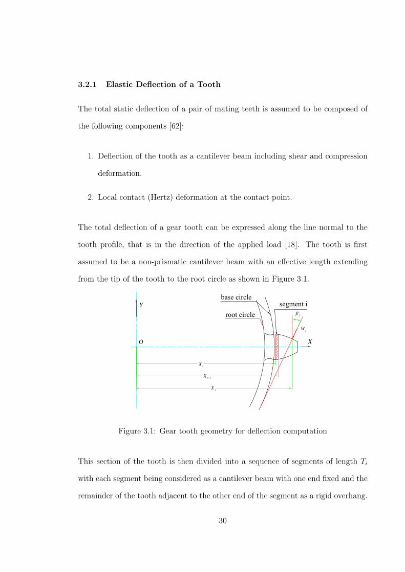
3.2.1 Elastic Deflection of a Tooth

The total static deflection of a pair of mating teeth is assumed to be composed of

the following components [62]:

1. Deflection of the tooth as a cantilever beam including shear and compression

deformation.

2. Local contact (Hertz) deformation at the contact point.

The total deflection of a gear tooth can be expressed along the line normal to the

tooth profile, that is in the direction of the applied load [18]. The tooth is first

assumed to be a non-prismatic cantilever beam with an effective length extending

from the tip of the tooth to the root circle as shown in Figure 3.1.

jβ

jW

jX

iX

1+iX

O

Y

X

Figure 3.1: Gear tooth geometry for deflection computation

This section of the tooth is then divided into a sequence of segments of length Ti

with each segment being considered as a cantilever beam with one end fixed and the

remainder of the tooth adjacent to the other end of the segment as a rigid overhang.

30

The total deflection at the loading point and in the direction of the applied load is

then obtained by applying the principle of superposition [63].

For each segment i, the height Yi, the cross-sectional area Ai and the area moment

of inertia, Ii are taken as the average of these values at both faces. The applied

load which is equal to the applied torque divided by the base circle radius can be

resolved into an equivalent system of forces and moments at the right hand face of

the segment as shown in Figure 3.2.

jY

jW

jβ

jW1

jW2

ijM

ijL

fl

fh

Figure 3.2: Components of the applied load

The components of this system of forces are given by:

W1j = Wj cos βj, (3.1)

W2j = Wj sin βj, (3.2)

Mij = Wj(Lij cos βj − Yj sin βj). (3.3)

31

Where i refers to the segment, j refers to the loading position, Lij is the distance

from j to i and,

Wj is the transmitted load

W1j,W2j are component loads at i

Mij is the resultant moment at i due to the load at j.

The contributions of bending, shear and axial deformations to the tooth deflection

can can be computed separately as shown in the following sections.

3.2.2 Bending Deflection

The total deflection at the load position associated with bending is given by:

i. Displacements due to W1j

(qw)ij =Wj cos βj

3EeIiT 3

i +Wj cos βj

2EeIiT 2

i Lij, (3.4)

ii. Displacement due to net moments Mij

(qm)ij =Wj(Lij cos βj − Yj sin βj)

2EeIi+Wj(Lij cos βj − Yj sin βj)

EeIi. (3.5)

The second terms of equations 3.4 and 3.5 are the displacements due to the rotations

of the rigid overhang [63].

Ee is the effective ‘Young’s modulus of elasticity’ whose value depends upon whether

the tooth is ‘wide’ or ‘narrow’. According to Cornell [21], a wide tooth is one for

which,

F

Y> 5, (3.6)

32

where Y is the tooth thickness at pitch point and F is the face width of the gear.

For such a tooth, plane strain applies and,

Ee =E

1− ν2, (3.7)

For a narrow tooth,

F

Y< 5, (3.8)

and Plane stress applies:

Ee = E. (3.9)

3.2.3 Shear Deformation

A deflection other than that due to bending moments occur in beams owing to the

shearing forces on transverse sections of the beam. This deflection may be found

approximately from strain energy principles and by making use of the equations for

shear stress at a point in the transverse section of a beam [64].

For a gear tooth, the shear deformation is caused solely by the transverse component

of the applied load. It displaces the centerline without causing any rotation [18].

For a rectangular cross-section, the shear deformation is calculated from equation

3.10.

(qs)ij =6

5

WjTi cos βj

GAi

. (3.10)

where,

G is the shear modulus of rigidity.

The moduli of elasticity in tension and shear (E and G) of a material are related

by equation 3.11 [65].

G =E

2(1 + ν). (3.11)

33

where,

ν is the poisson’s ratio for the material.

Substituting for G in equation 3.10, we obtain:

(qs)ij =12

5

WjTi(1 + ν)

AiEe

. (3.12)

3.2.4 Deformation Due to Axial Compression

The axial compression is caused by the axial load component, W1j and is given by

the relation:

(qc)ij =Wj sin βj

EeAi

Ti. (3.13)

The total displacement at the load position j, in the direction of the load, due to

deformation of the segment i can be expressed as:

(q1)ij = (qw + qm + qs)ij cos βj + (qc)ij sin βj. (3.14)

3.2.5 Deflection Due to Rim Flexibility

The deflection due to flexibility of the gear rim according to Cornell [21] are:

For plane stress case, narrow tooth,

(qfe)j =Wj cos2 βj

EeF[50

3π(lfhf

)2 + 2(1 + ν)(lfhf

)], (3.15)

For plane strain case, wide tooth,

(qfe)j =Wj cos2 βj

EeF(1− ν2)[

50

3π(lfhf

)2 + 2(1− ν − 2ν2)

1− ν2(lfhf

)]. (3.16)

34

where hf and lf are defined in Figure 3.2. The first term in the brackets is the

deflection at j due to the rotation caused by the moment at hf . The second term is

the sum of the deflection at j due to the displacement at hf caused by the moment

and rotation at hf due to the shear force at hf .

3.2.6 Hertzian Contact Deflection

When the surfaces of two solid bodies are brought into contact under load, they de-

form elastically. The “Theory of contact mechanics” is concerned with the stresses

and deformations which arise for such surfaces [66]. Hertz considered the stresses

and deformations in two perfectly smooth, ellipsoidal, contacting solids. The ap-

plication of the classical elasticity theory to this problem forms the basis of stress

and deformation calculations for machine elements such as ball and roller bearings,

gears, cams and followers [67].

Hertzian theory of contact utilizes the following assumptions

• The materials are homogenous and yield stress is not exceeded.

• The dimensions of each body are large compared to the radius of the circle of

contact.

• The radii of curvature of the contacting bodies are large compared with the

radius of the circle of contact.

• The contacting bodies are in frictionless contact.

• The surfaces in contact are continuous and nonconforming.

35

The contact problem of a pair of gears can be assumed to be a parallel axis cylinder

contact problem and therefore line contact deformation applies. The contact be-

tween parallel cylinders away from end effects is well represented by two-dimensional

Hertz theory [66]. The contact area is assumed to have constant width 2b over the

length of contact as shown in Figure 3.3.

δb b

1R

2R

P

P

Figure 3.3: Two cylinders in contact with axis parallel

Contact modulus, Ec is given by:

1

Ec

=1− ν2

1

E1

+1− ν2

2

E2

, (3.17)

Relative radius, Rc is given by

1

Rc

=1

R1

+1

R2

. (3.18)

36

Half width of contact, b is given by equation 3.19

b =(4PRc

πEc

) 12. (3.19)

The normal displacement depends on the distance that the reference points R1 and

R2 are from the contact point. This occurs because two dimensional theory only

allows the load to spread out in one direction.

Normal displacement is given by:

δ =P

πEc

{ln

(8R1

b

)+ ln

(8R2

b

)− 1

}. (3.20)

Contact between a pair of meshing gear teeth can be assumed to be cylinders of

radius equivalent to the radius of curvature of the gears at any instantaneous point

of contact and then by applying equation 3.20, the contact deformation is obtained.

1cR

2cR

2bR

1bR

Figure 3.4: Contact model for a pair of gears

37

Figure 3.4 shows the equivalent contact model of a pair of gears in mesh.

The total deflection at load position j and in the direction of the load is the sum of

all the deflections calculated above. If the number of segments is n, then

(qt)j =n∑

i=1

[(q1)ij] + (qfe)j + (δ)j. (3.21)

The stiffness value Km(t) is defined, according to Peeters [45], as the normal dis-

tributed tooth force in the normal plane causing deflection of one or more engaging

tooth pairs in the direction normal to the tooth profile divided by this deflection.

This deflection results from the bending of the teeth in contact between the two

gear wheels of which one is assumed to be fixed and the other loaded.

From a physical understanding, it is clear that the presented spring will only work

under compression. To ensure that this limitation will not be exceeded during sim-

ulation, it is assumed that no contact loss between the mating teeth will occur,

something that could happen for a system with backlash when the dynamic mesh

force becomes larger than the static force transmitted.

3.2.7 The Individual Tooth Stiffness

The individual tooth stiffness of a pair of teeth in contact is obtained by assuming

that one of the mating gears is rigid and applying load to the other. The individual

stiffness Kj at any meshing position j can be obtained by dividing the applied load

by the deflection of the tooth at that point as shown in equation 3.22 and 3.23.

Subscripts p and g refer to the pinion and gear respectively.

Kpj =Wj

qpj

, (3.22)

38

and

Kgj =Wj

qgj

. (3.23)

3.2.8 Combined Mesh Stiffness

At any position in the mesh cycle, a pair of teeth in contact can be modeled as

two linear springs connected in series [10]. The system stiffness against the applied

load, called the combined mesh stiffness at contact point j can be calculated by the

following equation;

Kmj =Kpj ·Kgj

Kpj +Kgj

. (3.24)

This equation is illustrated in Figure 3.5.

For a double pair of teeth in contact, the mesh stiffness is obtained by parallel

superposition of the corresponding mesh stiffness of the tooth pairs in contact. This

mesh stiffness is expressed as:

KTj = (Kmj)A + (Kmj)B. (3.25)

Where (Kmj)A and (Kmj)B refer to the mesh stiffness of the single tooth pair at

mesh positions A and B respectively. This equation is illustrated in Figure 3.6.

The procedures outlined in section 3.2 were coded into a FORTRAN program to

generate the mesh stiffness as a function of the contact position. The process starts

with the input of gear parameters and operating conditions. The actual profile of

the gear tooth is computed and used in the estimation of the mesh stiffness.

39

pjK

gjK

Figure 3.5: Single pair model of stiffness

AmjK )(

BmjK )(

Figure 3.6: Double pair teeth stiffness model

3.3 Modeling Friction in Spur Gears

Sliding friction between gear teeth is recognized as one of the main sources of power

loss in geared transmissions as well as a potential source of vibration and noise.

Its accurate modeling is therefore of primary importance in vibration and efficiency

analysis of geared transmissions. The free body diagram of an engaging spur gear

pair is shown in Figure 3.7 where T1 and T2 denote the input and output torque

40

respectively. The contact loads at the contact points A and B are PA and PB

respectively.

1fT

2fT

1θ

2θ

BcR )( 1

AcR )( 1

APAAPμ

AAPμ

BB Pμ

BB Pμ

BcR )( 2

AcR )( 2

BP

Figure 3.7: Free body diagram of a meshing gear pair

3.3.1 Frictional Torque

Sliding friction on the gear tooth surface causes frictional force Ft along the off-

line of action direction and a frictional torque Tf about the gear axis. During gear

meshing action, the tooth contact point moves along the line of action, and Tf

changes continuously due to linearly varying values of the radius of curvature. The

frictional torque can be obtained from the free body diagram of a meshing gear pair

(Figure 3.7) as:

41

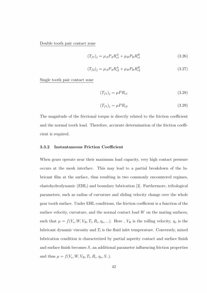
Double tooth pair contact zone

(Tf1)j = µAPARAc1 + µBPBR

Bc1 (3.26)

(Tf2)j = µAPARAc2 + µBPBR

Bc2 (3.27)

Single tooth pair contact zone

(Tf1)j = µPRc1 (3.28)

(Tf1)j = µPRc2 (3.29)

The magnitude of the frictional torque is directly related to the friction coefficient

and the normal tooth load. Therefore, accurate determination of the friction coeffi-

cient is required.

3.3.2 Instantaneous Friction Coefficient

When gears operate near their maximum load capacity, very high contact pressure

occurs at the mesh interface. This may lead to a partial breakdown of the lu-

bricant film at the surface, thus resulting in two commonly encountered regimes,

elastohydrodynamic (EHL) and boundary lubrication [3]. Furthermore, tribological

parameters, such as radius of curvature and sliding velocity change over the whole

gear tooth surface. Under EHL conditions, the friction coefficient is a function of the

surface velocity, curvature, and the normal contact load W on the mating surfaces,

such that µ = f(Vs,W, VR, Tl, Rc, ηo, ...). Here , VR is the rolling velocity, ηo is the

lubricant dynamic viscosity and Tl is the fluid inlet temperature. Conversely, mixed

lubrication condition is characterized by partial asperity contact and surface finish

and surface finish becomes S, an additional parameter influencing friction properties

and thus µ = f(Vs,W, VR, Tl, Rc, ηo, S..).

42

As the gear teeth move through the mesh cycle, the normal contact force between

the teeth changes its value as the number of teeth alternate between 1 and 2 as well

as the coefficient of friction. A large number of empirical formulae for determining

the coefficient of friction can be found in reference [3, 18, 20, 33]. Most of these for-

mulae are obtained by curve fitting measured data from experimental tests. They

have the following general formula µ = f(Vs,W, VR, Pmax, Rc, ηo, S..), where Pmax is

the contact pressure.

Commonly cited empirical formulas for coefficient of friction are shown in Table 3.1.

Other details of these formulas can be found in references [4, 20].

These formulae were shown to be inaccurate under certain conditions representing

the contact of a gear pair [20]. Specifically, as Vs approaches zero when the contact

nears the pitch point, most of these formulae predict a very large value of the fric-

tion coefficient while in real sense, the coefficient of friction should be zero under

no sliding. Consequently as indicated in Table 3.1, some of these formulas are only

valid in certain parameter ranges, specific roughness and lubricant types and there-

fore cannot be used as a general means of predicting the friction coefficient along

the path of contact for different gears. Figure 3.8 shows the curves for the friction

coefficient along the path of contact resulting from these formulas. Table 3.2 shows

some typical parameters used in the analysis.

43

Table 3.1: Commonly cited formulas for µ

Formula and author Parameter specific units

ranges

Drozdov and Gavrikov [20] νkε[4, 500] Vs, Vr(m/s)

µ = [0.8√νkVs + Vrφ+ 13.4]−1 Vs ≤ 15, Pmax(kg/cm

2

φ = 0.47− 0.13(10)−4Pmax − 0.4(10)−3νk Vrε[3, 20]

Benedict and Kelley [20] 5050−S

≤ 3 S(µin)

µ = 0.127[ 5050−S

]log10[3.17(10)8W

′

νkVsV 2r

] W′(lbf/in)

ISO TC60 [20] Vr(m/s)

µ = 0.12[W′S/(RVrν)]

0.25 S(µm),

W′(N/mm)

Kuang [4] Vs (m/s)

µ = Vs

PAtA

∫ +a

−aηAdx

44

10 12 14 16 18 20 22 24 26 28 300

0.02

0.04

0.06

0.08

0.1

0.12

0.14

Roll angle ( o )

Fric

tion

coef

ficie

nt, μ

Kuangs methodDrosdovs methodISO TC60 methodBenedicts method

Figure 3.8: Friction Coefficients from different empirical formulas

Table 3.2: Parameters and operating conditions used in the analysis of coefficient

of friction

module (m) 3.0mm

pressure angle φ 20o

pinion 28T

gear 20T

speed (N) 1500rpm

power 4847KW

45

In this study, an empirical formula developed by Xu and Kahraman [20] was adopted

as it was found to accurately model the instantaneous coefficient of friction along

the path of contact of a pair of gears in mesh. This model is based on Electro-

hydrodynamic lubrication (EHL) and was obtained by multiple linear regression

analysis. This model includes the key parameters influencing friction at the con-

tacting gear surfaces, namely sliding velocity, contacting pressure, surface roughness,

lubricant dynamic viscosity, radius of curvature and entrainment velocity. The for-

mula was found to correlate very well with experimental data [20]. The formula can

therefore be used with confidence for the prediction of friction coefficient for a pair

of contacting gears. This formula is written as:

µ = ef(SR,Ph,η,S)P b2h |SR|

b3V b6e ηb7Rb8 . (3.30)

where,

f(SR, Phη, S) = b1 + b4|SR|Phlog10(η) + b5e−|SR|Phlog10(η) + b9e

s (3.31)

Ve =u1+u2

2

Vr =u1 + u2

Vs =u1 − u2

SR = Vs

Ve

Ph =√

W ′E′

2πR

R = Rc1Rc2

Rc1+Rc2

E′

= 2[1−ν1

E1+ 1−ν1

E2]−1

The above set of equations were coded in a FORTRAN program and simulated. The

results are presented in chapter 5.

46

3.4 Natural Frequencies of the System

An n−degree-of-freedom system has n natural frequencies, and for each natural

frequency there is a corresponding normal mode shape that defines a distinct re-

lationship between the amplitudes of the generalized coordinates for that mode.

The squares of the natural frequencies and the corresponding sets of coordinate

values describing the normal mode shapes are referred to as eigenvalues and eigen-

vectors respectively, and they are of fundamental importance in the analysis of free

or forced vibration of multi-degree-of-freedom systems [68]. Prediction of the nat-

ural frequencies and vibration modes of a system provides important information

for tuning resonances away from the operating speeds and minimizing response [11].

Equations of motion for undamped systems, under the assumption of constant stiff-

ness, mass inertia and free oscillations, can be represented in matrix form (equation

3.32) and are used to find the natural frequencies of the system.

[J ]{θ̈}+ [K]{θ} = {0}, (3.32)

47

Where the inertia matrix [J ] is given by:

J1 0 0 0 0 0 0 0 0 0 0 0 0

0 J2 0 0 0 0 0 0 0 0 0 0 0

0 0 J3 0 0 0 0 0 0 0 0 0 0

0 0 0 J4 0 0 0 0 0 0 0 0 0

0 0 0 0 J5 0 0 0 0 0 0 0 0

0 0 0 0 0 J6 0 0 0 0 0 0 0

0 0 0 0 0 0 J7 0 0 0 0 0 0

0 0 0 0 0 0 0 J8 0 0 0 0 0

0 0 0 0 0 0 0 0 J9 0 0 0 0

0 0 0 0 0 0 0 0 0 J10 0 0 0

0 0 0 0 0 0 0 0 0 0 J11 0 0

0 0 0 0 0 0 0 0 0 0 0 J12 0

0 0 0 0 0 0 0 0 0 0 0 0 J13

(3.33)

and the stiffness matrix [K] is given by:

K1,1 −K1,2 0 0 0 0 0 0 0 0 0 0 0

−K2,1 K2,2 −K2,3 0 0 0 0 0 0 0 0 0 0

0 −K3,2 K3,3 −K3,4 0 0 0 0 0 0 0 0 0

0 0 −K4,3 K4,4 −K4,5 0 0 0 0 0 0 0 0

0 0 0 −K5,4 K5,5 −K5,6 0 0 0 0 0 0 0

0 0 0 0 −K6,5 K6,6 −K6,7 0 0 0 0 0 0

0 0 0 0 0 −K7,6 K7,7 −K7,8 0 −K7,10 0 0 0

0 0 0 0 0 0 −K8,7 K8,8 −K8,9 0 0 0 0

0 0 0 0 0 0 0 −K9,8 K9,9 0 0 0 −K9,13

0 0 0 0 0 0 −K10,7 0 0 K10,10 −K10,11 0 0

0 0 0 0 0 0 0 0 0 −K11,10 K11,11 −K11,12 0

0 0 0 0 0 0 0 0 0 0 −K12,11 K12,12 0

0 0 0 0 0 0 0 0 −K13,9 0 0 0 K13,13

48

Where,

K1,1 = Ks1 K1,2 = −Ks1

K2,1 = −K21 K2,2 = Ks1 +Kg1r22 K2,3 = −Kg1r2r3

K3,2 = −Kg1r2r3 K3,3 = Kg1r23 +Ks2 K3,4 = −Ks2

K4,3 = −Ks2 K4,4 = Ks2 +Kg2r24 K4,5 = −Kg2r4r5

K5,4 = −Kg2r4r5 K5,5 = Kg2r25 +Ks3 K5,6 = −Ks3

K6,5 = −Ks3 K6,6 = Ks3 +Kg3r26 K6,7 = −Kg3r6r7

K7,6 = −Kg3r6r7 K7,7 = Kg3r27 + 2Ks4 K7,8 = −Ks4 K7,10 = −Ks4

K8,7 = −Ks4 K8,8 = Ks4 +Kg4r28 K8,9 = −Kg4r8r9

K9,8 = −Kg4r8r9 K9,9 = Kg4r29 +Ks5 K9,13 = −Ks5

K10,7 = −Ks4 K10,10 = Ks4 +Kg5r210 K10,11 = −Kg5r10r11

K11,10 = −Kg5r10r11 K11,11 = Kg5r211 +Ks5 K11,12 = −Ks5

K12,11 = −Ks5 K12,12 = Ks5

K13,9 = −Ks5 K13,13 = Ks5

Since the mesh stiffness for the gears varies with the contact position, it is expected

that the natural frequencies should vary with the contact position. Therefore, equa-

tion 3.32 should be solved for each contact position of the gears in mesh.

Equation 3.32 was solved for the eigenvalues and eigenvectors by the householder

method and QL Algorithm with Implicit Shifts [69]. The Householder algo-

rithm reduces an n×n symmetric matrix A to tridiagonal form by n−2 orthogonal

transformations. Each transformation annihilates the required part of a whole col-

umn and whole corresponding row. Once the original, real, symmetric matrix has

been reduced to tridiagonal form, the QL Algorithm obtains all the eigenvalues

49

and associated eigenvectors simultaneously and has been found to work well in prac-

tice [69].

Equation 3.32 can be reformulated into equation 3.34 through a series of steps.

J−1Kθ = λθ. (3.34)

Although the matrices J and K are both symmetric, the matrix J−1K is not sym-

metric which means that the right hand side of equation 3.34 cannot be solved

directly by the Householder and QL algorithms. The matrix J is generally decom-

posed by employing Cholesky Decomposition procedure so that J is written

as:

J = LLT (3.35)

in which L is the lower triangular matrix and LT is the upper triangular transpose

of J . A symmetric matrix can thus be obtained and expressed as:

[L−1K(L−1)T ]{LT θ} = λ{LT θ}, (3.36)

AY = λY. (3.37)

where

A = L−1K(L−1)T , (3.38)

Y = LT θ.

With K being a symmetric matrix, A will also be symmetric, and thus equation

3.37 can be solved by the Householder and QL algorithms. The eigenvalues of

equation 3.37 are identical to those of the equation in its original form (Equation

3.34). However, it should be apparent from the second expression of equation 3.38

50

that the eigenvectors θ of the original equation must be obtained from:

θ = (LT )−1Y = (L−1)TY. (3.39)

3.5 Dynamic Stress Analysis

Tooth bending failure at the root is a major concern in gear design. If the bending

stress exceeds the fatigue strength, the gear tooth has a high probability of failure.

In this study, a modified Heywood formula [47] for tooth root stress was used for the

dynamic stress calculation at the root of a gear tooth. This formula has been found

to correlate well with experimental data and finite element analysis results [47]. This

formula is expressed as:

σj =Wj cos βj

F

[1 + 0.26

( hf

2Rf

)0.7][6lfh2

f

+

√0.72

hf lf

(1− hl

hf

tan βj

)− tan βj

hf

]. (3.40)

where, σj is the root bending stress, hf is the tooth thickness at the critical section,

Rf is the fillet radius, lf is the length of the tooth from the projected point of contact

on the neutral axis to the critical section and γ is the angle between the form circle

and the critical section. The formula of equation 3.40 consists of five factors:

i. Stress concentration at the fillet,Wjcosβj

F

[0.26

(hf

2Rf

)0.7][6lfh2

f+

√0.72hf lf

(1 −

hl

hftanβj

)− tanβj

hf

].

ii. Beam cantilever bending stress,Wj cos βj

F

6lfh2

f.

iii. Bending load proximity stress,Wj cos βj

F

√0.72hf lf

6lfh2

f.

iv. Axial load proximity stress,Wj cos βj

F

√0.72hf lf

hl

hftan βj

v. Axial stress,Wj cos βj

F

tan βj

hf

51

The formula has the proximity effects decreasing as the bending and axial load get

further from the fillet and closer to the neutral axis. Figure 3.9 shows the tooth

geometry for root stress calculation.

Lewis obtained the critical section of a gear tooth by inscribing a parabola within

the tooth profile [70], where the point of contact of the parabola with the tooth root

rounding determines the critical cross section. Other researchers, [18, 47] assumed

an average value of γ = 30o to obtain the cross section for maximum root stress.

However in this study, the tooth root stress was calculated at each point in the tooth

root area and subsequently the location for the maximum root stress was obtained.

Force application at the highest point of single tooth contact was found to yield the

maximum root stress in most cases.

Figure 3.9: Tooth geometry nomenclature for root stress calculation

52

CHAPTER 4

MODEL DEVELOPMENT

4.1 Model Description

The model for the gear train system was developed based on a four stage tractor

gearbox explained in appendix A. The essential elements of the gear train model

(Figure 4.1) are shown in Figure 4.2. The model contains five pairs of gear meshes

each with a periodic mesh stiffness and its damping constant, the moments of inertia

of the gears, moments of inertia of the input and output masses and the torsional

stiffness of the shafts. This yielded a thirteen (13) degree of freedom system which

was modeled as a purely torsional vibratory system.

53

1T1θ 2θ

3θ4θ

5θ6θ

7θ

119 ,θθ1312 ,θθ

1sK

2sK

3sK

4sK

5sK

)(2 tK g

)(3 tK g

)(4 tK g

)(4 tCg

)(3 tCg

)(2 tCg

)(1 tCg

32 ,TT

)(1 tK g

108 ,θθ

Figure 4.1: Gear train model

54

Figure 4.2: Gear train for bottom gear ratio

55

The major assumptions on which the dynamic model is based are as follows:

i. Gears are modeled as rigid disk with radius equal to the base circle radius

and flexibility at the gear teeth.

ii. Bearings and the casing are assumed to be rigid (deflections of the bear-

ings are much smaller than the deflections of the gear teeth and shafts

and can be neglected.)

iii. Static transmission error effects are much smaller than the dynamic trans-

mission error so they can be neglected [19].

iv. Gear teeth are assumed to be perfectly involute and manufacturing and

assembly errors are ignored.

v. Backlash is not considered in this model. This is because while running

at steady state, the gears are loaded in a single direction only and thus

tooth separation is not considered.

A set of governing equations of motion for the model was derived using the standard

Lagrangian equation, which is given here without proof [68]:

d

dt

(∂T∂q̇i

)− ∂T

∂qi+∂V

∂qi= Qi, (4.1)

Where,

qi generalized coordinate.

T Total kinetic energy of the system.

V Change in potential energy of a system with respect to its potential energy

56

in the static equilibrium position.

Qi generalized non-potential forces or moments resulting from excitation forces

or moments that add energy into the system, and damping forces and

moments that remove energy from it.

The kinetic energy of the system is given by:

T =1

2ΣJiθ̇

2i . (4.2)

The generalized non-potential forces or moments (Qi) result from excitation forces

or moments that add energy into the system, and damping forces and moments that

remove energy from it. The potential energy is classified into two groups of stored

energy caused by:

1. Distortion of the gear meshes, for example the potential energy stored in gear

mesh 1 is expressed as:

Vm1 =1

2Kg1(t)[R2θ2 −R3θ3]

2, (4.3)

2. Twisting of gear shafts, for example the potential energy stored in shaft 1 is

expressed as:

Vs1 =1

2Ks1[θ1 − θ2]

2. (4.4)

The application of equation 4.1 to the gear train system yielded 13 equations of

motion (4.5 - 4.17) given below:

J1θ̈1 + Cs1(θ̇1 − θ̇2) +Ks1(θ1 − θ2) = T1, (4.5)

57

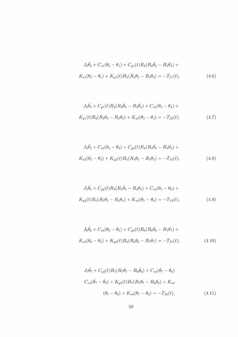
J2θ̈2 + Cs1(θ2 − θ1) + Cg1(t)R2(R2θ̇2 −R3θ̇3) +

Ks1(θ2 − θ1) +Kg1(t)R2(R2θ2 −R3θ3) = −Tf1(t), (4.6)

J3θ̈3 + Cg1(t)R3(R3θ̇2 −R3θ̇3) + Cs2(θ3 − θ4) +

Kg1(t)R3(R3θ3 −R2θ2) +Ks2(θ3 − θ4) = −Tf2(t), (4.7)

J4θ̈4 + Cs2(θ4 − θ3) + Cg2(t)R4(R4θ̇4 −R5θ̇5) +


J5θ̈5 + Cg2(t)R5(R5θ̇5 −R4θ̇4) + Cs3(θ5 − θ6) +


J6θ̈6 + Cs3(θ6 − θ5) + Cg3(t)R6(R6θ̇6 −R7θ̇7) +


J7θ̈7 + Cg3(t)R7(R7θ̇7 −R6θ̇6) + Cs4(θ̇7 − θ̇8)

Cs4(θ̇7 − θ̇9) +Kg3(t)R7(R7θ7 −R6θ6) +Ks4

(θ7 − θ8) +Ks4(θ7 − θ9) = −Tf6(t), (4.11)

58

J8θ̈8 + Cs4(θ8 − θ7) + Cg4(t)R8(R8θ̇8 −R9θ̇9)

+Ks4(θ8 − θ7) +Kg4(t)R8(R8θ8 −R9θ9) = −Tf7(t), (4.12)

J9θ̈9 + Cg4(t)R9(R9θ̇9 −R8θ̇8) + Cs5(θ9 − θ13) +


J10θ̈10 + Cs4(θ10 − θ7) + Cg5(t)R10(R10˙θ10 −R11

˙θ11)

+Ks4(θ10 − θ7) +Kg5(t)R10(R10θ10 −R11θ11) = −Tf9(t), (4.14)

J11θ̈11 + Cg5(t)R11(R11˙θ11 −R10

˙θ10) + Cs5(θ11 − θ12) +


J12θ̈12 + Cs5( ˙θ12 − ˙θ11) +Ks5(θ12 − θ11) = −T2, (4.16)

J13θ̈13 + Cs4( ˙θ13 − θ̇9) +Ks4(θ13 − θ9) = −T3. (4.17)

As can be observed from equations 4.6 to 4.15, the non-linear interactions of the

gear mesh couple the moment equations of each stage to each other. The gear mesh

moments are evaluated as functions of relative motion and rotation between two

59

meshing meshing gears and the corresponding gear mesh stiffnesses and damping

constants. The relative dynamic displacement and relative velocity of any pair of

gears in mesh are the most important factors that influence the dynamics of the

gear teeth and are given by equations 4.18 and 4.19.

δi(t) = Riθi(t)−Ri+1θi+1(t), (4.18)

δ̇i(t) = Riθ̇i(t)−Ri+1θ̇i+1(t). (4.19)

where, δi, δ̇i, (i = 1− 5) represent the relative displacement and relative velocity of

the gear teeth in mesh 1-5.

4.1.1 Damping Coefficients

The equations of motion contain damping terms for all components in the system.

Damping results from viscous damping which occurs as a result of a system vibrating

in a fluid. Most mechanical systems have damping which is quite complex but can

be represented by viscous damping [71]. It is usually convenient to represent the

damping coefficient in the differential equation as a factor of the critical damping

as given by equation 4.20.

ζ =C

Cc

. (4.20)

The damping factor can be determined experimentally for a system by obtaining a

free vibration record of the system showing how its amplitude of vibration varies

with time.

Since the mathematical description of the damping effect in gears is very compli-

cated, a simplified damping model between two lumped masses was introduced in

the study and the effective damping coefficients for the shafts and gears were given

60

by equations 4.21 and 4.22 respectively.

Cgi(t) = 2ζg

√Kgi(t)

JiJi+1

Ji+1R2i + JiR2

i+1

, (4.21)

Csi = 2ζs

√Ksi

JiJi+1

Ji + Ji+1

. (4.22)

The damping ratio for the shafts is mainly due to material damping which by ex-

periment has been found to range between 0.05 and 0.07 [18]. In this study, a value

of 0.05 was adopted. This value has been found to correlate very well with exper-

imental results for shafts running in an oil bath [3, 4, 18]. On the other hand, the

magnitude of the damping ratio for a gear mesh depends upon the lubrication film

between the contacting teeth and values ranging between 0.1 and 0.2 were suggested

by Kuang [4] by obtaining a correlation between analytical and experimental results.

A value of 0.1 was adopted in this study as it was found to correlate very well with

experimental results for gears running in an oil bath [3, 4, 18].

4.1.2 Gear Shaft Torsion

To calculate gear shaft torsion, equivalent torsional spring constants for the shafts

were determined. The complex shaft shapes were approximated by using a series

of sections having constant cross sections. The torsional spring constants for each

section were calculated by:

Ks =JG

L. (4.23)

where L is the section length, J is the polar moment of inertia, and G is the material’s

shear modulus. The equivalent torsional spring constants for the shafts were then

determined by treating the shafts as a set of torsional springs in series.

61

4.2 Numerical Simulation

The time domain behavior of the system was studied by integrating the set of govern-

ing differential equations using 4th order Runge-Kutta method. The differential

equations were linearized by dividing the mesh period of the output pair into many

small intervals. The mesh period for any pair of teeth in mesh was taken as the

time interval from the initial point of contact to the highest point of single tooth

pair contact.

To integrate initial value problems, one needs an appropriate set of initial condi-

tions. In this study, all generalized coordinates were set to zero. Starting with these

initial estimates of θi(0) and θ̇i(0) at the initial contact point, the values of θi(t) and

θ̇i(t) were calculated for one mesh period of the output pair of gears.

The calculated value of the relative displacement δi(τj) and relative velocity δ̇i(τj)

after the end of one period τj of each pair of gears j in mesh were compared with

the initial values δi(0) and δ̇i(0). Unless the difference between them is sufficiently

small as defined by the tolerance in equation 4.24, an iteration procedure was used

to obtain the (i + 1)th iteration values of θi(t) and θ̇i(t) by taking the ith iteration

values of θi(τj) and θ̇i(τj) as the new initial trial conditions. Once the solution has

converged, this state corresponds to the steady state rotational speed of the shafts.

Figure 4.3 shows a sample plot of the convergence of the relative displacement. For

this particular case, the solution converges to an acceptable percentage difference

(0.001%) after about 25 iterations.

toli =δi(τj)− δi(0)

δi(τj). (4.24)

62

0 5 10 15 20 25 30-150

-100

-50

0

50

100

No. of Iterations

% D

iffer

ence

in T

E

Convergence Plot

Figure 4.3: Sample plot of the convergence of relative displacement of a gear pair

The optimum time step was initially selected as the period for the path of contact

of the gears in stage I divided by 100. The time step was then reduced and the model

simulated for each time step until the point where further reduction in the time step

did not yield any appreciable change in the response and the time step at this point

was taken as the optimum time step.

The Runge-Kutta integration scheme requires values of Kgi(t+h2), Kgi(t+h), Cgi(t+

h2), Cgi(t+h), Tfi(t+

h2), Tfi(t+h). These values were obtained by employing cubic

spline interpolation technique [69]. The procedure described above for the time

domain studies yielded the response to both the time varying mesh stiffness and time

varying frictional torque. Figure 4.4 is the flow chart showing the computational

procedure.

63

Figure 4.4: Flowchart for the computational procedure

64

CHAPTER 5

RESULTS AND DISCUSSIONS

5.1 Introduction

The main objective of the study was to develop a mathematical model to analyze

the vibrations of a multistage tractor gearbox and to study the influence of gear

design parameters on the relative levels of vibration of the gears. The results of

the mesh stiffness, frictional torque, time domain vibration levels, frequency spec-

trum, dynamic load and dynamic stress are presented and discussed in the following

sections.

5.2 Mesh Stiffness

Figure 5.1 shows a sample plot of the normalized mesh stiffness on the face width.

A gear tooth enters contact at point A and between points A and B we have two

pairs of teeth in contact. In this region, the stiffness of one tooth falls as the contact

point moves towards the tip of the tooth while the stiffness of the mating tooth

increases as the contact point moves towards the root circle. This accounts for the

variation of the stiffness in this region. At point B, the stiffness falls drastically as

the gear moves from double pair contact zone to single pair contact zone. Again, the

stiffness varies along the single pair zone due to the movement of the contact point

towards the root circle for one tooth and towards the tip for the other. At point

C another pair of teeth enters contact and the cycle is repeated. Table 5.1 shows

the gear parameters used in the computation of the stiffness. In order to apply the

stiffness in the equations of motion, we need to be able to represent the stiffness as

a function of time.

65

12 14 16 18 20 22 24 26 280

0.5

1

1.5

2

2.5

3

3.5

4x 105

Roll Angle ( o )

Mes

h st

iffne

ss (

N/m

m )

A B

C D

E F

Figure 5.1: Gear mesh stiffness as a function of the contact position

Table 5.1: Gear set data and operating conditions for stiffness prediction

Parameter Pinion Gear Module 3.0 mm 3.0 mm

No. of teeth 28 20 Clearance 0.157 module 0.157 module

Pressure angle 20o 20o

Input speed 1500 rpm Power 4847 W

In practice, the stiffness will be a function of the angular rotation of the gear set

and this will only be known as a function of time if the mean rotational speed can

be assumed to be (or approximated as) constant [29].

Figure 5.2 is a plot of the periodic mesh stiffness for various face widths of the gear

pair. τi is the mesh period which can be computed from equation 5.4.

τi =60

Ni ×Nti(5.1)

66

0 0.5 1 1.5 2 2.5 3 3.5 4 4.5x 10-3

0

1

2

3

4

5

6

7

8x 105

Time ( sec )

Mes

h st

iffne

ss (

N/m

m )

15 mm Face width20 mm25 mm

τi

Figure 5.2: Periodic mesh stiffness for various face widths of the same gear set

The mesh stiffness increases significantly with the increase in the face width as seen

in Figure 5.2. By increasing the face width by 67% (from 15 mm to 25 mm), the

stiffness model developed in this study predicts that the mesh stiffness increases by

113%.

The discontinuities in the mesh stiffness as the number of pairs of teeth alternate

between one and two can be eliminated by increasing the contact ratio of the gear

set. Figure 5.3 shows the stiffness curves for various contact ratios. The contact

ratio was increased by increasing the addendum of the gear teeth. Increasing the

contact ratio reduces the bandwidth of the single contact zone and also the values of

the stiffness. For a contact ratio of 2.0, the zone of single contact is eliminated and

the only variation in the mesh stiffness is due to the change of the contact position.

67

0 0.01 0.02 0.03 0.04 0.05 0.060

1

2

3

4

5

6

7

8

9

10x 105

Time (sec)

Stiff

ness

( N

/mm

)

CR = 1.688CR = 1.893CR = 1.998

Figure 5.3: Periodic stiffness for different contact ratios

5.3 Frictional Torque

Figure 5.4 shows the variation of friction coefficient along the path of contact of a

mating pair of gears. The analysis was carried out using the parameters and oper-

ating conditions given in Table 3.2. As seen from Figure 5.4, the friction coefficient

approached zero as the contact point nears the pitch point. This is because the

rate of sliding decreases towards the pitch point, becomes zero at the pitch point,

changes the direction and increases as the contact point moves away from the pitch

point. Points A and B are points of transition from double tooth pair contact to

single tooth pair contact and from single tooth pair contact to double tooth pair

contact respectively. For a pair of gears with equal number of teeth, the curve on

the path of approach seems like a mirror of the curve of approach with the vertical

68

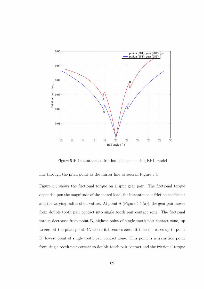
10 12 14 16 18 20 22 24 26 28 300

0.01

0.02

0.03

0.04

0.05

0.06

Roll angle ( o )

Fric

tion

coef

ficie

nt, μ

pinion (28T), gear (20T)pinion (28T), gear (28T)

A

B

A

B

Figure 5.4: Instantaneous friction coefficient using EHL model

line through the pitch point as the mirror line as seen in Figure 5.4.

Figure 5.5 shows the frictional torque on a spur gear pair. The frictional torque

depends upon the magnitude of the shared load, the instantaneous friction coefficient

and the varying radius of curvature. At point A (Figure 5.5 (a)), the gear pair moves

from double tooth pair contact into single tooth pair contact zone. The frictional

torque decreases from point B, highest point of single tooth pair contact zone, up

to zero at the pitch point, C, where it becomes zero. It then increases up to point

D, lowest point of single tooth pair contact zone. This point is a transition point

from single tooth pair contact to double tooth pair contact and the frictional torque

69

experiences an impulsive change. At point E, another pair of teeth enters into

contact beginning another double tooth pair contact zone. In practice, the frictional

torque will be a function of the angular rotation of the gear set and this will only

be known as a function of time if the mean rotational speed of the gears can be

assumed to be constant in which case the frictional torque will be periodic with a

time period of τ which is taken as the time that elapses before a successive pair of

teeth to enters into contact.

0 1 2 3 4x 10-3

0

100

200

300

400

500

600

700

800

Time (sec)

Fric

tiona

l tor

que

(N-m

m)

0 1 2 3 4x 10-3

0

100

200

300

400

500

600

700

800

Time (sec)

Fric

tiona

l tor

que

(N-m

m)

driving gear (28T)driven gear (20T)

A

B

C

D

τ E

(a) (b)

Figure 5.5: Periodic frictional torque (a) on the driving gear, (b) on both gears

The frictional torque changes abruptly at the transition points from single tooth

pair to single tooth pair and vice versa. This sudden change in the frictional torque

acts as a source of excitation for a gear pair and will be included in the dynamic

model of the spur gear train. Figure 5.5 (b) shows the frictional torque on both the

pinion and the gear. The shape of the curve for the gear torque is a scaled mirror of

the pinion torque. The parameters and operating conditions used in the simulation

are those in Table 3.2. Figure 5.6 shows the frictional torque curves for gears with

70

different contact ratios. It can be observed that the plot for a contact ratio close

to 2.0 is quite different from that of a contact ration less than 2.0. The zone of

single contact is not visible for a contact ratio close to 2.0 and the torque changes

impulsively only when a pair of teeth approaches end of contact and a new pair of

teeth enters into contact.

0 1 2 3 4

x 10-3

0

100

200

300

400

500

600

700

800

Time (sec)

Fric

tiona

l tor

que

(N-m

m)

driving gear (28T), CR=1.597

0 1 2 3 4

x 10-3

0

100

200

300

400

500

600

700

800

Time (sec)

Fric

tiona

l tor

que

(N-m

m)

driving gear (28T), CR=1.994

0 1 2 3 4

x 10-3

0

100

200

300

400

500

600

700

800

Time (sec)

Fric

tiona

l tor

que

(N-m

m)

driven gear (20T), CR=1.597

0 1 2 3 4

x 10-3

0

100

200

300

400

500

600

700

800

Time (sec)

Fric

tiona

l tor

que

(N-m

m)

driven gear (20T), CR=1.994

(a) (b)

(c) (d)

Figure 5.6: Frictional torque for different contact ratios

5.4 Code Validation

Computer codes in gear applications are usually developed to allow designers to

investigate the effect of various design parameters and optimum gear configurations

71

on vibrations and gear dynamics which would either be difficult to analyze exper-

imentally or that would require very expensive tests. Though the computer codes

provide a cheaper alternatives to analyze the gear dynamics, their validity must be

tested for the designer to be sure that the results obtained are within acceptable

limits. Usually, a code is validated by comparing the results obtained from the code

with those obtained from a simple experimental set up. In this study, the results

obtained from the code developed were compared with results obtained from tests

performed on the NASA gear noise rig [34].

The rig features a single mesh gearbox powered by a 150 KW variable speed electric

motor. An eddy current dynamometer loads the output shaft. The gearbox can

operate at speeds up to 6000 rpm. The rig was built to carry out fundamental

studies of gear noise and the dynamic behavior of gear systems [34]. Table 5.2

shows the test rig parameters.

To compare the experimental and numerical results, the measured dynamic loads

from Oswald et al [34] were placed next to dynamic load plots predicted by the

model developed in this study. Figures 5.7 to 5.10 show the measured and predicted

dynamic loads for four speeds with five different torque levels on each plot (20

operating conditions). The numerical and measured values match each other rather

well both in the general pattern and magnitude especially at 2000 and 4000 rpm,

where the percentage error between the measured and predicted peak load was found

to be between 0.07% and 1.2%. There are some differences in the waveforms at 800

and 6000 rpm which could have arisen from external factors not considered in the

model. Example of such factors are:

• Load fluctuations from the motor and / belt drive.

72

Table 5.2: Test rig parameters

Gear tooth type Standard, full depth

No. of Teeth 28 and 28

module 3.175 mm

Face width 6.35 mm

Pressure angle 20o

Tooth root radius 1.35 mm

Mesh damping coeff. 10% of critical

Gear inertia 301.55 Kg-mm2

Motor inertia 1100 Kg-mm2

Load inertia 1400 Kg-mm2

Input stiffness 17× 106 N -m/rad

Output stiffness 17× 106 N -m/rad

• Coupling between lateral and torsional vibrations.

• Low frequency vibration modes of the long shafts connecting the motor and

dynamometer to the gearbox [34]

73

(a) Measured dynamic loads

10121416182022242628300

500

1000

1500

2000

2500

3000

3500

Roll Angle ( o )

Dyn

amic

For

ce (

N )

142% torque110% 79% 47% 16%

(b) Predicted dynamic loads

Figure 5.7: Dynamic loads at different torques levels for 800 rpm


10121416182022242628300

500

1000

1500

2000

2500

3000

3500

Roll Angle ( o )

Dyn

amic

For

ce (

N )

142% torque110% 79% 47% 16%



74


10121416182022242628300

500

1000

1500

2000

2500

3000

3500

Roll Angle ( o )

Dyn

amic

For

ce (

N )

142% torque110% 79% 47% 16%




10121416182022242628300

500

1000

1500

2000

2500

3000

3500

4000

Roll Angle ( o )

Dyn

amic

For

ce (

N )

142% torque110% 79% 47% 16%



75

Correlation between the dynamic loads predicted by the model developed in this

study and the experimental results from Oswald et al [34], the peak dynamic loads

predicted by the model were plotted against the experimental results for all the 20

conditions as shown in Figure 5.11. The diagonal line shows the line of best fit where

the numerical and experimental values agree. The results show that apart from the

four conditions (142%, 110% and 79% nominal torque at 6000 rpm and 142% at

800 rpm), the numerical peak load agrees well with measured peak loads within an

average error of 5.5%

0 500 1000 1500 2000 2500 3000

500

1000

1500

2000

2500

3000

3500

Measured load ( N )

Pred

icte

d lo

ad (

N )

Correlation of the Numerical and Experimental Results

y vs. xline of best fit

Figure 5.11: Comparison of the peak loads predicted by the model with

experimental data

76

5.5 Multistage Gear Train Results

Two gear train configurations are presented in this study:

1. Bottom Gear Ratio; in this case, the gear train that produces the highest

reduction ratio is analyzed. This ratio produces the the maximum torque

with low speed at the wheel axles. This configuration is normally used when

moving the tractor from rest, ploughing land and moving up a steep hill whilst

loaded. The nominal output torque used in the design of the gears is 1300 Nm,

i.e, 650 Nm at each axle.

2. Top Gear Ratio; in this case, the gear train that produces the highest speed

at the axles is analyzed. The design torque used in this case is 130 Nm, i.e,

65 Nm at each axle.

5.5.1 Bottom Gear Ratio Configuration

The gear train for this configuration is shown in Figure 4.2. Table 5.3 shows the

rotor properties for this system while Table 5.4 shows the operating conditions and

gear parameters. In this thesis, this gear train will be referred to as gear train

1. The pinions in this gear train have a number of teeth less than the minimum

required to avoid undercut and therefore the addendum has been modified to avoid

undercut. Short and long addendum with standard center distance have been used.

77

Table 5.3: Rotor properties for gear train 1

Rotor No. Description

No. of teeth for

gears

Addendum modification

factor

Face width (mm)

Moment of inertia (Kg

mm2)

Theoretical contact ratio

1 Input pulley assembly - - - 10697.8 -

2 Stage I pinion 14 1.2987 m 15 51.2

3 Stage I gear 34 0.7013 m 15 1249.5 1.516

4 Stage II pinion 14 1.3106 m 20 63.9

5 Stage II gear 40 0.6894 m 20 3191.1 1.523

6 Stage III pinion 15 1.2385 m 25 96.3

7 Stage III gear 40 0.7615 m 25 4892.7

1.552

8 Stage IV pinion 14 1.3106 m 50 140.2

9 Stage IV gear 40 0.6894 m 30 4786.7

1.523

10 Stage IV pinion 14 1.3106 m 50 140.2

11 Stage IV gear 40 0.6894 m 30 4786.7

1.523

12 Output inertia - - - 291179.0 -

13 Output inertia - - - 291179.0 -

Table 5.4: Operating conditions and gear parameters for gear train 1

Input speed 1500 rpm

Nominal Torque 1300 Nm

module (m) 3 mm

Pressure angle 20o

ζg 0.1

ζs 0.05

78

The relative dynamic displacement of gear i and i + 1 represents the deflection of

the gear teeth from their mean position. If gear i is the driving gear, the following

situations will occur [18]:

i. δi > 0 This represents the normal operation case and the dynamic mesh

force is given by:

Wdi = Kgi(t)δi + Cgiδ̇i, (5.2)

ii. δi ≤ 0 and |δi| ≤ bh,

where bh is the backlash between the gears.

In this case, gears will separate and contact between the gear teeth will

be lost.

Wdi = 0,

iii. δi < 0 and bh < |δi|

In this case, gear i + 1 will collide with gear i on the back side, and the

mesh force will be given by:

Wdi = Kgi(t)(δi − bh) + Cgiδ̇i. (5.3)

where, Wdi is the dynamic load and bh is the backlash. In this study, one of the as-

sumptions in the development of the model was that there was no backlash, therefore

only the first case will be analyzed. Figures 5.12 to 5.15 show the dynamic trans-

mission error in the time domain and frequency domain for the various gear meshes.

The frequency analysis of the dynamic transmission error (DTE) was performed by

taking the Fast Fourier Transform (FFT) of its time wave. The FFT process trans-

forms time domain data to the frequency domain creating a spectrum. Signals that

79

are periodic in the domain appear as peaks in the frequency domain. The amplitude

of each peak is proportional to the vibration created by the source. While the time

domain analysis examines the level or shape of the vibration signal as a function of

time, frequency domain examines the harmonic content (repeating) elements of a

signal as a function of frequency.

In all the time plots, Figures 5.12(a), 5.13(a), 5.14(a) and 5.15(a), the tooth cycle is

clearly visible with the two distinct regions corresponding to single and double tooth

contact. The response is periodic with a period equal to the mesh period τ (shown

explicitly in Figure 5.12(a)) as the fundamental meshing period, given by equation

5.4. Larger displacements are seen to occur at the single tooth contact zone due to

the lower mesh stiffness in this region.

τ =60

NpTP

. (5.4)

The effect of reversal of the frictional torque at the pitch point can be seen in Figure

5.12(a), point P. The effect of friction is visible on stages I and II where the rotational

speeds are higher. However, at very low speeds, the effect of frictional torque are

minimal.

Referring to Figures 5.12(b), 5.13(b), 5.14(b) and 5.15(b), it can be seen that the

dynamic response corresponds proportionately to the tooth mesh frequency which

is the product of the shaft speed and the the number of teeth on the gear. For a

perfect tooth, the peak amplitude of the DTE is found at the mesh frequency. The

amplitudes of higher harmonics are relatively small and their contribution can be

neglected. Table 5.5 shows the tooth mesh frequencies for the various meshes in the

gear train. Both time and frequency spectra indicate that parametric excitations

have significant effect on the system response.

80

0 0.005 0.01 0.0152

3

4

5

6

7

8

9

10x 10-3

Time (sec)

δ 1 (mm

)

0 2000 4000 60000

0.2

0.4

0.6

0.8

1

x 10-3

Frequency (Hz)δ 1 (m

m)

(a) (b)

τ

Figure 5.12: Vibration signatures for gears in stage I (gear train 1)

0 0.01 0.02 0.030.006

0.008

0.01

0.012

0.014

0.016

Time (sec)

δ 2 (mm

)

0 500 1000 1500 20000

0.2

0.4

0.6

0.8

1

1.2

1.4

1.6

x 10-3

Frequency (Hz)

δ 2 (mm

)

(a) (b)

Figure 5.13: Vibration signatures for gears in stage II (gear train 1)

The dynamic relationship between all the gear stages are coupled through the non-

linear interactions in the gear mesh. The gear mesh forces and moments were eval-

81

0 0.02 0.04 0.060

0.005

0.01

0.015

0.02

Time (sec)

δ 3 (mm

)

0 200 400 600 800 10000

0.5

1

1.5

2

2.5x 10-3


m)

(a) (b)

Figure 5.14: Vibration signatures for gears in stage III (gear train 1)

0 0.05 0.1 0.15

0.006

0.008

0.01

0.012

0.014

0.016

0.018

0.02

0.022

Time (sec)

δ 4 (mm

)

0 100 200 300 400 5000

0.5

1

1.5

2

2.5

3x 10-3

Frequency (Hz)

δ 4 (mm

)

(a) (b)

Figure 5.15: Vibration signatures for gears in stage IV (gear train 1)

uated as functions of relative motion and rotation between two meshing gears and

the corresponding mesh stiffness as shown in equation 5.2.

82

Table 5.5: Mesh frequencies for gear train 1

mesh mesh frequency (HZ)

I 350.0

II 144.1

III 54.0

Iv 18.9

Figure 5.16 shows the static load and the dynamic load response for a single tooth

in mesh for all the reduction stages. The dynamic load is basically a static load

sharing in phase with the stiffness change due to the change in the number of teeth

in contact superimposed by an oscillating load.

The peak tooth force under dynamic conditions is much higher than the static load

especially in the single pair contact region as can be seen in Figure 5.16. Thus if

the gear teeth are designed using the static load, there are high possibilities of tooth

failure due to the resulting high bending and contact stresses. The dynamic load

is also influenced by the pitch-line velocity as shown on Table 5.6. The percentage

difference between the peak dynamic load and static load decreases as the pitch line

velocity reduces.

83

10 15 20 25 30 35400

600

800

1000

1200

1400

1600

1800

2000

Roll angle ( o )

Forc

e ( N

)

10 15 20 25 30 351000

1500

2000

2500

3000

3500

4000

4500

Roll angle ( o )

Forc

e ( N

)

10 20 303000

4000

5000

6000

7000

8000

9000

10000

Roll angle ( o )

Forc

e ( N

)

10 15 20 25 30 354000

6000

8000

10000

12000

14000

Roll angle ( o )

Forc

e ( N

)

static load dynamic load




(a) stage I (b) stage II

(c) stage III (d) stage IV

Figure 5.16: Comparison of the dynamic and static load on a single tooth over the

path of contact (gear train 1)

84

Table 5.6: Percentage difference between peak dynamic load and maximum static

load for gear train 1

Gear mesh velocity (m/s) static load Peak dynamic load % difference

(m/s) (N) (N)

I 3.299 1246.11 1610.58 29.25

II 1.358 3026.26 3727.95 23.19

III 0.509 8070.02 8586.22 6.02

IV 0.178 11528.59 12120.45 5.13

Figures 5.17 to 5.20 compare the static and dynamic stress on a single tooth of all

the gears in mesh. The pattern of the stress curves is similar to that of the dynamic

load pattern in that the dynamic stress is basically the static stress in phase with the

stiffness change superimposed by an oscillating stress. The figures show that both

the dynamic and static stress reach maximum in the single pair contact zone. The

only difference is that the root stress is determined not only by the magnitude of

the load (and hence the speed) but also by the position of the load along the tooth

profile as seen in Figures 5.17 to 5.20. For the driving gear, the point of contact

moves from the lowest point of contact along the tooth profile to the highest point

of contact and thus the cantilever beam length of the gear tooth increases along the

path of contact. This explains why both the static and dynamic stresses increase

with time for the driving gear. The converse is true for the driven gear.

85

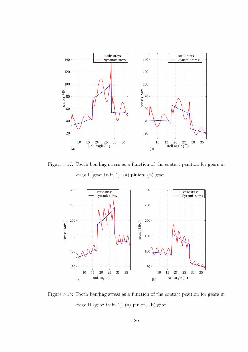
10 15 20 25 30 35

20

40

60

80

100

120

140

Roll angle ( o )

stre

ss (

MPa

)

10 15 20 25 30 35

20

40

60

80

100

120

140

Roll angle ( o )st

ress

( M

Pa )

static stress dynamic stress


(a) (b)

Figure 5.17: Tooth bending stress as a function of the contact position for gears in

stage I (gear train 1), (a) pinion, (b) gear

10 15 20 25 30 35

50

100

150

200

250

300

Roll angle ( o )

stre

ss (

MPa

)

10 15 20 25 30 35

50

100

150

200

250

300

Roll angle ( o )

stre

ss (

MPa

)



(a) (b)


stage II (gear train 1), (a) pinion, (b) gear

86

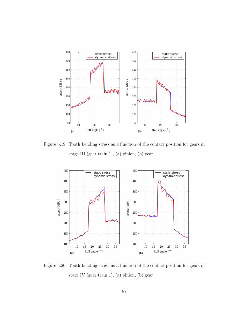
10 20 3050

100

150

200

250

300

350

400

450

Roll angle ( o )

stre

ss (

MPa

)

10 20 3050

100

150

200

250

300

350

400

450

Roll angle ( o )st

ress

( M

Pa )



(a) (b)


stage III (gear train 1), (a) pinion, (b) gear

10 15 20 25 30 35100

150

200

250

300

350

400

450

Roll angle ( o )

stre

ss (

MPa

)

10 15 20 25 30 35100

150

200

250

300

350

400

450

Roll angle ( o )

stre

ss (

MPa

)



(a) (b)


stage IV (gear train 1), (a) pinion, (b) gear

87

The peak dynamic stress during single pair contact is much higher than the static

stress which makes the dynamic analysis an important design tool for the gears. To

avoid tooth failure, the bending stress should be limited to the allowable bending

strength of the material suggested by AGMA [72]. AGMA bending strength equation

is given by:

σall =StKL

KTKRKV

. (5.5)

where,

σall allowable bending stress

KL life factor

St AGMA bending strength

KT temperature factor

KR reliability factor

KV dynamic factor

The dynamic factor is used to account for inaccuracies in the manufacture and

meshing of gear teeth in action. AGMA has defined a set of quality control numbers

to define the tolerances of gears of various sizes manufactured to a specified class.

More details on these classes can be found in reference [72]. The following equations

for the dynamic factor are based on these quality control numbers.

KV =[ A

A+√

200V

]. (5.6)

where

A = 50 + 56(1−B)

B = (12−Qv)23

4

88

Qv = quality control number

V = pitch-line velocity (m/s)

The allowable stress depends on the nature of heat treatment and surface hardness

of the material. Typical values used in this study are given in Table 5.7 [72]. In

this study, a typical value of 450MPa was used for the allowable stress for a case

hardened low carbon steel alloy [73]. Based on a life cycle of 107, the life factor can

Table 5.7: Values of allowable stress

Material Heat Treatment Hardness St MPa

Steel induction hardened 50-54 HRC 310-380

carburised 55 HRC 380-450

case hardened 60 HRC 380-480

be taken as KL = 1.0 with a corresponding reliability of 0.99 whose reliability factor

is 1.0. For oil or gear blank temperatures of up to 120oC, the temperature factor

is taken as 1.0. The allowable bending stress recommended by AGMA depends on

the magnitude of the pitch line velocity and from Table 5.8, it can be seen that the

allowable bending stress increases as the pitch line velocity increases.

The face width of the current gearbox design was obtained based on the modified

Lewis equation given by:

σL =Wt

KvFpcy, (5.7)

where

Kv =6.1

6.1 + V. (5.8)

Thus to analyze the possibility of gear tooth failure at the root, the values obtained

89

Table 5.8: Allowable root bending stress based on AGMA equation

Reduction stage Gear V (m/s) Kv

AGMA σall (MPa)

14 T I 34 T 3.29867 0.78409 573.91

14 T II 40 T 1.35828 0.84784 530.76

15 T III 40 T 0.50935 0.89995 500.03

14 T IV 40 T 0.17827 0.93783 479.83

from the Lewis equation and the peak values obtained from the dynamic analysis

need to be compared with AGMA allowable stress. Table 5.9 shows the factors

Table 5.9: Factors used to compute the bending stress using Lewis equation

Reduction stage Gear V (m/s) Kv y Wt (N) σL (MPa)

14 T 0.149 107.481 I 34 T 3.29867 0.64903 0.227 1469.414 70.549 14 T 0.149 155.352 II 40 T 1.35828 0.81788 0.233 3568.577 99.345 15 T 0.156 233.765 III 40 T 0.50935 0.92293 0.233 9516.204 156.511 14 T 0.149 199.274 IV 40 T 0.17827 0.97160 0.233 13594.578 212.388

used to compute the bending stress based on the Lewis equation, while Table 5.10

shows a comparison of the dynamic stress obtained from this study with the bending

stress obtained using the Lewis equation and the allowable stress recommended by

AGMA. The Lewis equation predicts low values of the bending stress than that

obtained from the dynamic analysis of the gear train as show on Table 5.10. This

implies that dynamic analysis of a geared system is necessary in the design stage

in order to analyze possibility of gear tooth failure and to predict the fatigue life of

90

Table 5.10: Comparison of the dynamic stress, Lewis stress and AGMA allowable

stress

Reduction stage Gear σj (MPa) σL (Mpa)

AGMA σall (MPa)

14 T 119.61 107.48 I 34 T 93.95 70.55 573.91

14 T 274.62 155.35 II 40 T 188.98 99.35 530.76

15 T 388.34 233.77 III 40 T 294.28 156.51 500.03

14 T 359.39 199.27 IV 40 T 409.61 212.39 479.83

a gear. The gear pairs in all the stages have a peak dynamic stress less than the

recommended AGMA bending stress for 107 cycles.

Figure 5.21 shows the variation of the natural frequencies with the contact position of

the first gear mesh for the first three modes. Table 5.11 shows the natural frequencies

range corresponding the the system configuration shown in Figure 4.2 while the

corresponding mode shapes are shown in Figures 5.22 to 5.24.

5 10 15 20 25 30 35 40200

400

600

800

1000

1200

1400

Roll angle ( o )

natu

ral f

requ

ency

( ra

d/s )

ω2

ω3

ω4

Figure 5.21: Variation of natural frequency with the contact position of the gears

91

Table 5.11: System Natural Frequencies corresponding to gear train 1

Natural frequency Predicted value (rad/s)

ω1 0 ω2 252 – 264 ω3 894 – 920 ω4 1044 – 1264 ω5 7174 – 7580 ω6 11722 – 12540 ω7 16000 – 17180 ω8 21647 – 27620 ω9 43812 – 57240 ω10 47743 – 60323 ω11 61935 – 79593 ω12 73167 – 83534 ω13 131292 - 169520

The mode shapes show the relative rotational displacements between the rotors when

the system is responding purely to the corresponding natural frequency. Figure 4.2

is a free-free (unconstrained) system and is also referred to as a semi definite system.

One of the natural frequencies of such a system will be zero, corresponding to the

zero root of the eigenfrequency equation when the body moves as a rigid body. The

rigid body motion corresponding to ω1 = 0.0 is not actually vibratory motion and

is of no importance.

Figure 5.22(a) shows the mode shape of the system corresponding to ω2. This

mode is influenced by the input pulley assembly, (element 1) which rotates at a

maximum angular speed of 157.08 rad/s. This speed is below the fundamental

frequency which implies that this gear train configuration operates at speeds below

the natural frequencies of the system and hence it is highly unlikely that resonance

would occur during normal operation.

92

1 2 3 4 5 6 7 8 9 10 11 12 13-1

-0.50

0.51

-1-0.5

00.5

1-1

Element

Nor

mal

ized

mod

e

(a) ω2

1 2 3 4 5 6 7 8 9 10 11 12 13-1

-0.8-0.6-0.4-0.2

00.20.40.60.8

1

Element

Nor

mal

ized

mod

e

(b) ω3

1 2 3 4 5 6 7 8 9 10 11 12 13-1

-0.8-0.6-0.4-0.2

00.20.40.60.8

1

Element

Nor

mal

ized

mod

e

(c) ω4

1 2 3 4 5 6 7 8 9 10 11 12 13-1

-0.8-0.6-0.4-0.2

00.20.40.60.8

1

Element

Nor

mal

ized

mod

e

(d) ω5

Figure 5.22: Mode shape corresponding to ω2 − ω5 for gear train 1

93

1 2 3 4 5 6 7 8 9 10 11 12 13-1

-0.8

-0.6

-0.4

-0.2

0

0.2

0.4

0.6

0.8

1

Element

Nor

mal

ized

mod

e

1 2 3 4 5 6 7 8 9 10 11 12 13-1

-0.8

-0.6

-0.4

-0.2

0

0.2

0.4

0.6

0.8

1

Element

Nor

mal

ized

mod

e

1 2 3 4 5 6 7 8 9 10 11 12 13-1

-0.8

-0.6

-0.4

-0.2

0

0.2

0.4

0.6

0.8

1

Element

Nor

mal

ized

mod

e

1 2 3 4 5 6 7 8 9 10 11 12 13-1

-0.8

-0.6

-0.4

-0.2

0

0.2

0.4

0.6

0.8

1

Element

Nor

mal

ized

mod

e

(a) ω6(b) ω7

(c) ω8 (d) ω9


94

1 2 3 4 5 6 7 8 9 10 11 12 13-1

-0.8

-0.6

-0.4

-0.2

0

0.2

0.4

0.6

0.8

1

Element

Nor

mal

ized

mod

e

1 2 3 4 5 6 7 8 9 10 11 12 13-1

-0.8

-0.6

-0.4

-0.2

0

0.2

0.4

0.6

0.8

1

Element

Nor

mal

ized

mod

e

1 2 3 4 5 6 7 8 9 10 11 12 13-1

-0.8

-0.6

-0.4

-0.2

0

0.2

0.4

0.6

0.8

1

Element

Nor

mal

ized

mod

e

1 2 3 4 5 6 7 8 9 10 11 12 13-1

-0.8

-0.6

-0.4

-0.2

0

0.2

0.4

0.6

0.8

1

Element

Nor

mal

ized

mod

e

(a) ω10 (b) ω11

(c) ω12 (d) ω13


95

To demonstrate the sensitivity of the eigenvalues to rotor properties, we reduced

the inertia of the input pulley by 20% (from 10697 Kgmm2 to 8558 Kgmm2) and

observed that the fundamental frequency increased by about 11% as shown in Table

5.12. Only the first four modes are given since the higher modes have no impact

on the system. The effect of shaft stiffness is negligible as seen in Table 5.12 where

an increase in the torsional stiffness of the shaft connecting the input pulley to gear

1 by about 90% (from 2.45× 107Nm/rad to 4.60× 107Nm/rad) by increasing the

shaft diameter from 24 mm to 28 mm results to an increase in the natural frequency

by only 0.8%. Thus it is possible to tune the natural frequencies away from the

operating speed range by either reducing or increasing the mass moment of inertia

of the system components.

Table 5.12: Predicted natural frequencies with modified system properties

Natural frequency Initial value

(rad/s) With modifiedInertia (rad/s)

With modified shaft stiffness (rad/s)

ω2 252 – 264 280 – 295 254 – 267 ω3 894 – 920 895 – 920 895 – 920 ω4 1044 – 1264 1044 – 1264 1044 – 1260 ω5 7174 – 7580 7200 - 7600 8078 – 8728

96

5.5.2 Top Gear Ratio Configuration

Gear arrangement for this configuration is shown in Figure 5.25. In this report, this

gear train will be referred to as gear train 2.

Figure 5.25: Gear train for top gear ratio

97

Table 5.13 show the system properties for the gear train 2 while Table 5.14 shows

the operating conditions for this gear train.

Table 5.13: Rotor properties for gear train 2

Rotor No. Description

No. of teeth for

gears

Face width (mm)

Addendum modification

factor

Moment of inertia (Kg

mm2)

Theoretical contact ratio

1 Input pulley assembly - - 10697.8 -

2 Stage I pinion 28 15 - 722.5

3 Stage I gear 20 15 - 151.1 1.597

4 Stage II pinion 30 20 - 759.2

5 Stage II gear 24 20 - 1631.9 1.628

6 Stage III pinion 15 25 1.2385 m 96.3

7 Stage III gear 40 25 0.7615 m 4892.7

1.552

8 Stage IV pinion 14 50 1.3106 m 140.2

9 Stage IV gear 40 30 0.6894 m 4786.7

1.522

10 Stage IV pinion 14 50 1.3106 m 140.2

11 Stage IV gear 40 30 0.6894 m 4786.7

1.522

12 Output inertia - - 291179.0 -

13 Output inertia - - 291179.0 -

Table 5.14: Operating conditions and gear parameters for gear train 2

Input speed 1500 rpm

Nominal Torque 130 Nm

module (m) 3 mm

Pressure angle 20o

Figures 5.26 to 5.29 show the dynamic response of the gears on each mesh. Similarly,

98

the response is periodic and the zones of single tooth contact and double tooth pair

contact are clearly visible in all the time plots. The effect of damping is more sig-

nificant on high speed and low torque applications as can be seen in Figures 5.26(a)

and 5.27(a). The peak amplitude of relative displacement occurs at the fundamental

mesh frequency. The fundamental mesh frequency for the various meshes are given

in Table 5.15.

0 1 2 3 4 5x 10-3

0

1

2

3

4

5

6x 10-3

Time (sec)

δ 1 (mm

)

0 5000 10000 150000

0.5

1

1.5

2

2.5

3

3.5

4

4.5x 10-4

Frequency (Hz)

δ 1 (mm

)

(a) (b)

Figure 5.26: Vibration signatures for gears in stage I (gear train 2)

99

0 1 2 3x 10-3

0

0.5

1

1.5

2

2.5

3

3.5x 10-3

Time (sec)

δ 2 (mm

)

0 5000 10000 150000

0.5

1

1.5

2

2.5

3

3.5x 10-4


m)

(a) (b)

Figure 5.27: Vibration signatures for gears in stage II (gear train 2)

0 2 4 6x 10-3

0

0.5

1

1.5

2

2.5x 10-3

Time (sec)

δ 3 (mm

)

0 2000 4000 6000 8000 100000

1

2

x 10-4

Frequency (Hz)

δ 3 (mm

)

(a) (b)

Figure 5.28: Vibration signatures for gears in stage III (gear train 2)

100

0 0.002 0.004 0.006 0.008 0.01 0.0120

0.5

1

1.5

2

2.5x 10-3

Time (sec)

δ 4 (mm

)

0 1000 2000 3000 4000 50000

1

2

x 10-4


m)

(a) (b)

Figure 5.29: Vibration signatures for gears in stage IV (gear train 2)

Table 5.15: Fundamental mesh frequencies for gear train 2

mesh mesh frequency (HZ)

I 700.0

II 1050.0

III 656.3

Iv 229.7

Figure 5.30 shows a comparison of the dynamic and static load on a gear tooth along

the path of contact. As previously discussed, the dynamic load is higher than the

static load and the percentage difference is shown in Table 5.16.

101

15 20 25200

400

600

800

1000

1200

Roll angle ( o )

Forc

e ( N

)

15 20 25

200

300

400

500

600

700

800

Roll angle ( o )Fo

rce

( N )

10 20 30300

400

500

600

700

800

900

1000

Roll angle ( o )

Forc

e ( N

)

10 15 20 25 30 35400

600

800

1000

1200

1400

1600

Roll angle ( o )

Forc

e ( N

)





(a) stage I (b) stage II

(c) stage III (d) stage IV

Figure 5.30: Comparison of the dynamic and static load on a single tooth over the

path of contact (gear train 2)

102

Table 5.16: Percentage difference between peak dynamic load and maximum static

load for gear train 2

Gear mesh velocity (m/s) static load Peak dynamic load % difference

(m/s) (N) (N)

I 6.597 756.56 909.44 20.21

II 9.896 504.38 644.09 27.70

III 6.185 807.00 862.84 6.92

IV 2.010 1152.86 1378.34 19.56

Figures 5.31 to 5.34 show the comparison of the dynamic stress and static stress

over the path of contact. In all the plots, the peak dynamic stress on a gear tooth

is higher than the static stress.

15 20 250

10

20

30

40

50

60

70

Roll angle ( o )

stre

ss (

MPa

)

15 20 250

10

20

30

40

50

60

70

Roll angle ( o )

stre

ss (

MPa

)



(a) (b)


stage I (gear train 2), (a) pinion, (b) gear

103

15 20 250

5

10

15

20

25

30

35

40

45

50

Roll angle ( o )

stre

ss (

MPa

)


15 20 250

5

10

15

20

25

30

35

40

45

50

Roll angle ( o )st

ress

( M

Pa )


(a) (b)


stage II (gear train 2), (a) pinion, (b) gear

10 20 300

5

10

15

20

25

30

35

40

45

50

Roll angle ( o )

stre

ss (

MPa

)

10 20 300

5

10

15

20

25

30

35

40

45

50

Roll angle ( o )

stre

ss (

MPa

)



(a) (b)


stage III (gear train 2), (a) pinion, (b) gear

104

10 15 20 25 30 350

5

10

15

20

25

30

35

40

45

50

Roll angle ( o )

stre

ss (

MPa

)

10 15 20 25 30 350

5

10

15

20

25

30

35

40

45

50

Roll angle ( o )st

ress

( M

Pa )



(a) (b)


stage IV (gear train 2), (a) pinion, (b) gear

Table 5.17 shows a comparison of the peak dynamic stress on each gear with the

recommended tooth stress by AGMA for 107 cycles. It can observed that the peak

dynamic stress for all the gears is way below the maximum stress recommended by

AGMA implying that the gears on gear train 2 would have a longer fatigue life.

Table 5.17: Recommended and maximum dynamic tooth stresses for gear train 2

Mesh Gear No. of Teeth V (m/s) Kv σj (MPa)

AGMA σall (MPa)

driver 28 0.7231 53.56 I driven 20 6.5973 0.7231 63.28 622.40

driver 30 0.6833 36.54 II driven 24 9.8960 0.6833 41.11 658.60

driver 15 0.7291 38.04 III driven 40 6.1850 0.7291 30.65 617.20

driver 14 0.8217 35.54 IV driven 40 2.0101 0.8217 36.43 547.64

105

Table 5.18 shows the natural frequencies corresponding the the system configuration

shown in Figure 5.25 while the corresponding mode shapes are shown in Figures 5.22

to 5.24. As explained previously, the first natural frequency is zero for a free-free

system. From the mode shapes corresponding to the natural frequencies obtained

for this system, Figures 5.22 to 5.24, the mode shape corresponding to the second

natural frequency is influenced by the output flywheel assembly whose angular speed

is much below the natural frequency. The operating speed range for the system is

below any of the natural frequencies implying that resonance is unlikely to occur.

Table 5.18: System Natural Frequencies corresponding to gear train 2

Natural frequency Predicted value (rad/s)

ω1 0 ω2 898 – 920 ω3 989 – 1003 ω4 1060 – 1249 ω5 5540 – 5680 ω6 11000 – 11625 ω7 19300 – 22240 ω8 22533 – 28216 ω9 26413 – 34650 ω10 42456 – 54318 ω11 75187 - 87227 ω12 79920 – 89450 ω13 135200 - 172250

106

1 2 3 4 5 6 7 8 9 10 11 12 13-1

-0.8

-0.6

-0.4

-0.2

0

0.2

0.4

0.6

0.8

1

Element

Nor

mal

ized

mod

e

1 2 3 4 5 6 7 8 9 10 11 12 13-1

-0.8

-0.6

-0.4

-0.2

0

0.2

0.4

0.6

0.8

1

Element

Nor

mal

ized

mod

e

1 2 3 4 5 6 7 8 9 10 11 12 13-1

-0.8

-0.6

-0.4

-0.2

0

0.2

0.4

0.6

0.8

1

Element

Nor

mal

ized

mod

e

1 2 3 4 5 6 7 8 9 10 11 12 13-1

-0.8

-0.6

-0.4

-0.2

0

0.2

0.4

0.6

0.8

1

Element

Nor

mal

ized

mod

e

(a) ω2 (b) ω3

(c) ω4 (d) ω5


107

1 2 3 4 5 6 7 8 9 10 11 12 13-1

-0.8

-0.6

-0.4

-0.2

0

0.2

0.4

0.6

0.8

1

Element

Nor

mal

ized

mod

e

1 2 3 4 5 6 7 8 9 10 11 12 13-1

-0.8

-0.6

-0.4

-0.2

0

0.2

0.4

0.6

0.8

1

Element

Nor

mal

ized

mod

e

1 2 3 4 5 6 7 8 9 10 11 12 13-1

-0.8

-0.6

-0.4

-0.2

0

0.2

0.4

0.6

0.8

1

Element

Nor

mal

ized

mod

e

1 2 3 4 5 6 7 8 9 10 11 12 13-1

-0.8

-0.6

-0.4

-0.2

0

0.2

0.4

0.6

0.8

1

Element

Nor

mal

ized

mod

e

(a) ω6(b) ω7

(c) ω8(d) ω9


108

1 2 3 4 5 6 7 8 9 10 11 12 13-1

-0.8

-0.6

-0.4

-0.2

0

0.2

0.4

0.6

0.8

1

Element

Nor

mal

ized

mod

e

1 2 3 4 5 6 7 8 9 10 11 12 13-1

-0.8

-0.6

-0.4

-0.2

0

0.2

0.4

0.6

0.8

1

Element

Nor

mal

ized

mod

e

1 2 3 4 5 6 7 8 9 10 11 12 13-1

-0.8

-0.6

-0.4

-0.2

0

0.2

0.4

0.6

0.8

1

Element

Nor

mal

ized

mod

e

1 2 3 4 5 6 7 8 9 10 11 12 13-1

-0.8

-0.6

-0.4

-0.2

0

0.2

0.4

0.6

0.8

1

Element

Nor

mal

ized

mod

e(a) ω10 (b) ω11

(c) ω12 (d) ω13


109

5.6 Effect of Gear Design Parameters

In this section, the effect of varying the gear design parameters on the gear vibrations

and dynamics is presented. The following gear design parameters are included:

1. Module 2.0, 2.5 and 3.0

2. Contact ratio

3. Pressure angle

5.6.1 Effect of Module on Gear Vibrations

The module of the gears was changed from 3.0 mm to 2.0 mm and 2.5 mm trying

to minimize the difference between the original pitch circle diameters and center

distances with the new ones by varying the numbers of teeth on the gears as shown

on Tables 5.19 and 5.20. The pressure angle, face width and pitch radius were held

constant. However, since the number of teeth on a gear is an integer, the pitch

radius of some gears varied slightly along with the center distance. Using a module

larger than 3.0 would compromise on the space requirements (overall center distance

of 325± 10 mm) of the gearbox since it would be necessary to increase the number

of teeth in order to avoid interference. For instance using a module of 4.0, a gear

previously with 14 teeth would be replaced by a gear with 11 teeth which would

require an addendum modification factor greater than 0.4m resulting to a very small

active profile on the mating gear tooth. On the other hand, changing the module

alone while holding the number of teeth constant would change the pitch radius and

hence the applied load. Figure 5.38 shows sample tooth profiles for selected number

of teeth on the gears.

110

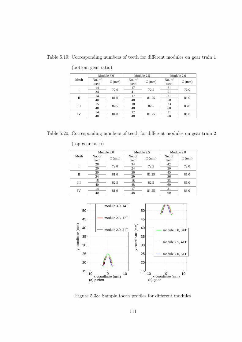
Table 5.19: Corresponding numbers of teeth for different modules on gear train 1

(bottom gear ratio)

Module 3.0 Module 2.5 Module 2.0 Mesh No. of

teeth C (mm) No. of teeth C (mm) No. of

teeth C (mm)

14 17 21 I 34 72.0 41 72.5 51 72.0

14 17 21 II 40 81.0 48 81.25 60 81.0

15 18 23 III 40 82.5 48 82.5 60 83.0

14 17 21 IV 40 81.0 48 81.25 60 81.0

Table 5.20: Corresponding numbers of teeth for different modules on gear train 2

(top gear ratio)

Module 3.0 Module 2.5 Module 2.0 Mesh No. of

teeth C (mm) No. of teeth C (mm) No. of

teeth C (mm)

28 34 42 I 20 72.0 24 72.5 30 72.0

30 36 45 II 24 81.0 29 81.25 36 81.0

15 18 23 III 40 82.5 48 82.5 60 83.0

14 17 21 IV 40 81.0 48 81.25 60 81.0

-10 0 1015

20

25

30

35

40

45

50

x-coordinate (mm)

y-co

ordi

nate

(mm

)

-10 0 1015

20

25

30

35

40

45

50

x-coordinate (mm)

y-co

ordi

nate

(mm

)

module 3.0, 14T module 2.5, 17T module 2.0, 21T module 3.0, 34T

module 2.5, 41T module 2.0, 51T

(a) pinion (b) gear

Figure 5.38: Sample tooth profiles for different modules

111

Figures 5.39 and 5.40 show the vibration levels of the various meshes on gear train 1

in the frequency domain for modules, 2.0, 2.5 and 3.0. It can be seen that the peak

amplitude of the vibrations for the different modules are almost the same though

gears with module 2.0 show slightly lower amplitudes for mesh I, III and IV. This

could be as a result of the high mesh stiffness as shown in Figure 5.41. The stiffness

of the gears increases with reduction in the module since the effective length of the

tooth as a cantilever beam reduces. However, from Figure 5.42 it can be observed

that the root stress on a gear tooth increases by reducing the module. The stresses

on the driven gear with a module of 2.0 and 2.5 for the fourth stage (Figure 5.42)

are higher than that calculated using the AGMA equation which implies that they

would have a lower fatigue life than gears with a module of 3.0. This could be due

to the decreased tooth thickness at the fillet area for gears with a smaller module

as shown in Figure 5.38.

112

0 2000 40000

0.2

0.4

0.6

0.8

1x 10-3

frequency (Hz)

δ 1 (mm

)

0 2000 40000

0.2

0.4

0.6

0.8

1x 10-3

0 2000 40000

0.2

0.4

0.6

0.8

1x 10-3

0 1000 20000

0.5

1

1.5

2x 10-3

frequency (Hz)

δ 2 (mm

)

0 1000 20000

0.5

1

1.5

2x 10-3

0 1000 20000

0.5

1

1.5

2x 10-3

module 3.0 module 2.5 module 2.0


(a) (b) (c)

(d) (e) (f)

Figure 5.39: Vibration levels for various modules for bottom gear ratio (stage I

and II)

113

0 500 10000

0.5

1

1.5

2

2.5

3x 10-3

frequency (Hz)

δ 3 (mm

)

0 500 10000

0.5

1

1.5

2

2.5

3x 10-3

0 500 10000

0.5

1

1.5

2

2.5

3x 10-3

0 200 4000

0.5

1

1.5

2

2.5

3x 10-3

frequency (Hz)

δ 4 (mm

)

0 200 4000

0.5

1

1.5

2

2.5

3x 10-3

0 200 4000

0.5

1

1.5

2

2.5

3x 10-3



(a) (b) (c)

(d) (e) (f)

Figure 5.40: Vibration levels for various modules for gear train 1 (stage III and IV)

114

0 0.001 0.002 0.003 0.004 0.005 0.006 0.007 0.008 0.009 0.010

0.5

1

1.5

2

2.5

3

3.5

4

4.5

5x 105

Time (sec)

mes

h st

iffne

ss (N

/mm

)

module 3.0module 2.5module 2.0

Figure 5.41: Sample mesh stiffness for gears with different modules but the same

pitch diameter and face width

0 10 20 30 400

100

200

300

400

500

600

700

Roll angle ( o )

Ben

ding

stre

ss (

MPa

)

0 10 20 30 400

100

200

300

400

500

600

700

Roll angle ( o )

Ben

ding

stre

ss (

MPa

)



(a) pinion (b) gear

Figure 5.42: Root stress on stage IV of gear train 1 for different modules

115

5.6.2 Effect of Pressure Angle on Gear Vibrations

The standard pressure angles normally used in the manufacture of gears are 14.5o,

20o and 25o. In this section, the results are presented for pressure angles of 25o

and 20o only since the minimum number of teeth to avoid interference for pressure

angle of 14.5o is 32 as shown on Table 2.1. This means that we would require very

large gears for the gear train and by considering the space requirements (overall

center distance of 325 ± 10 mm) of the gearbox, it would be uneconomical to use

this pressure angle. The pressure angle was varied while holding the module and

number of teeth of the various meshes constant.

Figure 5.43 shows sample profiles for teeth with a pressure angle of 20o and 25o

respectively.

-10 0 1015

20

25

30

35

40

45

50

55

x-coordinate (mm)

y-co

ordi

nate

(mm

)

-10 0 1015

20

25

30

35

40

45

50

55

x-coordinate (mm)

y-co

ordi

nate

(mm

)

φ = 25o, 34T φ = 20o, 34T

φ = 25o, 14T φ = 20o, 14T

(a) pinion (b) gear

Figure 5.43: Sample tooth profiles for different pressure angles

The tooth with a pressure angle of 25o has a larger thickness at the fillet area which

explains why the gears with pressure angle of 25o have a higher mesh stiffness than

a corresponding pair with a pressure angle of 20o as shown in Figure 5.44, which is

116

also attributed to the larger tooth thickness at the fillet area. However increasing

the pressure angle reduces the contact ratio and thus increasing the duration of

single pair contact zone as shown in Figure 5.44.

0 0.001 0.002 0.003 0.004 0.005 0.006 0.007 0.008 0.009 0.010

0.5

1

1.5

2

2.5

3

3.5

4

4.5

5x 105

Time (sec)

Mes

h st

iffne

ss (N

/mm

)

20o Pressure angle25o Pressure angle

single toothcontact zone

single contact zone

τ

Figure 5.44: Mesh stiffness for different pressure angles

Figures 5.45 and 5.46 show plots of the vibration amplitudes of the various meshes

of gear train 1. It can be observed that the vibration amplitudes of gears with a

pressure angle of 25o are slightly lower than those of corresponding gear pairs with

a pressure angle of 20o. This could be due to the higher mesh stiffness for pressure

angle of 25o. The root stress plots (Figure 5.47) show relatively lower root stress

for the pinion with a pressure angle of 25o which is mainly due to the larger tooth

thickness at the fillet area and the fact that the addendum of the pinion has not

been modified and therefore the effective length of the gear tooth is smaller as shown

in Figure 5.43.

117

0 1000 2000 3000 4000 50000

0.2

0.4

0.6

0.8

1x 10-3

frequency ( Hz )

δ 1 ( m

m )

0 1000 2000 3000 4000 50000

0.2

0.4

0.6

0.8

1x 10-3

frequency ( Hz )

δ 1 ( m

m )

0 500 1000 1500 20000

0.5

1

1.5

2x 10-3

frequency ( Hz )

δ 2 ( m

m )

0 500 1000 1500 20000

0.5

1

1.5

2x 10-3

frequency ( Hz )

δ 2 ( m

m )

φ = 20o φ = 25o

φ = 20o φ = 25o

(a) (b)

(c) (d)

Figure 5.45: Comparison of the vibration amplitudes for different pressure angles

(stage I and II)

0 500 10000

0.5

1

1.5

2

2.5x 10-3

frequency ( Hz )

δ 3 ( m

m )

0 500 10000

0.5

1

1.5

2

2.5x 10-3

frequency ( Hz )

δ 3 ( m

m )

0 200 400 6000

0.5

1

1.5

2

2.5

3x 10-3

frequency ( Hz )

δ 4 ( m

m )

0 200 400 6000

0.5

1

1.5

2

2.5

3x 10-3

frequency ( Hz )

δ 4 ( m

m )

φ = 20o

φ = 20o φ = 25o

φ = 25o

(a) (b)

(c) (d)

Figure 5.46: Comparison of the vibration amplitudes for different pressure angles

(stage III and IV)

118

10 20 30 400

50

100

150

200

250

300

350

400

450

500

Roll angle ( o )

Roo

t stre

ss (M

Pa)

10 20 30 400

50

100

150

200

250

300

350

400

450

500

Roll angle ( o )R

oot s

tress

(MPa

)

φ = 20o, 14Tφ = 25o, 14T

φ = 20o, 40Tφ = 25o, 40T

(a) pinion (b) gear

Figure 5.47: Sample root stress for gears with different pressure angle

5.6.3 Effect of Contact Ratio on Gear vibrations

The contact ratio of a pair of gears in mesh is given by equation B.42 and is affected

by the following parameters:

• addendum

• center distance

• pressure angle

• module

The contact ratio of a gear pair can be increased by varying one of the above parame-

ters or a combination of two or more of these parameters. Increasing the addendum

is normally recommended for increasing the contact ratio since this can be achieved

119

by simply adjusting the cutter depth [18]. The maximum permissible addendum

modification coefficients are obtained by iteratively varying the addendum modifi-

cation coefficient of the pinion and gear until the top land thickness is equal to the

minimum allowable (usually 0.3m) [74]. In this research work, a code was devel-

oped to obtain the maximum possible contact ratio for a gear pair by varying the

addendum and adjusting the center distance in order to avoid interference.

Table 5.21: Maximum possible contact ratio for a gear pair with module 3.0

Mesh Gear Ax Contact ratio Center distance (mm)

14 0.348I 34 0.156 1.594 72.915

14 0.348II 40 0.009 1.594 81.621

15 0.364III 40 0.341 1.651 83.809

14 0.348IV 40 0.009 1.594 81.621

From Table 5.21, it can be observed that for a pair of gears with a high reduction

ratio, it is difficult to obtain a contact ratio close to 2.0. However, this can be

achieved by using a smaller module as shown on Tables 5.22 and 5.23.



17 0.393I 41 0.407 1.970 72.969

17 0.393II 48 0.265 1.971 81.503

18 0.357III 48 0.384 1.991 82.903

17 0.393IV 48 0.265 1.971 81.503

120



21 0.360I 51 0.371 1.992 72.382

21 0.360II 60 0.273 1.992 81.267

23 0.347III 60 0.181 1.998 83.124

21 0.360IV 60 0.273 1.992 81.267

Figure 5.48 shows sample tooth profiles for teeth with modified addendum to increase

the contact ratio. In this case the minimum allowable top land thickness for the

pinions was set to 0.35m

-10 -5 0 5 1015

20

25

30

35

40

45

50

55

60

x-coordinate (mm)

y-co

ordi

nate

(mm

)

-10 -5 0 5 1015

20

25

30

35

40

45

50

55

60

x-coordinate (mm)

y-co

ordi

nate

(mm

)

module 3.0, 14T module 2.5, 17T module 2.0, 21T

module 3.0, 34T module 2.5, 41T module 2.0, 51T

(a) pinion (b) gear

Figure 5.48: Sample tooth profiles for teeth with modified addendum

121

Figure 5.49 shows the periodic mesh stiffness for various contact ratios. It can be

observed that as the contact ratio increases, the band width for single contact zone

reduces. As the contact ratio approaches 2.0, the variation in mesh stiffness is mainly

due to the change in contact point along the path of contact as shown in Figure 5.49.

The discontinuities in the mesh stiffness as the number of teeth in contact changes

are eliminated. As one pair of teeth leaves mesh, another pair of teeth enters the

mesh ensuring that there are always two pairs of teeth in contact. The applied load

is shared between two pairs of teeth at all times. However, the magnitude of the

mesh stiffness reduces due to the increase in the tooth height and consequently the

effective length of the cantilever beam that represents the tooth.

Figures 5.50 and 5.51 show sample plots for vibration levels of gear pairs with high

contact ratio. A pair of gears with a contact ratio close to 2.0 shows relatively low

vibration levels especially those with a module of 2.0. A contact ratio of 2.0 reduces

the vibration levels by up to 75% in both cases. This effect is due to the very narrow

band of single-tooth contact being passed so quickly during gear rotation that the

system could not respond until after excitation has passed resulting to a very gentle

dynamic response.

122

0 0.05 0.10

2

4

6

8

10

12x 105

Time (sec)

mes

h st

iffne

ss (N

/mm

)

0 0.05 0.10

2

4

6

8

10

12x 105

Time (sec)

mes

h st

iffne

ss (N

/mm

)

0 0.05 0.10

2

4

6

8

10

12x 105

Time (sec)

mes

h st

iffne

ss (N

/mm

)

CR = 1.552CR = 1.651

CR = 1.639CR = 1.935CR = 1.991

CR = 1.688CR = 1.874CR = 1.998

(a) module 3.0 (b) module 2.5

(c) module 2.0

Figure 5.49: Periodic mesh stiffness for different contact ratios

123

0 2000 40000

0.2

0.4

0.6

0.8

1

x 10-3

frequency (Hz)

δ 1 (mm

)

0 2000 40000

0.2

0.4

0.6

0.8

1

x 10-3

0 2000 40000

0.2

0.4

0.6

0.8

1

x 10-3

0 1000 20000

0.5

1

1.5

2

2.5

3x 10-3

frequency (Hz)

δ 2 (mm

)

0 1000 20000

0.5

1

1.5

2

2.5

3x 10-3

0 1000 20000

0.5

1

1.5

2

2.5

3x 10-3

CR = 1.664 CR = 1.874 CR = 1.992

CR = 1.677 CR = 1.874 CR = 1.992

(a) (b) (c)

(d) (e) (f)

Figure 5.50: Sample vibration levels for gear pairs with increased contact ratio

(gears with a module of 2.0 mm)

124

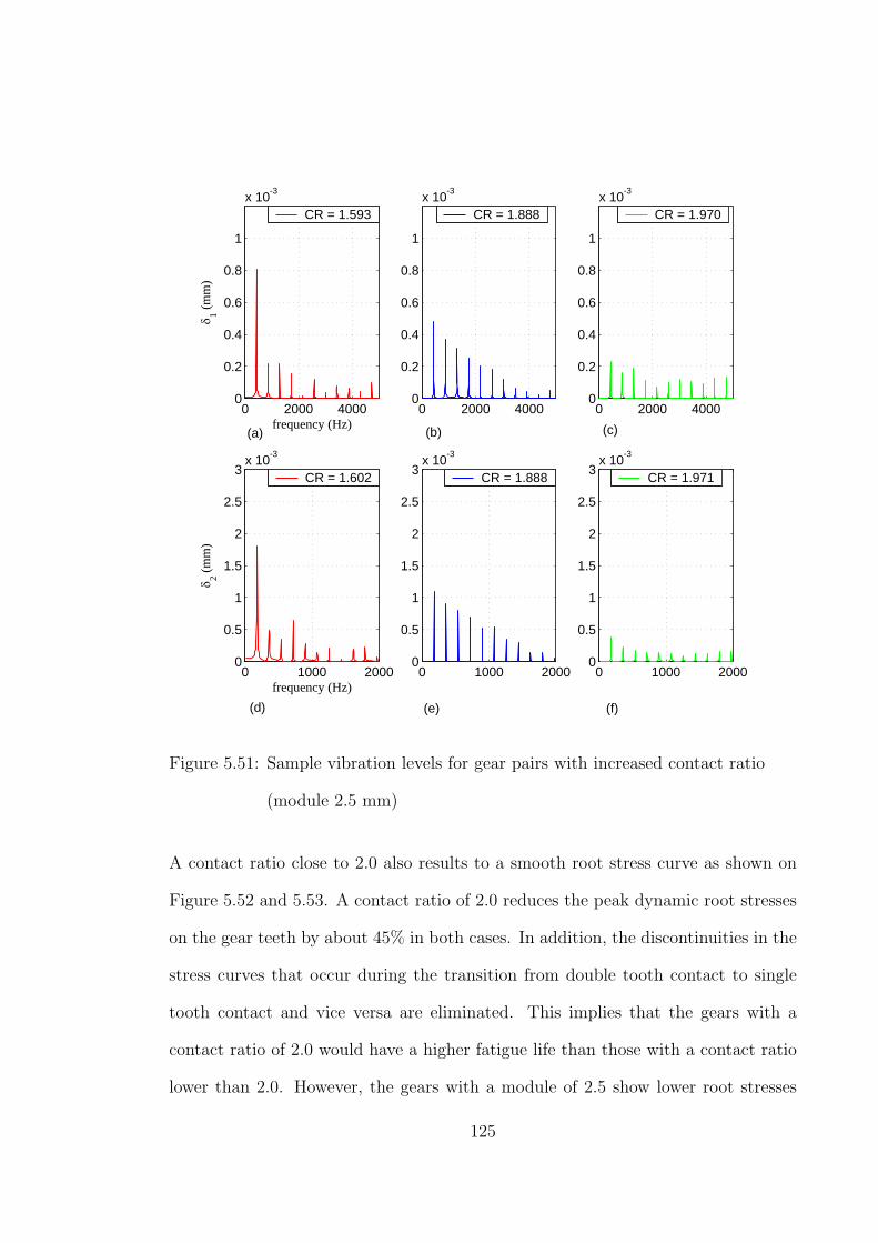
0 2000 40000

0.2

0.4

0.6

0.8

1

x 10-3

frequency (Hz)

δ 1 (mm

)

0 2000 40000

0.2

0.4

0.6

0.8

1

x 10-3

0 2000 40000

0.2

0.4

0.6

0.8

1

x 10-3

0 1000 20000

0.5

1

1.5

2

2.5

3x 10-3

frequency (Hz)

δ 2 (mm

)

0 1000 20000

0.5

1

1.5

2

2.5

3x 10-3

0 1000 20000

0.5

1

1.5

2

2.5

3x 10-3

CR = 1.593 CR = 1.888 CR = 1.970

CR = 1.602 CR = 1.888 CR = 1.971

(a) (b) (c)

(d) (e) (f)

Figure 5.51: Sample vibration levels for gear pairs with increased contact ratio

(module 2.5 mm)

A contact ratio close to 2.0 also results to a smooth root stress curve as shown on

Figure 5.52 and 5.53. A contact ratio of 2.0 reduces the peak dynamic root stresses

on the gear teeth by about 45% in both cases. In addition, the discontinuities in the

stress curves that occur during the transition from double tooth contact to single

tooth contact and vice versa are eliminated. This implies that the gears with a

contact ratio of 2.0 would have a higher fatigue life than those with a contact ratio

lower than 2.0. However, the gears with a module of 2.5 show lower root stresses

125

than those with a module of 2.0 as shown in Figure 5.54. This could be attributed

to the larger tooth thickness on the gears with a module of 2.5. As explained in

section 3.5, the root stress is dependent on the tooth thickness at the fillet area and

the length between the contact point and the critical section of the tooth in addition

to the load. The zone of single contact is also eliminated since a contact ratio of

2.0 implies that there are at least 2.0 pairs of teeth in contact at any one point.

The only variation in the root bending stress is due to the change in the contact

positions.

5 10 15 20 25 30 350

100

200

300

400

500

600

700

Roll angle ( o )

Dyn

amic

stre

ss (

MPa

)

5 10 15 20 25 30 350

100

200

300

400

500

600

700

Roll angle ( o )

Dyn

amic

root

stre

ss (M

Pa)

CR = 1.688CR = 1.893CR = 1.998

CR = 1.688CR = 1.893CR = 1.998

(a) pinion (b) gear

Figure 5.52: Root stress on stage IV gears of gear train 1 for different contact

ratios using a module of 2.0

126

10 20 300

100

200

300

400

500

600

700

Roll angle (o)

Dyn

amic

stre

ss (

MPa

)

10 20 300

100

200

300

400

500

600

700

Roll angle (o)

Dyn

amic

stre

ss (

MPa

)

CR = 1.639CR = 1.935CR = 1.991

CR = 1.639CR = 1.935CR = 1.991

(a) pinion (b) gear

Figure 5.53: Root stress on stage IV gears of gear train 1 for different contact

ratios using a module of 2.5

0 10 20 30 400

50

100

150

200

250

300

350

Roll angle ( o )

Dyn

amic

stre

ss (M

Pa)

0 10 20 30 400

50

100

150

200

250

300

350

Roll angle ( o )

Dyn

amic

stre

ss (M

Pa)

CR = 1.998, mdl = 2.0CR = 1.991, mdl = 2.5

CR = 1.998, mdl = 2.0CR = 1.991, mdl = 2.5

(a) pinion (b) gear

Figure 5.54: Root stress on stage IV gears of gear train 1 for a contact ratio of 2.0

The speed of the gearbox is varied by sliding the speed gears into mesh. This means

that the rate of wear for these gears is very high. Thus despite the fact that gears

with a module of 2.0 and a contact ratio of 2.0 show lower vibration levels than

those with a module of 2.5 and a contact ratio of 2.0, those with a module of 2.5

127

exhibit lower stresses and have a larger tooth thickness and would therefore be more

suitable for this application. It is therefore recommended that the gears with a

module of 2.5 and a contact ratio of 2.0 be adopted in the design of the gearbox.

128

CHAPTER 6

CONCLUSIONS AND RECOMMENDATIONS

6.1 Conclusions

This work investigated parametrically excited torsional vibrations for multistage

tractor gearbox through numerical methods. The primary concern of the study

was to model the vibrations of a multistage gear train and to analyze the effects of

gear design parameters (module, pressure angle and contact ratio) on the vibration

levels of the gear pairs in contact and consequently obtain the best configuration

of the gear train that would result to minimum vibrations while at the same time

maintaining low bending stresses.

Procedures for computing the tooth profile, mesh stiffness, periodic frictional torque

and simulation of the model were coded in a FORTRAN program. The validity of

the code was verified using experimental results from a single stage gear test rig

developed at the NASA Lewis gear research center. The results from the code were

found to correlate well with the experimental data which has led to the conclusion

that the analysis simulates the physical behaviors of the gears.

The results from this work indicate that parametric variations have a dominant

effect on the dynamic response of the system. The dynamic loads were found to be

much higher than the corresponding quasi-static load which resulted in much higher

dynamic stresses on the gear teeth. This shows that dynamic analysis of geared

systems is necessary at the design stage in order to predict the performance and life

of the gears. The dynamic stresses obtained from this study were compared with

the allowable AGMA bending strength to analyze the possibility of failure.

129

The results also show that reducing the module of the gears from 3.0 to 2.5 and 2.0,

reduces the vibration levels slightly especially for module 2.0. However, this results

to relatively high bending stresses which in some cases are above the recommended

AGMA bending stress. Increasing the pressure angle to 25o reduces the vibration

levels slightly and also the bending stresses. However, increasing the pressure angle

increases the single-tooth contact zone thereby increasing the fraction of time that

a single tooth carries all the load. Increasing the contact ratio to a value close to

2.0, reduces the vibration levels significantly and results to a gentle response. For

gears with a high reduction ratio, a contact ratio close to 2.0 can only be obtained

by using a smaller module. The results showed that increasing the contact ratio to

2.0 reduces the vibration levels by about 75% while the dynamic root stresses on the

gears are reduced by about 45%. Though the gears with a high contact ratio and

a module of 2.0 exhibit lower vibration levels than corresponding gear pairs with a

module of 2.5, they exhibit higher bending stresses. We can therefore conclude that

gears with a module of 2.5 and increased addendum to increase the contact ratio

produces the best combination of low vibration levels and bending stress.

The computer code developed in this study also predicts the torsional natural fre-

quencies and mode shapes of the system. Knowledge of the natural frequencies can

provide an insight on possibilities of resonance occurring within the operating speed

range of the gearbox when the rotation speed corresponds to one of the natural

frequencies. In this analysis, it was found that the operating speed range of the

gearbox is way below the natural frequencies of the system thereby ruling out any

possibilities of resonance occurring.

Finally, the computer code developed in this study can be easily adapted to any

130

multistage gear train with minimal changes. The inputs required by the program

are the gear parameters for each reduction stage, inertias of the rotors, lengths and

diameters of the shafts and whether they are solid, hollow or splined. For standard

gears, the program checks for interference and recommends a value for addendum

modification of the gear pair to avoid interference and minimize the bending stress at

the lowest point of contact for the pinion. The outputs from the code are the static

and dynamic transmission errors, static and dynamic loads, static and dynamic

bending stresses and natural frequencies and their mode shapes.

6.2 Recommendations for Future Work

Even though a model to study the parametrically induced vibrations on a multistage

tractor gearbox has been developed and verified using available experimental data,

there are other fundamental areas that should be addressed in future.

(a) The effect of coupling between lateral and torsional vibrations should be

analyzed. This will take into consideration lateral bending of shafts and

shaft deflections due to bearing deformations. This will play a vital role

in improving the accuracy of the model in determining the dynamic char-

acteristics of a multistage gear train.

(b) The effect of deformation of gear rims to the gear vibrations should be

analyzed. This will play a big role in exploring the use of thin-rimmed

gears in the system, thereby reducing the weight of the gearbox. The use

of finite element analysis should also be considered in this area.

(c) Thorough literature review has shown that experimental work on multi-

stage gear trains is limited. Experimental work will not only play a vital

131

role in validating the model but also contribute to the data bank on gear

dynamics that can be used by other researchers.

(d) The analysis should be extended to include helical gears and synchronizers.

This will lead to the design of a smooth running gearbox and a reliable

gearshift method.

(e) The development of a user-interface that is user friendly should be ex-

plored. This will ensure that even a designer who does not understand the

programming language used in this study can use the code to analyze the

dynamics of a gearing system.

132

REFERENCES

[1] J. Wang, “Numerical and Experimental Analysis of Spur Gears in Mesh,” PhD

Thesis, Curtin University of Technology, 2003.

[2] W. Zeping, “Stresses and Deformations in Involute Spur Gears By Finite El-

ement Method,” Master’s thesis, College of Graduate Studies and Research,

University of Saskatchewan, 2004.

[3] M. Vaishya and R. Singh, “Strategies for Modeling Friction in Gear Dynamics,”

Journal of Mechanical Design, vol. 125, pp. 383–393, 2003.

[4] J. H. Kuang and A. D. Lin, “The Effect of Tooth Wear on the Vibration

Spectrum of a Spur Gear Pair,” Journal of Vibrations and Acoustics, vol. 123,

pp. 311–317, 2001.

[5] M. Vaishya and R. Singh, “Analysis of Periodically Varying Gear Mesh Systems

with Coulomb Friction Using Floquet Theory,” Journal of Sound and Vibration,

vol. 243(3), pp. 525–545, 2001.

[6] R. G. Parker, S. M. Vijayakar and T. Imajo, “Non-linear Dynamic Response

of a Spur Gear Pair: Modelling and Experimental Comparisons,” Journal of

Sound and Vibrations, vol. 237(3), pp. 435–455, 2000.

[7] L. Gelman, V. Giurgiutiu and A. Bayoumi, “Statistical Analysis of the Dy-

namic Mean Excitation for a Spur Gear,” Journal of Vibrations and Acoustics,

vol. 127, pp. 204–207, 2005.

133

[8] G. Bonori, A. O. Andrisano and F. Pellicano, “Stiffness Evaluation and Vibra-

tion in a Tractor Gear,” ASME International Mechanical Engineering Congress

and Exposition, 2004.

[9] M. A. Faith and O. Milosav, “Gear Vibration in Supercritical Mesh-Frequency

Range,” Faculty of Mechanical Engineering (FME), Belgrade, vol. 32, pp. 87–

94, 2004.

[10] R. G. Timothy, “Computer- Aided Design Software for Torsional Analysis,”

Master’s thesis, Virginia Polytechnic Institute and State University, 1998.

[11] J. Lin and R. G. Parker, “Sensitivity of Planetory Gear Natural Frequencies

and Vibration Modes to Model Parameters,” Journal of Sound and Vibration,

vol. 228(1), pp. 109–128, 1999.

[12] Hsiang Hsi Lin and Chuen-Huei Liou, “A Parametric Study of Spur Gear Dy-

namics,” Tech. Rep., National Aeronautics and Space Administration (NASA),

Lewis Research Center, 1998.

[13] H. H. Lin, C. Lee, F. B. Oswald and D. P Townsend, “Computer-Aided Design

of High-Contact-Ratio Gears for Minimum Dynamic Load and Stress,” tech.

rep., National Aeronautics and Space Administration, 1991.

[14] Tae Hyong Chong, Jae Hyong Myong and Ki Tae Kim, “Tooth Modification of

Helical Gears for Minimization of Vibration and Noise,” International Journal

of the Korean Society of Precision Engineering, vol. 2, pp. 5–11, 2001.

[15] Chinwai, L., Hsiang, H. L., Fred, B. O. and Townsend, D. P., “Influence of

Linear Profile Modification and Loading Conditions on the Dynamic Tooth

134

Load and Stresses of High Contact Ratio Gears,” Tech Rep., NASA Lewis

Research Center, 1990.

[16] Y. Kikaganeshwala, “Vibration Analysis of Geared System as Combined Ro-

tor System based on Complex Rotor Variable,” Masters Thesis, University of

Cincinnati, 2005.

[17] S. Kim and R. Singh, “Gear Surface Roughness Induced Noise Prediction Based

on Linear Time Varying Model with Sliding Friction,” Journal of Vibrations and

Control, vol. 13, pp. 1045–1063, 2007.

[18] Hsiang-Hsi Lin, Computer - Aided Design and Analysis of Spur Gear Dynamics.

PhD Thesis, University of Cincinnati, 1985.

[19] Shengxiang Jia, Ian Howard and Jiande Wang, “The Dynamic Modeling of Mul-

tiple Pairs of Spur Gears in Mesh, Including Friction and Geometric Errors,”

International Journal of Rotating Machinery, vol. 9, pp. 437–442, 2003.

[20] H. Xu and A. Kahraman, “Prediction of Mechanical Efficiency of Parallel - Axis

Gear Pairs,” Transactions of ASME, vol. 129, pp. 58–68, 2007.

[21] R. W. Cornell, “Compliance and Stress Sensitivity of Spur Gear Teeth,” ASME

Journal of Mechanical Design, vol. 103, pp. 447–459, 1981.

[22] A. Crowther, “PowerTrain Vibration: Modelling, Simulation and Testing,”

Tech. Rep., University of Technology, Sidney, 2004.

[23] P. Heingartner and D. Mba, “Determining Power Losses in the Helical Gear

Mesh,” Gear Technology, pp. 32–37, 2005.

135

[24] S. M. Mahbub, M. A. Wahed and M. A. Salam, “Parametric Solution of Spur

Gear Tooth Under Tip Load,” Tech Rep., Mechanical Engineering Department,

Bangladesh University of Engineering and Technology, 2004.

[25] N. Sarkar, R. E. Ellis and T. N. Moore, “Backlash Detection in Geared Mech-

anisms: Modeling, Simulation and Experimentation,” Mechanical Systems and

Signal Processing, vol. 11(3), pp. 391–408, 1996.

[26] Tamminana, V. K., Kahraman, A. and Vijayakar, S., “A study of the Relation-

ship Between the dynamic factor and the dynamic transsmission error of spur

gear pairs,” in ASME 2005 International Design Engineering Technical Confer-

ences and Computers and Information in Engineering conference, September

24-28 2005.

[27] N. V. Khang, M. C. Thai and P. D. Nguyen, “Modelling Parametric Vibration of

Gear Pair System as a Tool for Aiding Fault Diagnosis,” Technische Mechanik,

vol. 24, pp. 198–205, 2004.

[28] Shaobin Li, H. Z. Huang, X. Fan, Q. Miao, “Nonlinear Dynamic Simulation of

Coupled Lateral-Torsional Vibrations of a Gear Transmission System,” Inter-

national journal of Computer Science and Network Security, vol. 6, pp. 27–35,

2006.

[29] K. G. Sejoong Oh and J. R. Barber, “Energy Conserving Equations of Mo-

tion for Gear Systems,” Journal of Vibrations and Acoustics, Transactions of

ASME, vol. 127, pp. 208–212, 2005.

136

[30] R. G. Parker, V. Agashe and S. Vijayakar, “Dynamic Response of a Planetary

Gear System Using a finite Element/Contact Mechanics Model,” Transactions

of ASME, Journal of Mechanical Design, vol. 122, pp. 304–310, 2000.

[31] Y. Diab, F. Ville and P. Velex, “Prediction of Power Losses Due to Tooth

Friction in Gears,” Tribology Transactions, vol. 49, pp. 260–270, 2006.

[32] E. Garcia, P. Gonzalez de Santos and C. Canudas de Wit, “Velocity Dependence

in the Cyclic Friction Arising with Gears,” International Journal of Robotics

Research, vol. 21, pp. 761–771, 2002.

[33] H. Xu, Developement of a generalized Mechanical Efficiency Prediction Method-

ology for Gear Pairs. Phd Thesis, The Ohio State University, 2005.

[34] F. B. Ostwald, D. P. Townsend, B. Rebbechi and H. H. Lin, “Dynamic Forces

in Spur Gears: Measurement, Prediction and Code Validation,” Tech. Rep.,

NASA Lewis Research Center, 1996.

[35] R. Maliha, C. U. Dogruer and H. N. Ozguven, “Nolinear Dynamic Modeling of

Gear-Shaft-Disk-Bearing Systems Using Finite Elements and Describing Func-

tions,” Journal of Mechanical Design, vol. 126, pp. 534–541, 2004.

[36] N. Driot, E. Rigaud and J. Perret-Liaudet, “Variability of Critical Rotational

Speeds of Gearbox Induced by Misalignment and Manufacturing Errors,” Tech

Rep., Laboratoire de Tribologie et Dynamique des Systemes, 2000.

[37] Y. H. Guan, W. S. Shepard Jr., T. C. Lim and Mingfeng Li, “Experimental

Analysis of an Active Vibration Control System for Gearboxes,” Journal of

Smart Materials and Structures, vol. 13, pp. 1230–1237, 2004.

137

[38] J. Leitner, “Transmission Simulation with Adams,” tech. rep., Steyr-Daimler-

Puch Engineering Center Steyr, 2000.

[39] J. S. Rao, T. N. Shiau and J. R. Chang, “Theoretical Analysis of Lateral

Response Due to Torsional Excitation of Geared Rotors,” Tech. Rep., National

Science Council of Taiwan, 1996.

[40] H. H. Li and R. L. Huston, “Dynamic Loading on Parallel Shaft Gears,” Tech

Rep., NASA Lewis Research Center, 1986.

[41] S. Vasilios and S. Christos, “Non-linear Dynamic Simulation of Spur Gears

with Indexing Errors and Profile Modifications,” in Modelling, Identification

and Control, vol. 500, pp. 354–359, February 2006.

[42] T. L. Krantz and M. Rashidi, “Vibration Analysis of a Split Path Gearbox,”

Tech. Rep., Army Research Laboratory, NASA, 1995.

[43] Jian Lin and R. G. Parker, “Mesh Stiffness Variation Instabilities in a Two stage

Gear System,” Transactions of ASME, Journal of Vibration and Acoustics,

vol. 124, pp. 68–76, 2002.

[44] T. Takuechi and K. Togai, “Gear Whine Analysis with Virtual Power Train,”

Tech Rep. 16, Mitsubishi Motors, 2004.

[45] D. V. J. Peeters and P. Sas, eds., Flexible Multibody Model of a Three-stage

Planetary Gearbox in a Wind Turbine, ISMA, 2004.

[46] F. K. Choy, Y. K. Tu and D. P. Townsend, “Vibration Signature Analysis of

a Multistage Gear Transmission,” Tech Rep., NASA Lewis Research Center,

1989.

138

[47] P. H. Lin, H. H. Lin, F. B. Oswald and D. P. Townsend, “Using Dynamic Analy-

sis for compact Gear Design,” Tech. Rep., National Aeronautics and Space

Administration, NASA, 1998.

[48] V. Spitas, T. H. Costopoulos and C. Spitas, “Increasing the Stength of Standard

Involute Gear Teeth with Novel Circular Root Fillet Design,” American Journal

of Applied sciences, vol. 6, pp. 1058–1064, 2005.

[49] Hsiang Hsi Lin, Chuen-Huei Liou, F. B. Oswald and D. P. Townsend, “Balanc-

ing Dynamic Strenth of Spur Gears Operated at Extended Center Distance,”

Tech. Rep., National Aeronautics and Space Administration, NASA, 1996.

[50] S. Cananau, “3-D Contact Stress Analysis for Spur Gears,” in National Tribol-

ogy Conference, pp. 349–351, September 2003.

[51] S. C. Mohanty, “Tooth Load Sharing and Contact Stress Analysis of High

Contact Ratio Spur Gears in Mesh,” IE(I) Journal-MC, vol. 84, pp. 66–70,

2002.

[52] S. Glodez, D. T. Jelaska and J. Kramberger , “A Computational Model for

Calculation of Load Capacity of Gears,” Tech. Rep., University of Maribor,

Faculty of Mechanical Engineering, 2000.

[53] H. J. Sutherland and D. P. Burwinkle, “The Spectral Content of the Torque

Loads on a Turbine Gear Tooth,” Wind Energy, ASME, vol. 16, pp. 91–97,

1995.

139

[54] M. Ristivojevic, “Developement of the Theoretical Model for Determining the

Stress Athoritative for Checking the Gear Tooth Volume Strength,” Mechanical

Engineering, vol. 1(9), pp. 1135–1145, 2002.

[55] P. Somprakit, R. L. Huston and F. B. Oswald, “Contact Stresses in Gear Teeth-

A New Method of Analysis,” Tech. Rep., National Aeronautics and Space Ad-

ministration (NASA), 1991.

[56] G. D. Bibel, S. K. Reddy, M. Savage and R. F. Handschuh, “Effects of Rim

Thickness on the Spur Gear Bending Stress,” Tech Rep., NASA Lewis Research

Center, 1991.

[57] N. E. Anderson and S. H. Loewenthal, “Efficiency of Non-Standard High Con-

tact Ratio Involute SpurGears,” Tech Rep., NASA Lewis Research Center,

1984.

[58] A. Kahraman, Donald R. Houser and Hai Xu, “Developement of a General-

ized Mechanical Efficiency Prediction Methodology For Gear Pairs,” Tech Rep.,

AGMA Foundation, October 2005.

[59] A. K. H. Xu and D. R. Houser, “A Model to Predict Friction Losses of Hypoid

Gears,” Tech Rep., AGMA Foundation, October 2005.

[60] E. Podzharov, A. Mozuras and J. A. Sanchez, “Design of High contact Ratio

Spur Gears to Reduce Static and Dynamic Transmission Error,” Ngenieria

Mecanica Tecnologia y Desarrollo, vol. 1(003), pp. 85–90, 2003.

[61] E.-S. Aziz and C. Chassapis, “Knowledge-based Geometry Generation for Spur

and Helical Gears,” Concurrent Engineering, pp. 251–261, 2002.

140

[62] J. D. Smith, Gears and Their Vibrations. New York and Basel London and

Basingstoke Publishers, 1983.

[63] J. M. Gere and S. P. Timoshenko, Mechanics of Materials. PWS Publishers,

Boston, second ed., 1987.

[64] P. P. Benham and R. J. Crawford, Mechanics of Engineering Materials. Long-

man Scientific and Technical, 1987.

[65] J. Case and A. H. Chilver, Strength of Materials and Structures. Edward Arnold

(Publishers) Limited, second ed., 1971.

[66] K. L. Johnson, Contact Mechanics. Cambridge University Press, 1985.

[67] B. J. Hamrock, Fundamentals of Fluid Film Lubrication. McGraw-Hill, Inc,

1994.

[68] M. L. James, G. M. Smith and P. W. Whaley, Vibration of Mechanical and

Structural systems. Harper Collins College Publishers, 2nd ed., 1994.

[69] H. Press William, P. Flannery Brian, P. Teukolsky Saul and T. Vetterling

William, Numerical Recipes in Fortran: The Art of Scientific Computing. Cam-

bridge University Press, 1992.

[70] E. Buckingham, Analytical Mechanics of Gears. Buckingham Associates, Inc,

Springfield, Vermont in Association with Dover Publications, Inc., Newyork,

1988.

[71] J. S. Rao and K. Gupta, Introductory Course on Theory and Practice of Me-

chanical Vibrations. New Age International (P) Limited, 1995.

141

[72] J. E. Shigley and C. R. Mischike, Mechanical Engineering Design. McGraw-Hill

International Editions, 5th ed., 1989.

[73] J. K. Kimotho, “Re-Design of a Tractor Gearbox,” Tech. Rep., Jomo Kenyatta

University of Agriculture and Technology, 2006.

[74] D. W. Dudley, GEAR HANDBOOK: The Design, Manufacture and Application

of Gears. McGraw-Hill Publishing Company, Newyork, 1st ed., 1962.

[75] D. P. Townsend, Dudley’s Gear Handbook. McGraw-Hill, Inc., 2nd ed., 1992.

142

APPENDIX A

Description of the Gearbox

The gearbox to be studied has been designed by the researcher [?] under the super-

vision of a departmental staff. It is part of the on-going Tractor Project at the

Department of Mechanical Engineering, JKUAT aimed at developing an affordable

tractor for small scale applications such as ploughing, lawn mowing, water pumping

and transport.

The gearbox has six forward speeds and two reverse speeds with a maximum road

speed of 35 Km/h. The gear train consists of seventeen (17) gears and six (6) shafts

and eleven (11) bearings. The gears and shafts are made of low carbon alloy steel

(EN9). The gearbox is to be powered by a 6.5 HP diesel engine via V-belts. The

speeds are achieved in two stages:

(a) Low range - applied when high torque and low speed is required for instance

in off-road duties like ploughing and when moving the loaded tractor up a

steep hill.

(b) High range - applied when high speed is required.

Table A.1 shows these speeds and their corresponding gear ratios and maximum

road speed. The gearbox is also fitted with a PTO (Power Take Off) shaft to drive

auxiliary equipment such as lawn mowers and water pumps. Figure A.1 shows a

3-D section of the gearbox while Figure A.2 shows the front and end views of the

gearbox. The speed change is achieved by sliding the speed gears into mesh and this

is the reason why the spur gears are recommended for this gearbox.

143

Table A.1: Speed ratios and corresponding maximum road speed for each speed

Low range

Speed Gear ratio Road speed (Km/h)

Reverse 63.440 2.407

1st 54.087 2.823

2nd 32.182 4.744

3rd 15.144 10.082

High range

Reverse 18.659 8.183

1st 15.908 9.598

2nd 9.465 16.131

3rd 4.354 35.067

Figure A.1: An isometric section of the gearbox

144

Figure A.2: Orthographic views of the gearbox

145

APPENDIX B

Analysis of Spur Gear Tooth Geometry

B.1 Introduction

The essential purpose of gear tooth profiles is to transmit rotary motion from one

shaft to another. In majority of cases, the additional requirement of uniform rotary

motion exists [70]. Gear teeth are a series of cam surfaces that contact similar

surfaces on a mating gear in an orderly fashion [75]. In order to drive in a given

direction and to transmit power or motion smoothly and with a minimum loss of

energy, the contacting cam surfaces on the mating gears must have the following

properties [75]:

1. The height and lengthwise shape of the active profiles of the teeth (cam sur-

faces) must be such that, before one pair of teeth goes out of contact during

mesh, a second pair will have picked up its share of load. This is called con-

tinuity of action.

2. The shape of the contacting surfaces of teeth (active profiles) must be such that

the angular velocity of the driving member of the pair is smoothly imparted

to the driven member in the proper ratio.

3. The spacing between the successive teeth must be such that a second pair of

the tooth contacting surfaces (active profiles) are in the proper positions to

receive the load before the first leaves mesh.

Many different shapes of surfaces can be used on teeth to produce uniform trans-

mission of motion. Curves that act on each other with a resulting smooth driving

146

action and with constant driving ratio are called conjugate curves. The funda-

mental requirements governing the shapes that any pair of tooth form acting on

each other must have can be summarized in Buckingham’s ”Basic law of gearing”,

which states that, ”normals to the profiles of mating teeth must at all points of

contact pass through a point located on the line of centers” [75]. In case of spur

and helical type gears, the curves used almost exclusively are those of the involute

family. In involute curves, the fixed point mentioned in the basic law is the pitch

point. The involute curve has the following properties which make it satisfy all the

requirements of the basic law of gearing [75]:

i. All contact takes place along the line of action.

ii. The line of action is normal to both the driving and the driven involutes

at all possible points of contact.

iii. The line of action passes through the pitch point.

Previously, the cycloidal family of curves was commonly used in power transmission

applications, but they have been replaced by involute curves due to the following

reasons [75]:

• greater ease of design.

• far less sensitive to manufacturing and mounting errors

• tools used to generate the cycloid are more difficult to make with same degree

of accuracy as those of the involute.

However, cycloidal gears still do find application in clockwork.

147

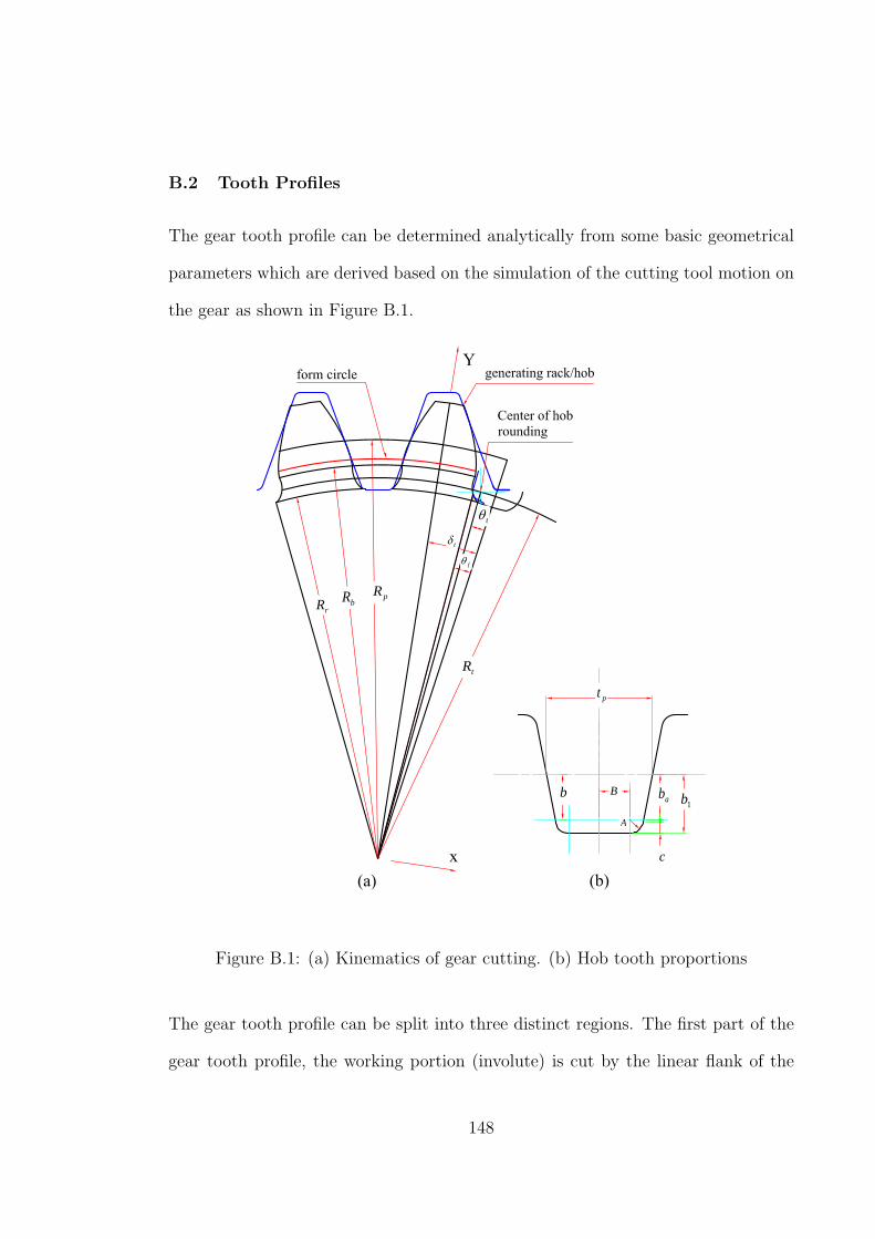
B.2 Tooth Profiles

The gear tooth profile can be determined analytically from some basic geometrical

parameters which are derived based on the simulation of the cutting tool motion on

the gear as shown in Figure B.1.

rR bR pR

tR

tθ

fθ

tδ

pt

ab1bb B

c

A

Figure B.1: (a) Kinematics of gear cutting. (b) Hob tooth proportions

The gear tooth profile can be split into three distinct regions. The first part of the

gear tooth profile, the working portion (involute) is cut by the linear flank of the

148

rack cutter. The second part, which is the root circle is generated by the tip of the

rack. The third portion, the fillet, connects the working portion to the root circle

and is generated by the cutter tip radius.

B.3 The Involute Curve as a Tooth Profile

The involute curve is used almost exclusively for spur gear tooth profiles that are

employed to transmit power. The involute meets all the kinematic requirements for

a gear tooth profile as explained in section B.1. The involute is the curve that is

described by the end of a line that is unwound from the circumference of a circle

as shown in Figure B.2. The circle from which the string is unwound is called the

base circle.

From the geometric conditions shown in Figure B.2, we have:

θ = β − ψ = β − tan−1

√r2 −R2

b

Rb

, (B.1)

The length of the generating line PA is also the length of the circumference of the

base circle subtended by the angle β, hence,√r2 −R2

b = Rbβ ⇒ β =

√r2 −R2

b

Rb

, (B.2)

Hence,

θ =

√r2 −R2

b

Rb

− tan−1

√r2 −R2

b

Rb

. (B.3)

Equation B.3 is known as the polar equation of the involute curve. The generating

line PA is always normal to the involute curve and its length is the radius of curvature

of the involute curve at any point described by the end of this line [18]. An involute

gear tooth form consists of two similar involute curves with a common base circle.

When relative positions are known at any radius, their relative positions at any

149

θ

ψ

β

p

A

bR

o

r

Figure B.2: Involute curve geometry

other radius can be readily determined. In general, this is accomplished by first

determining their relative positions at the base circle, and then adding or subtracting

the vectorial angle of the involute for any other radius. The process of calculating

involute gear tooth relationships is called involumetry [70]. These relationships

are shown in Figure B.3.

Given the pitch radius Rp, the pressure angle φ and the circular pitch pc, let an X-Y

coordinate system be defined as shown in Figure B.3. Along with the determination

of all points of the tooth, it is important, for the purpose of analyzing stress and

deflection, to be able to compute the thickness of a tooth at any radius. The circular

tooth thickness on the pitch circle, tp is half the circular pitch pc. The circular tooth

150

iβ

iβ

φφinv

iθiinvθ

iR pR

bR

Figure B.3: Involumetry of spur gears

thickness ti at any point i on the tooth profile, with radius Ri from the gear center

can be expressed as:

ti = 2Ri{tp

2Rp

+ invφ− invθi}, (B.4)

where

θi = cos−1Rb

Ri

, (B.5)

151

and

invx = tanx− x. (B.6)

The term on the left hand side of equation B.6 is the involute function of an angle

x. The angle ψi between the Y-axis and radius R can be found as

ψi =tp

2Rp

+ invφ− invθi, (B.7)

The direction βi of the transmitted load at any point i on the tooth profile with

respect to X-axis is given by:

βi = θi − ψi, (B.8)

The chordal thickness h at any point i on the tooth profile is given by:

hi = 2isinψi, (B.9)

The X and Y coordinates of any point i on the tooth profile are:

Yi = Risinψi, (B.10)

Xi = Ricosψi. (B.11)

These coordinates of points on the tooth profile will be used to generate geometry

properties for the calculation of deflection of involute gear teeth.

B.4 Root Fillet Profile

The tooth fillet is the curved surface that connects the root circle (dedendum circle)

and the tooth flank of the gear and is generated by the trochoidal envelope of the

cutter tip. A trochoid is a curve which is traced on a rotating plane by a designated

point on a second plane. When the second plane moves in a straight line, we have

152

Figure B.4: Simulation of the cutting tool motion on the gear

a rack trochoid, which is the curve on a gear traced by a point on a meshing rack

as shown in Figure B.4 [74].

When the rack tooth represents the form of the generating tool, then this trochoid

gives the form of the fillet of the gear tooth. When no undercut is present, this

trochoid will be tangent to the generated gear-tooth profile. When the rack is

represented by the cutting tooth of a rack-shaped cutter or of a hob, the corners of

these cutting teeth are generally rounded. In such cases the center of the rounding

will follow the trochoidal path but the actual form of the fillet will be the envelope

of the path of a series of circles equal in size to the rounding of the corners, and

153

with their centers on the trochoidal path as shown if Figure B.4.

Coordinates of a point on the fillet portion can be calculated from the geometric

conditions shown in Figure B.5

δ

fr

tr

tθ

tθ

ψ

A

Figure B.5: Geometry for calculation of fillet coordinates

From the geometric conditions shown in Figure B.5,

θt = tan−1{√r2t − (Rp − b)2

Rp − b−

√r2t − (Rp − b)2

Rp

, (B.12)

tanψt =Rp(Rp − b)− r2

t

Rp

√r2t − (Rp − b)2

, (B.13)

154

rf =√r2t + A2 − 2Artsinψt, (B.14)

θf = θt + cos−1{rt − Asinψt

rf

}. (B.15)

where:

b distance from pitch line of hob to center of rounding

A radius of rounding of the hob edges.

rt any radius of trochoid curve.

θt vectorial angle of trochoid radius.

ψt angle between tangent to trochoid curve and radius vector.

rf any radius of the fillet profile.

θf Vectorial angle of fillet radius

c clearance

Other symbols remain as defined in the text.

A =c

(1− sinφ), (B.16)

b = b1 − A, (B.17)

and

B =tp2− (btanφ+

A

cosφ). (B.18)

To determine the coordinates of the actual fillet when the corner of the hob is

rounded, we must first calculate the coordinates of the trochoid of the center of the

rounded corner and then calculate the actual fillet.

Let,

δt angle between centerline of gear tooth and origin of trochoid

155

θs vectorial angle of fillet radius in reference to the centerline of the tooth.

Xf abscissae of the fillet profile.

Yf ordinate of the fillet profile.

then,

δt =tp −B

Rp

, (B.19)

θs = δt − θf , (B.20)

Xf = rfcosθs, (B.21)

Yf = rfsinθs. (B.22)

When no undercut is present, the trochoidal fillet will be tangent to the involute

profile. This point of tangency for a hob will be the point where the end of the

straight-line profile of the hob or basic rack form crosses the path of contact. The

intersection of the involute and root fillet profiles lies on the form circle, whose radius

can be obtained from equation B.23.

Rt =

√(Rsinφ− ba

sinφ

)2+R2

b , (B.23)

The root radius Rr is given by

Rr = Rp − b1. (B.24)

When rt = (Rp − b), then ψt = 90o and rf = Rr. The above procedure for profile

generation were coded into a FORTRAN program. The process starts with the

input of gear parameters such as module, number of teeth, pressure angle, clearance

and cutter tip radius. The involute and trochoid curves of the gear tooth can then

be plotted on a cartesian coordinate system emanating from the center of the gear

156

as shown in Figure B.6. For the pair of gears in Figure B.6(a), the pinion has a

number of teeth less than that recommended to avoid interference and therefore the

addendum of both gears are modified by increasing that of the pinion and reducing

that of the gear by the same amount.

-10 -5 0 5 1015

20

25

30

35

40

45

50

55

60

65

X - co-ordinate (mm)

Y -

co-o

rdin

ate

(mm

)

(a) Tooth Profile

-10 -5 0 5 1015

20

25

30

35

40

45

50

55

60

65

X - co-ordinate (mm)

Y -

co-o

rdin

ate

(mm

)

(b) Tooth Profile

40T

15T

28T

20T

Figure B.6: Generated gear tooth profile (a) with addendum modification (b)

standard teeth

Tables B.1 and B.2 shows the parameters used in the generation of the above tooth

profiles.

157

Table B.1: Gear data for a pair of teeth with modified addendum

Parameter Pinion Gear

No. of teeth 15 40

module m 3.0 mm 3.0 mm

pressure angle 20o 20o

addendum 1.2385m 0.7615m

clearance 0.157m 0.157m

tip radius 0.7mm 0.7mm

Table B.2: Gear data for a pair of standard teeth

Parameter Pinion Gear

No. of teeth 28 20

module m 3.0 mm 3.0 mm

pressure angle 20o 20o

addendum 1.0m 1.0m

clearance 0.157m 0.157m

tip radius 0.7mm 0.7mm

B.5 Kinematics of Gears

Contact between a pair of meshing gears is arranged to occur purely along a specified

line of action as shown in Figure B.7. When two involutes are acting on each other, a

combined rolling and sliding action takes place between them because of the varying

lengths of equal angular increments on the profiles [70].

158

2aR

1aR

iR1

iR2

AcR 1

BcR 1

BcR 2

1bR

2bR

C

2O

1O

BcR 1

Figure B.7: Meshing action of a pair of spur gears

If we define the sliding velocity as the difference in speed at the ends of the generating

lines of the involutes as they pass through the line of action, we can obtain equations

for the sliding velocity from the kinematic relations in Figure B.7. The angular

velocities of these generating lines will be the same as the angular velocities of the

gears themselves. The actual sliding velocities will be the products of these relative

159

angular velocities and the length of the generating lines or radii of curvature.

Let,

Vp pitch line velocity of the gears.

Vs sliding velocity of the gears.

r1 any radius of driving gear tooth profile.

r2 mating radius of driven gear tooth profile.

Rc1 radius of curvature of driving gear at radius r1

Rc2 radius of curvature of mating gear at radius r2

Then,

Vp = Rp1ω1 ⇒ ω1 =Vp

Rp1

, (B.25)

Vs = (Rc1ω1 −Rc2ω2), (B.26)

ω2 =Rp1

Rp2

ω1, (B.27)

and,

Rc1 +Rc2 = Csinφ, (B.28)

Rc1 =√r21 −R2

b1, (B.29)

Therefore,

Rc2 =√r22 −R2

b2 = Csinφ−√r21 −Rb12. (B.30)

Substituting these equations into equation B.26, combining and simplifying, we

obtain:

Vs = VpRp1 +Rp2

Rp1Rp2

(√r21 −R2

b1 −Rp1sinφ), (B.31)

Equation B.31 may also be written as:

Vs = Vp{1

Rp1

+1

Rp2

}(√r21 −R2

b1 −Rp1sinφ), (B.32)

160

From equation B.32, if, √r21 −R2

b1 −Rp1sinφ = 0, (B.33)

then

r1 = Rp1 ⇒ Vs = 0. (B.34)

This implies that the rate of sliding is zero at the pitch point. Actually, the rate of

sliding starts quite high, reduces to zero at the pitch point, changes direction and

increases again [70]

The active profile of a gear-tooth is that portion of the tooth profile which actually

comes into contact with its mating tooth along the line of action. Considering Figure

B.7,

let,

Ra1 radius to bottom of active profile on driving gear.

Ra2 radius to bottom of active profile on driven gear.

Ra1 =

√[Csinφ−

√(R2

o2 −R2b2)]

2 +R2b1, (B.35)

Ra2 =

√[Csinφ−

√(R2

o1 −R2b1)]

2 +R2b2. (B.36)

Given the radius of the driving gear at any point of contact, the corresponding radius

on the mating gear can be obtained from equation B.37

R2i =

√[Csinφ−

√(R2

1i −R2b1)]

2 +R2b2. (B.37)

B.6 Analysis of Gear Teeth Meshing Cycle

The numbers of teeth in contact for a meshing pair of gears vary along the path

of contact depending on the contact position and contact ratio. For low contact

161

ratio gears, the number of teeth in contact alternates between 1 and 2. For the case

shown in Figure B.8, we have two pairs of teeth in contact, at point A and point C.

Figure B.8, illustrates the motion of a pair of meshing teeth when a gear rotating

about center O1 drives another gear rotating about center O2.

1O

2O

Figure B.8: Gear teeth meshing action

162

The initial contact occurs at A, where the addendum circle of the driven gear in-

tersects the line of action. As the gears rotate, the point of contact will move along

the line of contact, APD.

When the approaching tooth pair contacts at B, the recessing tooth pair disengages

at D leaving only one tooth pair in contact. From B through P to to C is a

single contact zone. When the tooth pair reaches point C, the next tooth pair

begins engagement at A and starts another meshing cycle. to perform a systematic

analysis, the position of contact of the gear teeth along the line of action is expressed

in terms of roll angles of the driving gear. The roll angle ε is given by:

εi = cos−1 ri

Rb

. (B.38)

B.7 Contact Ratio

The contact ratio is defined as the average number of tooth pair(s) in contact [12].

It may also be defined as the ratio of the length of contact for one tooth to the base

pitch. The path of contact is the length of the line of action where actual contact

between the mating gears takes place. For most practical designs of spur gears, the

contact ratio CR has a value between 1.0 and 2.0, implying that two teeth are in

contact 2(1− 1CR

) fraction of total mesh time and a single tooth pair is transmitting

torque during the rest of the mesh cycle. The path of contact may be divided into

two portions:

i. Path of approach, line (AP ) in Figure B.8

ii. Path of recess, line (PD)

163

From the geometric properties shown in Figure B.8, the path of approach and recess

can be obtained using the following relations:

AP =√R2

o2 −R2b2 −Rp2sinφ, (B.39)

PD2 =√R2

o1 −R2b1 −Rp1sinφ, (B.40)

Therefore, the path of contact is given by:

AD = AP + PD =√R2

o1 −R2b1 +

√R2

o2 −R2b2 − (Rp1 +Rp2)sinφ, (B.41)

and the contact ratio is given by:

C.R =

√R2

o1 −R2b1 +

√R2

o2 −R2b2 − (Rp1 +Rp2)sinφ

pccosφ. (B.42)

164

APPENDIX C

Parameters for Redesigned Gear Train

Table C.1 shows the gear parameters adopted for the new design. In the design of

subsequent gear trains, the center distance was held constant while the addendum

of the corresponding gear trains were varied to obtain a contact ratio close to 2.0

while avoiding interference. The gear properties of subsequent speeds’ gear trains

are given in Tables C.2 to C.6.

Table C.1: Adopted gear parameters for speed 1 gear train

Mesh Gear Ax C (mm) CR Ji (Kg mm2)

17 0.39338 52.075 I

41 0.40766 72.969 1.970

1273.234

17 0.35522 64.478 II

48 0.27664 81.503 1.971

3178.655

18 0.35690 77.725 III

48 0.38380 82.903 1.991

4192.515

17 0.39338 141.703 IV

48 0.26455 81.503 1.971

4767.982



17 0.39338 52.075 I

41 0.40766 72.969 1.970

1273.234

24 0.35522 149.711 II

41 0.27664 81.503 2.000

1627.157

18 0.35690 77.725 III

48 0.38380 82.903 1.991

4192.515

17 0.39338 141.703 IV

48 0.26455 81.503 1.971

4767.982

165



17 0.39338 52.075 I

41 0.40766 72.969 1.970

1273.234

36 0.35522 757.653 II

29 0.27664 81.503 2.000

1627.157

18 0.35690 77.725 III

48 0.38380 82.903 1.991

4192.515

17 0.39338 141.703 IV

48 0.26455 81.503 1.971

4767.982



34 0.42084 743.553 I

24 0.35522 72.969 1.990

149.711

17 0.39338 64.478 II

48 0.27664 81.503 1.972

3178.655

18 0.35690 77.725 III

48 0.38380 82.903 1.991

4192.515

17 0.39338 141.703 IV

48 0.26455 81.503 1.971

4767.982

166



34 0.42084 743.553 I

24 0.35522 72.969 1.990

149.711

24 0.35522 149.711 II

41 0.27664 81.503 1.972

1627.157

18 0.35690 77.725 III

48 0.38380 82.903 1.991

4192.515

17 0.39338 141.703 IV

48 0.26455 81.503 1.971

4767.982



34 0.42084 743.553 I

24 0.35522 72.969 1.990

149.711

36 0.35522 757.653 II

29 0.27664 81.503 2.000

1627.157

18 0.35690 77.725 III

48 0.38380 82.903 1.991

4192.515

17 0.39338 141.703 IV

48 0.26455 81.503 1.971

4767.982

167

modeling and simulation of vibrations of a tractor

Documents

Transcript of modeling and simulation of vibrations of a tractor