
factors influencing the accuracy of remote sensing classifications
278
FACTORS INFLUENCING THE ACCURACY OF REMOTE SENSING CLASSIFICATIONS: A COMPARATIVE STUDY by Mahesh Pal Thesis submitted to the University of Nottingham for the degree of Doctor of Philosophy May 2002
-
Upload
khangminh22 -
Category
Documents
-
view
2 -
download
0
Transcript of factors influencing the accuracy of remote sensing classifications

FACTORS INFLUENCING THE ACCURACY OFREMOTE SENSING CLASSIFICATIONS:
A COMPARATIVE STUDY
by
Mahesh Pal
Thesis submitted to the University of Nottingham forthe degree of Doctor of Philosophy
May 2002

ii
To
My Mother
and
Daughter Niharika

iii
Acknowledgement
First of all, I would like to express my sincere gratitude and thanks to my
supervisor, Professor Paul Mather. I am grateful to Professor Paul Mather for his
continuous support, help and guidance throughout the period of this study.
Without all his help and suggestions, this work would not have been possible.
I am very grateful to my sponsor, the Association of Commonwealth Universities,
for giving me the opportunity and financial support to pursue a PhD degree at the
University of Nottingham. I would like to convey my thanks to all the staff
members of the School of Geography, Nottingham University, especially to Dr.
Dee Omar, Ian Conway, Elaine Watts, Chris Lewis, and John Love for their co-
operation and support.
Thanks are also due to Dr. Carlos Vieira in providing help for my programming
problem and especially to Dr. Taskin Kavzoglu in allowing me to use his
MATLAB toolkit for feature selection. I am also thankful to Dr. Premalatha Balan
for helping me in the initial stage of my work and wish to thank Jorge Rubiano for
his invaluable assistance and advice as well as his friendship during this work. I
would like to acknowledge Prof. J. Gumuzzio, Autonomous University of Madrid
for providing the DAIS datasets that enabled me to carry out some part of this
study. Thanks are also due to Helmi Shafri for his valuable help during my field
visit to La Mancha, Spain.
I wish to extend my thanks to Prof. S. K. Sood, Prof. D. V. S. Verma, Prof. R. K.
Bansal, my friends in Regional Engineering College, Kurukshetra, Haryana
(INDIA), and Dr. Manoj Arora, IIT, Roorkee (INDIA) for their kind help. Gyan
Bhushan deserve special thanks for his help in getting my study leave sanctioned.
Special recognition is due to my family and relatives in India for their continuous
encouragement and support. Special thanks is due to my wife Ritu Singh for her
endless patience and understanding during all long hours of work that kept me
busy in my research.

iv
Table of Contents
ACKNOWLEDGEMENT……………………………………………………….III
TABLE OF CONTENTS……………………………………………………….IV
LIST OF FIGURES……………………………………………………………..X
LIST OF TABLES…………………………………………………………….XIII
ABSTRACT…………………………………………………………………....XV
CHAPTER 1: INTRODUCTION................................................................. 1
1.1 Introduction .......................................................................................... 1
1.2 Objective of research .............................................................................. 5
1.3 Thesis structure..................................................................................... 7
CHAPTER 2: CLASSIFICATION ............................................................ 10
2.1 Introduction........................................................................................ 10
2.2 The classification process.................................................................. 12
2.3 Classification techniques .................................................................. 14
2.3.1 Unsupervised classification ............................................................... 16
2.3.1.1 ISODATA method................................................................. 17
2.3.1.2 Self-organising Feature Maps (SOM) ................................... 18
2.3.2 Supervised classification................................................................... 19
2.3.3 Parametric classifiers ......................................................................... 22
2.3.3.1 Maximum Likelihood classifier ............................................ 22
2.3.4 Non-parametric classifiers ................................................................. 25
2.3.4.1 Parallelepiped classifier......................................................... 25
2.3.4.2 The Minimum Distance classifier ......................................... 27
2.3.4.3 Artificial Neural Network classifiers..................................... 28
2.3.4.4 Decision Tree classifiers........................................................ 32
2.3.4.5 Support Vector Machines ...................................................... 33
2.4 Incorporation of nonspectral features ............................................... 33

v
2.5 Accuracy assessment........................................................................35
2.5.1 Confusion matrix ................................................................................ 35
2.6 Conclusions ...................................................................................... 39
CHAPTER 3: ADVANCED CLASSIFICATION ALGORITHMS.............. 40
3.1 Introduction...................................................................................... 40
3.2 Multistage classifiers........................................................................ 42
3.3 Decision tree classifiers ................................................................... 44
3.4 Decision tree design approaches..................................................... 47
3.4.1 Bottom-up approach.......................................................................... 47
3.4.2 Top-down approach ........................................................................... 47
3.4.2.1 Attribute selection measures................................................ 49
3.4.2.1.1 Information Gain and Information Gain Ratio
criterion ..................................................................................... 49
3.4.2.1.2 The Gini Index ........................................................ 52
3.4.2.1.3 The Twoing rule...................................................... 52
3.4.2.1.4 The chi-square contingency table statistic ( 2χ ) ...... 53
3.4.3 Hybrid approach................................................................................ 54
3.4.4 Growing-pruning method................................................................... 55
3.5 Classification algorithms based on data splitting method ................. 56
3.5.1 Univariate decision trees.................................................................... 56
3.5.2 Multivariate decision trees................................................................ 57
3.5.3 Hybrid decision tree classifier ........................................................... 59
3.6 Tests on continuous attributes .......................................................... 60
3.7 Softening thresholds ......................................................................... 61
3.8 Pruning decision trees ...................................................................... 62
3.8.1 Cost-complexity pruning ................................................................... 66
3.8.2 Reduced-error pruning ....................................................................... 67
3.8.3 Pessimistic Pruning............................................................................ 68
3.8.4 Error based pruning............................................................................ 69
3.8.5 Critical value pruning ........................................................................ 70
3.9 Problems in the use of decision tree classifiers ............................... 71
3.10 Support Vector Machines (SVM) ..................................................... 72

vi
3.11 Statistical learning theory................................................................ 72
3.11.1 Empirical risk minimisation............................................................. 72
3.11.2 Structural risk minimisation............................................................. 75
3.12 Design of support vector machines................................................. 76
3.12.1 The linearly separable class .............................................................. 76
3.12.2 Non-separable data........................................................................... 79
3.12.3 Nonlinear support vector machines ................................................. 81
3.13 Multi-class classifier........................................................................ 83
3.13 Problems in the use of SVM ............................................................ 84
3.14 Ensemble of classifiers .................................................................... 85
3.14.1 Boosting ............................................................................................ 85
3.14.2 Bagging ............................................................................................. 87
3.15 Conclusions .................................................................................... 88
CHAPTER 4: DATA SETS...................................................................... 89
4.1 Introduction........................................................................................ 89
4.2 Synthetic Aperture Radar(SAR)........................................................ 89
4.3 Interferometric Synthetic Aperture Radar ......................................... 93
4.4 Differential interferometry ................................................................. 97
4.5 Coherence ........................................................................................ 98
4.5.1 Coherence magnitude estimation....................................................... 99
4.5.2 Image processing and generation of coherence images ................... 102
4.5.2.1 Co-registration and common band filtering ........................ 102
4.5.2.2 Interferogram generation and flat earth correction............. 103
4.5.2.3 Coherence estimation .......................................................... 103
4.5.2.4 Image coregistration ............................................................ 104
4.5.2.5 Speckle suppression............................................................. 106
4.5.3 Factors affecting coherence ............................................................. 107
4.6 ETM+ data ......................................................................................108
4.7 DAIS hyperspectral data.................................................................109
4.8 Conclusion.......................................................................................110

vii
CHAPTER 5: CROP CLASSIFICATION USING DECISION TREE ANDSUPPORT VECTOR MACHINE CLASSIFIERS ....................................112
5.1. Decision tree classifiers ...................................................................112
5.1.1 Introduction .................................................................................112
5.1.2 Study area ....................................................................................114
5.1.3 Methods........................................................................................115
5.1.3.1 Training set size ............................................................................ 116
5.1.3.2 Attribute selection measure........................................................... 119
5.1.3.3 Pruning methods ........................................................................... 120
5.1.3.4 Boosting ........................................................................................ 121
5.1.4 Results with ML and neural classifiers..........................................124
5.1.5 Inclusion of panchromatic band and its texture.............................126
5.1.6 Conclusions ..................................................................................131
5.2 Support vector machine classifiers .................................................132
5.2.1 Introduction ....................................................................................132
5.2.2 Study area and methods...............................................................132
5.2.2.1 Effect of kernel choice .................................................................. 133
5.2.2.2 Training sample size ..................................................................... 134
5.2.2.3 Use of different multi-class methods ............................................ 136
5.2.3 Conclusions ..................................................................................137
CHAPTER 6: CROP CLASSIFICATION USING INSAR DATA.............140
6.1 Introduction......................................................................................140
6.2 Description of study area .................................................................140
6.3 Ground reference image generation ................................................141
6.4 Feature extraction and selection......................................................143
6.5 Grey Level Co-occurrence Matrix (GLCM) ......................................144
6.5.1 Texture extraction from GLCM....................................................... 146
6.5.2 Feature based on local statistics....................................................... 148
6.6 Fractal dimension ...........................................................................148
6.7 Multiplicative Autoregressive Random Field (MAR) model ..............152
6.7.1 Estimation of parameters in the MAR model .................................. 153
6.8 Feature selection .............................................................................154

viii
6.8.1 Hotelling’s 2T ................................................................................. 156
6.9 Classification results and discussion ..............................................157
6.9.1 Results.............................................................................................. 157
6.9.2 Discussion........................................................................................ 161
6.10 Conclusions ....................................................................................163
CHAPTER 7: ISSUES IN THE CLASSIFICATION OF REMOTESENSING DATA.....................................................................................165
7.1 Introduction.....................................................................................165
7.2 Scale...............................................................................................166
7.2.1 Definition ......................................................................................... 167
7.3 Scaling............................................................................................170
7.3.1 The scaling process .......................................................................... 170
7.4 Sample size ....................................................................................173
7.5 Sampling plan .................................................................................175
7.6 Study area and data .......................................................................177
7.7 Classification...................................................................................179
7.7.1 Results and discussions .................................................................... 182
7.8 Dimensionality reduction.................................................................191
7.8.1 Principal Components Analysis....................................................... 192
7.8.2 Maximum Noise Fraction (MNF) transform ................................... 193
7.9 Conclusions ....................................................................................202
CHAPTER 8: OVERVIEW OF RESULTS AND FUTURE RESEARCHDIRECTIONS..........................................................................................204
8.1 Introduction......................................................................................204
8.1.1 The usefulness of decision tree classifiers and support vector machines
205
8.1.2 Use of coherence for land use classification .................................... 208
8.1.3 Issues in remote sensing image classification.................................. 209
8.2 Suggestions for future research.......................................................210
8.3 Algorithm choice - some guidelines ................................................213

ix
BIBLIOGRAPHY ....................................................................................216
APPENDIX A: CONFUSION MATRICES FOR CHAPTER 5…………..237
APPENDIX B: CONFUSION MATRICES FOR CHAPTER 5…………..247
APPENDIX C: CONFUSION MATRICES FOR CHAPTER 6 ………….251
APPENDIX D: CONFUSION MATRICES FOR "MNF" BASED FEATUREEXTRACTION (CHAPTER 7) ………………………….…………………..257
APPENDIX E: CONFUSION MATRICES FOR DECISION TREE BASEDFEATURE EXTRACTION (CHAPTER 7) …………….…………………..259
APPENDIX F: CONFUSION MATRICES FOR ETM+ SPAIN DATA(CHAPTER 7)…… ………………………….……………………………….261

x
List of Figures
Figure 1. 1. Principal stages in image classification (adapted from Townshend and
Justice, 1981)........................................................................................ 3
Figure 2. 1. The classification process (adapted from Schowengerdt, 1997) ....... 13
Figure 2.2. Principle of supervised classification................................................. 20
Figure 2. 3. Parallelepiped classification strategy................................................. 26
Figure 2. 4. Minimum distance to mean classification strategy............................ 27
Figure 2.5. A back-propagation neural network, showing the input layer, one
hidden layer and the output layer, with interconnecting links being
associated with weights. ..................................................................... 29
Figure 3. 1. A classification tree for a five dimensional feature space and three
classes. The ix are the feature values, the iη are the thresholds, and y
is the class label. ................................................................................. 46
Figure 3. 2. Axis-parallel decision boundaries of a univariate decision tree. ...... 57
Figure 3. 3. Decision boundaries for a multivariate decision tree classifier. ....... 58
Figure 3. 4. A hybrid decision tree classifier. ...................................................... 59
Figure 3. 5. Hyperplanes for the linearly separable data sets. Dashed line passes
through the support vectors.............................................................. 77
Figure 3. 6. Hyperplanes for non-separating data sets. ........................................ 80
Figure 3. 7. The idea of a non-linear support vector machine.............................. 82
Figure 3. 8. A classifier ensemble of decision tree classifier. .............................. 87
Figure 4. 1. Geometry of a SAR (adapted from http/:www.ccrs.nrcan.gc.ca/ccrs)
.......................................................................................................... 92
Figure 4. 2. Principle of interferometric synthetic aperture radar (adapted from
Gens and van Genderen, 1996). ....................................................... 93
Figure 4. 3. Geometry of across-track interferometry (adapted from Gens and
van Genderen, 1996). ....................................................................... 95
Figure 4. 4. Geometry of along-track interferometry (adapted from Gens and van
Genderen, 1996)............................................................................... 96
Figure 4. 5. Geometry of repeat-pass interferometry (adapted from Gens and van
Genderen, 1996)............................................................................... 97

xi
Figure 4. 6. Interferograms of the study area. (a) without flat earth correction and
(b) with flat earth correction. ......................................................... 103
Figure 4. 7. Coherence images of the study area............................................... 105
Figure 5.1.1. The ground reference image of the ETM+ data............................. 115
Figure 5.1.2. Variation of classification accuracy with increasing number of
training patterns using a univariate decision tree classifier. .......... 117
Figure 5.1.3. Variation of classification accuracy with increasing number of
training patterns using mulivariate decision tree classifier. ........... 118
Figure 5.1.4. Variation of accuracy with different attribute selection measures. 119
Figure 5.1.5. Variation of classification accuracy with different pruning methods.
........................................................................................................ 121
Figure 5.1.6. Classification accuracies for boosted decision trees for varying
number of boosting iterations. ....................................................... 122
Figure 5.1.7. Difference of classified images with ground reference image (a)
unboosted decision tree classifier (b) boosted decision tree classifier.
Visual comparison of individual fields shows that within-field
variation is reduced by boosting. ................................................... 123
Figure 5.1.8. Classified images of the study area using (a) maximum likelihood
classifier and (b) neural network classifier. The colour palette is the
same as in figure 5.1.8 (a). ............................................................. 125
Figure 5.1.9. Movement of pointer to extract internal texture of the panchromatic
image. ............................................................................................. 128
Figure 5.2.1. Variation in classification accuracy with different kernel functions.
........................................................................................................ 134
Figure 5.2.2. Variation in classification accuracy with change in training patterns.
........................................................................................................ 135
Figure 5.2.3. Classified image of the study area. ............................................... 137
Figure 6. 1. Ground reference image of the study area………………………...142
Figure 6. 2. (a) a 3×3 image with three grey levels; (b)-(e) glcm for angles of
angles 00 , 045 , 090 , and 0135 respectively. ................................... 145
Figure 6. 3. Neighbourhood support of central pixel. ........................................ 153
Figure 6. 4. Classified images of data set 7 using (a) decision tree classifier and
(b) with neural classifier. .................................................................. 162
Figure 7. 1. Meaning of scale (adapted from Cao and Lam, 1997)..................... 168

xii
Figure 7. 2. The strategy of up- and downscaling across the four spatial scales of
interest in relation to global environmental change (adapted from
Jarvis, 1995). .................................................................................... 171
Figure 7. 3. La mancha alta region, central spain (adapted from Oliver and Florin,
1995)................................................................................................. 178
Figure 7. 4. Study area in La Mancha region. .................................................... 178
Figure 7. 5. The "ground reference" image for the test area. .............................. 180
Figure 7. 6. Variation in classification accuracy with change in number of bands
with different training sets................................................................ 186
Figure 7. 7. Variation in classification accuracy with different classifiers using
different number of bands and training datasets............................... 188
Figure 7. 8. Images of the study area (a) DAIS hyperspectral image (5m
resolution) and (b) ETM+ image (30m resolution). ........................ 200
Figure 7. 9. Classified images using neural network classifier (a) DAIS
hyperspectral image (5m resolution) and (b) ETM+ image (30m
resolution)......................................................................................... 201
Figure 8. 1. Algorithm choice for different type of data depending on different
factors. Higher grading is given to the classifier, which provides high
accuracy and easy in use. A classifier that requires small
computational time and less sensitive to both sampling plan and
sample size is given high grading………………………………….215

xiii
List of Tables
Table 4. 1. The date and corresponding sensor of the slc used in the study. ..... 104
Table 4. 2. Landsat 7 ETM+ data characteristics. .............................................. 109
Table 4. 3. The DAIS 7915 system specifications. ............................................ 110
Table 5.1.1. Results from boosted and unboosted decision tree. ....................... 121
Table 5.1.2. Results from maximum likelihood and neural network classifier.. 124
Table 5.1.3. Results obtained by using internal texture of panchromatic band with
ETM+ multispectral data. .............................................................. 129
Table 5.1.4. JM distance for data set 1 and data set 2. ....................................... 130
Table 5.1.5. Results obtained by using data set 1 (Table 5.1.5 (a)) and data set 2
(Table 5.1.5 (b)). ............................................................................ 130
Table 5.2.1. Values of parameter c with different kernels. ................................ 133
Table 5.2.2. Classification accuracy and training time using different svms and
different multi-class methods......................................................... 136
Table 6. 1. Crops being used for classification with digital numbers in reference
image. ............................................................................................... 142
Table 6. 2. Various features obtained by applying hotelling’s 2T feature selection
method and used in final classification process. .............................. 159
Table 6. 3. Total classification accuracies for different data sets used in the
classification process. Table 6.3(a) is for maximum likelihood, Table
6.3 (b) for the neural network and Table 6.3(c) for decision tree
classifier............................................................................................ 160
Table 7. 1. Calculated z values for comparison among the different sampling plans
using kappa analysis. Shaded values indicate significant
improvements in the performance of the classifiers at the 95%
confidence level (Z critical value = 1.96). Negative value indicates
better performance of the systematic random sampling plan over the
random sampling plan. ..................................................................... 190
Table 7. 2. Results with MNF transformed image. ............................................ 197
Table 7. 3. Results obtained by applying decision tree based feature selection. 198
Table 7. 4. Classification results obtained with ETM+ data for the La Mancha
test area of Spain. ............................................................................. 199

xiv
Table 8. 1. Classification accuracies obtained using various algorithms and the
factor affecting the classifier……………...………………………211
Table 8. 2. Calculated z values for comparison between different classification
systems. Shaded values indicate significant improvements in the
performance of first classifier at the 95% confidence level (Z critical
value = 1.96). While unshaded value indicates that both classifier
performs equally well. WB means "without boosting" and B means
"boosting" a decision tree classifier. ................................................ 212

xv
Abstract
Within last 20 years, a number of methods have been employed for classifying
remote sensing data, including parametric methods (e.g. the maximum likelihood
classifier) and non-parametric classifiers (such as neural network classifiers).
Each of these classification algorithms has some specific problems which limits
its use. This research studies some alternative classification methods for land
cover classification and compares their performance with the well established
classification methods. The areas selected for this study are located near Littleport
(Ely), in East Anglia, UK and in La Mancha region of Spain. Images in the optical
bands of the Landsat ETM+ for year 2000 and InSAR data from May to
September of 1996 for UK area, DAIS hyperspectral data and Landsat ETM+ for
year 2000 for Spain area are used for this study. In addition, field data for the year
1996 were collected from farmers and for year 2000 were collected by field visits
to both areas in the UK and Spain to generate the ground reference data set. The
research was carried out in three main stages.
The overall aim of this study is to assess the relative performance of four
approaches to classification in remote sensing - the maximum likelihood, artificial
neural net, decision tree and support vector machine methods and to examine
factors which affect their performance in term of overall classification accuracy.
Firstly, this research studies the behaviour of decision tree and support vector
machine classifiers for land cover classification using ETM+ (UK) data. This
stage discusses some factors affecting classification accuracy of a decision tree
classifier, and also compares the performance of the decision tree with that of the
maximum likelihood and neural network classifiers. The use of SVM requires the
user to set the values of some parameters, such as type of kernel, kernel
parameters, and multi-class methods as these parameters can significantly affect
the accuracy of the resulting classification. This stage involves studying the
effects of varying the various user defined parameters and noting their effect on
classification accuracy. It is concluded that SVM perform far better than decision
tree, maximum likelihood and neural network classifiers for this type of study.

xvi
The second stage involves applying the decision tree, maximum likelihood and
neural network classifiers to InSAR coherence and intensity data and evaluating
the utility of this type of data for land cover classification studies.
Finally, the last stage involves studying the response of SVMs, decision trees,
maximum likelihood and neural classifier to different training data sizes, number
of features, sampling plan, and the scale of the data used. The conclusion from the
experiments presented in this stage is that the SVMs are unaffected by the Hughes
phenomenon, and perform far better than the other classifiers in all cases. The
performance of decision tree classifier based feature selection is found to be quite
good in comparison with MNF transform. This study indicates that good
classification performance depends on various parameters such as data type, scale
of data, training sample size and type of classification method employed.

1
Chapter 1
Introduction
1.1 Introduction
The interpretation of remotely sensed data uses techniques from a number of
disciplines including remote sensing, pattern recognition, artificial intelligence,
computer vision, image processing and statistical analysis. The move towards
automated analysis of remotely sensed data is encouraged by the ever increasing
volumes of data as well as by the high cost of ground surveying. The new
generation of satellite-borne instruments is providing higher spatial and spectral
resolution data, leading to the wider application of remotely sensed products and
further emphasising the need for more automated forms of analysis.
The methodology of pattern recognition applied to a particular problem depends
on the data, the data model, and the information that one is expecting to find
within the data (Bezdek, 1981). A number of methodologies have been developed
and employed for image classification from remotely sensed data within the past
20 years. Statistical image classification techniques are ideally suited for data in
which the distribution of the data within each of the classes can be assumed to
follow a theoretical model. The most commonly used statistical classification
methodology is based on maximum likelihood, a pixel-based probabilistic
classification method which assumes that spectral classes can be described by a
normal probability distribution in multispectral space (Swain and Davis, 1978).
This traditional approach to classification is found to have some limitations in
resolving interclass confusion if the data used are not normally distributed. As a
result, in recent years, and following advances in computer technology, alternative
classification strategies have been proposed.
Artificial intelligence and knowledge-based expert systems have been used in
image classification. The major contribution of the artificial intelligence and
expert system paradigm to pattern analysis has been the study of how domain-
specific and heuristic knowledge can be represented and used to control the
process of extracting meaningful descriptors and objects from images. The

2
problem with these classifiers is that heuristic knowledge requires a number of
experts to solve a single problem. Further details of these knowledge based
classifiers can be found in Civco (1989), Estes et al. (1986), Goldberg et al.
(1983), Friedl et al. (1988), Nagao and Matsuyama (1980) and Wharton (1987).
In most instances, human beings are good pattern recognisers. This observation
led researchers in the field of pattern recognition to consider whether computer
systems based on a simplified model of the human brain can be more effective
than the standard statistical and knowledge-based classification methods.
Research in this field led to the adoption of artificial neural networks (ANN),
which have been used in remote sensing over the past ten years, mainly for image
classification. Studies carried out using ANN suggest that, due to their
nonparametric nature, they generally perform better than statistical classifiers. The
performance of a neural network classifier depends to a significant extent on how
well it has been trained. During the training phase, the neural network learns
about regularities present in the training data and, based on these regularities,
constructs rules that can be extended to the unknown data. However, the user
must determine a number of properties such as the architecture of network,
learning rate, number of iterations and learning algorithms, all of which affect
classification accuracy. There is no clear rule to fix the values of these parameters,
and only rules of thumb exist to guide users in their choice of network parameters.
Kavzoglu (2001) discusses all these issue in detail.
Another type of classifier, called the decision tree (DT) classifier, is now being
used for image classification problems in remote sensing because, like ANN,
these classifiers are nonparametric. Unlike ANN, they do not need extensive
design and training (Friedl and Brodley, 1997, Safavian and Landgrebe, 1991,
Hensen et al., 1996). They are trained by iterative selection of individual features
or a combination of features at each node of a tree. During classification, only
those features are considered that are needed for the test pattern under
consideration, so feature selection is implicitly built-in. However, the main
advantage of the decision tree classifier as compared to ANN, besides its speed, is
the possibility to interpret the decision rule in terms of individual features (Borak
and Strahler, 1999). Other studies using decision tree classifiers in image

3
classification can be found in Evans (1998), Friedl et al. (1999), Gahegan and
West (1998) and Muchoney et al. (2000).
Figure 1. 1. Principal stages in image classification (adapted from Townshend andJustice, 1981).
Recently, a new classification technique based on statistical learning theory,
called support vector machines, has been applied to the problem of image
classification (Zhu and Blumberg, 2002; Huang et al, 2002; Gualtieri and Cromp,
1998; Chapelle et al., 1999). Support vector machines use optimisation algorithms
to find the optimal boundaries between classes, and generalise these boundaries to
Accuracy assessment
Pre-processing
Sample areaselection
Class definition
Training aclassifier/generation of
training statistics
Extrapolation to otherareas
Post processing
Unsupervised Classification
Supervised Classification
Unsupervised and supervised classification

4
unseen samples with the least errors among all possible boundaries separating the
classes and minimising confusion between classes.
Image classification involves the execution of several stages (Figure 1.1).
Moreover, within each of these principal stages there are several substages and
hence further decisions need to be made. The performance of a classifier
depends on the interrelationship between sample size, number of features, and
classifier complexity. One of the important stages in image classification is that of
collection of samples for training and testing the classifier. Sample size has an
influence on the classification accuracy with which estimates of statistical
parameters are obtained for statistical classifiers. Sample selection also depends
on a number of factors which finally affect classification accuracy. The factors
affecting sample selection are:
1. Number of training sites for sample collection.
2. Sampling method (random or systematic sampling).
3. Data source for labelling training sites (ground data, air photographs etc).
4. Timing of data collection.
With high-dimensional data sets, such as those acquired by an imaging
spectrometer, the training set size requirements for the correct application of a
classification system may be too high. It is well known that the probability of
misclassification of a decision rule does not increase as the number of features
increases, as long as number of training samples is arbitrarily large. However, it
has been observed in practice that additional features may degrade the
performance of a classifier if the number of training samples that are used to
design the classifier is small relative to the number of features. This behaviour is
referred to as the "peaking phenomenon" (Raudys and Jain, 1991; Jain and
Chandrasekaran, 1982). Several authors, including Hord and Brooner (1976),
Fitzpatrick-Lins (1981), Congalton (1988, 1991), Mather (1999) and Tso and
Mather (2001) study the effect of sample size and sampling plan in detail.

5
1.2 Objective of this research
The work reported in this thesis focuses on the various factors that influence the
accuracy of remote sensing classifications. As reported by a number of studies
(Raudys and Pikelis, 1980; Congalton, 1988; Mather, 1999; Swain and Davis,
1978; Markham and Townshend, 1981) several factors, such as type of classifier
and data used, sample size and sampling plan, and the scale of the data have a
significant effect on the resulting classification accuracy. Although individual
studies have highlighted specific problems, no comprehensive research study has
attempted to consider all these aspects in the context of the classification of
remotely sensed images. This study is designed to evaluate the behaviour of
different classifiers with optical and radar data as well as data at different scales.
Further, the behaviour of different classification algorithms with changing training
data set size and different sampling plans is explored.
The experiments reported in this thesis were undertaken in order to achieve the
objectives listed below, while at the same time addressing a variety of other issues
that are extremely important for successful applications of any classification
algorithm for land cover classification studies.
Decision tree classifiers have been used in land cover classification over the last
few years. However, a number of issues related to the performance of these
classifiers have not yet been fully discussed in the literature. The main issues that
need further clarification are:
1. Determining how different attribute selection measures and pruning
methods affect classification accuracy.
2. Determination of optimal number of samples required to train the decision
tree classifier.
Other problems relating to the use of the decision tree classifier that have been
recognised in the literature and which need further investigation are:
1. Effect of boosting on classifier performance.

6
2. Type of decision tree classifier (i.e., univariate or a multivariate), and
under what conditions each is to be used.
Although a few studies have highlighted specific problems, such as the influence
of boosting on the results produced by the decision tree classifiers, or the effect of
using univariate and multivariate decision tree classifiers on classification
accuracy, no research study to date has attempted to consider all of the factors
listed above in the context of the classification of remotely sensed images.
The level of classification accuracy achieved using support vector machines is
also affected by several factors. The research reported here discusses the
following points:
1. How classification accuracy changes by using various kernels and
different multi-class methods of generating support vector machines.
2. The effect of training set size on classification accuracy, and
3. Comparing the performance of this classifier with neural and decision tree
classifiers using hyperspectral data with small training data set sizes.
In addition to the above topics, this study involves the comparison of the
classification accuracy, training time, ease of use, and various user defined
parameters required for training neural, decision tree and support vector
classifiers.
Irrespective of the classifier used, the nature of the data (and of derived features
such as texture) also influences the accuracy of land cover classification. In view
of this, some further objectives that are set for this study are:
1. To study the effect of ETM+ panchromatic band and its texture features
for land cover classification in combination with ETM+ multispectral data.
2. To study the use of interferometric SAR data, especially coherence
images, for land cover classification in combination with the InSAR
intensity images. To improve the classification accuracy, the use of texture
features (based on GLCM, the MAR model, and fractals) derived from

7
coherence and intensity images were also studied, and feature selection
techniques were used to reduce the dimensionality of the datasets.
The research reported in this thesis involves a range of other experiments that are
carried out to achieve the following objectives:
1. To conduct an extensive study to investigate the effect of number of
training data with changes in the number of features, the sampling plan
used to select the pixels for training and testing classifiers, and the scale
(resolution) of remote sensing data on classification accuracy using DAIS
hyperspectral and ETM+ data of the same area.
2. To study the effectiveness of feature extraction methods such as maximum
noise fraction (MNF) applied to hyperspectral data for land cover
classification accuracy.
3. To study the effectiveness of decision tree classifiers for feature selection
with hyperspectral data.
1.3 Thesis structure
The work described in this thesis covers the period October 1999 to mid 2002.
Initially, attention was focused on the use of interferometric SAR in agricultural
crop classification. This work is reported in chapter 6. It proved more difficult
than expected to obtain suitable InSAR data for the study area, and so the scope of
the research was broadened to cover factors influencing the accuracy of
agricultural crop classification derived from remotely sensed data. The present
structure of the thesis reflects this re-orientation of the research. Naturally, new
ideas developed over the study period, and research is still progressing in areas
such as the use of support vector machines.
This study consists of eight chapters including this introductory chapter describing
the details of problem, techniques and methodologies used and analysis of results
obtained using different methodologies. The early chapters mainly provide
background information about the theory of classification and fundamentals of
decision tree and support vector machine classifiers.

8
• In chapter 2 the classification process and various classification algorithms
including unsupervised and supervised, parametric and non parametric
classification techniques, are discussed in detail. A general idea of the
incorporation of spatial information including context and texture in
classification is also discussed. Finally, the methodologies used to assess
classification accuracy, such as the Kappa value and its confidence limits,
are described.
• Chapter 3 consists of a detailed description of the decision tree classifier
and support vector machines to be used for image classification problems.
Various methods of designing a decision tree are discussed critically.
Details of various attribute selections and pruning methods used with
different decision tree classifiers are also discussed. A section is devoted
to a comparative study of various types of decision tree classifiers. Ways
of using continuous attributes in decision tree classifier are described. The
second part of this chapter deals with a recently developed nonparametric
classification technique, called the support vector machine (SVM) for
remote sensing image classification, which includes the theory behind the
development of this type of classifier. Finally, a new way to create an
ensemble of same base classifiers using boosting and bagging techniques
are discussed in detail.
• Chapter 4 considers the relevance of the type of data on the outcome of a
classification. The principles of interferometric SAR, including differential
interferometry, are discussed in detail, with details of the derivation of
coherence images. Various factors affecting the magnitude of coherence
are also discussed. Some details of Landsat 7 ETM+ and DAIS
hyperspectral data are also provided. The problems associated with the use
of DAIS data are also discussed.
• Chapter 5 presents the results achieved by decision tree and support vector
machine classifiers for a land cover classification problem. The various
factors that affect land cover classification accuracy are investigated using
both classification systems. A comparison of the results obtained using
decision tree classifiers, neural networks, support vector machines and

9
maximum likelihood classifiers is presented. The advantages and
disadvantage of using decision tree and support vector machine classifiers
are compared to those associated with neural network classifiers. Finally
the effect of including the Landsat ETM+ panchromatic band and its
internal texture on classification accuracy using a decision tree classifier is
discussed. The effects of changing the values of user defined parameters
affecting the classification accuracy of SVMs are also considered.
• Chapter 6 discusses the results obtained using interferometric SAR images
for land cover classification studies. The usefulness of texture information
derived from coherence as well as intensity images is also discussed. This
chapter contains a detailed consideration of the main approaches to texture
extraction used in this study (based on GLCM, the MAR model, and
fractals) as well as the method used to choose the most appropriate number
of features for a specific classification problem.
• Chapter 7 discuss the effects of factors such as sampling plan, sample
size, and scale of data on land cover classification using hyperspectral and
ETM+ data. Factors such as feature extraction using orthogonal techniques
and decision trees are also discussed. Results obtained using data at
different scales, with different number of features with fixed numbers of
training patterns as well as changing training patterns with fixed number of
features are discussed, so as to examine the relevance of the Hughes
phenomenon with four different classification systems.
• In chapter 8, overall conclusions drawn from this research are presented.
This chapter also summarises the major findings of this research, and
provides a number of recommendations for future work using different
classifiers.

10
Chapter 2
Classification
2.1 Introduction
The science of remote sensing consists of interpretation of measurements of
electromagnetic energy reflected from or emitted from a target. Sensors mounted
on aircraft or satellite platforms records this electromagnetic radiation. The first
civilian satellite, known as Television and Infrared Observation Satellite (TIROS),
was launched in 1960 for the purposes of meteorological observation, acquiring
images of weather patterns for use in forecasting. Landsat-1 was launched in 1972
to monitor the earth’s land surface using a multispectral imaging system. The
Landsat series has since proved to be one of the main sources of global
environmental information and still continues to provide coverage for the planet
between 082 N and 082 S, making a repeat coverage every 16-18 days
(Wilkinson, 2000; Mather, 1999).
According to Wilkinson (2000), "The main advantage of satellite remote sensing
over alternative forms of environmental data gathering is that large global surface
areas can be monitored without the need for ground level surveys. In addition,
satellite observations are less costly than aerial surveys for long term and large-
area mapping and monitoring".
Remote sensing satellites record data in digital form, which is then processed by
computer. Computer processing applications range from calibration of the data for
the effects of factors such as the changing response of sensors over time to the
identification of patterns in multi- and hyper-spectral data that relate to features on
the ground.
Classification of satellite images is one of the most commonly applied techniques
used in remote sensing data processing. "Classification involves performing a
transformation from the numerical spectral measurements into a set of meaningful
11
classes or labels, which can describe a landscape. Classification effects a
transformation from a physical measurement into a cartographic or thematic
description of the earth’s surface, for examples into terms such as forest, built-up
area, water bodies, etc. As such, classification can be viewed as a signal inversion
process" (Wilkinson, 2000). A number of techniques exist in the literature for
classification of remotely sensed data (Mather, 1999; Richards, 1993; Swain and
Davis, 1978; Schowengerdt, 1997).
Classification is a method by which labels are attached to pixels in view of their
character (Richards, 1993). This character is generally their response in different
spectral ranges. Labelling is implemented through pattern classification
procedures. The term “pattern” refers to the set of radiance measurements
obtained in the various wavebands for a given pixel, and spectral pattern
classification refers to the family of classification procedures that utilises this
pixel-by-pixel spectral information as the basis for land cover classification. In
contrast, spatial pattern recognition involves the classification of image pixels on
the basis of their spatial relationship with pixels surrounding them. Temporal
pattern recognition uses change in spectral reflectance over time as the basis of
feature identification.
The classification process has two main stages. In the first stage, the number and
nature of the categories are determined, whilst in the second stage every unknown
or unseen element is assigned to one of the categories according to its level of
resemblance (or similarity) to the basic patterns. These stages are often called
classification and identification, respectively. In the context of remote sensing, the
categories could be land cover features or cloud types, and the assignment to one
of the categories is carried out by allocating numerical labels, corresponding to
the classes, to individual pixels. Hence, for a researcher working in the remote
sensing field, classification basically means determining the class membership of
each pixel in an image by comparing the characteristics of that pixel to those of
categories known a priori.
12
2.2 The classification process
Image classification is the process of creating a meaningful digital thematic map
from an image dataset. The classes shown on the map are derived either from
known cover types (such as wheat or soil) or by algorithms that search the data for
similar pixels. Once data values are known for the distinct cover types in the
image, a computer algorithm can be used to divide or segment the image into
regions that correspond to each cover type or class. The classified image can be
converted to a land use map if the use of each area of land is known. The term
land use refers to the purpose for which people use the land (e.g. city, parks, and
road), whereas cover type refers to the material that an area is made from
(concrete, vegetation). Image classification can be done using a single image
dataset, multiple images acquired at different times, or image data with additional
information such as elevation measurements, or expert knowledge about the area.
Traditionally, land cover classification based on remotely sensed data involves
several steps (Schowengerdt, 1997), as shown in Figure 2.1:
(i) "Feature extraction: The term feature refers to a single element of a
pattern (such as one of the Landsat ETM+ bands). More generally, a
feature can be thought of “…as a distillation of that information contained
in the measurements which is useful for deciding on the class to which the
pattern belongs” (Swain and Davis, 1978). The original data may contain
information relating to atmospheric and topographic conditions. In
addition data are often highly correlated between spectral bands, which
may not be useful for land cover classification and even may reduce
classification accuracy. Thus, feature extraction performs two functions:
(1) separation of useful information from noise or non-information and
(2) reduction of the dimensionality of the data in order to simplify the
calculations performed by the classifier, and to increase the efficiency
of statistical estimators in a statistical classifier.
These aims can be achieved by applying spatial or spectral transform to
the image, such as selection of a subset of bands, or a principal
component transformation to reduce the data dimensionality.

This step is optional in classification of remotely sensed images i.e. the
images can be used directly, if desired.
(ii) Training: The term “training” arose from the fact that many pattern
recognition systems were “trainable”; i.e., they learned the discriminant
functions in the feature space by adjusting their parameters when applied
to a training pattern (pixel vector) whose true class is known. This process
of training a classifier is either supervised by the analyst or unsupervised.
Figure
(iii) L
cla
on
ex
sta
13
2. 1. The classification process (Adapted from Schowengerdt, 1997)
abelling: The process of allocating individual pixels to their most likely
ss is known as labelling. This process of labelling can be approached in
e of two ways. If the analyst knows the number of separable pixels that
ist in the area covered by the image, and if it is possible to estimate the
tistical properties of the values taken on by the features describing each

14
of these pixels (in statistical classifiers), then individual pixels (test pixels)
can be labelled as belonging to the classes based on these statistical
properties. The other method is where the analyst has no clear idea of the
number and character of the land cover classes present in the images. A
method of allocating and reallocating the individual pixels to one of an
initial set of randomly-chosen pixels is used. At each stage, each pixel in
turn is given the label of one of these randomly chosen pixels using some
classifier. At the end of first iteration, when every pixel has been labelled,
the randomly chosen pixels can be altered in character (either by
combining, splitting, and removing some of the pixels) according to the
nature of the pixels which have been associated with them. This process of
pixel labelling is repeated until the process converges. At this stage the
user can relate these pixels to some land cover class" (Schowengerdt,
1997).
2.3 Classification techniques
The methodology of pattern classification applied to a particular problem depends
on the data, the model of the data, and the information that one is expecting to
find within the data (Bezdek, 1981). The data may be qualitative, quantitative,
numerical, pictorial, textual, linguistic, or any combination of the above. Pictorial
data carry information about the object in the scene depicted in the image. Image
information can be described at many levels of abstraction. A description may
range from one expressed in terms of meaningful attributes of the scene depicted
in the image to one that describes only the spatial variation of intensity. Any of
these descriptions can be expressed with a model that captures only the relevant
features of the image at that level of abstraction and leaves others unspecified.
The role of a model is to convert information in the image into usable form and,
therefore, to enable the user to draw conclusions about the properties of the
objects being studied. The model used must be such that it transforms the data and
makes them compatible with the search and matching strategies to be used. Each
search and matching strategy corresponds to a different pattern classification
methodology. This is the reason for the use of different approaches to pattern

15
classification, e.g., mathematical or statistical, heuristic, and structural etc (Tou
and Gonzalez, 1974).
Human problem solving is generally an exercise in studying input conditions to
predict an outcome based upon previous experience with similar situations. Using
a computer program for developing rules based upon a series of these experiences
is called ‘‘supervised’’ learning. Supervised learning is used for data sets with
cases having known outcomes; this type of learning is the more common form
because data are usually collected with some outcome in mind. Unsupervised
learning, on the other hand, is not guided - the classes into which data fall are not
known a priori. Such might be the case for a new problem for which the user has
little experience.
Generally, image classification techniques in remote sensing can be divided into
supervised and unsupervised methods based on the involvement of the user during
the classification process. Methods can be further sub-divided into parametric and
non-parametric techniques, based on whether or not the classifier employs some
distributional assumption about the data.
Supervised classification techniques require training areas to be defined by the
analyst in order to determine the characteristics of each category. Each pixel in the
image is, thus, assigned to one of the categories using the extracted discriminating
information. Problems of diagnosis, pattern recognition, identification, assignment
and allocation are essentially supervised classification problems, since in each
case the aim is to classify an object into one of a pre-specified set of classes.
Unsupervised classification, on the other hand, searches for natural groups of
pixels, called clusters, present within the data by means of assessing the relative
locations of the pixels in the feature space. In these classification systems, an
algorithm is used to identify unique clusters of points in feature space, which are
then assumed to represent unique categories. These are automated procedures and
therefore require minimal user interaction.
Supervised learning is the more useful technique when the data samples have
known outcomes that the user wants to predict. On the other hand, unsupervised

16
learning is more appropriate when the user does not know the subdivisions into
which the data samples should be divided. Prior categorical division may not be
obvious because the problem may be a new one, for which the user has little
experience. In such a case, an unsupervised learning procedure can provide insight
into groupings that may make physical sense and facilitate future analysis.
Parametric classification procedures use some statistical measures to derive rules
from the data, which leads to some assumptions. The most common assumption of
this kind is that of the normal (Gaussian) frequency distribution of the data being
used. However, non-parametric methods do not make any assumptions about the
frequency distribution of the data used, and do not use statistical estimates. The
minimum distance and maximum likelihood classifiers are examples of statistical
classification methods, whilst the artificial neural network, support vector
machine, and decision tree methods can be given as examples of non-parametric
classification methods. Detailed information about unsupervised and supervised
and parametric and non-parametric classification methods is given in the
following sections.
2.3.1 Unsupervised classification
When ground information concerning the characteristics of individual classes is
not available in land cover classification problems, an unsupervised classification
technique is used to identify a number of distinct or separable categories. In other
words, an unsupervised classification method is used to determine the number of
spectrally-separable groups or clusters in an image for which there is insufficient
ground reference information available. These unsupervised methods can be
viewed as techniques of identifying natural groups, or structures, within
multispectral image data. While applying an unsupervised method, the analyst
generally specifies only the number of classes (or the upper and lower bound on
the number of classes) and some statistical measure, depending upon the type of
clustering algorithms used. These methods generate the specified number of
clusters in feature space, and the user assigns these clusters (spectral classes) to
information classes depending on his or her knowledge of the area. Determination
of the clusters is performed by estimating the distances or comparison of the

17
variance within and between the clusters. These automated classification methods
are expected to delineate (or extract) those land cover features that are desired by
the analyst. After the specified number of groups is determined, they are labelled
by allocating pixels to land cover features present in the scene. However, some
groups may be inappropriate since they represent either irrelevant categories for
the purpose of the study or else they are mixed classes. Therefore, the spectral
characteristics of the area of interest should be sufficiently well known to the
analyst to allow him/her to correctly label the clusters representing actual land
cover features. Unsupervised classification techniques generally require user
interaction in specifying the number of groups to be recognised and in labelling
the correctly identified areas with the individual feature (or class) label. Owing to
the minimal amount of user involvement, they are usually considered as
automated procedures. Clustering has been used for several decades in various
fields for grouping data. There are numerous clustering algorithms that can be
used to determine the natural spectral grouping present in the data set, each having
its own characteristics. Some procedures iterate to a local minimum for the
average distance from each pixel to the nearest cluster means. The most popular
clustering algorithms used in remote sensing image classification are ISODATA,
a statistical clustering method, and the SOM (self organising feature maps), an
unsupervised neural classification method. The details of other clustering
algorithms can be found in Jain and Dubes (1988) and Mather (1999).
2.3.1.1 ISODATA method
In the migrating means (or ISODATA, or nearest mean) algorithm (Ball and Hall,
1965), the value of the function to be minimised is the average Euclidean distance
between each sample point and the corresponding cluster mean. Intuitively, this is
equivalent to generating spherical clusters with small variances or scatter. There is
no analytical method for generating clusters that minimises the value of this
function. There are a number of different forms of this algorithm, but in all of
them at least two parameters must be specified by the user: the number of clusters
and the maximum number of iterations. The latter parameter ensures the method
will terminate if convergence is not achieved.

18
2.3.1.2 Self-organising Feature Maps (SOM)
This is an artificial neural network algorithm that has been used for unsupervised
data clustering in remote sensing (Schalle and Furrer, 1995; Tso, 1997). The self-
organising map neural network algorithms developed by Kohonen (1989) is a
unique type of neural network, having only two layers, the input (sensory cortex)
and output (mapping cortex) layers. A SOM’s learning strategy is based on the
competitive learning concept. The training procedures for SOM can be separated
into two stages: unsupervised and supervised training. At the learning stage, the
SOM is firstly driven by an unsupervised training algorithm. At the end of the
learning stage the weights connecting the two layers are adjusted in order to
simulate the input data distribution. The patterns in the input space are therefore
clustered. However, if a supervised classification task is to be performed, a second
stage of supervised training is carried out in order to label the output layer
neurones in terms of real-world objects. A SOM models data via a
multidimensional array of competing neurones, each of which learns to represent
a prototype cluster from a given data set. The learning algorithm for the SOM
accomplishes two important things. It starts by clustering the input data and then
proceeds to spatial ordering of the neurones in the competitive layer so that
similar input patterns tend to produce a response in units that are spatially close to
each other. After initialising the competitive layer with normalised random
vectors, the input pattern vectors are presented to all competitive units in parallel
and the best matching (nearest) unit is chosen as the winner. The topological
ordering is achieved by using a spatial neighbourhood relation between the
competitive units during training. The array of neurons effectively becomes a map
of the natural relationship between the patterns (spectral measurements) given to
the networks. SOM have been found to be powerful tools for complex pattern
recognition problems. "Their usefulness is not universally agreed upon as it has
also been found that they demand excessive computation time in comparison with
other methods for data clustering in the remote sensing context" (Wilkinson,
2000).
ISODATA and SOM are the most widely used clustering algorithms in remote
sensing image classification. Although the description of these methods as

19
automated procedures seems complicated and powerful, the results of such
methods are generally inferior to those achieved by supervised methods. This is
partly because most real-world features exhibit complexity in their nature, and
therefore may not be easily separable in terms of their spectral characteristics. In
addition, the assumption forming the basis of the unsupervised approach, that the
pixels belonging to a particular class will have similar spectral values in feature
space, and all classes are relatively distinct from each other in feature space, is
difficult to satisfy in practice. It also depends upon the user’s expertise in defining
appropriate parameter values and in correlating the clusters with information
classes. Consequently, the accuracy of the results obtained by unsupervised
classification methods is limited.
2.3.2 Supervised classification
Supervised classification methods are most commonly used in remote sensing and
based on the knowledge of the area to be classified. "These methods are often
central to the image analysis process, since these concerns the direct
transformation from pixel counts to thematic map" (Wilkinson, 2000). Supervised
classification may be defined as the process of identifying unknown objects by
using the spectral information derived from training data provided by the analyst.
The result of the identification is the assignment of unknown pixels to pre-defined
categories. The main difference between the unsupervised and supervised
classification approaches is that supervised classification requires training data.
The analyst locates specific sites in the remotely sensed image that represent
homogeneous examples of known land cover types. These areas are commonly
referred to as training sites because the spectral characteristics of these known
areas are used to train the classifier. The training data thus extracted is used to
find the properties of each individual class. The training data are generally derived
from fieldwork, analysis of aerial photographs, from the study of appropriate
maps, or from personal experience.
For the purposes of this research, four supervised classifiers: Maximum
Likelihood (ML), Artificial Neural Network using backpropagation (ANN), the
Decision Tree (DT), and Support Vector Machines (SVMs) are used to label

20
image pixels. These supervised classifiers perform a decision-making function on
a data vector by assigning it to one of a given set of possible classes. The data
vector can be derived from any set of measurements and, in the case of remotely
sensed data, the measurements are generally levels of reflected or emitted
electromagnetic energy. The measurements of the spectral bands form an n
dimensional vector, which is the input to the classifier used.
In the supervised approach (Figure 2.2) the information required from the training
data varies from one algorithm to another. The Maximum Likelihood classifier
requires estimates of the mean vector and variance-covariance matrix for each
class. In contrast, neural network models, support vector machines, and decision
tree classifiers do not use any statistical information to identify unknown pixels
present in an image, and no assumption is made about the frequency distribution
of the data.
Supervised classification is performed in two stages; the first stage is the training
of the classifier, and the second stage is testing the performance of the trained
classifier on unknown pixels. In the training stage, the analyst defines the regions
that will be used to extract training data, from which statistical estimates of the
Figure 2.2. Principle of supervised classification.
Trainingpixels
Test pixels
Full Image Data
Classifier Used
21
data properties are computed. At the classification stage, every unknown pixel in
the test image is labelled in terms of its spectral similarity to specified land cover
features. If a pixel is not spectrally similar to any of the classes, then it can be
allocated to an unknown class. As a result, an output image, or thematic map is
produced, showing every pixel with a class label. The characteristics of the
training data selected by the analyst have a considerable effect on the reliability
and the performance of a supervised classification process. The training data must
be defined by the analyst in such a way that they accurately represent the
characteristics of each individual feature and class used in the analysis. Two
features of the training data are of key importance. One is that data must represent
the range of variability within class and the other is that the size of the training
data set should be sufficient. In order to have a representative set of data, the
pixels should be so selected that they correctly represent the spectral diversity of
each class. Pixels should be selected from each of the fields to include all spectral
classes. The best sampling strategy is to select training pixels randomly from the
whole test image. Unfortunately, this is generally not possible in practice, as
ground data for the whole area are generally not available.
The size of the training data set is also very important in supervised classification,
if statistical estimates are to be reliable. Sample size is mainly related to the
number of features whose statistical properties are to be estimated. Typically, it is
recommended that the minimum training set size is some 10-30 times the number
of wave bands per class being used for classification (Mather, 1999; Piper, 1992).
Generally, a large training set is required for mapping from multispectral data
sets. Supervised classification methods require more user interaction, especially in
the collection of training data. The accuracy of supervised classification is
determined partly by the quality of the ground truth data and partly by how well
the set of ground truth pixels are representative of the full image. In order to
measure the accuracy, it is common practice to use only part of the ground truth
data for training the classifier and to use the remaining pixels for testing, that is to
see if the classifier output corresponds to reality.
22
2.3.3 Parametric classifiers
Parametric approaches to classification make use of a parameterised model of the
classes in the spectral feature space. These are generally more powerful than non-
parametric methods and lead to higher overall classification accuracy if the data
used satisfy the requirements of the model. The maximum likelihood method is
the most common parametric approach. This procedure models classes according
to the frequency distributions of the training pixels. Most often classes are
modelled by using the multivariate form of the normal probability density
function. Pixels are then classified by assigning them to the class to which they
have the highest statistical likelihood of belonging.
2.3.3.1 Maximum Likelihood classifier
In the past thirty years or so, maximum likelihood classification has found wide
application in the field of remote sensing. Based on multivariate normal
distribution theory, the maximum likelihood classification algorithm has been in
use since the late 1940s. Providing a probabilistic method for recognising
similarities between individual measurements and pre-defined standards, the
algorithm found increasing use in the field of pattern recognition (Nilsson, 1965).
In remote sensing, the development of multispectral scanning technology in the
1970s to produce layered multispectral digital images of land areas provided the
opportunity to use the maximum likelihood procedure to produce thematic
classification maps of large areas for the purpose of land use/land cover
determination.
The maximum likelihood method is a well known supervised classification
algorithm that is based on the assumption that the probability density function for
each class is normal (Gaussian) (Tou and Gonzalez, 1974). The normal
distribution describes the probability of a single feature and it is specified by two
parameters, the mean and the variance. The mean of the distribution controls the
location of the distribution and the variance controls the spread of the data. When
more than one feature is involved, then the multivariate generalisation of the
normal distribution has to be used, i.e. the multivariate normal distribution.
Instead of a single mean controlling the location of the distribution there is now
23
one mean for each feature making up a mean vector. The multivariate equivalent
of the variance is the variance-covariance matrix, representing the variability of
pixel values for each feature within a particular class and the correlations between
the features. These two parameters are computed for each sample, and they are
used to describe each class.
The maximum likelihood classifier generates estimates of both the variance-
covariance matrix and mean of the category spectral response patterns during the
classifier training process. These estimates are derived by selecting samples that
represent each class to be recognised from the total population to be classified.
The assumption of normality is generally reasonable for common spectral
response distributions. Under this assumption, the distribution of a class response
pattern can be completely described by the mean vector and the covariance
matrix. With these parameters, it is possible to compute the statistical probability
of a given pixel being a member of a particular land cover class. The pixel is
assigned to the class for which the probability of membership is the highest.
Although in practice the assumption of “normally distributed” data is not
generally met, the classifier generally outputs an acceptable result.
For the multivariate case, statistical theory describes the probability that an
observation vector ( )nxxxXX ,.....,,, 21= belongs to class jk , j = 1, 2, ….,c, based
on the following formula:
( ) ( ) ( ) ( )jk
1jk
Tjk
jj
X.X2/12/1
k2/1
k e2XPµ−µ−−−
ρ− ∑ −
×π= ∑ (2.1)
where ( )XP jk is the probability density value associated with the observation
vector X quantified for class jk , ∑ jk is the covariance matrix of the class jk with
dimension ρρ × , jkµ is the mean vector of the class jk , and . represents the
determinant of the given matrix. As applied in a maximum likelihood decision
rule,, equation 2.1 allows the calculation of the separate probabilities that an
observation is a member of each of k classes. The individual is then assigned to
the class for which the probability value is greatest. In an operational context, the
24
above equation can be reduced to the following expression by taking logarithms to
the base e.
( )[ ] ( ) ( ) ( )jjjjj k
1k
Tkkk mX.D.mX
2
1Dln
2
12ln.
2
1XPln −−−−πρ−= − (2.2)
where jkD is the estimate of matrix ∑ jk and jkm is the estimate of jkµ . These
estimates are computed from the training data. From equation 2.2 it is clear that
the use of the logarithmic form reduces the computational efforts, while using this
classifier. As the term ( )πρ 2ln is the same for all classes it can be regarded as a
constant and omitted. The remainder of the equation 2.2 can be written in the
following way:
-2 ( )[ ] ( ) ( )jjjjj k
1k
Tkkk mXD.mXDlnXPln −−+= − (2.3)
where the expression
−
− −
jjjk
1k
T
kmX.D.mX (2.4)
is the measure of the distance of one observation vector from the class mean
jk
m , corrected for the variance and covariance of the class jk , and is known as
the Mahalanobis distance. An observation vector will be assigned to the class for
which the value -2 ln )]x(P[j
k is the smallest.
The reliability of the results obtained with this classifier declines when the
frequency distribution of the data departs from normality, especially when the
distribution is bimodal. In extreme cases, where the multivariate normal
assumption does not properly describe the data distribution in feature space, the
results can be misleading. The other drawback of this method is the computational
cost required to classify each pixel. This is particularly important in
circumstances where data to be classified are measured in a large number of

25
spectral bands, or include many spectral classes to be discriminated. The
reliability of the estimates of mean vector and variance-covariance matrix, which
are fundamental to the calculation of the likelihood, is affected by the relationship
between sample size and the number of features. It should also be noted that all
features are used to discriminate between classes, rather than the minimum
effective set. It is not possible to use categorical data with this classifier as the
classifier assumes that the data forming each class are normally distributed. The
maximum likelihood classification method is available in almost all remote
sensing and image processing software packages, and it is generally used as the
standard supervised classification method.
2.3.4 Non-parametric classifiers
Many types of supervised classification algorithm are used for land cover
classification in remote sensing, and most software packages used by satellite
image analysis offer alternatives. The objective of training a classifier is to define
discrimination surfaces that divide the multidimensional feature space into regions
corresponding to different thematic classes. The simplest forms of classifier rely
on non-parametric methods, because these algorithms make no assumptions about
the probability distribution of the data, and are often considered robust because
they may work well for a wide variety of class distributions, as long as the class
signatures are reasonably distinct. A wide variety of non-parametric spectral
classifiers is available. These consist of statistical methods such as the
parallelepiped or box classifier, the minimum distance classifier, and non-
statistical methods such as the neural network, support vector machines, and
decision tree classifiers.
2.3.4.1 Parallelepiped classifier
This classifier, also known as the box classifier, is perhaps the simplest of all
nonparametric classification systems because this requires the least information
from the user of the supervised classification methods. In this method, for each of
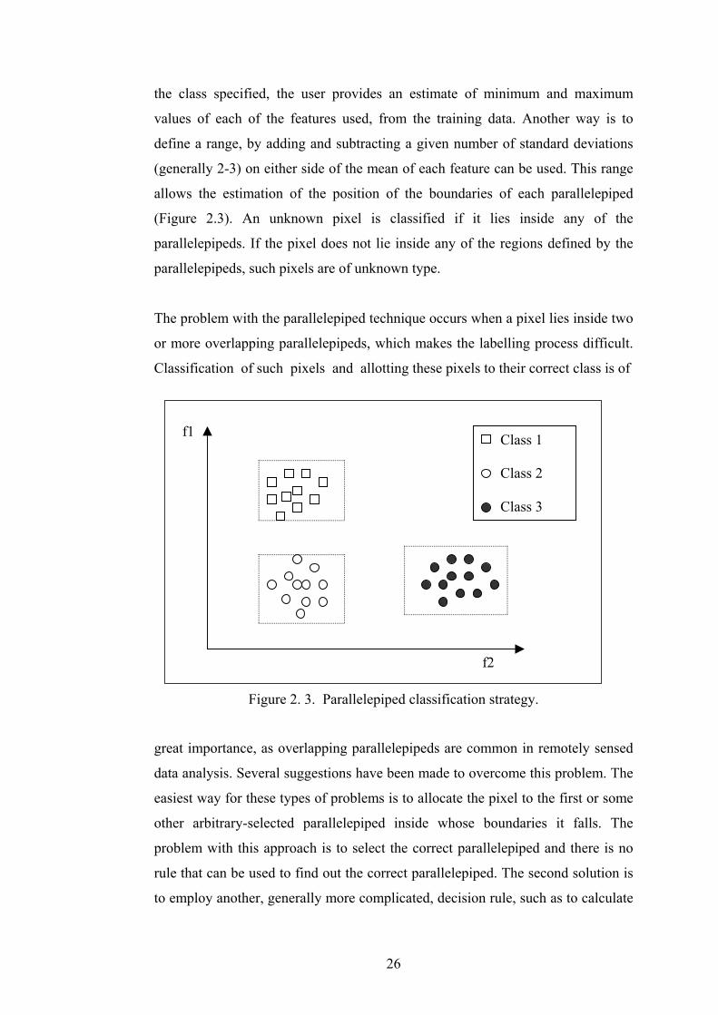
26
the class specified, the user provides an estimate of minimum and maximum
values of each of the features used, from the training data. Another way is to
define a range, by adding and subtracting a given number of standard deviations
(generally 2-3) on either side of the mean of each feature can be used. This range
allows the estimation of the position of the boundaries of each parallelepiped
(Figure 2.3). An unknown pixel is classified if it lies inside any of the
parallelepipeds. If the pixel does not lie inside any of the regions defined by the
parallelepipeds, such pixels are of unknown type.
The problem with the parallelepiped technique occurs when a pixel lies inside two
or more overlapping parallelepipeds, which makes the labelling process difficult.
Classification of such pixels and allotting these pixels to their correct class is of
Figure 2. 3. Parallelepiped classification strategy.
great importance, as overlapping parallelepipeds are common in remotely sensed
data analysis. Several suggestions have been made to overcome this problem. The
easiest way for these types of problems is to allocate the pixel to the first or some
other arbitrary-selected parallelepiped inside whose boundaries it falls. The
problem with this approach is to select the correct parallelepiped and there is no
rule that can be used to find out the correct parallelepiped. The second solution is
to employ another, generally more complicated, decision rule, such as to calculate
Class 1
Class 2
Class 3
f2
f1

27
the Euclidean distance between the doubtful pixel and the centre point of each
parallelepiped and use a minimum distance rule to allocate these pixels to a
specified class. To solve these problems, Lillesand and Kiefer (1994) suggested
another method of using a series of rectangles with stepped borders in place of the
single rectangle.
2.3.4.2 The Minimum Distance classifier
This is another simple non-parametric classification method, which uses the
minimum distance between the pixel and the centroid of the training class. This
classification method uses the Euclidean distance (or in a little more complicated
way by adopting the Mahalanobis distance) in multidimensional feature space to
measure the degree of dissimilarity between pixels and class centroids computed
Figure 2. 4. Minimum distance to mean classification strategy
from training data. The pixel is assigned to the least dissimilar class centroid. Like
the parallelepiped classifier, this algorithm does not take all the training data into
consideration. It considers the mean (or average) spectral value in each band for
each class. The mean centre of each class is estimated from the training dataset,
which results in a mean vector. In order to assign a pixel to a specified class,
Euclidean distances are calculated for each mean (or centroid) centre, and then the
Class 1
Class 2
Class 3
f2
f1

28
minimum value, i.e. the shortest distance, is determined. As a result, the pixel is
allocated to the class that is the closest in terms of the estimated multidimensional
Euclidean distance from mean centres (Figure 2.4).
.
This type of classifier is mathematically simple and computationally efficient, but
has certain limitations. Most importantly, it is sensitive to different degrees of
variance in the spectral response data. Due to these problems, this classifier is not
widely used in applications where spectral classes are close to one another in
measurement space and have high variance. However, it can give results that are
comparable to other statistical classifiers, such as the maximum likelihood
classifier in cases where the classes are well defined in feature space.
2.3.4.3 Artificial Neural Network classifiers
Since the late 1980s, supervised classification of satellite image data has also been
carried out using neural network classifiers. These classifiers differ significantly
from the parallelepiped and minimum distance algorithms in their approach to
classification. A neural network is a form of artificial intelligence that imitates
some function of the human brain. Neural networks are general-purpose
computing tools that can solve complex non-linear problems (Fischer, 1996). The
network comprises a large number of simple processing elements linked to each
other by weighted connections according to a specified architecture. These
networks learn from the training data by adjusting the connection weights
(Bishop, 1995). They have been used in remote sensing and image analysis
including supervised classification (Benediktsson et al., 1990; Hepner et al., 1990;
Heerman and Khazenie, 1992; Foody and Arora, 1997) and unsupervised
classification (Baraldi and Parmiggiani, 1995; Schaale and Furrer, 1995; Tso,
1997).
There are a range of artificial neural network architectures designed and used in
various fields, including pattern recognition (Bishop, 1995; Aleksander and
Morton, 1991). In remote sensing applications the multi-layered feedforward
network, also called the multi-layer perceptron, and the Kohonen networks are
generally used. These networks differ from each other in their approach to
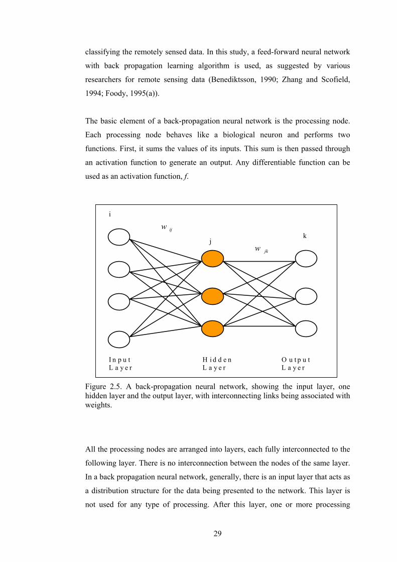
classifying the remotely sensed data. In this study, a feed-forward neural network
with back propagation learning algorithm is used, as suggested by various
researchers for remote sensing data (Benediktsson, 1990; Zhang and Scofield,
1994; Foody, 1995(a)).
The basic element of a back-propagation neural network is the processing node.
Each processing node behaves like a biological neuron and performs two
functions. First, it sums the values of its inputs. This sum is then passed through
an activation function to generate an output. Any differentiable function can be
used as an activation function, f.
Figuhiddwei
All
foll
In a
a di
not
i
29
re 2.5. A back-propagation neural network, showing the input layer, oneen layer and the output layer, with interconnecting links being associated with
ghts.
the processing nodes are arranged into layers, each fully interconnected to the
owing layer. There is no interconnection between the nodes of the same layer.
back propagation neural network, generally, there is an input layer that acts as
stribution structure for the data being presented to the network. This layer is
used for any type of processing. After this layer, one or more processing
ijwk
jjkw
I n p u tL a y e r
H i d d e nL a y e r
O u t p u tL a y e r
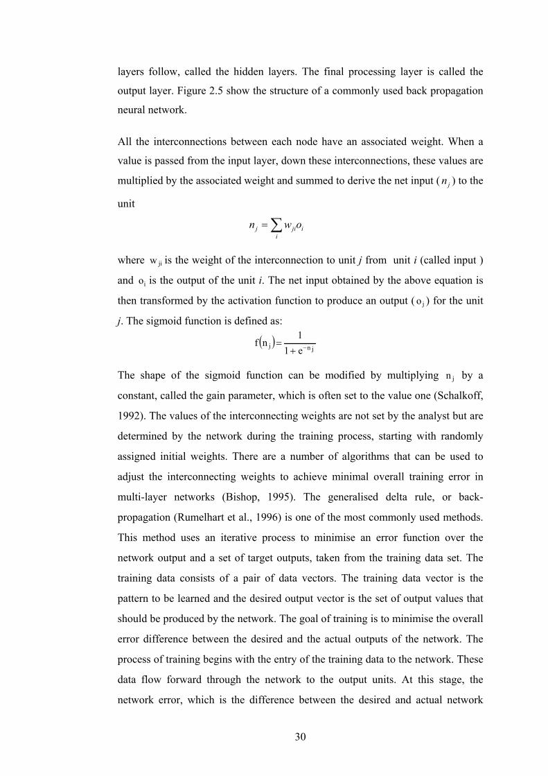
30
layers follow, called the hidden layers. The final processing layer is called the
output layer. Figure 2.5 show the structure of a commonly used back propagation
neural network.
All the interconnections between each node have an associated weight. When a
value is passed from the input layer, down these interconnections, these values are
multiplied by the associated weight and summed to derive the net input ( jn ) to the
unit
∑=i
ijij own
where jiw is the weight of the interconnection to unit j from unit i (called input )
and io is the output of the unit i. The net input obtained by the above equation is
then transformed by the activation function to produce an output ( jo ) for the unit
j. The sigmoid function is defined as:
( )jnj e1
1nf −+
=
The shape of the sigmoid function can be modified by multiplying jn by a
constant, called the gain parameter, which is often set to the value one (Schalkoff,
1992). The values of the interconnecting weights are not set by the analyst but are
determined by the network during the training process, starting with randomly
assigned initial weights. There are a number of algorithms that can be used to
adjust the interconnecting weights to achieve minimal overall training error in
multi-layer networks (Bishop, 1995). The generalised delta rule, or back-
propagation (Rumelhart et al., 1996) is one of the most commonly used methods.
This method uses an iterative process to minimise an error function over the
network output and a set of target outputs, taken from the training data set. The
training data consists of a pair of data vectors. The training data vector is the
pattern to be learned and the desired output vector is the set of output values that
should be produced by the network. The goal of training is to minimise the overall
error difference between the desired and the actual outputs of the network. The
process of training begins with the entry of the training data to the network. These
data flow forward through the network to the output units. At this stage, the
network error, which is the difference between the desired and actual network

31
output, is computed. This error is then fed backwards through the network
towards the input layer with the weights connecting the units being changed in
relation to the magnitude of the error. This process is repeated until the error rate
is minimised or reaches an acceptable level, or until a specified number of
iterations has been accomplished.
The neural network weights are adjusted either after the entire sum is obtained for
all training patterns, called batch or epoch training, or after each training pattern is
presented, called sequential training. The sequential training method allows more
flexibility with the training data but requires more training time as compared to
the batch training, because weights are adjusted with every training pattern instead
of at the end of the cycle in batch training.
Training a neural network involves the setting of several initial parameters that
strongly influence network performance, especially in terms of speed and
accuracy. Even if these parameters are selected judiciously there is no guarantee
that the neural network will provide an acceptable solution. The user-selected
values influencing the neural classifier are:
• Learning parameters - the back-propagation learning algorithm requires
that the user provides values of the learning rate and momentum. The
value of these parameters significantly influence the performance of a
network.
• Initial weights - the initial weight settings of the pre-trained network
influence the network performances. These settings are generally chosen
randomly.
• Number of training iterations - this is a very important parameter as it
controls the degree of generalisation as opposed to specialisation of the
solution: if network is trained using very large number of iterations on
training data, it might not function well on the test data and if it is not
trained well enough it will not be able to separate the classes.
• Number of hidden layers and units - this determines the capacity of the
network to learn and generalise.

32
• Number of input patterns - several studies suggested that classification
accuracy is affected by the number of training patterns.
In this study, all of the above parameters are set as suggested in an earlier study
carried out by Kavzoglu (2001).
2.3.4.4 Decision Tree classifiers
Decision tree induction algorithms have long been popular in machine learning,
statistics, and other disciplines for solving classification and related tasks (Morgan
and Sondquist, 1963; Hunt et al., 1966; Friedman, 1977; Breiman et al., 1984;
Quinlan 1993). A decision tree can be used to classify a query (or test) case as
follows.
Given a query q to classify, a tree is traversed along a path from its root to a leaf
node, whose class label is assigned to q. Each internal node contains a test that
determines which of its subtrees is traversed for q. A test typically evaluates a
feature used to describe cases, or a boolean or linear combination of features. A
decision tree algorithm has four inputs:
1. a training set, in which each case is defined by a set of features and their
respective values, and a class label,
2. a set of candidate tests that partition or split a set of training cases into
subsets,
3. a heuristic evaluation function that assesses the quality of a given test and
resulting partition, and
4. a stopping criterion function that defines when to terminate tree expansion.
The algorithm outputs a decision tree whose leaves typically bear a single class
label. Decision trees are usually induced from the root downwards using a
recursive divide-and-conquer algorithm (Quinlan 1993). The task of constructing
a tree from the training data is called tree induction. Most existing tree induction
systems proceed in a top-down fashion, starting with an empty tree and the entire
training set. Decision tree classifiers are discussed in detail in chapter 3.

33
2.3.4.5 Support Vector Machines
Support vector machines (SVM) are classification and regression methods which
have been derived from statistical learning theory (Vapnik, 1995). These
classification techniques are based on the principle of optimal separation, in
which - if the classes are separable - this method selects, from among the infinite
number of linear classifiers that separate the data, the one that minimise the
generalisation error, or at least an upper bound on this error, derived from
structural risk minimisation. Thus, the selected hyperplane will be one that leaves
the maximum margin between the two classes, where margin is defined as the
sum of the distances of the hyperplane from the closest point of the two classes
(Vapnik, 1995).
If the two classes are non-separable, the SVM tries to find the hyperplane that
maximises the margin and that, at the same time, minimises a quantity
proportional to the number of misclassification errors. The trade off between
margin and misclassification error is controlled by a positive constant that has to
be chosen beforehand.
This technique of designing a SVM can be extended to allow for non-linear
decision surfaces. This can be achieved by projecting the original set of variables
into a higher dimensional feature space and formulating a linear classification
problem in the feature space. Further details of SVM based classifiers are
discussed in chapter 3.
2.4 Incorporation of nonspectral features
Though, spectral information alone provides useful information about the
characteristics of land cover features, the addition of a different kind of
information may help in the identification of different classes that are not easily
distinguished using spectral data alone. Spatial information, such as texture and
context, which depends on the neighbourhood of the pixel, has been widely used,
while the second kind of information represents external or non-remotely-sensed
information such as elevation values or data derived from soil or geology maps.

34
Spectral, textural, and contextual features are the fundamental pattern elements
used in human interpretation of satellite images. Spectral features describe the
tonal variations in the various bands of the image, obtained in different bands of
the electromagnetic spectrum, whereas textural features contain information about
the spatial distribution of tonal variation within a band. Contextual feature contain
information derived from blocks of image data surrounding the area being
analysed.
A number of textural measures have been proposed in literature, including the
grey-level co-occurrence matrix (Haralick et al. (1973), auto-regressive models
(Frankot and Chellappa, 1987), fourier transform, and fractal based texture (Keller
and Chen, 1989). Recently, wavelet-based texture features (Fukuda and Hirosawa,
1999) have been used in classification of remotely sensed data. A considerable
amount of research has been carried out to investigate the effectiveness of texture
features for the classification of remotely sensed images. For example, Weszka
et al. (1976) perform a comparative study of texture measures including the
Fourier power spectrum, second-order grey-level statistics, and first-order
statistics of grey-level differences in a study aimed at identifying three geological
terrain types. Recently Mather et al. (1998) investigate the effectiveness of
spectral and textural information in the identification of surface rock type in an
arid region using Landsat TM and SIR-C SAR image data. A number of other
studies (Barber and LeDrew, 1991 and Peddle and Franklin, 1991) have shown
that classification accuracy can be improved by using the texture features in
combination with image.
Generally, contextual information can be used in classification processes for
smoothing purposes. The smoothing techniques can be categorised into pre-
smoothing and post-smoothing. In pre-smoothing processes, contextual
information is incorporated before classification by increasing the dimensionality
of the data with additional bands in which contextual information is present, while
post-smoothing processes are usually more or less smoothing filters (Townshend,
1986), so they work on previously classified images.

35
2.5 Accuracy assessment
The results of any classification process applied to remotely sensed data
classification must be quantitatively assessed in order to determine their accuracy.
As suggested by Lillesand and Kiefer (1994), a classification process is not
complete until its accuracy is assessed. There may be different ways to assess the
accuracy of a classification process. Accuracy assessment can be qualitative or
quantitative, expensive or inexpensive, quick or time consuming, well-designed
and efficient. The purpose of quantitative accuracy assessment is the identification
and measurement of map errors. Quantitative accuracy assessment involves
comparison of an area on a map against reference information of the same area,
assuming reference data to correct. There are number of ways to determine the
degree of error in the end-product, which is typically a thematic map or image, but
for this research accuracy assessment is carried out by measuring overall
classification accuracy, and calculation of the Kappa statistics for a given number
of test data.
2.5.1 Confusion matrix
The accuracy of classification has traditionally been measured by the overall
accuracy by generating a confusion matrix (Table 2.1) and determining accuracy
levels by dividing the total number of correctly classified pixels (sum of major
diagonal of confusion matrix, also called actual agreement) by the total number of
reference pixels. However as a single measure of accuracy, the overall accuracy
gives no insight into how well the classifier is performing for each of the different
classes (Fitzgerald and Lees, 1994). In particular, a classifier might perform well
for a single class that accounts for a large proportion of the test data and this will
create a bias in overall accuracy, despite low class accuracies for other classes. To
avoid such a bias when assessing the accuracy of a classifier, it is important to
consider the individual class accuracies. Individual class accuracy can be obtained
by dividing the total number of correctly classified pixels in that category by the
total number of pixels of that category. Individual class accuracy can be
determined by using the reference data (called producer's accuracy). The resulting
percentage accuracy indicates the probability that a reference pixel will be
correctly classified. Story and Congalton (1986) suggested that producer's

accuracy is a measure of error of omission. However, a misclassification error is
not only an omission from the correct class but also a commission into another
class. Individual class accuracy obtained from the classified data in that category
(user's accuracy) is a measure of error of commission (Story and Congalton,
1986). Before confusion matrices were the standard accuracy reporting
mechanism, it was common to report the overall accuracy and either only the
producer's or user's accuracy. Example in Table 2.1 demonstrate the need of the
entire confusion matrix so that all three accuracy measures can be computed.
Table 2.1. Confusion matrix
Class 1 2 3 4 5 6 7 8 Total Users
36
Considering the confusion matrix shown in Table 2.1, there exist considerable
differences between the user’s and producer’s accuracies for corresponding
classes. The values of user's and producer's accuracies shows significant variation
from the overall accuracy (69.9%). If the overall accuracy is solely taken into
account, it can be concluded that the classifier has an average accuracy of about
70%, without giving the effectiveness of the classification on a particular class,
which could be misleading. If the overall accuracy and one of the individual class
accuracy measures are considered, the analyst could again reach some misleading
conclusions. For example, a producer’s accuracy of 57.4% is achieved for the
class 3, which is quite low when compared to the overall accuracy. The analyst
can conclude at this stage that, although the overall accuracy is average, the class
3 can be classified with lower accuracy (57.4%). Drawing such a conclusion could
be a mistake because the user’s accuracy of the class 3 is 62.3%. This means that
1 423 0 70 0 0 0 2 14 509 83.12 0 500 0 0 0 0 0 0 500 1003 43 0 287 10 6 0 12 103 461 62.34 1 0 15 312 108 6 43 34 519 60.15 3 0 12 79 307 9 12 13 435 70.66 0 0 6 11 37 449 56 12 571 78.67 3 0 18 47 38 31 182 73 392 46.48 27 0 92 41 4 5 73 251 493 50.9
Total 500 500 500 500 500 500 380 500 3880Produc 84.6 100 57.4 62.4 61.4 89.8 47.9 50.2
Overall accuracy = 69.9 Kappa value = 0.655
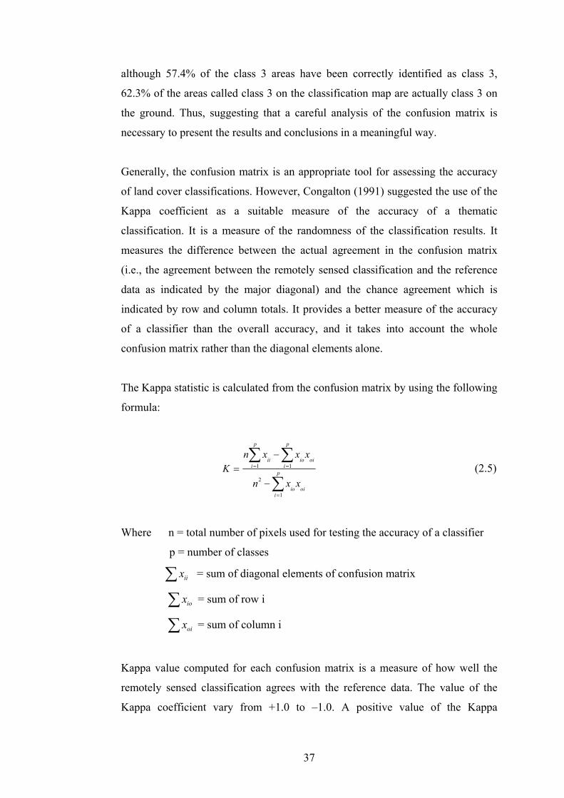
37
although 57.4% of the class 3 areas have been correctly identified as class 3,
62.3% of the areas called class 3 on the classification map are actually class 3 on
the ground. Thus, suggesting that a careful analysis of the confusion matrix is
necessary to present the results and conclusions in a meaningful way.
Generally, the confusion matrix is an appropriate tool for assessing the accuracy
of land cover classifications. However, Congalton (1991) suggested the use of the
Kappa coefficient as a suitable measure of the accuracy of a thematic
classification. It is a measure of the randomness of the classification results. It
measures the difference between the actual agreement in the confusion matrix
(i.e., the agreement between the remotely sensed classification and the reference
data as indicated by the major diagonal) and the chance agreement which is
indicated by row and column totals. It provides a better measure of the accuracy
of a classifier than the overall accuracy, and it takes into account the whole
confusion matrix rather than the diagonal elements alone.
The Kappa statistic is calculated from the confusion matrix by using the following
formula:
∑
∑ ∑
=
= =
−
−= p
ioiio
p
i
p
ioiioii
xxn
xxxnK
1
2
1 1 (2.5)
Where n = total number of pixels used for testing the accuracy of a classifier
p = number of classes
∑ iix = sum of diagonal elements of confusion matrix
∑ iox = sum of row i
∑ oix = sum of column i
Kappa value computed for each confusion matrix is a measure of how well the
remotely sensed classification agrees with the reference data. The value of the
Kappa coefficient vary from +1.0 to –1.0. A positive value of the Kappa

38
coefficient is expected to have a positive correlation between the image and
reference data being used for classification. A value of zero indicates no
agreement in classification, while a value of 1.0 indicates perfect agreement
between the classifier output and the reference data.
Confidence intervals can be calculated for the Kappa value using the approximate
large sample variance. The approximate large sample variance of Kappa is
calculated as follows (Bishop et al., 1975):
( ) ( )
( )
( )( )
( )
( ) ( )
( )
θ−
θ−θθ−+
θ−
θ−θθθ−+
θ−
θ−θ=σ
42
224
21
22
3211
22
11
1
41
1
212
1
1
n
1K (2.6)
where ∑=
=θ1i
ii1
n
x, ∑
=
∗=θ
1i 2
oiio2
n
xx, ∑
=
+=θ
1i
oiioii3
n
x
n
x
n
x and
∑∑= =
+=θ
1i 1j
2ojjoij
4
n
x
n
x
n
x
A test of significance for the Kappa statistic can be performed for each confusion
matrix separately to determine if the agreement between the classification and the
reference data is significantly greater than zero. In other words, a test can be
performed to see if the classification is significantly better than a random
assignment of land cover categories to pixels. The significance of a single
confusion matrix can be calculated by
( )K
KZσ
= (2.7)
where Z is standardised and normally distributed and σ is the large sample
variance of the Kappa coefficient.
A pair-wise test of significance can be performed between two independent Kappa
values using the normal curve deviate to determine if the two confusion matrices

39
are significantly different (Cohen, 1960). The test statistic for significant
difference in large sample is given by
( ) ( )21
21
KK
KKZ
σσ +
−= (2.8)
where Z is standardised and normally distributed and 1
K ,2
K are the two Kappa
coefficients being compared. This test between two independent Kappa values
allows any two error matrices to be compared in order to determine if they are
significantly different. In other words, error matrices generated from several
classification algorithms can be compared, two at a time, to determine which
classifications are significantly better than the others. The computed value of Z is
compared with a critical value 2/Zα for some predefined confidence level (i.e., α/2
is the confidence level of the two-tailed Z test and the degrees of freedom are
assumed to be infinity), and if 2/ZZ α≥ the classification is significantly better than
a random classification.
2.6 Conclusions
This chapter reviews the philosophy underlying classification procedures used in
remote sensing. Classification techniques, categorised using four criteria
(supervised and unsupervised, parametric and non-parametric) are discussed in
detail. Some of the advantages and disadvantages of the techniques are also
discussed. The most appropriate classification system used is dependent upon the
characteristics of the data (such as scale and type of data) used and also on the
nature of the classifier to be employed (the assumption on which classifier is
working). A short discussion is also included about incorporating spatial
information, texture and context, as both texture and context are sources of spatial
information which are widely used for image classification.

40
Chapter 3
Advanced Classification Algorithms
3.1 Introduction
Statistical procedures such as the maximum likelihood classifier require that data
must be based on some pre-defined model (usually the Gaussian normal
distribution). The performance of a statistical classification will thus depend on
how well the data match the pre-defined model. If the data are complex in
structure then to model them in an appropriate way can become a real problem.
These types of classifiers are also called single-stage classifiers because an
observation is given the label of one of a predetermined number of classes in a
single step. The statistical approach to classification has two significant
drawbacks (Swain and Hauska, 1977):
1. Only one of the possible combinations of features is used in the
classification.
2. Each sample is tested against all classes, which leads to a relatively high
degree of inefficiency.
An inherent weakness of the maximum likelihood procedure is that the subset of
features used in classification is not necessarily the optimal choice for all classes.
Usually, a set of features is selected by the criterion of maximum average
interclass separability, i.e., in a multi-class multi-feature classification the set of
features for which the average pair-wise separability is largest is used. The
problem of using only one feature subset as the basis of a classification is
particularly severe when there is a large number of classes. In principle, one could
combine the features that are useful in discriminating between all possible
combinations of pairs of classes and use the combination of these features in a
single stage classifier.

41
Much research effort in the past ten years has been devoted to analysis of the
performance of artificial neural networks in image classification. The preferred
algorithm is feed-forward multi-layer perceptron using back-propagation, due to
its ability to handle any kind of numerical data, and to its freedom from
distributional assumptions (section 2.3.4.3). A number of studies have reported
that users of neural classifiers have problems in setting the choice of various
parameters during training. The choice of architecture of the network, the sample
size for training, learning algorithms, and number of iterations required for
training are some of these problems.
In practice, and especially since the advent of hyperspectral data, the so-called
dimensionality problem can be encountered, i.e., with a fixed and relatively small
sample size, the classification accuracy may actually decrease as the number of
features is increased (Hughes, 1968). Hence, if a large number of features is used,
then a corresponding increase in the number of training and testing samples is
required in order to ensure that the results obtained are reliable. Furthermore,
some patterns may not need all the features in order to arrive at the correct
classification, but a one stage classifier uses these features anyway, which results
in decreased efficiency.
As progress in new sensor technology for earth observation remote sensing
continues, increasingly high spectral resolution multi-spectral imaging sensors are
being developed. These sensors give more detailed and complex data for each
picture element and greatly increase the dimensionality of the data compared with
multispectral systems. As the number of features, number of samples, and
classification accuracy are interrelated in a complex fashion, one may need to
know how many features should be used to maximise the overall classification
accuracy. Where training sample size is limited and the dimensionality of the
feature space is high, then the estimate of first and second-order statistics (e.g., as
required by maximum likelihood classifier) cannot accurately summarise all
information which is contained in the data and results are thus less reliable.
For such problems, it would be preferable to have a classification system which
could decompose the multi-class classification problem into several stages, and

42
which finally may simplify the decision-making process by taking partial
decisions at successive stages, or alternatively to use a classification system that is
independent of the dimensionality of the feature space. The technique of
decomposing the multi-class classification problem into several stages is termed
multistage classification. It has several attractive features, the most important of
which, perhaps, is understandability. In many instances, taking such partial
decisions is conceptually simpler, as each involves only that information relevant
to the current stage. This also saves the expense of gathering information not
required for the current stage. These points have contributed to the increased
popularity of multistage decision making in several engineering problems,
especially in pattern recognition.
Another classification system, called the support vector machine, is said to be
independent of the dimensionality of feature space. The main idea behind this
classification technique is to separate the classes with a surface that maximise the
margin between them, using boundary pixels to create the decision surface. It has
been observed that the optimal hyperplane is determined by only a small fraction
of the data points, thus requiring a small number of training data even at high
dimensionality.
This chapter discusses various stages for the development of multistage and
support vector machine classification algorithms.
3.2 Multistage classifiers
A large number of multistage classification techniques have been proposed for
pattern recognition. These techniques can be categorised into three groups.
1. Converting a decision table to an optimal decision tree.
2. Dynamic tree development.
3. Hierarchical classification methods.
The problem of converting a decision table to an optimal decision tree is to
design a decision tree to efficiently evaluate the value of a multiple input, multiple

43
output function given the values of independent variables. Each of the
independent variables has a finite domain. In pattern recognition, the range of the
output is the set of classes. There are a number of table conversion methods
available in the literature for pattern recognition problems. The details of these
methods can be found in Meisel and Michalopoulos (1973), Stoffel (1974), and
Sethi and Chatterjee (1977).
Dynamic tree development methods select a feature and split its region at every
stage (node). Later stages handle smaller regions of the feature space and repeat
the procedure. These are essentially top-down methods. Swain and Hauska (1977)
used an evaluation function to optimise decision trees. Every node in a tree is
taken as a classifier and a performance measure is defined for the node. All
possible specifications are searched to find the best node configuration. A variety
of other techniques use simple dynamic data splitting to design binary trees. For
further details readers are referred to Breiman et al. (1984), Casey and Nagy
(1984), Friedman (1977), Rounds (1980), and You and Fu (1976).
Hierarchical classifiers are multistage pattern classifiers in which classes are
sequentially rejected along a path to a finally accepted class label. The
hierarchical subgrouping of classes, the features required at nonterminal nodes of
the hierarchy and the decision rules are interdependent. With a class hierarchy,
individual nodes themselves acts as a pattern classifiers. However the node
classifiers cannot be designed independently of each other. In the analysis process
the potential advantages of using hierarchical classification are an increase in the
accuracy, speed, and the level of details which can be reached.
Classification trees offer an effective implementation of hierarchical classifiers.
Indeed, classification trees have become increasingly popular due to their
conceptual simplicity and computational efficiency. A decision tree classifier has
a simple form, which can be compactly stored, and it classifies new data
efficiently. A decision tree classifier carries out automatic feature selection and
complexity reduction, and the tree structure gives easily understandable and
interpretable information regarding the predictive or generalisation ability of the
data.

44
Another significant advantage of decision tree classifiers is that they are non-
parametric, i.e., capable of handling non-normal and non-homogenous data sets
(Quinlan, 1993) and can be very useful for land cover classification in remote
sensing due to their simplicity, flexibility, and computational efficiency (Friedl
and Brodley, 1997).
3.3 Decision tree classifiers
In general, there are two approaches to the design of decision trees (Swain and
Hauska, 1977). These approaches are similar in principle, but differ significantly
in the way the tree is designed in practice.
1. Manual design method
2. Heuristic search method
Manual methods use statistics such as the mean vector and covariance matrix,
which are calculated for all classes. Then a graph is derived in which the means
and variances for all the classes are plotted for each feature. This graph is called a
coincident spectral plot. It is often possible to estimate suitable decision
boundaries from this graph such that all classes are separated in a number of
decision steps. As long as one feature is used in each stage, this is roughly
equivalent to estimating a simple distance measure between the classes. This
method is not suitable, firstly, when two or more features are to be used in a given
stage of the tree, because the graph does not show how the interactions between
features can be used, and secondly, if the data are not normally distributed, thus
making it difficult to estimate the covariance matrices in an unbiased way.
The coincident spectral plot provides an estimate of interclass separability based
on single features. If the difficulty of discriminating the classes requires the use of
a combination of several features, the manual design approach based on the
spectral plot is severely limited. In general, a more analytical design procedure is
desirable when the complexity of the problem in terms of the number of classes or
the number of features required for adequate classification accuracy is significant.

45
To construct a classification tree using the heuristic approach, it is assumed that a
training data set consisting of feature vectors and their corresponding class labels
is available. The feature set is selected on the basis of problem-specific
knowledge. The decision tree is then constructed by recursively partitioning the
training data set into purer, more homogenous, subsets on the basis of a set of
tests applied to one or more attribute values at each branch or node in the tree.
This procedure involves three steps: splitting nodes, determining which nodes are
terminal nodes, and assigning class label to terminal nodes. The assignment of
class labels to terminal nodes is straightforward: labels are assigned based on a
majority vote or a weighted vote when it is assumed that certain classes are more
likely than others.
A tree is composed of a root node (containing all the data), a set of internal nodes
(splits), and a set of terminal nodes (leaves). Each node in a decision tree has only
one parent node and two or more descendent nodes (Figure 3.1). A data set is
classified by moving down the tree and sequentially subdividing it according to
the decision framework defined by the tree until a leaf is reached.
The method of constructing a decision tree is as follows (Quinlan, 1993):
To construct a decision tree from a set T of training data having m classes denoted
by 1C , 2C ,…., mC . There are three probabilities:
• If T contains one or more objects, all belonging to a single class iC , then
the decision is a leaf identifying class iC .
• If T contains no data, the decision tree is again a leaf determined from
information other than T.
• If T contains data that belongs to a mixture of classes then a test is chosen,
based on a single attribute or a combination of attributes, that has one or
more mutually exclusive outcomes O.......,OO k2,1 . T is partitioned into
subsets ,T,........,T,T k21 where iT contains all the data in T that have
outcome iO of the chosen test. The decision tree for T consists of a
decision node identifying the test, and one branch for each possible

outcome. The same tree building process is applied recursively to each
subset of training data.
A typical decision tree for classification is shown in Figure 3.1. The elliptical
nodes are decision nodes whose two descendants are determined by a threshold
iη on a specified feature value ix . The same feature may occur in different parts
of the tree associated with a different threshold. The rectangular nodes are
terminal nodes and are assigned a class label. Based on the outcome of testing a
feature value against a threshold, either a 'yes' or a 'no' branch will be taken. When
an unknown feature vector is submitted for classification, the feature vector is
assigned the class label of the terminal node that it reaches.
Fcl
η≤x
46
igure 3. 1. A classification tree for a five dimensional feature space and threelasses. The ix are the feature values, the iη are the thresholds, and Y is the classabel.
yes
no
yes
nono
nono
yes
yes
yes
noyes
11
44 η≤x 313 η≤x
323 η≤x
22 η≤x
Y = 1Y = 2
Y = 1
Y = 2Y = 3
Y = 1
Y = 3
55 η≤x

47
3.4 Decision tree design approaches
Numerous tree construction approaches have been developed in the last thirty or
so years, but most of the research in decision tree classifier design has
concentrated in the area of finding splitting rules, which finally gives the idea of
the termination rules. A number of algorithms have been developed to split the
training data at each internal node of a decision tree into regions that contain
examples from just one class, and this is the most important element of a decision
tree classifier. These algorithms either minimise the impurity of the training data
or maximise the goodness of split. The approaches to design a decision tree are:
• Bottom-up approach.
• Top-down approach.
• Hybrid approach.
• Growing-pruning approach.
3.4.1 Bottom-up approach
In the bottom-up approach (Landeweered et al., 1983), a binary tree is constructed
using the training set and some distance measure, such as the Mahalanobis
distance. The pairwise distances between a priori defined classes are computed
and in each step the two classes with the smallest distance are merged to form a
new group. The mean vector and covariance matrix for each group are computed
from training samples of classes in that group, and the process is repeated until
one is left with a single group at the root. In a tree constructed this way, the more
obvious discriminations are done first, near the root, and more difficult ones at
later stages of the tree.
3.4.2 Top-down approach
In top-down approach, the design of a decision tree classifier consists of the
following three tasks:
1. Selection of a node splitting rule,
2. Decision as to which nodes are terminal,

48
3. Assignment of each terminal node to a class label.
The class assignment problem is the easiest of above-mentioned tasks. Terminal
nodes are assigned to the classes that have the highest probabilities by using a
basic majority rule; i.e., assign to the terminal node the label of the class that has
most samples at that terminal node. The basic idea in choosing any splitting
criterion at an internal node is to make the data in the descendent nodes purer.
The overall approach adopted by this process is to choose the attribute that best
divides the training data into classes and then partition the data according to the
value of that attribute. This process is applied recursively to each partitioned
subset, with the procedure terminating when all examples in the current subset
have the same class. The result is represented as a tree in which each node
specifies an attribute and each branch emanating from a node specifies a possible
value of that attribute.
Thus, the main task of this process is to select the attribute to be used as criterion
because at each node in the development of a decision tree there will be a set of
observations and a number of attributes to classify them. One cannot select an
individual attribute without first determining the "quality" of all of the attributes,
and seeing how well each one separates the data into various classes. The quality
of an attribute should reflect the useful information provided by that attribute.
There are two major approaches to estimating the quality of an attribute.
In the first approach, the quality of an attribute may be estimated by ignoring the
other attributes, therefore assuming, for the purpose of estimation, the
independence of attributes. In the second approach, the quality of an attribute
may be estimated in the context of other attributes. The first approach is also
called the myopic approach (Kononenko and Hong, 1997), which has the
advantage of computational speed. The latter approach is computationally more
demanding but has the potential to discover higher-order dependencies among the
attributes.

49
3.4.2.1 Attribute selection measures
There are many approaches to the selection of attributes used for decision tree
induction, and these approaches have been studied in detail by researchers in
machine learning (Brieman et. al., 1984, Murthy et. al., 1994; Kononenko and
Hong, 1997; Mingers, 1989 (b); Quinlan, 1993). Some approaches measure the
“goodness of split” (Brieman et. al., 1984) while other approaches try to minimise
the impurity of the training data.
The quality of an attribute in classification is defined in term of the purity of
classes of training observations and most approaches assign a quality measure
directly to the attribute. A set of observations is pure if all the observations belong
to the same class, while the set is maximally impure if the proportion of
observations in all classes is uniform. The impurity function measures the
impurity of a set of observations and achieves the minimum for a pure set, and
maximum for a maximally impure set. Impurity functions are mainly used in
selecting the best attribute to further split the current node. The most frequently-
used impurity measures in decision tree induction are:
1. Information Gain and Information Gain Ratio criterion (Quinlan, 1986,
1987, 1993).
2. Gini Index (Brieman et. al., 1984).
3. Twoing rule (Brieman et. al., 1984).
4. Chi-square statistics (Mingers, 1989 (b)).
3.4.2.1.1 Information Gain and Information Gain Ratio criterion
Quinlan (1993) proposed the use of the information gain and information gain
ratio, based on a classic formula from information theory that measures the
theoretical information content of a code as ( )∑− ii pp log , where ip is the
probability of the i-th message. The value of this measure depends on the
likelihood of the various possible messages. If they are all equally likely (i.e., the
ip are equal), there is the greatest amount of uncertainty and the information

50
gained will be greatest. The less equal the probabilities, the less information there
is to be gained. The value of the function also depends on the number of possible
messages.
The information gain and information gain ratio measures (Quinlan, 1993) are
developed in the following way:
For a given training set T, selecting one case at random and saying that it belongs
to some class iC , has the following probability of being correct:
f ( iC , T)/ |T|
Where f ( iC , T) stands for the number of cases in T that belongs to class iC and
T denotes the number of cases in T. So the information it conveys is:
2log− (f ( iC , T)/ |T|) bits. (3.1)
Then the amount of information required to identify the class for an observation in
T can be quantified as
info(T) = -∑=
m
i 1 f ( iC , T)/ |T| × 2log (f ( iC , T)/ |T|) bits. (3.2)
This quantity is known as the entropy of the set T.
If a test Z that can partition T into k outcomes is defined, then a similar measure
can be defined that quantifies the total information content after applying Z:
info z (T) = ∑=
k
j 1 T
Tj × info ( jT ) (3.3)
Using this approach, the information gained by splitting T using Z can be
measured by the quantity:
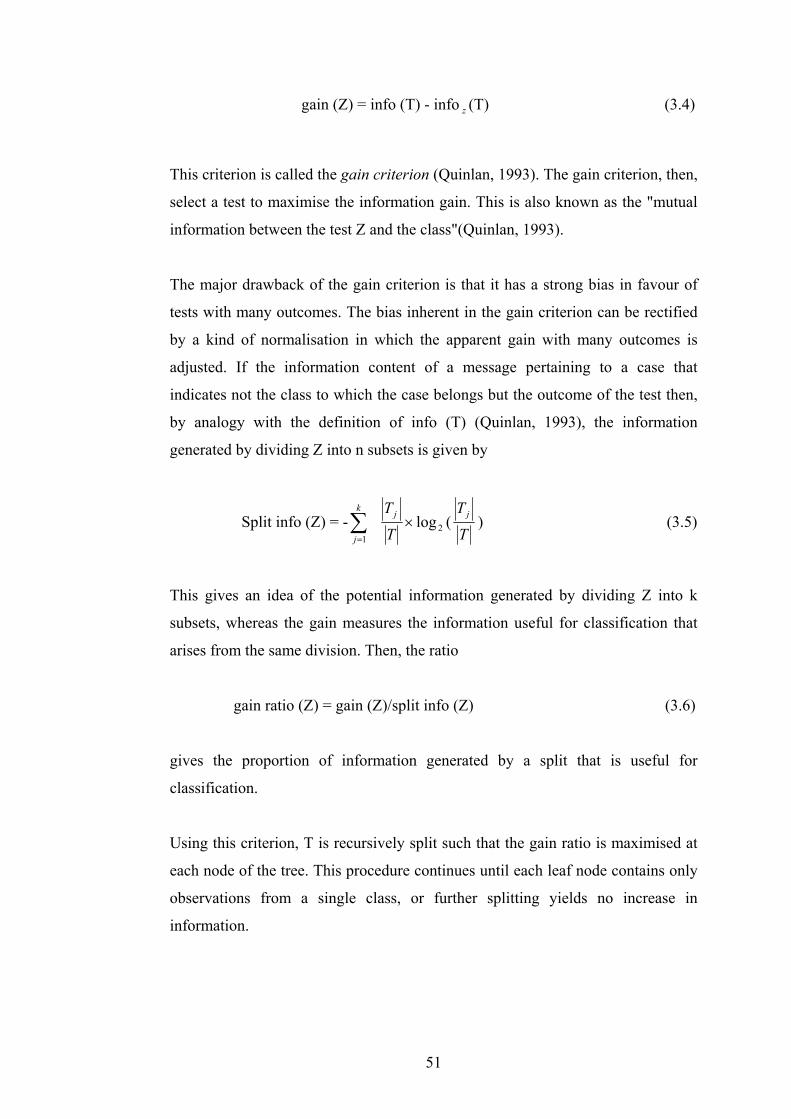
51
gain (Z) = info (T) - info z (T) (3.4)
This criterion is called the gain criterion (Quinlan, 1993). The gain criterion, then,
select a test to maximise the information gain. This is also known as the "mutual
information between the test Z and the class"(Quinlan, 1993).
The major drawback of the gain criterion is that it has a strong bias in favour of
tests with many outcomes. The bias inherent in the gain criterion can be rectified
by a kind of normalisation in which the apparent gain with many outcomes is
adjusted. If the information content of a message pertaining to a case that
indicates not the class to which the case belongs but the outcome of the test then,
by analogy with the definition of info (T) (Quinlan, 1993), the information
generated by dividing Z into n subsets is given by
Split info (Z) = -∑=
k
j 1 T
Tj× 2log (
T
Tj ) (3.5)
This gives an idea of the potential information generated by dividing Z into k
subsets, whereas the gain measures the information useful for classification that
arises from the same division. Then, the ratio
gain ratio (Z) = gain (Z)/split info (Z) (3.6)
gives the proportion of information generated by a split that is useful for
classification.
Using this criterion, T is recursively split such that the gain ratio is maximised at
each node of the tree. This procedure continues until each leaf node contains only
observations from a single class, or further splitting yields no increase in
information.

52
3.4.2.1.2 The Gini Index
Brieman et al. (1984) use a measure called the Gini index of diversity. The Gini
function measures the impurity of an attribute with respect to the classes. For a
given training set T, selecting one case at random and saying that it belongs to
some class iC has the following probability of being correct:
f ( iC , T)/ |T| .
The general Gini function, or measure of impurity, is
( ) ( ) )T/T,Cf)(T/T,Cf( jij
i∑∑≠
(3.7)
which can also be written as
( ) ( ) T/T,CfT/T,Cfj
j2
2
jj ∑∑ −
or
( ) T/T,Cf1j
j2∑− (3.8)
The Gini index is simple and can be computed quickly. This index uses the rule
that assigns an object selected at random from the node to the class i with
probability f ( iC , T)/ |T|, instead of using the plurality rule to classify objects in a
node.
3.4.2.1.3 The Twoing rule
The Twoing rule is described by Brieman et al. (1984). It uses a different
approach to attribute selection in decision tree construction.
Denote the set of classes by C, i.e., C = 1,…., j. At each node, separate the
classes into two super-classes, 1C = njj ,....,1 , and 12 CCC −= . For a given
split of a node, the decrease in impurity that results from this split of the node can
be computed as:

53
( ) ( )2
iRiLiRL T/RT/L*T/T*T/T
−∑ (3.9)
Where LT and RT are the number of examples on the left and right of a split at
the node and iL and iR are the number of examples in category i on the left and
right side of the split. This decrease in impurity is known as the twoing value. The
twoing value is actually a goodness of fit measure rather than an impurity
measure.
3.4.2.1.4 The Chi-square Contingency Table statistic ( 2χ )
Mingers (1989 (b)) discusses the use of this measure to select attributes for
decision tree induction. It is based on traditional statistics for measuring the
association between two variables in a contingency table, and is based on
comparing the observed frequencies with the frequencies that one would expect if
there were no association between the variables. The resulting statistic is
distributed approximately as chi-square, with larger values indicating greater
association. The basic equation for this function is
∑∑−
=ij
ijij
EEx 2
2 )(χ
(3.10)
Where N/xxE jiij = , i.e., the expected value for each cell in the contingency
table.
The final stage in top-down decision tree classifier design is the determination of
when splitting should be stopped. Initial approaches to selecting terminal nodes
were of the form where a threshold β > 0 is set, and node t is declared as a
terminal node if
TS∈
max ∆ i (S (t),t) < β

54
One way to accomplish this task is to define an impurity function i(t) (Breiman et
al., 1984) at every internal node t. If a candidate split S divides the internal node t
into left child node Lt and right child node Rt such that a proportion Lp of the
cases in t go into Lt and a proportion Rp go into Rt , then the goodness of the split
S can be measured by the decrease in impurity:
∆ i (S, t) = i (t) – i ( Lt ) Lp - i ( Rt ) Rp
Hence a split is chosen that minimises ∆ i (S, t) over all splits S in some set of
data T.
The problem with this rule is that partitioning is frequently halted too soon at
some nodes and too late at some others. Brieman et al. (1984) found that the
stopping rule has a greater impact on the efficiency of decision tree classifier than
the splitting rules. They suggested that, instead of using a stopping rule, one
should continue splitting until all the terminal nodes are pure, or nearly pure, thus
generating a large tree. This large tree is then selectively pruned, producing a
decreasing sequence of subtrees. Finally, use cross validation to pick out the
subtree that has the lowest estimated misclassification rate.
3.4.3 Hybrid approach
Hybrid methods of designing a decision tree classifier use both the bottom-up and
top-down approaches sequentially (Kim and Landgrebe, 1991). The procedure for
designing this type of classifier is as follows. First, considering the entire set of
classes, a bottom-up approach is used to divide the data into two subgroups. Then
the mean and covariance of each subgroup are calculated and used in a top-down
approach to generate two new subgroups. Each subgroup is checked to see if it
contains only one class. If so, that subgroup is labelled as terminal; otherwise, the
previous procedure is repeated. The procedure terminates when all the subgroups
are labelled as terminals.
Hybrid classifiers are found to have several advantages over both top-down and
bottom-up approaches (Kim and Landgrebe, 1991). They are found to converge to

55
classes of informational value, because the cluster initialisation provides early
guidance in this direction, while the straightforward top-down approach does not
guarantee such convergence. The hybrid approach can use overlapping classes,
while there are no overlapping classes in the bottom-up approach. Covariance
information can be applied in the hybrid approach to separate nonspherical
subgroups.
3.4.4 Growing-pruning method
Gelfand et al. (1991) proposed this method of constructing a decision tree
classifier for the following reasons:
1. A large decision tree is grown with the entire data set where partitioning
continues until all terminal nodes have pure class membership. If we then
attempt to prune it back by minimising an estimate of the error rate based
on the same data set, then that estimate of the error rate will be biased and
will result in selecting the large tree as the optimally pruned sub tree of
itself.
2. The above problem can be avoided by splitting the entire data set into two
subsets of nearly equal size, and using one data set for growing and other
data set for pruning the tree. But it is not clear how to use this method both
to grow and prune the tree with a small data set.
3. Brieman et. al. (1984) suggested a cost-complexity pruning method but
Gelfand et. al. (1991) found that the problem of tree pruning is reduced to
a problem of complexity parameter estimation so that cross validation may
be used. They suggested that in this method a pruned sub-tree is selected
by minimising over a parametric family of pruned sub-trees, and this
parametric family may not include the optimal or even a good pruned sub-
tree.
To overcome these difficulties, Gelfand et al. (1991) suggested the following
method of tree growing and pruning, while using all of the data to both grow and
prune a classification tree.

56
First, divide the entire data set into two subsets of nearly equal size. A large tree is
grown with pure terminal nodes using first data subset. A pruned sub-tree is then
selected by minimising an estimate of the error rate based on the second data
subset over all pruned sub-trees. This procedure is then iterated, using the second
subset to grow a tree starting from the terminal nodes of the previously selected
pruned sub-tree. The first subset is now used to select a new pruned sub-tree, and
so on. This process is continued till the sequence of selected pruned sub-trees
converges.
3.5 Classification algorithms based on data splitting method
Decision tree classification algorithms can be defined according to whether a
uniform or a heterogeneous set of algorithms is used to estimate the splits at
internal nodes. Such algorithms are described as having homogenous or
heterogeneous hypothesis space, respectively. Traditional approaches to the
design of decision trees are based on homogenous classification models for which
a single algorithm is used to estimate each split. Generally speaking, there are two
types of decision trees based on homogenous hypothesis space: univariate
decision trees and multivariate decision trees.
A hybrid hypothesis space is one that combines different homogenous hypothesis
spaces. The learning algorithms used to estimate a hybrid tree allow different
splitting methods to be applied within different subtrees of the larger decision tree
(Friedl and Brodley, 1997).
3.5.1 Univariate decision trees
A univariate decision tree is a type of decision tree in which the decision
boundaries at each node of the tree are defined by a single feature of the input data
(Swain and Hauska, 1977). At each internal node in a univariate decision tree, the
data are split into two or more subsets on the basis of a test on a single feature of
the input data, and each test is required to have a discrete and finite number of
outcomes. Thus, a univariate decision tree classification proceeds by recursively

57
partitioning the input data until a leaf node is reached, and the class label
associated with the leaf is then assigned to the observation. The specific values of
the decision boundaries in a univariate decision tree are estimated empirically
from the training data. In the case of continuous data, a boolean test of the form
iX > b is estimated at each internal node of a decision tree from the training data,
where iX is a feature in the data space and b is a threshold in the observed range
of iX . The value of b can be estimated by using some objective measure that
maximises dissimilarity or minimises similarity of the descendent nodes. As each
test in univariate decision tree is based on one of the input variables, it is restricted
to representing a split of the feature space that is orthogonal to the axis
representing that variable axis, as shown in Figure 3.2.
Figure 3. 2. Axis-parallel decision boundaries of a univariate decision tree.
3.5.2 Multivariate decision trees
Where the class structure can be revealed only by combinations of variables, a
univariate decision tree will perform poorly at uncovering the structure of the data
(Brieman et al, 1984; Utgoff and Brodley, 1990; Brodley and Utgoff,1992). In
problems where a linear structure is suspected, the set of allowable splits is
extended to include linear combinations of features in the input data (Figure 3.3).

58
Multivariate decision trees are similar to univariate decision trees except that the
splitting test at each node is based on more than one feature of the input data. A
set of linear discriminant functions is estimated at each interior node of a
multivariate decision tree, and the coefficients for the linear discriminant function
at each interior node are estimated from the training data. The test at each node
has the form:
∑i
ii Xa ≤ c
Where iX represent the features in the data space, a is the vector of coefficients of
the linear discriminant functions, and c is a threshold value. Multivariate decision
trees are often found to be more compact and can also be more accurate (Brodley
and Utgoff, 1992). The higher complexity of multivariate relative to univariate
decision tree algorithms introduces a number of factors that affect their
performance. First, different algorithms can be used to estimate the splitting rule
at internal nodes and each of these methods can have different degrees of
performance depending on the data and classification problem. Second, as the
split at each internal node of a multivariate decision tree is based on one or more
features, so several different algorithms are available to perform feature selection
at each internal node within a multivariate decision tree. These algorithms include
sequential forward selection and sequential backward elimination. Another
problem with multivariate decision tree algorithms is that these algorithms
Figure 3. 3. Decision boundaries for a multivariate decision tree classifier.

perform local feature selection rather than global feature selection. They choose
the features to include in each test on the basis of the data observed at a particular
node, rather than selecting a uniform set of features on which to base tests for the
entire tree.
3.5.3 Hybrid decision tree classifier
A hybrid decision tree is a decision tree in which different classification
algorithms may be used in different subtrees of a larger tree. These algorithms can
be linear discriminant functions, k nearest-neighbour classifiers, or any other
classification algorithms. The motivation for implementing hybrid decision
classification approach is based on the fact that different algorithms exhibit
selective superiority in regard to their performance in classification (Friedl and
Brodley, 1997) and the optimal classification algorithm depends on the data set to
be classified. If different classification algorithms are allowed within the
framework of a single hybrid tree, the data set can be partitioned in a fashion such
that the different classifiers can be applied to different subsets of the data.
Figure 3.4 shows an example of this type of classification structure in which three
different types of classification algorithms LDF (linear discriminant function),
K-NN (K-nearest neighbours) and UDT (univariate decision tree) are used to
classify a data set within a single classification tree.
F
1
59
igure 3. 4. A hybrid decision tree classifier (adapted from Friedl and Brodley,
997).
LDF
K-NN UDT
Class A Class C Class A Class B
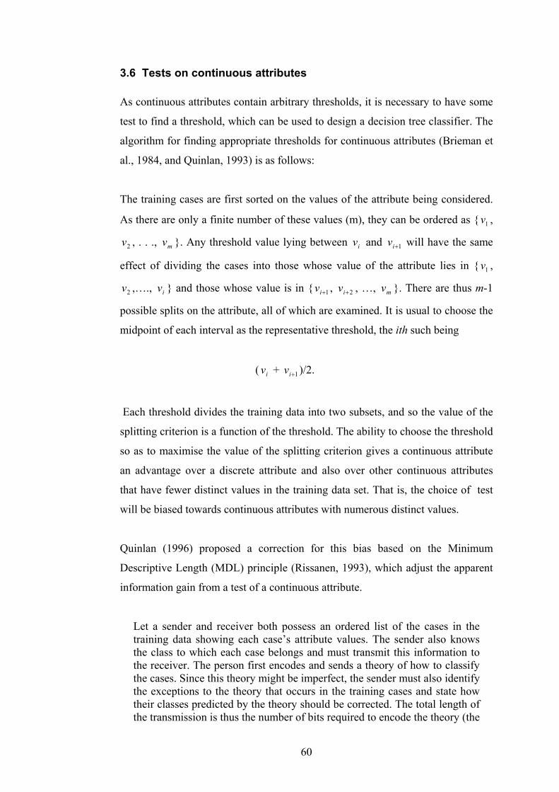
60
3.6 Tests on continuous attributes
As continuous attributes contain arbitrary thresholds, it is necessary to have some
test to find a threshold, which can be used to design a decision tree classifier. The
algorithm for finding appropriate thresholds for continuous attributes (Brieman et
al., 1984, and Quinlan, 1993) is as follows:
The training cases are first sorted on the values of the attribute being considered.
As there are only a finite number of these values (m), they can be ordered as 1v ,
2v , . . ., mv . Any threshold value lying between iv and 1+iv will have the same
effect of dividing the cases into those whose value of the attribute lies in 1v ,
2v ,…., iv and those whose value is in 1+iv , 2+iv , …, mv . There are thus m-1
possible splits on the attribute, all of which are examined. It is usual to choose the
midpoint of each interval as the representative threshold, the ith such being
( iv + 1+iv )/2.
Each threshold divides the training data into two subsets, and so the value of the
splitting criterion is a function of the threshold. The ability to choose the threshold
so as to maximise the value of the splitting criterion gives a continuous attribute
an advantage over a discrete attribute and also over other continuous attributes
that have fewer distinct values in the training data set. That is, the choice of test
will be biased towards continuous attributes with numerous distinct values.
Quinlan (1996) proposed a correction for this bias based on the Minimum
Descriptive Length (MDL) principle (Rissanen, 1993), which adjust the apparent
information gain from a test of a continuous attribute.
Let a sender and receiver both possess an ordered list of the cases in thetraining data showing each case’s attribute values. The sender also knowsthe class to which each case belongs and must transmit this information tothe receiver. The person first encodes and sends a theory of how to classifythe cases. Since this theory might be imperfect, the sender must also identifythe exceptions to the theory that occurs in the training cases and state howtheir classes predicted by the theory should be corrected. The total length ofthe transmission is thus the number of bits required to encode the theory (the
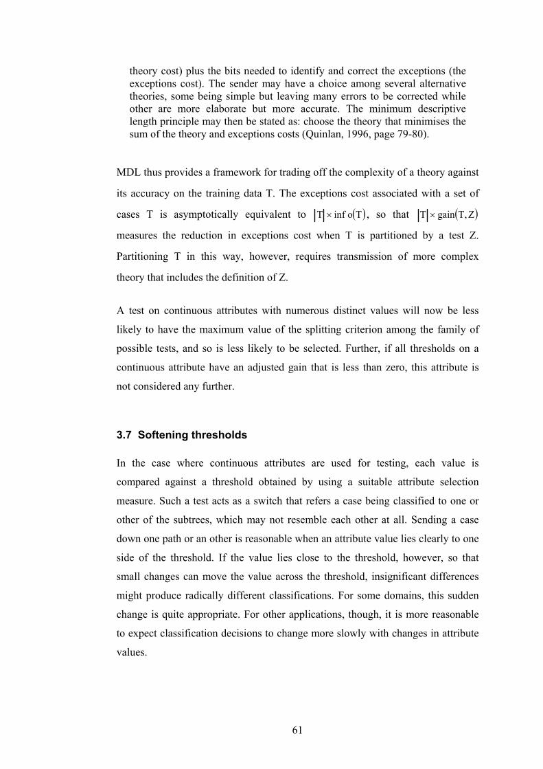
61
theory cost) plus the bits needed to identify and correct the exceptions (theexceptions cost). The sender may have a choice among several alternativetheories, some being simple but leaving many errors to be corrected whileother are more elaborate but more accurate. The minimum descriptivelength principle may then be stated as: choose the theory that minimises thesum of the theory and exceptions costs (Quinlan, 1996, page 79-80).
MDL thus provides a framework for trading off the complexity of a theory against
its accuracy on the training data T. The exceptions cost associated with a set of
cases T is asymptotically equivalent to ( )ToinfT × , so that ( )Z,TgainT ×
measures the reduction in exceptions cost when T is partitioned by a test Z.
Partitioning T in this way, however, requires transmission of more complex
theory that includes the definition of Z.
A test on continuous attributes with numerous distinct values will now be less
likely to have the maximum value of the splitting criterion among the family of
possible tests, and so is less likely to be selected. Further, if all thresholds on a
continuous attribute have an adjusted gain that is less than zero, this attribute is
not considered any further.
3.7 Softening thresholds
In the case where continuous attributes are used for testing, each value is
compared against a threshold obtained by using a suitable attribute selection
measure. Such a test acts as a switch that refers a case being classified to one or
other of the subtrees, which may not resemble each other at all. Sending a case
down one path or an other is reasonable when an attribute value lies clearly to one
side of the threshold. If the value lies close to the threshold, however, so that
small changes can move the value across the threshold, insignificant differences
might produce radically different classifications. For some domains, this sudden
change is quite appropriate. For other applications, though, it is more reasonable
to expect classification decisions to change more slowly with changes in attribute
values.

62
A simple scheme proposed by Quinlan (1993) defines subsidiary cutpoints −Z
and +Z below and above each threshold Z. If a test on continuous attribute A is
encountered while classifying a case whose value of A is V, the probability of the
outcome A ≤ Z is determined as follows:
1. If V is less than −Z , the probability is 1.
2. If V lies between −Z and Z, interpolate between 1 and 0.5.
3. If V lies between Z and +Z , interpolate between 0.5 and 0.
4. If V is greater than +Z , the probability is 0.
To calculate −Z and +Z Quinlan (1993) suggests that if the threshold Z were to be
changed to a new value 'Z , the decision tree would classify some cases of the
training set differently. The number of training cases misclassified by the tree can
be determined for a value of 'Z in the neighbourhood of Z. If E of the training
cases T are misclassified when the threshold has its original value, the standard
deviation of the number of errors can be estimated as
( ) ( ) TETE /5.05.0 −−×+ .
−Z and +Z are then chosen so that, if the threshold were set to either of them, the
number of misclassified training cases associated with this test would be one
standard deviation more than E. This approach allows for either sharp or vague
threshold effects. In the former situation, errors increase rapidly as Z is changed
so that −Z and +Z are close to Z. In the latter situation, cases with values near the
threshold might be expected to be classified equally well by the subtree associated
with either outcome, so error increase relatively slowly and the interval from −Z
to +Z is larger.
3.8 Pruning decision trees
Decision tree classifiers divide the training data into subsets, which contain only a
single class. The result of this procedure is often a very large and complex tree. In

63
most cases, fitting a decision tree until all leaves contain data for a single class
may overfit to the noise in the training data, as the training samples may not be
representative of the population they are intended to represent. If the training data
contain errors, then overfitting the tree to the data in this manner can lead to poor
performance on unseen cases. To reduce this problem, the original tree can be
pruned to reduce classification errors when data outside of the training set are to
be classified.
A decision tree is not usually simplified by deleting the whole tree in favour of a
leaf. Instead, parts of the tree that do not contribute to classification accuracy on
unseen cases are removed, thus producing a less complex and more
comprehensible tree. There are two ways in which a decision tree classifier can be
modified to produce a simpler tree (Breiman et al., 1984):
1. Deciding not to divide a set of training data any further, and
2. To remove retrospectively some part of the tree structure built by recursive
partitioning.
The first approach, sometimes called stopping or pre-pruning, has the advantage
that time is not wasted in assembling a structure that is not used in the final
simplified tree. The approach is to look at the best way of splitting a dataset and to
assess the split from the point of view of a factor such as information gain or
error reduction. If this assessment falls below some threshold, the division is
rejected and the tree for the data is just the most appropriate leaf. The problem
with this approach is to specify a correct stopping rule (Breiman et al., 1984). If
the threshold value is too high it can terminate division before the benefits of
subsequent splits become evident, while too low a value results in little
simplification of the tree.
In the second approach, the tree is allowed to grow to its full depth, when all
leaves contain data for a single class. This overfitted tree is then pruned. This
method needs more computation in building parts of the tree that are subsequently
discarded, but this cost is offset against benefits due to more thorough exploration
of possible partitions. Pruning a decision tree will cause it to misclassify more of

64
the training data. Thus, the leaves of the pruned tree will not necessarily contain
training data from a single class. Instead of a class associated with a leaf, there
will be a class distribution specifying, for each class, the probability that a training
data at the leaf belongs to that class.
The example below shows a decision tree before and after pruning .
Decision tree:
band2 <= 59 : 1 (343.0/2.0)
band2 > 59 :
| band2 <= 61 : 2 (55.0/21.0)
| band2 > 61 :
| | band1 <= 79 : 2 (293.0/18.0)
| | band1 > 79 :
| | | band1 <= 87 : 2 (101.0/16.0)
| | | band1 > 87 :
| | | | band2 <= 75 : 1 (3.0)
| | | | band2 > 75 : 2 (5.0/1.0)
Simplified decision tree:
band2 <= 59 : 1 (343.0/3.9)
band2 > 59 : 2 (457.0/64.7)
while the subtree
band2 > 59 :
| band2 <= 61 : 2 (55.0/21.0)
| band2 > 61 :
| | band1 <= 79 : 2 (293.0/18.0)
| | band1 > 79 :
| | | band1 <= 87 : 2 (101.0/16.0)
| | | band1 > 87 :
| | | | band2 <= 75 : 1 (3.0)
| | | | band2 > 75 : 2 (5.0/1.0)

65
has been replaced by the leaf "class 2" in the simplified tree after pruning. As
shown in the tree above every leaf is followed by a cryptic (n) or (n/m). For
observation the last leaf of the simplified decision tree is 2 (457.0/64.7), for which
n is 457 and m is 64.7. The value of n is the number of data that are mapped to
this leaf, and m is the number of items that are classified incorrectly by the leaf.
(A non-integral number of cases can arise because, when the value of an attribute
in the tree is not known, the See5.0 decision tree software splits the case and sends
a fraction down each branch.)
Decision trees are usually simplified by removing one or more subtrees and
replacing them with leaves if it is possible to predict the error rate of a tree and of
its subtrees, including leaves. The process is started from the bottom of the tree
and each nonleaf subtree is examined. This procedure is called the bottom-up
approach. Alternatively, the process starts from the root and moves towards the
leaves of the tree by examining the branches. This is called the top-down
approach. The tree is pruned if replacement of a subtree with a leaf, or with its
most frequently used branch, would lead to a lower predicted error rate. The error
rate for whole tree decreases as the error rate of any of its subtrees is reduced, and
this process will lead to a tree whose predicted error rate is minimal with respect
to the allowable form of pruning. As mentioned earlier, pruning always increases
error on training data, so it is necessary to have a suitable technique for predicting
error rates.
Two families of techniques to predict error rates of a tree are available. In the first
family, the error rate of the tree and its subtrees is predicted by using a new set of
data that is separate from the training data. Since these cases were not examined at
the time the tree was constructed, the estimate obtained from them will be
unbiased and, if we have enough data, the estimate will also be reliable. In the
second approach the training data are used to predict these error rates and pruning
the tree. The techniques for pruning the decision tree are as follows:
1. Cost-complexity pruning (Breiman et al., 1984)
2. Reduced-error pruning (Quinlan, 1987)
3. Pessimistic pruning (Quinlan, 1993)
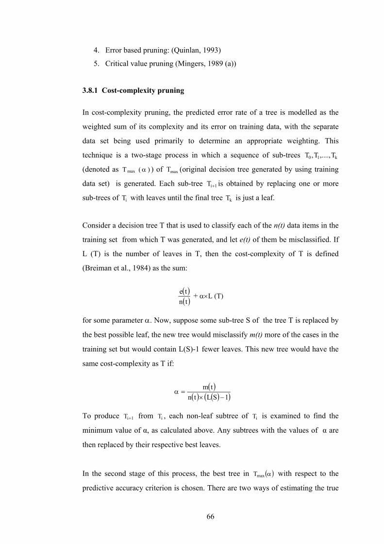
66
4. Error based pruning: (Quinlan, 1993)
5. Critical value pruning (Mingers, 1989 (a))
3.8.1 Cost-complexity pruning
In cost-complexity pruning, the predicted error rate of a tree is modelled as the
weighted sum of its complexity and its error on training data, with the separate
data set being used primarily to determine an appropriate weighting. This
technique is a two-stage process in which a sequence of sub-trees k10 T,....,T,T
(denoted as )(T max α ) of maxT (original decision tree generated by using training
data set) is generated. Each sub-tree 1iT + is obtained by replacing one or more
sub-trees of iT with leaves until the final tree kT is just a leaf.
Consider a decision tree T that is used to classify each of the n(t) data items in the
training set from which T was generated, and let e(t) of them be misclassified. If
L (T) is the number of leaves in T, then the cost-complexity of T is defined
(Breiman et al., 1984) as the sum:
( )( )tnte + α×L (T)
for some parameter α. Now, suppose some sub-tree S of the tree T is replaced by
the best possible leaf, the new tree would misclassify m(t) more of the cases in the
training set but would contain L(S)-1 fewer leaves. This new tree would have the
same cost-complexity as T if:
( )( ) ( )( )1SLtn
tm−×
=α
To produce 1iT + from iT , each non-leaf subtree of iT is examined to find the
minimum value of α, as calculated above. Any subtrees with the values of α are
then replaced by their respective best leaves.
In the second stage of this process, the best tree in ( )αmaxT with respect to the
predictive accuracy criterion is chosen. There are two ways of estimating the true

67
error rate of each tree in the family. One is based on cross-validation sets, and the
other on an independent pruning set. Assume that some test set containing 'N
cases and use each iT to classify all of the available test data. Let 'E be the
minimum number of errors observed with any iT , with the standard error of 'E
being given by
Se( 'E ) = ( )'
'''
NENE −×
The tree selected is the smallest iT whose observed number of errors on the test
set does not exceed 'E + Se( 'E ).
3.8.2 Reduced-error pruning
This method assesses the error rates of the tree and its components directly on a
separate set of test data. In this method, the original tree classifies all the test data.
For every non-leaf subtree S of T, the changes in misclassification over the test
data that would occur if S were replaced by the best possible leaf are examined. If
the new tree would give an equal or smaller number of errors, and if S contains no
subtree with the same property, then subtree S is replaced by the leaf. The process
continues until any further replacements would increase the number of errors over
the test set.
As with the cost-complexity pruning, this process generates a sequence of trees.
The final tree is the most accurate subtree of the original tree with respect to the
test data set and is the smallest tree with that accuracy. The disadvantages of this
method are, first, it requires a separate test data set and, second, “ …that part of
the original tree corresponding to rarer special cases not represented in the test set
may be excised” (Quinlan, 1987, pp. 226). These techniques of pruning may not
be much of a disadvantage when training and test data are abundant, but can lead
to poorer-performing trees when data are scarce. This makes it necessary to have a
technique for pruning a tree which uses only the training set from which the tree
was built.

68
3.8.3 Pessimistic pruning
This method increases the estimated error rates of subtrees to reflect the size and
composition of the training subsets, then replaces every subtree whose predicted
error rate is not significantly lower than that of a leaf. This method of pruning is
described by Quinlan (1987). It aims to avoid the necessity of a separate test data
set. A continuity correction for the binomial distribution is used to obtain a more
realistic estimate of the misclassification rate.
If n(t) represents the number of training set examples at a node t in the tree and
e (t) represents the number of examples misclassified at node t, then
( ) ( )( )tntetr =
is an estimate of the misclassification rate. The rate with the continuity correction
is
( ) ( )( )tn
tetr 2/1, += (3.11)
For a sub-tree tT , the misclassification rate will be:
( ) ( )( )∑
∑=inie
Tr t
where i covers the leaves of the sub-tree. Thus, the corrected misclassification rate
is:
( ) ( )( )( )
( )( )∑
∑∑
∑ +=
+=
innie
inie
Tr Tt
2/2/1, (3.12)
where Tn is the number of leaves.

69
In equations (3.11) and (3.12), ( ) ( )∑= intn as they refer to the same set of
examples; therefore, the misclassification rates can be simplified to numbers of
misclassifications:
( ) ( ) 2/1, += tetn for a node
( ) ( )∑ += 2/,Tt nieTn for a sub-tree.
Using training data, the sub-tree will always make fewer errors than the
corresponding node, but this is not so when the corrected figures are used, since
they depend on the number of leaves, not just on the number of errors. However,
it is likely that even this corrected estimate of the number of misclassifications
made by the sub-tree will be optimistic. Hence, the algorithm only keeps the sub-
tree if its corrected figure is more than one standard error better than the figure for
the node. The standard error for the number of misclassifications is derived from:
( )( ) ( ) ( ) ( )( )( )tn
TntnTnTnSE tt
t
,,, −×
= (3.13)
Quinlan (1993) suggests pruning the sub-tree unless its corrected number of
misclassifications is lower than that for the node by at least one standard error. As
this algorithm evaluates each node starting at the root of the tree. This means that
it does not need to consider nodes that are in subtrees which have already been
pruned.
3.8.4 Error based pruning
This pruning method is an improvement on the "pessimistic pruning" method, and
it is based on a far more pessimistic estimate of the expected error rate. Unlike the
method described in section 3.7.3, this method visits the nodes of the full-grown
tree according to a bottom-up, post-order traversal strategy instead of a top-down
strategy.

70
Taking the set of examples covered by a leaf t as a statistical sample, it is possible
to estimate a confidence interval )]t(U),t(L[ CFCF for the posterior probability
of misclassification of t. The upper limit of the interval is of particular interest for
a worst case analysis, and is defined as the real value such that
( ) ( )( ) CFUtn/teP CF =≤ , where CF is the confidence level. Under the further
assumption that errors in the training set are binomially distributed with
probability p in n(t) trials, it is possible to compute the exact value of CFU as the
value of p for which a binomially-distributed random variable X shows e(t)
successes in n(t) trials with probability CF, that is, p (X≤e (t)) = CF. In other
words, if X has a binomial distribution with parameters ))t(n,U( CF , the equality
above must hold. The value of CFU depends on both e(t) and n(t) so, having found
the upper limit, the error estimates for leaves and subtrees are computed assuming
that they are used to classify a set of unseen cases of the same size as the training
set. Thus the predicted error rate for t will be n (t)· CFU (Esposito et. al., 1997).
The sum of the predicted error rates of all the leaves in a branch tT is considered
to be an estimate of the error rate of the branch itself. Thus, by comparing the
predicted error rate for t with that of the branch tT and of the largest sub-branch
'tT rooted in a child 't of parent of t, one can decide whether it is convenient to
prune tT , to graft 'tT in place of parent of t, or to keep tT .
3.8.5 Critical value pruning
This method relies on estimating the importance or strength of a node from
classifications done at the tree creation stage. In creating the original tree, a
goodness of split measure determines the attribute at a node. The value of the
measure reflects how well the chosen attribute splits the data between the classes
at the node. The pruning method specifies a critical value and prunes those nodes
which do not reach the critical value, unless a node further along the branch does
reach that value. The larger the critical value selected, the greater the degree of
pruning and the smaller the resulting tree. In practice, a series of pruned trees is
generated using increasing critical values (Mingers, 1989 (a)). A single tree can be

71
chosen in the same way as for cost-complexity pruning. The particular critical
value used depends on the measure used in creating the tree.
3.9 Problems in the use of decision tree classifiers
Although decision tree classifiers are an effective and general learning tool, and
are used intensively in the field of machine learning research, few uses of decision
trees have been reported in the field of remote sensing image classification. Like
other classifiers based on different assumptions, these classifiers inevitably have
some limitations that may have an impact on their performance. There are fewer
factors affecting the accuracy of decision tree classifiers compared with the neural
classifier, where a number of factors affect the classification accuracy. The factors
affecting the decision tree classifiers can be summarised as:
1. Type of classifier, whether it is univariate or multivariate.
2. Attribute selection measure used in designing a classifier.
3. Pruning methods used to prune the tree.
4. Number of training pattern required for the optimum classification results.
A small number of studies report the effects of these factors on land cover
classification accuracy. Friedl and Brodley (1997) studied the behaviour of
different decision tree classifiers, such as univariate, multivariate and hybrid
classifiers, for land cover classification. They found that hybrid decision
classifiers outperform other types of decision tree. Except for this study, no other
studies have used remotely sensed data to study the effects of other factors on
classification accuracy. Brieman et al. (1984) and Mingers (1989 (a) (b)) use other
types of data and suggest that it is the pruning method that most affects the
classification accuracy. They also found that attribute selection measures have
little or no effect on classification accuracy. Oates and Jenson (1997) studied the
behaviour of a univariate decision tree classifier (C4.5) with five different pruning
methods, and found that increasing training set size often results in a linear
increase in tree size, even when that additional complexity results in no significant
increase in classification accuracy. On the other hand, Quinlan (1993) found that
in situations where the division of feature space by an oblique hyperplane

72
(multivariate decision tree) is easier, the number of training cases required to
approximate this oblique division by a collection of hyper-rectangles (univariate
decision tree) will be large, which increases the complexity of the decision tree
classifier.
3.10 Support Vector Machines (SVM)
This section gives an overview of another recent development in classification
methodology, called support vector machines (SVM) or sometimes support vector
networks. This classification system is based on statistical learning theory as
proposed by Vapnik and Chervonenkis (1971), which is discussed in detail by
Vapnik (1995, 1999). The SVM can be seen as a new way to train polynomial,
radial basis function, or multilayer perceptron classifiers, in which the weights of
the network are found by solving a Quadratric Programming (QP) problem with
linear inequality and equality constraints using structural risk minimisation rather
than by solving a non-convex, unconstrained minimisation problem, as in standard
neural network training technique using empirical risk minimisation. Empirical
risk minimises the misclassification error on the training set, whereas structural
risk minimises the probability of misclassifying a previously unseen data point
drawn randomly from a fixed but unknown probability distribution. The name
SVM results from the fact that one of the outcomes of the algorithm, in addition to
the parameters for the classifiers, is a set of data points (the "support vectors")
which contain, in a sense, all the information relevant to the classification
problem. A brief review of statistical learning theory is given in section 3.11.
3.11 Statistical learning theory
3.11.1 Empirical risk minimisation
In the case of two-class pattern recognition, the task of learning from examples
can be formulated in the following way: given a set of decision functions
( ) ,:f Λ∈αα x →αNR:f -1, 1
where Λ is a set of abstract parameters (Osuna et. al., 1997), and a set of examples

73
( ) ( )kk11 y,...,,.........y, xx , ∈∈ iN
i y,Rx -1, 1
drawn from an unknown distribution P(x, y). The aim is to find a function that
provides the smallest possible value for the average error committed on
independent examples randomly drawn from the same distribution P(x, y), called
the expected risk:
( ) ( ) ( )∫ −=α α dydy,PyfR xxx (3.14)
The functions αf are usually called hypotheses, and the set ( ) Λ∈αα :f x is called
the hypothesis space, and is denoted by H. The expected risk is therefore a
measure of the capability of a hypotheses to predict the correct label y for a point
x. The set of functions αf could be, for example, a set of radial basis functions or
a multilayer perceptron with a certain number of hidden units. In this case, the set
Λ is the set of weights of the network (Osuna et. al., 1997).
Since the probability distribution P(x, y) is unknown, it is not possible to compute,
and therefore minimise, the expected risk R(α). Thus, the straightforward
approach is to compute a stochastic approximation of R(α), the so called empirical
risk:
( ) ( )∑=
α−=α
k
1iiiemp
yfk
1R x (3.15)
A common approach consists in minimising the empirical risk rather than the
expected risk. The value ( )αempR is a fixed number for a particular choice of α and
a particular training set. The term ( ) ( ) ii y,f21 −αα x is called the loss. If the
number of training patterns (k) used to train the classifier is limited, the empirical
risk calculated in equation 3.15 may not guarantee a small actual risk. This can be
put another way: a low error value on a training set does not necessarily imply
that the classifier has a high generalisation ability, and the empirical risk
minimisation principle is therefore said to be non consistent. This problem is often
referred to as overfitting.
Vapnik and Chervonenkis (1971, 1991) showed that necessary and sufficient
condition for consistency of the empirical risk minimisation principle is the fitness

74
of the VC-dimension h of the hypothesis space H. The VC-dimension of the
hypothesis space H (or the VC-dimension of classifier αf ) is a natural number,
which is, loosely speaking, the largest number of data points that can be separated
in all possible ways by that set of functions αf . The VC-dimension is a measure of
the complexity of the set H, and it is often, but not necessarily, proportional to the
number of free parameters of the classifier αf .
The theory developed by Vapnik and Chervonenkis (1971) also provides a bound
on the deviation of empirical risk from the expected risk. For the learning problem
described, choosing some η such that 0 ≤ η ≤ 1 (e.g. for a 95% confidence level,
η= 0.05) the Vapnik and Chervonenkis bound, which holds with probability
1 - η, has the following form (Burges, 1998):
( ) ( )( )
ηφ+α≤α
k
log,
k
hRR emp (3.16)
where the confidence term φ is defined as
( )
( )
k
4log1h
k2logh
k
log,
k
hη−
+
=
ηφ (3.17)
where h is the VC-dimension of a set of functions and the right hand side of
inequality 3.16 can be called the "risk bound". This value describes the capacity
of a set of functions. From this bound it is clear that, in order to achieve a small
expected risk, that is, good generalisation performances, both the empirical risk
and the ratio between the VC-dimension and the number of data points has to be
small. The empirical risk is usually a decreasing function of h; thus, for a given
number of data points, there is an optimal value of the VC-dimension. The choice
of an appropriate value of h is crucial in order to get good performance, especially
when the number of data points is small. When using a multilayer perceptron or a
radial basis functions network, this is equivalent to the problem of finding the
appropriate number of hidden units (Osuna et. al., 1997).

75
3.11.2 Structural risk minimisation
The technique of structural risk minimisation developed by Vapnik (1982) is an
attempt to overcome the problem of choosing an appropriate VC-dimension.
Equation 3.16 suggests that a small value of the empirical risk does not
necessarily imply a small value of the expected risk. A different induction
principle, called the Structural Risk Minimisation (SRM) principle, was proposed
by Vapnik (1982). The principle is based on the observation that, in order to make
expected risk small, both sides in equation 3.16 should be small. Therefore, both
the VC-dimension and the empirical risk should be minimised at the same time. In
order to implement the SRM principle a nested structure of hypothesis space is
introduced by dividing the entire class of functions into nested subsets
......H.....HH n21 ⊂⊂⊂⊂
with the property that h(n) ≤ h(n + 1) where h(n) is the VC-dimension of the set
nH . For each subset, a value of h or a bound on h is computed. SRM then finds
that subset of function which maximise the bound on actual risk. This can be
achieved by training a set of machines, one for each subset and choose that trained
machine whose sum of empirical risk and VC confidence is minimal (Osuna et.
al., 1997).
The SRM principle is well founded mathematically, but it is difficult to
implement for the following reasons (Osuna et. al., 1997):
1. The VC-dimension of nH could be difficult to compute, and there are only
a small number of models for which it is possible to compute the VC-
dimension.
2. Even, if it possible to compute the VC-dimension of nH , it is not easy to
solve the minimisation problem in equation 3.16. In most cases one will
have to minimise the empirical risk for every set nH , and then choose the
nH , that minimise the equation 3.17.
Therefore, the implementation of this principle is not easy, because it is not trivial
to control the VC-dimension of a learning technique during the training phase.
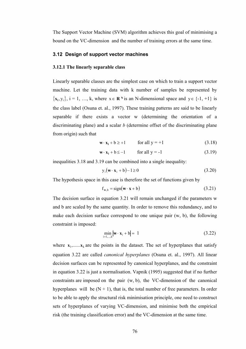
76
The Support Vector Machine (SVM) algorithm achieves this goal of minimising a
bound on the VC-dimension and the number of training errors at the same time.
3.12 Design of support vector machines
3.12.1 The linearly separable class
Linearly separable classes are the simplest case on which to train a support vector
machine. Let the training data with k number of samples be represented by
iy,ix , i = 1, …, k, where NR∈x is an N-dimensional space and ∈y -1, +1 is
the class label (Osuna et. al., 1997). These training patterns are said to be linearly
separable if there exists a vector w (determining the orientation of a
discriminating plane) and a scalar b (determine offset of the discriminating plane
from origin) such that
1b +≥+⋅ ixw for all y = +1 (3.18)
1b −≤+⋅ ixw for all y = -1 (3.19)
inequalities 3.18 and 3.19 can be combined into a single inequality:
( ) 01by ii ≥−+⋅ xw (3.20)
The hypothesis space in this case is therefore the set of functions given by
( )bsignf b, +⋅= xww (3.21)
The decision surface in equation 3.21 will remain unchanged if the parameters w
and b are scaled by the same quantity. In order to remove this redundancy, and to
make each decision surface correspond to one unique pair (w, b), the following
constraint is imposed:
=+⋅=
bmin ik,...,1i
xw 1 (3.22)
where k1,.......xx are the points in the dataset. The set of hyperplanes that satisfy
equation 3.22 are called canonical hyperplanes (Osuna et. al., 1997). All linear
decision surfaces can be represented by canonical hyperplanes, and the constraint
in equation 3.22 is just a normalisation. Vapnik (1995) suggested that if no further
constraints are imposed on the pair (w, b), the VC-dimension of the canonical
hyperplanes will be (N + 1), that is, the total number of free parameters. In order
to be able to apply the structural risk minimisation principle, one need to construct
sets of hyperplanes of varying VC-dimension, and minimise both the empirical
risk (the training classification error) and the VC-dimension at the same time.

It can be shown that the distance from a point x to the hyperplane associated to the
pair (w, b) is:
( )wwx
wxb
b,;d+⋅
= (3.23)
According to equation 3.22 the distance between the canonical hyperplane
(w, b) and the closest of the data points is simply w1 . If the set of examples is
linearly separable, the goal of the SVM is to find, from among the canonical
hyperplanes that correctly classify the data, the one with minimum norm, or
equivalently minimum 2w , because keeping this norm small will also keep the
VC-dimension small. Minimising 2w , in this case of linear separability, is
equivalent to finding the separating hyperplanes for which the distance between
the classes of training data, measured along a line perpendicular to the hyperplane,
is maximised. This distance is called the margin (Burges, 1998).
Fithr
To
co
77
gure 3. 5. Hyperplanes for the linearly separable data sets. Dashed line passesough the support vectors.
construct the maximal margin or optimal separating hyperplane one needs to
rrectly classify a set of training data
( ) ( )kk11 y,...,,.........y, xx ∈∈ iN
i y,Rx -1, 1
margin
w
Origin
x
ix
w.x + b = ±1
Optimalhyperplane

78
into two different classes, using the smallest norm of coefficients. This can be
formulated as follows:
2
b21
min ww,
subject to
( ) 01byi ≥−+⋅ ixw i = 1, …..,k. (3.24)
This problem can be solved using standard Quadratic Programming (QP)
optimisation techniques and is not very complex since the dimensionality is
N + 1, where N is the dimension of the input space. The quadratic optimisation
problem in equation 3.24 can be solved by replacing the inequalities with a
simpler form determined by transforming the problem to a dual space
representation using Lagrangian multipliers. The Lagrangian is formed by
introducing positive Lagrange multipliers iλ , i = 1,….,k and multiplying the
constraint equations by these Lagrange multipliers, and finally subtracting the
results from the objective function (i.e, ( ) 221 w ). The solution of this
optimisation problem can be obtained by locating the saddle point of the Lagrange
function and, can be written as:
( ) ( )∑ ∑= =
λ++⋅λ−=k
1i
k
1iiiii
2 byw2
1,b,L xwλw (3.25)
The solution of this optimisation problem requires that ( )λ,b,L w be minimised
with respect to w and b and simultaneously, that the derivatives of ( )λ,b,L w with
respect to all iα vanish, given iλ ≥ 0, thus generating the following conditions:
∑λ=i
ii x w iy (3.26)
∑ =λi
ii 0y (3.27)
By substituting equation 3.26 and 3.27 into equation 3.25, the optimisation
problem becomes one of maximising:
( ) )(yy2
1L
j,ijiji
ii ji xxλ ⋅λλ−λ= ∑∑ (3.28)

79
under constraints iλ ≥ 0, i = 1, …..,k.
Once the vector solution ( )ak
a1
a ,......,λλ=λ of the maximisation problem in equation
3.28 has been found, the optimal separating hyperplane (hyperplane for which the
distance to the closest point is maximal) has the following expansion:
ii
aii
a y xw ∑ λ= (3.29)
The Karush-Kuhn-Tucker (KKT) conditions (Fletcher, 1987) play a central role in
both the theory and practice of constrained optimisation. For the above problem,
the KKT conditions may be stated as:
( )
0,b,L
=∂
∂w
λw
( )
0b
,b,L=
∂∂ λw
( ) 01byi ≥−+⋅ ixw i = 1, …..k. (3.30)
iλ ≥ 0, for i = 1, …..,k
( )( ) 01by iii ≥−+⋅λ xw i = 1, …..k
According to KKT theory, only points that satisfy the equalities in equations 3.18
and 3.19 can have non-zero coefficients ai
λ . These points lie on the two parallel
hyperplanes shown in Figure 3.5 and are called support vectors. In other words,
support vectors are the points for which ai
λ > 0 and satisfy equalities in equation
3.18 and 3.19. For a two-class problem the decision rule that separates the two
classes can be written as (Osuna et. al., 1997)
( ) ( )
+⋅λ= ∑
=
k
1iiii bysignf xxx (3.31)
3.12.2 Non-separable data
Cortes and Vapnik (1995) generalised the method of finding the optimal
hyperplane to the case of non-separable data, in which there is no opportunity to
place a hyperplane such that data can be separated completely into two classes
(Figure 3.6). For this type of problem, Cortes and Vapnik (1995) suggested that
the restriction that every training vector of a given class lie on the same side of the

optimal hyperplane be relaxed by introducing a positive "slack variable" iξ , that
takes the value iξ ≥ 0. Equation 3.20 can now be written as:
( ) 01by ii ≥ξ+−+⋅ ixw (3.32)
In this case, the SVM algorithm searches for the hyperplane that maximises the
margin and that, at the same time, minimises a quantity proportional to the
number of misclassification errors. This trade-off between margin and
misclassification error is controlled by introducing a positive constant C such that
∞ > C > 0. Cortes and Vapnik (1995) introduce a new term ∑ξ iC with i = 1,…, k,
into equation 3.24 that balances the contribution of minimising ( ) 2w21 with
penalising solutions, for which iξ becomes large. The optimisation problem for
non-separable data thus becomes:
ξ+ ∑
=ξξ
k
1ii
2
,....,bCw
2
1min
k1w, (3.33)
( ) 01by iii ≥ξ+−+⋅ xw (3.34)
0i ≥ξ i = 1, ……k. (3.35)
As C
to th
80
Figure 3. 6. Hyperplanes for non-separating data sets.
∞→ the effect of any iξ deviating from 0 becomes increasing more costly
e minimisation. In the situation when ∞→C the optimisation problem
w
Origin
iξ
w.x + b = ±1
Optimalhyperplane
ix

81
becomes a formulation for the separable data case. Thus, C is a parameter chosen
by the user and a large C means assigning a higher penalty to errors. Minimising
the first term in equation 3.33 means minimising the VC-dimension of the
learning machine and minimising the second term in equation 3.33 controls the
empirical risk, which is the first term on the right hand side of equation 3.16. This
approach, therefore, constitutes a practical implementation of structural risk
minimisation on the given set of functions. In order to solve the equation 3.33 for
non separable data, equation 3.25 can be written as:
( ) ( ) ∑ ∑ ∑ ξµ−ξ+−+⋅λ−ξ+=i i i
iiiiiii2 1byC
2
1,,,b,L xwwµξλw (3.36)
where the iµ are the Lagrange multipliers introduced to enforce positivity of the
iξ .
The solution of equation 3.36 is determined by the saddle points of the Lagrangian
(equation 3.36), by minimising with respect to w, ξ and b, and maximising with
respect to iλ ≥ 0 and iµ ≥ 0.
3.12.3 Nonlinear support vector machines
In the situations where it is not possible to have a decision surface (a hyperplane)
defined by the linear equations on the training data, the techniques discussed in
section 3.12.1 and section 3.12.2 can be extended to allow for non-linear decision
surfaces. A technique introduced into machine learning as a part of the support
vector machine by Boser et al. (1992) is discussed next.
Boser et al. (1992) propose that a feature vector, NR x ∈ , is mapped into a higher
dimensional Euclidean space (feature space) F (Figure 3.7), via a non-linear
vector function F: N aRΦ . The optimal margin problem in the space F can be
written by replacing ji xx ⋅ with ( ) ( )ji xΦxΦ ⋅ , then solving the optimisation
problem for iλ in the transformed feature space by association with the iλ > 0. By
using this mapping, the solution of the SVM has the form:

82
( ) ( ) ( )
+⋅λ= ∑ bysignf
iii ixΦxΦx (3.37)
Figure 3. 7. The idea of a non-linear support vector machine.
As suggested by equation 3.37, the only quantities that one need to compute are
the scalar products, of the form Φ(x) . Φ(y). It is therefore convenient to introduce
the concept of the kernel function K (Vapnik, 1995) such that:
( ) ( ) ( )jiji ,K xΦxΦxx ⋅= (3.38)
In this optimisation problem, only the kernel function is computed in place of
computing ( )xΦ , which could be computationally expensive. By doing this, the
training data are moved into a higher-dimensional feature space where the training
data may be spread further apart and a larger margin may be found for the optimal
hyperplane. Thus, equation 3.28 can be written as:
( ) ( ) ( )( )∑∑ Φ⋅Φλλ−λ=j,i
jijii
i yy2
1L ji xxλ (3.39)
A number of kernel functions are used within SVM. To find a way to choose
among various kernels and the parameters of the kernel function, readers are
referred to Vapnik (1995). For this study, several kernels are considered in order
Φ
Input space Feature space

83
to compare the effect of choice of kernel type and associated parameters for land
cover classification. The kernels used for this study are:
• The simple dot product: K(x,y) = x·y.
• The simple polynomial kernel of degree d: ( ) ( )( )d1,K +⋅= yxyx .
• A radial basis function: 2
e yx−γ− with γ defined by user.
• A two-layer neural network: ( )( )cbtanh −⋅ yx where b and c
are user defined.
• A linear spline with an infinite number of points:
( ) ( )( ) ( )( )3
,minmin
2,min1
3ji2
jiji
jijijixx
xxxx
xxxxxx ++
−++ .
In order to find the optimal decision surface, the support vector training algorithm
tries to separate, as best as possible, the clouds of data points representing each
class. Data points closer to the boundary between the classes are more important
in the classification than are data points that are far away, since data points closer
to the boundary are harder to classify. These data points help shape and define
better decision surface than other points. The support vector machine tries to find
data points that are closest to the separating surfaces, therefore the support vectors
are border points, and due to this reason support vectors are very few. Finally,
SVMs are based on a QP optimisation problem that has only a global optimum.
The absence of local minima is a significant difference from standard pattern
recognition techniques such as neural networks (Osuna et. al., 1997).
3.13 Multi-class classifier
SVM was initially designed for binary (two-class) problems. When dealing with
several classes, as the case of land cover classification, an appropriate multi-class
method is needed. Different possibilities for this includes:
• Modify the design of SVM, such that it incorporate the multi-class
learning directly in the quadratic solving algorithm (Weston and Watkins,
1998).

84
• Combine several binary classifiers: the "one against the rest" approach
(Vapnik, 1995) compares a given class with all the others put together,
thus generating n classifiers, where n is the number of classes. The final
output of this SVM is the class that corresponds to the SVM with the
largest margin, the value of the argument of the sign function in equation
3.37.
• Combine several classifiers: the "one against one" approach (Knerr et al.,
1990) applies pairwise comparisons between classes. In this method, all
possible two-class classifiers are evaluated from the training set of n
classes, each classifier being trained on only two out of n classes. There
would be a total of n(n-1)/2 classifiers. Applying each classifier to the
vectors of the test data gives one vote to the winning class. The pixel is
given the label of the class with most votes.
In this study, the "one against one" and "one against the rest" approaches are
used so as to compare the results obtained. Two SVM based classification
software systems were used. One was obtained from Royal Holloway College
and AT&T, University of London; the other, LIBSVM, was provided by Chih-
Chung Chang of the University of Taiwan.
3.13 Problems in the use of SVM
So far, few studies have reported the use of support vector machines for
classification of remote sensing data (Huang et al., 2002; Zhu and Blumberg,
2002; Gualtieri and Cromp, 1998). In comparison to neural classifiers few factors
affect the performance of these classifiers and Huang et al. (2002) discussed some
of them in detail. Some of the factors that affect the classification accuracy of
SVM classifiers are:
1. Choice of kernel used.
2. Choice of the parameters related to a particular kernel.
3. Method used to generate the SVM for multi-class classification problems.
4. Choice of parameter C.

85
This study is designed to study the effect of all these parameters on classification
accuracy of remotely sensed data, details of which is provided in chapter 5
(section 5.2).
3.14 Ensemble of classifiers
In recent years, a number of papers proposing the combination of multiple
classifiers to produce a single classification have been published in the remote
sensing literature. The resulting classifier, referred to as an ensemble classifier, is
generally found to be more accurate than any of the individual classifiers making
up the ensemble. Some papers report the use of ensembles of neural networks
(Giacinto and Roli, 1997) and the integration of classification results of different
type of classifiers (Roli et al., 1997), and they find that this technique is effective
in improving classification accuracy. Much of this research is focused on
improving classification accuracy, as accuracy is the primary concern in all
applications of learning. So far, very few works (Friedl et al., 1999) have reported
the use of boosting, another technique that can improve the performance of any
learning algorithm, in image classification. The basic difference between the use
of ensembles of classifiers and boosting is that boosting uses the same learning
algorithm that consistently generates multiple classifiers in an iterative manner.
3.14.1 Boosting
Boosting is a general method for improving the performance of any learning
algorithm. Boosting can be used to reduce the error of any weak learning
algorithm that consistently generates classifications on various distributions over
the training data, and then combines the classifications produced by the weak
learner into a single composite classification. Figure 3.8 illustrates the basic
framework for a classifier ensemble.
In this study, a boosting algorithm called AdaBoost M1 (Freund and Schapire,
1996) is used with the C4.5 decision tree (Quinlan, 1993) as the base algorithm.
Boosting assigns a weight to each observation - the higher the weight, the more
that observation influences the classifier. At each trial, the vector of weights is

86
adjusted to reflect the performance of the corresponding classifier, with the result
that the weight of misclassified observations is increased. The final classifier
aggregates the classifiers generated after each iteration by voting, but each
classifier’s vote is a function of its accuracy.
Following Freund and Schapire (1996), let xtw be the weight assigned to
observation x at trial t where, for every x, and t=1,
N/1w x1 =
where N is the total number of observations in the training set and t is the iteration
or trial number (t = 1, 2, …..., T). At each trial, a classifier tC is constructed from
the given observations under the distribution tw (i.e., as if the weight xtw of
observation x reflects the probability of its occurrence). The error tε of this
classifier is also measured with respect to the weights, and consists of the sum of
the weights of the observations that it misclassifies. If tε is greater than 0.5, the
trials are terminated and the value of T becomes t-1. Conversely, if tC correctly
classifies all observations so that tε is zero, the trials terminate and the value of T
becomes t. Otherwise, the weight vector x1tw + for the next trial is generated by
( )ttxtx1t 1/ww ε−ε×=+
Conversely, if the observation was not correctly classified, xw is unchanged and
at each iteration the weight xw is normalised so that
∑ = 1wx .
By applying the above process, a new tree with a different error level is estimated
at each step. The final, boosted classifier is the result of a voting procedure, where
the vote for classifier tC is worth
( )t/1log β units.
with
( )ttt 1/ ε−ε=β .
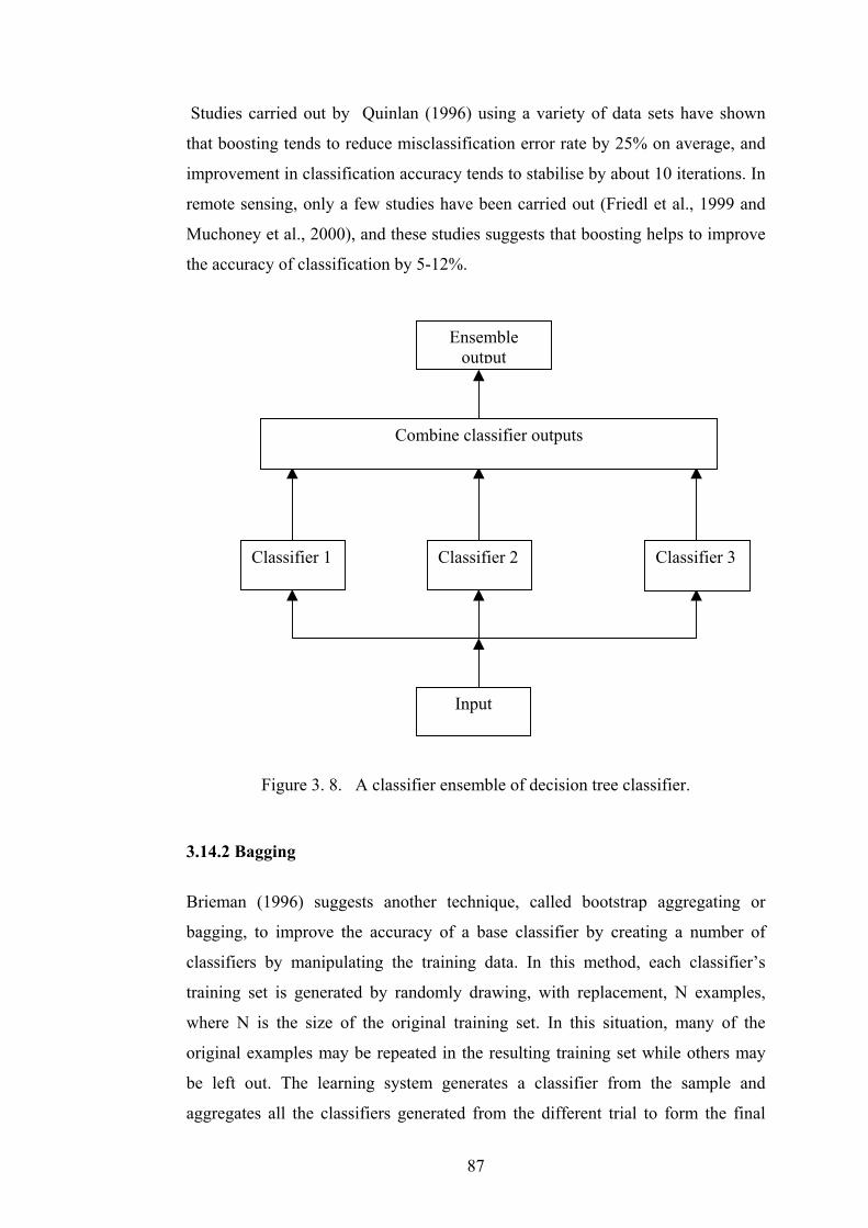
87
Studies carried out by Quinlan (1996) using a variety of data sets have shown
that boosting tends to reduce misclassification error rate by 25% on average, and
improvement in classification accuracy tends to stabilise by about 10 iterations. In
remote sensing, only a few studies have been carried out (Friedl et al., 1999 and
Muchoney et al., 2000), and these studies suggests that boosting helps to improve
the accuracy of classification by 5-12%.
Figure 3. 8. A classifier ensemble of decision tree classifier.
3.14.2 Bagging
Brieman (1996) suggests another technique, called bootstrap aggregating or
bagging, to improve the accuracy of a base classifier by creating a number of
classifiers by manipulating the training data. In this method, each classifier’s
training set is generated by randomly drawing, with replacement, N examples,
where N is the size of the original training set. In this situation, many of the
original examples may be repeated in the resulting training set while others may
be left out. The learning system generates a classifier from the sample and
aggregates all the classifiers generated from the different trial to form the final
Classifier 1 Classifier 2 Classifier 3
Combine classifier outputs
Ensembleoutput
Input

88
classifier. To classify an instance, every classifier records a vote for the class to
which it belongs, and the instance is labelled as a member of the class with the
most votes.
3.15 Conclusions
The fundamental principles underlying the design and use of decision tree and
support vector machine classifiers are discussed in this chapter. The main steps in
the design of a decision tree classifier, such as the choice of an attribute selection
measure, pruning methods, and various cases for the design of support vector
machines are described in detail. Boosting is a new technique that is used to
improve classification accuracy, and this technique is discussed in detail along
with another technique, called bagging, to create ensemble of classifiers using the
same classifier as the base classifier. So far few studies (Friedl and Brodley, 1997;
Gahegan, 1998; Huang et al., 2002) have compared the behaviour of support
vector machines and decision tree classifiers with statistical and neural classifiers.
These studies suggested that SVM and DT classifiers outperform statistical
classifiers but so far no study has attempted to compare the behaviour of SVM
and DT classifiers with neural and statistical classifiers in detail.
The question of relative performance of statistical, neural network, support vector
machines, and decision tree classifiers and various factors affecting these
classifier in term of ease of use is examined in the following chapters of this
thesis.

89
Chapter 4
Data Sets
4.1 Introduction
Several types of remote sensing data can be used in land cover classification. Data
can be taken from the optical or microwave regions of the spectrum, and can be
hyperspectral or multispectral in nature, depending on their availability and
quality for a particular region. Usually medium spatial resolution satellite sensor
data, such as Landsat TM/ETM+ and SPOT, have been used in several researches.
Data acquired by these sensors, which operate in the visible and near-infrared part
of the electromagnetic spectrum, are often hindered by clouds or haze. It may be
difficult to acquire cloud free data when using conventional optical satellite
sensors, thus impeding the regular updating of land cover maps, especially in
areas like the UK. Active microwave sensors, however, acquire data independent
of weather, cloud, solar angle, or solar illumination. This independence from
weather and illumination conditions allows data to be collected by these sensors at
any stage of the crop growth cycle.
Studies reporting on the use of optical and microwave data for land cover
classification suggest that choice of data type has an effect on classification
accuracy. This research is designed to evaluate the performance of both optical
(ETM+) and microwave (InSAR) data for the same area in the UK for land cover
classification, using different classification algorithms. DAIS hyperspectral data
of an area in Spain are employed to study the behaviour of different classification
algorithms with different training dataset sizes and increasing number of features.
As few studies have used interferometric SAR data for land cover classification, a
detailed description of the technique is given in this chapter.
4.2 Synthetic Aperture Radar(SAR)
A radar sensor operates by transmitting a pulse of electromagnetic energy and
then intercepting the backscattered or reflected radiation with an aperture of some

90
physical dimension. In traditional (non-SAR) systems, the angular resolution (the
angular spread of the radar beam) is governed by the ratio of the wavelength of
the electromagnetic radiation to the aperture size. The spatial resolution of the
image is the angular resolution times the distance from the sensor to the earth’s
surface. Therefore, as the sensor altitude increases, the spatial resolution of the
image decreases unless the physical size of the aperture is increased. At visible
and near infrared wavelengths, a high resolution image can be obtained even from
orbital altitudes for modest aperture sizes. However, for a microwave instrument,
which uses wavelengths that are very long compared to those of visible light, high
resolution imagery from a reasonably-sized antenna aperture is not possible.
Hence, to improve resolution without increasing physical antenna size, Synthetic
Aperture Radar (SAR) technology is employed. SAR is a coherent imaging
system in that it retains both the phase and magnitude (amplitude) component of
the backscattered signals. The value of a pixel in a complex SAR image may be
divided into phase and intensity parts in the following way:
( ) ( ) ( )y,xiey,xIy,xZ φ=
Where Z(x,y) is the complex pixel
x,y are image coordinates
I is the intensity of the pixel
Φ is the phase of the pixel
i is the imaginary unit
The phase information contained in a single SAR image is practically useless and
SAR intensity is generally used.
SAR operates on the principle of using the along track sensor motion to transform
a single physically short antenna into an array of such antennae that can be linked
together mathematically as part of the data recording and processing procedures
(Curlander and Mcdonough, 1991; Elachi, 1987). The successive positions of the
real antenna along the flight line are treated mathematically as if they were simply
successive elements of a single, long synthetic antenna. Points on the ground at

91
near range are viewed by proportionately fewer antenna elements than those at far
range, meaning effective antenna length increases with range. Through this
process, long antennas can be synthesised with spaceborne SAR systems. A SAR
system is therefore capable of achieving a given resolution independent of sensor
altitude. This characteristic makes SAR an extremely valuable instrument for
remote sensing. The major advantages of SAR are that it can provide high
resolution images of extensive areas of the earth’s surface irrespective of weather
conditions or solar illumination. The resistance to weather conditions derives from
the use of wavelengths of the order of centimetres, with X-band (3 cm), C-band (6
cm) and L-band (24 cm) being favoured. This all-weather and day/night capability
makes SAR a most attractive tool for environmental monitoring in regions
affected by clouds or darkness. An essential element of monitoring changes in the
earth’s environment is the ability to observe a study area on a regular and reliable
basis. Over many parts of the globe this is not possible using optical and infrared
radiation, so SAR not only has the ability to operate at all the times of the year but
also has sufficient resolution to detect environmental changes. A spaceborne SAR
generates a radar backscatter map by scanning the earth’s surface in a side-
looking fashion as shown in figure 4.1. While the sensor is moving along its
orbital path it transmits microwave pulses at the rate of pulse repetition frequency
and receives the echoes from each pulse via the same antenna. The spot on the
ground that is illuminated by a single pulse is referred to as the antenna footprint,
and the entire imaged strip is the swath.
In remote sensing radars, the size of a resolution cell on the surface is always
much larger than the signal wavelength and is generally significantly larger than
the size of the individual scattering objects. Microwave signals returning from a
given resolution cell on the earth's surface can be in phase or out of phase by
varying degree when received by the sensor. The image thus obtained has a
random pattern of brighter and darker pixels, giving them a distinctly grainy
appearance called speckle. Speckle can be reduced through the application of
image processing techniques such as averaging neighbouring pixel values, or by
special filtering and averaging techniques but it is more difficult to remove from
the image than is additive noise. One technique useful for reducing speckle is
multi-look processing (Lillesand and Kiefer 1994).

92
Figure 4. 1. Geometry of a SAR (adapted from http://www.ccrs.nrcan.gc.ca/ccrs).
This is usually done by computing some number of nominally independent
images (looks) of the same scene produced by different portions of the synthetic
aperture, and averaging them, pixel by pixel to produce a smoother image. The
image thus obtained will be called as multi-look image. Multi-looking is thus a
method for reducing speckle noise in SAR data. The SAR data can be multi-
looked to a specified number of looks, number of lines and samples, or azimuth
and range resolution. In addition to speckle reduction, multi-looking is often used
to give SAR data square pixels.

93
4.3 Interferometric Synthetic Aperture Radar
Global high-resolution digital topographic information is necessary for many
geographical applications. The simultaneous requirements of global coverage,
high spatial resolution, and high vertical accuracy pose severe demands that
cannot be met easily with conventional mapping techniques. A technique which
may meet these requirements, Interferometric Synthetic Aperture Radar (InSAR)
mapping was introduced by Graham (1974). Radar interferometry is a technique
for extracting three-dimensional information about the earth's surface by using the
relative phase difference of two coherent synthetic aperture radar images obtained
by two receivers separated by a cross-track baseline to derive an estimate of the
Figure 4. 2. Principle of interferometric synthetic aperture radar (adapted fromGens and Van Genderen, 1996).
earth surface deviation. The horizontal resolution (range and azimuth resolution)
of the system is dictated by the SAR bandwidth (frequency range contained in
a signal) and the antenna length. These parameters can be selected so as to satisfy
topographic resolution requirements. The vertical accuracy of the system is
ultimately limited by the wavelength used by the SAR which, for microwaves, is
on the centimetric scale. The general geometry of SAR interferometry is
illustrated in figure 4.2.
ξ
θ
xB zB

94
The phase difference φ between the signals received from the same surface
element at the two antenna positions is
Φ = 4π(r2 - r1)/λ (4.1)
Φ = ( )θθλπ cossin4
zx BB − (4.2)
Where λ is the SAR wavelength (which must be the same for the two
observations) and r1 and r2 are the distances between the radar antenna and the
scatterers for platform positions O1 and O2 in figure 4.2, xB and zB are the
baseline components and θ is the local incident angle.
The height of the point N can then be determined by
Z = H - r1 θcos
= H – r1 ( ) ( )( )ξθξξθξ −−−− sinsinsin1cos 2 (4.3)
where H is the flying height and ξ is the baseline tilt angle.
There are three main ways to acquire SAR interferometric data. These are by the
use of along track, across track, and repeat-track (multi-pass) interferometry. In
across-track interferometry two SAR antenna systems are mounted
simultaneously on a single platform, which can be an aircraft or a space shuttle.
The geometry of the across-track interferometry is shown in Figure 4.3.
The terrain height can be calculated by
h = H – r1 1cosθ (4.4)

95
The ground range is determined by
y = r1 1sinθ (4.5)
and the phase difference can be calculated by equation 4.1.
Figure 4. 3. Geometry of across-track interferometry (adapted from Gens and vanGenderen, 1996).
Along-track interferometry does not differ very much from across-track
interferometry in term of geometry. In principle, only the x- and y-axes are
changed, as shown in Figure 4.4.
The phase difference between the corresponding pixels in the two SAR images in
this geometry is caused by the movement of the object during measurement. The
velocity of the object, u can be derived from the expression
u = xBV
πφλ4
(4.6)
where λ is the radar wavelength, φ is the phase, V is the velocity of the aircraft
and xB is the baseline component.
H
1θ
r2
r1
Flightpath
yx
h
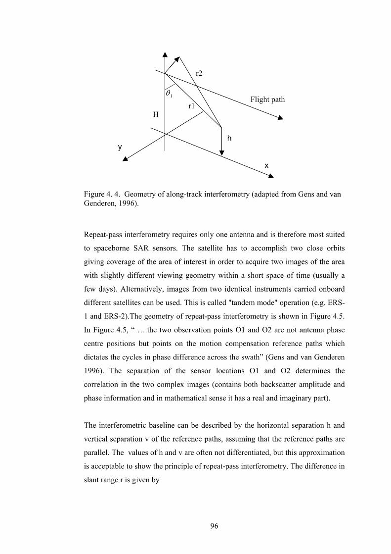
96
Figure 4. 4. Geometry of along-track interferometry (adapted from Gens and vanGenderen, 1996).
Repeat-pass interferometry requires only one antenna and is therefore most suited
to spaceborne SAR sensors. The satellite has to accomplish two close orbits
giving coverage of the area of interest in order to acquire two images of the area
with slightly different viewing geometry within a short space of time (usually a
few days). Alternatively, images from two identical instruments carried onboard
different satellites can be used. This is called "tandem mode" operation (e.g. ERS-
1 and ERS-2).The geometry of repeat-pass interferometry is shown in Figure 4.5.
In Figure 4.5, “ ….the two observation points O1 and O2 are not antenna phase
centre positions but points on the motion compensation reference paths which
dictates the cycles in phase difference across the swath” (Gens and van Genderen
1996). The separation of the sensor locations O1 and O2 determines the
correlation in the two complex images (contains both backscatter amplitude and
phase information and in mathematical sense it has a real and imaginary part).
The interferometric baseline can be described by the horizontal separation h and
vertical separation v of the reference paths, assuming that the reference paths are
parallel. The values of h and v are often not differentiated, but this approximation
is acceptable to show the principle of repeat-pass interferometry. The difference in
slant range r is given by
r1
r2
y
x
Flight path1θ
H
h

97
r = r1 – r2 = ( )rB
rvhHgh
2
2
−−− (4.7)
where
r = (r1+ r2)/2
B = 22 vh +
The phase difference can be derived from the path difference by the equation
φ = -4πr/λ (4.8)
Figure 4. 5. Geometry of repeat-pass interferometry (adapted from Gens and vanGenderen, 1996).
4.4 Differential interferometry
In addition to measuring the topography, an interferometric SAR may be used to
measure surface motion, provided that such motion is coherent. Coherence is
maintained if the group of scatterers within one resolution cell do not change
θ
h
v
O2
O1
r
Referencepaths
yx
g
O2
H
r2
r1
O1

98
significantly from the first pass to the second pass of the SAR sensor, and
provided that the scattering mechanism of the individual scatterers does not
change significantly between the two passes. If these assumptions are valid, then
it is possible to measure surface motion between the two passes of the SAR sensor
using repeat-pass interferometry. Differential interferometry provides relative
measures in the order of a few centimetres, or less, for movements in the vertical
and planimetric directions. In this technique a differential interferogram is
generated by the difference of two interferograms, which contains information
about small-scale displacements that occur between the times of data acquisition.
A differential interferogram can be produced in two different ways. Based on two
phase-unwrapped interferograms, the difference of these interferograms can be
calculated. Alternatively, an existing digital elevation model can be registered to
the viewing geometry of a calculated interferogram. The result of this approach is
a simulated interferogram. The difference of the original and simulated
interferogram is the required differential interferogram.
4.5 Coherence
The phase component in conventional SAR imagery is determined by two terms.
Firstly, the two-way electrical path length from the sensor to a specific resolution
cell and, secondly, the interference between different scatterers within the cell.
Constructive and destructive interference will introduce speckle and therefore
produces no useful phase information in one single SAR image. A second
observation from a different angle will, in principle, have the same speckle
interference term provided that the change of angle is small. The phase difference
between the two images will therefore be determined by the path length difference
between the two observation points to the resolution cell. The two images can
either be obtained by using two different sensors or the same platform (single-pass
interferometry) or by using the same sensor at two different parallel or nearly
parallel passes over the area (repeat-pass interferometry) as described above.
In SAR interferometry, coherence is defined as a measure of the degree of
resemblance of radar phase between two SAR images of the same area, and the
degree of correlation that exists between the two SAR images is called the
99
complex degree of coherence. The value of this coefficient varies between zero
and one, where a zero value means no interference, which implies that there will
be no interferometric fringes.
4.5.1 Coherence magnitude estimation
The complex coherence of two zero-mean complex signals 1g and 2g for
stationary random processes is defined as (Born and Wolf, 1980):
[ ]
[ ] [ ]22
21
*21
gEgE
ggE=γ (4.9)
Where *2g is the conjugate value of signal 2g and E[ ] denotes the expectation
value. The magnitude of γ ( γ ) is called the degree of coherence and the phase of
γ is called interferometric phase. Under the assumption that the processes involved
in equation (4.9) are ergodic in mean,1 the ensemble average is found by
coherently averaging the complex values of N single look pixels. The coherence is
then defined as:
∑ ∑
∑
= =
=∗
=γN
1i
N
1i
2i,2
2i,1
N
1i i,2i,1
gg
gg (4.10)
In equation (4.9), it can be noted that 1g and 2g ,which are assumed to be
stationary, are also jointly stationary.
1 There are two ways to calculate the mean of a random variable: 1. Time average: by integrating aparticular member function over all time or 2. Ensemble average: average together the values of allmember functions evaluated at some particular point in time. A random variable is ergodic if andonly if (1) the time averages of all member functions are equal, (2) the ensemble average isconstant in time, and (3) the time average and the ensemble average are numerically equal. Thus,for ergodic random variables, time average and ensemble average are interchangeable.

100
Stationarity of the processes ( 1g , 2g and *21gg ) is required such that the time
average of each process converges to a finite limit. Ergodicity in mean is also
required so that different time averages of each process converge to the same
limit, i.e. the ensemble average. The ensemble averages can then be substituted
in equation (4.9) with the time average and sample coherence of equation (4.10)
to provide an estimate of coherence. The coherence estimation considered above
is for stationary scenes in which the processes ( 1g , 2g and *21gg ) involved in
equation (4.9) are stationary. Such conditions are satisfied in homogeneous scenes
(Touzi et al., 1999).
In nonstationary areas, the processes ( 1g , 2g and *21gg ) involved in equation (4.9)
may not be stationary in mean and the sample coherence of equation (4.10) will
lead to a meaningless result (Foster and Guinzy, 1967). In practice, stationarity in
mean (the assumption that the mean E[ ] does not vary) may be relaxed: all that is
required is that E[ ] does not change within the observation interval (Foster and
Guinzy, 1967). If this condition is satisfied by each of the processes involved in
equation (4.9), the nonstationary processes can be considered to be locally
stationary (also called “stationary in increment”) and the coherence can be
estimated over a moving window.
In certain nonstationary areas, the processes involved in equation (4.9) cannot be
assumed to be stationary in increments, and coherence cannot be estimated even
locally. In some applications, the source of signal nonstationarity might be
removed and coherence can then be estimated. Especially in SAR interferometry,
nonstationarity of the cross channel product *21gg is assigned to the phase changes
due to topographic variations. The phase nonstationarity is compensated at the
spatial position i with a phase factor ije φ− for the local imaging geometry, and the
sample phase corrected coherence is used instead of sample coherence of equation
(4.10) (Touzi et al., 1999)

101
∑ ∑
∑
= =
=φ−
=γN
1i
N
1i
2i,2
2i,1
N
1iiji,2*
i,1
gg
egg (4.11)
After phase compensation, and under the assumption that the unique source of
signal nonstationarity is topographic phase variations, all processes involved in
equation (4.11) are stationary in the region of interest and the channels can still be
assumed to be zero-mean jointly gaussian. The results obtained in stationary
regions with the sample coherence of equation (4.10) can then be extended to the
modified sample coherence as given in equation (4.11) (Touzi et al. 1999).
The statistical confidence level of the sampled coherence depends on the number
of independent samples N that are combined to produce the coherence estimate.
Sampled coherence is usually estimated using a square estimator window. As a
first approximation, the standard deviation of the estimator is defined as (Prati et
al., 1994)
N
1=σ −
γ (4.12)
where N is the number of pixels in the window.
In practice, coherence has to be estimated from the combination of many pixels in
order to limit the statistical errors. The effects of the topography of the target
inside the estimator window have to be compensated for. This was not necessary
in this study due to extremely flat topography.
Another coherence estimator, suggested by Guarnieri and Prati (1997), is intended
for selection of interferometric pairs with good coherence, as its implementation is
quick. It is described as
=aγ 12 −ρ For ρ >1/2
102
Otherwise aγ =0
where
∑ ∑
∑
= =
==ρN
1i
N
1i
4i,2
4i,1
N
1i
2i,2
2i,1
gg
gg (4.13)
In SAR interferometry, interferometric correlation or degree of coherence as
expressed in a coherence image has potential as an input to classification for
different land surfaces. The degradation of coherence between two images is due
to several effects. The most important are spatial decorrelation (due to observation
angle change) and temporal decorrelation (due to changing scatterer
characteristics between the two images).
4.5.2 Image processing and generation of coherence images
4.5.2.1 Co-registration and common band filtering
In interferometric processing, two single-look complex images (SLC) are co-
registered at sub-pixel accuracy; an accuracy better than 0.2 pixels is required in
order not to degrade the interferometric correlation by more than 5%. In this
study, the GAMMA interferometric software was used for all interferometric
processing. The co-registration of the images in an interferometric pair was done
by calculating the local spatial correlation of the image intensities for at least 100
small square areas throughout the two images. The offset polynomial relating the
geometries of the two images was determined by finding the image offsets, which
maximises the local correlation in these small areas. The advantage of this method
is that it is possible to co-register images that have no interferometric correlation
into a common geometry, the only requirement being that there is some contrast in
the SAR intensity images. Before interferogram generation, common band
filtering (Gatelli et al., 1994) was performed in order to include only the parts of
the range and azimuth spectra common to the two interfering images. Common
band filtering improves the coherence estimate by minimising the effects of the
baseline geometry.
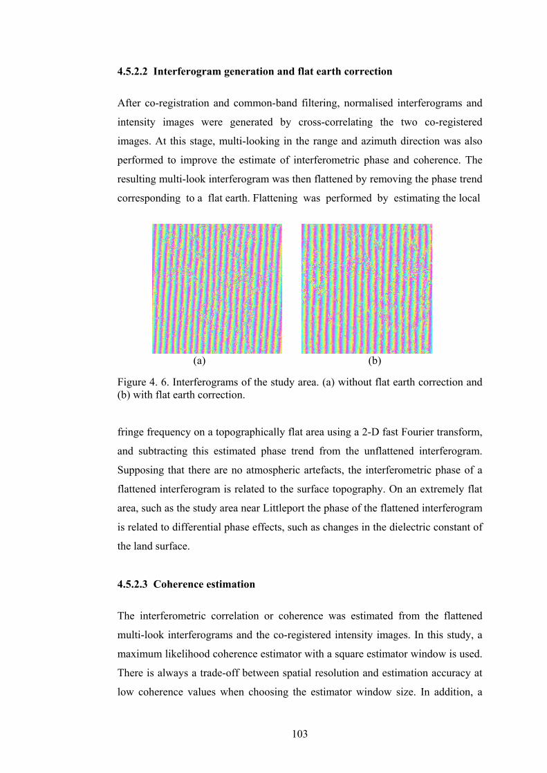
4.5.2.2 Interferogram generation and flat earth correction
After co-registration and common-band filtering, normalised interferograms and
intensity images were generated by cross-correlating the two co-registered
images. At this stage, multi-looking in the range and azimuth direction was also
performed to improve the estimate of interferometric phase and coherence. The
resulting multi-look interferogram was then flattened by removing the phase trend
corresponding to a flat earth. Flattening was performed by estimating the local
Figure (b) wit
fringe
and su
Suppos
flattene
area, su
is relat
the lan
4.5.2.3
The in
multi-l
maxim
There
low co
(a) (b)
103
4. 6. Interferograms of the study area. (a) without flat earth correction andh flat earth correction.
frequency on a topographically flat area using a 2-D fast Fourier transform,
btracting this estimated phase trend from the unflattened interferogram.
ing that there are no atmospheric artefacts, the interferometric phase of a
d interferogram is related to the surface topography. On an extremely flat
ch as the study area near Littleport the phase of the flattened interferogram
ed to differential phase effects, such as changes in the dielectric constant of
d surface.
Coherence estimation
terferometric correlation or coherence was estimated from the flattened
ook interferograms and the co-registered intensity images. In this study, a
um likelihood coherence estimator with a square estimator window is used.
is always a trade-off between spatial resolution and estimation accuracy at
herence values when choosing the estimator window size. In addition, a

104
weighing function, decreasing linearly with increasing distance from the central
pixel, was applied in the coherence estimation. With the data sets shown in Table
4.1, the following coherence images were generated (Figure 4.7):
1 1-day coherence image using 02/05/1996 and 03/05/1996 SLC.
2 35-day coherence image using 16/08/1996 and 20/09/1996 SLC.
3 70-day coherence image using 07/06/1996 and 16/08/1996 SLC.
Table 4. 1. The date and corresponding sensor of the SLC used in the study.
Sensor Date
ERS-1 02 May 1996
ERS-2 03 May 1996
ERS-2 07 June 1996
ERS-2 16 August 1996
ERS-2 20 September 1996
Due to the large base line length (>1000 m) and the time interval involved, the
phase coherence obtained at 35 days and 70 days was not very good. Hence, in
this study, only the 1-day coherence image and five intensity images produced
during the interferometric processing of the single look complex images are used
for land use classification.
4.5.2.4 Image coregistration
The 1-day coherence image used in this study was registered to the Ordnance
Survey (OS) of Great Britain’s National Grid using the ERDAS Imagine image
processing software by applying a first-order polynomial transformation using
fifteen ground control points. The RMS error value estimated for image
transformation was of the order of 0.87 pixels. Later, all the five intensity images
were co-registered to the coherence image. The nearest neighbour resampling
method was used and the spatial resolution (i.e. pixel size) of the image was
reduced to 20 metres. A 286-pixel by 386-pixel portion of the image covering the
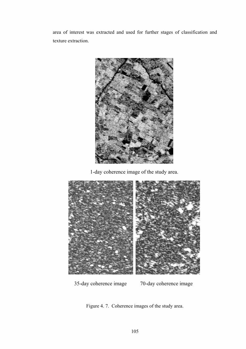
area of interest was extracted and used for further stages of classification and
texture extraction.
F
35-day
1-day coherence image of the study area.
coherence image 70-day coherence image
105
igure 4. 7. Coherence images of the study area.
106
4.5.2.5 Speckle suppression
In remote sensing radar images, the size of a resolution cell on the surface is
always much larger than the signal wavelength and is generally significantly
larger than the size of individual scattering objects. Because of the random
orientation of terrain surface elements, returns from multiple scatterers within a
resolution cell add incoherently to give a net backscattering coefficient, which has
a random distribution in the image plane. The image thus obtained has a randomly
fluctuating intensity at each pixel, which leads to a grainy appearance. This
random multiplicative noise/grainy appearance within a SAR resolution element
is called speckle. Speckle is one of the main problems in the use of synthetic
aperture radar image interpretation and classification because a zone that is
homogeneous on the ground has a granular appearance on image. For the purpose
of classification, it is desirable to reduce these fluctuations and to cluster the
observed intensities closer to the mean intensity, since it is the mean intensity that
expresses the required image information. In order to decrease the effects of
speckle, several different approaches can be used. These includes averaging of
images (Ulaby et al., 1986), filtering of images using adaptive filters (Nezry et al.,
1996), the use of texture features (Ulaby et al., 1986).
In this study, all of the intensity images obtained from interferometric processes
are single look images. A number of filters (Lee (Lee, 1986) Frost (Frost et al.,
1982) and Kuan (Kuan et al., 1985)) have been developed and tested for speckle
reduction in radar data. When applying the speckle filter, selection of window size
is important, because speckle suppression will not be satisfactory with a small
window size and with a large window size, the original image will also be
degraded by oversmoothing. There is a trade-off between speckle reduction and
preservation of image quality. In this study, a median filter with a window size of
5×5 is used for speckle reduction in all intensity and coherence images. The
median filter operates on the image so that the centre pixel of the filter window is
replaced by the median value of the pixels in window. In other words, low and
high valued pixels are considered as noise and are removed (Richards, 1993).
These filtered images were then used for classification studies.

107
4.5.3 Factors affecting coherence
As mentioned earlier, interferometric coherence is a by-product of SAR
interferometry and it provides a measure of the phase correlation between two
images of the same target obtained from two different positions, possibly at
different times. Phase coherence is affected by a number of factors, the most
important being:
1. Instrument parameters, including wavelength, signal to noise ratio, range
resolution, and number of independent looks.
2. Parameters related to the geometry, such as the baseline length and
incidence angle. The spatial extent of the baseline is one of the major
performance drivers in an interferometric radar system. If the baseline is
too short the sensitivity to signal phase differences will be undetectable,
while if the baseline is too long then additional noise due to spatial
decorrelation corrupts the signal. It can be shown that coherence (phase
correlation) decreases approximately linearly with the increase in baseline
length (Rodriquez et al., 1992). The length of the baseline for which the
attainable coherence is zero is called the critical baseline length, which
occurs when the change in look angle between the interfering images is
sufficient to cause backscatter from each pixel to become completely
uncorrelated. The critical baseline length for ERS-1/2 interferometry on
flat terrain is approximately 1100m. The effect of baseline decorrelation
may be reduced by the use of spectral filtering during interferometric
processing.
3. Volume scattering and temporal changes, i.e., movement of the scatterers
due to wind effects, growth, and loss of foliage. In other words, it is not
possible to illuminate the same patch of surface from two different aspect
angles and expect the signals to be fully correlated. This is also called
decorrelation due to the rotation of the targets with respect to the radar
look direction. Temporal effects which follows from physical changes in
the surface over the time period between observations. In practice, the
amount of temporal decorrelation depends on the soil and vegetation type

108
of the target area, as well as the weather conditions between the radar
passes.
4. Variation in the dielectric constant due to freezing, wetting, and drying of
surface, thus causing temporal decorrelation.
As long as the data used are from same system, instrument parameters remain the
same and have no effect on coherence. Common spectral band filtering2 (Gatelli et
al., 1994) of the SAR image pair before computation of the interferogram
helps to reduce the decorrelation introduced by baseline geometry3, if baseline
length is within an acceptable range. Repeat pass SAR interferometry is very
sensitive to temporal changes, i.e., change occurring between the two data
acquisition times.
4.6 ETM+ data
The main instrument carried by Landsat 7 is the Enhanced Thematic Mapper Plus
(ETM+). This instrument maintains the essential characteristics of Thematic
Mapper carried by Landsats 4 and 5 (Table 4.2). Ground resolution for ETM+
data remains unchanged at 30 m, except for the thermal band in which the
resolution is increased from 120 to 60 m. A panchromatic band with 15 meter
resolution is also added for rectification and image sharpening. Landsat 7
provides data with a swath width of 185 km and a repeat coverage interval of 16
days. For this study, ETM+ multispectral data for both study areas in the UK and
Spain acquired on 19 June 2000 and 28 June 2000 respectively, are used.
Panchromatic data for the UK study area is used to study its influence on
classification accuracy in combination with multispectral data.
2 Accounting for the spectral shift induced by the slight difference in incidence angle between twoSLC images. After this processing only the range spectrum interval common to the two SLCimages is retained.3 The distance between the satellite on the first pass and second pass should not be too large. Asthis distance increases, the coherence is increasingly lost. The loss of coherence in this way iscalled baseline decorrelation.

109
Table 4. 2. Landsat 7 ETM+ data characteristics.
Band number Spectral range (microns) Ground resolution (m)1 0.450 - 0.515 302 0.525 - 0.605 303 0.630 - 0.690 304 0.750 - 0.900 305 1.550 - 1.750 306 10.40 - 12.50 607 2.090 - 2.350 30
Panchromatic 0.520 - 0.900 15
4.7 DAIS hyperspectral data
The DAIS (Digital Airborne Imaging Spectrometer) sensor is a new generation
hyperspectral sensor, designed by the Geophysical Environmental Research
Corporation (GER) and funded by the European Union (EU). The development
was initiated in 1993 after European Remote Sensing Capabilities (EARSEC) and
European Commission (EC) decided to fund and support the development of an
imaging spectrometer. The sensor is operated by the German Space Agency or
German Aerospace Research Establishment, which is also known as the German
Aerospace Centre (DLR) since 1995 (Strobl and Zhukov 1998). Between 1996 to
1999, the Large-Scale Facility was developed. In the framework of the DAIS
Large-Scale Facility, DLR operates its Digital Airborne Imaging Spectrometer
(DAIS 7915) on board a DO-228 aircraft. It is a 79 channel imaging spectrometer
(Table 4.2) which measures energy in the range from visible to the thermal
infrared wavelengths. The spatial resolution of the sensor can vary from 5 to
20 m, depending on the altitude of the aircraft. The DAIS is a whisk broom
scanning instrument with an optomechanical scanner. The scanning principle is of
Kennedy type with a four-sided rotating polygon mirror. The advantages of this
technique are mainly the solely reflective optics, the large aperture realisable and
the high scan efficiency. These advantages are counterweighted by the high
susceptibility to produce striping (Strobl et al. 1997) and the presence of intrinsic
background signals ( (Strobl and Zhukov 1998).

110
Table 4. 3. The DAIS 7915 system specifications.
Spectrometer Bands Wavelength range (micrometer)
VIS/NIR 32 0.50 - 1.05
SWIR I 8 1.50 - 1.80
SWIR II 32 1.90 - 2.50
MIR 1 3.00 - 5.00
TIR 6 8.70 - 12.50
The DAIS data show moderate to severe striping problems in the optical infrared
region between bands 41 and 72. Initially, the first 72 bands in the wavelength
range 0.4 µm to 2.5 µm were selected. All 72 bands were visually examined to
determine the severity of striping. Seven bands with very severe striping (bands
41, 42 and 68 to 72) were removed from further study. The striping in the
remaining bands was removed by automatically enhancing the Fourier transform
of the image (Cannon et al., 1983; Srinivasan et al., 1988). The input image is first
divided into overlapping 128-by-128-pixel blocks. The Fourier transform of each
block is calculated and the log-magnitudes of each FFT block are averaged. The
averaging removes all frequency domain quantities except those which are present
in each block; i.e., some sort of periodic interference. The average power
spectrum is then used as a filter to adjust the FFT of the entire image. When the
inverse Fourier transform is performed, the result is an image with periodic noise
eliminated or significantly reduced.
4.8 Conclusion
This chapter gives a brief introduction to the data used for this study.
Interferometric SAR and the way interferometric coherence is calculated by using
the phase information in the radar return is discussed in detail. The factors
affecting the coherence are also discussed because - as mentioned in this chapter -
coherence is a by-product of SAR interferometry and it very important to know
these factors before selecting the Single Look Complex images to generate
coherence maps.

111
Some details of ETM+ and DAIS hypespectral data as well as the problems of
striping in DAIS data and the method used to remove these striping using Fourier
transformation are also discussed.
112
Chapter 5
Crop classification using decision tree and supportvector machine classifiers
5.1. Decision tree classifiers
5.1.1 Introduction
The effective management and use of land resources requires knowledge of the
properties and spatial distribution of these resources. The rapid evolution and
increasing number of applications of remote sensing methods in the last 20 years
shows that such methods are becoming more widely accepted for the purposes of
terrestrial resource survey, especially for the observation of land cover that
comprises the base for development projects. The cost of surveys using remote
sensing is less than that of ground-based methods. Other advantages include large
area of coverage under the same atmospheric conditions, and repeatability.
Multispectral and multitemporal properties are of great importance to land cover
studies. Nowadays, satellite products are widely used for the study and
classification of land cover, using data from the Landsat, SPOT, ERS and IRS
systems.
Accurate classification of terrain from remotely sensed data is essential, especially
for agricultural and forest monitoring, ecological monitoring of vegetation
communities, land cover mapping and monitoring, and many other similar
applications. Much work related to the classification of land use/land cover
categories using satellite data is reported in the literature. To achieve an accurate
classification of terrain, an image at a suitable resolution for the terrain needs to
be acquired first, and then the characteristics of each small segment of the image
must be classified accurately. A number of different types of classifiers are now in
routine use in remote sensing. The classification methodology implemented in
remote sensing has so far used statistical-based approaches, such as the maximum
likelihood classifier, unsupervised classifiers such as the ISODATA clustering
algorithm, and neural network classifiers, which offer a non-parametric

113
classification approach. Statistical classifiers basically depend on some pre-
defined data model (e.g. Gaussian normal distribution), and, therefore, the
performance of these classifiers will depend on how well the data match the pre-
defined model. The performance of these classifiers can be good if the distribution
of input data are approximately normal. For clustering algorithms, knowledge of
the area is very important because these classifiers basically depend on input from
the analyst. Within the last ten years, neural classifiers have been extensively
tested by the remote sensing community (Benediktsson et al., 1990; Civco, 1991;
Heermann and Khazenie, 1992; Foody, 1995(a)(b)) due to their non-parametric
nature (independence of frequency distribution), ability to handle data acquired at
different levels of measurement, precision, and - once trained - rapid data
processing. Although neural networks may generally be used to classify data at
least as accurately as statistical classification approaches, there are a range of
factors that limits their use (Wilkinson, 1997). Some of these factors are discussed
in section 2.3.4.3. Perhaps one of the most important problems is that
classification is highly subjective (Johnston, 1968). Despite the apparent
objectivity of the method, the analyst has control over a range of network
parameters that influences network performance and, even if these parameters are
selected judiciously, there is no guarantee that the neural network will provide an
acceptable optimal solution.
Decision tree classification techniques have been used successfully for a wide
range of classification problems but have not been tested in detail by the remote
sensing community (Safavian and Landgrebe, 1991). These techniques have
substantial advantages for remote sensing classification problems because of their
flexibility, nonparametric nature, and ability to handle nonlinear relations between
features and classes. Just like other classification algorithms, the accuracy of a
classification produced by a decision tree classifier can be a function of a number
of factors, such as size and composition of the training set, attribute selection
methods, various pruning methods, and boosting. So far, few studies have been
carried out to study the effects of these factors. Friedl et al. (1999) and Muchoney
et al. (2000) studied the effect of boosting of classifications using decision trees
on land cover classification accuracy. No study in remote sensing has tried to
assess the effects of training data size, various pruning methods, and attribute
114
selection measures on land cover classification accuracy. Studies carried out by
Brieman et. al., (1984) and Mingers (1989 a) suggest that the pruning method
affects the classification accuracy, whatever may be the attribute selection
measure. Oates and Jenson (1997) suggest that increasing the number of training
data only affects the size of the tree but has a little affect on the classification
accuracy.
This chapter presents an investigation into the effects of these factors on the
accuracy of crop classification using decision tree classifiers. Besides decision
tree classifier, maximum likelihood and neural classifiers have been used for
comparison, because these classifiers have already been used in numbers of
studies and give acceptable results.
5.1. 2 Study area
The study area selected is an agricultural area located near the town of Littleport
in Cambridgeshire, in the eastern part of England. ETM+ data acquired on 19
June 2000 are used. The classification problem involved the identification of
seven land cover types, namely, wheat, potato, sugar beet, onion, peas, lettuce and
beans that cover the bulk of the area of interest.
The ERDAS Imagine image processing software (version 8.4) was used to register
the images to the Ordnance Survey of Great Britain’s National Grid by applying a
linear transformation. The RMSE (Root Mean Square Error) values estimated for
image transformations were less than one pixel. An area of 307-pixel (columns)
by 330-pixel (rows) covering the area of interest was then extracted for further
analyses.
For this study field data for the relevant crops were collected from farmers and
their representative agencies, and other areas were surveyed on the ground. The
field boundaries visible on the multispectral image were then digitised using Arc
Info software. A polygon file was created by applying a buffering operation of
one pixel width to remove the boundary pixels during the classification process
and each polygon is assigned a label corresponding to the crop it contained.

Finally a ground reference image is generated by using the polygon file (Figure
5.1.1).
5.1.3 Methods
A series of classifications was performed in order to evaluate the effects of
training set size, attribute selection measure, pruning methods and boosting on the
accuracy of the output from a decision tree classifier. To study the effects of
various attribute selection measures, error based pruning was used while for the
purposes of studying the effects of pruning methods on classification accuracy,
the gain ratio was used as a selection measure. The effects of training set size
were evaluated using two different decision tree classifiers, See5.0, a univariate
classifier, and QUEST (Loh and Shih, 1997), a multivarite decision tree classifier.
115
Figure 5.1.1. The ground reference image of the ETM+ data.

116
5.1.3.1 Training set size
The characteristics of the data used to train a supervised classification have a
considerable influence on the quality of the resulting classification (Campbell,
1981, Labovitz, 1986). It is essential that the training data provide a representative
description of each class. For the maximum likelihood classifier, a key
requirement is to have the training data size for each class equal to from 10-30
times the number of features (Mather, 1999). The required training set size may
therefore be large, and acquiring such training sets may be difficult where a large
number of classes is involved or utilising data acquired in many wavebands.
Consequently, many investigations have been based on a sample size that is less
than the generally accepted guidelines and thus the information content of
remotely sensed data may not have been fully exploited. The lack of distributional
assumptions makes neural classifiers an attractive alternative to the conventional
statistical techniques. It has been proposed that neural network classification can
be performed successfully using smaller training data sets (Hepner et al., 1990;
Foody et al., 1995 (b)). Further investigations into the effects of training set
characteristics on the performance on neural network classification have revealed
that the training set size has a major effects on the classification accuracy (Foody
et al., 1995 (b); Foody and Arora, 1997; Kavazoglu, 2001).
So far few studies (Huang et al., 2002) have discussed the effects of training set
size on classification of remote sensing data using decision tree classifiers. It is
therefore important to investigate the effect of training set size on these
classifiers for crop classification problems. For this study, seven categories of
training set size were formed. Each category contains randomly selected pixels
representative of each class. The training sets contained 700, 1050, 1400, 1750,
2100, 2450 and 2700 pixels in total, respectively and a total of 2037 pixels was
used for testing the classifier. Figure 5.1.2 shows the variation of accuracy with
increase in training set using a univariate decision tree classifier.
For each of the training data sets a classification was performed and a confusion
matrix was generated to calculate the overall accuracy and the Kappa coefficient.
Comparing the classification accuracies obtained from different training sets
revealed that the rate of increase in classification accuracy with increasing training

117
set size is linear up to fifth data set (300 pixels per class). As the training set size
increases from 700 to 2100 pixels (100 per class to 300 pixels per class), there is a
marked increase in overall classification accuracy ranging from 78.3 to 84.1%
Figure 5.1.2. Variation of classification accuracy with increasing number oftraining patterns using a univariate decision tree classifier.
and the Kappa values increase from 0.746 to 0.815. However, further increases in
training set size, using the sixth and seventh data sets , produced a lesser increase
in classification accuracy and even shows a slight decrease in classification
accuracy with the sixth data set (using 2450 pixels for all classes). These results
indicate that the accuracy of a univariate decision tree classification increases as
the size of the training set is increased but suggests that there is no requirement of
very large training sets to be used. These results do not concur with the study
carried out by Oates and Jenson (1997) in that the rate of increase in classification
accuracy was found to be independent of training set size.
A second study was carried out to study the behaviour of a multivariate decision
tree classifier ((Figure 5.1.3) with increasing number of training patterns using the

118
same set of training and test data as were used to test the univariate decision tree
classifier. It was concluded that classification accuracy increases with the increase
in training set size and this increase is almost linear up to fourth data set (100
pixels per class to 250 pixels per class). Accuracy then starts to fall with the fifth
and sixth data sets but rises again so that the highest classification accuracy is
achieved by the seventh data set. These results suggest that classification
accuracy increases with the size of the training set, but only up to a point.
Figure 5.1.3. Variation of classification accuracy with increasing number oftraining patterns using mulivariate decision tree classifier.
The behaviour of the multivariate classifier was found to be somewhat
unpredictable as the training pattern increases beyond a certain limit. It is evident
also that the performance of the multivariate classifier is no better than the
univariate classifier for this data set. As the training time is always greater with a
multivariate decision tree classifier, it is suggested that the use of univariate
decision tree classifiers may be adequate for this type of data.

119
5.1.3.2 Attribute selection measure
It is reasonable to choose the attribute that best divides the data into their classes,
and then partition the data according to the value of that attribute. At each node in
the development of a decision tree there will be a set of data and a number of
attributes available to classify the data. One selects the best attribute for splitting
by seeing how well each one separates the data into the various classes. A number
of these splitting measures have been proposed by various authors in the literature
and are discussed in detail in section 3.4.2.1. The purpose of this section is to
examine the various attribute selection measures in terms of comparative
performance for land cover classification studies. Earlier studies carried out by
Breiman et al. (1984) and Mingers (1989 b) suggest that the predictive accuracy
of decision trees is not sensitive to the goodness of split measure or attribute
selection measures. For the present study, a univariate decision tree classifier
with error-based pruning and four different attribute selection measures is used. A
total of 2700 patterns for training and 2037 for testing were used for this study
(Figure 5.1.4).
Figure 5.1.4. Variation of accuracy with different attribute selection measures.
83
84
85
Attribute selection measure
Acc
urac
y(%
)
Accuracy 83.7 84.54 83.9 83.65
Information Gain Information Gain ratio
Gini Index Chi-square measure

120
Figure 5.1.4 essentially confirms the findings of Breiman et al. (1984) and
Mingers (1989 b) that classification accuracy is not seriously affected by the
choice of attribute selection measure, and shows that this conclusion applies to
remote sensing data also. Except for the information gain ratio, the accuracy
obtained with all four selection measure is almost the same, and the increase in
accuracy resulting from the use of the information gain ratio is less than 1%. It is
therefore concluded that the selection measure does not affect the predictive
accuracy of the decision tree.
5.1.3.3 Pruning methods
Studies carried out by the machine learning community and described in section
5.1.3.2 show that overall accuracy of a decision tree classifier on unseen data is
not sensitive to the goodness of the split. It is further suggested that the predictive
accuracy of the decision tree classifier depends on the pruning methods used in
the design of the tree. This section examines the effect of various pruning methods
on classification accuracy. Five different pruning methods are used with the
information gain ratio as the attribute selection measure in a univariate decision
tree classifer (C4.5). The pruning methods employed are: Reduced Error Pruning
(REP), Pessimistic Error Pruning (PEP) Error-Based Pruning (EBP) proposed by
Quinlan (1987,1993); Critical Value Pruning (CVP) proposed by Mingers (1989
a); and Cost-Complexity Pruning (CCP) proposed by Brieman et al. (1984).
Figure 5.1.5 show the variation in classification accuracy with respect to the
different pruning methods used.
As suggested by Figure 5.1.5, each of the five pruning methods produces a
different classification accuracy. The performance of the REP method is worst of
all the pruning methods employed in this study. The reason for this could be the
requirement of separate data set for pruning, a conclusion also suggested by
Esposito et al. (1997). Pessimistic error pruning gives the highest accuracy of
82.9% as compared to other four pruning methods but the study carried out by
Esposito et al. (1997) suggests that the introduction of the continuity correction
(section 3.8.3) in the estimation of error rate has no theoretical justification and
such a factor is improperly compared to an error rate, which may lead to either
underpruning or overpruning of the tree. The performance of CVP is affected by

121
the choice of the critical value set to prune a tree. CCP uses a separate data set or a
cross validation approach for pruning, while EBP uses training data for pruning
the tree. These results suggests that the choice of pruning method is important in
the design of a decision tree classifier. Error-based pruning, which gives an
accuracy of 82.8%, is used in this research for further studies.
Figure 5.1.5. Variation of classification accuracy with different pruning methods.
5.1.3.4 Boosting
Classification accuracies and Kappa values obtained from unboosted and boosted
decision trees, estimated by using 2700 training and 2037 test data, are shown in
Table 5.1.1. The boosted decision tree classifications were estimated using
Table 5.1.1. Results from boosted and unboosted decision tree.
Accuracy (%) Kappa value
Unboosted decision tree 84.24 0.816
Boosted decision tree 88.46 0.865

122
fourteen iterations of the base decision tree algorithm. In this study, different
numbers of boosting iterations varying from 2 to 20 were used to see how
variation in the number of iterations affects accuracy. It was found that little
change in accuracy is gained by performing different boosting runs after fourteen
iterations (Figure 5.1.6). These results confirm that the degree of accuracy
improvement achieved through the use of boosting starts to stabilise after eight
iterations and results indicates that relatively little increase in accuracy is
Figure 5.1.6. Classification accuracies for boosted decision trees for varyingnumber of boosting iterations.
gained beyond the twelfth iterations. This result suggests that ten to fifteen
boosting iterations is enough to achieve the best attainable accuracy for this type
of data. The result also concurs with those studies carried out using non-remote
sensing data. Quinlan (1996) concludes that about ten iterations provide the
maximum improvement in classification accuracy, and that little is gained by
performing additional boosting runs.

123
Figure 5.1.7. Difference of classified images with ground reference image (a)unboosted decision tree classifier (b) boosted decision tree classifier. Visualcomparison of individual fields shows that within-field variation is reduced byboosting.
(a)
(b)
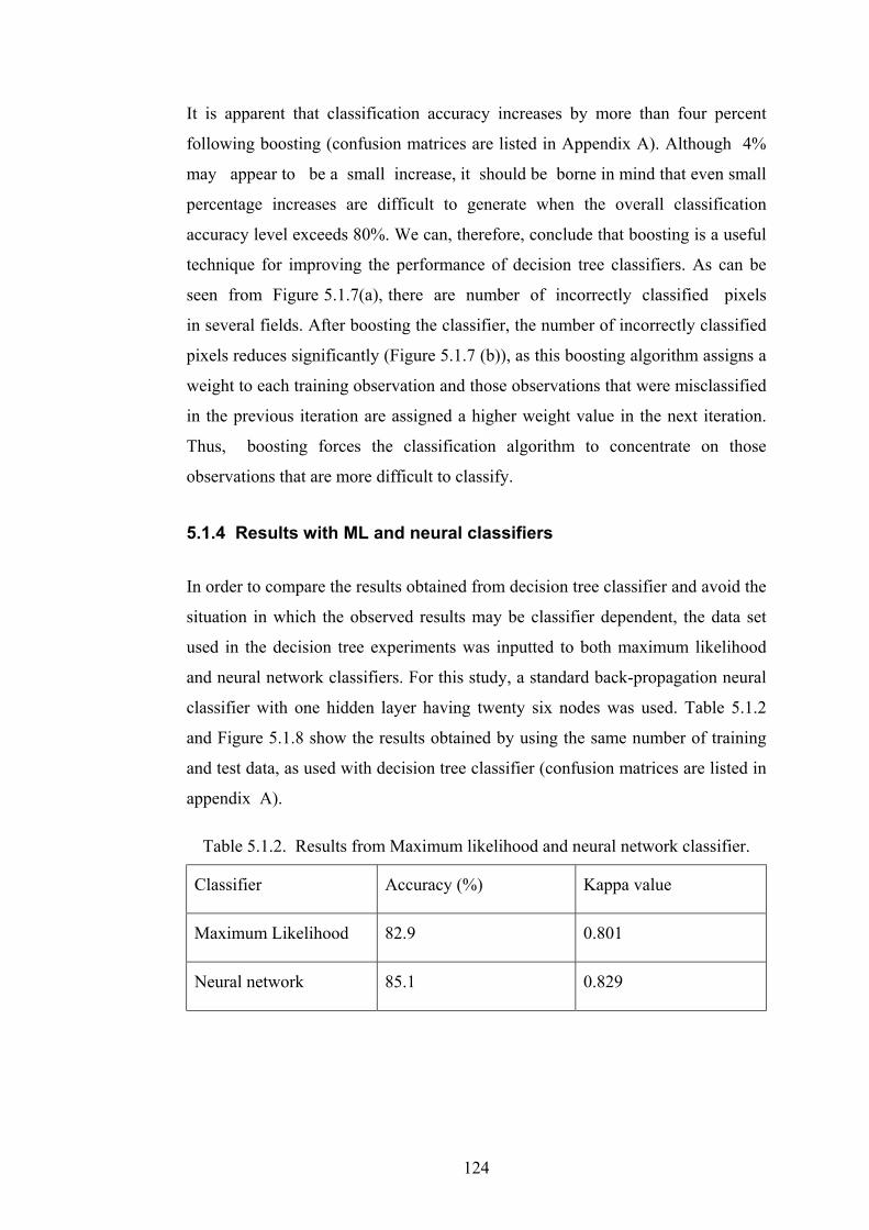
124
It is apparent that classification accuracy increases by more than four percent
following boosting (confusion matrices are listed in Appendix A). Although 4%
may appear to be a small increase, it should be borne in mind that even small
percentage increases are difficult to generate when the overall classification
accuracy level exceeds 80%. We can, therefore, conclude that boosting is a useful
technique for improving the performance of decision tree classifiers. As can be
seen from Figure 5.1.7(a), there are number of incorrectly classified pixels
in several fields. After boosting the classifier, the number of incorrectly classified
pixels reduces significantly (Figure 5.1.7 (b)), as this boosting algorithm assigns a
weight to each training observation and those observations that were misclassified
in the previous iteration are assigned a higher weight value in the next iteration.
Thus, boosting forces the classification algorithm to concentrate on those
observations that are more difficult to classify.
5.1.4 Results with ML and neural classifiers
In order to compare the results obtained from decision tree classifier and avoid the
situation in which the observed results may be classifier dependent, the data set
used in the decision tree experiments was inputted to both maximum likelihood
and neural network classifiers. For this study, a standard back-propagation neural
classifier with one hidden layer having twenty six nodes was used. Table 5.1.2
and Figure 5.1.8 show the results obtained by using the same number of training
and test data, as used with decision tree classifier (confusion matrices are listed in
appendix A).
Table 5.1.2. Results from Maximum likelihood and neural network classifier.
Classifier Accuracy (%) Kappa value
Maximum Likelihood 82.9 0.801
Neural network 85.1 0.829

125
Figure 5.1.8. Classified images of the study area using (a) Maximum Likelihoodclassifier and (b) Neural network classifier. The colour palette is the same as inFigure 5.1.8 (a).
(a)
(b)
126
Results shown in Tables 5.1.1 and 5.1.2 shows that the decision tree classifier
performs better than a maximum-likelihood classifier, and its performance is
comparable to a neural network, even without boosting. As suggested by Table
5.1.1, after boosting, the performance of the decision tree classifier improves by
about 3.26 percent as compared to the neural network classifier. Thus, these
results indicates that the boosted decision tree classifier performs better than the
neural network classifier. As discussed in section 2.3.4.3, a number of factors
affect the classification accuracy achievable by a neural network classifier
(Kavzoglu, 2001). The use of a decision tree classifier requires only the choice of
attribute selection measure and pruning method. This study suggests that only the
pruning method affects the predictive accuracy of a decision tree classifier, not the
attribute selection measure.
Another study was carried out to compare the training time of the decision tree
and neural classifier using the same training data. All other factors affecting the
neural network classifier were set as recommended by Kavzoglu (2001). The
training time for the neural network classifier was about 58 CPU minutes on a Sun
machine as compared to 0.7 CPU second using a personal computer with a
Pentium II processor by a decision tree without boosting. Even after using
boosting the decision tree classifier took about 7.1 CPU seconds for 14 iterations,
which is still far less than the time taken by a neural network classifier.
5.1.5 Inclusion of panchromatic band and its texture
Further studies were carried out to include information derived from the ETM+
panchromatic band with multispectral data for classification. In order to evaluate
the performance of different data sets, a statistical separability measure called the
Jeffreys-Matusita distance (JM distance) is used. Signature separability is a
measure of the statistical distance between two signatures. Separability can be
calculated for any combination of bands that is used in the classification enabling
the user to compare the contribution made by each or band combination to the
class separability using, the spectral distance between the mean vectors of each
pair of signatures. If the spectral distance between two samples is not significant
127
for any pair of bands, then signatures may not be distinct enough to produce a
successful classification.
Generally, three different formulae are used for calculating separability. These
three formulae take into account the covariances of the signatures of the bands
being compared as well as the mean vectors of the signatures. The first
separability index is called divergence and is denoted by ijD . It is derived from
the likelihood ratio of any pair of classes i and j. For multivariate Gaussian
distributions, ijD for classes i , j is defined by:
))).().(CC((tr21
))CC).(CC((tr21
D Tjiji
1j
1i
1i
1jjiij µ−µµ−µ++−−= −−−− (5.1.1)
where tr denotes the trace of a matrix, C is the sample class covariance matrix, µ
is the class mean vector, and T denotes the transpose of a matrix. The second
separability measure is called Transformed Divergence, represented by ijTD and
is calculated from
)]8/Dexp(1.[2000TD ijij −= (5.1.2)
where ijD is the divergence index. Transformed Divergence gives an exponentially
decreasing weight to increasing distance between the classes. The scale of
divergence values can range from 0 to 2000. According to Jenson (1996) if the
value is more than 1900, then the classes can be separated easily. Between 1700
and 1900, the class separation is fairly good and if this value is below 1700, the
class separation is poor.
A third method of computing the separability is to calculate the JM distance
between two classes i and j as
( )α−−= exp1.2ijJM (5.1.3)
in which α (the Bhattacharyya distance) is given by
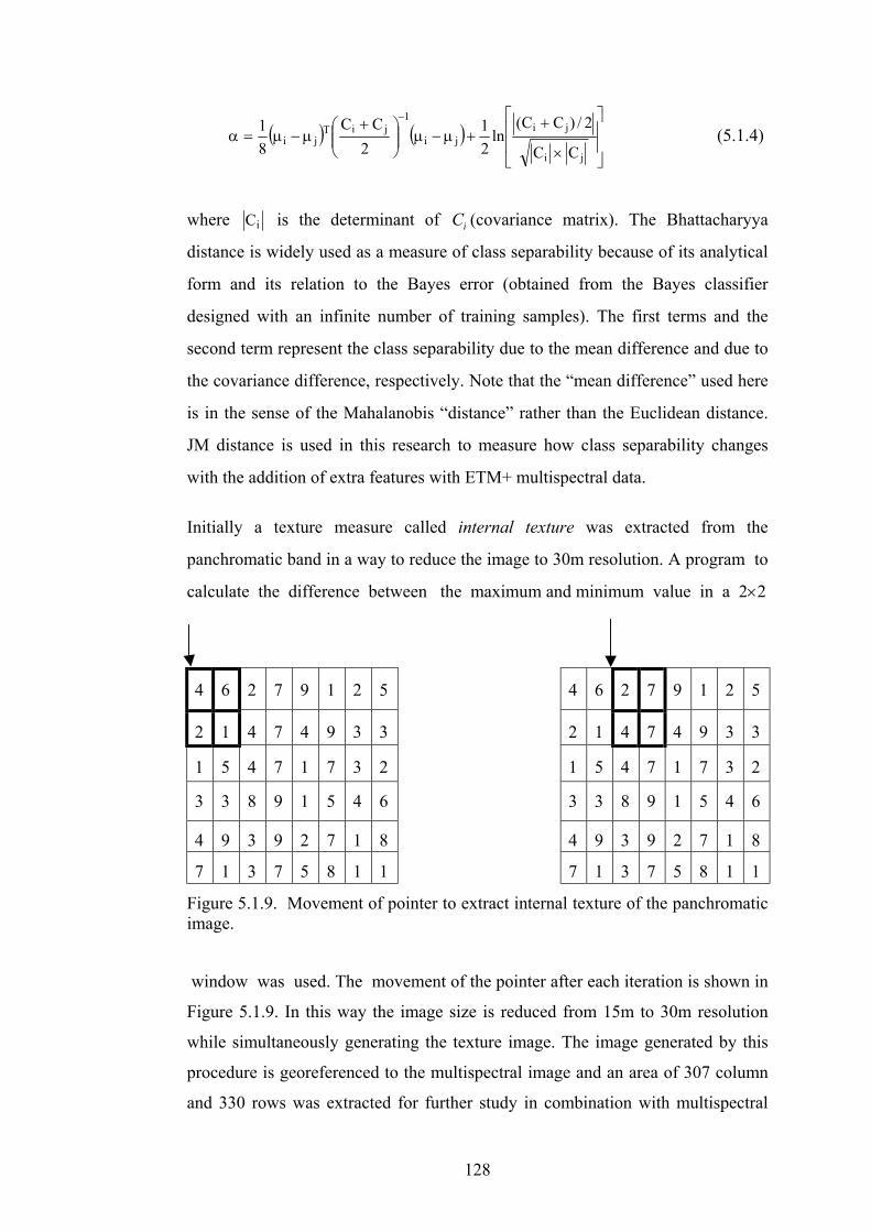
128
( ) ( )
×
++µ−µ
+µ−µ=α
−
ji
jiji
1jiT
jiCC
2/)CC(ln
21
2CC
81 (5.1.4)
where iC is the determinant of iC (covariance matrix). The Bhattacharyya
distance is widely used as a measure of class separability because of its analytical
form and its relation to the Bayes error (obtained from the Bayes classifier
designed with an infinite number of training samples). The first terms and the
second term represent the class separability due to the mean difference and due to
the covariance difference, respectively. Note that the “mean difference” used here
is in the sense of the Mahalanobis “distance” rather than the Euclidean distance.
JM distance is used in this research to measure how class separability changes
with the addition of extra features with ETM+ multispectral data.
Initially a texture measure called internal texture was extracted from the
panchromatic band in a way to reduce the image to 30m resolution. A program to
calculate the difference between the maximum and minimum value in a 2×2
4 6 2 7 9 1 2 5 4 6 2 7 9 1 2 5
2 1 4 7 4 9 3 3 2 1 4 7 4 9 3 3
1 5 4 7 1 7 3 2 1 5 4 7 1 7 3 2
3 3 8 9 1 5 4 6 3 3 8 9 1 5 4 6
4 9 3 9 2 7 1 8 4 9 3 9 2 7 1 8
7 1 3 7 5 8 1 1 7 1 3 7 5 8 1 1
Figure 5.1.9. Movement of pointer to extract internal texture of the panchromaticimage.
window was used. The movement of the pointer after each iteration is shown in
Figure 5.1.9. In this way the image size is reduced from 15m to 30m resolution
while simultaneously generating the texture image. The image generated by this
procedure is georeferenced to the multispectral image and an area of 307 column
and 330 rows was extracted for further study in combination with multispectral

129
data. All the three classifiers were used to evaluate the effect of the inclusion of
internal texture on classification accuracy (Table 5.1.3).
Comparing the results shown in Table 5.1.3 with those shown in Tables 5.1.1 and
5.1.2 suggests that there is little or no increase (in the case of decision tree
classifier this increase is only 0.06%) in classification accuracy with all the three
classification systems used in this study, thus indicating that the addition of an
internal texture feature derived from the panchromatic band of ETM+ does not
help in increasing the classification accuracy. The JM distance for this data set
was 1329 as compared to 1320 for ETM+ data alone.
Table 5.1.3. Results obtained by using internal texture of panchromatic band withETM+ multispectral data.
Classifier Accuracy (%) Kappa value
Maximum Likelihood 83.1 0.803
Neural Network 85.4 0.832
Decision Tree 84.3 0.816
Further studies were carried out to include the panchromatic band, internal texture
and GLCM features derived from the panchromatic band in combination with
ETM+ multispectral data. As the resolution of the ETM+ panchromatic data is
15m, bilinear resampling was used in this study to reduce the resolution to 30m
(i.e. the resolution of ETM+ multispectral data). The texture features used for this
study were extracted from the 30m resolution resampled panchromatic image. For
this study two different data sets were used. These are:
1. Combination of multispectral, panchromatic band and internal texture of
panchromatic band referred to as data set 1.
2. Combination of data set 1 and three GLCM based texture features
(correlation, entropy, and inverse different moment) of panchromatic band,
referred to as data set 2.
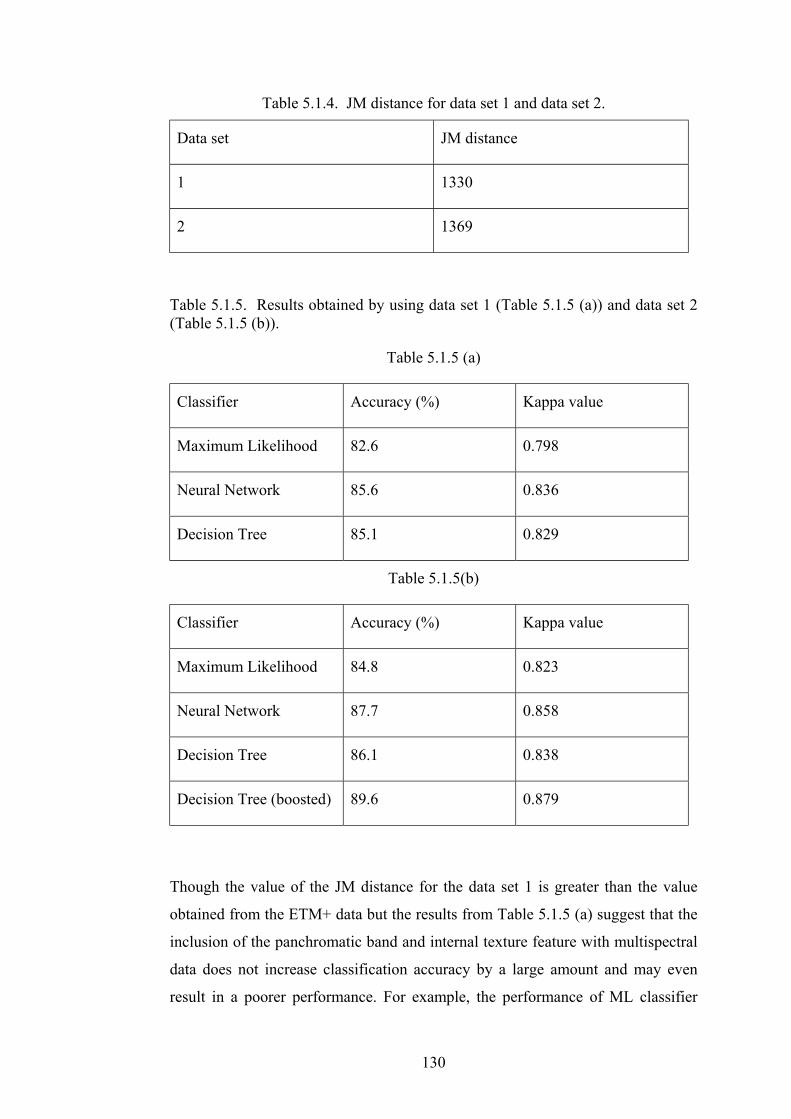
130
Table 5.1.4. JM distance for data set 1 and data set 2.
Data set JM distance
1 1330
2 1369
Table 5.1.5. Results obtained by using data set 1 (Table 5.1.5 (a)) and data set 2(Table 5.1.5 (b)).
Table 5.1.5 (a)
Classifier Accuracy (%) Kappa value
Maximum Likelihood 82.6 0.798
Neural Network 85.6 0.836
Decision Tree 85.1 0.829
Table 5.1.5(b)
Classifier Accuracy (%) Kappa value
Maximum Likelihood 84.8 0.823
Neural Network 87.7 0.858
Decision Tree 86.1 0.838
Decision Tree (boosted) 89.6 0.879
Though the value of the JM distance for the data set 1 is greater than the value
obtained from the ETM+ data but the results from Table 5.1.5 (a) suggest that the
inclusion of the panchromatic band and internal texture feature with multispectral
data does not increase classification accuracy by a large amount and may even
result in a poorer performance. For example, the performance of ML classifier

131
decreases by a small amount as compared to the results obtained by using
multispectral data alone. Otherwise, the results obtained from the neural and
decision tree classifiers improve by about one percent. Further, using data set 2
(Table 5.1.5(b)) gives the highest JM distance of 1369 but the classification
accuracies with all the three classification algorithms improve by about 1 to 2.5%,
thus suggesting the limited utility of panchromatic data and its texture for land
cover classification.
5.1.6 Conclusions
The main objective of the work reported in this section is to assess the utility of
decision tree classifiers for land cover classification. The specific objectives are to
study the behaviour of decision tree classifiers with changes in training data size,
different attribute selection measures, pruning methods, and boosting. The results
suggest several main conclusions. First, in spite of being non-parametric in nature,
the performance of the decision tree classifier is always affected by the size of the
training data set used. This study also concludes that it is the pruning method that
has the most significant effect on classification accuracy and not the attribute
selection measure, as suggested by some earlier studies. Boosting is found to
improve classification accuracy by about 3-4%. We can conclude that boosting is
a useful technique and should be used for crop classification problems using
remotely sensed data.
Studies carried out using maximum likelihood and neural classifiers for the same
data sets used with decision tree classifier show that the decision tree performs
better than the maximum likelihood classifier, while the performance of neural
classifier is better (but not significant in the statistical sense) than the unboosted
decision tree classifier for this type of data in crop classification studies. As
suggested by a number of earlier studies (Kavzoglu, 2001; Foody and Arora,
1997), the performance of a neural classifier depends on a number of user-
determined factors, and the training time is very large compared to that of the
decision tree classifier. Training time increases only slightly if boosting is used.
Inclusion of the ETM+ panchromatic band and its texture measures increases the
classification accuracy by about 1 to 2.5%.

132
5.2 Support vector machine classifiers
5.2.1 Introduction
Much research effort in the past ten years has been devoted to analysis of the
performance of artificial neural networks, particularly the feed-forward multi-
layer perceptron using back-propagation, due to their ability to handle any kind of
numerical data, and to their freedom from distributional assumptions (section
2.3.4.3). A number of studies have reported that uses of neural classifiers have
problems in setting various parameters during training. The choice of architecture
of the network, the sample size for training, choice of learning algorithms, and
number of iterations required for training are some of these problems. Within the
last few years, another nonparametric classification algorithm - the decision tree
classifier (chapter 3) has become more popular, due to its simplicity in use and
their performance, which is comparable and even better than neural classifiers.
Despite their simplicity in use, decision tree classifiers present some problems
which influence classification accuracy (section 3.9 and section 5.1.3).
This section gives the results of another recent development in classification
methodology, called support vector machines (SVM) using ETM+ data. Some of
the factors affecting support vector machines are discussed and the value of some
parameters affecting these classifier are suggested for this type of data.
5.2.2 Study area and methods
Details of the study area used in this part of the research are given in section 5.1.2.
As the main aim of this study is to compare the performance of decision tree,
neural network and SVM classifiers for land cover classification, the training and
testing data sets for the SVM classifier are the same as those used for the DT and
neural classifiers. To investigate the behaviour of the SVM classifier with the
variation in number of training patterns, seven training data set were used (section
5.1.3.1).

133
5.2.2.1 Effect of kernel choice
As discussed in section 3.12.3, in situations with non-linear decision surfaces,
support vector classifiers use a mapping to project the data in a higher
dimensional feature space, while to make computation simpler, the concept of the
kernel was introduced. A number of kernels are discussed in the literature, but it is
difficult to choose one which gives the best generalisation. In this study, five
different kernels are used in order to investigate the effect of kernel choice on
classification accuracy. Both the chosen kernel type and the values of other
parameters associated with these kernels affect the level of classification
accuracies. Another factor that affects the level of classification accuracy is the
choice of the value of the parameter C (section 3.12.2). After a number of trials,
the values of C used with various kernels are given in Table 5.2.1.
This comparison suggests that a value of C within the range 1000 to 5000 is
effective for this type of land cover classification study, depending on the type of
kernel used. Training time also increases as the value of C rises. The parameter
values found to be suitable for the various kernel functions are as follows:
• degree of polynomial = 5 for the polynomial kernel.
• γ = 2 for the radial basis function.
• b = 0.04 and c = 0.001 for the neural network.
Table 5.2.1. Values of parameter C with different kernels.
Kernel Parameter C
Polynomial 1000
Radial basis function 5000
Linear splines 10000
Simple dot product 5000
Neural network 5000
The classification accuracies achieved using the above values of C and the user-
defined parameters for different kernels are shown in Figure 5.2.1. For a

134
polynomial kernel, increasing the degree of the polynomial increases training time
but not the classification accuracy.
Figure 5.2.1 suggests that the radial basis and the linear splines perform equally
well and achieve the highest accuracy. The poor performance of the simple dot
product kernel function may be due to the fact that decision boundaries between
the classes may be non-linear. The reason of poor performance of neural network
kernel function may lie in the selection of appropriate values of the user defined
parameters, which is a topic that needs further study. The performance of the
polynomial function is comparable to that of the radial basis function. A radial
basis kernel function is used for the evaluations of SVM in the remainder of this
section.
Figure 5.2.1. Variation in classification accuracy with different kernel functions.
5.2.2.2 Training sample size
A support vector machine works on the principle of optimal separation of the
training data, if the classes are separable, the optimum solution hyperplane is that
which maximally separates the classes. The training of the SVM defines the
optimal hyperplanes and, in doing so, selects the data points which lie on or near
the class boundary closest to the neighbouring classes. It follows that by using

135
these pixels (the support vectors) for defining the decision surfaces, the use of a
very small number of training pixels can provide a good degree of generalisation.
To check this deduction, seven data sets containing 700, 1050, 1400, 1750, 2100,
2450 and 2700 training pixels in total, and a set of 2037 pixels was used for
testing the results of the SVM classifier. For all these data sets a "one against one"
multi-class technique and a radial basis kernel were used in generating SVM. The
accuracy of classification obtained using each data set is plotted in Figure 5.2.2
(confusion matrices are listed in appendix B).
Figure 5.2.2 suggests that classification accuracy increases as the number of
training patterns increases, thus indicating that SVM-based classification is
affected by training data size, in spite of the fact that this classification system
uses very few pixels to create decision surfaces. The probable reason for this
increase in classification accuracy with increasing number of training patterns
could be due to the quality of training pixels used, so that as the number of pixels
increases the system finds pixels that define better discriminating surfaces.
Figure 5.2.2. Variation in classification accuracy with change in training patterns.

136
5.2.2.3 Use of different multi-class methods
In this part of the study, two methods of generating multi-class support vector
machines are discussed, with respect to training time and classification accuracy.
Table 5.2.2 gives the classification accuracy as well as the training time taken
using SVM classifier from Royal Holloway College, University of London,
running on a Sun workstation.
The results shown in the Table 5.2.2 suggest that the time taken by using one
against the rest method is much higher than the one against one technique, thus
suggesting the use of one against one method for generating multi-class support
vector machines. Further, the accuracy obtained by using one against the rest
method is not as high as with the one against one method. One possible reason
could be unbalanced training data sizes in two classes while using the one against
the rest multi-class method and not finding suitable decision boundaries which
may affect the performance of classifier and affecting the final classification
accuracy.
Further studies carried out using the LIBSVM classifier using a one against one
multi-class technique suggests that this classifier takes only 0.30 CPU minutes to
train the SVM using 2700 training pixels and attains an accuracy of 87.9%
accuracy. Figure 5.2.3 shows a SVM classified image of the study area.
Table 5.2.2. Classification accuracy and training time using different SVMs anddifferent multi-class methods.
Multi-classmethod
Number oftraining pixels
Accuracy (%) Training time(CPU minutes)
700 76.19 6.09One against rest
2700 79.73 505.27
700 84.19 0.27One against one
2700 87.37 21.54
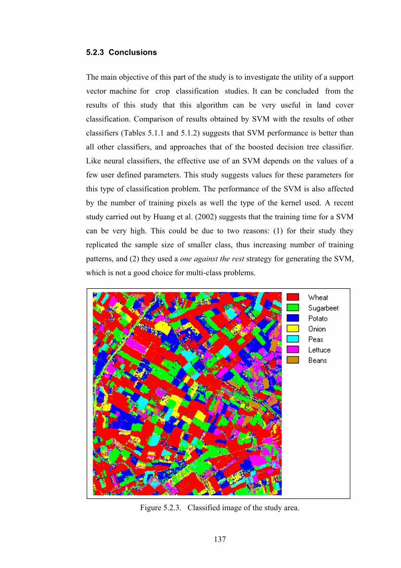
5.2.3 Conclusions
The main objective of this part of the study is to investigate the utility of a support
vector machine for crop classification studies. It can be concluded from the
results of this study that this algorithm can be very useful in land cover
classification. Comparison of results obtained by SVM with the results of other
classifiers (Tables 5.1.1 and 5.1.2) suggests that SVM performance is better than
all other classifiers, and approaches that of the boosted decision tree classifier.
Like neural classifiers, the effective use of an SVM depends on the values of a
few user defined parameters. This study suggests values for these parameters for
this type of classification problem. The performance of the SVM is also affected
by the number of training pixels as well the type of the kernel used. A recent
study carried out by Huang et al. (2002) suggests that the training time for a SVM
can be very high. This could be due to two reasons: (1) for their study they
replicated the sample size of smaller class, thus increasing number of training
patterns, and (2) they used a one against the rest strategy for generating the SVM,
which is not a good choice for multi-class problems.
137
Figure 5.2.3. Classified image of the study area.

This study also suggests that training time taken by SVM generated by using
one against one technique is far less than that with the one against the rest
strategy used by Huang et al. (2002). Even the performance of SVM by using one
against the rest is found to be very poor as compared to that with one against one
multi-class strategy. Further, a probable reason for the small training time using
LIBSVM could be the use of a good optimisation strategy to solve the QP
optimisation problem.
1.
2.
•
•
•
3.
4.
Decision tree classifier performance is affected by the choice of
pruning method to be used, while the performance of a neural
classifier is affected by several user defined parameters.
Performance of decision tree classifiers, both univariate and
multivariate, is affected by number of training patterns used:
Accuracy of a univariate decision tree classifier varies from 78.3%
to 84.1% when training data size varies from 100 pixels/class to 300
pixels/class. Further addition of training data has no significant
change in classification accuracy.
Multivariate decision tree classifier accuracy changes from 78.15 %
to 82.72% as data size changes from 100 pixels/class to 250
pixels/class.
Univariate decision trees perform as well as or better than the
multivariate classifier with this type of data.
Performance of a DT classifier is better than that of a maximum
likelihood classifier, while neural classifier performed better than
a univariate decision tree classifier.
Boosting a decision tree gives a significant improvement in
classification accuracy as compared to neural classifier.
138

5.
6.
•
•
•
•
7.
8.
9.
Training time of a univariate decision tree classifier is quite
small, even after applying boosting, in comparison with neural
classifier.
Performance of SVM is affected by several factors such as:
Choice of kernel
Choice of multi-class method used
Parameters for a particular kernel
Parameter C
SVM perform significantly better than decision tree and neural
classifier, even with very small training datasets.
Training time for SVM is small, even comparable with the
training time taken by the boosted decision tree classifier, if the
one against one technique is used to generate multi-class output.
The one against the rest technique is not suitable to generate
multi-class outputs.
139
140
Chapter 6
Crop Classification Using INSAR Data
6.1 Introduction
The ERS-1/2 SAR is a coherent sensor measuring both the magnitude and phase
of the backscattered signal. It operates at 5.3 GHz, vv-polarisation, at incidence
angles between 20 and 26 degrees, with a swath of 100 km and with a repeat cycle
of 35 days. Traditionally, only the backscatter intensity was interpreted. Now, by
means of SAR interferometry, the phase component has proven to be a very
valuable source of information. More recently, it has been demonstrated (Askne
and Hagberg, 1993; Wegmueller and Werner, 1994, 1995, 1996, 1997) that the
coherence component (which is a measure of accuracy of estimation of
interferometric phase) derived by using phase information from an interferometric
image pair gives useful information that can be used effectively for land cover
classification.
In this chapter, a classification scheme using both intensity and coherence
information derived from INSAR data is developed. In order to evaluate the
capability of SAR intensity and coherence images to discriminate between
agricultural crops, the classification experiments reported in this study are carried
out by using statistical, neural and decision tree classifiers. In particular, the
usefulness of texture features derived by using GLCM, the MAR model, and
fractal geometry from the intensity and coherence images for land cover
classification is also studied. The limitations of tandem and 35-day repeat-pass
interferometry for this application are also discussed.
6.2 Description of study area
The study area is located near Littleport, Ely Cambridgeshire, in the eastern part
of England. This area is close to sea level and the agriculture of the region is
characterised by the use of rotational crop planting techniques. Five SLC images,
from 2nd May to 20th September 1996, are selected for land cover classification.

141
Since the main purpose of this study is crop discrimination, it is necessary to
ensure that the selected images cover the entire crop growing period, which helps
to identify various crops during their growth period. After a detailed study of the
cropping pattern of the area, the SLC images listed in Table 4.1 were selected. As
mentioned in sections 4.5.2.3 and 4.5.2.4, one coherence and five intensity images
and an area of interest covering 286 pixels (columns) and 386 pixels (rows) was
used for further studies.
6.3 Ground reference image generation
The purpose of generating a ground reference image is to allow the collection of
pixels for training and testing the classifiers. Before creating a ground reference
image, field boundaries should first be defined. If no map reference data are
available, image segmentation can be used to identify the field boundaries. In this
study, the field boundaries were generated through on screen digitisation of
images. Reference data for the crop types in the year 1996 were collected from
farmers. On the basis of examination of the areas covered by each crop and the
geographical scale of the study, seven cover categories were selected. These are:
potatoes, sugar beet, wheat, barley, carrot, onions and peas. The field boundaries
were digitised using ARC-INFO software, by using a colour composite of
all the five intensity images generated by interferometric processing. The
field boundary file was transformed from arc into polygon format by applying a
buffering operation of 1 pixel width so as to remove the boundary pixels during
the classification process. This polygon file is then used to assign a unique label to
each of the polygons according to the crop type associated with that parcel. By
using the crop map, digital identifiers from “1” to “7” (each number represents a
particular class as shown in the Table 6.1) are assigned to the corresponding
fields. The digital identifier “0” is assigned to the unknown fields. The final
ground reference image is shown in Figure 6.1, which also shows the colours used
to represent each crop.

Table 6. 1. Crops being used for classification with digital numbers in referenceimage.
Digital Number Crop type1 Barley2 Wheat3 Sugar Beet4 Potato5 Onion6 Peas7 Carrot
142
Figure 6. 1. Ground reference image of the study area.

143
6.4 Feature extraction and selection
Methods to generate features based on combinations or transformations of
primary features are called feature extraction methods. Image derived features,
such as measures of spatial and spectral features, may provide useful information
for classification. Some features obtained by transforming primary features tend
to suppress undesirable variability in remote sensing signatures, such as noise, so
it is wise to use such features in classification because they allow the classifier to
better distinguish spectral classes.
Spectral and spatial features are not independent. They always simultaneously
exist in the image, although sometimes one will dominate the other, depending on
how fine or how rough the object is. Spectral features describe average tonal
variation, whilst spatial features reflect the spatial distribution of tonal variation.
Generally the words texture and context are used to represent this form of spatial
relationship in tonal variation. Texture features contain information about the
spatial distribution of tonal variations within a band while contextual features
contain information derived from blocks of image data surrounding the area being
analysed.
The concept of tone is based on the varying shades of the grey of the resolution
cells making up an image and the texture is concerned with the spatial distribution
of grey tones. Texture and tone are not independent concepts; rather, they bear a
very close relationship to one another. Texture is a natural property of objects. It
contains important information about the structural arrangement of surfaces and
their relationship to the surrounding environment.
A number of methods have been developed to deal with spectral and spatial
information, in order to achieve improved classification performance. In
comparison with tonal measures, the definition of texture features appears more
difficult. The main difficulty faced by the researcher is to define a set of
meaningful features to characterise texture properties.
Based on the texture descriptors available in the literature, four approaches are
used in this study. The first approach uses the grey-level co-occurrence matrix
(Haralick et al., 1973). The second approach uses the features derived from local

144
statistics. The third approach is based on the fractal geometry of the image (Sarkar
and Chaudhuri, 1994), and the fourth approach is based on the multiplicative
autoregressive random field model (Frankot and Chellapa, 1987).
6.5 Grey Level Co-occurrence Matrix (GLCM)
This section describes texture feature extraction based on the Grey Level Co-
occurrence Matrix (GLCM), or the grey-tone spatial-dependency matrix. A co-
occurrence matrix for an image region contains partial second order statistical
information about the image pixel intensities. When generating a co-occurrence
matrix, it is assumed that the intensity distribution is in a wide sense stationary
over a region of uniform texture. The main concept of the GLCM is that the
texture information contained in an image is defined by the adjacency
relationships that the grey tones in an image have to one another. In other words,
it is assumed that the texture information is specified by values d
ijf within the
matrix, where dijf denotes the frequency of occurrence of two cells of grey tone i
and j respectively separated by distance d with a specific direction on the image.
Values of dijf can be calculated by any direction and distance d inside the image
but only four directions corresponding to angles 00 , 045 , 090 , and 0135 are
generally used.
The appropriate frequency normalisation for each cell inside the matrices are
easily computed. For the horizontal direction process, with d = 1 and angle equals
to 00 , and the if the image to be analysed has C
N resolution cells in the horizontal
direction (number of columns) and R
N resolution cells in the vertical direction
(number of rows), there will be 2× (C
N – 1) neighbouring resolution cell pairs in
each row. As a result, the total number of nearest horizontal neighbour pairs can
be obtained by the expression 2× (C
N – 1) ×C
N . When the relationship between the
cells is nearest right-diagonal neighbour, with d=1 and angle = 045 , there will be
2(C
N -1) 045 neighbouring resolution cell pairs for each row except the first, for
which there are none. This provides a total of 2(C
N -1)( R
N -1) nearest right-

145
diagonal neighbour pairs. By symmetry there will be 2(R
N -1)C
N nearest
neighbour pairs for the vertical direction and 2(R
N -1)(C
N -1) nearest left-diagonal
neighbour pairs. For the right-diagonal direction, by symmetry, the number of
nearest pairs is the same as left diagonal. After the total number of neighbouring
resolution cell pairs used in computing a particular GLCM has been obtained, the
matrix is normalised by dividing each cell in the matrix by the total number of
pairs. Figure 6.2 shows a generated GLCM for a small image segment.
Figure 6. 2. (a) A 3×3 image with three grey levels; (b)-(e) GLCM for angles ofangles 00 , 045 , 090 , and 0135 respectively.
1 1 2
2 0 2
0 1 1(a)
2 0 10 0 21 2 0
(c)
0 2 02 0 20 2 0
(e)
0 1 21 4 12 1 0
(b)
0 2 12 0 21 2 2
(d)

146
6.5.1 Texture extraction from GLCM
If the texture contained in an image is coarse, and the measured distance d is
relatively small in comparison with texture structure, the neighbouring pairs being
measured should have very similar grey levels. As a result, the joint neighbouring
pair distribution within the GLCM will produce higher values concentrated
around its left diagonal direction (i.e. cells (i, j), i = j). Conversely, for a fine
texture, if the measured distance d is comparable to the texture structure or is
relatively large in scale, the grey level of points separated by distance d will be
quite different. Therefore, the values in the GLCM should be spread out more
uniformly.
Haralick et. al. (1973) proposed fourteen texture measures based on the GLCM.
These texture measures, called textural features, are found to be very useful for
image classification. Some of these measures relate to specific textural
characteristics of the image such as homogeneity, contrast, and the presence of
organised structure within the image. Other measures characterise the complexity
and nature of gray level transitions which occur in the image. In this study, five
indices are used as texture measures obtained from coherence and intensity
images. In what follows, g(i, j) denotes the (i, j)th entry in a normalised GLCM,
and gN denotes number of distinct grey levels in the quantised image. The
selected texture methods are:
(1) Angular Second Moment (ASM):
ASM = ( )[ ]∑∑i j
jig2
, (6.1)
The measure is smallest when the g(i, j) are all as equal as possible and is largest
when some values are high and others low, e.g., when the values are concentrated
near the origin. This parameter measures the homogeneity of the image.

147
(2) Contrast (Con):
Con = ( )∑ ∑∑−
= = =
1
0 1 1
2 ,g g gN
n
N
i
N
j
jign (6.2)
This is the second moment of g(i, j), i.e., its moment of inertia about the origin.
This is a measure of the contrast or the amount of local variation present in an
image.
(3) Correlation (Cor):
Cor =
( ) ( )
yx
i jyxjigji
σσ
µµ∑∑ −,,
(6.3)
where xµ and xσ are the means and standard deviations of the rows of GLCM,
and yµ and yσ are means and standard deviations of the columns. This feature is
used to reflect the degree to which the rows or columns resemble each other. It is
high when the values are uniformly distributed in the GLCM matrix, and low
otherwise, e.g., when the values off the diagonal are small. This is a measure of
gray-tone linear dependencies in the image.
(4) Inverse Different Moment (IDM):
IDM = ( )
( )jigji
i j
,1
12∑∑ −+
(6.4)
This measure will generate higher values for an image having large homogenous
patches because such an image will show high values on the main diagonal of the
GLCM. It gives lower weight to those elements g(i, j) that are away from the main
diagonal.
(5) Entropy (Ent):
Ent = ( ) ( )( )∑∑−i j
jigjig ,log, (6.5)
148
This measure is largest for equal g(i, j) and small when the values of g(i, j) are
very unequal.
6.5.2 Feature based on local statistics
Only one feature, “variance”, is calculated based on local statistics. It can be
calculated from the following formula using a moving window:
Variance = ( )
1
2
−
−∑n
DNij µ (6.6)
where ijDN represents the DN value of pixel at position (i, j), n is the number of
pixels in a moving window and µ represents the mean of the moving window,
which is calculated from:
nDNij∑=µ .
6.6 Fractal dimension
Simple objects can be described by the ideal shapes such as cubes, cones and
cylinders, but most natural objects are complex and so they can not be described
by these simple shapes. Hence, the concept of self-similarity found an important
role in the description of nature. When each piece of a shape is geometrically
similar to the whole, that is, when an object is composed of copies of itself and
each copy is scaled down by the same ratio in all directions from the whole, both
the shape and the cascading process that generates it are said to be self-similar.
The complex and erratic shape description in term of self-similarity was
introduced by Mandelbrot (1983), who proposed the fractal geometry of nature
and defined a fractal as"… a shape made of parts similar to the whole in some
way" (Mandelbrot, 1986, p. 8). One of the most important properties of fractals is
scaling. Mandelbrot (1983) defined scaling to mean invariance under certain
transformations of scale.

149
Self-similarity is manifested in two ways: it can be exact or statistical. The
concept of exact self-similarity is defined as follows: if one were to take a portion
of the perimeter of an object and look at it under a microscope, the magnified
portion would look exactly the same as the original large part of the boundary.
Objects in nature rarely exhibit such exact self-similarity. Nevertheless, they do
often posses a related property, statistical self-similarity. Statistical self-similarity
means that upon magnification a small portion of an objects looks very much like,
but never exactly like, the configurations at other scales. The simplest example of
statistically self-similar fractals is a coastline.
An important concept in fractal geometry is fractal dimension. In the Euclidean
universe, the dimension of an object is defined as the number of distinct
coordinates needed to specify a position on or within the object. A point object
has zero dimension; a line, whether straight or curved, has one dimension. Any
point on the line can be represented by a single parameter. However, this
definition of dimension is not satisfactory for a proper understanding of
irregularity or fragmentation in nature. The fractal concept provides a more
appropriate mathematical framework to study the irregular, complex shapes found
in nature. Fractal geometry has had a major impact in modelling and analysis in
the natural and physical sciences.
Two important types of dimension are commonly used in fractal research: the
topological dimension and the fractional dimension (D) (Xia and Clarke, 1997).
The topological dimension is always an integer and coincides with the intuitive
dimension in Euclidean geometry. The notion of a fractional dimension was
introduced by Hausdorff (1919) in order to put a size to a highly irregular non-
rectifiable sets. Thus the fractional dimension is sometimes called the "Hausdorff
dimension" or "Hausdorff-Besicovitch dimension". The Hausdorff-Besicovitch
dimensions of all cases studied in fractal geometry are greater than their
topological dimensions. In order to emphasise the fact that a fractal may also have
an integer dimension and to avoid the confusion of Hausdorff-Besicovitch
dimension with the dimension of the Hausdorff topological space, Mandelbrot
(1983, p. 15-17) proposed to call D the fractal dimension. On the other hand, most
people continue using the terms fractional dimension, Hausdorff dimension,
Hausdorff-Besicovitch dimension and fractal dimension interchangeably. The
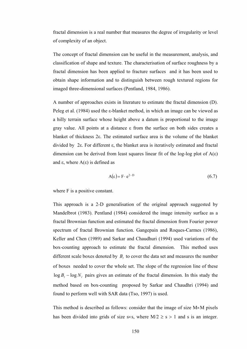
150
fractal dimension is a real number that measures the degree of irregularity or level
of complexity of an object.
The concept of fractal dimension can be useful in the measurement, analysis, and
classification of shape and texture. The characterisation of surface roughness by a
fractal dimension has been applied to fracture surfaces and it has been used to
obtain shape information and to distinguish between rough textured regions for
imaged three-dimensional surfaces (Pentland, 1984, 1986).
A number of approaches exists in literature to estimate the fractal dimension (D).
Peleg et al. (1984) used the ε-blanket method, in which an image can be viewed as
a hilly terrain surface whose height above a datum is proportional to the image
gray value. All points at a distance ε from the surface on both sides creates a
blanket of thickness 2ε. The estimated surface area is the volume of the blanket
divided by 2ε. For different ε, the blanket area is iteratively estimated and fractal
dimension can be derived from least squares linear fit of the log-log plot of A(ε)
and ε, where A(ε) is defined as
( ) D2eFA −⋅=ε (6.7)
where F is a positive constant.
This approach is a 2-D generalisation of the original approach suggested by
Mandelbrot (1983). Pentland (1984) considered the image intensity surface as a
fractal Brownian function and estimated the fractal dimension from Fourier power
spectrum of fractal Brownian function. Gangepain and Roques-Carmes (1986),
Keller and Chen (1989) and Sarkar and Chaudhuri (1994) used variations of the
box-counting approach to estimate the fractal dimension. This method uses
different scale boxes denoted by lB to cover the data set and measures the number
of boxes needed to cover the whole set. The slope of the regression line of these
ll NB loglog − pairs gives an estimate of the fractal dimension. In this study the
method based on box-counting proposed by Sarkar and Chaudhri (1994) and
found to perform well with SAR data (Tso, 1997) is used.
This method is described as follows: consider that the image of size M×M pixels
has been divided into grids of size s×s, where M/2 ≥ s > 1 and s is an integer.

151
Consider the image as a 3D surface with (x, y) denoting 2-D position and the third
co-ordinate (z) being grey level. The (x, y) space is divided into grids of size s×s.
Thus for each grid there is a column of boxes of size 'sss ×× , where s can be a
multiple of the side length of a pixel in (x, y) and 's can be a multiple of the grey
level in z-direction. If the total number of grey level is G then 's is calculated
from the expression
=
sM
sG
' (6.8)
where symbol indicates the integer part of the argument.
Assign the numbers 1, 2, …., n in turn to each box in the column from bottom to
top. Let the minimum and maximum grey level of the image on the (i, j)th grid
fall in boxes number p and k, respectively. Then the number of boxes needed to
cover the surface on the (i, j)th grid is
( ) =j,inr = p – k + 1 (6.9)
where
r = s/M
Because of the differential nature of computing rn , this method is called
differential box-counting approach. After taking contributions from all grids, the
total number of boxes needed to cover the whole image with box size 'sss ×× is
( )∑=j,i
rr j,inN (6.10)
rN is counted for different values of s. The fractal dimension D is estimated from
the least square linear fit of log ( rN ) against log (1/r). This method is
computationally efficient and counting rN in this manner gives a better
approximation to the boxes intersecting the image intensity surface when there is
sharp grey level variation in neighbouring pixels in the images.

152
6.7 Multiplicative Autoregressive Random Field (MAR) model
Research carried out to study the behaviour of the radar returns have found that
radar returns are corrupted by speckle (Ulaby, 1980). Thus, the use of lognormal
models for radar have been suggested for homomorphic filtering to separate
multiplicative illumination and reflective components (Stockham, 1972).
Frankot and Chellapa (1987) proposed the gaussian autoregressive random field
models for the logarithm of radar image intensity in two dimensions, which they
called the lognormal multiplicative autoregressive (MAR) model and suggested
that these models are useful for estimating spatial correlation structures which,
together with the image intensity distribution model, fits a variety of radar
imagery. Initially, the MAR concept was originally used to model image data,
and the parameters of the model have been found to be highly correlated with the
spatial distribution of image intensities. For this reason, they can be used as a
texture descriptors for image classification (Solberg and Jain, 1997; Tso, 1997).
Lognormal random fields with multiplicative spatial interaction are a special case
of the gaussian autoregressive random fields.
Let an image p(s), Ω∈s , with size M×M, be represented by the following white-
noise-driven multiplicative system:
( ) ( )[ ] ( )∏∈
θ ⋅+=Nr
svrspsp r (6.11)
where Ω = 0, 1, . . . ., M-1×0, 1, . . .., M-1, N is the neighbourhood set
defining model support (i.e., the number and location of pixels contributing to the
central pixel, as shown in Figure 6.3, v(s) is a lognormal white-noise process
referred to as the driving process, rθ is an exponent weighting factor for
neighbourhood r, and s = (m, n), a 2-D index to an image.
The random field p(s) is said to obey a lognormal MAR model if q(s) = ln p(s)
obeys the following gaussian autoregressive random field model with w(s) = ln
v(s):
( ) ( )∑∈
++⋅θ=Nr
r )s(wrsqsq (6.12)

153
where w(s) is zero mean white gaussian noise. The covariance of w(s) is given by
( ) =rcovw
σ ,
,0
2w
( )
( )0,0r
0,0r
=
≠
where wσ denotes the variance of w.
6.7.1 Estimation of parameters in the MAR model
The parameters of the MAR model, the neighbourhood weighting parameter
vector θ, the noise variance 2wσ , and the mean value qm of the stationary random
process q are estimated for each image, using a least squares estimation method
(Kashyap and Chellappa, 1983) and used as texture features. The neighbourhood
N = (0,-1), (-1,-1), (-1,0) is used to compute these three parameters (Figure 6.3).
Figure 6. 3. Neighbourhood supp
For MAR models, the least squares estimates ba
Covariance:
( )[s
Tq
2
2w msq
M
1∑Ω∈
θ−−=σ
where
( ) ( ) ( )(
⋅=θ ∑∑
Ω∈
−
Ω∈ s
1
s
T szszsz
N= (0,1), (-1,-1), (-1,0)
(-1,-1) (-1,0)(0,-1) (i,j)
ort of central pixel.
sed on p(s) are as:
( ) ] 2sz (6.13)
( ) )
− qmsq

154
while mean is defined as:
( )∑Ω∈
=s2
q sqM
1m (6.14)
where
( ) =sz ( ) qmrsq −+ , Nr∈
6.8 Feature selection
In real-world situations, all features relevant to the classification of an object are
often unknown a priori. Therefore, a number of candidate features are often
introduced to better represent the image classification problem. Unfortunately,
many of these features are either partially or completely irrelevant or redundant
for the problem concerned. A relevant feature is neither irrelevant nor redundant
while an irrelevant feature does not affect the results in any way, and a redundant
feature does not add anything new to the results. In many applications, the size of
a dataset is so large that learning might not work well unless these unwanted
features are removed. Reducing the number of irrelevant/redundant features
drastically reduces the running time of a learning algorithm as well as increasing
its effectiveness. Feature selection methods try to pick a subset of features that are
relevant to the problem.
A basic problem in pattern classification is to determine which features should be
employed for minimum error and maximum efficiency in classification. A large
number of pattern classification problems involve classification of patterns into
one of a set of classes, which are defined only by a limited number of labelled
representative patterns (which are pixel vectors in remote sensing). Feature
extraction can be viewed as finding a set of vectors that adequately represent an
observation but in a lower dimensional feature space. In pattern recognition, it is
desirable to extract features that have the highest discriminating power between
classes. Although a reduction in dimensionality is desirable, the error resulting
from the reduction in dimension has to be acceptably low. The development of

155
feature extraction methods has been a prominent research area in the field of
pattern analysis.
Feature selection is defined by many authors by looking at the problem from
various angles. But, as expected, many of the solutions are similar in intuition
and/or content. The following are some of the definitions those are conceptually
different and cover a range of definitions.
1. Idealised: find the minimally sized feature subset that is necessary and
sufficient to the target concept (Kira and Rendell, 1992).
2. Classical: select a subset of M features from a set of N features, M < N,
such that the value of a criterion function is optimised over all subsets of
size M (Narendra and Fukunaga, 1977).
3. Improving prediction accuracy: the aim of feature selection is to choose a
subset of features for improving prediction accuracy or decreasing the size
of the structure without significantly decreasing prediction accuracy of the
classifier built using only the selected features (Koller and Sahami, 1996).
4. Approximating original class distribution: the goal of feature selection is to
select a small subset such that the resulting class distribution, given only
the values for the selected features, is as close as possible to the original
class distribution given all feature values (Koller and Sahami, 1996).
The third definition emphasises the prediction accuracy of a classifier, using only
the selected features, whereas the last definition emphasises the class distribution
given the training data set. These two approaches are quite different conceptually.
Feature selection is a difficult task in classification because it is both dependent
on the input data and on the classifier used. The quality of a feature is measured
by its relevance, discriminative power, and ease of computation. Additionally, by
excluding redundant, irrelevant, or inconsistent features from the training set,
higher accuracy on an independent validation dataset can often be achieved.
The problem of feature selection is defined as follows: given a set of candidate
features, select a subset that performs best (according to some criterion) under

156
some classification system. This procedure can reduce both the cost of
classification by reducing the number of features that need to be collected and, in
some cases it can provide a higher classification accuracy due to finite sample size
effects. The term "feature selection" is taken to refer to algorithms that output a
subset of the input feature set. The procedure of feature selection must be based
on two components. First, a criterion must be defined by which it is possible to
judge the performance of each feature. Second, a systematic procedure must be
found for searching through candidate subsets of features. In principle, the feature
selection criterion should be the same as that used to assess the misclassification
rate for a image classification problem. Similarly, the search procedure could
simply consist of an exhaustive search for all possible subsets of features since
this is, in general, the only approach that is guaranteed to find the optimal subset.
In a practical application, however, a simplified selection criterion as well as a
non-exhaustive search procedure is used in order to limit the computational
complexity of the search procedure. A number of studies of feature selection
methods have been carried out in image classification (Jain and Zongker, 1997;
Kavzoglu, 2001). In this study, following Kavzoglu's (2001) guidelines,
Hotelling’s 2T statistical method is used to determine the best three texture
features out of the ten features of each intensity and coherence image.
6.8.1 Hotelling’s 2T
Several multivariate statistical techniques can be used to determine the degree of
discrimination between the classes present in a given dataset, by using the means
and co-variance matrices of the classes. Hotelling’s 2T statistic (Hotelling, 1931)
is one of the most popular statistical tests to estimate the discriminating power of
a feature or relative importance of a feature.
Hotelling’s 2T statistic is used to test the null hypothesis that the (population)
multivariate means of the two groups under study do not differ significantly. It
provides a multivariate generalisation of the Student’s t test and is related to the
problem of how best to discriminate between two groups. 2T is calculated from:

157
2
21
212 D.nn
nnT
+= (6.15)
( ) ( )211T
212 mmmmD −−= ∑ −
where 2D is the measure known as Mahalanobis’ D-squared, which measures the
overall similarity between the two groups. ∑ −1 is the inverse matrix of the
pooled co-variance matrix ∑ , and 1m and 2m are the mean vectors for the
groups, which contain 1n and 2n individuals, respectively.
The value of Hotelling’s 2T increases as inter-class separation increases. The
statistical significance of 2T can be evaluated using a transformation to the F
distribution. It should be noted that the number of observations need not be the
same for the two samples, but the number of features must be the same.
Hotelling’s 2T is used to identify only three best texture features for each image
(five intensity images and one coherence image) to be used for land cover
classification. For intensity and coherence images, nine texture features, including
five grey-level co-occurance features (asm, con, crr, ent and idm), two features
from the MAR model (markov mean and covariance), one feature calculated from
fractal geometry and one feature from first order statistics (variance) are used for
feature selection. With intensity images, the four best features selected for use in
further classification are the fractal dimension, the intensity image itself, contrast
from GLCM and variance from first order statistics. For the coherence image, the
four features selected are coherence, markov mean, plus correlation and entropy
from GLCM (Table 6.2).
6.9 Classification results and discussion
6.9.1 Results
Extensive experiments were carried out in order to test the performance of
classifiers using intensity images, the coherence image, and the texture features
derived from these, for crop classification. In order to achieve a comprehensive

158
analysis, different data types derived from the original intensity and coherence
images are included in the experimental process. Besides using the median-
filtered intensity and coherence images, other data sets used in this study include
texture features derived from coherence and intensity images based on GLCM,
local statistics, the MAR model and the fractal models. For each intensity and
coherence image, five features from GLCM, one feature from local statistics, two
features from the Markov autoregressive model and one feature from the fractal
model are derived (discussed in section 6.7). As the number of features becomes
large, a feature selection method is used to reduce the dimensionalty of the data
used for classification. For this study the different data sets used for classification
are:
1. All five median filtered intensity images.
2. A combination of filtered coherence image with all five intensity images.
3. Coherence, one intensity image obtained from 02 and 03 May 1996
(tandem pair of SLC) and the difference between the two intensity images
obtained from this pair.
4. A combination of the coherence image and its three best texture features
with all five median-filtered intensity images.
5. A combination of the coherence image and five intensity images with the
two best texture features for each of the coherence and intensity images.
6. All five intensity images in combination with the texture features of all
these five intensity images.
7. The coherence image, all five intensity images, and the three best texture
features for each of the coherence and intensity images.
Three different classifiers (maximum likelihood, neural network and decision
tree) were used. The user-defined parameters (section 2.3.4.3) for the neural
network are set according to the recommendations made by Kavzuglu (2001). The
best three texture features used to recognise land cover classes in the classification

159
process and obtained by employing the Hotelling’s 2T statistic are shown in
Table 6.2.
Table 6. 2. Various features obtained by applying Hotelling’s 2T featureselection method and used in final classification process.
Image Features selected Hotelling’s 2T
value
Coherence image Correlation and entropy from GLCM
and MAR mean
709.15
Intensity images Variance from local statistics, contrast
from GLCM and fractal dimension
476.18
Random sampling was used to collect the training and test pixels from the ground
reference image for all datasets. These pixels were divided into two subsets, one
for training and one for testing the classifiers, so as to remove any bias resulting
from the use of the same set of pixels during training and testing. The number of
observations to be used in training the classifiers should be enough so as to assure
that each class is properly sampled and the analysis performed for accuracy
assessment is statistically valid. Mather (1999) recommend that to generate a
representative training sample for the statistical classifier (multivariate case), there
should be at least 30 training pixels for each features per class, and preferably
more. In this study, different numbers of training data for every combination of
features were used to examine the above requirement. The same number of
training and test pixels was used for all the three classifiers.
To analyse the results, confusion matrices were generated using the three
classifiers for each of the combinations listed above. Overall classification
accuracy (in percentage) and Kappa coefficients are shown in Table 6.3. Figure
6.4 shows the classified images using coherence with five intensity images and
three best texture features for each, using neural and decision tree classifiers
respectively. The confusion matrices are listed in appendix C.

160
Table 6. 3. Total classification accuracies for different data sets used in theclassification process. Table 6.3(a) is for maximum likelihood, Table 6.3 (b) forthe neural network and Table 6.3(c) for decision tree classifier.
Table 6.3(a)
Data sets used Number offeatures
OverallClassification
accuracy
Kappa value
1 5 59.2 0.5242 6 68.7 0.6353 3 49.7 0.4134 9 70.6 0.6575 18 78.0 0.7446 20 68.7 0.6347 24 77.1 0.733
Table 6.3(b)
Data sets used Number offeatures
Overallclassification
accuracy
Kappa value
1 5 60.8 0.5722 6 69.7 0.6643 3 30.5 0.2794 9 73.7 0.7055 18 79.1 0.7656 20 73.1 0.7017 24 82.9 0.805
Table 6.3(c)
Data sets used Number offeatures
Overallclassification
accuracy
Kappa value
1 5 69.9 0.6502 6 77.8 0.7413 3 47.4 0.3904 9 77.9 0.7425 18 80.2 0.7696 20 78.6 0.7507 24 82.7 0.797

161
6.9.2 Discussion
Comparison of the results shown in Table 6.3 (data sets 1 and 2) suggests that the
inclusion of coherence information with the intensity images results in a
substantial improvement in overall classification accuracy for all of the three
classifiers used. The increase in accuracy with the maximum likelihood classifier
is from 59.2% to 68.7% (Kappa value 0.524 to 0.635), for the neural classifier the
increase is from 60.8% to 69.7% (Kappa value 0.572 to 0.664), while the overall
accuracies from the decision tree classifier rises from 69.9% to 77.8% (Kappa
value 0.65 to 0.741). There is an increase of about 8-9% in accuracy when
coherence information is added, irrespective of the classifier used. Wegmuller and
Werner (1994) found that the combination of coherence, one intensity and the
difference of intensity images obtained by interferometric processing of a tandem
pair to be very promising for land cover classification studies, so we carried out
classification using this combination also (data set 3). This combination performs
badly for this particular land cover classification problem. It gives a maximum
accuracy of 49.7% using a decision tree classifier, a result that is far lower than
the accuracy obtained with data set 1.
Evaluation of the results presented so far in this study suggests that the decision
tree classifier performs better than either the maximum likelihood or the neural
classifiers. It gives a considerable increase in accuracy (of about 10%) as
compared to both of the other classification systems with data sets 1 and 2.
The study further suggests that the inclusion of texture measures helps to improve
classification accuracy. A total of nine features per intensity and coherence image
was extracted using GLCM (five features), MAR model (two features), the
variance based on first order statistics, and the fractal model (one feature) making
a total of sixty features. It is necessary to apply feature selection so as to reduce
the dimensionality of the input feature space and to overcome the problem of
dimensionality (Hughes, 1968). For this study, the three best texture features are
selected for each intensity and coherence image. Initially, data set 4, which
includes texture features obtained from the coherence image, was used for
classification. The results suggests that an improvement of 4% in classification
accuracy is achieved by using the neural network classifier as compared to data

(a)
(b)
162
Figure 6. 4. Classified images of data set 7 using (a) decision tree classifier and(b) with neural classifier.

163
set 2, while use of the maximum likelihood and the decision tree classifiers
suggests no major improvement in classification accuracy.
When all five intensity images with their associated texture features (data set 6)
are used, a significant improvement in classification accuracy is shown as
compared to the data set 1. Classification accuracy increases by an amount
ranging from 8.7% to 12.3% depending on the classifier used, suggesting the
importance of texture features with InSAR intensity images in land cover
classification. Further studies were carried out after adding the coherence and its
texture features with dataset 6 (data set 7). An increase of between 4 and 9% in
classification accuracy as compared to data set 6 suggests that the coherence
image provides discriminating information about the land surface and can be used
effectively for land cover classification in combination with intensity images
obtained from interferometric SAR data. The highest accuracy obtained by this
combination (data set 7) is 82.9% with a neural classifier, which is slightly higher
than the overall accuracy of the decision tree classifier (82.7%). Another study
using data set 5 was carried out, using only two texture features per coherence and
intensity image. The results in Table 6.3 suggest that the accuracy reached by this
combination is not comparable to the performance of data set 7. The highest
accuracy of 80.2% was achieved by the decision tree classifier, but the accuracy is
still less than the highest accuracy achieved with data set 7.
6.10 Conclusions
A number of combinations of data sets derived from interferometric SAR
intensity and coherence images have been evaluated for crop discrimination. The
results obtained from seven different datasets (Table 6.3) shows that the use of the
coherence image in combination with the intensity images provides additional
discriminating power in land cover classification studies. The performance of
dataset 3 was found to be the worst among the different combination tested, which
contrasts with the results for land cover classification reported by Wegmuller and
Werner (1997). The highest accuracy obtained is about 82.9% while using 24
features, justifying the importance of the texture features, as suggested by

earlier work by Dutra and Huber (1999). However, in practice, one often
encounters the so-called dimensionality problem, i.e., with a fixed relatively small
sample size, the classification accuracy may actually decrease when the number of
features is increased (Hughes, 1968). This means that the use of a larger number
of features requires a corresponding increase in the number of training samples, so
that the results obtained are reliable.
It has also been found that decision tree classifier achieves better results (in terms
of overall accuracy) than the statistical and neural classifiers in almost all cases,
except with dataset 7, where the overall classification accuracy achieved with a
decision tree classifier is slightly less than that of the neural classifier. The same
number of training data were used for the three classifiers for dataset 7, thus
indicating the limitations of univariate decision tree with limited training data size
as the number of features increases.
1.
2.
3.
Coherence information provides additional discriminating power
in land cover classification studies.
Texture information is quite useful in improving classification
accuracy of InSAR data.
Tandem SLC pair is more suitable for good coherence
information.
164

165
CHAPTER 7
Issues in the classification of remote sensing data
7.1 Introduction
One of the fundamental characteristics of a remotely sensed image is its spatial
resolution, or the size of the area on the ground from which the measurements that
comprise the image are derived. Spatial resolution is analogous to the scale of the
observations. In most scientific works, the investigator selects the scale at which
observations are collected but, in case of remotely sensed imagery obtained from
space-borne sensors, investigators are limited to specific scales of observations.
Until 1990, this choice was extremely limited, with data being available at
medium resolution (such as 80m for Landsat MSS and 20m for SPOT) as well as
coarse resolution (NOAA). With the availability of airborne scanners and space-
borne sensors providing data at up to one-metre resolution, a problem of choice is
created. There are considerations beyond spatial resolution concerning the
spectral, temporal, and radiometric characteristics of the data, as well as the
sample size and sampling plan used for collection of test and training datasets.
The dimensionality of the dataset poses additional problem. Accuracy assessment
requires that an adequate number of samples per class be gathered so that any
analysis performed is statistically valid. In addition to the sample size, choice of
sampling scheme plays an important part in any accuracy assessment by
generating an error matrix that is representative of the entire map. Different
sampling schemes assume different sampling models and also determine the
distribution of the samples across the landscape, which in turn will significantly
affect accuracy assessment.
While sample size and sampling plan have been recognised as important factors in
classification accuracy assessment, it is becoming apparent that the factor of scale
also plays an important role in the planning of remote sensing investigations. In
the past, the selection of an appropriate scale has been left to the experience of
individual investigators. A series of studies (Sadowski et al., 1977; Markham and
166
Townshend, 1981; Irons et al., 1985; Cushnie, 1987) has assessed the effect of
spatial resolution on the ability to classify land use/land cover types using digital
classification techniques. The conclusions of these studies are that a change in
spatial resolution could significantly affect the classification accuracies and that,
in many cases, the use of higher spatial resolution data resulted in lower
classification accuracy. Woodcock and Strahler (1987) suggested that this may be
due to an increase in within-class spectral variability which confuses per-pixel
classifiers.
The aim of this chapter is to study the behaviour of different classification
algorithms in term of their overall classification accuracy, with fixed number of
training data and varying number of features as well as with fixed number of
features and varying number of training data. This study also considers the effect
of sampling plan on the classification accuracy of a classifier. Further, this study
investigate the effect of scale on classification accuracy, using data for the same
region at two different resolutions.
7.2 Scale
In general sense, scale refers to the spatial, temporal, quantitative, or analytical
dimensions used to measure and study objects and processes. The problem in
defining scale is that its meaning varies between disciplines. Conceptually,
"..scale represents the window of perception, the filter or the measuring tool
through which a landscape may be viewed or perceived" (Levin, 1992). Thus,
changing the scale changes the view of reality, which has obvious implications for
understanding the dynamics of any environmental system. The term "scale" has a
variety of meanings and has been used in different contexts in various disciplines.
Landscape ecologists define scale as having two components: grain and extent.
Grain corresponds to the smallest spatial sampling units used to gather a series of
observations. Extent is the total area over which observations of a particular grain
are made. To a cartographer, scale is defined simply as the ratio between distance
on the map and the distance on the ground. This issue is complicated further by
the use of scale as a basic dimension of generalisation. The effect of

167
generalisation is to introduce the uncertainty into the representation of a real
phenomenon that could only be mapped perfectly at a much larger scale.
To most scientists, the term “scale” is likely to imply a small linear dimension.
For remote sensing data, scale corresponds to spatial resolution (Woodcock and
Strahler, 1987) which refers to the ability of a sensor to record and display fine
spatial detail as separated from its surroundings. For other data types it may be
more difficult to identify a single linear dimension to characterise the
observations. In short, a small linear dimension representing spatial data “scale” is
well defined for some types of digital data, but not well defined for other types.
Geographic scale is important because it defines the limit to our observations of
the earth. All earth observation must have a small linear dimension, defined as the
limiting spatial resolution, the size of the smallest observable objects, the pixel
size, the grain of the photographic emulsion, or some similarly defined parameter.
Geographic scale is also important because it is often a parameter in the physical
and social processes that shape geographic phenomenon.
Further to the use of scale in spatial context, scale may also be used in a temporal
context. This is important in many remote sensing investigations where an ability
to monitor changes over time periods that ranges from hours (e.g., in
meteorology) through years (e.g., in urban growth) to centuries (e.g., soil
development) is vital. For a variety of reasons, notably practical constraints of
data handling and manipulation, the spatial and temporal aspects of scale need to
be considered together in many remote sensing applications.
7.2.1 Definition
Scale is one of the primary attributes in describing geographic data. As discussed
earlier, the concept of scale has a variety of meanings. Marceau (1999) defines
scale in relation to the absolute and relative representations of space. In an
absolute framework, scale can be defined in operational terms and refers to a
practical, standard system used to partition geographical space into operational
spatial units. In a relative framework, scale becomes a variable intrinsically linked
to the spatial entities, patterns, forms, functions, processes, and the rate under

investigation. In this study, the focus is on spatial scale. Within the spatial
domain, at least four meanings of the term scale can be identified in the literature
(Cao and Lam, 1997) (Figure 7.1):
(
(
(
Scale
168
Figure 7. 1. Meaning of scale (adapted from Cao and Lam, 1997).
1) The cartographic or map scale refers to the proportion of a distance on a
map to the corresponding distance on the ground. A large scale may cover
a small area and show more detailed information. On the other hand, a
small-scale map covers a larger area and the map often contains less
detailed information.
2) The geographic or observational scale refers to the size or spatial extent of
the study. A large scale (geographic) study covers a larger area, as opposed
to a small scale study which covers a smaller area. For example, a study of
the distribution of forests on a global level is considered a large scale study
compared with a study of crop classification in some part of
Cambridgeshire, UK.
3) The operational scale refers to the scale at which certain processes operate
in the environment. This scale is referred as the scale of action by some
researchers, and methods have been suggested to determine this scale of
action. The operational scale is inherited from the geographic phenomena,
Spatial Spatial-Temporal Temporal
Cartographic Geographic Operational Measurement (observational) (resolution)
169
as it is compared to the observational scale, which could be rather
subjective depending on the observer. Finding the operational scale of
phenomena is an important step in determining the observational scale of
the study because a phenomenon is best observed at its operational scale.
Also, a phenomenon observed at one scale may not exist at another scale.
(4) Spatial resolution refers to the smallest distinguishable parts of an object,
such as a pixel in remotely sensed imagery, and can be considered as a
measurable scale.
These four meanings of scale are closely related. Thus, small scale cartographic
maps are often used in large scale geographic studies, and only certain processes
can be observed from a map with a specific cartographic scale. In remote sensing,
a measurement scale of 30 m (in ETM+ data) results in a pixel size (spatial
resolution) of 30 m, but it takes a number of pixels (operational scale) for a
feature to be recognised and much larger area (geographical scale) to understand
the spatial pattern of the feature. The main concern in all the definitions of the
scale is the relative size of the object and its spatial representation or
generalisation. Scale dependency is an inherent property of geographic
phenomena. If the geographic pattern under consideration varies with scale, the
geographic phenomenon is considered scale dependent. If, however, the pattern
does not change across scale, the phenomenon is regarded as scale independent. In
reality, very few geographical phenomenon are scale independent.
Of the four definitions of scale, cartographic scale has been studied most
intensively. A large volume of literature in this field has contributed to the proper
use of both paper maps and their digital equivalents. Studies of resolution are
second to those of cartographic scale, with most of this research being done in the
last two decades. Resolution is explicitly linked to areal units. Most resolution
studies have focused on regular grid data such as remotely sensed images or raster
GIS data, such as digital elevation models.

170
7.3 Scaling
One of the major use of geographical information systems (GIS) is to provide an
environment that facilitates distributed modelling. Such modelling frequently
requires the integration of diverse datasets such as point ground measurements,
thematic maps, and areal remotely-sensed observations. The required input
parameters are rarely available at the desired modelling scale and their use at a
scale other than at which they were observed is not always straightforward.
Conversely, if the data are allowed to determine the scale at which the modelling
is to take place, the resulting model outputs may not be suitable for addressing the
research problem in question. In general, the modeller tends to find some middle
ground and make decisions on modelling scale based on the resolution of the
available input data, computational resources, and their perception of the required
resolution of the outputs. However, these decisions are not without consequences,
the most important of which is that model output may vary as a function of scale.
The scale of observation and measurement is thus one of the most essential
considerations to be made in the interpretation and analysis of remote sensing
data. It is widely recognised that many environmental processes and patterns are
scale-dependent. The recognition of such scale effect has led to research into the
scaling properties of environment fields. The term “scaling” has come to have
multiple definitions, depending not only on the general discipline (e.g., in
geography, and ecology) but the application within the discipline (e.g., within
geography, remote sensing as opposed to cartography).
7.3.1 The scaling process
The scaling process involves taking information at one scale and uses it to derive
information at another scale (Figure 7.2). As we have only a limited ability to
make representative measurements, integration and scaling techniques are used to
apply small-scale, short-term measurements to make larger-scale, longer-term
inferences. Although it is possible to make measurements at a large scale, by
using remote sensing data, applying these results to other ecosystems, locations,
time, or weather conditions has proven difficult for two reasons:
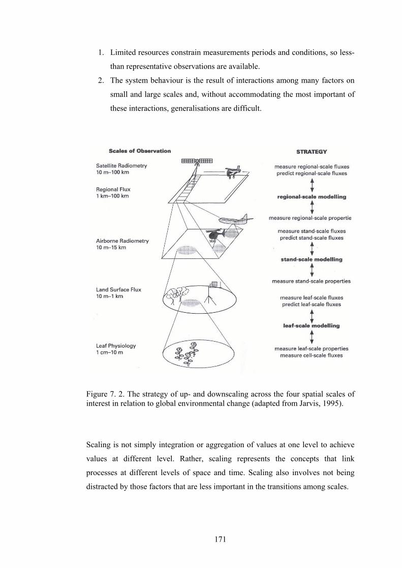
171
1. Limited resources constrain measurements periods and conditions, so less-
than representative observations are available.
2. The system behaviour is the result of interactions among many factors on
small and large scales and, without accommodating the most important of
these interactions, generalisations are difficult.
Figure 7. 2. The strategy of up- and downscaling across the four spatial scales ofinterest in relation to global environmental change (adapted from Jarvis, 1995).
Scaling is not simply integration or aggregation of values at one level to achieve
values at different level. Rather, scaling represents the concepts that link
processes at different levels of space and time. Scaling also involves not being
distracted by those factors that are less important in the transitions among scales.
172
Upscaling consists of taking information at smaller spatial and shorter temporal
scales and using that information to derive information at larger spatial and longer
temporal scales. A widely-used example of upscaling is to take a description of
the process of photo-synthesis at the scale of biochemical processes in the
chloroplast, combine that with a description of leaf structure and carbon dioxide
diffusion, and use that information to derive a description of the fluxes of carbon
dioxide at the leaf scale. Combination of leaf scale fluxes with information about
the physical structure of the vegetation canopy, together with appropriate driving
variables, can then lead to a description of carbon dioxide fluxes at the canopy
scale.
Generally, the objective of upscaling is to preserve the rate of the processes
involved, usually flux densities, such that the rate at the larger spatial and longer
temporal scales is equal to the sum of the rates of all the individual components in
the system. This would clearly be a very easy objective to achieve if all the
process involved were linear. But non-linearity between processes and variables,
and heterogeneity in properties, makes upscaling a challenge. For example, the
measurement of area of land cover from remote sensing images is heavily
influenced by the pixel size, because of the changes in the degree of heterogeneity
of the land cover across scales. Heterogeneous landscapes also lead to more rapid
information loss as the data are aggregated and analysed at coarser scales
(Meentemeyer and Box, 1987).
Downscaling consists of decomposing information at one scale into its
constituents at smaller spatial and shorter temporal scales. The information may
be a description of a process at a larger scale. Downscaling may also be usefully
applied to both state and environmental driving variables. For example, it may be
desirable to downscale a crude estimate of canopy structure, such as leaf area
index, to a more detailed description of the spatial distribution of leaf area density
for the purpose of radiative transfer modelling.
For many purposes, it is adequate, if not desirable, to seek to understand processes
at one particular scale and it is almost impossible to perform large scale
experiments at the scale of natural ecosystems, regional landscapes etc as well as

173
very small scale experiments at the scale of metres. That is why a need exists for
upscaling and downscaling of data.
A variety of tools are available for scaling, involving a combination of correlation,
extrapolation, and modelling, all of which being designed to relate patterns across
wide range of scale. For short-term or small-scale predictions, direct extrapolation
of observed trends may be the best technique, but the application of such methods
can give no hints about when the method will break down or about how patterns
will change beyond observed ranges or in response to environmental changes.
Some guidelines for scaling suggested by Caldwell et al. (1993) are:
1. Assess the scale of the phenomenon in question,
2. Identify the boundary conditions and constraints,
3. Search for consistencies at different scales,
4. Streamline the upscaling models to incorporate only salient features,
5. Incorporate feedback, both positive and negative, that may operate on
some scale but not necessarily on other scales, and
6. Test the results at different scales with independent estimates.
7.4 Sample size
After selecting data at a suitable scale for the study, the next task in assessing the
accuracy of the land use/land cover maps depends on the selection of samples for
training and testing a classifier that gives reliable results applicable both to the
whole land use map and to the individual land use/land cover categories
(Fitzpatrick-Lins, 1981). Due to time and cost constraints involving the collection
of reference data, it would be virtually impossible to consider the entire
population of pixels for classification. Therefore, a sample of pixels is required for
each of the land use class to estimate classification accuracy. Too large a sample
implies a waste of resources, and too small a sample diminishes the utility of the
results. A number of studies carried out by Fitzpatrick-Lins (1981), Hay (1979),
Hord and Brooner (1976), Rosenfield (1982) and Van Genderen and Lock (1977)
have reported a number of equations and guidelines for choosing an appropriate
sample size. The majority of these equations are based on assumption that the data

174
follow a binomial distribution or the normal approximation to the binomial
distribution.
The equation for the determination of the appropriate sample size, N, suggested
by Snedecor and Cochran (1967) (later used by Fitzpatrick-Lins, 1981) is based
on the binomial distribution and depends on the allowable error at a given
confidence level. This equation is:
( )2
2
L
abKN = (7.1)
where a is expected percent accuracy, b = 100 - a, L is the allowable error, and K
is the standard normal deviate for a desired confidence level (e.g. the value of
K = 2 is generalised from the standard normal deviate of 1.96 for the 95% two
sided confidence level). This formula assumes that pixels are selected by using a
simple random sampling technique. When more complex sampling methods such
as stratified sampling are employed, a useful quantity known as the design effect
of the sampling plan enable simple random sampling formulae to be used more
extensively (Snedecor and Cochran, 1967). The design effect is defined as the
ratio of the variance of the estimate given by the complex sampling plan to the
variance of the estimate given by a simple random sample of the same size.
Tortora (1978) suggested another method of estimating the sample size for
multinomial distribution based on the approximate large sample equations for the
simultaneous confidence limits. The equation has the form
( )
2i
1i2
k/1,1 1N
δ
−χ=
α− DD (7.2)
where i
D i = 1, 2 ,. . . . , c, is the proportion of the image area in the ith class,
parameter iδ is the half width of the desired confidence interval, and the value of
α/k1,1χ
−can be found from the tables of percentage points for the unit normal
distribution i.e. "…, the 2χ distribution, with one degree of freedom is the

175
distribution of the square of a normal deviate: the 5% significance level of 2χ ,
3.84, is simply the square of 1.96" (Snedecor and Cochran, 1967).
These techniques are statistically sound for computing the sample size needed to
compute the overall accuracy of a classification or the overall accuracy of a single
class. As suggested by Congalton (1991), these techniques are not designed to
chose a sample size for filling in a confusion matrix. In the case of a confusion
matrix, it is not a matter of correct or incorrect but it a matter of which categories
are being confused. Due to the large number of pixels in remotely sensed datasets,
practical considerations more often dictate the sample size selection than the
traditional methods of sampling. The sample size selected this way should be
such that a balance between what is statistically sound and what is practically
attainable must be maintained. Mather (1999) and Swain and Davis (1978)
recommended that a minimum sample of at least 30 times the number of features
(discriminating variable or wavebands) per class would be suitable, while
Congalton (1991) suggested a minimum of 50 samples for each land use class.
Lillesend and Kiefer (1994) suggested a minimum of from 10 to 100 times the
number of pixels should be used since the estimates of the mean vectors and
covariance matrices improves (if data are normally distributed) as the number of
training pixels increases. The number of pixels selected for each class can also be
adjusted based on the relative importance of the class or by the inherent variability
within each of the class. It is also useful to collect fewer number of pixels from
the classes having little or no within class variability (like water and snow) and
increase the number of sampled pixels in the classes that have more within class
variability.
7.5 Sampling plan
The nature of the sampling plan is an important part of any accuracy assessment,
due to the large volume of remotely sensed data in digital format. In remote
sensing, sampling consists of (i) the creation of sub-areas from large scenes and
(ii) the generation of pixel coordinate lists for use in various image processing
tasks (Franklin et al., 1991). The output of pixel sampling is usually a table which
176
is a compilation of image values and in some cases these values are referenced by
their location (coordinates). These pixel values can be subjected to various
statistical, image processing, and geographic information systems-type operations.
Selection of a proper sampling plan is important for assessing the accuracy of a
classification system because a poor choice of sampling plan may introduce bias
into the confusion matrix, which then may finally over- or under-estimate the
actual accuracy of the classification (Congalton, 1991). The most commonly used
sampling plans used in remote sensing studies are simple random sampling,
cluster sampling, stratified random sampling, and systematic sampling. A number
of studies have been carried out using different sampling plans, producing
different opinions about each of the plans used (Hord and Brooner, 1976;
Fitzpatrick-Lins, 1981; Congalton, 1988; Franklin et al., 1991; Stehman, 1992).
Simple random sampling is a method of selecting a sample of pixels from the total
number of pixels available of a particular class such that every one of the possible
distinct pixels has an equal chance of being selected (Cochran, 1977). In practice,
a random number generator is used to identify a random coordinate pairs in the
image to select the samples. At any stage, the process used must give an equal
chance of selection to any pixel in the population not already drawn. The sample
estimates (i.e. mean, variance) derived from simple random sampling are
consistent and unbiased. An estimate is said to be consistent if the estimate equals
the population parameter when the entire population is sampled. An estimate is
said to be unbiased if the average value of the estimate at a given sample size over
all possible samples is equal to the population average.
In cluster sampling, a group of pixels is selected. Each pixel must be unique to
only one cluster of pixels. This method of sampling is much easier and cheaper
than random sampling, but the disadvantages of cluster sampling are that the
variance for a given sample is greater as compared to simple random sampling
due to the homogeneity of elements in the clusters, and the complexity of
subsequent statistical analysis is greater (Congalton, 1988).
177
In stratified sampling a priori knowledge is used to subdivide the population into
non-overlapping categories. A number of samples is then selected from each
strata. This selection should be made independently for each stratum. Stratified
sampling is used when it is necessary to make sure that small, but important, areas
are represented in the sample.
In systematic sampling, pixels are selected at some equal interval over time or
space. The first sample drawn from the population is located at random and each
successive pixel is collected at a specified interval thereafter. Due to the uniform
spread of the sampled pixels over the entire population, systematic sampling is
more accurate than stratified random sampling (Cochran, 1977). Its major
disadvantage is that each sample in the entire population does not have an equal
chance of being included in the sample and, if the population contained some
periodicity, then the regular spacing of the sampling units might result in
unrepresentative samples (Berry and Baker, 1968).
For this study two different sampling plans, - random sampling and systematic
random sampling - were selected to collect pixels for training and testing the
classifiers. A reference image generated after a field visit of the study area was
used to select the pixels from the remotely sensed image.
7.6 Study area and data
The study area for this research is located within an area known as ‘La Mancha
Alta’ that covers an area of approximately 8000 km2 to the south of Madrid, Spain
(Figures 7.3 and 7.4). This is an area of semi-arid wetlands that is typical of a
Mediterranean environment. It is important as an area for migrating birds and
rain-fed agricultural activities, such as cultivation of wheat and barley and other
crops such as vines, and olives. However, the process of land degradation is
increasing due to intensive agricultural practices. For this study, hyperspectral
data acquired by the DAIS 7915 airborne imaging spectrometer taken on 29th
June 2000, at five meter resolution were used. The data were collected for Prof. J.
Gumuzzio of the Autonomous University of Madrid, who has kindly made
them available for this study. This spectrometer was developed by the German

Figure 7. 3. La Mancha Alta region, Central Spain (adapted from Oliver andFlorin, 1995).
178
Figure 7. 4. Study area in La Mancha region.

179
Space Agency and the European Union. DAIS 7915 is a 79 channel high-
resolution optical spectrometer operating in the wavelength range from 0.4 µm
to 12.5 µm. The spatial resolution of the sensor can vary from 5 to 20 m
depending on the altitude of the aircraft. With the exception of the 1.1 µm to
the 1.4 µm region, all atmospheric windows from visible to the thermal infrared
wavelengths are covered. The advantage of this system is that it has solely
reflective optics with a large aperture, which gives high scan efficiency. The
disadvantage is that it is highly susceptible to striping that results from intrinsic
background radiation to the detector (Muller et al., 1998).
Eight different land cover types, namely wheat, water body, salt lake, hydrophytic
vegetation, vineyards, bare soil, pasture lands and built up area were used for this
study. An area of 512 pixels by 512 pixels in 65 bands covering the area of
interest was extracted. As one aim of this study is to find out the effect of scale
(resolution) of data on land cover classification accuracy, another data set for the
same area from the ETM+ at 30 m resolution, acquired on 28th June 2000 was also
used.
To collect the ground reference information required for land cover classification,
field studies were carried out on 30th June 2001 with Prof. José Gumuzzio and
Thomas Schmid of UAM, Madrid, Spain. Due to non-availability of field data for
the year 2000 from the local farmers, a reference image was generated from the
2001 field data. While digitising the boundaries to create polygons for training
data, only those fields which were most likely to have the same crop as in the
previous year were used. Each polygon is assigned a label corresponding to the
land cover it contains (Figure 7.5).
7.7 Classification
Multispectral sensors have been used to gather data about the Earth’s surface
since the 1960’s. The number of spectral bands used by these sensors ranged from
three to seven for space-borne sensors and up to 18 for airborne sensors. In
contrast to such multispectral sensors, the new generation of remote sensing
instruments, referred to as hyperspectral sensors, have tens or hundreds of
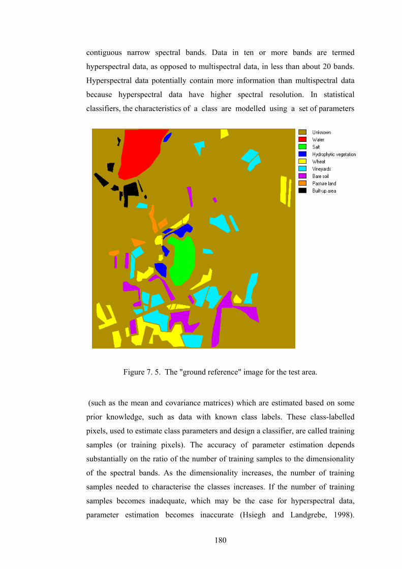
180
contiguous narrow spectral bands. Data in ten or more bands are termed
hyperspectral data, as opposed to multispectral data, in less than about 20 bands.
Hyperspectral data potentially contain more information than multispectral data
because hyperspectral data have higher spectral resolution. In statistical
classifiers, the characteristics of a class are modelled using a set of parameters
Figure 7. 5. The "ground reference" image for the test area.
(such as the mean and covariance matrices) which are estimated based on some
prior knowledge, such as data with known class labels. These class-labelled
pixels, used to estimate class parameters and design a classifier, are called training
samples (or training pixels). The accuracy of parameter estimation depends
substantially on the ratio of the number of training samples to the dimensionality
of the spectral bands. As the dimensionality increases, the number of training
samples needed to characterise the classes increases. If the number of training
samples becomes inadequate, which may be the case for hyperspectral data,
parameter estimation becomes inaccurate (Hsiegh and Landgrebe, 1998).

181
Although increasing the number of spectral bands (dimensionality) potentially
provides more information about class separability, this positive effect is diluted
by poor parameter estimation performance due to an inadequate number of
training pixels. As a result, classification accuracy first increases and then
declines as the number of spectral bands increases. This behaviour is often
referred to as the "Hughes phenomenon" (Hughes, 1968). In short, a small ratio of
training samples to dimensionality may result in unreliable parameter estimation,
leading to poor classification performance.
In general, classification performance depends on the following factors (Raudys,
and Pikelis, 1980):
1. Class separability,
2. training sample size,
3. dimensionality, and
4. classifier type.
Classification performance improves if (a) more precise class parameter values
are used (in case of a statistical classifier), (b) class separability increases, (c) the
ratio of training sample size to dimensionality increases, and/or (d) a more
appropriate classifier is chosen.
This research is designed to study the effects of change in number of training
pixels on classification accuracy with the change in dimensionality of the data.
Further, this study is extended to evaluate the effect of different sampling plans on
classification accuracy using different classifiers. Data sets having 100, 200, 250,
300, 350, 400, and 500 pixels per class, using random sampling methods, and 400
pixels per class using systematic sampling methods were selected to train different
classifiers. To generate the confusion matrix (which is used to compare the
performance of different trained classifiers) a total of 3800 and 3880 pixels
respectively were selected by random sampling and systematic sampling. Four
different classification schemes were used - maximum likelihood, neural network,
support vector machines, and decision tree classifiers. To compare the

182
classification results obtained using different sampling schemes all of the above
mentioned classifiers were employed.
7.7.1 Results and discussions
Figure 7.6 summarises the classification results obtained using different data sets
with increasing number of bands. In this figure, the classification accuracies were
obtained using Maximum Likelihood (ML), Artificial Neural Networks (ANN),
Decision Tree (DT), and Support Vector Machine (SVM) classifiers, respectively.
A total of sixty five features was used. Beginning with five bands, an additional
five bands were added at each cycle, thus generating thirteen accuracy values for
each data set. Figure 7.7 shows the variation in classification accuracy for
different classification systems with varying number of bands and training
patterns.
Results from Figure 7.6 suggests that there is no sharp fall in classification
accuracy, even with ML classifier, as the number of features increases for a fixed
number of training data, as suggested by earlier studies (Hughes, 1968). The
accuracy value begins to stabilise after forty features with different numbers of
training patterns. There is no significant change in classification accuracy as more
features are added. Figure 7.6 suggests that maximum accuracy achieved with
a small training data set occurs at lower dimensionality (number of features), as
compared to the higher dimensionality when a larger training data set is used.
One possible reason for this may be that a larger number of training patterns
allows a better estimation of ML parameters, thus giving better classification
accuracy. Generally, maximum accuracy is achieved at higher dimensions with
more training data, supporting the view that more training data is needed as the
number of features increases.
The results from neural and decision tree classifiers show a similar trend of
variation in accuracy as the ML classifier. The performance of the NN classifier is
almost quite similar to that of the ML classifier with all datasets and there is no
significant difference in accuracy, except in a few cases. The accuracy achieved

183
Figure 7.6 (a). Classification accuracies with 100 pixels/class.
Figure 7.6 (b). Classification accuracies with 200 pixels/class.
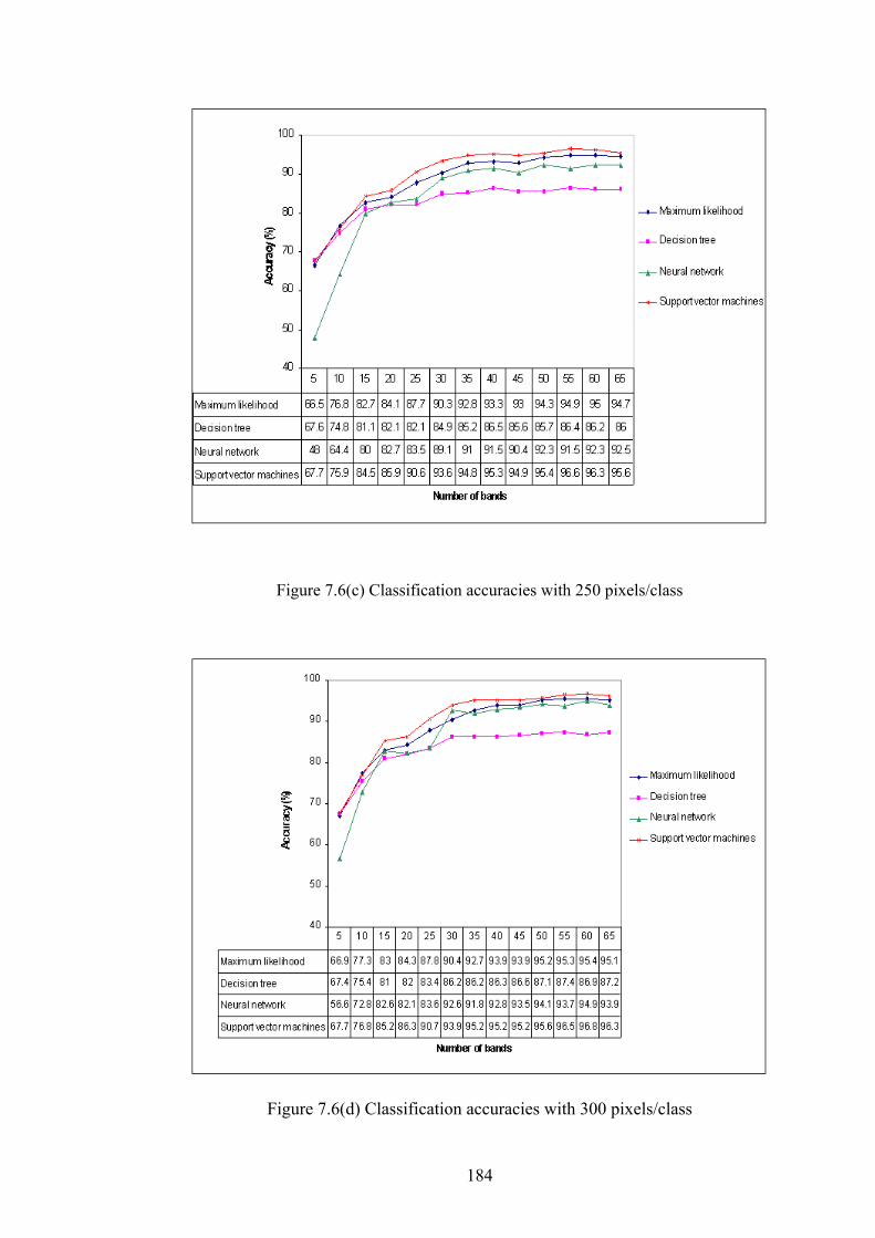
184
Figure 7.6(c) Classification accuracies with 250 pixels/class
Figure 7.6(d) Classification accuracies with 300 pixels/class

185
Figure 7.6(e) Classification accuracies with 350 pixels/class
Figure 7.6(f) Classification accuracies with 400 pixels/class

186
Figure 7.6(g) Classification accuracies with 500 pixels/class
Figure 7. 6. Variation in classification accuracy with change in number of bandswith different training sets.
Figure 7.7(a) Classification accuracies with maximum likelihood classifier

187
Figure 7.7(b) Classification accuracies with neural network classifier
Figure 7.7(c) Classification accuracies with decision tree classifier
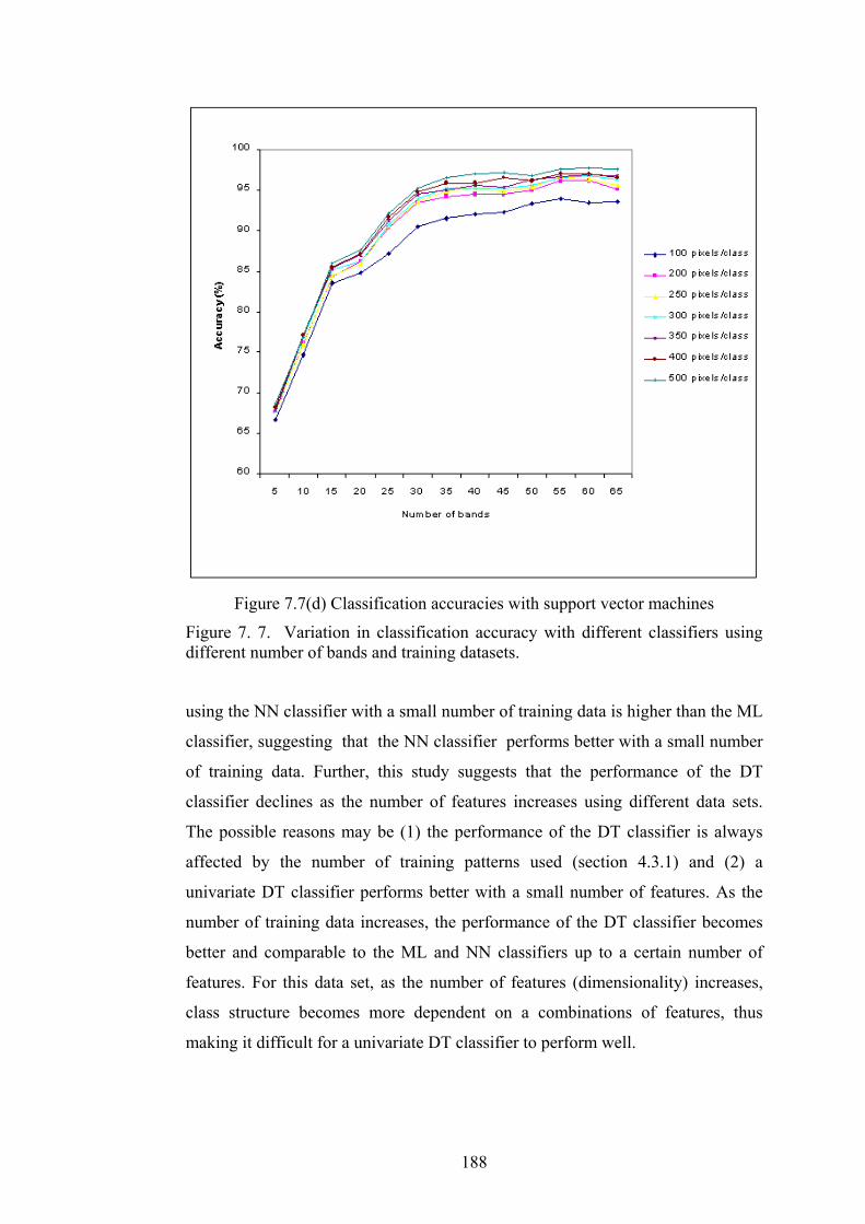
188
Figure 7.7(d) Classification accuracies with support vector machines
Figure 7. 7. Variation in classification accuracy with different classifiers usingdifferent number of bands and training datasets.
using the NN classifier with a small number of training data is higher than the ML
classifier, suggesting that the NN classifier performs better with a small number
of training data. Further, this study suggests that the performance of the DT
classifier declines as the number of features increases using different data sets.
The possible reasons may be (1) the performance of the DT classifier is always
affected by the number of training patterns used (section 4.3.1) and (2) a
univariate DT classifier performs better with a small number of features. As the
number of training data increases, the performance of the DT classifier becomes
better and comparable to the ML and NN classifiers up to a certain number of
features. For this data set, as the number of features (dimensionality) increases,
class structure becomes more dependent on a combinations of features, thus
making it difficult for a univariate DT classifier to perform well.

189
One remarkable property of SVM is that their ability to learn is independent of the
dimensionality of the feature space. SVMs measure the complexity of hypotheses
based on the margin with which they separate the data, not on the number of
features. This means that it is possible to generalise even in the presence of very
many features, if our data are separable with a wider margin using functions from
the feature space. Figure 7.6 suggests that the performance of an SVM is good
even with a small number of training data in comparison with other classifiers.
Further, results form Figure 7.7 suggests that classification accuracy increases
continuously with few exceptions in all datasets, with a fixed number of training
data and the increasing number of features, thus suggesting that this classification
system is unaffected by the Hughes (1968) phenomenon.
Figure 7.7 suggests that classification accuracy always increases as the number of
training data increases, irrespective of number of features and classifier used,
suggesting that the performances of all four classification algorithms used in this
study are affected by the number of training patterns, even with a fixed number of
features. Further, Figure 7.7 suggests that peak in classification accuracy occurs at
a much higher dimensionality as suggested by Hughes (1968). The results
reported here concur with the suggestion of Abend and Harley (1969) that highest
classification accuracy occurs when the number of features is higher than the
number suggested by Hughes (1968).
Further studies were carried out to compare the results of random and systematic
sampling plans used to collect pixels for training and for testing classifier
performances. For this study, Maximum Likelihood (ML), Neural Network (NN),
Decision Tree (DT), and Support Vector Machine (SVM) classifiers and 400
training pixels/class collected using both sampling methods were used. A total of
3800 pixels were selected by random sampling, and 3880 by systematic random
sampling for testing the classifiers. A pairwise statistic for testing the significance
of the classifiers is used (equation 2.8, where 1
K and 2
K correspond to kappa
values calculated from the random and the systematic random sampling plans
respectively). The results are summarised in Table 7.1.

190
This table shows that, there are “positive” improvements (grey coloured values) in
maximum likelihood classifier performances using the random sampling plan
(e.g., for the ML and 20 features, Z = 2.201 > 1.96 while Z = 2.186 > 1.96 using
45 features). Overall, the majority of experiments suggest that the use of a random
sampling strategy produces a higher classification accuracy than does the
systematic sampling plan, for the maximum likelihood classifier. Results obtained
with the neural network classifier are not consistent and suggest that the results
from both the systematic and the random sampling depend on the number of
features used (e.g., Z = 3.25 > 1.96 for 30 features, suggesting better results with
systematic random sampling).
Table 7. 1. Calculated Z values for comparison among the different samplingplans using Kappa analysis. Shaded values indicate significant improvements inthe performance of the classifiers at the 95% confidence level (Z critical value =1.96). Negative value indicates better performance of the systematic randomsampling plan over the random sampling plan.
Number of
features
ML classifier NN classifier DT classifier SVM
5 0.569 5.190 -1.004 0.33
10 0.548 1.114 1.620 -0.64
15 1.015 0.755 0.920 -1.21
20 2.201 -0.434 0.310 -1.77
25 2.080 -0.970 0.530 -1.71
30 2.100 -3.250 -0.110 -1.23
35 1.470 0.463 -1.690 -0.39
40 0.000 -1.622 0.360 -1.60
45 2.186 2.590 0.120 1.00
50 2.263 -.801 0.710 -0.82
55 2.155 3.087 0.810 -0.22
60 2.008 -0.857 1.180 -0.46
65 1.732 1.740 0.590 -1.28
Results obtained using DT and SVM suggests that these classifier perform equally
well with random and systematic random sampling plans. Thus, this study gives

191
an idea that NN, DT, and SVM classifiers perform comparably well with both
sampling plans as compared to maximum likelihood classifier, which works well
with a random sampling scheme only.
7.8 Dimensionality reduction
The recent development of more sophisticated sensors for remote sensing systems
enables the measurement of radiation in many more spectral intervals than was
previous possible. An example of this technology is the AVIRIS system, which
collects image data in 220 bands. The increased dimensionality of such
hyperspectral data provides a challenge to current techniques for analysing such
data. As the number of dimensions of high spectral resolution data increases, the
capability to detect more detailed classes should also increase, although, with the
increase of the number of features, with corresponding increase in the cost and
complexity of the feature extraction and classifier, it is expected that the
classification accuracy will also increase.
Usually the number of training samples is limited. It has been observed frequently
in practice that beyond a certain point, if the number of training samples per
feature is small, the addition of more dimensions leads to a worse performance in
terms of a penalty in the test samples classification accuracy. Hughes (1968)
suggested that the basic source of the problem is the limited number of training
samples. The problem becomes more serious in high dimensional cases. In order
to avoid what has been named the Hughes phenomenon, there have been some
empirical and analytical studies to find a relationship in the number of training
samples and the number of features. Fukunaga and Hays (1989) demonstrated that
the required number of training samples is linearly related to the dimensionality
for a linear classifier and to the square of the dimensionality for a quadratic
classifier.
The negative impact of high dimensionality on classifier performance means that
it is generally agreed that some form of dimensionality reduction, or feature
selection, is considered appropriate. A number of techniques for feature extraction
including Principal Components (Watanabe, 1965), maximum noise fraction
192
transformation (Green at al., 1988) and non-orthogonal techniques such as
projection pursuit (Jiminez and Landgrebe, 1999) have been developed to reduce
the dimensionality of the data. In this study the maximum noise fraction (MNF)
transformation is used to reduce the dimensionality of the hyperspectral data set,
but a brief description of principal component analysis (PCA) is also given, as the
MNF transform is a variant or development of PCA.
7.8.1 Principal Components Analysis
The principal component transformation is also known as the eigenvector
transformation, the Hotelling transformation, or the Karhunen-Loēve (K-L)
transformation in the remote sensing and pattern recognition literature. It is a
multivariate statistical technique that essentially consists of choosing uncorrelated
linear combinations of the variables in such a way that each successively extracted
linear combination, called a principal component, has a smaller variance than its
predecessor. If the variables have significant linear intercorrelations, the first few
components will accounts for a large part of the total variance. Principal
components transformation is based on pixel wise operation that does not take the
spatial nature of image data into account. Also, PCA does not always produce
components that show decreasing image quality with increasing component
number.
The application of this transformation requires an estimate of the variance-
covariance matrix of the features. The principal components maximise the
variance represented by each component. PC-1 is the linear combination of the
original bands that explains the maximum variance in the original data. A higher
order PC is the combination of the original bands that explains maximum variance
subject to the constraint that it is uncorrelated with lower order PCs.
Let A and D denotes the multiband image mean and pixel value vectors,
respectively. The covariance matrix σ can be calculated by the expression:

193
σ = ( ) ( )
1n
ADADn
1i
Tii
−
−×−∑= (7.3)
where n is the number of pixels. If the correlation matrix is used, each entry in
variance-covariance matrix is divided by the product of the standard deviations of
the features represented by the corresponding row and column.
The second step is the calculation of the eigenvectors of σ, which can be achieved
by solving the following equation:
( ) 0KI jj =×λ−σ (7.4)
where jK is the eigenvector corresponding to the eigenvalue jλ , and I is the
identity matrix. The new coordinate system is formed by the normalised
eigenvectors of the variance-covariance matrix and each pixel value is then
projected on this new coordinate system to get a new pixel value.
A drawback of principal components analysis is that its results depend on the unit
of measurement of the original variables. This problem can be circumvented by
performing the PC transformation on a correlation matrix instead of on the
covariance matrix. For details of principal components transformation, readers are
referred to Mather (1999).
7.8.2 Maximum Noise Fraction (MNF) transform
Principal components do not always produce components of decreasing image
quality with increasing component number (Townshend, 1984). While working
with spatial data, the maximisation of variance across bands is not an optimal
approach if the issue is ordering in term of image quality rather than variance.
One of the most common measures of image quality is the signal-to-noise ratio.
Thus, instead of choosing new components to maximise variance, as the principal
194
components transform does, the MNF transform choose components to maximise
the signal-to-noise ratio.
This transformation can be defined in several ways. It can be shown that the same
set of eigenvectors is obtained by procedures that maximise the signal-to-noise
ratio and the noise fraction. The procedure was first introduced by Green et al.
(1988) in continuation of the work on Minimum/maximum autocorrelation factors
by Switzer and Green (1984). Hence the name maximum noise fraction (MNF).
The application of the MNF transformation requires estimates of the signal and
noise covariance matrices. MNF number one is the linear combination of the
original bands that contains the minimum signal-to-noise ratio. A higher order
MNF is the linear combination of the original bands that contains minimum
signal-to-noise ratio subject to the constraint that it is orthogonal to the lower
order MNFs. The MNF transform is equivalent to a transformation of the data to a
coordinate system in which the noise covariance matrix is the identity matrix
followed by a principal component transformation. To deduce the maximum
noise transformation, consider a multivariate data set of p-bands with grey levels
( ),xZi i = 1, . . . ., p
where x gives the coordinates of the sample. If it is assumed that
Z(x) = S(x) + N(x) (7.5)
where ( ) )x(Z),......,x(ZxZ p1T = , and S(x) and N(x) are the uncorrelated
signal and noise component of Z(x). Thus
∑ ∑∑ +== NS)x(ZCov (7.6)
where ∑ S and ∑ N are the covariance matrices of S(x) and N(x), respectively. This
noise is assumed to be additive but this technique can be applied to multiplicative
noise by first taking logarithms of the observations.

195
The noise fraction of the thi band can be defined as:
)x(ZVar/)x(NVarii
(7.7)
the ratio of the noise variance to the total variance for that band. The maximum
noise fraction can be defined as the linear transformations:
( ) ( )xZaxY Tii = , i = 1, . . . . ., p (7.8)
such that the signal-to-noise ratio for ( )xYi is maximum among all linear
transformations orthogonal to ( ) ijxYj ,......,1, = . Furthermore it is assumed that
eigenvectors ia are normalised so that
∑ = ,1iT
i aa i = 1, . . . . ., p (7.9)
Using arguments similar to those used in the derivation of principal components,
it can be shown that the vectors ia are the left-hand eigenvectors of ∑ ∑ −1N
,
and that iµ , the eigenvalue corresponding to ia , equals the noise fraction in ( )xYi .
Hence, from the definition of the MNF transform, MNF components will show
steadily increasing image quality, with increasing component number.
An important property of the MNF transform, which is not shared by principal
components, is that - because it depends on signal-to-noise ratios - it is invariant
under scale changes to any feature. Another useful property is that it
orthogonalises S(x) and N(x), as well as Z(x). The central problem in the
calculation of the MNF transformation is the estimation of the noise component
with the purpose of generation a covariance matrix that approximates ∑ N.
A number of methods to calculate the noise covariance matrix are suggested in the
literature (Olsen, 1993). These are as follows:

196
1. Simple differencing. The noise is estimated as the difference between the
current and neighbouring pixel.
2. Differencing with the local mean. More pixels could be entered to the
estimation by differencing between the current pixel and the local mean of
a window.
3. The noise is estimated as the residual in simultaneous autoregressive
(SAR) model involving the neighbouring pixel to the W, NW, N and NE
of the current pixel.
4. Differencing with local median. To avoid the blurring of edges and other
details, the local median could be used instead of the local mean as in (2).
5. Quadratic surface. The noise is estimated as the residual from a fitted
quadratic surface in a neighbourhood.
For this study, a simple differencing method as suggested by Green et al. (1988)
was used to estimate the noise covariance matrix. The noise is estimated as the
difference between the current and a neighbouring pixel (horizontal neighbour). In
this case ∑ Nis referred as ∑ ∆
.
The hyperspectral data set contained 65 features (bands). A total of thirteen
maximum noise fraction components was extracted using the criterion of image
quality. A total of 4000 pixels for training and 3200 pixels for testing was selected
using a random sampling plan. The results obtained with four different
classification schemes used are shown in Table 7.2 (the corresponding confusion
matrices are provided in appendix D).
The results shown in Table 7.2 suggest that the maximum likelihood classifier
performs the worst of all four classifiers used with MNF transformed data. The
possible reason for this poor performance may be due to zero noise
covariance of two classes (water and salt) while calculating the MNF components
which finally affects the calculation of ML parameters for these two classes. The
decision tree classifier performs well, compared to the support vector machine,

197
maximum likelihood, and neural classifiers. Nevertheless the accuracy achieved is
lower than the highest accuracy achieved using the original hyperspectral data.
Table 7. 2. Results with MNF transformed image.
Classifier Accuracy (%) Kappa value
Maximum likelihood 61.10 0.556
Neural network 87.10 0.854
Decision tree 88.56 0.869
Support vector machine 88.20 0.865
Decision tree classifiers can be used to uncover structures in data (Breiman et al.
1984, Safavian and Landgrebe 1991) and the hierarchical relationships revealed
by partitioning feature space, thus, decision tree classifier can be used to eliminate
redundant or noisy features in input data. Feature selection was therefore
attempted, using the tree-based approach (using See 5.0 software) to reduce the
dimensionality of hyperspectral data. Initially, decision trees of maximum size
were generated using all sixty-five input features. By inspection of the full tree,
those features that contributed most of the variance in the training data were
retained for the subsequent classification phase. A total of 25 features was
selected this way and used to compare the capabilities of four different
classification systems (maximum likelihood, neural, support vector machines, and
decision tree classifiers). For this study a total of 3200 pixels (for 8 classes, with
400 pixels/class) and 3800 pixels, all randomly selected, were used for training
and testing, respectively. Table 7.3 gives the classification accuracy and Kappa
value achieved with this data set. The corresponding confusion matrix is listed in
appendix E.
The results listed in Table 7.3 suggest that feature selection using decision trees is
effective in reducing the dimensionality of input feature space. Although the
decision tree method reduced the number of input features by about
60%, classification accuracies were not significantly degraded. No classifier
performed as well or better with the feature subsets than with the total number of

198
features, yet the accuracies achieved are quite high and comparable to the
accuracies obtained with a full complement of features.
Table 7. 3. Results obtained by applying decision tree based feature selection.
Classifier Accuracy (%) Kappa value
Maximum likelihood 94.10 0.935
Neural network 92.10 0.911
Decision tree 87.60 0.858
Support vector machine 95.30 0.946
Further studies were carried out to find out the effect of scale (resolution) on
classification accuracy. For this study, ETM+ data (30 m resolution) of the same
area in Spain, acquired on 28th June 2000, were used. Figure 7.8 gives an idea of
the quality of the images at two different resolutions for same study area and
indicating how difficult is to locate field boundaries in the ETM+ data to
prepare a ground reference image. Thus, for this study, a ground reference image
generated using hyperspectral data was used to collect the pixels for training and
testing the different classifiers. The image shown in Figure 7.5 was resampled at
30m resolution so as to make it compatible with ETM+ data. Six classes (water,
salt, wheat, vineyards, bare soil, and built-up area) were used in place of the eight
classes used with DAIS data due to the lack of a sufficient number of pixels
for two classes - pasture land and hydrophytic vegetation. A total of 1395
pixels were collected using a random sampling plan, out of which 600 pixels
were used for training and remaining 795 pixels for testing the classifiers.
The results shown in Table 7.4 (and in the corresponding confusion matrices,
listed in appendix F) suggest that, even at this scale, high accuracy can be
obtained. The highest accuracy of 91.1% is achieved with support vector machine.
However, comparison of the classified images (Figures 7.9 (a) 7.9 (b)) suggests
that, except for the water and salt classes, no other class boundary is properly
located and it is very difficult to locate the area covered by other classes in the

199
Table 7. 4. Classification results obtained with ETM+ data for the La Manchatest area of Spain.
Classifier Accuracy (%) Kappa value
Maximum likelihood 83.9 0.797
Neural network 89.4 0.869
Decision tree 84.7 0.810
Support vector machine 91.1 0.880
classified image (Figure 7.9 (b)). Thus, one possible reason of achieving very high
classification accuracy may be due the small number and nature of data used
for testing the different Classifiers, as suggested by Congalton (1988), the nature
of the testing set can have a significant affect on the resulting classification
accuracy. As with the training data, the testing set must also be representative of
the classes and the test samples should be drawn from across the test area and the
sample large enough for a rigorous evaluation of the classification accuracy.

200
Figure 7. 8. Images of the study area (a) DAIS hyperspectral image (5mresolution) and (b) ETM+ image (30m resolution).
Figure 7.8 (a)
Figure 7.8 (b)

201
Figure 7. 9. Classified images using neural network classifier (a) DAIShyperspectral image (5m resolution) and (b) ETM+ image (30m resolution).
Figure 7.9 (a)
Figure 7.9 (b)
202
7.9 Conclusions
This work was carried out to study the effect of the factors of sample size,
sampling plan, number of features in relation with sample size, dimensionality
reduction, and scale (resolution) of the data on land cover classification
accuracy using different classification algorithms. First, this study suggests no
sudden change in classification accuracy after a peak value, even with a small
number of training data, with increasing numbers of features as suggested by
Hughes (1968) while using maximum likelihood, neural and decision tree
classifiers. Otherwise, the results suggest that accuracy starts to stabilise once a
maximum value is reached. This study also suggests that highest accuracy is
achieved at higher dimensionality with different data sets, contrary to the study
carried out by Hughes (1968), thus justifying the suggestions made by Abend and
Harley (1969). The results with support vector machines suggests its insensitivity
to the Hughes phenomenon. Further, this study suggests, that for the maximum
likelihood classifier, training and test data collected using a random sampling plan
produce higher classification accuracies than those achieved using a systematic
sampling plan. Both sampling plans perform well with support vector machine,
decision tree, and neural network classifiers for this type of data.
By applying an MNF transformation, the dimensionality of the hyperspectral
dataset reduces to thirteen features, but the level of classification accuracy
achieved is not comparable with that obtained from the use of all of the features
of DAIS data. This result suggests that the MNF technique may not be used
effectively for dimensionality reduction for this type of data. On the other hand,
decision tree (DT)-based dimensionality reduction techniques perform well, and
the accuracy achieved is higher than that achieved by using MNF transformation.
The accuracy achieved with features obtained using the DT-based dimensionality
reduction technique is comparable to the accuracy achieved by using the full set of
features, suggesting that the DT approach can be effectively used for feature
selection with hyperspectral data.
Further studies suggest that classification accuracy is always affected by the scale
(resolution) of the data used for a particular type of area because scale has an

influence on observed variability both within and between classes (Markham and
Townshend, 1981). Changes in classification accuracies using data at different
scales show the dependence of classification accuracy on scale or resolution of the
data used, suggesting a need to consider the spatial resolution of remotely sensed
data relative to the inherent characteristics of the study area.
1. 2. 3. 4.
5. 6.
7.
SVM classifier is not affected by Hughes (1968) phenomenon.
Training dataset size affects all classification algorithms.
MNF did not work well with this dataset.
DT, ANN, and SVM works well with both random and systematic
sampling plans.
ML works well with random sampling plans.
Decision tree provides an effective way for dimensionality
reduction.
Scale of remote sensing data affects the classification accuracy as
suggested by several other studies.
203

204
Chapter 8
Overview of results and future research directions
8.1 Introduction
Identifying land cover type and change in land cover is an important task for land
and resource management at local and regional scales. However, detecting and
monitoring these changes using ground measurements is limited by logistics and
cost. Remote sensing provides an alternate and useful perspective for collecting
the information for studying these changes, and producing land cover maps using
various classification methods. A number of statistical and neural classification
methods have been developed and used for classification of remotely sensed data.
However, each method has its limitations; for example, statistical classifiers,
being parametric in nature, assume that the data follow a particular frequency
distribution. Artificial neural networks, a nonparametric technique, have been
used extensively in a variety of problems in the remote sensing field, and perform
well when compared to statistical classifiers. However, a range of factors limit
their use in land use classification studies. Decision tree (DT) and support vector
machine (SVM) classifiers, new nonparametric techniques for analysing remote
sensing images, have the potential to improve the land cover classification
accuracy. It is worth mentioning that choice of scale (resolution), number of
features, type of data (optical or radar), training data as well as sampling plan
have as much as influence as the classifier on classification results.
The main aim of this chapter is to summarise the results presented in previous
chapters. The first part of this research demonstrates the utility of decision tree
classification methods for land cover classification derived from remotely sensed
images. This stage also involved a comparison of results obtained with decision
tree classifiers with the most widely-used methods (statistical and neural
classifiers) for classifying agricultural crops. The second stage of this study
involves assessing the behaviour of support vector machines for land cover
classification studies. The third part of this work involves the assessment of the

205
utility of interferometric SAR coherence measurements for land cover
classification. This stage also discusses some methods of feature extraction and
selection. Finally, a detailed study is carried out to analyse the performance of
various classifiers using different sampling plans, different numbers of training
data with changes in number of features, and data at different scales as well as the
effect of orthogonal transformation on classification accuracy using hyperspectral
data. Conclusions drawn from this research are summarised and presented in the
following subsections.
8.1.1 The usefulness of decision tree classifiers and support vector machines
Chapter 3 describes the decision tree classifier, which is a multi-stage
classification technique that decomposes a complex classification problem into
several stages, finally simplifying the decision-making process by taking partial
decisions at each stage of classification. This chapter also introduces support
vector machines, a classification technique which maximises the margin between
the class boundaries and based on structural risk minimisation techniques.
Classification results using decision tree classifiers are discussed in chapters 5
(section 5.1), 6 and 7. Chapters 5 (section 5.2) and 7 discuss the results obtained
using support vector machines. A critical assessment of the problems encountered
in the use and design of decision tree classifiers and support vector machines is
also presented in chapter 3.
The decision-tree and support vector machines-based classification approach, used
for classifying agricultural crops using various type of remotely sensed data, have
been found to be effective in identifying general agricultural crop classes, with
acceptable levels of overall classification accuracy in comparison with neural and
statistical classifiers.
The conclusions reached from this study using the three datasets described in
chapters 5 (sections 5.1, 5.2), 6 and 7 are presented in the conclusion section of
each chapter. The most important conclusions of this study are:
• The performance of DT classifiers (both univariate and multivariate) is
affected by the number of training patterns used to train the classifier.

206
• In spite of being nonparametric in nature, DT classifiers perform poorly
in comparison with neural and statistical classifier when using small
training datasets. This observation suggests that a sufficient number of
training data is required for DT classifiers.
• When a sufficient number of training data and small number of features
are used (e. g., data from ETM+), classification results achieved by a
univariate DT classifier are invariably better than those from a ML
classifier.
• SVM perform well - in fact, better than DT, ANN and ML classifiers -
with small training datasets, but classification accuracy improves as the
number of training pixels increases.
• As the number of features increases, with training dataset size held
constant, the performance of a univariate DT classifier starts to degrade,
and classification accuracy falls below that produced by the maximum
likelihood classifier, indicating that the univariate DT classifier performs
less well in high dimension feature space, where class information is
dependent on a combination of features. In contrast, support vector
machines perform well and better than DT, ANN, and ML classifiers with
a fixed training dataset size and increasing number of features.
• Results obtained employing various attribute selection measures with the
error based pruning method, and employing various pruning methods with
the information gain ratio as the attribute selection measure, suggest that
the performance of a DT classifier is affected by the pruning method used,
and not by the attribute selection methods.
• Assessment of the effect of boosting on the level of classification
accuracy achieved by the DT classifier indicates that classification
accuracy is increased by about 3-4%. The study also concludes that about
10 to 15 boosting iteration are enough to attain this increase in
classification accuracy.

207
• The DT classifier performance is slightly inferior to that of the ANN
classifier using ETM+ data. However, it performs better with InSAR data
even without boosting. After boosting, the DT classifier always perform
better than the ANN classifier. Performance of the SVM classifier is
always better than either the DT or the ANN with ETM+ data.
• Assessment of the effect of the number of factors affecting classification
accuracy using ANN and DT classifiers shows that the number of factors
affecting the performance of the ANN classifier is high in comparison to
the DT classifier, which is affected by only two factors. Classification
accuracy obtained using SVM is affected by a number of factors, such as:
choice of kernel, user-defined parameters for various kernels, number of
training data, and multi-class method used. This suggests that a skilled and
experienced person is needed to work with ANN and SVM, requiring extra
financial resources for training.
• This study suggests that when the SVM classifier is used, the "one against
one" multi-class method performs better than the " one against rest" multi-
class strategy.
• The time taken to train and test a DT classifier is very short compared to
an ANN classifier. For an ETM+ data set of the Littleport area, the training
time for a DT classifier is 0.7 seconds compared to 58 minutes for an
ANN. Even the use of boosting (14 iterations) increases the training time
for the DT by only a small amount (to 7.1 seconds).
• The time taken for training a SVM depends on the multi-class method
used. The one against the rest multi-class method requires several hours of
training time, while the one against one multi-class method needs a
significantly smaller training time, which is almost same as the time taken
by a ML.
• Further studies carried out include the use of the internal texture of
panchromatic ETM+ band with multispectral data using DT, ANN, and
ML classifiers suggest no significant improvement in classification
accuracy.
208
• A DT can be used effectively for feature selection.
8.1.2 Use of coherence for land use classification
Another important issue reviewed in this thesis is the use of InSAR data for land
cover classification studies. SAR data are now available with phase and intensity
information. It is possible to utilise the phase information to generate a coherence
image for use in land cover classification studies in combination with the intensity
images obtained during InSAR processing. Relatively few studies have used
coherence information in land cover studies; one reason may be that obtaining a
good quality coherence image depends on several factors. The value of texture
measures (e.g. GLCM, the MAR model, and fractals) and feature selection using
Hotelling's 2T test were assessed. The results obtained from this study using DT,
ANN and ML classifiers are discussed in chapter 6. The main conclusions are
summarised below:
• The combination of coherence and intensity images results in an improved
classification accuracy of the order of 8-9%, as compared to using
intensity images alone.
• The quality of coherence information depends on several factors (that is
why only one acceptably good coherence image was obtained from the
five Single Look Complex (SLC) used in this study). This, suggests that
tandem interferometric pairs are more suitable for good quality coherence
images.
• Inclusion of texture information with coherence and intensity images was
found to be effective in improving classification accuracy. By using three
texture features per coherence and intensity image, obtained after feature
selection, an increase in classification accuracy by an amount of 10% to
12% (depending on the classifier used) was observed.
• The highest accuracy obtained was from a data set with a total of 24
features is 82.9%, which justifies the value of texture information but at

209
the cost of increase in computation time as well as the requirement for a
large number of training data.
8.1.3 Issues in remote sensing image classification
Advancement in sensor technology provides data with a much higher
dimensionality than before. Although such high-dimensional data have the
potential to provide increased amounts of information, new problems arises that
have not been encountered in the analysis of relatively low dimensional data. The
more important of these problems in analysing high dimensional data are
investigated in chapter 7. Conclusions drawn from this study are as follows:
• Classification accuracy stabilises after reaching a peak as the number of
features increases, when the number of training data is fixed. Accuracy
increases with the increase in number of training patterns for a fixed
number of features with all four classifiers used in this study, suggesting
that performance of all of these classifiers depends on the number of
training data.
• A random sampling plan for training data selection was found to perform
well as compared to a systematic sampling plan when using a ML
classifier.
• The ANN classifier performs well with both random and systematic
sampling plans, depending on the number of features used, while SVM
and DT work well with both random and systematic random sampling
plans irrespective of the number of features used.
• The MNF transformation reduces the dimensionality of 65-band DAIS
hyperspectral data to thirteen features, but classification results suggests
that this method is not very suitable for this type of study.
• DT-based feature extraction methods, using twenty five features, perform
well with this data set. The level of accuracy obtained with this data set is
comparable with the highest accuracy achieved by using all features of

210
hyperspectral data, and results are better that those using the MNF
transformation.
• Classification accuracy is always affected by the scale of the data used as
well as the classifier used for a particular type of data, thus confirming that
the type of data and classifier used for classification studies are dependent
on the characteristics of the study area.
• Performance of the SVM classifier for hyperspectral data is very
encouraging, and is far better than ML, ANN and DT classifiers, with a
small training dataset sizes and with increasing number of features.
Further, this study suggests that the SVM classifier is not affected by the
Hughes phenomenon.
Work reported in this thesis provides evidence that the expected classification
accuracy for remotely sensed data is directly affected by a number of factors.
Tables 8.1 and 8.2 provide a comparison of classifier performance and various
factors affecting the classification accuracy with different classification
algorithms used in this study.
8.2 Suggestions for future research
Results obtained from this study suggests a considerable potential for extending
the investigating into developing new strategies for the design of DT and ANN
classifiers. In the design of multilayer feedforward neural networks, the structure
of the network (the number of hidden layer and number of neurons in each hidden
layer) is not known in advance, and is often chosen heuristically and by trial and
error. Studies carried out by Sethi (1990) offer a way to uncover the structure of
the network. This study suggests the use of a neural network design methodology
(called an entropy net) by exploiting the similarities between the hierarchical
classifiers and the multiple-layer neural network. The main advantage of this
approach is to eliminate the guess-work involved in the design of ANN classifiers.
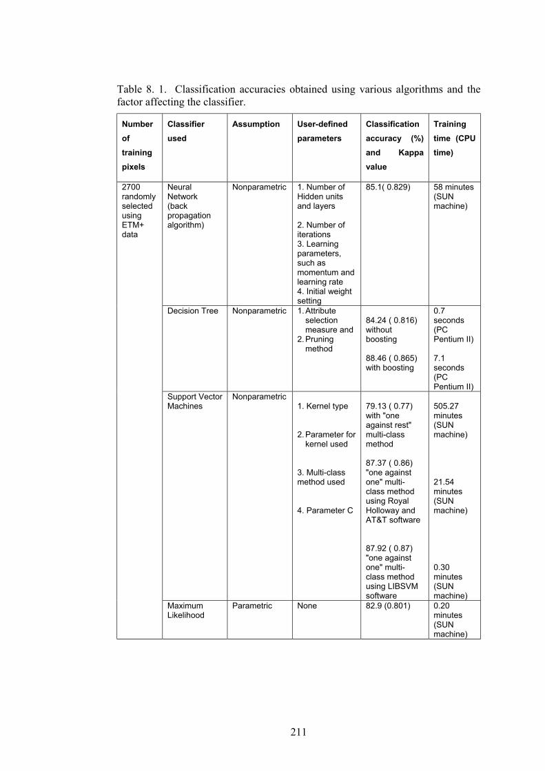
211
Table 8. 1. Classification accuracies obtained using various algorithms and thefactor affecting the classifier.
Numberoftrainingpixels
Classifierused
Assumption User-definedparameters
Classificationaccuracy (%)and Kappavalue
Trainingtime (CPUtime)
NeuralNetwork(backpropagationalgorithm)
Nonparametric 1. Number ofHidden unitsand layers
2. Number ofiterations3. Learningparameters,such asmomentum andlearning rate4. Initial weightsetting
85.1( 0.829) 58 minutes(SUNmachine)
Decision Tree Nonparametric 1. Attributeselectionmeasure and
2. Pruningmethod
84.24 ( 0.816)withoutboosting
88.46 ( 0.865)with boosting
0.7seconds(PCPentium II)
7.1seconds(PCPentium II)
Support VectorMachines
Nonparametric1. Kernel type
2. Parameter forkernel used
3. Multi-classmethod used
4. Parameter C
79.13 ( 0.77)with "oneagainst rest"multi-classmethod
87.37 ( 0.86)"one againstone" multi-class methodusing RoyalHolloway andAT&T software
87.92 ( 0.87)"one againstone" multi-class methodusing LIBSVMsoftware
505.27minutes(SUNmachine)
21.54minutes(SUNmachine)
0.30minutes(SUNmachine)
2700randomlyselectedusingETM+data
MaximumLikelihood
Parametric None 82.9 (0.801) 0.20minutes(SUNmachine)
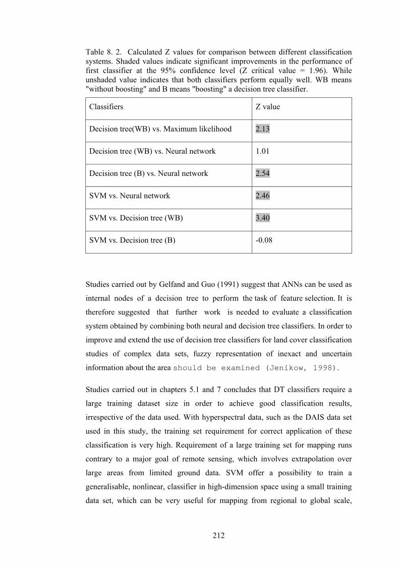
212
Table 8. 2. Calculated Z values for comparison between different classificationsystems. Shaded values indicate significant improvements in the performance offirst classifier at the 95% confidence level (Z critical value = 1.96). Whileunshaded value indicates that both classifiers perform equally well. WB means"without boosting" and B means "boosting" a decision tree classifier.
Classifiers Z value
Decision tree(WB) vs. Maximum likelihood 2.13
Decision tree (WB) vs. Neural network 1.01
Decision tree (B) vs. Neural network 2.54
SVM vs. Neural network 2.46
SVM vs. Decision tree (WB) 3.40
SVM vs. Decision tree (B) -0.08
Studies carried out by Gelfand and Guo (1991) suggest that ANNs can be used as
internal nodes of a decision tree to perform the task of feature selection. It is
therefore suggested that further work is needed to evaluate a classification
system obtained by combining both neural and decision tree classifiers. In order to
improve and extend the use of decision tree classifiers for land cover classification
studies of complex data sets, fuzzy representation of inexact and uncertain
information about the area should be examined (Jenikow, 1998).
Studies carried out in chapters 5.1 and 7 concludes that DT classifiers require a
large training dataset size in order to achieve good classification results,
irrespective of the data used. With hyperspectral data, such as the DAIS data set
used in this study, the training set requirement for correct application of these
classification is very high. Requirement of a large training set for mapping runs
contrary to a major goal of remote sensing, which involves extrapolation over
large areas from limited ground data. SVM offer a possibility to train a
generalisable, nonlinear, classifier in high-dimension space using a small training
data set, which can be very useful for mapping from regional to global scale,

213
where availability of ground truth information is limited. Further, the use of
boosting, a new methodology being used to generate ensembles of classifiers, is
also suggested with SVM.
8.3 Algorithm choice - some guidelines
The conclusions drawn and the experiments carried out during this study can be
used to form a number of guidelines that can greatly facilitate the use of various
classification algorithms with different datasets. It should be noted that these
guidelines are valid for similar datasets and classification problems used in this
study. The list of the guidelines is given as follows:
A. Ease of use:
1. Maximum likelihood and decision tree classifier - easiest
2. Support vector machines
3. Neural Network. - required skilled analyst
B. Accuracy (multispectral / InSAR data):
1. Support vector machines - highest
2. Neural network
3. Decision tree
4. Maximum likelihood - lowest
C. Accuracy (hyperspectral data):
1. Support vector machines - highest
2. Maximum likelihood
3. Neural network
4. Decision tree - lowest

214
D. Computational demand:
1. Neural network - high
2. Support vector machines / Maximum likelihood - medium
3. Decision tree - low
E. sensitivity to sample size and sampling plan:
1. Maximum likelihood - very sensitive to both sample size and sampling
plan.
2. Decision tree - very sensitive to sample size, not to sampling plan.
3. Neural network - sensitive to sample size, not to sampling plan.
4. Support vector machines - sensitive to sample size but performs very
well with small dataset; not sensitive to sampling plan.
F. Availability
1. Maximum likelihood - provided with almost all commercial image
processing software.
2. Decision tree - provided with statistical software packages. Some freely
downloadable from the internet. Some commercial (stand alone)
software packages.
3. Neural network - SNNS software free from internet; ENVI, and some
commercial (standalone) softwares.
4. Support vector machines - some freely downloadable software from
internet.
Figure 8.1 gives a graphical representation of the effects of the factors listed
above on the choice of a classification algorithm. A scale of 1-5 is chosen to grade
different factors. Two different choice of algorithms is represented in the Figure
8.1, one for multispectral/radar and other for hyperspectral data. The result
suggests that support vector machine classifier are the best choice for all datasets.

215
Figure 8. 1. Algorithm choice for different type of data depending on differentfactors. Higher grading is given to the classifier, which provides high accuracyand easy in use. A classifier that requires small computational time and lesssensitive to both sampling plan and sample size is given high grading.
A. Ease of use
B. Accuracy withoptical and InSARdata
C. Computationaldemand
D. Sensitivity to samplesize and samplingplan
E. Availability
Algorithm choice withmultispectral and radardata(A+3B+C+D+E)/10
F. Accuracy withhyperspectral data
Algorithm choice withhyperspectral dataA+C+D+E+3F/10
Maximum likelihood Support vector machine
Decision tree Neural network
1 2 3 4 5

216
Bibliography
Abend, K., and Harley, T. J. (1969) Comments "On the mean accuracy of statisticalpattern recognisers". IEEE Transactions of Information Theory, May, 420-421.
Aleksander, I., and Morton, H. (1991) An Introduction to Neural Computing.London: Chapman and Hall.
Antikidis, E., Arino, O., Laur, H., and Arnaud, A. (1998) ERS SAR coherence andATS R Hot Spots: a synergy for mapping deforested areas. The special case of the1997 fire event in Indonesia. Retrieval of Bio- and Physical Parameters from SARData for Land Application Workshop. ESTEC, The Netherlands, 21- 23 October1998, http://www.estec.esa.nl/CONFANNOUN/98c07/.
Askne, J., and Hagberg, J. O. (1993) Potential of interferometric SAR forclassification of land surfaces. Proceedings of the International Geoscience andRemote Sensing Symposium (IGARSS`93), Tokyo, Japan, 18-21 August, 985-987.
Askne, J., Dammert, P., and Smith, G. (1996) Interferometric SAR observations offorested areas. FRINGE-ESA Workshop on Application of ERS SAR Interferometry,University of Zurich, 30 September to 2 October,http://www.geo.unizh.ch/rsl/fringe96/.
Atlas, L., Cole, R., Muthusamy, Y., Lippman, A., Connor, J., Park, D., El-Sharkawi, M., and Mark Ii, R. J. (1990) A performance comparison of trainedmultilayer perceptrons and trained classification trees. Proceedings of the IEEE, 78,1614-1619.
Ball, G. H., and Hall, D. J. (1965) A Novel Method of Data Analysis and PatternClassification. Menlo Park, CA: Stanford Research Institute.
Bao, M. (1999) Classification of multi-temporal SAR images and InSAR coherenceimages using adaptive neighbourhood model and simulated annealing approach.Proceedings of 20th Asian Conference on Remote Sensing. 22-25 November 1999,Hongkong, China.
Barber, D. G., and LeDrew, E. F. (1991) SAR sea ice discrimination using texturestatistics: A multivariate approach. Photogrammetric Engineering and RemoteSensing, 57, 385-395.
Baraldi, A., and Parmiggiani, F. (1995) A neural network for unsupervisedcategorisation of multivalued input patterns: an application to satellite imageclustering. I.E.E.E. Transactions on Geoscience and Remote Sensing, 33, 305-316.
Belward, A. S., and Hoyos, A. D. (1987) A comparison of supervised maximumlikelihood and decision tree classification for crop cover estimation frommultitemporal LANDSAT MSS data. International Journal of Remote Sensing, 8,229-235.

217
Benediktsson, J. A., Swain, P. H., and Erase, O. K. (1990) Neural networkapproaches versus statistical methods in classification of multisource remote sensingdata. IEEE Transactions on Geoscience and Remote Sensing, 28,540-551.
Berry, B. J. L., and Baker, A. M. (1968) Geographical sampling. Spatial Analysis:A Reader in Statistical Geography, (Berry, B. J. L., and Marble, D. F. eds.),Englewood Cliffs, N. J.: Prentice-Hall.
Bezdek, J. (1981) Pattern Recognition with Fuzzy Objective Function Algorithms.New York: Plenum Press.
Bishop, Y., Fienberg, S., and Holland, P. (1975) Discrete Multivariate Analysis-Theory and Practice. Cambridge, MA: MIT Press.
Bishop, C. M. (1995) Neural Networks for Pattern Recognition. Oxford: ClarendonPress.
Booth, D. J., and Oldfield, R. B. (1989) A comparision of classification algorithmsin term of speed and accuracy after the application of a post-classification modelfilter. International Journal of Remote Sensing, 10, 1271-1276.
Borak, J. S., and Strahler, A. H. (1999) Feature selection and land coverclassification of a MODIS-like data set for semi-arid environment. InternationalJournal of Remote Sensing, 20, 919-938.
Born, M., and Wolf, E. (1980) Principles of Optics. Oxford: Pergamon Press.
Boser, B., Guyon, I., and Vapnik, V. N. (1992) A training algorithm for optimalmargin classifiers. Proceedings of 5th Annual Workshop on Computer LearningTheory, Pittsburgh, PA: ACM, 144-152.
Borgelt, C., Gebhardt, J., and Kruse, R. (1996) Concepts for Probabilistic andPossibilistic Induction of Decision Trees on Real World Data. Proceedings of 4thEuropean Congress on Intelligent Techniques and Soft Computing, Aachen,Germany, 3, 1556-1560.
Breiman, L. (1996) Bagging predictors. Machine Learning, 24, 123-140.
Breiman, L., Friedman, J. H., Olshen, R. A., and Stone, C. J. (1984)Classification and Regression Trees. Monterey, CA: Wadsworth.
Brodley, C. E., and Utgoff, P. E. (1992) Multivariate versus univariate decisiontrees. Technical Report 92-8. Department of Computer Science, University ofMassachusetts, Amherst, Massachusetts, USA.
Bryan, M. L. (1974) Extraction of urban land cover data from multiplexed syntheticaperture radar imagery. Proceedings of the Ninth International Symposium on RemoteSensing of the Environment, ERIM, Ann Arbor, Michgan, 271-288.

218
Buck, C. H., and Monni, S. (1999) Application of SAR Interferometer to FloodDamage Assessment. CEOS SAR Workshop, ESA-CNES Toulouse, 26-29 October,http://www.estec.esa.nl/ceos99/.
Burges, C. J. C. (1998) A tutorial on support vector machines for pattern recognition.Data Mining and Knowledge Discovery, 2, 121-167.
Caldwell, M. M., Matson, P. A., Wessman, C., and Gamon, J. (1993) Prospectsfor scaling. Scaling Physiological Processes: Leaf to Globe, Academic Press, SanDiego, 1993, 223-230.
Campbell, J. B. (1981) Spatial correlation effects upon accuracy of supervisedclassification of land cover. Photogrammetric Engineering and Remote Sensing, 47,355-363.
Canada Centre for Remote Sensing (CCRS), CCRS Remote Sensing Tutorials:Radar and Stereoscopy, http:/www.ccrs.nrcan.gc.ca/ccrs/eduref/sradar/.
Cannon., M., Lehar, A., and Preston, F. (1983) Background pattern removal bypower spectral filtering. Applied Optics, 22(6), 777-779.
Cao, C., and Lam, N. S. (1997) Understanding the scale and resolution effects inremote sensing and GIS. Scale in Remote Sensing and GIS, Quattrochi, D. A., andGoodchild, M. A. ed., Boca Raton: CRC Press, 57-72.
Casey, R. G., and Nagy, G. (1984) Decision tree design using a probabilistic model.IEEE Transactions on Information Theory. IT-30, 93-99.
Chapelle, O., Haffner, P., and Vapnik, V. N. (1999) Support vector machines forhistogram-based image classification. IEEE Transactions on Neural Networks, 10,1055-1064.
Civco, D. L. (1993) Artificial neural networks for land-cover classification andmapping. International Journal of Geographical Information Systems, 7, 173-186.
Chang, C., and Lin, C. (2001) LIBSVM: A Library for Support Vector Machines.Computer Science and Information Engineering, National Taiwan University,Taiwan.
Chorley, R. J., and Haggett, P. (1967) Models in Geography. London: Methuen andCompany Ltd..
Civco, D. (1989) Knowledge-based land use and land cover mapping. Proceeding ofAnnual Convention of American Society for Photogrammetry and Remote Sensing, 3,276-291.
Cochran, W. G. (1977) Sampling techniques. New York, John Wiley and Sons.
Cohen, J. (1960) A coefficient of agreement for nominal scales. Educational andPsychlogical Measurement, 20, 37-40.

219
Congalton, R. G. (1991) A review of assessing the accuracy of classifications ofremotely sensed data. Remote Sensing of Environment, 37, 35-46.
Congalton, R. G. (1988) A comparison of sampling schemes used in generating errormatrices for assessing the accuracy of maps generated from remotely sensed data.Photogrammetric Engineering and Remote Sensing, 54, 593-600.
Cortes, C., and Vapnik, V. N. (1995) Support vector networks. Machine Learning,20, 273-297.
Curlander, J. C., and Mcdonough, R. N. (1991) Synthetic Aperture Radar: Systemand Signal Processing. New York: John Wiley and Sons.
Cushnie, J. L. (1987) The interactive effect of spatial resolution and degree ofinternal variability with land-cover types on classification accuracies. InternationalJournal of Remote Sensing, 8, 15-29.
Dammert, P. B. G., Lepparanta, M., and Askne, J. (1998) SAR interferometeryover Baltic Sea ice. International Journal of Remote Sensing, 19, 3019-3037.
Defries, R. S., Hansen, M., Townshend, J. R. G., and Sohlberg, R. (1998) Globalland cover classification at 8 km spatial resolution: the use of training data derivedfrom Landsat imagery in decision tree classifiers. International Journal of RemoteSensing, 19, 3141-3168.
Dobson, M. C., Ulaby F. T., and Pierce L. E. (1995) Land-cover classification andestimation of terrain attributes using synthetic aperture radar, Remote Sensing ofEnvironment, 51, 199-214.
Durand, J.M., Gimonet, B.J., and Perbos, J.R. (1987) SAR data filtering forclassification. IEEE Transactions of Geoscience and. Remote Sensing, 25, 629-637.
Dutra, L. V., and Huber, R. (1999) Feature extraction and selection for ERS-1/2InSAR classification. International Journal of Remote Sensing, 20, 993-1016.
Elachi, C. (1987) Spaceborne Radar Remote Sensing: Applications and Techniques.New York, IEEE Press.
Engdahl, M., and Borgeaud, M. (1998) ERS-1/2 tandem interferometric coherenceand agricultural crop height. Retrieval of Bio- and Physical Parameters from SARData for Land Application Workshop. ESTEC, The Netherlands, 21-23 October 1998,http://www.estec.esa.nl/CONFANNOUN/98c07/.
Estes, J., Sailor, C., and Tinney, L. (1986) Applications of artificial intelligencetechniques to remote sensing. Professional Geographer, 38, 133-141.
Esposito, F., Malerba, D., and Semeraro, G. (1997) A comparative analysis ofmethods for pruning decision trees. IEEE Transactions on Pattern Analysis andMachine Intelligence, 19, 476-491.

220
Evans, F. (1998) An Investigation into the Use of Maximum Likelihood Classifiers,Decision Trees, Neural Networks and Conditional Probabilistic Network for Mappingand Predicting Salinity. M. Sc. Thesis, Department of Computer Science, CurtinUniversity of Technology, Australia.
Fischer, M. M. (1996) Computational neural networks: a new paradigm for spatialanalysis. Proceedings of First International Conference on Geocomputation,University of Leeds, UK, 1, 297-314.
Fitzgerald, R. W., and Lees, B. G. (1994) Assessing the classification accuracy ofmultisource remote sensing data. Remote Sensing of the Environment, 47, 362-368.
Fitzpatrick-Lins, K. (1981) Comaparision of sampling procedures and data analysisfor a land use and land cover map. Photogrammetric Engineering and RemoteSensing, 47, 343-351.
Fletcher, R. (1987) Practical Methods of Optimisation. John Wiley and Sons, 2nd
edition.
Floury, N., Toan, T. L., Souyris, J. C., Singh, K., Stussi, N., Hsu, C. C., andKong, J. A. (1996) Interferometry for forest studies. FRINGE-ESA Workshop onApplication of ERS SAR Interferometry, University of Zurich, 30 September to 2October, http://www.geo.unizh.ch/rsl/fringe96/.
Foody, G. M. (1995 a) Land cover classification by an artificial neural network withancillary information. International Journal of Geographical Information Systems, 9,527-542.
Foody , G. M., Mcculloch, M. B., and Yates, W. B. (1995 b) The effects of trainingset size and composition on artificial neural network. Photogrammetric Engineeringand Remote Sensing, 58, 1459-1460.
Foody, G. M., and Arora, M. K. (1997) An evaluation of some factors affecting theaccuracy of classification by an artificial neural network. International Journal ofRemote Sensing, 18, 799-810.
Foster, M. R., and Guinzy, N. J. (1967) The coefficient of coherence: Its estimationand use in geophysical data processing. Geophysics, XXXII, 602-616.
Franklin, S. E., Peddle, D. R., Wilson, B. A., and Blodgett, C. F. (1991) Pixelsampling of remotely sensed digital imagery. Computers and Geosciences, 17, 759-775.
Friedl, M., Estes, J., and Star, J. (1988) Advanced information-extraction tools inremote sensing, for earth science applications: AI and GIS. AI Applications, 2, 17-31.
Friedl, M. A., Brodley, C. E., and Strahler, A. H. (1999) Maximizing land coverclassification accuracies produced by decision tree at continental to global scales.IEEE Transactions on Geoscience and Remote Sensing. 37, 969-977.

221
Friedl, M. A., and Brodley, C. E. (1997) Decision tree classification of land coverfrom remotely sensed data. Remote Sensing of Environment. 61, 399-409.
Frankot, R. T., and Chellappa, R. (1987) Log Normal random field models andtheir applications to radar image synthesis. IEEE Transactions on Geoscience andRemote Sensing, 25, 195-207.
Freund, Y., and Schapire, R. E. (1996) Experiments with new boosting algorithm.Machine Learning: Proceedings of the Thirteenth International Conference. Bari,Italy, July 3-6.
Friedman, J. H. (1977) A recursive partitioning decision rule for non-parametricclassification. IEEE Transactions on Computers, C-26, 163-168.
Frost, V. S., Stiles, J. A., Shanmugan, K. S., and Hotzman, J. C. (1982) A modelfor radar images and its application to adaptive digital filtering of multiplicativenoise. IEEE Transactions on Pattern Analysis and Machine Intelligence, 4, 157-165.
Fu, K. S. (1968) Sequential Methods in Pattern Recognition and Machine Learning.New York: Academic Press.
Fukuda, S., and Hirosawa, H. (1999) A wavelet-based texture feature set applied toclassification of multifrequency polarimetric SAR images. IEEE Transactions onGeoscience and Remote Sensing, 37, 2282-2286.
Fukunaga, K., and Hayes, R. R. (1989) Effects of Sample Size in Classifier Design.IEEE Transactions on Pattern Analysis and Machine Intelligence, 11, 873-885.
Gabriel, A. K, and Goldstein, R. M. (1988) Crossed Orbit Interferometry: Theoryand Experimental Results from SIR-B, International Journal of Remote Sensing, 9,857-872.
Gahegan, M., and West, G. (1998) The classification of complex data sets: anoperational comparison of artificial neural networks and decision tree classifiers.Proceedings of the 3rd International Conference on Geocomputation, University ofBristol, UK, 17-19 September 1998, http://divcom.otago.ac.nz/sirc/webpages/conferences/GeoComp/GeoComp98/geocomp98.htm.
Gangepain, J., and Roques-Carmes, C. (1986) Fractal approach to two dimensionaland three dimensional surface roughness. Wear, 109, 119-126.
Gatelli F., Guarnieri A. M., Parizzi F., Pasquali P., Prati C., and Rocca F. (1994)The wavenumber shift in SAR interferometry , IEEE Transactions on Geoscience andRemote Sensing, 32, 855-865.
Gelfand, S., and Guo, H. (1991) Tree Classifiers with Multilayer PerceptronFeature Extraction. Ph. D. dissertation, School of Electrical Engineering, PurdueUniversity, West Lafayette, Indiana.

222
Gelfand, S. B., Ravishankar, C. S., and Delp, E. J. (1991) An iterative growing andpruning algorithms for classification tree design. IEEE Transactions on PatternAnalysis and Machine Intelligence, 13, 163-174.
Gens, R., and Van Genderen, J. L. (1996) SAR interferometry - issue, techniques,applications. International Journal of Remote Sensing, 17, 1803-1835.
Giacinto, G., and Roli, F. (1997) Ensembles of neural networks for softclassification of remote sensing images, Proceedings of the European Symposium onIntelligent Techniques, European Network for Fuzzy Logic and UncertaintyModelling in Information Technology, Bari, Italy, 166-170.
Goldberg, M., Karam, G., and Alvo, M. (1983) A production rule-based expertsystem for interpreting multi-temporal Landsat imagery. Proceedings of IEEEComputer Society Conference on Computer Vision and Pattern recognition. 77-82.
Graham, L. C. (1974) Synthetic Interferometer Radar for topographic mapping.Proceedings of the IEEE, 62, 763-768.
Green, A. A., Berman, M., Switzer, P., and Craig, M. D. (1988) A transformationfor ordering multispectral data in term of image quality with implications for noiseremoval. IEEE Transactions on Geoscience and Remote Sensing, 26, 65-74.
Guarnieri, A. M., and Prati, C. (1997) SAR Interferometry: A ”quick and dirty”coherence estimator for data browsing. IEEE Transactions on Geoscience andRemote Sensing. 35, 660-669.
Gualtieri, J. A., and Cromp, R. F. (1998) Support vector machines forhyperspectral remote sensing classification. Proceedings of the of the SPIE, 27th AIPRWorkshop: Advances in Computer Assisted Recognition, Washington, DC, October14-16, 221-232.
Hagberg, J. O., and Ulander, L. M. H. (1993) On the optimisation ofinterferometric SAR for topographic mapping. IEEE Transactions of Geoscience andRemote Sensing, 31, 303-306.
Hansen, M., Dubayah, R., and Defries, R. (1996) Classification trees: an alternativeto traditional land cover classifiers. International Journal of Remote Sensing, 17,1075-1081.
Hansen, M., Defries, R., Townshend, J. R. G., and Sohlberg, R. (2000) Globalland cover classification at 1 km spatial resolution using a classification treeapproach. International Journal of Remote Sensing, 21, 1331-1364.
Harlick, R.M., Shanmugam, K., and Dinstein, I. (1973) Texture features for imageclassification. IEEE Transactions on System, Man, and Cybernetics, 3(6), 610-621.
Hausdorff, F. (1919) Dimension und ausseres mass. Mathematische Annalen, 79,157.

223
Hay, A. M. (1979) Sampling design to test land use map accuracy. PhotogrammetricEngineering and Remote Sensing, 45, 529-533.
Heerman, P. D., and Khazenie, N. (1992) Classification of multispectral remotesensing data using a back propagation neural network. IEEE Transactions onGeoscience and Remote Sensing, 30, 81-88.
Henderson, F. M. (1975) Radar for small-scale land-use mapping. PhotogrammetricEngineering and Remote Sensing, 41, 307.
Henebry, G. M., and Kux, H. J. H. (1995) Lacunarity as texture measure for SARimagery. International Journal of Remote Sensing, 16, 565-571.
Hepner, G. F., Logan, T., Ritter, N., and Bryant, N. (1990) Artificial neuralnetwork classification using a minimal training set: comparison to conventionalsupervised classification. Photogrammetric Engineering and Remote Sensing, 56,469-473.
Herland, E. A. (1996) Operational use of SAR interferometer for DEM generationand land use mapping. FRINGE-ESA Workshop on Application of ERS SARInterferometry, University of Zurich, 30 September to 2 October,http://www.geo.unizh.ch/rsl/fringe96/.
Hord, R. M., and Brooner, W. (1976) Land use map accuracy criteria.Photogrammetric Engineering and Remote Sensing, 42, 671-677.
Hochschild, V., Klenke, M., Bartsch, A., and Flügel, W. A. (1999) Land coverclassification in hilly watersheds using SAR backscatter intensity and interferometriccoherence information. Second international symposium on operationalization ofremote sensing, ITC, The Netherlands, 16-20 August 1999,http://www.itc.nl/ags/research/ors99/abstracts.
Hotelling, H. (1931) The generalisation of students's ratio. Annals of MathematicalStatistics, 2, 360-378.
Hsieh, P., and Landgrebe, D. (1998) Classification of high dimensional data.Technical Report - ECE 98-4, School of Electrical and Computer Engineering PurdueUniversity West Lafayette, Indiana.
Huang, C., Davis, L. S., and Townshend, J. R. G. (2002) An assessment of supportvector machines for land cover classification. International Journal of RemoteSensing, 23, 725-749.
Hughes, G. F. (1968) On the mean accuracy of statistical pattern recognizers. IEEETransactions on Information Theory, IT-14, 55-63.
Hunt, E. B., Marian, J., and Stone, P. J. (1966) Experiments in Induction. NewYork: Academic Press.

224
Hwang, J., Lay, S., and Lippman, A. (1994) Nonparametric Multivariate DensityEstimation: A Comparative Study. IEEE Transactions on Signal Processing, 42,2795-2810.
Ichoku, C., Karnieli, A., Arkin, Y., Chorowicz, J., Fleury, T., and Rudent, J. P.(1998) Exploring the utility potential of SAR interferometric coherence images.International Journal of Remote Sensing, 19, 1147-1160.
Ince, F. (1987) Maximum likelihood classification, optimal or problematic: Acomparision with nearest neighbour classification. International Journal of RemoteSensing, 8, 1829-1838.
Irons, J. R., Markham, B. L., Nelson, R. F., Toll, D. L., Williams, D. L., Latty, R.S., and Stauffer, M. L. (1985) The effects of spatial resolution on the classificationof Thematic mapper data. International Journal of Remote Sensing, 6, 1385-1403.
Jain, A. K., and Dubes, R. C. (1988) Algorithms for Clustering Data. EnglewoodCliff, Prentice-Hall.
Jain, A. K., and Chandrasekaran, B. (1982) Dimensionality and sample sizeconsiderations in pattern recognition practice. Handbook of Statistics, Amsterdam:North-Holland.
Jain, A., and Zongker, D. (1997) Feature selection: evaluation, application, andsmall sample performance. IEEE Transactions on pattern Analysis and MachineIntelligence, 19, 153-158.
Jarvis, P. G. (1995) Scaling processes and problems. Plant, Cell and Environment,18, 1079-1089.
Jenikow, C. Z. (1998) Fuzzy decision trees: issue and methods. IEEE Transactionson Systems, Man, and Cybernetics. Part-B, 28, 1-14.
Jensen, J. R. (1 996) Introductory Digital Image Processing - A Remote SensingPerspective. London: Prentice Hall.
Jiminez, L., and Landgrebe, D. A. (1998) Supervised classification in highdimensional space: Geometrical, statistical and asymptotical properties ofmultivariate data. IEEE Transactions on System, Man, and Cybernetics, 28, Part C,39-54.
Johnston, R. J., Gregory, D., and Smith, D. M. (1981) The Dictionary of HumanGeography. Oxford: Blackwell.
Johnston, R. J. (1968) Choice in classification: the subjectivity of objective methods.Annals of the Association of American geographers, 58, 575-589.
Kashyap, R. L., and Chellappa, R. (1983) Estimation and choice of neighbours inspatial-interaction models of images. IEEE Transactions on Information Theory, IT-29, 60-72.

225
Kavzoglu, T. (2001) An Investigation of the Design and Use of Feed-forwardArtificial Neural Networks in the Classification of Remotely Sensed Images. PhDthesis. School of Geography, The University of Nottingham, Nottingham, UK.
Keller, J., and Chen, S. (1989) Texture description and segmentation through fractalgeometry. Computer Vision, Graphics, and Image Processing, 45, 150-166.
Kim, B., and Landgrebe, D. A. (1991) Hierarchical classifier design in high-dimensional, numerous class cases. IEEE Transactions on Geoscience and RemoteSensing. 29, 518-528.
Kira, K., and Rendell, L.A. (1992) The feature selection problem: Traditionalmethods and a new algorithm. Proceedings of Ninth National Conference onArtificial Intelligence, American Association for Artificial Intelligence, San Jose,
California, 129-134.
Koller, D., and Sahami, M. (1996) Toward optimal feature selection. MachineLearning: Proceedings of the Thirteenth International Conference. Department ofInformatics, University of Bari, Italy, 284-292.
Knerr, S., Personnaz, L., and Dreyfus, G. (1990) Single-layer learning revisited: Astepwise procedure for building and training neural network. Neurocomputing:Algorithms, Architectures and Applications, NATO ASI, Berlin: Springer-Verlag.
Knuth, D. E. (1971) Optimum binary search tree. Acta Informatica, 1, 14-25.
Kononenko, I., and Hong, J. S. (1997) Attribute selection for modelling. FutureGeneration Computer Systems, 13, 181-195.
Kohonen, T. (1989) Self-organisation and Associative Memory. New York:Springer-Verlag.
Koskinen, J., Pullianen, J., and Hallikainen, M. (1995) Land-use classificationemploying ERS-1 SAR data. Photogrammetric Journal of Finland, 14, 23-34.
Kuan, D. T., Sawchuk, A. A., Strand, T. C., and Chavel, P. (1985) Adaptive noisesmoothing filter for image with signal-dependent noise. IEEE Transactions onPattern Analysis and Machine Intelligence, 7, 165-177.
Kurzynski, M. W. (1983) The optimal strategy of a tree classifier. PatternRecognition, 16, 81-87.
Labivitz, M. L. (1986) Issue arising from sampling designs and the band selection indiscriminating ground reference attributes using remotely sensed data.Photogrammetric Engineering and Remote Sensing, 52, 201-211.
Landeweerd, G. H., Timmers, T., and Gelsema, E. S. (1983) Binary tree versessingle level tree classification of white blood cells. Pattern Recognition, 16, 571-577.

226
Lee, J. S., Hoppel, K. W., Mango, S. A., and Miller, A. R. (1994 a) Intensity andphase statistics of multilook polarimetric and interferometric SAR imagery. IEEETransaction of Geoscience and Remote Sensing, 32, 1017-1028.
Lee, J. S., Jurkewich, I., Dewaele, P., Wambacq, P., and Oosterlinck, A. (1994 b)Specle filtering of synthetic aperture radar images: A review. Remote SensingReviews, 8, 313-340.
Lee, J. S. (1986) Speckle suppression and analysis for Synthetic Aperture Radar.Optical Engineering, 25, 636-643.
Levin, S. A. (1992) The problem of pattern and scale in ecology. Ecology, 73, 1943-1967.
Li, S., Benson, C., Shapiro, L., and Dean, K. (1997) Aufeis in the Ivishak river,Alaska, mapped from satellite radar interferometer. Remote Sensing of Environment,60, 131-139.
Liew, S. C., Kwoh, L. K., Padmanabhan, K., Lim, O. K., and Lim, H. (1999)Delineating land/forest fire burnt scars with ERS interferometric SAR. GeophysicalResearch Letters, 26, 2409-2412.
Lillesand, T. M., and Kiefer, R. W. (1994) Remote Sensing and ImageInterpretation. New York: John Wiley and Sons.
Lim, H. H., Swartz, A. A., Yueh, H. A., Kong, J. A., and Shin, R. T. (1989)Classification of earth terrain using polarimetric synthetic aperture radar images.Journal of Geophysical Research, 94, 7049-7057.
Lin, Y. K., and Fu, K. S. (1983) Automatic classification of cervical cells using abinary tree classifier. Pattern Recognition, 16, 69-80.
Loh, W.-Y., and Shih, Y.-S. (1997) Split selection methods for classification trees.Statistica Sinica, 7, 815-840.
Mandelbrot, B. B. (1977) Fractals: Form, Chance and Dimension. San Francisco,CA: Freeman.
Mandelbrot, B. B. (1983) The Fractal Geometry of Nature. San Francisco, CA:Freeman.
Mandelbrot, B. B. (1986) Self-affine fractal sets I: the basic fractal dimensions.Fractals in Physics (ed.), Amsterdam: North-Holland Physics Publishing.
Markham, B. L., and Towenshend, J. R. G. (1981) land cover classificationaccuracy as function of sensor spatial resolution. Proceedings of the FifteenthInternational Symposium on Remote Sensing of Environment, ERIM, Ann Arbor,Michigan, 1075-1090.

227
Marceau, D. J. (1999) The scale issue in the social and natural sciences. CanadianJournal of Remote Sensing, 25, 347-356.
Marinelli, L., Michel, R., Beaudoin, A., and Astier, J. (1997) Flood mapping usingERS tandem coherence images: A case study in south France. Proceedings of ThirdERS Symposium, Florence, Italy, http://earth1.esa.it/florence/papers/ .
Mather, P. M. (1999) Computer Processing of Remotely-Sensed Images: AnIntroduction. Second Edition, Chichester: John Wiley and Sons.
Mather, P. M., Tso, B., and Koch, M. (1998) An evaluation of Landsat TM spectraldata and SAR-derived textural information for lithological discrimination in the RedSea Hills, Sudan. International Journal of Remote Sensing, 19, 587-604.
Meentemeyer, V., and Box, E. O. (1987) Scale effects in landscape studies.Ecological Studies, 64, 15-20.
Meisel, W. S., and Michalopoulos, D. S. (1973) A partitioning algorithm withapplication in pattern classification and the optimisation of decision trees. IEEEtransaction on computers, C-22, 93-103.
Mingers, J. (1989 a) An empirical comparison of pruning methods for decision treeinduction. Machine Learning, 4, 227-243.
Mingers, J. (1989 b) An empirical comparison of selection measures for decisiontree induction. Machine Learning, 3, 319-342.
Morgan, J., and Sonquist, J. A. (1963) Problem in the analysis of survey data, and aproposal. Journal of American Statistical Association, 58, 415-435.
Morley, J., Muller, J. P., and Madden, S. (1996) Wetland monitoring in Mali usingSAR interferometry. FRINGE-ESA Workshop on Application of ERS SARInterferometry, University of Zurich, 30 September to 2 October,http://www.geo.unizh.ch/rsl/fringe96/.
Muchoney, D., Borak, J., Chi, H., Friedl, M., Gopal, S., Hodges, J., Morrow, N.,and Strahler, A. (2000) Application of MODIS global supervised classificationmodel to vegetation and land cover mapping of Central America. InternationalJournal of Remote Sensing, 21, 1115-1138.
Mui, J. K., and Fu, K. S. (1980) Automated classification of nucleated blood cellsusing a binary tree classifier. IEEE Transactions on Pattern Analysis and MachineIntelligence, PAMI-2, 429-443.
Muller, A., Oertel, D., Richter, R., Strobl, P., Beran, D., Fries, J., Boehl, R.,Obermeier, P., Housold, A., and Reinhaeckel, G. (1998) The DIAS 7915 - Threeyears operating airborne imaging spectrometer. First EARSeL Workshop on ImagingSpectroscopy, University of Zurich, Zurich, 21-28.
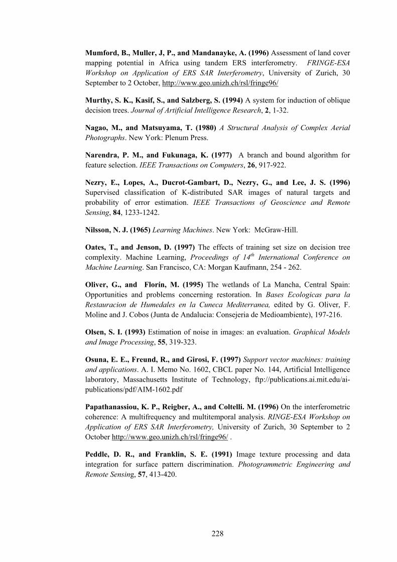
228
Mumford, B., Muller, J, P., and Mandanayke, A. (1996) Assessment of land covermapping potential in Africa using tandem ERS interferometry. FRINGE-ESAWorkshop on Application of ERS SAR Interferometry, University of Zurich, 30September to 2 October, http://www.geo.unizh.ch/rsl/fringe96/
Murthy, S. K., Kasif, S., and Salzberg, S. (1994) A system for induction of obliquedecision trees. Journal of Artificial Intelligence Research, 2, 1-32.
Nagao, M., and Matsuyama, T. (1980) A Structural Analysis of Complex AerialPhotographs. New York: Plenum Press.
Narendra, P. M., and Fukunaga, K. (1977) A branch and bound algorithm forfeature selection. IEEE Transactions on Computers, 26, 917-922.
Nezry, E., Lopes, A., Ducrot-Gambart, D., Nezry, G., and Lee, J. S. (1996)Supervised classification of K-distributed SAR images of natural targets andprobability of error estimation. IEEE Transactions of Geoscience and RemoteSensing, 84, 1233-1242.
Nilsson, N. J. (1965) Learning Machines. New York: McGraw-Hill.
Oates, T., and Jenson, D. (1997) The effects of training set size on decision treecomplexity. Machine Learning, Proceedings of 14th International Conference onMachine Learning. San Francisco, CA: Morgan Kaufmann, 254 - 262.
Oliver, G., and Florín, M. (1995) The wetlands of La Mancha, Central Spain:Opportunities and problems concerning restoration. In Bases Ecologicas para laRestauracion de Humedales en la Cuneca Mediterranea, edited by G. Oliver, F.Moline and J. Cobos (Junta de Andalucia: Consejeria de Medioambiente), 197-216.
Olsen, S. I. (1993) Estimation of noise in images: an evaluation. Graphical Modelsand Image Processing, 55, 319-323.
Osuna, E. E., Freund, R., and Girosi, F. (1997) Support vector machines: trainingand applications. A. I. Memo No. 1602, CBCL paper No. 144, Artificial Intelligencelaboratory, Massachusetts Institute of Technology, ftp://publications.ai.mit.edu/ai-publications/pdf/AIM-1602.pdf
Papathanassiou, K. P., Reigber, A., and Coltelli. M. (1996) On the interferometriccoherence: A multifrequency and multitemporal analysis. RINGE-ESA Workshop onApplication of ERS SAR Interferometry, University of Zurich, 30 September to 2October http://www.geo.unizh.ch/rsl/fringe96/ .
Peddle, D. R., and Franklin, S. E. (1991) Image texture processing and dataintegration for surface pattern discrimination. Photogrammetric Engineering andRemote Sensing, 57, 413-420.

229
Peleg, S., Naor, J., Hartley, R., and Avnir, D. (1984) Multiple resolution textureanalysis and classification, IEEE Transactions on Pattern Analysis and MachineIntelligence, 6, 518-523.
Pentland, A. P. (1984) Fractal based description of natural scenes. IEEETransactions of Pattern Analysis and Machine Intelligence, 6, 661-674.
Pentland, A. P. (1986) Shading into texture. Journal of Artificial Intelligence,29,147-170.
Pierce, L. E., Ulaby, F. T., Sarabandi, K., and Dobson, M. C. (1994) Knowledge-based classification of polarimetric SAR images, IEEE Transactions of Geoscienceand. Remote Sensing, 32, 1081-1086.
Piper, J. (1992) Variability and bias in experimentally measured classifier error rates.Pattern Recognition Letters, 13, 685-692.
Prati, C., Rocca, F., and Mouti Guaruieri, A. (1992) SAR InterferometryExperiments with ERS-1. First ERS-1 Symposium--Space at the Service of ourEnvironment, Cannes, France, 4-6 November, 211-217.
Prati, C., Rocca, F., Guarnieri, A. M., and Pasquali, P (1994) Report on ERS-1SAR interferometric techniques and applications. ESA Study Contract Report, ESAContract No.:3-7439/92/HE-1.
Quinlan, J. R. (1987) Simplifying decision trees. International Journal of Man-Machine Studies. 27, 221-234.
Quinlan, J. R., and Rivest, R. L. (1989) Inferring decision trees using minimumdescription length principle. Information and Computation. 80, 227-248.
Quinlan, J. R. ((1990) Decision tree and decision making. IEEE Transactions onSystems, Man, and Cybernetics. 20, 339-346.
Quinlan, J. R. (1993) C4.5: Programs for Machine Learning. San Mateo: MorganKaufmann.
Quinlan, J. R. (1996) Bagging, boosting and C4.5. Thirteenth National Conferenceof Artificial Intelligence. American Association for ArtificialIntelligence Portland, August 4 - 8, Oregon, USA.
Quinlan, J. R. (1996) Improved use of continuous attributes in C4.5. Journal ofArtificial Intelligence Research, 4, 77-90.
Raffy, M. (1992) Change of scale in models of remote sensing: a general method forspatialization of models. Remote Sensing of Environment, 40, 101-112.
Raudys, S., and Pikelis, V. (1980) On dimensionality, sample size, classificationerror, and complexity of classification algorithms in pattern recognition. IEEETransactions of Pattern Analysis and Machine Intelligence, 3, 242-252.

230
Raudys, S. J., and Jain, A. K. (1991) Small sample size effects in statistical patternrecognition: Recommendations for practitioners. IEEE Transactions of PatternAnalysis and Machine Intelligence, 13, 252-264.
Ribbes, F., Toan, T. L., Bruniquel, J., Floury, N., Stussi, N., Liew, S. C., andWasrin, U. R. (1997) Forest mapping in tropical region using multitemporal andInterferometric ERS-1/2 data. Proceedings of Third ERS Symposium, Florence, Italy,http://earth1.esa.it/florence/papers/.
Richards, J. A. (1993) Remote Sensing Digital Image Analysis- An Introduction.Berlin : Springer-Verlag.
Rissanen, J. (1983) A universal prior for integers and estimation by minimumdescription length. Annals of Statistics, 11, 416-431.
Rodriquez, E., Martin, J. M. (1992) Theory and design of interferometric syntheticaperture radars. IEE Proceedings-F, 139, 147-159.
Roli, F., Giacinto, G., and Vernazza, G. (1997) Comparison and combination ofstatistical and neural networks algorithms for remote-sensing image classification.Neurocomputation in Remote Sensing Data Analysis, Austin, J., Kanellopoulos, I.,Roli, F. and Wilkinson G. (Eds.), Berlin: Springer-Verlag, 117-124.
Rosenfield, G. H. (1982) Sample design for estimating changes in land use and landcover. Photogrammetric Engineering and Remote Sensing, 48, 793-801.
Rott, H., and Seigal, A. ( 1996) Glaciological studies in the Alps and in Antarcticausing ERS interferometric SAR. FRINGE-ESA Workshop on Application of ERS SARInterferometry, University of Zurich, 30 September to 2 October,http://www.geo.unizh.ch/rsl/fringe96/.
Rounds, E. M. (1980) A combined nonparametric approach to feature selection andbinary decision tree design. Pattern Recognition, 12, 313-317.
Roven, E., and Alvarez, L. (1998) Multitemporal coherence mapping forclassification of land surfaces around the Gulf of California. Proceedings of the 24th
Annual Conference and Exhibition of Remote Sensing Society, The University ofGreenwich, 9-11 September.
Rumelhart, D. E., Hinton, G. E., and Williams, R. J. (1996) Learning internalrepresentation by error propagation. Parallel Distributed Processing: Explorations inthe Microstructure of Cognition, Volume 1: Foundations (ed.), Cambridge, MA: TheMIT Press, 318-362.
Sadowski, F. G., Malila, D. A., Sarno, J. E., and Nalepka, R. F. (1977) Theinfluence of multispectral scanner spatial resolution on forest feature classification.Proceedings of the Eleventh International Symposium on Remote Sensing ofEnvironment, ERIM, Ann Arbor, Michigan, 1279-1288.

231
Safavian, S. R., and Landgrebe, D. (1991) A survey of decision tree classifiermethodology. IEEE Transactions of Systems, Man, and Cybernetics, 21, 660-675.
Saint-Jean, R., Singhroy, V., and Khalifa, S. M. (1995) Geological interpretation ofintegrated SAR images in Azraq area of Jordan. Canadian Journal of RemoteSensing, 21, 511-517.
Sarkar, N., and Chaudhuri, B. B. (1994) An efficient differential box-countingapproach to compute the fractal dimension of images. IEEE Transactions on System,Man, and Cybernetics, 24, 115-120.
Saunders, C., Stitson, M. O., Weston, J., Bottou, L., Schölkopf, B., and Smola, A.(1998) Support Vector Machine - Reference Manual. Technical Report, CSD-TR-98-03, Royal Holloway and AT&T, University of London.
Schowengerdt, R. A. (1997) Remote Sensing Models and Methods for ImageProcessing. New York: Academic Press.
Schalkoff, R. J. (1992) Pattern Recognition: Statistical, Structural and NeuralApproaches. New York: Wiley.
Schaale, M., and Furrer, R. (1995) Land surface classification by neural networks.International Journal of Remote Sensing, 16, 3003-3031.
Schistad, S. A. H., Jain, A. K., and Taxt, T. (1994) Multisource classification ofremotely sensed data: Fusion of Landsat-TM and SAR images. IEEE Transactions ofGeoscience and Remote Sensing, 32, 768-778.
Scholkopf, B. (1997) Support Vector Learning. Ph. D. thesis, Technische Universitat,Berlin.
Schwabisch, M., Lehner, S., and Winkel, N. (1997) Coastline extraction using ERSSAR interferometry. Proceedings of Third ERS Symposium, Florence, Italy,http://earth1.esa.it/florence/papers/.
Sethi, I. K. (1990) Entropy nets: from decision tree to neural networks. Proceedingsof the IEEE, 78, 1605-1613.
Sethi, I. K., and Chatterjee, B. (1977) Efficient decision tree design for discretevariable pattern recognition problems. Pattern Recognition, 9, 197-206.
Seynat, C., and Hobbs, S. (1998) Crop parameter retrieval with multi-temporal SARcoherence images. Retrieval of Bio- and Physical Parameters from SAR Data forLand Application Workshop. ESTEC, The Netherlands, 21- 23 October 1998,http://www.estec.esa.nl/CONFANNOUN/98c07/.
Sharkawi, M., and Mark II, R. J. (1990) A performance comparison of trainedmultilayer perceptrons and trained classification trees. Proceeding of the IEEE, 78,1614-1619.

232
Snedecor, G. W., and Cochran, W. G. (1967) Statistical Methods. Ames, Iowa: TheIowa State University Press.
Solberg, A. H. S., and Jain, A. K. (1997) Texture fusion and feature selectionapplied to SAR imagery. IEEE Transactions on Geoscience and Remote Sensing, 35,475-479.
Srinivasan, R., Cannon, M., and White, J. (1988) Landsat data destriping usingpower spectral filtering. Optical Engineering, 27, 939-943.
Stehman, S. V. (1192) Comparison of systematic and random sampling forestimating the accuracy of maps generated from remotely sensed data.Photogrammetric Engineering and Remote Sensing, 58, 1343-1350.
Stockham, T. G. (1972) Image processing in the context of a visual model.Proceeding of the IEEE, 60, 828-842.
Stoffel, J. C. (1974) A classifier design technique for discrete variable patternrecognition problems. IEEE Transactions on Computers, C-23, 428-441.
Story, M., and Congalton, R. G. (1986) Accuracy assessment: a user's perspective.Photogrammetric Engineering and Remote Sensing, 52, 397-399.
Stozzi, T., Dammert, P., Wegmuller, Martinez, J. M., Beaudoin, A., Askne, J.,and Hallikainen, M. (1998) European forest mapping with SAR interferometry.Retrieval of Bio- and Physical Parameters from SAR Data for Land ApplicationWorkshop. ESTEC, The Netherlands, 21- 23 October 1998,http://www.estec.esa.nl/CONFANNOUN/98c07/.
Stussi, N., Liew, S. C., Kwoh, L. K., Lim, H., Nicol, J., and Goh, K. C. (1997)Landcover classification using ERS SAR/INSAR data on coastal region of centralSumatra. Proceedings of Third ERS Symposium, Florence, Italy,http://earth1.esa.it/florence/papers/.
Strahler, A. H., Woodcock, C. E., and Smith, J. A. (1986) On the nature of modelsin remote sensing. Remote Sensing of Environment, 20, 121-139.
Strobl, P., and Zhukov, B. (1998) Recent developments in 3-12 µm radiometriccalibration of the DAIS 7915. Ist EARSeL Workshop on Imaging Spectroscopy,Remote Sensing Laboratories, University of Zurich, 6-8 October.
Strobl, P., Muller, A., Schlaepfer, D., and Schaepman, M. (1997) Laboratorycalibration and in-flight validation of DAIS 7915 data. Proceedings of SPIE:Algorithms for Multispectral and Hyperspectral Imagery III, 3071, 225-236.
Swain, P., and Davis, S. (1978) Remote Sensing: The Quantitative Approach. NewYork: McGraw-Hill.
Swain, P. H., and Hauska, H. (1977) The decision tree classifier: design andpotential. IEEE Transactions on Geoscience Electronics, 3, 142-147.

233
Switzer, P., and Green, A. (1984) Min/max autocorrelation factors for multivariatespatial imagery. Technical Report 6, Department of Statistics, Stanford University.
Tell, B. R., and Walker, N. P. (1998) Examining the effect of satellite repeat passtimes on interferometric coherence for land classification applications. Retrieval ofBio- and Physical Parameters from SAR Data for Land Application Workshop.ESTEC, The Netherlands, 21- 23 October 1998,http://www.estec.esa.nl/CONFANNOUN/98c07/.
Tortora, R. D. (1978) A note on sample size estimation for multinomial populations.The American Statistician, 32, 100-102.
Tou, J., and Gonzalez, R. (1974) Pattern Recognition Principles. Reading,Massachusetts: Addison-Wesley.
Touzi, R., Lopes, A., Bruniquel, J., and Vachon, P. W. (1999) Coherenceestimation of SAR imagery. IEEE Transactions on Geoscience and Remote Sensing,37, 135-149.
Townshend, J. R. G. (1984) Agriculture land-cover discrimination using thematicmapper spectral bands. International Journal of Remote Sensing, 5, 681-698.
Townshend, F. E. (1986) The enhancement of computer classifications by logicalsmoothing. Photogrammetric Engineering and Remote Sensing, 52, 213-221.
Townshend, J. R. G., and Justice, C. (1981) Information extraction from remotelysensed data: a user view. International Journal of Remote Sensing, 2, 313-329.
Townshend, J. R. G. (1992) Land cover. International Journal of Remote Sensing,13, 1319-1328.
Tso, B. C. K. (1997) An Investigation of Alternate Strategies for IncorporatingSpectral, Textural, and Contextual Information in Remote Sensing ImageClassification. PhD Thesis. School of Geography, The University of Nottingham,Nottingham, UK.
Tso, B. C. K., and Mather, P. M., (2001) Classification Methods for Remotelysensed Data. London: Taylor and Francis.
Ulaby, F. T. (1980) Vegetation clutter model. IEEE Transactions of Antennas andPropagation, 28, 538-545.
Ulaby, F. T., Kouyate, F., brisco, B., and Williams, L. (1986) Textural informationin SAR images. IEEE Transactions of Geoscience and. Remote Sensing, 24, 235-245.
Ulbricht, A. (1998) Evaluation of the potential of full-polarimetic airborne repeat-pass- SAR- interferometery for classification of changes detected by the coherence.Retrieval of Bio- and Physical Parameters from SAR Data for Land ApplicationWorkshop. ESTEC, The Netherlands, 21-23 October 1998,http://www.estec.esa.nl/CONFANNOUN/98c07/.

234
Usai, S., and Hanssen, R. (1997) Long time scale INSAR by means of highcoherence features. Proceedings of Third ERS Symposium, Florence, Italy,http://earth1.esa.it/florence/papers/.
Utgoff, P. E., and Brodley, C. E., (1990) An incremental method of findingmultivariate splits for decision trees. Machine Learning, Proceedings of the SeventhInternational conference on Machine Learning. Austin, Texas: Morgan Kaufmann.
Van Genderen, J. L., and Lock, B. F. (1977) Testing land use map accuracy.Photogrammetric Engineering and Remote Sensing, 43, 1135-1137.
Vapnik, W. N., and Chervonenkis, A. Y. (1971) On the uniform convergence ofrelative frequencies of events to their probabilities. Theory of Probability and itsApplications. 17, 264-280.
Vapnik, W. N., and Chervonenkis, A. Y. (1979) Theory of Pattern Recognition.Berlin: Akademia-Verlag.
Vapnik, W. N. (1982) Estimation of dependencies based on empirical data. Berlin:Springer-Verlag.
Vapnik, W. N., and Chervonenkis, A. Y. (1991) The necessary and sufficientconditions for consistency in the empirical risk minimisation method. PatternRecognition and Image Analysis. 1, 283-305.
Vapnik, V. N. (1995) The Nature of Statistical Learning Theory. New York:Springer-Verlag.
Vapnik, V. N. (1999) An overview of statistical learning theory. IEEE Transactionsof Neural Networks, 10, 988-999.
Watanabe, S. (1965) Karhunen-Loeve expansion and factor analysis, theoreticalremarks and applications. Transactions of the Fourth Prague Conference onInformation Theory, Prague, Czechoslovakia.
Wegmuller, U., and Werner, C. (1994) Analysis of interferometric land surfacesignatures. Proceedings of Progress in Electromagnetic Research Symposium,Noordwijk, July 11-15, Noordwijk, The Netherlands.
Wegmuller, U., Werner, C., Neusch, D., and Borgeoud, M. (1995) Land – surfaceanalysis using ERS-1 SAR interferometry, ESA Bulletin, 81, 30-37.
Wegmuller, U., and Werner, C. (1995) SAR interferometric signature of forests.IEEE Transactions on Geoscience and Remote Sensing, 33, 1153-1161.
Wegmuller, U., and Werner, C. (1996) Land application using ERS –1/2 tandemdata. FRINGE-ESA Workshop on Application of ERS SAR Interferometry, Universityof Zurich, 30 September to 2 October, http://www.geo.unizh.ch/rsl/fringe96/.

235
Wegmuller, U., and Werner, C. (1997) Retrieval of vegetation parameters withSAR interferometry, IEEE Transactions on Geoscience and Remote Sensing, 35, 18-24.
Westin, J., and Watkins, C. (1998) Multi-class Support Vector Machines. RoyalHolloway, University of London, U. K., Technical Report CSD-TR-98-04.
Weszka, J. S., Dyer, C. R., and Rosenfeld, A. (1976) A comparitive study of texturemeasures for terrain classification. IEEE Transactions on Systems, Man, andCybernetics, SMC-6, 269-285.
Wharton, S (1987) A spectral-knowledge-based approach for urban and land-coverdiscrimination. IEEE Transactions of Geoscience and Remote Sensing, 25, 272-282.
Wilkinson, G. G. (1997) Open questions in neurocomputing for earth observation. InNeuro-Computation in Remote Sensing Data Analysis, edited by I.
Kanellopoulos, G. G. Wilkinson, F. Roli and J. Austin.London: Springer, 3-13.
Wilkinson, G. G. (2000) Processing and classification of satellite images.Encyclopaedia of Analytical Chemistry, Edited by R. A. Meyers. John Wiley andsons, 8679-8693.
Woodcock, C. E., and Strahler, A. H. (1987) The factor of scale in remote sensing.Remote Sensing of Environment, 21, 311-332.
Xia, Z. G., Clarke, K., C. (1997) Approaches to scaling of geo-spatial data. Scale inRemote Sensing and GIS, Quattrochi, D. A., and Goodchild, M. A. (ed.), Boca Raton:CRC Press, 309-360.
You, K. C., and Fu, K. S. (1976) An approach to the design of a linear binary treeclassifier. Proceedings of the Symposium on Machine Processing of Remotely SensedData. 3A-1-3A-10.
Zebker, H. A., and Goldstein, R. M. (1986) Topographic mapping frominterferometric synthetic aperture radar observations. Journal of GeophysicalResearch, 91, 4993-4999.
Zebker, H. A., and Villasenor, I. (1992) Decorrelation in interferometric radarechoes. IEEE Transaction of Geoscience and Remote Sensing, 30, 950-959.
Zhang, M., and Scofield, R. A. (1994) Artificial neural network techniques forestimating heavy convective rainfall and recognising cloud mergers. InternationalJournal of Remote Sensing, 15, 3241-3261.
Zhu, G., and Blumberg, D. G., (2002) Classification using ASTER data and SVMalgorithms; The case study of Beer Sheva, Israel. Remote Sensing of Environment, 80,233-240.

236
Zmuda, A., Slater, J., Batts, A., and Seaman, E. (1988) Mapping land cover, soilcultivation and crop establishment for nitrate sensitivity analysis using ERS InSARdata. Retrieval of Bio- and Physical Parameters from SAR Data for Land ApplicationWorkshop. ESTEC, The Netherlands, 21-23 October 1998,http://www.estec.esa.nl/CONFANNOUN/98c07/.

237
APPENDIX A
CONFUSION MATRICES FOR CHAPTER 5 (Section 5.1)
Univariate decision tree classifier with different training data
700 training pixels
Class 1 2 3 4 5 6 7 Total User's1 281 7 15 2 0 0 0 305 92.132 10 191 37 14 23 10 0 285 67.023 7 32 179 8 3 10 1 240 74.584 2 28 61 249 7 19 7 373 66.765 0 22 1 3 266 0 0 292 91.16 0 17 4 17 1 209 10 258 81.017 0 3 3 7 0 52 219 284 77.11
Total 300 300 300 300 300 300 237 2037produc. 93.67 63.67 59.67 83 88.67 69.67 92.41
Overall Accuracy = 78.25 Kappa value = 0.75
1050 training pixels
Class 1 2 3 4 5 6 7 Total User's1 273 8 10 4 0 0 0 295 92.542 21 225 11 15 30 7 1 310 72.583 5 24 221 32 7 13 4 306 72.224 1 22 47 233 10 15 3 331 70.395 0 4 4 0 252 5 1 266 94.746 0 13 3 10 1 228 21 276 82.617 0 4 4 6 0 32 207 253 81.82
Total 300 300 300 300 300 300 237 2037produc. 91 75 73.67 77.67 84 76 87.34
Overall accuracy =80.46 Kappa value = 0.772
1400 training pixels
Class 1 2 3 4 5 6 7 Total User's1 282 8 4 2 0 0 0 296 95.272 12 236 22 24 34 6 0 334 70.663 4 15 233 21 8 10 2 293 79.524 2 17 29 233 3 10 4 298 78.195 0 5 1 2 254 0 0 262 96.956 0 19 9 11 1 237 27 304 77.967 0 0 2 7 0 37 204 250 81.6
Total 300 300 300 300 300 300 237 2037produc. 94 78.67 77.67 77.67 84.67 79 86.08
Overall accuracy = 82.43 kappa value = 0.795

1750 training pixels
Class 1 2 3 4 5 6 7 Total User's1 277 5 5 2 0 0 0 289 95.852 13 217 11 11 28 12 1 293 74.063 6 26 240 26 5 15 2 320 754 4 18 31 242 3 7 5 310 78.065 0 15 0 2 263 0 0 280 93.936 0 18 10 7 1 251 21 308 81.497 0 1 3 10 0 15 208 237 87.76
Total 300 300 300 300 300 300 237 2037produc. 92.33 72.33 80 80.67 87.67 83.67 87.76
Overall accuracy = 83.36 Kappa value = 0.806
2100 training pixels
Class 1 2 3 4 5 6 7 Total User's1 287 6 13 7 1 0 0 314 91.42 8 224 14 7 32 5 1 291 76.983 3 21 234 18 2 12 3 293 79.864 2 20 26 239 2 7 3 299 79.935 0 16 1 2 262 0 0 281 93.246 0 11 9 16 1 262 24 323 81.117 0 2 3 11 0 14 206 236 87.29
Total 300 300 300 300 300 300 237 2037produc. 95.67 74.67 78 79.67 87.33 87.33 86.92
Overall accuracy = 84.14 Kappa value = 0.815
2400 training pixels
Class 1 2 3 4 5 6 7 Total User's1 272 6 7 2 0 0 0 287 94.772 20 221 19 14 20 16 0 310 71.293 3 17 228 17 3 12 3 283 80.574 5 18 31 245 4 5 1 309 79.295 0 20 1 3 270 0 0 294 1006 0 17 10 13 3 257 30 330 77.887 0 1 4 6 0 10 203 224 90.63
Total 300 300 300 300 300 300 237 1696produc. 90.67 73.67 76 81.67 90 85.67 67.67
Overall accuracy = 83.26 Kappa value = 0.805
238
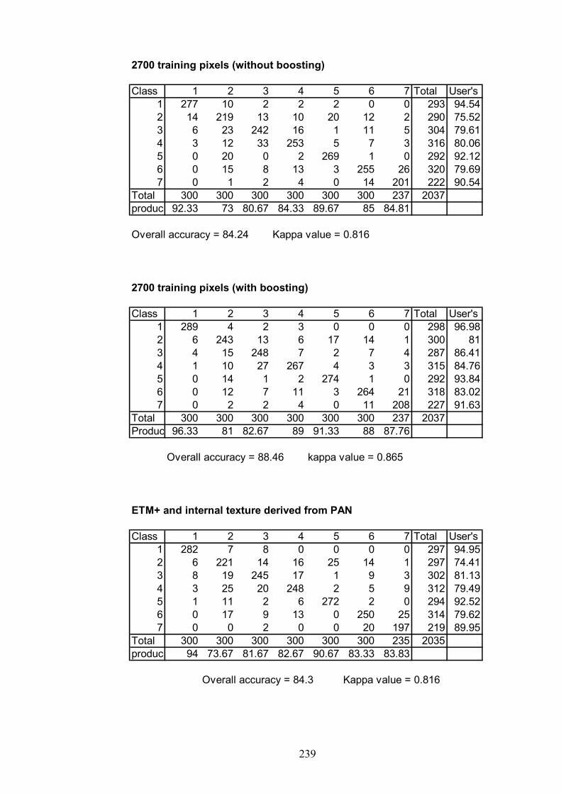
2700 training pixels (without boosting)
Class 1 2 3 4 5 6 7 Total User's1 277 10 2 2 2 0 0 293 94.542 14 219 13 10 20 12 2 290 75.523 6 23 242 16 1 11 5 304 79.614 3 12 33 253 5 7 3 316 80.065 0 20 0 2 269 1 0 292 92.126 0 15 8 13 3 255 26 320 79.697 0 1 2 4 0 14 201 222 90.54
Total 300 300 300 300 300 300 237 2037produc. 92.33 73 80.67 84.33 89.67 85 84.81
Overall accuracy = 84.24 Kappa value = 0.816
2700 training pixels (with boosting)
Class 1 2 3 4 5 6 7 Total User's1 289 4 2 3 0 0 0 298 96.982 6 243 13 6 17 14 1 300 813 4 15 248 7 2 7 4 287 86.414 1 10 27 267 4 3 3 315 84.765 0 14 1 2 274 1 0 292 93.846 0 12 7 11 3 264 21 318 83.027 0 2 2 4 0 11 208 227 91.63
Total 300 300 300 300 300 300 237 2037Produc 96.33 81 82.67 89 91.33 88 87.76
Overall accuracy = 88.46 kappa value = 0.865
ETM+ and internal texture derived from PAN
239
Class 1 2 3 4 5 6 7 Total User's1 282 7 8 0 0 0 0 297 94.952 6 221 14 16 25 14 1 297 74.413 8 19 245 17 1 9 3 302 81.134 3 25 20 248 2 5 9 312 79.495 1 11 2 6 272 2 0 294 92.526 0 17 9 13 0 250 25 314 79.627 0 0 2 0 0 20 197 219 89.95
Total 300 300 300 300 300 300 235 2035produc. 94 73.67 81.67 82.67 90.67 83.33 83.83
Overall accuracy = 84.3 Kappa value = 0.816

240
ETM+ with PAN and internal texture of PAN
Class 1 2 3 4 5 6 7 Total User's1 277 9 2 2 0 0 0 290 95.522 8 236 11 16 23 2 1 297 79.463 9 9 248 21 2 12 5 306 81.054 4 12 27 247 5 7 3 305 80.985 2 27 1 2 268 2 0 302 88.746 0 7 9 9 1 258 28 312 82.697 0 0 2 3 1 19 197 222 88.74
Total 300 300 300 300 300 300 234 2034Produc 92.33 78.67 82.67 82.33 89.33 86 84.19
Overall accuracy = 85.10 Kappa value = 0.826
ETM+ with PAN and internal texture+three GLCM features of PAN
class 1 2 3 4 5 6 7 Total User's1 291 10 2 0 0 0 0 303 96.042 5 235 15 16 16 4 0 291 80.763 3 21 246 26 4 4 6 310 79.354 1 19 28 243 8 5 5 309 78.645 0 9 0 2 269 0 0 280 96.076 0 6 8 12 3 261 18 308 84.747 0 0 1 1 0 26 214 242 88.43
Total 300 300 300 300 300 300 243 2043Produc 97 78.33 82 81 89.67 87 88.07
Overall accuracy = 86.1 Kappa value = 0.838
ETM+,PAN and internal texture+3GLCM features of PAN (boosted)
Class 1 2 3 4 5 6 7 Total User's1 292 7 1 2 0 0 0 302 96.692 5 252 8 12 14 1 3 295 85.423 3 21 269 15 6 6 4 324 83.024 0 8 16 254 4 4 6 292 86.995 0 8 0 2 273 1 0 284 96.136 0 4 5 14 3 272 11 309 88.037 0 0 1 1 0 16 219 237 92.41
Total 300 300 300 300 300 300 243 2043produc. 97.33 84 89.67 84.67 91 90.67 90.12
Overall accuracy = 89.6 Kappa value = 0.879

241
Maximum likelihood classifier results
ETM+ data
class 1 2 3 4 5 6 7 Total User's1 288 5 1 0 0 0 0 294 982 2 235 10 8 16 2 0 273 86.13 7 19 246 34 3 9 3 321 76.64 3 6 31 212 4 3 5 264 80.35 0 13 0 1 277 0 0 291 95.26 0 21 8 15 0 209 7 260 80.47 0 1 4 30 0 77 222 334 66.5
Total 300 300 300 300 300 300 237 2037Produ . 96.0 78.3 82 70.7 92.3 69.7 93.7
Overall accuracy = 82.9 Kappa Value = 0.801
ETM+ with internal texture of PAN
Class 1 2 3 4 5 6 7 Total Users1 283 8 0 1 0 0 0 292 96.92 6 234 4 12 24 4 0 284 82.43 8 10 249 30 2 12 2 313 79.64 1 13 27 226 1 8 3 279 815 0 10 2 2 273 0 0 287 95.16 2 25 14 18 0 204 7 270 75.67 0 0 4 11 0 72 223 310 71.9
Total 300 300 300 300 300 300 235 2035Produ. 94.3 78 83 75.3 91 68 94.9
Overall accuracy = 83.1 Kappa value = 0.803
ETM+ with PAN and internal texture of PAN
Class 1 2 3 4 5 6 7 Total Users1 279 7 0 1 0 0 0 287 97.22 9 241 12 18 19 3 0 302 79.83 6 10 232 25 1 8 1 283 824 6 5 41 232 1 4 13 302 76.85 0 22 1 1 276 0 0 300 926 0 15 14 15 3 215 14 276 77.97 0 0 0 8 0 70 206 284 72.5
Total 300 300 300 300 300 300 234 2034Produ. 93 80.3 77.3 77.3 92 71.7 88
Overall accuracy = 82.6 Kappa value = 0.798

242
ETM+ with PAN and internal texture+3 GLCM features of PAN
Class 1 2 3 4 5 6 7 Total Users1 292 6 1 0 0 0 0 299 97.72 5 256 8 24 21 8 0 322 79.53 1 11 237 10 7 8 0 274 86.54 0 5 43 250 1 2 1 302 82.85 0 12 0 0 269 0 0 281 95.76 2 10 4 8 2 197 11 234 84.27 0 0 7 8 0 85 231 331 69.8
Total 300 300 300 300 300 300 243 2043Produ. 97.3 85.3 79 83.3 89.7 65.7 95.1
Overall accuracy = 84.8 Kappa value = 0.823
Neural network classifier results
ETM+ data
Class 1 2 3 4 5 6 7 Total Users1 288 3 3 1 0 0 0 295 97.62 2 242 8 0 12 5 1 270 89.63 2 16 258 22 2 10 5 315 81.94 3 4 12 229 5 2 1 256 89.55 0 7 0 1 272 0 0 280 97.16 0 10 1 5 1 256 26 299 85.67 0 0 0 0 0 1 188 189 99.5
Uncla. 5 18 18 42 8 26 16 133 7Total 300 300 300 300 300 300 237 2037Produ. 96 80.7 86 76.3 90.7 85.3 79.3
Overall accuracy = 85.1 Kappa value = 0.829
ETM+ and internal texture of PAN
Class 1 2 3 4 5 6 7 Total Users1 277 3 1 1 0 0 0 282 98.22 8 251 7 4 27 0 1 298 84.23 4 16 262 14 1 12 1 310 84.54 1 8 14 250 1 4 5 283 88.35 0 2 0 2 266 0 0 270 98.56 0 4 2 5 0 245 25 281 87.27 0 0 0 0 0 6 186 192 96.9
Uncla. 10 16 14 24 5 33 17 119 6.2Total 300 300 300 300 300 300 235 2035Produ. 92.3 83.7 87.3 83.3 88.7 81.7 79.1
Overall accuracy = 85.4 Kappa value = 0.832

243
ETM+with PAN and internal texture of PAN
Class 1 2 3 4 5 6 7 Total Users1 285 9 1 4 0 0 0 299 95.32 0 238 3 2 16 0 0 259 91.93 5 5 231 10 1 5 0 257 89.94 2 4 31 259 0 7 4 307 84.45 0 10 0 0 269 0 0 279 96.46 0 6 3 1 3 261 24 298 87.67 0 0 1 0 0 6 199 206 96.6
Uncla. 8 28 30 24 11 21 7 129 6.8Total 300 300 300 300 300 300 234 2034produc. 95 79.3 77 86.3 89.7 87 85
Overall accuracy = 85.6 Kappa value = 0.836
ETM+ with PAN and internal texture+3 GLCM features of PAN
Class 1 2 3 4 5 6 7 Total Users1 287 5 1 0 0 0 0 293 982 7 271 8 9 20 0 1 316 85.83 2 3 257 13 3 7 1 286 89.94 1 6 8 247 0 3 4 269 91.85 0 3 0 0 270 1 0 274 98.56 0 3 4 2 2 251 14 276 90.97 0 0 0 0 0 14 208 222 93.7
Uncla. 3 9 22 29 5 24 15 107 5.5Total 300 300 300 300 300 300 243 2043Produ. 95.7 90.3 85.7 82.3 90 83.7 85.6
Overall accuracy = 87.7 Kappa value = 0.858

244
Multivariate decision tree (QUEST) classifier with differenttraining data
700 training pixels
Class 1 2 3 4 5 6 7 Total Users1 270 6 16 0 0 0 0 292 92.472 11 216 28 28 32 13 4 332 65.063 3 23 223 44 3 12 7 315 70.794 15 18 17 196 5 6 3 260 75.385 0 6 0 0 251 1 0 258 97.296 1 29 13 11 9 238 25 326 73.017 0 2 3 21 0 30 198 254 77.95
Total 300 300 300 300 300 300 237 2037Produ. 90 72 74.33 65.33 83.67 79.33 66
Overall accuracy = 78.15
1050 training pixels
Class 1 2 3 4 5 6 7 Total Users1 273 8 11 2 1 0 0 295 92.542 17 238 26 19 31 22 3 356 66.853 3 20 222 31 4 8 2 290 76.554 7 10 33 210 2 18 9 289 72.665 0 7 0 9 255 0 0 271 94.16 0 17 6 8 7 238 27 303 78.557 0 0 2 21 0 14 196 233 84.12
Total 300 300 300 300 300 300 237 2037Produ. 91 79.33 74 70 85 79.33 82.7
Overall accuracy = 80.12
1400 training pixels
Class 1 2 3 4 5 6 7 Total Users1 278 6 8 2 1 0 0 295 94.242 13 214 16 11 22 8 1 285 75.093 4 22 214 25 4 8 0 277 77.264 5 24 42 230 8 9 2 320 71.885 0 5 0 0 263 0 0 268 98.136 0 29 20 25 2 254 23 353 71.957 0 0 0 7 0 21 211 239 88.28
Total 300 300 300 300 300 300 237 2037Produ. 92.67 71.33 71.33 76.67 87.67 84.67 89.03
Overall accuracy = 81.69

245
1750 training pixels
Class 1 2 3 4 5 6 7 Total Users1 287 6 7 2 2 0 0 304 94.412 3 232 21 13 20 9 2 300 77.333 4 16 219 30 4 11 1 285 76.844 6 24 34 225 11 6 3 309 72.825 0 5 0 2 260 0 0 267 97.386 0 17 17 11 3 251 20 319 78.687 0 0 2 17 0 23 211 253 83.4
Total 300 300 300 300 300 300 237 2037Produ. 95.67 77.33 73 75 86.67 83.67 89.03
Overall accuracy =82.72
2100 training pixels
Class 1 2 3 4 5 6 7 Total Users1 281 6 7 0 2 0 0 296 94.932 10 223 21 16 20 6 1 297 75.083 2 14 209 16 4 13 0 258 81.014 7 24 52 246 7 14 11 361 68.145 0 12 0 1 263 6 0 282 93.266 0 21 10 12 4 245 29 321 76.327 0 0 1 9 0 16 196 222 88.29
Total 300 300 300 300 300 300 237 2037Produ. 93.67 74.33 69.67 82 87.67 81.67 82.7
Overall accuracy = 81.64
2400 training pixels
Class 1 2 3 4 5 6 7 Total Users1 285 9 9 1 4 0 0 308 92.532 7 232 21 7 17 9 1 294 78.913 2 7 210 16 2 4 0 241 87.144 6 21 42 239 10 8 4 330 72.425 0 5 0 0 256 0 0 261 98.086 0 24 7 9 11 252 23 326 77.37 0 2 11 28 0 27 209 277 75.45
Total 300 300 300 300 300 300 237 2037Produ. 95 77.33 70 79.67 85.33 84 88.19
Overall accuracy = 82.62

246
2700 training pixels
Class 1 2 3 4 5 6 7 Total Users1 286 5 3 2 1 0 0 297 96.32 5 245 19 8 28 7 2 314 78.033 4 16 234 36 6 4 3 303 77.234 5 10 32 232 9 12 2 302 76.825 0 4 0 0 245 0 0 249 98.396 0 20 10 15 11 254 17 327 77.687 0 0 2 7 0 23 213 245 86.94
Total 300 300 300 300 300 300 237 2037Produ. 95.33 81.67 78 77.33 81.67 84.67 89.87
Overall accuracy = 83.9
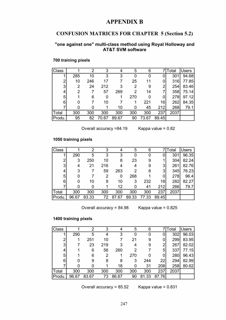
CONFUSION MATR
"one against one" multA
700 training pixels
Class 1 21 285 102 10 246 13 2 24 214 2 7 55 1 66 0 7 17 0 0
Total 300 300 30Produ. 95 82 70.6
Overall accu
1050 training pixels
Class 1 21 290 52 3 250 13 4 21 214 3 7 55 0 76 0 107 0 0
Total 300 300 30Produ. 96.67 83.33 7
Overall accu
1400 training pixels
Class 1 21 290 52 1 251 13 7 23 214 1 6 55 1 66 0 97 0 0
Total 300 300 30Produ. 96.67 83.67 7
Overall accu
APPENDIX B
ICES FOR CHAPTER 5 (Section 5.2)
i-class method using Royal Holloway andT&T SVM software
3 4 5 6 7 Total Users3 3 0 0 0 301 94.687 7 25 11 0 316 77.852 3 2 9 2 254 83.467 269 2 14 7 358 75.140 1 270 0 0 278 97.120 7 1 221 16 262 84.351 10 0 45 212 268 79.10 300 300 300 237 20377 89.67 90 73.67 89.45
racy =84.19 Kappa value = 0.82
3 4 5 6 7 Total Users3 3 0 0 0 301 96.350 8 23 9 1 304 82.246 4 4 9 3 261 82.769 263 2 8 3 345 76.232 0 268 1 0 278 96.49 10 3 232 18 282 82.271 12 0 41 212 266 79.70 300 300 300 237 20372 87.67 89.33 77.33 89.45
racy = 84.98 Kappa value = 0.825
3 4 5 6 7 Total Users4 3 0 0 0 302 96.030 7 21 9 0 299 83.959 3 4 9 2 267 82.026 260 2 7 5 337 77.152 1 270 0 0 280 96.438 8 3 244 22 294 82.991 18 0 31 208 258 80.620 300 300 300 237 20373 86.67 90 81.33 87.76
racy = 85.52 Kappa value = 0.831
247

248
1750 training pixels
Class 1 2 3 4 5 6 7 Total Users1 287 4 1 3 0 0 0 295 97.292 2 248 8 5 20 6 0 289 85.813 8 21 218 4 5 8 2 266 81.954 2 8 59 267 4 8 4 352 75.855 1 7 2 0 268 0 0 278 96.46 0 12 10 7 3 245 22 299 81.947 0 0 2 14 0 33 209 258 81.01
Total 300 300 300 300 300 300 237 2037Produ. 95.67 82.67 72.67 89 89.33 81.67 88.19
Overall accuracy = 85.52 Kappa value = 0.831
2100 training pixels
Class 1 2 3 4 5 6 7 Total Users1 289 4 1 3 0 0 0 297 97.312 1 252 8 7 19 7 0 294 85.713 7 21 225 3 5 8 2 271 83.034 3 6 57 269 2 9 5 351 76.645 0 7 0 0 271 0 0 278 97.486 0 10 7 11 3 251 25 307 81.767 0 0 2 7 0 25 205 239 85.77
Total 300 300 300 300 300 300 237 2037Produ. 96.33 84 75 89.67 90.33 83.67 86.5
Overall accuracy = 86.5 Kappa value = 0.842
2400 training pixels
Class 1 2 3 4 5 6 7 Total Users1 290 5 2 3 0 0 0 300 96.672 1 254 9 7 19 8 0 298 85.233 7 21 229 7 4 9 2 279 82.084 2 6 52 264 2 6 3 335 78.815 0 7 0 0 272 0 0 279 97.496 0 7 7 14 3 261 26 318 82.087 0 0 1 5 0 16 206 228 90.35
Total 300 300 300 300 300 300 237 2037Produ. 96.67 84.67 76.33 88 90.67 87 86.92
Overall accuracy = 87.19 Kappa value = 0.85
249
2700 training pixels
Class 1 2 3 4 5 6 7 Total Users1 289 5 3 3 0 0 0 300 96.332 2 248 8 6 18 6 0 288 86.113 7 20 242 9 4 7 2 291 83.164 2 6 39 263 1 6 4 321 81.935 0 9 1 1 276 0 0 287 96.176 0 12 7 18 1 267 27 332 2.7817 0 0 0 0 0 14 204 218 93.58
Total 300 300 300 300 300 300 237 2037Produ. 96.33 82.67 80.67 87.67 92 89 86.08
Overall accuracy = 87.37 Kappa value = 0.86
"one against one" multi-class method using LIBSVM software
With 2700 training pixels
Class 1 2 3 4 5 6 7 Total Users1 290 5 3 3 0 0 0 301 96.352 2 249 9 7 21 6 1 295 84.413 6 20 244 10 2 7 1 290 84.144 2 7 37 263 1 6 5 321 81.935 0 8 0 1 275 0 0 284 96.836 0 11 7 16 1 267 27 329 81.167 0 0 0 0 0 14 203 217 93.55
Total 300 300 300 300 300 300 237 2037Produ. 96.67 83 81.33 87.67 91.67 89 85.65
Overall accuracy = 87.92 Kappa value = 0.87

250
"one against rest" multi-class method
700 training pixels
Class 1 2 3 4 5 6 7 Total Users1 283 6 2 2 0 0 0 293 96.592 3 226 10 1 15 4 1 260 86.923 4 8 188 1 2 6 0 209 89.954 1 1 26 207 0 0 1 236 87.715 0 5 0 0 263 0 0 268 98.136 0 2 6 1 0 193 3 205 94.157 0 0 0 0 0 31 192 223 86.1
Uncla. 9 52 68 88 20 66 40 343Total 300 300 300 300 300 300 237 2037Produ. 94.33 75.33 62.67 69 87.67 64.33 81.01
Overall accuracy = 76.19 Kappa value = 0.73
2700 training pixels
Class 1 2 3 4 5 6 7 Total Users1 285 3 1 2 0 0 0 291 97.942 2 229 10 0 14 0 0 255 89.83 3 11 209 3 1 7 0 234 89.324 2 3 19 213 0 1 4 242 88.025 0 7 0 0 266 0 0 273 97.446 0 6 4 4 0 236 21 271 87.087 0 0 0 0 0 10 186 196 94.9
Uncla. 8 41 57 78 19 46 26 275Total 300 300 300 300 300 300 237 2037Produ. 95 76.33 69.67 71 88.67 78.67 78.48
Overall accuracy = 79.73 Kappa value = 0.77

251
APPENDIX C
CONFUSION MATRICES FOR CHAPTER 6
Confusion matrices with maximum likelihood classifier
Data set1
Class 1 2 3 4 5 6 7 Total Users1 265 48 10 15 147 14 17 516 51.42 7 155 35 34 8 2 69 310 503 5 25 190 66 20 0 21 327 58.14 1 24 45 160 10 1 9 250 645 17 13 6 10 80 11 3 140 57.16 2 24 10 13 11 272 60 392 69.47 3 11 4 2 24 0 121 165 73.3
Total 300 300 300 300 300 300 300 2100Produ. 88.3 51.7 63.3 53.3 26.7 90.7 40.3
Overall acuuracy = 59.2 Kappa value = 0.526
Data set 2
Class 1 2 3 4 5 6 7 Total Users1 277 33 4 7 47 0 13 381 72.72 12 189 7 27 26 0 83 344 54.93 2 23 192 43 15 1 26 302 63.64 0 27 61 199 15 0 13 315 63.25 6 7 12 13 154 10 3 205 75.16 0 6 18 8 33 287 17 369 77.87 3 15 6 3 10 2 145 184 78.8
Total 300 300 300 300 300 300 300 2100Produ. 92.3 63 64 66.3 51.3 95.7 48.3
Overall accuracy = 68.7 Kappa value = 0.635
Data set 3
Class 1 2 3 4 5 6 7 Total Users1 240 49 11 20 33 0 30 383 62.72 27 154 22 49 13 1 81 347 44.43 5 9 33 6 7 0 19 79 41.84 2 24 6 90 40 9 6 177 50.85 23 29 31 58 131 14 6 292 44.96 0 24 170 69 70 274 36 643 42.67 3 11 27 8 6 2 122 179 68.2
Total 300 300 300 300 300 300 300 2100Produ. 80 51.3 11 30 43.7 91.3 40.7
Overall accuracy = 49.7 Kappa value = 0.413

Data set 4
252
Class 1 2 3 4 5 6 7 Total Users1 272 54 6 4 32 0 17 385 70.62 9 148 12 36 6 3 31 245 60.43 4 21 193 39 20 1 16 294 65.64 2 26 50 194 10 1 6 289 67.15 9 18 15 15 186 20 8 271 68.66 0 5 3 7 12 271 4 302 89.77 4 28 21 5 34 4 218 314 69.4
Total 300 300 300 300 300 300 300 2100Produ. 90.7 49.3 64.3 64.7 62 90.3 72.7
Overall accuracy = 70.6 Kappa value = 0.657
Data set 5
Class 1 2 3 4 5 6 7 Total Users1 273 36 2 7 13 0 6 337 812 10 200 13 35 25 8 10 301 66.43 1 15 239 46 13 3 13 330 72.44 0 19 22 191 14 2 9 257 74.35 4 11 7 6 201 8 2 239 84.16 0 1 3 5 2 276 1 288 95.87 12 18 14 10 32 3 259 348 74.4
Total 300 300 300 300 300 300 300 2100Produ. 91 66.7 79.7 63.7 67 92 86.3
Overall accuracy = 78.0 Kappa value = 0.744
Data set 6
Class 1 2 3 4 5 6 7 Total Users1 262 39 2 1 79 0 7 390 67.22 7 169 32 28 44 7 46 333 50.83 4 28 207 35 18 0 10 302 68.54 1 30 39 222 14 9 28 343 64.75 15 5 5 2 119 4 1 151 78.86 0 22 5 6 4 280 25 342 81.97 11 7 10 6 22 0 183 239 76.6
Total 300 300 300 300 300 300 300 2100Produ. 87.3 56.3 69 74 39.7 93.3 61
Overall accuracy = 68.7 Kappa value = 0.634
Data set 7
Class 1 2 3 4 5 6 7 Total Users1 277 37 1 2 12 0 2 331 83.72 4 182 18 22 31 10 57 324 56.23 3 19 228 28 16 1 11 306 74.54 1 40 34 236 17 7 16 351 67.25 11 9 8 2 213 10 2 255 83.56 0 7 3 0 1 272 0 283 96.17 4 6 8 10 10 0 212 250 84.8
Total 300 300 300 300 300 300 300 2100Produ. 92.3 60.7 76 78.7 71 90.7 70.7
Overall accuracy = 77.1 Kappa value = 0.733

253
Confusion matrix using neural network classifier
Data set 1
Class 1 2 3 4 5 6 7 Total Users1 217 21 3 6 56 3 10 316 68.72 0 147 1 6 1 0 25 180 81.73 0 8 165 15 1 1 14 204 80.94 1 14 38 190 7 3 3 256 74.25 13 11 5 9 120 2 1 161 74.56 0 5 3 3 3 262 0 276 94.97 0 11 4 4 4 0 175 198 88.4
U 69 83 81 67 108 29 72 509 32Total 300 300 300 300 300 300 300 2100Produc 72.3 49 55 63.3 40 87.3 58.3
Overall accuracy = 60.8 Kappa value = 0.572
Data set 2
Class 1 2 3 4 5 6 7 Total Users1 243 20 1 0 2 0 2 268 90.72 7 171 5 13 5 0 16 217 78.83 0 0 188 24 2 1 11 226 83.24 0 13 28 188 3 2 3 237 79.35 4 14 9 20 240 3 7 297 80.86 0 9 3 2 2 288 4 308 93.57 0 9 1 2 0 1 145 158 91.8
U 46 64 65 51 46 5 112 389 22.7Total 300 300 300 300 300 300 300 2100Produ. 81 57 62.7 62.7 80 96 48.3
Overall accuracy = 69.7 Kappa value = 0.664
Data set 3
Class 1 2 3 4 5 6 7 Total Users1 160 14 5 8 14 0 18 219 73.12 9 123 2 31 0 0 31 196 62.83 0 3 79 1 0 3 10 96 82.34 0 3 2 45 8 2 0 60 755 19 29 27 50 130 28 3 286 45.56 0 0 1 0 0 0 0 1 07 0 3 21 2 0 0 104 130 80
U 112 125 163 163 148 267 134 1112 112.6Total 300 300 300 300 300 300 300 2100Produ. 53.3 41 26.3 15 43.3 0 34.7
Overall accuracy = 30.5 Kappa value = 0.279

254
Data set 4
Class 1 2 3 4 5 6 7 Total Users1 253 20 2 5 1 0 3 284 89.12 10 166 5 12 2 0 11 206 80.63 0 10 192 14 3 0 15 234 82.14 1 18 30 189 3 1 10 252 755 9 19 16 11 256 0 12 323 79.36 0 1 2 4 0 292 4 303 96.47 0 4 5 3 7 0 199 218 91.3
U 27 62 48 62 28 7 46 280 15.4Total 300 300 300 300 300 300 300 2100Produ. 84.3 55.3 64 63 85.3 97.3 66.3
Overall accuracy = 73.7 kappa value = 0.705
Data set 5
Class 1 2 3 4 5 6 7 Total Users1 266 19 3 7 1 0 2 298 89.32 10 201 7 13 5 0 2 238 84.53 0 6 207 14 3 1 8 239 86.64 1 5 21 197 5 1 2 232 84.95 1 10 5 6 244 1 3 270 90.46 0 8 1 0 1 292 2 304 96.17 0 7 6 6 1 0 255 275 92.7
U 22 44 50 57 40 5 26 244 13.1Total 300 300 300 300 300 300 300 2100Produ. 88.7 67 69 65.7 81.3 97.3 85
Overall accuracy = 79.1 Kappa value = 0.765
Data set 6
Class 1 2 3 4 5 6 7 Total Users1 193 3 0 0 9 0 0 205 94.12 11 190 2 5 9 4 4 225 84.43 2 7 235 14 4 11 20 293 80.24 0 20 16 224 3 2 12 277 80.95 37 7 0 0 222 5 3 274 816 0 4 0 4 0 249 0 257 96.97 0 3 1 6 1 0 222 233 95.3
U 57 66 46 47 52 29 39 336 19Total 300 300 300 300 300 300 300 2100Produ. 64.3 63.3 78.3 74.7 74 83 74
Overall accuracy = 73.1 Kappa value = 0.701
Data set 7
Class 1 2 3 4 5 6 7 Total Users1 255 7 0 1 0 0 1 264 96.62 13 208 5 12 1 1 2 242 863 1 14 254 27 1 2 17 316 80.44 0 23 12 216 3 1 3 258 83.75 3 4 3 7 285 9 1 312 91.36 0 3 0 1 0 272 0 276 98.67 0 3 6 9 0 0 250 268 93.3
U 28 38 20 27 10 15 26 164 8.5Total 300 300 300 300 300 300 300 2100Produ. 85 69.3 84.7 72 95 90.7 83.3
Overall accuracy = 82.9 Kappa value = 0.805

255
Confusion matrices using Decision tree classifier
Data set 1
class 1 2 3 4 5 6 7 Total Users1 225 23 7 7 43 3 11 319 712 24 178 11 17 14 1 27 272 65.43 6 22 191 45 9 6 19 298 64.14 3 18 55 191 19 2 12 300 63.75 35 18 12 24 197 7 12 305 64.66 2 12 5 4 3 275 8 309 897 5 29 19 12 15 6 211 297 71
Total 300 300 300 300 300 300 300 2100Produc 75 59.3 63.67 63.67 65.67 91.67 70.33
Overall accuracy = 69.9 Kappa value = 0.649
Data set 2
class 1 2 3 4 5 6 7 Total Users1 253 19 2 4 1 0 5 284 89.12 29 204 11 31 19 2 20 316 64.63 5 20 216 45 5 8 21 320 67.54 3 20 50 187 17 3 7 287 65.25 8 17 6 23 252 1 4 311 816 1 1 5 2 1 284 5 299 957 1 19 10 8 5 2 238 283 84.1
Total 300 300 300 300 300 300 300 2100Produc 84.3 68 72 62.3 84 94.7 0.793
Overall accuracy = 77.8 Kappa value = 0.741
Data set 3
Class 1 2 3 4 5 6 7 Total users1 182 30 6 16 17 0 17 268 67.912 51 165 16 48 38 9 61 388 42.533 7 21 175 43 37 124 49 456 38.384 20 28 30 113 48 51 17 307 36.815 30 41 29 56 141 25 12 334 42.226 1 2 23 18 15 80 4 143 55.947 9 13 21 6 4 11 140 204 68.63
Total 300 300 300 300 300 300 300 2100Produc 60.67 55 58.33 37.67 47 26.67 46.67
Overall accuracy = 47.43 Kappa value = 0.388
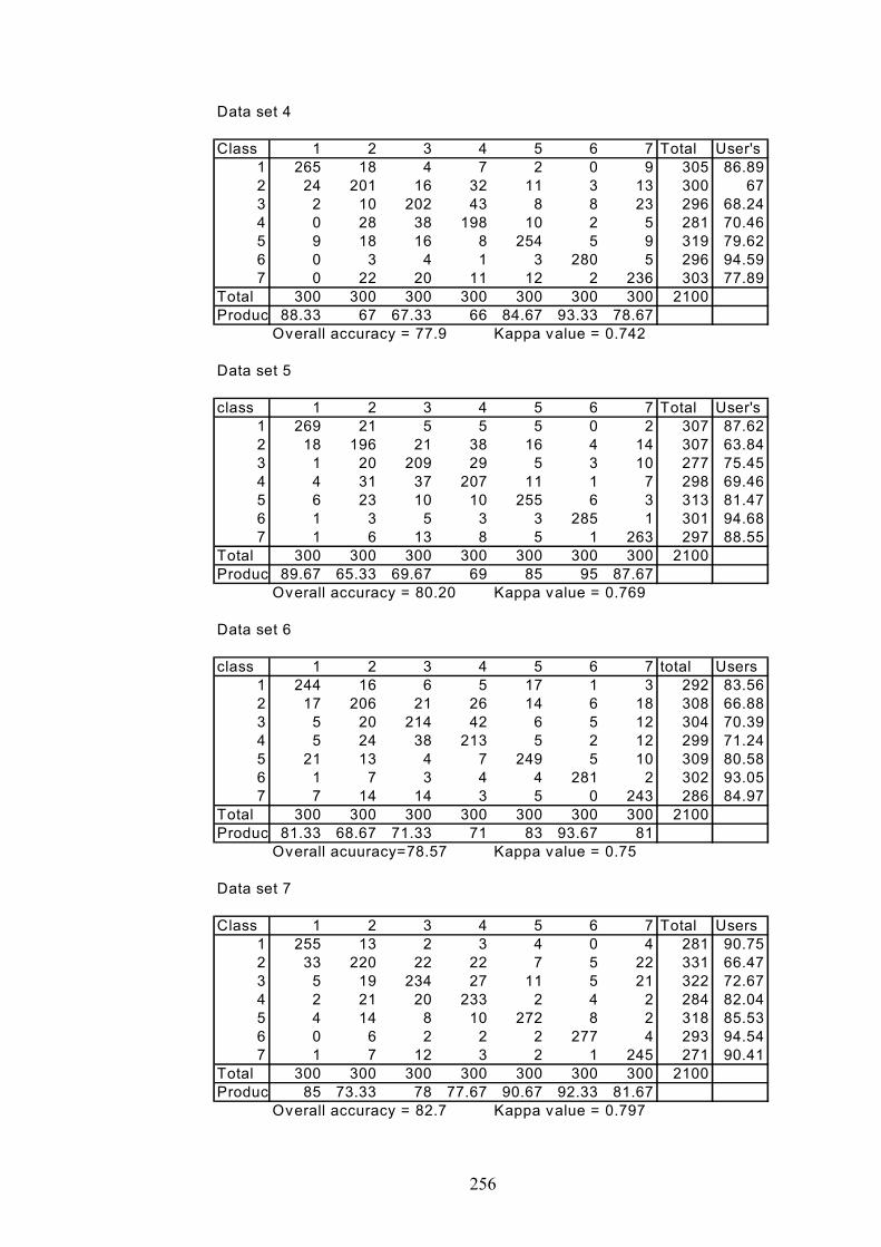
Data set 4
256
Class 1 2 3 4 5 6 7 Total User's1 265 18 4 7 2 0 9 305 86.892 24 201 16 32 11 3 13 300 673 2 10 202 43 8 8 23 296 68.244 0 28 38 198 10 2 5 281 70.465 9 18 16 8 254 5 9 319 79.626 0 3 4 1 3 280 5 296 94.597 0 22 20 11 12 2 236 303 77.89
Total 300 300 300 300 300 300 300 2100Produc 88.33 67 67.33 66 84.67 93.33 78.67
Overall accuracy = 77.9 Kappa value = 0.742
Data set 5
class 1 2 3 4 5 6 7 Total User's1 269 21 5 5 5 0 2 307 87.622 18 196 21 38 16 4 14 307 63.843 1 20 209 29 5 3 10 277 75.454 4 31 37 207 11 1 7 298 69.465 6 23 10 10 255 6 3 313 81.476 1 3 5 3 3 285 1 301 94.687 1 6 13 8 5 1 263 297 88.55
Total 300 300 300 300 300 300 300 2100Produc 89.67 65.33 69.67 69 85 95 87.67
Overall accuracy = 80.20 Kappa value = 0.769
Data set 6
class 1 2 3 4 5 6 7 total Users1 244 16 6 5 17 1 3 292 83.562 17 206 21 26 14 6 18 308 66.883 5 20 214 42 6 5 12 304 70.394 5 24 38 213 5 2 12 299 71.245 21 13 4 7 249 5 10 309 80.586 1 7 3 4 4 281 2 302 93.057 7 14 14 3 5 0 243 286 84.97
Total 300 300 300 300 300 300 300 2100Produc 81.33 68.67 71.33 71 83 93.67 81
Overall acuuracy=78.57 Kappa value = 0.75
Data set 7
Class 1 2 3 4 5 6 7 Total Users1 255 13 2 3 4 0 4 281 90.752 33 220 22 22 7 5 22 331 66.473 5 19 234 27 11 5 21 322 72.674 2 21 20 233 2 4 2 284 82.045 4 14 8 10 272 8 2 318 85.536 0 6 2 2 2 277 4 293 94.547 1 7 12 3 2 1 245 271 90.41
Total 300 300 300 300 300 300 300 2100Produc 85 73.33 78 77.67 90.67 92.33 81.67
Overall accuracy = 82.7 Kappa value = 0.797
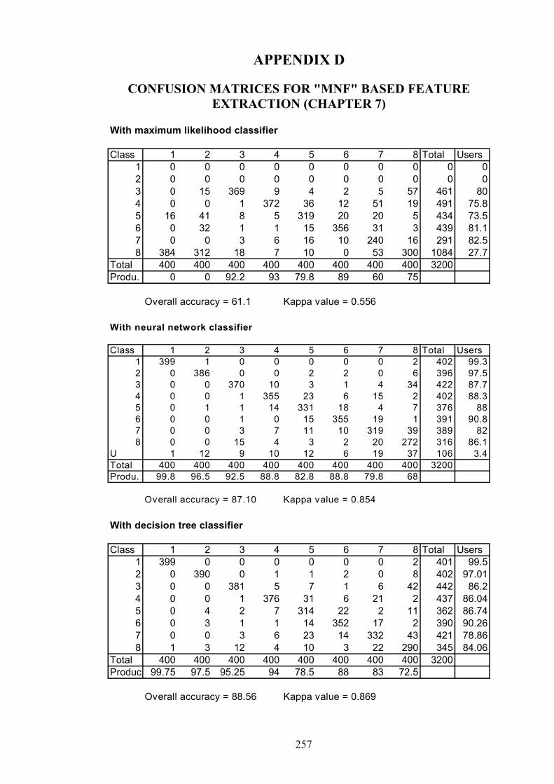
257
APPENDIX D
CONFUSION MATRICES FOR "MNF" BASED FEATUREEXTRACTION (CHAPTER 7)
With maximum likelihood classifier
Class 1 2 3 4 5 6 7 8 Total Users1 0 0 0 0 0 0 0 0 0 02 0 0 0 0 0 0 0 0 0 03 0 15 369 9 4 2 5 57 461 804 0 0 1 372 36 12 51 19 491 75.85 16 41 8 5 319 20 20 5 434 73.56 0 32 1 1 15 356 31 3 439 81.17 0 0 3 6 16 10 240 16 291 82.58 384 312 18 7 10 0 53 300 1084 27.7
Total 400 400 400 400 400 400 400 400 3200Produ. 0 0 92.2 93 79.8 89 60 75
Overall accuracy = 61.1 Kappa value = 0.556
With neural network classifier
Class 1 2 3 4 5 6 7 8 Total Users1 399 1 0 0 0 0 0 2 402 99.32 0 386 0 0 2 2 0 6 396 97.53 0 0 370 10 3 1 4 34 422 87.74 0 0 1 355 23 6 15 2 402 88.35 0 1 1 14 331 18 4 7 376 886 0 0 1 0 15 355 19 1 391 90.87 0 0 3 7 11 10 319 39 389 828 0 0 15 4 3 2 20 272 316 86.1
U 1 12 9 10 12 6 19 37 106 3.4Total 400 400 400 400 400 400 400 400 3200Produ. 99.8 96.5 92.5 88.8 82.8 88.8 79.8 68
Overall accuracy = 87.10 Kappa value = 0.854
With decision tree classifier
Class 1 2 3 4 5 6 7 8 Total Users1 399 0 0 0 0 0 0 2 401 99.52 0 390 0 1 1 2 0 8 402 97.013 0 0 381 5 7 1 6 42 442 86.24 0 0 1 376 31 6 21 2 437 86.045 0 4 2 7 314 22 2 11 362 86.746 0 3 1 1 14 352 17 2 390 90.267 0 0 3 6 23 14 332 43 421 78.868 1 3 12 4 10 3 22 290 345 84.06
Total 400 400 400 400 400 400 400 400 3200Produc 99.75 97.5 95.25 94 78.5 88 83 72.5
Overall accuracy = 88.56 Kappa value = 0.869

258
with SVMs
Class 1 2 3 4 5 6 7 8 Total Users1 498 0 0 1 0 0 0 6 505 96.82 0 495 0 1 1 5 0 4 506 97.83 0 1 447 1 7 1 5 46 508 884 1 0 20 448 25 2 16 10 522 85.85 0 0 1 16 411 16 10 22 476 86.36 0 1 3 12 31 447 16 5 515 86.87 0 0 4 18 18 28 393 19 480 81.98 1 3 25 3 7 1 60 388 488 79.5
Total 500 500 500 500 500 500 500 500Produc 99.6 99 89.4 89.6 82.2 89.4 78.6 77.6
Overall accuracy = 88.2 Kappa vlaue = 0.865

259
APPENDIX E
CONFUSION MATRICES FOR DECISION TREE BASEDFEATURE EXTRACTION (CHAPTER 7)
With maximum likelihood classifier
Class 1 2 3 4 5 6 7 8 Total Users1 499 0 0 0 0 0 0 0 499 1002 0 500 0 0 0 0 0 0 500 1003 0 0 483 12 1 0 5 34 535 90.34 0 0 4 462 7 3 5 3 484 95.55 0 0 1 13 463 10 6 19 512 90.46 0 0 0 10 27 480 22 2 541 88.77 0 0 3 0 2 6 257 3 271 94.88 1 0 9 3 0 1 5 439 458 95.9
Total 500 500 500 500 500 500 300 500 3800Produ. 99.8 100 96.6 92.4 92.6 96 85.7 87.8
Overall accuracy = 94.3 Kappa value = 0.935
With neural network classifier
Class 1 2 3 4 5 6 7 8 Total Users1 500 0 0 0 0 0 0 0 500 1002 0 500 1 0 0 0 0 0 501 99.83 0 0 475 7 0 0 3 39 524 90.64 0 0 2 474 2 2 1 4 485 97.75 0 0 0 3 463 4 0 12 482 96.16 0 0 0 7 9 459 9 7 491 93.57 0 0 1 4 0 20 258 6 289 89.38 0 0 16 4 3 0 4 372 399 93.2
U 0 0 5 1 23 15 25 60 129 3.5Total 500 500 500 500 500 500 300 500 3800Produ. 100 100 95 94.8 92.6 91.8 86 74.4
Overall accuracy = 92.1 Kappa value = 0.911
with decision tree classifier
Class 1 2 3 4 5 6 7 8 Total Users1 500 0 0 0 0 0 0 0 500 1002 0 500 2 0 0 0 0 0 502 99.63 0 0 430 4 11 2 5 71 523 82.224 0 0 10 455 10 3 3 14 495 91.925 0 0 2 6 409 7 12 27 463 88.346 0 0 4 12 26 449 21 16 528 85.047 0 0 3 10 18 33 243 30 337 72.118 0 0 49 13 26 6 16 342 452 75.66
Total 500 500 500 500 500 500 300 500 3800Produc 100 100 86 91 81.8 89.8 81 68.4
Overall accuracy = 87.6 Kappa value =0.858

260
with SVMs
Class 1 2 3 4 5 6 7 8 Total Users1 500 0 0 0 0 0 0 0 500 1002 0 500 2 0 0 0 0 0 502 99.63 0 0 458 4 1 0 3 34 500 91.64 0 0 4 481 5 1 3 3 497 96.85 0 0 0 3 481 9 0 3 496 976 0 0 0 6 8 471 6 6 497 94.87 0 0 6 4 2 19 287 11 329 87.28 0 0 30 2 3 0 1 443 479 92.5
Total 500 500 500 500 500 500 300 500Produc 100 100 91.6 96.2 96.2 94.2 95.7 88.6
Overall accuracy = 95.3 Kappa value = 0.946

261
APPENDIX F
CONFUSION MATRICES FOR ETM+ SPAIN DATA(CHAPTER 7)
With maximum likelihood classifier
Class 1 2 3 4 5 6 Total Users1 147 0 0 0 0 0 147 1002 0 0 0 0 0 0 0 03 0 0 163 5 1 2 171 95.34 0 0 13 207 12 6 238 875 0 6 4 12 108 0 130 83.16 3 40 9 7 8 42 109 38.5
Total 150 46 189 231 129 50 795Produ. 98 0 86.2 89.6 83.7 84
Overall accuracy = 83.9 Kappa value = 0.797
With neural network classifier
Class 1 2 3 4 5 6 Total Users1 148 0 0 0 0 0 148 1002 0 46 0 0 0 0 46 1003 1 0 174 10 2 6 193 90.24 0 0 3 196 8 1 208 94.25 0 0 4 10 107 1 122 87.76 0 0 4 7 6 40 57 70.2
U 1 0 4 8 6 2 21 2.7Total 150 46 189 231 129 50 795Produ. 98.7 100 92.1 84.8 82.9 80
Overall accuracy = 89.4 Kappa value = 0.869
With decision tree classifier
Class 1 2 3 4 5 6 Total Users1 147 0 0 0 0 0 147 1002 0 46 0 0 0 0 46 1003 0 0 161 23 1 4 189 85.194 0 0 11 168 11 2 192 87.55 0 0 4 23 109 2 138 78.996 3 0 13 17 8 42 83 50.6
Total 150 46 189 231 129 50 795Produc 98 100 85.19 72.73 84.5 84
Overall accuracy = 84.65 Kappa value = 0.808

262
with SVMs
Class 1 2 3 4 5 6 Total Users1 148 0 0 0 0 0 148 1002 0 46 0 0 0 0 46 1003 0 0 170 12 3 2 187 90.94 0 0 9 205 10 2 226 90.75 0 0 6 7 109 0 122 89.36 2 0 4 7 7 46 66 69.7
Total 150 46 189 231 129 50 795Produ. 98.7 100 89.9 88.7 84.5 92
Overall accuracy = 91.1 Kappa value = 0.887