Oblique fuzzy vectors and their use in possibilistic linear programming

Fuzzy Sets and Systems 135 (2003) 123–150www.elsevier.com/locate/fss

Oblique fuzzy vectors and their use in possibilisticlinear programming�

Masahiro Inuiguchia ; ∗, Jaroslav Ram*+kb, Tetsuzo Taninoa

aDepartment of Electronics and Information Systems, Graduate School of Engineering, Osaka University,2-1 Yamadaoka, Suita, Osaka 565-0871, Japan

bDepartment of Mathematical Methods in Economics, School of Business Administration, Silesian University,University Square 76, 733 40 Karvin.a, Czech Republic

Abstract

In this paper, we propose oblique fuzzy vectors to treat the interactivity among fuzzy numbers. Oblique fuzzyvectors are extensions of fuzzy numbers and vectors of non-interactive fuzzy numbers. The interactivity amongfuzzy numbers can be treated by a non-singular matrix in an oblique fuzzy vector. We discuss characterizationof an oblique fuzzy vector and the tractability of manipulation of oblique fuzzy vectors in fuzzy linearfunctions. Moreover, we discuss possibilistic linear programming problems with oblique fuzzy vectors. It isshown that the possibilistic linear programming problems are reduced to linear programming problems with aspecial structure. c© 2002 Elsevier Science B.V. All rights reserved.

Keywords: Interactive fuzzy numbers; Linear programming; Extension principle; Necessity measure; Bendersdecomposition method

1. Introduction

Interval arithmetic [10] and calculations of fuzzy numbers [3] have been developed mainly underthe assumption of non-interactivity among uncertain variables. In interval analysis, intervals are usedfor two purposes, i.e., (1) to enhance the accuracy of computer calculation (a countermeasure ofround-o: errors by ;oating point method) and (2) to treat uncertain parameters whose ranges areknown as intervals. In fuzzy systems theory, fuzzy numbers are used mainly for the second purposeof interval analysis, i.e., to treat uncertain parameters whose ranges are known as fuzzy numbers.

� This research is partly supported by the Ministry of Education, Science, Sports and Culture, Grant-in-Aid Scienti>cResearch for Encouragement of Young Scientists, No. 12780333.

∗ Corresponding author.E-mail addresses: [email protected] (M. Inuiguchi), [email protected] (J. Ram*+k),

[email protected] (T. Tanino).

0165-0114/03/$ - see front matter c© 2002 Elsevier Science B.V. All rights reserved.PII: S0165-0114(02)00252-X

124 M. Inuiguchi et al. / Fuzzy Sets and Systems 135 (2003) 123–150

For the >rst purpose in interval analysis, there is little importance in introduction of interactivityamong uncertain variables. On the other hand, for the second purpose, the non-interactivity assump-tion is too restrictive to represent real situations. Indeed, some unsuitable results are obtained inpossibilistic portfolio selection problems because of the non-interactivity assumption (see, for exam-ple, [7]). Therefore, it is required to introduce the interactivity among uncertain variables to intervalarithmetic and calculations of fuzzy numbers.

However, in general, the calculation with interactive fuzzy numbers is much more diKcult andcomplex than that with non-interactive fuzzy numbers. In applications of interactive fuzzy num-bers to possibilistic linear programming, to fuzzy linear regression and, etc., the tractability oflinear calculation is advantageous. Indeed, an advantage of possibilistic linear programming overstochastic linear programming is the linearity with respect to decision variables in calculations oflinear functions with uncertain coeKcients (see, for example, [6]). Therefore, for these method-ologies, it is better to preserve the tractability, i.e., linearity in linear calculation of fuzzynumbers.

Dubois and Prade [2] and Tanaka and Ishibuchi [13] showed that, in some special cases ofinteractive fuzzy numbers, the sum and linear function values of interactive fuzzy numbers canbe obtained easily. The case treated by Dubois and Prade [2] preserves the linearity to a cer-tain extent in calculation of sum of fuzzy numbers but it is rather restrictive to be applied to therepresentation of interactive fuzzy numbers in real problems. On the other hand, interactive fuzzynumbers treated by Tanaka and Ishibuchi [13] have a quadratic membership function and the lin-ear function values of those fuzzy numbers are not obtained by linear calculation but by quadraticcalculation.

In this paper, we propose a model of interactive fuzzy numbers that preserves the linearity to acertain extent. In order to treat the interactivity, we use a non-singular matrix called an obliquitymatrix and we assume the uncertain variables are non-interactive under the linear transformation bythe obliquity matrix. Similar approach was proposed by Ram*+k and Nakamura [12] and Miyakawaet al. [9] by the name of canonical fuzzy numbers. The model proposed in this paper is an extensionof the canonical fuzzy numbers and named oblique fuzzy vectors. Not only canonical fuzzy numbersbut also vectors of non-interactive fuzzy numbers, fuzzy numbers and intervals are covered by theconcept of oblique fuzzy vectors as special cases.

We also discuss some characterizations of oblique fuzzy vectors. Some conditions for obliquefuzzy vectors to be characterized by marginal fuzzy numbers and a non-singular matrix are shown.Calculation of linear function values of oblique fuzzy vectors is investigated. We show that linearfunction values of oblique fuzzy vectors can be calculated easily without a great loss of linearity.

Moreover, possibilistic linear programming problems with oblique fuzzy vectors are discussed. Theproblems are formulated by using necessity measures. Utilizing the result of a fuzzy linear functionwith an oblique fuzzy vector, it is shown that the formulated problems can be reduced to linearprogramming problems. From a special structure of the obtained linear programming problems, analgorithm based on Benders decomposition is presented.

This paper is organized as follows. In Section 2, we review brie;y the calculations of non-inter-active fuzzy numbers and properties of necessity measures as preliminaries. Oblique fuzzy vectorsare de>ned and their properties are investigated in Section 3. In Section 4, we discuss a possi-bilistic linear programming problem with oblique fuzzy vectors. Finally, some concluding remarksare given.

M. Inuiguchi et al. / Fuzzy Sets and Systems 135 (2003) 123–150 125

2. Preliminaries

2.1. Fuzzy numbers and non-interactivity

In this paper, fuzzy numbers are de>ned as follows.

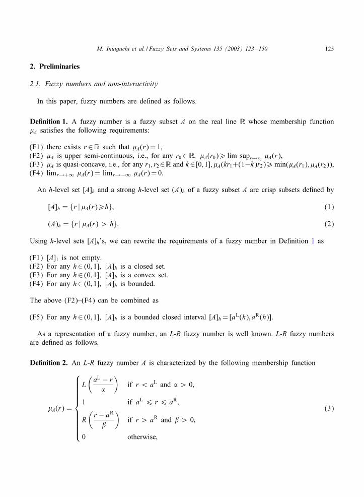
De�nition 1. A fuzzy number is a fuzzy subset A on the real line R whose membership function�A satis>es the following requirements:

(F1) there exists r ∈R such that �A(r) = 1,(F2) �A is upper semi-continuous, i.e., for any r0 ∈R; �A(r0)¿ lim supr→r0

�A(r),(F3) �A is quasi-concave, i.e., for any r1; r2∈R and k∈[0; 1]; �A(kr1+(1−k)r2)¿min(�A(r1); �A(r2)),(F4) limr→+∞ �A(r) = limr→−∞ �A(r) = 0.

An h-level set [A]h and a strong h-level set (A)h of a fuzzy subset A are crisp subsets de>ned by

[A]h = {r | �A(r)¿h}; (1)

(A)h = {r | �A(r) ¿ h}: (2)

Using h-level sets [A]h’s, we can rewrite the requirements of a fuzzy number in De>nition 1 as

(F1) [A]1 is not empty.(F2) For any h∈ (0; 1]; [A]h is a closed set.(F3) For any h∈ (0; 1]; [A]h is a convex set.(F4) For any h∈ (0; 1]; [A]h is bounded.

The above (F2)–(F4) can be combined as

(F5) For any h∈ (0; 1]; [A]h is a bounded closed interval [A]h = [aL(h); aR(h)].

As a representation of a fuzzy number, an L-R fuzzy number is well known. L-R fuzzy numbersare de>ned as follows.

De�nition 2. An L-R fuzzy number A is characterized by the following membership function

�A(r) =

L(

aL − r�

)if r ¡ aL and � ¿ 0;

1 if aL 6 r 6 aR ;

R(

r − aR

�

)if r ¿ aR and � ¿ 0;

0 otherwise;

(3)


where aL and aR satisfy aL6aR and denote the lower and upper bounds of [A]1, respectively. �¿0and �¿0 denote the left and right spreads of A, respectively. L and R : [0; +∞)→ [0; 1] are referencefunctions such that

(R1) L(0) = R(0) = 1 and L(r); R(r)¡1 for all r¿0,(R2) L and R are upper semi-continuous,(R3) L and R are non-increasing,(R4) limr→+∞ L(r) = limr→+∞ R(r) = 0.

The L-R fuzzy number A is denoted by A = (aL; aR ; �; �)LR.

As can be seen easily, any fuzzy number is identi>ed by an L-R fuzzy number. Namely, givena fuzzy number A, we have A = (inf [A]1; sup[A]1; 1; 1)LARA , where reference functions LA and RA

are de>ned by LA(r) = �A(inf [A]1 − r) and RA(r) = �A(sup[A]1 + r); r ∈R. There are many L-Rfuzzy numbers which identify the same fuzzy number if there is no normalization of referencefunctions. For example, when L1(x) = max(0; 1 − x) and L2(x) = max(0; 1 − 2x); (1; 1; 1; 1)L1L1 and(1; 1; 2; 2)L2 ; L2 identify the same fuzzy number. To avoid this problem, if there exists r0 ∈ [0; +∞)such that L(r0) = 0 and r0 = inf{r |L(r) = 0}, it is usually assumed that r0 = 1 so that we havecl(A)0 = [aL − �; aR + �], where cl S is the closure of a crisp set S. However, for general referencefunctions, such a simple normalization cannot be introduced. One conceivable normalization methodfor a general reference function L is as follows:

(i) if there exists r0 ∈ [0; +∞) such that L(r0) = 0 and r0 = inf{r |L(r) = 0}, then normalize L soas to be r0 = 1, thus we have cl(A)0 = [aL − �; aR + �].

(ii) if there is no r¿0 such that L(r)¿0, then L is already normalized, i.e., L(r) = 0 for all r¿0.(iii) Let q = 1.(iv) Calculate rq = inf{r |L(r)¡0:5q}.(v) If rq = 0 then update q = q + 1 and return to (iv). Otherwise, normalize L so as to be rq = 1,

thus we have [A]0:5q = [aL − �; aR + �].

Using such normalization of reference functions, we can divide fuzzy numbers into many classes inwhich reference functions are the same.

It should be noted that an interval is a fuzzy number, i.e., an L-R fuzzy number with referencefunctions satisfy L(r) = R(r) = 0 for all r¿0 or with � = � = 0. A fuzzy number that correspondsto an L-R fuzzy number (aL; aR ; �; �)LR is called an L-L fuzzy number if L = R and is said to besymmetric if � = � and L = R.

In many real applications, we should take into consideration several fuzzy numbers. Thus, weconsider a vector of fuzzy numbers, i.e., a multi-dimensional fuzzy subset. A question arises. It ishow we de>ne a membership function of a vector of fuzzy numbers. A solution to this question isto introduce the non-interactivity among fuzzy numbers, i.e., a kind of independence among fuzzynumbers (see Ref. [4]). Under this assumption, an n-dimensional fuzzy vector of fuzzy numbersA= (A1; A2; : : : ; An)T is de>ned by the following membership function:

�A(r) = mini=1;2;:::;n

�Ai(ri); (4)


Fig. 1. Non-interactive fuzzy numbers.

where �Ai is the membership function of Ai; r= (r1; r2; : : : ; rn)T and the superscript T stands fortransposition.

If a fuzzy vector A has a membership function represented by (4), it is called a vector of non-interactive fuzzy numbers, or simply, a non-interactive fuzzy vector. A two-dimensional vector ofnon-interactive fuzzy numbers is illustrated in Fig. 1. The level curves of the membership functionof the two-dimensional vector of non-interactive fuzzy numbers are shown in Fig. 2. As shown inFig. 2, each level curve is a rectangle whose edges are parallel to axes.

Let �S denote a characteristic function of a crisp subset S, i.e., �S(r) = 1 if r∈ S and �S(r) = 0otherwise. An important relation between a fuzzy subset and its h-level sets is given in the followingtheorem known as resolution principle (see Ref. [14]).

Theorem 1. Let A be a fuzzy subset of Rn. Then for any r∈Rn,

�A(r) = suph∈(0;1]

h · �[A]h(r) = suph∈[0;1)

h · �(A)h(r): (5)

2.2. Extension principle and calculations of fuzzy numbers

Given a function f :Rn →R, we can extend this function to a function from fuzzy subsets ofRn to a fuzzy subset of R by extension principle. The extension principle is given in the followingde>nition.


Fig. 2. Level curves of non-interactive fuzzy numbers.

De�nition 3. Given a function f :Rn →R, the image of a fuzzy subset A of Rn by f is a fuzzysubset f(A) of R with the following membership function:

�f(A)(y) =

supr∈f−1(y)

�A(r) if f−1(y) = ∅;

0 if f−1(y) = ∅;(6)

where r= (r1; r2; : : : ; rn)T and f−1 is an inverse image of f de>ned by

f−1(y) = {r ∈ Rn |f(r) = y}: (7)

For strong h-level sets, we have evidently

(f(A))h = f((A)h) for any h ∈ [0; 1): (8)

On the other hand, for h-level sets, the formula corresponding to (8) does not hold. We have only

[f(A)]h ⊇ f([A]h) for any h ∈ (0; 1]: (9)

Nguyen [11] gave a suKcient condition of the opposite inclusion relation of (9). Dubois and Prade[3] showed a weaker suKcient condition as in the following theorem.

Theorem 2. Let f be continuous. If [A]h is bounded and closed for any h∈ (0; 1], then we have

[f(A)]h = f([A]h) for any h ∈ (0; 1]: (10)

From Theorem 2, we have the following well-known results.


Corollary 1. Let f be a linear function, i.e., f(r) =∑n

i=1 kiri. Let A be a vector of non-interactivefuzzy numbers A= (A1; A2; : : : ; An)T. Then we have, for any h∈ (0; 1],

[f(A)]h =n∑

i=1

ki[Ai]h

=

[ ∑i:ki¿0

kiaLi (h) +

∑i:ki¡0

kiaRi (h);

∑i:ki¿0

kiaRi (h) +

∑i:ki¡0

kiaLi (h)

]; (11)

where aLi (h) and aR

i (h) are lower and upper bounds of [Ai]h.

For L-R fuzzy numbers having the same reference functions, the following corollary is obvious.

Corollary 2. Let f(r) =∑n

i=1 kiri; A be a vector of non-interactive fuzzy numbers A= (A1; A2; : : : ;An)T whose ith component Ai is an L-R fuzzy number Ai = (aL

i ; aRi ; �i; �i)LR.

(i) If ki¿0 for all i = 1; 2; : : : ; n, then

f(A) =

(n∑

i=1

kiaLi ;

n∑i=1

kiaRi ;

n∑i=1

ki�i;n∑

i=1

ki�i

)LR

; (12)

(ii) if ki60 for all i = 1; 2; : : : ; n, then

f(A) =

(n∑

i=1

kiaRi ;

n∑i=1

kiaLi ;

n∑i=1

ki�i;n∑

i=1

ki�i

)RL

; (13)

(iii) if L = R, then

f(A) =

( ∑i:ki¿0

kiaLi −

∑i:ki¡0

kiaRi ;∑

i:ki¿0

kiaRi −

∑i:ki¡0

kiaLi ;

∑i:ki¿0

ki�i −∑i:ki¡0

ki�i;∑

i:ki¿0

ki�i −∑i:ki¡0

ki�i

)LL

: (14)

2.3. Necessity measure

Let A and B be crisp subsets of a universal set X and u an uncertain variable which takes valuein X . Then, under information ‘u is in A’, we say that ‘u is in B’ is necessary if A⊆B and that ‘uis in B’ is possible if A∩B = ∅. A necessity measure N and possibility measure � are de>ned asfollows:

NA(B) =

{1 if A ⊆ B;

0 otherwise;(15)


�A(B) =

{1 if A ∩ B = ∅;0 otherwise:

(16)

In order to treat a case of fuzzy subsets A and B of X , necessity and possibility measures of (15)and (16) are extended as follows.

De�nition 4. Let u be an uncertain variable. The necessity and possibility measures of an event ‘uis in a fuzzy subset B’ under information ‘u is in a fuzzy subset A’ are de>ned as

NA(B) = infr∈X

max(1 − �A(r); �B(r)); (17)

�A(B) = supr∈X

min(�A(r); �B(r)); (18)

respectively.

In possibilistic linear programming [6], the necessity measure is used to evaluate to what extentit is necessary that a solution satisfy a constraint or a goal while the possibility measure is used toevaluate to what extent it is possible that a solution satisfy a constraint or a goal. In Section 4, weonly treat the necessity measure because of a technical reason. However, fortunately, the necessitymeasure will be more often used than the possibility measure in real problems since the necessitymeasure is a pessimistic measure and it is used in problems in which low risk is required (see, forexample, [5]). The following property of the necessity measure is used in Section 4.

Theorem 3. Let A and B be fuzzy subsets of a universal set X . Then

NA(B) ¿ h if and only if (A)1−h ⊆ [B]h: (19)

A proof of Theorem 3 can be found in [5].From Theorem 3, we obtain the following corollaries.

Corollary 3. If X =Rn and B has an upper semi-continuous membership function, then

NA(B) ¿ h if and only if cl(A)1−h ⊆ [B]h; (20)

especially, if n = 1, then

NA(B) ¿ h

if and only if inf (A)1−h ¿ inf [B]h and sup(A)1−h 6 sup[B]h: (21)

Corollary 4. Let X =R and A be a fuzzy number. If B has an upper semi-continuous non-decreasing membership function, then

NA(B) ¿ h if and only if inf (A)1−h ¿ inf [B]h: (22)

On the other hand, if B has an upper semi-continuous non-increasing membership function, then

NA(B) ¿ h if and only if sup(A)1−h 6 sup[B]h: (23)


3. Oblique fuzzy vectors

3.1. De?nition and characterizations

Non-interactive fuzzy numbers are tractable in linear functions since they preserve the linear-ity as shown in Corollaries 1 and 2. Because of its tractability, a vector of non-interactive fuzzynumbers has been widely utilized especially in >elds where linear functions of fuzzy numbers areused. However, in some applications, the assumption of non-interactivity (a kind of independence)among fuzzy numbers is not suitable (see, for example, [7]). Moreover, in order to enhance therepresentability of models by fuzzy numbers, we should treat a more general fuzzy numbers, usuallycalled interactive fuzzy numbers. In general, interactive fuzzy numbers are frequently intractable incomputations. Considering the tractability, we should make a compromise to restrict ourselves intosome special models for interactive fuzzy numbers.

In this paper, we propose oblique fuzzy numbers as a special model of interactive fuzzy numbersand show that they are tractable to a certain extent especially in calculations of fuzzy linear functions.

Oblique fuzzy vectors are de>ned as follows.

De�nition 5. Let B1; B2; : : : ; Bn be fuzzy numbers and let D = (d1; d2; : : : ; dn)T be a non-singular real-valued n× n matrix. A fuzzy subset A of Rn with the membership function de>ned for each r∈Rn

by

�A(r) = mini=1;2;:::;n

�Bi(dTi r); (24)

is called the oblique fuzzy vector (OFV) of B1; B2; : : : ; Bn. The matrix D is called the obliquitymatrix associated with A.

We say that a fuzzy subset A of Rn is an oblique fuzzy vector, if there exist fuzzy numbersB1; B2; : : : ; Bn and a non-singular matrix D such that A is an oblique fuzzy vector of B1; B2; : : : ; Bn.

Regarding D as a coordinate transformation from a rectangular coordinate system to an obliquecoordinate system, we may understand that an OFV is a vector of non-interactive fuzzy numbers inthe oblique coordinate system.

A two-dimensional OFV is illustrated in Fig. 3. The level curves of the membership functionof the OFV are shown in Fig. 4. As shown in Fig. 4, each level curve is not a rectangle whoseedges are parallel to axes but a parallelogram. Compared to a fuzzy vector of non-interactive fuzzynumbers in Figs. 1 and 2, the marginal possible ranges of a1 and a2 are the same, [1,3] and [1,4],but the membership degrees around the corners of the rectangle [1; 3]× [1; 4] are zero for the OFVwhile they remain still positive for the fuzzy vector of non-interactive fuzzy numbers. For example,a1 = (3− �; 1+ �)T and a2 = (1+ �; 1+ �)T do not take positive membership values in Fig. 4, but theyhave small positive membership values in Fig. 2, where � is a suKciently small positive number.

If all Bi; i = 1; 2; : : : ; n are symmetric fuzzy numbers, i.e. �Bi(r) = �Bj(−r) for each r ∈R, and forevery pair i; j∈{1; 2; : : : ; n}; i = j, there exists qij ∈R such that �Bi(r) = �Bj(r + qij) for all r ∈R,then the OFV is the canonical fuzzy number proposed by Ram*+k and Nakamura [12] and Miyakawaet al. [9].


Fig. 3. An oblique fuzzy vector.

Fig. 4. Level curves of the oblique fuzzy vector.

If the obliquity matrix D is the identity matrix I , then the OFV A of B1; B2; : : : ; Bn is a fuzzyvector of non-interactive fuzzy numbers B= (B1; B2; : : : ; Bn). Moreover, for n = 1, the OFV A ofB1; B2; : : : ; Bn reduces to a fuzzy number. Note that OFVs satisfy the assumption of Theorem 2 withrespect to A.


Example 1. Consider two uncertain variables a1 and a2. If we know the sum a1 + a2 is ‘about10’ expressed by a fuzzy number B1 and the di:erence a1 − a2 is ‘about 4’ expressed by a fuzzynumbers B2, then the possible range A1 of a= (a1; a2)T is de>ned by the following membershipfunction:

�A1(r1; r2) = min(�B1(r1 + r2); �B2(r1 − r2)):

This fuzzy vector A1 is an oblique fuzzy vector.Similarly, when we know 2a1 − a2 + 2 is ‘about 14’ expressed by a fuzzy number B3 and the

di:erence 3a1 + a2 − 1 is ‘about 17’ expressed by a fuzzy numbers B4, by the extension princi-ple, we obtain the possible ranges of 2a1 − a2 and 3a1 + a2 as fuzzy numbers B5 = B3 − 2 andB6 = B4 + 1 which can have linguistic expressions ‘about 12’ and ‘about 18’, respectively. Hence,the possible range A2 of a= (a1; a2)T is an oblique fuzzy vector with the following membershipfunction:

�A2(r1; r2) = min(�B5(2r1 − r2); �B6(3r1 + r2)):

More generally, when we know approximate values of n linear function of n uncertain variables asfuzzy numbers, the possible range of a vector of the uncertain variables can be represented by ann-dimensional oblique fuzzy vector.

We now de>ne marginal fuzzy numbers Ai ; i = 1; 2; : : : ; n associated with an OFV by the followingmembership function:

�Ai(r0i ) = sup

rri=r0

i

�A(r); (25)

where r= (r1; r2; : : : ; rn)T. Thus, a marginal fuzzy number Ai is a projection of OFV A to the ithaxis so that it shows the possible range of the i-the uncertain variable ai. From the de>nition ofOFV, Ai is also a fuzzy number.

Since Ai and Bi are fuzzy numbers, there exist real numbers aLi (h); aR

i (h); bLi (h) and bR

i (h),which depend on the number h∈ (0; 1] such that [Ai]h = [aL

i (h); aRi (h)] and [Bi]h = [bL

i (h); bRi (h)].

We can prove the following theorem.

Theorem 4. Let pij = max(0; d∗ij) and nij = min(0; d∗

ij); i = 1; 2; : : : ; n; j = 1; 2; : : : ; n, where d∗ij is

the (i; j) component of D−1, the inverse matrix of the obliquity matrix D. We have

aLi (h) =

n∑j=1

pijbLj (h) +

n∑j=1

nijbRj (h); i = 1; 2; : : : ; n; (26)

aRi (h) =

n∑j=1

pijbRj (h) +

n∑j=1

nijbLj (h); i = 1; 2; : : : ; n: (27)


Proof. By de>nition (25), we have

�A(r) = minj=1;2;:::;n

�Bj(dTj r):

Hence

r ∈ [A]h if and only if dTj r ∈ [Bj]h; j = 1; 2; : : : ; n:

We have

[A]h = {r0 | r0 = D−1r; bLj (h) 6 rj 6 bR

j (h); j = 1; 2; : : : ; n}:Since �A is upper semi-continuous and [A]h is bounded for any h∈ (0; 1], by de>nition of Ai, wehave

[Ai]h = [aLi (h); aR

i (h)] = Proji[A]h;

where Proji S is a projection of a set S to the ith axis. Therefore, by Corollary 1, we obtain

[Ai]h =

r0

i | r0i =

n∑j=1

d∗ijrj; b

Lj (h) 6 rj 6 bR

j (h); j = 1; 2; : : : ; n

=

∑

j:d∗ij¿0

d∗ijb

Lj (h) +

∑j:d∗

ij¡0

d∗ijb

Rj (h);

∑j:d∗

ij¿0

d∗ijb

Rj (h) +

∑j:d∗

ij¡0

d∗ijb

Lj (h)

:

By de>nitions of pij and nij, we obtain (26) and (27).

Note that, from this theorem, we know that Ai = fi(B) with fi(r) =∑n

j=1 d∗ijrj. Combining this

with Corollary 2, we have the following corollary.

Corollary 5. If every Bj is an L-L fuzzy number (bLj ; bR

j ; �Lj ; �R

j )LL, then every Ai is also an L-Lfuzzy number (aL

i ; aRi ; �L

i ; �Ri )LL, where

aLi =

n∑j=1

pijbLj +

n∑j=1

nijbRj ; aR

i =n∑

j=1

pijbRj +

n∑j=1

nijbLj ;

�Li =

n∑j=1

pij�Lj −

n∑j=1

nij�Rj ; �R

i =n∑

j=1

pij�Rj −

n∑j=1

nij�Lj ; i = 1; 2; : : : ; n: (28)

In applications, Ai is usually observable in the sense that its membership function can be estimated(e.g. by a direct measuring or from expert’s knowledge), which is usually not true for Bi. On theother hand, A is fully determined by Bi. Therefore, when we know D, it is reasonable to ask whetherBi can be determined by the marginal fuzzy numbers Ai and the matrix D.


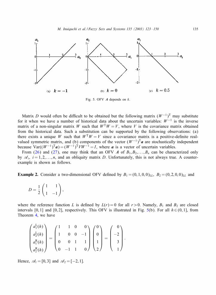
Fig. 5. OFV A depends on k.

Matrix D would often be diKcult to be obtained but the following matrix (W−1)T may substitutefor it when we have a number of historical data about the uncertain variables: W−1 is the inversematrix of a non-singular matrix W such that W TW = V , where V is the covariance matrix obtainedfrom the historical data. Such a substitution can be supported by the following observations: (a)there exists a unique W such that W TW = V since a covariance matrix is a positive-de>nite real-valued symmetric matrix, and (b) components of the vector (W−1)Ta are stochastically independentbecause Var((W−1)Ta) = (W−1)TVW−1 = I , where a is a vector of uncertain variables.

From (26) and (27), one may think that an OFV A of B1; B2; : : : ; Bn can be characterized onlyby Ai ; i = 1; 2; : : : ; n, and an obliquity matrix D. Unfortunately, this is not always true. A counter-example is shown as follows.

Example 2. Consider a two-dimensional OFV de>ned by B1 = (0; 1; 0; 0)LL; B2 = (0; 2; 0; 0)LL and

D =12

(1 1

1 −1

);

where the reference function L is de>ned by L(r) = 0 for all r¿0. Namely, B1 and B2 are closedintervals [0; 1] and [0; 2], respectively. This OFV is illustrated in Fig. 5(b). For all h∈ (0; 1], fromTheorem 4, we have

aL1 (h)

aL2 (h)

aR1 (h)

aR2 (h)

=

1 1 0 0

1 0 0 −1

0 0 1 1

0 −1 1 0

0

0

1

2

=

0

−2

3

1

:

Hence, A1 = [0; 3] and A2 = [−2; 1].


Conversely, let us assume A1 and A2 instead of B1 and B2 are given. In this case, we shouldsolve the following system of linear equalities:

1 1 0 0

1 0 0 −1

0 0 1 1

0 −1 1 0

bL1 (h)

bL2 (h)

bR1 (h)

bR2 (h)

=

0

−2

3

1

:

The general solution to this system is obtained as

bL1 (h)

bL2 (h)

bR1 (h)

bR2 (h)

=

0

0

1

2

+ k

1

−1

−1

1

; k ∈ R:

Because we should have bL1 (h)6bR

1 (h) and bL2 (h)6bR

2 (h), the parameter k is restricted as k ∈ [−1;0:5]. There are a lot of solutions and two extreme cases, i.e., k = −1; 0:5 are depicted in Figs. 5(a)and (c).

Let us discuss conditions for an OFV A characterized by Ai ; i = 1; 2; : : : ; n and an obliquity matrixD. Let P and N be an n× n matrices whose (i; j) components are pij and nij. Then, from (26) and(27), an OFV A is characterized by Ai ; i = 1; 2; : : : ; n and an obliquity matrix D if and only if thereexists a unique solution to

PbL(h) + NbR(h) = aL(h); ∀h ∈ (0; 1];

NbL(h) + PbR(h) = aR(h); ∀h ∈ (0; 1];

bL(h) 6 bR(h); ∀h ∈ (0; 1];

bL(h) is non-decreasing with respect to h;

bR(h) is non-increasing with respect to h: (29)

Generally, it is diKcult to establish conditions for the uniqueness of the solution to (29) since thesolution is not a vector but a vector function. Thus, in what follows, we restrict ourselves into somespecial cases where (a) every Ai is an interval, (b) every Ai is an L-L fuzzy number and (c) everyAi is a fuzzy number with a piecewise linear membership function.

3.1.1. Interval caseFirst we discuss the case where every Ai is an interval. In this case, since aL(h) = aL and

aR(h) = aR for all h∈ (0; 1], (29) is reduced to

PbL + NbR = aL; NbL + PbR = aR ; bL 6 bR : (30)


Note that we should have bL(h) = bL and bR(h) = bR for all h∈ (0; 1] because aL(h) = aL andaR(h) = aR for all h∈ (0; 1]. The following theorem shows the necessary and suKcient condition for(30) to have a unique solution.

Theorem 5. System (30) has a unique solution if and only if the following system has a uniquesolution:

(P − N )w = aR − aL; w¿ 0: (31)

Proof. Let bR = bL + w. Then, from D−1 = P + N , (30) is rewritten as

D−1bL + Nw = aL; D−1bL + Pw = aR ; w¿ 0:

This system is equivalent to

D−1bL + Nw = aL; (P − N )w = aR − aL; w¿ 0:

Given w; bL is uniquely determined by bL = D(aL −Nw). Hence, (30) has a unique solution if andonly if (31) has a unique solution.

If P −N is non-singular, then the solution of (31) is always unique whenever it exists. Thus, wehave the following corollary.

Corollary 6. Let P − N is non-singular. Then (31) has a unique solution if and only if(P − N )−1(aR − aL)¿0.

The non-singularity of P − N is closely related to the uniqueness of the solution of a systemcomposed of the >rst two equalities in (30). This fact is shown in the following remark.

Remark 1. P − N is non-singular if and only if the matrix(

P NN P

)is non-singular.

It follows from that fact that the rank of the matrix(P NN P

)is the same as the rank of

(0 P + N

P − N P

).

Let aL = (aL1 ; aL

2 ; : : : ; aLn )T; aR = (aR

1 ; aR2 ; : : : ; aR

n )T and w= (w1; w2; : : : ; wn)T. We have the follow-ing proposition.

Proposition 1. Let for some i∈{1; 2; : : : ; n}; aRi −aL

i = 0, and let w be a solution of (31). If |d∗ij|¿0

then wj = 0.

Proof. By de>nition, we have pij − nij = |d∗ij|; i = 1; 2; : : : ; n; j = 1; 2; : : : ; n. Under the assumption

of the theorem, a solution of (31) should satisfyn∑

j=1

|d∗ij|wj = aR

i − aLi = 0; wj ¿ 0; j = 1; 2; : : : ; n:


If wj¿0 for |d∗ij|¿0, for any w¿0, we have

∑nj=1 |d∗

ij|wj¿0. Hence, we should have wj = 0 for|d∗

ij|¿0.

From Proposition 1, we have the following corollary.

Corollary 7. If aR − aL = 0, then w= 0 is the unique solution to (31).

By Proposition 1, some wj’s may be >xed as zero if there exists i such that aRi −aL

i = 0. Thus, wecan reduce (31) to a system of linear inequalities with smaller numbers of variables and conditions.

3.1.2. L-L fuzzy number caseLet Ai be an L-L fuzzy number (aL

i ; aRi ; �L

i ; �Ri )LL; i = 1; 2; : : : ; n. In this case, we have aL

i (h) =aLi − �L

i L∗(h) and aRi (h) = aR

i + �Ri L∗(h); i = 1; 2; : : : ; n, where L∗ : (0; 1]→R is a pseudo-inverse

of L de>ned by L∗(h) = sup{r |L(r)¿h}. For convenience, we use �L = (�L1 ; �L

2 ; : : : ; �Ln )T and �R =

(�R1 ; �R

2 ; : : : ; �Rn )T.

We have the following theorem.

Theorem 6. Let Ai be an L-L fuzzy number (aLi ; aR

i ; �Li ; �R

i )LL; i = 1; 2; : : : ; n with a referencefunction L such that there exists h∈ (0; 1) with L∗(h)¿0. Then (29) has a unique solution if andonly if (30) and the following system has unique solutions.

PL − NR = �L; −NL + PR = �R ; L ¿ 0; R ¿ 0: (32)

Proof. Since L∗(1) = 0, we have aL(1) = aL and aR(1) = aR. Let bL = bL(1) and bR = bR(1). Aftersome rearrangements, from (29) we obtain

PbL + NbR = aL; NbL + PbR = aR ; bL 6 bR ;

P(bL − bL(h)) − N (bR(h) − bR) = �LL∗(h); ∀h ∈ (0; 1);

−N (bL − bL(h)) + P(bR(h) − bR) = �RL∗(h); ∀h ∈ (0; 1);

bL − bL(h) ¿ 0; bR(h) − bR ¿ 0; ∀h ∈ (0; 1);

bL − bL(h) is non-increasing with respect to h;

bR(h) − bR is non-increasing with respect to h:

This system can be decomposed into (30) and

P(bL − bL(h)) − N (bR(h) − bR) = �LL∗(h); ∀h ∈ (0; 1);

−N (bL − bL(h)) + P(bR(h) − bR) = �RL∗(h); ∀h ∈ (0; 1);


bL − bL(h) ¿ 0; ∀h ∈ (0; 1];

bR(h) − bR ¿ 0; ∀h ∈ (0; 1];

bL − bL(h) is non-increasing with respect to h;

bR(h) − bR is non-increasing with respect to h: (A1)

We shall prove that (A1) has a unique solution if and only if (32) has a unique solution.For h∈ (0; 1) such that L∗(h) = 0, we obtain bL(h) = bL and bR(h) = bR by the same discussion

as Proposition 1. For each h∈ (0; 1) such that L∗(h)¿0, the >rst three lines of (A1) become in fact(32). Therefore, if (A1) has multiple solutions then (32) has also multiple solutions. To prove theconverse, let SL and SR be a solution of (32). Then, bL−bL(h) = SLL∗(h) and bR(h)−bR = SRL∗(h)composes a solution of (A1) since L∗(h) is non-increasing with respect to h. Therefore, if (32) hasmultiple solutions, (A1) has multiple solutions.

When there is no h∈ (0; 1] such that L∗(h)¿0, the L-L fuzzy numbers are intervals. On theother hand, an interval [aL; bR] can be treated as an L-L fuzzy number (aL; aR ; 0; 0)LL with anyreference function L. Namely, there are two L-L fuzzy number representations of intervals: one witha reference function L such that there is no h∈ (0; 1] satisfying L∗(h)¿0 and the other with zerospreads. Thus, if an L-L fuzzy number (aL; aR ; �; �)LL with a reference function L such that thereis no h∈ (0; 1] satisfying L∗(h)¿0 is given, it is an interval [aL; aR] and is regarded as an L-Lfuzzy number (aL; aR ; 0; 0)L′L′ with a reference function L′ such that there exists h∈ (0; 1] satisfyingL′∗(h)¿0. Hence, Theorem 6 can cover all cases when each Ai is an L-L fuzzy number.

Having obtained unique solutions bL; bR ; L and R of (30) and (32), by Theorem 6, we obtainthe unique solution of (30) as

SbL(h) = bL − LL∗(h); Sb

R(h) = bR + RL∗(h): (33)

This means that if each Ai is an L-L fuzzy number then each Bj is also an L-L fuzzy number (theconverse of Corollary 5).

From Theorem 6, the uniqueness of the solution of (29) is equivalent to the uniqueness of thesolutions of (30) and (32). The uniqueness of the solution of (30) has already discussed in intervalcase. Since the discussion concerning the uniqueness of the solution of (32) is similar to that of(30), we present the results without proofs.

Theorem 7. System (32) has a unique solution if and only if the following system has a uniquesolution:

(P − N )w = �L + �R ; w¿ |D(�L − �R)|; (34)

where by the symbol |(r1; r2; : : : ; rn)T| we denote (|r1|; |r2|; : : : ; |rn|)T.


Corollary 8. Let P − N is non-singular. Then (34) has a unique solution if and only if (P −N )−1(�L + �R)¿|D(�L − �R)|.

Proposition 2. Let for some i∈{1; 2; : : : ; n}; �Li + �R

i = 0. If |d∗ik |¿0 for some k ∈{1; 2; : : : ; n} and

|∑nj=1 dij(�L

j − �Rj )|¿0, then there is no solution to (34). If |d∗

ik |¿0 and |∑nj=1 dij(�L

j − �Rj )|= 0,

then wk = 0 in the solution of (34).

Corollary 9. If �L + �R = 0, then w= 0 is the unique solution to (34).

3.1.3. Piecewise linear membership function caseLet us consider a case where each Ai has a piecewise linear membership function �Ai . Namely,

given 1 = h1¿h2¿ · · ·¿hz¿0; aLi (h1)¿aL

i (h2)¿· · ·¿aLi (hz) and aL

i (h1)6aRi (h1)6aR

i (h2)6 · · ·6aRi (hz), it is assumed that each �Ai is de>ned by

�Ai(r) =

(r − aLi (hj+1))hj + (aL

i (hj) − r)hj+1

aLi (hj) − aL

i (hj+1)if r ∈ [aL

i (hj+1); aLi (hj));

1 if r ∈ [aLi (h1); aR

i (h1)];

(aRi (hj+1) − r)hj + (r − aR

i (hj))hj+1

aRi (hj+1) − aR

i (hj)if r ∈ [aR

i (hj); aRi (hj+1));

0 otherwise:

(35)

Note that a membership function of any fuzzy number can be approximated by a piecewise linearmembership function even if it is nonlinear.

In this case, (29) becomes

PbL(h) + NbR(h) =h − hj+1

hj − hj+1aL(hj) +

hj − hhj − hj+1

aL(hj+1);

∀h ∈ (hj+1; hj]; j = 1; 2; : : : ; z;

NbL(h) + PbR(h) =h − hj+1

hj − hj+1aR(hj) +

hj − hhj − hj+1

aR(hj+1);

∀h ∈ (hj+1; hj]; j = 1; 2; : : : ; z;

bL(h) 6 bR(h); h ∈ (0; 1];

bL(h) is non-decreasing with respect to h;

bR(h) is non-increasing with respect to h; (36)

where we set aL(hz+1) = aL(hz) and aR(hz+1) = aR(hz) for convenience.


We have the following theorem.

Theorem 8. System (36) has a unique solution if and only if (30) with substitution aL = aL(h1)and aR = aR(h1) and the following systems have unique solutions:

PLj − NR

j = aL(hj) − aL(hj+1);

−NLj + PR

j = aR(hj+1) − aR(hj);

Lj ;

Rj ¿ 0 (37)

for j = 1; 2; : : : ; z − 1.

Proof. Eq. (36) has a unique solution if and only if the following system has a unique solution:

PbL(hj) + NbR(hj) = aL(hj); j = 1; 2; : : : ; z;

NbL(hj) + PbR(hj) = aR(hj); j = 1; 2; : : : ; z;

bL(hj+1) 6 bL(hj); j = 1; 2; : : : ; z − 1;

bR(hj) 6 bR(hj+1); j = 1; 2; : : : ; z − 1;

bL(h1) 6 bR(h1):

Since h1 = 1, this system is equivalent to

PbL(1) + NbR(1) = aL(1); NbL(1) + PbR(1) = aR(1); bL(1) 6 bR(1);

P(bL(hj) − bL(hj+1)) + N (bR(hj) − bR(hj+1)) = aL(hj) − aL(hj+1);

j = 1; 2; : : : ; z − 1;

N (bL(hj) − bL(hj+1)) + P(bR(hj) − bR(hj+1)) = aR(hj) − aR(hj+1);

j = 1; 2; : : : ; z − 1;

bL(hj) − bL(hj+1) ¿ 0; j = 1; 2; : : : ; z − 1;

bR(hj+1) − bR(hj) ¿ 0; j = 1; 2; : : : ; z − 1:

Let Lj = bL(hj) − bL(hj+1) and R

j = bR(hj+1) − bR(hj). Then we obtain the theorem.

The uniqueness of (30) has been already discussed in interval case. Since aL(hj) − aL(hj+1)¿0and aR(hj+1) − aR(hj)¿0, (37) is equivalent to (32). Thus, the uniqueness of (37) follows fromthe L-L fuzzy number case.


3.2. Linear function values of oblique fuzzy vectors

Let us discuss linear function values of OFVs. The following theorem shows that linear functionvalues of an OFV A can be calculated easily.

Theorem 9. Let f be a linear function, i.e., f(r) =∑n

i=1 kiri. Let A be an OFV with an obliquitymatrix D. Then f(A) is a fuzzy number and we have, for any h∈ (0; 1],

[f(A)]h =

∑

i:k∗i ¿0

k∗i bLi (h) +

∑i:k∗

i ¡0

k∗i bRi (h);

∑i:k∗

i ¿0

k∗i bRi (h) +

∑i:k∗

i ¡0

k∗i bLi (h)

; (38)

where k∗i ; i = 1; 2; : : : ; n are de?ned as

k∗i =n∑

j=1

d∗jikj: (39)

Proof. Let k= (k1; k2; : : : ; kn)T; k∗ = (k∗1 ; k∗2 ; : : : ; k∗n)T and g(r) =∑n

i=1 k∗i ri. Then k∗ = D−1Tk holds.From de>nition, we have

�f(A)(y) = supr

kTr=y

�A(r) = supr

kTr=y

minj=1;2;:::;n

�Bj(dTj r)

= supq

q=Dr; kTr=y

minj=1;2;:::;n

�Bj(qj) = supq

(k∗)Tq=y

minj=1;2;:::;n

�Bj(qj)

= �g(B)(y);

where B is a vector of non-interactive fuzzy numbers B= (B1; B2; : : : ; Bn)T. Therefore, f(A) equalsto g(B) which is a linear function value of non-interactive fuzzy numbers Bi; i = 1; 2; : : : ; n. FromCorollary 1, we obtain the theorem.

As shown in Theorem 9, linear function values of OFVs can be calculated easily. From thistheorem and Corollary 2, the following corollary is straightforward.

Corollary 10. Let Bi; i = 1; 2; : : : ; n be L-L fuzzy numbers, i.e., Bi = (bLi ; bR

i ; �i; �i)LL; i = 1; 2; : : : ; n.Then, linear function values of the OFV A de>ned by (25) are L-L fuzzy numbers. Namely, whenf(r) =

∑ni=1 kiri, we have f(A) = (fL; fR ; �f; �f)LL, where

fL =∑

i:k∗i ¿0

k∗i bLi +

∑i:k∗

i ¡0

k∗i bRi ; fR =

∑i:k∗

i ¿0

k∗i bRi +

∑i:k∗

i ¡0

k∗i bLi ;

�f =∑

i:k∗i ¿0

k∗i �i −∑

i:k∗i ¡0

k∗i �i; �f =∑

i:k∗i ¿0

k∗i �i −∑

i:k∗i ¡0

k∗i �i (40)

and k∗i ; i = 1; 2; : : : ; n are de?ned by (39).


Example 3. Let us consider an OFV A with

D =

(1 −2

1 1

); B1 = (−1:5;−1:5; 1:5; 1:5)LL and B2 = (4:5; 4:5; 1:5; 1:5)LL;

where L(r) = max(1 − r; 0). This OFV has been illustrated in Figs. 3 and 4. We obtain

A1 = (2:5; 2:5; 1:5; 1:5)LL and A2 = (2; 2; 1; 1)LL:

Consider a linear function f(r) = 9r1 + 6r2. We have k∗ = (1; 8)T. From Corollary 5, f(A) = (34:5;34:5; 13:5; 13:5)LL. If A1 and A2 are non-interactive fuzzy numbers corresponding to Figs. 1 and 2,then we obtain f(A1;A2) = (34:5; 34:5; 19:5; 19:5)LL. As exempli>ed by f(A) and f(A1; A2), impos-ing non-interactivity among fuzzy numbers gives a wider estimation of the linear function value.

4. Application to possibilistic linear programming

As an application of OFVs, let us consider the following linear programming problem with OFVs:

maximize aT0 x;

subject to aTi x. gi; i = 1; 2; : : : ; m;

Qx6 p;

(41)

where x= (x1; x2; : : : ; xn)T is a decision variable vector. Q is a q× n constant matrix and p=(p1; p2; : : : ; pq)T is a constant vector. ai ; i = 0; 1; : : : ; m are uncertain parameters that take values inranges given by OFVs Ai ; i = 0; 1; : : : ; m, respectively. We assume that Ai ; i = 0; 1; : : : ; m have obliq-uity matrices Di; i = 0; 1; : : : ; m and non-interactive fuzzy numbers Bij; i = 0; 1; : : : ; m, j = 1; 2; : : : ; n.The range aT

i x may take is given by a fuzzy subset Yi(x) with a membership function

�Yi(x)(y) = supr

rTx=y

�Ai(r); (42)

Since Ai is an OFV, Yi(x) is a fuzzy number.Notation r. gi stands for ‘r is substantially smaller than gi’ and which is represented by a

fuzzy constraint Ci. It is also assumed that each Ci has an upper semi-continuous non-increasingmembership function �Ci such that �Ci(gi) = 1.

Based on the fractile optimization model [6] using necessity measures, Problem (41) can beformulated as

maximize z;

subject to NY0(x)([z; +∞)) ¿ h0;

NYi(x)(Ci) ¿ hi; i = 1; 2; : : : ; m;

Qx6 p;

(43)


where hi ∈ (0; 1]; i = 0; 1; : : : ; m are constants determined by the decision maker. The higher hi is,the more certain x satis>es the constraint aT

i x. gi.From Corollary 4, Problem (43) is equivalent to

maximize inf (Y0(x))h0 ;

subject to sup(Yi(x))1−hi 6 sup[Ci]hi ; i = 1; 2; : : : ; m;

Qx6 p:

(44)

In the same way as we did for Theorem 9, for i = 0; 1; : : : ; m, we obtain

cl(Yi(x))h =

∑

j:kij(x)¿0

SbLij(h)kij(x) +

∑j:kij(x)¡0

SbRij(h)kij(x);

∑j:kij(x)¿0

SbRij(h)kij(x) +

∑j:kij(x)¡0

SbLij(h)kij(x)

; (45)

where cl(Bij)h = [SbLij(h); SbR

ij (h)]; i = 0; 1; : : : ; m; j = 1; 2; : : : ; n and

kij(x) =n∑

l=1

d∗iljxl: (46)

d∗ilj is the (l; j)th element of D−1

i . Hence Problem (44) is reduced to

maximize∑

j:k0j(x)¿0

SbL0j(1 − h0)k0j(x) +

∑j:k0j(x)¡0

SbR0j(1 − h0)k0j(x);

subject to∑

j:kij(x)¿0

SbRij(1 − hi)kij(x)

+∑

j:kij(x)¡0

SbLij(1 − hi)kij(x) 6 ci(hi); i = 1; 2; : : : ; m;

Qx6 p;

(47)

where ci(h) = sup[Ci]h; i = 1; 2; : : : ; m.Let ki(x) = (ki1(x); ki2(x); : : : ; kin(x))T; i = 0; 1; : : : ; m. Then we have ki(x) = D−1

iTx; i = 0; 1; : : : ; m.

Introducing deviational variable vectors y+i ; y−i ¿0 such that ki(x) = y+

i − y−i and y+T

i y−i = 0,


Problem (47) can be rewritten as

maximizen∑

j=1

SbL0j(1 − h0)y+

0j −n∑

j=1

SbR0j(1 − h0)y−

0j ;

subject ton∑

j=1

SbRij(1 − hi)y+

ij −n∑

j=1

SbLij(1 − hi)y−

ij 6 ci(hi); i = 1; 2; : : : ; m;

x = DTi (y+

i − y−i ); i = 0; 1; : : : ; n;

y+i

Ty−i = 0; i = 0; 1; : : : ; n;

Qx6 p; y+i ¿ 0; y−i ¿ 0; i = 0; 1; : : : ; n;

(48)

where y+i = (y+

i1; y+i2; : : : ; y

+in)T and y−i = (y−

i1 ; y−i2 ; : : : ; y

−in )T; i = 0; 1; : : : ; m.

The following theorem shows that Problem (48) is reduced to a linear programming problem.

Theorem 10. Problem (48) is equivalent to the following linear programming problem:

maximizen∑

j=1

SbL0j(1 − h0)y+

0j −n∑

j=1

SbR0j(1 − h0)y−

0j ;

subject ton∑

j=1

SbRij(1 − hi)y+

ij −n∑

j=1

SbLij(1 − hi)y−

ij 6 ci(hi); i = 1; 2; : : : ; m;

x = DTi (y+

i − y−i ); i = 0; 1; : : : ; m;

Qx6 p; y+i ¿ 0; y−i ¿ 0; i = 0; 1; : : : ; m:

(49)

Namely, complementary conditions y+i

Ty−i = 0; i = 0; 1; : : : ; m can be omitted.

Proof. It suKces to prove that we can produce that any optimal solution of Problem (48) canbe obtained from an optimal solution of Problem (49). Let x; y+

i and y−i ; i = 0; 1; : : : ; m be anoptimal solution to Problem (49). De>ne Sy+

i = ( Sy+1i ; Sy+

2i; : : : ; Sy+in)

T and Sy−i = ( Sy−1i ; Sy−

2i ; : : : ; Sy−in)T by

Sy+ij = max(0; y+

ij −y−ij ) and Sy−

ij = max(0; y−ij −y+

ij ); i = 0; 1; : : : ; m; j = 1; 2; : : : ; n. Then, from Sy+ij6y+

ij ,Sy−ij6y−

ij ; SbLij(1 − hi)6 SbR

ij (1 − hi); i = 0; 1; : : : ; m; j = 1; 2; : : : ; n, we have

n∑j=1

SbL0j(1 − h0) Sy+

0j −n∑

j=1

SbR0j(1 − h0) Sy−

0j ¿n∑

j=1

SbL0j(1 − h0)y+

0j −n∑

j=1

SbR0j(1 − h0)y−

0j;

n∑j=1

SbRij(1 − hi) Sy+

ij −n∑

j=1

SbLij(1 − hi) Sy−

ij 6n∑

j=1

SbRij(1 − hi)y+

ij −n∑

j=1

SbLij(1 − hi)y−

ij ;

i = 1; 2; : : : ; m;

x = DTi ( Sy+

i − Sy−i ); i = 0; 1; : : : ; m:


Hence, a solution composed of x; Sy+i and Sy−i ; i = 0; 1; : : : ; m is also an optimal solution to Problem

(49). Moreover, Sy+i

T Sy−i = 0; i = 0; 1; : : : ; m are satis>ed. Therefore, the solution is an optimal solutionto Problem (48), too.

Problem (48) has more constraints than Problem (49). Combining this with the fact that an optimalsolution of Problem (48) is obtained from that of Problem (49) and both optimal values are the same,we conclude that the optimal solution set of Problem (48) is obtained by a projection of the optimalsolution set of Problem (49) to a region where complementary conditions y+

iTy−i = 0; i = 0; 1; : : : ; m

are satis>ed. Thus, any optimal solution of Problem (48) can be obtained from an optimal solutionof Problem (49).

From Theorem 10, it is shown that a linear programming problem with OFVs can be solved by theconventional linear programming technique such as a simplex method, an interior point method andso on. To apply such a method directly, the following more compact linear programming problemequivalent to Problem (49) would be useful:

maximizen∑

j=1

SbL0j(1 − h0)y+

0j −n∑

j=1

SbR0j(1 − h0)y−

0j ;

subject ton∑

j=1

SbRij(1 − hi)y+

ij −n∑

j=1

SbLij(1 − hi)y−

ij 6 ci(hi); i = 1; 2; : : : ; m;

DTi (y+

i − y−i ) = DT0 (y+

0 − y−0 ); i = 1; 2; : : : ; m;

QDT0 (y+

0 − y−0 ) 6 p; y+i ¿ 0; y−i ¿ 0; i = 0; 1; : : : ; m:

(50)

In this problem x is erased because of the equality x= DT0 (y+

0 − y−0 ).Both of linear programming problems (49) and (50) have a special structure called a dual block

angular structure [8]. Because of this structure, Problem (49) can be solved by the following al-gorithm based on Benders decomposition where smaller linear programming problems are solvedsequentially.

Algorithm 1.Step 1: Set s = 0 and r0 = + ∞. Select x0 such that Qx06p, arbitrarily. For example, x0 can be

determined as an optimal solution to the following linear programming problem:

maximizen∑

j=1

inf [A0j] Sh0xj;

subject ton∑

j=1

sup[Aij] Shi xj 6 ci(hi); i = 1; 2; : : : ; m;

Qx6 p;

where Aij ; j = 1; 2; : : : ; n are the marginal fuzzy number associated with Ai. Shi may be de>ned byShi = min(1; 1:1(1 − hi)); i = 0; 1; : : : ; m.


Step 2: Calculate

yi = D−1i

Txs; i = 0; 1; : : : ; m;

b0 =∑

j:y0j¿0

SbL0j(1 − h0)y0j +

∑j:y0j¡0

SbR0j(1 − h0)y0j;

bi =∑

j:yij¿0

SbRij(1 − h0)yij +

∑j:yij¡0

SbLij(1 − h0)yij; i = 1; 2; : : : ; m;

where yij is the jth element of yi.Step 3: If all of the following formulae are satis>ed, terminate the algorithm:

b0 ¿ rs and bi 6 ci(hi); i = 1; 2; : : : ; m:

In this case, xk is an optimal solution to Problem (47).Step 4: Update s = s + 1. Generate the following linear functions of x:

f0s(x) =n∑

l=1

∑

j:y0j¿0

SbL0j(1 − h0)d∗

0lj +∑

j:y0j¡0

SbR0j(1 − h0)d∗

0lj

xl; (51)

fis(x) =n∑

l=1

∑

j:yij¿0

SbRij(1 − hi)d∗

ilj +∑

j:yij¡0

SbLij(1 − hi)d∗

ilj

xl;

i = 1; 2; : : : ; m: (52)

Step 5: Solve the following linear programming problem:

maximize r;

subject to f0j(x) ¿ r; j = 1; 2; : : : ; s;

fij(x) 6 ci(h); i = 1; 2; : : : ; m; j = 1; 2; : : : ; s;

Qx6 p:

(53)

Let (xsT; r s)T be the obtained optimal solution. Return to Step 2.The following simple numerical example illustrates the proposed approach.

Example 4. Let us consider the following linear programming problem with OFVs:

maximize a01x1 + a02x2;

subject to a11x1 + a12x2 . 20;

a21x1 + a22x2 . 14;

a31x1 + a32x2 . 24;

x1 ¿ 0; x2 ¿ 0;

(54)


where (ai1; ai2)T; i = 0; 1; 2; 3 are uncertain parameters whose ranges are given by OFVs Ai ; i = 0; 1;2; 3 with obliquity matrices,

D0 =

(1 −1

2 3

); D1 =

(1 2

2 3

); D2 =

(1 2

−1 3

); D3 =

(2 1

1 1

);

and fuzzy numbers,

B01 = (1; 1; 1; 1)LL; B02 = (12; 12; 3; 3)LL;

B11 = (4; 4; 0:2; 0:2)LL; B12 = (7; 7; 0:1; 0:1)LL;

B21 = (3; 3; 0:5; 0:5)LL; B22 = (2; 2; 1; 1)LL;

B31 = (4; 4; 0:2; 0:2)LL; B32 = (3; 3; 0:1; 0:1)LL;

where L(r) = max(1− r; 0). Fuzzy constraints Ci; i = 1; 2; 3 are given by the following membershipfunctions,

�Ci(r) =

1 if r 6 gi;

1 − r − gi

4if gi ¡ r 6 gi + 4;

0 if r ¿ gi + 4

i = 1; 2; 3; (55)

with g1 = 20; g2 = 14 and g3 = 24.We obtain

D−10 =

15

(3 1

−2 1

); D−1

1 =

(−3 2

2 −1

);

D−12 =

15

(3 −2

1 1

); D−1

3 =

(1 −1

−1 2

):

For Bi = (bi; bi; �i; �i)LL, we obtain SbLi (h) = bi − (1 − h)�i and SbR

i (h) = bi + (1 − h)�i. Moreover, wehave ci(h) = gi + 4h; i = 1; 2; 3.

Giving hi = 0:4; i = 0; 1; 2; 3, we formulate Problem (54) as Problem (43). Applying Algorithm1 starting with x0 = (6; 6)T, we obtain an optimal solution as xT = (6:02941; 9; 04412)T. The wholesolution procedure is given in Table 1.

5. Concluding remarks

In order to treat the interactivity among fuzzy numbers, we propose oblique fuzzy vectors. Thecharacterization of an oblique fuzzy vector is discussed. It is clari>ed that an oblique fuzzy vectorcannot always speci>ed by giving the possible ranges of components and an obliquity matrix butin special cases. The conditions for fuzzy oblique vectors to be speci>ed by the possible ranges of


Table 1The solution procedure in Example 4

Step 1. Set s = 0; r0 = + ∞ and x0 = (6; 6)T¿0.Step 2. We obtain y0 = (1:2; 2:4)T; y1 = (−6; 6)T; y2 = (4:6;−1:2)T; y3 = (0; 6)T; b0 = 26:64; b1 =

18:72; b2 = 13:44 and b3 = 18:24.Step 3. b0¡r0. Proceed to Step 4.Step 4. Update s = 1. We generate f01(x) = 2:52x1 + 1:92x2; f11(x) = 2:32x1 + 0:8x2; f21(x) = 1:28x1 + 0:96x2 and

f31(x) = 1:04x1 + 2x2.Step 5. We solve

maximize r;subject to 2:52x1 + 1:92x2 − r ¿ 0; 2:32x1 + 0:8x2 6 22:4;

1:28x1 + 0:96x2 6 16:4; 1:04x1 + 2x2 6 26:4;x1 ¿ 0; x2 ¿ 0:

We obtain an optimal solution (x11 ; x

12 ; r

1)T = (4:7746; 10:7172; 32:609)T. Return to Step 2.Step 2. We obtain y0 = (−1:4221; 3:0984)T; y1 = (7:1106;−1:1680)T; y2 = (5:0082; 0:2336)T; y3 =

(−5:9426; 16:6598)T; b0 = 31:4713; b1 = 1:8255; b2 = 16:5869 and b3 = 27:3508.Step 3. b0¡r1 = 32:609. Proceed to Step 4.Step 4. Update s = 2. We generate f02(x) = 3x1 + 1:6x2; f12(x) = 9:72x1 − 4:16x2; f22(x) = 0:96x1 + 1:12x2 and

f32(x) = 0:88x1 + 2:16x2.Step 5. We solve

maximize r;subject to 2:52x1 + 1:92x2 − r ¿ 0; 3x1 + 1:6x2 − r ¿ 0;

2:32x1 + 0:8x2 6 22:4; 9:72x1 − 4:16x2 6 22:4;1:28x1 + 0:96x2 6 16:4; 0:96x1 + 1:12x2 6 16:4;1:04x1 + 2x2 6 26:4; 0:88x1 + 2:16x2 6 26:4;x1 ¿ 0; x2 ¿ 0:

We obtain an optimal solution (xz1; x

z2; r

z)T = (6:0294; 9:0441; 32:5588)T. Return to Step 2.Step 2. We obtain y0 = (0; 3:0147)T; y1 = (0; 3:0147)T; y2 = (5:4265;−0:6029)T; y3 = (−3:0147;

12:0588)T; b0 = 32:5588; b1 = 21:2235; b2 = 16:4 and b3 = 26:8412.Step 3. b0¿r2 = 32:5588; b16c1(0:4) = 22:4; b26c2(0:4) = 16:4 and b36c3(0:4) = 26:4. Terminate the algorithm.

We obtain an optimal solution as x= (6:0294; 9:0441)T.

components and an obliquity matrix are given. It is shown that linear function values of obliquefuzzy vectors can be calculated easily. Namely, oblique fuzzy vectors preserve the tractability, ormore speci>cally, linearity in linear calculations of fuzzy numbers. Finally oblique fuzzy vectors areapplied to possibilistic linear programming problems. It is shown that a fractile optimization modelof a possibilistic linear programming problem based on a necessity measure can be reduced to alinear programming problem with a dual block angular structure. Because of the special structure, asolution algorithm based on Benders decomposition is presented.

Because of their tractability, it will be easy to apply oblique fuzzy vectors to various method-ologies. However, for utilizing oblique fuzzy vectors in real problems, we should discuss the de-termination of oblique fuzzy vectors. This will be a key issue toward application of oblique fuzzyvectors. In a case of linear functions with an oblique fuzzy vector, we may extend the possibilisticlinear regression method [1]. This would be one of our future topics on oblique fuzzy vectors.


References

[1] P. Diamond, H. Tanaka, Fuzzy regression analysis, in: R. S lowinski (Ed.), Fuzzy Sets in Decision Analysis,Operations Research and Statistics, Kluwer, Boston, 1998, pp. 349–387.

[2] D. Dubois, H. Prade, Additions of interactive fuzzy numbers, IEEE Trans. Automat. Control AC-26 (4) (1981)926–936.

[3] D. Dubois, H. Prade, Fuzzy numbers: an overview, in: J.C. Bezdek (Ed.), Analysis of Fuzzy Information, Vol. I:Mathematics and Logic, CRC Press, Boca Raton, FL, 1987, pp. 3–39.

[4] E. Hisdal, Conditional possibilities, independence and noninteraction, Fuzzy Sets and Systems 1 (1978) 283–297.[5] M. Inuiguchi, H. Ichihashi, Relative modalities and their use in possibilistic linear programming, Fuzzy Sets and

Systems 35 (1990) 303–323.[6] M. Inuiguchi, J. Ram*+k, Possibilistic linear programming: a brief review of fuzzy mathematical programming and a

comparison with stochastic programming in portfolio selection problem, Fuzzy Sets and Systems 111 (2000) 3–28.[7] M. Inuiguchi, T. Tanino, Portfolio selection under independent possibilistic information, Fuzzy Sets and Systems

115 (2000) 83–92.[8] L.S. Lasdon, Optimization Theory for Large Systems, Macmillan, New York, 1970.[9] M. Miyakawa, K. Nakamura, J. Ram*+k, I.G. Rosenberg, Joint canonical fuzzy numbers, Fuzzy Sets and Systems 53

(1993) 39–47.[10] R.E. Moore, Methods and Applications of Interval Analysis, SIAM, Philadelphia, PA, 1979.[11] H.T. Nguyen, A note on the extension principle for fuzzy sets, J. Math. Anal. Appl. 64 (1978) 369–380.[12] J. Ram*+k, K. Nakamura, Canonical fuzzy numbers of dimension two, Fuzzy Sets and Systems 54 (1993) 167–180.[13] H. Tanaka, H. Ishibuchi, Identi>cation of possibilistic linear systems by quadratic membership function, Fuzzy Sets

and Systems 41 (1991) 145–160.[14] L.A. Zadeh, Similarity relations and fuzzy orderings, Inform. Sci. 3 (1971) 177–200.

Oblique fuzzy vectors and their use in possibilistic linear programming

Documents

Transcript of Oblique fuzzy vectors and their use in possibilistic linear programming