LIBRARY

,1 ICSTGKAtUATE SCHOOtWGNWIKY, CALIFORNIA 93940

NPS-58DW9072A

UNITED STATESAVAL POSTGRADUATE SCHOOL

THE T-S GRADIENT METHOD, A NEW METHOD

OF COMPUTING GEOSTROPHIC CURRENTS

OVER LARGE OCEAN AREAS

by

Warren Wilson Denner

June 1969

This document has been approved for public

release and sale; its distribution is unlimited

FEDDOCSD 208.14/2NPS-58DW9072A

L E

9

NAVAL POSTGRADUATE SCHOOLMonterey, California

Rear Admiral R. W. McNitt, USN R. F Rinehart

Superintendent Academic Dean

ABSTRACT:

Requirements for indirect computation of geostrophic surface currents

over large ocean areas are discussed. These requirements point to a needto simplify standard geostrophic computations, and to separate the first

order thermal and haline contributions to geostrophic flow.

The equations of motion for geostrophic flow are reviewed and the

standard geostrophic computations discussed. Errors and limitations in the

geostrophic method are reviewed. Previous attempts to simplify geostrophic

computations are discussed and shown to be inadequate for synoptic compu-tation over hemispheric ocean areas.

It is shown that the Helland-Hansen equation can be rewritten suchthat the geostrophic velocity is composed of a temperature structure term

and a salinity structure term. In order to apply this modified equation to

hemispheric synoptic geostrophic computations, simple expressions are

required for the dependence of specific volume on temperature at constant

salinity and pressure, (3a/BT)g p, and on salinity at constant temperature

and pressure, (Ba/dS)x p . Two approaches are explored to derive these

expressions, using:

1) Experimental P-V-T-S data collected in the laboratory.

2) P-V-T-S data derived from an equation of state for sea water.

Numerical fitting of the experimental P-V-T-S data shows that the de-pendence of specific volume on temperature, a(T)g p , can be expressed

by a quadratic equation and the dependence of specific volume on salinity,

a(S)i- p, can be expressed by a linear equation. The coefficients in the

temperature dependence equation are a function of salinity and pressure,

and the coefficient in the salinity dependence is a function of temperature

and pressure. However, it is shown that the lack of experimental data andthe presence of small errors in the data lead to inconsistencies in the values

of the coefficients derived. This difficulty is corrected using Ekman's equa-tion of state for sea water to generate P-V-T-S data.

Using derived expressions for ( da/BT)s p

and (da/8S)T p

an equation

is derived from the Helland-Hansen relationship and is callea the Tempera-ture-Salinity Gradient scheme for computing geostrophic currents, or simply

T-S Gradient scheme. This scheme gives equivalent results to the standard

geostrophic computations, yet is computationally much simpler and faster

than the standard scheme. Other advantages are (1) the variables observedin the ocean, temperature and salinity structure are used directly in the com-putations (2) no other quantities such as 0" andcr need be computed, and

o t

(3) thermal and haline contributions to the geostrophic flow can be expressed

independently.

The T-S Gradient scheme is applied to existing hemispheric fields of

T and S data. It is shown that in the expressions for (da/dT)gp

and

(3a/dS)T p the use of fixed coefficients over the entire Pacific Ocean

relative to a reference level of 1000 db, introduces less than five percent

error in the surface velocity. This application shows the feasibility of

making geostrophic computations by the T-S gradient scheme. Unfortunately,

it also shows the deficiencies of the available fields for hemispheric compu-tations by any scheme. These deficiencies are (1) the inaccuracy of the

data, (2) the large grid spacing, and (3) the inconsistency of the tempera-

ture and salinity fields. These must be corrected before hemispheric geo-strophic computations can be made. The construction of new fields to meet

the requirements of geostrophic computations using available data is dis-

cussed.

Two other aspects of current computation were investigated. First,

using the capability of the T-S Gradient scheme to separate flow into thermal

and haline components, the relationship between the thermal component andthe total geostrophic surface current in the Gulf Stream water mass in the

Grand Banks was studied. Results show that these quantities are satis-

factorily related by a linear expression which allows the determination of

the total geostrophic surface flow in this water mass using only temperature

measurements. Such techniques may be useful in reducing survey time of

the Coast Guard Ice Patrol in this region.

A second aspect investigated is the relationship between the indirectly

computed currents and measured currents in the California current. Twoexperiments were performed in which drogue-measured surface currents werecompared to indirectly computed currents given by the Fleet Numerical WeatherCentral and those computed by the Helland-Hansen and T-S Gradient schemesusing standard hydrographic data. This investigation points out the signifi-

cant need for more work on this aspect.

This task was supported by: Fleet Numerical Weather Central

Monterey, California

WARREN W. DENNERAssistant Professor of Oceanography

D. F. LEIPPER, ChairmanDepartment of Oceanography

t&fAs.^&Y&<!fr**ZftflC. E. MENNEKEN

Dean of Research Administration

NPS-58DW9072A

The T-S Gradient Method, A New Methodof Computing Geostrophic Currents

over Large Ocean Areas

by

Warren Wilson Denner

Department of OceanographyNaval Postgraduate SchoolMonterey, California

A REPORT

submitted to

Fleet Numerical Weather CentralMonterey, California

in fulfillment of Work Request 9-0011

June 1969

ACKNOWLEDGEMENTS

I would like to acknowledge the contribution of my colleagues

and the students at the Naval Postgraduate School, whose interest

and discussions have encouraged me in my work. In particular, I

would like to acknowledge the efforts of Dr. Glenn Jung who read

my report in an early stage and made so many helpful suggestions.

I would also like to acknowledge the aid in computer programming

provided by Mr. Robert Middelburg.

Finally, I would like to acknowledge the support of Fleet

Numerical Weather Central, Monterey, California for making it

possible to complete this work.

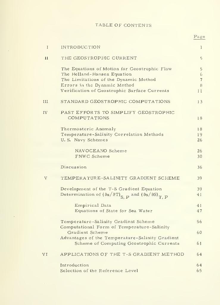
TABLE OF CONTENTS

Page

I INTRODUCTION 1

II THE GEOSTROPHIC CURRENT 5

The Equations of Motion for Geostrophic Flow 5

The Helland- Hansen Equation 6

The Limitations of the Dynamic Method 7

Errors in the Dynamic Method 8

Verification of Geostrophic Surface Currents 11

III STANDARD GEOSTROPHIC COMPUTATIONS 13

IV PAST EFFORTS TO SIMPLIFY GEOSTROPHICCOMPUTATIONS 18

Thermosteric Anomaly 18

Temperature-Salinity Correlation Methods 19

U. S. Navy Schemes 26

NAVOCEANO Scheme 26

FNWC Scheme 30

Discussion 36

V TEMPERATURE-SALINITY GRADIENT SCHEME 39

Development of the T-S Gradient Equation 39

Determination of (3a/aT) and(8a/9S) 41t3> P 1 > ±

Empirical Data 41

Equations of State for Sea Water 47

Temperature-Salinity Gradient Scheme 56

Computational Form of Temperature-SalinityGradient Scheme 60

Advantages of the Temperature-Salinity Gradient

Scheme of Computing Geostrophic Currents 6l

VI APPLICATIONS OF THE T-S GRADIENT METHOD 64

Introduction 64

Selection of the Reference Level 65

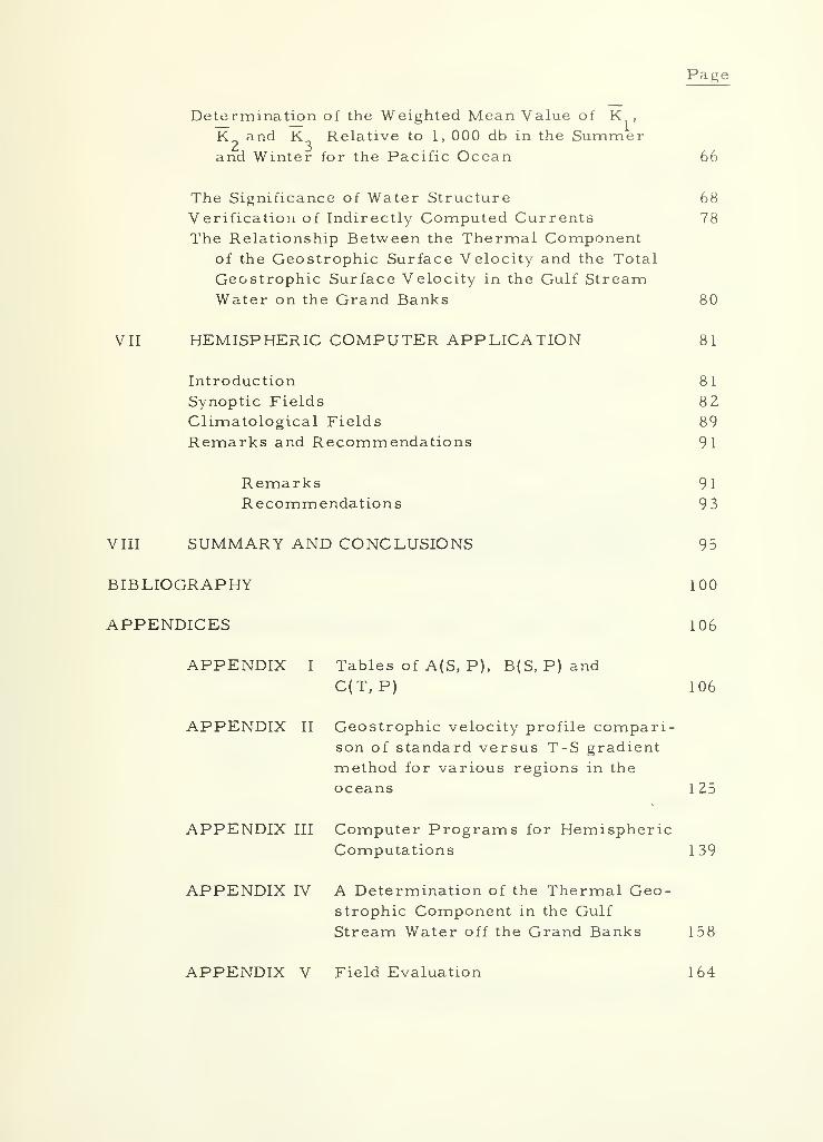
Page

Determination of the Weighted Mean Value of K ,

K and K Relative to 1, 000 db in the Summerand Winter for the Pacific Ocean 66

The Significance of Water Structure 68

Verification of Indirectly Computed Currents 78

The Relationship Between the Thermal Componentof the Geostrophic Surface Velocity and the Total

Geostrophic Surface Velocity in the Gulf StreamWater on the Grand Banks 80

VII HEMISPHERIC COMPUTER APPLICATION 81

Introduction 81

Synoptic Fields 82Climatological Fields 89

Remarks and Recommendations 91

Remarks 91

Recommendations 93

VIII SUMMARY AND CONCLUSIONS 95

BIBLIOGRAPHY 100

APPENDICES 106

APPENDIX I Tables of A(S, P), B(S, P) and

C(T, P) 106

APPENDIX II Geostrophic velocity profile compari-son of standard versus T-S gradient

method for various regions in the

oceans 125

APPENDIX III Computer Programs for HemisphericComputations 1 39

APPENDIX IV A Determination of the Thermal Geo-strophic Component in the Gulf

Stream Water off the Grand Banks 158

APPENDIX V Field Evaluation 164

LIST OF FIGURES

Figure Page

1 NAVOCEANO relationship between surface current speedand horizontal surface temperature gradient in the

Northwest Atlantic 28

2 FNWC polar stereographic projection and grid 32

3 FNWC current transport 34

4 FNWC stream function analysis 35

5 The dependence of specific volume as a function of

temperature at fixed salinity and pressure 43

6 The dependence of specific volume as a function of

salinity at fixed temperature and pressure 44

7 Variation of (3a/3T) , as a function of pressurefor a salinity of 34%p

', according to the Ekman, Eckart

and Tait-Gibson equations of state and Equation 23

with coefficients derived from the Ekman equation

of state 52

8 A(S, P) as a function of salinity and pressure 57

9 2B(S, P) as a function of salinity and pressure 58

10 C(T, P) as a function of temperature and pressure 59

1 1 Variation of K over the Pacific Ocean in the

summer 69

12 Variation of K over the Pacific Ocean in the winter 70

13 Variation of K over the Pacific Ocean in the summer 71

14 Variation of K over the Pacific Ocean in the winter 72

15 Variation of K over the Pacific Ocean in the

summer 73

16 Variation of K over the Pacific Ocean in the winter 74

Figure Page

17 Resolution of the i and j components of the velocity 83

18 Comparison of T-S gradient synoptic thermal currentfield and FNWC current transport for 0000 GMT,March 5, 1968 in the North Pacific 84

19 Comparison of T-S gradient synoptic thermal currentfield and FNWC stream function analysis for 0000

GMT, March 5, 1968 in the North Pacific 85

20 Geostrophic surface flow in the North Pacific relative

to 1, 000 db 87

21 T-S gradient atlas-climatology surface geostrophic

current field relative to 1, 000 db 90

AppendixFigure

AIV - 1 Relationship between the total geostrophic surface

current and the T-S gradient thermal component in

the Gulf Stream waters off the Grand Banks 162

AV - 1 Comparison of geostrophic velocity profiles using

reversing temperatures and XBT temperatures 181

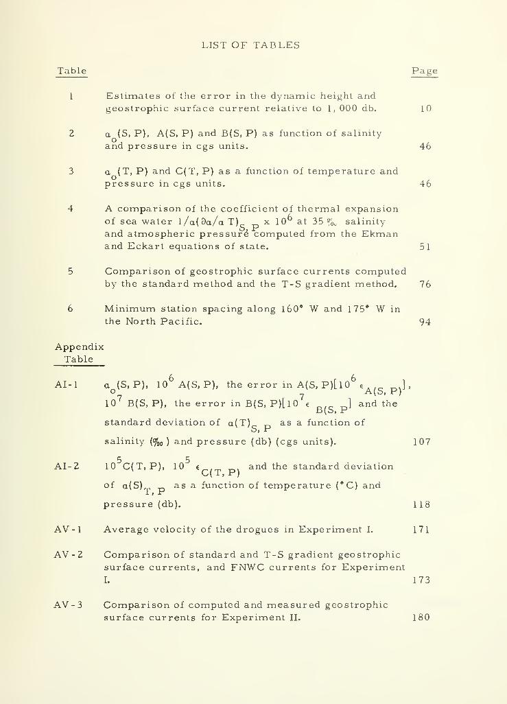
LIST OF TABLES

Table Page

1 Estimates of the error in the dynamic height andgeostrophic surface current relative to 1, 000 db. 10

2 a (S, P), A(S, P) and B(S, P) as function of salinity

and pressure in cgs units. 46

3 a (T, P) and C(T, P) as a function of temperature andpressure in cgs units. 46

4 A comparison of the coefficient of thermal expansionof sea water l/a(3a/a T) x 10 6 at 35 % salinity

and atmospheric pressure" computed from the Ekmanand Eckart equations of state. 51

5 Comparison of geostrophic surface currents computedby the standard method and the T-S gradient method. 76

6 Minimum station spacing along 160° W and 175* W in

the North Pacific. 94

AppendixTable

6 6AI-1 a (S, P), 10 A(S, P), the error in A(S, P)[l0 € ],

o A(b, P)

10 ' B(S, P), the error in B(S, P)[l0 e ] and ther3(o, P

standard deviation of a(T) as a function ofo> P

salinity (% ) and pressure (db) (cgs units). 107

5 5AI-2 10 C(T, P), 10 € p , T p . and the standard deviation

of a(S) as a function of temperature (*C) and1 > *?

pressure (db). 1 18

AV - 1 Average velocity of the drogues in Experiment I. 171

AV - 2 Comparison of standard and T-S gradient geostrophic

surface currents, and FNWC currents for ExperimentI. 173

AV-3 Comparison of computed and measured geostrophic

surface currents for Experiment II. 180

THE T-S GRADIENT METHOD, A NEW METHODOF COMPUTING GEOSTROPHIC CURRENTS

OVER LARGE OCEAN AREAS

I. INTRODUCTION

The purpose of the research reported in this study is to improve

the contemporary techniques of computing synoptic geostrophic ocean

surface currents over large ocean regions. Techniques that are used

today are either gross approximations with little scientific basis or

applicable to only small regions, or both. Yet knowledge of surface

currents is important, and in some cases essential to public, com-

mercial, and military use of the sea.

The U. S. Coast Guard uses surface current information in

search and rescue, as well as in the forecasting of iceberg drift for

the shipping lanes in the Northwest Atlantic (Lenczyk, 1964). The

U. S. Navy Fleet Numerical Weather Central, Monterey, California,

computes surface currents every 12 hours over the Northern Hemi-

sphere principally to aid in thermal structure forecasting (Hubert

and Laevastu, 1967). The U.S. Naval Oceanographic Office computes

surface currents in the ASWEPS (Antisubmarine Warfare Environ-

mental Prediction System) area of the Northwest Atlantic for thermal

structure forecasting (James, 1966).

Mariners have been using knowledge of ocean currents probably

since the beginning of navigation- As early as 600 BC the east to

west eircum-navigation of Africa may have been aided by favorable

winds and currents (von Arx, 1962). Early Greek and Arab traders

could penetrate the Arabian Sea and Bay of Bengal because of

favorable currents under the influence of the monsoon winds. Spanish

trade between Mexico and the Philippines was also aided by knowledge

of the winds and currents (Jones, 1939). The Spanish captains would

take advantage of the North Equatorial Current on their westerly

journey, and return to Mexico along a more northerly route reaching

land fall around Cape Mendocino. An early chart of the Gulf Stream

was published by Benjamin Franklin in 1770. This chart is said to

have improved mail service from England to the American Colonies

by two weeks per crossing (Groen, 1967). Pilot charts, published by

the Naval Oceanographic Office, provide monthly summaries of wind

and surface current conditions. Surface current atlases giving the

monthly mean values are also available from the Naval Oceanographic

Office.

Flow in the surface layers of the deep ocean is influenced by

several forces: the most important are the horizontal pressure

gradient and viscous forces within the fluid, the action of wind stress,

tidal forces, and the Coriolis force. Today incomplete knowledge of

ocean dynamics and lack of suitable available data restricts the in-

direct determination of surface currents to the computation of the

geostrophic and wind driven components (Hubert, 1965).

Computation of geostrophic flow over a large ocean area on a

synoptic basis are facilitated if the computations be as simple and as

fast as possible. Standard geostrophic computations are unsuitable

for many reasons:

1) The computations are numerous and consume more computer

time than is available for this task.

2) Several quantities must be computed that are not used beyond

the analysis of currents.

3) The temperature and salinity data that are required for

standard geostrophic computations are not yet available in the neces-

sary accuracy and density.

4) It would be useful to compute the temperature and salinity

structure contributions to the geostrophic current independently.

This is difficult by the standard method.

Further explanation ofthe last two points is in order. Because

of the relative ease of measuring temperature structure over the

salinity structure, temperature is a much more commonly observed

variable in the ocean. Until the recent development of in situ con-

ductivity measurement, rapid determination of salinity structure was

not possible. For this reason, while nearly synoptic thermal struc-

ture information may be available from many areas of the oceans,

salinity structure is available only from the historical records

contained in oceanographic data centers and various atlases derived

from this historical data. It will probably be several years before

salinity structure is as commonly observed as thermal structure.

It is because of this compatability that it is desirable to compute the

temperature and salinity contributions to the geostrophic flow sepa-

rately. Furthermore, salt is not as easily exchanged between the air

and sea as is heat, and therefore, it may be more acceptable to use

historical data for salinity information than for temperature informa-

tion. By directly computing the thermal and haline components of the

geostrophic flow the significance of air-sea heat exchanges on thermo-

haline flow may be more easily examined.

To summarize, the purpose of this thesis is to study a simpli-

fied method of computing geostrophic surface currents over large

ocean areas that gives essential agreement with currents computed

by the standard geostrophic method. The derived method must be

computationally faster on digital computers than the standard method.

Furthermore, that the method ought to express, at least to first

order, the thermal and haline components separately.

IL THE GEOSTROPH1C CURRENT

The Equations of Motion for Geostrophic Flow

Fluid is said to be in geostrophic balance if the flow is unac-

celerated and the horizontal pressure gradient is balanced by the

Coriolis force. The simplified equations of motion for geostrophic

flow in rectangular coordinates (x axis east, y axis north and z axis

positive down from the sea surface) are:

/v

where

fkxV H- qV^ (1)

g" a

az (2)

f = 2u> sin<J>

is the Coriolis parameter (l/ sec)

co - the angular velocity of the earth (radians/sec)

4> - the geographic latitude (degrees)

V ~ the horizontal velocity (cm/sec)H

g~ the local acceleration of gravity (cm/sec )

a = specific volume (cm /gm)

VI3 - the horizontal pressure gradient (dynes/cm )

9P 2—— - the vertical pressure gradient (dynes/cm )

k = the vertical unit vector

Given the horizontal pressure gradient along a level surface the

geostrophic flow along the surface could be determined directly from

Equation 1. However, direct measurement of the horizontal pressure

gradient in the sea has not been achieved. Several schemes have been

developed to compute the horizontal pressure gradient from the mass

distribution as determined from the measured temperature and

salinity distributions.

The Helland- Hansen Equation

Geostrophic computations, also often referred to as dynamic

computations or the dynamic method, are discussed in any elementary

physical oceanography text, for example Neumann and Pierson (1967).

Fomin (1964) discusses in considerable detail the application and the

limitation of the dynamic method. Yao (1967) gives an excellent re-

view of various computational schemes for computing geostrophic

currents. What might be called the standard or classical method is

based on an equation originally derived from Bjerknes' circulation

theorem (1900) by Sandstrom and Helland-Hansen (1903), (as cited by

Proudman, 1953). However, the resulting equation is commonly re-

ferred to in the literature as the Helland-Hansen equation. The

Helland-Hansen equation, written in terms of the horizontal gradient

of the geopotential between two levels P and P is,

P2

fk x (V, - V2

)= V

H\ a(x,y,p)dp (3)

P!

where

?2

J a(x, y, p)dp - the geopotential of level P with respect

to P (cm/sec)

(V - V ) - the horizontal velocity at P relative to the

level P (cm/sec)

The geopotential difference between two levels in the ocean is

determined by the integral in the right-hand term of Equation 3.

The integral is numerically evaluated (using the trapazoidal rule)

from computed vertical density distributions, determined from the

measured vertical temperature and salinity structure. Using two

stations the measured temperature and salinity structure can be used

to compute the horizontal gradient in geopotential along an isobaric

surface, and Equation 3 can be evaluated to give the geostrophic flow

between the two stations.

The Limitations of the Dynamic Method

Use of Helland- Hans ens ' formula suffers from several limita-

tions (Fomin, 1964). The feasibility of computing ocean currents

using the dynamic method is based on the following assumptions:

1) The horizontal velocity and the horizontal pressure gradient

is balanced by the Coriolis force.

?.) The horizontal velocity and the horizontal pressure gradient

become negligible at a moderate depth below the sea surface.

3) The fieid accelerations and frictional forces can be neglected

(Sverdrup, 1947).

That these assumptions are realistic for the large scale mo-

tions, at least sometimes, has been illustrated by Stommel (1965).

Even when the assumptions of geostrophy are satisfied, the neces-

sary measurements are difficult to obtain to the desired accuracy.

Errors in the Dynamic Method

Errors in the dynamic method have been estimated by many

authors, however, no completely satisfying error analysis of geo-

strophic procedures is available. The errors in computing the geo-

strophic current from standard hydrographic measurements (tem-

perature and salinity at discrete levels) can be divided into the two

categories, measurement errors and computational errors.

Errors in the geostrophic current due to errors in the hydro-

graphic measurements have been discussed by Wooster and Taft

(1958), Reid (1959) Fomin (1964), and others. Following Reid ( 1 959)

the measurement errors in classical hydrographic work are sum-

marized below:

1. Incorrect temperatures due to errors in temperature

readings.

2. Incorrect temperatures due to errors in the location of

the measurement.

3. Incorrect salinities due to errors in the salinity readings.

4. Incorrect salinities due to errors in the location of the

measurement.

5. Incorrect temperature due to time and space variability.

6. Incorrect salinity due to time and space variability.

The errors in computing geostrophic currents due to computa-

tional procedures have been discussed by Rattray (1961), Fomin

(1964), Yao (1967) and others. These errors are summarized below:

1. Errors in interpolation of point hydrographic data between

sampling levels.

2. Rounding and truncation errors in the numerical integra-

tion.

Due to the dependence of the measurement and computational

errors on one another, no completely rigorous analysis is yet avail-

able for the accumulated error in determining geostrophic currents

by the dynamic method. The analysis by Fomin (1964) appears to be

the most complete to date, but his discussion is not fully documented.

The magnitude of the total error in dynamic height due to measure-

ment and computational errors has been estimated independently by

10

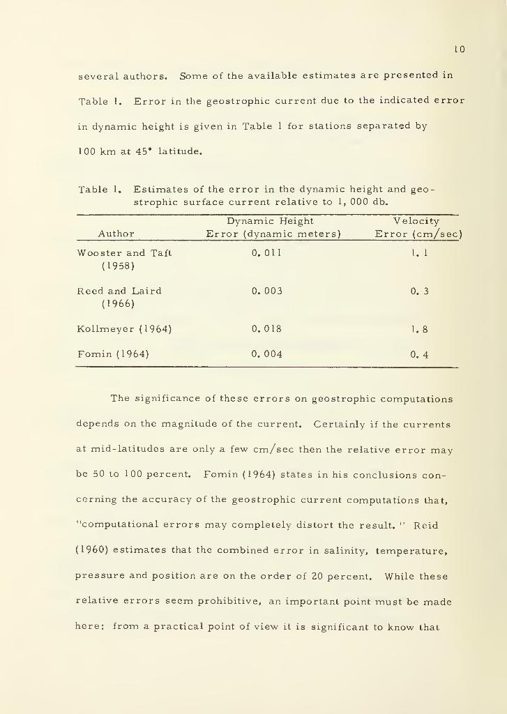
several authors. Some of the available estimates are presented in

Table 1. Error in the geostrophic current due to the indicated error

in dynamic height is given in Table 1 for stations separated by

100 km at 45° latitude.

Table 1. Estimates of the error in the dynamic height and geo-

strophic surface current relative to 1, 000 db.

Dynamic Height Velocity

Author Error (dynamic meters) Error (cm/sec)

Wooster and Taft 0.011 I. 1

(1958)

Reed and Laird 0. 003 0. 3

(1966)

Kollmeyer (1964) 0.018 1.8

Fomin (1964) 0. 004 0. 4

The significance of these errors on geostrophic computations

depends on the magnitude of the current. Certainly if the currents

at mid-latitudes are only a few cm/sec then the relative error may

be 50 to 100 percent. Fomin (1964) states in his conclusions con-

cerning the accuracy of the geostrophic current computations that,

"computational errors may completely distort the result. " Reid

(I960) estimates that the combined error in salinity, temperature,

pressure and position are on the order of 20 percent. While these

relative errors seem prohibitive, an important point must be made

here: from a practical point of view it is significant to know that

1

1

the geostrophic currents are weak. Therefore, if the currents are

less than a few centimeters per second, this fact can be determined

even if the relative error is large.

Verification of Geostrophic Surface Currents

A few direct current measurements have been collected in sup-

port of geostrophic computations from hydrographic measurements.

The classic case is a comparison reported by Wust (1924) of

Pillsbury's current observations (1885-1889) in the Straits of Florida

to geostrophic currents computed from hydrographic data collected

in 1888 and 1912. Observed currents are in remarkable agreement

with the computed geostrophic currents, von Arx (1962) reports a

comparison of currents observed with the geomagnetic electro-

kinetograph (GEK) and dynamic topography showing substantial agree-

ment in the Gulf Stream. Broida (1966) made simultaneous measure-

ments of currents and hydrographic casts in the Florida Straits.

His measured surface currents were in fair agreement with the com-

puted geostrophic surface currents. Reed (1965) compared geo-

strophic currents and currents measured by parachute drogue in the

Alaska Stream and found excellent agreement between the two values

for the surface current. Smith (1931) showed a definite association

between the geopotential topography in the Grand Banks Region and

12

the drift paths of icebergs that established the basis for the U. S.

Coast Guard hydrographic surveys of this region which continue

today.

13

III STANDARD GEOSTROPHIC COMPUTATIONS

Prior to exploring attempts to simplify the standard geo-

strophic computations these computations should be reviewed.

Several schemes have been suggested for computing geostrophic

currents: (1) the geopotential scheme using the Helland- Hansen

formula (Equation 3), (2) the acceleration potential scheme of

Montgomery and Stroup (1962), and (3) the isanosteric contour slope

scheme of Werenskjold (1935, 1937). These three methods have

been reviewed by Yao (1967). Only the geopotential scheme will be

reviewed here, because of its role in later sections of this thesis,

and its more frequent use over the other methods.

The standard computations in the geopotential scheme as ex-

pressed by the Helland- Hansen equation are expressed in the follow-

ing equation:

(AD - AD )

(V - V )- — (4)V

.1 Z' fAn V '

where

AD - AD = the difference in the anomaly of dynamic heightA B 7 7 6

/ 2at stations A and B (cm/sec)

AD - Z6.AP., where 6". is the average specifici i l i

volume anomaly in the i pressure interval

- 5 3( 1 cm /gm)

14

(V - V ) = the magnitude of the relative current normal

to a line joining the two stations (cm/sec)

In order to carry out geostrophic computations with Equation 4

several complicated formulae must be used, or the empirical ex-

pression of these formulae in tables (LaFond, 1951). The formulae

necessary to calculate in situ specific volume anomaly from meas-

ured or interpolated temperature and salinity are summarized by

Yao (1967).

Salinity as a function of chlorinity is given by Knudsen's (1901)

equation:

S = 0. 030 + 1.805 CI (Knudsen, 1901) (5)

where

S = salinity (% )

CI = chlorinity (% )

It the measurement of electrical conductivity is to be used to deter-

mine salinity or chlorinity then other formulae or tables must be

used.

Given the chlorinity the quantity o- can be computed.o

a = -0. 069 + 0. 4708C1 - 0. 001570C12

+ 0.0000398C13

(6)

And with cr the quantity a can be computed.

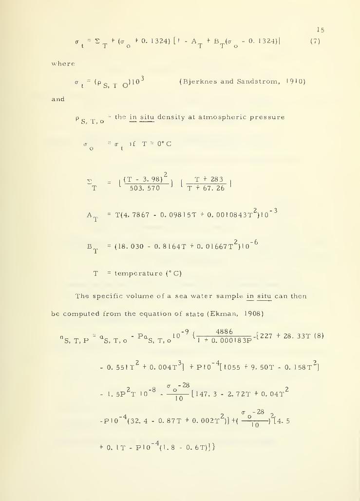
o- - S + (<r + 0. 1 324) [I - A + B {a - 0. 1 324)]

t To T T o

15

(7)

w here

and

a r:

(p c rp o)10 (Bjerknes and Sandstrom, 1910)

p _ m ~ the in situ density at atmospheric pressureS, 1 , o

a =o- if T = 0°Co t

: = |

(T - 3. 98)", T + 28 3

T 503. 570J L

T + 67. 26

A = T(4. 78 67 - 0. 098 1 5T + 0. 00 1 0843T2

) I0" 3

2 6B = (18. 30 - 0. 8 164 T + 0. 01 667 T )10

T = temperature (° C)

The specific volume of a sea water sample in situ can then

be computed from the equation of state (Ekman, 1908)

4886aS, T, P " a

S, T, o " PaS, T, o

101+0. 000183P

[227 + 28. 33T (8)

0. 551T2

+ 0. 004T3

] + Pl0_4

[l055 + 9- 50T - 0. 158T2

]

a - 28

1. 5P T 10" ^—— [147. 3 - 2. 72T + 0. 04T

2°"

~ 282

P10 (32. 4 - 0. 87T + 0. 002T )] +( —^—f[4. 5

-4+ 0. 1 T - P10~ (1.8-0. 6T)]}

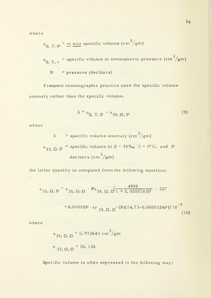
16

where

3a c

- in situ specific volume (cm /gm)

a = specific volume at atmospheric pressure (cm /gm)O) 1 > o

P = pressure (decibars)

Frequent oceanographic practice uses the specific volume

anomaly rather than the specific volume.

5 = QS, T,P "

Q 35,0,P (9)

where

6 = specific volume anomaly (cm /gm)

a - specific volume at S - 35%o, T = 0°C, and P

3decibars (cm /gm)

the latter quantity is computed from the following equation:

P r4886

35, O, P a35,O s O

a35> O, O l

1 + 0. 0000183P

+ 0.01055P -(a oc _ -28)(14.73-0.0000324P)] 10~ 9

35'°'°(10)

where

a35, O, O

=°* 972643 cmV

^35,0,0-" 28 - 126

Specific volume is often expressed in the following way:

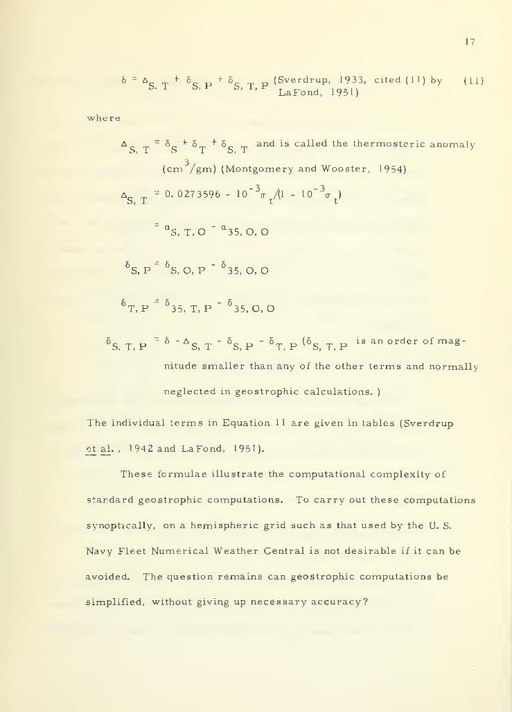
17

6 = A_ + 6 + 6 (Sverdrup, 1933, cited ( 1 I ) by (11)O.I O, r O, 1 , r inci\LaFond, 1951)

where

A -6+6+6 and is called the thermosteric anomaly

(cm /gm) (Montgomery and Wooster, 1954)

A _ = 0.0273596 - 1

" 3q- /(l - 10" 3

cr )

S, T t t

QS, T, O " a

35, O, O

6S, P

6S, O, P " 5

35, O, O

6T, P " 6

35 5 T, P ~ 635» O, O

6S, T, P

= 6 " AS, T " 6

S, P "6T, P (6

S, T, P1S an ° rd6r ° f mag "

nitude smaller than any of the other terms and normally

neglected in geostrophic calculations.)

The individual terms in Equation 11 are given in tables (Sverdrup

et al. , 1942 and LaFond, 1951).

These formulae illustrate the computational complexity of

standard geostrophic computations. To carry out these computations

synoptically, on a hemispheric grid such as that used by the U. S.

Navy Fleet Numerical Weather Central is not desirable if it can be

avoided. The question remains can geostrophic computations be

simplified, without giving up necessary accuracy?

18

IV. PAST EFFORTS TO SIMPLIFY GEOSTROPHIC COMPUTATIONS

Several attempts have been made to simplify geostrophic com-

putations. The attempts can be divided into three categories: those

which (1) neglect the pressure dependent terms in the specific volume

anomaly, (2) assume a simple relationship between the density of sea

water and the variables (temperature, salinity, and pressure), and

(3) determine the correlation function between two of the variables in

particular water masses. The first approach is the most direct and

will be the most generally applicable, and is discussed in the follow-

ing section.

Thermosteric Anomaly

Montgomery and Wooster (1954) showed that the "thermosteric

anomaly, "A , can be substituted for the specific volume anomalyo, 1

in geostrophic computations under some conditions without signifi-

cant loss of accuracy. One condition is that the computations be

limited to the upper layers, above 1, 000 db where the pressure

terms (6 and 6 ) are not large; thus the thermosteric anomalyOj X"^ I , r

is a good approximation to the specific volume anomaly.

Performing geostrophic computations on 47 hydrographic sta-

tions from the Atlantic and Pacific oceans, using both the complete

specific volume anomaly and the thermosteric anomaly, Montgomery

19

and Wooster showed that, except for one station in the Atlantic

Ocean, the pressure terms contribute at most five percent to the

station to station difference in the anomaly of dynamic height. These

authors stated (page 66):

The conclusion is reached that for hydrostatic computa-tion limited to the upper 500 db or I, 000 db, especially

in the Pacific Ocean, if extreme precision is not requiredand if significant convenience is gained, the pressureterms may be neglected; in other words the thermostericanomaly Ag -p may be used in place of the complete specific

volume anomaly 6.

While this is clearly a simplification of the standard geo-

strophic computations, the use of the thermosteric anomaly requires

determination of o~ and <j . Since the sole purpose for determin-o t

ing these quantities is to evaluate the thermosteric anomaly in geo-

strophic computations, a scheme which would allow geostrophic

computations without the determination of these preliminary

quantities would be more efficient. An interesting point made by

Montgomery and Wooster is that for all practical purposes the pres-

sure terms are nearly linear from the surface to the 2, 000 db level

or deeper.

Temperature-Salinity Correlation Methods

One of the earliest attempts to simplify dynamic computations

is that of Stommel (1947) through the use of temperature and

salinity correlation. Since specific volume is a function of

20

temperature, salinity and pressure, all three of these variables must

be accurately known in order to compute this quantity. However, if

a correlation exists between any two of the independent variables,

say temperature and salinity, then the specific volume anomaly could

be expressed in terms of only two quantities, since the correlation

function determines the relationship between the other two quantities.

Since temperature as a function of depth is an easier and more com-

mon measurement, Stommel suggested geostrophic computations

could be made from temperature structure measurements alone

using the temperature- salinity correlation to determine the salinity;

from this the specific volume anomaly and then the dynamic height

could be evaluated. Oceanographers have long recognized that tem-

perature and salinity are correlated in certain water masses

(Sverdrup et al. , 1942). That is, for each temperature there will

be a small range of salinity in a given water mass.

Assuming that a satisfactory temperature- salinity correlation

exists in a given water mass, then using this temperature-salinity

correlation a new set of tables can be constructed giving the specific

volume anomaly as a function of only two terms:

6 = [T] + [T, P] (12)

The first term on the right-hand side, [t], is in reality the thermo-

steric anomaly, Ag -p , which is a function of the temperature only

21

because of the established temperature-salinity correlation. The

second term, [T, P] , includes 6 _ and 6 „, but is fully deter-o, it 1 , r

mined from temperature and depth in the given water mass because

of the established temperature-salinity correlation. It is clear that

the accuracy of the temperature-salinity correlation method is de-

pendent on the nature of the temperature-salinity correlation. For

each temperature there will be a certain finite range of salinity

(R ) which will represent the uncertainty in specifying the salinity

from the temperature- salinity correlation. The uncertainty in

salinity decreases with the slope of the temperature-salinity curve

on the temperature-salinity diagram. Obviously this is due to the

fact that for small slopes a small error in the temperature leads to

a large change in the implied salinity. The uncertainty in salinity

will also be large whenever seasonal variation and mixing lead to a

poor temperature-salinity correlation. Values of R can be deter-s

mined at each level from the scatter of temperature-salinity pairs

around the mean. Associated with the value of R at each level fors

a given water mass is an uncertainty in specific volume R . Sum

-

6

mation of the values of R over the water column during the compu-o

tation of dynamic height gives a measure of the uncertainty in the

calculated dynamic height introduced by the uncertainty in the tem-

perature-salinity correlation.

Stommel applied the temperature- salinity correlation technique

22

to stations of the International Ice Patrol (327 5 to 3278) off the Grand

Banks, ATLANTIS stations 1637 to 1642 across the Gulf Stream, and

some stations (unidentified) from the Sargasso Sea. He found that

the use of temperature-salinity correlation was unsuited off the

Grand Banks as the temperature-salinity correlation is poor in this

region. His results are not surprising since the Grand Banks region

is a mixing region for water masses of the Labrador Current and

Gulf Stream (Kollmeyer, 1966). In the Gulf Stream he found that the

temperature-salinity correlation method can be applied, but only if

the stations are grouped, as the temperature-salinity correlation

changes across this current. However, in the Sargasso Sea where

temperature-salinity correlation is excellent the method seems well

suited. Stommel concludes (page 91):

As a result it appears that in certain restricted regionsthe temperature-salinity diagram may be used for roughdynamic computations. For more details survey workwhere great accuracy of the results is desired the methodusing the temperature-salinity diagram is clearly un-suitable.

LaFond (1949) applied the temperature-salinity correlation

scheme in the Marshall Island region in an attempt to determined

the geostrophic flow in this region using bathythermograms. He

used existing hydrographic data to establish the temperature-

salinity correlation function for this region. LaFond's conclusion

(page 236) summarizes the results of his studies:

23

To use bathythermograms in determining relative cur-rents, there are several prerequisites which must be

met: (1) the bathythermogram must extend at least to

900 ft. , (2) the temperature-salinity relation must be

established, with consideration of seasonal and geo-graphic effects, and (3) the effects of internal waves mustbe largely eliminated. If these conditions are attainable

the direction of relative currents can be established frombathythermograms. The results of this test indicate that

the speed of the current (0/305 db) can be within 25 per-cent of those obtained from Nansen bottle and reversingthermometer data (O/l, 000 db).

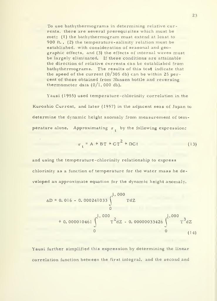
Yausi (1955) used temperature-chlorinity correlation in the

Kuroshio Current, and later (1957) in the adjacent seas of Japan to

determine the dynamic height anomaly from measurement of tem-

perature alone. Approximating cr by the following expression:

7o- = A +BT+CT + DC1 (13)

and using the temperature-chlorinity relationship to express

chlorinity as a function of temperature for the water mass he de-

veloped an approximate equation for the dynamic height anomaly.

1, 000

TdZ1

1,000 1,000

+ 0.000010461 f T2dZ - 0.00000033426

\T

3dZ

° (U)

Yausi further simplified this expression by determining the linear

correlation function between the first integral, and the second and

24

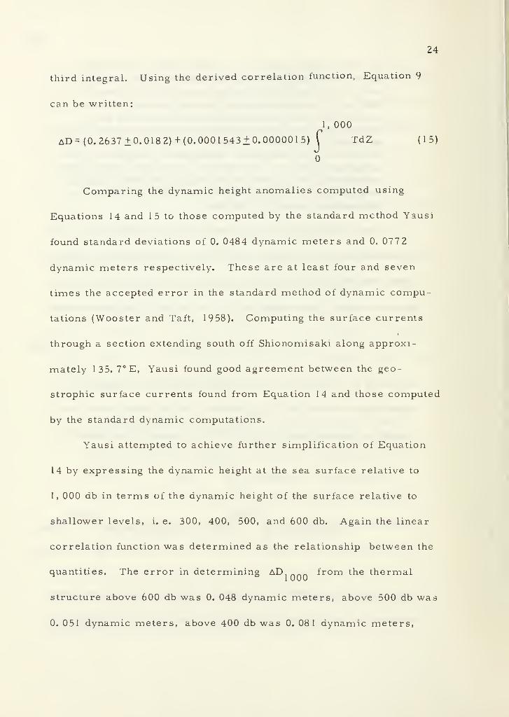
third integral. Using the derived correlation function, Equation 9

can be written:

1, 000

AD=(0.2637±0.0182)+(0.0001543±0.0000015) f TdZ (15)

Comparing the dynamic height anomalies computed using

Equations 14 and 15 to those computed by the standard method Yausi

found standard deviations of 0. 0484 dynamic meters and 0. 0772

dynamic meters respectively. These are at least four and seven

times the accepted error in the standard method of dynamic compu-

tations (Wooster and Taft, 1958). Computing the surface currents

through a section extending south off Shionomisaki along approxi-

mately 135. 7°E, Yausi found good agreement between the geo-

strophic surface currents found from Equation 14 and those computed

by the standard dynamic computations.

Yausi attempted to achieve further simplification of Equation

14 by expressing the dynamic height at the sea surface relative to

1, 000 db in terms of the dynamic height of the surface relative to

shallower levels, i. e. 300, 400, 500, and 600 db. Again the linear

correlation function was determined as the relationship between the

quantities. The error in determining AD from the thermal

structure above 600 db was 0. 048 dynamic meters, above 500 db was

0. 051 dynamic meters, above 400 db was 0. 081 dynamic meters,

25

and above 300 db was 0. 129 dynamic meters. He concluded that a

reasonably accurate measure of the geostrophic surface currents

could be obtained by using only the thermal structure above 500 db.

Yausi (1957) attempted to apply these methods to the adjacent

seas of Japan, east of Honshu. While the patterns of dynamic

topography obtained by the standard dynamic method and using the

simplified equations of the form of Equation 14 and 15 were similar,

an uncertainty of 0. 08 dynamic meters was inherent in the simple

method due to poor temperature-chlorinity correlation. This is not

unexpected because of the nature of the temperature-chlorinity cor-

relation curve in the adjacent seas and the strong seasonal variability

in this region.

Attempts were made to apply the method over other parts of

the North Pacific using stations 100 to 150 in the seventh cruise of

the CARNEGIE. The difference between the dynamic height computed

by Equation 14 and the standard method was less than 0. 06 dynamic

meters, except for stations 1 26 and 1 31 off the west coast of the

United States where the difference between the two methods reaches

0. 18 dynamic meters.

One concludes that the temperature-salinity or temperature-

chlorinity methods are applicable in specific regions. However, it

is not suited to other regions where the temperature-salinity curves

have small slopes or in regions where seasonal variations and mixing

26

lead to a large scatter of temperature- salinity pairs. Furthermore,

temperature-salinity correlations would have to be established for

each water mass, and the correlation functions altered at water mass

boundaries. Since water mass boundaries are not fixed such corre-

lation will be difficult to determine.

U. S. Navy Schemes

Two- groups in the U. S. Navy make ocean surface current com-

putations on a synoptic basis over large ocean regions. One group

uses techniques developed at the Naval Oceanographic Office

(NAVOCEANO) principally for application in the Northwest Atlantic

Ocean (James, 1966). The other group, Fleet Numerical Weather

Central (FNWC), computes surface currents over the Northern

Hemisphere every 12 hours (Hubert, 1964). Both groups rely on

synoptic thermal structure data transmitted from ships at sea. The

density and accuracy of thermal structure data has been discussed

by Wolff (1964).

NAVOCEANO Scheme

NAVOCEANO techniques were originally reported by Gibson

(1962). The technique is based on a relationship between the hori-

zontal surface temperature gradient and the surface current speed.

Discussing a hydrographic section along the 50th meridian Gibson

27

summarizes (page 4) the basis for the scheme;

These data and sections for other ocean areas (not shown)form the basis for the analytical approach describedbelow. Symmetrical undulation of the isotherms indicates

four major water masses.

Upon crossing each mass the surface current changesdirection in an orderly manner; that is, the circulation

is cyclonic for cold waters and anticyclonic for warmwaters. There is also general agreement between the

magnitude for temperature gradients and current velocity.

If V is the surface current velocity, k a vertical vector,

positive outwards, and AT is grad T, the relation,

V - k cross AT holds in principle. This relation,

analogous to that which applies for straight air flow sug-

gests that water bands can be treated as greatly elongated

air masses.

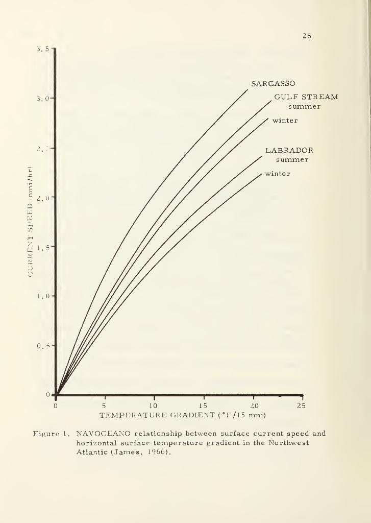
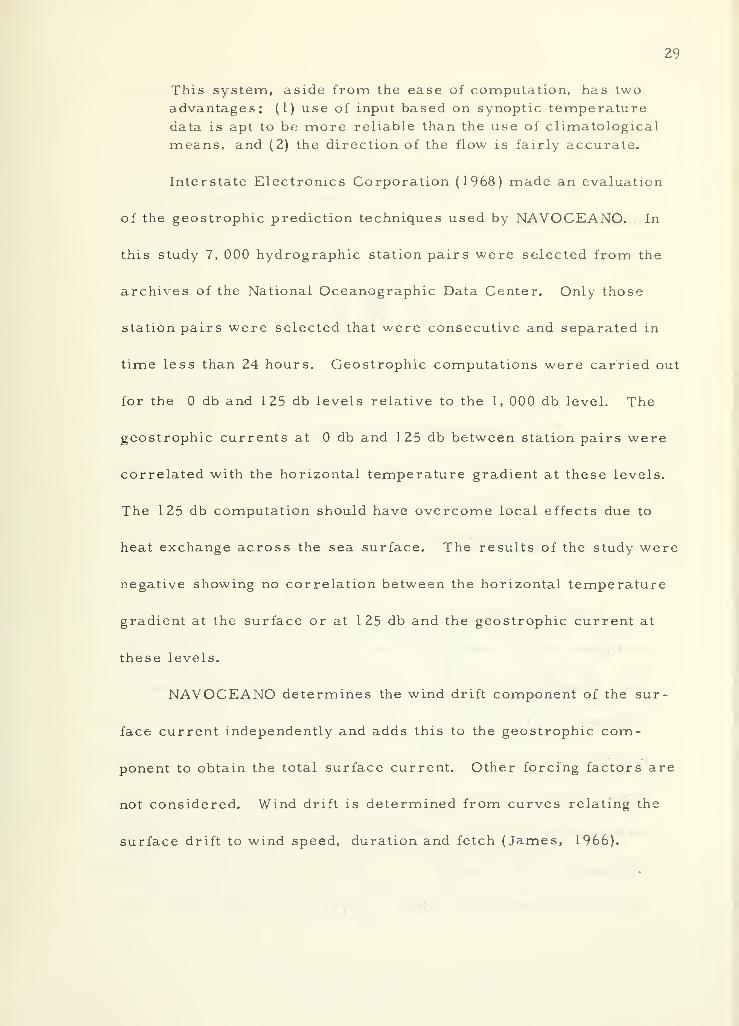
James (1966) discusses the application of Gibsons' suggestion

to synoptic analysis of ocean surface currents. Plotting observed

currents against observed horizontal surface temperature gradients

in the Northwest Atlantic, a set of curves is derived giving the sur-

face current as a function of horizontal surface temperature

gradient. The curves are shown in Figure 1 for the Gulf Stream,

Sargasso and Labrador water masses for summer and winter condi-

tions. The surface current is obtained by determining the sea sur-

face temperature gradient and reading current speed from the ap-

propriate curve. Direction of flow is assumed to be parallel to the

isotherms. James states (page 60):

28

3. 5

3.0-

w

H

W

0. 5-

SARGASSO

GULF STREAMsummer

winter

LABRADORsummer

i r

5 10 15 20

TEMPERATURE GRADIENT (°F/15 nmi)

Figure 1. NAVOCEANO relationship between surface current speed and

horizontal surface temperature gradient in the NorthwestAtlantic (James, 1966).

29

This system, aside from the ease of computation, has two

advantages: (1) use of input based on synoptic temperaturedata is apt to be more reliable than the use of climatological

means, and (2) the direction of the flow is fairly accurate.

Interstate Electronics Corporation (1968) made an evaluation

of the geostrophic prediction techniques used by NAVOCEANO. In

this study 7, 000 hydrographic station pairs were selected from the

archives of the National Oceanographic Data Center. Only those

station pairs were selected that were consecutive and separated in

time less than 24 hours. Geostrophic computations were carried out

for the db and 125 db levels relative to the I, 000 db level. The

geostrophic currents at db and 125 db between station pairs were

correlated with the horizontal temperature gradient at these levels.

The 125 db computation should have overcome local effects due to

heat exchange across the sea surface. The results of the study were

negative showing no correlation between the horizontal temperature

gradient at the surface or at 125 db and the geostrophic current at

these levels.

NAVOCEANO determines the wind drift component of the sur-

face current independently and adds this to the geostrophic com-

ponent to obtain the total surface current. Other forcing factors are

not considered. Wind drift is determined from curves relating the

surface drift to wind speed, duration and fetch (James, 1966).

30

FNWC Scheme

Hubert (1964) presents the equation used by FNWC to compute

surface geostrophic flow over the Northern Hemisphere oceans on a

synoptic basis.

'V .- V2»

=# V < 16 >

where

AZ - the depth of the level of no motion

V T - the horizontal gradient of T

~T = K,T , + K~T onn , where K. and K_ are "tuning1 sfc 2 200 1 2

constants "

T , and T„ = the surface and 200 meter temperatures respec-sfc 200

tively.

Hubert (1964) does not develop Equation 16, nor can this in-

vestigator find the development for application to the ocean. How-

ever, Equation 16 is of the same form as the thermal wind equation

(Haltiner and Martin, 1957). Development of the thermal wind equa-

tion requires that there be a linear relationship between the tempera-

ture and density, that is, the thermal wind is parallel to the mean

virtual isotherms with low temperature on the left. Such a relation-

ship cannot exist in the sea since the density of sea water is a nonlinear

function of temperature, salinity and pressure. Hubert points out

31

that the coefficients K, and K can be adjusted in areas where1 2

salinity gradients are known to be significant.

The use of only the surface and 200 meter temperature fields

cannot be justified over much of the ocean, as these two fields are

not necessarily representative of the fields at other levels. Clearly,

more of the water structure than just the sea surface temperature and

200 meter temperature is necessary to make meaningful geostrophic

computations.

The wind drift is computed from Wittings (1909) formula

W = K^xTv" (17)

where

W - the current velocity (cm/sec)

V = the 24 hour mean geostrophic wind speed (M/sec)

K - "wind factor"

The factor K is adjusted to account for the mass transport as-

sociated with waves and the change of velocity with depth. For the

surface wind drift K is taken to be 4. 8, and the surface wind drift

current is assumed to be parallel to the geostrophic wind.

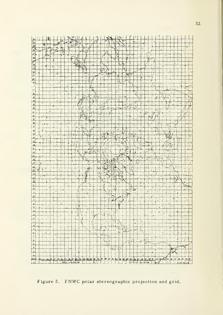
Both the geostrophic current and the wind drift current compu-

tations are carried out on a 63 x 63 linear grid system on a polar

stereographic projection over the Northern Hemisphere (Figure 2).

The grid point separation is given by the following expression:

32

al«

* •K » y. 4,

ft

jftL-^l ^'

. j L. _

*

"if) A :>r»» y u^ f n

' k ^

VL>--• »

tiftrK-*h^ ==r ^ v-

»f-

/1 1

—

> y *j—

1

.

5L -—r3 £h-r'.' b 3 \ "'

1

m • V'. T»

r^ bi ITl

} --^ . <

/->,'r;

r »

"

(

- ^ 7*

.

T •

SB.,> K~

~

4*

sH3 '1 '

/ ..'-

j

*

.

>};* s5

$^1 v ^ i v / J >

ii» V- ^V »-~l s (

'

J

'

5^ ? /*

Bi

Vs

,—

.

^i .

Si L' •

J,

Tjw' . ''\-4T^ •

/

^ *~

F (

/ -(

"^j

1

«+ . I

' & X.'-•' "\ v

^4- „ "'- —.

—

-

1

1

— •

t

i

i

P- ^—

i

:+ ; t s ; j:

^^. i

^> _.. %4-~-t^.

jt.*

—i—

i

~3

% ]

1 N 1 .

-

s^ A I S .1 i * '

.^g a * ^

jft.

'

—£ ™.

>S;

!

i

> 7/>•'•

"~-~i

\**T-

4•.

.-1 ., /

$* '

t v?,; '"*[ ^ r.« i

+

f

• rJ

J5* \

51/

>

.

r-K -- .-r.' •^

ft . 3^^

.

fVJ"

L t

j

!''

, if.

1'* S

-< y '

|^Q„ -

•V EVA .

^-^ }• f!

,'<\

! 4 h? . y7'*

t /

iL

. i

' //

J&r. r

,r

i*«.

/

37

'

."i

j'

.

•

i

.-1

1

) W- /

._i r^\ d j.

- -

r

2

•j K uS•

1

3S"| ,

; M ",^ - ^ .J

f; ,.tt

... •^ :i

» .:. ^ AJ

.» v ? . i>'1

.

-.? v

..t A

tfyV

-^i.

: 1.

. -L":

i :

•

'

,

.

\

(•a d#

1- \ •1/

yT/

2£H r •

1 ti

• 5'

. 1 "-.' i r

*

. f'I-'

> r t

S r: ' : I

f'-

i

:.]

:' i & i

s. fy" "

t^jfl

A5.Mr>; **i 1

<

} ,f J > j5%

'n^s

£2, v£ , .

''« ^ ? >> Ki-i

H-.,.»

;

, ._

ift.

{'

w« i\>is 13 2

.' 1ti

f iQ 7/^'"

t

SL > J ?^-, k

-Js lK

[ft

7 1

f

}-

'

j

i

f)/ i

,i- : i >•d flf "fi ?

r \"fe )

>"^fia <

sh> • f £ Mr/

>l

-I•; \ .•*

f- s

,

»l .-

•

\?

- 1

•A iPi<

'< \,• s^r'

** +

v•

•

i' ^ "*r *

i

^ts1

' '*

. -

.

.

«

'-,•

* jiJ^ ^.,1

''.

V ;f iT

&•

- K(

:.

1H

")i

1 *

[v

20i * ' 7

\ Sf

l b lif*

•i

* < •

N rv ; (5

• •

< *j

,

».

IS,

lt

£n_;

' >s V t' ,*

Jl-

/ f! £ r" i - -1. „

~

i

'

Jfa. . (>i-. r •

'.

fi , Iv' j ,.

' <\ * •

jt*"

ii

\

J ^ *

Li ^ I \ / -k * -1

'

.....i /•

*

J&-*

*\ V

l\* r

*

A r- / « VJ^,

*'.

'*

10 s[

- >, ,.

L.2. +^ \

, -iV

1

?•I >

j

JJL•

V-

N, 1" .

7*

^ * +

H&-' -\ .« .

r'ZV L ...

-

5.

IJ-'£

ar-~

1 ^ \j ---/,

<(o ^ , <

3)

+

# f1 »•

j

A

w ? «j,jy JL •ft Vi IL Pi. it* 2i. Ifl, 1? CP.i 6. it It) 6 ato 77 a Q *

!Rl i k #-, H iJVj r flu

MB K, « is i* *T * B sp p° sc «-E lb- i.OC ^oo >__ ^ ^ _ ON' f.t r, c un «» • ?"«>( T N$ 6-j

'

Figure 2. FNWC polar stereographic projection and grid.

33

X ^'; Si " fe°°'<200 („,

L 1 t sin <\>

The projection is true at 60° N where the grid spacing is 200 nautical

miles.

The wind drift and geostrophic surface current components

(i and j) are computed independently at each grid point, and these

components are added to arrive at the combined wind and geostrophic

u and v components. From these components the current magni-

tude and current direction are determined. The isotachs are con-

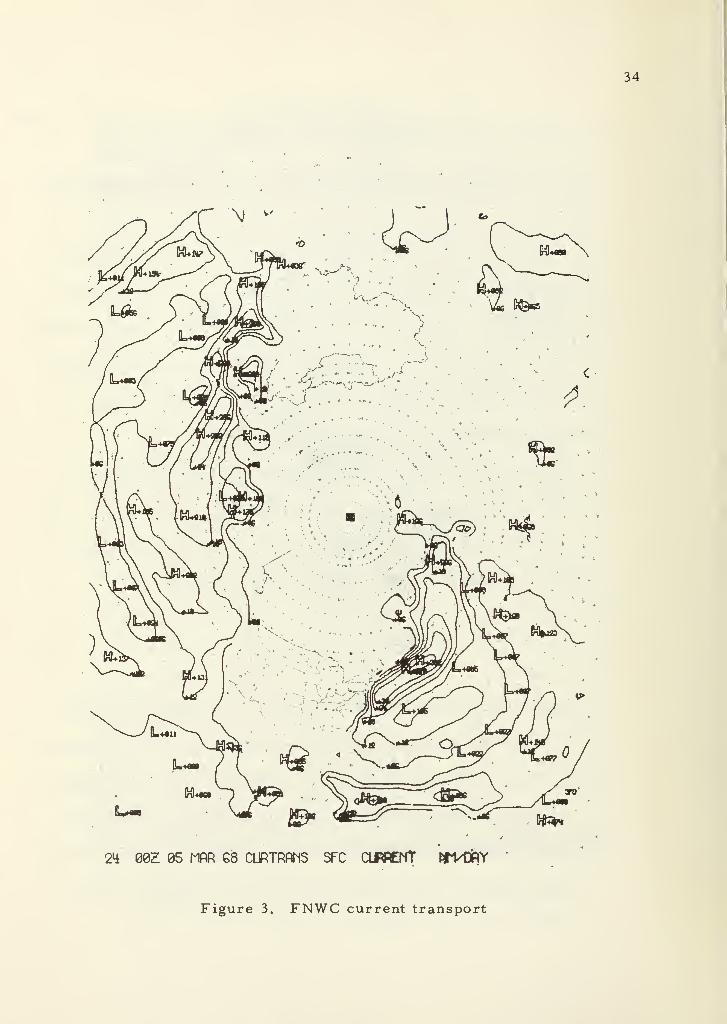
toured resulting in a total transport (Figure 3).

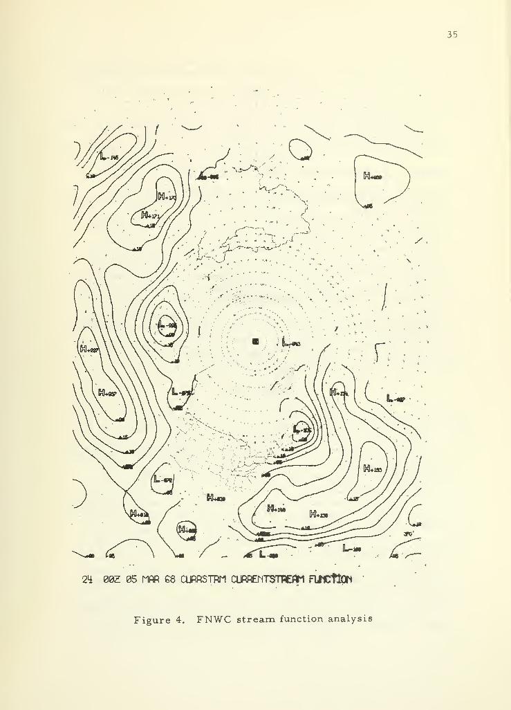
In order to obtain a single chart containing both speed and

direction the components are used to obtain the vorticity of the cur-

rent flow and the stream function \\> is obtained by a relaxation

solution of Poisson's equation (Hubert and Laevastu, 1965).

2 3v 9u ,, rt%

However, this stream function analysis is only applicable to non-

divergent irrotational flow. The stream function field corresponding

to the current transport field shown in Figure 3 is shown in Figure 4.

Direct verification of FNWC computed surface currents has

not been possible. Indirect verification of surface currents has been

made through the verification of sea surface temperature analysis

34

2>± 08Z 85 MAR 68 CURTRPNS SFC CURRENT tfVD&Y

Figure 3. FNWC current transport

35

2i 08Z 05 MAR 68 CURRSTRM CURRENTSTREftl FlTCttOh *

Figure 4. FNWC stream function analysis

36

(Hubert and Laevastu, 1965). Sea surface temperature analyses are

made twice a day at FNWC over the Northern Hemisphere (Wolff,

1964). Sea surface temperature changes computed from the air-sea

heat exchange are subtracted from the analysis. If the residual cor-

relates with the temperature advection field determined from the

surface current analysis then the currents are assumed to be correct.

If the residual does not correlate with the temperature advection

field then the currents can be "tuned" to achieve agreement. It

should be noted that the air-sea heat exchange formulae used in this

procedure are generally empirical and have not been subjected to

widespread rigid verification. This indirect verification procedure

may be questioned seriously when used for quantitative results.

Discussion

The methods for determining geostrophic flow described in

this section represent attempts to simplify geostrophic computations.

Each model had some success but all suffer from certain defi-

ciencies. The temperature- salinity correlation schemes of Stommel,

LaFond, and Yausi greatly reduce the number of computations re-

quired to determine geostrophic currents. These methods could

also reduce sharply the field measurements, allowing geostrophic

surface currents to be determined from temperature measurements

alone. However, temperature- salinity correlation is a regional

37

parameter, varying from water mass to water mass; and in indi-

vidual water masses it varies in both time and space. Furthermore,

in regions of intense mixing such as the Kuroshio-Oyashio confluence

(Tully, 1964), temperature-salinity curves are so variable that cor-

relation approaches are not applicable.

Use of the thermosteric anomaly v c „, instead of the specific

volume anomaly reduces the number of computations, or number of

tables, that need to be interpolated in geostrophic computations.

The error introduced by this simplification is acceptable if the com-

putations are limited to the upper 1, 000 db. However, even in this

simplified procedure the quantities <x and <j must be determined;

since these are not used beyond the geostrophic computations, their

determination represents unnecessary expenditure of computation

time.

NAVOCEANO correlation curves between current and surface

temperature gradient may provide adequate synoptic current informa-

tion in some regions where strong surface temperature gradients

are dynamically sustained, such as in the Gulf Stream. Over the

world oceans this is not the case; the surface temperature gradients

are small and often are determined by the local heat exchange and

mixing processes. In fact no definite relationship was found be-

tween the surface current and the horizontal temperature gradient

in 7, 000 selected hydrographic station pairs in the Northwest

38

Atlantic where the NAVOCEANO curves (Figure 1) were derived

(Interstate Electronics Corporation, 1968).

The application of the thermal wind equation to the ocean has

no foundation. The simplifying assumption that the density of sea

water is a linear function of temperature cannot be accepted

(Fofonoff, 1962). The adjustment of the coefficients used by FNWC

on the basis of sea surface temperature analysis verification must

be questioned. Since the sea surface temperature field is developed

using the surface current field to compute the advected heat the use

of sea surface temperature in surface current verification is not an

independent verification.

Geostrophic surface currents are most valuable if determined

over a short period of time, say over a seven day period (Lenczyk,

1964). This will be possible only when synoptic fields of tempera-

ture and salinity are available. While such fields are not available

at the present time, a more scientifically sound scheme of comput-

ing geostrophic currents must be available when these fields do be-

come available. Any scheme used must yield surface currents that

are in agreement with observed surface currents or at least those

computed by the standard geostrophic method. Every effort should

be made to verify by direct measurements any scheme of indirectly

computing surface currents.

39

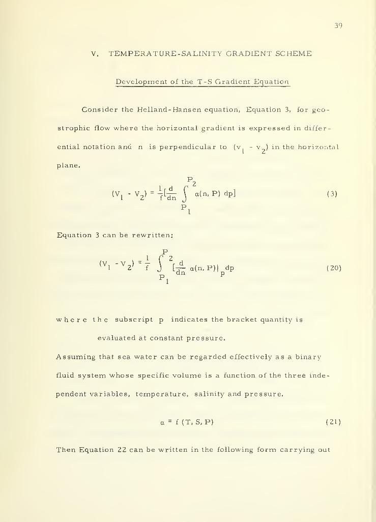
V. TEMPERATURE-SALINITY GRADIENT SCHEME

Development of the T-S Gradient Equation

Consider the Helland-Hansen equation, Equation 3, for geo-

strophic flow where the horizontal gradient is expressed in differ-

ential notation and n is perpendicular to (v - v ) in the horizontal

plane.

P2

fV, - V2

) ="j[^ f a(n, P) dp] (3)

Pl

Equation 3 can be rewritten:

P1 f 2

(V, -V J = 7 \ r d1 2 f J I— a (n,

pi

__P)] dp (20)

where the subscript p indicates the bracket quantity is

evaluated at constant pressure.

Assuming that sea water can be regarded effectively as a binary

fluid system whose specific volume is a function of the three inde-

pendent variables, temperature, salinity and pressure.

a = f (T.S.P) (21)

Then Equation 22 can be written in the following form carrying out

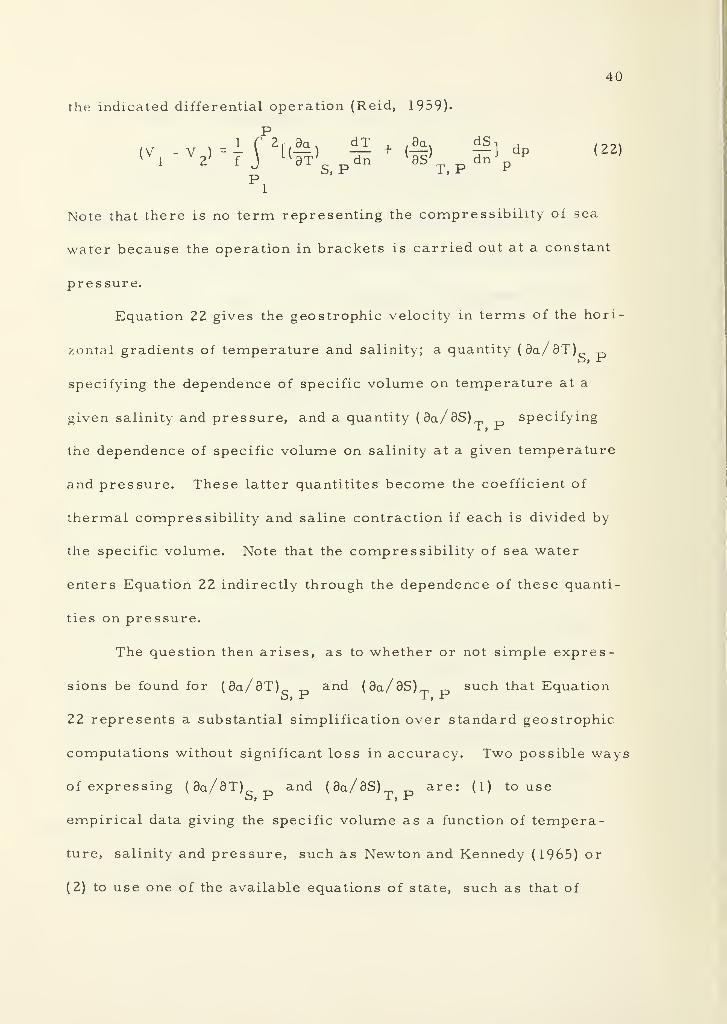
40

the indicated differential operation (Reid, 1959).

P1 f 2 r/ 3a. dT , .9a. dS -> ,

, 99 .

<vi

-v2)-

7 J [(eT)&p-E+

<8s'Tp^]

pdP (22)

Pl

Note that there is no term representing the compressibility of sea

water because the operation in brackets is carried out at a constant

pressure.

Equation 22 gives the geostrophic velocity in terms of the hori-

zontal gradients of temperature and salinity; a quantity (3a/3T)Of XT

specifying the dependence of specific volume on temperature at a

given salinity and pressure, and a quantity (3a/3S) specifyingt > A

the dependence of specific volume on salinity at a given temperature

and pressure. These latter quantitites become the coefficient of

thermal compressibility and saline contraction if each is divided by

the specific volume. Note that the compressibility of sea water

enters Equation 22 indirectly through the dependence of these quanti-

ties on pressure.

The question then arises, as to whether or not simple expres-

sions be found for (3a/3T) and (3q/3S) such that Equation

22 represents a substantial simplification over standard geostrophic

computations without significant loss in accuracy. Two possible ways

of expressing (3a/3T) and (3a/3S) are: (1) to use

empirical data giving the specific volume as a function of tempera-

ture, salinity and pressure, such as Newton and Kennedy (1965) or

(2) to use one of the available equations of state, such as that of

41

Ekman (1908), that have been numerically fitted to the available

empirical data.

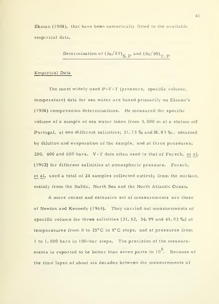
Determination of (3a/9T)_ and(9a/aS)

Empirical Data

The most widely used P-V-T (pressure, specific volume,

temperature) data for sea water are based primarily on Ekman's

(1908) compression determinations. He measured the specific

volume of a sample of sea water taken from 3, 000 m at a station off

Portugal, at two different salinities; 31. 13 %oand38.8 3 %o , obtained

by dilution and evaporation of the sample, and at three pressures;

200, 400 and 600 bars. V-T data often used is that of Forsch, et al.

(1902) for different salinities at atmospheric pressure. Forsch,

et al. used a total of 24 samples collected entirely from the surface,

mainly from the Baltic, North Sea and the North Atlantic Ocean.

A more recent and extensive set of measurements are those

of Newton and Kennedy (1965). They carried out measurements of

specific volume for three salinities (31. 52, 34. 99 and 41. 03 %o) at

temperatures from to 25° C in 5° C steps, and at pressures from

1 to 1, 000 bars in 100-bar steps. The precision of the measure-

5ments is reported to be better than seven parts in 10 . Because of

the time lapse of about six decades between the measurements of

42

Ekman and Forsch, and those of Kennedy and Newton, the latter

measurements should reflect any advance in technique and apparatus

in that interval. Furthermore, P-V-T-S data available prior to

Newton and Kennedy is not sufficient to determine the quantities

(3a/3T) and (3a/3S) over the range of temperature, salinity,

and pressure of interest in the ocean without extensive interpolation

of the data. However, Ekman's compressibility data is internally

consistant to a remarkable degree (Eckart, 1958; Li, 1967).

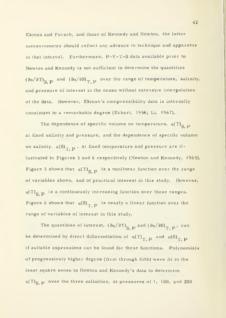
The dependence of specific volume on temperature, a(T)O, ir

at fixed salinity and pressure, and the dependence of specific volume

on salinity, a(S) _, , at fixed temperature and pressure are il-

lustrated in Figures 5 and 6 respectively (Newton and Kennedy, 1965).

Figure 5 shows that a(T) is a nonlinear function over the rangeO, P

of variables shown, and of practical interest in this study. However,

a(T) c D is a continuously increasing function over these ranges.O, ir

Figure 6 shows that a(S) is nearly a linear function over the

range of variables of interest in this study.

The quantities of interest, (3a/3T) and (3a/3S) , canS, P T, P

be determined by direct differentiation of a(T) and a(S)i. > ir 1 , r

if suitable expressions can be found for these functions. Polynomials

of progressively higher degree (first through fifth) were fit in the

least square sense to Newton and Kennedy's data to determine

a(T)g p over the three salinities, at pressures of 1, 100, and 200

43

9580

30. L 2%, , 1 bar

34.99% t . 1 bar

34. 99%o, 100 bars

34. 99%o, ZOO bars

41. 03% , 200 bars

TEMPERATURE (°C)

Figure 5. The dependence of specific volume as a function

of temperature at fixed salinity and pressure

44

.9820'

.9800-

9780.

97b0'

(^740

t .9720at

U9700

.9680-

O>O . 9660i—

i

i—

i

W .9640-1PhCO

. 9620

. 9600H

25°C, 1 bar

15°C, 1 bar

5°C, 1 bar

15 B C, 100 bars

25°C, 200 bars

1 5°C. 200 bars

5°C, 200 bars

9580 | i i i i | i i i i | i i

30 35 40

SALINITY (%c )

Figure 6. The dependence of specific volume as a function

of salinity at fixed temperature and pressure

45

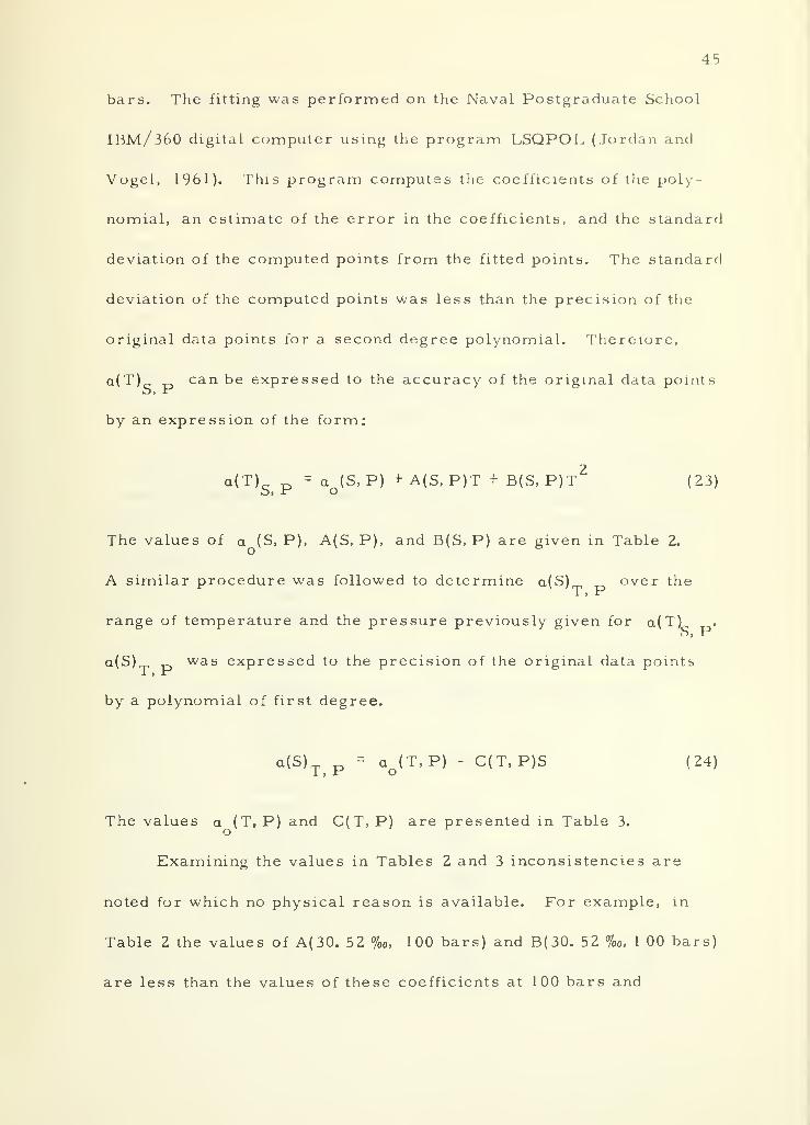
bars. The fitting was performed on the Naval Postgraduate School

IBM/360 digital computer using the program LSQPOL (Jordan and

Vogel, 1961). This program computes the coefficients of the poly-

nomial, an estimate of the error in the coefficients, and the standard

deviation of the computed points from the fitted points. The standard

deviation of the computed points was less than the precision of the

original data points for a second degree polynomial. Therefore,

a(T) can be expressed to the accuracy of the original data points

by an expression of the form:

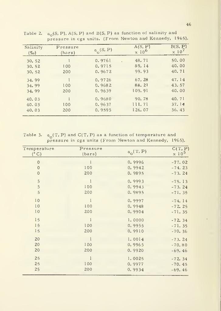
a(T)_ _ = a (S, P) + A(S, P)T + B(S, P)T2

(23)o> jet o

The values of a (S, P), A(S, P), and B(S, P) are given in Table 2.

A similar procedure was followed to determine a(S) over theJ. t lr

range of temperature and the pressure previously given for a(T)„O, IT

a(S) was expressed to the precision of the original data points

by a polynomial of first degree.

a(S) = a (T.P) - C(T, P)S (24)1 , f o

The values a (T, P) and C(T, P) are presented in Table 3.

Examining the values in Tables 2 and 3 inconsistencies are

noted for which no physical reason is available. For example, in

Table 2 the values of A(30. 52 %, 100 bars) and B(30. 52 %o, I 00 bars)

are less than the values of these coefficients at 100 bars and

46

Table 2. aQ (S, P), A(S, P) and B(S, P) as function of salinity and

pressure in cgs units. (From Newton and Kennedy, 1965).

Salinity

(%o)

Pressure(bars)

a (S, P)o

A(S,P)x 10 6

B(S, P)

x 10 7

30. 52 I 0.9761 48. 71 50. 00

30. 52 100 0. 9715 89. 14 40. 00

30. 52 200 0. 9672 99. 93 40. 71

34. 99 1 0. 9726 67. 28 47. 14

34. 99 100 0. 9682 88. 21 43. 57

34. 99 200 0. 9639 109. 91 40. 00

40. 3 1 0. 9680 90. 78 40. 7 1

40. 03 100 0. 9637 111. 71 37. 14

40. 03 200 0. 9595 126. 07 36. 43

Table 3. a (T, P) and C(T, P) as a function of temperature andpressure in cgs units (From Newton and Kennedy, 1965).

Temperature Pressure C(T, P)

(°C) (bars)ao (

' ' x 10 5

1

100

200

5 1

5 100

5 200

10 1

10 100

10 200

15 1

15 100

15 200

20 1

20 100

20 200

25 1

25 100

25 200

0. 9996 -77. 02

0. 9942 -74. 23

0. 9895 -7 3. 24

0. 9993 -75. 13

0. 9943 -73. 24

0. 9895 -71. 35

0. 9997 -74. 14

0. 9948 -7 2. 25

0. 9904 -71. 35

1. 0000 -72. 34

0. 9955 -71. 35

0. 9910 -70. 36

1. 0014 -73. 24

0. 9965 -70. 800. 9920 -69. 46

1. 0025 -72. 34

0. 9977 -70. 450. 9934 -69. 46

47

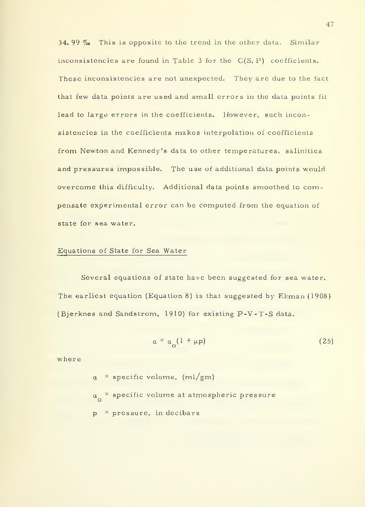
34. 99 %o This is opposite to the trend in the other data. Similar

inconsistencies are found in Table 3 for the C(S, P) coefficients.

These inconsistencies are not unexpected. They are due to the fact

that few data points are used and small errors in the data points fit

lead to large errors in the coefficients. However, such incon-

sistencies in the coefficients makes interpolation of coefficients

from Newton and Kennedy's data to other temperatures, salinities

and pressures impossible. The use of additional data points would

overcome this difficulty. Additional data points smoothed to com-

pensate experimental error can be computed from the equation of

state for sea water.

Equations of State for Sea Water

Several equations of state have been suggested for sea water.

The earliest equation (Equation 8) is that suggested by Ekman (1908)

(Bjerknes and Sandstrom, 1910) for existing P-V-T-S data.

a = aQ(l +HP) (25)

where

a = specific volume, (ml/gm)

a _ specific volume at atmospheric pressureo

p - pressure, in decibars

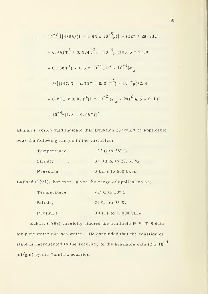
48

u = 10" 9{[4886/(1 + 1. 83 x 10

_5p)] - (227 + 28. 33T

0. 551T2

+ 0. 004T3

) + 10_4

p (105. 5+9. 50T

0. 158T2

) - 1. 5 x 10_8TP

2- 10

_1(o-

28[(147. 3 - 2. 72T + 0. 04T2

)- 10

_4p(32. 4

0. 87T + 0. 02T2)] + 10" 2

(<r - 28)2[4. 5 - 0. 1 T

o

10~ 4p(l. 8 - 0. 06T)]}

Ekman's work would indicate that Equation 25 would be applicable

over the following ranges in the variables:

Temperature -2* C to 26° C

Salinity , 31. 1 3 %o to 38. 53 %o

Pressure bars to 600 bars

LaFond (1951), however, gives the range of application as:

Temperature - 2° C to 30* C

Salinity 21 % to 38 %o

Pressure bars to 1, 000 bars

Eckart (1958) carefully studied the available P-V-T-S data

for pure water and sea water. He concluded that the equation of

-4state is represented to the accuracy of the available data (2 x 10

ml/gm) by the Tumlirz equation.

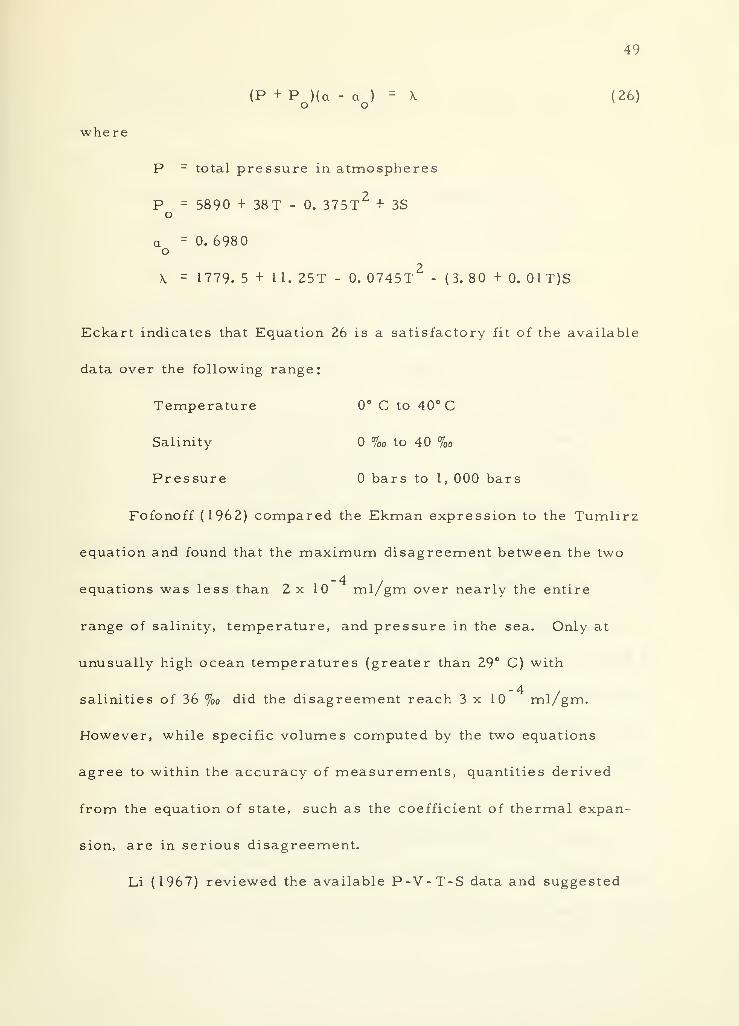
where

49

(P + P )(a - a ) = \ (26)

P - total pressure in atmospheres

P = 5890 + 38T - 0. 375T2+ 3S

o

a = 0. 6980o

2\ = 1779. 5 + 11. 25T - 0. 0745T - (3. 80 + 0. 1 T)S

Eckart indicates that Equation 26 is a satisfactory fit of the available

data over the following range:

Temperature 0° C to 40° C

Salinity % to 40 %o

Pressure bars to 1, 000 bars

Fofonoff (1962) compared the Ekman expression to the Tumlirz

equation and found that the maximum disagreement between the two

equations was less than 2x10 ml/gm over nearly the entire

range of salinity, temperature, and pressure in the sea. Only at

unusually high ocean temperatures (greater than 29° C) with

- 4salinities of 36 %o did the disagreement reach 3x10 ml/gm.

However, while specific volumes computed by the two equations

agree to within the accuracy of measurements, quantities derived

from the equation of state, such as the coefficient of thermal expan-

sion, are in serious disagreement.

Li (1967) reviewed the available P-V-T-S data and suggested

50

the Tait-Gibson equation as an equation of state. The Tait-Gibson

equation is given by Li as:

a = as> Tj l

- (1 - S x 10" 3)C Log [^ *

ft(27)

where

C = 0. 315 a _ ,

o, T, 1

2B"* = (2670. 8 + 6. 89056S) + (19. 39 - 0. 0703178S)T - 0.223T

Equation 27 is a satisfactory fit to existing P-V-T-S data over

the following range of variables:

Temperature 0° C to 20° C

Salinity 30 % to 40 %

Pressure (absolute) 1 bar to 100 bars

Equation 27 gives results that are in agreement with measurements

to the experimental error in the P-V-T-S data. The difference be-

tween the Tait-Gibson equation and Ekman's equation for sea water

of 35 %o i0° C from 1 to 1 , 000 bars is no more than 1x10 ml/gm.

At atmospheric pressure the agreement between the density of sea

water from Knudsen's tables (1901), in common usage in oceanog-

raphy, and Equation 27 is less than 3x10 gm/ml over the

chlorinity range of 1 5 to 22 %o and temperature range of to 20° C.

Li concludes (page 2073): "Ekman's very involved equation of state

of sea water is equivalent to the much simpler expression given

here. " However, as the Tumlirz equation proposed by Eckart did

51

not give the same values as the Ekman equation for derived properties

such as the coefficient of thermal expansion, the Tait-Gison equation

gives again different values.

The dependence of specific volume on temperature a(T)

is a function of temperature, salinity and pressure according to the

three proposed equations of state discussed above. In each case the

functional relationships are markedly different. Furthermore,

quantities derived from these expressions such as the coefficient of

thermal expansion , l/a(3a/3T) , may differ significantly.is, r

Fofonoff (1962) compared the coefficient of thermal expansion of sea

water 35 %o salinity at atmospheric pressure computed from the

Ekman and Eckart relationships. The results are given in Table 4.

Table 4. A comparison of the coefficient of thermal expansion of

sea water l/a(9a/3T)s p x 10 6 at 35 %o salinity and

atmospheric pressure computed from the Ekman andEckart equations of state (from Fofonoff, 1962).

Temperature (°C) Ekman Eckart

52 80

5 114 121

10 167 161

15 214 201

20 256 237

25 297 274

30 335 311

While the coefficient of thermal expansion computed by the two

equations are not significantly different at temperatures around 10*C

52

these differences increase significantly at higher and lower tempera-

tures.

Equation 22 requires the value of (3a/3T) before it can be

used for geostrophic computations. To illustrate how this quantity-

changes between the three equations of state, Ekman, Eckart, and

Tait-Gibson, the value of (3a/3T) as a function of pressure forO, ir

a salinity of 34 %o for temperatures 0, 10, 20, and 30° C is plotted

in Figure 7. The three proposed equations of state yield values for

(3a/3T) in closest agreement at temperatures near 10°C at pres-O, ir

sures near one atmosphere. However, the values diverge toward

higher and lower temperatures and higher pressures. There is no

clear cut way to specify which equation of state would yield the best

value of (3a/3T) c D . Furthermore, direct differentiation of theib, ir

Ekman, Eckart or the Tait-Gibson equations leads to rather compli-

cated expressions for (3a/3T) c as well as (3a/3S) . Sucho, ir 1 , ir

complicated expressions would give Equation 22 no advantage over

the Helland- Hansen equation, Equation 4.

Fofonoff (1962) has examined the coefficients of saline con-

traction, (3a/3S) , as computed from the Ekman and Eckart rela-i > ir

tionships and found that they differ by less than one percent. There-

fore, in geostrophic computations using Equation 22 there is little

advantage in either expression for (3a/3S) . Thus, while the1 , ir

value of (3a/3T)g p differs significantly between equations of state

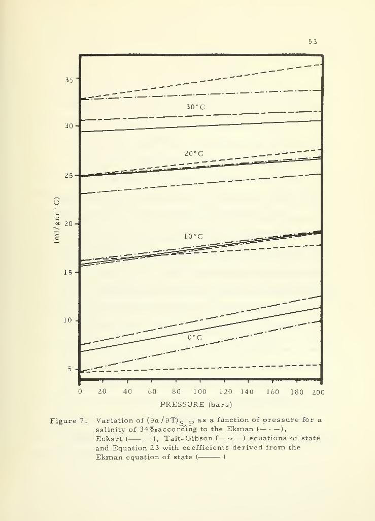
53

I I

60 80 100 120 140

PRESSURE (bars)

160 180 ZOO

Figure 7 Variation of (8a/9T)s p as a function of pressure for a

salinity of 3 4

%

according to the Ekman ( ),

Eckart ( ), Tait-Gibson( ) equations of state

and Equation 2 3 with coefficients derived from the

Ekman equation of state ( )

54

the value of (da/dS) does not.J- » -i

Another approach to the determination of (3a/3T) and

(3a/3S) would be to compute specific volume at sufficient values1 > XT

of temperature, salinity, and pressure using one of the equations of

state, and fitting the resulting values with polynomials as was at-

tempted with the Newton-Kennedy P-V-S-T data. This would over-

come the difficulty encountered in directly fitting the empirical

P-V-S-T data caused by experimental errors in the few data points

as the equations of state would smooth individual inconsistent points.

The question is which equation of state to use to compute the specific

volume? There is little evidence that any of the expressions gives

more reliable values of specific volume over the range of variables

of interest in computing geostrophic currents in the upper few

thousand meters of the ocean (Wilson and Bradley, 1968; Li, 1967).

The Ekman equation (Equation 25) has been the principle equa-

tion of state used by oceanographers (LaFond, 1951). Tables by

Bjerknes and Sandstrom (1910), Sverdrup (1942) and LaFond (1951)

are based on this expression. Since these tables have been and con-

tinue to be so widely used in oceanography the Ekman equation of

state is selected to determine a(T) and a(S) .

Specific volume was computed using Equation 25 over the range

of temperature, salinity, and pressure of interest in this study:

55

Temperature 0*0 to 30° C

Salinity 30 %o to 40 %

Pressure bars to 200 bars

Values of specific volume were computed for all possible combina-

tions of the variables at intervals of 2" C for temperature, 2 %o for

salinity and 10 bars for pressure.

Second degree polynomials were fit to the specific volume as

a function of temperature at fixed salinity and pressure to yield

a(T) , and first degree polynomials were fit to specific volume as

a function of salinity at fixed temperature and pressure to give

a(S) _,. Again the fitting was accomplished on the Naval Post-

graduate School IBM/360 digital computer using the program LSQPOL.

The values of the coefficients A(S, P) and B(S, P) as in Equation 23

and C(T, P) as in Equation 24, are given in Appendix I as a function

of their respective independent variables. The errors determined

for these coefficients and the standard deviation of the computed

versus the original data points is also given in Appendix I.

The standard deviation of the goodness of fit of the computed

to original data points, is always less than 2x10 ml/gm. Since

Eckart (1958) contends specific volume is not known any better than

2x10 ml/gm the use of higher degree polynomials is not justified.

Direct differentiation of a(T) (Equation 23) with respect to tem-S» P

perature yields the following expression:

56

(i£) = A(S, P) + 2B(S, P)T (28)8T

S,P

The values (8a/3T) from this equation were compared to theOj AT

values given by the Ekman, Eckart, and Tait-Gibson equations of

state in Figure 7. The quadratic expression of a(T) leads to

as good agreement with the commonly accepted Ekman equation of

state as do either of the other proposed equations of state (Equation

26 or Equation 27).

In the same way differentiation of a(S) (Equation 24) witht > ±

respect to salinity yields:

(||)B - C(T,P) (29)

3S T.P

Linear interpolation of the computed values of the three coefficients

leads to Figures 8, 9 and 10 for A(S, P), 2B(S, P) and C(T S P)

respectively.

Temperature-Salinity Gradient Scheme

Recall Equation 22.

P

Pl

S, P T, P P(V -V ) = i f [(-^) — +(—

)— ] dP (22)

Substitution from Equation 28 and Equation 29 for (3a/9T) and

(0a/3S) T p respectively in Equation 22 yields the following

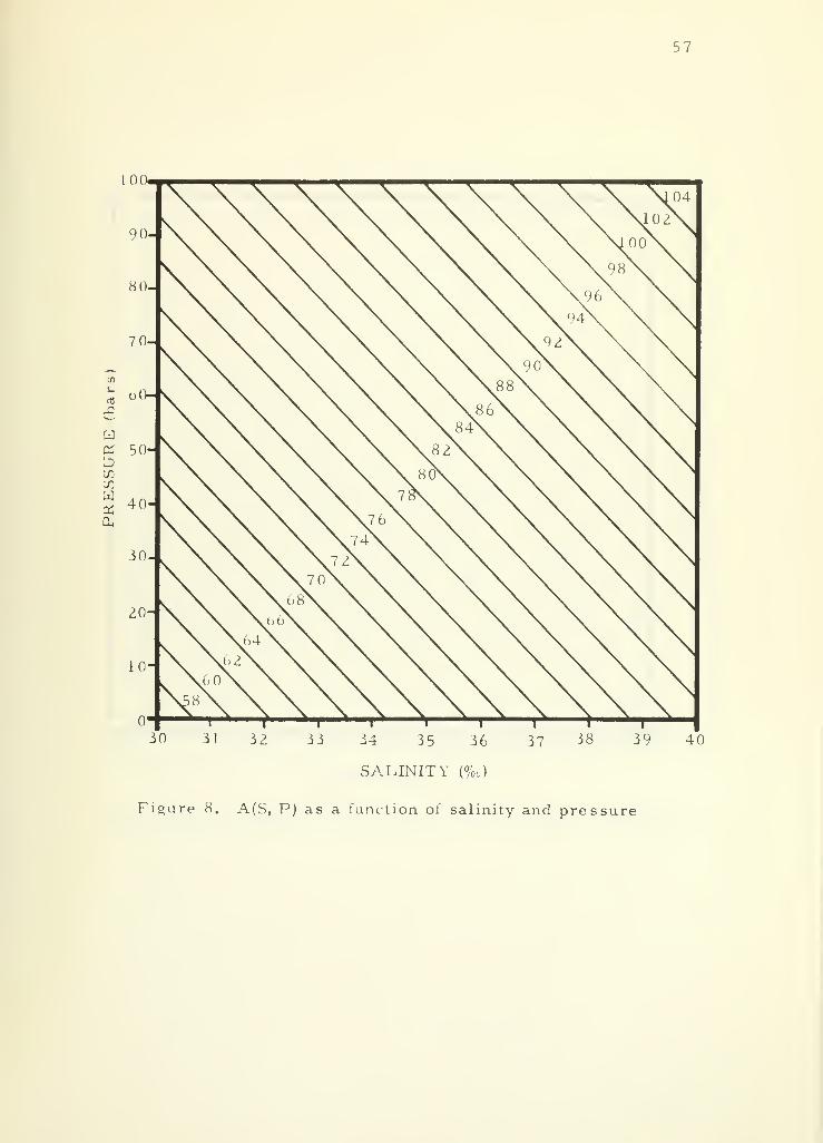
57

100.

30 31 32 33 34 35 36 37 38 39

SALINITY (%<.)

Figure 8. A(S, P) as a function of salinity and pressure

40

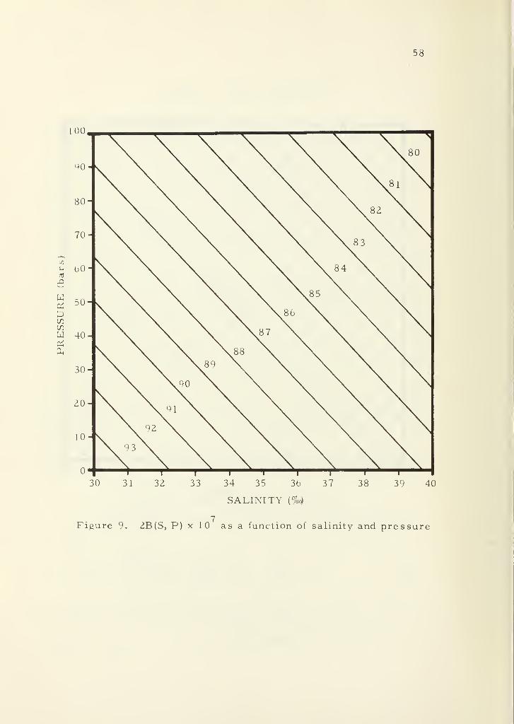
58

100

SALINITY (%o)

Figure 9. ZB(S, P) x 10 as a function of salinity and pressure

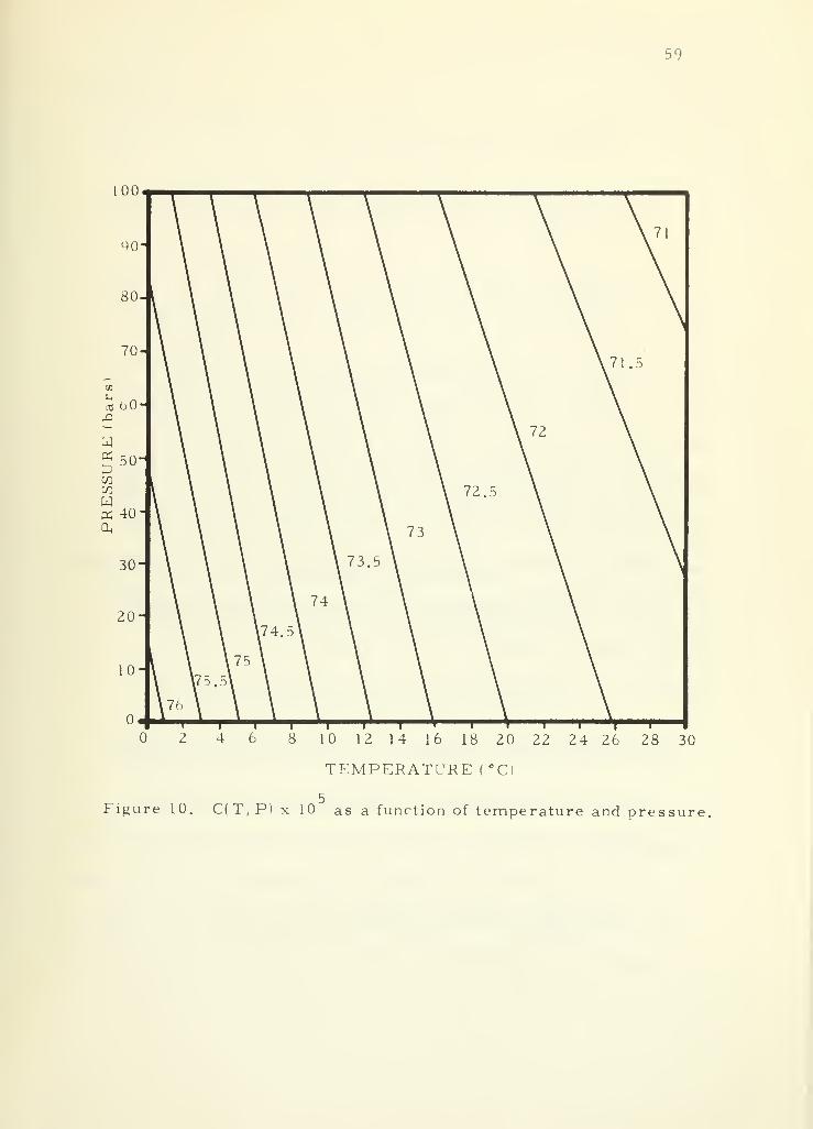
59

100

4 b 8 10 12 14 16 18 20 11 24 26 28 30

TEMPERATURE ( 'CI

Figure 10. C(T, P) x 10 as a function of temperature and pressure,

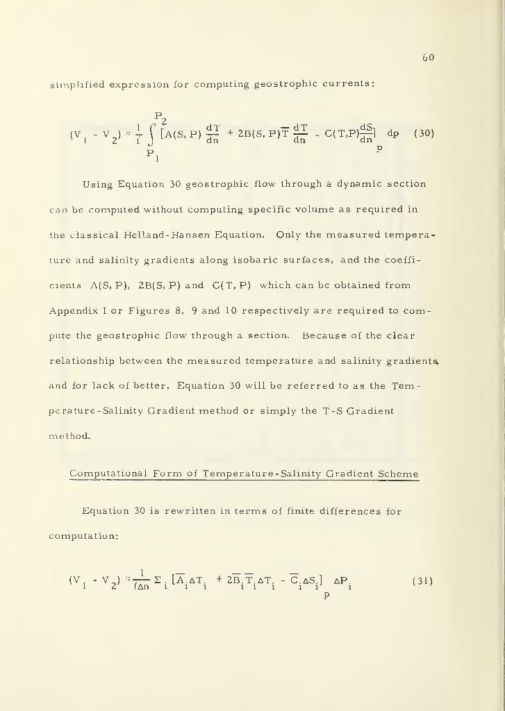
60

simplified expression for computing geostrophic currents:

(Vt

-V2)-| f [A(S,P)^ +2B(S,P)T|^ -C(T.P)^|] dp (30)

pi

Using Equation 30 geostrophic flow through a dynamic section

can be computed without computing specific volume as required in

the classical Helland-Hansen Equation. Only the measured tempera-

ture and salinity gradients along isobaric surfaces, and the coeffi-

cients A(S, P), 2B(S, P) and C(T, P) which can be obtained from

Appendix I or Figures 8, 9 and 10 respectively are required to com-

pute the geostrophic flow through a section. Because of the clear

relationship between the measured temperature and salinity gradients,

and for lack of better, Equation 30 will be referred to as the Tem-

perature-Salinity Gradient method or simply the T-S Gradient

method.

Computational Form of Temperature -Salinity Gradient Scheme

Equation 30 is rewritten in terms of finite differences for

computation:

<Vi

" V o) ^TT- S•[A. AT. + 2B.T.AT. - C.AS.] AP. (31)

1 2 fAn ill 11111 iv/

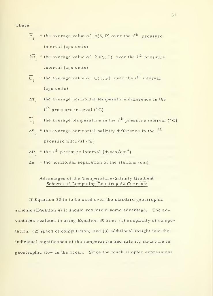
61

where

A. - the average value of A(S, P) over the i**1 pressure

interval (cgs units)

2B. = the average value oi' 2B(S, P) over the i^ pressure

interval (cgs units)

C. = the average value of C(T,P) over the i^ 1 interval

(cgs units)

AT. = the average horizontal temperature difference in the

i pressure interval (°C)

T. - the average temperature in the i1- 11 pressure interval (°C)th ^jiv^oanic; unci

AS. - the average horizontal salinity difference in the i

pressure interval (%o)

AP. - the i^1 pressure interval (dynes/cm )

An - the horizontal separation of the stations (cm)

Advantages of the Temperature-Salinity Gradient

Scheme of Computing Geostrophic Currents

If Equation 30 is to be used over the standard geostrophic

scheme (Equation 4) it should represent some advantage. The ad-

vantages realized in using Equation 30 are: (1) simplicity of compu-

tation, ( Z) speed of computation, and (3) additional insight into the

individual significance of the temperature and salinity structure in

geostrophic flow in the ocean. Since the much simpler expressions

62

for a(T) and a(S) reproduce values of specific volume toS, P T, P

the accuracy of the experimental measure of this quantity, these

advantages would seem to be gained without loss of accuracy over

the range of temperature, salinity and pressure considered in this

study. Furthermore the method is completely general and can be

used under any circumstances that the standard method can be ap-

plied.

The computational simplification of the T-S Gradient scheme is

apparent since no density computations are needed. Neither the

relatively involved tables commonly used to calculate specific volume

(or specific volume anomaly), nor the equations of state previously

discussed need to be used. Those properties that are directly meas-

ured in the ocean (temperature and salinity as a function of depth)

can be used to compute the geostrophic flow. Only the three coeffi-

cients A(S, P), 2B(S, P) and C(T, P) are needed.

The speed advantage of the T-S Gradient calculations on a

digital computer was established on an IBM 360 digital computer.

The time to compute the geostrophic flow through a section consist-

ing of two stations, by the standard method and by the T-S Gradient

method was measured. Only the actual time to carry out the mathe-

matical computations was determined. The average time to com-

pute the geostrophic flow for a single station pair was 0. 25 |j.sec for

the T-S Gradient method, and 1. 80 |j.sec for the classical method.

63

Therefore, the T-S Gradient method is approximately seven times

faster than the standard method using this digital computer.

Another significant advantage of the T-S Gradient scheme is

the potential for separating the thermal and haline contributions to

the geostrophic flow. The interaction that takes place between the

thermal and haline contributions to the flow is through A(S, P),

B(S,P) and C(T,P). Therefore, at least to first order, the first two

terms in Equation 30 can be considered the thermal contribution to

the geostrophic flow, and the last term the haline contribution.

64

VI. APPLICATIONS OF THE T-S GRADIENT METHOD

Introduction

It has been shown that the T-S Gradient scheme is simpler to

use than the standard geopotential scheme. It remains to evaluate

the T-S Gradient scheme for making geostrophic computations over

large ocean areas, say over the North Pacific.

Clearly, additional advantage is gained in these calculations

if the average value of the coefficients A(S, P), 2B(S, P) and C(T, P)

relative to a selected reference level did not vary greatly over the

ocean such that average values could be used and Equation 31 written:

(V, - V J = -— [K.Z T.AP. + K_2 ~T.AT.AP - K 2aS.aP.] (32)1 2 fAn L £ l l 2jii 3 i l l

where

K , K and K = weighted mean values of A(S, P), B(S, P) and

C(T, P) respectively between the surface and

the selected reference level (cgs units).

If the T-S Gradient scheme can be applied using Equation 32 then

only the three fixed value coefficients and the measured temperature

and salinity structure would be needed to make geostrophic computa-

tions. To determine if Equation 32 is applicable, three questions

must be answered:

65

1. What reference level should be used?

2. Relative to the selected reference level, what is the

spatial variation in the weighted mean values of the coeffi-

cients (A(S, P), 2B(S, P) and C(T, P)?

3. Relative to the selected reference level, what is the time

variation of the weighted mean values of the coefficients

A(S, P),2B(S, P) and C(T, P)?

Selection of the Reference Level

The question of the proper reference level to select is open to

question (Defant, 1961, and Fomin, 1964). Hopefully the level se-

lected would be a level of little or no motion. Many reference

levels have been used to compute surface currents (Neumann and

Pierson, 1966). FNWC uses 200 m over the entire Northern Hemi-

sphere oceans (Hubert and Laevastu, 1967). Reid (1958) used a

reference level of 500 db in the California Current region, and

I, 000 db reference level in his investigation (1961) of the dynamic

topography in the entire Pacific Ocean. Reed and Laird (1966) used

1, 000 db for dynamic computations in a section off central Cali-

fornia. Reed and Taylor (1965) used 1, 000 db for geostrophic calcu-

lations in the Alaska Stream. Stommel (1965) summarizes the

problem of selecting a reference level (page 20):

66

Thus the choice of the reference level for geostrophic

calculations becomes mostly a matter of taste, and weshould admit that that is ultimately intolerable. The

determination of the level of no motion is not a matter

for debate, but for direct measurement.

There are simply not sufficient direct current measurements in the

oceans to select suitable reference levels. However, Fomin (1964)

shows that it may be better to select a shallow reference level of

low velocity than a substantially deeper level where the velocity may

approach zero, thus reducing the computational errors. He points

out that in some cases the selection of a deep reference level may

completely distort the computed currents.

For this study a level of 1, 000 db is selected as this is pos-

sibly near an average value for the oceans. Furthermore, more

hydrographic data is available over most of the ocean to 1, 000 db

than to deeper levels. Lastly, to go to a deeper reference level

could introduce computational errors that may overcome any better

approximation to no motion. Stommel (1965) states (page 19)

"Fortunately, the choice of reference level has less effect upon

velocity in the very surface layer than on those of deep water. "

Determination of the Weighted Mean Value of K\, K£and K3 Relative to 1, 000 db in the Summer and

Winter for the Pacific Ocean

Determination of K , K and K relative to any reference

level requires that the distribution of temperature and salinity be

67

known to this level. These distributions are available from his-

torical data deposited at oceanographic data centers. However, it

requires a great quantity of data to accomplish oceanic coverage.

As a first approximation, atlas values of temperature and salinity

over the Pacific Ocean were used to determine weighted mean values

of the coefficients relative to the 1, 000 db level.

One of the most comprehensive atlases of temperature and

salinity distributions of the entire Pacific Ocean is that by

Muromotsev (1963). This atlas gives the fields of temperature and

salinity at selected levels between the sea surface and the deepest

part of the ocean. Fields are given for summer and winter condi-

tions at the following levels: 0, 10, 25, 50, 100, 150, 200, 300,

400 and 500 m. Below 500 m the seasonal variations are considered

negligible and only single fields of temperature and salinity are

available at each level: 600, 800, 1,000, 1,200, 1,500 m, and

thereafter every 500 m to the bottom. In all 30, 000 deep water

hydrographic stations were used to compile the atlas supplemented

in the upper layers by other temperature data.

The values of K , K and K were determined for summer

and winter conditions by interpolating the Muromotsev atlas tempera-

ture and salinity fields at the following levels: 0, 10, 25, 50, 100,

150, 200, 300, 400, 500, 600, 800 and 1, 000 m at the intersection

of the lines of latitude and longitude given in Figure 11. The

68

resulting weighted mean values of K,, K and K for summer and

winter are shown in Figures 11 and 12, 13 and 14, and 15 and 16

respectively. It can be seen from these Figures that the variation

in the coefficients over the entire ocean, or from season to season

does not change by more than a few percent. Using fixed values of

K , K and K over the entire ocean relative to the selected refer-

ence level of 1, 000 db should lead to only a small percent error which

is certainly acceptable in the geostrophic computation. The values of

the coefficients selected are:

K = 81. x 10" (cgs units)

K = 86. 5 x 10~ (cgs units)

— -5K = -74. 0x10 (cgs units)

At most an error of five percent will be introduced into the geo-

strophic surface current relative to 1, 000 db in the Pacific by the

selection of these values.

The Significance of Water Structure

The use of fixed value coefficients relative to the I, 000 db

reference level in the Pacific appears to be justified. To further

support this hypothesis, station pairs were selected in various re-

gions of the world oceans and geostrophic calculations using the

standard method and the T-S Gradient method using fixed values of

69

120 140 160 180 160 140 120 100 80 60

60 31.2 _ 81.0 80.9 80.8 80.7 80.7 80.6 M

120 140 160 180 160 140 120 100

Figure 1 1 . Variation of K over the Pacific Ocean in the summer

Figure 12. variation of K over the Pacific Ocean in the winter

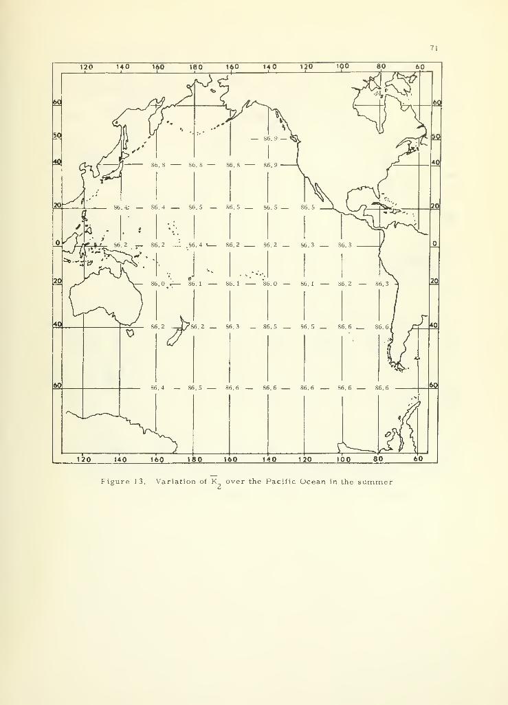
71

Vg&:\86.0 r— 86. 1 —

60 4 —86.5 86.6 — 86.6 — 86.6 86.6 — 86.6 .60.

120 140 160 180 160 140 120 100 80 60

Figure 13. Variation of K over the Pacific Ocean in the summer

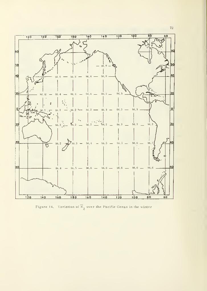
72

20 T75 160 TWO 160 TT6 120 190 80 60

60 86.4 — 86.5 86.6 — 86.6 — 86.6 86.6 — 86.6 .6Q

120 140 160 180 160 140 120 100

Figure 14. Variation of K over the Pacific Ocean in the winter

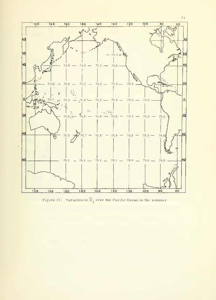
73

120 140 160 180 160 140 120 100 80 60

60

X>735 y^ 73 - 7

75.1 _ 75.1 75.1 75.1 75.0 75.0 75.0 .32

120 140 160 180 160 140 120 100 80 60_

Figure 15. Variation of K over the Pacific Ocean in the summer

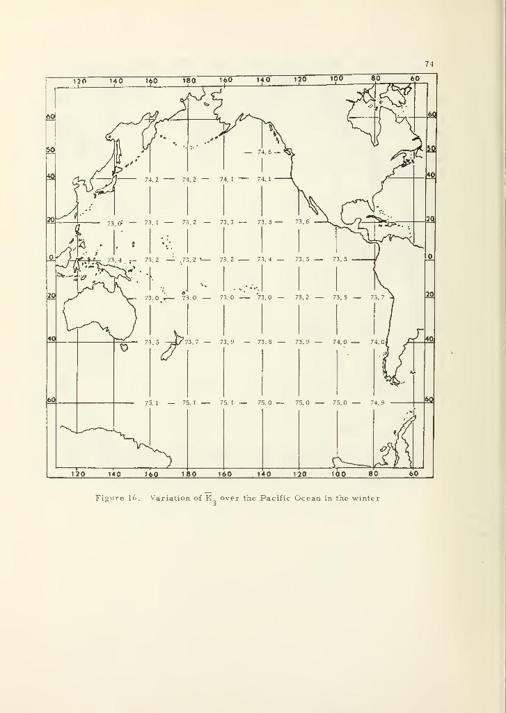
74

_$_JL_ 73.4— 73.2 — .73.2'

«*s* ••

20

40

73.0 r— 73.0 — 73.0 73.0 — 73.2 73.5 — 73.7

60

i -A? 73. 7 — 73.9 —73.8 — 73.9 — 74.0 — 74.0

75.1 — 75.1 75.1 — 75.0 — 75.0 75.0 — 74.9 m

120 140 \b0 180 160 140 120 100 80 60

Figure 16. Variation of K over the Pacific Ocean in the winter

75

the coefficients. Lack of agreement would indicate that adjustment

of the coefficients is required in some water masses.

Stations used are shown in Table 5 where region, station

identification, latitude and longitude, and the computed surface speed

by each method are listed. The stations were selected to be approxi-

mately perpendicular to the mean flow in each region. The complete

velocity profile between the surface and the selected reference level

shows small and generally not significant deviations between the two

methods. The velocity profiles computed by both methods are given

in Appendix II. The velocity profiles for each station pair computed

by the two methods agree to better than ten percent at all depths.

The comparison made in Table 5 shows the agreement required

between geostrophic surface currents computed by the two methods.

None of the values computed by the T-S Gradient method disagree by

more than five percent from the values computed by the standard

method. Therefore, the use of average coefficients in the T-S

Gradient method to calculate geostrophic flow in the surface layer

relative to the 1, 000 db reference level is justified. These results

are encouraging. However, the need for direct verification of in-

directly computed currents is great. Very few attempts to verify

indirectly computed currents have been made, some are reviewed

in Chapter II of this thesis. Clearly, more experiments are needed

to establish the relationship between indirectly computed currents

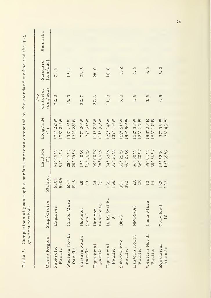
76

COi

NO)

XI

rd

X)o

X^1

rd

X)

rd

0)

X

XCD

£ou

c<u

j-i

o

<D

ord

en

u

XaorH

-t->

en

O0)

M-o>+H OO X

H->

en !-i

cda)

ft .HC XO rH

U DO

ID

<0

H

en

r*

rd

E0)

en

"2 °^ 0)

rd wX v.C Brd C

co .2 S' x\H cd c

O ^

<d

x+J•r-( ^^^

o

0)

X3

rd

Co

•r-i

00<u

en

c

ooO

CM

cm ttCM (Mo oT^ CO

o om m

uurd

XI=1

CO

coCM

CO

CO CM<M

00CM

00

(M

00

oCM

ID

ID

CO

co CO

ID

in in

CO

CO vD— CM

CM CMCO CO

o —i in co t^i incm m cm co —« -h

r- r- —i—i co co

r- ooi i

W W00 o Tf in in vO —i CM <, CQCM CM CM CM CO CO

co coCM CM

co -&

3u

u 03

0) su3

<*-)

ft OX XW u

i

o +->

a fl

cd

ft So CO

N ' ' N IhCO

i

Hft

•fH

rH

-t->

en 2 ^o 0)

rd XX CO £ W I O

du

T—'

rd

i sCO

acd

& 92

2

H->

co.—

i

i—

i

a)

U• t-t

*->

o

•4-J

u

Z Zu c u

• 1-1 tiu

•H• r-i o

rH u o•r-l

^1

cd

o• iH a.

u c or-l

"-H (h <+-! u >+H o ^*H >-M M-( u <+-! u 4H

U0)H->

•rH

o• iH

n3

•iH

Ucd

u d• r-l

o <0• rH

CJ t->

rHu

rd DO rd en o3 3 rd ^ rd cd

XI

CO

rd en rd en cd

Oh 0) Oh aJ Oh cr Oh cr Oh 0, rd Oh CU Oh

£ w W W W £

om

tj5

^^ww^^^^^^^^^^ww^-^Oin

vjO

COCM o

or-

coX)

LTl in

oCMCM

eCOCM

ocom

oCOin

e

CO co

ZZ 2:2; coco £2 22 coco 22 22 cocoin _

i

CO t> O s£) o o CO —i in r-H o O ^^ vO CM m"* ^ * CM •^ m o o CO CO CM CM m CM o m m m

• • a o o o o e o o o o o e1—1 —

i

00 00 m m o 00 Tt< CO CM O ^D vO o oo m min m CM CM —

i

—> o o O o in m CO co co CO —i i—

i

CM COCM CM

Xuo

cd

uU

rd •—

i

cr <W

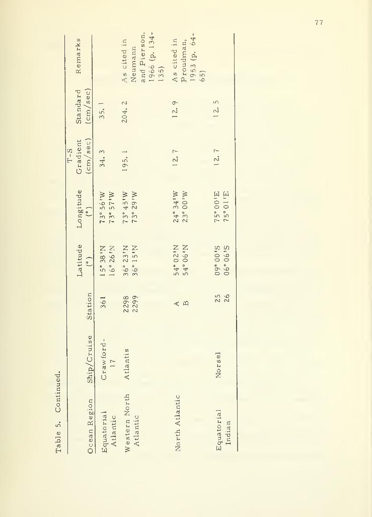
77

co

Xu

s

a;

Xr4

nj

Xd

u

co

d

a

a)

X!d

XI0)

darH+->

doO

lD

a)

ai

H

00 o

o

0)

Xd _

05r-l

uex

do

OO<D

Pi

drd

0)

uo

lOCO

co

m in

CO CO

co

I

XUOm

u

X0)

co

<

o a

ro i—

i

W

dd

sd

Z

oCO

i

CO•r-4 C

i

au>cL

XI<u d

•rH 4-> xi ^—

*

a,nO ^ U d co

X -o in o in _d o CO 10 m o^ in

n)—

'

< Oh —w vT>

OO

oOJ

in

£ £ £ £in C>*t< CMo oCO COr- I

s-

? ? IF ?00 v£) CO lOCO O0 OO —

i

o o o o

_i ^_! co co

00 oOO OJO0 CNJ

C7»

oo

oo

Tt* oCO o^ coOO CNJ

z zoo ^oo oo o

m in

<q CQ

OO

oo

w wo -^

o oo o

Lf) in

r- f>

O vDO Oo o

O O

m ^ooo oo

0)

CO

uoZ

u -!->

o d2

„cdr-H

i—

)

4-» •r-t

d "i

"1 d< 5 rt

<"ccj -d M A-1-1 ^ -•-> rd x)

CO +j >H ^ d<D <r O-1

t—

i

£ Z W

78

and actual observed currents.

Verification of Indirectly Computed Currents

Two field experiments were performed to investigate the ap-

proximation of computed geostrophic surface currents to measured

currents. These experiments are discussed in some detail in Ap-

pendix V. The surface currents computed by the classical scheme,

the T-S Gradient scheme and by FNWC were compared to the meas-

ured surface currents.

In both experiments the surface currents computed by the T-S

Gradient scheme were identical with those computed by the classical

scheme. In the first experiment the FNWC computed currents were

in the opposite direction to the measured surface currents and the

currents computed by both the T-S Gradient scheme and the standard

geostrophic scheme. FNWC currents are heavily weighted toward

the wind drift component. The computed geostrophic currents (4.

to 9. 5 cm/sec) were only about half as great as the observed cur-

rents (7. 1 to 14. 1 cm/sec) but they were in the correct direction.

In the second experiment as in the first the computed currents

and measured currents agree in direction, but the geostrophic com-

puted currents were again slower (5. 4 cm/sec) than the measured

currents (9. 7 cm/sec to 16. 8 cm/sec). The FNWC computed cur-

rents were the same speed ( I 2. 7 cm/sec to 25. 5 cm/sec) and

79

direction as the measured currents.

Thus in both experiments the geostrophic currents were nearly

half the directly measured currents. This might be completely ex-

plained by the fact that the mass structure was not sensed at the

same time as the currents were measured. Even though these meas-

urements were only separated by approximately 24 hours the mass

structure may have changed or in fact never been in balance with the

local currents. Furthermore, the geostrophic currents were calcu-

lated from the average mass structure over at least a 48 hour period,

and one would expect the average gradients to be less than the maxi-

mum gradient. One fact these experiments show is the need for

more field experiments to establish the validity of indirectly com-

puted currents.

In both experiments the T-S Gradient method and the standard

geostrophic computations lead to essentially the same currents.

That is, the simpler T-S Gradient computations give equivalent re-

sults to the standard geostrophic computations and the advantages

of simplicity are gained without giving up accuracy. Another ad-

vantage of the T-S Gradient scheme is the separation of the thermal

and saline contributions to the flow. An example of this advantage

is presented in the next section.

80

The Relationship Between the Thermal Component of the GeostrophicSurface Velocity and the Total Geostrophic Surface Velocity

in the Gulf Stream Water on the Grand Banks

One of the advantages of the T-S Gradient method over standard

geostrophic computations is the capability to separate the first order

thermal and haline components of the geostrophic flow. To illustrate

this feature of the method the thermal component and the total geo-

strophic surface velocities were computed for 33 station pairs of

the U. S. Coast Guard, International Ice Patrol stations in the Gulf

Stream water (Kollmeyer, 1966) off the Grand Banks (Appendix IV).

The linear correlation of the thermal component and the total geo-

strophic velocity for the 33 station pairs was determined (Moynihan,

1968):

V = 0. 39V + 2. 84g t

where

V - the total geostrophic velocity (cm/sec)

V = the thermal component of the geostrophic velocity

(cm/sec)

The standard deviation of the total geostrophic current from the

linear correlation function between it and the thermal component is

less than four (4) cm/sec. Therefore, in this water mass total geo-

strophic currents might be determined using only temperature data

through the relationship above.

81

VIL HEMISPHERIC COMPUTER APPLICATION

Introduction

The Fleet Numerical Weather Central, Monterey, California

is the only facility attempting to determine surface currents on a

hemispheric scale. The background of their computational technique

has been given in an earlier section of this thesis (Chapter IV). For

lack of any other hemispheric fields the FNWC 63 x 63 grid fields

will be used in this study. The following fields are available through

FNWC over their 63 x 63 grid:

1. Synoptic temperature fields between the surface and

1, 200 feet at 100 foot intervals.

2. Climatological (monthly means) temperature fields be-

tween the surface and 1, 200 feet at 100 foot intervals.

3. Climatological (summer and winter) temperature and

salinity fields in the Pacific and Atlantic, derived from

published atlases (Muromtsev, 1963 and Bohnecke, 1936).

Attempts were made in this study to use these fields to investigate

the geostrophic flow through the T-S Gradient computations in the

surface layers of the North Pacific.

82

Synoptic Fields

During April, 1968, Equation 33 was programed on the Naval

Postgraduate School IBM 360 digital computer to run over the FNWC

synoptic temperature field for 0000 GMT, March 5, 1968. The pro-

gram is found in Appendix III. While the program will calculate the

salinity term in Equation 32, a constant salinity of 35 %o was as-

sumed for lack of a salinity field. The output of the program is the

i and j components of the velocity between the grid points, and the

vector sum of these components at the southwest grid point of a four-

point element as is shown in Figure 17. The direction of the total

current was determined by hand computation from the ratio of the i,

j components. Because of the large number of points (3889) in the

63 x 63 grid only those in the North Pacific will be considered. How-

ever, since the major oceanic circulation features are thought to be

common to all oceans (Sverdrup, 1942) any conclusions drawn for

the Pacific Ocean should be valid in the other oceans.

For comparative purpose the FNWC Current Transport and

Stream Function maps for the same period are shown in Figures 18

and 19 respectively. Recall that these maps represent the sum of

their geostrophic and wind driven components. Independent control

for the geostrophic currents is provided by Tully (1964 after Reid,

1961) who gives the surface geostrophic flow relative to 1, 000 db

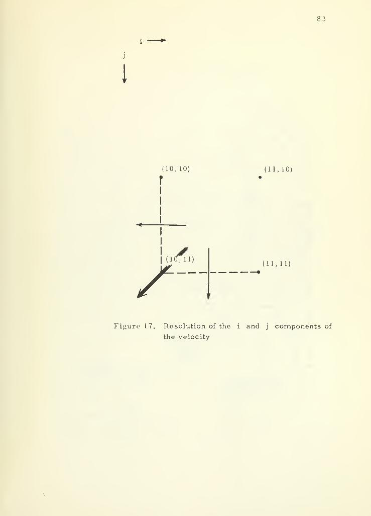
83

I

10, 10) (11,10)

•(10.11)

s—.(11,11)

Figure 17. Resolution of the i and j components of

the velocity

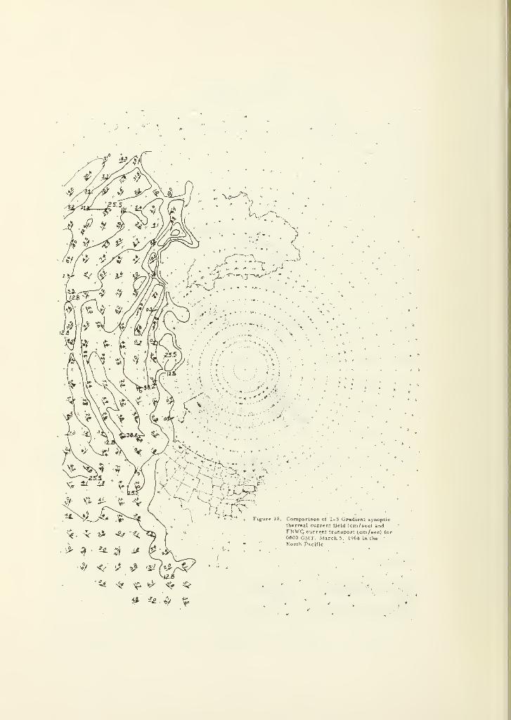
v•-•••'

; ? i >v

,3 »-*<-.Comparison of T-Sthermal current fje

FNWQ current tran0000 GMT, MarchNorth Pacific

GradientId ( cm/seisport tcm5, 196

synoptic

c) and/sec) for

the

*7

^ <* ^ •»> <* ^>

4* *£ %> ^

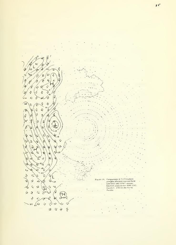
If

'\..'

>'-%M .•

*

,* * j»

• A" 'r • *.-->

Figure 19. Comparison of T-5 Gradient

synoptic thermal current-field

(cm/sec) and FNWC stream

function analysis for 0000 GMT,March 5 1968 -in the North

Pacific.

3? ? ^

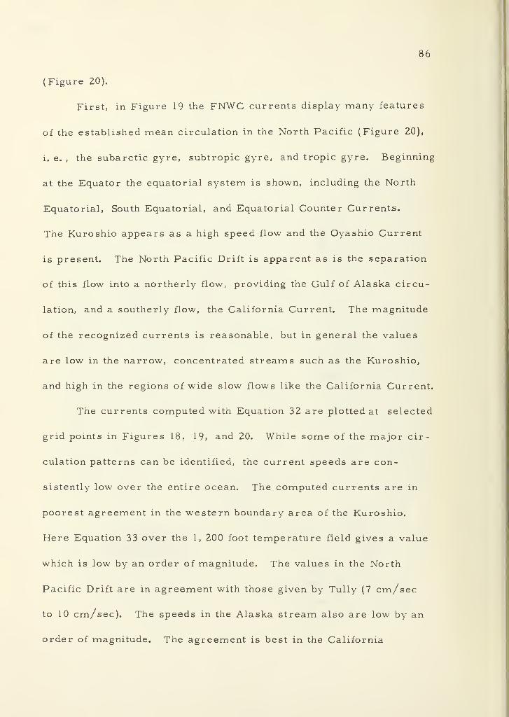
86

(Figure 20).

First, in Figure 19 the FNWC currents display many features

of the established mean circulation in the North Pacific (Figure 20),

i. e. , the subarctic gyre, subtropic gyre, and tropic gyre. Beginning

at the Equator the equatorial system is shown, including the North

Equatorial, South Equatorial, and Equatorial Counter Currents.

The Kuroshio appears as a high speed flow and the Oyashio Current

is present. The North Pacific Drift is apparent as is the separation

of this flow into a northerly flow, providing the Gulf of Alaska circu-

lation, and a southerly flow, the California Current. The magnitude

of the recognized currents is reasonable, but in general the values

are low in the narrow, concentrated streams such as the Kuroshio,

and high in the regions of wide slow flows like the California Current.

The currents computed with Equation 32 are plotted at selected

grid points in Figures 18, 19, and 20. While some of the major cir-

culation patterns can be identified, the current speeds are con-

sistently low over the entire ocean. The computed currents are in

poorest agreement in the western boundary area of the Kuroshio.

Here Equation 33 over the 1, 200 foot temperature field gives a value

which is low by an order of magnitude. The values in the North

Pacific Drift are in agreement with those given by Tully (7 cm/sec

to 10 cm/sec). The speeds in the Alaska stream also are low by an

order of magnitude. The agreement is best in the California

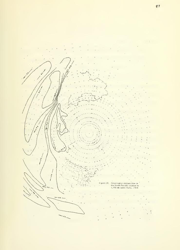
*7

r:~-^

• * .

: < i j

Figure 20. Geoatrophic aOrfa«e flow in

the North-Pacifre relative to

1. OOQ db (after Tully, 1964)

88

Current. Some of the features of the equatorial current system ap-

pear, but the speeds are high in the North Equatorial Current com-

pared to those given by Tully.

Several possible explanations are apparent for the low current

speeds in the Kuroshio Current and in the Alaska Current. First

these currents are narrow high speed flows. The grid spacing used

in these calculations is so large as to completely straddle the cur-

rents. Geostrophic computations assume that the velocity is uniform

between any two stations in a section. The statement that any par-

ticular stream is in geostrophic balance is meaningful only within

the boundaries of the stream. If one station of a station pair is re-

moved from the stream (and in many cases grid points used to calcu-

late the velocity in a stream lie outside the stream boundaries) then

geostrophic computations cannot be expected to be representative of

the stream velocity. For this reason alone one would expect the geo-

strophic velocity to be low in most cases since the mass gradients

are rarely sensed at their maximum. Secondly, in both these flows

a 1, 200 foot reference level is clearly too shallow. Lastly, only

the thermal component of the current has been computed. Possibly

the last two of these problems can be corrected by using the climato-

logical temperature and salinity fields.

89

Climatological Fields

To investigate the magnitude of the problems suggested in the

previous section Equation 32 was programmed to run over the FNWC

atlas climatological temperature and salinity fields on the FNWC

CDC 3600 computer. The program is found in Appendix III. Since

the atlas temperature fields were not digitized between the surface

and 400 m, either the synoptic or the monthly climatological tem-

perature fields must be used for temperatures above this depth.

Thus fields from different sources are combined to make the calcu-

lations. The compatability of the fields at any level and between

levels has not been investigated. A reference level of 1, 000 m was

selected as the average coefficients in Equation 32 had previously

been determined for that reference level (Chapter VI). Furthermore,

this was the reference level used by Reid (1961). The flow computed

is shown in Figure 21 where isotachs indicate the surface current

speed and arrows indicate the direction.

The currents exhibit few of the features of the geostrophic cir-

culation as given by Tully (1964), and many anomalies exist. In

particular, there is a high transport region shown extending off the

Japanese islands but the magnitude is too low by nearly half an order

of magnitude. There is some indication of a westerly drift across

the north Pacific, a southerly flow off the west coast of the United

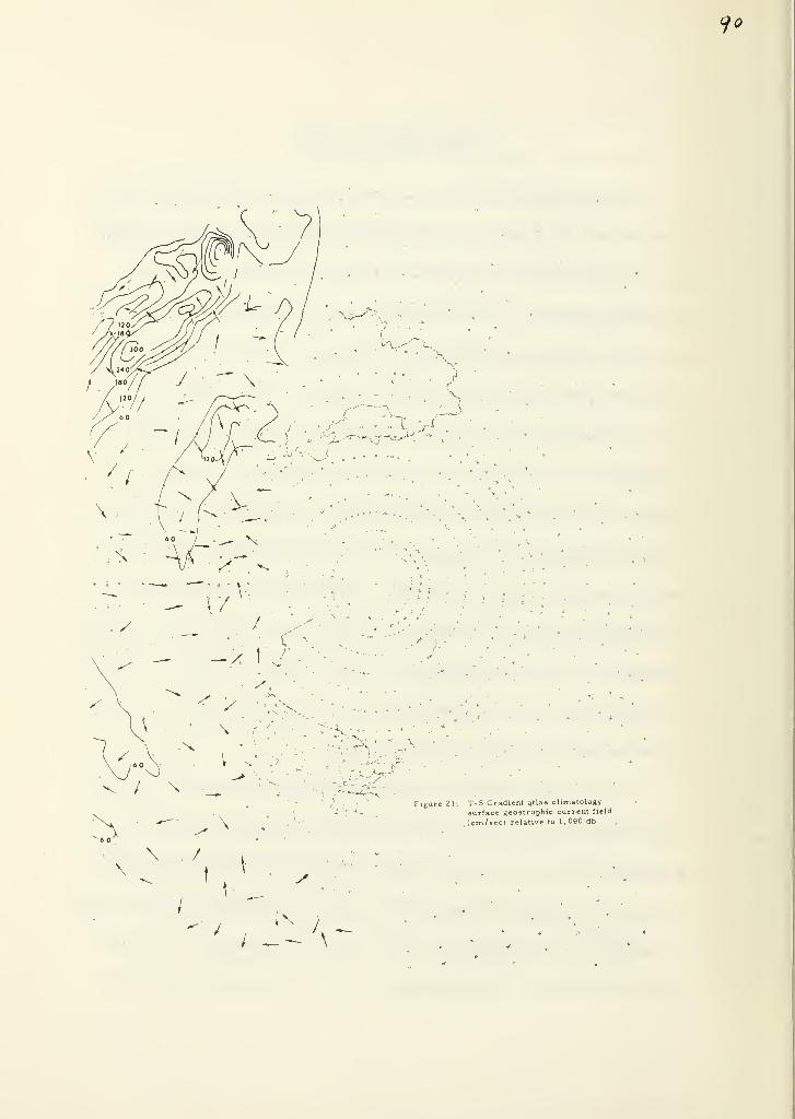
CjO

Figure Zl\ T- S Gradient atlas climatology

surface geostrophic current field

(cm/sec) relative to 1, 060 db

91

States and Mexico, and a cyclonic gyre in the Gulf of Alaska. The

magnitude of the computed currents are in most reasonable agree-

ment in the California Current region where values of a few centi-

meters per second appear. In general the central portion of the

subtropic gyre shows a strong northerly component which is not in

agreement with known geostrophic circulation. Furthermore, the

high transport in the western equatorial region is not in agreement

with Tully.

Remarks and Recommendations

Remarks

Equation 33 has been programed to run over the available

63 x 63 fields of FNWC. The results of these computations have been

compared to surface current computations presently made by FNWC

and with geostrophic flow relative to 1, 000 m given by Tully (1964)

for the Nortn Pacific. These comparisons show clearly that ac-

ceptable geostrophic surface currents cannot be computed from the

existing fields. While indications of accepted flow patterns appear,

several limitations of the available fields are clear.

For the synoptic fields one of the chief limitations is the fact

that these fields only extend to 1, 200 feet. This is too shallow for

a reference level over much of the ocean. Obviously, a second

92

limitation is the lack of salinity fields to complete the computations.

Another limitation of the synoptic fields is the coarseness of the grid

system. In many areas the grid spacing is larger than the known

width of the existing currents.

Using the existing climatological fields, the computations can

be extended to 1, 000 db. Unfortunately, in the Pacific these fields

do not represent adequately the mass field for geostrophic computa-

tions. Derived from atlases, the fields are smoothed in an undeter-

mined way. Furthermore, since the atlases present the temperature

and salinity as horizontal fields at each level, the interpolation of

these fields to the grid points undoubtedly will contribute errors.

A further problem with the existing climatological fields is the re-

quirement to use monthly climatological temperature fields in the

upper 400 m along with atlas salinity fields, without establishing the

compatability of the two fields. Again the coarseness of the available

63 x 63 grid is not appropriate for geostrophic computations in the

narrow current regions. If these computations are to be made then

several adjustments must be made in the available fields.

Clearly the available fields and coarse grid restrict geo-

strophic computations over the ocean by any method. The more ac-

ceptable agreement between currents computed by FNWC and

"accepted" currents is due to their capability to "tune" the flow.

This same procedure could be used to adjust the geostrophic flow

93

computed by the T-S Gradient scheme using the synoptic temperature

fields which appear from this study to be the best available fields.

However, "tuning" the ocean to an arbitrary standard seems ques-

tionable. Geostrophic computations should be objective and the use

of arbitrary "tuning" factors removes this objectivity. Several

recommendations are obvious which should be considered as possible

improvements, hopefully leading eventually to the capability of com-

puting actual geostrophic flow over the world oceans.

Recommendations

First, the 63 x 63 Northern Hemisphere grid used by FNWC

gives a grid spacing of 373 nmi at the equator, 200 nmi at 60° N

latitude, and 186 nmi at the pole. This grid spacing is too large for

geostrophic computations over most of the oceans. The minimum

spacing suggested by Reed and Laird (1965) for 160°W and 175°W

longitude is an indication of more acceptable spacing. Their values

are shown in Table 6. The basis for their recommendations is that

the dynamic height difference should be five times the error in

dynamic height computations. However, a grid spacing too much

larger than this will lead to poor results. Since the dynamic height

represents an integral of the water structure a grid should be de-

veloped for geostrophic computations using the dynamic height

gradient as one criterion in constructing a new grid and temperature

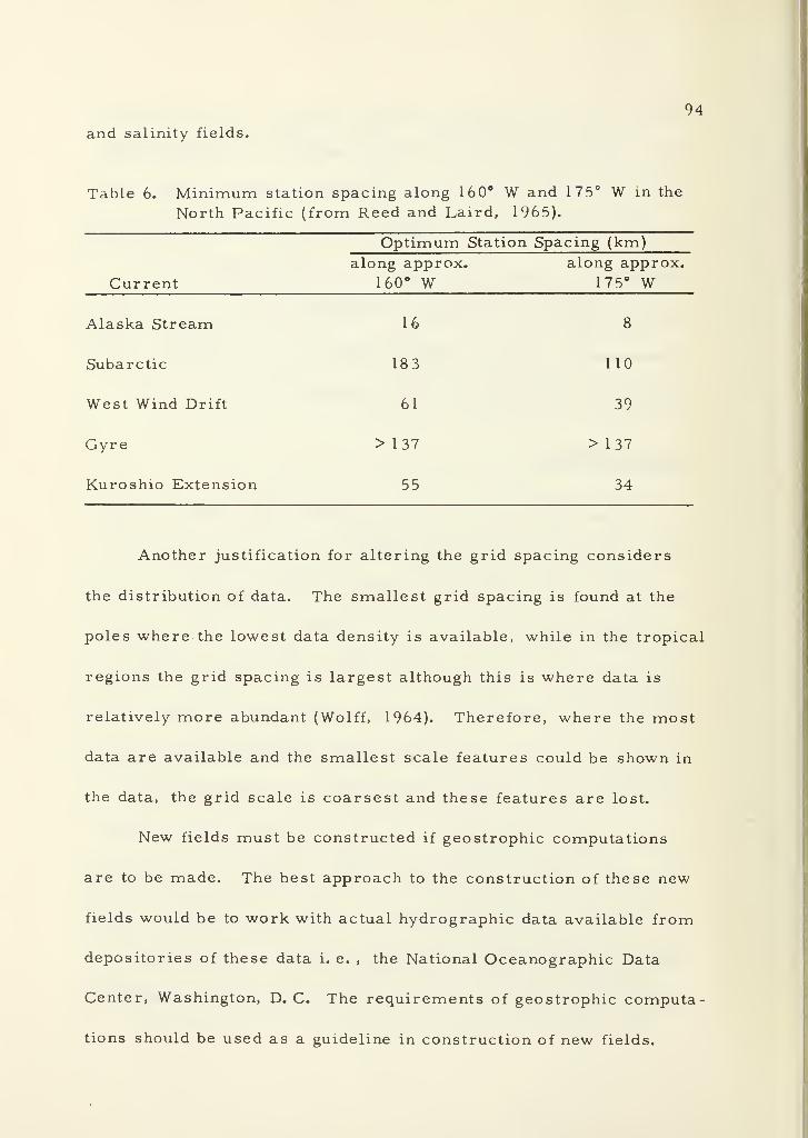
94

and salinity fields.

Table 6. Minimum station spacing along 160° W and 175° W in the

North Pacific (from Reed and Laird, 1965).

Optimum Station Spacing (km)

along approx. along approx.

Current 160° W 175° W

Alaska Stream 16 8

Subarctic 183 110

West Wind Drift 61 39

Gyre > 1 37 > 1 37

Kuroshio Extension 55 34

Another justification for altering the grid spacing considers

the distribution of data. The smallest grid spacing is found at the

poles where the lowest data density is available, while in the tropical

regions the grid spacing is largest although this is where data is

relatively more abundant (Wolff, 1964). Therefore, where the most

data are available and the smallest scale features could be shown in

the data, the grid scale is coarsest and these features are lost.

New fields must be constructed if geostrophic computations

are to be made. The best approach to the construction of these new

fields would be to work with actual hydrographic data available from

depositories of these data i. e. , the National Oceanographic Data

Center, Washington, D. C. The requirements of geostrophic computa-

tions should be used as a guideline in construction of new fields.

95

VIIL SUMMARY AND CONCLUSIONS

This study has examined schemes for simplifying geostrophic

computations. Several schemes have been previously proposed to

simplify these computations, but except for the use of the thermo-

steric anomaly proposed by Montgomery and Wooster (1954) none are

satisfactory over the entire ocean.

A simplification is proposed here which represents a signifi-

cant simplification of dynamic computations without loss of accuracy.

The scheme expresses the geostrophic velocity as three terms in-

volving the observed variables, temperature and salinity. Only three

coefficients are needed. These coefficients have been determined

and are given in graphical and tabular form. If a fixed reference

level of 1, 000 db is used it has been shown that fixed values of the

coefficients can be used for geostrophic surface current computations

over the entire Pacific Ocean without introducing more than a five

percent error. The name T-S Gradient scheme is proposed for the

simplification. It provides the following advantages over other

schemes:

1. Computations show no loss in accuracy from the classical

scheme for most practical purposes.

2. The computation of geostrophic currents is substantially

simplified.

96

3. The scheme is general and can be used in any region of

the ocean where the temperature, salinity and pressure fall within

the range for which the coefficients have been determined.

4. The scheme requires only the observed variables, tem-

perature, salinity and pressure, and the coefficients A(S, P),

2B(S, P) and C(T, P).

5. The first order thermal and haline structure contributions

to the geostrophic flow can be determined independently.

6. The scheme is computationally faster than the classical

scheme (seven times faster on the IBM 360).

7. The scheme is particularly well suited to use onboard

ships with small digital computers as involved equations of state

are not used.

The proposed scheme was used to compute surface geostrophic

flow over the 63 x 63 FNWC northern hemisphere fields, the only

hemispheric fields available at this time. The resulting computed

surface currents were compared to surface currents in the North

Pacific Ocean computed by FNWC, and by Tully (1964) from Reid's

(1961) investigation of the geopotential topography of the db level

relative to the 1000 db level. These comparisons lead to the con-

clusions that the FNWC 63 x 63 fields are unsuited to geostrophic

computations for the following reasons:

1. The grid spacing is too large even at its smallest spacing.

97

2. The atlas derived fields do not adequately depict the mass

distribution in the ocean.

3. The synoptic temperature fields do not extend to deep

enough level to reasonably approximate level of little or no motion.

The computations over the 63 x 63 fields do show, however, that it

is practical to make actual geostrophic computations over such a

large ocean area on a synoptic basis if the desired fields are avail-

able.

Two proposals are made to improve geostrophic computations

over hemispheric grids. First, that a new grid should be constructed

in which the grid spacing is compatible with geostrophic computa-

tional requirements; second, new temperature and salinity fields be

constructed from the available hydrographic data to replace the atlas

climatological fields presently available.

The T-S Gradient method can be used to compute independently

the first order thermal and haline contributions to the geostrophic

flow. It has been shown that the correlation of the first order

thermal geostrophic surface current (V ) with the geostrophic sur-

face current (V ) in the Gulf Stream water off the Grand Banks cang

be expressed by a simple linear relationship. This relationship is

useful for the determination of the total geostrophic surface current

from temperature measurements alone.

The reliability of the T-S Gradient scheme was tested by

98

comparing T-S Gradient and standard geostrophic computations in

several differing water masses. The current velocity structure was

nearly exactly the same in both cases (Appendix II). Never were the

computations in disagreement by more than ten percent even though

fixed coefficients were used.

Two field tests were performed to investigate the approxima-

tion of computed geostrophic surface currents (Appendix IV) to meas-

ured surface currents. The currents were measured prior to the

hydrographic measurements using parachute drogues. Geostrophic

currents were computed from the measured temperature and salinity

by both the classical geostrophic method and the T-S Gradient

method, and FNWC currents were obtained from their Current

Transport and Stream Function maps for the periods of the experi-

ments. On the second experiment the geostrophic computations

were also made with the reversing thermometer temperatures re-

placed by the expendable bathythermograph temperatures.

The geostrophic currents computed by both methods were

identical for both experiments. The substitution of expendable

bathythermograph temperatures raised the computed surface velocity

by both methods approximately one cm/sec. The computed geo-

strophic surface velocity was approximately half the observed cur-

rent in both experiments. The FNWC currents were in the opposite

direction to the observed flow in the first experiment but agreed

99

with the observed flow in the second.

Certainly two experiments should not be considered as verifi-

cation or condemnation of any scheme. The results of the experi-

ments do show the need for additional experimentation before a great

deal of confidence can be placed in any indirectly computed currents.

It is proposed that this research be continued to further in-

vestigate the relationships between indirectly computed surface cur-

rents and observed currents (see Appendix V).

100

BIBLIOGRAPHY

Bierknes, V. and J. W. Sandstrom. 1910. Dynamic meteorology

and hydrography, Part I. Statics. Washington, D. C. ,

Carnegie Institution of Washington. 146 p. (Publication 88)

Bisset-Berman Corporation. 1968. 9040 Salinity-temperature -

depth system. San Diego, n. p. (Specifications brochure)

Bowden, K. F. 1953. Measurement of wind currents in the sea by

methods of towed electrodes. Nature 1 71(4356) :735-736.

Broida, S. 1966. Interpretation of geostrophy in the straits of

Florida. Ph. D. thesis. Coral Gables, Florida, University

of Miami. 107 numb, leaves.

Brown, N. L. 1968. An in situ salinometer for use in the deep

ocean. In; Marine sciences instrumentation, ed. by Fred Alt.

Vol. 4. Proceedings of the Fourth National Instrument

Society of America Marine Sciences Instrumentation Sympo-sium, Coca Beach, Florida, 1968. New York, Plenum,p. 563-577.

Cox, C. S. 1962. Internal waves. Part I. In; The sea, ed. by M.N. Hill. Vol. 2. New York, Inter science, p. 752-763.

Defant, A. 1950. Reality and illusion in oceanographic surveys.

Journal of Marine Research 9( 2) :1 20- 1 38.

1961. Physical oceanography. Vol. 1 New York,Pergamon. 725 p.

Denner, W. W. , T. Green and W. H. Snyder. 1968. Large scale

oceanic drogue diffusion. Nature 219(51 52):36l - 362.

Eckart, C. 1958. Properties of water. Part III. The equation of

state of water and sea water at low temperatures and pres-sures. American Journal of Science 256:225-240.

Ekman, V. W. 1908. Die Zusammendruckbarkeit des Meerwassers.Publications de Circonstance du Conseil Permanent Inter-

national pour L'Exploration de la Mer 43:1-47.

101

Fofonoff, N. P. 1962. Physical properties of sea-water. In: Thesea, ed. by M. N. Hill. Vol. 2. New York, Interscience.

p. 3-28.

Fomin, L. M. 1964. The dynamic method in oceanography. NewYork, Elsevier. 21 2 p.

Forsch, C. , M. Knudsen and S. P. L. Sorensen. 1902. Berichteuber die Konstantenbestimmungen zur Aufsellung der hydro-graphischen Tabellen. Kongelige Danske VidenskabernesSelskab Skrifter, Naturvidenskabelig og Mathematisk Afdeling

12(1):1-151.

Gibson, B. W. 1962. Sea surface temperature synoptic analysis.

Washington, D. C. , U. S. Naval hydrographic office. 17 p.

(Antisubmarine Warfare Environmental Prediction SystemReport no. 7)

Groen, P. 1967. The waters of the sea, Princeton, New Jersey,Van Nostrand. 316 p.

Haltiner, G. J. , and F. L. Martin. 1957. Dynamical and physicalmeterology. New York, McGraw-Hill. 470 p.

Haurwitz, B. , H. Stommel and W. H. Munk. 1959. On the thermalunrest in the ocean. In: The atmosphere and the sea in

motion, ed. by Bert Bolin. New York, Rockefeller Institute

in association with Oxford University, p. 74-94. (RossbyMemorial Volume)

Hubert, W. E. 1964. Computer produced synoptic analysis of sur-

face currents and their application for navigation. Navigation

12(2):101-107.

Hubert, W. E. and T. Laevastu. 1967. Synoptic analysis and fore-

casting of surface currents. Norfolk, U. S. Navy WeatherResearch Facility. 55 p. (Report no. 36-0667-127)

Interstate Electronics Corporation. 1968. Critical evaluation of

geostrophic current prediction techniques for ASWEPS.Anaheim, California. 125 p. (Unpublished report)

James, R. W. 1966. Ocean thermal structure forecasting.

Washington, D. C. U. S. Naval Oceanographic Office. 217 p.

( Antisubmarine Warfare Manual no. 5)

102

Jones, T. B. 1939. An introduction to Hispanic American history.

New York, Harper. 577 p.

Knudsen, M. 1901. Hydrographic tables. Copenhagen, G. C. E. Gad.

o3 p.

Kollmeyer, R. C. 1964. An examination of errors in dynamic height

determinations. Washington, D. C, , U. S. Coast Guai J,

Oceanographic Unit. 23 p.

1966. Oceanography of the Grand Banks region of

Newfoundland in 1965. Washington, D. C. , U. S. Coast Guard,Oceanographic Unit. p. 157. (Report no. CG373-11)

LaFond, E C. 1949. The use of bathythermograms to determineocean currents. Transactions of the American Geoph :sical

Union 30(2):231-237.

1951. Processing oceanographic data. Washington,D. C. , U. S. Hydrographic Office. 1 1 3 p.

Lenczyk, R. E. 1962. Report of the International Ice Patrol Servicein the North Atlantic Ocean. Washington, D. C. , U. S. CoastGuard. 109 p. (Bulletin no. 50)

Li, Yuan-Hui. 1967. Equation of state of water and sea water.Jounral of Geophysical Research 72( 1 0) ;2665- 2678.

Magnavox Corporation. MX/702/hp Shipboard navigation system.Fort Wayne, Indiana, n. p. Specification brochure TP 67-1947)

Montgomery, R. B. and W. S. Wooster. 1954. Thermosteric anomalyand analysis of serial oceanographic data. Deep sea research2:63-70.

Montgomery, R. B. and E. D. Stroup. 1962. Equatorial waters andcurrents at 150°W in July-August 1952. Baltimore, JohnsHopkins Press. 88 p. (Johns Hopkins Oceanography Studies no. 1)

Moynihan, M. J. 1968. Investigation of Geostrophic current calcu-lations on the Grand Banks. Master's thesis. Monterey, U. S.

Naval Postgraduate School. 62 numb, leaves.

Neumann, G. and W. J. Pierson, Jr. 1966. Principles of physicaloceanography. Englewood Cliffs, New Jersey, Prentice- Hall.

545 p.

Newton, M. S. and G. C. Kennedy. 1965. An experimental study ofthe P.-V-T-S relations of sea water. Journal of MarineResea . ch 23( 2) :88- 1 03.

103

Proudman, J. 1953. Dynamical oceanography. London, Methuen.

409 p.

Rattray, M. 196Z. Interpolation errors and oceanographic sam-pling. Deep Sea Research 9:25-37.

Reed, R. K. and N. E. Taylor. 1965. Some measurements of the

Alaska Stream with parachute drogues. Deep Sea Research12:777-784.

Reed, R. K. and N. B. Laird. 1966a. On the reliability of geo-

strophic flow determinations across a section of the NorthPacific Ocean. Paper presented at the Northwest RegionalMeeting of the American Geophysical Union, Corvallis, Oregon,August. 7 numb, leaves.

1966b. An oceanographic section off the California

coast, February, 1966. Seattle, Environmental ScienceServices Administration, Pacific Oceanographic Laboratory.

51 p. (Technical Memorandum IER TM-POL-s)

Reid, J. L. , Jr. , G. I. Roden and J. G. Wyllie. 1958. Studies of the

California Current system. In: Progress report of the

California Cooperative Oceanic Fisheries Investigations, July

1, 1956, to January 1, 1958. [Sacramentof p. 27-57.

Reid, J. L. 1961. On the geostrophic flow at the surface of the

Pacific Ocean with respect to the 1, 000 decibar surface.

Tellus 13(4):489-502.

Reid, R. O. 1959. Influence of some errors in the equation of state

or in observations on geostrophic currents. In: Proceedingsof a Conference of Physical and Chemical Properties of Sea

Water. Washington, D. C. , (National Research Council, p. 10-

29. (Publication 600)

Sandstrom, J. W. and B. Helland-Hansen. 1903. Uber die Bere-chnung von Meer stromungen. Bergen, Norway. 43 p.

(Report on Norwegian Fisheries and Marine Investigation.

Vol. 2. No. 4)

Smith, E. H. 1931. Arctic ice with special reference to its distri-

bution to the North Atlantic Ocean. Washington, D. C. U. S.

Coast Guard. 221 p. ( The Marion Expedition, 1928.

Bulletin 19, part 3)

104

Stommel, H. 1947. Note on the use of the T-S correlation for

dynamic height anomaly computations. Journal of MarineResearch 6:85-92.

Stommel, H. 1965. The Gulf Stream, a physical and dynamicaldescription. Berkeley, University of California. 248 p.

Sverdrup, H. U. , M. W. Johnson and R. H. Fleming. 1942. Theoceans: their physics, chemistry and general biology.

Englewood Cliffs, New Jersey, Prentice-Hall. 1087 p.

Sverdrup, H. U. 1947. Wind-driven currents in a baroclinic ocean,

with application to the equatorial currents of the EasternPacific. Proceedings of the National Academy of Sciences

33:318-236.

Tully, J. P. 1964. Oceanographic regions and assessment of tem-perature structure in the seasonal zone of the North Pacific

Ocean. Journal of the Fisheries Research Board of Canada21:941-969.

Volkman, G. , J. Knauss and A. Vine. 1956. The use of parachutedrogues in the measurement of subsurface ocean currents.

Transactions of the American Geophysical Union, 37(5):573-

577.

von Arx, W. S. 1962. An introduction to physical oceanography.Reading, Massachusetts, Addison-Westley. 422 p.

Warriner, B. . 1958. Application of NNSS to marine navigation. In:

Marine sciences instrumentation, ed. by Fred Alt. Vol. 4.

Proceedings of the Fourth National Instrument Society of

America Marine Sciences Instrumentation Symposium, CocaBeach, Florida, 1968. New York, Plenum, p. 168-188.

Werenskiold, W. 1937. Die Berechnung von Meeresstromungen.In: Annual hydrographic report on maritime meteorology.Berlin, Hamburg Marine Observatory, p. 68-72.

Wilson, W. and D. Bradley. 1968. Specific volume of sea water asa function of temperature, pressure, and salinity. Deep SeaResearch and Oceanographic Abstracts 15:355-364.

105

Wolff, P. 1964. Operational analyses and forecasting of oceantemperature structure. Monterey, California, U. S. NavyFleet Numerical Weather Facility. 24 p. (Unpublished report)

Wooster, W. S. and B. A. Taft. 1958. On the reliability of field

measurements of temperature and salinity in the ocean.

Journal of Marine Research 17:552-556.

Wust, G. 1924. Florida und. Antillenstrom. Veroffentlichungendes Institutes fttr meereskunde and dem universitat. Berlin,

University of Berlin. 48 p.

Yao, N. 1967. Analysis of hydrographic techniques- -A study of

different effects on geostrophic current computations by usingvarious hydrographic data processing methods. Master'sthesis. Corvallis, Oregon State University. 70 numb, leaves.

Yausi, M. 1955. On the rapid determination of the dynamic depthanomaly in the Kuroshio area. Records of OceanographicWorks in Japan 2(2):90-95.

1957. On the rapid estimation of the dynamictopography in the seas adjacent to Japan. Records of

Oceanographic Works in Japan 3( 1 ):8 - 1 5.

106

APPENDIX I

Tables of A(S, P), B(S, P) and C(T, P]

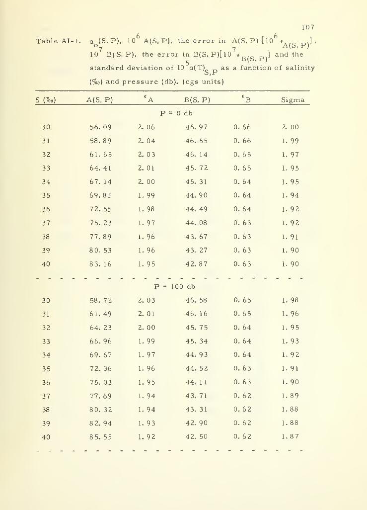
107

Table AI-1. a (S, P), 10 A(S, P), the error in A(S, P)[l0 € ],O A(b, P)

10 B(S, P), the error in B(S, P)[l0 c Jand the

c B(o, P)standard deviation of 10 a( T) as a function of salinity

0,sr

(%o) and pressure (db). (cgs units)

S (%o) A(S,P)CA B(S,P)

6

B Sigma

P = db

30 56. 09 2. 06 46. 97 0. 66 2. 00

31 58.89 2. 04 46. 55 0. 66 1. 99

32 61. 65 2. 3 46. 14 0. 6 5 1. 97

33 64. 41 2. 01 45. 72 0. 65 1. 95

34 67. 14 2. 00 45. 31 0. 64 1.95

35 69. 85 1.99 44. 90 0. 64 1. 94

36 72. 55 1. 98 44. 49 0. 64 1. 92

37 7 5. 23 1. 97 44. 08 0. 63 1. 92

38 77. 89 1. 96 43. 67 0. 6 3 1. 91

39 80. 53 1. 96 43. 27 0. 63 1. 90

40 8 3. 16 1.95 42. 87 0. 63 1. 90

P = 100 db

30 58. 72 2. 03 46. 58 0. 65 1. 98

31 61. 49 2. 01 46. 16 0. 6 5 1. 96

32 64. 23 2. 00 45. 75 0. 64 1. 95

33 66. 96 1.99 45. 34 0. 64 1. 93

34 69. 67 1. 97 44. 93 0. 64 1. 92

35 7 2. 36 1. 96 44. 52 0. 63 1. 91

36 75. 03 1.95 44. 11 0. 63 1. 90

37 77. 69 1. 94 43. 71 0. 6 2 1. 89

38 80. 32 1. 94 43. 31 0. 62 1. 88

39 8 2. 94 1.93 42. 90 0. 62 1.88

40 8 5. 55 1.92 42. 50 0. 62 1. 87

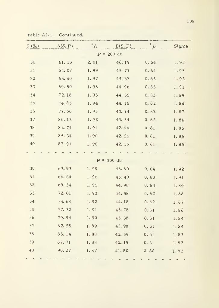
108

Table AI-1. Continued.

S (%o) A(S, P)eA B(S, P)

eB Sigma

P = 200 db

30 61. 33 2. 01 46. 19 0. 64 1. 95

31 64. 07 1.99 45. 77 0. 64 1. 93

32 66. 80 1. 97 45. 37 0. 63 1. 92

33 69. 50 1. 96 44. 96 0. 63 1. 91

34 7 2. 18 1.95 44. 55 0. 6 3 1. 89

35 74. 8 5 1. 94 44. 15 0. 62 1. 88

36 77. 50 1. 93 43. 74 0. 62 1. 87

37 8 0. 13 1. 92 43. 34 0. 6 2 1. 86

38 8 2. 74 1.91 42. 94 0. 61 1. 86

39 8 5. 34 1. 90 42. 55 0. 61 1. 85

40 8 7. 91 1. 90 42. 15 0. 61 1. 85

P = 300 db

30 6 3. 93 1. 98 45. 80 0. 64 1. 92

31 66. 64 1. 96 45. 40 0. 63 1. 91

32 69. 34 1.95 44. 98 0. 63 1. 89

33 7 2. 01 1. 93 44. 58 0. 6 2 1. 88

34 74. 68 1. 92 44. 18 0. 6 2 1. 87

35 77. 32 1. 91 43. 78 0. 61 1. 86

36 79. 94 1. 90 4 3. 38 0. 61 1. 84

37 8 2. 55 1.89 42. 98 0. 61 1. 84

38 8 5. 14 1. 88 42. 59 0. 61 1. 83

39 87. 71 1.88 42. 19 0. 61 1. 82

40 90. 27 1. 87 41. 80 0. 60 1. 82

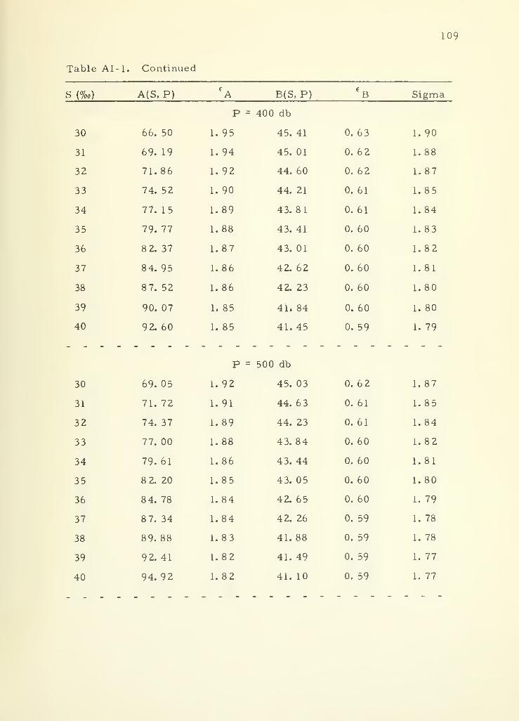
109

Table AI-1. Continued

S (%o) A(S, P)(

A B(S,P)e

B Sigma

P = 400 db

30 66. 50 1.95 45. 41 0. 6 3 1. 90

31 69. 19 1. 94 45. 01 0. 6 2 1. 88

32 71. 86 1. 92 44. 60 0. 6 2 1. 87

33 74. 52 1. 90 44. 21 0. 61 1. 85

34 77. 15 1.89 43. 81 0. 61 1. 84

35 79. 77 1. 88 43. 41 0. 60 1. 83

36 8 2. 37 1.87 43. 01 0. 60 1. 82

37 84. 95 1. 86 42. 62 0. 60 1. 81

38 87. 52 1.86 42. 23 0. 60 1.80

39 90. 07 1. 85 41. 84 0. 60 1. 80

40 9 2. 60 1. 85 41. 45 0. 59 1. 79

P = 500 db

30 69. 05 1.92 45. 03 0. 6 2 1. 87

31 71. 72 1. 91 44. 6 3 0. 61 1. 85

32 74. 37 1.89 44. 23 0. 61 1. 84

33 77. 00 1.88 43. 84 0. 60 1.82

34 79. 61 1.86 43. 44 0. 60 1. 81

35 8 2. 20 1.85 43. 05 0. 60 1.80

36 84. 78 1.84 42. 65 0. 60 1. 79

37 8 7. 34 1.84 42. 26 0. 59 1. 78

38 89.88 1.83 41. 88 0. 59 1. 78

39 9 2. 41 1.82 41. 49 0. 59 1. 77

40 94. 92 1.82 41. 10 0. 59 1. 77

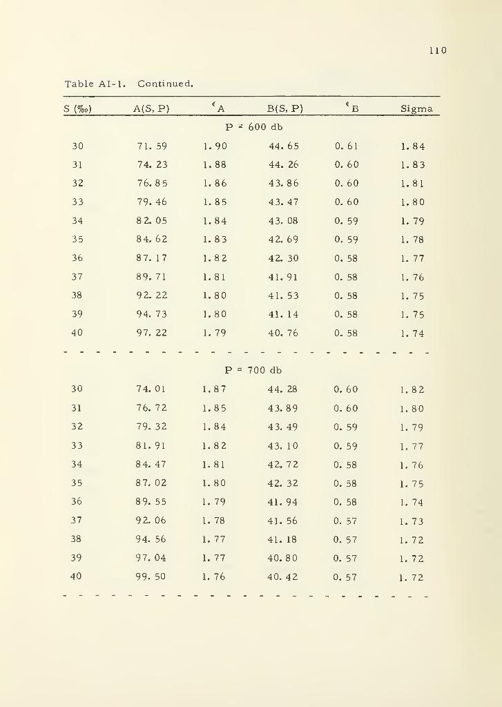
110

Table AI-1. Continued.

S (%o) A(S,P)CA B(S, P)

€B Sigma

P = 600 db

30 71. 59 1. 90 44. 65 0. 61 1. 84

31 74. 23 1.88 44. 26 0. 60 1. 83

32 76.85 1.86 43. 86 0. 60 1. 81

33 79. 46 1. 85 43. 47 0. 60 1.80

34 8 2. 05 1.84 43. 08 0. 59 1. 79

35 84. 62 1. 83 42. 69 0. 59 1. 78

36 8 7. 17 1. 82 42. 30 0. 58 1. 77

37 89. 71 1. 81 41. 91 0. 58 1. 76

38 92. 22 1. 80 41. 53 0. 58 1. 75

39 94. 73 1.80 41. 14 0. 58 1. 75

40 97. 22 1. 79 40. 76 0. 58 1. 74

P = 700 db

30 74. 01 1. 87 44. 28 0. 60 1.82

31 76. 72 1.85 43.89 0. 60 1.80

32 79. 32 1. 84 43. 49 0. 59 1. 79

33 81. 91 1.82 43. 10 0. 59 1. 77

34 84. 47 1. 81 42. 72 0. 58 1. 76

35 87. 02 1. 80 42. 32 0. 58 1. 75

36 89. 55 1. 79 41. 94 0. 58 1. 74

37 9 2. 06 1. 78 41. 56 0. 57 1. 73

38 94. 56 1. 77 41. 18 0. 57 1. 72

39 97. 04 1. 77 40. 80 0. 57 1. 72

40 99. 50 1. 76 40. 42 0. 57 1. 72

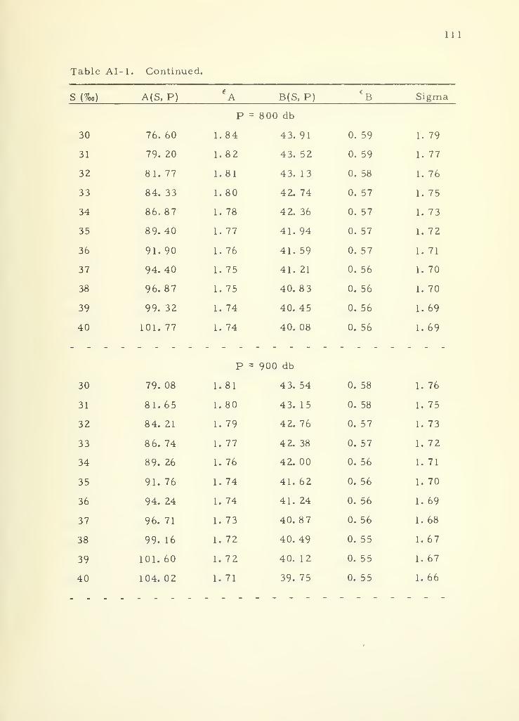
11

1

Table AI-1. Continued.

S (%o) A(S, P) ^A B(S, P) Vb Sigma

P = 800 db

30 76. 60 1.84 43. 91 0. 59 1. 79

31 79. 20 1. 82 43. 52 0. 59 1. 77

32 81. 77 1. 81 43. 13 0. 58 1. 76

33 84.33 1.80 42.74 0.57 1.75

34 86.87 1.78 42.36 0.57 1.73

35 89. 40 1. 77 41. 94 0. 57 1. 72

36 91. 90 1. 76 41. 59 0. 57 1. 71

37 94.40 1.75 41.21 0.56 1.70

38 96. 87 1. 75 40. 83 0. 56 1. 70

39 99. 32 1. 74 40. 45 0. 56 1. 69

40 101.77 1.74 40.08 0.56 1.69

P :: 900 db

30 79. 08 1. 81 4 3. 54 0. 58 1. 76

31 81. 65 1. 80 4 3. 15 0. 58 1. 75

32 84. 21 1. 79 4 2. 76 0. 57 1. 73

33 8 6. 74 1. 77 4 2. 38 0. 57 1. 72

34 89. 26 1. 76 42. 00 0. 56 1. 71

35 91. 76 1. 74 41. 62 0. 56 1. 70

36 94. 24 1. 74 41. 24 0. 56 1. 69

37 96. 71 1. 73 40. 87 0. 56 1. 68

38 99. 16 1. 72 40. 49 0. 55 1. 67

39 101. 60 1. 72 40. 12 0. 55 1. 67

40 104. 02 1. 71 39. 75 0. 55 1. 66

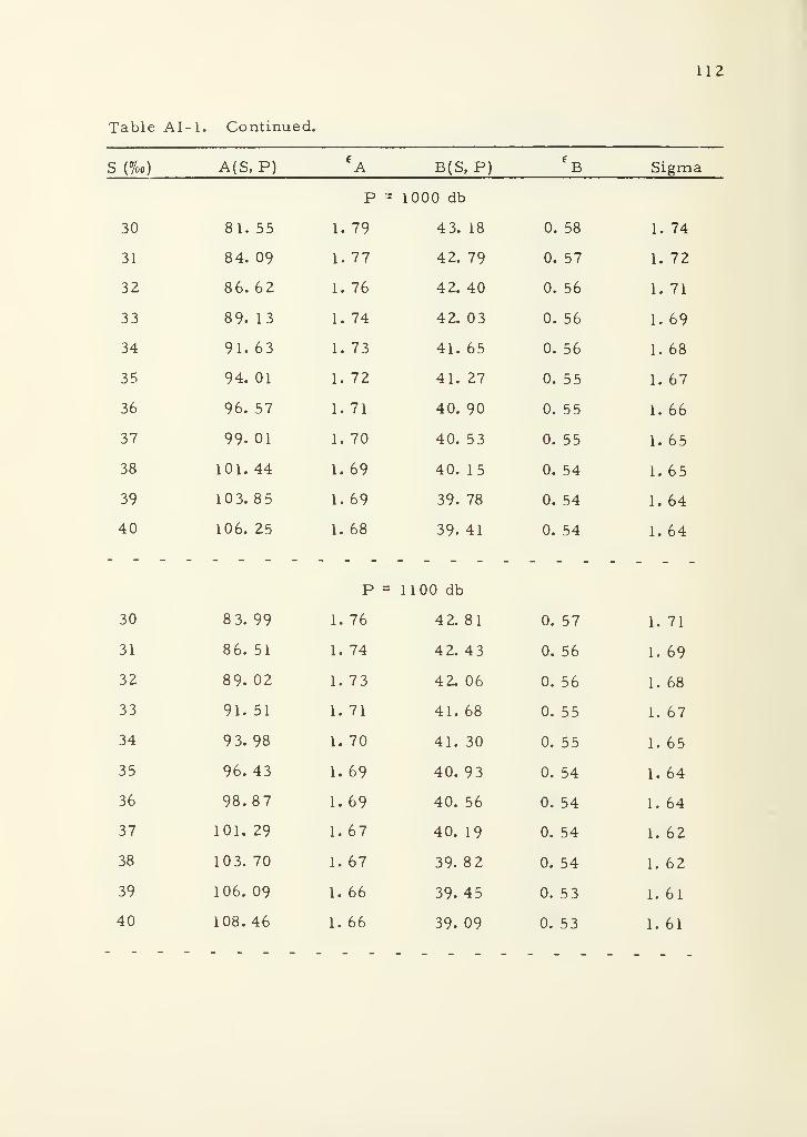
112

Table AI-1. Continued.

S (%o) A(S,P) <A B(S, P)€

B Sigma

P = 1000 db

30 81. 55 1. 79 43. 18 0. 58 1. 74

31 84. 09 1. 77 42. 79 0. 57 1. 72

32 86. 62 1. 76 4 2. 40 0. 56 1. 71

33 89. 13 1. 74 42. 03 0. 56 1. 69

34 91. 63 1. 73 41. 65 0. 56 1. 68

35 94. 01 1. 72 41. 27 0. 55 1. 67

36 96. 57 1. 71 40. 90 0. 55 1. 66

37 99. 01 1. 70 40. 53 0. 55 1. 65

38 101. 44 1. 69 40. 15 0. 54 1. 65

39 10 3. 8 5 1.69 39. 78 0. 54 1. 64

40 106. 25 1. 68 39. 41 0. 54 1. 64

P = 1100 db

30 8 3. 99 1. 76 4 2. 81 0. 57 1. 71

31 86. 51 1. 74 42. 43 0. 56 1. 69

32 89. 02 1. 73 4 2. 06 0. 56 1. 68

33 91. 51 1. 71 41. 68 0. 55 1. 67

34 9 3. 98 1. 70 41. 30 0. 55 1. 65

35 96. 43 1. 69 40. 93 0. 54 1. 64

36 98. 87 1. 69 40. 56 0. 54 1. 64

37 101. 29 1. 67 40. 19 0. 54 1. 62

38 103. 70 1. 67 39. 8 2 0. 54 1. 62

39 106. 09 1. 66 39. 45 0. 53 1. 61

40 108. 46 1. 66 39. 09 0. 53 1. 61

113

Table AI-1. Continued.

S (%o) A(S, P)( A B(S, P)

e

B Sigma

P = 1200 db

30 86. 41 1. 73 4 2. 46 0. 56 1. 68

31 88. 91 1. 72 4 2. 08 0. 55 1. 67

32 91. 40 1. 70 41. 70 0. 55 1. 65

33 93. 86 1. 69 41. 33 0. 54 1. 64

34 96. 31 1.67 40. 96 0. 54 1. 63

35 98. 74 1. 66 40. 59 0. 53 1. 61

36 101. 16 1. 65 40. 22 0. 53 1. 61

37 10 3. 56 1. 65 39. 85 0. 5 3 1. 60

38 105. 94 1. 64 39. 49 0. 53 1. 60

39 108. 31 1. 63 39. 12 0. 53 1. 59

40 110. 66 1. 63 38. 76 0. 52 1. 58

P = 1300 db

30 88.82 1. 70 4 2. 10 0. 55 1. 66

31 91. 29 1. 69 41. 73 0. 54 1. 64

32 9 3. 76 1. 67 41. 35 0. 54 1. 63

33 96. 20 1. 66 40. 98 0. 53*

1. 61

34 98. 63 1. 65 40. 61 0. 5 3 1. 60

35 101. 04 1. 64 40. 25 0. 53 1. 60

36 103. 43 1. 63 39. 88 0. 52 1. 58

37 105. 81 1. 62 39. 52 0. 52 1. 57

38 108. 17 1. 61 39. 16 0. 52 1. 57

39 110. 51 1. 61 38. 8 0. 52 1. 56

40 1 1 2. 84 1. 60 38. 44 0. 52 1. 56

114

Table AI-1. Continued.

S (%o) A(S, P)€A B(S, P)

eB Sigma

P = 1400 db

30 91. 21 1. 68 41. 75 0. 54 1. 63

31 9 3. 66 1. 66 41. 38 0. 53 1. 61

32 96. 10 1. 65 41. 01 0. 53 1. 60

33 98. 52 1. 63 40. 64 0. 52 1. 59

34 100. 92 1. 62 40. 28 0. 52 1. 57

35 103. 31 1. 61 39. 91 0. 5 2 1. 56

36 10 5. 68 1. 60 39. 55 0. 51 1. 55

37 108. 04 1. 59 39. 19 0. 51 1. 55

38 110. 38 1. 58 38. 83 0. 51 1. 54

39 112. 70 1. 58 38. 47 0. 51 1. 54

40 115. 01 1. 58 38. 12 0. 51 1. 53

P = 1500 db

30 9 3. 58 1. 65 41. 40 0. 53 1. 60

31 96. 01 1. 63 41. 03 0. 52 1. 59

32 98. 43 1. 62 40. 67 0. 52 1. 57

33 100. 82. 1. 60 40. 30 0. 52 1. 56

34 10 3. 20 1. 59 39. 94 0. 51 1. 55

35 105. 57 1. 58 39. 58 0. 51 1. 54

36 107. 92 1. 57 39. 22 0. 51 1. 53

37 110. 25 1. 56 38. 86 0. 50 1. 52

39 112. 57 1. 56 38. 51 0. 50 1. 51

39 114.87 1. 55 38. 15 0. 50 1. 51

40 117. 16 1. 55 37. 80 0. 50 1. 51

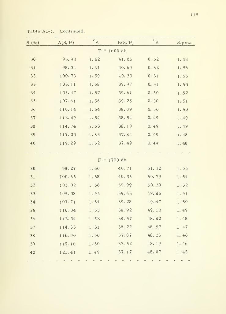
115

Table AI-1. Continued.

S (%o) A(S, P)€A B(S, P)

£

B Sigma

P = 1600 db

30 95. 93 1. 62 41. 06 0. 52 1. 58

31 98. 34 1. 61 40. 69 0. 52 1. 56

32 100. 73 1. 59 40. 33 0. 51 1. 55

33 10 3. 11 1. 58 39. 97 0. 51 1. 53

34 105. 47 1. 57 39. 61 0. 50 1. 52

35 107. 81 1. 56 39. 25 0. 50 1. 51

3b 110. 14 1. 54 38.89 0. 50 1. 50

37 112. 49 1. 54 38. 54 0. 49 1. 49

38 114. 74 1. 53 38. 19 0. 49 1. 49

39 117. 03 1. 53 37. 84 0. 49 1. 48

40 119. 29 1. 52 37. 49 0. 49 1. 48

P = 1700 db

30 98. 27 1. 60 40. 71 51 . 32 1. 55

31 100. 65 1. 58 40. 35 50 . 79 1. 54

32 103. 02 1. 56 39. 99 50 . 30 1. 52

33 105. 38 1. 55 39. 63 49.86 1. 51

34 107. 71 1. 54 39. 28 49 . 47 1. 50

35 110. 04 1. 53 38. 92 49 . 13 1. 49

36 1 1 2. 34 1. 52 38. 57 48 . 82 1. 48

37 114. 63 1. 51 38. 22 48 . 57 1. 47

38 116. 90 1. 50 37. 87 48 . 36 1. 46

39 119. 16 1. 50 37. 52 48 . 19 1. 46

40 121. 41 1.49 37. 17 48 . 07 1. 45

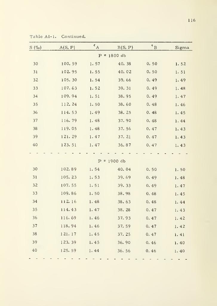
116

Table AI-1. Continued.

S (%o) A(S, P)€A B(S, P)

€

B Sigma

P = 1800 db

30 100. 59 1. 57 40. 38 0. 50 1. 52

31 102. 95 1. 55 40. 02 0. 50 1. 51

32 105. 30 1. 54 39. 66 0. 49 1. 49

33 107. 63 1. 52 39. 31 0. 49 1. 48

34 109. 94 1. 51 38. 95 0. 49 1. 47

35 1 1 2. 24 1. 50 38. 60 0. 48 1. 46

36 114. 5 3 1. 49 38. 25 0. 48 1. 45

37 116. 79 1. 48 37. 90 0. 48 1. 44

38 119. 05 1. 48 37. 56 0. 47 1. 43

39 121. 29 1.47 37. 21 0. 47 1. 43

40 123. 51 1. 47 36. 8 7 0. 47 1. 43

P = 1900 db

30 102. 89 1. 54 40. 04 0. 50 1. 50

31 105. 23 1. 53 39. 69 0. 49 1. 48

32 107. 55 1. 51 39. 33 0. 49 1. 47

33 109.86 1. 50 38. 98 0. 48 1. 45

34 112. 16 1. 48 38. 63 0. 48 1. 44

35 114. 43 1.47 38. 28 0. 47 1. 43

36 116. 69 1. 46 37. 93 0. 47 1. 42

37 118. 94 1. 46 37. 59 0. 47 1. 42

38 121. 17 1. 45 37. 25 0. 47 1. 41

39 123. 39 1.45 36. 90 0. 46 1. 40

40 125. 59 1.44 36. 56 0. 46 1. 40

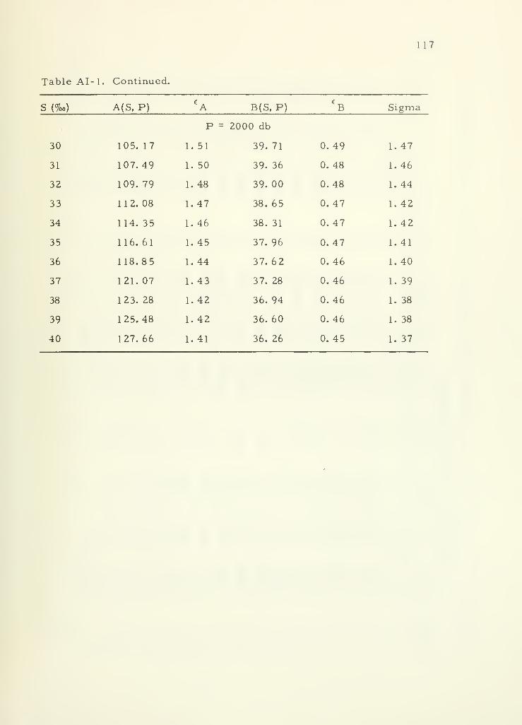
1 17

Table AI-1. Continued.

S (%o) A(S, P)fA B(S, P)

€

B Sigma

P = 2000 db

30 105. 17 1. 51 39. 71 0. 49 1. 47

31 107. 49 1. 50 39. 36 0. 48 1. 46

32 109. 79 1. 48 39. 00 0. 48 1. 44

33 112. 08 1. 47 38. 65 0. 47 1. 42

34 114. 35 1. 46 38. 31 0. 47 1. 42

35 116. 61 1. 45 37. 96 0. 47 1. 41

36 118. 85 1. 44 37. 62 0. 46 1. 40

37 121. 07 1. 43 37. 28 0. 46 1. 39

38 123. 28 1. 42 36. 94 0. 46 1. 38

39 125. 48 1.42 36. 60 0. 46 1. 38

40 127. 66 1.41 36. 26 0. 45 1. 37

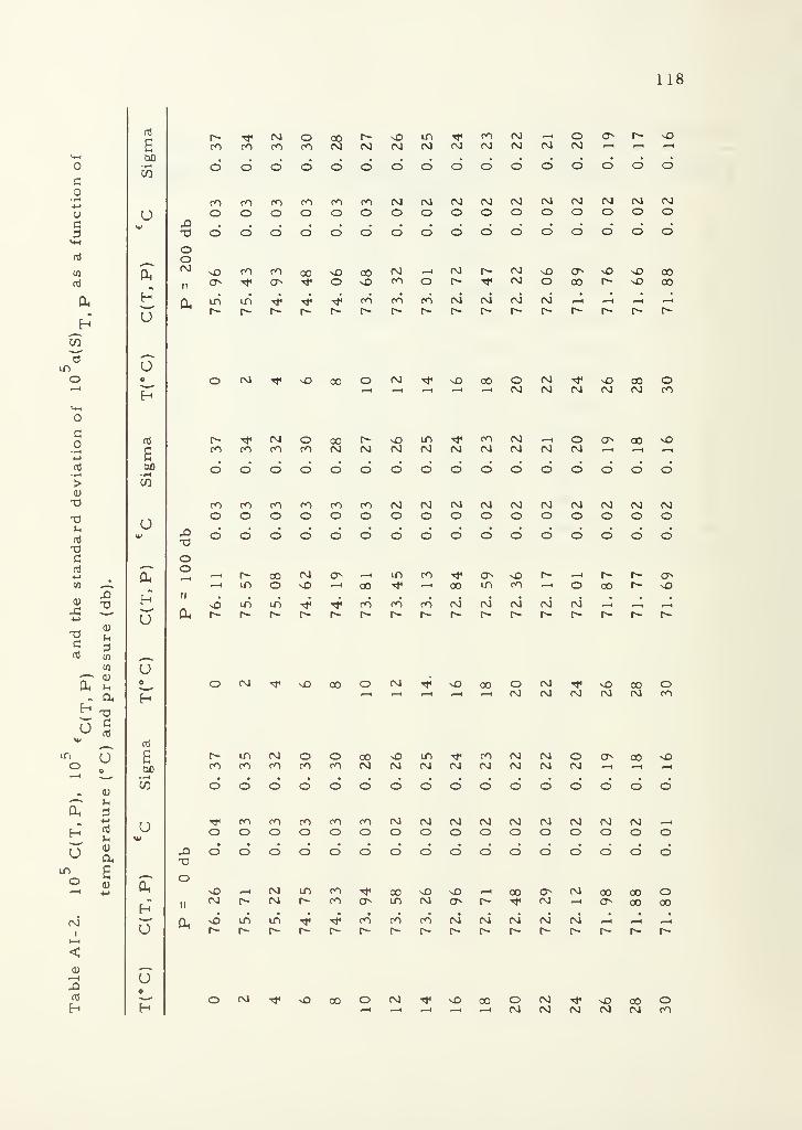
118

o

co+>oC3

CO

iri

>CD

X)

X

XC

<D HM "**

"

>->

0)U

X ufl 3o3 en , ,

w o<1)

cu u •

« a, H

uxi

U

^ V«^*».

»-.

^ d-i-"

HU^

fio<D

""* +J

ro

l-H

<<u•—

i

X*rt

H

£GO

• i-i

CO

U

HU

U

H

rd

£00

• fH

CO

U

00

CO

U

HU

ue

H

oo(M

Oh

^3XO

II

Oh

r^-^rMooor^somrj<mro^HOor^NO00*0000000000000

oooooooooooooooooooooooooooooooosO(v"><v">oo v-Ooo (VJ'-H(VJ r

s" (N^ v-ooN sOvOooONTfOTfOsO^or^^NOoor^-vOoo

ofMr^^ooOM-^vOooorOrfvrjooo

ddoddddcDdododdod0O0Om0OrO0O(\J<\](M<M(NJC\JCM(Mc\lC\loooooooooooooooo

XI

oH h > oo N ^ -i in CO t*< o sO r~- —i r^- [^- s-HinovO'—ioo^, ^ao |-'"> f>ri '-H Ooot-^sOn

OfMT^vUaoofMTFxOaoorO'^vOaoo

r^m(NJoooo^> L^) -^ (,rifNJ<NJoov oovO

ddddddddddddddddoooooooooooooooosX5^H<Mir>rOrfoOvOvD--<oOC7x fvJooooO(Mr^-fMr>-rr)C7Niri(Mos r^'^fsJ —

< o oo ao

NOini/^^cocoeocJc\3r\ir\3rj^^^

f\j ^o 00 (M vO oo o <M ^ vO 00 o<\1 <NJ <nj (NJ <N CO

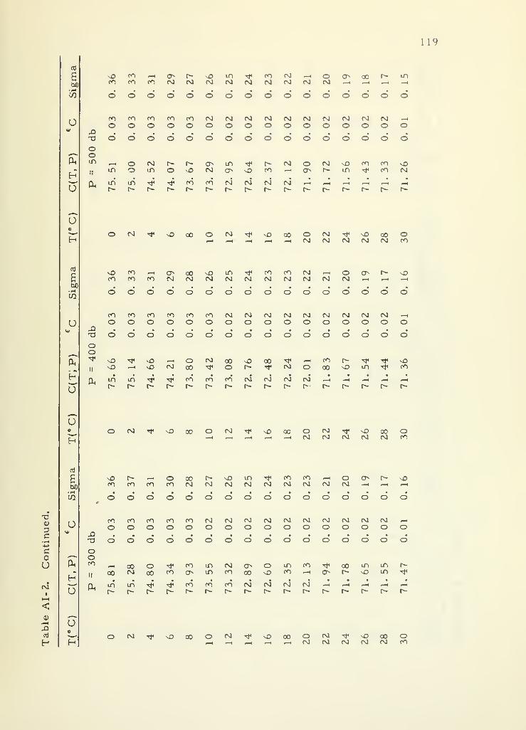
119

• r-t

U

KHU

uo

H

g

u

H

ooin

&

oo

cu

sOfn-^Or^vOLTi'<^rO(M--(00N oot^ ur>rooomcMcMCMcMcMcMcMcMCM—i--.—>~hooooooooooooooooc-iromcooocMCMcMcMcMCMCMCMCMcM —

i

ooooooooooooooooo'dddo*o"o"dddo"o*do*o'o"—lOcvJr^-r^-a^Ln^r-tMotMsDmcOsOLnoLTiOsO(NJos -vO<,r)^-ias r^i-nTt<cocM

0(M^vDooOrJ-<^s£>OOOfM-^vDoOO

vOon^-iOaOvOLn-^oOPOCM-—i O s t^ sOroonrOCMCMCMCMCMCMCMCMCMCM—i—<-hddo'dddooo'oddddddrnoorornoomcMCMCMCMCMcMCMcMCM —

<

ooooooooooooooooddo*ddo*do"o'o"o"o*o*o"o"o*

vO rf -£> —<OCVJoO^DoO^—tf~Or^--^^vOvX)^HvONoo'^tl or^'<ti<MOoo^OLO',^ <,r>

inin^T^corooocMCMCMcM ^ ^-i ,_« ^ _ir- r- r- Is- p- r- Is- r- ; r- i*-' r- r«- f- r- r- r-

T3(1)

C

C

u

CM

uo

H

ccj

w

u

HU

OCM-^vOooOCM-^sOooOCM-'^vOoOO.-h^^^^cmcmcmcmcmoo

vor^^^ooo^-^o Ln Tt,fy^ c>r>'^ooN r^sDromoOrocMCMCMCMCMCMCMCMCM—i—i—

t

do"ddo*o'o*o"o"o"do*do"ddrorooocooocMCMCMcMCMcMcMcMcMcM —

i

ooooooooooooooooJ3XIOOOOOOOOOOOOOOOOoo^ r—iooO'<4H f,riun(Mos OLnc,OTtiooLn |^i^~

Q^ir>LnTf'«4< f,r><,rlf,rlfVlfVJ<NJCMr^^H^Hr-Hr-H

<

Uo

CM xO 00 N >t vO 00 o CM -tf s£> oo oeg CM CM CM CM 0O

120

T3

a•rH

o

OX)rHw

U

&HU

u

oo

CO

re!

s

CO

U

u Oh

H1

U1—

1

<;

a>—

1

U

H H

T3

OOoo

n

PL,

OO

Oh

oo

Oh

ooooooooooooooooroo-irooooororJf\l(N)c\lf\lc\Jfsirsirsl--Hooooooooooooooooo"o"o'o*o"oo"o"o"o"o"oo*o"o*o*

r^r^or^oo --< oo oo --< r~- ^o oo coo r—i

coO-nr-tsOtMoi-nt^ot^LnoofM-Hooi/^xjImroNNriN _, _* ^ _ _h ^ ot— r^r^r^i— t— r^r^r— r^r^r^r^t— r-r^

OCM^^OoOOCMTHHsOooOtM-^vOoOO_,_ r_, r_ir-iC\lr\l(VJC\JCJrO

ir){MOoot^oiri'^ffr\fvJ'-iOON oor^Lr)mmrorsi(M(\irgt\j{varsirvj{Mr-(r-Hr-ir-io*ddo*ddo*o*o*o"o"o*do"o"o'rororororO(MCM(\j{\l(\a{\JCMCM(Mrslr-iOOOOOOOOOOOOOOOOo*dddo'o*o*o"o*o*o"o"o*o"o*o"

r\j^-(THHr-(r-iTti oofr)or^oN ',*l '-H^'^1(Mr^rOoO'^Ot^-Tf—< 00 -£> rj< on CM ,-h OLn^THHoorororJrsJcNir-Hr-Hr-n^H^H^Hr-H

OCMTtisDoOOCM-^sOooOfM^sDoOO

in oo —«os r>-v£)iriTt1 f,oc\ir-ioooor^Lr)rnrOrOfvJ(NJfvJ(M(M(MfsatM(Nar-i—i—i—i

o*do"do*do"o*o"o*do*o"do*ocomcococorvacM(MrM(Mrsi(\ifMcMfMr-ioooooooooooooooooooooo*o*o*o*o'do"o*o*o*o"

^o^oo^^^o^Ninoo—iLncMfsiiD^oo^oiTi-HooLnroor-vDT^roN'^in^'^rorocorg(Nirj(vi--Hr-H^r-H^r-Hr~r^i— r^c— r^r~-r~r^i— r^t— t— r- t— r-

0<MTHHs£>ooO(V)Tt<v£>oOO<M->^sOaoO_ _< _, r_, _iCMCMCVJcMCMrO

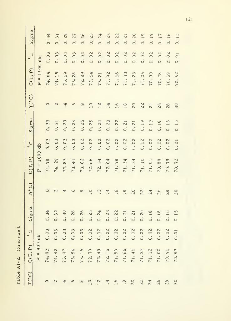
121

s

en

U

Oh

HU (X

co m CMr-cm CM

iTl

CM CMCOCM

CMCM CM

oCM

o o» r» sO m

O o O o O o O O o o o o o o o o

coO

coO

COo

coo

CMO

cmo

CMO

CMO

CMo

CMo

CMO

CMo

CMo

CMO

CMo o^oooooooooooooooo

oo^.(TfLnoooOTt1 -HCMsOt^f'OLnoooocM

vO -iNDCMcX3LriCMON ^0'^< CMOON r^NOvO-* "t CO CO CM CM CMr~ r~ r^ r- r- r- r- r-

o o o o

uCM Tf sD 00 CM vO 00 o CM tf sO oo O

CM CM CM CM CM CO

6SO

•r-i

CO

U

HU

coCO CO CM

00CM CM CM CM

coCM

CMCM CM

•—<

CMo o^ 00 vO lO

O o o o o o O O o O O o o o o O

,£>

COo

COo

COo

COo

CMo

CMo

CMO

CMo

CMo

CMo

CMO

CMo

CMo

CMO

CMo

i—4

o-d o o o o o o o o o o O o o O o oOooi-H

II

0,

00CM

CO00 •tf

CMO CO o

00lO CO

vOo 00

CM

CO CO CO CM CM CMr- r-

1—

1

o o o

T31)

C•i-HMCoU

CMi

i—

(

<

CCJ

H

Uo

H

cd

sCO)

u

Oh

HU

Uo

OO

Oh

OCMTfsOcOOCMTf^OOOCMT^xOoOO^^-.^H^-i^HtNlCMCMCMCMcO

T^CMOoO^O^I^fC^fM^-''—< O 00 00 vO iT>COcOcOCMCMCMCMCMCMCMCMCM^-i—i—<—ioooooooooooooooocOcOcOCOcOCMCMCMCMCMCMCMCMCMCM^OOOOOOOOOOOOOOOOooooooooooodo* o*oo*

cocMr--^ LnoosOOvD^Dr~-cMoocoO"<fOLn--ir^-Ttl ^00^0'*f fsl ^-| OO00^T^COCOCOCMCMCM^^--H^^r-^00

OCM-^vOoOOCMtFsOCOOCMt^vOOOO^i _^-i^i _CMCMCMCMCMcO

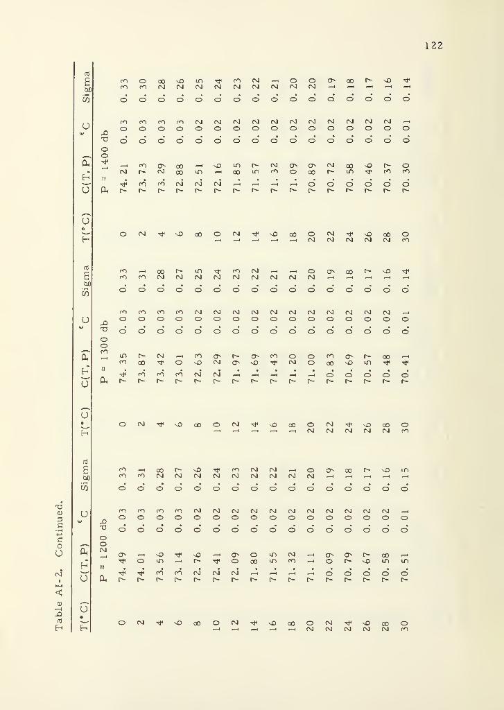
122

GO-iH

CO

U

u

oo

0,

cOOoO^Om^^f^ .—iOO0v 00['"~~-0 Tfcococmcmcmcmcmcmcmcmcm—<—i—<—i—

<

oooooooooooooooocOoorOrOCMCMCMCMCMCMCMCMCMCMCM^Hoooooooooooooooooooo"o"ooo*ooo"oo"ooo*—-i co s oo -Hvomr-cMo^cT-cMooot^ocMr^cMaoin—iootn o°Ooor>-

|-r> T*<(>'"> r'~>

^cococmcmcm^.-h--*^o"ooo*oo°

Uo

Hcm -JD 00 CM t^ vO 00 o 00 ^ vO 00 O

(M CM CM CM CM CO

a)

sOX)

CO

u

Oh

HU

COCO CO

00cm

r-CM

inCM CM

COCM

CMCM CM

,—

i

CMoCM

o-- oo r- vO ^

O o o o O o o O O O o o o o o o

n

COo

COo

COo

COO

CMO

CMo

CMo

CMO

CMO

CMO

CMo

CMo

CMo

CMO

CMO o

T3 o o o O o o o o o o o o o O o oOOco

II

Oh

inCO 00

CMO

COCM

r^o

CO oCM

oo

co

oo m 00

CO co CO CM CMr- r-

.—

t

r^-

o O o o o

uCM n£) 00 CM ^ sO CO o CM <tf ^O 00 o

CM CM CM CM CM CO

T3

c•r-l+->

oU

CMI

>—

I

<0)i—

i

X>cd

H

£

CO

U

0.

HU

U

coCO co

00CM CM CM CM

coCM

CMCM

CMCM CM

oCM

a*- 00 r^ v£> LD

o o o O O o o O o O O o o o O O

a

COo

coo

COo

COo

CMo

CMO

CMO

CMO

CMo

CMo

CMo

CMo

CMo

CMO

CMO O

T> o o o o o o o O o o o o o o o OooCM

II

Oh

o*.—

1

o m «** o

o00

lOLO

CMCO o

r- oolO m

CO CO CM CM CMr^

r—

I

l 1 o or-

O o o

CM nO CO CM ^o oo o CM ^ v£> 00 OCM CM CM CM CM CO

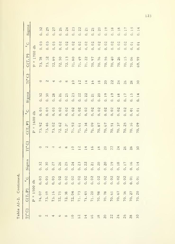
123

T3

di-H4->

OU

CMi

l—l

<

rrj

H

co

U

HU

uo

H

DC

CO

oo—

-

vO^

H II

U Oh

'.X!

£

CO

U

u

oo

H

X>

OoIs-

Dh

XI

oOCMCMCMCMCMCMCMCMCM—t—.—(--<—ir-ioooddoooodooooodoocorocMCMCMCMCMcMCMCMCMCMCM —i -hoooooooooooooooooofNJcJs ot,rioas tMr^v£>NDOs£ii-ns£)0N

ciroNNN-HH-ndddddddc>

OCMTfxOooOCM-^sOcOOCMTfvOoOO^_,^_<_^-i(\4C\JCMCMCMC-)

cMoco^oi^^fMfM ^-lOcr^ooor^LrirfrOoOCMCMCMCMCMCMCMCM—<—<-h~h—ir-iddddddddddddddddoOcOoOCMCMCMCMCMCMCMCMCMCMCM—<—iOOOOOOOOOOOOOOOO

N '^O^OCMOxOC'10oO^O Ln ori fsJ'-|

roroc-ofsirj—H-Hr-Hr-^ddddddd

fM xD 00 CM -<t O CO o M ^ sO CO oCM M CM CM CM m

CMCO

o Is-

CM CM cm<*CM

COCM

CM(M

.—

(

CMoCM

oCM

o 00 r* vO *

O o o O o O O O O O O o o o o o

,n

COo

mo o

CMO

CMo

CMO

CMO

CMO

CMO

CMo

CMo

CMO

CMO

CMO o

.-H

oT3 o o o o o o O o o o o O o O o oooLO

Is-

o LDsD IT) 00m o

00 oCM

00 ooIs- vD

Is-

CMoCM

II

Oh r-CM CM

Is-

CMr-

.—

i

Is- I

s-<—

i

Is-

o o O oIs-

OIs-

o oIs-

CM "t sD 00 CM xD 00 o CM * v£> 00 oCM CM CM CM CM CO

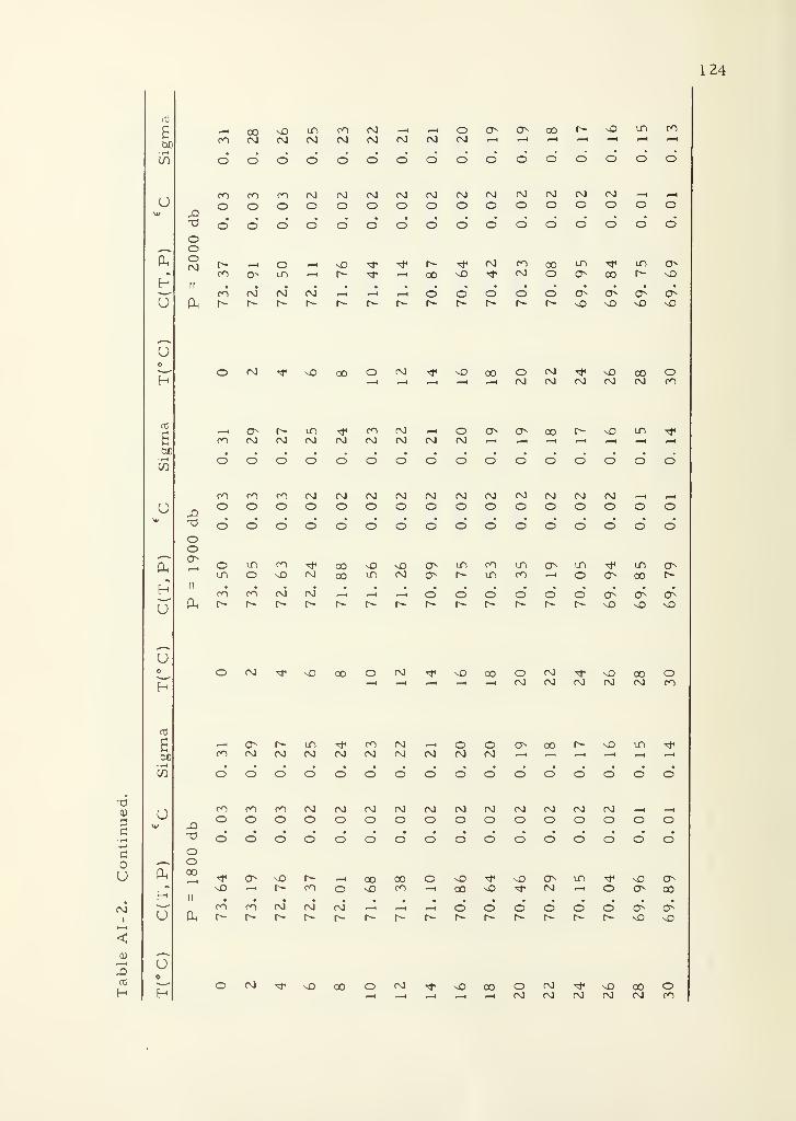
124

T3

a

co

aGO

CO

U

KHU

uo

£ofi

W

U

U

u Oh

HCM

IU

i—

i

<<u

—

~

1—

1

u

H H

oooCM

cu

T3

oo

-—

-

oUh

H II

u Ph

r-ioovOLnrofM^-i-Hoa^cr-oor^^D 1^ ^cocMCMCMCMCMCMCMCM—i —i—i —i —ir^^oooooooooooooooooomcOCMCMCMCMCMCMCMCMCMCMCMr-i^-iOOOOOOOOOOOOOOOOdddddddddddooooor~-^-.o-—ixO'^tl,*'^-Tt<cMoOQOLn ,t| LriON

ci on i-n —i r— xh •—loo^-o^f^oooor^-xon n n n ^—H^oooooa^ooo

cm vD 00 CM vO 00 o CM ^ v£> 00 O1—

1

r—

H

CM CM CM CM CM CO

^ot%-LnTt<cv~)CM--iooN as aor^-^0 Lr>''*1rOCMCMCMCMCMCMCMCM—i-h^-i—i—i—ir-n

d d d d d o" o" o" d o" o* o o" d d d

mmoOCMCMCMCMCMCMCMCMCMCMCMr-i_iooooooooooooooooo' o o S d d d d d d d d d d d d

ourirOTt| oo^vOOs Lr> (V^Lnov Ln'^t| LnoxLnovOCMoo^f^fT-r^Lnoo-Hoooor^co on cm cm ,_i —i-nddddddd'O^o^

OCMTt^OoOOCMTf^ooOCM-^vOOOO^h__h^__CM(M<MCMCM0O

—lor^-iriTticocM—'OOOoor^vOLTiTiHCOCMcMCMCMCMCMCMCMCM—<^^H-H~-<-HSS<SS<S<6cSSc6<D<D'cDSd>ScSrOOOcOCMCMCMCMCMCMCMCMCMCMCM—i —

i

^OOOOOOOOOOOOOOOO^000000000000 000oo00_^^FOsor^- ^-tooooOvD-^vOOLriTiHvOO

NDr-<rN-r/>OvDc,-)^Hoo^D-^CM-HOOs oOII mc">CMCMCMr-i—i—iOOOOOOOOPHr^r^r^r^r~t^r^-r-r^r-r^r^-r^r^-v£)NO

CM •tf vO oo CM sO 00 o CM <tf sD 00 oCM CM CM CM CM CO

125

APPENDIX II

Geostrophic Velocity Profile Comparison of

Standard Versus T-S Gradient Method for

Various Regions in the Oceans(Stations Positions are Given in Table 5)

Note: Original scales reduced in reproduction.

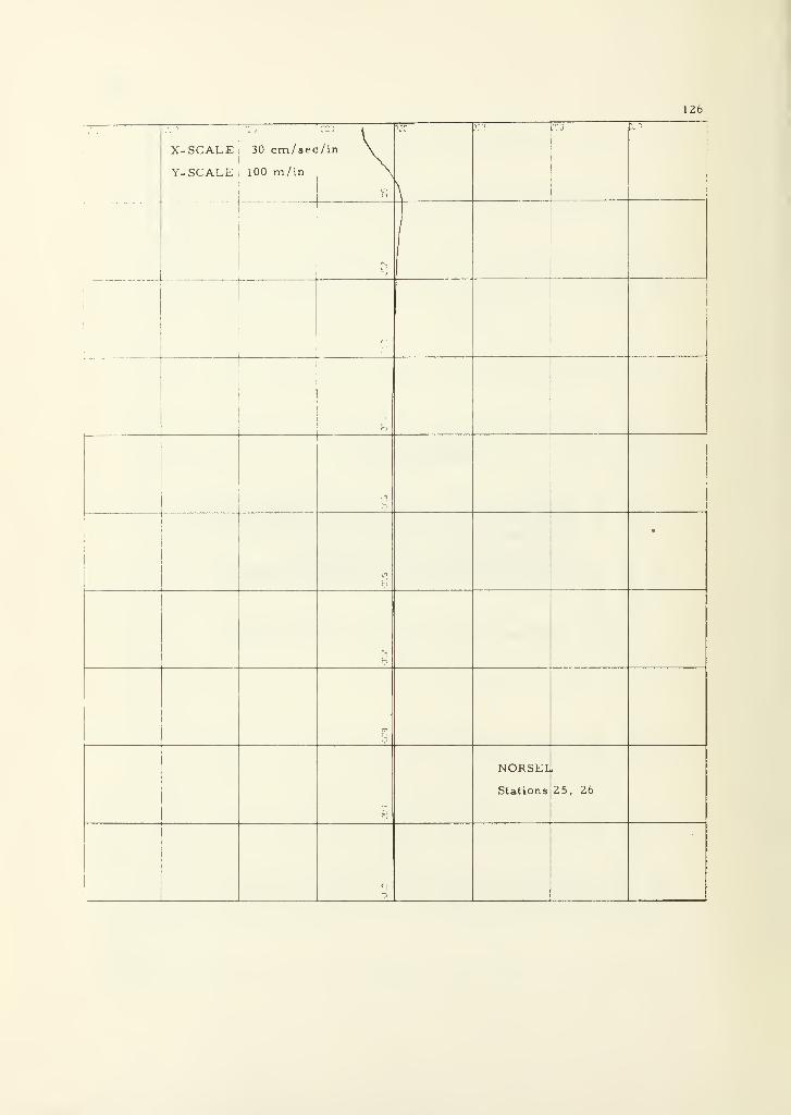
126

X-SCALE

Y-SCALE

30 cm/sec

100 m/in

/in \

r>

.'. o

i

j

,T

•

O

OP

Fj

NORSEL

Stations

1

25, 26

c;

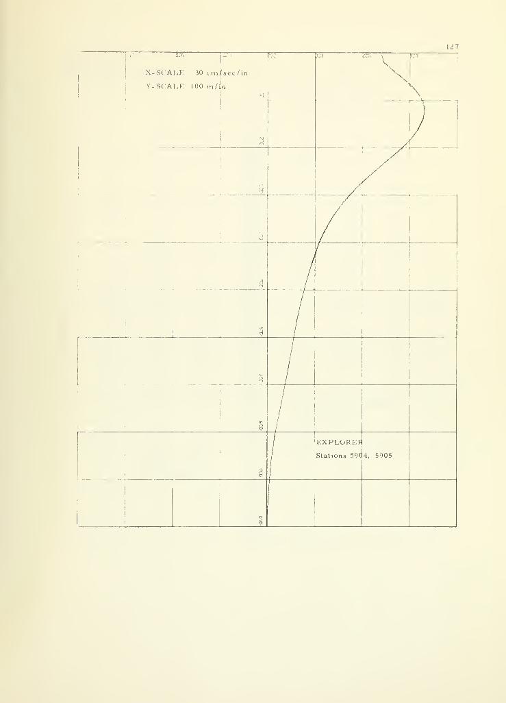
127

1

,

X-SCALE 30 cm

Y-SCALE 100 m/

f s e c / L n

in

b;.: 331 i

'

•

\K1

K1

i

i

1

i

CI

o

/ 1

///I

!

i

n

/

j

i

i

/

/ 1

/ i

/

/ i

/

/

1

I

1

1

/ ii

no

j'EXPLGREP

4, 5905

1

!

i

Ci

[

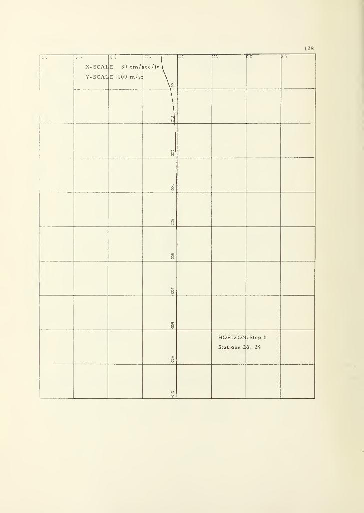
128

'-' D rc'j | 3c; V? 3 5

X-SCAL E 30 cm/ ;ec /in l

Y-SCAL E 100 m/ir

\ Ci

Ci

o

2

t j

in

o

fT

HORIZON -Step 1

Stations 2 8, 29

J1

Cj

^

X-SCALE

Y- SCALE

30 cm/se

100 m/in

/inF

129

ET

HORIZON

Station 24,

Eastropac

25

130

rX-SCALE 1 30 cm/sec

Y-SCALEj

100 m/in

/in 7i

i

"•Jj

\

\

i

i

Ha

LT

o

inCT

d

Cl

H. M. SMI

Stations I'.

TH-31

15, 136

CI

131

X-SOALE 30 cm/sec

Y-SCALE 100 m/in

/in

JJ? Ml Ki to,

1

1

1

1

i

1

1

c

i

1

I

i

n

ii

OB-

3

Stations . 191, 392

o

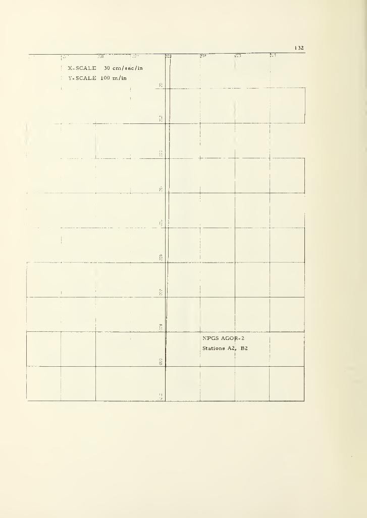
132

j,- :2G w. a P=^ res TO

X- SCALE 30 cm/sec /in

Y-SCALE 100 m/inL-i

i

i

9

!

i

r j

" ri

1

!

l

i

i !

i

rj

i

1

i

i

j

CIrj

•

i

I

i

o

c>IT

j

NPGS AGO R-2

Stations A2 , B2

ff

133

,):.

1

X '

j:'. -3S3 3X 181 )C0 ta

1

X-SCALE 30 cm/sei /in

Y-SCALE 100 m/in

CIi

1

a/

(T

i

i

O

'1

CICI

j

ct

QC)

IKUNA MARU

Stations 13, 14

a9

oa

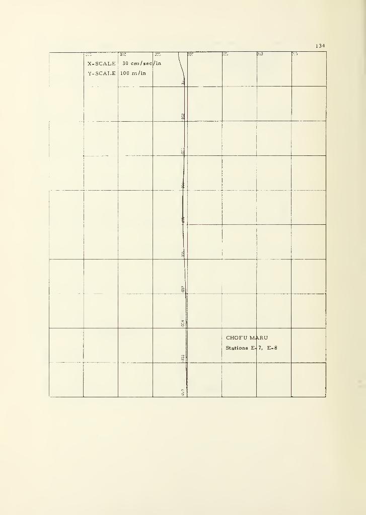
134

X-SCALE

Y- SCALE

30 cm/sec

100 m/in

= 1

/in \

30C 32C HO J13

aCI

c

I

.

-

1!

OO

TCI

CI

CHOFU M,

Stations E-

VRU

7, E-8

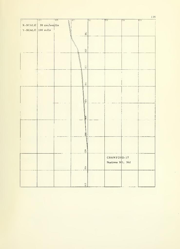
135

X- SCALE1

J

Y-SCALE

30 cm/sec

100 m/in

035

w

OCT

'4

)3C )3) J5E jci;

— \1 g

u fl

11 ^

.... laj

-

pCI

CRAWFOF

Stations 3(

D-17

1, 362

a

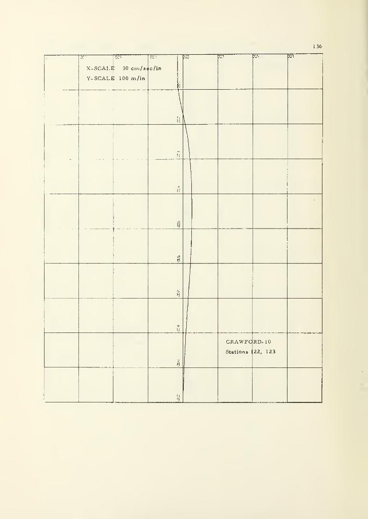
136

1 - 'X'

X-SCALE

Y- SCALE

0">

30 cm/s«

; 100 m/in

c/in

a: ?C1 Vj!3 3CT

\

\

f?

i'

in

,

>

*

CRAWFO

Stations ]

RD-10

22, 123

137

r ,\

J': OV 3DS JK KB Pi* r l j

X-SCALE 60 cm/nx/ini

\

! . - - X \

Y-SCALE 100 m/in !

1

*SI

1

\ \ i9

\\1 !

\ \\ \ ! !

• \ i

ti

i

i

i

\ !

\ :

i

i

\j

^i

i

\\ _) i

\ 1

r}

A !

A i

10

:

'Kci

kw

1

\\

\\ r- i

\CI

\i

1

i

ATLANTIS-5298

Stations 2298. 2299

aj

'?l

138

OS" IOC-5 |uC ljr Mil'rfi 33a

X-SCALEJ

30 cm/sec /in

Y- SCALE 100 m/in

.__y

- . . ... .. --

NM

It

h

f

C'

n.

j 1

?

Proudman Stations

1

139

APPENDIX III

Computer Programs for Hemispheric Computations

140

Program 1. A program to interpolate hydrographic data

on the IBM/360 computer

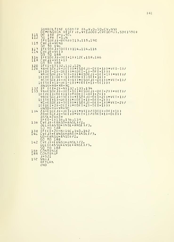
141

lil112

115

lil114

116113

120126

5URRDIME

132133

1 34

136

13814C

142

186188

19G

oninIF(CV(r,c

IF(CV(50IF<CV(GOIF(XA = (

1( (D(XR = (

1( <D<XC = (

K ( n(ANSUIF (

YAM1( (0(YB = (

U (0(YC = (

1( (0(ANSDZA = <

ZB = (

ANSLIF( I

cv( jOLL =

GO TIF( (

CV( JUD = (

GO TCV( JULL =

GO T

CONTCONTJ = 50NN = JRFTLdND

OLTINFNSIGN86 J = i

86 1=1L)(J)-D)=V( N)

19CD( Jl-D)=V( I )

188D( J 1-0»=V( 1 +

188-II 132SC( J »

-

I-ll-DSD( Jl-1 )-()( T

SC( Jl-I + 1I-U=XA+XB( I + 2I-SD< II-I )-D( I

SD( J>-1*1 1-0SDUI-1*21-0=YA+YPSC( Jl-SL( Jl-=ZA+ZB-II 136)-( ANS(ANSD*

188I+2I-N)=< ANSANSU+A

188)=( ANS( ANSU*

188IMJEINUF1

RN

TP (N.V,D,SD,CV,NN)n , vuoooi ,cv< iooa » , sd< igooi

LGINf)( 1( f,50.iN(Ml 113,115,190

(III 114,114,116

( H-ll1)

,132 ,

0< I I I

(III*)( 1-1-II I*

! ) ( I - 1

( I-ll+ XCN» 13?0(1 + 1

111*0(11)(III*0(111(III*+ YC0(1+10( I ) I

tl36,O + ANSANSL +

I14C ,

II* ANSNSD) /

U+ANSANSL +

I12C ,118,186

126*(SD( J)-D( 1 + 1) )*V( 1-1 )/(D( I-l)-D( I + ll I I

I >*<SD( Jl-D( I + ll >*V( I 1/(D( I )-0( I + ll I I

I )*<S0< Jl-D( I I l*V( 1 + 11/i*(0( i +i i -n ( i) i

i

,133,134I |*(SD( J>-0( 1 + 21 )*V< I )/(D( I >-0( I42IM*(SD( J)-D( 1 + 2) )*V( 1 + 11/(0( I+l)-D( 1 + 2) I I

*(SD( J)-0( I+ll )*V( 1+21/(D( I+2)-D( 1 + 1) I I

I )*V(I I /(D( I l-D( 1 + 1) I

«V( Ml) /(0( 1 + 1 )-D( I I I

138LI/2,ANSI 1/3.

140,142O+ANSU/3.2.

LI/2.ANSU /3.

142

Program 2. A program to compute specific volumeanomaly from hydrographic data on the

IBM/360 computer

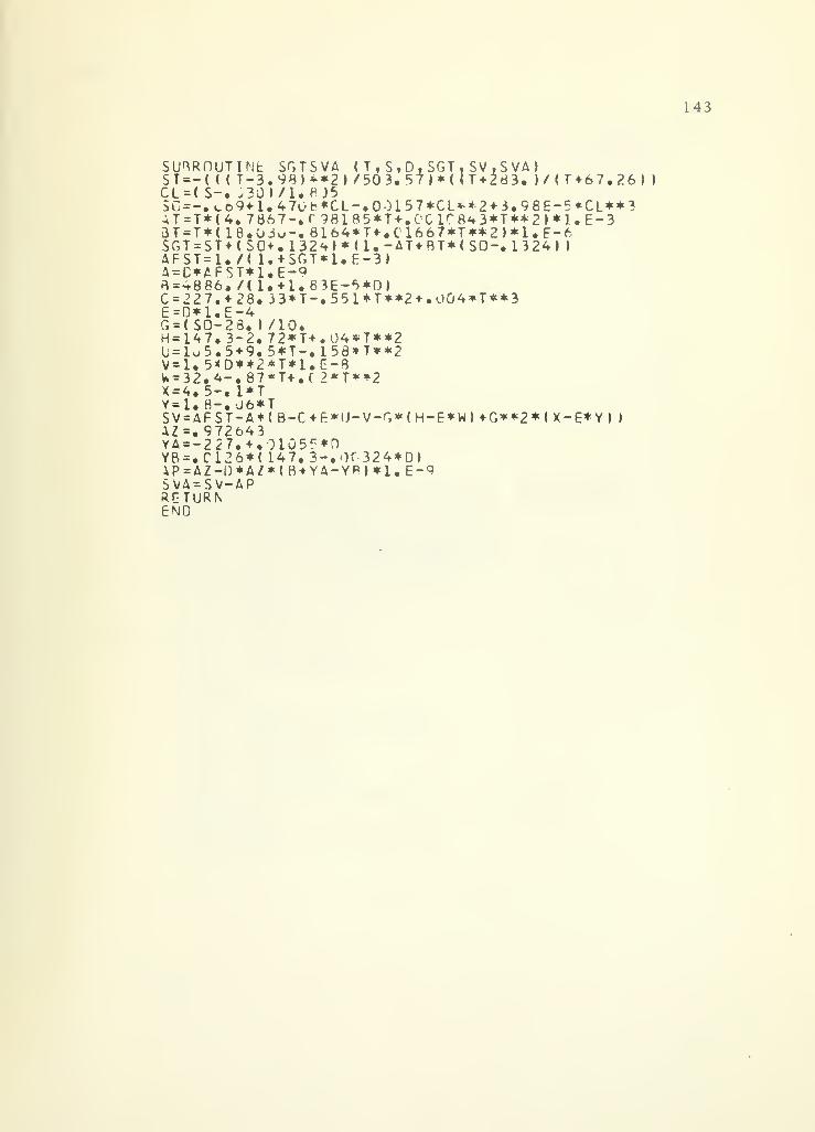
143

SUHRnST=-<CL = ( SSC = -.4T=T*3T = T*SGT = SAFST =

4 = L>AB=**88C = 227E=0*1G = ( SOH=147U = lo5V=l. 5U = 32.X = 4. 5Y=1.8SV = AFAZ=.9YA = -2YB = .CAP = AZSVA*SRETUREND

UT( <

- •

(4(1T*1.FS6...E-2. 3.5<D4-

ST722712-0V-N

INfcT-3>3J9+1.788.0(SO/(

1

T*l/(l28.-48.1-2.9.

**2.871*T•J 6*-A*643• .6*(*AZAP

SGT.98))/l..47067-.3u-..13

. +SG

.E-Q

.1.33*T

SVA (T,S,D,SGT.SV,SVA)**2> /503.5 7)*( (T+28 3. »/< 1*6 7.26

H

b*Cl-.O015 7*CL**2+3.9 8E-5*CL**3r98185*T*.CXlC8*3*T**2»*l«E-38l64*T«-.Cl66 7*T**2)*l.E-62<t)*U.-AT*BT*(S0-.13 24)

)

T*l.E-3>

63E-5*0)-.551*T**2-»-.UG4*T**3

72*T+,04*T**25*T-.158*T**2*T*l.E-8

/10.7;

T+.C 2*T**2

T( B-C*E*U-V-G*(H-E*W) «-G**2*( X-E*Y) )

•^ 1 ,"i e: e a noi05f*n147. 3-. Of 324*D)*(B+YA-YR»*1.E- C

144

Program 3. A program to compute geostrophic cur-

rents by the Helland- Hansen equation

and the T-S Gradient equation on the

IBM/360 computer

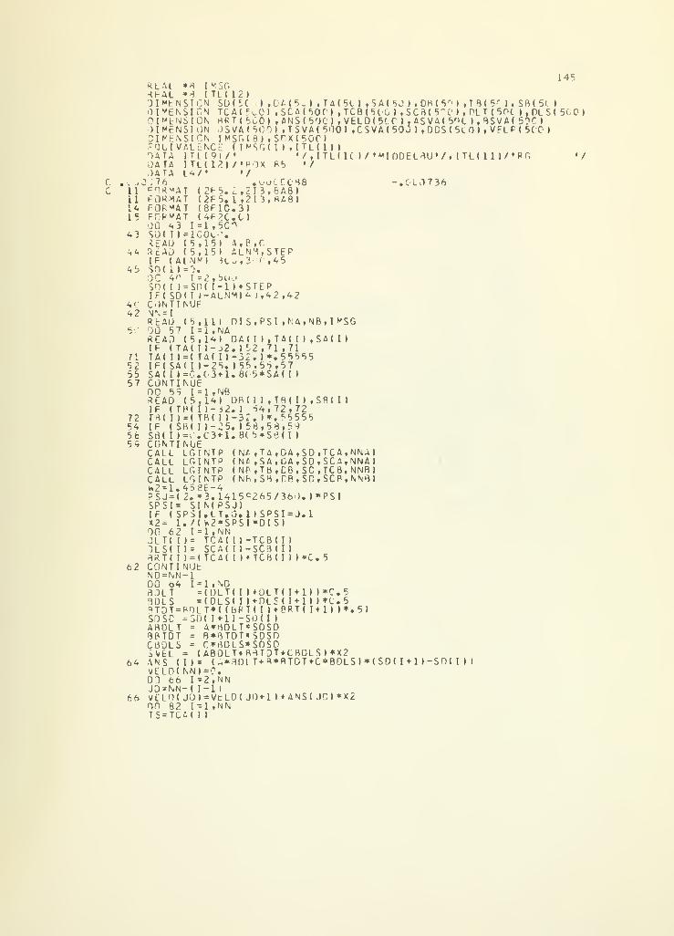
11il1415

43

^,4

45

4C^2

71525557

72545fc

59

62

64

66

KL-IF

011

011

CI'QOAOAOA

: :7enFaFOFO

soSEReIFsoocsnIFCON\RE00REIFTAIFSACO00REIFtbIFSBCOCACACACA*2PSSPIFX20001olBRCONO00SOBOBTSOABBBCDsvAN1

VEDOJOVEonTS

Al *AL *MENS*ENSMENSMENS^ENSLI VATA I

TA I

TA I

6^MATHMATRMATPMAT43

( I >=

AO (

AO (

( Al(11 =

40( I )

=

( SD(NTI N= 1

AO (

57AO (

(TA< I ) =

( SA(( I » =NTIN59

AD (

(TP( I » =

( SB( I )

=NTINLL LLL LLL LLL L= 1.4J=( 2SI =

( SP= 1.62

T( I I

S( I I

T( I )

NTIN= NN-64

LTLSOT = PSD =DLTTOTDLSEL =S ( I

LO(N66

= NN-L0( J82

= TCA

B I MSG8 I TL < 1 2 »

ION S0(5( )

,

TCA( C...C»

BRT( 500)DSVA(5CQIMSr,(8) ,

LENCE (I"SG<Tl ( 91 / •

T L < 1 2 ) / • P X

IONIONI ONION

145

LM5- I ,TA(5l ) ,SA( 50 I ,DB(S'' ) ,TB(5' ), SB(5<. I

,SCA(50f» , TCB (510 > ,SCft( 5~a') , PLT(50t ) , DL S ( 5<d, ANS(500) ,VELD<5'..T >

,

ASVAt 5'H. I, 8SVA( 50-' I

) ,TSVA< 500) ,CSVA(50j I , DCS ( 5i I , VFL F ( 5(0 )

S0X(50CI1 ) ,ITL(1M

•/.ITLdCI/'MIDDELBU'/.ITLdll/'PG •/85 ' /

,^13,( 2F5.(2F5. 1,213,(8F1C.3»(4F2C.C I

1=1,50?)lCO^-'.5,151 A , P , C5,15) ALNM,SNM| )C0t3-.!< ,

I=2,5ujS0( I-D + STEPI >-ALNM)^ ),4UE

•:rcs86A8)8A9)

TEP45

2,42

-.010736

5,11I=i,5,14( I )-( TA(I )-20.0 3UE1=1,5,14( I )-( TB(( I I-0.C3UEGINT01 NTG INT

1 NT58E-.*3.SIN(SI.L/( *21=1,= TC= SC= i TCUfc

11=1,= (D= <D

OLT*30( I

= A*= B*= C*

( AB) = (

NI=C1=2,( 1-1Dt=V1=1,( I )

) DI S.PSI ,NA,NB, IMSGNA) DA( I >

,

j2. )S2,7:I )-32. )*,5. I 55,55«-1.805*S/

TA( I » ,SA( I )

1,71.55555,57

»A( I )

MB) DB( II ,

3 2. ) 54,1 1-32. I*2 5. 15 8,51. 8( 5*S

(N(N(N(N

P

PPP41415PSJ)T.O.*SPSNNA( I I

All)A( I I

A ,TA£ ,SAP ,TBH,SB

c 265

1 I SPI *D I

-TCB-SCBTCB

TB( I I ,SB( I )

72,72.^55558,596(1 )

,DA,SD,TCA,NNAI,OA,SD,SCA,NNA), Ce.SC, TCB, NNB),nB,SC,SCP,N\B)

/36 0. )*PSI

SI=J.lSI

( 1

1

(I)( I I )*C5

NDLT( I )+0LLS( I )«-0L( (BRT( I

)

11-SD(

I

BDLT*SDSBTDT*SDSBDLS*SDSQLT+BBTD**BDl T+R

NNI

tLD( JO+1NN

IIMII*C5( Ul) ) +C. 5BRT( 1+1) I*. 51

CBDLSI+X2BTDT«-C*8QLSI*(SD< I 1 ) S0( I )

I

l*ANS( J0)*X2

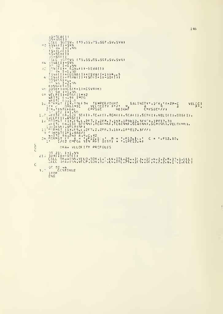
146

s s=<;c a < i

»

dS = Sf)'( ! I

C-ML SGTSV* ( TS ,SS ,DS ,SGT ,SV,SVA>>'? ASVA< I ) = SVA

D'"1rt't I=I»NN

TS=rcH( i

)

SS=SCB( I )

js=sn( 1

1

:'AL SGTSVA ( T.S.SS.OS ,SGT,SV,SVA>-A i = VA< I I =SVA

01" 92 I=1,NN»: >sva< 1 1= asvm( i »-bsva( 1

1

)'• •>«. I =1 ,MDTSVA( H = (DSVA( D+DSVAi I + l))*0«5

4 :. SVA(I»=TSVA(IIMSnU*l)-SO(IMTDS(NN) =u.m S6 I =2, MM<=NN-< 1-1

)

4* JDSi* )=|11jS« K*l H-CSVMK I

O.J "5 8 I=1»NN•; a v:lp( i )=uos( i >*x2

'aRITE (o,9l I«5Gv*R I TE (6,1.)

U c ^mat (IX, 'DEPTH TEMPERATURE S AL I N I T Y ' , ir x, • A+2 B-C VELTCl

UV i: DYNAMIC VELCCITY ?•/• ". A B A P«,2 'X, • INTERGAL C«/SEC HEIGHT CM/SEC//I>0 iC2 I=1,ND

1.,? *RfTt ( 6 » 1J I SD(I> tTCAU ) ,TCB(I ) ,SCA( I » ,SCBU ) ,VELDU ) f DDS( I > i

1-/CLPI I ) ,ANS( I )

1^ format ( 1X,F5.1, ,2F7.2j2FR.3,16X.lP3fcl2. 3/*r;X.lPFl?.3)*K I TL < b,13) SD(NN) »TCA(NN> tTCB(NN) »SCACNNI , SCR

(

HH 1 , VEL D( MM ),1 J!)S( NM , VFLP( NM

13 c ORMAT ( lx,F5.i ,2F7.2,2F8.3,16X,1P-»E1?. 3/// I

9 '" )RMAT< 1H1 ,6A6/)*kITC (o,24» A,H,C,X2

2A FHRmat (• A = • , F 1 2 . 1 » • B = SF^.K,' C = '.F12.10,1' 1/(2 OMEGA SIN PHI DISTJ = ',1PE12,4I

DRAfc VfcLOf I TY PRCFILES

t\:,

3.

:

do. 21!, I=i,NNsox( i »=-sn( 1

1

CALL DRmw( NN.VE LO ,SDX ,1

,

CALL 0^ A tri ( MN.VFLP , SOX ,3 ,

GO

, L4,ITL,25. ,1' J. ,1T ,<*, 2,2.3, 1 M.LLL )

,L4,ITL,?5.,1C "). ,lf , A,2,2,b, 1~,1,LLL I

TO 44CONTINUE

srooEND

147

Program 4. A program to compute the geostrophic

surface velocity over the FNWC 63 x 63

fields on the IBM/360 computer

148

5c>

7

1 1

iHWLNIni vt\

FCRMmFCkMAFCRMAFCKMAFCKMAF C P M AFLkMA

SIGN5 I JNION

3(T<VX

(5ILN VT tlril,T (/ )

T (13,1T ( IX, 1

T (1H1,T (IX, I

T (3F20

63,63),VCX(62,62),VCY(b2,fc2)6 3,o3) , ViX( 6 2,t 2) , VAY( 6 2,62) .VoXl 62 ,n2 >

,

VBY{62 ,62)(62,62)tVY(62»62)tIT(24)tD(6) t IX<62J ,1 Y(62)62,62)' A = ',lfh2U.~,' d = ',E20.5,« C = »,r20.5/)

3 F y . 2 )

319/)2*t£-*// )

3F3.2). 10, It>)

C IU'T CCNTRuL INTEGER IN COLUMN 65C IC'tJT = U PPINT VtLGCI T Y LISTING ONLYI I OUT = 1 PRIM CCNTGUPeD MAP ONLYC If'UT = 2 PS INT rtCTh LISTING, AND CONTOUREDf.

RF.AO (5,ll)£,a,C,I HJTD( 1)=0.C<2)=i21.3D(3)=6l.OC(4)=6L.O0( 5)=30.5D(6)=30 .5C(7)=30.5C( a

. )=30.5Cf M 1 = 1, a2IY( I )=I

<rl 1X( I ) = I

C OC 10 1 = 1, c3C DC 10 J=l,63

10 S(I,J)=35.DC 15 K=l,dRCiC (3) ( (T( I, J ), 1=1, b3) ,J=l,o3)READ (8) ITIF (K.EC.l.) GO TO 13GC TC 2 3

13 DC ZZ J=l,o2DC ZZ 1=1, o2VX( I , J)=Q.VY( I , J)=0.VAX( I , J )=T( I, J j-T( 1+1, J)VAY( I,J)=T( I , J )-T< I , J+l)VWX(I,J)=(T(I f J)*T(l*i t jj),.5#vAX(I,J)VBY(I,J) = (T(I,J)+T(I,J + 1))>..5*VAY(I,J)

C VCX( I, J )=S( It J )-S( 1*1, J )

C VCY( I, J )=i( I, J )-S( I , J+l )

ZZ CCNTINUEGC fc 15

23 DC 24 J=i,62DC 2^ 1=1, o2DTa=t( I ,J)-T( 1*1, J )

DTY=T( I ,J )-T( I , J + l)BCX=(T( I, Ji+TU + 1, J ) )*.5*CTX8CY=(T(I,J)+T(I,J+l))-.5«CTYDSX = S( I , J)-S( 1 + 1, J)

MAP

C CSY = S( I , J )-S( I , J + l )

DAX=(VAX( I, J )+DTX )* .5DAY=(VAY( I, J)+DTY H .5CPX= (VBX( I, J ) + BDX )> .5DRY= (VHY( I, J ) + BQY ) * .5

C DCX=(VCX( I, J)+OSX )*.5C DCY=(VCY( I,

J

)+D$Y )> .5CALL CCRFOR (I,J,CFL)VX( I , J) =VX( 1,J) + (<DaX-A + DBX*BVY(I,J)=VY( I, J )+( (OAY«a+CBY*RV( I , J)= SQRT(VX( I ,J)-»-VAX( I , J)=DTXVA Y( I, J )=DTYVBX( I, J)=BDXVEY( I , J )=BDYVCX( I, J )=DSXVCY( I , J )=DSY

2 + VY( I, J )**2)

)»D( K )~CFL )

)>-0<K) sCFL )

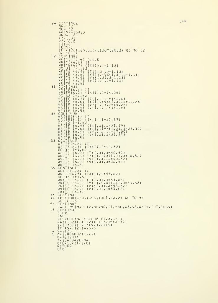
2-» CCNTINUtnr = b^NC = 6 2AW IN=-100HNU= 10.A/=.001BZ = 0.0IJT =

!CCN=1IF ( I CUTGc TP 14

52 CCNTINUEWRITE. (t,«t) A,i,CWPITE( 0t 6) ITWRITE(6,7) (IX(I)DC 31 1=1,62

(6,9) m i, j), j=i, 13)IY( I)<VY( I

(V( I,

149

31

32

33

34

3514

54

15

,u

E0.0.UK. I0UT.EQ.2) GJ TO 52

1 = 1, 13)

(6

(e,(6,

(6,( o , 6 )

(6,S)(6,^)(6,5)

wRITcWRITEWR ITEW « I T r

WR ITFCCNT INUE* R I T E < 6 , d)WR ITE (o,7)DC 32 1=1,WRITEWR ITFWHITEWRITEWP ITECCNT INUEWRITE(6,d)WRITE(6,7)DC 3 3WR ITEWR ITEWR ITEWR ITEWR ITECCNTINUEWR ITE(6,c)WRITE (6,7)DC 3<«

WR ITEWRITE

6)9)'->)

5)

( VX< I , J ), J=l, J ),J=1, 13)J) , J=l, 13)

13)

IT( Ix ( I )

b2) (T ( I.

I Y ( I >

(VY< I

,1=1^,26)

J), 1=14, 2c )

, ( VX( I , I ), J=14,26)J ) ,J=14,26)

I V < I.J) , J=14,2t)

IT( IX( I )

1=1,52(6,9) (T ( I

, 1=27, 3=1)

( <?,b )

(6,9)(6,=))(6,5)

J) , J=27, 3<=)

IY< I ) , < VX( I, J ), J = 27,39)(VY( I, J ), J=27,39)(V( I, J) , J = 27, 3 C )

IT( IX( I ) , 1=40,52)

1=1,62(6,9) ( T ( I

( 6,6 )

(6,9)(6, ?)(fc,5)

WW ITEWR ITEWR ITECCNT INUEWR ITE (6, 3)WPITE(6,7)CC 35 1=1,WR ITEWR ITEWR ITEWR ITEWR ITE

1Y( I )

(VY( I

<V( I,

J), J=40, 52), ( VX( I , J ) , J = tO,52), J ) , J = 40, 52)J), J=40, 52)

IT( IX( I )

6 2(6,9) (T ( I, J) , J

1=53,62)

(0,6)(6,9)(6,(6,

53,62)IY( I),

(

VX( I, J ), J = 53,62)(VY(I,J),J=53,62)

J) , J=53,*2)) (V( I

(V,NF,MC,IT,BNr,AZ,8Z,AMIN,IJT,IC0N)

CCNT INUEIE ( IOUT.EO. l.CR. IUUT.E0.2) GOGC TO 15CCNT INUECALL WPTMAPCCNTINUESTOPENDSUBROUTINE CCRFGP (I,J,CEL)R=(I-32)*(I-32)MJ-32)MJ-32>S=(973.71-R )/($73.71+R )

IF (S-. 125)4,5,5S=.125A= 1.86603/ ( i. + o)D=38l.O/AT= 1.45842E-04CFL=L./(T*S«"C)RETURNENC

TO 5<t

150

Program 5. A program to compute the geostrophic

surface velocity over the FNWC 63 x 63fields on the CDC/3600 digital computer

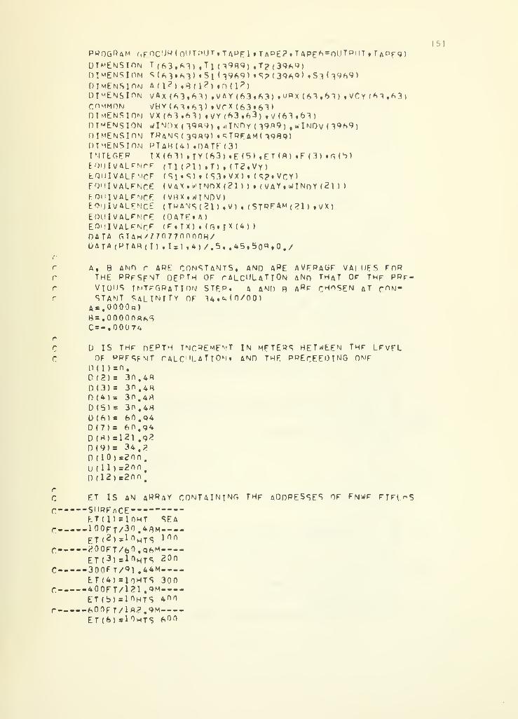
151

PPOGPftM r,FOC'-IW<Ol)T"r>UT»TAPEl t T ftP£2 t T APE^ = OilTPi IT , r,\c>F9)

DT MENS! ON T(63,fci),Tin9fl<»),T;? (39*9)DI MENS I ON S (6 3»63) «5l (3 96 9) »S? (39<S9> » Si

(

3969)DIMENSION A ( 1 ? ) iR ( 1?) in( 1?)DIMENSION \/Ax(63»61),VAY(63t63)«v/PX{63,6l),VCY<6l f *3)COMMON \/BY(61»61> tVpX (63«6l>DIMENSION VX (61,61) »VY (63,63) ,V (61,61)DIMENSION wlNf)x ( 39R9) t wINr)Y (39P9) , rtlNDV (3969)DIMENSION TPANS(39«9> «<;TqEAM(l9Q9)DIMENSION PTAH (4) .DATE (3)

I M TEGER T X ( 6 1 ) . i y ( 6 3 ) t E ( 5 ) . E T ( fl ) . F ( 3 ) » r, ( 4 )

EQUIVALENCE (Tl (?l) ,T) . (T2.VY)EQDIVALFMCF < S] . S ) ( S3t VX ) ( S2» VCY

)

EQUIVALENCE ( VAX.WINOX (?1 ) )

t

(VAY, WlNoY (21 )

)

EQUIVALENCE (VHX.WTNDV)EOiJ I VALENCE (TwANS(21),V)t(STPEAM(?l),vX)EQUIVALENCE (DATE, A)

EODIVALFNCF (P»TX) « (G»JX (4)

)

DATA GTAH/f707700f)0H/DATA(PTAR(T).I = 1,4)/.5,.45»50P»0,/

A, B AMD r APE CONSTANTS, AND APE AVERAGE VAt.UES FOPTHE PRFSFNT DfPTH OF rALCDLATlON ANn THaT Or THF PRf-VIOUS TMTFGPaTION STEP. ft AND P, A^F rHOSEN ftT CON-STANT SftLlNTTY OF Htm'O/00)

As.OOOOq]Bs.OOOOnPisSC = -. 00074

D ISOF P

D(l) =

D(2)aD ( 3 >

D (4) =

D (5) =

D(6) =

D(7) =

D(*) =

D(9) =

0(10)U(U)D ( 1 2 )

THFRFSFn.

30.3n.30.30.60.60.121,34.

s2on= 200e2oo

DEPTH INCREMENT IN METERS BETWEEN Thf LFVFLNT calculation, and the preceeding omf

4fl

484rt

4rt

Q494922

rc ET IS AN aRRay containing THF ADDRESSES OF ENWF FTFLnS

C SURFACEET(l)slDHT SEA

p 10 0FT/3 0.4pMET(2)= ln HTS inn

r 2 0FT/6 0.Q6ME T(3)alO HT «

i200

C 300FT/P1 ,44MET(4)*lr)HTS 300

C 400FT/121 ,<3M

ET(5)*10HTS 400

r -600FT/1A2.9MET (6) slOwTS ^00

•800FT/243.8M----ET (7)alO H TS flOO

.1200 FT /365.8m---ET(8)*l0HTSl?00

E IS AN ARWAY WHICHFOR THF. SUBROUTINE

DATE (1 ) aO.E (l)aDATF(l)E(2) IS DFFINED LATERE(3)=0E(4)s3ht (5)=5l_TAPEl

152

CONTAINS THE CALLING PARAMFTFPSRDmSTF WHFN RFAOINr, fmwF FIELDS

IN THE no LOOP

ISVO IS A VELOCITY FIElD PRINTING OPTION AS FOLLOWSr COMDLETE VELOCITY FIFLO PRINTOUT AT ALL OFPTHSC 1 SURFACE V/FLOCITY FIELD WILL HE PRINTED ONLYr 2 NO VELOCITY FIFLD PRINTOUT WTLl RESULT

ISVOa2C. ICO IS A CONTOUR PRINT SELECTOW AS FOLLOWSC ALL LEVELS CONTOUREDC I SURFACE COMTOUR(S) ONLYC 2 NO CONTOUR(S) PRINTOUT

ICO = 2

41

2(S

1351351

1361361

137

IF ( ISVO.E0.2)f,o TO 26IX AND TY ARE ARRAYS WhICH SERVE TO nUmhf Thf ROWSAND COLUMNS OF The GRjO FOR PRINTING PURPOSfS

DO 41 T*l »63IY(I)=II X ( I ) =1

READING IN OF TFHPFRATURE ANr) SAHNlT* FTELDS FOU OW<;

NailDO 19 K*l ,NlF(K.GT,fl)GO TO 1?7GO TO(135,l36,l3«,140,l*2,l**,l*6,l*«)KE (2)*ET(1 )

CALL »DMSTF»Tl,E)IF(E(3) ,njf.0)GO TO 1351READ(2) SI

GO TO 17

E(2)»ET (?)CALL RDMSTF(TltE)IF (E(3) ,mf,0) GO TO 1161READ(2) SIWFAD(2) S300 137 lx\ ,3R6QSI (I)a(i9,S2«Sl d) 5.4«#s3(I) ) /25.GO TO 17

138 L(2)*ET(3)1381 CALL RDMSTF(T1,F)

IF(E (3) ,MF.0)GO TO 1381REA0(2) S2DO 139 1*1*3969

139 SI (I)«(39.04»S3(I) ln,96*S2(I) >/50.

GO TO 17153

1401401

141

E (2)«ET(4)CALL R0M5TF (Tl »E)IF (E (3) .mf.0)Go TO 1401DO 141 1=1,39*9Si (I> = <A.5**S3(T> *4 1.44*S2( I> )/5n,go TO 17

1421421

143

E(2)=ET(5)CALL RPMSTFU1 iF)

IF (E (3) ,NF.0)Go TO 1*2]RFAD(2) S3DO 143 T=i»3969SI (I)*(?M.08«S2(I)*21.Q2»S3(T) >/50.GO TO 17

144

1441

145

E(2)«ET(6)CALL HPMSTF«TltF)IF<E < 3 > .MF.O)f,0 TO 1**1*EAD<2) S?uo 145 Ixi,3qftgSi (I)*(i7.i2*S3(I) *32»« fl *S2'T) )/5o»GO TO 17

1*^

147

E(2)-ET(7)CALL RD^STF (Tl *F)

IF (E (3) .MF.0)GO TO l4f>1

wEAD(?) T?RFAO(2) S3DO 147 I«l«3969SKI)s(156«lft»S?(I)**3.84»S3(T))/?00,GO TO 17

1 4*14B1

149

127

17

1^

U

E <2)*ET{fi)CALL ROMSTF(TlfF)IF (£(3) ,NF,0)6O TO 14R1UO 149 I»l,39*95i(I)«(34.24»S?(T)*lft5.7f.»S3«T))/?00.GO TO 17

«EAO(2) (Tl (I) ,1*21,3989)WEAR (2) SiTHE FIELDS ARE WRITTpN ON OlSKWRITE (9) T,SIF (K.E0.8) WRITE (9) T2»S'*CONTINUEREWIND 9

the actual calculation begins here# the first

LaTION INITIALISES cO MPnNIENTS at thf level of

eo motton*FAD(9) T.SDO 22 jsl ,*>2

DO 22 Ial % hZVX< I* JJ a n.

VY( ItJ)=0.VlllJlaO,

CaLCU.assum.

VAX(ltJ)*T(X*J)«T(T»l»J)VAY(IiJ)sTU»J»-T(T»J*1 >

VBX(ItJ)a(T(T»J)*T(I*l»J) )».S»VAX(Ifj)VRY(ItJ)«(T(ItJ)*T(ItJ*l))*.5«vAvdtj)VCX (It J)rS(I» J)-S( I 1 • J)

2 VCYdt J)sS(!*J)«S(TtJ*l)

154

THE ACCUMULATION OF COMPONENTS RFGINS HEREM2sN*l00 15 K*?,M2HEAD(9)TtS

23 UO 24 Jsl,6200 24 Ial .62OTX*T( It J)-T( 1*1 ». I)

OTY*T(ItJ)-T(ItJ*l )

«nxs(T(It I) *T ( 1*1 i.]) )*,5«0TXHf.)Ys(Tt It J) *T< I* J*l> >*.5*DTYDSX=S(ItJ)-S(I+l t J)

OSY=S(I«J)-S(IiJ*l )

OAXs(VAx (It J) *OTX) «,50AY3(VAY(T» J) 0TY)*.5OBXa ( V8X ( T t J) *RDXl *.SORYs(VBY ( I«J) ROY) ».5DCXs(vCX ( It J) *[)SX) *,5DCY=<VCY< !• JJ DSY> # .5

f CORFOW IS A SUBROUTINE FOR COMPUTING CORlOLlS FORCFC RASED ON GRID POSITION!

CALL CORFOR (ItJtCFL)VX(I#J)»VX(1»J) *< (DAX*A*DRX*B*nCX»C>»D(K) »CFl> *,4665VY(I»J)»VYlI|J)*( {OAY»A*OBY*R*nCv»C)»D{K) «CFL) #.46651*,4665V ( I tj) * SORT(VX (T«J)*»?*VY (It J) *•?)vax

( i ,j) snrxVAY ( I t J) rOTYVMX ( I » J) arjOX

VRY ( I t J) sROYVCX(I tJ)sOSXVCY(It J)snSY

24 CONTINUF

FOR COMPATIBILITYMUST BF EXTENDED

DO 40 1*1 ,63VX (63,1 ) =vX (<S2, T )

VX ( 1,63) svX ( It(S2)

VY(63t I)sVY(62t I)

VY< It63) svY ( It6?)V (63,1) iv (62, i j

40 V( It63) *v

(

It62)

CONTOUR ANO PRINTING SFLECTION18 IF

(

IC0.FQ.2JG0 TO 16IF (ICO.EO.l.AND.K.NE.N)GO TO 16WRITE (6,1

)

CALL CONTOUR (VXt 63,63 f 3. ,3lAvX)CALL CONTOUR VYt63t63t3.t3LAVY)

16 IF(ISV0.FQ.2) GO TO 15

*/ITH PLOTTING ROOGPAMt VX t VY AND \/

TO 63*63 ARRAYS dTH DUMMY VALUES

IF ( ISVO.FQ.l . Aivin.K.NF.NJ) GO TO 15155

1 F0RMAT(1H\)h FORMAT (/)6 FORMAT (T J tl3F9.4)7 FORMAT (1X«13X9/)H FORMAT (3XM3F9.4)q FORMAT (3xtl3F9,2)

WRITE (ft.l )

WRITER. 7) ( IX ( T ) Ial»l3)DO 31 Isl,63

<6.R) (T(I.J)tJ*l'l3'(S( It J) »J»1 «13)TY ( I) (VX(T»J> tjal»13)(VY ( It J) »Jal«13)(VMItJ) • J*1»13)

31

(8*9)(6,6)(ft. A)

(6»ft)

(6,5)

32

WRITEWRITEWRITEWRITEWRITEWRITEWRITE <k» 1

)

W*ITE(6,7)DO 32WRITEWRITEW»ITFWRITEWRITFWRITEwRITE(6,nWRITE (ft. 7)

(IX(T) ,1*14,26)I s l

.63(ft.9) (T(It.J) • J=l4t?ft)

(S(T« J) pj«1*#26)I Y ( T ) , (VX( I« J) » J«14i2ft)

<VY( I»J) .Jsl4»26)(Vlli J) «J«14 t 26)

(ft.9)

(6.6)(6»«)

(6. ft)

(6.5>

(IX (I) »Is27 t 39)

1=1, *3(6,9)(6*9)(6,6)(6»ft)

(6, ft)

(6,5)

DO 33WRITEWRITEWRITE*RITEWRITE

33 WRITEWRITE(6tl)WRITE (6*7)DO 34 I,WRITEWRITEWRITEWRITEWRITEWRITEWRITE (6*1 )

WPITE (&»7)

(T( Itjl t J»'7t39)(S(I.J) iJa?7,39)IY( I) , (VX ( T» J)

t

J*?7f39)(VY(T.J) ,J=27.39)(V(I»J) .J=?7.39)

( IX ( T) . I«40t52),63

(6,9) (T(I,J) t J«40,52)(S< I • J> J 3 40«?»2 )

TY(I) » (VX (T»J) J =40f52)

(VY(I«J) tj= 4 0.52)

(V( T, J) , Js40,52)

34

(6.9)(6.6)(ft.fl)

(*t«)(ftt5)

( IX ( T ) .lsS3,63)DO 15WRITEWRITFWRITEWRITEWRITEWRITE

1st, 63<*.Q>(6,9)(6,6)(6. ft)

(6, «)

(ft. 5)

(T( I. J) .J=c3i63)

(S(T. J)

•

J=S3,63)lY( T ) » (VX(NJ) |J«53i63)( S/Y ( T .)) »J=53»63)(V( T. J) * J«b3»63)

15 CONTIMIJFREWIND ltPEWINPREWIND Q

PAUSE 1

GO TO

1564"*

4?

43

UNLOAD TFmPEPATUOF TaPf 1 AND SALINITY TaPE 2

MOUNT WfKjO TAPE OM UNIT 1 FOP READINGMOUNT rJ'RTRANS/cURRSTRM FIELD T A PE ( OUTPUT) ONFOR WRITING

UNIT

READ IN WIND COMPONENTS48 G(1)=0

G(2)=10 H || W

G(3)a0G(4)e3hG(5)=5LTAPEl

44 CALL PDMSTF (WlNDX,G)IF (G(3) .FO.l ) GO TO 44G(?)=10HV W

4b CALL RDM<?TF(WINDY»G>IF (6(3) .FO.l ) GO TO 4bIT IS NFCFSSARY TO COMPUTE A wind dRtft TRANSPORT,SINCE ONLY THE U AND V COMPONENTS OF THE WIno DRIFTARE READ IN

DO 47 I=?1 ,39894 7 WINDV ( I-?0) = (SQRT ( W I NO Y ( I ) •*? w I NO Y ( T )»»?) )*.4«i65

REWIND 1

M1=M1 *1

COMblNE GFOSTROPHTO. CURRENT COMPONFNTS WITH WIMO FIE| D

WITH WINn MELD COMPONENTS (USING EQUIVALENT ^ToRAGr)DO 42 i = l f

*3DO 42 Jtl/3VX(I,J)s\/x(I,J)*(vaX(I,J) )«,4<Sft5

VY(Itj) = vY(I»j'*(y/AY(I»J' >*.46AbV ( I t J) =V ( T «J» *VHX ( I « J)

THE TRANSPORT FTELD TS NOW To «E WRlTTf-N ON TAPEE (4) s40E (5)=5LTAPE2TRANS (2) =140HTRANS (2)= (TRANS ( 2 ) . OR .HATE ( 1 )

)

TRANS (3) slOHTRANS<6)=10HACURTRANSTRANS (7) =10HCLIMATICIF (Ml .NF.l

)

TRANS(«)=10mG-STROPhICIF (Ml .EQ.l ) TRANS (8) si Oh TOTALTPANS(9)slOH NM/DAYTRANS(10)slO H FIG 7.

25 CALL WRMSTF(TRANS»E (3)

)

IF(E (3) .FO.l) GO TO ?b

COMPUTE STREAM FUMCTJOm USING SUBROUTINE PSNF AND PSSNCALL PSNF (PTAH»VX.\/Y.GTABiERR)

THF STRFAM FUNCTION FlFLD IS NOW TO p?E WRITTEN Dm TaofF(l)=F(2) S 38F (3)= bi TAPE2STREAM (?) sl40^

157

28

STREAM ( 2) = ( STREAM (?) ,OR.DATE( \ ) >

STREAMS xlOHSTREAM (^)sIOhACURRSTRMSTREAM ( 7) =10hCLIMATICI FJMl.NF, 1 ) STREAM (g)»lnH6-STP0PHirIF (Ml .EQ.l ) STREAM (fl)«lHHTOTALSTREAM(9) =10h NM/OAYSTREAm(10) 5 10h FIG 7.

CALL WRMSTF (STRFAMtF)IF (F ( 1 ) .FO.l) GO TO 28

IF(Ml.fcQ.o) GO29 END FILE ?

REWIND ?

TO 48

STOPEND

158

APPENDIX IV

A Determination of the Thermal Geostrophic Componentin the Gulf Stream Water off the Grand Banks

159

A DETERMINATION OF THE THERMAL GEOSTROPHICCOMPONENT IN THE GULF STREAM WATER

OFF THE GRAND BANKS

One of the important advantages of the T-S Gradient method is

the possibility of identifying the significance of the thermal and

haline components of the geostrophic flow. Furthermore, if the

thermal or haline components can be neglected or correlated with

the total geostrophic flow, then the possibility exists that only one

or the other measurement need be taken. If only the thermal struc-

ture is known the first order thermal contribution to the geostrophic

current can be computed:

(V - V ) =j[K EaT.AP. +KST.AT.AP.] (A. 111-1)1 L. rn I 1. 11 £111

1 l

Correlating the first order thermal current with the total geostrophic

current the correlation function can then be used to determine the

total geostrophic current from the temperature measurements alone.

The feasibility of accomplishing this is enhanced by the de-

velopment of the expendable bathythermograph (XBT) which allows

a ship to steam at full speed over a region and measure the tempera-

ture structure to 6, 000 feet. Prior to the development of the XBT,

temperature structure was commonly measured by mechanical

bathythermographs which were limited to 900 feet.

If this technique were possible, one application where it would

160

be valuable would be in the International Ice Patrol Survey of the U.S.

Coast Guard in the Grand Banks region. The purpose of these sur-

veys is to provide information on the currents in this region for ice-

berg drift movement during the ice season. This information is use-

ful for safe navigation. Unfortunately, two requirements of the sur-

vey are conflicting. First is the requirement to survey a relatively

large area with sufficient density to delineate the flow. Second is

the requirement to complete the survey in a short enough time to

give a reasonable synoptic picture. At the present time the surveys

take about two weeks during which time approximately 100 hydro-

graphic stations are occupied (Lenczyk, 1964). If even a 50 percent

reduction in the number of complete hydrographic stations could be

achieved by sampling these at full speed using XBT's the survey time

could be reduced by several days and the currents would be far more

synoptic than the present program allows. Unfortunately, this re-

gion is a region of rapid changes in water structure. The charts of

dynamic topography are considered of little value after two weeks

and another survey must be conducted. Several surveys are needed

in a single ice season, March through June.

Three water masses have been identified in the Grand Banks

region (Kollmeyer, 1966): Gulf Stream Water, Labrador Water,

and mixed water, representing the boundary between the two other

Waters. If the geostrophic currents are to be determined from the

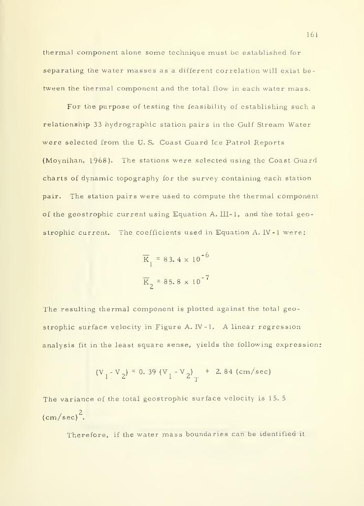
161

thermal component alone some technique must be established for

separating the water masses as a different correlation will exist be-

tween the thermal component and the total flow in each water mass.

For the purpose of testing the feasibility of establishing such a

relationship 33 hydrographic station pairs in the Gulf Stream Water

were selected from the U. S. Coast Guard Ice Patrol Reports

(Moynihan, 1968). The stations were selected using the Coast Guard

charts of dynamic topography for the survey containing each station

pair. The station pairs were used to compute the thermal component

of the geostrophic current using Equation A. Ill- 1 , and the total geo-

strophic current. The coefficients used in Equation A. IV - 1 were:

K = 83. 4 x 10" 6

K = 85.8 x 10" 7

The resulting thermal component is plotted against the total geo-

strophic surface velocity in Figure A. IV -1. A linear regression

analysis fit in the least square sense, yields the following expression:

(V -V )= 0. 39 (V - V ) + 2. 84 (cm/sec)

The variance of the total geostrophic surface velocity is 1 5. 5

(cm/sec) .

Therefore, if the water mass boundaries can be identified it

162

o oin

o o oI

O

o

oo

oOC

oLT)

o

O00

u0)

CO

u

nwwp,in

O

o

Hin

WOwXH

oH

U2

Oh

u

<J

w

. o

0)• i-C

u

mi

H<u

^j en

H 03

« C

S o

<^ isu

a o3 n

a*£ gCO cu

O Jh

M^

"S oCU

Ccu

cu

-t->

cu

cID

oa

a gx °

« 2« 5

i

>i—

i

<<U

In

be

(D3S/UI3) Q33dS DIHdOHXSOaO

163

is possible to compute the total geostrophic surface current from the

thermal component using the above expression. Hydrographic sur-

veys of this region could be made more synoptic using XBT's to

substitute for some of the standard hydrographic stations.

164

APPENDIX V

Field Evaluation

165

FIELD EVALUATION

Introduction

Based on the results of this research the T-S Gradient method

should allow the computation of surface geostrophic currents in good

agreement with those computed using the standard geostrophic calcu-

lations. Of course, both computations suffer from the limitations

inherent in the geostrophic assumptions. Therefore, the purpose

of this research to find a simplified scheme to make geostrophic

computations has been met, yet the computation of currents without

environmental verification is not very satisfying. However, it must

be concluded that at this time current observations are too few and

unreliable to be used as a quantitative measure of indirectly com-

puted currents. This appendix reviews two attempts by the author

to verify the representativeness of geostrophic currents to the actual

ocean currents, and proposes some refinements of these attempts

to continue the research. These two experiments are the only ones

known to the author as direct efforts to verify computed surface

currents in the open ocean in the slow California Current.

The major oceanic gyres appear to be revealed by geostrophic

computations (Reid, 1961, and Stommel, 1965). Yet at any point

or time in the ocean the geostrophic current may or may not be

166

representative of the instantaneous flow. As mentioned earlier,

many forces act to drive the waters of the ocean, and generally the

flow in the ocean will consist of both baroclinic and barotrophic

components (Foffonoff, 1962). Therefore, the determination of the

geostrophic current at any given time from a pair of hydrographic

stations does not yield the existing current. However, if the hydro-

graphic stations are sampled in a time-series fashion over a suffi-

cient length of time to remove the non-geostrophic periodic com-

ponents, then the resulting computed current can be expected to

come into closer agreement with the average current over the period

of the extended sampling.

Defant (1950) has shown that the internal oscillations in the

water structure can lead to significant errors in the geostrophic

currents. Particularly important in dynamic computations is the

change in the water structure associated with internal waves, and

the most significant periods are those of the diurnal and semidiurnal

tide (Defant, 1950). LaFond (1951) also identified the semidiurnal

and diurnal periods as the most significant perterbations in the

water structure.

Little is known of the internal oscillations in the ocean at the

present time. However, Haurwitz, et al. (1959) show that signifi-

cant peaks occur in their long series of records of temperature at

50 m and 500 m offshore from Castle Harbor, Bermuda, only at the

167

semidiurnal and inertial or diurnal periods. Except for a broad

maximum at about 0. 5 cycles per hour their spectra decreases

monotonically with increasing frequency. There appears to be no

statistically significant coherence between observations at 50 m and

500 m. Cox (1962) shows in observations taken from the U. S. Navy

Electronics Laboratory oceanographic tower with isotherm fol-

lowers that the observations between laterally- spaced sensors are

coherent only at low frequencies, well below the mean value of the

Vaisala frequency.

It would be advantageous to use more than one ship to deter-

mine geostrophic flow between hydrographic stations, such that the

measurements applied at the same "instant" in time. In general

oceanographic operations are conducted by single vessels. Single

vessel hydrographic surveys are limited to two possible sampling

procedures, both of which may significantly influence the resulting

computed geostrophic current. The choice lies between sampling

between stations, first one station then another, such that enough

casts are made at each station to remove the variability; or second

sampling each station in a time- series fashion a sufficient number

of times to remove the variability, moving on to the next station at

the completion of the first.

Rapid sampling between stations means that the samplings are

almost synoptic, that is, taken under nearly the same conditions.

168

Furthermore, in running between stations the intervening water

structure can be sampled. However, in the California current area

hydrographic stations for determining geostrophic flow should be at

least 35 kilometers apart. This means that a conventional oceano-

graphic vessel traveling at ten knots will require two hours to

steam between stations, and a total of four hours will be required

to complete both stations. Changes in the hydrographic conditions

at either station may be significant during this four hour period

(Defant, 1950).

On the other hand, time-series sampling at a single station

requires a sample of sufficient length and density to remove the

periodic variations. At least 12 hours and preferably 24 hours of

sampling should be made at each station; with a cast every two hours,

50 hours will be required to completely sample a station pair (24

hours per stations with two hours steaming). One disadvantage of

single station time-series sampling is that between any two station

pair only one sampling of the intervening water structure is made.

To test the two types of sampling (continuous time series

sampling at one station versus alternating sampling between stations)

two experiments were performed. In the first experiment the al-

ternating sampling between stations was used. In the second, the

24 hour sampling at each station was performed.

169

Experiment I

The first experiment was performed from August 31, 1967 to

September 4, 1967 off Santa Cruz, California.

Purpose

This experiment had a dual purpose: first, the verification of

computed surface currents for this research; second, to examine

the validity of Richardson's "4/3 law" for particle diffusion, at large

particle separations (in this case separations in excess of six

nautical miles). The results of this latter work have been pre-

viously reported (Denner, et al. , 1968).

Sampling Procedure

The experiment consisted of alternate sampling between two

stations A and B at intervals of every four to six hours. The

location of these stations were:

A = 36* 50' N, 122° 36. 2* W

B = 36* 20' N, 123° 12. 0' W

Temperature and salinity measurements were made using

standard hydrographic procedures. Temperatures were determined

as the average of paired thermometers, and salinities were deter-

mined from water samples on a Hytech model 6210 laboratory

170

salinometer. Temperature structure was measured to 1, 500 feet

every hour on station and at three equi-distant points between stations

with XBT casts. Surface currents were measured at Station A using

parachute drogues (Volkmann, et al. , 1956). The drogues were

positioned relative to a taut reference mooring, using radar. The

initial locations of Station A and Station B, and all later locations of

B were made using Loran C.

Meteorological Conditions

The meteorological conditions were favorable for the entire

cruise. Winds were always less than Beaufort 4 and predominantly

below Beaufort 3 from 330* true, with corresponding sea states.

The swell were always less than five feet from about 300° true. No

difficulty was experienced in sampling or holding station due to

weather conditions.

Current Measurements

Station A was established first by setting a taut moored sur-

face reference buoy for current measurements, diffusion studies,

and hydrographic casts. The drogues were seeded, as nearly as

possible, in an octagonal pattern at a range of two nautical miles

about the reference. Also, one drogue was placed next to the refer

ence marker. All drogues were shallow with a 10 m line between

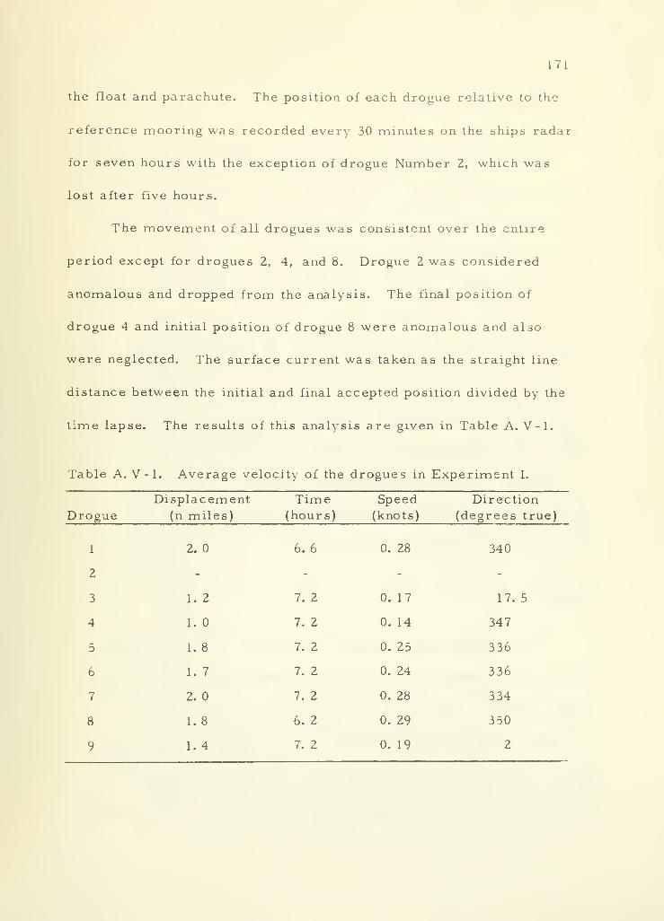
171

the float and parachute. The position of each drogue relative to the

reference mooring was recorded every 30 minutes on the ships radar

for seven hours with the exception of drogue Number 2, which was

lost after five hours.

The movement of all drogues was consistent over the entire

period except for drogues 2, 4, and 8. Drogue 2 was considered

anomalous and dropped from the analysis. The final position of

drogue 4 and initial position of drogue 8 were anomalous and also

were neglected. The surface current was taken as the straight line

distance between the initial and final accepted position divided by the

time lapse. The results of this analysis are given in Table A. V-l.

Table A. V-l. Average velocity of the drogues in Experiment I.

Displacement Time Speed Direction

Drogue (n miles) (hours) (knots) (degrees true)

1 2. 6. 6 0. 28 340

2 - -

3 1.2 7. 2 0. 17 17. 5

4 1.0 7. 2 0. 14 347

5 1. 8 7. 2 0. 25 336

6 1.7 7. 2 0. 24 336

7 2. 7. 2 0. 28 334

8 1. 8 6. 2 0. 29 350

9 1. 4 7. 2 0. 19 2

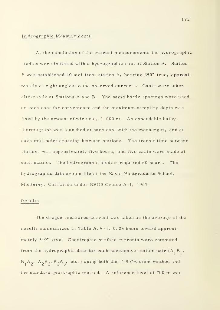
172

Hydrographic Measurements

At the conclusion of the current measurements the hydrographic

studies were initiated with a hydrographic cast at Station A. Station

B was established 40 nmi from station A, bearing 250° true, approxi-

mately at right angles to the observed currents. Casts were taken

alternately at Stations A and B. The same bottle spacings were used

on each cast for convenience and the maximum sampling depth was

fixed by the amount of wire out, 1, 000 m. An expendable bathy-

thermograph was launched at each cast with the messenger, and at

each mid-point crossing between stations. The transit time between

stations was approximately five hours, and five casts were made at

each station. The hydrographic studies required 60 hours. The

hvdrographic data are on file at the Naval Postgraduate School,

Monterey, California under NPGS Cruise A-l, 1967.

Results

The drogue-measured current was taken as the average of the

results summarized in Table A. V-l, 0. 25 knots toward approxi-

mately 340° true. Geostrophic surface currents were computed

from the hydrographic data for each successive station pair (A B ,

B A , A B , B A , etc. ) using both the T-S Gradient method and

the standard geostrophic method. A reference level of 700 m was

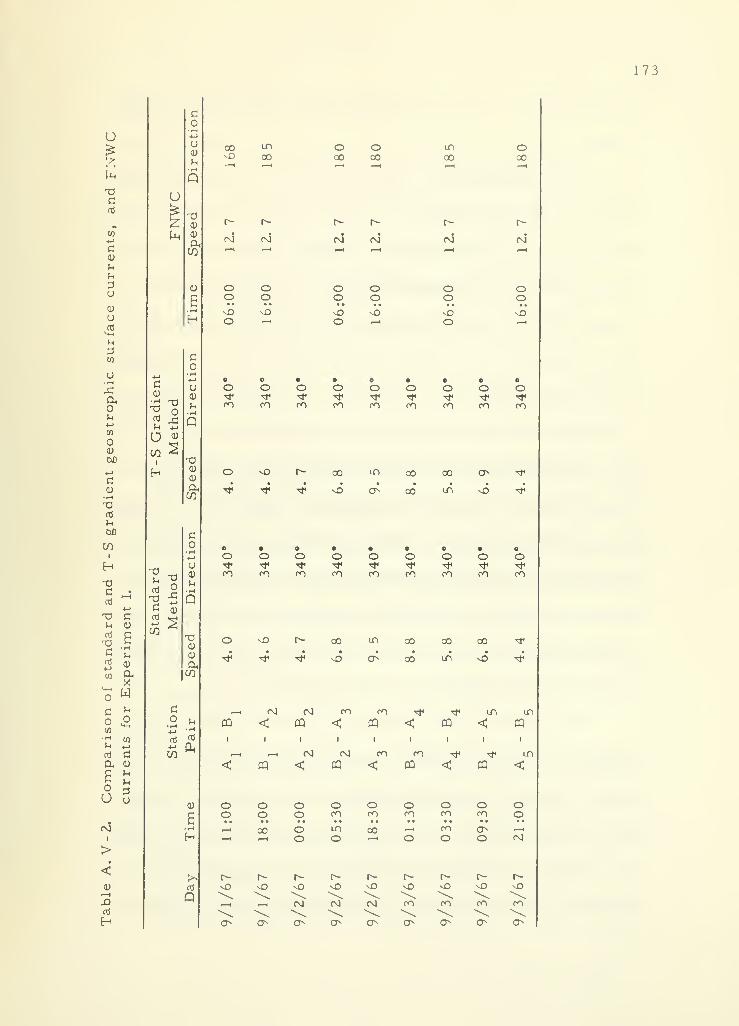
173

U

C(0

Uu

u

O

w

o•i-H

a,ou-!->

O<D

00

(->

0)•HX)0)

Vh

OjO

COI

H

rd

"0

Cd

o

1-4

0)

OhXW

H W

u

CMI

>

<0).—

(

cd

H

o

H

CO ^

t->

c0)

•r-* TlT)cd X!)h -M

o <D

CO 2

H

00 in o o lo ovO 00 CO CO 00 00

CM

CQ

oo

o

c\i

CM

<

ooCO

c-

CM* CM (M

CM co ^CQ CQ CQ

^

r-. CM

CQ <CM

oo

CQ

oCO

oCO

CQ

oCO

^

oCO

oo

CM

un ooo —

<

(NJ cm

vO

CO

COo

CO

CQ

oCO

CO

cm

o o o o o oo o o o o o• • • • • • * • • • •

-o vO xO vO nO vOo —1 o ^ o —

1

o o o o o o o o o* ^ "tf ^ * t ^ ^ *CO CO co CO co CO CO CO CO

o vO r- 00 LO CO 00 o -*

"* ^ * vO o CO LO sO *

o • • • • • • • oo o o o o o o o o^ * Tf •tf -tf "tf «* ^ •*CO CO CO CO CO CO co co CO

o ^D r- 00 un 00 00 00 <*

^ "* ^ o O 00 LT) ^D *

CQ

in

oo

o —iO CM

CO

174

selected for both calculations as this depth was achieved on each

«.n st.

The velocity profiles indicate a steady increase in velocity

relative to the 700 db reference level. The profiles obtained by the

two approaches to the geostrophic computations are essentially the

same. The relative geostrophic surface current was between

4 cm/sec and 9. 5 cm/sec, and the values for each station pair is

given in Table A. V - 2. These values are low compared to the meas-

ured velocity at Station A. There are several possible explanations

for the disagreement between the measured and computed velocity.

First, part of the measured flow may have been in the barotrophic

mode which is not revealed by geostrophic computations. Secondly,

the current measurements and the hydrographic measurements were

not concurrent, and the currents may have decreased after the

measurements. This would have been determined by longer current

measurements. In fact attempts were made to locate the drogues

on each return to Station A but without success.

Also shown in Table A. V - 2 are the surface current speed and

direction read from the FNWC synoptic current and stream function

charts. During this entire period the FNWC currents were to the

south-southeast (160* to 180* true) at approximately 1 2. 7 cm/sec.

This flow is in the opposite direction to the measured currents.

However, it should be noted that the FNWC currents are the sum

175

of their mass driven and wind driven components. FNWC uses

Witting's (1909) results (Equation 17) with a wind factor of 4. 8:

taking the winds at 10 m/sec from 330* true, a wind drift of 15.8

cm/sec to 330* true is computed. Therefore, it appears as if the

FNWC current is governed mainly by the wind component which in

this case does not lead to agreement with the measured currents.

This is true even though the wind was persistent over the entire

period.

Conclusion

This experiment shows that under these hydrographic condi-

tions the T-S Gradient method gives essentially identical results to

the standard geostrophic computations. These results give the geo-

strophic current in the same direction as directly-measured cur-

rents, but at a lower speed (4. cm/sec to 9. 5 cm/sec computed

versus 1 2. 8 cm/sec measured). Since there are many variables

that could not be controlled, better agreement probably cannot be

expected.

Currents computed by FNWC for this area are in the opposite

direction of measured flow at about 12.8 cm/sec. Since the FNWC

current consists of both geostrophic and wind components, the wind

component appears to be the dominant component in this case.

Two factors might improve the confidence in these results.

176

First would be better navigation control than the Loran C provides

In this area (+. 0. 5 nmi), and second, a longer period of current

observations. A second experiment was designed and performed to

correct these difficulties.

Experiment II

The results of the first experiment indicated that the T-S

Gradient method of computing geostrophic component of the flow

yielded better agreement between computed and observed currents

than did P NWC techniques. Yet the navigational control was not

completely satisfying. On this cruise the ship's Loran navigation

was supplemented with Lorac navigation, a highly accurate system

capable of providing fixes to within 0. 1 nmi. Experiment II was per-

formed 50 nmi south of Point Arguello (Station A) using the U. S.

Navy Pacific Missile Range Lorac system December 4, through

December 7, 1967.

Purpose

The purpose was the same as for Experiment I.

Sampling Procedure

The sampling procedure was altered from Experiment I to

provide two 24 hour stations (A and B) at which one cast was taken

177

approximately every two hours. Each station was marked with a

taut moored surface marker. Drogue current measurements were

made at each station. Station B was established perpendicular to

the flow measured at Station A. A savonius rotor current meter

was moored at Station B at a depth of 10 m. The locations of the

stations were

:

A = 33° 43. 8' N, 120° 45. 5* W

B = 33° 28. 7 ! N, 121° 40. 0' W

Meteorological Conditions

The winds were Beaufort 3 to Beaufort 5 over the entire cruise,

with Beaufort 3 prevailing at Station A and Beaufort 5 at Station B.

The winds were from 230° to 340° true over the entire cruise, pre-

dominantly from 320* to 340* true. The swell and sea were pre-

dominantly from 320* true.

Current Measurements

Station A was occupied first and a reference mooring was

established. Unfortunately the mooring did not hold and drifted

slowly to the south-southeast. However, six drogues were seeded

in an east-west line around the mooring. The movement of the

drogues relative to the reference float was determined by radar.

These measurements do not yield absolute currents since the

178

mooring was moving. However, the drogue positions were deter-

mined frequently between casts by running alongside the drogues and

noting their Lorac positions. Again the surface current was deter-

mined by averaging the straight line movement between successive

positions. The measurements were divided into three intervals.

During the first interval drogues 1 and 6 did not move consistently

with drogues 2, 3, 4, and 5 and were eliminated. During the second

period all drogues moved consistently. During the third interval

drogue 6 was eliminated.

During the first period, 21:33 on December 4, 1967 to 14:44

on December 5, 1967, the drogues moved at 9.8 cm/sec toward

127° true. During the second period, 14:40 to 17:40, December 5,

1967, the drogues moved at 16. 2 cm/sec toward 129° true. During

the last period. 17:28 on December 5, 1967 to 11:28 on December 6,

1967, they moved 1 3. 2 cm/sec toward 163° true.

At Station B another reference mooring was set, at right angles

to the flow measured at Station A, and again six drogues were

seeded. On this mooring a continuous recording savonious current

meter was placed at 10 m below the surface on the mooring. Several

problems were encountered at this station. Radar contact with the

drogues was lost after only a few hours, too short a time to deter-

mine significant movement. Attempts to position the drogues by

running alongside and taking their Lorac position failed when the

179

Lorac signal was lost. Reliable current measurements could not be

determined from the drogues. The current meter on the mooring

should have provided independent measure of the currents, but the

recorder paper failed to advance and the record was of no value.

Hydrographic Measurements

The hydrographic stations were established prior to the cruise.

Hydrographic casts were to be initiated every two hours, however,

delays of up to one hour were experienced. Only 10 casts of the 12

planned at each station were obtained. The hydrographic station

data is on file at the Naval Postgraduate School, Monterey,

California, under NPGS Cruise A- 2, 1967. Again, the stations

were approximately perpendicular to the measured drift of the

drogues at Station A. The section established will give the geo-

strophic current components along 160/340° true. The hydrographic

data at each station was averaged to remove insofar as possible any

short period variations, or measurement errors.

In a second analysis of the geostrophic currents, the XBT

temperatures were substituted for the reversing thermometer tem-

peratures and the computations repeated. The purpose of this

analysis was to see if the current structure derived from the XBT

data would agree with the analysis from the reversing thermometer

temperatures.

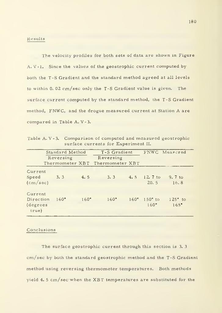
180

Results

The velocity profiles for both sets of data are shown in Figure

A. V-l. Since the values of the geostrophic current computed by

both the T-S Gradient and the standard method agreed at all levels

to within 0. 02 cm/sec only the T-S Gradient value is given. The

surface current computed by the standard method, the T-S Gradient

method, FNWC, and the drogue measured current at Station A are

compared in Table A. V - 3.

Table A. V - 3. Comparison of computed and measured geostrophic

surface currents for Experiment II.

Standard Method T-S Gradient FNWC MeasuredReversing Reversing

Thermometer XBT Thermometer XBT

CurrentSpeed 3.3 4.5 3.3 4. 5 1 2. 7 to 9. 7 to

(cm/sec) 20. 5 16. 8

CurrentDirection 160* 160° 160' l60 e

1 50° to 125* to

(degrees 160° 1 65*

true)

Conclusions

The surface geostrophic current through this section is 3. 3

cm/sec by both the standard geostrophic method and the T-S Gradient

method using reversing thermometer temperatures. Both methods

yield 4. 5 cm/sec when the XBT temperatures are substituted for the

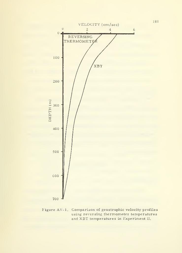
VELOCITY (cm/sec)

2 4

181

100 •

200 '

E— 300XHOh

WP

400

500 -

600 -

700 -»

REVERSINGTHERMOMET

Figure AV-1. Comparison of geostrophic velocity profiles

using reversing thermometer temperaturesand XBT temperatures in Experiment II.

182

reversing thermometer temperatures. The FNWC computations

yield a surface current between 1 2. 7 cm/sec and 20. 3 cm/sec with

directions between 125° true and 165* true. These values are in

substantial agreement with the drogue measurements of 9. 7 cm/sec

to 16.8 cm/sec with directions between 150* true and 165* true.

If the wind drift computed according to FNWC is added to the geo-

strophic surface currents the currents would be increased by 18

cm/sec. This would lead to surface currents somewhat larger than

those measured for the standard and T-S Gradient geostrophic com-

putations. However, the drogue measured surface currents aver-

aged over a depth interval of approximately eight meters around the

ten meter depth of the center of the parachute. Therefore, one

would expect the measured currents to be slightly lower than the

current at the very surface. The influence of other factors has not

been considered.

Recommendations

Introduction

Clearly the results of these two experiments cannot be con-

sidered conclusive. Much more experimental work is necessary to

establish any relationship between actual currents in the ocean and

those determined by indirect computation. Even though every effort

was made to maintain the tightest possible experimental control

183

during these studies further control is necessary and possible. Two

recent developments would have improved the possible control in

these experiments. These developments are the commercial avail-

ability of reliable continuous profiling salinity-temperature-pressure

systems (STP) (Brown, 1968), and satellite navigation systems

(Warriner, 1958). In the following paragraphs another experiment is

described, incorporating these developments and other improve-

ments that occur to this researcher for the continuation of this work.

The STP provides a continuous profile of temperature and

salinity as a function of depth to at least classical Nansen bottle and

reversing thermometer accuracy (± 0. 02 %o , + 0. 02* C, ± 4 m)

(Bissett Berman Corporation, 1968). The continuous profile of these

variables also eliminates the need to interpolate discrete Nansen

data and the associated interpolation error. Another advantage of

the STP over the classical Nansen approach is speed, since a cast

can be completed in less than half the Nansen cast time. Finally, a

distinct advantage of the STP is the repeatability of the measures.

The repeatability of the STP is two times better than the absolute

measurement accuracy, that is, ±0. 01%o, ±0. 01*C, and ± 2 m.

Taking advantage of this repeatability very precise difference meas-

urements necessary for geostrophic computations are possible.

Thus, using the STP the measurement and computational errors in

geostrophic computations could be substantially reduced.

184

The U. S. Navy has used satellite navigation on its vessels

since 1964 (Warnner, 1968). In 1967 the system was released for

private users, and receivers are now available commercially which

will yield position accuracy of better than 0. 1 nmi anywhere in the

ocean (Magnavox Corporation, 1968). This represents at least a

five-fold increase in accuracy over the best previous open ocean

navigation system.

Proposed Experiment

The purpose of the experimental work discussed here is to

establish the relationship between the currents at a point in the

ocean and driving forces. Since currents exhibit a turbulent nature

over a wide range of scales it is clear that we will never be able to

specify the instantaneous velocity indirectly. However, for the

purpose of contemporary forecasting this impossibility is not neces-

sary. In the continuation of this research a modification of the

experimental procedure used in this study is recommended.

Stations

Three stations should be established, initially in an area where

the surface currents are not disturbed by topographic influences,

such that the sections between the stations enclose a triangular re-

gion. The primary reason for the triangular array is the fact that

185

the three stations are the minimum number forming a closed ele-

ment. Continuity considerations can be used for a closed element to

help reduce ambiguities in the results. Furthermore, the geo-

strophic currents perpendicular to the three sections formed by the

sides of the triangular station pattern will allow vector resolution of

the actual current. Station locations should be marked with suitable

taut moorings. Station separation should be determined by the cri-

terion suggested by Reed and Laird (1965) that the dynamic difference

between the stations be five times the error in the dynamic computa-

tions (see Chapter III). However, because of the potential repeata-

bility of the STP and precision of the satellite navigation the station

separation might be reduced from that used in Experiments I and II,

keeping the transit time between stations to a minimum.

Sampling

Sampling of the following parameters should be performed at

each station as outlined in the following discussion:

1. Temperature and salinity should be measured from the

surface to 1, 000 m.

2. Surface currents and currents at 1, 000 m should be

measured over the period of the study.

3. Surface wind should be measured and recorded over the

period of the study.

186

4. Sea conditions should be measured and recorded over the

period of the study.

5. Barometric pressure should be recorded over the period

of the study.

Sampling should be conducted such that significant periodic variation

in the structure can be identified.

Phase I - Establish Initial Conditions

At each station the taut line moor should be established,

drogues with radar transponders should be set at the surface and

1, 000 m, and the best satellite position obtained. Once the station

has been established, two STD lowerings should be made to 1, 000

db, Nansen bottles with reversing thermometers placed at 0, 500,

and 1, 000 db. During the period of the STD casts XBT's should be

launched every ten minutes. This procedure should be followed at

each station. The vessel should proceed between stations at maxi-

mum cruising speed. Between stations XBT's should be launched

every one-half hour. Given a station separation of 40 km the first

phase will require approximately 24 hours. Phase I establishes the

stations to be used in Phase II, the initial hydrographic conditions,

and the short term variability.

187

Phase II - Sampling

The purpose of Phase II is to establish the median conditions

over the period to provide the best estimate of the factors contribut-

ing to the surface flow. Only the significant factors should be con-

sidered. Returning to each station in initial order, 24 hour time-

series sampling should be initiated to the 1, 000 db level. STD casts

will be made every hour, with XBT probes launched every one-half

hour. A parachute drogue will be established at the start of this

phase at 1, 000 db and at the surface, the position of the drogues in

the water at each station should be established every one-half hour.

As the drogues are lost, they should be replaced. The ships posi-

tion will be maintained at the reference position. Again the vessel

should proceed between 24 hour stations at maximum cruising speed,

launching XBT's every one-half hour.

At the conclusion of the time series sampling the vessel should

proceed to locate as many drogues as possible, recover the radar

transponders and then the surface buoys. Approximately 96 hours

would be required for Phase II exclusive of equipment recovery time.

Analysis

The currents through the array should be determined by both

direct and indirect methods. The computed surface currents should

188

be compared to the measured surface currents. Wind data should be

used to compute the wind component by various formulae to deter-

mine the best expression to use to obtain agreement between meas-

ured and computed surface currents. Significant periodic variations

in the measured currents could be correlated with variations in the

structure and local winds and tides to determine any relationships

between these factors and the currents.

Many other questions could be answered by the data collected

in this experiment. These questions should not be ignored, but the

goal of the experiment is to determine the relationships between ob-

served and computed ocean surface currents.

189

DISTRIBUTION LIST

No. of Copies

Defense Documentation Center 20

Cameron Station, Bldg . 5

Alexandria, Virginia 22314

Fleet Numerical Weather Center 20

Monterey, California

Dean of Research Administration 2

Naval Postgraduate School

Monterey, California 93940

Library 2

Naval Postgraduate School

Monterey, California 93 940

Professor Warren W. Denner 25

Department of OceanographyNaval Postgraduate School

Monterey, California 93940

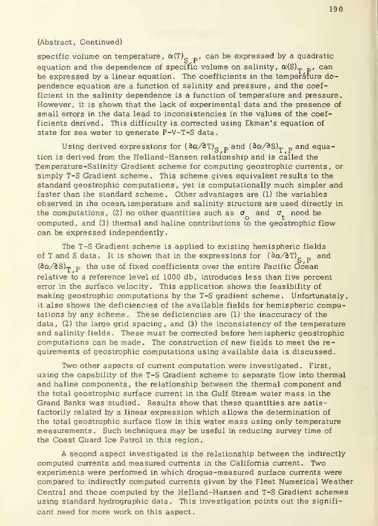
190

(Abstract, Continued)

specific volume on temperature, a(T) , can be expressed by a quadratic

equation and the dependence of specific volume on salinity, a(S)T p , can

be expressed by a linear equation. The coefficients in the temperature de-

pendence equation are a function of salinity and pressure, and the coef-

ficient in the salinity dependence is a function of temperature and pressure.

However, it is shown that the lack of experimental data and the presence of

small errors in the data lead to inconsistencies in the values of the coef-

ficients derived. This difficulty is corrected using Ekman's equation of

state for sea water to generate P-V-T-S data.

Using derived expressions for (da/dT)o p and (da/3s)T p

and equa-

tion is derived from the Helland-Hansen relationship and is called the

Temperature -Salinity Gradient scheme for computing geostrophic currents, or

simply T-S Gradient scheme. This scheme gives equivalent results to the

standard geostrophic computations, yet is computationally much simpler andfaster than the standard scheme. Other advantages are (1) the variables

observed in the ocean, temperature and salinity structure are used directly in

the computations, (2) no other quantities such as cr and cr need beo t

computed, and (3) thermal and haline contributions to the geostrophic flow

can be expressed independently.

The T-S Gradient scheme is applied to existing hemispheric fields

of T and S data. It is shown that in the expressions for (da/dT) and

(da/dS)rp p the use of fixed coefficients over the entire Pacific Oceanrelative to a reference level of 1000 db, introduces less than five percent

error in the surface velocity. This application shows the feasibility of

making geostrophic computations by the T-S gradient scheme. Unfortunately,

it also shows the deficiencies of the available fields for hemispheric compu-tations by any scheme. These deficiencies are (1) the inaccuracy of the

data, (2) the large grid spacing, and (3) the inconsistency of the temperature

and salinity fields. These must be corrected before hemispheric geostrophic

computations can be made. The construction of new fields to meet the re-

quirements of geostrophic computations using available data is discussed.

Two other aspects of current computation were investigated. First,

using the capability of the T-S Gradient scheme to separate flow into thermal

and haline components, the relationship between the thermal component andthe total geostrophic surface current in the Gulf Stream water mass in the

Grand Banks was studied. Results show that these quantities are satis-

factorily related by a linear expression which allows the determination of

the total geostrophic surface flow in this water mass using only temperature

measurements. Such techniques may be useful in reducing survey time of

the Coast Guard Ice Patrol in this region.

A second aspect investigated is the relationship between the indirectly

computed currents and measured currents in the California current. Twoexperiments were performed in which drogue -measured surface currents werecompared to indirectly computed currents given by the Fleet Numerical Weather

Central and those computed by the Helland-Hansen and T-S Gradient schemesusing standard hydrographic data. This investigation points out the signifi-

cant need for more work on this aspect.

191

UNCLASSIFIEDSiuunH Classification

DOCUMENT CONTROL DATA -R&Dirifr . lasxiticatian ol title, body ot .ihstrm t otnl indexing annotation must lie entered when the over. ill report i s rletmlHed)

)«h;in«tino activity [Corporate ,iuthor)

Naval Postgraduate School

Monterey, California

la. REPORT SECURITY CLASSIFICATION

UNCLASSIFIED26. GROUP

K t POR T TITLE

The T-S Gradient Method, A New Method of Computing Geostrophic Currents

over Large Ocean Areas

4 DESCRIPTIVE NOT BS (Type ol report and. inc lus ive date s

)

Technical Report, 1969Au THORiSl (First name, middle initial, last name)

Warren W. Denner

6 REPORT DATE1 July 1969

la. TOTAL NO. OF PAGES

20176. NO. OF REFS

628a. CONTRACT OR GRANT NO

6. PROJ EC T NO.

Work Request 9-0011

9a. ORIGINATOR'S REPORT NUMBERISI

NPS-58DW9072A

96. OTHER REPORT NOISI (Any other numbers that may be assignedthis report)

10 DISTRIBUTION STATEMENT

This document has been approved for public release and sale; its distribution is

unlimited

.

II. SUPPLEMENTARY NOTES

This project funded by:

Fleet Numerical Weather CentralMonterey, Cal ifornia

12. SPONSORING MILITARY ACTIVITY

Naval Postgraduate School

Monterey, California13. ABSTRACT

Requirements for indirect computation of geostrophic surface currents over large

ocean areas are discussed. These requirements point to a need to simplify standard

geostrophic computations, and to separate the first order thermal and haline contri-

butions to geostrophic flow.

The equations of motion for geostrophic flow are reviewed and the standard geo-

strophic computations discussed. Errors and limitations in the geostrophic method

are reviewed. Previous attempts to simplify geostrophic computations are discussed

and shown to be inadequate for synoptic computation over hemispheric ocean areas.

It is shown that the Helland-Hansen equation can be rewritten such that the

geostrophic velocity is composed of a temperature structure term and a salinity struc-

ture term. In order to apply this modified equation to hemispheric synoptic geostrophi<

computations, simple expressions are required for the dependence of specific volume

on temperature at constant salinity and pressure, (da/dT)gp , and on salinity at

constant temperature and pressure, (da/BS) . Two approaches are explored to

derive these expressions, using:

1) Experimental P-V-T-S data collected in the laboratory.

2) P-V-T-S data derived from an equation of state for sea water.

Numerical fitting of the experimental P-V-T-S data shows that the dependence of

DD F0RML>/ U 1 NOV 65

S/N 0101 -807-681 1

1473 (PAGE 1

)

UNCLASSIFIEDSecurity Classification

A-31408

192

UNCLASSIFIEDSecurity Classification

KEY WORDS

Surface currents

Geostrophic computationsDynamic computations

T-S Gradient method

DD FORM1 NOV 651473 (BACK

S/N 010! -907-63? '

UNCLASSIFIEDSecurity Classification

DUDLEY KNOX LIBRARY

3 2768 00396453 7