DISCRETE APPLIED

ELSEVIER Discrete Applied Mathematics 55 (1994) 281-293

MATHEMATICS

A new exact algorithm for the solution of quadratic assignment problems

Thierry Mautor, Catherine Roucairol*

INRIA md MASI, Domaine de Vi)lu~rau- Roc,yurnc’ourt BP. 105, 78153 Le Chesnuy Cede-y. France

Received 6 March 1992; revised 27 May 1993

Abstract

The Quadratic Assignment Problem is known as a combinatorial optimization problem, which is very hard to solve exactly. A survey of recent methods for solving this problem is given. Then an exact algorithm is presented along with computational results on a variety of test problems. This algorithm obtains very good results and, for the first time to our knowledge, solves exactly problems of size up to twenty, this in less than twenty minutes.

1. Introduction

The Quadratic Assignment Problem (QAP) is a combinatorial optimization prob-

lem with applications to location problems (e.g. facility location, VLSI design, back-

board wiring, . . .) [21,24,34], architecture design [16], scheduling [18] and many

others.

The problem consists to assign n units to II sites so that the cost of this assignment is

minimal. It can be formulated as follows:

given two (n x n) matrices

F = (,fij), whereAj is the flow between units i and j,

D = (&), where dkl is the distance between sites k and 1,

find a permutation p of the set N = { 1,2, . . . . n} which minimizes

Cost(p) = 1 Cf;.jdp(i,p(j,. I i

Many other formulations have been given, for example in the form of a matrix trace

minimization [ 171.

*Corresponding author. E.mail: Catherine.Roucairol@ inria.fr

0166-218X/94/$07.00 0 1994-Elsevier Science B.V. All rights reserved SSDI 0 166-2 18X(93)EOl 16-G

282 T. Mautor. c’. Roumirol / Discrrtt~ Applied Mathematics 55 (1994) 281-293

2. Solution methods

2.1. Exact algorithms

The QAP is known to be NP-hard [31] and has shown itself to be a very difficult

problem computationally. Even problems of moderate size are very difficult to solve

exactly.

There are two types of enumeration procedures applied to QA Problems: _ cutting plane methods,

~ branch and bound methods.

The cutting plane methods based on integer programming formulations

have not been very successful in computational tests. Such methods, developed

by Kaufman and Broeckx [20], Balas and Mazzola [2] and Bazaraa and

Sherali [4] did not manage to solve exactly problems of size higher than

eight.

The branch and bound methods yielded better results. They differ by: _ their branching scheme,

~ their “best first” or “depth first” search, _ their computation of bounds, _ their sequential or parallel running.

The most successful are the following ones:

- Burkard, Derigs [lo]: sequential,

~ Roucairol [30]: parallel,

~ Pardalos, Crouse [ 151: parallel.

Nevertheless, these algorithms remain limited to problems of size fifteen.

Unlike other combinatorial problems, the progress in the results of exact

methods for QAPs is very slow and due for a large part to the faster

computer hardware. The exact solution of QAPs is very hard and seems a little bit

disheartening. That is the reason why most recent approaches to this problem

propose heuristics.

2.2. Heuristics

The average results of the first heuristic solution methods:

~ approximate exact methods,

~ construction methods, _ exchange methods,

were rather good but these results could become really bad for some instances.

The most interesting heuristics applied to QAPs are recent ones issued from the use

of metaheuristics on QAP like:

- simulated annealing [S, 11,361,

- tabu search [33,35],

- genetic algorithm [6].

T. Mautor, C. Roucairol / Discrtvr Applied Mathematics 55 IIYYI) 281-293 283

The best solution is almost always found by these algorithms for small instances.

For problems of higher size, it is hard to estimate the quality of the results, as the best

value is unknown.

But for special instances, built with the knowledge of the optimum [25], the results

of these heuristics are very close to it.

2.3. Remarks

Because of this recent development of very good heuristics, the work of exact

methods on QAPs is changing. The main task can now be considered as proving that

the solution given by a good heuristic is optimal.

Indeed, as was stated before, exact methods can only work on instances of moderate

size (lower than twenty) on which heuristics nearly always give one of the best

solutions.

Of course, as this proof cannot be given by heuristics, the interest in exact methods

remains.

Consequences for branch and bound procedures are the following ones: _ all the BB procedures tried to find quickly some good solutions to reduce the search

tree; it seems now useless to choose a branching scheme and a search in this

aim, _ as the nodes examined are only the ones of the critical tree (evaluation lower than

the value of the best solution), Depth First Search and its simpler data structures

seems more efficient than Best First Search.

The branch and bound procedure we have developed will use these remarks.

3. A new branch and bound algorithm

3.1. Lower bound

To solve exactly QAPs the computation of the lower bound represents one of the

main difficulties. Indeed, either the bound is too loose (the number of nodes of the

search tree becomes too high), or the computational time to bound one node is

prohibitive.

The oldest and most commonly used one is the Gilmore-Lawler bound [19,22]

based on ordered products.

The ordered product of two vectors x and y is the scalar product, where one vector

is ordered increasingly and the other one is ordered decreasingly and is equal to the

minimal scalar product:

fx, Y > - = E’,” C xi.Yp(i).

284 T. Mauror, C. Roucairol / Discrrtr Applied Mathematics 55 (1994) 281-293

Table 1

Relative error of the GLB on the Nugent’s global problems

Size 5 6 I 8 I2 15 20

Error (%) 0 4.6 1.4 I3 14.7 16.3 20

Table 2

Average relative error of the GLB at different levels of the trees

Level I 2 3 4

Average error (X) 13 12 10.5 7.5

Table 3

Ameliorative rates of other bounds in comparison with GLB

Size Rend], Wolkowicz

(MEVB) Carraresi, Malucelli

6 - 300 0

I - 63 + 27

8 - 43 +I I2 +2 +2

15 + 14 +5

20 + 34 +2

The Gilmore-Lawler bound is the best value of the Linear Assignment Problem on

the matrix of the ordered products (obtained by taking the ordered products of the

rows of F with the columns of D).

So this bound is quickly computed (O(n3)) but the results are not very tight. As an

illustration we give in two arrays, the relative error for this bound.

In the first one, Table 1, this error is given for the roots of the trees, i.e. for the global

problems.

The problems are Nugent’s ones, classical benchmarks for QAP [24].

Hence, each problem will be designated by the name of its author, followed by its

size. Thus, Nugent 8 will be the Nugent’s problem of size eight.

In the second one, Table 2, the error is given for the nodes of different levels of the

trees, in comparison with the best solution of the branch (problems: Nugent 8, Nugent 10).

This array shows that the decrease of the error remains low, as assignments are fixed.

The most interesting other lower bounds have been developed by Rend1 and

Wolkowicz [27] (eigenvalue approach: introduced by Finke) and by Carraresi and

Malucelli [12] (equivalent dual formulations of the original QAP).

These two bounds are a little bit closer to the best solution than the Gil-

more-Lawler bound but this improvement remains low as it can be seen in Table

3 where the ameliorative rates of these bounds in comparison with the GLB are given

T. Mautor, C. Roucairol / Discrete Applied Matlwnmtics 55 (1994) 281-293 285

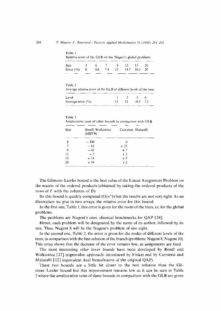
Fig. 1

in the roots of the decision trees of Nugent’s problems (if GLB # Best Value).

x = Ameliorative rate = 100 * New bound - GLB

Best value - GLB

While this improvement remains low, the computational time grows hugely. Carraresi

and Malucelli using their bound in a BB procedure [13], run their program 45 hours

to solve exactly Nugent 15, while the best algorithms using the GLB take only a few

minutes (in spite of some additional nodes to bound). That is the reason why, as all the

most successful Branch and Bound procedures did, we still use the Gilmore-Lawler

bound and concentrate our effort on an other way in order to reduce enumeration.

3.2. Symmetq

3.2.1. Symmetries on classical QAProblems

For most of the classical applications of QAP, the sites are on a regular figure: grid,

circle or line.

On Nugent’s problems, for instance, the sites are on a grid and the distances are

rectangular ones.

Of course, on these figures, symmetries can be pointed out. Thus, on a rectangle,

symmetrically equivalent solutions go by groups of four (see Fig. 1).

On the same way, symmetrically equivalent solutions go by groups of eight for

a square and by groups of (2~) for a circle.

3.2.2. Use of these symmetries

These characteristics are not used by any branch and bound method’. So, equiva-

lent nodes are created, studied and bounded independently, in different branches of

the tree.

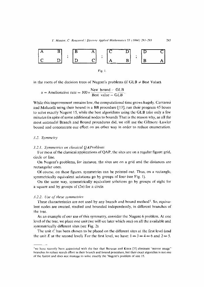
As an example of our use of this symmetry, consider the Nugent 6 problem. At one

level of the tree, we place one unit (we will see later which one) on all the available and

symmetrically different sites (see Fig. 2).

The unit C has been chosen to be placed on the different sites at the first level (and

the unit E at the second level). For the first level, we have: 1 o 3 e 40 6 and 2 * 5.

‘we have recently been acquainted with the fact that Bazaraa and Kirca [3] eliminate “mirror image” branches to reduce search effort in their branch and bound procedure, but their exact algorithm is not one

of the fastest and does not manage to solve exactly the Nugent’s problem of size 15.

286 T. Mautor. c’. Roucairol / Discrete Applied Mathematics 55 (1994) 281-293

Table 4

No more symmetries

Fig. 2.

1<=>3 ; 4<=>6

Effects of the symmetry test on the number of nodes

Problem With symmetry test Without Ratio Figure

Nugent 8 32

Nugent 9 70

Nugent 12 3474

Circle 10 115

128 4 Rectangle

522 7.46 Square

13833 3.98 Rectangle

2261 19.66 Circle

3.2.3. Consequences on the number qf nodes in the BB trees

Table 4 gives the number of nodes bounded (number of evaluations) with and

without this use of symmetry properties on Nugent’s problems and on a personal

example (Circle 10).

3.2.4. De$nition ?f symmetry equivalence

As we can have symmetry equivalences on some nodes of the tree where some units

are already assigned on some sites, let us call:

- S as the set of all sites,

~ S, as the set of sites already assigned,

- Sz as the set of the remaining sites: Sz = S - Sr.

Of course, for the root of the tree, i.e. for the global problem Sr = 0.

Definition 1. If there is a bijection n on S so that

(i) V’sES, 71(s) = s,

(ii) Vsr,s,~Sd(s,,s~) = d(r-+r), X(G)), all the sites s,,sz which satisfy rr(sz) = sr are said to be symmetrically equivalent.

T. Mautor. C. Rouc,airol / Dixrrtr Applied Mathcwtatics 55 (1994) 281-293 287

Sl=CW

Fig. 3.

In this case, for any solution of the problem p with p(u) = s2, we have an equivalent

solution of same cost where p’(u) = .si with p’ = rcop and so it is useless to study the

assignment p(u) = s2.

Proof.

‘Ost(P’) = Cost(noP) = C C_fijdn p(i)n p(j)>

= 7 Zf,id,,,,,,j,i=JCost(p). q j Moreover, this definition induces an equivalence relation, that we call symmetrical

equivalence relation. The unit u has to be placed only on one of the sites of each

symmetrical equivalence class.

3.2.5. Symmetry test

In order to find these symmetrical equivalence classes, we propose a property easy

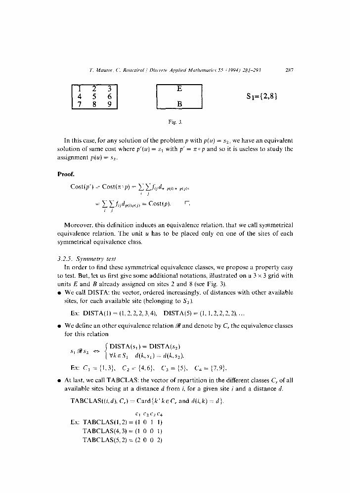
to test. But, let us first give some additional notations, illustrated on a 3 x 3 grid with

units E and B already assigned on sites 2 and 8 (see Fig. 3).

l We call DISTA: the vector, ordered increasingly, of distances with other available

sites, for each available site (belonging to S,).

Ex: DISTA(1)=(1,2,2,2,3,4), DISTA(5)=(1,1,2,2,2,2) ,...

l We define an other equivalence relation %! and denote by C, the equivalence classes

for this relation

S,G?Sl 0 DISTA(si) = DISTA(s2)

VkES, d(k,s,) = d(k,s,).

Ex: Ci = {1,3), Cz = {4,6}, C, = {Sj, C, = {7,9}.

l At last, we call TABCLAS: the vector of repartition in the different classes C, of all

available sites being at a distance d from i, for a given site i and a distance d.

TABCLAS( (i, d), C,) = Card { k ) k E C, and d( i, k) = d}.

Cl c2c2c4

Ex: TABCLAS(L2) = (1 0 1 1)

TABCLAS(4,3) = (1 0 0 1)

TABCLAS(5,2) = (2 0 0 2)

288 T. Mautor, C. Rouc~uirol i Discrrte Applied Mcrtlwmutics 55 i 1994) 2X1-293

Proposition. If; for any equivalence class C, and for any pair @sites (s, ,sz) belonging

to C,, s, and s2 have the same vectors TABCLAS, then the equivalence classes C,

correspond to the symmetrical equivalence classes. Two sites belonging to the same class

are symmetrically equivalent.

Proof. We consider the bijection rc, built according to the classes C, on S2 and

corresponding to the identity on Sr (VSES~ , n(s) = s).

- V(slrs2)~S1, n(sl) = s1 and n(sZ) = s2, so d(s,,s2) = d(x(s,), n(s2)).

~ VS~ES,, s2 and rc(s2) belong to the same class C,. So Vs, ES~, d(sI,s2) = d(s,,z(s,))

= d(4s,),z(sz)). - V(sI,s2)~S2, let us call d the distance between s, and s2. As TABCLAS(s,,d) =

TABCLAS(s,,d), d(x(s,), 7c(s2)) = d = d(sI ,s2). 0

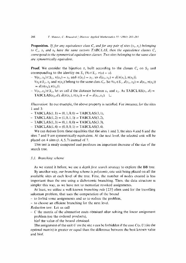
Illustration: In our example, the above property is satisfied. For instance, for the sites

1 and 3:

- TABCLAS(l, 1) = (0, l,O,O) = TABCLAS(3, l),

- TABCLAS(1,2) = (l,O, 1,1) = TABCLAS(3,2),

~ TABCLAS(1,3) = (0, l,O,O) = TABCLAS(3,3),

~ TABCLAS( 1,4) = (O,O, 0,l) = TABCLAS(3,4).

We can deduce from these equalities that the sites 1 and 3, the sites 4 and 6 and the

sites 7 and 9 are symmetrically equivalent. At the next level, the selected unit will be

placed on 4 sites (1,4,5,7) instead of 7.

This test is easily computed and produces an important decrease of the size of the

search tree.

3.3. Branching scheme

As we stated it before, we use a depth jrst search strategy to explore the BB tree.

By another way, our branching scheme is polytomic, one unit being placed on all the

available sites at each level of the tree. First, the number of nodes created is less

important than the one using a dichotomic branching. Then, the data structure is

simpler this way, as we have not to memorize revoked assignments.

At least, we utilize a well-known branching rule [23] often used for the travelling

salesman problem, that uses the computation of the bound

~ to forbid some assignments and so to reduce the problem, _ to choose an efficient branching for the next level.

Reduction test: Let us call

~ C the matrix of the alternative costs obtained after solving the linear assignment

problem (on the ordered products),

~ binf the value of the bound obtained.

The assignment of the unit U on the site s can be forbidden if the cost C(s, U) (in the

optima1 matrix) is greater or equal than the difference between the best known value

and binf.

T. Mirutor, C. Roucuirol ! Disc~rcte Applied Mat1wmatic.s 55 (1994) 281-293 289

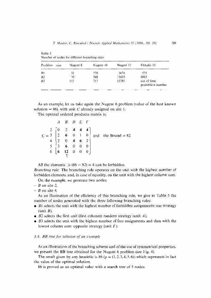
Table 5

Number of nodes for different branching rules

Problem size Nugent 8 Nugent IO Nugent 12 Elshafei 19

Bl 32 270 3474

82 70 568 11455

B3 113 711 15781

515

6943

out of time

prohibitive number

As an example, let us take again the Nugent 6 problem (value of the best known

solution = 86) with unit C already assigned on site 1.

The optimal ordered products matrix is:

2

C=3

4

5

6

ABDEF

0 2 444

2 6 0 1 0 and the Bound = 82.

2 0 462

3 6 000

6 12 0 0 0 t

All the elements > (86 - 82) = 4 can be forbidden.

Branching rule: The branching rule operates on the unit with the highest number of

forbidden elements, and, in case of equality, on the unit with the highest column sum.

On the example, we generate two nodes:

~ B on site 2,

~ B on site 4. As an illustration of the efficiency of this branching rule, we give in Table 5 the

number of nodes generated with the three following branching rules:

l Bl selects the unit with the highest number of forbidden assignments: our strategy

(unit B),

l B2 selects the first unit (first column): random strategy (unit A), a B3 selects the unit with the highest number of free assignments and then with the

lowest column sum: opposite strategy (unit F).

3.4. BB tree,for solution qf‘ an example

As an illustration of the branching scheme and of the use of symmetrical properties,

we present the BB tree obtained for the Nugent 6 problem (see Fig. 4).

The result given by any heuristic is 86 (p = (1,2,3,4,.5,6)) which represents in fact

the value of the optimal solution.

86 is proved as an optimal value with a search tree of 5 nodes.

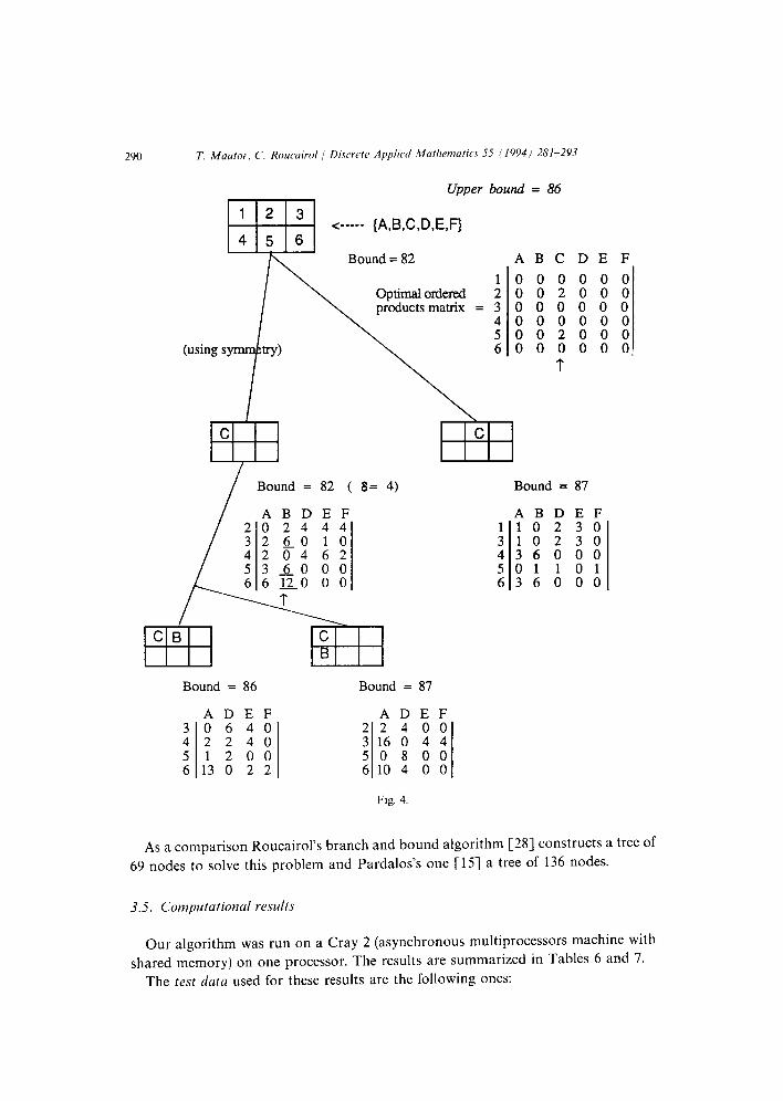
290 T. Mautor. C. Roucairol 1 Discrc~te Applied Mat1wmatic.s 55 (1994) 281-293

Upper bound

<----- {A,B,C,D,E,F}

Bound = 82 A

il 1 0

Optimal ordered products matrix = Z :

4 0

(using s try) : :

C C

0 6 40 22 4 00 2 2 40 3160 44 12 00 50 8 00

13 0 2 2 6104 00

Fig. 4.

= 86

BC

0 0

0”:

: Y 0 0

t

Bound = 82 ( 8= 4)

ABDEF 20 24 44 32&O 10 42 04 62 5360 00

CB

EH!I

C B

Bound = 86

ADEF

Bound = 87

_A D E F

Bound = 87

ABD 10 2 10 2 36 0 011 36 0

EF

G 0 0

DE F

0 0 0 0 0 0 0 0 0 0 0 0 0 0 0 0 0 0

As a comparison Roucairol’s branch and bound algorithm [28] constructs a tree of

69 nodes to solve this problem and Pardalos’s one [lS] a tree of 136 nodes.

3.5. Computational results

Our algorithm was run on a Cray 2 (asynchronous multiprocessors machine with

shared memory) on one processor. The results are summarized in Tables 6 and 7.

The test data used for these results are the following ones:

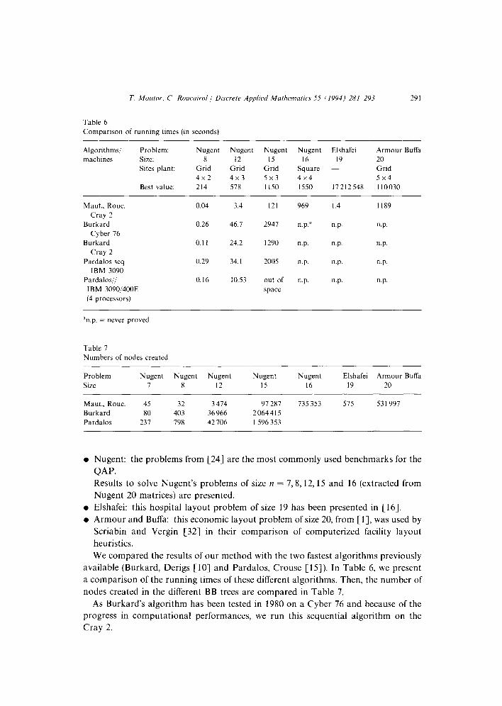
T. Mautor. C’. Roucairol / Discretr Applied Maihcwatics 55 11994) 281-293 291

Table 6

Comparison of running times (in seconds)

Algorithms/

machines Problem: Size:

Sites plant:

Best value:

Nugent Nugent Nugent Nugent Elshafei Armour Buffa

8 12 15 16 I9 20

Grid Grid Grid Square ~ Grid

4x2 4x3 5x3 4x4 5x4

214 578 1150 1550 17212548 110030

Maut., Rout.

Cray 2 Burkard

Cyber 76

Burkard Cray 2

Pardalos seq

IBM 3090 Pardaloslj

IBM 3090/400E (4 processors)

0.04 3.4

0.26 46.7

0.1 I 24.2

0.29 34.1

0.16 10.53

121 969 1.4 1189

2947 n.p.” np. np.

1290 np. n.p. np.

2005 n.p. n.p. np.

out of np. n.p. np.

space

‘np. = never proved

Table 7 Numbers of nodes created

Problem

Size Nugent Nugent Nugent Nugent Nugent Elshafei Armour Buffa

7 8 12 I5 I6 I9 20

Maut., Row. 45 32 3 474 97 287 735 353 515 53 1997 Burkard 80 403 36 966 2064415

Pardalos 237 798 42 706 I 596 353

Nugent: the problems from [24] are the most commonly used benchmarks for the

QAP.

Results to solve Nugent’s problems of size II = 7,8,12,15 and 16 (extracted from

Nugent 20 matrices) are presented.

Elshafei: this hospital layout problem of size 19 has been presented in [16].

Armour and Buffa: this economic layout problem of size 20, from [ 11, was used by

Scriabin and Vergin [32] in their comparison of computerized facility layout

heuristics.

We compared the results of our method with the two fastest algorithms previously

available (Burkard, Derigs [lo] and Pardalos, Crouse [15]). In Table 6, we present

a comparison of the running times of these different algorithms. Then, the number of

nodes created in the different BB trees are compared in Table 7.

As Burkard’s algorithm has been tested in 1980 on a Cyber 76 and because of the

progress in computational performances, we run this sequential algorithm on the

Cray 2.

292 T. Mautor. C. Roucairol / Discretr Applied Muthm~atics 55 (1994) 281-293

We present also two different results with the Pardalos algorithm. The first ones are

from a sequential running of this algorithm and the second ones from running the

algorithm in parallel on a four processors machine.

On each tested problem, our algorithm obtains the best results.

First, its running times for the exact solving of these problems are always the fastest

(4 to 20 times faster than the previous algorithms).

Then even on problems on which symmetries cannot be pointed out (Nugent 7,

Elshafei) it remains the most efficient one.

At last, it finds the best solution and proves the optimality of this solution for

problems of size sixteen to twenty which have never been solved exactly before. The

limit of size for the exact solving of quadratic assignment problems seems to be a little

bit pushed ahead.

4. Conclusions

We have presented a new exact and very efficient algorithm for solving the

quadratic assignment problem. It shows that the effort when trying to accelerate

a branch and bound procedure, must not always concentrate on a better computation

of lower bound. We have proved that, by studying some properties of the real world

applications like symmetries in the implementation sites, we can define good branch-

ing scheme and branching rules which drastically reduce the number of BB nodes to

explore. In this case, simple ideas easily and quickly computed are more efficient than

improvement (by “sophisticated” methods) of the bounding procedure.

In this way, we have been able to solve, for the first time exactly, problems of size up

to twenty in quite a reasonable time.

Furthermore, these ideas could be implemented in the future with any new revol-

utionary bound.

We expect that the parallelization of the BB procedure will lead to a very linear

speedup (nearly equal to the number of processors), as heuristics for QAP give very

good solutions and only the critical tree has to be explored.

References

[I] G. Armour and E. Buffa, A heuristic algorithm and simulation approach to the relative allocation of

facilities, Management Sci. 9 (1963) 294-309. [2] E. Balas and J.B. Mazzola, Quadratic O-l programming by a new linearization, Presented at the

TlMSjORSA Meeting, Washington DC (1980).

[3] MS. Bazaraa and 0. Kirca, A branch and bound based heuristic for solving the quadratic assignment problem, Naval Res. Logist. Quart. 30 (1983) 2877304.

[4] MS. Bazaraa and M.D. Sherali, Benders’ partitioning scheme applied to a new formulation of the

Quadratic Assignment Problem, Naval Res. Logist. Quart. 27 (1980) 29941. [5] E. Bonomi and J.L. Lutton, The asymptotic behaviour of quadratic sum assignment problems:

a statistical mechanics approach, European J. Oper. Res. 26 (1986) 2955300.

161 D. Brown, C. Huntley and A. Spillane, A parallel genetic heuristic for the quadratic assignment

problem, in: Proceedings of the 3rd Conference on Genetic Algorithms, Arlington (1989) 406-415. [7] E. Buffa, G. Armour and T. Vollmann, Allocating facilities with CRAFT, Har. Bus. Rev. 42 (1962) 136&158.

[X] R. Burkard, Some recent advances in quadratic assignment problems, in: Proceedings of the Congress

on Math. Programming, Rio de Janeiro (1984) 53-68.

[9] R. Burkard and T. BGnniger, A heuristic for quadratic boolean programs with applications to

quadratic assignment problems. European J. Oper. Res. 13 (1983) 374 386.

[IO] R. Burkard and U. Derigs, Assignment and Matching Problems: Solution Methods with FORTRAN

Programs (Springer, Berlin, 1980).

[I I] R. Burkard and F. Rendl, A thermodynamically motivated simulation procedure for combinatorial

optimization problems. European J. Oper. Res. 17 (1984) 169.-174.

[ 123 P. Carraresi and F. Malucelli, A new lower bound for the quadratic assignment problem, Oper. Res.

40 (I 992) S22mS27.

1131 P. Carraresi and F. Malucelli, A new’ branch and bound algorithm for the quadratic assignment problem, Presented at the 3rd ECCO Meeting, Barcelona (1990).

1141 N. Chrisofides, A Mingozzi and P. Toth. Contributions to the quadratic assignment problem,

European J. Oper. Res. 4 (1980) 243 247. [ 151 J. Crouse and P. Pardalos, A parallel algorithm for the quadratic assignment problem, Presented at

the ‘Proc. of Supercomputing 89’ Conference (ACM Press, New York, 1989) 351-360.

[I63 A. Elshafei, Hospital lay-out as H quadratic assignment problem, Oper. Res. Quart. 28 (1977) 167-179.

[I 71 G. Finke, R. Burkard and F. Rendl, Quadratic assignment problems, Ann. Discrete Math. 31 (1987) 61-82.

[I81 A. Geoffrion and G. Gravbes. Scheduling parallel production lines with changeover costs: practical

applications of a quadratic assignment/linear programming approach, Oper. Res. 24 (1976) 595-610.

1191 P. Gilmore, Optimal and suboptimal algorithms for the quadratic assignment problem, SIAM J.

Appl. Math. IO (1962) 305~ 313. 1201 L. Kaufman and F. Broeckx, An algorithm for the quadratic assignment problem using Benders’

decomposition, European J. Oper. Res. 2 (1978) 204 211.

[21] T. Koopmans and M. Beckmann, Assignment problems and the location of economic activities,

Econometrica 25 (1957) 53 76.

1221 E. Lawler, The quadratiuc assignment problem, Management Sci. 9 (1963) 586-599.

[23] E. Lawler, J. Lenstra, A. Rinnooy Kan and D. Shmoys, The Traveling Salesman Problem: A Guided

Tour of Combinatorial Optimization (Wiley, New York, 1985).

[24] C. Nugent, T. Vollmann and J. Rum], An experimental comparison of techniques for the assignment

of facilities to locations, Oper. Res. 16 (1968) 150 173.

[25] P. Pardalos and K. Murphy, A polynomial-time approximation algorithm for the quadratic assign-

ment problem, Technical Report, The Pennsylvania State University (1990).

1261 F. Rendl, Ranking scalar products to improve bounds for the quadratic assignment problem,

European J. Oper. Res. 20 (1985) 363-372.

[27] F. Rend1 and H. Wolkowicz, Applications of parametric programming and eigenvalue maximization

to the quadratic assignment problem, Math. Programming 53 (1992) 63-78.

[28] C. Roucalrol, A reduction method for quadratic assignment problems, Oper. Res. Verfahren 32 (1979) 183-187.

[29] C. Roucairol, Un nouvel algorithme pour le probltme d’affectation quadratique, RAIRO 13 (1979) 275-301.

[30] C. Roucairol, A parallel branch and bound algorithm for the quadratic assignment problem, Discrete

Appl. Math. 18 (1987) 21 I-225.

[31] S. Sahni and T. Gonzalez, P-complete approximation problems, J. ACM 23 (1976) 555-565.

1321 M Scrlabin and R. Vergin. Comparison of computer algorithms and visual based methods for plant layout, Management Sci. 22 (1975) 172-181.

1331 J. Skorin-Kapov, Tabu search applied to the quadratic assignment problem. ORSA J. Comput. 2 ( 1990) 33-45.

1341 L. Steinberg, The backboard wiring problem: a placement algorithm. SIAM Rev. 3 (1961) 37-50.

[35] E. Taillard, Robust tabu search for the quadratic assignment problem, Parallel Comput. I7 (1991) 443-455. [36] M. Wilhelm and T. Ward, Solving quadratic assignment problems by simulated annealing, IIE Trans.

19 (1987) 107 119.