Discrete Applied Mathematics 124 (2002) 103–116

Classes of quadratic assignment probleminstances: isomorphism and di"culty measure

using a statistical approach

Nair Maria Maia de Abreua ;∗, Paulo Oswaldo Boaventura Nettoa,Tania Maia Queridob, Elizabeth Ferreira Gouveaa;c

aProgram of Production Engineering, COPPE=UFRJ, BrazilbCEFET=RJ, Brazil

cFederal University of Rio Grande do Norte, Brazil

Received 13 September 1999; received in revised form 3 July 2000; accepted 19 March 2001

Abstract

In this work, we introduce the variance expression for quadratic assignment problem (QAP)costs. We also de;ne classes of QAP instances, described by a common linear relaxation form.The use of the variance in these classes leads to the study of isomorphism and allows for ade;nition of a new di"culty index for QAP instances. This index is then compared to a classicalmeasure found in the literature.? 2002 Elsevier Science B.V. All rights reserved.

Keywords: Quadratic assignment problem; Variance; Di"culty measure

1. Introduction

It is well known that the quadratic assignment problem (QAP) is NP-hard from atheoretical point of view, and only in instances of relatively small order can an optimalsolution be reached through exact algorithms. In response to that, considerable attentionis being currently given to the application of complexity theory to particular instancesof the QAP [5]. A complete survey of restricted versions of the QAP can be found in[7].

∗ Corresponding author.E-mail addresses: nair@pep.ufrj.br (N.M. Maia de Abreu), boaventu@pep.ufrj.br (P.O.B. Netto),

querido@openlink.com.br (T.M. Querido), bgouvea@pep.ufrj.br (E.F. Gouvea).

0166-218X/02/$ - see front matter ? 2002 Elsevier Science B.V. All rights reserved.PII: S0166 -218X(01)00333 -X

104 N.M. Maia de Abreu et al. / Discrete Applied Mathematics 124 (2002) 103–116

Applications of the QAP are discussed by CH ela [7], Dell’Amico et al. [8]. Pardalosand Wolkowicz [17] and include plant layout problems, computer backboard wiringproblems and control panel problems, among others.In this work, we present the partitioning of the set of QAP instances into classes, the

de;nition of isomorphic instances and the development of a statistical measure whichallows us to gauge the di"culty of solving a particular instance by relying on thevariance of the solutions. The variance expression has been ;rstly discussed in [3,4].We begin with the formulation of the problem by introducing a cost variance functioncalculated in polynomial time, in Section 2. In Section 3, we present one particularpartition within the set of QAP-instances. The variance is then applied in Sections 4and 5 as a measure of both isomorphism and di"culty of QAP instances that belongto the same class. Finally, in Section 6 we present the conclusions.

2. Variance for the QAP

Consider the set �n of permutations of the n elements in {1; 2; : : : ; n}. The symmetricQAP can be stated as

Min’∈�n

z’ =

∑16i¡j6n

fijd’(i)’( j)

: (2.1)

According to location theory, F = [fij] represents the 5ow matrix where fij is thequantity shipped from plant i to plant j and D= [dkl] represents the distance matrix,where dkl is the distance from location k to location l. The cost of simultaneouslyassigning plants i and j to its respective locations ’(i) and ’(j) is fijd’(i)’( j). The totalcost of an assignment ’ of plants to locations is z’. An instance represented by a pairof vectors (F;D) will be denoted by QAP(F;D). As F and D are symmetric, we cande;ne the N -dimensional column vectors F and D whose elements are, respectively,the N = Cn;2 upper diagonal entries of F and D and Q = FDT will be the matrixconsisting in the coe"cients indicated in (2.1).There are frequent occurrences of local optima in QAP instances. This suggests that

the functions of the average and variance of their solution costs could be useful parame-ters in establishing the di"culty of a particular instance. By means of these parameters,one can expect to decide upon the most suitable solving procedure or even to evaluatethe current values obtained by a given heuristic. Many researchers have been rankingthe problem’s di"culty such as [15,14]. The latter employed a variance-based measureover the Kow matrix to evaluate the particular instance di"culty in a branch-and-boundscheme. Herroeleven and van Gils [12] criticized this approach and claimed that up tothat date no measure could have been considered e"cient. Pardalos et al. [16] intro-duced a branch-and-bound algorithm based on variance reduction. In the early 1970s,Graves and Whinston [11] generalized the variance formula for the QAP linear re-laxation and suggested how the variance of QAP solution costs could be determined.However, the computation of their ideas was high on impossible and no polynomialexpression for this variance has been achieved so far, even though the mean expression

N.M. Maia de Abreu et al. / Discrete Applied Mathematics 124 (2002) 103–116 105

has already been obtained by Graves and Whinston [11], Angel and Zissimopoulos [1]and Boaventura-Netto and Abreu [4].The average of the costs z’ for QAP(F;D), over ’∈�n is

� = S=N; (2.2)

where we have

S =N∑

r=1

fr

N∑s=1

ds: (2.3)

Consider now the cost variance of the instance QAP(F;D):

�2FD = E(z2)− [E(z)]2: (2.4)

Seeking a cost variance parameter, we ;rst focus on the decomposition of the N 2

parcels of the term∑’∈�n

z2’ =∑’∈�n

∑16i¡j6n16r¡s6n

fijd’(i)’( j)frsd’(r)’(s); (2.5)

considering the index duplication over the set IN of indices (i; j):

∩k = {{(i; j); (r; s)}=|{(i; j) ∩ (r; s)}|= k};where k = 0; 1; 2 and 16 i; j; r; s6 n:

Lemma 2.1. For each pair of elements in IN ; it follows that

| ∩2 |= 1

| ∩1 |= 2(n− 2)

and

| ∩0 |= Cn−2;2:

Proof. Concerning the de;nition of ∩k we have for k = 0; 1; 2:for k = 2; ∩2 = {(i; j); (i; j)} ⇒ | ∩2 |= 1;for k=0; ∩0 ={{(i; j); (r; s)} | {i; j}∩{r; s}=∅}: There are Cn−2;2 elements for r = i

and s = j among the Cn;2 indices in JN . Finally for k = 1;∩1 = JN − ∩0 − ∩2; and| ∩1 |= Cn;2 − Cn−2;2 − 1 = 2(n− 2).

Considering the above notation and the following expression for Sk :

Sk(’) =∑∩k

fijfrsd’(i)’( j)d’(r)’(s); k = 0; 1; 2; (2.6)

we have the variance expression for the QAP, as stated in Theorem 2.1.

106 N.M. Maia de Abreu et al. / Discrete Applied Mathematics 124 (2002) 103–116

Theorem 2.1. The variance for QAP(F;D) is given as follows:

�2FD = [S0 + S1 + S2]=n!− �2;

where

S0 = 4(n− 4)!∑∩0

fijfrs

∑∩0

dijdrs;

S1 = (n− 3)!∑∩1

fijfrs

∑∩1

dijdrs

and

S2 = 2(n− 2)!∑

16i¡j6n

f2ij

∑16i¡j6n

d2ij :

Proof. We haven!∑t=1

z2’t=

n!∑t=1

∑k=0;1;2

Sk(’t):

For k = 0; S0 =∑n!

t=1 S0(’t) with S0(’t) =∑

∩0fijfrsd’t(i)’t( j)d’t(r)’t(s).

Considering Lemma 2.1, there are n!=Cn;2Cn−2;2 = 4(n− 4)! factors of the class∑∩0

fijfrs

∑∩0

dijdrs;

totaling

S0 = 4(n− 4)!∑∩0

fijfrs

∑∩0

dijdrs:

For k = 2,

S2 =n!∑t=1

S2(’t) with S2(’t) =∑

16i¡j6n

f2ijd

2’t(i)’t( j)

for which the number of repetitions is n!=Cn;2 = 2(n− 2)!.Thus,

S2 = 2(n− 2)!∑

16i¡j6n

f2ij

∑16r¡s6n

d2rs:

For k = 1, the number of repetitions is n!=Cn;2(Cn;2 − Cn−2;2 − 1) = (n− 3)!, resultingin

S1 = (n− 3)!∑∩1

fijfrs

∑∩1

dijdrs:

It can be easily observed that the total time required for the variance calculus isO(n4).

N.M. Maia de Abreu et al. / Discrete Applied Mathematics 124 (2002) 103–116 107

3. Classes of related instances

Ranking F and D elements in non-increasing and non-decreasing orders by permuta-tions ’− and ’+ ∈�N , we obtain vectors F− =(f’−(1;2); f’−(1;3); : : : ; f’−(n−1; n)) andD+=(d’+(1;2); d’+(1;3); : : : ; d’+(n−1; n)); in the form f’−(1;2)¿f’−(1;3)¿ · · ·¿f’−(n−1; n)and d’+(1;2)6d’+(1;3)6 · · ·6d’+(n−1; n). According to this notation, we de;ne thescalar products 〈F;D〉− = 〈F−; D+〉 and 〈F;D〉+ = 〈F+; D+〉. It is easy to prove that〈F;D〉−=〈F+; D−〉 and also that 〈F;D〉+=〈F−; D−〉. We will designate QAP(F−; D+)the standard instance, which has a coe"cient matrix Q∗ = (F−)(D+)T. The class ofrelated instances will then be de;ned by

Relclass(F−; D+) = {QAP(F;D)=(F−)(D+)T = Q∗}: (3.1)

The above set has the particular characteristic of yielding the same pair (F−; D+) forany instance in Relclass(F−; D+), with a common lower bound 〈F;D〉−. Alternatively,the set of related instances de;ned by (3.1) can be generated by pairs of permutations("; ’)∈�N ×�N over the standard-instance, as stated in the next lemma.

Lemma 3.1. Relclass(F−; D+)={QAP("(F−); #(D+))="; #∈�N}; where "(F−) is thevector (f"(’−(1;2)); f"(’−(1;3)); : : : ; f"(’−(n−1; n))); and #(D+) is the vector (d#(’+(1;2));d#(’+(1;3)); : : : ; d#(’+(n−1; n))).

Proof. By taking permutations " and # as inverses of ’− and ’+; respectively; weobtain "(’−(i; j))= (i; j) and #(’+(i; j))= (i; j). Thus; "(F−)=F and #(D+)=D.

Example. The Gavett–Plyter [9] instance is given by vectors FTGP=[28; 25; 13; 15; 4; 23]

and DTGP=[6; 7; 2; 5; 6; 1] and has a lower bound 〈F−; D+〉=389. Consider "=(1 3 6 4 2 5)

and #= $ the identity permutation. A related instance QAP(F1; D1) can be taken fromF1="(F−)=[28; 13; 25; 15; 4; 23] and D1=$(D+). Thus; QAP(FGP; DGP); QAP(F1; D1);QAP(F−; D+); among others; share the same family Relclass(F−; D+).

Lemma 3.2. The standard-instance QAP(F−; D+) is solvable in polynomial time.

Proof. Given a standard instance QAP(F−; D+); in order to calculate its cost it isenough to determine the scalar product 〈F+; D−〉; which is carried out in polynomialtime.

The QAP can be considered as the set of its instances. Let RN+ be the N -times

cartesian product of the R+, then

QAP = {QAP(F;D)=(F;D)∈RN+ × RN

+}: (3.2)

This way, we can obtain one particular partition in QAP. Following (3.1),

QAP =⋃

{F− ;D+}Relclass("(F−); #(D+)): (3.3)

108 N.M. Maia de Abreu et al. / Discrete Applied Mathematics 124 (2002) 103–116

Besides, one of diQerent vectors F− and D+ leads to disjoint Relclasses. For eachRelclass(F−; D+) we can de;ne the following subfamilies:(i) subRelclass("(F−); •) = {QAP("(F−); #(D+))=#∈�N} ∀"∈�N , and(ii) subRelclass(•; #(D+)) = {QAP("(F−); #(D+))="∈�N} ∀#∈�N .It is easy to see that

Relclass(F−; D+) =⋃

"∈�N

subRelclass ("(F−); •)

=⋃

#∈�N

subRelclass (•; #(D+)):

Then, the cardinality of Relclass(F−; D+) is (N !)2. This count considers all instances,even the isomorphic ones, which is discussed below.

4. Isomorphism for QAP instances

Let Kn(V; E; F) be the complete graph of order n, such that V is a set of vertices,E is a set of edges and F is a function which assigns one real number to each edgein Kn(V; E; F). We call F a weight-edge function and its graph, weight-edge-clique(w-clique), which we denote by wKF or simply KF . Two w-cliques Kn(V1; E1; F1) andKn(V2; E2; F2) are w-isomorphic when there is an +-permutation between V1 and V2

such that (i; j)∈E1 if (+(i); +(j))∈E2 and F1(i; j) = F2(+(i); +(j)). This permutationis called an +-w-isomorphism and we denote by wKF1 ≈ wKF2 their correspondingw-isomorphism of cliques. The Koopmans–Beckmann [13] formulation for the QAPwhich is de;ned by expression (2.1) allows a representative scheme on which Fand D data correspond to two weight-edge functions for two respective w-cliquesKF and KD. The objective function is thus to minimize the cost of simultaneouslyassigning KF vertices to KD ones. Instances QAP(F1; D1) and QAP(F2; D2) are iso-morphic (denoted by QAP(F1; D1) ≈ QAP(F2; D2)) if and only if wKF1 ≈ wKF2 andwKD1 ≈ wKD2.

Example. Let KF1 ; KF2 and KF3 be w-cliques in Fig. 1. For F1 = [1; 2; 10; 8; 3; 1] andF2 = [1; 2; 10; 8; 3; 1], considering + = (3 2 1 4), we have wKF1 ≈ wKF2 . On the otherhand, wKF1 and wKF3 are not w-isomorphic from F3 = [1; 3; 10; 1; 8; 2]. In this case,through enumeration of all permutations in �4, we will not ;nd any + such thatF1(i; j) = F2(+(i); +(j)).We call "∈�N , for N=Cn;2, a feasible solution to QAP(F;D) determined by ’∈�n

to the QAP-instance if for all 16 i6 j6 n,(1) F(i; j) = fi;j is the weight of edge (i; j) in w-clique KF and(2) D(’(i); ’(j)) = d(’(i);’( j)) is the weight of edge (’(i); ’(j)) in KD.This means that fi;j; d(’(i);’( j)) is a term of the cost in (2.1). We denote by FQAP(F;D)

the set of all QAP(F;D)-feasible solutions. Of course FQAP(F;D) is contained in �N andis isomorphic to �n.

N.M. Maia de Abreu et al. / Discrete Applied Mathematics 124 (2002) 103–116 109

Fig. 1. w-cliques, wKF1 ≈ wKF2 but (wKF2 �=wKF3 ).

Theorem 4.1. Two isomorphic instances; QAP(F1; D1) and QAP(F2; D2) ((QAP(F1; D1) ≈ QAP(F2; D2)) have the same feasible solution set; i.e.; FQAP(F1 ;D1) ≈FQAP(F2 ;D2).

Proof. Let QAP(F1; D1) and QAP(F2; D2) be isomorphic instances with F1 = [fi;j];F2 = [f′

i; j]; D1 = [di;j] and D2 = [d′i; j]. Consider "∈FQAP(F1 ;D1).

So, there is ’∈�n such that

z’ =∑

16i¡j6n

fijd’(i)’( j): (4.1)

From hypotheses, wKF1 ≈ wKF2 and wKD1 ≈ wKD2 . Then, there are # and 0∈�n with

fi;j = f′#(i) ;#(j) and d’(i);’( j) = d′

0(’(i)); 0(’( j)): (4.2)

Consider 1= 0 ◦ ’ ◦ #−1. After applying (4.2) to (4.1) we have

z’ =∑

16i¡j6n

f′#(i)#( j)d

′0◦’(i)0◦’( j): (4.3)

From (4.3) and considering 1 ◦ #= 0 ◦ ’ follows that

z’ =∑

16i¡j6n

f′#(i)#( j)d

′0◦’(i)0◦’( j) = z1: (4.4)

Then "∈�N is a feasible solution to QAP(F2; D2) determined by 1∈�N andFQAP(F1 ;D1) ⊆ JQAP(F2 ;D2). Analogously, we prove the other side of this inclusion.

The study of variance costs provides an opening to the study of isomorphism inQAP instances, considering that isomorphic instances have the same variance, sincethat they have the same feasible solution sets, as given by Theorem 4.1. In practice,this variance can be thought as an isomorphic invariant, pointing out non-isomorphicinstances, as stated below:

�2FD1

= �2FD2

⇒ (QAP(F1; D1) ≈ QAP(F2; D2)):

110 N.M. Maia de Abreu et al. / Discrete Applied Mathematics 124 (2002) 103–116

The instances Chr12a and Chr12b, available in the QAPLIB [6] are suitable examplesof instances sharing the same Relclass(F−; D+). However, these instances have therespective standard deviations 4413.99 and 4269.89, characterizing non-isomorphic in-stances. Note that the opposite is not always true—non-isomorphic instances can havethe same variance.An isomorphic quotient set {Relclass(F−1; D+)= ≈} is composed of classes, each

one of them containing isomorphic instances. Furthermore, two diQerent classes havedisjoint elements. Theorem 4.2 below states the number of such diQerent classes ineach family Relclass(F−; D+). Although this cardinality is easily obtained when con-sidering the subfamilies, the cardinality of the isomorphic quotient set is not immediate,suggesting the use of an upper bound, as stated in Corollary 4.2.1.

Theorem 4.2. The maximal cardinality of {subRelclass ("(F−); •)= ≈} is N !=n!;∀"∈�N ; except for n= 4; for which we have N !=2n!.

Proof. For n =4; the cardinality of automorphisms set is n!; which induces the numberof isomorphic instances. For n = 4; this cardinality is 2n! [2]. Thus; for n =4; anysubfamily in {Relclass(F−; D+)= ≈} has up to N !=n! diQerent classes; since each classhas n! isomorphic instances and each one of the vectors F and D has all diQerentcoordinates. The corresponding result follows for n= 4.

Theorem 4.2 can be extended to {subRelclass(•; "(D+))= ≈} through an analogousproof.

Corollary 4.2.1. For n =4 an upper bound for the isomorphic quotient set {Relclass(F−; D+)= ≈} cardinality is (N !)2=n!.

Proof. Immediate from Theorem 4.2 and from the subfamily de;nition in the previoussection.

As an example, let subRelclass(F−; •) = {QAP("(F+); +(D−)="∈�N} be a sub-family with + = (1 3 6 5 4 2) over the Gavett–Plyter instance [9]. According to theTheorems 4.1 and 4.2, there are 15 diQerent classes, with 48 isomorphic instancesin each. Among the related instances, there are up to 720 × 15 = 10; 800 instancesnon-isomorphic to QAP(FGP; DGP). Their standard deviations can be observed in Table 1.

5. The use of variance in complexity measures

Obviously, any complexity study must take instance size into account. However,even among instances of the same size one can ;nd diQerent computing times whenrunning an enumerative scheme, as seen in Table 2. This suggests that the nature of theinstance data is also a signi;cant factor. The computing times included in this table arethose spent by the Burkard branch-and-bound algorithm [6] to solve the correspondinginstances to optimality.

N.M. Maia de Abreu et al. / Discrete Applied Mathematics 124 (2002) 103–116 111

Table 1Isomorphism and standard-deviation for the Gavett–Plyter in-stance

Class �

1 19.02 19.03 22.14 47.35 47.36 48.67 48.68 52.39 54.610 54.611 54.612 57.913 57.914 59.015 59.9

Mojena et al. [15] and Mautor and Roucairol [14] use an index based on the meanand variance of the QAP Kow matrix when predicting the computing time of thebranch-and-bound algorithm. That index, called 5ow dominance, has been set forth byVollmann and BuQa [18] and is de;ned in the following way:

FD(F) = 100 s=m; (5.1)

where

m=∑i =j

fij=n(n− 1) (5.2)

and

s=

n∑16i≺j6n

(fij − m)2

/ (N − 1)

1=2

: (5.3)

The hypothesis is that the greater the value of a measure, the faster an exact algorithmwill ;nd an optimal solution. However, FD(F) is not enough to perfectly describe thereal complexity of the problem, especially when dealing with instances in the sameRelclass(F−; D+). It can be observed in Christo;des instances of order 12 and 15shown in Table 2 [6].Once polynomial expressions for mean and variance of QAP solutions are estab-

lished, a more sensitive di"culty measure can then be de;ned. The solution deviationfactor (SDF(Z)) has the same formula structure as FD(F), but its computation isbased on the average value and the standard deviation of the solution set

SDF(Z) = 100�=�; (5.4)

112 N.M. Maia de Abreu et al. / Discrete Applied Mathematics 124 (2002) 103–116

Table 2Evaluation of QAP instances of orders 12 up to 18

n Instance FD(F) SDF(Z) Time (s) DM

12 Chr12a 53.59 19.57 0.04 44.92Chr12b 53.59 18.93 ¡0.01 43.46Chr12c 53.59 19.93 ¡0.01 43.46Scr12 46.54 14.05 0.57 32.25Nug12 108.65 6.12 2.18 14.05Tai12a 60.01 4.88 0.33 11.20Rou12 62.59 4.43 1.93 10.17Had12 39.30 2.66 3.41 6.11

14 B1421 48.98 3.03 50.81 3.66B1409 67.49 3.53 27.35 4.26B1415 61.28 6.45 3.57 7.79B1420 54.81 3.65 44.16 4.41B1423 67.38 4.48 58.72 5.41Nug14 96.15 4.82 40.25 5.82Had14 39.45 2.48 28.34 2.99B1424 60.76 3.39 33.12 4.09

15 Chr15a 62.53 18.64 0.33 16.91Chr15b 62.53 19.10 0.58 17.32Chr15c 62.53 18.47 0.29 16.75Nug15 100.05 4.65 134.69 4.22Rou15 61.83 3.88 179.11 3.52Scr15 46.58 10.98 6.26 9.96Tai15a 63.39 3.42 311.81 3.10

16 B1615 62.71 5.69 212.34 3.95B1628 59.25 3.43 2726.18 2.38B1629 59.25 3.58 2602.42 2.49B1624 61.25 3.17 1068.63 2.20B16051 60.49 4.09 602.58 2.84Nug16a 49.56 4.25 619.83 2.95Nug16b 109.10 4.71 769.67 3.27Esc16d 78.03 15.90 13524.09 11.04Esc16g 78.03 13.74 24982.97 9.54B16052 65.50 4.91 970.70 3.41Had16 57.58 2.03 1696.00 1.41

17 B1715 58.19 3.61 2628.79 1.95Nug17 98.76 4.19 8541.18 2.26B1723 59.07 3.29 4628.24 1.78B1731 58.19 2.98 4549.15 1.61B17051 58.24 3.61 2790.77 1.95

18 B18051 58.04 3.48 22319.19 1.49Nug18 98.49 3.86 52182.99 1.64B1815 57.56 5.14 23321.26 2.19B1824 71.21 3.05 26169.30 1.30B1831 63.07 2.77 31213.83 1.18Had18 57.22 1.77 ¿86400 0.76

N.M. Maia de Abreu et al. / Discrete Applied Mathematics 124 (2002) 103–116 113

Table 3Relative errors of the sequences FD(F) and SDF(Z) with respectto the sict

Instance order Population size 5FD(F) (%) SDF(Z) (%)

12 8 46 3.614 8 46 2915 7 33 016 11 47 4017 5 47 018 6 80 0

where Z is the set of all costs of feasible solutions and � and � are given by (2.2)and Theorem 2.1, respectively. Table 2 gives the values of FD(F), SDF(Z) and com-puting time of the Burkard branch-and-bound algorithm for some instances of order12 to 18. A third indicator, DM , will be presented in (5.6). The instances Bxxxx andBxxxxx were generated by the authors and are available through their e-mails. Theother instances can be found in QAPLIB database [6].Finally, we emphasize the convenience of our proposed index by using the distance

measure [10] between the sequence of increasing computing times (sict) and the ordersled by FD(F) and SDF(Z).Consider a population of m objects o1; o2; : : : ; om and their m! permutations. Each

permutation induces a classi;cation Ok; 16 k6m!, by means of an order relation.The object oi is said to be easier than the object oj by order Ok when oi precedes oj

in Ok (or shortly oi ¡oj). The pair (oi; oj) is said to be a disagreeing pair betweenthe orders Op and Oq if oi ¡oj in order Op and oj ¡oi in order Oq. The distancebetween Op and Oq (dist(Op; Oq)) is de;ned as the number of disagreeing pairs amongthe total Cm;2 possible ones. We can then de;ne a relative error of Op with respect toOq as the quantity

5= 100dist(Op; Oq)=Cm;2: (5.5)

Table 3 shows the distances and the relative errors corresponding to the di"cultymeasures FD(F) and SDF(Z) in the set of instances given in Table 2, with respect tothe sict.The relative errors between FD(F) and sict and between SDF(Z) and sict are shown

in Table 3. In the ordering of SDF(Z) and FD(F) sequences (of the sict sequence),the diQerences up to 2.5 units (up to 1 s) were not considered. The correspondinginstances were considered as having the same place in the ordering.Table 3 indicates that SDF(Z) is more e"cient that FD(F). This e"ciency is im-

paired when the indicators are applied to highly sparse instances, such as Esc16 ones,which justi;es the elevated 5 value obtained with this ordering for SDF(Z).It remains that these indicators cannot be used to classify diQerently sized instances.

So we shall consider the instance size by de;ning the following di8culty measure(DM):

DM = kSDF(Z)=N 2; (5.6)

114 N.M. Maia de Abreu et al. / Discrete Applied Mathematics 124 (2002) 103–116

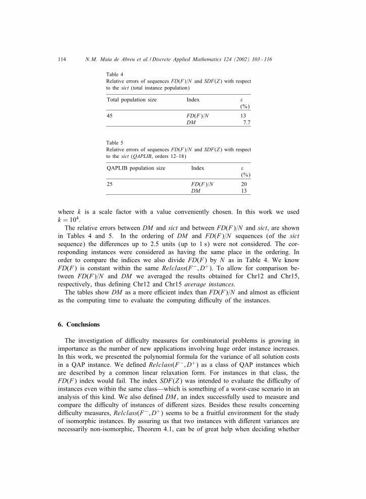
Table 4Relative errors of sequences FD(F)=N and SDF(Z) with respectto the sict (total instance population)

Total population size Index 5(%)

45 FD(F)=N 13DM 7.7

Table 5Relative errors of sequences FD(F)=N and SDF(Z) with respectto the sict (QAPLIB, orders 12–18)

QAPLIB population size Index 5(%)

25 FD(F)=N 20DM 13

where k is a scale factor with a value conveniently chosen. In this work we usedk = 104.The relative errors between DM and sict and between FD(F)=N and sict, are shown

in Tables 4 and 5. In the ordering of DM and FD(F)=N sequences (of the sictsequence) the diQerences up to 2.5 units (up to 1 s) were not considered. The cor-responding instances were considered as having the same place in the ordering. Inorder to compare the indices we also divide FD(F) by N as in Table 4. We knowFD(F) is constant within the same Relclass(F−; D+). To allow for comparison be-tween FD(F)=N and DM we averaged the results obtained for Chr12 and Chr15,respectively, thus de;ning Chr12 and Chr15 average instances.The tables show DM as a more e"cient index than FD(F)=N and almost as e"cient

as the computing time to evaluate the computing di"culty of the instances.

6. Conclusions

The investigation of di"culty measures for combinatorial problems is growing inimportance as the number of new applications involving huge order instance increases.In this work, we presented the polynomial formula for the variance of all solution costsin a QAP instance. We de;ned Relclass(F−; D+) as a class of QAP instances whichare described by a common linear relaxation form. For instances in that class, theFD(F) index would fail. The index SDF(Z) was intended to evaluate the di"culty ofinstances even within the same class—which is something of a worst-case scenario in ananalysis of this kind. We also de;ned DM , an index successfully used to measure andcompare the di"culty of instances of diQerent sizes. Besides these results concerningdi"culty measures, Relclass(F−; D+) seems to be a fruitful environment for the studyof isomorphic instances. By assuring us that two instances with diQerent variances arenecessarily non-isomorphic, Theorem 4.1, can be of great help when deciding whether

N.M. Maia de Abreu et al. / Discrete Applied Mathematics 124 (2002) 103–116 115

any two QAP instances are non-isomorphic. The use of variance costs to characterizeclasses of problem instances could potentially be used for other combinatorial problemsas well.

Acknowledgements

We are indebted to the Conselho Nacional de Desenvolvimento Cienti;co e Tec-nolUogico (CNPq) and the CoordenaHcao de AperfeiHcoamento do Pessoal de Ensino Su-perior (CAPES) for the ;nancial support given to this work. We are thankful for theimportant observations and suggestions given by the referees.

References

[1] E. Angel, V. Zissimopoulos, On the quality of the local search for the quadratic assignment problem,Discrete Appl. Math. 82 (1998) 15–25.

[2] C.C.P. Barbut, Automorphismes du permutoWedre et votes de Condorcet, Math. Inform. Sci. Hum. 28e(111) (1990) 73–82.

[3] P.O. Boaventura-Netto, N.M.M. Abreu, Quadratic assignment problem: a polynomial expression for thevariance of solutions (extended abstract), I ELIO=Optima 97, ConcepciUon, Chile, November 1997.

[4] P.O. Boaventura-Netto, N.M.M. Abreu, Cost solution average and variance in the quadratic assignmentproblem, Technical Report PEP 02=98, Programa de Engenharia de ProduHcao, COPPE=URFJ, 1998 (inPortuguese).

[5] R.E. Burkard, E. CH ela, A.M. Demidenko, N.N. Metelski, G.J. Woeginger, Perspectives of easy and hardcases of the quadratic assignment problem spezialforschungsbereich F003, Optimierung und Kontrolle,Bericht Nr104, Graz, 1997.

[6] R.E. Burkard, S.E. Karisch, F. Rendl, QAPLIB—a quadratic assignment problem libaray, Report No.287 CDLDO-41, Technische Universitat, Graz, 1994.

[7] E. CH ela, The quadratic assignment problem: theory and algorithms, in: Combinatorial Optimization,Kluwer Academic Publishers, Dordrecht, 1998.

[8] M. Dell’Amico, F. Ma"oli, S. Martello, Annotated Bibliographies in Combinatorial Optimization, Wiley,Chichester, 1997.

[9] J.W. Gavett, N.V. Plyter, The optimal assignment of facilities to locations by branch-and-bound, Oper.Res. 14 (1966) 210–232.

[10] E.F. Gouvea, Applications of statistics and algebra to QAP, qualifying examination to D.Sc., Programade Engenharia de ProduHcao, COPPE=UFRJ, 1999 (in Portuguese).

[11] G.W. Graves, A.B. Whinston, An algorithm for the quadratic assignment problem, Manage. Sci. 17(1970) 453–471.

[12] W. Herroeleven, A. Van Gils, On the use of Kow dominance in complexity measures for facility layoutproblems, Internat. J. Prod. Res. 23 (1985) 97–108.

[13] T.C. Koopmans, M. Beckmann, Assignment problems and the location of economic activities,Econometrica 25 (1) (1957) 53–76.

[14] T. Mautor, C. Roucairol, Di"culties of exact methods for solving the quadratic assignment problem,in: P. Pardlos, H. Wolkowics (Eds.), Quadratic Assignment and Related Problems, DIMACS Series inDiscrete Mathematics and Theoretical Computer Science, Vol. 16, AMS, Providence, RI, 1994.

[15] R. Mojena, T. Vollmann, Y. Okamoto, On perdicting computational time of a branch-and-boundalgorithm for the assignment of facilities, Dec. Sci. 7 (1976) 856–867.

[16] P. Pardalos, K.G. Ramakrishnan, M.G.C. Resende, Y. Li, implementation of a variance reduction-basedlower bound in a branch-and-bound algorithm for the quadratic assignment problem, SIAM J. Optim.7 (1) (1997) 280–294.

116 N.M. Maia de Abreu et al. / Discrete Applied Mathematics 124 (2002) 103–116

[17] P. Pardalos, H. Wolkowicz, The quadratic assignment problem: a survey of recent developments, in:P. Pardalos, H. Wolkowicz (Eds.), Quadratic Assignment and Related Problems, DIMACS Series inDiscrete Mathematics and Theoretical Computer Science, Vol. 16, AMS, Providence, 1994.

[18] T.E. Vollmann, E.S. BuQa, The facility layout problem in perspective, Manage. Sci. 12 (1966) 450–471.