Might the Rigorous Modeling of Economic Phenomena

Require Hypercomputation?

Selmer BringsjordDepartment of Cognitive Science

Department of Computer Science

Rensselaer Polytechnic Institute (RPI)

110 8th Street

Troy NY 12180-3590

selmer@rpi.edu • http://www.rpi.edu∼brings

Eugene EberbachDepartment of Engineering and Science

Rensselaer Polytechnic Institute (RPI)

275 Windsor Street

Hartford CT 06129-2991

eberbe@rpi.edu • http://www.ewp.rpi.edu/∼eberbe

Naveen Sundar G.Dept. of Computer Science

Rensselaer Polytechnic Institute (RPI)

110 8th Street

Troy NY 12180-3590

govinn@cs.rpi.edu • http://www.cs.rpi.edu/∼govinn

Yingrui YangDepartment of Cognitive Science

Rensselaer Polytechnic Institute (RPI)

110 8th Street

Troy NY 12180-3590

yangyri@rpi.edu

May 17, 2010

Contents

1 Introduction 1

2 The Science of Sciences 2

3 The Chain Store Paradox 2

4 Mental Decision Logic 5

5 Economic Planning and Prediction via Turing-level Actors 65.1 Description of Hutter’s AIXI model . . . . . . . . . . . . . . . . . . . . . . . . . . . . . . . 6

5.1.1 Preliminaries . . . . . . . . . . . . . . . . . . . . . . . . . . . . . . . . . . . . . . . 65.1.2 The AIXI Model . . . . . . . . . . . . . . . . . . . . . . . . . . . . . . . . . . . . . 85.1.3 Properties of AIXI . . . . . . . . . . . . . . . . . . . . . . . . . . . . . . . . . . . . 8

5.2 Generalized Economic Planning is an Enriched AIXI Problem . . . . . . . . . . . . . . . . 95.3 Some Examples . . . . . . . . . . . . . . . . . . . . . . . . . . . . . . . . . . . . . . . . . . 10

6 Conclusion and Next Steps 12

References 12

List of Figures

1 One-Stage, Two-Player Snapshot in CSP . . . . . . . . . . . . . . . . . . . . . . . . . . . . 32 Two-Stage, Three-Player Snapshot in CSP . . . . . . . . . . . . . . . . . . . . . . . . . . . 33 Economic-AIXI: Economic Planning Formalized via Primitives in Theory of Computation 9

List of Tables

1 Economic entities and their specification . . . . . . . . . . . . . . . . . . . . . . . . . . . . 10

1 Introduction

Mathematical logic was born from the rigorous formalization and study of mathematics using computationand formal logic, and includes such seminal results as Godel’s incompleteness theorems and Turing’shalting-problem result, proved at the dawn of computer science. Both results revealed that a coreproblem in mathematics (viz., deciding whether or not something is a theorem, and producing a proofthat certifies the answer), in certain contexts, is tremendously difficult. Mathematical logic continues tobe quite fertile; recent results include demonstrations that certain theorems in mathematics are in the“independent-of-Peano-Arithmetic” class drawn to our attention by Godel (e.g., Goodstein’s Theorem;for a nice overview, see Smith 2007), and so hard to obtain that humans currently find it necessary todeploy infinitary concepts and reasoning in order to secure them.

Might it be that the rigorous formalization and study of economics, carried out from the perspectiveof formal logic and computability theory, will reveal that core problems in that field are likewise tremen-dously difficult? Specifically, might it be that some economic phenomena involve hypercomputation, orare at least best modeled using schemes that are in part hypercomputational? In this short paper wedefend an affirmative answer to this question.

Please note that even if our answer is correct and successfully defended in the present paper, it doesn’tfollow that economic phenomena in fact involve hypercomputation.1 This can be seen immediately byreflecting for a moment upon the fundamental results from mathematical logic we alluded to above. Forexample, let h be the halting function from indices i for Turing machines paired with natural numbersn given to such machines as input, to 1 or 0 as a verdict on whether or not Turing machine Mi haltsor not after being started with n as input on its tape. As is well known, the Entscheidungsproblem isTuring-solvable if and only if h is Turing-computable. This shows immediately that it might be thathypercomputation is necessary in order to provide an accurate model of mathematical reasoning. Thismight be the case because human mathematicians (and others working in the formal sciences) might, forall we know, be capable of solving the Entscheidungsproblem. Of course, it could turn out that greatdiscoveries in mathematics, for example Wiles’ proof of Fermat’s Last Theorem (Wiles 1995, Wiles &Taylor 1995), happen in part because the specific instances of the general problem just happen to bewithin human reach, while the arbitrary instance isn’t.2

The plan of the paper is entirely straightforward. We simply explain how some formal modelingof economic phenomena may well naturally invoke hypercomputation. We touch upon modeling in thefollowing three areas, viz.,

1. The Chain Store Paradox, the modeling of which can be naturally carried out in logics whereinproof-finding is beyond Turing machines (§3);

2. use of so-called “mental” logics to model real-world human reasoning and decision-making in waysmore accurate than those enabled by standard, normatively correct logics; (§4); and

3. economic planning and prediction modeled using interacting Turing machines (§5).

We leave for another day consideration of the question of whether such modeling can be non-question-beggingly dispensed with in favor of mere Turing-level modeling without leaving aside crucial phenomena.It is easy enough to simplify economic phenomena in such a way that it can be modeled using elementarycomputation, as long as one is willing to beg questions. For example, Cottrell et al. (2009) explainthat socialist planning can be viewed as standard computation as long as we simply assume that humanpersons are themselves incapable of hypercomputation. But of course if human cognition itself involveshypercomputation, say in the creation of new products, it would hardly be possible for a Turing-levelplanning algorithm to model human innovation through time. (These issues are to some degree taken uplater in section 5.) We also leave aside, due to space constraints, many additional economic phenomenathe formal modeling of which might require hypercomputation.

1In a parallel, while a formal model of physical reality may involve information-processing above the Turing Limit, itdoesn’t follow from this that physical reality is in fact hypercomputational in nature. We suppose this is why despite suchsuper-Turing models as those presented by Pour-El & Richards (1981), many scientists refuse to accept the proposition thathypercomputation is physically real.

2In laying down at the outset an openmindedness as to whether or not hypercomputation is in fact active in thephenomena modeled in economics we leave aside consideration of some of our own work. E.g., Bringsjord (1992, 2003, 2004)has argued that human persons hypercompute.

1

2 The Science of Sciences

This section is to clarify what we set forth to show in the paper. The goal of the rational scientificenterprise can be thought of as that of finding models that fit some observed data. There has beensignificant work in studying and understanding the scientific process, a study we term the Science ofSciences. An introduction to the computational modeling of science can be found in (Jain, Osherson,Royer & Sharma 1999). Generally, the scientific process can be formalized as identifying a languageL where L ⊂ A∗, where A∗ is a finite alphabet, given a subset of strings L′ from the language L. Thatis, science can be equated with language identification3. In computational models of science, we havenature producing strings <w1, w2, . . . , wn, . . .> from the finite alphabet A, and the job of a scientistis to identify the true language L from which nature produces the strings. The scientist generateshypotheses/languages/theories <L1,L2, . . . ,Ln, . . .> over time which are consistent with the observeddata up to that time, i.e., {wi|wi is part of <w1, w2, . . . , wt>} ⊂ Lt. The hypotheses/theories generatedby the scientist should satisfy the following constraints in order to qualify as a science of the phenomenaunder consideration

C1: each hypothesis should be consistent with the observed dataC2: each hypothesis should be falsifiable (for example, should not predict everything, i.e., A∗)

With these minimal restrictions one generally has access to a large number of hypotheses. Thereare usually a few philosophical yardsticks which help a scientist to select one hypothesis from among allpossible hypotheses. For example, Occam’s Razor dictates (roughly put) that simpler theories should bepreferred over more complex theories. Examining any natural phenomena, one can produce a hierarchyof theories which satisify C1 and C2 but differ in their simplicity. For example, in the context of physicsif we assume that we live in a Newtonian world then we will have two theories to explain the phenomenaof gravitation, Einstein’s General Theory of Relativity and Newton’s theory of gravitation, both of whichwill satisfy C1 and C2. Using Occam’s razor we would then select Newton’s theory of gravitation as it ismore simple 4.

In the context of economics, we seek to produce theories which are consistent with economic phenom-ena (that is satisfy C1 and C2) but also require hypercomputational processes. This does not imply thateconomic phenomena observed so far are hypercomputational. Our work is to show the possibility ofhypercomputation in economic phenomena.

Structuralism Work (Balzer, Sneed & Moulines 2000, Balzer, Moulines & Sneed 1987, Sneed 1972,Sneed 1989, Wajnberg, Corruble, Ganascia & Moulines n.d.)

3 The Chain Store Paradox

Reinhard Selten (1978), Nobel laureate in economics, introduced the Chain Store Paradox (CSP); itprovides an excellent example of phenomena the fastidious formal modeling of which may well requirehypercomputation.

CSP centers around strategic interaction between a “chain store” (e.g., Wal-Mart, McDonalds, oreven, say, Microsoft) and those who may attempt to enter the relevant market and compete against thisstore. The game here is an n-stage, n + 1 one, in which the n + 1th player is our chain store (CS), andthe remaining players are the potential entrants E1, E2, . . . , En. At the beginning of the kth stage, Ekobserves the outcome of the prior k−1 stages, and chooses between two actions: Stay Out or Enter. Anentrant Ek opting for Stay Out receives a payoff of c, while CS receives a payoff of a. If, on the otherhand, Ek decides to enter the market, CS has two options: Fight or Acquiesce. In the case where CSfights, CS and Ek receive a benefit of d; when CS acquiesces, both receive b. Values are constrained bya > b > c > d, and in fact we shall here set the values, without loss of generality, to be, respectively, 52 1 0. Please see Figures 1 and 2, which provide snapshots of early stages in the game. We specificallydraw your attention to something that will be exploited later in this section, which is shown in Figure 1:viz., that we have used diagonal dotted lines, with labels, to indicate key timepoints in the action.

3The notion of equating Science with language identification is analogous to equating Computation with languagerecognition.

4The concept of simplicity of theories can be more rigorously defined and analyzed

2

Figure 1: One-Stage, Two-Player Snapshot in CSP

Figure 2: Two-Stage, Three-Player Snapshot in CSP

But why is CSP called a paradox? Please note that there are at least three senses of ‘paradox’ usedin formal logic and in the formal sciences generally, historically speaking. In the first sense, a paradoxconsists in the fact that it’s possible to deduce some contradiction φ ∧ ¬φ from what at least seems tobe a true set of axioms or premises. A famous example in this category of paradox is Russell’s Paradox,which pivots on the fact that in standard first-order logic

∃x∀y(Rxy ↔ ¬Ryy) ` φ ∧ ¬φ.

As Frege learned, much to his chagrin, Russell’s Paradox demonstrated that Frege’s proposed meta-mathematical set-theoretic foundation for mathematics was inconsistent.5 (Other examples of paradoxesof this form that are relevant to economics are the Lottery Paradox and the Paradox of the Preface, butdiscussing these would take us too far afield. Both of these paradoxes are in our opinion solved by Pollock(1995), using his Oscar system.)

In the second sense of ‘paradox’ in logic, a theorem is simply regarded by many to be extremelycounter-intuitive, but no outright contradiction is involved. A famous example in this category is Skolem’sParadox, elegantly discussed in (Ebbinghaus, Flum & Thomas 1994). Finally, in the third sense of‘paradox,’ a contradiction is produced, but not by a derivation from a single body of unified knowledge;rather, the contradiction is produced by deduction of φ from one body of declarative knowledge (or axiomset, if things are fully formal), and by deduction of ¬φ from another body of declarative knowledge (oroutright axiom set, in the fully formal version, if there is one). Additionally, both bodies of knowledgeare independently plausible, to a very high degree. A famous example of a paradox in this third sense —

5A classic presentation of axiomatic set theory as emerging from the situation in which naive set theory was plaguedby Russell’s Paradox (and others of the first type) is (Suppes 1972). Nice discussion of Russell’s Paradox can be found in(Barwise & Etchemendy 1999).

3

quite relevant to decision theory and economics, but for sheer space-conservation reasons outside of ourpresent discussion — is Newcomb’s Paradox; see for example the first published treatment, (Nozick 1970).It is into this third category of ‘paradox’ that CSP falls.

More specifically, we have first the following definition and theorem. (Selten himself doesn’t providea fully explicit proof of the theorem in question. For more formal treatments, and proofs of backwardinduction, see e.g. (Aumann 1995, Balkenborg & Winter 1997). In the interest of economy, we provideonly a proof sketch here, and likewise for the theorem thereafter for deterrence.)

————Definition (GT-Rationality): We say that an agent is GT-rational if it knows all the axioms of stan-dard game theory, and all its actions abide by these axioms.

Theorem(GT-Rationality Implies Enter & Acquiesce): In a chain-store game, a GT-rational entrant Ekwill always opt for Enter, and a GT-rational chain store CS will always opt for Acquiesce in response.

Proof-Sketch: Selten’s original strategy was “backward induction,” which essentially runs as followswhen starting with the “endpoint” of 20 as he did. Set k = 20. If E20 chooses Enter and CS Fight, thenCS receives 0. If, on the other hand, CS chooses Acquiesce, CS gets 2. Ergo, by GT-rationality,CS must choose Acquiesce. Given the common-knowledge supposition in the theorem, E20 knowsthat CS is rational and will acquiesce. Hence E20 enters because he receives 2 (rather than 1). Butnow E19 will know the reasoning and analysis just given from E20’s perspective, and so will as a GT-rational agent opt herself for Enter. But then parallel reasoning works for E18, E17, . . . , E1. QED

————

The other side of the “third-sense” paradox in the case of CSP begins to be visible when one ascertainswhat real people in the real world would do when they themselves are in the position of CS in the chain-store game. As has been noted by many in business, such people are actually inclined to fight those whoseek to enter — and looking at real-world corporate behavior shows that fighting is the strategy mostoften selected.6 For us, from the standpoint of formal logic and computability theory, these empiricalfactors are only of high relevance if they correspond with some formal result — and sure enough theredoes appear to be a formal rationale in favor of fighting. This rationale is bound up inseparably withdeterrence, and can be expressed by what can be called forward induction. The basic idea is perfectlystraightforward, and can be expressed via the following definition and theorem (which for lack of spacewe keep, like its predecessor, somewhat informal and compressed).

————Definition (Perception; m-Learning; Two-Option Rationality): We say that an agent α1 is perceptiveif, whenever an agent α2 performs some action, α1 knows that α2 does so. We say that an agent α is anm-learner provided that when it sees agents perform some action A m times, in each case in exactly thesame circumstances, it will believe that all agents into the future will perform A in these circumstances.And we say that an agent is two-option-rational if and only if when faced exclusively with two mutuallyexclusive options A1 and A2, where the payoff for the first is greater than the second, that agent will selectA1.

Theorem (Rationality of Deterrence from CS): Suppose we have a chain-store game based on n per-ceptive agents, each of whom are m-learners. Then after m stages of a chain-store game in which eachpotential entrant seeks to enter and CS fights, the game will continue indefinitely under the pattern ofStay Out.

Proof-Sketch: The argument is by induction on N (natural numbers). Suppose that the antecedents ofthe theorem hold. Then at stage m+ 1 all future potential entrants will believe that by seeking to enter,their payoff will be 0, since they will believe that CS will invariably fight in the future in response to anentering agent. In addition, as these agents are all two-option-rational, they will forever choose Stay Out.

6Selten (1978) prophetically remarked in his seminal paper that he never encountered someone who said “he wouldbehave according to induction theory [were he the Chain Store].”

4

QED ————

We see here that the two previous theorems, together, constitute a paradox in the aforementionedthird sense.7

In general, paradoxes of the third type can be solved if one simply affirms one of the two bodiesof knowledge, and rejects the other. But the key fact for our purposes in the present paper is that nomatter which body of knowledge one prefers over the other, the phenomena in question may well involvehypercomputation. This is easy to see, as follows.

One can fully formalize and prove a range of both “high-expressive” backward induction and deterrencetheorems under the relevant assumptions. These theorems are differentiated by way of the level ofexpressivity of the underlying logics used. The calculi use more detailed calculi than have been usedbefore in the chain-store literature in mathematical economics. For example, it is possible to prove aversion of both the induction and deterrence theorems using the “cognitive event calculus” (CEP) inventedby Arkoudas & Bringsjord (2009), which allows for epistemic operators to apply to sub-formulas in full-blown quantified modal logic, in which the event calculus is encoded. Any agents able to determine inthe arbitrary case whether or not some proposition holds in CEP under some axiom set would be capableof hypercomputation, and would therefore, if accurately modeled, require hypercomputation. From thestandpoint of theoretical computer science and logic, all versions of the chain store game, hitherto, haveinvolved exceedingly simple formalizations of what agents know and believe in this game, and of changethrough time. To see this more specifically, note that in standard axioms used in game theory, forexample in standard textbooks like (Osborne & Rubinstein 1994), knowledge is interpreted as a simplefunction, rather than as an operator that can range over very expressive formulas. This same limited,simple treatment of knowledge and belief is the standard fare in economics. Yet, it can be shown thatthe difficulty of computing, from the standpoint of some potential entrant Ek or chain store CS in someversion of a chain-store game, is at the level, minimally, of Σ1 when attempting to compute whether byinduction or deterrence they should opt for Enter or Stay Out.

4 Mental Decision Logic

Jones, suppose, is trying to decide which of two cars to purchase. One car is a so-called sport-utilityvehicle (SUV), and the other option is a sedan. In light of the key possibility that his drives will oftentake him through snowy mountains, which vehicle ought he to buy?

We can represent such a decision problem using the machinery of some established decision theory.The theory we prefer happens to be a merging of the decision theory of Savage (1954), often embracedby economists, with the decision theory of Jeffrey (1964), welcomed by those in related fields (logicand computer science, e.g.) inclined toward logic-based modeling. The hybrid theory is Joyce’s (1999).However, in the interests of space, we severely compress the language of Joyce, and regard a decisionproblem D as only the problem of deciding which one of two competing actions a1 and a2 provides moreutility to an agent s in the light of a set Φ of logical formulas. (When actions appear as arguments to >we assume that it’s the utility of the actions that are being related.) Φ is assumed to include informationabout the world, about causal connections between actions and outcomes, about the beliefs of s, andso on. We thus write a decision problem D as a quadruple (Φ, s, a1, a2), and such a problem would forexample be solved if it could be determined for or by s that Φ `C a1 > a2.

But what exactly does it mean to say that Φ `C a1 > a2? In general, this means that a1 > a2 canbe proved from Φ. However, we can only genuinely answer this question if we have defined the context;if, that is, we have defined the background logic and proof calculus C. Suppose for example that thebackground logic is standard first-order logic and that C is some standard proof calculus for first-orderlogic — say F from (Barwise & Etchemendy 1999). Then the meaning of a decision problem is clear.But it’s now well-known in cognitive science that if this background logic and associated calculus is anormatively correct one (such as first-order logic), the modeling will fail, for the simple reason that even

7We would be remiss if we didn’t mention two points of scholarship, to wit: (1) Game theorists have long proposedmodifications or elaborations of the chain-store game which allow game theory to reflect sensitivity to the cogency of thedeterrence line of reasoning. E.g., see (Kreps & Wilson 1982). (2) Innovative approaches to CSP that in some sense optfor a third approach separate from both backward induction and deterrence have been proposed. E.g., see the one based inevolutionary computation proposed by Tracy (2008).

5

the vast majority of college-educated adults are incapable of reasoning in normatively correct deductivefashion (for a nice survey, see e.g. Stanovich & West 2000). This brute fact, quite in line with whatis today called “behavioral” economics, has catalyzed the creation of “mental” logics: logics that arespecifically tailored to reflect how human beings (save for e.g. logicians and so on) reason. Prominentresearchers who have invented and refined such logics include Braine (1998), Johnson-Laird (1983), Rips(1994), and Yang et al. (1998). Of these, Yang (2006) has recently presented a logic (mental decision logic;‘MDL’ for short) designed specifically for representing decision-making in scenarios commonly studied byeconomists.

Let’s refer to the space of mental logics as M, let L ∈ M be without loss of generality here somemental logic whose inferential machinery is C, and let ΦL be some set of formulas expressed in the languageof L which captures the above situation involving Jones, where a1 > a2 is one such formula. (Note thatwe must speak of “inferential machinery” rather than a standard proof calculus (or theory). This is thecase because what can be inferred in C departs from standard deductive inference.) At present, so far aswe know, it’s an open question as to whether an ordinary Turing machine can decide in the general casewhether or not

ΦL `C a1 > a2.

8 Given this, and given that accurate modeling of Jones may posit that he has a capacity to judge whethera1 > a2 can be inferred from the knowledge base in question, it may be that hypercomputation is partof the processes in question.

5 Economic Planning and Prediction via Turing-level Actors

We now examine how a planned economy can be modeled in terms of basic computability and probabil-ity theory as a set of interacting Turing machines. Minimally, an economic system can be modeled asconsisting of a planning agent which tries to control the economy so that some utility is maximized, aset of independent economic agents, and an environment which provides a setting in which these agentsfunction. The purpose of this section is to argue for the following claim.

Claim: Even if real economies and agents in those economies can be modeled as Turing machines,formal solutions to non-trivial optimization problems can be hypercomputational.

To model such agents, we look at Hutter’s computational model — the AIXI Model (Hutter 2005)— for an agent seeking to maximize the reward that it obtains in an unknown environment. The purposeof Hutter’s model is to provide a formal model for artificial intelligence (AI). This model can be adaptedwith some extensions to model an economic planner seeking to derive maximum utility in an economycomprised of zero or more other cognitive agents. Hutter’s model is composed of simple conceptual in-gredients and can be naturally adapted to the economic domain. We start with a condensed descriptionof Hutter’s model. A simpler description can be found in (Legg & Hutter 2007).

5.1 Description of Hutter’s AIXI model

Hutter’s AIXI model is a formal model of an agent operating in an unknown environment. Given certainreasonable assumptions, this model is universally optimal across all possible environments and has certainprovable optimality properties. This model builds upon Solomonoff’s Theory of Induction (Solomonoff1978) and Sequential Decision theory (Sutton & Barto 1998). Before we describe Hutter’s AIXI model,we present some necessary preliminaries.

5.1.1 Preliminaries

We are concerned with sequence prediction tasks in the AIXI model. Any prediction task can be modeledas a sequence prediction task. In the AIXI model the agent will observe the sequence x1 . . . xt−1 from theenviroment, which corresponds to percepts that an agent will obtain in an enviroment. The agent then

8That this is an open question may not be due to the technical difficulty of obtaining proofs that settle the question forsome L and C. Openness may be due to other factors, e.g. to the fact that mental logics are often left too imprecise for thedecidability question to be posed with sufficient rigor.

6

predicts xt and then outputs an action y∗t which maximizes its expected reward. The following conceptsplay a role in the specification of the optimal action y∗t . Following Hutter, we denote the sequencex1, x2, . . . , xn by x1:n and the sequence x1, x2, . . . , xn−1 by x<n

Bayesian Mixture Distribution We have some data x which is explained/produced by a hypothe-sis/model H∗ ∈M. We don’t know the true model producing our data. We have prior probabilityfor model Hi given by prior(Hi). The Bayesian mixture distribution of Hi with respect to the priorprobabilities prior(Hi) is specified by ∑

i

prior(Hi)P (x|Hi)

A Bayes-optimal predictor based on the Bayesian mixture distribution is Pareto-optimal, and pre-dictors based on the Bayesian mixture distribution converge to the loss from the optimal predictorsoon.

Prefix Code A prefix code P is a set of strings such that no string in P is the prefix of another stringin P .

Monotone Universal Turing Machine A monotone Turing machine is a Turing machine with 1.) oneor more bi-directional working tapes 2.) a unidirectional input tape and 3.) a unidirectional outputtape. The unidirectional input and output tapes are necessary to make the technical task ofimposing chronological conditions on Turing machines easier.

Minimal Programs When the input tape of a monotone universal Turing machine U contains p to theleft of the input head when the last bit of a string x is output, we write U(p) = x∗. The set of allsuch strings p forms a prefix code, and the codes are called minimal programs.

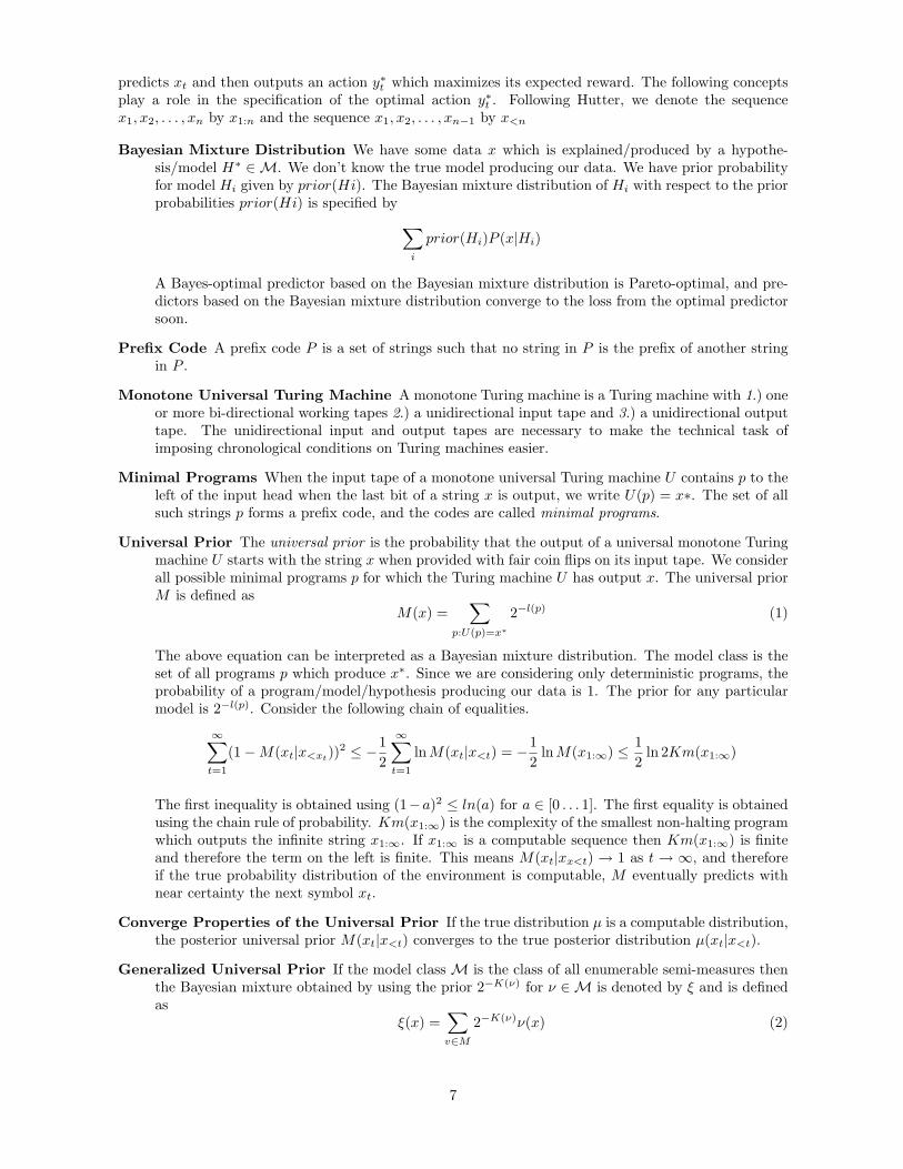
Universal Prior The universal prior is the probability that the output of a universal monotone Turingmachine U starts with the string x when provided with fair coin flips on its input tape. We considerall possible minimal programs p for which the Turing machine U has output x. The universal priorM is defined as

M(x) =∑

p:U(p)=x∗

2−l(p) (1)

The above equation can be interpreted as a Bayesian mixture distribution. The model class is theset of all programs p which produce x∗. Since we are considering only deterministic programs, theprobability of a program/model/hypothesis producing our data is 1. The prior for any particularmodel is 2−l(p). Consider the following chain of equalities.

∞∑t=1

(1−M(xt|x<xt))2 ≤ −1

2

∞∑t=1

lnM(xt|x<t) = −12

lnM(x1:∞) ≤ 12

ln 2Km(x1:∞)

The first inequality is obtained using (1−a)2 ≤ ln(a) for a ∈ [0 . . . 1]. The first equality is obtainedusing the chain rule of probability. Km(x1:∞) is the complexity of the smallest non-halting programwhich outputs the infinite string x1:∞. If x1:∞ is a computable sequence then Km(x1:∞) is finiteand therefore the term on the left is finite. This means M(xt|xx<t) → 1 as t → ∞, and thereforeif the true probability distribution of the environment is computable, M eventually predicts withnear certainty the next symbol xt.

Converge Properties of the Universal Prior If the true distribution µ is a computable distribution,the posterior universal prior M(xt|x<t) converges to the true posterior distribution µ(xt|x<t).

Generalized Universal Prior If the model class M is the class of all enumerable semi-measures thenthe Bayesian mixture obtained by using the prior 2−K(ν) for ν ∈M is denoted by ξ and is definedas

ξ(x) =∑v∈M

2−K(ν)ν(x) (2)

7

An enumerable function is one for which lower bounds can be finitely computable but the functionitself need not be finitely computable. A measure is a semi-measure which is also normalized. Thegeneralized prior is a Bayesian mixture of enumerable (not just finitely computable) semi-measures(not just measures) and takes into account more distributions than the universal prior definedabove. The generalized universal prior ξ is also an enumerable semi-measure.

Convergence and Loss Bounds of ξ It can be show that the posterior distribution ξ(xt|x<t) con-verges to the true posterior distribution µ(xt|x<t) in a finite amount of time and that losses sufferedby a Bayes-optimal predictor that uses the posterior ξ(xt|x<t) are bounded from the losses sufferedby a Bayes-optimal predictor that uses µ(xt|x<t) .

5.1.2 The AIXI Model

The AIXI model is an agent-based model in which an agent P performs an action yt ∈ Y in an environmentQ at time time t. The environment responds with xt ∈ X , which can be split into a unique percept otand a reward rt = r(xt). This continues till some time m termed as the horizon or the lifetime of theagent.

We assume that the environment is modeled by a true probability distribution µ. The probability ofthe environment producing the percept sequence x1:n is µ(x1:n) which can be reasonably approximatedby ξ(x1:n) if µ is computable. Now consider the agent at time k. The expected reward at time k + 1 ifthe agent chooses action y is

R(k + 1) =∑x∈X

r(x)µ(xk+1 = x|x1:k, y<ky) (3)

The action to maximize the expected reward at time k+1 denoted by y∗k+1 is then given by the actionwhich maximizes the above equation.

y∗k+1 = argmaxy∈Y

∑x∈X

r(x)µ(xk+1 = x|x1:k, y<ky) (4)

A rational agent will seek to maximize the rewards that it expects over its entire lifetime and not justthe reward it expects in the next time step. The expected reward to be obtained in cycles k + 1 to mgiven that agent performs actions y at time k + 1 is given by this recursive equation:

R(k + 1 : m) =∑x∈X

[r(x) +R(k + 2 : m)]µ(xk+1 = x|x1:k, y<ky) (5)

The action to maximize the expected reward to be obtained in cycles k + 1 to m is then

y∗k+1 = argmaxy∈Y

∑x∈X

[r(x) +R(k + 2 : m)]µ(xk+1 = x|x1:k, y<ky) (6)

The AIXI model is then obtained by replacing the unknown µ by ξ (the Greek letter pronounced as“Xi”) in the above equation. The AIXI Model is an ExpectiMax algorithm (Russell & Norvig 2002).Unfolding the recursive equation and renaming the corresponding indices we get the following equationwhich specifies the best action to choose at time k.

y∗k = argmaxyk

∑xk

. . .maxym

∑xm

(rk + · · ·+ rm).ξ(xk:m|x<k, y<ky)

5.1.3 Properties of AIXI

AIXI is Turing-uncomputable. Intuitively this is due to the involvement of the Turing-uncomputableKolmogorov complexity and an infinite sum in the specification of AIXI’s optimal action. The AIXImodel has many associated optimality properties and Hutter terms the AIXI model universally optimalas it can perform better than any other agent and can perform well in any enviornment.9 For proofs ofthese properties please consult (Hutter 2005).

9With some reasonable caveats.

8

5.2 Generalized Economic Planning is an Enriched AIXI Problem

Hutter’s model deals with a rational agent seeking to maximize the rewards it obtains in an unknownenvironment. It is easy to generalize the AIXI model to that of a rational agent seeking to maximizesome reward function in an environment containing some other cognitive agents. The agent which seeksto control the economy and maximize the reward/utility function models a planner in an economy andthe other agents model participants in the economy. We model the planner, constituent agents in theeconomy, and the environment/economy as monotone Turing machines.

Our model, termed as the Economic-AIXI model, consists of

1. A central planner in the economy. The planner outputs plans to control the economy and the goalof the planner is to maximize the reward that it obtains from the economy.

2. A set of agents which constitute the economy A = {A1, . . . , An}. The agents can be either producersor consumers in the economy or both. The agents in the economy can either ignore or adherepartially or fully to the planner’s commands.

3. The overall economy. The economy models interactions of different agents, natural resources,consumption and production in the economy. The economy represents inanimate forces that act inan economy, such as laws of nature, forces outside the economy, etc.

Figure 3 shows a schematic description of our model. At time k, the planner reads symbols x1k−1, . . . , x

nk−1

from the output tapes of the agents 1 . . . n and the symbol ek−1 from the output tape of the economy.The planner then writes pk on its output tape. Agent i, where i ranges from [1 . . . n], reads ek−1 fromthe output tape of the economy and pk from the output tape of the planner and then writes the symbolxik on its output tape. The economy reads symbols x1

k−1, . . . , xnk−1 from the output tapes of the agents

and the symbol pk from the output tape of the planner and then writes ek on its output tape.

Figure 3: Economic-AIXI: Economic Planning Formalized via Primitives in Theory of Computation

!!!

!!!

Planner

Economy

Agent 1

!!!

Work

Tape

Agent n

Work

Tape

q1

p2p3p4p5

q2q3

p1

a1a2a3a4a5

a1a2a3a4a5

p4 A shaded cell indicates a cell on the tape that is currently being written

many more agents

Output tape of the Planner

Output tape of the Economy

Work

Tape

Work

Tape

Output tapes of the Agents

q4

!!!

!!!

At time instance t, the planner outputs plan pt based on prior actions (x1<t, . . . , x

nt<) by different

agents in the economy and the past states of the economy characterized by e<t on the output tape of theeconomy. The agents compute their next action based on the plan history p1:t and the economic historye<t. The economy then moves to a different state based on the past actions of the agents (x1

<t, . . . , xnt<)

9

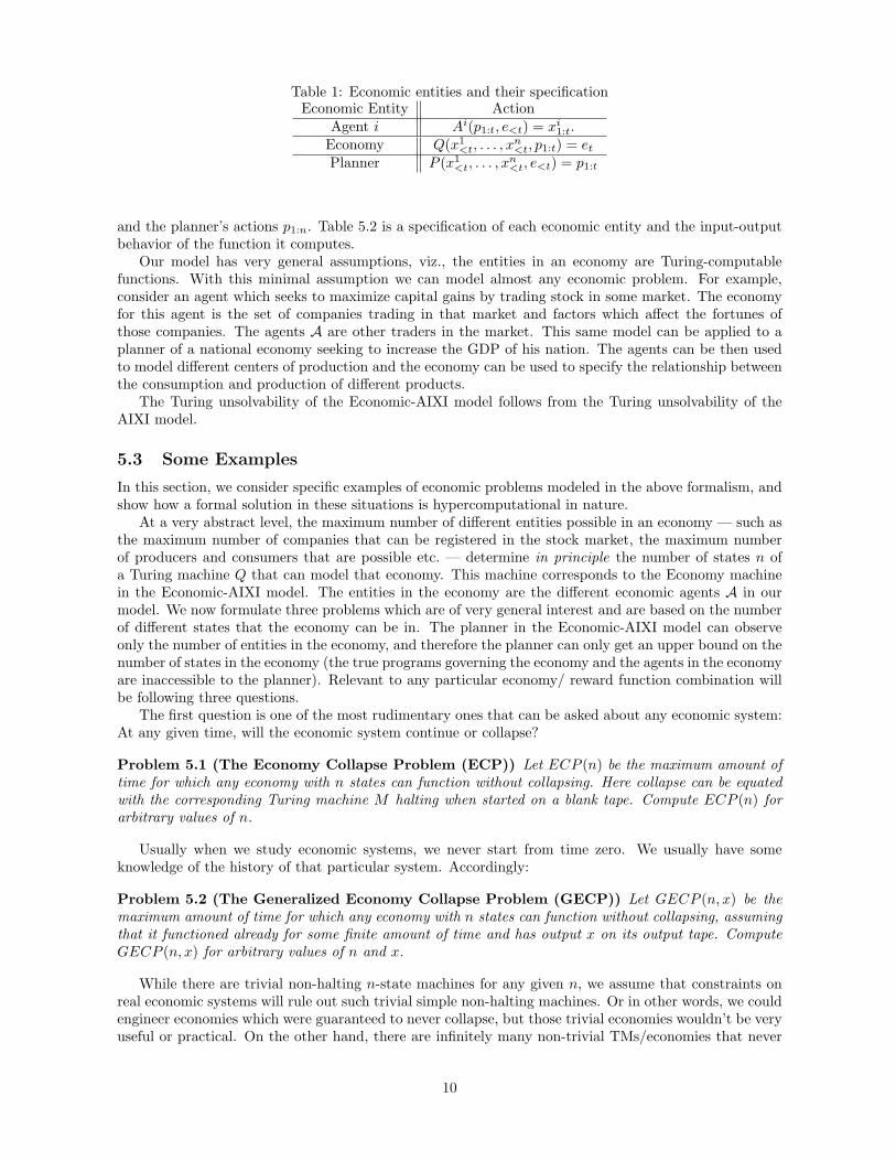
Table 1: Economic entities and their specificationEconomic Entity Action

Agent i Ai(p1:t, e<t) = xi1:t.Economy Q(x1

<t, . . . , xn<t, p1:t) = et

Planner P (x1<t, . . . , x

n<t, e<t) = p1:t

and the planner’s actions p1:n. Table 5.2 is a specification of each economic entity and the input-outputbehavior of the function it computes.

Our model has very general assumptions, viz., the entities in an economy are Turing-computablefunctions. With this minimal assumption we can model almost any economic problem. For example,consider an agent which seeks to maximize capital gains by trading stock in some market. The economyfor this agent is the set of companies trading in that market and factors which affect the fortunes ofthose companies. The agents A are other traders in the market. This same model can be applied to aplanner of a national economy seeking to increase the GDP of his nation. The agents can be then usedto model different centers of production and the economy can be used to specify the relationship betweenthe consumption and production of different products.

The Turing unsolvability of the Economic-AIXI model follows from the Turing unsolvability of theAIXI model.

5.3 Some Examples

In this section, we consider specific examples of economic problems modeled in the above formalism, andshow how a formal solution in these situations is hypercomputational in nature.

At a very abstract level, the maximum number of different entities possible in an economy — such asthe maximum number of companies that can be registered in the stock market, the maximum numberof producers and consumers that are possible etc. — determine in principle the number of states n ofa Turing machine Q that can model that economy. This machine corresponds to the Economy machinein the Economic-AIXI model. The entities in the economy are the different economic agents A in ourmodel. We now formulate three problems which are of very general interest and are based on the numberof different states that the economy can be in. The planner in the Economic-AIXI model can observeonly the number of entities in the economy, and therefore the planner can only get an upper bound on thenumber of states in the economy (the true programs governing the economy and the agents in the economyare inaccessible to the planner). Relevant to any particular economy/ reward function combination willbe following three questions.

The first question is one of the most rudimentary ones that can be asked about any economic system:At any given time, will the economic system continue or collapse?

Problem 5.1 (The Economy Collapse Problem (ECP)) Let ECP (n) be the maximum amount oftime for which any economy with n states can function without collapsing. Here collapse can be equatedwith the corresponding Turing machine M halting when started on a blank tape. Compute ECP (n) forarbitrary values of n.

Usually when we study economic systems, we never start from time zero. We usually have someknowledge of the history of that particular system. Accordingly:

Problem 5.2 (The Generalized Economy Collapse Problem (GECP)) Let GECP (n, x) be themaximum amount of time for which any economy with n states can function without collapsing, assumingthat it functioned already for some finite amount of time and has output x on its output tape. ComputeGECP (n, x) for arbitrary values of n and x.

While there are trivial non-halting n-state machines for any given n, we assume that constraints onreal economic systems will rule out such trivial simple non-halting machines. Or in other words, we couldengineer economies which were guaranteed to never collapse, but those trivial economies wouldn’t be veryuseful or practical. On the other hand, there are infinitely many non-trivial TMs/economies that never

10

halt. However, finding them is not easier than finding halting TMs. The problem is also unsolvable; evenworse, it is not even recursively enumerable.

Problem 5.3 (The Economy Immortality Problem (EIP)) Let EIP represent economies that nevercollapse, i.e., are immortal. For arbitrary values of n enumerate all economies with n states which areimmortal.

We now prove the Turing unsolvability of the above three problems. To prove the unsolvability ofECP let us recall another auxiliary term (Rado 1963):

Definition 5.4 (The Busy Beaver Problem (BBP)) Consider a deterministic 1-tape Turing ma-chine with unary alphabet {1} and tape alphabet {1, B}, where B represents the tape blank symbol. ThisTuring machine starts with an initial empty tape and accepts by halting. For an arbitrary (and, of course,finite) number of states n = 0, 1, 2, ... find two functions: the maximum number of 1s written on tapebefore halting (known as the busy beaver function Σ(n)) and the maximum number of steps before halting(known as the maximum shift function S(n).

Note that Σ(n) represents space complexity and S(n) represents time complexity of the BBP TM.Obviously, Σ(n) ≤ S(n). Both functions grow faster than any computable function, i.e., the Busy BeaverProblem has been proven to be TM-unsolvable. If it were possible to solve BBP, we could reduce BBP tothe halting problem of UTM and we would disprove its undecidability. We could do this by computingthe max-shift function S(n) and running TM up to S(n) steps. If BBP TM halted during first S(n)steps, then UTM would halt; otherwise it would run forever and the answer for UTM halting would beno. In both cases, we would be able to decide in a finite number of steps: yes or no regarding thehalting of UTM. Of course, the algorithm would not be too practical because both functions grow veryfast and their precise values are known only for small values of n. For example, it is known that S(0) = 0,S(1) = 1, S(2) = 6, S(3) = 21 and S(4) = 107, but S(n) is not known for n > 4. This is so becauseS(n) grows very rapidly; it is known that S(5) ≥ 47, 176, 870 and S(6) ≥ 2.5102879. Thus even assumingthat we could find S(n) for arbitrary n, the practicability of such testing would be at least dubious.Additionally, we do not know precise values or upper bounds of both functions for reasonable values ofn, say 20−−100.

We can generalize this observation as follows.

Remark 5.5 TM unsolvable problems have uncomputable time and space complexities.

Otherwise, the known upper limit of time complexity (the number of steps) or the upper limit onspace complexity (TM tape cells used) could be used to solve the halting problem of UTM, to disprovethe Rice Theorem, the unsolvability of the Post Correspondence Problem, and so on.

Theorem 5.6 (On unsolvability of ECP) The Economy Collapse Problem is Turing uncomputable.

Proof: By reduction of the BBP TM computing the max-shift function S(n). The reduction is straight-forward: The number of states in BBP TM and ECP TM are the same and equal n = 0, 1, 2, ... . IfBBP TM accepts its empty input and halts, then ECP TM halts and the economy collapses after a finitenumber of steps. If BBP TM does not accept its input, i.e., does not halt, then ECP TM does not halteither. Thus ECP is recursively enumerable but not recursive, i.e., uncomputable (semi-decidable).

We can generalize BBP to a TM starting with a nonempty tape.

Definition 5.7 (The Nonempty Tape Busy Beaver Problem (NBBP)) Compute functions Σ(n)and S(n) for Busy Beaver TMs staring with nonempty initial tapes.

Let’s recall another auxiliary notion. It is known that the language Lne of codes of TMs acceptingat least one string is recursively enumerable but not recursive, i.e., the halting problem of UTM can bereduced to Lne. On the other hand, the language Le of codes of TMs that do not accept any word is notrecursively enumerable. Note that Le is the complement of Lne.

11

Theorem 5.8 (On unsolvability of NBBP) The Nonempty Tape Busy Beaver Problem is Turing-uncomputable.

Proof: By reduction of language Lne to the NBBP. If TM computing Lne accepts word w, then NBBPTM computes Σ(n) and S(n) and halts. If TM computing Lne does not accept, then NBBP TM does nothalt either.

Theorem 5.9 (On unsolvability of GECP) The Generalized Economy Collapse Problem is Turing-uncomputable.

Proof: By reduction of NBBP to GECP.

We observe that the Economic Immortality Problem is the complement of the Extended GeneralizedEconomy Collapse Problem (EGECP), where we want to prove that an economy will collapse. We canprove that EGECP is Turing unsolvable by reduction from Lne. This implies immediately that EIP, asthe complement of EGECP is non-r.e. (another proof can be obtained directly from reduction from Le).

Theorem 5.10 (On undecidability of EIP) The Economy Immortality Problem is Turing uncom-putable.

A special case of EIP would be modeling problems that avoid collapse of economy caused by deadlockswhen multiple clients compete for shared resources/bank capital. This includes the algorithmic solution ofthe Banker Problem by Dijkstra’s famous Banker’s Algorithm (Madduri & Finkel 1984) and its unsolvablegeneralizations.

6 Conclusion and Next Steps

We conclude that economics might well be partially hypercomputational in nature. More precisely, weconclude that economics, insofar as it sets out formal models of phenomena that it customarily targets, canbe seen to make natural use of hypercomputation. Our conclusion may not be accepted by all readers,and we assume some will be skeptics chiefly because either our modeling is perceived as insufficientlydetailed, or because this modeling is unnatural, or both. In future work where more space is available,greater detail will be provided (e.g., we can provide formal analysis and theorems about decidability inconnection with mental logics). But it’s exceedingly difficult to determine whether a formal model of someeconomic phenomena is natural. At present, we admit that we don’t have a rigorous set of desideratawhich a formal model of targeted phenomena must satisfy in order to be classified as natural. But weare working on the problem.

References

Arkoudas, K. & Bringsjord, S. (2009), ‘Propositional attitudes and causation’, International Journal of Softwareand Informatics 3(1), 47–65.URL: http://kryten.mm.rpi.edu/PRICAI w sequentcalc 041709.pdf

Aumann, R. J. (1995), ‘Backward induction and common knowledge of rationality’, Games and Economic Be-havior 8, 6–19.

Balkenborg, D. & Winter, E. (1997), ‘A necessary and sufficient epistemic condition for playing backward induc-tion’, Journal of Mathematical Economics 27, 325–345.

Balzer, W., Moulines, C. & Sneed, J. (1987), An architectonic for science: The structuralist program, D ReidelPub Co.

Balzer, W., Sneed, J. & Moulines, C. (2000), Structuralist knowledge representation: paradigmatic examples,Rodopi.

Barwise, J. & Etchemendy, J. (1999), Language, Proof, and Logic, Seven Bridges, New York, NY.

Braine, M. (1998), Steps toward a mental predicate-logic, in M. Braine & D. O’Brien, eds, ‘Mental Logic’,Lawrence Erlbaum Associates, Mahwah, NJ, pp. 273–331.

Bringsjord, S. (1992), What Robots Can and Can’t Be, Kluwer, Dordrecht, The Netherlands.

12

Bringsjord, S. & Arkoudas, K. (2004), ‘The modal argument for hypercomputing minds’, Theoretical ComputerScience 317, 167–190.

Bringsjord, S. & Zenzen, M. (2003), Superminds: People Harness Hypercomputation, and More, Kluwer AcademicPublishers, Dordrecht, The Netherlands.

Cottrell, A., Cockshott, P. & Michaelson, G. J. (2009), ‘Is economic planning hypercomputational? The argumentfrom Cantor diagonalisation’, International Journal of Unconventional Computing 5(3-4), 223–236.URL: http://www.macs.hw.ac.uk/∼greg/publications/ccm.IJUC07.pdf

Ebbinghaus, H. D., Flum, J. & Thomas, W. (1994), Mathematical Logic (second edition), Springer-Verlag, NewYork, NY.

Hutter, M. (2005), Universal Artificial Intelligence: Sequential Decisions Based on Algorithmic Probability,Springer, New York, NY.

Jain, S., Osherson, D., Royer, J. & Sharma, A. (1999), Systems that learn, MIT press.

Jeffrey, R. (1964), The Logic of Decision, University of Chicago Press, Chicago, IL.

Johnson-Laird, P. N. (1983), Mental Models, Harvard University Press, Cambridge, MA.

Joyce, J. (1999), The Foundations of Causal Decision Theory, Cambridge University Press, Cambridge, UK.

Kreps, D. & Wilson, R. (1982), ‘Reputation and imperfect information’, Journal of Economic Theory 27(2), 253–279.

Legg, S. & Hutter, M. (2007), ‘Universal intelligence: A definition of machine intelligence’, Minds and Machines17(4), 391–444.

Madduri, H. & Finkel, R. (1984), ‘Extension of the Banker’s algorithm for resource allocation in a distributedoperating system’, Information Processing Letters 19(1), 1–8.

Nozick, R. (1970), Newcomb’s problem and two principles of choice, in N. Rescher, ed., ‘Essays in Honor of CarlG. Hempel’, Humanities Press, Highlands, NJ, pp. 114–146.

Osborne, M. & Rubinstein, A. (1994), A Course in Game Theory, MIT Press, Cambridge, MA.

Pollock, J. (1995), Cognitive Carpentry: A Blueprint for How to Build a Person, MIT Press, Cambridge, MA.

Pour-El, M. & Richards, I. (1981), ‘The wave equation with computable initial data such that its unique solutionis not computable’, Advances in Mathematics 39, 215–239.

Rado, T. (1963), ‘On non-computable functions’, Bell System Technical Journal 41, 877–884.

Rips, L. (1994), The Psychology of Proof, MIT Press, Cambridge, MA.

Russell, S. & Norvig, P. (2002), Artificial Intelligence: A Modern Approach, Prentice Hall, Upper Saddle River,NJ.

Savage, L. (1954), The Foundations of Statistics, Dover, New York, NY.

Selten, R. (1978), ‘The chain store paradox’, Theory and Decision 9, 127–159.

Smith, P. (2007), An Introduction to Godel’s Theorems, Cambridge University Press, Cambridge, UK.

Sneed, J. (1972), ‘The logical structure of mathematical physics’, American Journal of Physics 40, 497–498.

Sneed, J. (1989), ‘Machine models for the growth of knowledge: Theory nets in PROLOG’, Imre Lakatos andtheories of scientific change p. 245.

Solomonoff, R. (1978), ‘Complexity-based induction systems: comparisons and convergence theorems’, IEEEtransactions on Information Theory 24(4), 422–432.

Stanovich, K. E. & West, R. F. (2000), ‘Individual differences in reasoning: Implications for the rationalitydebate’, Behavioral and Brain Sciences 23(5), 645–665.

Suppes, P. (1972), Axiomatic Set Theory, Dover Publications, New York, NY.

Sutton, R. & Barto, A. (1998), Reinforcement learning, MIT Press.

Tracy, W. (2008), Paradox lost: The evolution of strategies in selten’s chain store game, in ‘Three Essays on FirmLearning’. This is a dissertation at UCLA in the Anderson School of Management.

Wajnberg, C., Corruble, V., Ganascia, J. & Moulines, C. (n.d.), A structuralist approach towards computationalscientific discovery, in ‘Discovery Science’, Springer, pp. 412–419.

Wiles, A. (1995), ‘Modular elliptic curves and Fermat’s last theorem’, Annals of Mathematics 141(3), 443–551.

Wiles, A. & Taylor, R. (1995), ‘Ring-theoretic properties of certain Hecke algebras’, Annals of Mathematics141(3), 553–572.

13

Yang, Y. (2006), Toward a mental decision logic of the small-grand problem: Its decision structure and arithmeti-zation, in ‘Proceedings of the Twenty-Eighth Annual Conference of the Cognitive Science Society’, LawrenceErlbaum Associates, Mahwah, NJ.

Yang, Y., Braine, M. & O’Brien, D. (1998), Some empirical justification of one predicate-logic model, in M. Braine& D. O’Brien, eds, ‘Mental Logic’, Lawrence Erlbaum Associates, Mahwah, NJ, pp. 333–365.

14