Exploring attractively interacting

fermions in 2D using a Quantum Gas

Microscope

Debayan Mitra

A Dissertation

Presented to the Faculty

of Princeton University

in Candidacy for the Degree

of Doctor of Philosophy

Recommended for Acceptance

by the Department of

Physics

Adviser: Professor Waseem Bakr

November 2018

c© Copyright by Debayan Mitra, 2018.

All rights reserved.

Abstract

Recent advances in the field of ultracold quantum gases have played an important

role in expanding our understanding of strongly-correlated quantum matter. These

gases are isolated, clean and fully controllable systems, allowing bottom-up engineer-

ing of idealized condensed matter models. Interacting Fermi gases are particularly

interesting because of their relevance to understanding systems ranging from high-

temperature superconductors to neutron stars.

In this thesis, I describe the development of a quantum gas microscope for studying

Fermi gases of lithium-6 in two dimensions. With this tool, we can probe 2D systems

containing over a thousand fermions and measure the spin or density on each site

as well as n-point correlations of these quantities. The design of our microscope

introduces several new simplifying features, including a novel Raman cooling scheme

for imaging that does not require confining the atoms in the Lamb-Dicke regime in

all directions.

I report on two experiments we have performed using this instrument. First I

present an exploration of attractive spin-imbalanced gases in two dimensions. We

observe in-trap phase separation characterized by the appearance of a spin-balanced

core surrounded by a polarized gas. In addition, we observe pair condensation in

momentum-space measurements even for large polarizations where phase separation

vanishes, indicating the presence of a polarized pair condensate.

In a second experiment, we explore fermions in an optical lattice, described by

the Fermi-Hubbard model. Compared to the repulsive model, the attractive model

has received less experimental attention despite its rich phase diagram, including a

possible FFLO phase in the polarized system. Using the microscope, we directly

image charge density wave correlations in our system and use them to put a lower

bound on pairing correlations. We also demonstrate that these correlations constitute

iii

a sensitive thermometer that might be useful in the development of future cooling

schemes.

These initial explorations with our fermion quantum gas microscope set the stage

for future work that might shed insights on a wide variety of condensed matter prob-

lems, ranging from the microscopic mechanisms for pairing in high-temperature su-

perconductors to Cooper pairing at non-zero momentum in large magnetic fields.

iv

Acknowledgements

As is the case for summarizing my gratitude for my years as a graduate student, I do

not know where to start. I think it is apt to begin by thanking my advisor, Professor

Waseem Bakr, not only for giving me this opportunity to work with him, but also

for being my guide and mentor through the entire process. Prior to starting my PhD

at Princeton, my experience was largely concentrated in the field of experimental

condensed matter physics. I was very generously offered to work on silicon qubits by

Professor Jason Petta. While working there, I acquired important nanofabrication

skills like photo and e-beam lithography. But when I found out that Waseem was

joining the department, I was excited by the prospect of building my own experiment.

I knew that I would be studying similar physics, but I would learn the new and

powerful tools of laser cooling and trapping of atoms.

Building an experiment was the most educational experience where I not only

had to think like an engineer but also like an electrician and a plumber. I learned

a lot from Stan Kondov, the first postdoc who joined our group. We spent many

hours assembling vacuum chambers, winding coils and discussing car problems. The

second postdoc to join us, now Professor Peter Schauß, was indispensable to the

science that we produced. I do not remember a time I asked him a question that

he could not answer. My fellow graduate student, Peter Brown and I worked side

by side for many years and he played a crucial role in ensuring the success of our

experiments. The next graduate student in our group, Elmer Guardado-Sanchez will

be the very capable hands to take care of the machine after the first generation of

graduate students depart. I would also like to wish our newer graduate student,

Lysander Christakis, success in the new experimental direction of our group.

Research cannot continue without all the administrative and technical assistance

we receive. I would like to start with Geoff Gettelfinger, our department manager.

The time and patience that he spared to deal with our day to day water cooling

v

problems has been incredibly valuable. I would like to thank Steve Lowe for training

me to use the student machine shop and always providing guidance and advice with

every machining project. Additionally, I’m very thankful for Vinod Gupta and Sumit

Saluja’s IT help and support navigating the Feynman cluster. In the beginning, we

had to place orders on a daily basis and sometimes deal with US customs delays. The

purchasing and logistics department deserves a huge thank you for their patience and

tireless help, especially Darryl Johnson, Julio Lopez, Ted Lewis, Lauren Callahan,

Barbara Grunwerg and Claudin Champagne. I would like to thank our administra-

tive assistant, Antonia Sarchi, for promptly resolving all financial queries. Lastly I

would like to thank my graduate administrators Jessica Heslin, Barbara Mooring and

Catherine Brosowsky for helping navigate different stages of grad school.

My graduate school experience would not be complete without thanking the pro-

fessors who taught me in the classroom. My biggest thanks goes to Professor Herman

Verlinde. Not only was he a great instructor to introduce quantum field theory to a

layman, but he was also the most caring director of graduate studies. Next I thank

Professor Ali Yazdani, Professor Frans Pretorius and Professor Andrei Bernevig for

teaching the other courses I took. I extend my gratitude to Professor David Huse.

Although I never took a class under him, I enjoyed the conversations we had about

our experiments and always learned a lot from his keen insights. I also thank him

for being part of my committee. I thank Trithep Devakul for helping us navigate

numerical simulations. In addition to taking classes, I also taught different courses

for four semesters. I would like to thank Catherine Visnjic and Kasey Wagoner for

introducing me to their new style of pedagogy. Finally I would like to thank Professor

Michael Romalis for being a part of my committee and Professor Jeff Thompson for

carefully reading my thesis.

Being in graduate school for six years, especially in a small town like Princeton,

could be a laborious experience without friends. My experience was particularly

vi

memorable because of living in the graduate college my first year. I spent countless

nights at the Dbar with my friends Gustavo Turiaci, Aitor Lewkowycz, Zach Sethna,

Mike McKeown, Jose Zamalloa and many others. I made more friends as I moved

along in grad school like Olya Krepchenko, Will Coulton and Mykola Dedushenko.

Every summer I would participate in the softball league to proudly play for the

Big Bangers. The team and all our triumphs will always be close to my heart. I also

made many friends outside of grad school, mostly through my girlfriend. A special

thank you to Alex Coulston, Audrey Jenkins and Angelika Hicks for being great

housemates and for throwing unforgettable parties. Also thank you to Princeton in

Asia for incorporating me as a member of their team.

At this point I would like to mention one of the most important moments of my

time in Princeton. During my time here I met my girlfriend, Emily Eckardt. For the

last three years, she has been both an inspiration and a motivation both in research

and personal life. Her positive outlook towards life has rubbed off on me and her

drive to work towards a social good motivates me to become a better educator and

not only a better researcher. In addition, her parents Bob Eckardt and Jane Shapiro,

have been my family away from my own family. I am indebted to them for their

kindness and generosity and for their endless curiosity and interest in people’s lives.

Her brothers even guest starred on the Big Bangers every now and then.

Last but not the least, I owe an immense debt of gratitude to my parents for the

sacrifices they made so that I could be here today. My mother, Susmita Mitra, left

behind her career as a promising young engineer to ensure that my brother and I were

raised well. She was not only my teacher but also my cheerleader who would lift me

up when I was down. My older brother, Debkishore Mitra, was the person I could go

to whenever I had difficulty in school and was a constant source of encouragement.

This thesis is a culmination of thirty years of work and I am grateful to have the

chance to thank each person who contributed to this accomplishment.

vii

To my family

viii

Contents

Abstract . . . . . . . . . . . . . . . . . . . . . . . . . . . . . . . . . . . . . iii

Acknowledgements . . . . . . . . . . . . . . . . . . . . . . . . . . . . . . . v

List of Tables . . . . . . . . . . . . . . . . . . . . . . . . . . . . . . . . . . xiii

List of Figures . . . . . . . . . . . . . . . . . . . . . . . . . . . . . . . . . . xiv

1 Introduction 1

2 Experimental Setup 9

2.1 Vacuum Chamber Design . . . . . . . . . . . . . . . . . . . . . . . . . 9

2.2 Reentrant Vacuum Viewports . . . . . . . . . . . . . . . . . . . . . . 13

2.3 AR/HR coatings . . . . . . . . . . . . . . . . . . . . . . . . . . . . . 15

2.4 Bakeout . . . . . . . . . . . . . . . . . . . . . . . . . . . . . . . . . . 18

2.5 Magnetic Field Coils : Design and Winding . . . . . . . . . . . . . . 24

2.5.1 Zeeman slower . . . . . . . . . . . . . . . . . . . . . . . . . . . 24

2.5.2 MOT coils . . . . . . . . . . . . . . . . . . . . . . . . . . . . . 28

2.5.3 Feshbach coils . . . . . . . . . . . . . . . . . . . . . . . . . . . 30

2.5.4 Coil Winding . . . . . . . . . . . . . . . . . . . . . . . . . . . 32

2.6 Water Cooling . . . . . . . . . . . . . . . . . . . . . . . . . . . . . . . 35

2.7 671 nm Laser System . . . . . . . . . . . . . . . . . . . . . . . . . . . 40

2.7.1 6Li Spectroscopy . . . . . . . . . . . . . . . . . . . . . . . . . 40

2.7.2 MOT and Zeeman slower . . . . . . . . . . . . . . . . . . . . . 43

ix

2.7.3 Low and High Field Imaging . . . . . . . . . . . . . . . . . . . 46

2.7.4 Raman laser system . . . . . . . . . . . . . . . . . . . . . . . 48

2.8 Optical Potentials . . . . . . . . . . . . . . . . . . . . . . . . . . . . . 50

2.8.1 Optical Dipole Trap . . . . . . . . . . . . . . . . . . . . . . . 50

2.8.2 Light Sheet and Bottom Beam . . . . . . . . . . . . . . . . . . 53

2.8.3 Accordion Lattice . . . . . . . . . . . . . . . . . . . . . . . . . 56

2.8.4 2D Square Science Lattice . . . . . . . . . . . . . . . . . . . . 62

3 Pathway to a Quantum Gas Microscope 69

3.1 Magneto-optical trap . . . . . . . . . . . . . . . . . . . . . . . . . . . 69

3.2 Evaporation . . . . . . . . . . . . . . . . . . . . . . . . . . . . . . . . 74

3.2.1 Radio frequency sweeps . . . . . . . . . . . . . . . . . . . . . 74

3.2.2 Molecular Bose-Einstein condensates . . . . . . . . . . . . . . 78

3.3 Single site imaging . . . . . . . . . . . . . . . . . . . . . . . . . . . . 83

3.3.1 Raman imaging . . . . . . . . . . . . . . . . . . . . . . . . . . 83

3.3.2 Microscope objective . . . . . . . . . . . . . . . . . . . . . . . 89

3.3.3 Reconstructing single atoms . . . . . . . . . . . . . . . . . . . 91

4 Phase separation and pair condensation in a spin-imbalanced 2D

Fermi gas 94

4.1 Degenerate Fermi gases . . . . . . . . . . . . . . . . . . . . . . . . . . 94

4.2 Fermi gas in 2 dimensions . . . . . . . . . . . . . . . . . . . . . . . . 100

4.3 BEC-BCS crossover in 3D and 2D . . . . . . . . . . . . . . . . . . . . 106

4.4 Superfluidity in 2D . . . . . . . . . . . . . . . . . . . . . . . . . . . . 108

4.5 Spin Imbalance: Phase separation and superfluidity . . . . . . . . . . 110

4.5.1 Creating 2D spin-imbalanced clouds . . . . . . . . . . . . . . . 112

4.5.2 Imaging . . . . . . . . . . . . . . . . . . . . . . . . . . . . . . 115

4.5.3 Measuring temperature . . . . . . . . . . . . . . . . . . . . . . 119

x

4.5.4 Measuring condenstate fraction . . . . . . . . . . . . . . . . . 122

4.5.5 Fitting in-situ profiles . . . . . . . . . . . . . . . . . . . . . . 124

4.5.6 Extracting critical polarization Pc . . . . . . . . . . . . . . . . 128

4.5.7 Phase diagram . . . . . . . . . . . . . . . . . . . . . . . . . . 131

5 Quantum gas microscopy of an attractive Fermi–Hubbard system 134

5.1 The Fermi-Hubbard model . . . . . . . . . . . . . . . . . . . . . . . . 134

5.2 Attractive (U < 0) or Repulsive (U > 0)? . . . . . . . . . . . . . . . . 139

5.3 Quantum gas microscopy . . . . . . . . . . . . . . . . . . . . . . . . . 144

5.3.1 Calibrating Hubbard parameters . . . . . . . . . . . . . . . . 145

5.3.2 Measuring double occupancies . . . . . . . . . . . . . . . . . . 148

5.3.3 Charge density wave and s-wave pairing . . . . . . . . . . . . 151

5.3.4 Measuring correlations vs n . . . . . . . . . . . . . . . . . . . 158

5.3.5 Measuring correlations vs U/t . . . . . . . . . . . . . . . . . . 163

5.3.6 Thermometry . . . . . . . . . . . . . . . . . . . . . . . . . . . 165

5.4 Mapping and further work . . . . . . . . . . . . . . . . . . . . . . . . 167

6 Conclusion 171

6.1 Future Work . . . . . . . . . . . . . . . . . . . . . . . . . . . . . . . . 172

A Properties of 6Li 175

A.1 Atomic properties . . . . . . . . . . . . . . . . . . . . . . . . . . . . . 175

A.2 Zeeman shifts . . . . . . . . . . . . . . . . . . . . . . . . . . . . . . . 176

A.3 Scattering lengths . . . . . . . . . . . . . . . . . . . . . . . . . . . . . 177

B Reentrant vacuum viewport design 178

C AR/HR coatings 179

xi

D Lattice description 181

D.1 Lattice potential . . . . . . . . . . . . . . . . . . . . . . . . . . . . . 181

D.2 Band structure calculation . . . . . . . . . . . . . . . . . . . . . . . . 183

E Objective specifications 187

Bibliography 189

xii

List of Tables

2.1 Bakeout parameters . . . . . . . . . . . . . . . . . . . . . . . . . . . . 22

2.2 Water cooling parameters . . . . . . . . . . . . . . . . . . . . . . . . 37

2.3 Thermal expansion and Sellmeir parameters for PP-MgO:SLT . . . . 59

4.1 Calculated and measured 2D parameters . . . . . . . . . . . . . . . . 116

4.2 Mean field theory fitting results . . . . . . . . . . . . . . . . . . . . . 126

A.1 Atomic properties of 6Li . . . . . . . . . . . . . . . . . . . . . . . . . 175

xiii

List of Figures

1.1 Quantum gas microscopy . . . . . . . . . . . . . . . . . . . . . . . . . 3

1.2 Observation of spin canting in the repulsive Hubbard model . . . . . 4

1.3 Conductivity versus temperature . . . . . . . . . . . . . . . . . . . . 6

2.1 Design of the experiment . . . . . . . . . . . . . . . . . . . . . . . . . 11

2.2 Reentrant vacuum viewport design . . . . . . . . . . . . . . . . . . . 14

2.3 Vacuum system bakeout . . . . . . . . . . . . . . . . . . . . . . . . . 21

2.4 Zeeman slower design and testing . . . . . . . . . . . . . . . . . . . . 27

2.5 MOT Coils . . . . . . . . . . . . . . . . . . . . . . . . . . . . . . . . 29

2.6 Feshbach Coils . . . . . . . . . . . . . . . . . . . . . . . . . . . . . . 31

2.7 Coil Winding . . . . . . . . . . . . . . . . . . . . . . . . . . . . . . . 33

2.8 Water cooling . . . . . . . . . . . . . . . . . . . . . . . . . . . . . . . 38

2.9 Spectroscopy . . . . . . . . . . . . . . . . . . . . . . . . . . . . . . . 42

2.10 MOT and Zeeman slower light . . . . . . . . . . . . . . . . . . . . . . 45

2.11 Low and high field imaging . . . . . . . . . . . . . . . . . . . . . . . . 47

2.12 Raman laser system . . . . . . . . . . . . . . . . . . . . . . . . . . . . 49

2.13 Optical Dipole Trap . . . . . . . . . . . . . . . . . . . . . . . . . . . 52

2.14 Light sheet and bottom beam . . . . . . . . . . . . . . . . . . . . . . 54

2.15 Second harmonic generation . . . . . . . . . . . . . . . . . . . . . . . 58

2.16 Accordion lattice . . . . . . . . . . . . . . . . . . . . . . . . . . . . . 61

2.17 Science lattice . . . . . . . . . . . . . . . . . . . . . . . . . . . . . . . 64

xiv

2.18 Pinning circuit . . . . . . . . . . . . . . . . . . . . . . . . . . . . . . 67

3.1 Properties of the MOT . . . . . . . . . . . . . . . . . . . . . . . . . . 71

3.2 RF antennas . . . . . . . . . . . . . . . . . . . . . . . . . . . . . . . . 75

3.3 Rabi oscillations . . . . . . . . . . . . . . . . . . . . . . . . . . . . . . 76

3.4 Bose-Einstein Condensation . . . . . . . . . . . . . . . . . . . . . . . 80

3.5 Raman cooling scheme . . . . . . . . . . . . . . . . . . . . . . . . . . 85

3.6 Raman sideband cooling setup . . . . . . . . . . . . . . . . . . . . . . 87

3.7 Objective mount . . . . . . . . . . . . . . . . . . . . . . . . . . . . . 90

3.8 Single atom reconstruction . . . . . . . . . . . . . . . . . . . . . . . . 93

4.1 Binding energy . . . . . . . . . . . . . . . . . . . . . . . . . . . . . . 101

4.2 BEC-BCS crossover . . . . . . . . . . . . . . . . . . . . . . . . . . . . 107

4.3 Phase separation in 3D and 1D . . . . . . . . . . . . . . . . . . . . . 111

4.4 Experimental setup . . . . . . . . . . . . . . . . . . . . . . . . . . . . 113

4.5 Imbalancing calibration . . . . . . . . . . . . . . . . . . . . . . . . . . 114

4.6 Checking single accordion layer . . . . . . . . . . . . . . . . . . . . . 115

4.7 Double imaging scheme . . . . . . . . . . . . . . . . . . . . . . . . . . 118

4.8 Average density profiles . . . . . . . . . . . . . . . . . . . . . . . . . 119

4.9 Temperature fitting . . . . . . . . . . . . . . . . . . . . . . . . . . . . 121

4.10 Time-of-flight expansion . . . . . . . . . . . . . . . . . . . . . . . . . 123

4.11 Azimuthal averages . . . . . . . . . . . . . . . . . . . . . . . . . . . . 125

4.12 Example mean field theory fits . . . . . . . . . . . . . . . . . . . . . . 128

4.13 In-situ difference images . . . . . . . . . . . . . . . . . . . . . . . . . 129

4.14 Central polarization and condensate fraction vs. global polarization . 130

4.15 Phase diagram . . . . . . . . . . . . . . . . . . . . . . . . . . . . . . 132

5.1 Fermi-Hubbard model phase diagram . . . . . . . . . . . . . . . . . . 138

5.2 Single site images of a repulsive Fermi-Hubbard system . . . . . . . . 140

xv

5.3 RF spectroscopy for Hubbard U calibration . . . . . . . . . . . . . . 147

5.4 Detecting double occupancies . . . . . . . . . . . . . . . . . . . . . . 150

5.5 DQMC simulations of pairing, total density and doublon density cor-

relators . . . . . . . . . . . . . . . . . . . . . . . . . . . . . . . . . . . 152

5.6 Contribution of different correlations to the total density correlator Cn 155

5.7 Fitting to Quantum Monte Carlo . . . . . . . . . . . . . . . . . . . . 157

5.8 Observation of doublon density correlations . . . . . . . . . . . . . . 159

5.9 Doublon density correlation matrices for varying density . . . . . . . 160

5.10 Observation of doublon density correlators in an attractive Hubbard

system prepared using scheme 2 . . . . . . . . . . . . . . . . . . . . . 161

5.11 Nearest-neighbor and next-nearest neighbor doublon density correla-

tors versus filling as a function of U/t . . . . . . . . . . . . . . . . . . 164

5.12 Thermometry of an attractive Hubbard system . . . . . . . . . . . . . 166

5.13 Mapping between the attractive and repulsive Hubbard model . . . . 168

5.14 Creating density excitations with a DMD . . . . . . . . . . . . . . . . 170

A.1 Zeeman shift for 6Li ground state . . . . . . . . . . . . . . . . . . . . 176

A.2 Scattering lengths for 6Li . . . . . . . . . . . . . . . . . . . . . . . . . 177

B.1 Reentrant vaccum viewport . . . . . . . . . . . . . . . . . . . . . . . 178

C.1 AR coating on side viewports . . . . . . . . . . . . . . . . . . . . . . 179

C.2 AR-HR coating on reentrant viewports . . . . . . . . . . . . . . . . . 180

D.1 Lattice Band Structure . . . . . . . . . . . . . . . . . . . . . . . . . . 185

E.1 Objective design . . . . . . . . . . . . . . . . . . . . . . . . . . . . . 187

E.2 AR coating on objective . . . . . . . . . . . . . . . . . . . . . . . . . 188

xvi

Chapter 1

Introduction

The field of atomic quantum gases can trace its roots back to Einstein’s prediction

in 1924 that an ideal gas of particles of integer spins would thermodynamically oc-

cupy the ground state below a certain temperature, forming a so-called Bose-Einstein

condensate. Superconductivity was discovered in 1911 and superfluidity of 4He was

discovered in 1938 but there was no obvious link between them and Einstein’s theory.

In 1950, Ginzburg and Landau introduced a phenomenological theory of superfluidity

in terms of a complex valued order parameter function, which was later interpreted as

a macroscopic quantum wavefunction of the superfluid [1]. This was followed by the

realization in 1957 that superconductivity could be understood as the Bose-Einstein

condensation of pairs of fermions, known as Cooper pairs [2]. It was not until 1995

that a weakly-interacting Bose-Einstein condensate, in the sense envisioned by Ein-

stein, was directly observed in a dilute gases of alkali atoms [3, 4]. The first degenerate

gas of fermionic atoms took even longer, until 1999, because fermions proved to be

notoriously harder to cool than bosons [5].

While early work in the field of atomic quantum gases centered on weakly inter-

acting systems, two experimental advances allowed the field to quickly shift focus

to strongly interacting systems in the early 2000s. The discovery of Feshbach res-

1

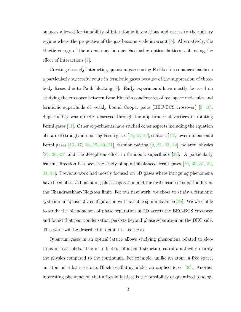
onances allowed for tunability of interatomic interactions and access to the unitary

regime where the properties of the gas become scale invariant [6]. Alternatively, the

kinetic energy of the atoms may be quenched using optical lattices, enhancing the

effect of interactions [7].

Creating strongly interacting quantum gases using Feshbach resonances has been

a particularly successful route in fermionic gases because of the suppression of three-

body losses due to Pauli blocking [8]. Early experiments have mostly focussed on

studying the crossover between Bose-Einstein condensates of real space molecules and

fermionic superfluids of weakly bound Cooper pairs (BEC-BCS crossover) [9, 10].

Superfluidity was directly observed through the appearance of vortices in rotating

Fermi gases [11]. Other experiments have studied other aspects including the equation

of state of strongly interacting Fermi gases [12, 13, 14], solitons [15], lower dimensional

Fermi gases [16, 17, 18, 19, 20, 21], fermion pairing [9, 22, 23, 24], polaron physics

[25, 26, 27] and the Josephson effect in fermionic superfluids [28]. A particularly

fruitful direction has been the study of spin imbalanced fermi gases [29, 30, 31, 32,

33, 34]. Previous work had mostly focused on 3D gases where intriguing phenomena

have been observed including phase separation and the destruction of superfluidity at

the Chandrasekhar-Clogston limit. For our first work, we chose to study a fermionic

system in a “quasi” 2D configuration with variable spin imbalance [35]. We were able

to study the phenomenon of phase separation in 2D across the BEC-BCS crossover

and found that pair condensation persists beyond phase separation on the BEC side.

This work will be described in detail in this thesis.

Quantum gases in an optical lattice allows studying phenomena related to elec-

trons in real solids. The introduction of a band structure can dramatically modify

the physics compared to the continuum. For example, unlike an atom in free space,

an atom in a lattice starts Bloch oscillating under an applied force [36]. Another

interesting phenomenon that arises in lattices is the possibility of quantized topolog-

2

(a) (b)

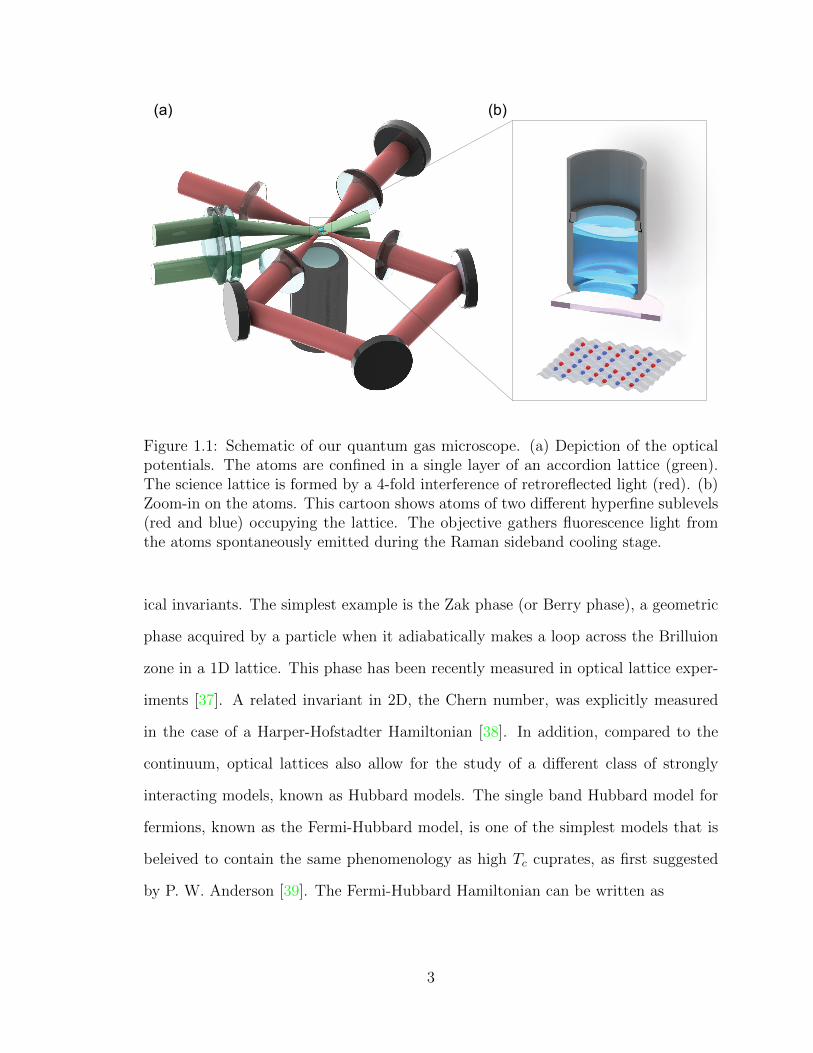
Figure 1.1: Schematic of our quantum gas microscope. (a) Depiction of the opticalpotentials. The atoms are confined in a single layer of an accordion lattice (green).The science lattice is formed by a 4-fold interference of retroreflected light (red). (b)Zoom-in on the atoms. This cartoon shows atoms of two different hyperfine sublevels(red and blue) occupying the lattice. The objective gathers fluorescence light fromthe atoms spontaneously emitted during the Raman sideband cooling stage.

ical invariants. The simplest example is the Zak phase (or Berry phase), a geometric

phase acquired by a particle when it adiabatically makes a loop across the Brilluion

zone in a 1D lattice. This phase has been recently measured in optical lattice exper-

iments [37]. A related invariant in 2D, the Chern number, was explicitly measured

in the case of a Harper-Hofstadter Hamiltonian [38]. In addition, compared to the

continuum, optical lattices also allow for the study of a different class of strongly

interacting models, known as Hubbard models. The single band Hubbard model for

fermions, known as the Fermi-Hubbard model, is one of the simplest models that is

beleived to contain the same phenomenology as high Tc cuprates, as first suggested

by P. W. Anderson [39]. The Fermi-Hubbard Hamiltonian can be written as

3

H = −t∑〈rr′〉,σ

(c†r,σcr′,σ + h.c.

)+ U

∑r

nr,↑nr,↓ (1.1)

where the first term denotes tunnelling between nearest neighbor sites and the

second term is the interaction between two fermions on the same site. Despite its

simplicity, it can only be solved exactly in 1D [40]. In higher dimensions, several

numerical methods [41, 42, 43, 44] have been used to study the Hubbard model

but its low temperature physics remains out of reach [45]. This has motivated the

“quantum simulation” of the Hubbard model with cold fermions in optical lattices.

Here “quantum simulation” is used in the sense originally proposed by Feynman [46],

where one uses an accessible quantum system to emulate another, less accessible one.

In our case, cold atoms are the well understood, controllable system, used to emulate

the physics of high temperature cuprates.

ps = 0.02

-4

0

4

j

ps = 0.18 ps = 0.34 ps = 0.48 ps = 0.77

-0.2

-0.1

0

0.1

C⊥(i,

j)-4 0 4

i

-4

0

4

j

-0.2

-0.1

0

0.1

Cz(i,

j)

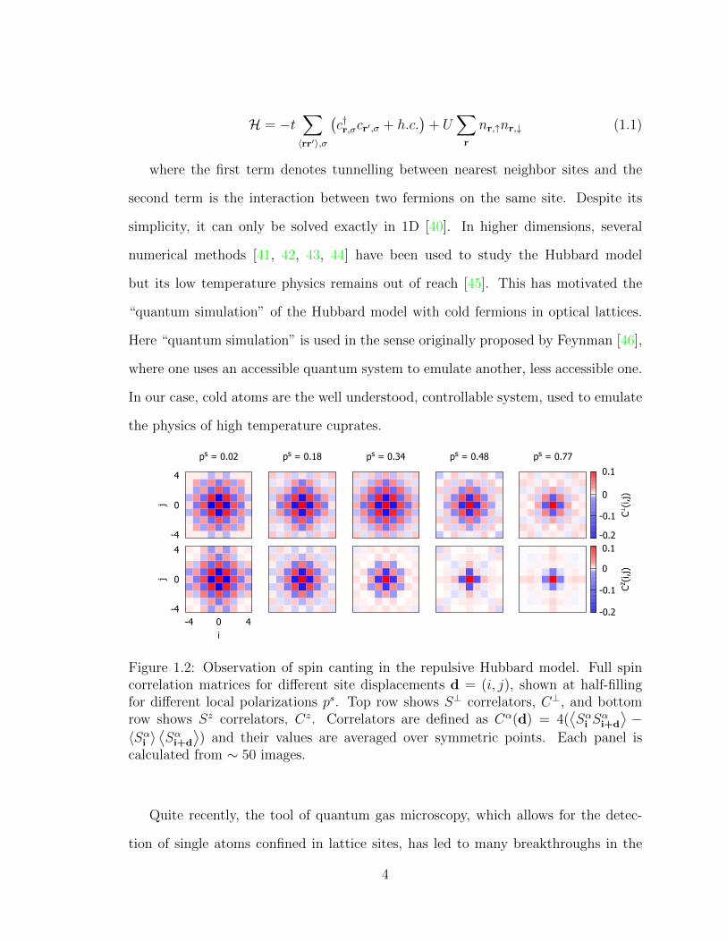
Figure 1.2: Observation of spin canting in the repulsive Hubbard model. Full spincorrelation matrices for different site displacements d = (i, j), shown at half-fillingfor different local polarizations ps. Top row shows S⊥ correlators, C⊥, and bottomrow shows Sz correlators, Cz. Correlators are defined as Cα(d) = 4(

⟨Sαi S

αi+d

⟩−

〈Sαi 〉⟨Sαi+d

⟩) and their values are averaged over symmetric points. Each panel is

calculated from ∼ 50 images.

Quite recently, the tool of quantum gas microscopy, which allows for the detec-

tion of single atoms confined in lattice sites, has led to many breakthroughs in the

4

understanding of the Hubbard model. When we started building our lab in 2013, the

only existing quantum gas microscopes were for bosons [47, 48]. Using that tool, the

superfluid to Mott insulator transition of the Bose-Hubbard model was studied [49].

Given the success of bosonic microscopes, it was not long before many groups started

working on extending the tools of quantum gas microscopy to fermions. The first

fermion microscopes were demonstrated in 2015 [50, 51, 52, 53, 54] and since then

enormous strides have been made in using them to probe Fermi-Hubbard systems,

including observations of Mott insulators [55, 56] and long-range antiferromagnets

[57, 58, 59]. Our first excursion with our own quantum gas miscroscope was to extend

the understanding of the antiferromagnetic state in the presence of spin imbalance

[60]. We prepared half-filled Mott insulators 〈n〉 = 1 with a higher number of spin-↑

than spin-↓. The local polarization is obtained from the local density of spins nsσ and

is defined as ps = (ns↑ − ns↓)/(ns↑ + ns↓). We measured the spin correlations along and

perpendicular to the effective magnetic field as a function of polarization. The main

result is shown in Fig. 1.2.

When the system is unpolarized, we measure spin correlations that are equally

strong along both directions. But as spin imbalance is introduced, the spins prefer

to be in a “canted” state to minimize energy. This leads to stronger correlations

orthogonal to the field versus along the field.

Next, we set out to explore the Hubbard model with attractive interactions. Al-

though a few prior experiments were done with attractive interactions [61, 62, 63, 64],

this work was the first to employ quantum gas microscopy to study a single band Hub-

bard system. We observed charge-density wave correlations expected for negative U

and established that density can be employed as a thermometer at high temperatures

while density correlators are a better thermometer at low temperatures [65]. This

experiment will be presented in detail in this thesis.

5

0

0.25

0.5

0 2 4 6 8

σ (1

/ħ)

Temperature (t)

0

5

10

15

0 2 4 6 8

ρ (ħ

)Temperature (t)

(a) (b)

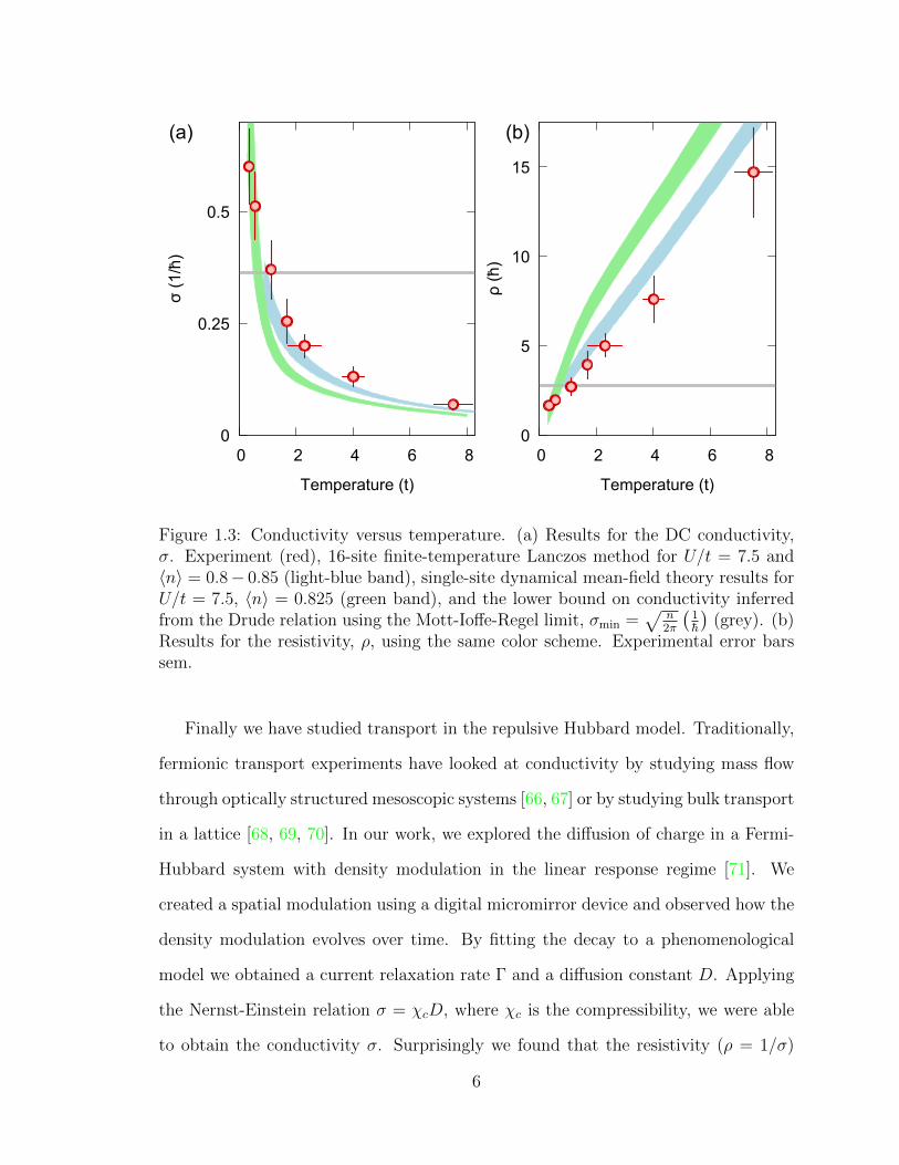
Figure 1.3: Conductivity versus temperature. (a) Results for the DC conductivity,σ. Experiment (red), 16-site finite-temperature Lanczos method for U/t = 7.5 and〈n〉 = 0.8− 0.85 (light-blue band), single-site dynamical mean-field theory results forU/t = 7.5, 〈n〉 = 0.825 (green band), and the lower bound on conductivity inferredfrom the Drude relation using the Mott-Ioffe-Regel limit, σmin =

√n2π

(1h

)(grey). (b)

Results for the resistivity, ρ, using the same color scheme. Experimental error barssem.

Finally we have studied transport in the repulsive Hubbard model. Traditionally,

fermionic transport experiments have looked at conductivity by studying mass flow

through optically structured mesoscopic systems [66, 67] or by studying bulk transport

in a lattice [68, 69, 70]. In our work, we explored the diffusion of charge in a Fermi-

Hubbard system with density modulation in the linear response regime [71]. We

created a spatial modulation using a digital micromirror device and observed how the

density modulation evolves over time. By fitting the decay to a phenomenological

model we obtained a current relaxation rate Γ and a diffusion constant D. Applying

the Nernst-Einstein relation σ = χcD, where χc is the compressibility, we were able

to obtain the conductivity σ. Surprisingly we found that the resistivity (ρ = 1/σ)

6

is linear with temperature and shows no sign of saturation at the Mott-Ioffe-Regal

(MIR) bound (Fig. 1.3). The MIR bound comes from the simple assertion that the

mean free path of a quasiparticle cannot be less than the lattice spacing [72, 73].

These two observations are signatures of non-conventional transport in our system

and a breakdown of Fermi liquid theory. Details of this publication and the one on

spin imbalanced Hubbard physics will be provided in a future thesis by P. T. Brown

from our group.

The outline of this thesis is as follows. I will describe in depth the experimental

setup in chapter 2. Since I was the first graduate student on this experiment, it

is important for me to lay out the details of the design and construction of the

experiment. I describe the design of the vacuum system, the bakeout and assembly.

I then describe the magnet coil design, their winding and the water cooling system.

Next I focus on all the different laser systems that were built to cool and trap the Li

atoms.

In chapter 3, I describe in detail each step along the way to imaging ultracold

fermions in an optical lattice. First I explain how we cool the atoms from the initial

700 K temperature out of the oven down to a few mK and trap them in the magneto-

optical trap. Next I describe the process of loading the atoms into an optical dipole

trap where, after evaporation, we achieve a quantum gas of fermions. Next, I present

our scheme to produce Fermi gases in a “quasi” 2D geometry. Finally I explain how

we image fermions with single site resolution in an optical lattice. It involves the

development of a Raman sideband cooling scheme that works with a 2D lattice and a

light sheet in the third direction where the atoms are not confined in the Lamb-Dicke

regime.

In chapter 4, I describe the work surrounding our first publication [35]. Before

exploring lattice gases, we embarked on a study of spin imbalanced Fermi gases in a

“quasi” 2D geometry. We explored the in-situ density of majority and minority spins

7

and saw that the density remained equal near the center of the trap even for large

imbalances. We studied this phase separation effect across the BEC-BCS crossover.

In addition, we observed condensation of fermions on the BEC side. Interestingly,

unlike 3D, condensation did not vanish when phase separation ended, pointing to the

possibility of a polarized condensate.

In chapter 5, I describe the work published in [65]. It is the first study of fermions

with attractive interactions in any quantum gas microscope. We observed the forma-

tion of charge density waves in our system by perfecting a technique to image only

sites with double occupancies. We established that the density correlators were a

better thermometer than densities at low temperatures. Finally we shed light on a

mapping that exists between the repulsive and the attractive Hubbard models due to

a particle-hole transformation.

In chapter 6, I summarize the important results from the experiments described

in this thesis. Furthermore, I present an outlook on the research being performed in

our lab and the exploration of many further aspects of fermions in lattices.

8

Chapter 2

Experimental Setup

2.1 Vacuum Chamber Design

The main components of our vacuum chamber are the science chamber, the oven

and the Zeeman slower. A large part of our vacuum chamber design was based

off a design by the Heidelberg group [74]. The science chamber is the spherical

octagon from Kimball Physics (MCF600-SphOct-F2C8) that has eight viewports for

optical access. It is made from 316 stainless steel. The viewports themselves were

CF40 fused silica from Kurt J. Lesker Company (VPZL-275Q). The top and bottom

viewports required a special design for reentrant windows that will be discussed later.

The spherical octagon was sent to GSI Helmholtzzentrum fur Schwerionenforschung

GmbH in Darmstadt to get a Non-Evaporable Getter (NEG) coating. This coating

helps in achieving ultra-high vacuum in our experiment. The coating process is a

magnetron sputtering performed under vacuum with a TiZrV wire as cathode and

the octagon as anode. Krypton is used as sputter gas. The NEG coating needs to be

activated normally at 250C for 24 hours. In case the coating needs to be reactivated,

which can occur if the system needs to be vented, then it is recommneded to start the

NEG activation at a lower temperature (220C for 24 hours), which can be increased

9

at each reactivation. In addition, the coating does not degrade if it is not under

vacuum. We performed this activation process during the bakeout stage.

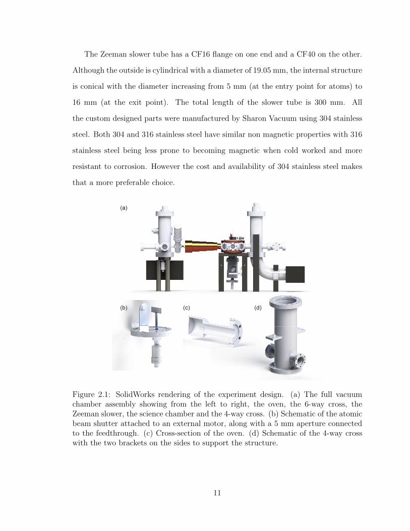
Our experiment required a number of custom parts. The main custom parts are

the oven, a 4-way and a 6-way cross, a vacuum feedthrough and the Zeeman slower rod

(Fig.2.1). The 6-way cross in sandwiched between the Lithium oven and the Zeeman

slower. On the inside, it houses a motorized atomic shutter mounted through the

vacuum feedthrough and a Titanium sublimation cartridge (Varian Model 9160050)

mounted on a CF100 to CF40 reducer flange (Kurt Lesker RF600X275). In addition,

the 6-way cross provides optical access through two CF40 extensions that can also be

used to mount an all metal angle valve (VAT 54132-GE02-0001) and an ion pump.

The 4-way cross is designed to be very similar to the 6-way cross except it is placed

after the science chamber.

The Lithium oven consists of a CF16 flange leading up to a 25 mm diameter

reservoir through a narrow neck of 10 mm inner diameter. We fill the reservoir

with isotopically purified 6Li (95% isotopic purity provided by Cambridge Isotope

Lab and then cleaned and repackaged under inert gas in a sealed ampule by Ames

laboratory) and with a band heater wrapped outside, we are able to generate sufficient

vapor pressure by heating up to 350C. In stand-by mode, we keep the oven at a

temperature of 250C where the vapor pressure is very low but it allows us to reach

high temperature faster during start-up. Usually we fill the oven with 1 gram of 6Li

which has a life span of ∼ 8,200 hours of continuous use.

The vacuum feedthrough is essentially a modified CF100 flange intended to be at-

tached to the bottom of the 6-way cross. It has an extension with a CF16 flange offset

from the center. We attach a motor connected to a vacuum feedthrough (MDC670000-

01) through this extension which in turn connects to a barrier for the atomic beam.

In addition, the feedthrough also holds an aperture of 5 mm diameter intended to

limit the solid angle of the atoms coming out of the oven.

10

The Zeeman slower tube has a CF16 flange on one end and a CF40 on the other.

Although the outside is cylindrical with a diameter of 19.05 mm, the internal structure

is conical with the diameter increasing from 5 mm (at the entry point for atoms) to

16 mm (at the exit point). The total length of the slower tube is 300 mm. All

the custom designed parts were manufactured by Sharon Vacuum using 304 stainless

steel. Both 304 and 316 stainless steel have similar non magnetic properties with 316

stainless steel being less prone to becoming magnetic when cold worked and more

resistant to corrosion. However the cost and availability of 304 stainless steel makes

that a more preferable choice.

Figure 2.1: SolidWorks rendering of the experiment design. (a) The full vacuumchamber assembly showing from the left to right, the oven, the 6-way cross, theZeeman slower, the science chamber and the 4-way cross. (b) Schematic of the atomicbeam shutter attached to an external motor, along with a 5 mm aperture connectedto the feedthrough. (c) Cross-section of the oven. (d) Schematic of the 4-way crosswith the two brackets on the sides to support the structure.

11

To connect the oven side of the experiment to the science side, we added an all

metal gate valve (VAT 48124-CE01-0001) with CF16 flange connectors on both sides.

The idea is to separate the two sections so that whenever we would need to replace

lithium in the over, we could avoid breaking vacuum on the experiment side. In

addition, we introduced a bellow (Kurt Lesker MEW0750251C1) in between the gate

valve and the Zeeman slower in order to mechanically decouple the two sides and it

also helps in aligning the atomic beam to the MOT center.

On the experiment side, we added a CF40 all metal gate valve (VAT 48132-

CE01-0002) to one of the optical accesses on the spherical octagon through a closed

coupler (Kimball Physics MCF275-ClsCplr-C2-700) for flexibility with orientation.

The purpose of this valve is to keep open the possibility of a future expansion of

the science chamber to a science cell where atoms could be transported. This valve

was also placed upside-down to decrease clutter on top of the science chamber. The

experiment side is also fitted with the same angle valve as the oven side for turbo

pump connection.

12

2.2 Reentrant Vacuum Viewports

The reentrant viewports that go on top and on the bottom of the spherical octagon

were custom designed especially keeping in mind that the crucial aspect of a quantum

gas microscope is the placement of a high numerical aperture (NA) objective. To

determine the vertical spacing between the top and bottom reentrant viewports, we

factored in that the diameter of the MOT beams passing in between the viewports

is ∼ 25 mm. The vertical thickness of the spherical octagon is 38.1 mm and the

viewports on the sides (Kurt J. Lesker Company VPZL-275Q) have an aperture of

35.6 mm, sufficiently larger than the MOT beam diameter.

For the aperture of the reentrant viewport itself, the maximum available diameter

is quite large at 110 mm. But the constraint of placing the Feshbach coils close to

the atoms meant that we would only be able to use a small fraction of the available

space. The Feshbach coils have an inner diameter of 55 mm and outer diameter of

90 mm.

To achieve the highest possible resolution with our microscope, the quantity that

matters is the numerical aperture (NA) that we can obtain from this system. For

a distance of 11 mm from the atoms to the reentrant viewport and an aperture of

38 mm, one can get an NA (sin(θ)) in excess of 0.5. The distance between the

reentrant viewports of 22 mm would also allow for sufficiently large MOT beams.

The reentrant viewports were manufactured by the UK Atomic Energy Authority.

The material used was 316 stainless steel. The viewport was manufactured in multiple

stages. First a fused silica disk (Spectrosil 2000) of thickness 5±0.03 mm, flatness

of λ/10 and polished to a scratch/dig of 20/10 was bonded to a stainless steel ring

(Fig.2.2(b)). Although the substrate flatness was sufficient for our applications, the

bonding process can lead to warping of the glass. So this subassembly was then sent

to Fineoptix GmbH in Germany for MRF polishing. Upon testing for the surface

flatness with reflection interferometry, each surface individually was measured to be

13

5λ in flatness. However when measured for transmission through both surfaces against

a mirror as reference, the relative flatness was around 0.02λ. Since we care more about

the relative flatness of the surfaces, we decided to skip the MRF polishing step.

At the end of this stage, the subassemblies were shipped back to Spectrum Thin

Films in the US for AR/HR coating (see section 2.3). After that, the subassemblies

were shipped back to the UK AEA to be welded on to the rest of the reentrant

viewport.

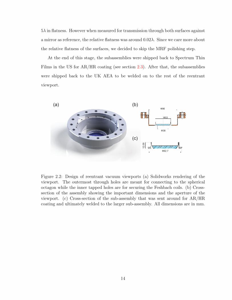
(a) (b)

(c)

Figure 2.2: Design of reentrant vacuum viewports (a) Solidworks rendering of theviewport. The outermost through holes are meant for connecting to the sphericaloctagon while the inner tapped holes are for securing the Feshbach coils. (b) Cross-section of the assembly showing the important dimensions and the aperture of theviewport. (c) Cross-section of the sub-assembly that was sent around for AR/HRcoating and ultimately welded to the larger sub-assembly. All dimensions are in mm.

14

2.3 AR/HR coatings

For the purpose of our experiment and for 6Li, we designed the coatings to be optimal

at the following wavelengths. At 671 nm for the MOT and Raman light, at 1064 nm for

the dipole trap and the 2D lattice, at 532 nm for the accordion lattice and at 323 nm

for a possible UV MOT in the future. The viewports on the 6-way cross on the oven

side of the experiment were left uncoated because we only need that optical access for

diagnostics. The 6 viewports on the side of the spherical octagon along with the one

viewport on the 4-way cross for the Zeeman slower beam were all anti-reflection coated

for the four wavelengths. All transmissions were optimized for normal incidence. The

coating company (Laseroptik GmbH) performed the coating process at 200C based

on the viewport manufacturer’s recommendation. The resulting measured coating

curve is shown in Fig. C.1. Below are the measured transmission at the design

wavelengths and for an angle of incidence of 0:

1. 671 nm : T ∼ 95%

2. 1064 nm : T ∼ 92%

3. 532 nm : T ∼ 92%

4. 323 nm : T ∼ 80%

The reentrant viewports had a slightly different set of requirements than the side

viewports. Although the bottom viewport needs to be anti-reflection coated like the

rest, the top one would need to be high transmission at 671 nm for the MOT beams,

while high reflection at 1064 nm only on the inside vacuum surface. The reason for

that is to enable the retro-reflection of a laser beam to form a lattice in the vertical

direction. As we will see later, we ended up not using the HR coating. High reflection

coatings are more complicated for a variety of reasons:

15

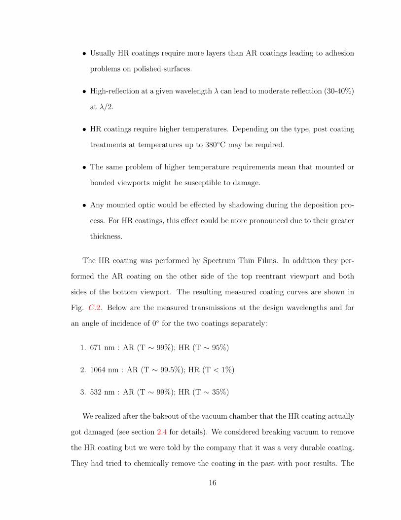
• Usually HR coatings require more layers than AR coatings leading to adhesion

problems on polished surfaces.

• High-reflection at a given wavelength λ can lead to moderate reflection (30-40%)

at λ/2.

• HR coatings require higher temperatures. Depending on the type, post coating

treatments at temperatures up to 380C may be required.

• The same problem of higher temperature requirements mean that mounted or

bonded viewports might be susceptible to damage.

• Any mounted optic would be effected by shadowing during the deposition pro-

cess. For HR coatings, this effect could be more pronounced due to their greater

thickness.

The HR coating was performed by Spectrum Thin Films. In addition they per-

formed the AR coating on the other side of the top reentrant viewport and both

sides of the bottom viewport. The resulting measured coating curves are shown in

Fig. C.2. Below are the measured transmissions at the design wavelengths and for

an angle of incidence of 0 for the two coatings separately:

1. 671 nm : AR (T ∼ 99%); HR (T ∼ 95%)

2. 1064 nm : AR (T ∼ 99.5%); HR (T < 1%)

3. 532 nm : AR (T ∼ 99%); HR (T ∼ 35%)

We realized after the bakeout of the vacuum chamber that the HR coating actually

got damaged (see section 2.4 for details). We considered breaking vacuum to remove

the HR coating but we were told by the company that it was a very durable coating.

They had tried to chemically remove the coating in the past with poor results. The

16

only way to completely remove the coating would be to polish the fused silica. Given

the complexity of the process, we decided to continue with the partially damaged

coating.

Another coating that we needed for the experiment was an HR coated dot of

2 mm diameter on top of an AR coated quarter-wave plate of 30 mm diameter. The

purpose of this piece was to act as the retro-reflection for the vertical MOT beam after

it goes through the objective (see section 2.7.2). This coating was also performed by

Spectrum Thin Films using a mask. The specs for the coating is R > 99% @ 671 nm

for an angle of incidence of 0.

17

2.4 Bakeout

In order to achieve ultra-high vacuum (UHV) inside our vacuum chamber, one needs

to remove the largest source of background gas - hydrogen. Although a vacuum pump

can easily remove other gases from the chamber, it is the hydrogen atoms that are

bound to interstitial sites of the stainless steel surface or that satisfy dangling bonds

that desorbs at a very slow rate - a process known as outgassing. But even before

reaching UHV pressures, there are other sources of outgassing that need to be taken

into account like fingerprints, oil/grease from machining, water vapor, etc. In this

section, I will describe the entire process that started with design considerations and

ended with a UHV system.

The material of choice is stainless steel. The various components were cleaned in

the following order:

1. First all items were inspected by eye for any visible signs of dirt or gunk. The

knife edges on the flanges were checked for damage.

2. For the vacuum parts that were manufactured by Sharon vacuum, we first

sonicated them with the soap Alconox mixed with tap water for 15 minutes.

Then we drained the soap water and sonicated again for 15 minutes in tap

water. To sonicate the large 4-way and 6-way crosses, we employed a large size

sonicator (Quantrex Q650H).

3. For all vacuum components except the vacuum windows, we sonicated them

first in acetone inside of a fume hood for 15 minutes and then in isopropyl

alcohol (IPA) to remove any residues left by acetone. The viewports were never

sonicated nor were they treated with soap or acetone to prevent damage to

the AR or HR coatings. The only cleaning process performed was using lens

cleaning paper and methanol.

18

4. The items were then placed in UHV grade aluminum foil (All Foils inc) and

allowed to dry in air. Thereon after the parts were kept completely wrapped in

UHV foil till they were ready to be assembled.

We assembled and baked out the oven side of the experiment first since it re-

quired fewer custom parts, no special coatings on the viewports and a less stringent

vacuum requirement. The various flanges were mated using copper gaskets except

for the lithium oven, for which a nickel gasket (Kurt Lesker GA-0133NIA) was used

to withstand possible degradation due to the high lithium flux. We used standard

silver plated hex bolts and nuts which were themselves sonicated in acetone and IPA.

They were tightened in a star pattern using a torque ratchet up to the recommended

torque values. We used an anti-seize (Kurt Lesker VZTL-4OZ) to ensure that the

bolts are removable in the event that we need to break vacuum in the future.

The next step is to check for leaks in the vacuum system. We did not use a leak

detector for this but instead just started the pumping process. We connected the

turbo pump (Varian Turbo V 81-M) to the angle valve and connected the outlet port

of the turbo to a roughing pump (Varian SH01101UNIV) through a 4 feet long bel-

low with NW25 KF ends (Kurt Lesker MHT-QF-B48). To measure the pressure, we

installed ion gauges (Varian UHV-24P) within standard straight CF40 nipples (Kurt

Lesker FN-0275S). This ion gauge is sensitive in a wide range from 10−3 down to

5×10−12 Torr. We attached another gauge (ConvecTorr L9090305) to measure a pres-

sure range from atmospheric down to 10−4 Torr. We started the evacuation process

while keeping the angle valve closed and turning on the roughing pump while keeping

the turbo off. The roughing pump can reach an ultimate pressure of 5×10−2 Torr.

After a few minutes of roughing when the pressure is low enough on the outlet of the

turbo, it is safe to turn on the turbo pump. The turbo pump was mounted to avoid

any stress and unwanted vibrations. Once the turbo reached its maximum speed

of 1350 rpm, we opened the angle valve. We can start measuring a readout of the

19

ion gauge when the ConvecTorr gauge bottoms out at a value close to ∼ 10−4 Torr.

At this point we can perform a crude leak check by spraying compressed air and/or

methanol around all the flanges and joints while looking for a pressure spike on the

ion guage. We never found any leaks in our system.

After reaching close to the base pressure of the turbo, we closed the angle valve

and turned off first the turbo and then the roughing pump (after the turbo came

to a complete stop). The sealed and partly evacuated vacuum system was then

wrapped with regular aluminum foil which inturn was wrapped with heating tape

(HTS/Amptek AWH-051-060DM-MP) to cover as much of the surface as possible.

The viewports were covered with a copper cap that ensured the heating tape or

aluminum foil could never make direct contact with the glass or any coating on

it. We placed thermocouples (Omega Engineering SA1XL-K-200-SRTC) at different

locations around the setup, sometimes using two thermocouples in sensitive areas like

in the vicinity of viewports. The setup was then wrapped over with another layer of

aluminum foil.

Each side of the experiment is in addition equipped with an ion pump. The oven

side has a smaller pump (Varian VacIon Starcell Plus 40) which has a CF40 flange

connector and a pumping speed of 36 l/s while the experiment side is larger (Varian

VacIon Starcell Plus 75) with a CF100 flange connector and a pumping speed of

65 l/s. In order to bake them out, we removed their outer cover and the magnets and

wrapped the rest with foil and heating tape. The pumps can’t be operated without

the magnets but they won’t be turned on anyway until the end of the bakeout process.

20

Figure 2.3: Vacuum system bakeout. (a) Connector diagram for Titanium sublima-tion filament. We connect one cartridge at a time to a 50 A DC power supply. Innormal mode of operation, we supply 30 A through a cartridge that requires a voltagedrop of 2.8 V. (b) Bakeout of the oven side of the experiment. This part was bakedfirst before assembling the rest of the experiment. In this picture one can see theheating tapes wound around the different parts already covered with aluminum foil.(c) Bakeout of the rest of the experiment.

21

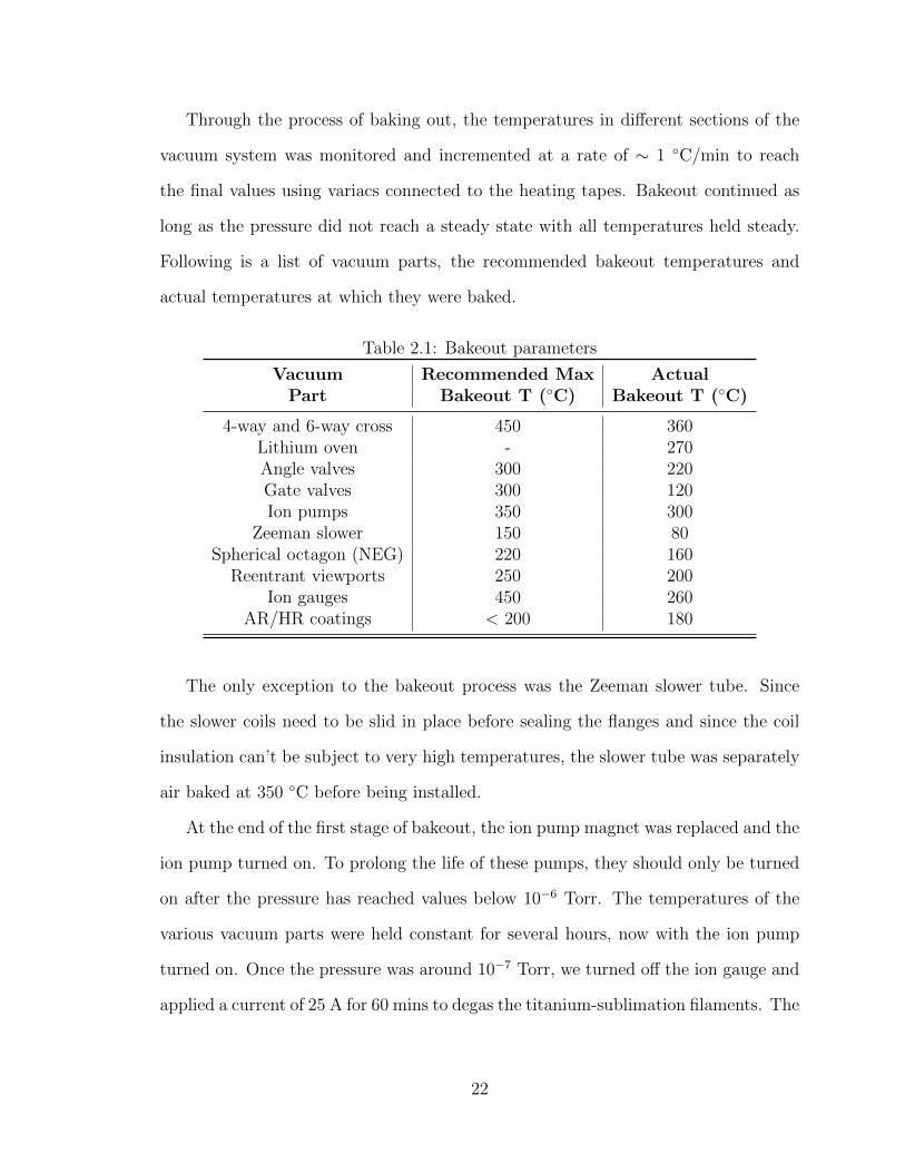
Through the process of baking out, the temperatures in different sections of the

vacuum system was monitored and incremented at a rate of ∼ 1 C/min to reach

the final values using variacs connected to the heating tapes. Bakeout continued as

long as the pressure did not reach a steady state with all temperatures held steady.

Following is a list of vacuum parts, the recommended bakeout temperatures and

actual temperatures at which they were baked.

Table 2.1: Bakeout parameters

Vacuum Recommended Max ActualPart Bakeout T (C) Bakeout T (C)

4-way and 6-way cross 450 360Lithium oven - 270Angle valves 300 220Gate valves 300 120Ion pumps 350 300

Zeeman slower 150 80Spherical octagon (NEG) 220 160

Reentrant viewports 250 200Ion gauges 450 260

AR/HR coatings < 200 180

The only exception to the bakeout process was the Zeeman slower tube. Since

the slower coils need to be slid in place before sealing the flanges and since the coil

insulation can’t be subject to very high temperatures, the slower tube was separately

air baked at 350 C before being installed.

At the end of the first stage of bakeout, the ion pump magnet was replaced and the

ion pump turned on. To prolong the life of these pumps, they should only be turned

on after the pressure has reached values below 10−6 Torr. The temperatures of the

various vacuum parts were held constant for several hours, now with the ion pump

turned on. Once the pressure was around 10−7 Torr, we turned off the ion gauge and

applied a current of 25 A for 60 mins to degas the titanium-sublimation filaments. The

22

bakeout process is complete and the temperatures can now be gradually decreased to

room temperature.

After the whole system was cooled down, we again applied 30 A to the titanium-

sublimation filaments. The heating due to the high currents causes titanium atoms

to sublimate and settle on the comparatively colder stainless steel. Hence it was also

important in the design to avoid any line-of-sight between the sublimation element

and the viewports. To ensure that, one must take into account the fact that the rods

elongate by several millimeters when hot. In our design of the 6-way cross, we left

a space of oonly 1.5 mm between the bottom of the titanium-sublimation filament

and the atomic shutter. So to avoid the expanding filament from hitting the shutter,

we had to keep the shutter in the “open” position where they would not touch. To

avoid line-of-sight from occuring on the 4-way cross due to expansion, we added an

extra double sided CF40 flange of 25.4 mm thickness (Kurt Lesker DFF275X150SS)

to connect the filament to the top of the 4-way cross. After firing the filaments,

the pressure in the vacuum system declined sharply to about 10−11 Torr. In normal

operation, the pressure on the experiment side is about 5×10−12 Torr and the oven

side about 3×10−10 when the oven is hot.

23

2.5 Magnetic Field Coils : Design and Winding

Magnetic fields play an important role in ultra-cold atom experiments, starting with

a spatially varying field for the Zeeman slower, an anti-Helmholtz field for the MOT

to a uniform field to tune the scattering length around a Feshbach resonance. Thus it

becomes paramount to design these field coils after performing accurate simulations.

The description of the design and implementation of each coil is laid out in the

subsequent sections. All the coils were wound using the same hollow core copper wire.

The wire itself was seamless Oxygen-free Copper alloy 101 (Small Tube Products).

This alloy is suitable for magnetic coils because of its very low resistance and its

soft temper makes it highly malleable for winding purposes. In addition, the wire

had a hollow square cross-section with outer dimension 3.18 mm and inner dimension

1.59 mm. The wire was, however, not insulated. So the spool of wire was coated

with Double Dacron glass insulation (Express Wire Services Inc.). Dacron glass

is specially well suited for our purposes because it is abrasion resistant, increases

flexibility and prevents overload burnout. The epoxy used to bind the coil was non-

magnetic (Duralco NM 25-1 sold by Cotronics Corp.). The total outer dimension

including the insulation and the epoxy was ≈ 3.5 mm.

2.5.1 Zeeman slower

The first stage of a typical cold atom experiment is the process of Zeeman slowing.

The basic idea of slowing is that an atom that posseses a cycling transition of energy

hωa can repeatedly absorb a resonant photon of momentum hk and get a recoil in its

momentum. This would imply effectively slowing down the velocity of the atom and

since the transition is cycling, the process can occur several times. The spontaneously

emitted photon after each absorption does not, on average, impart momentum to the

atom because of equal emission probability in all directions. The one caveat though

24

is in its rest frame, an atom moving with a velocity v sees an incoming photon

frequency to be Doppler shifted. So even if the photon was initially resonant to the

atom frequency, it ceases to be so as it gets slowed down. The Doppler shift in

frequency is given by ω′ − ωa = ωav/c.

There are many strategies to account for this Doppler shift. One approach is to

chirp the frequency of the incoming photons at a suitable rate. Another approach

more suitable for implementation in our experiment is using a magnetic field gradient

(B(z)). We designed the slower in a decreasing field configuration. In the presence

of this field gradient, the atoms experience a Zeeman shift leading to a total shift in

detuning of

δeff = δ0 + ωav

c− µBB(z)

h(2.1)

Where, δ0 is the bare detuning between the atomic transition and the laser fre-

quency (ωl) and µB is the Bohr magneton. We start out by first estimating the average

velocity of lithium atoms coming out of the oven. For a temperature of ∼ 400C, the

RMS velocity is given by the Boltzmann formula vRMS =√

3KBT/m ∼ 1300 m/s,

where KB is the Boltzmann’s constant and m is the mass of a lithium atom. We want

to calculate a B-field profile of the form B = B0

√1− z/z0 using Newtons law to ob-

tain a uniform deceleration. z0 is the length of the slower. At the end of this length,

we want to slow down most atoms in the ground state to around 50 m/s which is the

capture velocity of the MOT. At a given location z within the slower, suppose that

the velocity of an atom in v(z) and the field is B(z). One can calculate the Zeeman

shift in the ground and excited hyperfine states using the Breit-Rabi formula. For

any given ground hyperfine state, the detuning (∆E(F,mF , F′,m′F , B(z))/h) to the

excited manifold can be calculated.

Then the force the atom experiences due to absorption of a photon is

25

F = mdv

dt= −hkl

sΓ/2

(1 + s+ 4δ(z)2/Γ2)(2.2)

Where, s = I/Isat is the saturation parameter amd Isat is the saturation intensity

of the transition, Γ is the transition linewidth and δ(z) is the effective detuning at

the location z given by δ(z) = δ0 +ωav(z)/c−∆E(F,mF , F′,m′F , B(z))/h. Knowing

this, one can calculate the final velocity after accounting for deceleration through the

entire length of the slower.

In Fig. 2.4(a), one can see the result of the simulation for a slower of length 398 mm

(from center of the MOT to entry point of slower). We assume a saturation parameter

s = 4 and a maximum field strength of 750 G. We see that for the highest energy

ground state, one can slow atoms with speeds less than 750 m/s down to 50 m/s over

the length of the slower. In comparison, atoms with speeds less than 850 m/s in the

third highest energy state can be slowed down to ∼ 150 m/s.

With the theoretical B-field profile calculated, we now turn to simulating currents

in the coils of the slower to produce the required profile. For that we used a 3D

modelling package in conjugation with Mathematica called Radia [75]. We split the

slower into 6 parts. The first part is the coil that is closest to the chamber. It is

composed of a single layer of 8 turns and it has its own power supply and a single

input and output port for water cooling. The rest of the coils carry the same current

but have variable number of turns (layers). Starting from the second to the sixth,

the number of turns (layers) are 8 (3), 16 (4), 16 (5), 16 (6) and 16 (8). There are

in total five input and output ports for water cooling. To determine the currents

required in the coils, we simulated the coil geometry and fit Ifirst and Irest to best

fit the theoretical field profile (B = B0

√1− z/z0). We obtain Ifirst = 42 A and Irest

= 30 A. The fit required us to include the field due to the MOT coils such that the

total axial field smoothly reduced to 0 in the center of the science chamber.

26

0

300

600

900

0 0.1 0.2 0.3 0.4

Mag

netic

fiel

d (G

)

distance (m)

(a)

velo

city

(m/s

)

(b)

0

200

400

600

800

Mag

netic

fiel

d (G

)

distance (m)

(c)

0

300

600

900

0 0.1 0.2 0.3 0.4

(d)

93.

46 m

m

38.1

mm

290 mm

Figure 2.4: Zeeman slower design and testing. (a) The velocity profile for an atom instate |6〉, starting out with a velocity of 500 m/s (blue) and the maximally slowable765 m/s (red). Similarly for an atom in |1〉 starting out with the maximally slowablevelocity of 250 m/s (green). (b) Radia simulation of field profile for each slower coil(purple), MOT coil (green), total (black) and theoretical field profile (red). Distanceon the x-axis ends at the position of the center of the MOT. (c) Simulated total fielddue to all 6 slower coils (minus the MOT coils) (blue line) and the correspondingmeasured values (red circles) after the slower was built. (d) Schematic of the slowerdesign. Number of turns and layers are accurate although not to scale. Space betweentube and coils is filled with air. The first coil (red) is electrically isolated from therest. The rest of the coils have the same current flowing through each wire. Bluearrows depict direction of water cooling input/output. Color coding shows sectionssupplied by a single cooling water input/output.

27

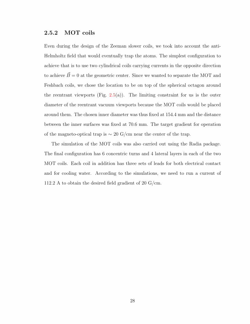
2.5.2 MOT coils

Even during the design of the Zeeman slower coils, we took into account the anti-

Helmholtz field that would eventually trap the atoms. The simplest configuration to

achieve that is to use two cylindrical coils carrying currents in the opposite direction

to achieve ~B = 0 at the geometric center. Since we wanted to separate the MOT and

Feshbach coils, we chose the location to be on top of the spherical octagon around

the reentrant viewports (Fig. 2.5(a)). The limiting constraint for us is the outer

diameter of the reentrant vacuum viewports because the MOT coils would be placed

around them. The chosen inner diameter was thus fixed at 154.4 mm and the distance

between the inner surfaces was fixed at 70.6 mm. The target gradient for operation

of the magneto-optical trap is ∼ 20 G/cm near the center of the trap.

The simulation of the MOT coils was also carried out using the Radia package.

The final configuration has 6 concentric turns and 4 lateral layers in each of the two

MOT coils. Each coil in addition has three sets of leads for both electrical contact

and for cooling water. According to the simulations, we need to run a current of

112.2 A to obtain the desired field gradient of 20 G/cm.

28

-200-100

0 100 200

-0.15 0 0.15

Mag

netic

fiel

d (G

)

distance (m)

(a)

(c)

-0.15 0 0.15

(d)

-0.15 0 0.15

(b)

xy

z

Figure 2.5: MOT coils. (a) Schematic of MOT coils with reference to the vacuumsystem. The inner diameter of the coils is constrained by the reentrant vacuumviewports. The distance between the coils is contrained by the spherical octagon.Color coding signifies the extent of the coils cooled by a single pair of leads. All coilsare electrically connected to the same power supply and carry current in oppositedirections between the top and the bottom. (b) Simulation of the x-component of ~B

along the x-axis for a current of 112.2 A. (c) The y-component of ~B along the y-axis.

(d) The z-component of ~B along the z-axis. The origin is defined as the geometriccenter of the spherical octagon.

29

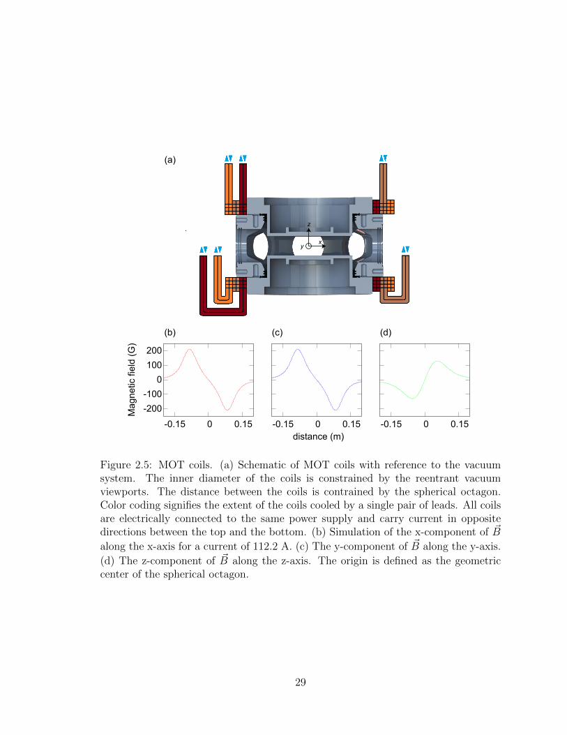
2.5.3 Feshbach coils

Probably the most crucial magnetic field in the experiment is the Feshbach field. This

field allows us to tune the interactions between 6Li atoms by using the magnetic field

dependence of the s-wave scattering length (as). It is important for this field to be

uniform over the size of the atomic cloud. For this reason we employ two coils in

Helmholtz configuration, unlike the MOT coils. One of the initial challenges is to

design a water cooled coil that can produce fields in excess of 1000 G. That is since

the |1〉− |2〉 Feshbach resonance occurs at 832 G, one would need to go to sufficiently

higher field to access the weakly interacting regime.

In order to reduce the requirement for current, we placed the Feshbach coils at a

location closest to the atoms yet outside the vacuum system. The reentrant vacuum

viewports were designed with this in mind, to utilize the region right next to the

window. We simulated the field due to the Feshbach coils also using the package

Radia. The inner diameter of the coil is 55 mm while the outer diameter is 90 mm. We

would also want the magnetic field to be uniform over a distance of a few millimeters.

The final configuration we used consisted of 5 concentric turns stacked in 4 layers.

The field profile is shown in Fig. 2.6. For a current of 200 A, we produce a field of

911 G with a curvature of 0.16 G/mm2 at this field at the center. The curvature of

the Feshbach field also produces magnetic confinement for the atoms, although it is

much smaller than the confinement produced by the trapping lasers.

30

0

2

4

-0.1 -0.05 0 0.05 0.1

Mag

netic

fiel

d (G

)

distance (m)

(a) (b)

4.01

4.02

4.03

4.04

-0.01 0 0.01

(c)

-0.1 -0.05 0 0.05 0.1

(d)

distance (m)

distance (m)

Mag

netic

fiel

d (G

)M

agne

tic fi

eld

(G)

0

2

4

xy

z

Figure 2.6: (a) Solid works rendering of the Feshbach coils and their placement relativeto the reentrant vacuum viewports. The coils (red) are sandwiched between theviewport and a piece of Macor (white). There are two sets of input and output forwater cooling for each coil. (b) Simulation of Bz along z-axis over a range of 100 mm(blue line) and actual measurements (red circles) for a current of 0.88 A (c) Simulationof Bz along the y or x-axis for 0.88 A. (d) The curvature of the field (Bz) along thez-axis around the geometric center in a smaller range of 10 mm. Simulation (redcircles) and quadratic fit (blue line) for a current of 0.88A.

31

2.5.4 Coil Winding

In order to facilitate the winding of the Zeeman slower coils and also to avoid twisting

of the hollow core wire during winding, we designed a wire feedthrough (Fig. 2.7(b))

machined from Teflon. The feedthrough can be mounted on a standard lathe and has

a square channel of side 3.18 mm running through the whole length. The reason we

avoided using metal to make the feedthrough was to prevent scratching the Dacron

insulation on the wire at any sharp edges. In addition, the added friction from the

feedthrough also increased the tension on the wire, making it easier to ensure close

packing. The whole setup was mounted on a lathe as shown in Fig. 2.7(a). The

lathe was used to rotate the tube at the slowest speed (20 rpm) while the epoxy

was spread on the wire with a brush after the feedthrough. Along with the rotation,

the feedthough was translated by hand. Once each layer was complete, about half a

meter of extra coil length was retained for connections before the wire was cut with

a saw to make sure the hollow opening was not constricted. Then once the layer had

dried out, the next one was layed over in the same fashion. The slower coils were the

hardest ones to wind and took several days to complete.

The MOT and Feshbach coils comprised of fewer turns and layers but were wound

on the lathe in a similar fashion. One difference, however, was that for the slower,

the extra length of wires for connections were tangential to the windings while for the

MOT and Feshbach coils, they needed to be bent out of plane to make them accessible.

This bending needs to be done carefully to avoid pinching and constriction of the coil.

In addition, these connections had to be meticulously placed out of the way of other

essential optics like the objective.

In order to make electric contacts, we stripped the insulation on the wire about

5 cm below the end. Then we silver soldered a custom made part out of copper that

contains a channel wide enough for the wire to slide through (Fig. 2.8(b)). This piece

had a circular hole to attach it with 1/4-20 bolts. Next to make connections with the

32

water cooling system, we used a standard swagelok compatible fitting with a square

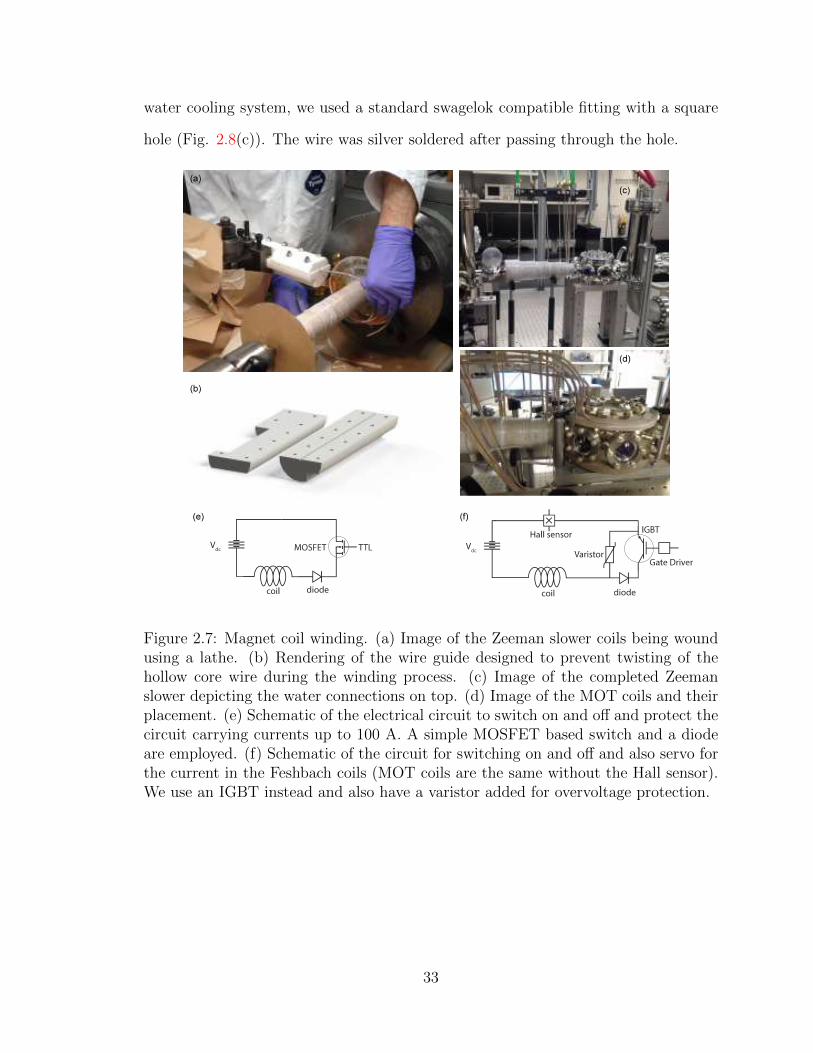
hole (Fig. 2.8(c)). The wire was silver soldered after passing through the hole.

Figure 2.7: Magnet coil winding. (a) Image of the Zeeman slower coils being woundusing a lathe. (b) Rendering of the wire guide designed to prevent twisting of thehollow core wire during the winding process. (c) Image of the completed Zeemanslower depicting the water connections on top. (d) Image of the MOT coils and theirplacement. (e) Schematic of the electrical circuit to switch on and off and protect thecircuit carrying currents up to 100 A. A simple MOSFET based switch and a diodeare employed. (f) Schematic of the circuit for switching on and off and also servo forthe current in the Feshbach coils (MOT coils are the same without the Hall sensor).We use an IGBT instead and also have a varistor added for overvoltage protection.

33

The current in the magnet coils were produced using standard power supplies.

Since current stability is not crucial for the slower and MOT coils, we used refurbished

DC power supplies: EMS 40 V-50 A for the slower last coil, Power Ten 50 V-50 A

for the rest of slower coils and Lambda EMS 13-200-2-D (13 V, 200 A) for the MOT

coils. The above supplies were run in constant current mode. In addition, we added

a simple 0-5 V analog current control for the MOT coil power supply to be used for

varying a magnetic gradient. The Feshbach coils need a better power supply because

we need to be able to stabilize the field to much better accuracy. We use the Delta

Elektronika SM 18-220 power supply with a passive current stability of 10−4.

The Zeeman slower currents were switched using a simple mosfet and a diode was

added to prevent damage to the power supply due to a negative voltage (D06D100 and

R5021213LSWS rated up to 100 A) (Fig. 2.7(e)-(f)). The MOT coils were switched

using an IGBT (CM600HA-24H), a varistor (V321DA40) was added to protect the

IGBT from high voltage inductive spikes when switching the current rapidly and a

diode (VS-400UR120D) to protect the power supply. The low field shim coils were sent

through another set of mosfets and diodes (D1D40 and 1N2128A rated up to 40 A).

The low current mosfets were mounted on heat sinks while the high current IGBTs

were additionally provided with water cooling. The Feshbach coils are essentially

the same setup as the MOT coils but in addition we add a Hall sensor (Danisense

DS200UBSA-10) on the current return path to read out the current and to stabilize

the same with a servo. The IGBTs in addition require high currents at the gate for

a fast switch on. So we added a driver (BG1A-KA) that is capable of providing up

to 20 A of current to the gate.

34

2.6 Water Cooling

Since the Zeeman slower, MOT and Feshbach coils are designed to run at currents of

30 A, 112 A and up to 200 A respectively, heating of the coils due to Joule heating

during the continuous operation of several seconds can be significant. To mitigate

that, we used a hollow core copper wire with square cross-section. Knowing the total

length of wire, the resistivity of Cu (ρ = 1.68×10−8 Ωm), the cross section area (a

= 7.56×10−6 m2) and the current flowing through, we can calculate the total power

dissipated (P = ρI2ltot/a):

• Zeeman slower, ltot = 74 m and P = 152 W

• MOT coils, ltot = 32 m and P = 893 W

• Feshbach coils, ltot = 13 m and P = 1126 W

Hence a combined power dissipation from all our coils would be 2.2 kW. In order

to calculate the pressure drop and flow rate required to keep the coils from heating

up too much, we make use of the Hazen-Williams equation:

dV

dt=

(C1.85d4.87∆P

4.52L

)0.54

(2.3)

Where, dV/dt is the flow rate in gallons per minute (gpm), ∆P is the pressure

drop over the length of the pipe in pounds per square inch (psi), C is a pipe roughness

coefficient (∼ 140 for Cu), d is the inside diameter of the pipe in inches and L is the

length of the pipe in feet. Using this equation, we can estimate the volume flow rate

of water through the hollow-core wires for a given maximum pressure differential and

then estimate the temperature rise in the wire knowing the power dissipated in the

coils due to Joule heating, the specific heat capacity of water (CV = 4.15 kJ/kgC at

20 C) and the density of water (ρ = 998 kg/m3). We use:

35

P =dQ

dt= ρ

dV

dtCV ∆T (2.4)

Using the above relation and the aforementioned power dissipated in the coils,

we get the following flow rates and temperature increase in our coils for a maximum

pressure drop of 500 psi:

• Zeeman slower, dV/dt = 0.06 gpm and ∆T = 10 C

• MOT coils, dV/dt = 0.1 gpm and ∆T = 35 C

• Feshbach coils, dV/dt = 0.2 gpm and ∆T = 27 C

The values above are for continuous operation of current in the coils. In the actual

experiment, currents are kept on for only a few seconds after every 16-18 seconds,

allowing the coil temperatures to reach an intermediate steady state value. Although

higher pressure drops than 500 psi would allow for better cooling, we were limited

by maximum pressure ratings on pumps and other plumbing parts like tubes and

connectors. The total flow rate that would flow through all the coils combined is

∼ 0.4 gpm, which is a rather small value.

In order to generate the high pressure, we decided to use a booster pump (Webtrol

EZ Series H15B40-1 5HP). The advantage of this particular pump is that it can

provide 500 psi of discharge pressure at a flow rate of up to 5 gpm through the pump,

much more than what we need. Next, we needed a heat exchanger that would also be

able to sustain the required flow rate through the booster pump for safe operation.

Our choice was Neslab System II (2 PD2). This heat exchanger is rated to discharge

at a pressure of 60 psi and a flow of 6 gpm. In addition, the maximum cooling capacity

is 34 kW for a temperature difference of 10 C which is higher than the load due to

our coils. In normal operation and in steady state, we have the following typical

parameters:

36

Table 2.2: Water cooling parameters

Property Value Units

Building Chilled Water Supply Pressure 80 psiBuilding Chilled Water Supply Flow Rate 4 gpmBuilding Chilled Water Supply Temperature In 7 CBuilding Chilled Water Supply Temperature Out 14 C

Neslab Heat Exchanger Discharge Pressure 60 psiNeslab Heat Exchanger Discharge Flow Rate 8 gpmNeslab Heat Exchanger Temperature Setpoint 14 CSteady-State Water Temperature 14.6 C

Booster Discharge Pressure 550 psiBooster Discharge Flow Rate 4 gpm

The heat exchanger is connected to chilled water from the building at the input

and its output is split between the booster and the low power load in the experiment

like beam dumps (Fig.2.8). The output of the booster is inturn connected to all

high power load in the experiment like the magnet coils. Since the total flow out

of the booster (4 gpm) is much higher than the flow through all the coils combined

(0.4 gpm), we introduced a low resistance channel in parallel to the load to have the

excess flow go through.

Since the water used for cooling is part of a closed loop, we added ways of prevent-

ing dirt and algae buildup that could lead to clogging of the heating coils. The water

used to fill the reservoir is deionized with a small amount of algae control fluid added

to it. There is a 50 µm filter after the chiller (Parker PM050-20AE-DO) that acts as

a first stage filtration. Then the high pressure path is further filtered by a 40 µm high

pressure filter (Swagelok SS-8F-K4-40). In the beginning we used aluminum gaskets

that would completely disintegrate in the time that the filters would need to be re-

placed (usually 2-3 months). So we switched to the stainless steel version (Swagelok

SS-8TF-K2) that tend to be essentially reusable.

37

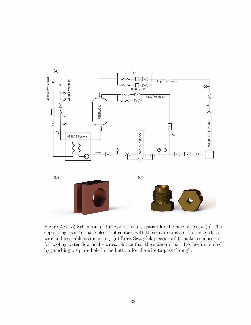
NESLAB System II

Chill

ed W

ate

r In

Chill

ed W

ate

r O

ut

PM

05

0-2

0A

E-D

O

P

T

T

T

P P P

P

P

Low Pressure

High Pressure

WE

BT

RO

L H

15

B4

0-1

SS-8F-k4-40

RE

SE

RV

OIR

(a)

(b) (c)

Figure 2.8: (a) Schematic of the water cooling system for the magnet coils. (b) Thecopper lug used to make electrical contact with the square cross-section magnet coilwire and to enable its mounting. (c) Brass Swagelok pieces used to make a connectionfor cooling water flow in the wires. Notice that the standard part has been modifiedby punching a square hole in the bottom for the wire to pass through.

38

In addition, we added temperature interlocks to the coil power supplies in the

event that either the chiller or the booster pump should stop working. The booster

itself is interlocked to the chiller to avoid dry operation. We attached thermocouples

(Omega Engineering SA1XL-K-200-SRTC) on each individual coil using Kapton tape

and used a standard digital temperature switch (Dwyer Instruments 40T-10). The

triggering of any one of the temperature switches would turn off the current on all

power supplies. But even after the temperatures have lowered to within acceptable

range, the system would not be restored without a manual button press. This would

ensure that the event of cooling failure does not escape the user’s attention.

It was also important to choose pipings and connectors that were appropriately

suited for high pressure operation. To go from the wall manifold to the experiment

table, we used a high pressure water hose (McMaster Carr 53115K29). Close to the

experiment, we used brass manifolds (McMaster Carr 5627K553) to split the flow

from one hose to many smaller diameter tubes that would carry the cooling water

to and from the coils. The tube used was a flexible nylon tube (McMaster Carr

9685T3) capable of withstanding 800 psi of pressure and had an outer diameter of

0.25 in. In order to couple this tubing to the square cross section hollow core copper

wires, we used a Swagelok tube cap (Swagelok B-400-C Fig. 2.8(b)). On the cap side

of the fitting, we pressed a square hole of side 3.18 mm such that the copper wire

with its insulation removed would snugly slide through. Then with enough length

fed through, we silvered soldered the junction to obtain a water tight seal. The rest

of the connections were done through standard Swagelok sleeves or with pipe thread

sealant tape for NPT type connections.

39

2.7 671 nm Laser System

2.7.1 6Li Spectroscopy

The first step of designing the laser system we use for laser cooling of lithium is to

define a frequency reference. We do that by dedicating a laser to be locked to the

D2 transition of 6Li using modulation transfer spectroscopy. The spectroscopy cell

was designed to be a simple straight nipple with CF40 flange ends, a small bucket in

the center to add lithium to and a CF16 extension to connect an angle valve (MDC

314001) for pumping (Fig. 2.9(a)). The cell was manufactured by Sharon Vacuum

using 304 stainless steel. The two ends have been fitted with viewports with the

same AR coating as the experiment chamber (Fig. C.1). The bucket is covered with

a band heater (Tempco NHL00112) of 38.1 mm inner diameter. The band heater

is connected to a variac and a thermocouple. The temperature of the cell is kept

fixed at 190 C. The lithium inside the bucket evaporates and creates a vapor in the

center of the cell that the laser beams can probe. However, if the vapor reaches the

viewports, then it would lead to coating by deposition. To avoid that, we introduced

some Argon in the cell and in addition, we water cool the ends of the cell to ensure

that the vapor condenses before reaching the viewports.

Since we do not need high vacuum conditions inside the cell, we use a cheaper

source of lithium (Sigma Aldrich 340421-10G) which is 95% isotopically purified 6Li

and is packaged in a bottle under oil. The oil prevents the oxidation of lithium in

air. Before placing the chunks of lithium inside the cell, we cleaned it by scraping on

the surface while immersed in a mixture of methanol and dry ice. Then we evacuated

the sealed cell using only the scroll pumps to reach base pressure and then slowly

introduced a small amount of Argon. To generate the spectroscopy light, we use a

tunable diode laser (Toptica DL PRO).

40

Modulation transfer spectroscopy is a pump-probe method of sub-Doppler spec-

troscopy. The advantages of this type of spectroscopy over saturated absorption

spectroscopy is two fold. Firstly, the error signal produced with this method is offset

free (Fig. 2.9(e)) while in regular spectroscopy, the error signal contains an intensity

dependent offset. Secondly, the absence of a linear background absorption leads to

a lower sensitivity to beam intensity and cell temperature. This feature eliminates

long time offset drifts of the error signal, which cannot be corrected by laser locks.

Ultimately this laser is locked to the D2 cooling transition (2S1/2 F=3/2 → 2P3/2).

In this scheme (Fig. 2.9(b)), we generate a sideband at 4.75 MHz using an EOM

designed using a LiTaO3 crystal (Castech J7116-1) on the pump beam that then is

overlapped with the un-modulated probe beam in a Doppler-free counter-propagating

way. At resonance, the modulation can be efficiently transfered to the probe beam if

the light-atom interactions are sufficiently non-linear by a process known as 4-wave

mixing [76]. This signal can be extracted through homodyne detection to produce

an error signal. Unlike saturated absorption spectroscopy where one looks for probe

beam absorption, the error signal is zero away from a resonance. We employed two

different channels of an RF generator (Rigol DG1022) to generate the sideband and

use for homodyne detection.

41

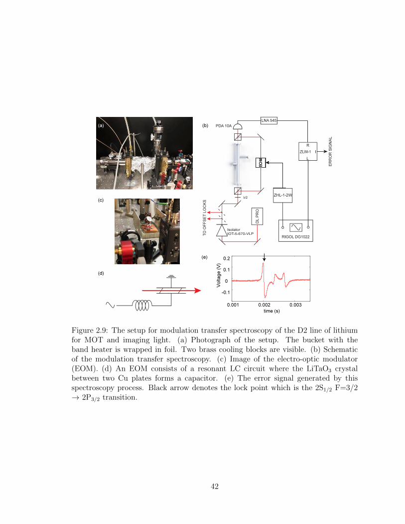
Figure 2.9: The setup for modulation transfer spectroscopy of the D2 line of lithiumfor MOT and imaging light. (a) Photograph of the setup. The bucket with theband heater is wrapped in foil. Two brass cooling blocks are visible. (b) Schematicof the modulation transfer spectroscopy. (c) Image of the electro-optic modulator(EOM). (d) An EOM consists of a resonant LC circuit where the LiTaO3 crystalbetween two Cu plates forms a capacitor. (e) The error signal generated by thisspectroscopy process. Black arrow denotes the lock point which is the 2S1/2 F=3/2→ 2P3/2 transition.

42

2.7.2 MOT and Zeeman slower

Light for the MOT beams and the Zeeman slower beam were generated using a

second DL PRO diode laser. The principle of operation of the magneto optical trap

will be discussed in section 3.1. The laser is offset locked to the spectroscopy laser as

depicted below. The detuning (δ) of the laser with respect to the D2 transition can

be tuned from -11 Γ to 2 Γ. The free running linewidth of the laser is 10 kHz, much

smaller than the linewidth of the transition (Γ = 5.87 MHz). The laser head outputs

∼ 25 mW of power which is not sufficient for efficient trapping of atoms. So we used

tapered amplifiers to amplify the laser power before being sent through other optical

elements.

The tapered amplifier chips are designed for amplification up to 500 mW at 670 nm

(Eagleyard EYP-TPA-0670-00500-2003-CMT02-0000). The mount design was based

off of the design by the Harvard group [77] and was machined out of copper (Fig.

2.10(d)-(e)). Temperature stabilization was performed by adding two peltier coolers

(Thorlabs TEC3-6) sandwiched between the mount and heat sinks, and a thermistor

(Thorlabs TH10K) connected to a temperature controller (Thorlabs TED200C). In

addition, the DC current required to drive the TA chip was provided by a laser diode

current controller (Thorlabs LDC220C) through a protection circuit (Fig. 2.10(f))

designed to avoid any electrical damage to the chip. To improve thermal contact, a

single layer of 50 µm thick, 99.99% indium foil was placed between the chip and the

mount.

The incident beam was focused down and the output beam collimated with as-

pheric lenses (Thorlabs C230TME-B for input and Melles Griot 06 GLC 001 for

output) placed on translation stages (Thorlabs SM1Z) for focus alignment. The lat-

eral alignment however was performed only once and fixed with epoxy. The normal

operating current of the amplifiers is around 0.9 A. After initial setup, we were able

43

to output ∼ 350 mW of power from the TAs for ∼ 30 mW input power but after a

few years, the output degraded to ∼ 200 mW.

The output of the first TA is used to generate the repump light and to seed a

second TA to generate the cooling light. The repump light is passed through an

acousto-optic modulator (AOM, Intraaction ATM-1141A1) to increase its frequency

by 114 MHz and the cooling light is passed through another AOM (Intraaction ATM-

80A1) to decrease its frequency by 114 MHz. Both AOMs have a first order diffraction

efficiency of 70-80%. Each beam is split into 4 parts, three of which are used for the

MOT beams in the three directions. The fourth beam is passed through another AOM

(Intraaction ATM-701A1) which decreases its frequency by 70 MHz to generate the

Zeeman slower beam. The beams were then fiber coupled and sent via polarization

maintaining optical fibers (OZ Optics PMJ-3A3S-633-4/125-3-20-1) to the experiment

table.

The MOT beams are first-passed through the science chamber, then the polariza-

tion is rotated by passing through a quarter-wave plate and retroreflecting the beams

to create a σ+ − σ− beam configuration required for the operation of the MOT. The

vertical direction MOT beam, however, has to be retroreflected after passing through

the objective. We retroreflect the beam at the Fourier plane of the obective. We HR

coated a 2 mm diameter dot on a quarter wave plate (Spectrum Thin Films). This

QWP was mounted on a plastic tube (Fig. 2.10(c)) and placed at the correct depth.

The effect of the HR dot on the point spread function in the fluorescence imaging will

be discussed in section 3.3.2.

44

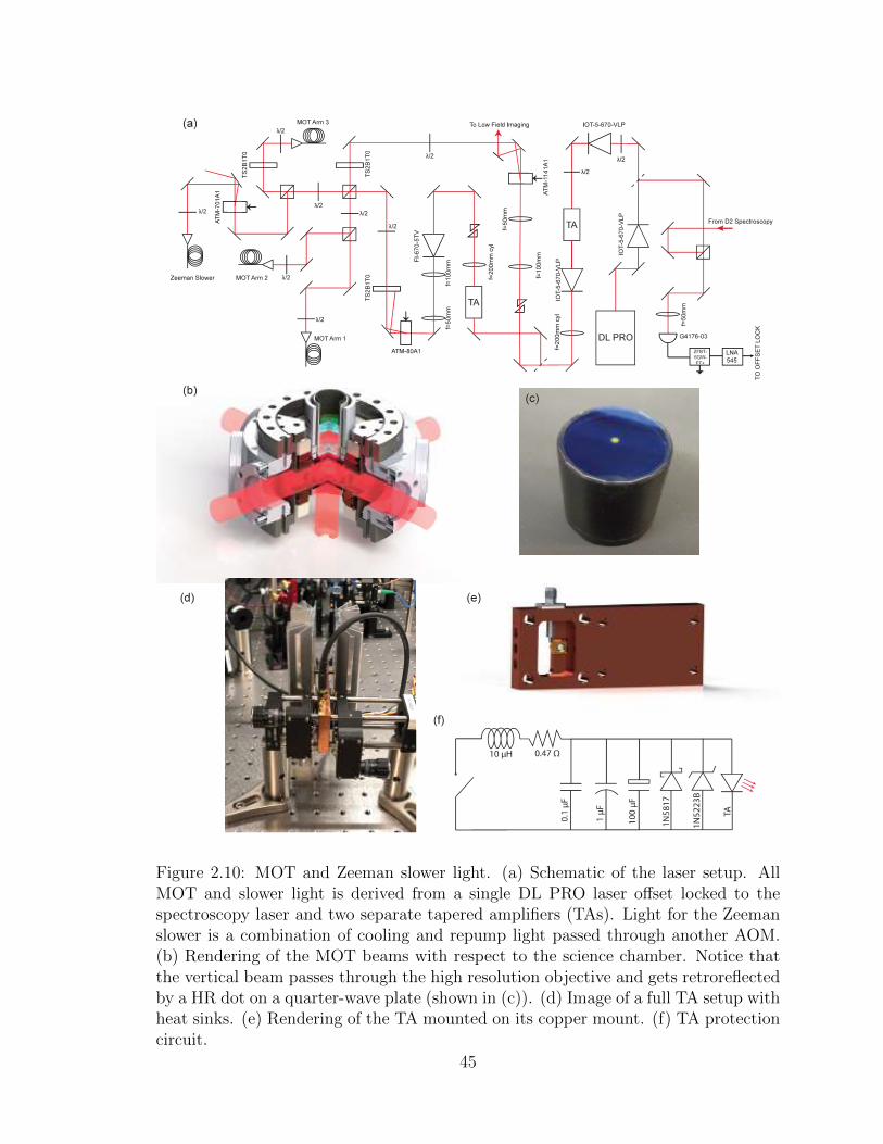
Figure 2.10: MOT and Zeeman slower light. (a) Schematic of the laser setup. AllMOT and slower light is derived from a single DL PRO laser offset locked to thespectroscopy laser and two separate tapered amplifiers (TAs). Light for the Zeemanslower is a combination of cooling and repump light passed through another AOM.(b) Rendering of the MOT beams with respect to the science chamber. Notice thatthe vertical beam passes through the high resolution objective and gets retroreflectedby a HR dot on a quarter-wave plate (shown in (c)). (d) Image of a full TA setup withheat sinks. (e) Rendering of the TA mounted on its copper mount. (f) TA protectioncircuit.

45

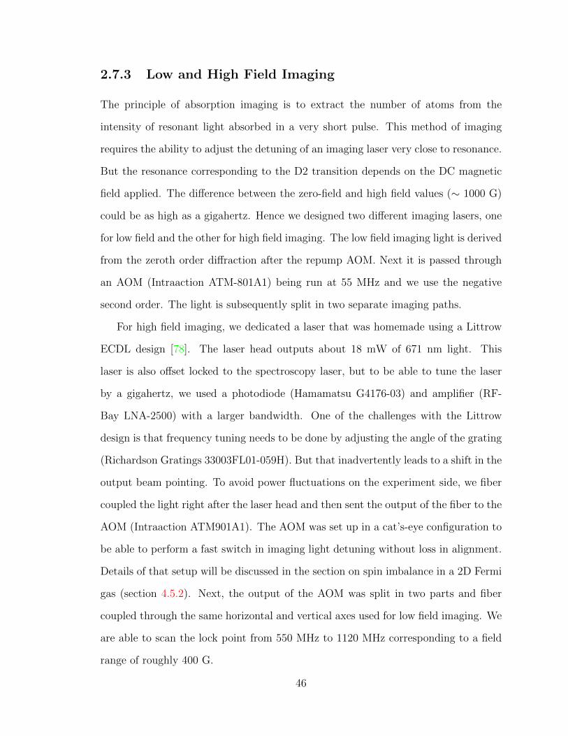
2.7.3 Low and High Field Imaging

The principle of absorption imaging is to extract the number of atoms from the

intensity of resonant light absorbed in a very short pulse. This method of imaging

requires the ability to adjust the detuning of an imaging laser very close to resonance.

But the resonance corresponding to the D2 transition depends on the DC magnetic

field applied. The difference between the zero-field and high field values (∼ 1000 G)

could be as high as a gigahertz. Hence we designed two different imaging lasers, one

for low field and the other for high field imaging. The low field imaging light is derived

from the zeroth order diffraction after the repump AOM. Next it is passed through

an AOM (Intraaction ATM-801A1) being run at 55 MHz and we use the negative

second order. The light is subsequently split in two separate imaging paths.

For high field imaging, we dedicated a laser that was homemade using a Littrow

ECDL design [78]. The laser head outputs about 18 mW of 671 nm light. This

laser is also offset locked to the spectroscopy laser, but to be able to tune the laser

by a gigahertz, we used a photodiode (Hamamatsu G4176-03) and amplifier (RF-

Bay LNA-2500) with a larger bandwidth. One of the challenges with the Littrow

design is that frequency tuning needs to be done by adjusting the angle of the grating

(Richardson Gratings 33003FL01-059H). But that inadvertently leads to a shift in the

output beam pointing. To avoid power fluctuations on the experiment side, we fiber

coupled the light right after the laser head and then sent the output of the fiber to the

AOM (Intraaction ATM901A1). The AOM was set up in a cat’s-eye configuration to

be able to perform a fast switch in imaging light detuning without loss in alignment.

Details of that setup will be discussed in the section on spin imbalance in a 2D Fermi

gas (section 4.5.2). Next, the output of the AOM was split in two parts and fiber

coupled through the same horizontal and vertical axes used for low field imaging. We

are able to scan the lock point from 550 MHz to 1120 MHz corresponding to a field

range of roughly 400 G.

46

IOT-

5-67

0-V

LP

LNA2500

G4176-03

ZFBT-6GW-FT+

671 nmECDL

FRO

M S

PE

CTR

OS

CO

PY

TO OFFSET LOCK

λ/2

NP

TO WAVEMETER

ATM-801A1

ATM

-901

A1

λ/2

λ/2

λ/2

λ/2

f=25

0mm

λ/4

λ/2

TS2B

1T0

VE

RTI

CA

L IM

AG

ING

HORIZONTAL IMAGING

NP

NP

TS2B1T0TS2B1T0

TS2B1T0FROM REPUMP AOM 0th ORDER

CM

OT

IMA

GIN

GR

AM

AN

IMA

GIN

G

f=50

mmf=

100m

m

TS2B1T0λ/2

λ/2

λ/2

TO AOM

FROM ECDL

TS2B1T0

Figure 2.11: Schematic of low (blue) and high (red) field imaging. Boxed inset showsthe generation of light for high field imaging and the offset lock with spectroscopylaser. The light is redirected via an optical fiber (green) to the AOM in double passcats-eye configuration. Both low and high field imaging light is coupled to the samefibers and sent to the experiment.

47

2.7.4 Raman laser system

In order to image single atoms in a lattice, we perform Raman sideband cooling

[53]. This method relies on the two hyperfine ground states of 6Li (2S1/2 F=1/2 and

F=3/2) and an excited state. Our Raman beams are red detuned by 5.6 GHz from

the D1 line. The details of the Raman cooling scheme can be found in section 3.3.

We dedicate two lasers for this purpose. We first take a homemade Littrow ECDL

laser [78] and lock it to the D1 (2S1/2 F=3/2 → 2P1/2) transition using modulation

transfer spectroscopy (Fig. 2.12(b)). We generate a sideband at 6.31 MHz using

an EOM and use the same spectroscopy cell used for the D2 master laser. This

laser serves as a reference to offset lock the Raman laser. In addition, this laser

serves as the pump laser that transfers atoms in the 2S1/2 F=1/2 state to the 2P1/2

state. This requires us to detune the laser by 228 MHz from the lock point. We

achieve that by double passing the beam through an AOM driven at 114 MHz using

a cat’s-eye configuration (Fig. 2.12(a)). In practice, the detuning of the pump beam

is tuned experimentally and will be discussed later. The Raman beam is obtained

from another Toptica DL PRO system. It is offset locked 5.6 GHz red detuned from

the 2S1/2 F=3/2 → 2P1/2 transition. The Raman beam is sent through an AOM

operating at 88.3 MHz, which is used as a fast switch.

48

DL PRO

EOM

/2

75mm

PDA-36A

FROM LASER

671 nm

ECDL

LNA

8G

ZX85-

12G-

S+

TO OFFSET LOCK

/2

/2

/2/2

/2

/4

Voltage (

V)

time (s)

-0.2

-0.1

0

0.1

0.2

0.001 0.002 0.003

IOT-5-670-VLP

IOT-5-670-VLP

100mm

200mm

50mm

50mm 100mm

G4176-03

PUMP

RA

MA

N

TO SPECTROSCOPY

ATM-114A1

ATD-881A1.67

SHUTTER

SHUTTER

(a)

(c)

(b)

Figure 2.12: Raman laser system. (a) Schematic of the Raman laser setup. A home-made ECDL is used to lock to the D1 transition of 6Li (2S1/2 → 2P1/2). A secondlaser (Toptica DL PRO) is offset locked to the first laser. (b) Modulation transferspectroscopy setup for locking to the D1 transition. (c) The error signal obtainedfrom this setup. The two main features are due to the hyperfine structure of theground state and are separated by 228 MHz. The central feature is due to crossover.The arrow indicates the location where the laser is locked (2S1/2 F=3/2 → 2P1/2).

49

2.8 Optical Potentials

2.8.1 Optical Dipole Trap

The atoms of lithium can be trapped in the intensity maximum of a red-detuned laser

beam [79]. The dipole potential experienced by an atom in the presence of a drive is

given by

U(~r) = −3πc2

2ω30

(Γ

δ+

Γ

ω0 + ω

)I(~r) (2.5)

where, ω0 is the frequency of the transition while ω is the frequency of the drive,

Γ is the transition linewidth and δ = ω0 − ω the detuning of the drive from the

transition. In addition, the rate at which photons belonging to the laser are scattered

by the atoms is given by

hΓsc =3πc2

2ω30

(ω

ω0

)3(Γ

δ+

Γ

ω0 + ω

)2

I(~r) (2.6)

So for a far red detuned beam (δ < 0 and |δ| ω0), we see that the potential is

attractive where intensity is maximum and the scattering rate is negligible, leading

to the potential being almost conservative. In such conservative potentials, trapped

atoms can have very long lifetimes, essentially limited by background gas scattering.

In our experiment, we generate the optical dipole trap (ODT) using an Ytterbium

fiber laser (IPG Photonics YLR-200-LP-AC-Y11). The laser outputs up to 200 W

of multimode light centered around 1070 nm. We focus a beam of 112 W down to

70 µm waist. Then the beam is retro-reflected and overlapped with a perpendicular

polarization at the focus at a shallow angle of 11. Due to the polarization, no

substantial interference effects occur at the intersection, leading to a trap of 1.7 mK

depth at the cross. This trap is cigar shaped with the tight trapping frequency of

(2π) 7 kHz and shallow trapping frequency of (2π) 24 Hz.

50

The intensity of the ODT is modulated by sending it through a high power AOM

(Gooch and Housego AOMO 3110-197). These AOMs require over 2 W of RF power

to reach saturation, unlike the Intraaction AOMs that only need about 1 W.

The evaporation process imposes two requirements on the control of the intensity

of the trapping laser: the intensity needs to be tunable over several orders of mag-

nitude and especially at the lowest intensities, it is important to have low intensity

noise. For this purpose, we designed a special intensity lock electronics with handover.

The setup as depicted in Fig. 2.13(b). The idea of handover is to use a comparator

(AD790), a latch (Quad NOR SN74LS02N) and two different photodiodes (PDs), one

dedicated to high power operation and the other to low power. The lock always starts

out at maximum power, where the low power PD is saturated. A comparator com-

pares that PD voltage to a voltage reference and is in logic 0 state in the beginning.

The latch is connected to the output of the comparator and an external override. As

the power of the laser is decreased, the low power PD voltage eventually falls below

the reference and the comparator switches to logic 1. This causes the latch to switch

to logic 1 and it stays in that state unless it is reset by passing logic 1 on the override.

The output of the latch controls an SPDT analog switch (MAX4544). The normally

open (NO) port is connected to the low power input while the normally closed (NC)

port to the high power input. The switch output then connects to a single OPAMP

(OP27) P-I feedback loop.

51

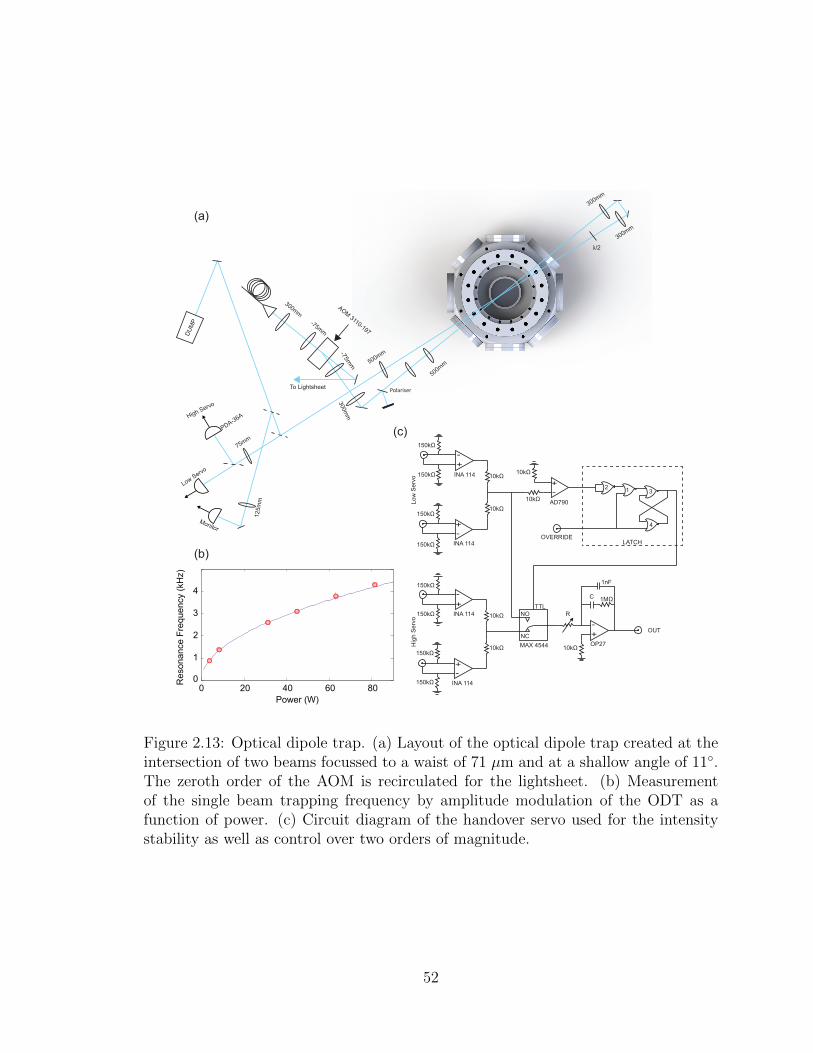
1M

10k

10k

150k

150k

150k

10k

10k

10k

10k

10k

150k

150k

150k

OUT

OP27

4

3

OVERRIDE

12

AD790

INA 114

INA 114

INA 114

INA 114

MAX 4544

+

-

+-

+

-

+-

+-

+

-

(c)

(b)

(a)

Resonance F

requen

cy (

kH

z)

Power (W)

0

1

2

3

4

0 20 40 60 80

Monitor

To Lightsheet

300m

m

300mm

-75mm

-75m

m

AOM

3110-197

125m

m

Hig

h S

erv

o

TTL

NC

NO

150k

150k

Low

Serv

o

Low Servo

High Servo

PDA-36A

75mm

500mm

Polariser

500mm

300mm

300mm

/2

DU

MP

1nF

C

R

LATCH

Figure 2.13: Optical dipole trap. (a) Layout of the optical dipole trap created at theintersection of two beams focussed to a waist of 71 µm and at a shallow angle of 11.The zeroth order of the AOM is recirculated for the lightsheet. (b) Measurementof the single beam trapping frequency by amplitude modulation of the ODT as afunction of power. (c) Circuit diagram of the handover servo used for the intensitystability as well as control over two orders of magnitude.

52

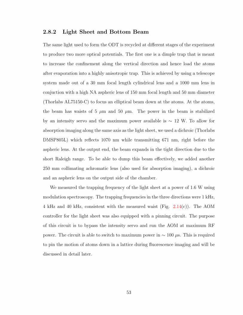
2.8.2 Light Sheet and Bottom Beam

The same light used to form the ODT is recycled at different stages of the experiment

to produce two more optical potentials. The first one is a dimple trap that is meant

to increase the confinement along the vertical direction and hence load the atoms

after evaporation into a highly anisotropic trap. This is achieved by using a telescope

system made out of a 30 mm focal length cylindrical lens and a 1000 mm lens in

conjuction with a high NA aspheric lens of 150 mm focal length and 50 mm diameter

(Thorlabs AL75150-C) to focus an elliptical beam down at the atoms. At the atoms,

the beam has waists of 5 µm and 50 µm. The power in the beam is stabilized

by an intensity servo and the maximum power available is ∼ 12 W. To allow for

absorption imaging along the same axis as the light sheet, we used a dichroic (Thorlabs

DMSP805L) which reflects 1070 nm while transmitting 671 nm, right before the

aspheric lens. At the output end, the beam expands in the tight direction due to the

short Raleigh range. To be able to dump this beam effectively, we added another

250 mm collimating achromatic lens (also used for absorption imaging), a dichroic

and an aspheric lens on the output side of the chamber.

We measured the trapping frequency of the light sheet at a power of 1.6 W using

modulation spectroscopy. The trapping frequencies in the three directions were 1 kHz,

4 kHz and 40 kHz, consistent with the measured waist (Fig. 2.14(c)). The AOM

controller for the light sheet was also equipped with a pinning circuit. The purpose

of this circuit is to bypass the intensity servo and run the AOM at maximum RF

power. The circuit is able to switch to maximum power in ∼ 100 µs. This is required

to pin the motion of atoms down in a lattice during fluorescence imaging and will be

discussed in detail later.

53

OD

Modulation Frequency (kHz)

0

0.2

0.4

0.6

0.8

0 2 4 6 8 10

(a)

Monitor

FROM ODT

AO

M 3

110-1

97

Servo

PDA-36A

75mm

500mm

/2

DU

MP

300mm-75mm

30mm cyl

AL75150-B

150mm asphere

1000mm

DMSP805L

dichroic

AOM 3110-197

32mm asphere

DUMP

250mm

dichroic

Monitor

Servo

PDA-36A

/2

300mm

Periscope mirror

(b)

(c)

BS 30R-70T

0

1

2

20 40 60 80 100 120

OD

Modulation Frequency (kHz)

(d)

Figure 2.14: Schematic of light sheet and bottom beam. (a) Light from the 0th orderof the ODT AOM is recirculated (brown) and split between two arms. The first one isused for the light sheet (blue) while the second one is used for the bottom beam (red).The highly anisotropic light sheet is created using a cylindrical lens telescope and ahigh NA aspheric lens. The use of dichroic mirrors allow us to perform absorptionimaging along the light sheet direction (pink). The bottom beam is coupled intoan optical fiber (green) to be sent below the main chamber. (b) The bottom beampath under the main chamber. (c) Light sheet trapping frequency measured usingmodulation spectroscopy for the two shallower of the three confinements. (d) Lightsheet trapping frequency along the tight axis measured separately.

54

The bottom beam is a single circular beam focussed down to 100 µm waist at the

atoms. It is also derived from the ODT light. Because of the highly anisotropic shape

of the light sheet, the atoms reside in a flat cigar shaped trap. In order to realize

more uniform 2D potentials, we need a uniform radial confinement that the bottom

beam can provide. The power of this beam is also stabilized with a servo and can

go up to 4 W, leading to a confinement up to ∼ 400 Hz in the radial direction. To

avoid retroreflection of this beam by the top viewport which is high reflection coated

at this wavelength, we send the beam up at a tilt such that the reflection does not

coincide with the position of the atoms.

55

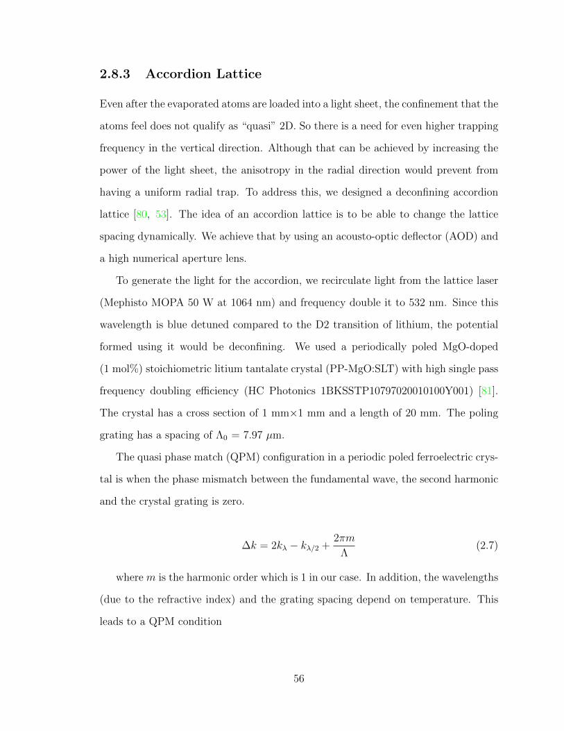
2.8.3 Accordion Lattice

Even after the evaporated atoms are loaded into a light sheet, the confinement that the

atoms feel does not qualify as “quasi” 2D. So there is a need for even higher trapping

frequency in the vertical direction. Although that can be achieved by increasing the

power of the light sheet, the anisotropy in the radial direction would prevent from

having a uniform radial trap. To address this, we designed a deconfining accordion

lattice [80, 53]. The idea of an accordion lattice is to be able to change the lattice

spacing dynamically. We achieve that by using an acousto-optic deflector (AOD) and

a high numerical aperture lens.

To generate the light for the accordion, we recirculate light from the lattice laser

(Mephisto MOPA 50 W at 1064 nm) and frequency double it to 532 nm. Since this

wavelength is blue detuned compared to the D2 transition of lithium, the potential

formed using it would be deconfining. We used a periodically poled MgO-doped

(1 mol%) stoichiometric litium tantalate crystal (PP-MgO:SLT) with high single pass

frequency doubling efficiency (HC Photonics 1BKSSTP10797020010100Y001) [81].

The crystal has a cross section of 1 mm×1 mm and a length of 20 mm. The poling

grating has a spacing of Λ0 = 7.97 µm.

The quasi phase match (QPM) configuration in a periodic poled ferroelectric crys-

tal is when the phase mismatch between the fundamental wave, the second harmonic

and the crystal grating is zero.

∆k = 2kλ − kλ/2 +2πm

Λ(2.7)

where m is the harmonic order which is 1 in our case. In addition, the wavelengths

(due to the refractive index) and the grating spacing depend on temperature. This

leads to a QPM condition

56

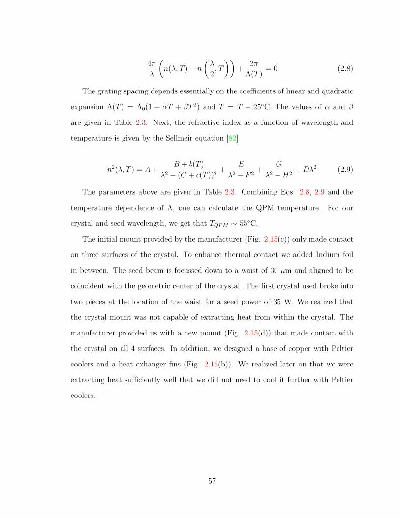
4π

λ

(n(λ, T )− n

(λ

2, T

))+

2π

Λ(T )= 0 (2.8)

The grating spacing depends essentially on the coefficients of linear and quadratic

expansion Λ(T ) = Λ0(1 + αT + βT 2) and T = T − 25C. The values of α and β

are given in Table 2.3. Next, the refractive index as a function of wavelength and

temperature is given by the Sellmeir equation [82]

n2(λ, T ) = A+B + b(T )

λ2 − (C + c(T ))2+

E

λ2 − F 2+

G

λ2 −H2+Dλ2 (2.9)

The parameters above are given in Table 2.3. Combining Eqs. 2.8, 2.9 and the

temperature dependence of Λ, one can calculate the QPM temperature. For our

crystal and seed wavelength, we get that TQPM ∼ 55C.

The initial mount provided by the manufacturer (Fig. 2.15(c)) only made contact

on three surfaces of the crystal. To enhance thermal contact we added Indium foil

in between. The seed beam is focussed down to a waist of 30 µm and aligned to be

coincident with the geometric center of the crystal. The first crystal used broke into

two pieces at the location of the waist for a seed power of 35 W. We realized that

the crystal mount was not capable of extracting heat from within the crystal. The

manufacturer provided us with a new mount (Fig. 2.15(d)) that made contact with

the crystal on all 4 surfaces. In addition, we designed a base of copper with Peltier

coolers and a heat exhanger fins (Fig. 2.15(b)). We realized later on that we were

extracting heat sufficiently well that we did not need to cool it further with Peltier

coolers.

57

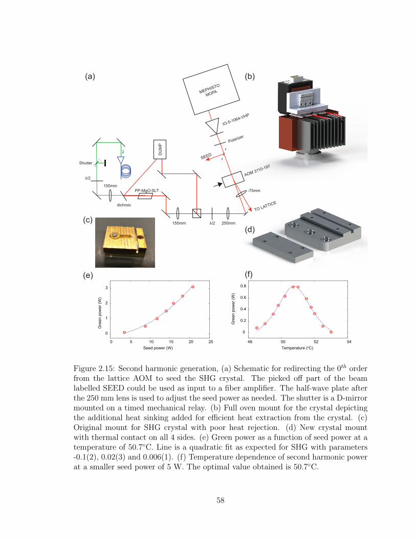
AOM 3110-197

-75mm

λ/2150mm 250mm

100mm

DU

MP

IO-5-1064-VHP

SEED

dichroic

λ/2

Shutter

PP-MgO:SLT

MEPHISTO

MOPA

TO LATTICE

Gre

en p

ower

(W)

Temperature (oC)

0

0.2

0.4

0.6

0.8

48 50 52 54

Gre

en p

ower

(W)

Seed power (W)

0

1

2

3

0 5 10 15 20 25

(a) (b)

(c)(d)

(e) (f)

Polarizer

Figure 2.15: Second harmonic generation, (a) Schematic for redirecting the 0th orderfrom the lattice AOM to seed the SHG crystal. The picked off part of the beamlabelled SEED could be used as input to a fiber amplifier. The half-wave plate afterthe 250 mm lens is used to adjust the seed power as needed. The shutter is a D-mirrormounted on a timed mechanical relay. (b) Full oven mount for the crystal depictingthe additional heat sinking added for efficient heat extraction from the crystal. (c)Original mount for SHG crystal with poor heat rejection. (d) New crystal mountwith thermal contact on all 4 sides. (e) Green power as a function of seed power at atemperature of 50.7C. Line is a quadratic fit as expected for SHG with parameters-0.1(2), 0.02(3) and 0.006(1). (f) Temperature dependence of second harmonic powerat a smaller seed power of 5 W. The optimal value obtained is 50.7C.

58

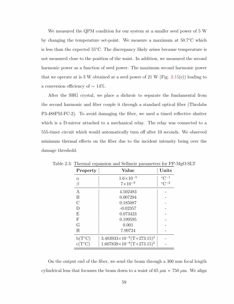
We measured the QPM condition for our system at a smaller seed power of 5 W

by changing the temperature set-point. We measure a maximum at 50.7C which

is less than the expected 55C. The discrepancy likely arises because temperature is

not measured close to the position of the waist. In addition, we measured the second

harmonic power as a function of seed power. The maximum second harmonic power

that we operate at is 3 W obtained at a seed power of 21 W (Fig. 2.15(e)) leading to

a conversion efficiency of ∼ 14%.

After the SHG crystal, we place a dichroic to separate the fundamental from

the second harmonic and fiber couple it through a standard optical fiber (Throlabs

P3-488PM-FC-2). To avoid damaging the fiber, we used a timed reflective shutter

which is a D-mirror attached to a mechanical relay. The relay was connected to a

555-timer circuit which would automatically turn off after 10 seconds. We observed

minimum thermal effects on the fiber due to the incident intensity being over the

damage threshold.

Table 2.3: Thermal expansion and Sellmeir parameters for PP-MgO:SLT

Property Value Units

α 1.6×10−5 C−1

β 7×10−9 C−2

A 4.502483 -B 0.007294 -C 0.185087 -D -0.02357 -E 0.073423 -F 0.199595 -G 0.001 -H 7.99724 -

b(TC) 3.483933×10−8(T+273.15)2 -c(TC) 1.607839×10−8(T+273.15)2 -

On the output end of the fiber, we send the beam through a 300 mm focal length

cylindrical lens that focusses the beam down to a waist of 65 µm × 750 µm. We align

59

the position of this focus to coincide with the center of an acousto-optic deflector

(Intraaction ATD-805AD5). The AOD is positioned in such a way that the plane

of beam diffraction is vertical. We block the zeroth order beam and make a factor

of 4 demagnifying imaging system to the position of the atoms. Along the way, the

beam is split evenly into two beams by using a polarizing beam splitter cube along

with a quarter wave plate. We designed a monolithic structure (the tower) to hold

this mechanism in place (Fig. 2.16(c)). Finally the two beams are focused on to the

position of the atoms using a high NA aspherical lens.

The working principle of the accordion lattice is the following (Fig. 2.16(b)).

When the RF drive frequency on the AOD is changed within a range of 99.8 MHz

to 88.3 MHz, the diffracted first order only changes angle in the vertical plane with

minimal change in intensity. This angular variation is converted into a variation in

beam height in the Fourier plane of the 600 mm lens. This beam height variation, in

turn, is converted to a vertical separation between two beams after the tower. These

two beams then fall parallel on the asphere and are focused down and interfere at the

position of the atoms. The result of this interference are 2D pancakes in the vertical

direction with variable separation. This separation can be varied from 12 µm down

to 3.5 µm.

The advantage of variable spacing is that we can load a cigar shaped cloud into a

single layer of the 2D pancakes at maximum separation and then compress the pancake

adiabatically to reach a more “2D” regime. We measured the vertical confinement in

the case of minimum spacing using modulation spectroscopy and get 21-23 kHz (Fig.

2.16(d)). The radial deconfinement in the central layer produced by this accordion

lattice has an effect on the confinement due to the bottom beam. We can measure this

combined radial trapping frequency through modulation spectroscopy for a setting

we use for the experiments described later in the thesis. We measure ωx = (2π)95Hz

and ωy = (2π)125Hz (Fig. 2.16(e)).

60

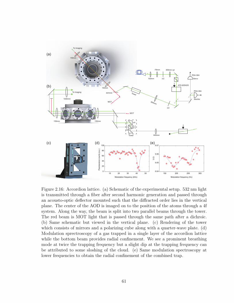
/2100mm

300mm cyl-75mm

/2

ATD-805AD5

Monitor

Servo

PDA-36A

600mm

Tower

150mm

150mm

/4

/2

600mm

150mm150mm

1000mm

Tower

To Imaging

To ImagingPDA-36A

MOT

Flu

ore

scence c

ounts

(a.u

.)

Modulation frequency (kHz)

0

20

40

60

80

100

10 20 30 40 50

O.D

.

Modulation frequency (Hz)

0.04

0.05

0.06

0.07

150 200 250 300

(a)

(d)

(b)

(c) (e)

dichroic

MOT

Figure 2.16: Accordion lattice. (a) Schematic of the experimental setup. 532 nm lightis transmitted through a fiber after second harmonic generation and passed throughan acousto-optic deflector mounted such that the diffracted order lies in the verticalplane. The center of the AOD is imaged on to the position of the atoms through a 4fsystem. Along the way, the beam is split into two parallel beams through the tower.The red beam is MOT light that is passed through the same path after a dichroic.(b) Same schematic but viewed in the vertical plane. (c) Rendering of the towerwhich consists of mirrors and a polarizing cube along with a quarter-wave plate. (d)Modulation sprectroscopy of a gas trapped in a single layer of the accordion latticewhile the bottom beam provides radial confinement. We see a prominent breathingmode at twice the trapping frequency but a slight dip at the trapping frequency canbe attributed to some sloshing of the cloud. (e) Same modulation spectroscopy atlower frequencies to obtain the radial confinement of the combined trap.

61

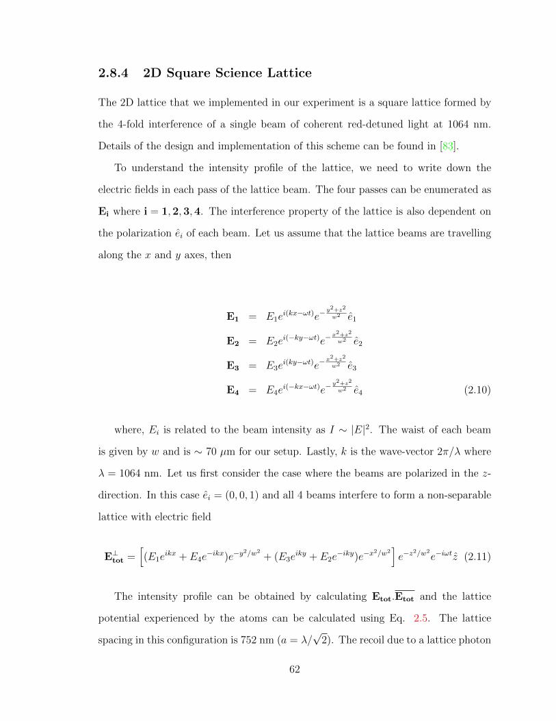
2.8.4 2D Square Science Lattice

The 2D lattice that we implemented in our experiment is a square lattice formed by

the 4-fold interference of a single beam of coherent red-detuned light at 1064 nm.

Details of the design and implementation of this scheme can be found in [83].

To understand the intensity profile of the lattice, we need to write down the

electric fields in each pass of the lattice beam. The four passes can be enumerated as

Ei where i = 1,2,3,4. The interference property of the lattice is also dependent on

the polarization ei of each beam. Let us assume that the lattice beams are travelling

along the x and y axes, then

E1 = E1ei(kx−ωt)e−

y2+z2

w2 e1

E2 = E2ei(−ky−ωt)e−

x2+z2

w2 e2

E3 = E3ei(ky−ωt)e−

x2+z2

w2 e3

E4 = E4ei(−kx−ωt)e−

y2+z2

w2 e4 (2.10)

where, Ei is related to the beam intensity as I ∼ |E|2. The waist of each beam

is given by w and is ∼ 70 µm for our setup. Lastly, k is the wave-vector 2π/λ where

λ = 1064 nm. Let us first consider the case where the beams are polarized in the z-

direction. In this case ei = (0, 0, 1) and all 4 beams interfere to form a non-separable

lattice with electric field

E⊥tot =[(E1e

ikx + E4e−ikx)e−y

2/w2

+ (E3eiky + E2e

−iky)e−x2/w2

]e−z

2/w2

e−iωtz (2.11)

The intensity profile can be obtained by calculating Etot.Etot and the lattice

potential experienced by the atoms can be calculated using Eq. 2.5. The lattice

spacing in this configuration is 752 nm (a = λ/√

2). The recoil due to a lattice photon

62

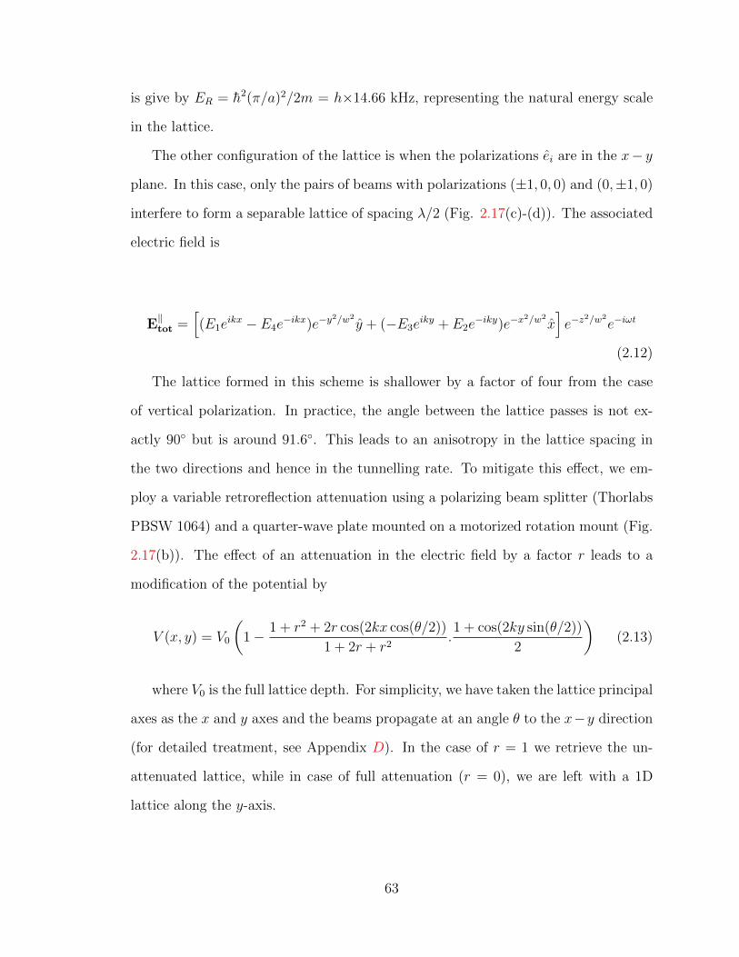
is give by ER = h2(π/a)2/2m = h×14.66 kHz, representing the natural energy scale

in the lattice.

The other configuration of the lattice is when the polarizations ei are in the x− y

plane. In this case, only the pairs of beams with polarizations (±1, 0, 0) and (0,±1, 0)

interfere to form a separable lattice of spacing λ/2 (Fig. 2.17(c)-(d)). The associated

electric field is

E‖tot =

[(E1e

ikx − E4e−ikx)e−y

2/w2

y + (−E3eiky + E2e

−iky)e−x2/w2

x]e−z

2/w2

e−iωt

(2.12)

The lattice formed in this scheme is shallower by a factor of four from the case

of vertical polarization. In practice, the angle between the lattice passes is not ex-

actly 90 but is around 91.6. This leads to an anisotropy in the lattice spacing in

the two directions and hence in the tunnelling rate. To mitigate this effect, we em-

ploy a variable retroreflection attenuation using a polarizing beam splitter (Thorlabs

PBSW 1064) and a quarter-wave plate mounted on a motorized rotation mount (Fig.

2.17(b)). The effect of an attenuation in the electric field by a factor r leads to a

modification of the potential by

V (x, y) = V0

(1− 1 + r2 + 2r cos(2kx cos(θ/2))

1 + 2r + r2.1 + cos(2ky sin(θ/2))

2

)(2.13)

where V0 is the full lattice depth. For simplicity, we have taken the lattice principal

axes as the x and y axes and the beams propagate at an angle θ to the x−y direction

(for detailed treatment, see Appendix D). In the case of r = 1 we retrieve the un-

attenuated lattice, while in case of full attenuation (r = 0), we are left with a 1D

lattice along the y-axis.

63

AOM 3110-197

/4

rotatable

IO-5-1064-VHP

SEED

MEPHISTO

MOPA

TO SHGM

onito

r

ServoPDA-36A

PDA-3

6A

TS2B1T0

300mm

-75mm 200mm

250mm

300mm

175mm

300mm

300mm

500mm

Polarizer

dichroic

DU

MP

Mon

itor

PDA-3

6

(a)

(d)

(b)

(c)

PBSW 1064

Figure 2.17: Science lattice. (a) Schematic of the lattice setup. Light from a 42 WMOPA at 1064 nm undergoes 4-fold interference with a polarization pointing outof plane. The attenuation of the reto-reflection is performed to adjust for a slightasymmetry along the two lattice directions. (b) The rotation mount that houses aquarter-wave plate used to tune the attenuation factor r. (c) Lattice potential contourplot for vertical beam polarization with maximum depth V0 and spacing 752 nm. (d)Lattice potential contour plot for horizontal beam polarization leading to a maximumdepth of V0/4 and spacing 532 nm.

64

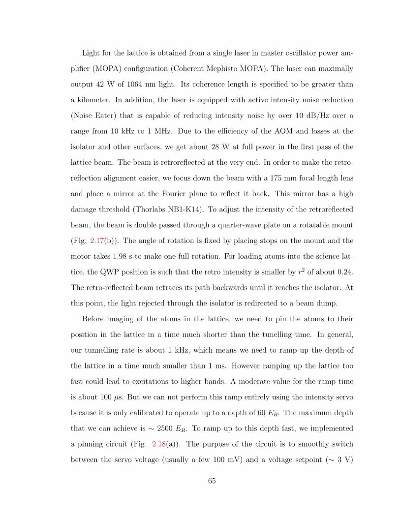
Light for the lattice is obtained from a single laser in master oscillator power am-

plifier (MOPA) configuration (Coherent Mephisto MOPA). The laser can maximally

output 42 W of 1064 nm light. Its coherence length is specified to be greater than

a kilometer. In addition, the laser is equipped with active intensity noise reduction

(Noise Eater) that is capable of reducing intensity noise by over 10 dB/Hz over a

range from 10 kHz to 1 MHz. Due to the efficiency of the AOM and losses at the

isolator and other surfaces, we get about 28 W at full power in the first pass of the

lattice beam. The beam is retroreflected at the very end. In order to make the retro-

reflection alignment easier, we focus down the beam with a 175 mm focal length lens

and place a mirror at the Fourier plane to reflect it back. This mirror has a high

damage threshold (Thorlabs NB1-K14). To adjust the intensity of the retroreflected

beam, the beam is double passed through a quarter-wave plate on a rotatable mount

(Fig. 2.17(b)). The angle of rotation is fixed by placing stops on the mount and the

motor takes 1.98 s to make one full rotation. For loading atoms into the science lat-

tice, the QWP position is such that the retro intensity is smaller by r2 of about 0.24.

The retro-reflected beam retraces its path backwards until it reaches the isolator. At

this point, the light rejected through the isolator is redirected to a beam dump.

Before imaging of the atoms in the lattice, we need to pin the atoms to their

position in the lattice in a time much shorter than the tunelling time. In general,

our tunnelling rate is about 1 kHz, which means we need to ramp up the depth of

the lattice in a time much smaller than 1 ms. However ramping up the lattice too

fast could lead to excitations to higher bands. A moderate value for the ramp time

is about 100 µs. But we can not perform this ramp entirely using the intensity servo

because it is only calibrated to operate up to a depth of 60 ER. The maximum depth

that we can achieve is ∼ 2500 ER. To ramp up to this depth fast, we implemented

a pinning circuit (Fig. 2.18(a)). The purpose of the circuit is to smoothly switch

between the servo voltage (usually a few 100 mV) and a voltage setpoint (∼ 3 V)

65

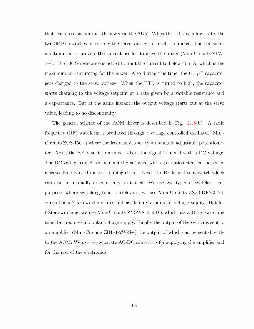
that leads to a saturation RF power on the AOM. When the TTL is in low state, the

two SPDT switches allow only the servo voltage to reach the mixer. The transistor

is introduced to provide the current needed to drive the mixer (Mini-Circuits ZLW-

3+). The 330 Ω resistance is added to limit the current to below 40 mA, which is the

maximum current rating for the mixer. Also during this time, the 0.1 µF capacitor

gets charged to the servo voltage. When the TTL is turned to high, the capacitor

starts charging to the voltage setpoint at a rate given by a variable resistance and

a capacitance. But at the same instant, the output voltage starts out at the servo

value, leading to no discontinuity.

The general scheme of the AOM driver is described in Fig. 2.18(b). A radio

frequency (RF) waveform is produced through a voltage controlled oscillator (Mini-

Circuits ZOS-150+) where the frequency is set by a manually adjustable potentiome-

ter. Next, the RF is sent to a mixer where the signal is mixed with a DC voltage.

The DC voltage can either be manually adjusted with a potentiometer, can be set by

a servo directly or through a pinning circuit. Next, the RF is sent to a switch which

can also be manually or externally controlled. We use two types of switches. For

purposes where switching time is irrelevant, we use Mini-Circuits ZX80-DR230-S+

which has a 2 µs switching time but needs only a unipolar voltage supply. But for

faster switching, we use Mini-Circuits ZYSWA-2-50DR which has a 10 ns switching

time, but requires a bipolar voltage supply. Finally the output of the switch is sent to

an amplifier (Mini-Circuits ZHL-1-2W-S+) the output of which can be sent directly

to the AOM. We use two separate AC-DC converters for supplying the amplifier and

for the rest of the electronics.

66

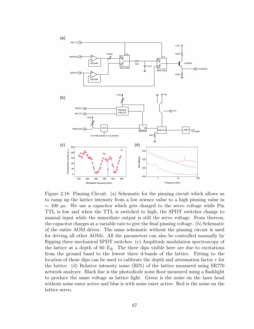
Fluo

resc

ence

cou

nts

(a.u

.)

Modulation frequency (kHz)

0

40

80

120

160

200

320 340 360 380 400 420

+-

MAX 4544

TTL

NC

NO

+-

10Ω

MAX 4544

TTL

NC

NO

470Ω

330Ω

0.1µF

+12V

100kΩ

LM324N

LM324N

PIN TTL

MANUAL

SERVO

TO MIXER

+16V

+10V

L RI

VCO

PINNINGCIRCUIT

SWITCH AMPTO AOM

TO FREQUENCY COUNTER

SERVO

PIN TTL

FREQ SET

TTL

+5V

MIXER

(a)

(c)

(b)

LM385Z

(d)R

IN (d

B/H

z)

Frequency (kHz)

-160

-140

-120

-100

1 10 100

50Ω

Figure 2.18: Pinning Circuit. (a) Schematic for the pinning circuit which allows usto ramp up the lattice intensity from a low science value to a high pinning value in∼ 100 µs. We use a capacitor which gets charged to the servo voltage while PinTTL is low and when the TTL is switched to high, the SPDT switches change tomanual input while the immediate output is still the servo voltage. From thereon,the capacitor charges at a variable rate to give the final pinning voltage. (b) Schematicof the entire AOM driver. The same schematic without the pinning circuit is usedfor driving all other AOMs. All the parameters can also be controlled manually byflipping three mechanical SPDT switches. (c) Amplitude modulation spectroscopy ofthe lattice at a depth of 60 ER. The three dips visible here are due to excitationsfrom the ground band to the lowest three d-bands of the lattice. Fitting to thelocation of these dips can be used to calibrate the depth and attenuation factor r forthe lattice. (d) Relative intensity noise (RIN) of the lattice measured using SR770network analyzer. Black line is the photodiode noise floor measured using a flashlightto produce the same voltage as lattice light. Green is the noise on the laser headwithout noise eater active and blue is with noise eater active. Red is the noise on thelattice servo.

67

To calibrate the depth of the lattice, we perform amplitude modulation spec-

troscopy. We modulate the lattice intensity with an external waveform generator and

observe losses while imaging fluorescence. A relatively high lattice depth (around

60 ER) is used for this spectroscopy to ensure that we can work in a tight-binding

regime. We scan a range of frequency where we see three dips associated with atoms

getting excited from the ground band to the three d-bands of the lattice. Excitation

to the lower lying p-bands is prohibited due to parity. Once atoms get excited to

the higher bands, they are either lost from the system or they do not participate in

Raman sideband cooling leading to a reduction in fluorescence counts (Fig. 2.18(c)).

To obtain a lattice depth from spectroscopy, we calculate the band structure for our

lattice with the depth V0/ER and the attenuation factor r as free parameters. The

band structure is obtained numerically using a plane wave expansion for a reasonable

number of reciprocal lattice vectors. We fit the position of the three dips and extract

the depth and r. Subsequently, we estimate the tunnelling rate of our lattice at the

science depth (usually between 5-10 ER) by calculating the bandwidth of the ground

band for a depth estimated from the ratio of light intensities. The tunnelling rate is

given as W/(4d), where W is the bandwidth and d is the dimensionality of the system

[84, 85, 86] and can be calculated for the two directions by taking cuts along them.

In addition, we can estimate the on-site interaction U that two atoms of oppo-

site spins would experience in the absence of tunnelling. This interaction is s-wave

in nature and occurs due to the proximity to a Feshbach resonance. In the tight

binding model, we assume that the Wannier functions of the fermions in the lattice

are sufficiently localized. We calculate the real space Wannier function of the lattice

from the Bloch wavefunctions or by using the projection method [87], [88]. Once the

Wannier functions w(x, y) are known, then the on-site interaction can be calculated

(see Appendix D.2).

68

Chapter 3

Pathway to a Quantum Gas

Microscope

3.1 Magneto-optical trap

There are 3 characteristic temperature scales associated with the cooling of neutral

atoms:

1. The first temperature scale is defined by choosing the atomic speed to be large

enough such that the Doppler shift in the atomic reference frame matches the

atom’s linewidth. The velocity in that limit would be ∼ Γ/k ∼ 1 m/s, where Γ

is the natural linewidth of the absorption line and k is the photon wave-vector.

The lowest achievable temperature of the order of several mK in this regime is

given by :

kBTc = mΓ2/k2 (3.1)

2. The next scale corresponds to the actual linewidth of the atomic transition, Γ.

This temperature is called the Doppler limit and is ∼ 140 µK for the D2 line of

69

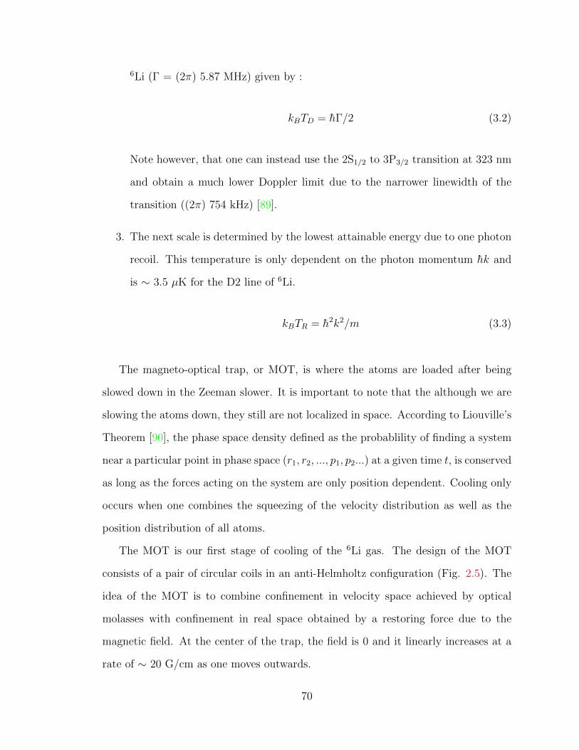
6Li (Γ = (2π) 5.87 MHz) given by :

kBTD = hΓ/2 (3.2)

Note however, that one can instead use the 2S1/2 to 3P3/2 transition at 323 nm

and obtain a much lower Doppler limit due to the narrower linewidth of the

transition ((2π) 754 kHz) [89].

3. The next scale is determined by the lowest attainable energy due to one photon

recoil. This temperature is only dependent on the photon momentum hk and

is ∼ 3.5 µK for the D2 line of 6Li.

kBTR = h2k2/m (3.3)

The magneto-optical trap, or MOT, is where the atoms are loaded after being

slowed down in the Zeeman slower. It is important to note that the although we are

slowing the atoms down, they still are not localized in space. According to Liouville’s

Theorem [90], the phase space density defined as the probablility of finding a system

near a particular point in phase space (r1, r2, ..., p1, p2...) at a given time t, is conserved

as long as the forces acting on the system are only position dependent. Cooling only

occurs when one combines the squeezing of the velocity distribution as well as the

position distribution of all atoms.

The MOT is our first stage of cooling of the 6Li gas. The design of the MOT

consists of a pair of circular coils in an anti-Helmholtz configuration (Fig. 2.5). The

idea of the MOT is to combine confinement in velocity space achieved by optical

molasses with confinement in real space obtained by a restoring force due to the

magnetic field. At the center of the trap, the field is 0 and it linearly increases at a

rate of ∼ 20 G/cm as one moves outwards.

70

Figure 3.1: Properties of the magneto-optic trap. Schematic of operation of a MOTtaken from [90]. An atom experiences a state specific Zeeman shift as it moves awayfrom the center. In turn the atom only absorbs photons that are counter-propagating,providing a restoring force back towards the center. (b) A picture of the MOT in oursetup and can be seen as a red dot near the center of the chamber. (c) Typical MOTloading rate in our system. We usually load the MOT for 5 seconds which leads to∼ 400 million atoms trapped at about 1.5 mK. (d) Plot of the detuning dependence ofthe atom number (red triangles) and the temperature (purple circles) after a stage ofcompression. During this cMOT stage, we ramp the intensity of cooling and repumplight down to 1 % in 5 ms and simultaneously decrease the detuning (δ) from -5.4 Γ to-0.7 Γ. Notice that we successfully cool the atoms down at a cost of number of atoms.The final operating point is chosen by maximum loading into the optical dipole trap.

71

Three retroreflected laser beams are used for cooling and trapping the atoms.

Each beam consists of cooling light, red detuned by -5.4 Γ from resonance and a

small fraction of repump light, usually 1/5th in intensity of the cooling beam. The

total beam intensity is usually set around 5Isat (The saturation intensity of the D2

line of 6Li is 2.54 mW/cm2) The incoming beam is circularly polarized and has the

opposite handedness to the retro-reflected beam.

In order to understand the trapping mechanism of a MOT, consider a 1D configu-

ration (Fig. 3.1(a)) for an atom with a simple level structure where the ground state

has 0 magnetic quantum number (Jg = 0 so Mg = 0) and the excited state has Je

= 1 and Me = 0, ±1. Consider z = 0 as the center of the trap. Due to the linearly

changing magnetic field, the states with a non-zero magnetic moment get Zeeman

shifted. Now as an atom moves outwards from the center in the positive z direction,

it finds itself closer to resonance with the Me = -1 state and hence absorbs a photon

from the σ− beam since ∆M = -1. Since this photon is counter-propagating, it kicks

the atom back towards the center of the trap, hence confining it. In a similar fashion,

an atom wandering out in the negative z direction, would absorb a σ+ photon which

in turn would kick it back towards the center of the trap.

To cool the atoms, the light beams must also provide a viscous force on the atoms.

The spontaneous force experienced by an atom due to the absorption of a photon is

simply h~kγp, where γp is the scattering rate of the atoms in steady state. The net

force due to the two counter-propagating photons is given by:

∆~F =8hk2δs0~v

Γ(1 + s0 + (2δ/Γ)2)2= −β~v (3.4)

Where δ is the detuning and s0 is the saturation parameter (s0 = I/Isat). Notice

that for red detuning (δ < 0), this force is like a viscous force that opposes the motion

of the atom; hence the name optical molasses. Combined with the spatial confinement

72

provided by the magnetic field and the laser beams, one achieves a reduction in phase

space density.

After about 5 seconds of loading into the MOT at a detuning of -5.4 Γ, we obtain

∼ 400 million atoms in the trap center at about 1.5 mK. The temperature of a cloud

is measured from time-of-flight (TOF). We let the cloud expand for increasing time

and image the atomic distribution in absorption. Then we fit the cloud profiles to

2D Gaussians. The cloud shape could be non-symmetric in trap but after sufficiently

long times of flight when the atoms have travelled a large distance compared to the

initial cloud size, it tends to be more symmetric. From the radius σ obtained from

the Gaussian fit, we can perform a temperature fit knowing

σ2(t) = σ2(0) +kBT

mt2 (3.5)

In order to further reduce the phase space density, we perform what is known

as a compressed MOT or a cMOT. After the MOT loading stage is complete, the

Zeeman slower fields are turned off along with the corresponding laser beam. Almost

simultaneously, we decrease the detuning of the MOT beams and bring them closer

to resonance at -0.7 Γ in 2 ms. At the same time, we also reduce the intensities of

the cooling and repumper laser beams to 1 % of their maximum values. This process

leads to an increase in the phase space density at the cost of losing a fraction of the

atoms and we end up with ∼ 100 million atoms at a temperature of ∼ 400 µK (Fig.

3.1(c)-(d)).

73

3.2 Evaporation

After the initial preparation in a cMOT, atoms are transfered into the crossed dipole

trap in 5 ms. The depth of the initial trap is 1.7 mK. We load about 300,000 atoms in

the ODT and we measure the temperature to be ∼ 400 µK, similar to the temperature

in the cMOT. Atoms are in a mixture of the two lowest ground hyperfine states. Since

we want the atoms to be in a mixture of states |1〉 and |2〉, we apply a short 100 µs

pulse of cooling light to transfer the leftover atoms in state 2S1/2 F=3/2 to F=1/2.

But even then, we don’t have an equal mixture in the two states. In order to achieve

that we rely on a combination of RF pulses with decohering processes to obtain an

equal spin mixture, as is described in more detail in the next section.

3.2.1 Radio frequency sweeps

The first step of this process is to ramp up the magnetic field to reach the Paschen

Back limit where the Zeeman shift of the energy levels becomes linear with field. We

ramp the Feshbach field to 528 G. At this field, the energy difference between |1〉

and |2〉 is (2π) 75.61 MHz. To drive coherent oscillations between the two hyperfine

sublevels, we designed resonant RF antennas. The antennas themselves are flexible

insulated copper wire made into the shape of a kidney bean ∼ 10 mm across (Fig.

3.2(a)) and are placed as close to the bottom reentrant viewport as possible without

significantly clipping the MOT beam. The two coils were designed to be resonant

over a field range of 300-1000 G to the transitions between |1〉− |2〉 (74-77 MHz) and

|2〉 − |3〉 (91-81 MHz) resonances. The circuit diagram for the resonant antennas is

given in Fig. 3.2(b) and is composed of a matching capacitance (CM) and a tuning

capacitance (CT ). We chose CM = 10 pF (surface mount) and CT = 100 pF (mica)

and tuned the resonance frequency by adjusting the shape of the coil. Both coils

are driven by a single 100 W RF amplifier (Minicircuits ZHL-100W-52-S+) since

74

Pic

k-u

p c

oil

voltage (

V)

Frequency (MHz)

0

0.5

1

1.5

2

70 75 80 85 90

CT

CM

ZX80

DR230

ZX80

DR230

ZX80

DR230 PE71S

6053

RF2B

RF2A

RF1B

RF1A

TTL1A

TTL1B

TTL2A

TTL2B

1 I/O

2 I/O

555

TIMER

555

TIMER

ZHL

100W

52-S+

TTL

TO 1-2 ANTENNA

TO 2-3 ANTENNA

(b)

(c)(a)

(d)

Figure 3.2: RF antennas. (a) Image of the resonant antenna. (b) Schematic of thesame antenna. The matching capacitance CM is 10 pF while the tuning capacitanceCT is 100 pF. (c) Schematic of the circuit that is used for driving the two antennas.Four separate RF generators are connected at the input of a multiplexer and a com-bination of 7 TTL signals are used to send the amplified RF signal to the antenna.The amplifier is rated up to 100 W and the switch after the amplifier up to 240 W.The timer circuits ensure high power is never on for more than 110 ms. (d) Voltageon a pick-up coil as a function of RF frequency. Red is |1〉 − |2〉 antenna resonantaround 76 MHz and blue is |2〉 − |3〉 antenna resonant around 85 MHz.

they never operate at the same time. But to ensure that we could quickly switch

between the two antennas, we added a high power SPDT RF switch (Pasternack

PE71S6053, 0-18 GHz, 240 W and 10 ms switch time). The circuit diagram of the

RF path is shown in Fig. 3.2(c). Since the amplifier running continuously at 100 W

could damage the antennas, we added a timer circuit based on LM555 that would

automatically switch the RF off after 110 ms.

We measured the response of the antennas at their final positions by measuring

the pick-up of RF through a general broadband antenna placed in proximity to both

75

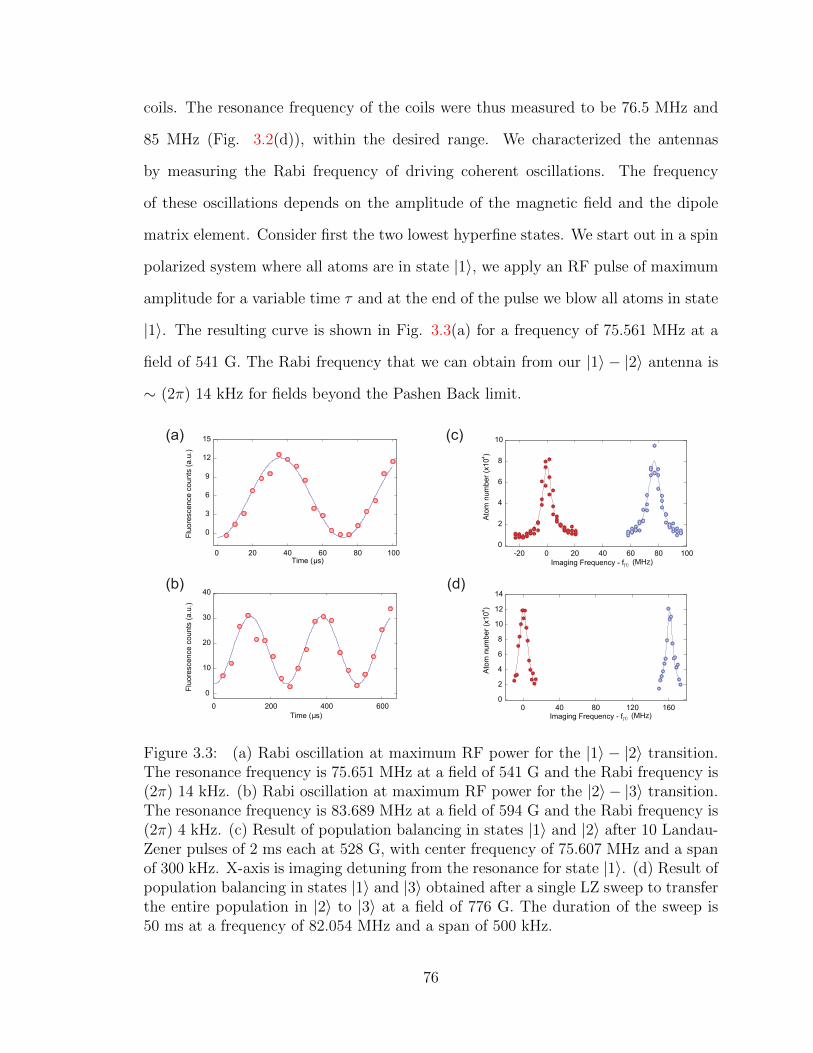
coils. The resonance frequency of the coils were thus measured to be 76.5 MHz and

85 MHz (Fig. 3.2(d)), within the desired range. We characterized the antennas

by measuring the Rabi frequency of driving coherent oscillations. The frequency

of these oscillations depends on the amplitude of the magnetic field and the dipole

matrix element. Consider first the two lowest hyperfine states. We start out in a spin

polarized system where all atoms are in state |1〉, we apply an RF pulse of maximum

amplitude for a variable time τ and at the end of the pulse we blow all atoms in state

|1〉. The resulting curve is shown in Fig. 3.3(a) for a frequency of 75.561 MHz at a

field of 541 G. The Rabi frequency that we can obtain from our |1〉 − |2〉 antenna is

∼ (2π) 14 kHz for fields beyond the Pashen Back limit.

Fluo

resc

ence

cou

nts

(a.u

.)

Time (µs)

0

3

6

9

12

15

0 20 40 60 80 100

Fluo

resc

ence

cou

nts

(a.u

.)

0

10

20

30

40

0 200 400 600

Ato

m n

umbe

r (x1

04 )

Imaging Frequency - f|1 (MHz)

0

2

4

6

8

10

-20 0 20 40 60 80 100

0

2

4

6

8

10

12

14

0 40 80 120 160Time (µs)

Ato

m n

umbe

r (x1

04 )

Imaging Frequency - f|1 (MHz)

(a)

(b)

(c)

(d)

Figure 3.3: (a) Rabi oscillation at maximum RF power for the |1〉 − |2〉 transition.The resonance frequency is 75.651 MHz at a field of 541 G and the Rabi frequency is(2π) 14 kHz. (b) Rabi oscillation at maximum RF power for the |2〉 − |3〉 transition.The resonance frequency is 83.689 MHz at a field of 594 G and the Rabi frequency is(2π) 4 kHz. (c) Result of population balancing in states |1〉 and |2〉 after 10 Landau-Zener pulses of 2 ms each at 528 G, with center frequency of 75.607 MHz and a spanof 300 kHz. X-axis is imaging detuning from the resonance for state |1〉. (d) Result ofpopulation balancing in states |1〉 and |3〉 obtained after a single LZ sweep to transferthe entire population in |2〉 to |3〉 at a field of 776 G. The duration of the sweep is50 ms at a frequency of 82.054 MHz and a span of 500 kHz.

76

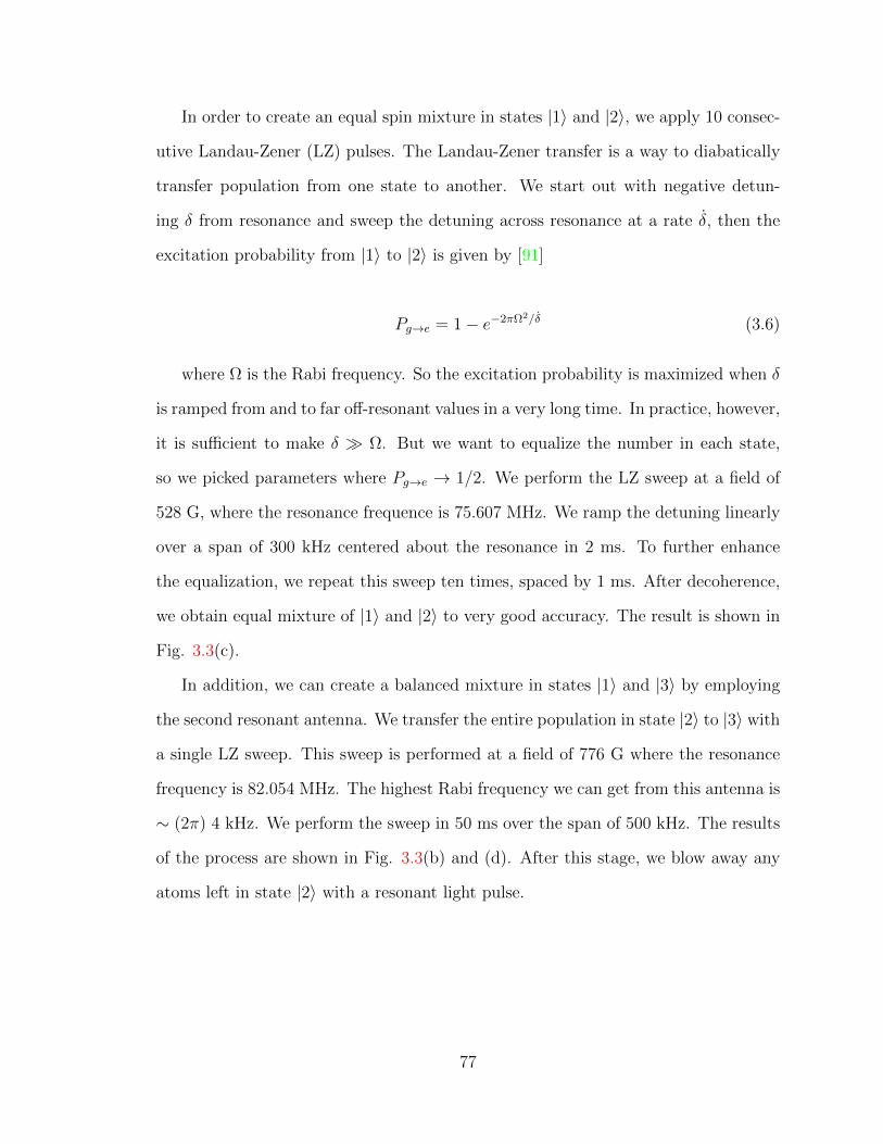
In order to create an equal spin mixture in states |1〉 and |2〉, we apply 10 consec-

utive Landau-Zener (LZ) pulses. The Landau-Zener transfer is a way to diabatically

transfer population from one state to another. We start out with negative detun-

ing δ from resonance and sweep the detuning across resonance at a rate δ, then the

excitation probability from |1〉 to |2〉 is given by [91]

Pg→e = 1− e−2πΩ2/δ (3.6)

where Ω is the Rabi frequency. So the excitation probability is maximized when δ

is ramped from and to far off-resonant values in a very long time. In practice, however,

it is sufficient to make δ Ω. But we want to equalize the number in each state,

so we picked parameters where Pg→e → 1/2. We perform the LZ sweep at a field of

528 G, where the resonance frequence is 75.607 MHz. We ramp the detuning linearly

over a span of 300 kHz centered about the resonance in 2 ms. To further enhance

the equalization, we repeat this sweep ten times, spaced by 1 ms. After decoherence,

we obtain equal mixture of |1〉 and |2〉 to very good accuracy. The result is shown in

Fig. 3.3(c).

In addition, we can create a balanced mixture in states |1〉 and |3〉 by employing

the second resonant antenna. We transfer the entire population in state |2〉 to |3〉 with

a single LZ sweep. This sweep is performed at a field of 776 G where the resonance

frequency is 82.054 MHz. The highest Rabi frequency we can get from this antenna is

∼ (2π) 4 kHz. We perform the sweep in 50 ms over the span of 500 kHz. The results

of the process are shown in Fig. 3.3(b) and (d). After this stage, we blow away any

atoms left in state |2〉 with a resonant light pulse.

77

3.2.2 Molecular Bose-Einstein condensates

At the start of evaporation, we have a phase space density of atoms in the trap of

about 10−5. The phase space density ρ is calculated from the optical depth, cloud

size in trap and the temperature of the atoms. We fit cloud images to a 2D Gaussian

(∼ e−(x−x0)2/2S2x−(y−y0)2/2S2

y). If the fit gives a peak optical depth (OD) and Gaussian

sigma of Sx and Sy, then the volume density n is given by

n =OD

σ(√

2πS2y)

(3.7)

where we have assumed that the cloud is cylindrically symmetric, i.e. it is cigar

shaped with Sx measuring the long axis and Sy measuring the short axis. σ is the

resonant cross section given by 3λ2/2π. The thermal deBroglie wavelength of the

cloud is defined as

λdB =

√h2

2πmkBT(3.8)

Finally, the phase space density ρ is defined as ρ = nλ3dB. It is a useful measure

of the degree of degeneracy of an atomic cloud. For example, in order for a gas of

non-interacting bosons to condense, the interparticle spacing must be of the order of

the thermal deBroglie wavelength (ρ ≥ 2.6). To increase our phase space density,

we perform a phase of evaporative cooling of the atoms trapped in the ODT. The

idea of evaporative cooling is to allow the highest energy atoms to escape from the

trap upon which the remaining atoms rethermalize to a Boltzmann distribution at

a lower temperature. This process is carried out at a variable rate until the leftover

atoms have a sufficiently large ρ. Naturally, in order for the atoms to thermalize,

they must be interacting. To achieve this interaction, we perform the evaporation at

a field where the |1〉 − |2〉 scattering length a12 is sufficiently large. One such place is

78

near the broad Feshbach resonance located around B = 832 G for a |1〉− |2〉 mixture

and one around B = 689 G for a |1〉 − |3〉 mixture.

For evaporation to a molecular condensate, we ramp down the intensity of the

ODT from the start value down to value that is 0.02% of the initial value in 6 seconds

(for degenerate Fermi gas, the final value only needs to be 2% of the initial value). The

ramp is exponential with a decay constant between 1 and 2 seconds. The handover

servo allows us to stabilize the intensity over the 4 orders of magnitude. At the end of

evaporation at 800 G, near the |1〉 − |2〉 Feshbach resonance, we are left with a cloud

of mostly Feshbach molecules. These bosonic molecules can further Bose condense to

form a molecular Bose-Einstein condensate (mBEC) that we detect as a bimodality in

the time-of-flight atom density (Fig. 3.4 (a)). In general we produce 20,000 - 30,000

molecules.

One of the uses of an mBEC is to calibrate the lattice spacing and depth [92]. Just

as the diffraction of light waves on a periodic grating produces many equally spaced

diffraction orders, the same would occur if a coherent matter wave would interact with

an optical grating. An mBEC is essentially matter with a macroscopic wavefunction

and an optical grating can be produced by forming a standing wave of two retro-

reflected laser beams. There are two possible scenarios, one where the atoms diffract

only when a momentum conservation criterion is met (Bragg diffraction) and the other

where the atoms simply diffract off the grating (Raman-Nath diffraction). To see the

difference between the two scenarios, consider first the total momentum transfer of an

atom interacting with far off resonant photons. The atoms absorb from one direction

and emit in the other, leading to a net momentum transfer of 2hk, where k is the

photon wave-vector. Let τ be the interaction time between the matter and light,

then the uncertainty principle states that the atoms sample a photon energy spread

of ∆E = h/2τ . When ∆E is much smaller than the recoil energy ER = h2k2/2m,

then diffraction is only possible when the Bragg condition is satisfied. On the other

79

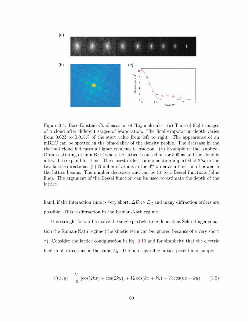
Ato

m n

um

ber

x 1

03

Power (W)

0

2

4

6

8

10

0 0.5 1 1.5 2

(a)

(b) (c)

Figure 3.4: Bose-Einstein Condensation of 6Li2 molecules. (a) Time of flight imagesof a cloud after different stages of evaporation. The final evaporation depth variesfrom 0.023 to 0.015% of the start value from left to right. The appearance of anmBEC can be spotted in the bimodality of the density profile. The decrease in thethermal cloud indicates a higher condensate fraction. (b) Example of the Kapitza-Dirac scattering of an mBEC when the lattice is pulsed on for 500 ns and the cloud isallowed to expand for 4 ms. The closest order is a momentum imparted of 2hk in thetwo lattice directions. (c) Number of atoms in the 0th order as a function of power inthe lattice beams. The number decreases and can be fit to a Bessel functions (blueline). The argument of the Bessel function can be used to estimate the depth of thelattice.

hand, if the interaction time is very short, ∆E ER and many diffraction orders are

possible. This is diffraction in the Raman-Nath regime.

It is straight forward to solve the single particle time-dependent Schrodinger equa-

tion the Raman-Nath regime (the kinetic term can be ignored because of a very short

τ). Consider the lattice configuration in Eq. 2.10 and for simplicity that the electric

field in all directions is the same E0. The non-separable lattice potential is simply

V (x, y) =V0

2[cos(2kx) + cos(2ky)] + V0 cos(kx+ ky) + V0 cos(kx− ky) (3.9)

80

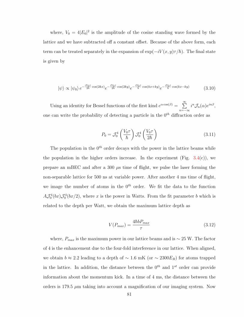
where, V0 = 4|E0|2 is the amplitude of the cosine standing wave formed by the

lattice and we have subtracted off a constant offset. Because of the above form, each

term can be treated separately in the expansion of exp(−iV (x, y)τ/h). The final state

is given by

|ψ〉 ∝ |ψ0〉 e−iV0τ2h

cos(2kx)e−iV0τ2h

cos(2ky)e−iV0τh

cos(kx+ky)e−iV0τh

cos(kx−ky) (3.10)

Using an identity for Bessel functions of the first kind eα cos(β) =∞∑

n=−∞inJn(α)einβ,

one can write the probability of detecting a particle in the 0th diffraction order as

P0 = J 40

(V0τ

h

)J 4

0

(V0τ

2h

)(3.11)

The population in the 0th order decays with the power in the lattice beams while

the population in the higher orders increase. In the experiment (Fig. 3.4(c)), we

prepare an mBEC and after a 300 µs time of flight, we pulse the laser forming the

non-separable lattice for 500 ns at variable power. After another 4 ms time of flight,

we image the number of atoms in the 0th order. We fit the data to the function

AJ 40 (bx)J 4

0 (bx/2), where x is the power in Watts. From the fit parameter b which is

related to the depth per Watt, we obtain the maximum lattice depth as

V (Pmax) =4hbPmax

τ(3.12)

where, Pmax is the maximum power in our lattice beams and is ∼ 25 W. The factor

of 4 is the enhancement due to the four-fold interference in our lattice. When aligned,

we obtain b ≈ 2.2 leading to a depth of ∼ 1.6 mK (or ∼ 2300ER) for atoms trapped

in the lattice. In addition, the distance between the 0th and 1st order can provide

information about the momentum kick. In a time of 4 ms, the distance between the

orders is 179.5 µm taking into account a magnification of our imaging system. Now

81

in time τ and after a momentum of 2hk imparted, one would expect the atoms to

travel a distance 2hkτ/2m. Here we divide by 2m because the cloud is composed

of molecules. Equating the two, we get that a = π/k = 739 nm. Here a is the

lattice spacing formed by the 4-fold interference and is expected to be 1064/√

2 nm

= 752 nm. So we can also verify the lattice spacing is what we expect.

82

3.3 Single site imaging

3.3.1 Raman imaging

To image the atoms in an optical lattice, one could employ absorption imaging by

shining near resonant light on to the atoms in a deep lattice and collect the scattered

photons. But each photon scattered would impart a kick on the atom and cause it to

move around or escape from the deep well before enough photons have been collected

to resolve the atom. So the signal to noise is limited and the atomic movement can

blurr the image. Hence one requires a technique that scatters enough photons from

a single atom without heating it up. In addition, by cooling the atoms in a deep

lattice where the atoms do not move, one can achieve single site resolution. One such

technique is electromagnetically induced transparency (EIT) cooling [93, 50]. The

other more widespread technique is called sideband resolved Raman cooling. This

technique was originally developed to cool ions to the vibrational ground state in a

radio frequency trap [94] and later demonstrated for atoms in optical lattices [95].

Raman cooling was introduced as an imaging technique in quantum gas microscopes

in experiments with 40K and 6Li [52, 53, 56]. This was a departure from previous

87Rb quantum gas microscopes which used polarization gradient cooling, which does

not work as well for these species. As the name suggests, we drive transitions between

resolved vibrational states of atoms on individual isolated sites of an optical lattice

(Fig. 3.5 (a)) using a coherent two photon process.

In order to drive stimulated transitions of atoms from a higher vibrational state ν

to ν − 1, we follow the scheme shown in Fig. 3.5(b). An atom starts out in the 2S1/2

F=3/2 manifold in vibrational state ν. A two photon Raman transition takes the

atom to the 2S1/2 F=1/2 manifold and in the vibrational state ν−1. This is achieved

by using two beams, first a Raman beam detuned by 5.6 GHz from the 2S1/2 → 2P1/2

transition and a retro-reflected beam detuned by (228.2 + ωlatt/(2π)) MHz. Then the

83

atom experiences a near resonant pump beam which excites the atom to the 2P1/2

state. The cooling cycle is closed when the atom spontaneously decays back to the

2S1/2 F=3/2 manifold while conserving the vibrational state ν − 1. Thus we have

effectively lowered the vibrational energy of the atom by 1 hωlatt and the photon

emitted during optical pumping is used for imaging.

An important factor for the above scheme to be efficient is that the spontaneous

emission process conserves the vibrational state. The recoil of the atom when it emits

a photon is given by the operator e−ikx, where k is the photon momentum. It causes

the momentum of the atom to change by hk. Now in the basis of harmonic oscillator

states |ν〉, the probability of transition is given by

Pν→ν′ = 〈ν| eikx |ν ′〉 = 〈ν| eikx0(a+a†) |ν ′〉 (3.13)

where, the position operator x can be written in terms of the harmonic oscillator

creation and annihilation operator a and a†. x0 =√h/(2mωlatt) is the harmonic

oscillator length. We define the Lamb-Dicke parameter η as

η = kx0 =

√hk2

2mωlatt(3.14)

And we perform Taylor expansion in orders of η to obtain

Pν→ν′ ∼ 〈ν| (1 + η(a+ a†) +O(η2)) |ν ′〉 (3.15)

84

Dep

th (E

R)

distance (a)

-2000

-1000

0

1000

-1.5 -1 -0.5 0 0.5 1 1.5

ωlatt = (2) 1.39 MHz

ΔHFS

Δ

F=3/2

F=1/2

2S1/2

2P1/2

O.D

.

Frequency (MHz)

0

0.1

0.2

0.3

228 228.5 229 229.5 230 230.5

O.D

.

Frequency (MHz)

0

0.1

0.2

0.3

228.2 228.21 228.22 228.23 228.24

O.D

.

Frequency (MHz)

0

0.05

0.1

0.15

228.36 228.37 228.38 228.39 228.4

(a)

(c)

(d)

(b)

(e)

δ

Figure 3.5: Raman cooling scheme.(a) 1D cut of our lattice potential at maximumdepth (red). X-axis is distance in units of the lattice spacing (a = 752nm). Max-imum depth as obtained from a tight binding calculation. Fit of a single latticesite to a harmonic potential (blue) to obtain the spacing between vibrational levels(ωlatt ∼ (2π) 1.39 MHz). (b) Schematic of the Raman cooling process. An atom inthe 2S1/2, F=3/2 state starts out in an excited vibrational state (blue) of the lattice.A beam (blue) red-detuned to the 2S1/2 → 2P1/2 by ∆ = 5.6 GHz and a counter-propagating beam (green) frequency detuned from the first one by ∆HFS = 228.2 +ωlatt/(2π) MHz are incident on the atomic cloud. A third beam (red) near resonantwith the 2S1/2, F=1/2 → 2P1/2 transition (δ ∼ 10 Γ) is also incident on the atoms.(c) Raman spectra at a field of ∼ 10-30 mG. The first peak at 228.2 MHz is thecarrier peak while the second one at 229.65 MHz is the blue Raman sideband. Theenergy difference between the two gives the lattice vibrational spacing of 1.45 MHz.(d) Radio-frequency (RF) spectroscopy at the lowest achievable magnetic field. Peaksat 228.206, 228.215, and 228.222 MHz correspond to a residual field of 10 mG. (e)RF spectroscopy at the magnetic field where we perform Raman cooling. The peakat 228.388 MHz corresponds to a field of 195 mG.

85

So we see that for a small Lamb-Dicke parameter η the branching ratio to decay

into ν±1 is ∼ η2/(1+η2) and to even further vibrational states is strongly supressed.

Hence obtaining the smallest possible η is crucial for Raman sideband cooling. For

our lattice directions in plane, we have η ≈ 0.22, while in the third direction, where

we do not have a lattice but only confinement due to the lightsheet of about 70 kHz,

we have ηz ≈ 1. So we are in the Lamb-Dicke regime only in the lattice plane but

we were still capable of performing single atom imaging. The reason for that is we

do not need to be able to cool the atoms very efficiently to be able to image them.

As long as an atom is capable of participating in the cooling process without being

ejected from a lattice site, we can cycle photons through it.

The beam setup for Raman sideband cooling is shown in Fig. 3.6(a). Light from

the Raman laser system (Fig. 2.12) is sent through optical fibers to the experiment.

The Raman beam is linearly polarized and it passes at 45 to the lattice principal axes

(so along one of the lattice beams). The beam is not coplanar with the lattice beam

to allow coupling to the vertical direction. It runs at an angle of ∼ 10 to the lattice

plane. After passing through the chamber, it is double-passed through an acousto

optic modulator set at 114.557 MHz. The polarization of the retro-reflected beam

is linear and perpendicular to the incoming beam. The beam waist at the atoms is

75 µm and the first pass power is 2.5 mW. The retro-reflected power is smaller by

a factor of 0.77 due to AOM efficiency. The pump beam is also sent at an angle

(shallower than the Raman beam), colinear with a lattice beam and has a waist of

about 1 mm. The polarization of the pump beam is circular. The intensity and the

detuning of the pump beam are tuned while optimizing the rate of hopping and loss

in our system and are of the order of 50 µW and 10 Γ relative to the free space

resonance. We estimate the Rabi frequency of the 2-photon Raman transition to be

(2π) 180 kHz by measuring power broadened Raman spectra for different powers.

86

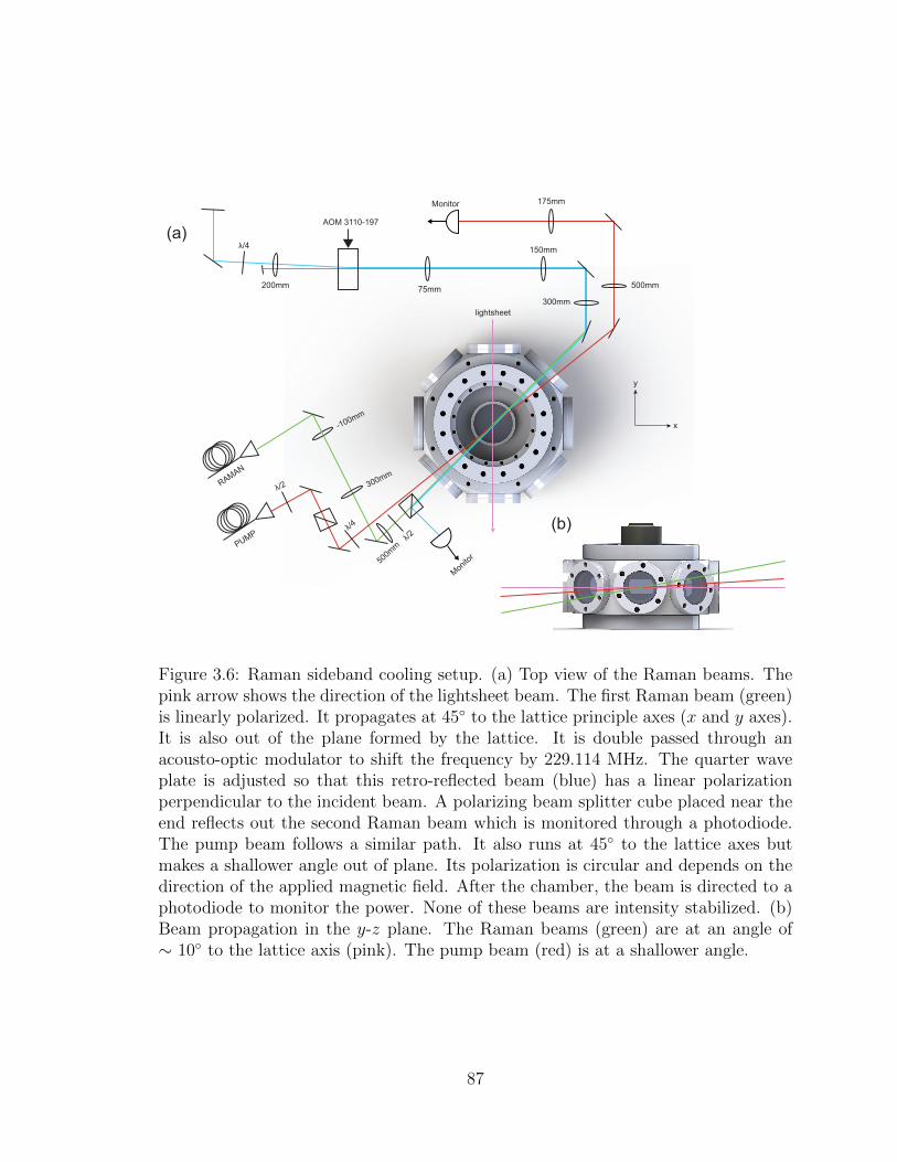
(a)

(b)

AOM 3110-197

200mm75mm

150mm

300mm

500mm

175mm

-100mm

300mm

500m

m

/2

/4

/2

/4

lightsheet

Mon

itor

RAMAN

PUMP

x

y

Monitor

Figure 3.6: Raman sideband cooling setup. (a) Top view of the Raman beams. Thepink arrow shows the direction of the lightsheet beam. The first Raman beam (green)is linearly polarized. It propagates at 45 to the lattice principle axes (x and y axes).It is also out of the plane formed by the lattice. It is double passed through anacousto-optic modulator to shift the frequency by 229.114 MHz. The quarter waveplate is adjusted so that this retro-reflected beam (blue) has a linear polarizationperpendicular to the incident beam. A polarizing beam splitter cube placed near theend reflects out the second Raman beam which is monitored through a photodiode.The pump beam follows a similar path. It also runs at 45 to the lattice axes butmakes a shallower angle out of plane. Its polarization is circular and depends on thedirection of the applied magnetic field. After the chamber, the beam is directed to aphotodiode to monitor the power. None of these beams are intensity stabilized. (b)Beam propagation in the y-z plane. The Raman beams (green) are at an angle of∼ 10 to the lattice axis (pink). The pump beam (red) is at a shallower angle.

87

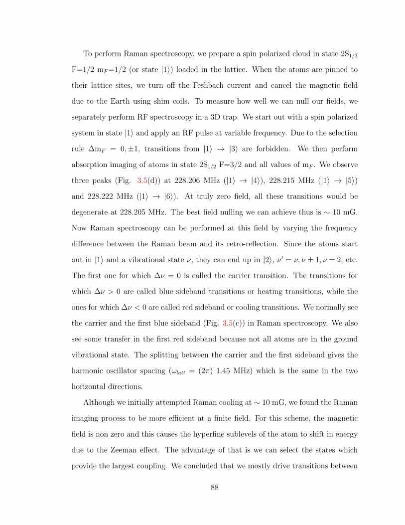
To perform Raman spectroscopy, we prepare a spin polarized cloud in state 2S1/2

F=1/2 mF=1/2 (or state |1〉) loaded in the lattice. When the atoms are pinned to

their lattice sites, we turn off the Feshbach current and cancel the magnetic field

due to the Earth using shim coils. To measure how well we can null our fields, we

separately perform RF spectroscopy in a 3D trap. We start out with a spin polarized

system in state |1〉 and apply an RF pulse at variable frequency. Due to the selection

rule ∆mF = 0,±1, transitions from |1〉 → |3〉 are forbidden. We then perform

absorption imaging of atoms in state 2S1/2 F=3/2 and all values of mF . We observe

three peaks (Fig. 3.5(d)) at 228.206 MHz (|1〉 → |4〉), 228.215 MHz (|1〉 → |5〉)

and 228.222 MHz (|1〉 → |6〉). At truly zero field, all these transitions would be

degenerate at 228.205 MHz. The best field nulling we can achieve thus is ∼ 10 mG.

Now Raman spectroscopy can be performed at this field by varying the frequency

difference between the Raman beam and its retro-reflection. Since the atoms start

out in |1〉 and a vibrational state ν, they can end up in |2〉, ν ′ = ν, ν ± 1, ν ± 2, etc.

The first one for which ∆ν = 0 is called the carrier transition. The transitions for

which ∆ν > 0 are called blue sideband transitions or heating transitions, while the

ones for which ∆ν < 0 are called red sideband or cooling transitions. We normally see

the carrier and the first blue sideband (Fig. 3.5(c)) in Raman spectroscopy. We also

see some transfer in the first red sideband because not all atoms are in the ground

vibrational state. The splitting between the carrier and the first sideband gives the

harmonic oscillator spacing (ωlatt = (2π) 1.45 MHz) which is the same in the two

horizontal directions.

Although we initially attempted Raman cooling at ∼ 10 mG, we found the Raman

imaging process to be more efficient at a finite field. For this scheme, the magnetic

field is non zero and this causes the hyperfine sublevels of the atom to shift in energy

due to the Zeeman effect. The advantage of that is we can select the states which

provide the largest coupling. We concluded that we mostly drive transitions between

88

states |3〉 and |2〉 at an offset field of 195 mG. We measure the value of this offset

field from RF spectroscopy (Fig. 3.5(e)). We observe a peak due to |1〉 → |5〉 at

228.388 MHz and one at 228.572 MHz for |1〉 → |6〉 transition.

3.3.2 Microscope objective

In order to image single atoms, we need an objective capable of resolving the distance

between neighboring lattice sites. That distance in our experiment is 752 nm. We

purchased a custom designed objective from Special Optics (Navitar) that suited

our needs. The objective (54-25-25-671&800nm) (see Appendix E) has the following

specifications:

• Effective focal length = 25 mm

• Working distance = 12 mm in air + 5 mm in fused silica

• Numerical aperture = 0.5

• Field of view in object plane = 150 µm

• Anti-reflection coated at 671 nm and 800 nm

• Diffraction limited up to 120 µm defocus

• Non-magnetic Ultem casing of 36 mm outer diameter

Due to the diffraction limited performance at the D1 transition wavelength, we

can resolve features as small as 800 nm given by the Rayleigh criterion (0.61λ/NA),

comparable to the lattice spacing. A 750 mm lens after the objective leads to a

magnification of 30. We employ an Andor Zyla 4.2 sCMOS camera for fluorescence

imaging. The quantum efficiency of the sensor is about 75% at 671 nm with 0.9 e−

readout noise and the pixel size is 6.5 µm.

89

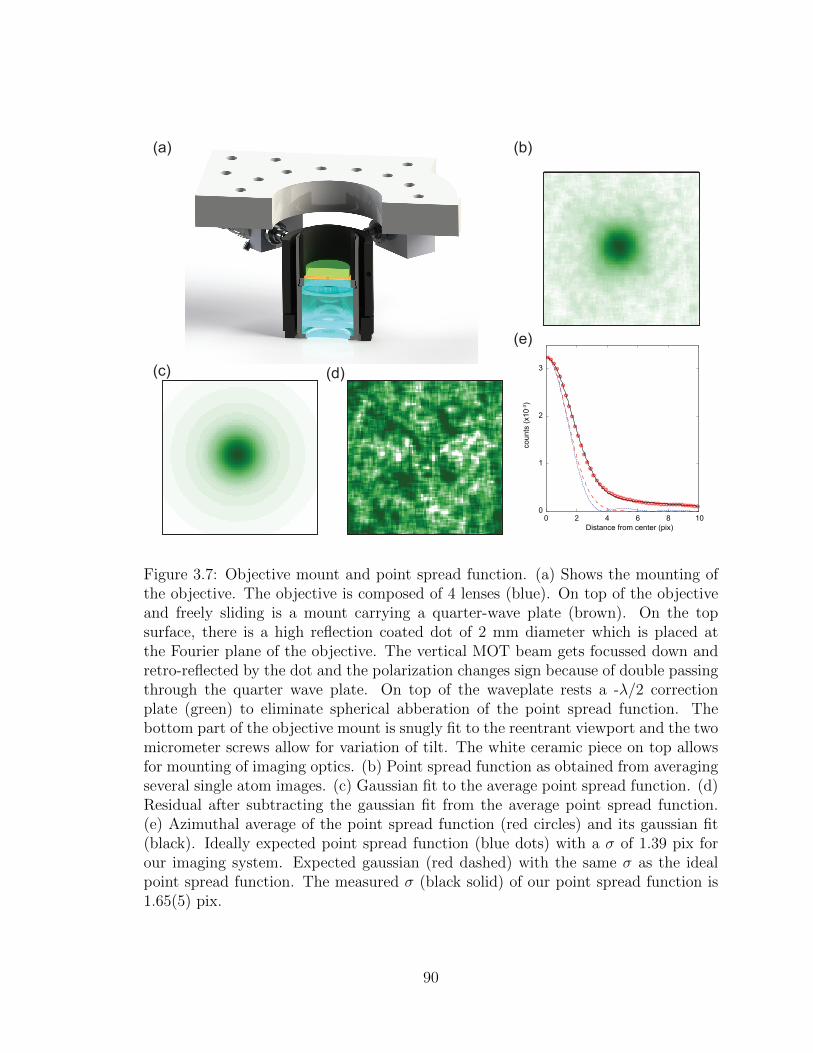
counts

(x10

-3)

Distance from center (pix)

0

1

2

3

0 2 4 6 8 10

(a) (b)

(e)

(c) (d)

Figure 3.7: Objective mount and point spread function. (a) Shows the mounting ofthe objective. The objective is composed of 4 lenses (blue). On top of the objectiveand freely sliding is a mount carrying a quarter-wave plate (brown). On the topsurface, there is a high reflection coated dot of 2 mm diameter which is placed atthe Fourier plane of the objective. The vertical MOT beam gets focussed down andretro-reflected by the dot and the polarization changes sign because of double passingthrough the quarter wave plate. On top of the waveplate rests a -λ/2 correctionplate (green) to eliminate spherical abberation of the point spread function. Thebottom part of the objective mount is snugly fit to the reentrant viewport and the twomicrometer screws allow for variation of tilt. The white ceramic piece on top allowsfor mounting of imaging optics. (b) Point spread function as obtained from averagingseveral single atom images. (c) Gaussian fit to the average point spread function. (d)Residual after subtracting the gaussian fit from the average point spread function.(e) Azimuthal average of the point spread function (red circles) and its gaussian fit(black). Ideally expected point spread function (blue dots) with a σ of 1.39 pix forour imaging system. Expected gaussian (red dashed) with the same σ as the idealpoint spread function. The measured σ (black solid) of our point spread function is1.65(5) pix.

90

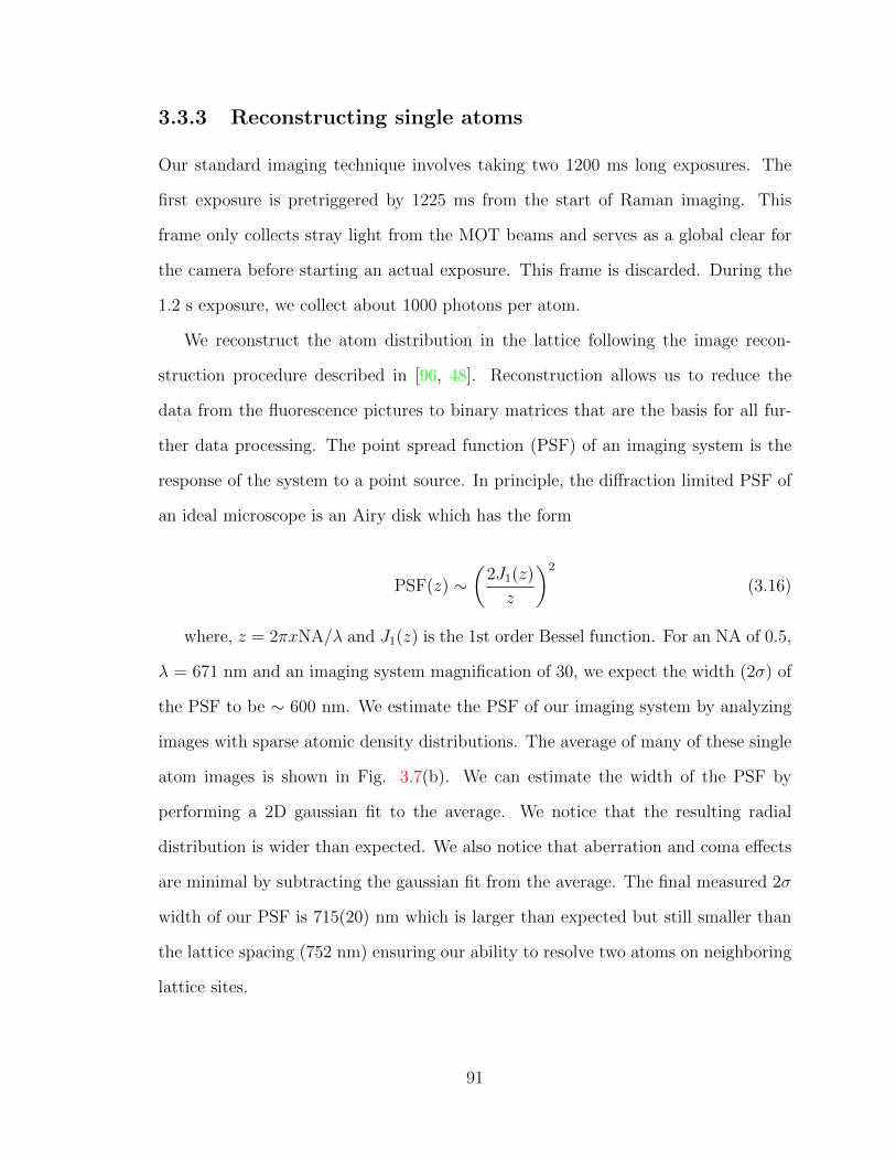
3.3.3 Reconstructing single atoms

Our standard imaging technique involves taking two 1200 ms long exposures. The

first exposure is pretriggered by 1225 ms from the start of Raman imaging. This

frame only collects stray light from the MOT beams and serves as a global clear for

the camera before starting an actual exposure. This frame is discarded. During the

1.2 s exposure, we collect about 1000 photons per atom.

We reconstruct the atom distribution in the lattice following the image recon-

struction procedure described in [96, 48]. Reconstruction allows us to reduce the

data from the fluorescence pictures to binary matrices that are the basis for all fur-

ther data processing. The point spread function (PSF) of an imaging system is the

response of the system to a point source. In principle, the diffraction limited PSF of

an ideal microscope is an Airy disk which has the form

PSF(z) ∼(

2J1(z)

z

)2

(3.16)

where, z = 2πxNA/λ and J1(z) is the 1st order Bessel function. For an NA of 0.5,

λ = 671 nm and an imaging system magnification of 30, we expect the width (2σ) of

the PSF to be ∼ 600 nm. We estimate the PSF of our imaging system by analyzing

images with sparse atomic density distributions. The average of many of these single

atom images is shown in Fig. 3.7(b). We can estimate the width of the PSF by

performing a 2D gaussian fit to the average. We notice that the resulting radial

distribution is wider than expected. We also notice that aberration and coma effects

are minimal by subtracting the gaussian fit from the average. The final measured 2σ

width of our PSF is 715(20) nm which is larger than expected but still smaller than

the lattice spacing (752 nm) ensuring our ability to resolve two atoms on neighboring

lattice sites.

91

We perform calibrations of our lattice angle and spacing by using very sparse

images of pinned atoms. The images are fit to a 2D grid with four free parameters,

the angles θ1 and θ2 that the grid makes with the x and the y axis defined by the

camera pixels and the spacings a1 and a2 that are the spacing between sites on this

grid along the two axes. These fit values are in turn used to define the lattice grid

for reconstruction. The fit values can change based on any modification done to

the imaging system, so they are measured every few weeks. For the stable working

condition of the experiment, the average values of these parameters are θ1 = -54(1),

θ1 = -36(1), a1 = 3.5(1) pixels and a2 = 3.4(1) pixels (1 pixel = 217 nm).

An example of reconstruction is shown in Fig. 3.8. We make a histogram of

detected photons on each site for a given image. Usually the histogram is bimodal,

with a peak near zero photons corresponding to empty sites and a peak at a higher

photon count corresponding to sites with a single atom. Due to strong light assisted

collisions, atoms in sites with more than one atom are lost and these sites appear

empty. Next we fit gaussians to these peaks and identify a threshold between them.

Any site with more counts than the threshold is identified as occupied. It is important

for reconstruction to work properly that the peaks associated with empty and occu-

pied sites be well separated. If it is not the case, either recalibrating lattice angles or

refocusing the camera must be performed.

We estimate fidelity errors due to Raman imaging imperfections by taking 40

consecutive images with our standard imaging time of 1200 ms of the same atom

cloud and determine the shot-to-shot differences. This leads to a hopping rate during

one picture of 0.4(2)% and a loss rate of 1.6(3)%. In addition, while holding the

atoms in a deep lattice for spin manipulations or doublon hiding/detection, we lose

2(1)% of the atoms, leading to a net detection efficiency of 96%.

92

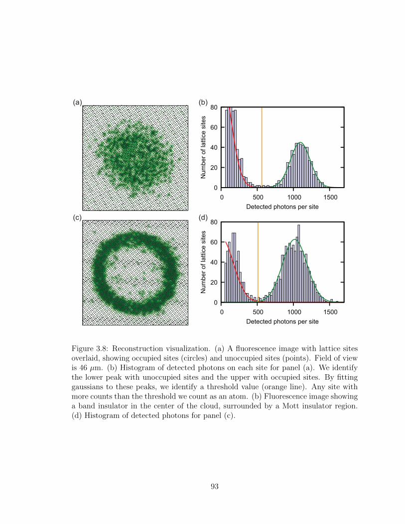
0

20

40

60

80

0 500 1000 1500N

umbe

r of l

attic

e si

tes

Detected photons per site

0

20

40

60

80

0 500 1000 1500

Num

ber o

f lat

tice

site

s

Detected photons per site

(a)

(c) (d)

(b)

Figure 3.8: Reconstruction visualization. (a) A fluorescence image with lattice sitesoverlaid, showing occupied sites (circles) and unoccupied sites (points). Field of viewis 46 µm. (b) Histogram of detected photons on each site for panel (a). We identifythe lower peak with unoccupied sites and the upper with occupied sites. By fittinggaussians to these peaks, we identify a threshold value (orange line). Any site withmore counts than the threshold we count as an atom. (b) Fluorescence image showinga band insulator in the center of the cloud, surrounded by a Mott insulator region.(d) Histogram of detected photons for panel (c).

93

Chapter 4

Phase separation and pair

condensation in a spin-imbalanced

2D Fermi gas

4.1 Degenerate Fermi gases

Degenerate Fermi gases are omnipresent in the universe. From the semiconductor

transistors located within our computers to the cores of neutron stars, the physics of

fermions dictates many important phenomena in our daily life. Fermi-Dirac statistics

describes the thermodynamics of an ideal gas of fermions [97]. The essential ingredient

is the Pauli exclusion principle [98], which states that two identical fermions can not

occupy the same quantum state simultaneously. Our experiments are motivated by

the understanding of exotic phenomena that appear in strongly interacting systems

of fermions.

As was described in the previous sections, we start with fermionic lithium atoms

in a |1〉−|2〉 mixture and evaporate near the Feshbach resonance at 832 G to create a

molecular BEC. Alternatively, it is possible to produce a degenerate gas of fermions,

94

where the atoms do not pair and form molecules. I will describe first the simplest of

such cases, a non-interacting gas of fermions in a 3D harmonic trap.

It is more difficult to cool down fermions to quantum degeracy than bosons

through evaporative cooling. Efficient evaporative cooling requires atoms to scat-

ter off one another and thermalize. Identical fermions can not scatter off one another

in the s-wave channel. One needs fermions of opposite spins. But even with fermions

of opposite spins, as the temperature approaches zero, Pauli blocking drives collision

rates down to zero as well. Despite the challenge of evaporative cooling, the first

degenerate gas of fermionic potassium was observed in 1999 [5] four years after the

first observations of BEC in rubidium and sodium in 1995 [3, 4].

Non-interacting fermions can be readily created in our experiments by using a

spin polarized gas or by working at a magnetic field where the s-wave interactions

between fermions vanish. In the limit of large N, many single particle fermionic states

are occupied and one can safely apply a semiclassical treatment to the system. The

semiclassical distribution function in such a system is given by

f(~k, ~r) =

(eβ(h2k2

2m+V (~r)−µ

)+ 1

)−1

(4.1)

where, β = 1/kBT , V (~r) = mω2r2/2 is the harmonic potential assumed to be

symmetric here and µ is the chemical potential. In most situations, however, the

harmonic potential is only cylindrically symmetric. The potential then can be written

as V (r, z) = mω2rr

2 + mω2zz

2 with ωz = λωr. This distribution tends to a Maxwell-

Boltzmann distribution at high temperatures and low particle density. The chemical

potential can be implicitly calculated from the particle number using [99]

N =

∫g(ε)dε

eβ(ε−µ) + 1(4.2)

95

where g(ε) is the single particle density of states given by ε2/(2λω3r) for a cylin-

drically symmetric potential and N is the number of particles in each non-interacting

spin state. If the harmonic oscillator potential is not cylindrically symmetric, one

can replace λ1/3ωr with the geometric mean (ωxωyωz)1/3. From the knowledge of the

Fermi function and the density of states, all other thermodynamic quantities can be

calculated. The energy scale of the system is given by the Fermi energy given by

EF = hωr(6λN)1/3 (4.3)

In the same way, the temperature scale of the system is called the Fermi temper-

ature and is given by EF = kBTF . The Thomas-Fermi radius of the cloud can be

calculated from mω2rR

2TF/2 = EF .

To understand interactions between cold fermions in 3D, consider the Schrodinger

equation of two colliding particles in their center of mass (COM) frame

(− h

2∇2

2µ+ V (r)

)ψk(r) = Ekψk(r) (4.4)

where, in COM coordinates, the reduced mass µ = m/2 and U(r) is the interaction

potential. The above equation can be rewritten as

(∇2 + k2)ψk(r) = v(r)ψk(r) (4.5)

where, the momentum k is given by Ek = h2k2/2µ and the modified potential

v(r) = 2V (r)µ/h2. Rewriting the above in spherical coordinates and rearranging one

gets

(kr)2d2ψk(r)

d(kr)2+ 2(kr)

dψk(r)

d(kr)+ ((kr)2 − v(r))ψk(r) = 0 (4.6)

96

Notice that the above equation is the Bessel differential equation of second order

in the variable kr. The solution of the above equation in the far field limit (i.e.

r r0, where r0 is the range of the interaction potential) can be written as

ψk(r) = eikz +eikr

r

∫v(r′)ψk(r

′)eikr′d3r′ = eikz + f(k)

eikr

r(4.7)

where, f(k) is known as the scattering amplitude and it depends on the form of

the interaction potential. The direction of propagation of the plane wave is the z axis.

The simplest approximation to make here is that the collisions happen predominantly

in the s-wave or spherically symmetric channel. Hence the scattering amplitude has

no angular dependence. This can be achieved by integrating over the spherically

symmetric part of the plane wave. In addition, the process of scattering only adds a

phase shift δ to the incoming wave. Combing the two, one obtains

ψk(r) ∼ eikr +eikr

r

eiδ sin δ

k(4.8)

Thus the scattering amplitude in the case of s-wave scattering is

f(k) =eiδ sin δ

k=

1

k cot δ − ik(4.9)

Now the calculation of the phase shift δ requires knowledge of the interaction

potential V (r). Let us consider a simple example of an attractive potential well.

Below r0, the well has a depth −V0 and above r0, the depth V (r) = 0. We assume

that the wavefunction inside the well and outside are both sinusoidal but with a phase

difference δ. But they have different momenta because of the potential. So

ψk(r) =

A sin(k′r), r < r0

B sin(kr + δ), r > r0

(4.10)

97

where, h2k′2/2µ− V0 = h2k2/2µ. Now the wavefunction must be continuous and

differentiable at r = r0 giving

k′ cot(k′r0) = k cot(kr0 + δ) (4.11)

Solving for δ after expanding in powers of kr0, one gets

k cot δ = − 1

as+rek

2

2

as = r0 −tan qr0

q

re =

(1

q− r2

0q

)cos(qr0) + r0 sin(qr0) +

q2r30 cos2(qr0/3)

sin qr0 − qr0 cos(qr0)(4.12)

where, q =√

2mV0/h, re is the effective range of the interaction and as is the s-

wave scattering length. Although the attractive well is only a pedagogical tool, it is a

close approximation to a real inter-atomic scattering potential like the Lennard-Jones

potential. In the limiting case of the effective range re → 0, which is true for point

interactions, one gets k cot δ ≈ −1/as. Hence the scattering amplitude at momentum

k approximately equals

f(k) ≈ −as1 + ikas

(4.13)

In addition, the scattering amplitude is maximum when as → ±∞, which is the

case of being at the Feshbach resonance for our atoms. When as > 0 and close to

this resonance, molecular bound states or dimers can form with a binding energy

E3Db =

h2

2ma2s

(4.14)

98

These dimers are weakly bound near the Feshbach resonance and the binding

energy increases as one moves to the BEC side (Fig. 4.1). Above the resonance,

however, where as < 0, no dimers can form and no bound states exist.

99

4.2 Fermi gas in 2 dimensions

Dimensionality is very important in nature. Many interesting properties appear when

fermions are confined in a plane like the Quantum Hall Effect [100, 101]. Another

example is high temperature superconductivity in the cuprates, where the lower di-

mensionality is believed to play an important role [102]. Yet another example is

the FFLO phase theorized in spin-imbalanced attractive Fermi gases, which can be

enhanced in 1D and 2D due to Fermi surface nesting [103, 104]. These examples mo-

tivate us to study strongly interacting atomic Fermi gases in 2 dimensions. A simple

way to change the dimensionality of a system is to increase the harmonic confinement

in the axial direction.

As a measure of the extent of 2 dimensionality, we can compare the Fermi energy

and the temperature to the harmonic oscillator level spacing in the axial direction. If

EF , T hωz, then the fermions occupy many axial states and the gas in 3D. However

if EF , T hωz, then only the ground state in the axis direction is occupied and the

gas is purely 2D. In our experiment, ωz is about (2π) 22 kHz for the accordion lattice.

The radial trapping frequency geometric mean ωr is about (2π) 135 Hz. In the case

of ωz ωx, ωy, one finds that the density of states is given instead by [105]

g(ε) =ε

(hωr)2(4.15)

where, if the trap is not uniform in plane, one can replace ωr with the geometric

mean√ωxωy. From this, the Fermi energy is

EF = hωr√

2N (4.16)

N is the number of particles in each non-interacting spin state. We have about

9×103 atoms giving a Fermi energy of (2πh) 18 kHz which puts us in a “quasi” 2D

regime.

100

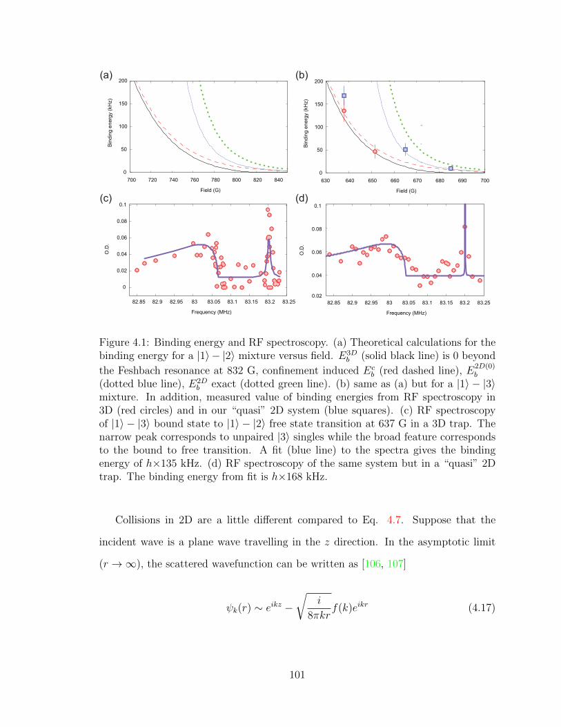
Bind

ing

ener

gy (k

Hz)

Field (G)

0

50

100

150

200

700 720 740 760 780 800 820 840

Bind

ing

ener

gy (k

Hz)

Field (G)

0

50

100

150

200

630 640 650 660 670 680 690 700

O.D

.

Frequency (MHz)

0.04

0.06

0.08

0.1

82.85 82.9 82.95 83 83.05 83.1 83.15 83.2 83.25

O.D

.

Frequency (MHz)

0

0.02

0.04

0.06

0.08

0.1

82.85 82.9 82.95 83 83.05 83.1 83.15 83.2 83.25 0.02

(a) (b)

(c) (d)

Figure 4.1: Binding energy and RF spectroscopy. (a) Theoretical calculations for thebinding energy for a |1〉 − |2〉 mixture versus field. E3D

b (solid black line) is 0 beyond

the Feshbach resonance at 832 G, confinement induced Ecb (red dashed line), E

2D(0)b

(dotted blue line), E2Db exact (dotted green line). (b) same as (a) but for a |1〉 − |3〉

mixture. In addition, measured value of binding energies from RF spectroscopy in3D (red circles) and in our “quasi” 2D system (blue squares). (c) RF spectroscopyof |1〉 − |3〉 bound state to |1〉 − |2〉 free state transition at 637 G in a 3D trap. Thenarrow peak corresponds to unpaired |3〉 singles while the broad feature correspondsto the bound to free transition. A fit (blue line) to the spectra gives the bindingenergy of h×135 kHz. (d) RF spectroscopy of the same system but in a “quasi” 2Dtrap. The binding energy from fit is h×168 kHz.

Collisions in 2D are a little different compared to Eq. 4.7. Suppose that the

incident wave is a plane wave travelling in the z direction. In the asymptotic limit

(r →∞), the scattered wavefunction can be written as [106, 107]

ψk(r) ∼ eikz −√

i

8πkrf(k)eikr (4.17)

101

To understand why the scattered wave has a eikr/√r dependence in 2D compared

to the eikr/r dependence in 3D, consider the conservation of |ψk(r)|2 before and after

scattering. The probability current j is defined as

j =h

i2m(ψk(r)

∗∇ψk(r)− ψk(r)∇ψk(r)∗) (4.18)

The divergence of j should be 0 for conservation of probability, i.e.

ψk(r)∗∇2ψk(r) = ψk(r)∇2ψk(r)

∗ (4.19)

Now using the expression for the laplacian in polar coordinates∇2 = 1/r∂/∂r(r∂/∂r),

one can verify that the above condition is satisfied when ψ ∼ eikr/√r. Similar to

the 3D case, one can derive the expression for f(k) in terms of a phase shift δ in the

s-wave channel

f(k) = − 4

cot δ − i(4.20)

For low energy elastic scattering, one can compute the phase shift to get [108]

cot δ = − 2

πlog

(1

ka2D

)+O(k2) (4.21)

where, a2D is the s-wave scattering length in 2D. This leads to the expression for

the scattering amplitude in a 2D system

f(k) = − 4π

2log(ka2D)− iπ(4.22)

In this case, the scattering amplitude is maximum when ka2D → 1, different from

the 3D case. Also different from the 3D case, in 2D, the scattering length is a more

complex quantity to define and compute. First of all, a realistic 2D system can be

thought of an asymmetric 3D system with an additional length scale lz =√h/mωz

102

that is given by the axial confinement ωz. Consider now the bound state of two

fermions in such a confined system. Far in the BCS limit, the bond length is large

compared to lz and the dimers are essentially confined in plane. But far on the BEC

side, tightly bound dimers form where the bond length could be much smaller than

lz. In that limit, the dimers experience no confinement and behave as if in 3D. So

one would expect the dimer binding energy far in the BEC limit to converge to E3Db .

In addition, confinement leads to the existence of a weakly bound dimer state even

above the Feshbach resonance [109]. The scattering amplitude obtained for the case

when the temperature kBT and EF are comparable to or smaller than hωz is given

by [110]

f(r) =4π√

2π lzas

+ w(k2l2z/2)(4.23)

where, the quantity w(x) is given by

w(x) = limJ→∞

(√4J

πlog

(J

e2

)−

J∑j=0

(2j − 1)!!

(2j)!!log(j − x− i0)

)(4.24)

For x 1, we get w(x) = ∆w(x) − log(2πx/0.905) + iπ. If, in addition lz is

sufficiently small, ∆w(x)→ 0 and we are left with

a(0)2D = lz

√π

0.905exp

(−√π

2

lzas

)(4.25)

And similarly we can define the 2D binding energy in this limit as

E2D(0)b =

h2

2ma(0)2D

(4.26)

Outside of this limit, one needs to calculate the correction ∆w(x) and obtain the

full 2D expression for the scattering length

103

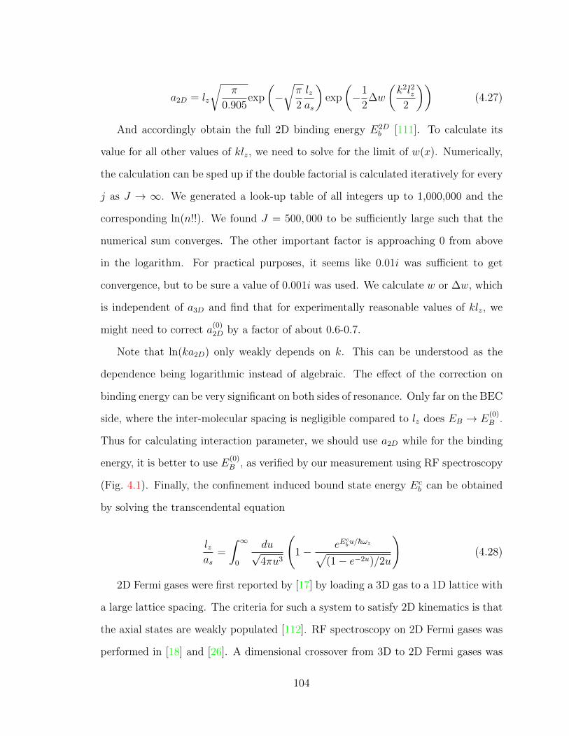
a2D = lz

√π

0.905exp

(−√π

2

lzas

)exp

(−1

2∆w

(k2l2z

2

))(4.27)

And accordingly obtain the full 2D binding energy E2Db [111]. To calculate its

value for all other values of klz, we need to solve for the limit of w(x). Numerically,

the calculation can be sped up if the double factorial is calculated iteratively for every

j as J → ∞. We generated a look-up table of all integers up to 1,000,000 and the

corresponding ln(n!!). We found J = 500, 000 to be sufficiently large such that the

numerical sum converges. The other important factor is approaching 0 from above

in the logarithm. For practical purposes, it seems like 0.01i was sufficient to get

convergence, but to be sure a value of 0.001i was used. We calculate w or ∆w, which

is independent of a3D and find that for experimentally reasonable values of klz, we

might need to correct a(0)2D by a factor of about 0.6-0.7.

Note that ln(ka2D) only weakly depends on k. This can be understood as the

dependence being logarithmic instead of algebraic. The effect of the correction on

binding energy can be very significant on both sides of resonance. Only far on the BEC

side, where the inter-molecular spacing is negligible compared to lz does EB → E(0)B .

Thus for calculating interaction parameter, we should use a2D while for the binding

energy, it is better to use E(0)B , as verified by our measurement using RF spectroscopy

(Fig. 4.1). Finally, the confinement induced bound state energy Ecb can be obtained

by solving the transcendental equation

lzas

=

∫ ∞0

du√4πu3

(1− eE

cbu/hωz√

(1− e−2u)/2u

)(4.28)

2D Fermi gases were first reported by [17] by loading a 3D gas to a 1D lattice with

a large lattice spacing. The criteria for such a system to satisfy 2D kinematics is that

the axial states are weakly populated [112]. RF spectroscopy on 2D Fermi gases was

performed in [18] and [26]. A dimensional crossover from 3D to 2D Fermi gases was

104

studied in [19] for weakly interacting Fermi gases and in [20] for strongly interacting

Fermi gases. In our experiments, lz = 270 nm. The different binding energies in 2D

and 3D are plotted in Fig. 4.1 for the |1〉 − |2〉 mixture (a) and for the |1〉 − |3〉

mixture (b). In order to measure the binding energy, we perform RF spectroscopy

in the trap. We prepare a |1〉 − |3〉 mixture at a given field and apply RF pulses to

transfer atoms from |3〉 to state |2〉 and finally we image the population in |2〉. The

first peak is the transition of |3〉 singles to |2〉. But the paired atoms require not only

the energy difference between the states but also the binding energy to transition to

a |2〉− |3〉 free state. We perform this spectroscopy in the light sheet potential for 3D

and in our final trap for 2D. We notice that in general, the higher axial confinement

leads to a higher binding energy of pairs.

105

4.3 BEC-BCS crossover in 3D and 2D

In 3D, molecular dimers formed at scattering lengths as > 0 are real space dimers with

decreasing pair size as one moves away from resonance. At resonance, as diverges and

the atoms enter a unitary regime. In this regime, the phase shift due to scattering

becomes π/2, the largest value it can have and the scattering amplitude becomes

f(r) ≈ i/k. In this regime, thermodynamic properties of the system become universal.

On the other side where as < 0, no bound states exist in 3D (but they are possible

in 2D). Due to the weak but attractive interaction, there is Cooper instability in the

system. This means that fermions with opposite spin and momenta on the Fermi

surface can pair up to form a Cooper pair that can further lead to superfluidity [2].

There is no sharp phase transition between the BEC and BCS regimes. They are

smoothly connected by a crossover.

Experiments in 3D demostrated superfluidity by creating vortices [11]. In a dif-

ferent experiment, RF spectroscopy was performed on the pairs across the crossover

[9]. In the BEC limit, the measured energy difference in spectroscopy matches the

two-particle binding energy calculations. But as one crosses over to the BCS side, the

difference between the two increases indicating many-body effects. Other experiments

include measuring the decay rate of atoms from the trap as a function of 1/kFas [10]

and measuring the release of energy across the crossover [113]. The 3D equation of

state was measured in [13] and [33].

More recently experiments were performed in a “quasi” 2D system [114] where the

equation of state was measured. The boundary between the BCS and BEC regimes in

2D is given by kFas = 1, so it is different from the unitary regime in 3D. Calculations

for superfluidity and weakly bound dimers in a “quasi” 2D geometry were done in

[115, 116]. The pairing pseudogap in a 2D Fermi gas was measured through momen-

tum resolved photoemission spectroscopy in the strong coupling regime (log(kFas)=0)

[24].

106

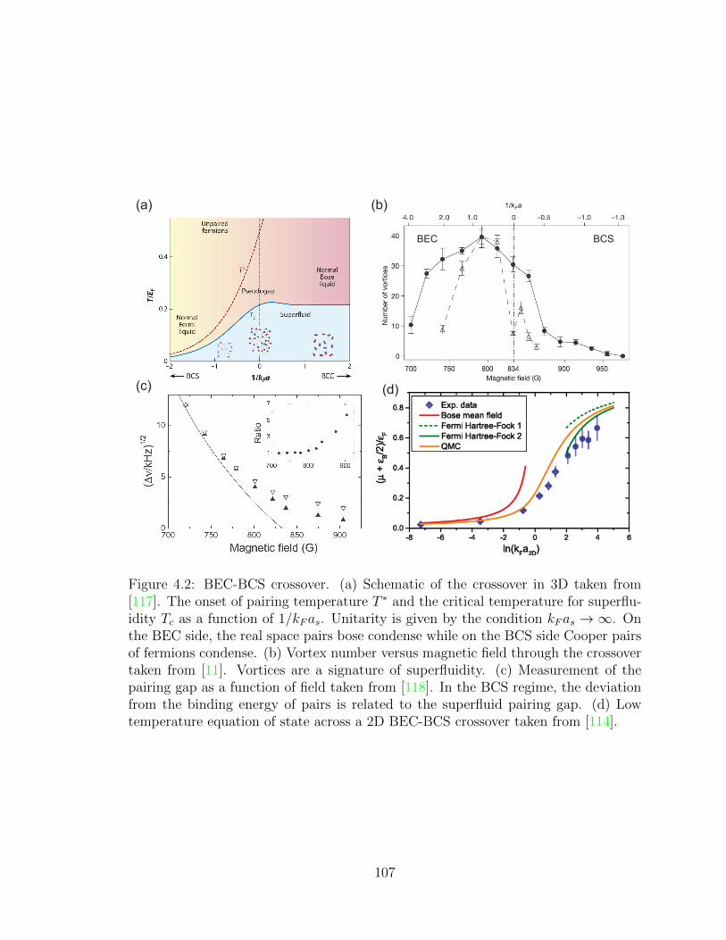
(a) (b)

(c) (d)

BEC BCS

Figure 4.2: BEC-BCS crossover. (a) Schematic of the crossover in 3D taken from[117]. The onset of pairing temperature T ∗ and the critical temperature for superflu-idity Tc as a function of 1/kFas. Unitarity is given by the condition kFas →∞. Onthe BEC side, the real space pairs bose condense while on the BCS side Cooper pairsof fermions condense. (b) Vortex number versus magnetic field through the crossovertaken from [11]. Vortices are a signature of superfluidity. (c) Measurement of thepairing gap as a function of field taken from [118]. In the BCS regime, the deviationfrom the binding energy of pairs is related to the superfluid pairing gap. (d) Lowtemperature equation of state across a 2D BEC-BCS crossover taken from [114].

107

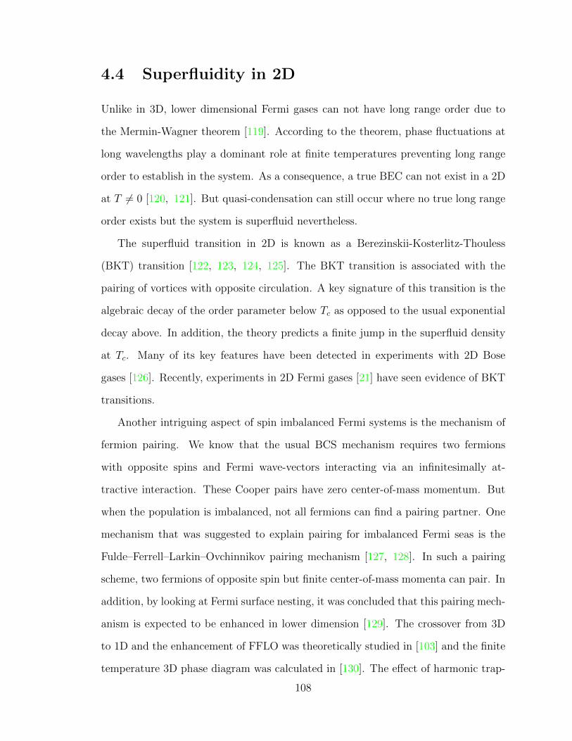
4.4 Superfluidity in 2D

Unlike in 3D, lower dimensional Fermi gases can not have long range order due to

the Mermin-Wagner theorem [119]. According to the theorem, phase fluctuations at

long wavelengths play a dominant role at finite temperatures preventing long range

order to establish in the system. As a consequence, a true BEC can not exist in a 2D

at T 6= 0 [120, 121]. But quasi-condensation can still occur where no true long range

order exists but the system is superfluid nevertheless.

The superfluid transition in 2D is known as a Berezinskii-Kosterlitz-Thouless

(BKT) transition [122, 123, 124, 125]. The BKT transition is associated with the

pairing of vortices with opposite circulation. A key signature of this transition is the

algebraic decay of the order parameter below Tc as opposed to the usual exponential

decay above. In addition, the theory predicts a finite jump in the superfluid density

at Tc. Many of its key features have been detected in experiments with 2D Bose

gases [126]. Recently, experiments in 2D Fermi gases [21] have seen evidence of BKT

transitions.

Another intriguing aspect of spin imbalanced Fermi systems is the mechanism of

fermion pairing. We know that the usual BCS mechanism requires two fermions

with opposite spins and Fermi wave-vectors interacting via an infinitesimally at-

tractive interaction. These Cooper pairs have zero center-of-mass momentum. But

when the population is imbalanced, not all fermions can find a pairing partner. One

mechanism that was suggested to explain pairing for imbalanced Fermi seas is the

Fulde–Ferrell–Larkin–Ovchinnikov pairing mechanism [127, 128]. In such a pairing

scheme, two fermions of opposite spin but finite center-of-mass momenta can pair. In

addition, by looking at Fermi surface nesting, it was concluded that this pairing mech-

anism is expected to be enhanced in lower dimension [129]. The crossover from 3D

to 1D and the enhancement of FFLO was theoretically studied in [103] and the finite

temperature 3D phase diagram was calculated in [130]. The effect of harmonic trap-

108

ping including the shell structure with phase boundaries on the FFLO state in lower

dimensions was studied in [104]. The effect of strong interactions across the BEC-

BCS crossover in 2D on the FFLO phase was also extensively studied [131, 132, 133].

Finally the effect of quantum fluctuations on the mean field phase diagram in 2D,

including the effect of the FFLO instability on the BKT transition has been studied

[134, 135].

109

4.5 Spin Imbalance: Phase separation and super-

fluidity

Pairing in both BEC and BCS regimes relies on fermions of two different spin states.

In the BEC limit, the two spin fermions form real space dimers that can Bose condense

while in the BCS limit, the fermions of opposite spin state and momenta on the

Fermi sea can form momentum space pairs. These mechanisms work if there are an

equal number of fermions in either spin state. But if there is an excess of one spin

state compared to the other, there will be some unpaired fermions left behind. The

first question that was posed is whether a system with spin imbalance can support

superfluidity [29]. Pair condensation was observed as a sudden deformation in the

cloud shape near the trap center [136]. The unpaired spin polarized fermions compete

with the condensate and can lead to phase separation. Such a separation of phases was

first observed in 3D fermi gases [30]. In this case, the paired atoms tend to occupy the

trap center while the unpaired atoms occupy the edge of the trap. The crossover from

BEC to BCS in 3D with spin imbalance was further studied in [137]. Spin imbalance

in 3D has also been studied theoretically quite extensively [138, 139, 140, 141].

An interesting aspect that ultracold atoms bring to the table is that most gases

are trapped in a harmonic potential, i.e. are not homogenous. This added complexity

allows for different phases to exist in different parts of the trap. When the fermion

populations in the two spin states are the same, then the position of the trap only

determines the local Fermi energy. But in the presence of imbalance, the variable

chemical potential in the trap can lead to a shell structure where the trap center is

superfluid and the edge is in the normal phase [142]. This was studied in depth [143] in

the context of trapped 3D Fermi gas experiments performed in [29] and [10]. One other

aspect of measurement of spin imbalance is to study the limit of superfluidity in the

system. It was observed that small amounts of population imbalance, equivalent to an

110

external magnetic field in traditional condensed matter experiments, do not destroy

superconductivity. But as the imbalance is increased, at some point superfluidity is

suppressed. This limit is known as the Chandrasekhar-Clogston limit [144]. This

limit of a critical polarization was studied for 3D systems both experimentally and

theoretically [145].

Similar experiment were performed in near 1D chains [32]. Phase separation in

1D is expected to be inverted, i.e. the condensed phase prefers to occupy the trap

edge while the unpaired phase prefers the trap center.

(a) (b)

(c)

Figure 4.3: Phase separation in 3D and 1D. (a) Phase separation observed in a 3Dgas at unitarity taken from [30]. Images are phase contrast that gives the differencedensity between the two states. (b) Phase separation in 1D chains taken from [32].The reconstructed radial profiles show that the density difference between the twospecies tend to decrease to zero near the trap edge while they are higher near the trapcenter effectively inverting the 3D profile. (c) Phase separation in 3D observed in ourexperiment for lithium atoms trapped in the lightsheet. The population imbalanceranges from < 10% for the leftmost frame to roughly 90% for the rightmost frame.

Our first experiment was motivated by the limited understanding of pairing and

superfluidity in spin-imbalanced “quasi” 2D systems. We observed the separation of

phases in the trap across the BEC-BCS crossover and measured it as a function of

population imbalance in the system. To establish pairing, we performed time-of-flight

expansion of the cloud on the BEC side and observed bimodality. We were able to

111

represent our data as a phase diagram. The paper can found in [35] and the following

sections describe the different aspects of the experiment in detail.

4.5.1 Creating 2D spin-imbalanced clouds

We start our experiment in the optical dipole trap discussed previously. After opti-

cally pumping the atoms to the lowest two hyperfine states |1〉 and |2〉, we produce a

balanced mixture of these states using ten consecutive diabatic Landau-Zener sweeps

at 537 G, with a sweep rate chosen to approximately transfer 50% of the atoms from

one state to the other (see Fig. 3.3). We then imbalance the mixture by transferring

a fraction of the atoms from state |2〉 into a third hyperfine state |3〉 using another

diabatic Landau-Zener sweep. We subsequently remove the atoms in state |3〉 with

a resonant pulse. We control the amount of imbalance using the sweep rate. By

varying the duration of the RF sweep, we were able to continuously vary the global

polarization of the cloud P = (N↑ −N↓)/(N↑ +N↓), where ↑ = |1〉 and ↓ = |2〉 (Fig.

4.5).

The imbalanced mixture is then evaporatively cooled at 800 G close to degener-

acy. We load the atoms into the lightsheet trap to compress the atoms axially in

preparation for loading them into a single well of the accordion lattice. To indepen-

dently control the radial confinement, we ramp up the bottom beam. The spacing

of the different layers of the accordion can be changed by controlling the angle at

which the lattice beams intersect, allowing us to load a single layer reproducibly at

large spacing (12 µm) and then adiabatically reduce the lattice spacing to 3.5 µm to

reach a “quasi”-2D geometry (Fig. 4.4). At this stage, we turn off the light sheet

confinement and all of the axial confinement is provided by the accordion lattice.

112

(a)

(b)

(c)

50 μm10 μm

Figure 4.4: Experimental setup. (a) A 1D optical lattice is formed at the intersectionof two interfering blue-detuned beams (green), providing axial confinement. The lat-tice spacing can be dynamically tuned by changing the angle between the beams. Theatoms are radially confined by a red-detuned beam (brown) in the vertical direction.A high-NA objective (grey) is used to image the in-plane density distribution. Theinset shows a section of the optical potential with color scale from red (attractive) toblue (repulsive). (b) Side absorption images illustrating our capability to load andresolve single (above) and multiple pancakes (below) after adiabatically increasingthe lattice spacing to ∼ 12 µm. (c) In-situ absorption images of majority (above)and minority (below) clouds along the vertical direction at 755 G and polarizationP = 0.6.

113

Finally, we perform a second evaporation in the combined 2D trap by ramping

down the radial confinement to its final value in 200 ms. The trapping frequencies of

our combined trap are ωx = (2π) 95 Hz, ωy = (2π) 125 Hz and ωz = (2π) 22.5 kHz.

The final number of atoms in state |1〉 is held constant while the number in state |2〉

is varied. The magnetic field is then ramped to its final value in 50 ms to set the

interactions in the 2D gas.

0

2000

4000

6000

8000

10000

3 4 5 6 7 8

Ato

m n

umbe

r

Imbalance pulse duration (ms)

0

0.2

0.4

0.6

0.8

1

3 4 5 6 7 8

Glo

bal p

olar

izat

ion

Imbalance pulse duration (ms)

(a) (b)

Figure 4.5: Calibrating the pulse length for imbalancing. (a) The number of atomsin the majority state (↑ = |1〉, red triangles) and the minority state (↓ = |2〉, purplecircles) as a function of the duration of the imbalance pulse. Imbalancing is performedat a field of 776 G for all final fields. Error bars are s.e.m. of 30 experimental shots.(b) Global polarisation P = (N↑ − N↓)/(N↑ + N↓) obtained from the data in (a).Note that we span the range from spin balanced to fully polarized by scanning asingle parameter. This particular calibration was used to obtain the data at a finalfield of 755 G.

To ensure that the gas is in the “quasi”-2D regime the chemical potential of

the majority atoms, µ0↑, is kept below the axial vibrational level spacing hωz. This

condition is satisfied by keeping the majority atom number fixed to∼ 9×103, resulting

in µ0↑/hωz < 0.7 over the full parameter regime. Our ability to load a single layer is

confirmed by taking an absorption image of the cloud on-edge through an auxiliary

imaging system (Fig. 4.6). We perform an adiabatic ramp of the accordion lattice

spacing back up to 12 µm and image to see the occupation in fully resolved layers.

114

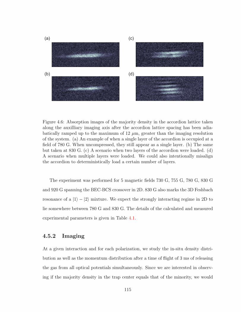
(a) (c)

(b) (d)

Figure 4.6: Absorption images of the majority density in the accordion lattice takenalong the auxilliary imaging axis after the accordion lattice spacing has been adia-batically ramped up to the maximum of 12 µm, greater than the imaging resolutionof the system. (a) An example of when a single layer of the accordion is occupied at afield of 780 G. When uncompressed, they still appear as a single layer. (b) The samebut taken at 830 G. (c) A scenario when two layers of the accordion were loaded. (d)A scenario when multiple layers were loaded. We could also intentionally misalignthe accordion to deterministically load a certain number of layers.

The experiment was performed for 5 magnetic fields 730 G, 755 G, 780 G, 830 G

and 920 G spanning the BEC-BCS crossover in 2D. 830 G also marks the 3D Feshbach

resonance of a |1〉 − |2〉 mixture. We expect the strongly interacting regime in 2D to

lie somewhere between 780 G and 830 G. The details of the calculated and measured

experimental parameters is given in Table 4.1.

4.5.2 Imaging

At a given interaction and for each polarization, we study the in-situ density distri-

bution as well as the momentum distribution after a time of flight of 3 ms of releasing

the gas from all optical potentials simultaneously. Since we are interested in observ-

ing if the majority density in the trap center equals that of the minority, we would

115

B(G) a2D(µm) Ecb(kHz) µ0↑(kHz) kF (µm−1) ln(kFa2D) T (nK)

730 0.0261 104.37 11.68 3.73 -2.33 179.31755 0.0598 51.56 12.39 3.84 -1.47 157.90780 0.1215 24.80 11.66 3.73 -0.79 137.69830 0.3090 5.84 12.59 3.87 0.18 145.41920 0.8994 0.83 12.27 3.82 1.23 111.75

Table 4.1: Calculated and measured parameters for the experiment. The 2D scatter-ing length a2D is obtained from Eq. 4.27. The confinement induced binding energyEcb is calculated by solving Eq. 4.28. The majority chemical potential µ0↑ is obtained

from Fermi-Dirac fits to the tail of the majority radial profile in Eq. 4.32.

ideally want to image the two states simultaneously. But imaging them together will

make it impossible to discern absorption due to each spin state separately. The other

option is to image one spin state and repeat the experiment to measure the other

spin state. The problem with the latter is that atom number fluctuations can only

be accounted for after repeating the experiment many times and requires twice the

amount of data collection. So the most efficient solution was to image both states in

the same experimental run, but separated by a short time.

In order to perform double imaging, we used a camera (Andor Neo 5.5 sCMOS)

that has a special feature called the overlap mode with global shutter where the

exposure for a frame begins while the previous frame is being read out (Fig. 4.7(a)).

The camera runs at a readout rate of 200 MHz which means that the exposure time is

set to 55.3 ms. We set the number of frames to 7 in the external exposure mode which

means that the camera waits for seven external triggers each cycle. The first trigger

starts exposure and the frame starts reading out half way through the exposure time.

The first frame is discarded. The second trigger starts exposure for frame 2 and the

imaging light resonant to state |1〉 is pulsed on for 10 µs at the end of the exposure.

At this time, a pulse is sent to the second switch (Minicircuits ZYSWA-2-50DR)

which has a short switching time of 20 ns and changes to the second VCO that is

running at the resonance for state |2〉. Thanks to the cat’s-eye setup for the high field

imaging beams (Fig. 2.11), this change in frequency of ∼ 80 MHz of the AOM does

116

not change the beam intensity and position. Finally the RF signal is sent through a

voltage variable attenuator (Minicircuits ZX73-2500M-S+) and the main I/O switch

1 to the amplifier. After only 6.4 µs from the end of the first imaging pulse, a second

imaging pulse hits the atoms. The very short time between the two pulses ensures

that no significant heating or displacement of the cloud occurs. The second frame

gets read out while the third one is exposed. Next, all traps are turned off and after

waiting for 1 s to allow for the atoms to completely escape, the same cycle is repeated

to obtain beam images for the two beams separately. Finally a seventh trigger in the

absence of the imaging light gives the frame with dark counts.

We noticed that if |1〉 was measured first, there was an effect of optically pumping

some atoms to |2〉 leading to a systematically 10-15% higher number in the second

image. To avoid that we switched the order and imaged |2〉 first. After that, imaging

of the first state had a systematic effect of ∼ 5% lower atom number of the second

state, well within the experimental fluctuations, hence it was not accounted for. To

calibrate the optical depth of the gas to the absolute density, we use the known density

of a band insulator in our optical lattice with 752 nm spacing. Examples of in-situ

and time-of-flight cloud images can be found in Fig. 4.8.

117

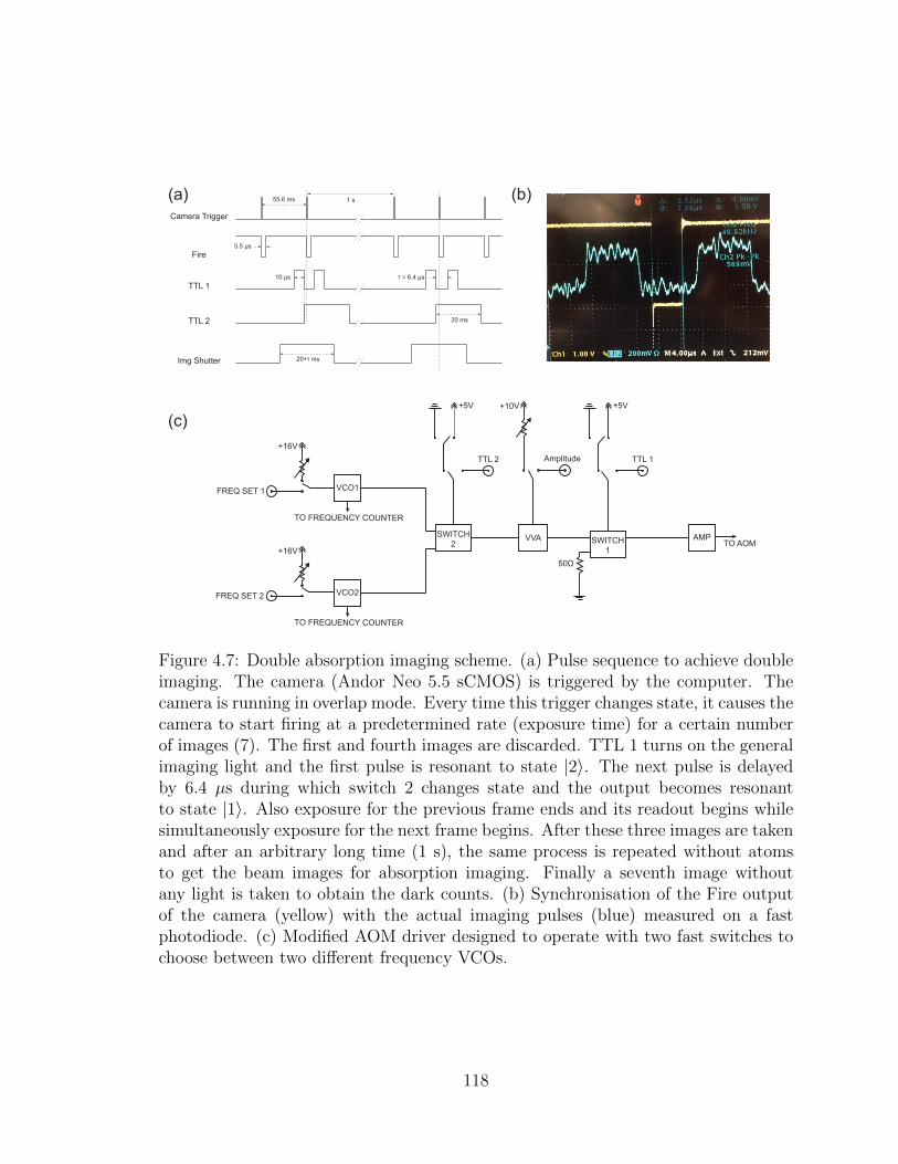
+16V

VCO2

SWITCH

1

AMPTO AOM

TO FREQUENCY COUNTER

FREQ SET 2

TTL 1

+5V

+16V

VCO1

TO FREQUENCY COUNTER

FREQ SET 1

SWITCH

2

TTL 2

+5V

VVA

+10V

Amplitude

50

Camera Trigger

Fire

TTL 1

TTL 2

Img Shutter

55.6 ms

5.5 s

10 s = 6.4 s

20+ ms

20 ms

(a) (b)

(c)

1 s

Figure 4.7: Double absorption imaging scheme. (a) Pulse sequence to achieve doubleimaging. The camera (Andor Neo 5.5 sCMOS) is triggered by the computer. Thecamera is running in overlap mode. Every time this trigger changes state, it causes thecamera to start firing at a predetermined rate (exposure time) for a certain numberof images (7). The first and fourth images are discarded. TTL 1 turns on the generalimaging light and the first pulse is resonant to state |2〉. The next pulse is delayedby 6.4 µs during which switch 2 changes state and the output becomes resonantto state |1〉. Also exposure for the previous frame ends and its readout begins whilesimultaneously exposure for the next frame begins. After these three images are takenand after an arbitrary long time (1 s), the same process is repeated without atomsto get the beam images for absorption imaging. Finally a seventh image withoutany light is taken to obtain the dark counts. (b) Synchronisation of the Fire outputof the camera (yellow) with the actual imaging pulses (blue) measured on a fastphotodiode. (c) Modified AOM driver designed to operate with two fast switches tochoose between two different frequency VCOs.

118

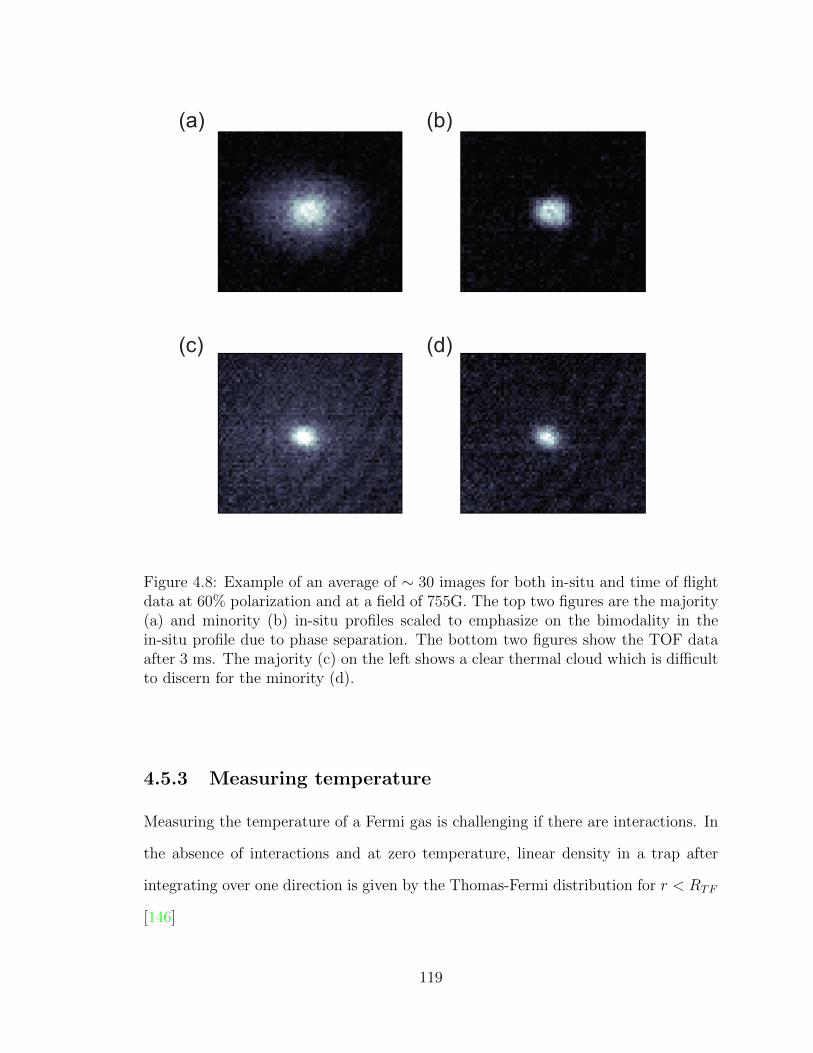
(a)

(c)

(b)

(d)

Figure 4.8: Example of an average of ∼ 30 images for both in-situ and time of flightdata at 60% polarization and at a field of 755G. The top two figures are the majority(a) and minority (b) in-situ profiles scaled to emphasize on the bimodality in thein-situ profile due to phase separation. The bottom two figures show the TOF dataafter 3 ms. The majority (c) on the left shows a clear thermal cloud which is difficultto discern for the minority (d).

4.5.3 Measuring temperature

Measuring the temperature of a Fermi gas is challenging if there are interactions. In

the absence of interactions and at zero temperature, linear density in a trap after

integrating over one direction is given by the Thomas-Fermi distribution for r < RTF

[146]

119

n(r) =8N

3πRTF

(1− r2

R2TF

)3/2

(4.29)

where, RTF =√

2EF/mω2r is the Thomas-Fermi radius. Above RTF , n=0. Now

at finite temperatures, if the gas is nearly an ideal Fermi gas, then the density profile

can be written as

n(r) = −√mωr2πh

(kBT

hωr

)3/2

Li3/2

(−e

β

(µ−mω

2rr

2

2

))(4.30)

where, Li3/2 is the polylog function of order 3/2. Finally for an interacting Fermi

gas at finite temperature, one can use a virial expansion of the phase space density

[147, 114, 148, 149].

n(r)λ2dB = log(1 + eβ(µ−V (r))) + 2b2e

2β(µ−V (r)) + 3b3e3β(µ−V (r)) + ... (4.31)

where, λdB is the thermal de-Broglie wavelength√

2πh2β/m and bi’s are the virial

coefficients. If we focus on the tail of the distribution where the density of fermions

is small and the interactions negligible, then the higher orders can be neglected and

one finds

n(r) =m

2πh2βlog

(1 + e

β

(µ−mω

2rr

2

2

))(4.32)

If the cloud is non interacting by virtue of being spin polarized, then one can

perform a fit on the local density n(r) starting at the tail of the distribution to obtain

the two unknown quantities, β and µ. In our experiment, we vary the polarization

of the cloud from balanced (P = 0) to almost fully polarized (P → 1). We take the

majority density for the cases with high polarization and perform the above mentioned

fit to only the tail (Fig. 4.9(a)). We notice that a Fermi-Dirac fit to the tail when

120

extrapolated to the entire cloud, deviates significantly from the actual density. This

is the reason why a balanced cloud can not be used to measure temperature unless

the virial coefficients (bi’s) have been taken into account.n(r

) (x

10

12 m

-2)

Radial position (µm)

0

0.5

1

1.5

2

2.5

0 20 40 60 80

kBT

/µ

0

EB/E

F

Field (G)

0

0.1

0.2

0 2 4 6

920 780 755 730(a) (b)

T/T

0

F a

nd k

BT

/µ0

Global Polarization P

0

0.1

0.2

0 0.2 0.4 0.6 0.8 1

(c)

Figure 4.9: Obtaining temperature from tail fit to cloud. (a) Fermi-Dirac fit to thefully-polarized tail of a majority profile to obtain temperature. Data depicted forP = 0.48 at 780 G. The majority density n↑(r) is shown in yellow and the minoritydensity n↓(r) in red. The black solid line is the fit to the majority density usingthe expression in Eq. (4.32) beyond the Thomas-Fermi radius of the minority cloud.The black dotted line is the fit extrapolated to the trap center. (b) Interactiondependence of kBT/µ0↑. The temperature (T ) and the majority chemical potential(µ0↑) are obtained from a Fermi-Dirac fit to the fully-polarized region of the cloud.(c) Polarization dependence of kBT/µ0↑ (red diamonds) and T/T 0

F (blue diamonds)for the 755 G dataset. kBT/µ0↑ stays essentially constant over the whole polarizationrange while T/T 0

F drops towards the balanced regime due to increased density in thecenter of the cloud.

A Fermi-Dirac fit to the tail of the radial majority density profile yields T/TF =

kBT/µ0↑ = 0.18(5) independent of polarization, and only weakly dependent on the

Feshbach field (Fig. 4.9(b) and (c)). An alternate definition of a temperature scale is

121

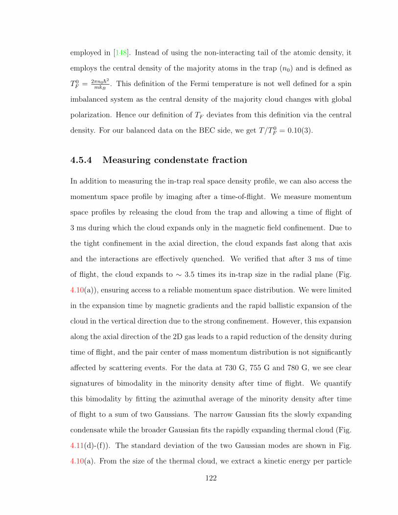
employed in [148]. Instead of using the non-interacting tail of the atomic density, it

employs the central density of the majority atoms in the trap (n0) and is defined as

T 0F = 2πn0h

2

mkB. This definition of the Fermi temperature is not well defined for a spin

imbalanced system as the central density of the majority cloud changes with global

polarization. Hence our definition of TF deviates from this definition via the central

density. For our balanced data on the BEC side, we get T/T 0F = 0.10(3).

4.5.4 Measuring condenstate fraction

In addition to measuring the in-trap real space density profile, we can also access the

momentum space profile by imaging after a time-of-flight. We measure momentum

space profiles by releasing the cloud from the trap and allowing a time of flight of

3 ms during which the cloud expands only in the magnetic field confinement. Due to

the tight confinement in the axial direction, the cloud expands fast along that axis

and the interactions are effectively quenched. We verified that after 3 ms of time

of flight, the cloud expands to ∼ 3.5 times its in-trap size in the radial plane (Fig.

4.10(a)), ensuring access to a reliable momentum space distribution. We were limited

in the expansion time by magnetic gradients and the rapid ballistic expansion of the

cloud in the vertical direction due to the strong confinement. However, this expansion

along the axial direction of the 2D gas leads to a rapid reduction of the density during

time of flight, and the pair center of mass momentum distribution is not significantly

affected by scattering events. For the data at 730 G, 755 G and 780 G, we see clear

signatures of bimodality in the minority density after time of flight. We quantify

this bimodality by fitting the azimuthal average of the minority density after time

of flight to a sum of two Gaussians. The narrow Gaussian fits the slowly expanding

condensate while the broader Gaussian fits the rapidly expanding thermal cloud (Fig.

4.11(d)-(f)). The standard deviation of the two Gaussian modes are shown in Fig.

4.10(a). From the size of the thermal cloud, we extract a kinetic energy per particle

122

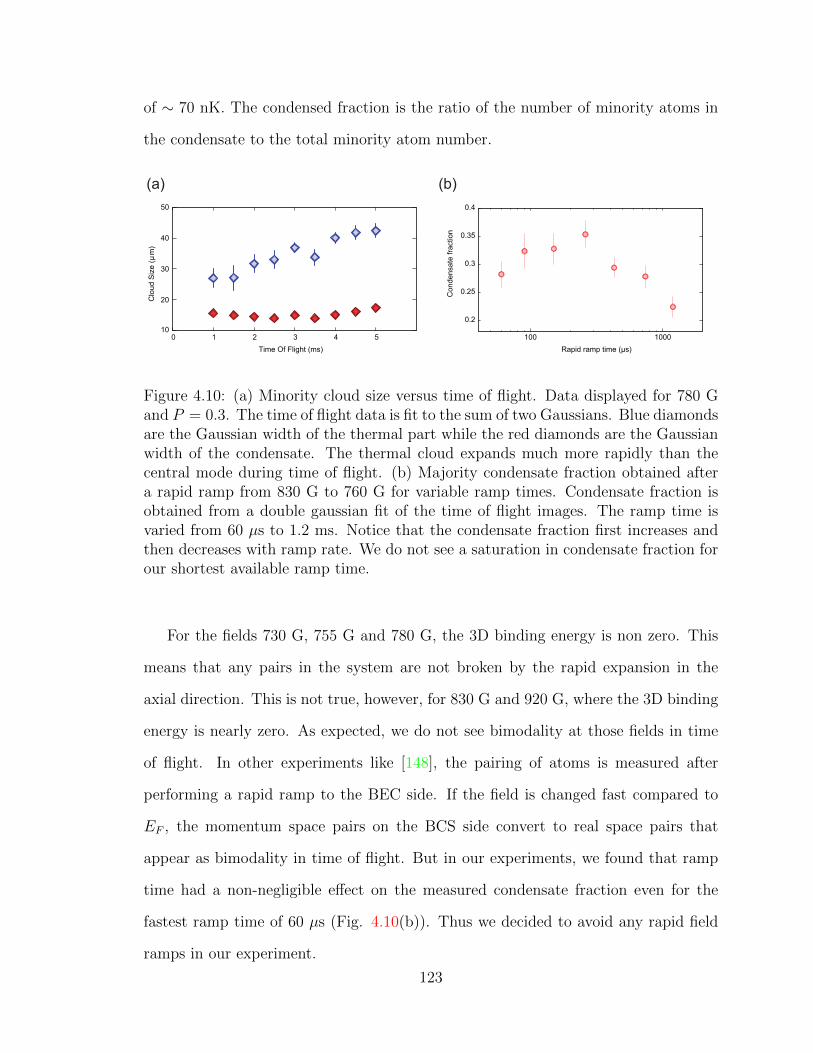
of ∼ 70 nK. The condensed fraction is the ratio of the number of minority atoms in

the condensate to the total minority atom number.C

loud

Siz

e (µ

m)

Time Of Flight (ms)

10

20

30

40

50

0 1 2 3 4 5

(a) (b)

0.2

0.25

0.3

0.35

0.4

100 1000

Con

dens

ate

fract

ion

Rapid ramp time (μs)

Figure 4.10: (a) Minority cloud size versus time of flight. Data displayed for 780 Gand P = 0.3. The time of flight data is fit to the sum of two Gaussians. Blue diamondsare the Gaussian width of the thermal part while the red diamonds are the Gaussianwidth of the condensate. The thermal cloud expands much more rapidly than thecentral mode during time of flight. (b) Majority condensate fraction obtained aftera rapid ramp from 830 G to 760 G for variable ramp times. Condensate fraction isobtained from a double gaussian fit of the time of flight images. The ramp time isvaried from 60 µs to 1.2 ms. Notice that the condensate fraction first increases andthen decreases with ramp rate. We do not see a saturation in condensate fraction forour shortest available ramp time.

For the fields 730 G, 755 G and 780 G, the 3D binding energy is non zero. This

means that any pairs in the system are not broken by the rapid expansion in the

axial direction. This is not true, however, for 830 G and 920 G, where the 3D binding

energy is nearly zero. As expected, we do not see bimodality at those fields in time

of flight. In other experiments like [148], the pairing of atoms is measured after

performing a rapid ramp to the BEC side. If the field is changed fast compared to

EF , the momentum space pairs on the BCS side convert to real space pairs that

appear as bimodality in time of flight. But in our experiments, we found that ramp

time had a non-negligible effect on the measured condensate fraction even for the

fastest ramp time of 60 µs (Fig. 4.10(b)). Thus we decided to avoid any rapid field

ramps in our experiment.

123

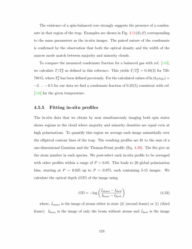
The existence of a spin-balanced core strongly suggests the presence of a conden-

sate in that region of the trap. Examples are shown in Fig. 4.11(d)-(f) corresponding

to the same parameters as the in-situ images. The paired nature of the condensate

is confirmed by the observation that both the optical density and the width of the

narrow mode match between majority and minority clouds.

To compare the measured condensate fraction for a balanced gas with ref. [148],

we calculate T/T 0F as defined in this reference. This yields T/T 0

F = 0.10(3) for 730-

780 G, where T 0F has been defined previously. For the calculated values of ln (kFa2D) =

−2 . . .− 0.5 for our data we find a condensate fraction of 0.25(5) consistent with ref.

[148] for the given temperature.

4.5.5 Fitting in-situ profiles

The in-situ data that we obtain by near simultaneously imaging both spin states

shows regions in the cloud where majority and minority densities are equal even at

high polarizations. To quantify this region we average each image azimuthally over

the elliptical contour lines of the trap. The resulting profiles are fit to the sum of a

one-dimensional Gaussian and the Thomas-Fermi profile (Eq. 4.29). The fits give us

the atom number in each species. We post-select each in-situ profile to be averaged

with other profiles within a range of P = 0.05. This leads to 20 global polarization

bins, starting at P = 0.025 up to P = 0.975, each containing 5-15 images. We

calculate the optical depth (OD) of the image using

OD = −log

(Iatoms − IdarkIbeam − Idark

)(4.33)

where, Iatoms is the image of atoms either in state |2〉 (second frame) or |1〉 (third

frame). Ibeam is the image of only the beam without atoms and Idark is the image

124

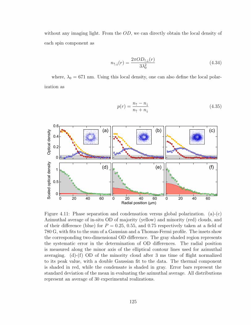
without any imaging light. From the OD, we can directly obtain the local density of

each spin component as

n↑,↓(r) =2πOD↑,↓(r)

3λ20

(4.34)

where, λ0 = 671 nm. Using this local density, one can also define the local polar-

ization as

p(r) =n↑ − n↓n↑ + n↓

(4.35)

Opt

ical

den

sity

0

0.2

0.4

0.6

Radial position (μm)

Sca

led

optic

al d

ensi

ty

0 20 40 60 0 20 40 60 0 20 40 60

(a) (b) (c)

(d) (e) (f)

0

0.5

1

Figure 4.11: Phase separation and condensation versus global polarization. (a)-(c)Azimuthal average of in-situ OD of majority (yellow) and minority (red) clouds, andof their difference (blue) for P = 0.25, 0.55, and 0.75 respectively taken at a field of780 G, with fits to the sum of a Gaussian and a Thomas-Fermi profile. The insets showthe corresponding two-dimensional OD difference. The gray shaded region representsthe systematic error in the determination of OD differences. The radial positionis measured along the minor axis of the elliptical contour lines used for azimuthalaveraging. (d)-(f) OD of the minority cloud after 3 ms time of flight normalizedto its peak value, with a double Gaussian fit to the data. The thermal componentis shaded in red, while the condensate is shaded in gray. Error bars represent thestandard deviation of the mean in evaluating the azimuthal average. All distributionsrepresent an average of 30 experimental realizations.

125

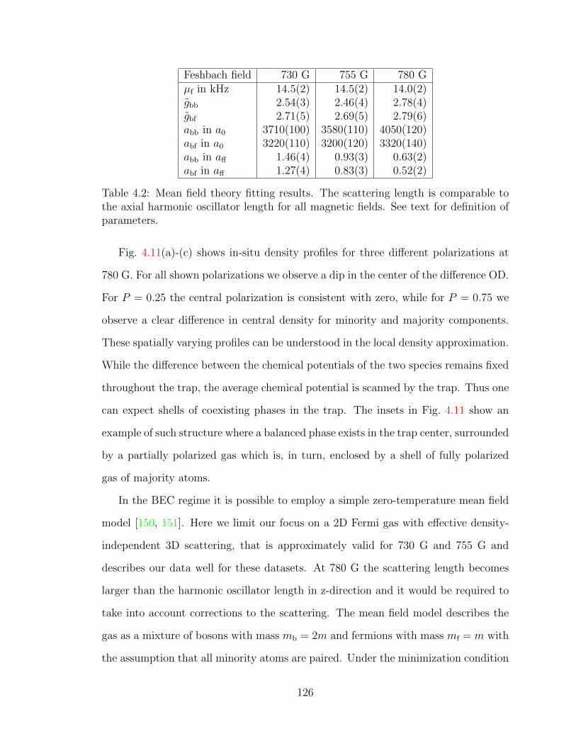
Feshbach field 730 G 755 G 780 Gµf in kHz 14.5(2) 14.5(2) 14.0(2)gbb 2.54(3) 2.46(4) 2.78(4)gbf 2.71(5) 2.69(5) 2.79(6)abb in a0 3710(100) 3580(110) 4050(120)abf in a0 3220(110) 3200(120) 3320(140)abb in aff 1.46(4) 0.93(3) 0.63(2)abf in aff 1.27(4) 0.83(3) 0.52(2)

Table 4.2: Mean field theory fitting results. The scattering length is comparable tothe axial harmonic oscillator length for all magnetic fields. See text for definition ofparameters.

Fig. 4.11(a)-(c) shows in-situ density profiles for three different polarizations at

780 G. For all shown polarizations we observe a dip in the center of the difference OD.

For P = 0.25 the central polarization is consistent with zero, while for P = 0.75 we

observe a clear difference in central density for minority and majority components.

These spatially varying profiles can be understood in the local density approximation.

While the difference between the chemical potentials of the two species remains fixed

throughout the trap, the average chemical potential is scanned by the trap. Thus one

can expect shells of coexisting phases in the trap. The insets in Fig. 4.11 show an

example of such structure where a balanced phase exists in the trap center, surrounded

by a partially polarized gas which is, in turn, enclosed by a shell of fully polarized

gas of majority atoms.

In the BEC regime it is possible to employ a simple zero-temperature mean field

model [150, 151]. Here we limit our focus on a 2D Fermi gas with effective density-

independent 3D scattering, that is approximately valid for 730 G and 755 G and

describes our data well for these datasets. At 780 G the scattering length becomes

larger than the harmonic oscillator length in z-direction and it would be required to

take into account corrections to the scattering. The mean field model describes the

gas as a mixture of bosons with mass mb = 2m and fermions with mass mf = m with

the assumption that all minority atoms are paired. Under the minimization condition

126

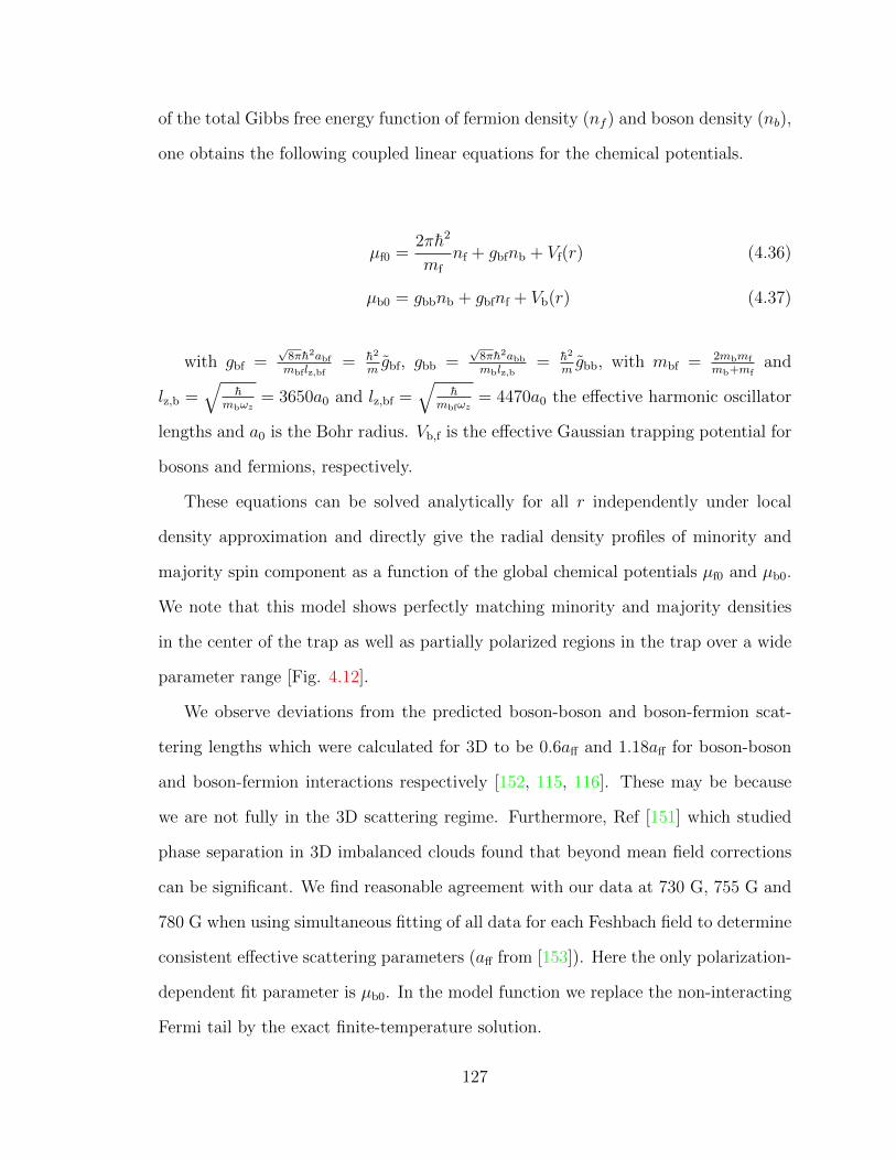
of the total Gibbs free energy function of fermion density (nf ) and boson density (nb),

one obtains the following coupled linear equations for the chemical potentials.

µf0 =2πh2

mf

nf + gbfnb + Vf(r) (4.36)

µb0 = gbbnb + gbfnf + Vb(r) (4.37)

with gbf =√

8πh2abf

mbflz,bf= h2

mgbf, gbb =

√8πh2abb

mblz,b= h2

mgbb, with mbf = 2mbmf

mb+mfand

lz,b =√

hmbωz

= 3650a0 and lz,bf =√

hmbfωz

= 4470a0 the effective harmonic oscillator

lengths and a0 is the Bohr radius. Vb,f is the effective Gaussian trapping potential for

bosons and fermions, respectively.

These equations can be solved analytically for all r independently under local

density approximation and directly give the radial density profiles of minority and

majority spin component as a function of the global chemical potentials µf0 and µb0.

We note that this model shows perfectly matching minority and majority densities

in the center of the trap as well as partially polarized regions in the trap over a wide

parameter range [Fig. 4.12].

We observe deviations from the predicted boson-boson and boson-fermion scat-

tering lengths which were calculated for 3D to be 0.6aff and 1.18aff for boson-boson

and boson-fermion interactions respectively [152, 115, 116]. These may be because

we are not fully in the 3D scattering regime. Furthermore, Ref [151] which studied

phase separation in 3D imbalanced clouds found that beyond mean field corrections

can be significant. We find reasonable agreement with our data at 730 G, 755 G and

780 G when using simultaneous fitting of all data for each Feshbach field to determine

consistent effective scattering parameters (aff from [153]). Here the only polarization-

dependent fit parameter is µb0. In the model function we replace the non-interacting

Fermi tail by the exact finite-temperature solution.

127

0

1

2

3

0 20 40 60Minor axis radial position r (µ m)

0 20 40 60

n(r)

(x10

12 m

-2)

(a) (b)

Figure 4.12: Example mean field theory fits. Data displayed for 755 G and P = 0.2 (a)and P = 0.8 (b) with interaction parameters given in table 4.2. The majority (nf+nb)is shown in yellow and the minority (nb) in red, points and line are experiment andtheory, respectively.

4.5.6 Extracting critical polarization Pc

Fig. 4.13 displays in-situ OD difference profiles in two-dimensions as a function of

interactions (rows) and global polarization (columns). The central polarization p(0)

is defined as the local polarization p(r) averaged over a 5 µm radius central disk of

the trap. It can be viewed as an indicator of phase separation in an imbalanced cloud.

The chemical potential of the fermions in the trap can be written as

µ↑,↓ = µ0↑,↓ −1

2mωxωyr

2 (4.38)

where, µ0↑,↓ is the chemical potential in the trap center and ωx,y arw the radial

confinements due to the trap. Now since the two spin states ↑ and ↓ experience the

same trap frequency, the chemical potential difference between the two states is

∆µ = µ0↑ − µ0↓ (4.39)

128

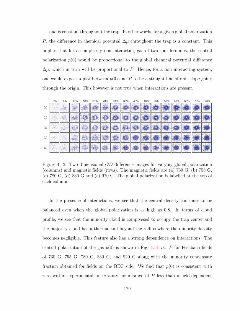
and is constant throughout the trap. In other words, for a given global polarization

P , the difference in chemical potential ∆µ throughout the trap is a constant. This

implies that for a completely non interacting gas of two-spin fermions, the central

polarization p(0) would be proportional to the global chemical potential difference

∆µ, which in turn will be proportional to P . Hence, for a non interacting system,

one would expect a plot between p(0) and P to be a straight line of unit slope going

through the origin. This however is not true when interactions are present.

(a)

(b)

(c)

(d)

(e)

3% 8% 13% 18% 23% 28% 33% 38% 43% 48% 53% 58% 63% 68% 73% 78%

Figure 4.13: Two dimensional OD difference images for varying global polarization(columns) and magnetic fields (rows). The magnetic fields are (a) 730 G, (b) 755 G,(c) 780 G, (d) 830 G and (e) 920 G. The global polarization is labelled at the top ofeach column.

In the presence of interactions, we see that the central density continues to be

balanced even when the global polarization is as high as 0.8. In terms of cloud

profile, we see that the minority cloud is compressed to occupy the trap center and

the majority cloud has a thermal tail beyond the radius where the minority density

becomes negligible. This feature also has a strong dependence on interactions. The

central polarization of the gas p(0) is shown in Fig. 4.14 vs. P for Feshbach fields

of 730 G, 755 G, 780 G, 830 G, and 920 G along with the minority condensate

fraction obtained for fields on the BEC side. We find that p(0) is consistent with

zero within experimental uncertainty for a range of P less than a field-dependent

129

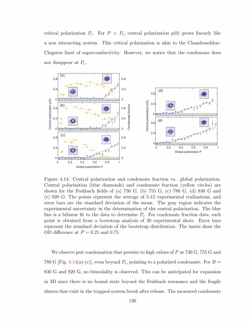
critical polarization Pc. For P > Pc, central polarization p(0) grows linearly like

a non interacting system. This critical polarization is akin to the Chandrasekhar-

Clogston limit of superconductivity. However, we notice that the condensate does

not disappear at Pc.

Global polarization P

0

0.4

0.8

0 0.2 0.4 0.6 0.8 1

0

0.4

0.8

Centr

al pola

rization p

(0)

Conden

sate

fra

ction

0

0.4

0.8

0

0.4

0.8

0

0.4

0.8

0

0.4

0.8

0

0.4

0.8

0

0.4

0.8

(a)

(b)

(c)

(d)

(e)

Centr

al pola

rization p

(0)

Global polarization P

0 0.2 0.4 0.6 0.8 1

Figure 4.14: Central polarization and condensate fraction vs. global polarization.Central polarization (blue diamonds) and condensate fraction (yellow circles) areshown for the Feshbach fields of (a) 730 G, (b) 755 G, (c) 780 G, (d) 830 G and(e) 920 G. The points represent the average of 5-15 experimental realizations, anderror bars are the standard deviation of the mean. The gray region indicates theexperimental uncertainty in the determination of the central polarization. The blueline is a bilinear fit to the data to determine Pc. For condensate fraction data, eachpoint is obtained from a bootstrap analysis of 30 experimental shots. Error barsrepresent the standard deviation of the bootstrap distribution. The insets show theOD difference at P = 0.25 and 0.75

We observe pair condensation that persists to high values of P at 730 G, 755 G and

780 G [Fig. 4.14(a)-(c)], even beyond Pc, pointing to a polarized condensate. For B =

830 G and 920 G, no bimodality is observed. This can be anticipated for expansion

in 3D since there is no bound state beyond the Feshbach resonance and the fragile

dimers that exist in the trapped system break after release. The measured condensate

130

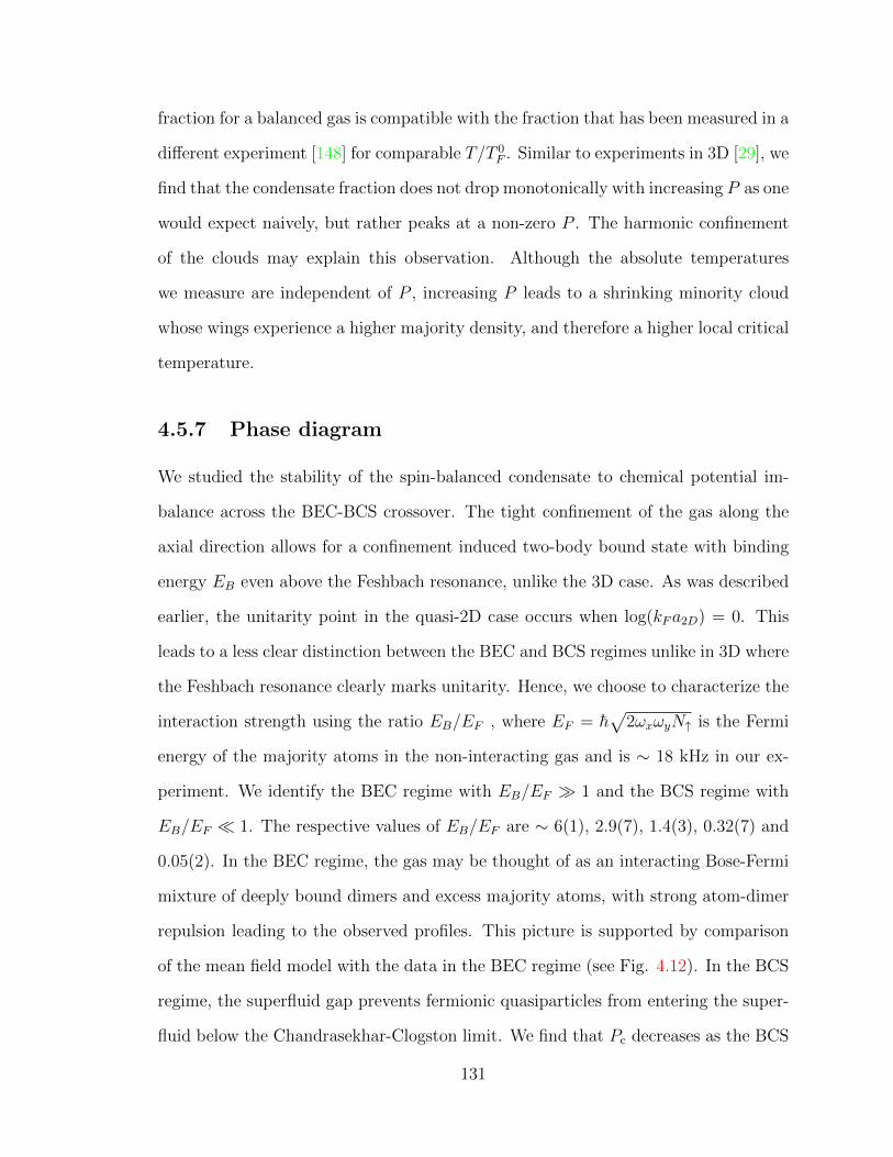
fraction for a balanced gas is compatible with the fraction that has been measured in a

different experiment [148] for comparable T/T 0F . Similar to experiments in 3D [29], we

find that the condensate fraction does not drop monotonically with increasing P as one

would expect naively, but rather peaks at a non-zero P . The harmonic confinement

of the clouds may explain this observation. Although the absolute temperatures

we measure are independent of P , increasing P leads to a shrinking minority cloud

whose wings experience a higher majority density, and therefore a higher local critical

temperature.

4.5.7 Phase diagram

We studied the stability of the spin-balanced condensate to chemical potential im-

balance across the BEC-BCS crossover. The tight confinement of the gas along the

axial direction allows for a confinement induced two-body bound state with binding

energy EB even above the Feshbach resonance, unlike the 3D case. As was described

earlier, the unitarity point in the quasi-2D case occurs when log(kFa2D) = 0. This

leads to a less clear distinction between the BEC and BCS regimes unlike in 3D where

the Feshbach resonance clearly marks unitarity. Hence, we choose to characterize the

interaction strength using the ratio EB/EF , where EF = h√

2ωxωyN↑ is the Fermi

energy of the majority atoms in the non-interacting gas and is ∼ 18 kHz in our ex-

periment. We identify the BEC regime with EB/EF 1 and the BCS regime with

EB/EF 1. The respective values of EB/EF are ∼ 6(1), 2.9(7), 1.4(3), 0.32(7) and

0.05(2). In the BEC regime, the gas may be thought of as an interacting Bose-Fermi

mixture of deeply bound dimers and excess majority atoms, with strong atom-dimer

repulsion leading to the observed profiles. This picture is supported by comparison

of the mean field model with the data in the BEC regime (see Fig. 4.12). In the BCS

regime, the superfluid gap prevents fermionic quasiparticles from entering the super-

fluid below the Chandrasekhar-Clogston limit. We find that Pc decreases as the BCS

131

limit is approached as summarized in Fig. 4.15(a). Our observed critical polarization

is consistent with a previous measurement [34] for comparable values of EB/EF .C

ritical P

ola

rizatio

n P

c

EB/EF

Field (G)

0

0.2

0.4

0.6

0.8

1

0.1 1 10

920 830 780 755 730

Phase separated

BEC BCS

0

0.2

0.4

0.6

0.8

0

0.2

0.4

0.6

0.8

0 0.2 0.4 0.6 0.8 0 0.2 0.4 0.6 0.8

Radia

l d

ista

nce (

r/R

)T

F

Global polarization P

0 0.2 0.4 0.6 0.8 1 p(r)

(b) (c)

(d) (e)

E /E = 6B F E /E = 2.9B F

E /E = 1.4B F E /E = 0.3B F

(a)

Figure 4.15: (a) Critical polarization (Pc) for phase separation vs. EB/EF (log-scale). The global polarization at which phase separation ends is extracted from abilinear fit to the central polarization data in Fig. 4.14 (red diamonds). Correspondingmagnetic fields for these points are shown on the secondary x-axis. For comparison,we extracted two points from the data of ref. [34] (blue squares). The error barsare given by the fit uncertainty. Phase diagram of an imbalanced 2D Fermi gas forfour different interactions determined by the Feshbach fields (b) 730 G, (c) 755 G,(d) 780 G and (e) 830 G. The corresponding interaction strengths EB/EF are shownin the top-right corner of each panel. The color indicates the local polarization of thegas in the trap p(r) as a function of the scaled position in the trap r/RTF↑ and theglobal polarization P . We distinguish three different phases: a balanced condensate(red), a partially polarized phase (white to gray) and a fully polarized normal gas(blue).

Fig. 4.15(b)-(e) shows an experimental phase diagram of a spin-imbalanced 2D

Fermi gas for four different values of the interaction strength EB/EF . These phase

diagrams show the local polarization p(r) as a function of the global polarization P

and the position in the trap r scaled by the Thomas-Fermi radius of a fully polarized

gas RTF↑, defined as mωxωyR2TF↑/2 = µ0↑. The global polarization P is the experi-

mental parameter that determines the chemical potential difference h = (µ↑ − µ↓)/2,

while r fixes the average local chemical potential µ = (µ↑ + µ↓)/2, so we can inter-

pret these diagrams as “µ− h” phase diagrams expressed in terms of experimentally

132

measured quantities. The partially polarized phase occupying the part of the phase

diagram between the balanced condensate and the fully polarized normal gas and

depending on EB/EF may be a Sarma phase induced by quantum or thermal fluctu-

ations, an FFLO phase or a Fermi liquid phase.

Unlike the 3D case [151], we have not observed discontinuities in the polarization

or density profiles. Zero temperature phase diagrams in refs. [131, 132, 129] predict

a first order phase transition between the superfluid and normal phases driven by the

change in the average local chemical potential in the trap. This would be manifested

by a sudden jump of the local polarization from zero in the superfluid to a finite

polarization in the normal phase. In 3D, the first order transition only occurs for

temperatures below the tricritical point [103]. If such a tricritical point exists in 2D,

it is possible that the temperature of our clouds is not low enough to observe the

first order transition or that the one-dimensional nature of the interface between the

superfluid and normal phases makes it very susceptible to fluctuations that smear

out discontinuities when averaging over trap contour lines. We also note that strong

quantum fluctuations in 2D can in principle drive the superfluid to normal transition

continuous [135].

133

Chapter 5

Quantum gas microscopy of an

attractive Fermi–Hubbard system

5.1 The Fermi-Hubbard model

The Fermi-Hubbard model is a fundamental model in condensed matter physics that

describes the behavior of strongly correlated fermions in a lattice [154, 155, 156].

It was originally formulated to describe electrons in solid state materials. The key

features of this model are fermions in two spin states ↑ and ↓, hopping between

neighboring lattice sites (t) and an on-site interaction between fermions of opposite

spins (U). To see how one arrives at the Hubbard Hamiltonian, one must start by

trying to describe electrons in solids. These electrons have a kinetic energy given by

their momentum pi, the periodic lattice potential VL and the Coulomb interaction

between them VC(r − r′). We work under the assumption that the ionic lattice is

stationary and only the electrons move. Then the Hamiltonian is given by

H =N∑i=1

(p2i

2m+ VL(ri)

)+∑r6=r′

VC(r− r′) (5.1)

134

We first make a mean field approximation to the above Hamiltonian. In the limit

of large N and adding one more electron to the system, this electron does not see the

ionic background due to an effective screening by the rest of the electrons. In second

quantized form in the basis of Wannier functions, the Hamiltonian can be written as

H =∑

α,r,r′,σ

tαr,r′c†αr,σcαr′,σ +

1

2

∑α,β,γ,δ,r,r′,r′′,r′′′

Uα,β,γ,δr,r′,r′′,r′′′c

†αr,↑c

†βr′,↓cγr′′,↓cδr′′′,↑ + h.c. (5.2)

where, α, β, γ and δ are Bloch band indices, σ is the spin index that can be either

↑ or ↓ and c†r,σ and cr,σ are the fermionic creation and annihilation operators. Here

we note that hopping matrix elements only exist within the same Bloch band and the

interaction parameter Uα..r.. between bands and sites is given by an overlap integral and

are similar to the ones described in appendix D. Next we consider a more practical

regime, when the interactions are strong but of a short range, a scenario characteristic

for transition and rare earth metals. In addition, it is sufficient to describe physics in

a single band α = 1 of the model knowing that the effect of higher bands can be taken

into account later. Furthermore, we can assume that the system can be described in a

tight binding approximation, where the electrons are strongly localized around a site.

In that case, we can assume the hopping matrix element is only nearest neighbor.

Under all these assumptions, we finally arive at the Fermi-Hubbard Hamiltonian

H = −t∑〈r,r′〉,σ

c†r,σcr′,σ + h.c.+ U∑r

nr,↑nr,↓ (5.3)

where, 〈..〉 means that the sum is over all nearest neighbors. This is the simplest

model beyond band theory that includes many body effects and has shed light on

many interesting phenomena, including the metal to Mott insulator transitions.

In a grand-canonical description of the model, one can introduce a chemical po-

tential µ which describes the energy cost of adding an extra particle into the system.

135

In addition, we can add a term corresponding to an external Zeeman field h which

leads to an imbalance in spin.

H = −t∑〈rr′〉,σ

(c†r,σcr′,σ + c†r′,σcr,σ

)+U

∑r

nr,↑nr,↓−µ∑r,σ

nr,σ−h∑r

(nr,↑−nr,↓) (5.4)

where, the density of spin σ on lattice site r is given by the number operator

nr,σ = c†r,σcr,σ. Despite its simplicity, the Fermi-Hubbard Hamiltonian is not tractable

for physically relevant scenarios. In 1D, one can solve for the ground state exactly

using the Bethe ansatz [40]. One finds that at exactly half filling (number of fermions

equals the number of lattice sites), the 1D chain undergoes a metal-insulator transition

for U ≥ 0. In addition, for the 1D and 2D case, the Mermin-Wagner theorem [119]

states that there cannot be long range order in the system. To numerically tackle

the Hubbard model, many approaches have been used like mean-field theory [41],

quantum Monte-Carlo [42, 43, 157], numerical linked cluster expansion [44] etc.

The Fermi-Hubbard model is also one of the simplest models that is expected to

contain the same phenomenology as high Tc cuprates. It was first suggested by P. W.

Anderson that the Hubbard model (or the closely related t− J model) incorporates

the strongly correlated nature of the 3d orbital electrons due to copper spins in CuO2

planes [39]. The similarity between the phase diagrams can be seen in Fig. 5.1. More

specifically, all cuprate superconductors seem to have similar traits like they are Mott

insulating when undoped and show antiferromagnetism up to small dopings [158].

Away from half filling (doped), there is the emergence of a pseudogap regime which

finally ends in a d-wave superconducting dome below Tc. The critical temperature

Tc is maximum around an optimal doping. All these features are essentially present

in the repulsive Fermi-Hubbard phase diagram, although d-wave superfluidity is only

speculated and neither observed definitively in numerical simulations nor experiments

136

[102]. The attractive Fermi-Hubbard model, however, is much more tractable theo-

retically because its not effected by the fermionic “sign problem” at low temperatures

[159]. But the type of superfluidity it describes is s-wave and is not the same as is

known for cuprates [160]. Nonetheless, it shares some phenomological features such

as a pseudogap phase with anomalous properties [161].

Finally, the spin-imbalanced attractive gases described in the previous chapter

can also be studied in a Hubbard setting. The FFLO state described in section 4.5

is expected to be enhanced in a 2D lattice geometry compared to 2D continuum

[162]. The basic idea is still to find a pairing mechanism that can exist in a system

with spin imbalance and attractive interactions. One of the reasons why the FFLO

pairing mechanism, where Cooper pairs carry a finite center of mass momentum, can

be enhanced in lattice geometries is due to Fermi surface nesting. The 2D continuum

Fermi surface is a circle while it gets modified to a square near half-filling in the

presence of a square lattice. It is believed that this modification increases the portion

covered by the FFLO phase in the mean field phase diagram [163]. Phase diagrams for

the attractive Hubbard model have been calculated and it has been established that

the spin imbalanced Fermi liquid would be unstable towards the FFLO phase [164].

The current prediction is to have weak interactions U ≈ −4t and low temperatures

T < 0.1t that have been very hard to achieve experimentally. In addition, its relation

to a striped phase in the doped repulsive Fermi-Hubbard model has been established

[165].

137

Density n0 1 2

Tem

pera

ture

T/t

0

BI

CDW

+SF

SFSF

PG PG

VAC

0.15

0.45

0.3

(a) (b)

(c)

Figure 5.1: Fermi-Hubbard pase diagram. (a) The phase diagram of high Tc cupratesuperconductors taken from [166]. As a function of doping (going away from half fillingwith electrons or holes), all cuprate superconductors behave similarly, i.e. are Mottinsulating and have anti-ferromagnetic (AF) order when lightly doped and undergoa transition to a d-wave superconductor when sufficiently doped. (b) A sketch ofthe Fermi-Hubbard phase diagram for positive (repulsive) and negative (attractive)interactions (U) taken from [86]. On the repulsive side, one gets the physics ofMott insulators and anti-ferromagnetism while on the attractive side, one gets s-wave superfluidity and a BEC-BCS crossover. (c) Schematic phase diagram of theattractive Fermi-Hubbard model at intermediate interaction (U/t ≈ −5), indicatingpseudogap (PG), superfluid (SF), charge-density-wave (CDW) and band-insulating(BI) regimes. The critical temperature vanishes at n = 1. The temperatures achievedin the experiment (gray band) are above the BKT critical temperature but precursorcorrelations are present in the system.

138

5.2 Attractive (U < 0) or Repulsive (U > 0)?

For the reasons mentioned above and many more, the attractive Fermi-Hubbard

model would seem to be an ideal platform for studying pairing in lattice context

and exotic pairing mechanisms. Although it has been theoretically studied quite ex-

tensively, it has not received much attention from the experimental community. So far

only a few experiments with the attractive interactions have been performed. One ex-

ample is the measurement of evidence of superfluidity in 3D optical lattices [61]. The

evolution of a band insulator as the system is swept across the Feshbach resonance

showed a continuous evolution into states occupying many bands [62]. The systems

in these experiments do not fall in the category of the single band Hubbard model be-

cause of multi-band couplings and off-site interactions [167, 168, 169, 170, 171]. There

have been a few experiments with single band attractive Hubbard systems. In one

experiment, the displacement of the center-of-mass of a gas with attractive interac-

tions in a 3D lattice was measured [63]. They observed that the oscillation frequency

strongly depends on the formation of local pairs. Another experiment measured an

anomalous expansion of the cloud with increasing attractive interactions [64]. Finally,

out of equilibrium transport in Hubbard systems was measured for both attractive

and repulsive interactions [172].

In contrast, the equilibrium repulsive Fermi-Hubbard model is very well studied

experimentally. The first measurements were done with absorption imaging where

the Mott insulator was observed as a reduction in double occupancy and a gap in the

excitation spectrum [173]. The in-situ compressibility was measured in [174]. Nearest-

neighbor antiferromagnetic correlations were measured by [175, 176]. Spin sensitive

Bragg spectroscopy was further employed to reveal antiferromagnetic correlations

[177]. The equation of state for a 2D repulsive Hubbard system was measured in

[178]. With the first fermionic quantum gas microscopes a flurry of new developements

followed like the direct observation of antiferromagnetic correlations in 2D [57, 58]

139

and 1D chains [59]. More recently, long range antiferromagnetic order was observed

in [179] and the effect of spin imbalance was measured by us [60].

-4 0 4

i

-4

0

4

j

-0.2

-0.1

0

0.1

Cz

(i,j)

(a) (b)

(c) (d)

Figure 5.2: Single site images of a repulsive Fermi-Hubbard system. (a) Shows theimage of a Mott insulator (MI) while (b) is when the filling has been increased suchthat the center of the trap becomes a band insulator (BI) with a Mott insulatingring around it. Due to parity imaging of the quantum gas microscope, all doublyoccupied sites in the BI region are lost and appear empty. (c) Image of a single spinstate ↑ within a MI taken by removing all atoms in state ↓. The underlying shortrange antiferromagnetic (AFM) order can be seen as a region with a checkerboard.Image taken at U/t = 8 and T/t = 0.4. (d) Quantification of the AFM order in aspin balanced repulsive Hubbard system at half-filling. The quantity Cz(i, j) is thetwo-point correlator of the projection of spin along the z-axis for spins at sites i andj.

There is, however, a mapping between the attractive and the repulsive Hubbard

models which leads to a one-to-one correspondence between their properties and ob-

140

served phenomena [180]. On a bipartite lattice, one can define a particle-hole trans-

formation given by following mapping of the annihilation operators

cr,↓ ↔ (−1)rx+ryc†r,↓, cr,↑ ↔ cr,↑. (5.5)

Under this transformation, n↑ ↔ n↑ and n↓ ↔ 1− n↓ and the Hubbard Hamilto-

nian (Eq. 5.4) transforms to (up to a constant energy offset)

H ↔ −t∑〈rr′〉,σ

(c†r,σcr′,σ + c†r′,σcr,σ

)− U

∑r

nr,↑nr,↓ − µ′∑r,σ

nr,σ − h′∑r

(nr,↑ − nr,↓)

(5.6)

where, µ′ = h− U/2 and h′ = µ− U/2. So under this transformation, the kinetic

term remains unchanged and the chemical potential µ swaps its role with the Zeeman

field h. Most importantly, however, the sign associated with the interaction term

changes. This implies that the negative U (attractive) Hubbard maps on to the

positive U (repulsive) Hubbard.

For a spin-balanced system, h = 0. Consider first the SU(2) spin symmetry of

the problem for h = 0. The vector spin operator on site r is given by (Sxr , Syr , S

zr ),

where S±r = Sxr ± iSyr . In terms of fermionic creation and annihilation operators, the

generators of spin rotations are

S−r = c†r,↓cr,↑

S+r = (S−r )† = c†r,↑cr,↓

Szr =1

2(c†r,↑cr,↑ − c

†r,↓cr,↓) =

1

2(nr,↑ − nr,↓) (5.7)

These operators obey the usual commutation relations

141

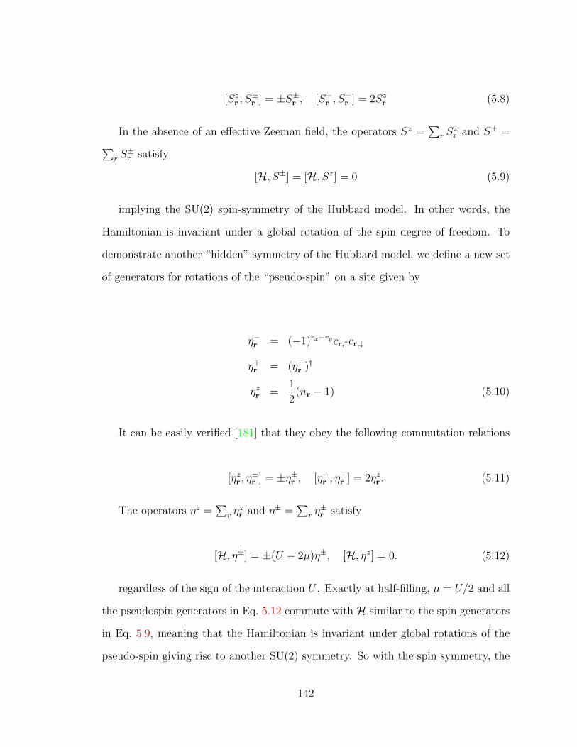
[Szr , S±r ] = ±S±r , [S+

r , S−r ] = 2Szr (5.8)

In the absence of an effective Zeeman field, the operators Sz =∑

r Szr and S± =∑

r S±r satisfy

[H, S±] = [H, Sz] = 0 (5.9)

implying the SU(2) spin-symmetry of the Hubbard model. In other words, the

Hamiltonian is invariant under a global rotation of the spin degree of freedom. To

demonstrate another “hidden” symmetry of the Hubbard model, we define a new set

of generators for rotations of the “pseudo-spin” on a site given by

η−r = (−1)rx+rycr,↑cr,↓

η+r = (η−r )†

ηzr =1

2(nr − 1) (5.10)

It can be easily verified [181] that they obey the following commutation relations

[ηzr , η±r ] = ±η±r , [η+

r , η−r ] = 2ηzr . (5.11)

The operators ηz =∑

r ηzr and η± =

∑r η±r satisfy

[H, η±] = ±(U − 2µ)η±, [H, ηz] = 0. (5.12)

regardless of the sign of the interaction U . Exactly at half-filling, µ = U/2 and all

the pseudospin generators in Eq. 5.12 commute with H similar to the spin generators

in Eq. 5.9, meaning that the Hamiltonian is invariant under global rotations of the

pseudo-spin giving rise to another SU(2) symmetry. So with the spin symmetry, the

142

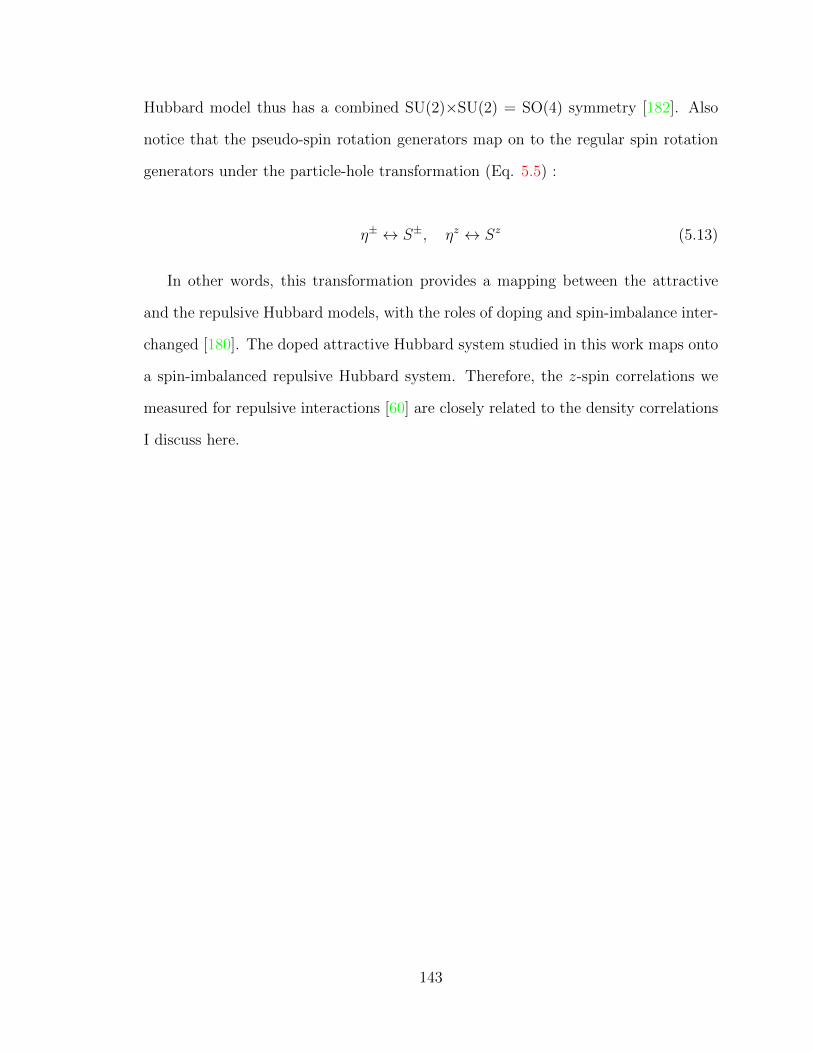
Hubbard model thus has a combined SU(2)×SU(2) = SO(4) symmetry [182]. Also

notice that the pseudo-spin rotation generators map on to the regular spin rotation

generators under the particle-hole transformation (Eq. 5.5) :

η± ↔ S±, ηz ↔ Sz (5.13)

In other words, this transformation provides a mapping between the attractive

and the repulsive Hubbard models, with the roles of doping and spin-imbalance inter-

changed [180]. The doped attractive Hubbard system studied in this work maps onto

a spin-imbalanced repulsive Hubbard system. Therefore, the z-spin correlations we

measured for repulsive interactions [60] are closely related to the density correlations

I discuss here.

143

5.3 Quantum gas microscopy

Quantum gas microscopes (QGM) bring a new advantage in the study of the Hub-

bard model. The ability to directly detect occupation on a site, with spin resolution,

implies that two point correlators can be directly measured. In addition this tech-

nique brings unprecedented signal to noise. The first QGM was actually achieved

for bosonic Rb atoms in 2009 [47]. This led to direct measurements of the bosonic

Mott insulator and the superfluid to Mott insulator transition [49]. QGMs of bosons

were subsequently realized by groups in Germany [48] and Japan [183, 184]. The first

QGM for fermionic atoms was demonstrated in 2015. They fall in two categories,

the first where electromagnetically induced transparency (EIT) cooling is employed

to cool the atoms while collecting scattered photons [50, 51]. The other category is

where Raman sideband cooling is employed for imaging [52, 53, 59]. Our experiment

falls in this latter category as described in section 3.3.

We realize the Fermi-Hubbard model using a spin-balanced degenerate mixture of

two Zeeman states (|1〉 = |↑〉 and |3〉 = |↓〉) of 6Li in an optical lattice. To create the

sample we evaporate near the 690 G Feshbach resonance. We stop the evaporation

before Feshbach molecules form and transfer the atoms to the light sheet trap where

the gas undergoes further evaporation to degeneracy at 305.4(1) G. At this field, the

scattering length is as = −889a0. Next we transfer the gas into the final trapping

geometry where the bottom beam provides radial confinement and the accordion

lattice with trapping frequency ωz = 2π× 21(1) kHz provides axial confinement. The

spin populations are balanced to within 2.1(9)%. We then load the gas into a 2D

square lattice with a 25 ms long ramp to varying depths from 4− 7.5 Er.

In addition to the scheme described above (scheme 1), we implemented another

very different scheme for preparing a lithium gas with a negative scattering length,

based on a different evaporation strategy commonly used in the lithium quantum gas

community. In this scheme 2, we perform the entire evaporation at the Feshbach

144

resonance. Three-body collisions lead to population of the molecular branch. Before

loading into the lattice, the bias field is ramped to 907 G where the scattering length

is -2800 a0. After pinning the atoms in a 55 ER lattice, we ramp the field to 725 G

where we perform a Landau-Zener sweep on an interaction-resolved transition to

the 2-3 upper branch. In order to convert the 2-3 doubles to |2〉-singles with high

efficiency, we ramp to 641 G where we apply the resonant pulses to remove |1〉 and

|3〉 atoms. This ramp is done quickly (within ∼800 µs) to avoid atom losses due to

the crossing of a narrow 2-3 Feshbach resonance around 714 G.

5.3.1 Calibrating Hubbard parameters

We calibrate our lattice depth by measuring the frequencies of the three d bands in

a deep lattice using lattice depth modulation, and compare these with a 2D band

structure calculation. This process is described in detail in Section 2.8.4. The in-

ferred depth of the lattice at which our measurements are performed is 6.2(2) ER,

where ER = 14.66 kHz. From that we obtain nearest-neighbor tunneling values

tx = 1200 Hz, ty = 1110 Hz (tx/ty = 1.08). The reduction of the lattice depth across

the cloud due to the Gaussian profile of the lattice beams leads to an increase in the

tunneling by 10% at the edge of the cloud compared to the central value. We also

calculate a non-zero but negligible diagonal tunneling t11 = 42 Hz = 0.04 tx, due to

the non-separability of the lattice.

We measure the interaction energy U at the lattice loading field of 305 G using

radio frequency spectroscopy. We transfer atoms from state |1〉 to |2〉 and resolve the

frequency shift between singly and doubly occupied sites. In the situation where a

|1〉 atom is part of a bounded pair, then one must take into account the interaction

between the |2〉 − |3〉 pair that is formed. This final state interaction can be taken

into account as

145

U13 = δUa13

a13 − a23

(5.14)

where δU is the measured difference between the singles and doublon peaks and

a13 (a23) is the scattering length at the spectroscopy field for a |1〉 − |3〉 (|2〉 − |3〉)

mixture. The measured RF spectra are shown in Fig. 5.3. When the spectra are

taken for deep lattices where tunneling is mostly supressed, we found good agreement

with tight binding estimates. For example, in Fig. 5.3(e), a lattice depth of 15 ER

and at 305 G is expected to give U = -12.81 kHz. Taking into account the final state

interaction of 2.05 for this field, we would expect |δU | = 6.25 kHz, which is very close

to the measured value (6.3 kHz). For a shallow lattice depth of 6.6 ER and 305 G

(Fig. 5.3(b)), we would expect U = -6.4 kHz, leading to an expected |δU | = 3.1 kHz.

However, we measure 2.2 kHz.

This indicates that for shallower lattices, many-body effects start influencing the

RF spectra. In general, to obtain the correct two body interaction U , the best place

to measure are isolated lattice sites. Once that condition is met, the tight binding

estimate matches that of RF spectroscopy.

The value of U determined from band structure calculations can also be modified

to include higher band corrections [185]. The resulting Hubbard interaction U is -

5.9(1) kHz for our lattice depth of 6.2(2) ER. Combining it with the tight binding

tunneling average t = 1150(50) Hz, we obtain a U/t ∼ -5.4(3).

146

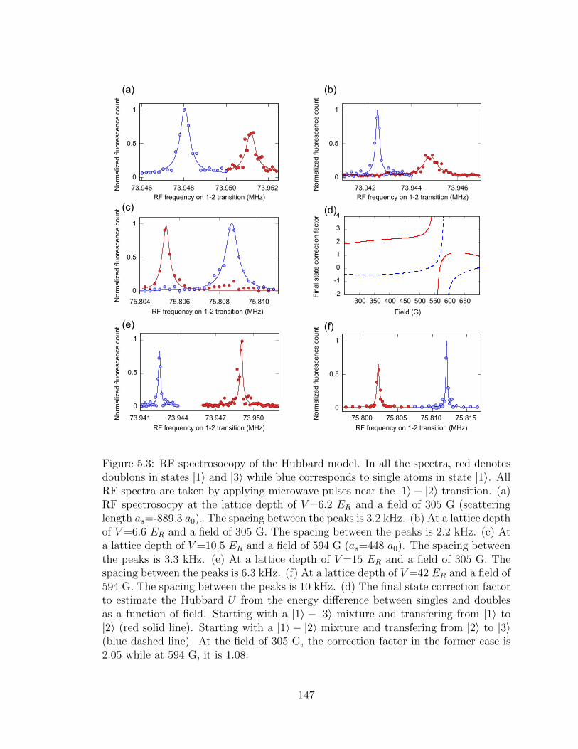
Nor

mal

ized

fluo

resc

ence

cou

nt

RF frequency on 1-2 transition (MHz)

(a)

0

0.5

1

73.946 73.948 73.950 73.952

RF frequency on 1-2 transition (MHz)75.800 75.805 75.810 75.815

RF frequency on 1-2 transition (MHz)

0

0.5

1

73.942 73.944 73.946

RF frequency on 1-2 transition (MHz)73.941 73.944 73.947 73.950

0

0.5

1

0

0.5

1

Nor

mal

ized

fluo

resc

ence

cou

nt

RF frequency on 1-2 transition (MHz)

0

0.5

1

75.804 75.806 75.808 75.810

Nor

mal

ized

fluo

resc

ence

cou

nt

(b)

(c)

(e) (f)

(d)

Nor

mal

ized

fluo

resc

ence

cou

ntN

orm

aliz

ed fl

uore

scen

ce c

ount

Fina

l sta

te c

orre

ctio

n fa

ctor

Field (G)

-2

-1

0

1

2

3

4

300 350 400 450 500 550 600 650

Figure 5.3: RF spectrosocopy of the Hubbard model. In all the spectra, red denotesdoublons in states |1〉 and |3〉 while blue corresponds to single atoms in state |1〉. AllRF spectra are taken by applying microwave pulses near the |1〉 − |2〉 transition. (a)RF spectrosocpy at the lattice depth of V=6.2 ER and a field of 305 G (scatteringlength as=-889.3 a0). The spacing between the peaks is 3.2 kHz. (b) At a lattice depthof V=6.6 ER and a field of 305 G. The spacing between the peaks is 2.2 kHz. (c) Ata lattice depth of V=10.5 ER and a field of 594 G (as=448 a0). The spacing betweenthe peaks is 3.3 kHz. (e) At a lattice depth of V=15 ER and a field of 305 G. Thespacing between the peaks is 6.3 kHz. (f) At a lattice depth of V=42 ER and a field of594 G. The spacing between the peaks is 10 kHz. (d) The final state correction factorto estimate the Hubbard U from the energy difference between singles and doublesas a function of field. Starting with a |1〉 − |3〉 mixture and transfering from |1〉 to|2〉 (red solid line). Starting with a |1〉 − |2〉 mixture and transfering from |2〉 to |3〉(blue dashed line). At the field of 305 G, the correction factor in the former case is2.05 while at 594 G, it is 1.08.

147

5.3.2 Measuring double occupancies

In the usual scheme of Raman imaging, a singly occupied lattice site produces a

fluorescence signal while atoms in a doubly occupied site are lost due to light-assisted

collisions. Thus we measure the singles density ns = n↑ + n↓ − 2n↑n↓. To gain

the full density information, one needs to measure the doubly occupied sites as well.

To measure density correlations between doubly-occupied sites, we developed a new

detection scheme (Fig. 5.4(a)). After the gas is loaded adiabatically into the optical

lattice, we pin the atoms by increasing the lattice depth to 55(1) ER in 100 µs where

tunnelling dynamics are frozen. The next step is to adiabatically ramp the field to

594 G where we perform an interaction resolved Landau-Zener sweep to selectively

transfer |1〉−|3〉 doublons to |2〉−|3〉 doublons while not effecting the |1〉 singles [173,

178]. Finally we ramp to a field of 641 G where the |2〉−|3〉 scattering length is 414 a0.

We apply resonant pushing pulses of 30 µs durations in the presence of a repulsive

interaction to remove |1〉 and |3〉 atoms, leaving behind only |2〉 atoms on sites that

originally had doublons. Since we have a relatively weak vertical confinement, the

atoms feel a cigar-shaped on-site potential. The large relative wavefunction of the

atoms on a site due to repulsive interactions and this weak vertical confinement

significantly reduces the probability of light-assisted collisions during the resonant

pulse. This procedure gives us access to the doublon density nd = n↑n↓.

The pushing pulse duration is very critical to ensure that we do not remove other

spin states with off-resonant light. Fig. 5.4(c) shows the effect of the pushing pulse

duration, resonant on state |1〉. There is no effective pushing for pulses shorter than

10 µs. But when the pulse is longer than ∼ 300 µs, we see off-resonant pushing of

state |3〉 atoms. That is why we chose a 30 µs duration for all our pushing pulses.

We can measure the efficiency of detecting doublons by analyzing the imaging

fidelity of band insulating regions in the cloud (Fig. 5.4(d)). The filling in the trap

center is saturated at two atoms per site. We perform the above-mentioned process

148

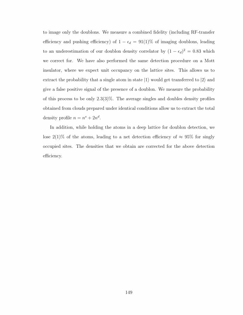
to image only the doublons. We measure a combined fidelity (including RF-transfer

efficiency and pushing efficiency) of 1 − εd = 91(1)% of imaging doublons, leading

to an underestimation of our doublon density correlator by (1 − εd)2 = 0.83 which

we correct for. We have also performed the same detection procedure on a Mott

insulator, where we expect unit occupancy on the lattice sites. This allows us to

extract the probability that a single atom in state |1〉 would get transferred to |2〉 and

give a false positive signal of the presence of a doublon. We measure the probability

of this process to be only 2.3(3)%. The average singles and doubles density profiles

obtained from clouds prepared under identical conditions allow us to extract the total

density profile n = ns + 2nd.

In addition, while holding the atoms in a deep lattice for doublon detection, we

lose 2(1)% of the atoms, leading to a net detection efficiency of ≈ 95% for singly

occupied sites. The densities that we obtain are corrected for the above detection

efficiency.

149

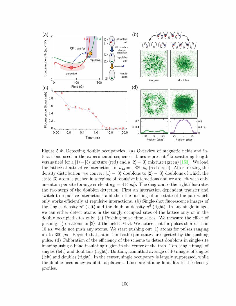
ns

Position (sites)

0

0.4

0.8

-20 0 20

Position (sites)

-20 0 20

nd

0

0.4

0.8

doublessingles

attractive

pair

repulsive

pair

remove

RF transfer +

change

interaction

single

atom

|3〉 |1〉

|3〉 |2〉

|2〉

RF transfer

-2

0

2

0 400 800

Scatt

ering length

(a

0 x

10³)

Field (G)

1-3 2-3

attractive

repulsive

(a) (b)

(c) (d)

Flu

ore

scence S

ignal (a

rb)

Time (ms)

0

0.2

0.4

0.6

0.8

1

0.001 0.01 0.1 1.0 10.0 100.0

Figure 5.4: Detecting double occupancies. (a) Overview of magnetic fields and in-teractions used in the experimental sequence. Lines represent 6Li scattering lengthversus field for a |1〉−|3〉 mixture (red) and a |2〉−|3〉 mixture (green) [153]. We loadthe lattice at attractive interactions of a13 = −889 a0 (red circle). After freezing thedensity distribution, we convert |1〉 − |3〉 doublons to |2〉 − |3〉 doublons of which thestate |3〉 atom is pushed in a regime of repulsive interactions and we are left with onlyone atom per site (orange circle at a23 = 414 a0). The diagram to the right illustratesthe two steps of the doublon detection: First an interaction dependent transfer andswitch to repulsive interactions and then the pushing of one state of the pair whichonly works efficiently at repulsive interactions. (b) Single-shot fluorescence images ofthe singles density ns (left) and the doublon density nd (right). In any single image,we can either detect atoms in the singly occupied sites of the lattice only or in thedoubly occupied sites only. (c) Pushing pulse time series. We measure the effect ofpushing |1〉 on atoms in |3〉 at the field 594 G. We notice that for pulses shorter than10 µs, we do not push any atoms. We start pushing out |1〉 atoms for pulses rangingup to 300 µs. Beyond that, atoms in both spin states are ejected by the pushingpulse. (d) Calibration of the efficiency of the scheme to detect doublons in single-siteimaging using a band insulating region in the center of the trap. Top, single image ofsingles (left) and doublons (right). Bottom, azimuthal average of 10 images of singles(left) and doubles (right). In the center, single occupancy is largely suppressed, whilethe double occupancy exhibits a plateau. Lines are atomic limit fits to the densityprofiles.

150

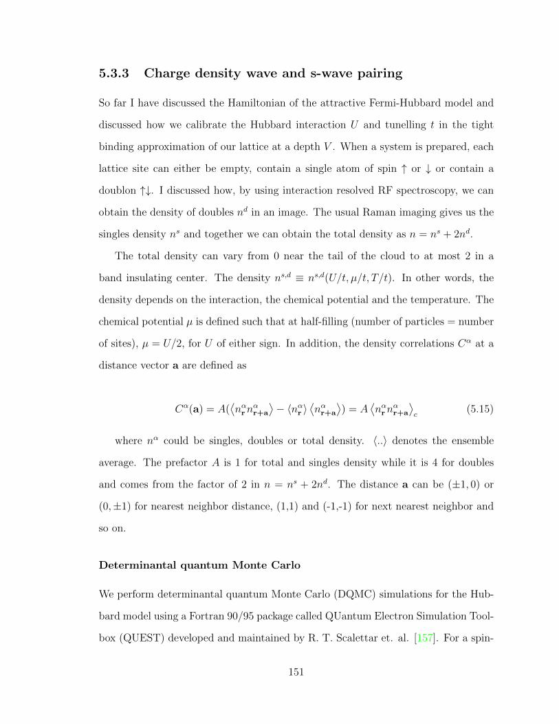
5.3.3 Charge density wave and s-wave pairing

So far I have discussed the Hamiltonian of the attractive Fermi-Hubbard model and

discussed how we calibrate the Hubbard interaction U and tunelling t in the tight

binding approximation of our lattice at a depth V . When a system is prepared, each

lattice site can either be empty, contain a single atom of spin ↑ or ↓ or contain a

doublon ↑↓. I discussed how, by using interaction resolved RF spectroscopy, we can

obtain the density of doubles nd in an image. The usual Raman imaging gives us the

singles density ns and together we can obtain the total density as n = ns + 2nd.

The total density can vary from 0 near the tail of the cloud to at most 2 in a

band insulating center. The density ns,d ≡ ns,d(U/t, µ/t, T/t). In other words, the

density depends on the interaction, the chemical potential and the temperature. The

chemical potential µ is defined such that at half-filling (number of particles = number

of sites), µ = U/2, for U of either sign. In addition, the density correlations Cα at a

distance vector a are defined as

Cα(a) = A(⟨nαrn

αr+a

⟩− 〈nαr 〉

⟨nαr+a

⟩) = A

⟨nαrn

αr+a

⟩c

(5.15)

where nα could be singles, doubles or total density. 〈..〉 denotes the ensemble

average. The prefactor A is 1 for total and singles density while it is 4 for doubles

and comes from the factor of 2 in n = ns + 2nd. The distance a can be (±1, 0) or

(0,±1) for nearest neighbor distance, (1,1) and (-1,-1) for next nearest neighbor and

so on.

Determinantal quantum Monte Carlo

We perform determinantal quantum Monte Carlo (DQMC) simulations for the Hub-

bard model using a Fortran 90/95 package called QUantum Electron Simulation Tool-

box (QUEST) developed and maintained by R. T. Scalettar et. al. [157]. For a spin-

151

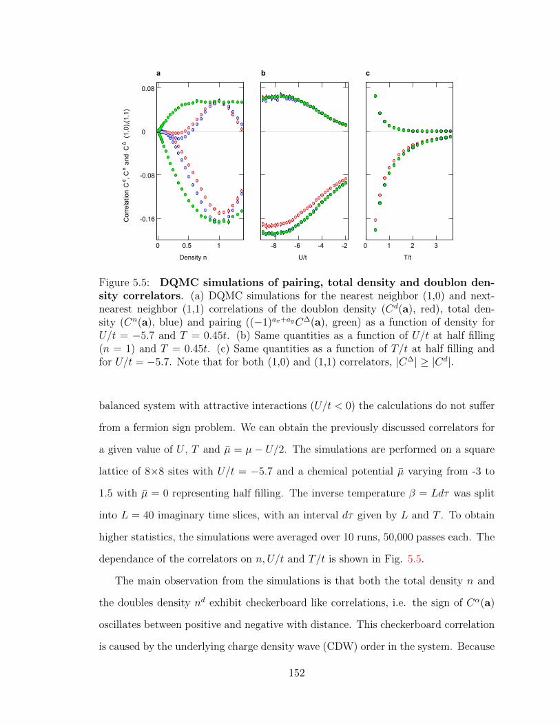
a

Cor

rela

tion

Cd ,C

n a

nd C

Δ(1

,0),(

1,1)

Density n

-0.16

-0.08

0

0.08

0 0.5 1

b

U/t

-8 -6 -4 -2

c

T/t

0 1 2 3

Figure 5.5: DQMC simulations of pairing, total density and doublon den-sity correlators. (a) DQMC simulations for the nearest neighbor (1,0) and next-nearest neighbor (1,1) correlations of the doublon density (Cd(a), red), total den-sity (Cn(a), blue) and pairing ((−1)ax+ayC∆(a), green) as a function of density forU/t = −5.7 and T = 0.45t. (b) Same quantities as a function of U/t at half filling(n = 1) and T = 0.45t. (c) Same quantities as a function of T/t at half filling andfor U/t = −5.7. Note that for both (1,0) and (1,1) correlators, |C∆| ≥ |Cd|.

balanced system with attractive interactions (U/t < 0) the calculations do not suffer

from a fermion sign problem. We can obtain the previously discussed correlators for

a given value of U , T and µ = µ− U/2. The simulations are performed on a square

lattice of 8×8 sites with U/t = −5.7 and a chemical potential µ varying from -3 to

1.5 with µ = 0 representing half filling. The inverse temperature β = Ldτ was split

into L = 40 imaginary time slices, with an interval dτ given by L and T . To obtain

higher statistics, the simulations were averaged over 10 runs, 50,000 passes each. The

dependance of the correlators on n, U/t and T/t is shown in Fig. 5.5.

The main observation from the simulations is that both the total density n and

the doubles density nd exhibit checkerboard like correlations, i.e. the sign of Cα(a)

oscillates between positive and negative with distance. This checkerboard correlation

is caused by the underlying charge density wave (CDW) order in the system. Because

152

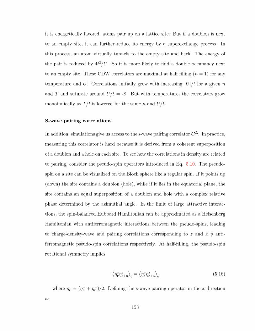
it is energetically favored, atoms pair up on a lattice site. But if a doublon is next

to an empty site, it can further reduce its energy by a superexchange process. In

this process, an atom virtually tunnels to the empty site and back. The energy of

the pair is reduced by 4t2/U . So it is more likely to find a double occupancy next

to an empty site. These CDW correlators are maximal at half filling (n = 1) for any

temperature and U . Correlations initially grow with increasing |U |/t for a given n

and T and saturate around U/t = -8. But with temperature, the correlators grow

monotonically as T/t is lowered for the same n and U/t.

S-wave pairing correlations

In addition, simulations give us access to the s-wave pairing correlator C∆. In practice,

measuring this correlator is hard because it is derived from a coherent superposition

of a doublon and a hole on each site. To see how the correlations in density are related

to pairing, consider the pseudo-spin operators introduced in Eq. 5.10. The pseudo-

spin on a site can be visualized on the Bloch sphere like a regular spin. If it points up

(down) the site contains a doublon (hole), while if it lies in the equatorial plane, the

site contains an equal superposition of a doublon and hole with a complex relative

phase determined by the azimuthal angle. In the limit of large attractive interac-

tions, the spin-balanced Hubbard Hamiltonian can be approximated as a Heisenberg

Hamiltonian with antiferromagnetic interactions between the pseudo-spins, leading

to charge-density-wave and pairing correlations corresponding to z and x, y anti-

ferromagnetic pseudo-spin correlations respectively. At half-filling, the pseudo-spin

rotational symmetry implies

⟨ηzrη

zr+a

⟩c

=⟨ηxrη

xr+a

⟩c

(5.16)

where ηxr = (η+r + η−r )/2. Defining the s-wave pairing operator in the x direction

as

153

∆xr = cr,↑cr,↓ + c†r,↓c

†r,↑ (5.17)

one concludes that the density correlations Cn(a) = 〈nrnr+a〉c = 4⟨ηzrη

zr+a

⟩c

and

pairing correlations C∆(a) =⟨∆x

r∆xr+a

⟩c

= 4⟨ηxrη

xr+a

⟩c

are equal in magnitude at

half-filling.

Deviation from half-filling introduces an effective Zeeman field along z that couples

to the pseudo-spin. This leads to canted antiferromagnetic pseudo-spin correlations,

with stronger correlations in the direction orthogonal to the field, i.e. the pairing

correlations become stronger than the density correlations. Therefore, measurement

of charge-density-wave density correlations in the attractive Hubbard model provides

a lower bound on the pairing correlations at any filling. In our experiment we measure

the more experimentally accessible quantity, the doublon density correlator Cd(a) =

4⟨ndrn

dr+a

⟩c.

154

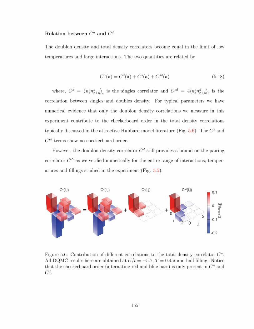
Relation between Cn and Cd

The doublon density and total density correlators become equal in the limit of low

temperatures and large interactions. The two quantities are related by

Cn(a) = Cd(a) + Cs(a) + Csd(a) (5.18)

where, Cs =⟨nsrn

sr+a

⟩c

is the singles correlator and Csd = 4〈nsrndr+a〉c is the

correlation between singles and doubles density. For typical parameters we have

numerical evidence that only the doublon density correlations we measure in this

experiment contribute to the checkerboard order in the total density correlations

typically discussed in the attractive Hubbard model literature (Fig. 5.6). The Cs and

Csd terms show no checkerboard order.

However, the doublon density correlator Cd still provides a bound on the pairing

correlator C∆ as we verified numerically for the entire range of interactions, temper-

atures and fillings studied in the experiment (Fig. 5.5).

Cn,d

,s,s

d(i,j)

Csd(i,j)Cs(i,j)Cd(i,j)Cn(i,j)

0

2 0

2i

j

-0.2

-0.1

0

0.1

= + +

Figure 5.6: Contribution of different correlations to the total density correlator Cn.All DQMC results here are obtained at U/t = −5.7, T = 0.45t and half filling. Noticethat the checkerboard order (alternating red and blue bars) is only present in Cn andCd.

155

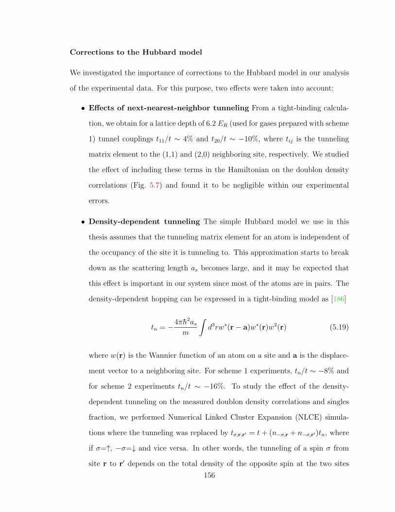
Corrections to the Hubbard model

We investigated the importance of corrections to the Hubbard model in our analysis

of the experimental data. For this purpose, two effects were taken into account:

• Effects of next-nearest-neighbor tunneling From a tight-binding calcula-

tion, we obtain for a lattice depth of 6.2 ER (used for gases prepared with scheme

1) tunnel couplings t11/t ∼ 4% and t20/t ∼ −10%, where tij is the tunneling

matrix element to the (1,1) and (2,0) neighboring site, respectively. We studied

the effect of including these terms in the Hamiltonian on the doublon density

correlations (Fig. 5.7) and found it to be negligible within our experimental

errors.

• Density-dependent tunneling The simple Hubbard model we use in this

thesis assumes that the tunneling matrix element for an atom is independent of

the occupancy of the site it is tunneling to. This approximation starts to break

down as the scattering length as becomes large, and it may be expected that

this effect is important in our system since most of the atoms are in pairs. The

density-dependent hopping can be expressed in a tight-binding model as [186]

tn = −4πh2asm

∫d3rw∗(r− a)w∗(r)w2(r) (5.19)

where w(r) is the Wannier function of an atom on a site and a is the displace-

ment vector to a neighboring site. For scheme 1 experiments, tn/t ∼ −8% and

for scheme 2 experiments tn/t ∼ −16%. To study the effect of the density-

dependent tunneling on the measured doublon density correlations and singles

fraction, we performed Numerical Linked Cluster Expansion (NLCE) simula-

tions where the tunneling was replaced by tσ,r,r′ = t+ (n−σ,r + n−σ,r′)tn, where

if σ=↑, −σ=↓ and vice versa. In other words, the tunneling of a spin σ from

site r to r′ depends on the total density of the opposite spin at the two sites

156

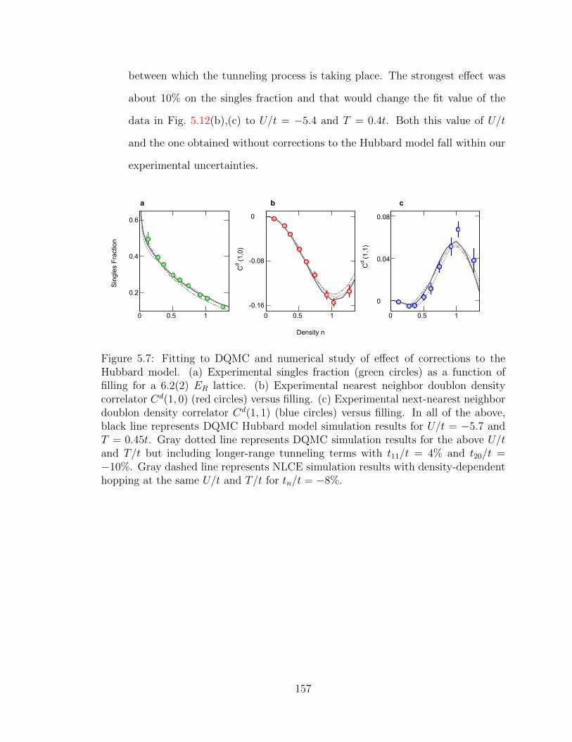
between which the tunneling process is taking place. The strongest effect was

about 10% on the singles fraction and that would change the fit value of the

data in Fig. 5.12(b),(c) to U/t = −5.4 and T = 0.4t. Both this value of U/t

and the one obtained without corrections to the Hubbard model fall within our

experimental uncertainties.

a

Sin

gles

Fra

ctio

n

0.2

0.4

0.6

0 0.5 1

b

Cd

(1,0

)

Density n

-0.16

-0.08

0

0 0.5 1

c

Cd

(1,1

)

0

0.04

0.08

0 0.5 1

Figure 5.7: Fitting to DQMC and numerical study of effect of corrections to theHubbard model. (a) Experimental singles fraction (green circles) as a function offilling for a 6.2(2) ER lattice. (b) Experimental nearest neighbor doublon densitycorrelator Cd(1, 0) (red circles) versus filling. (c) Experimental next-nearest neighbordoublon density correlator Cd(1, 1) (blue circles) versus filling. In all of the above,black line represents DQMC Hubbard model simulation results for U/t = −5.7 andT = 0.45t. Gray dotted line represents DQMC simulation results for the above U/tand T/t but including longer-range tunneling terms with t11/t = 4% and t20/t =−10%. Gray dashed line represents NLCE simulation results with density-dependenthopping at the same U/t and T/t for tn/t = −8%.

157

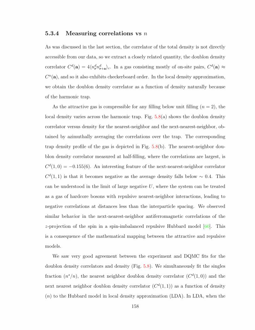
5.3.4 Measuring correlations vs n

As was discussed in the last section, the correlator of the total density is not directly

accessible from our data, so we extract a closely related quantity, the doublon density

correlator Cd(a) = 4〈ndrndr+a〉c. In a gas consisting mostly of on-site pairs, Cd(a) ≈

Cn(a), and so it also exhibits checkerboard order. In the local density approximation,

we obtain the doublon density correlator as a function of density naturally because

of the harmonic trap.

As the attractive gas is compressible for any filling below unit filling (n = 2), the

local density varies across the harmonic trap. Fig. 5.8(a) shows the doublon density

correlator versus density for the nearest-neighbor and the next-nearest-neighbor, ob-

tained by azimuthally averaging the correlations over the trap. The corresponding

trap density profile of the gas is depicted in Fig. 5.8(b). The nearest-neighbor dou-

blon density correlator measured at half-filling, where the correlations are largest, is

Cd(1, 0) = −0.155(6). An interesting feature of the next-nearest-neighbor correlator

Cd(1, 1) is that it becomes negative as the average density falls below ∼ 0.4. This

can be understood in the limit of large negative U , where the system can be treated

as a gas of hardcore bosons with repulsive nearest-neighbor interactions, leading to

negative correlations at distances less than the interparticle spacing. We observed

similar behavior in the next-nearest-neighbor antiferromagnetic correlations of the

z-projection of the spin in a spin-imbalanced repulsive Hubbard model [60]. This

is a consequence of the mathematical mapping between the attractive and repulsive

models.

We saw very good agreement between the experiment and DQMC fits for the

doublon density correlators and density (Fig. 5.8). We simultaneously fit the singles

fraction (ns/n), the nearest neighbor doublon density correlator (Cd(1, 0)) and the

next nearest neighbor doublon density correlator (Cd(1, 1)) as a function of density

(n) to the Hubbard model in local density approximation (LDA). In LDA, when the

158

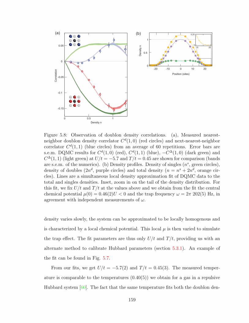
Corr

ela

tion

Density n

(a)

-0.15

-0.1

-0.05

0

0.05

0 0.5 1

Density n

Position (sites)

0

0.5

1

-20 -10 0 10 20

0

0.25

15 25

(b)

Figure 5.8: Observation of doublon density correlations. (a), Measured nearest-neighbor doublon density correlator Cd(1, 0) (red circles) and next-nearest-neighborcorrelator Cd(1, 1) (blue circles) from an average of 60 repetitions. Error bars ares.e.m. DQMC results for Cd(1, 0) (red), Cd(1, 1) (blue), −C∆(1, 0) (dark green) andC∆(1, 1) (light green) at U/t = −5.7 and T/t = 0.45 are shown for comparison (bandsare s.e.m. of the numerics). (b) Density profiles. Density of singles (ns, green circles),density of doubles (2nd, purple circles) and total density (n = ns + 2nd, orange cir-cles). Lines are a simultaneous local density approximation fit of DQMC data to thetotal and singles densities. Inset, zoom in on the tail of the density distribution. Forthis fit, we fix U/t and T/t at the values above and we obtain from the fit the centralchemical potential µ(0) = 0.46(2)U < 0 and the trap frequency ω = 2π 202(5) Hz, inagreement with independent measurements of ω.

density varies slowly, the system can be approximated to be locally homogenous and

is characterized by a local chemical potential. This local µ is then varied to simulate

the trap effect. The fit parameters are thus only U/t and T/t, providing us with an

alternate method to calibrate Hubbard parameters (section 5.3.1). An example of

the fit can be found in Fig. 5.7.

From our fits, we get U/t = −5.7(2) and T/t = 0.45(3). The measured temper-

ature is comparable to the temperatures (0.40(5)) we obtain for a gas in a repulsive

Hubbard system [60]. The fact that the same temperature fits both the doublon den-

159

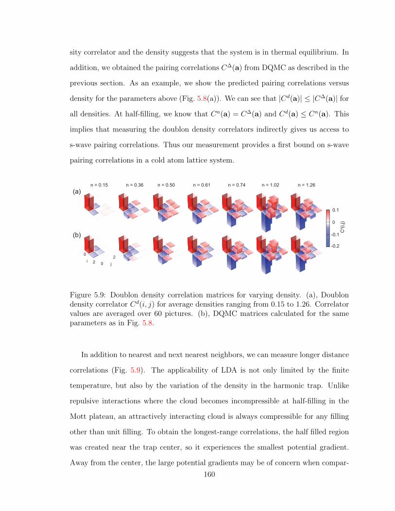
sity correlator and the density suggests that the system is in thermal equilibrium. In

addition, we obtained the pairing correlations C∆(a) from DQMC as described in the

previous section. As an example, we show the predicted pairing correlations versus

density for the parameters above (Fig. 5.8(a)). We can see that |Cd(a)| ≤ |C∆(a)| for

all densities. At half-filling, we know that Cn(a) = C∆(a) and Cd(a) ≤ Cn(a). This

implies that measuring the doublon density correlators indirectly gives us access to

s-wave pairing correlations. Thus our measurement provides a first bound on s-wave

pairing correlations in a cold atom lattice system.

n = 0.15 n = 0.36 n = 0.50 n = 0.61 n = 0.74 n = 1.02 n = 1.26

-0.2

-0.1

0

0.1

Cd(i,j)

0

2 0

2i

j

(a)

(b)

Figure 5.9: Doublon density correlation matrices for varying density. (a), Doublondensity correlator Cd(i, j) for average densities ranging from 0.15 to 1.26. Correlatorvalues are averaged over 60 pictures. (b), DQMC matrices calculated for the sameparameters as in Fig. 5.8.

In addition to nearest and next nearest neighbors, we can measure longer distance

correlations (Fig. 5.9). The applicability of LDA is not only limited by the finite

temperature, but also by the variation of the density in the harmonic trap. Unlike

repulsive interactions where the cloud becomes incompressible at half-filling in the

Mott plateau, an attractively interacting cloud is always compressible for any filling

other than unit filling. To obtain the longest-range correlations, the half filled region

was created near the trap center, so it experiences the smallest potential gradient.

Away from the center, the large potential gradients may be of concern when compar-

160

ing to numerics due to a possible breakdown of LDA. For the above cloud profiles,

we see doublon density correlations up to two sites on a diagonal shown in the cor-

relation matrices Cd(i, j). Again we can compare further neighbor correlations with

DQMC, always assuming LDA. We find good agreement with DQMC calculations

corresponding to the experimental densities, calculated using the same parameters as

above. We notice that the range of the correlation becomes maximal at half filling,

as one would expect from theory where the correlations are also the strongest.

n = 0.17 n = 0.36 n = 0.49 n = 0.62 n = 0.80 n = 1.03 n = 1.26

-0.2

-0.1

0

0.1

Cd(i,j)

0

2 0

2i

j

-4

-2

0

2

4

0 400 800

Scatt

ering length

(a

0 x

10³)

Field (G)

1-3 2-3

attractive

repulsive

RF

(a)

(b)

(c)

Figure 5.10: Observation of doublon density correlators in an attractive Hubbardsystem prepared using scheme 2. (a) The lattice is loaded at a scattering lengtha13 = −2800 a0 (red square). After freezing the density distribution, we convert1-3 doublons to 2-3 doublons of which the state |3〉 atom is pushed in a regime ofrepulsive interactions and we are left with only one atom per site (orange circle ata23 = 414 a0). (b) Measured doublon density correlator for systems prepared usingscheme 2 for varying filling. (c) Doublon density correlator obtained through DQMCsimulations for experimental values of filling.

161

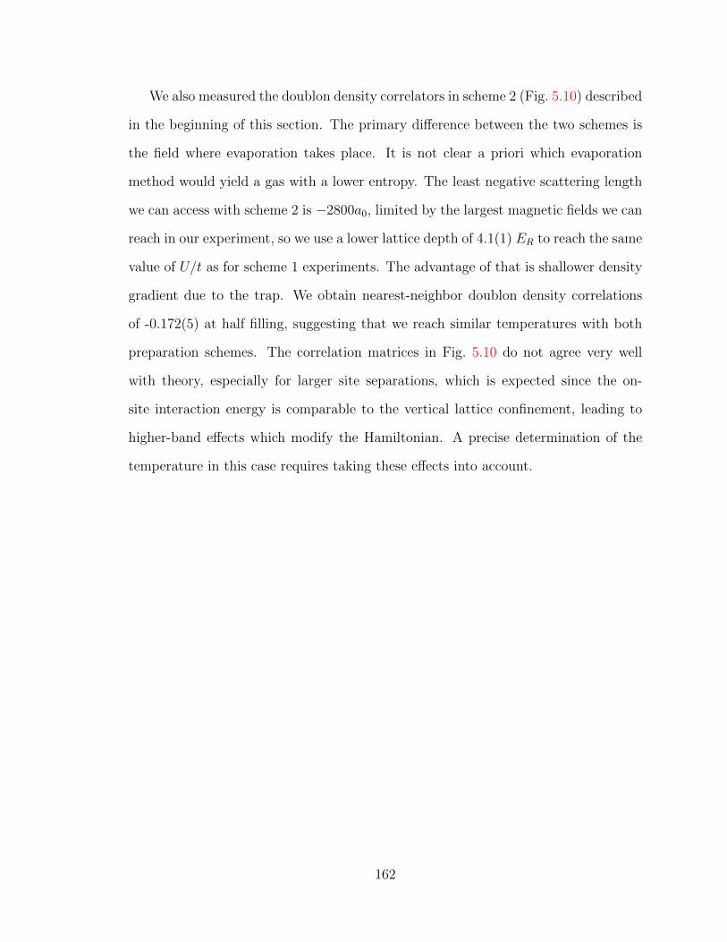
We also measured the doublon density correlators in scheme 2 (Fig. 5.10) described

in the beginning of this section. The primary difference between the two schemes is

the field where evaporation takes place. It is not clear a priori which evaporation

method would yield a gas with a lower entropy. The least negative scattering length

we can access with scheme 2 is −2800a0, limited by the largest magnetic fields we can

reach in our experiment, so we use a lower lattice depth of 4.1(1) ER to reach the same

value of U/t as for scheme 1 experiments. The advantage of that is shallower density

gradient due to the trap. We obtain nearest-neighbor doublon density correlations

of -0.172(5) at half filling, suggesting that we reach similar temperatures with both

preparation schemes. The correlation matrices in Fig. 5.10 do not agree very well

with theory, especially for larger site separations, which is expected since the on-

site interaction energy is comparable to the vertical lattice confinement, leading to

higher-band effects which modify the Hamiltonian. A precise determination of the

temperature in this case requires taking these effects into account.

162

5.3.5 Measuring correlations vs U/t

In the previous section, we studied the dependance of the local density on charge

density wave correlations. We saw that these correlations were maximized and had the

longest range at half filling (n = 1). In addition, we found that these correlations are

a lower bound for s-wave pairing correlations that one would expect in the attractive

Hubbard model at our temperatures. So as a natural extension of the general study

of the model, we next vary the interaction U/t. There are two ways to change U . The

first one is to change the scattering length (as) by varying the magnetic field and the

second is to change the lattice depth V . The disadvantage of the first method is that

a13 is already the largest negative value reached for the 1-3 mixture away from the

Feshbach resonance (for scheme 1) at 305 G. So we can only study lower U this way.

The disadvantage of the second method is that changing V has an effect on both U

and t. Another drawback is that the radial confinement changes with V .

The system was prepared with scheme 1 at a scattering length of −889 a0 and

U/t was varied by changing the lattice depth. Fig. 5.11 shows the nearest-neighbor

and next-nearest-neighbor correlator versus density for different lattice depths. The

data was fit to DQMC results with U/t and T/t used as fit parameters as described

previously. We observed a slight increase in the temperature for larger lattice depths.

The measured correlations initially increase as the lattice depth is increased, but do

not show significant variation for lattice depths between 6.2 ER and 7.4 ER. This

is expected from DQMC simulations as we saw in Fig. 5.5(b). At larger depths, it

became experimentally difficult to obtain a half-filling condition near the center of

the trap because of the increasing radial confinement from the lattice beams.

We also compared to DQMC in the presence of a spatially varying potential to

reproduce the largest experimentally observed density gradients to verify that the

LDA holds in our system. For data shown in Fig. 5.11, the density gradient at n = 1

varied from 0.07 atoms/(site)2 for a depth of 4.1 ER to 0.14 atoms/(site)2 for a depth

163

Cor

rela

tion

Cd(1

,0),(

1,1)

-0.15

-0.1

-0.05

0

0.05

0 0.5 1 0 0.5 1 0 0.5 1 0 0.5 1

Density n

0 0.5 1

(a) (b) (c) (d) (e)

Figure 5.11: Nearest-neighbor and next-nearest neighbor doublon density correlatorsvs. filling as a function of lattice depth. Cd(1, 0) (red circles) and Cd(1, 1) (bluecircles) obtained from different parts of the trap where filling varies from 0 to slightlyabove half-filling. (a) For lattice depth of 4.1(1) ER, (b) 5.5(1) ER, (c) 6.2(2) ER, (d)6.7(2) ER, (e) 7.4(2) ER. Shaded curves are DQMC fits for the data versus filling withU/t and T/t as fit parameters. (a) U/t = −2.75, T = 0.4t, (b) U/t = −4.5, T = 0.4t,(c) U/t = −5.7, T = 0.45t, (d) U/t = −6.75, T = 0.5t, (e) U/t = −7.5, T = 0.5t. Thewidth of the shaded band is the s.e.m. of the simulation data.

of 7.4 ER. We performed DQMC simulations in the presence of a linearly varying

chemical potential along one direction of the 2D Hubbard lattice to reproduce the

maximal density gradients observed in the experiment. The results of this calculation

showed that LDA holds to excellent approximation for our experimental parameters.

However, we note that violation of the LDA had been predicted for such a system at

much lower temperatures and higher gradients [187].

164

5.3.6 Thermometry

In the last few sections, I have shown how quantum gas microscopy can effectively

simulate the Hubbard model. But our consistency checks so far have been state-of-

the-art numerical simulations. These simulations, however, suffer from issues like the

fermion sign problem at low temperatures and with imbalanced spins and the inability

to simulate large systems. So at some temperature scale it is expected that quantum

gas microscopy will venture into numerically uncharted territory. One such territory

is the FFLO phase which is expected to occur below temperatures of 0.1t [163].

The equivalent phase for the repulsive Hubbard model would be an incommensurate

antiferromagnet at finite doping [86]. These phases are still out of reach of current

experiments as the coldest Fermi Hubbard system so far has reached a temperature of

∼ 0.25t [179]. The development of new cooling techniques to reach lower temperatures

will need to be accompanied by the development of low temperature thermometry

techniques.

Both the doublon fraction and doublon density correlations may be used as ther-

mometers in an attractive Hubbard system. To investigate their sensitivity as ther-

mometers, we heated the system in a controlled fashion by holding it for variable

times in the lattice before imaging. Technical noise leads to a linear increase in the

temperature. We observe a slight reduction in doublon fraction in the half filled region

for long hold times (Fig. 5.12(a)), while the doublon density correlators Cd(1, 0) and

Cd(1, 1) show a significant change during the same time. These observations illustrate

that the doublon fraction is a good thermometer for temperatures on the order of U ,

where doublon density correlations are small, while the latter are a more sensitive

thermometer for temperatures on the order of the exchange energy 4t2/U . This is

similar to the case of repulsive interactions, where spin correlations have been found

to be a more sensitive thermometer than density [176]. Fig. 5.12(b) and (c) show

the nearest-neighbor and next-nearest-neighbor doublon density correlators versus

165

the singles fraction at half-filling. Plotting the data this way allows a temperature-

independent comparison to DQMC with a single free-parameter (U/t), and we obtain

good agreement for U/t = −5.7.

0

0.5

1

0 500 1000 1500-0.2

-0.1

0 0.5 1 1.5 2

Sin

gles

/dou

blon

frac

tion

Cd (1

,0)

Hold time (ms)

Temperature, T/t(a)

-0.2

-0.1

0

Singles fraction

0.2 0.25 0.3 0

0.05

Cd (1

,0)

Cd (1

,1)

(b)

(c)

Figure 5.12: Thermometry of an attractive Hubbard system. (a) Temperature de-pendence of the paired fraction and nearest-neighbor doublon density correlations.Shown are the fraction of singles (green circles) and doubles (purple circles) at half-filling on the left axis as a function of hold time in the lattice. On the right axis isthe doublon density correlator Cd(1, 0) (red circles) at half-filling measured for thesame hold times. The upper x-axis are temperatures obtained from comparison toDQMC, giving a linear heating rate of 1.3(1) t/s. (b) Cd(1, 0) as a function of singlesfraction. Each data point corresponds to a single hold time. (c) The next-nearestneighbor doublon density correlator Cd(1, 1) as function of singles fraction. Bandscorrespond to DQMC results for U/t = −5.7 and half filling in all of the above. Eachpoint is averaged over 60 pictures. Error bars and bands are s.e.m.

166

5.4 Mapping and further work

In this section, we compare the results of this chapter on attractive Hubbard model

at finite doping with the results of our previous work on the spin-imbalanced repul-

sive Hubbard model [60]. We described in section 5.2 a particle-hole transformation

under which U ↔ −U , µ ↔ h and η±,z ↔ S±,z. In other words, a doped attractive

system maps on to a spin polarized repulsive system. In addition, the charge density

wave and s-wave superfluid order in the attractive system maps on to an isotropic

antiferromagnet in the repulsive system (Fig. 5.13). We see that the in-plane spin

correlator C⊥(a) follows the same trend as the s-wave pairing correlator C∆(a). Sim-

ilarly, the out-of-plane spin correlator Cz(a) should map on to the density correlator

Cn(a). We measure the doubles density correlator Cd(a) which is similar to Cn(a)

and we see similar behavior between the two.

Another related experiment that we have taken steps towards is to study the

collective modes of the Hubbard model. For repulsive interactions, spin-waves would

be generated in the system when it is excited through a Zeeman field, as is done in

neutron scattering experiments [188]. Such a measurement is expected to be difficult

for lithium because it requires a spin-dependent potential. For attractive interactions,

however, chemical potential modulations couple to a new class of collective excitations

[181].

To see the nature of these modes, consider the pseudo-spin operators defined in

Eq. 5.10 in momentum space

η− =∑k

ck+Q,↑c−k,↓

η+ = (η−)†

ηz =1

2(n− 1) (5.20)

167

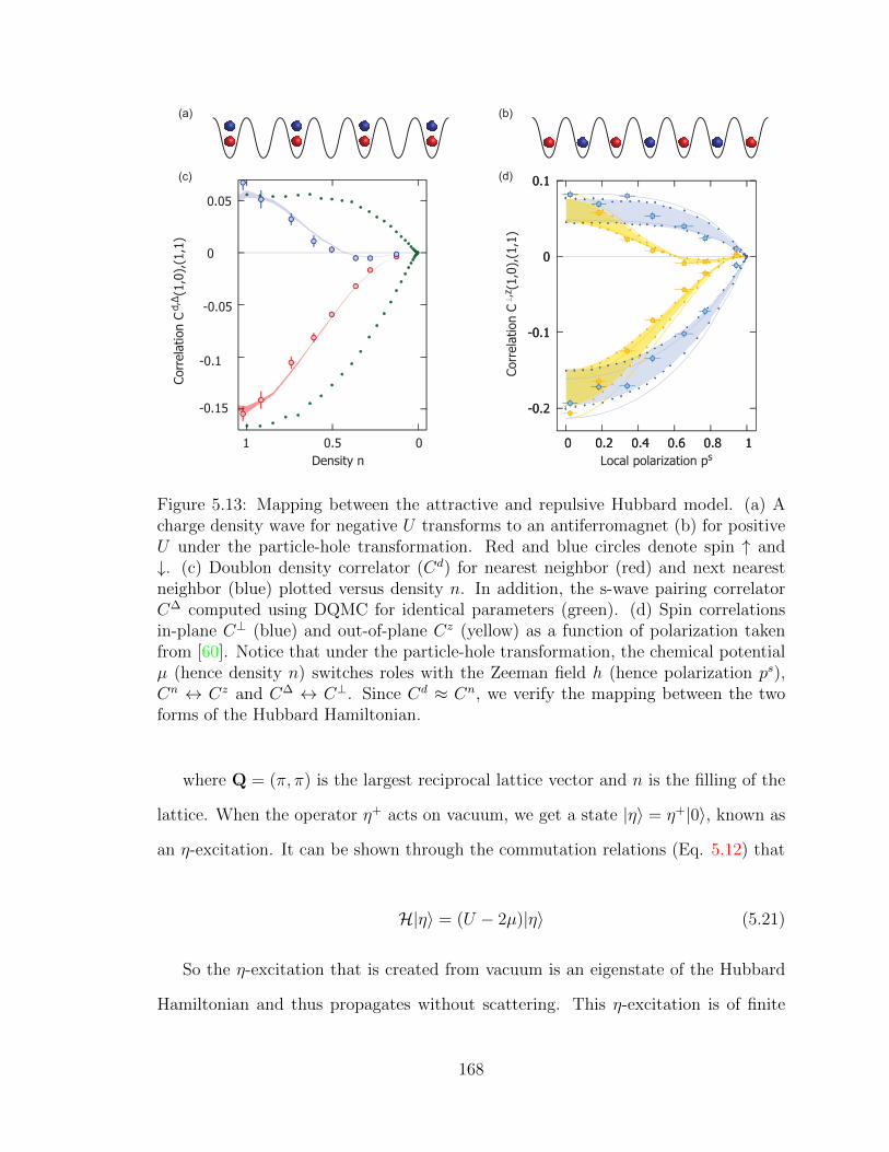
-0.2

-0.1

0

0.1

0 0.2 0.4 0.6 0.8 1

Corr

ela

tion C

,z(1

,0),

(1,1

)

Local polarization ps

-0.2

-0.1

0

0.1

0 0.2 0.4 0.6 0.8 1

Corr

ela

tion Cd,

(1,0

),(1

,1)

-0.15

-0.1

-0.05

0

0.05

Density n

0 0.5 1

(a)

(c)

(b)

(d)

Figure 5.13: Mapping between the attractive and repulsive Hubbard model. (a) Acharge density wave for negative U transforms to an antiferromagnet (b) for positiveU under the particle-hole transformation. Red and blue circles denote spin ↑ and↓. (c) Doublon density correlator (Cd) for nearest neighbor (red) and next nearestneighbor (blue) plotted versus density n. In addition, the s-wave pairing correlatorC∆ computed using DQMC for identical parameters (green). (d) Spin correlationsin-plane C⊥ (blue) and out-of-plane Cz (yellow) as a function of polarization takenfrom [60]. Notice that under the particle-hole transformation, the chemical potentialµ (hence density n) switches roles with the Zeeman field h (hence polarization ps),Cn ↔ Cz and C∆ ↔ C⊥. Since Cd ≈ Cn, we verify the mapping between the twoforms of the Hubbard Hamiltonian.

where Q = (π, π) is the largest reciprocal lattice vector and n is the filling of the

lattice. When the operator η+ acts on vacuum, we get a state |η〉 = η+|0〉, known as

an η-excitation. It can be shown through the commutation relations (Eq. 5.12) that

H|η〉 = (U − 2µ)|η〉 (5.21)

So the η-excitation that is created from vacuum is an eigenstate of the Hubbard

Hamiltonian and thus propagates without scattering. This η-excitation is of finite

168

energy away from half-filling and has a momentum Q. This is the new collective

excitation of the Hubbard model.

This excitation, however is particle-particle like and most experimental probes

can not directly access it. But particle-hole (or density ρq) excitations can lead to

particle-particle excitations via interactions with a superconducting ground state in a

process similar to Andreev reflection [189]. We can generate particle-hole excitations

by adding a time dependent modulation to the chemical potential µ of the form

δµei(qr+ωτ), where q is the wave-vector of the modulation and ω is its frequency. then

the perturbative term in the Hamiltonian (Eq. 5.4) will be of the form

Hpert =∑j,σ

nj,σδµj = δµ∑j,σ

c†j,σcj,σei(qrj+ωτ) (5.22)

If we perform the Fourier transform of the above expression, we get

Hpert = δµeiωτ∑k,σ

c†k,σck+q,σ = δµeiωτρq (5.23)

Where ρq =∑k,σ

c†k,σck+q,σ is the density operator. We are capable of creating these

modulations up to the largest k-vector (π, π) by projecting a travelling sinudoidal

wave using a digital micromirror device (DMD) through our high NA objective (Fig.

5.14).

Although our experiments are significantly over Tc for the s-wave BKT transition

in 2D, expected around 0.15-0.2t for our parameters [190], we would expect a mea-

surable effect in the density spectral function at our temperatures because of strong

superconducting fluctuations in the pseudogap regime above Tc [191].

169

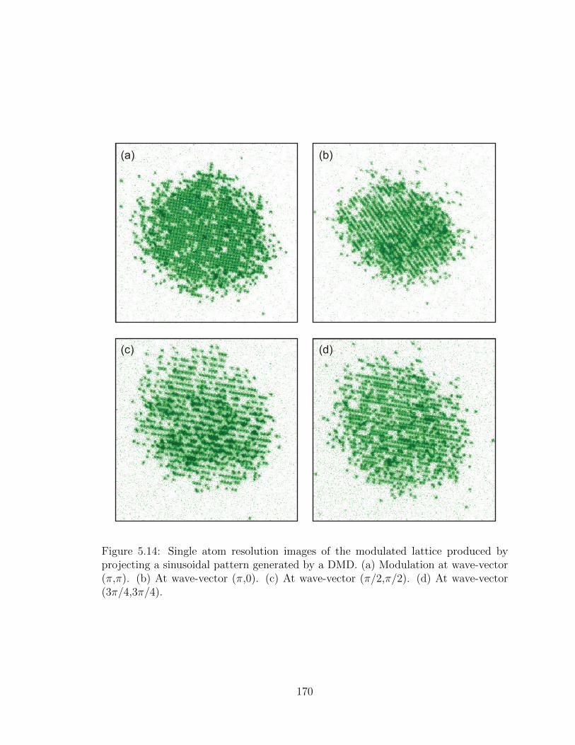
(a) (b)

(c) (d)

Figure 5.14: Single atom resolution images of the modulated lattice produced byprojecting a sinusoidal pattern generated by a DMD. (a) Modulation at wave-vector(π,π). (b) At wave-vector (π,0). (c) At wave-vector (π/2,π/2). (d) At wave-vector(3π/4,3π/4).

170

Chapter 6

Conclusion

In conclusion, I have described the process of building a fermionic lithium quantum

gas microscope in this thesis. We used the experimental setup to explore the physics

of strongly interacting fermions with a focus on attractive interactions. In the next

few paragraphs I will summarize the main scientific achievements of this thesis.

In chapter 4, I described in detail our study of pair condensation in “quasi” 2D

across the BEC-BCS crossover [35]. We studied a spin imbalanced “quasi” 2D Fermi

gas across the BEC-BCS crossover. We found that phase separation persists up to

an interaction-dependent critical polarization Pc. This critical polarization decreases

as one goes from the BEC regime, with high binding energy, to the BCS regime with

weak attractive interactions. In addition, we discovered that the condensate does not

vanish with phase separation, pointing to the existence of a polarized condensate.

Finally we mapped the phase diagram of the 2D interacting Fermi gas. We note the

existence of three phases, a balanced condensate, a partially polarized phase and a

fully polarized Fermi gas. The results are a step towards measuring exotic pairing

mechanisms in the presence of spin imbalance.

In chapter 5, I described our exploration of charge density wave correlations in

the attractive Hubbard model [65]. We perfomed the first quantum gas microscopy

171

of the attractive Fermi-Hubbard model. We measured the doublon density correlator

Cd(a). We measured the interaction U/t and the temperature T/t by simultaneously

fitting the singles fraction, the nearest neighbor Cd(1, 0) and the next nearest neighbor

Cd(1, 1) correlators. By measuring the sensitivity of the correlators and the density

to temperature, we concluded that the correlators are a better thermometer at the

exchange scale 4t2/U while the densities are more sensitive at the scale of U . Finally,

by employing DQMC simulations, we placed a lower bound on s-wave pairing in the

system.

6.1 Future Work

What I have described in this thesis is just a glimpse of the physics of correlated

fermionic systems that can be explored with quantum gas microscopes. Further work

is required to shed light on many more poorly understood properties of the Hubbard

model. One of the immediate challenges is to lower the temperature in our systems

to access the critical temperature for d-wave superconductivity and the FFLO phase.

One promising technique is entropy redistribution that has led to the lowest Hubbard

temperature to date [179]. But even at our current temperatures, there remain many

interesting aspects to explore.

One aspect is to measure the pseudogap regime in the attractive model at inter-

mediate interactions. Measuring spin susceptibility χs is one such route [167]. One

would expect χs to start descreasing as pairs begin to form. Another interesting

direction is to perform RF spectrosocpy in a regime where many-body effects are im-

portant. For example, I showed in section 5.3.1 that there is good agreement between

RF spectra and the expected tight-binding U in a deep lattice but deviations start

occuring when the lattice is shallow and tunneling is non-negligible. However, these

measurements are plagued by final state interactions. To circumvent the problem,

172

one can either work at a field where the final state is non-interacting or take them

into account numerically. The measurement of the spectral function of the Hubbard

model will shed light on the pairing mechanisms, including a crossover from BEC-like

to BCS-like pairing [192].

Another interesting direction lies in the study of Fermi gases with long-range

interactions. We have been working on the implementation of Rydberg dressing in

our experiments. When an atom is excited to a Rydberg state, dipolar interactions can

be induced. Recently we studied quench dynamics in a 2D transverse Ising system

using a UV laser to transfer atoms to the Rydberg state [193]. But the Rydberg

atoms suffer from very short lifetimes. So the idea is to dress a ground state atom

with a small admixture of the Rydberg state [194, 195]. One can study spin systems

with long range interactions [196] or go beyond the frozen gas regime, i.e. when the

fermions are free to tunnel in the lattice.

The study of dynamical properties of the Hubbard model poses a new set of

challenges for numerical simulations [197]. We have measured charge transport in the

repulsive Hubbard model [71]. But the same technique could be extended to measure

transport in the superfluid phase of the attractive Hubbard model. There, one would

expect an enhancement of conductivity as one crossed the pairing temperature scale.

The study of collective modes of the Hubbard model, as described in section 5.4,

would enable further study of the dynamics of the Hubbard model. Observation

of the conjectured η mode above Tc would be evidence of strong superconducting

fluctuations [191].

Recent experiments have explored the Hubbard model under a Floquet drive [198].

In these driven lattices, the effective Hubbard parameters can be thought of as renor-

malized by the drive and can lead to enhancement of antiferromagnetic correlations

or even their transformation to ferromagnetic correlations. They can be used to re-

alize the t− J model with independent control over t and J such that the large J/t

173

regime becomes accessible. This may lead to an enhancement of the superconducting

critical temperature. Such driven Floquet Hamiltonians can be easily generated in

our experiments and it would be interesting to study the microscopic spin correlations

in such a system with a quantum gas microscope.

174

Appendix A

Properties of 6Li

A.1 Atomic properties

Table A.1: Properties of 6Li [199]

Property Symbol Value Units

Mass m 1.0020×10−26 KgD1 transition λD1 670.992421 nmD2 transition λD2 670.977338 nmNatural linewidth Γ 5.8724 MHzElectron spin g-factor gs 2.0023Electron orbital g-factor gL 0.999996Total Nuclear g-factor gI -0.000448Total Electronic g-factor (22S1/2) gJ 2.0023Total Electronic g-factor (22P1/2) gJ 0.6668Total Electronic g-factor (22P3/2) gJ 1.33522S1/2 Magnetic Dipole Constant A22S1/2

152.13684 MHz

22P1/2 Magnetic Dipole Constant A22P1/217.386 MHz

22P3/2 Magnetic Dipole Constant A22P3/2-1.155 MHz

22P3/2 Electric Quadrupole Constant B22P3/2-0.10 MHz

D1 Saturation Intensity Isat 7.59 mW/cm2

D2 Saturation Intensity Isat 2.54 mW/cm2

175

A.2 Zeeman shifts

Energ

y s

hift

(MH

z)

-800

-600

-400

-200

0

200

400

600

800

Energ

y d

iffe

rence (

MH

z)

Field (G)

0

50

100

150

200

0 100 200 300 400 500

(a)

(b)

Figure A.1: (a) Zeeman shift for energy of the hyperfine sublevels of the ground state2S1/2 of 6Li as a function of B-field. The states are numbered as follows from bottomto top: |1〉 = [2S1/2, F = 1/2, mF = 1/2], |2〉 = [2S1/2, F = 1/2, mF = -1/2], |3〉 =[2S1/2, F = 3/2, mF = -3/2], |4〉 = [2S1/2, F = -1/2, mF = 1/2, |5〉 = 2S1/2, F =3/2, mF = 1/2 and |6〉 = [2S1/2, F = 3/2, mF = 3/2]. Above a field of ∼ 200 G, thesplitting becomes effectively linear in the Paschen-Back limit. (b) Energy differencebetween states |1〉 and |2〉 (blue dashed line) and states |2〉 and |3〉 (red solid line) asa function of field. Due to the effective saturation at high fields, the RF antennas weuse are resonant around 76 MHz for |1〉 − |2〉 and around 85 MHz for |2〉 − |3〉.

176

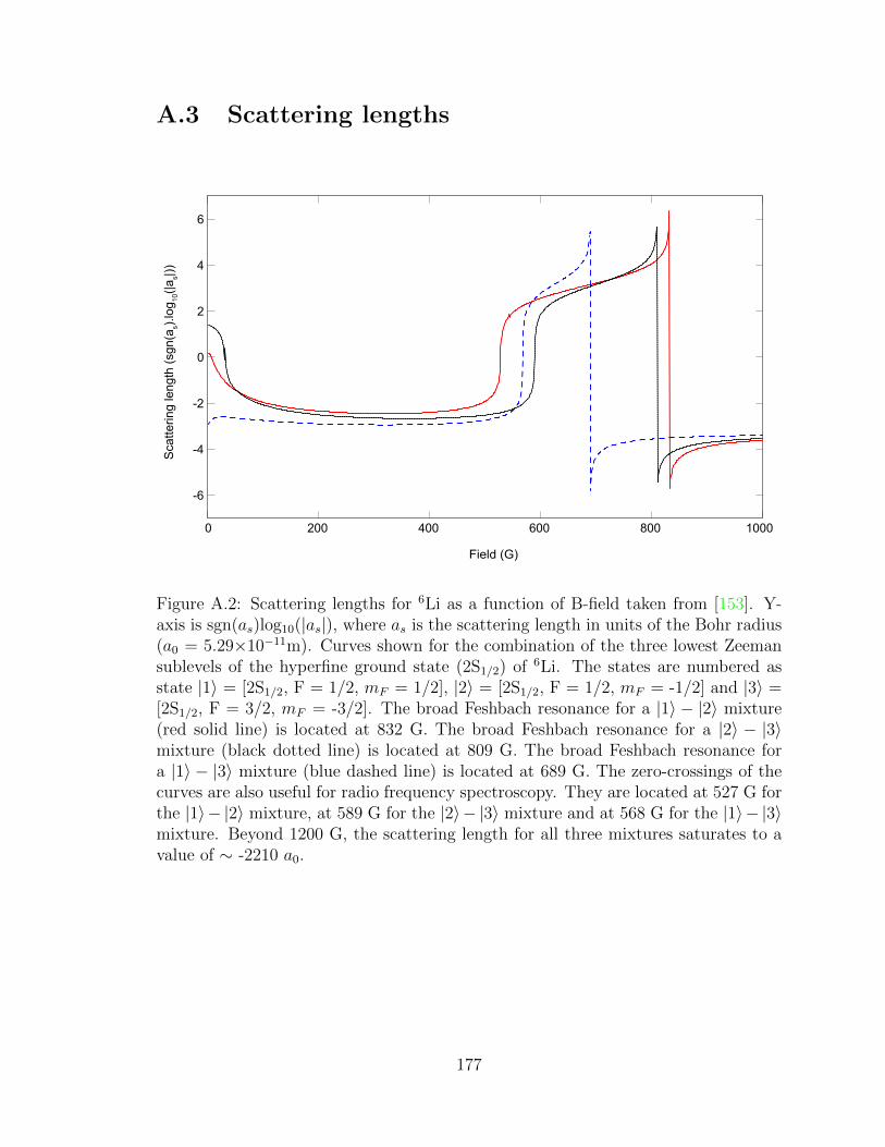
A.3 Scattering lengths

Scat

terin

g le

ngth

(sgn

(as).

log 10

(|as|)

)

Field (G)

-6

-4

-2

0

2

4

6

0 200 400 600 800 1000

Figure A.2: Scattering lengths for 6Li as a function of B-field taken from [153]. Y-axis is sgn(as)log10(|as|), where as is the scattering length in units of the Bohr radius(a0 = 5.29×10−11m). Curves shown for the combination of the three lowest Zeemansublevels of the hyperfine ground state (2S1/2) of 6Li. The states are numbered asstate |1〉 = [2S1/2, F = 1/2, mF = 1/2], |2〉 = [2S1/2, F = 1/2, mF = -1/2] and |3〉 =[2S1/2, F = 3/2, mF = -3/2]. The broad Feshbach resonance for a |1〉 − |2〉 mixture(red solid line) is located at 832 G. The broad Feshbach resonance for a |2〉 − |3〉mixture (black dotted line) is located at 809 G. The broad Feshbach resonance fora |1〉 − |3〉 mixture (blue dashed line) is located at 689 G. The zero-crossings of thecurves are also useful for radio frequency spectroscopy. They are located at 527 G forthe |1〉− |2〉 mixture, at 589 G for the |2〉− |3〉 mixture and at 568 G for the |1〉− |3〉mixture. Beyond 1200 G, the scattering length for all three mixtures saturates to avalue of ∼ -2210 a0.

177

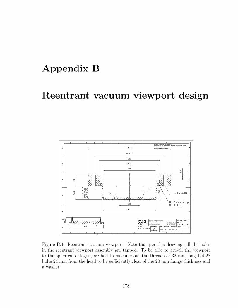
Appendix B

Reentrant vacuum viewport design

Figure B.1: Reentrant vaccum viewport. Note that per this drawing, all the holesin the reentrant viewport assembly are tapped. To be able to attach the viewportto the spherical octagon, we had to machine out the threads of 32 mm long 1/4-28bolts 24 mm from the head to be sufficiently clear of the 20 mm flange thickness anda washer.

178

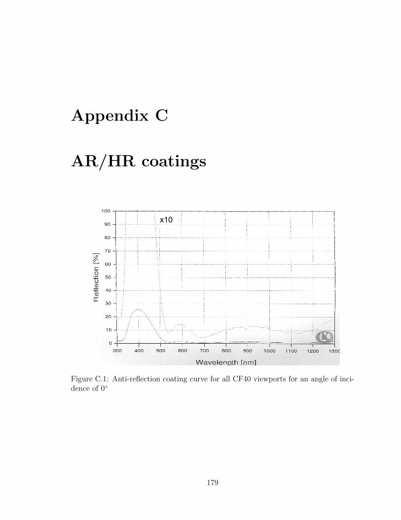
Appendix C

AR/HR coatings

x10

Figure C.1: Anti-reflection coating curve for all CF40 viewports for an angle of inci-dence of 0

179

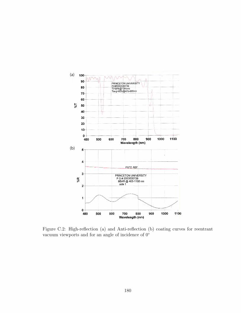
(a)

(b)

0

Figure C.2: High-reflection (a) and Anti-reflection (b) coating curves for reentrantvacuum viewports and for an angle of incidence of 0

180

Appendix D

Lattice description

D.1 Lattice potential

In this section, we derive the expression for the lattice potential. First consider the

case of a 4-fold interference (vertical polarization) of equal magnitude electric fields

E0. Let us consider that the lattice principle axes are the x and y-axis. Let us

define the origin as the point where the interference occurs and take time t = 0. The

magnitude of the electric fields are:

E1 = E0eik(x sin(θ/2)+y cos(θ/2))

E2 = E0eik(x sin(θ/2)−y cos(θ/2))

E3 = E0e−ik(x sin(θ/2)+y cos(θ/2))

E4 = E0e−ik(x sin(θ/2)+y cos(θ/2)) (D.1)

where k is the wave-vector given by 2π/λ and θ is the angle between the beams.

The potential due to the interference of the 4 beams would be proportional to |∑Ei|2,

which gives:

181

V ⊥(x, y) ∝ 4|E0|2(cos(kx sin(θ/2) + ky cos(θ/2)) + cos(kx sin(θ/2)− ky cos(θ/2)))2

∝ 16|E0|2 cos2(kx sin(θ/2)) cos2(ky cos(θ/2))

∝ 4|E0|2(1 + cos(2kx sin(θ/2)))(1 + cos(2ky cos(θ/2))) (D.2)

Now consider the case where only two pairs of beams interfere (horizontal polar-

ization), then the total potential is proportional to |E1 + E3|2 + |E2 + E4|2 giving

V ‖(x, y) ∝

4|E0|2(cos2(kx sin(θ/2) + ky cos(θ/2)) + cos2(kx sin(θ/2)− ky cos(θ/2))

= 4|E0|2(

1 + cos(2kx sin(θ/2) + 2ky cos(θ/2))

2+

1 + cos(2kx sin(θ/2)− 2ky cos(θ/2))

2

)= 4|E0|2(1 + cos(2kx sin(θ/2)) cos(2ky cos(θ/2))) (D.3)

In order to compare the two potentials, they need to be referenced with respect to

a standard energy scale of the system, which is the recoil energy. For the perpendular

configuration, lattice spacing is a = λ/√

2. So we define ER = E⊥R = h2(π/a)2/2m =

h2k2/4m. So the maximum depth is V0 = 16|E0|2/ER. But for the parallel configu-

ration, the spacing is a = λ/2 and so E‖R = h2k2/2m = 2ER. Hence the maximum

depth in this case is 4|E0|2/ER. Hence the first configuration gives a lattice that is 4

times deeper than the second.

Next, we can calculate the 4-fold interference but with an attenuation r in the

retro-reflected beams,

182

E1 = E0eik(x sin(θ/2)+y cos(θ/2))

E2 = E0eik(x sin(θ/2)−y cos(θ/2))

E3 = rE0e−ik(x sin(θ/2)+y cos(θ/2))

E4 = rE0e−ik(x sin(θ/2)+y cos(θ/2)) (D.4)

The resulting potential is proportional to

V ⊥r (x, y) ∝ 4|E0|2 cos2(ky cos(θ/2))(1 + r2 + 2r cos(2kx sin(θ/2)))

∝ 2|E0|2(1 + cos(2ky cos(θ/2)))(1 + r2 + 2r cos(2kx sin(θ/2))) (D.5)

We can rewrite the above potential in a normalized form, knowing that the max-

imum value possible is 4|E0|2(1 + r2 + 2r).

V (x, y) = V0

(1− (1 + cos(2ky cos(θ/2)))

2

(1 + r2 + 2r cos(2kx sin(θ/2)))

1 + r2 + 2r

)(D.6)

One can easily verify that in the case without attenuation (r = 1), the potential

V (x, y) = V ⊥(x, y).

D.2 Band structure calculation

The simplest method of numerical single particle band structure calculation is by

using the plane wave expansion. In this method, we expand the bloch wavefunctions

in the basis of plane waves

183

ψq(x, y) =∑m,n

am,nei(qx+2πm/a)x+i(qy+2πn/a)y (D.7)

where (m,n) are integers and am,n are complex coefficients. Consider first the

kinetic term of a Hamiltonian h2k2/2m. If we want to write this term in the basis of

(m,n) then the matrix will be diagonal. But the lattice potential V (x, y) has terms

of the form eikx + e−ikx which would hybridize plane waves with different n and m.

The number N of plane waves to include in the sum depends on the number of

bands to calculate. It leads to a Hilbert space of size (2N + 1)2 × (2N + 1)2). For

the lowest energy bands, N ∼ 10 is enough. The Hamiltonian that one generates at

a given value of q is:

Hq((n,m), (n′,m′)) =

= V01 + r(4 + r))

2(1 + r)2r + (qx + 2n cos(θ/2))2 + (qy + 2m sin(θ/2))2, n = n′;m = m′

= −V0r

2(1 + r)2, n = n′ ± 1;m = m′

= −V01 + r2

4(1 + r)2, n = n′;m = m′ ± 1

= −V0r

4(1 + r)2, n = n′ ± 1;m = m′ ± 1 (D.8)

So the eigenvalues of this Hamiltonian at a given q gives the energy of the different

bands and the eigenvectors give the Bloch wavefunction ψq(x, y). The value of q varies

between the edges of the Brilluoin zone. An example of the calculated band structure

is shown in Fig. D.1(b) for a lattice depth of 10 ER and r = 0.5.

From the Bloch wavefunctions, one can calculate the maximally localized Wannier

functions in the nth band as

wn(x, y) =1√N

∑k

ψk(x, y)eikR (D.9)

184

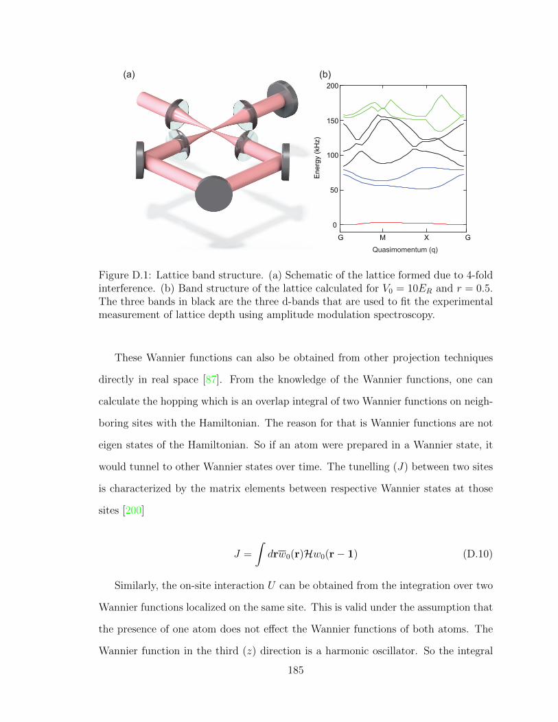
0

Energ

y (

kH

z)

50

Quasimomentum (q)

100

150

200

G M GX

(a) (b)

Figure D.1: Lattice band structure. (a) Schematic of the lattice formed due to 4-foldinterference. (b) Band structure of the lattice calculated for V0 = 10ER and r = 0.5.The three bands in black are the three d-bands that are used to fit the experimentalmeasurement of lattice depth using amplitude modulation spectroscopy.

These Wannier functions can also be obtained from other projection techniques

directly in real space [87]. From the knowledge of the Wannier functions, one can

calculate the hopping which is an overlap integral of two Wannier functions on neigh-

boring sites with the Hamiltonian. The reason for that is Wannier functions are not

eigen states of the Hamiltonian. So if an atom were prepared in a Wannier state, it

would tunnel to other Wannier states over time. The tunelling (J) between two sites

is characterized by the matrix elements between respective Wannier states at those

sites [200]

J =

∫drw0(r)Hw0(r− 1) (D.10)

Similarly, the on-site interaction U can be obtained from the integration over two

Wannier functions localized on the same site. This is valid under the assumption that

the presence of one atom does not effect the Wannier functions of both atoms. The

Wannier function in the third (z) direction is a harmonic oscillator. So the integral

185

along z just introduces a multiplicative factor

U =4πh2asm

√mωzh

∫|w0(x, y)|4dxdy (D.11)

where ωz is the confinement in the third direction.

186

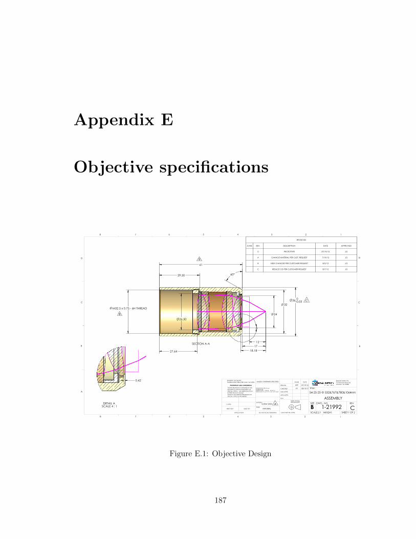
Appendix E

Objective specifications

Special Optics Inc.

D

C

B

A

B

C

D

12345678

8 7 6 5 4 3 2 1

THE INFORMATION CONTAINED IN THIS

PROJECTION

DRAWING IS THE SOLE PROPERTY OF

THIRD ANGLE

SPECIAL OPTICS. ANY REPRODUCTION

SPECIAL OPTICS IS PROHIBITED.

PROPRIETARY AND CONFIDENTIAL

NEXT ASSY USED ON

APPLICATION

WITHOUT THE WRITTEN PERMISSION OF

TOLERANCING PER:LATEST ANSI Y14.5 SPEC.

MATERIAL

FINISH

NATURAL

DRAWN

CHECKED

ENG APPR.

MFG APPR.

Q.A.

DATENAME

TITLE:

SIZE

BDWG. NO. REV

SCALE:2:1

UNLESS OTHERWISE SPECIFIED:

C

AFP

JO 08/13/12

07/19/12

ASSEMBLY

SHEET 1 OF 2

1-21992DO NOT SCALE DRAWING WEIGHT:

54-25-25 @ 532&767&780&1064nm

1-21992

INTERPRET GEOMETRIC

IN PART OR AS A WHOLE

wharton, NJ 07885

ULTEM 2300

CAD PART N0. 21992

315 Richard Mine Rd.

DIMENSIONS ARE IN mmTOLERANCES:LINEAR X= .5 .X= .25 .XX= .13ANGULAR: X°=±.25° .X°= ±.05° .XX°=.005°

SECTION A-A

A

0.050

27.64

26.50

29.50

61

60°

32

17

12

M32.5 x 0.75 - 6H THREAD

24

36 -

18.18

DETAIL A SCALE 4 : 1

0.42

C

A

B

B

REVISIONS

ZONE REV. DESCRIPTION DATE APPROVED

0 PROTOTYPE 07/19/12 JO

A CHANGE MATERIAL PER CUST. REQUEST 7/19/12 JO

B NEW CHANGES PER CUSTOMER REQUEST 8/2/12 JO

C REDUCE OD PER CUSTOMER REQUEST 8/7/12 JO

Figure E.1: Objective Design

187

Figure E.2: AR coating on objective

188

Bibliography

[1] V. Ginzburg and L. Landau. Toward the superconductivity theory. Zh. Eksp.Teor. Fiz., 29:1064, 1950.

[2] J. Bardeen, L. N. Cooper, and J. R. Schrieffer. Theory of Superconductivity.Phys. Rev., 108:1175–1204, 1957.

[3] M. H. Anderson, J. R. Ensher, M. R. Matthews, C. E. Wieman, and E. A.Cornell. Observation of Bose-Einstein Condensation in a Dilute Atomic Vapor.Science, 269(5221):198–201, 1995.

[4] K. B. Davis, M. O. Mewes, M. R. Andrews, N. J. van Druten, D. S. Durfee,D. M. Kurn, and W. Ketterle. Bose-Einstein Condensation in a Gas of SodiumAtoms. Phys. Rev. Lett., 75:3969–3973, 1995.

[5] B. DeMarco and D. S. Jin. Onset of Fermi Degeneracy in a Trapped AtomicGas. Science, 285(5434):1703–1706, 1999.

[6] Cheng Chin, Rudolf Grimm, Paul Julienne, and Eite Tiesinga. Feshbach reso-nances in ultracold gases. Rev. Mod. Phys., 82:1225–1286, 2010.

[7] Immanuel Bloch. Ultracold quantum gases in optical lattices. Nature Physics,1:23–30, 2005. Review Article.

[8] Ketterle W., M. Inguscio, and C. Salomon. Ultracold fermi gases. In Proceedingsof the Varenna ‘Enrico Fermi’ Summer School, volume 164, 2007.

[9] C. Chin, M. Bartenstein, A. Altmeyer, S. Riedl, S. Jochim, J. Hecker Denschlag,and R. Grimm. Observation of the Pairing Gap in a Strongly Interacting FermiGas. Science, 305(5687):1128–1130, 2004.

[10] G. B. Partridge, K. E. Strecker, R. I. Kamar, M. W. Jack, and R. G. Hulet.Molecular Probe of Pairing in the BEC-BCS Crossover. Phys. Rev. Lett.,95:020404, 2005.

[11] M. W. Zwierlein, J. R. Abo-Shaeer, A. Schirotzek, C. H. Schunck, and W. Ket-terle. Vortices and superfluidity in a strongly interacting Fermi gas. Nature,435:1047–1051, 2005. Article.

189

[12] Munekazu Horikoshi, Shuta Nakajima, Masahito Ueda, and TakashiMukaiyama. Measurement of Universal Thermodynamic Functions for a Uni-tary Fermi Gas. Science, 327(5964):442–445, 2010.

[13] N. Navon, S. Nascimbene, F. Chevy, and C. Salomon. The Equation ofState of a Low-Temperature Fermi Gas with Tunable Interactions. Science,328(5979):729–732, 2010.

[14] Mark J. H. Ku, Ariel T. Sommer, Lawrence W. Cheuk, and Martin W. Zwier-lein. Revealing the Superfluid Lambda Transition in the Universal Thermody-namics of a Unitary Fermi Gas. Science, 335(6068):563–567, 2012.

[15] Tarik Yefsah, Ariel T. Sommer, Mark J. H. Ku, Lawrence W. Cheuk, WenjieJi, Waseem S. Bakr, and Martin W. Zwierlein. Heavy solitons in a fermionicsuperfluid. Nature, 499:426–430, 2013. Article.

[16] Kenneth Gunter, Thilo Stoferle, Henning Moritz, Michael Kohl, and TilmanEsslinger. p-Wave Interactions in Low-Dimensional Fermionic Gases. Phys.Rev. Lett., 95:230401, 2005.

[17] Kirill Martiyanov, Vasiliy Makhalov, and Andrey Turlapov. Observation of aTwo-Dimensional Fermi Gas of Atoms. Phys. Rev. Lett., 105:030404, 2010.

[18] Bernd Frohlich, Michael Feld, Enrico Vogt, Marco Koschorreck, Wilhelm Zw-erger, and Michael Kohl. Radio-Frequency Spectroscopy of a Strongly Interact-ing Two-Dimensional Fermi Gas. Phys. Rev. Lett., 106:105301, 2011.

[19] P. Dyke, E. D. Kuhnle, S. Whitlock, H. Hu, M. Mark, S. Hoinka, M. Lingham,P. Hannaford, and C. J. Vale. Crossover from 2D to 3D in a Weakly InteractingFermi Gas. Phys. Rev. Lett., 106:105304, 2011.

[20] Ariel T. Sommer, Lawrence W. Cheuk, Mark J. H. Ku, Waseem S. Bakr, andMartin W. Zwierlein. Evolution of Fermion Pairing from Three to Two Dimen-sions. Phys. Rev. Lett., 108:045302, 2012.

[21] P. A. Murthy, I. Boettcher, L. Bayha, M. Holzmann, D. Kedar, M. Neidig, M. G.Ries, A. N. Wenz, G. Zurn, and S. Jochim. Observation of the Berezinskii-Kosterlitz-Thouless Phase Transition in an Ultracold Fermi Gas. Phys. Rev.Lett., 115:010401, 2015.

[22] C. A. Regal, M. Greiner, and D. S. Jin. Observation of Resonance Condensationof Fermionic Atom Pairs. Phys. Rev. Lett., 92:040403, 2004.

[23] Christian H. Schunck, Yong-il Shin, Andre Schirotzek, and Wolfgang Ketterle.Determination of the fermion pair size in a resonantly interacting superfluid.Nature, 454:739–743, 2008.

190

[24] Michael Feld, Bernd Frohlich, Enrico Vogt, Marco Koschorreck, and MichaelKohl. Observation of a pairing pseudogap in a two-dimensional Fermi gas.Nature, 480:75–78, 2011.

[25] Andre Schirotzek, Cheng-Hsun Wu, Ariel Sommer, and Martin W. Zwierlein.Observation of Fermi Polarons in a Tunable Fermi Liquid of Ultracold Atoms.Phys. Rev. Lett., 102:230402, 2009.

[26] Y. Zhang, W. Ong, I. Arakelyan, and J. E. Thomas. Polaron-to-Polaron Tran-sitions in the Radio-Frequency Spectrum of a Quasi-Two-Dimensional FermiGas. Phys. Rev. Lett., 108:235302, 2012.

[27] Marco Koschorreck, Daniel Pertot, Enrico Vogt, Bernd Frohlich, Michael Feld,and Michael Kohl. Attractive and repulsive Fermi polarons in two dimensions.Nature, 485:619–622, 2012.

[28] Giacomo Valtolina, Alessia Burchianti, Andrea Amico, Elettra Neri, KlejdjaXhani, Jorge Amin Seman, Andrea Trombettoni, Augusto Smerzi, Matteo Za-ccanti, Massimo Inguscio, and Giacomo Roati. Josephson effect in fermionicsuperfluids across the BEC-BCS crossover. Science, 350(6267):1505–1508, 2015.

[29] Martin W. Zwierlein, Andre Schirotzek, Christian H. Schunck, and WolfgangKetterle. Fermionic Superfluidity with Imbalanced Spin Populations. Science,311(5760):492–496, 2006.

[30] Y. Shin, M. W. Zwierlein, C. H. Schunck, A. Schirotzek, and W. Ketterle.Observation of Phase Separation in a Strongly Interacting Imbalanced FermiGas. Phys. Rev. Lett., 97:030401, 2006.

[31] G. B. Partridge, Wenhui Li, Y. A. Liao, R. G. Hulet, M. Haque, and H. T. C.Stoof. Deformation of a Trapped Fermi Gas with Unequal Spin Populations.Phys. Rev. Lett., 97:190407, 2006.

[32] Yean-an Liao, Ann Sophie C. Rittner, Tobias Paprotta, Wenhui Li, Guthrie B.Partridge, Randall G. Hulet, Stefan K. Baur, and Erich J. Mueller. Spin-imbalance in a one-dimensional Fermi gas. Nature, 467:567–569, 2010.

[33] S. Nascimbene, N. Navon, K. J. Jiang, F. Chevy, and C. Salomon. Exploringthe thermodynamics of a universal Fermi gas. Nature, 463:1057–1060, 2010.

[34] W. Ong, Chingyun Cheng, I. Arakelyan, and J. E. Thomas. Spin-ImbalancedQuasi-Two-Dimensional Fermi Gases. Phys. Rev. Lett., 114:110403, 2015.

[35] Debayan Mitra, Peter T. Brown, Peter Schauß, Stanimir S. Kondov, andWaseem S. Bakr. Phase Separation and Pair Condensation in a Spin-Imbalanced2D Fermi Gas. Phys. Rev. Lett., 117:093601, 2016.

191

[36] O. Morsch, J. H. Muller, M. Cristiani, D. Ciampini, and E. Arimondo. BlochOscillations and Mean-Field Effects of Bose-Einstein Condensates in 1D OpticalLattices. Phys. Rev. Lett., 87:140402, 2001.

[37] Marcos Atala, Monika Aidelsburger, Julio T. Barreiro, Dmitry Abanin, TakuyaKitagawa, Eugene Demler, and Immanuel Bloch. Direct measurement of theZak phase in topological Bloch bands. Nature Physics, 9:795–800, 2013.

[38] M. Aidelsburger, M. Lohse, C. Schweizer, M. Atala, J. T. Barreiro,S. Nascimbene, N. R. Cooper, I. Bloch, and N. Goldman. Measuring the Chernnumber of Hofstadter bands with ultracold bosonic atoms. Nature Physics,11:162–166, 2014.

[39] P. W. Anderson. The Resonating Valence Bond State in La2CuO4 and Super-conductivity. Science, 235(4793):1196–1198, 1987.

[40] Elliott H. Lieb and F. Y. Wu. Absence of Mott Transition in an Exact Solutionof the Short-Range, One-Band Model in One Dimension. Phys. Rev. Lett.,20:1445–1448, 1968.

[41] J. E. Hirsch. Two-dimensional Hubbard model: Numerical simulation study.Phys. Rev. B, 31:4403–4419, 1985.

[42] A. Moreo and D. J. Scalapino. Two-dimensional negative-U Hubbard model.Phys. Rev. Lett., 66:946–948, 1991.

[43] Thereza Paiva, Raimundo R. dos Santos, R. T. Scalettar, and P. J. H. Dente-neer. Critical temperature for the two-dimensional attractive Hubbard model.Phys. Rev. B, 69:184501, 2004.

[44] Marcos Rigol, Tyler Bryant, and Rajiv R. P. Singh. Numerical Linked-ClusterApproach to Quantum Lattice Models. Phys. Rev. Lett., 97:187202, 2006.

[45] Matthias Troyer and Uwe-Jens Wiese. Computational Complexity and Fun-damental Limitations to Fermionic Quantum Monte Carlo Simulations. Phys.Rev. Lett., 94:170201, 2005.

[46] Richard P. Feynman. Simulating physics with computers. International Journalof Theoretical Physics, 21(6):467–488, 1982.

[47] Waseem S. Bakr, Jonathon I. Gillen, Amy Peng, Simon Folling, and MarkusGreiner. A quantum gas microscope for detecting single atoms in a Hubbard-regime optical lattice. Nature, 462:74–77, 2009.

[48] Jacob F. Sherson, Christof Weitenberg, Manuel Endres, Marc Cheneau, Im-manuel Bloch, and Stefan Kuhr. Single-atom-resolved fluorescence imaging ofan atomic Mott insulator. Nature, 467:68–72, 2010.

192

[49] W. S. Bakr, A. Peng, M. E. Tai, R. Ma, J. Simon, J. I. Gillen, S. Folling,L. Pollet, and M. Greiner. Probing the Superfluid–to–Mott Insulator Transitionat the Single-Atom Level. Science, 329(5991):547–550, 2010.

[50] Elmar Haller, James Hudson, Andrew Kelly, Dylan A. Cotta, Bruno Peaudecerf,Graham D. Bruce, and Stefan Kuhr. Single-atom imaging of fermions in aquantum-gas microscope. Nature Physics, 11:738 – 742, 2015.

[51] G. J. A. Edge, R. Anderson, D. Jervis, D. C. McKay, R. Day, S. Trotzky, andJ. H. Thywissen. Imaging and addressing of individual fermionic atoms in anoptical lattice. Phys. Rev. A, 92:063406, 2015.

[52] Ahmed Omran, Martin Boll, Timon A. Hilker, Katharina Kleinlein, GuillaumeSalomon, Immanuel Bloch, and Christian Gross. Microscopic Observationof Pauli Blocking in Degenerate Fermionic Lattice Gases. Phys. Rev. Lett.,115:263001, 2015.

[53] Maxwell F. Parsons, Florian Huber, Anton Mazurenko, Christie S. Chiu,Widagdo Setiawan, Katherine Wooley-Brown, Sebastian Blatt, and MarkusGreiner. Site-Resolved Imaging of Fermionic 6Li in an Optical Lattice. Phys.Rev. Lett., 114:213002, 2015.

[54] Lawrence W. Cheuk, Matthew A. Nichols, Melih Okan, Thomas Gersdorf,Vinay V. Ramasesh, Waseem S. Bakr, Thomas Lompe, and Martin W. Zwier-lein. Quantum-Gas Microscope for Fermionic Atoms. Phys. Rev. Lett.,114:193001, 2015.

[55] Daniel Greif, Maxwell F. Parsons, Anton Mazurenko, Christie S. Chiu, Se-bastian Blatt, Florian Huber, Geoffrey Ji, and Markus Greiner. Site-resolvedimaging of a fermionic Mott insulator. Science, 351(6276):953–957, 2016.

[56] Lawrence W. Cheuk, Matthew A. Nichols, Katherine R. Lawrence, Melih Okan,Hao Zhang, and Martin W. Zwierlein. Observation of 2D Fermionic Mott In-sulators of 40K with Single-Site Resolution. Phys. Rev. Lett., 116:235301, 2016.

[57] Maxwell F. Parsons, Anton Mazurenko, Christie S. Chiu, Geoffrey Ji, DanielGreif, and Markus Greiner. Site-resolved measurement of the spin-correlationfunction in the Fermi-Hubbard model. Science, 353(6305):1253–1256, 2016.

[58] Lawrence W. Cheuk, Matthew A. Nichols, Katherine R. Lawrence, Melih Okan,Hao Zhang, Ehsan Khatami, Nandini Trivedi, Thereza Paiva, Marcos Rigol, andMartin W. Zwierlein. Observation of spatial charge and spin correlations in the2D Fermi-Hubbard model. Science, 353(6305):1260–1264, 2016.

[59] Martin Boll, Timon A. Hilker, Guillaume Salomon, Ahmed Omran, JacopoNespolo, Lode Pollet, Immanuel Bloch, and Christian Gross. Spin- and density-resolved microscopy of antiferromagnetic correlations in Fermi-Hubbard chains.Science, 353(6305):1257–1260, 2016.

193

[60] Peter T. Brown, Debayan Mitra, Elmer Guardado-Sanchez, Peter Schauß, Sta-nimir S. Kondov, Ehsan Khatami, Thereza Paiva, Nandini Trivedi, David A.Huse, and Waseem S. Bakr. Spin-imbalance in a 2D Fermi-Hubbard system.Science, 357(6358):1385–1388, 2017.

[61] J. K. Chin, D. E. Miller, Y. Liu, C. Stan, W. Setiawan, C. Sanner, K. Xu,and W. Ketterle. Evidence for superfluidity of ultracold fermions in an opticallattice. Nature, 443:961–964, 2006.

[62] Michael Kohl, Henning Moritz, Thilo Stoferle, Kenneth Gunter, and TilmanEsslinger. Fermionic Atoms in a Three Dimensional Optical Lattice: ObservingFermi Surfaces, Dynamics, and Interactions. Phys. Rev. Lett., 94:080403, 2005.

[63] Niels Strohmaier, Yosuke Takasu, Kenneth Gunter, Robert Jordens, MichaelKohl, Henning Moritz, and Tilman Esslinger. Interaction-Controlled Transportof an Ultracold Fermi Gas. Phys. Rev. Lett., 99:220601, 2007.

[64] Lucia Hackermuller, Ulrich Schneider, Maria Moreno-Cardoner, Takuya Kita-gawa, Thorsten Best, Sebastian Will, Eugene Demler, Ehud Altman, ImmanuelBloch, and Belen Paredes. Anomalous Expansion of Attractively InteractingFermionic Atoms in an Optical Lattice. Science, 327(5973):1621–1624, 2010.

[65] Debayan Mitra, Peter T. Brown, Elmer Guardado-Sanchez, Stanimir S. Kon-dov, Trithep Devakul, David A. Huse, Peter Schauß, and Waseem S. Bakr.Quantum gas microscopy of an attractive Fermi-Hubbard system. NaturePhysics, 14:173–177, 2017.

[66] Jean-Philippe Brantut, Jakob Meineke, David Stadler, Sebastian Krinner, andTilman Esslinger. Conduction of Ultracold Fermions Through a MesoscopicChannel. Science, 337(6098):1069–1071, 2012.

[67] Martin Lebrat, Pjotrs Grisins, Dominik Husmann, Samuel Hausler, Laura Cor-man, Thierry Giamarchi, Jean-Philippe Brantut, and Tilman Esslinger. Bandand Correlated Insulators of Cold Fermions in a Mesoscopic Lattice. Phys. Rev.X, 8:011053, 2018.

[68] H. Ott, E. de Mirandes, F. Ferlaino, G. Roati, G. Modugno, and M. Ingus-cio. Collisionally Induced Transport in Periodic Potentials. Phys. Rev. Lett.,92:160601, 2004.

[69] Wenchao Xu, William McGehee, William Morong, and Brian DeMarco. BadMetal in a Fermi Lattice Gas. arXiv:1606.06669, 2016.

[70] Rhys Anderson, Fudong Wang, Peihang Xu, Vijin Venu, Stefan Trotzky,Frederic Chevy, and Joseph H. Thywissen. Optical conductivity of a quantumgas. arXiv:1712.09965, 2017.

194

[71] Peter T. Brown, Debayan Mitra, Elmer Guardado-Sanchez, Reza Nourafkan,Alexis Reymbaut, Simon Bergeron, A. M. S. Tremblay, Jure Kokalj, David A.Huse, Peter Schauss, and Waseem S. Bakr. Bad metallic transport in a coldatom Fermi-Hubbard system. arXiv:1802.09456, 2018.

[72] N. F. Mott. Conduction in non-crystalline systems IX. the minimum metallicconductivity. The Philosophical Magazine: A Journal of Theoretical Experi-mental and Applied Physics, 26(4):1015–1026, 1972.

[73] A.F. Ioffe and A.R. Regel. Prog. Semicond., 4:237, 1960.

[74] Friedhelm Serwane. The setup of a Magneto Optical Trap for the preparationof a mesoscopic degenerate Fermi gas. Master’s thesis, University of Heidelberg,2007.

[75] Scientific Software Developed by the ID Group. Radia, Version 4.1, 2017.

[76] R. K. Raj, D. Bloch, J. J. Snyder, G. Camy, and M. Ducloy. High-FrequencyOptically Heterodyned Saturation Spectroscopy Via Resonant Degenerate Four-Wave Mixing. Phys. Rev. Lett., 44:1251–1254, 1980.

[77] F. Huber. Site-Resolved Imaging with the Fermi Gas Microscope. PhD thesis,Harvard University, 2014.

[78] Eryn C. Cook, Paul J. Martin, Tobias L. Brown-Heft, Jeffrey C. Garman, andDaniel A. Steck. High passive-stability diode-laser design for use in atomic-physics experiments. Review of Scientific Instruments, 83(4):043101, 2012.

[79] Rudolf Grimm, Matthias Weidemuller, and Yurii B. Ovchinnikov. OpticalDipole Traps for Neutral Atoms. 42:95–170, 2000.

[80] S. Al-Assam, R. A. Williams, and C. J. Foot. Ultracold atoms in an opticallattice with dynamically variable periodicity. Phys. Rev. A, 82:021604, 2010.

[81] Zhang Bai-Gang, Yao Jian-Quan, Lu Yang, Xu De-Gang, Ding Xin, Wang Peng,Zhang Tie-Li, and Ji Feng. High-efficiency single-pass cw quasi-phase-matchedfrequency doubling based on PP-MgO:SLT. Chinese Physics B, 14:353, 2005.

[82] Hwan Hong Lim, Toshio Katagai, Sunao Kurimura, Noriaki Ohmae, NorikatsuMio, Takahiro Shimizu, and Ichiro Shoji. Thermal Management in High PowerCW SHG Characterized by PMC. In Nonlinear Optics. Optical Society ofAmerica, 2011.

[83] J. Sebby-Strabley, M. Anderlini, P. S. Jessen, and J. V. Porto. Lattice of doublewells for manipulating pairs of cold atoms. Phys. Rev. A, 73:033605, 2006.

[84] Immanuel Bloch, Jean Dalibard, and Wilhelm Zwerger. Many-body physicswith ultracold gases. Rev. Mod. Phys., 80:885–964, 2008.

195

[85] Wilhelm Zwerger. Mott–Hubbard transition of cold atoms in optical lattices.Journal of Optics B: Quantum and Semiclassical Optics, 5(2):S9, 2003.

[86] Tilman Esslinger. Fermi-Hubbard Physics with Atoms in an Optical Lattice.Annual Review of Condensed Matter Physics, 1(1):129–152, 2010.

[87] Nicola Marzari, Arash A. Mostofi, Jonathan R. Yates, Ivo Souza, and DavidVanderbilt. Maximally localized Wannier functions: Theory and applications.Rev. Mod. Phys., 84:1419–1475, 2012.

[88] Thomas Uehlinger, Gregor Jotzu, Michael Messer, Daniel Greif, Walter Hof-stetter, Ulf Bissbort, and Tilman Esslinger. Artificial Graphene with TunableInteractions. Phys. Rev. Lett., 111:185307, 2013.

[89] P. M. Duarte, R. A. Hart, J. M. Hitchcock, T. A. Corcovilos, T.-L. Yang,A. Reed, and R. G. Hulet. All-optical production of a lithium quantum gasusing narrow-line laser cooling. Phys. Rev. A, 84:061406, 2011.

[90] H.J. Metcalf and P. van der Straten. Laser Cooling and Trapping. Springer,1999.

[91] Amar C Vutha. A simple approach to the Landau–Zener formula. EuropeanJournal of Physics, 31(2):389, 2010.

[92] Bryce Gadway, Daniel Pertot, Rene Reimann, Martin G. Cohen, and DominikSchneble. Analysis of Kapitza-Dirac diffraction patterns beyond the Raman-Nath regime. Opt. Express, 17(21):19173–19180, 2009.

[93] Giovanna Morigi, Jurgen Eschner, and Christoph H. Keitel. Ground StateLaser Cooling Using Electromagnetically Induced Transparency. Phys. Rev.Lett., 85:4458–4461, 2000.

[94] C. Monroe, D. M. Meekhof, B. E. King, S. R. Jefferts, W. M. Itano, D. J.Wineland, and P. Gould. Resolved-Sideband Raman Cooling of a Bound Atomto the 3D Zero-Point Energy. Phys. Rev. Lett., 75:4011–4014, 1995.

[95] Vladan Vuletic, Cheng Chin, Andrew J. Kerman, and Steven Chu. Degener-ate Raman Sideband Cooling of Trapped Cesium Atoms at Very High AtomicDensities. Phys. Rev. Lett., 81:5768–5771, 1998.

[96] P. Schauß. High-resolution imaging of ordering in Rydberg many-body systems.PhD thesis, LMU Munchen, 2014.

[97] E. Fermi. Zur Quantelung des idealen einatomigen Gases. Zeitschrift fur Physik,36(11):902–912, 1926.

[98] W. Pauli. Uber den Zusammenhang des Abschlusses der Elektronengruppen imAtom mit der Komplexstruktur der Spektren. Zeitschrift fur Physik, 31(1):765–783, 1925.

196

[99] D. A. Butts and D. S. Rokhsar. Trapped Fermi gases. Phys. Rev. A, 55:4346–4350, 1997.

[100] R. B. Laughlin. Quantized Hall conductivity in two dimensions. Phys. Rev. B,23:5632–5633, 1981.

[101] F. D. M. Haldane. Model for a Quantum Hall Effect without Landau Lev-els: Condensed-Matter Realization of the “Parity Anomaly”. Phys. Rev. Lett.,61:2015–2018, 1988.

[102] Elbio Dagotto. Correlated electrons in high-temperature superconductors. Rev.Mod. Phys., 66:763–840, 1994.

[103] Meera M. Parish, Stefan K. Baur, Erich J. Mueller, and David A. Huse. Quasi-One-Dimensional Polarized Fermi Superfluids. Phys. Rev. Lett., 99:250403,2007.

[104] T K Koponen, T Paananen, J-P Martikainen, M R Bakhtiari, and P Torma.FFLO state in 1-, 2- and 3-dimensional optical lattices combined with a non-uniform background potential. New Journal of Physics, 10(4):045014, 2008.

[105] W. C. Ong. Spin Imbalanced Quasi-Two-Dimensional Fermi Gases. PhD thesis,Duke University, 2015.

[106] Sadhan K. Adhikari. Quantum scattering in two dimensions. American Journalof Physics, 54(4):362–367, 1986.

[107] Jesper Levinsen and Meera M. Parish. Strongly interacting two-dimensionalFermi gases, chapter 1, pages 1–75.

[108] Mohit Randeria, Ji-Min Duan, and Lih-Yir Shieh. Superconductivity in a two-dimensional Fermi gas: Evolution from Cooper pairing to Bose condensation.Phys. Rev. B, 41:327–343, 1990.

[109] D. S. Petrov and G. V. Shlyapnikov. Interatomic collisions in a tightly confinedBose gas. Phys. Rev. A, 64:012706, 2001.

[110] Vasiliy Makhalov, Kirill Martiyanov, and Andrey Turlapov. Ground-State Pres-sure of Quasi-2D Fermi and Bose Gases. Phys. Rev. Lett., 112:045301, 2014.

[111] Chingyun Cheng, J. Kangara, I. Arakelyan, and J. E. Thomas. Fermi gasesin the two-dimensional to quasi-two-dimensional crossover. Phys. Rev. A,94:031606, 2016.

[112] P. Dyke, K. Fenech, T. Peppler, M. G. Lingham, S. Hoinka, W. Zhang, S.-G.Peng, B. Mulkerin, H. Hu, X.-J. Liu, and C. J. Vale. Criteria for two-dimensionalkinematics in an interacting Fermi gas. Phys. Rev. A, 93:011603, 2016.

197

[113] T. Bourdel, L. Khaykovich, J. Cubizolles, J. Zhang, F. Chevy, M. Teichmann,L. Tarruell, S. J. J. M. F. Kokkelmans, and C. Salomon. Experimental Studyof the BEC-BCS Crossover Region in Lithium 6. Phys. Rev. Lett., 93:050401,2004.

[114] I. Boettcher, L. Bayha, D. Kedar, P. A. Murthy, M. Neidig, M. G. Ries, A. N.Wenz, G. Zurn, S. Jochim, and T. Enss. Equation of State of Ultracold Fermionsin the 2D BEC-BCS Crossover Region. Phys. Rev. Lett., 116:045303, 2016.

[115] D. S. Petrov, M. A. Baranov, and G. V. Shlyapnikov. Superfluid transition inquasi-two-dimensional Fermi gases. Phys. Rev. A, 67:031601, 2003.

[116] D. S. Petrov, C. Salomon, and G. V. Shlyapnikov. Weakly Bound Dimers ofFermionic Atoms. Phys. Rev. Lett., 93:090404, 2004.

[117] Mohit Randeria and Edward Taylor. Crossover from Bardeen-Cooper-Schriefferto Bose-Einstein Condensation and the Unitary Fermi Gas. Annual Review ofCondensed Matter Physics, 5(1):209–232, 2014.

[118] M. Bartenstein, A. Altmeyer, S. Riedl, S. Jochim, R. Geursen, C. Chin,J. Hecker Denschlag, and R. Grimm. Exploring the BEC-BCS Crossover withan Ultracold Gas of 6Li Atoms. AIP Conference Proceedings, 770(1):278–288,2005.

[119] N. D. Mermin and H. Wagner. Absence of Ferromagnetism or Antiferromag-netism in One- or Two-Dimensional Isotropic Heisenberg Models. Phys. Rev.Lett., 17:1133–1136, 1966.

[120] P. C. Hohenberg. Existence of Long-Range Order in One and Two Dimensions.Phys. Rev., 158:383–386, 1967.

[121] J. W. Kane and L. P. Kadanoff. Long-Range Order in Superfluid Helium. Phys.Rev., 155:80–83, 1967.

[122] V.L. Berezinskii. Destruction of Long-range Order in One-dimensional and Two-dimensional Systems Possessing a Continuous Symmetry Group. II. QuantumSystems. Sov. Phys. JETP, 34:610, 1971.

[123] J M Kosterlitz and D J Thouless. Ordering, metastability and phase transi-tions in two-dimensional systems. Journal of Physics C: Solid State Physics,6(7):1181, 1973.

[124] J M Kosterlitz. The critical properties of the two-dimensional XY model. Jour-nal of Physics C: Solid State Physics, 7(6):1046, 1974.

[125] David R. Nelson and J. M. Kosterlitz. Universal Jump in the Superfluid Densityof Two-Dimensional Superfluids. Phys. Rev. Lett., 39:1201–1205, 1977.

198

[126] Zoran Hadzibabic, Peter Kruger, Marc Cheneau, Baptiste Battelier, and JeanDalibard. Berezinskii-Kosterlitz-Thouless crossover in a trapped atomic gas.Nature, 441:1118–1121, 2006.

[127] Peter Fulde and Richard A. Ferrell. Superconductivity in a Strong Spin-Exchange Field. Phys. Rev., 135:A550–A563, 1964.

[128] A.I. Larkin and Y.N. Ovchinnikov. Nonuniform state of superconductors. Sov.Phys. JETP, 20:762, 1965.

[129] Daniel E. Sheehy. Fulde-Ferrell-Larkin-Ovchinnikov state of two-dimensionalimbalanced Fermi gases. Phys. Rev. A, 92:053631, 2015.

[130] M. M. Parish, F. M. Marchetti, A. Lamacraft, and B. D. Simons. Finite-temperature phase diagram of a polarized Fermi condensate. Nature Physics,3:124–128, 2007.

[131] G. J. Conduit, P. H. Conlon, and B. D. Simons. Superfluidity at the BEC-BCScrossover in two-dimensional Fermi gases with population and mass imbalance.Phys. Rev. A, 77:053617, 2008.

[132] Lianyi He and Pengfei Zhuang. Phase diagram of a cold polarized Fermi gas intwo dimensions. Phys. Rev. A, 78:033613, 2008.

[133] Andrea M. Fischer and Meera M. Parish. Quasi-two-dimensional Fermi gasesat finite temperatures. Phys. Rev. B, 90:214503, 2014.

[134] Shaoyu Yin, J.-P. Martikainen, and P. Torma. Fulde-Ferrell states andBerezinskii-Kosterlitz-Thouless phase transition in two-dimensional imbalancedFermi gases. Phys. Rev. B, 89:014507, 2014.

[135] Philipp Strack and Pawel Jakubczyk. Fluctuations of Imbalanced FermionicSuperfluids in Two Dimensions Induce Continuous Quantum Phase Transitionsand Non-Fermi-Liquid Behavior. Phys. Rev. X, 4:021012, 2014.

[136] Martin W. Zwierlein, Christian H. Schunck, Andre Schirotzek, and WolfgangKetterle. Direct observation of the superfluid phase transition in ultracold Fermigases. Nature, 442:54–58, 2006.

[137] Ben A. Olsen, Melissa C. Revelle, Jacob A. Fry, Daniel E. Sheehy, and Ran-dall G. Hulet. Phase diagram of a strongly interacting spin-imbalanced Fermigas. Phys. Rev. A, 92:063616, 2015.

[138] Paulo F. Bedaque, Heron Caldas, and Gautam Rupak. Phase Separation inAsymmetrical Fermion Superfluids. Phys. Rev. Lett., 91:247002, 2003.

[139] J. Carlson and Sanjay Reddy. Asymmetric Two-Component Fermion Systemsin Strong Coupling. Phys. Rev. Lett., 95:060401, 2005.

199

[140] Daniel E. Sheehy and Leo Radzihovsky. BEC-BCS Crossover in “Magnetized”Feshbach-Resonantly Paired Superfluids. Phys. Rev. Lett., 96:060401, 2006.

[141] Daniel E. Sheehy and Leo Radzihovsky. BEC–BCS crossover, phase transi-tions and phase separation in polarized resonantly-paired superfluids. Annalsof Physics, 322(8):1790 – 1924, 2007.

[142] G. Sarma. On the influence of a uniform exchange field acting on the spins of theconduction electrons in a superconductor. Journal of Physics and Chemistry ofSolids, 24(8):1029–1032, 1963.

[143] K. B. Gubbels, M. W. J. Romans, and H. T. C. Stoof. Sarma Phase in TrappedUnbalanced Fermi Gases. Phys. Rev. Lett., 97:210402, 2006.

[144] A. M. Clogston. Upper Limit for the Critical Field in Hard Superconductors.Phys. Rev. Lett., 9:266–267, 1962.

[145] I. Bausmerth, A. Recati, and S. Stringari. Chandrasekhar-Clogston limit andphase separation in Fermi mixtures at unitarity. Phys. Rev. A, 79:043622, 2009.

[146] A V Turlapov and M Yu Kagan. Fermi-to-Bose crossover in a trapped quasi-2Dgas of fermionic atoms. Journal of Physics: Condensed Matter, 29(38):383004,2017.

[147] Vudtiwat Ngampruetikorn, Jesper Levinsen, and Meera M. Parish. Pair Cor-relations in the Two-Dimensional Fermi Gas. Phys. Rev. Lett., 111:265301,2013.

[148] M. G. Ries, A. N. Wenz, G. Zurn, L. Bayha, I. Boettcher, D. Kedar, P. A.Murthy, M. Neidig, T. Lompe, and S. Jochim. Observation of Pair Condensationin the Quasi-2D BEC-BCS Crossover. Phys. Rev. Lett., 114:230401, 2015.

[149] K. Fenech, P. Dyke, T. Peppler, M. G. Lingham, S. Hoinka, H. Hu, and C. J.Vale. Thermodynamics of an Attractive 2D Fermi Gas. Phys. Rev. Lett.,116:045302, 2016.

[150] H. P. Buchler and G. Blatter. Phase separation of atomic Bose-Fermi mixturesin an optical lattice. Phys. Rev. A, 69:063603, 2004.

[151] Yong-il Shin, Andre Schirotzek, Christian H. Schunck, and Wolfgang Ket-terle. Realization of a Strongly Interacting Bose-Fermi Mixture from a Two-Component Fermi Gas. Phys. Rev. Lett., 101:070404, 2008.

[152] G. V. Skorniakov and K. A. Ter-Martirosian. Three Body Problem for ShortRange Forces. I. Scattering of Low Energy Neutrons by Deuterons. Sov. Phys.JETP, 4:648, 1957.

200

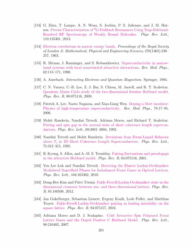
[153] G. Zurn, T. Lompe, A. N. Wenz, S. Jochim, P. S. Julienne, and J. M. Hut-son. Precise Characterization of 6Li Feshbach Resonances Using Trap-Sideband-Resolved RF Spectroscopy of Weakly Bound Molecules. Phys. Rev. Lett.,110:135301, 2013.

[154] Electron correlations in narrow energy bands. Proceedings of the Royal Societyof London A: Mathematical, Physical and Engineering Sciences, 276(1365):238–257, 1963.

[155] R. Micnas, J. Ranninger, and S. Robaszkiewicz. Superconductivity in narrow-band systems with local nonretarded attractive interactions. Rev. Mod. Phys.,62:113–171, 1990.

[156] A. Auerbach. Interacting Electrons and Quantum Magnetism. Springer, 1994.

[157] C. N. Varney, C.-R. Lee, Z. J. Bai, S. Chiesa, M. Jarrell, and R. T. Scalettar.Quantum Monte Carlo study of the two-dimensional fermion Hubbard model.Phys. Rev. B, 80:075116, 2009.

[158] Patrick A. Lee, Naoto Nagaosa, and Xiao-Gang Wen. Doping a Mott insulator:Physics of high-temperature superconductivity. Rev. Mod. Phys., 78:17–85,2006.

[159] Mohit Randeria, Nandini Trivedi, Adriana Moreo, and Richard T. Scalettar.Pairing and spin gap in the normal state of short coherence length supercon-ductors. Phys. Rev. Lett., 69:2001–2004, 1992.

[160] Nandini Trivedi and Mohit Randeria. Deviations from Fermi-Liquid Behaviorabove Tc in 2D Short Coherence Length Superconductors. Phys. Rev. Lett.,75:312–315, 1995.

[161] B. Kyung, S. Allen, and A.-M. S. Tremblay. Pairing fluctuations and pseudogapsin the attractive Hubbard model. Phys. Rev. B, 64:075116, 2001.

[162] Yen Lee Loh and Nandini Trivedi. Detecting the Elusive Larkin-OvchinnikovModulated Superfluid Phases for Imbalanced Fermi Gases in Optical Lattices.Phys. Rev. Lett., 104:165302, 2010.

[163] Dong-Hee Kim and Paivi Torma. Fulde-Ferrell-Larkin-Ovchinnikov state in thedimensional crossover between one- and three-dimensional lattices. Phys. Rev.B, 85:180508, 2012.

[164] Jan Gukelberger, Sebastian Lienert, Evgeny Kozik, Lode Pollet, and MatthiasTroyer. Fulde-Ferrell-Larkin-Ovchinnikov pairing as leading instability on thesquare lattice. Phys. Rev. B, 94:075157, 2016.

[165] Adriana Moreo and D. J. Scalapino. Cold Attractive Spin Polarized FermiLattice Gases and the Doped Positive U Hubbard Model. Phys. Rev. Lett.,98:216402, 2007.

201

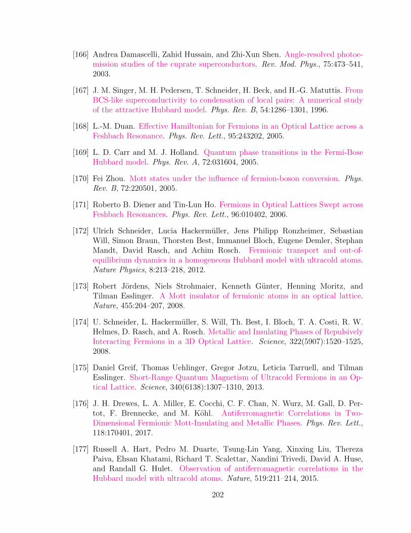
[166] Andrea Damascelli, Zahid Hussain, and Zhi-Xun Shen. Angle-resolved photoe-mission studies of the cuprate superconductors. Rev. Mod. Phys., 75:473–541,2003.

[167] J. M. Singer, M. H. Pedersen, T. Schneider, H. Beck, and H.-G. Matuttis. FromBCS-like superconductivity to condensation of local pairs: A numerical studyof the attractive Hubbard model. Phys. Rev. B, 54:1286–1301, 1996.

[168] L.-M. Duan. Effective Hamiltonian for Fermions in an Optical Lattice across aFeshbach Resonance. Phys. Rev. Lett., 95:243202, 2005.

[169] L. D. Carr and M. J. Holland. Quantum phase transitions in the Fermi-BoseHubbard model. Phys. Rev. A, 72:031604, 2005.

[170] Fei Zhou. Mott states under the influence of fermion-boson conversion. Phys.Rev. B, 72:220501, 2005.

[171] Roberto B. Diener and Tin-Lun Ho. Fermions in Optical Lattices Swept acrossFeshbach Resonances. Phys. Rev. Lett., 96:010402, 2006.

[172] Ulrich Schneider, Lucia Hackermuller, Jens Philipp Ronzheimer, SebastianWill, Simon Braun, Thorsten Best, Immanuel Bloch, Eugene Demler, StephanMandt, David Rasch, and Achim Rosch. Fermionic transport and out-of-equilibrium dynamics in a homogeneous Hubbard model with ultracold atoms.Nature Physics, 8:213–218, 2012.

[173] Robert Jordens, Niels Strohmaier, Kenneth Gunter, Henning Moritz, andTilman Esslinger. A Mott insulator of fermionic atoms in an optical lattice.Nature, 455:204–207, 2008.

[174] U. Schneider, L. Hackermuller, S. Will, Th. Best, I. Bloch, T. A. Costi, R. W.Helmes, D. Rasch, and A. Rosch. Metallic and Insulating Phases of RepulsivelyInteracting Fermions in a 3D Optical Lattice. Science, 322(5907):1520–1525,2008.

[175] Daniel Greif, Thomas Uehlinger, Gregor Jotzu, Leticia Tarruell, and TilmanEsslinger. Short-Range Quantum Magnetism of Ultracold Fermions in an Op-tical Lattice. Science, 340(6138):1307–1310, 2013.

[176] J. H. Drewes, L. A. Miller, E. Cocchi, C. F. Chan, N. Wurz, M. Gall, D. Per-tot, F. Brennecke, and M. Kohl. Antiferromagnetic Correlations in Two-Dimensional Fermionic Mott-Insulating and Metallic Phases. Phys. Rev. Lett.,118:170401, 2017.

[177] Russell A. Hart, Pedro M. Duarte, Tsung-Lin Yang, Xinxing Liu, TherezaPaiva, Ehsan Khatami, Richard T. Scalettar, Nandini Trivedi, David A. Huse,and Randall G. Hulet. Observation of antiferromagnetic correlations in theHubbard model with ultracold atoms. Nature, 519:211–214, 2015.

202

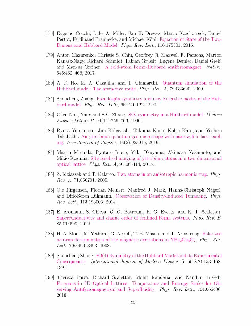
[178] Eugenio Cocchi, Luke A. Miller, Jan H. Drewes, Marco Koschorreck, DanielPertot, Ferdinand Brennecke, and Michael Kohl. Equation of State of the Two-Dimensional Hubbard Model. Phys. Rev. Lett., 116:175301, 2016.

[179] Anton Mazurenko, Christie S. Chiu, Geoffrey Ji, Maxwell F. Parsons, MartonKanasz-Nagy, Richard Schmidt, Fabian Grusdt, Eugene Demler, Daniel Greif,and Markus Greiner. A cold-atom Fermi-Hubbard antiferromagnet. Nature,545:462–466, 2017.

[180] A. F. Ho, M. A. Cazalilla, and T. Giamarchi. Quantum simulation of theHubbard model: The attractive route. Phys. Rev. A, 79:033620, 2009.

[181] Shoucheng Zhang. Pseudospin symmetry and new collective modes of the Hub-bard model. Phys. Rev. Lett., 65:120–122, 1990.

[182] Chen Ning Yang and S.C. Zhang. SO4 symmetry in a Hubbard model. ModernPhysics Letters B, 04(11):759–766, 1990.

[183] Ryuta Yamamoto, Jun Kobayashi, Takuma Kuno, Kohei Kato, and YoshiroTakahashi. An ytterbium quantum gas microscope with narrow-line laser cool-ing. New Journal of Physics, 18(2):023016, 2016.

[184] Martin Miranda, Ryotaro Inoue, Yuki Okuyama, Akimasa Nakamoto, andMikio Kozuma. Site-resolved imaging of ytterbium atoms in a two-dimensionaloptical lattice. Phys. Rev. A, 91:063414, 2015.

[185] Z. Idziaszek and T. Calarco. Two atoms in an anisotropic harmonic trap. Phys.Rev. A, 71:050701, 2005.

[186] Ole Jurgensen, Florian Meinert, Manfred J. Mark, Hanns-Christoph Nagerl,and Dirk-Soren Luhmann. Observation of Density-Induced Tunneling. Phys.Rev. Lett., 113:193003, 2014.

[187] E. Assmann, S. Chiesa, G. G. Batrouni, H. G. Evertz, and R. T. Scalettar.Superconductivity and charge order of confined Fermi systems. Phys. Rev. B,85:014509, 2012.

[188] H. A. Mook, M. Yethiraj, G. Aeppli, T. E. Mason, and T. Armstrong. Polarizedneutron determination of the magnetic excitations in YBa2Cu3O7. Phys. Rev.Lett., 70:3490–3493, 1993.

[189] Shoucheng Zhang. SO(4) Symmetry of the Hubbard Model and its ExperimentalConsequences. International Journal of Modern Physics B, 5(1&2):153–168,1991.

[190] Thereza Paiva, Richard Scalettar, Mohit Randeria, and Nandini Trivedi.Fermions in 2D Optical Lattices: Temperature and Entropy Scales for Ob-serving Antiferromagnetism and Superfluidity. Phys. Rev. Lett., 104:066406,2010.

203

[191] Eugene Demler, Shou-Cheng Zhang, Nejat Bulut, and Douglas J. Scalapino.A class of collective excitations of the Hubbard model: η excitation of thenegative-U model. International Journal of Modern Physics B, 10(17):2137–2166, 1996.

[192] Singer, J. M., Schneider, T., and Meier, P. F. Spectral properties of the attrac-tive Hubbard model. Eur. Phys. J. B, 7(1):37–51, 1999.

[193] Elmer Guardado-Sanchez, Peter T. Brown, Debayan Mitra, Trithep Devakul,David A. Huse, Peter Schauß, and Waseem S. Bakr. Probing the Quench Dy-namics of Antiferromagnetic Correlations in a 2D Quantum Ising Spin System.Phys. Rev. X, 8:021069, 2018.

[194] N. Henkel, R. Nath, and T. Pohl. Three-Dimensional Roton Excitations andSupersolid Formation in Rydberg-Excited Bose-Einstein Condensates. Phys.Rev. Lett., 104:195302, 2010.

[195] G. Pupillo, A. Micheli, M. Boninsegni, I. Lesanovsky, and P. Zoller. StronglyCorrelated Gases of Rydberg-Dressed Atoms: Quantum and Classical Dynam-ics. Phys. Rev. Lett., 104:223002, 2010.

[196] Johannes Zeiher, Rick van Bijnen, Peter Schauß, Sebastian Hild, Jae-yoon Choi,Thomas Pohl, Immanuel Bloch, and Christian Gross. Many-body interferome-try of a Rydberg-dressed spin lattice. Nature Physics, 12:1095–1099, 2016.

[197] Edward Perepelitsky, Andrew Galatas, Jernej Mravlje, Rok Zitko, EhsanKhatami, B. Sriram Shastry, and Antoine Georges. Transport and optical con-ductivity in the Hubbard model: A high-temperature expansion perspective.Phys. Rev. B, 94:235115, 2016.

[198] Frederik Gorg, Michael Messer, Kilian Sandholzer, Gregor Jotzu, Remi Des-buquois, and Tilman Esslinger. Enhancement and sign change of magneticcorrelations in a driven quantum many-body system. Nature, 553:481–485,2018.

[199] E. Arimondo, M. Inguscio, and P. Violino. Experimental determinations of thehyperfine structure in the alkali atoms. Rev. Mod. Phys., 49:31–75, 1977.

[200] P Blair Blakie and Charles W Clark. Wannier states and Bose–Hubbard pa-rameters for 2D optical lattices. Journal of Physics B: Atomic, Molecular andOptical Physics, 37(7):1391, 2004.

204