State transitions and the continuum limit for a 2D interacting, self-propelled particle system

State Transitions and the Continuum Limit

for a 2D Interacting, Self-Propelled Particle

System

Yao-li Chuang a,b,∗, Maria R. D’Orsogna b, Daniel Marthaler c,Andrea L. Bertozzi a,b, and Lincoln S. Chayes b

aDepartment of Physics, Duke University, Durham, NC, USAbDepartment of Mathematics, UCLA, Los Angeles, CA, USA

cACS-UMS, Northrop Grumman Corp, Rancho Bernardo, CA, USA

Abstract

We study a class of swarming problems wherein particles evolve dynamically viapairwise interaction potentials and a velocity selection mechanism. We find thatthe swarming system undergoes various changes of state as a function of the self-propulsion and interaction potential parameters. In this paper, we utilize a pro-cedure which, in a definitive way, connects a class of individual-based models totheir continuum formulations and determine criteria for the validity of the latter.H-stability of the interaction potential plays a fundamental role in determining boththe validity of the continuum approximation and the nature of the aggregation statetransitions. We perform a linear stability analysis of the continuum model and com-pare the results to the simulations of the individual-based one.

Key words: swarming, flocking, self-propelling particles, self-organizationPACS: 05.65.+b, 47.20.Hw, 47.54.-r, 87.18.Ed

∗ Corresponding authorEmail addresses: [email protected], [email protected] (Yao-li

Chuang), [email protected] (Maria R. D’Orsogna),[email protected] (Daniel Marthaler), [email protected](Andrea L. Bertozzi).

Preprint submitted to Elsevier Science 10 June 2006

1 Introduction

The collective behaviors of aggregating organisms are of interest in variousfields, including biology, engineering, mathematics, and physics [1–9]. Thereare primarily two classes of pertinent models: individual-based and continuumones. In the first case, one considers a collection of N individual entities, sothat the system is defined on the “microscopic” scale. Such models are par-ticularly useful for the study and algorithmic design of small-size aggregatessuch as artificial swarms of autonomous vehicles. Larger discrete systems areadaptive to statistical analysis [1,10–21]. Continuum models typically describeswarms through a density function ρ (~r) and a velocity vector field ~u (~r). Theseobey appropriate non-linear and often non-local equations. One may presumethese equations are derived from, or at least connected back to, the originalmicroscopic system. Continuum models are useful for theoretical analysis ofswarming systems [2,3,14,15,22–26]. Although both individual-based and con-tinuum models are applicable, the connection between the two has, in fact,not been particularly well established. A primary purpose of this paper is tobetter unify the two approaches, for a particular class of models, following theclassical statistical studies of fluids [27]. We investigate the validity of the con-tinuum model by a detailed comparison with the associated individual basedone. In particular, for certain interaction forms, the two descriptions yield thesame morphological patterns. Furthermore, and perhaps more importantly, weare able to explain why the continuum model fails qualitatively for the othercases, where discrepancies exist.

In Ref. [28], a criterion from classical statistical mechanics known as H-stabilitywas applied to individual based swarming models. A system of N interact-ing particles is said to be H-stable if the potential energy per particle isbounded below by a constant which is independent of the number of par-ticles present [29]. H-stability is a necessary and sufficient condition for theexistence of thermodynamics. Indeed, a system without this stability will, inthe thermodynamic limit, collapse onto itself; such systems are called catas-trophic. In Ref. [28], numerical simulations strongly suggest that a specificnon-Hamiltonian swarming system exhibits the same stability trends observedin classical Hamiltonian many-body systems. In this paper, we show that H-stability also plays an important role in determining the correct passage tothe continuum limit.

This paper is organized as follows. In Sec. 2, the individual-based model is pre-sented. We study various aggregation states and transitions between them vianumerical simulations. In Sec. 3, a continuum model is derived. In Sec. 4, wequantitatively compare steady states of both continuum and discrete models.We show that, while the proposed continuum model works well in the catas-trophic regime, discrepancies arise for large H-stable systems. In Sec. 5, the

2

�

�

�

�

�

��

�

�

�

�

�

�

�

�

�

�

�

�

�

�

�

�

��

�

�

�

�

!

"

#$%

&

'

(

)

*

+

,

-

.

/

0

1

234

5

67

8

9

:

;

<

=

>

?

@

A

B

C

D

E

F

G

H I

J

KL

MN

O

P

QR

S

T

U

V

W

X

Y

Z

[\

]

^_

`

a

b

c

de

f

g

h

i

j

k

l

mn

o p

q

r

s

t

u

v

w

x

y

z

{

|}

~

�

�

��

�

�

�

�

�

��

�

�

�

�

�

� � �

�

��

�

�

�

��

�

�

�

��

�

¡

¢

£

¤

¥

¦

§

¨

©

ª

«

¬

®

¯

°

±

²

³

´µ

¶

·

¸

¹

º

»

¼

½

¾

¿

ÀÁÂ

Ã

Ä

Å

Æ

Ç

�

�

�

�

�

�

�

�

�

�

�

� �

�

�

�

�

�

�

�

�

�

�

�

�

�

�

�

�

!

"

#$

%

&

')(

*

+

,

-

.

/

0

1

2

3 4

5

67

8

9

:

;

<

=

>

?

@

A

B

C

DE

F

G

H

I

J

K

L

M

N

O

P

Q

R

ST

U

V

W

X

Y

Z

[

\

]

^

_

`

a

b

c

d

e

f

g

h

i

j

k

l

m

n

o

p

q

r

s

t

u

v

w

x

y

z

{

|

}

~

�

�

�

�

�

�

�

�

�

�

�

�

�

�

�

�

��

�

�

�

�

�

��

�

�

�

�

�

�

�

�

¡

¢

£

¤

¥

¦ §

¨©

ª

«

¬

®

¯

°

±

²³

´

µ

¶

·

¸

¹

º

»

¼

½¾

¿

À

Á

Â

Ã

Ä

ÅÆ

Ç

È

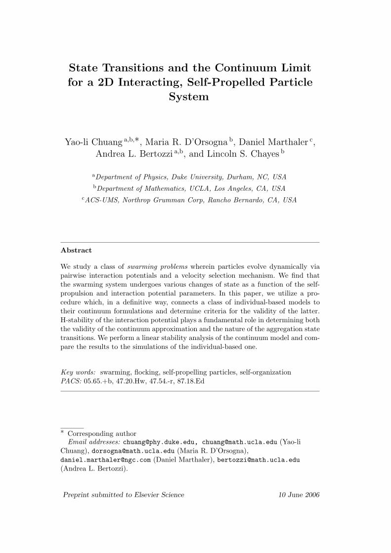
Fig. 1. Left: The swarming pattern of a single mill. Right: The swarming pattern oftwo interlocking mills.

stability of the homogeneous solution of the continuum model is studied andcompared to the numerical results of the individual-based model. In Sec. 6, wediscuss the choices between soft-core and hard-core interaction potentials.

2 The individual-based model

Background

Common swarming patterns have been observed and reported in various speciesin nature. One example is a coherent flock formation involving a polarizedgroup moving in the same direction. Another example is a single rotatingmill pattern, with a rather stationary center of mass, as in Fig. 1 (left). Therotating-mill pattern is frequently observed in both two and three dimensionsamong many species and across different sizes [5,7,30]. Various individual-based models have been able to reproduce these patterns within certain pa-rameter ranges [13,15–18,21]. An unusual pattern of overlapping double millsis also reported in Ref. [15], similar to the simulation shown in Fig. 1 (right).The double-mill phenomenon is observed in the early stages of aggregationof Myxococcus xanthus , a single-cell bacteria driven by self-propelling motors[31]. We show that this configuration can be obtained using the same swarm-ing mechanism that produces the single-mill pattern but exists in a differentparameter regime. The rarity of the double-mill state is discussed in Sec. 6.

3

Equations of motion

The swarming model we present in this paper is described by the followingequations of motion

d~xi

dt=~vi , (1)

mid~vi

dt= α~vi − β |~vi|2 ~vi − ~∇Ui, (2)

where mi, ~xi and ~vi are, respectively, the mass, position, and velocity of particlei. The terms α~vi and −β |~vi|2 ~vi define the mechanism of self-acceleration anddeceleration which give the particles a tendency to approach an equilibrium

speed veq =√

α/β. This Rayleigh-type dissipation was originally proposed in

Ref. [32] and is often used in the literature as a velocity-selecting mechanism[2,10,13,17,18,21,33]. The potential Ui describes the interaction of particle iwith the other particles. One common choice is the following [15,18,23,28]

Ui ≡ U (~xi) =∑j 6=i

V (|~xi − ~xj|) =∑j 6=i

−Ca e−|~xi−~xj|

à +Cr e−|~xi−~xj|

`r

. (3)

Eq. (3) assumes that only pairwise interactions are significant and ignores N -body interactions with N ≥ 3. The pairwise interaction consists of an attrac-tion and a repulsion with Ca, Cr specifying their respective strengths and à,`r their effective interaction length scales. Similar behaviors are also observedwith other functional forms of interaction potential that are characteristicallysimilar to Eq. (3). Note that to simplify the analysis, our model is determin-istic. Stochastic forces appear in many other models [1,10,13,17,18,21]. In oursimulations, we observe that noise affects the swarming patterns only beyondcertain thresholds, and thus its consequences are not investigated.

We can non-dimensionalize the equations of motion by substituting t′ =(mi/à

2β)t, ~x′i = ~xi/à, and thus, ~v′i = (àβ/mi)~vi into Eqs. (1) - (3)

d~x′idt′

=~v′i , (4)

d~v′idt′

= α′~v′i − |~v′i|2~v′i −

1

mi′~∇~x′i

Ui′, (5)

Ui′ =

∑j 6=i

(− e−|~x′i−~x′j|+C e−

|~x′i−~x′j|

`

), (6)

where α′ =(αβà

2)/mi

2, mi′ = mi

3/(β2Caà

2), C = Cr/Ca, and ` = `r/à;

4

� � � � � � � � � � � � � � � � � � � � � � � � ��

� � � � � � � � � � � � � � � � � � � � � � � � ��

C=C / Car

rl=

l / l

a

C=1

l=1

2 1C l = catas

troph

ic

cata

stro

phic H−stable

II

IV V

VI

I VIIcatastrophic

III H−stable

Fig. 2. The H-stability diagram of the interaction potential in Eq. (3) [28]. Theshaded region is the so-called biologically relevant region where the interaction con-sists of a long-range attraction and a short-range repulsion.

hence, the model is essentially a 4-parameter one. In Ref. [28] the effects ofvarying C and `, which affect H-stability, are explored. In this paper we inves-tigate the role of α′, the relative strength of the self-driving force with respectto the interaction. The parameter mi

′ affects the time scale of the particleinteraction and is fixed during our investigations. Note that the dimensionalparameter α only appears in the dimensionless parameter α′, which allows usto vary α to change α′ without affecting the other three independent parame-ters, provided that β, `a, and mi are fixed during the process. To preserve theoriginal meaning of the model parameters, our results are presented in the di-mensional form by using Eqs. (1) - (3). Only the biologically relevant cases thatconsist of a long-range attraction and a short-range repulsion are studied. Inother words, we confine our analysis to the parameter space where C > 1 and` < 1, which is shown by the shaded region of the H-stability phase diagramin Fig. 2. The extremely collapsing cases reported in [28], such as the ring for-mations and the clump formations illustrated in other regions, do not changemorphology with respect to α′.

5

Swarming states

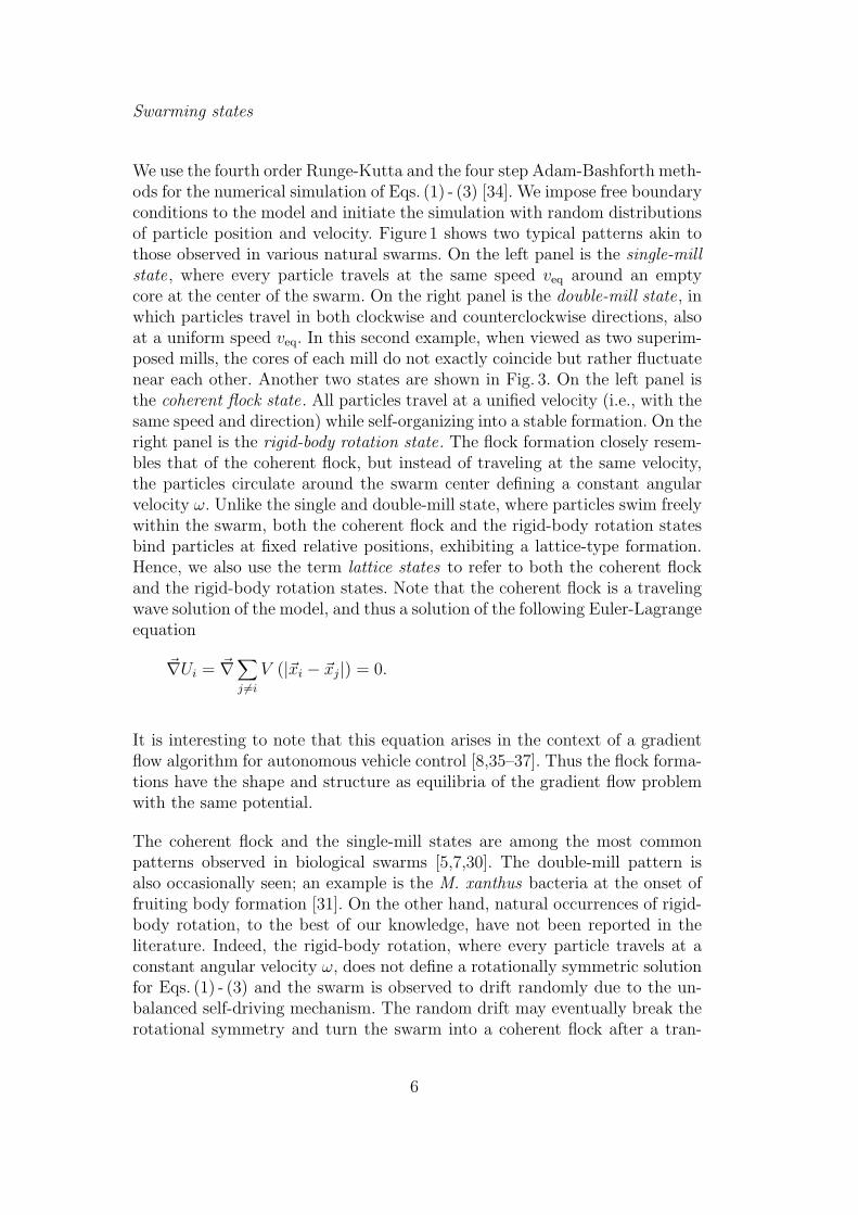
We use the fourth order Runge-Kutta and the four step Adam-Bashforth meth-ods for the numerical simulation of Eqs. (1) - (3) [34]. We impose free boundaryconditions to the model and initiate the simulation with random distributionsof particle position and velocity. Figure 1 shows two typical patterns akin tothose observed in various natural swarms. On the left panel is the single-millstate, where every particle travels at the same speed veq around an emptycore at the center of the swarm. On the right panel is the double-mill state, inwhich particles travel in both clockwise and counterclockwise directions, alsoat a uniform speed veq. In this second example, when viewed as two superim-posed mills, the cores of each mill do not exactly coincide but rather fluctuatenear each other. Another two states are shown in Fig. 3. On the left panel isthe coherent flock state. All particles travel at a unified velocity (i.e., with thesame speed and direction) while self-organizing into a stable formation. On theright panel is the rigid-body rotation state. The flock formation closely resem-bles that of the coherent flock, but instead of traveling at the same velocity,the particles circulate around the swarm center defining a constant angularvelocity ω. Unlike the single and double-mill state, where particles swim freelywithin the swarm, both the coherent flock and the rigid-body rotation statesbind particles at fixed relative positions, exhibiting a lattice-type formation.Hence, we also use the term lattice states to refer to both the coherent flockand the rigid-body rotation states. Note that the coherent flock is a travelingwave solution of the model, and thus a solution of the following Euler-Lagrangeequation

~∇Ui = ~∇∑j 6=i

V (|~xi − ~xj|) = 0.

It is interesting to note that this equation arises in the context of a gradientflow algorithm for autonomous vehicle control [8,35–37]. Thus the flock forma-tions have the shape and structure as equilibria of the gradient flow problemwith the same potential.

The coherent flock and the single-mill states are among the most commonpatterns observed in biological swarms [5,7,30]. The double-mill pattern isalso occasionally seen; an example is the M. xanthus bacteria at the onset offruiting body formation [31]. On the other hand, natural occurrences of rigid-body rotation, to the best of our knowledge, have not been reported in theliterature. Indeed, the rigid-body rotation, where every particle travels at aconstant angular velocity ω, does not define a rotationally symmetric solutionfor Eqs. (1) - (3) and the swarm is observed to drift randomly due to the un-balanced self-driving mechanism. The random drift may eventually break therotational symmetry and turn the swarm into a coherent flock after a tran-

6

�

�

�

�

�

��

�

�

�

�

�

�

�

�

�

��

�

�

�

�

�

�

�

�

�

�

�

!

"

#

$

%

&

'

(

)

*

+,

-

.

/

0

1

2

3

4

5 6

7

8

9:

;

<

=

>?

@

A

BC D

E

F

G

H

I

J

KL

M

N

OP

Q

R

S

T

U

V

W

X

Y

Z

[

\

]

^

_

`

a

b

cd

e

f

g

h

i

j

k

l

m

n

o

p

q

r

s

t

u

v

w

x

y

z

{

|

}

~

�

�

�

�

� ��

�

��

�

�

�

� ��

��

�

�

�

�

�

�

�

�

��

�

� �

�

�

¡

¢

£

¤

¥

¦

§

¨

©

ª

«

¬

®

¯

°

±

²

³

´

µ¶

·

¸

¹º

»

¼

½

¾

¿

À

Á

Â

Ã

Ä

ÅÆ

Ç

�

�

�

�

�

�

�

�

�

�

�

�

�

�

�

�

�

�

�

�

�

�

�

�

�

�

�

�

�

!

"#

$

%

&

'

(

)

*

+

,-

.

/

0

1

2

3

4

5

6

7

8

9

:;

<

=

>

?

@

A

B

C

D

E

F

G

H I

J

K

L

M

N

O

P

Q

R

S

T

U

V

W

X

Y

Z

[

\

]

^ _

`

a

b

c

d

e

f

g

h

i

j

k

l

m

n

o

p

qr

s

t

u

v

w

x

y

z{

|

}

~

�

�

�

�

�

��

�

�

�

�

�

�

�

�

�

�

�

�

�

�

�

�

�

�

�

��

�

�

�

�

�

¡

¢

£

¤

¥

¦

§

¨

©

ª

«

¬

®

¯

°

±

²

³

´

µ

¶

·

¸

¹

º

»

¼

½

¾

¿

À

Á

ÂÃ

Ä

Å

Æ

Ç

Fig. 3. Left: The coherent flock state. Right: The rigid-body rotation state.

sient period. Thus, we speculate that this pattern may only be a meta-stableor a transient state. In addition to the above aggregation states, the particlesmay simply escape from the collective potential field, and no aggregation isobserved. We name it the dispersed state.

Using numerical simulations, we find that the H-stable swarms undergo adifferent state transition process from that of the non-H-stable swarms. Forboth H-stable and catastrophic interactions, the lattice states, as shown inFig. 3, emerge for low values of α, and thus, of low veq. In this case, theconfining interaction potential is stronger than the kinetic energy of individualparticles and tends to bind the particles at specific “crystal” lattice sites. Mostinitial conditions lead to the coherent flock state while some occasions resultin the rigid-body rotation state. The state transition of H-stable swarms issimpler. As α increases, the particles eventually gain enough kinetic energy todissolve the aggregation.

The state transition of catastrophic swarms is characterized by more behav-ioral stages. Starting from the lattice states and upon increasing α, the parti-cles gain more kinetic energy from the environment to reach veq and are ableto break away from the crystal lattice sites. However, unlike H-stable swarms,the interaction potential in the catastrophic regime is still strong enough toaggregate medium-speed particles within a swarm. In this regime, core-freemill states emerge, as shown in Fig. 1. Since all particles travel at a non-zerouniform speed, the centripetal force provided by the collective interaction po-tential is not strong enough to sustain such particles too close to the rotationalcenter. As a result, the mill core is a particle-free region. At moderate α, asingle mill state emerges. At slightly higher α, we observe both single millsand double mills as possible states. In the latter case, the interaction potentialgradually loses its effectiveness to unify the clockwise (CW) and counterclock-

7

wise (CCW) rotational directions; particles traveling in the opposite directionwith respect to the majority tend to not change their direction of motion,and double mills can emerge. The transition from single to double mill is agradual process. Figure 4 shows the number of particles in each rotational di-rection for various values of α. In the single-mill regime, particles travelingat one direction are quickly assimilated into the other (Fig. 4, top). Upon in-creasing α, the particles no longer settle into a unified rotational direction(Fig. 4,middle), and for large enough α, approximately the same number ofparticles travel in each of the CW and CCW directions (Fig. 4, bottom). Thepresence of either a velocity alignment rule or a hard-core repulsive interac-tion will destroy this double-mill state. The latter case is because hard-coresalways provide a system with H-stability. Thus, it is clear that for sufficientlymany particles, the double mills will ultimately break apart. Notwithstanding,it appears that the double mills are especially sensitive to hard-cores and, evenfor small cores and moderate N , we have not observed these structures. As forthe coherent flock state, it still remains a possibility in this regime where themill states occur. However, the basin of attraction is greatly reduced, and onlyvery polarized initial conditions can lead to the coherent flock formation. Asα increases beyond the double-mill regime, particle kinetic energy eventuallybecomes high enough to break up the swarm. This is the dispersed state, andno aggregation can be found.

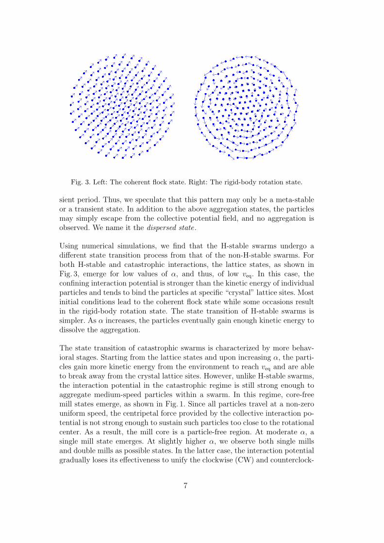
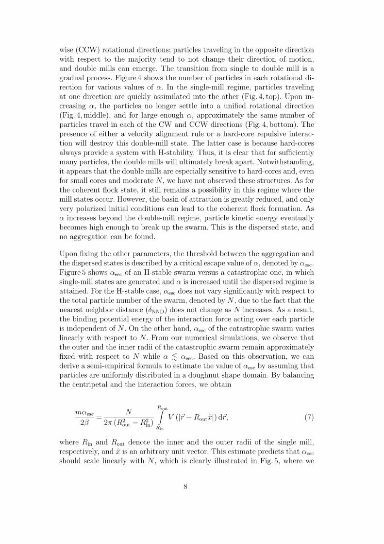
Upon fixing the other parameters, the threshold between the aggregation andthe dispersed states is described by a critical escape value of α, denoted by αesc.Figure 5 shows αesc of an H-stable swarm versus a catastrophic one, in whichsingle-mill states are generated and α is increased until the dispersed regime isattained. For the H-stable case, αesc does not vary significantly with respect tothe total particle number of the swarm, denoted by N , due to the fact that thenearest neighbor distance (δNND) does not change as N increases. As a result,the binding potential energy of the interaction force acting over each particleis independent of N . On the other hand, αesc of the catastrophic swarm varieslinearly with respect to N . From our numerical simulations, we observe thatthe outer and the inner radii of the catastrophic swarm remain approximatelyfixed with respect to N while α . αesc. Based on this observation, we canderive a semi-empirical formula to estimate the value of αesc by assuming thatparticles are uniformly distributed in a doughnut shape domain. By balancingthe centripetal and the interaction forces, we obtain

mαesc

2β=

N

2π (R2out −R2

in)

Rout∫Rin

V (|~r −Routx|) d~r, (7)

where Rin and Rout denote the inner and the outer radii of the single mill,respectively, and x is an arbitrary unit vector. This estimate predicts that αesc

should scale linearly with N , which is clearly illustrated in Fig. 5, where we

8

0

200

400

0

200

400

num

ber

of C

W/C

CW

par

ticle

s

0 200 400 600 800 1000time

240

260

Fig. 4. Time variation of the numbers of particles rotating in different directions:The triangles represent the number of CCW particles while the circles are of CWones. (Top) α = 1.5. (Middle) α = 4.0. (Lower) α = 6.0. The fixed parameters areβ = 0.5, Ca = 0.5, Cr = 1.0, `a = 2.0, `r = 0.5, and N = 500. All parameters hereand throughout the paper are in arbitrary units.

use the numerically simulated Rout = 5.2 and Rin = 1.2 for a quantitativecomparison.

State transitions of H-stable and catastrophic swarms

In order to quantitatively determine whether the swarm is in a coherent flockstate or a single-mill state, Couzin et al. have proposed two measures [16]: the

9

100 N

0.01

0.1

1

α esc

H-stableCatastrophicTheoretically estimated

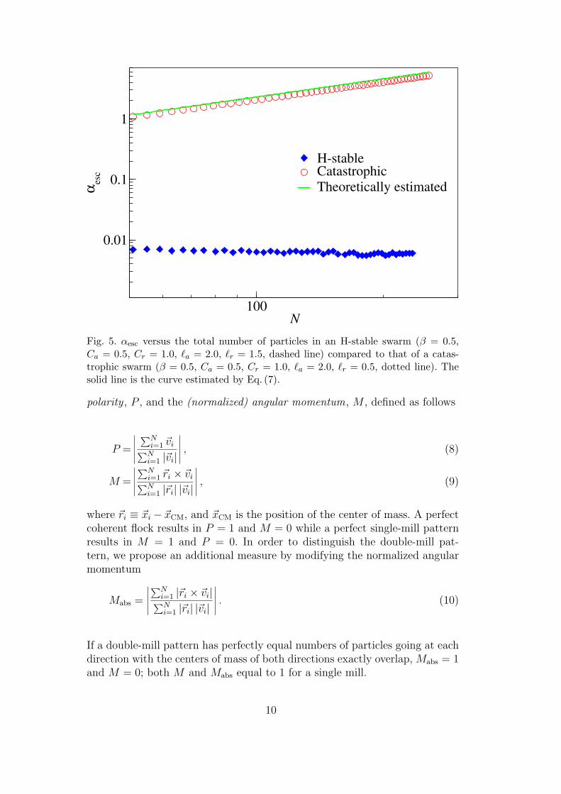
Fig. 5. αesc versus the total number of particles in an H-stable swarm (β = 0.5,Ca = 0.5, Cr = 1.0, `a = 2.0, `r = 1.5, dashed line) compared to that of a catas-trophic swarm (β = 0.5, Ca = 0.5, Cr = 1.0, `a = 2.0, `r = 0.5, dotted line). Thesolid line is the curve estimated by Eq. (7).

polarity , P , and the (normalized) angular momentum, M , defined as follows

P =

∣∣∣∣∣∑N

i=1 ~vi∑Ni=1 |~vi|

∣∣∣∣∣ , (8)

M =

∣∣∣∣∣∑N

i=1 ~ri × ~vi∑Ni=1 |~ri| |~vi|

∣∣∣∣∣ , (9)

where ~ri ≡ ~xi − ~xCM, and ~xCM is the position of the center of mass. A perfectcoherent flock results in P = 1 and M = 0 while a perfect single-mill patternresults in M = 1 and P = 0. In order to distinguish the double-mill pat-tern, we propose an additional measure by modifying the normalized angularmomentum

Mabs =

∣∣∣∣∣∑N

i=1 |~ri × ~vi|∑Ni=1 |~ri| |~vi|

∣∣∣∣∣ . (10)

If a double-mill pattern has perfectly equal numbers of particles going at eachdirection with the centers of mass of both directions exactly overlap, Mabs = 1and M = 0; both M and Mabs equal to 1 for a single mill.

10

0

0.04

0.08

0

0.1

0.2

0

0.2

0.4<v(r

)>ta

ng

0 1 2 3 r

0

0.5

1

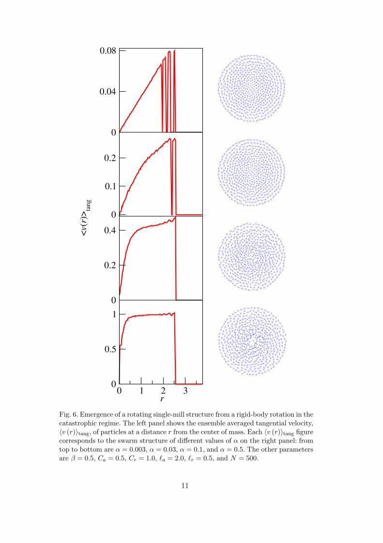
Fig. 6. Emergence of a rotating single-mill structure from a rigid-body rotation in thecatastrophic regime. The left panel shows the ensemble averaged tangential velocity,〈v (r)〉tang, of particles at a distance r from the center of mass. Each 〈v (r)〉tang figurecorresponds to the swarm structure of different values of α on the right panel: fromtop to bottom are α = 0.003, α = 0.03, α = 0.1, and α = 0.5. The other parametersare β = 0.5, Ca = 0.5, Cr = 1.0, `a = 2.0, `r = 0.5, and N = 500.

11

Although the presence of the coherent flock that yields P ' 1 allows us to useP to quantify the transition from lattice to single-mill state, the co-existingrigid-body rotation state, for which P ' 0, introduces spurious events. Sincethe rigid body state has a much smaller basin of attraction than the coherentflock, one choice is discarding all rigid-body rotation events and selecting onlythe coherent flock ones. However, the boundary between a rigid body rotationand a single mill is ambiguous, as shown in Fig. 6, where a rigid-body rotationtransforms to a single mill by increasing α. Since a constant tangential speedindicates a milling formation, and a constant angular velocity (i.e., a lineartangential speed against r) characterizes a rigid-body rotation, we can seefrom the figure that two states are mixed during the transition: the outerpart of the swarm begins to exhibit the milling phenomena while the innerpart still remains a rigid body. Indeed, the collective interaction potential isstronger in the inner part of the swarm, and particles need a higher kineticenergy injection from the self-driving terms to escape the binding potential.Since the lattice formation of the rigid-body rotation has an ordered particledistribution, and the milling formation exhibits more disordered distribution,we propose an ordering factor of period Q to quantitatively distinguish thesetwo states

O(Q) ≡1

Nµ

∣∣∣∣∣∣N∑

i=1

µ∑j

cos(Q · φ(i)

j,j+1

)∣∣∣∣∣∣ , (11)

where φ(i)j,j+1 is the angle between ~xi,j and ~xi,j+1 with ~xi,j defined as ~xj − ~xi.

The summation index j here represents the j-th nearest neighbor of particlei, and µ denotes the number of neighbors that are taken into consideration foreach particle. We also define ~xi,µ+1 ≡ ~xi,1 to simplify the formula. If all φ

(i)j,j+1

are distributed at 2πk/Q where k < Q is a positive integer, O(Q) = 1, andthe particles are distributed on a lattice of period Q. On the other hand, ifthe distribution is completely random, cancellation occurs in the summationof cosines, and O(Q) ' 0 for all Q. The number of nearest neighbors of eachparticle i can be arbitrarily chosen for µ ≥ 2. However, note that µ cannotbe too large; otherwise, second layer neighbors may be counted, which resultsin an incorrect Q. For the sake of definiteness, we choose µ = 3. In order toavoid incorrect estimations due to the dispersed state, we also impose thata particle pair must be separated by a distance no larger than 2`a for theparticles to qualify as neighbors. Figure 7 (b) shows the distribution of φ

(i)j,j+1

collected for all i and j on a rigid-body formation. Peaks are observed at kπ/3(1 ≤ k ≤ 5), indicating that the formation is a hexagonal lattice. Figure 7 (c)shows O(Q) versus Q for the same rigid-body formation. As expected for ahexagonal lattice, the curve peaks at Q = 6. Therefore, O(6) can be used toexplore the transition from a hexagonal lattice to a non-lattice mill state.

12

0 0.05 0.1α

0

0.2

0.4

0.6

0.8 O

(6)

CatastrophicH-stable

2 4 6 8 10 Q

00.20.4

O(Q

)

0 2π/3 4π/3 2πφ

050

100

even

ts

(a) (b)

(c)

i

jj+1

j+2

φ(i)j,j+1

Fig. 7. (a) The ordering factor of period 6 versus α and an illustration showing thedefinition of φ

(i)j,j+1. The triangles are data points of the catastrophic case while the

squares represent the H-stable case. The parameters other than α for both casesare the same as those in Fig. 5 with N = 200. (b) The distribution of φ

(i)j,j+1 for all

i and j. (c) Comparison of the ordering factors of different periods Q.

Using the quantities defined in Eqs. (8) - (11), different swarming states can beclassified. Dramatic changes in P , M , Mabs, and O(Q) are observed upon mod-ifying specific parameters in the model and indicate a change in the swarmingstate. Figure 7 (a) shows the transition from lattice to single-mill states forcatastrophic swarms as O(6) gradually decreases with respect to increasing α.Also shown in the figure are the same quantities for an H-stable swarm; notethat as α increases, O(6) suddenly drops to zero, corresponding to the suddendissolution of the hexagonal lattice structure into a dispersed state. The largervalue of O(6) in the H-stable swarm indicates a more regular hexagonal latticeformation.

For higher values of α, we further consider P , M , and Mabs to differentiate thecoherent state and the two mill states. Additionally, in order to distinguishthe dispersed state from the rest, we calculate the aggregation fraction, fagg,defined as the fraction of the N initial particles that aggregate as a swarm.In Fig. 8, we show how H-stable swarms differ from catastrophic ones duringthe transition between states. Figure 8 (a) shows that the H-stable swarm is acoherent flock for small α, indicated by P ' 1. For increasing α, the swarmdisperses and fagg = 0. Note that P remains close to one when fagg 6= 0,indicating that the aggregate goes from the coherent lattice state directly to

13

0 0.005 0.01 0.015 0.02α

0

0.5

1faggMabsMP

(a)

0 1 2 3 4 5α

0

0.5

1

faggMabsMP

(b)

Fig. 8. The state transition diagram of (a) an H-stable swarm and (b) a catastrophicswarm. The fixed parameters are the same as those in Fig. 5 with N = 200.

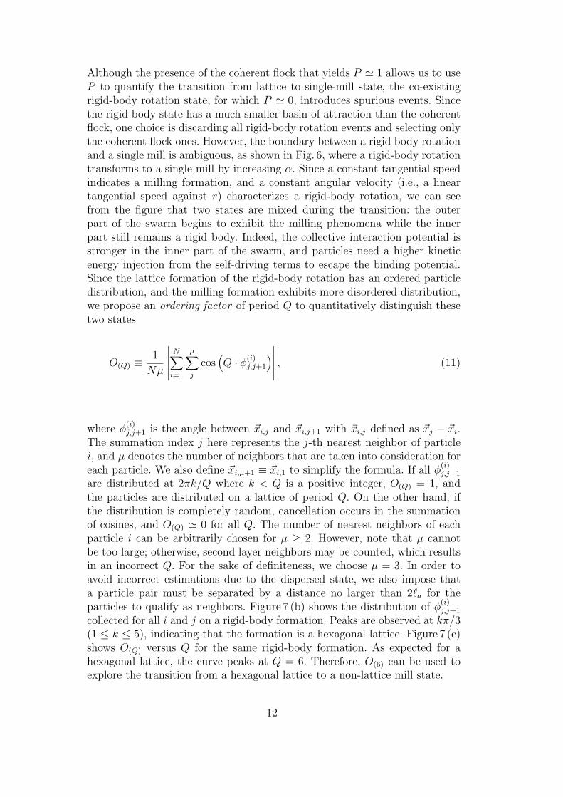
the dispersed one. Figure 8 (b) shows the transition of a catastrophic swarm,which displays a full four-stage transition: in the small α regime, particlesarrange as a coherent lattice with P ' 1; as α keeps increasing, the single-millstate appears (P ' 0 and M ' 1), followed by the double-mill state (Mabs ' 1and M ' 0) until the dispersed state (fagg = 0) is reached.

Drawing an analogy from the state transition of swarming patterns to thephase transition of materials, the lattice states can be regarded as “solid” sinceinterparticle distances are kept constant. The milling state allows particles to“swim” within a finite volume without being bound to a fixed lattice site; thus,it can be regarded as “liquid”. Finally, in the dispersed state, particles escape,similarly to a “gas”. Upon increasing α, a catastrophic swarm undergoes thesolid–liquid and liquid–gas transitions, which resemble the processes of meltingand vaporization. On the other hand, an H-stable swarm goes from the solidstate directly to the gas one, which is more similar to sublimation.

14

Consistently with granular media models [38], we may define a “temperature”analog using the variation of the individual particle velocity among the flock:Ts ≡

⟨(~v − 〈~v〉)2

⟩. Note that 〈~v〉 is the velocity of the center of mass, and

thus, Ts ' 0 for the coherent flock pattern, while Ts ' α/β for the steady millstates. The swarming patterns change from one state to another by varyingTs.

While different aggregation morphologies can be studied using the individual-based model, the large number of degrees of freedom involved pose a difficultyfor analyzing the dynamics of large N systems. In the following section, wetherefore develop and investigate a continuum model consistent with the mi-croscopic description of Eqs. (1) - (3).

3 Continuum model

The continuum approach is widely adopted for modeling swarming systems,especially on the ecological scale where massive movements of populationsare considered [2,3,22,23,25,26]. It is also more suitable for theoretical anal-ysis especially in large N limit. Due to the lack of connections between in-dividual rules and continuum “fluxes”, most continuum models in the litera-ture are constructed on the basis of heuristic arguments. Attempts have beenmade to bridge the gap. For example in Ref. [39], a continuum kinematic one-dimensional advection-diffusion model is derived based on a biased randomwalk process of a set of Poisson-distributed particles. This work is extended tohigher dimensions and to more general kinematic rules in Ref. [40,41]. However,our model is based on dynamic rules and the corresponding continuum limitis much more difficult to rigorously justify. In Ref. [14], a continuum modelis derived from a class of dynamic individual-based descriptions by using aFokker-Planck approach. In order for the flux term to be amenable to analyticinvestigations, the Fokker-Planck equations have to be closed under severalassumptions, but these assumptions, such as that the preferred velocity whichparticles tend to reach is small with respect to noise terms, are not applicableto our model.

In this paper, we derive a continuum model by explicitly calculating the en-semble average the model of Eqs. (1) - (2) using a probability distribution func-tion. This classical procedure is described in Ref. [27] where continuum hy-drodynamics equations are derived starting from a microscopic collection ofN particles. Let

f = f (~x1, ~x2, ..., ~xN ; ~p1, ~p2, ..., ~pN ; t) (12)

15

be the probability distribution function on the phase space, defined by positionand momentum (~xi, ~pi), 1 ≤ i ≤ N , at time t. The mass density ρ (~x, t), the

ensemble velocity field ~u (~x, t), and the continuum interaction force ~FV (~x, t)can be defined as

ρ (~x, t) = mN∑

i=1

〈δ (~xi − ~x) ; f〉, (13)

~u (~x, t) =~p (~x, t)

ρ (~x, t)=

∑Ni=1 〈~piδ (~xi − ~x) ; f〉

ρ (~x, t), (14)

~FV (~x, t) =N∑

i=1

⟨−~∇~xi

U (~xi) δ (~xi − ~x) ; f⟩. (15)

We consider the case of identical masses, mi ≡ m. The function δ (~x) is theDirac delta function, and U (~xi) the collective interaction potential actingon particle i. Using the generalized Liouville theorem that incorporates thedeformation of phase space due to the non-Hamiltonian nature of the systemat hand [42], we obtain the continuum equations of motion

∂ρ

∂t+ ~∇ · (ρ~u) = 0, (16)

∂

∂t(ρ~u) + ~∇ · (ρ~u~u) + ~∇ · σK = αρ~u− 2βEK~u− 2β~qK + 2β~u · σK + ~FV . (17)

The first is the equation of continuity, and the second is the momentum trans-port equation. Here, EK = ρ |~u|2 /2 is the kinetic energy. The terms ~qK (~x, t)and σK (~x, t) are mathematically defined as

~qK (~x, t) =N∑

i=1

⟨m

2

∣∣∣∣∣~pi

m− ~u

∣∣∣∣∣2 (

~pi

m− ~u

)δ (~xi − ~x) ; f

⟩,

σK (~x, t) =N∑

i=1

m

⟨(~pi

m− ~u

)(~pi

m− ~u

)δ (~xi − ~x) ; f

⟩,

and represent the energy flux and the stress tensor due to local fluctuations inparticle velocities with respect to ~u (~x, t). The derivation of the term ~∇·σK canbe found in Ref. [27] while the other terms related to ~qK and σK are derived inAppendix A. By simulating the discrete model, we estimate the magnitude of~qK and σK and find that both fluctuation terms become negligible with respectto the the other terms on the RHS of Eq. (17) in the lattice, single-mill, andthe dispersed states. Thus, neglecting the fluctuation terms, we obtain

∂ρ

∂t+ ~∇ · (ρ~u) = 0, (18)

16

∂

∂t(ρ~u) + ~∇ · (ρ~u~u) = αρ~u− 2βEK~u + ~FV . (19)

Continuum interaction force

In Eq. (19), the continuum interaction force can be obtained by substitutingthe explicit form of the interaction potential Eq. (3) into Eq. (15)

~FV (~x, t) =N∑

i=1

N∑j=1

⟨−~∇~xi

V (~xi − ~xj) δ (~xi − ~x) ; f⟩. (20)

Using the fact that an arbitrary function F (~xj) ∀~xj ∈ Rd can be written as

F (~xj) =∫Rd

F (~y) δ (~xj − ~y)d~y,

we can rewrite Eq. (20) as

~FV (~x, t) =N∑

i=1

N∑j=1

∫Rd

d~y⟨−~∇~xi

V (~xi − ~y) δ (~xi − ~x) δ (~xj − ~y) ; f⟩

=∫Rd

−~∇~xV (~x− ~y)N∑

i=1

N∑j=1

〈δ (~xj − ~y) δ (~xi − ~x) ; f〉d~y

=∫Rd

−~∇~xV (~x− ~y) ρ(2) (~x, ~y, t) d~y, (21)

where the ρ(2) is the pair density

ρ(2) (~x, ~y, t) ≡N∑

i=1

N∑j=1

〈δ (~xj − ~y) δ (~xi − ~x) ; f〉.

Note that we should take the ensemble average on a scale considerably largerthan the spacing between particles. If the particles are quite dispersed, thesuitable scale may be much larger than the characteristic lengths of the in-teraction force (−~∇V in Eq. (21)), rendering it localized. In this case, thecontinuum approach cannot capture the swarming characteristics occurringon the the interaction scale and fails to describe the individual-based modelon such a scale. This is what occurs in the H-stable regime, which we furtherdiscuss in Sec. 4.

17

For identical particles, the pair density can be written as

ρ(2) (~x, ~y, t) =1

m2ρ (~x, t) ρ (~y, t) g(2) (~x, ~y) ,

where the correlation function g(2) (~x, ~y) = 1 when the particles have no in-trinsic correlation. Using this assumption,

ρ(2) (~x, ~y, t) =1

m2ρ (~x, t) ρ (~y, t) , (22)

and

~FV (~x, t) =∫Rd

−~∇~xV (~x− ~y)1

m2ρ (~x, t) ρ (~y, t)d~y. (23)

If we further substitute the interaction potential specified in Eq. (3) into theabove equation, we get

~FV (~x, t) =−ρ (~x, t) ~∇∫Rd

(−Ca

m2e−

|~x−~y|`a +

Cr

m2e−

|~x−~y|`r

)ρ (~y, t)d~y. (24)

Since we assume that all particles have an identical mass, we may choose m = 1without loss of generality. In this case, Eq. (24) becomes the one proposed inRef. [15], on heuristic grounds. Using Eq. (18), we may modify Eq. (19) anddivide by ρ on both sides to obtain a more conventional expression

∂ρ

∂t+ ~∇ · (ρ~u) = 0, (25)

∂~u

∂t+ ~u · ∇~u = α~u− β |~u|2 ~u− 1

m2~∇∫Rd

V (~x− ~y) ρ (~y, t)d~y. (26)

4 Comparison to the individual-based model

The time-dependent variations of the density ρ (~x, t) and of the momentum~p (~x, t) ≡ ρ (~x, t) ~u (~x, t) can be obtained through numerical simulations ofEqs. (18) - (19). Here, we use the Lax-Friedrichs method [43] to integrate thepartial differential equations. We compare the results of the continuum modelto those of the individual-based model of Eqs. (1) - (2). Figure 9 shows the

18

frequently observed single-mill steady state solutions of both models in thecatastrophic regime. Both simulations use identical parameter values and thesame total mass

mtot =∫∞

ρ (~x)d~x = Nm,

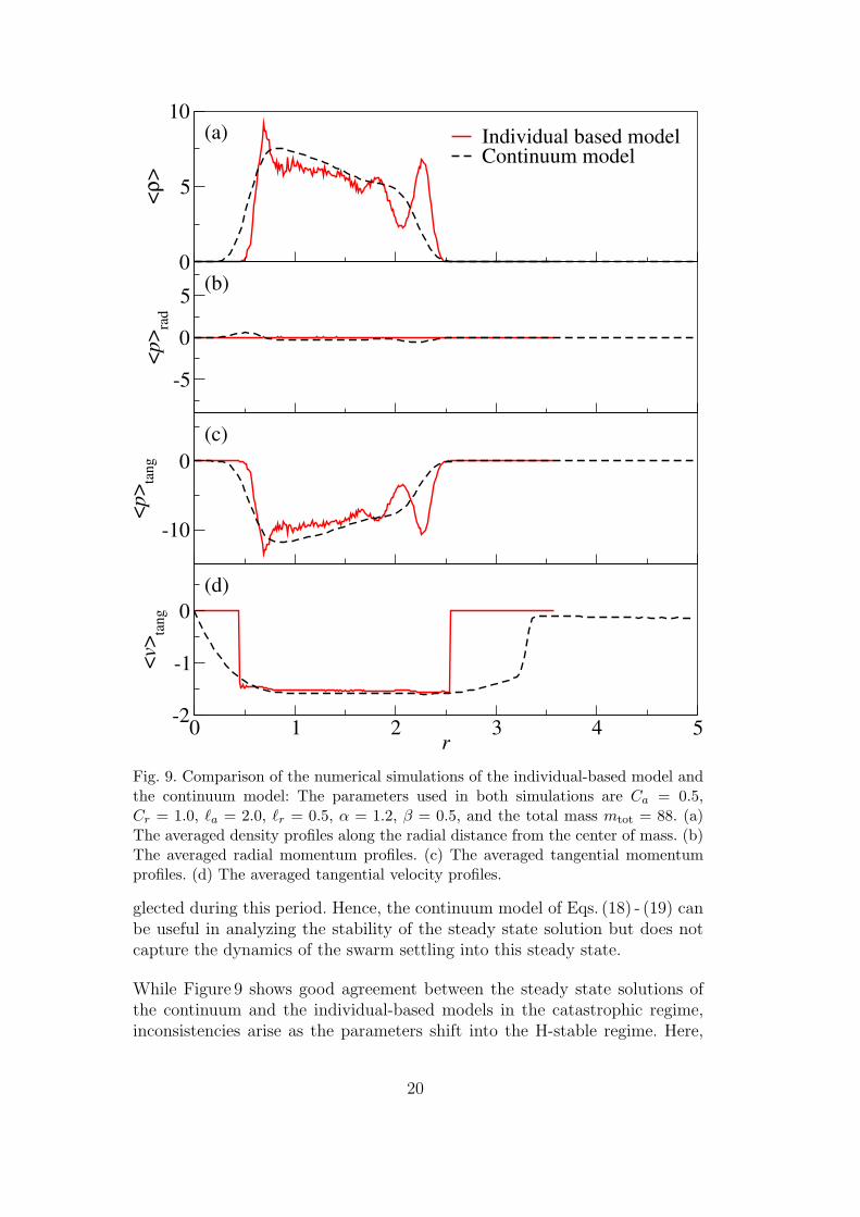
which are listed in the figure caption. In the individual-based model, particlesare initially distributed with random velocities and at random positions in a2à× 2à box. The initial condition of the continuum model is a homogeneousdensity in a box of the same size with randomized momentum field. Whilethe individual-based model adopts a free boundary condition that allows theparticles to move around over the entire space, the continuum model usesan equivalent boundary condition of out-going waves but on a fixed compu-tational domain of 5à × 5à size which is divided into 256 × 256 grid cells.The individual-based simulation uses an adaptive time step size that keepsthe increment in position of each step under à/10 and the increment in ve-locity under Ca/5m. The time step size of the continuum simulation is chosenso that the CFL number is 0.98. Figure 9 (a) illustrates the averaged den-sity 〈ρ〉 as a function of the radial distance from the center of mass. Thesetwo profiles are in good agreement despite the density oscillation shown inthe individual-based model, reflecting a multiple-ring ordering of the particledistribution. Figures 9 (b) and (c) match the averaged radial and tangentialmomenta (denoted by 〈p〉rad and 〈p〉tang respectively) from the simulations ofboth models. The negligible radial momenta in Fig. 9 (b) indicate that there isno net inward or outward mass movement, and thus, the density profile alongthe radial direction is steady. We can divide the momentum by the densityto obtain the velocity field. In Fig. 9 (d), we show the averaged tangential ve-locities, 〈v〉tang ≡ 〈p〉tang/〈ρ〉, from the simulations of both models; it showsthat both the individual-based and the continuum swarms are rotating at thesame constant speed, which equals to veq.

Validity of the continuum model

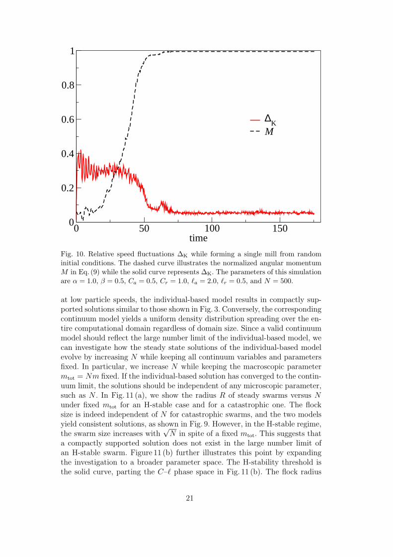
The ensemble average implicit in the continuum approach does not allow fordouble-milling in the continuum limit because the velocity inside a mesh cellis averaged and unified. Local velocity variations, which contribute to ~qK (~x, t)and σK (~x, t) in Eq. (17), are neglected. We calculate the ratio of the speed

variation to the equilibrium speed, ∆K ≡√〈(v − veq)

2〉/veq2, in order to ef-

ficiently estimate the contribution of these local velocity fluctuation terms.Figure 10 shows that ∆K becomes negligible after the swarm has reached thesingle-mill configuration and M ' 1. However, during the transient time, ∆K

is significantly larger, which implies that ~qK (~x, t) and σK (~x, t) cannot be ne-

19

0

5

10

<ρ>

Individual based modelContinuum model

-5

0

5

<p> ra

d

-10

0

<p> ta

ng

0 1 2 3 4 5r

-2

-1

0

<v> ta

ng

(a)

(b)

(c)

(d)

Fig. 9. Comparison of the numerical simulations of the individual-based model andthe continuum model: The parameters used in both simulations are Ca = 0.5,Cr = 1.0, `a = 2.0, `r = 0.5, α = 1.2, β = 0.5, and the total mass mtot = 88. (a)The averaged density profiles along the radial distance from the center of mass. (b)The averaged radial momentum profiles. (c) The averaged tangential momentumprofiles. (d) The averaged tangential velocity profiles.

glected during this period. Hence, the continuum model of Eqs. (18) - (19) canbe useful in analyzing the stability of the steady state solution but does notcapture the dynamics of the swarm settling into this steady state.

While Figure 9 shows good agreement between the steady state solutions ofthe continuum and the individual-based models in the catastrophic regime,inconsistencies arise as the parameters shift into the H-stable regime. Here,

20

0 50 100 150time

0

0.2

0.4

0.6

0.8

1

∆K

M

Fig. 10. Relative speed fluctuations ∆K while forming a single mill from randominitial conditions. The dashed curve illustrates the normalized angular momentumM in Eq. (9) while the solid curve represents ∆K. The parameters of this simulationare α = 1.0, β = 0.5, Ca = 0.5, Cr = 1.0, `a = 2.0, `r = 0.5, and N = 500.

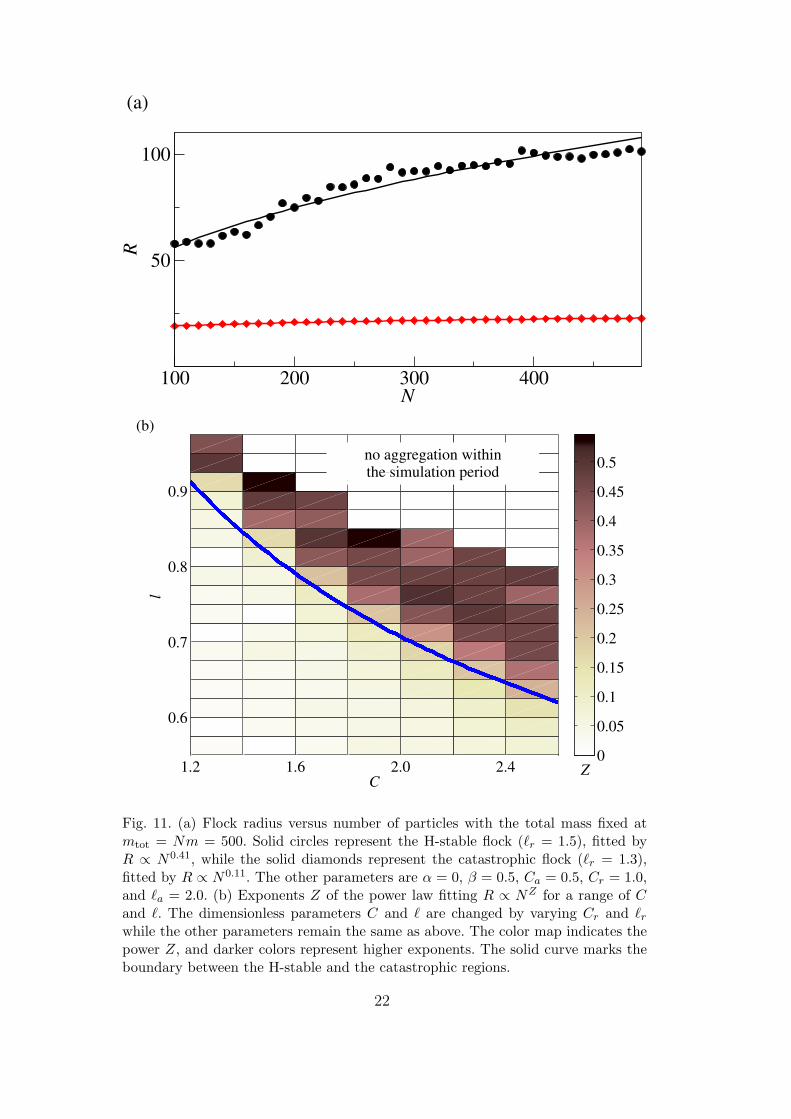
at low particle speeds, the individual-based model results in compactly sup-ported solutions similar to those shown in Fig. 3. Conversely, the correspondingcontinuum model yields a uniform density distribution spreading over the en-tire computational domain regardless of domain size. Since a valid continuummodel should reflect the large number limit of the individual-based model, wecan investigate how the steady state solutions of the individual-based modelevolve by increasing N while keeping all continuum variables and parametersfixed. In particular, we increase N while keeping the macroscopic parametermtot = Nm fixed. If the individual-based solution has converged to the contin-uum limit, the solutions should be independent of any microscopic parameter,such as N . In Fig. 11 (a), we show the radius R of steady swarms versus Nunder fixed mtot for an H-stable case and for a catastrophic one. The flocksize is indeed independent of N for catastrophic swarms, and the two modelsyield consistent solutions, as shown in Fig. 9. However, in the H-stable regime,the swarm size increases with

√N in spite of a fixed mtot. This suggests that

a compactly supported solution does not exist in the large number limit ofan H-stable swarm. Figure 11 (b) further illustrates this point by expandingthe investigation to a broader parameter space. The H-stability threshold isthe solid curve, parting the C–` phase space in Fig. 11 (b). The flock radius

21

100 200 300 400N

50

100R

(a)

1.2 1.6 2.0 2.4

0.6

0.7

0.8

0.9

C

l

0

0.05

0.1

0.15

0.2

0.25

0.3

0.35

0.4

0.45

0.5no aggregation withinthe simulation period

(b)

Z

Fig. 11. (a) Flock radius versus number of particles with the total mass fixed atmtot = Nm = 500. Solid circles represent the H-stable flock (`r = 1.5), fitted byR ∝ N0.41, while the solid diamonds represent the catastrophic flock (`r = 1.3),fitted by R ∝ N0.11. The other parameters are α = 0, β = 0.5, Ca = 0.5, Cr = 1.0,and `a = 2.0. (b) Exponents Z of the power law fitting R ∝ NZ for a range of Cand `. The dimensionless parameters C and ` are changed by varying Cr and `r

while the other parameters remain the same as above. The color map indicates thepower Z, and darker colors represent higher exponents. The solid curve marks theboundary between the H-stable and the catastrophic regions.

22

R is approximately independent of N for catastrophic swarms, but when theparameters C and ` cross over to the H-stable regime, R scales as NZ withZ ' 1/2. As N →∞, H-stable swarms tend to occupy the entire space.

The cue to the inconsistency between the solutions of the two models in theH-stable regime lies in the derivation of the continuum model. As previouslymentioned, the macroscopic variables are obtained as ensemble averages overa large number of microscopic ones. In the catastrophic regime, δNND � `a, `r

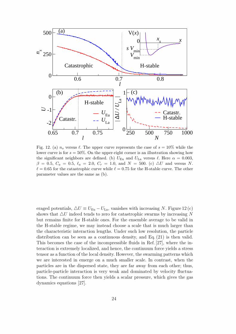
in large N limit, as shown in Fig. 11. Hence, as N →∞, the particle distribu-tion converges to a continuum density on a scale comparable to the interactionlength. On the other hand, for an H-stable swarm, δNND stays non-negligiblewith respect to the characteristic length of the interaction. Hence, Eq. (21)does not hold on a scale comparable to the interaction length, and as a re-sult, Eq. (23) is not a valid description of the continuum force on such a scalein the H-stable regime. This is also verified in Fig. 12. In Fig. 12 (a), we de-fine significant neighbors of a particle as neighbors that exhibit a “significantinteraction”. The quantitative definition is illustrated by the graph on theupper-right corner, in which the pairwise interaction potential V (r) is plottedversus the inter-particle distance r, and the potential well depth is denoted byVmin. We define a distance rs so that V (x) > sVmin if x > xs, where 0 ≤ s ≤ 1is a ratio. Then, the number of significant neighbors of each particle is thenumber of neighbors at a distance x for which x ≤ xs. In Fig. 12 (a), we countthe averaged number of significant neighbors of a particle, denoted by ns, fors = 0.5 and s = 0.1. In the H-stable regime, ns is very low and remains steady;it rises rapidly when the parameter crosses over into the catastrophic regime.The results suggest that the H-stable swarms are locally too sparse for Eq. (21)(and thus, Eq. (23)) to remain valid. Furthermore, we can use ensemble aver-ages to approximate the collective interaction potentials in the two models. Ifthe continuum limit properly describe the individual-based description, thesetwo potential energies should converge as N increases. Let us define UEu asthe continuum ensemble average interaction potential in the Eulerian frame

UEu (~x)≡ 1

m2

∫Rd

V (~x− ~y) ρ (~x) ρ (~y) d~y.

Here ρ (~x) is approximated by the ensemble average of the individual particlesduring the simulation. We also define ULa as the average collective potentialcalculated in the Lagrangian frame, ULa (~x) ≡ 〈U (~xi)〉~xi=~x, where U (~xi) isdefined in Eq. (3) of the individual-based model. Since the rigid-body rotationand the single-mill state have rotational symmetry with respect to ~xCM, weevaluate UEu and ULa after such states are reached and at position ~x such that|~x− ~xCM| = R/2, where R is the swarm radius. In Fig. 12 (b), UEu and ULa

are shown to converge in the catastrophic regime and diverge in the H-stableone. In Fig. 12 (c), we investigate whether the difference between these two av-

23

0.6 0.7 0.8l

0

250

500n s

0.65 0.7 0.75l

-2

-1

0

U UEu

ULa

250 500 750 1000N

0

1

| ∆U

/ U

La |

Catastr.H-stable

xV(x)

H-stableCatastrophic

H-stable

Catastr.

(a)

(b) (c)

s Vmin

Vmin

0 xs

Fig. 12. (a) ns versus `. The upper curve represents the case of s = 10% while thelower curve is for s = 50%. On the upper-right corner is an illustration showing howthe significant neighbors are defined. (b) UEu and ULa versus `. Here α = 0.003,β = 0.5, Ca = 0.5, `a = 2.0, Cr = 1.0, and N = 500. (c) 4U and versus N .` = 0.65 for the catastrophic curve while ` = 0.75 for the H-stable curve. The otherparameter values are the same as (b).

eraged potentials, 4U ≡ UEu−ULa, vanishes with increasing N . Figure 12 (c)shows that 4U indeed tends to zero for catastrophic swarms by increasing Nbut remains finite for H-stable ones. For the ensemble average to be valid inthe H-stable regime, we may instead choose a scale that is much larger thanthe characteristic interaction lengths. Under such low resolution, the particledistribution can be seen as a continuous density, and Eq. (21) is then valid.This becomes the case of the incompressible fluids in Ref. [27], where the in-teraction is extremely localized, and hence, the continuum force yields a stresstensor as a function of the local density. However, the swarming patterns whichwe are interested in emerge on a much smaller scale. In contrast, when theparticles are in the dispersed state, they are far away from each other; thus,particle-particle interaction is very weak and dominated by velocity fluctua-tions. The continuum force then yields a scalar pressure, which gives the gasdynamics equations [27].

24

5 Stability of the homogeneous solution

That the solutions of the continuum model of Eqs. (18) and (19) relax towarda uniform density distribution in the H-stable regime can also be shown bythe linear stability analysis of its homogeneous solution. Let us first considera more general case for a 2D self-driving continuum model with a non-localinteraction

∂ρ

∂t− ~∇ · (ρ~u) = 0; (27)

∂

∂t(ρ~u) + ~∇ · (ρ~u~u) = f (|~u|) ρ~u− ρ~∇

∫Rd

V (|~x− ~y|) ρ (~y) d~y,

where f (|~u|) is a scalar function specifying the self-driving mechanism, andthe non-local interaction is expressed by the convolution term. For our model,f (|~u|) = α − β |~u|2. The possible homogeneous steady state solutions canbe written as ρ (~x, t) = ρ0 and ~u (~x, t) = v0 v, where v is a unit vector andv0 can be 0 or any of the roots of f (v0) = 0. For our Rayleigh-type dissi-

pation, v0 =√

α/β. We perturb the steady state solution using ρ (~x, t) =

ρ0 + δρ exp (σt + i~q · ~x) and ~u (~x, t) = v0 v + (δu u + δv v) exp (σt + i~q · ~x),where δρ, δu, δv � 1 are small amplitudes. The unit vector u points tothe direction perpendicular to v on the 2D space. The wave vector is denotedby ~q while σ = σ (~q) represents its growth rate. By substituting this ansatzinto Eq. (27), the dispersion relation is

σ′

δρ

δu

δv

=

0 −iρ0q sin θ −iρ0q cos θ

−iqV (~q) sin θ f (v0) 0

−iqV (~q) cos θ 0 f (v0) + v0f′ (v0)

δρ

δu

δv

, (28)

where σ′ ≡ σ + iv0 v · ~q, and V (~q) is the Fourier transform of the pairwiseinteraction potential V (~x). The angle between the wave vector ~q and the unitvector u is denoted by θ.

For the case of v0 = 0, the solution is isotropic, and we can arbitrarily choosethe unit vector v. If the wave vector ~q is parallel to the arbitrarily chosen v,Eq. (28) reduces to

25

σ

δρ

δu

δv

=

0 0 −iρ0q

0 f (0) 0

iqV (~q) 0 f (0)

δρ

δu

δv

,

and σ = f (0) or(f (0)±

√f (0)2 − 4ρ0q2V (~q)

)/2. If f (0) > 0, the homoge-

neous solution is always unstable. If f (0) < 0, the homogeneous solution isstable only when ρ0q

2V (~q) > 0. Since ρ0 and q2 are both non-negative, thecriterion can be reduced to

V (~q) > 0. (29)

For our Rayleigh-type dissipation, f (0) = α. Since α is positive, the uniformdensity solution with zero speed is an unstable steady state solution.

For the case of v0 6= 0 satisfying f (v0) = 0, Eq. (28) becomes

σ′

δρ

δu

δv

=

0 −iρ0q sin θ −iρ0q cos θ

−iqV (~q) sin θ 0 0

−iqV (~q) cos θ 0 v0f′ (v0)

δρ

δu

δv

.

We thus obtain the growth rate by solving the following eigenvalue equation

σ′3 − v0f

′ (v0) σ′2+ σ′ρ0q

2V (~q)− v0f′ (v0) ρ0q

2V (~q) sin2 θ = 0. (30)

Let us consider the two cases of the wave vectors parallel and perpendic-ular to the v-direction. For the parallel case, i.e., θ = 0, σ′ = 0 or σ′ =[v0f

′ (v0)±√

(v0f ′ (v0))2 − ρ0q2V (~q)

]/2. On the other hand, in the perpen-

dicular case (θ = π/2), σ′ = v0f′ (v0) or σ′ = ±

√−ρ0q2V (~q). If f ′ (v0) > 0,

the homogeneous solutions are always unstable. For our Rayleigh-type dis-sipation, f ′ (v0) = −2βv0 < 0; hence, the homogeneous solution is stableonly when ρ0q

2V (~q) > 0, which is the same as the criterion in Eq. (29). Fur-ther analysis shows that for a general angle θ, Eq. (30) can be rewritten as

(σ′ − v0f′ (v0))

(σ′2 + ρ0q

2V (~q))+Γ cos2 θ = 0, where Γ ≡ v0f

′ (v0) ρ0q2V (~q).

In our model, Γ > 0 whenever the homogeneous solution is unstable. Thus, aninspection of the above equation shows that its largest root, i.e., the fastestgrowth rate, is at θ = π/2. As a result, perturbations on the direction perpen-dicular to the swarm velocity are the fastest growing mode, and their rate is√−ρ0q2V (q) for a given q.

26

C

l

Short-wave Instability

Unstable

Long-wave Instability

Stable

l=C

l=1/C1/2

C=1

l=1

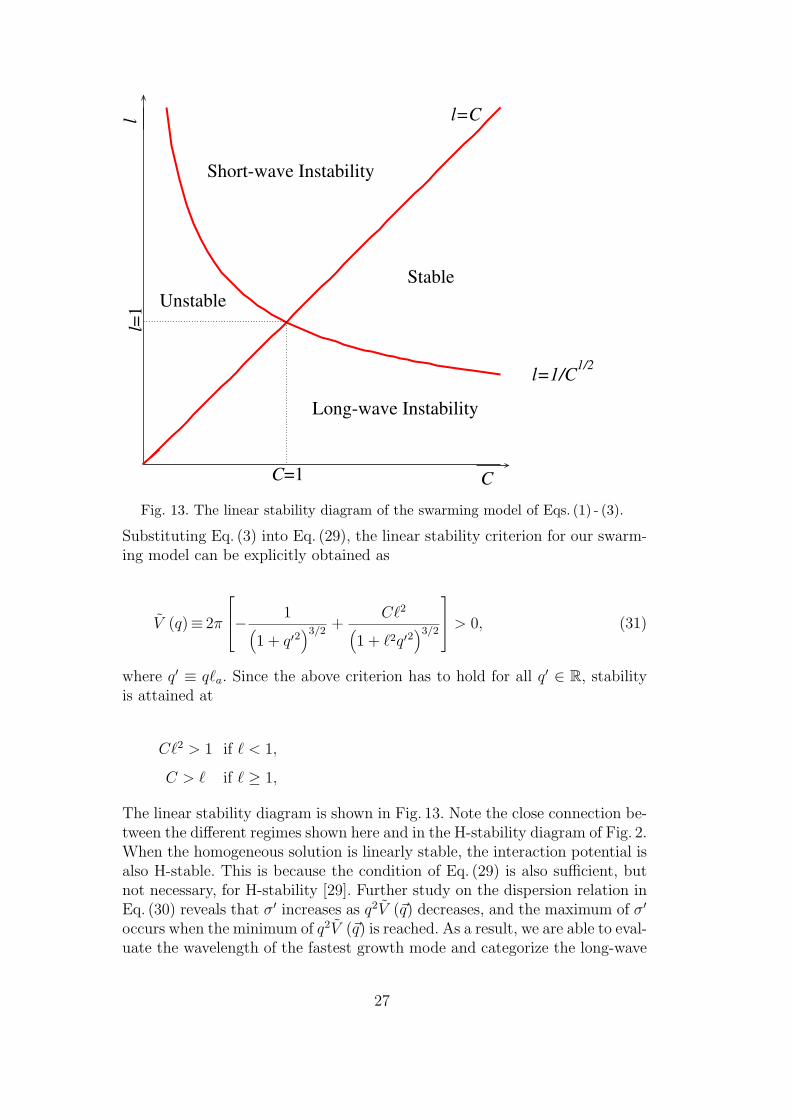
Fig. 13. The linear stability diagram of the swarming model of Eqs. (1) - (3).

Substituting Eq. (3) into Eq. (29), the linear stability criterion for our swarm-ing model can be explicitly obtained as

V (q)≡ 2π

− 1(1 + q′2

)3/2+

C`2(1 + `2q′2

)3/2

> 0, (31)

where q′ ≡ q`a. Since the above criterion has to hold for all q′ ∈ R, stabilityis attained at

C`2 > 1 if ` < 1,

C > ` if ` ≥ 1,

The linear stability diagram is shown in Fig. 13. Note the close connection be-tween the different regimes shown here and in the H-stability diagram of Fig. 2.When the homogeneous solution is linearly stable, the interaction potential isalso H-stable. This is because the condition of Eq. (29) is also sufficient, butnot necessary, for H-stability [29]. Further study on the dispersion relation inEq. (30) reveals that σ′ increases as q2V (~q) decreases, and the maximum of σ′

occurs when the minimum of q2V (~q) is reached. As a result, we are able to eval-uate the wavelength of the fastest growth mode and categorize the long-wave

27

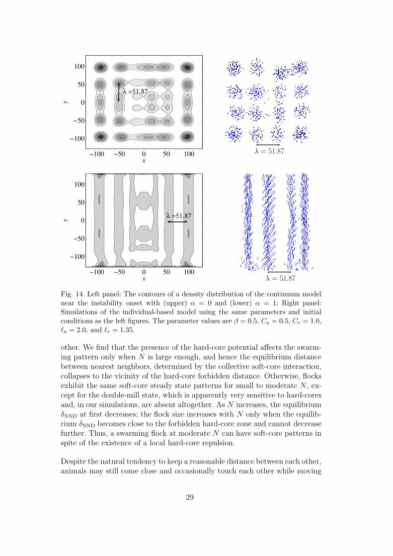
and the short-wave instability regions in the parameter space. Furthermore,we compare the fastest growth wavelength to the pattern of the fully nonlinearcontinuum model near the onset of the instability, shown in the left panel ofFig. 14. The simulations are initiated with a homogeneous density distributionand computed on a periodic domain of a 206.8× 206.8 box. The wavenumberof the fastest growth mode is calculated as the minimum of Eq. (31). For theparameters chosen in Fig. 14, |~q| = 0.121, which corresponds to a wavelengthλ = 51.87. This value matches the density aggregation patterns quite well. Inthe upper figure, α = 0; the steady state density has zero velocity, and the x-ydirections are isotropic. In the lower figure, α 6= 0, and the velocity field of the

swarm is initiated as ~u (t = 0) =√

α/βy. The direction of the stripes indicatesthat the fastest growth mode is indeed perpendicular to the initial velocity,which is also consistent with the theoretical prediction. The results can alsobe compared to the simulation of the individual-based model by using thesame parameter values and equivalent initial and boundary conditions. SinceV (r) decays rapidly in r, U (~xi) can be well approximated by including onlythe adjacent eight boxes surrounding the computational domain. The steadyparticle distributions of the individual-based simulations are shown on theright panel of Fig. 14. The theoretically predicted wavelength agrees with thepatterns seen in the simulations of the continuum and the individual-basedmodels.

6 Discussion

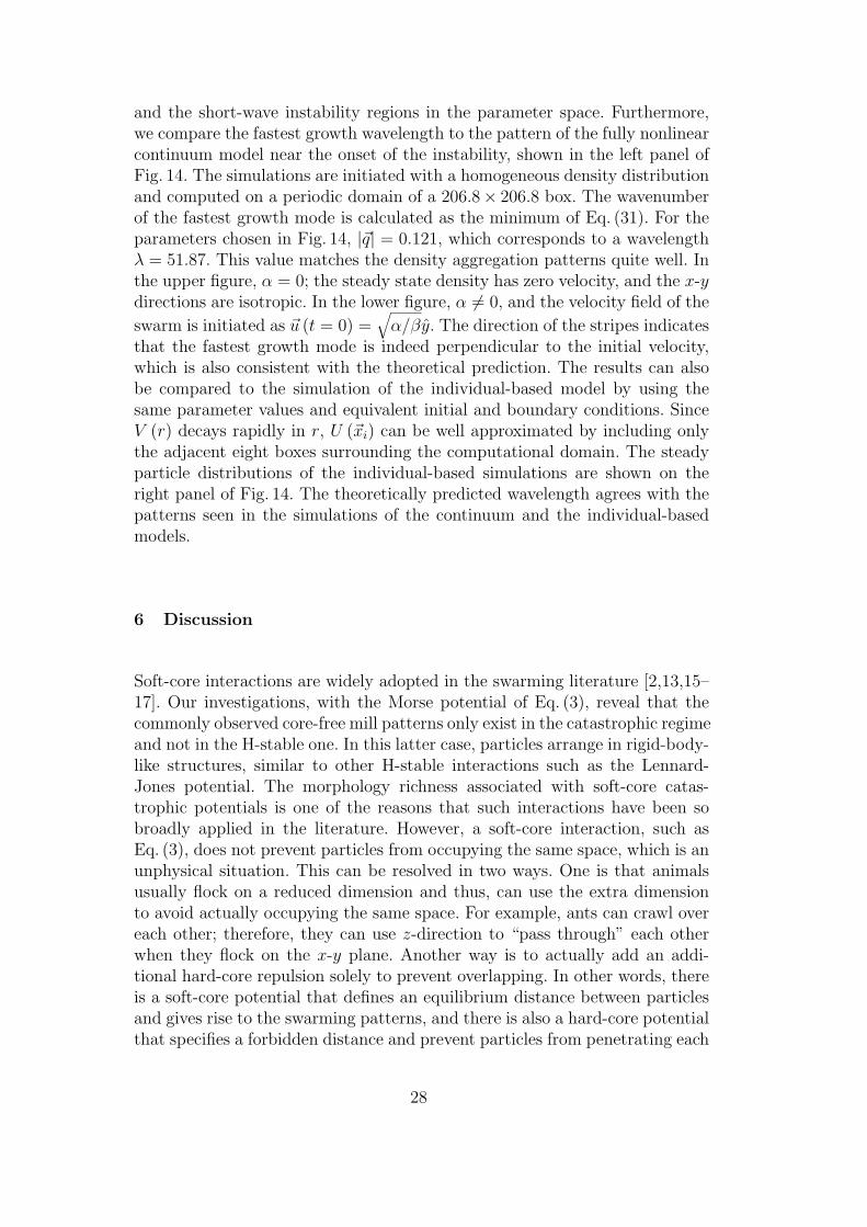
Soft-core interactions are widely adopted in the swarming literature [2,13,15–17]. Our investigations, with the Morse potential of Eq. (3), reveal that thecommonly observed core-free mill patterns only exist in the catastrophic regimeand not in the H-stable one. In this latter case, particles arrange in rigid-body-like structures, similar to other H-stable interactions such as the Lennard-Jones potential. The morphology richness associated with soft-core catas-trophic potentials is one of the reasons that such interactions have been sobroadly applied in the literature. However, a soft-core interaction, such asEq. (3), does not prevent particles from occupying the same space, which is anunphysical situation. This can be resolved in two ways. One is that animalsusually flock on a reduced dimension and thus, can use the extra dimensionto avoid actually occupying the same space. For example, ants can crawl overeach other; therefore, they can use z-direction to “pass through” each otherwhen they flock on the x-y plane. Another way is to actually add an addi-tional hard-core repulsion solely to prevent overlapping. In other words, thereis a soft-core potential that defines an equilibrium distance between particlesand gives rise to the swarming patterns, and there is also a hard-core potentialthat specifies a forbidden distance and prevent particles from penetrating each

28

x

y

−100 −50 0 50 100

−100

−50

0

50

100

λ =51.87

�

��

��

��

�

��

�

��

��

��

��

�

��

�

��

� !"

#

$%&'

()*

+,-

./012345

678 9:;

<=

>?@

ABC

D

EF G

HIJ

KLMNOP

QRST UVWXYZ

[\

]^_àbc defghi

jklmnopq rs

t

uvwxyz{|}~�

��

��

��

��

��

�

�

��

�

��

��

¡¢£

¤¥

¦§¨

©ª

«

¬

®

¯°

±²

³´

µ¶

·¸ ¹º

»

¼

½¾

¿ÀÁ

ÂÃ

Ä

ÅÆÇ

ÈÉÊ

ËÌÍÎ

ÏÐ

Ñ

ÒÓ

Ô

Õ

Ö

×

Ø

Ù

ÚÛ

Ü

ÝÞ

ß

à

áâ

ã

äå

æçèé

êë

ì

í

îïð

ñ òóô

õö÷

øùú

ûü

ýþ

ÿ� �

�

��

��

�

�

� ��

��

�

��

��

�

�

�� !"

#$%&'

(

) *+,-./0

1234

567

8

9:;<=

>?@

AB

CDEF

GHIJ

KLMNOPQ

RSTUVW

XYZ[\

]^

_àb

cd

e

fg

hijkl

mnop q

rstuvw

xyz{

|}

~�

��

�

��

��

�

��

�

��

��

�

¡

¢£¤

¥¦§¨©

ª«¬

®¯°

±

²

³´

µ¶·

¸¹º»

¼½¾

¿

À

ÁÂÃ

ÄÅÆÇÈ

ÉÊËÌ

ÍÎ

Ï

ÐÑ

ÒÓÔÕÖ×

ØÙ

Ú

ÛÜÝ

Þßàáâ

ãäå

æ

çè

é

êë

ìí

î

ï

ð

ñ òóô

õö

÷øùú

ûüý

þ

ÿ

��

�

�

��

��

��

�

��

�� !"

#$%

&'() *+,-./

0

1

2

34567 89:

;<=>?@ABC

DEF

GHIJ

KLMN

OPQ

RST UVW

XYZ[

\]^_àb

cdefghi

jklmno

pqrs

tuvwxyz

{|

}~� ��

��

��

�

��

��

��

��

� ¡

¢£¤¥¦§

¨© ª«¬

®¯

°±²³´µ

¶· ¸¹ º

»¼½

¾¿ÀÁÂÃÄÅ Æ

Ç

ÈÉ

ÊË

Ì

ÍÎÏÐ

Ñ

Ò Ó

Ô

ÕÖ

×ØÙ

Ú

ÛÜÝ

Þ

ßàáãâ

äåæçè

é

êëì

íî

ïðñòó

ô

õö÷ø

ùúû

üýþÿ

��

��

�

�

��

�

��

��

�

��

��

��

��

!"

#$

%&'()

*+,

-

.

/0

1234

5

6

78

9:

;

<=

>

?@

AB

CDEF G

H

I

J

KLM

NOPQR

ST UV

W

X

YZ

[

\]^_

àb

cd

ef

g

hi

jk

lm

no

pqrst

u

vw

xy

z

{|}

~� ��

��

��

��

��

��

� ¡¢

£¤¥

¦§

¨© ª«¬

®¯°

±²³´µ

¶·

¸¹º

»¼

½¾

¿ÀÁÂÃ

ÄÅÆÇÈÉ

ÊËÌ

Í

ÎÏ

ÐÑ

ÒÓÔ

ÕÖ×

Ø

ÙÚÛ

ÜÝ

Þ

ß

àáâã äå

æçè

λ = 51.87

x

y

−100 −50 0 50 100

−100

−50

0

50

100

λ =51.87��

��

�

��

�� !"#$%&'(*)

+, -

./10

2345678 9:; <=>@?ABCD EF

GHJIK L

MNOPQRSTUVWXY

Z[\]^_àbcd

efghijlk

mnopqrs

tu v

wxyz

{|}~��

��

��

�� ¡¢

£¤¥¦§¨©ª«¬®¯°±²³´

µ¶·¸¹º» ¼½¾¿ÀÁ

ÂÃÄÅÆÇÈÉÊËÌÍÎ

ÏÐÑÒÓÔÕÖ

×ØÚÙÛ Ü

ÝÞßàáâãäå

æçèé

êëìíîïðñòóôõ ö÷øùúüûý

þÿ��

�

��

��

��

!"#

$%&'()

*+,-./

01

2

3456

789:;<=>?@

ABDCEF

GHIJKL

M

NOP

QR

STUVWXYZ[\]

^_àbcdefg

hikjl mn

opqr

stuvwxyz

{|

}~��

��

��

��

��

�� ¡¢£ ¤ ¥¦

§¨©ª«¬®¯°±²³´ µ

¶·¸¹º

»¼½¾¿ÀÁÂÃ

ÄÅÆÇ

È

ÉÊËÌÍÎÏÐÑÒÓÕÔ

Ö×

ØÙÚÜÛÝÞß

àá

âã

äåæçèé ê

ëìí

îï

ðñòó

ôõö÷øùúû

üý þ

ÿ�

�

��

��

� ��

��

��

�� !"#$

%

&'

( )*

+,

-./01234

56789:

;<=>?@AB

CDE

FGH

IJKLMNOPQ R

STUVWXYZ[\]

^ _àbcde

fghijklnmo

pqrs

tuvwxyz{

|

}~��

��

��

�� ¡¢£¤¥

¦§¨

©ª¬«®¯°±²³´

µ

¶·¸¹

º»

¼½¾¿ÀÁÂÃÄÅÆÇÈÉ

ÊËÌÍÎÏÐÑ

ÒÓÔ

ÕÖ×ØÙÚÛÜÝ

Þßàáâ

ãäåæçèéêëìí

îïðñòóô

õö÷øùúûü ýþ

ÿ��

��

��

��

!"#$%&'

()*+,-./0123456789:;

<=>?@AB CD

EF

GHIJKLMNO

PQRS T

UVWXYZ[\]^_

à b

cdefghijklmn

op

qrstuvwxyz{|}

~�

��

��

�� ¡¢

£¤¥¦§©¨ª «

¬®¯°±

²³´µ¶·¸¹

º»¼½¾¿ÀÁÂÃÄÅÆÇ

ÈÉÊËÌ

ÍÎÏÐÑÒ ÓÔÕ Ö×ØÙÚÛÜÝÞßà áâã ä

åæçèéêëìíîïðñò óôöõ

÷ø

λ = 51.87

Fig. 14. Left panel: The contours of a density distribution of the continuum modelnear the instability onset with (upper) α = 0 and (lower) α = 1; Right panel:Simulations of the individual-based model using the same parameters and initialconditions as the left figures. The parameter values are β = 0.5, Ca = 0.5, Cr = 1.0,à = 2.0, and `r = 1.35.

other. We find that the presence of the hard-core potential affects the swarm-ing pattern only when N is large enough, and hence the equilibrium distancebetween nearest neighbors, determined by the collective soft-core interaction,collapses to the vicinity of the hard-core forbidden distance. Otherwise, flocksexhibit the same soft-core steady state patterns for small to moderate N , ex-cept for the double-mill state, which is apparently very sensitive to hard-coresand, in our simulations, are absent altogether. As N increases, the equilibriumδNND at first decreases; the flock size increases with N only when the equilib-rium δNND becomes close to the forbidden hard-core zone and cannot decreasefurther. Thus, a swarming flock at moderate N can have soft-core patterns inspite of the existence of a local hard-core repulsion.

Despite the natural tendency to keep a reasonable distance between each other,animals may still come close and occasionally touch each other while moving

29

in a biological swarm. Thus, the natural repulsive tendency can be realized asa soft-core repulsion while the body length of the swarming animals can beviewed as a hard-core forbidden zone. For biological swarms, the equilibriumδNND is visibly larger than the hard-core forbidden zone, which supports thedescription given in the previous paragraph. In contrast, the Lennard-Jonespotential, used for physical systems of molecules, defines an equilibrium dis-tance very close to where the potential rapidly rises toward infinity. In otherwords, the equilibrium distance is nearly the same as the hard-core forbiddenzone. Compressibility is perhaps the reason why various catastrophic patterns,which are not observed in the condensed phases of classical matter, can existin the aggregation states of natural swarms. In artificial swarms, the hard-corerepulsion can be understood as a collision avoidance strategy. If the distanceto invoke the collision avoidance is much shorter than the equilibrium spacingbetween agents, various collapsing patterns shown in Ref. [28] become possibleand might even be engineered for artificial swarming of vehicles.

7 Summary

Natural swarms may switch patterns under different circumstances. Whilethe changes of pattern have been understood as a result of changing individ-ual mobility and mutual interactions within the swarm, our individual-basedmodel similarly exhibits a state transition through various swarming patternsby varying the parameters. The same idea can be applied to artificial swarms,where a group of robots can be programmed to strategically change forma-tions by varying the self-driving and communicating parameters of the controlmodel. To analyze the stability of the emerging patterns with respect to themodel parameters, it is advantageous to have a continuum model that canprecisely describe the individual-based model. We illustrate a procedure toderive a continuum model from an individual-based model by using classicalstatistical mechanics. We show that the derived continuum model does not ap-proximate the individual dynamics when the interaction potential is H-stable.This is due to the fact that for H-stable systems, the length scale of the po-tential is comparable to interparticle distances, whereas in the catastrophicregime many particles can co-exist on a length scale comparable to the scaleof the potential. In the catastrophic regime, the steady state solution of thecontinuum model well matches the single-mill pattern of the individual-basedmodel. The long-wave instability also shows a match to both the continuumand the individual-based model simulations when we theoretically analyze thelinear stability of the homogeneous solution for the continuum model. Thus,the continuum model may be useful for further analysis, such as the stabilityof non-trivial solutions.

30

Acknowledgment. The authors thank Herbert Levine, Jianhong Shen, andChad M. Topaz for useful discussions. We acknowledge support from AROgrant W911NF-05-1-0112, ONR grant N000140610059, and NSF grant DMS-0306167.

A Derivation of the fluctuation terms

Following Ref. [27], the momentum transport equation can be obtained bysubstituting the macroscopic momentum

ρ (~x, t) ~u (~x, t) =

⟨N∑

i=1

~piδ (~xi − ~x); f

⟩

into the generalized Liouville Equation, valid for non-conserved systems [42],

∂ (ρ~u)

∂t=

∂

∂t

⟨N∑

i=1

~piδ (~xi − ~x); f

⟩

=N∑

k=1

⟨~pk

m· ~∇~xk

(N∑

i=1

~piδ (~xi − ~x)

)+ ~pk · ~∇~pk

(N∑

i=1

~piδ (~xi − ~x)

); f

⟩.

Here f is the probability density function described in Eq. (12). Since

~pk

m· ~∇~xk

(N∑

i=1

~piδ (~xi − ~x)

)=

~pk

m· ~∇~xk

~pkδ (~xk − ~x)

=−~∇~x ·(

~pk~pk

m

)δ (~xk − ~x) ,

~pk · ~∇~pk

(N∑

i=1

~piδ (~xi − ~x)

)= ~pkδ (~xk − ~x) ,

the transport equation can further be reduced to

∂ (ρ~u)

∂t=

N∑k=1

[−∇~x ·

⟨(~pk~pk

m

)δ (~xk − ~x) ; f

⟩+⟨~pkδ (~xk − ~x) ; f

⟩]. (A.1)

The first term on the right hand side can be modified by noting that

N∑k=1

m

⟨(~pk

m− ~u

)(~pk

m− ~u

)δ (~xk − ~x) ; f

⟩

31

=N∑

k=1

⟨(~pk~pk

m

)δ (~xk − ~x) ; f

⟩− ~u

N∑k=1

〈~pkδ (~xk − ~x) ; f〉

−N∑

k=1

〈~pkδ (~xk − ~x) ; f〉~u + ~u~uN∑

k=1

〈mδ (~xk − ~x) ; f〉

=N∑

k=1

⟨(~pk~pk

m

)δ (~xk − ~x) ; f

⟩− ρ~u~u,

where ~u is the macroscopic velocity defined in Eq. (14). Eq. (A.1) then becomes

∂ (ρ~u)

∂t+ ~∇~x · (ρ~u~u) =−~∇~x · σK (~x, t) +

N∑k=1

⟨~pkδ (~xk − ~x) ; f

⟩, (A.2)

where

σK =N∑

k=1

m

⟨(~pk

m− ~u

)(~pk

m− ~u

)δ (~xk − ~x) ; f

⟩.

We can substitute the explicit form of ~pk from Eqs. (14) and (15)

~pk = α~pk − β|~pk|2

m2~pk − ~∇U (~xk)

into the second term of Eq. (A.2)

N∑k=1

⟨~pkδ (~xk − ~x) ; f

⟩=

N∑k=1

⟨(α~pk − β

|~pk|2

m2~pk − ~∇U (~xk)

)δ (~xk − ~x) ; f

⟩

= αρ~u−N∑

k=1

⟨(β|~pk|2

m2~pk

)⟩+ ~FV .

The second term above can be further simplified as

N∑k=1

⟨(β|~pk|2

m2~pk

)δ (~xk − ~x) ; f

⟩=

βN∑

k=1

⟨(|~pk|2

m2~pk

)δ (~xk − ~x) ; f

⟩− β

N∑k=1

⟨|~pk|2

m~uδ (~xk − ~x) ; f

⟩

+ βN∑

k=1

⟨m

(−2

~pk

m· ~u + |~u|2

)(~pk

m− ~u

)δ (~xk − ~x) ; f

⟩

+ 2βEK~u− 2β~u · σK + βN∑

k=1

⟨m |~u|2

(~pk

m− ~u

)δ (~xk − ~x) ; f

⟩

32

= 2βN∑

k=1

⟨m

2

∣∣∣∣∣~pk

m− ~u

∣∣∣∣∣2 (

~pk

m− ~u

)δ (~xk − ~x) ; f

⟩+ 2βEK~u− 2β~u · σK

= 2β~qK + 2βEK~u− 2β~u · σK,

where

~qK =N∑

i=1

⟨m

2

∣∣∣∣∣~pi

m− ~u

∣∣∣∣∣2 (

~pi

m− ~u

)δ (~xi − ~x) ; f

⟩.

As a result, Eq. (A.2) can be written as

∂

∂t(ρ~u) + ~∇ · (ρ~u~u) + ~∇ · σK = αρ~u− 2βEK~u− 2β~qK + 2β~u · σK + ~FV ,

which is the momentum transport equation shown in Eq. (17).

References

[1] T. Vicsek, A. Czirk, E. Ben-Jacob, I. Cohen, O. Shochet, Novel type of phasetransition in a system of self-driven particles, Phys. Rev. Lett. 75 (1995) 1226–1229.

[2] J. Toner, Y. Tu, Long-range order in a two-dimensional dynamical xy model:how birds fly together, Phys. Rev. Lett. 75 (1995) 4326–4329.

[3] A. Mogilner, L. Edelstein-Keshet, Spatio-angular order in populations of self-aligning objects: formation of oriented patches, Physica D 89 (1996) 346–367.

[4] K. Sugawara, M. Sano, Cooperative acceleration of task performance: Foragingbehavior of interacting multi-robots system, Physica D 100 (1997) 343–354.

[5] J. Parrish, L. Edelstein-Keshet, Complexity, pattern, and evolutionary trade-offs in animal aggregation, Science 294 (1999) 99–101.

[6] N. E. Leonard, E. Fiorelli, Virtual leaders, artificial potentials and coordinatedcontrol of groups, in: Proc. 40th IEEE Conf. Decision Contr., 2001, pp. 2968–2973.

[7] J. Parrish, S. V. Viscido, D. Grunbaum, Self-organized fish schools: anexamination of emergent properties, Biol. Bullet. 202 (2002) 296–305.

[8] Y. Liu, K. M. Passino, M. M. Polycarpou, Stability analysis of m-dimensionalasynchronous swarms with a fixed communication topology, in: IEEE Trans.Autom. Contr., Vol. 48, 2003, pp. 76–95.

33

[9] A. Jadbabaie, J. Lin, A. S. Morse, Coordination of groups of mobile agentsusing nearest neighbor rules, in: IEEE Trans. Autom. Contr., Vol. 48, 2003, pp.988–1001.

[10] H. S. Niwa, Self-organizing dynamic model of fish schooling, J. Theor. Biol. 171(1994) 123–136.

[11] N. Shimoyama, K. Sugawara, T. Mizuguchi, Y. Hayakawa, M. Sano, Collectivemotion in a system of motile elements, Phys. Rev. Lett. 76 (1996) 3870–3873.

[12] W. L. Romey, Individual differences make a difference in the trajectories ofsimulated schools of fish, Ecol. Model. 92 (1996) 65–77.

[13] A. S. Mikhailov, D. H. Zanette, Noise-induced breakdown of coherent collectivemotion in swarms, Phys. Rev. E 60 (1999) 4571–4575.

[14] G. Flierl, D. Grunbaum, S. Levin, D. Olson, From individuals to aggregations:the interplay between behavior and physics, J. Theor. Biol. 196 (1999) 397–454.

[15] H. Levine, W. J. Rappel, I. Cohen, Self-organization in systems of self-propelledparticles, Phys. Rev. E 63 (2000) 017101.

[16] I. D. Couzin, N. R. Franks, Self-organized lane formation and optimized trafficflow in army ants,, Proc. R. Soc. Lond. B 270 (2002) 139–146.

[17] U. Erdmann, W. Ebeling, V. S. Anishchenko, Excitation of rotational modes intwo-dimensional systems of driven brownian particles, Phys. Rev. E 65 (2002)061106.

[18] W. Ebeling, U. Erdmann, Nonequilibrium statistical mechanics of swarms ofdriven particles, Complexity 8 (2003) 23–30.

[19] S. V. Viscido, J. K. Parrish, D. Grunbaum, Individual behavior and emergentproperties of fish schools: a comparison of observation and theory, Mar. Ecol.Prog. Ser. 273 (2004) 239–249.

[20] S. V. Viscido, J. K. Parrish, D. Grunbaum, The effect of population size andnumber of influential neighbors on the emergent properties of fish schools, Ecol.Model. 183 (2005) 347–363.

[21] U. Erdmann, W. Ebeling, A. Mikhailov, Noise-induced transition fromtranslational to rotational motion of swarms, Phys. Rev. E 71 (2005) 051904.

[22] L. Edelstein-Keshet, J. Watmough, D. Grunbaum, Do travelling band solutionsdescribe cohesive swarms? an investigation for migratory locusts, J. Math. Biol.36 (1998) 515–549.

[23] A. Mogilner, L. Edelstein-Keshet, A non-local model for a swarm, J. Math. Biol.38 (1999) 534–549.

[24] A. H. Øien, Daphnicle dynamics based on kinetic theory: an analogue-modellingof swarming and behaviour of daphnia, Bullet. Math. Biol. 66 (2004) 1–46.

34

[25] C. M. Topaz, A. L. Bertozzi, Swarming patterns in a two-dimensional kinematicmodel for biological groups, SIAM J. Appl. Math. 65 (2004) 152–174.

[26] C. M. Topaz, A. L. Bertozzi, M. A. Lewis, A nonlocal continuum model forbiological aggregation, Bullet. Math. Biol., to appear.

[27] J. H. Irving, J. G. Kirkwood, The statistical mechanical theory of transportprocesses. iv. the equations of hydrodynamics, J. Chem. Phys. 18 (1950) 817–829.

[28] M. R. D’Orsogna, Y. L. Chuang, A. L. Bertozzi, L. S. Chayes, Self-propelledparticles with soft-core interactions: patterns, stability, and collapse, Phys. Rev.Lett. 96 (2006) 104302.

[29] D. Ruelle, Statistical Mechanics, Rigorous Results, New York: W.A. Benjamin,1969.

[30] T. C. Schneirla, Army Ants: A Study in Social Organization, W. H. Freeman,1971.

[31] A. L. Koch, D. White, The social lifestyle of myxobacteria, Bioessays 20 (1998)1030–1038.

[32] J. W. S. Rayleigh, The Theory of Sound, 2nd Edition, Vol. 1, MacMillan,London, 1894.

[33] D. Weihs, Optimal fish cruising speed, Nature 245 (1973) 48–50.

[34] J. D. Lambert, Numerical Methods for Ordinary Differential Equations, JohnWiley & Sons, 1991.

[35] V. Gazi, K. Passino, Stability analysis of swarms, in: IEEE Trans. Autom.Contr., Vol. 48, 2003, pp. 692–697.

[36] V. Gazi, K. Passino, A class of attractions/repulsion functions for stable swarmaggregations, in: Proc. Conf. Decision Contr., 2002, pp. 2842–2847.

[37] V. Gazi, K. Passino, Stability analysis of social foraging swarms: combinedeffects of attractant/repellent profiles, in: Proc. Conf. Decision Contr., 2002,pp. 2848–2853.

[38] C. S. Campbell, Rapid granular flows, Annu. Rev. Fluid Mech. 22 (1990) 57–92.

[39] D. Grunbaum, Translating stochastic density-dependent individual behaviorwith sensory constraints to an eulerian model of animal swarming, J. Math.Biol. 33 (1994) 139–161.

[40] P. Gomez-Mourelo, From individual-based models to partial differentialequations. an application to the upstream movement of elvers, Ecol. Model.188 (2005) 93–111.

[41] D. Morale, V. Capasso, K. Oelschlager, An interacting particle system modellingaggregation behavior: from individuals to populations, J. Math. Biol. 50 (2005)49–66.

35

[42] M. E. Tuckerman, C. J. Mundy, M. L. Klein, Toward a statisticalthermodynamics of steady states, Phys. Rev. Lett. 78 (1997) 2042–2045.

[43] R. J. Leveque, Numerical Methods for Conservation Laws, 1st Edition,Birkhauser, 1992.

36

State transitions and the continuum limit for a 2D interacting, self-propelled particle system

Documents

Transcript of State transitions and the continuum limit for a 2D interacting, self-propelled particle system