The collective dynamics of self-propelled particles
25
arXiv:0707.1436v1 [cond-mat.soft] 10 Jul 2007 Under consideration for publication in J. Fluid Mech. 1 The collective dynamics of self-propelled particles By VISHWAJEET MEHANDIA AND PRABHU R. NOTT† Department of Chemical Engineering, Indian Institute of Science Bangalore 560 012, India We have proposed a method for the dynamic simulation of a collection of self-propelled particles in a viscous Newtonian fluid. We restrict attention to particles whose size and velocity are small enough that the fluid motion is in the creeping flow regime. We have proposed a simple model for a self-propelled particle, and extended the Stokesian Dy- namics method to conduct dynamic simulations of a collection of such particles. In our description, each particle is treated as a sphere with an orientation vector p, whose loco- motion is driven by the action of a force dipole S p of constant magnitude S 0 at a point slightly displaced from its centre. To simplify the calculation, we place the dipole at the centre of the particle, and introduce a virtual propulsion force F p to effect propulsion. The magnitude F 0 of this force is proportional to S 0 . The directions of S p and F p are determined by p. In isolation, a self-propelled particle moves at a constant velocity u 0 p, with the speed u 0 determined by S 0 . When it coexists with many such particles, its hydrodynamic interaction with the other particles alters its velocity and, more impor- tantly, its orientation. As a result, the motion of the particle is chaotic. Our simulations are not restricted to low particle concentration, as we implement the full hydrodynamic interactions between the particles, but we restrict the motion of particles to two dimen- sions to reduce computation. We have studied the statistical properties of a suspension of self-propelled particles for a range of the particle concentration, quantified by the area fraction φ a . We find several interesting features in the microstructure and statistics. We find that particles tend to swim in clusters wherein they are in close proximity. Con- sequently, incorporating the finite size of the particles and the near-field hydrodynamic interactions is of the essence. There is a continuous process of breakage and formation of the clusters. We find that the distribution of particle velocity at low and high φ a are qualitatively different; it is close to the normal distribution at high φ a , in agreement with the experimental measurements of Wu & Libchaber (2000). The motion of the particles is diffusive at long time, and the self-diffusivity decreases with increasing φ a . The pair correlation function shows a large anisotropic buildup near contact, which decays rapidly with separation. There is also an anisotropic orientation correlation near contact, which decays more slowly with separation. 1. Introduction Nature presents a wide and fascinating array of organisms that can propel themselves in a fluid medium. Collections of swimming organisms exhibit intricate patterns and complex dynamics, such as the flocking of birds, schooling of fish and coherent motion † Author to whom correspondence should be addressed. Email: [email protected].
-
Upload
independent -
Category
Documents
-
view
5 -
download
0
Transcript of The collective dynamics of self-propelled particles
arX
iv:0
707.
1436
v1 [
cond
-mat
.sof
t] 1
0 Ju
l 200
7
Under consideration for publication in J. Fluid Mech. 1
The collective dynamics of self-propelledparticles
By VISHWAJEET MEHANDIA AND
PRABHU R. NOTT†Department of Chemical Engineering, Indian Institute of Science
Bangalore 560 012, India
We have proposed a method for the dynamic simulation of a collection of self-propelledparticles in a viscous Newtonian fluid. We restrict attention to particles whose size andvelocity are small enough that the fluid motion is in the creeping flow regime. We haveproposed a simple model for a self-propelled particle, and extended the Stokesian Dy-namics method to conduct dynamic simulations of a collection of such particles. In ourdescription, each particle is treated as a sphere with an orientation vector p, whose loco-motion is driven by the action of a force dipole Sp of constant magnitude S0 at a pointslightly displaced from its centre. To simplify the calculation, we place the dipole at thecentre of the particle, and introduce a virtual propulsion force Fp to effect propulsion.The magnitude F0 of this force is proportional to S0. The directions of Sp and Fp aredetermined by p. In isolation, a self-propelled particle moves at a constant velocity u0 p,with the speed u0 determined by S0. When it coexists with many such particles, itshydrodynamic interaction with the other particles alters its velocity and, more impor-tantly, its orientation. As a result, the motion of the particle is chaotic. Our simulationsare not restricted to low particle concentration, as we implement the full hydrodynamicinteractions between the particles, but we restrict the motion of particles to two dimen-sions to reduce computation. We have studied the statistical properties of a suspensionof self-propelled particles for a range of the particle concentration, quantified by the areafraction φa. We find several interesting features in the microstructure and statistics. Wefind that particles tend to swim in clusters wherein they are in close proximity. Con-sequently, incorporating the finite size of the particles and the near-field hydrodynamicinteractions is of the essence. There is a continuous process of breakage and formationof the clusters. We find that the distribution of particle velocity at low and high φa arequalitatively different; it is close to the normal distribution at high φa, in agreement withthe experimental measurements of Wu & Libchaber (2000). The motion of the particlesis diffusive at long time, and the self-diffusivity decreases with increasing φa. The paircorrelation function shows a large anisotropic buildup near contact, which decays rapidlywith separation. There is also an anisotropic orientation correlation near contact, whichdecays more slowly with separation.
1. Introduction
Nature presents a wide and fascinating array of organisms that can propel themselvesin a fluid medium. Collections of swimming organisms exhibit intricate patterns andcomplex dynamics, such as the flocking of birds, schooling of fish and coherent motion
† Author to whom correspondence should be addressed. Email: [email protected].
2 V. Mehandia and P. R. Nott
in microorganisms (Childress et al. 1975; Kessler 1986; Wager 1911). While higher or-ganisms, such as fish and birds, have advanced sensory abilities to guide their motion,the sensory ability of microorganisms is quite rudimentary. Consequently, the interactionof microorganisms is largely mediated by the intervening fluid. Hence, understandingthe hydrodynamics associated with the motion of individual organisms, and their fluid-mediated interactions is necessary for understanding their collective behaviour.
The size a and swimming velocity u0 of most swimming microorganisms are such thatthe Reynolds number Re ≡ ρu0a/η is very small (Lighthill 1976; Purcell 1977; Taylor1951), and the Peclet number Pe ≡ (6πηu2
0a)/(kBT ) is very large (Pedley & Kessler1992). Here ρ and η are the density and viscosity, respectively, of the fluid, kB is theBoltzmann constant and T the absolute temperature. This means that the fluid motionis in the creeping flow regime, governed by Stokes equations, and Brownian motion ofthe microorganisms is negligible. If their density ρp does not differ very much from ρ, asis normally the case, the Stokes number St ≡ (ρp/ρ)Re is also very small. In this regime,the inertia of the fluid and the ‘particles’ (i.e. the microorganisms) play no role, andhence propulsion does not come from bursts of acceleration generated by ‘pushing’ thefluid back, as in larger organisms. In Stokes flow, the net force on each swimmer is zero atevery instant, and therefore the propulsion force balances the drag (Lighthill 1976; Taylor1951). Instead, propulsion is achieved by a cyclic deformation of the body of the organism.The reversibility of Stokes equations implies that a reciprocal deformation during a cycleachieves no net displacement; hence a non-reciprocating, cyclic deformation is required.
Microorganisms propel themselves in a number of ways: undulation of one or moreflagella, helical motion of flagella, and coordinated waving of a large number of cilia aresome examples. Since the pioneering work of Taylor (1951), a large number of studies haveconsidered the mechanics of propulsion by flagella and cilia (see, for example, Childress1981), and a reasonable understanding of the subject has emerged.
In this paper we focus on the collective behaviour of self-propelled particles in theregime of Stokes flow. For this purpose, we argue that the details of the mechanism ofpropulsion is not very important; regardless of the propulsion device, the fluid flow farfrom the particle is, to the lowest order of approximation, that due to a force dipole.We show that computing the hydrodynamic interactions between the self-propelled par-ticles is similar to that in a suspension of ‘passive’, or non-swimming, particles dis-persed in a fluid. It is well known that the hydrodynamic interaction between thesuspended particles plays a crucial role in determining the bulk properties, such asits rheology, of a suspension. Moreover, the many-body hydrodynamic interactions re-sult in a range of complex behaviour, such as shear-induced diffusion and migration ofparticles (Leighton & Acrivos 1987a,b; Nott & Brady 1994), anisotripic microstructure(Brady & Morris 1997; Parsi & Gadala-Maria 1987; Singh & Nott 2000), and non-linearrheology (Sierou & Brady 2002; Singh & Nott 2003; Zarraga et al. 2000). It is thereforequite likely that even our simple model will result in interesting and complex dynamicalbehaviour.
Following the early work of Childress et al. (1975), several studies have considered thecollective motion and pattern formation of populations of self-propelled particles in afluid by following a continuum mechanical approach. Childress et al. showed that the‘bioconvection’ patterns observed in suspensions of motile organisms for over a century(see, for example, Wager 1911) can be explained as a hydrodynamic instability akin tothe Rayleigh-Benard instability. It is caused when the equilibrium between the negativegeotaxis (i.e. their tendency to swim against gravity) of the particles and their sedimen-tation due to their higher density is perturbed. Kessler (1986) and Pedley et al. (1988),followed by other studies of the same group (Hill et al. 1989; Pedley & Kessler 1990),

The collective dynamics of self-propelled particles 3
coupled to this model the effect of gyrotaxis, or the competing effects of gravitationaland viscous torques on the particles which together determine the swimming direction.In these continuum models, the system is modelled as a multiphase medium for whichthe field variables are the velocity and pressure of the suspension (fluid and particles),the number density of the particles and their orientation. The governing equations arethe conservation of mass and momentum of the suspension, the number density of theparticles and an evolution equation for the orientation.
More recently, another class of models has emerged, starting from the work of Vicsek et al.(1995). They proposed a model in which the position of the self-propelled particles evolveaccording to a simple set of rules: each particle moves with constant speed, and its orien-tation at any time step is the average orientation of other particles in its neighbourhoodin the previous time step, with a random noise added. This simple model leads to a rangeof behaviour, including a continuous transition from a disordered ‘phase’ to an orientedphase with increasing number density and/or decreasing noise. The continuum analogueof this model was presented by Toner & Tu (1995), and in a form more appropriate forfreely swimming particles by Simha & Ramaswamy (2002), the latter being an extensionof the hydrodynamic theory of nematic liquid crystals. In all these models, there is animplicit assumption of the existence of short range forces between particles that result inalignment. These theories predict certain long wavelength instabilities and anomalouslylarge fluctuations in the number density, which are yet to be tested experimentally.
Though continuum models are useful in understanding behaviour on large length andtime scales, they cannot answer questions on the microstructure of the constituent par-ticles. Besides providing information on the small scale organization of the particles,knowledge of the microstructure also provides inputs to the continuum models, and helpsin refining them. The seminal work of Batchelor & Green (1972) related the viscosity ofa dilute suspension to the pair correlation of the suspended spheres; more recent studies(Brady & Morris 1997; Parsi & Gadala-Maria 1987; Sierou & Brady 2002; Singh & Nott2000) have related the anisotropy of the particle microstructure to the non-linear rheologyof the suspension, which is an important input in continuum models.
In this study, we attempt to understand the collective motion of self-propelled par-ticles at a microscopic and mesoscopic level. We propose a model for self-propulsion,and incorporate the full hydrodynamic interactions interactions between the particles.We extend the Stokesian Dynamics technique (Brady et al. 1988; Brady & Bossis 1988;Durlofsky et al. 1987) to incorporate self-propulsion, and carry out dynamic simulationsfor a range of the particle concentration. We track the motion of every particle as a func-tion of time, and extract the relevant statistical and microstructural properties. We findinteresting and unexpected aspects of the collective dynamics reflected in the distributionof particle velocity and the position and orientation correlations.
During the course of our investigation, a few papers have appeared in which mod-els for self-propulsion have been proposed (Hernandez-Ortiz et al. 2005; Ishikawa et al.2006; Ramachandran et al. 2006). Hernandez-Ortiz et al. (2005) modelled a swimmer asa dumbbell comprising two beads connected by a rigid rod, with propulsion effected bya ‘phantom’ flagellum attached to one of the spheres. The force exerted by the rigidrod is such that the net force on each bead vanishes. Ishikawa et al. (2006) developed amodel of a squirmer, on the basis of the work of Lighthill (1952), in which propulsionis generated by the tangential motion of the particle surface in a prescribed manner.Ramachandran et al. (2006) used the lattice-Boltzmann method (LBM) to simulate aswimmer, and achieved propulsion by an asymmetric distribution of forces on the sur-face of the particle with zero mean. In all these models, the net external force on theswimmer is zero, but there is a force dipole on it, as in our study. However, our model
4 V. Mehandia and P. R. Nott
differs from them in some significant ways: we consider the swimmers to be of finite sizeand implement the full hydrodynamic interactions, while Hernandez-Ortiz et al. treatthe beads as point forces. Ishikawa et al. consider finite sized particles, but the natureof the model makes the computation of the hydrodynamic interactions between particlesmore difficult. However, it may be a more accurate representation of certain types ofswimming organisms. While the LBM model of Ramachandran et al. also considers fi-nite sized particles, the computation of near-field interactions for particles in proximity iscomputationally intensive in their method (see the following paragraph) and inaccurate.Thus, we believe that the method we have proposed makes an optimal balance betweenaccurate representation of the physical phenomenon on the one hand, and computationalefficacy on the other. Moreover, the method we propose can be systematically refined byretaining higher moments of the surface force distribution, yielding a more sophisticatedmodel for propulsion.
Hernandez-Ortiz et al. (2005) used their model of a swimmer to simulate the collectivedynamics of a system of particles bounded by plane parallel walls. Due to the nature oftheir model, they computed only the far field, point-forces interactions between the beads.Llopis & Pagonabarraga (2006) used the propulsion model of Ramachandran et al. (2006)to simulate interacting swimmers; however, they choose a particle radius of only 2.5times the lattice spacing, making the spatial discretisation very coarse. Moreover, theyassumed an elastic collision between particles that are close to each other, which differsqualitatively from the dissipative lubrication interaction that is in force near contact.Our simulations show that a typical swimmer comes in close proximity with its neigh-bours; hence, we believe it is quite important to account for the finite particle size inthe far field interactions, and accurately represent the near-field interactions to correctlycapture the dynamics of the particles. We consider the collective dynamics of swimmersin a unbounded (spatially periodic) domain, while Hernandez-Ortiz et al. studied a sys-tem bounded by plane parallel walls. Finally, we present results on the microstructureand statistics of self-propelled particles that, to our knowledge, have not been reportedearlier.
2. Our model for a self-propelled particle
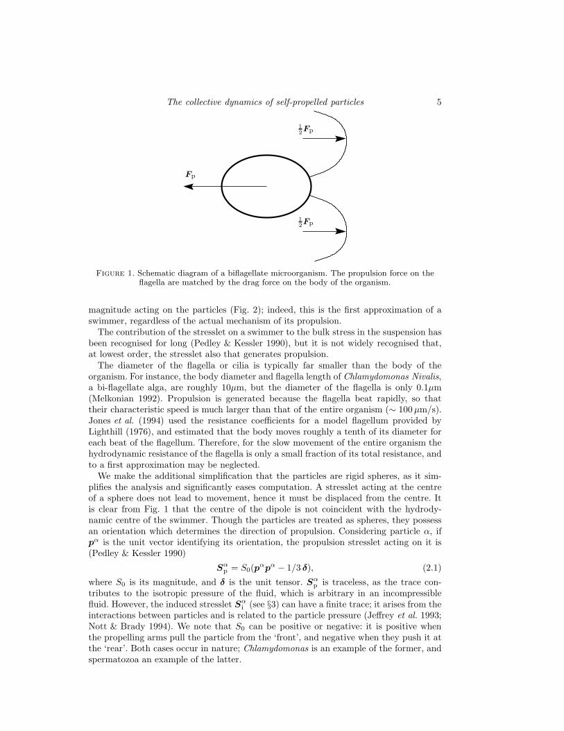
To motivate our model for a swimmer, consider the schematic of a bi-flagellate or-ganism, shown in Fig. 1. We ignore, for the moment, the effect of gravity or any otherexternal force. The periodic, but non-reciprocating ‘beating’ of its flagella results in theaction of a forward propulsive force 1
2Fp by the fluid on each flagella. The motion of theparticle is retarded by the fluid with drag force Fp, as the particle cannot accelerate inthe regime of Stokes flow. Though there is no net force, it is clear that there is a forcedipole Sp, and perhaps higher multipoles, acting on the particles. If there is no externaltorque on the particles, the dipole must be symmetric, i.e. it is a stresslet. We have usedthe biflagellate, in which one can make the distinction between the ‘propulsion arm’ andthe ‘body’ of the swimmer, only as an evocative example. Often it is not possible toseparate the propulsion force and the drag, an example being a waving filament or sheet(Taylor 1951). Thus, it is more accurate to say that, at lowest order, a Stokesian swimmeris propelled by a force dipole.
While the magnitude of the stresslet changes over the duration of a cycle, we areinterested in the behaviour over time scales much larger than the period of a beat, andtherefore assume the magnitude to be constant. However, the principal directions of thestresslet may vary in time, as interactions with other particles will cause the particleto rotate. The simplest model for propulsion, therefore, is a stresslet Sp of constant
The collective dynamics of self-propelled particles 5
1
2Fp
1
2Fp
Fp
Figure 1. Schematic diagram of a biflagellate microorganism. The propulsion force on theflagella are matched by the drag force on the body of the organism.
magnitude acting on the particles (Fig. 2); indeed, this is the first approximation of aswimmer, regardless of the actual mechanism of its propulsion.
The contribution of the stresslet on a swimmer to the bulk stress in the suspension hasbeen recognised for long (Pedley & Kessler 1990), but it is not widely recognised that,at lowest order, the stresslet also that generates propulsion.
The diameter of the flagella or cilia is typically far smaller than the body of theorganism. For instance, the body diameter and flagella length of Chlamydomonas Nivalis,a bi-flagellate alga, are roughly 10µm, but the diameter of the flagella is only 0.1µm(Melkonian 1992). Propulsion is generated because the flagella beat rapidly, so thattheir characteristic speed is much larger than that of the entire organism (∼ 100 µm/s).Jones et al. (1994) used the resistance coefficients for a model flagellum provided byLighthill (1976), and estimated that the body moves roughly a tenth of its diameter foreach beat of the flagellum. Therefore, for the slow movement of the entire organism thehydrodynamic resistance of the flagella is only a small fraction of its total resistance, andto a first approximation may be neglected.
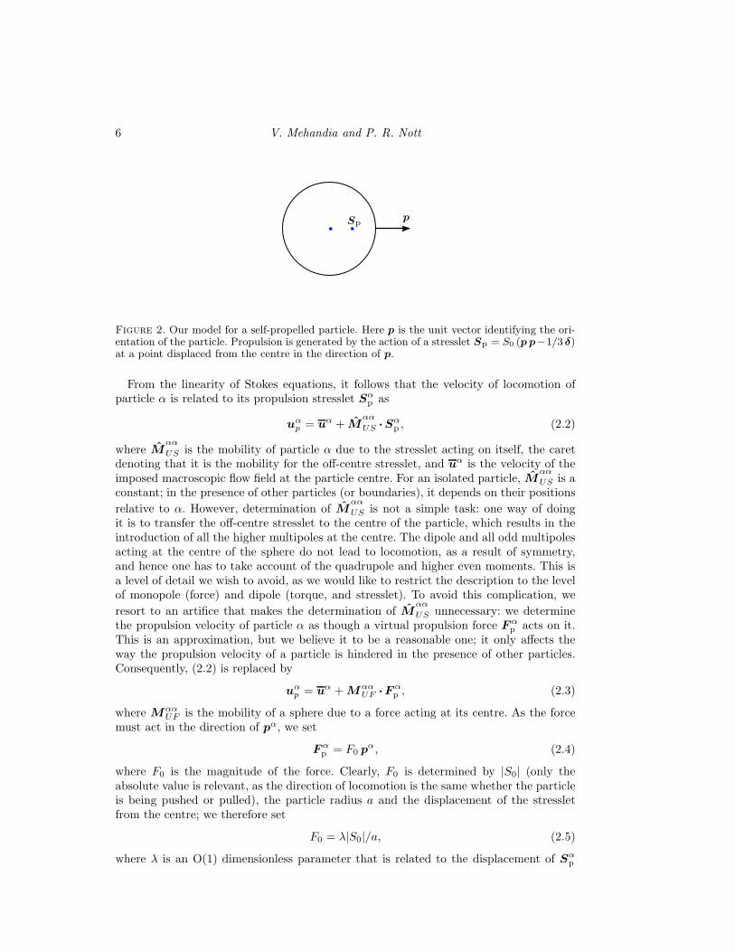
We make the additional simplification that the particles are rigid spheres, as it sim-plifies the analysis and significantly eases computation. A stresslet acting at the centreof a sphere does not lead to movement, hence it must be displaced from the centre. Itis clear from Fig. 1 that the centre of the dipole is not coincident with the hydrody-namic centre of the swimmer. Though the particles are treated as spheres, they possessan orientation which determines the direction of propulsion. Considering particle α, ifpα is the unit vector identifying its orientation, the propulsion stresslet acting on it is(Pedley & Kessler 1990)
Sαp = S0(p
αpα − 1/3 δ), (2.1)
where S0 is its magnitude, and δ is the unit tensor. Sαp is traceless, as the trace con-
tributes to the isotropic pressure of the fluid, which is arbitrary in an incompressiblefluid. However, the induced stresslet Sα
i (see §3) can have a finite trace; it arises from theinteractions between particles and is related to the particle pressure (Jeffrey et al. 1993;Nott & Brady 1994). We note that S0 can be positive or negative: it is positive whenthe propelling arms pull the particle from the ‘front’, and negative when they push it atthe ‘rear’. Both cases occur in nature; Chlamydomonas is an example of the former, andspermatozoa an example of the latter.
6 V. Mehandia and P. R. Nott
Spp
Figure 2. Our model for a self-propelled particle. Here p is the unit vector identifying the ori-entation of the particle. Propulsion is generated by the action of a stresslet Sp = S0 (p p−1/3 δ)at a point displaced from the centre in the direction of p.
From the linearity of Stokes equations, it follows that the velocity of locomotion ofparticle α is related to its propulsion stresslet Sα
p as
uαp = uα + M
αα
US ·Sαp , (2.2)
where Mαα
US is the mobility of particle α due to the stresslet acting on itself, the caretdenoting that it is the mobility for the off-centre stresslet, and uα is the velocity of theimposed macroscopic flow field at the particle centre. For an isolated particle, M
αα
US is aconstant; in the presence of other particles (or boundaries), it depends on their positions
relative to α. However, determination of Mαα
US is not a simple task: one way of doingit is to transfer the off-centre stresslet to the centre of the particle, which results in theintroduction of all the higher multipoles at the centre. The dipole and all odd multipolesacting at the centre of the sphere do not lead to locomotion, as a result of symmetry,and hence one has to take account of the quadrupole and higher even moments. This isa level of detail we wish to avoid, as we would like to restrict the description to the levelof monopole (force) and dipole (torque, and stresslet). To avoid this complication, we
resort to an artifice that makes the determination of Mαα
US unnecessary: we determinethe propulsion velocity of particle α as though a virtual propulsion force F α
p acts on it.This is an approximation, but we believe it to be a reasonable one; it only affects theway the propulsion velocity of a particle is hindered in the presence of other particles.Consequently, (2.2) is replaced by
uαp = uα + Mαα
UF ·F αp , (2.3)
where MααUF is the mobility of a sphere due to a force acting at its centre. As the force
must act in the direction of pα, we set
F αp = F0 pα, (2.4)
where F0 is the magnitude of the force. Clearly, F0 is determined by |S0| (only theabsolute value is relevant, as the direction of locomotion is the same whether the particleis being pushed or pulled), the particle radius a and the displacement of the stressletfrom the centre; we therefore set
F0 = λ|S0|/a, (2.5)
where λ is an O(1) dimensionless parameter that is related to the displacement of Sαp
The collective dynamics of self-propelled particles 7
from the centre. Pedley & Kessler (1990) arrived at a relation similar to (2.5) betweenthe thrust exerted by the flagella and the magnitude of the stresslet. In this simplifiedform, our model is similar to that of Hernandez-Ortiz et al. (2005), who used a ‘phan-tom flagellum’ to drive the dumbbells (see §1). The important difference between ourmodel and theirs is that interactions between particles modulate the effect of the virtualpropulsion force, as the mobility MUF (see below) of a particle is reduced if it is closeto another particle or a wall.
We emphasise that the other particles do not perceive a force acting on α, but onlythe stresslet Sα
p . The force on each particle serves only to determine its propulsion.In addition to the propulsion stresslet, a stresslet Sα
i is induced on α when it is placedin a non-uniform velocity field, as a result of its rigidity.
To summarise, our model for a self-propelled particle is the following: each particle αis treated as a rigid sphere with an orientation vector pα, on which a stresslet Sα
p (of theform given in eq. 2.1) acts at a point slightly displaced from its centre. The displacementof the stresslet from the centre of α is not perceptible to any other particle, and hence αappears as a sphere with a stresslet acting at its centre. The propulsion velocity of α isdetermined by introducing a virtual propulsion force F α
p (of the form is given in eqs 2.4and 2.5) on it. However, other particles do not perceive the force on α.
3. Collective dynamics
To place the problem in the framework of the Stokesian Dynamics method, let us firstconsider the dynamics of a suspension of passive particles. (We emphasise that the word‘passive’ is used in this paper to refer to particles that are not self-propelled, and not fortiny tracer particles that translate with the local fluid velocity.) For the motion of non-Brownian, rigid spheres in a Newtonian fluid at small Stokes number, Newton’s secondlaw reduces to
F H + F = 0, (3.1)
where F H is the vector of the hydrodynamic forces and torques on all the particles, andF is the vector of the non-hydrodynamic forces (external forces such as gravity, andinter-particle forces) and torques.
To determine the motion of the particles, we must relate F H to the vector of theirvelocities and angular velocities u; in the creeping flow regime, this is accomplished bysolving the Stokes equations, with the boundary conditions of no penetration and noslip on the surface of the particles. The hydrodynamic interactions between the particlescause the velocity and angular velocity of a given particle to depend not just on thehydrodynamic force and torque acting on itself, but also on the forces and torques actingon all the other particles. More precisely, u depends on the distribution of the hydro-dynamic force on the surfaces of all the particles. A convenient way of representing thedistribution of force on the surface of a particle is the multipole moment expansion (see,for example, Kim & Karrila 1991, chaps. 2–4): the zeroth multipole (monopole) is thenet force on the particle; the first multipole (dipole) may separated into its symmetricand antisymmetric parts, the former being the torque and the latter the stresslet. By thelinearity of Stokes equations, u is given by
(
u − u
−e
)
= M·
(
F
S
)
. (3.2)
where we have used (3.1) to replace F H with F . Here, S is the vector of the hydrodynamicstresslets, and u and e are vectors of the velocities and strain rates, respectively, of the
8 V. Mehandia and P. R. Nott
externally imposed flow field at the particle centres. The quantity M is the so-called‘grand’ mobility tensor, which can be decomposed into the mobility tensors representingthe various couplings,
M =
(
MUF MUS
MEF MES
)
, (3.3)
the subscripts indicating the nature of the coupling. In principle, the right hand sideof (3.2) must include higher moments of the force distribution on the particle surface,and the left hand side the higher gradients of the imposed velocity field—for each highermoment included, there will be an additional equation. The Stokesian Dynamics method(Brady et al. 1988; Brady & Bossis 1988; Durlofsky et al. 1987), which we shall modifyand use for the present problem, retains only the monopole and the dipole moments.
The physical meaning of (3.2) is as follows: the first line enforces (3.1), and determinesu; the second line can be thought of as the equation to determine S. The stresslet isinduced on each particle by the flow around it (externally imposed, and generated by themotion of other particles) so as to keep it rigid.
The main advantage of the Stokesian Dynamics method is that M (or equivalentlythe grand resistance R ≡ M
−1) is computed and assembled in an accurate and efficientmanner. This is done as a matched sum of the far-field and near-field interactions,
M−1 = M
−1ff + Rnf − R
∞nf . (3.4)
Here, Mff is the mobility tensor that captures the far-field interactions, Rnf is thenear-field resistance tensor, and R
∞nf is the far-field part of Rnf that is subtracted to
get a uniform asymptotic expansion. Though Mff is assembled pair-wise, it has beendemonstrated by Durlofsky et al. (1987) that its inversion captures the many body hy-drodynamic interactions.
The above framework must now be modified to incorporate the model for a swimmerwe have developed in §2. In principle, the propulsion of the particles does not depend onthe external force; hence, they can swim even when F=0. However, we have introducedthe virtual propulsion force Fp in §2 to avoid the inclusion of moments higher than thedipole in the multipole expansion. But Fp must be recognised is a special force, as F α
p
acting on particle α only determines its velocity, and has no effect whatsoever on theother particles. The other particles perceive only the stresslet acting on particle α. Inaddition, the propulsion stresslet Sp must be treated separately from the induced stressletSi—the former is an inherent property of the swimmers, whose magnitude is constantand directions are determine by their orientations, whereas the latter is induced by theflow of the fluid around them. Accordingly, we distinguish the virtual propulsion forceFp from the sum of external and inter-particle forces Fext, and the propulsion stressletSp from the induced stresslet Si. The vectors Fp and Sp depend on the orientations ofthe particles through (2.1) and (2.4).
After incorporation of the above modifications, the first line of (3.2) takes the form,
u − u = M selfUF ·Fp + MUF ·Fext + MUS·(Sp + Si) (3.5)
where M selfUF is the self mobility, i.e. the mobility of each particle due to a force on itself.
For the particle pair α-β, the self mobility is
Mself,αβUF = M
αβUF δαβ, (3.6)
where δαβ
is the Kronecker delta. The first term on the right hand side of (3.5) providespropulsion; only the self mobility acts on Fp, so that the virtual propulsion force on aparticle has no effect on the other particles, as per our prescription. The second term
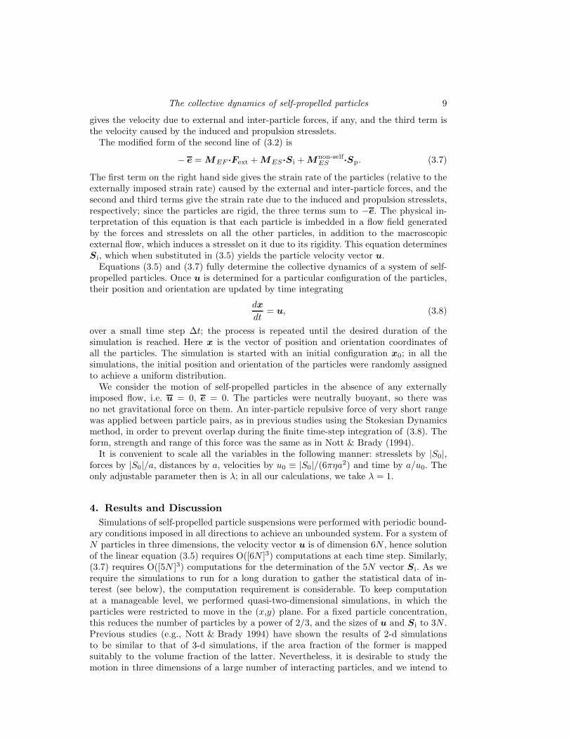
The collective dynamics of self-propelled particles 9
gives the velocity due to external and inter-particle forces, if any, and the third term isthe velocity caused by the induced and propulsion stresslets.
The modified form of the second line of (3.2) is
− e = MEF ·Fext + MES·Si + Mnon-selfES ·Sp. (3.7)
The first term on the right hand side gives the strain rate of the particles (relative to theexternally imposed strain rate) caused by the external and inter-particle forces, and thesecond and third terms give the strain rate due to the induced and propulsion stresslets,respectively; since the particles are rigid, the three terms sum to −e. The physical in-terpretation of this equation is that each particle is imbedded in a flow field generatedby the forces and stresslets on all the other particles, in addition to the macroscopicexternal flow, which induces a stresslet on it due to its rigidity. This equation determinesSi, which when substituted in (3.5) yields the particle velocity vector u.
Equations (3.5) and (3.7) fully determine the collective dynamics of a system of self-propelled particles. Once u is determined for a particular configuration of the particles,their position and orientation are updated by time integrating
dx
dt= u, (3.8)
over a small time step ∆t; the process is repeated until the desired duration of thesimulation is reached. Here x is the vector of position and orientation coordinates ofall the particles. The simulation is started with an initial configuration x0; in all thesimulations, the initial position and orientation of the particles were randomly assignedto achieve a uniform distribution.
We consider the motion of self-propelled particles in the absence of any externallyimposed flow, i.e. u = 0, e = 0. The particles were neutrally buoyant, so there wasno net gravitational force on them. An inter-particle repulsive force of very short rangewas applied between particle pairs, as in previous studies using the Stokesian Dynamicsmethod, in order to prevent overlap during the finite time-step integration of (3.8). Theform, strength and range of this force was the same as in Nott & Brady (1994).
It is convenient to scale all the variables in the following manner: stresslets by |S0|,forces by |S0|/a, distances by a, velocities by u0 ≡ |S0|/(6πηa2) and time by a/u0. Theonly adjustable parameter then is λ; in all our calculations, we take λ = 1.
4. Results and Discussion
Simulations of self-propelled particle suspensions were performed with periodic bound-ary conditions imposed in all directions to achieve an unbounded system. For a system ofN particles in three dimensions, the velocity vector u is of dimension 6N , hence solutionof the linear equation (3.5) requires O([6N ]3) computations at each time step. Similarly,(3.7) requires O([5N ]3) computations for the determination of the 5N vector Si. As werequire the simulations to run for a long duration to gather the statistical data of in-terest (see below), the computation requirement is considerable. To keep computationat a manageable level, we performed quasi-two-dimensional simulations, in which theparticles were restricted to move in the (x,y) plane. For a fixed particle concentration,this reduces the number of particles by a power of 2/3, and the sizes of u and Si to 3N .Previous studies (e.g., Nott & Brady 1994) have shown the results of 2-d simulationsto be similar to that of 3-d simulations, if the area fraction of the former is mappedsuitably to the volume fraction of the latter. Nevertheless, it is desirable to study themotion in three dimensions of a large number of interacting particles, and we intend to
10 V. Mehandia and P. R. Nott
do so in a future investigation by using the Accelerated Stokesian Dynamics scheme ofSierou & Brady (2001).
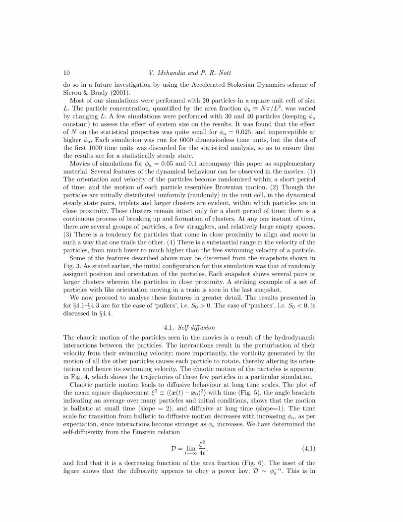
Most of our simulations were performed with 20 particles in a square unit cell of sizeL. The particle concentration, quantified by the area fraction φa ≡ Nπ/L2, was variedby changing L. A few simulations were performed with 30 and 40 particles (keeping φa
constant) to assess the effect of system size on the results. It was found that the effectof N on the statistical properties was quite small for φa = 0.025, and imperceptible athigher φa. Each simulation was run for 6000 dimensionless time units, but the data ofthe first 1000 time units was discarded for the statistical analysis, so as to ensure thatthe results are for a statistically steady state.
Movies of simulations for φa = 0.05 and 0.1 accompany this paper as supplementarymaterial. Several features of the dynamical behaviour can be observed in the movies. (1)The orientation and velocity of the particles become randomised within a short periodof time, and the motion of each particle resembles Brownian motion. (2) Though theparticles are initially distributed uniformly (randomly) in the unit cell, in the dynamicalsteady state pairs, triplets and larger clusters are evident, within which particles are inclose proximity. These clusters remain intact only for a short period of time; there is acontinuous process of breaking up and formation of clusters. At any one instant of time,there are several groups of particles, a few stragglers, and relatively large empty spaces.(3) There is a tendency for particles that come in close proximity to align and move insuch a way that one trails the other. (4) There is a substantial range in the velocity of theparticles, from much lower to much higher than the free swimming velocity of a particle.
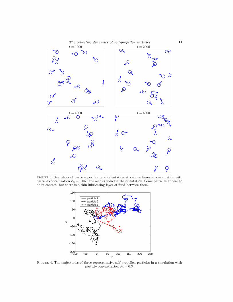
Some of the features described above may be discerned from the snapshots shown inFig. 3. As stated earlier, the initial configuration for this simulation was that of randomlyassigned position and orientation of the particles. Each snapshot shows several pairs orlarger clusters wherein the particles in close proximity. A striking example of a set ofparticles with like orientation moving in a train is seen in the last snapshot.
We now proceed to analyse these features in greater detail. The results presented infor §4.1–§4.3 are for the case of ‘pullers’, i.e. S0 > 0. The case of ‘pushers’, i.e. S0 < 0, isdiscussed in §4.4.
4.1. Self diffusion
The chaotic motion of the particles seen in the movies is a result of the hydrodynamicinteractions between the particles. The interactions result in the perturbation of theirvelocity from their swimming velocity; more importantly, the vorticity generated by themotion of all the other particles causes each particle to rotate, thereby altering its orien-tation and hence its swimming velocity. The chaotic motion of the particles is apparentin Fig. 4, which shows the trajectories of three few particles in a particular simulation.
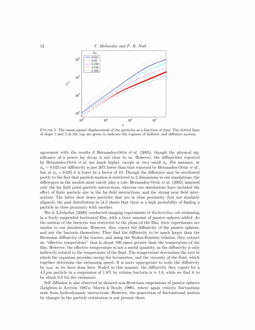
Chaotic particle motion leads to diffusive behaviour at long time scales. The plot ofthe mean square displacement ξ2 ≡ 〈(x(t)−x0)
2〉 with time (Fig. 5), the angle bracketsindicating an average over many particles and initial conditions, shows that the motionis ballistic at small time (slope = 2), and diffusive at long time (slope=1). The timescale for transition from ballistic to diffusive motion decreases with increasing φa, as perexpectation, since interactions become stronger as φa increases. We have determined theself-diffusivity from the Einstein relation
D = limt→∞
ξ2
4t, (4.1)
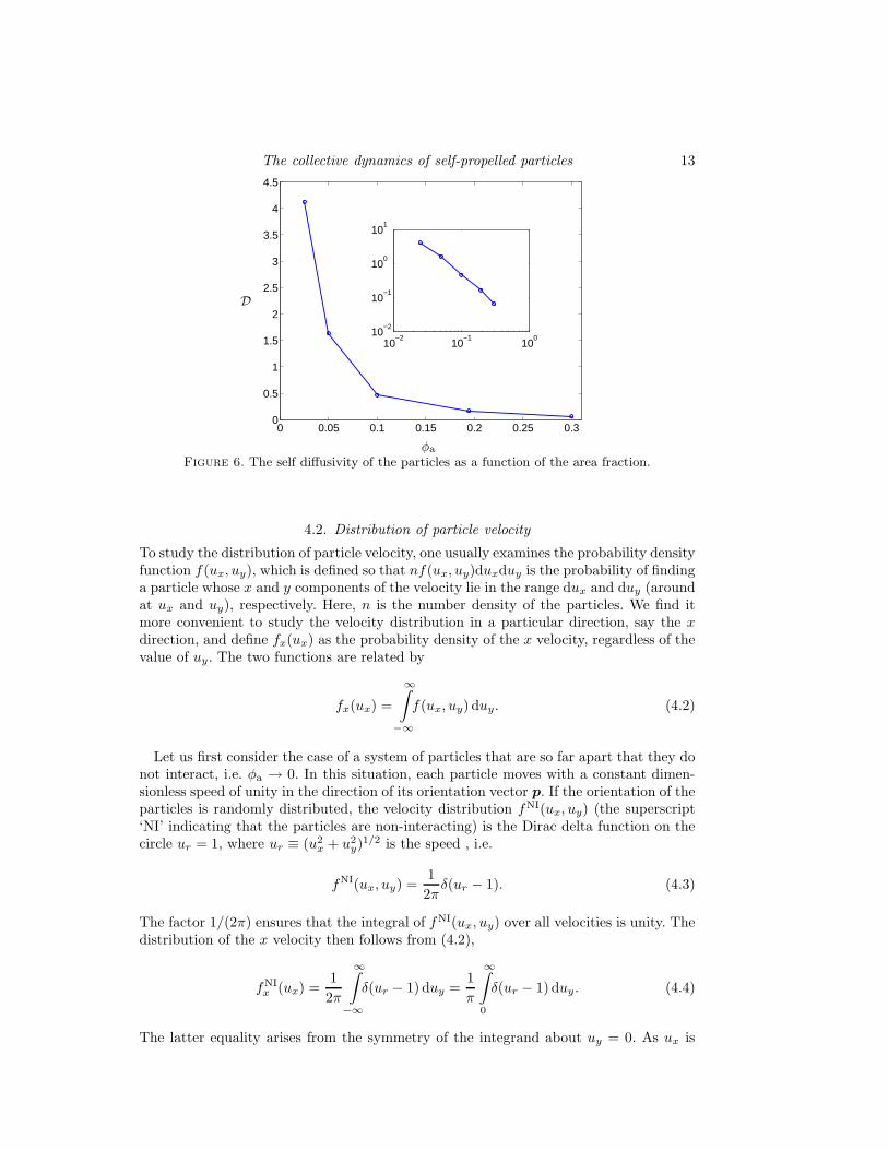
and find that it is a decreasing function of the area fraction (Fig. 6). The inset of thefigure shows that the diffusivity appears to obey a power law, D ∼ φ−n
a . This is in
The collective dynamics of self-propelled particles 11t = 1000 t = 2000
t = 4000 t = 6000
Figure 3. Snapshots of particle position and orientation at various times in a simulation withparticle concentration φa = 0.05. The arrows indicate the orientation. Some particles appear tobe in contact, but there is a thin lubricating layer of fluid between them.
−100 −50 0 50 100 150 200 250−200
−150
−100
−50
0
50
100
150
particle 1particle 2particle 3
x
y
Figure 4. The trajectories of three representative self-propelled particles in a simulation withparticle concentration φa = 0.3.
12 V. Mehandia and P. R. Nott
100
101
102
103
100
102
104
106 0.025
0.050.1000.1940.300
t
ξ2
φa
Figure 5. The mean square displacement of the particles as a function of time. The dotted linesof slope 1 and 2 at the top are given to indicate the regimes of ballistic and diffusive motion.
agreement with the results if Hernandez-Ortiz et al. (2005), though the physical sig-nificance of a power lay decay is not clear to us. However, the diffusivities reportedby Hernandez-Ortiz et al. are much higher, except at very small φa. For instance, atφa = 0.025 our diffusivity is just 20% lower than that reported by Hernandez-Ortiz et al.,but at φa = 0.025 it is lower by a factor of 10. Though the difference may be attributedpartly to the fact that particle motion is restricted to 2 dimensions in our simulations, thedifferences in the models must surely play a role: Hernandez-Ortiz et al. (2005) imposedonly the far field point-particle interactions, whereas our simulations have included theeffect of finite particle size in the far-field interactions, and the strong near field inter-actions. The latter slow down particles that are in close proximity (but not similarlyaligned); the pair distribution in §4.3 shows that there is a high probability of finding aparticle in close proximity with another.
Wu & Libchaber (2000) conducted imaging experiments of Escherichia coli swimmingin a freely suspended horizontal film, with a trace amount of passive spheres added. Asthe motion of the bacteria was restricted to the plane of the film, their experiments aresimilar to our simulations. However, they report the diffusivity of the passive spheres,and not the bacteria themselves. They find the diffusivity to be much larger than theBrownian diffusivity of the tracers, and using the Stokes-Einstein relation, they extractan “effective temperature” that is about 100 times greater than the temperature of thefilm. However, the effective temperature is not a useful quantity, as the diffusivity is onlyindirectly related to the temperature of the fluid. The temperature determines the rate atwhich the organism provides energy for locomotion, and the viscosity of the fluid, whichtogether determine the swimming speed. It is more appropriate to scale the diffusivityby u0a, as we have done here. Scaled in this manner, the diffusivity they report for a4.5 µm particle in a suspension of 1.8% by volume bacteria is ≈ 1.6, while we find it tobe about 0.8 for the swimmers.
Self diffusion is also observed in sheared non-Brownian suspensions of passive spheres(Leighton & Acrivos 1987a; Morris & Brady 1996), where again velocity fluctuationsarise from hydrodynamic interactions. However, the generation of fluctuational motionby changes in the particle orientation is not present there.
The collective dynamics of self-propelled particles 13
0 0.05 0.1 0.15 0.2 0.25 0.30
0.5
1
1.5
2
2.5
3
3.5
4
4.5
10−2
10−1
100
10−2
10−1
100
101
φa
D
Figure 6. The self diffusivity of the particles as a function of the area fraction.
4.2. Distribution of particle velocity
To study the distribution of particle velocity, one usually examines the probability densityfunction f(ux, uy), which is defined so that nf(ux, uy)duxduy is the probability of findinga particle whose x and y components of the velocity lie in the range dux and duy (aroundat ux and uy), respectively. Here, n is the number density of the particles. We find itmore convenient to study the velocity distribution in a particular direction, say the xdirection, and define fx(ux) as the probability density of the x velocity, regardless of thevalue of uy. The two functions are related by
fx(ux) =
∞∫
−∞
f(ux, uy) duy. (4.2)
Let us first consider the case of a system of particles that are so far apart that they donot interact, i.e. φa → 0. In this situation, each particle moves with a constant dimen-sionless speed of unity in the direction of its orientation vector p. If the orientation of theparticles is randomly distributed, the velocity distribution fNI(ux, uy) (the superscript‘NI’ indicating that the particles are non-interacting) is the Dirac delta function on thecircle ur = 1, where ur ≡ (u2
x + u2y)
1/2 is the speed , i.e.
fNI(ux, uy) =1
2πδ(ur − 1). (4.3)
The factor 1/(2π) ensures that the integral of fNI(ux, uy) over all velocities is unity. Thedistribution of the x velocity then follows from (4.2),
fNIx (ux) =
1
2π
∞∫
−∞
δ(ur − 1) duy =1
π
∞∫
0
δ(ur − 1) duy. (4.4)
The latter equality arises from the symmetry of the integrand about uy = 0. As ux is

14 V. Mehandia and P. R. Nott
kept constant in the integral, duy = (ur/uy)dur, and hence
fNIx (ux) =
1
π
∞∫
|ux|
δ(ur − 1)ur
(u2r − u2
x)1/2dur. (4.5)
From the sifting property of the delta function, we therefore have
fNIx (ux) =
1
π
1
(1 − u2x)1/2
(4.6)
Note that fNIx diverges as ux → ±1. As the orientations are uniformly distributed, and
there is no external force favouring motion in a particular direction, this distributionholds for all directions in the plane of motion. The distribution given by (4.6) is shownby the dotted line in Fig. 7.
The distribution will, of course, be altered when the particles interact. We have anal-ysed the results of our simulations to determine the velocity distribution. The particlevelocities were collected at dimensionless time intervals of unity, during which time afreely swimming particle moves a distance of its radius. The distribution function fx(ux)was determined by constructing a histogram of the number distribution in equally sizedintervals of ux, and normalising it so that
∫
fx dux = 1. The same was repeated for the ydirection. Due to the absence of directionality in the problem, the distribution functionshould be the same for all directions, which is indeed what we observe in Fig. 7 (comparethe the lines and symbols). Given the isotropy of the velocity distribution, we henceforthdenote by f(u) the distribution in any direction. It is evident from Fig. 7 that the velocitydistribution deviates from that of non-interacting swimmers (dotted line) even at smallφa.
For φa = 0.025, the velocity distribution is close to fNI for small |u|, but departs fromit when |u| is greater than a value slightly less than unity—it has maxima at u ≈ ±1, anddecays rapidly for |u| > 1. Thus, there is a finite probability of finding a particle with avelocity significantly higher than that of an isolated swimmer. For large φa, the velocitydistribution is very different from fNI; it appears to resemble the normal distribution(Fig. 8),
f(u) =1√
2πσ2exp
[
− (u − u)2
2σ2
]
, (4.7)
where u is the mean velocity and σ2 the variance. Small deviations from the normaldistribution are apparent, such as a slight deficit of the probability at small |u|, and afaster decay at large |u| (see inset of Fig. 8). In the study of Wu & Libchaber (2000),referred to earlier, it is reported that the distribution of the speed ur of Escherichia colifollows the Maxwell distribution f(ur) = ur
σ2 exp[−u2r/(2σ2)] at large particle concentra-
tions, which is in accord with the normal distribution of the velocity in any direction.Since the largest concentration they studied is a volume fraction of φ = 0.1, it appearsthat they found a normal distribution at lower concentrations than we do. Whether thedifference may be ascribed to the differences in the conditions of the experiments and thesimulations, or the simplicity of our model is difficult to say. Our results indicate thatcareful measurements of the velocity distribution for a range of concentration is neces-sary. Conducting simulations and experiments in which particles are free to move in allthree spatial dimensions would also be a worthwhile pursuit. Nevertheless, the qualitativeagreement is perhaps an indication that our description is fundamentally sound, and itcaptures some of the important features of collective motion.
Figure 9 compares the results obtained with and without the inclusion of the near-field

The collective dynamics of self-propelled particles 15
−2 −1 0 1 20
0.2
0.4
0.6
0.8
1
1.2
u
f(u)
fx, φa = 0.025fy , φa = 0.025fx, φa = 0.194fy , φa = 0.194
f(u), NI
Figure 7. The probability distribution function of particle velocity in a suspension of self-pro-pelled particles at concentrations φa = 0.025 and 0.3. The lines are symbols are the distributionsof ux and uy , respectively, where x and y are the coordinates of the (fixed) laboratory refer-ence frame. The equality of fx and fy shows the absence of directionality in the problem. Thedotted line is the velocity distribution for a collection of non-interacting, randomly orientedself-propelled particles, given by (4.6).
−2 −1 0 1 20
0.2
0.4
0.6
0.8
1
−2 0 2
10−2
100
u
f(u)
f(u)
normal
Figure 8. The velocity distribution for a suspension with φa = 0.3 compared with the normaldistribution having the same mean and variance. The inset shows the same plot in semi-logcoordinates.
hydrodynamic interactions, represented by the term Rnf − R∞nf in (3.4). We note that
the velocity distribution is unchanged by the inclusion of near-field interactions for adilute suspension of swimmers, but it is significantly altered for a relatively concentratedsuspension. This is not an unexpected result, as the frequency with which a typical par-ticle comes into close proximity with others is relatively low at small φa, but it increaseswith φa. It is pertinent to note that our simulations without the near-field interactions donot reduce to point-particle simulations, of the kind performed by Hernandez-Ortiz et al.(2005). In Stokesian Dynamics simulations, the finite size of a particles is accounted forby retaining the induced dipole moments, and parts of the quadrupole and octupole mo-

16 V. Mehandia and P. R. Nott
−2 −1.5 −1 −0.5 0 0.5 1 1.5 20
0.2
0.4
0.6
0.8
1
0.025, with NF0.025, without NF0.3, with NF0.3, without NF
u
f(u)
φa
Figure 9. Comparison of the velocity distribution for a dilute (φa = 0.025) and concentrated(φa = 0.3) suspension of swimmers with and without the inclusion of near-field hydrodynamicinteractions (NF).
−2 −1.5 −1 −0.5 0 0.5 1 1.5 20
0.2
0.4
0.6
0.8
1
0.0250.050.1000.1940.300
u
f(u)
φa
Figure 10. The velocity distribution for a range of the particle concentration.
ments (called the irreducible moments), in the multipole expansion of the force densitydistribution on the particle surface, and also the corresponding finite-size terms in theFaxen relations (Brady et al. 1988; Brady & Bossis 1988; Durlofsky et al. 1987).
Reverting to our simulations with the full hydrodynamic interactions, the velocitydistribution for all the particle concentrations that we have studied are shown in Fig. 10.As φa increases, the depth of the well between the two maxima decreases, vanishescompletely at φa slightly over 0.1, and the distribution resembles a normal distributionat high φa. The variance σ2 of the distribution decreases with increasing φa.
4.3. Correlations
As discussed earlier, the movies (see supplementary material) and the snapshots in Fig. 3show significant correlation in the position and orientation of the particles. We first anal-yse the correlation in particle position in terms of the pair correlation function g(r2, r1),
The collective dynamics of self-propelled particles 17
p1
p2
θ
r
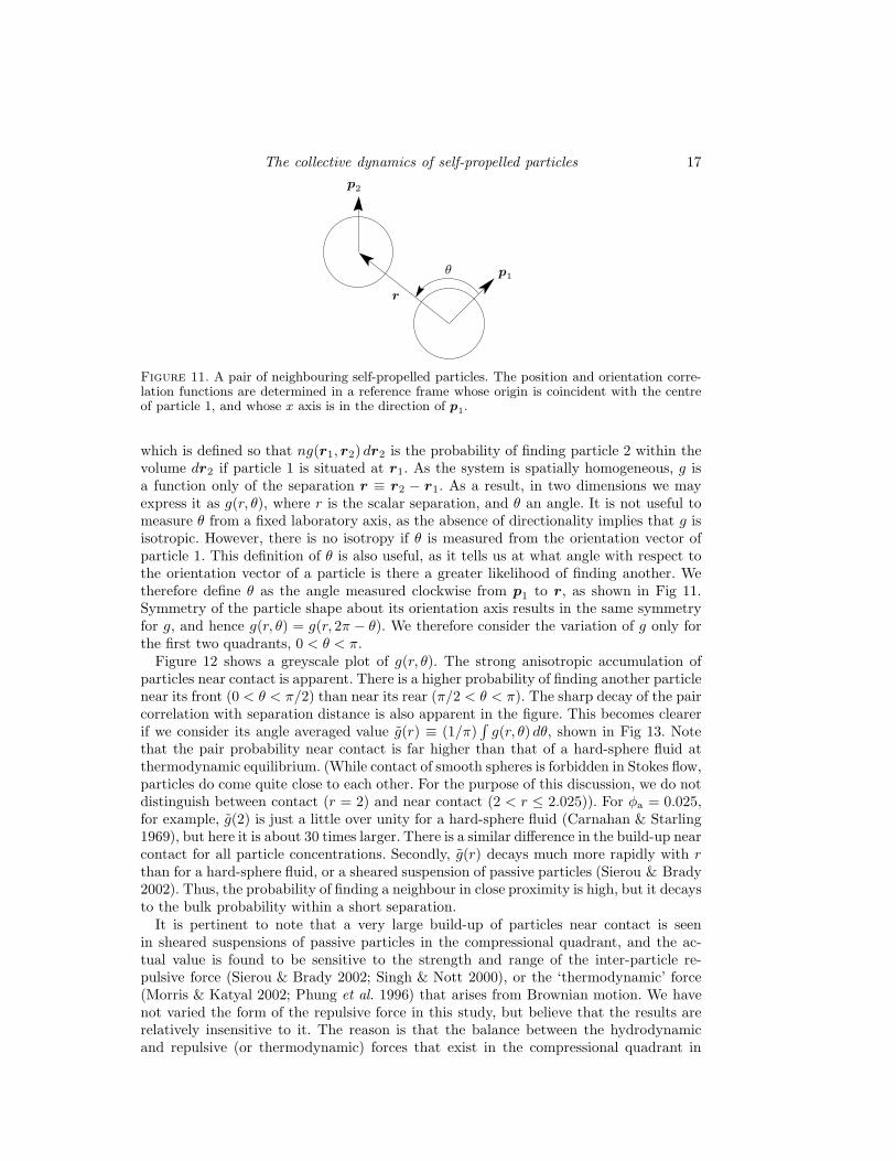
Figure 11. A pair of neighbouring self-propelled particles. The position and orientation corre-lation functions are determined in a reference frame whose origin is coincident with the centreof particle 1, and whose x axis is in the direction of p
1.
which is defined so that ng(r1, r2) dr2 is the probability of finding particle 2 within thevolume dr2 if particle 1 is situated at r1. As the system is spatially homogeneous, g isa function only of the separation r ≡ r2 − r1. As a result, in two dimensions we mayexpress it as g(r, θ), where r is the scalar separation, and θ an angle. It is not useful tomeasure θ from a fixed laboratory axis, as the absence of directionality implies that g isisotropic. However, there is no isotropy if θ is measured from the orientation vector ofparticle 1. This definition of θ is also useful, as it tells us at what angle with respect tothe orientation vector of a particle is there a greater likelihood of finding another. Wetherefore define θ as the angle measured clockwise from p1 to r, as shown in Fig 11.Symmetry of the particle shape about its orientation axis results in the same symmetryfor g, and hence g(r, θ) = g(r, 2π − θ). We therefore consider the variation of g only forthe first two quadrants, 0 < θ < π.
Figure 12 shows a greyscale plot of g(r, θ). The strong anisotropic accumulation ofparticles near contact is apparent. There is a higher probability of finding another particlenear its front (0 < θ < π/2) than near its rear (π/2 < θ < π). The sharp decay of the paircorrelation with separation distance is also apparent in the figure. This becomes clearerif we consider its angle averaged value g(r) ≡ (1/π)
∫
g(r, θ) dθ, shown in Fig 13. Notethat the pair probability near contact is far higher than that of a hard-sphere fluid atthermodynamic equilibrium. (While contact of smooth spheres is forbidden in Stokes flow,particles do come quite close to each other. For the purpose of this discussion, we do notdistinguish between contact (r = 2) and near contact (2 < r ≤ 2.025)). For φa = 0.025,for example, g(2) is just a little over unity for a hard-sphere fluid (Carnahan & Starling1969), but here it is about 30 times larger. There is a similar difference in the build-up nearcontact for all particle concentrations. Secondly, g(r) decays much more rapidly with rthan for a hard-sphere fluid, or a sheared suspension of passive particles (Sierou & Brady2002). Thus, the probability of finding a neighbour in close proximity is high, but it decaysto the bulk probability within a short separation.
It is pertinent to note that a very large build-up of particles near contact is seenin sheared suspensions of passive particles in the compressional quadrant, and the ac-tual value is found to be sensitive to the strength and range of the inter-particle re-pulsive force (Sierou & Brady 2002; Singh & Nott 2000), or the ‘thermodynamic’ force(Morris & Katyal 2002; Phung et al. 1996) that arises from Brownian motion. We havenot varied the form of the repulsive force in this study, but believe that the results arerelatively insensitive to it. The reason is that the balance between the hydrodynamicand repulsive (or thermodynamic) forces that exist in the compressional quadrant in
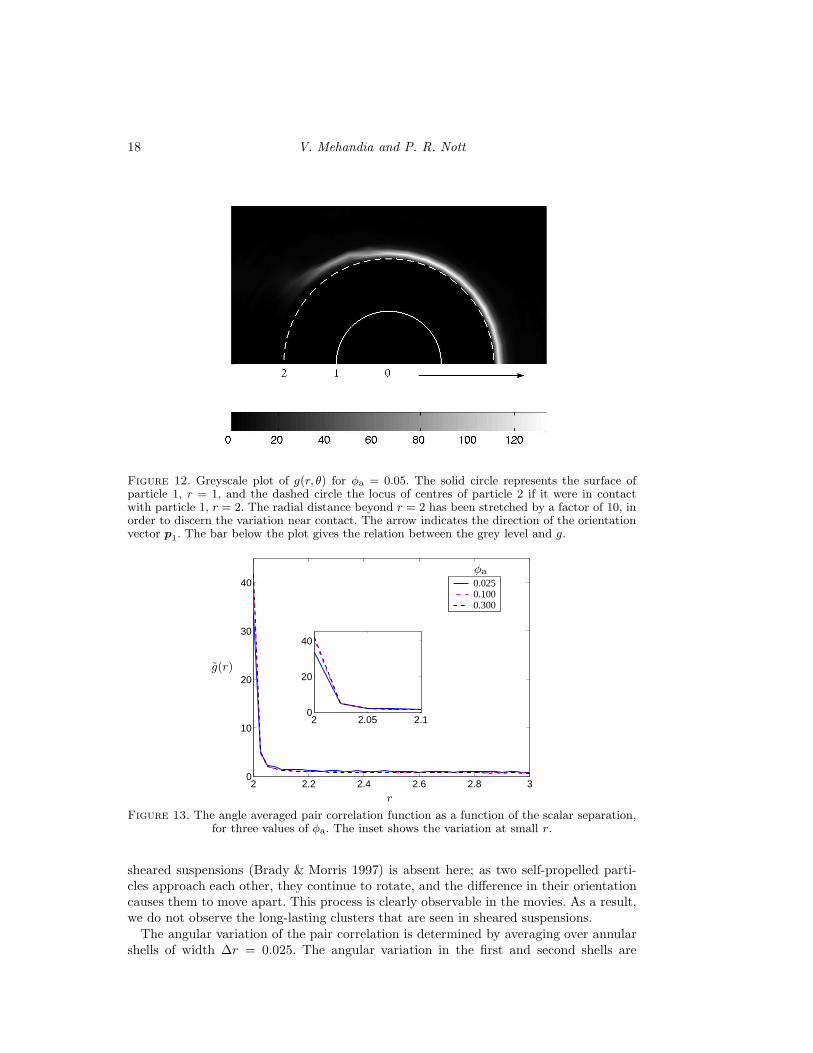
18 V. Mehandia and P. R. Nott
Figure 12. Greyscale plot of g(r, θ) for φa = 0.05. The solid circle represents the surface ofparticle 1, r = 1, and the dashed circle the locus of centres of particle 2 if it were in contactwith particle 1, r = 2. The radial distance beyond r = 2 has been stretched by a factor of 10, inorder to discern the variation near contact. The arrow indicates the direction of the orientationvector p
1. The bar below the plot gives the relation between the grey level and g.
2 2.2 2.4 2.6 2.8 30
10
20
30
40 0.0250.1000.300
2 2.05 2.10
20
40
r
g(r)
φa
Figure 13. The angle averaged pair correlation function as a function of the scalar separation,for three values of φa. The inset shows the variation at small r.
sheared suspensions (Brady & Morris 1997) is absent here; as two self-propelled parti-cles approach each other, they continue to rotate, and the difference in their orientationcauses them to move apart. This process is clearly observable in the movies. As a result,we do not observe the long-lasting clusters that are seen in sheared suspensions.
The angular variation of the pair correlation is determined by averaging over annularshells of width ∆r = 0.025. The angular variation in the first and second shells are

The collective dynamics of self-propelled particles 19
0 0.5 1 1.5 2 2.5 30
10
20
30
40
50
60
0.0250.10.3
1st shell
2nd shell
θ
g(∆
r,θ)
φa
Figure 14. Angular variation of the pair correlation function, averaged over annular shells ofwidth ∆r = 0.025. The upper cluster of lines are for the first shell 2 < r ≤ 2.025, and the lowercluster of lines for the second shell 2.025 < r ≤ 2.05.
shown in Fig. 14. The plots for all the concentrations are qualitatively similar; they showa higher probability of finding a neighbour towards the front of each particle than in itsrear, but only in the first shell. In the second shell, there is a smaller peak near θ = 3π/4in all the cases, which reflects the ‘peeling off’ of the accumulation from near contact, asseen in Fig. 12; apart from this peak, the pair correlation at all angles is roughly uniform.In the third and higher shells, the pair correlation at all angles is roughly uniform, andclose to the bulk value of unity (not shown). Thus, there is anisotropy in the distributionof the neighbours, but only at short separations.
Finally, we consider the correlation in the orientation of particle pairs. For particles 1and 2 located at r1 and r2, respectively, the orientation correlation function is 〈p1·p2〉,the angle brackets indicating an average over many particles and over time. It too isa function of r and θ, as defined in Fig 11. A greyscale plot of 〈p1·p2〉 is shown inFig. 15; note that, unlike in Fig. 12, the radial distance is not stretched here. The positivecorrelation of the orientations at the rear of the particle, around θ = π, and negativecorrelation around θ = 3π/4 are evident. There appears to be no correlation at the frontof the particle.
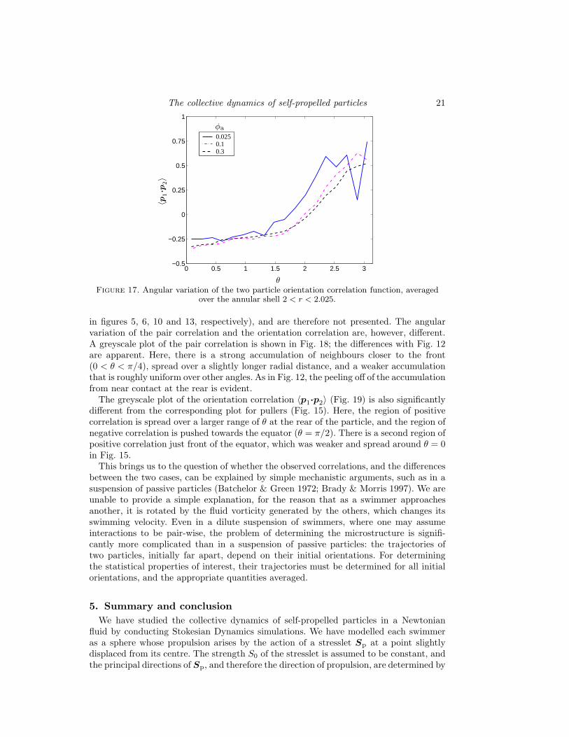
To consider the variation of 〈p1·p2〉 with r, we show its value as a function of r forθ = π and 3π/4 in Fig. 16. The positive correlation for the former and negative correlationfor the latter near contact is evident. The correlation vanishes at large r, as expected,but its decay with r is much slower compared to that of g(r) (compare Fig. 13), meaningthat particle orientations remain correlated over longer distances. The angular variationof 〈p1·p2〉 (Fig. 17), averaged in an annular shell of width ∆r = 0.1, shows a monotonicrise with θ, with maximum correlation near θ = π.
Considering Figs. 13 and 14, we see that while the probability of finding a neighbour ishigh near the front of a particle, the probability of the neighbour being of like alignmentis highest at the rear.
4.4. Statistical features of a suspension of pushers (S0 < 0)
As stated earlier, the results presented in §4.1–§4.3 are for S0 > 0, corresponding to caseof the propelling arms of the swimmer pulling it from the front (see Fig. 1). As mentioned

20 V. Mehandia and P. R. Nott
Figure 15. Greyscale plot of the orientation correlation 〈p1·p
2〉. The solid circle represents the
surface of particle 1, r = 1, and the dashed circle the locus of centres of particle 2 if it were incontact with particle 1, r = 2. The arrow indicates the direction of the orientation vector p
1.
The bar below the plot gives the relation between the grey level and 〈p1·p
2〉.
2 2.5 3 3.5−0.8
−0.4
0
0.4
0.8
0.0250.10.3
r
〈p1·p
2〉
φaθ = π
θ = 3π/4
Figure 16. The two particle orientation correlation function 〈p1·p
2〉 as a function of the scalar
separation for two values of θ. The upper cluster of lines, showing positive correlation, are forθ = π, and the lower cluster of lines, showing positive correlation, are for θ = 3π/4.
in §2, the opposite case of the propelling arms pushing from the rear, which in our modelis achieved by setting S0 < 0, is also observed in nature. The collective dynamics of asuspension of such particles is therefore also of interest.
We have performed simulations for this case at a particle concentration of φa = 0.05.The mean-square displacement, diffusivity, velocity distribution, and the radial variationthe pair correlation g(r) are found to be virtually identical to that of pullers (shown
The collective dynamics of self-propelled particles 21
0 0.5 1 1.5 2 2.5 3−0.5
−0.25
0
0.25
0.5
0.75
1
0.0250.10.3
θ
〈p1·p
2〉
φa
Figure 17. Angular variation of the two particle orientation correlation function, averagedover the annular shell 2 < r < 2.025.
in figures 5, 6, 10 and 13, respectively), and are therefore not presented. The angularvariation of the pair correlation and the orientation correlation are, however, different.A greyscale plot of the pair correlation is shown in Fig. 18; the differences with Fig. 12are apparent. Here, there is a strong accumulation of neighbours closer to the front(0 < θ < π/4), spread over a slightly longer radial distance, and a weaker accumulationthat is roughly uniform over other angles. As in Fig. 12, the peeling off of the accumulationfrom near contact at the rear is evident.
The greyscale plot of the orientation correlation 〈p1·p2〉 (Fig. 19) is also significantlydifferent from the corresponding plot for pullers (Fig. 15). Here, the region of positivecorrelation is spread over a larger range of θ at the rear of the particle, and the region ofnegative correlation is pushed towards the equator (θ = π/2). There is a second region ofpositive correlation just front of the equator, which was weaker and spread around θ = 0in Fig. 15.
This brings us to the question of whether the observed correlations, and the differencesbetween the two cases, can be explained by simple mechanistic arguments, such as in asuspension of passive particles (Batchelor & Green 1972; Brady & Morris 1997). We areunable to provide a simple explanation, for the reason that as a swimmer approachesanother, it is rotated by the fluid vorticity generated by the others, which changes itsswimming velocity. Even in a dilute suspension of swimmers, where one may assumeinteractions to be pair-wise, the problem of determining the microstructure is signifi-cantly more complicated than in a suspension of passive particles: the trajectories oftwo particles, initially far apart, depend on their initial orientations. For determiningthe statistical properties of interest, their trajectories must be determined for all initialorientations, and the appropriate quantities averaged.
5. Summary and conclusion
We have studied the collective dynamics of self-propelled particles in a Newtonianfluid by conducting Stokesian Dynamics simulations. We have modelled each swimmeras a sphere whose propulsion arises by the action of a stresslet Sp at a point slightlydisplaced from its centre. The strength S0 of the stresslet is assumed to be constant, andthe principal directions of Sp, and therefore the direction of propulsion, are determined by

22 V. Mehandia and P. R. Nott
Figure 18. Greyscale plot of g(r, θ) for swimmers that ‘push’ from the rear, i.e. S0 < 0 (seeeq. 2.1). This figure should be compared with Fig. 12 for particles that pull from the front.
Figure 19. Greyscale plot of 〈p1·p
2〉 for swimmers that ‘push’ from the rear, i.e. S0 < 0 (see
eq. 2.1). This figure should be compared with Fig. 15 for particles that pull from the front.
the orientation vector p of the particle. Rather than calculate the mobility due to an off-centre stresslet, we have determined the propulsion velocity of each particle by employingthe ansatz of a virtual propulsion force Fp acting in the direction of p. However, the forceon a given particle only goes to determine its propulsion velocity, and all other particlesonly perceive the stesslet acting on it.

The collective dynamics of self-propelled particles 23
The chaotic motion of the interacting particles yields diffusive motion at long times,and the self diffusivity decreases as the particle concentration φa increases. This trendis in agreement with the results of Hernandez-Ortiz et al. (2005), but their diffusivitiesare up to an order of magnitude higher, as they ignored the near field hydrodynamicinteractions. From the results of our simulations, we have extracted some importantstatistical indicators of the dynamics and microstructure. At high φa, we find that thedistribution of particle velocity u in any given direction is close to the normal distribution,which is in accord with the experimental observation of Wu & Libchaber (2000). At lowφa, however, the velocity distribution is qualitatively different: it has a local minimum atu = 0, peaks near ±u0, where u0 is the speed of a solitary swimmer, and decays rapidlyfor larger velocities.
Our analysis of the correlation of positions and orientations of particle pairs showsstrong correlation near contact. The pair correlation function shows a large buildup ofparticles near contact even at low φa, suggesting that even at low particle concentration,the effects of finite particle size and the strong lubrication interactions are importantin determining the collective dynamics. However, the pair correlation function decaysmuch more rapidly with separation that for a hard-sphere fluid or a sheared suspensionof passive (non-swimming) particles. Its angular variation shows anisotropy in the distri-bution of neighbours near contact, with a greater probability near the front of the testparticle than in the rear. This anisotropy too vanishes quite rapidly with separation. Theorientation correlation function decays relatively slowly with separation, and its angularvariation shows greater correlation at the rear of the test particle than in the front. Thus,while there is a greater probability of finding a close neighbour at the front, the prob-ability that the neighbour has like orientation is highest at the rear. This result tallieswith our observation in the movies that particles that come in close proximity often leavewith like alignment, one trailing the other.
A comparison of the statistical properties of suspensions of ‘pullers’ and ‘pushers’ revealinteresting similarities and some differences. The mean-square displacement, diffusivity,velocity distribution, and the radial variation the correlations are virtually identical inthe two cases, but there are differences in the angular variation of the correlations. Amechanistic explanation for the nature of the correlations eludes us, as the rotationof particles as they approach each other makes their dynamics unamenable to simpleanalysis.
A few words on how our model may be improved are in order. As remarked earlier,we consider this to be a simple ‘first cut’ model, which captures the most importantfeatures of interacting self-propelled particles. One important improvement would be tocompute the correct mobility for an off-centre stresslet on a sphere, which necessitatesthe inclusion of higher moments of the force distribution. As a starting point, it appearsuseful to include a quadrupole at the particle centre; while a dipole at the centre of asphere does not result in propulsion, due to symmetry, a quadrupole does. Another usefulextension would be to consider non-spherical swimmers, in order to simulate the motionof organisms such as E. coli, which are rod-like. A simple way of extending the currentframework to study rodlike swimmers is by ‘sticking’ two or more spheres together toform a linear extended object, and using constrained dynamics to ensure that they moveas a solid body. Lastly, we note that while no external or propulsive torque was imposedon the particles in this study, it is straightforward to impose either. An external torquearises, for example in gravitaxis when mass is asymmetrically distributed about the centreof the the particle, and its alignment differs from the vertical (Kessler 1986); an internalor propulsive torque causes the ‘tumbling’, or sudden change in orientation, of bacterialike E. coli.
24 V. Mehandia and P. R. Nott
We have benefited from discussions with Sriram Ramaswamy and Ganesh Subramanianduring the course of this work.
REFERENCES
Batchelor, G. K. & Green, J. T. 1972 The hydrodynamic interaction of two small freely-moving spheres in a linear flow field. J. Fluid Mech. 56, 375–400.
Brady, J. & Morris, J. 1997 Microstructure of strongly sheared suspensions and its impacton rheology and diffusion. J. Fluid Mech. 348, 103–139.
Brady, J., Philips, R., Lester, J. & Bossis, G. 1988 Dynamic simulation of hydrodynami-cally interacting suspensions. J. Fluid Mech. 195, 257–280.
Brady, J. F. & Bossis, G. 1988 Stokesian dynamics. Ann. Rev. Fluid Mech. 20, 111.
Carnahan, N. F. & Starling, K. E. 1969 Equation of state of nonattracting rigid spheres.J. Chem. Phys 51, 635–636.
Childress, S. 1981 Mechanics of swimming and flying . Cambridge: Cambridge University Press.
Childress, S., Levandowsky, M. & Spiegel, E. A. 1975 Pattern formation in a suspensionof swimming micro-organisms. J. Fluid Mech. 69, 591–613.
Durlofsky, L., Brady, J. F. & Bossis, G. 1987 Dynamic simulation of hydrodynamicallyinteracting particles. J. Fluid Mech. 180, 21–49.
Hernandez-Ortiz, J. P., Stoltz, C. G. & Graham, M. D. 2005 Transport and collectivedynamics in suspension of confined swimming particles. Phys. Rev. Lett. 95, 204501.
Hill, N. A., Pedley, T. J. & Kessler, J. O. 1989 Growth of bioconvection patterns in asuspension of gyrotactic micro-organisms in a layer of finite depth. J. Fluid Mech. 208,509–543.
Ishikawa, T., Simmonds, M. P. & Pedley, T. J. 2006 Hydrodynamic interaction of twoswimming model micro-organisms. J. Fluid Mech. 568, 119–160.
Jeffrey, D. J., Morris, J. F. & Brady, J. F. 1993 The pressure moments for two spheresin a low-Reynolds-number flow. Phys. Fluids A 5, 2317.
Jones, M. S., Baron, L. L. & Pedley, T. J. 1994 Biflagellate gyrotaxis in a shear flow. J.Fluid Mech. 281, 137–158.
Kessler, J. O. 1986 Individual and collective dynamics of swimming cells. J. Fluid Mech. 173,191–205.
Kim, S. & Karrila, S. J. 1991 Microhydrodynamics: Principles and selected applications.Butterworth Heinemann .
Leighton, D. & Acrivos, A. 1987a Measurement of shear-induced self-diffusion in concen-trated suspensions of spheres. J. Fluid Mech. 177, 109–131.
Leighton, D. & Acrivos, A. 1987b The shear-induced migration of particles in concentratedsuspensions. J. Fluid Mech. 181, 415–439.
Lighthill, J. 1976 Flagellar hyroddynamics. SIAM Rev. 18, 161–230.
Lighthill, M. J. 1952 On the squirming motion of nearly spherical deformable bodies throughliquids at very small Reynolds numbers. Comm. Pure Appl. Math. 5, 109–118.
Llopis, I. & Pagonabarraga, I. 2006 Dynamic regimes of hydrodynamically coupled self-propelling particles. Europhys. Lett. 75, 999–1005.
Melkonian, M. 1992 Algal cell motility. Chapman and Hall; New York and London; ISBN0-412-02431-4 .
Morris, J. F. & Brady, J. F. 1996 Self-diffusion in sheared suspensions. J. Fluid Mech. 312,223.
Morris, J. F. & Katyal, B. 2002 Microstructure from simulated Brownian suspension flowsat large shear rate. Phys. Fluids 14, 1920–1937.
Nott, P. & Brady, J. 1994 Pressure-driven flow of suspensions: Simulation and theory. J.Fluid Mech. 275, 157–199.
Parsi, F. & Gadala-Maria, F. 1987 Fore-and-aft asymmetry in a concentrated suspension ofsolid spheres. J. Rheol. 31, 725.
Pedley, T. J., Hill, N. A. & Kessler, J. O. 1988 The growth of bioconvection patterns ina uniform suspension of gyrotactic micro-organisms. J. Flud Mech. 195, 223–237.
The collective dynamics of self-propelled particles 25
Pedley, T. J. & Kessler, J. O. 1990 A new continuum model for suspensions of gyrotacticmicro-organisms. J. Fluid Mech. 180, 155–182.
Pedley, T. J. & Kessler, J. O. 1992 Hydrodynamic phenomenon in suspension of swimmingmicroorganisms. Ann. Rev. Fluid Mech. 24, 313–358.
Phung, T., Brady, J. & Bossis, G. 1996 Stokesian dynamics simulation of Brownian suspen-sions. J. Fluid Mech. 313, 181–207.
Purcell, E. M. 1977 Life at low Reynolds number. Americal J. of Physics 45 (1), 3–11.Ramachandran, S., Sunil Kumar, P. B. & Pagonabarraga, I. 2006 A lattice-Boltzmann
model for suspensions of self-propelling colloidal particles. Eur. Phys. J. E 20, 151–158.Sierou, A. & Brady, J. F. 2001 Accelerated Stokesian dynamics. J. Fluid Mech. 448, 115–146.Sierou, A. & Brady, J. F. 2002 Rheology and microstructure in concentrated non-colloidal
suspensions. J. Rheol. 46 (5), 1031–1056.Simha, R. A. & Ramaswamy, S. 2002 Hydrodynamic fluctuations and instabilities in ordered
suspensions of self-propelled particles. Phys. Rev. Lett. 89 (5), 58101.Singh, A. & Nott, P. R. 2000 Normal stresses and microstructure in bounded sheared sus-
pensions via Stokesian dynamics simulations. J. Fluid Mech. 412, 279–301.Singh, A. & Nott, P. R. 2003 Experimental measurements of the normal stresses in sheared
Stokesian suspensions. J. Fluid Mech. 490, 293–320.Taylor, G. I. 1951 Analysis of the swimming of microscopic organisms. Proc. Roy. Soc. A 209,
447.Toner, J. & Tu, Y. 1995 Long range order in a two-dimensional dynamical xy model: how
birds fly together. Phys. Rev. Lett. 75 (6), 1226.Vicsek, T., Czirok, A., Ben-Jacob, E., Cohen, I. & Shochet, O. 1995 Novel type of phase
transition in a system of self-driven particles. Phys. Rev. Lett. 75 (6), 1226.Wager, H. 1911 On the effect of gravity upon the movements and aggregation of Euglena
viridis, Ehrb., and other micro-organisms. Phil. Trans. B 201, 333–390.Wu, X. L. & Libchaber, A. 2000 Particle diffusion in quasi-two-dimensional bacterial bath.
Phys. Rev. Lett. 84, 3017.Zarraga, I. E., Hill, D. A. & Leighton, D. T. 2000 The characterization of the total stress
of concentrated suspensions of noncolloidal spheres in Newtonian fluids. J. Rheol. 44 (2),185.