Collective behavior of penetrable self-propelled rods in two dimensions

Masoud Abkenar, Kristian Marx, Thorsten Auth, and Gerhard GompperTheoretical Soft Matter and Biophysics, Institute of Complex Systems and Institute for Advanced Simulation,

Forschungszentrum Julich, D-52425 Julich, Germany

Collective behavior of self-propelled particles is observed on a microscale for swimmers such assperm and bacteria as well as for protein filaments in motility assays. The properties of such systemsdepend both on their dimensionality and the interactions between their particles. We introduce amodel for self-propelled rods in two dimensions that interact via a separation-shifted Lennard-Jonespotential. Due to the finite potential barrier, the rods are able to cross. This model allows us toefficiently simulate systems of self-propelled rods that effectively move in two dimensions but canoccasionally escape to the third dimension in order to pass each other. Our quasi-two-dimensionalself-propelled particles describe a class of active systems that encompasses microswimmers close to awall and filaments propelled on a substrate. Using Monte Carlo simulations, we first determine theisotropic-nematic transition for passive rods. Using Brownian dynamics simulations, we characterizecluster formation of self-propelled rods as a function of propulsion strength, noise, and energy barrier.Contrary to rods with an infinite potential barrier, an increase of the propulsion strength does notonly favor alignment but also effectively decreases the potential barrier that prevents crossing of rods.We thus find a clustering window with a maximum cluster size at medium propulsion strengths.

PACS numbers: 82.70.–y, 47.63.Gd, 87.18.Hf, 64.70.M–

I. INTRODUCTION

Collective behavior of active bodies is frequently foundin macroscopic systems such as bird flocks and fishschools [1], but also is found in microscopic systemssuch as sperm cells [2, 3], bacteria [4–7], and manmademicroswimmers that propel themselves forward using achemical or physical mechanism [8–12]. Despite the dif-ferent natures of these systems, they all exhibit interac-tions that favor alignment of neighboring bodies, thusleading to similar forms of collective behavior. Of partic-ular interest for us are experiments with elongated self-propelled particles on the microscopic scale in two dimen-sions, such as motility assays where actin filaments arepropelled on a carpet of myosin motor proteins [13, 14],microtubules propelled by surface-bound dyneins [15],and microswimmers that are attracted to surfaces [16–20].

In the pioneering work of Vicsek et al. [21], nonequi-librium phase transitions were observed for systems withself-propelled point particles that interact via an imposedalignment rule and thermal noise. This work led to nu-merous analytical [22–28] as well as computational [29–36] studies for systems of self-propelled particles. Be-cause each particle consumes energy to generate motion,the systems are far from equilibrium and interesting newdynamic properties emerge. For rods with strong short-range repulsive interactions (volume exclusion) it hasbeen shown that self-propelled motion leads to alignmentof rods [37–43]. Moreover, self-propulsion enhances ag-gregation and cluster formation [36, 40–42, 44, 45]. Nearthe transition from a disordered to an ordered state,the cluster size distribution obeys a power-law decay[6, 32, 40, 46]. In simulations at higher densities, longi-tudinally moving bands [36] and lanes [38, 41] have beenobserved.

Motility assays with actin filaments or microtubulesare essentially two-dimensional systems, but with a fi-nite probability for the filaments to cross each other[15, 47]. Because the filaments are not tightly bound tothe surface, one of them might be slightly and temporar-ily pushed away from the surface when two filamentscollide. In Ref. [15], microtubules have been found tocross each other with a probability of 40 % if they ap-proach perpendicularly. Two-dimensional models withimpenetrable swimmers thus do not adequately describethese systems, while full three-dimensional calculationsare computationally expensive. In Ref. [14], a cellularautomaton model with an imposed alignment rule thatallows two filaments to occupy the same site has beenused to simulate actin motility assays.

In this paper, we propose a model for self-propelledrods (SPRs) in two dimensions that interact with a phys-ical interaction potential. We discretize each rod by anumber of beads to calculate rod-rod interactions. Incontrast to previous models with strict excluded-volumeinteractions [38, 40–42, 44], our interaction potential al-lows rods to cross. Our simulations thus combine thecomputational efficiency of two-dimensional simulationswith a possibility to mimic an escape to the third dimen-sion when two rods collide. Simulation snapshots of thesystem which display disordered states, motile clusters,lanes, etc. are shown in Fig. 1, and movies can be foundin the Supplemental Material [48].

The paper is organized as follows. We introduce model,simulation methods, and numerical parameters in Sec. II.We calculate a phase diagram for passive (nonswimming)rods in Sec. III using Monte Carlo simulations, followedby a short discussion on the probability of crossing eventsin Sec. IV. We focus on cluster formation in Sec. V, in-troducing gas density and cluster break-up in Sec. V A,cluster size analysis in Sec. V B, and autocorrelation func-

arX

iv:1

309.

2829

v2 [

cond

-mat

.sof

t] 6

Jan

201

4

2

tions for rod orientations in Sec. V C. We summarize ourmain results in Sec. VI.

II. MODEL AND SIMULATION TECHNIQUE

We simulate rods with and without an intrinsic propul-sion force. Our systems consist of Nrod rods in a two-dimensional box of size Lx × Ly with periodic bound-ary conditions; see Fig. 1. We use Brownian dynamicssimulations for active systems and Monte Carlo simula-tions for passive systems. The rods are characterized bytheir center-of-mass positions rrod,i, their orientation an-gles θrod,i with respect to the x axis, their center-of-massvelocities vrod,i, and their angular velocities ωrod,i; seeFig. 2. To calculate energy, force, and torque due to rod-rod interactions, we discretize each rod into nb beads,separated from each other by a distance of Lrod/nb.Beads from different rods interact by a separation-shiftedLennard-Jones potential [49],

φ(r) =

{4ε[(α2 + r2)−6 − (α2 + r2)−3

]+ φ0, r < rmin

0, r ≥ rmin ,(1)

where r is the distance between two beads and ε givesthe interaction energy. The potential is shifted by φ0to avoid a discontinuity at r = rmin. The parameter αcharacterizes the capping of the potential. For α 6= 0,φ does not diverge at r = 0, hence allowing bead-beadoverlap; for α = 0, φ(r) becomes the truncated Lennard-Jones potential.

E = φ(0) − φ(rmin) is the energy for two beads thatcompletely overlap and is used as independent parameterin our simulations. Setting E to any value will dictateε = α12E/(α12 − 4α6 + 4). The constant α = (21/3 −r2min)1/2 is calculated by forcing φ(r) to be zero at r =rmin. Considering the weak repulsion between rods, wedefine r = rmin/2 as the effective radius for each bead,which results in the effective rod thickness rmin and therod aspect ratio Lrod/rmin. The number of beads nbused for discretization is chosen such that the rod has arelatively smooth potential profile, so that no interlockingoccurs when rods slide along each other; see Fig. 2.

For the Brownian dynamics simulations, we decomposethe rod velocity into parallel and perpendicular compo-nents with respect to its axis, vrod,i = vrod,i,‖ + vrod,i,⊥.In each simulation step, the velocities are calculated us-ing

vrod,i,‖(t) =1

γ‖

Nrod∑j 6=i

Fij,‖ + ξ‖e‖ + Frode‖

, (2)

vrod,i,⊥(t) =1

γ⊥

Nrod∑j 6=i

Fij,⊥ + ξ⊥e⊥

, (3)

and

ωrod,i(t) =1

γr

Nrod∑j 6=i

Mij + ξr

, (4)

where e‖ and e⊥ are unit vectors parallel and perpendic-ular to the rod axis, respectively. Frod is the propulsionforce for each rod. The friction coefficients are given byγ‖ = γ0Lrod, γ⊥ = 2γ‖, and γr = γ‖L

2rod/6, where Lrod is

the rod length [40]. The random values ξ‖, ξ⊥, and ξr forthe forces in parallel and perpendicular direction and forthe torque are drawn from Gaussian distributions withvariances σ2

rodLrod, 2σ2rodLrod, and σ2

rodL3rod/12, respec-

tively. We employ thermal noise, thus the variances arecalculated using σ2

rod = 2kBT/γ0∆t [50]. Finally, Fij andMij are the force and torque from rod j to rod i, calcu-lated using Eq. (1). Hydrodynamic interactions betweenthe rods are largely screened because of the nearby walland the high rod density [17–20], and hence are neglectedin our simulations.

We study systems with approximately 10 000 rods atscaled number densities ranging from ρL2

rod = 2.5 to10, where the number density of rods is defined as ρ =Nrod/LxLy. We measure lengths in units of rod lengthLrod, energies in units of kBT , and times in units of theorientational diffusion time for a single rod, τ0 = 1/Dr =γ0L

3rod/6 kBT . The system size is Lx = Ly = 36Lrod, the

cutoff rmin = Lrod/nb = 0.056Lrod, the rod aspect ratioLrod/rmin = 18, the time interval ∆t = 1.65 × 10−4 τ0,and unless mentioned otherwise, E = 1.5 kBT .

There are three different energy scales in our sys-tem; the thermal energy kBT , the propulsion strengthFrodLrod, and the energy barrier E. Therefore, thereare two dimensionless ratios that characterize the impor-tance of the different contributions: the Peclet number,defined as [51]

Pe =Lrodv0D‖

=LrodFrod

kBT, (5)

which is the ratio of propulsion strength to noise, and thepenetrability coefficient, Q, defined as

Q =LrodFrod

E, (6)

which is the ratio of propulsion strength to energy bar-rier. D‖ = kBT/γ‖ is the diffusion coefficient parallel tothe rod orientation.

We simulate rods with Peclet (Pe) numbers in therange 0 ≤ Pe < 200 and penetrabilities in the range0 ≤ Q < 200. We change Pe by changing Frod for fixedσ2rod and ∆t, i. e., for fixed temperature. We change Q

by changing both Frod and E.

III. ISOTROPIC-NEMATIC TRANSITION FORPASSIVE SYSTEMS

Suspensions of passive rodlike particles in thermalequilibrium are isotropic for low densities and nematic

3

(a) Pe = 0, ρ L2rod = 10.2 (b) Pe = 0, ρ L2

rod = 5.1 (c) Pe = 20, ρ L2rod = 5.1 (d) Pe = 100, ρ L2

rod = 5.1

(e) Pe = 25, ρ L2rod = 10.2 (f) close-up of (e) (g) Pe = 75, ρ L2

rod = 25.5 (h) color coding guide

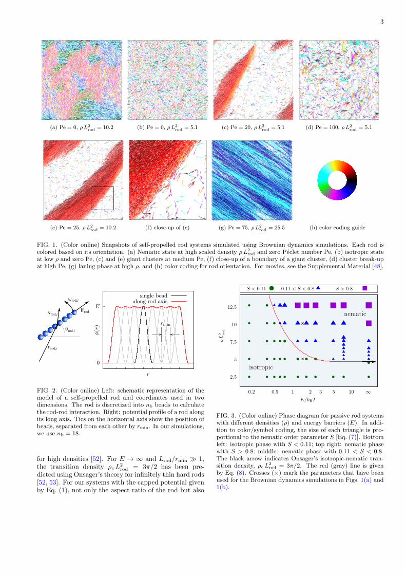
FIG. 1. (Color online) Snapshots of self-propelled rod systems simulated using Brownian dynamics simulations. Each rod iscolored based on its orientation. (a) Nematic state at high scaled density ρL2

rod and zero Peclet number Pe, (b) isotropic stateat low ρ and zero Pe, (c) and (e) giant clusters at medium Pe, (f) close-up of a boundary of a giant cluster, (d) cluster break-upat high Pe, (g) laning phase at high ρ, and (h) color coding for rod orientation. For movies, see the Supplemental Material [48].

vrod,iFrodθrod,i

rrod,i

ωrod,i

0

E

ϕ(r

)

r

single beadalong rod axis

rmin

FIG. 2. (Color online) Left: schematic representation of themodel of a self-propelled rod and coordinates used in twodimensions. The rod is discretized into nb beads to calculatethe rod-rod interaction. Right: potential profile of a rod alongits long axis. Tics on the horizontal axis show the position ofbeads, separated from each other by rmin. In our simulations,we use nb = 18.

for high densities [52]. For E → ∞ and Lrod/rmin � 1,the transition density ρc L

2rod = 3π/2 has been pre-

dicted using Onsager’s theory for infinitely thin hard rods[52, 53]. For our systems with the capped potential givenby Eq. (1), not only the aspect ratio of the rod but also

2.5

5

7.5

10

12.5

0.2 0.5 1 2 3 5 10 ∞

ρL

2 rod

E/kBT

S < 0.11 0.11 < S < 0.8 S > 0.8

isotropic

nematic

FIG. 3. (Color online) Phase diagram for passive rod systemswith different densities (ρ) and energy barriers (E). In addi-tion to color/symbol coding, the size of each triangle is pro-portional to the nematic order parameter S [Eq. (7)]. Bottomleft: isotropic phase with S < 0.11; top right: nematic phasewith S > 0.8; middle: nematic phase with 0.11 < S < 0.8.The black arrow indicates Onsager’s isotropic-nematic tran-sition density, ρc L

2rod = 3π/2. The red (gray) line is given

by Eq. (8). Crosses (×) mark the parameters that have beenused for the Brownian dynamics simulations in Figs. 1(a) and1(b).

4

the energy barrier E affects the density for the isotropic-nematic transition. As E becomes smaller, the tendencyfor rods to align becomes weaker because overlaps occurmore frequently. For E = 0, the rods do not interactmutually and thus are in the isotropic phase for all den-sities.

We performed Brownian dynamics simulations for sys-tems with Pe = 0 at various densities. At low densities,2.5 ≤ ρL2

rod ≤ 5.1, the systems are in an isotropic stateas shown in Fig. 1(b). For high densities, 7.7 ≤ ρL2

rod ≤10.2, nematic states are found that are composed of largeinterlocked groups of rods with similar orientations; seeFig. 1(a). Because the simulation of passive rods withBrownian dynamics is computationally very expensive,we used Monte Carlo simulations to systematically studythe state of the system for several values of ρ and E. Wecharacterize the state using the nematic order parameter[42],

S =

⟨N∑i 6=j

1

N(N − 1)cos[2(θi − θj)]

⟩, (7)

where the average is over cells of side length 4.5Lrod.S = 0 and S = 1 correspond to perfectly isotropic andnematic states, respectively.

Figure 3 shows a phase diagram of the system withvarying density and energy barrier. According to ana-lytical theory [52], for E = ∞ the transition from theisotropic to the nematic state occurs at ρc L

2rod = 3π/2,

as indicated by the black arrow in Fig. 3. This den-sity corresponds to S = 0.11, which we thus define asthreshold value to calculate the transition density for fi-nite values of the energy barrier; see Appendix A. Wehave also calculated the density for the isotropic-nematictransition,

ρc L2rod =

3π

2

1

[1− exp(−E/kBT )], (8)

by generalizing Onsager’s approach for finite energy bar-riers, as described in Appendix A. We find very goodagreement between the analytical theory shown by thered (gray) line in Fig. 3 and our Monte Carlo simulations.The phase diagram is also consistent with our Browniandynamics simulations for Pe = 0 and E = 1.5 kBT ; seesnapshots in Figs. 1(a) and 1(b).

IV. CROSSING PROBABILITY FOR ROD-RODCOLLISIONS

To find the probability of crossing events P (φ), we per-formed simulations for two rods that initially touch eachother in a tip-center arrangement with crossing angle φ;see Fig. 4. We measure P (φ) for several penetrabilitiesand Peclet numbers using Brownian dynamics simula-tions. We count a crossing event when two rods intersectsignificantly, i. e., such that the intersection point is at

0

0.2

0.4

0.6

0.8

1

10 30 50 70 90 110 130 150 170

P(ϕ

)

ϕ

Q Pe E/kBT17 25 1.512 25 2.010 25 2.57 10 1.55 10 2.04 10 2.5

experiment

ϕ

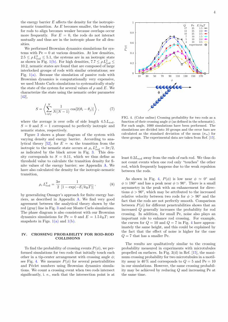
FIG. 4. (Color online) Crossing probability for two rods as afunction of their crossing angle φ (as defined in the schematic).For each angle, 1000 simulations have been performed. Thesimulations are divided into 10 groups and the error bars arecalculated as the standard deviation of the mean (σm) forthese groups. The experimental data are taken from Ref. [15].

least 0.2Lrod away from the ends of each rod. We thus donot count events when one rod only “touches” the otherrod, which frequently happens due to the weak repulsionbetween the rods.

As shown in Fig. 4, P (φ) is low near φ ' 0◦ andφ ' 180◦ and has a peak near φ ' 90◦. There is a smallasymmetry in the peak with an enhancement for direc-tions φ > 90◦, which may be attributed to the increasedrelative velocity between two rods for φ > 90◦ and thefact that the rods are not perfectly smooth. Comparisonbetween P (φ) for different penetrabilities shows that anincreased Q generally increases the probability for rodcrossing. In addition, for small Pe, noise also plays animportant role to enhance rod crossing. For example,the curves for Q = 10 and Q = 7 in Fig. 4 have approx-imately the same height, and this could be explained bythe fact that the effect of noise is higher for the caseQ = 7 that has a smaller Pe.

The results are qualitatively similar to the crossingprobability measured in experiments with microtubulespropelled on surfaces. In Fig. 3(d) in Ref. [15], the maxi-mum crossing probability for two microtubules in a motil-ity assay is 40 % and corresponds to Q = 5 and Pe = 10in our simulations. However, the same crossing probabil-ity may be achieved by reducing Q and increasing Pe atthe same time.

5

ρL

2 rod

Pe

giant cluster

small clusters

lanes

0

5

10

15

20

25

0 25 50 75 100

isotropic

nem

atic

FIG. 5. (Color online) Phase diagram for self-propelled rodswith different densities (ρ) and Peclet numbers (Pe). Theenergy barrier is E = 1.5 kBT ; the gray lines are guides to theeye. Note that the region Pe < 0 has no physical meaning andthat the nematic state is found for passive rods with Pe = 0.

V. CLUSTER FORMATION FOR ACTIVESYSTEMS

To characterize the collective behavior, we have per-formed simulations with large numbers of rods. Afterinitiating the rods with random positions and orienta-tions in the two-dimensional (2D) plane, the rods moveby their propulsion force and are affected by interactionswith other rods and thermal noise. Snapshots of the sys-tem are shown in Fig. 1. More snapshots and moviescan be found in the Supplemental Material [48]. A phasediagram of self-propelled rods with varying density andPeclet number is shown in Fig. 5.

For 1 ≤ Pe . 80, we find giant clusters that spanthe entire simulation box and form as a result of thealignment interaction due to the rod-rod repulsion, asexplained qualitatively in Refs. [36, 54]; see Figs. 1(c)and 1(e). At the cluster perimeter, the clusters steadilylose rods due to the rotational diffusion and at the sametime acquire new rods that collide and align. The clus-ters are polar and almost all rods within a giant clustermove in the same direction. However, we expect that thesystem is essentially in an isotropic phase, and that for asufficiently large system size the clusters can randomlychange direction. The polar order of our giant clus-ters which span the simulation box is due to symmetry-breaking collisions because of the roughness of the rods.In the early stage of the formation of giant clusters, someof the eventually polar clusters are composed of streamsof rods that move in opposite directions.

Upon further increase of Pe the clusters start to break;see Fig. 1(d). Smaller clusters are observed until theybecome as small as about five rods per cluster for Pe &100. For very high densities, 15.1 ≤ ρL2

rod ≤ 25.5, whenthe dense region spans the entire simulation box, we find

P(ρ

)

ρL2rod

Pe = 0, ρi L2rod = 10.2

Pe = 0, ρi L2rod = 5.1

Pe = 20, ρi L2rod = 5.1

Pe = 100, ρi L2rod = 5.1

0 5 10 15 20 25 30

FIG. 6. (Color online) Density distributions for the sys-tems shown in snapshots of Fig. 1. ρi is the average density.The distributions are not normalized and only the position ofpeaks can be compared.

a laning phase that is composed of streams of rods thatmove in opposite directions; see Fig. 1(g). The laningphase is nematic, similar to the nematic lanes that havebeen observed for the Vicsek model in simulations [36]and analytical calculations [55].

Our phase diagram in Fig. 5 may be compared with thephase diagram in Ref. [41] for self-propelled rods that in-teract segment-wise via a Yukawa potential. Since ourmodel incorporates noise and has a capped repulsive in-teraction potential, we can only compare both models inthe medium Pe regime, where the noise does not dom-inate (Pe � 1) and where the rods are not completelypenetrable (Pe . 75). For aspect ratio 18 used in oursimulation, we see qualitatively similar behavior with in-creasing density, namely the transition from the isotropicphase to the swarming (clustering) phase and then to thelaning phase.

A comparison of our phase diagram in Fig. 5 with thatof Ref. [40] shows that we do not observe jammed giantclusters as reported in Ref. [40], because we employ asmoother potential profile along the rod; see Fig. 2.

A. Rod densities

We measure densities of rods in cells of side length2Lrod and construct a distribution of monomer densitiesfor each system; see Fig. 6. For a homogeneous systemof rods, the distribution has a single narrow peak at theaverage density of the system, ρi. This can be seen forexample in the histograms for Pe = 0 that correspond tothe systems where no cluster formation is observed; seeFigs. 1(a) and 1(b). For systems with self-propelled rods,the density distribution can change from a binomial toa more complicated distribution that shows phase sep-aration between dilute and dense regions of rods. ForPe = 20 the distribution has a large peak at low density

6

(a)

0

2

4

6

8

10

0 25 50 75 100

ρgasL

2 rod

Pe

(a)

0.5

1

2

5

5 10 15 20 25

Pe−1

ρL2rod = 10.2

7.75.13.8

theory

(b)

0

2

4

0 25 50 75 100 125 150 175

ρgasL

2 rod

Pe

(b)

E/kBT = 1.01.52.02.53.0

10.0theory

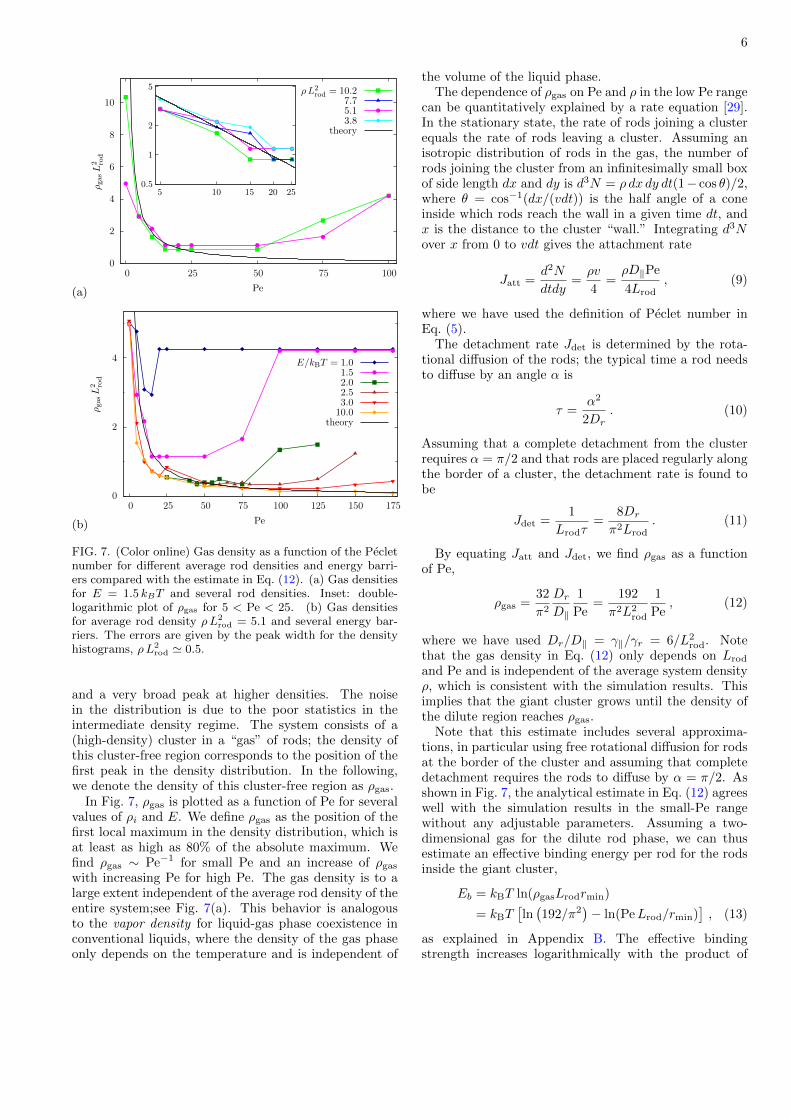
FIG. 7. (Color online) Gas density as a function of the Pecletnumber for different average rod densities and energy barri-ers compared with the estimate in Eq. (12). (a) Gas densitiesfor E = 1.5 kBT and several rod densities. Inset: double-logarithmic plot of ρgas for 5 < Pe < 25. (b) Gas densitiesfor average rod density ρL2

rod = 5.1 and several energy bar-riers. The errors are given by the peak width for the densityhistograms, ρL2

rod ' 0.5.

and a very broad peak at higher densities. The noisein the distribution is due to the poor statistics in theintermediate density regime. The system consists of a(high-density) cluster in a “gas” of rods; the density ofthis cluster-free region corresponds to the position of thefirst peak in the density distribution. In the following,we denote the density of this cluster-free region as ρgas.

In Fig. 7, ρgas is plotted as a function of Pe for severalvalues of ρi and E. We define ρgas as the position of thefirst local maximum in the density distribution, which isat least as high as 80% of the absolute maximum. Wefind ρgas ∼ Pe−1 for small Pe and an increase of ρgaswith increasing Pe for high Pe. The gas density is to alarge extent independent of the average rod density of theentire system;see Fig. 7(a). This behavior is analogousto the vapor density for liquid-gas phase coexistence inconventional liquids, where the density of the gas phaseonly depends on the temperature and is independent of

the volume of the liquid phase.The dependence of ρgas on Pe and ρ in the low Pe range

can be quantitatively explained by a rate equation [29].In the stationary state, the rate of rods joining a clusterequals the rate of rods leaving a cluster. Assuming anisotropic distribution of rods in the gas, the number ofrods joining the cluster from an infinitesimally small boxof side length dx and dy is d3N = ρ dx dy dt(1− cos θ)/2,where θ = cos−1(dx/(vdt)) is the half angle of a coneinside which rods reach the wall in a given time dt, andx is the distance to the cluster “wall.” Integrating d3Nover x from 0 to vdt gives the attachment rate

Jatt =d2N

dtdy=ρv

4=ρD‖Pe

4Lrod, (9)

where we have used the definition of Peclet number inEq. (5).

The detachment rate Jdet is determined by the rota-tional diffusion of the rods; the typical time a rod needsto diffuse by an angle α is

τ =α2

2Dr. (10)

Assuming that a complete detachment from the clusterrequires α = π/2 and that rods are placed regularly alongthe border of a cluster, the detachment rate is found tobe

Jdet =1

Lrodτ=

8Dr

π2Lrod. (11)

By equating Jatt and Jdet, we find ρgas as a functionof Pe,

ρgas =32

π2

Dr

D‖

1

Pe=

192

π2L2rod

1

Pe, (12)

where we have used Dr/D‖ = γ‖/γr = 6/L2rod. Note

that the gas density in Eq. (12) only depends on Lrod

and Pe and is independent of the average system densityρ, which is consistent with the simulation results. Thisimplies that the giant cluster grows until the density ofthe dilute region reaches ρgas.

Note that this estimate includes several approxima-tions, in particular using free rotational diffusion for rodsat the border of the cluster and assuming that completedetachment requires the rods to diffuse by α = π/2. Asshown in Fig. 7, the analytical estimate in Eq. (12) agreeswell with the simulation results in the small-Pe rangewithout any adjustable parameters. Assuming a two-dimensional gas for the dilute rod phase, we can thusestimate an effective binding energy per rod for the rodsinside the giant cluster,

Eb = kBT ln(ρgasLrodrmin)

= kBT[ln(192/π2

)− ln(PeLrod/rmin)

], (13)

as explained in Appendix B. The effective bindingstrength increases logarithmically with the product of

7

0

10

20

30

40

50

1 1.5 2 2.5 3

Q∗

E/kBT

theory

simulation

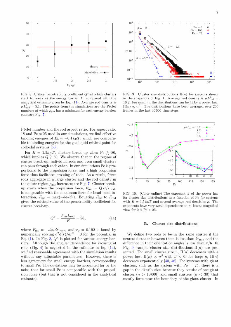
FIG. 8. Critical penetrability coefficient Q∗ at which clustersstart to break vs the energy barrier E, compared with theanalytical estimate given by Eq. (14). Average rod density isρL2

rod = 5.1. The points from the simulations are the Pecletnumbers at which ρgas has a minimum for each energy barrier;compare Fig. 7.

Peclet number and the rod aspect ratio. For aspect ratio18 and Pe ≈ 25 used in our simulations, we find effectivebinding energies of Eb ≈ −0.1 kBT , which are compara-ble to binding energies for the gas-liquid critical point forcolloidal systems [56].

For E = 1.5kBT , clusters break up when Pe & 80,which implies Q & 50. We observe that in the regime ofcluster break-up, individual rods and even small clusterscan pass through each other. In our simulations Pe is pro-portional to the propulsion force, and a high propulsionforce thus facilitates crossing of rods. As a result, fewerrods aggregate in a large cluster and the rod density inthe dilute region ρgas increases; see Fig. 7. Cluster break-up starts when the propulsion force, Frod = QE/Lrod,is comparable with the maximum force for bead-bead in-teraction, Fint = max(−dφ/dr). Equating Fint to Frod

gives the critical value of the penetrability coefficient forcluster break-up,

Q∗ =FintLrod

E= 28 , (14)

where Fint = −dφ/dr|r=r0 and r0 = 0.192 is found bynumerically solving d2φ(r)/dr2 = 0 for the potential inEq. (1). In Fig. 8, Q∗ is plotted for various energy bar-riers. Although the angular dependence for crossing ofrods (Fig. 4) is neglected in the estimate in Eq. (14),we find reasonable agreement with the simulation resultswithout any adjustable parameters. However, there isless agreement for small energy barriers, correspondingto small Pe. The deviations may be accounted for by thenoise that for small Pe is comparable with the propul-sion force (but that is not considered in the analyticalestimate).

10−2

10−1

100

101

102

103

104

100 101 102 103 104

Π

n

β = −2.1

β = −3.7

Pe = 25Pe = 100

Pe = 0

β = −1.6

FIG. 9. Cluster size distributions Π(n) for systems shownin the snapshots of Fig. 1. Average rod density is ρL2

rod =10.2. For small n, the distributions can be fit by a power law,Π(n) ∝ nβ . The distributions have been averaged over 200frames in the last 40 000 time steps.

−4

−3.5

−3

−2.5

−2

−1.5

0 25 50 75 100 125 150 175

β

Pe

−4

−3.5

−3

−2.5

−2

−1.5

0 5 10 15 20 25

ρL2rod = 10.2

7.75.13.8

FIG. 10. (Color online) The exponent β of the power lawfor cluster size distributions as a function of Pe for systemswith E = 1.5 kBT and several average rod densities ρ. Theexponents have very weak dependence on ρ. Inset: magnifiedview for 0 < Pe < 25.

B. Cluster size distributions

We define two rods to be in the same cluster if thenearest distance between them is less than 2rmin and thedifference in their orientation angles is less than π/6. InFig. 9, sample cluster size distributions Π(n) are pre-sented. For small cluster size n, Π(n) decreases with apower law, Π(n) ∝ nβ with β < 0; for large n, Π(n)decreases exponentially [40, 46]. For systems with giantclusters, such as the system with Pe = 25, there is agap in the distribution because they consist of one giantcluster (n > 10 000) and small clusters (n < 30) thatmostly form near the boundary of the giant cluster. In

8

0

5

10

15

20

0 25 50 75 100 125 150 175

0

100

200

300

400

500µ

N

σN

Pe

0

5

10

15

20

0 5 10 15 20 250

100

200

300

400

500

ρ L2rod µN σN

10.2

7.7

5.1

3.8

FIG. 11. (Color online) Cluster size average µN and spreadσN as function of Pe for several average system densities. Thenumber of rods in systems with ρL2

rod = 10.2 is 13107. Inset:magnified view for 0 ≤ Pe ≤ 25. The cluster sizes have beenaveraged over 200 frames in the last 40 000 time steps.

such systems, the exponent β is calculated only based onthe distribution of small clusters.

The power-law exponent for the cluster size distribu-tion first decreases with increasing Peclet number, has aminimum for Pe ∼ 25, and then increases for increasingthe values of Pe, see Fig. 10. We find the exponent tobe in the range −1.5 ≥ β ≥ −3.5, which agrees withthe range −2 ≥ β ≥ −3.6 found in Ref. [40] for rodswith different aspect ratio and a different interaction po-tential than in our simulations. A recent experimentalstudy found β = −1.88± 0.07 for clusters of M. xanthusbacteria [6]. As shown in Fig. 11, the average size of theclusters, µN , increases with increasing Peclet number forPe . 25 and decreases if Pe is further increased. Thespread of the cluster size, σN , shows the same qualita-tive behavior but decays faster at high Pe values, whichshows that the system becomes more homogeneous.

C. Polar autocorrelation functions

The clustering dynamics in the systems can be char-acterized by autocorrelation functions for the rod orien-tation

C(t) = 〈ni(t′) · ni(t′ + t)〉 , (15)

for lag time t, where ni(t′) is the orientation vector of

rod i at time t′, and the average is over all rods and overall times t′. Figure 12(a) shows C(t) for systems shownin Fig. 1. The autocorrelation function C(t) can be fitusing a shifted exponential function

A(t) = (1− a)e−t/τ + a , (16)

where τ is the autocorrelation time and a is an autocor-relation base value. A finite value of a is the ratio of

(a)

0.4

0.5

0.6

0.7

0.8

0.9

1

0 0.5 1 1.5

C(t

)

t/τ0

Pe = 0, ρ L2rod = 10.2

Pe = 25, ρ L2rod = 10.2

Pe = 20, ρ L2rod = 5.1

Pe = 0, ρ L2rod = 5.1

(b)

0

0.1

0.2

0.3

0.4

0.5

0.6

0.7

0.8

0.9

1

0 5 10 15 20 25

a,X

Pe

ρ L2rod a X

10.27.75.13.8

(c)

0

1

2

3

4

0 5 10 15 20 25

τ/τ

0

Pe

ρL2rod = 10.2

7.75.13.8

FIG. 12. (Color online) (a) Autocorrelation of rod orientationwith lag time t for the systems shown in Fig. 1. Thick linesare simulation results; thin horizontal lines are autocorrela-tion base values, calculated by fitting the data with Eq. (16).(b) Comparison of the autocorrelation base value a and thefraction of rods in the largest cluster X. (c) Autocorrelationtime τ of the rod orientation as function of Pe for several av-erage rod densities. τ0 = 1/Dr is the time unit; see Sec. II.The observables have been calculated based on 200 frames inthe last 40 000 time steps.

9

rods that do not lose their orientation for the time scaleof the measurement. Rods that are inside clusters areless likely to lose their orientation, which corresponds toa high value of a, while free rods in the gas change ori-entation more frequently because of rotational diffusion.

In Fig. 12(b), we compare a to the averaged fraction ofrods X that are part of the largest cluster in the systemfor several densities and Peclet numbers. In general, wefind good agreement between a and X [57]. The autocor-relation time τ , shown in Fig. 12(c), does not change sub-stantially for different values of Pe and ρ. The correlationtime τ obtained from the fit with Eq. (16) is very simi-lar to the autocorrelation time τ0 for a single rod, whichshows that the rotational diffusion is only weakly affectedby occasional collisions of the rods. Therefore, the giantcluster moves persistently within simulation time.

VI. SUMMARY AND CONCLUSIONS

We have studied collective behavior for self-propelledrigid rods in two dimensions constructed by single beadsthat interact with a separation-shifted Lennard Jones po-tential. The finite potential strength mimics the ability ofmicroswimmers close to a wall and of filaments in motil-ity assays to temporarily escape to the third dimensionand cross each other. For a high potential barrier, we re-cover the limit of impenetrable rods studied, for example,in Refs. [40, 41]. For most simulations, we have used aninteraction energy E = 1.5 kBT that for complete overlapof two beads is of the order of the thermal energy; cross-ing of rods therefore occurs with a high probability; seeFig. 4. However, the interaction energy is much largerthan the bead-bead interaction energy if rods cross at asmall angle or if a single rod approaches a cluster. Forour system with nb = 18 beads per rod, the energy forcomplete overlap is nbE = 27 kBT and thus the proba-bility for such events is very low.

We have calculated a phase diagram for rod densityand energy barrier to characterize the isotropic-nematictransition for passive rods. The isotropic-nematic tran-sition is shifted to higher densities for reduced overlapenergy, because of the reduced rod-rod interaction. Wefind significant deviations from the transition density cal-culated for hard rods [52, 53] if the bead-bead interactionenergy is below 2 kBT . For E = 1.5 kBT , the isotropic-nematic transition occurs for ρ = 1.3 ρc, where ρc is thetransition density for hard rods [52]. Our results using amodified Onsager theory show excellent agreement withour Monte Carlo simulations.

Using Brownian dynamics simulations, we have deter-mined the crossing probability for two colliding rods asfunction of their relative angles for several values of pen-etrability coefficient and Peclet number. The crossingprobability is highest for almost perpendicular collisions,which is qualitatively similar to the crossing probabilitymeasured in experiments with microtubules propelled onsurfaces. In Ref. [15], the maximum crossing probabil-

ity for two microtubules in a motility assay is 40 % andcorresponds to Q = 5 and Pe = 10 in our simulations[58].

Self-propelled rods align due to their soft repulsive in-teraction [54]. For high rod densities, we find a laningphase. For intermediate rod densities and Peclet num-bers, we observe the formation of giant clusters that spanthe entire simulation box, which we denote as “clusteringwindow.” Clusters break if the propulsion force is strongenough to overcome the repulsive force due to rod-rodinteraction. We find a critical value Q∗ = 28 for clusterbreak-up. We characterize our systems by cluster sizedistributions that can be fit by power-laws Π(n) ∝ nβ

with −1.5 ≥ β ≥ −3.5, which is consistent with previousexperimental and simulation results [6, 40]. By analyzingthe autocorrelation function for rod orientation, we canseparate the contributions from rods in a cluster from thecontributions from free rods. We find that the free rodsshow almost the same orientational correlation as singlerods.

We can analytically estimate the density of free rodsin systems with giant clusters, which we denote as “gasdensity,” ρgas = 192/(π2L2

rodPe). The gas density is inde-pendent of the average rod density in the system, whichis analogous to the molecule density in the gas phase forliquid-gas coexistence that does not depend on the vol-ume of the liquid phase but only on temperature. UsingEb = kBT ln[192rmin/(π

2LrodPe)], we calculate effectivebinding energies for rods in the cluster. For aspect ratio18 used in our simulations and Pe ≈ 25, we find effectivebinding energies of about 0.1 kBT , which is comparableto binding energies for the gas-liquid critical point forcolloidal systems [56].

Phase separation into high-density and low-density re-gions is an intrinsic property of self-propelled particle sys-tems and has also been observed for nonaligning sphericalparticles [29, 59–61]. As for the rods, the gas density ofthe spheres is inversely proportional to the propulsionvelocity [29]. However, the nature of cluster formation isdifferent in the two models: While we observe motile clus-ters as a result of particle alignment, systems with non-aligning spheres exhibit jammed nonmotile clusters as aresult of steric trapping. Moreover, the internal struc-ture of clusters is nematic in our model, contrary to theisotropic structure for nonaligning spheres. Of course,also laning phases are only possible for anisotropic par-ticles.

We have introduced and characterized a model of self-propelled rods that interact with a physical interactionthat allows for crossing events. The model can now beused to interpret experiments for almost two-dimensionalsystems with good computational efficiency and allowspredictions beyond those based on models using pointparticles with phenomenological alignment rules.

10

ACKNOWLEDGMENTS

We thank Adam Wysocki and Jens Elgeti for stimu-lating discussions. M.A. and K.M. acknowledge supportby the International Helmholtz Research School of Bio-physics and Soft Matter (IHRS BioSoft). CPU time al-lowance from the Julich Supercomputing Centre (JSC) isgratefully acknowledged.

Appendix A: Phase transition of passive rods

The nematic order parameter is plotted in Fig. 13 forvarious cuts through the phase diagram in Fig. 3. Ithas been suggested that the isotropic-nematic transitionof rods is continuous in two dimensions [52]. We havechosen a threshold value for the isotropic-nematic phasetransition, St = 0.11, such that for an infinite interactionenergy the value predicted by the Onsager theory is re-covered. Our threshold value is similar to the thresholdvalue S = 0.2 that has been chosen in Ref. [42].

(a)

0

0.2

0.4

0.6

0.8

1

4 6 8 10 12

S

ρ L2rod

E/kBT = ∞7.5

1.250.630.19

(b)

0

0.2

0.4

0.6

0.8

1

0 0.5 1 1.5 2 2.5

S

E/kBT

ρL2rod = 12.7

10.27.75.12.6

FIG. 13. (Color online) Nematic order parameter S, used todetermine the phase transition for passive rods, as a functionof (a) the rod density ρ for several energy barriers E and (b)the energy barrier E for several rod densities ρ.

For finite energy barrier E, we generalize the approachpresented in Ref. [52] based on bifurcation theory to ob-tain the critical density for the isotropic-nematic transi-tion. The distribution function for the rod orientation isgiven by f(θ), which satisfies

ln[2πf(θ)] = C + λ

∫ 2π

θ=0

F (θ, θ′)f(θ′)dθ′ , (A1)

where the constant C is determined by the normalizationof f(θ), ∫ 2π

θ=0

f(θ)dθ = 1 . (A2)

We define h(θ) as

h(θ) = 2πf(θ)− 1 , (A3)

such that h(θ) = 0 corresponds to an isotropic distribu-tion. Using Eqs. (A1)–(A3), we can write

h(θ) = −1 +exp(λ

∫F (θ, θ′)h(θ′)dθ′/2π)

(1/2π)∫

exp(λ∫F (θ, θ′)h(θ′)dθ′/2π)dθ

.

(A4)We assume that the interaction energy of two rods is ei-

ther 0 or E, depending on whether they cross each other.This approximation is justified if the rods are very thinand the complete overlap of two rods—which is energeti-cally very unfavorable—is excluded. In the regime whereLrod � rmin, the parameter λ and the kernel F are givenby

λ =1

4ρπL2

rod , (A5)

(1/2π)F (θ, θ′) = (−2/π2) sin(θ) (A6)

×[1− exp(−E/kBT )] .

Substituting Eqs. (A5) and (A6) in Eq. (A4) gives

h(θ) = −1 +exp[−ρKh(θ)]

(1/π)∫ π0

exp[−ρKh(θ)]dθ, (A7)

where the operator K is defined as

Kh(θ) = (L2rod/π)[1− exp(−E/kBT )] (A8)

×∫ π

0

sin(θ′)h(θ − θ′)dθ′ .

For h(θ) to have bifurcation point in ρ,

w(θ) = −ρKw(θ) (A9)

has to have an eigenfunction with two maxima at w(0) =w(π) and no further maxima. The corresponding eigen-value determines the density at which bifurcation occurs.The desired eigenfunction is cos 2θ with the eigenvalue−3/2; thus the bifurcation density that corresponds tothe isotropic-nematic transition is

ρc =3π

2L2rod

1

[1− exp(−E/kBT )]. (A10)

11

Appendix B: Effective binding energy for rodadsorption to the cluster

The independence of gas density ρgas from the averagedensity of the system ρ is analogous to a vapor densityfor rods. Here we follow this analogy to obtain an effec-tive binding energy gain Eb for rods that are part of thecluster.

We use an ideal-gas model in two dimensions to rep-resent the rods in the gas phase. The activity and theanisotropy of the rods are intentionally not taken intoaccount explicitly and enter via the effective binding en-

ergy. The free energy for the rods in the gas is thus

Fgas = NkBT ln

(N∆

A

)(B1)

= NkBT ln (ρgasLrodrmin) ,

where N is the number of rods in the gas, ∆ is the areaof each rod, and A is the area accessible for the rods inthe gas.

In the cluster, each rod gains a binding energy Eb,

Fcluster = NEb , (B2)

where N here is the number of rods in the cluster.In equilibrium, the chemical potential µ = ∂F/∂N inthe gas and in the cluster should be equal. This givesEq. (13).

[1] T. Vicsek and A. Zafeiris, Phys. Rep. 517, 71 (2012).[2] I. H. Riedel, K. Kruse, and J. Howard, Sci. Signal. 309,

300 (2005).[3] Y. Yang, J. Elgeti, and G. Gompper, Phys. Rev. E 78,

061903 (2008).[4] E. Ben-Jacob, I. Cohen, and H. Levine, Adv. Phys. 49,

395 (2000).[5] A. Sokolov, I. S. Aranson, J. O. Kessler, and R. E. Gold-

stein, Phys. Rev. Lett. 98, 158102 (2007).[6] F. Peruani, J. Starruß, V. Jakovljevic, L. Søgaard-

Andersen, A. Deutsch, and M. Bar, Phys. Rev. Lett.108, 098102 (2012).

[7] J. Gachelin, G. Mino, H. Berthet, A. Lindner, A. Rous-selet, and E. Clement, Phys. Rev. Lett. 110, 268103(2013).

[8] W. F. Paxton, K. C. Kistler, C. C. Olmeda, A. Sen, S. K.St. Angelo, Y. Cao, T. E. Mallouk, P. E. Lammert, andV. H. Crespi, J. Am. Chem. Soc. 126, 13424 (2004).

[9] G. Volpe, I. Buttinoni, D. Vogt, H.-J. Kummerer, andC. Bechinger, Soft Matter 7, 8810 (2011).

[10] Y. Mei, A. A. Solovev, S. Sanchez, and O. G. Schmidt,Chem. Soc. Rev. 40, 2109 (2011).

[11] S. Ebbens, M.-H. Tu, J. R. Howse, and R. Golestanian,Phys. Rev. E 85, 020401 (2012).

[12] M. Yang and M. Ripoll, Phys. Rev. E 84, 061401 (2011).[13] Y. Harada, A. Noguchi, A. Kishino, and T. Yanagida,

Nature (London) 326, 805 (1987).[14] V. Schaller, C. Weber, C. Semmrich, E. Frey, and A. R.

Bausch, Nature (London) 467, 73 (2010).[15] Y. Sumino, K. H. Nagai, Y. Shitaka, D. Tanaka,

K. Yoshikawa, H. Chate, and K. Oiwa, Nature (Lon-don) 483, 448 (2012).

[16] E. Lauga, W. R. DiLuzio, G. M. Whitesides, and H. A.Stone, Biophys. J. 90, 400 (2006).

[17] A. P. Berke, L. Turner, H. C. Berg, and E. Lauga, Phys.Rev. Lett. 101, 038102 (2008).

[18] J. Elgeti and G. Gompper, EPL 85, 38002 (2009).[19] J. Elgeti, U. B. Kaupp, and G. Gompper, Biophys. J.

99, 1018 (2010).[20] J. Elgeti and G. Gompper, EPL 101, 48003 (2013).[21] T. Vicsek, A. Czirok, E. Ben-Jacob, I. Cohen, and

O. Shochet, Phys. Rev. Lett. 75, 1226 (1995).

[22] J. Toner and Y. Tu, Phys. Rev. Lett. 75, 4326 (1995).[23] R. A. Simha and S. Ramaswamy, Phys. Rev. Lett. 89,

058101 (2002).[24] S. Ramaswamy, R. A. Simha, and J. Toner, Europhys.

Lett. 62, 196 (2003).[25] J. Toner, Y. Tu, and S. Ramaswamy, Ann. Phys. 318,

170 (2005).[26] F. Peruani, A. Deutsch, and M. Bar, Eur. Phys. J. Spe-

cial Topics 157, 111 (2008).[27] E. Bertin, M. Droz, and G. Gregoire, J. Phys. A: Math.

Theor. 42, 445001 (2009).[28] R. Golestanian, Phys. Rev. Lett. 102, 188305 (2009).[29] G. S. Redner, M. F. Hagan, and A. Baskaran, Phys. Rev.

Lett. 110, 055701 (2013).[30] B. Szabo, G. J. Szollosi, B. Gonci, Z. Juranyi,

D. Selmeczi, and T. Vicsek, Phys. Rev. E 74, 061908(2006).

[31] G. Gregoire and H. Chate, Phys. Rev. Lett. 92, 025702(2004).

[32] C. Huepe and M. Aldana, Phys. Rev. Lett. 92, 168701(2004).

[33] M. R. D’Orsogna, Y. L. Chuang, A. L. Bertozzi, andL. S. Chayes, Phys. Rev. Lett. 96, 104302 (2006).

[34] M. Aldana, V. Dossetti, C. Huepe, V. M. Kenkre, andH. Larralde, Phys. Rev. Lett. 98, 095702 (2007).

[35] H. Chate, F. Ginelli, G. Gregoire, and F. Raynaud, Phys.Rev. E 77, 046113 (2008).

[36] F. Ginelli, F. Peruani, M. Bar, and H. Chate, Phys. Rev.Lett. 104, 184502 (2010).

[37] A. Baskaran and M. C. Marchetti, Phys. Rev. E 77,011920 (2008).

[38] S. R. McCandlish, A. Baskaran, and M. F. Hagan, SoftMatter 8, 2527 (2012).

[39] A. Baskaran and M. C. Marchetti, Phys. Rev. Lett. 101,268101 (2008).

[40] Y. Yang, V. Marceau, and G. Gompper, Phys. Rev. E82, 031904 (2010).

[41] H. H. Wensink, J. Dunkel, S. Heidenreich, K. Drescher,R. E. Goldstein, H. Lowen, and J. M. Yeomans, Proc.Natl. Acad. Sci. U.S.A. 109, 14308 (2012).

[42] P. Kraikivski, R. Lipowsky, and J. Kierfeld, Phys. Rev.Lett. 96, 258103 (2006).

12

[43] A. Costanzo, R. Di Leonardo, G. Ruocco, and L. Ange-lani, J. Phys. Condens. Matter 24, 065101 (2012).

[44] F. Peruani, A. Deutsch, and M. Bar, Phys. Rev. E 74,030904 (2006).

[45] F. Peruani, L. Schimansky-Geier, and M. Bar, Eur.Phys. J. Special Topics 191, 173 (2010).

[46] C. Huepe and M. Aldana, Phys. A (Amsterdam, Neth.)387, 2809 (2008).

[47] F. Ruhnow, D. Zwicker, and S. Diez, Biophys. J. 100,2820 (2011).

[48] See Supplemental Material at [URL] for movies of self-propelled rod systems.

[49] M. E. Fisher and D. Ruelle, J. Math. Phys. 7, 260 (1966).[50] In biological and synthetic self-propelled systems, the

noise arises from the environmental noise, for exam-ple, from density fluctuations of signaling molecules forchemotactic swimmers or from motor activity. In thiscase, the noise is not proportional to kBT and also thecoupling between translational and rotational noise maybe different.

[51] The Peclet number can be alternatively defined as Per =v0/DrLrod with the rotational diffusion constant Dr. Insuch case, Pe = 6 Per.

[52] R. F. Kayser and H. J. Raveche, Phys. Rev. A 17, 2067

(1978).[53] L. Onsager, Phys. Rev. 65, 117 (1944).[54] A. Baskaran and M. C. Marchetti, Eur. Phys. J. E 35, 1

(2012).[55] A. Peshkov, I. S. Aranson, E. Bertin, H. Chate, and

F. Ginelli, Phys. Rev. Lett. 109, 268701 (2012).[56] G. Vliegenthart and H. N. Lekkerkerker, J. Chem. Phys.

112, 5364 (2000).[57] The values of a andX do not agree for Pe = 0, where rods

are either freely moving due to noise (isotropic regime) orstuck in small nonmotile clusters (nematic regime). In theformer case, there is hardly any orientation preservation(a � 1) and there is no large cluster (X � 1). In thelatter case, rods hardly change their orientation (a ∼ 1)but are distributed over small clusters (X � 1).

[58] The same crossing probability may be achieved by in-creasing E and Pe at the same time.

[59] J. Tailleur and M. E. Cates, Phys. Rev. Lett. 100, 218103(2008).

[60] Y. Fily and M. C. Marchetti, Phys. Rev. Lett. 108,235702 (2012).

[61] A. Wysocki, R. G. Winkler, and G. Gompper,arXiv:1308.6423 [cond-mat.soft].