Wavefront-division lateral shearing autocorrelator for ultrafast laser microscopy
Upload
khangminh22Category
view
4download
0
Field-resolved studies of ultrafastlight-matter interaction
Johannes Schotz
Munchen 2021


Field-resolved studies of ultrafastlight-matter interaction
Johannes Schotz
Dissertation
an der Fakultat fur Physik
der Ludwig–Maximilians–Universitat
Munchen
vorgelegt von
Johannes Schotz
aus Hof
Munchen, den 15.06.2021

Erstgutachter: Prof. Dr. Matthias Kling
Zweitgutachter: Prof. Dr. Emiliano Cortes
Tag der mundlichen Prufung: 27.09.2021

Contents
Zusammenfassung xv
1 Introduction 1
2 Theoretical foundations 92.1 Few-cycle pulses and dispersion . . . . . . . . . . . . . . . . . . . . . . . . 92.2 Strong-field photoemission . . . . . . . . . . . . . . . . . . . . . . . . . . . 11
2.2.1 Emission regimes . . . . . . . . . . . . . . . . . . . . . . . . . . . . 112.2.2 Simpleman’s model . . . . . . . . . . . . . . . . . . . . . . . . . . . 142.2.3 Strong-field photoemission spectra . . . . . . . . . . . . . . . . . . . 17
2.3 High-harmonic generation . . . . . . . . . . . . . . . . . . . . . . . . . . . 192.3.1 Phase matching of HHG . . . . . . . . . . . . . . . . . . . . . . . . 212.3.2 Phase-matching cutoff and critical ionization fraction . . . . . . . . 232.3.3 Gating techniques for isolated attosecond pulse generation . . . . . 27
2.4 Field enhancement and confinement on nanotips . . . . . . . . . . . . . . . 29
3 Experimental foundations 333.1 Nanotip etching . . . . . . . . . . . . . . . . . . . . . . . . . . . . . . . . . 333.2 Current measurements . . . . . . . . . . . . . . . . . . . . . . . . . . . . . 34
3.2.1 Transimpedance amplification . . . . . . . . . . . . . . . . . . . . . 343.2.2 Lock-in detection . . . . . . . . . . . . . . . . . . . . . . . . . . . . 35
3.3 Field-resolved measurement techniques . . . . . . . . . . . . . . . . . . . . 373.3.1 Attosecond streaking . . . . . . . . . . . . . . . . . . . . . . . . . . 373.3.2 Electro-Optic Sampling . . . . . . . . . . . . . . . . . . . . . . . . . 413.3.3 Tunneling ionization with a perturbation for the time-domain obser-
vation of an electric field (TIPTOE) . . . . . . . . . . . . . . . . . 433.3.4 Streaking of rescattering electrons . . . . . . . . . . . . . . . . . . . 453.3.5 Nonlinear photoconductive sampling . . . . . . . . . . . . . . . . . 47
4 The emergence of macroscopic optical-field-controlled currents in gases 494.1 Classification of plasma regimes . . . . . . . . . . . . . . . . . . . . . . . . 514.2 Experimental setup and approach . . . . . . . . . . . . . . . . . . . . . . . 524.3 Theoretical model and simulations . . . . . . . . . . . . . . . . . . . . . . 55

vi CONTENTS
4.4 Experimental results . . . . . . . . . . . . . . . . . . . . . . . . . . . . . . 614.5 Discussion . . . . . . . . . . . . . . . . . . . . . . . . . . . . . . . . . . . . 644.6 Conclusion . . . . . . . . . . . . . . . . . . . . . . . . . . . . . . . . . . . . 68
5 Transient field-resolved reflectometry from solid-state surfaces 715.1 Experimental foundations . . . . . . . . . . . . . . . . . . . . . . . . . . . 735.2 Theoretical background . . . . . . . . . . . . . . . . . . . . . . . . . . . . . 775.3 Experimental results . . . . . . . . . . . . . . . . . . . . . . . . . . . . . . 84
5.3.1 Surface recombination dynamics in GaAs . . . . . . . . . . . . . . . 845.3.2 Buildup of collective excitations in GaAs . . . . . . . . . . . . . . . 865.3.3 Intervalley scattering in Ge . . . . . . . . . . . . . . . . . . . . . . 885.3.4 Excitation-density dependence of the Drude scattering rate . . . . . 91
5.4 Conclusion and Outlook . . . . . . . . . . . . . . . . . . . . . . . . . . . . 94
6 Phase matching of HHG with ionization reshaped few-cycle pulses 976.1 Introduction . . . . . . . . . . . . . . . . . . . . . . . . . . . . . . . . . . . 976.2 Experimental section . . . . . . . . . . . . . . . . . . . . . . . . . . . . . . 99
6.2.1 Experimental setup . . . . . . . . . . . . . . . . . . . . . . . . . . . 996.2.2 Experimental approach . . . . . . . . . . . . . . . . . . . . . . . . . 1016.2.3 Experimental results . . . . . . . . . . . . . . . . . . . . . . . . . . 103
6.3 Theoretical modeling and analysis . . . . . . . . . . . . . . . . . . . . . . . 1046.4 Discussion of the results . . . . . . . . . . . . . . . . . . . . . . . . . . . . 106
6.4.1 Effects of the overdriven regime on HHG . . . . . . . . . . . . . . . 1066.4.2 Phase matching in the overdriven regime . . . . . . . . . . . . . . . 1106.4.3 Pressure and intensity variation . . . . . . . . . . . . . . . . . . . . 114
6.5 Phase matching in the overdriven regime with long wavelength driving pulses1156.6 Conclusion . . . . . . . . . . . . . . . . . . . . . . . . . . . . . . . . . . . . 122
7 Attosecond physics on metallic nanotips 1257.1 Introduction . . . . . . . . . . . . . . . . . . . . . . . . . . . . . . . . . . . 1257.2 Attosecond streaking from a metal nanotip . . . . . . . . . . . . . . . . . . 128
7.2.1 Experimental setup and approach . . . . . . . . . . . . . . . . . . . 1287.2.2 Theoretical approach . . . . . . . . . . . . . . . . . . . . . . . . . . 1297.2.3 Experimental results . . . . . . . . . . . . . . . . . . . . . . . . . . 1357.2.4 Discussion . . . . . . . . . . . . . . . . . . . . . . . . . . . . . . . . 1377.2.5 Conclusion and Outlook . . . . . . . . . . . . . . . . . . . . . . . . 140
7.3 Attosecond field-resolved measurements using photocurrents . . . . . . . . 1427.3.1 Experimental setup . . . . . . . . . . . . . . . . . . . . . . . . . . . 1427.3.2 Experimental approach . . . . . . . . . . . . . . . . . . . . . . . . . 1447.3.3 Onset of space-charge effects . . . . . . . . . . . . . . . . . . . . . . 1457.3.4 Characterization of near fields at the apex of a nanotip . . . . . . . 1527.3.5 Field and spatially resolved measurements of an OAM beam . . . . 162
7.4 Discussion . . . . . . . . . . . . . . . . . . . . . . . . . . . . . . . . . . . . 164

Table of Contents vii
7.5 Conclusion and Outlook . . . . . . . . . . . . . . . . . . . . . . . . . . . . 167
A Dual-frequency demodulation 169

viii Table of Contents

List of Figures
1.1 Attosecond field-resolved measurement techniques . . . . . . . . . . . . . . 3
2.1 Carrier-envelope phase . . . . . . . . . . . . . . . . . . . . . . . . . . . . . 102.2 Strong-field photoemission . . . . . . . . . . . . . . . . . . . . . . . . . . . 132.3 Simpleman’s model . . . . . . . . . . . . . . . . . . . . . . . . . . . . . . . 142.4 Above-threshold ionization photoemission spectrum . . . . . . . . . . . . . 172.5 Rescattering trajectories and high-harmonic generation . . . . . . . . . . . 192.6 Phase matching of HHG . . . . . . . . . . . . . . . . . . . . . . . . . . . . 222.7 Phase-matching cutoff of HHG . . . . . . . . . . . . . . . . . . . . . . . . . 242.8 HHG dipole phase . . . . . . . . . . . . . . . . . . . . . . . . . . . . . . . 252.9 HHG gating mechanisms for isolated attosecond pulse generation . . . . . 282.10 Field enhancement on a nanotip . . . . . . . . . . . . . . . . . . . . . . . . 29
3.1 Nanotip etching process . . . . . . . . . . . . . . . . . . . . . . . . . . . . 333.2 Microscope image of a nanotip . . . . . . . . . . . . . . . . . . . . . . . . . 343.3 Transimpedance amplifier . . . . . . . . . . . . . . . . . . . . . . . . . . . 343.4 Attosecond streaking scheme . . . . . . . . . . . . . . . . . . . . . . . . . . 363.5 Attosecond streaking scheme . . . . . . . . . . . . . . . . . . . . . . . . . . 383.6 Streaking spectrogram of chirped XUV pulses . . . . . . . . . . . . . . . . 393.7 Electro-optic sampling . . . . . . . . . . . . . . . . . . . . . . . . . . . . . 423.8 CEP-dependence of the current response function . . . . . . . . . . . . . . 443.9 Response function of the scattering cutoff variation . . . . . . . . . . . . . 463.10 CEP-dependence of the current response fucntion . . . . . . . . . . . . . . 47
4.1 Classification of plasmas . . . . . . . . . . . . . . . . . . . . . . . . . . . . 514.2 Experimental setup and signal . . . . . . . . . . . . . . . . . . . . . . . . . 534.3 Images of the electrodes . . . . . . . . . . . . . . . . . . . . . . . . . . . . 544.4 Homogeneous and inhomogeneous solution of the Poisson equation . . . . . 554.5 Signal induction and Ramo-Shockley weighting potentials . . . . . . . . . . 564.6 Scattering and Coulomb-interaction . . . . . . . . . . . . . . . . . . . . . . 584.7 Microscopic origin of the signal in the simpleman’s model . . . . . . . . . . 604.8 Pressure dependence . . . . . . . . . . . . . . . . . . . . . . . . . . . . . . 614.9 Electrode-distance dependence . . . . . . . . . . . . . . . . . . . . . . . . . 62

x LIST OF FIGURES
4.10 Intensity dependence and signal trace reshaping . . . . . . . . . . . . . . . 634.11 Role of scattering and Coulomb-interaction . . . . . . . . . . . . . . . . . . 65
5.1 Laser setup and pulse characterization . . . . . . . . . . . . . . . . . . . . 735.2 Experimental scheme and setup . . . . . . . . . . . . . . . . . . . . . . . . 745.3 Experimental pump-probe signal . . . . . . . . . . . . . . . . . . . . . . . 765.4 Bandstructure of GaAs and Ge . . . . . . . . . . . . . . . . . . . . . . . . 785.5 Photoexcitation processes and timescales . . . . . . . . . . . . . . . . . . . 795.6 Effect of an inhomogeneous excitation profile on the reflected field . . . . . 825.7 Influence of surface recombination in GaAs . . . . . . . . . . . . . . . . . . 845.8 Femtosecond reflectivity buildup on GaAs . . . . . . . . . . . . . . . . . . 875.9 Intervalley scattering in Germanium . . . . . . . . . . . . . . . . . . . . . . 895.10 Scattering rates in Germanium . . . . . . . . . . . . . . . . . . . . . . . . 925.11 Transient reflectivity change from a graphene sample . . . . . . . . . . . . 94
6.1 Experimental setup . . . . . . . . . . . . . . . . . . . . . . . . . . . . . . . 1006.2 Experimental attosecond streaking spectrograms in argon and neon . . . . 1026.3 Reconstructed streaking spectrograms and retrieved attosecond pulses . . . 1056.4 Spatio-temporal pulse reshaping . . . . . . . . . . . . . . . . . . . . . . . . 1076.5 Experimental signatures of pulse reshaping . . . . . . . . . . . . . . . . . . 1076.6 Simulation of the XUV generation in argon and driving laser pulse evolution 1086.7 Transient phase matching and XUV buildup . . . . . . . . . . . . . . . . . 1116.8 CEP-dependence of isolated attosecond pulse generation in argon . . . . . 1136.9 Intensity dependence . . . . . . . . . . . . . . . . . . . . . . . . . . . . . . 1146.10 Pressure-dependence of the HHG process . . . . . . . . . . . . . . . . . . . 1156.11 Pulse-reshaping in the overdriven regime . . . . . . . . . . . . . . . . . . . 1166.12 Pressure-scaling of the HHG yield and phase-matching contributions . . . . 1176.13 CEP-dependence and isolated pulse generation in helium . . . . . . . . . . 1196.14 Spatio-temporal phase-matching map . . . . . . . . . . . . . . . . . . . . . 1216.15 Pulsefront and -profile reshaping in the overdriven regime . . . . . . . . . . 121
7.1 Experimental setup and approach for attosecond streaking experiments froma nanotaper . . . . . . . . . . . . . . . . . . . . . . . . . . . . . . . . . . . 130
7.2 Attosecond streaking response function and surface field sensitivity in inho-mogeneous fields . . . . . . . . . . . . . . . . . . . . . . . . . . . . . . . . 133
7.3 Attosecond streaking spectrograms from a nanotaper and reference gas . . 1367.4 Reconstructed response function of the nanotaper . . . . . . . . . . . . . . 1397.5 Experimental setup and approach for current detection from a nanotip . . 1447.6 Energy-resolved electron spectra and charge interaction effects . . . . . . . 1467.7 Charge-interaction effects on the photoelectron spectral cutoff . . . . . . . 1487.8 Energy resolved CEP-asymmetry . . . . . . . . . . . . . . . . . . . . . . . 1497.9 Experimental signal and polarization dependence . . . . . . . . . . . . . . 1527.10 Driving pulse characterization and optimization . . . . . . . . . . . . . . . 153

List of Figures xi
7.11 CEP-dependence of the response function . . . . . . . . . . . . . . . . . . . 1557.12 Intensity dependence of pump and driving signal . . . . . . . . . . . . . . . 1577.13 Energy-resolved pump-probe spectra . . . . . . . . . . . . . . . . . . . . . 1607.14 Signal trace from an OAM driving beam . . . . . . . . . . . . . . . . . . . 1627.15 Spatially resolved measurement of an OAM beam . . . . . . . . . . . . . . 1647.16 Spatio-temporally/-spectrally resolved measurement of an OAM beam . . . 165
A.1 Dual-frequency demodulation . . . . . . . . . . . . . . . . . . . . . . . . . 169

xii List of Figures

List of Tables
5.1 Effective masses for Ge and GaAs . . . . . . . . . . . . . . . . . . . . . . . 78

xiv List of Tables

Abstract
The fastest light-matter interactions between electrons and optical laser pulses occur onattosecond timescales below the half-cycle oscillation period of the electric field. The inves-tigation of such ultrafast processes and ultimately their control, therefore, requires field-resolved measurements. In this work, the understanding of well-established and newlyemerging sub-cycle-resolved techniques for the characterization of optical pulses and ultra-fast light-induced processes is expanded and the application of the methods includes gases,bulk solids, and nanostructures.
In the first part, the mechanism behind the macroscopic current generation in opticalfield-induced photocurrent measurements in gases is studied theoretically and experimen-tally. A rigorous model is developed that connects the measured current to the micro-scopic movement of charge carriers and includes scattering with atoms and the interactionof charges via the Coulomb force. The model is validated against an extensive set of ex-periments which measure the carrier-envelope-phase dependent strong-field photoemittedcurrent induced on a pair of electrodes surrounding the focus of a few-cycle laser pulse.The role of the mean-free path as well as the Coulomb interaction is identified. The modelprovides a fundamental understanding of the signal generation mechanism in photocon-ductive sampling of laser pulses which had been missing before and which will allow toidentify fundamental limitations and strategies for further optimization of the detection.
The second set of experiments aims at the transient change of the reflectivity afterexcitation with a near-infrared pump pulse. Electro-optic sampling is used for the field-resolved characterization of the mid-infrared probe pulses which covers a wavelength rangefrom below 3µm to above 6µm. Measurements on semiconductors are performed anddynamics occuring on the femtosecond to the picosecond timescale after photoexcitationare studied. The demonstrated experiments represent an important milestone in pushingfield-sampling methods from the THz into the PHz domain.
The investigation of the generation of isolated attosecond pulses in the extreme ultra-violet photon energy range using high-harmonic generation (HHG) in noble gases is thetopic of the third section. The focus is put on the overdriven regime, where the driving laserundergoes severe reshaping due to plasma effects. Experimentally, attosecond streaking isused to demonstrate isolated attosecond pulses for the first time in this regime. Theoret-ically, the phasematching mechanism in this regime is studied using extensive numericalsimulations. An extension of conventional phasematching expressions is introduced whichdescribes the contribution of the HHG dipole phase due to the blue-shift of the driving

xvi Summary
laser. The results are important for a complete understanding of HHG phasematching andmight help to find routes towards more efficient HHG in the water window.
Finally, attosecond measurements on metal nanotips are presented. The attosecondfield-resolved characterization of the nanoscale near-fields on a nanotip and the responsefunction using attosecond streaking is demonstrated. Moreover, another field-reconstructionmethod based on the modulation of the strong-field photocurrent is used for the measure-ment of the enhanced near-fields at the nanotip apex and different aspects of the methodsare studied. Combining the latter approach with the concept of the nanotip as nanoscalelocalized field sensor, the attosecond characterization of an orbital angular momentumbeam in free-space below the diffraction limit is demonstrated. These results pave the waytowards nanoscale attosecond field-resolved measurements on generic nanostructures.

Zusammenfassung
Die schnellsten Prozesse der fundamentalen Licht-Materie-Wechselwirkung zwischen Elek-tronen und sichtbaren Laserpulsen finden auf der Attosekunden-Zeitskala statt, unterhalbder halben Schwingungsperiode des elektrischen Feldes. Feldaufgeloste Messungen derbeteiligten Laserpulse sind daher fur die Untersuchung solch schneller Prozesse und ihrerKontrolle unabdingbar. In der vorliegenden Arbeit wird das fundamentale Verstandnis vonetablierten als auch neu aufkommenden subzyklen-aufgelosten Messtechniken erweitert mitAnwendungen in Gasen, Festkorpern und Nanostrukturen.
Im ersten Teil wird der Mechanismus hinter der Erzeugung makroskopischer Stromein den Messungen feld-induzierter Photostrome experimentell und theoretisch untersucht.Die Entwicklung eines rigorosen Models wird prasentiert, das die gemessenen Strome mitder mikroskopischen Bewegung der Ladungstrager verknupft. Es beinhaltet außerdem dieStreuung an Atomen und die Coulomb-Wechselwirkung. Das Model wird in einer Reihevon umfassenden Experimenten bestatigt, in denen die Abhangigkeit der Strome von derPhase der Tragerwelle zur Einhullenden des Laserpulses gemessen werden. Zur Messungder Strome wird ein Elektrodenpaar, das den Fokus eines intensiven Wenigzyklen-Pulsesin verschiedenen Gasen umgibt, verwendet. Der Einfluss der mittleren freien Weglangeund der Ladungs-Wechselwirkung wird aufgeklart. Das Model liefert ein fundamentalesVerstandnis der Signalerzeugung in der auf Photoleitung beruhenden Messung von Laser-pulsen. Dies erlaubt die Identifizierung der fundamentalen Grenzen und eroffnet Wege zurOptimierung der Messmethode.
Die zweite Reihe von Experimenten hat die Messung der transienten Anderung der Re-flektivitat nach der Anregung durch einen Pumppuls in nahen Infrarotbereich zum Gegen-stand. Elektro-optisches Sampling wird verwendet fur die feldaufgeloste Charakterisierungder Probepulse im mittleren Infrarotbereich, von unter drei bis uber sechs MikrometernWellenlange. Messungen an Halbleitern werden durchgefuhrt und die Dynamik, die auf derZeitskala von Femtosekunden bis Pikosekunden nach der Photoanregung stattfindet, wirduntersucht. Die gezeigten Experimente sind ein wichtiger Meilenstein fur die Erweiterungfeldaufgeloster Messtechniken vom THz- in den PHz-Frequenzbereich.
Die Erzeugung von isolierten Attosekundenpulsen im extrem ultravioletten Wellen-langenbereich durch hohe Harmonische (HHG) in Edelgasen ist das Thema des drittenAbschnitts. Der Schwerpunkt liegt auf der Untersuchung des ubersteuerten Regimes, indem der Anregungslaser im Erzeugungsprozess eine starke Umformung durch Plasmaeffekteerfahrt. Auf experimenteller Ebene wird die Attosekunden Streaking Technik angewendet,

xviii Summary
um zum ersten Mal die Erzeugung isolierter Attosekundenpulse unter diesen Umstandennachzuweisen. Anhand umfangreicher numerischer Simulationen wird der Mechanismusder Phasenanpassung in diesem Regime theoretisch untersucht. Eine Erweiterung derkonventionellen analytischen Beschreibung der Phasenanpassung wird eingefuhrt, die denBeitrag der Dipolphase der hohen Harmonischen aufgrund der Blauverschiebung des An-regungslasers berucksichtigt. Die Ergebnisse sind von grundlegender Bedeutung fur einvollstandiges Verstandnis der HHG-Phasenanpassung und helfen moglicherweise dabei,Wege zu effizienter HHG-Erzeugung im sogenannten Wasserfenster zu finden.
Zuletzt werden Attosekundenmessungen an metallischen Nanospitzen vorgestellt. Diefeldaufgeloste Charakterisierung von Nahfeldern an einer Nanospitze auf der Attosekunden-und Nanometerskala und der entsprechenden Antwortfunktion durch die AttosekundenStreaking Methode werden demonstriert. Daruber hinaus wird eine andere Technik zur Fel-drekonstruktion auf die Messung der verstarkten Nahfelder an dem Ende der Nanospitzeangewandt. Verschiedene Aspekte der Messmethode, die auf der Modulation des durchStarkfeldemission erzeugten Photostroms beruht, werden untersucht. Schließlich wird dieKombination der demonstrierten Methodik mit dem Konzept der Nanospitze als nanolokali-siertem Feldsensor demonstriert. Damit wird die zeitlich und raumlich aufgeloste Charak-terisierung eines frei propagierenden Laserstrahls mit Drehimpuls auf der Attoekunden-Skala und unterhalb des Beugungslimits gezeigt. Die Resultate ebnen den Weg hin zufeldaufgelosten Messungen im Nanometer-Attosekunden Bereich an beliebigen Nanostruk-turen.

Chapter 1
Introduction
The first laser was demonstrated in 1960 by Maiman[1] and has developed into one of themost important tools in experimental physics due to its properties as a highly coherentlight source. Within the same decade pulsed laser sources with nanosecond[2] and picosec-ond pulse duration became available[3]. From a scientific perspective pulsed lasers areparticularly interesting since they enable the time-resolved measurement of physical pro-cesses using pump-probe experiments. Here, a pump pulse excites the system under studythrough the absorption of photons and a second pulse probes the state of the system at alater time. By varying the time-delay of the probe pulse in repeated measurements, theevolution of the system following excitation can be recorded. The availability of lasers withpulse durations below 100 fs[4] (1 fs=10−15 s) in the 1980s, enabled time-resolved studies ofchemical reactions, i.e. the rearrangement of atoms[5] (Nobel prize in chemistry 1999[6]).Nowadays, laser pulses as short as a few femtoseconds, close to the oscillation period ofvisible light, can be produced[7].
The crucial insight to advance the time-resolution even further to the attosecondtimescale (1 as=10−18 s), was that the light-matter interaction can effectively be confinedto a fraction of a half-cycle oscillation of a laser pulse by using extremely nonlinear, non-perturbative processes, such as tunneling photoemission of an electron from an atom in-duced by the instantaneous electric field of a strong laser pulse. This concept has led to thebirth of attosecond science[8] which now allows the study of electronic processes on theirnatural timescale. The close relation between attosecond and strong-field physics has led tothe demonstration of isolated attosecond pulses (IAPs) in the extreme ultra-violet (XUV)[9]with pulse durations on the 100 as scale produced via high-harmonic generation[10, 11](HHG) in the early 2000s. Since then, the attosecond streaking technique[12, 13] allowsthe field-resolved characterization of optical laser pulses. The method uses IAPs as pumppulses for triggering photoemission. The emitted electrons experience the electric field ofa time-delayed probe laser pulse which leads to a delay-dependent change of their finalkinetic energy.
The early research in attosecond science was mostly focused on the investigation of pho-toemission processes in atoms[14] and on solid surfaces[15]. However, the recent demon-stration of optical-field induced currents in dielectrics[16], semiconductors[17] and in 2d-

2 1. Introduction
materials[18] has opened an entirely new exciting perspective for the investigation of light-induced electronic processes inside solids on the attosecond timescale and for the develop-ment of solid-state based attosecond metrology. Moreover, combining this approach withthe enhanced light-matter interaction on nanostructures[19], which is the subject of at-tosecond nanophysics[20], holds promise for the sub-cycle control of electronic currents onthe nanoscale. This could form the basis of lightwave electronics[21] allowing processingspeeds on the PHz-scale, 5-6 orders of magnitude faster than current electronics[22]. Im-portantly, for both the measurement and control of sub-cycle light-matter interaction inatoms, molecules, bulk solids, and on nanostructures, attosecond field-resolved measure-ment techniques are an indispensable prerequisite.
Attosecond streaking which has so far been one of the workhorses of attosecond sci-ence, is a well-established tool and it has been used for the measurement of the sub-cyclenonlinear polarization dynamics in solids[23]. The application of the technique to thefield-resolved reconstruction of nanoscale near-fields on a nanostructure was demonstratedwithin the framework of this thesis (covered in Chap. 7 and Refs. [24, 25, 26, 27]). Onemajor disadvantage of attosecond streaking is that the IAP generation process is very in-efficient and the resulting low photon flux leads to long measurement times or may eveninhibit certain experiments, especially if higher photon energies are required. A possibleroute to overcome this limitation is the exploration of new generation regimes, such asthe overdriven regime[28], where the driving pulse undergoes strong pulse reshaping. Theoverdriven regime is investigated in this thesis (described in Chap. 6 and Ref. [29]) andisolated attosecond pulse generation is demonstrated. An even more severe disadvantageof attosecond streaking, however, is the required expensive and complex infrastructure forthe generation and handling of the XUV/soft-x-ray pulses which has restricted the use ofthe method to a few laboratories around the world. Therefore, within the last few years, anumber of simpler alternative sub-cycle field-resolved measurement techniques have beendeveloped or pushed towards the attosecond regime, but their potential and fundamentallimitations still need to be uncovered.
An overview of different attosecond field-resolved measurement techniques and the yearof their first demonstration is given in Fig. 1.1. They can be categorized according towhether they originate from THz metrology (red shaded areas) or rely on isolated at-tosecond pulses (gray shaded area) or on the perturbation of a strong-field process (blueshaded area). Attosecond streaking, as mentioned above, was established almost twodecades ago and can up to now be considered the gold-standard for sub-cycle opticalfield reconstruction. In contrast, the attosecond field measurement with the other tech-niques has only been demonstrated recently. The class of methods involving high-harmonicgeneration[34, 35, 36], which are also based on the perturbation of a strong-field process,have been omitted in this overview, since they pose similar infrastructure requirements asattosecond streaking and are not expected to be applicable to more complex systems suchas nanostructures.
While the origins of THz field-resolved metrology date back to the 1980s[37, 38, 39, 40,41], the electro-optic sampling (EOS) measurement of infrared waveforms down to 1.2µmwas only shown in 2016[31]. Electro-optic sampling is based on the polarization rotation

3
rescatteringstreaking
TIPTOE
EOS
attosecond streaking
THz metrology
perturbation of strong-field processes
isolated attosecond pulses
photoconductive sampling
1985 2004 2016 2018 2020
EOS of MIR
NPS
year of introduction
attosecond field-resolved
techniques
Figure 1.1: Overview of attosecond field-resolved measurement techniques: attosecondstreaking was demonstrated almost two decades ago[12, 13]. The other techniques haveonly been demonstrated within the last few years. Nonlinear photoconductive sampling(NPS)[16, 30] and electro-optic sampling (EOS) of midinfrared pulses[31] have their rootsin THz metrology. The perturbation of a strong-field process is used in tunneling ionizationwith a perturbation for the time-domain observation of an electric field (TIPTOE)[32] andstreaking of rescattering electrons[33].
of the sampling pulse through the interaction with the signal pulse via the second ordernonlinearity and is a heterodyne technique that allows sensitive measurements. However,it requires phasematching of the nonlinear optical processes which naturally limits theachievable bandwidth. Here, we demonstrate the application of the method for the ultra-fast field-resolved pump-probe experiments on semiconductors with probe pulses at slightlylonger wavelengths from below 3µm to 6µm (see Chap. 5). While the observed phenomenaranging from plasmon build-up to intervalley scattering to carrier recombination occur onthe femtosecond to picosecond timescale, the experiments constitute an important mile-stone towards field-resolved pump-probe measurements in the optical regime.
Similarly, nonlinear photoconductive sampling (NPS)[16, 30] can be considered an ex-tension of THz photoconductive sampling[37, 38]. Here, the sampling pulse creates free-charge carriers between a pair of electrodes and the signal pulse leads to a displacement ofthe carriers which induces a current on the electrodes. In nonlinear photoconductive sam-pling, as opposed to linear photoabsorption, the photoexcitation occurs nonlinearly. Thisprovides a sub-cycle gate and the bandwidth should only be limited by the photoexcitationtime. It is also possible to measure the waveform-dependent current of a single pulse. Sofar, despite the widespread use, the exact mechanism for the generation of the macroscopicoptical field induced current on the electrode from the ultrafast strong-field microscopiccharge carrier movement had not been clear. The mechanism is studied experimentallyand theoretically and is elucidated within this thesis (described in Chap. 6). It is shownthat electron scattering as well as the charge interaction poses fundamental limitations.

4 1. Introduction
Methods based on the perturbation of strong-field processes are particularly easy tounderstand. The change of the strong-field observable depends linearly on the probe field,if the latter is weak enough such that a first-order Taylor-expansion is appropriate. Oneexample is the streaking of rescattering electrons[33], where the probe field influences therescattering electron trajectories, leading to a change of the cutoff energy in the photo-electron spectrum. Especially intuitive is the tunnel ionization with a perturbation forthe time-domain observation of an electric field (TIPTOE)[32]. In a simple picture, thechange of the ionization yield is proportional to the perturbing field at the time of thetunnel ionization burst. TIPTOE has originally been applied to gases. On nanostructures,the advantage is that the strong-field processes are confined to the enhanced near-fields,which is used in Chap. 7 to demonstrate the field-resolved characterization of the enhancedoptical fields at the apex of a nanotip. With this approach in combination with the con-cept of the nanotip as a nanoscale field sensor, extensively used in tip-enhanced scanningnear-field optical microscopy, we demonstrate the direct measurement of the electric fieldof a laser beam with orbital angular momentum on the attosecond timescale below thediffraction limit. The generalization of this concept would open the door for attosecondnanoscale reconstruction of optical fields on arbitrary nanostructures.
The outline of this thesis is as follows. In the second chapter, the theoretical foundationsneeded for the understanding of this work are briefly reviewed. The experimental basics aswell as the field-resolved measurement techniques used in this thesis are discussed in moredetail in chapter 3. Subsequently, the results obtained within this thesis are presented,starting with the developed model for the macroscopic signal generation mechanism inthe optical field-induced current measurements and the comparison with experiments. Inthe fifth chapter, the pump-probe measurements on semiconductors using electro-opticsampling are presented. Chapter 6 discusses the experiments on the generation of isolatedattosecond pulses in the overdriven regime. Finally, in the seventh chapter the attosecondfield-resolved measurements on nanotips are presented.

5
List of publications by the author with high relevance to this thesis:
1. J. Schotz, L. Seiffert, A. Maliakkal, J. Blochl, D. Zimin, P. Rosenberger, B. Bergues,P. Hommelhoff, F. Krausz, T. Fennel and M. F. Kling, ”Onset of space-charge ef-fects in strong-field photocurrents from nanometric needle tips”, arXiv:2106.00503,submitted to: Nanophotonics (2021)
2. J. Schotz, A. Maliakkal, J. Blochl, D. Zimin, Z. Wang, P. Rosenberger, M. Alharbi,A.M. Azzeer, M. Weidman, V. S. Yakovlev, B. Bergues, and M. F. Kling, ”Theemergence of macroscopic currents in photoconductive sampling of optical fields”,arXiv:2105.10010, submitted to: Nature Communications (2021)
3. J. Schotz, B. Forg, W. Schweinberger, I. Liontos, H.A. Masood, A.M. Kamal, C.Jakubeit, N.G. Kling, T. Paasch-Colberg, S. Biswas, M. Hogner, I. Pupeza, M. Al-harbi, A.M. Azzeer and M.F. Kling, ”Phase-Matching for Generation of IsolatedAttosecond XUV and Soft-X-Ray Pulses with Few-Cycle Drivers”, Physical ReviewX 10, 041011 (2020)
4. J. Schotz, Z. Wang, E. Pisanty, M. Lewenstein, M. Kling and M. Ciappina, ”Per-spective on petahertz electronics and attosecond nanoscopy”, ACS Photonics 6, 3057(2019)
5. B. Ahn, J. Schotz, M. Kang, W. Okell, S. Mitra, B. Forg, S. Zherebtsov, F. Sußmann,C. Burger, M. Kbel, C. Liu, A. Wirth, E. Di Fabrizio, H. Yanagisawa, D. Kim, B.Kim and M. F. Kling, ”Attosecond-controlled photoemission from metal nanowire tipsin the few-electron regime”, APL Photonics 2, 036104 (2017)
6. J. Schotz, B. Forg, M. Forster, W. Okell, M. Stockman, F. Krausz, P. Hommelhoff,M. F. Kling, ”Reconstruction of nanoscale near-fields by attosecond streaking”, IEEEJournal of selected Topics in Quantum Electronics 23, 8700111 (2016)
7. B. Forg, J. Schotz, F. Sußmann, M. Forster, M. Kruger, B. Ahn, W. Okell, K.Wintersperger, S. Zherebtsov, A. Guggenmos, V. Pervak, A. Kessel, S. Trushin, A.Azzeer, M. Stockman, D. Kim, F. Krausz, P. Hommelhoff, M. F. Kling, ”Attosecondnanoscale near-field sampling”, Nature Communications 7, 11717 (2016)
Other publications by the author:
8. A. Korobenko, P. Rosenberger, J. Schotz, A. Yu. Naumov, D. M. Villeneuve, M. F.Kling, A. Staudte, P. B. Corkum, and B. Bergues, ”Single-shot dispersion samplingfor optical pulse reconstruction”, Optics Express 29, 11845-11853 (2021)
9. D. Zimin, M. Weidman, J. Schotz, M.F. Kling, V.S. Yakovlev, F. Krausz and N.Karpowicz, ”Petahertz-scale nonlinear photoconductive sampling in air”, Optica 8,586-590 (2021)

6 1. Introduction
10. P. Rosenberger, P. Rupp, R. Ali, M. S. Alghabra, S. Sun, S. Mitra, S. A. Khan,R. Dagar, V. Kim, M. Iqbal, J. Schotz, Q. Liu, S. K. Sundaram, J. Kredel, MarkusGallei, C. Costa-Vera, B. Bergues, A. S. Alnaser and M. F. Kling, ”Near-Field InducedReaction Yields from Nanoparticle Clusters”, ACS Photonics 7, 1885 (2020)
11. S. Mitra, S. Biswas, J. Schotz, E. Pisanty, B. Forg, G.A. Kavuri, C. Burger, W.Okell, M. Hogner, I. Pupeza, V. Pervak, M. Lewenstein, P. Wnuk and M. F. Kling,”Suppression of individual peaks in two-colour high harmonic generation”, Journal ofPhysics B: Atomic, Molecular and Optical Physics, 53(13), p.134004. (2020)
12. S. Biswas, B. Forg, L. Ortmann, J. Schotz, W. Schweinberger, T. Zimmermann, L. Pi,D. Baykusheva, H.A. Masood, I. Liontos, A.M. Kamal, N.G. Kling, A.F. Alharbi, M.Alharbi, A.M. Azzeer, G. Hartmann, H.J. Worner, A.S Landsman and M.F. Kling,”Probing molecular environment through photoemission delays”, Nature Physics 16,778783 (2020)
13. M. Kubullek, Z. Wang, K. von der Brelje, D. Zimin, P. Rosenberger, J. Schotz, M.Neuhaus, S. Sederberg, A. Staudte, N. Karpowicz, M. F. Kling, and B. Bergues,”Single-shot carrierenvelope-phase measurement in ambient air”, Optica 7, 35-39(2020)
14. T. Saule, S. Heinrich, J. Schotz, N. Lilienfein, M. Hogner, O. de Vries, M. Plotner,J. Weitenberg, D. Esser, J. Schulte, P. Russbuldt, J. Limpert, M. F. Kling, U.Kleineberg, I. Pupeza, ”High-flux ultrafast extreme-ultraviolet photoemission spec-troscopy at 18.4 MHz pulse repetition rate”, Nature Communications 10, 458 (2019)
15. I. Yavuz, J. Schotz, M. Ciappina, P. Rosenberger, Z. Altun, M. Lewenstein, M. F.Kling, ”Control of molecular dissociation by spatially inhomogeneous near fields”,Physical Review A 98, 043413 (2018)
16. J. Schotz, S. Mitra, H. Fuest, M. Neuhaus, W. Okell, M. Forster, T. Paschen, M.Ciappina, H. Yanagisawa, P. Wnuk, P. Hommelhoff, M. Kling ”Nonadiabatic pon-deromotive effects in photoemission from nanotips in intense midinfrared laser fields”,Physical Review A 97, 013413 (2018)
17. M. Neuhaus, H. Fuest, M. Seeger, J. Schotz, M. Trubetskov, P. Russbuldt, H-D.Hoffmann, E. Riedle, Z. Major, V. Pervak, M. F. Kling and P. Wnuk, ”10 W CEP-stable few-cycle source at 2µm with 100 kHz repetition rate”, Optics Express 26, 16074(2018)
18. H. Yanagisawa, M. Ciappina, C. Hafner, J. Schotz, J. Osterwalder, M. F. Kling”Optical control of Youngs type double-slit interferometer for laser-induced electronemission from a nano-tip”, Scientific Reports 7, 12661 (2017)

7
19. L. Ortmann, J. A. Perez-Hernandez, M. Ciappina, J. Schotz, A. Chacon, G. Zeraouli,M. F. Kling, L. Roso, M. Lewenstein and A. Landsman, ”Emergence of a higher en-ergy structure in strong field ionization with inhomogeneous electric fields”, PhysicalReview Letters 119, 053204 (2017)
20. H. Li, N. Kling, T. Gaumnitz, C. Burger, R. Siemering, J. Schotz, Q. Liu, L. Ban, Y.Pertot, J. Wu, A. Azzeer, R. de Vivie-Riedle, H. J. Worner and M. F. Kling, ”Sub-cycle steering of the deprotonation of acetylene by intense few-cycle mid-infrared laserfields”, Optics Express 25, 14192 (2017)
21. M. Ciappina, J. A. Perez-Hernandez, A. Landsman, W. Okell, S. Zherebtsov, B.Frg, J. Schotz, L. Seiffert, T. Fennel, T. Shaaran, T. Zimmermann, A. Chacon, R.Guichard, A. Zar, J. Tisch, J. Marangos, T. Witting, A. Braun, S.A. Maier, L. Roso,M. Kruger, P. Hommelhoff, M. F. Kling, F. Krausz and M. Lewenstein, ”Attosecondphysics at the nanoscale”, Reports on Progress in Physics 80, 054401 (2017)
22. Q. Liu, P. Rupp, B. Forg, J. Schotz, F. Sußmann, W. Okell, J. Passig, J. Tiggesbaumker,K.-H. Meiwes-Broer, T. Fennel, E. Ruhl, M. Furster, P. Hommelhoff, S. Zherebtsov,M. F. Kling, ”Photoemission from nanomaterials in strong few-cycle laser fields”,bookarticle in: Nano-Optics: Principles Enabling Basic Research and ApplicationsISBN: 978-94-024-0848-5 (2017)
23. B. Ahn, J. Schotz, W. Okell, F. Sußmann, B. Forg, S. C. Kim, M. F. Kling and D.Kim, ”Optimization of a nanotip on a surface for the ultrafast probing of propagatingsurface plasmons”, Optics Express 24, 92 (2016)
24. H. Li, A. Alnaser, X.-M. Tong, K. Betsch, M. Kubel, T. Pischke, B. Furg, J. Schotz,F. Sußmann, S. Zherebtsov, B. Bergues, A. Kessel, S. Trushin, A. Azzeer and M. F.Kling, ”Intensity dependence of the attosecond control of the dissociative ionizationof D2”, Journal of Physics B 47, 124020 (2014)

8 1. Introduction

Chapter 2
Theoretical foundations
In this chapter the theoretical foundations of attosecond physics and its extension to nanos-tructures are briefly reviewed. The major building block of attosecond science consists ofstrong-field electron processes driven by intense laser pulses. Strong-field tunneling pho-toemission confines the electron emission to a fraction of a half-cycle of the driving laserpulse. Furthermore, the laser field determines the dynamics of the emitted electrons, giv-ing rise to a number of different processes. Their experimental detection allows to obtaininformation about the electron dynamics on attosecond timescales. One of the most in-triguing processes is high-harmonic generation (HHG), where the recollision of the electronwith the parent ion leads to the coherent emission of a photon with a multiple times higherphoton energy than that of the driving laser pulse. Driven by waveform-controlled laserpulses, HHG allows the generation of isolated attosecond pulses (IAPs), forming a pow-erful tool for attosecond pump-probe spectroscopy. Combining experimental techniquesof attosecond science with nanophysics provides attosecond temporal and nanometer spa-tial resolution. However, due to the nanometer confinement of the electromagnetic nearfields around nanostructures, the electron dynamics might be strongly affected and requirescareful consideration.
This chapter is organized as follows: First, the description of waveform-controlled few-cycle laser pulses is presented. Secondly, strong-field photoemission and electron dynamicsin strong laser fields are discussed. Thirdly, in a slightly more detailed section, high-harmonic generation, phasematching and isolated attosecond pulse generation are consid-ered. Finally, the description of electromagnetic near-fields around nanostructures andtheir influence on the electron dynamics are discussed.
2.1 Few-cycle pulses and dispersion
Within this thesis, the laser pulses are described classically in terms of their time-dependentelectric field ~E(t). For a linearly polarized laser a single component is sufficient. The electricfield E(t) can be decomposed into a carrier wave exp(iωt + iφ) and an envelope function

10 2. Theoretical foundations
φCEP
φCEP=π/2
φCEP=0
Figure 2.1: Illustration of the electric-field of a few-cycle laser-pulse for an carrier-envelopephase (CEP) of 0 (red line) and π/2 (blue dashed line). The Gaussian envelope (TFWHM =3.5 fs) is shown as black solid line. The carrier wavelength is 750 nm.
g(t). The most common choice for the envelope is a Gaussian[42]:
E(t) = E0 · exp
(− 2 ln 2
t2
T 2FWHM
)· exp(iωt+ iφCEP), (2.1)
where TFWHM is the intensity full-width at half maximum (FWHM) and E0 is the electricfield amplitude. The physical electric field is described by the real part. The carrier-envelope phase φCEP (or CEP) is defined as the phase of the carrier wave with respect tothe peak of the envelope (here at t=0). Fig. 2.1 shows the electric field of a few-cycle pulsefor two different CEPs (red solid and blue dashed lines) together with the envelope (blackline). As can be seen, for the laser pulses in the visible and near-infrared wavelength regionused in this thesis, the half-cycle duration is on the order of 1 fs (1 femtosecond=10−15s).
The carrier-envelope phase of few-cycle pulses plays an important role in attosecondphysics. Firstly, by varying the CEP and detecting the change of experimental observables,processes that depend on the field (rather than the intensity envelope) can be identified.Conversely, such processes also allow the determination of the CEP. Secondly, by control-ling φCEP, dynamics unfolding on a sub-cycle timescale can be controlled with attosecondprecision and the contribution of an individual half-cycle can be separated. In this thesisthe former concept is used in the investigation of laser-field-dependent currents in plas-mas (Chap. 4) and photoemission from nanotips (Chap. 7). The latter is utilized in thegeneration of isolated attosecond pulses (IAPs) in Chap. 6 and Chap. 7. Often the termwaveform-controlled is encountered which usually refers to CEP-controlled.
In order to be able to observe CEP-effects, few-cycle pulses are required, since theelectric field strength difference between neighboring half-cycles increases as the pulse du-ration decreases. Pulse duration and spectral bandwidth are connected through the Fourier

2.2 Strong-field photoemission 11
transform. The required spectral intensity FWHM ∆ω can be obtained through the time-bandwidth product, which for a Gaussian pulse is given by ∆ω · TFWHM ≥ 2π · 0.441 [43].For a 1.5-cycle pulse at a central wavelength of 750 nm, this results in a spectral band-width ranging from 650 nm to 880 nm. However, the miminum duration is only reachedif all frequency components are in phase. Since any material exhibits dispersion, i.e. afrequency dependent refractive index, propagation of few-cycle pulses generally results ina frequency-dependent spectral phase and temporally broadened pulses. A major part ofsetting up an experiment therefore consists in managing and optimizing the dispersion inorder to achieve few-cycle pulses.
The strong-field regime of laser-matter interaction is reached once the electric fieldstrength becomes comparable to the Coulomb force acting on the bound electrons (see thenext section for a more rigorous discussion). A simple estimate, obtained from the conditionthat the electric field multiplied by the spatial dimension of the electron orbital (order 1 A)equals the binding energy (&1 eV), results in a peak intensity & 1013W/cm2. For a 5 fs-pulse and a typical focal spotsize of 100µm, a pulse energy of &10-100µJ is required.Nowadays, such pulses can routinely be produced from kHz repetition rate chirped pulseamplifier laser systems (CPA)[44] with Watt-level average power. One compelling featureof nanostructures is the enhancement of the electric near-field (see Sec. 2.4), which relaxesthe requirement on the pulse energy by a factor of 10-100 and in principle allows the useof MHz-repetition rate laser oscillators (see e.g. [45]).
Within this thesis, laser beam propagation is described in the scalar wave equation, orwithin the framework of Maxwell’s equations when considering reflections from surfaces orthe interaction with nanostructures (see Chap. 7). A Gaussian laser beam is assumed ifnot stated otherwise. Note that within this thesis generally the +iωt-convention is used,except for quantum mechanical wavefunctions, where −iωt is imposed by the Schrodingerequation.
2.2 Strong-field photoemission
2.2.1 Emission regimes
One major building block of attosecond science is strong-field photoemission. When thephoton energy ~ω of a laser is below the ionization potential Ip of an atom or molecule(or work function φ of a solid) photoemission can still occur through the absorption ofseveral photons, as depicted in Fig. 2.2 a). The number of required photons is given byn = dIp/~ωe. The ionization rate for multiphoton ionization wMPI can be described bylowest order perturbation theory (LOPT)[46]:
wMPI = σnIn, (2.2)
where I is the laser intensity and σn is the generalized cross-section for n-photon ionization[46].Once the laser intensity is increased, more photons than the minimum number n can beabsorbed and the potential of the atom starts to get deformed by the electric field of the

12 2. Theoretical foundations
laser. Eventually, the electric field becomes so strong that the emission process is domi-nated by tunneling of the electron through the potential barrier at the peak of the electricfield, as illustrated in Fig. 2.2 b). In the tunneling regime the ionization rate w(t) is givenby[47]:
w(t) ∝ exp
(−2(2Ip)3/2
3E(t)
), (2.3)
where E(t) is the instantaneous electric field strength. If the electric field is further in-creased the barrier-suppression regime is reached[48, 49]. There, the potential barrier isdecreased even below the binding energy of the initial state Ei. This latter regime is,however, not considered in this thesis.
The cycle-averaged strong-field photoemission rate in the multiphoton, tunneling andintermediate regime can be described by Keldysh theory[50]. The different regimes areclassified by the Keldysh parameter γ:
γ =
√Ip
2Up
, (2.4)
where Ip is the ionization potential and Up is the ponderomotive potential, the averagekinetic energy of the oscillatory motion of a free electron in an oscillating electric field.The ponderomotive potential is given by:
Up =e2E2
0
4mω2= 9.22 eV · I[1014W/cm2] · λ[µm]2, (2.5)
with the electron charge e and mass m and the laser electric field amplitude E0, angularfrequency ω, intensity I and wavelength λ. The multiphoton regime is reached in the limitγ 1 and the tunneling regime for γ 1 and it can be shown that Eq. 2.2 and Eq. 2.3emerge from Keldysh theory in the respective limit[51]. The intensity range for which bothexpressions are good approximations is discussed below.
Keldysh theory can be applied to the ionization of atoms, transitions in solids andhas also been extended to metal surfaces[53] and is valid under the condition Ip ~ω.The calculation of the rates involves the summation over all multiphoton orders as well asintegration over one oscillation cycle. The extension of the Keldysh theory by Perelomov,Popov, and Terentev (PPT)[54, 55, 56] usually shows good agreement with experimentaldata for simple atoms[57]. For complex systems or when intermediate resonances occur, thenumerical solution of the time-dependent Schrodinger equation (TDSE) might be required.
The intensity-dependence of the PPT rate (red line) according to the formulation inRef. [57] is shown in Fig. 2.2 c). The considerably simplified expression for the tunnelingregime (Eq. 2.3) has been derived by Ammosov, Delone and Krainov (ADK)[47] from PPTtheory. By comparing the expressions for the tunneling regime (black line) and the multi-photon regime (blue line, Eq. 2.2) with the PPT rate, it can be seen that the approximationsare valid for γ . 1 and γ & 5, respectively.
In the intermediate region, in the transition from the multiphoton to the tunnelingregime, characteristic kinks appear that are connected to so-called ”channel closings”[54,

2.2 Strong-field photoemission 13
Ip
Ip
ħω
a) c)
b)
Ei
Ei
(Ip+Up)/ħω=12
1314
~I11
PPTmultiphotontunneling
Figure 2.2: strong-field photoemission: schematic illustration of the a) multiphoton andb) tunneling regime. c) PPT rate (red line) compared to the multiphoton (blue line) andtunneling rate (black line). Channel closings are indicated by gray arrows. The prefactor ofthe multiphoton scaling has been fixed to match the PPT rate at the lowest intensities. ThePPT rate has been calculated for an ionization potential of 15.79eV and orbital quantumnumbers l=1, m=0 and photon energy of 1.5 eV (λ ≈ 825nm), [a-b adapted from [52]]
46, 57]. The nth-order multiphoton channel closes above a certain value of the ponderomo-tive potential, when the absorption of n photons can not provide the required energy, thesum of ionization and ponderomotive potential, for the transition from the ground stateto a free electron in the laser field anymore, i.e. n · ~ω < Ip + Up. The first three chan-nel closings are indicated in Fig. 2.2 b) by the gray arrows. Channel closing can also beseen in the photoelectron spectrum, by the down-shift or suppression of the lowest photonpeak[58, 59, 46].
The timing of the strong-field photoemission process, especially the question how longit takes an electron to tunnel through the barrier, has already been considered in the workof Keldysh[50] and has been studied in the context of attosecond science experimentally[60,61] and theoretically[62, 63]. A recent experiment has measured small but finite delays instrong-field tunneling photoemission from helium (on the order of 10 as) which could beexplained by theory[64]. For most practical purposes, such as the semi-classical modeling ofstrong-field processes below, however, these tunneling times will be negligible and tunnelingcan be considered to occur quasi-instantaneously. Moreover, it has been shown theoreticallythat even in the intermediate regime with a large multiphoton contribution, the emissionis still strongly centered around the electric-field maximum[62].
In this thesis, the experimental conditions are generally in the tunneling regime γ . 1.Therefore, for the description of photoionization rates, we use the modified ADK-rates fornoble gas atoms of Ref. [65] and the Fowler-Nordheim tunneling rate for nanostructures[66],unless stated otherwise.

14 2. Theoretical foundations
2.2.2 Simpleman’s model
1
3a
e-
V(r)
V(r) -r·EL(t)
ħωXUV
r
Ekin
Ebinding
Ip
2'
3b
2
2': directelectrons
3a: rescatteringelectrons
emissionrate
-e·E(t)
r
t
a) b)
Figure 2.3: The simpleman’s model: a) the three steps, as indicated by the red arrows: (1)tunneling photoemission and (2) electron acceleration and propagation. Upon recollisionthe electron can rescatter (3a) or recombine with the parent ion (3b) leading to the emissionof an XUV photon (blue line). Additionally, electrons can escape from the ion withoutrecollision (2’) . The combined potential of the atom and the laser is shown (green) andcompared to the unperturbed atomic potential (gray dashed line) [adapted from [27]]. b)Electron trajectories under the strong-field approximation: Electrons emitted before thehalf-cycle crest are direct electrons (black lines), while electrons emitted after the peakmay recollide with the ion giving rise to rescattered electrons (green lines).
The second major foundation of attosecond science is the understanding of the electronpropagation in the continuum after the strong-field ionization process. Historically, a majorbreakthrough came with the interpretation of the dynamics in terms of classical electrontrajectories[67] in the so-called simpleman’s model (SMM) also referred to as three-stepmodel. As the latter name suggests, the strong-field photoemission process is separatedinto three different steps as depicted with red arrows in Fig. 2.3 a):
1. Tunneling photoemission of the electron through the potential barrier
2. Acceleration of the electron in the oscillatory electric field. Due to the oscillatorynature of the field the electron can be accelerated back to the parent ion.
3. recollision of the electron with the parent ion
Several different processes can take place in the recollision event. First, the electron canelastically rescatter from the ion core and then propagate away from the core as a photo-electron (3a). Secondly, the electron can recombine with the parent ion (3b), leading to theemission of an extreme ultraviolet (XUV) photon (blue wiggly line) with an energy givenby the sum of the ionization potential and kinetic energy of the recolliding electron[67].This process is at the core of high-harmonic generation (HHG), which is discussed below.

2.2 Strong-field photoemission 15
There are further processes, such as non-sequential double ionization (NSDI)[68, 69], wherethe rescattering electron leads to the ionization of another electron[70, 71]. Moreover inco-herent recombination, Bremsstrahlung[72] or excitation of the ion can take place[73]. Thephenomena investigated in this thesis are based on the first two recollision processes (3aand 3b). Additionally, there are also trajectories that do not recollide (2’).
In the SMM, the electron is assumed to be born in the continuum at the origin withoutinitial velocity. In the description of the electron propagation usually the strong-fieldapproximation (SFA) is applied. In the SFA, after the tunneling step, the electric fielddue to the ionic potential is neglected compared to the laser electric field. With theseassumptions the equation of motion for the classical electron becomes especially simple:
d~v
dt= − e
m~E(r, t). (2.6)
Assuming a homogeneous field E(r, t) = E(t) this equation is readily solved for an electronemitted at time t0:
~v(t, t0) =e
m·(~A(t)− ~A(t0)
)+ v(t0) (2.7)
where ~A(t) = −∫ t−∞ dt′ ~E(t′) is the vector potential and v(t0) is the initial velocity. As
mentioned above, we assume here an initial velocity of zero. The electron position is givenby:
~r(t, t0) =e
m·(~B(t)− ~B(t0)− ~A(t0) · (t− t0)
)(2.8)
where we have defined ~B(t) =∫ t−∞ dt ~A(t). The condition for recollision is given by
~r(tr, t0) = 0 for the rescattering time tr > t0. This equation can easily be solved nu-merically and in the case of a linearly polarized laser pulse reduced to one dimension. Fora continuous wave (cw) laser with E(t) = −E0 cos(ωt) the vector potential is given byA(t) = E0
ωsin(ωt) and B(t) = −E0
ω2 cos(ωt).The resulting trajectories for a single cycle of a cw laser are shown Fig. 2.3 b) together
with an exemplary tunnel emission rate (gray area). Several important observations canbe made within this simple model: Firstly, electrons emitted before the peak of the electricfield do not recollide and are therefore called direct electrons (black line). Secondly, theother electrons rescatter about 3/4 of an optical cycle after their emission (green line),close to the zero-crossing of the field. Finally, if the electrons rescatter elastically, theirvelocity v(tr, t0) is reversed upon recollision. Therefore, they can be accelerated for roughlyan additional half-cycle compared to direct electrons and can reach higher velocities asevident from the slope of the depicted curves. We will revisit this point when discussingstrong-field photoelectron spectra below.
It is worth mentioning that in the SFA, the classical equations of motion can be madedimensionless by the transformation t → ϕ/ω, where ϕ is the phase of the driving laser,and introducing the ponderomotive potential Up as characteristic energy scale. This trans-formation results in a characteristic length scale which is the amplitude of the oscillatoryelectron motion (Fig. 2.3 b), the so-called quiver amplitude given by lq = eE0/mω
2 ≈1.36nm · λ[µm]2 ·
√I[1014W/cm2].

16 2. Theoretical foundations
In order to be able to describe for quantum effects such as interferences in strong-fieldphotoelectron spectra or the phase of the dipole in HHG (see Chapter 6), we shortly haveto consider the quantum solution to the problem. This paragraph closely follows Ref. [74].We recommend Ref. [75] for more detailed derivations and Ref. [76] for a more extensiveoverview. In the dipole approximation, the Schrodinger equation for a free electron (SFA)in the velocity gauge,[75] and momentum space reads:
i~∂tψ(k, t) =1
2m
(k + eA(t)
)2
ψ(k, t), (2.9)
where k is the canonical momentum and ~ is the reduced Planck constant. This equationis solved by straight-forward integration and yields the eigenstate of an electron in anoscillating electric field, the so-called Volkov-state ψV:
ψV(k, t) = ψV(k, t0) · exp
(− i
~
∫ t
t0
1
2m
(k + eA(t′)
)2
dt′). (2.10)
The term in the exponent is commonly referred to as Volkov-phase. In the velocity gaugethe instantaneous velocity v is related to the canonical momentum by mv = k + eA.Furthermore, from Eq. 2.7, mv = e[A(t)−A(t0)] = eA+k0, which means that the expressionunder the integral can be identified with the time-dependent kinetic energy of a classicalparticle. Therefore, the Volkov-phase is just the classical action integral[77]. Furthermore,the canonical momentum k is identical to the final kinetic momentum k0 (since A(t →∞) = 0 for an oscillating laser field). This also allows to attribute a quantum phaseto a classical trajectory. The quantum-classical correspondence and the success of thethree-step model is related to the Ehrenfest theorem[74] and the fact that the Volkov-statedescribes a free-electron.
Fully quantum mechanical descriptions of ATI[78] and HHG (Lewenstein model)[79]generally apply the SFA and use the Volkov-solution to expand the continuum wavefunc-tion. The resulting integral equations are typically solved by applying the saddle-pointapproximation making use of the rapidly oscillating Volkov-phase. The solutions of thesaddle-point equation can be identified with quantum orbits that are closely related to theclassical trajectories. However, unless the ionization potential is neglected[79], generallycomplex emission times, rescattering times and momenta and tunnel exits are required[63],where the complex parts can be related to probability amplitudes. These complex trajec-tories can also be understood in terms of Feynman path integrals[80].
Besides full-TDSE simulations[81] and time-dependent density-functional theory (TD-DFT)[82], recently Classical Trajectory Monte Carlo (CTMC)[83] or Classical WignerPropagation (CWP) methods[84], where an ensemble of electrons with initial conditionsderived from the initial wavefunction are propagated classically, have become increasinglypopular in modeling attosecond experiments. These quasiclassical methods allow the in-corporation of complex effects and typically show a much more favorable scaling of thecalculations.
In this thesis, we will mostly stay in the classical picture, especially for the description ofphotoemission in spatially varying near-fields from nanostructures (Chapter 7). However,

2.2 Strong-field photoemission 17
the classical-quantum correspondence is used in the description of the phase of the HHGdipole, and the numerical simulations of HHG in Chapter 6 make use of the Lewensteinmodel. Note, that the electron dynamics in the continuum for attosecond streaking isdescribed in the same theoretical framework as discussed here, by considering an electronthat is born by linear photoemission through an isolated attosecond pulse with an initialvelocity v0. A brief overview of attosecond streaking is presented in Sec. 3.3.1.
2.2.3 Strong-field photoemission spectra
a) b)
-e·E
direct
rescattered
emissionprobability
2·Up
10·Up
rescattering plateau
Figure 2.4: ATI spectra in the SMM: a) final electron kinetic energies of direct (blue)and rescattered (orange) electrons calculated for the central cycle of a multicycle pulse.The sign indicates the final emission direction. The force of the laser electric field is alsoshown (red line) together with the tunnel emission probability (gray area). b) Spectralcontribution of the half-cycle considered above and comparison with an experimental ATIspectrum recorded in nitrogen using a time-of-flight spectrometer (see Chapter 7 for details;central wavelength 750 nm, TFWHM =4.5 fs). The transition from the direct electrons to therescattering plateau is visible as a kink in the spectrum and occurs close to 2 Up. In thecalculation a uniform rescattering probability of 5 · 10−3 has been assumed.
One major success of the SMM is that it can explain the main features of strong-fieldphotoemission spectra, also often called above-threshold ionization spectra (ATI), thatstem from the different contributions of direct and rescattered electrons. This differenceis illustrated in Fig. 2.4 a) which shows the relation between the emission time and thefinal kinetic energy of the photoelectrons for the central half-cycle of a multicycle laserfield calculated in the three-step-model in one dimension. The sign of the curves indicatethe final emission direction. The force of the electric field (red line) and ADK-emissionrate (gray area) are also shown. Direct electrons (blue line) can reach a maximum final

18 2. Theoretical foundations
kinetic energy of 2 Up, which is determined by the vector potential A(t0) (see Eq. 2.7). Incontrast, rescattered electrons (orange line) can acquire up to 10.007 Up, since they can beaccelerated effectively up to two consecutive half-cycles due to the reversal of their velocityupon rescattering, as mentioned above (see Fig. 2.3 b)). Note that the direct electrons thatare emitted after t = 0 cross the origin but do not interact with the parent ion due to thefinite rescattering probability.
The contribution to the photoelectron spectrum can be calculated by weighting thefinal energies emitted in the positive direction with the emission rate, which is shownin b) together with an experimental ATI spectrum (black line) from molecular nitrogen.Direct electrons (blue line) lead to a distribution peaking at zero and quickly decayingwith increasing energy up to 2 Up. In contrast, rescattered electrons (orange line) form aplateau-like structure that reaches up to 10 Up, the so-called ”rescattering plateau”.
The difference in the shape of the two contributions originates from the relation of thefinal energy curves to the emission probability shown in a). Direct electrons are emittedwith close to zero final kinetic energy around the maximum of the emission rate at t = 0and the maximum energy of 2 Up is only reached when the tunneling rate is effectivelyvanishing (t = −0.25T ). For rescattered electrons the final kinetic energy is also zero att = 0 but quickly increases and reaches its maximum at tmax ≈ 0.04T before decayingagain. The fact that the maximum is reached at a finite tunneling probability leads to theplateau. Moreover, since emission times around tmax all result in similar final energies, apeak is formed at the cutoff.
In the experimental spectrum the rescattering plateau with the 10 Up-cutoff is clearlyvisible and the 2 Up-cutoff of direct electrons appears as a kink in the spectrum. Thesetwo features can be used to estimate the experimental Up and intensity in the experiment(see Eq. 2.5), here roughly 17 eV and 3.3 · 1014W/cm2, respectively. The direct cutoffand rescattering cutoff and plateau are a universal feature of ATI spectra since they are aconsequence of the electron dynamics in free space and have been observed from atoms[85],molecules[86] and nanosystems[45, 87]. However, if the electric fields around nanostructuresvary on a spatial scale comparable to the quiver amplitude, significant modifications canoccur[88, 89], which are briefly discussed in Sec. 2.4.
In the experimental data the peak at the cutoff is suppressed compared to the sim-ple calculation, which can be explained by the drastic simplifications in the 1d-model,most importantly the omission of any quantum mechanical aspects, the spreading of thewavefunction in the other two dimensions[90] and the double-differential scattering cross-section for the rescattering[91] with the parent ion. Moreover, in the experiment severalhalf-cycles with different cutoff energies contribute and averaging over the focal regionoccurs. Nevertheless, the contributions at the cutoff of different half-cycles usually causecharacteristic CEP-dependent variations in the rescattering plateau, which can be resolvedexperimentally (see e.g. [92]).
Finally, for laser pulses with smaller bandwidth than in Fig. 2.4 b), i.e. longer pulses,pronounced multiphoton peaks are visible in the kinetic energy spectrum. In the time-domain they can be understood in terms of the interference of the contributions fromdifferent cycles. Since they are separated by the oscillation period T of the driving laser,

2.3 High-harmonic generation 19
interference leads to oscillations in the energy domain of ~2πT
, which equals the photonenergy of the driving laser. For this picture the term temporal multislit (see e.g. [87])has been coined, since the more cycles contribute, the sharper the photon peaks becomeanalogous to a multislit interference experiment.
2.3 High-harmonic generation
a) b)
perturbative region
single-cycle burst(xSMM)
cutoff
plateauregion
emission time (T) recollision time (T)
~In
ħω-Ip (Up)
2·ħωL
3.17·Up
ħω (eV)
short
long trajectories
Figure 2.5: a) Recollision energy versus the phase of the laser field at the time of emission(left) and recollision (right) together with the electron trajectories (blue lines) calculatedusing the SMM. The emission probability and recollision rates are also shown (gray area).A maximum recollision energy of 3.17 Up is reached. Below the cutoff, two trajectorieslead to the same final energy and are classified into short and long trajectories. b) HHGspectrum of a single atom calculated using the Lewenstein model[79] together with thesingle cycle burst of the extended simpleman’s model (xSMM). The laser pulse and single-cycle burst are shown in the top right corner. Photon peaks are spaced by double thephoton energy.
Besides rescattering, HHG is one of the processes that can occur upon recollision of theelectron with the parent ion, leading to the emission of a photon with an energy given bythe sum of the kinetic energy and the binding energy. In this thesis we will focus on HHGin noble gases as a source for isolated attosecond pulses. What makes HHG an intriguingsource for attosecond physics is the intrinsic temporal sub-cycle synchronization of theemitted radiation with the driving laser and the coherent nature of the generation process.The latter implies that the HHG radiation has laser-like spatial and temporal coherenceproperties at photon energies far beyond the region where traditional active laser mediaare available.
The intrinsic temporal synchronization to the driving laser field can be understood interms of the recolliding electron trajectories in the SMM model within the SFA. This is

20 2. Theoretical foundations
illustrated in Fig. 2.5 a) where the dynamics within an individual laser cycle is considered.The emission time of the electrons is confined through the tunneling rate (gray area)to the fraction of a half-cycle around the peak of the laser field. As mentioned above,for a constant electric field amplitude considered here, only electrons emitted after themaximum lead to recolliding trajectories (blue lines). Since the process is driven by theelectric field, the recollision times are determined by the emission time, resulting in thesub-cycle synchronization between emitted HHG and driving laser.
The recollision energy (black line), shown for both the emission and recollision phase,reaches up to 3.17 Up. For lower energies, two different trajectories lead to the same finalenergy. Depending on the time of recollision with respect to the cutoff trajectory (red line),they can be classified into long and short trajectories. However, due to phasematching,usually only short trajectories are observed in experiment (see Sec. 2.3.1). In a laser pulseeach half-cycle leads to an emission burst resulting in an attosecond pulse train (APT).In order to extract an isolated attosecond pulse (IAP), gating techniques are required asdiscussed below in Sec. 2.3.3.
The simulated HHG spectrum of a single atom using the quantum-mechanical Lewen-stein model [79, 93](black line) is shown in Fig. 2.5 b). The driving laser pulse is depictedin the top right corner. Similar to the ATI spectra, a plateau region below the cutoff of3.17 Up+Ip is observed, as predicted in the three-step model in a). The low photon en-ergy region below Ip can not be understood in terms of the SMM, since it is dominatedby bound and quasi-bound electrons, which results in a perturbative scaling of the spec-trum ∝ In, where n is the photon order. Multiphoton peaks are visible at odd harmonicsthat are spaced by two times the photon energy ~ωL since every half-cycle contributes(∆t = T/2 → ∆E = 2~ωL), leading to spectral interference. Note that in the cutoff re-gion only a single half-cycle burst contributes and therefore no interference occurs. Evenharmonics can only be observed for systems breaking inversion symmetry, either in theelectronic system, e.g. for a molecule, or in the driving field(see e.g. [94]).
For comparison, the single cycle burst from a) is also shown (blue line). It is calculatedby approximating the HHG dipole d(t) as the product of the squareroot of the recollisionrate r(t) as envelope function with an instantaneous carrier-wave frequency given by thesum of the rescattering energy Erec(t) and the ionization potential and subsequent Fouriertransformation, similar to Refs. [95, 96]:
d(t) = r(t) · e+i∫ t−∞ Erec(t′)+Ipdt′ (2.11)
We have used the same approach in Ref. [94] and refer to it as extended SMM (xSMM). Thevisible fringes originate from the intraburst interference of short and long trajectories. Sincephasematching suppresses long trajectories, as discussed in Sec. 2.3.1, these interferencesare again usually not prominent in experiments.
So far, the coherent nature of the HHG process has only been mentioned, howeverit has important consequences. In order to understand its origin, we have to considerthe quantum mechanical picture. The electron wavefunction |ψ〉 can be approximated asthe sum of the ground state |0〉 and the continuum wavefunction expressed in terms of

2.3 High-harmonic generation 21
Volkov-solutions |ψV 〉 (Eq. 2.10) [75]:
|ψ〉 = a(t) |0〉+
∫dk bk(t) |ψV,k〉 , (2.12)
where a(t) and bk(t) are the amplitudes of the ground state and the Volkov-state withquantum number k, respectively. The expectation value of the HHG-dipole P (t) = 〈ψ|r|ψ〉can now be calculated:
P (t) = a(t)
∫dkbk(t) 〈0|r|ψV,k〉+ c.c., (2.13)
where c.c. is the complex conjugate and we have ignored continuum-continuum-transitionsand assumed a ground state without dipole moment. The important point to notice isthat the ground state amplitude a(t) appears in the expression, as the HHG-dipole is aconsequence of the interference of the bound state with the continuum wavefunction. Fora fully-depleted ground-state no HHG occurs. When visualizing the electron probabilitydensity in space, this interference leads to rapid oscillations in the region with non-negligiblebound state density. This finding also implies that the strong-field recollision of electrons isnot enough, but the coherence of the ground state is equally important for HHG emission.The most significant consequence is that due to the coherence the emitted electromagneticfields of an ensemble of N atoms can add up constructively, if properly phasematched,leading to a scaling of N2 in intensity. This is in contrast to the intensity of incoherentprocesses that only scales with N . For small N , however, as found e.g. in the firstexperiments that tried to produce HHG in the enhanced near-fields of nanostructures[97,98, 99, 100, 101], incoherent processes can dominate the emitted radiation.
In this thesis, HHG is driven by few-cycle pulses centered at around 750 nm and in-tensities of around 5 · 1014W/cm2 which lies in the tunneling regime and results in HHGcutoffs of around 100 eV in the extreme ultraviolet region (XUV). Going to higher energiesis in principle possible by either increasing the intensity or the wavelength since Up ∝ λ2I.Unfortunately the single atom HHG efficiency in a given energy range drops dramaticallywith the driving wavelength, scaling as ∝ λ−5.5±0.5, which can only partly be explainedby the longer diffusion time of the wavepacket in the continuum[102, 103, 104]. Going tohigher intensities is ultimately limited by the depletion of the ground state, but already atmuch lower intensities phasematching problems occur. Phasematching is discussed in thenext section.
2.3.1 Phase matching of HHG
In order to obtain a coherent buildup of HHG along the propagation axis (z) as the drivinglaser travels through the medium, the newly emitted HHG radiation at z0 must interfereconstructively with the radiation arriving from prior positions z0 − ∆z. This is referredto as phasematching and is quantified in terms of the phase-mismatch ∆k. Comparedto conventional, perturbative harmonic generation, such as second harmonic generation,

22 2. Theoretical foundations
Figure 2.6: Phase matching of HHG: a) illustration of the different contributions tothe phase mismatch. In addition to different phase-velocities of driving laser pulse (red)and HHG radiation (blue), the change of the driving pulse, which in turn affects theelectron trajectory, influences the phase of the HHG dipole thereby contributing to thephase mismatch. Semitransparent lines indicate the fields and trajectory at an earlierposition along the propagation direction. b) schematic representation of the HHG phasemismatch: source term contribution can be separated into the driving field (red) and dipolesource term (gray) which has to be compared to the wavevector of the HHG radiation(blue). c) Simplified situation when only the wavevectors of the driving field and the HHGradiation contribute to the phase mismatch.

2.3 High-harmonic generation 23
phasematching of HHG is considerably more complicated, mainly because of three factors.Firstly, the order of the harmonics q is generally much higher (q ∼ 15−100), thereby phasechanges of the driving laser result in a factor q higher phase change for the harmonics.Secondly, ionization changes the properties of the medium during the driving laser pulseduration. Finally, the phase of the HHG dipole for a given photon energy depends non-trivially on the intensity and wavelength of the driving laser.
The phase-mismatch ∆k at the q-th harmonic is defined as[105]:
∆k(ωq) = kωq +∇φsource, (2.14)
where kωq is the wavevector of the harmonic, ∇ is the spatial gradient and φsource isthe phase of the source term. Note that the ’+’-sign is a consequence of the employedexp(+iωt − kx)-convention (therefore k = −∇φ). The source contribution can be sepa-rated into the phase of the driving laser φIR multiplied by the harmonic order q and theintrinsic phase of the HHG dipole φdipole, which results in:
∆k(ωq) = kωq + q · ∇φIR +∇φdipole. (2.15)
The three different contributions to the phase-mismatch are illustrated in Fig. 2.6 a). Theintrinsic dipole phase is a result of the electron propagation in the continuum and thereforeaffected by the details of the driving laser pulse between emission and recollision. Theclassical respresentation of the phase-mismatch in terms of wavevectors is shown in b).
The advantage of Eq. 2.15 is that it allows to discuss the individual contributions sep-arately. In the following, we will first consider how the ionization induced dispersion ofthe driving laser affects the HHG phase matching, leading to the concept of the criticalionization fraction and phase-matching cutoff. Subsequently, we will focus our discussionon the intrinsic HHG dipole phase. Both aspects are important in order to understand theresults in Chap. 6. The presentation below will closely follow our discussion in Ref. [29].
2.3.2 Phase-matching cutoff and critical ionization fraction
For a driving laser pulse that is slowly varying, the gradient of the dipole phase as wellas the Gouy phase can be neglected. The phase-mismatch is therefore simply given bythe wavevector difference of the driving laser (multiplied by q) and HHG radiation, whichdepends on the contribution of the neutral atoms and the plasma generated by ionizationthrough the driving laser. Thus, ∆k is determined by the fraction of ionized gas atomsη[106, 107, 108]:
∆k = q · k0 ·ρ
ρ0
·[(1− η) · (nωq − nω0)− η ·
ρ0e2
2ε0mω20
·( 1
q2− 1)], (2.16)
with the electron mass m, the particle number density ρ, and wavevector k0 and angularfrequency ω0 of the driving laser. The angular frequency of the q-th harmonic is givenby ωq = q · ω0. The refractive indices nω0 and nωq at the fundamental and harmonic
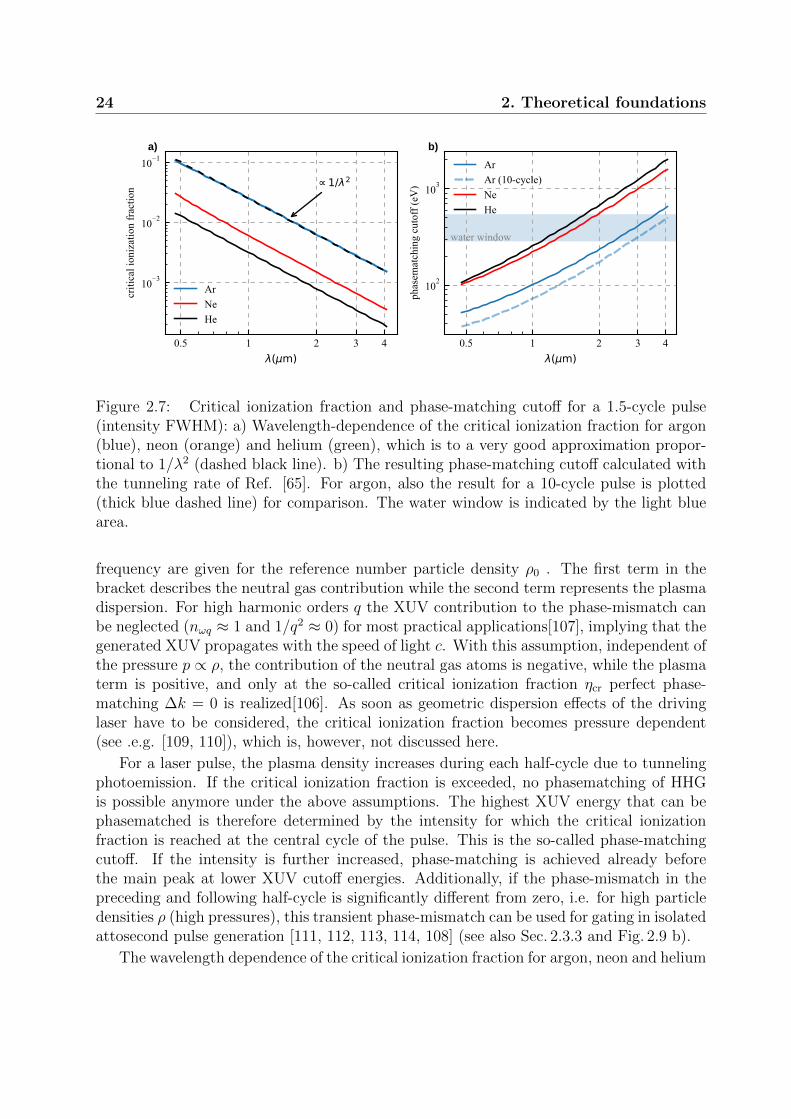
24 2. Theoretical foundations
Figure 2.7: Critical ionization fraction and phase-matching cutoff for a 1.5-cycle pulse(intensity FWHM): a) Wavelength-dependence of the critical ionization fraction for argon(blue), neon (orange) and helium (green), which is to a very good approximation propor-tional to 1/λ2 (dashed black line). b) The resulting phase-matching cutoff calculated withthe tunneling rate of Ref. [65]. For argon, also the result for a 10-cycle pulse is plotted(thick blue dashed line) for comparison. The water window is indicated by the light bluearea.
frequency are given for the reference number particle density ρ0 . The first term in thebracket describes the neutral gas contribution while the second term represents the plasmadispersion. For high harmonic orders q the XUV contribution to the phase-mismatch canbe neglected (nωq ≈ 1 and 1/q2 ≈ 0) for most practical applications[107], implying that thegenerated XUV propagates with the speed of light c. With this assumption, independent ofthe pressure p ∝ ρ, the contribution of the neutral gas atoms is negative, while the plasmaterm is positive, and only at the so-called critical ionization fraction ηcr perfect phase-matching ∆k = 0 is realized[106]. As soon as geometric dispersion effects of the drivinglaser have to be considered, the critical ionization fraction becomes pressure dependent(see .e.g. [109, 110]), which is, however, not discussed here.
For a laser pulse, the plasma density increases during each half-cycle due to tunnelingphotoemission. If the critical ionization fraction is exceeded, no phasematching of HHGis possible anymore under the above assumptions. The highest XUV energy that can bephasematched is therefore determined by the intensity for which the critical ionizationfraction is reached at the central cycle of the pulse. This is the so-called phase-matchingcutoff. If the intensity is further increased, phase-matching is achieved already beforethe main peak at lower XUV cutoff energies. Additionally, if the phase-mismatch in thepreceding and following half-cycle is significantly different from zero, i.e. for high particledensities ρ (high pressures), this transient phase-mismatch can be used for gating in isolatedattosecond pulse generation [111, 112, 113, 114, 108] (see also Sec. 2.3.3 and Fig. 2.9 b).
The wavelength dependence of the critical ionization fraction for argon, neon and helium

2.3 High-harmonic generation 25
is shown in Fig. 2.7 a) which is calculated using the refractive indices of Refs. [115, 116].The wavelength scaling is close to 1/λ2. With increasing ionization potential Ip of the noblegas atom, the neutral gas dispersion at a considered wavelength decreases and thereby alsothe critical ionization fraction. Nevertheless, larger Ip leads to a higher phasematchingcutoff, as illustrated in b), due to the highly nonlinear tunneling rate. The shown curvesare calculated for a 1.5-cycle pulse using the ADK-tunneling rate[65]. For comparison, wealso show the curve for a ten-cycle pulse in argon (blue dashed line), which has a lowerphasematching cutoff since more cycles contribute to the ionization before the maximumintensity is reached. The blue area indicates the photon energy range of the so-called waterwindow, which would allow interesting applications in biological samples immersed in anatural water environment (see Chap. 6 for more details).
Phase-matching contribution of the dipole phase
Figure 2.8: The dipole phase coefficient: a) in the temporal domain: short (long) tra-jectory contributions are indicated by solid (dashed) lines. The derivative of the dipolephase coefficient equals the rescattering energy (black line). The inset shows the dipoleoscillation. b) dipole phase coefficient in the spectral domain. The XUV spectrum froma 1.5-cycle pulse in argon obtained by the Lewenstein model is also shown (driving wave-length 1µm, intensity 2.8 · 1014W/cm2) (gray line).
The HHG dipole is the result of the interference of the recolliding electron wavepacketand the part of the wavefunction left in the ground state, as discussed in Sec. 2.3. Nev-ertheless, utilizing the SFA, the quantum-classical correspondence and the fact that theelectron dynamics in the continum can be expressed in terms of the characteristic energyand and time scale, a relatively simple expression for the HHG dipole phase can be derived.For a continuous-wave driving laser at frequency ω0 and a HHG photon energy ~ωq, it canbe written as[105, 117]:
φdipole(ωq) = αUp
Ephoton
+Ip
~(trec − t0)− ωq · trec, (2.17)

26 2. Theoretical foundations
where Up is the ponderomotive potential, Ephoton = ~ω0 the photon energy of the drivinglaser, trec is the recollision time at which the XUV photon is generated, t0 is the corre-sponding emission time and Ip is the ionization potential. The first term originates fromthe electron dynamics in the continuum. The HHG dipole coefficient α is a function of therecollision phase φ = ω0trec and further discussed below. The second term stems from theevolution of the ground state between emission and recollision time. The dipole phase hasto be determined with respect to a reference wave exp(iωqt) which is responsible for thelast term.
Within the Simple Man’s Model (SMM)[67], for an electron emitted at phase φ0 initiallyat rest, the dipole coefficient at the recollision phase φ is given by:
α(φ) = 2 ·∫ φ
φ0
(sinφ0 − sinφ′
)2
dφ′, (2.18)
which is basically the integral over the normalized electron kinetic energy (compare toEq. 2.7 with E(t) ∝ cosω0t). The dipole phase coefficient α therefore corresponds to thenormalized phase of the electron wavefunction at the time of recollision and is shownin Fig. 2.8 a) (blue line). Consequently, the derivative with respect to φ results in thenormalized rescattering energy (black curve) with the well known 3.17-Up-cutoff.
For practical purposes it would be more convenient to express α in terms of the HHGphoton energy, which is observable experimentally. For this goal, we briefly reconsider therelation of the high-harmonic photon energy to the recollision time (phase) and recollisionenergy, which is given essentially by the time derivative of the first two terms in Eq. 2.17:
ωq =
(dα
dt
)Up
Ephoton
+d
dt
(Ip
~· (trec − t0)
). (2.19)
From the inspection of above equation, we see that in addition to the sum of the ionizationpotential and the rescattering energy, the ground state evolution adds a small additionalterm to the photon energy through the dependence t0(trec), which is in agreement withmore rigorous quantum models[79]. The relation between photon energy and recollisionenergy is now given by Erecollision/Up ≈ (~ωq − 1.32 · Ip)/Up[117, 79, 118, 63].
The dipole phase coefficient in terms of the recollision energy is shown in b) (bluecurve). Since two trajectories lead to the same energy, short trajectories (solid line) andlong trajectories (dashed line) have to be distinguished which is accomplished by the indexj. By comparing a) and b) the connection between the temporal and energy domainbecomes obvious. For the rest of the thesis, we will utilize the dipole coefficient in theenergy domain αj.
We are now finally in a position to calculate the contribution of the dipole phaseφdipole to the phase-mismatch by performing the derivative of Eq. 2.17 with respect to thepropagation direction. Due to Eq. 2.19 most terms cancel and we are left with:
dφdipole
dz= αj
d
dz
(Up
Ephoton
). (2.20)

2.3 High-harmonic generation 27
Since Up ∝ I/ω20, with the driving laser intensity I and Ephoton ∝ ω0, the dipole phase
contribution to the phase-mismatch depends on the change of the driving laser intensity andcarrier-frequency. This finding will be important in Chap. 6, where HHG phasematchingwith strongly reshaped laser pulses is investigated.
Several phenomena connected to phase-matching can be explained from Fig. 2.8 b) andEq. 2.20. Firstly, it can be seen, why usually only short trajectories can be phase-matched ifthe driving laser varies in intensity along the medium. For short trajectories in the plateauregion the contribution of the dipole phase coefficient varies from 0 to about 1, comparedto 5-6 for long trajectories. Long trajectories can only be phase-matched efficiently underspecial conditions. Secondly, by noticing that Eq. 2.20 is in principle also valid for thederivative perpendicular to the propagation direction, we can conclude that compared tothe short trajectories, the phase of the long trajectory contribution changes more rapidlywhen moving away from the propagation axis due to the intensity decrease. This results ina higher curvature of the phasefront of long trajectories and thereby a larger divergence asconfirmed by experiments[119, 120, 121]. Finally, under normal conditions phase matchingis achieved by putting the generating medium about half the Rayleigh length behind thefocus. Ignoring the contribution of the medium, the positive phase-mismatch contributionof the Guoy-phase can be balanced by the negative dipole phase contribution caused bythe decrease in driving laser intensity. This is in contrast to the regime where the drivingpulse undergoes strong reshaping due to plasma effects, as discussed in Chap. 6.
2.3.3 Gating techniques for isolated attosecond pulse generation
In order to extract an isolated attosecond pulse, i.e. the contribution of a single half-cyclefrom the attosecond XUV/soft-x-ray pulse train, several gating techniques exist. Withinthis thesis we classify these techniques depending on whether the gating works on thesingle-atom level or on the macroscopic level, but other classification schemes exist (seee.g. [122]).
An example for a single-atom gating technique is amplitude gating[9], which is utilizedin the experiments in this thesis and further illustrated in Fig. 2.9 a). The techniquerequires a CEP-stabilized few-cycle laser (red line; top). The instantaneous photon energyis shown as orange line. For the right CEP, only one half-cycle burst from the XUVemission (blue shaded area) contributes above a certain photon energy. By filtering outlower photon energies, i.e. using a transmission filter or multilayer mirror, an isolatedattosecond pulse can be extracted. Another gating technique working on the single atomlevel is polarization gating[123, 124] and variants thereof[125, 126, 127], which make useof the fact that the recollision probability drastically decreases for elliptic polarization.Finally, in above-saturation gating, the ground state wavefunction is depleted in the leadingpart of the pulse through tunnel ionization, confining the highest XUV energies to a singlehalf-cycle[128].
On the other hand, gating techniques on the macroscopic level work by ensuring thatconstructive interference of the HHG emitters only occurs for a single half-cycle. Oneexample is phase-matching ionization gating[129, 114, 130], as illustrated in Fig. 2.9 b).

28 2. Theoretical foundations
a) b)
photonenergy
XUVemission
amplitudegate
electricfield
temporalgate phase
mismatch
XUVemission
attosecond pulseattosecond pulse
electricfield
Figure 2.9: Illustration of different gating mechanisms for isolated attosecond pulse gener-ation: a) amplitude gating and b) ionization gating. The driving laser pulse (red) and theresulting IAP (blue area) is shown above the panels. The maximum photon energy (orangeline) reaches into the spectral gating window (gray area) only for one half-cycle emissionburst. b) Ionization gating works on the macroscopic level by making use of phasematch-ing. Due to the varying ionization degree, perfect phasematching is achieved only for asingle half-cycle. Neighboring half-cycles are suppressed in the macroscopic buildup of theXUV pulse.

2.4 Field enhancement and confinement on nanotips 29
This technique also works for multicycle lasers and relies on the instantaneous HHG phasemismatch (orange line, see Sec. 2.3.1). In the beginning of the laser pulse, the disper-sion of the neutral gas determines the phase mismatch. Since the plasma density keepsaccumulating for later half-cycles, which counteracts the dispersion of the neutral gas, per-fect phase matching can be reached for a single half-cycle. In neighboring half-cycles thecoherent buildup of HHG is suppressed due to the phase mismatch, which results in anisolated attosecond pulse in the far-field even though the single-atom contribution consistsof a pronounced APT. Another example is the attosecond lighthouse[131, 132], where arotation of the wavefront of the driving laser field in the HHG focus leads to emission ofthe attosecond burst in separate directions.
Isolated attosecond pulses with a duration on the order of few 100 as can nowadays beproduced fairly routinely. The shortest attosecond pulse demonstrated up to now had aduration of 43 as generated by a driving laser pulse centered at around 1600µm wavelengthand a duration of 11 fs utilizing amplitude gating[133].
2.4 Field enhancement and confinement on nanotips
a) b)
Figure 2.10: Field enhancement and response function of a nanotip: a) Field enhancementand field confinement on a tungsten nanotip with a radius of 30 nm and an opening angleof 10 calculated at a wavelength of 780 nm. The incident laser pulse is propagating inz-direction and polarized vertically. The red line shows the field amplitude on the nanotipaxis. b) Amplitude (red line) and phase (blue line) of the response function at the apex ofthe nanotip.
The interaction of light with nanostructures leads to confinement and enhancement ofthe electromagnetic fields near the surface which constitutes the basis of nano-optics[134].The length scale for the near-field decay (confinement) around the sharp geometric features

30 2. Theoretical foundations
is given by its radius[135] which has found various applications for example in optical near-field microscopy well below the diffraction limit of light (see Sec. 7.1 for more examples).Moreover, mostly due to an analog of the lightning rod effect, the near-fields are enhancedat these hotspots[135] which can be used for sensing. The details of the field enhancementand confinement depend on the wavelength of the incident light λinc as well as the opticalproperties and exact geometry of the nanostructure.
Metal nanotips and their interaction with ultrashort laser pulses is the focus of Chap. 7.Nanotips represent a prototypical nano-optical hotspot and are therefore an ideal modelsystem for studying the interaction ultrafast laser pulses with nanostructures. They areeasy to produce by electro-chemical methods (see Sec. 3.1) and the obtained apex radiican routinely reach 50 nm and below, much smaller than the wavelength of the incidentlaser pulse. Compared to isolated nanospheres, nanotips can be electrically contacted andprecisely placed within the focus.
The field enhancement compared to the incident field around the apex of a tungstennanotip is shown Fig. 2.10 a) for an incident wavelength of 780 nm and an apex radiusof 30 nm. The outline of the nanotip is shown as white line. The calculation has beenperformed with a commercial finite-difference time-domain (FDTD) software (LumericalFDTD). The incident field is polarized along the y-axis. The magnitude of the near-fieldalong the nanotip axis (red line) clearly shows the confinement to the length scale ofthe apex radius. A field enhancement factor up to 5 can be observed, which translatesinto more than an order of magnitude increase in intensity. Besides the lightning rodeffect that dominates the response here, two resonant mechanisms can contribute to thefield enhancement[135]. Firstly, for plasmonics materials, the localized surface plasmonresonance can contribute. Secondly, if the length of the nanostructure happens to be anodd multiple of λinc/2, an antenna resonance might occur.
The wavelength dependence of the amplitude (red line) and phase (blue line) of thespectral near-field response function at the apex of the nanotip is shown in Fig. 2.10 b)for the spectral range covered by the laser pulses used in this thesis. From the near-fieldresponse the electric field in time for can be calculated for any incident pulse (see Sec. 7.2.2for more details on the response function). As can be seen, the field enhancement increaseswith wavelength from around 3 at 400 nm to above 6 at 1000 nm. In the absence ofresonances the field enhancement generally increases with the incident wavelength. Ourlaserpulses are mostly confined within 600-900 nm which results in an enhancement between4 and 5. The relative phase only decreases slightly from around -0.4π to marginally below-0.5π.
The near-fields around nanostructures can significantly influence the strong-field pho-toemission dynamics. Firstly, due to the field enhancement, the strong-field emissionregime can be reached with much lower input pulses that are available from oscillatorsat MHz repetition rates compared to the kHz rate provided by chirped amplifier systems.Moreover, the near-field confinement can affect the strong-field electron dynamics once thequiver amplitude is on the order of the field decay length[88], since the field that woulddrive the electrons back to the surface has already significantly decreased at the turningpoint. This quenching of the quiver motion leads to a reduction of the rescattering cutoff

2.4 Field enhancement and confinement on nanotips 31
well below 10 Up and can be characterized by an adiabaticity parameter δ, defined as theratio of near-field decay length and quiver amplitude. Additionally, as shown in a publica-tion by the author[89] which is not represented in this thesis, a shift of the low-energy peakto higher energies can be observed which can be interpreted in terms of a non-adiabaticponderomotive shift. Since the quiver amplitude scales with λ2, these two effects mostlyplay a role at longer wavelengths and can be ignored for our visible laser pulses. Addi-tionally, the near-field decay also affects the attosecond streaking amplitude and phase forelectrons emitted from the nanostructure and a related adiabaticity parameter has beenintroduced by the author in Refs. [25, 26] which is discussed in more detail in Chap. 7.

32 2. Theoretical foundations

Chapter 3
Experimental foundations
3.1 Nanotip etching
A
+-
A
+-
A
+-
NaOH
W
W042-
OH-
a) b) c)
Figure 3.1: Overview over the nanotip etching process: a) a tungsten wire is immersedin NaOH and the etching process is initiated by applying an etching voltage. b) Thinningof the immersed wire through etching. Tungsten is dissolved into soluable tungstate ionsWO2−
4 . c) Fast switch-off of the etching voltage after the etching process is finished.
The tungsten nanotips used in the photocurrent experiments presented in Sec. 7.3 wereproduced by an electrochemical etching setup described in Ref. [136] and built by HirofumiYanagisawa. The basic principle is shown in Fig. 3.1. A tungsten wire with a diameter onthe order of 100µm is immersed into a 5M NaOH solution (a). When a voltage is appliedbetween the tungsten wire and the submerged ring electrode, the etching process startswhich occurs predominantly around the meniscus at the interface of etchant solution, airand wire (b). Once the lower part is etched away, a nanotip is formed (c). In order toavoid further bluntening of the nanotip, the etching process has to be stopped as soon aspossible. Since the sudden drop of the etching current indicates that the lower part ofthe wire is etched away, this can be achieved by switching off the etching voltage with the

34 3. Experimental foundations
help of a dedicated analog electronic circuit that measures the etching current (for furtherdetails see Ref. [136]).
A microscope image of a tungsten nanotip is shown in Fig. 3.2. The diameter of thetungsten wire is around 100µm. The characteristic shape towards the nanotip stems fromthe etching process. The chemical etching process usually results in a very smooth surfaceon the shank of the nanotip[137] which is crucial for the spatially resolved experimentsperformed in Chap. 7. The gold nanotips in the attosecond streaking experiments weresupplied by the group of Prof. Hommelhoff[51].
100 μm
Figure 3.2: Microscope image of a tungsten nanotip produced with our nanotip etchingsetup.
3.2 Current measurements
3.2.1 Transimpedance amplification
gain: 1010V/A
Cin (pf)10
1001000
eq. i
np. c
urre
nt n
oise
(fA
/ H
z)
currentsource
OP amp
-+
IsCin
Rf
Cfa) b) c)
Figure 3.3: Transimpedance amplifier: a) schematic measurement circuit consisting of thecurrent source and the transimpedance amplifier (gray box). b) Frequency dependence ofthe relative gain for various input capacitances and c) equivalent input current noise (dataextracted from Ref. [138]).

3.2 Current measurements 35
For the sub-cycle resolved current measurements presented in Chap. 7 and Chap. 4 atransimpedance amplifier (TIA) is a key component which is also commonly found in e.g.photodiodes. TIAs convert a small current signal into a voltage signal. The conversionfactor is given in units of V
A. Here, only the basic principle is presented, details can be
found elsewhere (e.g. Ref. [139]).The fundamental building block of a TIA is an operational amplifier (OP amp) and
a feedback resistor with resistance Rf , as shown in Fig. 3.3 a). First, we consider lowfrequencies where any capacitances can be ignored. Here, the OP amp tries to cancel anyvoltage difference between its inputs due to the sensor current IS by sending an oppositefeedback current through the feedback resistor. Thus, Rf determines the current-to-voltagegain. For higher frequencies the input capacitance Cin starts to play a role. In order toavoid oscillations of the transimpedance amplifier, a feedback capacitance Cf has to beadded[140].
Commercial high-gain, low-noise TIAs (FEMTO DLCPA-200) are used for our measure-ments. The relative gain and equivalent input current noise density of a comparable TIA(NF Corp. SA-607F2) with a fixed transimpedance gain of 1010 V
Aare shown in Fig. 3.3 b)
and c), respectively. The gain bandwidth decreases with increasing Cin. Moreover, at thesehigh transimpedance gains, the 3dB-bandwidth of TIAs is limited to a few kHz-100kHz,which is significantly slower than would be required for the direct amplification of the fs-nsphotocurrent in our measurements. As further discussed in Chap. 4, the detected signalsin our experiments can therefore be better understood in terms of the total induced chargeon the electrodes or equivalently as the temporal integral of the current. The equivalentcurrent input noise (c) determines the minimum amount of current variation that canbe measured and is fundamentally limited by Johnson (thermal) noise of the electroniccomponents.
3.2.2 Lock-in detection
In addition to transimpedance amplifiers discussed above, for the sensitive detection ofweak signals a lock-in amplifier is another crucial instrument and is used for both thecurrent measurements in Chaps. 4 and 7 as well as the electro-optic sampling in Chap. 5.Usually, the modulation of the laser pulse is required at a reference frequency fref eitherby an optical chopper or by changing the CEP. This section closely follows Ref. [141] towhich we refer for more details.
The fundamental working principle of lock-in amplification relies on the detection of aninput signal within a narrowband frequency window around the reference frequency fref ,thereby discarding noise at other frequencies. This is schematically illustrated in Fig. 3.4 a),which shows the signal (red line) and the detection bandwidth (blue area). In addition tothe spectrally flat white noise (light blue area), there also appears so-called 1/f-noise atlower frequencies from various sources, such as mechanical and acoustical vibrations. Ascan be seen, with the help of the spectral gating, the lock-in amplifier is able to resolvesignal amplitudes below the low frequency noise amplitude.
In the lock-in amplifier the input voltage signal Vs is multiplied with a reference signal

36 3. Experimental foundations
whitenoise
1/f-noise
detectionbandwidth
signal
frequency
a) b)
Figure 3.4: Lock-in detection: a) Signal (red line) and detection bandwidth (blue area).For lower frequencies, considerable 1/f -noise is present while for higher frequencies prac-tically only white noise is left. Due to the limited detection bandwidth, even signals thatlie below the low-frequency noise amplitude can be resolved (adapted from Ref.[141]). b)Experimental input signal (blue line) together with the demodulation at the repetition ratefrep (red) and frep/2 (black line).
Vref which is either a cosine or sine wave oscillating at fref . Modern lock-in amplifiers canperform both demodulations simultaneously which is most conveniently described in thecomplex domain as Vref =
√2 exp(−iωreft). The multiplication yields the signal Z ′:
Z ′ = Vs · Vref = R ·(e+i·(ωs−ωref)t+iφ0 + e−i·(ωs+ωref)t−iφ0
), (3.1)
where√
2R is the signal amplitude at fs. Whether or not an additional factor√
2 appears,depends on the details of the modulation (see also Appendix A), the convention of thelock-in manufacturer and how the signal amplitude is defined. If fs = fref , the first term isquasi constant while the second term is oscillating with twice the reference frequency. Thelatter is eliminated by low-pass filtering of Z ′ resulting in the lock-in signal Z:
Z = Reiφ0 = X + iY. (3.2)
The relation between the lock-in detection and an experimental input signal is fur-ther illustrated in Fig. 3.4 b). The input voltage pulses (blue line) after transimpedanceamplification represent the signal from consecutive laser pulses. The signal componentcontributing to the demodulation at the repetition rate frep of the laser is shown as redsolid line. Additionally, the signal was modulated at frep (black solid line), which is how-ever not visible here due to noise components at other frequencies and only appears afteraveraging over many signal pulses. For completeness, boxcar averaging, where the signalis integrated over a well-defined temporal window can be advantageous over lock-in detec-tion, if the signal of interest has a low duty cycle, i.e. is temporally well confined and most

3.3 Field-resolved measurement techniques 37
of the time only noise is present[142]. This condition is not fulfilled for our signals andtherefore lock-in detection is preferred.
3.3 Field-resolved measurement techniques
This section serves as an overview of the field-resolved techniques used in this thesis and isalso intended as a reference for the discussion of more specific details. It might be helpfulfor some readers to first go through the experimental description in the later chapters toget a glimpse of the experimental implementation and applications, and then come backto this section.
Attosecond streaking is used for the characterization of isolated attosecond pulses andtheir driving laser pulses in the overdriven regime in Chap. 6 as well as for the charac-terization of nanoscale near-fields on a gold nanotaper (Chap. 7). The pump-probe mea-surements on semiconductors presented in Chap. 5 rely on electro-optic sampling (EOS).Tunneling ionization with a perturbation for the time-domain observation of an electricfield (TIPTOE) and streaking of rescattering electrons are utilized in the measurement ofthe enhancend near-fields of a nanotip apex and the application to the spatio-temporalcharacterization of a vortex beam (Chap. 7). Finally, Chap. 4 studies the fundamentalmechanism through which macroscopic currents in photoconductive sampling of opticalfields are generated on the electrodes.
3.3.1 Attosecond streaking
Description
Attosecond streaking[12, 13] is a pump-probe scheme that relies on an isolated attosecondpulse (IAP) in the XUV/soft-x-ray range generated through HHG. It is used to characterizea co-propagating near-infrared laser pulse (red line) with a variable time-delay ∆t. Asshown in Fig. 3.5 a), the IAP (blue line) leads to the photoemission of an electron (blackdot) from an atom (green circle) through linear absorption of an XUV photon. The emittedphotoelectron is accelerated by the near-infrared laser pulse (red line) which leads to anincrease or decrease of its final kinetic energy (or momentum) depending on the time-delay.The final momentum pfinal can be calculated classically within the simpleman’s model (seeSec. 2.2.2) for an electron emitted at time t0:
pfinal(t0) = p0 − eA(t0), (3.3)
where p0 is the field-free final momentum. The change of the photoelectron spectrum thusallows the reconstruction of the vector potential A(t) and thereby the electric field E(t) ofthe streaking laser pulse. Usually, the IAP is generated by the streaking laser pulse in thefirst place resulting in intrinsic timing synchronization between both pulses.
A simulated attosecond streaking spectrogram, i.e. delay-resolved photoelectron spe-tra, is depicted in Fig. 3.6 a) (see e.g. also Figs. 6.2 and 7.3 for experimentally measuredspectrograms). The central momentum shift closely follows −eA (red dashed line).

38 3. Experimental foundations
Δtelectron
atom
laserpulse
isolated attosecond XUV pulse
-4 0 4t (fs)
1
0
-1
E (
norm
.)
Figure 3.5: Principle of attosecond streaking: an isolated attosecond XUV pulse (blueline) photoemits an electron (black dot) from an atom (green ball) via linear photoemissionand with variable delay ∆t with respect to a near-infrared laser pulse (red line). After theemission, the electron experiences the electric field of the latter, leading to a variation ofits final kinetic energy.
Attosecond streaking does not only allow the reconstruction of the laser pulse but alsoof the attosecond XUV pulse. This is qualitatively illustrated in Fig. 3.6 b) for a positivelychirped XUV pulse, i.e. where the central photon energy under the envelope increases withtime. Here, the width of the photoelectron distribution for a fixed delay changes dependingon whether −eA is decreasing or increasing in contrast to an unchirped XUV pulse (a). Thereason can be seen in Fig. 3.6 c)-e), which shows the temporally resolved initial momentumdistribution (false color plot) that directly reflects the temporal structure of the XUV pulsetogether with −eA (red dashed line) which corresponds to the momentum shift inducedby the streaking field. For an unchirped pulse (c), integration along the time axis resultsin the same final momentum distribution independent on whether the vector potentialincreases or decreases. In contrast, for the chirped pulse, the emission time-dependentmomentum shift (black arrows) leads to narrowing (broadening) of the final momentumdistribution for decreasing (increasing) −eA as shown in d) (respectively e). Thereby,temporal information on the XUV pulse is encoded into the streaking spectrogram.
Pulse retrieval
For the retrieval of both the XUV and the streaking pulse from the attosecond streakingspectrogram S(p,∆t), the quantum mechanical expression based on the dipole transitionfrom the initial state to the Volkov state (see Eq.2.10) has to be used[79, 143, 144]:
S(p,∆t) =∣∣∣ ∫ ∞−∞
dt ~EXUV(t−∆t)~d(p+ A(t)
)e+i(p2/2+Ip)t · e−i
∫∞t dt′ [p·A(t′)+A(t′)2/2]
∣∣∣2, (3.4)

3.3 Field-resolved measurement techniques 39
t
-eA
-eA
-eA
pfinal(t)pfinal(t)
pfinal(t)
p0
Figure 3.6: Streaking spectrogram and the signature of chirped XUV pulses: photoelectronstreaking spectrogram of a) an unchirped XUV pulse and b) a positively chirped XUV pulsetogether with the vector potentials (red dashed line). c)-e) Schematic illustration of theeffect of the XUV pulse structure on the spectral width at a given pump-probe delay:The false color plots indicate the momentum of the electrons directly after photoemissionthereby carrying the signature of the XUV pulse. The final momentum is shifted by thevector potential (red line) indicated by the black dashed line. For a chirped pulse thisleads to a change of the width of the final momentum distribution which manifests itselfas a broadening or narrowing of the streaking trace.

40 3. Experimental foundations
where ~EXUV is the electric field of the XUV pulse, ~d is the dipole matrix element, p is thefinal momentum and Ip is the ionization potential. For notational simplicity, atomic unitsare employed. The integral in the last exponential originates from the Volkov state.
Commonly, the central momentum approximation (CMA) is being adopted where it isassumed that the central momentum pc is much larger than the range of momenta to beconsidered. In this case, p in the Volkov integral can be replaced with pc and the dipolematrix element can be considered constant. The advantage of the CMA is that it allowsthe use of well established fast Fourier-transform-based methods for the retrieval of boththe attosecond XUV and streaking pulse such as frequency-resolved optical gating for thecomplete reconstruction of attosecond bursts FROG-CRAB[145, 143, 146] or ptychographicreconstruction algorithms[147]. In this thesis, a ptychographic reconstruction algorithm isimplemented under conditions for which the CMA holds.
For broadband XUV pulses, the CMA has been shown to lead to errors in the extractionof timing information[148]. Recently, a reconstruction algorithm that does not rely onthe CMA has been demonstrated, the so-called Volkov transform generalized projectionalgorithm (VTGPA)[144] which has enabled the absolute complex dipole transition matrixelement reconstruction (ACDC)[149] from attosecond streaking spectrograms.
For completeness, there also exist frequency domain interferometric methods[149] forthe attosecond pulse retrieval, such as RABBITT[150], PROOF[151] or iPROOF[152].However, they are limited to perturbative intensities and narrowband driving pulses andare thus not appropriate for reconstructing the broadband driving laser pulses employedin our experiments.
Another problem can originate from incoherent contributions which can arise due tofluctuations or different final states of the unobserved ion, e.g. caused by shake-up pro-cesses. Indeed, the retrieved photoemission time-delay (see discussion below) betweendifferent initial states in neon[14] could only be explained by considering additional shake-up channels[153, 154, 155]. Incoherent processes can not be described by the coherentexpression in Eq. 3.4. A fully consistent retrieval therefore requires a density matrix ap-proach as in quantum state tomography, which has only very recently been demonstratedwithin the field of attosecond science[156].
Attosecond photoemission delays
Attosecond streaking has been successfully applied for the measurements of photoemissiontime delays in atoms[14, 155], molecules[84] and solids[15, 157]. These photoemissiontime delays manifest themselves as a time shift τs between the streaking traces originatingfrom different initial states. Photoemission time delays do not play a role for the finalinterpretation of the attosecond streaking experiments in this thesis. Nevertheless, theycould, in principle, affect the field reconstruction and are therefore discussed in Chap. 7.Hence, a brief overview is given here. For a more illustrative introduction, we refer toRef [158]. The streaking time delay can be decomposed into several contributions[159]:
τs = τEWS + τCLC + τdLC, (3.5)

3.3 Field-resolved measurement techniques 41
where τEWS is the so-called Eisenbud-Wigner-Smith time-delay, τCLC is the Coulomb lasercoupling term and τdLC is the dipole laser coupling time delay. Again, as for the strong-fielddynamics in the simpleman’s model (see Sec. 2.2.2), the streaking delays are generally verywell described by the classical equations of motion due to the Ehrenfest theorem[159, 160].
τEWS originates from the short-ranged potential and is specific to the type of mediumon which the attosecond streaking measurement is performed. It corresponds to the time-shift an electron experiences when leaving the potential compared to a free electron withthe same asymptotic kinetic energy. The latter implies that the Eisenbud-Wigner-Smithtime delay for an attractive potential is negative, since the electron has a higher velocitywithin the range of the potential. However, τEWS is not automatically negative. Dependingon the orbital angular momentum l of the final continuum state, the centrifugal potentiall(l + 1)/2r2 can act as a repulsive potential[159, 161].
The emitted electron is subject to both the Coulomb and the streaking laser field. Thiscoupled motion leads to the Coulomb laser coupling time delay which, in atomic units, isgiven to first order by[159]:
τCLC =Z
(2 · Ekin)3/2[2− ln(EkinTIR)], (3.6)
where Z is the charge of the ion, Ekin is the final kinetic energy and TIR is the oscillationperiod of the streaking laser field. τCLC does neither depend on the specific target nor,somewhat surprisingly, on the streaking field strength and is usually negative. The mag-nitude of τEWS and τCLC increases with lower kinetic energy and generally ranges between100 as and 10 as for kinetic energies between 20 eV and 100 eV. The dipole laser couplingτdLC originates from the interaction of the streaking laser with the (induced) dipole of theinitial or final state which in turn affects the outgoing electron.
Generally, photoemission time-delays can only be measured relative to a reference. Onlyrecently, the absolute timing of photoemission delays could be demonstrated[157] throughcomparison of experimental data with simulations for helium, which can be treated exactly.
3.3.2 Electro-Optic Sampling
Electro-optic sampling (EOS) is an all-optical field-resolved method. In this thesis, EOS isused for the transient field-resolved reflectometry experiments on semiconductors presentedin Chap. 5. EOS has been employed for the measurement of THz-pulses for almost threedecades[41]. Only recently, the extension of the concept down to 1.2µm[31] (near-infrared)could be demonstrated.
A schematic illustration of an EOS setup is shown in Fig. 3.7 a). The MIR pulse (blueline) to be sampled is focused into a nonlinear EOS crystal together with a gating pulse (redline) at a variable delay ∆t. The gating pulse duration generally needs to be shorter thanone half-cycle. The nonlinear crystal is tuned for phase-matching of the sum-frequencygeneration (SFG) process with the resulting electric field ESFG approximately given by:
ESFG(t, τ) ∝ Egate(t) · EMIR(t+ τ). (3.7)

42 3. Experimental foundations
1
0.5
0
inte
nsity
SFG
funda-mental
bandpass
a) b)
SFG
Wollastonpolarizer
bandpassfilter
λ/4-plate
EOScrystal
MIRpulse
gatingpulse
balancedphotodiode
600 800 1000λ (nm)
Δt
Figure 3.7: Electro-optic sampling: a) Setup for electro-optic sampling of an MIR pulsevia an NIR gate pulse. b) Schematic spectrum of the SFG-signal (blue line) and of thefundamental NIR gating pulse (red line) which serves as a local oscillator and additionallythe range of the bandpass filter (light blue shaded area). The figure is adapted fromRef. [162].
Strictly speaking Eq. 3.7 also contains a difference frequency generation (DFG) term, whichcould also be used in EOS. Here, we neglect it, since our considerations focus on theproportionality. Through the SFG process the MIR signal is transfered to the optical/NIRrange. As shown in Fig. 3.7 a), the SFG signal is normally orthogonal to the gatingpulse. In order to allow for a sensitive detection of the SFG signal, an optical heterodyneellipsometric detection scheme is employed where the transmitted gating pulse serves as alocal oscillator[31]. A bandpass filter is applied to limit the detected spectral range to aregion where both pulses interfere, as schematically shown in Fig. 3.7 b). Using a λ/4-plateand a Wollaston polarizer, the rotation of the polarization induced by the SFG-signal canbe detected in a balanced manner. Qualitatively, the signal intensity at the detector isproportional to:
IEOS ∝ |Egate + ESFG|2 ∝ E2gate + 2 · EgateESFG + E2
SFG. (3.8)
The first term on the r.h.s is delay-independent and eliminated by the balanced detection.Since the SFG-signal is usually weak, the last term can be neglected and only the inter-ference term is left. By using Eq. 3.7, it can be seen that the latter is proportional to theMIR field at time τ which yields for the EOS signal SEOS(τ):
SEOS(τ) ∝ Egate · ESFG(τ) ∝ Igate · EMIR(τ) (3.9)
Due to the interference, where the small ESFG is multiplied by the strong local oscillatorgiven by Egate, even very weak SFG signals and thereby small MIR fields can be detected.EOS generally shows outstanding sensitivity[163] and has been used to measure vacuumfluctuations[164].

3.3 Field-resolved measurement techniques 43
In a more rigorous treatment, the spectral response function S(Ω) of EOS detectioncan be derived[31]:
S(Ω) =
∫ ∞Ω
dωLOR(ωLO)|Egate(ωLO)||Egate(ωLO − Ω)|ei[φ(ωLO)−φ(ωLO−Ω)], (3.10)
where Ω is the MIR frequency, ωLO is the local oscillator frequency, φ is the spectral phaseof the gating pulse and R is the response of the detection system.
3.3.3 Tunneling ionization with a perturbation for the time-domainobservation of an electric field (TIPTOE)
A particularly intuitive method based on the perturbation of field driven processes is thetunneling ionization with a perturbation for the time-domain observation of an electricfield (TIPTOE)[32]. The mechanism is depicted in Fig. 3.8 a) for the case of a surface. Astrong pump field Ep (red solid line) leads to tunneling emission (blue shaded area) fromthe surface constituting a sub-cycle gate at around t0=0. Here, emission only occurs whenthe electric force for an electron −e · E points away from the surface. The emission rategets modified (dashed black line) by a weak time-delayed perturbing signal field Es (reddashed line). This leads to a change of the total emitted charge ∆Q depending of whetherthe total electric field magnitude during the gate, i.e. the magnitude of the sum of pumpand probe field at t0=0, decreases or increases.
The total emitted charge Q at time delay τ in the presence of the signal field can becalculated from the instantaneous tunneling rate w
(E(t)
)[32, 165]:
Q(τ) ∝∫w(Ep(t− τ) + Es(t)
)dt, (3.11)
where the time integral extends over the pulse length. Since the signal field is weak, thekernel of the integral can be Taylor-expanded up to first order:
Q(τ) ∝∫w(Ep(t− τ)
)+
dw
dE
∣∣∣∣∣Ep(t−τ)
· Es(t)dt, (3.12)
where the last term corresponds to the cross-correlation of the gating function with thesignal field[165]. The first term corresponds to the rate without signal field. Moreover, thegating function for a tunneling emission burst at t0 can be approximated as a delta-functionδ(t− τ − t0), yielding an expression for ∆Q:
∆Q(τ) ∝∫
dw
dE
∣∣∣∣∣Ep(t−τ)
· Es(t) dt ∝ dw
dE
∣∣∣∣∣Ep(t0)
· Es(t0 + τ). (3.13)
For a single emission burst, the charge modulation is thus approximately proportional tothe electric field.

44 3. Experimental foundations
For several tunneling emission bursts, the last expression on the left hand side in Eq. 3.13becomes a sum over all burst times tk. This is illustrated in Fig. 3.8 b) for a pump pulse(not shown) with CEP=0, where two dominating equal emission bursts occur. As can beseen, in this case, signal frequencies at 0.5 f0 (red line) and 1.5 f0 (black line), where f0 isthe pump pulse frequency, do not lead to a modulation of the emitted charge. The reasonis that the emission modulation of the first burst is counteracted by the second burst sincethe signal fields point into opposite direction. This is not the case for CEP=π.
t (fs)
1
0
-1
φCEP 0 πphaseamplit.
CEP=π ΔQ
a) c)
b)CEP=0
rate
0.5⋅f0
1.5⋅f0
10 fs
Figure 3.8: TIPTOE response function for surface emission: a) TIPTOE-principle: Theionization rate (blue line area) of a strong pump pulse (red line) is perturbed by a weaksignal pulse (red dashed line). The change in ionization is essentially proportional to theperturbing electric field at the time of the emission peak. At a surface, electron emissiononly occurs if the electric field points into the surface. b) Amplitude (solid lines) andphase (dashed lines) of the response function for CEP=0 (red) and CEP=π (black) fora pulse width of 4.5 fs (FWHM) calculated using the Fowler-Nordheim rate. For a 10 fs-pulse (blue line), practically no CEP-dependence is observed (intensity 3·1014W/cm2, workfunction=4.5 eV). c) Illustration of the reason for the minima in the amplitude response forCEP=0 at 0.5 · f0 (red line) and 1.5 · f0 (black line). The results shown here use a Fowler-Nordheim emission rate[66] assuming a work function of 4.5 eV and a pump pulse at anintensity-FWHM of 4.5 fs, a central wavelength of 750 nm and intensity of approximately3 · 1013W/cm2. In order to obtain a large bandwidth, we chose a signal pulse duration of1 fs at 375 nm wavelength and a relative field strength of 10−5.
This leads to a CEP-dependence of the spectral response function, as can be seen inFig. 3.8 c), and which has been extensively discussed in Ref. [165]. The spectral responsefunction can be calculated either by Fourier transforming the gating function in Eq. 3.12,or by evaluating the full expression for the emitted charge for a given pump and signal

3.3 Field-resolved measurement techniques 45
field in Eq. 3.11 and subsequently forming the ratio of ∆Q and Es in the Fourier-domain.We chose the latter approach, since it does not rely on the first-order Taylor-expansion.
The amplitude (solid lines) and phase (dashed lines) of the spectral response functionfor a CEP of 0 (black) and π (red) are shown in Fig. 3.8. As discussed above, for CEP=0,the amplitude response exhibits zeros at f = 0.5 f0 + n · f0, where n is an integer. Theresponse function for CEP=π only shows a slight modulation caused by the small satelliteemission bursts one cycle earlier and later as shown in Fig. 3.8 a). Around f0 the phaseof the response function changes with the CEP of the pump pulse. As pointed out inRef. [165], if both pump and signal pulse originate from the same laser source, this allowsthe auto-characterization of the pulse without CEP-stabilization, since the relative phaseof both pulses does not change. However, this statement only holds true, if the bandwidthis relatively narrow: we demonstrate in Chap. 7, that the change of the amplitude ofthe response function |H| with the CEP can be measured with broadband pulses. Forcomparison, we also show |H| for a pump pulse with the same parameters as above, buta pulse duration of 10 fs (solid blue line). In the latter case, the CEP-dependence is notvisible anymore.
Originally, TIPTOE has been employed in gas as an ionizing medium[32] and has beenused to characterize an optical near-single-cycle pulse[166] and multicycle laser pulses fromthe UV to the IR[167]. It has also been shown that the condition that the signal pulseis only a minor perturbation can be relaxed[167]. The TIPTOE principle is not limitedto charge measurements, but also can be used for ionization-induced fluorescence[168].Finally, the method has successfully been applied to the measurement of the near-fieldin a nanostructure array[165]. We employed TIPTOE as the main method for measuringenhanced near-field on the apex of a metallic nanotip based on the photocurrent in Chap. 7.
3.3.4 Streaking of rescattering electrons
It has been shown very recently that also the perturbation of the electron trajectoriescontributing to the cutoff of the ATI rescattering plateau can be used for field-resolvedmeasurements[33]. The approach is illustrated in Fig. 3.9 a). A strong pump field (red solidline) accelerates electrons after their emission and a fraction of the electron trajectoriesrescatters with the parent ion or surface. The classical trajectory (black solid line) leadingto the highest electron energy in the SMM (see Sec. 2), is emitted shortly after the fieldcrest at t = 0 and rescatters around t = 0.7T , where T is the oscillation period. If a weakperturbing signal field (red dashed line) is added, the cutoff trajectory is slightly modified(blue dashed line), resulting in a shift of the cutoff energy ∆Ecutoff in the ATI spectrum,as shown in Fig. 3.9 b). This approach is especially appealing for near-field measurementsfrom nanostructures and is one of the methods used in Chap. 7. Here, the strong-fieldemitted electrons from the enhanced nanoscale near-field itself are used to measure thevery same field, similar to the TIPTOE approach described above.
The description is simplified in terms of the final momentum shift ∆pcutoff . In the SMM,

46 3. Experimental foundations
sim. | model ampl.phase
t (T)
-E/x
(ar
b.u.
)
signalpump
a) c)
b)
ΔEcutoff
cutoff traj.
Figure 3.9: Response function of the cutoff rescattering streaking: a) principle: a weaksignal field (red dashed line) influences the cutoff trajectory (black and blue dashed line,respectively) driven by the strong pump pulse (red solid line). b) the perturbation leadsto a variation in the spectral cutoff that is proportional to the weak field. c) Responsefunction of the rescattering cutoff variation with respect to the perturbing electric fieldstrength calculated using the SMM. The amplitude (solid red line) and phase (red dashedline) response is compared with a heuristic model (blue solid and dashed lines).
it is approximately given in terms of the vector potential of the signal field As by[33]:
∆pcutoff(τ) = −2As(tr − τ) +1
tr − ti
∫ tr
ti
As(t− τ)dt, (3.14)
where ti and tr are the ionization and rescattering times in the absence of the signal field,respectively.
We have calculated the spectral response function to the electric field using pump andsignal fields with constant amplitude within the SMM. The amplitude (solid red line) andphase (dashed red line) of the response function are shown in Fig. 3.9 c). At the pumpfrequency ω0, the pump and signal fields are degenerate, which means that the amplitudeis related to the 10Up-cutoff and the phase is zero (see gray solid and dashed lines). Since∆pcutoff is dominated by the vector potential at the rescattering time (first term on ther.h.s. in Eq. 3.14), the amplitude follows an approximate 1/ω-dependence and the phaseincreases almost linearly by 2π · 0.7 · (T0/T − 1). A simplified heuristic spectral responsebased on both previous findings is shown in blue.
A similar approach exists based on the HHG cutoff modulation[35]. The advantage ofthe rescattering streaking approach over TIPTOE is that it allows in principle the straight-forward determination of the absolute signal field strength, but it requires an electronspectrometer. Moreover, it can be measured simultaneously with the TIPTOE approach(see Sec. 3.3.3) as done in Chap. 7. Since the approach assumes single electron dynamics,it might not work anymore in the multielectron emission regime when charge interaction
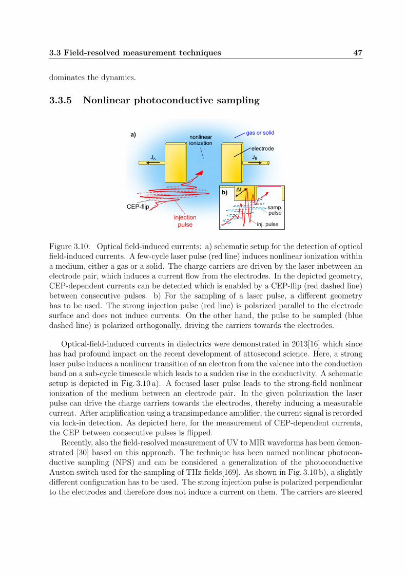
3.3 Field-resolved measurement techniques 47
dominates the dynamics.
3.3.5 Nonlinear photoconductive sampling
gas or solid
JA JB
electrode
a)
b)
inj. pulse
samp. pulse
Δt
nonlinearionization
injectionpulse
CEP-flip
Figure 3.10: Optical field-induced currents: a) schematic setup for the detection of opticalfield-induced currents. A few-cycle laser pulse (red line) induces nonlinear ionization withina medium, either a gas or a solid. The charge carriers are driven by the laser inbetween anelectrode pair, which induces a current flow from the electrodes. In the depicted geometry,CEP-dependent currents can be detected which is enabled by a CEP-flip (red dashed line)between consecutive pulses. b) For the sampling of a laser pulse, a different geometryhas to be used. The strong injection pulse (red line) is polarized parallel to the electrodesurface and does not induce currents. On the other hand, the pulse to be sampled (bluedashed line) is polarized orthogonally, driving the carriers towards the electrodes.
Optical-field-induced currents in dielectrics were demonstrated in 2013[16] which sincehas had profound impact on the recent development of attosecond science. Here, a stronglaser pulse induces a nonlinear transition of an electron from the valence into the conductionband on a sub-cycle timescale which leads to a sudden rise in the conductivity. A schematicsetup is depicted in Fig. 3.10 a). A focused laser pulse leads to the strong-field nonlinearionization of the medium between an electrode pair. In the given polarization the laserpulse can drive the charge carriers towards the electrodes, thereby inducing a measurablecurrent. After amplification using a transimpedance amplifier, the current signal is recordedvia lock-in detection. As depicted here, for the measurement of CEP-dependent currents,the CEP between consecutive pulses is flipped.
Recently, also the field-resolved measurement of UV to MIR waveforms has been demon-strated [30] based on this approach. The technique has been named nonlinear photocon-ductive sampling (NPS) and can be considered a generalization of the photoconductiveAuston switch used for the sampling of THz-fields[169]. As shown in Fig. 3.10 b), a slightlydifferent configuration has to be used. The strong injection pulse is polarized perpendicularto the electrodes and therefore does not induce a current on them. The carriers are steered

48 3. Experimental foundations
towards the electrodes by a weak orthogonally polarized sampling pulse (blue dashed line).The resulting current depends on the time-delay ∆t between signal and injection pulse andallows the reconstruction of the signal pulse.
The measurement principle has also been extended to gases as the nonlinear photo-conductive medium[170, 171, 172]. Here, one advantage is that the medium can not bedamaged unlike a solid which has to be driven close to the damage threshold in these ex-periments. Moreover, the densitiy of the medium can be changed by varying the pressure,which allows to obtain further information on the signal generation mechanism.
Despite the widespread use of the current-based detection in the attosecond sciencecommunity in recent years, the details on how the laser-induced charge dynamics leadsto the measured macroscopic currents from the electrodes has so far not been very wellunderstood. In the literature, two different contributions are commonly discussed, namelyeither charge carriers directly reaching the electrodes[16] (current contribution) or theformation of a macroscopic dipole between the electrodes that induces the measured current(dipole contribution)[171, 172]. In Chap. 4, a rigorous theoretical model is presented whichprovides a unified picture and overcomes these heuristic models.

Chapter 4
The emergence of macroscopicoptical-field-controlled currents ingases
Attosecond science has been heavily relying on photoelectron spectroscopy and XUV spec-troscopy on atoms and molecules since the beginning[173, 122]. Experimentally, the dis-advantage of both methods is that they require (ultra-)high-vacuum environments. Mostattosecond experiments, therefore, have to be conducted in dedicated vacuum beamlines[174, 175, 176]. These setups are expensive to build and are considerably bulky, restrictingthe number of laboratories that can conduct these types of experiments.
Within the effort to investigate attosecond dynamics in solid-state samples[16, 177],it has been demonstrated that intense few-cycle pulses can drive currents in dielectricsthat depend on the driving waveform with switching times on the sub-cycle timescale(∼100 attoseconds)[16]. Since then, CEP-dependent currents have been measured in var-ious materials[17, 178, 179, 180] and 2D-structures[18]. Moreover, by realizing that thesub-cycle current injection event could be used as a temporal gate, in a generalizationof the concept of THz photoconductive field-sampling[37, 181], the field-resolved mea-surement of optical waveforms up to PHz-frequencies has been shown[30]. The involvedcurrents can simply be measured by a set of electrodes fabricated on the sample, with rel-atively inexpensive measurement devices and under atmospheric conditions which makesthese experiments accessible to a far broader range of laboratories.
Very recently, the same concepts have been applied to CEP- and field-resolved currentmeasurements in air[170, 171, 172], which offers additional advantages[172]: Firstly, theelectrodes don’t need to be fabricated on the sample. Secondly, the medium (air) cannot get damaged. Finally, the microscopic response on the atomic/molecular level can benumerically calculated using time-dependent Schrodinger equation (TDSE) and may bewell understood in the framework of the strong-field approximation and the simpleman’smodel[67].
Moreover, the general experimental setup of strong-field sub-cycle controlled currentsis almost identical to broadband THz generation in gases[182, 183, 184] and both processes

50 4. The emergence of macroscopic optical-field-controlled currents in gases
are expected to be closely linked. Furthermore, the plasma density and mean kineticelectron energy of the resulting non-thermal partially ionized plasma fall into a regimeutilized not only for plasma spectroscopy[185] but also for a vast number of technologicaland industrial applications[186], such as catalysis.[187], biotechnology[188], medicine[189]and food processing[190].
Regarding the ultrafast current experiments in solids and gases the macroscopic aspectsof signal formation have largely been ignored even though processes such as scattering of theelectrons are expected to play an important role[171]. Apart from Refs. [191, 162] where therole of the electrode distance has been investigated, no systematic studies exist. Even worse,there currently seems to be no rigorous model that connects the microscopic single electrondynamics to the macroscopic current signal induced on the electrodes. Consequently, therole of the charges reaching the electrodes compared to the formed dipoles has not beenunderstood.
In this chapter, we present experimental measurements investigating the macroscopicaspects of signal formation of CEP-dependent currents in gases by varying the gas pressure,gas type, electrode distance and driving pulse intensity. Moreover, we present a rigoroustheoretical model that describes the induced currents in terms of the propagation of theindividual electrons which is based on the Ramo-Shockley description for moving pointcharges[192, 193, 194, 195]. Furthermore, by comparison of the experimental results withextensive numerical particle-in-cell (PIC) simulations, we are able to identify the role ofthe electron-atom scattering cross sections. We find a surprisingly large influence of theCoulomb interaction that leads to maximum in the current signals at around 1-10 mbarpressure for most conditions. Our results also imply that most of the heuristic modelsutilized so far will need to be modified. We believe that this work presents an importantstep in the understanding of the macroscopic signal formation not only for gases but alsofor solids and therefore will strongly help in the further development of the experimen-tal techniques. The work presented here has led to a manuscript that is submitted forreview[196].
This chapter is organized as follows. First, the characteristic time- and lengthscales andthe classification of plasmas is briefly reviewed. Secondly, the experimental setup is pre-sented before the theoretical model and simulations are discussed. Then, the experimentalresults are shown followed by the discussion. Finally, a short conclusion is given.
First preliminary measurements were performed together with Dmitry Zimin who alsohelped with the initial build-up of the setup. Final implementation and further develop-ment of the setup, electrode design and detection were done by the author and AncylineMalliakal (A.M.). Johannes Blochl (J.B.) and Zilong Wang (Z.W.) helped with the im-provement of the setup. Philipp Rosenberger and Z.W. helped with operating the laser.A.M., J.B. and the author performed the measurements. The experimental data was ana-lyzed together with A.M. and discussed with A.M., J.B., Z.W., Boris Bergues and MatthiasKling. The author developed the theoretical model, implemented the code, performed thesimulations and analyzed the numerical data. The presentation of the results has beendone by the author. The results and interpretation were discussed with all the authors ofthe submitted manuscript[196].

4.1 Classification of plasma regimes 51
4.1 Classification of plasma regimes
fusion reactor
tokamak
solar core
electron gasmetals
semi-conductor
flame
solarwind
ionosphereinterstellarplasma
this work
high-pressuredischargelow-pressure
discharge
<E
kin,
e>
(eV
)
laser-plasma
λD=1e-3m λD=1e-7mλD=1e-5m
Figure 4.1: Classification of plasmas according to the charge density and mean electronkinetic energy. The diagonal lines show the Debye length. Adapted from Refs. [197, 198,199, 200].
In our experiment (see below), laser pulses are focused into a gas medium with inten-sities on the order of 1014W/cm2 which, through strong-field ionization, leads to partiallyionized atoms and molecules. The emitted electrons together with the parent ions form aplasma where both species interact via the Coulomb force. This section will give only a verybrief overview, for more details we refer to the literature (e.g. Refs [197, 198, 199, 200]).
The behavior of plasmas is mainly determined by two factors, the charge density andthe mean electron kinetic energy (or temperature)[200]. An overview over different typesof plasmas is shown in Fig. 4.1. Naturally occuring plasmas (green areas) can for examplebe found inside the sun, interstellar medium and the earth’s ionosphere. Furthermore,electrons inside metals and semiconductors can often be approximated using a plasmadescription (orange areas). Finally, man-made plasmas (blue area) span from flames toartificial fusion. The field of laser-plasma research is currently pushing towards relativistichigh-density plasmas, but a huge parameter range can be accessed by laser matter inter-action (indicated by the blue-shaded gradient). As mentioned above, most technologicalapplications utilize gas discharges, which lie in a similar parameter range as our exper-iments. Moreover, these technical plasmas are also non-thermal which means that theelectron ensemble is not in thermal equilibrium with the ions and neutrals.
The characteristic timescale over which collective charge oscillations occur is given by

52 4. The emergence of macroscopic optical-field-controlled currents in gases
the plasma frequency ωp:
ωp =
√ηe2
ε0me
, (4.1)
where η is the charge density and ε0 is the vacuum permittivity. Collective oscillations onlyunfold if ωp is larger than the scattering rate of the electrons. Nevertheless, the plasmafrequency can be used as an estimate for the time it takes the plasma to adjust to a chargeimbalance.
The Debye length λD on the other hand is a measure for the lengthscale over whichcharge imbalances are shielded through the collective motion of charges and is given by:
λD =
√ε0kTe
ηe2, (4.2)
where k is the Boltzmann-constant and Te the electron temperature. In our case, the Debyelength is only a good estimate for the order of magnitude of the typical lengthscale, sincethe plasma in our experiment is not in thermal equilibrium but quickly relaxes. Moreover,the plasma is confined within 10µm due to the laser focal spot size. Both Debye lengthand plasma frequency are indicated in Fig. 4.1.
4.2 Experimental setup and approach
The experiment utilizes laser pulses with pulse durations down to 4.0 fs (FHWM) and pulseenergies up to 18µJ which are provided by a commercial Ti:Sa laser system (FemtopowerHR/CEP-4) that has been described in detail in Ref. [201]. In short, a Kerr-lens mode-locked oscillator (Femtolasers Rainbow) produces 7 fs pulses at a central wavelength of780 nm and at a repetition rate of 75.8 MHz which are CEP-stabilized in a feed-forwardscheme (Femtolasers CEP-4). The pulses are further amplified in a 9-pass Ti:Sa chirped-pulse amplifier (Femtopower HR) up to 0.7 mJ pulse energy with 27 fs pulse duration at10 kHz repetition rate. For spectral broadening the pulses are sent through a hollow-corefiber filled with argon at 0.5 mbar and subsequently compressed using chirped mirrors(Ultrafast Innovations PC70) and a pair of fused silica wedges (Lens Optics, custom).
The experimental setup is shown in Fig. 4.2 a). The fused silica wedges are mounted ona motorized stage which is utilized to control the dispersion. The laser pulses are focusedby an off-axis parabola (OAP, f=101.6mm) to a spotsize below 10µm, as determined bya CCD camera. Additionally a mirror-based telescope can be introduced in front of thesetup leading to an approximately factor three larger spotsize. The focused laser createsan ionization region between the two cylindrical copper electrodes. The propagation ofphotoemitted electrons induces currents on the electrodes which are individually amplifiedby two transimpedance amplifiers (Femto DLPCA-200) with a gain of 109. The resultingvoltage pulses are detected via a two channel lock-in amplifier (Zurich Instruments HF2LI).The focusing mirror and electrodes are placed in a UHV-chamber which is used to change

4.2 Experimental setup and approach 53
electrode Aelectrode B
OAP
fused silicawedges
copperelectrodes
ionizationregion
few-cyclepulse
dx
JA
JB
inducedcurrent
a) b)
air/nitrogen/argon0.1-1000mbar
CEP-flip
Figure 4.2: Experimental overview: a) experimental setup. The thin red line indicatesthe flip of the CEP between consecutive pulses. b) current dispersion scan trace obtainedby moving the fused silica wedges from electrode A (blue line) and B (red line). The linethickness corresponds to the standard deviation of three measurements. The inset showsa zoomed view (black bar in a) of the signal from electrode A with individual datapointsmarked as dots.
the gas species (air, nitrogen and argon) and vary the pressure (0.1 to 1000 mbar) in theionization region.
In order to be able to measure the CEP-dependence of the currents, the CEP is flippedbetween φ0 and φ0 +π for consecutive laser pulses (indicated by the thick and thin red line)using an acousto-optic dispersive programmable filter (Fastlite Dazzler). Consequently,the demodulation of the voltage signals in the lock-in amplifier is performed at half therepetition rate frep/2. An exemplary signal trace obtained by scanning the glass insertionis depicted in b) for both electrodes. The observed oscillations are caused by the changeof the CEP φ0 with dispersion, while the envelope reflects the pulse duration and peakintensity. Since the electrodes measure the current in opposite directions, both signalsare 180 out of phase (a more detailed discussion can be found below). Additionally, thesignal demodulated at frep is proportional to the total created charge separation sensedby the electrodes. It thereby proved useful for finding the laser focus and for the initialoptimization of the electrode position and pulse dispersion.
The electrodes are produced from a copper wire with a diameter of approximately500µm. The end of the wires forming the flat surface of the cylindrical electrodes was me-chanically polished, the other end was soldered into an SMB-pin. The pin was connectedto a BNC cable via an SMB-plug. The current signal was fed out of the vacuum chambervia a BNC-feedthrough with floating shield and finally amplified outside. A photo of theelectrode assembly is shown in Fig. 4.3 a). The electrodes are mounted individually onminiature stages (Mechonics MS15) which allows to vary the distance between them. The

54 4. The emergence of macroscopic optical-field-controlled currents in gases
200 μm
a) b)
Figure 4.3: Electrode images: a) Photo of the electrode assembly. The shape of theright wire is chosen to allow the placement of the electrodes in front of the time-of-flightdetector. b) In-situ imaging of the electrodes including the laser beam (white spot) in thecenter. The laser beam is strongly saturated in the image.
electrode assembly is placed on a linear closed-loop 3d-stage (Smaract SLC24) for fine po-sitioning with respect to the ionization region with few nanometer precision. The electrodedistance and positioning can be checked by an in-situ imaging system (shown in Fig4.3 b).The results presented in this chapter do not depend on the exact electrode geometry. Wehave measured similar results with different electrode materials and geometries.
For the calibration of the intensity, we measured the focal spotsize inside the exper-imental chamber via a CCD camera. Moreover, the relative peak intensity compared tothe Fourier limit for our 4.5 fs laser pulses was determined from a d-scan measurement infront of the chamber. We obtained a conversion factor from pulse energy measured by apowermeter to peak intensity in the experimental focus of 1.1 · 1014 W
µJ ·cm2 ± 20%. For the
situation including the telescope a factor of 0.11 · 1014 WµJ ·cm2 ± 50% is determined. Here, a
higher relative uncertainty is obtained, since the telescope introduces a slight astigmatism,affecting the accuracy of the focal spotsize determination. Generally, we found that itis necessary to check the experimental focus on a daily basis, since the off-axis parabolais rather sensitive to small misalignments. Therefore, we expect any errors to be mostlysystematic. Additionally, we used a time-of-flight spectrometer for intensity calibrationvia the 2Up and 10Up spectral cutoffs (see Sec. 2.2.3). A conversion coefficient smaller byroughly a factor 2 compared to the value stated above was determined. This discrepancycan be explained by focal averaging and the inability to optimize the focus prior to theexperiment due to the vacuum requirements of the detector. In the following, we will usethe above values.

4.3 Theoretical model and simulations 55
4.3 Theoretical model and simulations
+ +++
+
+
+++
q
Q
inhomogeneoussolution
homogeneoussolution I:
homogeneoussolution II:
_ _
_
_
_
_
_
_
_ _
_
_
-Q
-Q∑Q=0 φ=0
a) b) c)
Figure 4.4: Inhomogeneous and homogeneous solution of the Poisson equation at a singleelectrode by placing a charge q in the vicinity: The solution to the electrostatic problemis the sum of the inhomogeneous and the homogeneous solution. a) The inhomogeneoussolution is determined the external charge q and can be interpreted in terms of an inducedsurface charge Q. b) The homogeneous solution is determined by the boundary conditionon the electrode. If charge neutrality is required, a surface charge −Q is spread over thesurface of the electrodes and the potential at the surface changes. c) If the electrode is setto a fixed potential the surface charge −Q flows from the electrode towards the groundand is detectable as a current.
The mechanism through which the signal on the conducting electrodes is formed isbased on a simple electrostatic principle: The induced charge Q on an electrode is givenby the surface charge that is induced by placing the charged particle q in the vicinity. Ifthe electrode is grounded, the charge −Q flows from the electrode and can be measured asa current[192, 193].
This can be better understood in terms of the homogeneous and inhomogeneous solu-tion to the Poisson equation as is schematically illustrated in Fig. 4.4 a) for a negativelycharged particle. The induced surface charge represents the inhomogeneous solution ofthe Poisson equation and ensures that electric field lines (gray lines) are normal to themetal electrode surface. In contrast, the boundary condition imposed on the electrodefixes the homogeneous solution. If the electrode is isolated, then the total charge on theelectrode needs to be zero, which leads to a surface charge −Q distributed according to thehomogeneous solution and a change of the potential of the electrode surface, as depictedin Fig. 4.4 b). If the electrode is grounded, as in our experiments, the charge −Q flows toground as a current which is amplifed with the transimpedance amplifier. Practically, it isimpossible to create a charge out of nowhere in front of the electrode and it it is insteadthe change of the induced charge Q caused by a movement of the particle that is measured.
For our experiments, immediately after the emission process electron and parent ionare still at same position and since their charges have opposite signs, the induced surfacecharges cancel. A net charge is only induced if one charge gets displaced with respect to

56 4. The emergence of macroscopic optical-field-controlled currents in gases
Figure 4.5: The Ramo-Shockley weigthing potential: a) Illustration of the geometry andsurface mesh used in the numerical calculation. b) Radially-resolved weighting potentialfor a ratio of the distance D to the radius R of D/R=8. c) Weighting potentials on thecylinder axis for different ratios D/R for electrode A (red, left) and B (orange, right).

4.3 Theoretical model and simulations 57
the other. For practical applications it would be tedious to calculate the induced surfacecharge for each position of the electron/ion and then integrate over the electrode surface.This approach would be feasible only for very simple, highly symmetric geometries.
Fortunately, the calculation is considerably simplified through the Ramo-Shockley the-orem [194, 195] which states that the induced charge Q and current I on the electrodecaused by a particle with charge q at position ~r and velocity ~v is given by[192, 193]:
Q = −qφ0(~r) (4.3)
I = q~v ~E0(~r), (4.4)
where φ0 is the weighting potential and ~E0 is the weighting field. For an arrangementof electrodes the weighting potential can be calculated by setting the potential on theelectrode under consideration to unity (1V in SI units) and to zero on all other electrodes.For an ensemble of charges, the induced charge is given by the sum over the individualparticle contributions.
For infinitely extended parallel plates, the weighting potential can be obtained analyti-cally and has a very simple form: It depends on the position between the electrodes and isone at electrode under consideration and linearly decays to zero at the other electrode. Forrealistic geometries the weighting potential has to be calculated numerically. The resultsfor two opposing cylinders is shown in Fig. 4.5. The electrodes were meshed (see Fig. 4.5 a))using GMSH[202, 203] and the electrostatic calculation was performed using the boundary-element implementation of scuff-em[204, 205]. Figure 4.5 b) shows the radially resolvedcylindrical symmetric weighting potential of the left electrode for a rather large distance Dto radius R ratio of 8. As can be seen in Fig. 4.5 c), the weighting potential along the cylin-der axis (solid line) decays much faster when moving away from the considered electrodecompared to the infinite plate solution (dashed line). However, for a still considerable ratioof 2, φ0 only slightly deviates from the latter (dotted line). The weighting potentials forelectrode B are mirror symmetric with respect to the mid-plane. As a sidenote, an idealizedsingle infinitely extended plane electrode is not suited for measuring the displacement ofcharges. Independent from the distance to the surface, the full charge of the particle q isinduced as surface charge (given by the image charge −q) which makes the single infinitelyextended flat electrode insensitive to any charge movement.
The Ramo-Shockley theorem is heavily used for the modeling of radiation detectors inparticle physics (see e.g. Refs. [206, 207, 208, 209]) and has recently also been applied forthe design of optoelectronic probe circuits[210]. However, so far, the presented model ofsignal induction has not been employed in any study of field-dependent ultrafast currentmeasurements[16, 17, 178, 179, 18, 180, 30, 170, 171, 172]. Moreover, modeling of the signalgeneration on the fundamental single-charge level using the Ramo-Shockley theorem seemsto be largely ignored for the conventional simulation of THz photoconductive sampling evenfor the classical Auston switch[211, 212, 213].
For the numerical simulations of our experiments, an electrostatic particle-in-cell model(PIC), developed and implemented by the author, is used. After emission by the laser, theelectron propagation under the influence of scattering and electric fields is considered. The

58 4. The emergence of macroscopic optical-field-controlled currents in gases
laser is modeled as a Gaussian beam with Gaussian pulse envelope of 4.5 fs (FWHM). Dueto computational limitations, the model had to be restricted to two spatial dimensionsperpendicular to the laser beam propagation direction. This is a good approximationmainly because the spatial scale perpendicular to the focus, the focal spotsize ω0, is muchsmaller than the dimension along the propagation direction, the Rayleigh length zR.
a) b)
pote
ntia
l × p
(e
V/m
bar)
l mfp/p
(m
× m
bar)
Figure 4.6: Scattering mean-free path and Coulomb interaction: a) Mean-free path forargon (red) and nitrogen (blue) at 1 mbar. b) ionization fraction (red) and electrostaticpotential (black line) due to the background ions at 1 mbar calculated for argon and a laserwith ω0 = 25µm and I = 1.6 · 1014W/cm2
The electrons are modeled as an ensemble of pseudoparticles with an effective chargegiven by the total emitted charge divided by the number of pseudoparticles N . We usuallyuse N = 5 · 105. The total charge is obtained by radially integrating the final ionizationfraction calculated by the ADK-rate[65] multiplied by the atomic number density (∝ pres-sure p). For simplicity, we use atomic ADK-tunneling rates also for the molecules. The Ip
values are taken from Ref. [214]. For nitrogen (Ip=15.58 eV), the same tunneling rate asfor argon (Ip=15.76 eV) is employed. In order to model the contribution of oxygen in air,which has a much lower ionization potential (Ip=12.56 eV)[214] than nitrogen, we use theADK-parameters of xenon (Ip=12.13 eV), but with angular momentum quantum numbersof l=2 and m=1. The latter is important since it takes into account the symmetry of themolecular wavefunction of O2 in the tunneling region which leads to a significantly lowertunneling rate than in xenon (l=1, m=0)[214]. For simplicity, we model air as consistingof 80 % nitrogen and 20 % oxygen as an approximation to the literature values for dry air(78.1 % nitrogen, 20.9 % oxygen, 0.9 % argon and trace gases)[215].
In a Monte-Carlo approach, the initial position of a pseudoelectron and the correspond-ing pseudoion is randomly sampled from the radially-resolved ionization fraction and theemission time from the tunneling rate. From the latter the final emission velocity of thepseudoelectron is calculated in the SMM with the SFA under the assumption that ef-fectively only direct electrons contribute, which appears to be justified considering theexperimental TOF-spectra (see Fig. 2.4 b)). Pseudoelectrons have a charge-to-mass ratio

4.3 Theoretical model and simulations 59
of e/me such that they behave like normal electrons during propagation. Pseudoions areassumed to stay fixed at the birth position.
The propagation of pseudoelectrons is performed via the Velocity-Verlet algorithm[216]using a timestep of 20 fs, or smaller if required, over a timespan of 1 ns. For each timestepthe electron-neutral (atom or molecule) scattering probability is calculated via the meanfree path lmfp and Monte-Carlo sampling. lmfp is obtained from the MagBoltz[217] cross-sections available via the xcat-database[218], that contain elastic, excitation and ionizationcross-sections. The mean free path for argon (red line) and nitrogen (blue line) at 1 mbarare shown in Fig. 4.6 a). While both lmfps are of similar magnitude above 10 eV, for argonit increases below the threshold of ionization and excitation by more than an order ofmagnitude at electron kinetic energies around 0.5 eV. In nitrogen, on the other hand, thereare a lot more open excitation channels at lower energies due to the molecular structure,resulting in a minimum in lmfp at around 2 eV. It is important to note that the mean-freepath scales as ∝ 1/p, so lmfp is on the order of 1mm for 1 mbar, while for 1000 mbar it isaround 1µm. The scattering time is above 10−13 s even at atmospheric pressure. For theinelastic channels we assume a uniform probability for the energy loss from the thresholdof the inelastic process, e.g. the ionization potential for the ionization channel, up tothe electron kinetic energy. Secondary electrons are neglected. For simplicity, we assumeisotropic scattering in the lab frame for all processes. Since we deal with ionization fractionsof around 1 % and below, scattering and recombination with the ions is neglected. Forsimplicity, for air the scattering cross-sections of nitrogen are used, neglecting differencesin the mean free path to the other constituents (see above).
In order to calculate the electrostatic interaction, the Poisson equation is solved on a 2D-grid for each timestep. The dimension of the rectangular simulation region in x-directionis given by the electrode distance D, and by 3 ·D in the other direction. The laser focusis positioned in the center of the rectangle. The grid resolution is typically better than200 nm. The pseudoelectrons are sampled onto the grid using a linear weighting scheme.We impose the Dirichlet boundary condition for the potential φ = 0 at all four edgesof the simulation region using the method of image charges. To this end, the grid isdoubled in size and a charge of opposite sign is injected at the position mirrored along thepositive edge. Due to the implicit periodicity of the Fast-Fourier Transform (FFT) usedfor solving the Poisson equation, all contributions of the otherwise infinite sum of mirrorcharges are contained in the calculation. The electric field is obtained in the same stepand linearly interpolated onto the positions of the pseudoelectrons. If a particle leavesthe simulation region it is not considered anymore in the electrostatic interaction. Acrossthe boundary perpendicular to the electrodes the propagation is continued whereas it isstopped if the pseudoelectron reaches the electrodes. For the pseudoions, the potentialand field calculation on the grid is only calculated once at the start of the simulation. Thealgorithm is tested against the analytic solution of a uniform cylindrical charge distribution.Fig 4.6 b) shows the ionization fraction (red line) and the electrostatic potential of the ionbackground (blue line) from the center of the simulation towards one electrode for a laserwith ω0 = 25µm and I = 1.6 · 1014W/cm2 at 1 mbar argon. The strength of the ionpotential also explains why related experiments that measure the generated charge via

60 4. The emergence of macroscopic optical-field-controlled currents in gases
bias voltages[32], are conducted at low pressures or have to apply kV-level biases in orderto separate electrons and ions.
At each timestep, the induced charge Q on both electrodes is calculated using thelinear weighting potential of the infinite parallel plates shown above and summing over theensemble of pseudoelectrons. Since the induced current decays over a timescale of 100 fs-1 ps (see discussion below), much faster than the bandwidth of measurement electronics,the measured signal is assumed to be proportional to the induced charge averaged from0.5 ns-1 ns after the start of the simulation. In order to obtain the signal in the experimentfrom the 2d-simulation, the simulated induced charge density is multiplied by the repetitionrate of the laser (10 kHz), the transimpedance gain (109 V/A) and the effective ionizationlength ∆zion,eff which is a free parameter. A 3D-version of the code is being developedutilizing the fast-multipole method (FMM) for the electrostatic interactions. However,the FMM libraries tested so far, which were mostly not parallelized, proved too slow formeaningful simulations and especially the parameter scans presented in this work and adedicated, highly optimized FMM implementation would be required. All calculations arecarried out on the high-performance computing (HPC) cluster Cobra of the RechenzentrumGarching (RZG).
asym
me
try
(%)
a) b) c)
CEP=0
CEP= /2
emission(×100)
photocurrent
emissionasymmetry
total emission
photocurrent asymmetry
A (
t) (
norm
.)
sign
al
Figure 4.7: Signal origin in the single-atom picture calculated using SMM/SFA: a) CEP-variation relative to the mean-value of the total emission rate (blue) and the photocurrent(red). b) Final velocity of electrons (∝ A(t), blue line) and the emission rate (gray area)for CEP=0 and CEP=π/2. c) Intensity-scaling for CEP=0 of the emission asymmetry(blue), photocurrent (red) and the total emission rate (black).
Before turning our attention to the comparison of experimental and numerical results,the microscopic origin of the measured signal in our model is briefly reviewed by consideringthe signal from a single argon atom at I = 1014W/cm2. The CEP-dependence of theasymmetry, defined as the deviation from the mean-value averaged over the CEP, fordifferent signals is shown in Fig. 4.7 a). The photocurrent,
∫vfinal(t)w(t) dt, (red line)
asymmetry reaches several 10 %, whereas the total emission∫
(t)w(t) dt asymmetry is about

4.4 Experimental results 61
a factor 100 weaker. Moreover, in contrast to the former which is direction-dependent,the total emission shows a periodicity of π and therefore can not be measured with theexperimentally employed CEP-flipping scheme.
At first glance, it is surprising that the photocurrent asymmetry peaks at CEP=π/2.The reason becomes clear when realizing that vfinal ∝ A(t) as depicted in b). While theemission rate (gray area) is an even function in time for both φCEP, the vector potential(blue curve) is odd for CEP=0 and even for CEP=π/2. Therefore, the time-integral yieldszero in the former and a maximum in the latter case. This is an important realization ifthe CEP-asymmetry is used to obtain the CEP of the pulse. The direct electrons might,however, be influenced by the Coulomb interaction as Ref. [172] suggests, so a more in-depth theoretical study might be needed for further clarification.
Moreover, when scanning the intensity at a fixed CEP (=0), as can be seen in c),the emission asymmetry yields pronounced minima stemming from the vanishing CEP-effect[219]. In contrast, the photocurrent only yields a single dip which originates from thedepletion of the ground-state reducing the emission rate in the trailing part of the pulse.
4.4 Experimental results
N2
argon
air
N2
argon
air
experiment simulationa) b)
7.3±1.4·1013W/cm2 7.0·1013W/cm 2
Figure 4.8: Pressure dependence of the maximum signal amplitude: a) Experimentalmeasurement. Parameters can be found in the text. b) Simulation results. The thicknessof the curves indicates the standard deviation of 10 Monte-Carlo simulations with differentinitial random seed (ω0 = 8µm, I = 7 · 1013W/cm2, D = 100µm and ∆zion,eff = 7µm).
The dependence on pressure of the maximum signal amplitude for nitrogen (blue line),argon (black line) and air (red line) are shown in Fig.4.8 a). The experimental data

62 4. The emergence of macroscopic optical-field-controlled currents in gases
has been obtained by averaging over three dispersion scans per data point (see Fig. 4.2b) and the errorbars indicate the standard deviation. Performing these measurementsvia dispersion scans is necessary. Since, due to the optical path length of around 0.5 min the vacuum chamber before the focus, increasing the pressure leads to a shift of themaximum to lower glass insertions. The electrode distance was around 100µm. A ratherlow intensity of 7.3·1013 W/cm2 was used, in order to avoid reshaping of the dispersion tracewith increasing pressure. Starting from low pressure, all three curves are increasing andreach a maximum at different pressures, nitrogen at around 30 mbar, argon at 100 mbarand air at 10 mbar. They subsequently decay going towards 1000 mbar. The maximumsignal amplitude in argon and air is roughly equal, whereas it is around a factor of threelower for nitrogen.
The simulations reproduce the main features of the pressure-dependence very well, ascan be seen in Fig.4.8 b), especially the relative maximal amplitudes and the pressuresat which the maximum is reached. An intensity of 7.0 · 1014W/cm2 is used, close to theexperimental value. Since the individual pseudoelectrons have a larger weight for higherpressure, a larger standard deviation of the Monte-Carlo simulations is obtained for higherpressures. The simulated distributions are slightly narrower than the experimental ones,which is likely due to the 2D-approximation.
0 100 200 300 400 500electrode distance D (μm)
400
300
200
100
0
sign
al (μ
V)
10 mbar
sim. 10 mbar
100 mbar
sim. 100 mbar
530 mbar
~1/D
~1/D
Figure 4.9: Electrode-distance dependence of the maximum signal amplitude for pres-sures of 10 mbar (blue), 100 mbar (red) and 530 mbar (gray) at an intensity of 8.3 ± 1.8 ·1013W/cm2. Simulation for 10 mbar (light blue area) and 100 mbar (light red area) forω0 = 8µm, intensity of 8.0 · 1013W/cm2, and ∆zion,eff = 44µm. For comparison the 1/D-dependence is shown (dotted lines).
Figure 4.9 shows the electrode-distance dependence of the maximum signal amplitude innitrogen for pressures of 10 mbar (blue line), 100 mbar (red line) and 530 mbar (gray line)

4.4 Experimental results 63
at a peak intensity of approximately 8.3 ± 1.8 · 1013W/cm2. Again, each datapoint hasbeen obtained from the average of three dispersion scans. The inter-electrode-distance Dis changed via a miniature piezo-stage and determined via the imaging system. The signalamplitude increases nonlinearly by almost a factor of four when decreasing the distancefrom 420µm to roughly 30µm. At even lower distances, the laser starts to visibly hit theelectrodes which we intentionally avoid. The different amplitude for the various pressuresreflects the pressure dependence discussed above. The simulations (light blue and light redareas, peak intensity 8.0 · 1013W/cm2) reproduce the distance dependence above roughly150µm, however, they slightly overestimate the signal for lower distances, which is furtherdiscussed below. For comparison, two curves proportional to 1/D (dashed lines) are shown,which reproduce the evolution of experiment and theory for higher distances.
1.9±0.9
0.9±0.4
0.7±0.3
1.0
0.6
0.4
experiment N2 simulation N2a) b)
sign
al (
norm
.)
1014W/cm21014W/cm2
0.3 0.5 0.7 1
0.3 0.5 0.7 1
sim. intensity (1014W/cm2)
exp. intensity (1014W/cm2)
sign
al (
mV
)
exp. N2sim. N2exp. airsim. air
Figure 4.10: Intensity dependence and signal trace reshaping: a) Intensity-dependenceof the maximum signal amplitude for nitrogen (blue dot) and air (red triangles) togetherwith the respective simulations (black and gray crosses) at 25 mbar. b) Comparison ofexperimental and simulated signal traces for different peak intensities. Parameters for thesimulation: ω0 = 25µm, ∆zion,eff = 47µm.
The scaling of the maximum signal strength with intensity can be seen in Fig. 4.10 a)for nitrogen (blue dots) and air (red triangles) at 25 mbar. The additional telescope wasplaced in the beampath, increasing the focal spotsize by around a factor of three. Thesignal amplitudes grow rapidly by almost two orders of magnitude when increasing theexperimental intensity from about 4.0· to 8.0 · 1013W/cm2. Above, a kink is formed thatis connected to the saturation of the signal. In air the kink is reached slightly earlier andbelow the kink the signal amplitude is roughly a factor 3-5 higher compared to nitrogen.The simulations (ω0 = 25µm) for nitrogen (black crosses) and air (gray crosses) reproducerelative amplitudes and the initial transition from the rapid increase to the kink extremely

64 4. The emergence of macroscopic optical-field-controlled currents in gases
well. For the lowest intensities the simulations underestimate the measured signal, whichcan be traced back to the fact that the ADK rate is not appropriate anymore in this regimeand a more complete theory for photoemission would need to be employed[57].
In order to better illustrate the connection between signal saturation and the forma-tion of the kink, the experimentally measured dispersion traces in nitrogen are shown inFig. 4.10 b) (blue curves, left side) and compared to the simulated traces (black curves,right side). The laser pulse for the calculation is obtained from a d-scan-measurement atthe entrance of the vacuum chamber. Again, overall good agreement is observed. Thelow-intensity wings of the traces are underestimated in the simulation which can largelybe explained by the finding above. Most importantly, the saturation of the signal traceis reproduced. It is connected to a quenching of the amplitude growth for the highestintensities above the kink observed in Fig. 4.10 a). In contrast, for other glass insertionand correspondingly lower relative intensities the signal still keeps growing rapidly. Thesimulations suggest that the occurrence of the kink is not connected to a saturation of theionization (or the vanishing CEP-effect as shown in Sec. 4.3) since the maximum ionizationfraction is around 1%. Instead the saturation is rather a consequence of scattering andthe rapidly increasing Coulomb interaction. For higher ion densities, the charge interac-tion limits the asymmetric expansion of the electron distribution and thereby the inducedcharge on the electrode. The mechanism is further discussed in the following.
4.5 Discussion
In order to illustrate the effect of scattering and Coulomb interaction, we investigatetheir influence on the signal formation in the simulation. Figure 4.11 a) shows the time-dependence of the induced chargeQ on one electrode normalized by the total emitted chargewith scattering and Coulomb interaction selectively disabled for nitrogen at 100 mbar,7.0 · 1013W/cm2 and ω0 = 8µm. With neither scattering nor charge interaction (blackline), the relative induced charge increases rapidly and reaches several 10 % as would bepredicted from the photocurrent. Indeed, the initial slope of all three curves is proportionalto the standard expression for the photocurrent I =
∑q · v. However, when scattering
is enabled (blue line), the rise of the induced charge is quickly damped and reaches closeto the asymptotic value of about 1 % after 0.2 ns. Qualitatively, this observation can beunderstood by considering that electron propagation leads to charge induction only up tothe first (isotropic) scattering event, since afterwards, on average, the charge is induced inour model (if one neglects that the electrodes limit further propagation). If additionallythe charge interaction is switched on (red line), the rise is damped even faster and anasymptotic value of 0.2 % is reached, since the Coulomb interaction counteracts any chargeimbalance and pulls the electrons back. Additionally, small, fast-decaying oscillations canbe seen on the charge signal, that are connected to plasma oscillations. The figure alsoillustrates why the experimental signal is calculated from the total induced charge several0.5 ns after the initial rise. The transient initial current burst is not resolved experimentally.
Additionally, we simulated the pressure-dependence with and without both effects, as

4.5 Discussion 65
scatt. | Coul.ON ONON OFFOFF OFF
currentcontribution
4.2±1.96.6±3.3
9.07.06.0
sim. (1013W/cm2)
a)
b) c)
scatt. | Coul.ON ONON OFFOFF OFF
analyticmodel
indu
ced
cha
rge
Q (
%)
q cur
rent
(%
)exp. (1013W/cm2)
Figure 4.11: Role of scattering and the Coulomb-interaction: a) time-resolved inducedcharge at electrode A with selectively disabled scattering and Coulomb-interaction at100 mbar. The relative charge that reaches the electrode is shown in the inset. The differ-ence between the charges that have reached the left and right electrode can be identifiedwith the current contribution (red dashed line, main panel) . b) Pressure-dependence of theinduced charge for various conditions as indicated. c) Scaling of the pressure-dependencewith different laser-intensities in argon. Simulations are shown as solid lines and comparedwith experimental measurements (symbols). The standard deviation of three dispersionscans is shown as shaded area. Further experimental parameters can be found in thetext. Simulation parameters: a,b) ω0 = 8µm and I = 7.0 · 1013W/cm2, c) ω0 = 25µm,∆zeff,ion = 25µm.

66 4. The emergence of macroscopic optical-field-controlled currents in gases
can be seen in Fig.4.11 b). Without any interactions (black curve), the signal is simplyproportional to the pressure. Once scattering is considered, the signal saturates abovearound 50 mbar. Again, intuitively, for high pressures the contribution of a single chargeis proportional to the distance it travels until the first scattering occurs, i.e. the mean-freepath which scales as 1/p. On the other hand, the number of charges scales linearly with p,therefore, the signal is constant at high pressures. Since the distance between the electronand the parent ion is limited by the electrodes, the signal drops once the mean-free pathis on the order of the electrode distance.
This behavior can be described analytically. An electron with charge q undergoing thefirst scattering event at a distance x in electrode direction from its birth position x0 = 0,contributes on average q ·x/D to the induced charge Q on the electrode. Electrons reachingthe electrodes contribute q · D/2D (assuming the electron is born in the center betweenboth electrodes). Integrating the scattering probability over both regions ([0, D/2] and]D/2,∞]) and considering that the number of electrons is proportional to p results in:
Q ∝ qp · lmfp
D(1− e−0.5D/lmfp), (4.5)
which is shown as gray line in Fig.4.11 b). The best fit to the simulated curve is obtained byusing a mean-free path twice as large as the one used in the simulation. The expression alsocontains the approximate 1/D-dependence observed in the distance scans. The reasoningleading to Eq. 4.5 also suggests that instead of the velocity vx as for the photocurrent, theweighting factor for the macroscopic contribution of an individual electron should be theeffective mean free path leff in the electrode direction:
leff =vx · lmfp√v2
x + v2⊥, (4.6)
where vx and v⊥ is the velocity in detection direction and perpendicular to it, respec-tively, and where lmfp is energy-dependent. The same considerations are applicable to bothfemtosecond streaking[171]/PHz-scale nonlinear photoconductive sampling[172] in gases.
Additionally, taking into account the Coulomb interaction leads to electrons experienc-ing the positive ion background. Qualitatively, in the simplified picture above, after thefirst scattering event, the electron motion is not isotropic anymore but the Coulomb fieldacts to undo the created charge imbalance. Therefore, the contribution of an individualelectron, the average electron displacement, falls below the mean-free path. For a givenintensity, this effect becomes more pronounced at higher pressures, since the concentrationof free charges and the strength of the Coulomb interaction grows proportionally to thepressure. As a consequence, the measured signal is maximal at the gas pressure that max-imizes the mean displacement, which for most intensities in this study is in the range of 1to few 10 mbar.
The influence of the Coulomb interaction is further illustrated in Fig. 4.11 c) whichshows the pressure-dependence in argon measured for two different peak intensities of4.2·1013W/cm2 (red triangles) and 6.6·1013W/cm2 (blue dots) with the additional telescope

4.5 Discussion 67
in the beam. For comparison, the corresponding simulations at three distinct intensitiesof ( ω0=25µm) at 6.0 · 1013W/cm2 (light red line) and 9.0 · 1013W/cm2 (light blue line)and additionally at 7.0 · 1013W/cm2 (black line). Again, a slight systematic shift betweenexperimental and theoretical intensity values is observed which can be explained by theuncertainty in the intensity calibration. At higher intensities, due to the increased numberof charges the maximum signal grows, as does the Coulomb interaction leading to a shift ofthe maximum to lower pressures. A similar effect is observed in Fig. 4.8, when comparingthe pressure-dependence of nitrogen and air. While very similar total scattering cross-sections can be assumed for both gases, as is done in the simulation, the air contributionpeaks at lower pressures since a higher number of charges is generated due to the oxygencontribution. At the same time, once the peak intensity is so high that the maximumoccurs at lower pressures than where the measurement is taken, saturation occurs. This,in turn, leads to a convolution of the intensity and pressure dependence.
Regarding the signal generation mechanism, there is some debate on the roles of theasymmetric charge distribution (dipole contribution) compared to the charges that reachthe electrodes (current contribution). In the framework presented here, there is no realdifference on the single charge level. The weighting potential of the electrode smoothlyreaches a value of one at the electrode surface (see Fig. 4.5 b,c), meaning that the totalcharge of the particle q is induced in the electrodes regardless of whether the charge q hasentered the electrode or sits close to the surface. Moreover, for the idealized situation of aninfinite parallel plate electrodes, the induced charge Q just scales linearly with decreasingdistance of the particle to the electrode. In order to further clarify the roles of currentand dipole contribution, we specifically looked at the maount of free charges that reachesthe electrodes qcurrent, as shown in the inset of Fig. 4.11 a). and its’ contribution to theinduced charge (red dashed line, main panel, current contribution). As can be seen, qcurrent
constitutes a considerable fraction of the total free charge. Moreover, both the dipolecontribution as well as the current contribution take part in forming the total inducedcharge (solid red line) that is measured in the end.
However, realistic electrode configurations can be more sensitive to charges closer to theelectrodes (see Fig. 4.5c)), if the weighting potential is not linear. In an intuitive picture,this is the case, if more electric field lines of the particle charge do not end up on theelectrodes but escape to the surroundings. This situation applies to all real experiments,especially to most solid-state experiments, where thin electrodes are deposited on thesurface. As this finding suggests, the linearity of these measurements could be affected. Italso implies that the scaling of the signal with electrode distance investigated in Refs. [191,162], will depend on the actual electrode geometry.
We have also observed some deviations between experimental results and theoreticalmodel, which is likey connected to idealizations in the latter. The employed infinite parallelplate model would predict that the induced charge on one electrode has the opposite signthan on the other electrode flipping with CEP. In the experiment, however, we observethat both signal pulses after the transimpedance amplifier, observed on an oscilloscope,exhibit the same sign and the CEP-dependence only manifests itself as a small variationof the signal height. We observe that the signal pulses from both electrodes have similar

68 4. The emergence of macroscopic optical-field-controlled currents in gases
shape only if the laser focus is close to the center of the electrodes. However, while thevoltage signal pulse shape is strongly affected by the laser focus positioning, the CEP-dependence measured at frep/2 is not. There are a lot of different effects that might playan additional role here, such as the surface roughness of the electrodes, potentially dielectricpassivation layers and charging of the electrodes and consequently the interaction with theelectron dynamics. Nevertheless, we believe that in a carefully designed experiment withwell characterized electrodes and modeling of the whole electric circuit, in-situ informationon the weighting potentials could be obtained. This could be achieved by scanning thelaser focus between the electrodes and measuring the voltage signal pulse in addition tothe CEP-dependence.
Our model describes the experiments very well despite the approximations. The mostsevere simplification is likely the pure mean-field treatment of electrostatic interactions,that neglects electron-electron and electron-ion scattering as well as electron-ion recombi-nation. The former two effects likely have a similar influence as electron-neutral scattering.For our experimental parameters with ionization degrees below roughly 1 %, this simplifi-cation seems justified, but a microscopic extension might be necessary at higher intensities,where additional reshaping of the laser pulse due to the generated plasma[29] has to beconsidered. Moreover, the effect of ion movement has been neglected as well as the role ofdynamic electromagnetic fields. The latter are the foundation for the production of THzradiation in plasmas in almost the same experimental setting[182, 183, 184]. Finally, theplasma produced light could lead to electron emission from the electrodes. Theoretically,particle-particle particle-mesh PIC-codes should be able to describe most of these effects.Nevertheless, surprisingly good agreement with our measurements has been obtained withour simple model. Experimentally interesting aspects might be learned from experimentsthat simultaneously measure both the generated electromagnetic radiation (THz, possiblydown to GHz) and the electrode current.
4.6 Conclusion
In this chapter the macroscopic aspects of laser waveform dependent photocurrent signalgeneration measured by nearby electrodes has been investigated. Experimental measure-ments of the pressure-dependence of the signal amplitude for nitrogen, argon and air arepresented. A maximum of the current signal is found at few mbar to several tens of mbar.Moreover, the electrode-distance dependence has been measured for different pressures anda nonlinear increase of the signal with decreasing electrode separation is found. Finally, theintensity-dependence is investigated for air and nitrogen. After a fast increase, the signalamplitude starts to saturate slightly below 1.0 · 1014W/cm2. The signal in air is roughly afactor 3-5 higher and starts to saturate slightly earlier.
We present a theoretical model for the signal generation mechanism on the electrodesbased on the Ramo-Shockley-theorem which resolves the artificial separation into dipoleand current contribution. Using 2D particle-in-cell simulations, an excellent agreementwith the experimental results is obtained. Through a series of simulations, the role of scat-

4.6 Conclusion 69
tering and the Coulomb interaction is discussed. Scattering damps the directional motionof the electrons after photoemission, limiting the buildup of an asymmetric charge distri-bution which causes the macroscopic signal. The Coulomb-interaction reduces the signaleven further by suppressing the formation of charge imbalances. Finally, open questionsand potential further experiments are discussed.
Our findings present a way to boost the current signal measurements in gases, thathave so far been done at atmospheric pressures, by more than an order of magnitudeby going to lower pressures, thereby reducing scattering. At the same time our resultsalso seem to indicate that the Coulomb interaction is an important limitation for theseexperiments. We believe that this work represents an important step for the understandingof current measurements in attosecond science and will lay the basis for exploring furtheroptimizations and fundamental limitations.

70 4. The emergence of macroscopic optical-field-controlled currents in gases
Chapter 5
Transient field-resolved reflectometryfrom solid-state surfaces
Electro-optic sampling (EOS, see Sec. 3.3.2) has been for decades an invaluable tool forthe investigation of solid-state material properties in THz-time-domain spectroscopy (THz-TDS)[220, 221] and especially in optical-pump THz-probe (OPTP) experiments[222]. Thesetechniques have found a vast variety of applications from the study of bulk and nanostruc-tured semiconductors[223], polymers[224], biological relevant molecules[225] pushing formedical applications[163] to dynamical processes in strongly correlated systems such aspair-breaking and state recovery in superconductors[226]. A particularly important exam-ple for our work is the buildup of collective excitations, i.e. plasmons, after photoexcitationof a semiconductor as studied in Refs. [227, 228].
Time-domain spectroscopy via THz-EOS has several advantages over other approaches[220]. Firstly, since field-sampling provides both amplitude and phase of the THz field, adirect measurement of real and imaginary parts of the refractive index and its transientchanges becomes possible without having to resort to the Kramers-Kroning relation. Thismay sound like a mere technicality but has profound consequences if the relevant opticaltransition is not fully contained within the sampled frequency range. For our data, forexample, the real and imaginary parts of the transient reflectivity change caused by a plas-mon peak can be extracted even though our measured frequency window lies considerablyabove the plasmon resonance frequency.
Furthermore, compared to FTIR, the information on the THz-field gets encoded inthe sum-frequency signal that lies in the wavelength range of the VIS-NIR EOS gatingpulse, allowing for a much simpler, more sensitive detection via conventional photodiodescompared to MIR detectors that usually require cryo-cooling. Moreover, the EOS-signal istypically recorded in a heterodyne configuration which allows the detection of much smallersignals compared to sampling via photoconductive antennas. In addition, the time-gatedcoherent detection scheme allows to record signals way below the background black-bodyradiation level[229]. For pump-probe experiments, the generation of the THz-radiationvia femtosecond optical pulses means that well synchronized laser pulses are intrinsicallyavailable[222]. Finally, EOS as a field-resolved measurement technique offers sub-cycle

72 5. Transient field-resolved reflectometry from solid-state surfaces
time resolution.
Currently, field sampling via EOS is developing in two aspects. Firstly, the tech-nique is driven towards extreme sensitivity. EOS with a dynamic range of 12 orders ofmagnitude[163] and the measurement of vacuum fluctuations could be demonstrated[164].Moreover, the former study could show a time resolution down to the attosecond range[163]due to the high stability and phase resolution. Secondly, EOS field sampling is beingpushed towards shorter wavelengths from the THz to the short wavelength IR around1.2µm[31]. However, pump-probe implementations in the short-wavelength region havenot been demonstrated so far.
In principle, information on the transient dynamics of photoexcited carriers in solidsamples can be obtained either in transmission or reflection geometry. While transmis-sion measurements are easier to realize, they require transparent or very thin samples.The latter are usually hard to produce in the desired quality. Moreover, thin-films ornanostructured or otherwise functionalized samples usually require substrates that do notnecessarily transmit the MIR probe light which limits the applicability of pump-probestudies. In contrast, all these limitations are absent in the reflection geometry.
Here, we report the implementation of a pump-probe reflectometry setup in the 3-6µmwavelengths region which represents to our knowledge the shortest wavelength range forpump-probe reflectometry measurements using EOS reported to date. The focus of thischapter lies on the experimental implementation. In order to demonstrate the capabilites ofour instrument, measurements of the fs-ps dynamics of highly excited semiconductors arepresented. The field-resolved capability is used to measure the real and imaginary changeof the reflectivity, but the application to sub-cycle field-dependent processes is anticipated.
The outline is as follows: First, we describe the experimental setup and measurementapproach. Subsequently, we briefly discuss the theoretical basics for the interpretation ofour measurements with a focus on bandstructures and effective masses in semiconductorsas well as macroscopic aspects. Then, we describe the experimental measurements oftransient reflectivity changes ∆r. We find a strong influence of carrier diffusion and surfacerecombination on GaAs on a 10 ps timescale. We are also able to measure the 100 fs builduptime of collective excitations in GaAs in agreement with Ref. [227]. A significant differenceof ∆r between GaAs and Ge on the few ps timescale is observed which can be attributed tothe intervalley scattering of electrons in the conduction band and the accompanied changeof the effective mass. Furthermore, we discuss the dependence of the carrier-scatteringrate on the excited carrier density. Finally, we provide an outlook on 2D-materials bypresenting a measurement from a graphene sample and give a conclusion.
The NOPA laser system has been developed by Marcel Neuhaus (M.N.). The measure-ment approach including the MIR generation and pulse compression was developed andimplemented by the author, M.N., Zilong Wang (Z.W.) and Mario Aulich (M.A.). Thechirped mirrors are provided by Volodymyr Pervak (V.P.). The experimental data hasbeen taken by the author together with M.N. and M.A. The presented experimental datahas been analyzed and interpreted by the author and the results were discussed with M.N.,M.A., Z.W. and the Burgdorfer group.

5.1 Experimental foundations 73
5.1 Experimental foundations
Setup and approach
SCG SHG
NOPA
CM
DFG
FS
Fiber laser2.1 MHz
20μJ, 500fs
wavelength (nm) wavelength (μm)
inte
nsity
(no
rm.)
TOD=12⋅103fs3
0 200-15 0 15
inte
nsity
7.2 fs
FL
t (fs) t (fs)
E (
arb.
u.)
MIR
a) b) c)
Figure 5.1: Laser setup and pulse characterization: a) schematic overview of the NOPAseed laser including the iDFG crystal for MIR generation (adapted from Ref. [230]). b)NIR spectrum (black line and red shaded area) and phase (gray line) reconstructed via ad-scan measurement. The inset shows the temporal intensity (red line) compared to theFourier-limit (black line). c) MIR spectrum (black line and blue shaded area) and phase(gray) as measured by EOS. The inset shows the temporal evolution of the electric field.
The laser system and experimental setup for MIR field-resolved transient reflectometrywill be presented in detail in another publication[230]. In short, the laser frontend consistsof a non-collinear optical parametric amplifier (NOPA) delivering sub-8 fs pulses at around800 nm which is , in turn, used to excite the samples under investigation and generate andsample mid-infrared radiation. The NOPA is driven by a commercial fiber laser (ActiveFiber Systems) at a wavelength of 1030 nm and approximately 500 fs pulse length, as shownin Fig. 5.1 a). A part of the output is used for super-continuum generation (SCG) in YAGwhich leads to significant spectral broadening serving as the seed for the NOPA process.Another part is used for second harmonic generation acting as the pump. A broadbandNIR pulse is achieved at the NOPA output spanning from 650-980 nm. The NIR pulses arecompressed by a combination of fused-silica wedges and a set of complementary chirpedmirror pairs to a pulse duration below 8 fs at an energy of around 2µJ. The NIR pulses alsodrive the intrapulse difference frequency generation process (iDFG) in a LiIO3-crystal[231]through which MIR pulses are produced.
The NIR laser spectrum (black line and red shaded area) is shown in Fig. 5.1 b). Thespectral phase (gray line) has been reconstructed from a d-scan measurement obtainedby scanning the wedge position and taken at the position of the EOS sampling focus inthe pump-probe setup. The inset shows the reconstructed pulse intensity (red line) andduration of 7.2 fs in comparison to the Fourier limit (black line; FL).

74 5. Transient field-resolved reflectometry from solid-state surfaces
Figure 5.1 c) shows the mid-infrared spectrum (black line and blue shaded area) andphase (gray line) measured by electro-optic sampling. Here, the bandwidth spans from3-6µm, but can be extended down to roughly 2µm by slightly adjusting the DFG crystal.The strong absorption line at around 4.25µm originates from CO2 absorption[232] in airsince the measurements presented here are taken at ambient conditions. The spectralphase is dominated by a strong third-order phase. While the group-delay dispersion islargely compensated by the combination of normal and anomalous dispersive materials inthe beampath, the third order dispersion is always positive and adds up. As a consequence,even though the intensity FWHM can be as short as 30 fs, the MIR pulse always exhibitsconsiderable postpulses, as shown in the inset. While the residual phase of the MIR couldbe compensated in the future by specially designed chirped mirrors, here, we used the pulseas is. As further discussed below the time resolution in the experiments was not affectedby the MIR pulse shape.
sample
EOS
delaystage
delaystage
CM
BS
SiSi
SFGQWP
pol.
bal. PDchopper
chopper
DFG
2-chan.lock-in
FS
pump
gate
MIR
ΔEr
Δτ
Er
NIR-pump
MIR-probe
sample
a) b) imaging
Figure 5.2: Experimental setup: a) Illustration of the measurement scheme. A MIR-probepulse and a NIR-pump pulse impinge on a sample. The pump pulse leads to a changeof the reflected field. b) Experimental setup: 3-arm interferometer with MIR-arm, pumparm and EOS gating arm. Optical choppers are placed in the pump and MIR arms forlock-in-detection at two different reference frequencies (adapted from Ref. [230]).
The measurement approach is illustrated in Fig. 5.2 a). A MIR probe pulse (blue wave-form) and a time-delayed NIR pump pulse (red waveform) are focused onto the sample.The reflected field Er and the pump induced change of the reflected field ∆Er are measuredsimultaneously with EOS as a field-resolved measurement technique (see Sec. 3.3.2). Sincethe measurements are performed in reflection, arbitrary complex samples from bare semi-conductor surfaces to nanostructure enhanced thin-layer films on opaque substrates witharbitrary thickness (as in the illustration) can be measured. The price to pay is a slightlymore complex procedure for changing samples. Nevertheless, using two CCD cameras atdifferent positions for referencing the beam reflected from the surface, a sample changecan typically be performed in less than 30 minutes. The work presented here focuses on

5.1 Experimental foundations 75
measurements from GaAs wafers (<110>, Freiberger Compounds) and a monocrystallineGe sample (<111>, Edmund optics), since they allow good comparison with literature.
A scheme of the measurement setup is shown in Fig. 5.2 b). After the DFG crystal,a 1mm-thick silicon window separates MIR and NIR pulses. The NIR pulses undergofour reflections from a chirped mirror pair for pre-compensating the dispersion and arefurther split into pump and EOS gating beam. Both pump and gate pulse can be time-delayed individually via separate delay-stages. The pump beam is recombined with theMIR pulse and focused onto the sample. The overlap of both pulses can be checkedusing a microbolometric camera (FLIR systems) or even a CCD using a residual long-wavelength contribution from the supercontinuum generation. A maximum NIR fluenceof up to around 400µJ/cm2 is reached at the sample surface. For transmissive samples,the NIR spot on the sample can be imaged. The reflected MIR is recollimated with thesame focusing mirror under a slight angle before being recombined collinearly with the gatepulse on another Si-window. Thereafter, the MIR pulse and the pump-induced change issampled using an electro-optic sampling setup.
Two chopper wheels are employed in the experimental setup. One chopper wheel isplaced in the MIR beampath after the sample and another chopper in the pump arm. Theyare running at different non-commensurate reference frequencies fMIR and fPP, respectively.A 2-channel lock-in amplifier (Anfatec eLockin204) simultaneously demodulates the signalfrom the balanced photodiode at both reference frequencies and allows to measure thereflected field E and the pump-induced change ∆E at the same time. Some care needs tobe taken when assigning the measured signals to the field quantities, which is derived inappendix A.1. First, since the MIR beam that carries the modulation due to the pumpbeam is also chopped at fMIR, ∆E is proportional to two times the signal at fPP. Secondly,the pump induced reflectivity change also affects the average field amplitude and thereforeE is proportional to the signal at fMIR minus the signal at fPP.
Several issues are being tackled by M.N., M.A. and Z.W., which had affected theperformance of the system. The achievable signal-to-noise ratio in the setup was oftenlimited by the stability of the white light generation in combination with the fiber laser.We performed in-situ noise measurements and optimization via a photodiode and digitaloscilloscope while aligning the laser system which is, however, rather cumbersome and doesnot aid the long-term stability during the measurements. Currently, an active stabilizationscheme similar to Ref. [233] is being implemented.
Moreover, the system is being installed in a vacuum chamber, which allows to suppressthe CO2-absorption peak. Furthermore chirped mirrors for the MIR are developed by V.P.which could allow 20 fs MIR pulses. Additionally, here it is suggested to replace the siliconbeam combiner in front of the EOS setup, where the MIR is currently being transmitted,by an ITO-coated sample, where the MIR would be reflected and the NIR gating pulseis transmitted. This way, dispersion and phase distortions of the MIR pulse between thesample and the detection would be minimized, which is important in order to truly achievesub-cycle resolution for the fields reflected from the experimental sample.

76 5. Transient field-resolved reflectometry from solid-state surfaces
Experimental measurements
EΔE (×25)
a) b)
Δt=0
Figure 5.3: Experimental signal: a) EOS measurement of the reflected field (darkblue dotsand line) and the pump-field induced change (red dots and line) on GaAs for a fixed pump-probe delay of 150 fs. b) Pump-probe delay tPP resolved relative change of the reflectedfield. The diagonal (dashed line) indicates the propagation of the pump-pulse through theEOS sampling window.
An exemplary experimental signal trace is illustrated in Fig. 5.3 a), which shows thereflected MIR field (dark blue open dots) and the change of the reflected field (red opendots) at a fixed pump-probe delay from a GaAs sample. The solid lines have been obtainedby Fourier-filtering out wavelength components below 1.2µm and above 14µm, lying out-side the MIR spectrum. The measured ∆E is out of phase with E, which means thatunder the presence of the NIR pump pulse on the sample, the MIR reflectivity is reduced.Figure 5.3 b) shows a pump-probe delay resolved measurement of the relative change of thereflected field. It can clearly be seen how the signal builds up as the pump pulse startsto arrive before the MIR pulse (positive tPP), which is manifested in the diagonal struc-ture. The dashed diagonal line indicates how the peak of the pump pulse gets temporallydisplaced with respect to the MIR pulse due to the pump-probe delay.
The measurement of E and ∆E allows to determine the pump induced relative electricfield reflectivity change ∆r/r:
∆r(ω)
r(ω)=
∆Er(ω)
Er(ω), (5.1)
where r is the unexcited reflectivity and the relation is expressed in the spectral domain.Furthermore, in terms of the change of the reflected intensity ∆R = |r + ∆r|2 − |r|2, therelative reflectivity change ∆R/R is given by:
∆R
R= 2R
(∆r
r
)+R
(∆r
r
)2
+ I(∆r
r
)2
, (5.2)
where R and I are the real and imaginary parts, respectively. Interestingly it can be seen,that the imaginary part of ∆r/r only enters quadratically in the intensity expression. The

5.2 Theoretical background 77
field-resolved measurements are therefore more sensitive to I(∆r/r), which is connectedto electron scattering in the Drude model, compared to intensity resolved approaches.
Since the MIR pulse is measured in a field-resolved fashion, the time resolution in ourpump-probe experiments is not limited by the MIR pulse duration, but rather the NIRpump pulse duration at the sample (∼8 fs). In our case, the temporal resolution is slightlylimited by the dispersion of the MIR pulse between the pump-probe sample and the EOSfocus. Nevertheless, we expect it to be on the order of 10 fs or slightly above.
5.2 Theoretical background
Before we can turn our attention to the experimental results, we briefly have to reviewthe bandstructures and the mechanisms that can lead to a change of the optical propertiesunder excitation. Furthermore, the relation to the experimentally measured change ofthe reflectivity has to be established. Finally, we discuss how to treat an inhomogeneousexcitation as well as excited carrier diffusion.
Bandstructure and density of states
The bandstructure of GaAs and Ge is shown in Fig. 5.4 a) and b), respectively. The presen-tation is simplified as details of heavy-hole, light-hole and split-off hole band are neglected.The direct transitions from the valence band (blue line) to the conduction band (red line)that can be driven by our NIR pump laser are indicated as black arrows. The rangeswhere transitions are possible given the spectral extent of the pump pulse (1.2-1.9 eV) arealso shown (green shaded areas). Here, an immediate difference between both materialsbecomes apparent. For GaAs, direct transitions are only possible close to the Γ-point intothe bottom of the conduction band due to the relatively high bandgap of around 1.4 eV. Incontrast, for Ge the transitions occur away from the Γ-point mostly into a non-parabolicregion in the conduction band. Moreover, since the energy at the X-valleys (0.85 eV) andL-valleys (0.66 eV) is significantly lower than at the point in the conduction band wherethe transitions happen, these valleys can be expected to be easily reached by intervalleyscattering, which has been well studied for Ge (e.g. Refs. [234, 235, 236, 237, 238, 239]).
An important aspect regarding the properties of excited electrons in the conductionband is schematically illustrated by the shape of isoenergy surfaces around the Γ-valley(blue), X-valleys (red) and L-valleys (green), as shown in Fig. 5.4 c). The elliptic shape forX- and L-valleys indicates that two different effective masses have to be attributed to theelectrons in the conduction band valleys: a longitudinal effective mass mL along the longeraxis of the ellipsoid and the transverse effective mass mT perpendicular to it. Since theeffective mass is connected to the inverse of the curvature of the bandstructure: mL > mT.Which effective mass is relevant for the electron dynamics depends on the direction inwhich it is driven, e.g. the orientation of an external electric field. An overview of theeffective masses for GaAs and Ge used in this work is given in Tab. 5.1 based on Ref. [244].
Another quantity that is connected to the effective masses is the density of states of
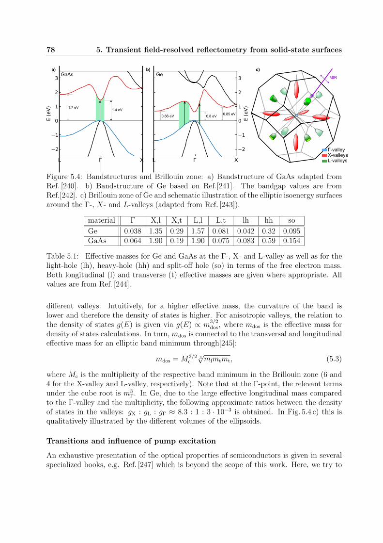
78 5. Transient field-resolved reflectometry from solid-state surfaces
Figure 5.4: Bandstructures and Brillouin zone: a) Bandstructure of GaAs adapted fromRef. [240]. b) Bandstructure of Ge based on Ref.[241]. The bandgap values are fromRef.[242]. c) Brillouin zone of Ge and schematic illustration of the elliptic isoenergy surfacesaround the Γ-, X- and L-valleys (adapted from Ref. [243]).
material Γ X,l X,t L,l L,t lh hh so
Ge 0.038 1.35 0.29 1.57 0.081 0.042 0.32 0.095GaAs 0.064 1.90 0.19 1.90 0.075 0.083 0.59 0.154
Table 5.1: Effective masses for Ge and GaAs at the Γ-, X- and L-valley as well as for thelight-hole (lh), heavy-hole (hh) and split-off hole (so) in terms of the free electron mass.Both longitudinal (l) and transverse (t) effective masses are given where appropriate. Allvalues are from Ref. [244].
different valleys. Intuitively, for a higher effective mass, the curvature of the band islower and therefore the density of states is higher. For anisotropic valleys, the relation tothe density of states g(E) is given via g(E) ∝ m
3/2dos, where mdos is the effective mass for
density of states calculations. In turn, mdos is connected to the transversal and longitudinaleffective mass for an elliptic band minimum through[245]:
mdos = M3/2c
3√mlmtmt, (5.3)
where Mc is the multiplicity of the respective band minimum in the Brillouin zone (6 and4 for the X-valley and L-valley, respectively). Note that at the Γ-point, the relevant termsunder the cube root is m3
Γ. In Ge, due to the large effective longitudinal mass comparedto the Γ-valley and the multiplicity, the following approximate ratios between the densityof states in the valleys: gX : gL : gΓ ≈ 8.3 : 1 : 3 · 10−3 is obtained. In Fig. 5.4 c) this isqualitatively illustrated by the different volumes of the ellipsoids.
Transitions and influence of pump excitation
An exhaustive presentation of the optical properties of semiconductors is given in severalspecialized books, e.g. Ref. [247] which is beyond the scope of this work. Here, we try to

5.2 Theoretical background 79
timescale (s)10-16 10-15 10-14 10-13 10-12 10-11 10-10 10-9 10-8 10-7 10 -6
fs ps ns μs
photon absorption
carrier-carrier scattering
carrier-phonon scattering
trap-assisted rec.
Auger rec.
radiative rec.
carrier diffusion
thermal diffusion
a) b)
electron
hole
interbandtransition
intrabandtransition
intersubbandtransition
bandgaprenormalization
bandfilling
so
lhhh
CB
VB
Figure 5.5: Photoexcitation processes and timescales: a) Schematical illustration of thepossible optical transitions and the effect of an excited carrier population. b) Timescaleof different processes leading to excitation (red), thermalization (blue) and carrier removal(dark gray) as well as heat diffusion (gray). The yellow area indicates the timescalescovered by our experiments (adapted from Ref. [246]).
capture the relevant aspects needed for the interpretation of our experiments in a simplifiedqualitative picture, as schematically illustrated in Fig. 5.5 a). We consider three types ofoptical transitions in a semiconductor: Firstly, interband transitions (red arrows) fromthe valence (VB) to the conduction band and secondly intersubband transitions (purplearrows) between subbands in the VB or CB, both driven by absorption of a photon. Finally,intraband transitions (blue arrows) within one subband for a charge carrier driven by theelectric fields. We neglect the influence of impurities and excitons.
In a semiconductor, there will be a number of thermally excited eletrons and holes inthe CB and VB, respectively due to the small bandgap. The intrinsic carrier concentrationis about 2 · 106cm−3 in GaAs[248] and 2 · 1013cm−3 in Ge[249]. Generally, which type oftransition dominates, depends on the photon energy. Around the bandgap energy, inter-band transitions dominate, which can be driven by the NIR pump, while for considerablylonger wavelengths intraband transitions play the major role, as for the MIR probe[250].The pump pulse excites electrons from the valence into the conduction band via interbandtransitions leading to charge densities on the order of 1018 ∼ 1019cm−3 for our experimentalconditions, much higher than the intrinsic densities. This changes the optical propertiesof the semiconductor for the MIR probe pulse in several regards, whose photon energy issignificantly below the bandgap. Firstly, the impact of intraband transitions increases dueto the much higher electron (hole) density in the CB (VB), which can be described viathe Drude model[250] introduced below. Secondly, intersubband transitions might opendue to the excited electrons and holes. For example, transitions from the split-off holeband (so) to the light hole (lh) or heavy hole (hh) band[251] might occur. For photonenergies around the bandgap, two additional effects would be visible, namely blocking oftransitions due to bandfilling and the renormalization of the bandgap due to the high free-

80 5. Transient field-resolved reflectometry from solid-state surfaces
carrier density[252, 253]. Most aspects of our measurements can be described within theDrude model even though intersubband transitions might play a role in certain wavelengthregions.
An overview of the different processes within semiconductors in our pump-probe experi-ments and their respective timescales is given in Fig. 5.5 b). After the initial excitation, thenon-equilibrium distribution of excited electrons and holes thermalizes via carrier-carriercollisions as well as interactions with the lattice via phonons. The former is usually muchfaster (10-100 fs)[246] which leads to the notion of separate effective temperatures of theexcited electrons (holes) in the conduction (valence) band and the phonon system in the so-called two-temperature model[254, 255]. The interaction between the excited carriers andphonon system and the equilibrium of their respective temperatures typically occurs on the100 fs-∼10 ps timescale[246]. The electron-phonon interaction is also responsible for scat-tering electrons from one conduction band valley to another (intervalley scattering)[256].Finally, recombination and diffusion lead to a reduction of the carrier density at the surfaceafter pump excitation. There are a number of different carrier recombination mechanisms,such as radiative band-to-band recombination and non-radiative Shockley-Read-Hall (de-fect/impurity assisted)[257, 258], Auger (three-carrier interaction)[259] and surface recom-bination (surface-defect assisted)[260, 261]. Recombination rates in semiconductors dependsignificantly on the sample parameters, such as impurity densities. The timescale for dif-fusion and recombination typically lies in the range of ∼10 ps-∼100 ns[246]. Althoughrecombination is not the central topic of this work, we will discuss surface recombinationin more detail below since it leads to a modification of the macroscopic excited carrierdistribution that can be measured in our setup.
Relation to experimental measurements
We express the permittivity of the sample that has been excited by the pump pulse εexc,as follows:
εexc(ω) = εunexc.(ω) + ∆ε(ω), (5.4)
where εunexc. is the permittivity of the unexcited sample and ∆ε is the pump-inducedchange. The photon energy of our probe pulses (0.2 eV-0.4 eV) is below the bandgaps ofGaAs and Ge and can therefore not drive interband transitions between the valence andconduction band. Hence, we only consider the intraband motion of excited electrons andholes in the conduction and valence band, respectively. This results in a Drude-type changeof the permittivity:
∆ε =−nfc,k · e2
meff,k · ε0· 1
ω2 − iωΓk
, (5.5)
where nfc is the free-carrier density, e is the electron charge, meff is the effective mass, ε0is the vacuum permittivity and Γ is the Drude scattering rate (i.e. momentum relaxationrate). The index k distinguishes electrons and holes and also valley contributions (seeSec. 5.3.3 below). The total ∆ε is therefore a sum of terms described by Eq. 5.5. Here,we only consider the case where the carrier density due to photoexcitation is much higher

5.2 Theoretical background 81
than due to any impurity doping, such that the density of electrons approximately equalsthe density of holes. Due to the denominator in Eq. 5.5, the Drude permittivity change islarger for longer wavelengths (i.e. THz pulses) which are therefore a particular sensitiveprobe of free-carriers.
More complete expressions that take bandgap renormalization and band occupationsinto account exist[253, 262], but are not necessary for our purposes. A complete quantummechanical first-order description of pump-induced changes is given in Ref. [263]. Our ap-proach neglects virtual intersubband transitions as well as interband transitions of electrons(holes) between different conduction (valence) bands. As has been shown in the frameworkof quantum mechanical calculations, even if interband transitions are taken into account,the Drude-term can still provide a decent functional description[262, 252, 263].
The pump-induced change of the optical properties can be measured by the changeof the reflectivity. For simplicity, we will first consider a homogeneously excited sample,which we refer to as homogeneous approximation. At normal incidence, the reflectivitycan be calculated by the Fresnel equation:
rexc =1− nexc
1 + nexc
, (5.6)
where nexc is the refractive index of the excited sample which is given by:
nexc =√n2 + ∆ε. (5.7)
Here, n is the refractive index of the unexcited sample and ∆ε is the change of the relativepermittivity given in Eq. 5.5. For small changes of the refractive index ∆n, the change ofthe reflectivity ∆r can be approximated by:
∆r = rexc − runexc. ≈−2∆n
(1 + n)2, (5.8)
i.e. for a real valued refractive index of the unexcited sample, the real and imaginary partof the refractive index change can be readily obtained from ∆r.
Macroscopic aspects
The pump pulse only has a finite penetration depth into the sample due to absorption whichmeans that also the excitation profile from the surface will not be homogeneous as assumedso far. Whether this inhomogeneity plays a role depends on the relative penetration depthlp of pump and probe pulses which can be calculated from the absorption coefficient (or thecomplex refractive index). For the NIR pump pulses in Ge we obtain lp ≈ 0.25µm, whereasthe sample is transparent for the MIR pulse. The opposite limit to the homogeneouslyexcited sample is a thin-film with conductivity σ and effective thickness d. The reflectivityis described by:
r =n1 cos θ1 − n2 cos θ2 − Z0σd
n2 cos θ2 + n2 cos θ2 + Z0σd, (5.9)

82 5. Transient field-resolved reflectometry from solid-state surfaces
d
real | imag. homo. exp.thin film
a) c)
b)
d
Figure 5.6: Influence of inhomogeneous excitation: a) ilustration of a homogeneous exci-tation compared with b) an inhomogeneous excitation with an exponential decay. c) Real(blue) and imaginary part (red) of the reflectivity change upon excitation for differentexcitation depths calculated from the transfermatrix approach (solid lines), the thin-filmapproximation (dashed-dotted line) and the homogeneous approximation (dashed lines).The calculations were performed on Ge at a wavelength of 5.5µm, surface excited electrondensity of 2.4·1018cm−3 using the transverse effective mass in the L-valley and a Drude-scattering rate of 2·1014Hz.
where n1 is the refractive index of the first medium (here air n1 ≈ 1) and n2 of the secondmedium and θ1 and θ2 are the angles with respect to the surface normal in medium 1 and2, respectively. Z0 = 1/ε0c is the vacuum impedance.
For an arbitrary refractive index distribution along the propagation direction of thebeam, the transfer-matrix approach can be employed[264, 223, 265]. Here the medium isdivided into thin slabs of length L with constant refractive index, as illustrated by the graydashed lines in Fig. 5.6 b). The electric field E(z + L) and magnetization field H(z + L)are related to the fields at position z via:(
E(z + L)H(z + L)
)= M ·
(E(z)H(z)
), (5.10)
where M is the transfer-matrix which is determined by the wavevector k′ = nω/c withinthe slab:
M =
(cos(k′L) sin(k′L)−k′ sin(k′L) cos(k′L)
). (5.11)
The transmission matrix Ms of a sample is simply given by:
Ms = MN · ... ·M2 ·M1, (5.12)
where Mi is the transmission matrix of the i-th slabs. The reflectivity r and transmittivityt can then be calculated from Ms. For a purely exponential decay of ∆n, analytic solutionsexist[266, 267].

5.2 Theoretical background 83
Figure 5.6 c) compares the real (blue) and imaginary (red) components of ∆r for the ho-mogeneous approximation (dashed lines), the thin-film approximation for different effectivethicknesses (dashed dotted lines) and the transfer-matrix calculation (solid lines, TMC)for different decay lengths of an exponentially decaying Drude contribution (as indicatedin b). As can be seen, only for very small decay length, the thin-film approximation andthe TMC agree. For increasing L, the transfer-matrix calculation converges towards thehomogeneous solution but generally yields smaller real and larger imaginary contributionsin comparison.
Over longer timescales (>1 ps), the excited electron distribution can not be consideredstatic but changes in the spatial profile are caused by diffusion. In 1D the diffusion equationis given by[268, 264]:
∂n(z, t)
∂t= D
∂2n(z, t)
∂z2− n(z, t)
τrec
, (5.13)
where D is the diffusion coefficient and τrec is the recombination rate. The carrier diffusioncoefficient is given by the Einstein relation:
D =µ
ekBT (5.14)
where µ is the carrier mobility given by µ = eτ/meff [269], which establishes a direct relationto the Drude-expression in Eq. 5.5. The carrier mobility determines the electrical conduc-tivity which explains the widespread use of the Drude-model in THz-TDS approaches forthe characterization of material properties[270]. We adopt here a simplified picture whereelectron and hole diffusion is treated as interdependent with an effective, so-called am-bipolar diffusion coefficient[264]. For a more precise description, electrons in the differentconduction band valleys and holes would have to be treated separately and any resultingelectric fields, that can e.g. lead to THz emission via the photo-Dember effect[271, 239, 272],need to be taken into account[273]. Despite the highly interesting aspects that would beadded in the context of our pump-probe experiments, any dependence of the mobility onthe excited charge density[268] or on the above-bandminimum energy for hot electrons[274]is neglected.
At the air-bulk interface, so-called surface recombination occurs that is caused by sur-face states which can help the recombination of excited carriers[260, 261]. In diffusionsimulations this leads to a special boundary condition, given by:
dn(0, t)
dt=
dJ(0, t)
dz+
dJs(0, t)
dz, (5.15)
where J = dn/dz and Js = −vs · n(0, t) with the surface recombination velocity vs. Ananalytic solution of the diffusion problem for a purely exponential initial distribution isavailable[268, 264], but suffers from convergence problems for small and large diffusiontimes. Therefore, we solve Eq. 5.13 by employing a Crank-Nicholson propagator, and usethe analytic solution for benchmarking.

84 5. Transient field-resolved reflectometry from solid-state surfaces
5.3 Experimental results
We are finally in a position where we can consider the experimental results. We willfirst look at the effect of surface recombination on the reflectivity on GaAs on the 10 pstimescale. Then, we investigate the buildup of collective excitations in GaAs on the 10 fstimescale and subsequently intervalley scattering in Ge on the 1 ps timescale. Finally, wediscuss the excitation density dependence of the Drude scattering rate.
5.3.1 Surface recombination dynamics in GaAs
tPP (ps)
a) b)
c)
𝜏=0 ps S (m/s) 0 2.5·104
2×S0
S0/2
tPP=12 ps
tPP=12 ps
real | imag. exp. data sim. sim. S=0
-Δr/
r (1
0-2
)
el. d
ensi
ty (
norm
.)Im
(-Δ
r/r)
(1
0-2
)
λ (μm)
Figure 5.7: The effect of surface recombination in GaAs: a) Measured real (blue dots)and imaginary (red dots) relative reflectivity change at 5.2µm. For comparison, simulationresults including diffusion with surface recombination (solid line) and without (dashedline) are shown. Simulation for a initial surface excited electron density of 6.3 · 1018cm−3,Drude scattering rate of 9 · 1013Hz, bulk carrier recombination rate of 30 ns and a surfacerecombination velocity of S0=2.5·104m/s. For comparison simulations with 2 ·S0 and S0/2are also shown. b) Simulated initial (black line) and diffused excited carrier density with(red line) and without (blue line) surface recombination at a pump-probe delay of 12 ps. c)Simulated surface recombination velocity dependence of the imaginary reflectivity changeat a pump-probe delay of 12 ps for different wavelengths.
Diffusion and recombination influence the dynamics of excited carriers on intermediate(few ps) to longer timescales and leave clear signatures in our measurements. Figure 5.7 a)shows the evolution of the real (blue open dots) and imaginary parts (red open dots) ofthe negative transient reflectivity change −∆r/r measured from GaAs at a wavelength of5.2µm. The real part shows a slightly delayed maximum and decays with a time constantof roughly 20 ps towards zero. In contrast, the imaginary part decays much quicker and∆r/r even reaches positive values around 10 ps, which might mistakenly be interpreted

5.3 Experimental results 85
as a sign of optical gain (Note that positive means below the gray line). This behavioris qualitatively uniform in the measured wavelength range from 3µm to 6µm. We haveconsistently observed this behavior in intrinsic and as well as p-doped GaAs samples.
In order to clarify to reason for the observation, we performed simulations where wesolve the diffusion equation (see Eq. 5.13) for the excited carrier density. The initial dis-tribution within the bulk is calculated from the experimental pump spectrum and thewavelength-resolved linear absorption coefficient of GaAs. The transient reflectivity changeis calculated in the frequency domain by the transfer-matrix approach. We use an initialexcited carrier density at the surface of 6.3 · 1018cm−3, and a Drude scattering rate of9 · 1013Hz. These two values determine the initial magnitude |∆r| and relative strengthof the imaginary component, respectively. The range of possible values is very well con-fined by comparison with the experimental data. A bulk recombination time of 30 ns hasbeen employed, which can, however, also be neglected for the considered timescale. Anambipolar diffusion constant of 25 cm2/s was used which is only slightly above the valueof 15-20 cm2/s of Ref. [275], but gave the best fit to the data. As can be seen in Fig. 5.7 a),using a surface recombination velocity S0 = 2.5 · 104m/s (solid lines), which is well withinthe range of values expected from literature (see further discussion of surface recombina-tion below), excellent agreement with the experimental data is observed. By comparisonwith simulations using a two times higher (lower) S0, it can be seen that the surface re-combination velocity in our simulations is relatively well defined by the slope of the initialdecreases and the maximum value of the positive imaginary part in the experimental data.In contrast, the simulations without surface recombination (thick dashed lines in Fig. 5.7 a)show a much slower decay of −∆r/r and do not exhibit a transient positive imaginary part.Remarkably, this observation indicates that the decay of the transient reflectivity can beunderstood in terms of diffusion and surface recombination alone without having to invokebulk recombination. Similar findings have been made e.g. in Ref. [251].
In order to understand the reason for the positive imaginary transient relative reflectiv-ity change, the carrier density profile within the bulk (surface at z=0), is shown in Fig. 5.7 b)at tpp = 0 (black line) and at tpp = 12 ps with (red line) and without (blue line) surfacerecombination, respectively. Interestingly, the calculated density profile with surface re-combination exhibits a peak density not at the surface but at a certain distance withinthe bulk. This profile is responsible for the transient positive imaginary part. The effect isalso expected to be more pronounced in our measurements than in THz-experiments, dueto the much smaller wavelength.
The question remains, for which ranges of surface recombination velocity S, the tran-sient positive imaginary reflectivity change can be observed. The simulated dependence ofthe imaginary part of −∆r/r on S at a pump-probe delay of 12 ps is shown in Fig. 5.7 c)for different wavelengths. The other parameters are kept at the values stated above. Allcurves only significantly decrease above 103 m/s and yield a zero-crossing around 104 m/s.For lower wavelengths the zero-crossing is reached at smaller S. For S > 105m/s, thenegative transient reflectivity change flattens again at negative values. The magnitudeof I(−∆r/r) is larger for longer wavelengths. These findings are in agreement with ourwavelength-resolved experimental data.

86 5. Transient field-resolved reflectometry from solid-state surfaces
The neglect of bulk recombination can be understood by looking at the timescalesof the different processes. The Auger recombination coefficients in GaAs are about 6 ·10−31cm6s−1[276]. Auger recombination could play a role at carrier densities obtained inattosecond transient absorption spectroscopy (ATAS) experiments of about 1021cm−3[277],where it reaches down to the ps-timescale. However, the excited carrier densities in ourexperiment of about 1018− 1019cm−3 result in ns-recombination times, two to three ordersof magnitude above the timescales considered here. Similarly, trap-assisted recombinationin the bulk might contribute on the ps-timescale in extremely defect-rich nanocrystallinesamples used for ATAS-experiments[241], but is expected to unfold on the ns-timescale forour single-crystalline wafer with no to moderate doping defects[278].
Surface recombination affects the excited carrier lifetime and the performance of opto-electronic devices especially for III-V semiconductors such as GaAs, InGaAs, GaSb and InPsince surface oxidation does not provide a passivation layer[260] and therefore, the wholesurface can be considered as consisting of defects unlike e.g. silicon. Measured surfacerecombination velocities of untreated GaAs surfaces lie in the range of 104 − 105m/s[279],which is consistent with the value in our simulations of 2.5 · 104m/s. Various surface pas-sivation techniques exist, such as sulfur passivation, atomic layer deposition or plasmatreatment which leads to S below 5 · 102[280]. At such low values of S the impact ofsurface recombination for our measurements would be drastically reduced, as can be seenin Fig. 5.7 c). Surface passivation of our samples, might therefore be an important step inthe improvement of the measurement approach to investigate bulk dynamics. In contrast,germanium yields already lower intrinsic surface recombination velocities on the order ofS ∼ 2 · 103m/s[261].
For our measurements, we will study the 100 fs dynamics in GaAs. For the investi-gation of few-ps processes we focus on Ge. In the interpretation of the experiments, ithas to be considered that the results might be slightly influenced by diffusion and surfacerecombination especially for longer pump-probe delays.
5.3.2 Buildup of collective excitations in GaAs
After photoexcitation, buildup of collective excitation such as plasmons does not occurinstantaneously but a certain amount of time is required until correlations between excitedcarriers are established, which can be resolved in our experiments. Figure 5.8 a) shows therise of the real part of the reflectivity on GaAs integrated over the MIR spectrum, for aslightly lower excitation than in the previous section. A Fermi function (red line) is fittedto the experimental data (open dots) and yields a 20-80 % risetime of 82 fs. A comparisonof the wavelength resolved R(−dr/r) at pump-probe delays of 12 fs (red open dots) and175 fs (blue open dots) is shown in Fig. 5.8 b), which are marked by arrows in in a). For thelarger delay (blue open dots), the experimental response shows a characteristic increasewith wavelength which can be described fairly well by a Drude-term (blue solid line, seeEq. 5.5) in the homogeneous approximation. An excited carrier density of 1.2 · 1018cm−3 isobtained. In contrast, the lower delay (red open dots) exhibits a rather flat response.
As shown by Huber et al.[227, 228], the above observations can be interpreted in terms

5.3 Experimental results 87
inte
gra
ted
Re(
-Δr/
r)
Re(
-Δr/
r) (
%)
exp.fit
a) b)12 fs175 fs
Drude
Figure 5.8: Buildup of the reflectivity from GaAs: a) Normalized real part of the ex-perimentally measured relative reflectivity change (dots) integrated over the wavelengthrange 3.5-6.4µm and Fermi-fit (red). Dashed lines indicate the determined 20-80% risetime of 82 fs. b) Wavelength resolved real part of ∆r/r for a delay of 12 fs (red dots anddashed line) and 175 fs (blue dots and dashed line). For the later delay the calculatedDrude expression in the homogeneous approximation is also shown (blue solid line) whichyields an excited carrier density of 1.2·1018cm−3 and a plasma oscillation period of ∼60 fswhich would yield an expected buildup time of roughly 96 fs.
of the buildup of dressed particles and the formation of Coulomb correlations in the pho-toexcited electron-hole plasma, which manifests itsef in the plasmon response described bythe Drude model.
In order to understand how the measurements reveal information about the particleinteractions, we have to briefly consider charge interactions in solids. The presentationhere closely follows Ref. [227]. In a solid, the Coulomb interaction is altered by many-bodyeffects and around each charge carrier a screening cloud of opposite charge is formed, whichtogether is also referred to as dressed particle. The bare Coulomb interaction potentialbetween two charges in momentum space 4πe2/q2 (q is the momentum transfer) is alteredby the dielectric function εq which results in the effective interaction potential Wq[227]:
Wq(ω, tD) =4πe2
εq(ω, tPP)q2, (5.16)
where a dependence on the pump-probe delay tPP has been added in order to account forthe dynamical evolution of εq after pump excitation of the sample. With optical experi-ments εq=0 is measured. The Coulomb interaction between dressed particles becomes timedependent through the ω dependence in frequency space. The real part of the dielectricfunction shows how much the bare charges are screened, while the imaginary part is pro-portional to the energy loss of the carriers. The latter is also the basis for most calculationsof inelastic electron scattering in solids[281, 282].
Huber et al.[227] performed optical-pump-terahertz-probe (OPTP) experiments also onGaAs. For similar excited carrier densities (2 · 1018cm−3), they found buildup times of the
88 5. Transient field-resolved reflectometry from solid-state surfaces
plasmon on the timescale of 70-100 fs close to our observation. The finite delay for thebuildup of correlations and resonances can be described by calculations using nonequilib-rium Green’s functions[228]. The time-delay for the buildup of the plasmon peak τcor ison the order of the plasmon oscillation period Tpl[228], more precisely τcor ≈ 1.6 · Tpl. Ourobservations are in close agreement with this finding: The Drude response takes about 82 fsto buildup compared to the predicted 96 fs, deduced from the plasma oscillation period of60 fs.
To be precise, for our MIR wavelength region the pump-probe response is not completelydescribed by the intraband picture underlying the Drude model. Ganikhanov et al.[251]found in pump-probe experiments that intersubband transitions from electrons in the split-off band into hole states in the light and heavy hole band occur around 3.8µm and 3.1µm,respectively. These transitions are also the basis of split-off band MIR detectors[283].However, the results of Ref. [251] also suggest that in reflection the response is dominatedby free-carriers and that intersubband transitions should not play a role beyond 4µm. Inour data, while oscillations in the reflectivity between 3-4µm could provide a hint of thesetransitions, they could not clearly be resolved. Upcoming experiments with an improvedSNR, higher spectral resolution and removal of the CO2 absorption peak could potentiallybe sensitive enough to identify their influence on the transient reflectivity.
Attosecond transient XUV absorption measurements pumped by few-cycle NIR pulseshave been performed on GaAs by Schlapefer et al.[277] at excited carrier densities of120 − 1021cm−3. They found that in this regime interband transitions as well as intrabandmotion lead to carrier excitation which results in a non-linear increase of carrier densitywith intensity. The transient decrease of the transmission of highly pumped solids hasbeen applied in Ref. [284] as a gating method for laser pulse reconstruction over a broadwavelength range. It would be interesting to investigate how the risetime of the plasmonresponse evolves with carrier densities up to 1021cm−3, since there, the plasma frequencywould lie on the few fs scale which corresponds to the expected temporal resolution ofour measurement setup. The required intensities might be reachable after a change of thesetup and tighter focusing.
5.3.3 Intervalley scattering in Ge
We observed a striking difference of the transient reflectivity ∆R/R between Ge and GaAson the few ps timescale, which can be explained by the intraconduction band dynamics ofexcited electrons in Ge, especially intervalley scattering, as discussed below. The compar-ison between Ge and GaAs is shown in Fig. 5.9 a). The signal on GaAs (blue open dots)rises rapidly within 100 fs and subsequently decays with a time constant of around 20 ps.In contrast, on Ge (red open dots) the reflectivity reaches its maximum only after about3 ps. On the other hand, for longer delays on the 50 ps timescale, the dynamics is overallsimilar, as can be seen in the inset. We have consistently observed this behavior on Ge inour measurements over several weeks of measurements. An explanation for the evolutionof the transient reflectivity in GaAs and Ge on the short timescale can be obtained basedon Fig. 5.4 and the related discussion in Sec. 5.2.

5.3 Experimental results 89
total
a) b)
calculation Ge
GaAs
Ge
Γ
X
L
-ΔR
/R (
norm
.)
1
00 50
Figure 5.9: Intervalley scattering in Ge: a) Comparison of the experimentally measuredrise in reflectivity between Ge (red dots) and GaAs (blue dots). The lines are a guide tothe eye, the curves are normalized. The black line shows the calculated Drude reflectivitychange for Ge based on the evolution of the conduction band valley occupations simulatedin Ref. [237] for an excitation with ~ω = 1.5 eV and the effective masses from Ref. [244].The inset shows the long term evolution with a double-exponential fit (solid lines). b)Contribution of the individual conduction band valleys to the effective Drude density,defined as the carrier density divided by the relative transverse effective mass. The insetshows the valley occupations extracted from Ref. [237] assuming a recombination timeconstant of 20 ps.

90 5. Transient field-resolved reflectometry from solid-state surfaces
For GaAs the interband excitation by the NIR pump beam occurs from the top of thevalence band into the bottom of the conduction band around the Γ-point, as shown inFig. 5.4 a). Since the other bandgap minima at the L- and X-valleys lie significantly higherin energy, most of the electron population is expected to stay centred around the Γ-point.Moreover, the holes are expected to quickly relax into the heavy-hole band.
In contrast for Ge, as can be seen in Fig. 5.4 b), the electron excitation occurs awayfrom the Γ-point, higher up into the valence band from which the X- and L-valleys areaccessible via horizontal transitions mainly through electron-phonon scattering. The insetof Fig. 5.9 b) shows the time evolution of the electron population in the different valleysafter pump excitation extracted from Ref. [237] based on Monte-Carlo simulations whichmodel the electron-phonon interaction via deformation potentials. In their simulations, theexcited carrier density is around 1 · 1018cm−3 and the photon energy is 1.5 eV. As can beseen, the initial population around the Γ-point (gray line) is quickly scattered within 100 fsinto the X-valleys (red line) and L-valleys (blue line) due to the much higher availabledensity of states. At first, most of the excited electrons end up in the X-valley since therethe density is highest. However, within 4-5 ps almost the whole electron population willrelax to the L-valley as it constitutes the conduction band minimum. For better agreementwith the experimental data, we added an exponential decay of the effective excited carrierdensity with τ = 20 ps which represents mostly diffusion and surface recombination, asdiscussed in Sec. 5.3.1 above.
A qualitative approximation for the evolution of the transient reflectivity is obtainedby combining the extracted time-dependent conduction band valley populations with thetransverse effective masses shown in Tab. 5.2. We use the sum of three Drude terms(Eq. 5.5) to represent the contribution of the Γ-, X- and L-valleys. For each valley, aneffective Drude density is defined as the ratio of valley population density and transverseeffective mass, which is shown in Fig. 5.9 b). Since mX,t/mL,t ≈ 3.6, the total effectivedensity (black line) rises with the population transfer from X- to L-valley. As can be seenin Fig. 5.9 a) with this model (black line) the slow increase of the transient reflectivity inGe can be reproduced. Here, we use an excited carrier density of ∼ 5 · 1018cm−3 and aDrude scattering time of 10 fs, but the exact values are not important for the qualitativeshape.
Several aspects of the above model need to be discussed. First of all, we neglect thehole contribution, which can be justified by the simulation results of Ref. [237], whichshow that the hole contribution gets localized in the heavy-hole band within a fractionof a picosecond and therefore doesn’t contribute to the few-picosecond time-dependence.Secondly, the initial peak of the simulated reflectivity around tpp = 0 which can be at-tributed to the Γ-valley contribution is absent in the experimental data. This can againbe explained by looking at Fig. 5.4 b) considering that the initial excitation occurs into anon-parabolic region of the conduction band. There, the effective mass is expected to beconsiderably larger than at the Γ-point which suppresses this contribution to the effectiveDrude density. An increased effective mass has also been predicted for strong-field exci-tation of semiconductors[252, 262, 263] which has been attributed to the same effect[252].Finally, the use of only the transverse masses is a severe approximation. In principle, for

5.3 Experimental results 91
each separate degenerate valley the effective mass would need to be calculated from the po-larization vector of the MIR and the present assumption overestimates the effective Drudedensity. However, tor the given surface orientation (111) and normal incidence of the MIRprobe beam, as can be seen in Fig. 5.4 c), two sub-L-valleys are always driven transverselyirrespective of the polarization orientation. A slight dependence on whether an X-valley isdriven transversely could exist and might be interesting to investigate further.
Intervalley scattering is a fundamental process for the relaxation excited carriers inthe conduction band and was invoked for the explanation of optical-pump optical-probeexperiments of Ge already more than three decades ago[234, 235, 236]. The timescaleof the X-L-intervalley scattering of around 2-3 ps is consistent with attosecond transientreflection measurements on Ge where a time constant of 3.2±0.2 ps was deduced[285]. Inthe OPTP experiments of Ref. [269] the same evolution of the transient reflectivity seemsto have been observed where it was, however, not interpreted (there also the excited carrierdensity seems to be overestimated through the use of the heavy-hole mass as effective mass).Theoretically, a similar conduction band valley population transfer has been simulated bythe use of deformation potentials[237, 238, 239]. Since there are countless theoreticaland experimental pump-probe investigations on semiconductors, especially on Ge, it isalmost certain that many more studies, that are not cited here, have observed very similarphenomena. Overall, the main reason for the observed delayed buildup of the reflectivity isthat the electrons are excited way above the conduction band minimum towards which theyrelax via intervalley scattering which leads to a change of the effective mass. It can thereforebe generalized to other semiconductors. For example, in GaAs related dynamics have beenmeasured when exciting the sample with a photon energy well above the bandgap (e.g.3.1 eV)[286]. Nevertheless, our measurements present a particularly clear demonstrationof the power of the concept of effective masses in solids.
5.3.4 Excitation-density dependence of the Drude scattering rate
Our setup can not only measure changes in the reflected intensity, but provides moreinformation in terms of the complex valued reflectivity change for the electric field, asdiscussed above. Figure 5.10 a) shows the few picosecond evolution of ∆r/r on Ge. Whilethe real part (blue open dots) keeps rising after the sharp initial increase around tpp = 0,the imaginary part (red open dots) quickly flattens and even starts to decrease.
As a side note, slight oscillations seem to be observable especially on the imaginary partwith a period of approximately 375 fs. The sudden excitation of electron into the conductionbands affects the interatomic binding forces and therefore can lead to the generation ofcoherent phonons in Ge which is detectable as oscillations in the reflectivity[287, 288][289] under similar excitation densities. However, a significantly faster oscillation period of∼100 fs would be expected. Potentially, future, more sensitive experiments could be ableto detect such oscillations.
We therefore focus on the difference in the increase of real and imaginary parts inFig. 5.10 a) which gives information on the scattering rate. For feasibility, the homogeneousapproximation is applied, but the eventual shortcomings discussed in Sec. 5.2 have to be

92 5. Transient field-resolved reflectometry from solid-state surfaces-Δ
r/r
(10
-3)
Drude el. density* (1019cm-3)
Dru
de s
catt.
rat
e* (
TH
z)
fitavg.
0.5⋅10-4Hz/cm3
a) b)
Figure 5.10: Drude scattering rates in Ge: a) exemplary evolution of the real (blue) andimaginary parts (red) of the reflectivity change in Ge at 5µm. b) Dependence of the Drudescattering rates on the Drude density for Ge both evaluated using the approximation for anhomogeneously excited sample (marked by *) at a pump-probe delay of 1.5 ps. The averageand standard deviation calculated in the wavelength range from 4.5-5.5µm are shown(black open dots and errorbars) together with the results of a Drude fit (red crosses). Eachdatapoint represents a separate measurement. The data was taken on different occasions.The blue dashed line indicates a linear dependence for lower densities.
kept in mind. In the homogeneous approximation and within the Drude model, it can beshown that for small relative changes of the refractive index in first order Taylor expansionthe following relation holds:
I(∆r/r
)R(∆r/r
) ≈ Γ
ω, (5.17)
if the unperturbed refractive index is real in the frequency range of interest. R and Idenote the real and imaginary parts and Γ is the Drude scattering rate. The evolutionof the real and imaginary part of ∆r/r after the sharp initial increase around tpp = 0,seems to suggest that while the effective density increases through intervalley scattering,the Drude scattering rate decreases. The measurement therefore shows that the Drudescattering rate under strong excitation is time-dependent, which is mostly caused by thedependence on the excited carrier density[266] but also the temperature[290].
Here, we investigate the dependence of the extracted Drude scattering time on theexcited carrier density, as illustrated in Fig. 5.10 b). The mean (open dots) and standarddeviation (errorbar) of the Drude-scattering time in the homogeneous approximation fromGe is shown, evaluated at tpp = 1.5 ps, when most of the density is in the L-valley and in thewavelength range from 4.5µm to 5.5µm. Moreover, the results of a Drude fit in the samewavelength region is shown (red cross). Excellent agreement between both approaches isobserved. Note that the effective Drude density might be underestimated by up to a factorof 4 by the use of the transverse effective mass, as discussed above. The low densities

5.3 Experimental results 93
between 0.5 − 1 · 1019cm−3 suggest an initial linear increase of the Drude scattering rate,as indicated by the blue dashed line. On the other hand, the highest datapoints seemto indicate saturation at a scattering rate slightly below 500 THz (2 fs). More systematicintensity scans, that could be performed at a single pump-probe delay, would be highlydesirable.
The topic of Drude scattering times in strongly pumped semiconductors and especiallythe transient excited carrier density dependence is highly debated ( Ref. [266] and referencestherein). Most of the work concerns silicon but the qualitative behavior is expected tobe similar to germanium such that we can relate it to our experiments. According toRef. [266], for low densities, carrier-phonon scattering is the major contribution whichleads to a quasi-constant Drude scattering time on the order of 200 fs. The carrier-carrierscattering rate which linearly increases with carrier density starts to dominate above ∼ 5 ·1017cm−3 up to around 5·1019cm−3 where it reaches a maximum (20 fs) due to the reductionof available final states for electron-electron and hole-hole scattering. The qualitativedependence is consistent with our experimental data but we extract even lower carrierscattering times. Upon a further increase of the density, the rate is expected to decreaseagain as the number of available final states reduces further, but it is not clear whether allrelevant effects in this regime where considered in Ref. [266]. The linear increase of thescattering rate with carrier density in the intermediate regime seems to be well accepted andhas been confirmed for example by another experimental study that additionally includedthe temperature dependence[290]. However, the question of how low the Drude scatteringtime can reach is debated, since several other measurements have also reported values onthe 1 fs scale[291, 253] or a much faster increase of the scattering rate with excited carrierdensity[292].
Within the framework of TDDFT simulations of pump-probe experiments in silicon[252,262], Drude fits to the calculations yielded scattering times on the 1 fs timescale eventhough no explicit collision effects were taken into account in the model. There, it wasargued that interband transitions, excited electrons or holes which undergo intersubbandtransitions driven by the probe pulse, are responsible for the finding[262]. The role ofinterband transitions on the apparent Drude response was further investigated and con-firmed in Ref. [263]. In this case, the classical interpretation of the Drude model where aparticle is considered that travels through the crystal and randomly scatters, becomes ques-tionable and extensions for explicit inclusion of interband transitions would be desirable.Regarding electron-phonon scattering times, first principle calculations have shown thathot electrons in GaAs, i.e. electrons significantly above the conduction band minimum,exhibit carrier-phonon scattering times also down to the 1 fs timescale[293]. These studiesshow that additional effects not considered in Ref. [266] could contribute to the effectiveDrude scattering times.
For our experimental results, as shown in Fig. 5.6, with the employed approximation ofan homogeneously excited sample, the imaginary part of ∆r is overestimated compared tothe real part, which results in a too high value for the extracted scattering rate. This canlikely only be accounted for with macroscopic simulations. Moreover, the role of interbandtransitions, which are especially expected for the hole bands would need to be identified, as

94 5. Transient field-resolved reflectometry from solid-state surfaces
discussed above. Finally, as pointed out by Ref [266], a reliable extraction of the scatteringrate in pump-probe experiments based on intensity measurements, ideally includes theplasmon peak in the detected wavelength range, since the scattering time determines itswidth. Even though this requirement might be relaxed for our field resolved measurements,extending the wavelength range by changing the nonlinear crystals in our setup would bedesirable for further investigation of scattering times in highly excited semiconductors.
5.4 Conclusion and Outlook
a) b)
4
2
0
-2
-4
3.25 μm4.75 μm
Figure 5.11: Transient reflectivity change from a graphene sample: a) Wavelength resolvedtransient reflectivity change. b) Evolution of the reflectivity change at 3.25µm (blue dots)and 4.75µm (red dots). The solids line are smoothed using a Savitzky-Golay filter andintended as a guide to the eye.
In conclusion, this chapter describes a newly developed field-resolved NIR-pump MIR-probe setup based on electro-optic sampling. To our knowledge, with a probe spectrumfrom 3-6µm, the presented experimental results constitute the shortest-wavelength field-resolved pump-probe reflectometry measurements using EOS ever reported.
Theoretically, the foundations for the understanding of pump-probe experiments onsemiconductors are discussed. Emphasis is laid on the description of effective masses andintervalley processes as well as macroscopic aspects.
Experimentally, we show that the decay of the transient reflectivity on the 10-100 pstimescale is dominated by diffusion and surface recombination. Furthermore, measure-ments on the rise of the reflectivity from GaAs reveal the buildup times of collectiveplasmon excitations on the 100 fs timescale in agreement with earlier studies[227]. FromGe a few picosecond increase of the transient reflectivity is observed, which can be ex-plained by the intervalley scattering and the different transverse effective masses. The

5.4 Conclusion and Outlook 95
same measurements also indicate an increased effective mass within more than few 100 fsafter photoexcitation due to excitation into a non-parabolic region of the bandstructure.Finally, the dependence of the scattering rate on the excited carrier density is discussed.
The measurements shown here, were mostly intended as a demonstration of the capabil-ities of the setup and variety of effects to be studied, but are, nevertheless, of significancefor the field of semiconductor optoelectronics. Considerably improved data is expectedafter the currently performed updates of the setup, purging of the experiment in order tosuppress the CO2-absorption peak and most notably the implementation of an active laserintensity stabilization. Furthermore, an increase of the pump power will enable studiesof extremely highly excited semiconductors as well as nonlinear excitations. Moreover,expansion of the wavelength region might enable many more interesting studies. Withthese improvements, several important aspects might be clarified such as the identifica-tion of intersubband transitions of photoexcited carriers discussed above, or the excitationdependence of the Drude scattering rate.
Apart from semiconductors, a significantly higher diversity of systems can be studiedwith our setup such as 2D-structures. Figure 5.11 a) shows the wavelength resolved tran-sient reflectivity from a graphene sample on a silicon nitride substrate provided by theAtwater group (Caltech). As can be seen, the dynamics unfolds on a much faster timescale(500 fs) compared to semiconductors. Moreover, the dynamics is not qualitatively uniformfor different wavelengths (see Fig. 5.11 b). Graphene is especially interesting, because itallows to tune the Fermi-level and thereby the effective bandgap for interband transitionsin the few 100 meV region, which is reachable with our wavelengths, by an external biasvoltage[294]. Our setup was partly build to investigate electron-plasmon coupling whichcould allow gain in the MIR (also Ref. [294]). Moreover the wavelength region coversthe range of almost all stretching vibrations in functional groups in molecules (2500 nm-6500 nm)[295]. In combination with the pump-probe scheme, a vast variety of photochem-ical reactions can be investigated. Overall, we believe that the developed setup will enablemany interesting applications from femtosecond- to picosecond timescales.

96 5. Transient field-resolved reflectometry from solid-state surfaces

Chapter 6
Phase matching of HHG withionization reshaped few-cycle pulses
6.1 Introduction
High-harmonic generation (HHG) is a nonlinear process during which an intense laser pulseis focused into a medium to non-perturbatively generate high harmonic orders of the fun-damental photon energy[10, 11, 296] (see Chap. 2). The emitted high-harmonic radiationexhibits two key properties. Firstly, it possesses longitudinal and transverse coherencethrough the coherent generation process. Secondly, HHG is intrinsically synchronized tothe driving laser field on a sub-cycle timescale and has therefore become one of the foundingpillars of attosecond science[150, 9, 8, 297, 122, 298].
High-harmonic radiation is generally emitted in sub-cycle bursts, forming an attosec-ond pulse train (APT). The generation of isolated attosecond pulses (IAPs) by extractinga single sub-cycle burst has been made possible through advances in laser technology andwaveform control of the driving laser[299, 7], extending the resolution of pump-probe spec-troscopy to the electronic timescale (1 as=10−18s)[12, 300, 301, 13] (see Sec. 2.3.3).
Isolated attosecond pulses based on HHG have allowed a vast number of experiments,such as the studies on the fundamental timing of the photoemission process in atoms[14,302, 155], molecules[84], liquids and solids[15, 303]. Moreover, the bound-state dynamics onits fastest timescale has been measured by attosecond transient absorption[304, 177, 305,306, 307, 308, 277, 309, 310, 311] and very recently attosecond transient reflection[176,312]. In the context of this thesis, the attosecond streaking measurements on isolatednanospheres[313, 314] as well as the reconstruction of the near fields around a nanotipon attosecond temporal and nanometer spatial scales [25] deserve a special mention. Thelatter experiment has been performed within the framework of this thesis and published inRefs. [26, 27], and several aspects of it are discussed in Chap. 7. For completeness, whilealso APTs have extensively been used in attosecond photoemission experiments[150, 315,316, 317, 318, 319, 320], for general applications the temporal resolution is given by thefew fs duration of the APT[321, 322, 323]. We will therefore focus here on the generation

98 6. Phase matching of HHG with ionization reshaped few-cycle pulses
of IAPs.In recent years, another source of ultrashort (soft) x-ray pulses has emerged in the form
of x-ray free-electron lasers (XFELs). XFELs are especially appealing due to the enormousphoton flux compared to HHG-based sources[324]. However, while progress is being madeto produce sub-fs pulses[325] and to overcome pulse fluctuations problems[326], the timingjitter between the XUV pulse and external laser sources is on the order of few fs[327] and,generally, single shot-techniques are necessary[328, 326, 325]. Most imortantly, XFELscan only be realized in dedicated large-scale facilities[329]. HHG will therefore remain animportant tool for attosecond science even in the long-term future.
So far, most HHG-based attosecond experiments have been performed at photon ener-gies of around 100 eV and below. Especially promising are, however, pump-probe experi-ments in the so-called water window between the K-shell absorption edges of carbon andoxygen (284 eV-543 eV)[330, 132]. In this photon energy range water is transparent for softx-ray pulses, which would allow the investigation of biological molecules in their naturalenvironment and therefore the fundamental processes of life with unprecedented temporalresolution.
In recent years, an increasing number of research groups has shown HHG potentiallysupporting IAPs in the water window[331, 132, 332, 322, 28, 333], and lately IAP generationhas been demonstrated by attosecond streaking[334]. However, the problem is that HHGat higher photon energies becomes inefficient for two reasons (see Chap. 2). First, sinceionization limits the maximum intensity for which phase matching of the HHG processis possible, longer driving wavelengths are required. This, however, dramatically reducesthe rescattering probability due to the longer excursion of the electron before recollision.Secondly, the phase-matching process itself becomes increasingly difficult over longer dis-tances with increasing harmonic order[28]. This opens the quest to explore new regimes ofHHG phase matching[324, 335]. A recent study has demonstrated that these limitationsmight partly be overcome in the so-called overdriven regime, where ionization-inducedplasma leads to severe pulse reshaping of the driving laser pulse[28] strongly influencingthe HHG buildup. A demonstration of IAP generation as well as a detailed analysis of thephase-matching conditions was, however, missing.
In this chapter, we present experiments demonstrating the generation of IAPs at 80 eVthrough HHG in argon and neon by attosecond streaking driven by 750 nm laser pulses.With the help of experimental signatures and numerical calculations, it is shown that theIAP generation process in argon takes place in the overdriven regime. An extended phase-matching expression for the HHG dipole contribution is derived that takes into account theblue-shift of the driving laser. With this expression the description of HHG phase matchingeven under extreme pulse reshaping conditions is possible. We show through simulationsthat the mechanism is important for the phase matching of long-wavelength, tightly-focusedlaser beams in high-pressure gas targets, which are currently being employed for scalingisolated attosecond pulse generation to water window photon energies.
The structure of this chapter is as follows: First, the fundamentals of HHG and phasematching are reviewed. Then, the experimental setup and the experimental results aredescribed. Thirdly, through simulations and comparison with experiment the HHG regime

6.2 Experimental section 99
for argon is identified. The fourth section describes the extended phase-matching expressionand applies it to the simulations. Then, the simulations for longer wavelength driversare discussed and the importance of the blue-shift contribution to the HHG dipole isdemonstrated. Finally, a short outlook and conclusion is given. The results of this chapterhave been published in Ref. [29] and the presentation here closely follows the one giventherein.
6.2 Experimental section
6.2.1 Experimental setup
The setup for attosecond streaking spectroscopy at the Attosecond Science Laboratory ofthe King Saud University is shown Fig. 6.1. A description of this setup has been given inRef. [27], which we will closely follow in this section and to which we refer for further details.The pulses used in the experiment are delivered by a commercial laser system consistingof an oscillator (Spectra-PhysicsTM ; rainbowTM DFG seed) pumped by a solid-state diodelaser (Coherent Inc.; Verdi V6 UNO) as depicted in Fig. 6.1 a). The carrier-envelope offsetfrequency is measured and controlled in a CEP module (Menlo Systems GmbH, XPS 800Femtosecond Phase Stabilization) via a feedback to the pump power. The oscillator delivers4 nJ pulses at a repetition rate of 75 MHz in the spectral range between 675 nm and 930 nm.The pulses are further amplified by a ten-pass chirped-pulse amplifier (Spectra-PhysicsTM ;FEMTOPOWERTM compact PRO HP/HR 3 kHz) which is pumped by a pulsed solid-statediode laser (Photonics Industries International Inc.; DM 30 Q-Switched DPSS Laser). Afterthe fourth pass, a Pockels cell selects pulses at a repetition rate of 3 kHz and an acousto-optic programmable dispersive filter (AOPDF; DAZZLER by FASTLITE) allows shapingof the pulse spectrum and phase. After the amplification, the pulses are compressed via agrating compressor to approximately 25 fs with an energy of 800µJ. A small portion of thepulses is sent into a carrier-envelope phase (CEP) module (APS800 by Menlo Systems),which stabilizes long-term drifts via feedback-controlled insertion of one of the prisms inthe stretcher. The pulses are spectrally broadened in a hollow-core fiber filled with neonat about 2 bar to a width of 300 nm centered at 750 nm, supporting sub-two-cycle pulses.The pulses are compressed by a set of chirped mirrors (Ultrafast Innovations PC70). Apair of fused silica wedges is used for dispersion fine tuning. Finally, phase-stable few-cyclepulses with 450µJ at 3 kHz repetition rate are delivered to the experiment.
The vacuum beamline is shown in Fig. 6.1 b). The laser is focused with a concavemirror (f=75 cm) into the HHG chamber. An iris is used to regulate the pulse power thatreaches the experiment. The gas target consists of a hollow metal tube with laser-drilledentrance and exit holes and has a length of roughly 1.5 mm. It is kept at a constantgas pressure of few 100 mbar of either neon or argon by controlling the gas flow. XUVand fundamental beam are spatially separated by using a concentric Zr-foil filter and thefocusing double mirror. The Zr-foil blocks the fundamental spectrum in the beam centerthat hits the inner mirror. The inner part of the double mirror (custom-made, Ultrafast

100 6. Phase matching of HHG with ionization reshaped few-cycle pulses
Figure 6.1: Overview of the experimental setup: a) the laser system consists of the CEP-stabilized oscillator that seeds the chirped-pulse amplifier which contains another slow-loopCEP-stabilization system. The amplified pulses are spectrally broadened in a noble-gas-filled hollow-core-fiber and subsequently compressed to below 4 fs using chirped mirrors.b) Fused silica glass wedges are used for fine-tuning of the dispersion. The laser beam isfocused into the HHG chamber of the attosecond vacuum beamline for XUV generation inthe HHG target. An iris is used to adjust the IR power in the experimental chamber. TheXUV-filter and the two-component multilayer XUV-mirror spectrally select the isolatedattosecond pulse. The synchronized XUV and IR pulses are focused into the streaking gas-target (neon) and photoelectron momenta are detected using a time-of-flight spectrometer.The double-mirror can be removed from the beampath to allow spectral characterizationof the XUV pulses (adapted from Refs. [27, 29]).

6.2 Experimental section 101
Innovations) has a special multilayer coating to reflect XUV with a bandwidth of 6.4 eVand a flat spectral phase around a central energy of 80 eV. The outer mirror substrate(fused silica) is coated with 10 nm of B4C in order to achieve a reflectivity of about 10 %for the driving laser pulse. The position of the outer and inner mirror can be changedwith nanometer-precision by a closed-loop piezo stage (PI Hera 620). The double-mirrorfocuses both beams into a neon gas jet produced by the streaking target, and a time-of-flight-spectrometer (STEFAN KAESDORF ETF10) is used to record the kinetic energy ofthe generated photoelectrons. Moreover, the double mirror can be removed such that thebeam falls onto an XUV spectrometer for optimizing HHG flux and coarse alignment.
6.2.2 Experimental approach
The gas flow through the HHG gas target is controlled via an automatic valve at the gastube feedthrough in order to guarantee a stable pressure within the target over longertimescales. The feedback to the controller is the background pressure within the HHG vac-uum chamber. This is a slight drawback since this does not permit to exactly determinethe backing pressure within the actual HHG gas target. The latter is also not possible cali-brate either since the dependence between HHG target backing pressure and the measuredchamber pressure is nonlinear. Moreover, it depends on the entrance and exit hole sizesin the target, which slightly changes due to ablation on the timescale of a few days dur-ing an experimental campaign. For our experimental parameters, maximum flux in neonis usually achieved between 100-300 mbar. We observed similar flow rates for argon andneon and therefore assumed a similar target pressure for both gas types of about 150 mbar.These pressures also give excellent agreement with experimental observations, as discussedbelow. The exact pressure is not critical, since the phase-matching mechanism relying onblue-shift and intensity-decay becomes significant already at much lower pressures, as weshow below in Sec. 6.4.3.
We used variable HHG target gas pressure, HHG focusing mirror position, and disper-sion control via fused silica wedge insertion to optimize the IAP generation. Experimen-tally, we start with HHG in neon by first optimizing the gas pressure for maximum XUVflux. We then continue by fine adjusting the fused silica wedge insertion for maximumCEP-dependence in the cutoff region of the XUV spectrum. Subsequently, a streakingspectrogram in neon is recorded by inserting the double-mirror. We then switch to argonafter evacuating the gas supply line. Besides gas pressure and dispersion, we also changethe position of the focusing mirror and optimize again flux, stability and CEP-dependencein the XUV spectrum. Originally, as inferred from plasma generation in low-pressure air,the HHG gas target had been placed several mm behind the focus. With this procedure,for argon compared to neon, we end up with a shift of the focusing mirror by about 5.5 mmtowards the target, an additional insertion of roughly 260µm of fused silica and similargas flow rates. Afterwards, again the streaking spectrograms are recorded.

102 6. Phase matching of HHG with ionization reshaped few-cycle pulses
HHG gas target
fused silica wedges
irisfilter double-mirror
TOF
streaking target
neon
neon or argon
focusingmirror
b) c)
d) e)
a)
70 75 80 85 90EXUV (eV)
1.0
0.6
0.2
1.0
0.6
0.2
Int (
norm
.)In
t (no
rm.)f)
g)
Figure 6.2: Description of the experiment: a) Principle components: The pulses are fo-cused into the HHG gas target either filled with neon or argon. Fused silica wedges are usedfor fine-tuning of the dispersion in front of the movable focusing mirror. A special filterspatially separates the IR and XUV pulses. The double mirror introduces the XUV-IR de-lay by displacing the inner multilayer XUV-mirror and focuses the pulses into the streakinggas target filled with neon. b) and c) attosecond streaking spectrograms recorded usingthe time-of-flight spectrometer in neon and argon, respectively. The streaking curve (blackline) is extracted through a Gaussian fitting procedure for each delay (dots) and subsequentFourier-filtering. d) and e) retrieved driving laser in the streaking target obtained throughthe Gaussian peak fitting procedure (red dashed line) and the ptychographic retrieval al-gorithm (black line). f) and g) experimentally measured and simulated CEP-dependentHHG spectra, respectively (adapted from Ref. [29]).

6.2 Experimental section 103
6.2.3 Experimental results
An overview of the experimental results is given in Fig. 6.2 b)-f) while the main elementsof the experimental setup are depicted in a). The measured attosecond streaking spectro-grams for XUV generated in neon and argon are shown in b) and c), respectively. Here,both spectrograms are normalized. Note, however, that the XUV photon flux for argonis roughly a factor of three lower than for neon. From the streaking spectrograms preciseinformation about the electric field of the IR laser pulses and the isolated attosecond XUVpulses can be obtained [12].
For a coarse reconstruction of the electric field, a streaking curve is extracted from thecentral energy of the fit of a Gaussian function to the photoelectron spectrum for eachdelay step (white dots). This curve is subsequently smoothed by filtering out frequencycomponents beyond the laser bandwidth, i.e. below 450 nm and above 1050 nm. From thestreaking curve, the vector potential and thereby the electric field can be calculated, asshown in d) and e) as red dashed lines (see e.g. Ref. [26] for more details).
In order to reconstruct the attosecond XUV-pulses a ptychographic reconstruction al-gorithm based on the description in Ref. [147] was implemented by the author. Thealgorithm is easy to realize and can simultaneously reconstruct the IR laser pulse. How-ever, it relies on having a good initial guess for the IR streaking field. The latter is derivedfrom the Gaussian fits above. We found that the bare reconstruction algorithm introducedconsiderable high frequency components to the reconstructed streaking field due to noisein the experimental measurements. We circumvented this by filtering out wavelength com-ponents below 100 nm in the streaking field and, in contrast to the original algorithm, byaveraging over the corrections over all delay steps in an iteration step instead of subse-quently applying the corrections after every delay step. The standard deviation of thecorrections also provides an estimate for the variation of the reconstruction. Furthermore,we dynamically adjusted the correction factor from 0.25 for the first 20 iterations to 0.1for the remaining iterations to improve the quality and speed of convergence. With thisapproach, we achieved considerably more consistent results and better convergence thanwith a FROG-CRAB algorithm [143, 146].
The results of the ptychographic retrieval are shown Fig. 6.3. The reconstructed a)-b)and input streaking spectrograms c)-d) agree very well. Since the algorithm can not dealwith incoherent contributions, the background below (above) an unstreaked photoelectronenergy of 51.8 eV (68.3 eV) has been removed (compare to Fig. 6.2). The reconstructionyields XUV temporal profiles (blue lines) for HHG in neon (e) and argon (f) with 309±9 asand 323±4 as full-width-at-half-maximum (FWHM) duration, respectively, with negligiblechirp (red line) and almost no satellite pulses (contrast better than 50:1) as is also evidentfrom the shape of the experimental spectrograms. In the spectral domain, a bandwidth ofaround 6.4 eV for neon g) and 6.0 eV for argon h) is obtained, which is close to a Gaussianwith 6.4 eV bandwidth (orange line) and the expectation from the reflectivity curve of themultilayer mirror (black dashed line). The retrieved streaking laser pulses for argon andneon are shown in Fig. 6.2(d) and (e) in black. Both streaking pulse shapes agree verywell with the ones obtained through the Gaussian fits.

104 6. Phase matching of HHG with ionization reshaped few-cycle pulses
At a closer look, our experimental results regarding the generation of IAPs in argon aresurprising. Firstly, the CEP of the measured streaking pulses is close to π/2, in contrastto neon and what would be expected for amplitude gating, even when considering thefocussing mirror adjustment. Secondly, for our experimentally measured pulse shape, thephase-matching cutoff would be expected at around 70 eV, while we observe HHG up to90 eV. The latter also implies that the ionization fraction should be above several 1 %,for which strong plasma effects on the driving laser pulse propagation are to be expected.In order to be able to turn our discussion to these intriguing findings, we first have tointroduce our theoretical model that will prove to be a valuable tool afterwards for theinterpretation of the experimental results.
6.3 Theoretical modeling and analysis
In order to gain insight into the pulse propagation dynamics in the HHG target, we per-formed numerical simulations with a HHG code developed by Maximilian Hogner which isdescribed in detail in Ref. [336] and part of which can be accessed online[337]. In short,for both the driving field and the XUV field, linear refraction and absorption is consid-ered in the paraxial approximation with cylindrical symmetry. Moreover, for the drivinglaser field the Kerr effect and the plasma generation, leading to ionization loss, plasmadefocussing, and blueshift, are taken into account. For the XUV emission, the dipole re-sponse of individual atoms is modeled using the strong-field approximation (SFA) withhydrogen-like dipole moments including ground state depletion through a static tunnelingionization rate[65]. Even though the use of hydrogen-like dipole moments means that wecannot expect absolute quantitative agreement in terms of photon flux, phase-matchingeffects are adequately described within the SFA. Converting attosecond pulses from thefrequency into the time domain is done by utilizing a Gaussian window with 6.4 eV spectralbandwidth at 80 eV central photon energy and Fourier transformation.
For the propagation of the laser pulses through the beamline into the streaking focus,we utilize the propagator of the cylindrically symmetric Helmholtz equation in the paraxialapproximation (see SI of Ref. [29]), as it allows to conveniently incorporate irises and filters.The input pulse for the simulations is obtained from the measured streaking trace in neonby iteratively simulating the HHG process and propagation through the beamline to thestreaking focus and correcting the input pulse in the frequency domain for the observeddifference in phase and amplitude between simulated streaking pulse and measurement.This approach is justified since the propagation through the HHG target is almost linearfor neon. The input pulse for the argon experiment is obtained by adding the dispersion of260µm fused-silica to the neon pulse, which originates from the HHG optimization. Alsothe focal mirror position adjustment is accounted for in the simulations. For the XUVpulses the 2-step Fresnel propagator[336] is used to propagate the pulses onto a sphericalscreen. The sphere of the screen is centered at the HHG gas target position and has aradius given by the distance of the target to the double-mirror. For the calculation of theXUV spectra, additionally, the geometry of the spectrometer is taken into account.
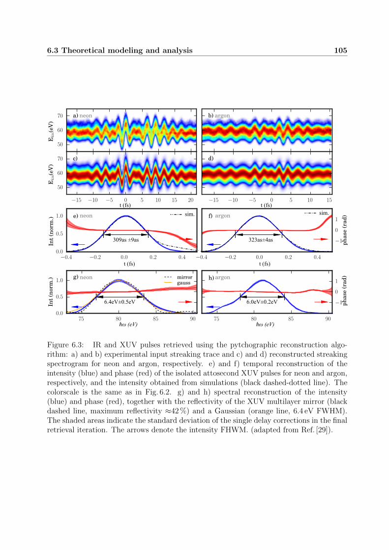
6.3 Theoretical modeling and analysis 105
t (fs) t (fs)
t (fs) t (fs)
309as ±9as 323as±4as
6.4eV±0.5eV 6.0eV±0.2eV
ħω (eV) ħω (eV)
sim. sim.
Figure 6.3: IR and XUV pulses retrieved using the pytchographic reconstruction algo-rithm: a) and b) experimental input streaking trace and c) and d) reconstructed streakingspectrogram for neon and argon, respectively. e) and f) temporal reconstruction of theintensity (blue) and phase (red) of the isolated attosecond XUV pulses for neon and argon,respectively, and the intensity obtained from simulations (black dashed-dotted line). Thecolorscale is the same as in Fig. 6.2. g) and h) spectral reconstruction of the intensity(blue) and phase (red), together with the reflectivity of the XUV multilayer mirror (blackdashed line, maximum reflectivity ≈42 %) and a Gaussian (orange line, 6.4 eV FWHM).The shaded areas indicate the standard deviation of the single delay corrections in the finalretrieval iteration. The arrows denote the intensity FHWM. (adapted from Ref. [29]).

106 6. Phase matching of HHG with ionization reshaped few-cycle pulses
Excellent agreement of our simulations with the experimental results is observed, as wewant to point out with several examples. Firstly, the experimental and simulated CEP-dependent XUV-spectra shown in Fig. 6.2 f) and g), respectively, match almost perfectly.Secondly, the simulated and experimentally retrieved isolated attosecond pulses agree verywell, as depicted in Fig. 6.3 e) and f). Finally, the CEP that optimizes the isolated at-tosecond pulse generation in argon in the simulation excellently reproduces the CEP of themeasured streaking laser field (see also Fig. 6.5), which is one of the intriguing experimentalobservations, as mentioned above and further discussed below.
In order to assess the fit of analytical phase-matching expressions for the conditions ofour experiment and simulations, we had to devise a method that allows the extraction of thetime-dependent phase-mismatch from the calculated spatio-spectral HHG source-term. Wechose a straight-forward approach using an energy-windowed fast Fourier transform (FFT).Unless noted otherwise, for all the conversions between frequency and time, we utilize theGaussian window mentioned above (6.4 eV bandwidth at 80 eV). The thus obtained time-resolved complex source-term allows the extraction of the phase φsource from which thephase mismatch can be calculated using Eq. 2.14. Since our simulations are performedin a co-moving frame of reference moving at the speed of light, we neglect the XUVdispersion (i.e. vphase = c). As we restrict ourselves to the on-axis phase mismatch alongthe propagation direction z, the phase mismatch is simply given by ∂zφsource. We find thismethod to work quite well. One drawback is that the phase is not well defined when thereis negligible amplitude. It also occurs that the instantaneous frequency away from themaximum of the calculated source bursts, can be significantly different from the centralenergy of the Gaussian window. Possible improvements could be achieved by utilizing aWigner transform that allows a fully consistent time-frequency picture.
We are not aware of any study that uses a similar method for the analysis of the time-dependent phase mismatch from full numerical simulations of the HHG process. As shownbelow, the developed approach represents a crucial step in the understanding of phasematching under strong pulse-reshaping conditions of the driving laser.
6.4 Discussion of the results
6.4.1 Effects of the overdriven regime on HHG
The overdriven regime of HHG is ”characterized by strong spatio-temporal reshaping of thelaser pulse by laser induced ionization over a short spatial extent” according to Ref. [28],which gives a definition based on the clamping of the driving laser pulse intensity. Indeed, inour simulations for argon we observe a strong spatio-temporal pulse reshaping as illustratedin Fig. 6.4 which shows the driving pulse electric field at the entrance (a) and exit (b) ofthe HHG target. After the maximum of the pulse (around 0 fs), a strong reduction of theelectric field amplitude is observed close to the propagation axis which is accompanied bya blue-shift. Both effects can mostly be attributed to plasma defocussing which is causedby the plasma density gradient in transverse direction from the propagation axis due to

6.4 Discussion of the results 107
−30 −25 −20 −15 −10 −5 0 5 10 15
t (fs)
0
20
40
60
80
100
120
r(µ
m)
a)
−30 −25 −20 −15 −10 −5 0 5 10 15
t (fs)
0
20
40
60
80
100
120
r(µ
m)
b)
−1.0
−0.8
−0.6
−0.4
−0.2
0.0
0.2
0.4
0.6
0.8
1.0
el.fi
eld
(nor
m.)
Figure 6.4: Simulated spatio-temporal profiles of the driving pulse in argon at the entrance(a) and the end (b) of the HHG target. A strong plasma-induced modification of the drivingpulse is observed after the main peak at around 0 fs (adapted from Ref. [29]).
no HHG150 mbar HHGexperiment
Figure 6.5: Signatures of pulse reshaping in the measured streaking field: Comparisonof the experimentally measured laser waveforms (white dots with black solid line) to thesimulated pulses for the case of 150 mbar pressure in the HHG target (red solid line) andthe case with no high-harmonic generation (blue dashed line). Panels a) and b) show thecomparison in the temporal domain and spectral domain, respectively. The main panelsshow the case of HHG in argon while the insets show the results for neon. In b), in additionto the spectral intensity, the spectral phase of the experimentally measured pulse is shown(black dashed line). The figure has been adapted from Ref. [29].

108 6. Phase matching of HHG with ionization reshaped few-cycle pulses
a)
b)
c)
d)
e)
Figure 6.6: Simulation of the driving laser pulse evolution in neon and argon (left column)and XUV generation in argon (right column): a) Maximum on-axis intensity for argon(red) and neon (black). The shaded area indicates the pressure distribution. b) Ionizationfraction (dashed line) and dipole strength (solid line) in the energy window defined in a)for argon (red) and neon (black), respectively. Note the different scaling of the quantitiesfor argon and neonc) spatio-temporally resolved XUV pulse at the end of the HHG targetin the energy window defined in the inset. d) the source term in the same energy windowintegrated along the propagation direction. e) Comparison of the radially integrated sourceterm and XUV pulse. The absence of the second peak around 1.2 fs in the XUV pulsecompared to the source contribution indicates the occurence of transient phasematching.(adapted from Ref. [29]).

6.4 Discussion of the results 109
the intensity profile of the driving laser. The plasma contribution reduces the refractiveindex of the gas medium and acts as a defocussing lens leading to an extra curvature of thewavefronts. The defocussing based on the plasma induced refractive index change scales asλ2 (see Drude model Eq. 5.5). Together with the time-dependent reduction of the refractiveindex during the plasma build-up, this explains the effective on-axis blue-shift.
A comparison of the effects of pulse reshaping on the streaking field between experimentand simulation is shown in Fig. 6.5 in the temporal (a) and spectral domain (b). Forneon (depicted in the insets), practically no change is observed regardless of whether thenonlinear propagation through the HHG target is considered (red solid line) or not (bluedashed line) and excellent agreement with experiment (white dots) is evident. In the caseof argon in the temporal domain, a strong reshaping after the main peak occurs that leadsto an intensity decrease and blue-shift when propagation in the HHG target is taken intoaccount. This reshaping is also evidenced in the experimental measurement (white dots) inthe region relevant for HHG up to 3 fs. Afterwards, some deviation occurs. In the spectraldomain a blue-shift can be observed both in experiment and simulation (500 nm-600 nm).Part of the deviation that is present can possibly be explained by the experimental setup,that blocks the central part of the HHG driving pulse before the streaking chamber whichmight make a more precise modeling of the laser beam and the filter necessary.
An analysis of how the HHG process is affected by the pulse reshaping in the simulationsis shown in Fig. 6.6. The peak on-axis laser intensity for argon (red line) and neon (black)can be seen in a). While the intensity evolution for neon practically follows a Gaussianbeam, in argon the peak intensity quickly decays once the pulse enters the gas target (blueshaded area) from about 4.6·1014W/cm2 to 3.0·1014W/cm2 over a distance of a few 100µm.The distinct behavior originates from the vastly different ionization rates as illustrated bythe fraction of ionized atoms at the end of pulse as shown in b) for argon (red dashedline) and neon (black dashed line), respectively. For argon the ionization is more than afactor of 100 higher, leading to a much stronger plasma loss and defocussing. The finalfraction of ionized atoms is also more than an order above the critical ionization fractionfor HHG phase-matching (see Fig. 2.7 b)). We can thus conclude that the experiments inargon were done in the overdriven regime. The fast driving pulse intensity decay also leadsto a confinement of the XUV dipole term in the considered energy window to the entranceof the HHG target for argon (red solid line). In contrast, the dipole term extends over thefull target in neon (black solid line) . Due to the higher ionization rate, the dipole strengthis considerably larger in argon than in neon for our simulation.
The strong spatio-temporal reshaping naturally raises the question on how the off-axiscontribution, not considered above, is influenced. In our simulations the time-resolvedXUV pulse profile at the end of the HHG target, depicted in Fig. 6.6 (a) seems to behardly affected. This is in contrast to Ref. [338], where HHG was dominated by off-axisemission. However, their experiments were done under considerably different conditions,especially much tighter focusing. Generally, care needs to be taken to account for potentialoff-axis contributions.
Nevertheless, an intriguing observation can be made, when comparing the time-resolvedXUV amplitude Fig. 6.6 (c) to the integrated XUV source term amplitude (d). The latter

110 6. Phase matching of HHG with ionization reshaped few-cycle pulses
has been obtained by calculating the time-resolved XUV source term (again in the Gaussianwindow given above) at each position on the simulation grid, and subsequently adding upthe time-resolved absolute values of the source term along the propagation direction. Apartfrom the main peak centered slightly after 0 fs there is another prominent contribution onehalf-cycle later at around 1.3 fs, which is suppressed in the XUV pulse. This is furtherillustrated in e), which shows both quantities radially integrated. As shown below, thesuppression of the satellite peak is a consequence of phase matching.
Before we can discuss how phase matching of HHG is possible under these strongspatio-temporal reshaping conditions and seemingly high plasma densities, and how thiscan explain the finding in the previous paragraph, we have to make a few fundamentalconsiderations on the description of phase matching in the overdriven regime.
6.4.2 Phase matching in the overdriven regime
Extension of the HHG dipole contribution
Even though the term overdriven regime has only been coined recently[28], several im-portant aspects of HHG under similar conditions have already been revealed theoretically.Generally, since the phase-mismatch is proportional to the harmonic order, for high pho-ton energies and a driving pulse undergoing reshaping, perfect phase-matching can onlybe achieved locally and transiently[28, 96]. Furthermore, the HHG dipole phase can coun-teract the plasma-induced phase increase of the driving laser, either through a blue-shift[339] or an intensity decrease [96], leading to perfect phase-matching and XUV buildupover propagation lengths of 10-100µm. While, the former has been used to explain ex-periments with an XUV cutoff significantly above the phase-matching cutoff up to thekeV energy range [340, 341, 342, 343], due to the low photon flux, it is not clear whetherphase-matching has been achieved. Finally, simulations of HHG with long-wavelengthdrivers and high-pressure gas targets with realistic pressure distributions have shown apronounced intensity clamping of the driving laser and identified different contributions tothe phase-mismatch[344].
On the experimental frontier, there have been several studies involving long wavelengthdrivers or tight focusing conditions or both [345, 331, 338], including one with additionalplasma density measurement [28], indicating the importance of plasma defocusing andpulse reshaping.
However, while the intensity-decay is usually included in the analysis, none of thesestudies has presented an expression for the phase-mismatch that contains explicitly theblue-shift contribution to the dipole phase. Indeed, except for the 1d-simulations in Refs.[339, 346], the latter is usually ignored. Here, we introduce an expression that includes allthe effects of pulse-reshaping on the HHG dipole phase, thereby allowing the descriptionof phase-matching in the overdriven regime:
∆k(t, z) = +q∂zφIR(t, z) + α · Up/~ω0 · (∂zI(t, z)
I− 3 · ∂zω0(t, z)
ω0
), (6.1)

6.4 Discussion of the results 111
which is a straight-forward extension of Eq. 2.15 and Eq. 2.20 through the addition of thelast term which describes the effect of the driving laser blue-shift on the dipole phase, oncethe proportionality Up/Ephoton ∝ Iλ2/ω0 ∝ I/ω3
0 is recognized. As a reminder, since we arein the co-propagating frame and neglect XUV dispersion, the XUV wavevector does notappear. Note that the numerically calculated φIR from the beam propagation simulationcontains all the effects of plasma and neutral dispersion and any geometric phase, such asthe Gouy-phase. We limit ourselves to the phase-mismatch in propagation direction, butEq. 6.1 can be easily generalized by replacing the partial derivative ∂z with the gradient∇. Since the focus in this chapter lies on photon energies close to the HHG cutoff, we willgenerally assume an α of 3.2 unless mentioned otherwise.
Analysis of the experimental phase-matching in argon
dk totaldk IR onlydk IR only analyticdk sourceXUV source
peak 1 XUV intensity
peak 1 XUV source
peak 2 XUV intensity
peak 2 XUV source
Figure 6.7: On-axis transient phase matching and XUV generation in argon: a) Thedriving laser pulse (red) and the time-dependent fraction of ionized atoms (black). (b) Theon-axis phase mismatch in the analytic expression without dipole (gray) and the calculatedphase-mismatch accroding to Eq. 6.1 with the dipole contribution (black) and without(black dashed). The numerical phase mismatch calculated from the complex source term(orange) and the source term amplitude (blue shaded area) is also shown. The quantitiesare shown at the entrance of the target at z = −0.8 mm. c) The on-axis source termamplitude (shaded area) and evolution of the XUV amplitude from the full simulation(solid line). The color indicates the first (orange) or second (blue) half-cycle centeredaround 0.1 fs and 1.2 fs, respectively, as shown in b). The figure has been adapted fromRef. [29].
An analysis of the phase-matching for our experimental conditions in argon is shown inFig. 6.7 at the entrance of the HHG target (z=-0.8 mm). Here, the XUV source term in theconsidered energy window peaks and a strong driving pulse intensity decrease is observed(see Fig. 6.6). The driving laser pulse (red line) and the fraction of ionized atoms (black

112 6. Phase matching of HHG with ionization reshaped few-cycle pulses
line) together with the critical ionization fraction (black dashed line) of 3.8% is illustratedin a). Already at the beginning of the pulse, the ionization fraction is at 4.8 % due to theprepulse (see Fig. 6.2 e) and rises up to around 13 % even before the main cycle.
Two strong bursts of the on-axis time-resolved XUV source term (blue shaded areas)can be observed at around 0.1 fs and 1.3 fs, as shown in Fig. 6.7 b). Considering the phasemismatch calculated according to Eq. 6.1 (black line), it can be understood why, neverthe-less, a single IAP is generated. Only up to the first main burst, the phase mismatch isclose to zero, while it rapidly increases afterwards, such that the second burst already ex-periences a considerable ∆k, limiting its coherent buildup to distances of only several tensof micron. The buildup of the XUV intensity of the first burst (orange line) and secondburst (blue line) is compared in c). Both bursts exhibit similar source strengths (shadedareas), however, only the first pulse is effectively phase-matched, whereas the buildup ofthe second pulse is strongly suppressed.
In order to validate the phase-matching expression further, we compare it to the numer-ical phase mismatch calculated from the simulated source term (orange lines), as shownin b). Relatively good agreement is achieved. Remarkably, the numerical phase mismatchexhibits a different curvature, i.e. it decreases within a burst. This observation can, how-ever, be explained considering that the instantaneous frequency of the calculated bursts ischanging and that α grows for increasing recollision times and from short to long trajec-tories.
In contrast, the analytical phase-mismatch expression based solely on the wavevectormismatch Eq. 2.16 (gray line), fails under our conditions. Nevertheless, it is worth noticingthat it describes the contribution of the driving laser phase change (black dashed line) to thephase mismatch surprisingly well. The dipole contribution is given by the difference of thelatter with the full expression which helps us to intuitively understand how phase matchingis achieved under our conditions. While the rising plasma density causes a positive phasemismatch through the blue-shift leading to an increase of φIR, the decrease of the drivingpulse intensity and the blue-shift result in a decrease of φdipole. Thereby, perfect phase-matching is allowed transiently even considerably above the critical ionization fraction.
The suppression of the second XUV burst due to phase-matching, as discussed above,explains the experimental observation that the IAP generation in argon is optimized at adifferent CEP than expected. This finding is further illustrated in Fig. 6.8 which shows thesimulated CEP-dependence of the integrated XUV source term (a) and intensity (b) at theend of the target as well the XUV intensity in the far-field (c). For better comparison, thelineouts for two different CEPs are shown (right panels, black and red lines), as indicatedby the dashed lines. In the source term, isolated pulse generation would be optimized ataround CEP=0, however, with noticeable pre- and postpulses. Due to the suppression ofthe later burst visible in the XUV intensity, the optimal CEP (red dashed line), shifts toaround 1 rad, as this allows to additionally minimize the prepulse. The remaining CEP-shiftof around 0.5 rad in the experiment stems from the focal mirror position adjustment. Thefar-field XUV intensity shows a similar behavior with the addition that the long-trajectorycontribution is quenched due to the increased divergence.

6.4 Discussion of the results 113
Figure 6.8: Simulations of the CEP-dependence: (a) time-dependence of the source termradially and longitudinally integrated over the whole target and (b) the XUV yield onaxis at the end of the target compared to (c) the far-field XUV yield integrated over theinner mirror. All quantities are calculated in the 6.4 eV energy window around 80 eV. TheCEP φ0 used to describe the experimental results is shown as red dashed line togetherwith another CEP-value of φ0 + π/2 (black dashed line). The temporal profiles for therespective CEPs are shown in the panels to the right (adapted from Ref. [29]).

114 6. Phase matching of HHG with ionization reshaped few-cycle pulses
6.4.3 Pressure and intensity variation
a)
b)
Figure 6.9: The intensity dependence of the XUV generation in argon: a) and b) thetime-resolved on-axis XUV source amplitude integrated along the propagation axis andthe far-field XUV intensity, respectively. Both quantities are calculated by applying afilter of 80 eV around 6.4 eV bandwidth (adapted from Ref. [29]).
The robustness of the phase-matching effects discussed above with respect to changesin the peak driving intensity is shown in Fig. 6.9. Over an intensity variation from 4.6to 5.4 · 1014W/cm2 the second burst of the XUV source term (a) is suppressed in theXUV-farfield (b) due to the its increased phase-mismatch.
Furthermore, the evolution of the HHG process in argon in dependence on gas targetpressure is discussed in Fig. 6.10. The on-axis XUV source term amplitude along thepropagation axis normalized for each pressure is shown in a) for the conditions of ourexperiment. While for low pressures, it extends over the full target length, already abovearound 5 mbar the source term gets localized at the entrance of the target, and even shiftsinto the region of increasing pressure above 100 mbar. This can be explained by the plasmainduced reduction of the driving laser pulse intensity, as observed above. At the same timethe FWHM of the source distribution (blue line) reduces from the target length down toslightly above 100µm.
Fig. 6.10 b) shows the XUV yield (blue solid line) and source term (red solid line)together with the contrast (dashed lines) defined as the ratio of the contribution of themain burst to the total yield. While the XUV source keeps increasing with pressure,albeit affected by pulse reshaping, the XUV yield exhibits a maximum at around 20 mbar.At higher pressures, the latter initially drops relatively fast but quickly flattens out above50 mbar. For the XUV source the contrast varies between 0.6 and 0.8, while the XUV yieldquickly reaches 0.95 at around 5 mbar and is close to 1.0 beyond 50 mbar. The maximum

6.5 Phase matching in the overdriven regime with long wavelength drivingpulses 115
Figure 6.10: Pressure-dependence of the XUV generation in argon (6.4 eV bandwidth at80 eV): a) spatially resolved XUV source term along the propagation direction (false colorplot). Above a few mbar the source term gets localized at the front of the gas target. TheFWHM (blue line) drops to around 100µm at 100 mbar and slightly increases again forhigher pressures. The region where the nominal target pressure is reached is indicated bythe two thin solid lines. b) Yield (solid lines, left axis) and contrast between main andsecondary peak (dashed lines, right axis, see main text for the definition) of the XUV pulse(blue line) and the source term (red line). The figure has been adapted from Ref. [29]
of the XUV yield is reached at conditions where the intensity decrease and blue-shift aresuch that phase-matching over long distances is possible. In the experiment, we are abovethis maximum, since the yield quickly drops already for a slight reduction of the pressurewhereas it is relatively insensitive at higher pressures. Our findings on the driving pulsedynamics and the phase-matching effects are therefore not affected by the uncertainty inthe experimental target pressure determination.
6.5 Phase matching in the overdriven regime with
long wavelength driving pulses
Naturally, the question comes up on how our findings scale to different gas types andlonger wavelengths, especially in the range of 1.5µm-2.0µm, where the overdriven regimewas first identified experimentally[28] and where the water window can be reached withfew-cycle drivers (see Fig 2.7). To this end, we perform simulations for 1.5-cycle drivingpulses in argon at 800 nm central wavelength, in neon at 1400 nm and helium at 1900 nm.This section closely follows the presentation in Ref. [29].
First of all, in order to achieve comparable pulse propagation at least in the linearregime, the same focusing conditions need to be used, i.e. all spatial dimensions are scaledwith the driving pulse wavelength. This also includes the gas target parameters. For heliumwe use a relatively tight focal spotsize of 47.5µm, a thin target with a length of roughly

116 6. Phase matching of HHG with ionization reshaped few-cycle pulses
9
Figure 6.11: Simulated intensity-decay and blue-shift for CEP=0: a) the instantaneousintensity at t=0 along the propagation axis for argon, neon, helium, and a vacuum reference.The propagation axis is expressed in terms of the Rayleigh range and the curves havebeen normalized to their maximum vacuum intensity of 6.5, 8.9, and 10.7 × 10¹⁴ W/cm2,respectively. The target is centered at −0.5 zR. b) the IR driving pulses at the end ofthe gastarget at −0.35 zR (as indicated by the black dashed vertical line in a). All pulses,except for a slightly different amplitude, overlap very well, and all show a similar blue-shiftand intensity decay around and after t=0 compared to the pulse propagated in vacuum(tin gray line). The figure has been adapted from Ref. [29]
0.8 mm and a half-width of approximately 0.16 mm for the Lorentzian increase/decreaseof the pressure distribution. The target center is half the Rayleigh length in front of thefocus, as this position has been found to approximately optimize HHG in the overdrivenregime[28] (see also discussion below). The scaling of the intensity is slightly less straight-forward. Here, since the present work studies phase matching in the overdriven regime, wechoose a vacuum peak intensity such that at the main electric field oscillation ten timesthe critical ionization fraction would be reached. This approach results in vacuum peakintensities of 6.5, 8.9 and 10.7×10¹⁴W/cm2 for argon, neon and helium, respectively.
With the above parameters, the pressure-dependence of HHG is calculated. Interest-ingly, for the pressures that maximize the considered XUV yield (see next paragraph fordetails), the evolution of the on-axis peak intensity as well as the laser pulse shape at theend of the target are surprisingly similar, as shown in Fig. 6.11 a) and b), respectively. Thepeak intensity starts to get severely quenched once the driving pulse enters the pressuredistribution and even decreases within the target from about 60 % of its maximum pos-sible value (gray line) to approximately 40 %. This behavior is mainly a consequence ofplasma defocussing. After the target, the intensity increases again since the wavevectorcomponents away from the optical axis have hardly been affected by the plasma and arestill focusing. The driving pulses at the target exit exhibit a strongly decreased intensityafter and including the main half-cycle (t=0) compared to the vacuum propagation (grayline). Moreover, a distinct blue-shift is observable. The first few cycles of the pulse arehardly affected. Overall, similar conditions have been found for the simulations of HHG inour experiment (see Fig. 6.6).

6.5 Phase matching in the overdriven regime with long wavelength drivingpulses 117
Figure 6.12: Simulated high-harmonic generation dynamics in the tight focusing regime fordifferent wavelengths and gases: (a) the normalized far-field XUV flux in the cutoff regionversus normalized pressure for a 1.75-cycle pulse in argon (solid blue line, p0 = 180 mbar),in neon (solid orange line, p0 = 1050 mbar) and in helium (solid black line, p0 = 2200 mbar).The flux in argon for a gas target positioned after the focus is shown (dashed blue line,upscaled by factor 10), as well as the experimental data extracted from Ref. [28] (opendiamonds). (b) The different contributions to the total phase-mismatch (thick red line)on-axis for the most intense XUV burst for argon at p = p0 calculated by Eq. 6.1: phase-mismatch IR due to the propagation of the laser driving pulse (black line), dip. dI/dz anddip. dω/dz from the HHG dipole caused by the change of laser intensity (solid blue line)and the blue shift of the laser pulse (dashed blue line), respectively. Also shown is thenumerically calculated total phase-mismatch within the half-cycle of the XUV burst (redshaded area) and the gas pressure distribution (blue shaded area). The figure has beenadapted from Ref. [29].

118 6. Phase matching of HHG with ionization reshaped few-cycle pulses
The pressure-scaling of the far-field XUV/soft-xray yield is shown in Fig. 6.12 a). Forthis analysis, the flux is integrated over a divergence angle of approximately 1.5 mradand an energy-window of 75 - 95 eV in argon, 250 - 320 eV in neon and 550 - 700 eV inhelium. The windows correspond to roughly 20 % of the total bandwidth placed at thespectral cutoff. The simulations are carried out only for a single CEP (= 0). The x-axisis normalized to the pressure p0 of maximum yield. All three curves, for argon (blue solidline), neon (orange) and helium (black), show a qualitatively similar behavior. After aninitial strong increase up to the maximum, the flux drops again rapidly but then stabilizesat an almost constant level depending on the gas type. This is consistent with Fig. 6.10 andthe calculation and analysis of spatially localized phase-matching in Ref. [96]. There, aneffective length of coherent harmonic buildup Leff was defined, that describes the distanceover which ∆k is close to zero. Leff is inversely proportional to the first derivative of ∆k,which in turn is in a coarse approximation proportional to the plasma density, leadingto Leff ∝ 1/p, where p is the gas pressure. Since the harmonic yield is proportional tothe square of the product of the number of contributing emitters N ∝ p and the effectivecoherence length Leff , the deep regime of spatially transient phase-matching results in quasipressure-independent HHG yields.
For comparison, we show the flux for argon (dashed blue line up-scaled by a factor of10), when the target is placed at 0.5 Rayleigh length behind the focus at an even increasedintensity that corresponds to 15 ηcr. There, the maximum flux occurs at a lower pressureand is almost two orders of magnitude smaller. Additionally we show the data extractedfrom Ref. [28] for helium (open diamonds, extracted at 3.3 bar, 410-700eV), which agreesqualitatively very well with our simulations for helium. Note, that averaging over the CEPin the simulations would likely result in smoother curves.
The maximum XUV/soft-x-ray flux is reached for specific phase-matching conditions.Figure 6.12 b) shows the individual contributions to the on-axis phase-matching accordingto Eq. 6.1 for the peak of the main XUV pulse at p0. A similar analysis has been donein Ref. [344]. The presented data is for argon, but the conditions for neon and helium arealmost identical (see SI of [29]). The contribution of the driving pulse (black solid line) ispositive throughout the target due to the strong plasma contribution. The HHG dipoleterm caused by the intensity change (blue solid line) is first positive followed by a change insign slightly before the full pressure is reached and subsequently increases again after thetarget exit. The dipole term due to the blue shift (blue dashed line) is negative before andwithin the target and then switches to positive at the end of the target. It is important tonotice that the blue-shift dipole term that we introduced in Eq. 6.1 dominates here, and istherefore absolutely crucial for the understanding of the total phase-mismatch.
Since the dipole terms counteract the driving laser contribution to the phase mismatch,the overall phase mismatch (red solid line) is close to zero within the gas target. Indeed, azero crossing slightly in front of the entrance and then close to the middle of the gas targetis observed. The zero crossing at the target entrance is located here in the rising edgeof the pressure distribution and seems to occur for a wide range of pressures. It explainsthe results of Ref. [28], that observed an XUV buildup at the target entrance in theirsimulations. We compare the semi-analytic expression to the full numerical calculation

6.5 Phase matching in the overdriven regime with long wavelength drivingpulses 119
Figure 6.13: Simulated CEP-variation and IAP generation for helium for a driving wave-length of 1800 nm and at p=2000 mbar. (a) CEP-resolved spectra. Transmission througha 0.1µm aluminum foil has been included to filter out the low energy contribution. Thecolorscale is the same as in Fig. 6.2. (b) XUV spectra near the cutoff for two differentCEP-values of φ0 and φ1 as indicated in a). The inset shows the data extracted from Ref.[28]. The IAPs generated in the energy window illustrated by the gray area, are depictedin (c). The figure has been adapted from Ref. [29].

120 6. Phase matching of HHG with ionization reshaped few-cycle pulses
averaged over the burst (red shaded area). Again, very good agreement is observed. Atthe condition of maximum flux, shown here, the source term, while starting to be localizedtowards the target entrance, still extends almost over the whole target length.
The pressure of maximum flux depends on the energy window and we observe that forlower photon energies, higher pressures are required as evident in the data of Ref.[28]. Inprinciple the discussed mechanism would allow to transiently phase match very high photonenergies, however, due to the strong intensity clamping at the conditions of maximizedphoton flux, the HHG cutoff lies in the region of the classical phase-matching cutoff.
In order to demonstrate that these conditions allow IAP generation in the overdrivenregime, we investigate the CEP-dependence of the XUV spectra for helium in Fig. 6.13 a).The used parameters are the same as above but scaled to 1.8µm at 2000 mbar helium. Thetransmission of a 0.1µm aluminum filter has been included. A strong CEP-dependenceis observed. The spectra in the cutoff region for two specific CEP-values are shown inFig. 6.13 b). They have a striking resemblance to the experimental data of Ref. [28],shown in the inset. The gray shaded area illustrates the bandwidth for which the resultingsoft-x-ray pulses, shown in Fig. 6.13 c), are calculated. Indeed, a very strong isolatedpulse is observed for φ1. Surprisingly, even at the complementary phase an nearly isolatedpulse is generated. The pulses are slightly positively chirped and therefore longer than theFourier-limit. For an energy window that covers almost the whole spectrum, the usabilityof the generated pulses depends on which contrast between the main soft-x-ray burst andsatellite bursts is acceptable. As can be seen in Fig. 6.13(a) from the half-cycle cutoffswhich are manifested as diagonal stripes, several half-cycles will contribute to the resultingpulses for all energies above 280 eV. Nevertheless, for most CEP values there is always onehalf-cycle that clearly dominates the spectrum and therefore enables IAP generation withmoderate contributions of satellite pulses.
The complexity of the transient phase-matching process is illustrated by the spatio-temporal phase-matching maps in Fig. 6.14 a) which is similar to the approach in Ref. [109].Here, the on-axis result for the optimized conditions in argon at 80 eV is shown, but similarstructures are obtained for the other gases (see SI of Ref. [29]). Here, the phase mismatchis calculated via Eq. 6.1. Perfect phase matching (red areas) can be achieved in severalregions. Firstly, at the beginning of the gas target within the region of increasing pressurearound z=-0.25 mm, as the ideal relation between the ionization fraction and pressure isreached transiently. Secondly, at around t=-2 fs practically all along the target when thecritical ionization fraction is reached within the leading part of the pulse that does notsuffer from reshaping. Thirdly, at the exit of the target at z=0.25 mm and finally for latertimes t=0 fs, when the plasma dispersion starts to dominate the phase-mismatch again,two more regions appear. However, these regions only contribute strongly to the resultingXUV pulse if the source term amplitude is not negligible. The latter (blue line) integratedalong the propagation axis is shown in Fig. 6.14 b). Only the central burst at around t=0 fsexperiences nearly perfect phase matching over longer distances and therefore contributesthe emission in the resulting XUV electric field amplitude (orange line). In contrast thesecond region connected to the critical ionization fraction, which was attributed to potentialIAP generation in Ref. [109], does seem to occur slightly too early for our conditions.

6.5 Phase matching in the overdriven regime with long wavelength drivingpulses 121
a) b)
Figure 6.14: Spatio-temporally resolved on-axis phase-matching: a) analytic phase-mismatch along the propagation axis for the central half-cycles of the pulse for argon. Theconsidered XUV energy window is the same as for Fig. 6.12.The red contour line shows theinstantaneous intensity where the classical harmonic cutoff lies above the central energyof the investigated energy window. b) source term integrated along the propagation axis(blue line) and the XUV pulse at the end of the target (orange line). The figure has beenadapted from Ref. [29].
20 15 10 5 0 5 10 15 20t (fs)
0
20
40
60
80
100
r (m
icro
n)
a)
0.25 0.50 0.75el. field
0
20
40
60
80
100b) ref
t=0 fs1 0 1el. field (norm.)
Figure 6.15: Reshaping of the driving laser: a) Spatiotemporal reshaping of the drivinglaser at the center of the gas target for helium and the driving laser conditions in Fig.6.13. b) Mode profile at t=0 fs. The plasma-induced defocusing leads to a flat phase-frontas well as a flattening of the driving pulse profile.

122 6. Phase matching of HHG with ionization reshaped few-cycle pulses
We want to point out, that unlike in Ref. [345], short trajectory contributions dominatethe plateau region of the HHG spectrum in the overdriven regime, even though the gastarget is placed in front of the focus,which is consistent with Ref. [28]. This can beexplained by the blue-shift dipole term, which is stronger for few-cycle lasers. Similar toRef. [345], we observe the formation of a flat-top electric field amplitude and flat wavefrontfor the main cycle, due to plasma-defocussing, as shown in Fig. 6.15. This spatial reshapingshould also lead to improved divergence properties of the emitted harmonics. Therefore,this finding can likely also explain observation of Ref. [28] that in the overdriven regimeall harmonics seem to originate from a common virtual source point. This is in contrastto conventional HHG, where the intensity decay transversely to the propagation axis andthe intensity-dependent HHG dipole phase lead to a strong dependence of the spatialdivergence on the harmonic order[121].
6.6 Conclusion
In conclusion, experimentally, our work presents the first unambiguous demonstration ofisolated pulse generation in the overdriven regime due to the employed attosecond streakingpulse characterization. Through experimental signatures, simulations and the comparisonbetween argon and neon, we find that in the overdriven regime, due to the driving pulsereshaping, the conditions for high-harmonic generation and phase-matching are stronglymodified.
Theoretically, we introduce an analytic expression that is able to describe phase match-ing in the overdriven regime by including the effect of the driving pulse blue-shift on theHHG dipole phase. Furthermore, a method is presented that allows to extract the phasemismatch from fully numerical calculations with which we validate the analytical expres-sions. Finally, we extent our findings to longer driving wavelengths through simulationsand observe that in the overdriven regime the contribution of the HHG dipole caused bythe blue-shift can dominate the phase mismatch.
There are several experiments that have been performed in a regime where our findingswould probably have been highly relevant. Apart from the experiments in Refs. [28, 345,338], we believe that this is likely also the case for Refs. [331, 109].
On both the experimental and theoretical side, several open questions regarding theoverdriven regime remain. Firstly, under which conditions is the overdriven regime de-sirable for HHG? Is it only efficient for tightly focused few-cycle laser pulses? Moreover,which requirements are to be fulfilled by the driving pulse wavefront quality? Recent re-search seems to indicate that for high energy driving pulses with non-perfect wavefronts,conventional phase-matching schemes could be more efficient[347]. Finally, it remains tobe answered which spectral bandwidth for isolated attosecond pulses in the water windowcan be achieved in the overdriven regime compared to conventional schemes[?, 109].
The present work will help to answer these questions and to furthermore understandthe limitations of different HHG phase-matching regimes. Therefore, these findings willplay a vital role for the development and analysis of current and future experiments that

6.6 Conclusion 123
aim at XUV generation in the water window and beyond, which in turn promises manyinteresting applications on biological samples in their natural environment.

124 6. Phase matching of HHG with ionization reshaped few-cycle pulses

Chapter 7
Attosecond physics on metallicnanotips
This chapter describes two different experiments on the PHz-scale for the electric fieldreconstruction on and using nanotips. First, the experimental reconstruction of opti-cal near fields on a nanotaper with attosecond precision is demonstrated. Secondly, thephotocurrent-based measurement of the electric field at the nanotip apex is shown. Thisconcept is in turn used to demonstrate the spatio-temporally resolved measurement of abeam with orbital angular momentum (OAM). Since both methods share the same generalmotivation and the shortcomings of the first technique inspired the latter approach, bothexperiments and their relation are introduced below. An overview of the outline is givenin the respective sections.
7.1 Introduction
The interaction of light with nanostructures exhibits unique features[348, 349]. In plas-monic materials, the excitation of collective oscillations of the electrons with respect tothe lattice (i.e. plasmons) may lead to the enhancement of the local near field up to sev-eral orders of magnitude in intensity compared to the incident field. At the same time,the enhanced fields are confined to the sharp geometrical features of the nanostructure,well below the diffraction limit of light. These nanoplasmonic phenomena have founda vast range of applications (see Ref. [349] for an overview) including biochemical sens-ing and detection[350], near-field enhanced optical microscopy with nanometer resolution(nanoscopy)[351], surface-enhanced Raman spectroscopy[352] with detectivity down to thesingle molecule level[353], thermal cancer treatment[354] and waveguiding of optical en-ergy on the nanometer scale[355]. Moreover, other nano-optical techniques make use ofthe subwavelength dimension of the nanostructures alone without relying on plasmons, e.g.optical metamaterials[356] or near-field scanning optical microscopy approaches[134]. Theprogress in nanofabrication in recent years[357, 358, 359] has made nano-optical techniquesmore widely available and has lead to a better control of the properties of nanostructures.

126 7. Attosecond physics on metallic nanotips
From the perspective of attosecond physics, nano-optics is especially interesting sinceit allows to the combine the natural timescale of electron motion (∼1 as-1 fs) with its’natural length scale (∼1 nm). [360]. The demonstration that strong-field photoemis-sion from nanotips[45, 361] and nanospheres can be controlled by the electric field ofthe driving laser[362, 87] and that the electron dynamics may be strongly modified bythe near-field decay[88, 363] has led to the development of attosecond nanophysics as anindependent research field[20, 360, 364]. Nanotips illuminated by few-cycle lasers havebeen used as sources of ultrashort electron pulses for electron microscopy[365, 366, 367] orfor the spatially-resolved detection of the CEP of a laser beam[368]. With the advent ofsolid-state HHG in attosecond physics[369, 370, 371, 372], nano-optics has been used forthe enhancement of HHG through nanoplasmonic[373, 374] or all-dielectric[375] nanostruc-tures. Moreover, the focusing of HHG and simultaneous generation of OAM via Fresnelzone plates could be shown[376, 377]. Significant progress has been made in the direction oflightwave electronics[21, 378, 22], i.e. electronics driven by optical fields on the PHz-scale.Based on plasmonic nano-bowtie antennas, the CEP-detection using currents[19, 379, 380]and recently a potential PHz-scale diode[381] have been demonstrated. However, for thefurther development and optimization of devices and for achieving ultimate control, thedevelopment of techniques that can resolve the near-fields on an attosecond temporal anda nanometer spatial scale is crucial.
Several theoretical studies have proposed attosecond streaking[12, 13] for the measure-ment of nanoscale near fields[382, 383, 384, 385, 386, 387, 388, 389] and some studies notedthat for short near-field decay lengths the streaking spectrogram does not sample the vec-tor potential[382, 384, 386]. Within our group the first proof-of-concept experiment usingattosecond streaking from a nanotip[24, 25, 26, 27] could be demonstrated, which consti-tutes an improvement in time resolution by almost three orders of magnitude comparedto previous THz experiments[390]. This work is presented in the first section of this chap-ter (Sec. 7.2). It is shown that attosecond streaking allows the near-field retrieval. Thestreaking adiabaticity parameter δ is introduced that enables a rigorous classification anddescription of the near-field streaking regimes and their implication for the field reconstruc-tion. Finally, it is demonstrated that through comparison with reference measurements ingas as well as trajectory simulations, the spectral response function of the nanotaper canbe reconstructed.
Despite the success of this experimental demonstration, one major limitation remained:Due to the small XUV photon/photoelectron flux available, the field reconstruction waslimited to the shank of the nanotaper and the contribution from the enhanced field atthe nanotip apex, which is used in nanoplasmonic applications, could not be resolved.The reason is that XUV photoemission occurs as a linear process. Therefore, even forrelatively tightly focused beams, the vast majority of the XUV photoelectrons originatefrom the nanotaper side which constitutes a much larger illuminated area compared to theapex. Consequently, a method that makes use of the strong-field photoemitted electrons,practically exclusively initiated from the enhanced apex near-field, would allow to overcomethis limitation.
Recently a number of alternative attosecond field-resolved measurement techniques

7.1 Introduction 127
have been developed[34, 35, 36, 32, 168, 33]. Instead of relying on isolated XUV pulses asin attosecond streaking[12, 13], they are based on the realization that the perturbation ofa strong-field-driven process by a weak laser pulse shows a linear dependence on the per-turbing field. Therefore, the delay-dependent observation of the perturbation allows thereconstruction of the weak field given that the field-driven process can be modeled. Oneof the first demonstrations is the PHz-oscilloscope[34]. There, a weak perturbing field isfocused under a slight angle with respect to a strong laser pulse into an HHG gas target inthe attosecond lighthouse scheme[131]. The weak pulse affects the transverse macroscopicphase-matching, leading to a delay-dependent change of the HHG burst emission angle.Other methods make use of the change of the cutoff energy in HHG[35] or of the cutoffenergy of rescattering electrons in strong-field photoemission spectra[33]. A particularlyintuitive approach is tunneling ionization with a perturbation for the time-domain observa-tion of an electric field (TIPTOE) [32, 168], where, as the name suggests, the change of thetunneling ionization rate is directly proportional to the weak perturbing field. Both, TIP-TOE and the streaking of rescattering electrons rely on strong-field emitted photoelectronsand can in principle be used to reconstruct the near-fields at the nanotip apex.
The attosecond field-resolved measurement of the apex near-field on an individual nan-otip using the TIPTOE-technique is described in the second part of this chapter, whichwe refer to as nanoTIPTOE. During our experiments, we have been made aware of relatedwork on nanostructure arrays in the group around Keathley, Berger and Kartner thathas been published[165] during the writing of this thesis. There, the measurement of thenear-field of an array of on-chip nano-bowtie structures has been demonstrated and theTIPTOE response function and its CEP-dependence is discussed. Besides differences in theexperimental approach, our work goes beyond this study in several regards. First, usingthe photocurrent in combination with energy-resolved photoelectron spectra, we identifythe onset of charge interaction effects in the dynamics of the emitted electrons. Secondly,we demonstrate that the method measures the spectral phase by changing the dispersion ofthe signal pulse. Moreover, the CEP-dependence of the response function is measured. Fur-thermore, we study the intensity dependence of both pump and signal pulses. We proposean extension of the current approach for a complete characterization of the nanoTIPTOEresponse function. Finally, making use of the nanotip as a single nanoscale emitter, wedemonstrate the application of the nanoTIPTOE concept to the spatio-temporal-resolvedmeasurement of the focus of a beam with orbital angular momentum (OAM) with a po-tentially sub-wavelength spatial resolution.
The presented results constitute a major progress both in the experimental demon-stration and understanding of attosecond nanoscale near-field measurements, which willboost the further development of these techniques as well as their application in the furtherdevelopment of PHz electronics and nanophotonics.

128 7. Attosecond physics on metallic nanotips
7.2 Attosecond streaking from a metal nanotip
The following section is structured as follows: First, the experimental setup and approachis described. Subsequently, the numerical modeling is discussed as well as the differentnear-field streaking regimes and their consequence on the field reconstruction. Then, theexperimental results are presented and compared with simulations. Moreover, the recon-struction of the response function of the near field at the nanotaper is demonstrated.Finally, limitations of the approach are discussed and a conclusion and outlook is given.This work has been presented in several publications[24, 25, 26, 27]. The chapter willclosely follow Ref. [26] and will focus more on the description of the near-field streakingregimes and the response function reconstruction.
The experiments and the experimental data analysis was performed together with Ben-jamin Forg (B.F.) and Frederik Sußmann (F.S.). The gold nanotips were produced byMichael Kruger and Michael Forster of the group of Prof. Hommelhoff. The numericalmodel was developed with initial help from F.S. and expanded and implemented by theauthor, which was crucial for the understanding of the experimental measurements. Theauthor developed the interpretation of the results in terms of response functions and thecategorization of the streaking regimes with the streaking adiabaticity parameter. Finally,the author conducted the numerical simulations and analyzed the results. All experimentaland theoretical results were discussed with all authors of Ref. [25].
7.2.1 Experimental setup and approach
For a detailed description of the laser, experimental setup and approach, we refer toRefs. [52, 25, 27]. In short, a Ti:Sa chirped pulse amplifier (CPA) delivers 26 fs pulseswith 1.4 mJ pulse energy at either 500 Hz or 1 kHz. The pulses are broadened in a hollow-core fiber from 500 nm up to 1000 nm and subsequently compressed using a set of chirpedmirrors (UFI PC70) resulting in pulses with a duration of 4-4.5 fs (FWHM) at a centralwavelength of about 720 nm. The experiments were conducted at the AS5-beamline at theMax-Planck-Institute of Quantum Optics, consisting of an HHG chamber where an iso-lated attosecond pulse is generated, a differential pumping stage, the XUV spectrometersection and the experimental chamber (see Ref. [27] for details).
The experimental scheme is shown in Fig. 7.1 a). An isolated XUV attosecond pulse(blue waveform) at a central photon energy of 95 eV with a bandwidth of 7 eV and pulseduration of 220 as (as reconstructed by a FROG-CRAB-algorithm[143]) and the drivinglaser pulse (red waveform) are focused at the entrance of a time-of-flight spectrometer(TOF, Stefan Kaesdorf ETF11). A variable time-delay ∆t is introduced using a doublemirror with a focal length of 12.5 cm. The inner part consists of a custom XUV-multilayermirror whose reflectivity defines the XUV photon range given above. It can be translatedvia a closed-loop piezo stage with nanometer precision. The kinetic energy spectrumof the emitted photoelectrons is recorded via the TOF using a time-to-digital converter(FASTComTec P7889). An attosecond streaking spectrogram is constructed from thedelay-dependent electron spectra, with which information about the near-fields on the

7.2 Attosecond streaking from a metal nanotip 129
gold nanotaper can be obtained. The nanotip is positioned in the laser focus using thecombination of strong-field and XUV photoemitted electrons as described in Ref. [25]. Thegold nanotip is produced via wet chemical etching[137, 51]. The nanotip can be replacedby a neon gas nozzle, allowing the reconstruction of the incident laser pulse as well as theisolated attosecond pulse.
7.2.2 Theoretical approach
Near field description
A proper interpretation of the experimental results requires some prior theoretical consid-erations, since the interaction of the nanostructure with the optical laser pulse leads tonear fields that vary on a nanometer spatial scale. Therefore, the usual assumption of ahomogeneous laser field is not valid anymore and the relation between the kinetic energyshift and the local near field can become intricate. Instead, both the near field around thenanotaper, which is the quantity that we aspire to measure, as well as the propagation ofthe electron in inhomogeneous near fields have to be understood.
The electromagnetic fields around the nanotaper are calculated in the framework of themacroscopic Maxwell’s equations using a commercial finite-difference time-domain solver(FDTD, Lumerical FDTD) assuming an incident Gaussian laser pulse of 4.5 fs FWHM ata central wavelength of 720 nm. The nanotip is modeled as a spherical apex with 100 nmradius and either a cylindrical shank or a tapered shank with 10 full opening angle.The conclusions regarding the near fields are not dependent on which geometry is chosen,however the latter corresponds slightly closer to the real situation. The refractive index ofgold is taken from Ref. [391].
The calculated maximum electric field strength along the nanotip axis (y-axis) normal-ized by the incident field is shown in Fig. 7.1 b) together with the outline of the nanotip(white line). The nanotip is illuminated from the left. As can be seen, the field at the apexis enhanced by almost a factor of 3. The maximum occurs slightly behind the apex whichis caused by a field propagation effect due to the relatively large apex size. In contrast,the field on the side of the nanotip is reduced in magnitude to about 0.6. Intuitively, thisfinding can be understood by considering the shank as an extremely deformed mirror. Thereflected field destructively interferes partially with the incident field at the surface. Thefield normal to the surface at the apex is strongly suppressed inside the nanotip whencrossing the surface while the parallel field component at the nanotaper side is continu-ous. This is a consequence of the Maxwell boundary conditions and the implications forattosecond streaking are further discussed below.
In order to obtain a description of the near-fields as a property of the nanostructurethat is independent of the incident laser pulse shape, in the spectral domain, the near-fieldEnf(r, ω) can be described in terms of the complex linear response function H(r, ω) andthe incident field E0(ω):
Enf(r, ω) = H(r, ω) · E0(ω). (7.1)
Due to the three possible electric-field polarization directions, the response function is gen-

130 7. Attosecond physics on metallic nanotips
Figure 7.1: Experimental setup and approach: a) experimental setup including the doublemirror, tapered nanotip and TOF. The nanotaper can be replaced by a gas nozzle forreference measurements. b) FDTD simulation of the field enhancement on a nanotaperilluminated from the left. c) and d) Amplitude and phase of the response at the apex (blacksolid line) and shank (red solid line) of the nanotip (black and red cross in b, respectively)and comparison to the Mie solution for a sphere (black dotted line) and an infinite cylinder(red dotted line). b)-d) are adapted from Ref. [26].

7.2 Attosecond streaking from a metal nanotip 131
erally a 3× 3-tensor. In the above expression, we consider a fixed incident beam geometrywhere the incident field is fully characterized by the value in the focus E0(ω). Other-wise, for arbitrary input beam geometries a dyadic Green’s function approach would benecessary[134]. In our calculations, we calculate the response with an x-position depen-dent time-shift, as would be seen by the co-propagating XUV pulse. For linearly polarizedincident pulses and if only one near-field direction is considered, H(r, ω) is a position de-pendent complex scalar function. The response is characterized by the absolute value,corresponding to the field enhancement, and the relative phase. Once the response func-tion is known, the resulting near-field can be calculated for any input pulse shape. At theend of this section, we will show the experimental reconstruction of the linear response forthe nanotaper based on our streaking measurements.
The amplitude and phase of the calculated response function at the two positionsindicated in Fig. 7.1 b) at the apex (black cross) and the frontside of the nanotip shank (redcross) are shown in c) and d) as black and red solid lines, respectively. The enhancementat the apex does not show a resonance but is quite constant down to about 500 nm, whereinterband transitions start to play a role. Small oscillations occur due to the excitation ofa surface plasmon traveling away from the apex. The same statement holds for the field atthe shank. In addition, a relative phase-shift of both fields with respect to the incident fieldcan be seen in d). At the apex, the phase is shifted by almost +1 rad (corresponding tolater times), whereas at the shank the shift is almost -1 rad (earlier times). For comparisonthe analytic Mie-theory[392, 393] solutions for a sphere (black dashed line) and an infinitecylinder (red dashed line) with radius 100 nm calculated by the MatScat-package[394, 395]are also depicted. While there is some difference between the sphere and apex fields, aclose correspondence between the field of an infinite cylinder and the nanotip shank isestablished.
In our measurement, it is those two features of the response function, the relative fieldstrength and phase compared to the incident field, that we want to resolve. Unfortu-nately, due to the velocity with which the photoelectrons emitted by the XUV radiation(v(100eV ) ' 6nm/fs) leave the surface, the electrons might experience the inhomogeneity(i.e. the change) of the near-field during the laser pulse, rendering the assumptions forEq. 3.3 invalid. Therefore, relating the streaking trace to the local vector potential at theemission position might not be possible. An identification of the different streaking regimesand their effect on the field reconstruction is given in the following subsection together witha brief description of the numerical simulations. This will be crucial for the interpretationof the experimental results presented afterwards.
Classification of near-field streaking regimes
The classification of the near-field streaking regimes requires a general description of theelectric fields and the streaking process therein and is partially based on primary consid-erations in Ref. [52]. The treatment presented in the following will require some equations,which involve, however, mostly only simple math and Fourier transformations. The totalfield Etot around a nanostructure can be separated into the incident field Einc and scat-

132 7. Attosecond physics on metallic nanotips
tered field Escatt. We will restrict our discussion to the emission direction of the electronx, apply the dipole approximation for the incident field, i.e. Einc(x) = Einc and assume anexponential decay of the scattered field with the near-field decay length lf :
Etot(x, t) = Eincident(t) + Escattered(t) · exp(−x/lf), (7.2)
as illustrated in Fig. 7.2 a). In attosecond streaking, the kinetic energy of the electron isonly slightly changed by the streaking field. Therefore, the classical equation of motioncan be Taylor-expanded in terms of the streaking field with the perturbation ε:
v(t) = v0 + ε · v1(t) +O(ε2) (7.3)
x(t) = v0 · (t− t0) + ε·∫ t
t0
v1(t)dt+O(ε2), (7.4)
where t0 is the emission time and the surface is assumed to be at x = 0. To first order, thechange in velocity v1 = ∆v can now be described by inserting the zeroth order solution forx into Newton’s equation of motion:
dv1
dt= − e
m
[Einc(t) + Escatt(t) · exp
(− v0(t− t0)/lf
)], (7.5)
which is equivalent to neglecting the change of the velocity in the description of the positionof the photoelectron in the equation of motion. Using the spectral representation of thefield, i.e. E(t) =
∫dωE(ω) exp(−iωt) in the above equation, the velocity change ∆v for
an electron emitted at t0 yields:
∆v(t0) = +e
m
∫ ∞−∞
dω exp(−iωt0)[Einc(ω)
−iω+
Escatt
−iω − v0/lf
], (7.6)
where the integral expression, in analogy to the homogeneous case, can be interpreted asan effective vector potential Aeff . Consequently, the Fourier transform of ∆v with respectto the delay t0, multiplied by mω
e, corresponds to the spectral representation of the effective
electric field Eeff(ω) measured by attosecond near-field streaking:
Eeff(ω) =Einc(ω) + Escatt(ω)
1− i v0lf ·ω
+Einc(ω)
1 + ilf ·ωv0
=Esurf(ω)
1− i 12πδ(ω)
+Einc(ω)
1 + i2πδ(ω), (7.7)
where we have used the field at the surface Esurf = Einc +Escatt(x = 0) and introduced thenear-field streaking adiabaticity parameter δ:
δ(ω) =lf
v0 · T0
=Tesc
T0
=lfl0
(7.8)
T0 = 2π/ω is the oscillation period, Tesc is the escape time from the near field defined asTesc = lf/v0, and l0 = v0 · T0 is the distance that the electron covers during an oscillation

7.2 Attosecond streaking from a metal nanotip 133
period. The relation to the strong-field adiabaticity parameter[88], that can directly bededuced from the classical equation of motion, is discussed in Ref. [26]. Different valuesof the adiabaticity parameter in terms of the distance that an electron travels within anoptical cycle, are illustrated in Fig. 7.2. The adiabaticity parameter can be interpreted asthe ratio of either the two timescales or the two length scales of the dynamics. As can beseen in Eq. 7.7, for large escape times, i.e. large δ, the effective field corresponds to thenear field as expected.
s
Etotal
Eincident
lf x
E
δ<1
δ~1
δ>1
electrona)
d)
b)
c)
fsurff0
Figure 7.2: Near-field attosecond streaking response function: a) illustration of the geom-etry and near-field decay model. b) and c) amplitude and phase of the response functionof the surface field (red line) and the incident field (blue line), respectively, in dependenceon the adiabaticity parameter δ. d) Relative surface field sensitivity s (details in the text).
For decreasing values of δ the interpretation becomes more complicated. For conve-nience and in order to simplify the discussion, we define the effective response function ofthe surface field fsurf and of the incident field finc, determining their respective weight andrelative phase (see Eq. 7.7) in the effective field:
fsurf(δ) = (1− i · 1
2π · δ)−1 (7.9)
finc(δ) = (1 + i · 2π · δ)−1. (7.10)
The absolute value and phase of both fsurf (red line) and finc (blue line) are shown inFig. 7.2 b) and c), respectively. Three different regimes can be identified:
• ponderomotive regime (δ > 1): The escape time of the electron from the near fieldis much larger than the period of the field. The measured effective field reconstructedfrom the streaking trace is determined in amplitude and phase by the surface field.

134 7. Attosecond physics on metallic nanotips
• intermediate regime (0.05 < δ < 5): The electron starts to experience the inho-mogeneity during one cycle and experiences a mixture of the surface field and theincident field. The phase of fsurf start to shift from 0 towards π, while a shift from−π to 0 occurs for finc.
• field-probing regime (δ < 0.05): The electron leaves the near field almost instan-taneously in a fraction of a cycle and sees a quasi-static near field. The naming hasbeen introduced in Ref. [382]. As the phase of the surface field function is π outof phase with Eeff , the shift in the measured streaking trace due to the near field isdirectly proportional to the surface electric field and not the surface vector potential.
The simple interpretation of the field-probing regime is, however, only true, if the incidentfield is neglected. This is problematic, since, as can be seen in Fig. 7.2 b), the amplitudeof fsurf goes to zero in the field probing regime, in contrast to |finc| which is close to unity.We therefore define the real-valued surface sensitivity s(δ) as:
s(δ) =|fsurf ||finc|
. (7.11)
The surface sensitivity is plotted in Fig. 7.2 d). Indeed, in the field probing regime, s(δ) <10−1. For the simple interpretation to be valid, in which the incident streaking field canbe neglected, the field enhancement needs to be significantly higher than 1/s.
We want to point out that the shift of the phase of the surface response function can alsobe interpreted as a streaking delay τinh caused by the near-field inhomogeneity[314]. Themodel presented here is capable of predicting τinh once the near-fields are known withouthaving to rely on numerical simulations.
Trajectory simulations
To gain an even better understanding of our experimental results, we perform trajectorysimulations of the XUV-emitted photoelectrons in the near field of the nanotaper. The nearfields are calculated with FDTD simulations using the experimental laser pulse parameters:4.5 fs pulse duration, 15µm focal spotsize and 1012 W/cm2 intensity. For an adequatedescription of the fields at the surface, a fine resolution of the rectangular simulationmesh is necessary around the nanotip, which results in file sizes of several 10 GB. Thefield files are transformed to the portable HDF5-format and read in by an object-orientedtrajectory simulation C++-code. The field class linearly interpolates the fields from theclosest meshgrid points in space and in time. The nanostructures are modeled based onan analytical description of geometries with compact volume and a combination thereof.This allows to determine whether a point is within the volume and to efficiently calculatethe intersection points with the surface for a given point and a vector including the surfacenormal which is important for treating the electron propagation.
The isolated attosecond pulse is described as a Gaussian beam with an FWHM of5µm and a Gaussian pulse with 220 as FWHM at 95 eV central photon energy (and 7 eV

7.2 Attosecond streaking from a metal nanotip 135
bandwidth). From the experimental reconstruction, negligible chirp is obtained, whichallows a simplified spectro-temporal description of the linear XUV photoemission process:The emission time and the kinetic energy of the photoelectron are randomly generatedindependently from the Gaussian intensity envelope in time and in photon energy (minusthe work function of gold). The emission points on the surface are obtained by projecting arandomly generated point in the XUV beam profile onto the surface of the nanostructure.The emission is assumed to be isotropic. Electrons re-entering the surface are ignored andonly electrons within the detection angle (full cone angle 45) are considered. The electronsare propagated independently using the Velocity-Verlet algorithm[216].
For the simulation of attosecond streaking spectrograms 106 electrons were propagated.Although not shown here, simulated streaking spectrograms where extremely valuable forunderstanding the experiments. In order to assess the contribution of a single point on thenanotaper surface, streaking traces are calculated where electron propagation is startedat each delay with a fixed kinetic energy of 89 eV and an emission angle of 15. For theresponse function, the mean and standard deviation of the local response function of 104
points on the surface weighted by the XUV beam profile are calculated.The tapered nanowire is modeled as a cone with an opening angle of 10 and a hemi-
sphere of 50 nm radius for the response function calculation. Extremely fine meshing isnecessary to avoid numerical hotspots in the nanocone geometry which impedes electrontrajectory calculations. For the streaking trace simulations, the nanotip is modeled as acylinder with a hemisphere at the end. The conclusions of this section, as mentioned above,are not affected by the choice of either geometry.
7.2.3 Experimental results
The experimentally measured attosecond streaking spectrograms from the gold nanotaperand the gas target are shown in Fig. 7.3 a) and b), respectively. The countrates from thenanotaper are more than an order of magnitude smaller than from the gastarget. Therefore,for reasonable statistics, overall acquisition times of up to a few hours are required. Inorder to exclude the influence of phase drifts and instabilities, several nanotaper streakingspectrograms are recorded with a gastarget streaking measurement before and after. Ifstable conditions are observed, the nanotaper streaking spectrograms are superimposed.Overall, several sets of attosecond streaking spectrograms are recorded on different daysand for different nanotips.
The photoelectron spectrum from the nanotaper is significantly broadened comparedto the gas target due to the extended density of states as well as inelastic scatteringof the photoelectrons within the medium. Moreover, there is a potential contributionof adsorption and passivation layers on the surface that have a higher work function[51,27] and contribute to the lower energy region. We assign the high-energy edge of thephotoelectron spectrum to electrons from gold dominated by the Au-4d band due to thedensity of states. The photoemitted electrons have to overcome the work function of gold(φ ≈ 5.4 eV )[396] which largely explains the energy of the cutoff of approximately 89 eV.The central energy of the neon streaking trace is shifted to around 74 eV due to the higher

136 7. Attosecond physics on metallic nanotips
-4 -2 0 2 4delay (fs)
95
90
85
90
88
77
75E
kin
(eV
)
Eki
n (e
V)
100
90
80
70
90
80
70
60
-4 -2 0 2 delay (fs)
0. 0.5 1cts. (norm.)
turningpoint
turningpoint
Fermifit
Fermifit
0 0.5 1counts (norm.)
Eki
n (e
V)
E
kin
(eV
)
Δt
nanotipshank
nanotipapex
gas reference
~20as
gas reference
nanotaper
Δt
a)
b)
c)
d)
Figure 7.3: Experimental results and comparison to simulations: a) and b) streakingspectrogram from the nanotip and the neon gas reference, respectively. The right panelsshow the extraction of the streaking trace (black dots) from a Fermi-fit to the high-energycutoff of the electron kinetic energy spectrum. A delay between the two streaking curves isevident. c) Fourier-filtered streaking traces and delay. d) The streaking curve retrieved viathe same approach from a Monte Carlo simulation (symbols) and the calculated streakingcurve for electrons emitted from the front of the nanowire at y=-200 nm (dark blue line)and y=-3,000 nm (light blue line), respectively. The latter two curves practically coincide.The simulated reference streaking trace in neon gas (red line) has been upshifted in energyto aid comparison. The inset shows the relation between the simulated streaking curve(dark blue solid line) and the local vector potential of the near-field (dark blue dashedline) at the emission point. The figure has been adapted from Ref. [25].

7.2 Attosecond streaking from a metal nanotip 137
ionization potential of neon (Ip = 21.56 eV )[397].
Clear streaking oscillations can be observed for both nanotip and gas measurements.The streaking amplitude was set deliberately low, in order to avoid damage of the nanotip.The traditional FROG-CRAB approach[143, 146] can not be applied for the extraction ofthe streaking pulse for photoelectron spectra with a large incoherent background, as is thecase for scattering contribution in the nanotip streaking spectrograms discussed above (seeRef. [156] for a density matrix description). Therefore, as illustrated in the panels right ofFig, 7.3 a) and b), we devised a different approach which consists of fitting a Fermi-function(red line) to the positive cutoff of the spectrum (black line) for each delay. The turningpoints of the Fermi-function are then used to define the raw streaking curve (open dotsin the main panels). For the gas streaking spectrogram, this approach is tested against aFROG-CRAB algorithm[143, 146] as well as against fitting the photoelectron peak with aGaussian function and excellent agreement is observed[25].
The extracted raw streaking curves are Fourier-filtered by excluding the wavelengthcomponents outside the laser spectrum below 400 nm to eliminate noise in the nanotaperdata caused by the limited statistics. As can be seen in Fig. 7.4 c), clear temporal shift∆t = 200±50 as to smaller delays is observed for the nanotaper curve (blue line) comparedto the gas reference (red line).
7.2.4 Discussion
For a better understanding of the experimental results, trajectory simulations in the near-field of the nanotaper were performed as shown in Fig. 7.3 d). The streaking curve re-trieved from a Monte-Carlo simulation of the streaking spectrogram from the nanotaperand subsequent application of the same reconstruction algorithm as for the experiment isrepresented by open dots. In addition, streaking curve calculations for the gas referencein the focus of the incident beam (red line) and for single emission points on the shank ofthe nanotip, 200 nm (dark blue line) and 3000 nm (light blue line) below the apex, as wellas from the apex (gray dashed line) are shown. There are two immediate findings furtherdiscussed below. Firstly, the streaking curves from the nanotip shank agree very well withthe Monte-Carlo simulation, while a potential contribution of the apex with significantlyhigher streaking amplitude and a temporal delay compared to the gas reference is notvisible neither in the simulated nor experimental streaking spectrogram (see Fig 7.3 a)).Secondly, good agreement of the simulated average temporal shift of around 260 as be-tween gas reference and Monte-Carlo nanotip streaking curve with the experimental resultof 200± 50 as (see Fig. 7.3 c)) is observed.
The first finding implies that the streaking spectrograms are dominated by electronsoriginating from the side of the nanotaper, while the apex contribution is negligible. Anestimate of the relative weight of both contributions in the experiment can be obtained bya simple consideration based on the geometrical cross section as seen by the incident XUVbeam and on the linearity of the XUV photoemission process, while neglecting furtherdetails of the latter. The number of detected XUV-emitted photoelectrons from a certain

138 7. Attosecond physics on metallic nanotips
region on the nanotip nregion with an effective cross-sectional area Aregion is given by:
nregion ∝nXUV
ω20,XUV
· Aregion · frep · Tacq, (7.12)
where nXUV is the number of XUV-photoelectrons per shot, ω0,XUV is the waist radius of theXUV beam, frep is the repetition rate of the laser and Tacq is the total acquisition time. Themaximum (illuminated) effective area is limited by the XUV spotsize. The illuminated areaon the nanotaper shank Ashank can be estimated by the product of the average diameterof the nanocone (∼150-300 nm) and the FWHM of the XUV beam (∼5µm). In contrast,the region of the enhanced field on the apex Aenh is limited to a fraction of the hemispherearea (∼ π[50 − 100 nm]2). This estimate suggests that around a factor of 250-2000 moreelectrons originating from the shank are detected compared to the enhanced apex region.Given that our streaking spectrograms typically consist of only a few hundred electronsper delay and even less close to the cutoff, resulting in less than an electron on averagefrom the apex per delay, we can not expect to see this contribution in our measurements.Nevertheless, the contribution from the near field of the shank of the nanotaper is clearlyresolved.
The observed correspondence of the experimentally measured and simulated temporalshifts and the agreement with the expected shift of the calculated nanotaper electric near-field response function at the shank of 260 as (see Fig. 7.4 d)), already suggest that the nearfield on the nanotaper can be extracted from streaking measurements. However, beforebeing able to draw this conclusion, several consideration regarding the intrinsic streakingdelays of neon and the gold surface as well as the near-field streaking regime and have tobe made.
The intrinsic delays of the photoemission process measured by attosecond streakingthat lead to a shift of the streaking curve with respect to the vector potential, could inprinciple influence our measurements (see Sec. 3.3.1). Theoretical studies for neon suggestan absolute time delay below 10 as at 95 eV photon energy[153, 154]. A large number ofexperimental studies exist for attosecond streaking from surfaces[15, 158, 398, 82, 161, 157].While attosecond streaking measures only relative time-delays, the absolute photoemissiondelays from surfaces has been demonstrated[157] by comparing the bulk emission to an ad-sorbate, and then subsequently the adsorbate to helium, which can be calculated exactlywithout approximations. The surface streaking experiments are performed at grazing in-cidence of the laser onto the bulk surface. There, it could be shown that the laser fieldis screened within one or two atomic layers[398] and that the delay is caused by the timeit takes the electrons to travel from the bulk to the field[158, 398, 82]. At our photonenergies, for valence band photoemission, absolute delays below a few tens of attosecondsare expected[157]. At the nanotaper shank the incident laser polarization is parallel tothe surface and therefore the field is continuous through the surface, as observed in thenear-field calculations above. In the above interpretation, this finding implies that an evenlower streaking delay is expected[26, 399]. Overall, we can conclude that the photoemissionstreaking delays are negligible compared to the measured streaking curve time shifts in ourexperiment and we treat the photoemission process as instantaneous.

7.2 Attosecond streaking from a metal nanotip 139
For an estimation of the near-field streaking regime, several parameters are needed(see Sec. 7.2.2). The kinetic energy (∼90 eV) of the XUV-emitted photoelectrons leadsto an escape velocity of approximately 5.5 nm/fs. A near-field decay length of around50-100 nm is obtained from the electromagnetic near-field calculations in agreement withthe expectations from the length scale of the nanotip geometry. The oscillation period atthe central laser wavelength is around 2.4 fs. Taking into account, that the comparativelysmall emission angle relative to the surface (<22.5) for the detected electrons from theshank leads to a reduction of the effective escape velocity, an estimate for the streakingadiabaticity parameter δ ≈ 10 − 30 is obtained. This is clearly in the ponderomotiveregime. Indeed, as the inset in Fig 7.3 d) shows, a shift of only around 20 as between thestreaking curve (solid line) compared to the local vector potential (dashed line) is obtained,which is negligible for our purpose. This finding implies that the nanotip streaking curverepresents the local vector potential from which the near field on the nanotaper can easilybe extracted.
91
90
89
88
87
86
1
0
-1
kine
tic e
nerg
y (e
V)
elec
tric
fiel
d (1
0⁸ V
/m)
electric field
streakingcurve
-4 -3 -2 -1 0 1 2 3 4
rel.
phas
e (
rad)
rel.
amp.
600 700 800 900 1000wavelength (nm)
1
0.5
0
1
0
-1
delay (fs)
a) c)
b)
Figure 7.4: Experimental reconstruction of the nanotaper response function: a) and b)experimentally retrieved amplitude and phase of the response function of the shank ofthe nanotaper. The individual measurements (black crosses) extracted by Fourier analysiswith their average and standard deviation (red lines and errorbars). The prediction of theMonte-Carlo simulation is shown as green area indicating the standard deviation aroundthe mean value. c) Comparison of the reconstructed electric field (red line) from theretrieved streaking trace (symbols and gray line) with the expectation, calculated from theMonte-Carlo response function (green area). The figure has been adapted from Ref. [26].
By comparing Fig, 7.3 c) and d), it can be seen that the gas streaking amplitude in thesimulation is significantly higher than for the nanotip, in contrast to what is observed inexperiment. This apparent discrepancy can be resolved by considering that for the gasstreaking, the laser intensity is averaged all over the focal volume, whereas the nanotaperalignment procedure makes sure that the nanotip is placed in the highest intensity. Asimiliar underestimation of the laser peak intensity from the gas streaking amplitude has

140 7. Attosecond physics on metallic nanotips
been observed in previous experiments, where additionally ATI has been measured[400]. Inorder to obtain correction factors, we compare the expected intensities from the gas streak-ing amplitude to the expected intensities from the observed cutoff energies of the ATI fromthe nanotip apex in the nanotip streaking measurements, for every set of measurements.Similar to Ref. [400] field amplitude correction factors of around 3 are obtained.
Finally, we can now calculate the incident electric field of the incident laser pulse andthe near field on the nanotaper shank from the gas and nanotip streaking measurements,respectively. Moreover, via inversion of Eq. 7.1 the response function of the near field at thenanotaper can be calculated by Fourier-transforming the reconstructed electric fields. Thephase and amplitude of the reconstructed response function are shown in Fig. 7.4 a) andb), respectively. Datapoints from different measurement sets (gray crosses) are averagedin order to obtain the mean response function (red lines, black dots) and the standarddeviation (errorbars). The simulated average response function and standard deviation(green shaded areas) are also shown. The simulated relative phase slightly overestimatesthe measured phase-shift. Good agreement is observed between the reconstructed andexpected relative amplitude of the response function.
The response function allows to calculate the near field on the nanotaper shank forany incident pulse. This is demonstrated in Fig. 7.4 c) where the expected electric fieldon the nanotaper calculated from the measured gas reference streaking electric field andthe simulated response function (green shaded area) is compared to the experimentallyreconstructed electric field (red line) from the measured streaking curve (open dots andgray line).
7.2.5 Conclusion and Outlook
In conclusion, we have demonstrated the first successful experimental streaking measure-ment of nanoscale near fields using a gold nanotip. A simple theoretical model has been de-veloped that allows the classification of different near-field streaking regimes. Furthermore,the model provides a description of the relation between the near fields and experimentallymeasured streaking curves. Using numerical simulations, the experimental streaking curvesare shown to originate from the side of the nanotaper. Finally, the successful demonstra-tion of the experimental retrieval of the near-field reponse function is demonstrated. Ourresults constitute a milestone in the experimental realization of and a major step in thetheoretical understanding of attosecond streaking spectroscopy of nanoscale near fields,which will be of considerable importance for the further development of this and relatedtechniques.
In our experiments, the limited photoelectron countrate obstructed the observationof the enhanced near fields at the apex. Different knobs to increase the electron fluxare given in Eq. 7.12. The most promising approach is likely the increase of the XUVphoton flux by going to lower photon energies and different generating gases. Indeed,attosecond streaking from isolated dielectric nanospheres (50 nm diameter) at XUV photonenergies below 40 eV using HHG in xenon has been demonstrated[313, 314]. Under thesame experimental conditions also the near fields at the nanotip apex should be resolvable.

7.2 Attosecond streaking from a metal nanotip 141
However, experiments demonstrating the measurement of enhanced plasmonic near fieldshave not been done so far. Moreover, while the nanosphere experiments were conductedin the transition region from the intermediate to the ponderomotive streaking regime[314],an experimental investigation of the different streaking regimes is still missing.
Spatial resolution, e.g. for device characterization, could be achieved by combiningthe attosecond near-field streaking concept demonstrated here with scanning approachesor photoemission electron microscopy (atto-PEEM)[382]. The latter approach is fueled bythe development of high-repetition rate XUV sources based on enhancement cavities[401,402, 403, 404, 405], circumventing space-charge problems that had impeded atto-PEEMmeasurements so far[406].
Another approach to resolve the enhanced near fields at the apex of the nanotaper andplasmonic hotspots of nanostructures in general based on photocurrents is presented in thenext section. The method does not rely on isolated attosecond XUV pulses but utilizesthe strong-field photoemitted electrons from the enhanced near fields itself and therebyovercomes the limited sensitivity of the attosecond streaking approach to the nanoscaleconfined near fields.

142 7. Attosecond physics on metallic nanotips
7.3 Attosecond field-resolved measurements using pho-
tocurrents
This section describes the measurement of enhanced near fields on the nanotip using strong-field photoemission from the apex. The outline is as follows: Firstly, the experimentalsetup and approach is presented. Secondly, the experimental results are presented whichare separated into three distinct sections: i) the onset of charge interaction effects, ii) thedemonstration of the reconstruction of the near field at the apex including the investigationof the CEP- and intensity-dependence, as well as the comparison with photoelectron spectraand iii) the application of the nanoTIPTOE approach to the spatially resolved measurementof the focus of a vortex beam. We subsequently devote a special section to the discussionof the nanoTIPTOE approach. Finally, we provide a brief conclusion and outlook.
The experimental setup was built and developed by the author with help from DmitryZimin with whom also first experimental feasibility tests were performed. The nanotipswere produced together with Johannes Blochl (JB) and Ancyline Malliakal (AM), using themethod described in Chap. 3.1. The TOF/CEP-current intensity-dependence was recordedby the author. The TIPTOE measurements, including TOF pump-probe, were performedtogether with JB and AM, including the compression of the pulses in the experiment andoperation of the laser. The latter was supported by Zilong Wang and Philipp Rosenberger.The preparation of the spatially resolved measurements was done by JB. The experimentaldata was discussed mostly with JB and AM. The presentation of the data in this chapterhas been prepared by the author. The measurements on the effects of space charge hasresulted in a manuscript draft[407] which has been discussed with all the authors thereof.
7.3.1 Experimental setup
The experimental setup and approach is illustrated in Fig. 7.5. As depicted in Fig. 7.5 a),a strong pump pulse (red line) and weak signal pulse (blue line) with variable relativedelay ∆t are focused onto a tungsten nanotip using an off-axis parabola (OAP, f=10 cm).The emitted photoelectrons can be detected using a TOF-spectrometer (Stefan KaesdorfETF10) and a time-to-digital-converter (FAST ComTec P7889). Due to the vacuum-requirements for the electron spectra measurements and the microchannel-plate detectorof the spectrometer, the setup is placed in a vacuum chamber. The photoemitted electronslead to a photocurrent within the nanotip. Similar to the measurement of currents ingases described in Chap. 4, the wire of the nanotip is electrically contacted to a BNC pinwhich in turn is inserted into the plug of a BNC cable. The photocurrent is fed throughto the outside of the chamber using a floating BNC feedthrough. It is amplified using alow-noise high-gain transimpedance amplifier (FEMTO DLPCA-200) and finally detectedvia a lock-in amplifier (Zurich Instruments HF2LI).
The laser frontend SMILE is the same as described in Chap. 4 and in more detail inRef. [201]. In short, the output of a commercial Ti:Sa chirped pulse amplifier is broadenedin a hollow-core fiber, spanning from 500 nm to∼1000 nm. The pulses are compressed down
7.3 Attosecond field-resolved measurements using photocurrents 143
to around 4.5 fs at 750 nm central wavelength using chirped mirrors (CM, UFI PC70). TheCEP-offset φ0 is stabilized and controlled via a slow-loop that provides feedback to theCEP-stabilization of the laser oscillator.
The pump and signal pulses are generated in a Mach-Zehnder interferometer depictedin Fig. 7.5 b). A broadband 50:50 beamsplitter (BS) separates the pulse into the two arms.Each arm contains a circularly variable neutral density filter (ND) and a pair of fused silica(FS) wedges for the fine tuning of the dispersion in the experimental focus. The pump arm(red line) contains a retroreflector mounted on a piezo stage (MCL OPM100) with 100µmtravel range for the precise control of the delay between signal and pump pulses. The signalarm (blue) additionally contains a telescope consisting of two off-axis parabolas (OAP1 andOAP2). An optical chopper (Thorlabs MC2000B) is placed in the intermediate focus. Formost experiments presented below, both mirrors had the same focal length (f=20 cm). Inthis configuration, the incident intensity calibration of Chap. 4 without telescope appliesfor the pump beam (1.1 · 1014 W
µJ ·cm2 ± 20%). This intensity calibration is not strictlyvalid for the signal beam due to different dispersive elements. Nevertheless, we will useit for estimations. Optionally, a λ/2-plate can be placed in the signal arm to rotate thepolarization.
For the measurement of the angular momentum beams, a vortex plate (Vx plate, VortexPhotonics V-780-20-1) for a wavelength range around 780 nm that preserves the linearpolarization is inserted into the signal arm together with a bandpass (BP, Edmund Optics86956) with 50 nm bandwidth around a central wavelength of 775 nm. Moreover, a 1:2.5-telescope using a combination of concave and convex mirrors is introduced in front ofthe interferometer for the reduction of the pump beam size. At the same time OAP1 isreplaced by an OAP with f=7.5 cm to increase the size of the signal beam. This way, in theexperiment the OAM beam gets tightly focused whereas the smaller incident pump beamresults in a bigger focal spot size. Here, the incident intensity calibration with telescope isvalid for the pump beam (0.11 · 1014 W
µJ ·cm2 ± 50%, see Chap. 4).For the measurements of the CEP-dependence, the signal arm is blocked and the CEP
of consecutive laser pulses is flipped between φ0 and φ0 +π using a Dazzler. The telescopewas in the beam and in the experimental chamber an OAP with f=5 cm was used. In thissetting, the arrangement of the HCF, the recollimation and CM compression were slightlydifferent from the above configuration.
For the nanostructures, the dynamics is determined by the enhanced near-field intensityrather than the incident intensity. Fortunately, the local enhanced intensity at the apexof the nanotip can directly be estimated from nonlinearity of the strong-field photoemis-sion rate as has been shown in Refs. [361, 408, 66, 409, 135]. At onset of the tunnelingregime (Keldysh parameter γ ≈ 1), a characteristic drop of the nonlinearity below themultiphoton scaling is observed (see also Sec. 2.2.1). We use this approach in the intensity-dependent measurements in Sec. 7.3.3 and Sec. 7.3.4 below. However, we want to mentionthat the intensity calibration based on that method is expected to exhibit relatively largesystematic uncertainties. Firstly, the onset of the tunneling regime is not strictly definedand the identification therefore intrinsically requires estimation. Secondly, the nanotip asa nanoscale emitter is very sensitive to the positioning in the laser focus, which has to be

144 7. Attosecond physics on metallic nanotips
adjusted on a daily basis. Finally, this approach can be affected, once charge interactioninfluences the emission probability.
pumppulseOAP
signalpulse (×10)
photocurrent
TOF
nanotipe-
e-e-
JPC
to imaging
BS
BC
Piezo stage
OAP1
OAP2
ND
ND
FS wedges chopper
FS wedges
from CMs
to experiment BP Vx plate
optional
signal
x (μm) x (μm)
y (μ
m)
λ/2
opt.
Δt
a) b)
c) d)emission current light attenuation
nanotip
Figure 7.5: Experimental setup and approach for the current measurement from a nanotip:a) Experimental setup with pump and signal pulse. In addition to the photocurrent, thekinetic energy spectrum can be measured using a TOF-spectrometer. b) Interferometer forthe pump-probe measurements. c) and d) experimental search for the nanotip apex usingboth the emission current and the light attenuation.
7.3.2 Experimental approach
Experimentally, an important aspect is to make sure that the apex of the nanotip ispositioned in the laser focus and not an occasional hotspot farther down on the shank ofthe nanotip. Therefore, the nanotip is scanned transversely through the laserbeam andboth the electron emission signal and the attenuation of the laser light in the imaging arerecorded, as shown in Fig. 7.5 c) and d), respectively. The photocurrent signal is verysensitive to the field enhancement at the apex, whereas the light attenuation allows to getan estimate for the contour of the nanotip and is used to make sure that emission reallyoccurs from the apex at the end of the tip. Without the latter signal, hotspots on theshank of the nanotip can be mistaken for the apex.
The employed digital lock-in amplifier is capable to demodulate the signal input atseveral frequencies in parallel. For the first demodulation frequency, we choose the laserrepetition rate frep = 10 kHz which results in a signal that is proportional to the totalphotocurrent. The second demodulation frequency is the chopping frequency fchop or theCEP-flipping frequency fCEP which is set to 5 kHz, making sure that we are as far aspossible from the 1/f-noise region at lower frequencies (see Sec. 3.2.2 for a more detaileddiscussion of lock-in amplification). For scanning applications, demodulation bandwidths

7.3 Attosecond field-resolved measurements using photocurrents 145
between 2-10 Hz are used.
The detection limit of the photocurrent measurement approach has to be considered.We observed the best signal-to-noise performance at the maximum gain of 109V/A of thetransimpedance amplifier even though the nominal gain bandwidth (f−3dB) is below 5 kHz.For simplicity, we will, nevertheless, use the value of 109 for conversion between voltage andcurrent, but want to point out that the effective gain will be slightly reduced. Moreover,the gain at 10 kHz will be lower than at 5 kHz. The conversion factor between signalamplitude and electrons per shot is approximately given by 0.6 electrons ·shot−1µV−1. Thetransimpedance amplifier specifies an equivalent input noise current density of 4.3 fA/
√Hz
which translates at the lock-in amplifier into 4.3µV/√
Hz close to the observed voltagenoise density of around 5-7µV/
√Hz.
In order to estimate the number of electrons required per shot in to get a detectablesignal, we make a striaght-forward consideration. For simplicity, we assume a lock-in de-modulation bandwidth of 1 Hz, a measurement of the signal in a 1 Hz window around thedemodulation frequency. Taking into account the repetition rate of the laser and the inputcurrent noise density level stated above, roughly means that a change of around 3 electronsper shot can be detected (neglecting any other noise contributions). For higher repetitionrate lasers, the sensitivity would increase accordingly due to the higher total number ofemitted electrons. As a consequence, in order to be able to measure a modulation of thetotal photocurrent as required in the TIPTOE experiments, a (maximum) modulation byseveral tens of electrons per shot has to be achieved which consequently results in a totalphotocurrent of at least several hundred electrons per shot. Our experiments are thereforenecessarily conducted in the multi-electron emission regime. The same, however, seems tobe true also for the nano-bowtie current experiments that are driven at MHz repetitionrates[165, 380]. While the work on TIPTOE[165] from a nanostructure array does notdiscuss total electron emission rates, the study on the on-chip CEP-measurements employ-ing similar nanostructure arrays[380] indirectly indicates 103 to 104 electrons per shot pernanostructure, based on the CEP-current per shot and nanostructure (0.11 electrons) andthe ratio of CEP-current to total current (10−4 to 10−5).
7.3.3 Onset of space-charge effects
Based on the considerations above that the nanoTIPTOE approach in our implementationrequires multi-electron emission, we first turn our attention to the investigation of chargeinteraction effects before demonstrating the attosecond near-field measurements via thephotocurrent further below. Space-charge interaction affects both the tunnel emission pro-cess and the subsequent electron dynamics in the continuum. The former effect is hardto assess directly. However, the latter leaves a trace in the kinetic energy spectra of thephotoelectrons which we can measure using a TOF spectrometer. For all measurementspresented in this section, the photocurrent and the TOF-spectrum were measured simulta-neously. Some part of the material presented below has led to a manuscript submission[407]and the presentation below partly follows the one therein.

146 7. Attosecond physics on metallic nanotips
Experimental results
2.96.18.412.3
intensity (1013W/cm2)a) b)
coun
ts (
1/sh
ot)
/ d
etec
ted
el. (
×70
/sho
t)
currentTOF cts.CEP curr.CEP TOF
nonlinearity
cutoff
near-field intensity (1013W/cm2)
γ≈1
Figure 7.6: TOF-measurements and evidence of charge interaction in the electron spectra:a) TOF (red dashed line) and current (blue dashed line) countrate and nonlinearities (solidlines) together with the detected CEP dependence (light and dark gray dashed lines).Around a factor of 70 more electrons are detected in the photocurrent compared to theTOF. The x-axis at the top shows the near-field intensity calibration based on the onset ofthe tunneling regime (black arrow). b) Electron spectra for different values of the near-fieldintensity.
The connection between the photocurrent and the TOF measurements is establishedin Fig. 7.6 a), which shows the intensity dependence of the number of detected electrons.The signal arm is blocked. Both photocurrent (blue cross and dashed line) and TOF(red triangles and dashed line) approach show a very similar evolution. However, in thephotocurrent, approximately a factor 70 more electrons are detected. The main reasonis likely that the TOF spectrometer has an acceptance angle of only around 2.5 sincewe did not apply a lens voltage in order to avoid distortions of the spectra. From arough comparison with the measured emission angles of Ref. [361], a factor of 40 wouldbe expected, which is close to our observation. This exemplifies one advantage of thephotocurrent approach where all emitted electrons contribute to the signal.
The total number of detected electrons per shot in the photocurrent increases frombelow 5 at the lowest input power of 0.1 mW to above 3000 at 2 mW. The nonlinearity (solidlines), calculated in a finite-difference scheme from the countrate scaling, decreases withincreasing input power. The change of the slope can be interpreted as the transition fromthe multiphoton to the tunneling regime[361]. The slightly higher slope in the multiphotonregime than would be expected from the photon energy (~ω = 1.7 eV) and work function oftungsten (φ = 4.5eV)[410] can be explained by the presence of the surface and rescatteringof the photoelectrons[408]. Additionally, since our nanotips are not cleaned in-situ, anincrease of the work function (up to 6.5 eV) caused by oxidized adlayers is also expectedto contribute[407, 82, 87].

7.3 Attosecond field-resolved measurements using photocurrents 147
As discussed in Sec. 2.2.1, the onset of the tunneling regime can be identified with aKeldysh parameter of γ ' 1[361, 408] which in turn can be used to obtain an estimateof the enhanced local intensity at the apex as shown in Refs. [66, 409, 135] (see Eq. 2.4).The thereby obtained local intensities for our experiment are shown on the top axis andthe power identified with γ = 1 (black arrow) is also indicated. We estimate a potentialsystematic error of the intensity calibration of up to almost a factor 2 due to the uncer-tainty of where to place the onset of the tunneling regime. At the highest intensities thenonlinearity drops below 1, which has been identified as the regime where not only theelectron dynamics is affected by charge interaction but also the tunneling emission processis suppressed[409]. However, already below, some suppression of the emission might occur,which has to be kept in mind, when using this calibration procedure. As discussed below inSec. 7.3.4, our experimental conditions allow to achieve high intensities without damagingthe nanotip. We believe that no significant damage occured to the nanotip even at thehighest intensities.
We also show the experimental CEP-dependence in the photocurrent (dark gray tri-angles and dashed line) and the TOF measurement (light gray crosses and dashed line)Fig. 7.6 a) by scanning the CEP over 20 values between 0 and 2π and flipping the CEP forconsecutive pulses. The statistical error in the TOF measurements is significantly higher(not shown for the sake of clarity of the figure; on the order of the oscillations betweenconsecutive datapoints) since in the present approach it is affected by slow laser powerdrifts and fluctuations unlike the photocurrent that is measured with a lock-in amplifier.A ratio of CEP-dependent to total countrate of around 10−2 is measured, which is morethan an order of magnitude, probably rather two, above what has been reported in otherstudies using nano-bowtie structures and MHz repetition rate sources[379, 379]. The rea-son could be twofold. Firstly, it has been reported that in MHz repetition rate nanotipexperiments the strong-field emission is suppressed due to accumulative heating[411]. Sec-ondly, we use shorter input pulses and non-resonant field enhancement that translates intoenhanced near fields with approximately the same pulse duration. We observe a flip byπ in the photocurrent CEP-dependence between the first (∼1.1·1013W/cm2) and second(∼2.0·1013W/cm2) datapoints that lie above the noise limit (thick horizontal gray line),which can be attributed to the vanishing CEP-effect[219].
The CEP-averaged photoelectron spectrum measured by the TOF for various local in-tensities is shown in Fig 7.6 b). At low intensities (black line), a low-energy peak connectedto a plateau is observed, reminiscent of the direct electron and rescattering contributionsof strong-field photoemission corresponding to the 2Up and 10Up-cutoffs (see Sec. 2.2.3),similar to e.g. Refs. [87]. Beyond the plateau the spectra decrease rapidly but can stillreach quite far in kinetic energy. This is measurable due to the high dynamic range ofthe spectrometer. For each intensity, the value of the cutoff of the plateau is evaluated byfitting straight lines to the logarithmic data below (orange) and above (green) the apparentcutoff and determining their intersection point, as illustrated here for the lowest intensityshown. As the intensity is increased the cutoff of the plateau evolves into a peak structure(gray line).
The formation of the peak indicates that space-charge effects play a role. A short time

148 7. Attosecond physics on metallic nanotips
local intensity (1014W/cm2)
cuto
ff en
ergy
(eV
)
28·Up*
16·Up*
×1.8
Figure 7.7: Scaling of the plateau cutoff: linear fit to the lowest three datapoints (red line)and the upper eight (black line). The slope is given in terms of the near-field ponderomotivepotential. The gray dashed line is the expectation from the 10U∗p -law based on the near-field intensity calibration, where U∗p is the ponderomotive potential of the enhanced near-field. Note that the uncertainty in the intensity calibration and therefore the slope isaround a factor 2. The ratio of the slopes (black arrow) is unaffected by this uncertainty.
after emission, slower electrons which are still closer to the nanostructure are deceleratedby both the positive image charges in the nanostructure as well as the faster electrons thatare further away. In turn the faster electrons are accelerated by the slower ones. Thiseffect is also evident in the intensity scaling of the plateau cutoff (open dots) shown inFig. 7.7. For the lowest intensities, a linear scaling of the cutoff is observed, which is onlyabout a factor 1.6 above what would be expected from the near-field intensity calibrationabove and using the 10Up∗-cutoff law (gray dashed line), where Up∗ is the enhancednear-field ponderomotive potential. Given the estimated uncertainty of up to a factor of2 of the intensity calibration, which in this case seems to be underestimating the realnear-field intensity, the experimental scaling is in agreement with the 10 U∗p-law. Once the
charge interaction peak at the cutoff starts to be formed above 0.4 · 1014W/cm2, or aboveapproximately 1000 electrons/shot, a nonlinear shift of the cutoff is observed. At evenhigher intensities, again a nearly linear scaling is recovered. The cutoff is about a factor2.8 above the expectation which can be explained by the additional acceleration causedby space-charge interaction. The relative increase of the cutoff due to charge interaction,which is not affected by the uncertainty of the intensity calibration, is about 1.8 which isin remarkably good agreement to the simulation result for nanospheres of around 1.7[362].However, unlike for dielectric nanospheres a suppression of the low-energy peak is notobserved here. This could potentially be explained by differences in the charge interaction,as further discussed below.
The evolution and influence of the space-charge interaction is even more evident in theCEP-resolved spectra. For a better visualization of the CEP-dependence in the signal vary-ing by several orders of magnitude, we investigate the asymmetry A(φCEP, E) calculated

7.3 Attosecond field-resolved measurements using photocurrents 149
a) b)
×5 ×5
asymmetry
2.9×10¹³W/cm2*8.4×1013W/cm2*
Figure 7.8: CEP-dependence of the electron spectra: CEP-asymmetry maps for near-fieldintensities of a) 2.9 · 1013W/cm2 and b) 8.4 · 1013W/cm2. The CEP asymmetry for theenergies below the gray dashed lines has been increased by a factor of 5 for better visibility.The shown colorbar applies to both a) and b).
from the energy-resolved photoelectron spectrum at CEP=φCEP using:
A(φCEP, E) =S(φCEP, E)− S(φCEP + π,E)
S(φCEP, E) + S(φCEP + π,E) + ε, (7.13)
where ε is a small regularization parameter to avoid division by zero. Intuitively, A indi-cates how strongly the spectra depend on the CEP. The asymmetries for an intensity of2.9 · 1013W/cm2 and 8.4 · 1013W/cm2 are shown in Fig.7.8 c) and d), respectively. For abetter visibility, the asymmetry-maps have been multiplied by a factor of 5 below 40 eVand 110 eV, respectively, as indicated by the gray line. Generally, the CEP-dependenceincreases with higher electron energies.
For the higher intensity a checkerboard-like structure, caused by phase jumps of πat distinct energies, is observed which has been identified as a clear signature of chargeinteraction in Ref. [66] (see SI and Fig. S7 therein). For the right CEP, only one electronburst is emitted, increasing the interaction between slow and fast electrons which leads toa maximum of the asymmetry at the lowest and highest electron energies. In the case oftwo emission bursts, the interaction is reduced and electrons at intermediate energies areless affected. For the lower intensity a smooth, tilted asymmetry is observed up to slightlybeyond the plateau cutoff. Only above, a sudden phase-flip occurs, followed by a quasi-straight CEP-dependence that extends up to 100 eV. Additionally taking into account thatthe cutoff peak is around 10U∗p , we speculate that for the lower intensity shown here thespectrum within the plateau and below is still dominantly laser driven. In contrast, webelieve that the electrons at the highest energies beyond the plateau cutoff, show clearsignatures of charge interaction.
Sudden phase jumps in the asymmetry were not visible in studies of CEP-resolvedstrong-field photoemission and charge interaction on isolated nanospheres[362, 52, 412,413]. We account a part of the difference to the absence of focal averaging in our experi-ments but again also to different characteristics of the charge interaction.

150 7. Attosecond physics on metallic nanotips
A simple estimate for the space-charge induced spectral broadening and shift ∆Esc canbe obtained from the Long-Itchkawitz-Kabler-model (LIK)[414, 415] that we also used forthe estimates in Ref. [405]. In its’ adaption to the high-energy edge of a uniform kineticenergy distribution, it is given by[405, 415]:
∆Esc[eV] ≈ 0.5 · 10−3Ne/dem[µm], (7.14)
where Ne is the total number of emitted electrons and dem is the diameter of the emissionspot. We identify the latter with the estimated diameter of the apex 40-60 nm. Using thedetected number of electrons in the photocurrent, we obtain a ∆Esc of around 5 eV for2.9 · 1013W/cm2 and 21 eV for 8.4 · 1013W/cm2 which appears to be a decent estimate forthe order magnitude of the space charge interaction observed in our experiment.
Discussion
Our measurements indicate that charge interaction starts to affect the electron dynamicsabove a near-field intensity of 0.5·1013W/cm2 or around 1000 e−/shot. At intensities above0.8 · 1013W/cm2 even the tunneling emission process itself seems to be affected. While thestrong-field tunneling photocurrent experiments on nano-bowties and triangles[19, 219, 416,381, 165] focus mainly on the CEP-dependent current which is on the order of one electronper shot, the total number of charges per shot is typically several orders of magnitudehigher[379, 219, 380] and therefore in a similar regime as for our experiment. The discussionof charge interaction given here is therefore of high relevance to these experiments as well.
So far, most systematic studies focusing on charge interaction in strong-field photoe-mission were performed on isolated nanospheres[362, 52, 412, 413]. Despite the differ-ences in the strong-field photoemission process between metallic nanotips and dielectricnanospheres, as discussed below, a comparison is very instructive. In the studies fornanospheres experiments, several effects could be identified by thorough analysis of theexperimental results and extensive numerical simulations.
Firstly, the cutoff is increased by a factor of around 1.7 compared to what would beexpected from the enhanced near fields[362]. We make a similar finding (factor around1.8). Moreover, we seem to experimentally observe the onset of the charge interaction withincreasing electron numbers.
Secondly, the low-energy direct electron peak is suppressed due to trapping in the com-bined potential of the holes and the faster rescattered electrons in the case of nanospheres[362, 52, 412, 413]. In contrast, we do not observe a suppression of the low-energy peak.
The disagreement of our experiment with the latter finding could potentially be ex-plained by different behaviors of the photohole inside the medium. In dielectrics the holeis not screened effectively and interacts with the photoelectrons via the quasi-bare Coulombforce over long distances and longer timescales. The isolated nanospheres effectively chargeup and stay charged. On the other hand, in the grounded metal nanotip hole screeningoccurs on the sub-femtosecond timescale[417, 418]. Afterwards, the interaction with thenanostructure solely occurs via the image charge that quickly decays with increasing dis-tance from the surface. As a consequence, at the nanotip a trapping potential is present over

7.3 Attosecond field-resolved measurements using photocurrents 151
short time and length scales, which could contribute to the increase of the cutoff energyby affecting the electron trajectories between emission and rescattering as for dielectricnanospheres[362]. In addition, the interaction of fast electrons with slower electrons onlonger timescales should not be affected significantly. Those two considerations can poten-tially explain why a similar cutoff extension is observed. On the other hand, we speculatethat the low-energy peak is not suppressed due to the photohole screening dynamics andgrounding of the metallic nanotip, which should lead to a quick decay of the trapping po-tential over intermediate timescales. Additionally, the so-called delayed emission channelcould contribute to the low-energy peak[419], where electrons are initially scattered backinto the nanotip and are released into the vacuum through a series of scattering events. Incontrast, emission from the side of the shank observed in Ref. [420], seems to be negligible,as can be seen from the position scans (see Fig. 7.5 c).
Thirdly, for nanospheres, it was found that the nonlinearity of the electron emissiondecreases to around one once significant charge interaction sets in, both due to trappingand suppression of emission rate. A similar drop of the nonlinearity to a sub-linear scaling,that was attributed to charge interaction suppressed tunneling emission, was observed fromnanotip-arrays[409]. For our experiments, a photoemission nonlinearity <1 is also observedfor the highest intensities in the CEP-dependent TOF measurements. In contrast, thechange from the initial multiphoton-scaling to a nonlinearity of around 2 can be attributedto the onset of tunneling[361, 66, 409, 135].
However, the details of the emission process on the metallic nanotip are different todielectric nanospheres. The initial multiphoton nonlinearity is significantly smaller due tothe lower work function of around 4.5 eV for tungsten[410], compared to the effective ion-ization potential of 9 eV for SiO2[412]. Moreover, the laserfield inside the metallic nanotipis screened on the length scale of an atomic layer, whereas significant field strengths arereached within dielectric nanospheres. Therefore, for nanotips charge creation by the laserfields only happens at the surface, whereas in nanospheres potentially the whole volumecose to the surface can contribute. In Refs. [361, 409] it has been argued that emission sup-pression does only play a minor role around the tunneling transition for nanotips. Indeed,even the study presented in Ref.[419] on electron emission from large nanotips (r=100 nm),where the shape of the kinetic energy spectrum was argued to be completely dominatedby charge interaction, did neglect space-charge suppression of the emission rate in thesimulations.
The argument, that the small dimension of the nano-emission site leads to highly di-vergent trajectories, is often used to justify the neglect of charge interaction[361, 66, 219].On the other hand, the electron kinetic energy spectrum from large nanotips (r∼100 nm)seems to be completely dominated by Coulomb interaction[419, 421]. Therefore a sys-tematic study of the intensity-dependence as presented above in Sec. 7.3.3 but for severaldifferent nanotip sizes would be highly desirable.
From a theoretical perspective, a model which allows numerical simulations of ourresults including laser-matter and charge interaction similar to Refs.[362, 409, 66, 419],would be beneficial for a deeper fundamental understanding. Especially interesting wouldbe a comparison of different photohole screening dynamics.

152 7. Attosecond physics on metallic nanotips
7.3.4 Characterization of near fields at the apex of a nanotip
Field-resolved measurements
0 90 180polarization angle (°)
avg.std.
filt.a) b)
Figure 7.9: Experimental photocurrent signal and polarization dependence: a) average(red line) of the photocurrent signal over 10 scans. The thickness of the blue curve showsthe standard deviation (gain 109V/A). The inset shows a closeup around t=0 (indicatedby the black bar in the main panel) together with a Fourier-filtered curve (thin black line).b) Signal amplitude (symbols) versus polarization angle φ controlled by the half-waveplatetogether with the expected | cos(φ)|-dependence (red line).
The nanoTIPTOE pump-probe approach described above, where the weak signal pulseperturbatively changes the tunneling photoemission current, allows to measure the en-hanced near field at the apex with attosecond resolution. A representative measure-ment is depicted in Fig. 7.9 a) which has been obtained at an incident pump intensityof around 2 ·1012W/cm2 (18 nJ/pulse) and an estimated incident signal intensity of around2 · 1010W/cm2 (0.2 nJ/pulse). Note that the required pulse energies could be significantlyreduced by using a higher numerical aperture (currently ∼ 0.05). The curve (red line) hasbeen obtained by averaging over 10 scans. The thickness of the blue line indicates the stan-dard deviation. The measured signal is proportional to the electric field of the signal pulse(see Sec. 3.3.3). Here, we obtain a pulse duration of 4.8 fs (intensity-FWHM). A maximumsignal amplitude of around 100µV is observed, corresponding to a signal pulse inducedmodulation of the photoemission yield of slightly more than 60 electrons per laser shot.The maximum modulation is about 16% of the total emitted photoelectron signal mea-sured at the repetition rate (see Sec. 7.3.2 for further details). The inset shows a closeuparound t=0 together with a Fourier-filtered curve (black line) where spectral componentsbelow 475 nm have been filtered out. The good agreement with the original curve (red line)illustrates that despite the relatively high signal power compared to the pump pulse forTIPTOE, no significant harmonic distortion occurs at the employed intensity. This is alsoconfirmed in the spectral domain (not shown), where the signal at the second harmonicis at the noise level of our measurements. As further discussed below, this finding can beexplained by the low nonlinearity of photoemission in the tunneling regime.

7.3 Attosecond field-resolved measurements using photocurrents 153
Figure 7.9 b) shows the polarization dependence at a slightly higher incident signal in-tensity of around 6 · 1010W/cm2 (0.6nJ/pulse) measured by inserting the half-waveplate(HWP) in the signal arm and compensating for the added dispersion by moving the wedges.The waveplate rotates the polarization angle of the signal pulse and the waveplate angle iscalibrated with respect to the incident pump beam polarization. As the signal polarizationangle φ is increased to 90, the nanoTIPTOE signal amplitude (open dots) experiencesa minimum and recovers for a polarization angle of 180. Overall, excellent agreementbetween the experimental data and the theoretical expectation | cos(φ)| (red line) for thesignal field amplitude along the polarization direction of the pump field is observed. Asmall field amplitude remains even at φ = 90, which could potentially be explained by theslight residual overlap of the surface normal near fields on the nanotip apex for perpen-dicular input polarizations and, in addition, to a slightly asymmetric nanotip geometry.In intensity, this contribution is only around 1%. While this could pose a limit on thesensitivity in arbitrary polarized signal fields, it could potentially be overcome by improve-ments in the nanotip symmetry. For the proof-of-principle experiment presented here, itis negligible.
In the context of polarization sensitivity, we also want to point out that due to the pres-ence of the surface which breaks the inversion symmetry of free-space, tunneling emissionis only possible when the electric field vector points into the surface. As a consequence,the nanoTIPTOE measurements do not exhibit directional ambiguity as the gas phasecounterparts, but also provide information on the field direction.
GDD=5.2 fs2
GDD=19.1 fs20.46 mm0.12 mm
t (fs)a)
b)
c)E
(no
rm.)
Figure 7.10: Pulse characterization and dispersion optimization of the signal pulse: a)Measured amplitude (solid line) and phase (dashed line) for fused silica insertion of 0.12 mm(red) and 0.46 mm (blue). The fit of the spectral phase (gray line) and extracted GDD at725 nm is also shown. b) Measured pulses from which the spectral phase and amplitude ina) are retrieved. c) Measured GDD for different fused silica insertion and fit showing theGVD. The literature value is 42.6 fs2/mm[422].

154 7. Attosecond physics on metallic nanotips
We also measured the change of the signal upon changing the dispersion in the signalarm by moving the wedges and adding a 1 mm fused silica window into the beampath. Thespectral amplitude (solid line) and phase (dashed line) for a fused silica insertion of 0.12 mm(red lines) and 0.46 mm (blue lines), respectively, are shown in Fig. 7.10 a). The insertionis defined relative to the amount for zero group-delay dispersion, discussed further below.Decent agreement of the spectral intensities is observed. The remaining discrepancy could,amongst other reasons, be explained by the limited sampling time window of around 133 fsand the shift of the absolute delay when changing the dispersion. Compared to the inputspectrum as measured by a grating spectrometer (not shown), the typical oscillations ofthe spectral intensity are reproduced, however, the longer wavelength contributions seemto suppressed in the nanotip measurements. Several factors could play a role here. Firstly,the nanotip apex measures only a very localized fraction of the focus and longer wave-length components get focused weaker (scaling as 1/λ2 in intensity). Secondly, for thesemeasurements the half-waveplate was placed in the beam which, however, is only specifiedup to 950 nm and which could also be connected to the observed jump of the spectral phasearound that wavelength. In principle, the field response function of the nanotip apex couldalso contribute. However, as shown in Sec. 2.4 the amplitude of the response function ofthe tungsten tip apex exhibits a slight increase with longer wavelengths.
In the spectral phase (dashed lines in Fig 7.10 a)), a higher second order contributionis visible for the larger fused silica insertion (blue dashed line), indicative of an increasedgroup-delay dispersion (GDD). A third order polynomial fit at a central wavelength of725 nm (gray lines) reveals a GDD of 19.1 fs2 compared to 5.2 fs2 for the reduced glassinsertion (red dashed line). The effect on the pulse shape in the temporal domain is shownin Fig.7.10 b). As expected, the pulse with less GDD (red line) exhibits a considerablyshorter pulse duration and a higher amplitude. Note that there is an arbitrary relativetime delay between both curves due to the required coarse delay correction with the manualstage. The extracted GDD values for a number of pulse measurements with differentglass insertion is shown in Fig. 7.10 c). A linear fit to the data points (blue line) yieldsa group-velocity dispersion of 42.3 fs2/mm which is very close to the literature value of42.6 fs2/mm[422]. These results indicate that the spectral phase and therefore indeed theelectric field oscillations of the signal pulse, at least up to a phase offset, are measured.
CEP dependence of the nanoTIPTOE-response
In order to investigate the relation between photocurrent signal and the electric field ofthe signal pulse, i.e. the TIPTOE response function, further field measurements wereconducted, where the CEP of both the pump and the signal pulse, was changed usingthe slow-loop feedback to the oscillator. The extracted CEP of the signal pulse from theTIPTOE measurement (open dots) versus the CEP set-value of the slow-loop is shownin Fig. 7.11 a) together with the mean value (gray dashed line) and standard deviation(gray shaded area). The measurement was obtained at an incident pump intensity ofaround 2 ·1012W/cm2 (18 nJ/pulse), and a signal intensity of approximately 2 ·1010W/cm2
(0.2 nJ/pulse). The measurements show a quasi constant value of the carrier-envelope

7.3 Attosecond field-resolved measurements using photocurrents 155
phase. In contrast, for a pump pulse with varying CEP and a signal pulse with constantCEP=0, based on the discussion in Sec. 3.3.3, a linear dependence (red line) of the measuredCEP would be expected.
a) b)
exp. sim. 0 π
|E|<|E|>CEP
|E|<|E|>CEP
sim. exp.c) d)
Figure 7.11: CEP-dependence of the response function of the measurement technique: a)Measured CEP (symbols) versus set-value of the CEP stabilization together with the mean(gray dashed line) and standard deviation (solid lines) calculated within 0.37-0.47 PHz. Ifboth pulses derive from the same source, as here, a constant value is expected. By contrast,if the signal pulse was CEP-stable, a linear evolution(red line) would be expected. b)Measured (dashed line) and simulated (solid line) relative spectral amplitude for CEP=0(red) and π (blue), respectively. c) and d) CEP-resolved simulated and measured relativespectral amplitude. A Gaussian filter has been applied to the experimental data for noise-reduction. Pump intensity for the simulations 5.5 · 1013W/cm2, work function 4.5 eV, laserFHWM 3.75 fs).
As shown in the discussion in Ref. [165] (and also here in Sec. 3.3.3), the TIPTOEresponse function only allows the measurement of the relative phase, which is caused bythe time/phase shift of the tunnel emission burst with the CEP of the pump pulse. Inorder to really measure the electric field of the signal field in nano-TIPTOE, the CEP ofthe pump pulse must be calibrated and set to π, which in principle should be possibleby measuring the CEP-dependence of the photocurrent[379, 219, 380]. However, if bothpulses are derived from the same laser source and exhibit the same CEP-variation (i.e.not involving DFG or SHG) as in our experiments, the relative phase between both pulses

156 7. Attosecond physics on metallic nanotips
does not change with CEP and the measured signal exhibits a constant φCEP. This can beinterpreted as a feature that TIPTOE inherits from autocorrelation measurements. This,however, allows for a simple interpretation, as pointed out in Ref. [165]. When varying theCEP of both pulses simultaneously, the situation is met where the carrier-envelope phaseof the pump pulse is π and therefore the true waveform of the signal pulse is measured.With the observation above, this implies, that irrespective of the actual pump CEP, allmeasurements represent this case and a CEP-stabilization is not necessarily required inthese auto-TIPTOE-measurements. For arbitrary signal pulses, however, CEP stability isrequired.
So far, we have only considered the phase of the response function and neglected thespectral amplitude. This approach is justified if the signal pulse has the same centralwavelength λ0 as the pump pulse and is considerably narrower than an octave[167]. How-ever, as has been discussed in Fig. 3.8 c), for few-cycle pulses a strong CEP-dependenceof the amplitude response is observed, amongst others, at 2λ0 and 2/3λ0 caused by theswitching between single and double tunneling emission bursts. Thus, in our measure-ments a CEP-dependence can be expected at the edges of the spectrum. Indeed, as shownin Fig. 7.11 b), the measured relative photocurrent spectral amplitude |E|/ < |E| >CEP,where < |E| >CEP is the CEP-averaged spectral amplitude, significantly differs for CEP=0(red dashed line) and CEP=π (blue dashed line). As expected, the former decreases atthe edges of the covered spectral range, while the latter increases. A comparison withtheoretical calculations (solid lines) based on the Fowler-Nordheim-rate[66] qualitativelyshows decent agreement, especially towards the edges. Additionally, the slightly increased(reduced) response in the frequency range from around 0.35 PHz to 0.5 PHz for CEP=0(CEP=π) is reproduced, albeit with a lower magnitude.
The good qualitative agreement is further illustrated by the CEP-resolved relative spec-tral amplitude shown in Fig. 7.11 c) and d) for the theoretical model and the experimentalmeasurement, respectively. In agreement with the above observation, at the edges of thefrequency range, i.e. below 0.32 PHz and above 0.5 PHz, a strong CEP-dependence withan amplitude of up to 0.5 is observed. It peaks at CEP=π, when a single emission burstis expected. The substructure in the experimental data might be due to noise in the mea-surement. In contrast, close to the central frequency, between 0.35 PHz and 0.45 PHz aweaker CEP-dependence is observed that is π out of phase with the former. Note that thismeasurement could in principle also be used for the calibration of the CEP.
For a better agreement with theory, more involved simulations than the simple Fowler-Nordheim calculation is likely to be necessary. A more complete information about theresponse function could be obtained by measuring a signal pulse at a different centralwavelength than for the pump pulse similar to Ref. [30], ideally around 0.5λ0, since therethe phase and amplitude response show a strong CEP-dependence (see Fig. 3.8 c)). In ourexperimental setup, this could be achieved rather easily by placing a nonlinear crystal inthe signal arm focus for the generation of DFG. We leave this to future work, but it isespecially interesting in order to quantify the influence of the charge interaction on theemission process, as further discussed below.

7.3 Attosecond field-resolved measurements using photocurrents 157
Intensity dependence
For a deeper understanding of the photoemission process and the signal formation mech-anism under our conditions, the dependence of the photocurrent on signal and pumpintensity is investigated. The current signal, demodulated at the repetition rate, whichis proportional to the total photoemission current versus the pump power is shown inFig. 7.12 a). Here, the number of detected electrons per shot (blue line) has been calcu-lated from the nominal transimpedance and the total number of electrons should be slightlyhigher, as mentioned above. The thickness of the line indicates the uncertainty. The signalarm has been blocked. When increasing the pump power from 70µW to 300µW (incidentintensity from 0.8 to 3.3 · 1012W/cm2) an increase of the number of detected electrons byalmost two orders of magnitude is observed from approximately 10 up to around 1000 pershot. At around 140µW (14 nJ/pulse), there is a noticeable change of the slope of thecurve, which is equivalent to the nonlinearity of the photoemission process. The nonlin-earity (gray triangles), calculated using finite differences between neighboring datapoints,changes from around 4.2 to roughly 1.8, as confirmed by fitting the slope of the measuredphotoemission current over the region indicated by the black lines.
Psignal/Ppump
Psignal/Ppump
pos.| neg.rawFNbgrfit
near-field intensity (1013W/cm2)
⋅⋅Ppump (μW)
countrate
nonlinearity
1.8
4.2
a) d)b)
c)
3 4 6 9
γ≈1 backgroundPsignal=60 μW
Psignal=3 μW
Figure 7.12: Intensity-dependence: a) detected emitted electrons per shot (blue line), thethickness shows the uncertainty. Calculated nonlinearity (symbols), as well as the non-linearity extracted from a fit at the lowest and highest power values (black lines). Thenear-field intensity (top x-axis) has been calibrated by identifying the onset of tunnelingemission (black arrow). b) The nanoTIPTOE-signals for two different driving powers at apump power of 180µW (gray vertical dashed line in a)). The slowly varying backgroundis shown as red line. c) Amplitude of the nanoTIPTOE-signal in positive (red signals)and negative direction (blue symbols) versus the squareroot of power together with FowlerNordheim calculations (red and blue solid lines). After background correction, the ampli-tudes both in the negative and positive direction (black and gray symbols) lie quasi on astraight line (gray line).

158 7. Attosecond physics on metallic nanotips
An almost identical curve, both in the total number of emitted electrons and evolutionof the nonlinearity, has been measured in the first work demonstrating tunneling emissionfrom a nanotip[361]. We use the same approach as discussed above (see Fig. 7.7 a)) toobtain the near-field intensity by identifying the change of the photoemission nonlinearitywith the transition from the multiphoton regime to the tunneling regime at a Keldyshparameter γ = 1 (black arrow)[361, 408, 66, 409, 135]. The obtained enhanced near-field intensities for our experiment are shown on the top axis. Again, a relative highsystematic error of the near-field intensity calibration of around 2 is to be expected due tothe uncertainty of where to place the onset of tunneling. The scaling of the nonlinearityis similar to the measurements investigating the onset of space-charge effects, presentedin Fig. 7.7 a). However, due to the slightly smaller intensity range, the nonlinearity doesnot consistently drop below 1, which would indicate Coulomb suppression of the tunnelingprocess, as discussed above. Furthermore, both measurements were taken from differentnanotips under slightly different conditions.
From measurements of ATI in the gas phase under the same experimental conditions(see Sec. 4) the intensity calibration for the incident pump field is determined rather pre-cisely (1.1 ·1014Wcm−2µJ−1±20%). At 14 nJ of incident pulse energy, an incident intensityof 1.5 · 1012W/cm2 is expected. By comparison with the determined corresponding localintensity at the apex of about 4 · 1013W/cm2, a field enhancement factor of around 4-6is obtained. From the nanotip focus scans (see Fig. 7.5 d), we determine a tip openingangle of around 15-20. The field enhancement together with the opening angle allows toestimate the nanotip radius from theoretical studies of the near-field enhancement[423].We obtain a tip radius of 15-30 nm. Unfortunately, the tip used here suffered mechanicaldamage during unmounting while the tip used above in the TOF measurements was laserdamaged in experiments, such that the tip apex radii could not be determined afterwardsvia an scanning electron microscope (SEM). Otherwise, a comparison of experimentallydetermined and theoretically predicted field-enhancements[423] would be interesting.
Similar intensities have been reached in other nanotip experiments[66, 368, 361] with-out observing damage to the nanotip. Specifically Ref.[361] states that, under conditionssimilar to our experiment, even at intensities up to a factor 6 above the kink, no damageseems to occur to the nanotip. Several studies indicate that one of the major damagingmechanisms for nanostructures is heating by the electric field inside the material in com-bination with inefficient heat conduction[424, 425, 426]. Acccumulated heating is rather aproblem at MHz repetition rates[424] which has also been shown to potentially alter theemission characteristics[411]. In contrast, at kHz rates there is enough time between con-secutive pulses for the heat to be dissipated. Moreover, since the nanotip quickly takes on amicron length scale away from the apex due to the conical structure of the shank, a betterheat dissipation can be expected compared to e.g. nanowires that, nevertheless, exhibit adamage threshold of around 1013W/cm2 of incident intensity at kHz repetition rates[426].Finally, as a general rule the damage threshold increases with decreasing pulse length. Inthis regard, our experimental conditions, a tungsten nanotip irradiated by sub-two-cyclelaser pulses at 10 kHz repetition rate and below 300µW average power seems to be idealfor achieving high local intensities without damage. Indeed, we do not observe significant

7.3 Attosecond field-resolved measurements using photocurrents 159
changes of the photocurrent over a day of measurements and intensity scans in the rangeof Fig. 7.12 yield reproducible results.
A comparison of the TIPTOE signal for two different signal powers of 60µW (6 nJ/pulse)and 3µW (0.3 nJ/pulse) is shown in Fig. 7.12 b) and c), respectively, for a pump powerof 180µW (18nJ/pulse) corresponding to an enhanced near-field peak intensity of around0.55 · 1013W/cm2. Originally, TIPTOE has been derived for conditions where the signalfield only constitutes a small perturbation of the pump field[32], but has also been extendedto conditions where this restriction does not hold at the expense of a more complicatedretrieval[167]. For the lower signal pulse powers where our experiments are typically con-ducted (see Fig. 7.12 c), no offset, asymmetry or harmonic distortion is observed despiterelatively high expected electric field ratios of 0.15 between signal and pump pulse. It canbe argued that the original TIPTOE conditions are still approximately fulfilled due to thelow nonlinearity (<2) in the tunneling regime. In contrast, at the highest signal powers(Fig. 7.12 b), we observe a prominent asymmetry of the TIPTOE signal that is charac-terized by a low-frequency offset background (red line), reminiscent of an autocorrelationsignal.
As illustrated in Fig. 7.12 d), we also investigated the maximum signal in the nanoTIP-TOE trace in positive (red triangles) and negative (blue squares) direction normalized bythe total photocurrent signal. The x-axis is expressed in terms of the squareroot of thepower ratio rather than the electric field ratio, since pump and signal pulses do not exactlyexhibit the same dispersion. As long as the signal pulse is only a small perturbation, thedatapoints would be expected to lie on a single straight line. As anticipated from thefinding above, this is only true for the lowest signal powers. When going to higher signal-pump ratios, the amplitude in negative direction starts to flatten out while the positiveamplitude keeps increasing, which is caused by the nonlinearity of the emission process.
This behavior is well reproduced by theoretical calculations of the amplitude ratios (redand blue solid line). Here, we used a Fowler-Nordheim (FN) tunneling rate[66] and a pulsewith 4.5 fs FWHM. However, as shown in Ref. [381] using time-dependent DFT calculations(see supplementary Fig. S5 therein) and also observed here, the experimental photoemis-sion rate undergoes a significantly faster evolution of the nonlinearity than predicted bythe FN rate. The latter only shows satisfactory agreement only deep in the tunnelingregime[381]. In order to obtain a nonlinearity in agreement with the experimental condi-tions, we therefore had to use an intensity about a factor 5 higher than in the experiment.A better expression for the photoemission rate would thus be desirable[361, 408]. Moreover,we had to scale the theoretical amplitude ratio by 0.3, which, however, can be explained bythe lower transimpedance gain at frep compared to frep/2 in the experiment. Finally, wenote that by subtracting the background offset (red line in Fig. 7.12 b)) a nearly identicallinear dependence for both maximum negative (gray star) and positive (black cross) am-plitudes is obtained. Some more discussion on the physical reason behind this observationmight be necessary, nevertheless we will use the same method later for the correction of ananoTIPTOE trace exhibiting the same effect.

160 7. Attosecond physics on metallic nanotips
Comparison of nanoTIPTOE and rescattering streaking
a) b)-0.5 0 0.5
asymmetry
currentTOF ctsΔEcut (raw)ΔEcut (filt.)
Figure 7.13: Spectrally-resolved pump-probe measurements: a) the delay-dependentasymmetry of the delay-normalized spectra. The current signal is indicated as black line(offset, arbitrary units) together with five different contour lines (black dashed lines). Theasymmetry below the gray dashed line has been increased by a factor of 5 for better vis-ibility. b) delay-dependence of the current signal (black line), of the TOF counts (redline), of the raw cutoff energy shift (gray dashed line with errorbars) and of the Fourier-filtered energy shift (blue solid line). The inset compares the cutoff energy shift and currentcalculated simulated in the 1D-SMM.
In order to obtain a deeper insight into the emission dynamics and the signal genera-tion, we also performed measurements were we simultaneously recorded the TOF-spectrumand the modulated photocurrent under the nanoTIPTOE conditions described before. Dueto our chopping rate at frep/2 for consecutive pump pulses there is either a signal pulsepresent or not. The TOF acquisition is triggered only when a signal pulse is present. Foran increased electron countrate we applied a small lens voltage (100 V) to the TOF. Sincethe effect of the signal pulse on the spectrum is largely dominated by the change in pho-toemission rate which obscures changes of the spectral shape, we calculate the pump-probeasymmetry App. We define it as the countrate normalized spectrum Snorm at delay t sub-tracted and subsequently divided by the delay-averaged countrate-normalized spectrum:
App(E, t) =Snorm(t, E)− < Snorm(t, E) >t
< Snorm(t, E) >t
(7.15)
The result for an estimated incident pump intensity of 1.2 · 1012W/cm2(11 nJ/pulse)(estimated near-field intensity of around 4 − 6 · 1013W/cm2) and incident signal intensityof around 1.6 · 1010W/cm2 (0.15nJ/pulse) is shown in Fig. 7.13 a). The asymmetry below7 eV (gray dashed line) was multiplied by a factor of 5 for better visibility. The shape ofthe TIPTOE signal (solid black line) is also shown. Additionally, we determined several

7.3 Attosecond field-resolved measurements using photocurrents 161
isocontourlines of the countrate-normalized spectra close to the cutoff (dashed lines). In-terestingly, the asymmetry also exhibits a phase-jump at 7 eV, above which it is in phasewith the current signal and out of phase below. While this could again be a hint at chargeinteraction, the phase-jump in this case more likely indicates the transition from direct torescattering electrons. The asymmetry above 7 eV is remarkably high, up to 50% whichwould also be consistent with rescattering dynamics.
Figure 7.13 b) shows the comparison between the current signal (black line) and theTOF-countrate (red line). Very good agreement is observed. Additionally, the modulationof the cutoff and its standard deviation is depicted (gray dashed line with errorbars),calculated from the isocontourlines in a). In principle, in the absence of charge interaction,this modulation can be used via the rescattering streaking approach as an alternativemethod to reconstruct the field. In turn, it can be used to gauge the influence of chargeinteraction by comparing it to the photocurrent signal. While clear oscillations that are inphase with the photocurrent signal are observable, the trace seems to be affected by a slowdrift. We took several traces but all with similar problems. For a qualitative comparisonof the current signal, we tried to remove this drift by filtering out wavelength componentsbelow 250 nm and above 1200 nm via Fourier-transformation. For lower pump-probe delays(negative delay: pump arrives first) the filtered cutoff curve (solid blue line) shows a largeramplitude compared to the current signal which is reversed for larger delays. As shown inthe inset, this behavior is qualitatively reproduced in single electron 1D-SMM calculationsusing an FN emission rate (near-field pump intensity 5 ·1013W/cm2, a Gaussian pulse with4 fs duration at 750 nm central wavelength, electric field ratio of 3.5%). The observationcan be understood by comparing the phase of the TIPTOE and rescattering streakingresponse function shown in Fig. 3.8 and Fig 3.9, respectively. The nearly linear increaseof the phase of the rescattering streaking response function corresponds to a shift of thesignal envelope by around 0.7 ·T0 ≈ 1.75 fs to smaller delays. As discussed in Sec. 3.3.4, thisleads to the interpretation that the rescattering streaking gate is approximately centeredaround the instance of electron rescattering, while the TIPTOE gate is localized aroundthe time of the electron tunneling emission burst.
This above observation is again consistent with field-driven electron dynamics despitemulti-electron emission. Care should be taken given the limited data quality of the rescat-tering cutoff trace. Nevertheless, a similar finding is provided by the 1D-SMM descriptionof the nano-bowtie experiments in Ref. [416]. Moreover, this interpretation is also in agree-ment with the results of Sec. 2, where the corresponding near-field intensity marked onlythe onset of charge interaction effects on the electron dynamics. A further analysis wouldrequire better data quality and a systematic study of the pump pulse CEP-dependence isdesirable. For both, rescattering streaking in the single electron picture and the effect ofstrong charge interaction, a modulation of the cutoff in phase with the countrate change isexpected, if signal and pump have the same central wavelength. Therefore, using a signalpulse at half of the pump wavelength and below, as already proposed above, would help togain additional insight since there not only the rescattering cutoff is shifted in phase butalso the CEP-dependence of the amplitude response function is significantly different toTIPTOE. Additionally, in case of several half-cycles adding to the signal, their contribution

162 7. Attosecond physics on metallic nanotips
would be discernible by different phase-shifts. Therefore, using DFG in the signal arm forfuture experiments, will help to gain a lot more information about the physical process atthe nanotip.
For completeness, we want to mention that the quenching of the quiver motion[88]that could also influence the spectral shape, does not play a role here. Firstly, the quiveramplitude is below 0.8 nm even at the highest intensities whereas the expected field decaylength is on the order of 10 nm, resulting a strong-field adiabaticity parameter δSF > 10which is in the quiver regime. Secondly, the influence of the quiver motion quenching wouldbe a reduction of the cutoff compared to the 10Up-law, which we do not observe.
7.3.5 Field and spatially resolved measurements of an OAM beam
40 20 0 20t (fs)
250
25
signa
l (V)
0
50
signa
l (V)
700 750 800 850wavelength (nm)
0.0
0.2
0.4
0.6
0.8
1.0sp
ectru
m (n
orm
.)
2
1
0
1
2
phas
e (
)Figure 7.14: nanoTIPTOE signal from the OAM beam: a) and b) raw and Fourier-filtered(background substracted) signal trace, respectively. c) Spectrum (blue line) and phase (redline) together with the transmission of the employed bandpass (gray dashed line).
Having demonstrated that the field at the apex of the nanotip can be reconstructed,we show below that the approach presented above allows spatially resolved measurementof laser fields in free-space is possible. This section is an extension to the spatially resolvedCEP-determination based on TOF-measurements presented in Ref. [368]. In our approach,the tip is scanned through the focus, thereby sampling the signal pulse at different positionsusing nanoTIPTOE.
Ideally, the pump field at the apex should not change while scanning the signal beamfocus. Co-moving the pump beam with the tip, or more generally moving both beamsrelative to another without changing the relative delay is practically almost impossible.Therefore, in our approach we decreased the pump beam input size by a factor of roughly2.5 (see Sec. 7.3.2). This results in an increase by the same factor in the pump beamfocus size, thereby providing an almost uniform field over the length scale of the signalbeam spotsize. In addition, we generate an orbital angular momentum (OAM) beam inthe signal arm by placing a Vortex plate which results in a donut-shaped focal intensity

7.3 Attosecond field-resolved measurements using photocurrents 163
and a phase-shift of 2π of the carrier wave when moving around the focus. Additionally,a bandpass filter corresponding to the working range of the Vortex plate is used.
The advantage of the OAM beam for demonstrating the spatially resolved measure-ments is twofold. Firstly, there is a clear expectation for the mode to be measured dueto the singularity in the center which makes it easy to compare theory and experiment.Secondly, a π phase jump occurs across the center which is a result of the singularityand in principle should appear as a sharp step. Moreover, the phase jump is protectedby topology, manifested in the orbital angular momentum of the beam, meaning that itwill occur even under non-perfect alignment and focusing conditions. Ideally, to show thelimit of the spatial resolution, near fields from nanostructures should be used to generatesubwavelength features. However, it would not be known what to expect and furthermorethey can only be measured in the near field and not in free-space due to the diffractionlimit in any imaging setup.
A representative raw signal trace for the employed incident pump intensity of around3.5 ·1012W/cm2 (320 nJ/pulse) and estimated incident peak signal intensity on the order of0.5−1·1010W/cm2(5 nJ/pulse) is shown in Fig. 7.14 a). As before, we remove the offset andnoise by Fourier-filtering, resulting in a zero-centered smooth curve (see b)). Again, thisapproach is motivated by Ref. [167]. The spectral intensity (blue line) and spectral phase(red line) are depicted in Fig. 7.14 c) together with the nominal bandpass transmission(dashed line; left axis).
The spatially resolved, delay-averaged amplitude of the OAM beam is illustrated inFig. 7.15 a). It has been obtained by spatially scanning the nanotip through the beamwhile keeping the delay between signal and pump pulse fixed and averaging the absolutevalue over four different delays. No offset correction has been applied in this case. Aclear, typical donut-shaped focus with a minimum in the middle is visible. The slightasymmetry manifested in the diagonal maxima is due to a small astigmatism introducedby the first telescope. For comparison the theoretical expectation for a Laguerre-Gaussmode is illustrated in Fig. 7.15 b). The amplitude of the pump field is shown in Fig. 7.15 c),which is mostly uniform but exhibits some decay towards the edges of the scanning range.
Finally, we demonstrate the attosecond field- and spatially-resolved measurement of theOAM focus by scanning the nanotip apex through the donut mode along the dotted lineindicated in Fig. 7.15 a) and performing a delay scan at each position. The result is shown inFig. 7.16 a). The stepsize is 1µm. Two distinct maxima at different positions separated bya minimum are observed, as expected from the mode profile depicted above. Additionally,since the phase changes continuously by 2π when moving around the minimum, there isa phase-jump by π when crossing the minimum of the OAM mode, which upon closerinspection is visible in the data. It can be seen even clearer in the close-up around delayzero, shown in Fig. 7.16 b).
With the help of the spatio-temporal measurements, we calculate the wavelength depen-dent amplitude (blue line) and phase (red line) of the OAM mode by Fourier-transformingalong the time axis, as can be seen in Fig. 7.16 c). While the amplitude (blue solid line)exhibits two maxima roughly separated by roughly 10µm and a smooth change in between,the phase (red solid line) undergoes a sudden jump of π across the amplitude minimum.

164 7. Attosecond physics on metallic nanotips
a) b)
c)
Figure 7.15: Spatially resolved signal from an OAM beam. a) Spatially-resolvednanoTIPTOE-signal by scanning the nanotip apex through the focus of the OAM sig-nal and Gaussian pump beam for four different time-delays. b) Theoretical amplitude ofthe electric field of a Laguerre-Gauss beam (l=1, p=0, ω0=5µm, λ=750 nm). c) Signalstrength at the laser repetition rate caused by the Gaussian pump beam.
The jump occurs on the length scale of a single step, i.e. 1µm. Overall, decent agreementbetween the theoretical expectation (dashed lines) and the measurement is observed. How-ever, an almost linear phase shift seems to be superimposed on the measured phase. Itcould originate from a misalignment of both beams, e.g. when propagating under a slightangle or the residual astigmatism of the OAM beam. In the present measurements, we useda bandpass to restrict the signal beam spectrum to the working range of the vortex plate.Without the bandpass the OAM pulses would develop a more complex spatio-temporalbehavior. Together with a tighter focusing and ultimately the exploitation of near-fieldsfor demonstrating sub-wavelength resolution and a smaller scanning stepsize, this approachcould reveal the full potential of our approach.
In the nanoTIPTOE approach the enhanced field at the apex is measured. In order toobtain the local electric field of the incident signal pulse, the response function of nanotipapex has to be taken into account. As shown in Fig. 2.10 the nanotip near-field responseexhibits a slightly increasing amplitude with wavelength, however, with a nearly constantphaseshift of -0.5π over the visible range. Moreover, in principle the response functioncould be determined experimentally by comparing TIPTOE measurements on the nanotipand in gas. If only the relative amplitude and phase at individual wavelengths is desired,no calibration is required.
7.4 Discussion
We have demonstrated that the near field on the nanotip apex can be measured usingthe nanoTIPTOE approach and studied different aspects of the response function. By

7.4 Discussion 165
exp.theo.
753 nm
a)
b) c)
Figure 7.16: Spatio-temporally resolved measurement of the OAM beam: a) scan alongthe dotted line indicated in Fig. 7.15 a). b) Close-up of the delay-scans around t=0. Theplot has been rotated w.r.t. a) for a better comparison with the next panel. c) Spatiallyresolved amplitude and spectral phase at a wavelength of 753 nm.

166 7. Attosecond physics on metallic nanotips
investigating the delay-dependent change of the photoemission spectra and comparing theresults to the dedicated discussion of charge interaction effects in Sec. 7.3.3, we have foundindications that the most of our nanoTIPTOE measurements are taken in a regime that isonly weakly affected by space-charge effects. Finally, we have shown that the nanotip canbe scanned spatially in order to obtain local measurements of a laser field in free-space.This section will therefore focus on the discussion of the limitations, possible improvements,implementations and applications of the method.
The shortest wavelengths that can be measured with this approach are ultimately lim-ited by the work function of the nanotip (i.e. 4.5 eV'275 nm), beyond which single photonionization is possible and likely dominates over the modulation of the tunneling emis-sion. However, already at longer wavelengths, effects such as multipath interference couldoccur[427]. The same limitation is true for the wavelength range of the pump pulse andstaying above a nonlinearity of two in the multiphoton regime ('530 nm) seems advisable.It would be preferential to go to longer wavelengths since the nonlinearity for multiphotonemission is increased and, moreover, the tunneling regime is reached at lower intensities.The latter could avoid damage to the nanotip. While not so important for our setup, itcould play a role for high repetition rate experiments. Ultimately, for very long pump wave-lengths, the sensitivity for short wavelength signal radiation will be suppressed. For thesignal pulse, there seems to be no apparent limit. The minimum relative intensity of signaland pump pulse that can be resolved, is estimated in our setup to lie between 2.5 ·10−3 and10−2 but could be improved at higher repetition rates or with longer integration times.
Experimentally, as discussed above, supplementing our experiments with signal pulsesat longer wavelengths created via DFG would allow a more complete characterization ofthe nanoTIPTOE response function and, moreover, could reveal in a clearer fashion howstrongly the electron continuum dynamics is driven by the near field and affected by chargeinteractions. Eventually, this approach could also be used to investigate the dynamicsof the excited electron distribution inside the nanotip[420], similar to the THz study inRef. [428], but on a two to three orders of magnitude faster timescale. Theoretically, afully dimensional numerical model that takes into account charge interaction effects on thenanotip, similar to Refs. [362, 409, 66, 419], would be desirable.
So far, spatial resolution could strictly speaking only be demonstrated down to about3 micron, the distance between the electric field minimum in the center and the position ofthe maximum of the donut mode, which is however already about a factor of two below thediffraction limit (' 7µm) for the given numerical aperture (NA' 0.05) used for focusing.A factor of 4-6 harder focusing is should be implementable in our setup with which sub-wavelength resolution should be possible to demonstrate. Ultimately, the resolution islimited by the interaction of the nanotip with the field close to the apex. In Ref. [423] ithas been shown theoretically, that the induced surface charge on the shank can contributeto the field enhancement at the apex. The effect is only important for small tips and largeopening angles and limited to a region of about 100 nm from the apex. We therefore expecta maximum resolution on the order of the radius of the nanotip.
For the further development of PHz electronics, the interfacing of lightwave driven de-vices, such as the nanotip in our experiments or the bowtie structures in Refs. [416, 381,

7.5 Conclusion and Outlook 167
380, 165] with classical GHz nanoelectronic switches would allow the creation of powerfulhybrid ultrafast integrated electronic circuits with an interface to the world of CMOS de-vices. It is, therefore, instructive to consider the amount of charges needed for switchingmodern field-effect-transistor (FETs), such as the fin FET (FinFET) or gate-all-aroundFET (GAAFET) which are found in the latest CPUs[429]. The gate-capacitance of Fin-FETs is on the order of 1 fF and even lower at switching voltages of around 1 V[430, 431].The resulting gate-charge is in the range of the total charge of around 0.1 fC per shotobserved in our experiments, which means that classical transistors could potentially beswitched with the nanotip photocurrent. For fewer electrons per shot, currently developednanowire transistors[432] or single-electron transistors[433, 434] could be suitable.
There are a lot of immediate applications of the demonstrated approach that shouldbe accessible to a large number of laboratories due to the simplicity of the method whichdoes not require XUV generation and large ultra-high vacuum infrastructures. An examplewould be the measurement of grating coupled nanoplasmonic fields from nanotapers, orgeneralizing the approach in Ref. [435] by combining the method with scanning tunnelingmicroscopy for attosecond nanometer resolution. Given that a charge modulation of around10 % is easily detectable in electron imaging setups, this method could potentially be com-bined with PEEM, or alternatively with field-electron microscopy (FEM) from a nanotipas in Ref [436], that would allow apex nanoscale emission-site resolved measurement of nearfields with attosecond resolution.
7.5 Conclusion and Outlook
In conclusion, we have demonstrated the attosecond field-resolved measurement of theenhanced near fields at the nanotip apex using photocurrents, by extending the approachof Ref. [165]. Since on the order of few 100 to 1000 electrons per shot are detected, weinvestigated the effect of space-charge on the electron dynamics by combining our approachwith TOF-detection. Clear signatures of charge interaction are observed at the highestintensities with hints remaining at lower powers. Secondly, we experimentally investigatedthe spectral phase reconstruction as well as the CEP-dependence of the amplitude andphase of the nanoTIPTOE response function. Furthermore, we measured the intensitydependence of the total photocurrent and the nanoTIPTOE traces. For the former, goodagreement with previous literature is achieved, which allows us to identify the onset of thetunneling regime, where our experiments are conducted. Moreover, the delay-dependentphotoelectron spectra were compared to the nanoTIPTOE signal results and agreementwith field-controlled dynamics was observed. Finally, the attosecond field and spatiallyresolved measurement of an OAM mode is demonstrated with a spatial resolution on theorder of the wavelength. The latter methodology could become a milestone for spatio-temporal beam characterization. In the context of lightwave electronics, the interfacing ofthe nanotip with current classical nano-electronic components is discussed.
While charge interaction clearly affects the electron dynamics at higher pump inten-sities, our results indicate that only minor effects are to be expected at the conditions of

168 7. Attosecond physics on metallic nanotips
the field-resolved measurements. A further clarification of the effect of charge interactionon both the electron dynamics and the tunneling process, could be obtained by using sig-nal pulses at longer wavelengths. Nevertheless, our results indicate that the field-controlof currents is possible even under significant influence of space-charge interaction on theelectron dynamics, which is of importance for potential applications.
So far, the demonstrated spatial resolution was limited to above the signal pulse wave-length due to the relatively loose focusing. A harder focusing is possible and should beenough to demonstrate sub-wavelength resolution. In the long-term, combining our ap-proach with the light-triggered CEP-dependent scanning tunneling microscopy demon-strated in Ref. [435], could provide a possibility for attosecond temporal characterizationof nanoscale near-field on nano-/optoelectronic devices and many more applications areconceivable.
This work pushes nanoscale near-field resolved measurements and its understanding.The demonstrated applications show the potential of the approach. Together with Ref. [165],our results, therefore, are breaking new grounds and open the door for rapid further de-velopment of the field.

Appendix A
Dual-frequency demodulation
Er
ΔEr
mod. Er mod. total
fMIR
fPP
Figure A.1:Schematic illustration of the dual-frequency demodulation approach used in the
solid-state reflectometry setup of Chap. 5.
Figure A.1 illustrates schematically the modulated voltage signal S(t) (black line) atthe input of the lock-in amplifier for the solid state reflectometry experiments describedin Chap. 5 at a fixed sampling and pump-probe delay. The MIR-pulse is modulated byan optical chopper at a frequency fMIR. The effect of this modulation is shown as orangedashed line which is proportional to the reflected field Er without pump. The pump beamis modulated at another incommensurate frequency fPP. The effect of this modulation isproportional to ∆Er. For simplicity we assumed the modulation to occur in a rectangularfashion, i.e. either fully blocking or fully transmitting the pulses. The modulation functionsare denoted as a(t) and b(t), for the MIR- and PP-modulation, respectively. The componentat the first harmonic at the respective modulation frequency, as would be measured by thelock-in-amplifier, is illustrated as solid blue and solid red line, respectively.
The signal can be described by:
S(t) = a(t) · Er + a(t) · b(t) ·∆Er = a(t)(Er + b(t)∆Er
)(A.1)

170 A. Dual-frequency demodulation
We can now make use of the Fourier-series expansion of the periodic rectangular function:
a(t) =1
2+ c1 cos(ωMIR · t) +O(3ωMIR), (A.2)
where c1 is the coefficient for the first harmonic, which scales with harmonic order k as|ck| ∝ 1/k and b(t) is expanded analogously. We neglect harmonic orders higher than 2, asindicated by O(3ωMIR). We can now insert the expansion into Eq. A.1, in order to obtainthe modulation at the frequencies fMIR and fPP:
S(t) =[
12
+ c1 cos(ωMIRt)]·(Er +
[12
+ c1 cos(ωPPt)]·∆Er
)+O(3ωMIR, 3ωPP)
= 12Er + 1
4∆Er
+(Er + 1
2∆Er
)· c1 cos(ωMIRt)
+12∆Er · c1 cos(ωPPt)
+∆Er · c21 cos(ωMIRt) cos(ωPPt)
+O(3ωMIR, 3ωPP).
Traditional approaches using cascaded demodulation (e.g. [437]), usually measure ∆Er viathe second to last term in the above equation, by first demodulating with ωMIR with a highenough bandwidth (small time constant), such that modulation at the much lower ωPP (inthat setting) is detectable on the first demodulated signal. In our case, we obtain ∆Er
through the third to last term and both ωMIR and ωPP are much higher and way above thedemodulation bandwidth of either channel. As can be seen, we need to manipulate thedemodulated signal, in order to obtain Er and ∆Er
Er ∝< S >MIR − < S >PP (A.3)
∆Er ∝ 2· < S >PP, (A.4)
where < ... >MIR and < ... >PP denote demodulation at fMIR and fPP, respectively. Theproportionality constant is c1/2 for both cases, but can be neglected since electro-opticsampling only yields relative amplitudes anyway. The intuitive interpretation of this resultis given in the main text.

Bibliography
[1] T. H. Maiman. Stimulated Optical Radiation in Ruby. Nature, 187(4736):493–494,1960.
[2] F. J. McClung and R. W. Hellwarth. Giant Optical Pulsations from Ruby. J. Appl.Phys., 33(3):828–829, 1962.
[3] H. W. Mocker and R. Collins. Mode competition and self-locking effects in aq-switched ruby laser. Appl. Phys. Lett., 7(10):270–273, 1965.
[4] R. Fork, B. Greene, and C. V. Shank. Generation of optical pulses shorter than 0.1psec by colliding pulse mode locking. Appl. Phys. Lett., 38(9):671–672, 1981.
[5] M. Dantus, M. J. Rosker, and A. H. Zewail. Real-time femtosecond probing oftransition statesin chemical reactions. J. Chem. Phys., 87(4):2395–2397, 1987.
[6] A. H. Zewail. Femtochemistry: Atomic-scale dynamics of the chemical bond. J.Phys. Chem. A, 104(24):5660–5694, 2000.
[7] T. Brabec and F. Krausz. Intense few-cycle laser fields: Frontiers of nonlinear optics.Rev. Mod. Phys., 72(2):545, 2000.
[8] F. Krausz and M. Ivanov. Attosecond physics. Rev. Mod. Phys., 81(1):163–234, 2009.
[9] M. Hentschel, R. Kienberger, C. Spielmann, G. A. Reider, et al. Attosecond metrol-ogy. Nature, 414(6863):509, 2001.
[10] A. McPherson, G. Gibson, H. Jara, U. Johann, T. S. Luk, I. A. McIntyre, K. Boyer,and C. K. Rhodes. Studies of multiphoton production of vacuum-ultraviolet radiationin the rare gases. J. Opt. Soc. Am. B, 4(4):595–601, 1987.
[11] M. Ferray, A. L’Huillier, X. F. Li, L. A. Lompre, G. Mainfray, and C. Manus.Multiple-harmonic conversion of 1064 nm radiation in rare gases. J. Phys. B,21(3):L31, 1988.
[12] J. Itatani, F. Quere, G. L. Yudin, M. Y. Ivanov, F. Krausz, and P. B. Corkum.Attosecond Streak Camera. Phys. Rev. Lett., 88(17):173903, 2002.

172 BIBLIOGRAPHY
[13] R. Kienberger, E. Goulielmakis, M. Uiberacker, A. Baltuska, et al. Atomic transientrecorder. Nature, 427(6977):817, 2004.
[14] M. Schultze, M. Fieß, N. Karpowicz, J. Gagnon, M. Korbman, M. Hofstetter,S. Neppl, A. L. Cavalieri, Y. Komninos, T. Mercouris, C. A. Nicolaides, R. Pa-zourek, S. Nagele, J. Feist, J. Burgdorfer, A. M. Azzeer, R. Ernstorfer, R. Kien-berger, U. Kleineberg, E. Goulielmakis, F. Krausz, and V. S. Yakovlev. Delay inphotoemission. Science, 328(5986):1658–1662, 2010.
[15] A. L. Cavalieri, N. Muller, T. Uphues, V. S. Yakovlev, A. Baltuska, B. Horvath,B. Schmidt, L. Blumel, R. Holzwarth, S. Hendel, M. Drescher, U. Kleineberg, P. M.Echenique, R. Kienberger, F. Krausz, and U. Heinzmann. Attosecond spectroscopyin condensed matter. Nature, 449(7165):1029–1032, 2007.
[16] A. Schiffrin, T. Paasch-Colberg, N. Karpowicz, V. Apalkov, D. Gerster,S. Muhlbrandt, M. Korbman, J. Reichert, M. Schultze, S. Holzner, J. V. Barth,R. Kienberger, R. Ernstorfer, V. S. Yakovlev, M. I. Stockman, and F. Krausz.Optical-field-induced current in dielectrics. Nature, 493(7430):70–74, 2013.
[17] T. Paasch-Colberg, S. Y. Kruchinin, Ozge Saglam, S. Kapser, S. Cabrini,S. Muehlbrandt, J. Reichert, J. V. Barth, R. Ernstorfer, R. Kienberger, V. S.Yakovlev, N. Karpowicz, and A. Schiffrin. Sub-cycle optical control of current ina semiconductor: from the multiphoton to the tunneling regime. Optica, 3(12):1358–1361, 2016.
[18] C. Heide, T. Higuchi, H. B. Weber, and P. Hommelhoff. Coherent Electron TrajectoryControl in Graphene. Phys. Rev. Lett., 121(20):207401, 2018.
[19] T. Rybka, M. Ludwig, M. F. Schmalz, V. Knittel, D. Brida, and A. Leitenstorfer.Sub-cycle optical phase control of nanotunnelling in the single-electron regime. Nat.Photonics, 10(10):667–670, 2016.
[20] P. Hommelhoff and M. F. Kling. Attosecond Nanophysics. Wiley-VCH Weinheim,2015.
[21] E. Goulielmakis, V. S. Yakovlev, A. L. Cavalieri, M. Uiberacker, V. Pervak,A. Apolonski, R. Kienberger, U. Kleineberg, and F. Krausz. Attosecond controland measurement: lightwave electronics. Science, 317(5839):769–775, 2007.
[22] J. Schotz, Z. Wang, E. Pisanty, M. Lewenstein, M. F. Kling, and M. Ciappina.Perspective on petahertz electronics and attosecond nanoscopy. ACS Photonics,6(12):3057–3069, 2019.
[23] A. Sommer, E. M. Bothschafter, S. A. Sato, C. Jakubeit, T. Latka, O. Razska-zovskaya, H. Fattahi, M. Jobst, W. Schweinberger, V. Shirvanyan, V. S. Yakovlev,

BIBLIOGRAPHY 173
R. Kienberger, K. Yabana, N. Karpowicz, M. Schultze, and F. Krausz. Attosec-ond nonlinear polarization and light-matter energy transfer in solids. Nature,534(7605):86–90, 2016.
[24] J. Schotz. Attosecond experiments on plasmonic nanostructures. LMU Master The-sis, 2014.
[25] B. Forg, J. Schotz, F. Sußmann, M. Forster, M. Kruger, B. Ahn, W. Okell, K. Win-tersperger, S. Zherebtsov, A. Guggenmos, et al. Attosecond nanoscale near-fieldsampling. Nat. Commun., 7(1):1–7, 2016.
[26] J. Schotz, B. Forg, M. Forster, W. A. Okell, M. I. Stockman, F. Krausz, P. Hom-melhoff, and M. F. Kling. Reconstruction of nanoscale near fields by attosecondstreaking. IEEE J. Sel. Top. Quantum Electron., 23(3):77–87, 2016.
[27] B. Forg. Attosecond dynamics of collective electron effects in nanostructures andmolecules. PhD thesis, Ludwig-Maximilians-Universitat Munchen, 2018.
[28] A. S. Johnson, D. R. Austin, D. A. Wood, C. Brahms, A. Gregory, K. B. Holzner,S. Jarosch, E. W. Larsen, S. Parker, C. S. Struber, et al. High-flux soft x-ray harmonicgeneration from ionization-shaped few-cycle laser pulses. Sci. Adv., 4(5):eaar3761,2018.
[29] J. Schotz, B. Forg, W. Schweinberger, I. Liontos, H. A. Masood, A. M. Kamal,C. Jakubeit, N. G. Kling, T. Paasch-Colberg, S. Biswas, M. Hogner, I. Pupeza,M. Alharbi, A. M. Azzeer, and M. F. Kling. Phase-Matching for Generation ofIsolated Attosecond XUV and Soft-X-Ray Pulses with Few-Cycle Drivers. Phys.Rev. X, 10(4):041011, 2020.
[30] S. Sederberg, D. Zimin, S. Keiber, F. Siegrist, M. S. Wismer, V. S. Yakovlev, I. Floss,C. Lemell, J. Burgdorfer, M. Schultze, F. Krausz, and N. Karpowicz. Attosecondoptoelectronic field measurement in solids. Nat. Commun., 11(1):430, 2020.
[31] S. Keiber, S. Sederberg, A. Schwarz, M. Trubetskov, V. Pervak, F. Krausz, andN. Karpowicz. Electro-optic sampling of near-infrared waveforms. Nat. Photonics,10(3):159–162, 2016.
[32] S. B. Park, K. Kim, W. Cho, S. I. Hwang, I. Ivanov, C. H. Nam, and K. T. Kim.Direct sampling of a light wave in air. Optica, 5(4):402, 2018.
[33] Y. H. Kim, I. A. Ivanov, S. I. Hwang, K. Kim, C. H. Nam, and K. T. Kim. Attosecondstreaking using a rescattered electron in an intense laser field. Sci. Rep., 10(1):22075,2020.
[34] K. T. Kim, C. Zhang, A. D. Shiner, B. E. Schmidt, F. Legare, D. Villeneuve, andP. Corkum. Petahertz optical oscilloscope. Nat. Photonics, 7(12):958–962, 2013.

174 BIBLIOGRAPHY
[35] A. S. Wyatt, T. Witting, A. Schiavi, D. Fabris, P. Matia-Hernando, I. A. Walms-ley, J. P. Marangos, and J. W. G. Tisch. Attosecond sampling of arbitrary opticalwaveforms. Optica, 3(3):303, 2016.
[36] P. Carpeggiani, M. Reduzzi, A. Comby, H. Ahmadi, S. Kuhn, F. Calegari, M. Nisoli,F. Frassetto, L. Poletto, D. Hoff, J. Ullrich, C. D. Schroter, R. Moshammer, G. G.Paulus, and G. Sansone. Vectorial optical field reconstruction by attosecond spatialinterferometry. Nat. Photonics, 11(6):383–389, 2017.
[37] D. Auston. Picosecond photoconductors: Physical properties and applications. InPicosecond Optoelectronic Devices, pages 73–117. Academic New York, 1984.
[38] P. R. Smith, D. H. Auston, and M. C. Nuss. Subpicosecond photoconducting dipoleantennas. IEEE J. Quantum Electron., 24(2):255–260, 1988.
[39] J. Valdmanis, G. Mourou, and C. Gabel. Picosecond electro-optic sampling system.Appl. Phys. Lett., 41(3):211–212, 1982.
[40] D. Auston and M. Nuss. Electrooptical generation and detection of femtosecondelectrical transients. IEEE J. Quantum Electron., 24(2):184–197, 1988.
[41] Q. Wu and X.-C. Zhang. Free-space electro-optic sampling of terahertz beams. Appl.Phys. Lett., 67(24):3523–3525, 1995.
[42] Z. Chang. Fundamentals of attosecond optics. CRC press, 2016.
[43] J.-C. Diels and W. Rudolph. Ultrashort laser pulse phenomena. Elsevier, 2006.
[44] D. Strickland and G. Mourou. Compression of amplified chirped optical pulses. Opt.Commun., 56(3):219–221, 1985.
[45] M. Schenk, M. Kruger, and P. Hommelhoff. Strong-Field Above-Threshold Photoe-mission from Sharp Metal Tips. Phys. Rev. Lett., 105(25):257601, 2010.
[46] J. Eberly and J. Javanainen. Above-threshold ionisation. Eu. J. Phys., 9(4):265,1988.
[47] N. Ammosov, MV Delone and V. Krainov. Tunnel ionization of complex atoms andof atomics ions in an alternating electromagnetic field. Sov. Phys. JETP, 74(6):1191,1987.
[48] F. A. Ilkov, J. E. Decker, and S. L. Chin. Ionization of atoms in the tunnelling regimewith experimental evidence using Hg atoms. J. Phys. B, 25(19):4005–4020, 1992.
[49] D. Bauer and P. Mulser. Exact field ionization rates in the barrier-suppression regimefrom numerical time-dependent Schrodinger-equation calculations. Phys. Rev. A,59(1):569, 1999.

BIBLIOGRAPHY 175
[50] L. Keldysh et al. Ionization in the field of a strong electromagnetic wave. Sov. Phys.JETP, 20(5):1307–1314, 1965.
[51] M. Kruger. Attosecond physics in strong-field photoemission from metal nanotips.PhD thesis, Ludwig-Maximilians-Universitat Munchen, 2013.
[52] F. Sußmann. Attosecond dynamics of nano-localized fields probed by photoelectronspectroscopy. PhD thesis, Ludwig-Maximilians-Universitat Munchen, 2013.
[53] F. Bunkin and M. Fedorov. Cold emission of electrons from the surface of a metalin a strong radiation field. Sov. Phys. JETP, 21(5):896, 1965.
[54] A. Perelomov, V. Popov, and M. Terentev. Ionization of atoms in an alternatingelectric field. Sov. Phys. JETP, 23(5):924–934, 1966.
[55] A. Perelomov, V. Popov, and M. Terentev. Ionization of atoms in an alternatingelectric field: II. Sov. Phys. JETP, 24(1):207–217, 1967.
[56] A. Perelomov and V. Popov. Ionization of atoms in an alternating electrical field.Ill. Sov. Phys. JETP, 25(2), 1967.
[57] Y. H. Lai, J. Xu, U. B. Szafruga, B. K. Talbert, X. Gong, K. Zhang, H. Fuest, M. F.Kling, C. I. Blaga, P. Agostini, et al. Experimental investigation of strong-field-ionization theories for laser fields from visible to midinfrared frequencies. Phys. Rev.A, 96(6):063417, 2017.
[58] H. Muller, A. Tip, and M. Van der Wiel. Ponderomotive force and AC Stark shiftin multiphoton ionisation. J. Phys. B, 16(22):L679, 1983.
[59] P. H. Bucksbaum, R. R. Freeman, M. Bashkansky, and T. J. McIlrath. Role ofthe ponderomotive potential in above-threshold ionization. J. Opt. Soc. Am. B,4(5):760–764, 1987.
[60] M. Uiberacker, T. Uphues, M. Schultze, A. J. Verhoef, V. Yakovlev, M. F. Kling,J. Rauschenberger, N. M. Kabachnik, H. Schroder, M. Lezius, K. L. Kompa, H. G.Muller, M. J. J. Vrakking, S. Hendel, U. Kleineberg, U. Heinzmann, M. Drescher,and F. Krausz. Attosecond real-time observation of electron tunnelling in atoms.Nature, 446(7136):627–632, 2007.
[61] P. Eckle, A. N. Pfeiffer, C. Cirelli, A. Staudte, R. Dorner, H. G. Muller, M. Buttiker,and U. Keller. Attosecond Ionization and Tunneling Delay Time Measurements inHelium. Science, 322(5907):1525–1529, 2008.
[62] G. L. Yudin and M. Y. Ivanov. Nonadiabatic tunnel ionization: Looking inside alaser cycle. Phys. Rev. A, 64(1):013409, 2001.

176 BIBLIOGRAPHY
[63] O. Smirnova and M. Ivanov. Multielectron High Harmonic Generation: Simple Manon a Complex Plane. In Attosecond and XUV Physics, chapter 7, pages 201–256.John Wiley & Sons, Ltd, 2014.
[64] A. S. Landsman, M. Weger, J. Maurer, R. Boge, A. Ludwig, S. Heuser, C. Cirelli,L. Gallmann, and U. Keller. Ultrafast resolution of tunneling delay time. Optica,1(5):343–349, 2014.
[65] X. M. Tong and C. D. Lin. Empirical formula for static field ionization rates of atomsand molecules by lasers in the barrier-suppression regime. J. Phys. B, 38(15):2593,2005.
[66] B. Piglosiewicz, S. Schmidt, D. J. Park, J. Vogelsang, P. Groß, C. Manzoni,P. Farinello, G. Cerullo, and C. Lienau. Carrier-envelope phase effects on thestrong-field photoemission of electrons from metallic nanostructures. Nat. Photonics,8(1):37–42, 2014.
[67] P. B. Corkum. Plasma perspective on strong field multiphoton ionization. Phys. Rev.Lett., 71(13):1994–1997, 1993.
[68] A. L’Huillier, L. A. Lompre, G. Mainfray, and C. Manus. Multiply Charged IonsFormed by Multiphoton Absorption Processes in the Continuum. Phys. Rev. Lett.,48(26):1814–1817, 1982.
[69] A. l’Huillier, L. A. Lompre, G. Mainfray, and C. Manus. Multiply charged ions in-duced by multiphoton absorption in rare gases at 0.53 µm. Phys. Rev. A, 27(5):2503–2512, 1983.
[70] B. Walker, E. Mevel, B. Yang, P. Breger, J. P. Chambaret, A. Antonetti, L. F.DiMauro, and P. Agostini. Double ionization in the perturbative and tunnelingregimes. Phys. Rev. A, 48(2):R894–R897, 1993.
[71] B. Bergues, M. Kubel, N. G. Kling, C. Burger, and M. F. Kling. Single-cycle non-sequential double ionization. IEEE J. Sel. Top. Quantum Electron., 21(5):1–9, 2015.
[72] M. Kohler, T. Pfeifer, K. Hatsagortsyan, and C. Heitel. Frontiers of Atomic High-Harmonic Generation. In P. Berman, E. Arimondo, and C. Lin, editors, Advances inAtomic, Molecular, and Optical Physics, pages 159–208. Elsevier Science.
[73] Z. Chen, Y. Wang, T. Morishita, X. Hao, J. Chen, O. Zatsarinny, and K. Bartschat.Revisiting the recollisional excitation-tunneling process in strong-field nonsequentialdouble ionization of helium. Phys. Rev. A, 100(2):023405, 2019.
[74] M. Kruger, M. Schenk, P. Hommelhoff, G. Wachter, C. Lemell, and J. Burgdorfer.Interaction of ultrashort laser pulses with metal nanotips: a model system for strong-field phenomena. New J. Phys., 14(8):085019, 2012.

BIBLIOGRAPHY 177
[75] A. Scrinzi. Lecture Notes: Attosecond Physics - Theory. https://www.physik.
uni-muenchen.de/lehre/vorlesungen/wise_11_12/attophysics_theory/
script/attophysics.pdf, 2011. Accessed: 2021-01-09.
[76] W. Becker, F. Grasbon, R. Kopold, D. Milosevic, G. Paulus, and H. Walther. Above-threshold ionization: From classical features to quantum effects. Adv. At. Mol. Opt.Phys., 48:35–98, 2002.
[77] M. Ivanov. Ionization in Strong Low-Frequency Fields. In Attosecond and XUVPhysics, chapter 6, pages 177–200. John Wiley & Sons, Ltd, 2014.
[78] M. Lewenstein, K. C. Kulander, K. J. Schafer, and P. H. Bucksbaum. Rings in above-threshold ionization: A quasiclassical analysis. Phys. Rev. A, 51(2):1495–1507, 1995.
[79] M. Lewenstein, P. Balcou, M. Y. Ivanov, A. L’Huillier, and P. B. Corkum. Theoryof high-harmonic generation by low-frequency laser fields. Phys. Rev. A, 49(3):2117–2132, 1994.
[80] P. Salieres, B. Carre, L. Le Deroff, F. Grasbon, G. G. Paulus, H. Walther, R. Kopold,W. Becker, D. B. Milosevic, A. Sanpera, and M. Lewenstein. Feynman’s Path-IntegralApproach for Intense-Laser-Atom Interactions. Science, 292(5518):902–905, 2001.
[81] A. Scrinzi. Time-Dependent Schrodinger Equation. In Attosecond and XUV Physics,chapter 8, pages 257–292. John Wiley & Sons, Ltd, 2014.
[82] G. Wachter. Simulation of condensed matter dynamics in strong femtosecond laserpulses. PhD thesis, Technische Universitat Wien, 2014.
[83] B. Willenberg, J. Maurer, B. W. Mayer, and U. Keller. Sub-cycle time resolution ofmulti-photon momentum transfer in strong-field ionization. Nat. Commun., 10:5548,2019.
[84] S. Biswas, B. Forg, L. Ortmann, J. Schotz, W. Schweinberger, T. Zimmermann,L. Pi, D. Baykusheva, H. A. Masood, I. Liontos, A. M. Kamal, N. G. Kling, A. F.Alharbi, M. Alharbi, A. M. Azzeer, G. Hartmann, H. J. Worner, A. S. Landsman,and M. F. Kling. Probing molecular environment through photoemission delays. Nat.Phys., 16(7):778–783, 2020.
[85] G. G. Paulus, W. Nicklich, H. Xu, P. Lambropoulos, and H. Walther. Plateau inabove threshold ionization spectra. Phys. Rev. Lett., 72(18):2851–2854, 1994.
[86] C. I. Blaga, F. Catoire, P. Colosimo, G. G. Paulus, H. G. Muller, P. Agostini, andL. F. Dimauro. Strong-field photoionization revisited. Nat. Phys., 5(5):335–338,2009.
[87] M. Kruger, M. Schenk, and P. Hommelhoff. Attosecond control of electrons emittedfrom a nanoscale metal tip. Nature, 475(7354):78–81, 2011.

178 BIBLIOGRAPHY
[88] G. Herink, D. R. Solli, M. Gulde, and C. Ropers. Field-driven photoemission fromnanostructures quenches the quiver motion. Nature, 483(7388):190–193, 2012.
[89] J. Schotz, S. Mitra, H. Fuest, M. Neuhaus, W. A. Okell, M. Forster, T. Paschen, M. F.Ciappina, H. Yanagisawa, P. Wnuk, P. Hommelhoff, and M. F. Kling. Nonadiabaticponderomotive effects in photoemission from nanotips in intense midinfrared laserfields. Phys. Rev. A, 97(1):013413, 2018.
[90] B. Walker, B. Sheehy, K. C. Kulander, and L. F. Dimauro. Elastic Rescattering inthe Strong Field Tunneling Limit. Phys. Rev. Lett., 77(25):5031–5034, 1996.
[91] C. D. Lin, A.-T. Le, C. Jin, and H. Wei. Elements of the quantitative rescatteringtheory. J. Phys. B, 51(10):104001, 2018.
[92] F. Sußmann, S. Zherebtsov, J. Plenge, N. G. Johnson, M. Kbel, A. M. Sayler, V. Mon-des, C. Graf, E. Rhl, G. G. Paulus, D. Schmischke, P. Swrschek, and M. F. Kling.Single-shot velocity-map imaging of attosecond light-field control at kilohertz rate.Rev. Sci. Instrum., 82(9):093109, 2011.
[93] M. Hogner. Optical high-order harmonic generation in gas targets with spatiallytailored driving fields. Master’s thesis, LMU Munchen, 2013.
[94] S. Mitra, S. Biswas, J. Schotz, E. Pisanty, B. Forg, G. A. Kavuri, C. Burger, W. Okell,M. Hogner, I. Pupeza, V. Pervak, M. Lewenstein, P. Wnuk, and M. F. Kling. Sup-pression of individual peaks in two-colour high harmonic generation. J. Phys. B,53(13):134004, 2020.
[95] M. Y. Ivanov, T. Brabec, and N. Burnett. Coulomb corrections and polarizationeffects in high-intensity high-harmonic emission. Phys. Rev. A, 54(1):742–745, 1996.
[96] V. S. Yakovlev, M. Ivanov, and F. Krausz. Enhanced phase-matching for genera-tion of soft X-ray harmonics and attosecond pulses in atomic gases. Opt. Express,15(23):15351–15364, 2007.
[97] S. Kim, J. Jin, Y.-J. Kim, I.-Y. Park, Y. Kim, and S.-W. Kim. High-harmonicgeneration by resonant plasmon field enhancement. Nature, 453(7196):757–760, 2008.
[98] I.-Y. Park, S. Kim, J. Choi, D.-H. Lee, Y.-J. Kim, M. F. Kling, M. I. Stockman, andS.-W. Kim. Plasmonic generation of ultrashort extreme-ultraviolet light pulses. Nat.Photonics, 5(11):677–681, 2011.
[99] M. Sivis, M. Duwe, B. Abel, and C. Ropers. Nanostructure-enhanced atomic lineemission. Nature, 485(7397):E1, 2012.
[100] M. Sivis, M. Duwe, B. Abel, and C. Ropers. Extreme-ultraviolet light generation inplasmonic nanostructures. Nat. Phys., 9(5):304–309, 2013.

BIBLIOGRAPHY 179
[101] M. B. Raschke. High-harmonic generation with plasmonics: feasible or unphysical?Ann. Phys., 525(3):A40–A42, 2013.
[102] J. Tate, T. Auguste, H. G. Muller, P. Salieres, P. Agostini, and L. F. DiMauro.Scaling of Wave-Packet Dynamics in an Intense Midinfrared Field. Phys. Rev. Lett.,98(1):013901, 2007.
[103] M. Frolov, N. Manakov, and A. F. Starace. Wavelength scaling of high-harmonicyield: threshold phenomena and bound state symmetry dependence. Phys. Rev.Lett., 100(17):173001, 2008.
[104] A. Shiner, C. Trallero-Herrero, N. Kajumba, H.-C. Bandulet, D. Comtois, F. Legare,M. Giguere, J. Kieffer, P. Corkum, and D. Villeneuve. Wavelength scaling of highharmonic generation efficiency. Phys. Rev. Lett., 103(7):073902, 2009.
[105] M. B. Gaarde, J. L. Tate, and K. J. Schafer. Macroscopic aspects of attosecond pulsegeneration. J. Phys. B, 41(13):132001, 2008.
[106] T. Popmintchev, M.-C. Chen, A. Bahabad, M. Gerrity, P. Sidorenko, O. Cohen, I. P.Christov, M. M. Murnane, and H. C. Kapteyn. Phase matching of high harmonicgeneration in the soft and hard X-ray regions of the spectrum. Proc. Natl. Acad. Sci.U.S.A., 106(26):10516–10521, 2009.
[107] C. Hernandez-Garcıa, T. Popmintchev, M. Murnane, H. Kapteyn, L. Plaja,A. Becker, and A. Jaron-Becker. Isolated broadband attosecond pulse generationwith near-and mid-infrared driver pulses via time-gated phase matching. Opt. Ex-press, 25(10):11855–11866, 2017.
[108] M.-C. Chen, C. Mancuso, C. Hernandez-Garcıa, F. Dollar, B. Galloway, D. Pop-mintchev, P.-C. Huang, B. Walker, L. Plaja, A. A. Jaron-Becker, A. Becker, M. M.Murnane, H. C. Kapteyn, and T. Popmintchev. Generation of bright isolated at-tosecond soft X-ray pulses driven by multicycle midinfrared lasers. Proc. Natl. Acad.Sci. U.S.A., 111(23):E2361–E2367, 2014.
[109] S. M. Teichmann, F. Silva, S. L. Cousin, M. Hemmer, and J. Biegert. 0.5-keV SoftX-ray attosecond continua. Nat. Commun., 7(1):11493, 2016.
[110] T. Popmintchev, M.-C. Chen, D. Popmintchev, P. Arpin, S. Brown, S. Alisauskas,G. Andriukaitis, T. Balciunas, O. D. Mucke, A. Pugzlys, A. Baltuska, B. Shim, S. E.Schrauth, A. Gaeta, C. Hernandez-Garcıa, L. Plaja, A. Becker, A. Jaron-Becker,M. M. Murnane, and H. C. Kapteyn. Bright Coherent Ultrahigh Harmonics in thekeV X-ray Regime from Mid-Infrared Femtosecond Lasers. Science, 336(6086):1287–1291, 2012.
[111] E. Constant, D. Garzella, P. Breger, E. Mevel, C. Dorrer, C. Le Blanc, F. Salin, andP. Agostini. Optimizing high harmonic generation in absorbing gases: Model andexperiment. Phys. Rev. Lett., 82(8):1668, 1999.
180 BIBLIOGRAPHY
[112] S. Kazamias, D. Douillet, F. Weihe, C. Valentin, A. Rousse, S. Sebban, G. Grillon,F. Auge, D. Hulin, and P. Balcou. Global optimization of high harmonic generation.Phys. Rev. Lett., 90(19):193901, 2003.
[113] A. S. Sandhu, E. Gagnon, A. Paul, I. Thomann, A. Lytle, T. Keep, M. M. Murnane,H. C. Kapteyn, and I. P. Christov. Generation of sub-optical-cycle, carrier-envelope-phaseinsensitive, extreme-UV pulses via nonlinear stabilization in a waveguide. Phys.Rev. A, 74(6):061803(R), 2006.
[114] M. J. Abel, T. Pfeifer, P. M. Nagel, W. Boutu, M. J. Bell, C. P. Steiner, D. M.Neumark, and S. R. Leone. Isolated attosecond pulses from ionization gating ofhigh-harmonic emission. Chem. Phys., 366(1):9–14, 2009.
[115] A. Bideau-Mehu, Y. Guern, R. Abjean, and A. Johannin-Gilles. Measurement of re-fractive indices of neon, argon, krypton and xenon in the 253.7–140.4 nm wavelengthrange. Dispersion relations and estimated oscillator strengths of the resonance lines.J. Quant. Spectrosc. Radiat. Transfer, 25(5):395–402, 1981.
[116] C. R. Mansfield and E. R. Peck. Dispersion of helium. J. Opt. Soc. Am. A, 59(2):199–204, 1969.
[117] E. Pisanty, M. F. Ciappina, and M. Lewenstein. The imaginary part of the high-harmonic cutoff. J. Phys. Photonics, 2(3):034013, 2020.
[118] Y. Okajima, O. I. Tolstikhin, and T. Morishita. Adiabatic theory of high-orderharmonic generation: One-dimensional zero-range-potential model. Phys. Rev. A,85(6):063406, 2012.
[119] M. Bellini, C. Lynga, A. Tozzi, M. B. Gaarde, T. W. Hansch, A. L’Huillier, andC.-G. Wahlstrom. Temporal Coherence of Ultrashort High-Order Harmonic Pulses.Phys. Rev. Lett., 81(2):297–300, 1998.
[120] M. B. Gaarde, F. Salin, E. Constant, P. Balcou, K. J. Schafer, K. C. Kulander,and A. L’Huillier. Spatiotemporal separation of high harmonic radiation into twoquantum path components. Phys. Rev. A, 59(2):1367–1373, 1999.
[121] E. Frumker, G. G. Paulus, H. Niikura, A. Naumov, D. M. Villeneuve, and P. B.Corkum. Order-dependent structure of high harmonic wavefronts. Opt. Express,20(13):13870–13877, 2012.
[122] F. Calegari, G. Sansone, S. Stagira, C. Vozzi, and M. Nisoli. Advances in attosecondscience. J. Phys. B, 49(6):062001, 2016.
[123] M. Kovacev, Y. Mairesse, E. Priori, H. Merdji, O. Tcherbakoff, P. Monchicourt,P. Breger, E. Mevel, E. Constant, P. Salieres, B. Carre, and P. Agostini. Temporalconfinement of the harmonic emission through polarization gating. Eur. Phys. J. D,26(1):79–82, 2003.

BIBLIOGRAPHY 181
[124] G. Sansone, E. Benedetti, F. Calegari, C. Vozzi, L. Avaldi, R. Flammini, L. Poletto,P. Villoresi, C. Altucci, R. Velotta, S. Stagira, S. De Silvestri, and M. Nisoli. IsolatedSingle-Cycle Attosecond Pulses. Science, 314(5798):443–446, 2006.
[125] Z. Chang. Controlling attosecond pulse generation with a double optical gating.Phys. Rev. A, 76(5):051403, 2007.
[126] H. Mashiko, S. Gilbertson, C. Li, S. D. Khan, M. M. Shakya, E. Moon, and Z. Chang.Double Optical Gating of High-Order Harmonic Generation with Carrier-EnvelopePhase Stabilized Lasers. Phys. Rev. Lett., 100(10):103906, 2008.
[127] X. Feng, S. Gilbertson, H. Mashiko, H. Wang, S. D. Khan, M. Chini, Y. Wu, K. Zhao,and Z. Chang. Generation of Isolated Attosecond Pulses with 20 to 28 FemtosecondLasers. Phys. Rev. Lett., 103(18):183901, 2009.
[128] F. Ferrari, F. Calegari, M. Lucchini, C. Vozzi, S. Stagira, G. Sansone, and M. Nisoli.High-energy isolated attosecond pulses generated by above-saturation few-cyclefields. Nat. Photonics, 4(12):875–879, 2010.
[129] T. Pfeifer, A. Jullien, M. J. Abel, P. M. Nagel, L. Gallmann, D. M. Neumark,and S. R. Leone. Generating coherent broadband continuum soft-x-ray radiation byattosecond ionization gating. Opt. Express, 15(25):17120–17128, 2007.
[130] I. Thomann, A. Bahabad, X. Liu, R. Trebino, M. M. Murnane, and H. C. Kapteyn.Characterizing isolated attosecond pulses from hollow-core waveguides using multi-cycle driving pulses. Opt. Express, 17(6):4611, 2009.
[131] K. T. Kim, C. Zhang, T. Ruchon, J.-F. Hergott, T. Auguste, D. M. Villeneuve,P. B. Corkum, and F. Quere. Photonic streaking of attosecond pulse trains. Nat.Photonics, 7(8):651–656, 2013.
[132] F. Silva, S. M. Teichmann, S. L. Cousin, M. Hemmer, and J. Biegert. Spatiotempo-ral isolation of attosecond soft X-ray pulses in the water window. Nat. Commun.,6(1):6611, 2015.
[133] T. Gaumnitz, A. Jain, Y. Pertot, M. Huppert, I. Jordan, F. Ardana-Lamas, andH. J. Worner. Streaking of 43-attosecond soft-X-ray pulses generated by a passivelyCEP-stable mid-infrared driver. Opt. Express, 25(22):27506–27518, 2017.
[134] L. Novotny and B. Hecht. Principles of nano-optics. Cambridge university press,2012.
[135] M. Kruger, C. Lemell, G. Wachter, J. Burgdorfer, and P. Hommelhoff. Attosecondphysics phenomena at nanometric tips. J. Phys. B, 51(17):172001, 2018.

182 BIBLIOGRAPHY
[136] J. Ibe, P. Bey Jr, S. Brandow, R. Brizzolara, N. Burnham, D. DiLella, K. Lee,C. Marrian, and R. Colton. On the electrochemical etching of tips for scanningtunneling microscopy. J. Vac. Sci. Technol. A, 8(4):3570–3575, 1990.
[137] M. Eisele, M. Kruger, M. Schenk, A. Ziegler, and P. Hommelhoff. Note: Productionof sharp gold tips with high surface quality. Rev. Sci. Instrum., 82(2):026101, 2011.
[138] Cosinus Messtechnik GmbH. Low Noise Amplifier SA Series. productoverview, Cosinus Messtechnik GmbH. https://www.cosinus.de/_downloads/
NF-SA-200-400-600Serie.pdf, last accessed: 2021-04-29.
[139] E. Sackinger. Analysis and design of transimpedance amplifiers for optical receivers.John Wiley & Sons, 2017.
[140] T. Wang and B. Erhman. Compensate Transimpedance Amplifiers Intuitively. ap-plication note, Texas Instruments, 2005. https://www.ti.com/lit/an/sboa055a/
sboa055a.pdf, last accessed: 2021-05-01.
[141] Zurich Instruments. Principles of lock-in detection and the state of the art.white paper, Zurich Instruments, 2016. https://www.zhinst.com/sites/default/files/li_primer/zi_whitepaper_principles_of_lock-in_detection.pdf, lastaccessed: 2021-04-29.
[142] Zurich Instruments. Basics of Boxcar Averaging. application note, Zurich Instru-ments. https://www.zhinst.com/europe/en/basics-of-boxcar-averaging, lastaccessed: 2021-05-01.
[143] J. Gagnon, E. Goulielmakis, and V. S. Yakovlev. The accurate FROG characteriza-tion of attosecond pulses from streaking measurements. Appl. Phys. B, 92(1):25–32,2008.
[144] P. D. Keathley, S. Bhardwaj, J. Moses, G. Laurent, and F. X. Krtner. Volkov trans-form generalized projection algorithm for attosecond pulse characterization. New J.Phys., 18(7):073009, 2016.
[145] Y. Mairesse and F. Quere. Frequency-resolved optical gating for complete recon-struction of attosecond bursts. Phys. Rev. A, 71(1):011401, 2005.
[146] J. Gagnon and V. S. Yakovlev. The robustness of attosecond streaking measurements.Opt. Express, 17(20):17678, 2009.
[147] M. Lucchini, M. Brugmann, A. Ludwig, L. Gallmann, U. Keller, and T. Feurer. Pty-chographic reconstruction of attosecond pulses. Opt. Express, 23(23):29502–29513,2015.
[148] L. Cattaneo, J. Vos, M. Lucchini, L. Gallmann, C. Cirelli, and U. Keller. Comparisonof attosecond streaking and RABBITT. Opt. Express, 24(25):29060–29076, 2016.

BIBLIOGRAPHY 183
[149] L. Pedrelli, P. D. Keathley, L. Cattaneo, F. X. Kartner, and U. Keller. Completephase retrieval of photoelectron wavepackets. New J. Phys., 22(5):053028, 2020.
[150] P. M. Paul, E. S. Toma, P. Breger, G. Mullot, F. Auge, P. Balcou, H. G. Muller,and P. Agostini. Observation of a Train of Attosecond Pulses from High HarmonicGeneration. Science, 292(5522):1689–1692, 2001.
[151] M. Chini, S. Gilbertson, S. D. Khan, and Z. Chang. Characterizing ultrabroadbandattosecond lasers. Opt. Express, 18(12):13006–13016, 2010.
[152] G. Laurent, W. Cao, I. Ben-Itzhak, and C. L. Cocke. Attosecond pulse characteri-zation. Opt. Express, 21(14):16914–16927, 2013.
[153] J. Feist, O. Zatsarinny, S. Nagele, R. Pazourek, J. Burgdorfer, X. Guan, K. Bartschat,and B. I. Schneider. Time delays for attosecond streaking in photoionization of neon.Phys. Rev. A, 89(3):033417, 2014.
[154] M. Isinger, R. J. Squibb, D. Busto, S. Zhong, A. Harth, D. Kroon, S. Nandi, C. L.Arnold, M. Miranda, J. M. Dahlstrom, E. Lindroth, R. Feifel, M. Gisselbrecht,and A. L’Huillier. Photoionization in the time and frequency domain. Science,358(6365):893–896, 2017.
[155] M. Ossiander, F. Siegrist, V. Shirvanyan, R. Pazourek, A. Sommer, T. Latka,A. Guggenmos, S. Nagele, J. Feist, J. Burgdorfer, R. Kienberger, and M. Schultze.Attosecond correlation dynamics. Nat. Phys., 13(3):280–285, 2017.
[156] C. Bourassin-Bouchet, L. Barreau, V. Gruson, J.-F. Hergott, F. Quere, P. Salieres,and T. Ruchon. Quantifying Decoherence in Attosecond Metrology. Phys. Rev. X,10(3):031048, 2020.
[157] M. Ossiander, J. Riemensberger, S. Neppl, M. Mittermair, M. Schaffer, A. Duensing,M. S. Wagner, R. Heider, M. Wurzer, M. Gerl, M. Schnitzenbaumer, J. V. Barth,F. Libisch, C. Lemell, J. Burgdorfer, P. Feulner, and R. Kienberger. Absolute timingof the photoelectric effect. Nature, 561(7723):374–377, 2018.
[158] M. Ossiander. Absolute Photoemission Timing. PhD thesis, Technische UniversitatMunchen, 2018.
[159] R. Pazourek, S. Nagele, and J. Burgdorfer. Attosecond chronoscopy of photoemission.Rev. Mod. Phys., 87(3):765–802, 2015.
[160] C. Goldsmith, A. Jaron-Becker, and A. Becker. Attosecond Streaking Time Delays:Finite-Range Interpretation and Applications. Appl. Sci., 9(3):492, 2019.
[161] F. Siek, S. Neb, P. Bartz, M. Hensen, C. Struber, S. Fiechter, M. Torrent-Sucarrat,V. M. Silkin, E. E. Krasovskii, N. M. Kabachnik, et al. Angular momentum–induceddelays in solid-state photoemission enhanced by intra-atomic interactions. Science,357(6357):1274–1277, 2017.

184 BIBLIOGRAPHY
[162] S. Keiber. Novel metrology techniques resolve strong-field-driven electron dynamicsin solids. PhD thesis, Ludwig Maximilians Universitat Munchen, 2016.
[163] I. Pupeza, M. Huber, M. Trubetskov, W. Schweinberger, S. A. Hussain, C. Hofer,K. Fritsch, M. Poetzlberger, L. Vamos, E. Fill, et al. Field-resolved infrared spec-troscopy of biological systems. Nature, 577(7788):52–59, 2020.
[164] C. Riek, D. Seletskiy, A. S. Moskalenko, J. Schmidt, P. Krauspe, S. Eckart, S. Eg-gert, G. Burkard, and A. Leitenstorfer. Direct sampling of electric-field vacuumfluctuations. Science, 350(6259):420–423, 2015.
[165] M. R. Bionta, F. Ritzkowsky, M. Turchetti, Y. Yang, D. C. Mor, W. P. Putnam,F. X. Kartner, K. K. Berggren, and P. D. Keathley. On-chip sampling of opticalfields with attosecond resolution. Nat. Photonics, 15(6):456–460, 2021.
[166] S. I. Hwang, S. B. Park, J. Mun, W. Cho, C. H. Nam, and K. T. Kim. Generation ofa single-cycle pulse using a two-stage compressor and its temporal characterizationusing a tunnelling ionization method. Sci. Rep., 9(1):1–6, 2019.
[167] W. Cho, S. I. Hwang, C. H. Nam, M. R. Bionta, P. Lassonde, B. E. Schmidt,H. Ibrahim, F. Legare, and K. T. Kim. Temporal characterization of femtosecondlaser pulses using tunneling ionization in the UV, visible, and mid-IR ranges. Sci.Rep., 9(1), 2019.
[168] N. Saito, N. Ishii, T. Kanai, and J. Itatani. All-optical characterization of the two-dimensional waveform and the Gouy phase of an infrared pulse based on plasmafluorescence of gas. Opt. Express, 26(19):24591–24601, 2018.
[169] D. H. Auston. Picosecond optoelectronic switching and gating in silicon. Appl. Phys.Lett., 26(3):101–103, 1975.
[170] M. Kubullek, Z. Wang, K. von der Brelje, D. Zimin, P. Rosenberger, J. Schotz,M. Neuhaus, S. Sederberg, A. Staudte, N. Karpowicz, M. F. Kling, and B. Bergues.Single-shot carrier–envelope-phase measurement in ambient air. Optica, 7(1):35–39,2020.
[171] A. Korobenko, K. Johnston, M. Kubullek, L. Arissian, Z. Dube, T. Wang, M. Kubel,A. Y. Naumov, D. M. Villeneuve, M. F. Kling, P. B. Corkum, A. Staudte, andB. Bergues. Femtosecond streaking in ambient air. Optica, 7(10):1372–1376, 2020.
[172] D. Zimin, M. Weidman, J. Schotz, M. F. Kling, V. S. Yakovlev, F. Krausz, andN. Karpowicz. Petahertz-scale nonlinear photoconductive sampling in air. Optica,8(5):586–590, 2021.
[173] S. R. Leone and D. M. Neumark. Attosecond science in atomic, molecular, andcondensed matter physics. Faraday Discuss., 194(0):15–39, 2016.

BIBLIOGRAPHY 185
[174] E. Magerl, S. Neppl, A. L. Cavalieri, E. M. Bothschafter, M. Stanislawski, T. Uphues,M. Hofstetter, U. Kleineberg, J. V. Barth, D. Menzel, F. Krausz, R. Ernstorfer,R. Kienberger, and P. Feulner. A flexible apparatus for attosecond photoelectronspectroscopy of solids and surfaces. Rev. Sci. Instrum., 82(6):063104–063104–6, 2011.
[175] M. Huppert, I. Jordan, and H. J. Worner. Attosecond beamline with actively stabi-lized and spatially separated beam paths. Rev. Sci. Instrum., 86(12):123106, 2015.
[176] G. D. Lucarelli, B. Moio, G. Inzani, N. Fabris, L. Moscardi, F. Frassetto, L. Po-letto, M. Nisoli, and M. Lucchini. Novel beamline for attosecond transient reflectionspectroscopy in a sequential two-foci geometry. Rev. Sci. Instrum., 91(5):053002,2020.
[177] M. Schultze, E. M. Bothschafter, A. Sommer, S. Holzner, W. Schweinberger,M. Fiess, M. Hofstetter, R. Kienberger, V. Apalkov, V. S. Yakovlev, M. I. Stock-man, and F. Krausz. Controlling dielectrics with the electric field of light. Nature,493(7430):75–78, 2013.
[178] O. Kwon and D. Kim. PHz current switching in calcium fluoride single crystal. Appl.Phys. Lett., 108(19):191112, 2016.
[179] O. Kwon, T. Paasch-Colberg, V. Apalkov, B.-K. Kim, J.-J. Kim, M. I. Stockman,and D. Kim. Semimetallization of dielectrics in strong optical fields. Sci. Rep.,6(1):21272, 2016.
[180] F. Langer, Y.-P. Liu, Z. Ren, V. Flodgren, C. Guo, J. Vogelsang, S. Mikaelsson,I. Sytcevich, J. Ahrens, A. L’Huillier, C. L. Arnold, and A. Mikkelsen. Few-cyclelightwave-driven currents in a semiconductor at high repetition rate. Optica, 7(4):276,2020.
[181] E. Castro-Camus and M. Alfaro. Photoconductive devices for terahertz pulsed spec-troscopy: a review. Photon. Res., 4(3):A36–A42, 2016.
[182] D. J. Cook and R. M. Hochstrasser. Intense terahertz pulses by four-wave rectificationin air. Opt. Lett., 25(16):1210–1212, 2000.
[183] M. Kreß, T. Loffler, S. Eden, M. Thomson, and H. G. Roskos. Terahertz-pulsegeneration by photoionization of air with laser pulses composed of both fundamentaland second-harmonic waves. Opt. Lett., 29(10):1120–1122, 2004.
[184] M. Kreß, T. Loffler, M. D. Thomson, R. Dorner, H. Gimpel, K. Zrost, T. Ergler,R. Moshammer, U. Morgner, J. Ullrich, and H. G. Roskos. Determination of thecarrier-envelope phase of few-cycle laser pulses with terahertz-emission spectroscopy.Nat. Phys., 2(5):327–331, 2006.
[185] A. R. Hanna and E. R. Fisher. Investigating recent developments and applications ofoptical plasma spectroscopy: A review. J. Vac. Sci. Technol. A, 38(2):020806, 2020.

186 BIBLIOGRAPHY
[186] A. Bogaerts, E. Neyts, R. Gijbels, and J. van der Mullen. Gas discharge plasmasand their applications. Spectrochim. Acta B, 57(4):609–658, 2002.
[187] A. Bogaerts, X. Tu, J. C. Whitehead, G. Centi, L. Lefferts, O. Guaitella, F. Azzolina-Jury, H.-H. Kim, A. B. Murphy, W. F. Schneider, T. Nozaki, J. C. Hicks,A. Rousseau, F. Thevenet, A. Khacef, and M. Carreon. The 2020 plasma catal-ysis roadmap. J. Phys. D, 53(44):443001, 2020.
[188] J. Simoncicova, S. Krystofova, V. Medvecka, K. Durisova, and B. Kalinakova. Tech-nical applications of plasma treatments: current state and perspectives. Appl. Mi-crobiol. Biotechnol., 103(13):5117–5129, 2019.
[189] T. von Woedtke, S. Emmert, H.-R. Metelmann, S. Rupf, and K.-D. Weltmann. Per-spectives on cold atmospheric plasma (CAP) applications in medicine. Phys. Plas-mas, 27(7):070601, 2020.
[190] F.-G. Chizoba Ekezie, D.-W. Sun, and J.-H. Cheng. A review on recent advancesin cold plasma technology for the food industry: Current applications and futuretrends. Trends Food Sci. Technol., 69:46–58, 2017.
[191] T. Boolakee, C. Heide, F. Wagner, C. Ott, M. Schlecht, J. Ristein, H. B. Weber, andP. Hommelhoff. Length-dependence of light-induced currents in graphene. J. Phys.B, 53(15):154001, 2020.
[192] Z. He. Review of the Shockley-Ramo theorem and its application in semiconductorgamma-ray detectors. Nucl. Instrum. Methods Phys. Res. A, 463(1-2):250–267, 2001.
[193] W. Riegler. An application of extensions of the Ramo-Shockley theorem to signalsin silicon sensors. Nucl. Instrum. Methods Phys. Res. A, 940:453–461, 2019.
[194] S. Ramo. Currents Induced by Electron Motion. Proc. IRE, 27(9):584–585, 1939.
[195] W. Shockley. Currents to Conductors Induced by a Moving Point Charge. J. Appl.Phys., 9(10):635–636, 1938.
[196] J. Schotz, A. Maliakkal, J. Blochl, D. Zimin, Z. Wang, P. Rosenberger, M. Alharbi,A. M. Azzeer, M. Weidman, V. S. Yakovlev, B. Bergues, and M. F. Kling. Theemergence of macroscopic currents in photoconductive sampling of optical fields.arXiv preprints arXiv:2105.10010, 2021.
[197] W. Moller. Fundamentals of Plasma Physics. https://www.hzdr.de/db/Cms?pOid=23689, 2006. lecture notes; last accessed: 2020-02-11.
[198] U. Schumacher. Basics of Plasma Physics. In A. Dinklage, T. Klinger, G. Marx, andL. Schweikhard, editors, Plasma Physics: Confinement, Transport and CollectiveEffects, pages 1–20. Springer Berlin Heidelberg, Berlin, Heidelberg, 2005.

BIBLIOGRAPHY 187
[199] A. Piel. Plasma Physics. Springer-Verlag Berlin Heidelberg, 2010.
[200] J. Bittencourt. Fundamentals of Plasma Physics. Springer-Verlag New York, 2004.
[201] C. Burger. Laser-induced nuclear dynamics in hydrocarbons. PhD thesis, lmu, 2018.
[202] C. Geuzaine and J.-F. Remacle. Gmsh: A 3-D finite element mesh generator withbuilt-in pre-and post-processing facilities. Int. J. Numer. Methods Eng., 79(11):1309–1331, 2009.
[203] C. Geuzaine and J.-F. Remacle. gmsh. https://gmsh.info/. last accessed 2020-02-12.
[204] M. T. Homer Reid and S. G. Johnson. Efficient Computation of Power, Force, andTorque in BEM Scattering Calculations. ArXiv e-prints, 2013.
[205] H. Reid. scuff-em. http://github.com/homerreid/scuff-EM. last accessed 2020-02-12.
[206] C. J. Schmidt. Lecture on Particle Detectors and Electronic Readout - 5th In-ternational FAIR School. https://indico.gsi.de/event/6416/contributions/
29455/attachments/21371/26925/FAIR-School_Detectors.pdf, 2017. Accessed:2021-05-14.
[207] E. Gatti, G. Padovini, and V. Radeka. Signal evaluation in multielectrode radiationdetectors by means of a time dependent weighting vector. Nucl. Instrum. MethodsPhys. Res., 193(3):651–653, 1982.
[208] W. Riegler. Extended theorems for signal induction in particle detectors VCI 2004.Nucl. Instrum. Methods Phys. Res. A, 535(1-2):287–293, 2004.
[209] J. Bortfeldt, O. Biebel, B. Flierl, R. Hertenberger, F. Klitzner, P. Losel, L. Magal-lanes, R. Muller, K. Parodi, T. Schluter, B. Voss, and A. Zibell. Low material budgetfloating strip Micromegas for ion transmission radiography. Nucl. Instrum. MethodsPhys. Res. A, 845:210–214, 2017.
[210] P. Seifert, M. Kundinger, G. Shi, X. He, K. Wu, Y. Li, A. Holleitner, and C. Kastl.Quantized Conductance in Topological Insulators Revealed by the Shockley-RamoTheorem. Phys. Rev. Lett., 122(14):146804, 2019.
[211] E. Castro-Camus, M. B. Johnston, and J. Lloyd-Hughes. Simulation of fluence-dependent photocurrent in terahertz photoconductive receivers. Semicond. Sci. Tech-nol., 27(11):115011, 2012.
[212] T. K. Nguyen, W. T. Kim, B. J. Kang, H. S. Bark, K. Kim, J. Lee, I. Park, T.-I.Jeon, and F. Rotermund. Photoconductive dipole antennas for efficient terahertzreceiver. Opt. Commun., 383:50–56, 2017.

188 BIBLIOGRAPHY
[213] R. A. Lewis. A review of terahertz detectors. J. Phys. D, 52(43):433001, 2019.
[214] B. Shan, X.-M. Tong, Z. Zhao, Z. Chang, and C.-D. Lin. High-order harmoniccutoff extension of the O2 molecule due to ionization suppression. Phys. Rev. A,66(6):061401, 2002.
[215] J. G. Calvert. Glossary of atmospheric chemistry terms (Recommendations 1990).Pure Appl. Chem., 62(11):2167–2219, 1990.
[216] W. C. Swope, H. C. Andersen, P. H. Berens, and K. R. Wilson. A computer simula-tion method for the calculation of equilibrium constants for the formation of physicalclusters of molecules: Application to small water clusters. J. Chem. Phys., 76(1):637–649, 1982.
[217] Fortran program, MAGBOLTZ v8.97. https://magboltz.web.cern.ch/magboltz/.
[218] Biagi database. www.lxcat.net. Retrieved on 2020-05-12.
[219] P. D. Keathley, W. P. Putnam, P. Vasireddy, R. G. Hobbs, Y. Yang, K. K. Berggren,and F. X. Kartner. Vanishing carrier-envelope-phase-sensitive response in optical-field photoemission from plasmonic nanoantennas. Nat. Phys., 15(11):1128–1133,2019.
[220] M. C. Nuss and J. Orenstein. Terahertz time-domain spectroscopy. In G. Gruner, ed-itor, Millimeter and Submillimeter Wave Spectroscopy of Solids, pages 7–50. SpringerBerlin Heidelberg, Berlin, Heidelberg, 1998.
[221] R. M. Smith and M. A. Arnold. Terahertz time-domain spectroscopy of solid samples:principles, applications, and challenges. Appl. Spectrosc. Rev., 46(8):636–679, 2011.
[222] H. Nemec, F. Kadlec, and P. Kuzel. Methodology of an optical pump-terahertzprobe experiment: An analytical frequency-domain approach. J. Chem. Phys.,117(18):8454–8466, 2002.
[223] R. Ulbricht, E. Hendry, J. Shan, T. F. Heinz, and M. Bonn. Carrier dynamics insemiconductors studied with time-resolved terahertz spectroscopy. Rev. Mod. Phys.,83(2):543, 2011.
[224] S. Wietzke, C. Jansen, M. Reuter, T. Jung, D. Kraft, S. Chatterjee, B. Fischer, andM. Koch. Terahertz spectroscopy on polymers: A review of morphological studies.J. Mol. Struct., 1006(1-3):41–51, 2011.
[225] O. Cherkasova, M. Nazarov, A. Shkurinov, and V. Fedorov. Terahertz spectroscopyof biological molecules. Radiophys. Quantum Electron., 52(7):518, 2009.
[226] J. Demsar, R. Averitt, A. Taylor, V. Kabanov, W. Kang, H. Kim, E. Choi, and S. Lee.Pair-Breaking and Superconducting State Recovery Dynamics in MgB2. Phys. Rev.Lett., 91(26):267002, 2003.

BIBLIOGRAPHY 189
[227] R. Huber, F. Tauser, A. Brodschelm, M. Bichler, G. Abstreiter, and A. Leitenstorfer.How many-particle interactions develop after ultrafast excitation of an electron-holeplasma. Nature, 414(6861):286–289, 2001.
[228] R. Huber, C. Kubler, S. Tubel, A. Leitenstorfer, Q. Vu, H. Haug, F. Kohler, andM.-C. Amann. Femtosecond formation of coupled phonon-plasmon modes in InP:Ultrabroadband THz experiment and quantum kinetic theory. Phys. Rev. Lett.,94(2):027401, 2005.
[229] C. A. Schmuttenmaer. Exploring dynamics in the far-infrared with terahertz spec-troscopy. Chem. Rev., 104(4):1759–1780, 2004.
[230] M. Neuhaus, J. Schotz, M. Aulich, A. Srivastava, D. Kimbaras, V. Pervak, A. Al-harbi, M. Alharbi, A. M. Azzeer, Z. Wang, and M. Kling. Transient field-resolvedmid-infrared reflectometry for probing highly-excited carrier dynamics in solids. inpreparation, 2021.
[231] T. Zentgraf, R. Huber, N. C. Nielsen, D. S. Chemla, and R. A. Kaindl. Ultrabroad-band 50-130 THz pulses generated via phase-matched difference frequency mixing inLiIO3. Opt. Express, 15(9):5775–5781, 2007.
[232] R. Kochanov, I. Gordon, L. Rothman, P. Wciso, C. Hill, and J. Wilzewski. HITRANApplication Programming Interface (HAPI): A comprehensive approach to workingwith spectroscopic data. J. Quant. Spectrosc. Radiat. Transfer, 177:15–30, 2016.XVIIIth Symposium on High Resolution Molecular Spectroscopy (HighRus-2015),Tomsk, Russia.
[233] M. Huber, W. Schweinberger, F. Stutzki, J. Limpert, I. Pupeza, and O. Pronin.Active intensity noise suppression for a broadband mid-infrared laser source. Opt.Express, 25(19):22499–22509, 2017.
[234] H. Roskos, B. Rieck, A. Seilmeier, and W. Kaiser. Cooling of a carrier plasmain germanium investigated with subpicosecond infrared pulses. Appl. Phys. Lett.,53(24):2406–2408, 1988.
[235] H. Roskos, B. Rieck, A. Seilmeier, and W. Kaiser. Carrier cooling in nonpolarsemiconductors studied with subpicosecond time-resolution. Solid State Electron.,32(12):1437–1441, 1989.
[236] A. Othonos. Probing ultrafast carrier and phonon dynamics in semiconductors. J.Appl. Phys., 83(4):1789–1830, 1998.
[237] D. W. Bailey and C. J. Stanton. Calculations of femtosecond differential opticaltransmission in germanium. J. Appl. Phys., 77(5):2107–2115, 1995.

190 BIBLIOGRAPHY
[238] S. Zollner, K. Myers, K. Jensen, J. Dolan, D. Bailey, and C. Stanton. Femtosec-ond interband hole scattering in Ge studied by pump-probe reflectivity. Solid StateCommun., 104(1):51–55, 1997.
[239] A. Urbanowicz, R. Adomavicius, A. Krotkus, and V. Malevich. Electron dynamicsin Ge crystals studied by terahertz emission from photoexcited surfaces. Semicond.Sci. Technol., 20(10):1010, 2005.
[240] J. H. Davies. The Physics of Low-dimensional Semiconductors: An Introduction.Cambridge University Press, 1997.
[241] M. Zurch, H.-T. Chang, L. J. Borja, P. M. Kraus, S. K. Cushing, A. Gandman, C. J.Kaplan, M. H. Oh, J. S. Prell, D. Prendergast, C. D. Pemmaraju, D. M. Neumark,and S. R. Leone. Direct and simultaneous observation of ultrafast electron and holedynamics in germanium. Nat. Commun., 8(1):15734, 2017.
[242] Ioffe Institute, database of semiconductor properties. http://www.ioffe.ru/SVA/NSM/Semicond/. Accessed: 2021-02-23.
[243] S. Smirnov. Physical Modeling of Electron Transport in Strained Silicon and Silicon-Germanium. PhD thesis, TU Wien, 2003.
[244] A. Dargys and J. Kundrotas. Handbook on physical properties of Ge, Si, GaAs andInP. Science and Encyclopedia Publ., 1994.
[245] M. A. Green. Intrinsic concentration, effective densities of states, and effective massin silicon. J. Appl. Phys., 67(6):2944–2954, 1990.
[246] S. Sundaram and E. Mazur. Inducing and probing non-thermal transitions in semi-conductors using femtosecond laser pulses. Nat. Mater., 1(4):217–224, 2002.
[247] H. Haug and S. W. Koch. Quantum theory of the optical and electronic properties ofsemiconductors. World Scientific, 1990.
[248] Gallium arsenide (GaAs), intrinsic carrier concentration, electrical and thermal con-ductivity: Datasheet from Landolt-Bornstein - Group III Condensed Matter · Vol-ume 41A1β: “Group IV Elements, IV-IV and III-V Compounds. Part b - Electronic,Transport, Optical and Other Properties” in SpringerMaterials, 2002.
[249] Germanium (Ge), intrinsic carrier concentration: Datasheet from Landolt-Bornstein- Group III Condensed Matter · Volume 41A1β: “Group IV Elements, IV-IV andIII-V Compounds. Part b - Electronic, Transport, Optical and Other Properties” inSpringerMaterials, 2002.
[250] M. S. Dresselhaus. Lecture Notes: Solid state physics - part II - optical propertiesof solids. http://web.mit.edu/course/6/6.732/www/6.732-pt2.pdf, 2001. Accessed:2021-04-24.

BIBLIOGRAPHY 191
[251] F. Ganikhanov, K. C. Burr, D. J. Hilton, and C. L. Tang. Femtosecond optical-pulse-induced absorption and refractive-index changes in GaAs in the midinfrared. Phys.Rev. B, 60(12):8890–8896, 1999.
[252] S. Sato, K. Yabana, Y. Shinohara, T. Otobe, and G. F. Bertsch. Numerical pump-probe experiments of laser-excited silicon in nonequilibrium phase. Phys. Rev. B,89(6):064304, 2014.
[253] K. Sokolowski-Tinten and D. von der Linde. Generation of dense electron-hole plas-mas in silicon. Phys. Rev. B, 61(4):2643–2650, 2000.
[254] S. Anisimov, B. Kapeliovich, T. Perelman, et al. Electron emission from metalsurfaces exposed to ultrashort laser pulses. Zh. Eksp. Teor. Fiz, 66(2):375–377, 1974.
[255] T. Shin, S. W. Teitelbaum, J. Wolfson, M. Kandyla, and K. A. Nelson. Extendedtwo-temperature model for ultrafast thermal response of band gap materials uponimpulsive optical excitation. J. Chem. Phys., 143(19):194705, 2015.
[256] C. Jacoboni and L. Reggiani. The Monte Carlo method for the solution of chargetransport in semiconductors with applications to covalent materials. Rev. Mod. Phys.,55(3):645, 1983.
[257] R. N. Hall. Electron-hole recombination in germanium. Phys. Rev., 87(2):387, 1952.
[258] W. Shockley and W. Read Jr. Statistics of the recombinations of holes and electrons.Phys. Rev., 87(5):835, 1952.
[259] P. Auger. Sur les rayons β; secondaires produits dans un gaz par des rayons X. C.R. Acad. Sci., 177:169–171, 1923.
[260] L. Zhou, B. Bo, X. Yan, C. Wang, Y. Chi, and X. Yang. Brief review of surfacepassivation on III-V semiconductor. Crystals, 8(5):226, 2018.
[261] R. Haight and M. Baeumler. Ultrafast-electron dynamics and recombination on theGe (111)(2× 1) π-bonded surface. Phys. Rev. B, 46(3):1543, 1992.
[262] S. Sato, Y. Shinohara, T. Otobe, and K. Yabana. Dielectric response of laser-excitedsilicon at finite electron temperature. Phys. Rev. B, 90(17):174303, 2014.
[263] M. Qasim, M. S. Wismer, M. Agarwal, and V. S. Yakovlev. Ensemble properties ofcharge carriers injected by an ultrashort laser pulse. Phys. Rev. B, 98(21):214304,2018.
[264] J. Kitagawa, Y. Kadoya, M. Tsubota, F. Iga, and T. Takabatake. Terahertz conduc-tivity of localized photoinduced carriers in a Mott insulator YTiO3 at low excitationdensity, contrasted with the metallic nature in a band semiconductor Si. J. Condens,19(40):406224, 2007.

192 BIBLIOGRAPHY
[265] M. Born and E. Wolf. Principles of optics: electromagnetic theory of propagation,interference and diffraction of light. Elsevier, 2013.
[266] F. Meng, M. D. Thomson, B. E. Sernelius, M. Jorger, and H. G. Roskos. Ultrafast dy-namic conductivity and scattering rate saturation of photoexcited charge carriers insilicon investigated with a midinfrared continuum probe. Phys. Rev. B, 91(7):075201,2015.
[267] J. Vinet, M. Combescot, and C. Tanguy. Influence of the electron-hole density profileon the reflectivity of laser irradiated silicon. Solid State Commun., 51(3):171–173,1984.
[268] J. Vaitkus. The nonequilibrium hall effect and related transport phenomena in semi-conductors under inhomogeneous excitation by a laser pulse. Phys. Status Solidi A,34(2):769–775, 1976.
[269] T.-T. Yeh, H. Shirai, C.-M. Tu, T. Fuji, T. Kobayashi, and C.-W. Luo. Ultrafastcarrier dynamics in Ge by ultra-broadband mid-infrared probe spectroscopy. Sci.Rep., 7(1):1–10, 2017.
[270] J. Lloyd-Hughes and T.-I. Jeon. A review of the terahertz conductivity of bulk andnano-materials. J. Infrared Millim. Terahertz Waves, 33(9):871–925, 2012.
[271] H. Dember. Photoelectromotive force in cuprous oxide crystals. Phys. Z, 32(1):554–556, 1931.
[272] M. B. Johnston, D. M. Whittaker, A. Corchia, A. G. Davies, and E. H. Linfield. Simu-lation of terahertz generation at semiconductor surfaces. Phys. Rev. B, 65(16):165301,2002.
[273] B. Honerlage. Diffusion and recombination of bipolar plasmas in highly excitedsemiconductors. Opt. Mater., 1(3):133–140, 1992.
[274] E. Najafi, V. Ivanov, A. Zewail, and M. Bernardi. Super-diffusion of excited carriersin semiconductors. Nat. Commun., 8(1):1–7, 2017.
[275] K. Chen, N. Sheehan, F. He, X. Meng, S. C. Mason, S. R. Bank, and Y. Wang.Measurement of ambipolar diffusion coefficient of photoexcited carriers with ultrafastreflective grating-imaging technique. ACS Photonics, 4(6):1440–1446, 2017.
[276] D. Steiauf, E. Kioupakis, and C. G. Van de Walle. Auger recombination in GaAsfrom first principles. ACS Photonics, 1(8):643–646, 2014.
[277] F. Schlaepfer, M. Lucchini, S. A. Sato, M. Volkov, L. Kasmi, N. Hartmann, A. Rubio,L. Gallmann, and U. Keller. Attosecond optical-field-enhanced carrier injection intothe GaAs conduction band. Nat. Phys., 14(6):560–564, 2018.

BIBLIOGRAPHY 193
[278] R. K. Ahrenkiel. Chapter 2 Minority-Carrier Lifetime in IIIV Semiconductors. InR. K. Ahrenkiel and M. S. Lundstrom, editors, Minority Carriers In III-V Semicon-ductors: Physics and Applications, volume 39 of Semiconductors and Semimetals,pages 39–150. Elsevier, 1993.
[279] H. Ito and T. Ishibashi. Surface recombination velocity in p-type GaAs. Jpn. J.Appl. Phys., 33(1R):88, 1994.
[280] M. Passlack, M. Hong, J. Mannaerts, J. Kwo, and L. Tu. Recombination velocityat oxide–GaAs interfaces fabricated by in situ molecular beam epitaxy. Appl. Phys.Lett., 68(25):3605–3607, 1996.
[281] W. S. Werner. Electron transport in solids for quantitative surface analysis. Surf.Interface Anal., 31(3):141–176, 2001.
[282] R. Shimizu and D. Ze-Jun. Monte Carlo modelling of electron-solid interactions.Rep. Prog. Phys., 55(4):487, 1992.
[283] H. Ghimire, P. Jayaweera, D. Somvanshi, Y. Lao, and A. Perera. Recent Progresson Extended Wavelength and Split-Off Band Heterostructure Infrared Detectors.Micromachines, 11(6):547, 2020.
[284] A. Leblanc, P. Lassonde, S. Petit, J.-C. Delagnes, E. Haddad, G. Ernotte, M. Bionta,V. Gruson, B. Schmidt, H. Ibrahim, et al. Phase-matching-free pulse retrieval basedon transient absorption in solids. Opt. Express, 27(20):28998–29015, 2019.
[285] C. J. Kaplan, P. M. Kraus, A. D. Ross, M. Zurch, S. K. Cushing, M. F. Jager, H.-T.Chang, E. M. Gullikson, D. M. Neumark, and S. R. Leone. Femtosecond tracking ofcarrier relaxation in germanium with extreme ultraviolet transient reflectivity. Phys.Rev. B, 97(20):205202, 2018.
[286] P. U. Jepsen, D. G. Cooke, and M. Koch. Terahertz spectroscopy and imaging–Modern techniques and applications. Laser Photonics Rev., 5(1):124–166, 2011.
[287] T. Pfeifer, W. Kutt, H. Kurz, and R. Scholz. Generation and detection of coherentoptical phonons in germanium. Phys. Rev. Lett., 69(22):3248, 1992.
[288] A. V. Kuznetsov and C. J. Stanton. Theory of coherent phonon oscillations in semi-conductors. Phys. Rev. Lett., 73(24):3243, 1994.
[289] G. Cho, W. Kutt, and H. Kurz. Subpicosecond time-resolved coherent-phonon oscil-lations in GaAs. Phys. Rev. Lett., 65(6):764, 1990.
[290] T. Terashige, H. Yada, Y. Matsui, T. Miyamoto, N. Kida, and H. Okamoto. Tempera-ture and carrier-density dependence of electron-hole scattering in silicon investigatedby optical-pump terahertz-probe spectroscopy. Phys. Rev. B, 91(24):241201, 2015.

194 BIBLIOGRAPHY
[291] D. Hulin, M. Combescot, J. Bok, A. Migus, J. Vinet, and A. Antonetti. Energytransfer during silicon irradiation by femtosecond laser pulse. Phys. Rev. Lett.,52(22):1998, 1984.
[292] E. Hendry, M. Koeberg, J. Pijpers, and M. Bonn. Reduction of carrier mobility insemiconductors caused by charge-charge interactions. Phys. Rev. B, 75(23):233202,2007.
[293] M. Bernardi, D. Vigil-Fowler, C. S. Ong, J. B. Neaton, and S. G. Louie. Ab initiostudy of hot electrons in GaAs. Proc. Natl. Acad. Sci. U.S.A., 112(17):5291–5296,2015.
[294] L. Kim, S. Kim, P. K. Jha, V. W. Brar, and H. A. Atwater. Mid-infrared radiativeemission from bright hot plasmons in graphene. Nat. Mater., 20(6):805–811.
[295] J. G. Smith. Mass Spectrometry and Infrared Spectroscopy. Org. Chem., 3:463–488,2011.
[296] X. F. Li, A. L’Huillier, M. Ferray, L. A. Lompre, and G. Mainfray. Multiple-harmonicgeneration in rare gases at high laser intensity. Phys. Rev. A, 39(11):5751–5761, 1989.
[297] L. Gallmann, C. Cirelli, and U. Keller. Attosecond Science: Recent Highlights andFuture Trends. Annu. Rev. Phys. Chem., 63(1):447–469, 2012.
[298] I. Orfanos, I. Makos, I. Liontos, E. Skantzakis, B. Forg, D. Charalambidis, andP. Tzallas. Attosecond pulse metrology. APL Photonics, 4(8):080901, 2019.
[299] G. Steinmeyer, D. Sutter, L. Gallmann, N. Matuschek, and U. Keller. Frontiersin ultrashort pulse generation: pushing the limits in linear and nonlinear optics.Science, 286(5444):1507–1512, 1999.
[300] M. Kitzler, N. Milosevic, A. Scrinzi, F. Krausz, and T. Brabec. Quantum theoryof attosecond XUV pulse measurement by laser dressed photoionization. Phys. Rev.Lett., 88(17):173904, 2002.
[301] E. Goulielmakis, M. Uiberacker, R. Kienberger, A. Baltuska, V. Yakovlev, A. Scrinzi,T. Westerwalbesloh, U. Kleineberg, U. Heinzmann, M. Drescher, and F. Krausz.Direct Measurement of Light Waves. Science, 305(5688):1267–1269, 2004.
[302] C. Cirelli, M. Sabbar, S. Heuser, R. Boge, M. Lucchini, L. Gallmann, and U. Keller.Energy-Dependent Photoemission Time Delays of Noble Gas Atoms Using Coinci-dence Attosecond Streaking. IEEE J. Sel. Top. Quantum Electron., 21(5):1–7, 2015.
[303] W. A. Okell, T. Witting, D. Fabris, C. A. Arrell, J. Hengster, S. Ibrahimkutty,A. Seiler, M. Barthelmess, S. Stankov, D. Y. Lei, Y. Sonnefraud, M. Rahmani,T. Uphues, S. A. Maier, J. P. Marangos, and J. W. G. Tisch. Temporal broadeningof attosecond photoelectron wavepackets from solid surfaces. Optica, 2(4):383–387,2015.

BIBLIOGRAPHY 195
[304] E. Goulielmakis, Z.-H. Loh, A. Wirth, R. Santra, N. Rohringer, V. S. Yakovlev,S. Zherebtsov, T. Pfeifer, A. M. Azzeer, M. F. Kling, S. R. Leone, and F. Krausz.Real-time observation of valence electron motion. Nature, 466(7307):739–743, 2010.
[305] M. Schultze, K. Ramasesha, C. Pemmaraju, S. Sato, D. Whitmore, A. Gandman,J. S. Prell, L. J. Borja, D. Prendergast, K. Yabana, D. M. Neumark, and S. R. Leone.Attosecond band-gap dynamics in silicon. Science, 346(6215):1348–1352, 2014.
[306] H. Mashiko, K. Oguri, T. Yamaguchi, A. Suda, and H. Gotoh. Petahertz opticaldrive with wide-bandgap semiconductor. Nat. Phys., 12(8):741–745, 2016.
[307] M. Lucchini, S. A. Sato, A. Ludwig, J. Herrmann, M. Volkov, L. Kasmi, Y. Shinohara,K. Yabana, L. Gallmann, and U. Keller. Attosecond dynamical Franz-Keldysh effectin polycrystalline diamond. Science, 353(6302):916–919, 2016.
[308] A. Moulet, J. B. Bertrand, T. Klostermann, A. Guggenmos, N. Karpowicz, andE. Goulielmakis. Soft x-ray excitonics. Science, 357(6356):1134–1138, 2017.
[309] M. Volkov, S. A. Sato, F. Schlaepfer, L. Kasmi, N. Hartmann, M. Lucchini, L. Gall-mann, A. Rubio, and U. Keller. Attosecond screening dynamics mediated by electronlocalization in transition metals. Nat. Phys., 15(11):1145–1149, 2019.
[310] F. Siegrist, J. A. Gessner, M. Ossiander, C. Denker, Y.-P. Chang, M. C. Schroder,A. Guggenmos, Y. Cui, J. Walowski, U. Martens, U. Martens, J. K. Dewhurst,U. Kleineberg, M. Munzenberg, S. Sharma, and M. Schultze. Light-wave dynamiccontrol of magnetism. Nature, 571(7764):240–244, 2019.
[311] K. F. Chang, M. Reduzzi, H. Wang, S. M. Poullain, Y. Kobayashi, L. Barreau,D. Prendergast, D. M. Neumark, and S. R. Leone. Revealing electronic state-switching at conical intersections in alkyl iodides by ultrafast XUV transient ab-sorption spectroscopy. arXiv preprint arXiv:2005.00668, 2020.
[312] M. Lucchini, S. A. Sato, G. D. Lucarelli, B. Moio, G. Inzani, R. Borrego-Varillas,F. Frassetto, L. Poletto, H. Hubener, U. D. Giovannini, A. Rubio, and M. Nisoli. Un-ravelling the intertwined atomic and bulk nature of localised excitons by attosecondspectroscopy. arXiv preprint: arXiv:2006.16008, 2020.
[313] L. Seiffert, Q. Liu, S. Zherebtsov, A. Trabattoni, P. Rupp, M. C. Castrovilli, M. Galli,F. Sußmann, K. Wintersperger, J. Stierle, G. Sansone, L. Poletto, F. Frassetto,I. Halfpap, V. Mondes, C. Graf, E. Ruhl, F. Krausz, M. Nisoli, T. Fennel, F. Cale-gari, and M. F. Kling. Attosecond chronoscopy of electron scattering in dielectricnanoparticles. Nat. Phys., 13(8):766–770, 2017.
[314] Q. Liu, L. Seiffert, A. Trabattoni, M. C. Castrovilli, M. Galli, P. Rupp, F. Frassetto,L. Poletto, M. Nisoli, E. Ruhl, F. Krausz, T. Fennel, S. Zherebtsov, F. Calegari, andM. F. Kling. Attosecond streaking metrology with isolated nanotargets. J. Opt.,20(2):024002, 2018.

196 BIBLIOGRAPHY
[315] Y. Mairesse, A. de Bohan, L. J. Frasinski, H. Merdji, L. C. Dinu, P. Monchicourt,P. Breger, M. Kovacev, R. Taıeb, B. Carre, H. G. Muller, P. Agostini, and P. Salieres.Attosecond Synchronization of High-Harmonic Soft X-rays. Science, 302(5650):1540–1543, 2003.
[316] J. M. Dahlstrom, D. Guenot, K. Klunder, M. Gisselbrecht, J. Mauritsson, A. LHuil-lier, A. Maquet, and R. Taıeb. Theory of attosecond delays in laser-assisted pho-toionization. Chem. Phys., 414:53–64, 2013.
[317] Z. Tao, C. Chen, T. Szilvasi, M. Keller, M. Mavrikakis, H. Kapteyn, and M. Murnane.Direct time-domain observation of attosecond final-state lifetimes in photoemissionfrom solids. Science, 353(6294):62–67, 2016.
[318] C. Chen, Z. Tao, A. Carr, P. Matyba, T. Szilvasi, S. Emmerich, M. Piecuch,M. Keller, D. Zusin, S. Eich, et al. Distinguishing attosecond electron–electronscattering and screening in transition metals. Proc. Natl. Acad. Sci. U.S.A.,114(27):E5300–E5307, 2017.
[319] S. Nandi, E. Plesiat, S. Zhong, A. Palacios, D. Busto, M. Isinger, L. Neoricic, C. L.Arnold, R. J. Squibb, R. Feifel, P. Decleva, A. L’Huillier, F. Martın, and M. Gissel-brecht. Attosecond timing of electron emission from a molecular shape resonance.6(31):1–7.
[320] I. Jordan, M. Huppert, D. Rattenbacher, M. Peper, D. Jelovina, C. Perry, A. vonConta, A. Schild, and H. J. Worner. Attosecond spectroscopy of liquid water. Science,369(6506):974–979, 2020.
[321] L. J. Borja, M. Zurch, C. D. Pemmaraju, M. Schultze, K. Ramasesha, A. Gandman,J. S. Prell, D. Prendergast, D. M. Neumark, and S. R. Leone. Extreme ultraviolettransient absorption of solids from femtosecond to attosecond timescales. J. Opt.Soc. Am. B, 33(7):C57–C64, 2016.
[322] Y. Pertot, C. Schmidt, M. Matthews, A. Chauvet, M. Huppert, V. Svoboda,A. Von Conta, A. Tehlar, D. Baykusheva, J.-P. Wolf, et al. Time-resolved x-ray absorption spectroscopy with a water window high-harmonic source. Science,355(6322):264–267, 2017.
[323] R. M. Karl, G. F. Mancini, J. L. Knobloch, T. D. Frazer, J. N. Hernandez-Charpak,B. Abad, D. F. Gardner, E. R. Shanblatt, M. Tanksalvala, C. L. Porter, et al. Full-field imaging of thermal and acoustic dynamics in an individual nanostructure usingtabletop high harmonic beams. Sci. Adv., 4(10):eaau4295, 2018.
[324] L. Young, K. Ueda, M. Guhr, P. H. Bucksbaum, M. Simon, S. Mukamel,N. Rohringer, K. C. Prince, C. Masciovecchio, M. Meyer, A. Rudenko, D. Rolles,C. Bostedt, M. Fuchs, D. A. Reis, R. Santra, H. Kapteyn, M. Murnane, H. Ibrahim,F. Legare, M. Vrakking, M. Isinger, D. Kroon, M. Gisselbrecht, A. L’Huillier, H. J.

BIBLIOGRAPHY 197
Worner, and S. R. Leone. Roadmap of ultrafast x-ray atomic and molecular physics.J. Phys. B, 51(3):032003, 2018.
[325] J. Duris, S. Li, T. Driver, E. G. Champenois, J. P. MacArthur, A. A. Lutman,Z. Zhang, P. Rosenberger, J. W. Aldrich, R. Coffee, et al. Tunable isolated attosecondX-ray pulses with gigawatt peak power from a free-electron laser. Nat. Photonics,14(1):30–36, 2020.
[326] P. K. Maroju, C. Grazioli, M. Di Fraia, M. Moioli, D. Ertel, H. Ahmadi, O. Plekan,P. Finetti, E. Allaria, L. Giannessi, et al. Attosecond pulse shaping using a seededfree-electron laser. Nature, 578(7795):386–391, 2020.
[327] S. Schulz, I. Grguras, C. Behrens, H. Bromberger, J. T. Costello, M. Czwalinna,M. Felber, M. Hoffmann, M. Ilchen, H. Liu, et al. Femtosecond all-optical synchro-nization of an X-ray free-electron laser. Nat. Commun., 6(1):1–11, 2015.
[328] N. Hartmann, G. Hartmann, R. Heider, M. Wagner, M. Ilchen, J. Buck, A. Lindahl,C. Benko, J. Grunert, J. Krzywinski, et al. Attosecond time–energy structure ofX-ray free-electron laser pulses. Nat. Photonics, 12(4):215–220, 2018.
[329] H.-S. Kang and I. S. Ko. Attosecond XFEL for pump–probe experiments. Nat.Photonics, 14(1):7–8, 2020.
[330] C. Spielmann, N. H. Burnett, S. Sartania, R. Koppitsch, M. Schnurer, C. Kan,M. Lenzner, P. Wobrauschek, and F. Krausz. Generation of Coherent X-rays inthe Water Window Using 5-Femtosecond Laser Pulses. Science, 278(5338):661–664,1997.
[331] N. Ishii, K. Kaneshima, K. Kitano, T. Kanai, S. Watanabe, and J. Itatani. Carrier-envelope phase-dependent high harmonic generation in the water window using few-cycle infrared pulses. Nat. Commun., 5(1):3331, 2014.
[332] G. J. Stein, P. D. Keathley, P. Krogen, H. Liang, J. P. Siqueira, C.-L. Chang, C.-J.Lai, K.-H. Hong, G. M. Laurent, and F. X. Kartner. Water-window soft x-ray high-harmonic generation up to the nitrogen K-edge driven by a kHz, 2.1 µm OPCPAsource. J. Phys. B, 49(15):155601, 2016.
[333] J. Pupeikis, P.-A. Chevreuil, N. Bigler, L. Gallmann, C. R. Phillips, and U. Keller.Water window soft x-ray source enabled by a 25W few-cycle 2.2 μm OPCPA at100kHz. Optica, 7(2):168–171, 2020.
[334] S. L. Cousin, N. Di Palo, B. Buades, S. M. Teichmann, M. Reduzzi, M. Devetta,A. Kheifets, G. Sansone, and J. Biegert. Attosecond Streaking in the Water Window:A New Regime of Attosecond Pulse Characterization. Phys. Rev. X, 7(4):041030,2017.
198 BIBLIOGRAPHY
[335] R. Schoenlein, T. Elsaesser, K. Holldack, Z. Huang, H. Kapteyn, M. Murnane, andM. Woerner. Recent advances in ultrafast X-ray sources. Philos. Trans. R. Soc. A,377(2145):20180384, 2019.
[336] M. Hogner, V. Tosa, and I. Pupeza. Generation of isolated attosecond pulses withenhancement cavities - a theoretical study. New J. Phys., 19(3):033040, 2017.
[337] M. Hogner. HHGmax. https://mhoegner.gitlab.io/hhgmax-homepage. last ac-cessed on 2021-05-01.
[338] H.-W. Sun, P.-C. Huang, Y.-H. Tzeng, J.-T. Huang, C. D. Lin, C. Jin, and M.-C.Chen. Extended phase matching of high harmonic generation by plasma-induceddefocusing. Optica, 4(8):976–981, 2017.
[339] G. Tempea, M. Geissler, M. Schnurer, and T. Brabec. Self-Phase-Matched HighHarmonic Generation. Phys. Rev. Lett., 84(19):4329–4332, 2000.
[340] M. Schnurer, C. Spielmann, P. Wobrauschek, C. Streli, N. H. Burnett, C. Kan,K. Ferencz, R. Koppitsch, Z. Cheng, T. Brabec, and F. Krausz. Coherent 0.5-keV X-Ray Emission from Helium Driven by a Sub-10-fs Laser. Phys. Rev. Lett.,80(15):3236–3239, 1998.
[341] E. Seres, J. Seres, F. Krausz, and C. Spielmann. Generation of coherent soft-X-rayradiation extending far beyond the titanium L edge. Phys. Rev. Lett., 92(16):163002,2004.
[342] J. Seres, E. Seres, A. J. Verhoef, G. Tempea, C. Streli, P. Wobrauschek, V. Yakovlev,A. Scrinzi, C. Spielmann, and F. Krausz. Laser technology: Source of coherentkiloelectronvolt X-rays. Nature, 433(7026):596, 2005.
[343] E. Seres, J. Seres, and C. Spielmann. X-ray absorption spectroscopy in the keV rangewith laser generated high harmonic radiation. Appl. Phys. Lett., 89(18):181919, 2006.
[344] C.-J. Lai and F. X. Kartner. The influence of plasma defocusing in high harmonicgeneration. Opt. Express, 19(23):22377–22387, 2011.
[345] C. Vozzi, M. Negro, F. Calegari, S. Stagira, K. Kovacs, and V. Tosa. Phase-matchingeffects in the generation of high-energy photons by mid-infrared few-cycle laser pulses.New J. Phys., 13(7):073003, 2011.
[346] M. Geissler, G. Tempea, and T. Brabec. Phase-matched high-order harmonic gener-ation in the nonadiabatic limit. Phys. Rev. A, 62(3):033817, 2000.
[347] Y. Fu, K. Nishimura, R. Shao, A. Suda, K. Midorikawa, P. Lan, and E. J. Takahashi.High efficiency ultrafast water-window harmonic generation for single-shot soft X-rayspectroscopy. Commun. Phys., 3(1):92, 2020.

BIBLIOGRAPHY 199
[348] S. A. Maier. Plasmonics: fundamentals and applications. Springer Science & BusinessMedia, 2007.
[349] M. I. Stockman, K. Kneipp, S. I. Bozhevolnyi, S. Saha, A. Dutta, J. Ndukaife,N. Kinsey, H. Reddy, U. Guler, V. M. Shalaev, et al. Roadmap on plasmonics. J.Opt., 20(4):043001, 2018.
[350] M. I. Stockman. Nanoplasmonic sensing and detection. Science, 348(6232):287–288,2015.
[351] R. J. Hermann and M. J. Gordon. Nanoscale Optical Microscopy and SpectroscopyUsing Near-Field Probes. Annu. Rev. Chem. Biomol. Eng., 9(1):365–387, 2018.
[352] J. Langer, D. Jimenez de Aberasturi, J. Aizpurua, R. A. Alvarez-Puebla, B. Auguie,J. J. Baumberg, G. C. Bazan, S. E. Bell, A. Boisen, A. G. Brolo, et al. Present andfuture of surface-enhanced Raman scattering. ACS nano, 14(1):28–117, 2019.
[353] K. Kneipp, Y. Wang, H. Kneipp, L. T. Perelman, I. Itzkan, R. R. Dasari, and M. S.Feld. Single molecule detection using surface-enhanced Raman scattering (SERS).Phys. Rev. Lett., 78(9):1667, 1997.
[354] A. M. Gobin, M. H. Lee, N. J. Halas, W. D. James, R. A. Drezek, and J. L. West.Near-infrared resonant nanoshells for combined optical imaging and photothermalcancer therapy. Nano Lett., 7(7):1929–1934, 2007.
[355] Z. Han and S. I. Bozhevolnyi. Radiation guiding with surface plasmon polaritons.Rep. Prog. Phys., 76(1):016402, 2013.
[356] W. Cai and V. M. Shalaev. Optical metamaterials, volume 10. Springer, 2010.
[357] M. Stepanova and S. Dew. Nanofabrication: Techniques and Principles. SpringerVienna, 2014.
[358] A. Sarangan. 5 - Nanofabrication. In J. W. Haus, editor, Fundamentals and Appli-cations of Nanophotonics, pages 149–184. Woodhead Publishing, 2016.
[359] C. Papadopoulos. Nanofabrication: principles and applications. Springer, 2016.
[360] M. F. Ciappina, J. A. Perez-Hernandez, A. S. Landsman, W. A. Okell, S. Zherebtsov,B. Forg, J. Schotz, L. Seiffert, T. Fennel, T. Shaaran, T. Zimmermann, A. Chacon,R. Guichard, A. Zaır, J. W. G. Tisch, J. P. Marangos, T. Witting, A. Braun, S. A.Maier, L. Roso, M. Kruger, P. Hommelhoff, M. F. Kling, F. Krausz, and M. Lewen-stein. Attosecond physics at the nanoscale. Rep. Prog. Phys., 80(5):054401, 2017.
[361] R. Bormann, M. Gulde, A. Weismann, S. Yalunin, and C. Ropers. Tip-enhancedstrong-field photoemission. Phys. Rev. Lett., 105(14):147601, 2010.

200 BIBLIOGRAPHY
[362] S. Zherebtsov, T. Fennel, J. Plenge, E. Antonsson, I. Znakovskaya, A. Wirth, O. Her-rwerth, F. Sußmann, C. Peltz, I. Ahmad, S. A. Trushin, V. Pervak, S. Karsch, M. J. J.Vrakking, B. Langer, C. Graf, M. I. Stockman, F. Krausz, E. Ruhl, and M. F. Kling.Controlled near-field enhanced electron acceleration from dielectric nanospheres withintense few-cycle laser fields. Nat. Phys., 7(8):656–662, 2011.
[363] K. E. Echternkamp, G. Herink, S. V. Yalunin, K. Rademann, S. Schafer, and C. Rop-ers. Strong-field photoemission in nanotip near-fields: from quiver to sub-cycle elec-tron dynamics. Appl. Phys. B, 122(4):80, 2016.
[364] P. Dombi, Z. Papa, J. Vogelsang, S. V. Yalunin, M. Sivis, G. Herink, S. Schafer,P. Groß, C. Ropers, and C. Lienau. Strong-field nano-optics. Rev. Mod. Phys.,92(2):025003, 2020.
[365] M. Muller, A. Paarmann, and R. Ernstorfer. Femtosecond electrons probing currentsand atomic structure in nanomaterials. Nat. Commun., 5(1):1–8, 2014.
[366] J. Vogelsang, G. Hergert, D. Wang, P. Groß, and C. Lienau. Observing chargeseparation in nanoantennas via ultrafast point-projection electron microscopy. LightSci. Appl., 7(1):1–8, 2018.
[367] A. Feist, G. Storeck, S. Schafer, and C. Ropers. Structural dynamics probed byhigh-coherence electron pulses. MRS Bulletin, 43(7):504–511, 2018.
[368] D. Hoff, M. Kruger, L. Maisenbacher, A. M. Sayler, G. G. Paulus, and P. Hommelhoff.Tracing the phase of focused broadband laser pulses. Nat. Phys., 13(10):947–951,2017.
[369] A. H. Chin, O. G. Calderon, and J. Kono. Extreme midinfrared nonlinear optics insemiconductors. Phys. Rev. Lett., 86(15):3292, 2001.
[370] S. Ghimire, A. D. DiChiara, E. Sistrunk, P. Agostini, L. F. DiMauro, and D. A.Reis. Observation of high-order harmonic generation in a bulk crystal. Nat. Phys.,7(2):138–141, 2011.
[371] O. Schubert, M. Hohenleutner, F. Langer, B. Urbanek, C. Lange, U. Huttner,D. Golde, T. Meier, M. Kira, S. W. Koch, and R. Huber. Sub-cycle control ofterahertz high-harmonic generation by dynamical Bloch oscillations. Nat. Photonics,8(2):119–123, 2014.
[372] T. T. Luu, M. Garg, S. Y. Kruchinin, A. Moulet, M. T. Hassan, and E. Goulielmakis.Extreme ultraviolet high-harmonic spectroscopy of solids. Nature, 521(7553):498–502, 2015.
[373] S. Han, H. Kim, Y. W. Kim, Y.-J. Kim, S. Kim, I.-Y. Park, and S.-W. Kim. High-harmonic generation by field enhanced femtosecond pulses in metal-sapphire nanos-tructure. Nat. Commun., 7(1):1–7, 2016.

BIBLIOGRAPHY 201
[374] G. Vampa, B. G. Ghamsari, S. Siadat Mousavi, T. J. Hammond, A. Olivieri,E. Lisicka-Skrek, A. Y. Naumov, D. M. Villeneuve, A. Staudte, P. Berini, and P. B.Corkum. Plasmon-enhanced high-harmonic generation from silicon. Nat. Phys.,13(7):659–662, 2017.
[375] H. Liu, C. Guo, G. Vampa, J. L. Zhang, T. Sarmiento, M. Xiao, P. H. Bucksbaum,J. Vuckovic, S. Fan, and D. A. Reis. Enhanced high-harmonic generation from anall-dielectric metasurface. Nat. Phys., 14(10):1006–1010, 2018.
[376] M. Sivis, M. Taucer, G. Vampa, K. Johnston, A. Staudte, A. Y. Naumov, D. Vil-leneuve, C. Ropers, and P. Corkum. Tailored semiconductors for high-harmonicoptoelectronics. Science, 357(6348):303–306, 2017.
[377] D. Gauthier, S. Kaassamani, D. Franz, R. Nicolas, J.-T. Gomes, L. Lavoute,D. Gaponov, S. Fevrier, G. Jargot, M. Hanna, W. Boutu, and H. Merdji. Orbitalangular momentum from semiconductor high-order harmonics. Opt. Lett., 44(3):546,2019.
[378] F. Krausz and M. I. Stockman. Attosecond metrology: from electron capture tofuture signal processing. Nat. Photonics, 8(3):205–213, 2014.
[379] W. P. Putnam, R. G. Hobbs, P. D. Keathley, K. K. Berggren, and F. X. Kartner.Optical-field-controlled photoemission from plasmonic nanoparticles. Nat. Phys.,13(4):335–339, 2017.
[380] Y. Yang, M. Turchetti, P. Vasireddy, W. P. Putnam, O. Karnbach, A. Nardi, F. X.Kartner, K. K. Berggren, and P. D. Keathley. Light phase detection with on-chippetahertz electronic networks. Nat. Commun., 11(1):3407, 2020.
[381] M. Ludwig, G. Aguirregabiria, F. Ritzkowsky, T. Rybka, D. C. Marinica, J. Aizpu-rua, A. G. Borisov, A. Leitenstorfer, and D. Brida. Sub-femtosecond electron trans-port in a nanoscale gap. Nat. Phys., 16(3):341–345, 2019.
[382] M. I. Stockman, M. F. Kling, U. Kleineberg, and F. Krausz. Attosecondnanoplasmonic-field microscope. Nat. Photonics, 1(9):539–544, 2007.
[383] E. Skopalova, D. Lei, T. Witting, C. Arrell, F. Frank, Y. Sonnefraud, S. Maier,J. Tisch, and J. Marangos. Numerical simulation of attosecond nanoplasmonic streak-ing. New J. Phys., 13(8):083003, 2011.
[384] F. Sußmann and M. F. Kling. Attosecond nanoplasmonic streaking of localized fieldsnear metal nanospheres. Phys. Rev. B, 84(12):121406, 2011.
[385] A. G. Borisov, P. M. Echenique, and A. K. Kazansky. Attostreaking with metallicnano-objects. New J. Phys., 14(2):023036, 2012.

202 BIBLIOGRAPHY
[386] F. Kelkensberg, A. Koenderink, and M. Vrakking. Attosecond streaking in a nano-plasmonic field. New J. Phys., 14(9):093034, 2012.
[387] J. S. Prell, L. J. Borja, D. M. Neumark, and S. R. Leone. Simulation of attosecond-resolved imaging of the plasmon electric field in metallic nanoparticles. Ann. Phys.,525(1-2):151–161, 2013.
[388] M. Lupetti, J. Hengster, T. Uphues, and A. Scrinzi. Attosecond photoscopy ofplasmonic excitations. Phys. Rev. Lett., 113(11):113903, 2014.
[389] J. Li, E. Saydanzad, and U. Thumm. Retrieving plasmonic near-field informa-tion: A quantum-mechanical model for streaking photoelectron spectroscopy of goldnanospheres. Phys. Rev. A, 94(5):051401, 2016.
[390] L. Wimmer, G. Herink, D. R. Solli, S. V. Yalunin, K. Echternkamp, and C. Ropers.Terahertz control of nanotip photoemission. Nat. Phys., 10(6):432–436, 2014.
[391] P. B. Johnson and R.-W. Christy. Optical constants of the noble metals. Phys. Rev.B, 6(12):4370, 1972.
[392] C. F. Bohren and D. R. Huffman. Absorption and scattering of light by small particles.John Wiley & Sons, 2008.
[393] S.-C. Lee. Dependent scattering of an obliquely incident plane wave by a collectionof parallel cylinders. J. Appl. Phys., 68(10):4952–4957, 1990.
[394] J.-P. Schafer. Implementierung und Anwendung analytischer und numerischer Ver-fahren zur Losung der Maxwellgleichungen fur die Untersuchung der Lichtausbreitungin biologischem Gewebe. PhD thesis, Universitat Ulm, 2011.
[395] J. Schaefer, S.-C. Lee, and A. Kienle. Calculation of the near fields for the scatteringof electromagnetic waves by multiple infinite cylinders at perpendicular incidence. J.Quant. Spectrosc. Radiat. Transfer, 113(16):2113–2123, 2012.
[396] W. M. H. Sachtler, G. J. H. Dorgelo, and A. A. Holscher. The work function of gold.Surf. Sci., 5(2):221–229, 1966.
[397] V. Kaufman and L. Minnhagen. Accurate ground-term combinations in Ne i. J. Opt.Soc. Am. A, 62(1):92–95, 1972.
[398] S. Neppl, R. Ernstorfer, A. L. Cavalieri, C. Lemell, G. Wachter, E. Magerl, E. M.Bothschafter, M. Jobst, M. Hofstetter, U. Kleineberg, J. V. Barth, D. Menzel,J. Burgdorfer, P. Feulner, F. Krausz, and R. Kienberger. Direct observation ofelectron propagation and dielectric screening on the atomic length scale. Nature,517(7534):342–346, 2015.

BIBLIOGRAPHY 203
[399] M. Lucchini, L. Castiglioni, L. Kasmi, P. Kliuiev, A. Ludwig, M. Greif, J. Oster-walder, M. Hengsberger, L. Gallmann, and U. Keller. Light-Matter Interactionat Surfaces in the Spatiotemporal Limit of Macroscopic Models. Phys. Rev. Lett.,115(13):137401, 2015.
[400] S. Zherebtsov, A. Wirth, T. Uphues, I. Znakovskaya, O. Herrwerth, J. Gagnon,M. Korbman, V. S. Yakovlev, M. J. J. Vrakking, M. Drescher, and M. F. Kling. At-tosecond imaging of XUV-induced atomic photoemission and Auger decay in stronglaser fields. J. Phys. B, 44(10):105601, 2011.
[401] C.-T. Chiang, M. Huth, A. Trutzschler, M. Kiel, F. O. Schumann, J. Kirschner, andW. Widdra. Boosting laboratory photoelectron spectroscopy by megahertz high-order harmonics. New J. Phys., 17(1):013035, 2015.
[402] A. K. Mills, S. Zhdanovich, A. Sheyerman, G. Levy, A. Damascelli, and D. J. Jones.An XUV source using a femtosecond enhancement cavity for photoemission spec-troscopy. In Advances in X-ray Free-Electron Lasers Instrumentation III, volume9512, page 95121I. International Society for Optics and Photonics, 2015.
[403] M. Hogner, V. Tosa, and I. Pupeza. Generation of isolated attosecond pulses withenhancement cavities—a theoretical study. New J. Phys., 19(3):033040, 2017.
[404] C. Corder, P. Zhao, J. Bakalis, X. Li, M. D. Kershis, A. R. Muraca, M. G. White,and T. K. Allison. Ultrafast extreme ultraviolet photoemission without space charge.Struct. Dyn., 5(5):054301, 2018.
[405] T. Saule, S. Heinrich, J. Schotz, N. Lilienfein, M. Hogner, O. deVries, M. Plotner,J. Weitenberg, D. Esser, J. Schulte, P. Russbueldt, J. Limpert, M. F. Kling,U. Kleineberg, and I. Pupeza. High-flux ultrafast extreme-ultraviolet photoemissionspectroscopy at 18.4 MHz pulse repetition rate. Nat. Commun., 10(1):458, 2019.
[406] S. H. Chew, F. Sußmann, C. Spath, A. Wirth, J. Schmidt, S. Zherebtsov, A. Guggen-mos, A. Oelsner, N. Weber, J. Kapaldo, A. Gliserin, M. I. Stockman, M. F. Kling, andU. Kleineberg. Time-of-flight-photoelectron emission microscopy on plasmonic struc-tures using attosecond extreme ultraviolet pulses. Appl. Phys. Lett., 100(5):051904,2012.
[407] J. Schotz, L. Seiffert, A. Maliakkal, J. Blochl, D. Zimin, P. Rosenberger, B. Bergues,P. Hommelhoff, F. Krausz, T. Fennel, and M. F. Kling. Onset of space-chargeeffects in strong-field photocurrents from nanometric needle tips. arXiv preprintsarXiv:2106.00503, 2021.
[408] S. V. Yalunin, M. Gulde, and C. Ropers. Strong-field photoemission from surfaces:Theoretical approaches. Phys. Rev. B, 84(19):195426, 2011.

204 BIBLIOGRAPHY
[409] M. E. Swanwick, P. D. Keathley, A. Fallahi, P. R. Krogen, G. Laurent, J. Moses,F. X. Kartner, and L. F. Velasquez-Garcıa. Nanostructured Ultrafast Silicon-TipOptical Field-Emitter Arrays. Nano Lett., 14(9):5035–5043, 2014.
[410] G. N. Derry, M. E. Kern, and E. H. Worth. Recommended values of clean metalsurface work functions. J. Vac. Sci. Technol. A, 33(6):060801, 2015.
[411] M. Bionta, S. J. Weber, I. Blum, J. Mauchain, B. Chatel, and B. Chalopin. Wave-length and shape dependent strong-field photoemission from silver nanotips. New J.Phys., 18(10):103010, 2016.
[412] F. Sußmann, L. Seiffert, S. Zherebtsov, V. Mondes, J. Stierle, M. Arbeiter, J. Plenge,P. Rupp, C. Peltz, A. Kessel, et al. Field propagation-induced directionality of carrier-envelope phase-controlled photoemission from nanospheres. Nat. Commun., 6(1):1–9,2015.
[413] Q. Liu, L. Seiffert, F. Sußmann, S. Zherebtsov, J. Passig, A. Kessel, S. A. Trushin,N. G. Kling, I. Ben-Itzhak, V. Mondes, et al. Ionization-Induced Subcycle Met-allization of Nanoparticles in Few-Cycle Pulses. ACS Photonics, 7(11):3207–3215,2020.
[414] J. P. Long, B. S. Itchkawitz, and M. N. Kabler. Photoelectron spectroscopy of laser-excited surfaces by synchrotron radiation. J. Opt. Soc. Am. B, 13(1):201–208, 1996.
[415] S. Hellmann, K. Rossnagel, M. Marczynski-Buhlow, and L. Kipp. Vacuum space-charge effects in solid-state photoemission. Phys. Rev. B, 79(3):035402, 2009.
[416] M. Ludwig, A. K. Kazansky, G. Aguirregabiria, D. C. Marinica, M. Falk, A. Leiten-storfer, D. Brida, J. Aizpurua, and A. G. Borisov. Active control of ultrafast electrondynamics in plasmonic gaps using an applied bias. Phys. Rev. B., 101(24):241412,2020.
[417] R. D. Muino, D. Sanchez-Portal, V. M. Silkin, E. V. Chulkov, and P. M. Echenique.Surface Chemistry Special Feature: Time-dependent electron phenomena at surfaces.Proc. Natl. Acad. Sci. U.S.A., 108(3):971–976, 2011.
[418] A. Borisov, D. Sanchez-Portal, R. Dıez Muino, and P. M. Echenique. Building upthe screening below the femtosecond scale. Chem. Phys. Lett., 387(1):95–100, 2004.
[419] H. Yanagisawa, S. Schnepp, C. Hafner, M. Hengsberger, D. E. Kim, M. F. Kling,A. Landsman, L. Gallmann, and J. Osterwalder. Delayed electron emission in strong-field driven tunnelling from a metallic nanotip in the multi-electron regime. Sci. Rep.,6(1):35877, 2016.
[420] H. Yanagisawa, M. Hengsberger, D. Leuenberger, M. Klockner, C. Hafner, T. Gre-ber, and J. Osterwalder. Energy Distribution Curves of Ultrafast Laser-Induced

BIBLIOGRAPHY 205
Field Emission and Their Implications for Electron Dynamics. Phys. Rev. Lett.,107(8):087601, 2011.
[421] H. Yanagisawa, T. Greber, C. Hafner, and J. Osterwalder. Laser-induced field emis-sion from a tungsten nanotip by circularly polarized femtosecond laser pulses. Phys.Rev. B, 101(4):045406, 2020.
[422] I. H. Malitson. Interspecimen Comparison of the Refractive Index of Fused Silica∗,.J. Opt. Soc. Am., 55(10):1205–1209, 1965.
[423] S. Thomas, G. Wachter, C. Lemell, J. Burgdorfer, and P. Hommelhoff. Large opticalfield enhancement for nanotips with large opening angles. New J. Phys., 17(6):063010,2015.
[424] N. Pfullmann, C. Waltermann, M. Noack, S. Rausch, T. Nagy, C. Reinhardt,M. Kovacev, V. Knittel, R. Bratschitsch, D. Akemeier, A. Hutten, A. Leitenstorfer,and U. Morgner. Bow-tie nano-antenna assisted generation of extreme ultravioletradiation. New J. Phys., 15(9):093027, 2013.
[425] L. Liu, P. Peng, A. Hu, G. Zou, W. Duley, and Y. N. Zhou. Highly localized heatgeneration by femtosecond laser induced plasmon excitation in Ag nanowires. Appl.Phys. Lett., 102(7):073107, 2013.
[426] A. M. Summers, A. S. Ramm, G. Paneru, M. F. Kling, B. N. Flanders, and C. A.Trallero-Herrero. Optical damage threshold of Au nanowires in strong femtosecondlaser fields. Opt. Express, 22(4):4235–4246, 2014.
[427] M. Forster, T. Paschen, M. Kruger, C. Lemell, G. Wachter, F. Libisch, T. Madlener,J. Burgdorfer, and P. Hommelhoff. Two-Color Coherent Control of Femtosec-ond Above-Threshold Photoemission from a Tungsten Nanotip. Phys. Rev. Lett.,117(21):217601, 2016.
[428] G. Herink, L. Wimmer, and C. Ropers. Field emission at terahertz frequencies:AC-tunneling and ultrafast carrier dynamics. New J. Phys., 16(12):123005, 2014.
[429] H. H. Radamson, H. Zhu, Z. Wu, X. He, H. Lin, J. Liu, J. Xiang, Z. Kong, W. Xiong,J. Li, H. Cui, J. Gao, H. Yang, Y. Du, B. Xu, B. Li, X. Zhao, J. Yu, Y. Dong, andG. Wang. State of the art and future perspectives in advanced CMOS technology.Nanomaterials, 10(8):1555, 2020.
[430] S. Venugopalan. From poisson to silicon-advancing compact SPICE models for icdesign. PhD thesis, UC Berkeley, 2013.
[431] S. Sinha, G. Yeric, V. Chandra, B. Cline, and Y. Cao. Exploring sub-20nm FinFETdesign with predictive technology models. In DAC Design Automation Conference2012, pages 283–288. IEEE, 2012.

206 BIBLIOGRAPHY
[432] A. Bindal and S. Hamedi-Hagh. Silicon Nanowire Transistors. Springer InternationalPublishing, 2016.
[433] M. A. Kastner. The single-electron transistor. Rev. Mod. Phys., 64(3):849–858, 1992.
[434] R. Patel, Y. Agrawal, and R. Parekh. Single-electron transistor: review in perspectiveof theory, modelling, design and fabrication. Microsyst. Technol., 25(5):1863–1875,2020.
[435] M. Garg and K. Kern. Attosecond coherent manipulation of electrons in tunnelingmicroscopy. Science, 367(6476):411–415, 2020.
[436] H. Yanagisawa, C. Hafner, P. Dona, M. Klockner, D. Leuenberger, T. Greber, J. Os-terwalder, and M. Hengsberger. Laser-induced field emission from a tungsten tip: Op-tical control of emission sites and the emission process. Phys. Rev. B, 81(11):115429,2010.
[437] P. Steinleitner, P. Merkl, P. Nagler, J. Mornhinweg, C. Schuller, T. Korn,A. Chernikov, and R. Huber. Direct observation of ultrafast exciton formation in amonolayer of WSe2. Nano Lett., 17(3):1455–1460, 2017.
Copyright © 2022 FDOKUMEN