Dissolution of a fibrous peptide by terahertz free electron laser - Nature
Upload
khangminh22Category
view
1download
0
Laser control and electron dynamics of
ultrafast energy transfer processes in
quantum dots
Inaugural-Dissertation
to obtain the academic degree
Doctor rerum naturalium (Dr rer nat)
submitted to the Department of Biology Chemistry and Pharmacy
of Freie Universitat Berlin
by
ANIKA HALLER
from Berlin
2019
This work was prepared under supervision of
Dr Annika Bande (Helmholtz-Zentrum Berlin)
between June 2015 and June 2019
1 Referee Dr Annika Bande
2 Referee Prof Dr Beate Paulus
Date of defense September 3rd 2019
Abstract
The inter-Coulombic decay (ICD) is an ultrafast energy transfer process between an electronically
excited species that relaxes and a neighboring one that is simultaneously ionized This Coulomb
interaction mediated mechanism has been recently discovered likewise in atomic molecular bio-
logical and nanostructured systems whereas the latter ones require more sophisticated theoretical
interpretations as well as an experimental proof
In this thesis ICD is theoretically studied focusing on the role of the efficient decay of a
two-electron resonance excited state in a pair of negatively charged quantum dots (QD) The
outcome is an electron in the continuum and the second one in the ground level of the formerly
excited QD To this end electron dynamics calculations are performed with the antisymmetrized
multiconfiguration time-dependent Hartree method
The initiation and control of ICD are carried out by means of a resonant infrared laser pulse
of picosecond length The process is optimized by studying competing excitation processes under
a variation of the focus and the intensity of the exciting laser Those competing processes are
direct ionizations and multi-photon excitations which prevent the QDs from undergoing ICD and
shall therefore be avoided Moreover the impact of the laser polarization on the electron emission
direction is studied
Two types of QDs are examined In the first type the QDs are embedded inside a nanowire
such that emitted electrons can only move along a single continuum direction For reasons of
experimental feasibility and in view of potential device applications the second type of QD con-
formation is considered which is generally more widely investigated In this case the QDs are
arranged on a two-dimensional wetting layer and the electrons can escape from the dots into the
continuous surface
Consequently the highest ICD efficiency is achieved for excitations by resonant π-pulses More-
over the laser should be focused on the specific dot that shall be brought to an excited level as part
of the resonance state Additional efficiency gain is obtained when allowing for a two-dimensional
continuum as in laterally arranged dots For these QDs the laser polarization has an impact on
the decaying state which is a mixture of resonance states of both directions
The QD-ICD in the presented systems is an efficient and promising process for future QD
infrared photodetectors This is due to its sensitivity to weak and low-frequency light Besides
the energy conversion into an electric current is enhanced through the intermediate ICD process
in comparison to already existing devices that function via direct QD ionization
Kurzzusammenfassung
Der inter-Coulomb-Zerfall (aus dem Englischen auch kurz ICD genannt) ist ein ultraschneller Ener-
gietransferprozess zwischen einem elektronisch angeregten Partner welcher relaxiert und einem
Nachbarn der infolgedessen ionisiert wird Dieser durch Coulombwechselwirkung herbeigefuhrte
Mechanismus wurde kurzlich entdeckt und gilt in Atomen Molekulen biologischen System und
Nanostrukturen Letztere benotigen im Vergleich zu den anderen Systemen noch mehr ausgereifte
theoretische Interpretationen sowie einen experimentellen Nachweis
Diese Doktorarbeit befasst sich mit der Theorie um ICD wobei der effiziente Zerfall eines reso-
nant angeregten zwei-Elektronen Zustands in einem Paar einfach negativ geladener Quantenpunk-
te (QP) betrachtet wird Am Ende befindet sich ein Elektron im energetischen Kontinuum und
das andere im Grundlevel des zuerst angeregten QPs Die Berechnungen der Elektronendynamik
werden mithilfe der antisymmetrierten ldquomulticonfiguration time-dependent Hartreerdquo (MCTDH)
Methode durchgefuhrt
Die Anregung und Kontrolle des ICD Prozesses werden mittels resonanter Laserpulse realisiert
welche energetisch im infraroten Bereich des Spektrums und zeitlich bei ein paar Picosekunden
liegen Zur Optimierung von ICD werden konkurrierende Prozesse unter variierendem Fokus und
Intensitat des anregenden Lasers untersucht Dabei handelt es sich um direkte Ionisationen oder
Multiphotonen-Angregungen welche verhindern dass ICD in den QP stattfinden kann und deshalb
moglichst vermieden werden sollen Daneben wird auch der Einfluss der Laserpolarisation auf die
Elektronenemissionsrichtung untersucht
Es werden hier zwei verschiedene Arten von QP betrachtet Zum einen befindet sich das QP-
Paar in einem Nanodraht sodass sich emittierte Elektronen nur entlang einer Kontinuumsdi-
mension bewegen konnen Aus Grunden der experimentellen Durchfuhrbarkeit und mit Blick
auf potentielle Anwendung fur elektronische Bauelemente wird noch eine zweite Art von QP-
Formation betrachtet welche auch generell mehr erforscht ist In diesem Fall sind die QP auf
einer zweidimensionalen Benetzungsschicht angeordnet Folglich kann sich das ICD-Elektron in
zwei Raumrichtungen bewegen
Es kann gezeigt werden dass ICD besonders effizient nach der Anregung mit einem resonanten
π-Puls ist Des weiteren sollte der Laser nur auf denjenigen QP fokussiert werden welcher das
angeregte Elektron des Zerfallszustands tragen soll Daneben kann die Effizienz erhoht werden
wenn sich das ICD-Elektron in zwei Kontinuumsdimensionen bewegen kann In diesem Fall haben
auch verschiedene Laserpolarisationen einen Einfluss auf den Zerfallszustand welcher sich aus den
Resonanzzustanden beider Dimensionen zusammensetzt
Der QP-ICD Prozess ist fur beide Systeme die hier prasentiert werden ein effizienter und
vielversprechender Mechanismus fur zukunftige QP Infrarotdetektoren Dies kommt durch seine
Sensitivitat fur schwaches und niederfrequentes Licht Daneben ist durch ICD als Zwischenschritt
der Lichtabsorption die Energieumwandlung in elektrischen Strom verbessert im Vergleich zu
existierenden Detektoren welche durch direkte Ionisation des QPs funktionieren
Danksagung
An dieser Stelle mochte ich mich bei allen Menschen bedanken die diese Arbeit durch ihre Un-
terstutzung ermoglicht haben
Allen voran danke ich meiner Betreuerin Annika Bande dafur dass sie in meine Fahigkeiten ver-
traut und mich als ihre erste Doktorandin gewahlt hat Durch ihre geduldige und verstandnisvolle
Art habe ich mich stets rundum gut betreut gefuhlt Dabei hat sie sich immer wieder die Zeit
genommen mir den richtigen Weg zu weisen Vielen Dank fur die Moglichkeit eines Forschungsauf-
enthalts in Lille sowie auch fur spannende Konferenzreisen Ich werde immer mit Freude auf den
Noraebang-Abend in Sudkorea zuruckblicken und den DPG Talk im Pathologiehorsaal in Erlangen
als kuriose Erfahrung in Erinnerung behalten Ich hoffe irgendwann einmal Quantenpunkt-ICD
als Anwendung im alltaglichen Leben begegnen zu konnen
Auszligerdem mochte ich mich ganz herzlich bei Beate Paulus fur die Ubernahme der Rolle als
Zweitgutachterin bedanken sowie fur die Einladung zu diversen Vortragen in das Seminar an der
FU
Vielen Dank an die ganze AG-Bande am HZB fur die gemeinsame Zeit Das sind Fabian Weber
Axel Molle Matthias Berg Pascal Krause und alle weiteren und ehemaligen Mitglieder Vielen
Dank auch an Christoph Merschjann dafur dass er mich in sein goldenes Buro einziehen lieszlig
Mein Dank gilt auch Daniel Pelaez fur die groszligartige Zusammenarbeit aus der mein letztes
Paper hervorgegangen ist sowie fur die freundliche Aufnahme in Lille fur einen zweiwochigen
Forschungsaufenthalt
Ein besonderer Dank geht an meine gesamte Familie fur die bedingungslose Unterstutzung und
den Zusammenhalt in jeder Lebenslage Ohne meine Eltern hatte ich es nicht so weit geschafft
I would like to thank Won Kyu Kim for his support and believing in me all the time
김원규 감사합니다
Ein letzter Dank soll an meinen Physik- und Mathelehrer Herrn Gohlert gerichtet sein Sein
Unterricht hat mich fur die Physik begeistert
Contents
List of Publications vii
1 Introduction 1
2 Theoretical Background 8
21 Quantum dots and laser control 8
211 Towards zero-dimensional semiconductors 8
212 Quantum dot model system 12
213 Light-matter interactions 15
214 Analysis of the electron dynamics 17
22 Wavefunction-based electron dynamics 20
221 The standard method 20
222 The time-dependent Hartree method 20
223 The multiconfiguration time-dependent Hartree method 21
224 Fermionic wave functions 25
23 Computational methods 26
231 Discrete variable representation 26
232 Potential fitting methods (POTFIT and multigrid POTFIT) 27
233 Integration scheme used for propagation 29
234 Relaxation of the wave function 29
235 Complex absorbing potentials 30
3 Results amp Conclusions 32
References 40
A Publications 49
A1 Strong field control of the interatomic Coulombic decay process in quantum dots 50
A2 Favoritism of quantum dot inter-Coulombic decay over direct and multi-photon
ionization by laser strength and focus 62
A3 Inter-Coulombic decay in laterally arranged quantum dots controlled by polarized
lasers 75
vi
List of Publications
Paper A1 Anika Haller Ying-Chih Chiang Maximilian Menger Emad F Aziz and Annika Bande
ldquoStrong field control of the interatomic Coulombic decay process in quantum dotsrdquo
Chem Phys 482135-145 2017
DOI 101016jchemphys201609020
URL httpsdoiorg101016jchemphys201609020
Paper A2 Anika Haller and Annika Bande
ldquoFavoritism of quantum dot inter-Coulombic decay over direct and
multi-photon ionization by laser strength and focusrdquo
J Chem Phys 149134102 2018
DOI 10106315042208
URL httpsdoiorg10106315042208
Paper A3 Anika Haller Daniel Pelaez and Annika Bande
ldquoInter-Coulombic decay in laterally arranged quantum dots controlled by polarized lasersrdquo
J Phys Chem C 12314754-14765 2019
DOI 101021acsjpcc9b01250
URL httpsdoiorg101021acsjpcc9b01250
vii
1 Introduction
Nowadays the biggest quantum leaps in research are achieved through interdisciplinary work
combining expertise from different fields of science This theoretical thesis presents a connection
of the laser control of ultrafast energy transfer processes with nano-sized solid state systems and
with electron dynamics calculations
Before talking about dynamics it is useful to take a look at static chemical and physical systems
as treated by quantum chemistry As a long-established field of theoretical sciences quantum
chemistry aims at describing the distribution of electrons within the orbitals ie the discrete
levels of an atomic or molecular system to conclude on its chemical properties The electron
configuration of lowest total energy represents the systemrsquos ground state in which orbitals are
filled with electrons from the lowest to the highest potential energy without leaving a hole ie
an electron vacancy The dynamical aspect comes into play for example in an excitation process
that brings the system from the ground state into an excited state thus a state of energy above
the ground state This process requires energy for example in form of a photon that is absorbed
by an electron inside an atom or molecule For resonant excitations the potential energy of the
electron is lifted by the photon energy ~ω and the electron resides consequently in a higher orbital
Otherwise for large enough excitation energies the electron may even be removed completely in
a photoionization process leaving a positively charged atom or molecule The inverse process in
which energy is released is the decay from an excited state into a state of lower energy that can
be above or equal to the ground state energy and either bound or ionized There exists a variety
of decay mechanisms The relative importance of a certain decay process depends on the presence
of competing processes as well as on their relative efficiencies
In principle the decay of an isolated excited atom or molecule takes place locally that means
within the same atom or molecule as shown in Fig 1 (a) and (b) On the one hand the decay
can occur spontaneously by emission of radiation (photon decay) or via vibrational relaxation
(phonon decay) as presented in (a) Those decaying states are long-lived and of low energy In
comparison high-energetic excited states are of much shorter lifetime and can decay by an intra-
atomic or -molecular autoionization mechanism known as the Auger process[1] as shown in (b)
There an electron of high potential ie from an outer orbital drops into an inner hole state of
low potential energy The excess energy is transferred to another electron within the same atom
or molecule The energy receiving electron is brought into a state above the ionization threshold
thus having non-zero kinetic energy to escape the system which is left doubly ionized Otherwise
in atoms very deep inner-shell excitations may also decay by emission of high-energetic X-rays[2]
For low-energetic excited states with a hole in an outer orbital the Auger decay is energetically
forbidden leaving seemingly radiative and vibrational decay as only options However the decay
processes were found to look very different within clusters of atoms or molecules with only weak
chemical bonding between the individual monomers as non-local processes tend to play a major
role here It has been found that inner-valence excited atoms are likely to decay by non-radiative
1
photon or phonon
ICD electron
Augerelectron
(b)(a)
(c)
Figure 1 Comparison of different decay mechanisms in atomic systems (a) An isolated atom
with an inner-valence excited state can decay by emission of a photon or a phonon (b) For a
core excited state the atom can decay by electron emission via the Auger process (c) Otherwise
an atom with an inner-valence excited state may decay non-locally via ICD if another atom is
present
energy transfer processes if at least one neighboring atom or molecule is present One type of
such a non-local and non-radiative process is the Forster resonance energy transfer (FRET)[3]
which is mostly described for biological systems ie uncoupled and loosely bound molecule com-
plexes[4] Here one site de-excites by transferring energy to a neighbor which is in consequence
resonantly excited however not ionized This energy transfer process is explained by the dipole-
dipole coupling between the two sites that means the electrostatic interaction between neighbors
with permanent dipole In general FRET can also be formulated for non-biological systems as
has been done for example for nanostructures[5]
In the sense of non-radiative energy transfer in clusters another more ubiquitous non-local
decay mechanism of an inner-valence excitation was proposed by Cederbaum et al[6] More pre-
cisely it is an autoionization process mediated by long-range Coulomb interactions between elec-
trons placed at different atomic or molecular sites It is called the interatomic or intermolecular
Coulombic decay or short ICD cf Fig 1 (c) This terminology has been introduced by Zobeley
et al[7] However one may also use the term inter-Coulombic decay which accounts for the gen-
erality of the process with respect to the system type In detail ICD is explained as follows an
outer-valence electron drops into the inner-valence vacancy and the excess energy is transferred to
an outer-valence electron in a neighboring atom or molecule which in consequence is ionized The
ejected ICD electron is of relatively low energy ie a few eV in comparison to several 100 eV for
a typical Auger electron[8] The result is a doubly outer-valence ionized cluster In weakly bound
systems this can lead to repulsion between two positively charged monomers and hence to frag-
mentation of the system also known as Coulomb explosion[6] [9] In comparison to the lifetimes
of the radiatively decaying states in small atomic clusters (asymp picoseconds)[10] ICD is ultrafast
with femtosecond decay times which makes it the dominant relaxation pathway Furthermore
2
other than for FRET the energy transfer in ICD takes place non-resonantly as the electronic final
state is unbound Therefore ICD is a more general process and possible in a large variety of
systems[10]ndash[13] as will be elaborated further below
Mathematically the matrix element
〈iv ε|VCoul|ov ovprime〉 =
intintdr1dr2 ψ
lowastivε(r1 r2)
1
|r1 minus r2|ψovovprime(r1 r2) (1)
describes the two-site transition process mediated by the Coulomb interaction VCoul between
two electrons with spatial coordinates r1 and r2 There one outer-valence (ov) electron drops
into the inner-valence (iv) vacancy and another outer-valence electron (ovrsquo) is ejected into a
continuum state with kinetic energy ε[6] Even without overlap the two orbitals |ov〉 and |ovprime〉 are
efficiently connected by the low energetic electron of large wavelength ejected from |ovprime〉[11] [14]
The matrix element Eq (1) factorizes into a direct and an exchange term which is due to the
indistinguishability of electrons More precisely the ov electron either drops into the iv vacancy
within the same atom (direct) or the neighbor atom (exchange) For the latter this would mean
that instead of energy an electron is transferred which is known as electron transfer mediated
decay [11] [15] [16] It was found that mainly direct contributions ie decay by energy transfer
determine ICD as the ov orbitals of the neighboring atoms or molecules overlap only little[14] Some
researchers also use the picture of a virtual photon to describe the energy exchange in ICD[14]
In general ICD after resonant excitation is called resonance ICD (RICD)[17] [18] If the excited
iv electron also de-excites into the iv hole the process is called participator RICD (pRICD)[19]
The iv hole may also be filled with an ov electron in spectator RICD (sRICD)[20] Besides ICD is
also possible via transfer of vibrational energy for vibrationally excited molecules that are in their
electronic ground state[21]
In the last three decades there have been many observations of ICD and ICD-like processes
theoretically and experimentally in various systems which have already been collected in sev-
eral reviews from theoretical[11] [12] and experimental view point[10] [13] The very first theoret-
ical predictions were made for small hydrogen bonded systems like HF compounds and water
molecules[6] [7] [22] [23] The continuously ongoing theoretical investigations of ICD have led to
the study of the neon dimer as prototype of van-der-Waals bonded systems in which ICD takes
place[24]ndash[26] A first experimental proof of ICD was found by analyzing the photon excited electron
spectra of large Ne clusters of average 70 atoms[27] Follow-up experimental observation of ICD
have been made in inner-valence ionized Ne dimers[9] [28]
The ICD decay rate as inverse of the lifetime increases with the number of open channels
and so does the efficiency of ICD For example the decaying electronic state of Ne+2 supports 11
discrete vibrational autoionizing states that are each decaying by ICD with their specific lifetime
adding to the rate[24] From the first years of study some conclusions on ICD intensified Firstly
the number of decay channels and thus the efficiency of ICD increases with number of neighbors
In this regard it was found for free Ne clusters that the ICD lifetime of a 2s vacancy at a surface
site is larger (gt 30 fs) than in bulk atoms (lt 10 fs)[28] Secondly the ICD lifetime is extremely
3
sensitive to internuclear distances For growing distances between the atoms ICD is suppressed
as the Coulomb interactions reduce[26] Thirdly the ICD rate shows prop Rminus6 behavior like for the
dipole-dipole coupled decay as in FRET but becomes much faster when overlapping sets in for
atoms or molecules approaching each other[14] [29] That is however only up to a minimal distance
as ICD is suppressed if monomers get too close[6]
That ldquoICD appears everywhererdquo[30] becomes obvious when looking at the over two hundred
publications that have described ICD or ICD-like processes as very common phenomena occurring
in many kinds of weakly bound systems ICD was found for example in a cascade after an Auger
decay[31]ndash[33] or within solutions[34] [35] and water clusters[36] [37] ICD may further occur after
electron capture[38]ndash[41] after collision with high-energetic ions[42] [43] or electrons[44] [45] or even
as a process in the repair of UV-radiation damaged DNA[46] [47]
So far ICD was presented to occur especially in atomic and molecular clusters In this thesis
it shall be treated within systems of nano-sized semiconductors named quantum dots (QD)[48]ndash[51]
where ICD was predicted recently[52]ndash[54] QD structures are solid state material usually assembled
by a few thousand atoms Their name reveals a three-dimensional spatial confinement (ldquodotrdquo) that
leads to a discretization in electronic energies (ldquoquantumrdquo) Obviously QDs are of much different
scales than atoms or molecules yet it was found that the same principles hold as actually QDs can
be considered as ldquoartificial atomsrdquo[55] In fact radiative[56] and Auger decay[57]ndash[60] have already
been observed for QDs thus researchers suggested that ICD should also work for systems of at
least two spatially separated QDs for which Auger decay is forbidden[52] [53]
The process has been first suggested in QD dimers by a theoretical approach of Cherkes et
al[52] In their theoretical model a confining potential of two three-dimensional negative Gaussian
potentials represents a pair of non-coupled spherically shaped QDs made of GaAs The resonantly
excited state of the two singly negatively charged QDs separated by a distance of 10 nm was
found to decay via ICD within a few ps In detail within the conduction band an excited electron
decays to a lower level within the same QD by simultaneously transferring its energy to the electron
in the other dot which in consequence is ionized
The QD-ICD idea was picked up by researchers from Heidelberg[53] [54] [61] [62] Their studies
build the fundament to which this thesis is tied Bande et al[53] used time-dependent calculation
methods for studying the electron dynamics of ICD in a QD pair in real time Similar to the QD
potential described above the dots are here represented by two finite wells in form of negative
Gaussian potentials however only within the aligning z direction The motion in the transversal
directions (x y) is strongly confined by infinite parabolic potentials in which the electrons are
strongly tied to their equilibrium ground state position In consequence the electrons are very
unlikely to be excited to a higher level in x and y at least not for the energies appearing here
This gives an overall simplified effective quasi one-dimensional system The potential parameters
are chosen such that the two QDs are well separated and the ldquoleftrdquo dot supports two levels (L0
L1) and the ldquorightrdquo one a single level (R0) cf Fig 2 For this system ICD looks as follows
4
L 0
L 1 R 0
C
energy
z
Figure 2 QD-ICD for the quasi one-dimensional model with continuum C only in the z direction
The figure shows the conduction band of a pair of each singly negatively charged QDs with the
electrons (gray) in the decaying resonance state L1R0 During ICD the electron in the left dot
drops into the energetically lower L0 level Simultaneously the excess energy is transferred to the
electron in the right dot which is consequently excited from the R0 level into a continuum state
the resonantly excited two-electron state L1R0 decays by an energy transfer from the left to the
right dot during which the one electron drops into the empty L0-level and the second electron
is simultaneously transferred into an unbound continuum state The energy condition for ICD
demands the energy level difference in the left dot ω = |EL1minus EL0
| to be large enough for the
electron in the right dot with energy ER0 to overcome the ionization barrier which is defined
at zero When also taking the Coulomb repulsion between both electrons into account ICD is
enabled already for ω + VCoul gt |ER0|
For well-separated QDs the kinetic energy of the ICD electron falls below the Coulomb barrier
such that it was found to predominantly escape to the right for a distance of 87 nm between the
dots[53] However electrons were also found left from the QDs as tunneling through the Coulomb
blockade is possible The distance dependent total decay rate Γ(R) shows oscillatory behavior
around Rminus6 which was not observed for atomic clusters[14] [29] This is explained as follows the
ICD electron reflected from the Coulomb barrier can be trapped again in the resonance and re-
emitted which in consequence causes a slower decay The probability for recapture depends on
the chance for tunneling as well as on the structure of the continuum states near the right dot
which alternates with R[53]
The decay time of ICD in the QDs was found to be in the picosecond regime (133 ps for a
distance of 87 nm between QDs made of GaAs)[53] which is about three to four orders of magnitude
longer than in molecules and atoms[24] Still ICD shows a higher efficiency than the photon decay
in QDs which is in the range of nanoseconds[53] [63] Furthermore vibrational relaxation is not
able to compete with ICD since the decay time for acoustic phonons would be within nanoseconds
and the coupling to longitudinal phonons is ruled out as excitation energies are small enough to
prevent inter-band transitions[64] There have been detailed studies on the ICD performance via
geometry control of the QDs to further optimize the process[62] [65]
Utilizing time-dependent methods in form of the multiconfiguration time-dependent Hartree
(MCTDH) algorithm[66] [67] does not only make the evolution of the system visible but also
allows to incorporate time-dependent electro-magnetic fields With that it was possible to study
5
the complete light-induced process like it would correspond to an experimental procedure ndash from
the resonant excitation of the ground state by a laser to the ensuing decay by ICD[54] A π-pulsed
laser excitation in the far-infrared (IR) regime and of linear z-polarization was used to invert the
ground state L0R0 population into the resonance state L1R0[54] After the pulse solely the decay
by ICD determines the electron dynamics
For the pure decay from the resonance state the ICD electron spectrum gives a single peak
Lorentzian shape whereas for the π-pulse induced ICD the spectrum takes the form of a Fano
profile[54] Such a profile arises if more than one decay channel is present which is here besides
ICD the direct ionization by the laser[68] In an experiment the electron spectra could be compared
to photocurrent spectra[69]
The continuous excitation of the two electron system with a monochromatic laser focused on
the left QD revealed Rabi oscillations[70] [71] ie sustained inversions of the electron population
between L0 and L1 however overlaid with the simultaneous decay by ICD[54]
There exists a high interest in the interaction of QDs with electromagnetic fields in the spectral
ranges of IR and visible light[72]ndash[76] This comes from the potential applications for opto-electronic
devices eg for QD lasers[77] or single-photon emitters[78] The herein discussed QD-ICD which
becomes operative after IR excitation is seen in the device application for the registration of very
weak low energetic electromagnetic radiation of specific wavelength ie as IR photodetector Ex-
isting QD IR-photodetectors (QDIP) register the photocurrent after the transition of an electron
from a discrete QD level into the continuum[79]ndash[82] However the direct ionization of a bound
electron from an isolated QD is relatively inefficient as the wave function overlap of a bound and
a continuum function is comparably low With ICD as the fundamental decay channel the QDIP
could be improved by enhancing the conversion of IR light into electron current By adding a
second QD the intermediate step of photon absorption brings the system into the metastable res-
onance state which has a significantly larger overlap with the ground state and then efficiently
decays by electron emission
This thesis shall increase the insight into the dynamics of the QD-ICD process as presented
above and in prior studies[53] [54] At the same time the anticipated experimental feasibility as
well as the possible device application as a QDIP shall be kept in mind Therefore different
possibilities for controlling the QD-ICD by means of the exciting laser are checked Besides the
laser focus which has been introduced in earlier studies[54] new control options are presented here
that are the intensity as well as the polarization of the laser Furthermore a second continuum
dimension is introduced which enables to treat a completely new type of QDs in a two-dimensional
lateral arrangement In order to optimize the ICD process in the QDs new analyzing tools have
been developed that help to trace back the path of the electrons during the excitation and the
ensuing decay
6
The thesis is structured as follows In Sec 2 a theoretical overview is given It covers the
physics of QDs and introduces the specific models studied here as well as their interaction with
light (Sec 21) Moreover the MCTDH wave function approach used for the electron dynamics
calculations is presented (Sec 22) and the computational methods are elaborated on (Sec 23)
The summary can be found in Sec 3 and an overview of the publications is given in Sec A
7
2 Theoretical Background
21 Quantum dots and laser control
This section introduces the physics of quantum dots (QD)[83]ndash[85] and presents the models that
were used for studying the QD-ICD Moreover the interaction with light is described in regard to
the laser control options Finally a collection of the analytical tools is given
211 Towards zero-dimensional semiconductors
The free electron
A single electron in vacuum where it is not exposed to any interactions and solely carries kinetic
energy represents the most simple electronic system Its state can be described by a plane wave
that is a function of space ~r = (x y z) and time t
ψ = ei(~kmiddot~rminusωt) (2)
with wave vector ~k = (kx ky kz) and frequency ω Within the quantum mechanical treatment of
the electron the particle-wave duality becomes apparent On the one hand the time-independent
Schrodinger equation
Hψ = Eψ (3)
with the time-independent Hamilton operator for the free electron H = |~p|2(2me) the electron
mass me momentum operator ~p = ~~k = minusi~~nabla and nabla operator ~nabla = ( partpartx partparty partpartz ) yields the
eigenenergies E = ~2|~k|2(2me) as for a classical particle The wave-like behavior of matter was
proposed by de Broglie who stated that particles can be connected to a wavelength λ = 2π|~k|[86]
On the other hand the time-dependent Schrodinger equation
i~part
parttψ = Hψ (4)
applied for the time-independent system and together with Eq (3) gives the energy E = ~ω This
is also known for photons and shows the particle-like behavior of the electron
Electrons within solid bodies
The research field of solid state bodies as part of condensed matter physics treats materials that
are built of a great number of densely packed atoms The main interest lies in crystalline struc-
tures that are assembled by regularly arranged atoms These structures can be described in terms
of three-dimensional periodic lattices The lattice sites are defined at the equilibrium position
of the spherically symmetric atomic core potentials The latter result from the heavy positively
charged atomic nuclei that are screened by the light cloud of negatively charged inner shell (core)
electrons
At finite temperature the core potentials vibrate about their equilibrium position These
lattice vibrations can be described by quantized harmonic oscillators leading to the concept of
8
Brillouin zone
energy
Egap
0-G2 G2
EF
k
Figure 3 A generic band structure in the first Brillouin zone of a one-dimensional homogeneous
crystal lattice at T = 0 The valence bands (solid lines) are filled up to the Fermi level EF and
the conduction bands (dotted lines) are empty The energy gap Egap between the top of the
most outer valence band and the minimum of the conduction band is the minimum energy that
is required to form an electron current
phonons The interaction with phonons is taken as negligible in this thesis since the decay in
the systems under investigation is faster by ICD than by a vibrational relaxation cf Sec 1 At
zero temperature the lattice is static and can be mathematically described in the ~r-space It was
found to be convenient to describe it also in the Fourier transformed space ie the reciprocal or
~k-space where the lattice sites are given at the reciprocal lattice vectors ~G The first Brillouin
zone (FBZ) defines the range of reciprocal space of the homogeneous crystal that lies closer to
~G = 0 than to any other lattice point ~G 6= 0 The FBZ repeats with the periodic lattice and is
thus representative for the whole structure
The relatively few outer shell (valence) electrons take part in the cohesion that means in
the inter-atomic forces that hold the crystal together For example covalent bonds are built
between the valence electrons of neighboring atoms Similarly metallic bonds exist between valence
electrons but the bond charges can move easily and are shared over the whole structure On the
other hand ionic bonds are established due to electrostatic attraction between oppositely charged
ions
The differently bonded crystals have unequal ability for conduction of an electronic current
which can be understood by introducing the concept of energy bands cf Fig 3 The high density of
valence electron states in a crystal forms the valence bands Instead of describing all the electrons
in the valence band one oftentimes rather only treats the empty states so-called holes Another
energy band is formed by continuum states ie states that energetically lie above the localized
states of the valence band and extend over the whole crystal Electrons in these states are able to
9
form a current flow hence this second band is known as conduction band In neutral compounds
all valence states are filled with electrons at zero temperature and the highest occupied state
describes the so-called Fermi level with energy EF The energy difference between the Fermi level
and the conduction band minimum is called energy band gap Note that minimum and maximum
can be at same or different |~k| which corresponds to a direct or indirect gap For metals this
gap is zero that means valence and continuum states lie in the same band and electrons can
easily spread over the whole structure Semiconductors which are crystals formed by covalent
bonds have a nonzero energy gap This means that an excitation by for example an external bias
voltage or light is necessary to provide sufficient energy for the valence electrons to transfer into
a conducting state In this regard one distinguishes between type-I and type-II semiconductors
depending on whether they posses a direct or indirect band gap For very large band gaps the
crystal becomes insulating that means the electrical resistivity gets very high and no current can
flow under normal electric potential difference This is the case for ionic bonded systems
To describe a single electron including all interactions in a rather large crystal is very demand-
ing However the problem can be simplified by fitting the mass of the electron within the crystal
potential such that it seems as if the electron was moving in vacuum with a different and material
specific mass mlowast Close to the minimum or maximum of a parabolic shaped energy band it can
be approximated by
mlowast =~2
d2Edk2 (5)
for which the energy bands are given by the dispersion relation
E(~k) = E0 plusmn~2|~k|2
2mlowast (6)
This concept is known as the effective mass approximation which is valid in the region of the
local extremum E0 of the respective energy band Thus the electron describes a different effective
mass within different bands
Nano-sized semiconductor heterostructures - quantum wells
Consider a semiconductor material A that is of narrower band gap than another material B
thus EAgap lt EB
gap If a sufficiently thin layer of A (asymp nanometers) is enclosed by a thick barrier
material B quantum phenomena like the quantum size effect become apparent The B-A-B band
alignment gives a finite confining potential within one dimension called a single quantum well
The states within the confining dimension of the well are discrete that means the energy is not
a continuous function of the wave vector anymore but rather of an integer quantum number as
shown in Fig 4 Since the confining potential is finite the bound state wave functions within A
reach into the barrier regions of B
There exist also states that lie energetically within the continuum thus they are unbound
but are still localized in the quantum well region These states are called resonance continuum
10
conduction band
valence band
B
z
|3⟩|2⟩|1⟩E
gapB
BA
EgapA
Figure 4 Quantum well band structure with discrete electron states |n〉 in the conduction band
of A Note that the electron densities are non-zero within the barriers B as the confining potential
is finite The discrete hole state in the valence band are not depicted
states or virtual levels Electrons in a resonance state can more easily transfer into neighboring
continuum states than real bound states
Assume the confinement is along the z-direction then the potential extends infinitely in x and
y with states of continuous energy Because of the confinement in the one dimension the states
within the quantum well are referred to as two-dimensional states The total energy E = En+Exy
gives energy domains that are called subbands
More complex structures are possible eg multiple quantum wells as a collection of non-
interacting single quantum wells or double quantum wells and superlattices where interaction
between the wells takes place
Further potential confinement - Quantum wires and dots
An electron in a quantum well can move freely within the two non-confining dimensions x and y
By adding another confining dimension for example in y the well turns into a one-dimensional
quantum wire for which states along y and z are discrete and x is the only continuum dimension
Finally confinement in all three spatial dimensions leads to zero-dimensional objects called
quantum dots (QD) Within the QD structure only discrete states exist There exist a range of
common techniques for producing QDs One of them is for example through self-assembly[87]ndash[89]
There a thin semiconductor layer is grown on top of another semiconductor substrate Due to
lattice mismatch of the two materials the thin layer spontaneously arranges into small ideally
pyramid-shaped islands which group in a lateral formation on a two-dimensional plane This
happens through an elastic response The lattice constant of the thin layer is reduced in the
plane to fit the lattice of the substrate followed by an extended lattice constant along the growth
11
direction This technique became known by the name ldquoStranski-Krastanovrdquo growth mode[90] In
other methods the QDs are electrostatically confined a two-dimensional electron gas is created
between two thin semiconductor films of different band gap and then further confined by metallic
gates to define the dot regions[91] [92] QDs that have been chemically synthesized in solutions are
known by the name nanocrystals or colloidal dots and have a spherical symmetry[93]
212 Quantum dot model system
The quantum mechanical system for which the QD-ICD by means of electron dynamics is studied
consists of a pair of well separated GaAs QDs surrounded by some barrier material of similar
effective mass Each dot is charged by a single electron Besides the fact that the two QDs shall
be of different size in order to fulfill a specific energy requirement for ICD the dots are rather
unspecific Hence a relatively simple model is applied
The QD pair that has been studied in previous works[53] [54] was described by a quasi one-
dimensional model potential that allows electronic motion in only one continuum direction and
shows strong confinement in the transversal directions This model represents the case where
the two QDs are embedded in a one-dimensional nanowire The following function models the
conduction band of the dots connected to the surrounding barrier region
V wireQD (x y z) = minus
sumj=LR
Dj exp minusbj [(z minus zj)2]+ VHO(x y) (7)
It contains the sum of two negative Gaussians aligned in the z direction The sum runs over the
two QDs j called ldquoleftrdquo (L) and ldquorightrdquo (R) that are centered at zLR = ∓4334 nm respectively
The dot potentials are of the different depths DL = 1030 meV and DR = 824 meV The sur-
rounding barriers are set to V = 0 which also corresponds to the ionization threshold The width
parameters bLR = 4 ln (2)r2LR are defined by the full widths at half maximum rL = 3608 nm
and rR = 1804 nm of the dots For the transversal directions strong confinement is assumed in
form of continuum-free harmonic oscillator potentials[53] [54] [62]
VHO(x y) =1
2me ω
2perp (x2 + y2) (8)
with the frequency of the transversal potential ωperp = 1030 meV The Fig 5 (a) shows the QDs-in-
a-wire potential Eq (7)
The potential Eq (7) can be extended by another continuum dimension say x in form of a
Gaussian centered at zero
V latQD (x y z) = minusD
sumj=LR
exp minusbj [(z minus zj)2 + x2]+ VHO(y) (9)
as depicted in Fig 5 (b) This makes electronic motion now possible in x and z which corresponds
to laterally arranged QDs (lat) on a two-dimensional wetting layer The two cylindrically-
symmetric dots of the potential Eq (9) are of equal depth D = 2167 meV and centered at
12
xy [nm] x [nm]z [nm]z [nm]
V
wire [meV] QD V
lat [meV] QD
(b)(a)
Figure 5 Comparison of the QD model potentials (a) QDs embedded in a nanowire with one-
dimensional continuum in z and strong confinement in the transversal directions x and y (b)
Laterally arranged QDs on a two-dimensional wetting layer and strong confinement in the third
dimension
zLR = ∓5418 nm The inter-dot distance was here slightly increased in comparison to Eq (7)
in order to keep the electron density sufficiently separated The width parameters are as above
Again the confinement in the third direction is assumed to be strong as comprised in VHO(y)
The electronic Hamiltonian for the pair of singly-charged QDs either embedded in a nanowire
or in lateral arrangement looks as follows
Hwirelatel =
2sumi=1
[minus ~2
2me
~nabla2i + V
wirelatQD (xi yi zi)
]+ VCoul(r12) (10)
It contains the kinetic energies of the two electrons i = 1 2 with nabla operator ~nablai = ( partpartxi
partpartyi
partpartzi
)
the QD potential Eqs (7) or (9) as well as the electron Coulomb interaction The latter is defined
as
VCoul(r12) = κ rminus112 (11)
with the prefactor κ = e2(4πε0ε) that contains the elementary electron charge e the vacuum
electric permittivity ε0 and the relative material specific permittivity ε as well as the distance
between the electrons
r12 = |~r1 minus ~r2| =radic
(x1 minus x2)2 + (y1 minus y2)2 + (z1 minus z2)2 (12)
To avoid singularities a regularized form of the Coulomb interaction can be used
V regCoul(r12) = κ
(r212 + a2eminusb r12
)minus12 (13)
The parameters a = 11 nm and b = 92 nmminus1 were chosen to not alter the Coulomb potential
anywhere except at the coalescence point of both electrons where the electrons are very unlikely
to be found[53]
13
For the QDs in a nanowire it has been shown that the transversal directions within the
Coulomb interaction can be accounted for by integrating over x and y beforehand[61] The result
is the effective Coulomb potential[94]
V effCoul(ζ) =
radicπ
2
κ
leζ
2
erfc(ζ) (14)
with the confinement scale l =radic~(me ωperp) the inter-electron distance parameter
ζ = |z1 minus z2|(radic
2l) and the complementary error function erfc The potential of strong confine-
ment in x and y Eq (8) can be neglected since excitations in these directions are very unlikely with
the energies appearing here It is then possible to perform calculations solely in the continuum z
dimension This gives the same results as computing with all three dimensions and additionally
reduces the computational effort However the effective potential where only y is integrated over
is not as trivial Thus for laterally arranged QDs the regularized Coulomb potential Eq (13) is
used and y is simply dropped in the Coulomb potential as well as the QD potential It was argued
that differences in the calculations for either a quasi (including y) or pure two-dimensional system
would be of numerical nature if at all
The time-independent Schrodinger equation
Hel |α〉 = Eα |α〉 (15)
can be solved either for the QDs in a nanowire or the laterally arranged dots Eq (10) This yields
the two-electron eigenfunctions |α〉 or in other words the electronic structure of the considered
QD system
|α〉wire =
|nz1 nz2〉 with nz1 6= nz2
|nz1 ε〉
|ε εprime〉 with ε 6= εprime
(16)
|α〉lat =
|mx1nz1 mx2
nz2〉 with mx16= mx2
or nz1 6= nz2
other continuum configurations(17)
where mx and nz label the discrete single-particle levels in the dots in x and z direction and ε gt 0
is the kinetic energy of an electron in a continuum state in either direction The two-electron states
can be combinations of bound states continuum states or a mixture of both Due to the Pauli
principle and the choice of spin-triplet states not all two-particle states are available cf Eqs (16)
and (17) This is to keep the total wave function antisymmetric cf Sec 224
14
213 Light-matter interactions
The electron dynamics can be studied by solving the time-dependent Schrodinger equation
i~part
parttΨ(t) = HΨ(t) (18)
If the system is initially in the decaying resonance state H is the time-independent electronic
Hamiltonian of Eq (10) Otherwise the resonance state can be prepared by applying a resonant
laser pulse on the ground state[54] In this case the Hamiltonian becomes time-dependent
H(t) = Hel + Hfield(t) (19)
In the semiclassical dipole approximation the additional time-dependent part for the electron-field
interaction looks as follows
Hfield(t) = minus~E(t) middot ~micro (20)
The scalar product in Eq (20) is taken between the dipole moment vector
~micro =
minusesum2i=1 (~ez zi) (wire)
minusesum2i=1 (~exxi + ~ez zi) (lat)
(21)
and the time-dependent electric field vector
~E(t) = η g(t) Θ(tpulse minus t)
~ez cos (ωt+ ϕ) (wire)
[~ex εx sin (ωt+ ϕ) + ~ez εz cos (ωt+ ϕ)] (lat)(22)
with the field strength η photon energy ω phase ϕ and the unit vectors ~exz The phase is kept
constant ϕ = 0 for all calculations The laser intensity is related to the field via I = 05 c nr ε0ε |~E|2
where c is the speed of light in vacuum and nr the refractive index The shape of the pulse is given
by the envelope function g(t) = sin2 (πttpulse) with the pulse length tpulse The Heaviside function
Θ sets the field to zero after the pulse When calculating with a single continuum dimension the
laser is linearly polarized along z The ellipticity εx and εz for the polarization of the laser field
in x and z is introduced for calculations in the plane of laterally arranged QDs If either εx = 0
or εz = 0 the light is linearly polarized Exciting with equal field components in x and z ie
εx = εz will result in light of circular polarization Accordingly elliptically polarized light is
obtained when εx 6= εz and εx and εz gt 0
The amount of population inversion from ground to resonance state can be controlled by the
intensity and the pulse length of the laser A resonant pulse that completely depopulates the
ground state and maximally populates the resonance state is called a π-pulse and corresponds to
12 of a so-called Rabi-cycle Otherwise for continuous resonant excitations the populations in
the two states are determined by Rabi oscillations ie ongoing population inversions Under the
rotating wave approximation the populations of a two-level system are described by the following
time-dependent expressions for the ground level |0〉 and the excited level |1〉[95]
P0(t) = cos2
(ΩRt
2
) (23)
P1(t) = sin2
(ΩRt
2
) (24)
15
The Rabi frequency ΩR is defined by the cycle duration T = 2πΩminus1R For the two-electron QD
pair Rabi oscillations between ground state (GS) and resonance state (RS) compete with the
exponential decay of the resonance state via ICD into a continuum state as well as with direct
ionization processes cf Sec 1 For low laser intensities ie within the regime of single-photon
excitations into a limited number of continuum states the ground and resonance state populations
can therefore be approximated by
PGS(t) = eminus(ΓICD+Γionη)t cos2
(ΩRt
2
) (25)
PRS(t) = eminus(ΓICD+Γionη)t sin2
(ΩRt
2
) (26)
The exponential factor introduces the decay via ICD with rate ΓICD as well as direct ionization
with the field-dependent rate Γionη Furthermore the Rabi frequency becomes time-dependent
and is given by the following expression
ΩR(t) = microηg(t) (27)
The transition dipole moment micro = |〈RS|~micro|GS〉| gives a measure of how well the transition between
the two states is performed under excitation with the laser of given polarization The time
dependence of the Rabi frequency results from the envelope function g(t) = sin2 (πttpulse) used
for the shape of the pulse in Eq (22) If all population within the QDs shall be excited from the
ground state into the resonance state by the end of the pulse it requires the fulfillment ofint tpulse
0
ΩR(t)dt = π (28)
according to Eqs (26) and (27) Thus a relation for the field strength in dependence on the pulse
length is obtained which describes the so-called π-pulse condition
ηπ =2π
micro tpulse (29)
Choosing a short pulse length results in high field strengths in favor for direct ionization processes
Otherwise for small field strengths a long pulse length is needed such that ICD becomes faster
than the pulse and cannot be detected anymore Hence the optimal laser parameters are found
when the resonance state is populated to a maximum However the ionization processes cannot
be completely avoided such that the maximum of the resonance state population will never reach
a value of one
Besides intensity and ellipticity the focus of the laser was studied here as well to control the
ICD process in the QDs Mathematically the laser can be adjusted in z onto the left QD by
multiplying the field Hamiltonian by a spatial Heaviside function
H primefield(t) = Θ(minusz)Hfield(t) (30)
Thus the laser solely acts on the negative z-axis where the left dot is located Experimentally
this can be achieved by the use of shadow masks[96]
16
214 Analysis of the electron dynamics
With the knowledge of the wave function as well as the single- and two-electron states a range of
observables can be analyzed The ones that were used for determination of the electron dynamics
in the QD-ICD are presented in the following
Firstly the populations of the two-electron states |α〉 Eqs (16) and (17) are obtained from
the expectation value of the projection operator Pα = |α〉〈α| as
Pα(t) = 〈Ψ(t)|Pα|Ψ(t)〉 = |〈α|Ψ(t)〉|2 (31)
The decay of the resonance state via ICD gives a population proportional to eminusΓICDt~ for inter-
mediate times from which the decay rate ΓICD can be obtained The inverse of the rate gives the
decay time τ ICD = ~Γminus1ICD
Due to the normalization condition the sum of populations in all the two-electron states must
equal one at all times Thus for the QDs-in-a-wire states Eqs (16) with the levels nz = L0 L1
and R0 cf Sec (1) it must be
1 =sumα
Pα(t)
= PL0R0(t) + PL1R0
(t) + PL0C(t) + PL1C(t) + PR0C(t) + PCCprime(t)
= PL0R0(t) + PL1R0(t) + PC(t) (32)
for which Pnprimeznz (t) = Pnznprimez (t) or PnzC(t) = PCnz (t) is valid Here we introduced the short
notation for the continuum terms PnzC(t) =intdεPnzε(t) or for two continuum electrons PCCprime(t) =intint
dεdεprimePεεprime(t) Moreover PC(t) combines all continuum populations thus gives the probability
for at least one electron to be in a continuum state Note that the L0L1 configuration does not
appear here This is because the electrons are supposed to be initially in different QDs and from
there tunneling is ruled out since the dots are well separated and the applied excitation energies
are low enough
One may equally calculate the one-electron level populations by a projection on the wave
function For the QDs-in-a-wire system Eq (10) with QD potential Eq (7) this looks as follows
Pnz (t) = 2|〈nz|12|Ψ(t)〉|2 (33)
where the prefactor two accounts for the two identical particles For inclusion of the coordinate
of the second electron the projection on the two-particle identity is necessary
12 =1
2
sumnznprimez
|nz nprimez〉〈nz nprimez|+sumnz
intdε |nz ε〉〈nz ε|+
1
2
intintdεdεprime |ε εprime〉〈ε εprime| (34)
To evaluate the overlap of one- and two-particle states the antisymmetric two-electron eigenstates
can be approximated by two-term products of single-particle solutions
|nz nprimez〉 =1radic2
(|nprimez〉|nz〉 minus |nz〉|nprimez〉) (35)
17
which holds also for the continuum states Thus by inserting Eq (34) with the usage of Eq (35)
Eq (33) turns into
Pnz (t) =sumnprimez
Pnprimeznz (t) + PnzC(t) (36)
This yields the following relations for the single-electron state populations expressed via the two-
electron states
PL0(t) = PL0R0
(t) + PL0C(t) (37)
PL1(t) = PL1R0(t) + PL1C(t) (38)
PR0(t) = PL0R0
(t) + PL1R0(t) + PCR0
(t) (39)
With Eqs (37)-(39) one can conclude on continuum state populations just by knowing the bound
and resonance state populations This is however only possible if absorbing boundaries are absent
since they remove continuum state density as described in Sec (235)
The same principles of Eqs (31)-(33) also hold for laterally arranged QDs In this case however
the four degrees of freedom (x xprime z zprime) and the many more combinations of bound states make
the analysis of the single populations way more complicated
Secondly the electron density of a specific state can be calculated as
ρα(z) =
int|Φα(z zprime)|2dzprime (40)
ρα(x z) =
intint|Φα(x xprime z zprime)|2dxprimedzprime (41)
or likewise the time-dependent electron wave function density is
ρ(z t) =
int|Ψ(z zprime t)|2dzprime (42)
ρ(x z t) =
intint|Ψ(x xprime z zprime t)|2dxprimedzprime (43)
The densities are analyzed for the QDs in the wire along the z direction Eqs (40) and (42) or
within the plane in x and z direction Eqs (41) and (43)
Thirdly to calculate quantum fluxes one can take advantage of the complex absorbing po-
tentials (CAP)[97]ndash[100] cf Sec (235) The flux into a CAP along dimension x or z and left
(ldquominusrdquo) or right (ldquo+rdquo) from the system can be calculated as expectation value of the CAP operator
Eq (105) integrated over a defined time interval δt and summed over both particles i
Fxzplusmn =
sumi=12
int t0+δt
t0
〈Ψ(t)|Wplusmnxizi |Ψ(t)〉 dt (44)
The total flux is then simply obtained by summing over the partial fluxes
F =
F zminus + F z+ (wire)
F xminus + F x+ + F zminus + F z+ (lat) (45)
18
Finally the electron spectrum can be calculated from the crosscorrelation function cα(t) =
〈α|Ψ(t)〉 of the decaying state α and for sufficiently long propagation times as follows
σα(E) = 2E
int T
0
Re[ cα(t)ei(E+Eα)t~ ] dt (46)
As discussed in Sec 1 electron spectra for light-induced ICD give Fano profiles because of addi-
tional decay channels via direct ionizations The ICD rate can be obtained from fitting the general
Fano line shape[68]
σFanoα (E) =
1
1 + q2
[q middot ΓICD2 + (E minus Eα)]2
(ΓICD2)2 + (E minus Eα)2(47)
onto the spectrum centered at the decaying state energy Eα The spectrum is normalized by
the factor (1 + q2)minus1 The Fano profile parameter q determines the relative importance of ICD in
comparison to direct ionizations In general the impact of direct ionization increases for decreasing
q
All calculations were usually performed in atomic units (au) Afterwards the physical quan-
tities were converted into the material specific International System (SI) Units of GaAs based
on the effective mass approximation[101] with the effective electron mass mlowastGaAs = 0063 and the
dielectric constant κGaAs = 129[102] Note that GaAs is the QD material and electrons in the
surrounding barrier material are assumed to be of similar effective mass
19
22 Wavefunction-based electron dynamics
In this section the multiconfiguration time-dependent Hartree (MCTDH) method[66] [67] for high-
dimensional quantum dynamics shall be introduced as it has been applied in this thesis to study
the electron dynamics for the QD-ICD process In the following the MCTDH method is explained
based on the standard and the time-dependent Hartree method
221 The standard method
As solution to the time-dependent Schrodinger equation (18) let us consider an f -dimensional
spatial wave function which can be expressed in Dirac notation as follows
Ψ(q1 q2 qf t) = 〈qf | 〈q2|〈q1|Ψ(t)〉 (48)
The f degrees of freedom (DOF) are described by the coordinates q1f By inserting f times
the identities 1(κ) =sumNκjκ|χ(κ)jκ〉〈χ(κ)
jκ| which are constructed of complete basis sets with Nκ basis
functions the wave function Eq (48) can be expanded as
〈qf |1(f) 〈q2|1(2)〈q1|1(1)|Ψ(t)〉 =sum
j1jf
〈qf |χ(f)jf〉 〈q2|χ(2)
j2〉〈q1|χ(1)
j1〉 〈χ(f)
jf| 〈χ(1)
j1|Ψ(t)〉︸ ︷︷ ︸
Cj1jf (t)
(49)
and further brought into the form
Ψ(q1 q2 qf t) =
N1sumj1
Nfsumjf
Cj1jf (t)
fprodκ=1
χ(κ)jκ
(qκ) (50)
with the product of the one-dimensional time-independent basis functions χ(κ)jκ
for which jκ
is the index of the κ-th DOF The time-dependent expansion coefficients Cj1jf (t) as defined
in Eq (49) form the so-called C-vector Applying the Dirac-Frenkel time-dependent variational
principle[103] [104]
〈δΨ|H minus i partpartt|Ψ〉 = 0 (51)
for the wave function Eq (50) yields the equations of motion for the coefficients which circumvents
to directly solve the Schrodinger equation The advantage of this method are the numerically ex-
act calculations which are however limited to systems with only a small number of nuclei That
is because the computation time and memory consumption increase exponentially with f
222 The time-dependent Hartree method
The computational effort can be reduced by moving from the exact solution of the wave function
to an approximate one A simple wave function ansatz of Hartree product form was developed[105]
where the f -dimensional wave function
Ψ(q1 q2 qf t) = a(t)
fprodκ=1
ϕκ(qκ t) (52)
20
contains the product of orthonormal one-dimensional time-dependent basis functions ϕκ(qκ t)
These functions are called single-particle functions (SPF) and for each DOF κ one SPF is used
Eq (52) is known as the time-dependent Hartree (TDH) method Again the Dirac-Frenkel
variation principle Eq (51) is applied and yields equations of motion for the SPFs These are
one-dimensional differential equations for each DOF κ thus turning the f -dimensional problem
Eq (52) into f one-dimensional ones The prefactor a(t) is a rescale factor to ensure normalization
That means that the wave function ansatz is not unique However unique equations of motion
for the SPFs can be obtained by introducing the following constraints
i〈ϕ(κ)|ϕ(κ)〉 = g(κ)(t) (53)
for κ = 1 f The arbitrary function g(κ)(t) determines the form of the equations of motion
The TDH wave function exactly solves the time-dependent Schrodinger equation for an un-
correlated system ie for uncoupled DOFs Hence the method becomes inaccurate for systems
with strong coupling between different modes as for example by Coulomb interactions
223 The multiconfiguration time-dependent Hartree method
In 1990 a wave function ansatz in terms of a multiconfigurational form of the TDH method was
presented by Meyer Manthe and Cederbaum[66] [67] It became well known as the multiconfigu-
ration time-dependent Hartree (MCTDH) method
The MCTDH wave function is expressed as linear combination of Hartree products
Ψ(q1 qf t) = Ψ(Q1 Qp t) (54)
=
n1sumj1=1
npsumjp=1
Aj1jp(t)
pprodκ=1
ϕ(κ)jκ
(Qκ t) (55)
where for each particle the composite coordinates Qκ = (qa qd) are introduced also known as
mode combinations[106] Usually not more than three coordinates are combined for the multi-mode
SPFs ϕ(κ)jκ
(Qκ t) or single-mode if d = 1 This leaves us with p = fd sets of d-dimensional SPFs
which lowers the computational effort The time-dependent expansion coefficients Aj1jp(t) build
the elements of the so-called A-vector
The TDH and the standard method can be seen as special cases of the MCTDH method By
setting the number of SPFs in Eq (55) to nκ = 1 for all κ yields the TDH wave function Eq (52)
For nκ = Nκ ie using complete basis sets the expansion is exactly like in Eq (50) However
we may truncate nκ such that nκ lt Nκ Hence the A-vector is smaller than the C-vector of the
standard method
The wave function Eq (55) can be written in a more compact form
Ψ(Q1 Qp t) =sumJ
AJΦJ (56)
21
with the composite index J = (j1 jp) and
AJ = Aj1jp(t) (57)
ΦJ =
pprodκ=1
ϕ(κ)jκ
(Qκ t) (58)
As before the Dirac-Frenkel variational principle Eq (51) is applied to solve the time-dependent
Schrodinger equation This gives the equations of motion for the expansion coefficients as well as
for the SPFs The following constraints are applied on the SPFs
〈ϕ(κ)j (0)|ϕ(κ)
l (0)〉 = δjl (59)
〈ϕ(κ)j (t)|ϕ(κ)
l (t)〉 = minusi〈ϕ(κ)j (t)|g(κ)|ϕ(κ)
l (t)〉 (60)
The arbitrary but Hermitian constraint operator g(t) is needed to uniquely define the equations of
motion It does not affect the resulting wave function but the computational effort The optimal
choice of the constraints also depends on the integration scheme for the propagation for example
g(κ) = 0 is used when the efficient constant mean-field integrator cf Sec (233) is applied
Otherwise g(κ) = h(κ) is used in the Heidelberg MCTDH program[106] [107] The Eqs (59) and
(60) also ensure that the SPFs are orthonormal at all times
In the following the working equations of motion are derived in detail For this purpose
the definition of some of the below quantities are helpful First of all the single-hole function is
defined as
Ψ(κ)l =
sumj1
sumjκminus1
sumjκ+1
sumjp
Aj1jκminus1ljκ+1jpϕ(1)j1 ϕ
(κminus1)jκminus1
ϕ(κ+1)jκ+1
ϕ(p)jp (61)
where the κth particle has been removed which leaves the hole l With that we can further define
the mean fields ie the energy expectation value by integrating over all particles except κ
〈H〉(κ)jl = 〈Ψ (κ)
j |H|Ψ(κ)l 〉 (62)
and density matrices
ρ(κ)jl = 〈Ψ (κ)
j |Ψ(κ)l 〉 (63)
of which the eigenfunctions represent the so-called natural orbitals Moreover the projector on
the space spanned by the SPFs for the kth DOF is defined as
P(κ) =
nκsumj=1
|ϕ(κ)j 〉〈ϕ
(κ)j | (64)
The notation of the single-hole function Eq (61) and the short-hand notation of the SPF product
Eq (58) can be used to rewrite the parts that are needed for applying the variational principle
22
Eq (51) which are the following
Ψ =sumJ
AJΦJ =
nκsumjκ=1
ϕ(κ)jκΨ
(κ)jκ (65)
Ψ =sumJ
AJΦJ +
psumκ=1
nκsumjκ=1
ϕ(κ)jκΨ
(κ)jκ (66)
δΨδAJ = ΦJ (67)
δΨδϕ(κ)jκ
= Ψ(κ)jκ (68)
For variations with respect to the coefficients Eq (67) the Dirac-Frenkel variational principle
Eq (51) yields
0 = 〈δΨ|H|Ψ〉 minus i〈δΨ|Ψ〉 (69)
= 〈ΦJ |H|Ψ〉 minus i〈ΦJ |Ψ〉 (70)
Using Eq (66) as well as g(κ) = 0 for the constraint Eq (60) we obtain
0 = 〈ΦJ |H|Ψ〉 minus i〈ΦJ |sumL
AL|ΦL〉 (71)
and hence together with Eq (65)
iAJ = 〈ΦJ |H|Ψ〉 (72)
=sumL
〈ΦJ |H|ΦL〉AL (73)
For the variation with respect to the SPFs Eq (68) we get
0 = 〈δΨ|H|Ψ〉 minus i〈δΨ|Ψ〉 (74)
= 〈Ψ (κ)jκ|H|Ψ〉 minus i〈Ψ (κ)
jκ|Ψ〉 (75)
= 〈Ψ (κ)jκ|H|Ψ〉︸ ︷︷ ︸I
minus isumL
〈Ψ (κ)jκ|ΦL〉AL︸ ︷︷ ︸
II
minus ipsum
κ=1
nκsumlκ=1
〈Ψ (κ)jκ|ϕ(κ)lκΨ
(κ)lκ〉︸ ︷︷ ︸
III
(76)
where Eq (66) has been inserted into Eq (75) The three single terms of Eq (76) can be rewritten
23
as follows
I 〈Ψ (κ)jκ|H|Ψ〉 =
nκsumlκ=1
〈Ψ (κ)jκ|H|ϕ(κ)
lκΨ
(κ)lκ〉 with Eq (65) (62) (77)
=
nκsumlκ=1
〈H〉(κ)jκlκ|ϕ(κ)lκ〉 (78)
II isumL
〈Ψ (κ)jκ|ΦL〉AL =
sumL
〈Ψ (κ)jκ|ΦL〉〈ΦL|H|Ψ〉 with Eq (72) (58) (61) (59) (79)
=suml1lp
Aj1jκjp |ϕ(κ)lκ〉
pprodκ=1
〈ϕ(κ)lκ|H|Ψ〉 (80)
times δj1l1 δjκminus1lκminus1δjκ+1lκ+1
δjplp (81)
=sumlκ
|ϕ(κ)lκ〉〈ϕ(κ)
lκ|〈Ψ (κ)
jκ|H|Ψ〉 with Eq (64) (65) (62) (82)
= P(κ)nκsumlκ=1
〈H〉(κ)jκlκ|ϕ(κ)lκ〉 (83)
III i
psumκ=1
nκsumlκ=1
〈Ψ (κ)jκ|ϕ(κ)lκΨ
(κ)lκ〉 = i
nκsumlκ=1
ρ(κ)jκlκ|ϕ(κ)lκ〉 with Eq (63) (84)
Hence Eq (76) can be restructured as
i
nκsumlκ=1
ρ(κ)jκlκ|ϕ(κ)lκ〉 = (1minusP(κ))
nκsumlκ=1
〈H〉(κ)jκlκ|ϕ(κ)lκ〉 (85)
As a consequence the Eqs (73) and (85) turn out as the MCTDH working equations of motion
that look after rearranging as follows
iAJ =sumL
〈ΦJ |H|ΦL〉AL (86)
i|ϕ(κ)lκ〉 = (1minusP(κ))
(ρ
(κ)jκlκ
)(minus1)
〈H〉(κ)jκlκ|ϕ(κ)lκ〉 (87)
For all possible configurations J and all particles κ Eqs (86) and (87) present a system of
coupled nonlinear first order differential equations When building the inverse of the density
matrix on the right side in Eq (87) singularities can be avoided by using a regularized form[106]
ρ(κ)reg = ρ(κ) + ε exp (minusρ(κ)ε) (88)
with very small ε asymp 10minus8
The advantage of the MCTDH method lies in the flexible wave function ansatz that allows
for compactness such that a small number of functions already yields good qualitative results
In contrast to the beforehand presented methods with MCTDH it is possible to include different
types of correlations Thus the accuracy increases in comparison to TDH while at the same time
MCTDH is of less effort than the standard method
24
224 Fermionic wave functions
It should be noticed that the MCTDH method does not imply the antisymmetry of fermions per
se The general solution of the Schrodinger equation for indistinguishable particles fulfilling the
Pauli exclusion principle is given in form of a Slater determinant (SD)
Ψ(SD) =
radic1
N
∣∣∣∣∣∣∣∣∣∣∣∣
ϕ1(r1 σ1) ϕ2(r1 σ1) middot middot middot ϕN (r1 σ1)
ϕ1(r2 σ2) ϕ2(r2 σ2) middot middot middot ϕN (r2 σ2)
ϕ1(rN σN ) ϕ2(rN σN ) middot middot middot ϕN (rN σN )
∣∣∣∣∣∣∣∣∣∣∣∣
where the spin orbital functions ϕj(ri σi) = ψj(ri)θj(σi) are products of molecular orbitals ψj and
spin functions θj The molecular orbital function itself can be described by a linear combination
of orthonormal basis functions |ψj〉 =sumν cνj |χν〉
In the studies presented in this thesis the system is assumed to be initially in a triplet state
|sm〉 for which the spin quantum number s = 1 and the magnetic quantum number m = minus1 0 1
apply These quantum numbers give the spin triplet states |1 1〉 =uarruarr |1 0〉 = 1radic2(uarrdarr + darruarr) and
|1minus1〉 =darrdarr As the triplet states are symmetric the spatial part is required to be antisymmetric
This is to maintain the antisymmetry of the total wave function being the product of spin and
orbital function It is taken into account by imposing the condition
Aj1jκjκprime jp = minusAj1jκprime jκjp (89)
for particle exchange on the A-vector of the MCTDH wave function Eq (55)
25
23 Computational methods
The MCTDH Heidelberg code[106] [107] has been used for computations It utilizes grid-based
computational methods which store quantities like the wave function and operators in tensor-
form The following section shall give an overview over these methods
231 Discrete variable representation
Solving the MCTDH equations of motion Eq (86) and (87) needs evaluation of the Hamilton
matrix elements 〈ΦJ |H|ΦL〉 as well as the mean fields 〈H〉(κ)jl as defined in Eq (62) This means
to calculate multidimensional integrals To cope with this task the MCTDH Heidelberg program
utilizes time-independent bases with orthonormal functions in a discrete variable representation
or short DVRs[108]ndash[110]
Consider the DVR basis setχ(ν)(qν)
defined for coordinate qν The matrix representation
of the position operator qν in this basis is diagonal ie
〈χ(ν)i |qν |χ
(ν)j 〉 = q
(ν)j δij (90)
for which the matrix element can be evaluated analytically and the set of position operator eigen-
values q(ν) define a grid of points in the specific DVR basis These points build the basis on
which the wave function will be represented and the number of grid points corresponds to the
number of DVR basis functions Different types of DVRs have been developed for standard wave
packet propagations eg harmonic oscillator DVRs that use harmonic oscillator eigenfunctions
for vibrational motion Legendre DVRs for rotations or exponential and sine DVRs that uses the
particle-in-a-box eigenfunctions to describe free moving particles
The integrals in Eqs (86) and (87) are still in the basis of the SPFs of the MCTDH wave
function Eq (55) However the SPFs can be expanded in the DVRs which results in the so-called
primitive basis functions
ϕ(κ)j (Qκ) =
Nκsumk=1
a(κ)kj χ
(κ)k (Qκ) (91)
Note that Nκ is the number of DVRs and different from the number of SPF nκ as defined in
Eq (55) The DVRs are usually one-dimensional but the SPFs might be of higher dimension due
to possible mode combinations (cf Sec 223) For a particlersquos combined coordinate Q1 = (q1 q2)
the multidimensional SPFs can be expressed by products of primitive basis functions
ϕ(1)j (Q1) =
N1sumk1=1
N2sumk2=1
a(1)k1k2j
χ(1)k1
(q1)χ(2)k2
(q2) (92)
The transformation of the SPFs yields the full primitive product grid of sizeprodfκ=1Nκ To reduce
the dimensionality of the integral in Eq (86) the Hamiltonian is expressed as a sum of products
of single-particle operators which depend on the p particle coordinates
H(Q1 Qp) =
nssumr=1
crh(1)r (Q1) middot middot middoth(p)
r (Qp) (93)
26
With this the multidimensional integral can be converted into
〈ΦJ |H|ΦL〉 = 〈ϕ(1)j1middot middot middotϕ(p)
jp|H|ϕ(1)
l1middot middot middotϕ(p)
lp〉 (94)
=
nssumr=1
cr〈ϕ(1)j1|h(1)r |ϕ
(1)l1〉 middot middot middot 〈ϕ(p)
jp|h(p)r |ϕ
(p)lp〉 (95)
Together with the primitive basis functions Eq (91) we are now left with the product of integrals
of significantly lower dimension d for each particle κ The integrals are now evaluated on the
primitive grid of size Ndκ
The kinetic energy operator and other single-particle Hamiltonians can be brought into product
form of Eq (93) This is not possible for potential energy functions that contain inter-particle
correlation like for example the Coulomb interaction between two particles To bring those
functions into the desired product form the POTFIT method has been developed as introduced
in the following section
232 Potential fitting methods (POTFIT and multigrid POTFIT)
The MCTDH method requires the Hamilton operator to be of product form (Eq (93)) which is
not trivial for non-separable potentials The multi-dimensional exact potential which might be
given as a list of points or an analytical function must be defined on the whole product grid
V (q(1)i1 q
(f)if
) equiv Vi1if (96)
where q(κ)iκ
is the iκth grid point of the one-dimensional grid that represents the κth DOF with
1 le iκ le Nκ Then the non-separable potential can still be brought into product form by its
expansion in an orthonormal product basis that is complete over the grid points For p particles
with combined modes Qκ the approximated potential then looks as follows
V app(Q(1)i1 Q
(p)ip
) =
m1sumj1=1
mpsumjp=1
Cj1jpv(1)j1
(Q(1)i1
) v(p)jp
(Q(p)ip
) (97)
with the expansion coefficients Cj1jp and expansion orders mκ The latter must be large enough
for an accurate expansion but at the same time as small as possible to minimize the computational
effort If the expansion orders mκ are set equal to the number of grid points Nκ then the
approximated potential is equal to the exact one at the grid points The basis functions v(κ)jκ
are
called single-particle potentials (SPPs) and are of the kth particlersquos dimension The expansion
coefficients are accordingly the overlaps between the exact potential and the SPPs on all grid
points
Cj1jp =
N1sumj1=1
Npsumjp=1
Vi1ipv(1)j1
(Q(1)i1
) v(p)jp
(Q(p)ip
) (98)
The one-particle potential density matrix elements are defined as
ρ(κ)kkprime =
sumIκ
VIκk VIκkprime (99)
27
with the sum over all grid points for all DOFs except the κth one whose grid points are fixed at
k and kprime or more precisely with the composite index Iκ = (i1 iκminus1 iκ+1 if ) and Iκk =
(i1 iκminus1 k iκ+1 if ) After diagonalization of ρ whose elements are defined in Eq (99)
the resulting eigenvectors are taken as the SPPs The eigenvalues indicate the relevance of the
eigenvectors such that the series can be truncated after small enough eigenvalues
The coefficients are determined by error minimization between the exact and approximated
potential ie minimizing
∆2 =sumI
(VI minus V appI )2w2
I (100)
with the composite index I running over the full product grid With the weight functions wI it is
possible to regulate at which points the minimization should be performed how accurately
To allow for further reduction of the numerical effort without affecting the accuracy of the
MCTDH calculations so-called contracted expansion coefficients are introduced
Dj1jκminus1jκ+1jp =
mκsumjκ=1
Cj1jpv(κ)jκ
(101)
which reduce the number of the expansion terms in Eq (97) by a factor mκ Contractions should
best be done for the particle κ with the largest expansion order mκ
The standard POTFIT consumes large memory for expressing and storing a quantity on the
full grid This limits the grid size that it can handle numerically that is typically up to 109 grid
points or a six-dimensional system Alternatively the multigrid POTFIT (MGPF) method[111] can
treat systems up to 12 dimensions It is a POTFIT-based approach that manages to significantly
decrease computation times for bringing the potential into product form while still being of
equal quality as POTFIT MGPF circumvents the dimensionality issues of POTFIT by avoiding
computation on the full grid and instead using a hierarchy of grids The full primitive product
grid of sizeprodfκ=1Nκ for which the numerical results are converged up to a desired accuracy is
called here the fine grid with the composite grid point index I For each DOF a subset of the fine
grid is defined called coarse grid with index I MGPF performs a series of POTFIT calculations
in which a particular mode lies on the fine grid whereas the rest lie on the coarse grid This
results in a series of stepwise minimizations one for each DOFsumIκ
sumiκ
(VIκiκminus V app
Iκiκ
)2 = minimum for κ = 1 f (102)
where V appIκiκ
is the approximated potential in which the coarse grid SPPs for the kth DOF have
been replaced by the corresponding SPPs on the fine one
The MGPF method is by nature less accurate than standard POTFIT on the other hand it
allows to treat systems with significantly larger numbers of DOFs For us it was only recently
possible to treat the two-particle system in a two-dimensional continuum ie a four-dimensional
grid of 140 grid point per dimension as presented in Sec 3 or [A3]
28
233 Integration scheme used for propagation
The constant mean-field (CMF) integration scheme is the algorithm which is used for solving the
MCTDH equations of motion for the coefficients Eq (86) and the SPFs Eq (87) and consequently
for propagating the wave function Eq (55)
In principle the integration must be done for very small consecutive time steps as the MCTDH
coefficients and SPFs are strongly coupled The CMF algorithm uses the fact that the Hamil-
tonian matrix elements 〈ΦJ |H|ΦL〉 and the product of inverse density and mean-field matrices
(ρ(κ)jκlκ
)(minus1)〈H〉(κ)
jκlκchange much slower in time than the MCTDH coefficients and SPFs Hence
the former two quantities can be held constant for some time during propagation and do not have
to be updated as often as the coefficients and SPFs Moreover during the constant mean field
time the equations of motion for the coefficients and SPFs are uncoupled from each other which
facilitates their integration
234 Relaxation of the wave function
For the propagation of the wave function an initial state needs to be provided that constitutes
the starting point |Ψ(0)〉 Oftentimes the ground state is used ie the eigenfunction of the
systemrsquos Hamiltonian with lowest energy With the method of energy relaxation the ground
state eigenfunction can be generated by propagating a guess function in negative imaginary time
t = minusiτ [112]
|Ψrelax(τ)〉 = N(τ)eminusHτ |Ψguess(0)〉 (103)
The guess function can be expanded in the eigenfunctions of the time-independent Hamiltonian
H by making use of the completeness of the basis and inserting the unity 1 =sumj |φj〉〈φj |
|Ψrelax(τ)〉 = N(τ)sumj
ajeminusEjτ |φj〉 (104)
with coefficients aj = 〈φj |Ψguess(0)〉 and eigenvalues Ej of H After each time step Eq (104) must
be renormalized by the factor N(τ) = eminusHτ |Ψguess(0)〉minus1 The guess wave packet is usually
a simple product of SPFs which can be given for example in form of Gaussian functions It is
also possible to use eigenfunctions obtained through diagonalization of single-particle Hamiltoni-
ans The combination of both mathematical functions and operator eigenfunctions into a guess
function is also possible
As decay times are inverse proportional to the energies the ground state |φ0〉 relaxes the
slowest since it is of lowest energy E0 lt Ej for j = 1 2 For long enough propagation times
the wave function Ψrelax(τ) hence converges to the ground state By removing the ground state
from the Hilbert space through keeping Ψrelax(τ) orthogonal to φ0 the first excited state can be
computed by the same principle of energy relaxation and so on for higher states
There is a more efficient way to compute the eigenstates which is called improved relaxation
By making use of the CMF integration scheme when propagating the equations of motion Eq (86)
29
and (87) the A-coefficients can be treated as decoupled from the SPFs Rather than by energy
relaxation the A-vector can then be determined by diagonalization of the matrix which is built of
the elements 〈ΦJ |H|ΦL〉 in Eq (86) Moreover the SPFs are obtained through energy relaxation
as before
235 Complex absorbing potentials
There is one drawback when using grid-based methods for electron dynamics calculations that
is any free moving wave packet part will be unnaturally reflected at the grid ends or reenters
from the other side of the grid for periodic boundary conditions In the case of our studies the
continuum electron that was ejected due to ICD returns towards the QDs where it can interact
again with the other electron that is still bound in the left dot This needs to be circumvented
The straightforward solution would be making the grids very large to obtain long enough
observation times but of course this is not in favor of memory consumption Another answer to
this problem is the use of complex absorbing potentials (CAP)[97] [113] The CAP as part of the
Hamiltonian annihilates the free wave packet before it reaches the ends of the grids CAPs of the
following form have been used
Wplusmnqκ = minusi ηCAP|qκ minus qκplusmn|nΘ(plusmn (qκ minus qplusmn)) (105)
For each DOF qκ the operator Wplusmnqκ defines the CAP of nth order that is placed right (ldquo+rdquo) or
left (ldquominusrdquo) from the bound system and starts at qκ+ or qκminus respectively The Heaviside step
function keeps the inner region between qκminus and qκ+ CAP-free The CAP strength ηCAP must
be optimized to maximize absorption and at the same time minimize reflections from the CAP
Furthermore it should be long enough such that the wave packet is sufficiently removed before it
can reach the gridrsquos end
As a consequence using CAPs allows to compute on much smaller grids for which otherwise
reflected particles would disturb the process within the localized regions after only short propaga-
tion times However the CAP as a complex operator also introduces a non-Hermitian potential
term to the Hamiltonian The total Hamiltonian can be written as
H = H prime minus iH primeprime and Hdagger = H prime + iH primeprime (106)
and the Schrodinger equation is
|Ψ(t)〉 = minusiH|Ψ(t)〉 and 〈Ψ(t)| = i〈Ψ(t)|Hdagger (107)
Then by calculating the time-derivative of the wave function norm
part
partt〈Ψ|Ψ〉 = 〈Ψ|Ψ〉+ 〈Ψ|Ψ〉 (108)
= i〈Ψ|Hdagger|Ψ〉 minus i〈Ψ|H|Ψ〉 (109)
= minus2〈Ψ|H primeprime|Ψ〉 lt 0 (110)
30
reveals that the norm decreases when a CAP is present Usually for Hermitian systems the wave
function norm 〈Ψ(t)|Ψ(t)〉 integrated over the whole coordinate space equals unity at all times
Here however the CAP annihilates free wave packets which afterwards are not part of the system
anymore This feature of the CAPs must be kept in mind when analyzing state populations
31
3 Results amp Conclusions
In this thesis the inter-Coulombic decay process was studied in pairs of singly-charged quantum
dots where one QD gets excited and relaxes by transferring energy to the other one which in
consequence is ionized The ICD process was predicted in many calculations for atomic and
molecular systems and recently for charged QDs Various experimental observations have been
made already for atoms and molecules however none for QDs so far
The goal of this thesis was to perform electron dynamics calculations of the QD-ICD with
particular regard to the experimental feasibility and to check here different possibilities for laser
control The three main control options are the focus the intensity and the polarization of the ex-
citing laser In all works covered by this thesis[A1]-[A3] the electron dynamics calculations for the
two same-spin electrons were performed in terms of a highly-accurate wave function approach ie
the multiconfiguration time-dependent Hartree method Furthermore two different QD geometries
have been studied which were QDs in a nanowire with a single continuum dimension[A1][A2] and
self-assembled QDs of lateral arrangement connected to a two-dimensional continuum[A3] Both
are well-characterized QD arrangements and are promising for identifying ICD in a future exper-
iment
In [A1] and [A2] the calculations were performed for a one-dimensional Gaussian binding
model potential for which the QD pair expands over approximately 100 nm The computations
were done on two different grids firstly a short grid of ca 11microm length with 140 points and
with absorbing boundary conditions and secondly a long grid of ca 76microm length and with
980 points The long grid is hard-walled as ICD can be observed for reasonable durations before
backscattered electrons start to penetrate again the QDs at the grid center
The laser which has an initiating and a controlling function shall optimally excite the ground
state into the resonance state which afterwards decays via ICD Hence competing excitation
processes that hinder the QDs to undergo ICD shall be minimized With regard to this it was
studied how direct ionization and multi-photon processes depend on the focus and intensity of the
laser For this purpose the populations of the different two-electron states were determined as
a function of time[A2] Fig 6 shows all possible excitation paths from the ground state into the
resonance or the different continuum states as well as the decay by ICD It was found that after
an infrared π-pulse excitation with a resonant and linearly polarized laser 70 of the ground state
L0R0 is excited into the resonance state L1R0 if the laser is applied on the whole system[A1] The
remaining population is excited by multi-photon processes into the L1C (continuum) states which
includes direct ionization of the right dot (R0 rarr C) On the other hand when the laser is focused
on the left dot the resonance state is populated by 95 thus the almost exclusive excitation
pathway is L0R0 rarr L1R0 and other excitation processes are mostly ruled out[A2] This is also
shown in the rate for direct ionization which is five times higher when the laser is applied on both
dots in comparison to being focused on the left dot only Independent of the focus contributions
32
DIres ex
ENERGY
EL0R0
EL0R0+ω
sing
le-p
hoto
n
mul
ti-ph
oton
ICD
L1R0L0ε
L0ε+ωL1εʹεʹʹR0
L0R0
EL0R0+mω
EL0R0+2ω
2e
2e
2e
2e
Figure 6 The light-induced ICD process in the two-electron QD pair with the ground state
|L0R0〉 as the initial state here shown for a laser directed on both QDs After resonant excitation
(res ex) by a short laser pulse the resonance state |L1R0〉 decays via ICD into a continuum
state |L0ε〉 of the same energy Besides ICD the direct ionization (DI) of the ground state by the
laser is possible During the excitation states of higher energies E2eL0R0
+mω with m gt 1 can be
populated via multi-photon processes either via direct m-photon excitation (dotted arrows) or
m consecutive single-photon processes (short arrows) Reprint with permission from Haller et al
[A2] ( ccopy2018 American Institute of Physics)
for ionization of the left dot (L0 rarr L1 rarr C) were found to be marginal for the π-pulse These
results coincide with what was found in earlier studies[54] however here the excitation path of the
electron can be followed in detail due to novel analyses techniques
For increasing laser intensities the direct ionization of the left QD by means of multi-photon
excitations becomes more and more relevant[A2] For example 1 of the population that is initially
in the L0 level will be ionized after a left-focused π-pulse This value rises to 51 for an also left-
focused 5π-pulse ie a pulse of the same length but an approximately five times higher intensity
that oscillates the population five times between ground and resonance state For a 9π-pulse
already 91 of the population in the left dot is ionized As a consequence the impact of ICD
becomes negligible After the pulse for either laser focus and intensity solely ICD can take place
via L1R0(ICD)minusminusminusrarr L0C as long as the resonance state population in non-zero Hence all other state
populations stay constant
The total ionization probability is a measure for all ionization pathways ie ICD as well as
direct ionizations including multi-photon excitations The probability was calculated for a scan
over different field strengths at constant pulse length (ca 15 ps or 110 of the ICD time)[A1][A2]
The scan as shown in Fig 7 was used to determine the distinct field strengths which induce a
33
0 5 10 1500
02
04
06
08
10
ion
iza
tion
pro
ba
bili
ty
multiples of the π-pulse field strength
Figure 7 Total ionization probability for the QD-in-a-wire system scanned over the field strength
of the exciting left-focused laser for constant pulse length The field strength is given in units of the
π-pulse field strength that induces exactly one population inversion between ground and resonance
state Figure adapted from [A2]
certain number of Rabi cycles ie population inversions from the ground to the resonance state
and back during the lasing period As a matter of fact the ionization probability oscillates as well
with varying field strength The probability for ionization becomes one at field strengths of odd
nπ-pulses It means that by the end of the pulse the laser has transferred the complete electronic
density that is still within the dot region into the resonance state which then eventually decays
via ICD The oscillation minima are found at those field strengths for which the electrons have
been brought back to the ground state and thus remain in the dots when the pulse has finished
ie at even nπ For those field strengths ICD and direct ionizations are only possible during the
short lasing period Since direct ionization gains importance with increasing field strength the
minima of the total ionization probability increase as well
The Rabi oscillations can directly be observed in the population of the resonance state where
an nπ-pulse induces n2 Rabi cycles as shown in Fig 8 for the focused laser Generally for odd
nπ-pulses (a) the electron density within the QDs is in the resonance state by the end of the pulse
and decays via ICD afterwards Otherwise even nπ-pulses (b) induce completed Rabi cycles
such that the dot population is in the ground state at the end of the pulse and the resonance
is completely depopulated preventing further ICD Since the laser focus strongly influences the
impact of direct ionization only 15 Rabi cycles were visible for an unfocused laser (not shown in
Fig 8)[A1] whereas for a laser focused on the left dot up to 6 Rabi cycles were observed[A2]
A number of several other analyses were performed Besides explicitly solving the time-
dependent Schrodinger equation in the space-resolved fashion of MCTDH calculations an alter-
native but more simplistic state-resolved ansatz has been applied This additional method was
used to consolidate and interpret the results of the space-resolved method[A1][A2] The derivation
which was originally developed for the description of the resonant Auger decay in atoms[114] [115]
was adapted for the QD-ICD scenario[A1] In this ansatz the total wave function is expanded
34
0 5 10 15 20 25 300
02
04
06
08
1
0 5 10 15 20 25 300
02
04
06
08
1
n=6
n=4
n=2
n=5
n=3
n=1
t [ps]
(a)
(b)P
L1R
0nπ
PL1
R0
nπ
Figure 8 Resonance state populations for the nπ-laser pulse excitations for (a) n = 1 3 5 and
(b) n = 2 4 6 with a focus on the left QD The space-resolved calculations are performed on
the long CAP-free grid (solid lines) A comparison is made to the state-resolved method for the
3π-pulse (dashed blue line) For the constant pulse length tpulse = 141 ps the field strengths ηnπ
are applied as obtained from the scan Reprint with permission from Haller et al [A2] ( ccopy2018
American Institute of Physics)
in the orthonormal basis of the time-independent two-electron eigenstates thus it is represented
by a linear combination of the states with time-dependent coefficients The latter contain the
information on the state populations For simplification a restriction is made on the states that
are allowed to be populated by excluding multi-photon excited states This means that only the
scenario for weak and left-focused lasers can be described with this ansatz The calculations are
significantly faster but require an a priori calculation of all relevant energies and transition rates
thus they cannot replace the main MCTDH method
Another analysis was done concerning the absorbing boundary conditions that showed to
have an impact on the computations[A2] After the resonant excitation of the ground state the
computations on the short grid with absorbing boundaries revealed an overall lower thus physically
wrong population of the resonance state This was explained by the presence of the absorbing
boundaries that may accelerate the direct photoionization of the electron in the right QD By
contrast the computations on the long grid gave the physically correct description of the state
populations but require a compromise on computational effort and limitation of the propagation
times until the dynamics is disturbed by backscattered electrons In fact the decay for the given
example can only be observed for ca 64 ps that is about 13 of the ICD decay time Despite the
deviations in absolute values the resonance state populations decrease with always the identical
35
|0001 rangL
R|00rang |01rang|0010 rang
|0002 rang
|0023 rang
|0110 rang |01rang|10rang|0102 rang |02 rang |01rang|1002 rang
|2301 rang |01rang|23 rang
GS RES-X
RES-Z
Figure 9 Electronic structure of two laterally arranged QDs represented by two-dimensional
confining potentials The figure shows the wave function densities of the two-electron states
|mx1 nz1 mx2 nz2〉 in the triplet configuration The ground state (GS) and the two degenerate
resonance states in x (RES-X) and in z (RES-Z) are the relevant states for which ICD was studied
Figure adapted from [A3]
ICD rate independent of the grids and boundaries Therefore if only the ICD rate is of interest
computing on the short grid provides sufficiently accurate results
Turning to the third laser control option of the QD-ICD process the laser polarization was
studied with the aim to control the emission direction of the ICD electron[A3] Therefore a second
continuum direction was allowed by using a two-dimensional Gaussian binding model potential
for the QD pair It has three discrete levels in x (mx = 0 1 2) and four in z of which three
lie in the left QD (nz = 0 2 3) and one in the right dot (nz = 1) They combine to the five
different single-electron states |mx nz〉 = |0 0〉 |0 1〉 |1 0〉 |0 2〉 |2 3〉 from which one obtains
eight two-electron states for uncoupled electrons in the triplet configuration as depicted in Fig 9
In the interacting two-electron picture each dimension reveals one resonance state that was
found to decay via ICD The process was initiated by a resonant π-pulse sampling different polar-
izations The efficient preparation of the resonance states was as in [A2] achieved by a focused
36
0 50 100 150 200 250 30000
02
04
06
08
10
t [ps]
(a)
Pα(t
)P
α(t
)
Pα(t
)
(b)
(c) (d)
(e)
00
02
04
06
08
10
00
02
04
06
08
10
0 50 100 150 200 250 300
t [ps]0 50 100 150 200 250 300
t [ps]
Figure 10 Time evolution of the population Pα(t) for the ground state (blue solid line) and
resonance states in x (green dotted line) and z direction (red dashed line) for resonant π-pulse
excitations The upper row displays the case of linear polarization with εx = 00 and εz = 10 (a)
and εx = 10 and εz = 00 (b) for the pulse length tlinearpulse = 166 ps The middle row shows elliptical
polarization with εx = 05 and εz = 10 (c) and εx = 10 and εz = 05 (d) with tellipticalpulse = 148 ps
In (e) the system is excited by circularly polarized light with εx = εz = 10 and tcircularpulse = 116 ps
Reprint with permission from Haller et al [A3] ( ccopy2019 American Chemical Society)
laser directed on the left QD to minimize excitations by direct ionization Fig 10 shows the time-
dependent populations under the excitations by differently polarized light with the ground state as
initial configuration Under linearly polarized light either in z (a) or x (b) one of the resonances
is populated while the other stays unpopulated When changing to elliptical polarization (c)
and (d) the other resonance state is admixed to the total population For circular polarization
(e) both resonances get equally populated For excitations with non-linearly polarized light the
decay of the z-resonance is overlaid with oscillations cf red line in Fig 10 (c)-(e) The reason for
this is the beating between the two resonances due to a small difference in the resonance energies
In general the decay of the z-resonance is four times faster than that of the x-resonance This
is due to geometrical reasons as the overlap of both electrons is larger for the z-resonance and
hence energy transfer from the left to the right QD is more efficient
In [A3] it could be shown that the emission direction of the electron depends on the polarization
of the exciting laser cf Fig 11 As discussed before linearly polarized light excites only one of
37
8times10ndash8
ρ (xzt)
(c)
(a) (b)
6times10ndash8
4times10ndash8
2times10ndash8
10ndash7
0
100 ps 100 ps
100 ps 180 ps 240 ps
Figure 11 Electron wave function density for ICD in QDs with two-dimensional continuum The
decay is shown after exciting the ground state with linearly polarized light in z (a) and in x (b)
and with circularly polarized light (c) The ldquotimesrdquo mark the centers of the QDs Figure adapted
from [A3]
the resonance states It was found that the decay of either resonance is uniform that means
the emission direction does not change over time cf Fig 11 (a) and (b) For the decay of the
z-resonance (a) the electron in the right QD leaves particularly into plusmnx and +z The negative
z direction is avoided because of the Coulomb barrier that is formed by the electron in the left
QD As the density splits equally into positive and negative x a drift towards negative z can be
observed which means that momentum transfer from x to z is possible which is here due to
the non-separable Gaussian potential Moreover it was shown that the decay becomes 16 times
slower if the electron is hindered to move into x which was realized by applying infinitely high
walls left and right from the dots in x direction
For the uniform decay of the x-resonance (b) most density leaves into x with equal distribution
into positive and negative direction and with drift towards the positive z direction Again the
barrier that is formed by the electron in the left dot does not allow motion in negative z
The density for the decay of the mixed resonances as realized by excitation with the circularly
polarized laser is shown in Fig 11 (c) Here the emission direction oscillates which results from
the beating between the two resonances as explained above for the oscillating populations Again
the negative z direction is avoided The same behavior can be found for excitations with elliptically
polarized light which is not shown here
38
The impact of the Coulomb barrier in the left dot which hinders the ICD electron in moving
into the negative z direction was also observed in [A3] for a geometrical study where the ICD
rate for the decay of either resonance was determined in dependence of the inter-QD distance It
was found that for the pure decay of the x- and z-resonance the ICD rate oscillates about Rminus6
with mean deviations of 30 and 24 Those oscillations have been observed earlier for the QDs-
in-a-wire scenario with deviations of 85 on average[53] where they came from the reflection of
the ICD electron at the left QD Coulomb barrier followed by a recapture The oscillations for the
dots with two-dimensional continuum are however smaller which means the chance for recapture
is diminished
In conclusion the QD-ICD is a highly-efficient decay process either inside a one-dimensional
nanowire or on a two-dimensional wetting layer where ICD is faster for the latter system in
which the ICD electron can move along two directions For the initiation of ICD in negatively
charged QDs weak infrared laser pulses with a focus on the eventually energy emitting dot are
best suited Moreover the polarization of the resonantly exciting laser controls the mixture of
resonance states that forms the decaying state which itself has an impact on the electron emission
direction Going beyond the formerly investigated QDs in a wire a more easily accessible quantum
dot system was proposed here in terms of laterally arranged quantum dots on a two-dimensional
surface which are commonly realized through self-assembly or lithographically Those structures
are more widespreadly investigated Hence they are promising for detecting ICD inside QDs in
a future experiment as well as for a possible device application eg for improved QD infrared
photodetectors that function by means of ICD
It is for sure that the QD-ICD has a lot more features than what can possibly be explained by
the simplified model of this thesis There is an indescribable amount of theory waiting and many
device applications could profit from this For example in a more concrete experimental setup the
system might consist of a cluster of more than two QDs with as many electrons This would make
the study of a cascade of ICD processes interesting but would also require the computation of a
high-dimensional problem QD-ICD could also be a prominent process to be used for sensitized
solar cells[116] [117] Respective QDs are neutral and have a band gap in the range of 1 eV such
that excitations by visible or near-IR light lead to inter-band transitions thus to the formation
of excitons QD-ICD in combination with exciton Rabi oscillations can be also interesting for
quantum information processing[96] [118] [119] Another promising type of system are colloidal
QDs since they are relatively straightforward to produce in solution with a possibility to control
the inter-dot distance[93] [120] To study ICD in these types of dots would require to incorporate
a third continuum dimension
39
References
[1] M Thompson M D Baker A Christie and J F Tyson Auger Electron Spectroscopy
Wiley New York 1985
[2] L V Azaroff X-Ray Spectroscopy McGraw-Hill New York 1974
[3] T Forster Zwischenmolekulare Energiewanderung und Fluoreszenz Ann Phys 43755ndash
75 1948
[4] T W J Gadella FRET and FLIM Techniques Elsevier Science Amsterdam 2009
[5] G D Scholes and D L Andrews Resonance energy transfer and quantum dots Phys Rev
B 72125331 2005
[6] L S Cederbaum J Zobeley and F Tarantelli Giant intermolecular decay and fragmenta-
tion of clusters Phys Rev Lett 794778ndash4781 1997
[7] J Zobeley L S Cederbaum and F Tarantelli Intermolecular Coulombic decay of molecular
clusters Identification of the decay mechanism using a new hole-population analysis J
Phys Chem A 10311145ndash11160 1999
[8] K Kreidi T Jahnke Th Weber T Havermeier X Liu Y Morisita S Schossler LPhH
Schmidt M Schoffler M Odenweller N Neumann L Foucar J Titze B Ulrich F Sturm
C Stuck R Wallauer S Voss I Lauter H K Kim M Rudloff H Fukuzawa G Prumper
N Saito K Ueda A Czasch O Jagutzki H Schmidt-Bocking Stoychev S Ph V De-
mekhin and R Dorner Relaxation processes following 1s photoionization and Auger decay
in Ne2 Phys Rev A 78043422 2008
[9] T Jahnke A Czasch M S Schoffler S Schossler A Knapp M Kasz J Titze C Wimmer
K Kreidi R E Grisenti A Staudte O Jagutzki U Hergenhahn H Schmidt-Bocking
and R Dorner Experimental observation of interatomic Coulombic decay in neon dimers
Phys Rev Lett 93163401 2004
[10] U Hergenhahn Interatomic and intermolecular Coulombic decay The early years J
Electron Spectrosc Relat Phenom 18478 2011
[11] R Santra and L S Cederbaum Non-Hermitian electronic theory and applications to clus-
ters Phys Rep 3681ndash117 2002
[12] V Averbukh PhV Demekhin P Kolorenc S Scheit SD Stoychev AI Kuleff Y-C
Chiang K Gokhberg S Kopelke N Sisourat and LS Cederbaum Interatomic elec-
tronic decay processes in singly and multiply ionized clusters J Electron Spectrosc Relat
Phenom 18336ndash47 2011
40
[13] T Jahnke Interatomic and intermolecular Coulombic decay The coming of age story J
Phys B At Mol Opt Phys 48082001 2015
[14] V Averbukh I B Muller and L S Cederbaum Mechanism of interatomic Coulombic
decay in clusters Phys Rev Lett 93263002 2004
[15] R Santra J Zobeley and L S Cederbaum Electronic decay of valence holes in clusters
and condensed matter Phys Rev B 64245104 2001
[16] T Jahnke A Czasch M Schoffler S Schossler M Kasz J Titze K Kreidi R E Grisenti
A Staudte O Jagutzki L Ph H Schmidt Th Weber H Schmidt-Bocking K Ueda and
R Dorner Experimental separation of virtual photon exchange and electron transfer in
interatomic Coulombic decay of neon dimers Phys Rev Lett 99153401 2007
[17] S Barth S Joshi S Marburger V Ulrich A Lindblad G Ohrwall O Bjorneholm and
U Hergenhahn Observation of resonant interatomic Coulombic decay in Ne clusters J
Chem Phys 122241102 2005
[18] T Aoto K Ito Y Hikosaka E Shigemasa F Penent and P Lablanquie Properties of
resonant interatomic Coulombic decay in Ne dimers Phys Rev Lett 97243401 2006
[19] K Gokhberg A B Trofimov T Sommerfeld and L S Cederbaum Ionization of metal
atoms following valence-excitation of neighbouring molecules Europhys Lett 72228 2005
[20] K Gokhberg V Averbukh and L S Cederbaum Interatomic decay of inner-valence-excited
states in clusters J Chem Phys 124144315 2006
[21] L S Cederbaum Ultrafast intermolecular energy transfer from vibrations to electronic
motion Phys Rev Lett 121223001 2018
[22] J Zobeley L S Cederbaum and F Tarantelli Highly excited electronic states of molecular
clusters and their decay J Chem Phys 1089737ndash9750 1998
[23] R Santra LS Cederbaum and H-D Meyer Electronic decay of molecular clusters Non-
stationary states computed by standard quantum chemistry methods Chem Phys Lett
303413 ndash 419 1999
[24] R Santra J Zobeley L S Cederbaum and N Moiseyev Interatomic Coulombic decay in
van der Waals clusters and impact of nuclear motion Phys Rev Lett 854490ndash4493 2000
[25] N Moiseyev R Santra J Zobeley and L S Cederbaum Fingerprints of the nodal structure
of autoionizing vibrational wave functions in clusters Interatomic Coulombic decay in Ne
dimer J Chem Phys 1147351ndash7360 2001
[26] S Scheit L S Cederbaum and H-D Meyer Time-dependent interplay between electron
emission and fragmentation in the interatomic Coulombic decay J Chem Phys 1182092ndash
2107 2003
41
[27] S Marburger O Kugeler U Hergenhahn and T Moller Experimental evidence for inter-
atomic Coulombic decay in Ne clusters Phys Rev Lett 90203401 2003
[28] G Ohrwall M Tchaplyguine M Lundwall R Feifel H Bergersen T Rander A Lind-
blad J Schulz S Peredkov S Barth S Marburger U Hergenhahn S Svensson and
O Bjorneholm Femtosecond interatomic Coulombic decay in free neon clusters Large
lifetime differences between surface and bulk Phys Rev Lett 93173401 2004
[29] S Kopelke K Gokhberg V Averbukh F Tarantelli and L S Cederbaum Ab initio
interatomic decay widths of excited states by applying Stieltjes imaging to Lanczos pseu-
dospectra J Chem Phys 134094107 2011
[30] T Ouchi K Sakai H Fukuzawa X-J Liu I Higuchi Y Tamenori K Nagaya
H Iwayama M Yao D Zhang D Ding A I Kuleff S D Stoychev Ph V Demekhin
N Saito and K Ueda Three-electron interatomic Coulombic decay from the inner-valence
double-vacancy states in NeAr Phys Rev Lett 107053401 2011
[31] R Santra and L S Cederbaum Coulombic energy transfer and triple ionization in clusters
Phys Rev Lett 90153401 2003
[32] Y Morishita X-J Liu N Saito T Lischke M Kato G Prumper M Oura H Yamaoka
Y Tamenori I H Suzuki and K Ueda Experimental evidence of interatomic Coulombic
decay from the Auger final states in argon dimers Phys Rev Lett 96243402 2006
[33] S D Stoychev A I Kuleff F Tarantelli and L S Cederbaum On the interatomic
electronic processes following Auger decay in neon dimer J Chem Phys 129074307
2008
[34] E F Aziz N Ottosson M Faubel I V Hertel and B Winter Interaction between liquid
water and hydroxide revealed by core-hole de-excitation Nature 45589 2008
[35] W Pokapanich H Bergersen I L Bradeanu RRT Marinho A Lindblad S Legendre
A Rosso S Svensson O Bjorneholm M Tchaplyguine G Ohrwall N V Kryzhevoi and
L S Cederbaum Auger electron spectroscopy as a probe of the solution of aqueous ions
J Am Chem Soc 1317264 2009
[36] M Mucke M Braune S Barth M Forstel T Lischke V Ulrich T Arion U Becker
A Bradshaw and U Hergenhahn A hitherto unrecognized source of low-energy electrons
in water Nat Phys 6143 2010
[37] T Jahnke H Sann T Havermeier K Kreidi C Stuck M Meckel M Schoffler N Neu-
mann R Wallauer S Voss A Czasch O Jagutzki A Malakzadeh F Afaneh Th Weber
H Schmidt-Bocking and R Dorner Ultrafast energy transfer between water molecules
Nat Phys 6139 2010
42
[38] K Gokhberg and L S Cederbaum Environment assisted electron capture J Phys B At
Mol Opt Phys 42231001 2009
[39] K Gokhberg and L S Cederbaum Interatomic Coulombic electron capture Phys Rev A
82052707 2010
[40] F M Pont A Bande and L S Cederbaum Controlled energy-selected electron capture
and release in double quantum dots Phys Rev B 88241304 2013
[41] A Molle E R Berikaa F M Pont and A Bande Quantum size effect affecting envi-
ronment assisted electron capture in quantum confinements J Chem Phys 150224105
2019
[42] J Titze M S Schoffler H-K Kim F Trinter M Waitz J Voigtsberger N Neumann
B Ulrich K Kreidi R Wallauer M Odenweller T Havermeier S Schossler M Meckel
L Foucar T Jahnke A Czasch L Ph H Schmidt O Jagutzki R E Grisenti H Schmidt-
Bocking H J Ludde and R Dorner Ionization dynamics of helium dimers in fast collisions
with He++ Phys Rev Lett 106033201 2011
[43] H K Kim H Gassert M S Schoffler J N Titze M Waitz J Voigtsberger F Trinter
J Becht A Kalinin N Neumann C Zhou LPhH Schmidt O Jagutzki A Czasch
H Merabet H Schmidt-Bocking T Jahnke A Cassimi and R Dorner Ion-impact-
induced interatomic Coulombic decay in neon and argon dimers Phys Rev A 88042707
2013
[44] S Yan P Zhang X Ma S Xu B Li X L Zhu W T Feng S F Zhang D M
Zhao R Zhang D Guo and H P Liu Observation of interatomic Coulombic decay and
electron-transfer-mediated decay in high-energy electron-impact ionization of Ar2 Phys
Rev A 88042712 2013
[45] S Yan P Zhang X Ma S Xu S X Tian B Li X L Zhu W T Feng and D M
Zhao Dissociation mechanisms of the Ar trimer induced by a third atom in high-energy
electron-impact ionization Phys Rev A 89062707 2014
[46] P H P Harbach M Schneider S Faraji and A Dreuw Intermolecular Coulombic decay
in biology The initial electron detachment from FADHminus in DNA photolyases J Phys
Chem Lett 4943ndash949 2013
[47] A Dreuw and S Faraji A quantum chemical perspective on (6-4) photolesion repair by
photolyases Phys Chem Chem Phys 1519957ndash19969 2013
[48] A I Ekimov and A A Onushchenko Quantum size effect in three-dimensional microscopic
semiconductor crystals JETP Lett 34345 1981
43
[49] A L Efros Interband absorption of light in a semiconductor sphere Sov Phys Semicond
16772ndash775 1982
[50] L E Brus A simple model for the ionization potential electron affinity and aqueous redox
potentials of small semiconductor crystallites J Chem Phys 795566ndash5571 1983
[51] M A Reed R T Bate K Bradshaw W M Duncan W R Frensley J W Lee and H D
Shih Spatial quantization in GaAs-AlGaAs multiple quantum dots J Vac Sci Technol
B 4358ndash360 1986
[52] I Cherkes and N Moiseyev Electron relaxation in quantum dots by the interatomic Coulom-
bic decay mechanism Phys Rev B 83113303 2011
[53] A Bande K Gokhberg and L S Cederbaum Dynamics of interatomic Coulombic decay
in quantum dots J Chem Phys 135144112 2011
[54] A Bande Electron dynamics of interatomic Coulombic decay in quantum dots induced by
a laser field J Chem Phys 138214104 2013
[55] M A Kastner Artificial atoms Phys Today 4624ndash31 1993
[56] U Bockelmann Exciton relaxation and radiative recombination in semiconductor quantum
dots Phys Rev B 4817637ndash17640 1993
[57] U Bockelmann and T Egeler Electron relaxation in quantum dots by means of Auger
processes Phys Rev B 4615574ndash15577 1992
[58] Al L Efros and M Rosen Random telegraph signal in the photoluminescence intensity of
a single quantum dot Phys Rev Lett 781110ndash1113 1997
[59] V I Klimov A A Mikhailovsky S Xu A Malko J A Hollingsworth C A Leatherdale
H-J Eisler and M G Bawendi Optical gain and stimulated emission in nanocrystal
quantum dots Science 290314ndash317 2000
[60] A Kurzmann A Ludwig A D Wieck A Lorke and M Geller Auger recombination in
self-assembled quantum dots Quenching and broadening of the charged exciton transition
Nano Lett 163367ndash3372 2016
[61] A Bande F M Pont P Dolbundalchok K Gokhberg and L S Cederbaum Electron
dynamics of interatomic Coulombic decay in quantum dots Singlet initial state EPJ Web
Conf 4104031 2013
[62] P Dolbundalchok D Pelaez E F Aziz and A Bande Geometrical control of the inter-
atomic Coulombic decay process in quantum dots for infrared photodetectors J Comput
Chem 372249ndash2259 2016
44
[63] P Lodahl A F van Driel I S Nikolaev A Irman K Overgaag D Vanmaekelbergh
and W L Vos Controlling the dynamics of spontaneous emission from quantum dots by
photonic crystals Nature 430654ndash657 2004
[64] A Bande Acoustic phonon impact on the inter-Coulombic decay process in charged quan-
tum dot pairs Mol Phys 2019 DOI 1010800026897620191574986
[65] F Weber E F Aziz and A Bande Interdependence of ICD rates in paired quantum dots
on geometry J Comput Chem 382141ndash2150 2017
[66] H-D Meyer U Manthe and L S Cederbaum The multi-configurational time-dependent
Hartree approach Chem Phys Lett 16573ndash78 1990
[67] U Manthe H-D Meyer and L S Cederbaum Wave-packet dynamics within the multicon-
figuration Hartree framework General aspects and application to NOCl J Chem Phys
973199ndash3213 1992
[68] U Fano Effects of configuration interaction on intensities and phase shifts Phys Rev
1241866ndash1878 1961
[69] S-W Lee K Hirakawa and Y Shimada Bound-to-continuum intersubband photoconduc-
tivity of self-assembled InAs quantum dots in modulation-doped heterostructures Appl
Phys Lett 751428ndash1430 1999
[70] I I Rabi Space quantization in a gyrating magnetic field Phys Rev 51652ndash654 1937
[71] I I Rabi S Millman P Kusch and J R Zacharias The molecular beam resonance
method for measuring nuclear magnetic moments the magnetic moments of 3Li6 3Li7 and
9F19 Phys Rev 55526ndash535 1939
[72] A Zrenner A close look on single quantum dots J Chem Phys 1127790ndash7798 2000
[73] M G Bawendi P J Carroll William L Wilson and L E Brus Luminescence properties
of CdSe quantum crystallites Resonance between interior and surface localized states J
Chem Phys 96946ndash954 1992
[74] H Drexler D Leonard W Hansen J P Kotthaus and P M Petroff Spectroscopy of
quantum levels in charge-tunable InGaAs quantum dots Phys Rev Lett 732252ndash2255
1994
[75] S Sauvage P Boucaud F H Julien J-M Gerard and V Thierry-Mieg Intraband ab-
sorption in n-doped InAsGaAs quantum dots Appl Phys Lett 712785ndash2787 1997
[76] P Guyot-Sionnest and M A Hines Intraband transitions in semiconductor nanocrystals
Appl Phys Lett 72686ndash688 1998
[77] N N Ledentsov Quantum dot laser Semicond Sci Technol 26014001 2011
45
[78] P Michler A Kiraz C Becher W V Schoenfeld P M Petroff L Zhang E Hu and
A Imamoglu A quantum dot single-photon turnstile device Science 2902282ndash2285 2000
[79] S Maimon E Finkman G Bahir S E Schacham J M Garcia and P M Petroff Inter-
sublevel transitions in InAsGaAs quantum dots infrared photodetectors Appl Phys Lett
732003ndash2005 1998
[80] D Pan E Towe and S Kennerly Normal-incidence intersubband (In Ga)AsGaAs quan-
tum dot infrared photodetectors Appl Phys Lett 731937ndash1939 1998
[81] H C Liu M Gao J McCaffrey Z R Wasilewski and S Fafard Quantum dot infrared
photodetectors Appl Phys Lett 7879ndash81 2001
[82] S-F Tang S-Y Lin and S-C Lee Near-room-temperature operation of an InAsGaAs
quantum-dot infrared photodetector Appl Phys Lett 782428ndash2430 2001
[83] P Harrison and A Valavanis Quantum Wells Wires and Dots John Wiley amp Sons Ltd
Chichester 2016
[84] H Bruus and K Flensberg Many-Body Quantum Theory in Condensed Matter Physics
An Introduction Oxford University Press Oxford 2004
[85] H Ibach and H Luth Festkorperphysik Einfuhrung in die Grundlagen Springer Berlin
Heidelberg 2013
[86] L de Broglie Waves and quanta Nature 112540 1923
[87] P M Petroff A Lorke and A Imamoglu Epitaxially self-assembled quantum dots Phys
Today 5446ndash52 2001
[88] L Wang A Rastelli S Kiravittaya M Benyoucef and O G Schmidt Self-assembled
quantum dot molecules Adv Mater 212601ndash2618 2009
[89] E Zallo P Atkinson L Wang A Rastelli and O G Schmidt Epitaxial growth of lateral
quantum dot molecules Phys Status Solidi B 249702ndash709 2012
[90] D Bimberg M Grundmann and N N Ledentsov Quantum Dot Heterostructures John
Wiley amp Sons Ltd Chichester 1999
[91] L P Kouwenhoven C M Marcus P L McEuen S Tarucha R M Westervelt and N S
Wingreen Mesoscopic Electron Transport Kluwer Academic Dordrecht 1997
[92] W G van der Wiel S De Franceschi J M Elzerman T Fujisawa S Tarucha and L P
Kouwenhoven Electron transport through double quantum dots Rev Mod Phys 751ndash22
2002
[93] Y Yin and A P Alivisatos Colloidal nanocrystal synthesis and the organic-inorganic
interface Nature 437664ndash670 2005
46
[94] S Bednarek B Szafran T Chwiej and J Adamowski Effective interaction for charge
carriers confined in quasi-one-dimensional nanostructures Phys Rev B 68045328 2003
[95] D J Tannor Introduction to Quantum Mechanics University Science Books USA 2007
[96] J Luo W Lai D Lu C Du Y Liu S Gong D Shi and C Guo Pronounced enhancement
of exciton rabi oscillation for a two-photon transition based on quantum dot coupling control
J Phys B At Mol Opt Phys 45035402 2012
[97] R Kosloff and D Kosloff Absorbing boundaries for wave propagation problems J Comput
Phys 63363ndash376 1986
[98] D Neuhauser and M Baer The time-dependent Schrodinger equation Application of
absorbing boundary conditions J Chem Phys 904351ndash4355 1989
[99] U V Riss and H-D Meyer Calculation of resonance energies and widths using the complex
absorbing potential method J Phys B At Mol Opt Phys 264503ndash4535 1993
[100] U V Riss and H-D Meyer Investigation on the reflection and transmission properties of
complex absorbing potentials J Chem Phys 1051409ndash1419 1996
[101] Y Sajeev and N Moiseyev Theory of autoionization and photoionization in two-electron
spherical quantum dots Phys Rev B 78075316 2008
[102] NSM Archive - Physical properties of semiconductors httpmatpropruGaAs basic (ac-
cessed 21-Nov-2018)
[103] P A M Dirac Note on exchange phenomena in the Thomas atom Math Proc Cambridge
26376ndash385 1930
[104] J Frenkel Wave Mechanics Clarendon Press Oxford 1934
[105] AD McLachlan A variational solution of the time-dependent Schrodinger equation Mol
Phys 839ndash44 1964
[106] M Beck The multiconfiguration time-dependent Hartree (MCTDH) method A highly
efficient algorithm for propagating wavepackets Phys Rep 3241ndash105 2000
[107] H-D Meyer F Gatti and G A Worth Multidimensional Quantum Dynamics - MCTDH
Theory and Applications Wiley-VCH Weinheim 2009
[108] J C Light I P Hamilton and J V Lill Generalized discrete variable approximation in
quantum mechanics J Chem Phys 821400ndash1409 1985
[109] J C Light Discrete variable representations in quantum dynamics in Time-Dependent
Quantum Molecular Dynamics pages 185ndash199 Springer US New York 1992
47
[110] J C Light and T Carrington Jr Discrete Variable Representations and their Utilization
in Advances in Chemical Physics pages 263ndash310 Wiley-Blackwell 2007
[111] D Pelaez and H-D Meyer The multigrid POTFIT (MGPF) method Grid representations
of potentials for quantum dynamics of large systems J Chem Phys 138014108 2013
[112] R Kosloff and H Tal-Ezer A direct relaxation method for calculating eigenfunctions and
eigenvalues of the Schrodinger equation on a grid Chem Phys Lett 127223ndash230 1986
[113] C Leforestier and R E Wyatt Optical potential for laser induced dissociation J Chem
Phys 782334ndash2344 1983
[114] Y-C Chiang Ph V Demekhin A I Kuleff S Scheit and L S Cederbaum Linewidth
and lifetime of atomic levels and the time evolution of spectra and coincidence spectra Phys
Rev A 81032511 2010
[115] Ph V Demekhin and L S Cederbaum Strong interference effects in the resonant Auger
decay of atoms induced by intense x-ray fields Phys Rev A 83023422 2011
[116] AJ Nozik Quantum dot solar cells Physica E 14115ndash120 2002
[117] P V Kamat Quantum dot solar cells Semiconductor nanocrystals as light harvesters J
Phys Chem C 11218737ndash18753 2008
[118] T H Stievater Xiaoqin Li D G Steel D Gammon D S Katzer D Park C Piermarocchi
and L J Sham Rabi oscillations of excitons in single quantum dots Phys Rev Lett
87133603 2001
[119] G Ya Slepyan A Magyarov S A Maksimenko A Hoffmann and D Bimberg Rabi oscil-
lations in a semiconductor quantum dot Influence of local fields Phys Rev B 70045320
2004
[120] P Alivisatos Colloidal quantum dots From scaling laws to biological applications Pure
Appl Chem 723ndash9 2000
48
A Publications
In this chapter the scientific publications [A1]-[A3] composing this thesis are presented in chrono-
logical order For each publication the contributions by the individual authors are outlined
49
A1 Strong field control of the interatomic Coulombic decay process in
quantum dots
Anika Haller Ying-Chih Chiang Maximilian Menger Emad F Aziz and Annika Bande
Chem Phys 482 135-145 (2017)
DOI 101016jchemphys201609020
URL httpsdoiorg101016jchemphys201609020
Figure A1 Graphical abstract Reprint with permission from Haller et al [A1] ( ccopy2017 Elsevier)
Author contributions The conception of this work was conceived by AB Preliminary cal-
culations were conducted by MM during his Bachelor thesis with AB in 2013 AH performed
all calculations data analysis and visual presentation of the results YCC derived the analytical
expressions for the state resolved equations of motions and wrote a Fortran program for numer-
ical solution The theory section was written by AH The introduction and the conclusion were
written by AB AB and AH analyzed and discussed the results in detail and composed the results
section of this article All authors contributed to bring the pre-final version of the manuscript into
a submittable form
50
51 - 61
A2 Favoritism of quantum dot inter-Coulombic decay over direct and
multi-photon ionization by laser strength and focus
Anika Haller and Annika Bande
J Chem Phys 149 134102 (2018)
DOI 10106315042208
URL httpsdoiorg10106315042208
ICD
ICD
laser focus amp field strength
variation
Figure A2 Graphical abstract created exclusively for this thesis Figure adapted from [A2]
Author contributions The conception of this work was conceived by AB AH performed all
calculations data analysis and visual presentation of the results The manuscript was mostly
written by AH with considerable input from AB
62
63 - 74
A3 Inter-Coulombic decay in laterally arranged quantum dots con-
trolled by polarized lasers
Anika Haller Daniel Pelaez and Annika Bande
J Phys Chem C 123 14754-14765 (2019)
DOI 101021acsjpcc9b01250
URL httpsdoiorg101021acsjpcc9b01250
Figure A3 Graphical abstract Reprint with permission from Haller et al [A3] ( ccopy2019 Amer-
ican Chemical Society)
Author contributions The conception of this work was conceived by AB DP provided the
Coulomb potential files (natpot) that he calculated with the Multigrid POTFIT program (MGPF)
that was developed by him earlier with another co-author AH performed all electron dynamics
calculations data analysis and visual presentation of the results AB wrote the introduction and
the conclusions AH the theory section except for the MGPF part that was written by DP The
results section was written by AH All authors contributed to the final version of the manuscript
by multiple iterations
75
76 - 87
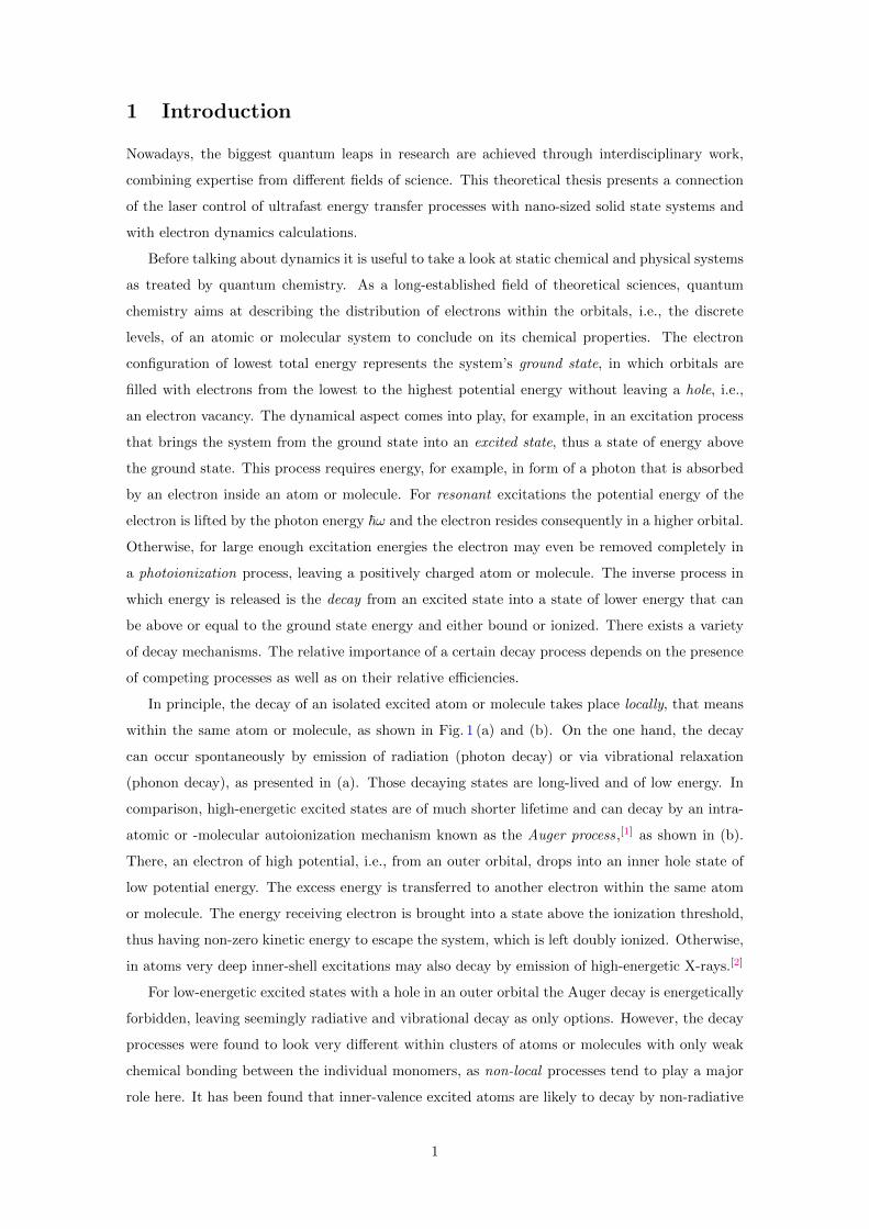
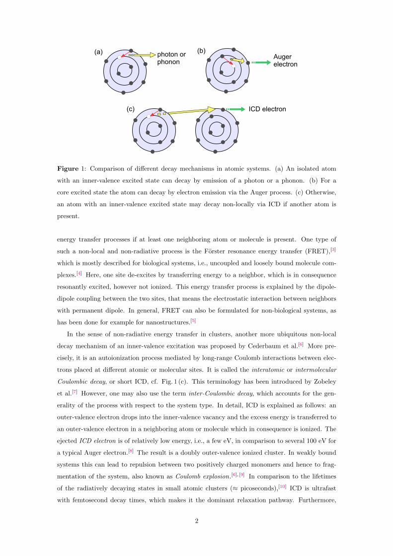
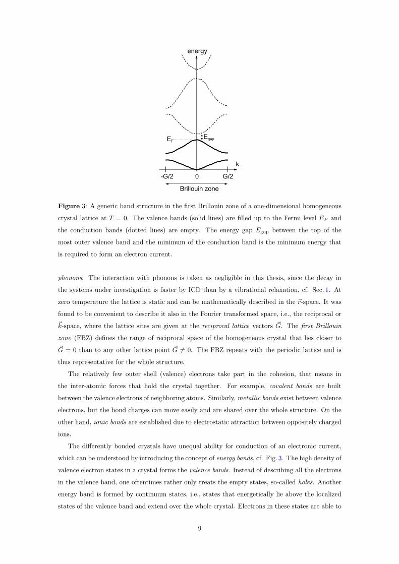
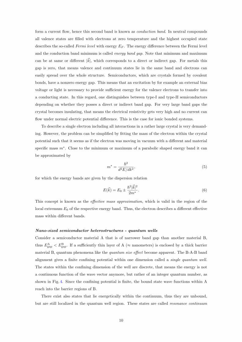
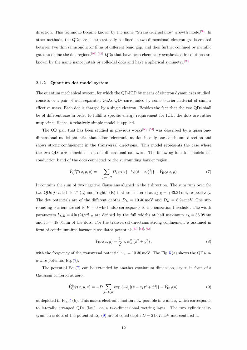
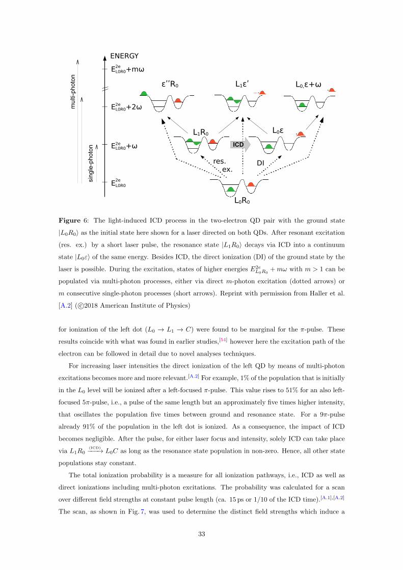
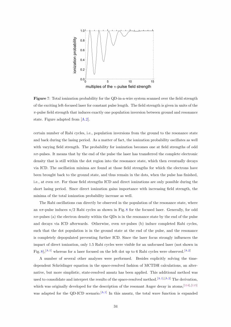

0 5 10 15 20 25 300
02
04
06
08
1
0 5 10 15 20 25 300
02
04
06
08
1
n=6
n=4
n=2
n=5
n=3
n=1
t [ps]
(a)
(b)P
L1R
0nπ
PL1
R0
nπ
Figure 8 Resonance state populations for the nπ-laser pulse excitations for (a) n = 1 3 5 and
(b) n = 2 4 6 with a focus on the left QD The space-resolved calculations are performed on
the long CAP-free grid (solid lines) A comparison is made to the state-resolved method for the
3π-pulse (dashed blue line) For the constant pulse length tpulse = 141 ps the field strengths ηnπ
are applied as obtained from the scan Reprint with permission from Haller et al [A2] ( ccopy2018
American Institute of Physics)
in the orthonormal basis of the time-independent two-electron eigenstates thus it is represented
by a linear combination of the states with time-dependent coefficients The latter contain the
information on the state populations For simplification a restriction is made on the states that
are allowed to be populated by excluding multi-photon excited states This means that only the
scenario for weak and left-focused lasers can be described with this ansatz The calculations are
significantly faster but require an a priori calculation of all relevant energies and transition rates
thus they cannot replace the main MCTDH method
Another analysis was done concerning the absorbing boundary conditions that showed to
have an impact on the computations[A2] After the resonant excitation of the ground state the
computations on the short grid with absorbing boundaries revealed an overall lower thus physically
wrong population of the resonance state This was explained by the presence of the absorbing
boundaries that may accelerate the direct photoionization of the electron in the right QD By
contrast the computations on the long grid gave the physically correct description of the state
populations but require a compromise on computational effort and limitation of the propagation
times until the dynamics is disturbed by backscattered electrons In fact the decay for the given
example can only be observed for ca 64 ps that is about 13 of the ICD decay time Despite the
deviations in absolute values the resonance state populations decrease with always the identical
35
|0001 rangL
R|00rang |01rang|0010 rang
|0002 rang
|0023 rang
|0110 rang |01rang|10rang|0102 rang |02 rang |01rang|1002 rang
|2301 rang |01rang|23 rang
GS RES-X
RES-Z
Figure 9 Electronic structure of two laterally arranged QDs represented by two-dimensional
confining potentials The figure shows the wave function densities of the two-electron states
|mx1 nz1 mx2 nz2〉 in the triplet configuration The ground state (GS) and the two degenerate
resonance states in x (RES-X) and in z (RES-Z) are the relevant states for which ICD was studied
Figure adapted from [A3]
ICD rate independent of the grids and boundaries Therefore if only the ICD rate is of interest
computing on the short grid provides sufficiently accurate results
Turning to the third laser control option of the QD-ICD process the laser polarization was
studied with the aim to control the emission direction of the ICD electron[A3] Therefore a second
continuum direction was allowed by using a two-dimensional Gaussian binding model potential
for the QD pair It has three discrete levels in x (mx = 0 1 2) and four in z of which three
lie in the left QD (nz = 0 2 3) and one in the right dot (nz = 1) They combine to the five
different single-electron states |mx nz〉 = |0 0〉 |0 1〉 |1 0〉 |0 2〉 |2 3〉 from which one obtains
eight two-electron states for uncoupled electrons in the triplet configuration as depicted in Fig 9
In the interacting two-electron picture each dimension reveals one resonance state that was
found to decay via ICD The process was initiated by a resonant π-pulse sampling different polar-
izations The efficient preparation of the resonance states was as in [A2] achieved by a focused
36
0 50 100 150 200 250 30000
02
04
06
08
10
t [ps]
(a)
Pα(t
)P
α(t
)
Pα(t
)
(b)
(c) (d)
(e)
00
02
04
06
08
10
00
02
04
06
08
10
0 50 100 150 200 250 300
t [ps]0 50 100 150 200 250 300
t [ps]
Figure 10 Time evolution of the population Pα(t) for the ground state (blue solid line) and
resonance states in x (green dotted line) and z direction (red dashed line) for resonant π-pulse
excitations The upper row displays the case of linear polarization with εx = 00 and εz = 10 (a)
and εx = 10 and εz = 00 (b) for the pulse length tlinearpulse = 166 ps The middle row shows elliptical
polarization with εx = 05 and εz = 10 (c) and εx = 10 and εz = 05 (d) with tellipticalpulse = 148 ps
In (e) the system is excited by circularly polarized light with εx = εz = 10 and tcircularpulse = 116 ps
Reprint with permission from Haller et al [A3] ( ccopy2019 American Chemical Society)
laser directed on the left QD to minimize excitations by direct ionization Fig 10 shows the time-
dependent populations under the excitations by differently polarized light with the ground state as
initial configuration Under linearly polarized light either in z (a) or x (b) one of the resonances
is populated while the other stays unpopulated When changing to elliptical polarization (c)
and (d) the other resonance state is admixed to the total population For circular polarization
(e) both resonances get equally populated For excitations with non-linearly polarized light the
decay of the z-resonance is overlaid with oscillations cf red line in Fig 10 (c)-(e) The reason for
this is the beating between the two resonances due to a small difference in the resonance energies
In general the decay of the z-resonance is four times faster than that of the x-resonance This
is due to geometrical reasons as the overlap of both electrons is larger for the z-resonance and
hence energy transfer from the left to the right QD is more efficient
In [A3] it could be shown that the emission direction of the electron depends on the polarization
of the exciting laser cf Fig 11 As discussed before linearly polarized light excites only one of
37
8times10ndash8
ρ (xzt)
(c)
(a) (b)
6times10ndash8
4times10ndash8
2times10ndash8
10ndash7
0
100 ps 100 ps
100 ps 180 ps 240 ps
Figure 11 Electron wave function density for ICD in QDs with two-dimensional continuum The
decay is shown after exciting the ground state with linearly polarized light in z (a) and in x (b)
and with circularly polarized light (c) The ldquotimesrdquo mark the centers of the QDs Figure adapted
from [A3]
the resonance states It was found that the decay of either resonance is uniform that means
the emission direction does not change over time cf Fig 11 (a) and (b) For the decay of the
z-resonance (a) the electron in the right QD leaves particularly into plusmnx and +z The negative
z direction is avoided because of the Coulomb barrier that is formed by the electron in the left
QD As the density splits equally into positive and negative x a drift towards negative z can be
observed which means that momentum transfer from x to z is possible which is here due to
the non-separable Gaussian potential Moreover it was shown that the decay becomes 16 times
slower if the electron is hindered to move into x which was realized by applying infinitely high
walls left and right from the dots in x direction
For the uniform decay of the x-resonance (b) most density leaves into x with equal distribution
into positive and negative direction and with drift towards the positive z direction Again the
barrier that is formed by the electron in the left dot does not allow motion in negative z
The density for the decay of the mixed resonances as realized by excitation with the circularly
polarized laser is shown in Fig 11 (c) Here the emission direction oscillates which results from
the beating between the two resonances as explained above for the oscillating populations Again
the negative z direction is avoided The same behavior can be found for excitations with elliptically
polarized light which is not shown here
38
The impact of the Coulomb barrier in the left dot which hinders the ICD electron in moving
into the negative z direction was also observed in [A3] for a geometrical study where the ICD
rate for the decay of either resonance was determined in dependence of the inter-QD distance It
was found that for the pure decay of the x- and z-resonance the ICD rate oscillates about Rminus6
with mean deviations of 30 and 24 Those oscillations have been observed earlier for the QDs-
in-a-wire scenario with deviations of 85 on average[53] where they came from the reflection of
the ICD electron at the left QD Coulomb barrier followed by a recapture The oscillations for the
dots with two-dimensional continuum are however smaller which means the chance for recapture
is diminished
In conclusion the QD-ICD is a highly-efficient decay process either inside a one-dimensional
nanowire or on a two-dimensional wetting layer where ICD is faster for the latter system in
which the ICD electron can move along two directions For the initiation of ICD in negatively
charged QDs weak infrared laser pulses with a focus on the eventually energy emitting dot are
best suited Moreover the polarization of the resonantly exciting laser controls the mixture of
resonance states that forms the decaying state which itself has an impact on the electron emission
direction Going beyond the formerly investigated QDs in a wire a more easily accessible quantum
dot system was proposed here in terms of laterally arranged quantum dots on a two-dimensional
surface which are commonly realized through self-assembly or lithographically Those structures
are more widespreadly investigated Hence they are promising for detecting ICD inside QDs in
a future experiment as well as for a possible device application eg for improved QD infrared
photodetectors that function by means of ICD
It is for sure that the QD-ICD has a lot more features than what can possibly be explained by
the simplified model of this thesis There is an indescribable amount of theory waiting and many
device applications could profit from this For example in a more concrete experimental setup the
system might consist of a cluster of more than two QDs with as many electrons This would make
the study of a cascade of ICD processes interesting but would also require the computation of a
high-dimensional problem QD-ICD could also be a prominent process to be used for sensitized
solar cells[116] [117] Respective QDs are neutral and have a band gap in the range of 1 eV such
that excitations by visible or near-IR light lead to inter-band transitions thus to the formation
of excitons QD-ICD in combination with exciton Rabi oscillations can be also interesting for
quantum information processing[96] [118] [119] Another promising type of system are colloidal
QDs since they are relatively straightforward to produce in solution with a possibility to control
the inter-dot distance[93] [120] To study ICD in these types of dots would require to incorporate
a third continuum dimension
39
References
[1] M Thompson M D Baker A Christie and J F Tyson Auger Electron Spectroscopy
Wiley New York 1985
[2] L V Azaroff X-Ray Spectroscopy McGraw-Hill New York 1974
[3] T Forster Zwischenmolekulare Energiewanderung und Fluoreszenz Ann Phys 43755ndash
75 1948
[4] T W J Gadella FRET and FLIM Techniques Elsevier Science Amsterdam 2009
[5] G D Scholes and D L Andrews Resonance energy transfer and quantum dots Phys Rev
B 72125331 2005
[6] L S Cederbaum J Zobeley and F Tarantelli Giant intermolecular decay and fragmenta-
tion of clusters Phys Rev Lett 794778ndash4781 1997
[7] J Zobeley L S Cederbaum and F Tarantelli Intermolecular Coulombic decay of molecular
clusters Identification of the decay mechanism using a new hole-population analysis J
Phys Chem A 10311145ndash11160 1999
[8] K Kreidi T Jahnke Th Weber T Havermeier X Liu Y Morisita S Schossler LPhH
Schmidt M Schoffler M Odenweller N Neumann L Foucar J Titze B Ulrich F Sturm
C Stuck R Wallauer S Voss I Lauter H K Kim M Rudloff H Fukuzawa G Prumper
N Saito K Ueda A Czasch O Jagutzki H Schmidt-Bocking Stoychev S Ph V De-
mekhin and R Dorner Relaxation processes following 1s photoionization and Auger decay
in Ne2 Phys Rev A 78043422 2008
[9] T Jahnke A Czasch M S Schoffler S Schossler A Knapp M Kasz J Titze C Wimmer
K Kreidi R E Grisenti A Staudte O Jagutzki U Hergenhahn H Schmidt-Bocking
and R Dorner Experimental observation of interatomic Coulombic decay in neon dimers
Phys Rev Lett 93163401 2004
[10] U Hergenhahn Interatomic and intermolecular Coulombic decay The early years J
Electron Spectrosc Relat Phenom 18478 2011
[11] R Santra and L S Cederbaum Non-Hermitian electronic theory and applications to clus-
ters Phys Rep 3681ndash117 2002
[12] V Averbukh PhV Demekhin P Kolorenc S Scheit SD Stoychev AI Kuleff Y-C
Chiang K Gokhberg S Kopelke N Sisourat and LS Cederbaum Interatomic elec-
tronic decay processes in singly and multiply ionized clusters J Electron Spectrosc Relat
Phenom 18336ndash47 2011
40
[13] T Jahnke Interatomic and intermolecular Coulombic decay The coming of age story J
Phys B At Mol Opt Phys 48082001 2015
[14] V Averbukh I B Muller and L S Cederbaum Mechanism of interatomic Coulombic
decay in clusters Phys Rev Lett 93263002 2004
[15] R Santra J Zobeley and L S Cederbaum Electronic decay of valence holes in clusters
and condensed matter Phys Rev B 64245104 2001
[16] T Jahnke A Czasch M Schoffler S Schossler M Kasz J Titze K Kreidi R E Grisenti
A Staudte O Jagutzki L Ph H Schmidt Th Weber H Schmidt-Bocking K Ueda and
R Dorner Experimental separation of virtual photon exchange and electron transfer in
interatomic Coulombic decay of neon dimers Phys Rev Lett 99153401 2007
[17] S Barth S Joshi S Marburger V Ulrich A Lindblad G Ohrwall O Bjorneholm and
U Hergenhahn Observation of resonant interatomic Coulombic decay in Ne clusters J
Chem Phys 122241102 2005
[18] T Aoto K Ito Y Hikosaka E Shigemasa F Penent and P Lablanquie Properties of
resonant interatomic Coulombic decay in Ne dimers Phys Rev Lett 97243401 2006
[19] K Gokhberg A B Trofimov T Sommerfeld and L S Cederbaum Ionization of metal
atoms following valence-excitation of neighbouring molecules Europhys Lett 72228 2005
[20] K Gokhberg V Averbukh and L S Cederbaum Interatomic decay of inner-valence-excited
states in clusters J Chem Phys 124144315 2006
[21] L S Cederbaum Ultrafast intermolecular energy transfer from vibrations to electronic
motion Phys Rev Lett 121223001 2018
[22] J Zobeley L S Cederbaum and F Tarantelli Highly excited electronic states of molecular
clusters and their decay J Chem Phys 1089737ndash9750 1998
[23] R Santra LS Cederbaum and H-D Meyer Electronic decay of molecular clusters Non-
stationary states computed by standard quantum chemistry methods Chem Phys Lett
303413 ndash 419 1999
[24] R Santra J Zobeley L S Cederbaum and N Moiseyev Interatomic Coulombic decay in
van der Waals clusters and impact of nuclear motion Phys Rev Lett 854490ndash4493 2000
[25] N Moiseyev R Santra J Zobeley and L S Cederbaum Fingerprints of the nodal structure
of autoionizing vibrational wave functions in clusters Interatomic Coulombic decay in Ne
dimer J Chem Phys 1147351ndash7360 2001
[26] S Scheit L S Cederbaum and H-D Meyer Time-dependent interplay between electron
emission and fragmentation in the interatomic Coulombic decay J Chem Phys 1182092ndash
2107 2003
41
[27] S Marburger O Kugeler U Hergenhahn and T Moller Experimental evidence for inter-
atomic Coulombic decay in Ne clusters Phys Rev Lett 90203401 2003
[28] G Ohrwall M Tchaplyguine M Lundwall R Feifel H Bergersen T Rander A Lind-
blad J Schulz S Peredkov S Barth S Marburger U Hergenhahn S Svensson and
O Bjorneholm Femtosecond interatomic Coulombic decay in free neon clusters Large
lifetime differences between surface and bulk Phys Rev Lett 93173401 2004
[29] S Kopelke K Gokhberg V Averbukh F Tarantelli and L S Cederbaum Ab initio
interatomic decay widths of excited states by applying Stieltjes imaging to Lanczos pseu-
dospectra J Chem Phys 134094107 2011
[30] T Ouchi K Sakai H Fukuzawa X-J Liu I Higuchi Y Tamenori K Nagaya
H Iwayama M Yao D Zhang D Ding A I Kuleff S D Stoychev Ph V Demekhin
N Saito and K Ueda Three-electron interatomic Coulombic decay from the inner-valence
double-vacancy states in NeAr Phys Rev Lett 107053401 2011
[31] R Santra and L S Cederbaum Coulombic energy transfer and triple ionization in clusters
Phys Rev Lett 90153401 2003
[32] Y Morishita X-J Liu N Saito T Lischke M Kato G Prumper M Oura H Yamaoka
Y Tamenori I H Suzuki and K Ueda Experimental evidence of interatomic Coulombic
decay from the Auger final states in argon dimers Phys Rev Lett 96243402 2006
[33] S D Stoychev A I Kuleff F Tarantelli and L S Cederbaum On the interatomic
electronic processes following Auger decay in neon dimer J Chem Phys 129074307
2008
[34] E F Aziz N Ottosson M Faubel I V Hertel and B Winter Interaction between liquid
water and hydroxide revealed by core-hole de-excitation Nature 45589 2008
[35] W Pokapanich H Bergersen I L Bradeanu RRT Marinho A Lindblad S Legendre
A Rosso S Svensson O Bjorneholm M Tchaplyguine G Ohrwall N V Kryzhevoi and
L S Cederbaum Auger electron spectroscopy as a probe of the solution of aqueous ions
J Am Chem Soc 1317264 2009
[36] M Mucke M Braune S Barth M Forstel T Lischke V Ulrich T Arion U Becker
A Bradshaw and U Hergenhahn A hitherto unrecognized source of low-energy electrons
in water Nat Phys 6143 2010
[37] T Jahnke H Sann T Havermeier K Kreidi C Stuck M Meckel M Schoffler N Neu-
mann R Wallauer S Voss A Czasch O Jagutzki A Malakzadeh F Afaneh Th Weber
H Schmidt-Bocking and R Dorner Ultrafast energy transfer between water molecules
Nat Phys 6139 2010
42
[38] K Gokhberg and L S Cederbaum Environment assisted electron capture J Phys B At
Mol Opt Phys 42231001 2009
[39] K Gokhberg and L S Cederbaum Interatomic Coulombic electron capture Phys Rev A
82052707 2010
[40] F M Pont A Bande and L S Cederbaum Controlled energy-selected electron capture
and release in double quantum dots Phys Rev B 88241304 2013
[41] A Molle E R Berikaa F M Pont and A Bande Quantum size effect affecting envi-
ronment assisted electron capture in quantum confinements J Chem Phys 150224105
2019
[42] J Titze M S Schoffler H-K Kim F Trinter M Waitz J Voigtsberger N Neumann
B Ulrich K Kreidi R Wallauer M Odenweller T Havermeier S Schossler M Meckel
L Foucar T Jahnke A Czasch L Ph H Schmidt O Jagutzki R E Grisenti H Schmidt-
Bocking H J Ludde and R Dorner Ionization dynamics of helium dimers in fast collisions
with He++ Phys Rev Lett 106033201 2011
[43] H K Kim H Gassert M S Schoffler J N Titze M Waitz J Voigtsberger F Trinter
J Becht A Kalinin N Neumann C Zhou LPhH Schmidt O Jagutzki A Czasch
H Merabet H Schmidt-Bocking T Jahnke A Cassimi and R Dorner Ion-impact-
induced interatomic Coulombic decay in neon and argon dimers Phys Rev A 88042707
2013
[44] S Yan P Zhang X Ma S Xu B Li X L Zhu W T Feng S F Zhang D M
Zhao R Zhang D Guo and H P Liu Observation of interatomic Coulombic decay and
electron-transfer-mediated decay in high-energy electron-impact ionization of Ar2 Phys
Rev A 88042712 2013
[45] S Yan P Zhang X Ma S Xu S X Tian B Li X L Zhu W T Feng and D M
Zhao Dissociation mechanisms of the Ar trimer induced by a third atom in high-energy
electron-impact ionization Phys Rev A 89062707 2014
[46] P H P Harbach M Schneider S Faraji and A Dreuw Intermolecular Coulombic decay
in biology The initial electron detachment from FADHminus in DNA photolyases J Phys
Chem Lett 4943ndash949 2013
[47] A Dreuw and S Faraji A quantum chemical perspective on (6-4) photolesion repair by
photolyases Phys Chem Chem Phys 1519957ndash19969 2013
[48] A I Ekimov and A A Onushchenko Quantum size effect in three-dimensional microscopic
semiconductor crystals JETP Lett 34345 1981
43
[49] A L Efros Interband absorption of light in a semiconductor sphere Sov Phys Semicond
16772ndash775 1982
[50] L E Brus A simple model for the ionization potential electron affinity and aqueous redox
potentials of small semiconductor crystallites J Chem Phys 795566ndash5571 1983
[51] M A Reed R T Bate K Bradshaw W M Duncan W R Frensley J W Lee and H D
Shih Spatial quantization in GaAs-AlGaAs multiple quantum dots J Vac Sci Technol
B 4358ndash360 1986
[52] I Cherkes and N Moiseyev Electron relaxation in quantum dots by the interatomic Coulom-
bic decay mechanism Phys Rev B 83113303 2011
[53] A Bande K Gokhberg and L S Cederbaum Dynamics of interatomic Coulombic decay
in quantum dots J Chem Phys 135144112 2011
[54] A Bande Electron dynamics of interatomic Coulombic decay in quantum dots induced by
a laser field J Chem Phys 138214104 2013
[55] M A Kastner Artificial atoms Phys Today 4624ndash31 1993
[56] U Bockelmann Exciton relaxation and radiative recombination in semiconductor quantum
dots Phys Rev B 4817637ndash17640 1993
[57] U Bockelmann and T Egeler Electron relaxation in quantum dots by means of Auger
processes Phys Rev B 4615574ndash15577 1992
[58] Al L Efros and M Rosen Random telegraph signal in the photoluminescence intensity of
a single quantum dot Phys Rev Lett 781110ndash1113 1997
[59] V I Klimov A A Mikhailovsky S Xu A Malko J A Hollingsworth C A Leatherdale
H-J Eisler and M G Bawendi Optical gain and stimulated emission in nanocrystal
quantum dots Science 290314ndash317 2000
[60] A Kurzmann A Ludwig A D Wieck A Lorke and M Geller Auger recombination in
self-assembled quantum dots Quenching and broadening of the charged exciton transition
Nano Lett 163367ndash3372 2016
[61] A Bande F M Pont P Dolbundalchok K Gokhberg and L S Cederbaum Electron
dynamics of interatomic Coulombic decay in quantum dots Singlet initial state EPJ Web
Conf 4104031 2013
[62] P Dolbundalchok D Pelaez E F Aziz and A Bande Geometrical control of the inter-
atomic Coulombic decay process in quantum dots for infrared photodetectors J Comput
Chem 372249ndash2259 2016
44
[63] P Lodahl A F van Driel I S Nikolaev A Irman K Overgaag D Vanmaekelbergh
and W L Vos Controlling the dynamics of spontaneous emission from quantum dots by
photonic crystals Nature 430654ndash657 2004
[64] A Bande Acoustic phonon impact on the inter-Coulombic decay process in charged quan-
tum dot pairs Mol Phys 2019 DOI 1010800026897620191574986
[65] F Weber E F Aziz and A Bande Interdependence of ICD rates in paired quantum dots
on geometry J Comput Chem 382141ndash2150 2017
[66] H-D Meyer U Manthe and L S Cederbaum The multi-configurational time-dependent
Hartree approach Chem Phys Lett 16573ndash78 1990
[67] U Manthe H-D Meyer and L S Cederbaum Wave-packet dynamics within the multicon-
figuration Hartree framework General aspects and application to NOCl J Chem Phys
973199ndash3213 1992
[68] U Fano Effects of configuration interaction on intensities and phase shifts Phys Rev
1241866ndash1878 1961
[69] S-W Lee K Hirakawa and Y Shimada Bound-to-continuum intersubband photoconduc-
tivity of self-assembled InAs quantum dots in modulation-doped heterostructures Appl
Phys Lett 751428ndash1430 1999
[70] I I Rabi Space quantization in a gyrating magnetic field Phys Rev 51652ndash654 1937
[71] I I Rabi S Millman P Kusch and J R Zacharias The molecular beam resonance
method for measuring nuclear magnetic moments the magnetic moments of 3Li6 3Li7 and
9F19 Phys Rev 55526ndash535 1939
[72] A Zrenner A close look on single quantum dots J Chem Phys 1127790ndash7798 2000
[73] M G Bawendi P J Carroll William L Wilson and L E Brus Luminescence properties
of CdSe quantum crystallites Resonance between interior and surface localized states J
Chem Phys 96946ndash954 1992
[74] H Drexler D Leonard W Hansen J P Kotthaus and P M Petroff Spectroscopy of
quantum levels in charge-tunable InGaAs quantum dots Phys Rev Lett 732252ndash2255
1994
[75] S Sauvage P Boucaud F H Julien J-M Gerard and V Thierry-Mieg Intraband ab-
sorption in n-doped InAsGaAs quantum dots Appl Phys Lett 712785ndash2787 1997
[76] P Guyot-Sionnest and M A Hines Intraband transitions in semiconductor nanocrystals
Appl Phys Lett 72686ndash688 1998
[77] N N Ledentsov Quantum dot laser Semicond Sci Technol 26014001 2011
45
[78] P Michler A Kiraz C Becher W V Schoenfeld P M Petroff L Zhang E Hu and
A Imamoglu A quantum dot single-photon turnstile device Science 2902282ndash2285 2000
[79] S Maimon E Finkman G Bahir S E Schacham J M Garcia and P M Petroff Inter-
sublevel transitions in InAsGaAs quantum dots infrared photodetectors Appl Phys Lett
732003ndash2005 1998
[80] D Pan E Towe and S Kennerly Normal-incidence intersubband (In Ga)AsGaAs quan-
tum dot infrared photodetectors Appl Phys Lett 731937ndash1939 1998
[81] H C Liu M Gao J McCaffrey Z R Wasilewski and S Fafard Quantum dot infrared
photodetectors Appl Phys Lett 7879ndash81 2001
[82] S-F Tang S-Y Lin and S-C Lee Near-room-temperature operation of an InAsGaAs
quantum-dot infrared photodetector Appl Phys Lett 782428ndash2430 2001
[83] P Harrison and A Valavanis Quantum Wells Wires and Dots John Wiley amp Sons Ltd
Chichester 2016
[84] H Bruus and K Flensberg Many-Body Quantum Theory in Condensed Matter Physics
An Introduction Oxford University Press Oxford 2004
[85] H Ibach and H Luth Festkorperphysik Einfuhrung in die Grundlagen Springer Berlin
Heidelberg 2013
[86] L de Broglie Waves and quanta Nature 112540 1923
[87] P M Petroff A Lorke and A Imamoglu Epitaxially self-assembled quantum dots Phys
Today 5446ndash52 2001
[88] L Wang A Rastelli S Kiravittaya M Benyoucef and O G Schmidt Self-assembled
quantum dot molecules Adv Mater 212601ndash2618 2009
[89] E Zallo P Atkinson L Wang A Rastelli and O G Schmidt Epitaxial growth of lateral
quantum dot molecules Phys Status Solidi B 249702ndash709 2012
[90] D Bimberg M Grundmann and N N Ledentsov Quantum Dot Heterostructures John
Wiley amp Sons Ltd Chichester 1999
[91] L P Kouwenhoven C M Marcus P L McEuen S Tarucha R M Westervelt and N S
Wingreen Mesoscopic Electron Transport Kluwer Academic Dordrecht 1997
[92] W G van der Wiel S De Franceschi J M Elzerman T Fujisawa S Tarucha and L P
Kouwenhoven Electron transport through double quantum dots Rev Mod Phys 751ndash22
2002
[93] Y Yin and A P Alivisatos Colloidal nanocrystal synthesis and the organic-inorganic
interface Nature 437664ndash670 2005
46
[94] S Bednarek B Szafran T Chwiej and J Adamowski Effective interaction for charge
carriers confined in quasi-one-dimensional nanostructures Phys Rev B 68045328 2003
[95] D J Tannor Introduction to Quantum Mechanics University Science Books USA 2007
[96] J Luo W Lai D Lu C Du Y Liu S Gong D Shi and C Guo Pronounced enhancement
of exciton rabi oscillation for a two-photon transition based on quantum dot coupling control
J Phys B At Mol Opt Phys 45035402 2012
[97] R Kosloff and D Kosloff Absorbing boundaries for wave propagation problems J Comput
Phys 63363ndash376 1986
[98] D Neuhauser and M Baer The time-dependent Schrodinger equation Application of
absorbing boundary conditions J Chem Phys 904351ndash4355 1989
[99] U V Riss and H-D Meyer Calculation of resonance energies and widths using the complex
absorbing potential method J Phys B At Mol Opt Phys 264503ndash4535 1993
[100] U V Riss and H-D Meyer Investigation on the reflection and transmission properties of
complex absorbing potentials J Chem Phys 1051409ndash1419 1996
[101] Y Sajeev and N Moiseyev Theory of autoionization and photoionization in two-electron
spherical quantum dots Phys Rev B 78075316 2008
[102] NSM Archive - Physical properties of semiconductors httpmatpropruGaAs basic (ac-
cessed 21-Nov-2018)
[103] P A M Dirac Note on exchange phenomena in the Thomas atom Math Proc Cambridge
26376ndash385 1930
[104] J Frenkel Wave Mechanics Clarendon Press Oxford 1934
[105] AD McLachlan A variational solution of the time-dependent Schrodinger equation Mol
Phys 839ndash44 1964
[106] M Beck The multiconfiguration time-dependent Hartree (MCTDH) method A highly
efficient algorithm for propagating wavepackets Phys Rep 3241ndash105 2000
[107] H-D Meyer F Gatti and G A Worth Multidimensional Quantum Dynamics - MCTDH
Theory and Applications Wiley-VCH Weinheim 2009
[108] J C Light I P Hamilton and J V Lill Generalized discrete variable approximation in
quantum mechanics J Chem Phys 821400ndash1409 1985
[109] J C Light Discrete variable representations in quantum dynamics in Time-Dependent
Quantum Molecular Dynamics pages 185ndash199 Springer US New York 1992
47
[110] J C Light and T Carrington Jr Discrete Variable Representations and their Utilization
in Advances in Chemical Physics pages 263ndash310 Wiley-Blackwell 2007
[111] D Pelaez and H-D Meyer The multigrid POTFIT (MGPF) method Grid representations
of potentials for quantum dynamics of large systems J Chem Phys 138014108 2013
[112] R Kosloff and H Tal-Ezer A direct relaxation method for calculating eigenfunctions and
eigenvalues of the Schrodinger equation on a grid Chem Phys Lett 127223ndash230 1986
[113] C Leforestier and R E Wyatt Optical potential for laser induced dissociation J Chem
Phys 782334ndash2344 1983
[114] Y-C Chiang Ph V Demekhin A I Kuleff S Scheit and L S Cederbaum Linewidth
and lifetime of atomic levels and the time evolution of spectra and coincidence spectra Phys
Rev A 81032511 2010
[115] Ph V Demekhin and L S Cederbaum Strong interference effects in the resonant Auger
decay of atoms induced by intense x-ray fields Phys Rev A 83023422 2011
[116] AJ Nozik Quantum dot solar cells Physica E 14115ndash120 2002
[117] P V Kamat Quantum dot solar cells Semiconductor nanocrystals as light harvesters J
Phys Chem C 11218737ndash18753 2008
[118] T H Stievater Xiaoqin Li D G Steel D Gammon D S Katzer D Park C Piermarocchi
and L J Sham Rabi oscillations of excitons in single quantum dots Phys Rev Lett
87133603 2001
[119] G Ya Slepyan A Magyarov S A Maksimenko A Hoffmann and D Bimberg Rabi oscil-
lations in a semiconductor quantum dot Influence of local fields Phys Rev B 70045320
2004
[120] P Alivisatos Colloidal quantum dots From scaling laws to biological applications Pure
Appl Chem 723ndash9 2000
48
A Publications
In this chapter the scientific publications [A1]-[A3] composing this thesis are presented in chrono-
logical order For each publication the contributions by the individual authors are outlined
49
A1 Strong field control of the interatomic Coulombic decay process in
quantum dots
Anika Haller Ying-Chih Chiang Maximilian Menger Emad F Aziz and Annika Bande
Chem Phys 482 135-145 (2017)
DOI 101016jchemphys201609020
URL httpsdoiorg101016jchemphys201609020
Figure A1 Graphical abstract Reprint with permission from Haller et al [A1] ( ccopy2017 Elsevier)
Author contributions The conception of this work was conceived by AB Preliminary cal-
culations were conducted by MM during his Bachelor thesis with AB in 2013 AH performed
all calculations data analysis and visual presentation of the results YCC derived the analytical
expressions for the state resolved equations of motions and wrote a Fortran program for numer-
ical solution The theory section was written by AH The introduction and the conclusion were
written by AB AB and AH analyzed and discussed the results in detail and composed the results
section of this article All authors contributed to bring the pre-final version of the manuscript into
a submittable form
50
51 - 61
A2 Favoritism of quantum dot inter-Coulombic decay over direct and
multi-photon ionization by laser strength and focus
Anika Haller and Annika Bande
J Chem Phys 149 134102 (2018)
DOI 10106315042208
URL httpsdoiorg10106315042208
ICD
ICD
laser focus amp field strength
variation
Figure A2 Graphical abstract created exclusively for this thesis Figure adapted from [A2]
Author contributions The conception of this work was conceived by AB AH performed all
calculations data analysis and visual presentation of the results The manuscript was mostly
written by AH with considerable input from AB
62
63 - 74
A3 Inter-Coulombic decay in laterally arranged quantum dots con-
trolled by polarized lasers
Anika Haller Daniel Pelaez and Annika Bande
J Phys Chem C 123 14754-14765 (2019)
DOI 101021acsjpcc9b01250
URL httpsdoiorg101021acsjpcc9b01250
Figure A3 Graphical abstract Reprint with permission from Haller et al [A3] ( ccopy2019 Amer-
ican Chemical Society)
Author contributions The conception of this work was conceived by AB DP provided the
Coulomb potential files (natpot) that he calculated with the Multigrid POTFIT program (MGPF)
that was developed by him earlier with another co-author AH performed all electron dynamics
calculations data analysis and visual presentation of the results AB wrote the introduction and
the conclusions AH the theory section except for the MGPF part that was written by DP The
results section was written by AH All authors contributed to the final version of the manuscript
by multiple iterations
75
76 - 87
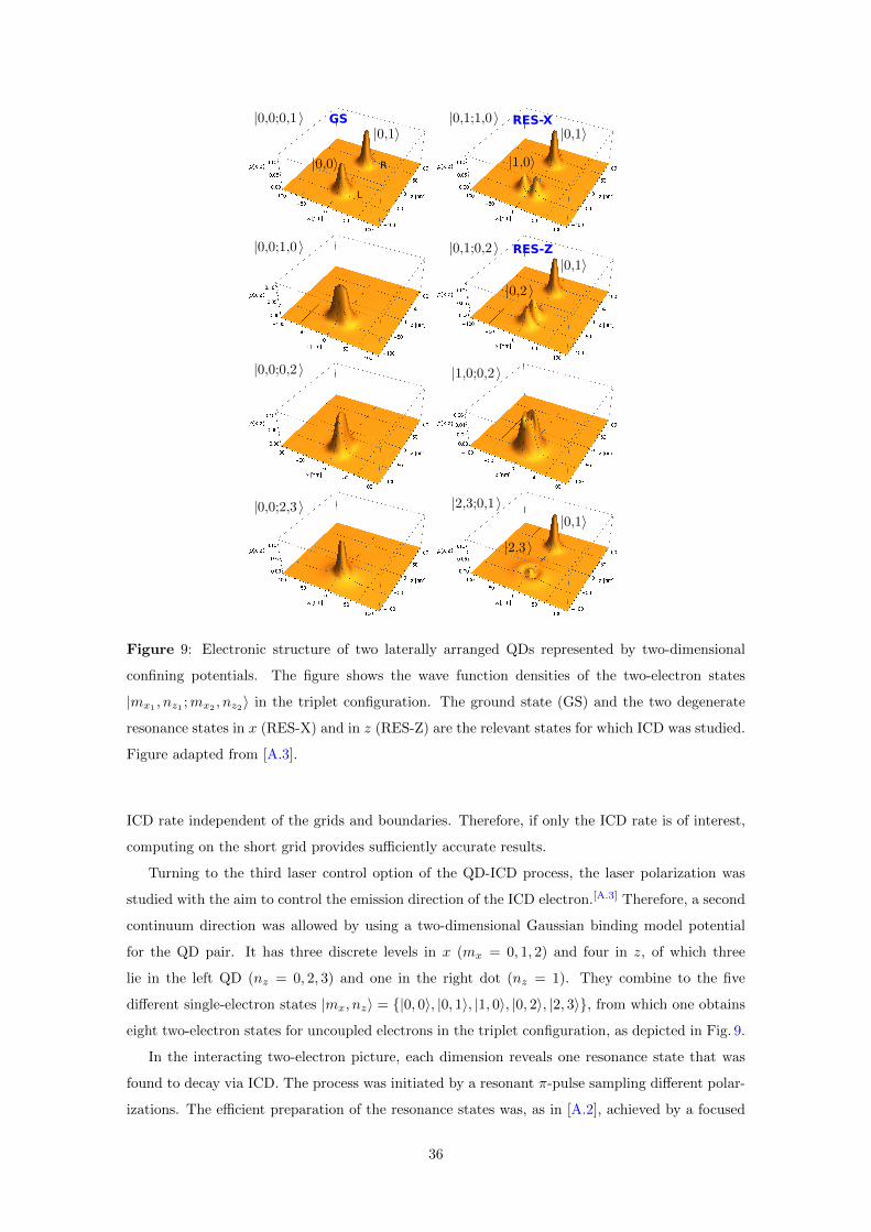
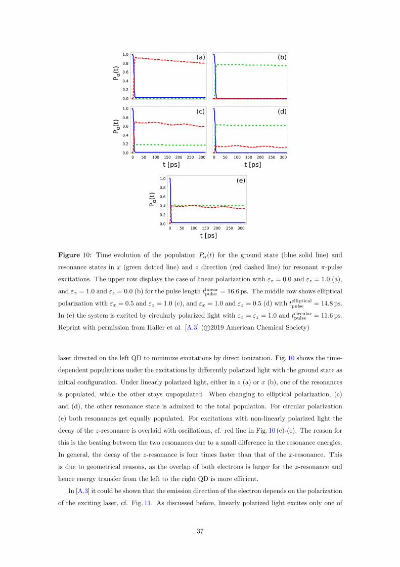
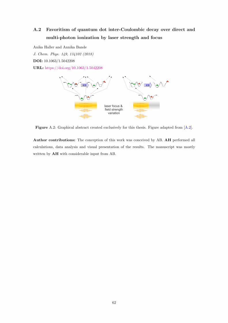
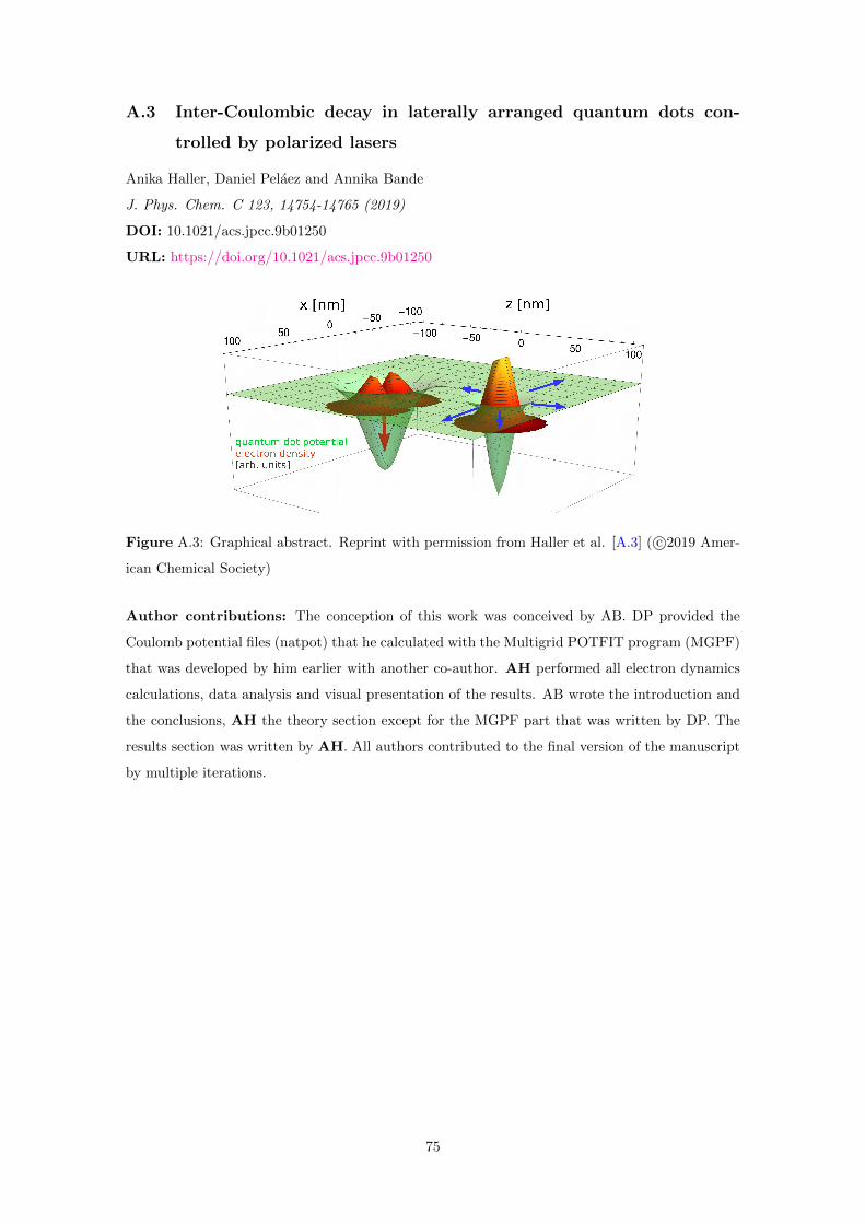

76 - 87
Copyright © 2022 FDOKUMEN