Trajectory-based analyses of ultrafast strong field phenomena
197
Trajectory-based analyses of ultrafast strong field phenomena Dissertation zur Erlangung des akademischen Grades Doctor rerum naturalium (Dr. rer. nat.) vorgelegt der Fakultät Mathematik und Naturwissenschaften der Technischen Universität Dresden von Lisa Ortmann (geb. Keller) geboren am 15.11.1990 in Freiburg i. Br. Max-Planck-Institut für Physik komplexer Systeme Dresden 2019
-
Upload
khangminh22 -
Category
Documents
-
view
0 -
download
0
Transcript of Trajectory-based analyses of ultrafast strong field phenomena

Trajectory-based analyses ofultrafast strong field phenomena
Dissertation
zur Erlangung des akademischen GradesDoctor rerum naturalium
(Dr. rer. nat.)
vorgelegtder Fakultät Mathematik und Naturwissenschaften
der Technischen Universität Dresden
von
Lisa Ortmann(geb. Keller)
geboren am 15.11.1990 in Freiburg i. Br.
Max-Planck-Institut für Physik komplexer Systeme
Dresden 2019


1. Gutacher: Prof. Dr. Manfred Lein2. Gutacher: Prof. Dr. Jan-Michael Rost3. Gutacher: Prof. Dr. Walter Strunz
Eingereicht am 21.05.2019
Verteidigt am 09.09.2019


Contents
Chapter Preamble PAGE 1
Abstract . . . . . . . . . . . . . . . . . . . . . . . . . . . . . . . . . . . . . . . . . . . 1Publication list . . . . . . . . . . . . . . . . . . . . . . . . . . . . . . . . . . . . . . . 5Recurring acronyms and abbreviations . . . . . . . . . . . . . . . . . . . . . . . . . 7
Chapter 1 Introduction and thesis outline PAGE 9
Chapter 2 Fundamental concepts PAGE 15
2.1 Introduction to strong field ionization . . . . . . . . . . . . . . . . . . . . . . 152.1.1 From single to multiphoton ionization . . . . . . . . . . . . . . . . . 152.1.2 Multiphoton versus tunneling ionization . . . . . . . . . . . . . . . . 172.1.3 Atomic units . . . . . . . . . . . . . . . . . . . . . . . . . . . . . . . . . 182.1.4 Basic equations . . . . . . . . . . . . . . . . . . . . . . . . . . . . . . . 19
2.2 Approximations . . . . . . . . . . . . . . . . . . . . . . . . . . . . . . . . . . . 202.3 Classical and Quantum Trajectory Monte Carlo simulations . . . . . . . . . 21
2.3.1 The trajectory picture . . . . . . . . . . . . . . . . . . . . . . . . . . . 212.3.2 The initial conditions . . . . . . . . . . . . . . . . . . . . . . . . . . . 22
2.3.2.1 The adiabatic ionization rate . . . . . . . . . . . . . . . . . 222.3.2.2 The tunnel exit . . . . . . . . . . . . . . . . . . . . . . . . . 252.3.2.3 Implementation of the sampling process . . . . . . . . . . 27
2.3.3 Propagation . . . . . . . . . . . . . . . . . . . . . . . . . . . . . . . . . 292.3.3.1 Propagation in CTMC simulations . . . . . . . . . . . . . . 292.3.3.2 Propagation in QTMC simulations . . . . . . . . . . . . . . 30
Chapter 3 Revisiting nonadiabatic effects on initial conditions PAGE 35
3.1 Introduction to nonadiabatic theories . . . . . . . . . . . . . . . . . . . . . . 353.2 Description of the problem addressed in this chapter . . . . . . . . . . . . . 39

3.3 Relation between the nonadiabatic theories of Yudin/Ivanov and Li . . . . 413.4 Distinguishing between nonadiabatic theories at the detector . . . . . . . . 453.5 Conclusion and Outlook . . . . . . . . . . . . . . . . . . . . . . . . . . . . . . 49
Chapter 4 Intensity and pulse duration dependence of Rydberg states PAGE 53
4.1 Introduction to Rydberg states . . . . . . . . . . . . . . . . . . . . . . . . . . . 544.2 Intensity dependence . . . . . . . . . . . . . . . . . . . . . . . . . . . . . . . . 55
4.2.1 Prior analytical estimates . . . . . . . . . . . . . . . . . . . . . . . . . 554.2.2 Including the ionization time width . . . . . . . . . . . . . . . . . . . 574.2.3 Nonadiabatic effects . . . . . . . . . . . . . . . . . . . . . . . . . . . . 584.2.4 Wavelength correction . . . . . . . . . . . . . . . . . . . . . . . . . . . 624.2.5 Conclusion and Discussion . . . . . . . . . . . . . . . . . . . . . . . . 65
4.3 Pulse duration dependence . . . . . . . . . . . . . . . . . . . . . . . . . . . . 664.3.1 A primer on principal quantum numbers of Rydberg states . . . . . 674.3.2 Simulation results for the principal quantum number distribution . 674.3.3 Physical interpretation of the pulse duration effect . . . . . . . . . . 684.3.4 Testing the effect of the envelope shape . . . . . . . . . . . . . . . . . 694.3.5 Analysis of trajectories . . . . . . . . . . . . . . . . . . . . . . . . . . . 704.3.6 Dependence of the Rydberg yield on pulse duration . . . . . . . . . 724.3.7 Comparison to other models . . . . . . . . . . . . . . . . . . . . . . . 744.3.8 Dependence of the principal quantum number distribution on
pulse duration . . . . . . . . . . . . . . . . . . . . . . . . . . . . . . . . 754.3.9 Conclusion and Discussion . . . . . . . . . . . . . . . . . . . . . . . . 77
Chapter 5 Emergence of a Higher Energy Structure in inhomogeneous fields PAGE 79
5.1 Introduction to inhomogeneous fields . . . . . . . . . . . . . . . . . . . . . . 805.1.1 Introduction to nano-attophysics . . . . . . . . . . . . . . . . . . . . 805.1.2 Mathematical description of inhomogeneous fields . . . . . . . . . 825.1.3 Three different inhomogeneity regimes . . . . . . . . . . . . . . . . . 86
5.2 Emergence of a higher energy structure . . . . . . . . . . . . . . . . . . . . . 875.2.1 Choosing the parameters . . . . . . . . . . . . . . . . . . . . . . . . . 875.2.2 Simulations . . . . . . . . . . . . . . . . . . . . . . . . . . . . . . . . . 88
5.3 Analysis and optimization of the higher energy structure . . . . . . . . . . . 935.3.1 Analytical approximation via Mathieu equations . . . . . . . . . . . 94
5.3.1.1 Analytical approximation for the acceleration and thusthe inhomogeneous field . . . . . . . . . . . . . . . . . . . 95
5.3.1.2 Analytical approximation for the velocity . . . . . . . . . . 965.3.2 Analytical approximation using a perturbative approach . . . . . . 985.3.3 Spectral position of the HES . . . . . . . . . . . . . . . . . . . . . . . . 1005.3.4 Spectral width of the HES . . . . . . . . . . . . . . . . . . . . . . . . . 1035.3.5 Summary of the analysis of the HES . . . . . . . . . . . . . . . . . . . 106
5.4 Unifying effects in strong inhomogeneous fields . . . . . . . . . . . . . . . . 1075.4.1 An intuitive model for the energy upshift observed in the HES . . . 1085.4.2 Unified model for HES and LEP . . . . . . . . . . . . . . . . . . . . . 1095.4.3 A new analytical description of the energy upshift . . . . . . . . . . . 115
5.4.3.1 An analytical description including subcycle effects . . . . 117

5.4.4 Explaining the experimentally observed linear intensity scaling . . 1205.4.5 Conclusion and Outlook . . . . . . . . . . . . . . . . . . . . . . . . . . 121
Chapter 6 Tracking the ionization site in a neutral diatomic molecule PAGE 123
6.1 Goals and challenges in describing molecular effects . . . . . . . . . . . . . 1236.2 The problem of tracking the ionization site in a molecule . . . . . . . . . . . 1256.3 A new method for tracking the ionization site in a molecule . . . . . . . . . 127
6.3.1 Experimental results . . . . . . . . . . . . . . . . . . . . . . . . . . . . 1276.3.2 Performing molecular QTMC simulations . . . . . . . . . . . . . . . 1296.3.3 Explanation for the asymmetry via trajectory analysis . . . . . . . . 1316.3.4 Comparison of theoretical and experimental results to identify
the ionization site . . . . . . . . . . . . . . . . . . . . . . . . . . . . . . 1346.4 Conclusion and Outlook . . . . . . . . . . . . . . . . . . . . . . . . . . . . . . 136
Chapter 7 Conclusions and Outlook PAGE 139
Chapter A Appendix PAGE 145
A.1 Tunnel exits and transverse momentum spreads in nonadiabatic theories . 145A.2 Ionization time spreads of Yudin/Ivanov and Li as special cases of Bondar . 146A.3 Interpretation of the intensity dependence of the Rydberg yield . . . . . . . 148A.4 Equations of motion in the Coulomb-free electric field . . . . . . . . . . . . 149A.5 Term v1 in the perturbative approach . . . . . . . . . . . . . . . . . . . . . . 150A.6 Graphically estimating β for minimal HES width . . . . . . . . . . . . . . . . 153
Chapter Bibliography PAGE 155
Chapter Addendum PAGE 185
Acknowledgments . . . . . . . . . . . . . . . . . . . . . . . . . . . . . . . . . . . . . 185Declaration . . . . . . . . . . . . . . . . . . . . . . . . . . . . . . . . . . . . . . . . . 189


1
Abstract
Semiclassical theories have proven to be a versatile tool in ultrafast strong field sci-ence. In this thesis, the power of classical trajectory Monte Carlo (CTMC) and quantumtrajectory Monte Carlo (QTMC) simulations is celebrated by applying them in variousstrong field ionization settings.
One question to be addressed concerns the way nonadiabaticity in the ionizationprocess manifests itself. It will be shown how the assumption of a vanishing initiallongitudinal momentum is the reason for the strong broadening of the initial timespread claimed in a popular nonadiabatic theory. Moreover, it will become clear howthe broader time spread of this theory and the non-zero initial longitudinal momentaof another widely applied nonadiabatic theory approximately compensate each otherduring propagation for typically studied nonadiabatic parameters. However, param-eters in the nonadiabatic but still experimentally relevant regime will be found wherethis approximation breaks down and the two different theories lead to distinguishablydifferent momentum distributions at the detector after all, thus allowing to test whichtheory describes the situation at the tunnel exit more accurately.
After having tunneled through the barrier formed by the laser and Coulomb poten-tial, the electron does not necessarily leave the atom for good but can be captured ina Rydberg state. A study of the intensity-dependence of the Rydberg yield will reveal,among other things, nonadiabatic effects that can be used as an independent test ofnonadiabaticity in strong field ionization. Moreover, it will be shown that the durationof the laser pulse can be used to control both the yield and principal quantum numberdistribution of Rydberg atoms.
The highly enhanced and spatially inhomogeneous fields close to a nanostructureare another setting in which atoms can be ionized. Here, the emergence of a promi-nent higher energy structure (HES) in the spectrum of photoelectrons will be reported.The narrow time-window in which the corresponding electrons are released suggestsa promising method for creating a localized source of electron pulses of attosecondduration using tabletop laser technology. Having such potential applications in mind,analytical expressions are derived to describe the electrons’ motion in the inhomo-geneous field, thus being able to control the spectral position and width of the HES.Moreover, a unifying theory will be developed in which the recently reported experi-mental finding of a low-energy peak (LEP) can be understood to arise due to the samemechanism as the theoretically predicted HES, despite those two effects having beenfound in different energy regimes so far. This unifying theory will show how the well-established experimental technique in which the LEP was reported, i.e. ionization di-rectly from the nanotip rather than from atoms in its vicinity, should allow the realiza-tion of a prominent and narrow peak at higher energies as it was theoretically describedin the framework of the HES.
Despite being much weaker, the spatial inhomogeneity of the Coulomb potentialcan influence the photoelectron spectrum as well. It will be shown how the asymmet-ric Coulomb potential of a tilted diatomic molecule introduces an asymmetry in thephotoelectron momentum distribution at the detector. The degree of asymmetry de-pends on whether the electron is born at the up- or downfield atom. This informationis then used to quantify the ratio of ionization from the up- and downfield site fromexperimental photoelectron momentum distributions.


3
Kurzfassung
Semiklassische Theorien haben sich als vielfältiges Werkzeug in dem Forschungs-bereich der ultrakurzen und starken Laserfelder herausgestellt. In der vorliegenden Ar-beit wird die Leistungsfähigkeit von Monte Carlo Simulationen mit klassischen undquantenmechanischen Trajektorien gefeiert, indem diese auf verschiedene Systemeder Starkfeldionisation angewendet werden.
Eine der Fragen, die behandelt werden wird, betrifft die Art und Weise, in dersich nichtadiabatische Effekte im Ionisationsprozess manifestieren. Es wird gezeigtwerden, wie die Annahme eines verschwindenden Anfangsimpulses der Grund fürdie starke Verbreiterung der Startzeitenverteilung ist, welche in einer weitverbreitetennichtadiabatischen Theorie angegeben wird. Zudem wird klar werden, wie die breite-re Startzeitenverteilung dieser Theorie und der nichtverschwindende Anfangsimpulseiner anderen häufig angewandten nichtadiabatischen Theorie sich näherungsweisewährend der Propagation kompensieren, wenn typische nichtadiabatische Parameterverwendet werden. Es werden jedoch Parameter im nichtadiabatischen und dennochexperimentell relevanten Bereich gefunden werden, wo diese Näherung versagt unddie zwei verschiedenen Theorien doch noch zu erkennbar verschiedenen Impulsver-teilungen am Detektor führen. Dies erlaubt zu testen, welche Theorie die Situation amTunnelausgang genauer beschreibt.
Nachdem das Elektron durch die Barriere getunnelt ist, die Coulomb- und Laser-potential formen, verlässt das Elektron das Atom nicht unbedingt endgültig, sondernkann in einem Rydbergzustand gefangen werden. Die Untersuchung der Intensitäts-abhängigkeit des Rydbergertrags wird unter anderem nichtadiabatische Effekte her-vorbringen, die als unabhängiger Test von Nichtadiabatizität in der Starkfeldionisationgenutzt werden können. Zudem wird gezeigt, dass die Dauer des Laserpulses verwen-det werden kann, um sowohl den Ertrag als auch die Verteilung der Hauptquantenzahlder Rydbergatome zu kontrollieren.
Ein anderes System, in welchem Atome ionisiert werden können, sind die hochgra-dig verstärkten und räumlich inhomogenen Felder nahe einer Nanostruktur. Hier wirdvon dem Auftreten einer markanten Hochenergiestruktur (HES) berichtet werden. Dasschmale Zeitfenster, in welchem die zugehörigen Elektronen abgegeben werden, weistauf eine vielversprechende Methode zur Erschaffung einer lokalisierten Quelle hin,von der Elektronenpulse mit Pulsdauern im Attosekundenbereich ausgehen und inwelcher ausschließlich Technologie verwendet wird, die auf einen optischen Experi-mentiertisch passt. Mit solchen Anwendungen im Hinterkopf werden analytische Aus-drücke hergeleitet, um die Bewegung der Elektronen im inhomogenen Feld zu be-schreiben und auf diese Weise die spektrale Position und Breite der HES zu kontrol-lieren. Darüber hinaus wird eine verallgemeinernde Theorie entwickelt, in der derkürzlich berichtete experimentelle Fund eines Niederenergiepeaks aufgrund dessel-ben Mechanismus erscheint wie die theoretische vorhergesagte HES, obwohl die bei-den Effekte bislang in verschiedenen Energiebereichen gefunden wurden. Diese ver-allgemeinernde Theorie wird zeigen, wie die gut etablierte experimentelle Technik, mitwelcher die Niederenergiestruktur erzeugt wurde, d.h. Ionisation direkt von der Nano-spitze statt von Atomen in deren Nähe, die Realisierung eines markanten und schma-len Peaks bei hohen Energien ermöglicht, wie er zuvor nur theoretisch im Rahmen derHES beschrieben wurde.
Auch wenn die räumliche Inhomogenität des Coulombpotentials viel schwächerist, kann auch sie das Photoelektronenspektrum beeinflussen. Es wird gezeigt werden,

4
wie das asymmetrische Coulombpotential eines verkippten zweiatomigen Molekülseine Asymmetrie in der Elektronenimpulsverteilung am Detektor erzeugt. Der Gradder Asymmetrie hängt davon ab, ob das Elektron das Molekül am Atom, das oben oderunten im Laserpotential liegt, verlassen hat. Diese Information wird dann genutzt, umdas Verhältnis der Ionisation von den beiden Atomen, die oben oder unten im Laser-potential liegen, aus experimentellen Photoelektronenimpulsverteilungen quantitativzu ermitteln.

Publication list 5
Publication list
The work presented in this thesis has partially already been published as follows:
➔ Emergence of a higher energy structure in strong field ionization with inhomo-geneous electric fieldsL. Ortmann, J. Pérez-Hernández, M. Ciappina, J. Schötz, A. Chacón, G. Zeraouli,M. F. Kling, L. Roso, M. Lewenstein, and A. S. Landsman.Physical Review Letters 119.5 (2017), p. 053204.(see Chapter 5 of this thesis)
➔ Analysis of the higher-energy structure in strong-field ionization with inhomo-geneous electric fieldsL. Ortmann and A. S. Landsman.Physical Review A 97.2 (2018), p. 023420.(see Chapter 5 of this thesis)
➔ Dependence of Rydberg-state creation by strong-field ionization on laser inten-sityL. Ortmann, C. Hofmann, and A. S. Landsman.Physical Review A 98.3 (2018), p. 033415.(see Chapter 4 of this thesis)
Manuscripts in preparation that cover contents of this thesis:
➔ Nonadiabatic effects on the initial longitudinal momentum and the ionizationtime distribution in strong field ionizationL. Ortmann, I. Ivanov, and A. S. Landsman.(see Chapter 3 of this thesis)
➔ Controlling the quantum number distribution and yield of Rydberg states via theduration of the laser pulseL. Ortmann, C. Hofmann, and A. S. Landsman.arXiv:1810.07164(see Chapter 4 of this thesis)
➔ Unifying effects in strong inhomogeneous fieldsL. Ortmann, L. Pi, and A. S. Landsman.(see Chapter 5 of this thesis)
➔ Tracking the ionization site in neutral moleculesAuthor list not finalized yet.(see Chapter 6 of this thesis)
Work that I have been involved in during my PhD studies but that is not presented inthis thesis resulted in the following publications:
➔ Double-electron ionization driven by inhomogeneous fieldsA. Chacón, L. Ortmann, F. Cucchietti, N. Suárez, J. A. Pérez-Hernández, M. F.Ciappina, A. S. Landsman, and M. Lewenstein.appeared in Applied Physics B 4.123 (2017), p. 1 as part of the topical collection‘Enlightening the World with the Laser’, Springer, 2018, p. 491.

6
➔ Wannier-Bloch approach to localization in high-harmonics generation in solidsE. N. Osika, A. Chacón, L. Ortmann, N. Suárez, J. A. Pérez-Hernández, B. Szafran,M. F. Ciappina, F. Sols, A. S. Landsman, and M. Lewenstein.Physical Review X 7.2 (2017), p. 021017.
➔ Instantaneous ionization rate as a functional derivativeI. A. Ivanov, C. Hofmann, L. Ortmann, A. S. Landsman, C. H. Nam, and K. T. Kim.Communications Physics 1.1 (2018), p. 81.
➔ Above-threshold ionization in multicenter molecules: The role of the initial stateN. Suárez, A. Chacón, E. Pisanty, L. Ortmann, A. S. Landsman, A. Picón, J. Biegert,M. Lewenstein, and M. F. Ciappina.Physical Review A 97.3 (2018), p. 033415.
➔ Extraction of higher-order nonlinear electronic response in solids using high har-monic generationS. Han, L. Ortmann, H. Kim, Y. W. Kim, T. Oka, A. Chacon, B. Doran, M. Ciappina,M. Lewenstein, S.-W. Kim, S. Kim, and A. S. Landsman.Nature Communications 10, 3272 (2019)
➔ Attosecond streaking delays in multi-electron systemsT. Zimmermann, L. Ortmann, C. Hofmann, J.-M. Rost, and A. S. Landsman.arXiv:1804.09583
➔ Symphony on Strong Field ApproximationK. Amini, J. Biegert, F. Calegari, A. Chacón, M. F. Ciappina, A. Dauphin, D. K. Efi-mov, C. F. de Morisson Faria, K. Giergiel, P. Gniewek, A. S. Landsman, M. Lesiuk,M. Mandrysz, A. S. Maxwell, R. Moszynski, L. Ortmann, J. A. Pérez-Hernández,A. Picón, E. Pisanty, J. Prauzner-Bechcicki, K. Sacha, N. Suárez, A. Zaïr, J. Za-krzewski, and M. Lewenstein.arXiv:1812.11447

Recurring acronyms and abbreviations 7
Recurring acronyms and abbreviations
ADK referring to the adiabatic theory developed by Ammosov, Delone,and Krainov in [1]
ATI above-threshold ionization
Bondar referring to the nonadiabatic theory of Bondar published in [2]
CEP carrier-envelope phaseCREI charge resonance enhanced ionizationCTMC classical trajectory Monte CarloCWP classical Wigner propagation
FTI frustrated tunneling ionization
HES higher energy structureHHG high-harmonic generation
IR infrared
KER kinetic energy release
LEP low-energy peakLi referring to the nonadiabatic theory of Li et al. published in [3]LIED laser-induced electron diffraction
PPT referring to the nonadiabatic theory developed by Perelomov,Popov and Terent’ev in [4, 5]
QTMC quantum trajectory Monte Carlo
SFA strong field approximation
TDSE time-dependent Schrödinger equationTIPIS tunnel ionization in parabolic coordinates with induced dipole
and Stark shift, see [6] for details
XUV extreme ultraviolet
YI referring to the nonadiabatic theory of Yudin and Ivanov pub-lished in [7]


CHAPTER
1Introduction and thesis outline
“In science one tries to tell people, in such a way as to be understood by ev-
eryone, something that no one ever knew before. But in poetry, it’s the exact
opposite.”
— Paul Dirac
In 2018, half of the Nobel prize in physics was awarded to Gérard Mourou and DonnaStrickland ‘for their method of generating high-intensity, ultra-short optical pulses’ [8,9]. This reminded us not only of the ingenuity that was needed to create a laser that wasboth short-pulsed and of high intensity, but first and foremost it showed the relevanceand impact of this invention. On the one hand, the intensity is so high that it canbend the Coulomb potential of an atom or molecule, making tunneling through theresulting barrier possible, or enables multiple photons to be absorbed by the atom ormolecule [10]. On the other hand, the pulse duration of such lasers is at the time scaleof electron motion in atoms and molecules, thus making it possible to time-resolveelectron dynamics during and after ionization [11].
In the past decades, the methods to create short, intense laser pulses have beenfurther refined: Ever shorter pulses have been generated and nowadays not only fem-tosecond but also attosecond pulses are routinely produced [11], high-harmonic gen-eration (HHG) allows to create pulses over a wide range of wavelengths, and stabiliza-tion of the carrier-envelope phase (CEP) was achieved [12, 13].
These and many further advancements went hand in hand with the developmentof a wide variety of new applications. For example, control over the CEP allowed toobserve electron localization during chemical reactions [14] and even steer such pro-cesses [15]. Another powerful technique is laser-induced electron diffraction (LIED),in which electrons that tunnel out and then diffract from their parent ion carry thefingerprint of the ionized orbital and the position of the nuclei [16–19]. Thus, themolecule can ‘take a picture of itself’ [20]. Similarly, also HHG uses the return of thetunnel-ionized electron to the parent ion for structural retrieval. Here, the electronrecombines with its parent ion and the resulting radiation can not only be used as alight-source of smaller wavelengths but also contains information about the atomic ormolecular structure [21–25] and the tunneling process itself [26]. Moreover, the recentfinding that strong ultrashort laser pulses also lead to HHG radiation in solids [27] hasopened a whole new subfield of attosecond science, which promises to help gain sofar inaccessible information about electronic properties of a wide range of materials[28–32].

10 CHAPTER 1: Introduction and thesis outline
Many more techniques could be listed here which helped gain insights into thequantum mechanical process of strong field ionization and the properties of atoms,molecules, and solids. However, as with every physical technique, meaningful inter-pretation of all of those observations is not possible without a theoretical model. Inthe case of strong field attosecond physics, the highly nonlinear and typically non-perturbative nature of the underlying processes makes this a non-trivial task. The mainproblem originates from the fact that the Schrödinger equation cannot be solved ex-actly for the superposed laser and Coulombic field [33]. Of course, the Schrödingerequation can be solved numerically but even that usually only allows for a single-activeelectron approximation and, moreover, often it is not clear how to analyze and inter-pret such a ‘numerical experiment’.
Therefore, many models introducing various approximations have been developedwhich allow for less numerically expensive calculations and, in particular, provide re-sults that can be interpreted more intuitively. The strong field approximation (SFA)has proven to be such a tool. In it, the time-dependent Schrödinger equation (TDSE)is solved in an approximate way by applying a systematic perturbation theory in whichthe Coulomb potential is typically completely neglected in the continuum [33, 34]. De-spite such a crude approximation, this theoretical model has reproduced and helpedunderstand many strong field phenomena, such as HHG [35], above-threshold ioniza-tion (ATI) [36, 37] or double-ionization [38]. One way to further simplify SFA calcula-tions is to apply saddle point approximations when evaluating highly oscillatory inte-grals, which reduces computational costs appreciably and lets the resulting quantumpaths be interpreted as the most likely trajectories [35].
This, however, is by far not the only model that allows for an intuitive interpretationof strong field phenomena by means of trajectories. In fact, one of the first methods toreveal that the return of the tunnel-ionized electron to the parent ion accounts for theintriguing strong field phenomenon of HHG was an unsophisticated and yet power-ful trajectory model, the aptly named ‘simple-man model’, which is also referred to asthe ‘three-step model’ [39]. In this one-dimensional model a classical trajectory de-scribing the electron is started with zero initial velocity and the Coulomb potential ofthe residual ion is not included during propagation. In this framework, the highestkinetic energy a returning electron can have is 3.17 times the cycle-averaged kineticenergy Up , which explains the cutoff of the HHG spectrum found at 3.17Up + Ip (withIp the ionization potential). Thus, we have already made the acquaintance with allthree steps of the ‘three-step model’: ionization, propagation, and recollision. Sinceits initial success, the simple-man model has been applied to many other strong fieldsettings and has been developed further into ever more elaborate ways to describe thepost-ionization electron dynamics [40–42].
Obviously, one can easily extend the model and include the Coulomb potential ofthe residual ion, even though one thus sacrifices analytical tractability. Another crucialimprovement of this model is the use of not only a single trajectory released at the fieldmaximum with zero velocity, which in the framework of quasistatic ionization theoriescan be interpreted as the most likely trajectory, but employing a swarm of trajectorieswith initial conditions that follow the probability distribution obtained from strongfield ionization rates [43, 44]. The statistical nature of the selection of initial conditionsalong with the fact that the propagation is done classically by solving Newton’s equa-tion of motion explains the name of these methods: classical trajectory Monte Carlosimulations, often abbreviated as CTMC simulations.

11
The strength of CTMC models lies in their full inclusion of the Coulomb poten-tial, which e.g. the SFA does not have, and in the possibility to analyze trajectories,which the numerical solution of the TDSE does not allow. These advantages have madeCTMC simulations a tool that has helped understand many effects in different areas ofstrong field ionization in the past decades, among which are double-ionization [45–47],Rydberg states [48–52] and Coulomb-related effects such as the low-energy structure[53–55] or Coulomb focusing [43, 46], to mention but a few.
The power of CTMC simulations has grown with ever more accurate probabilitydistributions to describe the initial conditions of the electron at the tunnel exit. Espe-cially going beyond using a quasistatic ionization theory and capturing nonadiabaticeffects has been of interest in recent years and is still under discussion [2, 3, 7, 56–61].
One effect that cannot be captured in the framework of purely classical trajecto-ries, though, is the interference pattern the photoelectron distribution at the detectorexhibits. However, a method to include a semiclassical phase along the pathway of theclassical trajectory was introduced to overcome this shortcoming. Indeed, the resultingmodel named ‘Quantum Trajectory Monte Carlo’ (QTMC) [62] and further refinements[60] successfully reproduce key features of the photoelectron interference pattern [60,63–68], thus having opened a wide range of new phenomena that can be explained bytrajectory-based Monte Carlo methods.
The work presented in this thesis celebrates the power of CTMC and QTMC by mak-ing copious use of it and, in particular, by applying it to cases that are difficult or impos-sible to describe in the framework of SFA. To highlight this point, let us briefly reviewthe main prerequisites for the application of the SFA [33]:
1. The field of the laser is so strong that multiphoton and tunnel ionization are thedominant ionization processes.
2. The Coulomb potential of the residual ion has a negligibly small effect on thedynamics in the continuum.
3. The dipole approximation can be applied which, in particular, requires a spa-tially homogeneous description of the electric field.
Although there are adaptions of the SFA that introduce Coulomb corrections [69, 70],they are just that: corrections. In processes where the Coulomb potential plays a keyrole and needs to be included with high accuracy, this is often not sufficient and CTMCand QTMC reveal their power. In chapter 4, this will become clear in the study of frus-trated tunneling ionization and the herein created Rydberg states, which is an effectthat was first understood by that very method of CTMC [48]. Revisiting the researchdone on the intensity dependence [49], it will be shown how Rydberg states can beused to test nonadiabatic effects in a way that contrasts the commonly used methodsin that it does not depend on the momentum distribution and therefore does not in-volve the issues of adiabatic or nonadiabatic calibration of the absolute intensity [71].Moreover, section 4.3 will show how the pulse duration can be used to control the yieldand quantum number distribution of Rydberg states. As it will become clear that theunderlying effect depends sensitively on the Coulomb potential, this will be a case inpoint for showing the importance of including the Coulomb potential during the prop-agation process [72].
The versatility of CTMC will become even clearer in chapter 5, where it is applied toinhomogeneous fields as they are typically created in the vicinity of a nanostructure.

12 CHAPTER 1: Introduction and thesis outline
In this case, the electric field exhibits a strong spatial dependence and consequentlythe dipole approximation breaks down and thus also the applicability of the SFA (seepoint 3. in the above list). CTMC, in contrast, can fully include the inhomogeneity ofthe electric field and with its help we will, for the first time, observe and understandthe emergence of a higher energy structure (HES) in the photoelectron spectrum [73,74]. The fact that this accumulation of highly energetic electrons is observed in bothTDSE and CTMC simulations shows that the underlying mechanism can be capturedin the classical limit. This insight will lead us to a more general understanding of theformation of peak structures in inhomogeneous fields and in the last section of thischapter a theory will be developed to describe these features in a unified framework.In particular, a peak structure that was observed independently by experimentalists[75] in inhomogeneous fields and was named ‘low-energy peak’ due to its location inthe low-energy regime is found to be explained by that unified theory in which also theappearance of the HES is understood.
Chapter 6 will then present a theory that allows to retrieve information about theionization site in a diatomic molecule. So far, such studies were restricted to ioniza-tion from charged molecules with Coulomb explosion ensuing the ionization process.Here, in contrast, a method is developed for the ionization of neutral molecules thatmakes use of the deflection of the electron in the asymmetric Coulomb potential ofthe tilted molecule. Since the degree of deflection depends strongly on which atomthat electron was ionized at, the resulting asymmetry in the photoelectron momen-tum distribution at the detector can be mapped onto the ionization rates of the up-and downfield atom in the molecule. Including the Coulomb potential as accuratelyas possible is of utmost importance in this case, which serves as another example of asystem that can be described better by a CTMC or QTMC method than by SFA. In thischapter, experimental data will prove that the mentioned deflection effect is indeedvisible. Comparing the resulting experimental asymmetry to the theoretically calcu-lated one, the ionization rates at the different ionization sites can be determined fromexperimentally obtained photoelectron momentum distributions. This direct appli-cability to experimental data and the fact that the momentum distribution that is ob-served at the detector exhibits strong interference fringes calls for using a QTMC ratherthan a CTMC simulation in that case in order to model the experimental setting withhighest accuracy.
Speaking of accuracy in the description of the physical system leads us to the con-tent of chapter 3, which will set the stage for the above-described applications by dis-cussing nonadiabatic effects on the initial conditions at the tunnel exit. If the laser fieldchanges slowly when compared to the dynamics of the bound state, the bound statecan adapt adiabatically to the changing laser field. In this limit, quasistatic assump-tions work very well. However, it is less clear how to describe the ionization processtheoretically when the laser field and thus also the potential barrier move faster andnonadiabatic effects set in. Different nonadiabatic theories developed in the past giveseemingly contradictory answers to the question of how nonadiabaticity manifests it-self at the tunnel exit. While one of the most popular theories claims a strong broaden-ing of the ionization time spread and makes the case for zero longitudinal momentumat the tunnel exit [7], another prominent nonadiabatic theory [3] shows that the ini-tial longitudinal momentum is by far not negligible and arrives at a considerably lessbroad time spread. Chapter 3 is devoted to resolving the confusion that has resultedfrom these discrepancies by showing how these two major nonadiabatic theories relate

13
to each other and by presenting a test that aims at finding out which theory describesthe situation at the tunnel exit more accurately by means of comparison with TDSEsimulations.
The thesis will be rounded off in chapter 7 by a short summary of the findings pre-sented in this work along with some concluding remarks and an outlook on open ques-tions and potential future work related to this thesis.


CHAPTER
2Fundamental concepts
“If I have seen further, it is by standing on the shoulders of giants.”
— Isaac Newton
This chapter introduces various general concepts and the related nomenclature thatwill be used and referred to throughout the thesis. Introductions to the more special-ized subfields for which new results are presented in chapters 3 to 6 are found at thebeginning of the respective chapters.
2.1 Introduction to strong field ionization
2.1.1 From single to multiphoton ionization
In 1905, Einstein’s work on the photoelectric effect and the light quantum hypothe-sis were published [76], thus revolutionizing the field of light-matter interaction. Thephotoelectric effect as described by Einstein is characterized by the following features[77]:
(a) For a given material, meaning a specific work function, there is a minimum fre-quency of the incident radiation below which the photoelectrons will not beemitted.
(b) At a fixed frequency of the incident light and for a given material, the photoelec-tron rate is proportional to the intensity of the incident light.
(c) Above the minimum frequency described in (a), the maximal kinetic energy ofthe photoelectron does not depend on the intensity of the incident light and isdescribed by Eki n,max = ħω− Ip , with Ip the ionization potential or work func-tion.
Even though all experimental data available at that time could be explained in thisframework, the advent of lasers, in particular those with higher intensities, producedresults that contradicted these ‘laws’. The reason for this breakdown is that Einstein’sphotoelectric effect is built on the assumption of a single photon being absorbed. How-ever, as theoretically postulated by Maria Göppert-Mayer in 1931 [78] even before thefirst laser was built, and as verified experimentally in the early 1960s [79, 80], an elec-tron can be ionized by the help of two photons. With the rise of ever more intense
16 CHAPTER 2: Fundamental concepts
lasers, this concept was found to be more general with multiple photons bridging theenergy gap from the binding energy to the continuum. This process is depicted in thetop left panel of Fig. 2.1 and is sometimes referred to as the ‘vertical channel’. Concern-ing the features listed above to describe photoionization, these have to be modified inthe following way:
(a’) Even below the minimum frequency for the onset of single-photon ionization,multiple photons can provide the energy for the release if the intensity of theincident laser is sufficiently high.
(b’) In the perturbative regime, the ionization rate scales like I nph with nph the num-ber of photons absorbed [33]. Einstein’s single-photon ionization can be consid-ered a special case of that, with nph = 1.
(c’) The maximal kinetic energy of the photoelectrons needs to be modified.
As for the last point, it was formulated in such a vague way on purpose since thephotoelectron spectrum in strong field ionization turned out to be more complicatedthan one would think [81, 82] and warrants some more words than fit into the abovelist. What one expected from the photoelectron spectrum was that it would followEki n,max = n′
phħω− Ip , with n′
phthe minimal number of photons required to over-
come the ionization potential Ip . However, it was observed that far more photons canbe absorbed in the ionization process than are needed to overcome the ionization po-tential, leading to higher maximal kinetic energies than had been predicted [81]. Thiseffect is nowadays called above-threshold ionization, short ATI, and manifests itself inphotoelectron spectra of several peaks that are separated by the photon energy ħω.One observation that did not quite fit into the picture, though, was that as intensity in-creases, the lowest order peaks are reduced and eventually suppressed [82, 83]. Later,the explanation for this peak suppression was found in the shift of the atomic states’energies in the presence of a laser field [84, 85]. The level-shift due to the dynamic starkeffect is given by the ponderomotive energy
Up =E 2
0
4ω2, (2.1)
the cycle-averaged kinetic energy of the electron’s quiver motion in the laser field [86,87], where E0 is the maximum field strength and ω the angular frequency of the laserfield. Consequently, the kinetic energy of the photoelectrons is given by
Eki n = nphħω− Ip −Up , (2.2)
with nph the number of actually absorbed photons. Seeing this equation one mightbe wondering why the effect of the Stark shift was not recognized faster since it shouldalso shift all peaks from the expected position at nphħω− Ip by Up . This shift, though,was not observed in the early experiments due to the long pulses utilized in those days[82, 85, 88]. The long pulse duration entailed that the electron could leave the laserfocus before the intensity had decreased significantly. Upon leaving the focus, the gra-dient force gave the electron energy of the amount of the ponderomotive potential.Thus, the energy loss from the shift of the ionization potential was compensated andthe peaks appeared at nphħω− Ip after all, leaving the suppression of the lowest orderpeaks the only conspicuous feature hinting at the Stark shift. Only when the pulsesbecame shorter did the peaks in the ATI spectrum shift by Up .

2.1. Introduction to strong field ionization 17
Figure 2.1: Illustration of the different ionization channels in the strong field regime.
Top left panel: Multiphoton regime, Top right panel: Tunneling regime, Bottom panel:
Intermediate nonadiabatic regime.
2.1.2 Multiphoton versus tunneling ionization
Multiphoton ionization, or the ‘vertical channel’, is not the only way an electron canleave an atom or molecule. If the ponderomotive energy Up is much larger than theionization potential, the electron can tunnel through the barrier that is formed by thesuperposed atomic or molecular potential and the laser electric field [83]. This so-called ‘horizontal channel’ is depicted in the top right panel of Fig. 2.1. Even thoughthe tunneling process seems to be distinctly different from the multiphoton ioniza-tion channel, the seminal work by Keldysh [89] from 1965 showed that these mech-anisms are closely related, being the two limiting cases of nonlinear photoionization[90]. To quantify which laser and atomic parameters lead to ionization in which ofthese regimes, Keldysh introduced the following parameter
γ=ω
√2Ip
E0=
√
Ip
2Up. (2.3)
For γ≪ 1, we are in the adiabatic limit with tunneling as the dominant ionization pro-cess, whereas γ≫ 1 marks the multiphoton regime, often referred to as the deep non-adiabatic regime. This also makes sense intuitively, as with a higher laser frequencyω, hence a larger γ, fewer photons are required to overcome the ionization energy Ip
and multiphoton ionization is more likely. Conversely, for more intense fields, corre-sponding to a smaller γ, the barrier width, which can be approximated by Ip /E0 whenassuming a triangular barrier, is smaller and the tunneling probability increases expo-nentially [91]. From Fig. 2.1 it also becomes clear that in tunnel ionization the timeand direction of the electron’s liberation strongly depends on the instantaneous elec-tric field, whereas multiphoton ionization is commonly assumed to happen indepen-dently of the phase of the laser field since the electron is released over the top of thepotential well [7, 91].

18 CHAPTER 2: Fundamental concepts
In the intermediate regime of γ≃ 1 the two ionization processes co-exist, ‘ready tolend each other a helping hand’ [33], with the electron absorbing energy while movingunder the barrier, thus experiencing a narrower barrier and escaping more easily [92].A pictorial description of this process can be found in the bottom panel of Fig. 2.1.While this intermediate regime is of particular interest as many strong field experi-ments are conducted in it, it is less straight-forward to describe the ionization processtheoretically here. In the past decades, this has resulted in a vivid discussion aboutthe nature of nonadiabaticity, particularly about how it affects when and at which ve-locity the electron appears in the continuum. Although these questions were not onlyaddressed by CTMC and QTMC simulations [93, 94], they are of particular relevancefor these Monte Carlo calculations since this type of simulation relies on an accuratedescription of initial conditions. Chapter 3 of this thesis contributes to the nonadiaba-ticity discussion in the framework of CTMC by showing why two seemingly contradic-tory and yet widely-used nonadiabatic theories for initial conditions give equivalentmomentum distributions at the detector over a wide range of parameters and how, af-ter all, there are parameters at which one can distinguish which theory describes thesituation at the tunnel exit more accurately. As this requires a more exhaustive de-scription of the intermediate nonadiabatic regime, a more detailed introduction intothis field is deferred to the beginning of chapter 3.
For the sake of completeness, I want to close this section with a brief word of cau-tion concerning the applicability of the Keldysh parameter. Even though an extremelylow frequency, ω→ 0, or a significantly high intensity, I →∞, would technically resultin a small γ, the above mentioned concepts break down in these limits, as expoundedin [95].
2.1.3 Atomic units
As some equations in the previous section were already written in a unit system differ-ent from the canonical SI units, it is high time we introduced this system of ‘atomicunits’, short ‘a.u.’. It is built on the introduction of four independent quantities inatomic units given in Table 2.1.
atomic unit of mass me ≈ 9.1×10⁻³¹ kg electron mass
atomic unit of electric charge e ≈ 1.6×10⁻¹⁹ Cabsolute value of electroncharge
atomic unit of action ħ ≈ 1.05×10⁻³⁴ Js reduced Planck’s constant
atomic unit of permittivity 4πǫ0 ≈ 1.1×10⁻¹⁰ F/minverse of Coulomb’sconstant
Table 2.1: Fundamental atomic units.
Using these units in the context of atomic and molecular systems has many advan-tages, not least because they render the electronic Schrödinger equation dimension-less [96]. Moreover, many key atomic properties have values of order unity in atomicunits. For example, in the classical Bohr model of the hydrogen atom in its groundstate (with infinite nuclear mass), the electron moves on a circle of a radius of 1 a.u.with an orbital velocity of 1 a.u., the electric field strength due to the nucleus is 1 a.u.,and the ionization energy amounts to 1/2 a.u. [97]. The conversion of these derived

2.1. Introduction to strong field ionization 19
atomic units into SI units, along with further quantities that are frequently used in thecontext of strong field phenomena, are listed in Table 2.2.
Unless explicitly stated otherwise, atomic units will be used throughout this thesis,frequently omitting ‘a.u.’.
Length a0 = 1 a.u. ≈ 0.529×10⁻¹⁰ mVelocity 1 a.u. ≈ 2.1877×10⁶ m/sEnergy Eh = 1 a.u. ≈ 4.359744×10⁻¹⁸ JTime 1 a.u. ≈ 2.4188×10⁻¹⁷ sElectric field Eh/(ea0) = 1 a.u. ≈ 0.51422×10¹² V/mIntensity for peak electric field at 1 a.u. ≈ 3.51×10¹⁶ W/cm2
Table 2.2: A selection of derived atomic units that are frequently used in strong field
ionization physics.
2.1.4 Basic equations
Throughout this thesis, except for chapter 5 about spatially inhomogeneous fields, alaser pulse that is linearly polarized in the x-direction and that is defined as follows willbe used:
E(t ) = E0 cos(ωt +φC EP )cos2(ωt
2N
)
x. (2.4)
As already mentioned, E0 and ω are the maximal field strength and central angularfrequency of the laser, respectively. φC EP denotes the carrier-envelope phase (CEP),which determines the absolute phase shift of the primary oscillation (first cosine func-tion in eq. (2.4)) under the envelope (cos2 function in eq. (2.4))) and which is of par-ticular importance in short pulses. Unless stated otherwise, φC EP = 0 is chosen. Thelength of the pulse is encoded in the number of optical cycles N . At various points,when the context is deemed sufficiently clear concerning the single dimension of thelaser pulse, the vector notation of the electric field may be omitted.
Closely related to the electric field, there is the vector potential A(t ), the negativetime derivative of which is the electric field E(t ):
− ∂A
∂t= E(t ). (2.5)
The importance of the vector potential lies in the fact that if the Coulomb potential isneglected during the propagation step, the translation invariance leads, according toNöther’s theorem, to the conservation of the canonical momentum p
p = ∂L
∂r= mr+qA = v−A = const, (2.6)
where L is the classical Lagrangian and it was used that, as the moving particle is anelectron, the mass is 1 a.u. and the charge q = −1 a.u.. Since the vector potential canbe set to zero after the pulse has passed, we can use the following relation
v(t f ) = v(t0)−A(t0), (2.7)
where t0 and t f are the times at which the electron is born in the continuum and arrivesat the detector, respectively.

20 CHAPTER 2: Fundamental concepts
So far, only the laser field has been described. When propagating the electron afterthe ionization step, we also have to take into account the Coulomb potential of theresidual ion, though:
V (r) =− 1p
r 2 +SC. (2.8)
The softcore parameter SC is introduced for mere numerical reasons so as to smooththe singularity. It was chosen to be SC = 0.01 in the calculations presented in this the-sis, unless stated otherwise.
In addition, one can also take account of the dipole of the ion in the laser field [6,98]:
VD (r, t ) =−αIE(t ) · r
r 3. (2.9)
This term describes the dipole that is induced due to the asymmetry in the charge dis-tribution of the residual ion in the laser field and is characterized by the polarizabilityαI .
2.2 Approximations
In the following, the most common, if often tacit, assumptions of theoretical strongfield physics [99] are presented, which are also applied throughout this thesis with onlya few exceptions that will be noted explicitly when relevant.
1. Dipole Approximation:The underlying assumptions of the dipole approximation are that the lengthscales of the atom and the electron excursion are small compared to the wave-length of the laser and that the velocity of the electron is considerably smallerthan the speed of light [100, 101]. As a consequence, the vector potential canbe approximated to be spatially homogeneous and it is merely left with a time-dependence, A(t ), which was already applied in the definitions presented in theprevious section. The lack of spatial dependence also implies that the magneticfield component of the laser field vanishes due to the relation B = ∇×A(t ) = 0[101]. The dipole approximation will break down in chapter 5 when we will bedealing with inhomogeneous electric fields close to a nanostructure.
2. Depletion is neglected:If the laser field is particularly strong or the pulse exceptionally long, ionizationmay become saturated with no atoms left to be ionized [102]. As the laser pa-rameters used in this thesis should not lead to such depletion, this effect is com-pletely neglected.
3. Electron does not leave the laser focus:Even though this point can be considered a special case of the dipole approxi-mation, for historical reasons it is mentioned separately here. In the early daysof strong field ionization physics, pulse durations exceeded some hundreds offemtoseconds and as a consequence the electron could leave the laser focus andeffects due to the gradient force at the focus margins had to be taken into account[99], as illustrated above by the example of ATI in section 2.1.1. However, nowa-days pulses typically are much shorter and this effect can be neglected [103].

2.3. Classical and Quantum Trajectory Monte Carlo simulations 21
4. Non-relativistic approximation:The onset of relativistic effects is expected to be observed when 2Up gets into theregime of the rest energy of the electron, 2Up /c2 ⋍ 1, and is actually one way toviolate the dipole approximation [95, 101]. However, even for the smallest wave-length used in this thesis, which is 400 nm, one would have to exceed an inten-sity of I = 1019 W/cm2 to get into this relativistic regime. As the largest intensitiesused in this thesis will be in the order of I = 1015 W/cm2, we can safely neglectrelativistic effects.
5. Clamped-nuclei approximation:The nucleus in atoms is assumed to be fixed, positioned at the origin of the co-ordinate system, since its mass is more than a thousand times larger than that ofthe electron. Analogously, also the nuclei in molecules are approximated to stayfixed at equilibrium internuclear distance during and after ionization.
In some special cases, which will be marked as such, the Coulomb potential will be ne-glected to attain analytical estimates, making use of the relations presented in section2.1.4 that contain the velocity and vector potential.
2.3 Classical and Quantum Trajectory Monte Carlo
(CTMC/QTMC) simulations
2.3.1 The trajectory picture
Considering that the release of the electron via strong field ionization is a process thatflies in the face of classical mechanics, as we have seen at the beginning of this chap-ter, one may expect semiclassical models to be of little help. There are a large numberand diversity of features that can be captured in a classical or semiclassical picture [43,45–55], though, and in one way or another many of these theories draw on a conceptthat is commonly referred to as the three-step model [39]. Actually, as far as this the-sis is concerned, we only need the first two steps of this model, namely ionization andpropagation. An important feature of many semiclassical models is that the propaga-tion step is performed in a classical framework. Even though one should have to dealwith the dynamics of a complicated wavefunction in the propagation step, ‘the central
object in time-dependent quantum mechanics – the wavepacket – behaves very much
like a classical trajectory. Its center, both in position and momentum, is often well de-
scribed by a guiding classical trajectory, while its spatial width is simply a manifestation
of the Heisenberg uncertainty principle. In other words, the correspondence principle
between classical and quantum mechanics is fully operative in time-dependent quan-
tum mechanics, often even at low energies, in contrast with the correspondence prin-
ciple in time-independent quantum mechanics which is valid only at high quantum
numbers’ (David Tannor in his book on time-dependent quantum mechanics [104]).This quantum-classical correspondence, often expressed in Ehrenfest’s theorem [105],can be applied in typical strong field systems to approximate the electron’s motion inthe continuum as long as the electron does not return too close to the parent ion andrecombination becomes relevant [106–108].
The following two sections are devoted to introducing the classical and quantumtrajectory methods employed in the framework of this thesis and basically follow the

22 CHAPTER 2: Fundamental concepts
above-mentioned concept of separation into an ionization and propagation step: Theionization step is described by a statistical ensemble of trajectories mimicking thequantum mechanical ionization rates (section 2.3.2), and the propagation step is im-plemented as a classical propagation of these trajectories solving Newton’s equationof motion where quantum features can be added by dragging a phase along (section2.3.3). Note that in this thesis the term ‘semiclassical’ will be used in reference toboth the classical trajectory Monte Carlo (CTMC) and quantum trajectory Monte Carlo(QTMC) method as in both cases the initial conditions are to mimic the quantum me-chanical nature of the ionization process. Other authors, however, prefer to reservethe term ‘semiclassical’ for methods that include a quantum-mechanically motivatedphase during propagation, such as is the case in QTMC, and refer to methods that don’texhibit this feature, such as CTMC, as ‘classical’.
2.3.2 The initial conditions
The term ‘Monte Carlo’ in the classical and quantum trajectory Monte Carlo methodsstems from the statistical nature of the first step in these simulations: In the ioniza-tion step, an ensemble of trajectories is used to sample the probability distribution ofionization times and initial momenta, which then also determine the initial spatial co-ordinates. This part of setting the initial conditions is crucial and, as the subsequentpropagation step is deterministic, defines the quality of the final momentum distribu-tion. Here, we summarize the derivation of the most frequently used probability distri-bution, often referred to as ADK (short for Ammosov, Delone, and Krainov, the authorsof [1]) or KFR (short for Keldysh [89], Faisal [109], and Reiss [110]), in the quasistaticlimit, basically following Ref. [33]. At the end of this section also the tunnel exit, theinitial condition in space, and the implementation of the sampling will be discussed.
2.3.2.1 The adiabatic ionization rate
As expounded in sections 2.1.1 and 2.1.2, the ionization step in the typical strong fieldregime cannot be captured in a classical theory but requires a (non-relativistic) quan-tum mechanical description. Therefore one obviously starts with the Schrödinger equa-tion
i∂
∂t|Ψ(t )⟩ = H(t ) |Ψ(t )⟩ =
( 1
2p2 +V (r)
︸ ︷︷ ︸
H0
+r ·E(t )︸ ︷︷ ︸
VL
)
|Ψ(t )⟩ , (2.10)
where V (r) denotes the Coulomb potential, H0 the field-free Hamiltonian and the termVL describes the interaction with the laser in the length gauge. Even though the choiceof the gauge is not of physical relevance at this point, it will be so later on when thegauge invariance is broken due to approximations [111, 112]. Even though
|Ψ(t )⟩ =−i
∫t
0dt ′
(
e−i∫t
t ′ H(t ′′)dt ′′)
VL
(
t ′)(
e−i∫t ′
0 H0(t ′′)dt ′′)
|Ψi ⟩+e−∫t
0 H0(t ′′)dt ′′ |Ψi ⟩ ,
(2.11)with the initial state |Ψ(t = 0)⟩ = |Ψi ⟩, is an exact solution of eq. (2.10), evaluating theoperators in the exponential function is not analytically tractable [33]. However, wecan assign physical meaning to the individual terms which will set the stage for intro-ducing some powerful approximations. From time 0 to t ′ the electron is bound in theatomic or molecular potential and is only affected by the field-free operator H0. Then,

2.3. Classical and Quantum Trajectory Monte Carlo simulations 23
at t ′ the laser field VL induces the electron to transition to the continuum, where theevolution then continues from time t ′ to the time t the system is evaluated at. Now,the key approximation of the strong field approximation (SFA) is made by neglectingthe Coulomb potential after the electron’s transition to the continuum. This entailsthat the continuum operator is the Volkov operator He = 1
2 p2 + r ·E(t ), which can beexpressed analytically using the instantaneous energy e(t ′′) = (v(t )−A(t )+A(t ′′))2/2,thus obtaining
e−i∫t
t ′ He (t ′′)dt ′′ |v′⟩ = e−i∫t
t ′ e(t ′′)dt ′′ |v⟩⇔ ⟨v|e−i∫t
t ′ He (t ′′)dt ′′ = e−i∫t
t ′ e(t ′′)dt ′′ ⟨v′| (2.12)
for the continuum states |v⟩ and |v′⟩, which are plane waves of velocities v = v(t ) andv′ = v(t ′). Using this result and v′ = v−A(t )+A(t ′) , the transition amplitude to a Volkovstate of velocity v is given by
⟨v|Ψ⟩ =Ψ(v, t ) =−i
∫t
0dt ′e−i 1
2
∫tt ′ dt ′′(v−A(t )+A(t ′′))2
⟨v−A(t )+A(t ′)|VL(t ′)|Ψi ⟩e i Ip t ′ .
(2.13)The last term of eq. (2.11) does not appear here since we assume that there isno initial population in the continuum [33]. Moreover, we can see that the term⟨v−A(t )+A(t ′)|VL(t ′)|Ψi ⟩ only contributes as a non-exponential prefactor. For thesake of analytical tractability we content ourselves with exponential accuracy andtherefore work with
Ψ(v, t ) ∝∫t
0dt ′e−i S(v,t ,t ′), (2.14)
where
S(v, t , t ′) =∫t
t ′dt ′′
(1
2
(
v(t )−A(t )+A(t ′′))2
)
− Ip t ′. (2.15)
As the exponent in the integral of eq. (2.14) is highly oscillatory, cancellation effectsappear when evaluating this integral and the saddle point approximation can be usedto find those parts that contribute significantly to this integral. The saddle point ts withrespect to t ′ is found by solving the following equation:
∂S(v, t , t ′)
∂t ′
∣∣∣∣
ts
=−1
2(v(t )−A(t )+A(ts))2 − Ip = 0 (2.16)
and Ψ(v, t ) is then calculated as e−i S(v,t ,ts ). In the following, eq. (2.16) is solved for acontinuous wave that is linearly polarized in x-direction, E(t ) = Ex(t ) = E0 cos(ωt ), witha vector potential A(t ) =−E0/ωsin(ωt ):
1
2
(
vx(t )+ E0
ωsin(ωt )− E0
ωsin(ωts)
)2
+ 1
2
(
v2⊥(t )+2Ip
)
= 0, (2.17)
where v⊥ =√
v2y + v2
z . Since the saddle point is complex, we write ts = t0 + i ti and as
we are interested in the time when the electron appears in the continuum, which weassume to coincide with the time becoming real-valued, we set t = t0. Note that this as-sumption also forces the ionization process to be instantaneous (in real time), which isa controversial feature of the ionization process that has led to heated debates of whatsome call the ‘tunneling time’ [91, 92, 113–118]. Moreover, a common approximationin this step is to set v = 0. Even though this is motivated by that velocity having the

24 CHAPTER 2: Fundamental concepts
largest transition amplitude, one has to be careful in particular about setting the veloc-ity component along the polarization axis to zero, as - contrary to the belief of many[7, 33, 119] - any assumption about vx is strongly intertwined with the ionization timespread one obtains. This insight is at the heart of the discussion of nonadiabatic ef-fects in chapter 3 and will be explained in more detail there. For now, though, we areinterested in slowly varying fields, in the adiabatic limit, where the mentioned effect issmall and v = 0 is set also here. Thus being interested in the most probable trajectory,one then also sets t0 = 0, meaning ionization is assumed to happen at the peak of thefield where the field is strongest and the barrier is most suppressed. Applying varioustrigonometric relations, one can separate eq. (2.17) into a real and an imaginary part.The imaginary part can be solved by setting either ti = 0 or t0 = 0, where the latter ischosen due to its physical meaningfulness, as has just been discussed. From the realpart of the equation we then obtain
sinh(ωti ) = ω
E0
√
2Ip = γ. (2.18)
In the adiabatic limit, for small ω, one can approximate this to be ωti = γ [33] andti = γ/ω =
√2Ip /E0 coincides with the Keldysh tunneling time [91]. One possible in-
terpretation of this is that for the electron to appear in the continuum with vx = 0 att = 0, it has to start tunneling at ts = i ti =
√2Ip /E0. Using vx(i ti ) = vx(ts) = vx(t )−
Ax(t )+ Ax(ts) in the saddle point equation (eq. (2.16)), one obtains
1
2(vx(i ti ))2 =−Ip ⇒ vx(i ti ) = i
√
2Ip . (2.19)
This imaginary momentum is decelerated to 0 at t = 0 (vx(0) = 0) [91]. Assuming aconstant deceleration a this leads to vx(0)− vx(i ti ) =−i
√2Ip ≈−ats =−a · i ti . Using
ti =√
2Ip /E0, a = E0 solves this equation and thus E0 can be interpreted as the drivingforce of the deceleration. Thus, we have vx(t ′′) = E0t ′′ and using vx(t ′′) = vx(t )−Ax(t )+Ax(t ′′) in the action integral of eq. (2.15) results in
S(v = 0, t = 0, t ′ = ts = i ti ) =∫0
i ti
(1
2
(
E0t ′′)2
)
dt ′′− i Ip ti =−1
2E 2
01
3(i ti )3 − i Ip ti
= i1
2E 2
01
3
(√
2Ip /E0
)3− i Ip
√
2Ip /E0 =− i
3
(2Ip )3/2
E0.
(2.20)
Consequently, the probability of ionization at the peak of the laser field with velocityv = 0 is
P ∝|Ψ(v = 0, t = 0)|2 =∣∣∣e−i S(v=0,t=0,t ′=ts )
∣∣∣
2= exp
(
−2(2Ip )3/2
3E0
)
. (2.21)
Strictly speaking, this equation does not include any time-dependence. After all, wenot only assumed a slowly varying, quasistatic field but also set t0 = 0. However, whatis commonly done to sneak in a time-dependence is to assume that the field changes soslowly that the system adapts adiabatically to the new field strength and that thereforeone can replace E0 by the absolute value of the instantaneous field, |E(t )|, in order toapproximate the time-dependence of the ionization rate in the adiabatic limit γ≪ 1.
In a similar fashion, one can also obtain a transverse velocity distribution – despitethe fact that v⊥ was set to zero above. The way this is done is motivated by eq. (2.17),

2.3. Classical and Quantum Trajectory Monte Carlo simulations 25
where the term Ip + v2⊥/2 is found. Replacing Ip in eq. (2.21) by that term results in a
velocity distribution
P ∝ exp
(
−2(2Ip + v⊥)3/2
3E0
)
. (2.22)
This can be interpreted as v⊥ 6= 0 decreasing the ionization probability due to an in-crease of the ionization potential to Ip + v2
⊥/2. Being bound more deeply, the electronhas to penetrate a broader tunneling barrier and tunneling is less likely. As the veloc-ities v⊥ that contribute significantly to the ionization are therefore relatively small, acommon simplification is
(
2Ip + v2⊥)3/2 = (2Ip )3/2
(
1+v2⊥
2Ip
)3/2
≈ (2Ip )3/2
(
1+ 3
2
v2⊥
2Ip
)
, (2.23)
where in the last step the assumption v2⊥/(2Ip ) ≪ 1 was used. The velocity dependence
can therefore be written as a Gaussian function that is multiplied to eq. (2.21)
P ∝ exp
(
−2(2Ip )3/2
3E0
)
·exp
(
−√
2Ip
E0v2⊥
)
. (2.24)
2.3.2.2 The tunnel exit
Ionization rates, as the ones that were derived in the preceding section, can be used asprobability distributions for the initial times and momenta. To actually launch thosetrajectories we also need to know where to start them, though. For one particulartrajectory in the ensemble, the tunnel exit is determined by the fixed ionization timeand initial momentum. However, despite being deterministic in the mentioned sense,there is a variety of theories that give different prescriptions for how to calculate theinitial spatial coordinate for a trajectory with given ionization time and initial momen-tum. In the following, a brief overview of the most common of these tunnel exit theo-ries is given.
• The triangular barrier:By far the most simple ansatz to calculate the tunnel exit is to assume that thebarrier formed by the superposed laser and Coulomb field can be approximatedby a triangle, as illustrated by the red lines in the left panel of Fig. 2.2. This cor-responds to only taking account of the laser field, in terms of the shape of thepotential, and reducing the effect of the Coulomb potential to putting the elec-tron at the correct binding energy −Ip . More formally, this concept is describedby a constant electric field and a short-range potential [33]. The width of thisbarrier is Ip /E(t0), with E(t0) the electric field at the time the electron is born inthe continuum and, taking into account the direction into which the potentialis bent, the tunnel coordinate is given by x = −Ip /E(t0). Note that the conceptof the triangular barrier is the same as the one underlying the Keldysh tunnelingtime and, as there the assumption is a static field, this description works best inthe adiabatic limit.
• The TIPIS-exit:TIPIS is an acronym for ‘tunnel ionization in parabolic coordinates with induced

26 CHAPTER 2: Fundamental concepts
Figure 2.2: Left panel: Pictorial description of the tunnel exit in the triangular bar-
rier and in the field-direction model (FDM). Right panel: Comparison of the different
tunnel exit theories. A similar figure is found in [120], where also further details con-
cerning the various tunnel exit theories are discussed. In both panels neon is ionized
(Ip = 21.56 eV, αN = 2.67, αI = 1.33). The field strength in the left panel is E0 = 0.05and the wavelength in the right panel is λ = 800 nm. The field strength at which the
FDM curve ends corresponds to the apex of the barrier coinciding with the energy of
the ionization potential so that beyond this field strength the FDM obviously does not
give physically meaningful results.
dipole and Stark shift’ [6]. As the name suggests, the dipole and Stark shift areincluded in the description of the potential and parabolic coordinates are used toseparate the Schrödinger equation of the superposed laser and Coulombic field[121], using the approximation that the electron does not tunnel out too closeto the ion (rtunnel > 5 a.u.). This reduces the problem to one dimension andallows for an analytical description of the tunnel exit, which is usually given inthe following approximate form [122]:
rtunnel =Ip (t0)+
√
I 2p (t0)+4β2E(t0)
2E(t0)with β2 = 1−
√2Ip (t0)
2(2.25)
with the Stark shifted ionization potential Ip (t0) = Ip,0 + 12 (αN −αI )E 2(t0), where
αN and αI denote the polarizability of the atom and ion, respectively, and Ip,0
is the ionization potential in the absence of any shifts [98, 122]. Note that theunderlying assumption is still a quasistatic field and TIPIS should therefore bemost valid in the adiabatic regime. Also, as eq. (2.25) only provides the tunnelradius, one has to calculate the coordinates from it by taking the instantaneousfield direction into account.
• Nonadiabatic tunnel exits:Even though different nonadiabatic theories arrive at different results concern-ing the ionization time spread and the initial longitudinal momentum (see chap-ter 3 for details), they usually agree on the tunnel exit
rtunnel =
∣∣∣∣∣∣
E0
ω2cos(ωt0)
1−
√
1+ω2(2Ip + v2
⊥)
E 2(t0)
∣∣∣∣∣∣
. (2.26)
Note that here linear polarization and a field of E0 cos(ωt ) were assumed. As thisrendering of the equation following the notation in [3] may appear unusual tothose familiar with what is usually referred to as the PPT (short for Perelomov,

2.3. Classical and Quantum Trajectory Monte Carlo simulations 27
Figure 2.3: Illustration of the concept behind a reject-sampling algorithm for sam-
pling initial conditions: Events are sampled uniformly in the X -Y -space. All events
with Yi > P (Xi ) (red dots) are rejected, all events with Yi ≤ P (Xi ) (green dots) are ac-
cepted.
Popov and Terent’ev, the authors of [4, 5]) tunnel exit, the equivalence of thesetunnel exits is shown in Appendix A.1.
• Some lesser-known tunnel exit equations:In order to demonstrate that the above list is not exhaustive, the mention of twoadditional ways to calculate the tunnel radius seems appropriate. The first is thefield-direction model [48], in which the equation −1/x −|E(t0)|x =−Ip is solved,yielding
rtunnel =Ip +
√
−4|E(t0)|+ I 2p
2|E(t0)|. (2.27)
Per definition and as can be seen in the left panel of Fig. 2.2, this tunnel coor-dinate is found directly on the superposed laser and Coulomb potential, at theintersection with the horizontal line through the ionization potential, −Ip . A re-lated approach can be taken for molecular potentials, where the situation gets farmore complicated due to the mutual distortion of the Coulomb potentials at dif-ferent atomic sites. Using the point where the Ip -line intersects the superposedlaser and Coulombic potential as the tunnel exit, similar to the way it is done inthe field direction model from above, can sometimes help take into account thespecial geometry of the molecular potential better [123].
A visual comparison of the different tunnel radii according to the above-mentionedtheories is shown in Fig. 2.2. One can see how the nonadiabatic theory differs from thethree other, adiabatic approaches at small field strengths (corresponding to a larger γ)and converges to the triangular exit in the adiabatic limit of strong fields.
Even though the discrepancies seem minor, one has to bear in mind that directly atthe tunnel exit the Coulomb potential is largest. Therefore, many strong field ioniza-tion features are highly sensitive to the choice of the tunnel exit [115, 120, 124, 125].
2.3.2.3 Implementation of the sampling process
The creation of initial conditions is done in two steps: First, the ionization time t0
and the initial momentum v0, which in the following are summarized in the variableX = [t0, v0,x , v0,y , v0,z], are sampled according to a chosen probability distribution P (X),e.g. the adiabatic rate given in eq. (2.22). Then, in the second step, the tunnel exit is

28 CHAPTER 2: Fundamental concepts
calculated individually for each trajectory in the resulting ensemble {X1,X2, ...XN }, i.e.for all Xi with i ∈ {1, ..,N }.
In principle, there are two ways to deal with the fact that the trajectories areweighted according to the probability distribution P (X): One can sample trajectoriessuch that in each dimension of X the values are sampled according to a uniform dis-tribution and the corresponding weights P (X) are stored during the propagation pro-cess until the trajectories are evaluated at the detector, with their weights taken intoaccount only then. Alternatively, one can create the initial conditions such that theensemble of trajectories exhibits a distribution of initial conditions that fulfills P (X).
The way of uniform sampling turns out to be problematic because the probabilitydistribution we are dealing with usually peaks rather sharply around the field maximadue to the exponential dependence on the field strength. Therefore, most trajectoriesof the uniform distribution carry a small weight. As the computational cost of propa-gating such a trajectory with negligible weight is about the same as for any other tra-jectory, this approach is computationally expensive and becomes a real problem whenwe include the phase using the QTMC method and need more trajectories to resolvethe interference pattern.
Conversely, sampling the trajectories such that the distribution of their initial con-ditions already follows P (X), where then each trajectory has equal weight after the sam-pling, is computationally less demanding since then only a few trajectories whose ini-tial conditions correspond to a negligibly small P (X) have to be propagated [60].
As built-in pseudo-random number generators of most programming languagesonly provide uniform or Gaussian distributions, some extra work has to be done tosample initial conditions according to P (X) in this second way, though. Here, two op-tions to solve this problem are shown, where the first one was used only for the adia-batic results presented in chapter 4.2 and the second version was used in the remainingparts of this thesis:
1. Sampling with Gaussian functions and correcting the weight:As can be seen from eq. (2.24), the momenta perpendicular to the instantaneouspolarization approximately follow a Gaussian distribution in the adiabatic limit.Even though it is less obvious, also the time spread can be approximated bya Gaussian function. To see this feature analytically, one has to replace E0 byE0 cos(ωt0) := E0 cos(φ) in the first exponential term of eq. (2.24) and expand theexponent into a Taylor series in φ around 0 up to second order [71, 90]:
1
E(φ)= 1
E0 ·cos(φ)≈ 1
E0
(
1+ 1
2φ2 +O
(
φ4))
⇒ P (φ) ≈ exp
(
− φ2
2σ2φ
)
with σφ =p
3 ·E0
25/4 · I 3/4p
.(2.28)
Since implementations of Gaussian distributed random numbers are readilyavailable, sampling this distribution can be realized in almost as simple a wayas sampling a uniform distribution. This distribution can then either be usedas an approximation, e.g. for quick calculations that aim at merely estimatingeffects, or the weight of each trajectory can be corrected in the final evaluationof the trajectories ‘at the detector’ according to the full eq. (2.22) or any otherprobability distribution [106].

2.3. Classical and Quantum Trajectory Monte Carlo simulations 29
2. Reject-sampling algorithm:Another way to sample non-Gaussian probability distributions is a reject-sam-pling algorithm. To that end, the maximum of the probability distribution P (X) isnormalized to 1 and N uniformly distributed random numbers Yi (i = {1, ...,N })are generated in the interval [0,1]. Also, in each dimension of X, N uniformlydistributed random numbers are generated. Then, for each of the N resultingtuples the condition
Yi < P (Xi ) (i = 1, ...,N ) (2.29)
is evaluated and if found ‘true’, the set of initial conditions Xi is accepted as atrajectory, otherwise it is rejected and discarded. The concept of this reject-sampling process is illustrated in Fig. 2.3 for a hypothetical one-dimensional dis-tribution. In the limit of large N , the ensemble of trajectories that were acceptedin that process will have initial conditions X distributed according to P (X). Inpractice, about 105-106 trajectories suffice to converge a CTMC calculation andabout 108 trajectories are required in QTMC simulations. Even though the above-mentioned problem of the ionization time distribution peaking sharply aroundthe field extrema also affects the efficiency of the reject-sampling mechanism ad-versely as it results in most trajectories being rejected, the numerical advantageover sampling uniformly and doing book-counting of the weights after propaga-tion lies in the fact that only the evaluation of eq. (2.29) and not a full numericalpropagation has to be done on those ‘non-contributing’ trajectories.
2.3.3 Propagation
2.3.3.1 Propagation in CTMC simulations
After the trajectories are sampled, they are propagated solving Newton’s equation ofmotion in the superposed laser and atomic field,
r =−E(t )−∇ (V (r)+VD (r)) =−E(t )−∇(
−1√
r 2(t )+SC−αI
E(t ) · r(t )
r 3(t )
)
, (2.30)
where the last term in the gradient describes the induced dipole of the residual ion inthe laser field, which is characterized by the polarizability αI [58, 124]. The softcore pa-rameter SC is chosen to be 0.1 and its purpose lies in softening the Coulomb singular-ity so as to avoid numerical complications. Note that here, in contrast to the situationwhen solving the TDSE numerically [126, 127], the choice of the softcore parameter hasnothing to do with the ionization potential. Moreover, it is found that variation of thesoftcore parameter does not significantly influence the CTMC result [106]. Therefore,the choice of the exact value of SC is not relevant here.
The time integration of eq. (2.30) is done numerically using matlab’s ode45 func-tion [128, 129]. This adaptive time-step explicit Runge-Kutta scheme is of fourth orderin calculation and of 5th order in error estimate. Each electron is propagated beingoblivious of the existence of the other trajectories. This single-active electron approachmakes the propagation processes of the individual trajectories independent of eachother, thus allowing for parallelized computation [60].
The numerical propagation is done till the end of the pulse. As the electron is ex-posed to the long-range Coulomb potential even after the pulse is over, the propaga-tion needs to continue, though. However, with the Coulomb potential exerting the

30 CHAPTER 2: Fundamental concepts
Figure 2.4: Results of CTMC simulations with helium ionized by an 8-cycle laser pulse
with a central wavelength of λ = 800 nm and an intensity of I = 2 ·1014 W/cm2. Left
panel: 2D momentum distribution with Rydberg states filtered out and asymptotic
propagation performed as described in the text. The yield is given in arbitrary units
on a logarithmic scale in the colorbar. Right panel: Longitudinal momentum distri-
bution for various ways of propagating the electrons. In the case where no Coulomb
potential was included, no Rydberg states were filtered out and no asymptotic propa-
gation was performed as these steps are only physically meaningful with a Coulomb
potential included in the calculation.
only remaining force this can be done analytically. The classical mechanics of the hy-perbolic motion uniquely determines the asymptotic momentum to be
pa = papa(L×a)−a
1+p2aL2
(2.31)
with L = r×p and a = p×L− r/r the conserved angular momentum and Runge-Lenzvector, respectively [124]. The momentum p and position r at the end of the pulsedetermine the absolute value, pa , of the asymptotic momentum
p2a
2= p2
2− 1
r. (2.32)
Obviously, these equations for the asymptotic propagation only lead to physicallymeaningful results if the right-hand side of eq. (2.32) is positive, corresponding to a to-tal energy that is positive at the end of the pulse. The fate of electrons with a negativetotal energy, in contrast, is not to end up at the detector but to stay bound. More de-tails on these Rydberg states can be found in chapter 4. For now, suffice it to say thatRydberg electrons need to be filtered out when one is interested in the momentum dis-tribution at the detector. As Rydberg electrons are naturally related to small momentap at the end of the pulse, this filtering leaves a characteristic dip in the momentumdistribution close to zero when looked at directly after the pulse has passed [49]. TheCoulomb potential that is taken account of in the asymptotic propagation leads to apartial ‘mending’ of this ‘hole’, as can be seen by the exemplary calculation show inFig. 2.4.
All of the above procedures for the ionization and propagation of trajectories isvalid for atoms. The description of molecular processes requires modifications of thepresented concepts and equations, which will be dealt with in chapter 6.
2.3.3.2 Propagation in QTMC simulations
So far, the propagation step was completely classical and only the sampling step in-cluded quantum mechanical information encoded in the ionization rates that are used

2.3. Classical and Quantum Trajectory Monte Carlo simulations 31
as probability distributions of the initial conditions. However, using the concept ofFeynman’s quantum paths one can assign a phase to each trajectory that then changesduring propagation [62]. Taking this phase into account when evaluating the trajecto-ries at the detector has shown to reproduce quantum mechanical interference features[60, 62, 63, 65, 130–135].
The way the phase is introduced is based on the Feynman path integral formalismunder the assumption of the classical action being asymptotically large compared tothe quantum action ħ, which allows to evaluate the corresponding integrals in the sad-dle point approximation [60]. In that classical limit, the probability transition ampli-tude between two points in space-time, (r0,t0) and (r f ,t f ), corresponding to the tunnelexit and the detector, respectively, can be written as [62]
⟨r f |Usc |r0⟩ =Ce i Scl (r0,r f ), (2.33)
where USC is the semiclassical propagator and C denotes a prefactor that is of sec-ondary importance since our primary interest is in the phase [60]. This phase is deter-mined by the classical action
Scl (r0,r f ) =∫t f
t0
L dt =∫t f
t0
(
pr−H(r,p))
dt (2.34)
with L denoting the Lagrangian and H being the classical Hamiltonian which, in lengthgauge, reads
H(r,p) = p2
2+E(r) · r− Z
r. (2.35)
At the detector, we are interested in the final momentum rather than in the final po-sition1 and, therefore, we need ⟨p f |Usc |r0⟩ rather than ⟨r f |Usc |r0⟩. Inserting a unityoperator, ⟨p f |Usc |r0⟩ =
∫
dr f ⟨p f |r f ⟩⟨r f |Usc |r0⟩, and using the momentum space rep-
resentation of the position eigenstate2, ⟨p|r⟩∝ e−i pr, we obtain
⟨p f |Usc |r0⟩∝ e i Scl (r0,r f )e−i p f r f . (2.36)
Equivalently, the new phase reads
φ′ = Scl (r0,r f )−p f r f =∫t f
t0
(
pr−H(r,p))
dt −p f r f
=∫t f
t0
(
−pr−H(r,p))
dt +pr∣∣∣
t f
t0−p f r f
=∫t f
t0
(
−pr−H(r,p))
dt −p0r0,
(2.37)
where in the last but one step integration by parts was employed:∫t f
t0
prdt = pr∣∣∣
t f
t0−
∫t f
t0
prdt . (2.38)
1More formally, one may argue that a full scattering process is characterized by p0 for t →−∞ andp f for t → ∞, which would be described by ⟨p f |Usc |p0⟩. Analogously, the ‘half-scattering process’ ofionization is described by ⟨p f |Usc |r0⟩ [60].
2The equation to obtain the eigenstates of the position operator is x |x⟩ = x |x⟩. The equation forthe corresponding eigenfunction in momentum space consequently reads iħ ∂
∂p ⟨p|x⟩ = x ⟨p|x⟩, where
iħ ∂∂p is the representation of the position operator in momentum space. The solution of this equation
is ⟨p|x⟩ = a ·e−i px/ħ with a constant a.

32 CHAPTER 2: Fundamental concepts
Now, one can use
pr =−Er− Z
r, (2.39)
which equals Newton’s equations of motion when derived with respect to the spatialcoordinates (p =−E−∇Z /r ). Adding p2/2−Z /r to both sides of eq. (2.39) and applyingeq. (2.35) yields
pr+H(r,p) = p2
2− 2Z
r. (2.40)
Using this relation in eq. (2.37) gives
φ′ =−∫t f
t0
(p2
2− 2Z
r
)
dt −p0r0. (2.41)
Including also the initial phase from the time evolution of the ground state, exp(i Ip t0),we obtain the semiclassical phase [60]
φ=−∫t f
t0
(p2
2− 2Z
r
)
dt −p0r0 + Ip t0, (2.42)
which, for a more general potential V (r), reads
φ=−∫t f
t0
(p2
2+V (r)− r ·∇V (r)
)
dt −p0r0 + Ip t0. (2.43)
Each trajectory is assigned such a semiclassical phase. The evaluation at the detectoris then performed by binning the space of final momenta and summing up the trajec-tories coherently in each bin:
RQT MC (p) =∣∣∣∣∣
∑
j
√w j exp(iφ(t0, j ,v0, j ))
∣∣∣∣∣
2
. (2.44)
Note that the weight of each bin in CTMC, in contrast, is obtained by an incoherentsum
RC T MC (p) =∑
j
w j . (2.45)
In practice, the fact that w j appears under a square root in eq. (2.44) is best accountedfor by directly sampling
pw rather than w [60]. With the trajectories distributed that
way the weight of each bin is calculated as
RQT MC (p) =∣∣∣∣∣
∑
j
exp(iφ(t0, j ,v0, j ))
∣∣∣∣∣
2
. (2.46)
Note, though, that samplingp
w instead of w is just one option to implement theQTMC method. It seems also worth emphasizing that including the phase as it wasderived above does not change the probability distribution w , but w is still the sameprobability distribution as the one used in CTMC simulations, in the most simple casegiven by the ADK rate presented in eq. (2.24).
After this lengthy derivation, let us step back and think about how CTMC and QTMCfit into the bigger picture. As we have seen, most clearly probably in the derivation

2.3. Classical and Quantum Trajectory Monte Carlo simulations 33
of the adiabatic ionization rate in section 2.3.2.1, CTMC and QTMC use the quantummechanical information encoded in the transition amplitudes of the SFA to sample theinitial conditions at the tunnel exit. At this point, the transition to trajectories comes atthe expense of losing the quantum information of the propagation process, albeit ad-vantageous in that it allows us to fully include the Coulomb force of the residual ion, aswell as other effects such as forces due to the induced dipole or electron-electron cor-relation. However, including the semiclassical phase, thus making the CTMC a QTMC,some quantum information interference can be captured after all. Even though QTMCdoes not capture all features encoded in the full TDSE, the basic features in the interfer-ence pattern of the momentum distribution are reproduced in QTMC and have helpedunderstand experimental results and TDSE outcomes better [60, 62, 63, 65, 130–135].Of course, not all effects need the inclusion of the phase - e.g. the effects that will bepresented in chapters 3, 4, and 5 can be explained in the framework of CTMC simu-lations. However, when comparing to experimental data in which interference effectsplay a prominent role, as will be the case in chapter 6, including the phase becomesimportant.


CHAPTER
3Revisiting nonadiabatic effects on
initial conditions
“How wonderful that we have met with a paradox. Now we have some hope
of making progress."
— Niels Bohr
Overview of this chapter
The long-standing question of how nonadiabaticity manifests itself in strong fieldionization has brought up two seemingly contradictory effects. Firstly, that non-adiabaticity leads to a strong broadening in the spread of ionization times, whichis obtained in a theory that assumes a vanishing initial longitudinal momentum[7]. And secondly, non-zero longitudinal momenta at the tunnel exit are predictedin a nonadiabatic theory which yields a narrower time spread [3].In this chapter, it is shown that these findings about the ionization time spreadand the initial longitudinal momentum are not independent of each other but thatassumptions about the initial longitudinal momentum strongly influence the ion-ization time distribution. Moreover, it will be found that the broader time spreadin one theory and the non-zero initial longitudinal momentum in the other theorycompensate each other during propagation leading to about the same longitudi-nal momentum distribution at the detector to a good approximation for typicallystudied nonadiabatic parameters. Thus, it is explained why both theories were sosuccessful so far in explaining nonadiabatic experiments despite their fundamen-tally different predictions of initial conditions.However, parameters in the nonadiabatic but still experimentally relevant regimewill be found where this approximation breaks down and the two different theorieslead to distinguishably different momentum distributions at the detector after all.Comparison with numerical solutions of the time-dependent Schrödinger equa-tion provides evidence for the theory with a non-zero initial longitudinal momen-tum and narrow time spread to be the more accurate one.
3.1 Introduction to nonadiabatic theories
Before we dive into the intricacies of the different nonadiabatic effects described in theoverview above, we should acquaint ourselves with the basics of nonadiabatic theories.As we have seen in chapter 2, the initial conditions are vital for the success of CTMC

36 CHAPTER 3: Revisiting nonadiabatic effects on initial conditions
Figure 3.1: Normalized ionization probabilities P as a function of (a) the ionization
times t0, (b) the velocity along a direction transverse to the polarization axis, and (c)
parallel to it. In all cases helium is ionized at an intensity of I = 5 ·1013 W/cm2 and a
wavelength of λ = 800 nm with the time dependence of the field being a plain cosine
function (E0 cos(ωt )). The different theories used are specified in the legend, with YI
referring to the work of Yudin and Ivanov [7], Li using [3], PPT being described in [4, 5,
136], and the label ‘adiabatic’ uses the theory introduced in section 2.3.2.1. In (a) and
(c), the initial transverse momentum was set to zero and in (b) ionization at the peak
of the field (t0 = 0) was assumed. Note that the distribution of the initial longitudinal
momentum in (c) was obtained by calculating PLi (t0(vx,0)), where eq. (3.6) determines
the relation between t0 and vx,0. Also, the reason for not including velocity spreads
for the theory of YI in these plots is the fact that this theory does not give any such
distribution since it focuses solely on the time dependence of the ionization rate.
and QTMC simulations and it was shown how the ionization rate can be used as theprobability distribution describing these initial conditions. However, the derivation ofthe ionization rate in section 2.3.2.1 assumed a static field and the time-dependencewas snuck into the equations by replacing the static field E0 by the time-dependentfield E(t ), the underlying assumption being that the potential changes so slowly thatthe system adapts adiabatically to the changing field. This approximation is fully validonly in the adiabatic limit of γ ≪ 1, though, and most strong field experiments areperformed at a wavelength of λ = 800 nm and an intensity of I = 1013 −1015 W/cm2.When a typical target like helium (Ip = 0.9) is ionized under these conditions, this cor-responds to a Keldysh parameter of γ= 0.45−4.5 and we are not in the adiabatic limitanymore but in the intermediate nonadiabatic regime.
Different theories have tried to take into account that the system does not adaptadiabatically because, loosely speaking, the barrier is moving while the electron is tun-neling out. The first theory to tackle this nonadiabaticity problem was developed byPerelomov, Popov, and Terent’ev (PPT) [4, 5] in 1966. They solved the Schrödingerequation for an atomic potential described as V (x) =
√2Ipδ(x), which allowed them
to use a Green’s function ansatz. From the resulting wavefunction they calculated the
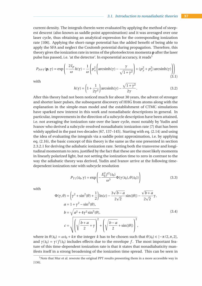
3.1. Introduction to nonadiabatic theories 37
current density. The integrals therein were evaluated by applying the method of steep-est descent (also known as saddle point approximation) and it was averaged over onelaser cycle, thus obtaining an analytical expression for the corresponding ionizationrate [106]. Applying the short-range potential has the added benefit of being able toapply the SFA and neglect the Coulomb potential during propagation. Therefore, thistheory gives the ionization rate in terms of the photoelectron momenta p after the laserpulse has passed, i.e. ‘at the detector’. In exponential accuracy, it reads1
PPPT (p,γ) = exp
(
−2Ip
ωh(γ)− 1
ω
(
p2x
(
arcsinh(γ)− γ√
1+γ2
)
+ (p2y +p2
z)arcsinh(γ)
))
(3.1)with
h(γ) =(
1+ 1
2γ2
)
arcsinh(γ)−√
1+γ2
2γ. (3.2)
After this theory had not been noticed much for about 30 years, the advent of strongerand shorter laser pulses, the subsequent discovery of HHG from atoms along with theexplanation in the simple-man model and the establishment of CTMC simulationshave sparked new interest in this work and nonadiabatic descriptions in general. Inparticular, improvements in the direction of a subcycle description have been attained,i.e. not averaging the ionization rate over the laser cycle, most notably by Yudin andIvanov who derived a subcycle-resolved nonadiabatic ionization rate [7] that has beenwidely applied in the past two decades [67, 137–145]. Starting with eq. (2.14) and usingthe idea of evaluating the integrals via a saddle point approximation, i.e. by applyingeq. (2.16), the basic concept of this theory is the same as the one presented in section2.3.2.1 for deriving the adiabatic ionization rate. Setting both the transverse and longi-tudinal momentum to zero, justified by the fact that these are the most likely momentain linearly polarized light, but not setting the ionization time to zero in contrast to theway the adiabatic theory was derived, Yudin and Ivanov arrive at the following time-dependent ionization rate with subcycle resolution
PY I (t0,γ) = exp
(
−E 2
0 f 2(t0)
ω3Φ(γ(t0),θ(t0))
)
(3.3)
with
Φ(γ,θ) =(
γ2 + sin2(θ)+ 1
2
)
ln(c)− 3p
b −a
2p
2sin(|θ|)−
pb +a
2p
2γ,
a = 1+γ2 − sin2(θ),
b =√
a2 +4γ2 sin2(θ),
c =
√√√√√
√
b +a
2+γ
2
+
√
b −a
2+ sin(|θ|)
2
,
(3.4)
where in θ(t0) = ωt0 +kπ the integer k has to be chosen such that θ(t0) ∈ [−π/2,π,2],and γ(t0) = γ/ f (t0) includes effects due to the envelope f . The most important fea-ture of this time-dependent ionization rate is that it states that nonadiabaticity man-ifests itself in a strong broadening of the ionization time spread. This can be seen in
1Note that Mur et al. rewrote the original PPT results presenting them in a more accessible way in[136].

38 CHAPTER 3: Revisiting nonadiabatic effects on initial conditions
Fig. 3.1 (a), which shows that the time distribution according to eq. (3.3) (dotted orangeline) is considerably broader than the distribution of the adiabatic ionization theory(dash-dotted red line).
More recently, a nonadiabatic theory was published by Li et al. [3] which gives anon-negligible longitudinal momentum at the tunnel exit. Just like in the derivation ofthe adiabatic ionization rate in section 2.3.2.1 and just like it was done by Yudin andIvanov, this derivation builds again on eq. (2.14) and draws on the concept of eval-uating the integrals via a saddle point approximation, i.e. applying eq. (2.16). Here,however, no assumption about the initial longitudinal or transverse velocity is made,which results in the following ionization rate
PLi (t0, v⊥,0) =ω2(2Ip )5/2
2E 40γ
2(t0, v⊥,0)(
γ2(t0, v⊥,0)+cos2(ωt0))
cos2(ωt0)
×exp
(
−E 2
0
ω3
{(
sin2(ωt0)+γ2(t0, v⊥,0)+ 1
2
)
arcsinh(γ(t0, v⊥,0))
− 1
2γ(t0, v⊥,0)
√
1+γ2(t0, v⊥,0)(1+2sin2(ωt0))
})
,
(3.5)
where γ(t0, v⊥,0) = ω√
2Ip + v2⊥,0/|E(t0)| with v⊥,0 denoting the initial transverse ve-
locity and where the electric field is assumed to be E(t ) = E0 cos(ωt ). Thus, envelopeeffects are not inherently included and can only be accounted for in an approximatefashion replacing E0 by E0 f (t ), analogously to the way it was done in the formulation ofYudin and Ivanov. Therefore, one has to bear in mind that this ionization rate is mostaccurate for long pulses and that deviations due to the approximate manner of ac-counting for envelope effects may appear for short pulses. Looking at the time spreadof eq. (3.5) displayed in Fig. 3.1 (a) we can see that this ionization rate does not exhibitthe strong nonadiabatic broadening predicted by Yudin and Ivanov but has about thesame width as the adiabatic curve. Moreover, not having set the initial longitudinalmomentum to zero, this theory arrives at the following expression for this quantity
v||(t0, v⊥,0) = E0
ωsin(ωt0)
√√√√1+
ω2(v2⊥,0 +2Ip )
E 20 cos2(ωt0)
−1
. (3.6)
Comparing panels (b) and (c) of Fig. 3.1 makes clear that in the intermediate nonadi-abatic regime the initial longitudinal momentum spread2 of Li et al. has a width com-parable to that of the initial transverse spread and is thus fundamentally different fromthe initial longitudinal ‘spread’ of Yudin and Ivanov, which is a δ function at zero.
These findings of Yudin and Ivanov on the one hand and of Li et al. on the otherhand, and the fact that these results seem to contradict each other will be at the core
2Note that even though an ensemble of trajectories sampled in the framework of this theory exhibitsa distribution of initial longitudinal momenta, for fixed values of the ionization time and initial trans-verse velocity the longitudinal momentum is deterministic. Therefore, the way a spread of initial lon-gitudinal momenta is obtained is not by sampling e.g. the distribution displayed in Fig. 3.1 (c). Rather,a distribution of ionization times and initial transverse velocities is obtained by sampling PLi (t0, v⊥,0)(eq. (3.5)) and then each trajectory with initial condition (t0, v⊥,0) is assigned an initial longitudinal mo-mentum according to eq. (3.6). Thus, the non-zero initial longitudinal momentum obtained here is con-ceptually different from the artificially assumed spreads of this quantity that were introduced to matchexperimental results in many a nonadiabatic theory [58, 59, 146–151].

3.2. Description of the problem addressed in this chapter 39
of the rest of this chapter. First, though, let us try to gain a more complete picture ofnonadiabatic theories by also looking at the transverse momentum at the tunnel exit.From Fig. 3.1 (b) it can be seen that the transverse distribution is broader in the nonadi-abatic cases (PPT and Li) than in the adiabatic limit. Moreover, this figure reveals thateven though the various nonadiabatic theories seem to disagree in terms of the initiallongitudinal momentum and the ionization time spread, the situation is much clearerfor the distribution of the transverse momenta, for which most common nonadiabatictheories give identical results. Consequently, there is not much need for discussionsalong these lines and therefore the initial transverse distribution will take a backseat inthis chapter.
Another quantity that is modified when taking nonadiabatic effects into account isthe tunnel exit, the initial spatial coordinate. As we have already seen in the right panelof Fig. 2.2, the electron is born closer to the nucleus in nonadiabatic theories. Thiseffect can be understood by the pictorial description of the tunneling process in thebottom panel of Fig. 2.1, where the energy gain under the barrier effectively reduces thebarrier width. Even though it may not be directly obvious due to different notations,the tunnel exit derived in PPT [4, 5] on the one hand, which is commonly used when thetime-dependence of Yudin and Ivanov is applied, and by Li et. al on the other hand, areidentical, as is shown in Appendix A.1. Therefore, the subject of nonadiabatic tunnelexits will not be addressed further here.
Note that all of the above-mentioned results are valid for linearly polarized light.In elliptically polarized light further nonadiabatic effects are observed, for a more de-tailed discussion of which the reader is referred to e.g. [58, 61, 136, 152, 153]. Here,only one of the most prominent effects shall be mentioned, which is the shift of themost likely initial transverse momentum. In the adiabatic limit, the initial transversemomentum is centered around zero. Taking into account nonadiabatic effects in el-liptically polarized light, however, the most probable initial transverse momentum isshifted in the direction perpendicular to the electric field at the peak and inside theplane of polarization, in the rotation direction of the field [154].
3.2 Description of the problem addressed in this chapter
As already indicated above, the predictions for the initial longitudinal momentum andthe ionization time spread as obtained by Yudin and Ivanov [7] and Li et al. [3], whichwe will from now on frequently abbreviate as ‘YI’ and ‘Li’, respectively, are fundamen-tally different. While YI sets the initial longitudinal momentum to zero due to its sup-posed negligibility and obtains a strong broadening in the spread of ionization times,Li derives a theory in which the initial longitudinal momentum is not negligible at alland the ionization time spread is considerably more narrow.
These theories, of course, are not the only ones aiming at describing nonadiabaticeffects in strong field ionization. In this chapter, though, both YI and Li will serve as therespective poster child of the works that claim or make use of a vanishing initial longi-tudinal momentum and/or a broad time spread on the one hand, or make the case fora non-zero initial longitudinal momentum distribution on the other hand. To brieflyillustrate that YI and Li are only the tip of the iceberg, let us briefly take stock of non-adiabatic results and their applications: Even though there are not many who claim tohave found evidence for the longitudinal momentum to be zero at the tunnel exit [56],a lot of theories claim that despite a non-zero initial longitudinal momentum being

40 CHAPTER 3: Revisiting nonadiabatic effects on initial conditions
physically possible in principle, it can be set to zero if one is interested only in expo-nential accuracy even in the nonadiabatic regime [7, 33]. And many a theory [94, 116,143] and theoretical explanation [67, 137–145] was built on this assumption. Others, incontrast, find evidence for and emphasize the non-negligible effect of not setting theinitial longitudinal momentum to zero [3, 58–61, 93, 146–151, 155, 156], some of which[58, 59, 146–151] were criticized for introducing a longitudinal momentum spread atthe tunnel exit in a way that made calculations match experimental results but with-out further physical justification [93, 119]. To add to the confusion, both YI and Lisucceed in explaining many experiments in the nonadiabatic regime [61, 67, 130, 137–141] despite their strongly different initial conditions.
A vigilant reader may now ask if these issues might be resolved by the fact that thelongitudinal momentum at the detector depends not only on the longitudinal momen-tum at the tunnel exit but also on the time-spread, as e.g. expressed in eq. (2.7). Thus,this apt remark may continue, could not the larger time spread in YI compensate forthe lack of initial longitudinal momentum spread? The answer will be yes and no. Yes,in the sense that in this chapter it will be shown that indeed the theories of YI and Li arecoupled in a way that predicts similar longitudinal momentum distributions at the de-tector to an approximation that is applicable to parameters under which many typicalnonadiabatic strong field experiments are performed. And ‘No’ in that we will see thatthis approximation breaks down for parameters that are not even exotic but should beexperimentally feasible and relevant.
Those who skipped the ‘No’ part of the preceding section or who are generally waryof theorists warning against approximations breaking down in some seemingly arcaneregime may wonder why one should care to find out which theory is more accurate ifboth lead to the same final result to a good approximation anyway. Besides the ob-vious reason that answering this question sheds light on the nature of the tunnelingprocess (an argument which may not convince the pragmatic type of reader just de-scribed), this question is also crucial for any experiment and theory where the highestaccuracy to describe the initial conditions at the tunnel exit is required, as it is e.g. thecase in attoclock experiments and their interpretation [92, 113–116, 118]. One theoret-ical method where the answer to the question about the initial conditions after tunnelionization is of very obvious relevance is the recently proposed method of backpropa-gation [116], which interprets the attoclock. There, electrons are propagated forwardstill the end of the pulse first by solving the TDSE numerically and are backpropagatedto the tunneling event classically afterward. The crucial question, though, is when tostop the backpropagation [94], and using the condition of the trajectory having strictlyzero longitudinal velocity to reconstruct the instance of the electron’s birth in the con-tinuum was employed but is still under discussion [157]. Moreover, even though thefinal longitudinal momentum spread is found to be comparable for initial conditionsfrom YI and Li for a wide range of typical nonadiabatic parameters, other strong fieldobservables, such as HHG spectra or Rydberg state characteristics, may be more sen-sitive to the described difference in initial conditions.
After this motivation, we now tackle the problem of the exact form of the spread ofthe ionization time and of the longitudinal momentum at the tunnel exit.

3.3. Relation between the nonadiabatic theories of Yudin/Ivanov and Li 41
3.3 Relation between the nonadiabatic theories of
Yudin/Ivanov and Li
Both the theory presented in YI and Li invoke the saddle point equation
∂S
∂ts= 1
2(p+A(ts))2 =−Ip (3.7)
with the complex-valued saddle point ts , the vector potential A, and the canonical mo-mentum p, where the latter is assumed to be conserved in the tunneling process andis evaluated at the time t0 = Re{ts} at which the electron appears in the continuumwith initial velocity v0, p = v0 −A(t0). We will restrict our study to linearly polarizedlight with the direction of polarization along the x-axis, as described in eq. (2.4). Upto here, things follow the derivation of the adiabatic ionization rates in section 2.3.2.1.The main difference in the nonadiabatic derivation is that the the time-dependence ofthe carrier oscillation, E0 cos(ωt ), is used throughout3, instead of resorting to the ap-proximation of a static field E0. Despite the basic approach being the same for YI andLi, the derivations diverge at the point where assumptions are made about the initialmomenta.
In YI it is claimed that one can set both v⊥,0 and v||,0, the initial transverse and lon-gitudinal momentum, to zero if one is interested only in exponential accuracy of thetime-dependent ionization rate. The resulting ionization rate exhibits the typical non-adiabatic broadening that has already been shown in Fig. 3.1 (a) and seems to be widelyaccepted as one of the central nonadiabatic features [158, 159]. As already pointed out,the ionization distribution derived by Li et al. [3] also starts with eq. (3.7). Contraryto YI, though, the real and imaginary part of the resulting saddle point equations arethen solved making no further assumptions regarding v||,0 or v⊥,0. Thus, an ionizationrate P (v⊥,0, t0) (see eq. (3.5)) is obtained and, in particular, an expression for the initiallongitudinal momentum (see eq. (3.6)), which is zero only for ionization directly at thefield extrema.
Given the strongly different ionization time distributions obtained from YI and Liand given that the non-zero initial longitudinal momenta from Li are not negligibleeven in the intermediate nonadiabatic regime (see e.g. Fig. 2 in [3]), one is probablyinclined to think that it should not be too difficult to find out which of the two theo-ries describes experimental results more accurately. The fact that the discussion on theway nonadiabaticity manifests itself has been going on for over a decade now [57, 160–163] and that both theories were used successfully to explain experiments and TDSEresults [60, 61, 67, 130, 137–141] already shows that it is probably not so easy after all.In the following, we show that the initial longitudinal velocity and the time spread arecoupled in a way that, under approximations valid for the parameters that were typi-cally chosen in nonadiabatic studies so far, leads to almost the same final momentumdistribution.
First of all, we look for numerical evidence for this claim and perform CTMC sim-ulations. Electrons with a total energy that is negative after the pulse has passed (Ryd-berg states) are filtered out and an asymptotic propagation is performed as described
3The envelope f (t ) is not included explicitly in the derivation of either nonadiabatic theory, as al-ready mentioned in section 3.1. However, for not too short pulses one can include the envelope to a goodapproximation by replacing E0 by E0 · f (t ) in the final result. This procedure is also explicitly suggestedin YI and is commonly used to account for the envelope [2, 60].

42 CHAPTER 3: Revisiting nonadiabatic effects on initial conditions
Figure 3.2: Left panel: Longitudinal momentum distribution at the detector obtained
from a CTMC simulation with initial conditions according to [4, 7] (YI) and [3] (Li),
where helium is ionized in a 5-cycle laser with I = 5 · 1013 W/cm2 and λ = 800 nm.
Right panel: Time-dependent longitudinal velocity for trajectories with P = 0.6, which
are born at t0,Y I = 6.14 a.u. and t0,Li = 2.61 a.u. according to Fig. 3.1 (a), and the initial
longitudinal momentum set to zero or described by eq. (3.6), respectively.
Figure 3.3: Normalized ionization probability P as a function of ionization times t0
for the same parameters as those used in Fig. 3.1 and, again, the transverse momenta
were set to zero. The difference to Fig. 3.1 (a) is that the ionization time distributions
as obtained by Bondar [2] are added. Using p|| =−A(t0) (corresponding to v||(t0) = 0)
in doing so, we retrieve the time distribution given by YI and using p|| = v||(t0)− A(t0)with v||(t0) according to eq. (3.6), we retrieve the time distribution of Li.

3.3. Relation between the nonadiabatic theories of Yudin/Ivanov and Li 43
in section 2.3.3.1. The results are displayed in the left panel of Fig. 3.2. For the calcu-lations with YI the nonadiabatic initial transverse momentum spread and tunnel exitgiven in [4, 5, 136] were used since YI only provides the time spread. Although thecalculations presented in Fig. 3.2 are done in the obviously nonadiabatic regime, withthe parameters being the same as in Fig. 3.1 and thus γ = 2.0, the two nonadiabatictheories under consideration indeed give about the same final momentum distribu-tion with discrepancies too minor to be expected to be seen in an experiment. In theright panel of Fig. 3.2, the longitudinal velocity is plotted as a function of time for twotrajectories with initial conditions according to YI and Li which - despite the differentionization time and initial velocity - both correspond to the same ionization probabil-ity according to Fig. 3.1. Here, we can see intuitively how the broader time spread inYI (corresponding to the dashed orange line of YI being born further away from t0 = 0than the blue line of Li) compensates for the lack of initial longitudinal momentumand can therefore result in the same final longitudinal momentum as Li. From thesetrajectories it also becomes clear that compensation happens at the very beginning ofpropagation.
To understand that this compensation is not due to a particular choice of laser andatomic parameters but holds true over a wide range of parameters, it is instructiveto look at the nonadiabatic theory presented by Bondar [2]. Designed to generalizethe result of YI, this theory does not replace the canonical momentum p at all, alsonot by p = v(t0)−A(t0) as is the case in Li. Moreover, Bondar neglects the Coulombpotential during propagation and therefore the conserved canonical momentum p
equals the final velocity at the detector. Thus, Bondar obtains a probability distributionP (v||, f , v⊥, f ).
Why is Bondar’s theory mentioned here when we are actually interested in under-standing why YI and Li give about the same momentum distribution at the detectorover a wide range of nonadiabatic parameters? The reason lies in the fact that theionization time distributions of YI and Li can be obtained as special cases of the the-ory presented by Bondar by replacing the canonical momentum by −A(t0) for YI orv||(t0) − A(t0) with v||(t0) according to eq. (3.6) for Li, which is also seen in Fig. 3.3.As these relations between the ionization time spread of Bondar and those of YI andLi are not directly obvious, they are explained in Appendix A.2. The important con-clusion from this finding is that YI and Li are two different ways of shifting the non-adiabatic velocity spread at the detector into time and velocity spreads at the tunnelexit. Or, more generally, that the different assumptions YI and Li make about the initiallongitudinal velocity strongly influence the time distribution and that, therefore, thesetwo quantities are strongly coupled. At this point it should also be emphasized thatthis statement goes beyond the long-known effect the ionization time has on the lon-gitudinal momentum at the detector, v||, f = v||(t0)− A(t0), when Coulomb effects areneglected during propagation. Here, in contrast, the different assumptions about thelongitudinal momentum at the tunnel exit affect the ionization time distribution.
As for the distribution at the detector, the fact that the initial conditions of YI and Liboth lead to the final distribution of Bondar is the key to understanding why YI and Lilead, to a good approximation, to the same final results. Since P (p||) according to Bon-dar determines at which probability the final velocity v||, f = p|| is found at the detector,independent of whether the replacement of that canonical momentum p|| with initialconditions is done according to YI or Li, it is clear that for both theories we should find

44 CHAPTER 3: Revisiting nonadiabatic effects on initial conditions
the same longitudinal velocity distribution at the detector under the given approxima-tions.
In order to get a more intuitive picture of how this fixed momentum distribution atthe detector can be shifted into time and velocity spreads at the detector, some illus-trative calculations are presented in the following. At the expense of introducing somefurther approximations, it will become clear that even though the longitudinal veloc-ity and time spread in Li are motivated physically, there are – in principle – infinitelymany ways to shift one particular momentum distribution at the detector to time andvelocity spreads at the tunnel exit:
Even though the full probability distribution given by Bondar in Ref. [2] for the mo-mentum distribution at the detector includes many terms for which it is not immedi-ately clear how they can be approximated, for illustrative purposes we assume that wecan approximate it by a Gaussian distribution of width σp :
P (p||) ≈ exp
(
−p2||
2σ2p
)
. (3.8)
The main point this equation should convey is that there is a unique probability dis-tribution for the longitudinal momentum at the detector, independent of how we in-troduce ionization times or initial longitudinal velocities. This statement is also true, ifmaybe less obvious, for the full expression given in [2].
Since the underlying assumption for the momentum distribution at the detector in[2] is that the Coulomb potential can be neglected during propagation, which leads toconservation of the canonical momentum p, the longitudinal velocity at time t is givenby v||(t0)+ A(t )− A(t0) and since A(t ) = 0 at the end of the pulse, the final velocity is
v||, f = p|| = v||(t0)− A(t0). (3.9)
Setting v||(t0) = 0, as it is done in YI [7], we obtain
v||, f ,Y I =−A(t0,Y I ) = E0
ωsin(ωt0,Y I ) ≈ E0t0,Y I (3.10)
for the longitudinal momentum at the detector, where in the last step the underlyingassumption is that ionization happens close to the field maximum.Conversely, using the non-zero velocity according to eq. (3.6), as obtained by Li, we get
v||, f ,Li =E0 sin(ωt0,Li )
ω(
√√√√1+
ω22Ip
E 20 cos2(ωt0,Li )
−1
+1)
=E0 sin(ωt0,Li )
ω
√√√√1+
ω22Ip
E 20 cos2(ωt0,Li )
≈ E0t0,Li
√
1+γ2 = E0t0,Liα
(3.11)
with α=√
1+γ2 and γ= ωp
2Ip
E0, where – again – ionization close to the field maximum
was assumed and hence sin(ωt0) ≈ωt0 and cos(ωt0) ≈ 1.

3.4. Distinguishing between nonadiabatic theories at the detector 45
Plugging eqs. (3.10) and (3.11) into eq. (3.8) we obtain a probability distribution forthe ionization times for YI and Li, respectively:
PY I (t0) ∝ exp
(
−E 2
0 t 20
2σ2p
)
= exp
(
−t 2
0
2σ2t0,Y I
)
,with σt0,Y I =σp
E0(3.12)
and
PLi (t0) ∝ exp
(
−E 2
0 t 20α
2
2σ2p
)
= exp
(
−t 2
0
2σ2t0,Li
)
,with σt0,Li =σp
E0α. (3.13)
From this we can conclude σt0,Li ·α=σt0,Y I . As α> 1 originates from the non-vanishinginitial longitudinal momentum, we can thus see how the non-vanishing initial longitu-dinal momentum in Li leads to a smaller ionization time spread, with the effect becom-ing larger as we venture into the deeper nonadiabatic regime since a larger γ results ina larger α. Or, put the other way around, it shows how the lack of initial longitudi-nal momentum in YI leads to a broadening of the ionization time spread. The abovederivation is instructive also in that we see that even though α is physically motivatedto be
√
1+γ2 in Li, in principle any real number greater or equal 1 could be inserted in-stead. This would modify the ionization time spread and the longitudinal momenta atthe tunnel exit, but we would still obtain the probability distribution given by eq. (3.8).This illustrates how much freedom a probability distribution for only the longitudinalmomenta at the detector gives in terms of the ionization time spread and the longitudi-nal momenta at the tunnel exit. One may even consider starting all trajectories directlyat the field maximum (zero ionization time spread) and consequently use the momen-tum spread σp at the detector directly for the longitudinal momentum distribution atthe tunnel exit. Extreme cases such as this make clear that not any arbitrary choiceof how to convert the momentum distribution at the detector to the ionization timespread and longitudinal momenta at the tunnel exit is physically meaningful and thatwe should try to find out which replacement is the most physical. Further reasons fornot replacing the canonical momentum arbitrarily will be seen in section 3.4, wherewe will observe that the freedom of shifting the momentum spread to the ionizationtime spread is restricted.
3.4 Distinguishing between the nonadiabatic theories at
the detector
In the preceding section, we have seen that Bondar gives a probability distributionthat prescribes the distribution of longitudinal momenta at the detector v||, f and thatthe initial conditions of YI and Li can be derived as special cases of this theory, whichhelped us understand why Li and YI agree so well at the detector despite their differ-ent initial conditions. Moreover, the numerical example presented in Fig. 3.2, wherethe Coulomb potential was fully included, shows that the underlying approximation ofBondar, i.e. neglecting the Coulomb potential, works well. Under these circumstances,one may consider looking for parameters at which YI and Li give discernible results atthe detector pointless.
In the following, however, we will see that it is possible after all and that the pa-rameters that do the trick are experimentally feasible: Ionizing hydrogen with a laserpulse at an intensity of I = 1 ·1014 W/cm2 and a wavelength of λ= 400 nm (γ= 2.1), the

46 CHAPTER 3: Revisiting nonadiabatic effects on initial conditions
Figure 3.4: Distribution of the final longitudinal momentum obtained from CTMC
simulations using Li and YI as well as from TDSE simulations for hydrogen ionized in
a 5-cycle pulse with an intensity of I = 1·1014 W/cm2 and a wavelength of λ= 400 nm.
The curves are normalized such that the areas under the TDSE and CTMC results are
identical. The TDSE result gives much better agreement with the CTMC result using Li
than with the CTMC result obtained with YI.
two nonadiabatic theories produce two distinguishable final longitudinal momentumdistributions, as is shown by the CTMC results in Fig. 3.4. Note that we are in the sameγ-regime as in the example presented in Fig. 3.2, where we had γ = 2.0. In Fig. 3.4,the theory of YI leads to a sharp cut-off in the longitudinal momentum distribution,whereas the theory of Li yields more of a Gaussian-like profile.
Now that we obtained two different results from the two nonadiabatic theories, theobvious question is which one describes the physics of ionization more accurately. Tothis end, TDSE simulations were performed by Igor Ivanov, the technical details ofwhich are described in [117, 164–166]. The result is shown in Fig. 3.4. As the TDSEresult exhibits quantum interference which manifests itself as oscillations that cannotbe captured in the CTMC calculations, we smooth the TDSE curve to guide the eyeby replacing the TDSE result at each longitudinal momentum value by the average ofall values that are found in a window that is centered at the respective momentumand has a total width of 0.28 a.u. along the longitudinal momentum axis. The windowwidth was chosen in a way to smooth the oscillations while not being too broad to loseinformation about the averaged curve.
Comparing the smoothed TDSE result to the CTMC data in Fig. 3.4, it can be seenthat the TDSE result exhibits the same Gaussian-like decay obtained in CTMC with thetheory of Li, rather than the sharp cut-off we get using the theory of YI. To make thisvisual observation more quantitative, we look at the averaged absolute value of the dif-ference between the smoothed TDSE and the CTMC results: the averaged deviationbetween the smoothed TDSE and the CTMC result with YI in the range of [−1,+1] onthe momentum axis is 0.177 and thus more than twice as high as the averaged devi-ation between the smoothed TDSE and the CTMC result with Li, which is 0.070. Assome may worry about the smoothing of the TDSE curve having biased that outcome,also the deviation between the unsmoothed TDSE (solid purple line in Fig. 3.4) and the

3.4. Distinguishing between nonadiabatic theories at the detector 47
Figure 3.5: Normalized ionization probability P as a function of ionization time t0
for Li and YI, where for Li the initial transverse momentum was set to zero (YI sets the
initial transverse momentum to zero already in the derivation of the ionization rate).
The laser and atomic parameters are the same as in Fig. 3.4, except for the constant
envelope used here. In the lower part also the vector potential A(t0) is displayed as
a green line. Since P (t0) does not drop down to zero for YI, the maximal vector po-
tential A0 gets sampled to a non-negligible amount. This leads to a sharp cut-off in
the final longitudinal momentum distribution (orange histogram at the bottom right)
if one performs CTMC calculations without the Coulomb force during propagation.
The blue histogram, in contrast, was obtained in a CTMC simulation using the ini-
tial conditions according to Li (and again propagating without Coulomb potential). It
retrieves the final longitudinal momentum distribution predicted by Bondar. The rea-
son for the final distribution according to Li (blue histogram) having a tail that goes
beyond ±A0 is the non-zero initial longitudinal momentum.
CTMC with Li and YI, respectively, seem worth mentioning: The averaged4 deviationbetween the TDSE and the CTMC result using Li is 0.1049, whereas the averaged devi-ation between the TDSE and the CTMC result using YI amounts to 0.2102 and is thusagain about twice as large as for the CTMC with Li. We therefore find that the theoryof Li is closer to the TDSE result, making it a more accurate theory to describe the sit-uation at the tunnel exit. This observation not only corroborates the non-negligiblelongitudinal momenta at the tunnel exit, but it also implies that nonadiabaticity doesnot necessarily manifest itself in a time spread that is significantly broader than pre-dicted by quasistatic theories, contrary to what is claimed in YI (see e.g. Fig. 3.3).
The observation of different momentum distributions at the detector using YI andLi obviously begs the question as to how this can be possible when we have just seenin the previous section (3.3) that the ionization times and initial longitudinal momentacan be obtained from the same theory (Bondar, [2]) which gives a unique probabilitydistribution P (v||, f ) for the final longitudinal momentum. One may think that this isdue to the Coulomb effect playing a non-negligible role in this process, but as we willsee this effect persists even without the Coulomb potential during propagation and the
4Note that averaged signifies that the the difference between TDSE and CTMC (=deviation) is cal-culated for each longitudinal momentum value, added up and then divided by the total number of lon-gitudinal momentum bins. Thus, the term ‘averaged’ has nothing to do with the smoothing proceduredescribed before.

48 CHAPTER 3: Revisiting nonadiabatic effects on initial conditions
reason is far more fundamental revealing the limits of shifting the final momentumspread arbitrarily to ionization time and initial longitudinal momentum distributions.
The key to understanding the different results obtained with Li and YI (Fig. 3.4) isthe ionization time distribution displayed in Fig. 3.5. Since P (t0) never drops down tozero for YI, the maximal vector potential A0 (green line) gets sampled to an appreciableamount leading to a considerable fraction of electrons ending up at |v||, f | = ±A0. Thisresults in a sharp cut-off at |v||, f | = ±A0 in the final momentum distribution (orangehistogram at the bottom right panel of Fig. 3.5) for YI if one performs CTMC calcula-tions without the Coulomb force during propagation. Including the Coulomb potentialduring propagation blurs this sharp line but does not destroy its basic characteristic,as we have seen in Fig. 3.4.
One consequence of the YI theory is that with its zero initial longitudinal velocitythe resulting final momentum p|| is restricted to [−A0, A0] because we have to applyp|| = −A(t0) (assuming no Coulomb potential). However, the final distribution givenby Bondar in [2] predicts a non-negligible probability P (p||) at |p||| > A0 at these spe-cific parameters (The P (p||) predicted by Bondar at these parameters is shown as a lightblue histogram in the inset at the bottom of Fig. 3.5). Therefore, the initial conditions ofYI cannot retrieve P (p||) given by Bondar whereas Li can due to its non-zero initial lon-gitudinal momentum. Actually, the light blue histogram at the bottom of Fig. 3.5 wascalculated with the initial conditions from Li and is identical to the final momentumdistribution predicted by Bondar. The reason for this is that, as mentioned above, Li’sinitial conditions can be obtained from Bondar’s final momentum distribution. Andafter Coulomb-free propagation from the tunnel exit to the detector, Li’s initial condi-tions directly result in Bondar’s final momentum distribution again.
The obvious question now is why the same arguments are not valid for YI. Also theionization time spread of YI can be obtained from Bondar’s probability distributionP (v||, f ). This is done by setting v||, f =−A(t0) in P (v||, f ), corresponding to propagatingthe momentum distribution from the detector without Coulomb potential back to thetunnel exit, where the ensemble of trajectories exhibits zero momentum but a spreadof ionization times. Nonetheless, we have witnessed that reversing this process andpropagating these initial conditions from the tunnel exit to the detector, again neglect-ing the Coulomb potential, we do not recover the final momentum distribution P (v||, f )from which we started. Mathematically, this puzzling effect boils down to the followingquestion: Why is
(A): P (v||, f ) (3.14)
different from(B): P (v||, f (t0(v||, f )))? (3.15)
In (B), t0(v||, f ) is the ionization time obtained from propagating a trajectory with v||, f
at the detector back to the tunnel exit via
v||, f (t0) = A0 sin(ωt0) ⇒ v−1||, f (v||, f ) = t0(v||, f ) = 1
ωarcsin
(v||, f
A0
)
. (3.16)
Therefore, one may think that one should be able to modify expression (B) as followsand obtain equality with expression (A):
P (v||, f (t0(v||, f ))) = P (v||, f (v−1||, f (v||, f ))) = P (v||, f ). (3.17)
However, from eq. (3.16) we can see that, on the one hand, we have v−1||, f
: [−A0, A0] →[−∞,∞]. On the other hand, we had P : [−A0−ζ, A0+ζ] → [0,1] with ζ> 0, meaning we

3.5. Conclusion and Outlook 49
Figure 3.6: From PBond ar (v||, f ) we can obtain PY I (t0) by replacing v||, f with
A0 sin(ωt0). This corresponds to backpropagation from the detector to the tunnel exit,
where the Coulomb potential is neglected. However, reversing this process and propa-
gating the electrons with ionization times that follow PY I (t0) without Coulomb to the
detector, i.e. applying v||, f = A0 sin(ωt0), we do not recover PBond ar (v||, f ). This is due to
the fact that PBond ar (v||, f ) has a non-zero probability for |v||, f | > A0 but no ionization
time t0 leads to such a |v||, f | > A0 when applying v||, f = A0 sin(ωt0). Mathematically,
the problem is found in the fact that in PBond ar (v||, f ) the domain of definition, i.e. the
range of values v||, f one can plug into PBond ar , goes beyond [−A0, A0]. In contrast, the
domain of definition for t0 = v−1||, f
= arcsin(v||, f /A0)/ω is restricted to v||, f ∈ [−A0, A0].
want to input |v||, f | > A0, which is not defined for the v−1||, f
function in eq. (3.16). Con-sequently, the expressions (A) and (B) are different in their domain of definition, i.e. inthe range of values v||, f one can plug into them. To put it another way, eq. (3.17) doesnot work because v−1
||, fas defined by eq. (3.16) is not defined for arguments (i.e. v||, f
values) outside of [−A0, A0], whereas P (v||, f ) (as given by Bondar in [2]) has P 6= 0 forv||, f ∉ [−A0, A0]. An illustration of this line of reasoning is given in Fig. 3.6.
All of this shows that one cannot replace the canonical momentum arbitrarily byionization time and initial longitudinal momentum distributions, but that a physicaljustification for it, just as it is the case in Li, is crucial. In particular, it reveals thatthe assumption of a vanishing initial longitudinal momentum is not physical and canproduce misleading results ‘at the detector’.
3.5 Conclusion and Outlook
In conclusion, it was shown that the nonadiabatic broadening of the time spread de-rived in YI is a direct consequence of setting the initial longitudinal momentum to zero.More generally, we saw that the strong coupling of the ionization time spread and theinitial longitudinal momentum helps us understand why the theories of Li and YI, in

50 CHAPTER 3: Revisiting nonadiabatic effects on initial conditions
spite of their fundamentally different initial conditions, lead to approximately the samelongitudinal momentum distribution at the detector if P (p||) is negligible for |p||| > A0
and if the Coulomb potential during propagation can be neglected. As these conditionsare widely met in strong field systems, we can now understand why the two nonadia-batic theories with their contrasting initial conditions were both successfully used toexplain experiments in the nonadiabatic regime. This should account to some extentfor the confusing character the discussions about nonadiabatic effects sometimes as-sume.
Despite the indistinguishability of the results obtained from the two theories ina wide range of typical nonadiabatic parameters, laser and atomic parameters werefound that are still in the experimentally realizable and relevant regime for which thementioned approximations break down and the two nonadiabatic theories yield exper-imentally distinguishable momentum distributions. The difference was understoodby P (p||) (as given by Bondar in [2]) having a non-negligible probability for |p||| > A0
at these parameters. Using the replacement of p|| = −A(t0), corresponding to a van-ishing initial longitudinal momentum and thus shifting the spread completely to theionization times as done in YI, only |p||| ≤ A0 can be obtained when propagating thisinitial condition to the detector again. Thus, P (p||) is not retrieved. Conversely, the useof non-zero initial longitudinal momenta in Li allows to reproduce P (p||) (as given byBondar) and consequently, the momentum distribution at the detector obtained withthe initial conditions of YI and Li differs at the detector for these parameters.
In line with this explanation, a ‘numerical experiment’ in the form of a TDSE sim-ulation showed good agreement with the theory of Li, which uses a non-zero initiallongitudinal momentum. With λ= 400 nm, I = 1·1014 W/cm2 and Ip = 0.5 a.u., the pa-rameters of these calculations are in a regime that should be experimentally realizable.Therefore, this system is proposed for experimental testing of nonadiabatic effects onthe initial conditions directly at the tunnel exit.
The strong evidence for the theory of Li being the more accurate one to describethe situation at the tunnel exit motivates, as a next step, to refine this theory. As al-ready mentioned in section 3.1, the derivation of said nonadiabatic theory assumes aconstant envelope. Consequently, envelope effects are so far accounted for only in anapproximate fashion by replacing E0 by E0 f (t ) in the final result, with f (t ) denotingthe envelope. In principle, however, the derivation should also allow to include theenvelope in the description of the field. It remains to be seen, though, whether analyt-ical tractability can be maintained when fully including the envelope in the derivationand if not, one will have to think about numerical ways to solve the relevant equationsefficiently.
Even though the Coulomb effect during propagation was not found to be the ma-jor effect to decide which of the two ionization theories describes the situation at thetunnel exit more accurately, it should be commented on briefly. The equivalence of YIand Li described in section 3.3 assumed that the Coulomb field is neglected. One mayargue that, since the lack of initial longitudinal velocity is compensated by the ear-lier/later birth of the electron in YI directly at the beginning of propagation (see rightpanel of Fig. 3.2), the Coulomb effect can only be of relevance during that short timebefore the compensation is done. However, especially during that early time after thebirth in the continuum the Coulomb potential matters due to the electron’s close loca-tion to the parent ion. The reason the Coulomb potential has a negligible effect in theparameter regime chosen in section 3.3 is mostly the fact that the low intensity leads to

3.5. Conclusion and Outlook 51
a rather large tunnel exit. A smaller tunnel exit is achieved mainly with a larger inten-sity, which entails getting into the more adiabatic regime. Therefore, one usually doesnot have a small tunnel exit in the nonadiabatic regime. Consequently, to make use ofthe Coulomb potential to distinguish between the results of YI and Li one would needto evaluate a quantity that exhibits strong sensitivity to the Coulomb potential directlyat the tunnel exit.


CHAPTER
4Intensity and pulse duration
dependence of Rydberg states
“Problems worthy of attack prove their worth by fighting back."
— Piet Hein (Danish mathematician, 1905-1996)
Overview of this chapter
The investigation of Rydberg states that are created due to frustrated tunneling ion-ization in strong field processes has helped explain many strong field phenomenain the past decade. In this chapter, two new ways are presented for how to makeuse of and control the creation of Rydberg states:Firstly, in section 4.2, the intensity dependence of the fraction of electrons thatend up in a Rydberg state after strong field ionization with linearly polarizedlight is investigated numerically and analytically [71]. It is found that includingthe intensity-dependent distribution of ionization times and nonadiabatic effectsleads to a better understanding of experimental results. This suggests that Ryd-berg yield measurements can be used as an independent test for nonadiabaticityin strong field ionization. Furthermore, using classical trajectory Monte Carlo sim-ulations it is observed that the intensity dependence of the Rydberg yield changeswith wavelength and that the previously observed power-law dependence breaksdown at longer wavelengths.In the second part, in section 4.3, it will be shown how the duration of the laserpulse can be used to control both the yield and principal quantum number distri-bution of Rydberg atoms [72]. An intuitive explanation for the underlying mech-anism is provided and a scaling law for the position of the peak in the quantumnumber distribution on the pulse duration is derived. In particular, it will be-come clear that low principal quantum numbers are less likely to ‘survive’ longerpulses. This is relevant to studies and applications that rely on the principal quan-tum number distribution of Rydberg atoms like the recently developed method ofcreating coherent extreme-ultraviolet radiation from Rydberg atoms, in which theoccupation of low principal quantum numbers is crucial. Furthermore, it will be-come clear that including the Coulomb potential during propagation is crucial forthe understanding of pulse duration effects of Rydberg states and cannot be ne-glected as it was done so far in analytical descriptions of Rydberg states.

54 CHAPTER 4: Intensity and pulse duration dependence of Rydberg states
4.1 Introduction to Rydberg states
The liberation of an electron in the process of strong field ionization via tunneling doesnot necessarily lead to the electron leaving the atom for good [48, 49]. Rather, a consid-erable fraction of atoms survives the laser pulse in neutral excited states [48], so-calledRydberg states. The detection of excited neutral states in the multiphoton regime [167,168] had been known long before the experiment of Ref. [48] presented neutral excitedstates in the tunneling regime and had been explained in the framework of a purelyquantum mechanical picture as a stabilization process in multiphoton excitation. Forthe experiment in the tunneling region [48], a new mechanism to explain the creationof Rydberg states in this regime was required. As a consequence, the concept of ‘frus-trated tunneling ionization’ (FTI) was born [48]. The idea behind FTI is based on thesemiclassical model of tunneling ionization and subsequent propagation of the elec-tron in the superposed laser and Coulombic field. The low kinetic energy of some elec-trons at the end of the laser pulse does not allow them to leave the Coulomb potentialbut results in their capture in a Rydberg state.
The relevance of FTI already becomes clear by the observation that under typ-ical strong field conditions 10-20% of tunnel ionized electrons are trapped in Ryd-berg states [48], thus affecting many more electrons than other post-tunnel ionizationmechanisms such as high-harmonic generation (HHG) or double ionization by colli-sion [169, 170]. FTI not only explains the significant reduction of ionization rates [48]but can also be used to e.g. calibrate laser intensities [171], study nonadiabatic effects[71], probe the spatial gradient of the ponderomotive potential in a focused laser beam[172], or control the motion of neutral atoms in strong laser fields [170, 173].
There are some effects in strong field excitation, such as certain molecular effectsor oscillations due to channel-closings in multiphoton excitation, that can only be un-derstood based on the time-dependent Schrödinger equation [174–177]. However, es-pecially the effect of FTI has been found to be described well in models that treat thepropagation step and the capture in a Rydberg state classically [48–52, 178–180] andCTMC simulations have proven to be a powerful tool in the study of Rydberg state cre-ation by FTI.
As the electron in a Rydberg state forms a bound state, this situation is character-ized by a total energy that is negative after the pulse has passed
E = v2
2− 1
r< 0. (4.1)
In CTMC simulations the Rydberg yield is computed by evaluating this relation at theend of the pulse and calculating the ratio of the number of electrons in a Rydberg staterelative to the total number of electrons that have tunneled out of the atom. The Ryd-berg yield strongly depends on the intensity and pulse duration of the laser pulse, ashas been pointed out before [48, 49]. In this chapter, we will continue the researchalong these lines, which will lead to a better understanding of Rydberg state creationvia FTI and, in turn, give birth to completely new applications. For example, studyingthe intensity dependence of Rydberg states will open up a new way to detect nonadia-batic effects in strong field ionization [71], and the mechanism that is found to explainthe pulse duration dependence of the yield can also be used to control the distributionof the principal quantum number of Rydberg states [72].

4.2. Intensity dependence 55
4.2 Intensity dependence
The content of this section has been published in a similar way in Phys. Rev. A 98,033415 (2018) and a corresponding correction in Phys. Rev. A 99, 019901(E) (2019) (seeRefs. [71, 181]). The copyrights of contents from those articles lie with the AmericanPhysical Society.
Already the first experiment that detected Rydberg state creation in the tunnelingregime and introduced the concept of frustrated tunneling ionization (FTI) measuredthe intensity dependence of Rydberg states [48]. The takeaway from this measurementwas that even though both the number of atoms in a neutral excited state (Rydbergstate) and the number of ionized atoms grow with increasing intensity, the relativenumber of Rydberg states is smaller for higher intensities. Only a few months later ananalytical model was proposed in Ref. [49] to explain not only the dependence of theRydberg yield on the intensity but also on the wavelength and the pulse duration.
Below, we build on this work of Ref. [49] by including nonadiabatic effects, as wellas introducing further corrections and expansions to the intensity-dependence of thistheory. An analytical dependence of the Rydberg yield on intensity is presented thatagrees better with the experimental results in Ref. [48]. Additionally, wavelength de-pendent effects in the intensity dependence are found which have not been predictedbefore and should be experimentally measurable. As we will see, especially the inclu-sion of nonadiabatic effects promises to be a new tool to study nonadiabaticity usingRydberg states instead of the momentum distribution of ionized electrons at the de-tector. This new approach to test nonadiabatic features does not depend on absoluteintensity calibration that other nonadiabaticity studies struggle with (for a discussionsee [154]).
4.2.1 Prior analytical estimates
In this section, the analytical tools that are developed and employed in Ref. [49] toestimate the Rydberg yield are explained and reviewed before they are modified in thefollowing sections. The Rydberg yield, as defined in the present thesis, is the ratio ofthe number N∗ of electrons which are captured in a Rydberg state and the number Nt
of all electrons which tunneled through the potential barrier1. The key idea behind theanalytical work in [49] is to assume a uniform distribution of electrons in the plane ofinitial conditions (t0, v⊥,0) and to estimate the Rydberg yield to be proportional to thearea Σ
∗ in this plane that contains those initial conditions that end up in a Rydbergstate divided by the area Σt containing all ionization events
N∗
Nt∝ Σ
∗
Σt. (4.2)
In Fig. 4.1, we can observe the characteristic crescent-like shape of the Rydberg areaΣ∗ marked in shades of blue. In this plot, just as in the analytical estimate, we only
consider ionization in the central half-cycle for the sake of analytical tractability. Toestimate the area of the crescent it is instructive to look at the sketch in Fig. 4.2, where
1Note that in [49] the Rydberg yield is defined as the ratio N∗/N+, with N+ the number of finallyionized atoms. Since Nt = N∗+N+, the two definitions coincide only in the limit of N∗ ≪ Nt . In thecorresponding analytical calculations in [49] we find a measure proportional to Nt in the denominator.Therefore, the definition of N∗/Nt as Rydberg yield would have been more accurate also in [49].

56 CHAPTER 4: Intensity and pulse duration dependence of Rydberg states
Figure 4.1: The total energy (see colorbar) at the end of the pulse for electrons ion-
ized at time t0 in the central half-cycle with initial transverse momentum v⊥,0, and
propagated in the superposed laser and Coulomb potential. All quantities are given in
atomic units. The laser pulse was chosen to have a wavelength of λ = 800 nm and 8
cycles for two different intensities I specified in the plots. Rydberg states have a total
energy that is negative (colored in shades of blue) and one can see how the Rydberg
area shrinks for larger intensities.
Figure 4.2: Illustration for why the crescent-like Rydberg area can be approximated
by the relative complement of two ellipses with equal height but different widths and
why, as a consequence, the Rydberg area can be approximated to scale linearly with ∆t
and ∆v⊥.
the crescent-shaped area is approximated by the relative complement of two ellipsesof equal height (i.e. along the v⊥,0-axis) but different widths (i.e. along the t0-axis). Asa consequence, we can assume that the crescent-shaped Rydberg area scales linearlywith ∆v and ∆t , the range of v⊥,0 and t0 as defined in Fig. 4.2, respectively. This shouldbecome clear from the following calculation:
Acrescent =1
4(Alarge ellipse − Asmall ellipse)
= 1
4
∣∣π ·∆v⊥ · (t0,center − t0,mi n)−π ·∆v⊥ · (t0,center − t0,max)
∣∣
= π
4· (t0,max − t0,mi n) ·∆v⊥ = π
4·∆t ·∆v⊥.
(4.3)
Consequently, to estimate the Rydberg area it is sufficient to estimate the minimaland maximal ionization times t0,mi n and t0,max when v⊥,0 = 0 and the initial velocitiesv⊥,0,mi n and v⊥,0,max that lead to a Rydberg state. Determining those four boundariesrequires propagation in the superposed laser and Coulomb field. To keep this step an-alytically tractable, the electron trajectory is calculated without the Coulomb potential,which is further justified by the observation that including the Coulomb potential per-

4.2. Intensity dependence 57
turbatively does not affect the intensity-dependence of the size of the Rydberg area2.The Coulomb potential is only ‘turned on’ at the end of the pulse by means of eq. (4.1),which contains the Coulomb potential and which is evaluated in the limit of setting thetotal energy to 0. All in all, this results in the following estimate for the Rydberg area, asgiven in [49]:
Σ∗ ∝∆φ ·∆v ≈ ω
E0
(2
τ
)2/3
, (4.4)
where τ is the time at which the pulse has passed. As the center of the pulse is definedto be at t = 0, 2τ equals the pulse duration τL .
What still remains to be done is to estimate the ionization area. In Ref. [49], this isdone by assuming that the ionization area scales linearly with the width of the distri-bution of the initial transverse velocity. The transverse velocity is estimated to scale asp
E0 since the width of the Gaussian transverse velocity distribution of eq. (2.24) scalesas
pE0
Σt ∝σv⊥ ∝√
E0. (4.5)
Combining eq. (4.4) and (4.5), one then obtains
N∗
Nt∝ Σ
∗
Σt∝ ω
E 3/20 τ2/3
. (4.6)
Another point worth mentioning concerns the interpretation of this result. Eventhough Σ
∗ ∝ 1/E0 agrees with the observation of the Rydberg area getting smaller withincreasing intensity in Fig. 4.1, at first glance this does not seem to tally with the exper-imental observation of the number of neutral excited atoms increasing with increasingintensity [48]. This seeming contradiction is resolved by the fact that eq. (4.2) onlyholds in the relative sense, meaning under evaluation of the ratio rather than separateevaluation of the nominator and the denominator. Details concerning this point arepresented in Appendix A.3.
4.2.2 Including the ionization time width
A vigilant reader may have noticed that in the estimation of Σt in eq. (4.5) only thewidth of the velocity spread was used, while the width of the ionization time spreadwas neglected. As the time width also depends strongly on the intensity, this shall berectified in this section, thus introducing the first modification to the result presentedin Ref. [49].
As we have already seen in eq. (2.28), the adiabatic ADK distribution for ionizationphases φ= w ·t0 [1, 182] can be approximated as a Gaussian function with an intensity-dependent width σφ that is proportional to
pE0. Consequently, we should set
Σt ∝σv⊥ ·σφ ∝√
E0 ·√
E0 = E0 =p
I (4.7)
2In Ref. [49], the Coulomb force is taken account of in a perturbative manner by calculating thechange of the momentum due to the Coulomb force accrued along the path of a trajectory that ispropagated in only the laser field. However, the Coulomb correction cancels out in ∆φ = ω∆t sinceit enters φl atest and φear l i est in the form of the exact same summand. For details see eqs. (10) to(12) in [49], where Coulomb effects are hidden in the parameter λ, which is not the wavelength there:
φear l i est = ωt0< ≈ −λ− ωE0
(4τL
)1/3and φl atest = ωt0> ≈ −λ. Thus, in ∆φ = φl atest − φear l i est , the
Coulomb-correction contained in λ cancels out and only shifts the Rydberg area along the φ-axis butdoes not affect its size.

58 CHAPTER 4: Intensity and pulse duration dependence of Rydberg states
obtainingN∗
Nt∝ Σ
∗
Σt∝ I−1. (4.8)
This result enables a better understanding of the adiabatic CTMC simulation resultsdisplayed in Fig. 4.3 where a power law fit to the intensity-dependent Rydberg yieldgives an exponent of −1.02. Note that even though the Coulomb effect is neglectedin the propagation in the analytical estimates made in this chapter, the Coulomb po-tential is fully taken into account during propagation in the CTMC simulations. Theobservation that the CTMC result and the analytical estimate agree so well shows usthat neglecting the Coulomb force during the propagation and the other approxima-tions introduced above work well in the study of the intensity dependence of Rydbergstates.
4.2.3 Nonadiabatic effects
From the experiment reported in [48], the ratio N∗/Nt can be extracted for variousintensities. These values exhibit an intensity dependence that can be fitted very wellby a power law function a · I b with fitting parameters a and b. The fit yields
N∗
Nt∝ I−0.86, (4.9)
displayed as a blue line in Fig. 4.3. So, even though taking into account the intensity-dependent ionization phase width in the analytical estimation in the preceding sec-tion, which shifted the power law exponent from b = −0.75 as obtained in [49] tob = −1, was well captured by the adiabatic CTMC simulations giving b = −1.02, westill do not fully understand the experimental result of b = −0.86 in this framework.However, when looking at the adiabaticity parameter γ=ω
√2Ip /E0 [89], we find that
– for the intensity regime of I = 1.4 · 1014 − 1015 W/cm2 at λ = 800 nm and Ip = 0.9 –γ ranges from 0.5 to 1.2. This is the typical strong field ionization regime where therelevance of nonadiabatic effects is still under debate [57, 154, 161, 163].
We now show that nonadiabatic effects can be observed in Rydberg yield measure-ments from the power-law dependence alone. This eliminates the concerns about in-tensity calibration that have haunted prior experiments attempting to observe non-adiabatic effects by measuring electron momenta distributions [57, 154]. At this point,it seems important to emphasize that the factor correcting for the decay of neutral ex-cited atoms into metastable states, which had to be applied in [48] to match theoreticaland experimental results, does not depend on the intensity. Therefore it only affectsthe prefactor of the power law, but not its exponent, which makes the anyway highrobustness of the exponent of a power law fit even less subject to issues arising fromcalibration of the absolute intensity.
In Fig. 4.3, CTMC simulation results are shown where on the one hand the non-adiabatic ionization theory described by Li et al. [3] (Li) was used and, on the otherhand, the time spread by Yudin and Ivanov [7] (YI) combined with the transverse veloc-ity spread of PPT3. A power law fit to the resulting intensity-dependent Rydberg yield
3The YI/PPT version, in short labeled as YI, was implemented using the theory of Bondar [2] wherethe final longitudinal momentum was replaced such that the ionization time distribution of YI was ob-tained (see chapter 3 for details). The initial transverse momentum distribution of Bondar matches thatof PPT, which is shown in Fig. A.1 in Appendix A.1 for the two intensities that limit the intensity rangeconsidered in this chapter.

4.2. Intensity dependence 59
Figure 4.3: Rydberg yield for the parameters found in [48]: I = 1.4 ·1014−1015 W/cm2,
the FWHM of the pulse envelope is 30 fs, λ = 800 nm, a helium atom with Ip = 0.9is ionized. The experimental yield (blue dots) was extracted from [48]. The adiabatic
CTMC simulation (red diamonds) was performed using the ADK distribution [1, 182]
and the nonadiabatic simulations are based on [4, 7] (YI, purple stars) and [3] (Li,
green squares), respectively. The power law used for fitting is described by N∗/Nt =a · I b with b given in the legend. The fitting results are represented by lines. Note that
the lower absolute values of the experimental yields are due to the decay of the excited
states which is not accounted for here (for details see [48]). The correction factor that
takes account of this effect and was applied in [48] for comparison between theory
and experiment is found to be independent of the laser intensity. Therefore, it affects
only the prefactor of the power law (and thus the offset on a log-log scale), but not the
power law exponent (corresponding to the slope in the log-log plot) we are interested
in here. For better visual comparison of the experimental result with the simulation
data, the dashed blue line shows the experimental data artificially shifted closer to the
simulation data.
gives an exponent of −0.86 and −0.85 for YI and Li, respectively. The good agreementbetween Li and YI is not surprising given the compensation effects that were describedin chapter 3.3. More importantly, both nonadiabatic results are in much better quan-titative agreement with the experimental value of b =−0.86 than the adiabatic model.
Qualitatively, the nonadiabatic effect on the intensity dependence of the Rydbergyield observed here can be explained by the width in the distributions of the startingvelocity and the ionization phase, which both increase more slowly with increasingintensity in the nonadiabatic case than in the adiabatic one. The slower growth withintensity can be understood qualitatively by the nonadiabatic broadening of the distri-butions of initial conditions at lower intensities, which makes these spreads of initialconditions drop less fast with decreasing intensity than in the adiabatic case. This shal-lower intensity dependence affects the denominator of the Rydberg yield, resulting ina less negative exponent in the power law.
In order to estimate the extent of the nonadiabatic effect quantitatively, we firstevaluate how the spread of initial transverse velocities changes with intensity. Since thetheory of Li and PPT agree in their description of the initial transverse velocity to a verygood approximation (see e.g. the comparison in Fig. 3.1 (b) or in Fig. A.1 in AppendixA.1), we do not have to worry about which nonadiabatic theory to choose. We will

60 CHAPTER 4: Intensity and pulse duration dependence of Rydberg states
Figure 4.4: Left panel: cy (γ) as given in [136] with the respective power law fits in the
γ-regime defined by the parameters listed in Fig. 4.3. Right panel: Fit to the standard
deviation σt0 of the ionization time spread as they are obtained from Gaussian fits to
the theory of Refs. [4, 58, 136] (orange, PPT) and of Ref. [7] (green, YI). A power law fit
A ·E B0 was performed with the resulting exponents shown in the legend. For compari-
son, also the adiabatic case is shown which scales asp
E0 according to eq. (2.28).
work with PPT here as it is easier to handle analytically. The transverse width of PPTis given in eq. (3.1) or equivalently in [136], where in the latter we find the notationσv⊥ =
√ω/(2cy ) for the width of the transverse velocity distribution with
cy = τ0 = sinh−1(γ), (4.10)
which in the adiabatic limit, γ≪ 1, reduces to
cy = τ0 ≈ γ∝ 1/E0 ∝ I−0.5 ⇒σv⊥ ∝ E 0.50 ∝ I 0.25 (4.11)
in accordance with eq. (4.5). For the nonadiabatic regime used here we fit a power lawto eq. (4.10) (see left panel of Fig. 4.4) and obtain cy ∝ γ0.84 and thus
σv⊥ ∝ γ−0.84/2 ∝ E 0.84/20 ∝ I 0.84/4. (4.12)
Concerning the second quantity of interest, the ionization time spread, the nonadi-abatic effects described in YI and Li are different from each other, where in the latter wealso saw effects on the initial longitudinal velocity spread (see ch. 3). In the following,we use the theory of YI rather than the theory of Li to describe nonadiabaticity. Thereason for this choice is found in the fact that in the theory of Li the non-zero longitu-dinal velocity plays a crucial role. However, this quantity is not included in the modelwe use here, which focuses solely on the ionization time and initial transverse velocityspread. In chapter 3 we have seen that over a wide range of nonadiabatic parametersthe lack of initial longitudinal momentum in YI is compensated to a good approxima-tion by a broader ionization time spread and therefore yields almost identical resultsfor the final longitudinal momentum spread as Li. This approximation is also valid atthe parameters used in this chapter and, therefore, we use YI to estimate the extent ofnonadiabatic effects here even though we found in chapter 3 that Li can be considereda more general nonadiabatic theory than YI.
The right panel of Fig. 4.4 shows how the ionization time spread of YI changes sig-nificantly less with intensity than in the adiabatic case. One feature of the YI-curvethat may seem unexpected at first glance is that the width does not grow monotoni-cally with increasing intensity but that there is a minimum around E0 ≈ 0.08 a.u.. Thiscan be understood as follows: In the adiabatic limit the ionization time width decreases

4.2. Intensity dependence 61
monotonically when the field strength becomes smaller. Smaller intensities, however,are related to the more nonadiabatic regime where nonadiabatic broadening of theionization time distribution is found. As this nonadiabatic broadening is strong in YI,it dominates at small intensities, resulting in the curve going up for E0 <∼ 0.08 a.u. in theright panel of Fig. 4.4. Despite the resulting minimum, we perform a power law fit tothe field strength dependence of the ionization time spread of YI since it still reflectsthe fact that the nonadiabatic curve has a much more shallow intensity dependencethan the adiabatic case. The resulting power law exponent is 0.15 and combining thiswith the result from eq. (4.12) we obtain
N∗
Nt∝ 1/I 0.5
I 0.84/4+0.15/2= I−0.79, (4.13)
At this point, it seems important to highlight that the aim of the estimate in eq. (4.13) isnot to attain a perfect match with the power law exponent of the CTMC simulation, butto qualitatively understand the CTMC simulation result. Even though the exponentsdo not match perfectly, we can learn from the above analysis that the main reason forthe strong nonadiabatic effect lies in the much shallower intensity-dependence of theionization time spread in the nonadiabatic case.
In the right panel of Fig. 4.4 the time-dependence as it was introduced into PPT in[58] is also included since this approach was used when the results shown here wereoriginally published in [71, 181]. In the following, it is explained why in this thesis thenonadiabatic theory of YI is used instead. As outlined in the introduction to chapter 3,the PPT result is cycle-averaged and does not include instantaneous time-dependence.Even though the way the time-dependence is included into PPT in [58] worked well inthe context it was applied to there, the right panel of Fig. 4.4 reveals that in the pa-rameter regime used here, the theory of PPT and YI strongly differ in the ionizationtime spread. Since YI, in contrast to PPT, is designed to include instantaneous time-dependence, applying this theory of YI here seems more appropriate. This argumentis corroborated by the nonadiabatic simulation results with YI yielding a power lawexponent of b = −0.86 that matches the experimental result of b = −0.86 better thanthe exponent of b =−0.95 [71, 181] obtained in the simulation with PPT with the time-dependence included following [58].
The results presented in this section do not only highlight the relevance of takingaccount of nonadiabatic effects, but it also shows in what way FTI can be used to in-vestigate the initial conditions at the tunnel exit. In particular, as the discussed effectsconcern the denominator of the Rydberg yield and thus the total number of tunneledelectrons, they are not only relevant for Rydberg related studies but for tunnel ioniza-tion in general. For example, the slower growth of the momentum width with intensitywhen applying nonadiabatic theories as compared to adiabatic theories can also beseen in the data presented in [154, 161].
The nonadiabatic observation made here now opens the door to use this effect fortesting nonadiabaticity in a way that complements the tests employing momentumdistributions. The latter is the way nonadiabaticity is usually studied: The quantity un-der scrutiny is typically the width of the momentum distribution [3, 57, 93, 154, 161,183], which differs in adiabatic and nonadiabatic theories. The problem with this ap-proach is that the momentum distribution is sensitive to the exact absolute value of theintensity. And this intensity is difficult to measure and is usually calibrated a posterioriby applying either an adiabatic or nonadiabatic theory on the photoelectron momen-

62 CHAPTER 4: Intensity and pulse duration dependence of Rydberg states
Figure 4.5: Intensity-dependent Rydberg yield at λ = 1200 nm (all other parameters
are chosen as listed in Fig. 4.3). Purple dashed line: The adiabatic power law with
b = −1 (see eq. (4.8)). Red diamonds: Adiabatic CTMC simulation data with power
law fit (orange line) to it. Blue dashed-dotted line: Estimation by solving eq. (4.18) and
(4.20) exactly, Green dotted line: Approximation given by eq. (4.33).
tum distribution, finding different intensity values depending on which framework ischosen. So, the theory under test is already used for calibration, which is certainlyproblematic [154]. Here, in contrast, we do not look at the momentum distribution ofionized electrons at all but study only the Rydberg yield. In this study of Rydberg stateswe are not interested in total but only in relative intensities, which can be controlledand measured independently of the mentioned calibration issues. Therefore, Rydbergstates can be used for testing nonadiabaticity effects independent of the absolute in-tensity, thus complementing the way nonadiabaticity is tested using momentum dis-tributions.
4.2.4 Wavelength correction
For a wavelength of λ = 800 nm the estimation of a power law with exponent b = −1matched the adiabatic simulation results rather well (see Fig. 4.3, b =−1.02 for the adi-abatic CTMC simulations). Even though eq. (4.6) contains ω, the exponent of the powerlaw of the intensity dependence in this adiabatic theory is wavelength-independent andwe would expect the same power law scaling with about b =−1 to hold for larger wave-lengths as well – or even better since the system would be more adiabatic. However,the Rydberg yield from adiabatic CTMC simulations at λ = 1200 nm shows a fasterdrop with intensity, which is reflected in the more negative exponent of b = −1.16 inthe power law fit (red diamonds with orange line in Fig. 4.5). For larger wavelengths,the drop increases even faster with increasing intensity. In the following, a theory isderived that explains this effect and that allows to make predictions about observingthis effect in experimental data as well.
As expounded in section 4.2.1, we need the maximal initial transverse velocityv⊥,0,max and the range ∆φ of ionization phases (at v⊥,0 = 0) for estimating the areaof initial events in the v⊥,0 −φ plane which end up in a Rydberg state. The Coulombforce is neglected during propagation, as explained in section 4.2.1, and therefore weonly use the Coulomb potential at the end of the pulse for the evaluation of eq. (4.1).

4.2. Intensity dependence 63
Moreover, the tunnel exit is set to xe = 0. The position and velocity at a time τ just whenthe pulse has passed are then approximated by
x(τ) ≈ E0
ω2cos(φ)− E0
ωsin(φ) ·τ (4.14)
y(τ) ≈ v⊥,0 ·τ (4.15)
vx =−E0
ωsin(φ) (4.16)
v⊥ = v⊥,0, (4.17)
where a CEP of π was assumed (see Appendix A.4 for an explanation) and τ= τL/2 is thetime at the end of the pulse because τL denotes the pulse duration and the ionizationphase of φ= 0 is defined to correspond to ionization at the central field extremum.Thedetailed derivation of these equations along with an explanation of the approximationsapplied here are given in Appendix A.4. The important point about these equations isthat they differ from the ones used in [49] in that they include the term E0
ω2 cos(φ) inx(τ). The wavelength effect in the intensity dependence that is derived in the followingarises from this discrepancy. Therefore, the mentioned effect is weakened for longerpulses where the second term in x(τ) dominates and the term E0
ω2 cos(φ) is less relevant.For the calculation of v⊥,0,max , we can plug eqs. (4.14) and (4.15) into eq. (4.1) in
the limit of E = 0 and set φ= 0
E =v2⊥,0,max
2− 1
√
E 20
ω4 + v2⊥,0,max
·τ2
= 0. (4.18)
Analogously, we set v⊥,0 = 0 in the calculation of φear l i est in eq. (4.1), which leads to:
1
2
(E0
ω
)2
· sin2 (φear l i est )− 1E0ω2 cos(φear l i est )− E0
ωsin(φear l i est ) ·τ
= 0. (4.19)
This expression can be approximated by
1
2
(E0
ω
)2
·φ2ear l i est −
1E0ω2 − E0
ω φear l i est ·τ= 0 (4.20)
since φear l i est < 0.1 for the parameters used here. Equations (4.18) and (4.20) can besolved analytically for v⊥,0,max and φear l i est , respectively. The solutions are
v⊥,0,max =
√√√√−E 2
0ω4 +
E 40
ω8·h +h
3τ2(4.21)
with
h =(
−E 60 +6ω6
(
9τ4ω6 +√
−3E 60τ
4 +81τ8ω12))1/3
/ω4 (4.22)
and
|φear l i est | =1+ g + 1
g
3τω(4.23)

64 CHAPTER 4: Intensity and pulse duration dependence of Rydberg states
with
g = E 30/
(
E 90 −27E 6
0τ2ω6 +3
√
−6E 150 τ2ω6 +81E 12
0 τ4ω12)1/3
. (4.24)
As before, the Rydberg yield is then estimated by plugging these results into
N∗
Nt∝
|φear l i est | · |v⊥,0,max |E0
. (4.25)
The resulting intensity dependence at λ = 1200 nm can be seen in Fig. 4.5 (blue line),a power law fit to which gives an exponent of b = −1.15. This analytical derivationmatches the simulation data (red diamonds), yielding b = −1.16, very well. As thelengthy, full analytical solutions of (4.18) and (4.20) given above do not allow for adeeper understanding of which parameters dominate this wavelength effect in the in-tensity dependence, an approximation for them is derived in the next paragraph.
The idea is to plug the approximate and simpler results v⊥,0,∗ = (2/τ)1/3 and φ∗ =−
(2τ
)1/3 · ωE0
from [49] into the Coulomb term of eq. (4.1) but not into its kinetic energyterm. For v⊥,0,max , this means
v2⊥,0,max
2− 1
√
E 20
ω4 + v2⊥,0,∗ ·τ2
≈ 0 ⇒ v⊥,0,max ≈p
2(
E 20
ω4 +22/3 ·τ4/3)1/4
. (4.26)
And for the phase we obtain
1
2
(E0
ω
)2
·φ2 − 1E0ω2 − E0
ωφ∗ ·τ
≈ 0, (4.27)
from which follows
|φear l i est | ≈ω/E0 ·
p2
√
E0ω2 − E0
ω
(
−(2τ
)1/3 · ωE0
)
τ
= ω/E0 ·p
2√
E0ω2 +21/3 ·τ2/3
. (4.28)
Setting m = E0ω2 and n = 21/3 ·τ2/3, the Rydberg yield can be expressed as follows:
N∗
Nt∝ Σ
∗
Σt=
|v⊥,0,max | · |φear l i est |E0
(4.29)
=p
2(
m2 +n2)1/4
·p
2 ·ω/E0
(m +n)1/2· 1
E0(4.30)
= 2ω
E 20 ·
pn ·
(
1+ m2
n2
)1/4·p
n ·(
1+ mn
)1/2(4.31)
≈ 2ω
E 20 ·
pn ·
pn ·
(
1+ 12
mn
) (4.32)
∝ ω
21/3 ·E 20 ·τ2/3
(
1+ E024/3·ω2·τ2/3
) , (4.33)
where eq. (4.32) is expanded in a Taylor series around m/n ≈ 0 neglecting terms withO (m2/n2). This expansion to first order seems reasonable since for the studied pa-rameter regime m < n holds true. For the case of λ = 1200 nm, the approximation is

4.2. Intensity dependence 65
plotted in Fig. 4.5 (green line) and a power law fit to it gives an exponent of b =−1.12.This approximation makes clear that for large wavelengths and small pulse durationsthe Rydberg yield as a function of intensity is less well described by a power law thanfor small wavelengths and longer pulses. It bears repeating that this discrepancy be-tween the description in [49] and the one derived above stems from the fact that herethe term E0
ω2 cos(φ) is included in the equation of motion whereas it is omitted in [49].
4.2.5 Conclusion and Discussion
In conclusion, it was found that taking account of the ionization time width into the an-alytical model describing the intensity dependence of the power law explains adiabaticCTMC simulations more accurately. In a next step, it became clear that nonadiabaticCTMC simulations match the experimental results better. The less negative power lawexponent in the nonadiabatic case could be understood by the shallower intensity de-pendence of the spread of the initial transverse momentum and, in particular, of theionization times. As the two mentioned corrections affect the denominator of the Ryd-berg ratio and thus the total number of electrons that tunneled out of the atom, theseinsights and approximations can be used beyond studies of Rydberg atoms when oneis interested in the intensity dependence of tunnel ionization in a more general con-text. Moreover, we saw that the power law intensity dependence observed for infraredlight breaks down for longer wavelengths. This correction is based on and highlightsthe importance of including the offset term E0/ω2 cos(φ) in the approximation of theposition of an electron that is driven by a laser field.
All in all, these results show new ways to use Rydberg atoms for retrieving informa-tion about the tunneling and propagation step in strong field ionization processes. Inparticular, measuring the Rydberg yield can be used as an independent test for non-adiabatic effects in strong field ionization. So far, the question of the importance ofnonadiabatic effects in strong field ionization was addressed by investigating photo-electron momenta distributions [57, 61, 154, 161]. These investigations, however, haveproved to be inconclusive, with some experiments confirming adiabatic assumptions[57, 161] and others pointing to relevance of nonadiabatic effects under typical strongfield ionization conditions [61, 154]. As we have seen here, the intensity dependence ofthe Rydberg yield can be described by a power law, with nonadiabaticity affecting theexponent. Since the absolute value of intensity is therefore not important, the resultsdo not depend on the calibration procedure which has been a serious issue in priorstudies [154].
Thinking about pushing the nonadiabatic study of Rydberg states presented abovedeeper into the nonadiabatic regime, we need to be aware of the fact that multipho-ton excitation effects become relevant and a description that is restricted to the tun-neling picture is insufficient. As a consequence, CTMC simulations are expected tofall short when penetrating deeper into the nonadiabatic regime. For example, theyield of strong field excited atoms exhibits modulations in the vicinity of channel-closings in the multiphoton regime [184], which cannot be captured in the frameworkof CTMC. While adapting the SFA allows for a unified description of strong field exci-tation in the multiphoton and tunneling regime [184], this ansatz fails to include theCoulomb potential during propagation. This may not be a problem in cases wherethe Coulomb potential has a negligible effect on the observed quantity and can betreated perturbatively, but will be problematic in e.g. studying pulse duration effects

66 CHAPTER 4: Intensity and pulse duration dependence of Rydberg states
where the Coulomb potential plays a key role, as we will see shortly in section 4.3. Afuture challenge therefore seems to lie in finding a trajectory-based method that cap-tures strong field excitation effects in the multiphoton regime while at the same timeincluding Coulomb effects during propagation.
4.3 Pulse duration dependence
As the title suggests, this section deals with the pulse duration dependence of Rydbergstates. Just like the intensity in the previous section, also the pulse duration affects theRydberg yield. To those who read the previous section carefully this might not evencome as a surprise since eq. (4.6) already predicted a drop of the Rydberg yield withincreasing pulse duration, which was qualitatively corroborated by the experimentalobservations in Ref. [48]. However, the mechanism that led to this relation in Ref. [49]neglected the Coulomb potential during propagation. In the following we will see that,even though we arrive at a similar law to describe the decrease of the Rydberg yieldwith increasing pulse duration, the Coulomb potential is vital in the explanation ofpulse duration effects on Rydberg states and that the underlying mechanism cannotbe captured in a model with Coulomb-free propagation. It will thus become clear thatthe mechanism for the pulse duration dependence identified here is fundamentallydifferent from the one suggested in [49].
Moreover, it will be found that the pulse duration changes the distribution of theprincipal quantum numbers of Rydberg states. So far, the principal quantum numberpopulations are generally believed to be determined primarily by the field strength andwavelength, shifting to higher values for larger intensities and longer wavelengths ofthe laser pulse [176, 177, 185, 186]. Here, in contrast, it will be shown that the pulseduration offers an independent control knob, which allows to increase the relativeoccupation of low quantum number states without affecting other properties of thepulse. Understanding and controlling the principal quantum numbers is relevant asthis quantity is crucial in characterizing excited neutral atoms, e.g. in terms of their life-time before decaying into metastable states [48]. In the past decade, the distributionof principal quantum numbers has helped understand the stability of excited statesunder the influence of a second laser pulse [170, 171], ionization channels and theirclosings [184, 187] as well as the effect of spatial gradients in the laser field [188].
Most recently, a new source of coherent extreme-ultraviolet light emission was de-monstrated [189] based on Rydberg states created by FTI. In this radiation scheme,atoms are coherently excited into a Rydberg state ΨR by the interaction with the in-coming laser field. There can then be a spatial overlap of this excited state ΨR (r) withthe ground state Ψ0(r) and this superposition state can emit coherent extreme ultravi-olet (XUV) light. One may interpret the radiation as due to the beating of the Rydbergstate ΨR and the ground state Ψ0 (for an illustration of the mechanism, see Fig. 1a in[189]). This novel technique is expected to find applications in imaging with nanome-ter resolution, next-generation lithography for high precision circuit manufacturing,and ultrafast spectroscopy [190]. Interestingly, this new XUV light source relies on Ryd-berg states that occupy low principal quantum numbers [189]. Therefore, the insightsgained about the control of the quantum number distribution via the pulse durationshould prove helpful in tuning the XUV radiation scheme. Even though an adaptedstrong field approximation (SFA) model was developed and successfully applied toexplain certain features of the mentioned XUV radiation [191], this description can-

4.3. Pulse duration dependence 67
not capture the Coulomb-dependent pulse duration effect presented here. EmployingCTMC simulations, which fully include the Coulomb potential during propagation, theimportance of using short pulses for the newly developed XUV scheme is revealed byshowing that the excited states of small principal quantum numbers, which contributesignificantly to that radiation scheme, cease to be a Rydberg state first when the pulseduration is increased.
More generally and beyond the specific application to the XUV radiation scheme,the mechanism that is identified to explain both the depletion of small quantum num-bers and the overall reduction of the Rydberg yield with longer pulses will teach usmore about fundamental post-ionization dynamics: We will see a counter-intuitive ef-fect at work, with deeply bound Rydberg states being less likely to survive longer pulsesthan loosely bound Rydberg states due to the electron’s interaction with the Coulombpotential.
4.3.1 A primer on principal quantum numbers of Rydberg states
In this section, the way principal quantum numbers of Rydberg states have been com-monly dealt with so far is explained in a brief summary. The basic idea behind intro-ducing principal numbers of Rydberg states is Bohr’s model. Since the Rydberg elec-tron’s motion can be well described by a classical Kepler orbit around the parent ionafter the laser pulse has passed, one can assign a principal quantum number to thatRydberg state in the following way [49, 179],
Energy =−0.5
n2(4.34)
where the factor of 0.5 is the Rydberg constant in atomic units. In addition, invokingthe Virial theorem gives the following relations for the time-averaged kinetic energy⟨T ⟩ and potential energy ⟨U ⟩ for the motion in a Coulomb potential
⟨T ⟩ =−1
2⟨U ⟩
⇒ ⟨T ⟩+⟨U ⟩ = 1
2⟨U ⟩ =−0.5
⟨r ⟩=−0.5
n2
⇒ n =√
⟨r ⟩,
(4.35)
where for the last equality in the second line the total average energy ⟨T ⟩+⟨U ⟩ was setequal to eq. (4.34). Assuming that the average position ⟨r ⟩ can be approximated by thequiver amplitude E0/ω2 of the electron in the laser field the most probable principalquantum number is estimated to be
n ≈p
E0
ω, (4.36)
which is found in [49, 176].
4.3.2 Simulation results for the principal quantum number
distribution
The relation given in eq. (4.36) states that the principal quantum number of Rydbergstates increases with laser intensity and wavelength, which is in line with prior results

68 CHAPTER 4: Intensity and pulse duration dependence of Rydberg states
Figure 4.6: Left panel: Distribution of principal quantum numbers for various pulse
durations specified by the number of cycles N in the legend. The maximal yield of each
distribution is normalized to 1. The result was obtained for ionization of hydrogen at
a laser intensity of I = 1.5 ·1014 W/cm2 and a central wavelength of λ= 800 nm. Right
panel: Position of the peak in the distribution of the principal quantum number vs.
pulse duration for ionization of hydrogen at two different laser parameters that are
specified in the legend. The lines represent fits according to eq. (4.42).
[48, 176, 177, 185, 186]. However, no dependence on the pulse duration is mentioned.As can be seen in Fig. 4.6, though, CTMC simulations reveal that the distribution ofprincipal quantum numbers also depends on the pulse duration. These results makeclear that the quantum number distribution in general and its peak in particular shiftto larger n for longer pulse durations. The fit to the peak position presented in the rightpanel of Fig. 4.6 shows that the growth of the peak position of the principal quantumnumber distribution can be well described by a function that scales like
pN , where N
is the total number of cycles in the laser pulse.
4.3.3 Physical interpretation of the pulse duration effect
Before trying to understand the reason for that particular scaling, we want to obtain aqualitative and intuitive understanding for the growth of n with increasing pulse dura-tion. To this end, we look at Fig. 4.7 showing the dependence of the final energy on theionization time t0 and initial transverse velocity v⊥,0 at the tunnel exit, where the finalenergy was converted into the principal quantum number n according to eq. (4.34).The Rydberg area, the area in the plane of initial conditions (t0, v⊥,0) that correspondsto electron capture into a Rydberg state, is crescent-shaped, in accordance with thefindings presented in section 4.2 (see e.g. Fig. 4.1). At the inner edge of the crescent,we find those initial conditions that lead to Rydberg states of small principal quantumnumbers, with n increasing towards the outer edge of the crescent. This makes senseas the earlier and thus farther away from the field maximum the electron is born, themore it is accelerated by the laser field4. Consequently, at the outer edge of the crescentwe find electrons with a relatively large kinetic energy due to acceleration in the laserfield and/or due to a large initial transverse velocity. Thus, the total energy is higher(less negative) here, corresponding to larger principal quantum numbers.
More importantly, Fig. 4.7 reveals that the position of the quantum numbers inthe crescent does not change significantly with pulse duration, but that for increas-
4This can be seen, for example, from eq. (2.7), where, for a quick estimate, we can approximateA(t0) ≈ −E0/ωsin(ωt0) ≈ −E0t0. Assuming vx (t0) ≈ 0, the longitudinal momentum at the detector isvx (t f ) ≈−A(t0) ≈ E0t0.
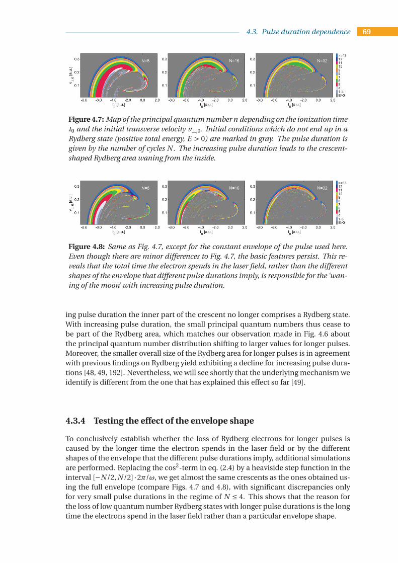
4.3. Pulse duration dependence 69
Figure 4.7: Map of the principal quantum number n depending on the ionization time
t0 and the initial transverse velocity v⊥,0. Initial conditions which do not end up in a
Rydberg state (positive total energy, E > 0) are marked in gray. The pulse duration is
given by the number of cycles N . The increasing pulse duration leads to the crescent-
shaped Rydberg area waning from the inside.
Figure 4.8: Same as Fig. 4.7, except for the constant envelope of the pulse used here.
Even though there are minor differences to Fig. 4.7, the basic features persist. This re-
veals that the total time the electron spends in the laser field, rather than the different
shapes of the envelope that different pulse durations imply, is responsible for the ‘wan-
ing of the moon’ with increasing pulse duration.
ing pulse duration the inner part of the crescent no longer comprises a Rydberg state.With increasing pulse duration, the small principal quantum numbers thus cease tobe part of the Rydberg area, which matches our observation made in Fig. 4.6 aboutthe principal quantum number distribution shifting to larger values for longer pulses.Moreover, the smaller overall size of the Rydberg area for longer pulses is in agreementwith previous findings on Rydberg yield exhibiting a decline for increasing pulse dura-tions [48, 49, 192]. Nevertheless, we will see shortly that the underlying mechanism weidentify is different from the one that has explained this effect so far [49].
4.3.4 Testing the effect of the envelope shape
To conclusively establish whether the loss of Rydberg electrons for longer pulses iscaused by the longer time the electron spends in the laser field or by the differentshapes of the envelope that the different pulse durations imply, additional simulationsare performed. Replacing the cos2-term in eq. (2.4) by a heaviside step function in theinterval [−N /2, N /2] ·2π/ω, we get almost the same crescents as the ones obtained us-ing the full envelope (compare Figs. 4.7 and 4.8), with significant discrepancies onlyfor very small pulse durations in the regime of N ≤ 4. This shows that the reason forthe loss of low quantum number Rydberg states with longer pulse durations is the longtime the electrons spend in the laser field rather than a particular envelope shape.

70 CHAPTER 4: Intensity and pulse duration dependence of Rydberg states
4.3.5 Analysis of trajectories
Even though the plots of the Rydberg areas in Figs. 4.7 and 4.8 gave us some idea of theeffect the pulse duration has on Rydberg states, it did not tell us why these effects areobserved. To address this question, a closer look at trajectories with initial conditionsaround the inner edge of the crescent is enlightening. Fig. 4.9 shows such exemplarytrajectories from around the inner edge of the crescent for two different pulse dura-tions – one that still allows the electron to end up in a Rydberg state (N = 16) and onethat doesn’t do so any more (N = 17). A constant envelope is used since it simplifiesthe following considerations without a loss of generality, as just discussed. In the cen-tral panel of Fig. 4.9, we can see that during the first optical cycles the electron is –on cycle average – driven away from the residual ion and comes closer to it later on,approximately following a parabola-like curve.
How can we understand that the electron is – on cycle average – moving along aparabola-like curve? Loosely speaking, this is due to two competing effects: On theone hand, the laser field drives the electron away from the parent ion and, on the otherhand, the Coulomb force of the residual ion has an attractive effect on the electron.For a deeper understanding, let us look at the bottom panel of Fig. 4.9, from whichit becomes clear that the oscillation of the electron’s position around a parabola-likecurve is directly linked to the approximately linear function with positive slope thatthe velocity vx(t ) follows on cycle average. As we will see, the positive slope of thislinear function is entirely due to the pull of the Coulomb potential in the directionof the residual ion. If the electron were driven merely by the laser field and were notinfluenced by the Coulomb potential, then the velocity of the electron would be givenby
vx(t ) =−E0
ω(sin(ωt )− sin(ωt0)) (4.37)
for a constant envelope5. This function oscillates around the mean value ofE0/ωsin(ωt0), which can be approximated by E0t0 and is thus negative for ionizationtimes before the peak of the optical cycle, which is the time regime in which Rydbergelectrons are typically born (the negative ionization time of Rydberg states can also beseen from Figs. 4.7 and 4.8). This negative offset in the velocity, when only consid-ering the laser field and neglecting the Coulomb potential, explains why the electronis initially – on cycle average – slightly driven away from the residual ion (see centerpanel of Fig. 4.9). Now, as one can see in the central panel of Fig. 4.9, even though thechange of the ‘mean’ position – the position of the electron in the x-direction that theelectron oscillates around (green line) – is vital in the understanding of the electron’sreturn, it changes rather slowly. Consequently, as the Coulomb force merely dependson the electron’s position, the Coulomb force averaged over one optical cycle also doesnot change quickly and can be considered almost constant. A constant force, whichis proportional to a constant acceleration, then leads to a linearly changing velocity,which agrees with what we observe numerically. The slope of this linear function ispositive since the Coulomb potential exerts an attractive force on the electron. Thelinearly scaling velocity, in turn, leads to the cycle-averaged elongation following anapproximate parabola, which tallies with the numerically obtained result (see central
5This equation differs from eq. 4.16 in the sign of the prefactor because here we use a CEP of 0,whereas for eq. 4.16 a CEP of π was used, which is explained in Appendix A.4.

4.3. Pulse duration dependence 71
Figure 4.9: Data for trajectories released at t0 =−6.4 with v⊥,0 = 0.09 from a hydrogen
atom and propagated in a laser field with I = 1.5·1014 W/cm2 and λ= 800 nm that has
a constant envelope with a total number of cycles N = 16 and N = 17, respectively. The
fact that the electron experiences only about half of the respective numbers of optical
cycles is due to the electron being born in the central cycle. Top panel: Coordinates
x and r⊥ =√
y2 + z2. Central and bottom panel: Position x and velocity vx along
the polarization axis as a function of propagation time, respectively. After the pulse is
over, the respective trajectory is displayed in a lighter shade (i.e. orange and light-blue)
of the color it had while the pulse was still on (i.e. red and dark blue).
and bottom panel of Fig. 4.9). At this point, one may be wondering why consider-ing the cycle-averaged trajectory should be sufficient. Concerning that question, thereader is referred to Refs. [193, 194], which provide a detailed elaboration on the powerof cycle-averaged descriptions of post-ionization dynamics, in particular in the contextof including Coulomb effects during propagation.
The observation that the averaged position approximately follows a parabola nowhelps us explain why certain initial conditions lead to a Rydberg state for a short pulsebut not for a longer one: If a critical number of optical cycles (N = 16 in Fig. 4.9) isexceeded, the electron comes back so close to the ion that it ‘recollides’ gaining a lot ofkinetic energy and therefore does not end up in a Rydberg state. In the return process,the cycle-averaged motion described approximately by the parabola is more relevantthan the amplitude of the oscillation which strongly depends on the envelope. Thus,
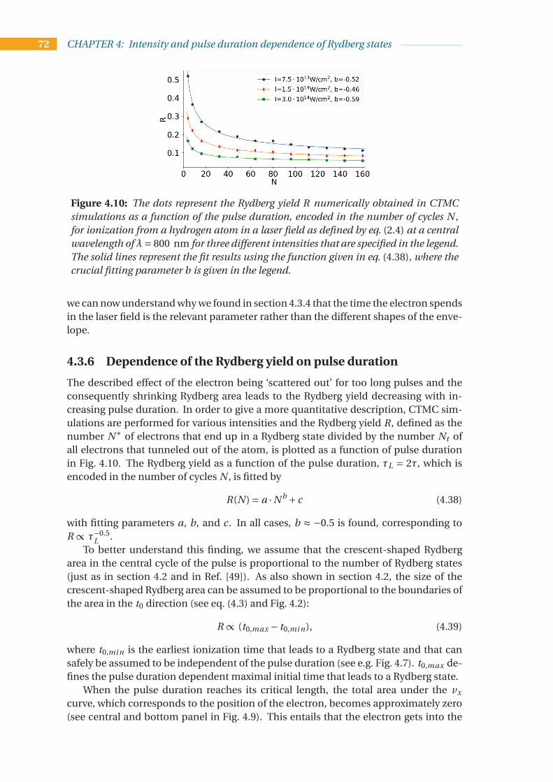
72 CHAPTER 4: Intensity and pulse duration dependence of Rydberg states
Figure 4.10: The dots represent the Rydberg yield R numerically obtained in CTMC
simulations as a function of the pulse duration, encoded in the number of cycles N ,
for ionization from a hydrogen atom in a laser field as defined by eq. (2.4) at a central
wavelength of λ= 800 nm for three different intensities that are specified in the legend.
The solid lines represent the fit results using the function given in eq. (4.38), where the
crucial fitting parameter b is given in the legend.
we can now understand why we found in section 4.3.4 that the time the electron spendsin the laser field is the relevant parameter rather than the different shapes of the enve-lope.
4.3.6 Dependence of the Rydberg yield on pulse duration
The described effect of the electron being ‘scattered out’ for too long pulses and theconsequently shrinking Rydberg area leads to the Rydberg yield decreasing with in-creasing pulse duration. In order to give a more quantitative description, CTMC sim-ulations are performed for various intensities and the Rydberg yield R, defined as thenumber N∗ of electrons that end up in a Rydberg state divided by the number Nt ofall electrons that tunneled out of the atom, is plotted as a function of pulse durationin Fig. 4.10. The Rydberg yield as a function of the pulse duration, τL = 2τ, which isencoded in the number of cycles N , is fitted by
R(N ) = a ·N b + c (4.38)
with fitting parameters a, b, and c. In all cases, b ≈ −0.5 is found, corresponding toR ∝ τ−0.5
L .To better understand this finding, we assume that the crescent-shaped Rydberg
area in the central cycle of the pulse is proportional to the number of Rydberg states(just as in section 4.2 and in Ref. [49]). As also shown in section 4.2, the size of thecrescent-shaped Rydberg area can be assumed to be proportional to the boundaries ofthe area in the t0 direction (see eq. (4.3) and Fig. 4.2):
R ∝ (t0,max − t0,mi n), (4.39)
where t0,mi n is the earliest ionization time that leads to a Rydberg state and that cansafely be assumed to be independent of the pulse duration (see e.g. Fig. 4.7). t0,max de-fines the pulse duration dependent maximal initial time that leads to a Rydberg state.
When the pulse duration reaches its critical length, the total area under the vx
curve, which corresponds to the position of the electron, becomes approximately zero(see central and bottom panel in Fig. 4.9). This entails that the electron gets into the

4.3. Pulse duration dependence 73
Figure 4.11: Linear fit to the minima of vx (see e.g. the bottom panel of Fig. 4.9) ob-
tained for ionization from hydrogen at a laser intensity of I = 3.0 ·1014 W/cm2, a cen-
tral wavelength of λ = 800 nm, and an initial transverse velocity v⊥,0 = 0.15 a.u. for
different ionization times t0. The pulse duration differs in each case and is chosen in a
way that one optical cycle more would cause a strong Coulomb interaction that would
accelerate the electron such that it would not be captured in a Rydberg state.
immediate vicinity of the residual ion and is strongly accelerated, gaining enough en-ergy in the scattering process to leave the atom for good. In Fig. 4.11, linear fits to theminima of vx (in analogy to the green line in the bottom panel of Fig. 4.9) are shownfor different ionization times in the central cycle at a fixed intensity, wavelength, andinitial transverse velocity. The parameter that is varied is the pulse duration, which ischosen in each case as the maximal pulse duration, Nmax , that will still lead to a Ryd-berg state, meaning one additional optical cycle would bring the electron so close tothe ion that the Coulomb potential would strongly accelerate the electron such that itwould not be captured in a Rydberg state. From Fig. 4.11 we can see that the differ-ent ionization times mainly affect the slope of these lines6 but both the offset and therange of vx , ∆vx , are almost constant with variations below 1% for the offset and below15% for ∆vx from the respective mean value. Therefore, the following approximationis done
∆vx ≈ const = d(t0,max) ·Nmax(t0,max), (4.40)
where d is the slope of vx . Furthermore, we find numerically for the dependence oft0,max on the slope d that we can fit it nicely to a function
t0,max = p ·dβ+q (4.41)
with fitting parameters p, q , and β (Fig. 4.12). In particular, we find similar values forβ for the different laser parameter sets shown in Fig. 4.12 (which are the same laserparameters as in Fig. 4.10 that we try to understand): β≈ 0.6.
How can we understand this result? As has already been discussed in the contextof the explanation of the approximately parabola-shaped elongation, the electron is,on cycle average, exposed to an approximately constant force that pulls it closer to
6Note that the different slopes of the linear cycle-averaged velocity curve correspond to differentcurvature radii of the parabola-like function the position is oscillating around. A steeper velocity slopecorresponds to a smaller curvature radius of the parabola-like position curve and thus means the elec-tron returns to the parent ion in fewer optical cycles. Also see Fig. 4.13, from which the relation betweenionization time, parabola curvature and the maximal pulse duration that still leads to a Rydberg statebecomes clear.

74 CHAPTER 4: Intensity and pulse duration dependence of Rydberg states
Figure 4.12: Left panel: The markers represent slopes of the linear fits to the minima of
vx (see e.g. Fig. 4.11) versus the maximal ionization times that still lead to the electron
ending up in a Rydberg state for different intensities specified in the legend. A laser
with a central wavelength of λ= 800 nm was used for ionization of hydrogen, and the
trajectories were started at an initial transverse velocity of v⊥,0 = 0.15 Note that, as in
Fig. 4.11, the maximal pulse durations Nmax that still lead to a Rydberg state were cho-
sen for each point separately and thus vary in the plot. Nmax grows as t0,M ax becomes
more negative, as indicated by the arrow. The solid lines represent the corresponding
fit of eq. (4.41) to the data, with the crucial fitting parameter β given in the legend.
Right panel: Sketch showing how one can understand that a 1/t 20 scaling can locally
be approximated by a t 20 scaling.
the ion. This Coulomb force is represented as the slope d in eq. (4.40) and it obviouslydepends on how far the electron is away from the ion on average. The drift momentumimposed by the laser field is E0/ω · sin(ωt0) ≈ E0t0 and can be used as a quantifier forhow far away from the residual ion the electron is pushed on cycle average. So, theCoulomb force, which scales as−1/r 2 with distance r , can be assumed to scale as−1/t 2
0with the ionization time, meaning d ∝ 1/t 2
0 . This seems to contradict our finding ofd ∝ t 1/0.6
0,max ≈ t 20,max from the fit at first glance. However, as one can understand by
the sketch in the right panel of Fig. 4.12, the approximate 1/t 20 drop of the Coulomb
force can be further approximated around the typical values of t0, i.e. slightly negativevalues, by a function that scales like a parabola t 2
0 .Thus, we have seen that in order to quantify how the Rydberg yield decreases with
increasing pulse duration it is sufficient to quantify how fast the inner edge of the Ryd-berg area, i.e. the maximal ionization time that still leads to a Rydberg state, is shiftedfurther away from the field maximum. We have learned that ionization closer to thefield maximum leads to a steeper slope in the cycle-averaged linear velocity curve, cor-responding to a smaller curvature radius the position is oscillating around and result-ing in a return to the parent ion after fewer optical cycles. This was understood byionization times further away from the field maximum leading to a larger drift by thelaser field and hence the Coulomb force pulling the electron back more slowly.
4.3.7 Comparison to other models
Even though the scaling of R ∝ τ−1/2L
is not dramatically different from prior results [48,49], which gave a τ−2/3
Ldependence, it offers a completely different explanation for the
underlying mechanism. Prior treatments neglected the Coulomb potential, which wasviewed as a higher-order correction, during propagation [49, 180]. Only after the pulse

4.3. Pulse duration dependence 75
was over, the Coulomb potential was accounted for by including it when checking ifthe total energy was negative [49]7. Our analysis, however, shows that including theCoulomb potential during propagation is vital in explaining that for sufficiently longpulses the electron is driven back to the parent ion, which leads to ionization. Withoutthe Coulomb potential, the electron that can potentially form a Rydberg state (and istherefore born before the peak of the laser field) would be, on cycle average, monoton-ically driven away from the residual ion. Consequently, the electron would never, oncycle average, slowly move back to the ion and strongly interact with its Coulomb po-tential when a critical pulse duration is exceeded. Yet even sophisticated models likethe modified SFA [191] that explains many features of the mentioned newly developedXUV radiation scheme [189] do not include the Coulomb effect during propagationand thus do not take this effect of ‘ionization through scattering’ into account and, asa consequence, cannot capture the pulse duration effects described here.
Furthermore, the analysis in Ref. [49] builds on the assumption that the ‘outer edge’of the Rydberg area, corresponding to minimal ionization times and maximal trans-verse velocities, is affected by the pulse duration and the Rydberg area ‘shrinks fromthe outside’. The outer edge of the Rydberg area defines the limit E = 0 when check-ing if the total energy E is negative according to eq. (4.1). Therefore, focusing on E = 0seems intuitively reasonable as close to this limit we find the most loosely bound Ryd-berg states, which one would intuitively (if wrongly) expect to be least stable and tosurvive only short pulses. In section 4.2, we have successfully applied this criterion ofE = 0 in the intensity dependence study. The pulse duration, in contrast, barely af-fects this outer edge of the Rydberg area but makes the Rydberg crescent wane fromthe inner edge, as we have seen above, e.g. in Fig. 4.7. Thus, the deeply bound Rydbergstates found at the inner edge only survive short pulses, whereas the loosely boundRydberg states close to the outer edge (corresponding to E = 0) stay bound even forlonger pulses. This counter-intuitive effect of loosely bound Rydberg states being morestable against pulse duration changes can only be explained in a model that includesthe above-described effect of the electron returning to the parent ion and being ac-celerated in a scattering process. All of this highlights the importance of includingthe Coulomb effect when studying the pulse duration dependence of Rydberg states,which is further backed by the study by Dubois et al. that was published most recentlyin [195] (sec. IV. therein).
4.3.8 Dependence of the principal quantum number distribution on
pulse duration
The observation that the inner edge of the crescent scatters out first when the pulse du-ration increases is also crucial for understanding the effect of the pulse duration on theprincipal quantum number distribution (Fig. 4.6). The Rydberg states that are found atthis inner edge have a more negative energy, corresponding to smaller quantum num-bers. The fact that these smaller principal quantum numbers cease to be a Rydbergstate first when the pulse duration increases is in agreement with the principal quan-tum number distribution shifting to larger n for longer pulses (see Fig. 4.6). To under-stand why the pulse duration affects small and large quantum numbers differently, itis instructive to look at two trajectories for the same initial transverse velocity but dif-
7Even though in Ref. [49] the Coulomb potential was accounted for in a perturbative manner, theeffect cancels out in this description, as was explained in section 4.2.1.

76 CHAPTER 4: Intensity and pulse duration dependence of Rydberg states
ferent ionization times, where the smaller principal quantum number corresponds toan ionization time that is closer to the field maximum (t0 = 0), being found at the in-ner edge of the crescent. Fig. 4.13 shows such a comparison and we can see that beingborn closer to t0 = 0, the electron moves along a smaller parabola-shaped curve. Thisis mainly due to the smaller vector potential of the laser field closer to the field maxi-mum. Therefore, the acceleration by the laser field driving the electron away from theion is weaker and the Coulomb potential pulls the electron back faster. Consequently,the critical number of optical cycles for which the electron recollides with the parention and ceases to be a Rydberg state is smaller for initial conditions corresponding tosmaller principal quantum numbers.
To make these findings more quantitative, we look again at the right panel of Fig. 4.6.As indicated by the lines in this plot, we find that the principal quantum number n
peaks at values npeak that can be fitted by the following function
npeak = A+Bp
N (4.42)
with fitting parameters A and B . We can understand that the increase can be describedby such a
pN -scaling by looking at the parabola that x oscillates around (e.g. in Fig. 4.9
or 4.13). As mentioned before, we expect n ≈p⟨r ⟩ (see eq. (4.35)). Similarly to section
4.3.6, we are again interested in Nmax , the maximal number of cycles in the pulse thatstill leads to a Rydberg state (e.g. Nmax = 16 in Fig. 4.9) since it is directly linked to thezero-crossing of the parabola and its value depends strongly on the initial conditions(t0, v⊥,0). We find that Nmax depends linearly on the extreme value of the parabola,which we call xmax . This relation will be explained in the next paragraph, but now letus first look at the consequence: Since xmax depends linearly on Nmax , also the meanelongation ⟨x⟩ of the parabola depends approximately linearly on Nmax , hence ⟨x⟩ de-pends linearly on Nmax . Also the motion transverse to the polarization axis happensalong a parabola and an analogous line of reasoning can be applied here and we findthat ⟨r⊥⟩ depends linearly on Nmax . Therefore, we obtain n ≈
p⟨r ⟩ ≈
√
⟨x⟩2 +⟨r⊥⟩2,which then depends linearly on
pNmax . As the maximal number of cycles Nmax de-
fines the inner edge of the crescent and also the most likely n value, we can replaceNmax by N and obtain eq. (4.42).
Now, back to the question of how we can understand that numerically it is foundthat the maximal number of optical cycles Nmax that the pulse can have for a specificinitial condition so that the electron still ends up in a Rydberg state depends linearlyon the maximal elongation xmax of the parabola that we fit to the x(t ) curve. Let usassume that the approximate parabola which x oscillates around returns to x = 0 afterpropagation for about Nmax/2 cycles, which should become clear from Fig. 4.13 andfrom the fact that for x close to zero the recollision is increasingly likely8. In Fig. 4.13we see that the maximal value xmax is found after a propagation time of about Nmax/4.If we define the parabola fit function as x f i t (t ) = d · (e − t )2 + f with fitting parametersd , e, and f , then we realize that e ≈ Nmax/4 and f ≈ xmax . So, mathematically thequestion is why we find approximately that e depends linearly on f . As we can see inFig. 4.13, the parabolas for different t0 are noticeably similar directly after ionization.In terms of the parabolic fit function, we can therefore write
x f i t (0) = de2 + f = P1 ≈ const
x ′f i t (0) =−2de = P2 ≈ const
(4.43)
8Note that we assume that the electron is born in the central cycle and that thus the pulse is on onlyfor about Nmax /2 cycles after ionization.

4.3. Pulse duration dependence 77
Figure 4.13: Position x vs. propagation time t for trajectories ionized from hydrogen
in a laser field of an intensity I = 1.5·1014 W/cm2 and a central wavelength λ= 800 nmwith an initial transverse velocity v⊥,0 = 0.15 for two different ionization times t0 and
correspondingly two different pulse durations, which are chosen such that a pulse du-
ration of one optical cycle more would have led to the electron not ending up in a Ryd-
berg state anymore. The dashed lines show a parabolic fit through the value that x
oscillates around.
and thus it follows
f = P1 −de2 = P1 +P2/2 ·e, (4.44)
which means that f depends linearly on e and which tallies with our numerical obser-vations described above.
Thus, similar to the analysis in section 4.3.6, we have used that an ionization timeclose to the field maximum leads to an earlier return to the parent ion. Instead of quan-tifying this in terms of a steeper slope of the cycle-averaged linear velocity curve as insection 4.3.6, here we used that, correspondingly, the parabola-like curve the positionoscillates around has a smaller curvature radius. Focusing on the position allowed usto make a connection to the principal quantum number via n =
p⟨r ⟩. Consequently,
we could quantify approximately how an ionization time closer to the field maximum –corresponding to a smaller parabola and hence a smaller n – can only lead to a Rydbergstate for shorter pulses.
4.3.9 Conclusion and Discussion
In summary, using CTMC simulations it was found that an increase in the pulse du-ration of the laser shifts the principal quantum number n of Rydberg states to largervalues and that this increase scales approximately like the square root of the pulse du-ration. Moreover, we observed a decrease in the fraction of electrons that end up in aRydberg state with increasing pulse duration. We could understand this general dropof the Rydberg yield by finding that the attractive Coulomb potential slowly drives theelectron back to the parent ion. If the propagation is too long, the electron gets so closeto the parent ion that the strong interaction causes a significant acceleration prevent-ing the electron from forming a Rydberg state. We have seen that electrons ending upin Rydberg states of small quantum numbers return to the parent ion more quickly andare thus ‘scattered out’ already for shorter pulse durations. This explains the shift of theprincipal quantum number distribution to larger quantum numbers for longer pulse

78 CHAPTER 4: Intensity and pulse duration dependence of Rydberg states
durations. As the mechanism that explains these pulse duration effects stands in con-trast to the mechanism found in a model that neglects the Coulomb force during thepropagation in the laser field [49], the results presented here show that the Coulombforce has important consequences for the yield and quantum number distribution ofRydberg states.
The insights gained in the study of pulse duration effects allow us to not only un-derstand but also control the distribution of principal quantum numbers, which willprove helpful in studies and applications that are based on this distribution, such asthose presented in Refs. [170, 171, 184, 187–189, 196, 197]. Interestingly, the effectof the longer pulse duration ionizing Rydberg states of low principal quantum num-ber reported in this work is similar to the effect reported in recent studies that useda second laser pulse to investigate the stability of Rydberg atoms [170, 171] since alsothe use of a second laser pulse leads to ionization of Rydberg states of low principalquantum numbers. Thinking in terms of control of the principal quantum number ofRydberg states the study presented in this chapter might prove helpful as modifyingthe pulse duration might be easier to implement than installing a second laser pulsein certain systems. One particular application for which the control of the quantumnumber distribution is vital is the recently developed scheme that uses radiation fromRydberg excited states created via FTI to generate coherent XUV emission [189]. As theXUV emission yield is larger if Rydberg states with low principal quantum numbers arepopulated, choosing a short pulse duration is vital here since we have seen that the lowprincipal quantum number states are the ones affected most severely when the pulseduration becomes longer.
Stepping back and considering this chapter about Rydberg states as a whole, oneopen question seems to be why the intensity dependence in section 4.2 gave rea-sonable results in a model that neglected the Coulomb potential during propagationwhereas in the pulse duration dependence in section 4.3 including the Coulomb po-tential was indispensable. The key to resolve this problem lies in the observation thatthe Rydberg area decreases from the ‘outside’ for increasing intensity and from the ’in-side’ for increasing pulse duration. In other words, the initial conditions that lead toRydberg states for only small intensities or only short pulse durations have an energythat is close to zero or deeply negative, respectively. Thus, as the Rydberg states whichcease to be a Rydberg state upon increasing the intensity are loosely bound anyway,the recollision mechanism is not the dominant process that leads to the decrease inRydberg states and neglecting the Coulomb potential during propagation worked well.This stands in contrast to the deeply bound Rydberg states that cease to be a Rydbergstate when the pulse duration increases because of the above-explained return to andrescattering at the parent ion.

CHAPTER
5Emergence of a Higher Energy
Structure in inhomogeneous fields
“One sometimes finds what one is not looking for."
— Alexander Fleming (Nobel Prize Laureate in 1945)
Overview of this chapter
This chapter reports on the emergence of a prominent higher energy peak [73] in the spec-trum of photoelectrons that were ionized from the gas phase in a laser pulse with time-varying spatial dependence as it is typically found in the vicinity of a nanostructure. Thehigher energy structure (HES) originates from direct electrons released in a narrow time-window and is separated from all other ionization events, with its location and width highlydependent on the strength of the spatial inhomogeneity. Hence, the HES can be used as asensitive tool for near-field characterization in the “intermediate regime”, where the elec-tron’s quiver amplitude is comparable to the field’s decay length. Moreover, the large ac-cumulation of electrons with tuneable energy suggests a promising method for creating alocalized source of electron pulses of attosecond duration using tabletop laser technology.In section 5.3, closed-form expressions are derived [74] to describe the movement in this“intermediate regime”, which is notoriously difficult to describe analytically. These de-scriptions will help us understand how the spectral position and width of the HES dependson the inhomogeneity of the field and thus how to control the parameters to obtain a spec-trally narrow electron pulse of tunable energy.In section 5.4, it will be shown that the recently reported experimental finding of a low en-ergy peak (LEP) can be understood in the same theoretical framework as the theoreticallypredicted emergence of the HES. Even though the two peaks were observed in differentenergy regimes, and despite the LEP being detected for electrons that were released froma nanotip whereas the HES was found for electrons ionized from a gas that is placed inthe vicinity of a nanotip, a single mechanism that causes the peak formation is identified.Based on this mechanism, a more general analytical model is derived to describe the en-ergy upshift electrons experience in inhomogeneous electric fields. It will also explain theexperimentally observed linear scaling of the peak energy of the LEP with the intensity ofthe incident laser pulse. Moreover, parameters are found at which electrons ionized di-rectly from a nanostructure, the setting in which the LEP was found, form a prominent andnarrow peak at higher energies as it was described in the framework of the HES. As ioniza-tion from the tip is experimentally better established than ionization from the gas phasenear a nanostructure, this should pave the way for the experimental realization of almostmonoenergetic electron beams of attosecond duration as they are predicted for the HES inthe gas phase.

80 CHAPTER 5: Emergence of a Higher Energy Structure in inhomogeneous fields
5.1 Introduction to inhomogeneous fields in the vicinity
of a nanostructure
5.1.1 Introduction to nano-attophysics
In this chapter, we will leave the regime of ‘pure’ strong field attosecond science thatfocuses on lasers and atoms and include nanostructures that enhance the fields andintroduce a spatial inhomogeneity. Of course, also ionizing ‘just’ atoms introduces aninhomogeneity via the Coulomb potential that cannot always be neglected, as we haveseen in the previous chapter and which will also play a crucial role in chapter 6. In thischapter, however, the dominant inhomogeneity is produced by a nanostructure andthus much more extreme resulting in completely different effects.
‘Traditional’ nano-optics, i.e. using electromagnetic fields that are neither particu-larly strong nor short-pulsed, describes optical phenomena that arise at the nanometerscale [198]. This involves using solid state structures that are of nanometer size or atleast exhibit edges and protrusions at this scale. These scales cannot be spatially re-solved by typical wavelengths of several hundred nanometers, due to the diffractionlimit [198]
∆x ≥ 1
2∆kx. (5.1)
Now, the clue and mathematical trick that the field of nano-optics is based on and thatfacilitates subwavelength resolution after all is the fact that we can increase the spreadin kx beyond k as long as we make sure that the relation
k =√
k2x +k2
y +k2z (5.2)
is fulfilled. Choosing for example kz to be imaginary, thus finding k2z < 0, we can afford
kx > k and still satisfy eq. (5.2). However, having an imaginary kz results in an expo-nentially decaying field exp(−|kz |z) in the positive z-direction, commonly referred toas an evanescent wave. In the opposite z-direction, the field would grow exponentially,which is unphysical and cannot be true. If, however, we are not in an infinitely ex-tended space but at a surface between two different media, then the exponential decaycan exist in one half-space while in the other half-space the other material and refrac-tive index result in a different solution that does not necessarily lead to the exponentialgrowth [198].
This principle of achieving subwavelength spatial resolution by introducing animaginary wavevector and thus an evanescent wave has led to many powerful toolsand applications in the field of nano-optics [199–206]. Prominent examples includescanning near-field optical microscopy (SNOM) [207], tip-enhanced Raman scattering(TERS) [208–210], photon scanning tunneling microscopy (PSTM) [211, 212] or totalinternal reflection fluorescence (TIRF) microscopy [213, 214], to mention but a few.The interest in nano-optics has certainly been boosted by the miniaturization and inte-gration of electronic circuits for the computer industry [198] and nano-optics is there-fore relevant beyond the realms of basic research with many applications in e.g. opto-or microelectronics [215–217].
Although nano-optics is a well-researched and mature field on its own, its mergerwith ultrafast strong fields is relatively new. This ‘marriage’ is interesting on (at least)two counts: Firstly, the local field enhancement that is found near nanostructures al-

5.1. Introduction to inhomogeneous fields 81
lows the incident laser beam to have a relatively small intensity which – after enhance-ment – is in the typical strong field intensity regime [162]. And secondly, when thehigh spatial resolution of nano-optics teams up with the high temporal resolution ofultrashort pulses, the resulting system becomes a promising contender in the quest ofachieving higher spatio-temporal resolution [218, 219].
Analyzing the electron dynamics in strongly enhanced, short-pulsed near-fieldshas allowed to characterize the near-field with subcycle resolution [220–222], which– in turn – opened up new perspectives to control electron dynamics in such near-fields and thus to create new electron sources. The extreme localization of electrons inspace and time allows to use nanostructures illuminated by short pulses as femtosec-ond electron sources with outstanding beam qualities [223–226]. The highly coherentelectron pulses from nanotips are, for example, exploited in studies of fundamentalmatter-wave quantum optics [226–228] or are used in exploring implementations oftime-resolved point-projection microscopy (PPM), in which magnification is achievedby placing a field emission tip close to a specimen [229–231].
Speaking of coherent emission, one obvious question that arises is whether high-harmonic generation (HHG) in a system containing a nanostructure is possible andcan be used as a coherent source of e.g. XUV light, which is discussed and reviewed inthe following since it played an important role and shaped the field of nano-attosecondscience in the past decade. At this point, it is crucial to distinguish between the twomain paths that were chosen when trying to attain HHG using nanostructures:
(i) HHG using electrons that were released from atoms or molecules in a gas that islocated close to a nanostructure and therefore feels the near-field of it.
(ii) HHG using electrons that were emitted directly from the nanotip.
Concerning mechanism (i), there was an early experiment in 2008 that claimed to haveproduced HHG light from argon atoms that were placed in the strongly enhanced fieldin between a bow-tie structure [232]. While indeed XUV radiation had been produced,the origin of the radiation remained contentious [233–235] and it is now generally be-lieved that is was atomic line emission (ALE), rather than HHG, that was the underly-ing mechanism that produced the radiation [236, 237]. Even though the produced XUVlight can be used in applications where spatial and temporal coherence are not essen-tial, for example in implementations of near-field XUV lithography [236], the incoher-ent nature of the dominant ALE process clearly distinguishes it from a coherent HHGsource. Despite many attempts to produce HHG at yields and repetition rates that arecomparable to those achieved from the gas phase in homogeneous strong fields, so farthis aim was not attained [238]. On the upside, though, the quest for HHG from atomsor molecules in the vicinity of a nanostructure has sparked further experimental andtheoretical results along these lines [239–249], which helped develop the field of nano-attophysics.
Similarly, also the second category of attempts, (ii), which tried to produce HHGby emitting electrons directly from the nanotip, proved futile. Even though theoreticalworks made optimistic predictions about the feasibility of that method [250], as of yetno ‘direct HHG’ from metal tips, or any other nanostructure for that matter, has beenreported [226]. The following estimate presented in Ref. [226] makes the problem withthis approach to produce HHG clear: The surface of a typical nanotip consists of about103-104 atoms. In contrast, the number of gas atoms in the laser focus is of the order of

82 CHAPTER 5: Emergence of a Higher Energy Structure in inhomogeneous fields
1010. Thus, on a nanostructure surface the number of potential emitters is too low tolead to a reasonable HHG yield via strong field emission and recollision.
In the midst of all of these vain attempts to generate HHG employing nanostruc-tures, a silver lining appeared in the horizon. In 2016, the very group who set the dis-cussion about HHG with nanostructures off with their contentious results in 2008 [232]achieved HHG radiation employing solid tips that are made of monocrystalline sap-phire surrounded by a gold thin-film layer [251]. The underlying mechanism, though,is not found in either of the two categories presented above but coherent XUV light iscreated by means of inter- and intraband processes. This mechanism is the one that isalso used to describe the HHG radiation from bulk solids and it does not involve pho-toemission but the radiation promotes the electron from the valence to the conductionband. Anharmonic oscillations and recombination then lead to intra- and interbandradiation, respectively [27, 28, 252–257]. The main difference between HHG from bulksolids and this experiment therefore stems from the enhancement of the incident laserfield at the metal-sapphire nanostructure in the latter. This enhancement was furtherimproved upon by Vampa et al., who used a nanoantenna array of gold embeddedin a layer of silicon [258]. The nanoantenna array produces localized surface plas-mons and thus complements the experiment reported in Ref. [251] in which surfaceplasmon-polaritons enhanced the field [259]. Using localized surface plasmons hasthe advantage that the geometry of the nanoarray can be adapted to engineer e.g. thepolarization of the harmonic beam [258].
Also, even though processes (i) and (ii) have not led to satisfactory HHG produc-tion, the theoretical studies that emerged around this discussion made clear that thestrong field enhancement and field inhomogeneity near a nanostructure significantlyinfluence the electrons’ post-ionization dynamics [243, 244, 260] thus also affectingprocesses like double ionization [47]. Most directly, though, the effect of the nano-structure on an ionized electron can be observed by analyzing the photoelectron mo-mentum spectrum: Shifts and suppression of peaks in the photoelectron spectrumand the extension of the rescattering cutoffs have been reported in the presence of ananostructure [162, 218, 221, 261–264]. These effects were suggested to be used for thecharacterization of both the incident laser pulse, especially the carrier-envelope phase,and the near-field of the nanostructure [162, 218, 222, 263, 265].
The effect of the inhomogeneity on the photoelectron momentum spectrum willalso be at the center of the discussions in this chapter. We will see how photoemissionof atoms that are placed in the vicinity of a nanostructure is followed by electron dy-namics that is characterized by acceleration due to the inhomogeneous field and howthe resulting high-energetic electrons accumulate in a peak that we will name ‘higherenergy structure’ (HES) [73, 74]. Moreover, we will realize that the motion of photoelec-trons released directly from the tip bears great similarity to the dynamics underlyingthe HES and that it can be captured in the same theoretical framework.
5.1.2 Mathematical description of inhomogeneous fields
In the following, common theoretical models to describe the electric field in the vicin-ity of a nanostructure upon irradiation with a laser pulse are reviewed and discussed,thus setting the stage for the calculations that will be performed later in this chapter.Even though the nanostructures employed in nano-attophysics rarely are close to per-fect spheres in free space and even though in certain cases taking into account the

5.1. Introduction to inhomogeneous fields 83
exact geometry of the nanostructure matters [266–268], the electric fields near the na-nostructure are often found to be well approximated by that of a sphere. Typically, theminimal radius of curvature of the nanotip’s apex or of the protruding edges in moreelaborate nanogeometries determines the size of the corresponding sphere in the the-oretical model [198]. The electric field close to a dielectric sphere in a quasi-static ap-proximation is a common example in undergraduate physics courses on theoreticalelectrodynamics [269, 270] and we will now see that this system does not only serve asa nice pedagogical tool to introduce the expansion in Legendre polynomials but thatthe result can help us model real-life nanosystems. For a sphere of radius R and dielec-tric constant ǫs positioned at the origin in a medium with ǫm = 1, the electric field atposition r reads [271, 272]
E(r) =
3
ǫs +2Ei if |~r | < R,
Ei +3r(r ·p)−p
|r|3if |~r | > R,
(5.3)
where r is the unit vector in space and Ei denotes the spatially homogeneous incidentfield that is assumed to change so slowly that the system can adapt adiabatically to thechange. The dipole moment p is given by
p = R3 ǫs −1
ǫs +2Ei . (5.4)
As becomes clear from eq. (5.3), the electric field close to the sphere exhibits a strongspatial inhomogeneity. The maximal field strength is obtained directly at the surfaceof the sphere at the poles along the polarization direction of the incident field. Thecorresponding field enhancement is [238]
∣∣∣∣
E(r = R ex)
Ei
∣∣∣∣=
∣∣∣∣1+2
ǫs −1
ǫs +2
∣∣∣∣ , (5.5)
where linear polarization in x-direction was assumed. For a gold sphere at λ= 720 nmthe dielectric constant is ǫs =−16.41+1.38i [238] and the field enhancement amountsto 3.4, corresponding to an intensity enhancement by a factor of 11.6. Even though thatmay appear to be a large enhancement already, compared to other nanostructures itis considered relatively low [273] and typical enhancement factors can be one or twoorders of magnitude larger [241, 267]. For a more intuitive understanding of the en-hancement and inhomogeneity it is instructive to be aware of the fact that the secondline of eq. (5.3) is the superposition of the incident field Ei and the general expressionfor an electric field of a dipole with dipole moment p. Here the dipole moment, as ex-pressed by eq. (5.4), is induced by displacement of charges in the dielectric sphere bydint of the exposure to the incoming electric field. The resulting local positive chargesurplus at one pole of the sphere and the concomitant local negative charge surplus atthe other pole lead to the mentioned dipole.
The underlying assumption so far was that the charges follow the incident field in-stantaneously. However, the collective electronic response of the medium leads to aphase shift between the incident and the induced field at typically used parameters[221, 226, 274, 275]. The retardation does not only depend on the nanostructure’s ma-terial but also on its geometry. As a consequence, the absolute phase profile of the re-sulting near-field cannot be directly determined from the incident pulse. In principle,

84 CHAPTER 5: Emergence of a Higher Energy Structure in inhomogeneous fields
-500 -450 -400 -350 -300 -250 -2000
20
40
60
80
100
x [a.u.]
r⊥[a.u.]
r⊥=0 a.u.r⊥=30 a.u.r⊥=60 a.u.
-500 -450 -400 -350 -300 -250 -200
0.02
0.04
0.06
0.08
0.10
0.12
0.14
0.16
x [a.u.]
Ex(x)[a.u.]
-R
Figure 5.1: Electric field close to a sphere of a radius of 200 a.u. (= 10.6 nm) in the
polarization direction. The maximal induced field strength (at the poles, x = −R, y =z = 0) is E = 0.15 a.u. and the incident field is Ei = 0.01 a.u., corresponding to an en-
hancement factor of 15 (corresponding to e.g. ǫ=−2.5 in eq. (5.5)). Left panel: 2D plot
with the x-axis being parallel to the polarization axis of the incident light and r⊥ de-
noting the direction perpendicular to it. One can see that the inhomogeneity is mainly
found along the polarization axis of the incident light and is smaller perpendicular to
it. Right panel: Three cuts through the field profile with constant r⊥ values that are
highlighted as lines in the corresponding color in the left panel.
Einduced
exponential approximation
linear approximation
-500 -450 -400 -350 -300 -250 -2000.00
0.05
0.10
0.15
x [a.u.]
Ex(x,r⊥=0)[a.u.]
x0 -R
Figure 5.2: Left panel: Exponential and linear approximation at x = x0 to the induced
part of the field presented in Fig. 5.1 (with r⊥ = 0). Right panel: Sketch showing the
notation presented in eq. (5.7), which is used to describe the ionization of gas atoms
located at x = 0. The near-field is approximated by a linear function with a slope of 2βin that point x = 0 and E0 is defined as the field strength an atom is exposed to at this
position.
the superposition of the incident and phase-shifted, enhanced induced field can leadto a complicated temporal pulse profile. Usually, though, the induced field dominatesthe resulting near-field and the resulting total field bears strong resemblance with thetemporal profile of the incident field up to the mentioned phase shift, as numericalsimulations show [221, 275].
As Fig. 5.1 shows, the inhomogeneity in the vicinity of a nanostructure is most pro-nounced along the polarization axis and is relatively small in the direction perpendic-ular to it. Therefore, it is common to theoretically model the movement of the ionizedelectron in a one-dimensional system along the polarization axis [75, 219, 222, 238,241, 246, 248, 273, 276–281].

5.1. Introduction to inhomogeneous fields 85
Furthermore, a common way to approximate the spatial decay of the induceddipole field is to use an exponential function
E(x) = E(0)e−|x|/l f , (5.6)
as it is done in the example shown in the left panel of Fig. 5.2. Note that the field thatis approximated here does not contain the incident field. Neglecting the ‘small offset’of the incident field is usually a good approximation as it is significantly weaker thanthe enhanced field of the induced dipole, particularly in the regime where the inhomo-geneity is strong and where the relevant effects that we are interested in here happen.Therefore, eq. (5.6) is often used to describe the full near-field close to a nanostructure.The scale at which the exponential function decays is determined by the constant l f .In the example presented in Fig. 5.1 and the left panel of Fig. 5.2, l f = 100 a.u. was used.This decay length is thus in the same order of magnitude as the size of the nanostruc-ture (R = 200 a.u.) – a relation which is often used to estimate the decay length of thenear-field [238].
The exponential approximation for the field close to a nanostructure is frequentlyapplied [75, 219, 222, 273]. In some cases, however, even further approximations areused and only the linear term in the Taylor expansion of the exponential field is takeninto account, thus making the equations easier to handle numerically and also analyt-ically [238, 241, 246, 248, 276–281]. In sections 5.2 and 5.3 of this chapter, such a linearapproximation will be used in the following notation:
E(x, t ) = E0(1+2βx) f (t )cos(ωt +φC EP ), (5.7)
where φC EP is the carrier-envelope phase (CEP) and f (t ) = cos2(ωt2N
)
describes thepulse envelope, with N being the number of optical cycles in the pulse. This notationassumes a shift of the system along the x-axis as compared to the notation presented inFig. 5.1 and the left panel of Fig. 5.2 such that now x = 0 does not determine the centerof the nanostructure anymore but is a point in its near-field at which we find a fieldstrength E0. At this point in space, atoms to be ionized are positioned and here theslope of the linear approximation matches the actual near-field drop, as is depicted inthe sketch in the right panel of Fig. 5.2. This linear approximation does not only allowTDSE simulations of inhomogeneous fields with reasonable computational effort butwill also open the door to an analytical description of the electron’s movement in theinhomogeneous field, as we will see in section 5.3.
The linear approximation brings about one important restriction though: If theterm (1 + 2βx) changes sign due to sufficiently large negative values of x, the forcethat acts on the electron also changes its sign, which is unphysical. The parametersin this chapter ensure that this zero-crossing does not happen, mainly by choosingshort pulses. One may, of course, argue that also close to the mentioned zero-crossingthe linear approximation gets increasingly worse and does not reflect the actual inho-mogeneity very well any more. While it is true that indeed the linear approximationbecomes increasingly worse close to the sign change of (1+2βx), the pulse envelope isusually already reduced considerably when the electron gets into that regime and themain acceleration effects due to the inhomogeneous nature of the near-field happenaround the central cycle when the pulse envelope is maximal, as we will see. A moreexhaustive discussion about the extent to which the linear approximation captures theeffects observed in the more accurate description of the exponentially decaying fieldwill follow in section 5.4.

86 CHAPTER 5: Emergence of a Higher Energy Structure in inhomogeneous fields
Figure 5.3: The different inhomogeneity regimes are defined by the different ratios of
the decay length l f of the near-field and the quiver amplitude of the electron lq . The
figure follows the ideas presented in Fig. 1 in [282].
5.1.3 Three different inhomogeneity regimes
When talking about electrons moving in the near-field of a nanostructure, driven by ashort laser pulse, it has proven helpful to introduce the following parameter in orderto quantify how much of the inhomogeneity is explored by the electron, and at whatrelative time scales [218]:
δ= decay length of the electric field
quiver amplitude of the electron=
l f
lq=
l f ω2
E0. (5.8)
Here, l f is the decay length we became acquainted with in eq. (5.6) and the quiver am-plitude is estimated by the amplitude E0/ω2 of an electron moving in a homogeneousfield with maximal field strength E0 and angular frequency ω.
As illustrated in Fig. 5.3, for δ ≫ 1 the electron explores so little of the near-fieldwhile the pulse is on that it sees an almost homogeneous field. This is easy to describesince we can draw on the physics developed in plain strong fields without nanostruc-tures, but at the same time we cannot expect any interesting new effects due to thespatial structure of the near-field here.
In the opposite limit of small δ, the electron sees so much of the inhomogeneitywithin a fraction of an optical cycle that it leaves the inhomogeneity almost immedi-ately. As the escape from the near-field happens on a subcycle time scale, the near-field itself can be described by a quasistatic approximation to explain the results in thisregime [218, 283].
In the intermediate regime of δ≈ 1, the decay length of the near-field is of the sameorder as the quiver amplitude and the electron explores a considerable part of the in-homogeneous spatial profile during multiple oscillatory cycles. According to Ref. [238]‘the other two regimes are most desirable’ (i.e. δ ≪ 1 and δ ≫ 1) since the intermedi-ate regime of δ ≈ 1 ‘requires extensive modeling’. In this chapter, we will venture intothis less understood intermediate regime and find that it is indeed a nontrivial task to

5.2. Emergence of a higher energy structure 87
describe systems at such parameters theoretically. In particular, finding an analyticaldescription will pose a genuine challenge. However, our efforts will be well-rewardedas we will see new effects arise in this regime.
5.2 Emergence of a higher energy structure
The content of this section has been published in a similar way in Phys. Rev. Letters119, 053204 (2017) (see Ref. [73]). The copyright of content from said article lies withthe American Physical Society.
5.2.1 Choosing the parameters
As already announced in the previous section, the regime in which we will work in thischapter is the intermediate δ-regime, where the electron explores a lot of the inhomo-geneity of a nanostructure’s near-field while the pulse is on. According to eq. (5.8) wehave three control knobs to adjust the δ parameter.
The first parameter is the field strength and we choose it to correspond to an in-tensity of I = 1 ·1014 W/cm2. Note that this intensity neither defines the maximum in-tensity of the incident nor the enhanced field but describes the intensity that the atomis exposed to when placed in the vicinity of the nanostructure (see the right panel ofFig. 5.2). For the time being, we will use the linear approximation of the near-field pre-sented in eq. (5.7), meaning the atom we ionize from is defined to be found at x = 0 andE0 is the field strength it experiences there. The choice of I = 1·1014 W/cm2 is thereforemotivated by the ionization potential of atoms typically used in strong field ionizationand leads to ionization in the tunneling regime, which we will be able to quantify afterhaving set the wavelength in the next paragraph.
The wavelength λ is the second parameter and rather than working at the typical800 nm produced by the ubiquitous Ti:sapphire laser, a wavelength of λ= 2 µm is cho-sen here. Extending the wavelengths used for strong field ionization experiments intothis mid-infrared (mid-IR) regime is a relatively recent development [284–287]. Thelarger excursion amplitude the electron has at larger wavelengths should lead to a sys-tem in which spatial inhomogeneities due to the Coulomb potential should be partic-ularly small. Thus, one may think, if such a mid-IR field is spatially homogeneous, itshould be a perfect system for applying the strong field approximation. However, asthe discovery and explanation of the low energy structure (LES) in the mid-IR rangehas shown, the small spatial dependence introduced by the 1/r Coulomb potentialcan lead to surprising and clearly experimentally measurable effects at these wave-lengths. This unexpected finding stimulated a great amount of experimental [55, 286,288–290] and theoretical work [53, 55, 290–294], and highlighted the dramatic impactthat even a small spatial inhomogeneity in force can have on electron dynamics afterstrong field ionization. In the following we will go one step further and, while still work-ing in the mid-IR, add a significantly stronger inhomogeneity to the system by meansof a nanostructure. As we will see, this leads again to another interesting feature in thephotoelectron momentum spectrum. A wavelength in the mid-IR in combination withnanostructures has the advantage of enabling the electron to explore a lot of the inho-mogeneity while still using nanostructures that do not need to be too small. Workingin the mid-IR has the added benefit that at an intensity of I = 1 ·1014 W/cm2 we are inthe tunneling regime, e.g. we have γ= 0.4 if we ionize hydrogen. Thus, we can apply an

88 CHAPTER 5: Emergence of a Higher Energy Structure in inhomogeneous fields
adiabatic ionization theory as described in chapter 2.3.2.1 and as often referred to asADK. This makes things easier to describe analytically and, moreover, we do not needto worry about nonadiabatic effects as they were e.g. described in chapter 3 but canfocus on studying effects originating from the spatial field inhomogeneity.
The third and last parameter to tune is the decay length l f of the nanostructure.For δ to be in the intermediate regime, we choose two different decay lengths of l f =8.8 nm = 167 a.u. and l f = 13.2 nm = 250 a.u., corresponding to δ = 1.62 and 2.43,respectively. Since the decay length can be estimated to be in the same order of magni-tude as the extent of the nanostructure [238], this implies the use of a nanostructure ofa size as it is readily available for such experiments [162, 218, 220]. With δ∝ l f /λ2, wecan understand the advantage of using a rather long wavelength, in the mid-IR, evenbetter now as it allows us to employ larger decay lengths and hence larger nanostruc-tures that are fabricated more easily, while still being in the intermediate δ-regime. Aswe want to apply the linear approximation given in eq. (5.7), the decay length needsto be converted to the inhomogeneity parameter β using β = 1/(2l f ), which yieldsβ= 0.002 and β= 0.003 for the above-mentioned values.
5.2.2 Simulations
Using the linearly approximated near-field described by eq. (5.7), TDSE simulations,run by Jose Pérez-Hernández, and CTMC simulations are performed. The number ofoptical cycles is chosen to be N = 2 and the CEP, denoted by φC EP in eq. (5.7), is set to π.Note that even though TDSE and CTMC simulations are solved in a three-dimensionalframework, the one-dimensional approximation of the near-field implies that the fol-lowing calculations should match experimental results best for those electrons whosedirection of propagation is along the direction of the polarization of the incident elec-tric field. Such electrons can be isolated experimentally by measuring electrons emit-ted within a narrow cone around the polarization axis. The 3D-TDSE is considered inthe length gauge,
i∂Ψ(r, t )
∂t= HΨ(r, t ) =
(
−∇2
2+V (r )+Vl (r, t )
)
Ψ(r, t ), (5.9)
and is solved following the method described in [262], where V (r ) is the atomicCoulomb potential and Vl (r, t ) = −
∫rdr′E(r′, t ) represents the interaction with the
laser field given in eq. (5.7). The single active electron approximation is applied, us-ing the potentials given in [295] and starting from the ground-state wave function.
Figure 5.4 shows photoelectron momentum spectra for hydrogen, helium, and ar-gon atoms obtained in the 3D-TDSE simulations just described for two different decaylengths, l f = 8.8 nm (β= 0.003) and l f = 13.2 nm (β= 0.002). As expected, the electronyield from helium is significantly lower than from hydrogen and argon due to a higherionization potential. What is far more interesting here, though, is that in each case theelectrons accumulate around a prominent peak, which we call Higher Energy Structure(HES) as it goes beyond two times the ponderomotive potential Up (here: Up = 37 eV),which would be the classical limit for direct electrons in homogeneous fields.
Prior theoretical work using inhomogeneous fields in the infrared regime [246, 262,276] found a large enhancement in electron yield forming an extended high energytail. This enhancement resulted in a substantial extension in the maximum cutoff en-ergy, well above the usual 10Up cutoff for rescattered electrons [296, 297]. The HES

5.2. Emergence of a higher energy structure 89
Figure 5.4: 3D-TDSE photoelectron spectra for hydrogen, helium, and argon atoms
generated by laser pulses described in eq. (5.7) for different values of the inhomogeneity
parameter β. The laser intensity at the atom is I = 1 · 1014 W/cm2 (corresponding to
E0 = 0.0534 a.u.), the wavelength is λ= 2 µm, the number of cycles N = 2, and the CEP
is set to φC EP =π.
emerging here, in contrast, is found near 2Up and rather than extending a plateau it ischaracterized by a prominent hump. The location near 2Up also hints at the electronscomprising the HES being direct electrons [82, 298, 299], i.e. no significant interactionwith the Coulomb potential of the ion has occurred and rather than returning close tothe parent ion and being deflected the electrons get to the detector ‘directly’. The ‘di-rect’ nature of the HES electrons is also corroborated by CTMC simulations in whichthe Coulomb potential is turned off and which still yield the HES.
At first glance, the higher energy structure may look like a resonance. However, asbecomes clear from Fig. 5.4, its location is independent of the atomic species and ismainly determined by the inhomogeneity of the near-field instead. This dependenceon the inhomogeneity will be analyzed in depth in section 5.3.
To gain a better understanding of the origin of the HES, CTMC simulations are per-formed as well. Single trajectories are launched at a starting phase ϕ0 = ωt0, with ve-locity v⊥,0 perpendicular to the laser polarization direction. The probability distribu-tion of these initial conditions at the tunnel exit is described by the Ammosov-Delone-Krainov (ADK) formula given in eq. (2.24), which is typically used to model strong fieldionization in the tunneling limit. The tunnel exit radius is obtained using parabolic co-ordinates, as described by eq. (2.25). Note that the ionization step in the CTMC simula-tion, in which the initial conditions are determined, is the same as in a homogeneousfield. In the propagation step, in contrast, the inhomogeneity of the electric field istaken account of by using the electric field of eq. (5.7) in the equation of motion givenin eq. (2.30).
Figure 5.5 shows the electron yield as a function of energy resulting from suchCTMC simulations. As can be seen, the prominent higher energy peak starting around40 eV that is observed in the TDSE simulation (blue curve) is well reproduced by theCTMC result. The surprising accuracy of the adiabatic ADK approximation is due to thelarge wavelength of the laser light, which results in a Keldysh adiabaticity parameter ofγ = 0.4, well within the tunnel ionization regime. The figure also includes the photo-

90 CHAPTER 5: Emergence of a Higher Energy Structure in inhomogeneous fields
Figure 5.5: Histogram of the photoelectron yield as a function of the final kinetic en-
ergy obtained in a CTMC calculation for hydrogen with the same laser parameters as
given in Fig. 5.4 for two different values of β, where β = 0 corresponds to a homoge-
neous field. The blue line shows the photoelectron yield obtained in a 3D-TDSE calcu-
lation for the same parameters and equals the dark blue curve in Fig. 5.4.
Figure 5.6: Kinetic energy of photoelectrons as a function of the ionization phase from
a CTMC calculation for hydrogen for the same homogeneous (β = 0) and inhomoge-
neous (β= 0.002) electric fields as used in Figs. 5.4 and 5.5. Each dot corresponds to a
single trajectory. For visual guidance, the time-dependence of the homogeneous field
is plotted in the background in gray in arbitrary units.

5.2. Emergence of a higher energy structure 91
electron energy distribution in the absence of field inhomogeneity (β= 0), which peaksclose to zero energy. This stands in contrast to the distribution obtained with β= 0.002,which peaks around 40 eV. Thus, we can see how the field inhomogeneity significantlyaccelerates a large fraction of the electrons.
Figure 5.6 establishes the physical origin of the HES further by comparing the finalelectron kinetic energy as a function of ionization time, t0, for homogeneous and in-homogeneous fields. By far the most dramatic influence of the spatial inhomogeneityoccurs in the central cycle, corresponding to the maximum probability of ionization,along the direction of increasing field. As Fig. 5.6 shows, field inhomogeneity causeselectrons ionized near the laser field maximum to get accelerated to over 30 eV, whereasthese same electrons have much smaller energies in homogeneous fields. In fact, theelectrons ionized near the peak by homogeneous fields are known to have low finalenergies (see also Fig. 5.5), thereby contributing to Rydberg states [180] and the zeroenergy structure [55, 286, 287]. This also suggests, in agreement with prior findings[242], a depletion of long trajectory contributions to high harmonic generation in in-homogeneous fields, since these trajectories are made up of electrons ionized shortlyafter the peak of the laser field. Importantly, in addition to accelerating, the field in-homogeneity also significantly narrows the electron energy distribution, leading to awell-defined peak observed in CTMC and TDSE simulations (see Fig. 5.5). This canbe understood from Fig. 5.6, in which we can see that the inhomogeneity has a hugeeffect on the electrons ionized directly at the center of the pulse but a comparativelylow effect on the electrons ionized before or after the central peak thus leading to anaccumulation of electrons in a narrow energy regime.
Moreover, we can see that even though a few electrons are also ionized in the non-central half-cycles, they are distinctly separated in energy from the ionization eventsin the central half-cycle. A better understanding of this separation will be obtained inthe framework of the unifying theory presented in section 5.4.
Based on the above analysis, the appearance of a HES should coincide with a deple-tion of low energy electrons, which get accelerated by the field inhomogeneity. This de-pletion can be clearly observed in Fig. 5.7, which shows 3D-TDSE simulations of elec-tron momentum distributions for hydrogen for homogeneous and inhomogeneouselectric fields. The high energy electrons with positive (negative) momentum alongthe x-axis come from a narrow time window before (after) the peak of the laser pulse.This narrow time window is a feature of the tunnel ionization regime, which is charac-terized by a strong exponential dependence in ionization probability on the laser fieldstrength. The striking accumulation of electrons near kx = 2 a.u., combined with theknowledge that these electrons come from a narrow time window, given by the low-γtunnel ionization regime, suggests a new method for producing tightly focused elec-tron beams of subfemtosecond duration.
Moreover, CTMC simulations show that the photoelectron spectrum obtained withinhomogeneous fields strongly depends on whether the electron is born when the elec-tric field has a positive or a negative sign. For short pulses this results in a strong CEPdependence. This effect is at the center of the unifying theory that will be developed insection 5.4 and the discussion of CEP effects is therefore deferred to this later section.It seems to be worth mentioning already now, though, that the strong CEP dependenceof the HES can be used as a tool to characterize the near-field. Strong influence of theCEP on the photoelectron momentum distribution has been reported for electrons re-leased from a nanotip [162, 218, 261, 263]. The HES can play a similar role in measuring

92 CHAPTER 5: Emergence of a Higher Energy Structure in inhomogeneous fields
β=0, CEP=π
β=0.002, CEP=π
β=0.003, CEP=π
(a)
(b)
(c)
x
Figure 5.7: Two-dimensional electron momentum distributions (kx ,kr ) (x: along po-
larization axis, r: perpendicular to it) obtained in 3D-TDSE simulations for hydrogen
at the laser parameters given in Fig. 5.4 for three different inhomogeneity parameters
β, where β= 0 corresponds to a homogeneous field.
Figure 5.8: CTMC simulations of the HES for different laser intensities, for a fixed spa-
tial inhomogeneity of β = 0.002 using hydrogen and with all other parameters as de-
scribed above (see e.g. the caption of Fig. 5.4). Increasing the laser intensity broadens
the peak and shifts it to higher energies.
the CEP in a system that ionizes the gas-phase.
In terms of characterizing the near-field, it seems worth mentioning that the spec-tral position and width of the HES also strongly depend on the field strength and in-homogeneity parameter β, as can be seen from Fig. 5.8 and 5.9, respectively. There-fore, the HES promises to be suited for characterizing the field enhancement and de-cay length of the near-field, which in turn gives information about material propertiesand the geometry of the nanostructure.
Let us conclude this section with a short recap: We have seen a prominent higher

5.3. Analysis and optimization of the higher energy structure 93
Figure 5.9: Histograms of the final electron energy shows the accumulation of electrons
at higher energies in an inhomogeneous field, where the inhomogeneity is quantified
by the parameter β given in the legend. The intensity is chosen to be I = 1·1014 W/cm2,
the central wavelength is λ = 2 µm in a 2-cycle pulse (N = 2) with a CEP of φC EP = π
in helium (Ip = 0.9 a.u.).
energy peak emerge in the ‘intermediate’ regime where the spatial decay length, lF , ofthe electric fields is comparable to the electron quiver amplitude. The sensitive de-pendence of the location and width of the HES on the intensity, field decay length, andCEP suggests a new precise tool for near-field characterization. Finally, the fact that theprominent higher energy peak comes from a narrow time window, well within a singlehalf-cycle of the laser pulse, may be used to create localized sources of monoenergeticelectron beams of sub-femtosecond duration. Such sources would take the techniquesof classical electron diffraction into the attosecond domain, enabling the investigationof dynamic changes of electron distribution in complex systems, such as nanostruc-tures and biological molecules [300, 301].
5.3 Analysis and optimization of the higher energy
structure
The content of this section has been published in a similar way in Phys. Rev. A 97,023420 (2018) (see Ref. [74]). The copyright of content from said article lies with theAmerican Physical Society.
In the previous section, we have witnessed the emergence of a higher energy structure(HES) due to a spatial inhomogeneity in the laser electric field. For practical applica-tions, such as the characterization of near-fields or the creation of almost monoen-ergetic electron beams with tuneable energies, further insight into the nature of thishigher energy structure is needed.
In Fig. 5.9 the HES is displayed for four different degrees of inhomogeneity. Theenergy at which this peak is located turns out to be very sensitive to the inhomogene-ity of the field. This allows to tune the energy around which the electrons accumulateby varying the geometry of the nanostructure. In addition, it is important for certainapplications to have a narrow energy distribution in the HES peak in order to generateultrashort and nearly monoenergetic electron beams. So at which inhomogeneity does

94 CHAPTER 5: Emergence of a Higher Energy Structure in inhomogeneous fields
the HES peak appear at minimal width? Both issues, the position and width of the HESpeak, were only touched on qualitatively in the previous section. However, a deeperand, in particular, analytic understanding for the dependence of the HES on field in-homogeneity is still missing but is vital in order to tailor the parameters for potentialapplications. The presence of inhomogeneous electric fields considerably complicatesthe equations of motion, making tractable analytic approximations difficult, especiallyin the intermediate δ-regime.
In this section, two different ways to describe the movement of the electron in theinhomogeneous electric field in closed-form analytical approximations are presented[74]. Based on these descriptions a simple scaling law for the location of the HES peakwill be derived and a scheme for tuning the width of the peak will be given, both ofwhich will prove useful in optimizing the nanostructure size or geometry for creatingthe HES in experimental settings [74].
The comparison between TDSE and CTMC simulations in the previous section (seeFig. 5.5) revealed that the sizeable gain in electron energy can be explained classicallyby the movement of the electron in the inhomogeneous field. Consequently, it is suffi-cient to solve Newton’s equation of motion
r(t ) =−E(x, t )− r
r 3(5.10)
in order to investigate the HES further. Moreover, we will neglect the Coulomb force,which is usually a good approximation in strong field ionization anyway and here inparticular as the inhomogeneity of the electric field is significantly stronger than theinhomogeneity of the Coulomb field. This approximation will also be validated later bycomparing CTMC simulations with and without the Coulomb potential included (seeFig. 5.13). Neglecting the Coulomb force, the motion along the different coordinatesdecouples, with non-trivial motion being driven by the laser electric field along thex-direction:
x(t ) =−E0 f (t )cos(ωt +φC EP ) · (1+2βx) (5.11)
with the envelope f (t ) = cos2(ωt2N
)
. Thus, we also neglect the spread of transverse ve-locities, which approximately stays constant during propagation as it is not influencedby the inhomogeneity of the laser field and would not modify the shape of the higherenergy structure in a significant way as the corresponding velocities are much smallerthan those along the direction of polarization.
In the following, two different ways are suggested to describe the motion of theelectron in the inhomogeneous field analytically. The first way draws on Mathieu dif-ferential equations having an exact solution [279, 302, 303] and the second path followsa perturbative approach.
5.3.1 Analytical approximation via Mathieu equations
The differential equation presented in eq. (5.11) is easier to handle after a coordinatetransformation in which the x-coordinate is shifted such that the position-dependentpotential is centered around zero. The shift xM = x +1/(2β) does the trick and yields
xM (t ) =−E0 f (t )cos(ωt +φC EP ) · (2βxM ). (5.12)
For a slowly varying envelope relative to the laser frequency, or 1/(2N ) ≪ 1, we can ne-glect the time-dependence in the envelope, f (t ), when solving the equation of motion.

5.3. Analysis and optimization of the higher energy structure 95
In this case, the solution is given by Mathieu functions [302]. Using initial conditionsof xM (t0) = −Ip /E(x = 0, t0)+ 1/(2β) and xM (t0) = 0 at the time of ionization t0 (witht0 = 0 corresponding to ionization at the center of the pulse) the solution to equation(5.12) under the described approximations reads
xM (t ) ≈(
M ′C (η0)MS(η)−MC (η)M ′
S(η0))
D
2βE0(
M ′C
(η0)MS(η0)−MC (η0)M ′S
(η0)) , (5.13)
where η0 = (0,α,ζ0) and η = (0,α,ζ) denote the three arguments of the even and oddMathieu functions, MC and MS (respectively), as they are defined in Mathematica [304]
and where α=−4βE0
ω2 , ζ= 12 (φC EP +ωt ), ζ0 = 1
2 (φC EP +ωt0), and D is defined as
D =(
E0 −2βIp sec2(ωt0
2N
)
sec(φC EP +ωt0)
)
. (5.14)
Moreover, the prime denotes the derivative of the Mathieu function with respect totime, which can, just as the Mathieu functions themselves, be evaluated with the helpof standard libraries.
5.3.1.1 Analytical approximation for the acceleration and thus the
inhomogeneous field
Plugging this solution xM of the Mathieu equation into the original differential equa-tion with no envelope approximations (eq. (5.12)), we obtain an expression for the ac-celeration
aappr ox(t ) =−E0 f (t )cos(ωt +φC EP ) · (2βxM (t ))
= aM (t ) · f (t ).(5.15)
The same result can be obtained by calculating the second derivative of xM and multi-plying it by the pulse envelope, which is shown by the expression in the second line ofeq. (5.15), where aM denotes the second order time derivative of eq. (5.13).
Fig. 5.10 compares the approximation of the acceleration according to eq. (5.15)with the full numerical solution of eq. (5.11) for two different ionization times. Theagreement between the numerical result and the analytical approximation is surpris-ingly good, given that only a two-cycle (N = 2) pulse is used. An even better agreementshould be expected for longer pulses, where the slowly-varying envelope assumption ismore valid. At this point, it seems important to emphasize that even though we neglectthe envelope in solving the differential equation assuming a slowly varying envelope ineq. (5.13), envelope effects are included later on in refining the approximation by plug-ging xM back into the original differential equation containing the envelope, whichshould also become clear by the relation given in the second line of eq. (5.15).
Also, note that eq. (5.15) serves as a closed-form approximate analytic expressionfor the time-dependent force experienced by the electron following ionization or theinhomogeneous field strength (the latter is obtained by multiplying the accelerationby -1). Up till now, due to the spatial field inhomogeneity, force and field could onlybe calculated by numerically solving the equation of motion (eq. (5.11)) first. Having aclosed-form expression for force and field at our hands now, paves the way for furtherinvestigations of inhomogeneous fields.

96 CHAPTER 5: Emergence of a Higher Energy Structure in inhomogeneous fields
numerical solutionanalytical approx. (Mathieu)
50 100 150 200 250t
-0.08
-0.06
-0.04
-0.02
0.02
0.04
0.06
a(t)
numerical solutionanalytical approx. (Mathieu)
50 100 150 200 250t
-0.08
-0.06
-0.04
-0.02
0.02
0.04
0.06
a(t)
Figure 5.10: Full numerical solution of eq. (5.12) for the acceleration a (dashed blue
line) compared to the approximate analytical solution (solid orange line) according
to eq. (5.15) as a function of time for two different ionization times, t0 = 0 (left panel)
and t0 =−16 a.u. (right panel). As approximately 96% of all electrons forming the HES
should be launched between about t0 =−16 a.u. and t0 = 16 a.u., the good agreement
between the depicted curves shows that this approximation should yield good results
for all relevant trajectories. The depicted quantities are given in atomic units. The
parameters are chosen as before in Fig. 5.9 and the inhomogeneity is given by β= 0.002.
numerical solution
analytical approx.: vapprox1
analytical approx.: vend
50 100 150 200 250t
-2
2
4
6
v(t)
numerical solution
analytical approx.: vapprox1
analytical approx.: vend
50 100 150 200 250t
-2
2
4
6
v(t)
Figure 5.11: Numerical solution for the velocity v (dashed blue line, solution of
eq. (5.11)) compared to the approximate analytical solution for the first part of prop-
agation (solid orange line, eq. (5.18)) and for the second part of propagation (dotted
red line, eq. (5.21)) as a function of time for two different ionization times t0 = 0 (left
panel) and t0 = −16 a.u. (right panel). The depicted quantities are given in atomic
units. All parameters were chosen to be the same as those in Fig. 5.10 and as before
(see e.g. caption of Fig. 5.9). The initial conditions for eq. (5.21) were chosen at time
t∗ = π/ω, one half-cycle away from the center of the pulse. The dashed gray vertical
and horizontal lines mark the parameters t∗ and v∗, respectively.
5.3.1.2 Analytical approximation for the velocity
The acceleration approximation invoking the analytical solution of Mathieu’s equationhas worked out quite nicely. However, for the velocity things turn out to be not equallyeasy. Since the velocity at the end of the pulse determines the final energy of elec-trons forming the HES, an analytical description of the velocity would be of great help,though. This motivates us to take on the velocity description as well.
A first approximation of the velocity is to merely derive the approximation of the

5.3. Analysis and optimization of the higher energy structure 97
position according to eq. (5.13) with respect to time, which yields
vM (t ) =ω
(
M ′C (η0)M ′
S(η)−M ′C (η)M ′
S(η0))
D
2βE0(
M ′C
(η0)MS(η0)−MC (η0)M ′S
(η0)) (5.16)
following the same notation as in eq. (5.13). As this result poorly matches the numeri-cal solution for the velocity, further refinement is needed. To this end, we approximatethe velocity by integrating the acceleration we obtained in eq. (5.15), using integrationby parts and dropping the terms that contain higher order derivatives of the envelopef (t ), assuming a slowly-varying envelope:
vappr ox1(t ) =∫t
t0
aM (t ′) · f (t ′)d t ′
=[
vM (t ′) · f (t ′)]t
t0−
∫t
t0
vM (t ′) · d
d t ′f (t ′)d t ′
≈[
vM (t ′) · f (t ′)]t
t0−
∫t
t0
(vM · f (t ′)) · d
d t ′f (t ′)d t ′
=[
vM (t ′) · f (t ′)]t
t0−
([
xM (t ′) · f (t ′) · d
d t ′f (t ′)
]t
t0
−V
)
,
(5.17)
where, for further improvement of the approximation, in the third line vM was replacedby vM · f as the latter is the lowest order approximation (first summand in lines 2 to 4)
of vappr ox1. Moreover, V denotes∫
xM (t ′)
(
f (t ′) · d 2
d t ′2 f (t ′)+(
dd t ′ f (t ′)
)2)
d t ′, which we
drop assuming a slowly-varying envelope. As a result, we obtain the following approx-imation for the velocity of the electron
vappr ox1(t ) =[
vM (t ′) · f (t ′)−xM (t ′) · f (t ′) · d
d t ′f (t ′)
]t
t0
. (5.18)
The result of this approximation is depicted as a solid orange line in Fig. 5.11 for twodifferent ionization times t0 = 0 (left panel) and t0 = −16 a.u. (right panel). We findthat this approximation matches the numerical solution of eq. (5.11) (dashed blue line)nicely in the first half of propagation, but deviates considerably in the second half. Thereason for this is the breakdown of the slowly-varying envelope assumption for short-cycle pulses. Our assumptions work well near the center of the pulse envelope wherethe time derivative is small but breaks down for sufficiently short pulses later on, asthe derivative of f (t ) becomes larger. To take account of this, we include the time-dependence of the pulse envelope at later times in electron propagation but drop theprimary oscillation of the laser field, so as to keep the equation analytically tractable:
xend (t ) =−E∗ · (2βxend (t )) ·cos2(ω∗t ) (5.19)
with initial conditions v∗ = xend (t∗) = vappr ox1(t∗) and x∗ = xend (t∗) = xM (t∗)−1/(2β),where t∗ is chosen as the time where the first part of the solution vappr ox1 starts todeviate considerably from the numerical solution of eq. (5.11). E∗ is chosen such thatthe solutions vappr ox1 and vend match at t∗ and, consequently, is given by
E∗ =−aM (t∗) f (t∗)/(2βxend (t∗)cos2(ω∗t∗)) (5.20)

98 CHAPTER 5: Emergence of a Higher Energy Structure in inhomogeneous fields
with aM denoting the second time derivative of xM and ω∗ is determined by the fre-quency of the envelope given by ω/(2N ). The solution xend of eq. (5.19) is again ob-tained by employing the Mathieu functions and this solution for the electron’s positioncan be easily derived with respect to time, vend = d/d t xend , thus obtaining the follow-ing approximation for the velocity of the electron at the end of the pulse:
vend (t ) =(
−v∗MC (ζ0)+ω∗x∗M ′C (ζ0)
)
·M ′S(ζ)+MC (ζ) ·
(
v∗MS(ζ0)−ω∗x∗M ′S(ζ0)
)
M ′c (ζ0)MS(ζ0)−MC (ζ0)M ′
S(ζ0)
,
(5.21)where ζ denotes the following three arguments of the respective Mathieu function(βE∗
ω∗2 ,− βE∗
2ω∗2 ,ω∗t)
and analogously ζ0 replaces(βE∗
ω∗2 ,− βE∗
2ω∗2 ,ω∗t∗)
. As Fig. 5.11 shows,
this approximate solution (dotted red line) matches well the second part of the elec-tron’s propagation in the laser field and, in particular, it also allows us to calculate thefinal kinetic energy at the end of the pulse. Hence we find that an analytic approx-imation given by eq. (5.21), where the explicit time-dependence of the laser field isapproximated by the pulse envelope, gives an accurate estimate for the final electronenergy independent of the ionization time, even though it may deviate considerablyfrom the exact solution during the propagation.
5.3.2 Analytical approximation using a perturbative approach
Although using Mathieu equations worked nicely to approximate the acceleration andthus the inhomogeneous field itself and even though an approximation for the velocityat the end of the pulse was obtained in that framework as well, the latter required atwo-step approach and is rather cumbersome to handle. Therefore, in the following,a perturbative model is presented for the analytical description of the velocity whichwill provide a more direct access to the β-dependence of the final velocity. The startingpoint for this approach is the differential equation presented in eq. (5.11), which iswritten out fully here again for easier reading
x(t ) =−E0 cos2(ωt
2N
)
cos(ωt +φC EP ) · (1+2βx). (5.22)
The first step, or zeroth order step if you will, is to integrate the homogeneous part ofthe equation to obtain the zeroth order solution for the velocity:
v0(t ) =∫t
t0
(
−E0 cos2(ωt
2N
)
cos(ωt +φC EP )
)
dt . (5.23)
One more integration step yields the zeroth order position, where the offset is deter-mined by the tunnel exit xtunnel :
x0(t ) =∫t
t0
v0(t )d t +xtunnel . (5.24)
Using this result for the position in the RHS of eq. (5.22) one can calculate the first ordervelocity:
v1(t ) =∫t
t0
(
−E0 cos2(ωt
2N
)
cos(ωt +φC EP ) ·x0(t )
)
dt . (5.25)
And then, we can put it together as follows
vappr ox,per tur b(t ) = v0(t )+2βv1(t ) (5.26)

5.3. Analysis and optimization of the higher energy structure 99
numerical solutionperturbative approximation
50 100 150 200 250t
-2
-1
0
1
2
3
4v(t)
numerical solutionperturbative approximation
50 100 150 200 250t
-2
-1
1
2
3
4v(t)
Figure 5.12: Numerical solution for the velocity v (dashed blue line, solution of
eq. (5.11)) compared to the perturbative analytical solution of first order (solid green
line, eq. (5.26)). The depicted quantities are given in atomic units. The parameters are
chosen as before in Fig. 5.9, with β = 0.002 here. The ionization time is chosen to be
t0 = 0 (left panel, corresponding to ionization at the center of the pulse) and t0 = −16(right panel).
since the underlying assumption of the perturbative ansatz was that we can expressthe position as x(t ) = ∑∞
i (2β)i xi (t ) and thus the velocity should have the form v(t ) =∑∞
i (2β)i vi (t ), where we went only up to first order here. The comparison with thenumerical solution shows very good agreement for different ionization times, as canbe seen from Fig. 5.12.
While the above equations look neat and innocuous enough, one needs to keep inmind that despite all the integrals being analytically tractable, the analytical expres-sions of those terms are lengthy and not as easy to handle as one would hope. To makethis point clearer the solutions for x0 and v0 are written out here, and the even moreunwieldy expression for v1 is given in appendix A.5:
v0(t ) =− E0
4(
−1+N 2)
ω
{
2(−1+N 2)sin(φC EP +ωt )+2N 2 sin
(
φC EP + (−1+N )ωt
N
)
−2(
−1+N 2)sin(φC EP +ωt0)−2N 2 sin
(
φC EP + (−1+N )ωt0
N
)}
,
(5.27)
x0(t ) = xtunnel −E0
4(
−1+N 2)
ω
{2(−1+N 2)(−cos(φC EP +ωt )+cos(φC EP +ωt0))
ω
+N 2(1+N )(−cos
(
φC EP + (−1+N )ωtN
)
+cos(
φC EP + (−1+N )ωt0N
)
)
(−1+N )ω
+(−1+N )N 2(−cos
(
φC EP + (1+N )ωtN
)
+cos(
φC EP + (1+N )ωt0N
)
)
(1+N )ω
−2(−1+N 2)(t − t0)sin(
φC EP +ωt0)
−N (1+N )(t − t0)sin
(
φC EP + (−1+N )ωt0
N
)
− (−1+N )N (t − t0)sin
(
φC EP + (1+N )ωt0
N
)}
.
(5.28)

100 CHAPTER 5: Emergence of a Higher Energy Structure in inhomogeneous fields
●●
● ●●
●●
●●
●●
●●
●●
●●
●●
●●
●●
●●
▲▲
▲▲
▲▲
▲▲
▲▲
▲▲
▲▲
▲▲
▲▲
▲▲
▲▲
▲▲
▲
■■
■■
■■
■■
■■
■■
■■
■■
■■
■■
■■
■■
■
◆◆
◆◆
◆◆
◆◆
◆◆
◆◆
◆◆
◆◆
◆◆
◆◆
◆◆
◆◆
◆● numerical with Coulomb
▲ numerical w/o Coulomb
■ anal. approx. (Mathieu)
◆ anal. approx. (perturb.)
0.0005 0.0010 0.0015 0.0020 0.0025 0.0030β
0.5
1.0
1.5
2.0
2.5
v(tend) [a.u.]
● ●● ● ● ●
●●
●●
●●
●●
●●
●
●
●
●
●
●
●
●
●
▲ ▲ ▲ ▲ ▲ ▲ ▲ ▲ ▲ ▲▲
▲▲
▲▲
▲▲
▲▲
▲▲
▲▲
▲▲
■ ■ ■■
■■
■■
■■
■■
■■
■■
■■
■■
■■
■
■
■
◆ ◆ ◆ ◆ ◆ ◆◆
◆◆
◆◆
◆◆
◆◆
◆
◆
◆
◆
◆
◆
◆
◆
◆
◆
● numerical with Coulomb
▲ numerical w/o Coulomb
■ anal. approx. (Mathieu)◆ anal. approx. (perturb.)
0.0005 0.0010 0.0015 0.0020 0.0025 0.0030β
20
40
60
80
Ekin(tend)[eV]
Figure 5.13: Final velocity (left panel) and kinetic energy (right panel) as a function of
the inhomogeneity parameter β for an electron that is released at t0 = 0 (center of the
pulse, corresponding to the time of most likely ionization) and the remaining param-
eters are chosen as before in Fig. 5.9. One can clearly see the linear dependence of the
final velocity and equivalently the quadratic dependence of the final kinetic energy on
β.
5.3.3 Spectral position of the HES
Having obtained analytical descriptions of the velocity during any time during propa-gation and thus also at the end of the pulse, we can use this as a tool to estimate howthe HES, its spectral position and width, depends on the inhomogeneity parameter β.
Concerning the spectral position of the peak, we look at those trajectories that werereleased at the center of the pulse, at t0 = 0, where the ionization probability is maxi-mal. Fig. 5.13 shows the final velocity and the kinetic energy calculated from this cen-tral trajectory as a function of the inhomogeneity parameter β obtained from four dif-ferent calculations. The two numerical results with and without the Coulomb potentialincluded were obtained from numerically solving eq. (5.10) and (5.11), respectively, forinitial conditions t0 = 0, v0 = 0 and a TIPIS tunnel exit according to eq. (2.25). Compar-ing these results we can see that they hardly differ, with maximal deviations of 2.2 eVin the kinetic energy plot, which reassures us that neglecting the Coulomb potentialapproximates the system well.
Moreover, we can see from Fig. 5.13 that both the estimate for the final velocity ob-tained using Mathieu functions (see section 5.3.1.2) and with a perturbative ansatz (seesection 5.3.2) show good agreement with the numerical solution not only for the caseof β = 0.002 that was used to test those approximations before but over a wider rangeof β. The perturbative approximation matches the numerical particularly well and, aswe will see shortly, this can be used to further describe the inhomogeneity dependenceof the peak position.
From the data depicted in the left panel of Fig. 5.13, we can already guess that thescaling of the final velocity as a function of field inhomogeneity, β, has a linear depen-dence. To investigate this further, we perform a power law fit AβB with fitting parame-ters A and B on the numerical solution of eq. (5.11) for the final electron velocity (bluetriangles in Fig. 5.13). Note that this power law is consistent with the fact that for β= 0,the case of a homogeneous field, we expect that an electron launched at the center ofthe pulse will end up with a negligibly small velocity. We find that such a power law fitgives B = 1.01, which substantiates the assumption of a linear dependence of the finalvelocity on the inhomogeneity parameter.
The insights gained from the analytical approximations in the previous sections

5.3. Analysis and optimization of the higher energy structure 101
can now help us understand this linear scaling of the final velocity, or equivalently thequadratic scaling of the spectral position of the peak. In fact, the perturbative approachhas the linear scaling already encoded in its description of the velocity: Taking anotherlook at the equations in section 5.3.2, we can see that neither v0 nor v1 contains any β-dependence and the inhomogeneity enters eq. (5.26) only by the obvious factor of β infront of v1. Thus, the linear dependence of the final velocity on β can be seen directlyfrom eq. (5.26).
However, we should keep in mind that this prefactor of β in front of v1 is part of theperturbative approach up to first order by design, and going to higher orders would in-troduce higher order β prefactors. Thus, rather than explaining the linear dependenceof the numerically obtained final velocity on β as being due to the linear prefactor ofβ in eq. (5.26) we should say that the fact of a perturbative approach of first order in β
describing the velocity so well concurs with the numerically observed linear scaling ofthe final velocity with β.
With that said, we are still looking for an intuitive physical explanation for why thefinal velocity grows with β, and does so in a linear fashion. To this end, we first takea look at how the acceleration a(t ) depends on β, keeping in mind that the final ve-locity corresponds to the area under this curve. As the top panel in Fig. 5.14 shows,the zeros of a(t ) are scarcely affected by β and the inhomogeneity mainly influencesthe amplitude of the oscillation in between. As the ‘second hump’, the curve betweenthe two zeros (around t ≈ 125 a.u.), bears a strong resemblance to a sine function, thearea under this half-cycle part of the curve approximately scales linearly with the am-plitude. (For an intuitive understanding of this concept one may think of the integralover a half-cycle sine function with amplitude C ,
∫π0 C sin(x)d x =C ·2, which obviously
depends linearly on the amplitude C .)Fig. 5.15 shows that indeed the final velocity scales linearly with the amplitude of
the ‘second hump’, the minimum of the acceleration ami n , which determines the areaunder the second hump and thus the final velocity
v(tend ) ∝ ami n . (5.29)
Looking at eq. (5.12), it is clear that the acceleration is proportional to the inhomo-geneity β at times where the position is independent of β. At the time where the ac-celeration is minimal (and the position is around its maximum), the position is indeedapproximately independent of the inhomogeneity parameter as becomes clear fromthe bottom panel of Fig. 5.14. Therefore, we can use the relation
ami n ∝β (5.30)
and combining this with eq. (5.29) we can infer the approximate proportionality
v(tend ) ∝β (5.31)
or equivalently
Eki n(tend ) ∝β2, (5.32)
which confirms above findings. Thus, we have seen that the linear dependence of thefinal velocity on β is due to the amplitude of the acceleration curve approximately scal-ing linearly with β.

102 CHAPTER 5: Emergence of a Higher Energy Structure in inhomogeneous fields
β=0.001β=0.002β=0.003
50 100 150 200 250t
-0.06
-0.04
-0.02
0.02
0.04
0.06
a
β=0.001β=0.002β=0.003
50 100 150 200 250t
-2
-1
1
2
3
v
β=0.001β=0.002β=0.003
50 100 150 200 250t
-50
50
100
150
200
250
x
Figure 5.14: Top panel: The numerical solution for a(t ) according to eq. (5.11) for three
different β values where all the other parameters were chosen as in Fig. 5.9. The area
under this curve, which equals the electron’s final velocity, is influenced by β mainly
via the amplitude of the oscillations in a(t ). Central and bottom panel: Same as the
top panel but with velocity v (central panel) and position x (bottom panel) instead
of the acceleration a. The parameters were chosen as before in Fig. 5.9. All depicted
quantities are given in atomic units.

5.3. Analysis and optimization of the higher energy structure 103
▲▲
▲▲
▲▲
▲▲
▲▲
▲▲
▲▲
▲▲
▲▲
▲▲
▲▲
▲▲
▲
▲ numerical solution (w/o Coulomb)
0.04 0.05 0.06 0.07|amin| [a.u.]
0.5
1.0
1.5
2.0
2.5
v(tend) [a.u.]
Figure 5.15: The final (t = tend ) electron velocity as a function of the absolute value
of the amplitude ami n of a(t ) according to the numerical solution of eq. (5.11). The
straight line represents a linear fit which confirms that the final velocity can be ap-
proximated to depend linearly on ami n .
5.3.4 Spectral width of the HES
As Fig. 5.9 already revealed in a qualitative fashion, not only the center of the HESbut also its width strongly depends on the inhomogeneity parameter β. Reducing theHES width is potentially of great importance when using the HES in the creation ofnear monoenergetic electron beams. For the determination of the energy at which theHES peak is centered in section 5.3.3, we had a closer look at trajectories of electronslaunched at the center of the pulse t0 = 0 as here the ionization probability is largest. Toestimate the width of the peak, it is relevant to describe how different ionization timeslead to different final energies. A minimized peak width is attained when the differentionization times lead to a range of final energies as small as possible.
The distribution of ionization times in the adiabatic ionization rate can be approx-imated by a Gaussian function, as derived in eq. (2.28). Its standard deviation
σ=√
3E0
25/2I 3/2p
1
ω(5.33)
helps us estimate the width of the time span in which the majority of trajectories arelaunched. We analyze electrons that are launched at t0 =−σ and t0 =+σ in order to beable to quantify how deviating from t0 = 0 changes the final energy. It is worth repeat-ing that we want a deviation from t0 = 0 to have the least effect on the final energy inorder to minimize the HES peak width.
The central plot in Fig. 5.16 shows the final energy for the three mentioned ioniza-tion times over a range of inhomogeneity parameters. Here, the three curves intersectat about β ≈ 0.002. Note that the fact that all three curves intersect in one point doesnot imply that the peak is infinitely sharp. As Fig. 5.9 shows for the case of β = 0.002,even though the peak is narrow, it has finite width. The evaluation of the final en-ergy of trajectories starting at t0 = ±σ does not provide us with a reasonable measurefor the absolute width of the HES, it merely tells us at which inhomogeneity differentionization times have the least effect on the final energy, which should be the very in-homogeneity at which the HES width is minimized.
So, how can we understand that the HES peak width does not depend monoton-ically on β but that there is an inhomogeneity at which the width is minimized? To

104 CHAPTER 5: Emergence of a Higher Energy Structure in inhomogeneous fields
Figure 5.16: The final kinetic energy (central panel), the acceleration (upper panels)
and the velocity (lower panels) as a function of time according to the numerical so-
lution of eq. (5.11). The electrons are launched at t0 = 0 (dotted green lines), t0 = −σ
(dashed blue lines), and t0 =+σ (solid red lines). Note that velocity, acceleration, and
time are given in atomic units, whereas the kinetic energy in the central panel is given
in electron volts (eV). Both panels on the left show results for β= 0.002, whereas on the
right-hand side β= 0.003 was used. In the central panel the final energy is shown over
a large range of inhomogeneities. The HES peak width is assumed to be minimal at the
inhomogeneity for which ionization before or after the center of the pulse has the least
effect on the final kinetic energy, which is the case for β≈ 0.002 here.
0.0010 0.0015 0.0020 0.0025 0.0030β
0.2
0.4
0.6
0.8
1.0
1.2
1.4
Area
Figure 5.17: Scheme for estimating graphically the β value which minimizes the HES
peak width. It is found at the intersection of the dashed orange line representing the
initial additional positive area Apos of the head start trajectory and the solid blue
curve, which represents the additional negative area Aneg the head start trajectory ac-
crues later on. Here, both curves intersect at β≈ 0.002. For details see appendix A.6.

5.3. Analysis and optimization of the higher energy structure 105
Figure 5.18: Difference of the final energy of two trajectories born at t0 = 8 and t0 =−8(blue curve) or t0 = 16 and t0 = −16 (orange curve). The minimum of the (absolute
value of the) energy difference, given by the zero-crossing, can be used as an estimate
for the β yielding the narrowest HES. The figure shows that this zero-crossing has a
negligible dependence on the choice of ionization times.
answer this question, it is instructive to look at the acceleration and velocity duringpropagation for electrons launched at t0 = 0 and t0 =±σ. For β= 0.002, these quanti-ties are depicted in the left panel of Fig. 5.16. Now, it is easy to see that the head startof the electron released at t0 = −σ will initially add a positive area (marked in orange)under the acceleration curve as compared to the trajectory launched at t0 =+σ. How-ever, later on this head start trajectory also gains an additional negative area (light blueshaded area) under the second hump. In the case of β = 0.002, which optimizes thepeak width, the additional positive area and the additional negative area cancel outeach other and the total area under the acceleration curve and thus the final veloc-ity is the same for all three trajectories. So we can understand the appearance of theminimal peak width as due to cancellation of two competing effects: Electrons ionizedearlier will be initially accelerated more, but will experience greater deceleration lateron in the pulse.
For other inhomogeneities either the initial orange head start area or the blue neg-ative area will dominate and different ionization times will lead to more different finalvelocities. This can be seen in the example of β = 0.003, which is shown in the rightpanel of Fig. 5.16. Here, the positive area due to the head start of the electron launchedat t0 = −σ as compared to the one launched at t0 = +σ, shaded in orange, is of ap-proximately the same size as it was the case for β = 0.002. In contrast, the differencein the negative area under the second hump of the acceleration curve (shaded in blue)has grown with β. As a consequence, the overall area under the acceleration curve fort0 =−σ is more negative than it is for t0 =+σ and, thus, the latter ends up at a smallerkinetic energy.
The same concept can be used for arbitrary inhomogeneities: The initial orangehead start area adding a positive area, Apos , can be approximated to be independentof β, represented by the dashed orange horizontal line in Fig. 5.17. The negative area,Aneg , under the second hump is shown by a linearly growing solid blue curve in Fig. 5.17(for details concerning this figure see appendix A.6). The minimum width of HES oc-curs where the dashed orange and the solid blue curve intersect, near β≈ 0.002, signi-fying the convergence in energy of trajectories starting at different ionization times.
Having established the origin of the minimum peak width, we want to proceed
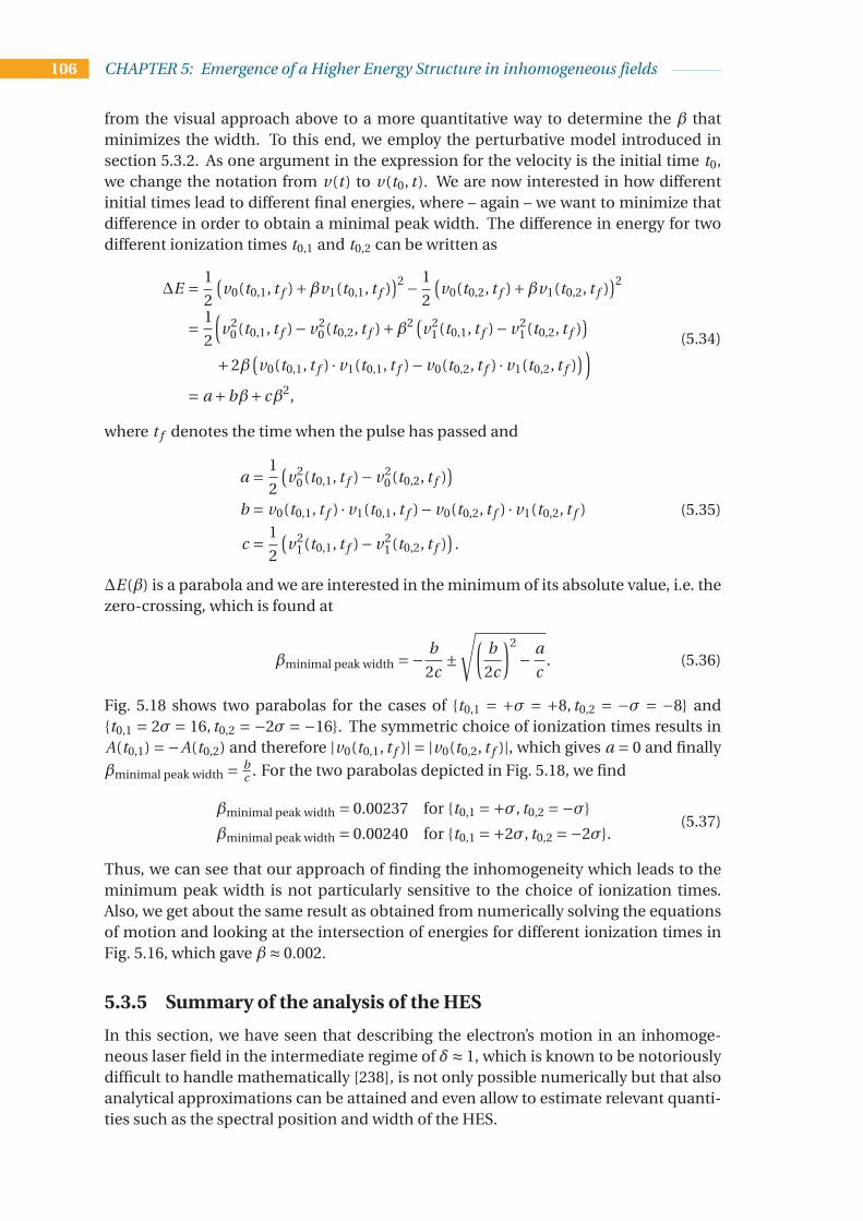
106 CHAPTER 5: Emergence of a Higher Energy Structure in inhomogeneous fields
from the visual approach above to a more quantitative way to determine the β thatminimizes the width. To this end, we employ the perturbative model introduced insection 5.3.2. As one argument in the expression for the velocity is the initial time t0,we change the notation from v(t ) to v(t0, t ). We are now interested in how differentinitial times lead to different final energies, where – again – we want to minimize thatdifference in order to obtain a minimal peak width. The difference in energy for twodifferent ionization times t0,1 and t0,2 can be written as
∆E = 1
2
(
v0(t0,1, t f )+βv1(t0,1, t f ))2 − 1
2
(
v0(t0,2, t f )+βv1(t0,2, t f ))2
= 1
2
(
v20(t0,1, t f )− v2
0(t0,2, t f )+β2 (
v21(t0,1, t f )− v2
1(t0,2, t f ))
+2β(
v0(t0,1, t f ) · v1(t0,1, t f )− v0(t0,2, t f ) · v1(t0,2, t f )))
= a +bβ+ cβ2,
(5.34)
where t f denotes the time when the pulse has passed and
a = 1
2
(
v20(t0,1, t f )− v2
0(t0,2, t f ))
b = v0(t0,1, t f ) · v1(t0,1, t f )− v0(t0,2, t f ) · v1(t0,2, t f )
c = 1
2
(
v21(t0,1, t f )− v2
1(t0,2, t f ))
.
(5.35)
∆E(β) is a parabola and we are interested in the minimum of its absolute value, i.e. thezero-crossing, which is found at
βminimal peak width =− b
2c±
√(
b
2c
)2
− a
c. (5.36)
Fig. 5.18 shows two parabolas for the cases of {t0,1 = +σ = +8, t0,2 = −σ = −8} and{t0,1 = 2σ = 16, t0,2 = −2σ = −16}. The symmetric choice of ionization times results inA(t0,1) =−A(t0,2) and therefore |v0(t0,1, t f )| = |v0(t0,2, t f )|, which gives a = 0 and finally
βminimal peak width = bc
. For the two parabolas depicted in Fig. 5.18, we find
βminimal peak width = 0.00237 for {t0,1 =+σ, t0,2 =−σ}
βminimal peak width = 0.00240 for {t0,1 =+2σ, t0,2 =−2σ}.(5.37)
Thus, we can see that our approach of finding the inhomogeneity which leads to theminimum peak width is not particularly sensitive to the choice of ionization times.Also, we get about the same result as obtained from numerically solving the equationsof motion and looking at the intersection of energies for different ionization times inFig. 5.16, which gave β≈ 0.002.
5.3.5 Summary of the analysis of the HES
In this section, we have seen that describing the electron’s motion in an inhomoge-neous laser field in the intermediate regime of δ≈ 1, which is known to be notoriouslydifficult to handle mathematically [238], is not only possible numerically but that alsoanalytical approximations can be attained and even allow to estimate relevant quanti-ties such as the spectral position and width of the HES.

5.4. Unifying effects in strong inhomogeneous fields 107
Observing numerically that the inhomogeneity of the laser field dominates overthe inhomogeneity of the Coulomb potential of the ionized atom, we could neglect theCoulomb potential in the equation of motion. Making use of the pulse envelope vary-ing more slowly than the primary oscillation of the laser field, the equations of motionscould be reduced to Mathieu differential equations that can be solved analytically. In-cluding the shape of the envelope perturbatively after solving the Mathieu differentialequation, a closed-form expression for the acceleration was found. This serves alsoas an analytical description of the inhomogeneous field that the electron experiences,which otherwise needs to be computed numerically.
Although the ansatz of Mathieu equations also led to an analytical description ofthe velocity of the electron, it was found that a perturbative approach yields betteragreement with the numerical solution. The fact that the perturbative ansatz up tofirst order is sufficient to describe the electron’s velocity in the inhomogeneous field,i.e. it has the form v0 +βv1, also helped us derive a simple scaling law stating that thefinal velocity of an electron born at the center of the pulse scales linearly with the inho-mogeneity and, equivalently, that the spectral position of the HES peak scales quadrat-ically with β.
Moreover, it was found that there is an inhomogeneity at which the width of theHES peak is minimal and a scheme to estimate this optimal inhomogeneity based onthe analytical descriptions of the velocity was presented.
Being able to estimate the dependence of both the spectral width and position ofthe HES on the inhomogeneity should help tune the parameters to realize the HESexperimentally and to control, for example, the spectrum of potentially resulting fem-tosecond electron beams.
5.4 Unifying effects in strong inhomogeneous fields in
the intermediate regime
Only briefly after the emergence of the HES was discovered, the appearance of anotherpeak was reported in the spectrum of electrons that move in the inhomogeneous fieldof a nanostructure [75]. The latter was named ‘low-energy peak’ (LEP) and, as the namesuggests, was found at rather low energies of about 1 eV, whereas the HES was locatedat about 40 to 80 eV. Additionally, the HES was produced in a system where electronsare ionized from a gas target that is placed in the inhomogeneous field of a nanotip,whereas the LEP is formed of electrons that are released directly from the surface of ananotip. Moreover, the HES was a theoretical prediction while the LEP was measuredexperimentally.
Given the diametrically opposed nature and naming of the HES and LEP, one maywonder why we should bother to compare them to each other at all. The objectionsinsinuated by such a question are further supported by the fact that the publicationwhich reported on the LEP [75] does not even mention the HES. However, both the LEPand HES emerged in the intermediate regime of δ& 1 and in both cases the electron’smotion in the inhomogeneous laser field was claimed to cause the accumulation ofelectrons in the respective peaks. From what we have learned about the HES above, weshould therefore expect that similar effects are at play.
Indeed, we will see that even though the two peaks were observed in different en-ergy regimes, we can identify one mechanism in which both observations are explained.

108 CHAPTER 5: Emergence of a Higher Energy Structure in inhomogeneous fields
We thus unify the theories behind LEP and HES, finding that LEP and HES are twomanifestations of the same energy upshift due to propagation in an inhomogeneousfield. It will then become clear that the sole difference between HES and LEP is that inthe setting in which the HES was observed the electrons initially move towards the na-nostructure whereas the electrons that form the LEP leave the nanostructure directlyafter liberation. Even though this difference leads to a slightly larger energy gain ofelectrons that initially approach the nanotip than of those directly leaving it, we findthat this effect is small and does not explain why the LEP was found at much lowerenergies, of about 1 eV, than the HES, which was found to peak at around 40 to 80 eV.Rather, we establish that the underlying dynamics are the same and that the main rea-son for the different final energies is the different parameters that were chosen in theobservation of the HES and LEP. This insight is of particular interest as it allows us topropose a modification of the setting in which the low energy peak (LEP) was experi-mentally observed such that it leads to a photoelectron distribution at energies as highand as spectrally confined as it was observed in the HES. This promises the still out-standing experimental realization of almost monoenergetic electron bunches as theywere described in the framework of the HES.
5.4.1 An intuitive model for the energy upshift observed in the HES
As a first step, we need to understand why electrons experience an energy upshift at allwhen moving in inhomogeneous fields. Even though the analysis of the HES in section5.3 already provided some insights into how one can describe the electron movementmathematically and we understood how the spectral position and width changes withthe inhomogeneity of the field, a simple and physically intuitive model for why theelectrons accumulate in a prominent peak was not given in the previous section, orany other publication for that matter.
For a better understanding of the upshift mechanism, we look at the dynamics of anelectron in a typical inhomogeneous field that leads to a HES, presented in Fig. 5.19. Itis important to note that we now use an exponential description of the inhomogeneousfield
E(x, t ) = E0 cos
(ωt
2N
)2
cos(ωt +φC EP )exp
(
− x
l f
)
(5.38)
and not the linear approximation of it (see eq. (5.7)) anymore. Thus, we do not needto worry about zero-crossings of the (1+ 2βx) term and can include longer pulses inour study as well. Moreover, in order to make things easier mathematically, we focuson the field-decay along the positive x-axis rather than having the field decay alongthe negative x-axis as was the case before (see e.g. Fig. 5.2). This entails that the finalvelocity vx is positive rather than negative now (compare e.g. Fig. 5.12 and 5.19) andthat a CEP of π (at which the HES was observed in the linearly approximated field)needs to be converted to a CEP of 0. The advantage of moving to the positive x-axis isthat we do not have to deal with evaluating the absolute value of x in the exponentialterm (see eq. (5.6)) and the concomitant mathematical problems.
Now, to understand the energy upshift due to the movement in the inhomoge-neous field, we first look at the acceleration curve of an exemplary trajectory plotted inFig. 5.19. After all, the area under this curve determines the final velocity. For an elec-tron born at the center of the pulse and propagated in a homogeneous field (case notshown in Fig. 5.19), the acceleration curve would oscillate symmetrically around zero

5.4. Unifying effects in strong inhomogeneous fields 109
(when neglecting envelope effects) leading to equally large positive and negative areasand thus to zero velocity at the end of the pulse [39, 305]. The spatial inhomogeneity,in contrast, introduces an asymmetry in the acceleration curve, which we can evaluatebetter by splitting the pulse in half-cycles (see the striped background in Fig. 5.19) andlooking closer at the acceleration amplitudes of varying height that lead to a non-zeroarea under the acceleration curve in the individual half-cycles.
At the beginning of the propagation, it is very clear that in each half-cycle (corre-sponding to one stripe) the amplitude is larger for the acceleration with a positive signthan for the one with a negative sign because for the positive sign the electron is closerto the nanotip. As a consequence, we gain ‘positive area’ under the acceleration curveand thus positive final velocity in each of these early half-cycles1. Later on, however,the electron has already gained so much energy that it does not change the sign of itsvelocity anymore and is only leaving the tip. Then, in the half-cycles highlighted inwhite, where the negative acceleration comes prior to the positive one, we have an en-ergy loss since here the negative acceleration is larger than the positive acceleration.In the blue half-cycles, though, where the positive acceleration part comes first, westill gain energy. Now, the key to understanding the overall energy upshift is that theloss during the white half-cycle is always smaller than the gain in the neighboring bluehalf-cycle and consequently there is an energy gain during one full optical cycle. Thiseffect is due to the fact that the velocity during the white half-cycle is moving aroundits minimum. Consequently, the distance gained during that half-cycle is smaller andthe difference in the amplitudes of a < 0 and a > 0 is much smaller than in the bluehalf-cycle where the velocity is around its maximum and the gain in distance and thusthe difference of the amplitudes at a > 0 and a < 0 is larger.
Consequently, we can understand the energy upshift as due to the asymmetry whichthe inhomogeneous field introduces in the acceleration curve such that we obtain anon-zero total area under it even for electrons ionized at the center of the pulse. Eventhough there are half-cycles in which we lose a little energy, the half-cycles in whichwe gain energy (blue stripes in the background) always dominate. And in the begin-ning, while the electron has gained so little energy that it still oscillates back and forthand approaches the tip in the white half-cycles we even have an energy gain in ev-ery half-cycle, which explains the particularly fast energy gain at the beginning of thepropagation.
5.4.2 Unified model for HES and LEP
An important point in the above mechanism is that it does not only explain the energyupshift in the setting that was employed in [73] for the HES, which was used in Fig. 5.19,but equally explains the energy upshift at the parameters that led to the LEP [75]. Thisshould become clear from Fig. 5.20, in which the parameters were chosen to coincidewith those used for the experimental realization of the LEP [75]. Even though theseparameters differ considerably from those in Fig. 5.19, which are in the regime wherethe HES was predicted theoretically, the overall shape of the curves does not greatlydiffer. The main reason for the strong resemblance of the curves in Fig. 5.19 (HES) andFig. 5.20 (LEP) is the fact that both are in the intermediate δ-regime.
1For an illustration of this concept, see the top panel of Fig. 5.24, where the green quarter-cycle areacontributes positively and the red quarter-cycle area negatively, yielding a total positive area for thathalf-cycle.

110 CHAPTER 5: Emergence of a Higher Energy Structure in inhomogeneous fields
Figure 5.19: Acceleration a, velocity v, position x as a function of time t , and the ex-
ponential decay factor exp(−x/l f ) for an electron released from an atom in an electric
field as described by eq. (5.38) at the center of a 12 cycles pulse with λ= 2 µm, C EP = 0,
l f = 750 a.u. and where the atom is exposed to a maximal intensity of I = 1·1014 W/cm2
(‘HES setting’). The numbered red dots are plotted at every half-cycle of the laser pulse
for visual guidance.
In terms of the mechanism outlined in section 5.4.1, which explained the gain ofkinetic energy in the inhomogeneous field by the asymmetry of the field and thus ac-celeration amplitudes, there is one major difference between Fig. 5.19 and Fig. 5.20,though. In the framework of the HES (Fig. 5.19), the electron is ionized from atomsplaced in the vicinity of a nanostructure and the electron initially moves towards thenanotip, thus initially exploring fields that are even higher than during the ionizationprocess. Consequently, these electrons gain more energy than in the LEP case, wherethe electrons are ionized directly from the nanostructure and initially move away fromthe tip. Even though electrons that initially leave the nanostructure gain less energythan electrons initially approaching the nanostructure, they are still upshifted consid-erably in energy due to the mechanism explained in section 5.4.1.
In a setting where the initial movement both towards and away from the tip is al-lowed, one may think of HES and LEP as two manifestations of the same energy up-shift that are found in neighboring half-cycles, where the higher energy upshift (HES)is found in the half-cycle in which the electron initially moves towards the tip andthe lower energy upshift (LEP) is found in the half-cycle in which the electron ini-tially leaves the tip. This is illustrated in Fig. 5.21, from which it should also becomeclear that one can switch between HES and LEP in one fixed half-cycle by changing thecarrier-envelope phase by π.
Even though the electrons ionized in the ‘LEP half-cycle’ (orange dots in Fig. 5.21)and the ‘HES half-cycle’ (blue dots) end up at different energies, it becomes clear fromFig. 5.21 that the energy difference due to the opposed initial directions of the electronis not several orders of magnitude but only a factor of about 3. This is important tonote since the fact that the LEP was experimentally observed at about 1 eV [75] and the
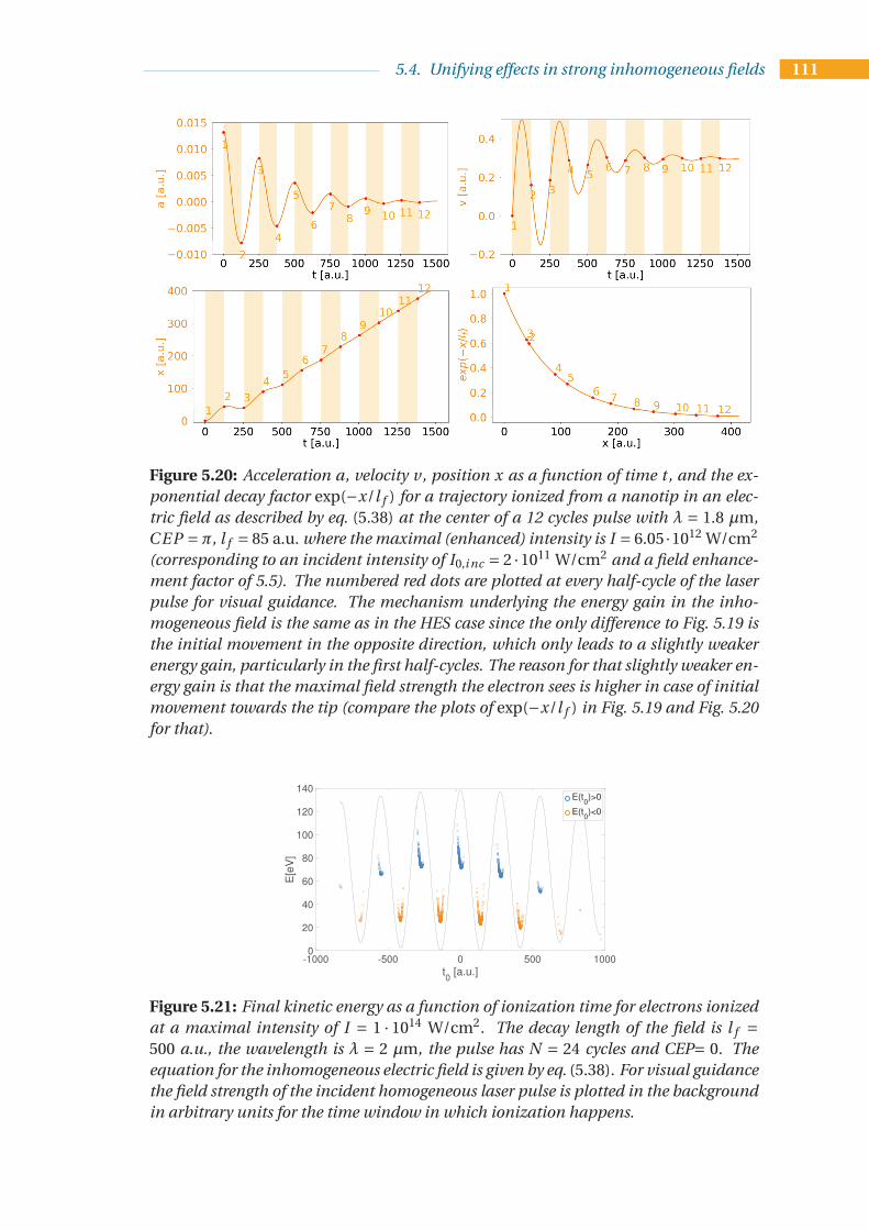
5.4. Unifying effects in strong inhomogeneous fields 111
Figure 5.20: Acceleration a, velocity v, position x as a function of time t , and the ex-
ponential decay factor exp(−x/l f ) for a trajectory ionized from a nanotip in an elec-
tric field as described by eq. (5.38) at the center of a 12 cycles pulse with λ = 1.8 µm,
C EP =π, l f = 85 a.u. where the maximal (enhanced) intensity is I = 6.05 ·1012 W/cm2
(corresponding to an incident intensity of I0,i nc = 2 ·1011 W/cm2 and a field enhance-
ment factor of 5.5). The numbered red dots are plotted at every half-cycle of the laser
pulse for visual guidance. The mechanism underlying the energy gain in the inho-
mogeneous field is the same as in the HES case since the only difference to Fig. 5.19 is
the initial movement in the opposite direction, which only leads to a slightly weaker
energy gain, particularly in the first half-cycles. The reason for that slightly weaker en-
ergy gain is that the maximal field strength the electron sees is higher in case of initial
movement towards the tip (compare the plots of exp(−x/l f ) in Fig. 5.19 and Fig. 5.20
for that).
-1000 -500 0 500 1000
t0 [a.u.]
0
20
40
60
80
100
120
140
E[e
V]
E(t0)>0
E(t0)<0
Figure 5.21: Final kinetic energy as a function of ionization time for electrons ionized
at a maximal intensity of I = 1 · 1014 W/cm2. The decay length of the field is l f =500 a.u., the wavelength is λ = 2 µm, the pulse has N = 24 cycles and CEP= 0. The
equation for the inhomogeneous electric field is given by eq. (5.38). For visual guidance
the field strength of the incident homogeneous laser pulse is plotted in the background
in arbitrary units for the time window in which ionization happens.

112 CHAPTER 5: Emergence of a Higher Energy Structure in inhomogeneous fields
HES was theoretically calculated at 40 eV up to 120 eV [73], might create the illusion ofa large energy gap between those two effects. Most of this large difference in energiesin [75] and [73], though, is due to the choice of disparate parameters: For the HES in[73], an enhanced intensity of I = 1 · 1014 W/cm2 and an inhomogeneity parametercorresponding to a decay length of about l f = 170−500 a.u. and a wavelength of λ =2 µm was used, whereas the experimental observation of the LEP was made at I =1 ·1012 W/cm2, l f = 85 a.u. and λ= 1.8 µm [75].
Thus, there are two effects that explain the energy difference of the HES reportedin [73] and the LEP in [75]: First, in [73], the electron initially moves towards the tipand sees a larger maximal electric field, which accounts only for about a factor of 2-3to energies of electrons that directly leave the tip, as it is the case in [75]. Second, thechoice of laser and nanotip parameters differs significantly, which accounts for mostof the discrepancy in energy. These parameters we can change, though. And as themechanism of energy gain is in principle the same, independent of the initial directionof the electron, we should be able to create confined photoelectron distributions alsoat high energies for electrons ionized directly from the nanotip, which initially leavethe nanotip, if we choose our parameters appropriately.
Fig. 5.22 shows that indeed such parameters exist. The top panel depicts CTMCsimulation results for ionization directly from the nanotip where we follow the modelapplied in [75] using the one-dimensional exponentially decaying field of eq. (5.6). Theionization probability is described by the Fowler-Nordheimer tunneling formula [218,220, 306], which gives the ionization current from the tip (with exponential accuracy)as
J (t ) ∝ exp
(
−2(2W )3/2
3E(t )
)
, (5.39)
where W denotes the work function of the nanotip. Comparing this function to theadiabatic ionization rate for the gas phase (see eq. (2.21)), we can see that it is iden-tical save for the ionization potential Ip which is replaced by the work function W .Following Ref. [307], we only allow electrons to be born during half-cycles of negativefield strength, as only then the field drives the electrons from the inside towards thesurface of the nanotip and allows ionization (assuming that only emission in positivex-direction is possible). Moreover, we model the electrons to be born at the surfaceof the tip with zero initial velocity and rescattering at the tip is implemented as elasticscattering with a reflection coefficient of 1 [75, 307].
In the top panel of Fig. 5.22, the lowest peak reproduces the LEP peak at about 1 eVthat was reported in [75]. However, at other intensities, wavelengths and decay lengthsthe peak is shifted to higher energies, while still being spectrally confined. In particular,we can even reach energies as high as they were so far only reported for the HES, whilenow being produced in a LEP setting, i.e. by ionization from a tip and not from the gasphase in the vicinity of the tip.
To get a better understanding of the spectra shown in the top panel of Fig. 5.22, itis instructive to analyze in which part of the laser pulse the electrons are born. Suchan analysis is presented in Fig. 5.23, where the electrons are color-coded accordingto having been rescattered at the nanostructure (green dots) and not having under-gone rescattering (purple dots). From this it becomes clear that the high energeticlong tails of the electron distributions in Fig. 5.22 are due to rescattering events andthat the prominent peak that arises in the spectral electron distribution is formed bydirect electrons, which is in agreement with the findings in [75] and in line with the

5.4. Unifying effects in strong inhomogeneous fields 113
Figure 5.22: Top panel: Final kinetic energy of photoelectrons ionized directly from a
nanostructure for various laser and nanostructure parameters specified in the legend,
where a 48 cycle pulse was used. The peak at small energies (blue) reproduces the ex-
perimental result reported in [75] and is found at about 1 eV. These simulations also
show how we can obtain considerably higher energies in the same setup when choos-
ing other parameters. The electrons that form the tail are from rescattering events,
which becomes clear from Fig. 5.23. Bottom panel: Velocity as a function of time for
a trajectory ionized at the center of the pulse at the surface of the nanostructure with
zero initial velocity for the same parameters as in the top panel. The dashed lines are
analytical approximations according to eq. (5.45).
mechanism outlined in section 5.4.1 where the energy gain is due to movement in theinhomogeneous fields and not rescattering.
Obviously, the question of experimental realizability arises at this point. There isreason to be optimistic that the parameters that led to the high-energetic peaks in thetop panel of Fig. 5.22 can indeed be used experimentally, mainly since similar param-eters have been used before. Not only the LEP around 1 eV has already been mea-sured [75] but also a sharp peak at about 10 eV has already been experimentally re-alized [141] where enhanced field strengths and decay lengths were applied that arein the regime used for the high-energetic peaks in the top panel of Fig. 5.22. In [141],though, a wavelength of λ= 800 nm is used and going to longer wavelengths at similarintensities promises to lead to higher absolute photoelectron energies that are in theregime of energies as they were predicted for the HES in [73] and as they are found inthe top panel of Fig. 5.22. Using a setting where the electrons are released directly fromthe nanostructure should be easier to implement experimentally than ionization fromatoms in the vicinity of the nanostructure. The latter was the setting in which the HESwas predicted theoretically (see section 5.2 and [73]) but has the disadvantage that the

114 CHAPTER 5: Emergence of a Higher Energy Structure in inhomogeneous fields
-6000 -4000 -2000 0 2000 4000 6000
t0 [a.u.]
0
200
400
600
800
1000
1200
E[e
V]
not rescatteredrescattered
(a) I = 1.5 ·1014 W/cm2, λ= 3 µm, l f = 1300 a.u.
-5000 0 5000
t0 [a.u.]
0
100
200
300
400
500
600
E[e
V]
not rescatteredrescattered
(b) I = 1 ·1014 W/cm2, λ= 2.7 µm, l f = 750 a.u.
-5000 0 5000
t0 [a.u.]
0
50
100
150
200
250
300
350
E[e
V]
not rescatteredrescattered
(c) I = 8 ·1013 W/cm2, λ= 2.25 µm, l f = 470 a.u.
-3000 -2000 -1000 0 1000 2000 3000
t0 [a.u.]
0
5
10
15
E[e
V]
not rescatteredrescattered
(d) I = 6.65 ·1012 W/cm2, λ= 1.8 µm, l f = 85 a.u.
Figure 5.23: Final kinetic energies of photoelectrons as a function of ionization times
for the parameters specified below each panel, corresponding to the results shown in
Fig. 5.22. Even though in all cases the same number of optical cycles (N = 48) was
chosen, the part of the pulse which contributes significantly to ionization differs de-
pending on the laser intensity.

5.4. Unifying effects in strong inhomogeneous fields 115
theoretically assumed precise location of the atoms in the inhomogeneous field is dif-ficult to realize experimentally and the spread of the atoms would probably result in abroadening of the HES. With ionization directly from the nanotip, in contrast, the ini-tial position of the electron after ionization can be controlled better and is locally moreconfined, consequently reducing blurring effects.
Thus, it seems expedient to use the setting in which the low energy peak was ob-served to produce electron distributions as they were theoretically predicted for thehigh energy structure, where the seeming contradiction due to the different names isresolved by the fact that both effects have the same underlying mechanism for the en-ergy upshift in the inhomogeneous field but have so far been investigated at stronglydifferent parameter sets.
5.4.3 A new analytical description of the energy upshift
Based on the cycle-averaged model that was described qualitatively above, we can nowalso derive a quantitative analytical description for the energy that an electron gainswhile moving in an inhomogeneous field. Following the same basic idea as the oneunderlying the explanation of Figures 5.19 and 5.20, we can calculate the change ofvelocity v during every half-cycle by calculating the change of the area under the ac-celeration curve in the corresponding half-cycle:
x = ∆v
∆t= |A1|− |A2|
T /2(5.40)
with A1 and A2 being the area under the acceleration curve in the first and secondhalf of the half-cycle under consideration, respectively (see top panel of Fig. 5.24 fora visualization). Denoting g (x) = exp(−x/l f ) and using
∫T /40 E0 cos(ωt )dt = E0/ω, we
can thus approximate:
x = |A1|− |A2|T /2
=1ω (|E0,1|− |E0,2|)
π/ω=
(|E0,1|− |E0,2|)π
= E0∆g
π= E0∆x
πl f. (5.41)
In the second equality in eq. (5.41), the assumption is that the amplitude of the accel-eration curve in the half-cycle of interest determines the area. This ‘local’ amplitude ofthe acceleration curve can easily be expressed by the amplitudes of the field strength,E0,1 and E0,2. In the last step in eq. (5.41), a local linear approximation to the expo-nentially decaying field was assumed (see central panel of Fig. 5.24), where ∆x is thelocal amplitude of the oscillation, which depends on the local value of the electric fieldE0,l oc
∆x = E0,l oc /ω2 = E0 exp(
−x/l f
)
/ω2 (5.42)
and also 1/l f , the absolute value of the slope of the local linear approximation, varieslocally:
1
l f→ 1
l fexp
(
−x/l f
)
, (5.43)
which corresponds to the derivative of g (x) with respect to x. Plugging eqs. (5.42) and(5.43) into eq. (5.41) we obtain
x =E0
(
E0 exp(−x/l f )/ω2)
πl f exp(x/l f )=
E 20 exp
(
−2x/l f
)
l f πω2. (5.44)
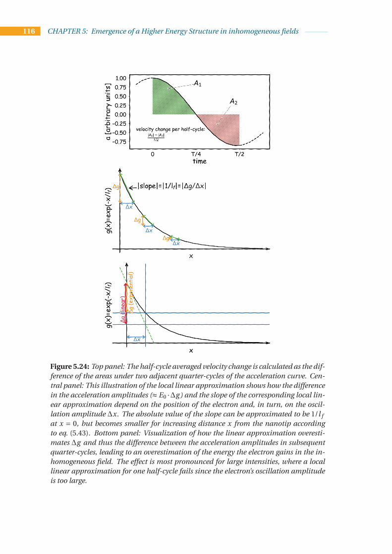
116 CHAPTER 5: Emergence of a Higher Energy Structure in inhomogeneous fields
Figure 5.24: Top panel: The half-cycle averaged velocity change is calculated as the dif-
ference of the areas under two adjacent quarter-cycles of the acceleration curve. Cen-
tral panel: This illustration of the local linear approximation shows how the difference
in the acceleration amplitudes (≈ E0 ·∆g ) and the slope of the corresponding local lin-
ear approximation depend on the position of the electron and, in turn, on the oscil-
lation amplitude ∆x. The absolute value of the slope can be approximated to be 1/l f
at x = 0, but becomes smaller for increasing distance x from the nanotip according
to eq. (5.43). Bottom panel: Visualization of how the linear approximation overesti-
mates ∆g and thus the difference between the acceleration amplitudes in subsequent
quarter-cycles, leading to an overestimation of the energy the electron gains in the in-
homogeneous field. The effect is most pronounced for large intensities, where a local
linear approximation for one half-cycle fails since the electron’s oscillation amplitude
is too large.

5.4. Unifying effects in strong inhomogeneous fields 117
This differential equation is analytically solvable:
xappr ox = l f log
(
cosh
(
E0t
l f
pπω
))
⇒ vappr ox =dxappr ox
dt= l f
1
cosh(
E0t
l fp
πω
) sinh
(
E0t
l f
pπω
)
E0
l f
pπω
=E0 tanh
(E0t
l fp
πω
)
pπω
⇒ Eki n,appr ox =v2
appr ox
2=
E 20 tanh2
(E0t
l fp
πω
)
2πω2.
(5.45)The validity of the approximation can be seen in the bottom panel of Fig. 5.22. Note,though, that the model is restricted to the applicability of the ‘linear local approxima-tion’, which implies that the electric field the electron experiences within one half-cyclecan be well approximated by a linear function. The breakdown of this assumption willbe further addressed in section 5.4.4.
Also, even though this cycle-averaged description is a powerful and simple estimateof how the electron’s velocity, and thus energy, changes while moving in the inhomo-geneous field, it does not resolve the subcycle dynamics and is thus also insensitive to,for example, variations in the ionization time. However, crucial properties of the peak,such as its width, depend strongly on how different ionization times lead to differentenergies, as we have seen in the analysis of the HES width in section 5.3.4. This moti-vates the derivation of an analytical approximation for the subcycle dynamics, whichwill be done in the following subsection. It seems important to emphasize already now,though, that the cycle-averaged nature of the above description also leads to the factthat eq. (5.45) does not capture the difference between the electrons that are ionized ata positive or negative sign of the electric field. This difference may be included in themodel by using the maximal field strength the electron sees during propagation ratherthan the field strength during ionization for E0.
5.4.3.1 An analytical description including subcycle effects
One way to include subcycle effects is found in combining the cycle-averaged descrip-tion derived in the preceding section with the perturbative model derived in section5.3.2. The perturbative model in its pure form worked well in section 5.3.2, where theshort pulse duration allowed to describe the inhomogeneous field by a linear model.Now, however, we use longer pulses and a more accurate approximation of the in-homogeneous field by applying the exponential description of eq. (5.38) is required.Technically, we could approximate this by the linear model again, of course, in order toapply the perturbative approach, which would then read
vper tur b(t ) = v0(t )− 1
l fv1(t ). (5.46)
Note that this is the same perturbative ansatz as in eq. (5.26), the only difference be-ing the notation of −1/l f corresponding to 2β in eq. (5.26). Therefore, this linear ap-proximation of the exponential case also has the same problem as the linear ansatz ineq. (5.26): We need to avoid the zero crossing of (1−x/l f ), which requires short pulses.
One way to make use of the perturbative approach that is based on the linearapproximation after all is to realize that eq. (5.46) can be improved upon by adapt-

118 CHAPTER 5: Emergence of a Higher Energy Structure in inhomogeneous fields
Figure 5.25: Velocity as a function of time for an electron. The maximal enhanced
intensity of the electric field is I = 1 · 1014 W/cm2 at the position where the electron
is released, the wavelength is λ = 2 µm, φC EP = π, and the decay length of the field
is l f = 750 a.u.. The number of optical cycles is N = 20 and the electron is born at
the center of the pulse at t0 = 0. The local perturbative solution according to eq. (5.47)(solid purple line) matches the numerical solution (solid dark blue line) well in the first
few cycles, but diverges considerably later on. One can see that neglecting the envelope,
i.e. using eqs. (5.50) to (5.52) (dashed pink line), gives a similarly good approximation.
Note that even though the approximation vsi mpl e according to eq. (5.49) (dash-dotted
turquoise line) gives a better overall agreement with the numerical solution, the local
perturbative model describes the subcycle dynamics more accurately in the first few
cycles. Moreover, for other parameters the local perturbative model can also be the
more accurate approximation for the final velocity than vsi mpl e as becomes clear from
Fig. 5.26.
ing the field strength in the zeroth order terms. This is done by replacing E0 byE0 exp(−xappr ox(t )/l f ) in the zeroth order terms x0 and v0, where xappr ox is the cycle-averaged approximation according to eq. (5.45). We are thus taking into account thatthe maximal field strength the electron sees during one particular half-cycle decayswith increasing distance from the nanostructure. As the zeroth order term x0 is alsoused in the calculation of the first order velocity, this modification introduces a factorof exp(−xappr ox(t )/l f ) also in the first order velocity v1, leading to
vper tur b,i mpr oved (t ) =(
v0(t )− 1
l fv1(t )
)
·e−xappr ox (t )/l f . (5.47)
In the following, this model is called the local perturbative model since it correspondsto the slope of the linear approximation being adapted locally. This can be seen fromcomparing the prefactor of v1 in eq. (5.46) and (5.47) realizing that
1
l f→ 1
l fe−xappr ox (t )/l f (5.48)
was applied, which corresponds to the local linear approximation presented ineq. (5.43) of the previous section (also see the central panel of Fig. 5.24 for a visualiza-

5.4. Unifying effects in strong inhomogeneous fields 119
Figure 5.26: Velocity as a function of time. The maximal enhanced intensity of the
electric field is I = 1 · 1014 W/cm2 at the position where the electron is released, the
wavelength is λ = 2 µm, φC EP = π, and the decay length of the field is l f = 1600 a.u..
The number of optical cycles is N = 8 and the electron is born at times t0 specified in
the legend. Here, the subcycle dynamics is resolved better with the local perturbative
approach (‘loc. pert.’, eq. (5.47)) than with the approximation according to eq. (5.49)(‘vsi mpl e ’). This is the case over a wide range of t0, which are chosen to be t0 =±σ= 8(see eq. (5.33)) and t0 = 0.
tion and eq. (5.41) for the derivation). In contrast to eq. (5.43), the position is directlyestimated by the cycle-averaged position xappr ox described in eq. (5.45) here. Withincreasing distance from the nanostructure, the slope of the local linear function getsprogressively shallower and we do not need to worry about the zero-crossing of thislocal linear function.
An exemplary velocity curve approximated by eq. (5.47) is shown as a solid pur-ple line in Fig. 5.25, where we can see that it matches the numerical solution (soliddark blue line) well in the first few cycles but deviates later on. At the point where theapproximation starts to deviate, however, the approximation is already close to the ve-locity the full numerical solution converges to. Therefore, one may still use the pertur-bative approach of eq. (5.47) to estimate the final velocity by evaluating it at the pointwhere it diverges e.g. from the cycle-averaged velocity vappr ox given in eq. (5.45).
In Fig. 5.25 we find another approximation, which in that case matches the numer-ical solution better at the end of the pulse. It is described by
vsi mpl e = v0(t )e−xappr ox (t )/l f + vappr ox . (5.49)
Here, the first term equals the first term of eq. (5.47) but the second term is replacedby vappr ox (eq. (5.45)), based on the assumption that vappr ox approximates the finalvelocity well. Note that even though the approximation vsi mpl e according to eq. (5.49)(dash-dotted turquoise line) gives a better overall agreement with the numerical solu-tion in Fig. 5.25, the local perturbative model describes the subcycle dynamics moreaccurately in the first few cycles. Moreover, for other parameters the local perturbativemodel can also be the more accurate approximation than vsi mpl e . Fig. 5.26 presents

120 CHAPTER 5: Emergence of a Higher Energy Structure in inhomogeneous fields
a case where the local perturbative model according to eq. (5.47) approximates thenumerical solution better than eq. (5.49) over a wide range of ionization times t0. Inparticular, this figure shows how the effect of the different ionization times on the fi-nal velocity can be approximated in the subcycle models, which is vital in studying thewidth of the resulting peak in the photoelectron spectrum, as we learned in section5.3.4.
The fact that with the exponentially decaying field we are now able to use longerpulses than in the linear approximation in sections 5.2 and 5.3 opens the door to ne-glecting envelope effects. This has the advantage that the lengthy, albeit analytical,expressions of the perturbative approach from section 5.3.2 can be reduced to a moreconvenient size. Neglecting the envelope we obtain the following expressions:
v0(t ) =−∫t
t0
E0 cos(ωt ′+φC EP )d t ′ = E0(sin(ωt0 +φC EP )− sin(ωt +φC EP ))
ω(5.50)
x0(t ) =∫t
t0
v0(t ′)d t ′
=−E0(cos(ωt0 +φC EP )−cos(ωt +φC EP ))
ω2+ E0 sin(ωt0 +φC EP )(t − t0)
ω
(5.51)
v1(t ) =−∫t
t0
E0 cos(ωt ′+φC EP )x0(t ′)d t ′
=E 2
0
4ω3
(
2ω(t0 − t )+4sin(ω(t − t0))
+2ω(t0 − t )(cos(ω(t0 − t ))−cos(2φC EP +ω(t0 + t )))
+ sin(2(φC EP +ωt0))− sin(2(φC EP +ωt )))
.
(5.52)
Comparing this version of v1 with the unwieldy expression in appendix A.5 shows thatneglecting the envelope significantly reduces the length of this term. The dashed pinkline in Fig. 5.25 shows how using eqs. (5.50) to (5.52) in the local perturbative approachgiven in eq. (5.47) is a reasonable approximation which starts deviating from the nu-merical solution at about the same point as the local perturbative solution with theenvelope included.
5.4.4 Explaining the experimentally observed linear intensity
scaling
In the framework of the cycle-averaged approximation introduced in section 5.4.3 wecan now also understand directly the linear scaling of the energy of the LEP with in-tensity reported in [75]. As can be seen from the approximate description in eq. (5.45),the final energy should scale as E 2
0 since tanh → 1 for large t . Note that this state-ment differs from the widely known effect that the cycle-averaged kinetic energy of anelectron in a homogeneous field scales with E 2
0 . In homogeneous fields this statementpertains to the quiver motion during propagation whereas the statement made herefor the inhomogeneous fields concerns the final energy at the end of the pulse for anelectron born at the center of the pulse. Such an electron has zero energy at the endof propagation in a homogeneous laser pulse, but undergoes an energy upshift in aninhomogeneous field due to the mechanism that is qualitatively described in section5.4.1 and mathematically captured in eq. (5.45).

5.4. Unifying effects in strong inhomogeneous fields 121
Figure 5.27: Final photoelectron energy as a function of the incident laser inten-
sity (note that the enhanced intensity is significantly larger). The experimental data
and the linear fit to it were extracted from [75]. The analytical result is described by
eq. (5.45) where a field enhancement factor of 5 was assumed, which lies in the regime
estimated in [75].
The theoretically predicted linear scaling of the final energy with intensity was in-deed observed in the experiment of the LEP in [75] for not too large intensities. Theexperimental results are depicted in Fig. 5.27 along with the linear fit done in [75] andthe estimation according to eq. (5.45), which matches the experimental result nicely.Moreover, we can understand intuitively why the experiment in [75] exhibits a break-down of the linear scaling for larger intensities: The local linear approximation overone half-cycle overestimates the amplitude of ∆g and thus overestimates the energygain (see bottom panel of Fig. 5.24). This effect becomes stronger with increasing os-cillation amplitudes ∆x, which we get for larger E0, and explains why our model over-estimates the spectral position of the peak for large intensities.
Furthermore, from the visualization in Fig. 5.24 it becomes clear that the break-down of the linear scaling with intensity also marks the regime where the electronexplores very different parts of the inhomogeneous fields during one half-cycle andwhere changes during one half-cycle are so strong that they cannot be approximatedlinearly and the cycle-averaged approach fails. This makes clear that the approximatedescription derived in section 5.4.3 is restricted to δ-parameters in the intermediateregime. Thus, we can also understand the seemingly odd feature of eq. (5.45) accordingto which the final energy depends only on E0 and ω but not on l f . The decay length l f
only determines how fast the final velocity is reached in this approximation. However,via the δ-parameter, E0 and ω implicitly contain (approximate) information about l f ,which explains why the approximation of eq. (5.45) works so well to describe the finalenergy, as we have seen e.g. in Fig. 5.22. In this figure, all combinations of the stronglydifferent intensities, wavelengths and decay lengths correspond to a δ-parameter ofabout 4.
5.4.5 Conclusion and Outlook
This last section 5.4 in the chapter on inhomogeneous fields was devoted to showingthat the seemingly different effects dubbed low-energy peak (LEP) and higher energy

122 CHAPTER 5: Emergence of a Higher Energy Structure in inhomogeneous fields
structure (HES) can be understood in one unified theory in which the different ob-served peaks emerge because of an upshift in energy due to the motion of the electronin the inhomogeneous field. In both the LEP and HES setting the asymmetric ampli-tude profile of the acceleration curve, introduced by the inhomogeneity of the field,leads to a systematic energy gain in the inhomogeneous field. Two reasons for the HEShaving appeared at high energies in [73] and the LEP having been measured at lowenergies in [75] were identified: First, the LEP was measured in a spectrum of photo-electrons that were released directly from the nanotip leading to an initial movementaway from the tip, towards smaller field strengths. In contrast, the HES was predictedin a setting where the electrons are ionized from an atom in the near-field of a nanotipwith the electron initially approaching the nanostructure. The higher maximum fieldthe electron therefore sees in the HES setting than in the LEP setting accounts for afactor of the order of two to three in the final energy. The more important reason forthe different energy scales at which the HES and LEP were reported previously, though,is the fact that vastly different intensities and decay lengths were chosen in the corre-sponding publications.
As for both the HES and LEP the combination of intensity, decay length, and wave-length was nonetheless in the same intermediate δ-regime, we have seen that the over-all dynamics is the same at the different energy scales and can be described by the sametheory. Closed-form expressions were derived to describe the cycle-averaged energygain in the inhomogeneous field, which also explain the linear scaling of the spectralposition of the peak with intensity that was reported for the experimentally observedLEP.
Unifying the electron dynamics for high and low energies on the one hand, and forthe different settings of electrons being released directly from the nanotip and fromthe gas phase on the other hand, paves the way of experimentally realizing the favor-able features that have been theoretically predicted for the HES [73, 74]. One problemwith realizing the HES in the way it was described in sections 5.2 and 5.3 is the fact thatthe ionization happened from the gas phase. While our theoretical model allowed usto neatly place the atom at a clearly defined position thus experiencing a well-definedfield strength and decay length, a real system would not allow such precise atom loca-tion. Rather, one would need to employ an atomic beam with a finite spread in space.The atoms in that beam would consequently be exposed to different field strengthsand slopes thereof, which would lead to blurring and thus broadening of the HES peak.Now, however, we have seen that we can use the LEP setting, i.e. ionization from the tip,to create spectrally narrow peaks at energies as formerly only reported for the HES (toppanel of Fig. 5.22). The advantage of using ionization from a tip is not only that it is awell-established experimental technique but, more importantly, that here the electronposition upon ionization and thus the field strength and decay length the electron ex-periences after its birth in the continuum are more clearly defined and controllable andcan be kept almost constant for a large ensemble of photoelectrons. Thus, we can beoptimistic about the experimental realization of creating almost monoenergetic elec-tron beams of tuneable energy in the higher-energetic regime using inhomogeneousfields.

CHAPTER
6Tracking the ionization site in a
neutral diatomic molecule
“A diatomic molecule is a molecule with one atom too many."
— Arthur Leonard Schawlow (Nobel Prize Laureate in 1981)
Overview of this chapter
Coulomb explosion has proven to be a powerful technique to investigate the effectof ionization enhancement and to track the ionization site in molecules. However,this technique does not allow to determine the ionization site in neutral homonu-clear molecules. Here, a new method is proposed for quantitatively retrieving theratio of ionization happening at the up- and downfield atomic site in a neutral di-atomic molecule from experimental data by means of comparison with numericalsimulations. The key mechanism is based on the deflection of the electron in theasymmetric Coulomb potential of a tilted diatomic molecule, which introduces anasymmetry in the final photoelectron momentum distribution. As the degree ofasymmetry depends on whether the electron is born at the up- or downfield atomand as the ionization site ratio can be controlled in trajectory-based simulations,this information can be used to quantify the ratio of ionization from the up- anddownfield site from experimental photoelectron momentum distributions.
6.1 Goals and challenges in describing molecular effects
After having studied the effect of field inhomogeneities as they are typically found inthe vicinity of a nanostructure in the previous chapter, this chapter deals with inho-mogeneities that arise in a more natural way: the inhomogeneities of the molecularpotential. Despite of, and maybe even because of, the inhomogeneities in molecularsystems not being as extreme as near nanostructures, we will find that describing theresulting effects is a challenging task and requires numerical treatment.
As we have seen, for instance in chapter 3, already superposing an atomic Coulombpotential and a homogeneous laser field is challenging to describe theoretically. Enter-ing the regimes of molecules, however, we have to handle far more degrees of freedomsthat play a role at different time scales: The rotational degree of freedom is relevant onthe picosecond timescale, vibrational freedoms are observed on a femtosecond scaleand the electronic movement happens on the attosecond scale [308]. Even in seem-ingly benign diatomic molecules the symmetry of molecular orbitals [309–314], the
124 CHAPTER 6: Tracking the ionization site in a neutral diatomic molecule
possibility to dissociate into atomic fragments [315–318], and variable internuclear dis-tances [319–321] already complicate matters considerably. This makes it all the moresurprising that molecular targets in strong field ionization have been studied from theearly days on [322–330] – beginning in the late 1980s. Even though we are still dis-cussing the description of the ionization process in the hydrogen atom (see chapter3 or Refs. [116, 117, 331, 332]), strong field ionization is already employed as a tool tounderstand molecular effects better [308, 333, 334]. For example, in Ref. [335] strongfield holography [336–338] is used to resolve the difference of the nuclear dynamics ofH2 and D2 with subangstrom spatial and subcycle temporal resolution. Other publica-tions helped understand how the phase of the electron depends on the atomic site theelectron is born at [130, 339].
The key to success in investigating molecular systems with strong field pulses is of-ten based on a concept one may describe as the ‘molecule taking a selfie’ [20], i.e. thevery electron that was ionized can, on its way to the detector, return (close) to the re-maining molecular ion. Thus, information about the molecule itself is encoded in theionized electron. Among these ‘self-interrogating’ techniques, methods referred to aslaser-induced electron diffraction (LIED) [16–19] and photoelectron holography [336–338] have been particularly successful in recovering information about the molecularstructure and dynamics [130, 131, 339–348]. Similarly, high-harmonic generation spec-tra from molecules contain information about the molecule the electron has accruedbefore recombination, i.e. during ionization and propagation [310, 311, 349–353].
Despite all of this success in dealing with molecules, even nature’s simplestmolecule, H+
2 , isn’t fully understood yet [308]. A great deal of the problems arising inthe context of molecules is due to the difficulties in modeling molecules theoretically.The additional degrees of freedom of a molecule are difficult to capture by numericalsolutions of the TDSE [354–356] and this method is therefore usually only used for ei-ther very small molecules like H+
2 or in proof-of-principle calculations with model or-bitals [357, 358]. Resorting to other popular techniques such as SFA and CTMC usingADK rates often yields surprisingly good results for a large variety of molecules [357,359–367] but does not make things less contentious. For example, the molecular ex-pansion of SFA (MO-SFA) including Stark corrections [98] predicts a maximized ion-ization rate for a CO molecule when the laser field points in the C-O direction whereasthe molecular expansion of ADK (MO-ADK) that includes Stark corrections [368, 369]predicts such a maximum for the laser field being directed in the O-C direction [370].An experiment devised to test these predictions indicated that double ionization of COis more likely to occur when the laser field is pointing from C to O [371] and that moregenerally the linear Stark effect plays a minor role in this system.
The importance of taking account of traits of the molecular orbital one is ionizingfrom, e.g. its symmetry [309–314], makes information from quantum chemistry cal-culations beneficial for many theoretical models. But, again, while including orbitalinformation is relatively straight forward in the atomic case and can, for example, bedescribed in a method called partial Fourier transform [372], it is less clear how to ex-pand this theory for the molecular case [131, 373–375]. Therefore, even though theorywas able to make experimentally validated predictions about molecular effects (seee.g. [319, 326, 376, 377] or [378–381]), it seems even more vital for molecular theoriesthan for atomic theories to be backed up by experimental results, which is the path wealso chose for the present chapter.

6.2. The problem of tracking the ionization site in a molecule 125
Figure 6.1: Illustration of a diatomic potential for alignment of the internuclear axis
along the polarization axis. The horizontal gray lines represent the linearly Stark-
shifted ionization potential (see e.g. eq. (1) and Fig. 2 in [384] or Fig. 1(c) and the equa-
tions on p. 043002-4 in [123]). The ionization barrier for the upper well is considerably
narrowed by the influence of the lower well, which can lead to ionization enhance-
ment, provided electron localization at the upfield atom is significant. However, the
force F of the electric field can drive the electron towards the downfield well, which is
expected to play a role if the electron position adapts adiabatically to the laser field
and which would result in the downfield atom to be the dominant ionization site.
6.2 The problem of tracking the ionization site in a
molecule
This chapter is devoted to answering the question at which atomic site in a moleculethe electron is born. More precisely, we are interested in the ratio at which the electronsare born from the upfield and downfield atom, where upfield and downfield refer to theatom where the potential is heightened or lowered due to the laser field, respectively.Knowledge about the site the electron is born at is not only vital in understanding thetunneling process in molecules itself but is relevant for theoretically modeling, andthus the analysis and interpretation, of molecular imaging techniques [382] such asmolecular orbital tomography [21, 383], photoelectron holography [336–338], or laser-induced electron diffraction (LIED) [16–19].
This problem of identifying the tunneling site in molecules is usually addressed inthe context of an effect called charge resonance enhanced ionization (CREI), some-times also referred to as ionization enhancement. Therefore some introductory wordson this effect seem warranted.
The experimentally observed effect of ionization being larger when the molecularaxis of a diatomic molecule is aligned along the polarization axis of the electric fieldwhen compared to the perpendicular orientation [322, 385] was explained by Codlinget al. in 1989 [326]. They proposed a mechanism in which the internuclear barrier issuppressed for certain internuclear distances. Thus, the barrier that an electron lo-cated in the upfield well has to tunnel through is narrower than the barrier in perpen-dicular orientation and ionization is enhanced (see Fig. 6.1). Even though this modelwas introduced decades ago, doubts about its validity haunted physicists for a longtime [318, 386] and only recently various major breakthroughs were obtained in thisdebate [123, 374, 382, 387–391]. The dominant tool in the study of CREI is the mecha-nism of Coulomb explosion since the enhancement depends strongly on the internu-

126 CHAPTER 6: Tracking the ionization site in a neutral diatomic molecule
Figure 6.2: Left panel: Equipotential lines of the Coulomb potential of a N2 molecule
tilted by 45◦ against the polarization axis under the influence of a constant electric
field (E0 = 0.061 a.u. ↔ I = 1.3 ·1014 W/cm2). Right panel: Cuts through the potential
surface of the left panel parallel to the polarization axis through the upfield atom (or-
ange line, also marked in the left panel) or downfield atom (green line), respectively.
The horizontal dashed lines in the right panel represent the linearly Stark-shifted ion-
ization potential (similar to the dashed gray lines in Fig. 6.1).
clear distance which can be easily determined from the kinetic energy release (KER)during Coulomb explosion by invoking Coulomb’s law telling us that the KER is in-versely proportional to the distance between the atoms at the time of defragmentation[392].
While more and more experiments have validated that there are indeed internu-clear distances at which ionization is enhanced, the underlying mechanism remainsunder debate [378, 379, 393]. One path to understanding the ionization mechanismin molecules better is the determination of the tunneling site and recent studies alongthis line have provided strong evidence for the suppressed upfield barrier at certaininternuclear distances leading to the enhancement [123, 374, 382, 387–391]. An im-portant step was achieved in Ref. [391], where the dominance of ionization from theupfield atom in an ionization enhancement setting was measured. This experimentrelied again on the mechanism of Coulomb explosion and could distinguish betweenthe ionization ratios from the up- and downfield atom by making use of the fact thatthe ionization of ArXe+ happened at the Ar atom. Thus, this method is not only re-stricted to doubly charged ionization products but also requires a diatomic moleculeof different atomic species.
Ionization enhancement is explained by the idea that the electron is born at theupfield atom, escaping through the lowered internuclear barrier, as can be seen fromthe sketch in Fig. 6.1 of a molecule whose internuclear axis is parallel to the polar-ization axis. However, as also becomes clear from this sketch, the field should drivethe electron cloud towards the downfield atom. This effect plays a role if the electronposition adapts to the laser field adiabatically, which is expected to happen if the in-ternuclear distance is small and the laser field changes relatively slowly. Therefore, forthe electron to escape over the suppressed internuclear barrier, the potential barrieris required to move sufficiently fast to allow trapping of the electron in the upper wellin the first place [319, 333, 377, 384, 394–396]. Since this effect only happens at inter-nuclear distances that lead to ionization enhancement, studying it does not provideinformation on what atomic site the electron is born at when the molecule is found atother internuclear distances.
Obviously, things are further complicated if the molecular axis is tilted with respect

6.3. A new method for tracking the ionization site in a molecule 127
to the laser polarization axis (see Fig. 6.2). Such a system will be discussed in the fol-lowing: A neutral N2 molecule that is tilted against the laser polarization axis by 45degrees is (single) ionized. This setup equals the one described in [339], the experi-mental data of which will be used for comparison later on. This system does not resultin defragmentation via Coulomb explosion, which is usually drawn on when investi-gating the atomic site at which the electron is born in a molecule. Even though a re-cently proposed method for the determination of the tunneling site [382] does not usethe concept of Coulomb explosion and could be applied to neutral molecules, it doesnot allow quantitative insights into the likelihood of electrons being ionized from thetwo different atomic sites. Below, we develop an approach to quantize ionization ratesfrom the up- and downfield site in the tilted diatomic molecule.
6.3 A new method for tracking the ionization site in a
molecule
6.3.1 Experimental results
The fact that electrons that are born at the two different atomic sites and should thusexplore different Coulombic potentials, which in addition are asymmetric with respectto the polarization axis of the laser, is expected to lead to an asymmetry of the photo-electron momentum distribution at the detector. However, looking at the experimen-tally detected photoelectron momentum distribution of a tilted N2 molecule in Fig. 6.3no asymmetry is visible, to the bare eye, in the holographic fringes. The effect onlybecomes perceptible when averaging over the vz-values for each vx in the followingway
vz,mean(vx(i )) =∑n
j=1 w(i , j )vz( j )∑n
j=1 w(i , j ), (6.1)
where w(i , j ) is the momentum distribution at the detector in the i th bin of vx and thej th bin of vz . This quantity, as directly extracted from the experimental data shownin Fig. 6.3, is plotted as a blue line in Fig. 6.4 and we can see that it exhibits an asym-metry, meaning it is not a horizontal line located at vz,mean = 0. Surprisingly, also thecases of 0◦, 90◦, and even the orientation-averaged curve show an asymmetry. Theo-retically, one would expect the photoelectron momentum distribution in these cases tobe symmetric resulting in a (almost) horizontal line at vz,mean = 0, which is observed inQTMC simulations of these systems. The fact that the asymmetry found in these threeexperimental systems where one would expect no asymmetry (0◦, 90◦, and orientation-averaged) is about the same in all of these cases points to a systematic tilt of the exper-imental setting, which needs to be corrected. This is done following the idea that wasalready successfully applied in Ref. [339], where these data sets were previously used,by subtracting the orientation-averaged case from the 45-degree case. The correctedcurve is shown in green in Fig. 6.4 and in the following will be referred to as the experi-mental curve. This curve can also be found as a bold green line in Fig. 6.6.
We can see that for vx < 0 the mean value vz,mean(vx) is mostly negative for thatcurve, whereas for vx > 0 this quantity is found primarily in the positive regime. Thiseffect will be further explained in section 6.3.3 on the basis of QTMC simulations, thedetails of which will be given first in section 6.3.2.

128 CHAPTER 6: Tracking the ionization site in a neutral diatomic molecule
Figure 6.3: Experimental 2D photoelectron momentum distribution for the 45◦ case.
The data was previously published in [339].
Figure 6.4: vz,mean as a function of vx calculated by applying eq. (6.1) to the experi-
mental data published in [339] and shown in Fig. 6.4 for the case of 45◦. One can see
that not only the 45◦ data (blue curve) exhibits an asymmetry in vz,mean but also the
orientations of 0◦, 90◦, and the orientation-averaged curve are asymmetric (i.e. they
are not a flat curve at vz,mean = 0). As the asymmetry is about the same in all of these
three cases for which one would expect no asymmetry (i.e. 0◦, 90◦ and averaged ori-
entation), this effect is interpreted as due to a systematic tilt in the experimental setup
that needs to be corrected for. This is done by subtracting the orientation-averaged
curve from the curve for 45◦ (green line).

6.3. A new method for tracking the ionization site in a molecule 129
6.3.2 Performing molecular QTMC simulations
To understand the asymmetry observed in the experimental data, Quantum Trajec-tory Monte Carlo (QTMC) simulations are performed [62], where the corrections pro-posed in [60] and the phase depending on the atomic positions with respect to thepolarization direction introduced in [130] are included. The peak intensity is set toI = 1.3 ·1014 W/cm2 and the wavelength is 800 nm, just as in the experiment [339, 397].
As we want to compare our results directly to experimental results now, assuming aconstant intensity, as we have done up till now, is not sufficient but we have to take intoaccount that there is a spatial variation of the intensity in the focal volume. This inten-sity profile is commonly described by a Lorentzian along the laser beam axis, which forthe sake of consistency with the nomenclature of cylindrical coordinates we will set toz for the following derivation, and by a Gaussian profile in ρ, the distance perpendicu-lar to the beam axis [398]. It reads
I (ρ, z) = I0
(w0
w(z)
)2
exp
(
− 2ρ2
w 2(z)
)
, (6.2)
where I0 denotes the maximal intensity in the focus and w(z) = w0
√
1+ (z/z0)2 is the z-dependent waist with the minimal waist w0 and with z0 =πw 2
0/λ denoting the Rayleighrange. The rate of electrons generated within the focal volume is given by [399]
dN
dt=
∫
d3r R(I (ρ, z)), (6.3)
where R(I ) = d4N /(d3r dt ) denotes the number of electrons generated per volume andtime at the constant intensity I . In order to transform the integral in eq. (6.3) into anintegral over intensity, we need the contour surface of constant intensity I , a visualiza-tion of which can be found in Fig. 1a in [400]. More specifically, we need the volumebetween two intensity surface shells with constant intensities I and I +d I [401]
VFV (I , I0) =πz0w 20
[
4
3
(I0 − I
I
)1/2
+ 2
9
(I0 − I
I
)3/2
− 4
3tan−1
(I0 − I
I
)1/2]
. (6.4)
Thus, we can transform eq. (6.3) into an integral over intensity [400, 402]
dN
dt=
∫
R(I (ρ, z))d3r =∫
R(I )dV (I , I0) =∫I0
0R(I )
∣∣∣∣
∂VFV
∂I(I , I0)
∣∣∣∣dI , (6.5)
where we can use eq. (6.4) to obtain
∣∣∣∣
∂VFV
∂I(I , I0)
∣∣∣∣=
πz0w 20
3
2I + I0
I 5/2
√
I0 − I . (6.6)
Consequently, the relative weight of each intensity is given by [130, 402]
2I + I0
I 5/2
√
I0 − I . (6.7)
This is implemented as follows: Prior to the sampling process described in chapter2.3.2, intensities are sampled according to eq. (6.7) using a reject-sampling algorithm.For each intensity a batch of trajectories (typically 500 trajectories) is sampled such

130 CHAPTER 6: Tracking the ionization site in a neutral diatomic molecule
Figure 6.5: 2D momentum distribution obtained in a QTMC simulation as described
in section 6.3.2 for the case of an ionization site ratio of q = 0.6 (as defined in eq. 6.8).
The color bar is given on a logarithmic scale.
that the initial times and momenta follow a probability distribution which treats thisspecific intensity as the maximal intensity.
Furthermore, in order to take into account that the shape of the molecular orbitalchanges the probability distribution of the initial transverse momentum, we modifythe probability distribution by a prefactor obtained in a partial Fourier transform [372]analogously to the way it is described in [131]. The molecular orbital that is needed forthis method was computed in the STO-6G Gaussian basis with the restricted Hartree-Fock (RHF) method using the quantum chemistry package GAMESS [403]. In the ba-sis set name, STO stands for ’Slater Type Orbitals’ and 6G signifies that each atomicSlater-type orbital is represented by six Gaussian basis functions. The accuracy ofthe RHF/STO-6G calculation is supported by the fact that the ionization potential,computed according to Koopmans’ theorem [404] as minus the energy of the highest-occupied molecular orbital, is 0.57 a.u. = 15.5 eV. This value is very close to the experi-mentally observed ionization potential of 15.6 eV [405].
The laser is polarized along the x-axis and is six cycles long under a cos2-envelope(see eq. (2.4)). The ionization potential is chosen to be Ip = 15.6 eV [339, 405]. Since weare in the intermediate nonadiabatic regime (γ= 0.9994), the nonadiabatic ionizationtheory of Li et al. [3] is used to describe the initial conditions at the tunnel exit (fordetails also see chapter 3). The Coulomb potential used during propagation is the sameas the one described in the supplementary of [339] and in [130], where the positivecharge that the molecule has after ionization is distributed equally between the twoatomic centers. However, we do not adapt the internuclear distance as it was done in[339] to obtain a more pronounced effect of the phase offset studied there but stick tothe physical distance of 2 a.u. [406, 407].
As can be seen from Fig. 6.2 and as already mentioned, one of the main challengesis that the tunneling barrier is not only modified by the laser field but also by theCoulomb potential from the other nucleus. From the bottom panel of Fig. 6.2 one cansee that the mutual distortion of the Coulomb wells is so weak at the tunnel exit thatit is a good approximation to employ the atomic theory of Ref. [3] with the unshiftedionization potential of Ip = 15.6 eV to calculate the initial spatial conditions. Subse-quently, as this theory assumes an atom placed at the origin, we merely shift this result

6.3. A new method for tracking the ionization site in a molecule 131
Figure 6.6: vz,mean as a function of vx . The green line represents the values extracted
from the experimental data. The ensemble of curves was obtained from QTMC simula-
tions over a range of ionization ratios q, which is specified by the color of the curve (see
colorbar). The theoretical curve that matches the experimental data best according to
the comparison of the asymmetry parameter a (see Fig. 6.9) is printed in bold with a
dotted black line on top of it. In both the theoretical and experimental evaluation the
photoelectron momentum distribution was restricted to vz ∈ [−1,1] and vx ∈ [−1,1].
by the central position of the respective atom the electron is born at. Thus, we calculatethe tunnel exits.
In contrast, the tunnel width that mainly determines the tunneling probability isstrongly affected by the internuclear Coulomb distortion and we cannot simply em-ploy an atomic ionization theory that does not properly account for this effect whencalculating the rates. Since solving this problem of the ratio of ionization from the up-and downfield well is the aim of this work, we scan through different ionization ratios.This will lead to different degrees of asymmetry, which can then be compared to theasymmetry obtained from the experiment. To this end, we define the ratio q of ioniza-tion from the two different sites as
q = #up−#down
#up+#down, (6.8)
where #up and #down are the number of electrons born upfield and downfield, re-spectively. The limits of q =−1 and q =+1 therefore correspond to the electrons beingborn exclusively downfield or upfield, respectively. Note that the two different atomschange being the up- and downfield atom several times during the pulse as the sign ofthe electric field changes.
A sample momentum distribution obtained in the described QTMC simulation canbe found in Fig. 6.5.
6.3.3 Explanation for the asymmetry via trajectory analysis
Fig. 6.6 shows vz,mean(vx) of QTMC results over a range of ionization ratios q specifiedin the colorbar. The evaluation of the final momentum distribution was done in thesame way as in the experiment, which also does integration over vy that is limited toan out-of-plane angle of θ < 10◦ before calculating vz,mean(vx) [339]. The vz,mean(vx)

132 CHAPTER 6: Tracking the ionization site in a neutral diatomic molecule
Figure 6.7: Top panel: Field strength and vector potential in the pulse. Quarter cycles
with decreasing absolute field strength are highlighted in green, whereas increasing
absolute field strengths are orange. Bottom left panels: Field > 0 and the final veloc-
ity is positive. The electrons fly around the parent molecular ion and accrue much
asymmetric Coulomb deflection. Bottom right panels: Field < 0 but the final velocity is
again positive because the same sign of the vector potential A is chosen. The electrons
fly directly to the detector and are less deflected by the asymmetric Coulomb potential.
Note that these trajectories were calculated with an oversized molecule for illustrative
purposes. For an accurate calculation with trajectories of the real system see Fig. 6.8
and Table 6.1.

6.3. A new method for tracking the ionization site in a molecule 133
curves in Fig. 6.6 exhibit a clear pattern: The more electrons are released from the up-field atom (redder on the colorbar), the more positive vz,mean is for vx < 0 and themore negative for vx > 0. If the majority of electrons are born at the downfield atom,qualitatively the same effect is observed with the signs of vz,mean reversed.
How can we understand this effect? Analyzing the QTMC trajectories, the deflec-tion of the trajectories in the asymmetric Coulomb potential is identified as the originof the asymmetry in vz,mean(vx). Fig. 6.7 displays an illustration of the mechanismthat is explained in the following. Note that these trajectories were calculated with anoversized molecule for illustrative purposes and a quantitative description with trajec-tories that are propagated in the system with the correct parameters is deferred to thesubsequent paragraph.
Without loss of generality, we focus on those electrons that end up at vx > 0. Theywere born at a time when the vector potential, A, was negative (which is true underthe assumption that the trajectories under consideration do not interact strongly withthe Coulomb potential). As the depiction of the pulse in the top panel of Fig. 6.7 shows,this can happen at a positive field strength that is decreasing (green stripes) or at a neg-ative field strength whose absolute value is increasing (orange stripes). The four lowerpanels each show two trajectories with a transverse velocity of opposite sign but sameabsolute value. In all cases, the absolute value of the transverse velocity is reducedduring propagation due to general Coulomb focusing. However, we are interested onlyin the asymmetric deflection due to the asymmetric Coulomb potential which is ob-tained as the sum of the change in vz during propagation of both of those trajectorieswith opposite signs, denoted ∆vz .
In the left half of the lower panels (green, corresponding to a positive field strengththat is decreasing) the asymmetric deflection ∆vz of electrons born at the upfield atomis negative due to the pull from the downfield atom. Vice versa, if the electron is bornat the downfield atom, the overall deflection is positive. Alternatively, one can under-stand the sign of the overall deflection ∆vz by checking whether the electron is bornbelow or above the center of charge along the z-axis, which leads to ∆vz > 0 or ∆vz < 0,respectively. For vx > 0, a deflection of ∆vz > 0 for electrons born at the downfieldatom and of ∆vz < 0 for electrons born at the upfield atom is also in line with the signsof vz,mean(vx) observed in Fig. 6.6.
But what about the trajectories born when the field strength is inverted? Then, theatom that was formerly the downfield atom is the upfield one, and vice versa. Conse-quently, also the signs of the overall deflections ∆vz are inverted: positive for a birthat the upfield atom and negative for a start at the downfield atom (see right (orange)bottom panels of Fig. 6.7). However, since in the case of the absolute value of the fieldstrength increasing (orange) the electrons directly leave the parent ion, the asymmet-ric deflection is weaker than in the case when the electron goes around the parent ion(green). Therefore, even though the overall deflections ∆vz have opposite signs in ad-jacent quarter-cycles with the same sign of A, they do not compensate each other asthe deflection in the ‘green’ quarter-cycles dominates since in these cases the electrongoes around the parent ion and is affected by the asymmetric Coulomb potential morestrongly than in the ‘orange’ quarter-cycles. An analogous line of reasoning can be ap-plied to vx < 0, where the signs of the deflections need to be swapped. This explainsqualitatively the asymmetric shifts observed in Fig. 6.6.
To also get a more quantitative impression of the asymmetry of the electron’s de-flection, let us take a look at the trajectories depicted in Fig. 6.8. Here, the laser and

134 CHAPTER 6: Tracking the ionization site in a neutral diatomic molecule
t0 vz,0upfield (u) /downfield (d)
final vz d vz∆vz (d vz summed upseparately for u and d)
4 0.3 u 0.090 -0.210d 0.152 -0.148 u: -0.210 + 0.176 = -0.034
-0.3 u -0.124 0.176 d: -0.148 + 0.163 = +0.015d -0.137 0.163
t0 vz,0upfield (u) /downfield (d)
final vz d vz∆vz (d vz summed upseparately for u and d)
-4 0.3 u 0.205 -0.095d 0.244 -0.056 u: -0.095 + 0.072 = -0.023
-0.3 u -0.228 0.072 d: -0.056 + 0.062 = +0.006d -0.238 0.062
Table 6.1: Changes of ∆vz for the trajectories depicted in Fig. 6.8. For t0 = 4 the elec-
trons go around the molecular ion and end up at vx > 0. For t0 = −4 the electrons
fly directly to the detector and end up at vx < 0. The corresponding trajectories are
displayed in Fig. 6.8.
atomic parameters applied in the simulations shown in Fig. 6.6 are used. The scenar-ios depicted in Fig. 6.8 differ from each other in the following parameters. Electronsare either released ...
• ... from the up- or downfield atom.
• ... at a transverse velocity vz,0 =−0.3 or vz,0 = 0.3.
• ... at t0 =−4 (before the peak of the pulse, increasing positive field strength) or att0 = 4 (after the peak, decreasing positive field strength).
The resulting 23 = 8 combinations are depicted as trajectories of different colors inFig. 6.8. One can directly see from the insets vz(t ) that for the trajectory that goesaround the parent ion (upper panel) the Coulomb deflection is much larger than whenthe electron directly leaves the ion (lower panel). The quantitative change of vz for asingle trajectory from the birth in the continuum till after the pulse has passed, de-noted d vz , is listed in Table 6.1. From these values the following can be seen: Theasymmetry in the deflection, expressed as ∆vz in the last column, is larger (in absolutevalues) when the electron has to go around the molecular ion (t0 = 4) than when it di-rectly leaves it (t0 = −4). This is the case for birth at both the up- and downfield atomand thus corroborates the qualitative arguments for the asymmetric deflection givenabove.
6.3.4 Comparison of theoretical and experimental results to identify
the ionization site
In order to describe the asymmetry observed in the experiment and in the QTMC sim-ulations quantitatively, we define the asymmetry parameter a as follows
a =∑m
i=1 sign(vx(i )) · vz,mean(vx(i ))
m. (6.9)

6.3. A new method for tracking the ionization site in a molecule 135
d
u
d
u
Figure 6.8: Trajectories for different scenarios showing that the asymmetric deflection
is larger when the electron goes around the parent ion (top panel) than when it directly
leaves the molecule (bottom panel). The quantitative description of the deflection is
given in Tab. 6.1 and commented on in section 6.3.3. All depicted quantities are given
in atomic units.
The multiplication with the sign of vx enables us to distinguish between the corre-sponding vz,mean curves rising or falling for increasing vx and leads to a unique map-ping between q and a. This quantity is calculated, on the one hand, for the range ofionization ratios in the QTMC simulation and, on the other hand, for the single experi-mental data set. The results are depicted in Fig. 6.9. Comparing the experimental valueof a = 0.0031 with the theoretical curve now allows us to estimate the ionization ratioq of the up- and downfield atom in the experiment. The value obtained is q =−0.377,which means that for every 100 electrons born downfield 45 electrons are born upfield.Thus, this result indicates that ionization from the downfield well is favored. Accordingto the introductory discussion in section 6.2 (also see Fig. 6.1), this hints at an adiabaticadaption of the electron location as the electric field changes sign.

136 CHAPTER 6: Tracking the ionization site in a neutral diatomic molecule
Figure 6.9: Asymmetry parameter a according to eq. (6.9) as a function of the ioniza-
tion site ratio q according to eq. (6.8). The colors of the theoretically obtained dots are
chosen according to the color-coding for q in the colorbar of Fig. 6.6. The experimental
value is plotted as a larger green dot.
6.4 Conclusion and Outlook
To conclude, it was found that the experimental photoelectron momentum distribu-tion of electrons ionized from a neutral diatomic nitrogen molecule that is tilted by45◦ against the laser polarization direction exhibits an asymmetry. QTMC simulationsreproduced this asymmetry and revealed that the extent and sign of the asymmetry de-pend strongly on the fraction of atoms born at the up- and downfield atom. Trajectoryanalysis made clear that the asymmetry of the momentum distribution is due to theasymmetric Coulomb potential that the electron explores on its way to the detector.
Sweeping over the ionization ratio in QTMC simulations, we obtained a uniquemap of the ionization site ratio onto the asymmetry parameter. Locating the experi-mental asymmetry parameter on this theoretical map allows to estimate the ratio atwhich the electrons were released from the up- and downfield well from the experi-mental data. The result indicates that ionization from the downfield well is favored inthe studied system. Asymmetries like the one described here can be expected to beobserved in any system that exhibits a notable asymmetry in the molecular potentialwith respect to the axis of polarization direction and thus to have a wide range of ap-plications. The method presented here stands out in that it tracks the ionization sitefor single ionization of neutral molecules, where the technique of analyzing Coulombexplosion, that has so far been used to track ionization sites in diatomic molecules, isnot applicable.
As the asymmetry in the momentum distribution is due to the asymmetry in theCoulomb potential, this work also stands in line with those recent publications thathighlight the importance of including the Coulomb effect as accurately as possiblewhen theoretically describing holographic effects [65, 135, 408–412]. In particular, thisstudy is a case in point for the strength of QTMC simulations over using SFA theories.As highest accuracy is required in terms of the Coulomb potential here, it is not suf-ficient to include the Coulomb potential perturbatively as it is, for example, done inCoulomb-corrected SFA theories [69, 70].

6.4. Conclusion and Outlook 137
Improvement of the theory presented in this chapter could be achieved by higheraccuracy in the theoretical description of the diatomic model. For example, it is notclear whether it is a good approximation to distribute the ionic charge evenly to thetwo atomic centers after ionization. Even though the model of even charge distribu-tion has been successfully applied in the theoretical interpretation of the very experi-mental data that are again used here, in the TDSE simulations presented in (the sup-plementary of) [339] and the QTMC simulations in [130], a deeper study along theselines seems warranted, in particular if the theory is applied to other molecular systems.
Speaking of other systems, it seems important to emphasize that the theory pre-sented in this chapter can be applied to other molecules and laser parameters as well.A larger bond length of the molecule would be expected to lead to a more pronouncedasymmetry in the photoelectron momentum distribution, as long as the underlyingassumptions of our model are satisfied. However, one should keep in mind that alarger bond length might change the whole underlying process, for example, of howthe remaining positive charge is distributed to the ionic cores. Varying the bond lengthwould be interesting in particular in that one might observe the transition from theelectron being primarily born at the downfield atom to the electron being localized atthe upfield well. Whereas dominant ionization from the downfield atom is expected insmall molecules in which adiabatic adaption of the electron position plays a dominantrole, as it was found to be the case for the N2 molecule presented in this chapter, theelectron can be localized at the upfield well in larger molecules due to nonadiabaticeffects that are crucial in the phenomenon of ionization enhancement (CREI).

CHAPTER
7Conclusions and Outlook
“The whole strenuous intellectual work of an industrious research worker
would appear, after all, in vain and hopeless, if he were not occasionally
through some striking facts to find that he had, at the end of all his criss-
cross journeys, at last accomplished at least one step which was conclusively
nearer the truth."
— Max Planck in his Nobel Lecture in 1920
At the end of this thesis we can look back on a ‘journey’ through a variety of ways toapply trajectory-based models in strong field ionization. Let us take the time to reca-pitulate what we have learned on our ‘exploration’ – especially for future ventures intothese realms.
We have ‘departed’ from the question that haunts every trajectory Monte Carlomethod: What probability distribution should the initial conditions of the trajectoriesfollow? Focusing on nonadiabatic effects, we have revisited two popular theories thatdescribe how nonadiabaticity manifests itself at the tunnel exit in a seemingly contra-dictory way. While one popular nonadiabatic theory claims a strong broadening of theionization time spread and assumes zero longitudinal momentum at the tunnel exit[7] (YI), another prominent nonadiabatic theory [3] (Li) shows that the initial longitu-dinal momentum is by far not negligible and arrives at a significantly less broad timespread. The confusion about these discrepancies was resolved in chapter 3 by show-ing that the nonadiabatic broadening of the time spread derived in YI [7] is a directconsequence of setting the initial longitudinal momentum to zero. More generally, wesaw that the strong coupling of the ionization time spread and the initial longitudinalmomentum leads to the theories of Li and YI, in spite of their fundamentally differentinitial conditions, to end up at approximately the same longitudinal momentum dis-tribution at the detector in an approximation that is valid for common experimentalset-ups using 800 nm light. Thus, we can now understand why the two nonadiabatictheories with their contrasting initial conditions were both successfully used to explainexperiments in the nonadiabatic regime. This should account to some extent for theconfusing character the discussions about nonadiabatic effects sometimes assumed.
Despite the indistinguishability of the results obtained from the two theories ina wide range of typical nonadiabatic parameters, laser and atomic parameters werefound that are still in the experimentally realizable and relevant regime for which thementioned approximations break down and the two nonadiabatic theories yield clearly

140 CHAPTER 7: Conclusions and Outlook
distinguishable momentum distributions. Comparing TDSE simulations to the CTMCresults obtained with the initial conditions of Li and YI gave much better agreementwith the theory of Li [3]. The open question is whether experimental data can back thisresult. At this point, one ’take home’ message is that any assumption about the initiallongitudinal momentum directly and significantly affects the ionization time spreadand that it is, therefore, important to physically motivate the choice of the initial lon-gitudinal momentum.
Our journey then continued in the field of Rydberg state creation by frustrated tun-nel ionization. Here, we picked up on the study of the intensity dependence of the Ryd-berg yield described in [49] and found that including (i) the intensity-dependent distri-bution of ionization times and (ii) nonadiabatic effects leads to a better understandingof experimental results. The latter point suggests that Rydberg states can be used totest nonadiabatic effects in a way that contrasts the commonly used methods for non-adiabaticity tests in that it does not use the momentum distribution at the detector. Asthe nonadiabatic effects can be observed in the slope of the power-law scaling of theintensity dependence of the Rydberg yield alone, this eliminates the concerns aboutthe calibration of the absolute intensity that have haunted prior experiments attempt-ing to observe nonadiabatic effects by measuring electron momenta distributions [57,154].
Moreover, we have seen how an increase of the pulse duration shifts the princi-pal quantum number distribution of Rydberg states to larger values and reduces theoverall Rydberg yield. These effects could be understood by the observation that theelectrons that potentially end up in a Rydberg state are slowly driven back to the par-ent ion by the attractive Coulomb potential. When the pulse duration exceeds a criticalvalue, the electron gets so close to the ion that it gains too much kinetic energy in theinteraction with the ionic potential to be a Rydberg state. As this critical pulse dura-tion is smaller for more deeply bound Rydberg states (corresponding to small n), lowprincipal quantum numbers are less likely to ‘survive’ longer pulses. This is relevantto studies and applications that rely on the principal quantum number distributionof Rydberg atoms like the recently developed method of creating coherent extreme-ultraviolet radiation from Rydberg atoms, in which the occupation of low principalquantum numbers is crucial [189]. Also, this study is a case in point for showing theimportance of including the Coulomb potential during the propagation process [72].In particular, the mechanism presented here, which relies on the Coulomb potential,stands in contrast to prior explanations of the Rydberg yield dropping with increasingpulse duration which neglected the Coulomb potential during propagation.
The next stop on our journey were laser fields with a time-varying spatial depen-dence as it is typically found in the vicinity of nanostructures. We have seen the emer-gence of a prominent higher energy structure (HES) in the spectrum of photoelectronsthat were ionized from the gas phase in such an inhomogeneous laser field. The laserand tip parameters were chosen to be in the ‘intermediate regime’ where the electron’squiver amplitude is of the same order as the decay length of the nearfield and theelectron dynamics is therefore difficult to describe theoretically. Trajectory-analysisrevealed that the electrons comprising the HES are born within a narrow time win-dow and may therefore be used to create localized sources of monoenergetic electronbeams of sub-femtosecond duration. Having such applications in mind, analytical ex-

141
pressions to describe the electrons’ motion in the inhomogeneous field were derived.From this we have learned how the spectral position and width of the HES depend onthe inhomogeneity parameter of the nearfield and can thus be optimized.
Moreover, we have seen that the recently reported experimental finding of a lowenergy peak (LEP) [75] can be understood in the same theoretical framework as thetheoretically predicted emergence of the HES. Even though the two peaks were ob-served in different energy regimes, and despite the LEP being detected for electronsthat were released from a nanotip whereas the HES was found for electrons ionizedfrom a gas that is placed in the vicinity of a nanotip, a single mechanism that causesthe peak formation was identified. Based on this mechanism, a more general analyticalmodel was derived to describe the energy upshift that electrons experience in inhomo-geneous electric fields. This theoretical description also explained the experimentallyobserved linear scaling of the peak energy of the LEP with the intensity of the incidentlaser pulse.
In particular, parameters were found at which electrons ionized directly from a na-nostructure, the setting in which the LEP was found, form a prominent and narrowpeak at higher energies as it was described in the framework of the HES. As ionizationfrom the tip is experimentally better established than ionization from the gas phasenear a nanostructure, this should pave the way for the experimental realization ofalmost monoenergetic electron beams of sub-femtosecond duration as they are pre-dicted for the HES in the gas phase.
The last part of our journey led us into the realms of molecules. A new method wasproposed for quantitatively retrieving the ratio of ionization happening at the up- anddownfield atomic site. So far, such studies were restricted to ionization from chargedmolecules with Coulomb explosion ensuing the ionization process. Here, in contrast,a method was developed for the ionization of neutral molecules that makes use of thedeflection of the electron in the asymmetric Coulomb potential of the tilted molecule,which introduces an asymmetry in the photoelectron momentum distribution at thedetector. As the degree of asymmetry depends on whether the electron is born at theup- or downfield atom and as the ionization site ratio can be controlled in QTMC sim-ulations, this asymmetry information can be used to quantify the relative ionizationprobabilities from the up- and downfield site from experimental photoelectron mo-mentum distributions.
The site from which the electron is ionized also gives insights into the time scale onwhich the electronic distribution within the molecule adapts to the changing electricfield. Therefore, one particularly interesting direction for future work is the variationof the bond length. Varying the bond length one might observe the transition from theelectron being primarily born at the downfield atom to the electron being localized atthe upfield well. Whereas dominant ionization from the downfield atom is expected insmall molecules in which adiabatic adaption of the electron position plays a dominantrole, as it was the case for the N2 molecule in this work, the electron can be local-ized at the upfield well in larger molecules due to nonadiabatic effects that are crucialin the phenomenon of ionization enhancement (CREI). In particular when changingthe bond length, but not only then, the way the ionic charge is distributed among theatomic sites in the theoretical model needs to be reconsidered.
142 CHAPTER 7: Conclusions and Outlook
The molecular system also served as a case in point to show that including theCoulomb potential as accurately as possible is of utmost importance. Therefore, mod-eling this system using CTMC/QTMC simulations should be favored over SFA ap-proaches in which Coulomb effects can, at best, be included perturbatively [69, 70].Similarly, the relevance of fully including the Coulomb potential during propagationwas relevant in the study of the pulse duration effects on Rydberg states presented insection 4.3. Speaking of the advantages of CTMC/QTMC over SFA simulations, we havecome full circle to the motivation given in the introduction in chapter 1, where on page11 the prerequisites for the application of SFA were listed. In addition to the spatialinhomogeneity of the atomic or molecular Coulomb potential, we have also seen thethird point in said list being violated: In chapter 5, the strong inhomogeneity of theelectric field in the vicinity of a nanostructure also revealed the power of a trajectory-based method such as CTMC in which the field inhomogeneity can be fully includedin the equation of motion.
Considering the SFA prerequisites further, also the first point in the list on page11, stating that the laser field should be strong enough for multiphoton or tunnel ion-ization to be the dominant ionization process, seems worth some consideration. Af-ter all, the flourishing field of streaking [413–421] often uses pump pulses that are ofhigh frequency and low intensity resulting in single-photon ionization being the dom-inant liberation mechanism. The weakness of the high-frequency pump pulse ensuresa negligible effect on the post-ionization dynamics, which is dominated by a secondlaser pulse, the probe pulse, that is stronger and of lower frequency. Scanning the de-lay between the two pulses has proven to be a powerful tool in the study of ionizationdelays. Modeling single-photon ionization semiclassically, in particular in combina-tion with the stronger probe pulse, is far less common and mature than strong fieldionization in attosecond science [422]. Nonetheless, semiclassical models provide sev-eral advantages over the numerical solution of the TDSE also here. Among those, themost notable is probably the insight which trajectory analysis allows into the streak-ing process, into the origin of and different contributions to the measured streakingdelay [414, 423]. Moreover, the lower computational cost of semiclassical models rel-ative to numerical solutions of the TDSE is becoming increasingly important as thefield of attosecond spectroscopy, which until recently was dominated by experimentsperformed on rare gas atoms and metal surfaces [66, 424], is moving increasingly to-wards molecules [422]. In the following, a semiclassical method to simulate attosecondstreaking experiments which is particularly suited to include information about themolecular potential is briefly summarized. In the framework of my PhD studies I wasinvolved in work with and on this ‘Classical Wigner Propagation’ (CWP) method whichis the brainchild of Dr. Tomáš Zimmermann and details about which can be found inRef. [422].
The CWP method treats the ionization step quantum mechanically followed byclassical propagation in the infrared probe field. The two key advantages of this methodover other semiclassical approaches such as CTMC or QTMC are found in (i) the fullyquantum mechanical treatment of the ionization step, where the weakness of the pumpfield allows to use perturbation theory and (ii) the description of the wavepacket by aWigner quasi-probability distribution [422]. The latter serves as a distribution to sam-ple initial conditions for trajectories and is not only a proper phase-space density dis-tribution with well-defined classical limit of the dynamics but – even when propagatedclassically – it also incorporates (some) quantum effects through interference of pos-

143
itive and negative weights. Moreover, this method allows to include the electrostaticpotential of the atomic or molecular ion, computed from the one-electron density ma-trix obtained in quantum chemistry calculations for the respective system.
As the electrostatic potential plays a crucial role in streaking delays [414, 425–429], afuture model to simulate streaking experiments may combine the electrostatic atomicor molecular potential obtained from quantum chemistry calculations during propa-gation with a CTMC model for describing the initial conditions. Using CTMC insteadof CWP for sampling the initial conditions would not only be easier to implement butwould have the added benefit of a straight-forward trajectory analysis, which is moreinvolved in the CWP due to the negative weights trajectories can have. Then, how-ever, we need to think about appropriate initial conditions for the CTMC simulations.Even though models to describe such a weak(er) field single-photon ionization processin CTMC simulations have been developed and successfully applied in the past [274,414, 418, 430], they are far less tested against experiments than it is the case for strongfield ionization processes, and consequently may need to be adapted. For example,it is not clear where and with momenta in which direction to start. While [414, 418]just start with momenta in random directions, in [274, 430, 431] the initial momentaare chosen according to a cosine distribution. Moreover, using molecules we need tothink about the atomic site at which to start the trajectories. In the CWP method, in-formation about the ionization site was obtained from the Wigner function. In CTMC,in contrast, such information has to be included indirectly, e.g. from studies similar tothe one presented in chapter 6 about the ionization site ratios in a molecule.
Dealing with more complicated molecular structures and nanostructures while stilltrying to answer basic questions in atomic systems has not only been a feature of thisPhD thesis but is a more general attribute of ultrafast strong field physics. Hopefully,this thesis has shown that CTMC and QTMC simulations are a powerful and versatiletool that can contribute to discussions in many facets of this field.


CHAPTER
AAppendix
A.1 Tunnel exits and transverse momentum spreads in
nonadiabatic theories
Here, it is shown that the tunnel exit obtained by Perelomov, Popov and Terent’ev (PPT)[4, 5] or Mur et al. [136] is the same as the one obtained in the theory of Li et al. [3]. Thereason for this is that – as becomes most clear in chapter 3 – all nonadiabatic theoriesdiscussed in this work follow the same basic tools in their derivations (imaginary timeand saddle point method). As the results in PPT/Mur and Li for the tunnel exit lookdifferent in notation, we show here that the equations are actually the same.In PPT/Mur, the tunnel radius is given as
rtunnel ,PPT =∣∣∣∣∣
E0
ω2
(
cosh(arctanh
(√
γ2
1+γ2
)
)−1
)∣∣∣∣∣. (A.1)
Using the trigonometric relation
cosh(arctanh(a)) = 1/√
1−a2, (A.2)
which is valid for −1 < a < 1, we can recast this into
rtunnel ,PPT =
∣∣∣∣∣∣∣∣∣
E0
ω2
1√
1− γ2
1+γ2
−1
∣∣∣∣∣∣∣∣∣
=
∣∣∣∣∣∣∣∣∣
E0
ω2
1√
1+γ2−γ2
1+γ2
−1
∣∣∣∣∣∣∣∣∣
=
∣∣∣∣∣∣∣
E0
ω2
1√
11+γ2
−1
∣∣∣∣∣∣∣
=∣∣∣∣
E0
ω2
(√
1+γ2 −1
)∣∣∣∣ .
(A.3)
Introducing instantaneous time-dependence, E0 → E0 cos(ωt0) and γ → γ(t0, v⊥) =ω
√
Ip+v2⊥
E0 cos(ωt0) , this matches the result from Li et al. [3]
rtunnel ,Li =∣∣∣∣
E0
ω2cos(ωt0)(1−
√
1+γ2(t0, v⊥))
∣∣∣∣ . (A.4)

146 CHAPTER A: Appendix
Figure A.1: Normalized ionization probability as a function of the initial transverse
velocity. The three inner curves correspond to an intensity of I = 1.6 ·1014 W/cm2 and
the three outer curves were obtained for an intensity of I = 1 · 1015 W/cm2. In both
cases helium was ionized at λ= 800 nm. The initial longitudinal momentum and the
ionization time were set to zero if these quantities appear in the respective theories.
Similarly, also the transverse momentum distribution is approximately identicalfor the theories of PPT, Li and Bondar [2]. This becomes clear from Fig. A.1, where thedistribution of the initial transverse velocity is shown for two different intensities. Thetwo intensities were chosen to correspond to the minimum and maximum intensity ofthe intensity range that is considered in chapter 4.2.
A.2 Ionization time spreads of Yudin/Ivanov and Li as
special cases of the theory of Bondar
In the following, the statement used in section 3.3 claiming that the distribution of ion-ization times presented by Yudin/Ivanov (YI) [7] and Li [3] can be obtained as specialcases of the theory derived by Bondar [2] is shown.
Concerning YI, it can be referred directly to Ref. [2] by Bondar, where it is statedexplicitly in the comment below eq. (16) that the result of YI is retrieved from the re-sults in [2] by setting v|| at the tunnel exit to 0, meaning the canonical momentum isexpressed as p|| = −A(t0). The only point one has to keep in mind when looking atRef. [2] is that Bondar denotes the canonical momentum as k. Therefore, when it iswritten in eq. (16) in Ref. [2] that the transformation k|| → k||− A(t ) is done and thenk = 0 is set to zero, this corresponds to k|| =−A(t ) and thus to v||,0 = v⊥,0 = 0, as in YI.
Moreover, Li [3] is a special case of [2] for the assumption of p|| = v||(t0)− A(t0) aswill become clear in the following. Even though both Li and Bondar use the saddlepoint equation and calculate the action
S(p, ts) =∫tr
ts
d t
(1
2(p+A(t ))2 + Ip
)
(A.5)
and then the ionization probability
P ∝ exp(−2Im{S}) (A.6)
in the same way, the final equations and also intermediate results found in these tworeferences look so different that it is not immediately obvious that just plugging in p|| =

A.2. Ionization time spreads of Yudin/Ivanov and Li as special cases of Bondar 147
v||(t0)− A(t0) into Ref. [2] one obtains the result of Ref. [3]. On closer inspection, onecan see that the differences mainly stem from the different trigonometric relations thatare used to calculate the real and imaginary part of the saddle point ts = t0 + i ti . In thefollowing, it will be shown that starting from the result presented in eq. (6) in [2],
ωts = arcsin
p||√
2Ip
+ i
√√√√
p2⊥
2Ip+1
·γ
, (A.7)
we obtain the same relations for ti , t0 and v||(t0) (and thus p||) as the ones presentedin Li [3] when using p|| = v||(t0)− A(t0). Due to Li [3] and Bondar [2] using the samerelations for S and P (see eq. (A.5) and (A.6)) this suffices for showing that the ionizationtime distribution of [3] is a special case of [2].Using γ=
√2Ip
ωE0
and p⊥ = v⊥,0, we can rearrange eq. (A.7) as follows
sin(ωts) =
p||√
2Ip
+ i
√√√√
v2⊥,0
2Ip+1
·
√
2Ipω
E0(A.8)
⇒ sin(ωt0) ·cosh(ωti )+ i ·cos(ωt0)sinh(ωti ) = ω
E0p||+ i
√√√√
v2⊥,0
2Ip+1
√
2Ipω
E0(A.9)
where in the last step the trigonometric relation sin(a+b) = sin(a)cos(b)+cos(a)sin(b)along with sin(i x) = i sinh(x) and cos(i x) = cosh(x) were applied. Now, we can extractthe real and imaginary part of this equation:
sin(ωt0) ·cosh(ωti ) = ω
E0p|| (A.10)
cos(ωt0)sinh(ωti ) =
√√√√
v2⊥,0
2Ip+1
√
2Ipω
E0(A.11)
So far, this is simply Bondar’s intermediate result from eq. (A.7) recast. Now, the as-sumption that is used in Li [3] is introduced, which is p|| = v||(t0)− A(t0) with A(t0) =−E0
ωsin(ωt0). For the real part we obtain
sin(ωt0) ·cosh(ωti ) = ω
E0
(
v||(t0)+ E0
ωsin(ωt0)
)
(A.12)
⇒v||(t0) = E0
ωsin(ωt0) ·cosh(ωti )− E0
ωsin(ωt0) (A.13)
⇒v||(t0) = E0
ωsin(ωt0)(cosh(ωti )−1). (A.14)
And the imaginary part (eq. (A.11)) can be rewritten as
sinh(ωti ) =ω
√
v2⊥,0 +2Ip
E0 cos(ωt0). (A.15)
Combining eq. (A.14) and (A.15) and using cosh2−sinh2 = 1, we obtain the same lon-gitudinal momentum at the tunnel exit, v||,Li (t0), as given in eq. (5) in [3]:
cosh2(ωti )− sinh2(ωti ) = 1 (A.16)
148 CHAPTER A: Appendix
⇒(
v||(t0)ω
E0 sin(ωt0)+1
)2
−ω2(v2
⊥,0 +2Ip )
E 20 cos2(ωt0)
= 1 (A.17)
⇒v||(t0)ω
E0 sin(ωt0)+1 =
√√√√1+
ω2(v2⊥,0 +2Ip )
E 20 cos2(ωt0)
(A.18)
⇒v||(t0) = E0
ωsin(ωt0)
√√√√1+
ω2(v2⊥,0 +2Ip )
E 20 cos2(ωt0)
−1
= v||,Li (t0). (A.19)
In Li, t0 and ti are not directly expressed in terms of E0, Ip and w , but as eqs. (A.15)and (A.19) agree with eqs. (4) and (5) in Li ([3]), respectively, this should suffice to re-assure us that t0 and ti relate to E0, Ip and w in the same way as in Li. In addition, wehave also retrieved v||,Li (t0) of Li from Bondar, and thus also p|| = v||(t0)− A(t0) of Li.Consequently, using these results in eqs. (A.5) and (A.6), which are used not only inBondar but also in Li, the ionization time distribution of Li is obtained.
A.3 Interpretation of the intensity dependence of the
Rydberg yield
In the following, we resolve the confusion that may arises from the fact that the Ryd-berg area is observed to become smaller with increasing intensity (see Fig. 4.1 and alsoe.g. eq. (4.4)) while it is experimentally observed in [48] that the number of Rydbergstates is increasing with increasing intensity. The key to understanding these seem-ingly contradictory features lies in the correct interpretation of eq. (4.2). The argu-ments presented in the following use the result of eq. (4.6) but are equally valid for themodifications of this equation derived in sections 4.2.2 to 4.2.4.
The confusion arises from eq. (4.2) implicitly suggesting that N∗ ∝Σ∗ and Nt ∝Σt ,
which is not true. Eq. (4.2) only holds in the relative sense, meaning under evaluation ofthe ratio rather than separate evaluation of the nominator and the denominator. If oneis interested in the total number of atoms that are ionized or end up in a Rydberg state,respectively, the intensity-dependent ionization rate has to be accounted for properly,e.g. by the adiabatic factor exp(−2(2Ip )3/2/(3E0)) (see eq.(2.21)):
Nt (E0) ∝ exp− 2(2Ip )3/2
3E0 Σt (E0) ∝ exp− 2(2Ip )3/2
3E0√
E0
N∗(E0) ∝ exp− 2(2Ip )3/2
3E0 Σ∗(E0) ∝ exp
− 2(2Ip )3/2
3E01
E0.
(A.20)
Therefore, the dominant contribution to the total number of electrons captured in aRydberg state comes from the intensity-dependent ionization rate factor, which is in-creasing with increasing intensity. Thus we can understand why with increasing in-tensity the area Σ
∗ ∝ 1/E0 decreases despite the experimentally observed increase ofRydberg atoms. In the ratio N∗/Nt , the prefactor exp(−2(2Ip )3/2/(3E0)) cancels outand therefore we do not need to care about it. This concept is illustrated in Fig. A.2 andfurther explained in the corresponding caption.

A.4. Equations of motion in the Coulomb-free electric field 149
Figure A.2: Illustration of the difference between the area concept, which is applied
in this work, and estimating total numbers of events. The unlabeled x-axes repre-
sent the initial conditions at which the electrons are born, t0 and v⊥,0, which are ab-
stractly represented in a single dimension for the sake of simplicity here. The depicted
Gaussian-like curves show the ionization rate and the striped rectangular curves show
the initial conditions that lead to a Rydberg state. Note that in all depictions above
(area and total number concept) we are interested in the areas under the Gaussian
and rectangular-like curves shown, not the curves themselves. In the area concept, the
different ionization rates at different intensities is not accounted for. This is illustrated
as equal heights of all curves in the upper panel. Here, only the widths of the curves
matter. As Σ∗ ∝ 1/E0, the Rydberg area decreases with increasing intensity. However,
when one is interested in the total number of electrons that ever tunneled out (Nt ) or
that end up in Rydberg states (N∗) separately, one has to also account for the ioniza-
tion rate increasing severely with increasing intensity, e.g. by weighting the height with
exp(−2(2Ip )3/2/(3E0)). Since the ratio of N∗ and Nt is evaluated at each intensity in-
dividually, the height does not matter when we are interested in N∗/Nt because that
weighting factor cancels out and N∗/Nt equals the ratio Σ∗/Σt .
A.4 Equations of motion in the Coulomb-free electric
field
In the following, an analytical description of the motion of an electron in a laser fieldwithout Coulomb potential is derived. We only consider the motion along the directionof polarization. In addition, approximations as they proved helpful in the context ofstudying the intensity dependence of Rydberg states in section 4.2.4 are included. Thestarting point is the following equation of motion:
∂2x
∂t 2=−E(t ) =−E0 f (t )cos(ωt +π) = E0 f (t )cos(ωt ). (A.21)
where f (t ) denotes the envelope of the laser field. The choice of setting the CEP toπ introduces a minus sign and is made here because thus the position x at the endof the pulse will be obviously positive for typical t0 that lead to Rydberg states (i.e. t0
slightly negative) and in the evaluation of r = |x| in eq. (4.19) we can directly insert x

150 CHAPTER A: Appendix
without having to change signs in order to obtain the absolute value |x|. Otherwisethe different sign in the prefactor has no bearing on the calculations in section 4.2.4.Integrating eq. (A.21) once, the velocity is obtained as follows
x(t ) = E0
∫t
t0
dt ′ f (t ′)cos(ωt ′)
= E0
[
f (t ′)sin(ωt ′)
ω
]t
t0
−∫t
t0
dt ′∂ f (t ′)
∂t ′︸ ︷︷ ︸
≈0
sin(ωt ′)
ω
≈ E0
ω
(
f (t )sin(ωt )− f (t0)sin(ωt0))
,
(A.22)
where in the second step the derivative of the envelope was neglected, which is justi-fied in the application in section 4.2.4 as the pulse duration is rather long (30 fs) andconsequently the envelope changes significantly more slowly than the primary oscil-lation of the field. Evaluating this result at t = τ, i.e. after the pulse has passed, we canuse f (τ) = 0. Moreover, assuming ionization in the central cycle we can approximatef (t0) ≈ 1 and thus obtain eq. (4.16)
vx(τ) ≈−E0
ωsin(ωt0). (A.23)
Integrating once more with respect to time gives the position
x(t ) ≈ E0
ω
∫t
t0
dt ′(
f (t ′)sin(ωt ′)− f (t0)sin(ωt0))
≈ E0
ω
{[
− f (t ′)cos(ωt ′)
ω
]t
t0
−∫t
t0
dt ′(
− ∂ f (t ′)
∂t ′︸ ︷︷ ︸
≈0
cos(ωt ′)
ω
)
− f (t0)sin(ωt0)(t − t0)
}
≈ E0
ω
{
− f (t )cos(ωt )
ω+ f (t0)
︸ ︷︷ ︸
≈1
cos(ωt0)
ω− f (t0)
︸ ︷︷ ︸
≈1
sin(ωt0)(t − t0)
}
≈ E0
ω2
(
cos(ωt0)− f (t )cos(ωt ))
− E0
ωsin(ωt0)(t − t0).
(A.24)Evaluating eq. (A.24) at t = τ= τL/2, at the time the pulse has passed, we have f (τ) = 0and thus
x(τ) ≈ E0
ω2cos(ωt0)− E0
ωsin(ωt0)τ, (A.25)
where in the last term the approximation (τ− t0) ≈ τ was applied because of τ ≫ t0.Setting φ=ωt0, this result equals eq. (4.14).
A.5 Term v1 in the perturbative approach
Here, the term v1 of the perturbative approach presented in section 5.3.2 is written outin order to show that even though eq. 5.26 does look benign, the terms used in it, suchas v1, can be unwieldy. Note that, for the sake of brevity, φC EP was replaced by φ.
v1(t ) =−E0
(E0
(
(2N +1)sin(ωtN
)
+ sin(
2φ+(
2+ 1N
)
ωt))
N 3
16(N +1)2(2N +1)ω3

A.5. Term v1 in the perturbative approach 151
−E0
(
cos(
φ+ (N+1)ωt0N
)
(N −1)2 + (N +1)2 cos(
φ+ (N−1)ωt0N
))
sin(
φ+ (N−1)ωtN
)
N 3
16(N −1)3(N +1)2ω3
−E0 cos
(
φ+ (N−1)ωt0N
)
sin(
φ+ (N+1)ωtN
)
N 3
16(N −1)2(N +1)ω3−
E0 cos(
φ+ (N+1)ωt0N
)
sin(
φ+ (N+1)ωtN
)
N 3
16(N +1)3ω3
+E0
(
(2N −1)sin(ωtN
)
+ sin(
2φ+ (2N−1)ωtN
))
N 3
16(N −1)2(2N −1)ω3+
E0t0 sin2(
φ+ (N+1)ωt0N
)
N 2
16(N +1)2ω2
−E0
(
(2N +1)sin(ωt0
N
)
+ sin(
2φ+(
2+ 1N
)
ωt0))
N 3
16(N +1)2(2N +1)ω3
+E0 cos
(
φ+ (N+1)ωt0N
)
sin(
φ+ (N−1)ωt0N
)
N 3
16(N −1)(N +1)2ω3+
E0 sin(
2(
φ+ (N−1)ωt0N
))
N 3
32(N −1)3ω3
+E0 cos
(
φ+ (N−1)ωt0N
)
sin(
φ+ (N+1)ωt0N
)
N 3
16(N −1)2(N +1)ω3+
E0 sin(
2(
φ+ (N+1)ωt0N
))
N 3
32(N +1)3ω3
−E0
(
(2N −1)sin(ωt0
N
)
+ sin(
2φ+ (2N−1)ωt0N
))
N 3
16(N −1)2(2N −1)ω3+
E0t0 sin2(
φ+ (N−1)ωt0N
)
N 2
16(N −1)2ω2
−E0
(
cos
(
φ+ (N +1)ωt0
N
)
(N −1)2 + (N +1)2 cos
(
φ+ (N −1)ωt0
N
))
·cos
(
φ+ 12 (t + t0)ω
)
sin(1
2 (t − t0)ω)
N 2
4(
N 2 −1)2
ω3
+E0
(
N sin(2ωt
N
)
+ sin(2(φ+ωt )))
N 2
64(N −1)2ω3+
E0(
N sin(2ωt
N
)
+ sin(2(φ+ωt )))
N 2
64(N +1)2ω3
+E0
(
−2ωt +2N (φ+ωt )+N sin(
2(
φ+ (N−1)ωtN
)))
N 2
64(N −1)3ω3
+E0
(
2ωt +2N (φ+ωt )+N sin(
2(
φ+ (N+1)ωtN
)))
N 2
64(N +1)3ω3
−E0
(
N sin(
2ωt0N
)
+ sin(2(φ+ωt0)))
N 2
64(N −1)2ω3−
E0
(
N sin(
2ωt0N
)
+ sin(2(φ+ωt0)))
N 2
64(N +1)2ω3
−E0t0 sin
(
φ+ (N−1)ωtN
)
sin(
φ+ (N−1)ωt0N
)
N 2
16(N −1)2ω2
+E0
(
N cos(
φ+ (N−1)ωtN
)
+ (N −1)ωt sin(
φ+ (N−1)ωtN
))
sin(
φ+ (N−1)ωt0N
)
N 2
16(N −1)3ω3
−E0t0 sin
(
φ+ (N+1)ωtN
)
sin(
φ+ (N−1)ωt0N
)
N 2
16(
N 2 −1)
ω2
+E0
(
N cos(
φ+ (N+1)ωtN
)
+ (N +1)ωt sin(
φ+ (N+1)ωtN
))
sin(
φ+ (N−1)ωt0N
)
N 2
16(N −1)(N +1)2ω3
−E0
(
−2ωt0 +2N (φ+ωt0)+N sin(
2(
φ+ (N−1)ωt0N
)))
N 2
64(N −1)3ω3

152 CHAPTER A: Appendix
−E0t0 sin
(
φ+ (N−1)ωtN
)
sin(
φ+ (N+1)ωt0N
)
N 2
16(
N 2 −1)
ω2
+E0
(
N cos(
φ+ (N−1)ωtN
)
+ (N −1)ωt sin(
φ+ (N−1)ωtN
))
sin(
φ+ (N+1)ωt0N
)
N 2
16(N −1)2(N +1)ω3
−E0t0 sin
(
φ+ (N+1)ωtN
)
sin(
φ+ (N+1)ωt0N
)
N 2
16(N +1)2ω2
+E0
(
N cos(
φ+ (N+1)ωtN
)
+ (N +1)ωt sin(
φ+ (N+1)ωtN
))
sin(
φ+ (N+1)ωt0N
)
N 2
16(N +1)3ω3
+E0t0 sin
(
φ+ (N−1)ωt0N
)
sin(
φ+ (N+1)ωt0N
)
N 2
8(
N 2 −1)
ω2
−E0
(
N cos(
φ+ (N−1)ωt0N
)
+ (N −1)ωt0 sin(
φ+ (N−1)ωt0N
))
sin(
φ+ (N+1)ωt0N
)
N 2
16(N −1)2(N +1)ω3
−E0
(
2ωt0 +2N (φ+ωt0)+N sin(
2(
φ+ (N+1)ωt0N
)))
N 2
64(N +1)3ω3
+E0
(
(2N +1)sin(ωtN
)
+ sin(
2φ+(
2+ 1N
)
ωt))
N
16(2N +1)ω3
−E0 cos(φ+ωt0)sin
(
φ+ (N−1)ωtN
)
N
8(N −1)ω3−
E0 cos(φ+ωt0)sin(
φ+ (N+1)ωtN
)
N
8(N +1)ω3
+xtunnel sin
(
φ+ (N+1)ωtN
)
N
4(N +1)ω+
E0
(
(2N −1)sin(ωtN
)
+ sin(
2φ+ (2N−1)ωtN
))
N
16(2N −1)ω3
−E0t0 sin
(
φ+ (N−1)ωtN
)
sin(φ+ωt0)N
8(N −1)ω2
+E0
(
N cos(
φ+ (N−1)ωtN
)
+ (N −1)ωt sin(
φ+ (N−1)ωtN
))
sin(φ+ωt0)N
8(N −1)2ω3
−E0t0 sin
(
φ+ (N+1)ωtN
)
sin(φ+ωt0)N
8(N +1)ω2
+E0
(
N cos(
φ+ (N+1)ωtN
)
+ (N +1)ωt sin(
φ+ (N+1)ωtN
))
sin(φ+ωt0)N
8(N +1)2ω3
−E0
(
(2N +1)sin(ωt0
N
)
+ sin(
2φ+(
2+ 1N
)
ωt0))
N
16(2N +1)ω3
+E0 cos(φ+ωt0)sin
(
φ+ (N−1)ωt0N
)
N
8(N −1)ω3+
E0t0 sin(φ+ωt0)sin(
φ+ (N−1)ωt0N
)
N
8(N −1)ω2
−E0(cos(φ+ωt0)+ωt0 sin(φ+ωt0))sin
(
φ+ (N−1)ωt0N
)
N
8(N −1)ω3
+E0(cos(φ+ωt )+ (t − t0)ωsin(φ+ωt )+ωt0 sin(φ+ωt0))sin
(
φ+ (N−1)ωt0N
)
N
8(N −1)ω3

A.6. Graphically estimating β for minimal HES width 153
−xtunnel sin
(
φ+ (N−1)ωt0N
)
N
4(N −1)ω
−E0
(
2(N −1)sin(φ+ωt0)+N sin(
φ+ (N−1)ωt0N
))
16(N −1)3ω3
·(
N cos
(
φ+ (N −1)ωt0
N
)
+ (N −1)ωt0 sin
(
φ+ (N −1)ωt0
N
))
N
+E0 cos(φ+ωt0)sin
(
φ+ (N+1)ωt0N
)
N
8(N +1)ω3+
E0t0 sin(φ+ωt0)sin(
φ+ (N+1)ωt0N
)
N
8(N +1)ω2
−E0(cos(φ+ωt0)+ωt0 sin(φ+ωt0))sin
(
φ+ (N+1)ωt0N
)
N
8(N +1)ω3
+E0(cos(φ+ωt )+ (t − t0)ωsin(φ+ωt )+ωt0 sin(φ+ωt0))sin
(
φ+ (N+1)ωt0N
)
N
8(N +1)ω3
−xtunnel sin
(
φ+ (N+1)ωt0N
)
N
4(N +1)ω+ 1
2xtunnel
(cos(ωt )sin(φ)
ω+ cos(φ)sin(ωt )
ω
)
−E0
(
2(
N 2 −1)
sin(φ+ωt0)+N (N +1)sin(
φ+ (N−1)ωt0N
)
+ (N −1)N sin(
φ+ (N+1)ωt0N
))
16(N −1)(N +1)3ω3
·(
N cos
(
φ+ (N +1)ωt0
N
)
+ (N +1)ωt0 sin
(
φ+ (N +1)ωt0
N
))
N
−E0
(
(2N −1)sin(ωt0
N
)
+ sin(
2φ+ (2N−1)ωt0N
))
N
16(2N −1)ω3
− 1
2xtunnel
(cos(ωt0)sin(φ)
ω+ cos(φ)sin(ωt0)
ω
)
+ E0(2(φ+ωt )+ sin(2(φ+ωt )))
16ω3
+2N xtunnel sin
(
φ+ (N−1)ωtN
)
ω2
N−1 −E0 sin(ω(t − t0))+2E0 cos(
2φ+ 12ω(t +3t0)
)
sin(1
2ω(t0 − t ))
8ω3
− E0(2φ+2ωt0 −2ω(t − t0)cos(ω(t − t0))+2ω(t − t0)cos(2φ+ω(t + t0)))
16ω3
− E0(+2sin(ω(t − t0))+3sin(2(φ+ωt0))−2sin(2φ+ω(t + t0)))
16ω3
)
A.6 Graphically estimating β for minimal HES width
(details of Fig. 5.17)
In the following it is explained how the curves presented in Fig. 5.17 were obtained.Note, however, that even though the intersection of the blue and orange curve inFig. 5.17 allows a graphical estimate for the β that leads to a minimal peak width, thequantitative method using the perturbative approach, presented in section 5.3.4, isrecommended to be used for quantitative estimates of the β that leads to a minimizedHES width. The purpose of Fig. 5.17 is to visualize the compensation effect presentedin Fig. 5.16 and the way the exact numbers of that figure are obtained is of secondaryrelevance and are presented in the following for the mere sake of completeness.
The initial additional positive area Apos of the head start trajectory, marked in or-

154 CHAPTER A: Appendix
ange in Fig. 5.16, can be approximated to be independent of β as the acceleration (andconsequently the field strength) is rather shallow around t = 0 and, in particular, thefield strength at the center of the pulse at the position of the atom is E0 per definitionand thus also independent of β. Apos can therefore be estimated by assuming a rect-angle of a width in time of 2σ. The rectangle’s height can be estimated by |a(0)| = E0.
The negative area, Aneg , under the second hump is depicted by a solid blue curvein Fig. 5.17. It grows linearly with β because |ami n | ∝ β (see eq. (5.30)). Thus, in orderto estimate the negative area Aneg under the second hump we do a trick similar tothe one done to estimate the β dependence of the energy at which the HES peak iscentered (see section 5.3.3): As the zeros of the acceleration are scarcely affected by β
and as the function looks close to something like a sine or cosine, we can assume thatthe area scales linearly with the minimum ami n of the curve: Aneg ∝ |(at0=−σ(tmi n)−at0=+σ(tmi n))|. We also need to determine the prefactor Ar e f , which determines theslope:
Aneg = Ar e f |ami n,t0=−σ(tmi n)−ami n,t0=+σ(tmi n)|. (A.26)
As this equation calculates just the difference between the full area under the secondhump for t0 = −σ and the full area under the second hump for t0 = +σ, this prefac-tor can be determined by the knowledge about the area under the second hump fora single ionization time. We choose t0 = 0 as for this case we can use eq. (5.18) andeq. (5.21) (velocity estimate from Mathieu functions) to determine the area under thesecond hump immediately as |vend (tz,1)−v Appr ox,1(tz,2)| where tz,1/2 denote the limitsin time of the negative hump, the zeros of a(t ). Thus, we obtain
Ar e f ≈|vend (tz,1)− v Appr ox,1(tz,2)|
|at0=0(tmi n)|. (A.27)
Now, the inhomogeneity at which the additional positive area Apos of the head starttrajectory (dashed orange line) and the additional negative Area Aneg (solid blue line)intersect, should be a good estimate for the inhomogeneity leading to a minimal widthin energy of the HES peak. In the case shown in Fig. 5.17, this graphical method givesβ≈ 0.0019 for the optimal inhomogeneity, which agrees well with β≈ 0.002 that we gotfrom solving eq. (5.11) numerically for t0 = 0,±σ for various β (see central panel in Fig.5.16).

Bibliography
[1] M. Ammosov, N. Delone, and V. Krainov. “Tunnel ionization of complex atomsand of atomic ions in an alternating electric field”. Sov. Phys. JETP 64 (1986),p. 1191.
[2] D. I. Bondar. “Instantaneous multiphoton ionization rate and initial distribu-tion of electron momentum”. Physical Review A 78.1 (2008), p. 015405.
[3] M. Li, J.-W. Geng, M. Han, M.-M. Liu, L.-Y. Peng, Q. Gong, and Y. Liu. “Subcyclenonadiabatic strong-field tunneling ionization”. Physical Review A 93.1 (2016),p. 013402.
[4] A. Perelomov, V. Popov, and M. Terent’ev. “Ionization of atoms in an alternatingelectric field”. Sov. Phys. JETP 23.5 (1966), p. 924.
[5] A. Perelomov, V. Popov, and M. Terent’ev. “Ionization of atoms in an alternatingelectric field: II”. Sov. Phys. JETP 24.1 (1967), p. 207.
[6] A. N. Pfeiffer, C. Cirelli, M. Smolarski, D. Dimitrovski, M. Abu-Samha, L. B. Mad-sen, and U. Keller. “Attoclock reveals natural coordinates of the laser-inducedtunnelling current flow in atoms”. Nature Physics 8.1 (2012), p. 76.
[7] G. L. Yudin and M. Y. Ivanov. “Nonadiabatic tunnel ionization: Looking inside alaser cycle”. Physical Review A 64.1 (2001), p. 013409.
[8] D. Strickland and G. Mourou. “Compression of amplified chirped opticalpulses”. Optics Communications 55.6 (1985), p. 447.
[9] Groundbreaking inventions in laser physics: optical tweezers and generation of
high-intensity, ultra-short optical pulses. Scientific background on the Nobel
Prize in Physics 2018. The Nobel Prize Committee in Physics (2018).
[10] T. Brabec and F. Krausz. “Intense few-cycle laser fields: Frontiers of nonlinearoptics”. Reviews of Modern Physics 72.2 (2000), p. 545.
[11] A. Scrinzi, M. Y. Ivanov, R. Kienberger, and D. M. Villeneuve. “Attosecondphysics”. Journal of Physics B: Atomic, Molecular and Optical Physics 39.1(2005), R1.

156 BIBLIOGRAPHY
[12] A. Baltuška, T. Udem, M. Uiberacker, M. Hentschel, E. Goulielmakis, C. Gohle,R. Holzwarth, V. Yakovlev, A. Scrinzi, T. W. Hänsch, et al. “Attosecond control ofelectronic processes by intense light fields”. Nature 421.6923 (2003), p. 611.
[13] S. T. Cundiff and J. Ye. “Phase stabilization of mode-locked lasers”. Journal of
Modern Optics 52.2-3 (2005), p. 201.
[14] M. Kremer, B. Fischer, B. Feuerstein, V. L. B. de Jesus, V. Sharma, C. Hofrichter,A. Rudenko, U. Thumm, C. D. Schröter, R. Moshammer, et al. “Electron local-ization in molecular fragmentation of H2 by carrier-envelope phase stabilizedlaser pulses”. Physical Review Letters 103.21 (2009), p. 213003.
[15] I. J. Sola, E. Mével, L. Elouga, E. Constant, V. Strelkov, L. Poletto, P. Villoresi,E. Benedetti, J.-P. Caumes, S. Stagira, et al. “Controlling attosecond electrondynamics by phase-stabilized polarization gating”. Nature Physics 2.5 (2006),p. 319.
[16] M. Meckel, D. Comtois, D. Zeidler, A. Staudte, D. Pavicic, H. Bandulet, H. Pépin,J. Kieffer, R. Dörner, D. Villeneuve, et al. “Laser-induced electron tunneling anddiffraction”. Science 320.5882 (2008), p. 1478.
[17] T. Zuo, A. D Bandrauk, and P. B. Corkum. “Laser-induced electron diffraction:a new tool for probing ultrafast molecular dynamics”. Chemical Physics Letters
259.3-4 (1996), p. 313.
[18] C. I. Blaga, J. Xu, A. D. DiChiara, E. Sistrunk, K. Zhang, P. Agostini, T. A. Miller,L. F. DiMauro, and C. Lin. “Imaging ultrafast molecular dynamics with laser-induced electron diffraction”. Nature 483.7388 (2012), p. 194.
[19] M. G. Pullen, B. Wolter, A.-T. Le, M. Baudisch, M. Hemmer, A. Senftleben, C. D.Schröter, J. Ullrich, R. Moshammer, C.-D. Lin, et al. “Imaging an aligned poly-atomic molecule with laser-induced electron diffraction”. Nature Communica-
tions 6 (2015), p. 7262.
[20] J. Yeston. “Acetylene’s scission visualized by selfie”. Comment in Science 354(2016), p. 299.
[21] J. Itatani, J. Levesque, D. Zeidler, H. Niikura, H. Pépin, J.-C. Kieffer, P. B. Corkum,and D. M. Villeneuve. “Tomographic imaging of molecular orbitals”. Nature
432.7019 (2004), p. 867.
[22] T. Morishita, A.-T. Le, Z. Chen, and C. D. Lin. “Accurate retrieval of structural in-formation from laser-induced photoelectron and high-order harmonic spectraby few-cycle laser pulses”. Physical Review Letters 100.1 (2008), p. 013903.
[23] M. Lein, N. Hay, R. Velotta, J. P. Marangos, and P. L. Knight. “Interference ef-fects in high-order harmonic generation with molecules”. Physical Review A
66.2 (2002), p. 023805.
[24] T. Kanai, S. Minemoto, and H. Sakai. “Quantum interference during high-orderharmonic generation from aligned molecules”. Nature 435.7041 (2005), p. 470.
[25] S. Baker, J. S. Robinson, C. A. Haworth, H. Teng, R. A. Smith, C. C. Chirila, M.Lein, J. W. G. Tisch, and J. P. Marangos. “Probing proton dynamics in moleculeson an attosecond time scale”. Science 312.5772 (2006), p. 424.
[26] D. Shafir, H. Soifer, B. D. Bruner, M. Dagan, Y. Mairesse, S. Patchkovskii, M. Y.Ivanov, O. Smirnova, and N. Dudovich. “Resolving the time when an electronexits a tunnelling barrier”. Nature 485.7398 (2012), p. 343.

BIBLIOGRAPHY 157
[27] S. Ghimire, A. D. DiChiara, E. Sistrunk, P. Agostini, L. F. DiMauro, and D. A.Reis. “Observation of high-order harmonic generation in a bulk crystal”. Na-
ture Physics 7.2 (2011), p. 138.
[28] S. Ghimire and D. A. Reis. “High-harmonic generation from solids”. Nature
Physics 15.1 (2019), p. 10.
[29] G. Vampa, T. J. Hammond, N. Thiré, B. E. Schmidt, F. Légaré, C. R. McDonald, T.Brabec, D. D. Klug, and P. B. Corkum. “All-optical reconstruction of crystal bandstructure”. Physical Review Letters 115.19 (2015), p. 193603.
[30] A. Sommer, E. Bothschafter, S. Sato, C. Jakubeit, T. Latka, O. Razskazovskaya,H. Fattahi, M. Jobst, W. Schweinberger, V. Shirvanyan, et al. “Attosecond non-linear polarization and light–matter energy transfer in solids”. Nature 534.7605(2016), p. 86.
[31] Y. S. You, D. A. Reis, and S. Ghimire. “Anisotropic high-harmonic generation inbulk crystals”. Nature Physics 13.4 (2017), p. 345.
[32] S. Han, L. Ortmann, H. Kim, Y. W. Kim, T. Oka, A. Chacon, B. Doran, M. Ciap-pina, M. Lewenstein, S.-W. Kim, et al. “Extraction of higher-order nonlinearelectronic response to strong field excitation in solids using high harmonic gen-eration”. arXiv preprint 1904.11103 (2019).
[33] M. Y. Ivanov, M. Spanner, and O. Smirnova. “Anatomy of strong field ioniza-tion”. Journal of Modern Optics 52.2-3 (2005), p. 165.
[34] K. Amini, J. Biegert, F. Calegari, A. Chacón, M. F. Ciappina, A. Dauphin, D. K.Efimov, C. F.d. M. Faria, K. Giergiel, P. Gniewek, et al. “Symphony on Strong FieldApproximation”. arXiv preprint 1812.11447 (2018).
[35] M. Lewenstein, P. Balcou, M. Y. Ivanov, A. L’Huillier, and P. B. Corkum. “Theoryof high-harmonic generation by low-frequency laser fields”. Physical Review A
49.3 (1994), p. 2117.
[36] B. Yang, K. J. Schafer, B. Walker, K. C. Kulander, P. Agostini, and L. F. DiMauro.“Intensity-dependent scattering rings in high order above-threshold ioniza-tion”. Physical Review Letters 71.23 (1993), p. 3770.
[37] M. Lewenstein, K. C. Kulander, K. J. Schafer, and P. Bucksbaum. “Rings in above-threshold ionization: A quasiclassical analysis”. Physical Review A 51.2 (1995),p. 1495.
[38] W. Becker, X. Liu, P. J. Ho, and J. H. Eberly. “Theories of photoelectron correla-tion in laser-driven multiple atomic ionization”. Reviews of Modern Physics 84.3(2012), p. 1011.
[39] P. B. Corkum. “Plasma perspective on strong field multiphoton ionization”.Physical Review Letters 71.13 (1993), p. 1994.
[40] G. G. Paulus, W. Becker, W. Nicklich, and H. Walther. “Rescattering effects inabove-threshold ionization: a classical model”. Journal of Physics B: Atomic,
Molecular and Optical Physics 27.21 (1994), p. L703.
[41] A. Staudte, C. Ruiz, M. Schöffler, S. Schössler, D. Zeidler, T. Weber, M. Meckel,D. M. Villeneuve, P. B. Corkum, A. Becker, et al. “Binary and recoil collisions instrong field double ionization of helium”. Physical Review Letters 99.26 (2007),p. 263002.

158 BIBLIOGRAPHY
[42] F. Lindner, M. G. Schätzel, H. Walther, A. Baltuška, E. Goulielmakis, F. Krausz,D. Miloševic, D. Bauer, W. Becker, and G. G. Paulus. “Attosecond double-slitexperiment”. Physical Review Letters 95.4 (2005), p. 040401.
[43] T. Brabec, M. Y. Ivanov, and P. B. Corkum. “Coulomb focusing in intense fieldatomic processes”. Physical Review A 54.4 (1996), R2551.
[44] B. HuP, J. Liu, and S.-G. Chen. “Plateau in above-threshold-ionization spectraand chaotic behavior in rescattering processes”. Physics Letters A 236.5-6 (1997),p. 533.
[45] L.-B. Fu, J. Liu, J. Chen, and S.-G. Chen. “Classical collisional trajectories as thesource of strong-field double ionization of helium in the knee regime”. Physical
Review A 63.4 (2001), p. 043416.
[46] K. I. Dimitriou, D. G. Arbó, S. Yoshida, E. Persson, and J. Burgdörfer. “Originof the double-peak structure in the momentum distribution of ionization ofhydrogen atoms driven by strong laser fields”. Physical Review A 70.6 (2004),p. 061401.
[47] A. Chacón, L. Ortmann, F. Cucchietti, N. Suárez, J. A. Pérez-Hernández, M. F.Ciappina, A. S. Landsman, and M. Lewenstein. “Double-electron ionizationdriven by inhomogeneous fields”. Exploring the World with the Laser. Springer,2018, p. 491.
[48] T. Nubbemeyer, K. Gorling, A. Saenz, U. Eichmann, and W. Sandner. “Strong-field tunneling without ionization”. Physical Review Letters 101.23 (2008),p. 233001.
[49] N. I. Shvetsov-Shilovski, S. P. Goreslavski, S. V. Popruzhenko, and W. Becker.“Capture into Rydberg states and momentum distributions of ionized elec-trons”. Laser Physics 19.8 (2009), p. 1550.
[50] K.-y. Huang, Q.-z. Xia, and L.-B. Fu. “Survival window for atomic tunneling ion-ization with elliptically polarized laser fields”. Physical Review A 87.3 (2013),p. 033415.
[51] W.-H. Xiong, X.-R. Xiao, L.-Y. Peng, and Q. Gong. “Correspondence of below-threshold high-order-harmonic generation and frustrated tunneling ioniza-tion”. Physical Review A 94.1 (2016), p. 013417.
[52] H. Price, C. Lazarou, and A. Emmanouilidou. “Toolkit for semiclassical com-putations for strongly driven molecules: Frustrated ionization of H2 driven byelliptical laser fields”. Physical Review A 90.5 (2014), p. 053419.
[53] C. Liu and K. Z. Hatsagortsyan. “Origin of unexpected low energy structure inphotoelectron spectra induced by midinfrared strong laser fields”. Physical Re-
view Letters 105.11 (2010), p. 113003.
[54] C. Lemell, K. I. Dimitriou, X.-M. Tong, S. Nagele, D. V. Kartashov, J. Burgdörfer,and S. Gräfe. “Low-energy peak structure in strong-field ionization by midin-frared laser pulses: Two-dimensional focusing by the atomic potential”. Physi-
cal Review A 85.1 (2012), p. 011403.
[55] B. Wolter, C. Lemell, M. Baudisch, M. G. Pullen, X.-M. Tong, M. Hemmer, A.Senftleben, C. D. Schröter, J. Ullrich, R. Moshammer, et al. “Formation of very-low-energy states crossing the ionization threshold of argon atoms in strongmid-infrared fields”. Physical Review A 90.6 (2014), p. 063424.

BIBLIOGRAPHY 159
[56] M. Li, Y. Liu, H. Liu, Q. Ning, L. Fu, J. Liu, Y. Deng, C. Wu, L.-Y. Peng, and Q. Gong.“Subcycle dynamics of coulomb asymmetry in strong elliptical laser fields”.Physical Review Letters 111.2 (2013), p. 023006.
[57] R. Boge, C. Cirelli, A. S. Landsman, S. Heuser, A. Ludwig, J. Maurer, M. Weger,L. Gallmann, and U. Keller. “Probing nonadiabatic effects in strong-field tunnelionization”. Physical Review Letters 111.10 (2013), p. 103003.
[58] C. Hofmann, A. S. Landsman, A. Zielinski, C. Cirelli, T. Zimmermann, A. Scrinzi,and U. Keller. “Interpreting electron-momentum distributions and nonadiaba-ticity in strong-field ionization”. Physical Review A 90.4 (2014), p. 043406.
[59] X. Sun, M. Li, J. Yu, Y. Deng, Q. Gong, and Y. Liu. “Calibration of the initial lon-gitudinal momentum spread of tunneling ionization”. Physical Review A 89.4(2014), p. 045402.
[60] N. I. Shvetsov-Shilovski, M. Lein, L. Madsen, E. Räsänen, C. Lemell, J. Burgdör-fer, D. G. Arbó, and K. Tokési. “Semiclassical two-step model for strong-fieldionization”. Physical Review A 94.1 (2016), p. 013415.
[61] M. Li, M.-M. Liu, J.-W. Geng, M. Han, X. Sun, Y. Shao, Y. Deng, C. Wu, L.-Y.Peng, Q. Gong, et al. “Experimental verification of the nonadiabatic effectin strong-field ionization with elliptical polarization”. Physical Review A 95.5(2017), p. 053425.
[62] M. Li, J.-W. Geng, H. Liu, Y. Deng, C. Wu, L.-Y. Peng, Q. Gong, and Y. Liu.“Classical-quantum correspondence for above-threshold ionization”. Physical
Review Letters 112.11 (2014), p. 113002.
[63] M. Richter, M. Kunitski, M. Schöffler, T. Jahnke, L. P. Schmidt, M. Li, Y. Liu, andR. Dörner. “Streaking temporal double-slit interference by an orthogonal two-color laser field”. Physical Review Letters 114.14 (2015), p. 143001.
[64] J.-W. Geng, L. Qin, M. Li, W.-H. Xiong, Y. Liu, Q. Gong, and L.-Y. Peng. “Nonadia-batic tunneling ionization of atoms in elliptically polarized laser fields”. Journal
of Physics B: Atomic, Molecular and Optical Physics 47.20 (2014), p. 204027.
[65] H. Xie, M. Li, Y. Li, Y. Zhou, and P. Lu. “Intra-half-cycle interference of low-energy photoelectron in strong midinfrared laser fields”. Optics Express 24.24(2016), p. 27726.
[66] L.-Y. Peng, W.-C. Jiang, J.-W. Geng, W.-H. Xiong, and Q. Gong. “Tracing and con-trolling electronic dynamics in atoms and molecules by attosecond pulses”.Physics Reports 575 (2015), p. 1.
[67] X. Gong, C. Lin, F. He, Q. Song, K. Lin, Q. Ji, W. Zhang, J. Ma, P. Lu, Y. Liu,et al. “Energy-resolved ultrashort delays of photoelectron emission clockedby orthogonal two-color laser fields”. Physical Review Letters 118.14 (2017),p. 143203.
[68] J.-P. Wang and F. He. “Tunneling ionization of neon atoms carrying differentorbital angular momenta in strong laser fields”. Physical Review A 95.4 (2017),p. 043420.
[69] S. Popruzhenko, G. G. Paulus, and D. Bauer. “Coulomb-corrected quantum tra-jectories in strong-field ionization”. Physical Review A 77.5 (2008), p. 053409.

160 BIBLIOGRAPHY
[70] S. Popruzhenko and D. Bauer. “Strong field approximation for systems withCoulomb interaction”. Journal of Modern Optics 55.16 (2008), p. 2573.
[71] L. Ortmann, C. Hofmann, and A. Landsman. “Dependence of Rydberg-statecreation by strong-field ionization on laser intensity”. Physical Review A 98.3(2018), p. 033415.
[72] L. Ortmann, C. Hofmann, and A. Landsman. “Controlling the quantum num-ber distribution and yield of Rydberg states via the duration of the laser pulse”.arXiv preprint 1810.07164 (2018).
[73] L. Ortmann, J. Pérez-Hernández, M. Ciappina, J. Schötz, A. Chacón, G. Zeraouli,M. F. Kling, L. Roso, M. Lewenstein, and A. Landsman. “Emergence of a higherenergy structure in strong field ionization with inhomogeneous electric fields”.Physical Review Letters 119.5 (2017), p. 053204.
[74] L. Ortmann and A. Landsman. “Analysis of the higher-energy structure instrong-field ionization with inhomogeneous electric fields”. Physical Review A
97.2 (2018), p. 023420.
[75] J. Schötz, S. Mitra, H. Fuest, M. Neuhaus, W. Okell, M. Förster, T. Paschen, M. F.Ciappina, H. Yanagisawa, P. Wnuk, et al. “Nonadiabatic ponderomotive effectsin photoemission from nanotips in intense midinfrared laser fields”. Physical
Review A 97.1 (2018), p. 013413.
[76] A. Einstein. “Über einen die Erzeugung und Verwandlung des Lichtes betref-fenden heuristischen Gesichtspunkt”. Annalen der Physik 322.6 (1905), p. 132.
[77] C. Müller. The structure of the lists describing single and multiphoton ioniza-tion in this dissertation is based on the slides of the “Lecture on multiphoton
physics". https://www.mpi- hd.mpg.de/imprs- qd/fileadmin/user_upload/Internal_School_2013/IMPRS_2013_CMueller.pdf. 2013 (ac-cessed March 14, 2019).
[78] M. Göppert-Mayer. “Über Elementarakte mit zwei Quantensprüngen”. An-
nalen der Physik 401.3 (1931), p. 273.
[79] P. A. Franken, A. E. Hill, C. W. Peters, and G. Weinreich. “Generation of opticalharmonics”. Physical Review Letters 7.4 (1961), p. 118.
[80] W. Kaiser and C. G. B. Garrett. “Two-photon excitation in C aF2: Eu2+”. Physical
Review Letters 7.6 (1961), p. 229.
[81] P. Agostini, F. Fabre, G. Mainfray, G. Petite, and N. K. Rahman. “Free-free transi-tions following six-photon ionization of xenon atoms”. Physical Review Letters
42.17 (1979), p. 1127.
[82] P. Agostini. “The Simple Rahman’s Theory”. Universality And Diversity In Sci-
ence: Festschrift in Honor of Naseem K Rahman’s 60th Birthday. World Scientific,2004, p. 1.
[83] C. J. Joachain, N. J. Kylstra, and R. M. Potvliege. Atoms in intense laser fields.Cambridge University Press, 2012.
[84] P. Kruit, J. Kimman, H. G. Muller, and M. J. Van der Wiel. “Electron spectra frommultiphoton ionization of xenon at 1064, 532, and 355 nm”. Physical Review A
28.1 (1983), p. 248.

BIBLIOGRAPHY 161
[85] H. G. Muller, A. Tip, and M. J. Van der Wiel. “Ponderomotive force and AC Starkshift in multiphoton ionisation”. Journal of Physics B: Atomic and Molecular
Physics 16.22 (1983), p. L679.
[86] B. J. Sussman. “Five ways to the nonresonant dynamic Stark effect”. American
Journal of Physics 79.5 (2011), p. 477.
[87] P. Mulser, S. Uryupin, R. Sauerbrey, and B Wellegehausen. “Ponderomotive po-tential and dynamical Stark shift in multiphoton ionization”. Physical Review A
48.6 (1993), p. 4547.
[88] P. Agostini and G Petite. “Photoelectric effect under strong irradiation”. Con-
temporary Physics 29.1 (1988), p. 57.
[89] L. V. Keldysh. “Ionization in the field of a strong electromagnetic wave”. Sov.
Phys. JETP 20.5 (1965), p. 1307.
[90] V. S. Popov. “Tunnel and multiphoton ionization of atoms and ions in a stronglaser field (Keldysh theory)”. Physics-Uspekhi 47.9 (2004), p. 855.
[91] A. S. Landsman and U. Keller. “Attosecond science and the tunnelling timeproblem”. Physics Reports 547 (2015), p. 1.
[92] M. Klaiber, K. Z. Hatsagortsyan, and C. H. Keitel. “Tunneling dynamics in mul-tiphoton ionization and attoclock calibration”. Physical Review Letters 114.8(2015), p. 083001.
[93] J. Tian, X. Wang, and J. H. Eberly. “Numerical Detector Theory for the Longitu-dinal Momentum Distribution of the Electron in Strong Field Ionization”. Phys-
ical Review Letters 118.21 (2017), p. 213201.
[94] H. Ni, N. Eicke, C. Ruiz, J. Cai, F. Oppermann, N. I. Shvetsov-Shilovski, and L.-W. Pi. “Tunneling criteria and a nonadiabatic term for strong-field ionization”.Physical Review A 98.1 (2018), p. 013411.
[95] H. R. Reiss. “Limits on tunneling theories of strong-field ionization”. Physical
Review Letters 101.4 (2008), p. 043002.
[96] F. Weinhold. Discovering chemistry with natural bond orbitals. John Wiley &Sons, 2012.
[97] G. W. Drake. Springer handbook of atomic, molecular, and optical physics.Springer Science & Business Media, 2006.
[98] D. Dimitrovski, C. P. Martiny, and L. B. Madsen. “Strong-field ionization of polarmolecules: Stark-shift-corrected strong-field approximation”. Physical Review
A 82.5 (2010), p. 053404.
[99] E. Pisanty Alatorre. “Electron dynamics in complex time and complex space”.PhD thesis. Imperial College London, 2016.
[100] T. Keil and D. Bauer. “Coulomb-corrected strong-field quantum trajectories be-yond dipole approximation”. Journal of Physics B: Atomic, Molecular and Opti-
cal Physics 50.19 (2017), p. 194002.
[101] A. Ludwig, J. Maurer, B. W. Mayer, C. R. Phillips, L. Gallmann, and U. Keller.“Breakdown of the dipole approximation in strong-field ionization”. Physical
Review Letters 113.24 (2014), p. 243001.

162 BIBLIOGRAPHY
[102] P. Agostini and L. F. DiMauro. “Atomic and molecular ionization dynamics instrong laser fields: from optical to x-rays”. Advances In Atomic, Molecular, and
Optical Physics. Vol. 61. Elsevier, 2012, p. 117.
[103] R. R. Freeman, P. Bucksbaum, H. Milchberg, S. Darack, D. Schumacher, andM. E. Geusic. “Above-threshold ionization with subpicosecond laser pulses”.Physical Review Letters 59.10 (1987), p. 1092.
[104] D. J. Tannor. Introduction to quantum mechanics: a time-dependent perspective.University Science Books, 2007.
[105] P. Ehrenfest. “Bemerkung über die angenäherte Gültigkeit der klassischenMechanik innerhalb der Quantenmechanik”. Zeitschrift für Physik A Hadrons
and Nuclei 45.7 (1927), p. 455.
[106] C. Hofmann. “Attosecond electron dynamics in strong-field ionization”. PhDthesis. ETH Zurich, 2016.
[107] P. B. Corkum and F. Krausz. “Attosecond science”. Nature Physics 3.6 (2007),p. 381.
[108] N. Shvetsov-Shilovski, D. Dimitrovski, and L. B. Madsen. “Ehrenfest’s theoremand the validity of the two-step model for strong-field ionization”. Physical Re-
view A 87.1 (2013), p. 013427.
[109] F. H. Faisal. “Multiple absorption of laser photons by atoms”. Journal of Physics
B: Atomic and Molecular Physics 6.4 (1973), p. L89.
[110] H. R. Reiss. “Effect of an intense electromagnetic field on a weakly bound sys-tem”. Physical Review A 22.5 (1980), p. 1786.
[111] D. Bauer, D. Miloševic, and W. Becker. “Strong-field approximation for intense-laser-atom processes: The choice of gauge”. Physical Review A 72.2 (2005),p. 023415.
[112] R. Schlicher, W. Becker, J. Bergou, and M. Scully. “Interaction Hamiltonian inQuantum Optics”. Quantum Electrodynamics and Quantum Optics. Springer,1984, p. 405.
[113] P. Eckle, M. Smolarski, P. Schlup, J. Biegert, A. Staudte, M. Schöffler, H. G. Muller,R. Dörner, and U. Keller. “Attosecond angular streaking”. Nature Physics 4.7(2008), p. 565.
[114] P. Eckle, A. N. Pfeiffer, C. Cirelli, A. Staudte, R. Dörner, H. G. Muller, M. Büttiker,and U. Keller. “Attosecond ionization and tunneling delay time measurementsin helium”. science 322.5907 (2008), p. 1525.
[115] L. Torlina, F. Morales, J. Kaushal, I. Ivanov, A. Kheifets, A. Zielinski, A. Scrinzi,H. G. Muller, S. Sukiasyan, M. Ivanov, et al. “Interpreting attoclock measure-ments of tunnelling times”. Nature Physics 11.6 (2015), p. 503.
[116] H. Ni, U. Saalmann, and J.-M. Rost. “Tunneling ionization time resolved bybackpropagation”. Physical Review Letters 117.2 (2016), p. 023002.
[117] I. Ivanov, C. Hofmann, L. Ortmann, A. S. Landsman, C. H. Nam, and K. T. Kim.“Instantaneous ionization rate as a functional derivative”. Communications
Physics 1.1 (2018), p. 81.
[118] C. Hofmann, A. S. Landsman, and U. Keller. “Attoclock revisited on electrontunnelling time”. arXiv preprint 1901.07015 (2019).

BIBLIOGRAPHY 163
[119] S. Popruzhenko. “Keldysh theory of strong field ionization: history, applica-tions, difficulties and perspectives”. Journal of Physics B: Atomic, Molecular and
Optical Physics 47.20 (2014), p. 204001.
[120] A. S. Landsman and U. Keller. “Tunnelling time in strong field ionisation”. Jour-
nal of Physics B: Atomic, Molecular and Optical Physics 47.20 (2014), p. 204024.
[121] L. D. Landau and E. M. Lifshitz. Quantum mechanics: non-relativistic theory.Vol. 3. Pergamon press, 1958.
[122] C. Hofmann, A. S. Landsman, C. Cirelli, A. N. Pfeiffer, and U. Keller. “Compari-son of different approaches to the longitudinal momentum spread after tunnelionization”. Journal of Physics B: Atomic, Molecular and Optical Physics 46.12(2013), p. 125601.
[123] J. Wu, M. Meckel, S. Voss, H. Sann, M. Kunitski, L. P. H. Schmidt, A. Czasch, H.Kim, T. Jahnke, and R. Dörner. “Coulomb asymmetry in strong field multielec-tron ionization of diatomic molecules”. Physical Review Letters 108.4 (2012),p. 043002.
[124] N. Shvetsov-Shilovski, D. Dimitrovski, and L. B. Madsen. “Ionization in el-liptically polarized pulses: Multielectron polarization effects and asymmetryof photoelectron momentum distributions”. Physical Review A 85.2 (2012),p. 023428.
[125] S. Goreslavski, G. Paulus, S. Popruzhenko, and N. Shvetsov-Shilovski. “Coulombasymmetry in above-threshold ionization”. Physical Review Letters 93.23 (2004),p. 233002.
[126] N. Eicke and M. Lein. “Trajectory-free ionization times in strong-field ioniza-tion”. Physical Review A 97.3 (2018), p. 031402.
[127] M. Magrakvelidze, F. He, S. De, I. Bocharova, D. Ray, U. Thumm, and I.Litvinyuk. “Angular dependence of the strong-field ionization measured in ran-domly oriented hydrogen molecules”. Physical Review A 79.3 (2009), p. 033408.
[128] L. F. Shampine and M. W. Reichelt. “The matlab ode suite”. SIAM Journal on
Scientific Computing 18.1 (1997), p. 1.
[129] R. Ashino, M. Nagase, and R. Vaillancourt. “Behind and beyond the MATLABODE suite”. Computers and Mathematics with Applications 40.4-5 (2000),p. 491.
[130] M.-M. Liu, M. Li, C. Wu, Q. Gong, A. Staudte, and Y. Liu. “Phase structure ofstrong-field tunneling wave packets from molecules”. Physical Review Letters
116.16 (2016), p. 163004.
[131] S. G. Walt, N. B. Ram, M. Atala, N. I. Shvetsov-Shilovski, A. Von Conta, D. Bayku-sheva, M. Lein, and H. J. Wörner. “Dynamics of valence-shell electrons and nu-clei probed by strong-field holography and rescattering”. Nature Communica-
tions 8 (2017), p. 15651.
[132] M.-M. Liu and Y. Liu. “Semiclassical models for strong-field tunneling ioniza-tion of molecules”. Journal of Physics B: Atomic, Molecular and Optical Physics
50.10 (2017), p. 105602.
[133] Y. Shao, M. Li, M.-M. Liu, X. Sun, X. Xie, P. Wang, Y. Deng, C. Wu, Q. Gong, and Y.Liu. “Isolating resonant excitation from above-threshold ionization”. Physical
Review A 92.1 (2015), p. 013415.

164 BIBLIOGRAPHY
[134] Y. Wang, S. Yu, X. Lai, H. Kang, S. Xu, R. Sun, W. Quan, and X. Liu. “Separat-ing intracycle interferences in photoelectron momentum distributions by apolarization-gated pulse”. Physical Review A 98.4 (2018), p. 043422.
[135] N. Shvetsov-Shilovski and M. Lein. “Effects of the Coulomb potential in interfer-ence patterns of strong-field holography with photoelectrons”. Physical Review
A 97.1 (2018), p. 013411.
[136] V. Mur, S. Popruzhenko, and V. Popov. “Energy and momentum spectra of pho-toelectrons under conditions of ionization by strong laser radiation (the caseof elliptic polarization)”. Journal of Experimental and Theoretical Physics 92.5(2001), p. 777.
[137] M. Uiberacker, T. Uphues, M. Schultze, A. J. Verhoef, V. Yakovlev, M. F. Kling, J.Rauschenberger, N. M. Kabachnik, H. Schröder, M. Lezius, et al. “Attosecondreal-time observation of electron tunnelling in atoms”. Nature 446.7136 (2007),p. 627.
[138] A. Shiner, C. Trallero-Herrero, N. Kajumba, H.-C. Bandulet, D. Comtois, F. Lé-garé, M. Giguère, J. Kieffer, P. Corkum, and D. Villeneuve. “Wavelength scalingof high harmonic generation efficiency”. Physical Review Letters 103.7 (2009),p. 073902.
[139] A. Rupenyan, P. M. Kraus, J. Schneider, and H. J. Wörner. “High-harmonic spec-troscopy of isoelectronic molecules: Wavelength scaling of electronic-structureand multielectron effects”. Physical Review A 87.3 (2013), p. 033409.
[140] S. Chelkowski and A. D. Bandrauk. “Asymmetries in strong-field photoioniza-tion by few-cycle laser pulses: Kinetic-energy spectra and semiclassical expla-nation of the asymmetries of fast and slow electrons”. Physical Review A 71.5(2005), p. 053815.
[141] P. Dombi, A. Horl, P. Racz, I. Marton, A. Trugler, J. R. Krenn, and U. Hohenester.“Ultrafast strong-field photoemission from plasmonic nanoparticles”. Nano
Letters 13.2 (2013), p. 674.
[142] P. M. Kraus, B. Mignolet, D. Baykusheva, A. Rupenyan, L. Horny, E. F. Penka,G. Grassi, O. I. Tolstikhin, J. Schneider, F. Jensen, et al. “Measurement andlaser control of attosecond charge migration in ionized iodoacetylene”. Science
350.6262 (2015), p. 790.
[143] A. Staudte, S. Patchkovskii, D. Pavicic, H. Akagi, O. Smirnova, D. Zeidler, M.Meckel, D. Villeneuve, R. Dörner, M. Y. Ivanov, et al. “Angular tunneling ioniza-tion probability of fixed-in-space H2 molecules in intense laser pulses”. Physi-
cal Review Letters 102.3 (2009), p. 033004.
[144] L. Zhang, X. Xie, S. Roither, Y. Zhou, P. Lu, D. Kartashov, M. Schöffler, D. Shafir,P. B. Corkum, A. Baltuška, et al. “Subcycle control of electron-electron correla-tion in double ionization”. Physical Review Letters 112.19 (2014), p. 193002.
[145] H. J. Wörner and P. B. Corkum. “Imaging and controlling multielectron dynam-ics by laser-induced tunnel ionization”. Journal of Physics B: Atomic, Molecular
and Optical Physics 44.4 (2011), p. 041001.
[146] D. Comtois, D. Zeidler, H. Pépin, J. Kieffer, D. Villeneuve, and P. Corkum. “Ob-servation of Coulomb focusing in tunnelling ionization of noble gases”. Journal
of Physics B: Atomic, Molecular and Optical Physics 38.12 (2005), p. 1923.

BIBLIOGRAPHY 165
[147] X. Hao, W. Li, J. Liu, and J. Chen. “Effect of the electron initial longitudinal ve-locity on the nonsequential double-ionization process”. Physical Review A 83.5(2011), p. 053422.
[148] H. Xiao-Lei, L. Wei-Dong, L. Jie, and C. Jing. “The effect of electron initial longi-tudinal velocity on the non-sequential double ionization process in an ellipti-cally polarized laser field”. Chinese Physics B 21.8 (2012), p. 083304.
[149] A. N. Pfeiffer, C. Cirelli, A. S. Landsman, M. Smolarski, D. Dimitrovski, L. B. Mad-sen, and U. Keller. “Probing the longitudinal momentum spread of the electronwave packet at the tunnel exit”. Physical Review Letters 109.8 (2012), p. 083002.
[150] W. Ming-Yan, W. Yan-Lan, L. Xiao-Jun, L. Wei-Dong, H. Xiao-Lei, and C. Jing.“Effect of Electron Initial Longitudinal Velocity on Low-Energy Structure inAbove-Threshold Ionization Spectra”. Chinese Physics Letters 30.7 (2013),p. 073202.
[151] X.-H. Tu, X.-L. Hao, W.-D. Li, S.-L. Hu, and J. Chen. “Nonadiabatic Effect on theRescattering Trajectories of Electrons in Strong Laser Field Ionization Process”.Chinese Physics Letters 33.9 (2016), p. 093201.
[152] W. Quan, M. Yuan, S. Yu, S. Xu, Y. Chen, Y. Wang, R. Sun, Z. Xiao, C. Gong, L. Hua,et al. “Laser intensity determination using nonadiabatic tunneling ionization ofatoms in close-to-circularly polarized laser fields”. Optics Express 24.20 (2016),p. 23248.
[153] J. Cai, Y.-j. Chen, Q.-z. Xia, D.-f. Ye, J. Liu, and L.-b. Fu. “Nonadiabaticity ofelectron-tunneling-ionization processes in elliptical strong laser fields”. Physi-
cal Review A 96.3 (2017), p. 033413.
[154] C. Hofmann, T. Zimmermann, A. Zielinski, and A. S. Landsman. “Non-adiabaticimprints on the electron wave packet in strong field ionization with circularpolarization”. New Journal of Physics 18.4 (2016), p. 043011.
[155] N. Teeny, E. Yakaboylu, H. Bauke, and C. H. Keitel. “Ionization time and exit mo-mentum in strong-field tunnel ionization”. Physical Review Letters 116.6 (2016),p. 063003.
[156] N. Camus, E. Yakaboylu, L. Fechner, M. Klaiber, M. Laux, and C. H. Keitel. “Ex-perimental Evidence for Quantum Tunneling Time”. Physical Review Letters
119.2 (2016), p. 023201.
[157] H. Ni, N. Eicke, C. Ruiz, J. Cai, F. Oppermann, N. I. Shvetsov-Shilovski, and L.-W. Pi. “Tunneling criteria and a nonadiabatic term for strong-field ionization”.Physical Review A 98.1 (2018), p. 013411.
[158] M. P. Bircher, E. Liberatore, N. J. Browning, S. Brickel, C. Hofmann, A. Patoz,O. T. Unke, T. Zimmermann, M. Chergui, P. Hamm, et al. “Nonadiabatic effectsin electronic and nuclear dynamics”. Structural Dynamics 4.6 (2017), p. 061510.
[159] C. F. de Morisson Faria, X. Liu, A. Sanpera, and M. Lewenstein. “Classical andquantum-mechanical treatments of nonsequential double ionization with few-cycle laser pulses”. Physical Review A 70.4 (2004), p. 043406.
[160] G. Sansone, C. Vozzi, S. Stagira, and M. Nisoli. “Nonadiabatic quantum pathanalysis of high-order harmonic generation: Role of the carrier-envelope phaseon short and long paths”. Physical Review A 70.1 (2004), p. 013411.

166 BIBLIOGRAPHY
[161] L. Arissian, C. Smeenk, F. Turner, C. Trallero, A. Sokolov, D. Villeneuve, A.Staudte, and P. Corkum. “Direct test of laser tunneling with electron momen-tum imaging”. Physical Review Letters 105.13 (2010), p. 133002.
[162] M. Krüger, M. Schenk, and P. Hommelhoff. “Attosecond control of electronsemitted from a nanoscale metal tip”. Nature 475.7354 (2011), p. 78.
[163] K. Liu, S. Luo, M. Li, Y. Li, Y. Feng, B. Du, Y. Zhou, P. Lu, and I. Barth. “Detect-ing and Characterizing the Nonadiabaticity of Laser-Induced Quantum Tun-neling”. Physical Review Letters 122.5 (2019), p. 053202.
[164] I. Ivanov and A. Kheifets. “Strong-field ionization of He by elliptically polarizedlight in attoclock configuration”. Physical Review A 89.2 (2014), p. 021402.
[165] I. Ivanov, A. Kheifets, and V. V. Serov. “Attosecond time-delay spectroscopy ofthe hydrogen molecule”. Physical Review A 86.6 (2012), p. 063422.
[166] I. Ivanov. “Evolution of the transverse photoelectron-momentum distributionfor atomic ionization driven by a laser pulse with varying ellipticity”. Physical
Review A 90.1 (2014), p. 013418.
[167] M. De Boer and H. Muller. “Observation of large populations in excited statesafter short-pulse multiphoton ionization”. Physical Review Letters 68.18 (1992),p. 2747.
[168] R. Jones, D. Schumacher, and P. Bucksbaum. “Population trapping in Kr and Xein intense laser fields”. Physical Review A 47.1 (1993), R49.
[169] B. Walker, B. Sheehy, L. F. DiMauro, P. Agostini, K. J. Schafer, and K. C. Kulander.“Precision measurement of strong field double ionization of helium”. Physical
Review Letters 73.9 (1994), p. 1227.
[170] S. Eilzer and U. Eichmann. “Steering neutral atoms in strong laser fields”. Jour-
nal of Physics B: Atomic, Molecular and Optical Physics 47.20 (2014), p. 204014.
[171] U. Eichmann, A. Saenz, S. Eilzer, T. Nubbemeyer, and W. Sandner. “Observingrydberg atoms to survive intense laser fields”. Physical Review Letters 110.20(2013), p. 203002.
[172] E. Wells, I. Ben-Itzhak, and R. Jones. “Ionization of atoms by the spatial gradientof the pondermotive potential in a focused laser beam”. Physical Review Letters
93.2 (2004), p. 023001.
[173] U. Eichmann, T. Nubbemeyer, H. Rottke, and W. Sandner. “Acceleration of neu-tral atoms in strong short-pulse laser fields”. Nature 461.7268 (2009), p. 1261.
[174] S. Popruzhenko. “Quantum theory of strong-field frustrated tunneling”. Jour-
nal of Physics B: Atomic, Molecular and Optical Physics 51.1 (2017), p. 014002.
[175] H. Lv, W. Zuo, L. Zhao, H. Xu, M. Jin, D. Ding, S. Hu, and J. Chen. “Comparativestudy on atomic and molecular Rydberg-state excitation in strong infrared laserfields”. Physical Review A 93.3 (2016), p. 033415.
[176] E. Volkova, A. Popov, and O. Tikhonova. “Ionization and stabilization of atomsin a high-intensity, low-frequency laser field”. Journal of Experimental and The-
oretical Physics 113.3 (2011), p. 394.
[177] Q. Li, X.-M. Tong, T. Morishita, H. Wei, and C. D. Lin. “Fine structures in theintensity dependence of excitation and ionization probabilities of hydrogenatoms in intense 800-nm laser pulses”. Physical Review A 89.2 (2014), p. 023421.

BIBLIOGRAPHY 167
[178] H. Liu, Y. Liu, L. Fu, G. Xin, D. Ye, J. Liu, X. He, Y. Yang, X. Liu, Y. Deng, etal. “Low yield of near-zero-momentum electrons and partial atomic stabiliza-tion in strong-field tunneling ionization”. Physical Review Letters 109.9 (2012),p. 093001.
[179] B. Zhang, W. Chen, and Z. Zhao. “Generation of Rydberg states of hydrogenatoms with intense laser pulses: The roles of Coulomb force and initial lateralmomentum”. Physical Review A 90.2 (2014), p. 023409.
[180] A. Landsman, A. Pfeiffer, C. Hofmann, M. Smolarski, C. Cirelli, and U. Keller.“Rydberg state creation by tunnel ionization”. New Journal of Physics 15.1(2013), p. 013001.
[181] L Ortmann, C Hofmann, and A. Landsman. “Erratum: Dependence of Rydberg-state creation by strong-field ionization on laser intensity [Phys. Rev. A 98,033415 (2018)]”. Physical Review A 99.1 (2019), p. 019901.
[182] N. Delone and V. P. Krainov. “Energy and angular electron spectra for the tun-nel ionization of atoms by strong low-frequency radiation”. JOSA B 8.6 (1991),p. 1207.
[183] I. Dreissigacker and M. Lein. “Quantitative theory for the lateral momentumdistribution after strong-field ionization”. Chemical Physics 414 (2013), p. 69.
[184] H. Zimmermann, S. Patchkovskii, M. Ivanov, and U. Eichmann. “Unified timeand frequency picture of ultrafast atomic excitation in strong laser fields”. Phys-
ical Review Letters 118.1 (2017), p. 013003.
[185] I. Burenkov, A. Popov, O. Tikhonova, and E. Volkova. “New features of inter-action of atomic and molecular systems with intense ultrashort laser pulses”.Laser Physics Letters 7.6 (2010), p. 409.
[186] M. V. Fedorov, N. P. Poluektov, A. M. Popov, O. V. Tikhonova, V. Y. Kharin, andE. A. Volkova. “Interference stabilization revisited”. IEEE Journal of Selected Top-
ics in Quantum Electronics 18.1 (2012), p. 42.
[187] Q. Li, X.-M. Tong, T. Morishita, C. Jin, H. Wei, and C. Lin. “Rydberg states in thestrong field ionization of hydrogen by 800, 1200 and 1600 nm lasers”. Journal of
Physics B: Atomic, Molecular and Optical Physics 47.20 (2014), p. 204019.
[188] H. Zimmermann, S. Meise, A. Khujakulov, A. Magaña, A. Saenz, and U. Eich-mann. “Limit on Excitation and Stabilization of Atoms in Intense Optical LaserFields”. Physical Review Letters 120.12 (2018), p. 123202.
[189] H. Yun, J. H. Mun, S. I. Hwang, S. B. Park, I. A. Ivanov, C. H. Nam, and K. T.Kim. “Coherent extreme-ultraviolet emission generated through frustratedtunnelling ionization”. Nature Photonics 12.10 (2018), p. 620.
[190] L. Diamante. New Way to Control Meandering Electrons and Generate Extreme-
Ultraviolet Emissions. https://www.ibs.re.kr/cop/bbs/BBSMSTR_000000000738 / selectBoardArticle . do ? nttId = 16234. 2018 (accessedFebruary 8, 2019).
[191] J. H. Mun, I. A. Ivanov, H. Yun, and K. T. Kim. “Strong-field-approximationmodel for coherent extreme-ultraviolet emission generated through frustratedtunneling ionization”. Physical Review A 98.6 (2018), p. 063429.

168 BIBLIOGRAPHY
[192] R. D. Glover, D. Chetty, B. A. deHarak, A. J. Palmer, M. A. Dakka, J. L. Holdsworth,I. V. Litvinyuk, A. N. Luiten, P. S. Light, and R. T. Sang. Frustrated Tunnel Ioniza-
tion with Few-cycle Pulses. http://www.osapublishing.org/abstract.cfm?URI=FiO-2018-JW3A.54. 2018 (accessed April 1, 2018).
[193] J. Dubois, S. Berman, C. Chandre, and T. Uzer. “Capturing Photoelectron Mo-tion with Guiding Centers”. Physical Review Letters 121.11 (2018), p. 113202.
[194] J. Dubois, S. Berman, C. Chandre, and T. Uzer. “Guiding-center motion for elec-trons in strong laser fields”. Physical Review E 98.5 (2018), p. 052219.
[195] J. Dubois, S. Berman, C. Chandre, and T. Uzer. “Inclusion of Coulomb effects inlaser-atom interactions”. arXiv preprint 1902.01607 (2019).
[196] B. Piraux, F. Mota-Furtado, P. O’Mahony, A. Galstyan, and Y. V. Popov. “Excita-tion of Rydberg wave packets in the tunneling regime”. Physical Review A 96.4(2017), p. 043403.
[197] J. Venzke, R. Reiff, Z. Xue, A. Jaron-Becker, and A. Becker. “Angular momentumdistribution in Rydberg states excited by a strong laser pulse”. Physical Review
A 98.4 (2018), p. 043434.
[198] L. Novotny and B. Hecht. Principles of nano-optics. Cambridge university press,2012.
[199] E. Betzig and J. K. Trautman. “Near-field optics: microscopy, spectroscopy, andsurface modification beyond the diffraction limit”. Science 257.5067 (1992),p. 189.
[200] S. Lal, S. Link, and N. J. Halas. “Nano-optics from sensing to waveguiding”. Na-
ture Photonics 1.11 (2007), p. 641.
[201] A. V. Zayats, I. I. Smolyaninov, and A. A. Maradudin. “Nano-optics of surfaceplasmon polaritons”. Physics Reports 408.3-4 (2005), p. 131.
[202] X. Zhang and Z. Liu. “Superlenses to overcome the diffraction limit”. Nature
Materials 7.6 (2008), p. 435.
[203] S. C. Kehr, R. G. McQuaid, L. Ortmann, T. Kämpfe, F. Kuschewski, D. Lang, J.Döring, J. M. Gregg, and L. M. Eng. “A local superlens”. ACS Photonics 3.1 (2015),p. 20.
[204] A. Kabashin, P. Evans, S. Pastkovsky, W. Hendren, G. Wurtz, R. Atkinson, R.Pollard, V. Podolskiy, and A. Zayats. “Plasmonic nanorod metamaterials forbiosensing”. Nature Materials 8.11 (2009), p. 867.
[205] V. Fiehler, F. Patrovsky, L. Ortmann, S. Derenko, A. Hille, and L. M. Eng. “Plas-monic nanorod antenna array: Analysis in reflection and transmission”. The
Journal of Physical Chemistry C 120.22 (2016), p. 12178.
[206] S. Kawata, M. Ohtsu, and M. Irie. Nano-optics. Vol. 84. Springer, 2012.
[207] P. Bazylewski, S. Ezugwu, and G. Fanchini. “A review of three-dimensionalscanning near-field optical microscopy (3D-SNOM) and its applications innanoscale light management”. Applied Sciences 7.10 (2017), p. 973.
[208] E. Bailo and V. Deckert. “Tip-enhanced Raman scattering”. Chemical Society Re-
views 37.5 (2008), p. 921.

BIBLIOGRAPHY 169
[209] R. M. Stöckle, Y. D. Suh, V. Deckert, and R. Zenobi. “Nanoscale chemical analysisby tip-enhanced Raman spectroscopy”. Chemical Physics Letters 318.1-3 (2000),p. 131.
[210] A. Hartschuh, E. J. Sánchez, X. S. Xie, and L. Novotny. “High-resolution near-field Raman microscopy of single-walled carbon nanotubes”. Physical Review
Letters 90.9 (2003), p. 095503.
[211] R. C. Reddick, R. Warmack, D. Chilcott, S. Sharp, and T. Ferrell. “Photon scan-ning tunneling microscopy”. Review of Scientific Instruments 61.12 (1990),p. 3669.
[212] T. Ferrell, S. Sharp, and R. Warmack. “Progress in photon scanning tunnelingmicroscopy (PSTM)”. Ultramicroscopy 42 (1992), p. 408.
[213] H. Schneckenburger. “Total internal reflection fluorescence microscopy: tech-nical innovations and novel applications”. Current Opinion in Biotechnology
16.1 (2005), p. 13.
[214] D. Axelrod. “Total internal reflection fluorescence microscopy in cell biology”.Traffic 2.11 (2001), p. 764.
[215] M. Grundmann. Nano-optoelectronics: concepts, physics and devices. SpringerScience & Business Media, 2002.
[216] W. M. Duncan. “Near-field scanning optical microscope for microelectronicmaterials and devices”. Journal of Vacuum Science & Technology A: Vacuum,
Surfaces, and Films 14.3 (1996), p. 1914.
[217] G. S. Shekhawat and V. P. Dravid. “Nanoscale imaging of buried structures viascanning near-field ultrasound holography”. Science 310.5745 (2005), p. 89.
[218] G. Herink, D. Solli, M. Gulde, and C. Ropers. “Field-driven photoemission fromnanostructures quenches the quiver motion”. Nature 483.7388 (2012), p. 190.
[219] F. Süßmann, S. L. Stebbings, S. Zherebtsov, S. H. Chew, M. I. Stockman, E. Rühl,U. Kleineberg, T. Fennel, and M. F. Kling. “Attosecond nanophysics”. Attosecond
and XUV Physics: Ultrafast Dynamics and Spectroscopy (2014), p. 421.
[220] M. Krüger, M. Schenk, P. Hommelhoff, G. Wachter, C. Lemell, and J. Burgdörfer.“Interaction of ultrashort laser pulses with metal nanotips: a model system forstrong-field phenomena”. New Journal of Physics 14.8 (2012), p. 085019.
[221] M. Krüger, S. Thomas, M. Förster, and P. Hommelhoff. “Self-probing of metalnanotips by rescattered electrons reveals the nano-optical near-field”. Journal
of Physics B: Atomic, Molecular and Optical Physics 47.12 (2014), p. 124022.
[222] B. Förg, J. Schötz, F. Süßmann, M. Förster, M. Krüger, B. Ahn, W. Okell, K. Win-tersperger, S. Zherebtsov, A. Guggenmos, et al. “Attosecond nanoscale near-field sampling”. Nature Communications 7 (2016), p. 11717.
[223] P. Hommelhoff, C. Kealhofer, and M. A. Kasevich. “Ultrafast electron pulsesfrom a tungsten tip triggered by low-power femtosecond laser pulses”. Physical
Review Letters 97.24 (2006), p. 247402.
[224] P. Hommelhoff, C. Kealhofer, A. Aghajani-Talesh, Y. R. Sortais, S. M. Foreman,and M. A. Kasevich. “Extreme localization of electrons in space and time”. Ul-
tramicroscopy 109.5 (2009), p. 423.

170 BIBLIOGRAPHY
[225] J. Vogelsang, J. Robin, B. J. Nagy, P. Dombi, D. Rosenkranz, M. Schiek, P. Groß,and C. Lienau. “Ultrafast electron emission from a sharp metal nanotaperdriven by adiabatic nanofocusing of surface plasmons”. Nano Letters 15.7(2015), p. 4685.
[226] M. Krüger, C. Lemell, G. Wachter, J. Burgdörfer, and P. Hommelhoff. “Attosec-ond physics phenomena at nanometric tips”. Journal of Physics B: Atomic,
Molecular and Optical Physics 51.17 (2018), p. 172001.
[227] E. Jones, M. Becker, J. Luiten, and H. Batelaan. “Laser control of electron matterwaves”. Laser & Photonics Reviews 10.2 (2016), p. 214.
[228] M. Kozák, J. McNeur, K. J. Leedle, H. Deng, N. Schönenberger, A. Ruehl, I. Hartl,J. Harris, R. Byer, and P. Hommelhoff. “Optical gating and streaking of freeelectrons with sub-optical cycle precision”. Nature Communications 8 (2017),p. 14342.
[229] E. Quinonez, J. Handali, and B. Barwick. “Femtosecond photoelectron pointprojection microscope”. Review of Scientific Instruments 84.10 (2013), p. 103710.
[230] A. Bainbridge, C. Barlow Myers, and W. Bryan. “Femtosecond few- to single-electron point-projection microscopy for nanoscale dynamic imaging”. Struc-
tural Dynamics 3.2 (2016), p. 023612.
[231] M. Muller, V. Kravtsov, A. Paarmann, M. B. Raschke, and R. Ernstorfer. “Nanofo-cused plasmon-driven sub-10 fs electron point source”. ACS Photonics 3.4(2016), p. 611.
[232] S. Kim, J. Jin, Y.-J. Kim, I.-Y. Park, Y. Kim, and S.-W. Kim. “High-harmonic gener-ation by resonant plasmon field enhancement”. Nature 453.7196 (2008), p. 757.
[233] M. Sivis, M. Duwe, B. Abel, and C. Ropers. “Nanostructure-enhanced atomicline emission”. Nature 485.7397 (2012), E1.
[234] S. Kim, J. Jin, Y.-J. Kim, I.-Y. Park, Y. Kim, and S.-W. Kim. “Kim et al. reply”. Na-
ture 485.7397 (2012), E1.
[235] N. Pfullmann, C. Waltermann, M. Noack, S. Rausch, T. Nagy, C. Reinhardt, M.Kovacev, V. Knittel, R. Bratschitsch, D. Akemeier, et al. “Bow-tie nano-antennaassisted generation of extreme ultraviolet radiation”. New journal of Physics
15.9 (2013), p. 093027.
[236] M. Sivis, M. Duwe, B. Abel, and C. Ropers. “Extreme-ultraviolet light generationin plasmonic nanostructures”. Nature Physics 9.5 (2013), p. 304.
[237] A. Blättermann, C.-T. Chiang, and W. Widdra. “Atomic line emission and high-order harmonic generation in argon driven by 4-MHz sub-µJ laser pulses”.Physical Review A 89.4 (2014), p. 043404.
[238] M. F. Ciappina, J. A. Pérez-Hernández, A. S. Landsman, W. A. Okell, S. Zherebtsov,B. Förg, J. Schötz, L. Seiffert, T. Fennel, T. Shaaran, et al. “Attosecond physics atthe nanoscale”. Reports on Progress in Physics 80.5 (2017), p. 054401.
[239] I.-Y. Park, S. Kim, J. Choi, D.-H. Lee, Y.-J. Kim, M. F. Kling, M. I. Stockman, and S.-W. Kim. “Plasmonic generation of ultrashort extreme-ultraviolet light pulses”.Nature Photonics 5.11 (2011), p. 677.

BIBLIOGRAPHY 171
[240] S. L. Stebbings, F. Süßmann, Y. Y. Yang, A. Scrinzi, M. Durach, A. Rusina, M.Stockman, and M. F. Kling. “Generation of isolated attosecond extreme ultravi-olet pulses employing nanoplasmonic field enhancement: optimization of cou-pled ellipsoids”. New Journal of Physics 13.7 (2011), p. 073010.
[241] A. Husakou, S.-J. Im, and J. Herrmann. “Theory of plasmon-enhanced high-order harmonic generation in the vicinity of metal nanostructures in noblegases”. Physical Review A 83.4 (2011), p. 043839.
[242] I. Yavuz, E. Bleda, Z. Altun, and T. Topcu. “Generation of a broadband xuvcontinuum in high-order-harmonic generation by spatially inhomogeneousfields”. Physical Review A 85.1 (2012), p. 013416.
[243] M. Ciappina, S. S. Acimovic, T. Shaaran, J. Biegert, R. Quidant, and M. Lewen-stein. “Enhancement of high harmonic generation by confining electron mo-tion in plasmonic nanostrutures”. Optics Express 20.24 (2012), p. 26261.
[244] M. Ciappina, J. Biegert, R. Quidant, and M. Lewenstein. “High-order-harmonicgeneration from inhomogeneous fields”. Physical Review A 85.3 (2012),p. 033828.
[245] T. Shaaran, M. Ciappina, and M. Lewenstein. “Estimating the plasmonic fieldenhancement using high-order harmonic generation: the role of the field inho-mogeneity: JMO Series: Attosecond and Strong Field Science”. Journal of Mod-
ern Optics 59.19 (2012), p. 1634.
[246] T. Shaaran, M. Ciappina, and M. Lewenstein. “Quantum-orbit analysis of high-order-harmonic generation by resonant plasmon field enhancement”. Physical
Review A 86.2 (2012), p. 023408.
[247] M. F. Ciappina, T. Shaaran, and M. Lewenstein. “High order harmonic gener-ation in noble gases using plasmonic field enhancement”. Annalen der Physik
525.1-2 (2013), p. 97.
[248] T. Shaaran, M. Ciappina, R. Guichard, J. Pérez-Hernández, L. Roso, M. Arnold,T. Siegel, A. Zaïr, and M. Lewenstein. “High-order-harmonic generation by en-hanced plasmonic near-fields in metal nanoparticles”. Physical Review A 87.4(2013), p. 041402.
[249] J. Pérez-Hernández, M. Ciappina, M. Lewenstein, L. Roso, and A. Zaïr. “Beyondcarbon K-edge harmonic emission using a spatial and temporal synthesizedlaser field”. Physical Review Letters 110.5 (2013), p. 053001.
[250] M. Ciappina, J. Pérez-Hernández, T. Shaaran, M. Lewenstein, M. Krüger, and P.Hommelhoff. “High-order-harmonic generation driven by metal nanotip pho-toemission: Theory and simulations”. Physical Review A 89.1 (2014), p. 013409.
[251] S. Han, H. Kim, Y. W. Kim, Y.-J. Kim, S. Kim, I.-Y. Park, and S.-W. Kim. “High-harmonic generation by field enhanced femtosecond pulses in metal-sapphirenanostructure”. Nature Communications 7 (2016), p. 13105.
[252] S. Ghimire, G. Ndabashimiye, A. D. DiChiara, E. Sistrunk, M. I. Stockman, P.Agostini, L. F. DiMauro, and D. A. Reis. “Strong-field and attosecond physics insolids”. Journal of Physics B: Atomic, Molecular and Optical Physics 47.20 (2014),p. 204030.

172 BIBLIOGRAPHY
[253] G. Vampa, C. McDonald, G. Orlando, D. Klug, P. Corkum, and T. Brabec. “Theo-retical analysis of high-harmonic generation in solids”. Physical Review Letters
113.7 (2014), p. 073901.
[254] O. Schubert, M. Hohenleutner, F. Langer, B. Urbanek, C. Lange, U. Huttner, D.Golde, T. Meier, M. Kira, S. W. Koch, et al. “Sub-cycle control of terahertz high-harmonic generation by dynamical Bloch oscillations”. Nature Photonics 8.2(2014), p. 119.
[255] T. T. Luu, M. Garg, S. Y. Kruchinin, A. Moulet, M. T. Hassan, and E. Goulielmakis.“Extreme ultraviolet high-harmonic spectroscopy of solids”. Nature 521.7553(2015), p. 498.
[256] G. Vampa, T. Hammond, N. Thiré, B. Schmidt, F. Légaré, C. McDonald, T.Brabec, and P. Corkum. “Linking high harmonics from gases and solids”.Nature 522.7557 (2015), p. 462.
[257] H. Kim, S. Han, Y. W. Kim, S. Kim, and S.-W. Kim. “Generation of coherentextreme-ultraviolet radiation from bulk sapphire crystal”. ACS Photonics 4.7(2017), p. 1627.
[258] G Vampa, B. Ghamsari, S. S. Mousavi, T. Hammond, A Olivieri, E Lisicka-Skrek,A. Y. Naumov, D. Villeneuve, A Staudte, P Berini, et al. “Plasmon-enhanced high-harmonic generation from silicon”. Nature Physics 13.7 (2017), p. 659.
[259] A. Landsman. “High-harmonic generation: The bright side of downsizing”. Na-
ture Physics 13.7 (2017), p. 626.
[260] I. Yavuz. “Gas population effects in harmonic emission by plasmonic fields”.Physical Review A 87.5 (2013), p. 053815.
[261] S. Zherebtsov, T. Fennel, J. Plenge, E. Antonsson, I. Znakovskaya, A. Wirth, O.Herrwerth, F. Süßmann, C. Peltz, I. Ahmad, et al. “Controlled near-field en-hanced electron acceleration from dielectric nanospheres with intense few-cycle laser fields”. Nature Physics 7.8 (2011), p. 656.
[262] M. Ciappina, J. Pérez-Hernández, T. Shaaran, L. Roso, and M. Lewenstein.“Electron-momentum distributions and photoelectron spectra of atoms drivenby an intense spatially inhomogeneous field”. Physical Review A 87.6 (2013),p. 063833.
[263] P. Hommelhoff, Y. Sortais, A. Aghajani-Talesh, and M. A. Kasevich. “Field emis-sion tip as a nanometer source of free electron femtosecond pulses”. Physical
Review Letters 96.7 (2006), p. 077401.
[264] M. Schenk, M. Krüger, and P. Hommelhoff. “Strong-field above-thresholdphotoemission from sharp metal tips”. Physical Review Letters 105.25 (2010),p. 257601.
[265] A. Apolonski, P. Dombi, G. G. Paulus, M. Kakehata, R. Holzwarth, T. Udem, C.Lemell, K. Torizuka, J. Burgdörfer, T. W. Hänsch, et al. “Observation of light-phase-sensitive photoemission from a metal”. Physical Review Letters 92.7(2004), p. 073902.
[266] K. L. Kelly, E. Coronado, L. L. Zhao, and G. C. Schatz. “The optical properties ofmetal nanoparticles: the influence of size, shape, and dielectric environment”.The Journal of Physical Chemistry B 107.3 (2003), p. 668.

BIBLIOGRAPHY 173
[267] S. Thomas, G. Wachter, C. Lemell, J. Burgdörfer, and P. Hommelhoff. “Large op-tical field enhancement for nanotips with large opening angles”. New Journal
of Physics 17.6 (2015), p. 063010.
[268] A. Goncharenko, H.-C. Chang, and J.-K. Wang. “Electric near-field enhancingproperties of a finite-size metal conical nano-tip”. Ultramicroscopy 107.2-3(2007), p. 151.
[269] W. Nolting. “Elektrodynamik”. Grundkurs Theoretische Physik 3. Springer, 2013,p. 51.
[270] G. Lautz. Elektromagnetische Felder. Springer-Verlag, 2013.
[271] J. D. Jackson. Classical electrodynamics. 1999.
[272] S. A. Maier. Plasmonics: fundamentals and applications. Springer Science &Business Media, 2007.
[273] F. Süßmann and M. F. Kling. “Attosecond measurement of petahertz plasmonicnear-fields”. Plasmonics: Metallic Nanostructures and Their Optical Properties
IX. Vol. 8096. International Society for Optics and Photonics. 2011, p. 80961C.
[274] G. Wachter. “Simulation of condensed matter dynamics in strong femtosecondlaser pulses”. PhD thesis. Technische Universität Wien, 2014.
[275] G. Wachter, C. Lemell, J. Burgdörfer, M. Schenk, M. Krüger, and P. Hommelhoff.“Electron rescattering at metal nanotips induced by ultrashort laser pulses”.Physical Review B 86.3 (2012), p. 035402.
[276] M. Ciappina, J. Pérez-Hernández, T. Shaaran, J. Biegert, R. Quidant, and M.Lewenstein. “Above-threshold ionization by few-cycle spatially inhomoge-neous fields”. Physical Review A 86.2 (2012), p. 023413.
[277] M. F. Ciappina, J. Pérez-Hernández, L. Roso, A. Zaïr, and M. Lewenstein. “High-order harmonic generation driven by plasmonic fields: a new route towardsthe generation of UV and XUV photons?” Journal of Physics: Conference Series.Vol. 601. 1. IOP Publishing. 2015, p. 012001.
[278] T.-Y. Du, Z. Guan, X.-X. Zhou, and X.-B. Bian. “Enhanced high-order harmonicgeneration from periodic potentials in inhomogeneous laser fields”. Physical
Review A 94.2 (2016), p. 023419.
[279] C. Zagoya, M. Bonner, H. Chomet, E. Slade, and C. F. de Morisson Faria. “Differ-ent time scales in plasmonically enhanced high-order-harmonic generation”.Physical Review A 93.5 (2016), p. 053419.
[280] T. Shaaran, R. Nicolas, B. Iwan, M. Kovacev, and H. Merdji. “Nano-plasmonicnear field phase matching of attosecond pulses”. Scientific Reports 7.1 (2017),p. 6356.
[281] Y. Xiang, Z. Cui, J. Lu, Y. Xu, H. Feng, X. Wang, and J. Wang. “Isolated sub-30-aspulse generation from few-cycle spatially inhomogeneous laser pulses”. Jour-
nal of Nonlinear Optical Physics & Materials 26.02 (2017), p. 1750026.
[282] F. Kelkensberg, A. F. Koenderink, and M. J. J. Vrakking. “Attosecond streaking ina nano-plasmonic field”. New Journal of Physics 14.9 (2012), p. 093034.
[283] E. Skopalová, D. Lei, T. Witting, C. Arrell, F. Frank, Y. Sonnefraud, S. Maier, J.Tisch, and J. Marangos. “Numerical simulation of attosecond nanoplasmonicstreaking”. New Journal of Physics 13.8 (2011), p. 083003.
174 BIBLIOGRAPHY
[284] C. Blaga, F. Catoire, P. Colosimo, G. Paulus, H. Muller, P. Agostini, and L. Di-Mauro. “Strong-field photoionization revisited”. Nature Physics 5.5 (2009),p. 335.
[285] I. Pupeza, D. Sánchez, J. Zhang, N. Lilienfein, M. Seidel, N. Karpowicz, T.Paasch-Colberg, I. Znakovskaya, M. Pescher, W. Schweinberger, et al. “High-power sub-two-cycle mid-infrared pulses at 100 MHz repetition rate”. Nature
Photonics 9.11 (2015), p. 721.
[286] J. Dura, N. Camus, A. Thai, A. Britz, M. Hemmer, M. Baudisch, A. Senftleben, C.Schröter, J. Ullrich, R. Moshammer, et al. “Ionization with low-frequency fieldsin the tunneling regime”. Scientific Reports 3 (2013), p. 2675.
[287] B. Wolter, M. G. Pullen, M. Baudisch, M. Sclafani, M. Hemmer, A. Senftleben,C. D. Schröter, J. Ullrich, R. Moshammer, and J. Biegert. “Strong-field physicswith mid-IR fields”. Physical Review X 5.2 (2015), p. 021034.
[288] W. Quan, Z. Lin, M. Wu, H. Kang, H. Liu, X. Liu, J. Chen, J. Liu, X. He, S. Chen,et al. “Classical aspects in above-threshold ionization with a midinfrared stronglaser field”. Physical Review Letters 103.9 (2009), p. 093001.
[289] C. Wu, Y. Yang, Y. Liu, Q. Gong, M. Wu, X. Liu, X. Hao, W. Li, X. He, and J.Chen. “Characteristic spectrum of very low-energy photoelectron from above-threshold ionization in the tunneling regime”. Physical Review Letters 109.4(2012), p. 043001.
[290] M. Möller, F. Meyer, A. Sayler, G. Paulus, M. F. Kling, B. Schmidt, W. Becker, andD. Miloševic. “Off-axis low-energy structures in above-threshold ionization”.Physical Review A 90.2 (2014), p. 023412.
[291] T.-M. Yan, S. Popruzhenko, M. Vrakking, and D. Bauer. “Low-energy structuresin strong field ionization revealed by quantum orbits”. Physical Review Letters
105.25 (2010), p. 253002.
[292] Q. Xia, D. Ye, L. Fu, X. Han, and J. Liu. “Momentum distribution of near-zero-energy photoelectrons in the strong-field tunneling ionization in the longwavelength limit”. Scientific Reports 5 (2015), p. 11473.
[293] A. Kästner, U. Saalmann, and J.-M. Rost. “Electron-energy bunching in laser-driven soft recollisions”. Physical Review Letters 108.3 (2012), p. 033201.
[294] K. Zhang, Y. H. Lai, E. Diesen, B. E. Schmidt, C. I. Blaga, J. Xu, T. T. Gorman,F. Légaré, U. Saalmann, P. Agostini, et al. “Universal pulse dependence of thelow-energy structure in strong-field ionization”. Physical Review A 93.2 (2016),p. 021403.
[295] X. Tong and C. Lin. “Empirical formula for static field ionization rates of atomsand molecules by lasers in the barrier-suppression regime”. Journal of Physics
B: Atomic, Molecular and Optical Physics 38.15 (2005), p. 2593.
[296] G. Paulus, W. Nicklich, H. Xu, P. Lambropoulos, and H. Walther. “Plateauin above threshold ionization spectra”. Physical Review Letters 72.18 (1994),p. 2851.
[297] G. Paulus, W. Becker, and H. Walther. “Classical rescattering effects in two-colorabove-threshold ionization”. Physical Review A 52.5 (1995), p. 4043.
BIBLIOGRAPHY 175
[298] T. F. Gallagher. “Above-threshold ionization in low-frequency limit”. Physical
Review Letters 61.20 (1988), p. 2304.
[299] D. B. Miloševic, G. G. Paulus, D. Bauer, and W. Becker. “Above-threshold ioniza-tion by few-cycle pulses”. Journal of Physics B: Atomic, Molecular and Optical
Physics 39.14 (2006), R203.
[300] E. Fill, L. Veisz, A. Apolonski, and F. Krausz. “Sub-fs electron pulses for ultrafastelectron diffraction”. New Journal of Physics 8.11 (2006), p. 272.
[301] C. Kealhofer, W. Schneider, D. Ehberger, A. Ryabov, F. Krausz, and P. Baum.“All-optical control and metrology of electron pulses”. Science 352.6284 (2016),p. 429.
[302] É. Mathieu. “Mémoire sur le mouvement vibratoire d’une membrane de formeelliptique.” Journal de mathématiques pures et appliquées 13 (1868), p. 137.
[303] J. C. Gutiérrez-Vega, R. Rodrıguez-Dagnino, M. Meneses-Nava, and S. Chávez-Cerda. “Mathieu functions, a visual approach”. American Journal of Physics 71.3(2003), p. 233.
[304] Mathematica 11.1.1. Wolfram Research Inc., 2017.
[305] M. Protopapas, C. H. Keitel, and P. L. Knight. “Atomic physics with super-highintensity lasers”. Reports on Progress in Physics 60.4 (1997), p. 389.
[306] E. L. Murphy and R. Good. “Thermionic emission, field emission, and the tran-sition region”. Physical Review 102.6 (1956), p. 1464.
[307] D. J. Park, B. Piglosiewicz, S. Schmidt, H. Kollmann, M. Mascheck, and C.Lienau. “Strong field acceleration and steering of ultrafast electron pulses froma sharp metallic nanotip”. Physical Review Letters 109.24 (2012), p. 244803.
[308] H. Ibrahim, C. Lefebvre, A. D. Bandrauk, A. Staudte, and F. Légaré. “H2: thebenchmark molecule for ultrafast science and technologies”. Journal of Physics
B: Atomic, Molecular and Optical Physics 51.4 (2018), p. 042002.
[309] J. Muth-Böhm, A. Becker, and F. Faisal. “Suppressed molecular ionization for aclass of diatomics in intense femtosecond laser fields”. Physical Review Letters
85.11 (2000), p. 2280.
[310] X. Zhou, X.-M. Tong, Z. Zhao, and C.-D. Lin. “Alignment dependence of high-order harmonic generation from N2 and O2 molecules in intense laser fields”.Physical Review A 72.3 (2005), p. 033412.
[311] R. De Nalda, E. Heesel, M. Lein, N. Hay, R. Velotta, E. Springate, M. Castillejo,and J. Marangos. “Role of orbital symmetry in high-order harmonic generationfrom aligned molecules”. Physical Review A 69.3 (2004), p. 031804.
[312] M. Lein. “Antibonding molecular orbitals under the influence of ellipticallypolarized intense light”. Journal of Physics B: Atomic, Molecular and Optical
Physics 36.10 (2003), p. L155.
[313] V. I. Usachenko and S.-I. Chu. “Strong-field ionization of laser-irradiated lighthomonuclear diatomic molecules: A generalized strong-field approximation–linear combination of atomic orbitals model”. Physical Review A 71.6 (2005),p. 063410.

176 BIBLIOGRAPHY
[314] K. Lin, X. Jia, Z. Yu, F. He, J. Ma, H. Li, X. Gong, Q. Song, Q. Ji, W. Zhang, etal. “Comparison study of strong-field ionization of molecules and atoms bybicircular two-color femtosecond laser pulses”. Physical Review Letters 119.20(2017), p. 203202.
[315] G. Gibson, M. Li, C. Guo, and J. Neira. “Strong-field dissociation and ioniza-tion of H+
2 using ultrashort laser pulses”. Physical Review Letters 79.11 (1997),p. 2022.
[316] P. Dietrich and P. B. Corkum. “Ionization and dissociation of diatomic moleculesin intense infrared laser fields”. The Journal of Chemical Physics 97.5 (1992),p. 3187.
[317] K. Codling and L. Frasinski. “Dissociative ionization of small molecules in in-tense laser fields”. Journal of Physics B: Atomic, Molecular and Optical Physics
26.5 (1993), p. 783.
[318] B. Sheehy, B. Walker, and L. F. DiMauro. “Phase control in the two-color pho-todissociation of HD+”. Physical Review Letters 74.24 (1995), p. 4799.
[319] T. Seideman, M. Y. Ivanov, and P. B. Corkum. “Role of electron localizationin intense-field molecular ionization”. Physical Review Letters 75.15 (1995),p. 2819.
[320] M. Lein. “Attosecond probing of vibrational dynamics with high-harmonic gen-eration”. Physical Review Letters 94.5 (2005), p. 053004.
[321] M. Kling, C. Siedschlag, A. J. Verhoef, J. Khan, M. Schultze, T. Uphues, Y. Ni, M.Uiberacker, M. Drescher, F. Krausz, et al. “Control of electron localization inmolecular dissociation”. Science 312.5771 (2006), p. 246.
[322] L. Frasinski, K. Codling, P. Hatherly, J. Barr, I. Ross, and W. Toner. “Femtoseconddynamics of multielectron dissociative ionization by use of a picosecond laser”.Physical Review Letters 58.23 (1987), p. 2424.
[323] K. Codling, L. Frasinksi, P. Hatherly, and J. Barr. “On the major mode of multi-photon multiple ionisation”. Journal of Physics B: Atomic and Molecular Physics
20.16 (1987), p. L525.
[324] T. S. Luk and C. K. Rhodes. “Multiphoton dissociative ionization of moleculardeuterium”. Physical Review A 38.12 (1988), p. 6180.
[325] J. Verschuur, L. Noordam, and H. V. L. Van Den Heuvell. “Anomalies in above-threshold ionization observed in H2 and its excited fragments”. Physical Review
A 40.8 (1989), p. 4383.
[326] K. Codling, L. J. Frasinski, and P. A. Hatherly. “On the field ionisation of diatomicmolecules by intense laser fields”. Journal of Physics B: Atomic, Molecular and
Optical Physics 22.12 (1989), p. L321.
[327] K. Boyer, T. Luk, J. Solem, and C. Rhodes. “Kinetic energy distributions of ionicfragments produced by subpicosecond multiphoton ionization of N2”. Physical
Review A 39.3 (1989), p. 1186.
[328] C. Cornaggia, J. Lavancier, D. Normand, J. Morellec, and H. Liu. “Intensity de-pendence of the multielectron dissociative ionization of N2 at 305 and 610 nm”.Physical Review A 42.9 (1990), p. 5464.

BIBLIOGRAPHY 177
[329] P. H. Bucksbaum, A. Zavriyev, H. G. Muller, and D. W. Schumacher. “Softeningof the H+
2 molecular bond in intense laser fields”. Physical Review Letters 64.16(1990), p. 1883.
[330] D. Normand, L. Lompre, and C. Cornaggia. “Laser-induced molecular align-ment probed by a double-pulse experiment”. Journal of Physics B: Atomic,
Molecular and Optical Physics 25.20 (1992), p. L497.
[331] M. Klaiber and J. S. Briggs. “Crossover from tunneling to multiphoton ioniza-tion of atoms”. Physical Review A 94.5 (2016), p. 053405.
[332] T. Zimmermann, S. Mishra, B. R. Doran, D. F. Gordon, and A. S. Landsman.“Tunneling time and weak measurement in strong field ionization”. Physical
Review Letters 116.23 (2016), p. 233603.
[333] J. Posthumus. “The dynamics of small molecules in intense laser fields”. Reports
on Progress in Physics 67.5 (2004), p. 623.
[334] A. D. Bandrauk. Molecules in laser fields. CRC Press, 1993.
[335] M. Haertelt, X.-B. Bian, M. Spanner, A. Staudte, and P. B. Corkum. “Probingmolecular dynamics by laser-induced backscattering holography”. Physical Re-
view Letters 116.13 (2016), p. 133001.
[336] Y. Huismans, A. Rouzée, A. Gijsbertsen, J. Jungmann, A. Smolkowska, P. Log-man, F. Lepine, C. Cauchy, S. Zamith, T. Marchenko, et al. “Time-resolvedholography with photoelectrons”. Science 331.6013 (2011), p. 61.
[337] T. Marchenko, Y. Huismans, K. Schafer, and M. Vrakking. “Criteria for the obser-vation of strong-field photoelectron holography”. Physical Review A 84.5 (2011),p. 053427.
[338] X.-B. Bian and A. D. Bandrauk. “Attosecond time-resolved imaging of molecularstructure by photoelectron holography”. Physical Review Letters 108.26 (2012),p. 263003.
[339] M. Meckel, A. Staudte, S. Patchkovskii, D. Villeneuve, P. Corkum, R. Dörner, andM. Spanner. “Signatures of the continuum electron phase in molecular strong-field photoelectron holography”. Nature Physics 10.8 (2014), p. 594.
[340] C. Lin, A.-T. Le, Z. Chen, T. Morishita, and R. Lucchese. “Strong-field rescatter-ing physics – self-imaging of a molecule by its own electrons”. Journal of Physics
B: Atomic, Molecular and Optical Physics 43.12 (2010), p. 122001.
[341] J. Xu, C. I. Blaga, K. Zhang, Y. H. Lai, C. Lin, T. A. Miller, P. Agostini, and L. F.DiMauro. “Diffraction using laser-driven broadband electron wave packets”.Nature Communications 5 (2014), p. 4635.
[342] M. Lein, J. Marangos, and P. Knight. “Electron diffraction in above-thresholdionization of molecules”. Physical Review A 66.5 (2002), p. 051404.
[343] B. Wolter, M. G. Pullen, A.-T. Le, M. Baudisch, K. Doblhoff-Dier, A. Senftleben,M. Hemmer, C. D. Schröter, J. Ullrich, T. Pfeifer, et al. “Ultrafast electron diffrac-tion imaging of bond breaking in di-ionized acetylene”. Science 354.6310 (2016),p. 308.
[344] M. Peters, T. Nguyen-Dang, C. Cornaggia, S. Saugout, E. Charron, A. Keller, andO. Atabek. “Ultrafast molecular imaging by laser-induced electron diffraction”.Physical Review A 83.5 (2011), p. 051403.

178 BIBLIOGRAPHY
[345] M. Peters, T. Nguyen-Dang, E. Charron, A. Keller, and O. Atabek. “Laser-inducedelectron diffraction: a tool for molecular orbital imaging”. Physical Review A
85.5 (2012), p. 053417.
[346] X.-B. Bian and A. D. Bandrauk. “Orientation-dependent forward-backwardphotoelectron holography from asymmetric molecules”. Physical Review A
89.3 (2014), p. 033423.
[347] M. Li, J. Yuan, X. Sun, J. Yu, Q. Gong, and Y. Liu. “Recollision-induced subcycleinterference of molecules in strong laser fields”. Physical Review A 89.3 (2014),p. 033425.
[348] M. Li, X. Sun, X. Xie, Y. Shao, Y. Deng, C. Wu, Q. Gong, and Y. Liu. “Revealingbackward rescattering photoelectron interference of molecules in strong in-frared laser fields”. Scientific Reports 5 (2015), p. 8519.
[349] J. Marangos. “Development of high harmonic generation spectroscopy of or-ganic molecules and biomolecules”. Journal of Physics B: Atomic, Molecular
and Optical Physics 49.13 (2016), p. 132001.
[350] Y. Liang, S. Augst, S. Chin, Y. Beaudoin, and M. Chaker. “High harmonic gener-ation in atomic and diatomic molecular gases using intense picosecond laserpulses-a comparison”. Journal of Physics B: Atomic, Molecular and Optical
Physics 27.20 (1994), p. 5119.
[351] A. D. Bandrauk, S. Chelkowski, S. Kawai, and H. Lu. “Effect of nuclear motionon molecular high-order harmonics and on generation of attosecond pulses inintense laser pulses”. Physical Review Letters 101.15 (2008), p. 153901.
[352] O. Smirnova, Y. Mairesse, S. Patchkovskii, N. Dudovich, D. Villeneuve, P.Corkum, and M. Y. Ivanov. “High harmonic interferometry of multi-electrondynamics in molecules”. Nature 460.7258 (2009), p. 972.
[353] Y. He, L. He, P. Lan, B. Wang, L. Li, X. Zhu, W. Cao, and P. Lu. “Molecular rota-tion movie filmed with high-harmonic generation”. arXiv preprint 1902.05662(2019).
[354] M. Lein, T. Kreibich, E. Gross, and V. Engel. “Strong-field ionization dynamicsof a model H2 molecule”. Physical Review A 65.3 (2002), p. 033403.
[355] H. Yu, T. Zuo, and A. D. Bandrauk. “Molecules in intense laser fields: enhancedionization in a one-dimensional model of H2”. Physical Review A 54.4 (1996),p. 3290.
[356] A. D. Bandrauk and H. Lu. “Generalized space translation and new numericalmethods for time-dependent Schroedinger equations of molecules in intenselaser fields”. Journal of Molecular Structure: THEOCHEM 547.1-3 (2001), p. 97.
[357] I. Petersen, J. Henkel, and M. Lein. “Signatures of molecular orbital structure inlateral electron momentum distributions from strong-field ionization”. Physi-
cal Review Letters 114.10 (2015), p. 103004.
[358] M. Abu-Samha and L. B. Madsen. “Interrogation of orbital structure by ellip-tically polarized intense femtosecond laser pulses”. Physical Review A 84.2(2011), p. 023411.

BIBLIOGRAPHY 179
[359] C. Martiny, M. Abu-Samha, and L. B. Madsen. “Ionization of oriented targetsby intense circularly polarized laser pulses: Imprints of orbital angular nodes inthe two-dimensional momentum distribution”. Physical Review A 81.6 (2010),p. 063418.
[360] D. Miloševic. “Strong-field approximation for ionization of a diatomic moleculeby a strong laser field”. Physical Review A 74.6 (2006), p. 063404.
[361] N. Suárez, A. Chacón, M. F. Ciappina, B. Wolter, J. Biegert, and M. Lewenstein.“Above-threshold ionization and laser-induced electron diffraction in diatomicmolecules”. Physical Review A 94.4 (2016), p. 043423.
[362] N. Suárez, A. Chacón, E. Pisanty, L. Ortmann, A. S. Landsman, A. Picón, J.Biegert, M. Lewenstein, and M. F. Ciappina. “Above-threshold ionization inmulticenter molecules: The role of the initial state”. Physical Review A 97.3(2018), p. 033415.
[363] C. Chirila and M. Lein. “Assessing different forms of the strong-field approxi-mation for harmonic generation in molecules”. Journal of Modern Optics 54.7(2007), p. 1039.
[364] X.-M. Tong, Z. Zhao, and C.-D. Lin. “Theory of molecular tunneling ionization”.Physical Review A 66.3 (2002), p. 033402.
[365] I. V. Litvinyuk, K. F. Lee, P. W. Dooley, D. M. Rayner, D. M. Villeneuve, and P. B.Corkum. “Alignment-dependent strong field ionization of molecules”. Physical
Review Letters 90.23 (2003), p. 233003.
[366] E. Benis, J. Xia, X. Tong, M. Faheem, M. Zamkov, B. Shan, P. Richard, and Z.Chang. “Ionization suppression of C l2 molecules in intense laser fields”. Physi-
cal Review A 70.2 (2004), p. 025401.
[367] A. Alnaser, S. Voss, X.-M. Tong, C. Maharjan, P. Ranitovic, B. Ulrich, T. Osipov, B.Shan, Z. Chang, and C. Cocke. “Effects of molecular structure on ion disintegra-tion patterns in ionization of O2 and N2 by short laser pulses”. Physical Review
Letters 93.11 (2004), p. 113003.
[368] L. Holmegaard, J. L. Hansen, L. Kalhøj, S. L. Kragh, H. Stapelfeldt, F. Filsinger,J. Küpper, G. Meijer, D. Dimitrovski, M. Abu-Samha, et al. “Photoelectron an-gular distributions from strong-field ionization of oriented molecules”. Nature
Physics 6.6 (2010), p. 428.
[369] M. Abu-Samha and L. B. Madsen. “Photoelectron angular distributions frompolar molecules probed by intense femtosecond lasers”. Physical Review A 82.4(2010), p. 043413.
[370] H. Li, D. Ray, S. De, I. Znakovskaya, W. Cao, G. Laurent, Z. Wang, M. F. Kling, A.-T. Le, and C. Cocke. “Orientation dependence of the ionization of CO and NOin an intense femtosecond two-color laser field”. Physical Review A 84.4 (2011),p. 043429.
[371] J. Wu, L. P. H. Schmidt, M. Kunitski, M. Meckel, S. Voss, H. Sann, H. Kim, T.Jahnke, A. Czasch, and R. Dörner. “Multiorbital tunneling ionization of the COmolecule”. Physical Review Letters 108.18 (2012), p. 183001.
[372] R. Murray, W.-K. Liu, and M. Y. Ivanov. “Partial Fourier-transform approach totunnel ionization: Atomic systems”. Physical Review A 81.2 (2010), p. 023413.

180 BIBLIOGRAPHY
[373] R. Murray, M. Spanner, S. Patchkovskii, and M. Y. Ivanov. “Tunnel ioniza-tion of molecules and orbital imaging”. Physical Review Letters 106.17 (2011),p. 173001.
[374] M. Liu and Y. Liu. “Application of the partial-Fourier-transform approach fortunnel ionization of molecules”. Physical Review A 93.4 (2016), p. 043426.
[375] N. I. Shvetsov-Shilovski, M. Lein, and K. Tokési. “Semiclassical two-step modelfor ionization of the hydrogen molecule by a strong laser field”. The European
Physical Journal D 73.2 (2019), p. 37.
[376] A. Talebpour, S. Larochelle, and S.-L. Chin. “Suppressed tunnelling ionizationof the molecule in an intense Ti: sapphire laser pulse”. Journal of Physics B:
Atomic, Molecular and Optical Physics 31.2 (1998), p. L49.
[377] D. Normand and M. Schmidt. “Multiple ionization of atomic and molecular io-dine in strong laser fields”. Physical Review A 53.4 (1996), R1958.
[378] N. Takemoto and A. Becker. “Multiple ionization bursts in laser-driven hydro-gen molecular ion”. Physical Review Letters 105.20 (2010), p. 203004.
[379] N. Takemoto and A. Becker. “Time-resolved view on charge-resonance-enhanced ionization”. Physical Review A 84.2 (2011), p. 023401.
[380] M. Odenweller, N. Takemoto, A. Vredenborg, K. Cole, K. Pahl, J. Titze, L. P. H.Schmidt, T. Jahnke, R. Dörner, and A. Becker. “Strong Field Electron Emissionfrom Fixed in Space H+
2 Ions”. Physical Review Letters 107.14 (2011), p. 143004.
[381] M. Odenweller, J. Lower, K. Pahl, M. Schütt, J. Wu, K. Cole, A. Vredenborg, L. P.Schmidt, N. Neumann, J. Titze, et al. “Electron emission from H+
2 in strong laserfields”. Physical Review A 89.1 (2014), p. 013424.
[382] K. Liu and I. Barth. “Identifying the Tunneling Site in Strong-Field Ionization ofH+
2 ”. Physical Review Letters 119.24 (2017), p. 243204.
[383] C. Zhai, X. Zhu, P. Lan, F. Wang, L. He, W. Shi, Y. Li, M. Li, Q. Zhang, and P.Lu. “Diffractive molecular-orbital tomography”. Physical Review A 95.3 (2017),p. 033420.
[384] T. Zuo and A. D. Bandrauk. “Charge-resonance-enhanced ionization of di-atomic molecular ions by intense lasers”. Physical Review A 52.4 (1995), R2511.
[385] L. Frasinski, K. Codling, and P. Hatherly. “Covariance mapping: A correlationmethod applied to multiphoton multiple ionization”. Science 246.4933 (1989),p. 1029.
[386] M. Thompson, M. Thomas, P. Taday, J. Posthumus, A. Langley, L. Frasinski,and K. Codling. “One and two-colour studies of the dissociative ionization andCoulomb explosion of with intense Ti:sapphire laser pulses”. Journal of Physics
B: Atomic, Molecular and Optical Physics 30.24 (1997), p. 5755.
[387] D. Ray, F. He, S. De, W. Cao, H. Mashiko, P. Ranitovic, K. Singh, I. Znakovskaya, U.Thumm, G. Paulus, et al. “Ion-energy dependence of asymmetric dissociationof D2 by a two-color laser field”. Physical Review Letters 103.22 (2009), p. 223201.
[388] K. Betsch, D. Pinkham, and R. Jones. “Directional emission of multiply chargedions during dissociative ionization in asymmetric two-color laser fields”. Phys-
ical Review Letters 105.22 (2010), p. 223002.
BIBLIOGRAPHY 181
[389] L. Xin, H.-C. Qin, W.-Y. Wu, and F. He. “Fraunhofer-like diffracted lateral photo-electron momentum distributions of H+
2 in charge-resonance-enhanced ion-ization in strong laser fields”. Physical Review A 92.6 (2015), p. 063803.
[390] H. Xu, F. He, D. Kielpinski, R. Sang, and I. Litvinyuk. “Experimental observa-tion of the elusive double-peak structure in R-dependent strong-field ioniza-tion rate of H+
2 ”. Scientific Reports 5 (2015).
[391] J. Wu, M. Meckel, L. P. H. Schmidt, M. Kunitski, S. Voss, H. Sann, H. Kim, T.Jahnke, A. Czasch, and R. Dörner. “Probing the tunnelling site of electronsin strong field enhanced ionization of molecules”. Nature Communications 3(2012), p. 1113.
[392] B. Ulrich, A. Vredenborg, A. Malakzadeh, M. Meckel, K. Cole, M. Smolarski, Z.Chang, T. Jahnke, and R. Dörner. “Double-ionization mechanisms of the argondimer in intense laser fields”. Physical Review A 82.1 (2010), p. 013412.
[393] W. Lai and C. Guo. “Direct detection of enhanced ionization in CO and N2 instrong fields”. Physical Review A 90.3 (2014), p. 031401.
[394] A. Saenz. “Enhanced ionization of molecular hydrogen in very strong fields”.Physical Review A 61.5 (2000), p. 051402.
[395] M. Brewczyk and L. Frasinski. “Thomas-Fermi-Dirac model of nitrogenmolecules ionized by strong laser fields”. Journal of Physics B: Atomic, Molecu-
lar and Optical Physics 24.13 (1991), p. L307.
[396] J. H. Posthumus, L. J. Frasinski, A. Giles, and K. Codling. “Dissociative ionizationof molecules in intense laser fields: a method of predicting ion kinetic energiesand appearance intensities”. Journal of Physics B: Atomic, Molecular and Opti-
cal Physics 28.10 (1995), p. L349.
[397] M. Meckel. “Laser-Induced Electron Tunneling and Diffraction”. PhD thesis.Johann-Wolfgang-Goethe-Universität Frankfurt, 2011.
[398] P. Hansch, M. Walker, and L. Van Woerkom. “Spatially dependent multiphotonmultiple ionization”. Physical Review A 54.4 (1996), R2559.
[399] R. Kopold, W. Becker, M. Kleber, and G. Paulus. “Channel-closing effects inhigh-order above-threshold ionization and high-order harmonic generation”.Journal of Physics B: Atomic, Molecular and Optical Physics 35.2 (2002), p. 217.
[400] M. Walker, P. Hansch, and L. D. Van Woerkom. “Intensity-resolved multipho-ton ionization: Circumventing spatial averaging”. Physical Review A 57.2 (1998),R701.
[401] S. Augst, D. D. Meyerhofer, D. Strickland, and S.-L. Chin. “Laser ionization ofnoble gases by Coulomb-barrier suppression”. JOSA B 8.4 (1991), p. 858.
[402] G. Gibson, R. Freeman, T. McIlrath, and H. Muller. “Excitation and ioniza-tion dynamics in short-pulse multiphoton ionization”. Physical Review A 49.5(1994), p. 3870.
[403] M. W. Schmidt, K. K. Baldridge, J. A. Boatz, S. T. Elbert, M. S. Gordon, J. H.Jensen, S. Koseki, N. Matsunaga, K. A. Nguyen, S. Su, et al. “General atomicand molecular electronic structure system”. Journal of Computational Chem-
istry 14.11 (1993), p. 1347.
182 BIBLIOGRAPHY
[404] K. Ramachandran, G. Deepa, and K. Namboori. Computational chemistry and
molecular modeling: principles and applications. Springer Science & BusinessMedia, 2008.
[405] K.-P. Huber. Molecular spectra and molecular structure: IV. Constants of di-
atomic molecules. Springer Science & Business Media, 2013.
[406] B.-P. Stoicheff. “High resolution raman spectroscopy of gases: III. Raman spec-trum of nitrogen”. Canadian Journal of Physics 32.10 (1954), p. 630.
[407] D. Page and J. Powles. “The internuclear distance in N2, gas and liquid, by neu-tron diffraction”. Molecular Physics 29.4 (1975), p. 1287.
[408] X. Song, C. Lin, Z. Sheng, P. Liu, Z. Chen, W. Yang, S. Hu, C. D. Lin, and J. Chen.“Unraveling nonadiabatic ionization and Coulomb potential effect in strong-field photoelectron holography”. Scientific Reports 6 (2016), p. 28392.
[409] G. Shi, J. Xu, H. Zhang, C. Lin, X. Song, J. Chen, and W. Yang. “Coulomb poten-tial effects in strong-field photoelectron holography with a midinfrared laserpulse”. Journal of Physics: Conference Series. Vol. 869. 1. IOP Publishing. 2017,p. 012003.
[410] A. Maxwell and C. F. de Morisson Faria. “Coulomb-free and Coulomb-distortedrecolliding quantum orbits in photoelectron holography”. Journal of Physics B:
Atomic, Molecular and Optical Physics 51.12 (2018), p. 124001.
[411] J. Danek. “Coulomb effects in the dipole and nondipole regimes of strong-fieldionization”. PhD thesis. Ruprecht-Karls-Universität Heidelberg, 2018.
[412] S. D. López and D. G. Arbó. “Holographic interferences in photoelectron spec-tra: different approaches”. The European Physical Journal D 73.2 (2019), p. 28.
[413] M. Schultze, M. Fieß, N. Karpowicz, J. Gagnon, M. Korbman, M. Hofstetter, S.Neppl, A. L. Cavalieri, Y. Komninos, T. Mercouris, et al. “Delay in photoemis-sion”. science 328.5986 (2010), p. 1658.
[414] R. Pazourek, S. Nagele, and J. Burgdörfer. “Attosecond chronoscopy of photoe-mission”. Reviews of Modern Physics 87.3 (2015), p. 765.
[415] J. Dahlström, A. L’Huillier, and A. Maquet. “Introduction to attosecond delaysin photoionization”. Journal of Physics B: Atomic, Molecular and Optical Physics
45.18 (2012), p. 183001.
[416] A. Kheifets and I. Ivanov. “Delay in atomic photoionization”. Physical Review
Letters 105.23 (2010), p. 233002.
[417] K. Klünder, J. Dahlström, M. Gisselbrecht, T. Fordell, M. Swoboda, D. Guenot,P. Johnsson, J. Caillat, J. Mauritsson, A Maquet, et al. “Probing single-photonionization on the attosecond time scale”. Physical Review Letters 106.14 (2011),p. 143002.
[418] S. Nagele, R. Pazourek, J. Feist, K. Doblhoff-Dier, C. Lemell, K. Tokési, and J.Burgdörfer. “Time-resolved photoemission by attosecond streaking: extrac-tion of time information”. Journal of Physics B: Atomic, Molecular and Optical
Physics 44.8 (2011), p. 081001.
[419] M. Sabbar, S. Heuser, R. Boge, M. Lucchini, T. Carette, E. Lindroth, L. Gallmann,C. Cirelli, and U. Keller. “Resonance effects in photoemission time delays”.Physical Review Letters 115.13 (2015), p. 133001.

BIBLIOGRAPHY 183
[420] M. Huppert, I. Jordan, D. Baykusheva, A. Von Conta, and H. J. Wörner. “Attosec-ond delays in molecular photoionization”. Physical Review Letters 117.9 (2016),p. 093001.
[421] M. Ossiander, F. Siegrist, V. Shirvanyan, R Pazourek, A. Sommer, T. Latka, A.Guggenmos, S Nagele, J Feist, J Burgdörfer, et al. “Attosecond correlation dy-namics”. Nature Physics 13.3 (2017), p. 280.
[422] T. Zimmermann, L. Ortmann, C. Hofmann, J.-M. Rost, and A. S. Lands-man. “Attosecond streaking delays in multi-electron systems”. arXiv preprint
1804.09583 (2018).
[423] J. Vos, L. Cattaneo, S. Patchkovskii, T. Zimmermann, C. Cirelli, M. Lucchini, A.Kheifets, A. S. Landsman, and U. Keller. “Orientation-dependent stereo Wignertime delay and electron localization in a small molecule”. Science 360.6395(2018), p. 1326.
[424] L. Gallmann, C. Cirelli, and U. Keller. “Attosecond science: recent highlightsand future trends”. Annual Review of Physical Chemistry 63 (2012), p. 447.
[425] P. Hockett, E. Frumker, D. M. Villeneuve, and P. B. Corkum. “Time delay inmolecular photoionization”. Journal of Physics B: Atomic, Molecular and Opti-
cal Physics 49.9 (2016), p. 095602.
[426] A. Chacon, M. Lein, and C. Ruiz. “Asymmetry of Wigner’s time delay in a smallmolecule”. Physical Review A 89.5 (2014), p. 053427.
[427] S. Nagele, R. Pazourek, J. Feist, and J. Burgdörfer. “Time shifts in photoemis-sion from a fully correlated two-electron model system”. Physical Review A 85.3(2012), p. 033401.
[428] S. Beaulieu, A. Comby, A. Clergerie, J. Caillat, D. Descamps, N. Dudovich, B.Fabre, R. Géneaux, F. Légaré, S. Petit, et al. “Attosecond-resolved photoioniza-tion of chiral molecules”. Science 358.6368 (2017), p. 1288.
[429] D. Baykusheva and H. J. Wörner. “Theory of attosecond delays in molecularphotoionization”. The Journal of Chemical Physics 146.12 (2017), p. 124306.
[430] G. Wachter, S. Nagele, S. A. Sato, R. Pazourek, M. Wais, C. Lemell, X.-M. Tong, K.Yabana, and J. Burgdörfer. “Protocol for observing molecular dipole excitationsby attosecond self-streaking”. Physical Review A 92.6 (2015), p. 061403.
[431] C. Lemell, B. Solleder, K. Tokési, and J. Burgdörfer. “Simulation of attosecondstreaking of electrons emitted from a tungsten surface”. Physical Review A 79.6(2009), p. 062901.


Acknowledgments
I remember that I have started thinking about how to write this acknowledgment along time ago, long before I started writing this thesis or even started thinking aboutthis thesis’ other details. The reason for this strange order of events is certainly thatthroughout my time as a PhD student I have met so many people to whom I owe grati-tude that I was looking forward to expressing my thankfulness. And I know I am, rathergenerally, bad at expressing my appreciation in direct interaction with people, so I washoping the acknowledgment part of my PhD thesis could be the place to finally saywhat probably should have been said a while ago.
First of all, I want to express my thanks to Jan-Michael Rost, my ‘Doktorvater’, whonot only bears a lot of the administrative burdens and runs the Finite Systems Departe-ment and this institute in a way that allows us to focus on science, but who ensured thateverything went smoothly with my PhD studies and my dissertation and who providedencouragement and helpful advice concerning future career perspectives.
Great thanks is also due to my direct supervisor, Alexandra Landsman, aka Sasha.Thank you for getting me involved in so many different and excellent projects and col-laborations that whenever I was asked what things I am currently working on, I usuallyhad to briefly stop and think in order to figure out which ones I should mention. Andthank you that, besides providing me with great projects, you gave me a lot of freedomto come up with my own ideas. Concerning these projects that I started off my ownbat, I am particularly grateful that your experience and ideas helped me steer my workinto directions in which it became of interest to more people than just me. Thank youfor explaining many strong field effects to me in a way that was more concise, to thepoint, and intuitive than I could find it in any book or publication. Thank you for in-troducing me to the art of paper writing, responding to referee comments, reviewingother people’s work, and many other academic skills. Thank you for teaching me a lotof the unwritten rules of academia. Thank you for encouraging without pushing.
A special thank goes to Cornelia Hofmann. You took a lot of your time at the be-ginning of my PhD studies to introduce me to the world of attoscience, nonadiabatictheories and the intricacies of CTMC simulations. I appreciate that you always mademe feel welcome, gave in-depth answers to my many questions, discussed a lot of de-tails with me, and always provided encouragement with your uplifting attitude. I wantto particularly thank you for a lot of proofreading that you have done for me, for being

186
thorough without being nitpicky. Not only have you provided great feedback to ma-jor parts of this thesis, but I also enjoyed having you as a coauthor on our commonpublications.
I am deeply indebted to Tomáš Zimmermann, who put a lot of effort and time intointroducing me to the intricacies of his implementation of the Classical Wigner Prop-agation method. Even though I still have not ventured into the deeper layers of theprogram, or shall I say program package, you have succeeded in teaching me how touse and work with the upper layers of it. Thank you for your indefatigable patiencein answering my numerous questions. A quick search through my email account tellsme that you have written about 600 emails to me in the past few years, most of whichwere triggered by me having questions concerning the CWP method, quantum chem-istry, or computational details. In addition, you have answered many more questionspersonally during your time in Dresden. Thank you for your exceptional commitmentfrom which I have benefited a lot!
Also, I want to thank the people in the project with inhomogeneous fields for thegreat collaboration: Jose Pérez-Hernández, Marcelo Ciappina, Johannes Schötz, AlexisChacón, Ghassan Zeraouli, Matthias Kling, Luis Roso, and Maciej Lewenstein. Here, Iwant to specially thank Jose who performed the TDSE simulations and who, togetherwith Marcelo, patiently walked me through my first arXiv upload and my first papersubmission.
Alexis Chacón has not only made my involvement in double-ionization with inho-mogeneous fields possible, but he also visited us in Dresden several times. Two of thosevisits were dedicated to giving me a personal introduction into two different codes forcalculating HHG in solids, written by him and Edyta Osika, respectively. Thanks fortaking the time to teach me how to work with these codes. And thank you, Alexis andEdyta, for sharing your codes with me.
Speaking of visitors, I also want to offer my sincere gratitude to Igor Ivanov, who vis-ited us in Dresden several times as well. Thanks for getting me involved in the projectusing the functional derivative to calculate the instantaneous ionization rate. Andthanks a lot for providing TDSE results for comparison with my nonadiabatic CTMCsimulations shown in chapter 3.
I also owe thanks to Liangwen Pi for the idea of using a perturbative approach to de-scribe the movement of the electron in the inhomogeneous field. As you know, Liang-wen, the perturbative approach works much better to describe the velocity than thecomplicated scheme I had devised before you came along with the perturbative ansatz.
Another direct and important contribution to what is presented in this thesis camefrom André Staudte. He dug up the experimental data presented in chapter 6 andprovided crucial additional information on how to deal with and interpret these data.Thanks a lot for your always kind and really helpful emails! Actually, the data on N2 wasnot the only occasion on which you provided help – you also helped us with an impor-tant question concerning classical simulations for double-ionization, which I want tothank you for as well.
There are various collaborations and projects with different experimental groupswhich I am grateful to be part of. Even though these projects are still ‘work in progress’or have not made it into this thesis for other reasons, I consider them part of my PhDstudies and therefore consider this dissertation an apt occasion to extend my thank tothose great people: I want to thank Matthias Kling, Benjamin Förg and ShubhadeepBiswas for bearing with our theoretical back and forth with ethyl iodide without com-

Acknowledgments 187
plaint. Thanks also go to Jens Biegert and coworkers for giving me the opportunity tocontribute to the theory explaining your exciting experimental data. I am also grate-ful to Marcus Ossiander and Martin Schultz for getting me involved into an interestingstreaking experiment and for having waited patiently when our calculations were notfinished as fast as expected. Thanks is also due to Seunghwoi Han, Yong Woo Kim,Seungchul Kim and all the other people in the rotating sapphire project. This projecthas been one of the longest I have been involved in and I want to thank you for yourperseverance and for sparing no effort to improve our publication.
Without the help from the IT department of our institute a lot of the calculationspresented in this thesis and in other work I did during my time as a PhD student wouldnot have been possible. Anyone in this institute who frequently ran the ‘qtop’ com-mand (or, more recently, ‘slurmtop’) has probably noticed that I was one of those usersof the institute’s cluster, and of the cluster in Garching as well, who occupied a lot of thecomputational resources. Needless to say, various challenges appeared while prepar-ing, running (and sometimes even post-processing) these calculations. The IT depart-ment, and especially Hubert Scherrer-Paulus, always provided help in these situations.I asked a lot of questions and you spared no effort to answer them or to solve the un-derlying problem for me yourself. Thank you!
The IMPRS for ‘Dynamical Processes in Atoms, Molecules and Solids’ and later theIMPRS for ‘Many Particle Systems in Structured Environments’ are what made my PhDstudies, and thus this dissertation, possible from a financial point of view.
On a more personal note, I want to thank Cornelia Hofmann, Xiao-Yu Dong andHamed Koochaki Kelardeh for, one after another, having been great office mates.Thanks that all three of you were really nice to me even though I was mostly quiet andreticent. I also want to thank Koen van Kruining for sharing organizational details ofhanding in a dissertation at TU Dresden with me.
Last but not least, I want to thank my family for their steadfast support. A big thankyou goes to my parents and my sister for being a great family to have grown up in.Thank you for putting many efforts into staying in touch with me despite the long dis-tance between Freiburg and Dresden. Thanks for being a living reminder of the factthat there is a life beyond physics. A special thanks goes to my great husband who,being a physicist himself, kept trying to understand what I was working on and who –sometimes just by listening – helped me disentangle my thoughts. Thank you for en-couraging me when I was second-guessing myself and for supporting me in so manydifferent ways.


Versicherung
Die vorliegende Arbeit wurde am Max-Planck-Institut für Physik komplexer Systemeunter wissenschaftlicher Betreuung von Prof. Dr. Jan-Michael Rost und Dr. Alexandra S.Landsman durchgeführt.Hiermit versichere ich, dass ich die vorliegende Arbeit ohne unzulässige Hilfe Dritterund ohne Benutzung anderer als der angegebenen Hilfsmittel angefertigt habe; die ausfremden Quellen direkt oder indirekt übernommenen Gedanken sind als solche ken-ntlich gemacht. Die Arbeit wurde bisher weder im Inland noch im Ausland in gleicheroder ähnlicher Form einer anderen Prüfungsbehörde vorgelegt.Ich erkenne die Promotionsordnung der Fakultät Mathematik und Naturwissenschaftender Technischen Universität Dresden vom 23. Februar 2011 an.
Ort, Datum, Unterschrift
Lisa Ortmann