12 course

Explore Kapitza’s Pendulum Behavior viaTrajectory Optimization

Project for: Mechanics of Manipulation, 16­741

Yifan HouAndrew id: yifanh

houyf11@gmail.com or yifanh@andrew.cmu.edu

Abstract Small amplitude oscilication of pendulum axis could cause the pendulum to rotate, this phenomenon is called Kapitza’s Pendulum. Inthis project I explore method to generate Kapitza’s pendulum like behavior using trajectory optimization, rather than manually specify theaxis motion. Using Newton dynamics and LCP friction model, the problem is formulated as a nonlinear constrained optimizationproblem, and is then solved by SNOPT. The results is shown in simulation.

Table of Contents

Explore Kapitza’s Pendulum Behavior via Trajectory OptimizationYifan Hou

1 Introduction1.1 Kapitza’s pendulum1.2 Trajectory optimization1.3 Problem Statement

2 Modeling2.1 Dynamics of a Pendulum2.2 LCP Friction formulation2.3 Other quantities

3 Implementation3.1 Specific problem3.2 Programming3.3 Results

3.3.1 Normal results and phenomenon3.3.2 Generate Kapitza’s shaking pendulum

5 Conclusion6 AcknowledgmentsReference

1 Introduction

1 IntroductionAn recent trending research topic in manipulation is to use extrinsic dexterity to achieve flexible manipulation. A robot arm could use itsown DOF as well as gravity, inertia force, contact force, friction and so on, to move an object to expected state. Control of pendulum isone good example: the joint of the pendulum is passive. The robot has to move the pendulum axis with certain acceleration profile,utilizing inertia force to change the orientation of pendulum. Among all kinds of pendulum problem, the Kapitza’s pendulum is the one ofgreat interest to me for its special stability property.

1.1 Kapitza’s pendulumKapitza’s pendulum is the class of pendulums whose axis is driven periodically in a specific direction. Despite seemingly simplicity, theKapitza’s pendulum could show very complicated nonlinear behavior depending on the frequency and amplitude of its constrained axisoscillation[1]. Some modes of them are very counterintuitive. Specifically, when the frequency is not very high, the inertia force will formtwo asymptotic stable equilibrium at both poles on the line of oscillation. This phenomenon doesn’t require a certain frequence[2], whichmake it easy to implement. When the pendulum is vertical and inertia force is greater than gravity, the shaky pendulum could bestablized vertically. Experiments on this behavior could be found in [3] and [4].

We are interested in Kapitza’s pendulum for its good convergence feature: a pendulum in such oscillation has a large area of attraction.

1.2 Trajectory optimizationTrajectory optimization is widely used in contact/friction related motion planning[5][6][7]. Use complimentary condition to model thediscontinuous dynamics between contact normal force / normal velocity, as well as tangential force(friction) / slip velocity, the problemof forward simulation could be written as a NCP problem. Furthermore, if the columb friction cone is replaced with a pyramid, theproblem could be further simplified into a LCP problem, and solved by solving the equivalent QP problem[5][6]. When control and goalsare added to the system, the resulting planning problem has the form of nonlinear constrained optimization, with complimentaryconstraints from contact, constraints from system dynamics and so on.

Compared with traditional control approach, the main merit of trajectory optimization lies in the flexibility in problem formulation, andconvenience in making trade off between different goals. So in this work I choose trajectory optimization as the main tool for ourproblem.

1.3 Problem StatementThere are very extensive research on different kinds of pendulum in the control community, including the Kapitza’s pendulum. However,to our best knowledge, all of them rely on specific modeling of the axis motion, i.e. explicitly specify that the motion of the axis is aperiodical oscillation on a certain direction. This kind of modeling eliminate the flexibility in problem formulation, for example, it’s almostimpossible to generate a oscillated pendulum motion with specific axis final position.

On the other hand, trajectory optimization could generate rich behavior as well as leaving plenty of freedom in problem formulation.However, it is unclear what kind of requirement could result into this behavior.

The goal of this work is to find, under what kind of physics constraints and goal, could the trajectory optimization automatically discoverthe Kapitza’s pendulum like oscillation behavior on a pendulum. The key is that we do not specify the periodical oscillation feature of theaxis, thus leaving possibility and flexibility for achieving other goals.

2 Modeling

2.1 Dynamics of a PendulumConsider a planar pendulum with mass and moment of inertia . The distance between axis and center of mass is . Denote asthe pendulum angle. The robot control the motion of axis with acceleration , and the resulting velocity and position is denoted

and . As shown follows:

Treat the acceleration as the input of the system. The system dynamics is clearer in the non­inertia frame fixed on the axis[1]. In thisframe, the input is acting on the pendulum as inertia force:

where denotes the frictional torque. This is the dynamics of the robot.

All the numerical derivatives are implemented as backward Eular for numerical stability.

where is length of a time step.

2.2 LCP Friction formulationWe need to plug in a friction model to complete the above dynamics. Using LCP formulation introduced in [7], assume constant normalforce , we can describe the friction dynamics as

where is an slack variable that represents the magnitude of the contact velocity when the friction is non­zero, and

.

2.3 Other quantitiesTo show the flexibility of trajectory optimization, here we try to achieve multiple goals, including: A. minimizing the pressure acting on the axis, which is described by

B. restriction on final position of axis, which means we don’t want the axis to move arbitrarily far away. C. Minimize the magnitude of axis acceleration. This term is necessary for avoiding arbitrary large input, thus ensuring numericalstability.

All optimization goals are expressed as a weight sum cost.

3 Implementation

3.1 Specific problemThe pendulum begins with zero state. The goal is to rotate it to as fast as possible, then stay there. The axis will go through some kind of swing, and the end position is restricted at the original position, which basically means it has toswing back. Simutaneously, try to minimize the pressure acting on the axis.

For all the experiments, I use time step .

3.2 ProgrammingI implement the optimization in Matlab. All codes are in the code folder. To run the optimization, follow the following steps:

1. specify parameters in m1_Parameters.m, then run it to save parameters;2. specify cost weights in m2_solver.m, then run it to call SNOPT solver. This could take several minutes. When done, resulting

trajectories are automatically saved in q.mat.3. run m3_show.m to see drawing of trajectories, and animation.

3.3 Results

3.3.1 Normal results and phenomenon

After a few trials for parameter adjustment, the original problem is solved with a smooth, single circle swing, as shown in the green linebelow:

The change of is shown here:

3.3.2 Generate Kapitza’s shaking pendulum

Above subsection shows the natural response. To generate more “shaky” trajectories, I tried many modifications, e.g. adding penalty toaxis displacement, decrease penalty on robot acceleration and axis tangential pressure and so on. Finally the most effective method ofachieving this is:

1. Constrain axis movement range to a small area.

The first one basically is putting an additional constraint on the admittable axis position:

where is some user specified constant. This could lead to axis motion quite similar with Kapitza’s shaking pendulum:

And the solution successfuly move the pendulum to the goal orientation:

2. Use an informative starting point

For non­convex optimization, the choice of starting point could have considerable influence on the optimization result. In trajectoryoptimization, the starting point is the initial trajectory. Here we try to use a shaking initial trajectory to replace the previous zero initialtrajectory, hoping this could help the solver exporing a larger region of the energy landscape.

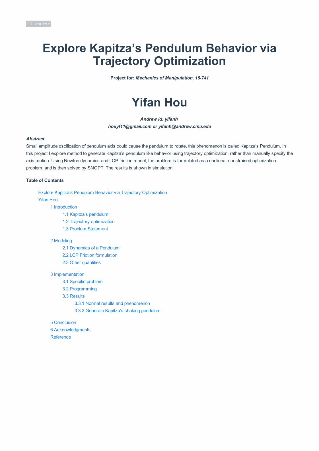
The axis movement of the initial trajectory is shown as follows:

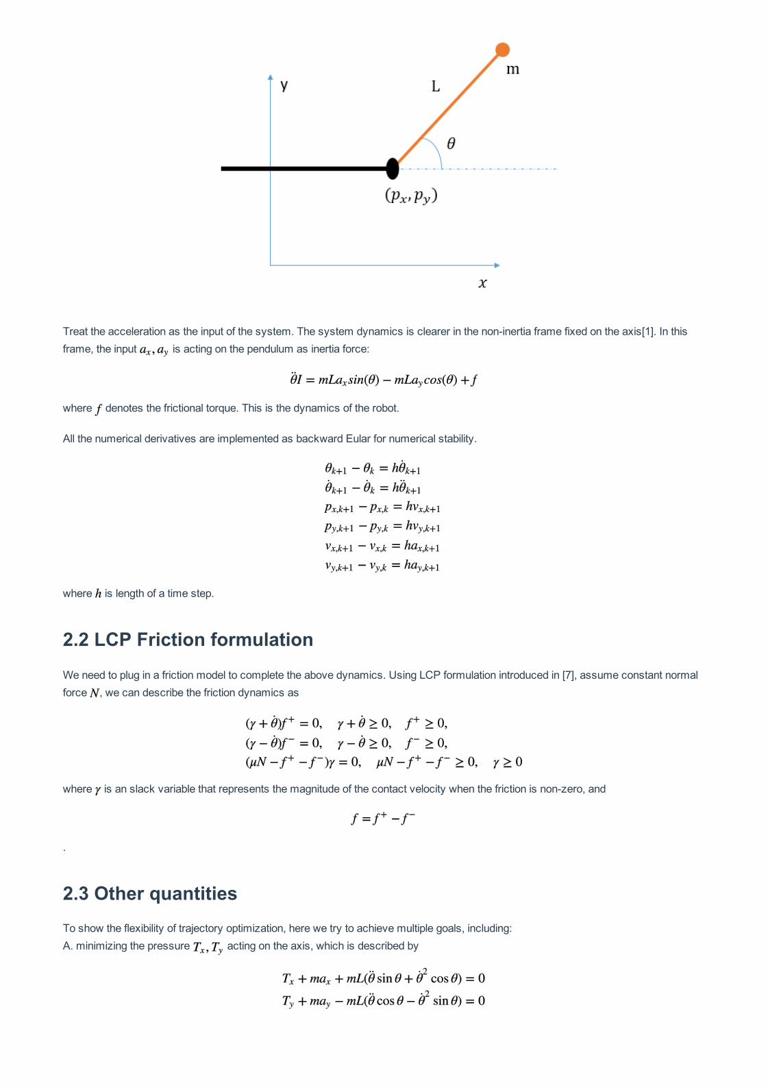
This kind of initial trajectory helps to find a better solution, where the desired pendulum orientation angle is achieved:

The corresponding trajectory converged nicely:

The axis motion of the solution is shown below. Two things are worth attention: 1. the solution does have Kapitza Compared with theinitial trajectory, the solver change both the frequency and amplitude of the axis motion to fit our goal.

With an informative starting point, the optimizer is able to find trajectories with better periodical feature.

Here is another good results, where we constrain the position of axis to be within a 1cm square, while the goal is to move the pendulumby an right angle.

Here is some selected frames from the result:

Corresponding change:

5 ConclusionIn this work, we show that we can use trajectory optimization techniques to generate Kapitza’s pendulum like behavior, where a smallamplitude axis oscillation could effectively move the pendulum to another orientation. The only necessary specification is a constraint onaxis position range, and an informative starting point will make thing even better.

6 AcknowledgmentsThanks Matt for bring us the excellent lectures. Thanks Sung for his work for this course. Thanks Gilwoo for helpful discussion ontrajectory optimization.

Reference

K

[1] Butikov, E. I. (2001). On the dynamic stabilization of an inverted pendulum. American Journal of Physics, 69(7), 755.http://doi.org/10.1119/1.1365403

[2] Mitchell J. Techniques for the Oscillated Pendulum and the Mathieu Equation[J].

[3] Youtube video, https://www.youtube.com/watch?v=rwGAzy0noU0

[4] Youtube video, https://www.youtube.com/watch?v=lgI1mha8z90

[5] Stewart, D. ., & Trinkle, J. C. (1996). An Implicit Time­Stepping Scheme for Rigid Body Dynamics With Inelastic Collisions andCoulomb Friction. International Journal for Numerical …, 39(15), 2673–2691.

[6] Trinkle, J., & Pang, J.­S. (1997). On Dynamic Multi­Rigid­Body Contact Problems with Coulomb Friction. ZAMM ­ Journal of AppliedMathematics and Mechanics / Zeitschrift Für Angewandte Mathematik Und Mechanik, 77, 267–279.

[7] Posa, M., & Tedrake, R. (2013). Direct Trajectory Optimization of Rigid Body Dynamical Systems through Contact. AlgorithmicFoundations of Robotics X, 86, 527–542.