Analytical solutions for a nonlinear coupled pendulum

Analytical solutions for a nonlinear coupled pendulum

LIGIA MUNTEANU, VETURIA CHIROIU

Institute of Solid Mechanics of Romanian Academy

Ctin Mille 15, P O Box 1-863, Bucharest 010141

[email protected], http://www.imsar.ro

ŞTEFANIA DONESCU

Technical University of Civil Engineering

Bd. Lacul tei nr. 122-124, Bucharest 020396

[email protected], http://www.utcb.ro

Abstract: - In this paper, the motion of two pendulums coupled by an elastic spring is studied. By extending the

linear equivalence method (LEM), the solutions of its simplified set of nonlinear equations are written as a linear

superposition of Coulomb vibrations. The inverse scattering transform is applied next to exact set of equations. By

using the Θ - function representation, the motion of pendulum is describable as a linear superposition of cnoidal

vibrations and additional terms, which include nonlinear interactions among the vibrations. Comparisons between

the LEM and cnoidal solutions and comparisons with the solutions obtained by the fourth-order Runge-Kutta

scheme are performed. Finally, an interesting phenomenon is put into evidence with consequences for dynamic of

pendulums.

Key-Words: cnoidal method, linear equivalence method, cnoidal vibrations, Coulomb vibrations, coupled

pendulum.

1 Introduction Since the original paper by Korteweg and deVries,

there has remained an open fundamental question

[1]: if the linearized equation can be solved by an

ordinary Fourier series as a linear superposition of

sine waves, can the equation itself be solved by a

generalization of Fourier series which uses the

cnoidal wave as the fundamental basis function?

This paper belongs of a series of papers, which

addresses an original, practical and concrete

resolution of this old problem. Starting with the

above idea, we attach to the coupled pendulum’s

motion equations two sets of nonlinear differential

equations: an exact one and a simplified one. The

capability of the linear equivalence method (LEM)

[2]-[8] is extended to the analysis of the simplified

system of equations. The LEM representation of the

solutions is describable as a linear superposition of

Coulomb vibrations.

The analysis of these LEM solutions allows us to

solve further the exact nonlinear system of equations

by using a generalization of Fourier series (the

cnoidal method). The cnoidal method uses the

cnoidal waves as the fundamental basis function [9]-

[11]. The Θ -function representation of the solutions

is derived as a linear superposition of Jacobean

elliptic functions (cnoidal vibrations) and additional

terms, which include nonlinear interactions among

the vibrations. The cnoidal vibrations are much

richer than sine vibrations; i. e. the modulus m of

the cnoidal vibration (0 1)m≤ ≤ can be varied to

obtain a sine vibration ( 0)m ≅ , Stokes vibration

( 0.5)m ≅ or soliton vibration ( 1)m ≅ .

In order to clarify the essence of the proposed

methods, we note that both methods are applicable

to the analysis of complex dynamical systems that

have non-simple-harmonic solutions.

It is the case of the nonlinear differential

equations having algebraic nonlinearities [12]

1

( )N

n n in n

i

z Az F z=

= +∑& (1)

where

1

N

n np p

p

Az a z=

=∑ , 1

, 1

( )N

n npq p q

p q

F z b z z=

= ∑ ,

2

, , 1

( )N

n npqr p q r

p q r

F z c z z z=

= ∑ ,

3

, , , 1

( )N

n npqr p q r l

p q r l

F z d z z z z=

= ∑ ,

4

, , , , 1

( )N

n npqrlm p q r l m

p q r l m

F z e z z z z z=

= ∑ ,

with 1,2,....n = . The general theory of integrable

conservative systems due to Hamilton-Jacobi and

the formulation of Morino [13] and Smith and

WSEAS TRANSACTIONS on MATHEMATICS

Ligia Munteanu, Veturia Chiroiu, Stefania Donescu

ISSN: 1109-2769 503 Issue 7, Volume 7, July 2008

Morino [14] predict only simple harmonic limit-

cycle solutions.

The singular perturbation method known as the

Lie transformation method introduced by Morino,

Mastroddi and. Cutroni [15] can be extended to the

analysis of dynamical systems capable of producing

not-so-regular vibrations, because not only the zero-

divisor terms, but certain small-divisor terms are

included into analysis.

So, the Lie transformation method is applicable to

the Bolotin systems of equations, but is not adequate

for the more complex systems as (1), because of the

non-standard type of involved nonlinearities. There are many other nonlinear differential

equations like (1) of physical importance that admit

such kind of solutions. We think that the cnoidal

method can be successfully applied to a wider class

of nonlinear equations [16], [17].

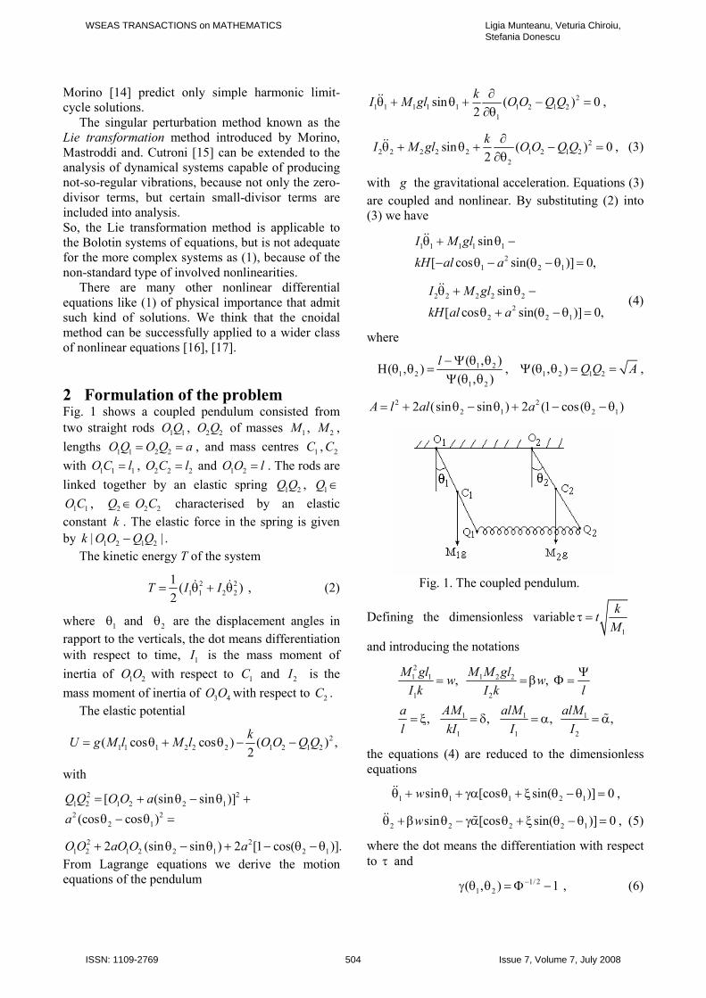
2 Formulation of the problem Fig. 1 shows a coupled pendulum consisted from

two straight rods 1 1OQ , 2 2O Q of masses 1M , 2M ,

lengths 1 1 2 2OQ O Q a= = , and mass centres 1C , 2C

with 1 1 1OC l= , 2 2 2O C l= and 1 2OO l= . The rods are

linked together by an elastic spring 1 2QQ , 1Q ∈

1 1OC , 2Q ∈ 2 2O C characterised by an elastic

constant k . The elastic force in the spring is given

by 1 2 1 2| |k OO QQ− .

The kinetic energy T of the system

2 2

1 1 2 2

1( )

2T I I= θ + θ& & , (2)

where 1 θ and 2 θ are the displacement angles in

rapport to the verticals, the dot means differentiation

with respect to time, 1I is the mass moment of

inertia of 1 2OO with respect to 1C and 2I is the

mass moment of inertia of 3 4O O with respect to 2C .

The elastic potential

2

1 1 1 2 2 2 1 2 1 2( cos cos ) ( ) ,2

kU g M l M l OO QQ= θ + θ − −

with

2 2

1 2 1 2 2 1[ (sin sin )]QQ OO a= + θ − θ + 2 2

2 1(cos cos )a θ − θ =

2 2

1 2 1 2 2 1 2 12 (sin sin ) 2 [1 cos( )].OO aOO a+ θ − θ + − θ − θFrom Lagrange equations we derive the motion

equations of the pendulum

2

1 1 1 1 1 1 2 1 2

1

sin ( ) 02

kI M gl OO QQ

∂θ + θ + − =

∂θ&& ,

2

2 2 2 2 2 1 2 1 2

2

sin ( ) 02

kI M gl OO QQ

∂θ + θ + − =

∂θ&& , (3)

with g the gravitational acceleration. Equations (3)

are coupled and nonlinear. By substituting (2) into

(3) we have

1 1 1 1 1

2

1 2 1

sin

[ cos sin( )] 0,

I M gl

kH al a

θ + θ −

− θ − θ − θ =

&&

2 2 2 2 2

2

2 2 1

sin

[ cos sin( )] 0,

I M gl

kH al a

θ + θ −

θ + θ − θ =

&&

(4)

where

1 21 2

1 2

( , )( , )

( , )

l −Ψ θ θΗ θ θ =

Ψ θ θ, 1 2 1 2( , ) QQ AΨ θ θ = = ,

2 2

2 1 2 12 (sin sin ) 2 (1 cos( )A l al a= + θ − θ + − θ − θ

Fig. 1. The coupled pendulum.

Defining the dimensionless variable1

kt

Mτ =

and introducing the notations

2

1 1 1 2 2

1 2

1 1 1

1 1 2

, ,

, , , ,

M gl M M glw w

I k I k l

AM alM alMa

l kI I I

Ψ= =β Φ =

= ξ = δ = α = α%

the equations (4) are reduced to the dimensionless

equations

1 1 1 2 1sin [cos sin( )] 0wθ + θ + γα θ + ξ θ − θ =&& ,

2 2 2 2 1sin [cos sin( )] 0wθ +β θ − γα θ + ξ θ − θ =&& % , (5)

where the dot means the differentiation with respect

to τ and

1/ 2

1 2( , ) 1−γ θ θ = Φ − , (6)

WSEAS TRANSACTIONS on MATHEMATICS Ligia Munteanu, Veturia Chiroiu, Stefania Donescu


1 2 2 1

2

2 1

( , ) 1 2 (sin sin )

2 (1 cos( )).

Φ θ θ = + ξ θ − θ +

ξ − θ − θ

The associated initial conditions are

0 0

1 1 2 2

0 0

1 1 2 2

(0) , (0) ,

(0) , (0) .p p

θ = θ θ = θ

θ = θ θ = θ& & (7)

We begin with constructing a simplified form of

(6) by taking

1 2 2 1

2

2 1

( , ) (sin sin )

(1 cos( )),

γ θ θ = −ξ θ − θ −

ξ − θ − θ (8)

with

2

2 1 2 1| 2 (sin sin ) 2 (1 cos( ) | 1ξ θ − θ + ξ − θ − θ < ,

verified for 0.3ξ ≤ . By using (8) the substantial

simplifications are made that restricts the accuracy

of the approach. But the simplified set of equations

solved by the LEM method will help us to

understand and to solve the exact set of equations by

using the cnoidal method. By noting

1 1 2 2 1 3 2 4 , , ,z z z zθ = θ = θ = θ =& & ,

the equations (9) become

1 3z z=& , 2 4z z=& ,

3 1 1 2 1sin [cos sin( )]z w z z z z= − − γα + ξ −& ,

4 2 2 2 1sin [cos sin( )]z w z z z z= −β + γα + ξ −%& , (9)

with the initial conditions (7) 0 0 0 0

1 1 2 2 3 3 4 4(0) , (0) , (0) , (0) ,z z z z z z z z= = = = (10)

We refer to (5) and (7) (or (9) and (10)) as the exact

motion equations for the pendulum. Substituting for

1 2( , )z zγ given by (8) in (9) we can obtain a

simplified form of the pendulum motion equations.

In addition, for | |2

pzπ

≤ and approximating the

trigonometric functions by polynomials of five-order

3 5 4

2 4 4

sin ( ), | ( ) | 2 10 ,

0.16605, 0.00761

cos 1 ( ), | ( ) | 9 10 ,

0.49670, 0.03705,

z z az bz z z

a b

z cz dz z z

c d

−

−

= + + + ε ε ≤ ×

= − =

= + + + ε ε ≤ ×

= − =

%%

%%

%%

%%

the system of equations (9) can be written as

1 3z z=& , 2 4z z=& ,

3 1 1 1 2 1 2( ) ( , ) ( , )z wP z Q z z z z= − −α γ& ,

4 2 2 1 2 1 2( ) ( , ) ( , )z wP z Q z z z z= −β + α γ%& , (11)

with

3 5( )P z z az bz= + + %% ,

1 1 2 1 1 2 1 2( , ) ( ) ( , ),Q z z R z R z z= +

2 1 2 1 2 2 1 2( , ) ( ) ( , )Q z z R z R z z= + ,

2 4

1( ) 1R z cz dz= + + %% , 1/ 2

1 2 1 2( , ) 1 ( , )z z f z z−γ = − + ,

3 2

2 1 2 1 2 2 2 1

2 3 5 4

2 1 1 2 2 1

3 2 2 3 4 5

2 1 2 1 2 1 1

( , ) 3

3 5

10 10 5 ,

R z z z z a z a z z

a z z a z b z b z z

b z z b z z b z z b z

= −ξ + ξ + ξ − ξ +

+ ξ − ξ + ξ − ξ +

+ ξ − ξ + ξ − ξ

% %

% %% %

% % % %

2 2 2

1 2 1 2 1 2 1

2 2 3 3 2 4 2 4

2 1 2 2 1

2 3 2 2 2 2 3 5 5

2 1 2 1 2 1 2 1

( , ) 1 2 2 4 2

2 2 2 2 2

8 12 8 2 2 .

f z z z z c z z c z

c z a z a z d z d z

d z z d z z d z z b z b z

= − ξ + ξ + ξ − ξ −

− ξ − ξ + ξ − ξ − ξ

+ ξ − ξ + ξ + ξ − ξ

% %

% %% % %

% % % % %

On inserting (8) in (11), a system (1) is obtained

for 1,2,3,4n = and 4N = . We refer to (1) and (10)

as the simplified motion equations for the pendulum.

The matrix npA a= is

0 0 1 0

0 0 0 1

0 0

0 0

Aw

w

= −αξ − αξ

αξ −αξ −β % %

, (12)

where

0.16605, 0.00761,

0.49670, 0.03705,

a b

c d

= − =

= − =

%%

%%

13 241, 1a a= = ,

31 32

41 42

, ,

, ,

a w a

a a w

= −αξ − = αξ

= αξ = −αξ −β% %

35 56, 1,a a= δ =2 2

312 3222 (1 ), ( 1),b c b c= − αξ − = −αξ −% %

2 2

412 4222 ( 1), (1 ),b c b c= − αξ − = −αξ −% %% %

3

3111 ,c a c c wa= −αξ −αξ + αξ −% % % %

2 3

3112 3122(3 1), 3 ,c c c c= −αξ ξ − = αξ% %

2 3

4122 4112(3 1), 3 ,c c c c= −αξ ξ − = αξ% %% %

2

3222 ( )c c a= −αξ ξ −% % , 2

4111 ( ),c c a= −αξ ξ −% % %

3

4222c a c c wa= −αξ −αξ + α ξ −β% % %% % % % ,

2 2

31111 ( 2 ),d d c a= −αξ + −% % %

2 2

31112 ( 4 2 ),d a d c= −αξ − −%% %

2 2

31122 (6 6 ),d d c a= −αξ + −% % %2

31222 (5 4 ),d a d= −αξ − %%



2

32222 ( 2 ),d d a= −αξ −% %2

41111 (2 )d a d= −αξ − %% ,

2

41112 (4 5 ),d d a= −αξ −%% %2 2

41122 (6 6 ),d a d c= −αξ − −%% % %

2 2

41222 ( 5 4 2 ),d a d c= −αξ − + +%% % % , 2 2

42222 ( ).d d c= αξ +%% %

3 The LEM method We begin with a brief explain of LEM in the spirit

of [2], [3]. Consider a nonlinear Cauchy problem

( ) ( )0 0 0, Rz F z z t = z , t I= ∈ ⊂& , (13)

where F is a vector of n analytic functions

( )1

ν

j jν

ν

F z a z∞

=

=∑ with the coefficients ja ν ∈ I R⊂ .

Here 1 2 nν (ν , ν ,...ν )= are multi-indexes of length n ,

and 1

j

nν

jj

z zν

== Π .The LEM method consists in

introduction of a new variable ( , )v t σ defined as an

exponential transformation of real parameters σ

( ) zv t e<σ >σ = ,, ,

1

n

j j

j

z z=

< σ >= σ∑, , (14)

where 1 2[ , ,... ] n

n Rσ = σ σ σ ∈ . Using (14), the system

(13) is transformed into a partial linear differential

equation

1

( ) 0sN

j j

j

vF D v

t =

∂− σ =

∂ ∑ , (15)

where ( , )jF t D is the formal differential operator

associated to ( )jF σ

( )|ν|

ν ν1

j jF D a∞

ν =

∂=

∂σ∑ , | 1 2 n

n1 2

ν ν ... ν|ν

νν νν

1 2 n...

+ +∂ ∂=

∂σ ∂σ ∂σ ∂σ. (16)

The linear equivalence transformation (14),

where nz , 1,2,...,6n = , is a solution of (13) and

satisfies the partial linear differential equation (15)

and initial conditions

( ) 0 0 0

0 1 1 2 2exp( ... )n nv t z z z= σ + σ + + σ . (17)

Because ( )z t satisfies the initial problem (13),

the initial solution ( )z t is easily obtained from

( , )v t σ . This method is applied now for a simplest

problem.Let consider the problem [1]

2d

d

yy

t= , 0(0)y y= , (18)

By applying the transformation yv eσ= to (18)

we obtain a linear equivalent equation

2

2

v v

t

∂ ∂= σ

∂ ∂σ, (19)

and the condition 0(0, )y

v eσσ = . (20)

For

( , ) ( ) ( )v t tσ = φ ψ σ , (21)

we have from (19)

d

dt

φ= λφ ,

2

2

d( )

d

ψσ = λψ σσ

, (22)

with λ an arbitrary constant. For ψ we take the

form

0

( )!

j

j

j j

∞

=

σψ σ = ϕ∑ , (23)

that yields to a recurrent linear algebraic system

1j jj +ψ = λψ , *j N∈ . (24)

We see that 0 0ψ = . The other coefficients are

determined from 1

1( 1)!

j

jj

−λψ = ψ

−, j N∈ . (25)

For ( , )v t σ we have the general representation

0 1

1

1

( , ) 1( 1)! !

j jt

j

v t e dj j

−∞λ

=−∞

λ σσ = + ψ λ

−∑∫ , (26)

for 0t ≥ . From the initial condition (18) it results

0 1

1 0d( 1)! !

j jj

yj j

−

−∞

λ σψ λ =

−∫ , j N∈ . (27)

So,

0

1

ye

λ−

ψ = , (28)

and the solution.(26) becomes

0

0

0

10 1( )

1

1

1

0

( , ) 1 d( 1)! !

11 .

1 !

j jty

j

j

yjty

j

v t ej j

ej

ty

−∞λ −

=−∞

∞ − σ−

=

λ σσ = + λ =

−

σ + − = −

∑∫

∑ (29)

that yields to the solution of the problem (18) which

is 0

0

( )1

yy t

ty=−

.



Now we return to the nonlinear system of

equations (1) and apply LEM, by introducing the

linear equivalence transformation (LEM) that

depends on four parameters i Rσ ∈ , 1,2,3,4i = .

( )1 2 3 4

1 1 2 2 3 3 4 4

, , , ,

exp( ),

v t

z z z z

σ σ σ σ =

σ + σ + σ + σ (30)

By inserting (30) into (1) we obtain a linear

partial differential equation

24 4 4

1 1 , 1

34

, , 1

44

, , , 1

54

, , , , 1

(

),

n np n npq

n p p qp p q

n npqr

p q r p q r

n npqrl

p q r l p q r l

n npqrlm

p q r l m p q r l m

v v va b

t

vc

vd

ve

= = =

=

=

=

∂ ∂ ∂= σ + σ +

∂ ∂σ ∂σ ∂σ

∂σ +

∂σ ∂σ ∂σ

∂σ +

∂σ ∂σ ∂σ ∂σ

∂σ

∂σ ∂σ ∂σ ∂σ ∂σ

∑ ∑ ∑

∑

∑

∑

(31)

with the initial conditions

( )1 2 3 4

0 0 0 0

1 1 2 2 3 3 4 4

0, , , ,

exp( ),

v

z z z z

σ σ σ σ =

σ + σ + σ + σ (32)

and the boundless condition at t→∞

( )1 2 3 4 0| , , , , |v t vσ σ σ σ ≤ at t→∞ . (33)

The last condition (33) eliminates the unbounded

solutions at t→∞ of (31). We investigate

numerically the existence of bounded solutions for

this equation. Taking the solution ( , )v t σ of the form

4`

1 2 3 4

1 1

4` `

, 1 , 1

4` ` `

, , 1 , , 1

4` ` ` `

, , , 1 , , , 1

( , , , , ) 1!

! !

! ! !

,! ! ! !

ii kk

k i

i ji j k lk l

k l i jk l

i j ri j r k l m

k l m

k l m i j rk l m

i j r si j r s k l m n

k l m n

k l m n i j r sk l m n

v t Ai

A Ai j

A A Ai j r

A A A Ai j r s

= =

= =≠

= =≠ ≠

= =≠ ≠ ≠

σσ σ σ σ = + +

σ σ+

σ σ σ+ +

σ σ σ σ+

∑ ∑

∑ ∑

∑ ∑

∑ ∑

(34)

and introducing in (31) it results straightforwardly

that the functions ( )nA t , 1,2,3,4n = , i.e. vibrations

of permanent form at t→∞ satisfying (32) has the

form

1

, 0

( ) {( ) ( ) ( , )

( ) ( ) ( , )},

k

n nk k

k

k

nk k

A t t A t

t B t

+

η=

= µ η Φ µ η +

µ η ψ µ η

∑ %

%

(35)

and max0,1,2..k k= , 0,1,2,3,....η = In (35) the

functions ( , )k tΦ µ η and ( , )k tψ µ η are given by

1 ( )

1

( , ) ( ) ( )m k k

k m

m k

t t A− −

= +

Φ µ η = µ η∑ ,

1 ( )

1

( , ) ( ) ( )m k k

k m

m k

t t B− −

= +

ψ µ η = µ η∑ , (36)

and ( )µ = µ η

4

1

j j

j=

µ = α λ∑ , (37)

with 4

1

1j

l=

α = η+∑ , 0jα ≥ , 1,2,3,4j = .

The quantities jλ in (37) are

1 1 2 1 3 2 4 2, , ,p p p pλ = λ = − λ = λ = − ,

where jp , 1,2,3,4j = are the roots of the

characteristic equation 4 2 ( ) 0pλ + λ + ∆ = ,

with

p w w= αξ + αξ +β +% , 2 w w w∆ = αξβ + αξ + β% ,

The unknowns nkA% , nkB are expressed

( ) ( ) ( ), ( ) ( ) ( ),nk k nk nk k nkA C B B C Cη = η η η = η η% %

where the constants ( )kC η verify the recurrence

relation 2 2

1( ) ( )(2 1)

k k

kC C

k k−

+ ηη = η

+, 0

| (1 ) |( )

2!

p iC

Γ + ηη = .

Γ is the gamma function and

22 1

20

(1 )| | [1 ]

(2) (2 )n

i

n

−

=

Γ + η η= +

Γ +∏ .

The constants ( )k

mA , ( )k

mB are related by the

relation ( ) ( )( ) ( )k k

m mB m Aη = ∆ η , where ( ) ( )k

mA η are

given by

( ) ( )

1 2

( ) ( ) ( )

1 2

1,1

( )( 1) 2 ,

2

k k

k k

k k k

m m m

A Ak

m k m k A A A

m k

+ +

− −

η= =

++ − − = η −

> +

(38)



The constants ( )nkB η , ( )nkC η depend on initial

conditions and on coefficients from (1). From (38)

and (36) 2 we obtain

1 ( )

1

( , ) ( ) ( )m k k

k m

m k

t t B− −

= +

ψ µ η = µ η∑ .

The function ( , )tψ µ η is linked to the ( , )tΦ µ η by

( , ) ( , ) ( , )d

t t tdt

Ψ µ η = µ Φ µ η = µΦ µ η& .

By noting 1( , ) ( ) ( ) ( , )k

k k kF t C t t+µ η = η µ Φ µ η ,

the functions (35) become

, 0

( ) { ( ) ( , ) ( ) ( , )}n nk k nk k

k

A t B F t C F tη =

= η µ η + η µ η∑ & .

We have

0 0( ,0) sin , ( ,0) cosF t t F t tµ = µ µ = µ& .

The solution (34) is reduced to

1 1 2 2 3 3 4 4exp( )v A A A A= σ + σ + σ + σ .

Finally, the LEM representation of the solution of

the nonlinear simplified system of equations (1) and

(10) is found to

, 0

( ) ( )

{ ( ) ( , ) ( ) ( , )}.

n n

nk k nk k

k

z t A t

B F t C F tη=

= =

η µ η + η µ η∑ & (39)

The functions ( , )kF tµ η have the form of

Coulomb wave functions [18]. If ( , )v t σ is a solution

bounded at t→∞ them v

t

∂∂

is also bounded at

t→∞ .

We summarize the result in the following result:

The bounded solutions (39) (LEM

representations) of the simplified system of

equations (1) and (10) are describable as a linear

superposition of Coulomb vibrations ( , )kF tµ η .

4 The cnoidal method The investigation is not limited to the analysis of the

simplified set of equations (1) and (10). The analysis

of the LEM solutions of this system is designed in

an attempt to establish some qualitative conclusions

about the solutions of the exact set of equations. So,

we find some interesting cases that uncouple the

equations (4) and reduce them to the Weierstrass

equations of fifth order, with solutions describable

as a linear and nonlinear superposition of cnoidal

waves.

We consider the simple case in the modified

version (α = α% )

1 1 1sin cos 0wθ + θ + α θ =&& ,

2 2 2sin cos 0wθ +β θ − α θ =&& , (40)

and associated initial conditions

0 0 0 0

1 1 2 2 1 1 2 2(0) , (0) , (0) , (0) ,p pθ = θ θ = θ θ = θ θ = θ& & (41)

Multiplying the first equation by 12θ& , and the

second one by 22θ& , and integrating we obtai

2

1 1 1 12 cos 2 sinw Cθ = θ − α θ +& ,

2

2 2 2 22 cos 2 sinw Cθ = β θ + α θ +& , (42)

with iC , 1,2i = integration constants.

Approximating the trigonometric functions by

polynomials of five-order we have 2 ( )i i iPθ = θ& ,

1,2i = , where ( )i iP θ are polynomials of fifth-order

in iθ , 1,2i =

2 3 4 5

0 1 2 3 4 5( )i i i i i i i i i i i i iP a a a a a aθ = + θ + θ + θ + θ + θ ,

with

01 1 02 2

11 12

2 , 2 ,

2 , 2 ,

a w C a w C

a aA

= + = β +

= − α = α

21 22

31 32

2 , 2 ,

2 , 2 ,

a wc a wc

a a a a

= = β

= − α = α

% %

% %

41 42

51 52

2 , 2 ,

2 , 2 ,

a wd a wd

a b a b

= = β

= − α = α

% %

% %

where, for sake of simplicity, we have taken

1 22 , 2w C w C− = − β = and 11 12 2 0a a= − = α ≠ .

The equations (44) are similar with the equation

2 2 3 4 5

1 2 3 4 5A A A A Aθ = θ + θ + θ + θ + θ& , (43)

where

1 1 2 2 3 ,3 4 4 5 5

1 3 5, , 2 , .

2 2 2A a A a A a A a A a= = = = =

This equation admits a particular solution

expressed as an elliptic Weierstrass function that is

reduced, in this case, to the cnoidal function cn [18]

2 3

2

2 2 3 1 3

( ; , )

( )cn ( ),

t g g

e e e e e t

′℘ + δ =

′− − − + δ (44)



where ′δ is an arbitrary constant, 1 2 3, ,e e e are the

real roots of the equation 3

2 34 0y g y g− − = with

1 2 3e e e> > and 2 3,g g the invariants expressed in

term of the parameters of the exact system of

equations (9) and (10). As we know, a linear

superposition of cnoidal functions (44) is also a

solution for (43).

To see the form of the nonlinear superposition

term we assume the solution of (43) in the Krishnan

form [19]

int

( )( )

1 ( )

tt

t

λ℘θ =

+ µ℘, (45)

where ( )t℘ is the Weierstrass elliptic function

satisfying the differential equation [18]

2 3

2 14 g g′℘ = ℘ − ℘− , (46)

with the invariants 2g and 1g real in the pendulum

case, and satisfying 3 2

2 327 0g g− > , λ and µ are

arbitrary constants.

Substituting (45) into (43) we obtain four

equations for the unknowns λ , µ , 2g and 1g

2

4 3 2 2 3 4

1 2 3 4 5

2

,A A A A A

− λµ =

µ + λµ + λ µ + λ µ + λ (47)

3 2 2 3

1 2 3 44 4 3 2A A A Aλµ = µ + λµ + λ µ + λ , (48)

2 2 2

2 1 2 3

36 6 3

2g A A Aλ + λµ = µ + λµ + λ , (49)

2

2 3 1 22g g A Aλµ + λµ = µ + λ . (50)

From (47), (48) we have

4 3 2 2

1 2 3

3 4

4 5

6 5 4

3 2 0.

A A A

A A

µ + λµ + λ µ +

λ µ + λ = (51)

Let us consider the special case where (54) is

reducible to 4( ) 0R Sλ + µ = , (52) 1/ 4

5

13

A

A

µ = − λ

, (53)

with 1/ 4

5(2 )R A= , 1/ 4

1(6 )S A= ,

3

2

4

5A RS= , 2 2

3

3

2A R S= , 3

4

4

3A R S= .

We observe that both quantities R and S in (52)

are both or real or imaginary. In the last case this

equation leads to 4( ) 0i R S′ ′λ + µ = with R′ and S ′ real quantities.We calculate

1 1

10

2A a= = −α ≠ for the first equation (42)

and 1 1

10

2A a= = α ≠ for the second equation (42),

with 0α > . In both cases we have 5

1

50

3 3

Ab

A= >% .

Then 1/ 4

5

3

b µ = − λ

%

. (54)

Using (53) we can obtain a unique constant λ from (47) and (48)

3/ 2

1 530(3 )A A −λ = − . (55)

The constant 5A is 5 5

55

2A a b= = − α % or

5 5

55

2A a b= = α % with 0b >% . From (55) we have for

the both situations

2 3/ 230(15 )b −λ = − α % with 2 0bα >% . (56)

From (54) and (56) we obtain 1/ 4

2 3/ 2530 (15 )

3

bb −

µ = α

%% . (57)

The unknowns 2g and 3g are computable from

(52) and (53). For the considered pendulum we

found that λ , µ , 2g and 1g are always real. The

nonlinear term becomes

2 3

2 3

( ; , )( )

1 ( ; , )

t g gt

t g g

′λ℘ + δθ =

′+ µ℘ + δ,

where λ and µ are given by (55) and (57), and ′δ

is an integration constant of the equation (46). The

exact periodical solutions are obtained by using (44)

where ′δ is an arbitrary real constant, and 1 2 3, ,e e e

the real roots of 3

2 34 0y g y g− − = with

1 2 3e e e> > .

The nonlinear interaction solution of (46) is a

bounded periodical function

2

2 2 3 1 3

int 2

2 2 3 1 3

[ ( )cn ( )]( )

1 [ ( )cn ( )]

e e e e e tt

e e e e e t

′λ − − − + δθ =

′+ µ − − − + δ. (58)

The modulus m of the Jacobean elliptic function

is 2 3

1 3

e em

e e

−=

− .The solitary vibration is a vibration

with the period (m =1 or 1 2e e= ). In this case the

solution is



2

1 1 3 1 3

int 2

1 1 3 1 3

[ ( )sech ( )]( )

1 [ ( )sech ( )]

e e e e e tt

e e e e e t

′λ − − − + δθ =

′+ µ − − − + δ .

Now we return to the exact system of equations

(5) and (7) (or (9) and (10)). We begin by taking the

solutions ( )kz t , 1,2k = of the forms [1], [11]

2( )

2( ) 2 log ( )k

k nz tt

∂= Θ η

∂ , (59)

where Θ - function is given by

( )

( ) ( ) ( ) ( ) ( )

1 , 1

1

1( ) exp( i )

2ki

n nk k k k k

n j j i ij j

j i jMi n

M M B M∞

= ==−∞≤ ≤

Θ η = η +∑ ∑ ∑

and

1 2[ ... ]nη = η η η with j j jtη = −ω +β , 1 j n≤ ≤ .

Here n is the finite number of degrees of

freedom for a particular solution of the problem, jω

the frequencies and jβ the phases.

The solution (59) can be written in the form

2

int2( ) 2 log ( ) ( ) ( )n cnz t z z

t

∂= Θ η = η + η

∂,

where we have omitted for simplicity the index

k .The first term cnz represents a linear

superposition of cnoidal waves and it is given by

2

2( ) 2 log ( )cnz G

t

∂η = η

∂,

1( ) exp(i )

2

T

M

G M M DMη = η+∑ ,

and the second term intz , a nonlinear superposition

of the cnoidal functions and it is given by

2

int 2

( , )( ) 2 log(1 )

( )

F Cz

t G

η∂η = +

∂ η,

1( , ) exp(i )

2

T

M

F C C M M DMα

η = η+∑ ,

1exp( ) 1

2

TC M OM= − .

The interaction matrix B is composed by a

diagonal matrix D and an off-diagonal matrix O ,

B D O= + . The first term cnθ has an explicit form

as

2

1

( ) 2 cn ( )n

cn m m m

m

z t A C=

= η∑ ,

with ,m mA C unknown constants. The second term

intz has an explicit form as

2

1int

2

1

cn ( )

( )

1 cn ( )

n

m m m

m

n

m m m

m

E C

t

D C

=

=

ηθ =

+ η

∑

∑,

with ,m mE D unknown constants. The parameters

jω , jβ , ijB , ,m mA C , ,m mE D , 1 ,j m n≤ ≤ , can be

analytically determined by an identification

procedure.

So, the bounded solutions of the exact system of

equations (5) and (7) (or (9) and (10)) are

2

1

2

1

2

1

( ) 2 cn ( )

cn ( )

,

1 cn ( )

n

k km m m

m

n

km m m

m

n

km m m

m

z t A C

E C

D C

=

=

=

= η +

η

+ η

∑

∑

∑

(60)

for 1,2,3,4k = .

We summarize the result in the following result:

The bounded solutions (75) (the cnoidal

representation) of the exact system of equations (5)

and (6) (or (9) and (10)) is a linear superposition of

cnoidal vibrations and a nonlinear interaction

among the vibrations.

The LEM solutions (39) of the system of

equations (1) and (10) and the cnoidal solutions (75)

of the system of equations (5) and (7) (or (9) and

(10)) are obtained by the two different methods.

These solutions appear distinct. In the case for

which the simplification (8) is possible, the exact

system of equations is reduced to the simplified

system of equations. This case is a good test to

compare these apparently distinct solutions. Even

though it does not seem possible to analytically

show the similarity between these solutions, it may

be shown numerically, if suitable values for

parameters, pertinent to the condition 0.3ξ ≤ , can

be considered. The stability of pendulum motion can

be easily studied through both methods, LEM and

the cnoidal methods.

5 Examples The theoretical results are firstly carried out as some

validation examples for LEM and cnoidal

representations.

We assess the efficiency of the LEM method for

2η = and 63k = . For 63k > the computing

complicates without adding new significant terms in

solutions. The cnoidal solutions for the exact set of

equations are computed for 3n = and 2 2M− ≤ ≤ .



Comparison between LEM and cnoidal solutions

for 0.3ξ ≤ , and comparison with the numerical

results obtained by the fourth-order Runge-Kutta

scheme are performed.

The examples involve the pendulums:

( 210 /g m s= )

P1: 1.5, 0.25, 70m k= ξ = = N/m ),

2 10kgM = , 0.2ml = , 1 22

al l= = ,

P2: ( 1m = , 0.5ξ = , 44 10k = ⋅ N/m ),

2 15kgM = , 0.1ml = , 1 22

al l= = ,

P3: (uncoupled pendulum) 1kgM = , l = 0.5 m,

a = 0.125 m, 1l = 2 m, k = 40 N/m .

An interesting phenomenon is putting into

evidence for the pendulum. Two kind of vibration

regimes are found: an extended (phonon)- mode of

vibration to both masses, and a localised (fracton) -

mode of vibration to a single mass, the other mass

being practically at rest.

Fig. 1a The extended- mode of vibrations given by LEM

solutions (continuum line) and by cnoidal solutions

(dashed lines) for the solution 1( )tθ of P1 ( 1(0) 1.5θ = ,

2 (0) 0.5θ = , 1(0) 0.05θ =& , 2 (0) 0.05θ =& ).

The first regime of vibrations is presented in Fig.

2a,b by the LEM solutions for P1 with 1(0) 1.5θ = ,

2 (0) 0.5θ = , 1(0) 0.05θ =& , 2 (0) 0.05θ =& . Calculated

by cnoidal method the solutions are practically the

same. In fig. 2a dashed lines represent the cnoidal

solutions, and in fig. 2b dashed lines represent the

LEM solutions. Although we are unable to

determine theoretically the precise connection

between LEM and cnoidal solutions for 0.3ξ ≤ , we

remark here similarity between them clearly

depicted from graphs.

Fig. 1b The extended- mode of vibrations given by

cnoidal solutions (continuum line) and by LEM solutions

(dashed lines) for the solution 2 ( )tθ of P1

( 1(0) 1.5θ = , 2 (0) 0.5θ = , 1(0) 0.05θ =& , 2 (0) 0.05θ =& ).

Fig. 2a The extended -mode of vibrations given by

cnoidal solution 1θ (sum of cnoidal vibrations plus

nonlinear interactions) for P2

( 1 2 1 20.045, 0.02θ = θ = θ = θ =& & ).

The same regime of vibrations is given by

solutions iθ , 1,2i = for P2 (sum of cnoidal

vibrations plus nonlinear interactions) with the

initial conditions 1 2 1 20.045, 0.02θ = θ = θ = θ =& & in

fig.3a,b. The three spectral components have the

moduli 0.96, 0.68m = , 0.27 for 1θ , and

0.87, 0.59m = , 0.31 for 2θ .

The error function ( )e t is defined as

2 2

1 1 2 2( ) ( ( ) ( )) ( ( ) ( ))e t t t t t′′ ′ ′′ ′= θ − θ + θ − θ , (61)



where ( 1 2( ), ( )t t′ ′θ θ ) are solutions obtained by using a

method and ( 1 2( ), ( )t t′′ ′′θ θ ) solutions obtained by other

method, applied to the same set of equations.

Fig.2b The extended -mode of vibrations given by cnoidal

solution 2θ (sum of cnoidal vibrations plus nonlinear

interactions) for P2 ( 1 2 1 20.045, 0.02θ = θ = θ = θ =& & ).

Fig. 3a The error function ( )e t between LEM and

Runge-Kutta solutions for the pendulum P1.

Fig. 3b The error function ( )e t between cnoidal and

Runge-Kutta solutions for the pendulum P2.

The error function (61) between LEM and

Runge-Kutta solutions for P1 is represented in

fig.4a. The error function between cnoidal and

Runge-Kutta solutions for P2 is represented in

fig.4b.

Fig. 4. The localized –mode of vibrations given by

cnoidal solution 2θ ( 1θ 0≅ ) for P1 ( 1(0) 0.5θ = ,

2 (0) 0.6θ = − , 1(0) 0.5θ =& , 2 (0) 0θ =& ).

Fig.5. The localized –mode of vibrations given by cnoidal

solution 1θ ( 2θ 0≅ ) for P1 ( 1(0) 0.6θ = − ,

2 (0) 0.5θ = , 1(0) 0.5θ =& , 2 (0) 0.5θ = −& ).

Fig.6a The first part of the solution ( )tθ (superposition of

two cnoidal vibrations) for P3 ( (0) 0.05θ = − ,

(0) 0.1θ =& ).

Fig.6b The second part of the solution ( )tθ (nonlinear

interactions between two cnoidal vibrations) for P3

( (0) 0.05θ = − , (0) 0.1θ =& ).

The second regime of vibrations is represented

in fig..4 for P1, with 1(0) 0.5θ = , 2 (0) 0.6θ = − ,

1(0) 0.5θ =& , 2 (0) 0θ =& . The vibrations are mostly

localized on 2M , the 1M being practically at rest.



The vibrations of 1M have almost negligible

amplitudes in comparison with the amplitudes of the

2M vibrations. If we change the conditions as

1(0) 0.6θ = − , 2 (0) 0.5θ = , 1(0) 0θ =& , 2 (0) 0.5θ =& ,

the mass 1M is vibrating having the same evolution

as shown in fig.5, and the mass 2M is resting.

Fig.6c The final cnoidal solution ( )tθ expressed as the

sum between both previous parts for P3 ( (0) 0.05θ = − ,

(0) 0.1θ =& )

The first part of the solution ( )tθ (superposition

of three cnoidal vibrations), the second part of the

same solution (nonlinear interactions between three

cnoidal vibrations) and the final cnoidal solution

expressed as the sum between them, for P3 are

represented in fig.6a,b,c for (0) 0.05θ = − ,

(0) 0.1θ =& . We see that the nonlinear part of this

solution is not at all negligible.

5 Conclusions

The remarkable property – whereby the solutions of

certain systems of nonlinear differential equations

like (5) can be represented by a sum of a linear and a

nonlinear superposition of cnoidal vibrations - is

shared by a large number of nonlinear differential

equations.

Two methods – the LEM and cnoidal methods-

have been applied in this paper with the objective to

capture and examine this property for a coupled

pendulum.

The LEM representations of solutions for a

simplified set of motion equations available for

0.3ξ ≤ are describable as a superposition’s of

Coulomb vibrations. The LEM analysis is designed

in an attempt to establish some qualitative

conclusions about the solutions of the exact set of

equations.

The cnoidal method is applied next to this system

of equations. The cnoidal representations of

solutions are described as a superposition of cnoidal

vibrations and nonlinear interactions among

vibrations. So, we can say that the real virtue of the

cnoidal method is to give the elegant and compact

expressions for the solutions in the spirit of this

property.

The results of numerical computations by LEM

and by cnoidal methods for the case 0.3ξ ≤ have

shown that both solutions are equivalent. The both

solutions were compared to the Runge-Kutta

numerical solutions.

The both methods describe successfully the

stable behaviour of the coupled pendulum. The

LEM method looks like partial generalisation of the

linear theory and help the nonlinear analysis of

dynamical systems having algebraic nonlinearities

written in the form (1) and known as the Bolotin

equations. These equations have the property they

are reducible to the coupled and uncoupled

Weierstrass equations of third, and fifth or higher

order.

The cnoidal method can provide the nonlinear

analysis of complex dynamical systems like (5).

This method looks like a generalization of Fourier

series with the cnoidal wave as the fundamental

basis function, but is a completely different than an

ordinary Fourier series expressed as a linear

superposition of sine waves.

The analytical solutions allow the possibility of

investigating in detail the effects of changing the

initial conditions. For certain values of these

conditions it is possible to locate two kind of

vibration regimes: an extended (phonon)- mode of

vibrations to both masses, and a localised (fracton) -

mode of vibrations to a single mass, the other mass

being practically at rest.

An advantage of the cnoidal method is that the

procedure is quite elegant, straightforward, requiring

only the Θ -function formulation

ACKNOWLEDGEMENT. The authors acknowledge

the financial support of the PNII project nr.

106/2007, code ID_247/2007.

References:

[1] Osborne, A.R., Soliton physics and the periodic

inverse scattering transform, Physica D 86, 1995,

81-89.

[2] Toma, I., The linear equivalence method and

applications (in romanian), Ed.Flores, Bucharest,

1995.

[3] Toma, I., The linear equivalence method and

applications to mechanics (in roumanian) Ed.

Tehnică, Bucharest, 2008.

[4] Toma, I., On Polynomial Differential Equations,

Bull. Math. Soc. Sci. Math. RSR, 24 (72), 4, 1980,

417-424.



[5] Toma, I., Techniques of Computation by Linear

Equivalence, Bull. Math. Soc. Sci. Mat. de la

Romanie, 33 (81), 4, 1989, 363-373.

[6] Teodorescu, P.P., Toma, I., On the Postcritical

Study of a Cantilever Bar, Lecture Notes in Eng.,

Springer Verlag, Berlin-Heidelberg-NY-Paris-

Tokio, 9, 1989, 233-244.

[7] Teodorescu, P.P., Toma, I., A postcritical study

of an elastic structure, Rev. Roum. Math. Pures et

Appl., 34, 6, 1989, 591-594.

[8] Teodorescu, P.P., Toma, I., An application of the

linear equivalence method to the postcritical study

of a Bernoulli-Euler bar, Rev. Roum. des Sci. Tech.,

série Mec. Appl., 34, 4, 1989, 309-321.

[9] Drazin, P.G., Johnson, R.S., Solitons: An

Introduction, Combridge Univ. Press, 1989.

[10] Ablowitz, M.J., Clarkson, P.A., Solitons,

Nonlinear Evolution Equations and Inverse

Scattering, Cambridge Univ. Press, Cambridge,

1991.

[11] Munteanu, L., Donescu, Şt., Introduction to

Soliton Theory: Applications to Mechanics, Book

Series “Fundamental Theories of Physics”, vol.143,

Kluwer Academic Publishers, 2004.

[12]Bolotin, V.V., Nonconservative Problems of the

Theory of Elastic Stability, The Macmillan

Company, NY, 1963, 274-312.

[13] Morino, L., A perturbation method for treating

nonlinear panel flutter problems, AIAA Journal, 7,3,

1969, 405-411.

[14] Smith, L.L., Morino, L., Stability analysis of

nonlinear differential autonomous system with

applications to flutter, AIAA Journal, 14, 3, 1976,

333-341.

[15] Morino, L., Mastroddi, F., Cutroni, M., Lie

Transformation Method for Dynamical Systems

Having Chaotic Behaviour, Nonlinear Dynamics, 7,

1995, 403-428.

[16] Taghi, M., Javidi, D., Javidi, M., Method of

lines for solving systems of time-dependent partial

differential equations, WSEAS Transactions in

Mathematics, Vol 1, No. 1-4, 2002, 218-222.

[17] Lima, P., Morgado, L., Asymptotic and

numerical approximation of a boundary value

problem for a quasi-linear differential equation,

WSEAS Transactions in Mathematics, Vol 1, No. 1-

4, 2007, 639-647.

[18] Krishnan,E.V., On the Ito-Type Coupled

Nonlinear Wave Equation, J. of the Physical Society

of Japan, 55, 11, 1986, 3753-3755..

[19] Abramowitz, M., Stegun, I. (eds.), Handbook of

mathematical functions, U. S. Dept. of Commerce,

1984.

[20] Ohmiya, M., Ohkura, H., Okaue, D., Numerical

study of Benjamin-Feir type instability of sine-

Gordon equation, WSEAS Transactions in

Mathematics, Vol 5, No. 6, 2006, 763-769.



Analytical solutions for a nonlinear coupled pendulum

Documents

Transcript of Analytical solutions for a nonlinear coupled pendulum