Analytical methods manual 1984

B.H. SHELDRICK, Editor Land Resource Research Institute Ottawa, Ontario

LRRI Contribution No. 84-30

Research Branch Agriculture Canada 1984

4 --.--- -. _-..- --*--

Copies of this publication are available frmn: Land Resource Research Institute Research Branch, A<griculture Canada Ottawa, Ontario KlA OC6

Produced by Research Program Servk~

c Minister of Supply and Services Canada 1984

-

ABSTRACT

This manual is a compilation of details of methods of analysis currently being used routinely in the Land Resource Research Institute (LRRI) Ottawa. It includes physical, chemical, and microscopic procedures for analyzing mineral and organic soils as well as several chemical procedures for analyzing water samples. For a number of analyses, several methods are presented and information is given on how to choose the most appropriate one for the purpose. Statements of accuracy and precision have been included whenever there were sufficient data available as a result of testing in the analytical service laboratory LRRI, Ottawa.

Ce manuel est un r&ueil des m&hodes detaill6es d'analyse utilisees actuellement de faqon courante 5 VInstitut de recherches sur les terres (I.R.T.) d'ottawa. 11 comprend des m&hodes d'analyse physique, chimique et q icroscopique des sols min&aux et organiques de msme que plusieurs pro&d& d'analyse chimique de l'eau. Pour un bon nombre d'analyses, on pr&ente plusieurs methodes et l'on explique comment choisir celle qui convient le mieux aux buts poursuivis. La 'preccision des methodes est mentionnee quand elle est appuyGe par des donnGes suffisantes, accumul+es au fil des essais qui ont @te rGalis& au laboratoire des services d'analyse de 1'I.R.T.

._ __~_ .- -_--_ --

COMMITTEE ON ANALYTICAL METHODS

The Committee on Analytical Methods, who actively participated in reviewing, updating and rewriting methods for inclusion in this manual, is comprised of the following personnel of the Land Resource Research Institute, Central Experimental Farm, Ottawa, Canada KlA OC6:

R.K. Guertin P.A. Schuppli B.H. Sheldrick (editor) K.C. Wires W.D. Zebchuk

-

--

ANALYTICAL METHODS MANUAL 1984 LRRI, OTTAWA

PREFACE

This manual is a compilation of details of methods of soil and water analysis currently being used routinely in the Land Resource Research Institute (LRRI), Ottawa. It was prepared by, and largely for, the technical staff of LRRI but it may have wider use. All of the basic methods have been published previously in the Manual on soil sampling and methods of analysis second edition 1978 J.A. McKeague editor. Some methods have been deleted, other methods have been added and details of all procedures are updated and tailored to equipment and facilities at LRRI Ottawa. A brief outline of soil sample collection and preparation has been included as general information.

This edition of the manual has adopted the loose-leaf format and different numbering system to permit flexibility in the revision of approved methods and in the addition of new ones as they are published. As methods are revised they will be forwarded automatically to known holders of this manual. Users of this manual are requested to note errors in the text and to forward this information to the editor.

For a number of analyses, several methods are presented and information is given on how to choose the most appropriate one for the purpose. For example, in choosing an extractant for Fe, dithionite-citrate (method 84-010) would be used to estimate non-silicate Fe, and pyrophosphate (method 84-012) would be a more suitable extractant of organic-associated Fe. Other choices depend on the degree of accuracy required relative to time involved. For example, method 84-008 for carbonates is more rapid but less accurate than method 84-009.

When sufficient data were available accuracy and precision data have been included. They are the results of testing in the analytical service laboratory, LRRI, Ottawa. Interlaboratory studies are currently being conducted to generate specifications for precision and accuracy.

The editor wishes to thank the research technicians and scientists who contributed to this manual either by revising and updating methods or by criticizing the first draft of the material. Particular thanks are due to Dr. J.A. McKeague for his guidance in completion of this manual.

Comments and suggestions for improvement in this manual are cordially invited.

B.H. Sheldrick Editor

_-

TABLE OF CONTENTS

PREFACE

1. SAMPLE COLLECTION AND PREPARATION

1.1 Field sampling 1.2 Laboratory preparation 1.3 Size-fraction base for reporting data

2. CHEIIICAL ANALYSIS

2.1 pH 84-001 pH in O.OlM CaC12 (1:2) and water (1:l) 84-002 Lime requirement buffer method.

2.2 Soluble Salts 84-003 Soluble salts in 1:2 soil:water ratio.

2.3 Cation Exchange Capacity and Exchangeable Cations 84-004 Permanent charge CEC, and exchangeable cations by 2N NaCl

extraction 84-005 1N ammonium acetate extractable Ca, Mg and K 84-006 Cation exchange capacity at pH 7.0 by Ca (OAc)2-CaC12 84-007 Barium acetate exchange capacity of organic soils

2.4 Carbonates 84-008 Gravimetric method, approximate 84-009 Pressure transducer method (calcite and dolomite

differentiation possible)

2.5 Extractable Al, Fe and Mn (and Si> 84-010 Dithionite-citrate extraction 84-011 Acid ammonium oxalate extraction 84-012 Sodium pyrophosphate extraction

2.6 Carbon 84-013 Total carbon, LECO induction furnace 84-014 Organic carbon by wet oxidation (modified Walkley-Black) 84-015 Pyrophosphate solubility index of organic matter.

2.7 Phosphorus 84-016 Total phosphorus, acid digestion

l/1-3 2/l-3

3/l-6

4/l-3

5/l-2 6/L-3 7/l-2

8/l-2 9/l-4

10/l-3 11/l-3 12/l-3

13/l-4 14/l-3 15/l-2

I 16/l-3 84-017 Sodium bicarbonate extractable phosphorus (by autoanalyser) 17/l-5 84-018 Extractable phosphorus by 0.03 N NH4F + 0.025N HCl (Bray) 18/l-5 84-019 Total phosphorus in water (by autoanalyser) 19/l-6 84-020 Orthophosphate in water (by autoanalyser) 20/l-5

2.8 Ammonia and Nitrate 84-021 Ammonia and nitrate extractable by 2N KC1 21/l-8 84-022 Ammonia and nitrate in water (by autoanalyser) 22/l-6

--.--.....- --..-- -_-.

2.9 Major and minor elements 84-023 Acid dissolution of total major and minor elements

(other than C, N, P, and S) 84-024 Extractable trace elements by either DPTA or EDTA 84-025 Total mercury in soils.

3. PHYSICAL ANALYSIS

3.1 Particle size distribution 84-026 Particles ~2 mm pipet method using filter candle system 84-027 Sieve analysis (mechanical method)

3.2 Bulk density and particle density 84-028 Bulk density (Clod method) 84-029 Bulk density (Core method) 84-030 Particle density or specific gravity

3.3 Shrinkage 84-031 Shrinkage factors of a disturbed soil (ASTM D427-61) 84-032 Shrinkage of disturbed samples (COLE rod) 84-033 Shrinkage of natural clod samples

3.4 Water content and water retention (porosity) 84-034 Water content 84-035 Soil water desorption curves for soil cores by tension 84-036 Water retention 4 and 15 bar

3.5 Saturated hydraulic conductivity 84-037 Core method 84-038 Clod method

3.6 Atterberg Limits 84-039 Liquid limit (ASTM D423-66) 84-040 Liquid limit by drop cone penetrometer 84-041 Plastic limit (ASTM 424-59)

3.7 Surface area determination 84-042 Specific surface area (EGME retention)

3.8 Fiber content 84-043 Fiber content and particle size distribution of organic 84-044 Fiber content (unrubbed and rubbed)

soils

3.9 Loss on Ignition 84-045 Loss on ignition at 550°C

4. NICROSCOPY

84-046 Stereo microscope 84-047 Thin sections 84-048 Scanning electron microscopy applied to soils 84-049 Sand mineralogy by microscopy

23/l-3

24/l-3 25/l-5

26/l-8 27/l-4

28/l-4 29/l-3 30/l-3

31/l-4 32/l-2 33/l-4

3411-Z 35/l-9 36/l-2

e

37/l-4 38/l-2

39/l-5 40/l-4 41/l-3

42/l-3

43/l-3 44/l-3

45/l-2

46/l 47/l-10 48/l-2 49/l-3

Fig. 1

Fig. 2

Fig. 3

Fig. 4

Fig. 5

Fig. 6

Fig. 7

Fig. 8

Fig. 9

Fig. 10

Fig. 11

Fig. 12

Fig. 13

Fig. 14

LIST OF FIGURES

Flow diagram for the determination of sodium bicarbonate extractable phosphorus.

Flow diagram for the determination of 0.03 N NHQF + 0.025N HCl (Bray) extractable phosphorus.

Flow diagram for the determination of total phosphorus in water samples.

Flow diagram for the determination of orthophosphate in water samples.

Flow diagram for the determination of ammonia in 2N KC1 extracts.

Flow diagram for the determination of ammonium and nitrate extractable by 2N potassium chloride.

Distillation apparatus used in the determination of ammonia and nitrate.

Flow diagram for the determination of ammonium in water samples.

Flow diagram for the determination of ammonia and nitrate in water samples.

Digestion assembly for mercury determination.

Flow diagram and flow cell for the determination of mercury.

A comparison of particle-size limits in 4 systems of particle-size distribution.

Grain size analysis mechanical.

Grain size distribution.

Fig. 15 Glass bead and aluminum oxide tanks for water desorption.

Fig. 16 Liquid limit device.

Fig. 17 Drop cone penetrometer.

Fig. 18 Apparatus for particle-size analysis and fiber content of peat.

Fig. 19 Apparatus for impregnation of soil samples.

17/5

18/5

19/6

20/5

21/6

2117

2118

2215

2216

2514

25/5

2618

27/3

2714

35/9

3915

4014

4313

47/10

LIST OF TABLES

Table 1.

Table 2.

Table 3.

Table 4.

Table 5.

Table 6.

Quantity of limestone in tons per acre required to raise soil pH 2/3 to 6.5 to a 6 inch depth.

Factors for converting conductivity values to 25OC. 314

Specific conductivity values for potassium chloride solution. 3/5

Soluble salts in soils (1:2 soil:water ratio). 3/6

Settling depths for specific times and temperatures for particle-size = 2 P.

26/7

Equilibration times for 76 mm high soil cores. 35/6

1. Sample collection and preparation

1 -.

C-.

1. - SAMPLE COLLECTION AND PREPARATION

1.1 FIELD SAMPLING

1.1.1 Site Selection

Select sample sites typical of the soils that the samples are intended to represent. The site should be away from roads, fences, abandoned farmsteads and other features that may have caused aberrant properties. Ideally, two or more sites several kilometers apart should be selected for each soil. The reason for the selection of a particular site should be noted.

1.1.2 Soil Sampling

The method of sampling depends upon the purposes for which the samples are taken. These purposes should always be recorded when sampling. The methods described herein apply to soil characterization and genesis studies. Other kinds of samples include: Composite sample of surface soil for fertility tests and grab samples of a specific horizon for checking classification.

Take samples from freshly dug pits and not from roadcuts. Dig the pit wide enough to expose one face of a pedon and deep enough to expose part of the C horizon, or to the bottom of the control section (Canada Soil Survey Committee, 1978), whichever is deeper. Describe the pedon and any variations within the pedon. In laterally uniform pedons, sample from a face about 50 cm wide. Each sample should be representative of the entire cross section of each horizon. If horizons of a pedon are discontinuous or vary greatly in thickness or degree of expression, collect samples from different parts of pedon or different locations on the pit face to ensure a representative sample of each horizon. Do not mix horizons if they are interfingered or discontinuous. If contrasting soil components are so small or so intimately associated that they cannot be sampled separately, estimate the proportion of each component and record it in the pedon description. Otherwise sample the contrasting materials separately and record their proportion. Make arbitrary sub- horizons if morphologically recognizable sub-horizons are more than 25 cm thick in the upper part of the pedon or more than 50 cm in the lower part. If coarse fragments (>20 mm) are present, follow the procedures outlined in 1.1.3. If convenient, start sampling at the bottom of the pit.

The characterization of several physical properties of soil, such as porosity and saturated hydraulic conductivity, requires undisturbed samples that are representative of the horizon being sampled. Suitable samples of friable, stone free soils can usually be obtained but problems arise with stony soils and with soils of coarse structure. For example, some fragipans have dense , prismatic structural units about 30 cm wide separated by more porous "gray streaks". A representative sample should include both the prismatic unit and the "gray streak" material in the

-

2.

proportions in which they occur. Such samples are difficult to obtain and very bulky. An alternative approach is to sample the major part of' the prismatic units and the "gray streaks" separately. No generally applicable methods can be specified for obtaining suitable undisturbed soil samples. The quality of the samples depends upon the judgement and ingenuity of the sampler and the reliability of many physical data depends more upon the quality of the llundisturbedf' samples than on any other factor.

1.1.3 Stony Soils (Soil Conservation Service, 1972)

Volume estimates - In each horizon or crop of horizons estimate the volume percentage of the 20 to 75 mm and the 75 to 250 mm fractions. Record the percentages in the pedon description. Collect a 5 to 7 kg sample of the ~20 mm fraction and store it in an airtight plastic bag, if field moisture content is to be determined. After drying, sieve and weigh the 2-20 mm material. Calculate the volume percentage of the 2-20 mm fraction (see 2.142).

Weight estimates - Estimate and record the volume percentages of the >75 mm fraction as outlined in volume estimates. Collect a 15 to 25 kg sample of the <75 mm fraction and weigh. Sieve out and weigh the 20 to 75 mm fraction. Record the weights of the 20 to 75 mm fractions and store the <20 mm material in an airtight plastic bag if field moisture content is to be determined. Calculate the weight percentage of coarse fractions.

-

1.2 LABORATORY PREPARATION

Spread the field samples on trays or on plastic sheeting and air-dry (except for special procedures requiring moist soil). Thoroughly mix and roll the samples to break up clods. Continue rolling or gently crushing and sieving until coarse fragments (>2 mm) that do not slake in water or sodium metaphosphate remain on the sieve. (If the samples are to be analysed for minor elements, nylon or stainless steel sieves should be used.) Weigh and discard the >2 mm fraction. Calculate the percentages of the various fractions.

NOTE: Preparation of samples of strongly cemented soils is difficult as they are as hard as some rocks. No general method can be specified for such samples.

If C, total N, extractable Fe and Al, etc. are to be determined, grind a subsample of the <2 mm material to pass a 35 mesh sieve..

1.3 SIZE-FRACTION BASE FOR REPORTING DATA

1.3.1 Particles <2 mm

Unless otherwise specified report all data on the basis of <2 mm material.

3.

1.3.2 Particles < specified size >2 mm

The maximum coarse-fragment size for the >2 mm base varies. The base usually includes fragments as large as 75 mm if they are present in the soil. The maximum size for fragments larger than 75 mm is decided during sampling. It is established either because of the difficulty of handling larger material or because, by definition soil does not include material larger than 250 mm in diameter. Record the particle size set as the maximum for the soil being sampled. The base used to calculate the percentages of fractions >2 mm includes all material smaller than the maximum size specified for the sample.

References

(1) Canada Soil Survey Committee, 1978. The Canadian System of Soil Classification. Agr. Can. Publ. 1646.

(2) Soil Conservation Service, 1972. Soil Survey Laboratory Methods and Procedures for Collecting Soil Samples. Soil Survey Investigations Report No. 1 (Revised 1972). U.S.D.A. Washington, D.C.

Notes

-

84-001 pH

1. Application

1.1 The two main methods of measuring soil pH are outlined in this procedure. They are 1:l soil:water ratio and 1:2 soil:O.OlM CaC12 ratio. The measurement of soil pH in O.OlM CaC12 is the preferred method for most purposes because of advantages pointed out by Peech (1965).

1. The pH is almost independent of dilution over a wide range.

2. The pH measured is almost independent of the concentration of soluble salt present in non-saline soils.

3. It provides a good approximation of the pH of the soil solution under field conditions.

4. Errors due to the liquid junction potential are minimized because the soil suspensions are flocculated.

Measurement of the pH of a saturated soil is not recommended because of theoretical (junction potential) and practical (difficulty of obtaining reproducible results) disadvantages.

There is no point in measuring the pH of most soils containing free carbonates of Ca and Mg as the value obtained depends upon the partial pressure of CO2 which is generally uncontrolled during pH measurements (Turner and Clark, 1956). It is, however, useful to measure the pH of saline, calcareous soils as pH values above about 8.5 indicate sodium carbonate (Richards, 1954).

2. Apparatus

2.1 50 mL disposable paper cups or beakers.

2.2 pH meter and electrodes.

3. Reagents

3.1 O.OlM Calcium chloride (CaC12): Dilute l.lg of calcium chloride to 1 liter in a volumetric flask with distilled water. Alternatively, if large volumes are required make a stock solution of 3.6M CaC12 (CaC12.H20 1059g/2L). Dilute 50 mL of this stock solution to 18 liters with distilled water. Check the pH of this solution; it should be between 5.0 and 6.5. If it is not adjust by adding Ca(OH)2 or HCl. To check the concentration of the solution, measure its conductivity; the specific conductivity should be 2.32 + 0.08 millisiemens per cm (mS/cm) at 25OC.

l/2

4. Procedure

4.1 pH in O.OlM CaC12 (1:2, soil:solution ratio)

4.1.1 Weigh about 10 g of 2 mm soil into a 50 mL disposable paper cup or beaker.

4.1.2 Add about 20 mL of O.OlM CaC12 solution and stir the suspension several times during the next 30 minutes. For organic soils that absorb all of the solution use a 1:4 soil:solution ratio.

NOTE: Weight and volume measurements are not critical as +l - will not affect pH in O.OlM CaC12.

4.1.3

4.1.4

Let the suspension stand for 30 minutes to allow most of the sediment to settle.

Measure the pH by immersing the glass electrode into the partly settled suspension (do not immerse it to the bottom of the container) and placing the calomel electrode in the clear supernatant solution. If a combination electrode is used immerse it in the supernatant solution. The pH meter is adjusted by setting it to the pH of buffer solutions at the same temperature as the soil suspension. The meter should be checked against two buffers one of which has a pH at the lower end and the other at the upper end of the range of the expected pH of the soils being measured.

4.1.5 Record the pH in O.OlM CaC12 to one decimal place.

4.2 pH in water (1:l soil:water ratio).

4.2.1 Weigh 20 g of 2 mm soil into a 50 mL disposable paper cup or beaker.

'4.2.2 Add 20 mL of distilled water and stir the suspension several times during the next 30 minutes. For samples with a high organic matter content use a 1:4 soil:water ratio.

4.2.3 Allow the suspension to settle for 30 minutes.

4.2.4 Measure the pH as outlined in step 4.1.4.

4.2.5 Record the pH in water to one decimal place.

5. Calculations

5.1 nil

6. Precision

6.1 Within the analytical service lab the coefficients of variation at pH levels of 4.6 and 7.6 in O.OlM CaC12 were 1.7% and 1.7% respectively.

_I_-- -- - P- .__--- -

l/3

7. References

7.1 Peech, M. 1965. Hydrogen-ion activity in Methods of Soil Analysis Part 2; C.A. Black, ed. pp. 914-926.

7.2 Richards, L.A., ed. 1954. Diagnosis and Improvement of Saline and Alkali Soils. U.S. Salinity Laboratory. U.S. Dept. Agr., Handbook 60, 160 pp.

7.3 Turner, R.C. and Clark, J.S. 1956. The pH of, calcareous soils. Soil Sci. 82. 337-341.

Notes

.-. --

84-002 LIME REQUI- Buffer method

1. Application

1.1 This procedure is used as a rapid method for determining lime requirement of acid soils. The amount of lime required is based or change in pH of the buffer solution by the soil.

2. Apparatus

2.1 pH meter and electrode

2.2 100 mL beakers

2.3 20 L carboy with spigot.

2.4 Hot plate

3. Reagents

3.1

3.2

3.3

3.4

3.5

Para-nitrophenol: Dissolve 360 g of reagent grade, (crystal), para-nitrophenol in 3 liters of hot distilled water. Allow to cool. The para-nitrophenol should be allowed to cool slowly on the hot plate.

Boric Acid (H B03): Dissolve 270 g of boric acid in 3 liters of hot distil ? ed water. Allow to cool.

Potassium Hydroxide (KOH): Dissolve 189 g of potassium hydroxide in approximately 200 mL of distilled water.

Potassium Chloride (KCl): Dissolve 1332 g of potassium chloride in 8 liters of distilled water. It is very important to have this solution completely dissolved and well mixed.

Buffer solution: Pour the 8 liters of potassium chloride into a 20 liter carboy. Make certain that it is completely dissolved and mixed. Add in this order with thorough mixing between each addition: the potassium hydroxide (KOH), the boric acid (H BO >, and the para-nitrophenol solutions. Make to 18 liters wi h z a istilled water and mix. Adjust the pH to 8.0 with either KOH or HCl.

NOTE: If the above procedure is followed carefully, there will be a minimum of residue formed.

4. Procedure

4.1 Weigh out 20 g of 2 mm soil in a 100 mL beaker

4.2 Add 20 mL of distilled water, mix and let stand for 30 minutes

5.

6.

4.3 Read pH to the nearest 0.05 unit on expanded scale and record reading

4.4 TO the above soil:water suspension add 20 mL of the buffer solution and stir thoroughly. Let stand for a minimum of 10 minutes.

4.5 Standardize the pH meter to read 8.0 with a 1:l buffer-water mixture

4.6 Stir thoroughly and measure the pH of the soil-water-buffer Suspension immediately to the nearest 0.05 unit on expanded scale.

Calculations

5.1 To raise the soil pH values to 6.5, add the pounds of limestone per acre in the table at the intersection of the soil pH and buffer pH values (Table 1).

NOTE: (1) The T/A limestone table (Table 1) has a built-in factor of 1.65 from 60% immediately available CaC03 in the marketed product.

(2) A method outlined by Shoemaker et al. (1961) gives similar results. See references 6.1 and 6.2.

References

6.1 Shoemaker, H.E., McLean, E.O. and Pratt, P.F., 1961. Buffer method for determining lime requirment of soils with appreciable amounts of extractable aluminum. Soil Sci. Sot. Am. Proc. 25, 274-277.

6.2 Webber, M.D., Hoyt, P.B., Nyborg, M., and Corneau, D. 1977. A comparison of lime requirement methods for acid Canadian soils. Can. J. Soil Sci. 57, 361-370.

6.3 Adams, F. and Evans, C.E. 1962. A rapid method for measuring lime requirement of red-yellow podzolic soils. Soil Sci. Sot. Amer. Proc. 26, 355-357.

Table 1 - Quantity of limestone in tons per acre required to raise soil pH to 6.5 to a 6 in. depth'

pH of soil Soil - pH

Buffer 6.0 5.9 5.8 5.7 5.6 5.5 5.4 5.3 5.2 5.1 5.0 4.9 4.8 4.7 4.6 4.5

7.85 0.5 0.5 0.5 0.5 0.5 0.5 1.0 1.0 1.0 1.0 1.0 1.0 1.0 1.0 1.0 1.0 7.80 0.5 0.5 1.0 1.0 1.0 1.0 1.0 1.0 1.0 1.0 1.0 1.5 1.5 1.5 1.5 1.5 7.75 1.0 1.0 1.0 1.0 1.0 1.0 1.5 1.5 1.5 1.5 1.5 1.5 1.5 1.5 1.5 2.0 7.70 1.0 1.0 1.0 1.5 1.5 1.5 1.5 1.5 1.5 2.0 2.0 2.0 2.0 2.0 2.0 2.5 7.65 1.0 1.0 1.5 1.5 1.5 1.5 2.0 2.0 2.0 2.0 2.0 2.0 2.5 2.5 2.5 2.5 7.60 1.0 1.5 1.5 1.5 2.0 2.0 2.0 2.0 2.0 2.5 2.5 2.5 2.5 2.5 3.0 3.0 7.55 1.5 1.5 2.0 2.0 2.0 2.0 2.5 2.5 2.5 2.5 3.0 3.0 3.0 3.0 3.0 3.5 7.50 1.5 2.0 2.0 2.0 2.5 2.5 2.5 3.0 3.0 3.0 3.0 3.0 3.5 3.5 3.5 3.5 7.45 1.5 2.0 2.0 2.5 2.5 2.5 3.0 3.0 3.0 3.5 3.5 3.5 3.5 4.0 4.0 4.0 7.40 2.0 2.0 2.5 2.5 3.0 3.0 3.0 3.5 3.5 3.5 4.0 4.0 4.0 4.0 4.5 4.5 7.35 2.0 2.5 2.5 3.0 3.0 3.0 3.5 3.5 4.0 4.0 4.0 4.0 4.5 4.5 4.5 5.0 7.30 2.0 2.5 3.0 3.5 3.5 3.5 4.0 4.0 4.5 4.5 4.5 5.0 5.0 5.0 5.5 5.5 7.25 2.0 2.5 3.0 3.5 3.5 3.5 4.0 4.0 4.5 4.5 4.5 5.0 5.0 5.0 5.5 5.5 7.20 2.5 3.0 3.0 3.5 3.5 4.0 4.0 4.5 4.5 5.0 5.0 5.0 5.5 5.5 5.5 6.0 7.15 2.5 3.0 3.5 3.5 4.0 4.0 4.5 4.5 4.5 5.0 5.0 5.5 5.5 6.0 6.0 6.5 7.10 3.0 3.0 3.5 4.0 4.0 4.5 5.0 5.0 5.0 5.5 5.5 6.0 6.0 6.0 6.5 6.5 7.05 3.0 3.5 4.0 4.0 4.5 5.0 5.0 5.5 5.5 5.5 6.0 6.0 6.5 6.5 7.0 7.0 7.00 3.0 3.5 4.0 4.5 4.5 5.0 5.5 5.5 6.0 6.0 6.5 6.5 6.5 7.0 7.0 7.5

1 To change these quantities to tonnes/ha (15 cm depth) multiply the values by 2.24.

ru \ w

3/l

84.003 SOLUBLE SALTS IN SOILS (1:2 soil:water ratio)

1. Application

1.1 Soluble salts in soil can be estimated by measuring the specific conductivity of a water extract of soil with a conductivity meter. The value is corrected at 25OC and reported as millisiemens/cm (mS/cm). The most easily interpretable conductivity values are those on a saturation extract, prepared from a saturated soil paste. It is also useful to obtain conductivity readings on soil:water mixtures at other ratios, usually 1:l or 1:2 or 1:5, separating soil as much as possible by settling or centrifugation. The soil:water ratio used generally in this laboratory is 1:2.

2. Apparatus

2.1 125 mL Erlenmeyer flasks.

2.2 Conductivity meter.

2.3 Conductivity cell (dip type).

2.4 Thermometer covering room temperature.

2.5 Reciprocating shaker.

3. Reagents

3.1 0.05 N Potassium chloride stock solution (KCl): Dilute 3.728 g of oven dry potassium chloride to 1 liter in a volumetric flask with distilled water.

3.2 0.01 N Potassium chloride: Dilute 50 mL 0.05 N solution to 250 mL in a volumetric flask with distilled water.

3.3 0.005 N Potassium chloride: Dilute 25 mL 0.05 N solution to 250 mL in a volumetric flask with distilled water.

3.4 0.002 N Potassium chloride: Dilute 50 mL 0.01 N solution to 250 mL in a volumetric flask with distilled water.

4. Procedure (cell constant and meter performance)

Most conductivity meters have a logarithmic scale marked in micromhos and also a range switch giving a number of multiplication factors which are powers of 10 so that the meter can measure specific conductivities from 1 to 100,000 micromhos.

_-.- .-- _--___.-____ - -

312

4.1 Check the cell constant and meter performance by obtaining scale readings for each of the standard KC1 solutions (0.002 N, 0.005 N, 0.01 N, 0.05 N).

4.2 Calculation of cell constant. Let B be the range or multiplication factor. Let E be the dial reading. Let Rl the electrical resistance in ohms, obtained with

a standard KC1 solution be B x E. Let Sl the electrical conductance in mhos be 1

K Let M be the published conductivity value in mhos (see table

of specific conductivity values for potassium chloride solutions) of the standard KC1 solution at the temperature of reading.

Let C be the cell constant C=M

s Example: (For conductivity bridge, model RC) B= 100 R= 100 x 65 = 6500 E = 65 Temp. = 280~ S=l = 153.8 x ld KC1 = 0.002 N G-50 M(from table) = 310 x 10°06

C = 310 x 10-6 153.8 x loo6

= 2.02 mmhos/cm (or mS/cm)

-

5. Procedure

5.1 Weigh 15 g of soil into an 125 mL Erlenmeyer flask.

5.2 Add 30 mL distilled water.

5.3 Shake the mixture for 30 min. on a reciprocating shaker.

5.4 Allow the bulk of the soil to settle.

5.5. Measure the conductivity of the suspension using a conductivity meter and a conductivity cell with a cell constant of 1.

5.6 Record temperature of the filtrate to the nearest O.l°C.

6. Calculations of unknown solutions

Let B, E, S and C have the same meaning as in 4.2 Let Rl the electrical resistance in ohms, obtained from an

unknown solution be B x E. Let T be the temperature of unknown solution.

313

.- Let F be the temperature factor (see table on factors for converting conductivity values to 25OC)

6.1 Conductivity of the sample at 25OC = SxFxC = FxC mhos/cm - --- BxE

6.2 Conductivity is normally reported in mS/cm (millimhos/cm) millimhos/cm = FxCxlOO

BxE

Example: E= 245 B = 10 Temp. = 20°C F (from table) = 1.112 c = 2.02

mS/cm = 1.112 x 2.02 x 1000 245 x 10

= 0.92

7. References

7.1 Bower, C.A. and Wilcox, L.V. 1965. Soluble salts In Agronomy No. 9. Methods of soil analysis, Part 2, Black, C.A. ed., pp. 933-951.

314

Table 2. Factors for converting conductivity values to 25OC

OC Factor OC Factor OC Factor

18 1.163 22.0 1.064 26.0 0.979 18.2 1.157 22.2 1.060 26.2 0.975 18.4 1.152 22.4 1.055 26.4 0.971 18.6 1.147 22.6 1.051 26.6 0.967 18.8 1.142 22.8 1.047 26.8 o. 964 19.0 1.136 23.0 1.043 27.0 0.960 19.2 1.131 23.2 1.038 27.2 0.956 19.4 1.127 23.4 1.034 27.4 0.953 19.6 1.122 23.6 1.029 27.6 0.950 lg.8 1.117 23.8 1.025 27.8 0.947 20.0 1.112 24.0 1.020 28.0 0.943 20.2 1.107 24.2 1.016 28.2 0.940 20.4 1.102 24.4 1.012 28.4 0.936 20.6 1.097 24.6 1.008 28.6 0.932 20.8 1.092 24.8 1.004 28.8 0.929 21.0 1.087 25.0 1.000 29.0 0.925 21.2 1.082 25.2 0.996 29.2 0.921 21.4 1.078 25.4 0.992 29.4 0.918 21.6 1.073 25.6 0.988 29.6 0.914 21.8 1.068 25.8 0.983 29.8 0.911

- -. ------ --- --

-

Table 3. Specific conductivity values of Potassium Chloride solution.

Temperature 0.002 N 0.005 N 0.01 N 0.05 N in OC KC1 KC1 KC1 KC1

----------------mhos x 10-O ---------------

15 239 585 1.147 5404 16 244 598 1173 5527 17 249 611 1199 5651 18 255 625 1225 5775 19 260 638 1251 5889 20 266 651 1278 6024 21 271 665 1305 6149 22 276 678 1332 6275 23 282 692 1359 6402 24 287 706 1386 6529 25 293 720 1413 6656 26 299 734 1440 6784 27 304 748 1468 6912 28 310 763 1496 7041 29 316 777 1524 7170 30 321 792 1552 7300

316 .

Table 4. Soluble Salts in Soils (1:2 Soil:Water Ratio)

Conductivity Approximate Plant Salt Content Response

mhos x low5 parts per million

25 150 30 210 35 310 40 400 45 500

Suitable for most plants.

50 600 55 650 May result in 60 750 a slightly 65 850 stunted condition 70 940 in most plants

------------------------------------------------------------------ 75 1050 80 1120 Slightly to severe 85 1225 burning of most 90 1300 plants. 95 1400 100 1500

------------------------------------------------------------------

125 1950 150 2400 175 2850 200 3300 250 4200 300 5100 400 7150 500 9200 600 11200

Excessive salts. Prevents normal growth of most plants.

-

-

84-004 PERMANENT CHARGE CEC and exchangeable cations by NaCl extractions.

1. Application

1.1 The cation exchange capacity (CEC) of a soil varies with pH. Thus, there are two general approaches to the measurement of CEC: 1) to extract the soil with a neutral salt and thus measure CEC at the pH of the soil, 2) to extract the soil with a solution buffered at a given pH, often 7, and thus measure CEC at a fixed pH. The preferred method for most purposes is to determine CEC at the pH of the soil using NaCl as extractant. However ammonium acetate at pH 7 has been widely used for determining CEC despite the problem of ammonium fixation by some soils. The use of NaCl as an extractant has the disadvantage that exchangeable Na+ cannot be determined. For many acid soils exchangeable Na+ values are low, and Na+ is commonly not determined. For soils of arid areas and especially those developed in saline materials, however, the determination of exchangeable Na+ is important. It can be extracted with other suitable salts.

2. Apparatus

2.1 Disposable culture tubes (16 x 125 mm and 16 x 150 mm)

2.2 Eppendorf pipette and disposable tips.

2.3 Repipet dispensing bottles (accuracy l%, reproducibility 0.1%)

2.4 End-over-end shaker (40-50 rpm).

2.5 Atomic absorption spectrophotometer (Model 1200 Varian Techtron).

2.6 Centrifuge p (IEC low speed).

2.7 50 mL plastic centrifuge tubes.

3. Reagents

3.1 2N Sodium chloride (NaCl): Dilute 116.9 g of sodium chloride to 1 liter in a volumetric flask with distilled water.

3.2 Prepare a solution containing a concentration of 40,000 pg/mL La from La203 (46.88 g/L). The La20 must be dissolved carefully in about 200 mL of 12N ii Cl or 900 mL of 1M HCl and made to volume with distilled water.

3.3 Certified atomic absorption standards ~1%.

4. Procedure

4.1 Selection of sample weight.

4.1.1

4.1.2

4.2

4.2.1

4.2.2

4.2.3

4.2.4

4.3

4.3.1

Sample weight is based upon an estimate of the pH and the CEC of the soil. Estimates of permanent charge cation exchange capacity may be made on the basis of the clay and organic matter content of the soil samples. Permanent charge CEC (meq/lOO g) can be estimated by the equation (-11 + 0.2 clay % + 2 organic C % + 2.5 pH in CaC12).

A guideline to weights for estimated CEC is CEC 15-20 meq/lOO g weigh 1 g CEC lo-15 meq/lOO g weigh 3 g CEC 5-10 meq/lOO g weigh 6 g CEC l- 5 meq/lOO g weigh 9 g CEC 0.1. 1 meq/lOO g weigh 12 g

Extraction of exchangeable cations.

Transfer an appropriate weight of soil into a 50 mL plastic centrifuge tubes.

Use a repipet dispensing bottle and add 30 mL of 2N NaCl solution, stopper tightly and shake end-over-end for four hours.

Remove stoppers and centrifuge at 510 G for 20 minutes. n.

Filter the centrifugate through Whatman No. 2V filter paper into plastic vials. Exchangeable cations should be analyzed within a few days.

Determination

Dilute an aliquot of the extract with distilled water containing 2000 vg/mL Lanthanum (usually 1:40 for Ca and Mg and usually 1:lO for K) and determine Ca, Mg and K. For most samples, the weights and dilutions suggested will result in concentrations of the cations in the optimum range for atomic absorption determination. Note the following points.

4.3.1.1 The concentrations of Na in test solutions and standards should be approximately the same.

4.3.1.2 A concentration of about 2000 pg/mL Lanthanum in both samples and standards is required to supress interferences.

4.3.2 If the O.OlM CaC12 pH of the soil is less than 5.0 determine exchangeable Al. The preferred method is 8-hydroxyquinoline because it is reliable and more sensitive. However, it is not recommended because chloroform is now known to be a carcinogen in

413

- man. Exchangeable Al can be determined by atomic absorption on the 1:lO dilution without the difficulty of burner clogging. Values for exchangeable Al measured by atomic absorption are usually slightly higher than those by 8-hydroxyquinoline.

5. Calculations

5.1 Exchangeable cations in meq/lOO g = ug/mL measured x 100 x vol. of extract (mL) x dilution eq wt of cation x 1000 wtof soil (g)

5.2 For the following conditions: 3 g sample, 30 mL extractant, 1:40 dilution and 5 pg/mL Ca measured. Exchangeable Ca = 5 x 100 x 30 x 40 = 10 meq/lOO g

20 x 1000 3

6. Precision

6.1 In the LRRI Analytical service lab the coefficients of variation at Ca levels of 20.5 meq/lOO g, Mg levels of 5.5 meq/lOO g and K levels of 1.1 meq/lOO g were 6.6%, 7.4% and 6.346 respectively.

7. References

7.1 Clark, J.S. 1965. The extraction of exchangeable cations from soils. Can. J. Soil Sci. 45, 311-322.

7.2 Clark, J.S. and Hill, R.G. 1968. Vessel for long term soil-solution equilibration. Can. J. Soil Sci. 48, 221.

7.3 McKeague, J.A. Ed. 1978. Manual on soil sampling and methods of analysis 2nd edition. Can. Sot. Soil Sci. Suite 907, 151 Slater St., Ottawa, Ont.

Notes

__-._-__~-

84-005 AMMONIUM ACETATE Extractable Ca, Mg and K

-

1. Application

1.1 Exchangeable cations (i.e. Ca, Mg, Na and K) may be determined by displacing these ions from soil colloids with NH4. Thissf;i;z;e by shaking the soil with 1N NH4OAc adjusted to pH '7.0. to permanent charge CEC this method does not correct for Ca and Mg extracted from free carbonates; thus acetate-extractable Ca and Mg are not usually measured on calcareous soils.

2. Apparatus

2.1 Disposable culture tubes (16 x 125 m and 16 x 150 UUII)

2.2 125 mL Erlenmeyer flasks.

2.3 Repipet dispensing bottles (accuracy I%, reproducibility 0.1%).

2.4 Repiprocating shaker.

2.5 Eppendorf pipettes and disposable tips.

2.6 Atomic absorption spectrophotometer (Varian Techtron model 1200).

3. Reagents

3.1 1.0 N Ammonium acetate (NH4OAc): Dilute 77.1 g of ammonium acetate to 1 liter in a volumetric flask with distilled water. Adjust pH to 7.0 with ammonium hydroxide or acetic acid as required.

3.2 Prepare a solution containing a concentration of 40,000 pg/mL La from La203 (46.88 g/L). carefully in about 200 mL

The La203 must be dissolved 12N HCl and made to volume with distilled

water.

3.3 Certified atomic absorption standards 21%.

4. Procedure

4.1 Extraction

4.1.1 Weigh 2.5 g of air dry 2 mm soil into 125 mL Erlenmeyer flasks.

4.1.2 Use a repipet dispensing bottle and add 25 mL of 1N NH40Ac to the soil sample.

4.1.3 Stopper the flasks and shake on a reciprocating shaker for 30 minutes.

5/2

4.1.4 Filter the extract through Whatman No. 2V filter paper and save the filtrate in a plastic vial for analysis.

4.2 Determination

4.2.1 Dilute an aliquot of the extract with distilled water containing 2000 pg/mL Lanthanum (usually 1:40 for Ca and Mg and usually 1:lO for K) and determine Ca, Mg and K. For most samples, the dilution suggested will result in concentration of the cations in the optimum range for atomic absorption determination. Note the following point.

4.2.1.1 A concentration of about 2000 pg/mL Lanthanum in both samples and standards is required to supress interferences.

5. Calculations

5.1 Exchangeable cations in meq/lOO & = pg/mL measured X 100 x vol. of extract (mL) x dilution eq. wt. of cation x 1000 wt. of soil (g)

5.2 For the following condition: 2.5 g sample, 25 mL extractant, 1:40 dilution and 3 pg/mL Ca measured. Exchangeable Ca = 3 x 100 x 25 x 40 =

20x1000 2.5 6.0 meq/lOO g

6. Precision

6.1 Insufficient data available.

7. References

7.1 McKeague, J.A. Ed. 1978. Manual on soil sampling and methods of analysis, 2nd edition. Can. Sot. Soil Sci. Suite 907, 151 Slater St., Ottawa, Ont.

82-006 CATION EXCHANGE Capacity at pH 7.0 by Ca(OAc)2=CaC12

1. Application

1.1 The measurement of cation exchange capacity both at the pH of the soil (neutral salt) and at pH 7.0 permits the calculations of the pH dependent charge. The pH dependent charge is generally high in acid soils containing appreciable amounts of either organic matter or amorphous inorganic substances. This procedure has some advantages over NH4 saturation for the determination of CEC at pH 7.0: a) Ca can be determined readily by atomic absorption b) Ca is the dominant exchangeable cation in many soils c) Ammonium fixation is a problem in many soils.

2. Apparatus

2.1 50 mL plastic centrifuge tubes that can withstand both low speed and high speed centrifugation.

2.2 Repipet dispensing bottles (accuracy I%, reproducibility 0.1%).

2.3 Centrifuges (low speed IEC, high speed IEC).

2.4 Shakers (paint type Red Devil, end-over-end 40-50 rpm).

2.5 Eppendorf pipettes and disposable tips.

2.6 100 mL volumetric flasks.

2.7 Disposable culture tubes (16 x 150 mm or larger)

3.

4.

Reagents

3.1 Prepare a solution of 0.9N Ca(OAc)2 - O.lN CaC12 at pH 7.0. Combine 1426 g of Ca(OAc)2 and 101 g of CaC12, dissolve and make to 18 liters with distilled water. Check the pH and adjust to 7.0 by adding either 0.5N Ca(OH)2 or HCl as required. The Ca(OH)2 solution is made up with freshly distilled water.

3.2 2N Sodium chloride (NaCl): Dilute 116.88 g of sodium chloride to 1 liter in a volumetric flask with distilled water.

3.3 Prepare a solution containing a concentration of 40,000 pg/mL La from La203 (46.88 g/L). The La20 must be dissolved carefully in about 200 mL of 12N il Cl and made to volume with distilled water.

Procedure

4.1 Extraction --.

6/2

4.1.1 Weigh 3.0 g of 2 mm soil into a 50 mL centrifuge tube. -,

4.1.2 Extract with three successive portions of 30 mL each of 0.9N Ca(OAc)2 + O.lN CaC12 solution at pH 7.0 using 30 minute shaking intervals (paint shaker) except for one which is shaken end-over-end overnight.

4.1.2.1 After each of the three shaking intervals, centrifuge and discard the centrifugate. Make certain that the soil is loosened from the bottom of the test tube during each shaking interval.

4.1.3

4.1.4

4.1.5

4.1.6

4.2

4.2.1

Wash the sample free of the Cl' by washing three times with 30 mL distilled water. If the centrifugate is not clear, high speed centrifuge. Check for the presence of Cl' by adding a few drops of AgN03 solution to a subsample of the centrifugate.

Extract once with 40 mL of 2N NaCl by shaking 30 minutes on paint shaker and centrifuging. Decant and save supernatant in 100 mL volumetric flask.

Repeat the extraction by adding 40 mL of 2N NaCl, shaking 5-10 minutes on paint shaker to loosen the soil, then overnight end-over-end. Centrifuge and decant saving the supernatant in the same 100 mL flask.

Make the extract to volume with water and store for analysis.

Determination

Dilute an aliquot of the extract (usually 1:40) and determine Ca by atomic absorption. The final solution should contain a concentration of 2000 pg/mL La to supress interferences.

5. Calculation

5.1 Exchangeable Ca in meq/lOO g pg/mL measured x 100 x vol. of extract (mL) x dilution eq wt. of Ca x 1000 Tit. of soil (g)

5.2 For the following conditions: 3 g sample, 100 mL extractant, 1:40 dilution and 4 vg/mL measured. Exchangeable Ca = 4 x 100 x 100 x 40 = 26.7 meq/lOO g

20x1000 3

6. Precision ,

6.1 Insufficient data available.

-

- 7. References

7.1 Clark, J.S., McKeague, J.A. and Nichol, W.E. 1966. The use of pH - dependent cation-exchange capacity for characterizing the B horizons of Brunisolic and Podzolic soils. Can. J. Soil Sci. 46, 161-166.

7.2 McKeague, J.A., Ed. 1978. Manual on soil sampling and methods of analysis, 2nd edition. Can. Sot. Soil Sci. Suite 907, 151 Slater St., Ottawa, Ont.

*I

-

Notes

84-007 BARIUM ACETATE CEC of Organic Soils

1. Application

1.1 This AOAC method is the preferred method for CEC of organic soils. It yields somewhat higher values than the ammonium acetate method.

2. Apparatus

2.1 250 mL Erlenmeyer flasks.

2.2 Reciprocating shaker.

2.3 Whatman f41 filter paper.

2.4 Large flasks to contain final washings.

2.5 Large funnels.

3. Reagents

3.1 0.5 N Hydrochloric acid (cont. HCl 42 mL/L).

3.2 Prepare a 0.5N solution of barium acetate (Ba(OAc)2 63.86 g/L) l

3.3 Prepare a 1% solution of silver nitrate (AgN03 lg/lOO mL).

3.4 Prepare a O.lN solution of sodium hydroxide (NaOH 4g/L).

3.5 Prepare a solution of acid potassium phthalate (4.0846 g/200 mL). Oven dry the acid potassium phthalate at 12OOC before making the solution.

3.6 Phenolthalein indicator solution (1 g/100 mL of 95% Ethyl alcohol).

4. Procedure

4.1 Extraction

4.1.1 Weigh 2.0 g of 2 mm air dry soil in a 250 mL Erlenmeyer flask. Use 0.5 g for organic soils.

4.1.2 Add 50 mL of 0.5N HCl, stopper the flasks and shake on a reciprocating shaker for 30 minutes.

4.1.3 Filter through Whatman 841 filter paper in a large funnel.

4.1.4 Wash with 100 mL portions of H20 until 10 mL wash shows no precipitate with 3 mL 1% AgN03. Discard the filtrate.

C

4.1.5

4.1.6

4.1.7

4.2

4.2.1

4.2.2

Immediately transfer sample to 250 mL Erlenmeyer flask by puncturing the filter paper and washing the sample through the funnel with a fine spray from a wash bottle containing 0.5N Ba(OAc)2. Add a total of 100 mL.

Shake flask for 15 minutes on a reciprocating shaker.

Filter and wash the sample with three successive 100 mL portions of distilled water. Save the washings and discard the sample.

Titration

Standarize the O.lN sodium hydroxide solution by titrating against 10 mL of the acid potassium phthalate solution. This gives the true normality of the sodium hydroxide solution.

Titrate the washings with O.lN NaOH to first pink using 5 drops of phenolthalein, as indicator.

5. Calculations

5.1 CEC meq/lOO g = mL x Normality of NaOH x 100 g sample

6. Precision

6.1 In the LRRI analytical service lab the coefficient of variation at a CEC level of 166 meq/lOO g is 1.6%.

.e.

7. References

7.1 AOAC (Association of Official Agricultural Chemists) 1975. Methods of Analysis. pp. 32 and 246.

7.2 MacLean, A.J., Halstead, R.L., Mack, A.R. and Jasmin, J.J. 1964. Comparison of procedures for estimating exchange properties and availability of phosphorus and potassium in some eastern Canadian organic soils. Can. J. Soil Sci. 44, 66-75.

84-008 CARBONATES - Gravimetric Method Approximate.

1. Application

1.1 The accuracy of this semiquantitative method depends on the accuracy of weighing. It is suitable if a rapid, approximate result is adequate. A more quantitative result can be obtained with the addition of an absorption trap for the water evolved with the CO2 as the soil and acid react. Calcite and dolomite cannot be distinguished but if the weight decreases markedly after thirty minutes, some dolomite is present.

2. Apparatus

2.1 50 mL Erlenmeyer flasks and stoppers.

3. Reagents

3.1 4N Hydrochloric acid (331 mL cone HCl/L).

3.2 Prepare a solution of hydrochloric acid-ferrous chloride (HCl-FeC12.4H20) by dissolving 3 g of FeC12.4H20 per 100 mL of 4N HCl immediately before use.

4. Procedure

4.1

4.2

4.3

4.4

4.5

Weigh to the nearest 0.1 mg a stoppered, 50 mL Erlenmeyer flask containing 10 mL of HCl-FeC12 solution.

Transfer a 1 to 10 g soil sample weighed to the nearest 0.1 mg containing 0.1 to 0.3 g of carbonate to the weighed flask. Add the soil gradually to prevent excessive frothing and sample loss.

After effervescence has subsided, replace the stopper loosely in the flask and set it aside, swirling it occassionally for about 30 minutes. Replace the stopper and weigh its contents.

At intervals of about 30 minutes, remove the stopper and swirl the flask for 10 to 20 seconds. be displaced with air.

This allows any accumulated CO2 to Replace the stopper and weigh the flask and

its contents.

Repeat swirling and weighing about every 30 minutes until the weight change is 3 mg or less. The reaction is usually complete within 2 hours and commonly within 30 minutes.

5. Calculations of CaC03 equivalent and carbonate C

5.1 Weight of CO2 lost = Difference in initial and final weights of (flask + stopper + acid + soil).

5.2 CaCO3 equivalent, % = gC07 lost x 228 wt 'bf soil (g)

5.3 C as Carbon, $ = g CO2 lost X 27.3 wt. Tf soil (g>

6. Precision

6.1 In the LRRI analytical service lab the coefficient of variation at a CaC03 equivalent level of 47% was 3.6%.

7. References

7.1 Allison, L.E. and Moodie, C.D. 1965. Carbonate, In Methods of Soil Analysis, Part 2. Black, C.A. ed. pp. 1379-1396.-

7.2 McKeague, J.A. and Sheldrick, B.H. 1976. A comparison of some methods for determining carbonates in soils. Can. J. Soil Science. 56:125-127.

84-009 CARBONATES Using Pressure Transducer

1. Application

1.1 This method uses a pressure transducer and recorder to measure the change in pressure with time in a closed system as CO2 is evolved from a soil sample placed in an HCl-FeC12 solution. This method has two distinct advantages. It is possible to detect accurately as little as 5 mg of CaC03 or as much as 1 g of CaC03 with the apparatus described. It also allows for the calculation of calcite and dolomite. If only calcite is present in the sample the reaction will be complete in about 10 minutes. However if dolomite is present it will require approximately 1 hour to complete the determination. Clay-sized dolomite is not distinguished from calcite by this method.

2. Apparatus

2.1 Pressure transducer 0 to 10 PSIG.

2.2 Power supply 6V.

2.3 Recorder - 10 mv full scale.

2.4 Wrist action shaker.

A..---

2.5 Constant temperature bath

2.6 Reaction bottle - thick walled, wide mouth glass bottle, about 1L capacity, fitted with 2 hole stopper and tubing.

3. Reagents

3.1 Ferrous chloride (FeC12.4H20).

3.2 4N Hydrochloric acid (331 mL cont. HCl/L).

4. Procedure

4.1 Weigh the oven-dry sample ground (35 mesh) into a 15 mL lily cup (paper cup). The sample weight depends upon the carbonate content and the volume of the reaction vessel. For a 1 liter reaction vessel estimate the weight of soil that contains 0.2 to 0.6 g of CaC03.

4.2 Turn on the power supply and recorder and allow at least 10 min. warmup time. Set the recorder's mv span at 10, and the power supply at 6 v. Set the gain as high as possible without causing vibration of the pen, and adjust the pen to read 5 units on the chart paper.

4.3

4.4

4.5

4.6

4.7

4.8

4.9

Clamp the shaker bottle to the arm of a wrist-action shaker and immerse the bottle up to the neck in a water bath maintained at a constant temperature (about room temperature, the exact temperature is not important but samples and standards must be run at the same temperature).

Measure 50 mL of 4 N HCl into the shaker bottle and add about 1 g of FeC1.4H20. Place a rubber stopper, about No. 6, in the acid at the bottom of the bottle and avoid splashing acid on the top of the stopper. Put the cup containing the soil sample on top of the stopper.

Stopper the bottle tightly with a dry 2-hole stopper. From one of the holes, a tube goes to the transducer. The tube from a stopcock is inserted into the other hole; the stopcock is left open until the stopper is fully inserted and then closed. (This avoids an increase in pressure due to insertion of the stopper.)

Set the recorder chart on llfastl' (about 12.5 cm/minute) and turn on the power. When the pen reaches a line on the chart, turn on the shaker and mark the starting point, sample weight and sample no. on the chart. Check to ensure that the sample has mixed completely with the acid.

After the sample has shaken for 1 or 2 minutes, turn the speed to "mediumff (2.5 cm/minute) and mark the chart where the change was made. For samples containing dolomite, set the chart speed on "s10w~~ (0.5 cm/mi nute) after the sample has shaken for about 10 minutes and mark the chart where the change was made. Run the samples until the reading is constant for 5 minutes or more. stop shaking, release the pressure and check the zero reading after the stopper is removed. Turn off the recorder.

Remove the stopper and the shaker bottle and wash out the bottle with water at about the temperature of the bath. Dry the mouth of the bottle and proceed with the next sample.

Prepare a standard curve by running 0 to 1.0 g samples of oven-dry CaC03 in exactly the same way as the soil samples. The reaction is complete in about a minute.

5. Calculations

5.1 Record the final (Hf) on the chart and also a reading (Hfc) corrected for any deviation from the zero setting (5.0 units) after the pressure is released. For example, if Hf = 50.0 and if the reading is 4.5 after the stopper is removed, Hfc = 50 + (5-4.5) = 50.5.

5.2 Record readings (Ht) from 1 to 8 minutes from the beginning of shaking at 1 minute or l/2 minute intervals. If the pen was not

-.

5.3

5.4

5.5

.-

zeroed exactly at 5 units before starting, correct Ht accordingly (Htc). For example, if Ht at 1 min. is 10.5 and if the pen was zeroed at 5.5 instead of 5.0, Htc is (10.5 - 0.5) = 10.

Subtract Htc from Hfc for each time and plot (Hfc - Htc) On a log scale against time on a linear scale. Draw a line through the points and extrapolate it to 0 time. Frequently these points do not all fall on a straight line; in this case, construct the line through the points from about 1.5 to 5 minutes. The intercept of this line on the (Hfc - Htc) axis is the reading for dolomite.

The weight of CaC03 corresponding to Hfc is read from the standard curve prepared by plotting Hfc against g of CaC03. The weight of CaCO

T corresponding to the dolomite reading obtained in

(5.3) is read rom a line through 0 parallel to the standard graph.

The CaC03 equivalent of the sample and the CaC03 equivalent attributable to calcite and to dolomite are calculated. The percentage of dolomite is 0.92 x the CaC03 equivalent attributable to dolomite, e.g., suppose that a 5.000 sample is used, Hfc is 60 and the dolomite reading from (5.3) is 20. The standard graph (which does not pass through the origin) shows that the Hfc reading is equivalent to 0.540 g of CaC03. The parallel curve through the origin shows that a dolomite reading of 20 is equivalent to 0.185 g of CaC03.

Thus the CaC03 equivalent of the sample is

0.540 x 100 = 10.8%; 0.185 x 100 = 3m7% 5.000 1 5.000 1

is attributable to dolomite and (10.8 - 3.7) = 7.1% to calcite. The percentage of dolomite in the sample is 0.92 x 3.7 = 3.4%.

6. Precision

6.1 Insufficient data available.

7. References

7.1 Skinner, S.I.M., Halstead, R.L. and Brydon, J.E. 1959. Quantitative manometric determination of calcite and dolomite in soils and limestones. Can. J. Soil Sci. 39, 197-204.

7.2 Turner, R.C. and Skinner, S.I.M. 1960. An investigation of the intercept method for determining the proportions of dolomite and calcite in samples consisting of a number of crystals. Can. J. Soil Sci. 40, 232-241.

9/4

7.3 McKeague, J.A. and Sheldrick, B.H. 1976. A comparison of some methods for determining carbonates in soil. Can. J. Soil Science. 56:125-127.

-- --

10/l

84-010 DITHIONITE-CITRATE extractable Fe and Al (Mn and Si)

1. Application

1.1 Dithionite-citrate, removes finely divided hematite and goethite, amorphous inorganic Fe and Al oxides and organic-complexed Fe and Al. It extracts Fe and Al from most silicate minerals only slightly. The procedure is often used for removing the sesquioxide coatings from soils and clays prior to x-ray analysis. It provides an estimate of "free" (non-silicate) Fe in soils,but sand-sized goethite and hematite are not dissolved completely and magnetite is not dissolved.

2. Apparatus

2.1 50 mL plastic centrifuge tubes.

2.2 Eppendorf pipette and disposable tips.

2.3 Repipet dispensing bottles (accuracy 18, reproducibility 0.1%)

2.4 End-over-end shaker (40-50 rpm)

2.5 Centrifuge (IEC low speed)

2.6 Atomic Absorption Spectrophotometer (Varian Techtron model 1200)

2.7 Disposable culture tubes (16 x 100 mm)

3. Reagents

3.1 Sodium hydrosulfite (dithionite) Na2S204.

3.2 Certified atomic absorption standards 21%

3.3 0.68 M Sodium citrate (Na3C6H507.2H20): Dilute 200 g of sodium citrate to 1 liter in a volumetric flask with distilled water.

4. Procedure

4.1 Extraction

4.1.1 Weigh 0.500 g of soil that has been ground to pass a 35 mesh sieve into a 50 mL plastic centrifuge tube.

4.1.2 Using a repipet dispensing bottle, add 25 mL of the sodium citrate solution.

4.1.3 Using a calibrated scoop, add about 0.4 g of dithionite (Na$204)

.-

10/2

4.1.4

4.1.5

4.1.6

4.2

4.2.1

4.2.2

4.2.3

4.2.4

4.2.5

Stopper tightly and shake end-over-end overnight

Remove stoppers and centrifuge for 15 minutes at 500 G

Save the centrifugate in an appropriate container (plastic vial, etc).

Determination

Extracts containing suspended material should be filtered

Dilute the extracts (1mL of extract and 4mL distilled water) to give a convenient concentration.

Standard solutions containing Fe and Al (Mn and Si) are prepared in a matrix containing the extracting solution diluted with water (1:4>. Sodium dithionite is dissolved in this solution (3.2 g/L) and heated gently. Standard solutions of Fe and Al (Mn and Si) are made to volume with this solution after it has cooled.

An air acetylene flame is suitable for the determination of Fe and Mn, and a nitrous oxide-acetylene flame for Al.

Calorimetric methods can be used to determine Fe and Al if desired (McKeague ed. 1978).

5. Calculations 5.1 % Fe, Al = &mL in final sol% x extractant (mL) x dil. x 100

(Mn, Si) sample wt. (mg) x 1000

5.2 For 0.500 g of soil, 25 mL of extractant, a 5X dilution and 48 ug/mL of Fe determined. % Fe = 48 x 25 x 5 x 100

500 x 1000

= 1.2

6. Precision

6.1 In the LRRI analytical service lab, the coefficients of variation at Fe levels of 1.8% and Al levels of 0.9% were 4.0% and 5.6% respectively.

7. References

7.1 Mehra, O.P. and Jackson, M.L. 1960. Iron oxide removal from soils and clays by a dithionite-citrate system buffered with sodium bicarbonate. 7th Natl. Conf. Cl ays and Clay Minerals. pp. 317-327.

7.2 Sheldrick, B.H. and McKeague, J.A. 1975. A comparison of extractable Fe and Al data using methods followed in the U.S.A. and Canada. Can. J. Soil Sci. 55, 77-78.

10/3

7.3

7.4

7.5

Soil Conservation Service, U.S.D.A. 1972. Soil survey laboratory methods and procedures for collecting soil samples. Soil Survey Investigations Report No. 1 (Revised), U.S. Govt. Printing Office, Washington, D.C.

Webber, M.D., McKeague, J.A., Raad, A.T., DeKimpe, C.R., Wang, C., Haluschak, P., Stonehouse, H.B., Pettapiece, W.W., Osborne, LE. and Green, A.J. 1974. A comparison among nine Canadian laboratories of dithionite -) oxalate -) and pyrophosphate- extractable Fe and Al in soils. Can. J. Soil Sci. 54, 293-298.

McKeague, J.A., Ed. 1978. Manual on soil sampling and methods of analysis, 2nd edition. Can. Sot. Soil. Sci. Suite 907, 151 Slater St. Ottawa, Ont.

c-

Notes

-.

---

11/l

84-011 ACID AH4OIVIuH. OXALATE extractable Fe and Al (Mn and Si if desired)

1. Application

1.1

2. Apparatus

2.1

2.2

2.3

2.4

2.5

2.6

3. Reagents

3.1

A.

B.

cm

3.2

3.3

4.Procedur-e

4.1

4.1.1

This method is applicable to the determination of amorphous inorganic Fe and Al and organic complexed Fe and Al from soils. It attacks most silicate minerals and goethite and hematite only slightly, but it dissolves magnetite and finely divided, easily-weathered silicates such as olivine to a considerable extent.

Disposable culture tubes (16 x 125 mm)

Eppendorf pipette and disposable tips

Repipet dispensing bottles (accuracy 15, reproducibility 0.1%)

End-over-end shaker (40 - 50 rpm)

Atomic Absorption Spectrophotometer (Model 1200 Varian Techtron)

Centrifuge (IEC Low Speed)

Acid oxalate extracting solution

0.2 M Ammonium oxalate (NH4)2 C2O4.H2O: Dilute 28.3 g of ammonium oxalate to 1 liter in a volumetric flask with distilled water.

0.2 M Oxalic acid (H2C204.2H20): Dilute 25.2 g of oxalic acid to 1 liter in a volumetric flask with distilled water.

Extracting solution: Mix 700 mL of A and 535 mL of B, check pH and adjust to 3.0 by adding either A or B.

Sodium chloride (2000 ug/mL): Dilute 5.084 g of sodium chloride to 1 liter in a volumetric flask with distilled water.

Certified atomic absorption standards + 1%.

Extraction

Weigh 0.250 g of soil ground to pass a 35 mesh sieve into a 15 mL disnosable test tube.

llj2

4.1.2

4.1.3

4.1.4

4.2

4.2.1

4.2.2

4.2.3

4.2.4

4.2.5

Use a repipet dispensing bottle and add 10 mL of the acid oxalate solution and stopper the tube tightly.

Place the tubes in an end-over-end shaker and shake for hours (the extraction has to be done in the dark).

four (4)

Centrifuge the tubes for 20 minutes at 510 G and decant the clear centrifugate into a suitable container (disposable scintillation vials, handiclean) and store for analysis within a few days.

Determination

Dilute the extracts (1 mL of extract and 4 mL NaCl solution) to give a convenient concentration.

The matrix of the standard solutions should also contain the same concentration of acid oxalate extracting solution as the dilutions and Na at 2000 pg/mL to suppress interferences.

Extracts containing suspended material should be filtered.

An air-acetylene flame is suitable for the determination of Fe and Mn, and a nitrous oxide-acetylene flame for Al.

Calorimetric methods can be used to determine Fe, Al and Si if desired (McKeague ed. 1978).

5. Calculations

5.1 % Fe, Al, Mn = ug/mL in final sol'n x extractant (mL) x dil x 100 wt. of soil (mg) x 1000

5.2 For 0.250 g of soil, 10 mL of extractant, 5 x dilution and 12.0 pg/mL of Fe determined

% Fe q 12.0 x 10 x 5 x 100 250 x 1000

= 0.24

6. Precision

6.1 In the LRRI analytical service lab, the coefficients of variation at Fe levels of 2.7% and Al at levels of 1.2% were 4.5% and 5.0% respectively.

7. References

7.1 Baril, R. and Bitton, G. 1967. Anamalous values of free iron in some Quebec soils containing magnetite. Can. J. Soil Sci. 47,261.

I_

-

11/3

7.2 Blume, H.P. and Schwertmann, U. 1969. Genetic evaluation of profile distribution of aluminum, iron, and manganese oxides. Soil Sci. Sot. Am. Proc. 33, 438-444.

7.3 McKeague, J.A. and Day, J.H. 1966. Dithionite and oxalate-extractable Fe and Al as aids in differentiating various classes of soils. Can. J. Soil Sci. 46, 13-22.

7.4 Schwertmann, W. 1964. The differentiation of iron oxide in soils by a photochemical extraction with acid ammonium oxalate. Z. Pflanzenernahr Dung. Bodenkunde, 105, 194-201.

7.5 Schwertmann, U. 1973. Use of oxalate for Fe extraction from soils. Can. J. Soil Sci. 53, 244-246.

7.6 Webber, M.D., McKeague, J.A., Raad, A.T., DeKimpe, C.R., Wang, C., Haluschak, P., Stonehouse, H.B., Pettapiece, W.W., Osborne, V.E. and Green, A.J. 1974. A comparison among nine Canadian laboratories of dithionite -, oxalate -, and pyrophosphate-extractable Fe and Al in soils. Can. J. Soil sci. 54,293~298.

-.-

Notes

---

12/l

84-012 SODIUM PYROPHOSPHATE extractable Fe and Al (W-J and Si if desired)

1. Application

1.1 This method extracts Fe and Al that is associated with organic matter from soils. It dissolves amorphous inorganic oxides only slightly and silicate minerals and crystalline Fe and Al oxides are not attacked to a significant extent. It has been used in Canada as a basis of differentation of podzolic B horizons from other horizons. It is more suitable for this purpose than oxalate because it avoids problems with some soils containing either volcanic ash or magnetite.

2. Apparatus

2.1 Repipet dispensing bottles (accuracy l%, reproducibility 0.1%).

2.2 End-over-end shaker (40 - 50 rpm)

2.3 Atomic Absorption Spectrophotometer (Model 1200 Varian Techtron)

2.4 Centrifuge (IEC high speed refrigerated).

2.5 Eppendorf pipette and disposable tips

2.6 Test tubes (50 mL of a type suitable for high speed centrifugation)

3. Reagents

3.1 O.lM Sodium pyrophosphate (Na4P207.10H20): Dilute 44.6 g of sodium pyrophosphate in a liter volumetric flask with distilled water.

3.2 Certified atomic absorption standards 2 1%

3.3 Superfloc solution: Dilute 0.1 g of superfloc in a 100 mL volumetric flask with distilled water. Superfloc (N-100) is available from Cyanamid of Canada Ltd., P.O. Box 1038, Montreal, Que. H3C 2X4.

4. Procedure

4.1 Extraction

4.1.1 Weigh 0.300 g of soil ground to pass a 35 mesh sieve into a 50 mL plastic centrifuge tube (use 1 g for samples low in extractable Fe and Al.

4.1.2 Use a repipet dispensing bottle and add 30 mL of 0.1 M sodium pyrophosphate solution, stopper, shake end-over-end overnight.

4.1.3

4.1.4

4.2

4.2.1

4.2.2

4.2.3

4.2.4

4.2.5

12/2

Centrifuge at 20,000 G for 10 minutes, or alternatively add 0.5 mL of 0.1% superfloc solution and centrifuge at 510 G for 10 minutes. Note the following points:

a) Concentrations of Fe and Al in O.lM sodium pyrophosphate extracts decrease progressively by centrifuging for longer times or at higher speeds.

h) Ultrafiltration through a 0.025 urn millipore filter is recommended for tropical soils and for soils giving doubtful results by the centrifugation method.

Decant a portion of the clear centrifugate into a suitable container and store for analysis.

Determination

The concentrations of Fe and Al (Mn and Si) in the extracts are determined by atomic absorption spectrophotometer.

The matrix of the standard solutions should contain the same amount of sodium pyrophosphate as is present in the extracts.

Extracts containing suspended material should be filtered.

An air-acetylene flame is suitable for the determination of Fe and Mn, and a nitrous oxide-acetylene flame for Al.

Calorimetric methods can be used to determine Fe and Al if desired (McKeague ed. 1978).

5. Calculations

5.1 % Fe, Al, Mn = pg/mL in final sol'n x extractant (mL) x 100 wt of soil (mg) x 1000

5.2 For 0.300 g of soil, 30 mL of extractant and 75 pg/mL of Fe determined

% Fe q 75 x 30 x 100 300 x 1000

= 0.75

6. Precision

6.1 In the LRRI analytical service lab, the coefficients of variation at Fe levels of 0.4% and Al at levels of 0.9% were 7.5% and 3.2% respectively.

7. References

7.1 Bascomb, C.L. 1968. Distribution of pyrophosphate-extractable iron and organic carbon in soils of various groups. 251-268.

J. Soil Sci. 19,

12/3

- 7.2 McKeague, J.A. 1967. An evaluation of O.lM pyrophosphate and

pyrophosphate-dithionite in comparison with oxalate as extractants of the accumulation products in Podzols and some other soils. Can. J. Soil Sci. 47, 95-99.

7.3 McKeague, J.A., Brydon, J.E. and Miles N.M. 1971. Differentation of forms of extractable iron and aluminum in soils. Soil Sci. Sot. Am. Proc. 35, 33-38.

7.4 Sheldrick, B.H. and McKeague, J.A. 1975. A comparison of extractable Fe and Al data using methods followed in the U.S.A. and Canada. Can. J. Soil Sci. 55, 77-78.

7.5 McKeague, J.A. and Schuppli, P.A. 1982. Changes in concentration of Fe and Al in pyrophosphate extracts of soil, and composition of sediment resulting from ultra centrifugation in relation to spodic horizons. Soil Sci. 134, 265-270.

7.6 Schuppli, P.A., Ross, G.J. and McKeague, J.A. 1983. The effective removal of suspended materials from pyrophosphate extracts of soils from tropical and temperate regions. Soil Sci. Sot. Am. J. 47: 1026-1032.

Notes

-.

13/l

84-013 TUTAL Cm, LECO induction furnace

1. Application

1.1 Several quantitative methods are available for the determination of total C in soils. The use of a LECO induction furnace provides an accurate, fast and convenient method of analysing for total C. For samples containing carbonates, organic C can be determined by subtracting carbonate C from total C. The procedures differ depending on the age and model of the instrument and the CO2 measuring system involved. The following method is suitable for the model 577-100 carbon analyser and requires approximately five minutes per sample. The newer models permit more rapid determinations of total C.

2. Apparatus

2.1 Leco induction furnace equipped with purifying train, and carbon determinator.

2.2 A supply of spare parts that require replacement on a regular basis (combustion tubes, filter cloths, etc)

2.3 Crucibles

3. Reagents

3.1 Red levelling solution - Dissolve 0.4g of methyl orange in 200 mL distilled water, boil, cool to room temperature, and filter. Dilute this solution to 800 mL and add 40 mL concentrated H2SO4. To this solution add 2 mL LECONAL wetting agent. This solution will last indefinitely and need be changed only when dirty or for some other obvious reason. This solution is poured into the levelling bottle and the bottom of the meniscus in the calibrated stem is adjusted to the zero point by either adding or removing red solution.

3.2 Caustic solution - Dissolve 450 g of KOH in 900 mL distilled water. Allow solution to cool to room temperature and pour all of the solution into the absorption vessel.

3.3 Manganese dioxide is used in the sulphur trap to absorb sulphur gases which interfere with the determination.

3.4 Concentrated sulphuric acid, drierite, ascarite, and glass wool are required to prepare the purifying train.

3.5 Iron chip and tin metal accelerators.

-_-.-. - - -.- --.-_ ---

13/2

4. Procedure

4.1

4.1.1

4.1.2

4.1.3

4.1.4

4.1.5

4.1.6

4.1.7

4.1.8

Blanking the apparatus and testing for leaks

Plug in the furnace 15 minutes or so before analyzing a sample. This allows the catalyst furnace, which converts CO to C02, to warm up. Turn on the filament switch (green pilot light) 5 minutes before blanking the apparatus.

Turn on the 02 tank to about 4 psi and close the needle valve on the purifying train. DO NOT apply too much force to the needle valve. Turn the buret stopcock to the exhaust position (down) and raise the levelling bottle to the upper cup until the red solution fills the buret and seats the float valve. Seat the valve SLOWLY BY PINCHING the tubing BEFORE the liquid reaches the valve. This keeps the solution out of the stopcock.

Turn the buret stopcock to the furnace position (left) and place a crucible on the pedestal of the raising mechanism. The crucible should contain l/2 scoop of tin accelerator and one scoop of iron chip accelerator.

Open the needle valve and adjust the 02 flow to 0.5 liters/minute. Close the raising mechanism on the furnace and set the levelling bottle on the base. Lay the tubing on the bench.

When the red solution is about Z/3 of the way down the calibrated stem of the buret, open the raising mechanism and turn the stopcock to the exhaust position (down).

n

Allow the buret to drain (about 30 seconds, use a stopwatch). Check the drainage time periodically by turning the stopcock to the lock position (right) and noting if the red fluid rises above zero. If the red liquid is not at zero after drainage, add or remove some red solution from the levelling bottle.

Turn the buret stopcock to the caustic position (up) BEFORE (to avoid loss of C02) raising the levelling bottle to the upper cup and above to remove all the gas from the buret. Lower the levelling bottle below the table level until the KOH solution in the absorption vessel rises and seats the float valve (this can be seen through the window).

Turn the buret stopcock to the lock position (right) and then place the levelling bottle on the base and lay the tubing on the bench. Allow the buret to drain for 60 seconds and read. It should be 0. Frequently there is a blank reading of .04 or so after the first flushing with 02. If this occurs, repeat the blanking procedure.

-- .--__ -. _ l

13/3

- 4.1.9

4.2

4.2.1

4.2.2

4.3

4.3.1

4.3.2

4.3.3

4.3.4

Test for leaks by filling the buret with the red solution and letting 02 enter until the red solution reaches some level on the calibrated stem of the buret. Turn off the needle valve. If the solution continues to fall, a leak is indicated. Progressively pinch off sections of tubing between the needle valve and the carbon determinator to find at what point the solution stops falling. The leak is then BEHIND the last pinched off point.

Selection of sample weight

Sample weight is based upon an estimate of the C present in the soil. The maximum C that can be determined by this model is 15 m65 The samples should be ground to 35 mesh or finer prior to analysis.

A guideline to weight (nearest mg> for estimated C is C 1% Weigh 500 mg c l-4% Weigh 250 mg c 4-8s Weigh 125 mg C 8-20s Weigh 50 mg C 20-50% Weigh 25 mg

Analyzing a sample

Add one scoop of iron chip accelerator, l/2 scoop of tin accelerator. Include standards and blanks with each set of samples. MAKE SURE THAT THE ACCELERATOR COVERS ALL OF THE SAMPLE. The amount of accelerator required may vary depending upon the furnace.

Repeat steps 4.1.2 to 4.1.8 inclusive. The O2 flow rate should be 0.5 L/min. The meter above the filament switch should read over 300 milliampers at the hottest stage of combustion and it should read this level before the red solution is half way down the bulb of the buret. If this does not occur, the results will be low as combustion and sweeping will be incomplete. It is important to lower the raising mechanism before the red fluid reaches the bottom of the buret.

Read the buret by raising the levelling bottle until the liquid in the side arm reading tube is at exactly the same level as the liquid in the buret. Read the right scale of the buret. The right scale is calibrated in % C for 0.250 g samples; the left scale for 1.00 g samples. By weighing the above recommended amounts, calculations of % C are simplified.

When the instrument is not in use, pull out the furnace plug. Fill the buret with red solution to just below the valve. DO NOT SEAT the valve. Turn the stopcock to the lock position (right) and place the levelling bottle on the base.

.-

13/4

NOTES: (1) The combustion tube must be cleaned about four times each day.

A brass brush is supplied and the vacuum cleaner is quite helpful. TURN OFF the filament switch before cleaning. A partly plugged tube will result in low temperature and incomplete combustion.

(2) Replace dust filter cloth periodically. Clean it with a vacuum cleaner at least twice each day.

(3) Replace Mn02 periodically when samples high in S are being run.

(4) The temperature in the tube during combustion is directly related to the amount of accelerator added and the 02 flow rate. If the previously mentioned values are used, one will seldom have any trouble using this instrument. If the meter above the filament switch should reach 500 milliamps and hold for more than three seconds, IMMEDIATELY lower the raising mechanism. Repeat the sample using less accelerator.

5. Calculations

5.1 Corrections are made for temperature and pressure by reading the thermometer in the buret and reading a barometer (once a day is usually sufficient). The correction is made with the aid of the factor chart supplied.

5.2 For the following conditions: sample weight 0.200 g, correction factor 0.950 and a final reading of 2.40

% c = 0.250 x 0.950 x 2.40 = 2.85 0.200

6. Precision

6.1 In the LRRI analytical service lab the coefficients of variations at carbon levels of 11.2% and 3.3% were 1.8% and 3.1% respectively.

7. References

7.1 Bremner, J.M. and Tabatabai, M.A. 1971. Use of automated combustion techniques for total carbon, total nitrogen and total sulphur analysis of soils. In Instrumental methods for analysis of soils and plant tissue. ~71-16. L.M. Walsh, ed. Soil Sci. Sot. Am. Proc., Madison, Wisconsin.

7.2 Tabatabai, M.A. and Bremner, J.M. 1970. Use of the Leco automatic 70-second carbon analyzer for total carbon analysis of soils. Soil Sci. Sot. Am. Proc. 34, 608-610.

14/l

-

84-014 ORGANIC CARBON by wet oxidation (modified Walkely-Black method)

1. Application 1.1 A number of assumptions are made in this method, and some are not

strictly correct. Two of these are:

a) Organic carbon is the only substance present that reduces dichromate.

b) 75% of the organic matter present is oxidized. Thus, the results are approximate but adequate for some purposes.

2. Apparatus

2.1 1000 mL beakers

2.2 Repipet dispensing bottles (accuracy I%, reproducibility 0.1%)

2.3 Acid dispenser (Brinkman dispensettes, adjustable lo-50 mL, teflon coated, adapted to fit acid reagent bottles).

2.4 Magnetic stirrer and magnets

2.5 Burettes, 0.1 mL graduations

2.6 Sheet of asbestos

3. Reagents

3.1 1.0 N potassium dichromate (K2Cr207): Dilute 49.04 g of potassium dichromate to 1 liter in a volumetric flask with distilled water. The dichromate should be dried for 1 hr. at 105oc.

3.2 0.5N ferrous sulphate (FeS04.7H20): Dilute 14Og of reagent grade of FeS04.7H20 in distilled water, add 40 mL of cone Hp4, cool and dilute to 1 liter. Standardize daily by titrating against 10 mL of N K2Cr207 solution as directed in method below.

3.3 Barium diphenylaminesulphonate indicator solution. Dissolve 0.16 g/100 mL distilled water.

3.4 Sulphuric acid - H2SO4, not less than 96%.

3.5 Phosphoric acid - H3P04, 85% U.S.P. grade.

4. Procedure

4.1 Digestion

1412

4.1.1

4.1.2

4.1.3

11.2

4.2.1

4.2.2

4.2.3

4.2.4

Weigh 0.100 to 2.00 g (depending on the organic matter content) of 35 mesh soil into a 1000 mL beaker and add 10 mL of 1.0 N K2Cr207 solution.

Add 20 mL of concentrated H2SO4 rapidly, directing stream into solution. This should be done in a fume hood since strong acid fumes are evolved.

Immediately swirl vigorously by hand for 1 minute and then let beaker stand on a sheet of asbestos for 30 minutes. If the solution has a green colour, add more K2Cr207 and H2SO4 keeping the same proportions 1:2.

Titration

Add 500 mL distilled water, 10 mL H3PO4 and 1.0 mL of barium diphenylaminesulphonate indicator solution.

Stir with a magnetic stirrer and from a burette, add FeSO4 rapidly until liquid in beaker is purple or blue, then more slowly

until the color flashes to green.

If end point is passed, add a small volume (0.5-l mL) of 1.0 N K Cr207 t i

solution and complete titration. If more than 8 of e available 10 mL of K2Cr207 solution is reduced, repeat

the determination with less soil.

Standardize the ferrous sulphate solution by titrating against 10 mL of the 1N K2Cr207 solution. This gives the true normality of the ferrous sulphate solution.

5. Calculations

5.1 $ Organic C in soil sample = (mL N K,Cr3e7 reduced) x 0.40 --we*ght of sample (g)

5.1.1 mL N K2Cr207 reduced = mL N K2Cr207 - mL NK2Cr2C7 not reduced.

5.1.2 mL N K2Cr207 not reduced = mL of FeSO4 req'd for the titration x N (N determined in 4.2.4)

6. Precision

6.1 Insufficient data available

7. References

7.1 Allison, L.E. 1960. Wet-combustion apparatus and procedure for organic and inorganic carbon in soil. Soil Sci. Sot. Am. Proc. 24, 36-40.

1413

- 7.2 Grewling, T. and Peech, M. 1960. Chemical soil tests. Cornell

Univ. Agr. Exp. Sta., Bull 960 pp. 34-36.

7.3 Walkley, A. and Black, I.A. 1934. An examination of the Degtjareff method for determining soil organic matter, and a proposed modification of the chromic soil titration method. Soil Sci. 37, a-38.

Notes

.________ -------

15/l

-

84-015 SODIUM PYROPHOSPHATE SOLUBILITY INDEX

1. Application

1.1 This method provides a calorimetric estimation of the degree of humification of organic soil by measuring the color intensity of an extract obtained by treating the peat sample with sodium pyrophosphate solution which is able to extract the dark coloured substance more or less quantitatively. This method has the advantage that it yields a sodium pyrophosphate index fairly rapidly under controlled lab conditions.

2. Apparatus

2.1 Reciprocating shaker (Eberbach).

2.2 Filter funnels.

2.3 Filter paper (Whatman 2V folded).

2.4 125 mL Erlenmyer flask.

2.5 Spectrophotometer (Bausch and Lomb Spectronic 20).

2.6 Eppendorf pipette and disposable tips.

2.7 Disposable culture tubes (16 x 125 mm).

2.8 Disposable plastic vials (scintillation).

3. Reagents

3.1 0.025 M Sodium pyrophosphate (Na4P207.10H20): Dissolve 11.152 g of sodium pyrophosphate in a 2 liter volumetric flask with distilled water.

4. Procedure

4.1 Weigh 0.5 g of air dried soil into a 125 mL Erlenmeyer flask.

4.2 Add 50 mL of 0.025 M sodium pyrophosphate and shake overnight (18 hrs).

4.3 Filter through # 2V folded filter paper and save the filtrate in plastic vials.

4.4 Make a five times dilution of the filtrate with distilled water and mix thoroughly.

4.5 Measure the absorbance of this solution at 550 IQJ.

-

15/2

5. Calculations

5.1 Multiply absorbance by 100 to give an index of solubility.

6. Precision

6.1 Insufficient data available.

7. References

7.1 Schnitzer, M. and Desjardins, J.G. 1965. Carboxyl and phenolic hydroxyl groups in some organic soils and their relation to degree of humification. Can. J. Soil Sci. 45, 257-264.

7.2 Karl, A. 1956. Determination of the degree of humification in peat samples. Journal of the Scientific Agricultural Sot. of Finland 28, 18-35.

-

--- -------

-.

16/l

84-016 TOTAL PHOSPHORUS acid digestion

1. Application

1.1 Total phosphorus is determined spectrophotometrically in solutions obtained by dissolving the soil sample with acid or alkali. For some soils, acid digestion is reported to result in slightly low P values, due perhaps to undissolved mineral grains containing P. However, for most soils, acid digestion is suitable and it is more convenient than alkali fusion.

2. Apparatus

2.1 Perchloric acid fume hood.

2.2 Spectrophotometer.

2.3 I!00 mL tall form teflon beakers.

2.4. 100 mL and 50 mL volumetric flasks.

2.5 Repipet dispensing bottles (accuracy l%, reproducibility 0.1%).

2.6 Hot plate.

3. Reagents

3.1 Concentrated nitric acid HN03.

3.2 Perchloric acid HClO4 60%.

3.3 0.5N HCl (41 mL concentrated HCl per liter).

384 5N H2SO4 (139 mL concentrated H2SO4 per liter).

3.5 p-nitrophenol.

3.6 Stock solution A: Dissolve 12 g of ammonium molybdate in 250 mL of distilled water. In 100 mL of distilled water dissolve 0.2908 g antimony potassium tartrate. Add both of these solutions to 1000 mL of 5N H2SO4. Make to 2000 mL with distilled water and store in a dark Pyrex bottle in a cool compartment.

3.7 Solution B: Dissolve 1.056 g of ascorbic acid in 200 mL of solution A and mix thoroughly. Prepare this solution B daily as required, it is stable for only 24 hours.

3.8 Certified atomic absorption standards t-15. Alternatively the P standard may be prepared as follows: Dilute 0.4393 g of oven dry KH2P04 to 1 liter in a volumetric flask with distilled water. The concentration is 100 pg/mL.

-

---- .- - -_--~

16/2

4. Procedure

4.1

4.1.1

4.1.2

4.1.3

4.1.4

4.1.5

4.2

4.2.1

4.2.2

4.2.3

4.2.4

Digestion

Accurately weigh 1.000 g of soil (80 mesh or finer) into a 100 mL tall form teflon beaker. A reagent blank should be run through the digestion process.

Add 20 mL concentrated HN03, cover with a watch glass and heat (130°C) to oxidize organic matter. NOTE: The following step must be done in a perchloric acid fumehood.

Add 10 mL of 60% HC104 and digest at 200°C until dense white fumes appear, use a little extra HClO4 to wash down the sides of the beaker as necessary, continue heating for an additional lo-15 minutes, cool the solution and dilute to about 25 mL with warm distilled water.

Filter through a Whatman No. 41 filter paper into a 100 mL volumetric flask. Wash the residue with 0.5N HCl. The residue may be discarded or saved for further analysis.

Make the digestions to volume (100 mL) with 0.5N HCl.

Calorimetric determination of P.

Pipette aliquots of the digests containing up to 1 pg/mL P into 50 mL volumetric flasks, add distilled water to make 35 mL.

If necessary acidify (use 5N H2S04) to pH 5.0 with p-nitrophenol (colorless in acidic , yellow in alkaline solution). This will generally not be necessary for soil extracts since the p is dissolved in 0.5N HCl.

Add 10 mL of reagent B and add distilled water to bring to a final volume of 50 mL, mix, allow 10 minutes for color development and read at 690 or 880 u (there are two absorption maxima, the one at 880 is a little more intense).

Prepare a standard curve by making up a range of P standards with concentrations of O-l pg/mL in the same manner as above.

5. Calculations

5.1 Total P% = clg/mL P in final sol'n X 100 x 100 sample weight (mg) x 1000 aliquot (mL)

= ~g P in final sol9 x 10 sample wt. (mg) x aliquot (mL)

-. 6. Precision

16/3

6.1 Insufficient data available.

7. References

7.1 Alexander, T.G. and Robertson, J.A. lg68., Ascorbic acid as a reductant for total phosphorus determination in soils. Can. J. Soil Sci., 48, 217-218.

7.2 Hesse, P.R. 1971. A textbook of soil chemical analysis. John Murray, London. pp. 520.

7.3 Olsen, S.R. and Dean, L.D. 1965. Phosphorus. In Methods of soil analysis, Part 2, p. 1035-1049. C.A. Black, ed-in-chief, Number 9 in Agronomy series, Am. Sot. Agron., Madison, Wisconsin.

7.4 Syers, J.K., Williams, J.D.H., Tyner, E.H. and Walker, T.W. 196% Primary and secondary origin of Van-extractable" soil inorganic phosphorus. Soil Sci. Sot. Am. Proc. 35, 635-636.

7.5 Watanabe, F.S. and Olsen, S.R. 1965. Test of an ascorbic acid method for determining phosphorus in water and NaHC03 extracts from soil. Soil Sci. Sot. Am. Proc., 29, 677-678.

Notes

-

17/l

84-017 SODIUM BICARBONATE Extractable Phosphorus

1. Application

1.1 Phosphorus is extracted from the soil with 0.5 M NaHC03 at a nearly constant pH of 8.5. In calcareous, alkaline or neutral soils containing calcium phosphate, this extractant decreases the concentration of Ca in solution by causing precipitation of Ca as CaC03; as a result, the concentration of P in solution increases. In acid soils containing aluminum,and iron phosphate such as variscite and strengite, P concentration in solution increases as the pH rises.

This method provides an index of available P. The relation between the P soluble in the extract and the expected yield response to applied fertilizer P is as follows: <5 ppm, a response; between 5 and 10 ppm, a probable response; and >lO ppm, a response unlikely. It has been determined that there is a high correlation between the NaHC03 extractable P and uptake of P by plants.

NOTE: Variation of the analytical results in this method are associated with the temperature of the extracting solution and the shaking speed. It has been shown (Stone, 1971) that extractable P increases with an increase in temperature. Also higher values will be determined if the shaking speed increases greatly from that outlined below.

2. Apparatus

2.1 Reciprocating shaker (160 vibrations per minute).

2.2 Repipet dispensing bottle (accuracy +-l%, reproducibility .l%).

2.3 Whatman #40 filter paper or 2V folded.

2.4 Filter funnels.

2.5 125 mL Erlenmyer flasks.

2.6 Auto-analyser and proper manifold for automatic calorimetric determination (Technicon), or calorimeter for doing conventional calorimetry at 880 mu.

3. Reagents

3.1 O.5M Sodium bicarbonate (NaHC03): Dilute 42 g of sodium bicarbonate in a liter volumetric flask with distilled water. Adjust the pH of this solution to 8.5 with 1M NaOH. Prepare a fresh extracting solution if it has been standing over one month in glass container. It is preferable to store the solution in a polyethylene container for periods longer than 1 month, but check the pH of the solution each month or before using.

1712

3.2 Carbon black G.

3.3 Stock solution A: Dissolve 8 g of ammonium molybdate [(NH4)6 Mo7024.4H20] in 3000 mL distilled water. Add 312 mL of concentrated HCl gradually with stirring. Allow to cool and dilute to 4000 mL with distilled water. Store in a dark bottle.

3.4 Solution B: Prepare this solution B daily as required (120 mL/hr), it is only stable for 24 hours. Dissolve 0.4 g L-ascorbic acid in each 100 mL of solution A required, and store in a dark bottle.

3.5 Certified atomic absorption standard ~1%. Alternatively the P standard may be prepared as follows: Dilute 0.4393 g of oven dry KH2P04 in a liter volumetric flask with distilled water. The concentration is 100 ug/mL. Add 5 drops toluene to diminish microbial activity. Prepare a set of standards in a range of O-5 pg/mL made up of NaHC03 solution.

4. Procedure

4.1

4.1.1

4.1.2

4.1.3

4.1.4

4.1.5

4.2

4.2.1

4.2.2

4.2.3

Extraction

Weigh 2.5 g of 2 mm of soil into a 125 mL Erlenmyer flask.

Using a calibrated scoop add l/2 teaspoon of carbon black.

Add 50 mL of the extracting solution (0.5M NaHC03 pH 8.5) to the sample.

Stopper tightly and shake for 30 minutes on an appropriate shaker (160 vibrations per minute). Parafilm may be used instead of rubber stoppers.

At completion of shaking time immediately filter the suspensions through Whatman No. 40 filter paper. If the filtrates are dark colored add more carbon black and filter again to obtain a clear filtrate. Save the filtrate in plastic vials and analyse within a few days.

Determination of P by auto analyzer.

Check that the correct filter and aperture are in the calorimeter: 815 n4.1 filters and No. 2 aperture (reference side).

Turn on calorimeter lamp and allow at least 30 minute warm-up before running baseline as in 4.2.10 below.

Place proper manifold on pump and attach all connections: a> manifold to heating bath set at 53OC. Heating the sample

speeds up color development b) heating bath to delay coil - c> delay coil to calorimeter

-..“- --- - . II _ ̂ -_ _ .--._. -

17/3

d) calorimeter to manifold return 4 manifold to sampler wash receptacle f> manifold, calorimeter, and wash receptable overflow to

waste sink 43) place delay coil in constant temperature water bath.

4.2.4 Place all reagent lines in distilled water.

4.2.5 Stretch manifold pump tubes, lower pump rollers and start pump. Run for at least 5 minutes with lines in water.

4.2.6 Arrange standards and samples on sampler, starting at position No. 1 on the inner rim. Insert U - shaped pin in appropriately numbered hole on the outer rim to stop sampler at the last sample.

4.2.7 Insert reagent lines in full reagent bottles. Check with diagram for correct connections. Put sample lines and probe into the NaHC03 reagent bottle and run for about 5 minutes.

NOTE: During the analysis the sample is mixed with solution B (molybdate-ascorbic acid) to react with orthophosphate, then debuhbled to remove excess C02, remixed and heated at 53OC to speed up color development and passed through a delay coil. See figure No. 1.

4.2.8 Turn on pen drive of recorder (bottom switch). Top switch must never be turned off.

4.2.9 Check zero adjustments with zero aperture on sample side of calorimeter. Adjust pen to 0% transmittance (T) by means of the zero control on the calorimeter. Remove the zero aperture.

4.2.10 With reagents running and sample line in NaHC03 solution establish baseline at 100% transmittance (T) by means of the 100% T control on the calorimeter.

4.2.11 Check the gain on the recorder and adjust it if necessary.

4.2.12 When reagent baseline is satisfactory, switch on sampler.

4.2.13 Shut off sampler after the last sample has been taken, stopping the probe in the wash receptable (or transfer the probe to the NaHC03 reagent bottle).

4.2.14 When the last sample has been recorded, shut off the pen drive (bottom switch) and, if work has been completed the calorimeter lamp.

. . .

4.2.15 Place sample and reagent lines in detergent solution and run for 15 minutes. Rinse sample and reagent lines with 10% HCl for 15 minutes.

17/4

4.2.16

4.2.17

4.2.18

4.2.19

4.2.20

4*3

4.3.1

4.3.2

4.3.3

4.3.4

Remove sample and reagent lines from acid rinse, place in distilled water and rinse for 15 minutes.

Stop pump and raise roller assembly.

Release tension of pump tubes on manifold.

Cap all reagent bottles and return to shelf. Remove all samples from sampler and clean up any spillage.

Prepare standard curve from recorded readings of standards and calculate P in samples.

Determination of P by conventional calorimetry.

Pipet an aliquot of the extract (usually 5 mL) containing 1 to 20 ug of P into a 25 mL volumetric flask.

Reduce the pH of the sample to 5.0 with 5N H2SO4. If a 5 mL aliquot is taken, 0.5 mL of 5N H2SO4 is sufficient. Check to ensure that the pH is 5.0 otherwise there will be interferences in color development.

Add distilled water to bring the volume to about 20 mL, then add 4 mL of reagent B. Make to volume and mix well.

Read absorbance at 880 nq! after 10 minutes. The color is stable for 24 hours.

5. Calculations

5.1 ug/g P in soil = 20 x pg/mL in extract.

6. Precision

6.1 Insufficient data available.

7. References

7.1 Olsen, S.R. and Dean, L.A. 1965. Phosphorus In Methods of Soil Analysis. Part 2, pp. 1035-1049, C.A. Black ed. Agron. No. 9, Am., Sot. Agron., Madison, Wisconsin.

7.2 Stone, B. 1971. Effect of temperature and shaking rate on sodium bicarbonate soluble phosphorus. Can. J. Soil Sci. 51, 312-313.

7.3 Watanabe, F.S. and Olsen, S.R. 1965. Test of an ascorbic acid method for determining phosphorus in water and NaHC03 extracts from soil. Soil Sci. Sot. Am. Proc., 29, 677-678.

-

1. NaHC03 Wash

2. Air

3. Sample

4. Solution B

5. Arr

6. Resample

7 Return Waste

SAMPLER II Sgmplmg rate: 20ihr

DetectIon range: O-5 PgimL

6 Purple-Black

c Waste

HEATING BATH

COLORIMETER

15 mm Tubular f/c

815 rnk Filters

RECORDER

Fig. 1 Flow diagram for the determination of NaHCO, extractable phosphorus by an autoanalyser.

-

Notes

-.-

18/l

- 84-018 EXTRACTABLE PHmPHORUS by 0.03 N NHQF + 0.025 N HCl (Bray)

1. Application

1.1 This method has been widely used in eastern North America as an index of available P in soils. The combination of ammonium fluoride and hydrochloric acid as an extractant is designed to remove easily acid soluble forms of phosphorus. These are largely calcium phosphate, and a portion of the aluminum and iron phosphates. The ammonium fluoride dissolves aluminum and iron phosphate by its complex formation with these metal ions in acid solution. In general this method has been most successful on acid soils.

2. Apparatus

2.1 Erlenmyer flasks 125 mL.

2.2 Reciprocating shaker.

2.3 Filter paper (Whatman #42).

2.4 Filter funnels.

2.5 Scintillation vials.

2.6 Auto-analyser and proper manifold for automatic calorimetric determination (Technicon), or calorimeter for doing conventional calorimetry at 660 m.

3. Reagents

3.1 Ammonium fluoride hydrochloric acid extracting solution.

A. l.ON Ammonium fluoride (NH4F): Dissolve 37g of NH4F in 1 liter of distilled water. Store this solution in a polyethylene bottle.

B. 0.5N Hydrochloric acid (HCl): Dilute 40.4 mL of concentrated HCl to a liter with distilled water.

c. Extracting solution: Add 30 mL of solution A (1N NH4F) and 50 mL of solution B (0.5N HCl) to 920 mL distilled water. This gives a solution of 0.03N NH4F and 0.025N HCl. It will keep in glass more than one year.

3.2 0.8M Boric acid (H3B03): Dilute 50 g of Boric acid to 1 liter in a volumetric flask with distilled water.

1812

3.3 Stannous Chloride (SnCl .2H20), stock solution: Dissolve log of reagent-grade Sn 6 12. 2H20 in 25 mL of concentrated HCl. Keep the solution in a black, glass-stoppered bottle, and prepare a fresh solution every six weeks. Store the solution in a refrigerator in a polyethylene bottle to lengthen the life of the reagent.

3.4 Stannous chloride, dilute solution: Mix 1mL of SnC12 stock solution with 333 mL of distilled water. Make a fresh solution daily.

3.5 Ammonium molybdate [(NH4)6 M07024.4H201: Dissolve 15g of reagent grade (NH4)6MO7024.4H20 in 350 mL of distilled water. Add 350 mL of 10 N HCl to the flask slowly with stirring. Cool the contents to room temperature and make to 1 liter with distilled water. Store this solution in a dark bottle. Prepare a fresh solution every 2 months.

3.6 Darco G-60 Carbon Black (Check for P content and acid wash if necessary).

3.7 Certified Phosphorus standards.

4.1 Extraction

4.1.1 Weigh 3g of 2 mm soil into a 125 mL Erlenmeyer flask.

4.1.2 Using a calibrated scoop add 0.5g of Darco G-60 Carbon black.

4.1.3 Add 30 mL of the extracting solution (0.03N NH4F and 0.025 HCl) to the sample.

4.1.4 Immediately shake vigorously for 1 minute on shaker.

4.1.5 At completion of shaking time quickly filter through #42 Whatman filter paper and save filtrate in a plastic vial. Analyse within a few days.

4.2 Determination of P by autoanalyzer.

4.2.1 Check that the correct filters and aperature are in the calorimeter: 660 IQJ and No. 7 aperature (reference side).

4.2.2 Turn on calorimeter lamp and allow at least 30 minutes to warm-up before running baseline as in 4.2.10 below.

18/3

4.2.3 Place proper manifold on pump and attach all connenctions.

a) manifold to sampler b) calorimeter to manifold return cl manifold to sampler wash receptacle d) manifold, calorimeter, and wash receptacle overflow to

waste sink.

4.2.4

4.2.5

4.2.6

4.2.7

4.2.8

4.2.9

4.2.10

4.2.11

4.2.12

4.2.13

4.2.14

Place all reagent lines in distilled water.

Stretch manifold pump tubes, lower pump rollerseand start pump. Run for at least 5 minutes with lines in the water.

Arrange standards and samples on sampler, starting at position No. 1 on the inner rim. Insert u-shaped pin in appropriate numbered hole on the outer rim to stop sampler at the last sample.

Insert reagent lines in full reagent bottles. Check with the diagram for proper connections. Put sample line and probe into 0.03N NH4F + 0.025N HCl reagent bottle and run for about 5 minutes. NOTE: During analysis the sample is mixed with boric acid to

remove fluoride interference, then debubbled, and ammonium molybdate is added, mixed, and stannous chloride is added to selectively reduce the molybdate phosphate complex.

Turn on pen drive of recorder (bottom switch). Top switch must never be turned off.

Check zero adjustment with zero aperature on sample side of calorimeter. Adjust pen to 0% transmittance (T) by means of the zero control on the calorimeter. Remove the zero operature.

With reagents running and sample line in NH4F + HCl solution, establish baseline at 100% transmittance by means of 100% T control on the calorimeter.

Check the gain on recorder and adjust if necessary.

When reagent baseline is satisfactory, switch on the sampler.

Shut off sampler after last sample has been taken, stopping the probe in the wash receptacle (or transfer the probe to the NH4F + HCl reagant bottle).

When the last sample has been recorded, shut off the pen drive (bottom switch) and, if work has been completed for the day, the calorimeter lamp.

4.2.15 Place sample and reagent lines in detergent solution and run for 15 minutes.

4.2.16 Remove sample and reagent lines from detergent solution, place in distilled water and rinse for 15 minutes.

4.2.17

4.2.18

4.2.19

Stop pump by raising the roller assembly.

Release tension of pump tubes on manifold.

4.2.20

Cap all reagent bottles and return to shelf. Remove all samples from sampler. Clean up any spillage.

Prepare standard curve from recorded readings of standards and calculate P in samples.

4.3

4.3.1

4.3.2

4.3.3

Determination of P by conventional calorimetry.

Transfer 2.0 mL of sample to a calorimeter tube.

Add 5 mL of 0.8M H3B03.

Add 2.0 mL of the ammonium molybdate solution and mix the contents well.

4.3.4

4.3.5

Add 1.0 mL of the fresh dilute stannous chloride solution, and mix the solution again.

After 5 or 6 minutes and before 20 minutes, measure the color at 660 mu on a calorimeter.

5. Calculations

5.1 pg/g P in soil = 10 x ug/mL in extract.

6. Precision

6.1 Insufficient data available.

7. Reference

7.1 Olsen, S.R. and Dean, L.A. 1965. Phosphorus In Agronomy No. 9. Methods of Soil Analysis, Part 2, Black, C.a.ed., pp. 1035-1049.

18/4

SAMPLER II

Sampling rate: 20ihr

Detection range: O-l 0 FgimL

1 Blue

2 Blue - .

3 White

4 -

Purple-Orange

5 Grey

6 White -

7 Green

- 8 Orange

9 Green

-

(2.00) n

I

c Waste

28 turns

COLORIMETER

15 mm Tubular f/c

660 rnp Filters

RECORDER

1. Sample Wash

2. Air

3. Sample

4. Boric Acid

5. Air

6. Ammonlum Molybdate

7. Re-sample 8. Stannous Chloride

9. Return Waste

Fig. 2 Flow diagram for the auromated analysis of phorphorus on 0.03N NH4F + 0.025N HCI (Bray) soil extracts.

,-

_- -- . __.---

Notes

---- ---

19./l

- 84-019 TOTAL PHOSPHORUS in water

1. Application

-

1.1. This calorimetric method is applicable to surface and groundwaters with inorganic phosphorus levels in the range l-500 JJg/L P. Samples having higher concentrations than this can be measured by appropriate dilution of an aliquot. The only known interferences with the method are mercury and arsenic: Mercury at levels above 1 mg/L Hg gives a precipitate of mercurous chloride and mercury in the reduction step. This is not a problem with natural waters unless mercuric chloride has been used to "preserve" the sample. At the concentration of sulphuric acid used in the method, silica does not interfere.

2. Apparatus

2.1 Steam heated autoclave or equivalent.

2.2 Technicon autoanalyser unit consisting of:

2.2.1 Sampler

2.2.2 Manifold

2.3.3 Proportioning pump

2.2.4 Colorimeter with a 50 mm flow cell and 660 npl filters.

2.2.5 Recorder

3. Reagents

3.1 Ammonium molybdate solution, (NH4)6M07024.H20: Dissolve 11.9 g of ammonium molybdate in 500 mL of distilled water; to 500 mL distilled water add 73.8 mL of concentrated H2SO4. Cool and add the molybdate solution to the acid solution and mix.

3.2 Stannous chloride stock solution (SnC12.2H20): Dissolve 1.2 g of stannous chloride in 100 mL concentrated hydrochloric acid. This stock is stable for 2 weeks at 5OC storage.

3.3 Stannous chloride working solution: To 80 mL of H20 add 4 mL of saturated hydrazine sulphate and mix. Then add 4 mL of stannous chloride stock solution in small portions with mixing after each addition. Make to a final volume of 100 mL with distilled water.

3.4 Sulphuric acid, 30% (H2S04): To 600 mL distilled water carefully add 300 mL concentrated sulphuric acid. Allow to cool then dilute to 1 liter.

3.5 Potassium persulphate (K2S208): Saturated solution.

3.6 Phosphorus standards:

19/2

3.6.1 Stock phosphorus solution, 1000 mg/L P: Dissolve 4.393 g of anhydrous potassium dihydrogen phosphate, KH2P04 (oven-dried at 105OC), in distilled water and dilute to 1 liter. Store in an amber or dark-coloured bottle.

3.6.2 Intermediate phosphorus solution, 10 mg/L P: Pipette 10 mL stock solution (3.6.1) into a 1 liter volumetric flask and dilute to the mark.

3.6.3 Standard phosphorus solution, 1000 pg/L P: Pipette 50 mL intermediate solution (3.6.2) into a 500 mL volumetric flask and dilute to the mark; prepare daily.

3.6.4 Working phosphorus solution: Using the standard solution (3.6.3) prepare the following working solutions in 100 mL volumetric flasks:

mL of standard solution Concentration (loooVg/L P) (Pg;/L)

0 0 0.5 5 1.0 3.0 ;i 5.0 50

4. Procedure

4.1 Sample digestion

4.1.1 Transfer 25 mL of the standard solutions into a 125 mL Erlenmyer flask and add 0.25 mL of potassium persulphate and 0.25 mL of 30% H2SO4.

4.1.2 Transfer 25 mL of the water sample into a 125 mL Erlenmyer flask and add 0.25 mL of potassium persulphate and 0.25 mL Of 30% H2SO4. The sample should be well mixed before the sample is taken.

19/3

4.1.3 Autoclave the flasks by the following procedure: .-

4.1.3.1 Place the flasks in the autoclave and close door.

4.1.3.2 Turn on steam (bottom valve) and when the chamber pressure reaches 15 psi (25O'C) time the digestion for 30 minutes.

4.1.3.3 After digestion shut off steam (bottom valve) and permit chamber pressure to drop to zero.

4.1.3.4 Remove flasks and allow to cool.

4.2 Determination of total P by autoanalyser.

4.2.1 Run the standards and samples after autoclaving at 20 samples per hour using the manifold shown in Figure 3.

4.2.2 Check that the correct filters and aperature are in the calorimeter: 66Omp; aperature (reference side) No. 4-7.

4.2.3 Turn on calorimeter lamp and allow at least 30 minutes to warm-up before running baseline as in 4.2.11 below.

4.2.4 Place proper manifold on pump and attach all connections.

_.- a) manifold to sampler b) calorimeter to manifold return cl manifold to sampler wash receptacle d) manifold, calorimeter, and wash receptacle overflow to

waste sink.

4.2.5 Place all reagent lines in distilled water.

4.2.6 Stretch manifold pump tubes, lower pump rollers and start

pump. Run for at least 5 minutes with lines in water.

4.2.7 Arrange standards and samples on sampler, starting at position No. 1 on the inner rim. Insert U-shaped pin in appropriate numbered hole on the outer rim to stop sampler at the last sample.

4.2.8 Insert reagent lines in full reagent bottles. Check with the diagram for proper connections. Put sample line and probe into the wash solution (0.3% H2SO4) reagent bottle and let run for about 5 minutes.

NOTE: During analysis the orthophosphate resulting from the digestion plus the orthophosphate originally present is reacted with ammonium molybdate to

19/4

form heteropolymolybdophosphoric acid

H?(pMo3010)4* This is then reduced with

s annous chloride to form molybdenum blue.

4.2.9 Turn on pen drive of recorder (bottom switch). Top switch must never be turned off.

4.2.10 Check zero adjustment with zero aperature on sample side of calorimeter. Adjust pen to 0% transmittance (T) by means of the zero control on the calorimeter. Remove the zero aperature.

4.2.11 With reagents running and sample line in wash solution, establish baseline at 100% transmittance by means of 100% T control on the calorimeter.

4.2.12 Check the gain on recorder and adjust if necessary.

4.2.13 When reagent baseline is satisfactory, switch on the sampler.

4.2.14 Shut off sampler after last sample has been taken, stopping the probe in the wash receptacle.

4.2.15 When the last sample has been recorded, shut off the pen drive (bottom switch) and, if work has been completed for the day, the calorimeter lamp.

4.2.16 Place sample and reagent run for 15 minutes.

lines in detergent solution and

4.2.17 Remove sample and reagent lines from detergent solution, place in distilled water and rinse for 15 minutes.

4.2.18 Stop pump by raising the roller assembly.

4.2.19 Release tension of pump tubes on manifold.

4.2.20 Cap all reagent bottles and return to shelf. Remove all samples from sampler. Clean up any spillage.

5. Calculations

5.1 Prepare a calibration curve derived from the peak heights obtained with the standard solutions.

5.2 Determine the concentration of inorganic phosphorus in the samples by comparing sample peak heights with the calibration curve.

19/5

6. Precision and Accuracy -

6.1 Insufficient data available.

7. References

7.1 Analytical methods manual, 1979. Inland Waters Directorate Water Quality Branch, Ottawa, Canada.

c-

-.-.-II__--

SAMPLER II

Sampling rate: 20/hr

Detection range: O-50 pg/L

1 Orange (0.42) n u

2 Orange-Green (0.10) n w

3 Green (2.00) n w

4 White (0.60) n w

5 Orange-Yellow (0.16) n w

6 (2.90) m Purple-Black w

7 Yellow (1.20)

/\

- co H3 DI

-

COLORIMETER

50 mm Tubular f/c

660 rnp Filters

RECORDER

Fig. 3 Flow diagram for the determination of total P in water by an autoanalyser.

s 0 0 Mlxlng Coil

s 14turns

s

1. Waste (excess sample)

2. Stannous Chloride

3. Sample

4. Air

5. Ammonium Molybdate

6. Sample Wash

7. Waste from Colorimeter

.----I-Y.. -l-_ --_.. -- .-

20/l

- 84-020 ORTHOPHOSPHATE in water

1. Application

1.1 This calorimetric method is applicable to surface and groundwater with orthophosphate levels in the range from 1 pg/L to 500 pg/L P. Samples having higher concentrations than this can be measured by appropriate dilution of an aliquot. The only known interferences with the method are mercury and arsenic: Mercury at levels above 1 mg/L Hg gives a precipitation of mercurous chloride and mercury in the reduction step. This is not a problem with natural waters unless mercury chloride has been used to "preserve' the sample. At the concentratin of sulphuric acid used in the method, silica does not interfere.

2. Apparatus

2.2 Technicon autoanalyser unit consisting of:

2.2.1 Sampler

2.2.2 Manifold

2.2.3 Proportioning pump

2.2.4 Colorimeter with a 50 mm flow cell and 660 pm filter.

2.2.5 Recorder

3. Reagents

3.1 Ammonium molybdate solution (NH4) Mo7024.4H20: Dissolve 25 g ammonium molybdate in 175 mL distilled water; to 400 mL distilled water add 280 mL concentated H2SO4. Add the molybdate solution to the acid solution and dilute to 1 liter.

3.2 Stannous chloride (ZnC12.2H20) stock solution: Dissolve 5g of stannous chloride in 25 mL concentrated hydrochloric acid and dilute to 500 mL with distilled water; this stock solution is stable for 2 weeks at 5OC storage.

3.3 Stannous chloride working solution: To 30 mL stock solution (3.2) add 25 mL concentrated hydrochloric acid and dilute to 500 mL with distilled water; this solution is stable for 12 hours and generally is sufficient quantity for 1 day.

-_

20/2

3.4 Phosphorus standards:

3.4.1 Stock phosphorus solution, 1000 pg/mL P: Dissolve 4.393 g of anhydrous potassium dihydrogen phosphate, KH2PO4 (oven-dried at 105OC), in distilled water and dilute to 1 liter. Store in amber or dark-coloured bottle. Alternatively certified atomic absorption standards can be used.

3.4.2 Intermediate phosphorus solution, 10 pg/mL P: Pipette 10 mL stock solution (3.4.1) into a 1 liter volumetric flask and dilute to the mark.

3.4.3 Standard phosphorus solution, 1000 ug/L P: Pipette 50 mL intermediate solution (3.4.2) into a 500 mL volumetric flask and dilute to the mark; prepare daily.

3.4.4 Working phosphorus solution: Using the standard solution (3.4.3) prepare the following working solutions in 100 mL volumetric flasks:

mL of standard solution Concentration (1000 l-&L P) (L&L)

0 0 0.5 5 1.0 10 3.0 30 5.0 50

4. Procedure

4.1

4.1.1

4.1.2

4.2

4.2.1

4.2.2

4.2.3

Sample preparation

The sample should be cooled to about 4OC as soon as it has been taken and analysis should be carried out the same day.

The sample aliquot used for the analysis should be either free from turbidity or filtered through a 0.45 pm membrane filter.

Determination of Orthophosphate by autoanalyser.

Run the standards and samples at 20 samples per hour using the manifold shown in Figure 4.

Check that the correct filters and aperature are in the calorimeter: 660 m; aperature (reference side) No. 4-7.

Turn on calorimeter lamp and allow at least 30 minutes to warm-up before running baseline as in 4.2.11 below.

.-

_ _.. .

20/3

4.2.4 Place proper manifold on pump and attach all connections.

a) manifold to sampler b) calorimeter to manifold return c> manifold to sampler wash receptable d) manifold, calorimeter, and wash receptable overflow to waste

sink.

4.2.5 Place all reagent lines in distilled water.

4.2.6 Stretch manifold pump tubes, lower pump rollers and start pump. Run for at least 5 minutes with lines in water.

4.2.7 Arrange standards and samples on sampler, starting at position NO. 1 on the inner rim. Insert U-shaped pin in appropriate numbered hole on the outer rim to stop sampler at the last sample.

Note: Every time a new stannous chloride working solution is diluted a set of standard solutions must be run. Standard solutions should be run periodically to check the validity of the calibration curve.

4.2.8 Insert reagent lines in full reagent bottles. Check with the diagram for proper connections. Put sample line and probe into the wash solution (0.3% H2SO4) reagent bottle and let run for about 5 minutes.

NOTE: During analysis the orthophosphate is reacted with ammonium molybdate to form heteropolymolybdophosphoric acid H$~M~3~lo~~. This is then reduced with stannous c lori e in aqueous sulphuric acid medium to form molybdenum blue.

4.2.9 Turn on pen drive of recorder (bottom switch). Top switch must never be turned off.

402.10 Check zero adjustment with zero aperature on sample side of calorimeter. Adjust pen to 0% transmittance (T) by means of the zero control on the calorimeter. Remove the zero aperature.

4.2.11 With reagents running and sample line in wash solution, establish baseline at 100% transmittance by means of 100% T control on the calorimeter.

4.2.12 Check the gain on recorder and adjust if necessary.

4.2.13 When reagent baseline is satisfactory, switch on the sampler.

4.2.14 Shut off sampler after last sample has been taken, stopping the probe in the wash receptacle.

20/4

4.2.15 When the last sample has been recorded, shut off the pen drive (bottom switch) and, if work has been completed for the day, the calorimeter lamp.

4.2.16 Place sample and reagent lines in detergent solution and run for 15 minutes.

4.2.17 Remove sample and reagent lines from detergent solution, place in distilled water and rinse for 15 minutes.

4.2.18 Stop pump by raising the roller assembly.

4.2.19 Release tension of pump tubes on manifold.

4.2.20 Cap all reagent bottles and return to shelf. Remove all samples from sampler. Clean up any spillage.

5. Calculations

5.1 Prepare a calibration curve derived from the peak heights obtained with the standard solutions.

5.2 Determine the concentration of orthophosphorus in the samples by comparing sample peak heights with the calibration curve.

6. Precision and accuracy

6.1 Insufficient data available

7. References

7.1 Analytical methods manual, 1979. Inland Waters Directorate Water Quality Branch, Ottawa, Canada.

SAMPLER II

Sampling rate: 20/hr

Detection range: O-50 kg/L

6 Purple (2.50) n w t-

COLORIMETER

50 mm Tubular f/c

660 rn)* Filters

RECORDER

Mixing Co11

14 Turns

1. Sample Wash

2. Ammonium Molybdate

3. Sample

4. Air

5. Stannous Chloride

6. Waste from Colorimeter

Fig. 4 Flow diagram for the determinatin of ortho-P in water by an autoanalyser.

Notes

84-021 AWlONIuM AND NITRATE extracted by 2N KC1

1. Application

1.1 This method involves an equilibrium extraction of the soil sample with 2N KC1 and determination of ammonium and nitrate by an auto analyser system. It appears very suitable as a standard procedure for the determination of exchangeable ammonium, because it is simple and convenient and yields highly reproducible results. Also this extraction procedure is satisfactory for the determination of nitrate and nitrite and it yields extracts which can be safely stored for a short period of time before analysis. A possible defect of this method is that some loss of ammonium by volatization may occur when 2N KC1 is used for analysis of alkaline soils. Note the following points:

a) Since this extraction is done on a sample at field moisture content it is important to do the analysis immediately after sampling to avoid erroneous results due to rapid changes through ammonification, nitrification, and other microbial processes.

h) It is difficult to avoid some delay in analysis, therefore transport the samples to the laboratory and store in air tight plastic bags at a cool temperature. However, airtight and cool will give anaerobic conditions and reduction of NO3 within a few days (l-2) for some samples.

2. Apparatus

2.1 Reciprocating shaker (160 vibrations per minute).

2.2 Repipet dispensing bottle (accuracy Al%, reproducibility .l%).

2.3 125 mL Erlenmeyer flasks.

2.4 Filter funnels.

2.5 Whatman f2 filter paper or 2V folded.

2.6 Drying cans.

2.7 Auto-analyser, proper manifold and distillation apparatus for automatic calorimetric determination (Technicon). Colorimeters have flow cells 50 mm for ammonia and 15 mm for nitrate.

3. Reagents

3.1 2N Potassium Chloride (KCl): Dilute 149.2 g of potassium chloride in a liter volumetric flask with distilled water.

3.2

3.3

3.4

3.5

3.6

3.7

3.8

3.9

2112

Lithium acetate buffer: Dissolve 335.7 g of lithium hydroxide (LiOH.H20) slowly with stirring in 545 mL of glacial acetic acid. Dilute with distilled water until volume is near 2 liters. Allow to cool and check the pH (it should read between 5.0-5.5) adjust if necessary and make to final volume of 2 liters. Filter this solution to remove fine particles.

Ninhydrin: Disolve 16 g of ninhydrin in 600 mL of dimethyl sulfoxide (DMSO). Add 160 mL lithium acetate buffer. Add 36 mL of glacial acetic acid to a pH of 8.0. Use more acetic acid if necessary. Make up to 1 liter with distilled water. Store in an amber bottle open to air. The reagent is stable for months at room temperature.

Hydrazine Sulfate solution (NH2NH2.H2S04): Dilute 0.52 g of hydrazine sulfate in a liter volumetric flask with distilled water. Add 2-3 drops of concentrated sulfuric acid. Store in an acid washed borosilicate glass bottle.

Titanous chloride solution, 20%: Dilute 15 mL of 20% titanous chloride stock solution to 100 mL in volumetric flask with distilled water. This is made up fresh each day.

0.5N Sodium Hydroxide (NaOH): Dilute 20 g of sodium hydroxide in a liter volumetric flask with distilled water.

O.lN Hydrochloric Acid (HCl): Dilute 8.9 mL of concentrated hydrochloric in a liter volumetric flask with distilled water. This acid is used to convert NH3 gas from the distillation apparatus back to solution.

Levor IV wetting agent.

Standard (ammonium and nitrate - N) solution: Dissolve 2.3596 g of ammonium sulfate (NH4)2SO4 and 3.611 g of potassium nitrate KN03 in water, dilute the solution to a volume of 500 mL in a volumetric flask, and mix the solution thoroughly. If pure, dry reagents are used, this solution contains lOOO~g/mL of ammonium - N and lOOO11g/mL of nitrate - N. Store this solution in a refrigerator.

4. Procedure

4.1 Moisture Content

4.1.1 Weigh 10.0 g of wet soil in a preweighed can.

4.1.2 Dry in an oven at 105'C overnight.

4.1.3 Cool, weigh and record the weights of the oven dry soil.

21/3

4.2 Extraction Procedure

4.2.1 Weigh 12.5 g of moist sample into a 125 mL Erlyenmyer flask.

4.2.2 Use a repipet dispensing bottle and add 50 mL of 2 N potassium chloride solution and stopper.

4.2.3 Shake for 30 mintues at 160 oscillations per minute.

4.2.4 Filter gravimetrically through #2 filter paper into a scintillation vial. Store the extracts in a refrigerator until analysed.

4.2.5 The extracts can be analysed directly on a Technicon auto-analyser. Dilutions are made when necessary.

4,3 Determination of NH4 and NO3 by autoanalyser.

4.3.1 Check that the correct filters and aperature are in the calorimeter: 570 mu and No. 5 aperature (reference slide).

4.3.2 Turn on calorimeter lamp and allow at least 30 minutes to warm up before running baseline as in 4.3.10 below.

4.3.3 Allow the oil bath to reach 115'C before starting the proportioning pump. This is done because the glass to teflon parts have to be hot to seal the distillation apparatus joints.

4.3.4 Place proper manifold on pump and attach all connections.

a) manifold to sampler b) manifold to sampler wash receptacle c> manifold, calorimeter, and wash receptacle overflow to waste

sink. d) connect manifold to heating bath (115'C) and distillation

system e> connect manifold to delay coil in heating bath 95OC f) connect heating bath to jacketed mixer to calorimeter t3) connect cooling bath (72OC) to jacketed mixer.

4.3.5 Place all reagent lines in distilled water.

4.3.6 Stretch manifold pump tubes, lower pump rollers and start pump. Run for at least 5 minutes with lines in water.

4.3.7 Arrange standards and samples on sampler, starting at position No. 1 on the inner rim. Insert U-shaped pin in appropriately numbered hole on the outer rim to stop sampler at the last sample.

4.3.8 Insert reagent lines in full reagent bottles. Check with diagram for correct connections. Distilled water is used as sample wash.

21/4

4.3.9 Turn on pen drive of recorder (bottom switch). Top switch must never be turned off.

4.3.10 Check zero adjustments wtih zero aperature on sample side of calorimeter. Adjust pen to 0% transmittance (T) by means of the zero control on the calorimeter. Remove the zero aperature.

4.3.11 With reagents running and sample line in distilled water establish a baseline at 100% transmittance (T) by means of the 100% T control on the calorimeter.

4.3.12 Check the gain on the recorder and adjust it if necessary.

4.3.13 When reagent baseline is satisfactory, switch on sampler.

4.3.14 Shut off the sampler after the last sample has been taken, stopping the probe in the wash receptacle (or transfer the probe to a container of distilled water).

4.3.15 When the last sample has been recorded, shut off the pen drive (bottom switch) and, if work has been completed the calorimeter lamp.

4.3.16 Place sample and reagent lines in detergent solution and run for 15 minutes. Rinse sample and reagent lines with 10% HCl for 15 minutes. Remove sample and reagent lines from acid rinse, place in distilled water and rinse for 15 minutes

4.3.17 Stop pump and raise roller assembly.

4.3.18 Release tension of pump tubes on manifold.

4.3.19 Cap all reagent bottles and return to shelf. Remove all samples from sampler and clean up any spillage.

4.3.20 Prepare standard curve from recorded readings of standards and calculate NO3 - N and NH4 - N in samples.

5. Calculations

5.1 Moisture factor = moist soil dry soil

5.2 m/g NH4, & NO3 = pg/mL in sol% x extractant (mL) x moisture factor x dil.

wt. of soil (g>

5.3 I-lg/g Nh+ = pg/mL in sol'n x extractant (mL) x moisture factor x dil.

wt. of soil (g)

* __“-. ._-.-----. _ _ -

21/5

5.4 NH4 & NO3 - NHj, = pg/g NO3

6. Precision

6.1 Insufficient data available

7. References

7.1 J.R. Quinn, J.G.A. Boisvert, and I. Wood 1973. Semi-automated Ninhydrin assay of Kjeldahl Nitrogen. Analytical Biochemistry 58, 609-614.

7.2 Bremner, J.M. 1965. Inorganic forms of nitrogen In Methods of Soil Analysis. C.A. Black, ed. Agron. No. 9, Part 2 pp. 1179-1237.

-.

,-

Waste

84

Lr 1

2

3

4

5

SAMPLER II Sampling rate: 20/hr

Detection range: 0.1-5 KgimL

See Fig. 7 for detail

Green

Yellow

Purple-White

(2.00) n v

(1.20) n v

(3.90) n v

Mixrng Coil

14Turns

Cooling Out

N2 10 psi from Tank

Splash Head Waste

Mixing Coil - 28 Turns

0

95°C

Yellow-Orange (0.16) n Heatmg Bath w

Blue 40’ Delay Coil

(1.60) n v

16

72°C

k- Glass Tubing

Flow Cell - 50 mm

Filter - 570 rn(* y!Jqq COLORIMETER RECORDER

1. Sample

2. 0.5N NaOH

3. Nitrogen

4. Waste from Splash Head

5. O.lH HCI

6. 2nd Sampling

7. Nitrogen

8. Ninhydrin

9. Hydrazine Sulphate

10. Return Waste from Colorimeter

Cooling Bath

(Haake)

Fig. 5 Flow diagram for the determination of ammonium in 2N potassium chloride extracts by an autoanalyser.

El

c .-

Glass Tubing 3~” OD

GlassTubing 1”OD

Teflon

4” OD

Fig. 7 Distillation apparatus used in the determination of ammonia and nitrate.

22/l

C 84-022 AM4OMIA and NITRATE in water

1. Application

1.1 This automated method is applicable to the determination of ammonium and nitrate in surface and ground water in the range of O-5 ug/mL and O-20 pg/mL respectively. The sample containers should be tightly capped immediately after the sample is collected and analysis carried out the same day. If this is not possible store samples at 4OC.

2. Apparatus

2.1 Technicon auto-analyser unit consisting of:

2.1.1 Sampler

2.1.2 Manifold and distillation apparatus

2.1.3 Proportioning pump

2.1.4 Colorimeters with flow cells (Ammonia 50 mm and nitrate 15 mm) and 570 mu filters.

2.2 Oil bath (115OC).

3. Reagents

3.1

3.2

3.3

3.4

Lithium acetate buffer: Dissolve 335.7 g of lithium hydroxide (LiOH.H20) slowly with stirring in 545 mL of glacial acetic acid. Dilute with distilled water until volume is near 2 liters. Allow to cool and check the pH (it should read between 5.0-5.5) adjust if necessary and make to final volume of 2 liters. Filter this solution to remove fine particles.

Ninhydrin: Dissolve 16 g of ninhydrin in 600 mL of dimethyl sulfoxide (DMSO). Add 160 mL lithium acetate buffer. Add 36 mL of glacial acetic acid to a pH of 8.0. Use more acetic acid if necessary. Make up to 1 liter with distilled water. Store in an amber bottle open to air. The reagent is stable for months at room temperature.

Hydrazine Sulfate solution (NH2NH2.H2SO4): Dilute 0.52 g of hydrazine sulfate in a liter volumetric flask with distilled water. Add 2-3 drops of concentrated sulfuric acid. Store in an acid washed borosilicate glass bottle.

Titanous chloride solution, 20%: Dilute 15 mL of 20% titanous chloride stock solution to 100 mL in volumetric flask with distilled water. This is made up fresh each day.

4.

3.5

3.6

3.7

3.8

2212

0.5N Sodium Hydroxide (NaOH): Dilute 20 g of sodium hydroxide in a liter volumetric flask with distilled water.

O.lN Hydrochloric Acid (HCl): Dilute 8.9 mL of concentrated hydrochloric in a liter volumetric flask with distilled water. This acid is used to convert NH3 gas from the distillation apparatus back to solution.

Levor IV wetting agent.

Standard (ammonium and nitrate - N) solution: Dissolve 2.3596 g of ammonium sulfate (NH4)2S04 and 3.611 g of potassium nitrate KN03 in water, dilute the solution to a volume of 500 mL in a volumetric flask, and mix the solution thoroughly. If pure, dry reagents are used, this solution contains 1000 pg/mL of ammonium - N and 1000 pg/mL of nitrate - N. Store this solution in a refrigerator.

Procedure

4.1 Determination of NH4 and NO3 by autoanalyser.

4.1.1 Check that the correct filters and aperature are in the calorimeter: 57Omp and No. 7 aperature (reference side).

4.1.2 Turn on calorimeter lamp and allow at least 30 minutes to warm up before running baseline as in 4.1.10 below.

4.1.3 Allow the oil bath to reach 115OC before starting the proportioning

pump. This is done because the glass to teflon parts have to be hot to seal the distillation apparatus joints.

4.1.4 Place proper manifold on pump and attach all connections.

a> manifold to sampler b) manifold to sampler wash receptacle c> manifold, calorimeter, and wash receptacle overflow to waste

sink d) connect manifold to heating bath (115OC) and distillation

system e> connect manifold to delay coil in heating bath 95OC f-1 connect heating bath to jacketed mixer to calorimeter d connect cooling bath (72OC) to jacketed mixer.

4.1.5 Place all reagent lines in distilled water.

4.1.6 Stretch manifold pump tubes, lower pump rollers and start pump. Run for at least 5 minutes with lines in water.

4.1.7 Arrange standards and samples on sampler, starting at position No. m 1 on the inner rim. Insert U-shaped pin in appropriately numbered hole on the outer rim to stop sampler at the last sample.

2213

-.

-

4.1.8 Insert reagent lines in full reagent bottles. Check with Fig. 9 for correct connections. Distilled water is used as sample wash.

4.1.9 Turn on pen drive of recorder (bottom switch). Top switch must never be turned off.

4.1.10 Check zero adjustments with zero aperature on sample side of calorimeter. Adjust pen to 0% transmittance (T) by means of the zero control on the calorimeter. Remove the zero aperature.

4.1.11 With reagents running and sample line in distilled water establish a baseline at 100% transmittance (T) by means of the 100% T control on the calorimeter.

4.1.12 Check the gain on the recorder and adjust it if necessary.

4.1.13 When reagent baseline is satisfactory, switch on sampler.

4.1.14 Shut off the sampler after the last sample has been taken, stopping the probe in the wash receptacle (or transfer the probe to a container of distilled water).

4.1.15 When the last sample has been recorded, shut off the pen drive (bottom switch) and, if work has been completed the calorimeter lamp.

4.1.16 Place sample and reagent lines in detergent solution and run for 15 minutes. Rinse sample and reagent lines with 10% HCl for 15 minutes. Remove sample and reagent lines from acid rinse, place in distilled water and rinse for 15 minutes.

4.1.17 Stop pump and raise roller assembly.

4.1.18 Release tension of pump tubes on manifold.

4.1.19 Cap all reagent bottles and return to shelf. Remove all samples from sampler and clean up any spillage.

4.1.20 Prepare standard curve from recorded readings of standards and calculate NO3-N and NH4-N in samples.

5. Calculations

5.1 pg/mL NH4 & NO3 = 'g/rnL in sol*n x dil.

5.2 pg/mL NH4 = 'g/mL in sol9 x dil.

where dil. is the dilution factor.

5.3 NH4 & NO3 - NH4 = vg/mL NO3

2214

6. Precision

6.1 Insufficiant data available

7. References

7.1 J.R. Quinn, J.G.A. Boisvert, and I. Wood 1973. Semi-automated Ninhydrin assay of Kjeldahl Nitrogen. Analytical Biochemistry 58, 609-614.

7.2 Bremner, J.M. 1965. Inorganic forms of nitrogen In Methods of Soil Analysis. C.A. Black, ed. Agron. No. 9, Part 2 pg 1179-1237.

_-.- ..-__--l- __ 1

f

SAMPLER II

Sampling rate: 20ihr

Detection range: 0.1-5 PgimL

‘detarl

Coolrng Out

N2 10 PSI from Tank

. . 14Turns 1 - Splash Heat Waste

to Pump

Heating Bath 115’C

4’ Stainless Steel

%“Tubmg

I Y --I I Yellow-wrange (0.16) 1

13 I

40’ Delay Coil Cooling Bath

(Haake)

k Glass Tubing

1. Sample

2. 0.5N NaOH

3. Nitrogen

4. Waste from Splash Head

5. O.lN HCI

Flow Cell -50 mm Filter - 570 ml*

COLORIMETER RECORDER 6. 2nd Sampling

7. Nitrogen

8. Ninhydrin

9. Hydrazme Sulphate

10. Return Waste from Colonmeter

Fig. 8 Flow diagram for the determination of ammonium in water by an autoanalyser.

Samplmg rate: 20ihr

Detection range: 0.1-20 pg/mL

SAMPLER II

Fig. 9 Flow diagram for tl ie determinatior 7 of ammonium plus nitrate in water by an autoanalyser.

See Fig. 7 for detarl

Cooling Out

N2 10 psi from 1 Green (2.00)

2 Yellow (1.20) / . . . . A .I I

Purple-White %“Tubing

Blue (1.60)

8 Purple-White (3.90)

9 Yellow (solvaflex) (0.056)

(0.16) 1 0 1 = 1 Heating Bath a-.-. -..

11 Blue -

(1.60) n w

40’ uelay c;oil

Flow Cell - 15 mm (N03)

-50mm(NH4)

Filtre - 570 rnk

/ I

k Glass Tubing

COLORIMETER RECORDER

2.

3.

4.

5.

6.

7.

8.

9

10.

11.

Sample

0.5N NaOH

Nitrogen

Titanous Chloride

Waste from Splash Head

O.lN HCI

2nd Sampling

Nitrogen

Ninhydnn

Hydrazine Sulphate

Return Waste from Colonmeter

Tank

Cooling Bath

(Haake)

23/l

84-023 DETERMINATION OF TOTAL MAJOR AND MINOR ELEMENTS (other than C, N, P and S)

1. Application

1.1 There are many adequate methods for both dissolving soil samples and determining the elements in solution and for non-destructive total analysis of soils. The choice of methods depends to a large degree upon the equipment available. Total contents of elements are absolutes and thus the adequacy of data can and should be checked by analysis of standard soil samples and comparisons with the best data available. For many laboratories, atomic absorption spectroscopy is the simplest and most efficient way of determining elements in solution. Procedures required are usually given in manuals supplied with the instrument. Thus details of total analysis of soils are not given.

2. Apparatus

2.1 Perchloric acid fume hood.

2.2 Atomic Absorption Spectrophotometer (Varian Techtron, model 1200, A6).

2.3 Hot plate.

2.4 Teflon beakers (100 and 250 mL) and covers.

2.5 Eppendorf pipette and disposable tips.

2.6 25 and 50 mL volumetric flasks.

2.7 Plastic bottles (30 and 50 mL)

3. Reagents

3.1 Nitric acid (HN03) concentrated.

3.2 Perchloric acid (HC104) concentrated.

3.3 Hydrofluoric acid (HF) concentrated.

394 Certified atomic absorption standards 21%.

3.5 Lanthanum 40,000 pg/mL stock solution: Carefully dissolve 46.88 g of lanthanum oxide (La203) in 100 mL of concentrated nitric acid (HN03). Add this solution to 800 mL distilled water, cool and make to final volume of 1 liter.

23/2

4. Procedure (Acid dissolution) e

4.1

4.2

4.3

4.4

4.5

4.6

4.7

Weigh 1000 mg oven-dry, 300 mesh sample (mineral soil) into a 100 mL Teflon beaker. (Use a 250 mL beaker for organic soils).

Add 10 mL cont. HN03, cover, boil gently for l/2 hour on a hot plate at 100-150°C, and cool.

In a perchloric acid fumehood, add 10 mL cont. HC104, cover, boil gently for l/2 hour on a hot plate at 235OC, cool and remove covers.

Add 10 mL cont. HF, heat in a perchloric acid fumehood for 1 hour at 80'~ and gradually increase heat to intense white fumes as the HF evaporates and take nearly to dryness at 250°C but do not dry completely.

Cool and wash down walls of beaker with 25 mL 1N HCl or 1N HN03.

Cover and bring to a boil to dissolve residue, cool and make up to 50 mL in a volumetric flask. Make to 25 mL in a volumetric flask for organic soils.

Determine elements by atomic absorption. Run a reagent blank and a standard soil with each set of samples. Note the following points:

a>

b)

c>

d)

e>

f-1

g)

Low values for Cr may result from volatilization of Cr02C12 (Sulcek, Povondra and Dolez al, 1977). Longer periods of digestion in HClO4 and HF are necessary for some refractory samples. Fine grinding is critical to complete dissolution. For organic samples, weigh 1000 to 5000 mg of dry sample, moisten with water and heat with 20 to 50 mL of cont. HNO for an hour or more. The HClO4 treatment is the same as 2 or mineral soils except that digestion time is increased to 1 hour. Only 10 mL of HF is used. For some elements, a correction was made for non-atomic absorption. The wavelengths used for the corrections are: Ni - 237.1 nm, Pb - 220.1 nm, Cd - 226.4 nm. For Ca at 422.7 nm, increase lamp current to 100 mA to overcome shot noise caused by the high emission intensity of Ca. For K, add Na at 1000 F.rg/mL to standards and sample solutions. For Na, add K at 1000 pg/mL to standards and sample solutions.

-.

23/3

5. Calculations

5.1 % Ca, Mg, K, Na = pg/mL in final sol'n x 50 x dil x 100 Fe, Al, Li wt. of soil (mg) x 1 000

5.2 pg/mL Cu, Zn, Co = fl/mL in final sol% x 50 x dil Mn, Sn, Pb, Ni, Cr wt. of soil (g)

6. Precision and Accuracy

6.1 Insufficient data available.

7. References

7.1 McKeague, J.A. Ed. 1978. Manual on soil sampling and methods of analysis 2nd edition. Can. Sot. Soil Sci., Suite 907, 151 Slater St;., Ottawa, Ont.

-

Notes

24/l

84-024 EXTRACTABLE TRACE ELEMENTS

-

1. Application

1.1 These two methods provide a fairly rapid procedure for determining trace elements in soils. It has been recognized that contamination can be minimized prior to analysis by grinding with mortar and pestle and sieving through nylon screens. Both of the outlined procedures have been used to assess metal solubilities and contamination in soils. 0.05M EDTA has been used to assess copper availability for regulating sludge application to soils. Similarly, 0.005M DTPA has been used to assess the solubilities in soils of both nutrient and non-nutrient metals. Evidence indicates that the DTPA-extractable metals are generally related to plant availabilities.

2. Apparatus

2.1 125 mL Erlenmeyer flasks.

2.2 Parafilm.

2.3 Filter funnels.

2.4 Filter paper (Whatman 1142).

2.5 Repipet dispensing bottle (accuracy 18, reproducibility 0.1%).

2.6 Reciprocating shaker (176 oscillations per minute).

2.7 Atomic absorption spectrophotometer (Model 1200 Varian techtron).

2.8 Test tubes (50 mL of a type suitable for high speed centrifugation).

3. Reagents

3.1 DTPA (diethylenetriaminepentaacetic acid) extracting solution: The DTPA extraction solution is prepared to contain 0.005M DTPA, O.OlM CaC12, O.lM TEA and is adjusted to pH 7.30. To prepare 4 liters of this solution dissolve 59.68 g of reagent grade TEA (triethanolamine), 7.868 g of DTPA (diethylenetria- menepentaacetic acid), and 5.88 g of CaC12.2H20 in approximately 200 mL of dionized water. Allow sufficient time for the DTPA to dissolve, and dilute to approximately 3.5 liters. Adjust the pH to 7.30 2 0.05 with 1N HCl, dilute to 4 liters and mix well. This solution is stable for several months.

3.2 EDTA (disodium ethylenediaminetetraacetic acid) extracting solution: The EDTA extracting solution is prepared to contain 0.05M disodium EDTA, O.OlM

2412

CaC12, and OJM TEA. To prepare 20 liters of this solution dissolve 372.2 g of disodium EDTA, 29.4 g of CaC12 and add 268 mL of TEA (triethanolamine) and make the volume to 20 liters. Adjust pH to 7.0 with NaOH or HCl.

3.3 Certified atomic absorption standards +I%.

4. Procedure

4.1

4.1.1

4.1.2

4.1.3

4.1.4

4.1.5

4.2

4.2.1

4.2.2

4.2.3

4.2.4

DTPA extractable trace elements.

Weigh 20 g of air dry soil ground to pass a 2 mm sieve (nylon) into a 125 mL Erlenmeyer flask.

Add 40 mL of DTPA extracting solution.

Cover each flask with stretchable parafilm and secure uprights on a reciprocating shaker.

Shake at a speed of about 176 cycles/min for 2 hours.

Filter by gravity through Whatman 1142 filter paper. Analyse the filtrates for Zn, Cu, Ni, Pb and Cd by atomic absorption.

NOTE: a) Make the appropriate standards in DTPA extracting solution.

b) It is preferable to keep DTPA soil extracts refrigerated and analysis completed within several days. DTPA soil extracts will develop a precipitate within 2 or 3 days if left standing at room temperature.

EDTA extractable trace elements.

Weigh 10 g of air dry soil ground 2 pass a 2 mm sieve (nylon) into a 50 mL plastic test tube.

Add 20 mL of EDTA extracting solution, stopper and shake for 30 minutes.

Centrifuge at 20,000 G for 10 minutes. If necessary filter through Whatman #42 filter paper to remove any floating particles.

Save the filtrate for the determination of Cu, Mn, Zn, Pb, Fe, Ni, Co, Cd, Cr by atomic absorption.

NOTE: a) Make up appropriate standards in EDTA extracting solution.

2413

A 5. Calculations

5.1 vg/g element in soil = pg/mL in extract x 2

6. Precision

6.1 Insufficient data available.

7. References

7.1 Lindsay, W.L. and Norwell, W.A. 196% Equilibrium relationships of Zn2+, Fe3+, Ca2' and H+ with EDTA and DTPA in soils. Soil Sci. Sot. Am. Proc. 33, 62-68.

7.2 Webber, M.D. and Corneau, D.G.M. Metal Extractability from sludge-soil mixtures. Int. Conf. on Heavy Metals in the Environment Proc., Vol. 1 205-225.

Notes

25/l

-

,-

84-025 TOTAL MERCURY in Soils

1. Application

1.1 The determination of mercury in soils in the pg/L range became feasible with the development of flameless atomic absorption spectrophotometry techniques. The procedure outlined was adopted from that of Malaiyandi and Barrette (1970) for biological materials. It is also suitable for the determination of Hg in plant materials.

2. Apparatus

2.1 Cold finger digestion assembly as shown in Fig. 10.

2.2 Hot plate.

2.3 Atomic absorption spectrophotometer, a recorder and a mercury lamp.

2.4 A gas absorption cell 210 mm long, 3 mm inside diameter made of Pyrex with quartz end windows cemented in place with epoxy (Fig. 11).

2.5 Technicon autoanalyzer proportional pump equipped with platter prepared as in Fig. 11.

3. Reagents

3.1

3.2

3.3

3.4

3.5

3.6

3.7

3.8

Sulphuric acid, cont. H2SO4

Nitric acid, cone HN03.

Vanadium pentoxide.

Hydrogen peroxide 50%.

Dry ice.

Prepare a solution of hydroxylamine sulphate - sodium chloride by dissolving 15 g of hydroxylamine sulphate and 15 g of sodium chloride in 500 mL of distilled water. Make fresh daily as required.

Prepare a solution of stannous sulphate by dissolving 25 g of stannous sulphate and 5 g of sodium chloride in 250 mL of 2N sulphuric acid (cone H2SO4 55.5 mL/L). Add 1 g of mossy tin. This solution is stable for two weeks.

Prepare a wash solution by adding 120 mL of concentrated sulphuric acid and 80 mL of concentrated nitric acid to 800 mL of distilled water. Make fresh solution daily as required.

2512

3.9 Prepare a 1000 pg/mL standard by dissolving 1.3535 g of mercuric chloride in 1 liter of 1N sulphuric acid (cont. H2SO4 27.8 mL/L). From this stock solution prepare fresh standards as required containing mercury concentrations of 2.5, 5 and 10 ug/L.

4. Procedure

4.1

4.1.1

4.1.2

4.1.3

4.1.4

4.1.5

4.1.6

4.1.7

4.1.8

4.1.9

4.2

4.2.1

4.2.2

4.2.3

4.2.4

Digestion.

Select a weight between 2 to 5 g of 2mm soil and place in a modified 200 mL Erlenmeyer flask (Fig. 10).

Add 0.1 g of vanadium pentoride (Do not weigh vanadium pentoxide on paper) and 3-4 glass beads to sample. Assemble the glassware and add powdered dry ice to cold finger.

Turn on condenser cooling water and add 5 mL of concentrated HN03 dropwise from dropping funnel.

Lower apparatus to preheated hot plates, 125OC for soils.

Heat samples gently for five minutes and add 5 mL of concentrated H2S04 dropwise from dropping funnel. While adding the acid lift the digestion assembly from the hot plate and swirl while the exothermic reaction occurs. (a> keep the brown fumes (NO?) and the bluish green nitrous anhydride (N2O3) at least one third below the top of the cold finger by keeping the cold finger well filled with dry ice and cold water running through the condensers.

Resume heating and reflux digest for about 30 minutes, maintaining the dry ice level.

Allow the digest to cool and add 3-4 drops of hydrogen peroxide (50%) while swirling.

When room temperature is reached remove the dry ice from the cold finger and wash the apparatus parts with a minimum of 2% aqueous sulphuric acid (30-40 mL), catching washings in the digestion flask.

Filter digest through prewashed glass wool into 100 mL volumetric flask and make to volume with l.ON H2SO4.

Determination

Mercury wavelength 253.7 nqr, 5 mAmps.

Maximize signal from mercury lamps.

Align gas cell where the flame would normally be.

Start the proportional pump with reagent lines in place Fig. 11.

-

2513

,- 4.2.5 Manually input samples and standards for up to one minute.

NOTES: (1) Clean glassware with tap water followed by rinsing with 10% nitric

acid and 5-6 rinses with distilled water. (2) Hydrochloric and Hydrofluoric acids contain small amounts of mercury.

5. Calculations

5.1 Prepare a standard curve from readings of standards.

5.2 Convert peaks for samples to pg/L Hg using standard graphs.

5.3 Frg/L Hg in soils = Vg/L in solution x 100 wt of sample (g)

6. Precision

6.1 Insufficient data available.

7. References

7.1 Malaiyandi, M. and Barrette, J. 1970. Determination of sub micro quantities of mercury in biological materials. Anal. Lett. 3, 579-584 l

.-

$29 42

Leibig condenser

50 mL Pyrex Erlenmeyer No. 4980 Johns glass

Stopcock No. 7282 Pyrex (Johns glass) PS 1 with handle and lock nut (1 mm Bore)

\

200 mL Pyrex Erlenmeyer Y No. 4980 Johns glass

Fig. 10 Digestion assembly for Hg determination.

-

Sampling rate: 20/hr

Detection range: O-l 0 kg/L

Air and Mercury

84 Technicon bottom cut

‘Acidflex Tubing

Flow Cell Pyrex

t JI -

3 mm I.D. -

Quartz Window

1,3. Sample (divided)

2. Hydroxylamine Sulphate

4. Air

5. Stannous Sulphate

6,7. Pull through from Cell

8,9. Air

part with Off

Fig. 11 Flow diagram and flow cell for the determination of Hg.

Notes

_-

26/l

--

84.026 PARTICLE SIZE DISTRIBUTION (Filter Candle System)

1. Application

1.1 Particle-size analysis is the measurement of the proportions of the various sizes of primary soil particles as determined usually either by their capacities to pass through sieves or various mesh size or by their rates of settling in water. The proportions are usually represented by the relative weights of particles within stated size classes. The limits of these size classes differ in various commonly used systems of soil particle-size classification (Fig. 12). In this Manual the CSSC system is used. For engineering interpretations, the AASHO and the Unified systems are used.

There is no general 'best' method of doing particle-size analysis. The best method in a particular case depends upon the nature of the soil being analyzed, the purpose of the analysis, time constraints, and the equipment available. The following method was adapted from the U.S. soil survey Lincoln, Nebraska and reduces the time required to do the analysis by replacing the numerous centrifuge washing steps with a filter candle system. The data determined using the filter candle system corresponds well with the data from the pipette method and centrifuge washing.

2. Apparatus

2.1

2.2

2.3

Fleakers - 300 mL plus plastic caps.

Filter candles - ~~-88-02.

Shakers 1. end-over-end (40-60 rpm) 2. sieve shaker (500 oscillations per minute).

2.4

2.5

2.6

2.7

2.8

2.9

Cylinder - soil suspension (1205 mL) marked at 1000 mL.

Racks 1. Custom built metal frame to hold 4 motor driven stirrers equipped with propeller type stirrer and teflon guard.

2. Shaw pipet rack modified to hold four 25 mL Lowy pipets. 3. Custom built wood frame to support fleakers, filter

candles, and vacuum system.

Styrofoam pipe insulating cover.

100 mL beakers or wide mouth glass pill bottles.

Balance (0.1 mg sensitivity).

Sieves 1. 300 mesh 6". 2. Set of sieves brass 2 l/2". U.S. series and Tyler screen

scale equivalent designations as follows: -

26/2

Opening mm U.S.A. No. Tyler Mesh Size 1.00 18 16 0.50 35 32 0.25 60 60 0.105 140 150 0.046 300 300

3. Reagents

3.1 Hydrogen peroxide (30 or 50%).

3.2 Hydrochloric acid 1N.

3.3 Citrate-bicarbonate buffer. Prepare a 0.3M solution of sodium citrate (88.4 g/L) and add 125 mL of 1M sodium bicarbonate (84 g/L) to each liter of citrate solution.

3.4 Sodium hydrosulphite (dithionite).

3.5 Saturated sodium chloride solution.

3.6 Prepare a solution of sodium metaphosphate with enough sodium carbonate added to bring the pH to 10 (Na P03) 35.7 g/L + Na2C03 7.9 g/L is suitable.

4. Procedure

4.1

4.1.1

4.1.2

4.2

4.2.1

4.3.2

4.2.3

Removal of Carbonates

Weigh 10 g of 2 mm air dry soil into a 300 mL fleaker (tared to 1

mg). If the sample appears to be sandy, weigh a larger sample (e.g. 30 gL

Add 50 mL of water, mix and add 1N HCl slowly until the pH falls between 3.5 and 4.0 and remains there for 10 minutes. Stronger HCl can be used to avoid having a large volume of solution in soils high in carbonate content. Soils requiring a large amount of HCl to adjust the pH are washed several times with water to remove excess acid by using the filter candle system.

Removal of Organic Matter

Add 10 mL of hydrogen peroxide (H202 30 or 50%) to the fleakers, cover and allow to stand. If a violent reaction occurs, repeat the cold H202 treatment until no more frothing occurs.

When frothing subsides heat to about 90°C. Continue adding H202 and heating until most of the organic matter is destroyed (as observed by the color and the rate of reaction of the sample).

Rinse down the sides of the reaction vessel occasionally. Continue heating the sample for about 45 minutes after the final addition of hydrogen peroxide to remove excess hydrogen peroxide.

-. NOTE: 1. It may be necessary to transfer samples containing high amounts of organic matter (>5%) to large beakers (e.g. 1000 mL tall form).

2. If excessive frothing occurs cool the container either with cold water or by the addition of methyl alcohol to avoid sample loss.

4.3

4.3.1

Removal of Soluble Salts.

Place the fleakers in a rack and filter the remaining peroxide and water off from step 4.23 using a filter candle system.

4.3.2 Add 150 mL water in a jet strong enough to stir the sample and filter the suspension through a filter candle (~~-88-02) system. Five such washings and filterings are usually enough except for soils containing much coarse gypsum. To test for salts check with silver nitrate (AgN03) for Cl and barium chloride for SOc2.

4.3.3 Remove soil adhering to the filter candle by applying back pressure gently, and using a rubber tipped finger as a policeman.

NOTE: If iron oxides are to be removed DO NOT complete step 4.34 at this time.

4.3.4 Place the sample in an oven overnight at 105OC, cool in a dessicator, and weigh to the nearest milligram. Use the weight of the oven-dry treated sample as the base weight for calculating percentages of the various fractions.

4.4 Removal of Iron Oxides (Optional)

NOTE: Iron oxides should be removed from samples to permit the determination of phyllosilicate minerals by x-ray diffraction but this is not necessary for most samples. However, if the interest is in iron oxides in the clay fraction , pretreatments with dithionite-citrate-bicarbonate must be avoided.

4.4.1 Add 150 mL of citrate-bicarbonate buffer to the samples in the fleakers. Stir and add 3 g of sodium hydrosulfite (Na2S204) gradually as some samples may froth.

4.4.2 Put the fleakers in a water bath at 800~ and stir intermittently for 20 minutes.

4.4.3 Remove the fleakers from the bath, place in the holding rack and filter the suspension through the filter candle system. If a brownish color remains repeat steps 4.4.1 to 4.4.3 inclusive. If the samples are completely gleyed (gray) proceed to step 4.4.4.

2614

4.4.4

4.4.5

4.5

4.5.1

4.5.2

4.6

4.6.1

4.6.2

4.6.3

4.6.4

4.7

4.7.1

4.7.2

Wash five times with a jet of water strong enough to stir the sample and filter the suspension through the filter candle system.

Do step 4.3.4 to determine the oven dry weight.

Dispersion of Sample.

Add 10 mL of sodium metaphosphate dispersing agent to the fleakers containing the oven dry treated samples. Make the volume to 200 mL with distilled water.

Stopper tightly and shake end-over-end (50-60 rpm) overnight.

Separation of Sand Fractions.

Pour the suspensions through a 300 mesh (47 pm) sieve into a sedimentation cylinder marked at one liter. The 300 mesh sieve of about 14 cm diameter is placed in a large funnel held above the cylinder (2.4) by a retort stand.

Wash the sand retained on the sieve thoroughly with a fine jet of water and collect the washings in the cylinder until the volume in the cylinder is about 950 mL. Remove sieve and make final volume to 1000 mL.

Transfer the sand to a 100 mL beaker and oven dry at 105OC. Weigh the sand and record weight at this time if only total sand is being determined. Otherwise proceed with sand fractionation.

Transfer the dried sand to a set of sieves (6 cm diameter) arranged as follows from top to bottom: 1 mm, 0.5 mm, 0.25 mm (60 mesh), 0.105 (140 mesh), 0.047 (300 mesh) and pan. Pour sand on the top .

sieve, put the cover in place and shake the sieves on a sieve shaker. The time of shaking depends on the type of shaker and volume of sand (usually 5 to 10 minutes is sufficient). Weigh each sand fraction and record weight.

Determination of Clay (O-2 Mm)

Before placing cylinders in sedimentation room (any vibration free area equipped with Shaw pipet rack), stir the material in the sedimentation cylinders for 4 minutes with a motor driven stirrer (8 minutes if suspension has stood for longer than 16 hours).

Remove from stirrer, slip a length of Styrofoam pipe-insulating cover over sedimentation cylinder. Stir the suspension for 30 seconds with a hand stirrer, using an up and down motion. Note the time at the completion of stirring.

--

.- 4.7.3

4.7.4

4.8

4.8.1

-

4.8.2

Sample the 2 pm fraction after a predetermined settling time (usually 4.5 to 6.5 hrs), varying depth according to time and temperature. About 1 minute before sedimentation is complete, lower the tip of a closed Lowy 25 mL pipet slowly into the suspension to the proper depth with a pre-calibrated shaw pipet rack. Regulate the filling time of the pipet to about 12 seconds. Fill the pipet and empty it into a tared 90 mL wide mouth bottle (or 100 mL beaker) and rinse the pipet into the bottle once.

Evaporate the water and dry in an oven at 105OC for at least 24 hours. Cool in a desiccator containing phosphorus pentoxide (P2O5> as a desiccant. Weigh and record the weight.

Determination of Clay 0.2 pm (optional)

Pour about 200 mL of suspension from the sedimentation cylinders into 250 mL centrifuge bottles. Shake the suspensions, and centrifuge at the appropriate speed for the time necessary to sediment particles coarser than 0.2 urn to a depth of 5 cm (54 minutes at 1500 RPM on an IEC Model V Centrifuge). The formula to use is based on Stokes' law:

t = 63.0 x l& n log R/S where NLDLAs

n= viscocity in poises at the existing temperature

R = radius of rotation (cm) of the top of the sediment in the tube

s = radius of rotation (cm) of the surface of the suspension in the tube

N = revolutions per minute

D = particle diameter in urn

As = difference in specific gravity between the solvated particle and the suspending liquid (usually use s q 1.65)

t = time in minutes (see Jackson, 1956 for tables of centrifuging times and speeds)

Withdraw a 25 mL aliquot from a depth of 5 cm. Discharge the sample into a tared weighing bottle or beaker, rinse the pipette, add the rinsing to the weighing bottle, dry at 105OC, cool in a desiccator and weigh.

5. Calculations

5.1 A = weight (g) of pipetted fraction (2 pm or 0.2 urn)

B = weight correction for dispersing agent (g)

26/6

NOTE: To determine the correction factor, add 10 mL of the sodium metaphosphate solution (3.6) to a 1 liter cylinder, make to volume, stir thoroughly, withdraw duplicate 25 mL samples, dry and weigh (about 0.012 g).

K= 1000 pipet (ml4

D= 100 H202 treated oven dry total sample (g)

5.2 Sand fraction(s): Percentage of sand fraction (s) = weight (g) of fraction on sieve times D.

Pipetted fraction(s): Percentage of pipetted fraction(s) = (A-B)KD.

Silt fraction: Percentage of silt = 100 - (O-2 u clay + sand).

6. Precision

6.1 Within the LRRI analytical service lab the coefficients of variation at sand levels of 56$, silt levels of 31% and clay levels of 12.2% were 6.9%, 9.2% and 9.0% respectively.

7. References

7.1 McKeague, J.A. Ed. 1978. Manual on soil sampling and methods of analysis. 2nd Edition. Can. Sot. Soil Sci. Suite 907, 151 Slater st., Ottawa, Ont.

2617

Table 5. Settling Depths for Specific Times and Temperatures for Particle Size = 2 vrn.

Temp. Co Time

4 l/2 hrs. Depth-cm.

5 hrs. Depth-cm.

5 l/2 hrs. Depth-cm.

6 l/2 hrs. Depth-cm.

20.0 5.79 6.44 7.08 8.37 20.3 5.81 6.48 7.13 8.43 20.5 5.86 6.52 7.17 8.47 20.7 5.89 6.55 7.20 8.51 21.0 5.93 6.59 7.25 8.57 21.3 5.97 6.64 7.30 8.63 21.5 6.01 6.68 7.33 8.68 21.7 6.04 6.72 7.39 8.73 22.0 6.09 6.75 7.43 8.78 22.3 6.13 6.80 7.49 8.85 22.5 6.15 6.83 7.51 8.88 22.7 6.18 6.86 7.55 8.92 23.0 6.22 6.91 7.60 8.98 23.3 6.27 6.96 7.66 9.05 23.5 6.29 6.98 7.68 9.08 23.7 6.33 7.04 7.74 9.15 24.0 6.37 7.08 7.78 9.20 24.3 6.40 7.12 7.83 9.25 24.5 6.43 7.15 7.86 9.29 24.7 6.45 7.18 7.89 9.33 25.0 6.51 7.24 7.96 9.41 25.3 6.56 7.28 8.01 9.47 25.5 6.58 7.31 8.04 9.50 25.7 6.61 7.35 8.08 9.55 26.0 6.66 7.40 8.14 9.62 26.3 6.69 7.44 8.18 9.67 26.5 6.72 7.47 8.22 26.7

9.72 6.76 7.51 8.26 9.76

27.0 6.81 7.56 8.32 9,83 27.3 6.85 7.61 8.37 9.89 27.5 6.87 7.64 8.40 9.93 27.7 6.91 7.68 8.44 9.98 28.0 6.97 7.74 8.51 10.06 28.3 7.01 7.79 8.57 10.13 28.5 7.04 7.82 8.61 10.17 28.7 7.07 7.86 8.65 10.22 29.0 7.12 7.91 8.70 10.28 29.3 7.16 7.95 8.75 10.34 29.5 7.19 7.99 8.79 29.7

10.39 7.22 8.02 8.82 10.43

30.0 7.27 8.08 8.88 10.50

001

002

003

004

006

006

01

02

03

04

20

30

40

60

60

10

20

1 30

40

60

60

I

300

-270

200

140

60 I

40 i

20 10 !

4

%"

3/a

- 3

cssc USDA UNIFIED AASHO

COARSE

CLAY

FINE SILT

MEDIUM SILT

COARSE

SILT

VERY FINE VERY FINE

SAND SAND

FINE SAND FINE SAND

MEDIUM SAND MEDIUM SAND

COARSE SAND COARSE SAND

VERY COARSE VERY COARSE

SAND SAND

GRAVEL

COBBLES COBBLES COBBLES BOULDERS

SYSTEM

CLAY

SILT

FINE

GRAVEL

COARSE

GRAVEL

FINE SAND FINE SAND

I I

MEDIUM SAND COARSE SAND

COARSE SAND

. FINE GRAVEL

FINE GRAVEL

MEDIUM

GRAVEL

COARSE

GRAVEL COARSE

GRAVEL

I

STONES

Fig. 12 A comparison of particle size limits in 4 systems of particle size classification.

AASHO -American Association of State Highway Officials

USDA - United States Department of Agriculture

CSSC - Canada Soil Survey Committee

27/l

84-027 SIEVE ANALYSIS (Mechanical Method)

1. Application 1.1 The grain-size analysis is used in the classification of soils for

engineering purposes. The resulting grain-size distribution curves are used as part of the criteria for road and embankment construction and for prediction of a soils susceptibility to frost action. The grain-size analysis is an attempt to determine the relative proportions of the different grain-sizes which make up a given soil mass.

2. Apparatus and Materials 2.1 Sieves and pan (20 cm diam). 2.1.1 Recommended ASTM Sieve sizes

No. 4 (4.76 mm), No. 10 (2.00 mm), No. 40 C-42 mm) and a No. 200 LO74 InnI)

2.2 Sieve brush. 2.3 l-500 mL glass beaker. 2.4 Porcelain evaporation dish (20 cm diam). 2.5 Balance (capacity 1000 g; sensitivity 0.1 g. 2.6 Mortar and rubber-tipped pestal. 2.7 Drying oven (Capable of 105'C). 2.8 Sieve shaker. \

Procedure 3.1 Thoroughly clean and weigh each sieve to be used to 0.1 g.

NOTE: Sieves should always be brushed clean from the bottom side. Particles which are forced through the sieve from the top enlarge the opening and reduce the life expectancy of the sieve. Particles which are tightly lodged in the mesh may be loosened by tapping the side wall of the sieve against the palm of the hand.

3.2 Select and weigh a representative sample of approximately 500 gm, break the soil into individual particles by crushing with either the fingers or a rubber-tipped pestle.

3.2-l The size of sample which is considered to be representative is dependent upon the maximum size fragment present or to be analysed. The following representative sample guidelines are commonly employed; ,Particles up to 5 mm - 500 g Particles up to 20 mm - 5 kg Particles up to 75 mm - 20 kg Note: For fine grained soils which dry into hard aggregates the

most reliable and most easily duplicated method of performing the sieve analysis is to take an oven-dry quantity of soil, break it as fine as possible, wash it on the No. 200 sieve, oven-dry it and sieve the residue through a stack of sieves by shaking horizontally by hand or mechanically for at least 10 minutes.

2712

3.3

3.4

3.5

3.6

3.7

3.8

3.9

3.10

3.11

The initial washing of the soil should be carefully conducted to avoid damaging the sieve or losing any soil by splashing the material out of the sieve. The soil is washed through the sieve using tap water until the water runs clear. Using a wash bottle, carefully back wash the residue into a large porcelain evaporation dish, decant as much of the excess water as possible ensuring that none of the sample is lost in the process, oven-dry the remaining soil-water suspension for 16-24 hrs. Remove the sample from the drying oven, place watch glass on top of the evaporation dish and allow the dish and contents to cool to room temperature. Record the weight of the sample. Pass the sample through the stack of sieves, using as an "absolute" minimum the following sieve sizes, #4, #/lo, #40, 11200. Since the object of this exercise is to obtain a semi-logarithmic curve it is highly recommended that the following sieves be included in the sieve stack, 1120, #60, #lOO or 11140. Following the required 10 minutes of shaking, weigh each sieve and record the gross weight of the sieve plus soil. Subtract the weight of the sieve as determined on step 3.1 and determine the amount of the total sample retained on each sieve as a percentage of 100. Sum the weight of the residue collected on each sieve and compare this to the sample weight recorded in step 3.5. A discrepancy of more than 2% by weight is considered unsatisfactory and the test should be repeated. Compute the percentage passing each sieve by starting with 100% and subtracting the percent retained on each sieve as a cumulative procedure. Plot the grain-size distribution curve as a semi-logarithmic plot ensure that the information requested at the top of the Figure 1 has been properly filled out. If less than 10% of the total sample passes the #200 sieve this completes the test, if more than 10% passes then continue with a particle size distribution method. From the curve grain-size distribution compute the coefficient of uniformity (Cu D60/D10); where D refers to the effective diameter of the soil particles and the subscripts (10 and 60) denote the percent which is smaller. An indication of the spread or range of grain sizes is given by Cu, with a large Cu value indicating that the D60 and DlO sizes differ appreciably.

4. References 4.1 ASTM D422-33 4.2 Bowles, J.E. 1970. Engineering Properties of Soils and their

Measurement, McGraw-Hill, Toronto.

Project Job No.

II--

Location of Project Boring No. Sample No.

Description of Soil Depth of Sample

Tested By Date of Testing

(ASTM D1140-54)

Soil Sample Size

Nominal diameter of Approximate minimum

largest particle wt. of sample: g No. 10 sieve 200

No. 4 sieve 500

3/s in. 1500

Wt. of dry sample + container

Wt. of container

Wt. of dry sample

Sieve analysis and grain shape

Sieve No. Diam. (mm)

4 4.760

IO 2.000

20 0.840

40 0.420

60 0.250

100 0.149

200 0.074

PAN

Wt. retained % retained % passing

% passing = 100 - 2: % retained

Fig. 13 Grain size analysis mechanical.

Project

Location of Project

Description of Soil

Tested By

Gravel

Sand

Coarse to medium

Job No.

Boring No. Sample No

Depth of Sample

Date of Testing

Fines

Fine Silt Clay

I U.S.‘Standard Sieie Sizes I

0 8 0 - 8 s c w G < 0 z” z” 2 2 P s

Fig. 14 Grain size distribution

..---- -

-

28/l

84-028 BULK DENSITY (Clod Method)

1. Application

-

1.1 Soil bulk density (Db) is the3ratio of the mass (g) of an oven-dry soil sample to the volume (cm ) of that sample at a specified moisture condition, e.g., field-moisture, l/3 bar, oven-dry, etc. It provides a measure of soil porosity and permits the recalculation on a volume basis of data expressed on a weight basis: $ water in soil by volume = bulk density X % water in soil by weight.

The commonly used methods of measuring bulk density are the clod and core methods. In soil with well developed structure, the clod method generally gives somewhat higher bulk density values than the core method as the larger interpedal voids are not included in clod samples. However, for many soils lacking structure, clod and core methods yield closely similar results if the volume measurements are made at the same water contents. The choice of method depends upon the nature of the soil. For coherent soils, cores should be used; for cemented or stony soils, the clod method is more suitable.

Several replicate samples are necessary to provide a good estimate of the bulk density of a soil horizon. In reporting bulk density data, the water content at which the volume measurement was made should be stated. Also indicate whether or not the values were corrected for particles coarser than 2 mm.

The bulk density of clods can be calculated from their mass and volume. The volume may be determined by coating the clod with a water-repellent substance and by weighing it first in air, then again while immersed in a liquid of known density, making use of Archimedes' principle. The clod must be sufficiently stable to cohere during coating, weighing and handling.

2. Apparatus and Materials 2.1 Balance capable of weighing suspended samples. 2.2 Nylon string (fishing line) 2.3 Identification tags 2.4 Oven

3. Reagents 3.1 Methyl ethyl ketone 3.2 Dow Sarin Resin - 310 3.3 Saran-methyl ethyl ketone solutions of ratios 1:4 and 1:8.

Dissolve the resin by shaking on a paint shaker or by stirring with an electric stirrer in a fumehood. Keep the containers tightly closed to avoid evaporation and breathing the vapour.

4. Procedure 4.1 Select clods of about 50 to 200 cm3,

off roots with scissors. trim off protrusions and cut

28/2

4.2

4.3

4.4

4.5

4.6

4.7

4.8

4.9

Attach identification tags to string tied around sample. Determine the average weight of the string and tag (Wl). Under a fumehood, dip the sample into the plastic solution (1:8 for most soils; 1:4 for porous soils) and let dry for 30 minutes before weighing (W2). Dipping the samples before weighing prevents loss of sample if some slaking occurs. Previous experiments have shown that the first coating can be two to three times heavier than the average of many coatings. Therefore the first coating must be accomplished by rapid immersion in the Saran solution. Repeat dipping every 15 minutes until a thin continuous coat is observed and bubbles are no longer released during dippings. About 3 to 7 dippings should be sufficient. Allow the final coat to dry for about 30 minutes. Record the total number of coatings (N). Weigh the sample in air (W3) and in water (W4) by suspending below the balance. Oven dry the clod on a sheet of aluminum foil by gradually raising the temperature from 50 to 105OC over a period of 3 days. This gradual heating gives the resin time to shrink and reduces charring. Remove the clod from the oven, allow it to cool to room temperature and weight it in air (W5). Dip the clod in the plastic solution a few times and allow to dry for 30 minutes. Weigh in air 046) and in water (W7). Oven drying commonly cracks the coating and the clod takes up water as indicated by air bubbles. Coating the clod removes this possibility. Break the clod apart and separate the 2 mm material by sieving. The coarse material is washed in water, dried and weighed (a). The volume (b) is determined by measuring the displacement of water in a graduated cylinder when the material is added. This step is only carried out if the clod is suspected to contain more than 5% of the coarse material or there is wide variation in the bulk density values.

5. Calculations 5.1 Weight and volume of Saran coatings applied before oven

drying.

a)

b)

c)

d)

air-dry weight = Al = W3-W2 + W3 - W2 N-l

oven-dry weight = A2 = 0.9Al (Saran loses about 10% of its weight on drying)

air-dry volume = Vl = Al 1.3

oven-dry volume = V2 = A2 1.3

The density of Saran is 1.3 g/cm3.

2813

5.2 Weight and volume of Saran coatings applied after oven drying

a) air-dry weight = A3 = W6 - W5

b) volume = V3 = A3 1.3

5.3 Corrected weight of clods.

a> field moisture = A4 = W3 - Al - Wl

b) oven dry = A5 = W5 - A2 - Wl

5.4 Corrected volume of clods.

a) field moisture = V4 = W3 - W4 - ~1

b) oven-dry = V5 = W6 - W7 - V2 - V3

5.5 Bulk density

a) field moisture = Dbm = A5 TX

b) oven-dry = Dbod = A5 v5

5.6 Field water content

a) percent by weight = A&A5 X 100 A5

b) percent by volume = percent by weight X Dbm

5.7 Clod bulk density corrected for coarse fragments

a> Dbm = A5-a V&b

b) Dbod = A5-a V5-b

6. Precision and Accuracy

6.1 After correction for the coarse material (if necessary) on duplicate samples, more than 50% of the results would be within 0.05, more than 90% would b g/cd.

e within 0.1 and more than 99% would be within 0.15

2814

7. References

7.1 Brasher, B.R., Franzmeier, D.P., Valassis, V.T., and Davidson, S.E. 1966. Use of Saran resin to coat natural soil clods for bulk density and water retention measurements. Soil Sci. 101:108.

7.2 Tunny, J. 1970. The influence of Saran resin coatings on swelling of natural soil clods. Soil Sci. 109: 245-256.

29/l

84-029 BULK DENSITY (Core Method)

1. Application

-.

1.1 Soil bulk density is the ratio of the oven-dried mass of soil to its volume either at time of sampling or at a specified moisture content. centimeter

It is ysually expressed in terms of grams per cubic

( Q/m3 > . (g/cm ) or SI units of megagram per cubic meter

Measurement of bulk density generally require cores or clods in their natural structure.

1.2 To obtain core samples is relatively simple if no stones are present, however, it is more difficult to obtain good quality cores. The core sampler is pushed or driven into the soil to the desired depth and then removed. Many samplers are available which are provided with a metal casing to hold the core and permit easy removal and handling of the sample during weighing, wetting and drying. If the soil sampler is assumed to be full its volume may be used as the volume of soil. If the sampler is not full an independent measurement must be made of the volume of soil.

2. Apparatus

2.1 Core sampler - hand operated sampler such as a modified Uhland sampler (7.62 cm dia. x 7.62 cm length) or truck mounted hydraulic sampler.

2.2 Sharp, rigid knife or spatula.

2.3 Balance sensitivity 0.01 gms.

2.4 Oven capable of 105OC.

2.5 Plastic bags - large enough to hold sample.

2.6 Weighing tins - 32 oz or large enough to hold soil sample.

2.7 Metal disk to cover ends of core.

2.8 Tape - (masking).

2.9 Glass beads (260 pm) - to be used to measure the volume of the core sampler unoccupied by soil.

3. Procedure

3.1 Prepare a smooth QndisturbedV' vertical or horizontal soil surface at the depth to be sampled.

3.2 Drive or press the sampler into the soil far enough to fill the inner cylinder but not so far as to compress the soil. Do not rock the sampler as this tends to disturb the soil.

-- _. .-

29!2

3.3 Carefully remove the sampler so as to preserve the sample. Separate the two cylinders, retaining the "undisturbed*' soil in the inner cylinder.

3.4 Carefully trim the soil sample flush with each end of the cylinder. If the sample is to be used for other purposes such as pore-size distribution it is not necessary to trim the ends completely flush.

3.5 If only bulk density and water content are to be determined and assuming the sample fills the cylinder completely the soil can be pushed out of the cylinder into a plastic bag. The bag should be closed and labeled.

3.6 If the soil is kept in the cylinder, place a metal disk on each end and carefully place in a plastic bag. The opening of the bag is folded alongside the cylinder and taped in place. The sample should be transported to the laboratory with a minimum of disturbance.

3.7 For samples which do not completely fill the cylinder proceed to step 4.

3.8 The full cylinder or the soil from the cylinder is placed in a weighing tin and weighed. The weight of the wet soil plus tin plus cylinder is recorded as Wl. Record the weight of the tin as W2 and the weight of the cylinder as W3. These weights (W2 and W3) may be measured before sampling or after drying. The samples are then dried in an oven at 105OC. The time required to dry the sample varies with the amount of soil present. For cores, 7.62 cm dia. X 7.62 cm long, we used 72 hrs to dry; for smaller samples less time is required. Record the weight of the oven dry sample, tin and cylinder as W4. The wet weight (Wl) is used to calculate the moisture content at time Of sampling.

3.9 Calculate the bulk density

Db = W4-W2-W3 Vol. of cylinder

and moisture content

QV = Wl-(W4-W2-W3) x Db W4-W2-W3

4. Procedure to calculate volume of soil in partially filled cores

4.1 A metal disk is placed on one end of the cylinder containing the soil. It is advisable to start with the disk on the end which requires the greatest correction.

4.2 A graduated cylinder is filled with glass beads and then weighed. The weight and volume of glass heads are recorded as Wgl and Vgl.

2913

4.3 The soil sample and cylinder are placed in a tray. The end with the disk is placed downwards.

4.4 Glass beads are poured onto the soil surface. The glass beads are then leveled to the top of the cylinder using a stiff spatula.

4.5 Another disk is fastened on this end and the cylinder is turned over. The other end of the cylinder is now filled with glass beads and leveled.

4.6 The cylinder containing the soil and glass beads is placed in a weighing can and placed in a drying oven at 105OC until dry.

4.7 The excess glass beads from the tray are poured back into the graduated cylinder and the volume and weight recorded as Vg2 and Wg2 respectively.

4.8 After the sample is dried it is removed from the oven and cooled over a desiccant. It is then weighed and the weight recorded as Wg3.

4.9 Using calipers or ruler measure the diameter and length of the cylinder and record as Vl.

4.10 The weight of the empty cylinder and the tin are recorded as W3 and W2 respectively.

5. Calculations

5.1 Calculations: Volume of Soil = Vl - (%1-s)*

C

Bulk density = wg3-(w_@;L-w&+w -w Volume of-ZoF!Z

*NOTE: Although the volume of glass beads added is recorded it is not a very accurate measurement of volume. It is advisable to pack cylinders of known volume with glass beads in the same manner as glass is added to the soil sample. The weight of glass beads added is divided by the volume of the cylinder. This is the density of the glass beads (C) and is used to calculate the volume of glass beads added to the soil sample. In our laboratories we use glass beads with a nominal diameter of 260 pm. beads will pack at a density of 1.499 g/cm3.

These glass

6. References

6.1 Blake, G.R. 1965. Bulk Density in Methods of Soil Analysis, (Agronomy, No. 9, Part 11, C.A. Black, ed. pp. 374-390.

Notes

30/l

84-030 PARTICLE DENSITY OR SPECIFIC GRAVITY (After Blake 1965)

-

1. Application

1.1 The particle density or specific gravity of soil is expressed as the ratio of the total mass (in grams) of solid particles to their total volume (cm3). The soil volume is determined by observing the displacement of a fluid with a known density and is dependent on the liquid completely surrounding each individual particle.

2. Apparatus

2.1 Pycnometer (Specific Gravity Flask, 50 mL capacity with a capillary tube).

2.2 Balance (Sensitive to 0.001 g>

2.3 Desiccator (Vacuum)

2.4 Thermometer (range 5 O-40°C Sensitive to 0.5OC)

2.5 Vacuum Flask (2 liter)

2.6 Syringe (10 mL with a 22 gauge needle)

2.7 Beakers (250 mL)

3. Reagents

3.1 Degassed distilled water

4. Procedure

4.1 Thoroughly clean and dry the pycnometer.

4.2 Fill the pycnometer with degassed distilled water, insert the pycnometer top ensuring that all air bubbles have been dispelled. The problem of air entrapment is reduced if the following steps are followed: (a) The flask portion of the pycnometer is filled until an inverted

meniscus forms. (b) The pycnometer top is thoroughly cleaned and dried, taking care

to remove any water from the capillary tube. (c) On insertion of the top it is rotated slowly as it is lowered

into place. (d) When the water level nears the capillary tube opening, tilt the

top slightly such that the air bubble is directed towards the capillary opening, tap the pycnometer top until the air bubble moves away from the edge, slowly lower the top the remaining distance.

4.3

4.4

4.5

4.6

4.7

4.8

‘1.9

30/2

(e) Should an air bubble remain, seat the pycnometer top; fill the syringe with 5 mL of degassed distilled water; expel1 any air inside the syringe and the needle; insert the syringe needle into the capillary tube ensuring that the tip of the needle is below the capillary opening; very carefully withdraw water from the pycnometer until the entrapped air bubble is dislodged; slowly replace the water while tapping the top of the bottle. The top of the air bubble should always be directed towards the capillary opening; continue to add water as the syringe needle is being withdrawn; leave a drop of water on top of the capillary tube as an evaporation check.

(f) Dry the outside of the pycnometer and adjust the drop of water on top of the capillary tube until the meniscus is just visible in the capillary; the adjustment is best achieved with a small piece of paper towel while the pycnometer is on the balance thus reducing the evaporation problem.

(g) Record the weight of the pycnometer and water (Ww) to the nearest 0.001 g.

(h) Remove the pycnometer from the balance and take the top off, insert a thermometer, observe and record the temperature (used to determine the water density).

Empty, clean and dry the pycnometer; add approximately 10 g of air dry soil; add about 25 mL of degassed distilled water and stir the contents with a glass rod (the glass rod should be wiped clean between samples); fill the pycnometer flask to the top, allowing any organic matter to float over the side.

Place the pycnometer in a desiccator and apply 7-8 cm of Hg vacuum for 2 hours (stir the sample after one hour).

Release the vacuum and remove the pycnometer from the desiccator, wipe the outside clean and rinse off any soil on the inside of the neck.

Repeat steps 4.2 a-f record the weight of the pycnometer plus soil plus water as Wsw; remove the pycnometer top and record the water temperature.

Empty and carefully rinse the contents of the pycnometer into a preweighed 250 mL beaker (B).

Place the beaker and contents in a drying oven set at lO5OC for 24 hours (the period of 24 hours commences from the point at which free water is no longer visible in the beaker).

Weigh the beaker plus soil and record as Bs.

4.10 The weight of soil Ws = Bs - B.

3G/3

,- 5. Calculation

5.1 The equation used to determine particle density (Dp) is:

Dp = dw l (ws)

(wsb(wsw-ww)

Where dw = density of water (g/cm3) at the temperature observed.

ws = weight of soil sample (oven dry) wsw = weight of pycnometer, soil and water ww = weight of pycnometer and water.

6. References

6.1 Blake, G.R. 1965. Particle density. pp. 371-373. in Methods of Soil Analysis, Part I, Agronomy, No. 9, C.A. Black, ed., American Society of Agronomy, Madison, Wise.

C.

Notes

31/l

84-031 SHRINKAGE FACTORS OF A DISTURBED SOIL

1. Application

1.1 The accurate measurement of the change in volume and moisture content of a disturbed soil provides the data base required to calculate the following soil constants: shrinkage limit, shrinkage ratio, volumetric shrinkage, linear shrinkage and an approximate specific gravity.

2. Apparatus

2.1 Shrinkage mould: A circular metal dish (44.4 mm diameter) having a flat bottom, an inside depth of 12.7 mm such that the top rim and bottom of the dish are parallel.

2.2 Balance (sensitivity 0.01 g).

2.3 Glass cup: Approximately 57 mm in diameter and 31 mm deep, the top rim and bottom of the cup being parallel.

2.4 Glass or acrylic plastic plate: Approximately 76 mm square x 3.0 mm thick, with 3 metal prongs 1 mm in diameter extending 3.5 mm from the plate, the prongs are equally spaced (radially) 1.37 cm from the center of the plate.

2.5 Evaporation dish (diameter 14 cm).

2.6 Glass plate (25 cm square or larger).

2.7 Spatula (metal lo-15 cm)

2.8 Desiccator.

2.9 Drying chamber.

2.10 Graduated cylinder (25 mL).

2.11 Syringe (10 mL).

2.12 Water bottle.

3. Reagents

3.1 Mercury (sufficient to fill the glass cup to overflowing).

3.2 Petrole urn jelly or some other equivalent heavy grease.

3.3 Desiccant (CaSOq or P2O5).

F

31/2

4. Procedure

4.1 Weigh out 30 g of air dry sample ground to pass a 425 pm sieve,

4.2 Place the sample in an evaporation dish or on the glass plate, add distilled water and mix thoroughly; adjust the water content by adding water with the syringe until a fluid state is reached approximately 10% higher than the liquid limit value.

4.3 Coat the inside of a preweighed shrinkage mould (Wd) with a thin layer of petroleum jelly (Use a Q-tip or equivalent to spread the grease evenly). This prevents adhesion of the soil to the mould on drying.

4.4 Place a volume of soil which is approximately l/3 of the mould volume in the center of the dish.

4.5 Tap the mould on a firm surface, this causes the sample to move to the edges of the mould and removes any trapped air bubbles. Caution: prolonged tapping will result in a migration of water to the soil surface which will result in cracking and flaking of the sample along this plane when the sample is oven dried. An upward adjustment of water content will reduce this problem.

4.6 Repeat 4.4 and 4.5 until the mould is filled.

4.7 Strike off the excess soil with the edge of a metal spatula (a sawing action rather than a straight pull of the spatula across the sample will result in a smoother surface).

4.8 Remove any excess soil from the outside of the shrinkage mould.

4.9 Weigh the mould plus soil and record the value as Ww.

4.10 Allow the sample to air dry (in the mould) until a colour change is apparent (i.e. dark to light grey), oven-dry at 105OC for 24 hours.

4.11 Remove the sample from the oven and immediately place it in a desiccator containing desiccant, cool to room temperature, weigh the sample and record the value as Ws.

4.12 Determine the volume of the dry soil by the following procedure which involves removing the sample from the shrinkage mould and immersing the sample in the glass cup which is filled with mercury.

a> Place the glass cup in an evaporation dish and fill to overflowing with mercury.

b) Remove the excess mercury by pressing the 3 prong plate over the top of the cup.

---

“-

-

cm

c>

d) e>

f)

65)

h)

31/3

Carefully remove the plate (the level of mercury will appear to decrease slightly, this is due to the inverted meniscus), remove the cup (filled with mercury) from the evaporation dish and pour the excess mercury from the evaporation dish into a storage container, return the mercury filled glass cup to the evaporation dish. Place the soil sample on the surface of the mercury. Position the glass plate such that the prongs are in contact with the soil, tilt the sample slightly and slowly press it into the mercury (air bubbles should not be present under either the glass plate or the soil sample). To accurately determine the volume of the soil sample it is critical that following the immersion of the sample "no" additional mercury is displaced from the glass dish. The most common occurance of accidental mercury overflow is when the sample is being brought back up to the surface of the mercury. To prevent this overflow the following is recommended. With the soil sample immersed, move the glass plate to one side of the glass dish and slowly lift the glass plate while tilting the inner most portion of the sample up, when the soil breaks the mercury's surface make certain the mercury does not splash over the side (Should this happen repeat steps a-f). Remove the glass cup from the evaporation dish and measure the volume of mercury which was displaced by immersion of the soil sample using a graduate cylinder, observe and record the top of the meniscus as Vo (volume of the dry soil sample). An alternative method is to determine the weight of the displaced mercury and divide by the density of the mercury at the observed temperature at the time of measurement. The volume of the shrinkage mould (V) which is equal to the volume of the wet sample is determined by; filling the mould with mercury, remove the excess mercury by pressing the glass plate to the top of the shrinkage mould, the mercury in the mould is poured into the graduated cylinder and the volume is recorded as V.

5. Calculations

5.1 Water Content ($) = 0 8 = (ww - Ws)/(Ws - Wd) x 100

where: Ww = wt of mould plus soil (wet). ws = wt of mould plus soil (oven-dry). Wd = wt of shrinkage mould.

5.2 Shrinkage Limit (SL) SL =Q - [(v-Vo>/Wo] x 100

where: SL = the maximum water content at which a reduction in 0 will not cause a decrease in the volume of the soil mass.

V = volume of soil (wet). vo = volume of soil (dry). wo = weigh of soil (dry) Wo = Ws - Wd

3114

The following assumptions are made: 1) that the soil was fully saturated and it remained saturated to

the shrinkage limit a and that the volume change was the result of water loss, and the

density of the water was equal to 1 g/cm3.

5.3 Shrinkage Ratio (R) R= wo/vo

where: R = the ratio of a given volume change expressed as a percentage of dry volume, to the corresponding change in water content above the shrinkage limit, expressed as a percentage of the mass of oven-dry soil (assumes a density of water equal to 1 g/cm3).

5.4 Volumetric shrinkage (VS> Vs = (01 - SL) R

where: Vs = the decrease in volume expressed as a percentage of the soil mass when dried, of a soil mass when the water content is reduced from a given percentage to the shrinkage limit.

01 q given percentage of water content.

5.5 Linear Shrinkage (Ls) Ls = 100 [l-[lOO/(Vs + 100)11’31

where: Ls = the decrease in one dimension of a soil mass expressed as a percentage of the original dimension when the water content is reduced from a given value to the shrinkage limit.

5.6 Specific Gravity (Gs) approximate Gs = l/ [(l/R)-(SL/lOO)l

The assumption is made that half of the water loss is from shrinkage and half is from the extraction of water from the soil pores.

6. References

6.1 ASTM D427-61, 1967.

6.2 Bowles, J.E. 1970. Engineering Properties of Soils and their Measurement, McGraw-Hill Book Co. pp. 25-31.

6.3 Lambe, T.W. 1957. Soil Testing for Engineers, John Wiley and Sons Inc., pp. 22-28.

-.

6.4 McKeague, J.A. ed. 1978. Manual on soil sampling and methods of analysis. Can. Sot. of Soil Sci. Suite 907, 151 Slater St., Ottawa, Ont.

-

43-032 SHRINKAGE OF DISTURBED SAMPLES (COLE rod) -

1. Application

1.1 COLE is the measure of linear extensibility which is the l-dimensional length change of a soil body between two moisture contents. If facilities are available, this test can be run between any standard moisture content and oven dry.

Most soils change volume with change in water content. The coefficient of linear extensibility (COLE) is a commonly used measure of the shrink-swell capacity of soil and can be determined for disturbed as well as undisturbed samples. For disturbed soils COLE is defined as

COLE = Lm - Ld = Lm Ld Ld -l

where Lm = length of moist sample and Ld = length of dry sample.

2.

3.

4.

Apparatus and Materials

2.1 Paper 200 cups mL 2.2 Spatula 2.3 25 mL plastic syringe with a 1 cm diameter orifice 2.4 Calipers or travelling microscope

Reagents

3.1 Water

Procedure

4.1 Fill a paper cup about half full with <2 mm soil. Add water and mix with a spatula until a paste slightly drier than saturation is obtained. After covering, allow the paste to equilibrate for 24 hours.

4.2 Readjust the paste to the proper moisture content. The paste should glisten slightly, but should not flow when tilted. The surface of the paste should become smooth after repeatedly tapping the cup on the table. With the plunger removed and using the spatula, load the syringe with soil paste. Insert the plunger and tap on the table to get rid of any bubbles that may be present in the paste.

4.3 After discarding the first 3 cm, extrude as many rods as possible that are 5-7 cm long. The surface on which the rod is laid is important because the rod may curl. Teflon is superior because of its low coefficient of friction and wet soil will not adhere to it. TO prevent the rod from curling when placed on any other surface the rod must be rolled l/4 turn after measuring the length and the exterior starts to dry.

3212

4.4 Measure the lengths of the rods. After the rods are air dry (about 48 hours) remeasure the lengths. Experiments have shown that making a groove at each end of the rod and measuring with calipers is fairly accurate, but inserting a fine wire through each end of the rod and measuring with a travelling microscope is much more accurate.

n

5. Calculations

5.1 COLE rod = Lm-Ld Ld

where Lm = length moist and Ld = length dry

6. Interpretation of Results

6.1. The COLE rod value for a sample is determined by averaging the values obtained for many rods. COLE rod values are less than 0.2.

7. References

7.1 Schafer, W.M. and Singer, M.J. 1976. A new method of measuring shrink-swell potential using soil pastes. Soil Sci. Sot. Am. J. 40:805-806.

-

.C

33/l

84-033 SHRIIIKAGE OF NATURAL CLOD SAMPLES (COLE clod)

,C

1. Application

1.1 The coefficient of linear extensibility for clod samples is determined using the dry and moist bulk densities. Bulk densities are obtained using natural clods, 5 to 8 cm. in diameter that have been coated with Saran resin. Volume is measured at l/3 bar (33 kPa) retention and at oven dryness. The weight and volume of the coarse fragments (>2 mm) are subtracted from the weight and volume of the cold. Bulk density is reported only for the <2 mm material.

For undisturbed samples or clods, volume measurements are used rather than length measurements. It is assumed that dimensional changes per unit length along the three axes are equal. Then

COLE = Et;;) l/31-1

where Vm = volume of moist soil and Vd = volume of dry soil. If the reciprocals of the dry and moist bulk densities are substituted for the respective volumes then

COLE = ((Dbd) 113) -1 Dbm

2. Apparatus and Materials

2.1 Identification tags 2.2 Nylon strings (fishing line) 2.3 Balance capable of weighing suspended samples 2.4 Diamond saw 2.5 Tension table 2.6 Pressure pot (optional) 2.7 Oven 2.8 2 mm sieve

3. Reagents

3.1 Methyl ethyl ketone 3.2 Saran resin F-310 3.3 Saran - methyl ethyl ketone solutions of ratios 1:4 and 1:8.

Dissolve the resin by shaking on a paint shaker or by stirring with an electric stirrer in a fume hood. Keep containers tightly closed to avoid evaporation and breathing of fumes.

4. Procedures

4.1 Select clods of about 50 to 200 cm3, trim off loose material and tie a tagged string around the clod. Determine the average weight of the string and tag (Wl).

33/Z

4.2

4.3

4.4

4.5

4.6

4.7

4.8

4.9

Dip the clod in Saran solution and let dry for 30 minutes. Any loose material is usually removed by the first dipping and weighing after one coating compensates for any loss of material. Previous experiments have shown that the first coating can be two to three times heavier than the average of many coatings. Therefore, the first coating must be accomplished by a rapid immersion in the Saran solution. Weigh the clod (W2) and then apply additional coatings at 15 minute intervals until the sample is waterproofed and bubbles are no longer released during dippings. Record the total number of coatings (N) and allow 30 minutes before weighing in air (W3). Using a diamond saw cut off some of the clod and coating and create a flat surface. Determine the weight of the plastic remaining on the clod (Pr). Previous experiments have shown that Pr will be 0.8 times the weight of coating for most samples. The flat surface of the clod is seated on a tension table at 5-10 cm tension until the entire coating has turned white. Poking a few holes in the coating on top of the clod allows any air present in the sample to escape. Then apply l/3 bar tension (33 kPa) for 5-6 days on the tension table or pressure pot. The clod is carefully removed from the table or pot, weighed in air (W4) and waterproofed by applying about 5 coats of Saran. After the final coating has dried for at least 30 minutes, the clod is weighed in air (W5) and in water (~6). The clod is oven dried by gradually raising the temperature from 50°C to 105OC over a period of 3 days. After cooling in a desiccator, the clod is weighed in air (W7). Apply as many coats as necessary to waterproof the clod and then weigh in air (W8) and in water (W9). Oven drying commonly cracks the coating and the clod takes up water as indicated by air bubbles. Coating the clod removes this possibility.

4.10 If the clod is suspected to contain more than about 5% gravel, break the clod apart and separate the >2 mm material by sieving. The coarse material is washed with water, dried and weighed (WlO). The volume (Vg) is deterined by measuring the displacement of water in a graduated cylinder when the material is added.

5. Calculations

5.1 Weight and volume of Saran coatings

a> weight of air dry plastic after 4.6 is Al Al = (F + W3-W2) Pr + (W5-W4)

b) weight of oven dry plastic after 4.6 is A2 = O.gAl (on drying Saran loses about 10% of the weight).

cl weight of plastic after 4.8 is A3 = A2 + (w8-~7).

ch

Aq

3313

d) volume of coatings after 4.6 is Vl = Al 1.F

The density of Saran is 1.3 g/cm3.

4 volume of coatings after 4.8 is V2 = A3 1.F

5.2 Corrected weight of clods

a) at, l/3 bar = A4 = W5 - Al - Wl - WlO

b) oven-dry = A5 = W7 - A2 - Wl - WlO

5.3 Corrected volume of clods

a) at l/3 bar = V3 = (WSW6) - Vl - Vg

b) oven-dry = V4 = (W8-Wg) - V2 - Vg

5.4 Corrected bulk density

a) at l/3 bar = Db l/3 bar = A5 v3

b) oven-dry = Dbod = A5 7%

5.5 Water content at l/3 bar

a> percent by weight = All-A5 X 100 A5

b) percent by volume = percent by weight X Db l/3 bar

5.6 Coefficient of linear extensibility = COLE =

((Dbod Db l/3 bar

) 113) -1

6. Interpretation of Results

6.1 Since COLE clod values are usually less than 0.1 and provide an estimate of shrinkage, the validity of results depends on the number of replicate clods per horizon.

7. References

7.1 Brasher, B.B., Franzmeier, D.P., Valassis, V.T. and Davidson, S.E. 1966. Use of Saran resin to coat natural clods for bulk density and water retention measurements. Soil Sci. 101:108.

3314

7.2 Grossman, R.B., Brasher, B.R., Fransmeier, D.P. and Walker, J.L. 1968. Linear extensibility as calculated from natural clod bulk density measurements. Soil Sci. Sot. Am. Proc. 32570-573.

7.3 Franzmeier, D.P. and Ross, S.J., Jr. 1968. Soil swelling: Laboratory measurements and relation to other soil properties. Soil Sci. Sot. Am. Proc. 32: 573-577.

34/l

83-034 WATER CONTENT

1. Application

1.1 The capacity of soil to retain water is a property of major importance. Direct or indirect measurements of soil water content are needed in many types of soil studies. Water content is usually expressed as a ratio of water mass to dry soil mass or water volume to total soil volume.

2. Apparatus

2.1 Weighing tins.

2.2 Balance

2.3 Oven

2.4 Desiccator with active desiccant.

3. Reagents

3.1 NO reagents are required.

4. Procedure

4.1

4.2

4.3

4.4

4.5

Weigh a clean weighing tin to nearest mg. Record this weight as Wl.

Add the moist sample or sub-sample of the moist soil to the can. Weigh can plus moist soil and record as W2.

Place tin in an oven set at 105OC and dry sample to constant weight (usually 16 to 72 hrs depending on quantity soil).

Place the cover on the container and allow the sample to cool (to room temperature) in a desiccator.

Record weight of sample plus container to nearest mg as W3.

5. Calculations

5.1 Percent water by weight (ew>: Qw = 100 x C(w2 - w3uw3 - w,)l

or Qw = [(w, - W,MW3 - w,) - 13 x 100

5.2 Percent water by volume (Q,): Qv = QW x Db

(Db q bulk density of soil)

,-.

34/Z

6. Precision and Accuracy

6.1 With reasonable care in controlling drying-oven conditions, and losses due to evaporation during handling and weighing, water content values reproducible to within ~0.5% can be achieved.

35/l

- 84-035 SOIL WATER DESORPTION CURVES for Soil Cores by Tension

1. Application 1.1 Soil-Water desorption curves provide information on pore size

distribution which is valuable for characterizing soils for various applications relating to soil-plant interactions, aeration, irrigation, drainage and liquid waste disposal. Soil-water desorption curves are determined by applying a negative potential to a specific volume of soil for sufficient time to allow the pores which will drain at the applied suction to do so. The equilibrated sample is weighed and this value is used to calculate the water content for the applied tension.

2. Apparatus and Materials 2.1 Figure 15 2.1.1 Tension tank 2.1.2 2.1.3 2.1.4

Glass beads (median dia. 30 pm) Aluminum oxide (median dia. 9.5 I-rm> Nylon cloth 2 piece; .6 x .6 m; 15 urn mesh.

2 piece; .6 x .6 m; 6 urn mesh. Stainless steel screen; 2 piece, .6 x .6 m;

-

2.1.5

2.1.6 2.1.7 2.1.8 2.1.9 2.2 2.2.1 2.2.2 2.2.3 2.2.4

2.2.5 2.3 2.4 2.5 2.6 2.7 2.8 2.9 2.10

2.11 2.12 2.13 2.14

150 pm mesh. Constant head burette (500 mL) Constant head burette (100 ml) Mercury manometer with vacuum regulator. 2 liter vacuum flask Figure 15 76. mm dia. aluminum cores. Disc (Galvanized or Plastic) 76. mm dia x 16 gauge. Elastic bands. Nylon cloth 53 pm mesh, (large enough to fit over the end of the 76. mm core (i.e. 150 x 150 mm) and held in place by the elastic band). Weighing dish -90 mm dia x 10 mm high with a flat bottom. Balance (Range O-2.0 kg; Sensitivity 1.0 g> Drying oven (Capable of 105OC). Drying tins (400 mL). 4 liter vacuum flask. Trowel (pointed, loo-150 mm long) Paper Towels. 2 liter beaker or wide mouth container to collect outflow. Scarifier (a 20 mm x 50 mm x 10 mm wooden block with 2 or 3 rows of 25. mm long finishing nails protruding 15. mm). Vacuum pump or aspirator (Vacuum range of O-70 mm Hg) Temperature Controlled Room. 22OC + 1°C

- Tray (600 mm x 600 mm x 10 mm) Spoonula lab-spoon (230 mm long)

35/Z

3. Reagents 3.1 Degassed water 3.2 Mercury 3.3 Desiccant (P2O5 or CaSO4)

4. Procedure 4.1

4.1.1

4.1.2

4.1.3

4.1.4

4.2 4.2.1

4.2.2

4.2.3

4.2.4 4.2.5

4.2.6

Core Preparation: The procedure outlined will be that used for the 76. mm dia. cores commonly used by members of LRRI- Ottawa; this technique may be adapted to various core sizes. Having removed the core from cold storage, remove the protective plastic bag and place the core on a flat working surface. Using a sharp knife or equivalent, trim the excessive soil off the end of the core until a smooth surface which is even with the core wall is obtained. Cover the end with a rigid non-corrosive (i.e. plastic or galvanized steel) cover. Carefully invert the core such that the covered end now rests on the flat working surface. Trim the excess soil from the uncovered end of the core until it is also flat and even with the core wall. Take a 150 x 150 mm piece of 53 pm nylon mesh and pull it tight to the smoothest face of the core and fix it in place with a rubber band. Brush any loose soil from the outside of the core, weigh and record the value as field moisture.

Tension Tank Design, Fundamentals of Operation and Procedure. The tension tank illustrated in Figure 1 provide a "tension medium" with both a high saturated hydraulic conductivity and a high air-entry value. Glass beads with a median diameter of 30 pm are used as the tension medium for negative pressure heads from 0 to -1000 mm of water, and aluminum oxide powder of 9.5 Mm median diameter is used from -1000 to -5000 mm of water. The saturated tension medium is supported on a layer of nylon cloth with a pore size of 6 urn to retain the medium while the subsequent layer had a mesh size of 100 pm and thus allowed free drainage of water from beneath all regions of the medium. The combination of medium plus supporting mesh (screen) is contained in a covered stainless steel tank measuring 0.6 x 0.6 x 0.2 m deep. The upper surface of the tension medium is covered with a nylon cloth to prevent adhesion of the medium to the soil. The tension medium is saturated using degassed tap water. The pressure heads (i.e. suctions) applied to the tension media is controlled by a hanging water column for the range 0 to -1000 mm of water, while vacuum regulator and mercury manometer are used to obtain suctions of -1000 to -5000 mm of water, providing control to 210 mm of water. The experiments are carried out in a temperature- controlled room at 22OC + l°C. -

-

3513

-

,-.

-

4.3 Desorption Procedure. 4.3.1 The saturation of the soil cores may be carried out on the

tension tanks. Place the cores into the tank and raise the level of the constant head burette above the surface of the tension medium (glass beads) and allow the inflow of degassed water to the bottom of the core until the water level of the tank is 5 mm below the top of the core. Adjust the constant head burette to this level and maintain for 16-72 hours. Samples which are not saturated after 72 hours should be placed in a vacuum desiccator with the water level adjusted to 5 mm from the surface and vacuum applied.

4.3.2 The weight of the saturated core is determined by removing the core from the tank, immediately wipe the bottom with a paper towel, pat the excess water from the core surface, place the core into the weighing dish, carefully wipe the excess water from the side wall of the core and from both sides of the disk. *Do not discard the water collected in the weighing dish, this water has occupied pore space prior to the cores removal from the tank. Using a balance previously tared for the weight of the weighing dish, weigh the core and record the value as the gross weight at saturation (GWS). Return the core to the tension table, apply a slight downward pressure and rotate the core (lo-20 degress of arc) to ensure a good contact between the soil core and tension media.

4.3.3 To achieve desorption of the soil cores, a negative pressure head or suction is applied to the glass bead tank by lowering the constant-head burette to give the desired negative head. The mid-point of the core is used as a reference for zero pressure head or suction. The stopcock of the burette is opened and the excess water is allowed to drain from the system into a suitable container. The negative pressure head (suction) applied to the aluminium oxide tank is the combined suction from two sources. 1) the suction created on the system by the hanging water column beneath the tank is determined by measuring from the mid-point of the core to the middle of the large vacuum flask inlet and 2) the suction created using the vacuum regulator and the mercury manometer (see Figure 15). If for example a negative pressure head of -2500 mm of water is required and the centre of the core to the middle of the vacuum flask inlet distance is 220 mm then the manometer setting is 168.4 mm of mercury i.e.: (2500 mm-220 mm = 2280 mm/l3.54 g /mL (density of Hg at 21OC)). The excess water is collected in a sealed vacuum flask which is placed in the vacuum line, between the tension tank and regulator. Caution: Ensure that the vacuum flask is large enough to collect all the excess water as the regulator can be damaged if water is pulled through it.

4.3.4 When the cores have equilibrated for the appropriate amount of time, (see Table 6) (based on the 76. mm high cores) at the desired pressure head or suction, the samples are removed from the tank, the bottom is wiped with a paper towel and it is placed in the weighing dish, the outside of the

3514

placing it in a large plastic beaker add degassed water and mix by hand. Pour this slurry evenly over the surface of the remaining medium in the tank.

4.3.6 Adjust the pressure head to the desired level; ensure that the collection vacuum flask is of sufficient volume to contain all the surplus water. Immediately after the free water has been removed from the surface of the tension tank and while the aluminium oxide is still plastic run the back of the spoonula lab-spoon around the outer edge of the tank. The spoon should sink into the aluminium oxide slightly compacting and sealing the material in this region, should the surface have dried beyond the plastic state use a wash bottle to apply water. Pull the spoon using a vibrating action along the edge progressing around the tank.

4.3.7 Repeat 4.3.3 - 4.3.6 for each desired pressure head or suction, record the appropriate information on Table 2. Note that the procedure of tension tank preparation varies slightly between the glass bead tank (pressure heads from 0 to -1000 mm of water) and the aluminum oxide tank (-1000 to -5000 mm of water). When the core has been weighed, following the last desired pressure head, remove the nylon cloth, elastic band and disk, weigh and record their collective weight (column 22). Determine the volume of soil missing from the core by filling the voids with 30 pm diameter glass beads strike off the excess and pour the surplus back into the container, repeat for both ends of the core, record both the volume and weight of the beads (Columns 16 and 17 of data sheet) required to fill the voids. Place the core in a 400 mL moisture tin, record the tin 11 (column 18) and weight (column 20), and place the core in a drying oven at 105OC, for approximately 72 hrs (average drying time for a 76. mm soil core).

4.4

4.5

core and disk are wiped dry; and the core is weighed. The weight is recorded as GW(i) where (i) is the pressure head setting (data sheet, columns 4-15). The core is set off to the side on a tray until all the core weights have been recorded.

4.3.5 Following each run at a given pressure head or suction, the tension medium is resaturated with degassed water, which is reintroduced to 1) the glass bead tank from the constant-head burette, and 2) the aluminium oxide tank has degassed water flushed down through the system and the entrapped air is dissolved. To ensure good contact between the cores and the tension medium, remove the nylon cloth from the top of the tank and rinse the cloth clean, work the surface lo-20 mm of the medium into slurry*, replace the cloth and immediately replace the cores, apply both a downward and rotational force. "To facilitate the working of the aluminum oxide into a slury, rake the surface with the scarifier, remove the disturbed aluminium oxide from the tank

UPon removal of the core from the drying oven place it immediately in a desiccation chamber containing a layer of desiccant, allow the tin and contents to cool to room temperature.

35/5

Weigh and record the oven-dry weight of the core and soil (column 19).

4.6 Remove the soil from the aluminum cylinder, clean thoroughly with extra fine steel wool or a brass brush. Weigh and record the cylinder weight as Cyl (column 21).

4.7 Determine the final water content for each tension by using Equation 1, record the value in the appropriate column of Table 2b.

4.8 Bulk density of the soil may be determined by using Equation 2. 4.9 Approximate porosity may be determined by using Equation 3. 4.10 The data recorded in columns C-N of the data sheet are the end

result of the experiment. The data is plotted as in Figure 3 if a curve is desired.

5. Calculations Equation 1 Volumetric Water Content (x/l) =

(Gross wt(g) of Core at Tension 'lt" (columns 4-15) - Gross wt(g) of core_O.D. (Column 24))

Vol. of Soil (oven dry) cm3 (Column 25)

Equation 2 Bulk Density (g/cm% = Weight of Oven Dry Soil (g) (Vol. of Cylinder (mL) - Vol of Glass Beads added (mL))

Equation 3 Approximate Porosity = 1 - (Bulk Density) 2.65

where 2.65 = Estimated Particle Density (g/cm%

6. References Topp, G.C. and Zebchuk, W. 19'79. The determination of soil-water desorption curves for soil cores. Can. J. Soil Sci. 59:19-26.

.-

3516

Table 6

Equilibration times for 76. mm high soil cores

Pressure Head Equilibration time (mm of water) (days)

0 overnight -50 1 -100 1 -200 1 -400 3 -500 3 -600 3 -800 4

-1000 4-6 -1500 6-8 -2250 10 - 3000 10-12 -3500 10-12 - 5000 12-14

3517

- DATA SHEET (example)

1 2 3 4 5 6 7 8 9 10

CORE SITE #

GROSS GROSS DEPTH wt wt GW GW GW GW (mm> SAT (gd at -50 -100 -200 -400 -100

416 PIPERVILLE 460 878.3 872.9 871.8 870.8 868.5 868.3 860.7

11 12 13 14 15 16 17 18

VOL. NET CORE SITE GW GW GW GW GW GLASS WT GLASS TIN I/ -1000 -1500 -2250 -3500 -5000 BEADS BEADS I/

850.3 844.2 801.7 790.7 780.8 ICC 2.7 gm 61

19 20 21 22 23 24 25

WT OF SOIL O.D. WT WT CLOTH NET GROSS VOL.

CORE SITE + TIN OF OF DISK- WT WT OF # + CYL. TIN CYL. BAND SOIL (O.D.) O.D. SOIL

805.1 83.5 161.2 21.5 557.7 740.4 346.5

35/8

DATA SHEET (example)

1 2 3 A B C D E

BULK WATER CORE SITE DEPTH DENSITY APPROX. CONTENT 0 0 li (mm) gm/cm3 POROSITY at SAT at -50 at -100

416 PIPERVILLE 460 1.610 0.393 .398 .382 l 379

F G H I J

CORE SITE 8 8 8 0 # at -200 at -400 at’-600 at -800 at -1000

,376 l 370 l 317

K L M N

CORE SITE 8 8 8 8 # at -1500 at -2250 at -3500 at -5000

.300 J77 .145 .117

Glass Bead Tank Aluminum Oxide Tank

1. 2. 3. 4. 5. 6. 7. 8. 9.

10. 11. 12. 13. 14.

Stainless Steel Tank Nylon Cloth (15 rnp mesh) Glass Beads (30 rnk dia.) Nylon Cloth (6 mp mesh) Stainless Steel Screen (150 mp mesh) Aluminum Core (76 mm dia.) Constant Head Burette Metre Stick Aluminum Oxide (9.5 rnk dia.) 2 litre Vacuum Flask Teflon Tubing 4 litre Vacuum Flask Vacuum Regulator Mercury Manometer

IOOmm

l- J6

2- 3 * 4- 5/

El 1000 mm

Fig. 15 Glass bead and aluminum oxide tanks for water desorption.

-...- .___ - _ _-- - .-- . - ---

Notes

36/l

84-036 WATER RETENTION by pressure plate extraction (1, 4 and 15 bars)

1. Application

1.1 The capacity of soils to absorb and retain water provides a reservoir from which water may be withdrawn by plants during periods between rainfalls and/or irrigation. The water retention properties of soils and the extraction of water from soils by plants have been intensively studied. Of these, the properties defining the range of plant available water have been the most universally used. The moist end of the range is defined by the field capacity; the dry end, by the wilting point (15 bar). Field capacity is approximately l/20, l/10 or l/3 bar depending upon the region of application.

1.2 The following method is considered to be the most feasible for analyzing a large number of disturbed samples with relatively simple equipment. The preferred method for l/3 bar is to use undisturbed cores and a tension tank (Method 84-035).

2. Apparatus

2.1 Pressure apparatus with appropriate ceramic plates to withstand various pressures and a system for controlling pressure.

2.2 Retainer rings about 1 cm high and 4 cm diameter.

2.3 Balance (sensitivity 0.1 mg)

2.4 Drying oven

2.5 Drying cans

3. Reagents

3.1 None required.

4, Procedure

4.1 Place numbered retainer rings on porous plate and put about a teaspoon-full of sample in each ring.

NOTE: Make certain that the plate being used will withstand the pressure required.

4.2 Cover the plate with water to wet the samples from below, cover the plate with a plastic sheet and let the samples stand overnight.

4.3 Remove excess water and place the plate in the pressure pot.

4.4 Close the apparatus carefully and gradually apply pressure to the desired level (1 bar 15 psi; 4 bar 60 psi; 15 bar 225 psi).

3612

4.5 After about a day, apply a 4 psi pressure differential to the rubber diaphragm above the samples (if there is such a diaphragm on the apparatus used).

4.6 When outflow has ceased (6-10 days depending on the water retention required) remove the samples, transfer them to tared drying cans, weigh, oven-dry, and reweigh.

5. Calculations

5.1 Report water content as a percentage of the oven dry weight.

6. Precision

6.1 In the LRRI analytical service lab the coefficients of variation for 15 bar water retention at levels of 7.45% is 1.74%.

7. References

7.1

7.2

7.3

7.4

7.5

Soil Conservation Service. 1972. Soil survey methods and procedures for collecting soil samples. Soil Survey Investigations Report no. 1 (Revised 1972). U.S.D.A., Washington, D.C.

Soil Moisture Equipment Corp., Technical notes on equipment. (Hoskins Scientific Limited).

Topp, G.C. and Zebchuk, W. 1979. The determination of soil-water desorption curves for soil cores. Can. J. Soil Sci. 59:19-26.

Peters, D.B. 1965. Water availability in Methods of Soil Analysis, Part 1, C.A. Black, ed., pp. 279-285. -

McKeague, J.A., Ed. 1978. Manual on soil sampling and methods of analysis 2nd edition. Ottawa, Ont.

Can. Sot. Soil Sci. Suite 907, 151 Slater St.,

37/l

84.037 SATURATED HYDRAUIJC CONDUCTIVITY (Core method)

1. Application

1.1 Saturated hydraulic conductivity is a measure of the ability of saturated soil to transmit water. Cores, clods or disturbed samples measured in the laboratory have been used to approximate the field situation. The use of core samples results in values more representative of the field, for those soils from which cores can be obtained. However, field measurements are much more likely to estimate the real situation.

1.2 Soil samples may be obtained in the field in metal or plastic cylinders with either horizontal or vertical orientation. McIntyre (1974) suggests diameter and lengths between 7.5 and 10 cm to be representative of the natural soil structure. A simple method for measuring the hydraulic conductivity of saturated soil samples is a constant-head method (Klute 1965).

1.3 Both bulk density and saturated moisture content may be determined simultaneously as hydraulic conductivity on core samples.

2. Apparatus and materials

2.1 Burette - 500 mL (Mariotte type for constant-head, Klute 1965).

2.2 Burette - 100 mL (Mariotte type for constant-head, Klute 1965).

2.3 Filter paper - same diameter as the i.d. of the cylinder for the top of the sample and others the same as the o.d. of the cylinder for the bottom of the sample.

2.4 Wire screens - one for each end with a diameter the same as the o.d. of the sample holder (cylinder).

2.5 Ring having the same i.d. and o.d. as sample cylinder and a length of about 2.5 cm. This ring will have a water inlet tube inserted through the wall and extended approximately to the center of the ring, so that water is supplied centrally to the soil. Hereafter this ring will be called a reservoir.

2.6 A plastic or metal disc with a 0.6 cm diameter hole about 1 cm from the edge. This disc, used as a lid for the reservoir, serves to regulate or damp out pressure head fluctuations resulting from bubbling of the Mariotte burette.

2.7 Beakers (50 mL or graduated cylinders). If one uses beakers have a number of them having the same weight. This can be accomplished by adding tape to the lighter beakers.

2.8 Funnels with top diameters slightly larger than the sample cylinder.

3712

2.9 Tubing (rubber or plastic) to connect Mariotte burettes to each other and to reservoir.

2.10 Tubing T and Y connections.

2.11 Balance (sensitivity of 0.1 g).

2.12 Weighing tins, 500 mL.

2.13 Water bath - to melt the paraffin (may consist of two beakers, one fitting into the other).

2.14 Timer.

2.15 Deep container in which to saturate samples.

2.16 Paraffin Wax.

3. Reagents

3.1 None required.

4. Procedure

4.1 Collect undisturbed soil samples in metal or plastic cylinders using method 2.21 in Manual on Soil Sampling and Methods of Analysis (McKeague ed. 1978).

4.2 Trim excess flush with both ends of cylinder.

4.3 On the top end of the cylinder placed next to the soil, a filter paper with inside diameter (cut notches or small holes in this paper) followed by a screen, the reservoir and a cover disc. Fasten these pieces together at the outer cylinder edge with melted paraffin wax and allow to cool and harden.

4.4 On the bottom end of the cylinder place next to the soil a filter paper with outside diameter equal to that of the cylinder followed by a screen and a funnel. Fasten these pieces together at the outer cylinder edge with melted paraffin wax and allow to cool and harden.

NOTE: Use a small pin to pierce a small hole through the wax between the cylinder and the funnel. This allows air to escape when the funnel is submerged in water otherwise an air lock is created preventing the sample from saturating.

4.5 Carefully place the assembled cylinder in the water container to saturate. Maintain the water level slightly above the soil surface but below the reservoir inflow tube. Leave the sample submerged in water until it is completely saturated. This will take approximately 16 to 72 hours depending on soil texture and field moisture content.

4.6

4.7

4.8

4.9

3713

Support the sample above a 50 mL beaker or graduated cylinder and using rubber tubing connect the reservoir to the burettes.

The reservoir is filled from the larger burette and then the smaller burette is used for reading flows. The air inlet of the burette should be set at the level of the top of the reservoir.

When outflow and inflow are both occurring start the timer. A record is kept of the inflow by recording burette readings after specific time intervals and the outflow by weighing the amount collected in 50 mL beakers (or graduated cylinders) during equal time intervals, until a steady inflow is equal to the outflow.

After a sufficient number of readings (5-6) in which the inflow equals the outflow, turn off the water inflow and remove the water from the reservoir.

NOTE: If the core samples are to be used for water retention data after determining hydraulic conductivity, the sample should not be removed from the holder and the bulk density and moisture content are not determined at this time. If this is the case a record should be kept of the wet soil weight and the holder.

4.10 Disassemble the apparatus, and place the wet soil in a drying tin. Record the weight of the tin as Wl, and the weight of wet soil plus tin as W2. Place the tin plus wet soil in an oven at 105OC for 48 to 72 hours.

4.11 After removing the tin from the oven allow it to cool with a lid in place. Weight the tin plus oven dry soil and record the weight as

w3*

5. Calculations

5.1 Bulk density (Db)

Db = (W3 - W1) /V

where V = volume of soil sample or sample holder.

5.2 Moisture content by volume (ev)

Qv = [(W3-W2>/(W3-W1>3 x Db

5.3 Hydraulic conductivity (K);

K(cm/hr) = (QL)/(ATAH)

where Q = volumetric flow over a period of time T L = length of the sample (cm) T = time in hours A = cross sectional area of core (cm2> AH = hydraulic head difference in cm.

3714

6. Precision

6.1 Due to the high variability of the soil in the field, the saturated hydraulic conductivity will vary widely from sample to sample.

7. References

7.1 Klute, A. 1965. Laboratory measurement of hydraulic conductivity of saturated soil. In Methods of Soil Analysis. C.A. Black, ed. Agronomy No. 9, Pzt 1. American Society of Agronomy, Madison, WI.

7.2 McIntyre, D.S. 1974. Methods of soil analysis of irrigated soils. Commonwealth Bureau of Soils. Tech. Communic. No. 54.

7.3 McKeague, J.A. ed. 1978. Manual on soil sampling and methods of analysis, 2nd edition. Can. Sot. Soil Sci. Suite 907, 151 Slater St., Ottawa, Ont.

38/l

84-038 SATURATED HYDRAULIC C~ND~CTIVITY (clod Method)

1. Application

1.1 This method is useful for cemented horizons for which undisturbed cores are difficult to obtain with the normal soil sampling tools.

2. Apparatus and Materials

2.1 Calipers 2.2 Small brush l-2 cm 2.3 Plastic cylinders open at both ends 2.4 Spatula 2.5 Metal rod 2.6 Cheesecloth 2.7 Large funnel 2.8 Various size graduated cylinders

3. Reagents

3.1 Paraffin wax 3.2 Water

4. Procedure

4.1

4.2

4.3

4.4

4.5

4.6

4.7

Select a clod of reasonably uniform thickness and trim it to a regular shape. Minimum size of clod should be 4 x 6 and 3 cm. thick. Measure the thickness, length and width as accurately as possible. Use calipers and make several measurements of each dimension. Melt a large amount of paraffin wax. Coat the sides of the sample with hot wax (1OOOC) using a brush. Support the sample inside a plastic cylinder so that the bottom of the clod is flush with the end of the cylinder. Using a spatula, fill the gap between the soil clod and the cylinder wall with wax of a soft plastic consistency. Avoid dropping any wax on the bottom of the clod. Allow the wax to cool. Invert the cylinder and pour melted wax carefully into the cylinder (down the side) until the thickness of the wax is approximately three-quarters the thickness of the sample. After the wax has cooled, heat a metal rod and melt the wax along the edge of the sample to prevent leaking. Cover the bottom of the cylinder with cheesecloth and seal the cheesecloth to the cylinder with wax. Mark the outside of the cylinder in centimeters measured from the bottom of the cylinder. Place the sample in water and let it saturate overnight.

-

38/2

4.8 Support the cylinder above a funnel leading to a graduated cylinder. Apply a head of water 10 to 20 cm above the base of the cylinder using a constant head device or by adding water manually to maintain a constant head + 1 cm. Allow to flow for about 15 minutes before taking readings.

4.9 Measure the outflow of water during measured time intervals with a constant head of water (or while the head falls 1 cm). Take several readings for each clod.

5. Calculations

5.1 Determine the hydraulic conductivity, K.

K(cm/hr) = Q L,'AtAH where Q = water outflow (ml)

L = thickness of clod (cm> A = cross sectional area of clod (cm21 t = time during which outflow was measured (h)

AH = hydraulic head difference (cm), measured from the water level to the bottom of the clod.

NOTE: If a constant head device is not used, record AH as the average head during the interval when the outflow was collected. The error is slight if the drop in head is small in relation to AH (10% or SO).

-

6. Interpretation and Results

6.1 Since hydraulic conductivity values vary considerably for replicate samples of a soil horizon, the validy of results depends on the number of replicate clods per horizon.

7. References

7.1 Klute, A. 1965. Laboratory measurement of hydraulic conductivity of saturated soil, No. 9.,

in Methods of Soil Analysis, C.A. Black, ed. Agronomy Part 1. Am. Sot. Agron., Madison, Wisconsin.

7.2 McKeague, J.A. ed. 1978. Manual on soil sampling and methods of analysis, 2nd edition. Can. Sot. Soil Sci. Suite 907, 151 Slater St., Ottawa, Ont. .

39/l

-

-

84-039 LIQUID LIMIT

1. Application

1.1 The liquid limit is defined as the water content above which a cohesive soil ceases to behave as a semi-solid material and reacts as a viscous liquid (a soil-water mixture with no measurable shear strength). It is the water content at which 25 blows from a controlled height and at a specific rate will result in the closing of a standard groove cut in the soil pat for a distance of 12.7 cm (l/2 inch). (Bowles 1979).

1.2 An alternative method using a drop-cone penetrometer has been developed, tested, and approved as a standard method (BS 1377: 1967 Test 2(A)). The procedural requirements of the drop-cone penetrometer method require that this method be discussed separately from the following method.

2. Apparatus

2.1 Liquid Limit Device with grooving tool (Fig. 16) 2.2 Spatula. (lo-15 cm in length, 2 cm wide) 2.3 Glass Plate (minimum size, 25 cm square) 2.4 Plastic Bags (Small) 2.5 Moisture Tins (100-200 mL) 2.6 Balance (sensitive to 0.01 g) 2.7 Drying oven (capable of 105OC) 2.8 Syringe (10 mL)

3. Procedure

3.1 3.1.1

3.1.2

3.1.1

3.1.4

3.1.5

3.1.6

Liquid Limit Inspect the liquid limit device to ensure that the cup and can are not worn and that there is no side play of the cup at the hinge pin. Inspect the grooving tool for wear, if necessary, adjust the dimensions as shown in Figure 16. Adjust the cup to drop exactly 1 cm (the grooving tool has a gauge on its handle), the drop is measured from the block to the contact point (usually a shiny mark) on the base of the cup. Ensure that the adjustment screws are locked, rotate the crank several times, check the drop height of the cup, readjust if necessary. Should the height of drop vary repeatedly, check both the cam and hinge pin for wear, replace if necessary. Weigh 100 grams of less than 425 pm air dry soil into a tared plastic bag. Using the syringe, add a small amount of distilled water (5-10 mL) to the soil, mix thoroughly, continue this procedure until the soil reaches a semi-rigid consistency (just above the water content at which the plastic limit occurs).

39/2

3.1.7

3.1.8

3.1.9

3.1.10

3.1.11

3.1.12

3.1.13

3.1.14

3.1.15

3.1.16

3.1.17

3.1.18

Seal the plastic bag and allow the sample to equilibrate for 24 hours. Remove the soil from the bag and place it on the glass plate, mix thoroughly. Using the syringe to add water adjust the soil mixture until it is nearly liquid in consistency. Place a portion of the soil mixture in the cup; squeeze it down and spread it evenly with as few strokes of the spatula as possible. NOTE: The entire cup is not filled with soil, the sample

occupies a zone which runs parallel with the base from the lower lip of the cup (Figure 16).

Level the soil and trim to a maximum thickness of 1 cm (thickness of the grooving tool), return the excess soil to the glass plate. Using the grooving tool divide the soil in the cup, with firm strokes of the grooving tool, along the diameter of the vertical centerline. The resulting groove should have smooth walls, sharp corners and a clean bottom of the proper dimensions. While up to six strokes may be used to make the groove, one or two strokes are preferred to avoid widening of the groove. Ensure that the grooving tool is wiped clean between each stroke. It may be necessary to reduce the height of the soil sample, the height of the groove wall may be greater than 1 cm due to the cutting of the groove which forces soil outwards and creates a raised edge. Using the edge of the spatula carefully reduce the sample height to the line created by the top edge of the grooving tool. Lift and drop the cup by turning the crank at a steady rate of two revolutions per second ( a timer helps standardize the rate), until the two halves of soil come in contact at the bottom of the groove for a distance of about 13 mm or l/2". Record the number of drops required to close the groove (see data sheet). Remove a slice of soil at the groove contact which is approximately the width of a spatula (2 cm). Place the soil in a moisture tin, weigh and record tin plus wet soil on the data sheet, oven dry at 105OC for 24 hours, allow the sealed containers to cool to room temperature, reweigh and record as tin plus dry soil on the data sheet. Remove the remaining soil from the cup and return it to the glass plate, add a small quantity of water with the syringe and mix well. Detach the cup from the carriage (see Figure 16). Wash and dry the cup and the grooving tool and reassemble the unit. Repeat steps 3.1.6 - 3.1.17, adding water as necessary to obtain at least 3 readings between 15 and 35 blows, with at least one value above and another value below 25 drops.

3913

3.2 One Point Method

32.1 Repeat 3.1.1 - 3.1.10 with one exception, a moisture content sample is taken only for the accepted trial run, which requires between 20 and 30 drops. Before the moisture sample is taken, two consistent, consecutive closures must be obtained with the same sample. This test shall always proceed from the drier to the wetter condition of the soil.

3.3.2 The one point method should only be undertaken by experienced personnel. The number of blows between consecutive tests must not exceed one. Preferably both tests will yield the same number of blows.

4. Calculations

4.1 Liquid Limit

.-

4.1.1

4.1.2

4.1.3

4.2 4.1.1 4.1.2

4.1.3

a>

calculate the water content (Wn) of the soil for each test as follows. Wn-Wt of Tin plus wet Soil - Wt of Tin plus dry soil x 100

Wt of Tin plus dry soil - Wt of Tin

Wn-Wt of water Wt of Oven dry soil'

x 100

Plot water content vs number of blows on semilog paper (see data sheet) with water content on the arithmetic scale. Draw a straight line as nearly as possible through the 3 or more points. Liquid limit value is the water content corresponding to the intersection of the 25 drop ordinate with the line plotted in 4.1.2. Record the liquid limit (WL) as the nearest whole number.

Calculations, One-point Method Water content (Wn), same as 4.1.1 Determine the liquid limit <WL) using the formula WL=Wn (N/25)O*12 where Wn = % Water content

N = number of blows of the cup required to close the groove at Wn.

Report the liquid limit value to the nearest whole number. Values of (N/25)'*12 are given in Table 7. Note the following points: The results are influenced by the time required to make the test and the initial water content. The ASTM procedure for reference purposes calls for a mixing period of 5 to 20 minutes (the longer period for the more plastic soils); seasoning or curing the sample for 24 hours in a plastic bag; remixing before placing the sample in the cup; and adding water in increments of 1 ml.

3914

b) Usually a portion of the soil taken for the liquid test is used for the plastic limit test. The sample is taken before the water content has reached the liquid limit.

Table 7. Values of (N/25)O*12 for calculating Liquid Limit

N N

20 0.974 26 1.005 21 0.979 27 1.009 22 0.985 28 1.014 23 0.990 29 1.018 24 0.995 30 1.022 25 1.000

5. References

7.1 ASTM D423-66 7.2 Bowles, J.E. 1979. Physical and Geotechnical Properties of Soil.

McGraw-Hill Inc. 7.3 BS 1377:1967 7.4 McKeague, J.A. ed. 1978. Manual on Soil Sampling and Methods of

Analysis 2nd Edition. Can. Sot. of Soil Sci. Suite 907, 151 Slater St., Ottawa, Ont.

7.5 Sowers, G.F. 1965. Consistency. pp 394-397. in Methods of Soil Analysis, Part 1, Agronomy, No. 9 C.A. Black, e& American society of Agronomy, Madison, Wise.

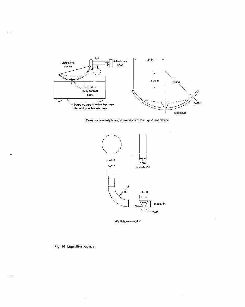
Adjustment

knob

- 1.84in.-

1 ” ~ shin;;;-&%” 1

Standard type: Hard rubber base

Harvard type: Micarta base

I Base cup

Construction details and dimensions of the Liquid limit device

:d AJ lcm

(0.3937 in.)

0.53 in.

L -

8ooW t 0.3937 in.

-

+llf%in.

ASTM grooving tool

Fig. 16 Liquid limit device.

Notes

40/l

84-040 LIQUID LIMIT Drop-Cone Penetrometer

.-

1. Application

1.1 The liquid limit is defined as the water content at which a cohesive soil ceases to behave as a semi solid material and reacts as a viscous fluid. It is the water content at which a polished stainless steel cone of a specific weight (80 g) and an angle of (30" + lo> will penetrate a specific distance (as determined from a calibration curve) when allowed to free fall for 5 seconds.

2. Apparatus

2.1 Drop-cone Penetrometer (ELE 24-055).

2.2 Metal cup (approximately 5.5 cm in diameter and 4.0 cm deep with the rim parallel to the flat base).

2.3 Spatula, metal (lo-15 cm in length, 2 cm wide).

2.4 Glass plate (minimum size, 25 cm square).

2.5 Plastic bags (small).

2.6 Moisture tins (100-200 mL).

2.7 Balance (sensitive to 0.01 g)*

2.8 Drying oven (capable of 105'G).

2.9 Syringe (10 mL).

3. Procedure

3.1 Inspect the drop-cone penetrometer (Figure 17) ensure that it is in good working order i.e.: the cone is clean, the tip is sharp (determined with the gauge supplied with the unit), the manual release button should not interfere with the plunger upon being released, and ensure that the knurled rack adjuster knob rotates smoothly.

3.2 Position the drop-cone penetrometer on a counter at a comfortable working height and adjust the unit level.

3.3 Weigh 200 g of less than 42sm air dry soil into a tared plastic bag.

3.4 Using a syringe, add a small amount of distilled water (5-10 mL) to the soil, mix thoroughly, continue this procedure until the soil reaches a semi-rigid consistency (just above the water content at which the plastic limit occurs).

40/2

3.5 Seal the plastic bag and allow the sample to equilibrate for 24 hours.

3.6 Remove the soil from the bag and place it on the glass plate, mix thoroughly.

3.7 Using the syringe t o add water 9 adj ust the soil mixture so that the first cone penetrat ion reading will be am Noximately 15 mm .

3.8 Using the spatula push the soil into the sample cup, taking care not to trap air bubbles or to work the mixture excessively (both air bubbles and excessive working will cause erroneous results).

3.9 Strike over the excess soil with the side of the spatula to give a smooth surface. (This is best achieved by tilting the top edge of the spatula forward and using a sawing action.)

3.10 Lower the cone (using the rack adjustor knob) so that it just touches the surface of the soil. Ensure that the cone can travel freely for a minimum distance of 30 mm. Adjust the penetrometer head if necessary. When the cone is in the correct position, a slight movement of the cup will just mark the surface of the soil. Adjust the pointer to zero.

3.11 Release the cone for a period of 5 seconds +l second. If the apparatus is not fitted with an automatic release and locking device take care not to jerk the apparatus during these operations. Both the action of releasing and locking of the cone must be instantaneous.

3.12 After th e cone has been locked in position lower the dial gauge to the new position of the cone shaft and note the reading to the nearest 0.1 mm. The difference between the readings at the beginning and end of the test is recorded as the cone penetrated.

3.13 Remove the cone from the cup and using the metal spatula remove lo-15 grams of soil from the area of penetration.

3.14 Remove the soil from the dish and remix with the soil on the glass plate, using the syringe add a small quantity of water l-2 mL (assuming the penetration value was approximately 15 mm, if it was greater than 20 mm allow the soil to dry); thoroughly mix the soil and allow it to equilibriate. The cup and cone should be thoroughly cleaned and dried at the end of each test.

3.15 Thoroughly remix the soil and repeat 3.8 - 3.13.

n

.A

3.16 Record the penetration value for the second trial and collect a moisture sample.

40/3

- 3.17 The r e a 1 t ionship between the water content of the soil and the depth of cone penetration, near the liquid limit value, is linear, therefore it is possible to predict the change in cone penetration which should result from the addition of a specific volume of water. It is suggested that the operator add sufficient water to the dry sample so as to increase the cone penetration reading to a position on the penetration curve which is slightly less than the liquid limit value. This procedure reduces the number of test readings required and thereby saves time.

3.18 Proceed from the drier to wetter condition, until a minimum of four penetration values have been obtained.

3.19 Plot the penetration values against moisture content and draw the best straight line through them.

3.20 Draw the calibration line on the same graph. This line is defined by a penetration of 20.5 mm at a moisture content of 25 per cent of 21 mm at a moisture content of 40 per cent of 22 mm at a moisture content of 72 percent and of 23 mm at a moisture content of 100 per cent.

3.21 The intersection of the penetration line and the calibration line gives the moisture content of the soil liquid limit. This liquid limit value corresponds to that obtained with the Casagrande apparatus.

4. Calculations

4.1 Calculate the water content (Wn) of the soil for each test as follows.

Wn-Wt of Tin plus wet Soil - Wt of Tin plus dry soil xloO Wt of Tin plus dry soil - Wt of Tin

Wn-Wt of water xl00 Wt of Oven dry soil

5. References

5.1 British Standards Institute. 1967. "Methods of testing soils for civil engineering purposes", British Standard 1377. London, England. 207 PP.

5.2 Engineering Laboratory Equipment Limited. "Penetrometer Test Frame EL 24-055 operating instructions", Hertfordshire, England. 10 pp.

C

Clamp

Spirit level

Fig. 17 Drop cone penetrometer.

--- -

84-041 PLASTIC LIMIT

1. Application

1.1 The plastic limit is defined as the water content below which a cohesive soil ceases to behave as a plastic material and reacts as a semi-solid. It is the lowest water content at which a thread of soil when rolled to a diameter of 3 mm (l/8,0 will just crumble (Bowles, 1979).

2. Apparatus

2.1 Glass plate (minimum size 25 cm square)

2.2 Balance (Sensitive to 0.01 g>

2.3 Moisture tins (small i.e: 10 mL)

2.4 Spatula (lo-15 cm in length)

2.5 Syringe (10 mL)

2.6 Plastic bags (small)

2.7 Evaporation dish (15 cm dia.)

2.8 Plastic wrap (Saran or a similar type)

2.9 Drying Oven (capable of 105'G)

3. Procedure

3.1 Weigh out 15 g of less than 425 pm air dry soil into a tared evaporation dish.

3.2 Using the syringe add distilled water and mix thoroughly until the mass becomes plastic enough to shape into a ball.

3.3 Place the sample in a piece of plastic equilibrate for several hours.

wrap and allow it to

3.4 If both liquid and plastic limits are required, it is recommended that a moist 15 g sample be taken from the thoroughly mixed portion of the soil sample which has been prepared in accordance with the liquid limit method.

3.5 The determination of Wp requires that the water content of the soil sample will initially have to be above the plastic limit. The water content is adjusted downward by working the ball of soil by hand until it no longer adheres to the fingers when pressed firmly.

4112

3.6 Roll the ball of soil into a 9-10 mm thread on the glass plate using the heel of the thumb or finger tips to apply the force (pressure).

3.7 Subdivide the thread and set one half of the soil aside.

3.8 Continue to roll the soil at a rate of 80-90 strokes per minute using light pressure until a 3 mm diameter thread is produced. Subdividing the thread when its length exceeds 15 cm, facilitates the rolling of a thread of uniform thickness.

3.9 Should the thread crumble before it reaches a diameter of 3 mm, discard the last thread and remould the remainder, add a small volume of distilled water, mix thoroughly; repeat 3.6-3.8.

3.10 Should the th read not crumble at a diameter of 3 mm, discard the last piece, remould the remainder into a ball, adjust the water content downward by working the sample in the hand; repeat 3.6-3.8.

3.11 The thread is at the plastic limit when surface checks (cracks) are apparent at a diameter of 3 mm and the thread will fracture without bending when held off the glass and a light pressure is applied.

3.12 Collect the pieces of soil which are at Wp as defined in 3.11 and place them in the moisture tins, weigh and record the values on the data sheet.

3.13 Repeat 3.6-3.12 on two additional threads for a total of 3 reps per soil sample.

3.14 Oven dry the samples for 24 hours at 105OC.

3.15 Cool the sealed moisture tins to room temperature, weigh and record the values on the data sheet.

4. Calculations

4.1 Calculate the plastic limit, which is expressed as the mass of the water to the mass of the oven-dry soil in percent.

Plastic limit (Wp) = Wt of water Wt. of oven dry soil

x 100

4.2 Average the Wp readings from reps 1, 2 and 3, record the plastic limit.

4.3 Plasticity Index (%)=(Liquid limit - Plastic limit)

-

NOTE the following exceptions

41/3

a> When the liquid and/or plastic limit cannot be determined the soil is non-plastic (NP) and is identified as such.

b) When the soil is high in percent sand or silt, the plastic limit test shall be made before the liquid limit test. If the plastic limit value cannot be determined 'Ido not" determine a liquid limit value record both as N.P.

cl When the plastic limit is equal to or greater than the liquid limit report the Plasticity index as N.P.

6. Precision

6.1 Insufficient data available

7. References

7.1 ASTM. 424-59.

7.2 Bowles, J.E. 1979. Physical and Geotechnical Properties of Soil. McGray-Hill Inc.

7.3 McKeague, J.A. 1978. Manual on Soil Sampling and Methods of Analysis 2nd Edition. Can. Sot. of Soil Sci. Suite 907, 151 Slater St., Ottawa, Ont.

Notes

42/l

84-042 SPECIFIC SURFACE AREA

1. Application

1.1 Physical and chemical properties of a material may be greatly influenced by the extent of its surface area. Soils differ markedly in surface area as a result of differences in texture, types of clay minerals, and amounts of organic matter. Such important properties as water retention and exchangeable cations have been shown to be highly correlated with the surface area of soils. For example, Ca-saturated clay fractions from some soils have surface area values that are 40% higher than the same fraction when Na-saturated.

The term "specific surface" refers to area per unit weight of soil or clay and is usually expressed in square meters per gram (m2per g.). The method for determining surface area is based on the principle that solid materials will absorb a monomolecular layer of a polar liquid.

2. Apparatus and Materials

2.1 25 cm. I.D. vacuum desiccators.

2.2 Aluminum moisture dishes (50 mm diameter x 23 mm high).

2.3 Drying trap containing drierite.

2.4 Oven.

2.5 Vacuum pump.

2.6 Analytical balance.

3. Reagents

3.1 Ethylene glycol monoethyl ether (EGME).

3.2 Phosphorous pentoxide, anhydrous.

3.3 Calcium chloride, anhydrous, granular.

3.4 Calcium sulphate, anhydrous (drierite).

4. Procedure

4.1 Place oven dried aluminum moisture dishes in an evacuated desiccator over fresh P2O5 for a few hours. Use fresh P2O5 for every other run for increased accuracy and speed.

-

42/2

4.2 Weigh about 1.1 g. of 35 mesh air dried soil samples in the dishes. Place dishes in desiccator, evacuate for 45 minutes with a vacuum pump and let stand overnight. Precision is increased and time saved by placing a maximum of 6 samples per 25 cm. I.D. desiccator. 35 mesh samples are used because it is a standard grind in this laboratory and surface area values are not greatly affected by different mesh sizes.

4.3 In the morning release the vacuum using a drying trap and weigh to the nearest 0.1 mg. Always use a drying trap while releasing vacuum to prevent adsorption of water which is also a polar liquid.

4.4 Re-evacuate for 45 minutes and weigh again before noon.

4.5 Repeat again in early afternoon. The weights should be constant (within 1 mg.) but if not repeat until constant.

4.6 As soon as a constant weight is attained add just enough EGME (l-2 ml) to form a soil-EGME slurry, cover the samples about 80% with the lids, place in a desiccator over CaC12 and allow to equilibrate for 30 minutes. Add the EGME as soon as a constant weight is attained to prevent adsorption of water. Adding just enough EGME and covering the samples prevents loss of sample if and when the EGME boils under high vacuum and spattering occurs. Also oven dry the CaC12 at about 150°C every week to destroy the EGME-CaC12 solvate and make the CaC12 more effective.

4.7 Evacuate the desiccator for 45 minutes and let stand overnight.

4.8 In the morning weigh the samples and re-evacuate for 45 minutes.

4.9 Repeat before noon and again in early afternoon. A constant weight (within 1 mg.) should b e attained but if not repeat until constant. Note that prolonged and repeated high evacuations of the EGME treated samples will give lower results because parts of the monomolecular layer will be removed.

5. Calculations

5.1 The total surface area for each sample is calculated by dividing the grams of adsorbate per gram of soil by 0.000286 g/cm2. Suppose 1.100 g of soil loses 21 mg over P2O5 and weighs 1.079 g. After the EGME treatment the sample weighs 1.109 g which means that there is 30 mg. of adsorbate on the sample. Therefore the surface area is .030 f 0.000286 = 97 m2/g. 1.079

4213

- 6. Precision and Accuracy

6.1 Surface area values range from less than 10 m2/g. for sandy soils to greater than 300 m2/g. for clay soils. Since 1 mg. of adsorbate represents a surface area of 3 m2/g., variabilit

3 of surface area

values in the range of 2025, lOO+lO and 200220 m /g. are considered very good. No known interlaboratory comparison of surface area values has been carried out.

7. References

7.1 McNeal, B.L. 1964. Effect of exchangeable cations on glycol retention by clay minerals. Soil Sci. 97: 96-102.

7.2 Heilman, M.D., Carter, D.L. and Gonzalez, C.L. 1965. The ethylene glycol monoethyl ether (EGME) technique for determining soil surface area. Soil Sci. 100: 409-413.

7.3 Carter, D.L., Heilman, M.D. and Gonzalez, C.L. 1965. Ethylene glycol monoethyl ether for determining surface area of silicate minerals. Soil Sci. 100: 356-360.

7.4 Cihacek, L.J. and Bremner, J.M. 1979. A simplified ethylene glycol monoethyl ether procedure for assessment of soil surface area. Soil Sci. SOC. Am. J. 43: 821-822.

-

Notes

----- ---- *

43/l

-.

84-043 FIBER CONTENT and PARTICLE SIZE DISTRIBUTION of organic soils.

1. Application

1.1 This method is applicable to the determination of total fiber content and the various size fractions of fiber contained in organic soils. It is done by wet sieving to avoid the drying effect on peat fiber.

2. Apparatus (Figure 18)

2.1 The apparatus consists of a cylinder with an interior diameter of 14.5 cm and a height of about 46 cm with a hole near the base for entry of air (A) and outlet of water (B).

2.2 A piece of rubber tubing about 1.5 cm in diameter and 45 cm long is formed into a ring (C) and placed at the bottom of the cylinder. A nest of sieves (10, 20, 40, 100 and 200 mesh), 13.5 cm in diameter is a assembled with a "gasket" (D) made from thin (2 mm) tygon tubing between sieves to provide a seal. The sieves are held together with an elastic band. The top of the cylinder is closed with a funnel (G).

2.3 Reciprocating shaker.

2.4 500 mL Erlenmeyer flask.

3.5 Drying cans.

2.6 Filter paper (coarse).

3. Reagents

3.1 None are required.

4. Procedure

4.1 Place 25 g of moist sample broken into small pieces, in 300 mL of water and shake the suspension for 16 hours. Determine the water content of duplicate 25 g samples by weighing, drying at 70°C and reweighing.

4.2 Pour the suspension onto a 200 mesh sieve and wash with water to remove the material finer than 200 mesh.

4*3 Assemble the apparatus and place the material retained on the 200 mesh sieve on the top sieve (10 mesh).

4.4 Fill the cylinder with water to just above the level of the screen in the top sieve.

-

4312

4.5 Introduce air through A at a rate sufficient to shake the nest of sieves and continue bubbling air through vigorously for 1 hr.

4.6 Remove the nest of sieves, recover the fibers remaining on each sieve by washing the fibers onto a funnel fitted with a coarse filter paper, dry the various fractions at 70°C and weigh.

5. Calculations

5.1 Calculate the proportion of the sample in each particle size range, as a percentage of the dry weight of the total sample.

6. Precision

6.1 Insufficient data available.

7. References

7.1 Dinel, H. and Levesque, M. 1976. Une technique simple pour l'analyse granulom&rique de la tourbe en milieu aqueaux. Can. J. Soil Sci. 56, 119-120.

-

-

C.

J--Y---L -1 i

]loow

A. Air Inlet B. Water Outlet C. Rubber Tubing, 1.5 cm diameter D. Tygon Tubing Gasket E. Water Level F. Path of Air G. Funnel

Fig. 18 Apparatus for particle size analysis and fiber content of peat.

Notes

A

44/l

84-044 FIBER CONTENT of organic soil (unrubbed and rubbed)

1. Application

1.1 This method provides a measure of the degree of decomposition of organic soil material. The syringe procedure for unrubbed and rubbed fiber can be used in the laboratory or in the field. This procedure is used in both Canada and the United States as a rapid method with adequate precision for most purposes.

2. Apparatus

2.1 Sieve, 100 mesh, 8 cm diameter

2.2 Modified plastic hypodermic syringe. The syringe is modified by cutting away half of the cylinder wall, in a longitudinal direction between the zero and the 5 mL marks. The plunger end, the needle end and the piston are not altered. Only those brands of syringes (e.g. Brunswick, Monojet) that have calibration marks embedded in the plastic are suitable for extended use.

2.3 Scissors, spatula, paper towelling.

3. Reagents

3.1 None required.

4. Procedure

4.1

4.1.1

4.1.2

4.1.3

4.1.4

4.2

4.2.1

Sample preparation

Place about 25 cm3 of moist sample on a strip of paper towel and form the sample into a cigar shape.

Roll up the sample in the paper towel and squeeze lightly to express surplus water. The objective is to dry the sample until it does not glisten but it is still very moist.

Unroll the towel and, using scissors, cut the sample into about 6 mm lengths.

Mix the cut-up sample to ensure random selection of sub-sample.

Unrubbed fiber content.

Pack the modified syringe adjusted to 5 mL capacity level full with sample pressing hard enough to express air but not water.

-

4412

4.2.2 Transfer all of the soil material in the syringe, using the rounded end of a 6 mm wide spatula, onto the 100 mesh sieve.

4.2.3 Wash the sample with cold water from a faucet adjusted to deliver about 400 mL in 5 seconds until the water passing through the sieve appears clean when observed against a white surface. Collect the sample together at one side of the sieve, and dry it by pressing a finger against the sample while holding a wad of paper towel against the bottom of the sieve.

4.2.4 Transfer the sample completely into the modified syringe and pack it level into the smallest volume by simultaneously pushing the syringe piston and levelling the surface with a spatula. Ensure that the water content is about the same as that of the initial sample (step 4.2.1). Water can be withdrawn if necessary by lightly pressing a piece of paper towel onto the sample surface.

4.2.5 Record the volume of the sample in the syringe.

4.2.6 Transfer the sample onto the 100 mesh sieve for the determination of rubbed fibber content.

4.3 Rubbed fiber content

4.3.1 Use the sample remaining after the unrubbed fiber content determination (step 4.2.6). Rub this sample lightly between thumb and finger(s) under a stream of water until the water passing through the sieve is clean as observed against a white surface.

NOTE: Clean fibers will roll between thumb and fingers like fragments of string rather than gliding or smearing.

4.3.2 Collect the sample together at one side of the sieve and dry it by pressing a finger against the sample while holding a wad of paper towel agaist the bottom of the sieve.

4.3.3 Transfer the sample residue completely to the modified syringe and pack it level as in step 4.2.4.

4.3.4 Record the volume of the sample in the syringe.

4.3.5 Discard the residue.

5. Calculations

5.1 Unrubbed fiber: Express the volume percentage of the initial volume.

recorded in step 4.2.5 as a

-

5.2 Rubbed fiber: Express the volume recorded in step 4.3.4 as a percentage of the initial volume.

ht.

4413

A 6. Precision

6.1 Insufficient data available.

7. References

7.1 Syringe method from unpublished procedure of W. Lynn, SCS, Lincoln, Nebraska.

-

---

Notes

-

__I__- - -- --.- -----.

45/l

84-045 LOSS on IGNITION

1. Application

t..

1.1 The loss in weight resulting from igniting a soil in contact with air includes that due to combined water in soil colloids, to combustion of organic matter and to decomposition of carbonates. The temperature recommended for determining loss on ignition varies depending upon the information desired. Weight loss at 550°C is approximately equal to the amount of organic matter in the sample, although the result obtained is usually somewhat higher than that determined from the amount of carbon present. Weight loss resulting from ignition at 850°C includes structural water and carbonates as well as organic matter. The latter temperature may be used in procedures for total analysis of a soil sample.

2. Apparatus

2.1 Muffle furnace.

2.2 Porcelain or vycor crucibles

3. Reagents

3.1 None are required.

4. Procedure (at 55OOC)

4.1 Weigh a suitable amount of sample ground to pass a 2 mm sieve into a tared porcelain or vycor crucible. Use less sample for organic soils.

4.2 Dry the sample overnight at 105OC and reweigh to determine the oven dry weight of the sample. Record this weight.

4.3 Place the crucible containing the oven dry sample in a muffle furnace. Heat slowly (increase temperature about 2OC/min.) to 550°C and continue heating at that temperature overnight.

4.4 Remove the crucible from the furnace , place it in a desiccator, cool, weigh and record weight.

NOTE: It has been determined that there is a loss of metals at temperatures higher than 550°C when compared to wet oxidation (perchloric acid) results. Organic matter is most effectively removed at 55OOC.

-

45/2

5. Calculations

5.1 Loss on Ignition at 550°C =

%=Weight of O.D. sample - weight of sample after ignition x 100 weight of O.D. sample

6. Precision

6.1 Insufficient data available

7. References

7.1 Atkinson, H.J., Giles, G.R., MacLean, A.J. and Wright, J.R. 1958. Chemical methods of soil analysis. Contrib. No. 169 (Revised), Chem. Div., Sci. Serv., CDA, Ottawa.

7.2 Ball, D.F. 1964. Loss on ignition as an estimate of organic matter and organic carbon in non calcareous soils. J. Soil Sci. 15, 84-92.

7.3 McKeague, J.A. Ed. 1978. Manual on soil sampling and methods of analysis 2nd edition. Can. Sot. Soil Sci., Suite 907, 151, Slater St., Ottawa, Ont.

46/l

.-

84-046 STEREO MICROSCOPE

1. Application

1.1 Examination of a soil sample under a stereomicroscope complements the description of the macromorphology of the horizon. Features such as the arrangement of fine peds, thin coatings on ped surfaces, and linings of the wall of voids become visible.

2. Apparatus and materials

2.1 Stereomicroscope 2.2 Tools such as macro spatulas, knives, needles for manipulating

the soil sample.

3. Reagents - none

4. Procedure

4.1

4.2

4.3

Obtain a relatively undisturbed soil sample. This may be a soil monolith including all horizons to the depth of lm, a Kubiena box sample (see 84-047) or a clod.

Examine the field-moist sample under a stereomicroscope and describe features of interest. Start at low magnification (approx. 10X) and proceed to higher magnification if required. For soil monoliths, it is convenient to use a Bausch and Lomb microscope 7 to 30X magnification, that slides on a horizontal arm. Dissect the sample to uncover fresh surfaces, or to expose the interior of peds as required. For very small features such as fungal hyphae it is convenient to use magnification of 50X or more. A Wild Macroscope (10 to 400X magnification) is convenient for the purpose.

Examine numerous fields before recording general features of the sample.

5. References

5.1 Brewer, R. 1964. Fabric and mineral analysis of soils. Wiley, New York.

-

Notes

-

--- --

47/l

84-047 THIN SECTIONS -

1. Application

.-

1.1 Examination of soil thin sections under a polarizing microscope allows the microscopist to see the size, shape and arrangement of solid particles and voids, and to determine, to a degree, the nature of mineral and organic particles. Thin sections are made by impregnating an 'undisturbed' soil sample with plastic, mounting a smooth surface on a glass slide, and grinding the soil down to a thickness of 25 to 30 pm. Soil thin sections can be made using equipment that ranges tremendously in sophistication and cost. Generally, the best results are obtained with good equipment but the skill of the technician is at least as important.

2. Apparatus and Materials

2.1 Kubiena boxes - made from galvanized iron about 20 gauge. The usual size is approximately 7.6 cm long by 6.5 cm wide and 5.0 cm high with open top and bottom; other sizes used are 8.6 x 6.5 x 3 cm and 6.5 x 4 x 3 cm.

2.2 Lids - plywood 8.5 x '7.0 x 0.5 cm (or appropriate sizes for larger or smaller boxes

2.3 200 mL waxed paper "coffee" cups 2.4 Ultrasonic cleaner 2.5 Fume hoods 2.6 Ovens 2.7 Diamond saws - large (50 cm) and small (20 cm) blades 2.8 Grinders and polishers 2.9 Grinding wheels fitted with diamond discs having grit sizes of

70 urn, 45 pm, 30 urn and 15 urn 2.10 Hot plate 2.11 Aluminum foil , plastic bags, pins, Styrofoam 2.12 Wide mouth plastic bottles approximately 12 cm diameter and 2

liter capacity, or plastic boxes of appropriate sizes for Kubiena boxes

2.13 Diamond pencil 2.14 Impregnation desiccator - 25 cm vacuum desiccator

modified to hold a 500 mL reservoir that will permit the addition of the plastic solution to the sample container which is under vacuum, Figure 19

2.15 Vacuum guage 2.16 Petrographic slides 2.17 Vacuum resectioning holder (Copeland, 1965) 2.18 Slide holder (Cochrane and King, 1957) 2.19 Nylon and Texmet polishing cloths 2.20 Plate glass 2.21 Polarizing microscope for checking thickness of section 2.22 Polarizing microscope equipped with accessories for

photomicrography.

-

.-.- . ---- --

3. Reagents

4712

3.1 Acetone - technical grade 3.2 Polyester resin (Canus C-32, available in Ottawa) 3.3 Catalyst - 60% methyl ethyl ketone peroxide in dimethyl

phthalate (Lupersol DDM, from Wallace and Tiernan) 3.4 Accelerator - 1% cobalt napthanate in styrene, dilute from 6%

which is commercially available 3.5 Petroleum ether - technical grade 3.6 Plastic solution - 2000 mL acetone, 2000 mL polyester resin, 1

mL catalyst and 0.2 mL accelerator. To avoid an explosion, mix in catalyst thoroughly before adding accelerator. For some studies such as pore analysis, a fluorescent chemical may be added to the resin. Uvitex OB (Ciba-Geigy) has been found suitable. (Solubility 2.0 g in 1000 mL acetone). Mix 2.0 g of Uvitex in the 2000 mL acetone then add to 2000 mL resin. Add catalyst and mix, then add accelerator.

3.7 Canada balsam neutral (Buehler) 3.8 Epoxy - Araldite 502 resin with hardener HY956 and styrene

(avoids bubbles), ratio 10:2:1. The proportion of styrene required depends on the kind of epoxy resin. Prepare immediately before use (Araldite and hardner are available from Ciba-Geigy)

3.9 Diamond paste 6 pm and 1 urn (Buehler) 3.10 Aluminum oxide 9 pm and 0.3 urn (Buehler) 3.11 Lapping Oil 3.12 Chloroform 3.13 Uvitex OB fluorescent dye (Ciba-Geigy)

4. Sampling for micromorphology

4.1 Site selection and description. It is of the utmost importance that the site and the soil be representative of the segment of the terrain that is to be studied. If soil maps are available, they should be used to select areas were the soil to be studied is dominant. Checking soil features at regular intervals along a transect through the area provides information on the variability of properties. Depending on the purpose of the work, the investigator may wish to include the full range of observed properties in the samples, or he may wish to focus on the site showing maximum or mean expression of the feature of interest. The basis of site selection should be included with a description of slope, aspect, vegetation and other site data (Day, ed. 1983). Ideally, the soil feature of interest should be sampled at a number of sites.

-,

4.2 Sampling for thin section preparation. The goal is to obtain undisturbed samples.

4.2.1

4.2.2

a)

b)

d

d)

4713

Use a Kubiena box to support the soil when taking the sample from the pedon. The size of the box depends upon soil properties and size of section described. For sampling organic soils with a Macaulay Auger plastic PVC tubing is suitable. The 3.75 cm PVC pipes are cut to obtain half cylinders of 15 cm lengths.

Prepare the face of the pedon by smoothing the surface. Push the box into the soil carefully to minimize the damage from stress cracks. The following approaches can be used: Hand pressure. The box is pushed slowly into the soil by using hand pressure. This is usually suitable for sands and very wet clays that offer little resistance. Knife. Cut (using an oblique angle) around the outside edges of the box to ease it in. Or, take a large clod and carefully cut the soil to fit into the box. This may be necessary for dense clays and organic layers that are very fibrous. Hydraulic Jack. Place a board (2" x 4") across the Kubiena box and apply pressure to push the box into the soil. This approach is often good for very dense clays with minimum disturbance resulting. Hammer. Place a board across the Kubiena box, and use a hammer to gently pound the box into the soil. This method can often lead to shattering of the structure, therefore it is not a preferred method.

When the front end of the box is even with the soil face (the box has been completely pushed into the soil), carefully cut the box out from the pedon using a sharp knife. Trim the soil level with sides of the box. Place the sample in a plastic bag to prevent moisture loss. Cover the open ends of the box with precut l/4" plywood lids. Wrap together tightly with masking tape and label (see 4.2.5).

4.2.3 For organic samples , place the plastic tube over the sample removed with the Macaulay Auger. Carefully cut the soil with a knife and slide the soil off the auger. Place the tube in a plastic bag, and cover with a piece of plywood (l/4"). Wrap tightly with masking tape and label (see 4.2.5).

4.2.4 Extremely dense and cemented horizons such as fragipans or duric horizons may be too hard to sample as described in 4.2.2. Also, some soils contain frequent large stones that interfere with the box as it is pushed. In these cases, clods (approx. 5 cm minimum dimension) should be removed from the soil and carefully wrapped in plastic and masking tape. For transporting long distances these clods should be packed in a box as protection against breaking.

4714

4.2.5 All samples (clods, Kubiena boxes, or plastic tubes) should have the following information marked on the container. a) Profile site number and soil name b) Horizon designation c> Depth from which sample was taken d) The direction to the soil surface. In addition, the

front of the Kubiena box (the exposed face of the pedal , and the compass orientation to which the profile face is exposed can be included.

4.2.6 Supporting environmental information about the pedon is as crucial as good sampling for the interpretation of the fabric. The following supporting data are highly recommended: a> Profile description (a soil survey form such as CanSIS

Soil Data File-Detailed Form or Canada Wetland Registry forms or similar form)

b) Sketch (draw to scale) of the soil profile with the locations of the samples noted

c> Environmental data - topography, vegetation, parent material

d) A bulk soil sample for determination of chemical and physical data.

4.2.7 For transportation of the samples long distances, use a heavy cardboard box, wooden crate or 5 gallon steel container. Fill any empty spaces remaining with Styrofoam packing material or paper so that the Kubiena boxes and/or clods are prevented from moving about during shipping and handling.

n

---N

5. Sample preparation for impregnation

Since polyester resins and epoxides are immiscible with water, water must be removed from the soil sample prior to impregnation. Two main methods are used: 1. Air drying and 2. Replacement with acetone. The choice of method will depend on the requirements of the study. Air drying may result in substantial shrinkage of the sample, and thus may be unsuitable for some studies requiring quantitative data for example, pore space analysis. Air drying is usually unsuitable for organic soil samples. Exchange with acetone is used in order to maintain the sample morphology close to field conditions, and thus provide greater confidence for quantitative characterization of the observed features. Murphy (1982) discusses the advantages of acetone-replacement of soil water for pore analysis studies in mineral soils.

5.1 Air drying

5.1.1 Place sample (Kubiena box or clod) into a tray for drying. A piece of tissue paper can be placed on surface to prevent dust accumulation.

<-

F

4715

5.1.2 Weigh the samples periodically until a constant weight is obtained.

5.2 Replacement with Acetone

5.2.1 5.2.1.1

5.2.1.2

5.2.1.3

5.2.1.4

5.2.1.5

a>

b)

c>

Capillary Exchange Place the sample on a heavy wire screen positioned over a stand (empty Kubiena tin 3 cm high) inside a glass container of appropriate size. Add acetone until the bottom of the sample is covered to a 5 mm depth. Cover the container tightly to prevent vapourization of the acetone. Exchange the acetone according to the following suggested sequence: 1, 2, 4, 8, 12, 16, 24, 32, . . . days after initial set-up. At each exchange test for the presence of water using one of the methods outlined below. For each method a standard curve of 1, 5, 10% distilled water in 100% acetone should be prepared using the same volumes used in the particular method.

Petroleum Ether: Add 10 mL of the acetone-soil solution to 40 mL petroleum ether in a graduated centrifuge tube. Shake for 30 seconds let stand for 3 hours. Observe any layering and record depth of layer. (If water is present, a layer at the base of the centrifuge tube will be visible). Compare to the standard curve. This method will detect water down to approximately 2% but the readings are not accurate. Thus it is suitable for the first few exchanges but not for later exchanges. Fitz Patrick (1980) describes this method of testing for water. Specific Gravity: Preweigh (4 decimal places) 10 mL culture tube and rubber stopper. Add 5 mL subsamples of the acetone-soil solution and weigh. Determine weight of acetone-soil solution and compare to standard curve. This method can determine the presence of water to less than 1%. It is suitable throughout the exchange process. NMR (Nuclear Magnetic Resonance): Take l-2 mL subsamples of the acetone-soil solution and place in NMR tubes. Determine % water in acetone using a nuclear magnetic resonance instrument that is set for determining the number of protons (H+) in the sample. Calculate the ratio of the peak heights that is, water: acetone for each sample. Calculate the % water using the standard curve. This method can determine the presence of water to less than 0.5% but it is somewhat more time consuming than the other methods.

47/6

5.2.1.6 When the water determined in the acetone-soil solution reaches 1% exchange for 3 additional times and determine water content. If water content remains less than 18, impregnate the sample.

5.2.2 Exchange by Immersion

5.2.2.1 In a glass container or tray, place the Kubiena box or stable clod on a heavy wire screen positioned over a stand.

5.2.2.2 Fill the container with 100% acetone until the top of the same is covered for 1 cm depth.

5.2.2.3 Tightly cover the container to prevent vapourization. 5.2.2.4 Exchange according to procedure outlined in Sec. 5.2.1

Steps 4 to 6. NOTE: This method is unsuitable for samples of very low bulk density (organic soils) as the samples will tend to float, or very sandy soils as the soil material may slake and slump severely.

5.2.3 Vapour Exchange 5.2.3.1

5.2.3.2

5.2.3.3

In a vacuum desiccator, place the sample on a heavy wire screen positioned over a dish. The dish will catch any liquid dripping from the sample. Add 100% acetone to the bottom of the desiccator so that there is at least a 5 cm space between the sample and the surface of the acetone. Replace the lid of the desiccator and exchange the acetone according to the procedure outlined in Sec. 5.2.1 Steps 4 to 6. NOTE: This method may be suitable for organic soils containing large amounts of soluble humic material.

6. Impregnating of Samples

6.1 Place samples in the modified desiccator (Fig. 19) for adding resin to the sample. For large sample containers, the rotating platform (9) is removed. If smaller containers are used, the rotating platform facilitates adding resin to more than one sample.

6.2 Place samples in desiccator and cover with lid and reservoir assembly. Fill reservoir (1) with plastic solution.

6.3 Evacuate the air in the entire system by using j-way stopcock (2) and approximately 50 cm mercury of vacuum (the building vacuum line is suitable).

6.4 Open the 2-way stopcock (11) and add the plastic solution very slowly down the side of the container to allow time for the sample to wet up by capillarity. When the sample is completely immersed close the 2-way stopcock (11). If more than one sample is placed in the desiccator, rotate the platform and repeat procedure.

4717

.-

7.

-

6.5 When all samples are immersed in the resin solution close stopcock (11) and release the vacuum using 3-way stopcock (2) and remove the samples.

6.6 Cover the samples tightly with lids to prevent vapourization of the acetone and rapid polymerization. Place samples in fume hood and keep covered for a minimum of two weeks. Longer or shorter times may be used depending on the size of sample and type of study. After the selected time period, remove the cover from the sample to allow the acetone to vapourize. Add resin solution as required to keep the sample immersed.

6.7 Note when the plastic has hardened completely, leave it at room temperature for 3 or 4 more days and then place the sample in an oven (with fume hood) at 50°C for 2 days. Remove from the oven and allow to cool. Remove sample from the container and cut into slabs for preparing thin sections or thick slices for macro-observations.

Preparing Thin Sections

7.1

7.2

7.3

7.4

7.5

7.6

7.7

Cut the impregnated sample with a large diamond saw using oil as the lubricant to obtain a few slabs about 1 cm thick. Thoroughly clean the slabs in an ultrasonic cleaner containing pretroleum ether. For samples that are not well impregnated, place the slabs on aluminum foil covered trays and coat the surface of the slabs with the plastic solution. Place in an oven at 50°C overnight. Remove the slabs from the oven and allow to cool. Using the small diamond saw and water as the lubricant, cut the slabs into chips of appropriate size for the dimensions of the thin section required. The usual size in this laboratory is 3.5 x 2.5 x 1 cm. Grind one side of each chip successively on 70, 45, 30 and 15 urn diamond laps to obtain a smooth, flat surface. Wash with water and dry with compressed air. Place the chip on a piece of aluminum foil marked with the sample number on a hot plate at 12OOC. Coat the heated chip with the epoxy mixture, remove from hot plate, place a clean, heated petrographic slide on the epoxy-covered chip and gently squeeze out air bubbles. Place the mounted chip on a sheet of styrofoam and hold the glass slide in place on the chip with pins. The epoxy cures completely in approximately 24 hours. Using a diamond pencil label the slide with the sample number and orientation. Place the mounted chip in the vacuum resectioning holder (Copeland, 1965) and saw off the excess soil with a small diamond saw; the remaining soil should be approximately 0.5 mm thick. Insert the slide in the holder (Cochrane and King, 1957) and grind the resectioned sample on diamond laps taking care to obtain a flat surface. Grind on the 70 pm lap only until the

47/S

sample becomes translucent. Next grind on the 45 pm lap and check under the polarizing microscope periodically; stop when quartz grains appear red under crossed nicols. Grind on the 30 pm lap until quartz appears yellow, and then on the 15 pm lap until quartz appears white to grey. In the later stages of grinding check under the polarizing microscope to ensure uniform thickness of the section. Clean the section in water in the ultrasonic cleaner, rinse, and dry with compressed air.

7.8 Place the slide on a hot plate set at 120°C and cover the thin section portion with neutral Canada balsam. Place a clean, moisture free (pass the glass slide through an alcohol flame) cover glass on the thin section and remove air bubbles from between cover glass and thin section using gentle pressure. Leave the section on the hot plate for 30 minutes. After cooling, the excess Canada balsam can be removed with chloroform. The slide can be touched up by using xylene to remove the chloroform-balsam stains. Label the bottom of the slide with sample number and orientation using a black pen. The thin section is now ready for microscopic study.

8. Microscopic Study of Thin Sections

The thin sections facilitate the description of the arrangement of the constituents as well as provide information on particular features and how these features are interrelated. Both qualitative and quantitative data can be obtained depending on the objective of the study. For example, evidence for translocation of materials may be obtained from the description and analysis of clay coatings (using EDXRA, Sec. 84-048). Characterization of the voids, their shape, size, arrangement may be undertaken and quantitative information obtained by using the thin sections together with computerized image analysis instruments.

8.1 For many purposes, a useful first step is to examine the entire thin section in one field and note the nature and distribution of major features. Distinctly different areas may be delineated. This examination may be done with a stereomicroscope at 5 x magnification or higher depending on the size of the section.

8.2 Study the whole section at low magnification (10 to 25X) with a polarizing microscope using both plane light and crossed nicols. Describe the features of the whole section or of distinct areas delineated (8.1) according to a system of description. Currently, the system of Bullock et al. (1984) is being tested. It involves description under the following headings: microstructure, basic components, groundmass, and pedofeatures. A description system for describing organic soils at low magnification has been outlined by Fox (1984). Formerly the system of Brewer (1964) including modifications by Brewer and Pawluk (1975) was used.

47/9

8.3 Study particular features of the thin section at higher magnifications, up to approximately 400X as required and complete the description. Magnification of 50 to 100X are commonly used for describing the fabric of fine materials (birefringence fabric).

8.4 If required, estimate or point count the area1 proportion of features such as nodules, clay coatings, or voids (Brewer, 1964).

8.5 If required, photograph features seen in thin section.

9. References

9.1

9.2

9.3

9.4

9.5

9.6

9.7

9.8

9.9

Brewer, R. 1964. Fabric and mineral analysis of soils. Wiley, New York. Brewer, R. and Pawluk, S. 1975. Investigations of some soils developed in hummocks of the Canadian sub-Arctic and southern-Arctic regions. 1. Morphology and Micromorphology. Can. J. Soil Sci. 55, 301-319. Bullock, P., Fedoroff, N., Jongerius, A., Stoops, G., Tursina, T. and Babel, U. 1984. Handbook for soil thin section description. Waine Research Publ., Woluerhampton, England. Cochrane, M. and King, A.G. 1957. Two new types of holders used in grinding thin sections. Amer. Mineral. 42, 422-425. Copeland, D.A. 1965. A simple apparatus for trimming thin sections. Amer. Mineral. 50, 1128-1130. Fitzpatrick, E.A. 1980. The Micromorphology of Soils. A manual for the preparation and description of thin sections of soils. Department of Soil Science, University of Aberdeen. Fox, C.A. 1984. A Morphometric system for describing the micromorphology of organic soils and organic layers. (Submitted to Can. J. Soil Sci.). Guertin, R. and Bourbeau, G.A. 1971. Dry grinding of soil thin sections. Can. J. Soil Sci. 51, 243-248. Innes, R.P. and Pluth, D.J. 1970. Thin section preparation using epoxy impregnation for petrographic and electron microprobe analysis. Soil Sci. Sot. Am. Proc. 34, 483-484.

9.10 Jongerius, A. and Heintzberger, G. 1973. The preparation of mammoth-sized thin sections. Soil Survey Papers, Neth. Soil Survey Inst. 1, 37 pp.

9.11 Miedema, R., Pape, T., and Van de Waal, G.J. 1974. A method to impregnate wet soil samples, producing high-quality thin sections. Neth. J. Agric. Sci. 22, 37-39.

9.12 Murphy, C.P. 1982. A comparative study of three methods of water removal prior to resin impregnation of two soils. J. Soil Sci. 33, 719-735.

1. Separatory funnel, 500 mL capacity 6 rubber stopper;

2. Three-way, T-shape stopcock, T4 glass stopcock;

3. Outer groundjoint and tube, T 5550, to fit desiccator sleeve;

4. Ball and socket ground joint with clip; 5. Teflon flat “0” ring, approx. 20 mm wide

by 250 mm I.D.; 6. Pyrex desiccator and cover with

T 55/38 sleeve, 250 mm I.D.; 7. Hot drink cup (200 mL) for soil samples

and plastic or 2 litre plastic bottle; 8. Vacuum tubing, 1 cm I.D.; 9. Remote control rotating platform;

10. Plastic T-joint, 1 cm O.D.; 11. Stopcock with T3 teflon plug;

Fig. 19 Apparatus for impregnation of soil samples.

-

48/l

84-048 SCAHNING ELECTRON MICROSCOPY APPLIED TO SOILS

-

1. Application

1.1 Study of soil fragments or of polished sections with the scanning electron microscope (SEMI is the final step in the sequence from macromorphological study of soil in the field, through morphological observations of soil samples at low magnification under the stereomicroscope, to study of thin sections, and finally to SEM. SEM makes possible the study of microfabrics involving particles and voids finer than approximately 5 pm (Smart and Tovey, 1982). Combined with energy dispersive X-ray analysis (EDXRA) it is a powerful tool for determining the elemental composition of soil features such as fine particles and thin coatings in situ (Bisdom, ed. 1980). --

2. Apparatus and Materials

2.1

2.2

2.3 2.4 2.5 2.6 2.7 2.8 2.9

Apparatus and materials for preparing thin sections are listed in 84-047. Nylon or Texmet polishing cloth, 6 urn and 1 pm diamond paste and 0.3 pm aluminum oxide Scanning electron microscope (Cambridge Stereoscan) Apparatus for carbon coating or gold coating of samples Energy dispersive X-ray analyser (Kevex 5100) Polaroid camera for photomicrography Polarizing miscrocope SEM stubs, silver cement Other materials such as marking pens, micro spatulas, etc.

3. Reagents - none

4. Procedure

4.1 Studying fabric of Qndisturbed' fragments 4.1.1 Select suitable fragments under a stereomicroscope to show

the feature of interest. For example, if a ped coating is to be studied, select fragments with the coating intact. Brush some of the fragments to expose a cross section of the coating on the coated matrix.

4.1.2 Dry the fragments and mount them with the surface of interest positioned upwards on 1 cm SEM stub. Use silver paste to cement the fragment to the stub. If the dry fragment is not coherent , partially impregnate it by allowing a suitable solution (agar, collodion) to soak in by capillarity, and cure.

4.1.3 Coat the fragment with carbon, gold, or both so as to prevent charging.

4.1.4 Study the fabric under the SEM at low (50X) to high (20,000X) magnification depending on the nature of the feature. To avoid bias, observe and photograph the feature at regular intervals along one or more transect across the feature. It is essential to examine the feature of interest in several fragments.

.--__- _-.

4812

4.2 SE&EDXRA of Polished Sections

4.2.1

4.2.2

4.2.3

4.2.4

4.2.5

4.2.6

4.2.7

Using normal procedures for thin section preparation (84.047), bring the slide to about 35 pm thickness. Clean in ultrasonic cleaner containing petroleum ether. Cover back of slide with a thin layer of grease or Vaseline and insert in holder. Using 9 urn aluminum oxide and distilled water on plate glass, bring the surface condition closer to the polishing stage. This should be done by hand and in a straight one direction movement. Thoroughly clean the sample and holder. Charge the nylon or Texmet polishing cloth with a 3-4 cm bead of 6 urn diamond paste. Place sample on polisher and run until surface appears to be flat and polished. Check about every 15 minutes. Always grind samples with similar hardness in groups. Use all three weights supplied with polisher during this step. After thorough cleaning, run sample for about 15 minutes using 1 pm diamond paste and two weights. After thorough cleaning polish sample for about 30 seconds using 0.3 urn aluminum oxide and distilled water. Use one weight during this step. The polishing cloth should have a thick nap similar to billiard cloth. Thoroughly clean sections and take to microscope for evaluation. The degree of polish depends almost entirely on the type of sample, polishing times, abrasive size, amount of abrasive, and polishing cloth type, and not the type of polisher. Study the polished section under the polarizing microscope and circle features to be analyzed using ink containing an element that will show clearly on the SEM (circle approximately 2 mm diameter, Koh-i-noor 3084F ink). Photograph the features of interest within the circle. cut out with a diamond saw approximately 1 cm2 of the section including the circled area, mount the sample on an SEM stub with silver cement and coat the chip with carbon, gold or both to prevent charging. Locate the circled area under the SEM and then locate features of interest with the aid of the photographs. Analyze several microareas within each feature by EDXRA and relate the spectra to those of suitable standards (McKeague and Wang, 1980).

5. References

5-l Bisdom,. E.B.A. (ed.) 1981. Submicroscopy of soils and weathered rocks. Pudoc. Wageningen.

5.2 McKeague, J.A. and C. Wang. 1980. Micromorphology and energy dispersive analysis of ortstein horizons of Podzolic soils from New Brunswick and Nova Scotia. Canada Can. J. Soil Sci. 60, g-21.

5.3 Smart, P. and N.K. Tovey. 1982. Electron microscopy of soils and sediments, techniques, Clarendon Press, Oxford.

I ^ --

49/l

84-049 SAND MINERALOG Y BY MICROSCOPY

1. Application

1.1 Determining the relative abundance of different sand sized minerals and their extent of weathering provides information on the nature of soil materials and on soil genesis. The most abundant sand-sized minerals in many soils are quartz and feldspars, both relatively resistant to weathering. These and other light minerals (specific gravity less than 2.9) are usually separated from the scarcer heavy mineral fraction that usually includes both readily weathered minerals such as olivine and highly resistant minerals such as zircon (Jackson and Sherman, 1953). Heavy mineral grains in a sample are identified and counted; weathering ratios are calculated by comparing the proportions of specific weatherable and stable minerals from different horizons.

A weathering index based on light minerals can be determined by comparing the proportions of relatively stable quartz to less stable feldspars in thin sections or in separated sand fractions.

2. Apparatus and Materials 2.1 Conical centrifuge tubes 2.2 Centrifuge 2.3 Funnels 2.4 Filter paper 2.5 Petrographic slides 2.6 Cover glasses 2.7 Etching Vessel

3. Reagents 3 -1 Tetrabromoethane 3.2 Dry ice - alcohol 3.3 Acetone 3.4 Canada balsam, neutral 3 -5 Hydrofluoric acid 3.6 Epoxy 3.7 Sodium cobaltinitrite 3.8 Barium chloride 5% 3.9 Amaranth Red

4. Procedure

4.1 Heavy Mineral Analysis

4.1.1 Place the cleaned fine sand fraction obtained from

4.1.2 mechanical analysis on a conical centrifuge tube. Add tetrabromoethane and mix well to "wet" all the grains in a fume hood when using tetrabromoethane.

4.1.3 Centrifuge for 10 minutes at about 510 G.

-_- .- _--~ .- --__. . .

4.1.4 Freeeze bottom of tube in dry ice - alcohol. 4.1.5 Filter off the light minerals and recover the

tetrabromoethane. Wash the light minerals well with acetone.

4.1.6 After thawing wash the heavy minerals with acetone. 4.1.7 To make a grain mount place about 1000 heavy mineral grains

on a petrographic slide. Place the slide on a hot plate at 120°C and "wet" the grains with Canada balsam. APPLY a cover glass. after 30 minutes remove the slide from the hot plate and allow to cool.

4.1.8 Quantify the heavy minerals by microscopy and if desired, calculate a weathering index. Refer to Brewer (1964) to determine the number of grain that must be counted for a given confidence level.

4.2 Light Mineral Analysis

4.2.1 Cement loose grains of light fraction to a petrographic slide with a thin layer of epoxy. Allow 24 hours for epoxy to harden.

4.2.2 Etch over HF fumes. Time depends on distance from sample and temperature of HF. Some procedures use boiling HF. This step should be carried out in a fume hood.

4.2.3 Immerse in saturated sodium cobaltinitrite solution for one minute. Rinse and blow dry with compressed air.

4.2.4 Immerse in 5% barium chloride solution for about 15 seconds. Rinse and dry.

4.2.5 Immerse in 1% amaranth red solution for 30 seconds to 3 rq,

minutes. Rinse and dry. Plagioclase feldspars are stained red, K-feldspars are stained yellow, and quartz is unaffected.

4.2.6 Quantify the light minerals on a microscope. The slide can be used as is or it can be covered with Canada balsam and a cover glass as per heavy mineral grain mounts.

4.2.7 Determine the weathering index (ratio of quartz to total feldspar& Indexes are only useful when comparing soils developed from the same parent material.

4.3 Other Specific Gravity Analysis

4.3.1 Volcanic ash, plant opal and sponge spicules can be separated from the light fraction by following the heavy mineral separation procedure but using a tetrabromoethane - benzene mixture of specific gravity 2.5. Opal etc. will float.

4913

5. References

5.1 Jackson, M.L. and Sherman, G.D. 1953. Chemical weathering of minerals in soils. Adv. Agron. 5, 221-309.

5.2 Krumbein, W.C. and Pettijohn, F.J. 1938. Manual of sedimentary petrography, Appleton-Century Crofts, New York.

5.3 Laniz, P.V., Stevens, R.E. and Norman, M.B. 1964. Staining of plagioclase feldspar and other minerals with F.D. and C. Red. No. 2, U.S. Geol. Surv. P.P. 501-B, B152-B153.

5.4 Milner, H.B., ed. 1962. Sedimentary petrography, 4th revised ed., MacMillen, New York, Vol. II.

5.5 Reeder, S.W. and McAllister, A.L. 1957. A staining method for the quantitative determination of feldspars in rocks and sands from soils. Can. J. Soil Sci., 37, 57-59.