DOT-HS806-494

DOT-TSC-NHTSA-83-5

•vf

Analytical Methods inMultivariate Highway SafetyExposure Data Estimation

Peter MengertEdwin Roberts

Transportation Systems CenterCambridge MA 02142

January 1984Final Report

This document is available to the publicthrough the National Technical InformationService, Springfield, Virginia 22161.

©US.Department of Transportation

National Highway Traffic SafetyAdministration

Office of Research and DevelopmentNational Center for Statistics and AnalysisWashington DC 205S0

NOTICE

This document is disseminated under the sponsorshipof the Department of Transportation in the interestof information exchange. The United States Government assumes no liability for its contents or usethereof.

NOTICE

The United States Government does not endorse products or manufacturers. Trade or manufacturers'names appear herein solely because they are considered essential to the object of this report.

t. Raport No.

DOT-HS806-494

4. Titlo «i4 Subtitle

2. Gavammant Aacasaion No.

ANALYTICAL METHODS IN MULTIVARIATE HIGHWAYSAFETY EXPOSURE DATA ESTIMATION

7. Author's.

P. Mengert and E. Roberts'• *•»*«!<«• Organ* soMoti Nan* and AddressU.S. Department of TransportationResearch and Special Programs AdministrationTransportation Systems CenterCambridge MA 02142

'2. Sponsoring Agoncy Nob* and AddressU.S. Department of TransportationNational Highway Traffic Safety AdministrationOffice of Research and DevelopmentNational Center for Statistics and AnalysisWashington DC 20590 7

IS. Supplatoentary Notos

16. Abstract

Technical Report Documentation Pag*3. Rscipiont's Catalog No. I

S. Raport Dot*

January 1984o. Perforating Organisation Coda

TSC/DTS-4S8. Performing Organisation Report No.

D0T-TSC-NHTSA-83-S10. Work Unit No. (TRAIS)HS470/R4418

11• Contract or Grant No.

13. Typeof Report end Period Covered

Final ReportOct. 1982-Nov. 1983

,4- Sponsoring AgencyCodaNRD-31

Three general analytical techniques which may be of use in"extending, enhancing, and combining highway accident exposure data areJ}™?8!-:*-™6 t!ch?iques are log-linear modelling, iterative proportional fitting and the expectation maximization (EM) method. A generaldiscussion identifies a number of frequently encountered exposure datadeficiences and indicates how one or more of the three analytical techniques may be of use in addressing each deficiency. The moremathematically-oriented sections provide a general introduction to each?5 lUi™ *• andAdlscu?s some of their properties of special interestin applications. A section illustrating applications to driving exposure data is included, together with computer program listings.

t7. Kay Words

Iterative Proportional Fitting,Log-Linear Modelling, ExpectationMaximization, Accident ExposureData (Highway), Categorical Data'2aiv!*s> Discrete Data Analysis,19. Security CUmU. (of thU report)

i

18. Oiarribution Statement

DOCUMENT IS AVAILABLE TO THE PUBLICTHROUGH THE NATIONAL TECHNICALINFORMATION SERVICE, SPRINGFIELD,VIRGINIA 22181

UNCLASSIFIED

20. Security Cloaaii. (of this poga)

UNCLASSIFIED

21. No. o» Pegaa

134

22. Priea

Foim DOT P 1700.7 (8-72) Reproduction of complotod page authorised

PREFACE

This report presents the results of the first year of researchon a task entitled "Analytical Alternatives to Multivariate Ex

posure Data Collection," conducted by the Transportation SystemsCenter (TSC) for the Mathematics Analysis Division of the National

Center for Statistics and Analysis under the Office of Research

and Development of the National Highway Traffic Safety Administration (NHTSA).

The authors thank Robert Arnold, the sponsor's technicalmonitor for useful suggestions and guidance.

iii

r*

<

ME

TR

ICC

ON

VE

RS

ION

FA

CT

OR

S

Ap

aia

xim

iti

Ccn

yir

uo

ni

laM

ali

kM

aa

taia

t

!,.

.,!

Wk.

aV

an«

...

Mul

tipl

ya>

Ta

Fil

lS

y.k

.l

ia • 1*

ia* ft MP

Ibtp

IIH

i

0"

I.1

LE

NG

TH

MC

ha

t•2

.»U

.IU

WIW

IC

m

Uo

l3

4C

MM

um

lifl

ca

t

ytf

df

11

(r-!;i:l

••

•ili

a1

.1

AR

EA

kil

am

ala

ra

Kyu

afa

ca

atu

na

lara

k™

ftfl

juar

aU

cfv«

»it

cm'

•o.u

4ia

loot

0.M

ao

ua

ram

vu

ib

MV

UI

VaW

att

•••

Ku

ki

ma

lata

i1

i-;-"n

wU

lM

•aa

alS

kil

tan

aa

aia

k~

J

•cta

i0

1ka

cla

ra

aka

MA

SS|w

ai|

at.

ou

ncet

it

BW

H•

po

un

d!

0.4

1kil

oo

rara

ak.

kti

O)l

lon

g0

.1lo

nA

aa

I

(20

00

lb}

VO

LU

ME

wll

iliU

fl••

•sp

oo

ns

t•4

ub

Utp

oo

ni

It

au

llil

ila

".

•1

flu

idO

UA

Cfl

M•u

llih

laia

-.1

Cu

p*

0.2

4M

ara

1

pm

IB0

.41

Msa

ta1

OjH

aHtl

0.H

lila

ia1

0«

llo

n»

l.t

PM

M

.>C

ub

ic(••!

0.0

1C

ub

icm

ala

ta

Cu

blC

Va

Ud

t0

.7J

Cu

bic

ma

lata

.'

TE

MP

ER

AT

UR

E|•

.act)

Fa

hia

nrta

il

I...

,.ril.fi

t/1

Nil

-.

au

bli

aclM

ig

m

Ca

laiu

a

IW

t•

«•-&

•|*

*A

kll

«|.

lie-

uM

xi

P.*

.I»

m.«

l.v

r-U

.•>!

ati

jMk

•"-,

U4

tJV

.-f»

.P

i.to

»•?2

4.

SOC

jA

ral

Mil

da

-le.l

ej

l*t.

l«..

.««

HA

SU

.v,

I*.a

t)I

.'*

..

lug

Nw

CO

IO^Io

.

2

Aa

sisi

iau

laC

aav

iiii

asi

liso

)M

ali

kM

aa

iuia

i

Sio

atl

Wh

»V

aaK

bsm

M.l

il.l

,a,

lafl

aa

IEN

6T

H

Ita

kil

k-1

ka I

•r

-1

0

•N

llH

MIM

I

C-

'

»q

UM

tC

afl

lwn

ala

ra

aq

uM

aM

MIM

I

l^u

ikll

on

al*

fa

kKW

U11

0.00

0•*

,

•.0

4

a.4 I.I

o.t

AR

EA

0.1

1

I.J

a.i

l.i

MA

SS

|xil

|kl|

pa

M

Maa

prao

au

wM

ilio

oo

ka

l

•ail

llli

lafa

Ham

in*

*.

lila

lB

CuC

MC

MM

jlM

t

Cu

kWC

M«

l

0.0

»

I.I

V0

1U

ME

00

)

2.1

l.o

a

a.2

*

3* 1

.1

TE

MP

ER

AT

UR

E(a

nd

)

Ca

laiu

a

lam

pa

ialu

ra

tYH

iha

a

«d

JM

l

r-^

Y-

14

0a

o

1I

'•'

Vft

tO|4

l-4

0

•C

•acka

a

lack*

a

l*a

t

yn

da

aii

laa

ao

ua

r*in

ca

aa

aoua

faya

rda

aqua

iafa

ilaa

acta

a

ou

nca

a

po

un

da

atu

al

Io

n.

llu

ido

un

ca

a

•m

ii

Qu

ail

a

oa

llo

na

cu

bic

laa

l

cu

bic

yard

a

farw

an

ha

it

Iwn

pa

rali

Ma

•F 21

2

20

0I

i.

H ir.'

IIS

I

•« 4'

TABLE OF CONTENTS

Section Page

1. INTRODUCTION 1-1

2. AN OVERVIEW OF EXPOSURE DATA PROBLEMS AND ANALYTICAL REMEDIES... 2-1

2.1 Counted Data Sets and Analytic Methods 2-32.2 Incomplete Classification of Exposure Data 2-52.3 Small Samples - Insufficient Cell Counts 2-72.4 Presence of Zero Cells 2-82.5 Levels of Variable(s) Missing 2-82.6 -Classification of Levels Variable(s) Not Consistent

Across Samples 2-92.7 Outliers 2-92.8 Exposure Data from Wrong Time or Place 2-10

3. DISCUSSION OF ANALYTICAL TECHNIQUES 3-1

3.1 Introduction 3-13.2 Log Linear Models 3-2

3.2.1 Definition 3-23.2.2 Maximum Likelihood Estimation Using IPF 3-43*2.3 Statistics for Goodness of Fit 3-53.2.4 Discussion of Problems Encountered in Applying Log

Linear Models to Continuous Data 3-8

3.3 Iterative Proportional Fitting (IPF) 3-11

3*3.1 General Discussion 3-113.3.2 Three Equivalent Formulations For IPF 3-133*3*3 Discussion on the Consequences of Formulation 1 of

IPF 3-143*3*4 Disoussion of the Consequences of Formulation 2 of

IPF 3-183*3*5 Discussion of the Consequences of Formulation 3 of

IPF 3-21

3*4 The EM Method 3-23

3*4.1 General 3-233.4.2 Application to Log Linear Models For Incompletely

Classified Data 3-253*4.3 Convergence and Uniqueness in Typical Examples 3-28

TABLE OF CONTENTS (CONT.)

Section Page

3.5 Properties of Techniques- inApplications 3-33

3.5.1 IPF 3-333*5.2 Log Linear Modelling 3-343.5.3 EM 3-34

3.6 Summry 3-36

4. COMPUTATIONAL EXAMPLES 4-1

4.1 Log Linear Modelllng-NPTS Data Set Applications 4-24.2 Synthesis of Multivariate Data Sets From Lower Dimensional

Data (CASE l-Dummy Core) 4-274.3 Synthesis of Multivariate Data Sets From Lower Dimensional

Data (CASE 2-Actual Core) 4-28

APPENDIX A - FURTHER DETAILS ON APPLICATION OF LOG LINEAR MODELS TO

CONTINUOUS DATA A-1

APPENDIX B - FEASIBLE AND INFEASIBLE MARGINAL CONDITIONS B-1

APPENDIX C - LISTINGS OF PROGRAMS C-1

REFERENCES R-l

vi

LIST OF ILLUSTRATIONS

Figure Page

1. Graph of A Function.... 3_20

2. Graph of A Function 4.3

•vii/viii

LIST OF TABLES

Table Page

1. DATA PROBLEMS AND REMEDIAL TECHNIQUES 2-2

2. DEFINITION OF VARIABLE LEVELS 4-3

3. 4-WAY TABLE OF VMT (BILLIONS) 4-4

4. THREE-DIMENSIONAL MARGIN: AGE, SEX, WEIGHT OF VEHICLE (ANNUALBILLIONS OF VMT, 1977 NPTS) 4-5

5. THREE-DIMENSIONAL MARGIN: AGE, SEX, YEAR OF MODEL (ANNUALBILLIONS OF VMT, 1977 NPTS) 4-6

6. THREE-DIMENSIONAL MARGIN: AGE OF DRIVER WEIGHT OF VEHICLE AND

YEAR OF MODEL (ANNUAL BILLIONS OF VMT, 1977 NPTS) 4-7

7. THREE-DIMENSIONAL MARGIN: SEX OF DRIVER, WEIGHT OF VEHICLE,AND YEAR OF MODEL 4-8

8. CELL ESTIMATES FROM LOG LINEAR MODEL BASED ON 3-DIMENSIONALMARGINS.: 4-9

9. TWO-DIMENSIONAL MARGINS (ANNUAL BILLIONS OF VMT, 1977 NPTS) 4-10

10. TWO-DIMENSIONAL MARGINS (ANNUAL BILLIONS OF VMT, 1977 NPTS) 4-11

11. CELL ESTIMATES, FROM A LOG LINEAR MODEL BASED ON 2-DIMENSIONALMARGINS 4-12

12. ONE-DIMENSIONAL MARGINS (ANNUAL BILLIONS OF VMT, 1977 NPTS) 4-13

13. CELL ESTIMATES FROM LOG LINEAR MODEL BASED ON 1-DIMENSIONALMARGINS 4-14

14. CHI-SQUARE, G2 AND DEGREES OF FREEDOM FOR THREE HOMOGENEOUSHIERARCHICAL LOG LINEAR MODELS 4-16

15. TWO-DIMENSIONAL MARGINS (PERCENTAGE DISTRIBUTIONS OF VMT) 4-18

16. 5-WAY OUTPUT FROM IPF (PERCENTAGE DISTRIBUTIONS OF VMT) 4-20

17. COMPARISON OF TABLES FOR AGE, TIME AND YEAR OF MODEL (PERCENTAGEDISTRIBUTIONS OF VMT) * 4-21

18. COMPARISON OF TABLES FOR SEX, AGE AND YEAR OF MODEL (PERCENTAGEDISTRIBUTIONS OF VMT)... 4-22

IX

LIST OF TABLES (CONT.)

Table Page

19. COMPARISONS OF 3-WAY TABLES FOR SEX, TIME AND YEAR OF MODEL(PERCENTAGE DISTRIBUTIONS OF VMT) 4-23

20. U.S. REGISTERED DRIVERS BY AGE AND SEX, 1975, 1979, 1980(1000*s) 4-24

21. .1975 SATURATED LOG-LINEAR MODEL 4-25

22. 1980 SATURATED LOG-LINEAR MODEL 4-25

23. 1980/1975 SATURATED LOG-LINEAR MODEL 4-26

24. DIFFERENCES IN INTERACTIONS 1980 MODEL MINUS 1980/1975 MODEL.... .4-26

25. CORE OF AGE-SEX DISTRIBUTIONS CORRESPONDING TO 1975 TABLESECOND ORDER INTERACTIONS ONLY 4-31

LIST OF ABBREVIATIONS

DF degrees of freedom

E-M (EM) Expectation - Maximization

FHWA Federal Highway Administration

IPF Iterative Proportional Fitting

LLM Log-Linear Modelling

NHTSA National Highway Traffio Safety Administration

NPTS Nationwide Personal Transportation Survey

TSC Transportation Systems Center

VMT Vehicle Miles Travelled

xi/xii

1. INTRODUCTION

This report presents the results of the first year of research on a task

entitled "Analytical Alternatives to Multivariate Exposure Data Collection,"

conduoted by the Transportation Systems Center (TSC) for the National Center

for Statistics and Analysis of the National Highway Traffic Safety

Administration (NHTSA).

Multivariate exposure data are used In conjunction with accident data to

produce estimates of accident rates for various subsets of highway use,

determined by different combinations of driver, vehicle, and road

characteristics, and environmental conditions. This type of detailed

information is particularly needed In crash avoidance and accident causation

analysis and can be used to oonfirm serious safety problem areas and to aid

In the evaluation of countermeasures. In contrast to the collection of

multivariate accident data, which is routinely done by reporting requirements

and follow-up studies, the collection of useful multivariate exposure data

usually requires the implementation of expensive, large-scale surveys. The

purpose of this task is to develop ways to use mathematical analysis to

obviate the need for primary collection of multivariate exposure data.

The specific goal of this research effort is to develop methods to

estimate needed "large" dimensional multivariate exposure tables from data

sources of smaller dimension and/or more limited context. In general,

existing multivariate exposure data are limited In geographic coverage or

time period, are generated from a small sample and are otherwise limited in

detail or accuracy. Often, exposure data of significantly different types or

non-exposure related data (e.g., census, registration, accident data) are all

that is available.

The key methodological problem is to expand and integrate the disparate

data sources to develop "best" estimates of multi-dimensional exposure tables

in ways which maintain relationships among data elements. Because there are

1-1

so many possible combinations of variables that could conceivably be of

interest, the research effort has focused on the development of statistically

sound and demonstrably valid methods rather than on the generation of a few

specific tables.

Section 2 "An Overview of Exposure Data Problems and Analytical

Remedies," provides an overview of the type of exposure data set that is

commonly used in traffic safety analysis, and of the common deficiencies

encountered In existing exposure data. A preliminary description is given of

the major analytical methods for treating such data problems, and there is

discussion of which methods may be most appropriate for particular problems.

Section 3 "Discussion of Analytical Techniques," is the heart of the

report, containing a detailed mathematical description of the major

analytical techniques, a summary of their properties derived from the

literature, and a description of new results, relevant to exposure data

analysis, which were discovered in the course of this research. Section 3

also contains a discussion of important statistical considerations in the

context of exposure data applications.

Section 4 contains some simple, preliminary examples of applications of

several techniques to exposure data.

1-2

2. AN OVERVIEW OF EXPOSURE DATA PROBLEMS AND ANALYTICAL REMEDIES

This section describes some of the common deficiencies encountered in

existing highway safety exposure data (i.e., VMT),» and a brief overview of

how oertaln analytical techniques might be used to Improve the situation. A

more extensive treatment of these techniques, their properties, and their

potential for mitigating exposure data problems is given in Section 3. Some

preliminary applications of these techniques to exposure data are shown in

Section 4. The major issues to be addressed in Section 2 are:

How existing exposure data fall short of fulfilling multivariate

exposure data needs.

Which analytical methods have potential for mitigating some of the

shortcomings in existing exposure data.

Which techniques are relevant to what data problems.

Table 1 displays a matrix whose row headings are a list of prototypical

problems which plague existing exposure data. The column headings refer to

mathematical techniques which seem to have the highest potential for

mitigating these problems. An X is entered in a cell where a particular

technique is believed to have application to a particular problem.

Section 2.1 provides a background description of the type of data sets

under consideration, and a brief overview of the principal relevant

analytical techniques. Sections 2.2 through 2.8 contain brief discussions of

each problem area and how the various techniques may be employed to mitigate

that problem.

•It has been assumed throughout this report that the exposure data measure ofinterest is vehicle miles travelled (VMT).

2-1

TABLE 1. DATA PROBLEMS AND REMEDIAL TECHNIQUES

Common \ Possible RemedialDefects/Deficiencies\ Techniquesin Multivariate >.

Exposure Data >

Log-Linear

ModellingIPF

E-M

Algorithm

1. Incomplete Classification ofExposure Data

X X

2. Small Samples - Insufficient CellCounts

X X

3* Presence of Zero Cells X X

4. Missing Levels (Categories) X

5. Classification of Levels

Inconsistent Across SamplesX

6. Incorrect Data X

7. Wrong Location or Timeframe X

2-2

2.1 COUNTED DATA SETS AND ANALYTIC METHODS

The data under consideration are known generically as "counted" data.

They are arranged in arrays, each cell of which contains the number of

individuals from an underlying population (or sample) classified by certain

characteristics. (Accident data generally conform to this type of data.

Exposure data also conform to the classification aspects of counted data, but

the cell entries (VMT) more closely resemble continuous data. More is said

in Section 3*2.4 regarding adjustments needed to apply the theory of oounted

data to exposure data.) The characteristics are described by means of

variables and levels of variables. For example, the population might be the

licensed drivers in a State. One variable might be gender, with levels male

and female. Another variable might be age, with levels 0-15, 15-35, 35-55,

over 55. A typical arrangement for such a two-variable set would be a 2x4

matrix whose rows correspond to the two levels of gender, whose columns

correspond to the four levels of age. In general, a k1xk2x...xk array is

an n-dimensional array whose ith. dimension has k. levels. In the following section, the terms

"core" and "margin" will be used frequently. By "core" we always mean a data

set (real or dummy) having the full set of variables (and usually the full

set of levels) of interest. "Margins" are defined as data sets that can be

derived from a core by summing over all the levels of one variable or all the

levels of several variables. For example, the margins of a matrix are the 2

one-idimensional arrays corresponding to the row sums and the column sums,

respectively. Note that we include under the term "margin," arrays whioh

correspond to a subset of variables and their levels of a particular core,

but have oell counts observed independently of that core. Thus, the cell

counts do not equal the cell counts of the corresponding margin summed from

the core. When it is necessary to distinguish such margins, they are

referred to as "exogenous" margins.

The following'mathematical techniques are briefly discussed below, in

order to provide background for the remainder of this Section: Log-linear

Modelling (LLM), Iterative Proportional Fitting (IPF) and Dempster's

Expectation-Maximization Algorithm (E-M). A thorough discussion of these

techniques, including their definitions and reference to prior literature, is

presented in Section 3.

2-3

Log-linear modelling is the most natural general method for fitting a

model to counted data: It can be used for data smoothing, including

estimating the value of zero cells, and for detecting outliers. (See Section

3.2 for a complete description).

IPF is a method of fitting a core to a set of (compatible) exogenous

margins. For example, in the two-dimensional case, given an nxm matrix M

with positive cell counts, an n-vector A and an m-vector B with positive

entries such that the sum of the entries of A equals the sum of the entries

of B, the procedure consists of alternately scaling: the rows of M so that

the new sums equal the corresponding entries of A, the columns of M so that

the column sums equal the corresponding entries of B. The procedure usually

converges when all the input arrays are positive. A complete description of

IPF, including properties of convergence, uniqueness of solutions and a

mathematical characterization of the qualitative relationship of the solution

to the input core is given in Section 3*3*

The E-M algorithm is a very general procedure for obtaining maximum

likelihood estimates of cell counts, due to Hartley* and Dempster.**6,(See

Seotion 3.4). Its application to our problems is a systematic way of pooling

different observations of the same data (in the form of cores and margins) by

a process that includes alternately estimating a log-linear model based on

the current expected values of the cell counts and updating the expected

value of the cell counts based on the current parameters of the model. A

complete technical description of the method and the result of our

investigation of such issues as convergence and uniqueness is given in

Section 3.4.

The sections below discuss the relevance of these techniques to the

various problem areas.

*See Reference 7.•f*See Reference 4.

2-4

2.2 INCOMPLETE CLASSIFICATION OF EXPOSURE DATA

In this case the situation is that exposure for the population of

interest needs to be (or is desired to be) classified, jointly, by a certain

set K of variables. However, each of the several existing samples is

classified aocording to some proper subset of K, so that there is no fully

classified sample. Let the number of variables by which a sample S is

classified be called the dimension of S, and suppose that the desired

dimension of a fully classified sample is k. In this case, there are

basically two analytical approaches to enhancing the data in a manner aimed

at approximating a fully classified sample. Both involve piecing together

the existing data sets (each of a dimension less than k) to form a data set

of dimension k.

In the first case:

Assume that unobserved interactions among variables are zero.

Iterative Proportional Fitting (IPF) can then be used to estimate the

completely classified sample using a k-dimensional (dummy) core of all 1's,

after adjusting the available data sets for use as (compatible) margins. The

Expectation-Maximization (E-M) algorithm can also be used in this case, if an

unsaturated* log-linear model (of order not greater than the dimension of the

largest sample) is used. As the theory described in Section 3.2.2 will

reveal, the former (IPF) approach actually results in the maximum likelihood

estimation of a log-linear model for any core having the given margins. As

discussed in Section 3.5, however, the latter approach (EM) is probably the

preferred method in this case.

In the second case:

Utilize information on the unobserved interactions from other

sources (e.g., a fully classified sample from another time or place). In

this case, the only apparently practical method is to fit the margins to a

•See Section 3*2 for definition.

2-5

core, containing interactions approximating the unobserved interactions, via

IPF. An interesting implication of the theory expounded in Section 3*3.3 is

that it is only these interactions (in the core) that have any effect on the

outcome of IPF, i.e., the given core could be replaced in the replaced in the

computation by a core with identical unobserved interactions and an arbitrary

set of interactions corresponding to the observed (in the margin)

interactions, and the outcome array of IPF will be the same. Thus, the

resulting data set will contain the interactions present in the margins

together with higher level interactions derived from the surrogate core.

(See Section 3.3.3 for a more detailed discussion.) The E-M algorithm could

be applied formally to obtain a unique solution in this case for the

saturated or unsaturated log-linear model, but it would not be clear what the

outcome of EM would mean. Hence, EM is not a desired method for this case.

Various complications can be present in all these cases due to basic

deficiencies in the available samples themselves. The major anticipated

problems appear to be: -

The core is unstable due to insufficient observations (cell

counts).

The core or marginal samples contain too many zero cells.

Certain levels (categories) of some variables were not observed in

the core or in some of the marginal samples.

Classification of levels for some variables is not consistent

across samples.

Incorrect data is present in one or more samples.

Completely classified data are available but from the wrong

location or time frame.

Each of these complications is a data deficiency in its own right, which

analytical methods may or may not be able to mitigate. Each is described in

more detail in the following sections.

2-6

2.3 SMALL SAMPLES - INSUFFICIENT CELL COUNTS

The situation is that a (fully classified) multivariate sample of

exposure (or accident) data consists of a small number of observations so

that, at least for desired levels of disaggregation, cell counts have

unacceptably large standard errors. There appear to be two possible

approaches to mitigating this problem:

(a) Fit an unsaturated log-linear model to the data set. While some

information (probably of dubious value due to the small sample) on

higher order interactions will be sacrificed, this process should

reduce the standard error in the cell counts.

(b) If marginal samples (incompletely classified observations) of

reasonably large size, from the same population, are available, the

E-M algorithm can be used to systematically combine the samples to

fit log-linear model.

Note the similarity between the situation discussed in this section and

the case of piecing together incompletely classified samples in the presence

of a fully classified core, described in section 2.2. The difference lies in

the following facts. In the former case, the focus of interest is on the

margins, which are the only direct observations of the population of

interest. The core plays the surrogate role of supplying subjectively

adequate estimates of interaction information missing from the marginal

samples. In this case there need be no statistical evidence that the core is

sampled from the same population as the margins. In the latter case, the

focus of interest is the core (which contains an insufficient number of

observations). The objective here is to find a valid way of pooling marginal

data to reduce the standard error of the core cells. In this case, it is

imperative to have evidence that the core and marginal samples belong to the

same population.

2-7

2.4. PRESENCE OF ZERO CELLS

Where cells in a multivariate table are not structural zeros (e.g., a

cell representing the number of motorcycles with weight = 4000 lbs.), a

sample may still have a zero cell count beoause of the combined effect of a

limited number of observations and a relatively small count for that cell in

the entire population. In this event it can be useful to have a technique

for estimating the correct relative count for that cell from the given

population. The fitting of an unsaturated log-linear model should give such

an estimate for zero cell counts. If marginal information is present, it may

be useful to fit an unsaturated log-linear model using the E-M algorithm.

Additional complications that can be caused by zeros in the core or

marginal samples are: failure of IPF to converge, and non-uniqueness of the

outcome of the E-M algorithm (dependence of the outcome on the starting

array). This indicates that, where IPF is used, considerable smoothing of

core and marginal tables by means of unsaturated log-linear models will

probably be required. (In the case of the E-M algorithm, the analogous

adjustment is to avoid the saturated model when too many zeros are present in

the input tables).

2.5. LEVELS OF VARIABLE(S) MISSING

This situation can best be illustrated by means of a (fictitious)

example: suppose that VMT is to be classified jointly by driver age and sex,

vehicle type, vehicle age and day vs. night. Suppose further that.there is

available a special study which observed all these variables, but only for

drivers under 24 years of age. The possible age categories for drivers over

24 are the "missing levels" for the variable called "driver age." This is an

incomplete data situation, one for which the E-M algorithm was designed.

Carrying the example a bit further, suppose that, for the population of

interest, VMT has been estimated by driver age and day/night Jointly, and

also by driver age and vehicle age jointly (for all levels of variables).

Theoretically, the E-M algorithm can be used to obtain maximum likelihood

estimates for the fully classified data set, using a saturated (or

2-8

unsaturated) log-linear model for those cells where age is less than 24 and

an unsaturated model for those cells where age is over 24. The extent to

which missing levels can be successfully mitigated by E-M or other analytical

techniques is not clear. After preliminary analysis as to whether such

problems might arise significantly in practice, the situation should be

carefully investigated, if warranted.

2.6 CLASSIFICATION OF LEVELS (I.E., BOUNDARIES OF CATEGORIES) FOR

VARIABLE(S) NOT CONSISTENT ACROSS SAMPLES

Resorting again to an example, suppose we have a fully classified

multivariate core of exposure data, (e.g., VMT), and suppose there are also

partially classified, independently observed margins. Suppose further that

one of the variables is driver age, and that the levels (in the margin) for

each sample are: 15-24, 25-40, 40-55, 55-65, over 65. Suppose that the

classification of driver age in the core is 15-24, 25-55, and over 55. This

. is a case where the classification of levels are incompatible but

commensurate, in fact the levels (categories) in the core are aggregates

(set-theoretic union) of the levels (categories) in the margins. The case

where levels are incommensurate as well as incompatible may be a more

difficult problem. This is illustrated by taking the marginal levels for

driver age as given in the example above, and supposing that the core has as

levels: 15-30, 30-45, 45-60, and over 60. The E-M algorithm is theoretically

capable of addressing the problem of commensurate incompatible levels, and we

feel it could be extended to cover the incommensurate case as well. As with

the problem described in section 2.5, it is not obvious how successful

analytical techniques might be in mitigating this problem, and the extent to

which this problem can be tolerated or corrected for.

2.7 OUTLIERS

The final type of problem.is the presence of errors in the data. One of

the established uses of log-linear models for categorical data tables (the

form of all data of interest in this study) is to detect outliers. This is

done by fitting.log-linear models to the data set of interest and checking

2-9

the relative goodness of fit of each cell. The usefulness of this cheok and

the determination of effective ways of dealing with detected outliers is an

area that may warrant some investigation.

2.8 EXPOSURE DATA FROM WRONG TIME OR PLACE

The situation is that partially classified (marginal) data sets exist

for the population of interest, and a fully classified data set (core) exists

for all the variables of interest, but the core is not from the same

population as the margins because the core is from an earlier time frame, or

a different geographic locale. This is a special occurence of the second

case described in Section 2.2, where IPF is recommended if the oore (i.e.,

the core interaction observed in the margins) is thought to be a reasonable

surrogate for the time or place of interests. Confidence in the outcome of

the result can be enhanoed by testing (if data are available) for stability

of the unobserved interaction over time or place.

2-10

3. DISCUSSION OF ANALYTICAL TECHNIQUES

3.1 INTRODUCTION

In this chapter three general analytical procedures for dealing with

categorical or cross-classified data are described and some of their

properties discussed. The three procedures are:

1. Log linear modeling

2. Iterative proporational fitting (IPF)

3. The expectation-maximization (EM) "algorithm"

The three procedures are related. Log linear modelling will be discussed

first since its concepts and techniques play a role in the other two. Each

of the three procedures involves similar concepts and will use some common

notation. They will all be discussed in terms of similar simple hypothetical

examples. •

The hypothetical examples will refer to a completely classified matrix Y^, •

of count data. The matrix Y^j^ is called count data sinoe it takes only non-

negative integral values, it is called completely classified since it gives a

count corresponding to specific values of each of the "variables" indicated

by 1 j and k (which are the entire set of variables in this three dimensional

example). Thus, variable 1 has been indexed by i, variable 2 by j and

variable 3 by k. Variable 1 could, for example, be driver age, variable 2

driver sex, and variable 3 could be vehicle type. Yjije could be a count of

vehicles classified by these three variables. Variable 1 will be assumed to

have the levels 1, 2, ..., I. This means that i can take on the values 1

through I. Variable 2 will have J levels (1 through J) and variable 3 will

have K levels. Less than completely classified data sets (or marginal data

sets) will also be of interest. For example, Rjj might be a table of countsclassified by only the first two variables (for each observation the third

variable is assumed unknown). Similarly Sjj will denote a table of counts

classified by only the third variable. The margins of Yjjk are also examples

of less than completely classified data. For example, Yjj+ will

3-1

represent the margin of Yjjk formed by summing over the third variable, k.

K

Thus *ij+s<fc'1Yijk • Other margins are similarly represented e.g.

Although the log linear modelling, IPF and EM procedures will be described in

this report in terms of a hypothetical 3 dimensional completely classified

matrix with one and two dimensional margins of interest, the techniques are

applicable to more general arrays with some unusual exceptions which will be

noted. It will be convenient to keep the notation simple to the greatest

possible extent but it should be borne in mind that the Y matrix could have

any number of subscripts, e.g.-, Y^^im and any number of these can be summed

over to provide marginal matrices of interest, e.g., 1^++!+.

3.2 LOG LINEAR.MODELS

Log linear models have received far more extensive treatment in literature

than the other analytical techniques reviewed In this report (IPF and EM).

Reference to the books by Bishop and Goodman (reference 1 and 2) is

sufficient to indicate the impressive literature on the subject. The

fundamentals are however essentially simple and are reviewed briefly below.

3.2.1 Definition .

Let Yijic denote a matrix of counted data i.e. each entry is an integer.

Further let ZjjjfsBCYijk) §and assume that Yijk is distributed as a Poissonrandom variable with mean Z±jk or as a multinominal random variable withY+++=Z+++=N and Pijk=zijk/N* Then a log linear model for Yijk corresponds

to a multiplicative form for Z^jic The saturated log linear model is of the

form

zijka aiVk6ij Vki*ijk 3-L(This is no restriction on Zjjfc.) The second order unsaturated model sets Jt^i/3!:

Zuk - aiVk 6ij *ik ♦ki-

•The notation "E( )" denotes the expected value of the quantity in the

parentheses.

3-2

The (homogeneous) first order unsaturated model states that in addition 6.

^k'^ki a11 e<»ual one 30: Zijfcs a.Q.y.. These are examples ofhierarchical log linear models, a term which will now be explained.

Consider the saturated model for Zjjk and take logarithms of both sides ofthe defining equation:

l08 Zijk =Uo+Ul(i)+U2(j)+U3(k)+U12(ij)+U23(jk)+O13(ik)+U123(ijk). 3'2

The U's in the above equation are indeterminate since there are a total of

1+1+J+K+IJ+JK+IK+IJK

of them while there are a total of UK of the quantities log Z^j^. The

ambiguity is resolved by requiring that any U summed over any of its

subscripts yields zero, e.g.

Ul(+) " 0>°12(i+) ". °' U123(+jk) = °- 6tC- . 3'3Then the U's. are completely determined by equation 3.2 and the zero summation

conditions. In what follows when any matrix is expressed in the form (3*2)

(with some of the U's possibly missing or set equal to zero) it is to be

understood that the zero summation conditions hold. With this notation

°123(ijk) measures the third order interaction (in Z±^) (or the "three

factor effect"). Similarly, for example, U23(jk) represents a specific two

factor effect and U«(i) a specific one factor effect.*

Hierarchical (log linear) models are characterized by the condition that

whenever an effect is zero, all higher order effects involving all the

variables in the zero effeot must also be zero.

•In this report the terms "interaction" and "effect" will be synomymous as

will "two factor effect" and "second order interaction." The term "two

factor effect" with respect to the model expressed by equation 3.2 will refer

to U-|2(ij) or U23(jic) or U^^jj) where for example, U«2(ij) represents aset of terms indexed by i and j.

3-3

For example,

loS Zijk =VUl(i)+U2(j)+U3(k)+012(ij)+U23(jk)is a hierarchical model. The key missing (zero) effect is U-|3(ik). Since it

is missing, U-|23(ijk) must De zero also. Consider also:

lo* Zijk ° Uo+Ul(i)+02(j;U3(k)+U12(iJ) • 3-*

this is also a hierarchical model since no low order effect is missing with a

higher order effect involving its variables present. Consideration of log

linear models in this report will be limited to hierarchical log linear

models. One example of a nonhierarchical model is given for illustration:

lo§ Zijk =Uo+Ul(i)+O2(j)+O13(jk)3.2.2 Maximum Likelihood Estimation Using IPF

Under the assumption of multlnomially distributed Yj.jk, a maximum likelihoodestimate of Zjjjj is obtained using Iterative Proportional Fitting or (IPF).

This process will be described in more generality in Section 3.3 but its

application to log linear models is described here.

To fit a given log linear model to Y^ i.e. to find a maximum likelihood

estimate of Z-jjjj given Yjjk, the procedure will be given. Xjjfc will denotethe estimate to be derived. Let the model* to be fit be given by

log Zijk = U0+U1(i)+U2(j)+U3(jc)+U12(ij) .

The procedure is as follows:

1. Form the margins of Y^ corresponding to the highest order effect

involving each variable. So in this case form Y++K (corresponding

to U3(i£)) and Yij+ (corresponding to Ui2(ij))*

2. Initialize the matrix which will be iteratively scaled to give the

final estimate of Xjj^ :

*A brief discussion will be given subsequently of the process of choosing amodel.

3-4

Set X^ -1

3. Scale to each margin successively and iterate the process:

(2n+l) (2n) (2n)

Set Xijk = «&&!&> Xijk

and then set

(2n+2) (2n+l) (2n+l)

ijk = (T++k^X4+k^ Xijkfor n = 0, 1, 2, 3, ...

4. When convergence is reached Xjjfc ±3 f0Und:

(Convergence is assured, see Section 3.3).

This prooess will be recognized as a special case of IPF. In the notation to

be used in Section 3.3 on IPF, Xijk represents the result of applying IPF toa core, in this case M^ = 1, with margins R^j s Yij+ and Sk s Y^*Incidentally, if structural zeroes are required in the model, they are

inserted into the matrix M^.

3.2.3 Statistics For Goodness of Fit

The fit of a log linear model is assessed by either the X2 or the G2

statistic using the appropriate number of degrees of freedom. Before

describing how to compute X^ and G the computation of the number of degreesof freedom is given.

Each term in a log linear model has a specific number of degrees of freedom

associated with it: e.g. U*2(ij) has (1-1)(J-1) degrees of freedom while

°123(ijk) has (1-1) (J-1) (K-1) degrees of freedom and ^(.jj) has K-1 degreesof freedom. The parameter U0 (e.g. in equation 3.2) has one degree of

freedom. The degrees of freedom for the model equals the sum of the degrees

of freedom of its terms. For example, consider the degrees of freedom (DF)

for the model in equation 3.4, i.e.

3-5

lo8 Zijk - Uo + Ul(i) + U2(j) + U3(k) + U12(ij) 3.5

For this model:

DF=1+(I-1) + (J-1) + (K-1) + (I-1)(J-1) - K+IJ-1 3.6

The statistic X or q ^g a ^^ square distribution with degrees of freedom

equal to UK minus the number of degrees of freedom in the model i.e.,

IJK-(K+IJ-1) = UK-K-IJ+1

in the preceding example.

2 2The definitions of G and X are as follows:

x2 =£ (xijk - Yijk>2/Xijk 3-7

G' "2S Yijk l08 <Xijk/Yijk> ,-3-8The sums are over all cells in the original data matrix, Y^j^, except, in the

case of G2, for cells where Yijfc . 0, in which case the contribution to G2

for those cells is zero.

If two models are under consideration and the second contains all the effects

that the first does plus one or more added effects, then a decision to choose

between them may be based on the difference in X2 (or G2) divided by the

difference in degrees of freedom. The more complex model is chosen if the

difference in X2 (G2) is statistically significant (too large to be

reasonably due to chance) for the given difference in degrees of freedom.

The difference in X2 (G2) will have a chi square distribution with degrees of

freedom equal to the difference of degrees of freedom of the models [under

the null hypothesis that the extra effects in the more complex model are not

needed (i.e. have the value zero)].

The process of log linear modelling consists of these steps:

3-6

1. Select a set of candidate log linear models.

2. Fit the selected models to the data.

3. Drop from consideration any model whioh is:

a. a special case (i.e. a restriction) of a more complex model which

has a significantly smaller X2 (G2);

b. an extension of a simpler model which does not have a significantly

larger X2 (G2).

4. Consider additional models which contain more effects as suggested by

the effects present in the retained models.

In summary, the key tools for estimating and evaluating log linear models

are:

1. Margin building.

2. IPF.

2 23. Computation of G and/or X

3-7

3.2.4 Discussion of Problems Encountered in Applying Log Linear Models to

Continuous Data

In general, when exposure is to be calculated, the sum of VMT over each cell

is the variable of interest. This is not a "counted" variable as required in

the development of the standard statistical techiques for log linear models.

The cumulative VMT in a cell is not a count variable both because it is a

cell sum of a (practically) continuous quantity and because sample weighting

factors are applied (in the case of NPTS data at least). Even if trips were

analyzed instead of VMT, the individual trips would not be independent (in

the case of the NPTS data) and hence the assumptions needed in the

development of standard statistical techniques for log linear models would

not be satisfied. In general, standard discrete multivariate statistical

modelling techniques are developed under assumptions not satisfied by VMT

data.

In this section, the log linear modelling problem is considered from a point

of view which recognizes that the cell measures Involved in some cases (in

particular, VMT) are not counts but instead sums of random numbers of terms

each of which is positive and for practical purposes continuously distributed

(the individual terms may be weighted trip lengths for example).

The problem is then how to model VMT cross-classified by several variables.

Clearly log linear models provide a useful mathematical form for describing

cumulative VMT classified, for example, by driver, vehicle, roadway and

environment classes. This is because log linear models are useful for

describing non-negative quantities in which a multiplicative model for the

joint effects of factors is of interest. In short, the log linear model

structure is just as useful whether the quantity in each cell is a cumulative

sum (of continuous terms) or is instead a cumulative count.

Other aspects of the log linear modelling process as developed for count data

are problematic however. In particular, the maximum likelihood method for

fitting the model must be examined and the statistical criteria for model

adequacy must also be examined.

3-8

With regard to the method of fitting the model, two questions need to be

addressed:

1. What is the form of the likelihood in the case of continuous cell

sums instead of cell counts, and to what extent is maximizing it

approximately accomplished by the olassical discrete method.

2. Is the classical fitting method useful in providing satisfactory

fits in the more general continuous case?

In Appendix A it is shown that the olassical fitting method (i.e. applying

IPF to margins as done in the log linear modelling process) leads to log

linear models fit to the data according to a closeness of fit criterion which

is reasonable and this is independent of the statistical properties of the

data. This is a situation analogous to the application of linear regression

in cases where the statistical properties assumed for the residuals do not

hold (even though a linear relationship' between the variables is postulated).

The question of whether the fitted model remains a maximum likelihood

estimate is examined and it is concluded that a maximum liklihood estimate is

obtained if these assumptions hold:

1. The cell sums of VMT are normally distributed (this will be so if

each cell sum is over many records).

2. The ratio of variance to mean is constant across cells.

Assumption 1 is probably valid to the necessary degree. Assumption 2

probably is not valid to a substantial degree. However, if the two

assumptions were valid, the ohi square statistics obtained in the course of

the standard log linear modelling process could be modified by a single

factor (the same for any model based on the initial data) easily calculated

from the original data. The factor can be calculated in any case by the

formula given in Appendix A. The validity of such a calculation is discussed

in Appendix A.

3-9

Since log linear models are appropriate in the continuous case (e.g. when

cell values are VMT) and since the classical method of estimating log linear

models (developed for the discrete case) leads to models of closest fit by a

reasonable criterion, the chief weakness of applying the classical or

standard method in the general case is the problematic nature of the

statistical fit criterion (chl square values in the classical case) used to

decide what degree of model complexity is justified by the data. It should

be noted that except where the assumptions needed to make the classical

approach give true maximum likelihood estimates in the general case hold, it

appears to be a nearly impossible job to develop methods for produoing true

maximum likelihood estimates in the general situation. This point is brought

out in Appendix A.

It is concluded that log linear models will remain of great interest in the

general case. It is also likely that they may effectively be estimated using

the classical method of applying IPF to selected margins. However, the

statistical criterion used in model development based on chi square

statistics will need to be modified. The modified version (as described in

Appendix A) may not be entirely satisfactory in all cases. Other methods for

assessing statistical stability suoh as the jackknlfe and infinitesimal

jackknlfe* techniques or other methods based on split samples may be of use.

If a general robust method for assessing statistical stability is developed,

it can be used in conjunction with the modified chi square (i.e. chi square

multiplied by the correction factor) to gain experience on the validity of

the latter (which should be much easier to use than general robust methods).

•See Reference 8.

3-10

3.3 ITERATIVE PROPORTIONAL FITTING (IPF)

The second analytical technique to be dealt with in this report is

Iterative Proportional Fitting or IPF. It can be a useful technique when

marginal data id available relating to the oontext of interest and complete

data is available relating to a somewhat different oontext. The analytical

technique and some of its properties will be discussed in this section.

3.3.1 General Discussion

In IPF, a completely classified matrix (of any number of dimensions) is

initialized to some "core" matrix which determines the high order

interactions. In the course of the computation, the matrix is successively

scaled to match in turn each of a set of marginal matrices and the scaling

. process is repeated (i.e., iterated) until it converges. The resulting

matrix matches each of the marginal matrices and as noted has its higher

order interactions determined by the initial core matrix.

In the next section, three equivalent formulations of IPF will be given,

utilizing a representative hypothetical example similar to the one

considered in Section 3*2

Various properties of the IPF technique will be discussed in relation to one

or another of the equivalent formulations.

Before proceeding to give the three equivalent formulations, the procedure

will be defined in the usual way by describing the computational process

involved. This will be the same as the third of the equivalent formulations

to be given in the next section. The technique is illustrated in terms of

the representative example:

Suppose Mjjk is given as the (initial) core matrix and Rjj and S^ aregiven as marginal matrices. The result of the IPF process applied to

these data will be denoted by the matrix X^j^. Let Xjj^ denote the

value at the initial step. By definition of the IPF process X^jfc =Mijk« Then the current Xjjfc matrix is scaled to each of the margins in

turn and the scaling process is repeated until convergence is obtained

3-U

(below there will be a discussion of oases where convergence is not

obtained). Suppose that X^j*. is to match Rj.j and X++ie is to match S^.This is achieved through repetitively scaling the X^j^ matrix until

agreement with both incompletely classified or margined matrices (i.e.

Rij and Sfc) is reached (to a prespecified accuracy).

An algebraic formulation of the process is as follows:

1. Set xfjfc" sMiJk (for all values of i, j, k)

2. For each n in turn (starting with n=0) update X^ as follows:

Set

(2n+l) (2n) (2n)

Xijk ' Xijk (Rij/XlJ+>then set

(2n+2) (2n+l) (2n+l)

Xijk " Xijk (Sk/X++k)(repeat for n=0, 1, 2, ..., etc.)

3* xijk oonverges to Xijk:

(n)

£ Xijk "Xijk

(Cases under which convergence may not occur are discussed below.)

3-12

3.3.2 Three Equivalent Formulations for IPF

IPF as described in the previous section is equivalent to two other

formulations given here. In the statement of the theorem below the previous

formulation is repeated for completness. The problem statements define the

same problem in the sense that each calls for finding a matrix* which has

certain properties, satifies certain conditions, and/or is constructed in a

certain way. Eaoh of the three formulations leads to the same matrix Xjjic(or else none of the problems can be solved due to infeasible conditions).

The three formulations are as follows:

Formulation 1: Find Xjjfc of the form Xijk = aij 6^ M^such that

Xij+ " Rij

X++k - hFormulation 2:** Find X which minimizes

F(- " £k (x«k l08e (x^/lV "x^subject to the constraints:

Xijk a Rij

XfHe B Sk

Xijk >°"Formulation 3: Find

xw= iS Xi"kwhere

X(0) o MXijk = Mijk

•The formulations are given in terms of the standard example but allstatements carry over to more general dimensionalities except where noted.

••See, e.g., Referenoe 3.

3-13

and

(2n+l) (2n) (2n+2) (2n+l) (2n+l)

Xijk =Xijk VXij+'lXijk ' Xijk Wk for n - O'1'2. •••

(Formulation 3 is merely the formulation given in the previous section.)

3.3.3 Discussion on the Consequences of Formulation 1 of IPF

Formulation 1states that Xjjfc = MijjcaijSic where aij and 6k are uniquelydetermined by the margin conditions (Xij+ 3 Rj^ x^ s Sfc) (The uniquenessis a property of IPF addressed in Section 3.3.4).

Some consequences of this formulation of IPF related to log linear models

will now be noted. In order to state these consequences precisely, define the

following saturated log linear models:

Let

+ UM + DM 'U13(ik) + °123(ijk)

log R±j -Uj +UR(±) +0*(J) +UR(ij)

log Sfc =Uo +u|(fc) 3.11

lo* Xijka0o +U£(i) +%) +^(k) +UL(ij)

+°2X3(jk) +Ul3(ik) +U123(ijk) 3'12

The interactions in Mijjj which do not correspond to any interactions in Rijor Sfc will be called "margin-absent" interactions (or effects)'.* Thus, the

last three terms in equation 3.9 represent margin-absent effects. The

effects in M^j^ which correspond to effects represented in one or more of the

data margins will be called "margin-present" effects. Thus the first five

terms in equation 3.9 represent margin-present effects. In general, the

margin-absent effects are higher order effects based on factors whose lower

order effects are margin-present effects. (Thus the margin-absent effects

•The term "effect" is synonymous with "interaction" (see Section 3.2.1).

3-14

3.9

3.10

can be spoken of loosely as higher order effects and margin-present effects

as lower order effects.) The first characteristic of IPF to be observed is:

1. The result, Xijk, of performing IPF with core data Mijk and margin data

Rij and Sk does not depend on the margin-present effects in Mijk* That

is, if the margin-present effects in Mijk are changed in any way, the

result, Xijk, is unchanged.

2. The second observation is:

The margin-absent effects in Xijk are equal to the margin-absent effects

in Mijk* (Roughly speaking, the higher order interactions in theinitial core are preserved intact.)

To these observations, a third obvious one may be added:

3. The margins of Xijk are equal to the corresponding marginal data

matrices (Rij and Sk respectively).

Properties 1, 2, and 3 are characteristic of IPF. Any procedure

characterized by properties 2 and 3 is equivalent $o IPF. The importance of

the properties lies in the fact that oores for IPF are characterized

completely by their margin-absent effects. The margin absent effects of a

matrix can be isolated and compared to those of another matrix to determine

if they are equivalent for use in IPF. Each matrix Mijk can be converted to

a reduced matrix M^ where log Mijk equals the sum of the terms In 3.9corresponding to margin-absent effects. Then Mijk does not contain (non zero

values for) the margin-present effects and so represents an equivalent core

to Mijk which can be compared to the reduced matrix of another core matrix.

The remainder of this seotion is devoted to brief outline of the proof of the

assertions regarding the characteristics of IPF given earlier in this

section.

The second stated property (margin-absent effects in the core are preserved)

will be derived first:

Since Xijk =°<ij|SkMijk.

3-15

we have:

and

log xijk =uj +ux(i) +ux(j) +ux(k) +„x2(±i) +0x3(jfc)

+U13(ik) +U123(ijk) "lQ8 aij +lo* 6k +%

+U?(i)+^(j)+U^(k)+U?2(ij)

u23(jk) 13(ik) U123(ijk)

log ^ =l£ +»«(k)

Then effects of various types must be equal individually* so that e.g. Uq

U0 +uj +uj and in particular UX23(ijk) s0l23(ijk)ttX a ir^ nX = rr*U23(jk) U23(jk), U13(ik) °13(ik)

which state the equality of the margin-absent effeots in Xijk and Mijk

(property 2).

The first property (that margin-present effects in the core are completely

inconsequential) is derived as follows:

Let M^jk be like Mijk in its margin-absent effects but different in itsmargin-present effects.

Then

l0« Mijk- < +<d +<j) +<k) +"Saj) 3nJI' .M' -M'

+U23(jk) + °13(ik) + ri23(ijk)

•Since the representation of a positive matrix as a saturated log linearmodel is unique.

3-16

where the last three terms of log M'... equal the corresponding terms of

log M k but the other terms are different. Then

log M'ijk - log M±jk + a±i +bk

where a^j and bk are arbitrary.

Let X'ijk =c^ 6k M'ijk

and X'ij+ - Rtj and X'^ - Sk

Then since*

M'ijk° MljkexP(aij)exp(bk)

we have

^jk^'ij e*p (aij)ekexP (VMijk

By the uniqueness of IPF (and since X'. is now expressed in the form o^B, M,,, )ijk r ij k ijk

we must have

X,ijk " Xijk «*»That properties 2 and 3 characterize IPF may be shown as follows:

Let X'ijk be a matrix characterized by properties 2 and 3 i.e. such that

x'ij+ = Rj and X'++k = Sk and such that the margin-absent effects in X'ijk

are the same as those in Mijk. Then X'ijk !^. e. Mijkij k

and by the uniqueness property of IPF, X'ijk = xijk*

•Notation: exp (x) = ex

3-17

3.3.4 Discussion of the Consequences of Formulation 2 of IPF

Formulation 2 may be called the mathematical programming formulation. It

constitutes an-optimization problem with a strictly convex objective function

and linear constraints. Let

f(u) = u loge u - u. 3.14

Then the mathematical programming formulation is:

Min £ Mrst f(Xrst/Mrst> (a F(£» 3-"x rst

subject to the constraints

Xij+ " Rij

X++k - Sk 3.16

Xijk 1 °

(This assumes Mijk > 0; some modifications in the following observations areneeded if any of the Mijk are zero. IPF is not recommended in such a caseunless it is a structural zero.)

It is easy to show that F is strictly convex in the Xr3fc's (since d2f(u)/du2 <0).

A mathematical programming problem with linear constraints and a strictly

convex objective function either has a unique solution or else is infeaslble

(i.e. the constraints cannot be satisfied) and has no solution. This shows

that there is a unique solution to IPF- (convergence of the IPF algorithm will

be dealt with In Section 3.3*5) so long as the margins are feasible.

Unfortunately it is possible to have infeaslble margins either because they

are incompatible {e.g. if R++?'S+) or essentially infeaslble, i.e. compatible

but still infeaslble. The latter condition is dealt with in Section 3.3.5 and

in in Appendix B. It is not expected to be a common problem. In any case,

there can be no more than one solution to any of the three equivalent

formulations of IPF.

3-18

The math programming formulation thus provides a useful assurance of

uniqueness of the solution as well as an indication of the importance (and •

sufficiency) of feasibiltiy.

Perhaps more Important is the characterization provided of the meaning of the

result of the IPF procedure. Figure 1 shows a plot of f(u) vs. u. It has a

minimum at u = 1. Thus minimizing the objective function F (X), consists in

drivng Xijk as olose as possible to Mijk, subject to the marginal constraints.Other objeotive functions can be proposed with the same constraints, but the

resulting formulations are not necessarily equivalent to IPF. Examples of

different objective functions with the same constraints (i.e. those in 3.16)

leading to procedures different from IPF include an example in reference 3 and

a special case of EM given in Section 3.4.3.

3-19

2r-

f(x)=xlogx-x

CJ

o

FIGURE1.GRAPHOFAFUNCTION

3-3.5 Dlsoussion of the Consequences of Formulation 3 of IPF

Formulation 3 is simply the specification of the calculation procedure as

given in Section 3.3.1. A convergence proof is given in Reference 1 (Bishop

et al). The proof given there is for the case of IPF used to fit log linearmodels, but appears to be extendable to the case of general IPF if the

assumption of the existence of a feasible solution is included (Reference to

other proofs may be found in Reference 1 and Reference 6).

Appendix B discusses the general problem of oriteria for the existence of

feasible solutions. An example of compatible but infeaslble margins is giventhere.

In practice convergence will take place quickly (in the IPF procedure) if the

margins are feasible. Convergence is characterized by the condition that(n)

xljk» fop sufficiently large n stops changing to any appreciable extent i.e.

,„(n+d) (n),'xijk " xijk'

is very small ford- 1, 2, 3, ....*

If the margins are infeaslble, x£}kwill cycle Instead of converging** The. length of the oycle is equal to the number of margins being scaled to. In the

example where two margins are being scaled to this means that Ix^2- Xijklisvery small but IXijk -Xijkl is not small. The matrix Xijk comes back to thesame place each time it is scaled to a particular margin but wanders away whenscaled to another margin.

The condition of stable cycling will indicate infeaslble margins, but thiscondition can be broken down into two subcategories.

1. Incompatible but otherwise feasible ("simply incompatible") margins.

2. Essentially infeasible margins.

•A convergence criterion based on comparing the margins of X&l with theirtarget values can also be used, and has some advantages.

**Cycling sets in gradually, i.e., is established asymptotically.

3-21

In the first case, "simply incompatible margins," the problem is simply thatthe margins do not agree along common (sub-) margins. In this case if the

disagreement is not too large a satisfactory compromise can be reached bychoosing Xijk after scaling to the most significant margin or taking theaverage of Xfjk over a cycle.

In the case of infeaslble margins, the marginal matrices may even becompatible but a serious inconsistency exists such that no non-negative matrix

has the given marginal matrices as its margins. It appears that then the Xjjkmatrix will develop zeroes where no zeroes are found in the margins. Nosatisfactory IPF solution can be found in this case.

See Appendix B for more discussion of the margin conditions.

Some general guidelines can be established for detecting and dealing withanomolies in the computational procedure.

1. In the case of feasible, compatible margins, convergence will be rapid.

2. If the margins are feasible but not compatible, stable cycling of thealgorithm will be observed with no zeros present in the Xijk- In thiscase:

a. If the swings in the cycle are not large, an average or best

solution (of the cycling outcome matrices) may be an adequatesolution.

b. If the swings in the cycle are large, then the margins may be too

incompatible to represent the same population* (recall that the

core need not represent the same population).

3. If the margins are essentially infeaslble, cycling will occur, with zeros

appearing in certain cells of Xijk- In this case, IPF is .not anappropriate treatment of the given data.

•Marginal discrepancies in scale are likely to be less troublesome thanmarginal descrepancies in distribution. Discrepancies in scale can beeliminated altogether by scaling all margins to the same grand total beforecommencing IPF.

3-22

3.4 THE EM METHOD

The Expectation Maximization Method or "EM Algorithm" was expounded by

Dempster, Laird and Rubin in 1976 (Reference 4). The EM method is a general

means of finding maximum likelihood estimates of model parameters in the face

of incomplete data. Incomplete data is data to be used in estimating a model

which actually models some (additional) data or information which is not

available. For example, if some of the observations in the data lack (i.e.

are missing) information on some of the variables considered by the model,

this would be a case of incomplete data. A typical example would involve log

linear models to be estimated from samples which contained some observations

which were fully classified and some which were not classified by one or more

of the variables of interest in the model.

3.4.1 General

The expectation maximization method (for estimating models using incomplete

data) assumes that all the data are governed by the same underlying

distribution (as embodied in the modelling assumptions). An iterative process

is undertaken to estimate (certain of the) parameters of the distribution

(i.e. the model parameters). The technique uses initial estimates of model

parameters to estimate the complete data by an expectation process (the E

step) and then uses the estimated complete data to find a maximum likelihood

estimate of the model parameters (the M step). Then the model parameters

which result from the M step are used again to estimate complete data in the E

step and the steps are repeated alternately to convergence. There is a

certain intuitive appeal to the procedure, but more importantly Dempster et al

showed that the process as they describe it leads to actual maximum likelihood

estimates pertinent to the actual data and model at hand.

All the applications to be considered are expected to be representable by

exponential family type distributions (certainly this is the case for log

linear models for count data). Dempster et al have developed a particularly

elegant formulation for the EM method in the case where the data is assumed to

3-23

arise from an exponential family distribution. An exponential family

distribution* is one for which the density function has the form

f(xjW - b(x) exp (<J>t(x)T)/a(<J>) 3.17

Here x represents the random variable describing the (hypothetical) complete

data, (x, <()and t(x) are multivariate i.e. each may be a vector),** <f»

represents the parameters of the distribution of x for which it is desired to

find a maximum likelihood estimate; t(x) is a sufficient statistic for $

given x, a(d>) and b(x) are arbitrary functions subjeot to the requirements of

probability distributions.

The EM algorithm states that a maximum likelihood estimate of <J> can be

obtained by iterating the following two steps:

1. The E step:

t(p) =E (t(x)|y, <J.Cp))

Here t(p) is referred to as an "estimate" of the complete data. In theabove expression y denotes the actual incomplete data (y is known, x if

known would determine y by a many to one mapping of x). d>'P' representsthe estimate of <|>as it stands at the pth iteration. Under favorable

conditions as p gets larger <t> will approach a maximum likelihood

estimate of <J>.

2. The M step:

Determine a maximum likelihood estimate of <J> based on tp; this will

be <|>(P+i). Then go back to the E step with <f>(P+D in place of 4><P>

•Familiarily with the exponential family is not required in the followingdiscussiona

••Dempster's notation is used here. Elsewhere in this report vectors andmatrices are indicated by subscripts or underlines. Note that t(x)* heredenotes the transpose of the vector t(x).

3-24

3.4.2 Application to Log Linear Models for Incompletely Classified

Data

A translation of this formal specification in the particular case of some

completely classified and incompletely classified data matrices of count data

will give a better idea of the procedure.

Let the data be given in the form of matrices of count data, Mijk, Rij and Sk*

Then the Mijk data is said to represent a completely classified sample whileRij and Sk are incompletely olassified in that the observations that make themup (i.e. the individuals counted in the matrices) are not olassified by all

three variables(only by the first two variables in the case of Rij and only bythe third variable in the case of Sk). Thus Rij and Sk in this sense

represent incomplete data. Let R'ijk represent the (hypothetical) completedata for Rij and S'ijk represent the complete data for Sk' •* Then Rij =

R'1J+ and. Sk * S'^k*

Now Mijk, R,ijk» s'ijk represent the complete data for determination of the

model parameters. As in the usual Incomplete data problem the complete data

set is not actually known since in place of R'ijk* Rij is given and in place

of S'ijk, sk i3 given. Since in the general statement of the technique x was

used to represent the complete data, Mijk, R'ijkt S'ijk will take the place

of x in the procedure. Similarly the .incomplete data will be Mijk, Rij, Sk

(recall that the incomplete data was denoted by y in the general exposition).

Let*

Tijk =Mijk t R'ijk + S'ijk 3.19

Then T^k is a sufficient statistic for**

*ijk " E<Tijk)a E (Mijk +R'ijk +S'ijk> 3.20

•Note that Tijk represents the total number of observations in cell ijk.

••The <j>ijk are the model parameters in this problem. This is discussed inmore detail below.

3-25

Under the usual assumptions of log linear modelling T^jk is Poisson with mean*ijk or multinomial (with Pijk = *ijk/T+++).

Since Mijk, R'ijki S'ijk are all from the same population it will be assumed

that Mijk ia Poisson with mean a<j>ijk, R'ijk with mean 6<)>ijk and similarlyS'ijk with mean Y<t>ijk (<*. 6, Y are not known.)

Under these assumptions*

E(R,ijk|<(,ijk' V - <*iJk/*ij+) Ru 3-21This represents part of the E step since Rij is part of the incomplete data,<Hjk denotes the model parameters, and R'ijk will provide an additive part ofthe sufficient statistic.

The other equation needed is:

E(S,ijkl*ijk> Sk>-<4>ijk/W Sk 3-22This then leads to:

E(Tijkl*ijk' Mijk« V V =Mijk+Rij <♦«!.'W + sk (*ijk/*++k) 3-23and so the E step is:

*i?k - ««k ♦ hi «Siv*^>+ sk <♦&/«+&The M step calls for finding the maximum likelihood estimate of <J>ijk givenTijk sTijk.. This estimate will then be used for ^Jj1^.

If a saturated model is being considered then the maximum likelihood estimate

°f 4>ijk given Tijk is just Tijk and so for this case

4(P+1). T<P)9ijk Lijk

If an unsaturated hierarchical log linear model is being considered then the

log linear modelling process is applied to Tijk and the resulting cell

estimates are used for <j>ijk . Note that the expected values of cell counts

•This follows from the properties of the Poisson or the multinomialdistribution

3-26

(i.e. <)>ijk»s) are not the usual way of expressing the parameters of a loglinear model but they are in one-to-one correspondence with the usual

parameters (such as U*2(ij) etc.). Consequently it is proper to consider theparameters of the log linear model to be the expected values of the cell°

counts. According to the process of log linear modelling 4>ijk is determinedby forming the appropriate margins of T^k (minimal sufficient statistics for*ijk) and performing IPF with these margins and a core of all ones, (theprocedure is described in some detail in Section 3.2.2).

This completes the outline of how the EM algorithm works in a typical case of

interest.

As with IPF there are computational questions of interest regarding EM:

1. Under what circumstances does the process converge and under what

circumstances does it not oonverge.

2. Is there a unique result independent of the initialization of <t>ijk ?

3. When does the process converge to a maximum likelihood solution?

These questions appear to be hard to answer in general. Dempster et al

stated, "we demonstrate the key results which assert that successive

iterations always increase the likelihood, and that convergence implies a

stationary point of the likelihood." This statement falls far short of

guaranteeing that the process always converges to a unique point of maximum

likelihood. Such a guarantee is hardly to be expected. It is easy to devise

examples which do not converge to a unique solution and in which there is no

unique maximum likelihood solution.

The next section considers questions of convergence and uniqueness in typicalexamples such as would be encountered in dealing with tables of incompletelyclassified count data which are to be described by log linear models using theEM method.

3-27

3.4.3 Convergence and Uniqueness in Typical Examples

Given two models, one of which is a direct extension In complexity of the

other, i.e. such that the simple model is equivalent to the complex one with

particular values (e.g. zero) for some of its parameters, then it is clear

that the simpler model will lead to fewer local maxima of the likelihood than

the more complex model (or at most the same number). It seems that similar

statements should hold in regard to the EM procedure: it might be expected

that the EM procedure would be more likely to yield a unique result when

applied to a simpler model than when applied to a more complex model. In

particular if the EM algorithm is applied to a particular situation assuming

on the one hand a saturated or high order log linear model, and on the other

assuming a lower order log linear model, then uniqueness of the result would

be more likely in the latter case. This conjecture is based on intuition and

a very limited amount of experience with the procedure.

Initial experience with the EM procedure applied to saturated models suggests

that it usually converges but sometimes very slowly. EM appears to converge

much more slowly than IPF. Non-uniqueness of the EM method may be confined to

the case where the completely olassified data matrix has zero cells.

Although it is not possible to answer questions of convergence and uniqueness

in general, the conjectures stated above may be supplemented by a more

detailed analysis of a special case.

Consider a case where a completely olassified data matrix Mijk is available as

well as one dimensional data matrices Ai, Bj, Ck* (The dimensionality of

Mijk i3 arbitrary but the imcompletely classified matrices must be onedimensional for this analysis.) Suppose that it is desired to fit a saturated

log linear model to this data using the EM method. The EM calculation

proceeds as follows:

n*l (n) <n> («) .**) , Cn> x <tl)Tijk s"ijk + (Ai/T1++) Tijk + (Bj/T+j+) Tijk + (Ck/T^k) Tijk

3-28

If this process converges, the result T^k = lim Tiikn-*»

satisfies the following equations:

Tijk - Mijk + <VW Tijk + <Bj/T+j+> Tijk+ (Ck/T-H.k> Tijkor

Tijk (1 - VTi+f - Bj/T+J+ - VW - Mijk 3-24

Now suppose that A+, B+, C+ » m,,, i.e. the core, Mijk, has small cell

counts compared to the marginal data Ai, Bj, Ck* This represents a situation

which is expected to lead to a greater lack of determinism in the result than

any other case (if enough completely classified data is available then there

should be no indetermlnlsm). Assuming further that Mijk is small oompared to

Tijk H follows that

(1 - VTu+ - VT+j+ - vw * °-

This implies that*

Ti++ = a Ai

.T . -SB.

T-H* s Y Ck

with

1/a + 1/3 + 1/y = 1

and

a A+ =• B B+ = y C+

•For example, Ai/T^ approximately depends only on J and k and not on i andso is approximately a constant, a>

3-29

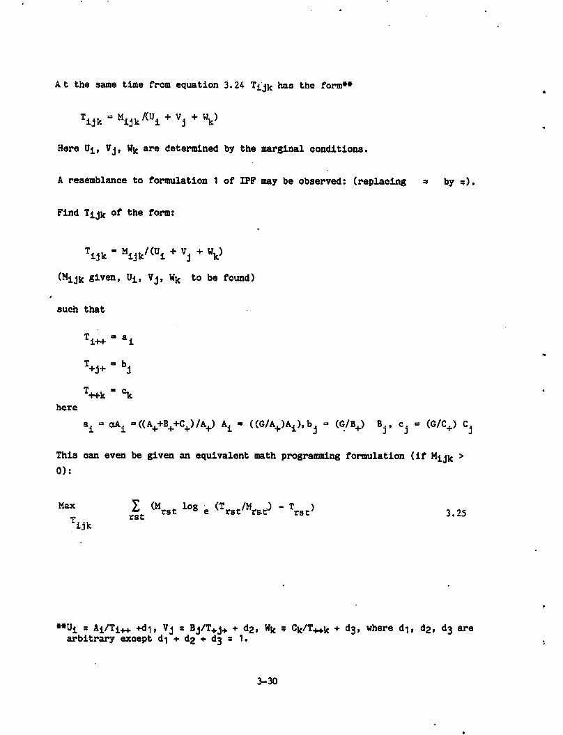
At the same time from equation 3.24 Tijk has the form**

Tijk - Mijk/(ui + Vj + V

Here Ui, Vj, Wk are determined by the marginal conditions.

A resemblance to formulation 1 of IPF may be observed: (replacing * by =).

Find Tijk of fche form:

Tijk - Mijk/(ui+ vj + V

(Mijk given, Ui, Vj, Wk to be found)

such that

Ti++ - ai

Ti.4.1. - b.+j+ 3

T4+k"ekhere

a± =oA^ =((A++B++C+)/A+) A± - ((G/A+)A±),bj = (G/B^ B.., Cj = (G/C+) Cj

This can even be given an equivalent math programming formulation (if Mijk >0):

Max I (Mrst log e(Trgt/Mrstf) -T^)T rst " '""• 3,2S

**Ui s Ai/Ti+4. +di, Vj s Bj/T+j+ + d2, Wk 5 Ck/T++k + d3t where d«, d2, d3 arearbitrary except d* ••• dg ••• 0*3 = 1.

3-30

subject to

and

T. = a.i++ i

T«k • % 3-26

Tijk ± °

As in the case of IPF, existence and uniqueness of a solution Tijk can beguaranteed if and only if the feasibility conditions 3.26 are satisfied. It

is easy to show that the feasibility conditions always have a solution. (This

comment is restricted to the case of one dimensional margins.)

If Mijk s ° for any ijk then, from the form Tijk = Mijk/(Ui+Vj+Wk) there.is athreat of indetermlnateness of the solution. If too many of the Mijk=0 it

seems likely that no unique solution for Tijk will exist. (The math

programming formulation ensures uniqueness but does not apply if Mijk = 0).

However, if Mijk > 0 for all ijk then the EM process can have only one

solution and there is no possibility of the solution depending on the

initialization of Tij^0*. The existence of the solution to 3.25, 3.26 i.e.,to the alternative formulation is guaranteed, but this does not strictly prove

that the EM process itself converges. However, it seems likely that it will.

In this simple case with non-zero values in all cells of M.., , using EM with aijK

saturated model cannot lead to more than one solution (i.e. depending on the

initialization). Consequently the previous conjecture that simpler models

(i.e., models with fewer parameters) are more likely to lead to unique

solutions would suggest that all log linear models would lead to a unique

solution if the process converges. It seems likely that the process converges

and that the unique solution is the maximum likelihood solution. These

arguments strictly speaking apply only to the case where the margins dominate

the core and where the margins are all one dimensional.

3-31

With a large sample determining Mijk and with higher dimensional margins given

for the Incompletely classified data, it might be conjectured.that non

uniqueness would be less likely (than with small Mijk and one dimensional

margins). As a consequence it is conjectured that the EM method applied as

outlined in Section 3*4.2 will always lead to a unique maximum likelihood

estimate of a log linear model if it oonverges unless some cells of the

completely classified data are empty. In the case of margins of higher

dimensions it is possible that convergence depends on the feasibility of the

margins (no conjecture is offered in the case of infeaslble margins but

feasibility of the margins may not matter in the case of EM). -

It is worth noting again that the conjectures concerning convergence in this

section are based on limited experience and on the above analysis of a special

case.

3-32

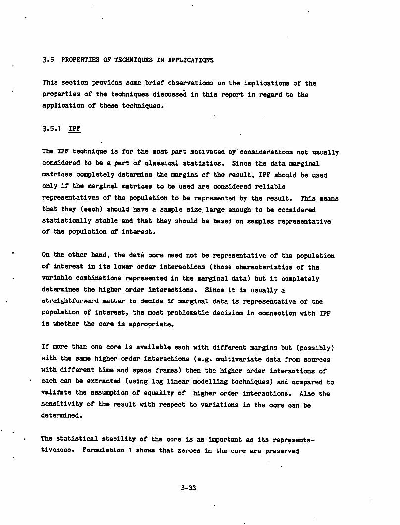
3.5 PROPERTIES OF TECHNIQUES IN APPLICATIONS

This section provides some brief observations on the implications of the

properties of the techniques discussed in this report in regard to the

application of these techniques.

3.5.1 IPF

The IPF technique is for the most part motivated by considerations not usually

considered to be a part of olassical statistics. Since the data marginal

matrices completely determine the margins of the result, IPF should be used

only if the marginal matrices to be used are considered reliable

representatives of the population to be represented by the result. This means

that they (each) should have a sample size large enough to be considered

statistically stable and that they should be based on samples representative

of the population of interest.

On the other hand, the data core need not be representative of the population

of interest in its lower order interactions (those characteristics of the

variable combinations represented in the marginal data) but it completely

determines the higher order interactions. Since it is usually a

straightforward matter to decide if marginal data is representative of the

population of interest, the most problematic decision in connection with IPF

is whether the core is appropriate.

If more than one core is available each with different margins but (possibly)

with the same higher order interactions (e.g. multivariate data from sources

with different time and space frames) then the higher order interactions of

each can be extracted (using log linear modelling techniques) and compared to

validate the assumption of equality of higher order interactions. Also the

sensitivity of the result with respect to variations in the core can be

determined.

The statistical stability of the core is as important as its representa

tiveness. Formulation 1 shows that zeroes in the core are preserved

3-33

in the result. .The same is true of thin spots. It also is clear that the

result of IPF is sensitive on a cell by cell basis to fluctuations in cell

counts (a p% change in a low population cell dominated by the rows and columns

it is in will result in a pit change in the result). This shows that

statistical stability of the core is important. A thinly populated core

should never be subjected to IPF with high population margins with the hopes

that the proces will "smooth out" the thin spots in the core. Instead, the

core can in some cases be smoothed out prior to applying IPF by first using it

to construot a log linear model with some of the highest order interactions

left out. However, some interactions not represented in the marginal data

matrices must be retained in the core or else the IPF process will yield the

same result as would be obtained using an independent core (i.e. a core of all

ones; See Section 3.3.3).

3*5.2 Log Linear Modelling

Log linear modelling is used to provide smoothed cell estimates of

multivariate data and to separate interactions or multivariable effects so

that they may be evaluated and compared. Log linear models help determine

whioh interactions are significant in the data and must be considered in

further analysis or in using the data in further constructions.

It also allows smoother and therefore lower variance cell estimates to be

produced. This can be of use in connection with IPF.

3.5.3 EM

The EM method is primarily of use for combining data from several samples each

classified by a different set of variables but each from the same population.

In the case where no external "core" or measure of higher order interactions

is available, the EM method provides a smooth and even "optimal"* method for

combining the available marginal (and completely classified if available)

data.

•If it is assumed that the various data sets represent the same population andthat the data are multinomially distributed according to a log linear model,then the EM method leads to maximum likelihood estimates. In this sense it

is "optimal."

3-34

The key assumption is that all data is from the same population. It is

advisable to statistically test this assumption (chi square tests comparing

the individual data sets to estimates of them derived from the complete data

estimated by EM can be used).

In cases where several good, incompletely classified data sets each pertinent

to (and representative of) the population of interest are available, the

choice of using EM or IPF to combine them depends on the following

considerations:

1. If a core from a separate population is to be used to determine the

higher order interactions, then IPF must be used.

2. If no external core is to be used and especially if an internal

completely olassified data set is available, then EM should be used.

3 In spite of its theoretically optimal properties, the EM method is

rather sharply limited by the requirement that all data be assumed to

be from the same population.

In summary IPF is capable of producing rather dramatic extensions of

input data while the EM method bolsters the effective sample size of a data

set by combining with an incompletely classified data set.

3-35

3.6 SUMMARY

This chapter has considered three analytical techniques:

1. Log linear modelling,

2. Iterative proportional fitting,

3. The EM Expectation-Maximization) algorithm,

focussing on aspects likely to be of interest in producing useful estimates of

multivariate exposure to driving accidents.

The section on log linear modelling gave a brief overview of that process.

The concepts and procedures are also of use in regard to the other two

methods. The last subsection of the section on log linear modelling

considered the problems involved when log linear modelling is to be applied to

continuous data (such as VMT). It is concluded that log linear models are of

great interest for modelling continuous data such as VMT. The main problems

are with the means of estimating the model parameters and with assessing the

goodness of fit.

It is shown that the standard method for estimating descrete log linear models

(based on IPF) is still satisfactory for the continuous case (although it does

not necessarily yield maximum likelihood estimates) but the chi square

statistics (calculated as if the cell VMT totals were cell counts) are not in

general valid (i.e., not chi square distributed with the appropriate degrees

of freedom). However, if certain conditions on the data are valid, the formal

chi square statistic is easily scaled to a valid chi square (distributed)

statistic (with the usual degrees of freedom). The conditions except for one

are mild and probably satisfied in very many instances. The condition which

will often not hold is that the ratio of VMT mean to VMT variance is constant

across cells. This condition would usually hold only if the variance in cell

VMT was mostly caused by fluctuations in the number of records in each cell

(i.e., if each record made about the same contribution to VMT).

3-36

Even though the condition is not reasonable in many cases, the scale factor

for the chi square statistic can be calculated. A goodness of fit could also

be based on some robust procedure such as jackknlfe, infinitesimal jackknlfe

or sample splitting unless and until the adjusted chi square statistic

proposed here is found to work satisfactorily.

The section on IPF describes the procedure for calculating IPF and then goes

on to. show two other equivalent formulations leading to the same solution.

The alternative formulations are not alternative methods of solution but

formulations of problems which have the same solution as the usual formulation

of IPF. From the alternative formulations various properties of the IPF

procedure are developed:

1. The solution, if it exists, is unique.

2. The resulting matrix is.as close to the core matrix as possible

(according to an Information type metric which is concerned with the

ratio of the result matrix to the core matrix) subject to the marginal

and pbsitivity constraints.

3. The result of IPF has the same margin-absent effeots as the oore. The

margin-absent effects are defined in Section 3*2.2. They are roughly

speaking the higher order interactions.

4. The result of IPF is unaffected by the margin-present effeots in the

oore.

5. IPF has a solution only if the margins are feasible.

The problem of the feasibility of the margins is discussed in Section 3.3 and

also in Appendix B. It is concluded that the best practical method for

determining margin feasbility is to apply IPF and observe the assymptotic

properties (convergence or cycling, development of zeroes or not). The

application of IPF in reasonable situations should not often lead to

infeaslble margins but the discussion given here should assist in handling any

such cases that might arise.

3-37

The section on the EM method gives a brief introduction to the method and then

presents the method as it would apply to developing log linear models for

incompletely classified data. A discussion on convergence and uniqueness is

given based on an explicit analysis of a case which might be expected to have

a greater propensity for indeterminarcy than most other cases: saturated

modelling in the case of one dimensional marginal data (incompletely

classified data sets) and a thinly populated completely classified data set.

In this special case it is concluded that if the process converges the answer

will be unique so long as the completely olassified data set does not have too

many zero cells. Extrapolating to other cases it is conjectured that

convergence almost always occurs (if the margins are fairly compatible) and

that uniqueness is guaranteed if there is a completely classified data set

with no zero cells. If there is no completely olassified data set then the

process is likely to converge to a unique maximum likelihood estimate only if

the order of the log linear model is not too high.

The EM method appears to be very slowly convergent in some cases.

Sinoe the EM method is derived for the case where all the data sets come from

populations having the same distribution its application may be rather

restricted.

3-38

4. COMPUTATIONAL EXAMPLES

In this section, several of the techniques described in Section 3 are

applied to exposure data sets of modest complexity. One of the major benefits

of these exercises was to test out software, develped for the TSC computer (a

PDP10/KL), to compute margins of general arrays, to perform Iterative

Proportional Fitting (IPF) on a broad class of cores and margins, and to

compute log linear models for a large class of arrays. These computer

programs are listed in Appendix C. The set of problems that can be addressed

is limited only by computer storage requirements. Although not represented by

an example in this section, the software has been further extended to compute

maximum likelihood cell-count estimates for a variety of cases involving

incomplete data, via the EM algorithm.

In Section 4.1, a variety of log linear models are fit to a 4-dimensional

Vehicle Miles Travelled (VMT) data set derived from the 1977 Nationwide

Personal Transportation Survey (NPTS). Goodness of fit measures are given for

first, second and third order models. (See Section 3 for a description of the

special problems involved in applying log linear theory to VMT (continuous)

data.)

In Section 4.2, an example of IPF with a dummy core of 1's is given.

This is an elementary example of incomplete data' classification discussed in

Section 2.2. Ten bivariate margins are given representing pairwise

distribution of VMT among five variables, taken from a North Carolina driver

survey from which an estimate of the fully classified 5-dimensional array is

made by fitting the margins to a 5-dimensional core of ones. Three-

dimensional margins from the estimated array are compared with actual three-

way distributions taken from the driver survey, as an indication of

effectiveness of the estimation.

In Section 4.3, an example of IPF with a real core is given. This is an

elementary example of the situation described in Section 2.8 - the updating of

out-of-date data. Matrices of registered drivers by age and sex categories

for 1975 and for 1979 are each fit to the corresponding 1980 margins by IPF.

4-1

The results are compared with the actual 1980 matrix. Since, in this case the

data are counted data, a statistical goodness of fit test is applied.

Saturated log linear model coefficients are calculated for the data sets, to

traoe the effect of IPF on the interactions. A major theoretical result of

Section 3*3*3 is demonstrated computationally.

4.1 LOG LINEAR MODELLING - NPTS DATA SET APPLICATIONS

The log linear modelling method was applied to a multivariate data set

consisting of 1977 annual VMT, classified by four variables: driver age,

driver sex, vehicle weight and model year. The definition of variable levels

(together with a key to their use with data tables) is shown in Table 2. The

actual data set is displayed in Table 3. The data set was aggregated from a

larger multivariate set (more variables and more levels), constructed by TSC

from the 1977 NPTS data tapes. The particular 4-variable set used here was

chosen for several reasons, the principal one being to have a relatively

smooth data set of modest size, for an initial software testing. (The more

disaggregate data are quite noisy and have many zero cells.)

Three hierarchical log linear models were fit to the data, using the

standard technique described in Section 3.2.

The first model fit was a homogeneous hierarchical model of order 3

(meaning all 3-variable effects and lower order effects were present, all

effeots for more than 3 variables were not present). The four 3-dimensional

margins used as sufficient statistics for the estimation are shown in Tables

4, 5, 6, and 7. The outcome cell estimates for this model are shown in

Table 8.

The second model fit was a homogeneous hierarchical model of order 2.

The six 2-dimensional margins (sufficient statistics) are shown in Tables 9

and 10. The cell estimates under this model are shown in Table 11.

The final log linear model fitted was a homogenous hierarchical model of

order 1. The four 1-dimensional margins (sufficient statistics) are shown in

Table 12. The cell estimates under this model are shown in Table 13.

4-2

TABLE 2. DEFINITION OF VARIABLE LEVELS

VARIABLE/LEVELS KEY

SEX OF DRIVER

Male M

Female F

AGE OF DRIVER

0-24 0+

25-34 25+

35-44 35+

45-54 45+

55 and older 55+

WEIGHT.OF VEHICLE

0-2500 lbs. 0.0+

2501-3500 lbs. 2.5+

3501-4500 lbs. 3.5+

Over 4500 lbs. 4.5+

YEAR OF MODEL

1976-1978 76+

1973-1975 73+

1969-1972 69+

1965-1968 65+

1964 or older 0+

4-3

eooesonn

25

CO

r

<-9

ZCO

§>

O•<

7-7

t* t>oo*r*. oioc«^ooo»oe>e»0*0o.ooio©oo»©oooitv0*0oo©ee*o©•©one. ... . . • •. ... ♦ — . ■♦ ♦■♦ ... ♦ • ♦ * * ♦ •. •• • •• • *•♦ ... ••♦... ... ♦••.•no

' «««-• a —• * . .:— r•"«>. —: y •*! 5 — * :** >• '*: a •*! 3 — X'* x * &t—: s :* ^*— 5:*^r•— ^r— j»!»

A A.— &.Ki»--0 <3-A A W W-Kia. S C A J..UUU W-C O.A A-t. UWWie B:A* W WlM»£S ex...................... aaa...a. -........•« . c. «01 u.sr. ai-m «r-o so* sr mm-tn ir:c««« tr m m-a e:m u»m «w»u« s o:tr mm mm tn a » ^ mv ......... ... * * ... ... ... ... . . ... «... ... «... ........ ........ s.

rB CBS'S* W B"'C O'C C C" S'S C-«<—.«*«»•— —.«.—.— ^.w •.«•*.«.— a* Ia 010 ».v» oio 01m m-m m>m m-m m.* vois <«<o «s;<o dw ww w>w uauwrr a> s»a* »a o*«o 1

—.0. MIO a—a. a*, a* a^ a m*0* *—<L•S OIO laMO MIS WO O.MO»W«£B) 01

a —-<o 9IOS UH— IA* BV«0 ui'— o»— to—,* O'— osie- a—o> owe «*o» exw e-*> mho <0 «so> a«M<o wim o» a 010 u>m »o> ao.<o .

11. m'M inaiic mw .410)1..a* o>iaj m>o «u>*u «..b> <~«j —1<a sass*»«! bow «a<o >

i : 1 ' I

ua.SMA-m <ai>;w«

» u»C O«o> unaj oiljt w I- at» w*O0.fa» Aim aukwaw Man> B»— What .»"— diBJ «;3

m uammimmim utminoiiKiiiiitiii m-m miifitnitnmimutim tnm mim mm mm mim (nmmimmn o. ... ... ... ... ... . . ... ... ... ... ... ...... ... ... ... ... ... ...... B

1 • I J > I • ' j : o»«e*i Wi «!"> si"": »*• ^fi «•* s*>.> *n» *:•« si"* -tft si**! 3?^ sh »*s W*; —"> "»"* tsi^r -est r-

i : ' 1 1 I I i : •»» »•i i j I i j 1*da*W WlKaawlO CTAAiav h»fc»lt»0 Oiaa>^tekMM atflo J ! J k»c 0..UU.1UOCT

mwtfltr.mm.oe.tr m>u!ui,min>c>c>ifiuriftm'ui inpoic mmmimm.oo.mm^r immne «•«••.

I

o 0.0 ciav co om m<m t

J.i-«o"»r

C CisJ•TTTXJj' ! I aj. —

oa.&eioHa<«tuWC.nO>«BlN«ai-uwu«all>«la'BO-Mai.'.ui.»—

o *im auiw *>— we. tm— »»— a.m 0"o tinw m>«t wr «ia. tr>— eim -»tt> —<o> «ib> «oc e*e>a—r* a.AaaB«iBBlM«al*IIIIO«**MWIIIl4«a MUi«uoi»«ie—«imo«iu<jiu—W—4

w «*» BMW mim batsua ci*. b-wcmubmm —i« w*e> «.•» *iw m* tnm o>Ha. «ao —•—*Jic: . ; 1 I 1 i 11 III ~ I ; I ' 1 «

m tnm mim nc earn tnm tnm moo m tnm mm two am tnm tnm ineew tnm tnm giec^n♦ •*•♦••♦»* ... .r. ... ... • ♦ ... ... .i. .i. ♦!. .i. ... ... ... ... ....»

1 I . ' ' • I I 1 I J • • J 'ieceaeaosKU>iiiiiiuin«iiM«iiiti««i«iauaiuuwkiuu»nB< ajanaaixr. ... ...... .1. ... ... —....... .1. .a*... .1. ...... .t. ... ... .1. .»a

•-. ' • • . I 1 - I « I J - . I -j : ls«••» m Bw«iea.iainuiu*>a>.w»aiBOD«a«ba>aivi«uaBia«ac i».oo<r:

m mm tnm mm mm m*m tnm mm tnm mm tnm tnm tnm mm tnm mm mm tnm tnm tnm ma*m mm tnm tnm mm mm mm mm mm mm mm worn mm mm mm mm tntr tn.mm<mm.mmo 1

*js*;siac"» x-t xt"r p*.it x:—: sb^ wi xt^s»«a ac^i a:^i x-^i »^i b-*i ar^s»••*• x.rs 1.

mjtmurmmoommmmmmoo.mmmmmmAoimmmtnmm'n'vmm'mmmmeo-ti.

aooooooammmmummm.

>CD

t-PJ

CO

I

!

CDrpj

o

rf

o

(A

TABLE 4. THREE-OIMENSIONAL MARGIN: AGE, SEX, WEIGHT OF VEHICLE(Annual Billions of VMT, 1977 NPTS)

AGE

0-24

MALE

SEX

FEMALE

11.606 8.577

25-34 19.575 7.926

35-44 13.146 5.436

45-54 7.696 3.525

55 & over 8.235 2.455.

Weight of Vehicl e<2500 lbs.

AGE

0-24

SEXMALE FEMALE

49.104 23.258

25-34 70.041 31.520

35-44 53.936 24.131

45-54 51.335 18.512

55 & over 50.670 16.050

Weight of Vehicle 3501-4500 lbs.

AGE

0-24MALE

SEX

FEMALE39.954 24.373

25-34 59.175 26.746

35-44 37.362 16.314

45-54 35.799 16.946

55 & over 30.264 11.517

Weight of Vehicle 2501-3500 lbs.

AGEMALE

SEXFEMALE

0r24 6.161 4.195

25-34 10.044 4.350

35-44 10.353 5.473

45-54 • 10.393 5.091

55 & over 12.506 3.012

Weight <jf Vehicle over 4500 lbs.

4-5

TABLE 5. THREE-DIMENSIONAL MARGIN: AGE, SEX, YEAR OF MODEL(Annual Billions of VMT, 1977 NPTS)

AGE

0-24MALE

SEXFEMALE

22.800 12.824

25-34 41.681 17.190

35-44 31.816 12.652

45-54 30.875 11.434

55 & over 26.640 8.418

Year of Model 1976 -78

AGE

0-24

SEX

MALE32.857-

FEMALE20.797

25-34 51.411 24.673

35-44 32.895 17.792

45-54 34.028 15.326

55 & over 30.634 10.936

Year of Model 1973-75

AGE

0-24

MALESEX

FEMALE

29.255 17.782

25-34 40.559 21.346

35-44 32.235 14.528

45-54 26.218 10.721

55 & over 29.553 8.538

Year of Model 1969- 72

AGESEX

MALE FEMALE

0-24 15.753 6.703

25-34 17.803 6.237

35-44 12.815 5.462

45-54 10.430 5.632

55 & over 12.071 4.185

Year of Model 1965- 68

AGESEX

MALE FEMALE

0-24 6.160 2.297

25-34 7.381 1.097

35-44 5.037 0.920

45-54 3.673 0.960

55 & over 2.775 0.958

Year of Model 1964 or older

4-6

£

UI

oz«*

UJ—Io

UI2»

u.

o

IS

UIVt31-

o.•z

UJCJJI-^<l^

on

(9£

<VIzeooa—.«r-

t/1a—Za—

I<0UJ3UICatc3:«*

CD

in0000j.O•*1-.CMtn01tntoto*CM•*>•.•••.

o«*CMin10CM0

,-_

.tnv>•CMtoOCOto

JO•*o>0CMin00

*"t

intnCMin«o00

O•

COtoin0«oOmCM-toCM•nrOto

*•"in

tnCM

ai.totn«oinina—0"♦0ontoU•inCMtotnCM01

•a—in••.••

JC00toononto"*~

a*CMCMCM>0

«»-M-

0in•»01*rto00O••0a—0tor-»

4->CMa—0toCOanOlf*71

•.o>cnOenr—**«—0<t

••—1—

ai3

U.00inCMCOi_(.o_ii"«.r»»r«.to001

UJ1111•0ocatotoanin**•«*or>.r«»tototc0bJX>-

t>»toOenr«.(.on0*»•to•*01into•»tocoCM>•...•

0•*CMtoCM•"O

,.

.intil*

00to00CMCOJO•*r>.toO*»•ena—1on0Otoon

tn••••.

0.ina*onento

0to1—CM0•»r-*CM

'—'in

1O

Ol«1—a—00inCMa—co!>.on00onCOL.O1CM0oni»»01

•r"in•....>JC.CM00en0IO•a—

aiCM^—•jaaaa.f.t.>0

M-<*-

OinCM^a—0•_0

•r-»CMOinto♦JCMtoB—

«fren001JC1.••.enenO•*COin0a"—<

.»—

Ol3

U.O-J00tnCMCO(.t-

UJr».r-»t>.toc01ee01111•0««ototoonin•*UJ3Zr~r^tototo0>-

toonto090t-r^r«»00•*•*01inCOCOonCOCM>•

•.*••

0*totntor~O

t~.

•inVt.

«*inintoa~

J3•tftoCO•*inCM9mm1to10tn0•*

in»*...

O•0CO10COCM

OtoCMCMCMO^~a™•*

*-'in

Oltnto

a."•ononCOf*"onUto00.»•inCOon

•a-1ononCOCMCOOlJCin

a..•.>

01.CMto•*r~CM•a—

s»CMa—a—a—i-

<*-04-

inCM•*•*•*r-»O+».•*r-«.r>»ononJCCMCMa.^a—OCO01cn1

..•en•a-

0)Or-»Ttinr—0<t

U.00inCMCOt-t-O—1f«.r*l>vtoc01

UJ1111•00CCItoCOcnin•a«*or»»r-»totote0UJ9Z>-

toenr^.tot-inonCOto<o01inr-.^~r»•*CO

^*^>.

o«*CMto^1-.—0VIJO

I—in

0•O«*to

0•«*•Tt<oCMo»r—

010p^on•*a*r—in

•••CM«*

*--*•0onCO•Ji

OlL.41

U>

..-tnO

JC.toCOon

01totoCOCOO•*>100«*•*tnl-~01

in...t-.CM«»-•onto»—•••a-

0CMa—a—tn•—t-

+JJC«»-

enina—COonOCMO^™.toCMCOo\in01CM•*r».Or~•0Ol

3••Ol

OCMCMCO~~0«*

u.o_i00inCMCOL.f-

UJr>~rv.r~<oC01ceo1111t><ototooninriu.z.t^r-«totote0>-

00*fCOCOf-00onCOo«r«.

oiin0a^on0a—

>.••..•

•""•Oa*«*IOCOa™O

VI

JO

"~in

inwmm

r».O««•r>»in*ftor>»O1CMtooncn!>>.

Oin•••COto

a—•OCOin

a•

*-*toCMCMa—1".CM•*in

011in

Utn•*•a™.

,^-inOJCcoOOontnCMt-Ol•COcocncnin01

>tn•••

CMCO>•

a*toto•a•a—

«t-CMfmmtna^(.

OO

4J<»-JCinCM•*O00toOen.

»*•0!•>.1^CM•a-CMtoinOt>.CMOl011

...ao»3

U.

OcoCOCO0O<

C-JoninCMCOt-!_UIr~!•-.r^to001

CCO1111•O<c0totoontn*l-a^

UIXr-.r»totovcO>-

r>.

I

TABLE 7. THREE-DIMENSIONAL MARGIN: SEX OF DRIVER, WEIGHT OFVEHICLE, AND YEAR OF MODEL (Annual Billions of VMT,1977 NPTS)

*1ale Drivers

Weight of Vehicle (1000 lbs.)

YEAR OFMODEL 0-2.5 2.5-3.5 3.5-4.5

over

4.5

76-78 19.075 46.453 76.669 11.615

73-75 19.740 59.715 83.778 18.594

69-72 13.800 58.294 72.909 12.817

65-68 4.789 28.507 30.138 .5,437

64 orolder 2.853 9.585 11.593 0.994

Female Drivers

Weight of Vehicle (1000 lbs.)

YEAR .OFMODEL 0-2.5 2.5-3.5 3.5-4.5

over

4.5

76-78 8.052 21.490 28.581 4.395

73-75 9.808 31.327 39.665 8.723

69-72 7.538 24.483 29.937 5.957

65-68 1.691 11.208 12.760 2.559

64 or

older 0.830 2.387 2.529 0.487

4-8

Ito

TABLE8.CELLESTIMATESFROMLONGLINEARMODELBASEDON3-DIMENSIONALMARGINS

OHIVLKVEilICLcVMTDRIVE.!VEHICLEVHTilillVE*VEHICLEVHTDRIVERVEliki."'VHTbi>lVEflvChIcLl1tfa.'!1ICESCXHiat.VR.KILLWfl0*i,hMIJ.*"2.'IJ6'

»CESCXbCT.fR.BUI.IONHitSEINCT.VR.BILIUM»GESFIKfitaVR.BILLIONXCESEIHCTaVR.UILLIUN25*H..}iItt'CSI]35*ho;o?-7Br—s;35i-45*—H-6:0*16*2;58255*H0.0*16*1.681

0*rO.O*16*1.94125*r0.0*16*2.S2135*F0.0*16*1.98545*F0.0*16*1.06C55*F0.0*16**>.S45d»iti.S*J6»"1.42225*IT2.5*16riJ.BB5~35?"M-I75r7sr—9ni3<5r-«r""j:5*i6*'9.891SS*il2.5*16*1.015)»»2.b»16*4.8492S»F2.5*16*S.6S1•IS*F2.5*16*3.91645*F2.5*16*4.401SS»F2.5*16*2.161)*r.3.5*16*.6.944"isr'TT'j.srisrsaijsrJ5»1.5*16*14.63445*iijrsrisris.iia55*(13.S*16*15.1619*f3.5*76*5.03425*f3.5*16*6.33635*F3.5*14*S.129*5»F3.5*16*4.821S3*F3.5*16*4.6S?0*ii4.5*76*"1.618is*'h~i;s*i**~i:9jb"35*R-•~i:5»-15*—77I5J-15J—V.~^:5*-16*2.941SS*H4.5*1«*2.29?0*F4.S*16*0.99925*F4.S*16*0.61435*F4.5*16*1.12145*F4.5*16*1.14155*F4.5*16*0.4610*"i,"0.0»'13»4.olt~25*"R-'O.j*13*~i:i19-35TH"PTOT-TI*-37B33T«r-H-g;a*73*-j.39355*HO.f*13*7.0810*'t0.0*13*3.416s*s5.5*u;n9.issr

25*r0.0*13*3.24)J5*"R-2.5J-!jni.55r

35*F0.0*13*1.34145*F0.0*13*1.11055*

55*Fii

0.9*13*2.5*13*

0.64C9.499 15*H3.5*IJ*11.09145*M2.5*13*10.808

}♦I-i.S*il»1.42925*r2.5*13*6.56435*F2.5*11*5.85245*F2.5*13*5.49953*F2.5*13*3.9010*ai3.5*13*'15.511""J5I"B~3:5*"'11*-32:0BJ-35*H3.5*ITnsnBB-15T-T—3.-5*"73n6:71555*H3.5*11*14.1*953**3.5*13*B.4S9a*a4.5*uri;oj'»-

25*F3.5*13*11.1232SJH—4.S.-13*™3:B9B_

35*35*

F3.5*13*8.3984.5*11*3.67T-

45*F3.5*13*6.616«r~h—4:5*"ij*~4:a94

SS*

55*F

ii3.5*13*4.5*13*

5.0104.954

0*r4.5*1J*1.4J3J*"A0.0*«$♦S.9ll~

2b»F4.5*13*1.146isrin.j*8i*y.iir

3S*r4.5*13*2.20245*F4.5*13*2.100SS*55*

F

'ii4.5*13*0.0*69*

1.2422.375 3b'»'H«.»♦61*3.491"«♦KC.A*69*3:044

0*t0.9*69*2.4902S»F0.0*69*1.63035*F0.0*69*1.61645*F0.0*69*1.026SS*FO.C*69*0.114"S*iii.b*b§»13I6d?~k*sj:s*M*na:i8j"35*HJ.5»89*9.«r15*-.T-J.S^89*-9.5fl555*H3.5*69*9.516

0*F2.5*09*1.901"5*.ii.S*u9»~i2.63S

25*Fi.S*69*9.8402s*„i.S*6§*~1&.6S$

35*

35*F

H2.S*69*4.33645*Fi.S*69*4.405s.s«"84»~i8n«9-«»jn:s»89*"u:9ii

SS*55*

F

ii2.5*69*3.5*64*

2.92114.184

9*f1.5*99»6,11425L1}•*♦69*8.66025*~ll"4.b*&i~17Hr

3S»3.5*61*1.09545*F3a5*69*3.91855*F3.5*69*4.9119*n4.5*o"f»1.552™isrH4.5*69*2.568«»it4.5*-69r-j.6ir55*K4.5*69*3.612»♦»4.5*o9»1.13625*F4.5*69*1.21535*F4.5*61♦1.41945*F4.5*69*1.32055*F4.5*69*0.11660*i.b.o*»5»6.416IS*.ii"3.3*'is*~1.MS"is*—h—o:u*~B5»o.bjs-«—r—3:or65*~c:so655*iiP."*6S*1.3960*r0.0*bS*0.31425*F0.0*6b*0.42135*F0.0*65*0.28945*F0.0*65*0.213SS*FCO*65*0.395J*n2.5*ob»'*#.S7125*VJ.i*85*—K3HB*35*H2.5*-65—57311"\S*~H—J.5*85*"4:«6955»k2.5.65*4.2310*»'2.S*i»5*3.2160*k3.5*bb*6.611'

2f*f._J.5».|St_2.2Bi.25*II3.5*8srn.«2

35*f2.5*65*1.96345*F2.5*65*2.225Sb»

55*F

ii2.5*65*3.S*6S»

1.5135.794 IS*H3.5*6<i*5.1,0}45*X3.5*85*l.iil

0*1-3.5*65*2.66525*F3.5*65*2.91635*F3.5*65*2.55145*F3.5*6S*2.614SS*F3.5*65*I.9S4?»:«4.3*o$»"6.6S3~;s*B~4.5*85«~i:sor35*H1."5*bS*l.TVT15*iii:5*65*0.613SS*H4.5*65*1.1450*t4.5*o5»P.5056*n6.-I*o»""d.6l5

25*F4.5*65*0.613.§♦h0.6*o*d.161'

35*

3S»FII

4.5*65*0.65815*F4.5*65*0.460is*ho:9*e»0:111

Sb»55*

Fii

4.5*6S»0.0*n*

0.121C.49I* f.o*a*n.nv

.}♦•').Q»0*O.Jbfi0*r2.5*0*2.26a-

25*FU.O*0*0.114i§»it3.b»"o*T.blY

35*r0.0*n«0.14345*F0.0*0*0.05555*

SS*Fii

0.0*9*

2.5*0*0.167".936 3s*HJ.5*li*J.ftSI"45*v:.'5*0*1.443

0*t7.S*0*P.896""8*K3.5*»♦S.«1J"

25*r2.5*0*0.397}S*?•3.b*'8*~j:4flJ

35*35*

FH

2.5*0*0.3463.5*r»j.»51~

45*F2.5*0*0.4104S*~n'_3:5*"0*"K952

SS*

5b*Fii

2.5*0*3.5*0.

P.3381.104

0*»3.5*11*0.9262b»13.5*0*0.4633b*r3.5*n*0.3S845*FJ.S*0*0.42555*F3.5*9*C.3J7""5»i«4.b»pio.ii?25*H4.5*0*6.J46

t>»r4.s»o»o.ijr.hs»r4.b*o»0.10235*H4.5*-T*«7I81isr-p-i.s*'B*a.ieiIss*H4.S*0*".245135*f4.5**♦0.C1345^F4.5*0*0.011|55*F4.5*P*P.I2I|

3C

"*CO

asascn

3!!E z>oa-,<*-inozUIVIz:t=a-,oO-a-

Ia—

Oa-

to**10**00incnCM00a—

«_roroCO•*inaiin.aaa.

>•0>*tnininOtt

01

0

inJ=*♦»*»*CMCMCOr>-O01

•«*IOIO10«*CM5»v>ICOtn000f».0ina*•a

«*-f—•CMa—00cntoO

rol-»Or*.1010Oa.—

*JOJEOOl»»™•a-*fc^»in01

.r-»f-mtoin03oiroCMCMf»-t-00

•COo»10.r-».

0in•.•a•m

•.•».•*inCOCMa.—>

JCCMtoCOtnintf01L.

>01>

•a— <a-COOCMOOOtnCO0COCMOtt-

a^•ointnCMtoO4->CM•.a.a

J=10r-»00t—O<*-Ot•COCMCM•—r—a»

O•a-

ttl•0013•*•*

3*tccn

CMroin<oU«tut|11•101

*2Ointntnin>

«*CMCO•*in0

UllcoCM^fro•*_lOttinr-»CO<*-

<•»inroO00«*•

•..•.

UIO0a*•*COXu.|tot>»in•»ro01

tn

X.

UItotninin00^«*>

CMCOcnCMo~UllCOCOiv.CMtou_l*•••a

0<to00•*ina.—

>zl0ina—00•a-

•0

O

•a-tr<W•*c001CMcotfin«oL.>

hi11110101-a-

S?Oinininin>cnk<•CMCO«*in0«*o

1.

01•0l-»COr-«*COr-a-

inr*.inroro•*0«*•*cn10r-»10••«aa

L.COCOin•«*roO

09toOi-»CM10<oin•tfr>»IOin

1•*0CMOCMtn•••aa

toCMtt-00totoCMCMfa»

CMr-HinroCOCM01*•».roO10rocn•0

-j1Ocnr-»cn00UIcnaa«aa

je0to•VaMtoIO000«*to•*COro<*•

.0

u.L.0ro

01or>-«cin«t•*Is*•*OUIr>»in0000tnr-»a

>-1100toroinOTro.»..a

>r-COto0cnt—

inr-in•**tt-01>

•a-

«-O

«*-00Or«.COa—00cnco

1CMr-»toOtn01to10co•*ro0cni-«••...a*

inCO**•CMtn

*

coin•»•#ro

11-**•**rL.u.«Mro*»•in001

UJI1111•019Ointnintna—

«*CMro•*tn0

I

TABLE 10. TWO-DIMENSIONAL MARGINS (CONT.)(Annual Billions of VMT, 1977 NPTS)

Weight of Vehicle (1000 lbs.)

SEX 0.25 2.5-3.5 3.5-4.5over

4.5

MALE 60.257 202.554 275.087 49.458

FEMALE 27.918 95.896 113.471 22.121

Sex of Driver vs. Weight of Vehicle

SEX

YEAR OF MODEL

76-78 73-75 69-72 65-68 64 or older

MALE 153.812 181.826 157.820 68.872 25.026

FEMALE 62.518 89.523 72.915 28.218 6.232

Sex of Driver vs. Year of Model

WEIGHT OFVEHICLE

YEAR OF MODEL

76-78 73-75 69-72 65-68 64 or older

0-2.5 27.127 29.547 21.338 6.479 .3.583

2.5-2.5 67.943 91.043 87.777 39.715 11.972

• 3.5-4.5 105.250 123.443 102.846 42.898 14.122

over 4.5 16.010 27.316 18.774 7.997 1.481

Weight of Vehicle vs. Yea r of Model

4-11

I

TABLE11.CELLESTIMATESFROMALOGLINEARMODELBASEDON2-DIMENSIONALMARGINS

ORlVtR-'JEillCLiVMTUHIVEKVEHICLEVHTDRIVE.VEHICLEVHtOKIVEKVEIIICLEVMTDRIVERVEHICLEVFTACE

"6*SL«HUT.2R.BILLION

H0.0*16*"3.415»CES«.»MCI.VR.OILLIUNi5*'ili»;3*16*"5.'988"

(GE

15iSEI

MHCT.VII.BILLIONo:o*ibt—itjw

»CtS*.XkCI.VR.R1LLIUN15*"R"070*76*2.153

HitSEX55*H

HUT.VR.0.4*16*

BILLION2.600

0*

"6*rO.U*16*1.811hJ.5*!6*-'l.145

25*F0.3*16*2.542is*ri:s*is*i3.'6«

IS*3Si

F

H

0.0*16*j.sns*

1.811-B7B54"

15*F0.0*16*1.105i5»-ir-;;5*16*-9.600

55*F55*b

0.0*76*2.5*18*

P.Oil1.364

_P*0*H1.5*16*.9.6*5

25*f.2.5*lb*6.01435*F2.5*16*3.94S45*F2.S*16*1.98155*F

55*ii2.5*76*3.**16*

2.31714.328 is**h"i.s*"i6*"i5nflrIS*H"l.'sripr15.18845*i*3.5*16*15.412

0*-a*

t3.S*J6»5.423i,4.5»'J6J-i:J21

25*F3.5*16*1.68115*fil.Si'lSr"2:221"

35*35*

FH

1.5*16*i:stib*

6.215•j:5sr

45*FI.S*16*S.65445*—VT~4.'5*'76*—27716

55*F55*H

I.S*16*4.5*161

4.9812.661

0*

~5*F4.5*76*0.668

«o..»nr-*i:iir25*F4.b*16*0.94235*F4.5*16*25*ba:a*"i3*sniris*ito.oni*

1.0993.BB3"

45*F4.5*16*1.09155*F55*ii

4.5*16*O.C*111

fl.DJO2.50" 45»"ii0:e»73*"2.577

0*0*

r0.0*71*2.121fi"2.5*"}S*Ti:866~

25*F0.0*11*3.20435*F0.0*11*1.99845*F0.0*11*1.23655*F55*'H

0.0*13*2.5*11*

0.912B.7b) IS*iii.S"*73*I1:B19"35*H5.5*11*10.11945*hIt.5*73*11.121

0*0»

12.S*13*1.8SCk1.5*11*14.511-

2S»F:.S*11*9.318is*"F-s;5»-i3*-22:94r

3S*F2.5*13*5.3814S»F2.S*13*5.SI115*H1.5»-11*18:082-IS*-H—375*11*15:B41

55*F55*'il

2.5*11*1.5*13*

3.31815.14?

0*~a*

t'3.5*11*8.666«4.5*-ll*•2:413"

25*F3.5*11*10.61135r~iT-4."5*~11*-3786r

35*15*

F

rl

1.5*13*1.521-1751-11*3.821

45*F3.5*11*6.9485S»F55*ii

1.5*11*4.5*11*

5.1594.151 45*il4:5*13*4.128

9*~8*

»4.5*13*1.515f"0.0*65*"ini?"

25*F4.5*11*1.92635*F4.5*13*1.96545*F4.5*13*1.919SS*F55*-a

4.5*11*8.8*69*

1.5461.992 2b*p.d.b*89*4.41935*H8.6*84*3.11545*ii8.0*69*1.866

0*6*

1O.O*69*1.926'k2.5*69*11.868

25*Fb.C*69*2.09825*a-i.5issns.Hr

3S»15*

F

H

0.0*69*l.SOSj:sr89*-io;f4r

4S*F0.0*69*0.148isr-p—}:5*"69»—9:613

55*F55*K

0.0*69*2.5*69*

0.6959.195

0*0*

t2.S*b9»_1.416i3.5*ii*u:«i"

25*F2.5*69*8.26225*fii:S»"89*16:535""

35*15*

FH

2.5*69*5.452srsnwrriTBsr

45*F2.5*69*4.49255*F55*ft

2.5*69*3.5*69*

1.19ft

11.911 45*H3.5*69*11.629Of6*

«l.ft.SSl_7t5«.•I4.5*o9»1.741

J5*F3.5*69*8.04235*F1.5*61*6.54645*F3.5*69*4.85555*F55*N

1.5*69*4.5*69*

4.4443.145 25*h"4.S*"59*i'.SJTiirH4.5*69*1.9*245*h4.5*69*3.531

ot6*

»'4.5*69*1.060i.n.6*uSi1.145

25*F4.5*69*1.19925*B8.6*85*"i:i91

35*15*

Fil

4.5*64*-*:o*-B5.

1.4010.93I-

45*F4.5*69*1.13615*-H-0:or6S*-0.539

55*F55*H

4.5*69*O.IW6S»

I.C910.632

0*0*

1I'.O*bb»0.613h2.5*65*6.3»2

25*F0.0*65*0.S39IS*ii2.5*"65*"7."317"

35*is*•

F

H

0.0*65*-J75T-55*

0.39n4.8GT~

45*F0.0*65*0.21145—Fr-2:5»"15*-"4.657

Sb»F55*M

0.0*6S»2.5*65*

0.1944.4J4

0*"6*

1i.b*t>5*3.S421.3.5*"is*1"6.31J"

25*F2.a»65*3.16035*f2.5*65*2.10445*F2.5*65*1.90255*F55*k

2.5*65*3.S*6S»

1.4016."SB 2b»iii.b*6s*1742Tii*H3.5*85*8.86445*H3.5*65*5.241

0*-4*

F3.5*6S»3.091K4.5*»5*o.6e6

25*F3.5*65*2.81425*•n~4.S*'85r-i:33ff"

35*-F3.5*65*2.32145*FJ.5*65*1.894IS*-8—4:5*65*1:154

55*F55*it

3.5*6S»4.5*6S»

1.6991.402 15*H4:5*65*I.211

a*•i*

F4.b»6S»0.414ii*#.**8»_o.iisS

2S»F4.5*65*0.431is*~ii8.8*"fl*-"oreB3"

35*15*

F4.5*65*fl.O*A»

0.513o;59w

45*F4.S*65*0.45Sis•"H-0:0*—0*-0.110

55*F55*<i

4.5*65*0.0*0*

0.4110.281

0*—y.

\U.O*0*0.272"»ii.b»"fi*"-j.51§"

25*F0.0*0*0.2182SJ-R-i:s*"Ti*—27595"

35*F0.0*9*0.14845*F0.0*0*O.iill55*F55*H

0.0*0*2.5*0*

O.OSI1.011 35*Hj;s*1*1.65645*ii,-j:5*""0t"-1.441

0*-6*

I2.5*«>*0.846i."i.s*o*r.iiv

25*F2.5*0*0.69JJSJ'P"1.5*"0*""3:383

35*35*

F2.5*n*0.43"2:215-

45*12.5*0*6.3S055*F55*il

2.5*0*1.5*0*

P.201I.6C4 45*{•i:S*0*1.108

0*Oi

t3.5*0*0.81*ii4.5*5*6.5J9

25*Fl.b*3*0.619i$i»4.si8*'3:24s

3S«

15*F

.4

1.5*Q»

4.5***0.522»:j86"

45*F3.5*0*0.38215*—r~4:S*-0*0.129

55*F55*»

3.5*P»4.S*0*

0.2660.211

)*r4.b»0*0.01325*F4.5*0*0.0613S*F4.5*<>♦0.06145*F4.5*0*0.3545b♦F4.5*ft*P..719

TABLE 12. ONE-DIMENSIONAL MARGINS (AnnualBillions of VMT, 1977 NPTS)

0-24

167.227

25-34 35-44

229.378 166.152

Age of Driver

MALE FEMALE

587.356 259.406

Sex of Driver

45-54

149.297

55 and over

134.709

0-2.5 2.5-3.5 3.5-4.5 over 4.5

88.175 298.450 388.558

Weight of Vehicle

(1000 lbs.)

71.579

76-78 73-75 69-72 65-68 64 or older

216.330 271.349 230.735

Year of Model

97.089 36.259

4-13

4>I

I-*

TABLE13.CELLESTIMATESFROMLOGLINEARMODELBASEDON1-DIMENSIONALMARGINS

URiytHWEHICLt_1MT.w.Billion16*3.086isr-r.Hi16*10.445is*~»:sirJ6J_.13.599_

~16*6.00616*2.505J6»—i:ios13*3.811iiv-f.wr

11*5.18sT13*11.051jjr-i:5ir13*3.142ij~i:jba»9*_3.29109*..•,54»9*11.141U9»i.Holi9*14.504

"69*6.486!__2__Jt6_2_

69*1.1B0i.5»_1.385iS»0.6i2dS*_4.68853*"i:eiBttS»_6.10|65*2.695'Ii5»1.12455r-i.w0»_0.446

"0*6.151"_0*_1.«509

0*0.66T"0*_1.9658*o.'iJg0*_0,3625T0.160

ICESfcXHUT.0

0

>il0.0*

f-f-a.e*0i«2.5*i~r2.5*

__80

'..H.3.5*•13.5*

0—5

iH4.5*r»i:s*

00

>no.o*

ifO.fi*0<

5•_!!___.5*•r2.5*

0<~0(

>H3.5*•»J.sr

*-6

i.14.5*rj4.si

00

1H0.0*

i»•5.6*0

~8«in2.5*i»'"5.5*"

OiOi

>H3.b»>f~3.sr

Oi>._tt„_.§_•1•4.5*

Oi""Oi

IHO.P*•io.e*

Oi

~fil>h2.5*

¥2.M...Oi

Oirs.s*9<

—5<h4.S*

"T-«.sr

91f.0.0*»~B.e»"

__9!9i1-2.5*Oi

~5i•iJ.5*

—pi.srJiH4.5*

T4.5*^

-OBiJES-HUlCfcEt|}|_AGESEXMCT.T0.BILLIUh25

2525

IS?§2525

2525

25

II25252S2525is25

2525

25

?i252525

25S5

25

252525

2525

252S

25

li

3.S*'3.5*'4.5*«.sr

»*

o*6*-

N0.0*16*4.233r~JKijns*-i:B55H2.5*16*14.321

—r~r.&«r~6:3JtrMJ.5*16*18.653

~p!.^ri6*i:33rM4.S*16*3.436ri.snsr-i.sibH0.0*13*5.309

T-j;.nirj;usM2.5*13*11.911f-j.snjir.nr

H3.5*13*23.391"r-i:5*-i3*-i8:33J

H4.5*13*4.319-f~i.s*-ij*—i;ni-J»0.il*69*4.515T~i:a*-t9*~r.wrH_2.S*69*15.281

"f2.5*69*SHIS'H3.S*69*19.89Sr3.5*69*"_B;iir

JJ_Ht_§S__Js66S.F4.5*69*1.819H0.0*65*1.909f—B;u*"iS*-6:B39"H2.5*6S*6.430F-2:5»-l5*~37fl»B_M3.5*65*8.311

"n..."??*—j.nrH4.5*65*1.542F-*;srisr-n.jflrH0.0*0*0.612f-B:o*-«*-w;jn-

_JL_2f5t._9*_Jt01jf2.5*or^.iir

2.695

"i:nr>t49_ii.2ir

IcTsnnet.SirBiKloi0.0*16*2.1SSu:o*-«*~r.iii

II2.5*16*9.32SMIS

45*HJ.5*16*12.141

H

TH3.5*16*13.511

N

T

r2.S*H3.5*r3.5rM4.5*

o.o**

F1.5*16TM4.5*16*

T

billIon3.066

"Oronj*1.3512.5*16*10.318

"275*-«»I.SBr

2.4891;5*~16*1.09910.0*13*

2.5*13*13.011

3.846

13i5.H»13*16.94813*7.«r13*3.122

69*3.210M*1.44469*11.069-9*OB9"69*14.411.9*.nsr69*2.6S5

45*15*45*15*rT..rui

HJ.5*16*

11*F3.5n8r-5.-3«45*H4.5*16*2.236is*-r~i;5rw*--o:9bb45*H0.0*13*3.456

TJ.0n3*~l.'5262.5*13*11.691

isr-r

**~~J2.5*13*5.UJ45*N3.5*13*15.228is*-f—3;5»-w-8:ih45*II4.5*13*2.805isr-r-i:5ri3*~i:33945*M0.0*69*2.939w*¥a.orM*-i:j«-45*II2.5*69*9.946

f—J.sr8§i—r.mH3.5*69*12.949T~3.*5r655—5.119

5*H4.S*69*2.385i:ssi'1.2360.5464.185i;b<8S.449~:m1.0040:4430.3980:i1S1.3410.5951.1540:i150.3230.141

TToT2.S*i:sr3.5*

OBO"15»

45*175T

-MI.S.69«M0.0*65*

1—oior-isrM2.5*65*

H3,5*65*F1.5*65*

»M4.5*65*iF4.51.r_5r

H0.0*0*o.o*—ur2.5*C»

f1.5*f*__3.5*0*-r~iT5r--r

H4.5*0*-r~i:?r-irr

1.316oT808~11S»F0:D*~J54.6583T051-6.06

l.iu•oTwr0.441•oinr1.500

•o^^fiT1.9S2

-7B53-0.360

•flTTSO

4.^4.5*<9~45*H0.0*65* 44f~H

45*M2.5*65*is*-r~2r5r85545*IIJ.5*65*h*fi.sr.s*45*M4.5*6S*is*-f—i:5r-85*~45*II0.0*0*is*fa;o*~or4S*H2.S*0*4TT45*isr45*

H3.5*

T

or0*

3:sr"0i4.5*0*i:sf~o«-

1

OHIVERicESLi55*H55*-F55*H55*FS5*H

lEUICLEiiiii.fB.o.e*16*0.0*16*2.5*16*2.5*16*3.5*16*3.5*16*4.5*16*4.5*IS*0.0*13*0.8*13*2.5*13*3.5*13*3.5*11*1.5*13*4.5*11*4.5*IJ.0.0*69*0.«*69*2.5*69*3.5*69*3.5*69*3.5*60*4.5*69*4.Si69*0.0*65*0.0»65*2.5*65*2.5*65*3.S*65*1.5*65.4.S*6S»4.5*65.0.0*0*

55555*

5SJ-55*SS*55*55.55*55*SS*ssrF55*H55*—P55*H55*"F55*H55♦F55*H55*FSS*55»SS*55.55*55*SS*55*FSS*H55rSS*ssrSS*II55*55*55*

0.0*2.5*3.Si3.5*3.Si4.5*4.«i*

Oi0*Pi0*1*0*

Oi

VHtblLLidii

2.4861.098C.4143.116

19.9544.8J82.018P.B9I3.1181.311

10.SS44.661

13.1406.0682.5311.1192.651I.HI8.9143.461

11.684S.I642.152(I.9511.1160.4913.1161.6684.9162.Ill0.9060.401P.3590.1591.216•>.5311.581

*.6990.2920.124

The standard statistics for the three models are shown in Table 14. As

noted earlier, the chi-square and likelihood-ratio statistics are not valid;

in fact, they are derived from VMT cell entries and are thus grossly distorted

(and inflated) by weights and expansion faotors (See Section 3*2.4 and

Appendix A for a suggested correction factor estimates). Nevertheless, the

statistics are a crude measure of relative goodness of fit, so that one may

observe that the 3-level model appears to be the best fit* the 1-level model

the worst fit of the three models. The degrees of freedom, on the other, hand,

are valid since they depend only on the total number of cells and the number

of parameters utilized in the model. If one assumes that the inflation factor

in the VMT data is approximately constant aoross cells, one can observe that

the ratio of chi-square (2.963) and of D.O.F. (2.833) for models 2 and 1 are

almost equal. This can mean that chi-square is measuring noise. This

suggests that the better fit for model 1 is not statistically significant.

The same crude test tells us with somewhat oore confidence that model 3 is

probably not as good a fit as models 1 or 2. Of course, these observations

are highly intuitive and qualitative. Rigorous goodness-of-fit tests cannot

be applied unless successful scaling adjustments can be made to the VMT data,

or to the chi-square statistics.

Another observation that can be made from these tests has to do with the

ability of log-linear models to deteot data instabilities. In particular, if

one divides the given data set of 200 cells into two sets of 100 cells each,

corresponding' to male drivers and female drivers respectively, one can pair

the cells naturally i.e., for each "female1* cell, there is exactly one "male"

cell having the same levels for all variables except sex. Inspection of Table

3 reveals that for 91 of these cell-pairs the VMT for the "male" cell is much

greater than the VMT for the corresponding "female" cell. In 9 of the cell-

pairs, however, the "female" VMT is larger or olose to equal to the "male"

VMT. (This can be verified' easily since Table 3 is arranged so that

corresponding cells are adjacent.) If one now looks at the cell estimates for

the three models, it is observed that, in each case, all 9 cell-pairs are

reversed, so that the "male" cell dominates for all 100 cell-pairs. This, in

turn prompts an investigation of the marginal tables which reveals that for

all margins (3, 2, and 1-dimensional) the "male" cell has a

*I.e the closest fit as measured by chi-square. It could not be otherwise sincethe all three factor model contains the others.

4-15

TABLE 14. CHI-SQUARE, G* AND DEGREES OF FREEDOM FOR THREE HOMOGENEOUSHIERARCHICAL LOG LINEAR MODELS

MODEL 1 (3-variable effects)

MODEL 2 (2-variable effects)

MODEL 3 (1-variable effects)

CHI-SQUARE

.707 X IO10G<

.715 X 10

2.095 X IO10 2.050 X 10

5.295 X IO10 5.227 X 10

10

10

10

4-16

D.O.F.

48

136

187

substantially larger VMT than the corresponding "female" cell for all cell

pairs. Thus, it is not surprising that the (unsaturated) log linear models,

which are estimated from marginal information alone, reversed the male/female

VMT ratio in the 9 anomolous cell-pairs. One can now zero in on the more

disaggregate data to look for evidenoe of something wrong in the VMT values

for these cells. In fact, preliminary evidence that there may be some thin

sampling problems in these cells can be obtained from Table 3* by observing

that each of the cells correspond to the lightest (0.0+) and heaviest (4.5+)

auto classes which, according to Table 12, comprise approximately 10.4 percent

and 8.5 percent of the population, respectively.

In summary, we have prepared a modest-sized multivariate data set, for

test purposes, from the 1977 NPTS tapes. He have formally fit a sample set of

unsaturated hierarchical log linear models to the data in order to demonstrate

and test the capability.

4-17

TABLE 15. TWO-DIMENSIONAL MARGINS (PercentageDistributions of VMT)

SEX

AGE

24 25-54 55-

Male 7.1 39.8 12.8

Female 6.6 28.0 5.7

TIMEAGE

24 25-54 55

Day 9.3 52.1 15.5

Night 4.4 15.7 3.0

PLACE

AGE

24 25-54 55

Urban 6.6 36.3 10.0

Rural 7.1 31.5 8.5

YEAR OF

MODEL

AGE

24 25-54 55

72-74 5.0 21.4 6.9

69-71 3.6 22.0 4.3

68 5.1 24.5 7.3

SOURCE: White, S. B., C. A. Clayton, L. D. Bressler and J. R. Stewart,"Improved Exposure Measures" Final Report, Research TriangleInstitute, Contract No. DOT-HS-022-2-418, September, 1975.

4-18

TABLE 15. TWO-DIMENSIONAL MARGINS(Percentage Distribution

(CONT.)of VMT)

TIME

SEX SEX

MALE FEMALE PLACE MALE FEMALE

Day 44.0 32.9 Urban 29.4 23.5

Night 15.7 7.5 Rural 30.2 16.9

YEAR OF

MODELSEX YEAR OF TIME

MALE FEMALE MODEL DAY NIGHT

72-74 20.3 12.9 72-74 25.4 7.8

69-71 15.9 14.0 69-71 22.4 7.5

68 23.4 13.4 68 29.1 7.8

YEAR.OFMODEL

PLACE PLACE

URBAN RURAL TIME URBAN RURAL

72-74 16.9 16.4 Day 39.7 37.1

69-71 17.6 12.3 Night 13.2 10.0

68 18.5 18.4-

SOURCE: White, Clayton, Bressler and Stewart

4-19

TABLE 16. 5-WAY OUTPUT FROM IPF (PercentageDistributions of VMT)

YEAR OF

MODEL TIME PLACE

o

< 25MALE25-55 > 55 < 24

FEMALE__-55 > 55

U 0.65 4.30 1.90 0.84 3.84 1.06

72-74R 0.98 5.07 2.01 0.88 3.11 0.77

NU 0.47 1.85 0.50 0.35 0.95 0.16

D

R 0.54 • 1.67 0.41 0.28 0.59 0.09

U 0.45 4.33 1.20 0.79 5.21 0.90

69-71R 0.51 3.79 0.94 0.61 3.13 0.49

NU 0.36 2.06 0.35 0.36 1.42 0.15

n

R 0.31 1.38 0.21 0.21 0.65 0.06

U 0.72 5.28 2.11 0.84 4.23 1.05

< 68R 1.11 6.29 2.27 0.89 3.47 0.78

NU 0.45 1.96 0.48 0.30 0.90 0.14 •

R 0.53 1.79 0.39 0.24 0.57 0.08

4-20

TABLE 17. COMPARISON OF TABLES FOR AGE, TIME AND YEAR OF MODEL(Percentage Distributions of VMT)

YEAR OFMODEL.

72-74

69-71

<68

YEAR OFMODEL

72-74

69-71

C68

YEAR OFMODEL

72-74

69-71

<68

AGE

TIME£24

Day Night

3.6 1.3

2.4 1.2

3.3 1.8

25-54

Day Night

16.1 5.3

16.6 5.4

19.4 .5.1

}55Day Night

5.6 1.2

3.4 0.9

6.4 0.9

3-WAY TABLE - ORIGINAL DATA

SOURCE: White, Clayton, Bressler and Stewart

AGE ^24TIME Day Night

25-54

Day Night}55

Day Night

3.4 1.6 16.3 5.1 5.7 1.2

2.4 1.2 16.5 5.5 3.5 0.8

3.6 1.5 19.3 5.2 6.2 1.1

3-DIMENSIONAL MARGIN - 5-WAY IPF OUTPUT TABLE

AGE .24TIME Day Night

25Day

-54

Night2-55

Day Night

3.5 1.1 17.3 5.2 4.7 1.4

3.2 0.9 15.6 4.7 4.3 1.3

3.9 1.2 19.2 5.8 5.2 1.6

INDEPENDENT 3-WAY TABLE

4-21

:ar OF

MODEL

72-•74

69--71

68

TABLE 18. COMPARISON OF TABLES FOR SEX, AGE AND YEAR OF MODEL(Percentage Distributions of VMT)

SEX MALEAGE ,24 25-54 >55

2.6 12.7 5.1

1.7 11.7 2.6

2.8 15.5 5.1

3-WAY TABLE - ORIGINAL DATA

SOURCE: White, Clayton,

FEMALE

<24 25-54 >55

2.4 8.7 1.8

1.9 10.3 1.7

2.3 9.0 2.2

essler and Stewart

YEAR OF

MODELSEXAGE

MALE FEMALE<24 25-54 >55 <24 25-54 >55

72-74 2.6 12.9 4.8 2.4 8.5 2.1

69-71 1.6 11.6 2.7 2.0 10.4 1.6

68 2.8 15.3 . 5.3 2.3 9.2 2.0

3-DIMENSIONAL MARGIN FROM 5.•WAY IPF OUTPUT

YEAR OF

MODEL

SEX

AGEMALE FEMALE

<24 25-54 >55 <24 25-54 >55

72-74 2.7 13.4 3.7 1.8 9.1 2.5

69-71 2.4 12.1 3.3 1.7 8.2 2.2

68 3.0 14.9 4.1 2.0 10.1 2.8

INDEPENDENT 3-WAY TABLE

4-22

TABLE 19. COMPARISONS OF 3-WAY TABLES FOR SEX, TIME AND YEAR OF MODEL(Percentage Distributions of, VMT)

YEAR OFMODEL

SEX

TIMEMALE FEMALE

Day Night Day Night

72-74 15.0 5.3 10.4 2.5

69-71 11.3 4.6 11.1 2.9

68 17.7 5.7

3-WAY TABLE - ORIGINAL

11.3

DATA

2.1

50URCE: White, Clayton , Bressler and Stewart

YEAR OFMODEL

SEX

TIMEMALE FEMALE

Day Night Day Night

72-74 14.9 5.4 10.5 2.4

69-71 11.2 4.7 11.1 2.9

68 17.8 5.6 11.3 2.2

3-DIMENSIONAL MARGIN FROM 5-WAY IPF OUTPUT

YEAR OFMODEL

SEX

TIME

MALE FEMALE

Day Night Day Night

72-74 15.2 4.6 10.3 3.1

69-71 13.7 4.1 9.3 2.8

68 16.9 5.1 11.5 3.4

INDEPENDENT 3-WAY TABLE

4-23

enr>»

cn

in

cn

xuioo

Qz«c

UJUI•a:

>-CO

ooe_

c_

a

£_«—UIVII--00oMOOO

•Oooco

•cn

oCM

co

_

+»idE

•a—

+>VI

UI

aiaiCOo4-»in4-00^rUJ*j-mCM

UJcn00UJEnUJEn

CM_Ja—CMCOCMOa—II—1cminocoto•r-CM-jtntootn—-4r—•—coinenCM«*Nr-WlflN+»Xetr—inCOr—cn4JX£COoto«*•to+»X£^•_oiin<*VI£co«*cnmcoVIUIu.

^r*-i—cnin_UIu.

«*!>.a—Ol^-UI_

_

UJu.

**r>»I—Ola^-UIOl_

13Oooo

XC—X

COen

t_>

XCOcn

'_>

UICIUIinUIa—*OlooOI00r-»oor«.

a—CMOCOCO"OcOO00COCO

u.O.

cnISr-OOr-M

U.CL

Ol

UIniCOOTr-O)•—•U)tooocoa—cni—iUIa—"*cntoCO _J(MCVIr-SN_Jotocotocn_lcmoocotoin«ctocncooi*».•a:to00CMO00.—^<toCOCMO00

,_^

e•—•—a——-a—•o£01£—-r-a—a—>—-.H-

.<*"Si-"5f«*,**•*«a-«»<***^«*•uilcmco^finOl•II1+

ujIcmco•*inOl11II+

ujIcmco**•tnCD1|||+Ootntntnin «t|oin^tinin<C|ointninin

cmco«4-incmco^-incmco«*in

uiuiUI_jtnr*.co«*•a—_icoinocoto-J1—Cftl^r-in•<00a—00Or—•*cor—'cncncn«*ooa—intoco£cm^j-coino——£incmo-rcn

_-~?.cocoinin^

^_

UI^•r«.—win(0UJco^-oOla—10UJ^-toa—en^j-<o u.a—a—a—_—au.r-a—a—a—_•u.3+»+J+J

XouajUI<tX«<X<ooUIUJ

oootnoocn00r-»a%^

r*.coocmcocnONOONcn.o^fauicucnUITr«—IO_a—UIoo»*ooenmUIooto^-CMCM _jcmoocnto**•_Jr-oocmotn-J•4*COIOCOCM«tto00CMOCO•*-*»<inina—•—to.*~*<s.lOooNooa

.—^

£a—a—a—r—r—m_»-:1a—,—•a—a—,—•u

^r^r****,^i-.*.*.»Ul|«****f"* LUfMCO^-inujIcmco•*inC_|CMCO«sf_>COM111+C_lI111+<C\IIii+«<p>ininmin«C|oininintnotnininin

cmco«*incmco»*incmco«*in

•a:3

oo

VI

u

+»v>

•a—

+>(0

+>OO

>l

_:

cn

_

u_

_

ooo

si-CM

TABLE 21. 1975 SATURATED LOG-LINEAR MODEL

uo =9.45345684

Vn • +.13652076

V2) - +.16293741

«,(3) - -.18189439

^(4) - -.21740229

^(5) - +.09983851

«2(0 • +.08587358

u2(2) - -.08587358

U12(1D • -.00878238

U12(2D - -.03153233

«12(31) - -.02664953

U12(41) - -.00812903

U12(51) - +.07509327

"12(12) » +.00878238

«12(22) - +.03153233

U12(32) - +.02664953

«12(42) -" +.00812903

U12(S2) - -.07509327

4-25

TABLE 22. 1980 SATURATED LOG-LINEAR MODEL

uo =9.55989186

Vu * +.07142259

V2) =+.24558539

V3) =-.13421016

11,(4) =-.34293721

^(5) =+.16013939

u20) 3 +.06160014

•

U.(2) - -.06160014

«12(11)

«12(21)

U12(31)

U12(41)

U12(51)

U1202)

U12(22)

U12(32)

U12(42)

U12(52)

• +.00274901

- -.02132489

- -.01920324

= -.00411349

- +.04189261

= -.00274901

= +.02132489

- +.01920324

= +.00411349

- -.04189261

TABLE 23. 1980/1975 SATURATED TABLE 24.LOG-LINEAR MODEL

uc! • 9.55945323

Vn » +.07257557

^(2) • +.24640532

V3) » -.13345763

U.(4) • -.34223593

^(5) • +.15671267

u20) • +.06084445

U2(2) • +.06084445

u12di) • -.00878235

U12(21) • -.03153230

U12(31) • -.02664955

«12(41) • -.00812905

U12(51) • +.07509325

U]202) = +.00878235

U12(22) = +.03153230

U12(32) » +.02664955

U12(42) • +.00812905

U12(52) = -.07509325

4-26

DIFFERENCES IN INTERACTIONS1980 MODEL MINUS 1980/1975MODEL

11,(1 ) = -.00115298

«,(2 ) = -.00081993

",(3 ) = -.00075253

«,{4 ) = -.00070128

V5 ) - +.00342672

«,0 ) = +.00075569

U2(2 ) = -.00075569

U12<" ) = +.01153136

«„(« 1 = +.01020741

»„(S1) = +.00744631

»„(«) • +.00401556

»„(B1) » -.03320064

U,.(12) • -.01153136

»„(-) • -.01020741

U,2(32) = -.00744631

U,2(42) » -.00401556

",,(51) • +.03320064

4.2 SYNTHESIS OF MULTIVABIATE DATA SETS FROM LOWER DIMENSIONAL DATA (CASE 1 -

DUMMY CORE)

This section describes the application of iterative proportional fitting

(IFF) to the construction of a 5-dimensional data set, using a complete set of

(2) - ten 2-dimensional margins. The data are taken from a study conductedin North Carolina in 1973t from which a table of VMT was prepared, classified

by six variables: vehicle type, model year, driver sex, driver age, day/night

and urban/rural. A 4-way table of the number of drivers, olassified by the

first four variables, was also prepared. The North Carolina (N.C.) report

contains an extensive set of 2-way and 3-way tables of % distribution of VMT.

The data in these tables formed the basis for the data synthesis example

described below.

A set of ten 2-way tables of % distribution of VMT was constructed from

the North Carolina report, one for each pair of variables from the following 5

variable set: model year, driver sex, driver age, day/night (time), and

urban/rural (place). These tables are displayed in Table 15. The table was

fitted to a five dimensional core of one's by IPF. The resulting 5-way table

is shown as Table 16. For three subsets of three variables each (age, time,

and model year; age, sex, and model year; and sex, time and model year,

respectively), 3-way margins were computed from the IPF output table, and were

compared with the corresponding 3-way tables taken from the N.C. report. In

addition, for each case, the corresponding "independent1* table (i.e., the

table with no 2-factor or 3-factor effects) was computed. The three cases are

shown in Tables 17, 18 and 19. As can be seen from these tables, in each

case, the IPF procedure using ten 2-way margins with a dummy core estimated

the 3-way tables quite well, certainly much better than the independent table.

A further experiment was conducted. For each case, the three corresponding

two-way margins were fitted by IPF to a 3-dimensional core of one's. In each

case the output 3-way table was almost

S.B. White, et al, "Improved Exposure Measurements" Final Report byResearch Triangle Institute, under NHTSA Contract No. DOT-HS-022-2-418,September, 1975.

4-27

identical to the corresponding 3-dimensional margins computed from the synthe

sized 5-way table. We do not believe that the latter result is to be expected

in general. It seems likely that there would be situations in which, for

example, the 3-way margins computed from the 5-way table (synthesized from 10

2-way margins) would be significantly better estimates than the corresponding

3-way table synthesized from three 2-way margins.

It is of some interest to note that, if the ten 2-way margins were count

data, the 5-way table derived from them by IPF would be the maximum likelihood

cell estimates for an unsaturated hierarchical log linear model of any 5-way

table of count data that yielded those margins.

The 3-way tables were the largest dimension of marginal tables published

in the N.C. report. The complete data for the 6-way VMT table and the 4-way

number-of-drivers table are in the appendix, but are largely illegible. If

these data could be obtained from the authors, they could, after some

manipulation in the computer, be used to conduct more extensive tests with

IPF, including a direct comparison of the 5-way IPF table with the

corresponding actual table.

4.3 SYNTHESIS OF MULTIVARIATE DATA SETS FROM LOWER DIMENSIONAL DATA (CASE 2 -

ACTUAL CORE)

The final test of IPF involves the estimation of a two-dimensional table

by fitting a fully classified core from a previous timeframe to the margins of

a (more current) year of interest. The data were tables of registered

drivers, classified by sex and age categories, compiled from 1975, 1979, and

1980 "Highway Statistics" (a FHWA publication). These tables are shown in

Table 20, a, b, and c, respectively. The margins of the 1980 table were used

to calculate the corresponding "independent" 2-way table (no 2-way

interactions equivalent to fitting the margins to a core of 1's via IPF) shown

in Table 20(d). The 1980 margins were fit via IPF to the 1975 Table 20(e) and

the 1979, Table 20(f).

4-28

The main idea of the example was to see how well IPF performs with a core

and, in particular, as an initial test of IPF's potential for updating a table

with later year margins. (Conversely, of estimating a later year's tables

given the later year margins and a core from an earlier year.) By comparing

Table 20(a) with Tables d, e, and f, it is clear that fitting the 1975 core or

the 1979 core gives better results than assuming independence. In the case of

1979, Table 20(f), the estimated table is very close to the 1980 table, in

fact, the difference between the two tables is not significantly different

from 0 at the 5% level. (The model estimates ten cells from 6 independent

fixed margins, leaving 4 degrees of freedom. The value of X2 at the 5% level

for 4d.o.f. is 9.488.) In the case of the estimate based on a 1975 core, the

difference between the 1980 and the estimated tables is completely determined

by the different 2-way interactions in the 1975 table. Inspection of Tables

20(a) and e reveals that this effect is strongest on rows 1,2, and especially

5, corresponding to the two youngest and the oldest age groups, respectively.

These observations suggest changes in the sex composition of the corresponding

age groups between-1975 and 1980. * -

The saturated log-linear model parameters were computed for the 1975 and

1980 matrices, and for the matrix derived from fitting the 1975 matrix to the

1980 margins (hereafter denoted the 1980/1975 matrix.) The parameters are

shown in Tables 21, 22 and 23, respectively. Table 24 shows the difference in

the parameters between the 1980 matrix and the 1980/1975 matrix. Inspection

of this table reveals, as expected, that the second order interaction

differences are dominant, and are strongest in the effect qn the elements of

rows 1 and 2 and especially 5. This is consistent with the differences

observed in the matrices for 1980 and 1980/1975.

These calculations afford an opportunity to exemplify some of the

properties of IPF described in section 3* For example, a comparison of Tables

21 and 23 shows that the 1975 second order interactions are preserved exactly

(except for roundoff errors) by IPF. A comparison of Tables 22 and 23 shows

that the 1980/1975 first-order interactions are slightly different. However,

4-29

the main result of section 3.3*3 implies that the 1980/1975 first-order

interactions are completely independent of the first-order interactions of the

1975 (core) matrix. To illustrate this result by example, a matrix (Table 25)

was constructed, having second order interactions exactly equal to those shown

in Table 21 for the 1975 matrix, but with first-order and zero-order

interactions equal to zero. When the matrix shown in Table 25 was fit to the

1980 margins, the outcome was, as predicted, exactly equal to the 1980/1975

matrix.

4-30

TABLE 25. CORE OF AGE-SEX DISTRIBUTIONS CORRESPONDING TO 1975 TABLESECOND ORDER INTERACTIONS ONLY

AGE MALESEX

FEMALE

0-24 .9912561 1.0088210

25-34 .9689596 1.0320347

35-44 .9737024 1.0270076

45-54 .9919039 1.0081621

55+ 1.0779846 .9276570

4-31/4-32

APPENDIX A

FURTHER DETAILS ON APPLICATION OF LOG LINEAR MODELS TO CONTINUOUS DATA

The first question to be addressed in this Appendix is the effeot of the

classical (descrete) technique for estimating log linear models in the

continuous case. Let V_j^ be the VMT for cell ijk (summed over all

observations or records in the cell). Let X_jk be the model estimate (say of

E (Vijic)) for the cell.

The process of IPF applied to particular margins of V_jie is the classical

method of fitting log linear models to V_ji{. This process has two properties.

1. It maximizes

E Vijk loge (Xijk/Vijk)

(see Bishop et al Reference 1, p. 65.)

2. It makes the selected margins of Xjj^ identical to those of V_jk.

These two properties imply that the process minimizes

£ Vijk <Xijk/Vijk -lo8e ^iak^ijk"(The latter quantity is related to the Poisson likelihood.)

This quantity may be reexpressed:

FW = £ vijk g Cxijk/vijk)where

g (u) - u - loge u

then

g' (u) = 1 - 1/u

and

g" (u) = 1/u2

A-l

It follows that F OC) is convex in the model parameters X^j^. It is the sumof terms each of which attains its minimum when Xijjj - V_jk.

The function g (u) is sketched in Figure 2. g (u) attains its minimum when •

u=1. The criterion of fit used by this process is thus very much like the sum

of the squares error criterion used in linear regression, having the following

similar properties:

1. The criterion is a convex function of the model parameters.

2. It achieves its minimum when the model fits exactly.

The fact that the criterion is based on a sum of terms each 'dependent on only

one data point is also similar in the two cases. In the present case similar

to the case of least squares, each term is weighted by the magnitude of the

data element. This is obvious from the presence of the V_jk factor in thepresent case. The fact that large deviations are weighted much more heavily

than small deviations is a familar property of least squares.

The chief difference is that g (u) goes to <*> when u approaches zero. This

prevents X_jic from going to zero when V_jk is positive and it also prevents

negative values of Xjj^. These are necessary properties in the log linear

modelling case.

The conclusion is that the fit criterion is very resaonable for general

applications of log linear modelling independent of whether it gives a maximum

likelihood estimate.

The second matter to be investigated in this Appendix is under what

circumstances an actual maximim likelihood estimate (of cell means) can be

obtained.

Let Vjjfc denote the cell sum of VMT. Thus

A-2

2-

UI

1-

FIGURE2.GRAPHOFAFUNCTION

where Xr denotes the weighted trip length of a given record in cell ijk. If n

is fairly large and is Poisson distributed and independent of the Xr's(although both may be dependent on the choice of cell) then V_jfc will beapproximately normally distributed. This will be assumed:

1# vijk ia normally distributed with mean Mijjj and variance aij^.

If the distribution of V_jk in each oell is characterized by two parameters

then a likelihood function based on one parameter per cell cannot be

constructed. In order to construot a likelihood function similar to the one

maximized by the standard log linear model procedure it will be assumed that

° ijk =a ^ijk» i.e.,

2. The ratio of o2ijk and Uijk does not depend on the oell (ijk).

On the assumption that Vijjj is normally distributed the log likelihood iseasily written down:

L""̂ S.-0^*" UiJk)2/a2ijk +Constantwhere the constant does not depend on the data or the distribution parameters.

On the assumption that ^ijic = aW_jk this becomes

L--l/(2a)L (Vljk -Mijk)2/Mijk

(dropping the oonstant as irrelevant to maximizing the likelihood).

The expression for -2a_ is identical to the standard expression for the chi

square statistio with respect to the model u^. If a s 1 as it does in thecase where V_jk represents cell counts with a Poisson or multinomial

distribution then what has been derived is the identity of -2L and chi square

in the case of large samples. Since it is known that -2L has a chi square

distribution in the case of large samples whatever the underlying distribution,

it follows that the ordinary chi square statistic when divided by a will have

a chi square distribution in the more general case.

A-4

Consequently if the number of observations in each cell is fairly large and if

°2ijk =aviijkthen

will have a chi square distribution and will serve as a statistical goodness

of fit measure for the model P_jic

Decisions regarding the appropriate degree of model complexity can be based on

the chi square statistic. The relevant number of degrees of freedom can be

calculated In the same manner as for standard discrete log linear models as

discussed in Section 3.2.3.

The final matter to be considered in this Appendix is the question of whether

the assumption that o\jk is proportional tou_jk is agood one and, if it isvalid, how the constant of proportionality, a can be estimated.

Let

Suppose that the Xr's are independent and identically distributed (within a

given cell ijk) and that n is Poisson distributed and independent of Xr

(although n and Xr both have distributions dependent on the cell ijk).

Let yijk - E (Vljk)

°2ijk =E<Vijk> - <E<Vijk»2n <• E (n)

n2 - E (n2)

4 " E(x2r >-<E<xr>)2

A-5

Then

E(Viik} =S Pr(n) E 'E(V1JK n=0 r• r=»l r

" E 'P_(n)»ri*E(X_) - n un=0 r r x

00

- E Pr(n)(n E(X2) + (n2-n)(E(X))2)n-0 r___ r r

- n o2 + n2 u2x 'x

-5a„ +Sp2 +(ijpx)2(since n2" = n + (n)2 for a Poisson distribution)

Therefore

yijk =Swxand

°ijk *S<°i-+ »£> ==E(X2)Therefore

°=CTijk/liijk =°£/m* +M- "E<*2)'/E<Xr>For a to be constant across cells E(x2)/E(x) must be constant across cells.

This is unlikely. However, it may happen that the greatest source of cell

variance is the variance in n. In that case the assumption may not be too far

off. In any case an estimate for a as if it were constant over cells is

obtained as •

a= <£"£xr>/< E EVcells r r cells r r

where the summations are over all records in all cells. This quantity is

easily estimated before the rest of the log linear analysis takes place.

2Clearly the assumption that a^ - au_jk is not likely to be valid under many

circumstances and so the validity of the chi square values corrected by 1/a is

not determined by these considerations. It nevertheless appears to be

advisable to calculate these corrected chi square values in order to gain

experience concerning their usefulness in model selection.

A-6

APPENDIX B

FEASIBLE AND INFEASIBLE MARGINAL CONDITIONS

As noted in Section 3.3.2 a requirement for the existence of a solution to any

of the three equivalent formulations of IPF (and hence for the existence of a

unique solution to all three) is the existence of a feasible solution to the

marginal and positivity conditions:

xij+ = "ij

x++k 3 Sk

and

xijk > 0 .in the case of the usual example.

The margins are said to be compatible if they agree along all common lower

order margins e.g. R_j and Sk are compatible if R++ s S+ CR_j and Tjk would becompatible if R+j s T_+). It is a perhaps surprising fact that there arecompatible sets of (multi-dimensional) margins whioh are nevertheless

infeaslble. As noted in Section 3.3.5 this leads to a particularly

intractable situation whioh cannot be dealt with satisfactorily using IPF.

The margins in this case are essentially inconsistent and the situation can be

referred to as essential infeasiblllty. As noted In Section 3.3.5, the

practical technique for detecting essential infeasiblllty recommended in

this report is to attempt to apply IPF and check for stable cycling with the

developent of zero cells in the matrix being computed (see Section 3.3.5 for

details). However, it is of some interest to note that at least in special

cases explicit conditions for essential infeasiblllty can be given.

Note that the marginal conditions always have some solution (assuming they are

compatible) and infeasiblllty arises only when any solution must have negative

elements (of the X_jk matrix).

Darroch (reference 5)considered the 2X2X2 case (three variables each with two

levels) and found that the following conditions are necessary and sufficient

for the existence of a positive solution. Suppose P++1, Pi++, P+n, etc.

stand for specific positive margins of a positive matrix P_jie (_jk each have 2levels) then:

B-l

P+++- Pi++ - P+1+ - P++1 + P+11 + P1+1 + P11+ >. 0

P+11 - Pui - Pn+ + P1++ > 0

P1+1 - P11+ - P+11 + P+1+ > o

P11+ - P+11 - Pl+1 + P++1 > o

P+jk > 0, Pi+k > 0, PiJ+ > 0are the conditions.

A set of three compatible all-positive two dimensional margins which do not

satisfy these conditions is easy to find. The following are an example:

xij+ =

xi+k s

^jk s

CO

When a core matrix of all ones (it could be any positive core to illustrate

the point) is scaled to these margins, convergence does not take place and

instead stable oyoling is observed. In addition, as expected from the

discussion in Section 3.3.5 zeros develop in the matrices produced while

attempting IPF. The matrices

(3n+l) (3n+2) (3n+3)

Xijk »Xijk ' Xijkrepresenting the three stages in a cycle are:

1.000 1.01199

1.04853 0.0000.000 1.998010.95147 1.000

1.46447 0.5001.53553 0.0000.000 1.663321.000- 0.83668>

'1.49046 0.50904>1.500 0.000

0.000- 1.000

1.36115 1.13885.

B-2

APPENDIX C

LISTING OF PROGRAMS

The following program listingas are included in this report:

1. PRSCAL.FOR - for IPF (Page C-2)

2. EM.FOR - for EM (Page C-9)

3. LOGLIN - for fitting log-linear models(Page C-16)

The first and last programs are well checked out but the program EM.FOR isnot.

C-l

C l-NUliKAM KK»CAt.l'UK BUllC.O JUflb 22, \VH2C PKUI.KAH IU OU ITtKAflVb PKUPURTlUNAl. SCALlfKi.C 1Mb t-HUiiNAn KbAU* ChUh A Kile. A UJKb nATkIa ultH Tub MAXIMUM NilHBbk OFt ULtlShSiUflS 3 AM) A NAAlnUM NUNUEK Of b Lb»tUS PKk DIMENSION.t HAKlUNAL MATKlCt* U» LtSsEK UlHtNSlUNS THAN 1Mb CUMb Ak£C nbAU tkUH A StCUtlU flLb, AHU THb CUHb IS ITbKAtlVli_» SCA-bU TOC trtb HAkiilHALS. Tlib PnuUhah DUb* HUT ChbtR tMAt THE MAfcOlfiAU —C AKb CUtUilSrbNT.c • - — •

C UbflftlTlUN U* VAKlABLtSc 1TO ttE, MLlabll 1NJ "~ "C

iNtfiiabk C(JkkUMUO/b>,bNUrU.OlftNSIUn CUkblb,b/b,S,9J,LbVCUN(0/*>J,HAKDlnU0)UlNbNSlUtt CUmJUHS,5,5,5,5>DlMbNtflUN N(b},fH4>,CUflAkUl5/S,5,5>HCAL M*KU(10/b,b,5,.5JUUUB-G PkbClSlUN CURtlL,MAKFlLl/ATA LtvCUktOi/l/

IHbAU i b - • -IKbAul •* 20lkbAU2 * 21

lTYPb •« SIKlTb * b

»kirbllTtPb,-22_20^222^ t-UKMATUAa-'T.Pt In 1 l? tdU iCsH dUtPTIfTa "tjTTffrHTbTr

1 'Oh 1-li.fc OUTPUT.UAT*,/,lA,2 *T»Pb Ih 0 l» IUU «(5ri UUTPUT TiPbi) UN ft ¥»J

KtAD(9,22J tKHlTb

lUlnHlTi .btl. 0) uo TU bIk 1Tb * 22

UHbNiUHrt-^2«UbVlCb2'UiiK*/rlLb-'uiltr'ut.bAT%ACCbS$i'j£UaUT*X

CUtiTlNUb'

• HlTtUTtPba-BUB)o»JO fUkWATlU/'TlPb 1M 1 It IOU ulSH IMPUT DATA TU Bb PKINTEO'//

1 /lA/'UTHbKulSb TKPb IN 0'> .....kbAUUKbAO,22> IfHINT .

»<*•* rCJkMATUA,'TlPb.lf» I It XOO albH CUMAHU TO Bb PH1KTBIJ'//1 /IA,'UMbklalSb TlPb IN d'»

KbA0UKbAl),22) KfHlttT(j ...... _

U lNlTlAtUAtlUN tit LtVCUHC

Ull 10 1 s l/3

-tVCUKUj a 110 UUHtlNUb

C

C IMiriALUATlUfl UC CUhHUHC

UU 20 1 - 1,1CUU JO J - l,b

cukhumiI/J; - 0JC cunrikub

C-2

20 LU'riTlNUt

c UtfTAli. USbk INPUT

C HfcAU Ih MAKE Uf COKb MATKlA tHUH TH6 TT*C

•klTbUTiPb,lll>111 rOHNATlbX/'MANb OF COHb MATRIX FlLb: *,:>X, S)

kEAIHlkbA(,,llJ COPrlk11 FUkflATlAlUi

C

UPb«iU»lT=lKbAUl/UbVlCb3*OSl,'/rlLfc*CURFlL/ACCfcSS-,5EMlN*J

C UbT 1NFOKMATION ON CoHb MATRIX FKUH FlLt CURFlLu

kr.AUllKtAUl/^2; ND1*22 F0kMAT(1012J

hrAUUKiAUl,22, UbVCOkU), U1,BD1H>

1FUKH1NI .tu. Oj GO TU SO

C

C

C

nitlTbUkllb/llllj NOIH -— - -1111 HJKMATUA/'fllUN^'/U,//),.-.> •"!TbllklTba-22i2i ll,LbVCOR(l),l-l,NUlM)2222 FOHitATllA/'NUHttbK UF LfcVblS DOk DIMENSION *,12,' s ',12)

bO CONTINUEC

C kEAI) In CUkE haTHU frKUN FlLfc COkFlL AND WRITE OUT ON TT«

IFUPHlNl .t«. Oj laU TO 60

a)Hirt(lHlTt,j3iJ>JJJJ tOKMATl//,20A,'CURb MATKlA*,/)

OO LUNTlNUb - •

UU 100 Mb=l/LbVCUR(Si ..._-_UU 110 Nt^l/LfcVCURlti

VO UO N3-l4Lb«CURUi "UU UO N2=l,LbVCORl2j

HbAOUkEA01/JJJtCUk6(Nl,rt2/NJ/N4a-NSi1 /Nlsl/LCVCOKd))

3J rOkiUUbf)

l»UPMlNT.tU.O)UU TO idO

nkirbllHlTb/44441 lNl,N2,N.i,H4,N:>,1 C0kE(Nl/N2/NJ/N4/N9)/* Nl-1/LtVCOkU))

4,1,4 tOkMATUA,bOl2,fU.3,2Aj;<UO CONTINUE "120 CONT1HUE110 CONTlNUb100 CUNTlNUb

C

C htAU III NAME Of MAKC1NAL MATrflA tHUH THb TTYt

nKlTcUT.l'b,22^/222 fUhMATl//,9A,*NAKfc (Jf MAKClNAl MAThlCES FILE: *, bA, »>

C-3

KT.»m 1hp.au, U , KAKrlt.c

UPe,NlUNU-lKbAU2/UbiriCb''USft'a-FlLEaMAkFlL/ACCEaS£#SbalN*)C .

C GEl 'INrOKMATlON UN MAMGlNAL MATKlCbJi FkOM FILE MAHFlLC

kEAOUHEAO^a-^2) NMAKIaC

IFUPxlNT .b«. 0> GO TO ISOu

•eltbtlMlTb/bbaSj NMARGb9b9 FOkMATUA,'NUHBEH UF MAktflNAL MATRICES**, IJ)

c

IbU lUNTlNUbu

UU 200 1-1,NMAKGKbAUUkEAU2,22i NAKUlM(l)

c

IFltFKlNT .EU.Oi GO TO 170

*<r<lTb(lKlTb,o<>06i l,MAKOlMlliOObO »UkMaTUa,*NUMBEk OF UlHbNSlUN5 UF MARGINAL '12,' =',12)

c • - •-•

170 CUNTlNUb

C

200 ClINTlhUbC

C kbAU IN HAKblNAL. FRUM FlLt MAKFIL ANO ..KITE UUT UN TT»C

IFllfHlNT .Eg. Oi GU TU 2b0 . .C

«KlTb(lklTb,tfBaBi8M8B »OKMATl//,20X,*MAkblNALS',//i _

2b0 CUNTlNUbC

UU 30U J-1,NNAKG

UU 310 K4=l,LE.CUklCURK0n(J,4ii "UO J20 MJsl,LEVCURlCUkkUHtJ,J)i

UU JJO M2al/LE«CUklCURHOM(J/ Jjj """' ~"kEAUllKEA02,JJi<MAKGCJ,Hl,M2,M3,M4i,

1 Ml-l,LtVCOk(CUkMUMU,l)))

IFUPKlNT.bVI.OiUO TU 330

KEAU1IKEAU2/22.J lCUKKOMll,J>/Jil,MARUlM<l)J

Ir-UPRlN? .El.. Oj GO TU 200

»RlTbllRlTb,7777i U,J,CURKUMll,J),J-1,MAKUlM< Ui'777 FUkMATllA,*CURKDa1',lA,b(2lJ,.»X,la«,bXiJ

KkirbURlTb,4444i \.J~,hi,n2,hJ,nA;\ HAkU(J,Nl,H2,rtJ,N4i,

.-* Nl.»l,LbVCOk<CUKkUMlJ/l)jj' JJO CONTINUE

320 CONTINUE310 CONTINUEJOU CONTINUE

c

C COMPUTE MAhialNALS FKOM CUHb ANU SCALE CUkE

C-4

t-'Jiil'lNUfc UNtlL CUN.Ekbt.NLI-. Ok MAXIMUM NUMBEK Or INTEkAllUhall«a br.t.N kbACHbUa paCii lTbkAflON LOOPS TMkU ALL MAHGINALS

•kirbvir«Pb,oeoi060 rUtlf AU//,lA, "tflftk MAXIMUM NUMHbk OF lTbK AT IONS',3A,$i

k-.AUl tKtAU,60i MAA1Too rUkMATilai

•kirbUTiPb,777i777 FOkHATl//,lA,*bNTEk bPSlL',bA,>i

kEAUUKEAI>,7/i bPSlL77 FUkMATlFlO.Ji

»HlTblli'lTb,»bbbbi MAXlT,bPSiL ~bbbbb rUkMATil *l*ill," MAXlTs*C

ltth-0

tOO bNUFLG •1

ITbk-llEK*!

c

IFUTEk • Kvl. Ii bNUFLG sc

UlFMAX £ 0.Nluir 2 0

N2U1F S 0

N3U1F •i 0

N4Ulr S 0

NbU|r -

c

KAtMAX 2 0.

NlkAT ± c

N2kAI - 0

N3kAl i 0

N4kAt S 0

1*

NbKAT S 0fe

UbLNAA i 0.

NlUEL = c

N2UEL & 0

N3UEL s 0t H4UEL - 0

c

NbUEL s 0

b

PkUMAA £ 0.

NlPKU 3 0

N2PKU i 0

NJPkU S 0

N4PHU s 0

NbfkU - 0

UO O00 J-l,NMAkG

kblNlTlALUb COMPUtbU NAkGlNAL NATktX

440430

420

UU 410 11=1,3UO 4.10 l2*l,b

UO 430 13*1,bUO 440

CONTINUECUNT1NUE

C-5

14*1,bCUMAkGU 1,12, 13,14,-0.

CONTINUE

ilC tUMlnutC

lFl««KUlM(J).bw.4iG0T0 4oOC

C SEI UNUSbU UlMbftSlUN iNUlCbS UF MARGINALS TO I *C

UU IbO H-MAKUlM(J)*l,4MtAi-1

IbO CUNTlNUbC

c S6i i-ussitiLt UNUSbU uImensiun ur CUkb nolets tu 1' ""C

400 UO 470 iU3,b • • •Nll.i-1

470 CUNTlNUb • •C

C LUUP THRU ALL CUkb VALUES ANU COMPUTE MARGINAL VALUES 7 RUrTTJOST"

ClFlKKKlNT .bW. Oi GO TU 47b

«ki*b(lklTb,lUili11111 FUkRAT(//,20A,*CUMAKb*,//i _

47b CUNTlNUb

UU 4o0 N9*l,LbVCUfttbiftOj*Nb ""UU 4»0 N4*l,LEVCUR14i

N(4i-N4 " ~-

UU bOO N3*l,LfcVCOKl3i(IU/-NJUO blO N2*1,lE¥CUR12)

N(2i-N2UO S_0 Nl=l,LEVCURUi

NUJ*Nl " ' :UU 5J0 K*l,MAttUlM(«ii

N(il>-NlCUHkUH<J,a.)jb30 CONTINUE

CUMAKG(Nlli,H(2i,Mi5i;M<4~}j1 =CUMAKG(Mtli,Ml2i,MtJ),M_4ii+2 CUkE(Nl,N2,NJ,N4,N9J "

IFUPRlNT.bU.Oi GU TU b20•KlTbURifb,4444i '

1 M(l),M(2i,M(3),M(4),2 . CUMAkGiM(i,,M(2i,M(3i,M(4Xi

b20 CUNT1NUE _310 CONTINUEbOO CONTINUE490 LUNT1NUE480 CONTINUE

C

C sCALb CUkb bt GIVEN MAmGINAL OlVlUbU BK COMPUTbO MARGINALC • • —

UO 340 113*1,LEVCURlSiNO)*fl3

UO bbO N4*l,LbVCORl4iN14i*N4

UU bOO N3*l,LEVCUKl3iNiJi-NJ

UO 370 N2*l,LEVCUR(2iNUi*N2

C-6

Ull bOO Nl*l,L».VCOKUiN11)*N1

UO b*0 K*l,MAHUlH(JiN(Ai-NlCUkkUHlJ,aVii

3V0 LUNT1NUEafACT*MAKG(J,Mlli,M(2),

1 NUi,M(4ii/CUMAHGl2 M(li,R(2i,M(3),N(4i)

CUkVAL-CUHtlNl,N2,N3,N4,N5iCUkNbH*CUkVAL*SFACTUlFF*AbS(CUkNEa>-CUkVALiIFlUlFF.LE.UlFMAAiGU TU b92UlrHAA*UlFF

NlUlrsNl

N2U1F*N2N3U1F*N3N4UIF*N4

NbUlF=NbC

b*2 CONTINUERAT10*COMNbn/CUHVALIFlHATlO.Lb.RATMAXiUO TU SV4MAIMAX*RATIUNlkAI*Nln2kat*n2N3kAI*NJ

N4kAT-N4 ~

NbMAT*NSC . .

b^4 CONTINUEIFtJ.Nb.NHAKGJGU TU b9¥

t

lFUTEk.GT.UGU TO 5»S "CUkULOlNl,N2,N3,N4,Nbi*CUHNEaGO TU b9»

C .

b*3 CONTINUE ~" —

UlFF*AttSlCUKN£ii-CUkOL0<Nl,N2,N3,N4,Nb)iIFlOlPF.LE.UELMAXiGU TU b9bUbLMAX*01FFN1UEL*N1

N2UEL*N2

N3UEL*N3

N4UEL*N4

N5UbL*NbC

bVO CONTINUE

kAT10*COkNbn/COHULU(Nl,N2,N3,N4,N5iIFlRATlU.Lb.PRUMAXiGU TU b*BPkUMAA*HAT10NlPKUsNlN2PRU*N2

N3PRU*N3

N4PkU*N4

NbPKU*N5

3Va CONTINUEiflAoStCURNE»-CUKOLUlNl,N2,«J,N4,NSii

1 .Lb.bPSlLlGU TU 397bNUFLG*0

C

C-7

Ill

39V

380

370300

350

3 40

OOO

CUNTlNUh

ClikOLDlNl,N2,NJ,N4,Nbl*CURNE*

LONTlNUb

CUkclNl,ft2,NJ,N4,Nbl*CUHNEaiCUNTlNUb

CUNT1HUECUNllNUE

CONTINUE

CUNTINUE

CUNTlNUb

lFiE.iUrLGabU.liGUTU 700IFlllbk.LTaMAXlTiGU TU 400

IHAVE FINAL CUkE MATRlAIMAA1HUN » UF .ITERATIONS NOT HEACHEU

C MAX

C

700

C

C IfPe, IlUt FINAL CURb VALUbSC

ImUm (.UMBER OF ITbMATlOHS RbACHbU Ok METHUO CONVEkGbS

CIJAflnUb

4411

I

442<

44JJ

1

44b3

4400

*kirb(lklTb,44ll)rUkMATUOX,'L0MPAK1SUN OF FINAL MARGINALS', .' rOk Tnu CUNSbCUTlVb ITbRATlONS'i ~ "• KITfcUKlTb,44221 ITERrUkMATi/,3A,'NUMBER UF ITEkATIUNS*',15iRklTbtlRlTb,44331 UeLMAX,N10bL,N20bL,NJI)EL,N40EL,N30ELFUkMATl/,bA,'AHSULUTb VALUb UF MAX ObVlATlUN IS ',bl5.7,' AT PUlNT ',blJJifITblIk ITb,44991 PKUMAX,NIPkO,N2PN0,NJPRO>N4PkO,NbPkCJFOkMATl/,bX,'KAX RATIO IS *,blb.7,' AI POINT ',5l3i

aklTbia,44lli•klTbO,44*21 ITbRnklTblb,44331 UbLMAX,NlUbL,N20bL,N30bL,N40bL,NbDbL*Mrt(9,443bl PkUMAA,NlPkO,N2PkO,NjPkO,N4PkO,NbPkO

nKlTbUklTb,44oo>rOkMATl///,20A,'CijMPAklSUN UF T«U CUNSbCUTlVb MAHGlNALS'la>klTbllklTb,44J3) U1FMAX,N1U1F,1201F,NJUIF,N401F,H&01F>it)lTbUKlTb,44bbl kATMAX,NlRAT,N2RAT,N3RAT,N4RAT,NbftAT

»rUTfcl3,44001a>Kltbl3,44JJl UlFMAA,NlUlF,N201P,NJUlF,N4DlF,NbUlF•RlTt(3,44991 kAtMAX,NlRAT,N2RAT,>l3MAT,N4RAT,N3RAT

• * . . mm

4477

MO

7 30

12<)710

• niTbllKlTb,44771 "'"" 'FUkMATUnl,///!

UU 710 N9*l,LbVC0RlbiUU 7*0 N4*1,LB*CUR141

UO 7j0 N3*l,LEVCURl3lUU 740 N2-l,LEVCURl2l '

HklTE(lKlTb,4444i IN1,N2,N3,N4,N9,LUkblNl,N2,NJ,N4,Nbl,Nl*l,LE«CUkll)l

CUNTINUELONTlNUb

CUNTINUE

'CUNTlNUbCALL fc.U T

C-8

P.tU'Sr AN E"

c p?u™ah em.fop sorgo octu«»es 7, ie«2C I'f-UGMM TO OO 1TEP*TI"E 'aUCHTEO SCALING.C THE PROGRAM R3APS.FP.O" ..A .FILE A.COPE MATRIX fclTP THE PAX1PUH NUMBER OFC 5 CIPifiSIONJ AMD A MAXIMUM I'UVBER CF 5 LEVELS P^R DIMENSION.C MARGINAL MATRICFS CF LfSSFR DIMENSIONS THAN THE COFE AREC RFAO FF.Ok A SSCOND FILE, ANO THE CORE IS it'-RATTVELY SCALED TOC A KEIGHTED COP01NATTOH OF T"E HARBIHALS.C THE PROGRAM DOES NOT CilPCK THAT THE MARGINALS ARE CONSISTENT.C ARE CONSISTENT.C

KJTEGER C0RF0M(10,5)/EN0FLGDIKSN310N CrJBS(5,5,S,5,l5),LEVCOR(0/5>,HARbll*(10)DIP-NSION N(5),M(4),.COkJR.G(?yS,5,5)/HF:iGHTl6/lC)REAL MARC(1C,5,5,5,5)UINEiiSIQN TPPC0P(5,.5_5*5,.5JxCnRNt'«C5,.5,.5#5,5)DCUHLE PRECISION rOPFIL,MARFIL,OUTFILCATA LEVC0R(0.)/1/ _.

1P.EA0 = «IREAOl a 20 " -.—-..1PEAD2 * 21.

I TYPE a 5IP1TE = 5

222?KRITEdTYPE, 22222)

2 eORMAT(lX,,:i.YJ»E_m I fF YOW WTSH.miEM3L-L0-.BE-PJ»lNTE0 ',1 -ON A FILE',/,1X,t 'TYPE IS *) IF.YOU.KTSH_ OUTPUT TYPED ON TIY')

»f-AD<5,22) IHRITE ' - - . . .2 F0h.MAT(lJT2)

IF(I m? ITE . FQ ._.ID_G0_1CL_S1RITE = 22kmE(I*YPE,ll44)_

1144 FUFHAT(2X,'TYPE NAME OF OUTPUT FiLE'isx^sTFEAD(lREAO,U55j OUTF IL

11*5 FCk"AT(AlO) " """C

b»H

OPEN(UNITs27,DEVICE='DSK',FlLEanUTFIL,ACCESS='SEQnUT:)"' "CONTINUE

•»RITE(ITYPE,8?9) ~FOK^Ar{lX,*TYPE..IN.JL_If_y_10_«.I.SH._IHPUT.J)ATA TO RE PRINTED',/

. ,tX,*OTHEPIiTSE TYPE IN C)HEAD(IREA0,22) TPRINTK3ITE(ITYPE,999)

999 F0R"ATC1X,'TYPE IN 1 IF YOU '4ISH CO-APG TO PE PRINTED',/1 ,U,'QTHEP.iISE TYPE IN P') r«**ft.u ,f

KA0(IHEAD,?2) fPOIMT

C INITIALIZATION OF LEVCCPC

OQ tn I = 1,5L^VrOPd) * 1

IP CUNTINUEC - • -

C INITIALIZATION OF CQRPfC

C-9

0) 2;' 1 = 1,1000 '0 J : i,s

CnHPO*!(T,J) = 0V) CINTlNUF2t cijhriiius

c

C OBTAIN USER 'NPUTC

C READ IN NAHF OF CORE MATRIX FPOM THE TTYC

«9irE(lTYPE,lll)111 FOhNATOX, 'NAVE OF_CORE HATPIX FILE:*,5X,$)

h£AO(IREAO,ii) CtiPFiL11 FOFMAT(AIO)

C ~ .

0?E-UUNIT=lREA01,0EVICE='0SK'.FILE3CqRFILfACCBSS='SBQIN»)C "

C C'T INFORMATION ON CORE MATRIX FROH FIL*. CURFILc

PEAO( IREAOl,1122) NOIH,HEIGHT(0)1172 FOIi"IAT(I2,F10.3) ~

C

C

C

hSA0(IREADl,22) (LEVCOR(I),I=1,HDIM) ~

IFdPRlHT .EQ: *) o(f f0 50"

WRirE(IPlTE,iiii) NDiH,UEiGHT(dA " ' *' "llll FCfeiATdX,'HOIHs', I3,3X,'WEICHT(0)3',E15.7,//)

•aiTE{ISITE,2222) (I,LEVCOR(I),I=t,NOIH)2222 FGh«AT(lX,'NU»BER OF LEVELS FOP DTMEHSION *,I2,' = *,I2)

C

*U CONTINUE . _

C REAO IN CORP MATRIX FROM FILE CORFIt, ANp yRTTR OUT^nM TTY.

IFdPRIHT .EQ._.*l) GO .TO 60

«RItE(lRITE,3333) _•\i-*2 FCRHAT(ihi,//,16x,'Initial cope Mifpix*,7i

«(» CONTINUEc _C READ IN CORE "MATRIX" ANO 1NITI ALiZE*""COPNEIiC

00 100 N5=t,LEVC0R(5)DO 110 N4=1,LF!CC._____

00 120 N3=l,LF:VCOR(3)READ IN CORF MATRIXDO 13? N2-l,LEVCdP(?)

RrA0dfif.AJ).l,33}(CORE(Nl,N2,N3,N4,NS)I ,H1*1,LFVC0P(1))

13 _ FOhNATJIfJiNITIALIZ* COPNEW00 140 •!!=»;,LFVCOR (I)

COR,iEW(N'l,N2,'l3,N4,N5)sCOPE(Kl,N2,N3,H4,NS)140 CONTINUE.

IF(JPPI.N1.EO,0.)GO TO 130

ai"ITE(I=ITE,4444) (Wl, N2,'I3,«4,15,I C0RF(N1,N2,N3,«4,«I5),

C-10

7 Hl=l,LEVCOR(l))•1441 FnRMAT(lX,5(5I2,Fl3.5,2X))

1?" CONTINUE1?'> CONTINUE.lt<- C'JNriXUFiO'J CONTINUE

C

C READ IN NAM" OF .MARGINAL MATRIX FPOM THE TTYC

n'»irE(ITYPE,222).272 FOPMAT(//,5X,'NAME OF MARGINAL MATRICES FILE:',5X,S)

READUREAD, 11) MARFIL .C

0PE!J(UNII»IPEAD2,DEV1.CE=_J)SK',FILE=«»ARFIL,A'CCESS3*SEQIN*)C

C GET IMFORKAtlON O.H..HARCJULAL_MAIRICES FROH FILE MARFILC

C

C

RPAO{IREA02,22) NMARG ..

IFdP<UNT «FQ. <!)_GO._tflL.150

«"l n (I»ITE,555.5JLJHABJL"!5«5 FCHMAT(1H1,//,1X,'HUHeEP OF MARGINAL HATRICES=*,I3,/)

C150 CONTINUE

CDO 200 t=l,NMIRC

REA0UPXA!U^.122lJHXBJlIK_.I)_MEIGHT.(n

IF(tPRlNt..EQ,.0_LJ.O TO 170

aj?ITEdRlTE,6Q66J 1«MAR0IH{ r),I,KEIGHT(I)66«0 FORVtT(lX,'NUMBFR OF DIMENSIONS OF MARGINAL '12,' *',I2

1 ,1X*'HEIGHX11a12_11-JL_E15.7)c

17C CONTINUEC

RE»I)(IREA02,221. CC0RR0K(I,J),J=1,HARD IHCD)C

IFCIPRINI..5a.. 0j_GO_lD_2CQ .. ..C

rfRITEdPlTE,77?T).d*J'C0RRDMd,J),J=l,MARDIM(I))7777 FORMATdX,'CORROM',lX,5«2I3,3X,I2,6X))

C2"0 CONTINUE

C

C READ IN MARGINALS FROH FILE MARFIL ANO WRITE OUT ON TTYC

IFdPRINT .EQ. 1) G(i TO 250C

C

Wr*lTE(IRITE,8P8«)Rfi^B FURMAr(//,20X,.*MARGlNALSJ_!_/J

2*0 CONTINUSC

UO 303 Jsl,NMARGOn ?10 M4sl,LEVi*0R(C0RRDM(J,4))

D0..32«».u3=l*L5VCOR(COPRDN(J,3))DO 330 M2sl,LEVC0R(CCSRDM(J,2))

R«'A0(TRFA02,31)(KARG(J,Ml,M2,H3,H4),Ml =l,LEVCOR rCORPDM(J,l)))

C-ll

c

IFdPRINT.E'J.'McO TO 33"C

. . WP1TE(IPITE,4444) (J,H1,M2,M3,M4,1 MARn(J,Ml,M2,M3,H4),

Ml=l,LEVCOR(CORRDM(J,l)))3-,«.' CONTINUE370 CONTPIU?31!' COHTIMUF395 CONTINUE _

C

C COMPUTE MARG1MALS FPO« CORE ANO SC.ALE COREC CONTINUE UNTIL CONVERGENCE PR MAXIMUM NUMBER OF INTER ATIONSC HAS BEEN SfcACHEP. EACH ITERATION LOOPS THRU ALL MARGINALSC

H>irEdTYPE,666)._o$6 FCt*:!Ar(//,lX,'EHTER MAXIMUM NUMPEP OF ITERATIONS',5X,S)

1«EAD(IPEAD,66) MAX1T*b F0?MAT(I5)

WPirE(irYPE,777)777 fCR'IAK//,IX,'ENTER EPSIL',5X,S)

i«SA0(IRSAO,77) «-pSIL77 FOPMAT'FIO.3)

k?iri{I0ITE,55555) MAX1T,?PS1L55b** FCRMATC1H1,//,' MAXTT=',I5,5X,*EPS1L=',E15.7,//)C

ITE3*.) •4"0 EriOFLG*!

lTtR=ITER*l _C

C

C RMNITIALIZS TEMPORARY CORE MATPix "C

on 41) 11=1,50U 112 12=1,5

00 414 13=1,SDO 41* 14=1,5

01 41B 15=1,5.. IHPJ:.PJR_JU_J.2_I.3,14, IS)=0.

416 CONTI NO*416 CONTINUE414 CONTINUE412 CONTINUE

c

410 COM

UC

ITINUS "

c

c

c

900 J=i,f!MRG

RE INITIALIZE CUPPUTED MARGINAL MATRIX

DO .20 11=1,5U-7 43?» 12=1,5

UO 440 13=1,500 44* 14=1,5

COHARG(il,i2,i3,I4)=?.44b CONTINUE440 CONTINUE43 0 C3NTI*IUE470 CON TI'JU."

lF(«ARDI.4(J).EC.4)GniO 460

C-12

C

C JST U;iCJSD niMENSTOH INPICES OF MAPClNALS TU 1C

OO Is) K*MAfDTM(J)i-l/4M(S)=1

4sO CONTINUEC

C S?T FCSSIRLY UNUSED DIMFNSION CF COPE INDICES TO 1C

4fiO OO 171 K=3,S.1(10=1

470 COhflNUi

C

C LOOP THPU ALL CORE VALUES _AN.P COMPUTE ..MARGINAC VALUES FROM COPEC

1F(KPRINT .EQ.„0)..CO_10_435.

KRITL(IRITE,tllll)11 111 F0kMAT(//,2<»X,'C0MARC*///)C _ _

475 CONTINUEC

00 IHi? '.5 = l,LEVC0R(*):i(5)*U503 490 H4=l,LEVCbR(4)

N(4)=N400 500 N3=1,LEVC0R(3)

N.C.3_=_3_DO ?10 H2=1,LEVC0P(2)

-N(.2)=H2 _DO 520 'ir=l,LEVCOR(l)

NCO=Nl _On 530 K=1,MAPDTH(J)

J_0___lij:.QPJDHW,.KJJ_5?C CONTINUE

.... CaHA.8CtHUj,Ml21_H(3)„H.(4)). ...1 *C0MARG(M(l),M(2),M(3),P(4))-»2 . C0BSfW(Bt/N2.,Jf3,H4,NS)

IF(KPRINT.EQ.O) GO TO 520kPJLlEi.lElIE_«.4441

1 M(1),H(2),M(3),M<4),2 . ... COMRG(HU),M(2)_H<3),H<4))

44444 FOHvAT(lX,5(4I2,El5.7,2X))520 CONTINUE. .SK CONTINUE5^0 CONTINUE4^0 CONTINUE490 CONTINUE _

CC SCALE CUP?. BY GIVEN MARGINAL DIVIDED BY COMPUTEO MARGINALC

00 54) NS=l,LEVCOR(*)N(5)=15 ' "'00 550 N4=1,LPVCOO(4)

N(4)=M400 *60 N3=l,L5VC0R(3)

N(3)=H3DO 57" N2=1,LEVC0P(2)

N(2)=N2DO 580 «lsl,L?VCOR(l)

lid >=Kl

C-13

DO -CO r3l,MAPOIM<J)M(K) =M(CURR0;1(J,K))

^i- CON'INUF

. . SFACT=MARC(J/M(1),M(2), M(3),»(4))/I COM»HC(M(l),M(2),M(3),M(4))

TMPC0R(H1,N2,H3,N4,N5)=1 THPCOR(Hl,N2,N3,N4,N5) *2 .. «E1GHT(J)'SFACT«C0RNEN(N1,N2,N3,N4,N5)

5"t CONTIMUE570 . .CONTINUE3fic CONTINUE5*0 CONTINUE540 CONTINUE

C6AC CONTINUE "" — —

C

l/IFHAX = 0.

00 MO !i3=l,t.FVC0P(5iN(5)=15OO 650 N4=l,LFVCOR(4)

N(4)a_L400 660 M3=1,LEVC0P(3)

N(3)=N300 6?«" *i2=T7LEVC0P(2)

N(2)=N2' 00 680 «i'3i,LEVC0PTlT

N(1)=H1

CORVAL=WEIGHT(0)»CORE(N1,N2,N3,N4,N5)*THFC0R(N1,N?,N3,N4,NS)DIFF=ABS(CCRNEai(Ni,H2,N3,N4,NSJ-cdRVAL)IF(DIFF.LE.DIFMAX) GO TO 675blFMAX = OIFF " " " "" "

•ihmi * m1K0X2 = N2IH0'3 = _N3IN0X4 3 M4 ""

JN0X5 = N5C

675 CONTINUEIF(DIFF.LE.SPSIL) GO TG 678

.EHOFLG = 0C -—..- ........

678 __ CONTINUECORltlW(Nl,N2,H3,N4,N5)=C0RVAL

6HC CONT 1HUf67ii CONTINUE "6*0 CONTINUE6*0 CONTINUE " * '"640 CONTINUE _ _

c " ""IF(»NDFLG,EP.1)G0T0 700 IH*?5.J.INAL CORE MATRIXIK(ITER.LT.vAXIT)CO TO 403 (MAXIMUM ff CF 1TERAT1CNS NOT REACHED

C _C MAXIMUM NUMBER CF ITEPATiONS'PEACHED OR METHOD CCNVFRGESC _

7)0 cciiriNUE " "CC TYPE UUT FINAL COPE VALUESC

»RirE(IHlTF.,4422) iTEP,P.FM«X,INUXl,IN0X2,IN0X3,INDX4,INDXS

C-14

4422 FCpMfcr(5X,*NUMPEH UF ITpRAtICNS=',I*,1 bX,*!!AX DEVIATION ',E15.7/2X,'OCCURS AT POINT (',2 4(12,','),i:,*)',//,i«X,'FINAL CORE MATRIX',/)

DO 71.) •I5 = 1,LEVCUP(*)OO 720 H4=l,LEVCqP(4)

00 730 «3=l,LEVCOR(3).00 740 S2=l,LEVC0R(2)

HRITE(IPITE,4444) (H1,N2,N3,N4,N5,1 ... C0RMSW(HX,N2,N3,N4,.N5),2 N1=1,LEVC0R(1))

741 CONTINUE730 CONTINUE720 CONTINUE710 CONTINUE

C'LL exit.EMO

C-15

PrUSPAh lo::lin

C FfUTRAH LOGIIN STUPED ON FILE LOCLIN.FORC CREATED AUGUST 16, i9*2 KEVISEO AUGUST 25, 1982C

C MUSS AM TO INPUT CORE MATP1X ANO CRFATE DESIRED MARGINALS (MAPCEN)C USING THESE MARGINALS TO OBTAIN NFW COR" MATRIX (PRSCAL)C 09TMN .STATISTICS COMPARING OLD AND NEK CORF MATRICES (CUISQR)C

C MAHCINAL INFO'RMATtbN IS READ FROM A FILE DESIGNATED BY THE USERC THE MAIN PROGPAM_PE»D_S_TN THE FIRST CORE MATRIXC THIS MATRIX HIS A MAXIMUM OF 5 DIMENSIONS ANO A MAXIMUM NUMBERC OF 5 LEVELS PEh EACH DIMENSIONC

C

C

C

INTEGER CCRPDM

REAL MARG

DCU3LE PRECISION CORFIL,CORINI,IHMAPC,OUTFIL

COMMUN /CURES1/ CORFST(5,S,S,S,5>CUh.HON /CORFS2/ CPRHEW(5,5,5,5,«i)COMMON /MARGIN/ HOIH,LEVCOB(0/5),NMARG,MARDIM(10),CORBDM(10,S),

1 M«RG(10,5,5,5,5) "*COMMON/INOUT/_IREAO,IREA01,IREAD2,IREA03,!TYPE,IRITE,IRITF1,

1 1H1TC2 --- • - -. - •

COMMON /PRINT/ IPPINT,".PRINTCOHI'ON/'SCALE/ SCALE

DATA LEVCOR(O)/!/

IP.f.AU s 5IRtADt = 20IREAD2 = 211READJ = 22

C

1TYPE s *c

I3ITE = 51R1TE1 = 24

IRITL2 = 25

c

V)PirE(ITYPE,lll)til FORMATdX, 'TYPE IN 1 If YOU kISH OUTPUT TO «E PRINTED *,

1 'OH A FILE*,/,IX,I 'TYPE IN 0 IF YOU kISH OUTPUT TYPED ON TTY*j"

_ READ (1READ, RL IW2JIE11 FORMATU0T2)

C _IFd'aiRITE .EQ."0) GO TO S "" " 'ISITE =23 _ _SRITE(ITYPE,222)

222 F0KMAT(1X,'TYPE NAME OF OUTPUT FILE'.SX.S) _PEAC(IREAO,22) OUTFTL

22 FCfiMAT(Air) _ _ _C

C UPEN OUTPUT FILF OUTFILC

0PE.N(UNIIsIPITE,UEJ»__JE;=*.DSKJ/.FILE30UTFIL,ACCESS=*SEQ0UT')C

5 CONTINUEC

C-16

a.r>irFd TYPE,333)313 FCK«'AT(U,'TYPE IN I IF YOU ViISH INfUT DATA TO PE PRINTED*,/

I ,U,'OTHERWISE TYPE IN '•')PEAO(lRfe,AD,ll) IPPINT .

C

C - INITIALIZE-MAPGTNIL M.TFIX MA"GC

OO 701 15= 1,5DO 7l-» 14 = i,b

00 720 I3.s_l,5_

C

DO W T2 s 1,500 740 11.s 1,1?

MARCdl,12,13,14,15) = 0,740 CONTINUF730 CONTINUE

770 .. CONTINUE710 CONTINUF7<H CONTINUE _

C

C INITIALIZATION OF LEVCC _C

DC 10 I s .l,5_.LEVCOP(I) = 1

10 CONTINUE _C

C INITIALIZATION OF_CQPR_D__

00 20 I s. 1_10_00 30 J = 1,5

CORR0XU,J) .3 0?0 CONTINUE70 CONTINUE

CC OBTAIN USER INPUT

C

C REA3 IN SCALINa..FACT0R._L0.J{AK-L.OUTPUT MORE REAOABLEC

hRirE(ITYPE,777)777 FOk.MAT(lX,*cNTEP SCALING FACTOR IH F FOPMAT*)

FEAD(IREAD,44) .SCALE44 FCftMAT(F)

C

C kiAD IN NAHF OF HARci»»AL THFGRHATIOM FILEC

a>RirE(ITYPE,444)44-4 FOPMAT(lX,r.TYPE._NAME_QF_H»pCjg.AL. INFORMATION FILE*,5X,S)

PF.A0(IPEAD,22) TN"ARGC

C FEAJ IN N>ME OF FIRST CORE MATRIX FILE FROM THE TTYC

•ftRlTC(irYPE,SS5)

5Fb FORMATUX, 'TYPE_HAHE_ OF. FJ.RST_CORE MATRIX FILE*,5X,S)PFA0(IREA0,72) CU9FIL

C

C PrAl) IN NAM* OF FTL* THAT INiTIALIZFS THE CCFE MATRIXC FOR SUBROUTINE FRSCALC

k»IT;(ITYPE,656)0*6 FOPMAT(lX,'TYPE FTLE NA"E FPR FtllTlAL CORE MATRIX FOR PPSCAL*,

1 bX,S)PEA0(lPEAO,22) COOINI

C-17

c

C OPEN MARGINAL INFORMATION FILE INMARGC

OPr.:i(UNlT=IPF»Dl,.DEV!CE.=_SCIA*,FILE=lNHARG,ACCESSs'SEClN*)C

C GET COkS INFOOMATION FROM FILE INMARGC

c

c

c

READ(IREA01,U) UDIM

MEA3(IREAPl,ll) (LEVCOR.CU, I=lvKDIH)

IFdPRINT .FO. 0) GO TO 50

hPlTE(lRITE,llll) N01Mtill fURMAT(lX,*N0IM=*,i3,//,

»airEdRITE/2222)_i*yLE_Cp__I2_J=l,NOIM)2272 FOkMATdX,'NUMBER OF LEVELS FOR DIMENSION *,I2,* = *,I2)

C

*'i CONTINUEC

C GET INFORMATION UN MARGINAL MATRICES FROM FILE INMARGC

HEA0(IREAD1,11) NMARG

IFdPRINT .EQ. fl) CB TO 65 '

VPITE(IRITE,3333) NMARG. " "3333 FChMATdX,'NUMBER OF MARGINAL MATRICESa*. 131

C

60 CONTINUEC

DO 100 1=1,NMARG _REAP(IRFADl,il) MAROIm(I)

IFdPPINT .EQ.O) GO TO 130

W9ITE(IP1TE,4444) I,MAR01M(T)4444 FORMATdX, 'NUMBER OF. DIMENSIONS OF MARGINAL '12,* =*,I2)

C

131- CONTINUEC

C

C

»EA-"(TREAOl,.ll>. (C0PPPM(I,J),j3t,MAFDIM(I))

IFdPRINT .EQ. 0).CO TO_.10O .

yRlTE(lFilE«v55§51_J[I_J_C_0RRDHd,J),J=t,MAPDIMd))*555 FORMATdX,*C0RRnM*,lX,5(2T3,3X,T2,6X))

C

in<J CONTINUEC

C CLOSE FILE 7NMAPGC

CLOSE(UNlfsIREAOi)C

C OPEN FIRST CORE MATRIX FILE CORFU.C

0Ph»(UNIT=IPEA02,bEVlCE=*SCIA*,FILEsCniiFIL,ACCESSs'SEQIH*)C _C PFAO IN FIRST CORE "ATRIX FPO" FILE C0PF1LC

IF(1P»IHT .1"). C) GO TO 160

C-18

c

.•;md?ITE,666«)->o«6 fOhur(iHi,////////,:ix,'Pi?ST cope matrix - not scaled*,/)

c

16" CONTINUEc

c

c

DC 200 •I5 =1,L*'VCUP(1')UO 210 N4=1,LFVC0P(4)

00 220 N3=l,LEVC0R(3)._. 00.23" .M2 =ULEY.C.DR12) .

R«-A0dRFA02,33)(C0RFST(Nl,N2,N3,N4,N5)1 ,'U=l..LcVCOS(l))

33 FCR»AT(*F)

iF(TPPfNT.EQ.6)G0 TO 230

WP1TE(191TE,7777) (H1,N2,N3,N4,N5,1 CORFST(*!l,N2,N3,N4,HS),2 Nl=t,LEVCOR(l))

7777 F.riP,M.AT.CtX,5(SI2,F15.0,lX))_ _230 CONTINUE270 CONTINUE210 CJHTINUE200 CONTINUEc . _- _.. ... _

C SPECIAL OUTPUTC ""

C

C CLUSE FILE COPFILC

CL0SE(UNIT=IPEA02)C

CALL MARGENC

C OPEN lNiriAL_COPE..NA_T£IX_.FJLE_CORIJIIc "

UFEH(UNIT =IREA03,0EVl.CEs*SCIA_*,FILE3C0RIN*,ACCESS=-SEQlN*)C

CALL PRSCALC ~ - •

C CLCSE FILE CORlHIC ~ "

CALL UUTPOT.Ui.

CLUSE(U»IT=IREA03)C

CALL CHISQRC

C CLOSE UUTPUT FILEC

CLOSE(UNIT=IRITE)C

STU?

END

C-19

S"!'<"JJTl..? vA»CF!lC

C .Vlj-CIN .JltNECATOP "UPROUTINE STOPED ON FILE MAPGN.FOPC CREATED AUGUST_l6, 1962.__ . REVISED AUGUST 16, 1982C THIS 3U1R0UTPIE USES A GIVEN CCRE MATRIX TO CALCULATE DFSIRED MARGINALSCC DcFiHtfiUH f)F VARIA5Le§C .(TO BE PILLED IN)C

c

c

INTEGER CORFDM

REAL MARG

DIMENSION N(5),M(,) __ _DIMENSION TPPMAPdO, 5,5,5,5)

COMMON /CORES1/ C0RE(5,5,5,5,5)COMMON /MARGIN/.NOIM,.LE.VCOR(0/5),NMARG,MARDIP(10),CQRPOM(10,5),

1 M»KG(19,5,5,5,5)

CCMMON/INOUT/..IREAD_lP.L»01it.IREAD2, IRE A03,ITYPP, TRITE, IRITS 1,i mrs2

COMMON /PRINT/ IPQINT.KPRINTCOMMON/ISCALE/ SCALE

CC

C COMPUTE MARGINALS FROM C0PE..MATR_1X__C

OO 503 .J=l,J!MA_t_

lF(MARDIM(J).EqA.4JG0TIL_460C

C SET UNUSED PIMENSTON.INDICES OF MARGINALS TO Ic

DO 450 KsMAFDIiLtaiJtl-A.M(K)=1

4*0 CONTINUE _C

C S-T PCSSIBLY UNUSED DIMENSION CF...COPE INDICES TO tC

4*0 00 470 X=i,5.N(K)=1

470 CONTINUEC

C LOUP THPU ALL CCRE VALUES. AKO.COMPUTE MARGINAL VALUES FROH COPEC

00 4H0 N5=1 ,AEVCQR.C5JN(S)s>i5UO 490 N4=1,LEVCC9(4)

N(4)=N4DO 500 N3=1,LEVCCR(3)

N(3)=N3.DO 51.n_»l2=l_LS.VC0P(2)

N(2)=H2DO 520 Nl=l,LEVCOP(l)

N(1)3N1UO e30 rsl,MARDIM(J)

H(K)=N(CORRDM(J,K))3-H' CONTINUE....

K*Pr(j,v(l),H(2),«(3),P(4))1 =MAFG(J,H(1),M(2),K(3),M(4))+2 COFt-(Hl,N2,N3,N4,N5)

C-20

57C CONTiNUP510 CONTINUE500 CONTINUE490 CUNTINUE4PC CONTINUE

C

600 CONTINUEC

kPITE(IRITE,8AB8) SCALEIbBB FCRMAT(1HI,//,20X,*HARGINALS - SCALED BY FACTOR *,E15.7,/////)

00 300 J=1,HHIPG

DO 310 M4=l,LSVCGP(C0RfibH(J,4))DO 320 v3=l,LPVCOR(CORR0M(ji3))

00 330 N2=1,LEVC0R(C0RRDM(J,2)).__ . DO 340 Ml=l,LEVCOR(CORfiOH(J,l))

TMPMAP(J,Ml,i»2,M3,M4) =1 ... .. . _. ... HARG(J,M1,M2,M3,M4)

340 CONTINUEkRITE(IRITE,7777) (J,M1,M2,M3,H4,

1 TMPHAR(J,Ml,M2,M3,H4),2 Hj=l,LEVCOR(C0HRDM(J,l)))

7777 FORMAT(1X,5(SI2,F15.0,1X))3^0 CONTINUE310 CONflNUF310 CONTINUE _

*01TEdRiTE,9999) ""."909 FORMAT^)

300 CONTINUEC _ _

PET'JPNENO

c

C-21

SJHriUUTINE PRSCALC

C SUB«OJTINE PRSCAL STOPED ON FILE PROSCL.FORC SUBROUTINE TO OU ITERATIVE P-ROPORTIONAL SCALING. (IPF METHOD)C REAUS FROM A FILE AN INITIAL CORE MATRIX MITH THE MAXIMUM NUMBER OF "C DIMENSIONS 5 AND A MAXIMUM NUMBER OF 5 LEVELS PER DIMENSION.C HARCINAL.MATRICES OF LESSER DIMENSIONS THAN THE CORE AREC OBTAINED FROM SUBROUTINE MAPGEN, AND THE CORE ISi ifERATIVELY SCALED TO"C THE MARGINALS. THE PROGPAM DOES NOT CHECK THAT THE MARGINALSC . ARE. CONSISTENT. _

C DEFINITION OF VARIABLES? . . (TO BE FILLED IH)C

C

INTEGER SNOFLG

DIMSNJi UN CORflLO(§,§,'§, §,§) "" "OIMENSIUN CORTHP(5,S,S,S,5)DIMENSION C0HARC(5,5,5,5)DIllSNoiJii N(5),M(4) "

INTEGER COREOM .

REAL MARG

COMMON /C0RES2/ CORE(5,5,5,5,5) -----COMMON /MARGIN/ NOIM,LEVCOR(0/S),NHARC,HARDIM(10),CORROM(10,5),

I MARG(10,S,5,5,5J!common/iiidiif/ iREAb,iREAbt,iR_Ab2,lRnb3;ifYPE;TRlTXlRmi7

1 IRlTEiCOMMON /PRINT/ IPPINT,KPRINTCOMMON/ISCALE/ SCALE .

URITE(ITYPE,999)999 FORMATdX,'TYPE IH 1 IF YOU hlSH COHARG TO BE PMiiTBD~,T

1 ,IX,'OTHERWISE TYPE IN 0*)PEAU(lREAO,U) KPRINT

it FORMAT(l0i2) '" '•"-C

C REAt) IN INITIAL CORE MATRIX FROM FILE CORINIc

IF(IPR-1NT .EG. 0) GO TO 60

SRlrS(lRlfE;3333i3333 F0RrtAT(lHl,///,20X,'INITIAL CORE MATRIX - NOT SCALED*,/////)

C _'50 ceNflSUB "' '" —

c

00 tOO N5=1,LEVC0R(5)DO" 110 N4"=i,LevcOR(4)

"C"

c

00 120 N3=1,LEVC0R(3)DO 130 N2=l,LEYCOR(2)

REAd(tReA03,33)?eoReeNr,Nr,"N5;N?^iST1 ,Nl3l,LEVC0R(t))

33 _ FORMAT(SF)

IFdPRINT.EQ.0)G0 TO 130

~" »RITE(IR1TE,4444J tNl,'N2",fl3",N4,li5,1 C0RE(N1,N2,N3,N4,N5),i Nl=t,LEVCOR(l))

C-22

4444 . FOPMAT(1X,5(5I2,F15.0,1X))130 . CONTINUE120 CONTINUF110 CONTINUE150 CUNT.NUE

C

?. COMPUTE MARGINALS FROM CORE AND SCALE COREC CONTINUE JNTIL CONVERGENCE OR MAXIMUM NUMBER OF iHTERATIONS"C HAS BEES REACHED. EACH ITERATION LOOPS THRU ALL MARGIHALSC _

"FaiiE(iTYPE,666j "666 F0RMAT(//,1X,*ENTER MAXIHUH NUMBER OF ITERATIONS*,5X,$)

R£A0(IREAD,66) MAXIT55 PUgMATdSf • • • .-—

WRITE(irYPE,777)777 FORHAK//,IX,'ENTER EPSIL',5X,$)

fiei0dREAb,7f) EPSiL77 FUR.UT(flQ.3)

C

•»airE(iRitE,55555) MAX If,EPSIL ' "~55555 FORMATdHl,///,' HAXIT=*,IS,5X, *EPSIL=*,E15.7,//)

' Iters,)400 ENUFLG=1

ITERalTSR+lc " .. . ..

IFdTER .EQ, 1) ENOFLG = 0C

01FMAX = 0. - - -NiDIF s 0N2DIF = 0N3DIF soN40IF s 0USD IF s 0

C • ' . ., .

PATMAX = 0.N1RAT s 0N2RAT soN3RAT s 0N4RAT 3 0N5RAT s 5

C

0ELMAX : 0.NiDEL 3 6 •• — -' " -N20EL 3 0NJOSL 3 QiJ4bEL' ="o - . . .N503L = 0

C

PfiUMAx = 5.""- ~ -'-N1PRO s 0

H2PRO 3 9N3PRO s 0N4PKU = 0

N5PRO = 0"C --••••-•

00 600 Jsl,NMARGC

C StlBlflALiZE COMPUTED MARGINAL MATRIXC

00 413 Il3l,5

C-23

OO 420 12=1,500 430 I3=i,S ~" "

00 440 14=1,5...... . ... ..... COHARGdl, 12,13,14)30.

440 CONTINUE430 CONTINUE

. 420 CONTINUE410 CONfiNUS -•• -•

C

.__.. ... ... 1F(MARDIM(J).EQ.4)G0T0 460C -

C SET UNUSED DIMENSION INDICES OF MARGINALS TO 1C

e

DO 450 K=MAPbiM(J)*l,4M(K)=1

450 CONTINUE

C SET POSSIBLY UNUSED DIMENSION OF CORE INDICES TO 1C

480 DU 473 K33,S -•- •N(K)=1

470 CONTINUEC .

C LOOP THRU ALL CORE VALUES AND COMPUTE MARGINAL VALUES FROH COREc

IFUPRtNT .Ed. 0) GO TO 475 """C

..... *RirE(IRlTE,UHi)illil FdRMAT(lHi,////,20X,*COSARG*,//)c

475 CONTINUE

00 480 N5=1,LEVC0R(5)N(5)=N5DO 490 N4=i,LEVCbR(4)

N(4)=N400 500 N3=l,LEVCOR(3)

N(3)=N3 •—

00 510 N2=l,LEYCOR(2).. . ... N(2)=N2

DO 520 Ni=i,LEVCOR(l) 'N(l)=Nl

.00 530 K=1,MARDIH(J)MtKS=N(CORRbN(J,k)}

530 CONTINUE, CPMARG<M(1),M(2),H(3),M(4))1 =COMARG(M(l),M(2),M(3),H(4))*2 C0RE(N1,N2,N3,N4,NS)

_ IF(ICPRINT.EQ.O) GO TO 520SRifE(iRITE,44444)

i M(1),M(2),M(3),M(4),.,,,:,' . - .... CqMARC(M(l),H(2),M(3),M(4))44444 FOR(!iT(lX,5(5I2,Ei5.7,iXJ)

520 CONTINUE.. -jlO CONTINUE

5(J0 "CaNfliiUE ""490 . CONTINUE

._. 480 CONTINUE

C SCALE CURE BY GIVEN MARGINAL DIVIDED BY COMPUTED MARGINAL

C-24

DO 54) N5=l,LEVCUR(5)N(5)=N5UU 550 N4=l,LEVC0R(4)

H.t4)=N4 ...00 560 N33l,LEVC0R(3)

N(3)=N3DO..S7Q N2=l,LEVCOR(2)

N(2)=M200 S80 Nl=l,LEVCOR(l)

_. . .._ N(l)=HlDO 590 K=l,MARDIH(J)

M(K)=H(CORRDM(J,K)).590 _ __ CONTINUE

SFACT=HARC(J,M(1 ),H(2),'I M(3),H(4))/COMARG(? H(1),M(2),H(3),M(4))

C

592 CONTINUE

C0RVAL=C0RE(N1,N2,N3,N4,H5)CORNEW=CORVAL»SFACTDIFF=ABS(CORNEW-CORVAL)IF(blFF.LE.0IFHAX)GO TO 592DIFMAX=DIFFN1DIF=N1N20IP=N2N3D1F=N3N4DIF=N4N5DiF=N5

RATiO=cbPNEV/CORVALIF(RATI0.LE.RATMAX)GO TO 594RATMAX=RATIONlRAT=HiN2RAT=N2N3RAT=N3N4hAt3N4 " ~~N5RAT=N5

C

594 " ' a ' CONTINUEIF(J.NE.NMARG)GO TO 599

tFdfER.GT.l)GU TO 595 'COROLD(N1,N2,N3,N4,NS)=CORNE«GO TO 599

C

595 CONTINUE

C

596 CONTINUE

DIFF=ABS(CORNEK-COROLD(NleN2,N3,N4,N5))1P(01FF.LE.DELMAX)CO TO 598 " 'DELMAX=OIFFHIDELsNlh2DEl"=N2N3DEL=N3N4DEL3N4NSDEL=N5

RATlO=CORNEV/COROLD(N'l,H2,N3,N'4,N"SrIF(RATIO.LE.PROMAX)GO TO 598PROMAX=RAT10HlfRO=Nl ~N2PPO=N2N3PRO=N3

C-25

N4PSO=N4

N5PF0=N5

.598 CONTINUEIF(ABS(CORNEV.-COROLD(Nl,N2,N3,N4,N5)).LE.EPSIDGO TO 597ENDFLC=0

C

597 CONTINUEC0R0LD(N1,N2,N3,N4,N5).=C0RNEW_

599 CONTINUE_ ... CPRE(N1,N2,N3,N4,N5)=C0RNEN580 CONTINUE570 CONTINUE560 CONTINUE550 CUNTINUE "540 CONTINUE600 CONTINUE

IF(SN0FLC.2Q.1)G0TQ 700 .HAVE FINAL CORE MATRIXIF(ITER.LT.MAXIT)GO TO 400 IMAXIMUM § OF ITERATIONS NOT REACHED

C MAXIMUM NUM9ER OF ITERATIONS REACHED OR METHOD CONVERGESC

. 700 CONTINUE .

C TYPE OUT FINAL CORE VALUESC

WRiTE(ikifS,44il) '"4411 FORMAT(20X,*COHPARISON OF FINAL MARGINALS',

1 * -FUR TWO CONSECUTIVE ITERATIONS')WRITEdNITE,4422) ITER "

4422 FORMAT(/,SX,'NUMBER OF ITERATIOHS=',IS). WSirE(IRITE,4433) 0ELHAX,N1DBL,N2DEL,N30EL,N40EL,N50EL

4433 F0RMAT(/,5X,'ABSOLUTE VALUE OF MAX OEVUTION IS ',Zi~S.TT~I ' AT POINT *,513)

WRITS(IRITB,4455).P;R0HAX<N1PR0,N2PR0,H3PR0/N4PR0,H5PR04455 F0RMAT(/,5X,*MAX RATIO IS *,E15.7,* AT POINT *,5i3)

HRITE(IRITE,4466)4466 FORMAT'///,20X<:C0HPARIS0N OP TWO CONSECUTIVE MARGINALS*)

MRITE(IRITE,4433) OIFMAX,NioiF,N2blF,N3biF,N4DiF,N56iFa.RITE(IRITE,4455) RATHAX,N1RAT,N2RAT,N3RAT,N4RAT,H5RAT

c

C SPECIAL OUTPUT-C

CALL 0UTPUTC2)

WRITE(IRITE,4477) SCALE^1T.7._-FORM«UHl _///_,IX, 'FINAL CORE HATRIX - SCALED BY FACTOR

1 El5.?,///7)C

C SCALE KURIX FOR FINAL PRINTOUTc "

00 it) N5=l,LEVCOR(5>00 620 N4=l,LEVCOR(4)

U8 530 M33t,LEVC0R(3) ""00 640 N23l,LEVC0R(2)

_ _ OO 650 Nl=l,LEVCOR(l)CbPTMP(Nl,N2,N3,H4,N5)

,1 =SCALE*C0PB(Nl,N2,N3,N4,H5)_ 650 CONTINUE

C-26

640_ CONTINUE639 CONTINUE620 CONTINUE610 CONT INUE •

C

C PRINT OUT FINAL CORE MATRIX SCALED BY FACTOR SCALEC

00 710 N5=t,LEVC0R(5) '""DO 720 H4=l,LEVCOR(4)

00 730 N3=1,LEVC0R(3)DO 140 N2=l,LEVCO*R(2)

HRITE(IRITE,4444) (N1,N2,N3,N4,N5,.—-I. _ . CORTHp'N.i<N3at.N3,.N.4,N!_t

2 Nl3l,LEVC0R(l))740 CONTINUE730 _ CONTINUE720 'CONTINUE — ••- - ••710 CONTINUE

RETURNEND """

C-2 7

•JiJfcP'J'lUNE CH'SCR

C

C SUUROUTINE CHtSCK ' STORED OH FILE CHISGR.FORCC SUU90UTINE 10 OBTAIN STATISTICS FOR ORIGINAL COPE VERSUS NEH COREC

COMMON /COHFSl/ COROl5(*,5,5,5,5)COMMON /CORES?/ CORNER*, 5,5, 5, 5)_C'JMMUN /MARTIN/ .Nbi"H,LEVCbR(0/5"),NMARGiMAR0fM(iO),CORR0M(10,5),

1 MARG(10,5,5/5,5JCOH«UN/INPUT/ IFEAD,IREJDl,IREA02,IPEA01,ITYPE,IRITE,IRTTEl,

1 IRITE2

EPSIL = l.OE-10

sum = a. "SUM2 s J.

DC 10 N5.3_1/LEVC3R'.5.1.00 20 (M3l,LEVCnR(4)

0Q.-30 .N.i_l_UiV.C_!_il_.DO 40 N23l,LFVCGR(2)

. UO. 5Q. Nls^LEVCOB'lJ. _X s AMAX1(C0R0LD(N1,N2,N3,N4,N5),EPSIL)Y 3 AMAXl(C0RHEW(Hl.N2,H3,N4.HSi,EPSIL)

Dl = r(X-Y)«2)/YD2 = X • ALOCU/Y)P_l_=_02.t.V.-_X

SO

._. SUMl. s.SUMl ♦ 0\SUM2 s SUM2 ♦ 02

COHTINUf40

30CONTINUE

CONTINUE2'J10

CONTINUF

CONTINUE _...._

SUM2 s 2. • SUM2

WR1TE(1RITE,11) SUM1,SU"211 FOnMAT(lHl,*CHI SQUAFE = *,Ei5.7,/,ix,*C SQUARE = ',E15.7)

REIUKH _END " '" '

C-2 8

SUBROUTINE CUTPUTdSii)C

C DUMMY SU3P0UTINE FOP SPECIAL OUTPUTC . .

RETUPNEND

C-29/C-30

References

1. Bishop, Y.M.M., S.E. Fienberg, P.W. Holland, "Discrete MultivariateAnalysis," MIT Press, Cambridge, MA, 1975.

2. Goodman, L.A., J. Magidson (ed.), "Analyzing Qualitative/CategoricalData," Abt Books, Abt Associates, Inc., Cambridge, MA, 1978.

3. C.T. Ireland and S. Kullbaok, ?Contlngency Tables with GivenMarginals", Biometrika (1968) 55, P. 179-188.

4. Dempster, A.P., N.M. Laird and D.B. Rubin, "Maximum Likelihood fromIncomplete Data via the EM Algorithm," J. Roy, Statist. Soc. Ser. B,39, 1-38, 1977.

5. J.N. Darroch "Interactions in Multifactor Contingency Tables", J. RoyStatist Soc Ser B (1962) 24 p 251-263.

6. S.E. Fienberg "An Iterative Procedure for Estimation in ContingencyTables" The Annals of Mathematical Statistics (1970) jn, 907-917.

7. H.O. Hartley "Maximum Likelihood Estimation from Incomplete Data",Biometrics (1958) 14. 174-195.

8. Efron, Bradley, The Jackknife, the Bootstrap, and Other Resampling|__ms, Monograph No. 38, Society for Industrial and Applied Mathematics,1982.

150 copies R-l/R-2

<?••

USDep<3Ttmeritc*Transportation

RsMorchancISpecialProgramsAchTrinlitftrtlon•

MnMSquaraC-T*tUB».UimchuMtUj03I4>

OftldalButlnM*PwitJlrAwPrivateUmtJOD

<•*J-'A

PotltpttfldFtMPtMFtoMiiehandSpacttlPiogtcn-aVMntttnutanDOTSIS