�����������������

Citation: Messikh, L.; Guechi, E.-H.;

Blažic, S. Stabilization of the

Cart–Inverted-Pendulum System

Using State-Feedback

Pole-Independent MPC Controllers.

Sensors 2022, 22, 243. https://

doi.org/10.3390/s22010243

Academic Editors: Jose Machado,

Katarzyna Antosz, Vijaya

Kumar Manupati, Yi Ren, Rochdi El

Abdi, Dariusz Mazurkiewicz,

Marina Ranga, Pierluigi Rea,

Emilia Villani and Erika Ottaviano

Received: 29 November 2021

Accepted: 23 December 2021

Published: 29 December 2021

Publisher’s Note: MDPI stays neutral

with regard to jurisdictional claims in

published maps and institutional affil-

iations.

Copyright: © 2021 by the authors.

Licensee MDPI, Basel, Switzerland.

This article is an open access article

distributed under the terms and

conditions of the Creative Commons

Attribution (CC BY) license (https://

creativecommons.org/licenses/by/

4.0/).

sensors

Article

Stabilization of the Cart–Inverted-Pendulum System UsingState-Feedback Pole-Independent MPC ControllersLotfi Messikh 1, El-Hadi Guechi 1 and Sašo Blažic 2,*

1 Laboratoire d’Automatique de Skikda (LAS), Département de Génie Électrique, Faculté de Technologie,Université 20 Août 1955, BP 26, Route El-Hadaeik, Skikda 21000, Algeria; l.messikh@univ-skikda.dz (L.M.);e.guechi@univ-skikda.dz (E.-H.G.)

2 Faculty of Electrical Engineering, University of Ljubljana, Tržaška 25, 1000 Ljubljana, Slovenia* Correspondence: saso.blazic@fe.uni-lj.si

Abstract: In this paper, a pole-independent, single-input, multi-output explicit linear MPC con-troller is proposed to stabilize the fourth-order cart–inverted-pendulum system around the desiredequilibrium points. To circumvent an obvious stability problem, a generalized prediction modelis proposed that yields an MPC controller with four tuning parameters. The first two parameters,namely the horizon time and the relative cart–pendulum weight factor, are automatically adjusted toensure a priori prescribed system gain margin and fast pendulum response while the remaining twoparameters, namely the pendulum and cart velocity weight factors, are maintained as free tuningparameters. The comparison of the proposed method with some optimal control methods in theabsence of disturbance input shows an obvious advantage in the average peak efficiency in favor ofthe proposed SIMO MPC controller at the price of slightly reduced speed efficiency. Additionally,none of the compared controllers can achieve a system gain margin greater than 1.63, while theproposed one can go beyond that limit at the price of additional degradation in the speed efficiency.

Keywords: cart–inverted pendulum (CIP) system; explicit control scheme (ECS); cascade controlscheme; model predictive control (MPC); coefficient diagram method (CDM); coincident poleplacement method (CPP)

1. Introduction

The cart–inverted pendulum (CIP) system that belongs to the class of fast single-input, multiple-output (SIMO), under-actuated systems and satisfies a set of complicatedcharacteristics, such as fourth-order highly nonlinear dynamics, open-loop instability,state coupling, and non-minimum-phase (NMP) behavior, provides many challengingproblems to standard and modern control techniques [1]. In the context of the CIP systemstabilization, moving the cart from an initial position to a final destination while keepingthe pendulum erected in the upright position has been extensively studied in the past, andmany output-feedback and (static and dynamic) state-feedback control techniques havebeen developed to solve it. However, solving this task efficiently in the framework of linearstatic state-feedback control (SFC) to ensure prescribed system gain margin in addition togood time response behavior with pole-independent parameter tuning is a subject that stillneeds further investigation.

There are different types of control methods that have been applied to the invertedpendulum systems [1], including model predictive control (MPC) and non-MPC methods.With regard to the complicated characteristics of the inverted pendulum plants, the neededcontrolled system performance, and the limited control input effort resource, time-domainoptimization techniques, such as the MPC [2–6], seem to be one of the most convenient waysto tackle the above control problem, especially when state and control input constraintsare considered. The key feature of the MPC method is based on the following threesuccessive steps [3]: (i) the explicit use of a model and system measurements to predict

Sensors 2022, 22, 243. https://doi.org/10.3390/s22010243 https://www.mdpi.com/journal/sensors

Sensors 2022, 22, 243 2 of 28

the future behavior of the controlled variables over a specified future time horizon, (ii) thecalculation of a control sequence minimizing a cost function, and (iii) the application ofthe first control signal of the sequence for a given time before returning to step (i). MPCalgorithms differ amongst themselves in the model used to represent the plant, the costfunction to be minimized, the optimization method, and the adopted horizon time size andpartition. Depending on the optimization problem underhand, they can lead to explicitor non-explicit control schemes. For fast, NMP, and under-actuated systems, such as theCIP system, the above design issues appear to be more challenging when dealing with thedesign of SIMO MPC controllers, especially if the stabilization requirements are to obtain(i) prescribed system gain margin, (ii) short CIP settling time with insignificant overshootand undershoot, and (iii) reduced control effort. Examples of MPC and non-MPC methodsare described in the next sections.

Based on the linearized CIP dynamics about the upright (unstable) equilibrium pointand the linear MPC theory, many linear MPC control schemes have also been designedto solve the CIP stabilization problem. In [7,8], the concept of predictive pole placementwas established, and the application of its intermittent linear quadratic formulation to aninverted pendulum was successfully realized in [9], showing good control performance.In [10], a mathematical model of the PS600 CIP system was derived and linearized. Then, amodel predictive controller was designed on the basis of a linearized discrete model anda quadratic cost function. The controller was verified in both simulations and real-timeexperiments. In [11], a linear model predictive control with a quadratic cost function wasdesigned and experimentally validated on a rotary inverted pendulum apparatus to studythe effect of the input disturbance. In [12], a cascade MPC CIP stabilization controller wasderived from the minimizing of two separate pendulum and cart-associated quadraticfunctions. The inner and outer controllers are tuned to obtain a double critically dampedbehavior for the inner and outer loops using a set of two adjusted parameters. NonlinearMPC techniques have been also proposed to stabilize the CIP system [13–16]. Althoughthese techniques have shown promising performance in tracking and stabilization problems,they are the most complicated control techniques in implementation due to the difficultiesin obtaining an accurate nonlinear model, in adjusting the quadratic cost function weightfactors, and in choosing or developing appropriate dedicated online optimization methods.The linear MPC technique shows fewer implementation difficulties, especially for explicitcontrol schemes, in comparison to the nonlinear MPC at a price of reduced performance.Therefore, whenever linear MPC shows good performance for the considered problem, itusually is favored.

On the other hand, there are many proposed (MPC or non-MPC) linear explicitcontrol schemes (ECS) to stabilize the CIP system, where the control input is evalu-ated directly in a single step and applied at the same time on the cart control input.These ECS include the coincident pole placement (CPP) [17], dominant pole placement(DPP) [18,19], two proportional-integral-derivatives (TPID) [20–23], and linear quadraticregulator (LQR) [22–24]. From the linear control theory point of view, the design task tosatisfy some prescribed time (i.e., steady-state and transient) response performance maybe regarded as a pole placement problem, especially when using CPP, DPP, and LQRmethods. Once this problem is solved off-line by specifying the pole locations a prioriwith a pole-dependent method, as in the case of the CPP and DPP, or a posteriori with apole-independent method, as in the LQR method, and the control parameter computation isalso conducted off-line, the ECS-based control can be implemented easily in hardware andrun in real-time. The design phase with controller tuning, which consists of determiningthe pole locations for the CPP and DPP and the weight matrices for the LQR, is the mainchallenge of such methods. It is usually performed by trial and error and depends on thedesigner’s experience [23]. In general, the use of such a tuning method to obtain someprescribed requirements not only takes much time but also does not guarantee that thebest solution possible is found. To solve these difficulties, advanced numerical tuningalgorithms, such as the genetic and particle swarm optimization algorithms have been

Sensors 2022, 22, 243 3 of 28

proposed for automatic parameter tuning [24]. Notice that with a reduced set of parameters,the tuning difficulty becomes less problematic. Therefore, if a controller with few tuningparameters shows good performance for the considered problem, this can be seen as a hugepractical advantage.

As can be seen, there are several interesting attempts to design linear static SFC forthe CIP system stabilization in the form of MPC or non-MPC control schemes. MPCcontrol schemes are more significant, because they can be considered optimal for a specifiedcost function. Notice that an ECS can be considered as an MPC method if there is acorrespondence between the ECS gains and MPC parameters. The comparison, conductedin [25], between the MPC and LQR has shown that the MPC method is more suitable forthe trajectory tracking task and smoothing in the control input, while the LQR is moreconvenient for fixed-value control and disturbance rejection, but it may generate adverseand rapid changes in the control signal. However, for both approaches, MPC and non-MPC,the presence of real NMP zeros in the cart part of the fourth-order linearized CIP transferfunction limits the robustness performance and prevents the achievement of monotonic cartstep responses. In order to obtain the best possible performance, the optimal choice of theSFC gains needs to be addressed. An important contribution in this line for pole-dependentnon-MPC SFC controllers is attributed to the authors of [17], who proposed an analyticalformula for optimal tuning of the SFC gains for the CIP system. In the derivation of theformula, the authors promote a priori a coincident-pole structure, which has a single tuningparameter (see Appendix C) for the closed-loop poles before maximizing the worst gainmargin associated with the CIP output signals. In doing so, it is clear that the adoptedconfiguration will impose an upper limit for the achievable system gain margin and preventthe controller from exploiting other possible pole configurations that may be more helpfulin specifying a priori a prescribed gain margin and in reducing the impact of the closed-loop CIP zeros on its performance. In addition to the CIP stabilization problem, designingcontrollers that achieve non-overshooting/undershooting for all-pole systems (i.e., systemsonly having poles in their transfer functions) or minimum overshooting/undershootingfor non-all-pole systems (i.e., systems having poles and zeroes in their transfer functions)have received considerable attention [26–30]. In [26], for example, the authors studied theovershoot of an all-pole fourth-order system with respect to the variation of pole locations,where the poles are parameterized with two damping ratios and two undamped naturalfrequencies. One of the main obtained results states that the system step input overshootremains unchanged if the ratio of their two natural frequencies is kept constant. The othermain result states that the overshoot of the considered system does not have monotonicitywith respect to each damping ratio or their sum. The above statements no longer hold forour CIP system, which is a non-all-pole system. In this case, and due to the presence ofa single real NMP zero, achieving the cart step response monotonicity with linear SFC isalmost impossible [29,30], and it appears natural, as a possible objective, to turn towardthe design of controllers that achieve as little undershoot/overshoot as possible whilemaintaining good robustness stability.

On the other hand, addressing the SFC gains tuning problem to achieve monotonicstep responses with pole-independent tuning methods can be performed for all-pole sys-tems using the well-known coefficient diagram method (CDM) [27,28,31]. In this method,controllers are designed via the assignment of the so-called characteristic ratios and general-ized time constant (GTC), which may have a strong physical relationship with the damping(i.e., overshoot) and speed of response of the closed-loop system, respectively. With non-all-pole systems, the complexity of pole–zero interaction makes the standard CDM no longervalid. However, in the case of a non-all-pole system with one pair of jω-axis zeroes, theauthors of [28] showed the possibility to obtain monotonic step response if the GTC iskept above a certain lower bound. For the CIP system, the cart system can be decomposedinto the difference between a non-all-pole system with one pair of jω-axis zeroes and anall-pole system. Since it is impossible to ensure the cart monotonic step response, one cansuggest as another possible objective to ensure the monotonicity of the non-all-pole system

Sensors 2022, 22, 243 4 of 28

in the context of Manabe form, as is done in [28], without considering the impact of theremaining all-pole system (see Appendix A). In such a case, the robustness stability issuemust be addressed, as well as the overshoot and undershoot response requirements (seeAppendix A).

To the authors’ knowledge, the attempts to meet a prescribed system gain margin, shortCIP settling time with insignificant overshoot and undershoot, and reduced control effortwith pole-independent parameter tuning have not been considered before in the context oflinear static SIMO MPC SFC control schemes. The proposed MPC controller is designedwith a generalized prediction model to circumvent an obvious stability problem [32] anda quadratic cost function with four control parameters. The first two parameters, namelythe horizon time and the relative cart–pendulum weight factor, are automatically adjustedto ensure a priori prescribed system gain margin and fast pendulum response, while theremaining two parameters, namely the pendulum and cart velocity weight factors, aremaintained as free tuning parameters to tackle the damping and the reduced control effortproblem. In contrast to the existing state-feedback methods to stabilize the CIP system, thiswork has the following main distinguishing features:

• From the theoretical point of view, a new robust pole-independent SIMO MPC con-troller with only two adjusted control parameters is proposed to solve the fourth-orderCIP stabilization problem under full state availability, known CIP parameters, anda pendulum mass that is negligible in comparison to the cart mass. It is shown inthis paper how to constraint the SFC controllers to ensure a priori a prescribed CIPsystem gain margin and how to constrain the MPC controller to have a fast pendulumresponse in comparison to the cart response, i.e., satisfying a two-time-scale structurein which the closed-loop pendulum subsystem responds faster than the closed-loopcart subsystem [33]. This contribution leads effectively to the reduction in the numberof free tuned parameters from four to two. Another contribution, mainly inspired bythe work of [17], is to derive optimal controllers that maximize the system gain marginfor the standard CDM and cascade methods (see Appendices A–C). Finally, in orderto obtain the optimal MPC weight factors and to allow performance comparison, theindices of speed and average peak efficiencies are introduced for characterizing theclosed-loop CIP transient responses.

• From a practical point of view, for a prescribed system gain margin, the impact ofthe velocity cost function weight factors on the closed-loop system transient perfor-mance in the context of the proposed MPC method can be evaluated off-line, and theobtained trends can be easily clarified using two-dimensional graphical and contourplot representations. Some useful guidelines for rapid weighting factor adjustment aredeveloped for the proposed method in the presence (or absence) of disturbance input.Additionally, standard and advanced numerical tuning algorithms can benefit fromthe obtained reduced two-dimensional space search to achieve global optimality for agiven criterion. Such a situation helps in rapidly obtaining a solution to the parametertuning problem and also helps in checking easily its optimality.

The paper is organized as follows. Section 2 defines the CIP models and states theproblem under consideration. Section 3 deals with the SIMO MPC controller design.Section 4 provides simulations results, and finally, Section 5 concludes this paper.

2. CIP Models and Problem Statement2.1. Nonlinear Inverted Pendulum Dynamics

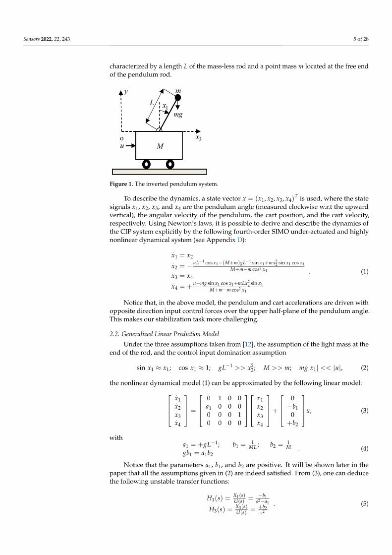
The CIP system consists of a cart and a rigid rod pendulum with a pivot mountedon the top of the cart, as shown in Figure 1. Under the action of the horizontal force thatis regarded as the control input u(t), the cart moves left or right on a one-dimensionalbounded track, whereas the pendulum swings in the vertical plane determined by the track.It is assumed that no friction exists in the system between the cart and the track or betweenthe cart and the pendulum. The cart is characterized by a mass M, and the pendulum is

Sensors 2022, 22, 243 5 of 28

characterized by a length L of the mass-less rod and a point mass m located at the free endof the pendulum rod.

Sensors 2022, 22, 243 5 of 30

track. It is assumed that no friction exists in the system between the cart and the track or between the cart and the pendulum. The cart is characterized by a mass M , and the pen-dulum is characterized by a length L of the mass-less rod and a point mass m located at the free end of the pendulum rod.

Figure 1. The inverted pendulum system.

To describe the dynamics, a state vector ( )Txxxxx 4321 ,,,= is used, where the state signals 1x , 2x , 3x , and 4x are the pendulum angle (measured clockwise w.r.t the up-ward vertical), the angular velocity of the pendulum, the cart position, and the cart veloc-ity, respectively. Using Newton’s laws, it is possible to derive and describe the dynamics of the CIP system explicitly by the following fourth-order SIMO under-actuated and highly nonlinear dynamical system (see Appendix D):

( )

12

12211

4

43

12

11221

11

1

2

21

cossincossin

coscossinsincos

xmmMxmLxxxmgux

xxxmmM

xxmxxgLmMxuLx

xx

−++−+=

=−+

++−−=

=−−

. (1)

Notice that, in the above model, the pendulum and cart accelerations are driven with opposite direction input control forces over the upper half-plane of the pendulum angle. This makes our stabilization task more challenging.

2.2. Generalized Linear Prediction Model Under the three assumptions taken from [12], the assumption of the light mass at the

end of the rod, and the control input domination assumption 1 2

1 1 1 2 1sin ; cos 1; ; ;x x x gL x M m mg x u−≈ ≈ >> >> << , (2)

the nonlinear dynamical model (1) can be approximated by the following linear model:

u

b

b

xxxx

a

xxxx

+

−+

=

2

1

4

3

2

1

1

4

3

2

1

0

0

000010000000010

, (3)

with

Figure 1. The inverted pendulum system.

To describe the dynamics, a state vector x = (x1, x2, x3, x4)T is used, where the state

signals x1, x2, x3, and x4 are the pendulum angle (measured clockwise w.r.t the upwardvertical), the angular velocity of the pendulum, the cart position, and the cart velocity,respectively. Using Newton’s laws, it is possible to derive and describe the dynamics ofthe CIP system explicitly by the following fourth-order SIMO under-actuated and highlynonlinear dynamical system (see Appendix D):

.x1 = x2.x2 = − uL−1 cos x1−(M+m)gL−1 sin x1+mx2

2 sin x1 cos x1M+m−m cos2 x1.

x3 = x4.x4 = +

u−mg sin x1 cos x1+mLx22 sin x1

M+m−m cos2 x1

. (1)

Notice that, in the above model, the pendulum and cart accelerations are driven withopposite direction input control forces over the upper half-plane of the pendulum angle.This makes our stabilization task more challenging.

2.2. Generalized Linear Prediction Model

Under the three assumptions taken from [12], the assumption of the light mass at theend of the rod, and the control input domination assumption

sin x1 ≈ x1; cos x1 ≈ 1; gL−1 >> x22; M >> m; mg|x1| << |u|, (2)

the nonlinear dynamical model (1) can be approximated by the following linear model:.x1.x2.x3.x4

=

0 1 0 0a1 0 0 00 0 0 10 0 0 0

x1x2x3x4

+

0−b1

0+b2

u, (3)

witha1 = +gL−1; b1 = 1

ML ; b2 = 1M

gb1 = a1b2. (4)

Notice that the parameters a1, b1, and b2 are positive. It will be shown later in thepaper that all the assumptions given in (2) are indeed satisfied. From (3), one can deducethe following unstable transfer functions:

H1(s) =X1(s)U(s) = −b1

s2−a1

H3(s) =X3(s)U(s) = +b2

s2

. (5)

Sensors 2022, 22, 243 6 of 28

Let us now define the following generalized linear CIP model with k ∈ {−1,+1},which can be seen as a generalization or modification of model (3):

.x1.x2.y3.y4

=

0 1 0 0a1 0 0 00 0 0 10 0 0 0

x1x2y3y4

+

0−b1

0+kb2

u, (6)

where the pendulum subsystem model remains unchanged when compared to the originalmodel (3) while the cart subsystem model is substituted by a fictitious one. This lastsubsystem, with the new states y3 and y4, is driven at each instant t with the control inputku. Using the above-adopted model (6), and assuming y3 = x3 and y4 = x4 at the instant t,we define the following pendulum and cart generalized prediction models:

x1 (t + h) = A1x1(t) + B1x2(t) − E1ux2(t + h) = A2x1(t) + B2x2(t) − E2uy3 (t + h) = x3(t) + h x4(t) + kE3uy4(t + h) = x4(t) + kE4u

, (7)

where h is a positive constant horizon time. If u(t) = u is constant on the interval [t, t + h],then by solving (6) and using the last equality of (4), we obtain (7) with the followingparameters:

A1 = cosh(

a1/21 h

)A2 = a1/2

1 sinh(

a1/21 h

)B1 = a−1/2

1 sinh(

a1/21 h

)B2 = cosh

(a1/2

1 h)

E1 = 2a−11 b1sinh2

(a1/2

1 h/2)

E2 = a−1/21 b1sinh

(a1/2

1 h)

E3 = 0.5b2 h2

E4 = b2 h

. (8)

Notice that the parameters A1, A2, B1, B2, E1, E2, E3, and E4 are positive.

2.3. Problem Statement

For the CIP system stabilization, we are interested in using the following static state-feedback control law (SFC):

u(t) = +Nx(t)− N3x3d= +N1x1(t) + N2x2(t) + N3[x3(t)− x3d] + N4x4(t)

, (9)

where N = (N1, N2, N3, N4) is the control gain vector to be determined, and x3d is theconstant cart reference position. The main result of this paper is how to simplify thecontrol tuning based on the good robustness properties of the control system and theoptimized two-time controller structure. The controllability of the linear system (3) ensuresthe existence of a set of SFC having the form (9) that can achieve the stabilization of the CIPsystem in the vicinity of the unstable equilibrium point. Combining (5) and the Laplacetransform of (9) yields:

F1(s) =X1(s)X3d(s)

= +b1 N3s2

P(s)

F3(s) =X3(s)X3d(s)

=−b2 N3(s2−a1)

P(s)

Fu(s) =U(s)

X3d(s)=−N3s2(s2−a1)

P(s)P(s) = s4 + (b1N2 − b2N4) s3 + (b1N1 − b2N3 − a1) s2 + a1b2N4 s + a1b2N3

. (10)

Sensors 2022, 22, 243 7 of 28

The obtained linearized closed-loop CIP system is of the fourth order and has the basicconfiguration shown in Figure 2. Obviously, each controller belonging to the class (9) canbe interpreted as the combination of two PD controllers (one for the pendulum subsystemand the other for the cart subsystem).

Sensors 2022, 22, 243 7 of 30

( ) ( )( ) ( ) ( )[ ] ( )txNxtxNtxNtxN

xNtNxtu

d

d

443332211

33

+−+++=−+=

, (9)

where ( )4321 ,,, NNNNN = is the control gain vector to be determined, and dx3 is the constant cart reference position. The main result of this paper is how to simplify the con-trol tuning based on the good robustness properties of the control system and the opti-mized two-time controller structure. The controllability of the linear system (3) ensures the existence of a set of SFC having the form (9) that can achieve the stabilization of the CIP system in the vicinity of the unstable equilibrium point. Combining (5) and the La-place transform of (9) yields:

( ) ( )( ) ( )

( ) ( )( )

( )( )

( ) ( )( )

( )( )

( ) ( ) ( ) 3214212

132113

42214

122

3

3

12

32

3

33

231

3

11

NbasNbasaNbNbsNbNbssP

sPassN

sXsUsF

sPasNb

sXsXsF

sPsNb

sXsXsF

du

d

d

++−−+−+=

−−==

−−==

+==

. (10)

The obtained linearized closed-loop CIP system is of the fourth order and has the basic configuration shown in Figure 2. Obviously, each controller belonging to the class (9) can be interpreted as the combination of two PD controllers (one for the pendulum subsystem and the other for the cart subsystem).

Figure 2. State-feedback linearized CIP control system.

Remark 1. The fourth-order transfer functions (10) must at least be stable. The Routh necessary and sufficient stability conditions for such a system are given in (11). From these conditions and the pos-itivity of the parameters (4), it follows that the controller gains ( )4321 ,,, NNNN must be positive.

21

1

4

3

2

12

44221

3

4

13211

4221

00

00

Nba

NN

NN

gNNNbNb

NN

aNbNbNbNb

−−>−

>>

>−−>−

. (11)

Remark 2. The cart transfer function ( )sF3 has two real opposite zeroes, 2/112,1 az ±= . The single

real NMP zero, 2/112 az += , provokes the appearance of an undesirable initial undershoot in the

cart step response. The amplitude of this undershoot grows to infinity if the settling time is reduced to 0 [30]. This behavior therefore places a limitation on the cart speed of response. Overshoot in the

Figure 2. State-feedback linearized CIP control system.

Remark 1. The fourth-order transfer functions (10) must at least be stable. The Routh necessaryand sufficient stability conditions for such a system are given in (11). From these conditions andthe positivity of the parameters (4), it follows that the controller gains (N1, N2, N3, N4) mustbe positive.

b1N2 − b2N4 > 0b1N1 − b2N3 − a1 > 0N4 > 0N3 > 0b1N2 − b2N4 > N4

N2

gN1N2− N3

N4− a1

b1 N2

. (11)

Remark 2. The cart transfer function F3(s) has two real opposite zeroes, z1,2 = ±a1/21 . The single

real NMP zero, z2 = +a1/21 , provokes the appearance of an undesirable initial undershoot in the

cart step response. The amplitude of this undershoot grows to infinity if the settling time is reducedto 0 [30]. This behavior therefore places a limitation on the cart speed of response. Overshoot in theabove response is another undesirable effect that may be reduced with the undershoot phenomenon ifan appropriate selection of SFC controller gains is conducted.

Remark 3. From (10), it can be seen that the pendulum and cart transfer functions F1(s) and F3(s)have fixed zeroes and adjustable poles. Thus, whatever the method used to determine the SFC gains,it is always considered as a pole placement method. In the sequel, we shall refer to the SFC controlmethod (9) as pole-dependent and pole-independent if its gain tuning method specifies a priori and aposteriori the closed-loop pole locations of (10), respectively.

In this paper, we investigate a subclass of SFC controllers (9), where the designedcontroller carries all the key features of SIMO MPC controllers and can be implemented inan ECS fashion. As it is depicted in Figure 3, the considered controller receives as its inputsthe cart reference position, x3d, and the state vector, x = (x1, x2, x3, x4), and produces as itssingle output the control signal, v, which is fed directly to the control input u of the CIPsystem. In our investigation, we need to consider the following assumption.

Sensors 2022, 22, 243 8 of 30

above response is another undesirable effect that may be reduced with the undershoot phenomenon if an appropriate selection of SFC controller gains is conducted.

Remark 3. From (10), it can be seen that the pendulum and cart transfer functions ( )sF1 and ( )sF3 have fixed zeroes and adjustable poles. Thus, whatever the method used to determine the

SFC gains, it is always considered as a pole placement method. In the sequel, we shall refer to the SFC control method (9) as pole-dependent and pole-independent if its gain tuning method specifies a priori and a posteriori the closed-loop pole locations of (10), respectively.

In this paper, we investigate a subclass of SFC controllers (9), where the designed controller carries all the key features of SIMO MPC controllers and can be implemented in an ECS fashion. As it is depicted in Figure 3, the considered controller receives as its inputs the cart reference position, dx3 , and the state vector, ( )4321 ,,, xxxxx = , and pro-duces as its single output the control signal, v , which is fed directly to the control input u of the CIP system. In our investigation, we need to consider the following assumption.

Assumption 1: • the state vector ( )4321 ,,, xxxxx = is measurable; • the parameters ( )dxLmM 3,,, are known constants; and • the set of hypotheses in Equation (2) is satisfied.

Figure 3. The proposed CIP SIMO MPC control system.

Under Assumption 1, the CIP stabilization problem may be formulated in two steps as follows. In the first step, restrict the class of SFC controllers so as to satisfy the following property: • Property 1: The SFC controller (9) ensures robust stability with a prescribed closed-

loop gain margin, minGM .

In the second step, and under the above gain margin constraint and the generalized prediction model (7) and (8), design a pole-independent SIMO MPC controller such that the following properties are satisfied: • Property 2: The closed-loop CIP system satisfies a two-time-scale structure in which

the closed-loop pendulum subsystem responds faster than the closed-loop cart sub-system [33].

• Property 3: In the absence of disturbance input, the controller ensures low cart set-tling time 0>T without excessive peaking (undershoot and overshoot) phenome-non in the CIP input and output responses.

3. SIMO MPC Controller Design To design robust SIMO MPC controllers, we first developed Equation (23), associated

with the SFC gain margin property, using the stability conditions (11) and the prescribed gain margin, minGM . Then, Property 1 holds when the above-mentioned equation is sat-isfied. Next, based on the generalized prediction model (7–8) and the quadratic cost func-tion (24) that is characterized by a set of MPC parameters ( )21 ,,, ρρϕ rh= , i.e., the horizon

Figure 3. The proposed CIP SIMO MPC control system.

Sensors 2022, 22, 243 8 of 28

Assumption 1:

• the state vector x = (x1, x2, x3, x4) is measurable;• the parameters (M, m, L, x3d) are known constants; and• the set of hypotheses in Equation (2) is satisfied.

Under Assumption 1, the CIP stabilization problem may be formulated in two stepsas follows. In the first step, restrict the class of SFC controllers so as to satisfy thefollowing property:

• Property 1: The SFC controller (9) ensures robust stability with a prescribed closed-loopgain margin, GMmin.

In the second step, and under the above gain margin constraint and the generalizedprediction model (7) and (8), design a pole-independent SIMO MPC controller such thatthe following properties are satisfied:

• Property 2: The closed-loop CIP system satisfies a two-time-scale structure in which theclosed-loop pendulum subsystem responds faster than the closed-loop cart subsystem [33].

• Property 3: In the absence of disturbance input, the controller ensures low cart settlingtime T > 0 without excessive peaking (undershoot and overshoot) phenomenon inthe CIP input and output responses.

3. SIMO MPC Controller Design

To design robust SIMO MPC controllers, we first developed Equation (23), associatedwith the SFC gain margin property, using the stability conditions (11) and the prescribedgain margin, GMmin. Then, Property 1 holds when the above-mentioned equation issatisfied. Next, based on the generalized prediction model (7–8) and the quadratic costfunction (24) that is characterized by a set of MPC parameters ϕ = (h, ρ1, r, ρ2), i.e., thehorizon time and the positive weight factors to be defined later, we establish the explicitrelationship (26) between ϕ and N. Finally, we propose a pole-independent tuning methodthat relies primarily on choosing the parameter set ϕ of the cost function as a starting pointof the optimal control. This method leads to determining the pole locations a posteriori, i.e.,at its final stage. Notice that the controller design developed hereafter uses the linearizedCIP model (3) in the neighborhood of the equilibrium point, where it is assumed to bejustified at least from the approximation point of view. The validity of the adopted designmethods is demonstrated from the control point of view in Section 4, where the nonlinearmodel (1) is used instead of its linearized version.

3.1. Closed-Loop SGM Constraint

Let us consider the following change of variables:

N1 = α12N2N3 = α34N4α = α12 − α34

, (12)

where α12 > 0 and α34 > 0. Introducing (12) in the last condition of (11) gives:

b1N2 >

[1 +

b1

b2

gb1N2α− a1

]b2N4. (13)

This means that there exists a critical gain N4 that depends on the fixed value of N2.The critical positive gain b2N4i > 0 at which the system becomes marginally stable is:

b2N4i =b1N2

1 + b1b2

gb1 N2α−a1

> b2N4. (14)

Sensors 2022, 22, 243 9 of 28

From (14), we define the cart-loop gain margin as follows:

GMC =b2N4ib2N4

=b1N2

b2N4

11 + a1

b1 N2α−a1

. (15)

On the other hand, the critical positive gains b1N2iα > 0 and yi = b1N2iα− a1 at whichthe system becomes marginally stable is deduced from (13) as the positive solutions of thefollowing system of equations:

y2i + [a1 − b2N4α]yi − gb1N4α = 0

yi = b1N2iα− a1, (16)

withyi =

12 [b2N4α− a1] +

12

√[b2N4α− a1]

2 + 4gb1N4α > 0b1N2iα = yi + a1

. (17)

Using the last equality gb1 = a1b2 of (4), (17) reduces to:

yi = b2N4α > 0b1N2iα = b2N4α + a1

. (18)

From (18), we define the pendulum-loop gain margin as follows:

GMP =b1N2α

b1N2iα=

b1N2

b2N4

11 + a1

b2 N4α

. (19)

Taking into account the worst case, the system gain margin index can be defined asfollows [17]:

GM = min(GMP, GMC)

GM =

{GMC if (b1N2 − b2N4)α < a1GMP if (b1N2 − b2N4)α ≥ a1

. (20)

Since the gain margins, GMC and GMP, must be greater than 1, from (16) and (19), wededuce, respectively:

(b1N2 − b2N4)α = a1 + (GMC − 1)αb2N4 ≥ a1(b1N2 − b2N4)α = GMPa1 + (GMP − 1)αb2N4 ≥ a1

. (21)

Regarding (21), the system gain margin (20) reduces to:

GM = GMP =b1N2

b2N4

11 + a1

b2 N4α

. (22)

The following remark states some of the obvious properties of the closed-loop systemgain margin.

Remark 4. Consider the fourth-order closed-loop system in (10) with the change of variables (12)and the system gain margin (22). Then, the following properties hold: (i) with fixed parameters αand b1N2, GM decreases with the increase in b2N4; (ii) with fixed parameters α and b2N4, GMincreases with the increase in b1N2; and (iii) with fixed parameters b1N2 and b2N4, GM remainsunchanged for any value γ if N1 and N3 are increased by the amounts N2γ and N4γ, respectively.

Remark 5. Given the value of GMmin and using Equation (22), Property 1 can be satisfied underthe following constraint:

(b1N2 − GMminb2N4)α = GMmina1, (23)

where α is defined in (12).

Sensors 2022, 22, 243 10 of 28

3.2. Deriving the SIMO MPC Control Law

To derive the SIMO MPC control law, we first adopt the generalized linear predictionmodel (7) and (8) as a prediction model for the CIP system. Then, we consider the followingquadratic cost function:

JMPC(t, h) = 12 e2

1(t + h) + 12 ρ1e2

2(t + h) + 12 re2

3(t + h) + 12 rρ2e2

4(t + h)e1(t + h) = 0− x1(t + h)e2(t + h) = 0− x2(t + h)e3(t + h) = x3d − y3(t + h)e4(t + h) =

.x3d − y4(t + h) = 0− y4(t + h)

, (24)

where ϕ = (h, ρ1, r, ρ2) ∈ <+4 is the set of positive MPC parameters, e1(t + h) and e2(t + h)are the predicted pendulum angle and velocity errors, while e3(t + h) and e4(t + h) are thepredicted cart position and velocity errors. Now, given the cart destination x3d and theprediction models (7), we obtain the optimal input v0, which minimizes the value of thequadratic cost function (24). Recall that the references associated with x1, x2, and x4 areassumed to be zero. Substituting (7) into (24) and setting the gradient of JMPC(t, h) withrespect to v to zero yields:

v0(t) = +N1x1(t) + N2x2(t) + N3[x3(t)− x3d] + N4x4(t), (25)

with the SIMO MPC controller gains given below:

N1 = D−1 A1E1 + D−1ρ1 A2E2N2 = D−1B1E1 + D−1ρ1B2E2N3 = −D−1r× kE3N4 = −D−1r× k(hE3 + ρ2E4)D = E2

1 + ρ1E22 + r× k2(E2

3 + ρ2E24) . (26)

Notice that the positivity of (ρ1, r, rρ2) together with the positivity of (8) imply thepositivity of N1 and N2 in addition to the fact that the gains N3 and N4 have an undefinedsign that follows the one associated with the value of k.

Remark 6. Since the signs of N3 and N4 are identical to the sign of k, the designed SIMO MPCcontroller that is defined by (23) and (24) does not ensure the stability condition (11) when using thetrivial prediction model, i.e., the generalized prediction model (10) with k = +1. To circumvent sucha drawback, we put k = −1 in the above model. This modification is equivalent to the substitution ofthe original cart subsystem model by another cart subsystem model that is driven at each instant andfrom the same state point with an opposite control input sign. The modification of the cost functionwhile keeping the trivial prediction model is another option to solve the encountered stability problem.However, this option is more complicated and is not considered in this paper.

3.3. Time-Scale Structure Constraint

Here, we are interested in designing a SIMO MPC controller that ensures Property 2,i.e., a two-time-scale structure, without using a priori targeted closed-loop pole locations.To this end, the CIP control system of Figure 2 is transformed to the configuration ofFigure 4, where a virtual reference x1d and a new gain K are introduced for the closed-looppendulum subsystem. The pendulum transfer function to the considered reference and thevalue of K that leads to a unity static gain are given by:

F1F(s) =X1(s)X1d(s)

= −Kb1s2+b1 N2s+b1 N1−a1

K = −N1 + a1b−11 = −N1 + Mg

. (27)

Sensors 2022, 22, 243 11 of 28

Sensors 2022, 22, 243 11 of 30

( ) ( ) ( ) ( )[ ] ( )txNxtxNtxNtxNtv d 4433322110 +−+++= , (25)

with the SIMO MPC controller gains given below:

( )( )2

4223

2221

21

4231

4

31

3

2211

111

2

2211

111

1

EEkrEED

EhEkrDN

kErDN

EBDEBDN

EADEADN

ρρ

ρ

ρ

ρ

+×++=

+×−=

×−=

+=

+=

−

−

−−

−−

. (26)

Notice that the positivity of ( )21 ,, ρρ rr together with the positivity of (8) imply the positivity of 1N and 2N in addition to the fact that the gains 3N and 4N have an un-defined sign that follows the one associated with the value of k .

Remark 6. Since the signs of 3N and 4N are identical to the sign of k , the designed SIMO MPC controller that is defined by (23) and (24) does not ensure the stability condition (11) when using the trivial prediction model, i.e., the generalized prediction model (10) with 1+=k . To circumvent such a drawback, we put 1−=k in the above model. This modification is equivalent to the substitution of the original cart subsystem model by another cart subsystem model that is driven at each instant and from the same state point with an opposite control input sign. The modification of the cost function while keeping the trivial prediction model is another option to solve the encountered stability problem. However, this option is more complicated and is not considered in this paper.

3.3. Time-Scale Structure Constraint Here, we are interested in designing a SIMO MPC controller that ensures Property 2,

i.e., a two-time-scale structure, without using a priori targeted closed-loop pole locations. To this end, the CIP control system of Figure 2 is transformed to the configuration of Fig-ure 4, where a virtual reference dx1 and a new gain K are introduced for the closed-loop pendulum subsystem. The pendulum transfer function to the considered reference and the value of K that leads to a unity static gain are given by:

( ) ( )( )

MgNbaNK

aNbsNbsKb

sXsXsF

dF

+−=+−=

−++−==

−1

1111

111212

1

1

11 . (27)

The GTC associated with (10) and (27) are given, respectively, by:

121

212111

21

343

4

321

421

11

1

ατ

ατ

ατ

=>−

=−

=

===

− PLP

C

MgNaNbNb

NN

NbaNba

, (28)

where PLτ is a lower bound for the pendulum GTC.

Figure 4. Equivalent state-feedback linearized CIP control system. Figure 4. Equivalent state-feedback linearized CIP control system.

The GTC associated with (10) and (27) are given, respectively, by:

τC = a1b2 N4a1b2 N3

= N4N3

= 1α34

τP = b1 N2b1 N1−a1

= 1α12−MgN−1

2> τPL = 1

α12

, (28)

where τPL is a lower bound for the pendulum GTC.For the sake of developing a general tuning method that is valid for a large class of

CIP systems, let us define the following normalized parameters:

h0 = a1/21 h ρ10 = a1ρ1 ρ20 = a1ρ2

r0 = a−21 g2r r12 = a−1/2

1 α12 r34 = a−1/21 α34

ϕ0 = (h0, ρ10, r0, ρ20)

, (29)

where ϕ0 is the set of normalized positive MPC cost function parameters. Substituting (29)into (28) and (26), we obtain:

r12 = N10N20

= a−1/21 τ−1

PLr34 = N30

N40= a−1/2

1 τ−1C

, (30)

N1 = a1b−11 N10D−1

0N2 = a1/2

1 b−11 N20D−1

0N3 = a1b−1

2 N30D−10

N4 = a1/21 b−1

2 N40D−10

, (31)

withN10 = 2sinh2(h0/2) cosh(h0) + ρ10sinh2(h0)

= 4sinh4(h0/2) + 2sinh2(h0/2) + ρ10sinh2(h0)

N20 = 2sinh(h0)sinh2(h0/2) + ρ10 cosh(h0)sinh(h0)N30 = 0.5r0h2

0N40 = r0

(0.5h2

0 + ρ20)

h0D0 = 4sinh4(h0/2) + ρ10sinh2(h0) + r0

(0.25h2

0 + ρ20)

h20

. (32)

Now, combining (30) and (32) yields:

r12 = a−1/21 τ−1

PL =4sinh4(h0/2) + 2sinh2(h0/2) + ρ10sinh2(h0)

2sinh(h0)sinh2(h0/2) + ρ10 cosh(h0)sinh(h0). (33)

In order to speed the pendulum response, we plan to maximize (33) by a proper choiceof the horizon time. More precisely, for a given positive value ρ10, setting the gradient ofr12 with respect to h0 to zero yields:

h0 = ln

[1 + ρ10 + ρ2

10 +√

ρ10(1 + 2ρ10)(2 + ρ10)

1− ρ210

]. (34)

Sensors 2022, 22, 243 12 of 28

From (34) and Figure 5, it is clear that the parameter ρ10 increases with the increase inh0 and satisfies 0 < ρ10 < 1. Concerning the amount r12, it is obvious that this parameterdecreases toward 1 with the increase in h0.

Sensors 2022, 22, 243 13 of 30

Figure 5. Evolution of ( 12r , 10ρ , min20ρ ) versus 0h .

Now, introducing the expressions of 12α and 34α from (29) together with the ex-pressions of 2N and 4N from (31) in (23) gives

( )( ) 0min341240min20 DGMrrNGMN =−− . (35)

Substituting the expressions of 40N and 0D from (32) in (35) and solving for 0r gives:

( ) ( ) ( )( )( ) ( ) 2

02020020

203412

02

1004

3412201

min0

25.05.0

sinh2/sinh4

hhhhrr

hhrrNGMrρρ

ρ

+++−

−−−=−

. (36)

Since 0h and 10ρ are linked by the relationship (34) and the fact that 0r and ( )20100 ,, ρρh are linked by the relationship (36), we only need to specify two parameters among the elements of the set 0ϕ to achieve the controller design. In our case, we shall fine-tune the weight factor vector ( )20100 , ρρρ = inside an appropriate domain. We have already shown that 10 10 << ρ , and the interval associated with 20ρ remains to be deter-mined. To this end, it is reasonable to satisfy Property 2 by assuming that the GTC of the closed-loop cart subsystem is lower than the GTC of the pendulum subsystem. According to (30) and (32) and the fact that 00 >r , this leads us to impose the constraint:

1220

20

034 5.0

5.00 rhh

r <+

=<ρ

, (37)

from which we obtain:

( ) 001

12min20

20min20

21 hhr −=

∞<<

−ρ

ρρ. (38)

A lower bound min20ρ , which is shown in Figure 5 as a function of 0h , is then im-posed to 20ρ to ensure Property 2.

Now, let us define a set of five indices to evaluate the CIP transient response perfor-mance: ( )01 ρxP , the maximum absolute value of the pendulum angle response; ( )03 ρxV , the cart response overshoot; ( )03 ρxD , the cart response undershoot; ( )0ρuP , the maxi-mum absolute value of the control input signal; and ( )0ρcst , the cart settling time at 5%. To derive general comments on the behavior of the CIP system, it is useful to introduce

Figure 5. Evolution of (r12, ρ10, ρ20min) versus h0.

Now, introducing the expressions of α12 and α34 from (29) together with the expressionsof N2 and N4 from (31) in (23) gives

(N20 − GMminN40)(r12 − r34) = GMminD0. (35)

Substituting the expressions of N40 and D0 from (32) in (35) and solving for r0 gives:

r0 =GM−1

minN20(r12 − r34)− 4sinh4(h0/2)− ρ10sinh2(h0)

(r12 − r34)(0.5h2

0 + ρ20)

h0 +(0.25h2

0 + ρ20)

h20

. (36)

Since h0 and ρ10 are linked by the relationship (34) and the fact that r0 and (h0, ρ10, ρ20)are linked by the relationship (36), we only need to specify two parameters among theelements of the set ϕ0 to achieve the controller design. In our case, we shall fine-tune theweight factor vector ρ0 = (ρ10, ρ20) inside an appropriate domain. We have already shownthat 0 < ρ10 < 1, and the interval associated with ρ20 remains to be determined. To thisend, it is reasonable to satisfy Property 2 by assuming that the GTC of the closed-loop cartsubsystem is lower than the GTC of the pendulum subsystem. According to (30) and (32)and the fact that r0 > 0, this leads us to impose the constraint:

0 < r34 =0.5h0

0.5h20 + ρ20

< r12, (37)

from which we obtain:ρ20min < ρ20 < ∞ρ20min = 1

2

(r−1

12 − h0

)h0

. (38)

A lower bound ρ20min, which is shown in Figure 5 as a function of h0, is then imposedto ρ20 to ensure Property 2.

Now, let us define a set of five indices to evaluate the CIP transient response perfor-mance: Px1(ρ0), the maximum absolute value of the pendulum angle response; Vx3(ρ0),the cart response overshoot; Dx3(ρ0), the cart response undershoot; Pu(ρ0), the maximumabsolute value of the control input signal; and tcs(ρ0), the cart settling time at 5%. To derivegeneral comments on the behavior of the CIP system, it is useful to introduce the changevariable s = a1/2

1 z and the gains (31) in (10) to obtain the following transfer functions:

Sensors 2022, 22, 243 13 of 28

F1(z) = L−1 N30 D−10 z2

P(z)

F3(z) =−N30 D−1

0 (z2−1)P(z)

Fu(s) = −MgL−1 N30 D−10 z2(z2−1)

P(z) =

P(z) = z4 +(

N20D−10 − N40D−1

0

)z3 +

(N10D−1

0 − N30D−10 − 1

)z2 + N40D−1

0 z + N30D−10

(39)

With the above processing, all the considered CIP transient response characteristicsremain unchanged, except the one associated with the modified (normalized) cart settlingtime tcsn, which is now linked to the original cart settling time tcs by the relationship:

tcsn = a1/21 tcs. (40)

Regarding the transfer functions (39), it appears naturally useful to normalize theindices associated with the pendulum angle response and control input signal as follows:

Px1n = LPx1Pun = Pu/

(MgL−1) . (41)

Now, we are ready to summarize in Algorithm 1 how to design the proposed SIMOcontroller and how to obtain the closed-loop linearized CIP performance when the systemgain margin GMmin and the weight vector ρ0 = (ρ10, ρ20) are chosen.

Algorithm 1: Controller design and closed-loop linearized CIP system evaluation.

1. Set the worst system gain margin, GMmin, and choose the weight vector ρ0 = (ρ10, ρ20);2. Evaluate (h0, r12, r34, r0, ρ20min) using (34), (33), (37), (36), and (38), respectively;3. If r0 < 0 or ρ20 ≤ ρ20 min, go to step 7;4. Evaluate (N10, N20, N30, N40, D0) using (32);5. Evaluate the step responses of (39) with (L,Mg) = (1,1);6. Evaluate the indices (Px1n, Vx3n, Dx3n, Pun, tcsn) from the obtained step responses;7. End.

3.4. Parameter Tuning

In this section, parameter tuning for the weight vector ρ0 is performed to ensurethe validity of Property 3. To this end, the peaking and speed constraints need to beconsidered simultaneously. To solve this problem, a time-domain optimization techniquethat involves tackling two issues, namely the choice of the performance criterion and themean to optimize it, is proposed hereafter. For the first issue, we have found it useful,regarding the desirable Property 3, to define two proposed sound and scaled-free indices.These indices are the speed efficiency SE(ρ0) and the average peak efficiency SE(ρ0) andare defined for a given standard (reference) state-feedback method (SSF) and our controlmethod as follows:

SE(ρ0) = 100 P4,SSFP4(ρ0)+P4,SSF

GE(ρ0) =100

3

3∑

i=1

Pi,SSFPi(ρ0)+Pi,SSF

, (42)

where P1(ρ0) = Px1(ρ0), P2(ρ0) = Px3(ρ0), P3(ρ0) = Pu(ρ0), and P4(ρ0) = tcs(ρ0). Theindex Pi,SSF has the same interpretation as the index Pi(ρ0), with the proposed controlmethod replaced by the SSF one. Obviously, an efficiency index greater than 50% indicatesthat the proposed control method outperforms the SSF method; otherwise, degradationin the performance of our method in comparison to the SSF one is noted. Then, taking

Sensors 2022, 22, 243 14 of 28

into account the worst efficiency case, we may formulate the setting problem as a maximinoptimization model as follows:(

ρ10,g, ρ20,g)= arg

(ρ10,ρ20)

max0 ≤ ρ10 ≤ ρ10,max0 ≤ ρ20 ≤ ρ20,max

J1(ρ0)

J1(ρ0) = min(SE(ρ0), λ−1GE(ρ0)

) , (43)

where λ = 0 if speed efficiency is the only concern, and λ = 1 if peaking and speed effi-ciency are both considered in the optimization. It should be noted that (43) is a continuousnonlinear optimization model with a highly nonlinear (possibly discontinuous) objectivefunction J1(ρ0), and it is difficult to know a priori whether such a function is unimodal ormultimodal before starting the optimization. To avoid erroneous solutions, problem (43)has to be solved to global optimality in the considered parameter space domain. Then, tosolve the second issue, we opt for global optimization using an exhaustive search over thedomain that is defined by 0 ≤ ρ10 ≤ ρ10,max and 0 ≤ ρ20 ≤ ρ20,max. This is interesting, sincethere are only two tuning parameters.

4. Numerical Simulations

Numerical simulations are conducted in several separate sections to show the poten-tial of the proposed pole-independent SIMO MPC controller (SIM) and its advantage incomparison to the pole-independent standard CDM controller (CDM), the pole-dependentCASC MPC controller (CAS), and the coincident pole controller (CPP). The definitions ofthe CDM, CAS, and CPP controllers are given in Appendices A–C, respectively. Thesecontrollers are chosen for their efficiencies and for the reduced number of adjusted pa-rameters, which leads to yield, without significant difficulty, a guarantee of the overallbest performance for each tuned controller. Based on the linearized CIP system, we beginthe numerical simulation in Section 4.1 with the establishment of some guidelines that helpin choosing the SIM weight factors for a prescribed system gain margin in the absence ofdisturbance input. These guidelines are quite general, since they can be applied to any linearCIP model of the form (3), as long as Assumption 1 stays satisfied. Additionally, they are veryuseful since they inform us how to tune the SIM weight factors to get some desirable transientclosed-loop linearized CIP system performance. Next, to make a fair comparison, we tune, fora given physical CIP system, the best possible CDM, CAS, and CPP controller so as to obtain amaximum system gain margin for each tuned controller. For the SIM controller, the systemgain margin is set a priori as the best one so far obtained by the above controllers, and the SIMweight factors are tuned according to (43). In Sections 4.3 and 4.4, we compare the obtainedcontrollers on the nonlinear CIP system in the absence and presence of disturbance input.

4.1. Guidelines for Weighting Factor Adjustment

To obtain some insights into how to choose the weight vector ρ0 = (ρ10, ρ20) fordifferent system gain margin values in the absence of disturbance input, we conducted50,000 simulations with Algorithm 1 (obtained by using a coarse grid discretization with50 points for ρ10 in the interval 0 < ρ10 < 0.5, 50 points for ρ20 in the interval 0 < ρ20 < 5,and 20 points for GMmin in the interval 1 < GMmin < 3). Figures 6 and 7 show the obtainedcontour plots for the considered transient response characteristics for GMmin = 1.63.To generate the contours, we constructed a grid interpolant using the Matlab function“griddedInterpolant” with the “pchip” option and interpolate the considered index with10−3 spacing. To avoid dummy solutions, only the contours that have more than 103 pointswere retained.

Sensors 2022, 22, 243 15 of 28

Sensors 2022, 22, 243 16 of 30

50,000 simulations with Algorithm 1 (obtained by using a coarse grid discretization with 50 points for 10ρ in the interval 5.00 10 << ρ , 50 points for 20ρ in the interval

50 20 << ρ , and 20 points for minGM in the interval 31 min << GM ). Figures 6 and 7 show the obtained contour plots for the considered transient response characteristics for

63.1min =GM . To generate the contours, we constructed a grid interpolant using the Matlab function “griddedInterpolant” with the “pchip” option and interpolate the con-sidered index with 310− spacing. To avoid dummy solutions, only the contours that have more than 310 points were retained.

From Figures 6 and 7, one can observe that the choice of the weight factors cannot be performed independently to address the peaking phenomenon and the cart speed of re-sponse issues simultaneously. Additionally, a strong correlation between the contours of

nxP 1 and 3xD is noticed. For the peaking phenomenon, it is clearly seen that the increase in 20ρ while maintaining 10ρ constant reduces without ambiguity the cart overshoot

( )03 ρxV . Ensuring a non-overshooting behavior for the cart subsystem thus appears pos-sible with a high enough value of 20ρ . For a constant 10ρ , the peaking phenomenon in-dices, namely nxP 1 , 3xD , and unP , are only reduced when 0ρ is located above their asso-ciated red line frontiers, as shown in Figures 6 and 7. The evaluation of these frontiers is performed without considering the interpolation processing. Ensuring a reduced under-shooting behavior for the cart subsystem appears to be possible with the increase in 20ρ . In addition to that, one can also clearly observe that the increase in 10ρ while maintaining

20ρ constant contribute, without ambiguity, to reduce the control input effort unP and to increase the cart overshoot ( )03 ρxV , as long as the value of 10ρ still far enough from the frontier that it defines the validity of the MPC controller (see step 3 of Algorithm 1). For a constant 20ρ , the increase in 10ρ may lead to an increase in nxP 1 and 3xD . Concerning the cart speed of response, there are two separate regions, i.e., the upper region UR and the lower region LR , where the settling time can be reduced below the value 20. These regions are located above the red line, where the increase in 20ρ while maintaining 10ρ constant reduces the peaking phenomenon. Table 1 shows the associated region frontier locations and transient performance intervals. Obviously, choosing 0ρ in the UR ap-pears to be more recommended than choosing it in the LR .

(a) (b)

Figure 6. CIP control performance 63.1min =GM . (a) Normalized pendulum maximum absolute value index; (b) cart overshoot and undershoot indices.

Figure 6. CIP control performance GMmin = 1.63. (a) Normalized pendulum maximum absolutevalue index; (b) cart overshoot and undershoot indices.

Sensors 2022, 22, 243 17 of 30

(a) (b)

Figure 7. CIP control performance for 63.1min =GM . (a) Normalized control input maximum ab-solute value index; (b) normalized cart settling time index.

Table 1. Transient response performance on the UR and LR frontiers.

10ρ 20ρ nxP 1 3xV (%) 3xD (%) unP

LR 10.003.0 − 96.038.0 − 61.505.3 − 55.2632.12 − 68.715.3 − 47.011.0 − UR 16.002.0 − 23.387.0 − 80.297.0 − 31.636.0 − 61.382.0 − 22.002.0 −

When the cart speed is the only concern, i.e., when using the proposed tuning method (43) with 0=λ , there is no need to select an SSF method, and the best-achieved cart set-tling time, bcsnt , , and its associated weight factor, b,10ρ , are defined as follows:

( )

( )min2010505.00,10

min2010

505.00,

,,minarg

,,min

201010

2010

GMt

GMtt

csnb

csnbcsn

ρρρ

ρρ

ρρρ

ρρ

≤≤≤≤

≤≤≤≤

=

=

. (44)

Figure 8 shows the above indices together with the cart overshoot and undershoot as a function of the prescribed system gain margin. It is clearly seen that the best-achieved cart settling time is obtained with 2.1min ≈GM ; additionally, the increase in minGM above this value leads to an increase in the optimal cart settling time and a reduction in the cart under-shoot. The cart overshoot remains between 4 and 5%, while the optimal weight factor b,10ρ remains, in all studied cases, under 0.12. As we shall see in the next section, the considered controllers for the comparison task do not exceed a system gain margin of 63.1 , while our SIM controller can go beyond this limit, as is indicated in Figure 8.

Figure 7. CIP control performance for GMmin = 1.63. (a) Normalized control input maximumabsolute value index; (b) normalized cart settling time index.

From Figures 6 and 7, one can observe that the choice of the weight factors cannotbe performed independently to address the peaking phenomenon and the cart speed ofresponse issues simultaneously. Additionally, a strong correlation between the contours ofPx1n and Dx3 is noticed. For the peaking phenomenon, it is clearly seen that the increase inρ20 while maintaining ρ10 constant reduces without ambiguity the cart overshoot Vx3(ρ0).Ensuring a non-overshooting behavior for the cart subsystem thus appears possible witha high enough value of ρ20. For a constant ρ10, the peaking phenomenon indices, namelyPx1n, Dx3, and Pun, are only reduced when ρ0 is located above their associated red linefrontiers, as shown in Figures 6 and 7. The evaluation of these frontiers is performedwithout considering the interpolation processing. Ensuring a reduced undershootingbehavior for the cart subsystem appears to be possible with the increase in ρ20. In additionto that, one can also clearly observe that the increase in ρ10 while maintaining ρ20 constantcontribute, without ambiguity, to reduce the control input effort Pun and to increase thecart overshoot Vx3(ρ0), as long as the value of ρ10 still far enough from the frontier that itdefines the validity of the MPC controller (see step 3 of Algorithm 1). For a constant ρ20,the increase in ρ10 may lead to an increase in Px1n and Dx3. Concerning the cart speed ofresponse, there are two separate regions, i.e., the upper region UR and the lower regionLR, where the settling time can be reduced below the value 20. These regions are locatedabove the red line, where the increase in ρ20 while maintaining ρ10 constant reduces the

Sensors 2022, 22, 243 16 of 28

peaking phenomenon. Table 1 shows the associated region frontier locations and transientperformance intervals. Obviously, choosing ρ0 in the UR appears to be more recommendedthan choosing it in the LR.

Table 1. Transient response performance on the UR and LR frontiers.

ρ10 ρ20 Px1n Vx3 (%) Dx3 (%) Pun

LR 0.03 − 0.10 0.38 − 0.96 3.05 − 5.61 12.32 − 26.55 3.15 − 7.68 0.11 − 0.47UR 0.02 − 0.16 0.87 − 3.23 0.97 − 2.80 0.36 − 6.31 0.82 − 3.61 0.02 − 0.22

When the cart speed is the only concern, i.e., when using the proposed tuningmethod (43) with λ = 0, there is no need to select an SSF method, and the best-achievedcart settling time, tcsn,b, and its associated weight factor, ρ10,b, are defined as follows:

tcsn,b = min0 ≤ ρ10 ≤ 0.5

0 ≤ ρ20 ≤ 5

tcsn(ρ10, ρ20, GMmin)

ρ10,b = argρ10

min0 ≤ ρ10 ≤ 0.50 ≤ ρ20 ≤ 5

tcsn(ρ10, ρ20, GMmin). (44)

Figure 8 shows the above indices together with the cart overshoot and undershoot asa function of the prescribed system gain margin. It is clearly seen that the best-achievedcart settling time is obtained with GMmin ≈ 1.2; additionally, the increase in GMmin abovethis value leads to an increase in the optimal cart settling time and a reduction in the cartundershoot. The cart overshoot remains between 4 and 5%, while the optimal weightfactor ρ10,b remains, in all studied cases, under 0.12. As we shall see in the next section, theconsidered controllers for the comparison task do not exceed a system gain margin of 1.63,while our SIM controller can go beyond this limit, as is indicated in Figure 8.

Sensors 2022, 22, 243 18 of 30

(a) (b)

Figure 8. Impact of the gain margin on the cart transient of response. (a) Optimal cart control sub-system performance versus gain margin; (b) weight factor versus gain margin setting for high cart speed of response.

4.2. Disturbance-Free Parameter Tuning Now, let us consider the nonlinear CIP system (1) with a set of physical parameters

kg4.2=M , kg23.0=m , m36.0=L , 2m/s819.g = , and a cart track length limited between m5.0± [23]. Since the behavior of the linearized CIP system is considered quite similar to

the behavior of the nonlinear CIP system in the vicinity of the equilibrium point, the tun-ing of the controllers is thus based only on the linearized system. Figures 9 and 10 show the evolution of the system gain margin together with the associated linearized cart tran-sient performance for the considered controllers. In contrast to non-undershooting cart response behavior, ensuring a non-overshooting cart response behavior is a feasible ob-jective for all controllers. Reducing the cart response undershoot can be undertaken at the price of an increase in the cart settling time and/or deterioration in the system gain margin performance. Regarding the system gain margin trend, it is seen that the system gain mar-gin is limited by about 1.4 for the CDM method and by about 1.6 for the CAS and CPP methods. For these methods, dependencies are typically observed between the system gain margin and the tuning parameters, which render them less flexible. Now, following [17], we retain the best tuning parameter for the CDM, CAS, and CPP as those that max-imize the system gain margin. The gains of these controllers and the resulting linear CIP system transient performance are summarized in Tables 2 and 3, respectively. The transi-ent performances are obtained for zero initial conditions and a cart step 1.03 =dx .

(a) (b)

Figure 8. Impact of the gain margin on the cart transient of response. (a) Optimal cart controlsubsystem performance versus gain margin; (b) weight factor versus gain margin setting for highcart speed of response.

4.2. Disturbance-Free Parameter Tuning

Now, let us consider the nonlinear CIP system (1) with a set of physical parametersM = 2.4 kg, m = 0.23 kg, L = 0.36 m, g = 9.81 m/s2, and a cart track length limitedbetween ±0.5 m [23]. Since the behavior of the linearized CIP system is considered quitesimilar to the behavior of the nonlinear CIP system in the vicinity of the equilibrium point,the tuning of the controllers is thus based only on the linearized system. Figures 9 and 10show the evolution of the system gain margin together with the associated linearized cart

Sensors 2022, 22, 243 17 of 28

transient performance for the considered controllers. In contrast to non-undershootingcart response behavior, ensuring a non-overshooting cart response behavior is a feasibleobjective for all controllers. Reducing the cart response undershoot can be undertaken atthe price of an increase in the cart settling time and/or deterioration in the system gainmargin performance. Regarding the system gain margin trend, it is seen that the systemgain margin is limited by about 1.4 for the CDM method and by about 1.6 for the CASand CPP methods. For these methods, dependencies are typically observed between thesystem gain margin and the tuning parameters, which render them less flexible. Now,following [17], we retain the best tuning parameter for the CDM, CAS, and CPP as thosethat maximize the system gain margin. The gains of these controllers and the resultinglinear CIP system transient performance are summarized in Tables 2 and 3, respectively.The transient performances are obtained for zero initial conditions and a cart step x3d = 0.1.

Sensors 2022, 22, 243 18 of 30

(a) (b)

Figure 8. Impact of the gain margin on the cart transient of response. (a) Optimal cart control sub-system performance versus gain margin; (b) weight factor versus gain margin setting for high cart speed of response.

4.2. Disturbance-Free Parameter Tuning Now, let us consider the nonlinear CIP system (1) with a set of physical parameters

kg4.2=M , kg23.0=m , m36.0=L , 2m/s819.g = , and a cart track length limited between m5.0± [23]. Since the behavior of the linearized CIP system is considered quite similar to

the behavior of the nonlinear CIP system in the vicinity of the equilibrium point, the tun-ing of the controllers is thus based only on the linearized system. Figures 9 and 10 show the evolution of the system gain margin together with the associated linearized cart tran-sient performance for the considered controllers. In contrast to non-undershooting cart response behavior, ensuring a non-overshooting cart response behavior is a feasible ob-jective for all controllers. Reducing the cart response undershoot can be undertaken at the price of an increase in the cart settling time and/or deterioration in the system gain margin performance. Regarding the system gain margin trend, it is seen that the system gain mar-gin is limited by about 1.4 for the CDM method and by about 1.6 for the CAS and CPP methods. For these methods, dependencies are typically observed between the system gain margin and the tuning parameters, which render them less flexible. Now, following [17], we retain the best tuning parameter for the CDM, CAS, and CPP as those that max-imize the system gain margin. The gains of these controllers and the resulting linear CIP system transient performance are summarized in Tables 2 and 3, respectively. The transi-ent performances are obtained for zero initial conditions and a cart step 1.03 =dx .

(a) (b)

Figure 9. Evolution of the system gain margin and the cart response performance. (a) CDM method;(b) CAS method.

Sensors 2022, 22, 243 19 of 30

Figure 9. Evolution of the system gain margin and the cart response performance. (a) CDM method; (b) CAS method.

(a) (b)

Figure 10. Evolution of the system gain margin and the cart response performance. (a) CPP method; (b) SIM method.

Table 2. State-feedback controller gains and associated parameters.

1N 2N 3N 4N Control Parameter GM CPP 43.91 46.17 08.13 99.14 49.3−=p 62.1

CDM 08.82 87.14 35.16 81.14 90.0=τ 39.1 CAS 9.230 31.53 72.73 72.73 20.00 =h 59.1

SIM 39.75 21.10 63.5 55.7 ( ) ( )5.1,09.0, 2010 =ρρ 63.1

Table 3. Controller performance comparison using linearized CIP model.

1xP (deg) 3xV (%) 3xD (%) ( )NuP cst (s) ES (%) EG (%) CPP 93.0 00.0 83.3 31.1 14.2 0.50 0.50

CDM 44.1 03.0 92.5 68.1 47.1 2.59 8.40 CAS 63.1 00.0 22.8 53.7 36.2 5.47 6.27 SIM 62.0 51.4 40.2 56.0 55.2 6.45 6.58

For the proposed SIM method, one can impose a priori the system gain margin as a constraint to the controller. Using a gain margin of 1.63 and applying the proposed tuning method (43) with 1=λ , we obtain 09.0,10 =gρ and 5.1,20 =gρ . The obtained controller gains and their associated performances are also given in Tables 2 and 3, respectively. Notice that the last assumption of Equation (2) is satisfied, since we have, for all control-lers, mgN >>1 . In comparison to the other control methods, the proposed SIM method has the best pendulum angle deviation, cart undershoot, and control input effort at the price of degradation in the cart overshoot and settling time. Using the CPP for the linear-ized CIP system as an SSF, we obtained the best EG at a price of a slight degradation in

ES , as is indicated in Table 3. Figure 11 indicates that the obtained optimal SIM controller depends only on ES , since we always have EE GS < . In addition to that, Table 4 and Fig-ure 11 show that the optimal SIM controller is characterized by a set of two complex con-jugates poles: one of them has a real part that is equal to the CPP controller pole, and the other one has the highest real part, which somewhat explains why the SIM controller has the largest cart settling time. Finally, Figure 10 tells us that the proposed SIM method allows to further reduce the peaking phenomenon while maintaining the system gain

Figure 10. Evolution of the system gain margin and the cart response performance. (a) CPP method;(b) SIM method.

Sensors 2022, 22, 243 18 of 28

Table 2. State-feedback controller gains and associated parameters.

N1 N2 N3 N4 Control Parameter GM

CPP 91.43 17.46 13.08 14.99 p = −3.49 1.62CDM 82.08 14.87 16.35 14.81 τ = 0.90 1.39CAS 230.9 53.31 73.72 73.72 h0 = 0.20 1.59SIM 75.39 10.21 5.63 7.55 (ρ10, ρ20) = (0.09, 1.5) 1.63

Table 3. Controller performance comparison using linearized CIP model.

Px1 (deg) Vx3 (%) Dx3 (%) Pu (N) tcs (s) SE (%) GE (%)

CPP 0.93 0.00 3.83 1.31 2.14 50.0 50.0CDM 1.44 0.03 5.92 1.68 1.47 59.2 40.8CAS 1.63 0.00 8.22 7.53 2.36 47.5 27.6SIM 0.62 4.51 2.40 0.56 2.55 45.6 58.6

For the proposed SIM method, one can impose a priori the system gain margin as aconstraint to the controller. Using a gain margin of 1.63 and applying the proposed tuningmethod (43) with λ = 1, we obtain ρ10,g = 0.09 and ρ20,g = 1.5. The obtained controllergains and their associated performances are also given in Tables 2 and 3, respectively.Notice that the last assumption of Equation (2) is satisfied, since we have, for all controllers,N1 >> mg. In comparison to the other control methods, the proposed SIM method hasthe best pendulum angle deviation, cart undershoot, and control input effort at the priceof degradation in the cart overshoot and settling time. Using the CPP for the linearizedCIP system as an SSF, we obtained the best GE at a price of a slight degradation in SE, as isindicated in Table 3. Figure 11 indicates that the obtained optimal SIM controller dependsonly on SE, since we always have SE < GE. In addition to that, Table 4 and Figure 11 showthat the optimal SIM controller is characterized by a set of two complex conjugates poles:one of them has a real part that is equal to the CPP controller pole, and the other one hasthe highest real part, which somewhat explains why the SIM controller has the largest cartsettling time. Finally, Figure 10 tells us that the proposed SIM method allows to furtherreduce the peaking phenomenon while maintaining the system gain margin constant byincreasing ρ20 above 1.5 and maintaining ρ10 = 0.09, but this enhancement is followed byan increase in tcs. In the vicinity of ρ20 = 2.5, the overshoot vanishes, and the cart settlingtime takes a value of about 4.8 s.

Sensors 2022, 22, 243 20 of 30

margin constant by increasing 20ρ above 5.1 and maintaining 09.010 =ρ , but this en-hancement is followed by an increase in cst . In the vicinity of 5.220 =ρ , the overshoot vanishes, and the cart settling time takes a value of about 4.8 s.

Table 4. Closed-loop poles for the considered controllers.

11 pip + 22 pip + 33 pip + 44 pip + CPP 49.3− 49.3− 49.3− 49.3−

CDM i90.078.2 −− i82.378.2 −− i82.378.2 +− i90.078.2 +− CAS i05.408.3 −− 39.1− 77.23− i05.408.3 +− SIM i58.549.3 −− i84.085.0 −− i84.085.0 +− i58.549.3 +−

(a) (b)

Figure 11. Analysis of the SIM method performance. (a) Speed and peak efficiencies; (b) pole locations.

4.3. Performance Analysis without a Disturbance Input To compare the performance of the above controllers, the reference cart position dx3

is set to m0 , and all the initial state values are set to zeros, except the initial cart position,

which is set to ( )3 0 0.1x = − m. The simulation results applied to the nonlinear CIP sys-tem (1), without considering disturbance input, are shown graphically in Figures 12 and 13 and numerically in Table 5. One can notice at this point that all the assumptions given by Equation (2) are satisfied. The strong similarity that exists between the performance of the closed-loop linearized CIP system in Table 3 and the performance of the closed-loop nonlinear CIP system in Table 5 for each controller confirms the potential of linear control theory in solving the considered stabilization problem. On the other hand, Figure 12 shows that the SIM method exhibits good performance in the control input effort, the pen-dulum angle, and the cart position undershoot at the price of relatively large cart position overshoot and settling time. Concerning Figure 13, the fact that the control input effort demand occurs essentially at the beginning of the CIP system stabilization for all the con-sidered controllers is obviously distinguished.

When the initial states begin from an equilibrium point and reach another one while the assumptions of Equation (2) are satisfied during the motion, the controlled nonlinear CIP system behaves similarly to the controlled linear CIP system. In such a situation, the performance of the controlled nonlinear CIP system can be naturally evaluated using the contour plots of Figures 6 and 7 for a gain margin of 1.63 and given MPC parameters. However, when the states are far away from the equilibrium point, the classical prediction model, defined by Equations (7) and (8) together with 1+=k , gives only partially con-sistent estimation or no longer holds at all. In the former case, which is not covered by the numerical study, it may perhaps be interesting to design the SIMO MPC controller in such

Figure 11. Analysis of the SIM method performance. (a) Speed and peak efficiencies; (b) pole locations.

Sensors 2022, 22, 243 19 of 28

Table 4. Closed-loop poles for the considered controllers.

p1 + ip1 p2 + ip2 p3 + ip3 p4 + ip4

CPP −3.49 −3.49 −3.49 −3.49CDM −2.78− 0.90i −2.78− 3.82i −2.78 + 3.82i −2.78 + 0.90iCAS −3.08− 4.05i −1.39 −23.77 −3.08 + 4.05iSIM −3.49− 5.58i −0.85− 0.84i −0.85 + 0.84i −3.49 + 5.58i

4.3. Performance Analysis without a Disturbance Input

To compare the performance of the above controllers, the reference cart position x3d isset to 0 m, and all the initial state values are set to zeros, except the initial cart position, whichis set to x3(0) = −0.1 m. The simulation results applied to the nonlinear CIP system (1),without considering disturbance input, are shown graphically in Figures 12 and 13 andnumerically in Table 5. One can notice at this point that all the assumptions given byEquation (2) are satisfied. The strong similarity that exists between the performance ofthe closed-loop linearized CIP system in Table 3 and the performance of the closed-loopnonlinear CIP system in Table 5 for each controller confirms the potential of linear controltheory in solving the considered stabilization problem. On the other hand, Figure 12shows that the SIM method exhibits good performance in the control input effort, thependulum angle, and the cart position undershoot at the price of relatively large cartposition overshoot and settling time. Concerning Figure 13, the fact that the control inputeffort demand occurs essentially at the beginning of the CIP system stabilization for all theconsidered controllers is obviously distinguished.

Sensors 2022, 22, 243 21 of 30

a way to increase enough ( )20100 , ρρρ = in the hope to simultaneously increase the pen-dulum gains 1N and 2N while reducing the cart gains 3N and 4N , as is suggested by Equations (26) and (29). When the pendulum angle is too large, the linearized model loses its validity, and it is necessary to apply some nonlinear technique to bring the pendulum to the vicinity of the upright equilibrium state. Then, it is possible to switch to the pro-posed control.

(a) (b)

Figure 12. CIP output responses using CAS, CPP, CDM, and SIM methods. (a) Pendulum angle responses; (b) cart position responses.

(a) (b)

Figure 13. CIP input responses using CAS, CPP, CDM, and SIM methods. (a) Overall input re-sponses; (b) restricted input responses.

Table 5. Controller performance comparison using nonlinear CIP model.

1xP (deg) 3xV (%) 3xD (%) ( )NuP cst (s) ES (%) EG (%)

CPP 95.0 00.0 88.3 31.1 16.2 8.49 7.49 CDM 47.1 00.0 99.5 68.1 42.1 1.60 5.40 CAS 64.1 00.0 26.8 53.7 37.2 4.47 5.27 SIM 62.0 65.3 37.2 54.0 55.2 6.45 6.60

4.4. Performance Analysis with a Disturbance Input To check the sensitivity of the studied controllers to disturbance input, a Matlab-Sim-

ulink band-limited white noise ( )tn with sampling time 0.01 s , seed = 23,341 , and power 310−=P was added to the control input signal of the nonlinear CIP system over

Figure 12. CIP output responses using CAS, CPP, CDM, and SIM methods. (a) Pendulum angleresponses; (b) cart position responses.

Table 5. Controller performance comparison using nonlinear CIP model.

Px1 (deg) Vx3 (%) Dx3 (%) Pu (N) tcs (s) SE (%) GE (%)

CPP 0.95 0.00 3.88 1.31 2.16 49.8 49.7CDM 1.47 0.00 5.99 1.68 1.42 60.1 40.5CAS 1.64 0.00 8.26 7.53 2.37 47.4 27.5SIM 0.62 3.65 2.37 0.54 2.55 45.6 60.6

Sensors 2022, 22, 243 20 of 28

Sensors 2022, 22, 243 21 of 30

a way to increase enough ( )20100 , ρρρ = in the hope to simultaneously increase the pen-dulum gains 1N and 2N while reducing the cart gains 3N and 4N , as is suggested by Equations (26) and (29). When the pendulum angle is too large, the linearized model loses its validity, and it is necessary to apply some nonlinear technique to bring the pendulum to the vicinity of the upright equilibrium state. Then, it is possible to switch to the pro-posed control.

(a) (b)

Figure 12. CIP output responses using CAS, CPP, CDM, and SIM methods. (a) Pendulum angle responses; (b) cart position responses.

(a) (b)

Figure 13. CIP input responses using CAS, CPP, CDM, and SIM methods. (a) Overall input re-sponses; (b) restricted input responses.

Table 5. Controller performance comparison using nonlinear CIP model.

1xP (deg) 3xV (%) 3xD (%) ( )NuP cst (s) ES (%) EG (%)

CPP 95.0 00.0 88.3 31.1 16.2 8.49 7.49 CDM 47.1 00.0 99.5 68.1 42.1 1.60 5.40 CAS 64.1 00.0 26.8 53.7 37.2 4.47 5.27 SIM 62.0 65.3 37.2 54.0 55.2 6.45 6.60

4.4. Performance Analysis with a Disturbance Input To check the sensitivity of the studied controllers to disturbance input, a Matlab-Sim-

ulink band-limited white noise ( )tn with sampling time 0.01 s , seed = 23,341 , and power 310−=P was added to the control input signal of the nonlinear CIP system over

Figure 13. CIP input responses using CAS, CPP, CDM, and SIM methods. (a) Overall input responses;(b) restricted input responses.

When the initial states begin from an equilibrium point and reach another one whilethe assumptions of Equation (2) are satisfied during the motion, the controlled nonlinearCIP system behaves similarly to the controlled linear CIP system. In such a situation, theperformance of the controlled nonlinear CIP system can be naturally evaluated using thecontour plots of Figures 6 and 7 for a gain margin of 1.63 and given MPC parameters.However, when the states are far away from the equilibrium point, the classical predic-tion model, defined by Equations (7) and (8) together with k = +1, gives only partiallyconsistent estimation or no longer holds at all. In the former case, which is not coveredby the numerical study, it may perhaps be interesting to design the SIMO MPC controllerin such a way to increase enough ρ0 = (ρ10, ρ20) in the hope to simultaneously increasethe pendulum gains N1 and N2 while reducing the cart gains N3 and N4, as is suggestedby Equations (26) and (29). When the pendulum angle is too large, the linearized modelloses its validity, and it is necessary to apply some nonlinear technique to bring the pen-dulum to the vicinity of the upright equilibrium state. Then, it is possible to switch to theproposed control.

4.4. Performance Analysis with a Disturbance Input

To check the sensitivity of the studied controllers to disturbance input, a Matlab-Simulink band-limited white noise n(t) with sampling time 0.01 s, seed = 23,341, andpower P = 10−3 was added to the control input signal of the nonlinear CIP system over atime interval of 120 s [23]. This disturbance input, which has an amplitude between −1.17and 1.25, is depicted in Figure 14. Table 6 summarizes the resulting maximum absolutevalues of the CIP input and output signals that are obtained from the analysis of the last100 s, i.e., in the assumed steady-state region. Regarding the disturbance input amplitudethat appears in Figure 14, the controller performance of Table 5, and the maximum absolutevalues of Table 6, all the considered controllers appear to exhibit useful noise rejectioncapabilities. The CAS method, with its highest gains (see Table 2) and high transient controlinput effort (see Table 5), exhibits the best noise rejection capabilities in the steady-stateregion, whereas the proposed SIM method, with its lowest gains (see Table 2) and lowesttransient control input effort (see Table 5), exhibits the worst one in the same steady-stateregion. Figures 15 and 16 show graphically the obtained CIP output responses. Althoughthe disturbance input level appears to dominate completely the amplitude of the SIMtransient noise-free control effort, i.e., 0.54 N (see Table 5), the proposed SIM method stillperforms well even with a tuning method that does not take into account the presence of adisturbance input.

Sensors 2022, 22, 243 21 of 28

Sensors 2022, 22, 243 22 of 30

a time interval of 120s [23]. This disturbance input, which has an amplitude between 17.1− and 25.1 , is depicted in Figure 14. Table 6 summarizes the resulting maximum

absolute values of the CIP input and output signals that are obtained from the analysis of the last 100s , i.e., in the assumed steady-state region. Regarding the disturbance input amplitude that appears in Figure 14, the controller performance of Table 5, and the maxi-mum absolute values of Table 6, all the considered controllers appear to exhibit useful noise rejection capabilities. The CAS method, with its highest gains (see Table 2) and high transient control input effort (see Table 5), exhibits the best noise rejection capabilities in the steady-state region, whereas the proposed SIM method, with its lowest gains (see Ta-ble 2) and lowest transient control input effort (see Table 5), exhibits the worst one in the same steady-state region. Figures 15 and 16 show graphically the obtained CIP output responses. Although the disturbance input level appears to dominate completely the am-plitude of the SIM transient noise-free control effort, i.e., N54.0 (see Table 5), the pro-posed SIM method still performs well even with a tuning method that does not take into account the presence of a disturbance input.

Figure 14. Input disturbance signal.

Table 6. Performance in a noisy situation for 20s 120st≤ ≤ .

CPP CDM CAS SIM 1xσ (deg) 2014.0 3107.0 0750.0 2647.0

3xσ (m) 0080.0 0078.0 0016.0 0153.0

uσ (N) 4271.0 4615.0 5623.0 4203.0

Figure 15. Pendulum angle responses with a disturbance input.

Figure 14. Input disturbance signal.

Table 6. Performance in a noisy situation for 20 s ≤ t ≤ 120 s.

CPP CDM CAS SIM

σx1 (deg) 0.2014 0.3107 0.0750 0.2647σx3 (m) 0.0080 0.0078 0.0016 0.0153σu (N) 0.4271 0.4615 0.5623 0.4203

Sensors 2022, 22, 243 22 of 30

a time interval of 120s [23]. This disturbance input, which has an amplitude between 17.1− and 25.1 , is depicted in Figure 14. Table 6 summarizes the resulting maximum

absolute values of the CIP input and output signals that are obtained from the analysis of the last 100s , i.e., in the assumed steady-state region. Regarding the disturbance input amplitude that appears in Figure 14, the controller performance of Table 5, and the maxi-mum absolute values of Table 6, all the considered controllers appear to exhibit useful noise rejection capabilities. The CAS method, with its highest gains (see Table 2) and high transient control input effort (see Table 5), exhibits the best noise rejection capabilities in the steady-state region, whereas the proposed SIM method, with its lowest gains (see Ta-ble 2) and lowest transient control input effort (see Table 5), exhibits the worst one in the same steady-state region. Figures 15 and 16 show graphically the obtained CIP output responses. Although the disturbance input level appears to dominate completely the am-plitude of the SIM transient noise-free control effort, i.e., N54.0 (see Table 5), the pro-posed SIM method still performs well even with a tuning method that does not take into account the presence of a disturbance input.

Figure 14. Input disturbance signal.

Table 6. Performance in a noisy situation for 20s 120st≤ ≤ .

CPP CDM CAS SIM 1xσ (deg) 2014.0 3107.0 0750.0 2647.0

3xσ (m) 0080.0 0078.0 0016.0 0153.0

uσ (N) 4271.0 4615.0 5623.0 4203.0

Figure 15. Pendulum angle responses with a disturbance input. Figure 15. Pendulum angle responses with a disturbance input.

Sensors 2022, 22, 243 23 of 30

Figure 16. Cart position responses with a disturbance input.

Let us now study the impact of the weight vector ( )20100 , ρρρ = on the closed-loop nonlinear CIP steady-state performance when the adopted disturbance input is consid-ered. To this end, we keep 63.1min =GM and conduct 2500 simulations (obtained by using a coarse grid discretization with 50 points for 10ρ in the interval 5.00 10 << ρ and 50 points for 20ρ in the interval 50 20 << ρ ). Figure 17 shows the obtained contour plots for the maximum absolute values of the input and outputs nonlinear CIP system. It can be seen that the weight factor 10ρ has a strong impact on 1xσ , 3xσ , and uσ , while

20ρ has only a moderate impact on 3xσ . In addition, one can clearly see that the increase in 10ρ reduces the CIP input index uσ , but as a side effect, it increases the CIP output indices 1xσ and 3xσ .

(a) (b)

Figure 17. CIP steady-state performance with a disturbance input using SIM controllers. (a) Maxi-mum absolute values of the pendulum angle and cart position; (b) maximum absolute values of the control input signal.

Remark 7. This paper does not address the measurement noise issue explicitly. The experience with the cascade MPC controller in [17] suggests that low and moderate measurement noises are not problematic, and simple low-pass filtering can be used. This is also favored in [33]. However, high measurement noises present a challenge to the implementation of linear static state-feedback controllers. The problem lies in the need for differentiation of the pendulum angle and the cart position w.r.t. time. In such a situation, it is useful to consider sophisticated differentiations or other controller structures such as the output-feedback controller with or without observers to per-form more efficient noise filtering at the price of an increase in controller design complexity.

Figure 16. Cart position responses with a disturbance input.

Let us now study the impact of the weight vector ρ0 = (ρ10, ρ20) on the closed-loopnonlinear CIP steady-state performance when the adopted disturbance input is considered.To this end, we keep GMmin = 1.63 and conduct 2500 simulations (obtained by using a

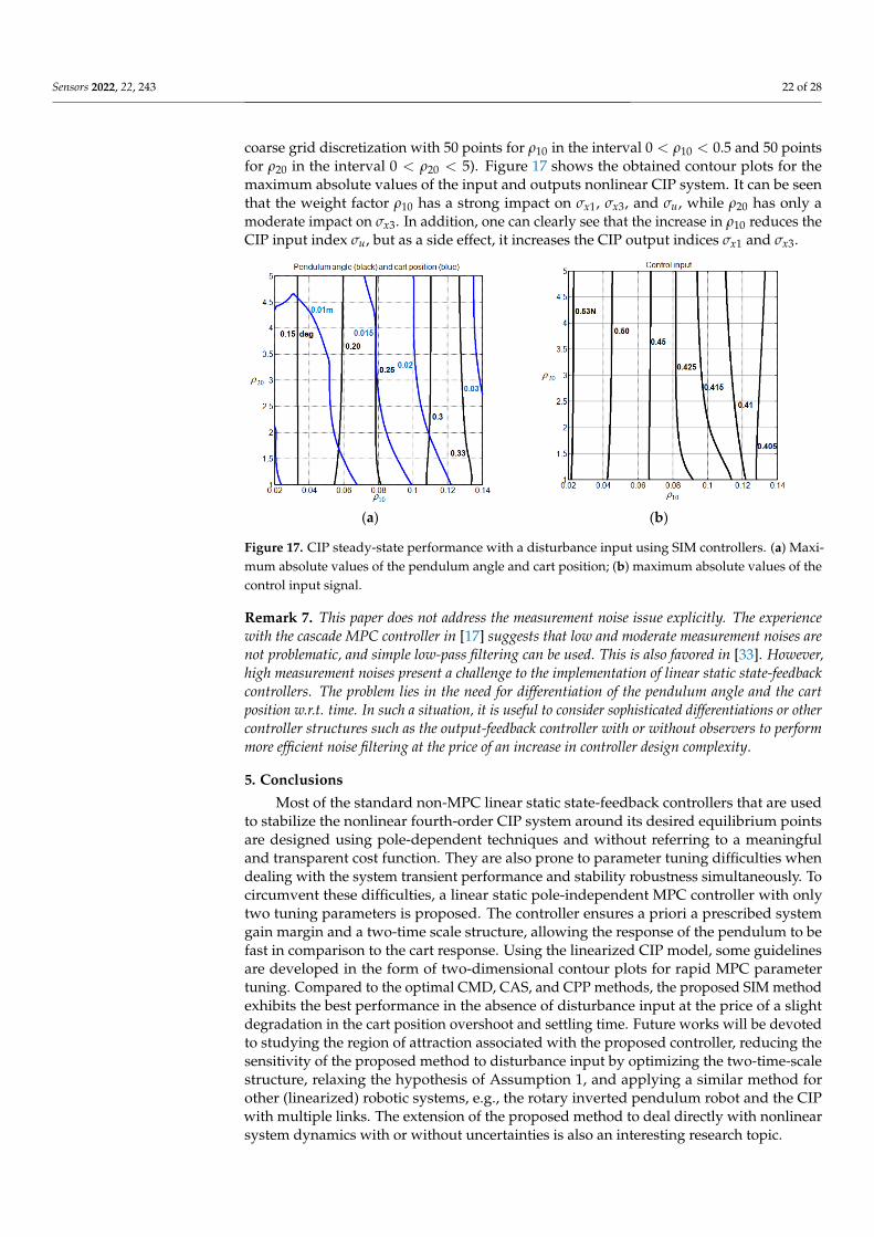
Sensors 2022, 22, 243 22 of 28

coarse grid discretization with 50 points for ρ10 in the interval 0 < ρ10 < 0.5 and 50 pointsfor ρ20 in the interval 0 < ρ20 < 5). Figure 17 shows the obtained contour plots for themaximum absolute values of the input and outputs nonlinear CIP system. It can be seenthat the weight factor ρ10 has a strong impact on σx1, σx3, and σu, while ρ20 has only amoderate impact on σx3. In addition, one can clearly see that the increase in ρ10 reduces theCIP input index σu, but as a side effect, it increases the CIP output indices σx1 and σx3.

Sensors 2022, 22, 243 23 of 30

Figure 16. Cart position responses with a disturbance input.

Let us now study the impact of the weight vector ( )20100 , ρρρ = on the closed-loop nonlinear CIP steady-state performance when the adopted disturbance input is consid-ered. To this end, we keep 63.1min =GM and conduct 2500 simulations (obtained by using a coarse grid discretization with 50 points for 10ρ in the interval 5.00 10 << ρ and 50 points for 20ρ in the interval 50 20 << ρ ). Figure 17 shows the obtained contour plots for the maximum absolute values of the input and outputs nonlinear CIP system. It can be seen that the weight factor 10ρ has a strong impact on 1xσ , 3xσ , and uσ , while

20ρ has only a moderate impact on 3xσ . In addition, one can clearly see that the increase in 10ρ reduces the CIP input index uσ , but as a side effect, it increases the CIP output indices 1xσ and 3xσ .

(a) (b)

Figure 17. CIP steady-state performance with a disturbance input using SIM controllers. (a) Maxi-mum absolute values of the pendulum angle and cart position; (b) maximum absolute values of the control input signal.

Remark 7. This paper does not address the measurement noise issue explicitly. The experience with the cascade MPC controller in [17] suggests that low and moderate measurement noises are not problematic, and simple low-pass filtering can be used. This is also favored in [33]. However, high measurement noises present a challenge to the implementation of linear static state-feedback controllers. The problem lies in the need for differentiation of the pendulum angle and the cart position w.r.t. time. In such a situation, it is useful to consider sophisticated differentiations or other controller structures such as the output-feedback controller with or without observers to per-form more efficient noise filtering at the price of an increase in controller design complexity.

Figure 17. CIP steady-state performance with a disturbance input using SIM controllers. (a) Maxi-mum absolute values of the pendulum angle and cart position; (b) maximum absolute values of thecontrol input signal.

Remark 7. This paper does not address the measurement noise issue explicitly. The experiencewith the cascade MPC controller in [17] suggests that low and moderate measurement noises arenot problematic, and simple low-pass filtering can be used. This is also favored in [33]. However,high measurement noises present a challenge to the implementation of linear static state-feedbackcontrollers. The problem lies in the need for differentiation of the pendulum angle and the cartposition w.r.t. time. In such a situation, it is useful to consider sophisticated differentiations or othercontroller structures such as the output-feedback controller with or without observers to performmore efficient noise filtering at the price of an increase in controller design complexity.

5. Conclusions

Most of the standard non-MPC linear static state-feedback controllers that are usedto stabilize the nonlinear fourth-order CIP system around its desired equilibrium pointsare designed using pole-dependent techniques and without referring to a meaningfuland transparent cost function. They are also prone to parameter tuning difficulties whendealing with the system transient performance and stability robustness simultaneously. Tocircumvent these difficulties, a linear static pole-independent MPC controller with onlytwo tuning parameters is proposed. The controller ensures a priori a prescribed systemgain margin and a two-time scale structure, allowing the response of the pendulum to befast in comparison to the cart response. Using the linearized CIP model, some guidelinesare developed in the form of two-dimensional contour plots for rapid MPC parametertuning. Compared to the optimal CMD, CAS, and CPP methods, the proposed SIM methodexhibits the best performance in the absence of disturbance input at the price of a slightdegradation in the cart position overshoot and settling time. Future works will be devotedto studying the region of attraction associated with the proposed controller, reducing thesensitivity of the proposed method to disturbance input by optimizing the two-time-scalestructure, relaxing the hypothesis of Assumption 1, and applying a similar method forother (linearized) robotic systems, e.g., the rotary inverted pendulum robot and the CIPwith multiple links. The extension of the proposed method to deal directly with nonlinearsystem dynamics with or without uncertainties is also an interesting research topic.

Sensors 2022, 22, 243 23 of 28

Author Contributions: Conceptualization, L.M.; Formal analysis, E.-H.G. and S.B.; Investigation,S.B.; Methodology, E.-H.G. and S.B.; Validation, L.M.; Writing—Original draft, L.M. and E.-H.G.;Writing—Review and editing, E.-H.G. and S.B. All authors have read and agreed to the publishedversion of the manuscript.

Funding: This research was funded by PHC Tassili project (project code: 43790QB) and the SlovenianResearch Agency (research core funding No. P2-0219).

Institutional Review Board Statement: Not applicable.

Informed Consent Statement: Not applicable.

Data Availability Statement: The study did not report any data.

Acknowledgments: The authors would like to thank the Ministry of Higher Education and ScientificResearch of Algeria for its support (PRFU A01L08UN210120220001).

Conflicts of Interest: The authors declare no conflict of interest.

Appendix A. The Standard CDM Controllers (CDM)

The CDM method is a general design tool that can be applied for example to a generalfourth-order all-pole closed-loop system with the following transfer function:

G(s) =c0

c4s4 + c3 s3 + c2 s2 + c1s + c0, (A1)

where c0, c1, c2, c3, c4 are the coefficients of its the characteristic polynomial:

C(s) = c4s4 + c3 s3 + c2 s2 + c1s + c0. (A2)

Using the CDM method, the characteristic polynomial of a fourth-order control systemcan be written in the following form [28]:

C(s) =1

γ3γ22γ3

1τ4c0s4 +

1γ2γ2

1τ3c0 s3 +

1γ1

τ2c0 s2 + τc0s + c0, (A3)

where γ1, γ2, γ3 are the characteristic ratios, and τ is the GTC of the targeted closed-loopsystem. The set of adjusted parameters is then given by ϕ = (γ1, γ2, γ3, τ). It is well knownthat the step response of an all-pole system with such a characteristic polynomial has asmall overshoot under the condition that the characteristic ratios are larger than 2 [28]. Inaddition, non-overshooting in the step response can be obtained using γ1 ≥ γ1LB withγ2 = γ3 = 2, where γ1LB = 2.53 is the minimum value of γ1 that enable non-overshootingstep responses. The standard CDM method, i.e., the Manabe form, is obtained by settingγ1 = 2.5 and γ2 = γ3 = 2. In this case, the settling time is about 2.5τ to 3τ, and for thefourth-order control system, all the poles are exactly on the vertical line, which means thatthe obtained two sets of complex conjugate poles have the same pole real part and differentpole imaginary parts [31].

The design of an SFC using the CDM method for the CIP system can be conducted asfollows. First, the cart transfer function F3(s) is transformed to the following form:

F30(s) = −F3(s) =s2 − a1

1b2 N3

s4 + b1 N2−b2 N4b2 N3

s3 + b1 N1−b2 N3−a1b2 N3

s2 + a1N4N3

s + a1. (A4)

By equating the denominator of (A4) with the characteristic polynomial (A3) andusing the standard CDM method, we obtain the following set of equations:

b1N2 − b2N4 = γ3γ2γ1τ−1 = 10τ−1

b1N1 − b2N3 − a1 = γ3γ22γ2

1τ−2 = 50τ−2

N3 = a−11 b−1

2 γ3γ22γ3

1τ−4 = 125a−11 b−1

2 τ−4

N4 = a−11 b−1

2 γ3γ22γ3

1τ−3 = 125a−11 b−1

2 τ−3

. (A5)

Sensors 2022, 22, 243 24 of 28

Solving (A5) gives the SFC gains as follows:

N1 = (a1b1)−1τ−4(a2

1τ4 + 50a1τ2 + 125)

N2 = 5(a1b1)−1τ−3(2a1τ2 + 25

)N3 = 125a−1

1 b−12 τ−4

N4 = 125a−11 b−1

2 τ−3

, (A6)

where the GTC, i.e., τ, is the only parameter to be adjusted.On the other hand, the transfer function (A4), which has two real zeroes, can be

decomposed as follows:

F30(s) =s2−a1P(s) = C1(s)− C2(s)

C1(s) =s2+a1P(s) ; C2(s) =

2a1P(s)

, (A7)

where C1(s) is a non-all-pole system with one pair of jω-axis zeroes, and C2(s) is an all-polesystem. Under the Manabe form, the authors of [28] showed the possibility to obtain amonotonic step response for C1(s) if τ is kept above a certain lower bound. However,obtaining the step response monotonicity for (A7) is almost impossible due to the presenceof the NMP zero in this transfer function [29,30].

Now, combining (12), (22), and (A6) yields:

GMmin = 1 +55a1τ2

2a21τ4 + 50a1τ2 + 1000

= 1 +55τ2

0

2τ40 + 50τ2

0 + 1000, (A8)

where τ0 = a1/21 τ. The maximum system gain margin is equal to 0.5 + 2

√5/5 ≈ 1.39 at the

normalized GTC τ0 = 5001/4 ≈ 4.73.

Appendix B. The Cascade MPC Controller (CAS)

In a previous paper [12], we have developed a two-horizon time cascade linear MPCcontroller to stabilize the CIP system. The controller scheme is composed of two MPCcontrollers in cascade. These controllers are tuned so as to obtain a doubly critically dampedbehavior for the inner and outer loops. For the purpose of a fair comparison, the cascadeMPC (CAS) controller presented hereafter and shown in Figure A1 is an adapted version ofthe one developed in [12]. More precisely, to develop this version, we assume, as for theproposed SIMO MPC controller of this paper, that Assumption 1 is satisfied. In this case,the associated CAS pendulum prediction model, which is identical to the SIMO one, andthe CAS cart prediction model, which is distinct from the SIMO one, are given hereafter:

x1 (t + h) = A1x1(t) + B1x2(t) − E1ux2(t + h) = A2x1(t) + B2x2(t) − E2u

(A9)

x3 (t + h2) = x3(t) + h2 x4(t) + 0.5gx1dx4(t + h2) = x4(t) + gh2x1d

, (A10)

where (Ai, Bi, Ei) with i = 1, 2 are evaluated using (8), and x1d is an unknown low-speedpendulum angle reference.

Sensors 2022, 22, 243 25 of 28

Sensors 2022, 22, 243 26 of 30

Appendix B. The Cascade MPC Controller (CAS) In a previous paper [12], we have developed a two-horizon time cascade linear MPC

controller to stabilize the CIP system. The controller scheme is composed of two MPC con-trollers in cascade. These controllers are tuned so as to obtain a doubly critically damped behavior for the inner and outer loops. For the purpose of a fair comparison, the cascade MPC (CAS) controller presented hereafter and shown in Figure A1 is an adapted version of the one developed in [12]. More precisely, to develop this version, we assume, as for the proposed SIMO MPC controller of this paper, that Assumption 1 is satisfied. In this case, the associated CAS pendulum prediction model, which is identical to the SIMO one, and the CAS cart prediction model, which is distinct from the SIMO one, are given hereafter:

( ) ( ) ( )( ) ( ) ( ) uEtxBtxAhtx

uEtxBtxAhtx

222122

121111

ˆˆ

−+=+−+=+

(A9)

( ) ( ) ( )( ) ( ) d

d

xghtxhtxgxtxhtxhtx

12424

142323

ˆ5.0ˆ

+=+++=+

, (A10)

where ( )iii EBA ,, with 2,1=i are evaluated using (8), and dx1 is an unknown low-speed pendulum angle reference.

Figure A1. Cascade MPC controller for CIP system stabilization.

The cascade controller design can be conducted using two successive steps. In the first step, the design of the inner MPC controller ( )1312111 ,, KKKK = is considered using the following quadratic cost function:

( ) ( ) ( )( ) ( )( ) ( )htxhte

htxxhtehtehtehtJ

d

+−=++−=+

+++=

22

111

221

211

ˆ0ˆ

, ρ. (A11)

From the angle prediction model (A9), the control input is obtained by minimization of (A11) as follows:

( ) ( ) ( )

221

21

1132

2121

22111122

2121

2211111

1132121110

;;EE

EKEEEBEBK

EEEAEAK

xKtxKtxKtv d

ρρρ

ρρ

+−=

++−=

++−=

+−−= (A12)

Imposing the critically damped constraint to the second-order inner loop gives [12]:

( ) 4/;;4/4 20

111130

11

2/1112

20

11111 dbaKdbaKdbaK −−− −=−=+−= , (A13)

where 100

2/110 2.12 −− ≈= had nω with the inner loop undamped natural frequency

10 6.0 −≈ hnω .

In the second step, the design of the outer MPC controller ( )2322212 ,, KKKK = is considered using a second quadratic cost function:

Figure A1. Cascade MPC controller for CIP system stabilization.

The cascade controller design can be conducted using two successive steps. In the firststep, the design of the inner MPC controller K1 = (K11, K12, K13) is considered using thefollowing quadratic cost function:

J1(t, h) = e21(t + h) + ρ1e2

2(t + h)e1(t + h) = x1d − x1(t + h)e2(t + h) = 0− x2(t + h)

. (A11)

From the angle prediction model (A9), the control input is obtained by minimizationof (A11) as follows:

v0(t) = −K11x1(t)− K12x2(t) + K13x1d

K11 = − A1E1+ρ1 A2E2E2

1+ρ1E22

; K12 = − B1E1+ρ1B2E2E2

1+ρ1E22

; K13 = − E1E2

1+ρ1E22

(A12)

Imposing the critically damped constraint to the second-order inner loop gives [12]:

K11 = −a1b−11

(d2

0 + 4)

/4; K12 = −a1/21 b−1

1 d0; K13 = −a1b−11 d2

0/4, (A13)

where d0 = 2a−1/21 ωn0 ≈ 1.2h−1

0 with the inner loop undamped natural frequencyωn0 ≈ 0.6h−1.

In the second step, the design of the outer MPC controller K2 = (K21, K22, K23) isconsidered using a second quadratic cost function:

J2(t, h2) = e23(t + h2) + ρ2e2

4(t + h2)e3(t + h2) = x3d − x3(t + h2)e4(t + h2) = 0− x4(t + h2)

. (A14)

Using the cart prediction model (A10), the remaining control input is obtained byminimization of (A13) as follows:

x1d0(t) = −K21x3(t)− K22x4(t) + K23x3d

K21 = K23 = 2g−1

h22+4ρ2

; K22 =2h2

2+4ρ2h2

2+4ρ2h−1

2 g−1 (A15)

Assuming that K21 = K22 = K23 = K and ωn0 is high enough to obtain, the poledominant principle leads to approximate the fourth-order cart transfer function by a simplesecond-order model [12]. Tuning the gain K to obtain a critically damped behavior for theouter loop leads to determining it with the following expression:

K = K21 = K22 = K23 = 4/(4L + g). (A16)

From Figure A1, we get the following ECS:

u(t) = +N1x1(t) + N2x2(t) + N3x3(t) + N4x4(t)− N3x3d, (A17)

Sensors 2022, 22, 243 26 of 28

withN1 = −K11N2 = −K12 − L KK13N3 = N4 = −KK13

, (A18)

where the cascade MPC controller gains are given in Equations (A13) and (A16).Finally, let us notice here that by construction, the obtained cascade MPC gains are

positive. The trivial prediction models, defined in (A9) and (A10), appear to be sufficientto conduct the design, and there is no need to define a generalized prediction model asin the case of the SIMO MPC method. Additionally, the evaluation of the optimal systemgain margin for this controller leads to solving a fourth-order polynomial equation that ispreferable to solve numerically.

Appendix C. The Coincident Pole Placement Controller (CPP)

Taking into account the usefulness of driving the cart system with little or no oscillationto x3d, a standard approach to design SFC controllers consist of determining the SFCcontroller gains (N1, N2, N3, N4) so as to obtain a coincident real negative pole p structurefor the targeted closed-loop system F3(s) [17]. In this situation, the CIP characteristicpolynomial follows the configuration P(s) = (s− p)4 that leads directly to evaluate theSFC controller gains by:

N1 = b−11 a−1

1 p4 + 6b−11 p2 + b−1

1 a1N2 = −4b−1

1 a−11 p3 − 4b−1

1 pN3 = a−1

1 b−12 p4

N4 = −4a−11 b−1

2 p3

. (A19)

The above controller can be viewed as optimal if its pole maximizes the gain margin (22). Tothis end, let us define the following normalized pole parameter:

p0 = a−1/21 p. (A20)

Then, from (31), (A19), and (A20), we obtain the set of algebraic equations:

N10D−10 = p4

0 + 6p20 + 1

N20D−10 = −4p3

0 − 4p0N30D−1

0 = p40

N40D−10 = −4p3

0

. (A21)

Now, substituting (31) in (22) and combining the obtained result with (A21) yields:

GMmin =N20D−1

0 (r12 − r34)

1 + N40D−10 (r12 − r34)

= 1 +4p2

0

5p40 + 2p2

0 + 1. (A22)

The maximum gain margin is equal to 0.5(

1 +√

5)≈ 1.62 at the pole location

p0 = −5−1/4 ≈ −0.6687. As it is stated in [17], the parameters (A19) that result fromthe above pole location choice allow one to tune the controller gains for any CIP system inthe simplest fashion to ensure significantly improved performance and robustness. In thispaper, we take this controller as a reference for the comparison task.

Appendix D. Derivation of the Nonlinear CIP Dynamics

In this appendix, the basic equations for the CIP system, shown in Figure 1, aregiven as well as relevant explanation and derivation of the system of Equation (1). It isassumed that the pendulum rigid rod is mass-less, and the whole pendulum mass m isconcentrated in the center of gravity of the pendulum ball. It is also assumed that nofriction exists in the system between the cart and the track or between the cart and the

Sensors 2022, 22, 243 27 of 28

pendulum. The coordinates of the center of the ball at the end of the pendulum, which arealso the coordinates of the center of gravity of the mass-less pendulum, are given by:

xG = x3 + L sin x1yG = L cos x1

. (A23)

Now, Newton’s second law is applied to the cart to obtain:

M..x3 = u−m

..xG. (A24)

Then, substituting (A23) into (A24) and using the fact that x2 =.x1 and x4 =

.x3 gives:

u = M.x4 + m

( .x4 + L

[ .x2 cos x1 − x2

2 sin x1])

= (M + m).x4 −mLx2

2 sin x1 + mL.x2 cos x1

. (A25)

From (A25), it is easy to get:

.x4 =

1M + m

[u + mLx2

2 sin x1 −mL.x2 cos x1

]. (A26)

The rotational motion of the pendulum about its center of gravity involves two forces:the force due to gravity and the force due to the acceleration of the cart. Indeed, sincethe cart is moving, it applies a force on the pendulum. The moment of the force due togravity is mgL sin x1, and the moment of the force due to the acceleration of the cart is−mL

.x4 cos x1. The equation that describes the above motion is obtained by applying the

rotational version of Newton’s second law. Summing the moments about the center ofgravity of the pendulum, we obtain:

mL2 .x2 = mgL sin x1 −mL

.x4 cos x1. (A27)

From (A27), it is easy to get:

.x2 =

1mL2

[mgL sin x1 −mL

.x4 cos x1

]. (A28)

Equations (A26) and (A28) describe the basic equations of the CIP system. Substituting(A26) into (A28) obtains:

.x2 = −

uL−1 cos x1 − (M + m)gL−1 sin x1 + mx22 sin x1 cos x1

M + m−m cos2 x1. (A29)

Then, substituting (A29) into (A26) obtains:

.x4 = +

u−mg sin x1 cos x1 + mLx22 sin x1

M + m−m cos2 x1. (A30)

Finally, from.x1 = x2, x4 =

.x3, (A29), and (A30), we obtain the state-space format (1)

of the nonlinear CIP dynamics.

References1. Boubaker, O. The inverted pendulum benchmark in nonlinear control theory: A survey. Int. J. Adv. Robot. Syst. 2013, 10, 1–9.

[CrossRef]2. Magni, L.; Scattolini, R. On the solution of the tracking problem for non-linear systems with MPC. Int. J. Syst. Sci. 2005, 36,

477–484. [CrossRef]3. Camacho, E.F.; Bordons, C. Model Predictive Control; Springer: New York, NY, USA, 2004.4. Zarzycki, K.; Ławrynczuk, M. Fast Real-Time Model Predictive Control for a Ball-on-Plate Process. Sensors 2021, 21, 39–59.

[CrossRef]

Sensors 2022, 22, 243 28 of 28

5. Li, L.; Xie, Z.; Luo, X.; Li, J. Trajectory Planning of Flexible Walking for Biped Robots Using Linear Inverted Pendulum Model andLinear Pendulum Model. Sensors 2021, 21, 1082. [CrossRef] [PubMed]

6. Ławrynczuk, M.; Nebeluk, R. Computationally Efficient Nonlinear Model Predictive Control Using the L1 Cost-Function. Sensors2021, 21, 5835. [CrossRef] [PubMed]

7. Gawthrop, P.J. Linear predictive pole-placement control: Practical issues. In Proceedings of the 39th IEEE Conference on Decisionand Control, Sydney, Austrilia, 12–15 December 2000; pp. 160–165.

8. Gawthrop, P.J.; Ronco, E. Predictive pole-placement control with linear models. Automatica 2002, 38, 421–432. [CrossRef]9. Gawthrop, P.J.; Wang, L. Intermittent predictive control of an inverted pendulum. Control Eng. Pract. 2006, 14, 1347–1356.

[CrossRef]10. Chalupa, P.; Bobál, V. Modelling and predictive control of inverted pendulum. Proceeding of the 22nd European Conference on

Modelling and Simulation, Nicosia, Cyprus, 3–6 June 2008; pp. 531–537.11. Askari, M.; Mohamed, H.A.; Moghavvemi, M.; Yang, S.S. Model predictive control of an inverted pendulum. In Proceedings of

the International Conference for Technical Postgraduates, Kuala Lumpur, Malaysia, 14–15 December 2009; pp. 1–4. [CrossRef]12. Messikh, L.; Guechi, E.H.; Benloucif, M.L. Critically damped stabilization of inverted-pendulum systems using continuous-time

cascade linear model predictive control. J. Frankl. Inst. 2017, 354, 7241–7265. [CrossRef]13. Mills, A.; Wills, A.; Ninness, B. Nonlinear model predictive control of an inverted pendulum. Proceeding of the American Control

Conference, St. Louis, MO, USA, 10–12 June 2009; pp. 2335–2340.14. Jung, S.; Wen, J.T. Nonlinear model predictive control for the swing-up of a rotary inverted pendulum. J. Dyn. Syst. Meas. Control

2004, 126, 666–673. [CrossRef]15. Altmannshofer, S. Fast suboptimal nonlinear model predictive control of an inverted pendulum. IFAC Proc. Vol. 2012, 45, 442–447.

[CrossRef]16. Magni, L.; Scattolini, R.; Åström, K.J. Global stabilization of the inverted pendulum using model predictive control. IFAC Proc.

Vol. 2002, 35, 141–146. [CrossRef]17. Chatterjee, S.; Das, S.K. An analytical formula for optimal tuning of the state feedback controller gains for the cart-inverted

pendulum system. IFAC-Pap. 2018, 51, 668–672. [CrossRef]18. Roshdy, A.A.; Mokbel, H.F.; Lin, Y.Z.; Wang, T. Stabilization of real inverted pendulum using pole separation factor. Proceedings

of International Conference on Mechanical Engineering and Material Science, Chicago, IL, USA, 4–8 June 2012. [CrossRef]19. Bugeja, M. Non-linear swing-up and stabilizing control of an inverted pendulum system. Proceeding of IEEE Region 8 EUROCON,

Ljubljana, Slovenia, 22–24 September 2003; Volume 2, pp. 437–441. [CrossRef]20. Wang, J.J. Simulation studies of inverted pendulum based on PID controllers. Simul. Model. Pract. Theory 2011, 19, 440–449.

[CrossRef]21. Kuczmann, M. Comprehensive Survey of PID Controller Design for the Inverted Pendulum. Acta Tech. Jaurinensis 2019, 12, 55–81.

[CrossRef]22. Shehu, M.; Ahmad, M.R.; Shehu, A.; Alhassan, A. LQR, double-PID, and pole placement stabilization and tracking control of

single link inverted pendulum. In Proceedings of the 5th IEEE International Conference on Control System, Computing andEngineering (ICCSCE), Penang, Malaysia, 27–28 August 2015; pp. 218–223.

23. Prasad, L.B.; Tyagi, B.; Gupta, H.O. Optimal control of nonlinear inverted pendulum system using PID controller and LQR:Performance analysis without and with disturbance input. Int. J. Autom. Comput. 2014, 11, 661–670. [CrossRef]

24. Önen, Ü.; Cakan, A.; Ilhan, I. Performance comparison of optimization algorithms in LQR controller design for a nonlinearsystem. Turk. J. Electr. Eng. Comput. Sci. 2019, 27, 1938–1953. [CrossRef]

25. Jezierski, A.; Mozaryn, J.; Suski, D. A comparison of LQR and MPC control algorithms of an inverted pendulum. In Polish ControlConference; Springer: Cham, Switzerland, 2017; pp. 65–76.

26. Kim, Y.C.; Lee, J.G. Some Remarks on the Maximum Overshoot of a Fourth-order System. Trans. Korean Inst. Electr. Eng. 2016, 65,1854–1859. [CrossRef]

27. Manabe, S. Importance of coefficient diagram in polynomial method. Proceeding of the 42nd IEEE International Conference onDecision and Control, Maui, HI, USA, 9–12 December 2003; pp. 3489–3494.

28. Qiao, Y.; Ma, C. The assignment of generalized time constant for a non-all-pole system. IEEE Trans. Ind. Electron. 2015, 62,4276–4287. [CrossRef]

29. Lau, K.; Middleton, R.H.; Braslavsky, J.H. Undershoot and settling time tradeoffs for nonminimum phase systems. IEEE Trans.Autom. Control 2003, 48, 1389–1393. [CrossRef]

30. Stewart, J.; Davison, D.E. On overshoot and nonminimum phase zeros. IEEE Trans. Autom. Control 2006, 51, 1378–1382. [CrossRef]31. Manabe, S. Brief tutorial and survey of coefficient diagram method. In Proceedings of the 4th Asian Control Conference,

Singapore, 25–27 September 2002; pp. 1161–1166.32. Müller, M.; Worthmann, K. Quadratic costs do not always work in MPC. Automatica 2017, 82, 269–277. [CrossRef]33. Lee, J.; Mukherjee, R.; Khalil, H.K. Output feedback stabilization of inverted pendulum on a cart in the presence of uncertainties.

Automatica 2015, 54, 146–157. [CrossRef]