POST-TENSIONING THE INVERTED-T BRIDGE SYSTEM ...
224
POST-TENSIONING THE INVERTED-T BRIDGE SYSTEM FOR IMPROVED DURABILITY AND INCREASED SPAN-TO-DEPTH RATIO by RIM M. NOUREDDIN NAYAL B. SC., ALEPPO UNIVERSITY, SYRIA, 2000 M.S., KANSAS STATE UNIVERSITY, 2003 AN ABSTRACT OF A DISSERTATION submitted in partial fulfillment of the requirements for the degree DOCTOR OF PHILOSOPHY DEPARTMENT OF CIVIL ENGINEERING COLLEGE OF ENGINEERING KANSAS STATE UNIVERSITY Manhattan, Kansas 2006
-
Upload
khangminh22 -
Category
Documents
-
view
0 -
download
0
Transcript of POST-TENSIONING THE INVERTED-T BRIDGE SYSTEM ...
POST-TENSIONING THE INVERTED-T BRIDGE SYSTEM FOR IMPROVED
DURABILITY AND INCREASED SPAN-TO-DEPTH RATIO
by
RIM M. NOUREDDIN NAYAL
B. SC., ALEPPO UNIVERSITY, SYRIA, 2000
M.S., KANSAS STATE UNIVERSITY, 2003
AN ABSTRACT OF A DISSERTATION
submitted in partial fulfillment of the requirements for the degree
DOCTOR OF PHILOSOPHY
DEPARTMENT OF CIVIL ENGINEERING
COLLEGE OF ENGINEERING
KANSAS STATE UNIVERSITY
Manhattan, Kansas
2006

Abstract
Possibly the most pressing need in highway construction today is the repair or
replacement of existing bridges. Due to increased needs and growing traffic, in addition to aging
and extensive use, more than 2000 bridges in Kansas alone need to be replaced during the next
decade. The majority of these bridges has spans of 100 ft or less, and has relatively shallow
profiles. It is becoming increasingly important to implement a standard method for replacement
in which the process is expedited and accomplished in cost-effective manner.
Requirements for design and construction of concrete bridges have drastically changed
during recent years. A main change in design is live-load requirements.
Nebraska inverted-T bridge system has gained increasing popularity for its lower weight
compared to I-girder bridges. However, there are some limiting issues when using IT system in
replacing existing CIP bridges.
Implementation of a post-tensioned IT system, which is the focus of this research, is
believed to be one excellent solution for the IT deficiencies. Post-tensioning is added by placing
a draped, post-tensioning duct in the stems of the IT members. Post-tensioning will lead to a
higher span-to-depth ratio than IT system, and will reduce the potential transverse cracks in the
(CIP) deck. Finally, the undesired cambers of pretensioned beams will be reduced, because fewer
initial prestressing will be needed.
This study was intended to explore the behavior of the PT-IT system, identify major
parameters that control and limit the design of this system, and investigate different construction
scenarios. This was achieved by conducting an extensive parametric study. For that purpose, PT-
IT analysis program was developed and written using C++ programming language. The program
was used to analyze various post-tensioning procedures for the post-tensioned inverted-T system.
A Visual Basic friendly interface was provided to simplify the data input process.
The findings of this research included recommendation of construction scenario for PT-
IT system, as well as examining different methods for estimating time-dependent restraining
moments. Effect of different concrete strengths on the behavior of PT-IT system was also

determined. Most importantly, the effect of timing on different construction stages was also
evaluated and determined.
POST-TENSIONING THE INVERTED-T BRIDGE SYSTEM FOR IMPROVED
DURABILITY AND INCREASED SPAN-TO-DEPTH RATIO
by
RIM M. NOUREDDIN NAYAL
B. SC., ALEPPO UNIVERSITY, SYRIA, 2000
M.S., KANSAS STATE UNIVERSITY, 2003
A DISSERTATION
submitted in partial fulfillment of the requirements for the degree
DOCTOR OF PHILOSOPHY
DEPARTMENT OF CIVIL ENGINEERING
COLLEGE OF ENGINEERING
KANSAS STATE UNIVERSITY
Manhattan, Kansas
2006
Approved by:
Major Professor
ROBERT J. PETERMAN

Copyright
RIM NAYAL
2006

Abstract
Possibly the most pressing need in highway construction today is the repair or
replacement of existing bridges. Due to increased needs and growing traffic, in addition to aging
and extensive use, more than 2000 bridges in Kansas alone need to be replaced during the next
decade. The majority of these bridges has spans of 100 ft or less, and has relatively shallow
profiles. It is becoming increasingly important to implement a standard method for replacement
in which the process is expedited and accomplished in cost-effective manner.
Requirements for design and construction of concrete bridges have drastically changed
during recent years. A main change in design is live-load requirements.
Nebraska inverted-T bridge system has gained increasing popularity for its lower weight
compared to I-girder bridges. However, there are some limiting issues when using IT system in
replacing existing CIP bridges.
Implementation of a post-tensioned IT system, which is the focus of this research, is
believed to be one excellent solution for the IT deficiencies. Post-tensioning is added by placing
a draped, post-tensioning duct in the stems of the IT members. Post-tensioning will lead to a
higher span-to-depth ratio than IT system, and will reduce the potential transverse cracks in the
(CIP) deck. Finally, the undesired cambers of pretensioned beams will be reduced, because fewer
initial prestressing will be needed.
This study was intended to explore the behavior of the PT-IT system, identify major
parameters that control and limit the design of this system, and investigate different construction
scenarios. This was achieved by conducting an extensive parametric study. For that purpose, PT-
IT analysis program was developed and written using C++ programming language. The program
was used to analyze various post-tensioning procedures for the post-tensioned inverted-T system.
A Visual Basic friendly interface was provided to simplify the data input process.
The findings of this research included recommendation of construction scenario for PT-
IT system, as well as examining different methods for estimating time-dependent restraining
moments. Effect of different concrete strengths on the behavior of PT-IT system was also

determined. Most importantly, the effect of timing on different construction stages was also
evaluated and determined.
viii
Table of Contents
List of Figures ................................................................................................................... xii
List of Tables .................................................................................................................... xx
Acknowledgements.......................................................................................................... xxi
Dedication ....................................................................................................................... xxii
CHAPTER 1 - Introduction ................................................................................................ 1
Overview......................................................................................................................... 1
Objectives ....................................................................................................................... 2
Outline ............................................................................................................................ 4
CHAPTER 2 - Literature Review....................................................................................... 5
General Description ........................................................................................................ 5
Available Methods for Evaluating Time-Dependent Losses .......................................... 8
Time-Step Prestress Loss Methods ............................................................................. 9
Refined Prestress Loss Methods ............................................................................... 10
Lump-Sum Methods ................................................................................................. 12
Methods to Calculate Time-Dependent Restraining Moments..................................... 12
PCA Method ............................................................................................................. 13
Texas Transportation Institute .................................................................................. 15
CTL Method.............................................................................................................. 16
P Method................................................................................................................... 18
Creep-Transformed Section Properties Method ....................................................... 20
Positive Moment Connection for Girders Made Continuous with CIP Deck............... 23
CHAPTER 3 - Analysis of Post-Tensioned Prestressed Inverted T System .................... 30
Time-Dependent Material Properties............................................................................ 31
Concrete Compressive Strength................................................................................ 31
Modulus of Elasticity................................................................................................ 33
Shrinkage Strain........................................................................................................ 34
Creep Coefficient ...................................................................................................... 39
Relaxation of Steel .................................................................................................... 43
ix
Instantaneous Losses in Post-tensioning................................................................... 45
Design-Limit State ........................................................................................................ 46
Strength I Limit State................................................................................................ 46
Service I Limit State ................................................................................................. 47
Service III Limit State............................................................................................... 47
Flexural Design and Capacity Check............................................................................ 47
Vertical Shear Design and Capacity Check.................................................................. 48
Allowable Stresses ........................................................................................................ 50
Vehicular Live-load ...................................................................................................... 51
Algorithm...................................................................................................................... 51
Comparison with Consplice.......................................................................................... 55
Example 1: IT-700 .................................................................................................... 55
Example 2: IT-500 .................................................................................................... 60
Discussion of P Method and CTL Method ................................................................... 61
CHAPTER 4 - RESULTS OF PARAMETRIC STUDY ............................................... 103
Scope of Parametric Study.......................................................................................... 103
Parametric Study Results ............................................................................................ 104
Different Construction Scenarios............................................................................ 104
Effect of Concrete Strength .................................................................................... 109
Effect of girder concrete strength ....................................................................... 109
Effect of deck concrete ....................................................................................... 110
Effect of Different Creep and Shrinkage Models ................................................... 110
Effect of Timing...................................................................................................... 111
Effect of time of cutting prestressing strands ..................................................... 111
Effect of time of establishing continuity and casting the deck ........................... 111
Effect of time of establishing continuity 111
Effect of time of casting the deck 112
Effect of time of post-tensioning ........................................................................ 112
Comparison with Experimental Data.......................................................................... 112
Experiment 1: Mattock ........................................................................................... 113
Experiment 2: Peterman and Ramirez .................................................................... 113
x
CHAPTER 5 - CONCLUSION AND RECOMMENDATIONS................................... 157
Conclusion .................................................................................................................. 157
Recommendation ........................................................................................................ 159
Notations ......................................................................................................................... 161
References....................................................................................................................... 164
Appendix A - Details of Reinforcement ......................................................................... 168
Concrete Cover ........................................................................................................... 168
Minimum Spacing of Prestressing Tendons ............................................................... 168
Maximum Number of Post-Tensioning Tendons and Duct Size ................................ 168
Design and Detailing of Anchorage Zone .................................................................. 169
Appendix B - Program Documentation .......................................................................... 176
Class “Data”................................................................................................................ 177
Class “Solve” .............................................................................................................. 181
Class “Element”.......................................................................................................... 183
Class “Element2”........................................................................................................ 184
Class “Diaphragm” ..................................................................................................... 185
Class “Node”............................................................................................................... 185
Class “ESM” ............................................................................................................... 186
Class “BCEssential” ................................................................................................... 187
Class “DOF” ............................................................................................................... 187
Class “FixedEM” ........................................................................................................ 188
Class “BCNodalLoad”................................................................................................ 189
Class “MomentandShear”........................................................................................... 190
Class “Concrete Stresses”........................................................................................... 190
Class “Meterial”.......................................................................................................... 192
Class “Steel” ............................................................................................................... 192
Class “Concrete”......................................................................................................... 193
Class “PreStrands”...................................................................................................... 194
Class “PostTend” ........................................................................................................ 195
Class “Straight”........................................................................................................... 197
Class “ParabolicPT” ................................................................................................... 197

xi
Class “Section” ........................................................................................................... 198
Class “TimeDepLosses” ............................................................................................. 200
Class “Time”............................................................................................................... 201
Class “Matrix” ............................................................................................................ 201
xii
List of Figures
Figure 2. 1 PT-IT bridge system under construction ........................................................ 25
Figure 2. 2 PT-IT bridge system under construction ........................................................ 25
Figure 2. 3 IT section and modified IT section................................................................. 26
Figure 2. 4 PT-IT bridge system....................................................................................... 27
Figure 2. 5 Realtive humidity correction factor (Texas Technology Institute method) ... 28
Figure 2. 6 Volume-to-surface ratio correction factor (Texas Technology Institute method)
................................................................................................................................... 28
Figure 2. 7 (a) Deformation due to differential shrinkage, (b) Restraining moments in
continuous prestressed, precast beams made continuous by CIP deck..................... 29
Figure 3. 1 Experimental shrinkage strain versus predicted strain for SCC..................... 66
Figure 3. 2 Experimental creep coefficient versus predicted creep coefficient for specimen
loaded at Day 1 ......................................................................................................... 66
Figure 3. 3 SCC-Experimental creep coefficient versus predicted creep coefficient for specimen
loaded at day 29 ........................................................................................................ 67
Figure 3. 4 Experimental creep coefficient versus predicted creep coefficient using equation for
specimen loaded at day 1 and corrected for loading age of 29 days......................... 67
Figure 3. 5 Structural analysis model ............................................................................... 68
Figure 3. 6 Example 1. IT 700 section properties............................................................. 68
Figure 3. 7 Example 1. beam layout ................................................................................. 69
Figure 3. 8 Post-tensioning tendons profile ...................................................................... 69
Figure 3. 9 Example 1-PT-IT front page .......................................................................... 70
Figure 3. 10 Example 1-concrete properties form ............................................................ 70
Figure 3. 11 Example 1-beam layout................................................................................ 71
Figure 3. 12 Example 1-section properties ....................................................................... 71
Figure 3. 13 Example 1-deck dimensions and material .................................................... 72
Figure 3. 14 Example 1-strands properties ....................................................................... 72
Figure 3. 15 Example 1-post-tensioned tendons............................................................... 73

xiii
Figure 3. 16 Example 1-supports ...................................................................................... 73
Figure 3. 17 Example 1-externally applied loads ............................................................. 74
Figure 3. 18 Example 1-staging........................................................................................ 74
Figure 3. 19 Example 1-stress in prestressed strands along the bridge ............................ 75
Figure 3. 20 Example 1-stress in post-tensioned tendons along the bridge...................... 75
Figure 3. 21 Example 1-moments resulting from girder and deck weight ....................... 76
Figure 3. 22 Example 1-moments resulting from prestressing forces .............................. 76
Figure 3. 23 Example 1-moments due to post-tensioning forces...................................... 77
Figure 3. 24 Example 1-moments resulting from differential shrinkage between deck and girder
................................................................................................................................... 77
Figure 3. 25 Example 1-moments resulting from barrier weight...................................... 78
Figure 3. 26 Example 1-positive moments due to lane load............................................. 78
Figure 3. 27 Example 1-negative moments due to lane load............................................ 79
Figure 3. 28 Example 1-positive moments due to design tandem .................................... 79
Figure 3. 29 Example 1-negative moments due to design tandem ................................... 80
Figure 3. 30 Example 1-positive moments due to design truck........................................ 80
Figure 3. 31 Example 1-Negative moments due to design truck...................................... 81
Figure 3. 32 Example 1-Negative moments due to double tandem.................................. 81
Figure 3. 33 Example 1-Negative moments due to double truck ..................................... 82
Figure 3. 34 Example 1-HL-93 Positive moment............................................................. 82
Figure 3. 35 Example 1-HL-93 Negative moment ........................................................... 83
Figure 3. 36 Example 1-Factored required moment ......................................................... 83
Figure 3. 37 Example 1-(1.2 Times cracking moment) .................................................... 84
Figure 3. 38 Example 1-ΦMn (Nominal resistance moment)........................................... 84
Figure 3. 39 Example 1-Time-dependent deflection due to prestressing ......................... 85
Figure 3. 40 Example 1-Time-dependent deflection due to component weight and shrinkage
................................................................................................................................... 85
Figure 3. 41 Example 1-Time-dependent deflection due to post-tensioning.................... 86
Figure 3. 42 Example 1-Time-dependent deflection due to barriers weight .................... 86
Figure 3. 43 Example 2 IT 500 section properties............................................................ 87
Figure 3. 44 Example 2-Beam layout ............................................................................... 88

xiv
Figure 3. 45 Example 2-Post-tensioning tendons profile.................................................. 88
Figure 3. 46 Example 2-Stresses in prestressed strands along the bridge ........................ 89
Figure 3. 47 Example 2- Stresses in post-tensioned tendons along the bridge................. 89
Figure 3. 48 Example 2- Moments resulting from girder and deck weights .................... 90
Figure 3. 49 Example 2- Moments resulting from prestressing forces............................. 90
Figure 3. 50 Example 2-Moments due to post-tensioning forces ..................................... 91
Figure 3. 51 Example 2- Moments resulting from differential shrinkage between deck and girder
................................................................................................................................... 91
Figure 3. 52 Example 2- Moments resulting from barriers weight................................... 92
Figure 3. 53 Example 2-HL-93 Positive moment............................................................. 92
Figure 3. 54 Example 2- HL-93 Negative moment .......................................................... 93
Figure 3. 55 Example 2-Factored required moment ......................................................... 93
Figure 3. 56 Example 2-Φ times nominal resistance moment .......................................... 94
Figure 3. 57 Example 2-time-dependent deflection due to prestressing........................... 94
Figure 3. 58 Example 2-time-dependent deflection due to component weight and shrinkage
................................................................................................................................... 95
Figure 3. 59 Example 2-time-dependent deflection due to post-tensioning ..................... 95
Figure 3. 60 Example 2-time-dependent deflection due to barrier weight ....................... 96
Figure 3. 61 Forces in deck and girder due to differential shrinkage ............................... 96
Figure 3. 62 Deformations affecting both deck and girder ............................................... 97
Figure 3. 63 Example 1-prediction of restraining moment due to differential shrinkage using
published versus suggested CTL equation................................................................ 97
Figure 3. 64 Example 1-prediction of restraining moment due to differential shrinkage using
published versus suggested P equations ................................................................... 98
Figure 3. 65 Example 1-prediction of restraining moment due to differential shrinkage using
PCA, suggested CTL, and suggested P expressions ................................................. 98
Figure 3. 66 Example 2-prediction of restraining moment due to differential shrinkage using
published versus suggested CTL equations .............................................................. 99
Figure 3. 67 Example 2-prediction of restraining moment due to differential shrinkage using
published versus suggested P equation ..................................................................... 99
xv
Figure 3. 68 Example 2-prediction of restraining moment due to differential shrinkage using
PCA, suggested CTL, and suggested P expressions ............................................... 100
Figure 4. 1 Maximum spans for different IT sections for different construction scenarios, for
girder concrete strength of 8 ksi.............................................................................. 115
Figure 4. 2 Time-dependent restraining moments using different methods for Dia & Deck-PT
construction scenario; continuity established @ 14 days of girder's age................ 115
Figure 4. 3 Time-dependent restraining moments using different methods for Dia - Deck-PT
construction scenario; continuity established @ 14 days of girder age.................. 116
Figure 4. 4 Time-dependent restraining moments using different methods for Dia -PT - Deck
construction scenario; continuity established @ 14 days of girder age.................. 116
Figure 4. 5 Time-dependent restraining moments using different methods for (two-stage PT)
construction scenario; continuity established @ 14 days of girder age.................. 117
Figure 4. 6 Secondary moment due to post-tensioning for different construction scenarios;
continuity established @ 14 days............................................................................ 117
Figure 4. 7 Post-tensioning tendon path with respect to C.G. of the girder and C.G. of the
composite section.................................................................................................... 118
Figure 4. 8 Maximum positive restraining moment in the pier including LL, for different
construction scenario according to CTL method; continuity established @ 14 days of girder
age ........................................................................................................................... 118
Figure 4. 9 Maximum positive restraining moment in the pier including LL, different
construction scenarios, P method; continuity established @ 14 days of girder age119
Figure 4. 10 Maximum negative restraining moment in the pier, for Dia & Deck-PT construction
scenario, P method; continuity established @ 14 days of girder age ..................... 119
Figure 4. 11 Maximum negative restraining moment in the pier for Dia - Deck-PT construction
scenario, P method; continuity established @ 14 days of girder age ..................... 120
Figure 4. 12 Time-dependent restraining moment in the pier for Dia - Deck -PT construction
scenario according to P method .............................................................................. 120
Figure 4. 13 Restraining moment in the pier for Dia - Deck -PT construction scenario resulting
from time-dependent effect and secondary moment due to post-tensioning .......... 121
xvi
Figure 4. 14 Maximum negative restraining moment in the pier for Dia -PT - Deck construction
scenario, P method; continuity established @ 14 days of girder age ..................... 121
Figure 4. 15 Time-dependent restraining moment in the pier for Dia -PT - Deck construction
scenario according to P method .............................................................................. 122
Figure 4. 16 Restraining moment in the pier for Dia – PT - Deck construction scenario resulting
from time-dependent effect and secondary moment due to post-tensioning .......... 122
Figure 4. 17 Maximum negative restraining moment in the pier for two-stage PT construction
scenario, P method; continuity established @ 14 days of girder age ..................... 123
Figure 4. 18 Time-dependent restraining moments using different methods for Dia & Deck-PT
construction scenario; continuity established @ 224 days of girder age................ 123
Figure 4. 19 Time-dependent restraining moments using different methods for Dia - Deck-PT
construction scenario; continuity established @ 224 days of girder age................ 124
Figure 4. 20 Time-dependent restraining moments using different methods for Dia-PT - Deck
construction scenario; continuity established @ 224 days of girder age................ 124
Figure 4. 21 Time-dependent restraining moments using different methods for two-stage PT
construction scenario; continuity established @ 224 days of girder age................ 125
Figure 4. 22 Secondary moment due to post-tensioning for different construction scenarios;
continuity established @ 224 days of girder age .................................................... 125
Figure 4. 23 Maximum negative restraining moment in the pier for Dia & Deck-PT construction
scenario, P method; continuity established @ 224 days of girder age ................... 126
Figure 4. 24 Maximum negative restraining moment in the pier for Dia- Deck- PT construction
scenario, P method; continuity established @ 224 days of girder age ................... 126
Figure 4. 25 Time-dependent restraining moment in the pier for Dia - Deck -PT construction
scenario according to P method .............................................................................. 127
Figure 4. 26 Restraining moment in the pier for Dia - Deck -PT construction scenario resulting
from time-dependent effect and secondary moment due to post-tensioning .......... 127
Figure 4. 27 Maximum negative restraining moment in the pier for Dia- PT- Deck construction
scenario, P method; continuity established @ 224 days of girder age ................... 128
Figure 4. 28 Time-dependent restraining moment in the pier for Dia-PT- Deck construction
scenario according to P method .............................................................................. 128
xvii
Figure 4. 29 Restraining moment in the pier for Dia -PT- Deck construction scenario resulting
from time-dependent effect and secondary moment due to post-tensioning .......... 129
Figure 4. 30 Maximum negative restraining moment in the pier for two-stage PT construction
scenario, P method; continuity established @ 224 days of girder age ................... 129
Figure 4. 31 Shear reinforcement detailing for Dia & Deck-PT construction scenario . 130
Figure 4. 32 Shear reinforcement detailing for Dia & Deck-PT construction scenario . 130
Figure 4. 33 Shear reinforcement detailing for Dia -Deck-PT construction scenario .... 131
Figure 4. 34 Shear reinforcement detailing for Dia -Deck-PT construction scenario .... 131
Figure 4. 35 Shear reinforcement detailing for Dia –PT - Deck construction scenario.. 132
Figure 4. 36 Shear reinforcement detailing for Dia –PT - Deck construction scenario.. 132
Figure 4. 37 Shear reinforcement detailing for two-stage PT construction scenario...... 133
Figure 4. 38 Shear reinforcement detailing for two-stage PT construction scenario...... 133
Figure 4. 39 Time-dependent restraining moment in the pier for different concrete strength of the
girder using PCA method........................................................................................ 134
Figure 4. 40 Time-dependent restraining moment in the pier for different concrete strength of the
girder using CTL method........................................................................................ 134
Figure 4. 41 Time-dependent restraining moment in the pier for different concrete strength of the
girder using P method ............................................................................................. 135
Figure 4. 42 Time-dependent restraining moment in the pier for different concrete strength of the
girder using creep-transformed section properties method..................................... 135
Figure 4. 43 Time-dependent restraining moment due to creep under prestressing, according to
CTL method ............................................................................................................ 136
Figure 4. 44 Time-dependent restraining moment due to creep under girder weight, according to
CTL method ............................................................................................................ 136
Figure 4. 45 Time-dependent restraining moment due to differential shrinkage, according to CTL
method..................................................................................................................... 137
Figure 4. 46 Losses in prestressing strands for different concrete strengths .................. 137
Figure 4. 47 Losses in post-tensioning tendons for different concrete strengths............ 138
Figure 4. 48 Time-dependent restraining moment for different concrete strengths of the deck
using CTL method .................................................................................................. 138
xviii
Figure 4. 49 Time-dependent restraining moment for different concrete strengths of the deck
using P method........................................................................................................ 139
Figure 4. 50 Prediction of shrinkage strain using different models for 6-ksi concrete... 139
Figure 4. 51 Prediction of creep coefficient using different models for 6-ksi concrete . 140
Figure 4. 52 Prediction of shrinkage strain using different models for 10-ksi concrete. 140
Figure 4. 53 Prediction of creep coefficient using different models for 10-ksi concrete 141
Figure 4. 54 Predicted losses in pretensioned strands using different models................ 141
Figure 4. 55 Predicted losses in post-tensioning using different models........................ 142
Figure 4. 56 Time-dependent restraining moment for different creep-and-shrinkage models using
PCA method............................................................................................................ 142
Figure 4. 57 Time-dependent restraining moment for different creep-and-shrinkage models using
CTL method ............................................................................................................ 143
Figure 4. 58 Time-dependent restraining moment for different creep-and-shrinkage models using
P method ................................................................................................................. 143
Figure 4. 59 Time-dependent restraining moment for different creep-and-shrinkage models using
creep-transformed section properties method......................................................... 144
Figure 4. 60 Effect of time of cutting strands on losses in prestressing ......................... 144
Figure 4. 61 Time-dependent restraining moment in the pier for continuity established @ 14 days
of girder age ............................................................................................................ 145
Figure 4. 62 Time-dependent restraining moment in the pier for continuity established @ 28 days
of girder age ............................................................................................................ 145
Figure 4. 63 Time-dependent restraining moment in the pier for continuity established @ 56 days
of girder age ............................................................................................................ 146
Figure 4. 64 Time-dependent restraining moment in the pier for continuity established @ 112
days of girder age.................................................................................................... 146
Figure 4. 65 Time-dependent restraining moment in the pier for continuity established @ 224
days of girder age.................................................................................................... 147
Figure 4. 66 Secondary moments due to post-tensioning for different times of establishing
continuity ................................................................................................................ 147
Figure 4. 67 Restraining moment in the pier for continuity established @ 14 days of girder age
................................................................................................................................. 148
xix
Figure 4. 68 Restraining moment in the pier for continuity established @ 28 days of girder age
................................................................................................................................. 148
Figure 4. 69 Restraining moment in the pier for continuity established @ 56 days of girder age
................................................................................................................................. 149
Figure 4. 70 Restraining moment in the pier for continuity established @ 112 days of girder age
................................................................................................................................. 149
Figure 4. 71 Restraining moment in the pier for continuity established @ 224 days of girder age
................................................................................................................................. 150
Figure 4. 72 Effect of time of casting the deck on time-dependent restraining moment using CTL
method..................................................................................................................... 150
Figure 4. 73 Effect of time of casting the deck on time-dependent restraining moment using P
method..................................................................................................................... 151
Figure 4. 74 Effect of time of casting the deck on the restraining moment in the pier .. 151
Figure 4. 75 Cross section for experiment conducted by (4) .......................................... 152
Figure 4. 76 Comparison with experimental data (4) ..................................................... 152
Figure 4. 77 Cross section of panels tested by (7) .......................................................... 153
Figure 4. 78 Comparison with experimental data from (7) ............................................ 153
Figure A. 1 General zone and local zone........................................................................ 174
Figure A. 2 Bearing plate dimension for tendons consisting of 5-0.6” strands .............. 174
Figure A. 3 Detailing of anchorage zone for tendons consisting of 5-0.6” strands ........ 174
Figure A. 4 Bearing plate dimension for tendons consisting of 5-0.6” strands .............. 175
Figure A. 5 Detailing of anchorage zone for tendons consisting of 5-0.6” strands ........ 175

xx
List of Tables
Table 3. 1 Values of the constants α and β and the time ratio for the concrete compressive
strength (24)
.............................................................................................................. 101
Table 3. 2 Values for K1 and K2 (14)
................................................................................ 102
Table 3. 3 Shrinkage factor γcp (14)
................................................................................... 102
Table 3. 4 Recommended values for friction and wobble coefficient ............................ 102
Table 4. 1 Variation of parameters ................................................................................. 154
Table 4. 2 Maximum spans for different construction scenarios for IT 500-IT 1000 .... 155
Table 4. 3 Maximum span-to-depth ratio for different construction scenarios for IT 700155
Table 4. 4 Details for IT 500 for different concrete strengths ........................................ 156
Table 4. 5 Restraining moment in the pier due to girder weight .................................... 156
Table 4. 6 Effect of time of establishing continuity (casting diaphragm) on maximum span-to-
depth ratio ............................................................................................................... 156

xxi
Acknowledgements
I express my appreciation and thanks to Dr. Robert J. Peterman, for giving me this
opportunity and supporting me during the course of this research.
I’d like to extend my appreciation and thanks to Dr. asadollah Esmaeily, his inspiration
and encouragement strengthened my ability to tackle the difficulties encountered during
my graduate study.
I’m grateful to Dr. Hayder Rasheed who prepared me and guided me to the successful
path of graduate studies; his advising and teachings formed my strong background in
structural engineering.
Special thanks to Dr. Youqi wang and Dr. Malgorzata J. Rys for being members in my
dissertation committee and generously giving their time to better this work.
This work would have not been possible without the generous support and funding from
Kansas Department of Transportation.
I’d like to acknowledge Mr. Kenneth F. Hurst, Mr. Loren Risch, and Mr. Steve Burnette,
for their help during this research.

xxii
Dedication
To my parents,
M.Noureddin Nayal and Lamis Kudsi
This would have not been possible without their sacrifices, encouragement, patience and
endless love.
Thanks for their sincere prayers and blessing
To my father, and mother in law
Farouk Charkas and Amira Bayaa
For all love and care they gave to me
and to
my husband
Hasan Charkas
For his continued support, understanding, love, and care
To my sister and brother
Lama and Tawfiq Nayal
For their love and support
For my son
Farouk Charkas
For being the light and blessing of my life
To my Friends in Manhattan, Ks
Especially Safa Attassi and Sara Asmar
For making me feel family as part of their families.

1
CHAPTER 1 - Introduction
Overview
Bridges are a key element in transportation systems, if for any reason a bridge is unable
to meet traffic needs, it becomes a constriction to the flow of traffic, and needs to be replaced.
The requirements for the design and construction of reinforced concrete bridges in terms of live-
load requirements, material properties, structural shapes, etc. has evolved based on both
increased needs and available materials. For example, these bridges were often designed for a
live-load less than HL-93 as determined by AASHTO LRFD (1). Due to the aforesaid facts, and
also due to aging of and extensive use, there are a number of bridges in Kansas need to be
replaced. The majority of these bridges has spans of 100 ft or less, and relatively shallow
profiles.
It is apparent that when a bridge is taken out-of-service for repair or replacement, it
causes major inconveniency for traffic passing through that area. As there are many options for
replacement of existing bridges or construction of new ones, a wise decision must be made when
selecting a specific bridge system. A balance must be achieved among strength, cost, and
construction time factors, while not compromising safety.
Introduction of the prestressed reinforced concrete concept in 1950 paved the way for a
revolution in bridge design. More than 50% of bridges are now constructed of prestressed
concrete (2).
In prestressed concrete, the steel reinforcement is tensioned against the concrete, which
precompresses the surrounding concrete, giving it the ability to resist higher loads prior to
cracking.
Practical prestressed concrete was introduced in 1928 by Eugene Feyssient of France,
who recommended use of high-strength steel wires and high strength-concrete to provide higher
levels of precompression (2).
Two different procedures for prestressing concrete were developed: post-tensioning,
(used by Feyssient) in which the steel is tensioned after the concrete has been cast and hardened;
and prestressing (developed by the German engineer E.Hoyer in 1938), in which the steel is
tensioned prior to casting of the concrete. Currently, in North America, about two-thirds of

2
prestressed steel is used to manufacture precast, pretensioned products, with the remaining one-
third used for post-tensioning (2).
Cast-in-place (CIP) reinforced concrete slab has been the typical replacement option for
short spans of approximately 30-60 ft. Post-tensioned concrete-haunched slab bridges have
become an increasingly popular option within the last few years for medium spans between 60-
100 ft, but these are relatively complicated to design and expensive to build. These strategies are
also weather-dependent and require intensive labor, which extends road-closure time for
construction. In addition, availability of large volumes of consistently good-quality, ready-mixed
concrete required for these bridges can be a problem in rural areas.
Precast members are widely used in construction. Obviously, prefabrication of
components provides significant reduction in construction or replacement time, and cost savings
because of the reduced field labor employed. However, challenges to meet high span-to-depth
ratio with prestressed, precast I-girders motivated researchers to come up with lighter and more
cost-effective solutions. Recently, the inverted-T (IT) bridge system has become more popular
for short-to medium-span bridges during the past few years. The IT system consists of
longitudinal prestressed concrete members having an “Inverted-Tee” shaped cross section.
Inverted-T girders are adjacently placed and serve as stay-in-place formwork for a composite
CIP topping. This reduces the construction time and labor work as it eliminates a large portion of
false work required in CIP systems. These girders support their own weight and the weight of the
composite topping. The girders act compositely with the CIP topping to carry the live-load.
despite the advantages and merits of IT system, there are some limiting issues when using the IT
beams in replacing existing bridges. First, the span-to-depth ratio which cannot compete with
that of post-tensioned concrete haunched bridges. Currently IT members are constructed
continuous only for live-load. In addition IT members contain only straight pre-tensioned strands
that are contained in the bottom flanges. This fact often necessitates the use of de-bonding of the
strands to control top tensile stresses at the members ends. In addition, the top tension can lead to
increased transverse cracking of the composite top deck slab over the piers when experiencing a
combination of live loads and the loads induced by the restraint of time-dependent deformations.
Objectives
3
The post-tensioned, inverted-T bridge system (PT-IT) is believed to be a good option for
new system construction or replacing existing bridges. Construction of the PT-IT system
involves post-tensioning of the pretensioned, Inverted-T beam sections. Adding post-tensioning
to the IT system increases the durability of the section so it can handle more loads. In addition,
post-tensioning allows reduction of the span-to-depth ratio of the beam, and reduces cracks in the
deck over the piers.
The objective of this research was to provide guidelines for designing the PT-IT system,
this was achieved by conducting an extensive and detailed analytical study in which major
parameters influencing the design of these post-tensioned structures were determined, this
included considering of different scenarios for construction. The effect of these parameters on
the system response at different construction stages was also explored and the optimal values and
conditions for successful post-tensioning scheme for the IT system were determined. The main
challenge in this study was to account for the effect of creep and shrinkage on the stresses in the
strands, and the continuity of the bridge structure. Different creep and shrinkage models were
considered in the study, including and not limited to AASHTO LRFD, ACI, and NCHRP
models. Shrinkage and creep of the girder not only affect the stresses in the strands, but also
affect continuity of the entire structure. Since the precast girders and CIP topping are of different
ages, the time-dependent restraining moment tends to form at the piers. Generally, the CIP
concrete tends to shrink more than that of precast girders. Differential shrinkage between the
deck and girder, along with creep of the girder under prestressing and post-tensioning, affects the
development of restraining moments at interior piers of the bridge. This effect might become
critical when it leads to cracking of the diaphragm over the piers and consequently deterioration
of post-tensioning tendons, thereby reducing the life of the entire structure.
Current AASHTO provisions for the design of prestressed girders made continuous do
not specify how to consider the effects of creep and shrinkage on the restraining moments. If this
case is not carefully considered in design, premature cracking of concrete may occur.
Different methods have been proposed to calculate restraining moments, such as the
Portland Cement Association (PCA) method by Mattock and Freyermuth (3)
and (4) (1961),
Construction Technology Laboratories (CTL) method developed by Oesterle et al. (5) and (6)
(1989), P method developed by Peterman and Ramirez (7) (1998), and creep-transformed-section
properties method by Dilger (8) (1982).

4
Outline
The study and results are presented within the following scope:
Chapter two includes a literature review discussing different bridge replacement options,
and pros and cons of each option. The review also includes different prestress loss calculation
methods. This chapter discusses different methods for calculating creep and shrinkage effect on
restraining moments at interior piers.
Chapter three discusses the analogy used in analysis and design of the post-tensioned,
inverted-T system, including different material, creep, shrinkage, and relaxation models. This
chapter three also includes two examples comparing results from the commercial program
Consplice with results obtained from PT-IT, highlighting major differences by analysis. A
discussion about CTL and P methods used in the analysis is presented at the end of this chapter,
along with proposed modifications for these methods.
Chapter four specifies main parameters affecting the design of PT-IT along with the
results of parametric study including the effects of each of these parameters on the response of
the system
Chapter five includes conclusions and recommendations for future research.
Appendix A Includes detailing of reinforcement for PT-IT system
Appendix B presents documentation for the program developed to analyze and simulate
the behavior of the structure; user instructions are also provided
5
Equation Section 2
CHAPTER 2 - Literature Review
General Description
Precast prestressed concrete bridges constitute an increasingly large share of the total
bridge market, because they are economical, durable, and elegant. There are many different
forms of prestressed concrete bridges. The most common form in small-to-medium-span-range
bridges is the precast, pretensioned standard I-girder with a cast-in-place deck slab. For longer
spans, the precast prestressed concrete I-girder can be made continuous by using reinforcement
over the supports in the cast-in-place deck slab.
Inverted-T beams have been used in bridges as bentcap beams to support precast
stringers. The stringers are supported on the flange of the IT section. Mirza and Furlung (9)
performed a study on this type of inverted-T beams. Based on observations from laboratory tests
and analysis of IT sections, they proposed a procedure for proportioning of cross-section
dimensions as well as reinforcement detail for such sections.
The Precast, prestressed, Inverted-T (IT) bridge system was developed at the
University of Nebraska-Lincoln (10)
. The IT system consists of longitudinal, prestressed concrete
members with an inverted-T-shaped cross section. In this system, inverted-Ts are adjacently
placed to serve as a stay-in-place formwork for a composite CIP topping. This reduces
construction time and labor, as it eliminate the large portion of false work required in CIP
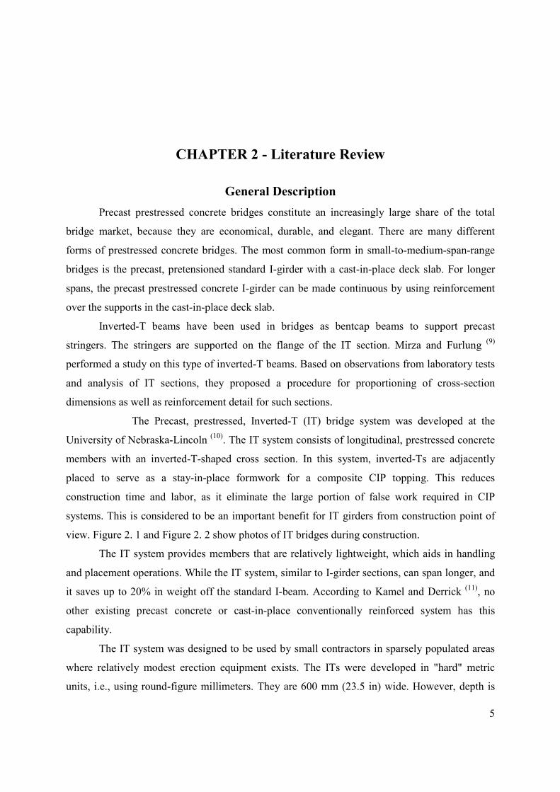
systems. This is considered to be an important benefit for IT girders from construction point of
view. Figure 2. 1 and Figure 2. 2 show photos of IT bridges during construction.
The IT system provides members that are relatively lightweight, which aids in handling
and placement operations. While the IT system, similar to I-girder sections, can span longer, and
it saves up to 20% in weight off the standard I-beam. According to Kamel and Derrick (11)
, no
other existing precast concrete or cast-in-place conventionally reinforced system has this
capability.
The IT system was designed to be used by small contractors in sparsely populated areas
where relatively modest erection equipment exists. The ITs were developed in "hard" metric
units, i.e., using round-figure millimeters. They are 600 mm (23.5 in) wide. However, depth is
6
varied as needed per design. The fact that ITs have the same flange width makes it possible to
use a single set of formwork when casting sections with varying depth.
Ambare and Peterman (12)
(2001) at Kansas State University suggested modifications to
the IT system. Modified IT sections have curved edges instead of the knife edges of the Inverted
sections. This helps eliminate bug pores during casting of the section. Figure 2.3 shows a
graphical comparison between an IT section and a modified IT section.
Ambare and Peterman (12)
also studied live-load distribution factors for IT girders, as
current codes don’t address systems with adjacent composite precast girders like the IT bridge
system. The study included computer modeling in order to evaluate the accuracy of current
AASHTO LRFD equations for IT girders. They concluded that the AASHTO LRFD (2nd
Edition) approximate equation gave live-load distribution factors that were higher than those
obtained by refined methods for moments. Shear-load distribution factor values are generally
conservative but may become unconservative at large skew angles. Ambare and Peterman
recommended using the AASHTO standard specification formula for predicting live-load
distribution factor for moments.
5.5Moment
SDF = (2.1)
where S is girder spacing (in).
For shear, the authors recommended a distribution factor of 0.42 be used for interior non-
skew bridges, exterior non-skew bridges, interior skewed bridges, and exterior skewed bridges
with skew angle less than 20 degrees. For exterior skew bridges with skew angle larger than 20,
shear distribution factors should be taken as
( 20)0.42
100Shear
skewangleDF
−= + (2.2)
where skew angle is taken in degree.
Despite the advantages and merits of the IT system, there are some limiting issues
when using IT beams in replacing existing bridges. First, the maximum span-to-depth ratio of the
IT system (close to 30) cannot compete with post-tensioned, concrete-haunched bridges with
span-to-depth ratios approaching 40. IT bridge systems are constructed continuously only for
live-loads; the beams act as simple-supported members for dead loads, including the weight of
the top CIP deck slab. In addition, IT members contain only straight pre-tensioned strands in the
7
bottom flanges. This causes the bottom of the beam to be under compression and the top of the
beam to be under tension. However, in sections where moment due to self-weight of the beam or
the applied loads is significant this tension in the top is reduced, while in sections where the
moment is small, the tension causes cracks in the deck. This fact often necessitates de-bonding of
the strands to control normal stresses and top-tensile stresses at the member ends. This in turn
leads to a reduction in the shear capacity of these members. In addition, the top tension can lead
to increased transverse cracking of the composite top deck slab over the piers when experiencing
a combination of live-loads and loads induced by restraint of time-dependent deformations.
Longer spans can be achieved by post-tensioning the precast girders to form continuous
spans by splicing together individual precast beams. Spliced girders that are continuous over
interior supports may be constructed with many configurations; girders may be spliced at the
interior supports, or continuous over the support and spliced within the span. Most common
spliced girders are I-girders, which are relatively deep. For medium-span-length girders, spliced
girders are not cost effective, as they need false work.
This study investigates the use of post-tensioning, prestressed inverted-T girders. The
system is referred to as post-tensioned, inverted-T beams (PT-IT). Post-tensioning is believed to
overcome the deficiencies of the IT system explained above and make it more structurally
efficient. Post-tensioning effectively increases span ranges of IT systems and consequently,
span-to-depth ratio. This helps in replacing existing bridges with bridges of more capacity and
same or lower depth, without raising the finished roadway elevation or restricting the hydraulic
flow. Post-tensioning is applied by threading tendons through a draped duct provided while
casting the IT section. Figure 2. 4 shows a sketch of a PT-IT bridge system. The design
implementation is accomplished by either applying one-stage post-tensioning before or after
casting the CIP top-deck slab, or partially post-tensioning before casting the deck and apply
second-stage post-tensioning afterwards.
Use of post-tensioning allows for flexibility in tendon placement with greater eccentricity
at mid span and reduced eccentricity at the ends. Use of post-tensioning decreases the number of
pre-tensioned straight strands required. Additional benefits of the PT-IT system are reducing top
tension in these continuous structures and reducing the potential for transverse cracks in the CIP
deck (thereby decreasing vulnerability of the bridges to deicing salts). An additional benefit of
8
the PT-IT system is that cambers of the pre-tensioned concrete members will be significantly
reduced (since fewer pre-tensioned strands will be used).
Many points are to be carefully addressed in analyzing the PT-T system. Since
construction of PT-IT is done in many stages, using different construction scenarios, and the
factors causing losses in prestressing and post-tensioning are time-dependent, losses should be
incrementally evaluated at the beginning and end of each stage. Accordingly stresses in the
concrete should be checked at each stage so as not to exceed allowable stresses at any time
during construction and service life of the bridge. Factors that are time-dependent and cause
losses in prestressing are shrinkage of concrete, relaxation of prestressing and post-tensioning
steel, as well as creep of the concrete under the pre-tensioning and post-tensioning, and dead
load stresses.
When precast girders are made continuous using a cast-in-place deck and diaphragm,
aforesaid time-dependent factors create restraint moments in the piers. Factors affecting and
causing restraining moments are discussed later in this chapter.
A review of published literature was conducted focusing on methods for evaluating losses
in prestressing and post-tensioning, as well as methods of estimating time-dependent moments
developed at the cast-in-place (CIP) joints after girders are made continuous. The literature
review includes different recommended types of positive moment connection over the piers.
Available Methods for Evaluating Time-Dependent Losses
Evaluating effective prestress force is of great importance in analysis of prestreesed
concrete structures. Effective prestress force is used to calculate stress in concrete and evaluate
deformations under service loads. Loss of prestress is defined as loss of compressive force acting
on the concrete component of a prestressed concrete section. Creep and shrinkage affect a
prestressed concrete member, causing it to shorten. This results in loss of tension in prestressing
strands. For prestressed members and grouted post-tensioning members, the sum of the reduction
in tensile force in the strands is equal and opposite to the incremental loss of compression force
in concrete. Two factors affect tension force in the strands: loss of prestress and elastic gain of
prestress. Loss of prestress is a time-dependent loss counted from the time strands are tensioned
until a certain time. Elastic loss or gain in prestress is an instantaneous change. As the
prestressing force is released from the bed and transferred to the concrete member; the member
9
undergoes shortening and cambers upward between its two ends. The net elastic loss at transfer
is equal to the stress loss due to prestress, combined with stress gain due to member self weight.
The strands further elongate and undergo elastic gain as additional load is introduced to the
member, such as deck weight or as post-tensioning is applied to the section.
Components of prestress losses (13)
:
1. Loss due to prestressing bed anchorage seating, and relaxation between the time of
initial tensioning and transfer. For post-tensioned strands, there is an instantaneous loss due to
friction.
2. Instantaneous prestress loss at transfer due to pre-stressing force and self-weight.
3. Prestress loss between transfer and deck placement due to shrinkage and creep of
girder, and relaxation of prestressing strands.
4. Instantaneous prestress gain due to deck weight on the noncomposite section and
superimposed dead loads on the composite section.
5. Long-term prestress losses after deck placement due to shrinkage and creep of girder
concrete, and relaxation of prestressing strands.
Estimating prestress loss requires an accurate prediction of material properties, the
interaction between creep and shrinkage of concrete, and the relaxation of steel (13)
. In addition,
prestress losses are influenced by composite action between the cast-in-place concrete deck and
the precast, prestressed concrete girder. Existing approaches for estimating prestress losses can
be divided into three categories, listed as follows in descending order of complexity and
accuracy.
Time-Step Prestress Loss Methods
These methods calculate prestress loss based on a step-by-step numerical procedure. This
is usually implemented in computer programs for accurate estimation of long-term prestress
losses. This approach is especially useful in multi-stage bridge construction, which is considered
during the course of this study.
The interaction of relaxation of steel with creep and shrinkage is considered in such
methods. As concrete creeps and shrinks, the prestressing strands shorten and decrease in
tension. This, in turn, decreases relaxation of the steel. As tension in strands is decreased,
compressive force applied on concrete sections is decreased, causing concrete to creep less.

10
To account for continuous interactions between creep and shrinkage of concrete and
relaxation of strands with time, time will be divided into intervals. The duration of each time
interval can be made larger as the concrete age increases (13)
. Stress in the strands at the end of
each time interval equals stress in the strands at the beginning of that time interval, minus
calculated prestress losses during the interval. Stresses and deformations at the beginning of an
interval are the same as those at the end of the preceding interval. In this time-step method, the
prestress level can be estimated at any critical time during the life of the structure.
Refined Prestress Loss Methods
In these methods, individual components of prestress loss are calculated separately, and
the total prestress loss is then calculated by summing up the separate components.
However, none of these methods account for composite action between deck slabs and
precast girders. Because the deck concrete shrinks more and creeps less than the precast girder
concrete, prestress gain rather than prestress loss may occur.
In these methods, data representing the properties of materials, loading conditions, and
environmental conditions have been incorporated into the prediction formulas used for
computing individual prestress loss components.
Over the years, several methods have been developed. Among these are the current
AASHTO-LRFD (1)
refined method and the AASHTO Standard Specifications method (14)
. In
AASHTO LRFD, prestress losses are computed at release and at final time in the location of
midspan section only. According to LRFD Art 5.9.5, prestress losses in pretensioned members,
∆fpT, at transfer is given as
1p pES pRf f fD = D + D (2.3)
where
∆fpES is the loss due to elastic shortening given as
p
pES cgp
ci
Ef f
ED = . (2.4)
fcgp is the sum of concrete stresses at the center of gravity of prestressing tendons due to
the prestressing force at transfer and the self-weight of the member at the sections of maximum
moments, Ep modulus of elasticity of prestressing steel, and Eci modulus of elasticity of concrete
at transfer.
11
∆fpR1 is the loss due to relaxation of steel at transfer, which is given according to the type
of strands as follows:
For stress relieved strands,
1
log(24.0 )[ 0.55]
10.0
pj
pR pj
py
ftf f
fD = - ; and (2.5)
for low-relaxation strands,
1
log(24.0 )[ 0.55]
40.0
pj
pR pj
py
ftf f
fD = - (2.6)
where t is time estimated in days from stressing to transfer, fpj is the initial stress in the
tendon at the end of stressing, and fpy is specified yield strength of prestressing steel.
At the final stage, total loss is calculated at midspan only as the sum of individual
components.
S 2p p p p pE SH CR Rf T= f + f + f + f∆ ∆ ∆ ∆ ∆ (2.7)
where
∆fpT is total loss of prestress, and
∆fpES is loss due to elastic shortening and is given in equation (2.4).
∆fpSH is the loss due to concrete shrinkage and is given as follows:
For pretensioned members,
1 (17.0 0.150 ) ( )pSHf H ksiD = - ; And (2.8)
for post-tensioned members,
1 (13.5 0.123 ) ( )pSHf H ksiD = - (2.9)
where H is the average annual ambient relative humidity (%).
∆fpCR is the loss due to creep of concrete.
12.0 7.0 0 ( )pCR cgp cdpf f f ksiD = - D >= (2.10)
fcgp is concrete stress at the center of gravity of prestressing steel at transfer.
∆fcdp is change in concrete stress at the center of gravity of prestressing steel due to
permanent loads.
∆fpR2 is loss due to relaxation of steel after transfer
12
for pretensioning with stress-relieved strands.
2 20.0 0.4 0.2( ) ( )pR pES pSR pCRf f f f ksiD = - D - D + D ; and (2.11)
for post-tensioning with stress-relieved strands
2 20.0 0.3 0.4 0.2( ) ( )pR pf pES pSR pCRf f f f f ksiD = - D - D - D + D . (2.12)
For low-relaxation, loss due to relaxation is taken as 30 % of the loss for stress-relieved
strands.
Lump-Sum Methods
Lump-sum methods are commonly used in preliminary design. According to the
AASHTO LRFD (1)
lump-sum method, prestress loss for girders with 270 ksi low-relaxation
strands is given by the following formulas:
For box girders
19 4 4 ( )PPR ksi+ − ; (2.13)
for rectangular beams and solid slabs
26 4 6 ( )PPR ksi+ − ; and (2.14)
for I-girders
' 6.033.0[1.0 0.15 ] 6.0 6 ( )
6.0
f cPPR ksi
−− + − (2.15)
in the case of single t, double-T, hollow-core and voided slab
' 6.033.0[1.0 0.15 ] 6.0 8 ( )
6.0
f cPPR ksi
−− + −
(2.16)
where PPR is the partial prestress ratio, which is normally equal to 1 for precast,
pretensioned members. These formulas reflect trends obtained from a computerized time-step
analysis of different beam sections for ultimate creep coefficient ranging from 1.6 to 2.4,
ultimate concrete shrinkage ranging from 0.0004 to 0.0006, and relative humidity ranging from
40% to 100%.
Methods to Calculate Time-Dependent Restraining Moments
13
Design of multi-span, continuous, precast, prestressed concrete bridges requires certain
additional considerations which do not arise in the case of simple span. Concrete bridge
structures are subject to time-dependent deformations produced by creep of the deck and beam
concrete, and by differential shrinkage between the deck and beams. In continuous girders, these
deformations cannot occur freely due to the restraint of continuity. As a result, additional
moments and shear forces are produced in the beams, which must be considered during design.
Since precast members are often fabricated several months before they are installed in the field,
most concrete shrinkage due to drying has occurred before the CIP concrete is cast. As the fresh
CIP concrete cures, its shrinkage will be partially restrained by the girders. In the case of a
simply supported beam, the beam will be free to rotate at the ends. In the case of a continuous
beam, the interior ends are not free to rotate. This produces negative restraint moments. The
effect of creep under prestressing usually has an opposite effect to shrinkage. This will produce
positive moments. Figure 2. 7(a) shows the effect of differential shrinkage on deformation of a
two span continuous beam. Figure 2. 7(b) shows restraint moments due to differential shrinkage
and creep on a two-span beam. The value of the resultant restraint moment should be considered
in the design. According to the PCI bridge design manual (15)
8.13.4.3.2.1, “Only loads
introduced before continuity can cause time-dependent restraint moments due to the time-
dependent effects”.
Some of the methods available for estimating restraint moments are discussed below.
PCA Method
The PCA method was developed by Mattock (4)
1961. Adopted by the Portland Cement
Association; in 1969, the method was investigated by Freyermuth (1).
The Portland Cement Association conducted an experimental research program on
precast I-girders with a continuous situ-cast deck, studied the influence of creep in precast
girders and differential shrinkage between the precast girders and CIP deck slab on continuity
behavior after an extended period of time. The experimental study was restricted to observation
and evaluation of the behavior of two half-scale, two-span continuous bridge girders over a
period of approximately two years from the time of construction. The girders were identical in all
particulars, except that one girder incorporated positive-moment connection at the interior
support, while the other did not. Long-term variations of support reactions and deflections due to
14
creep and differential shrinkage effects were measured. The continuity behavior of the girders
were investigated at intervals by loading them within service-load range. Finally, the girders
were loaded to destruction in order to determine the effect, if any, of creep and shrinkage on the
ultimate strength of the girders.
In this method, the uniform differential shrinkage moment in a composite concrete
section at any time is given by
( )2
s s d d c
hM E A ee= + (2.17)
where εs is the differential shrinkage strain;
Ed is the modulus of elasticity of CIP concrete;
Ad is the cross-sectional area of CIP slab;
h is CIP thickness; and
ec is the distance between the top of the precast member and the centroid of the
composite section.
In the first step, the restraint moments are calculated as if the prestress, dead load, and
shrinkage moments had been applied to the continuous girder and not to the individual spans. In
the second step, the restraint moments calculated in the first step are multiplied by (1-e-ф) for
prestress and dead load, and by (1-e-ф)/ф for moments due to shrinkage.
The restraint moment at the center support of the two-span continuous beam is given as
3 3 1( )(1 ) ( )2 2
r p d s
eM M M e M
φφ
φ
−− −
= + − + (2.18)
where Mp is the moment caused by prestressing force around the centroid of the
composite member;
Md is midspan moment due to dead load;
e is the base of the Naperian logarithm; and
ф is the creep coefficient (ratio of creep strain to elastic strain at time of investigation).
The study by Mattock concluded that deformations due to creep and differential
shrinkage do not influence the ultimate load-carrying capacity of a continuous I-girder. The
influence of creep and shrinkage is restricted to deformations and the possibility of cracking at
the service-load level.

15
Texas Transportation Institute
In 1974 the Texas Transportation Institute (16)
and Texas A&M University performed a
study about precast, prestressed concrete girders made continuous by CIP deck. This included
developing a computer program to perform calculations for design of such girders.
In this method, the restraining moments resulting from creep under self weight, weight of
deck, and prestressing along with moments resulting from differential shrinkage between the
girder and the deck are computed by the slope-deflection method of elastic analysis and then
scaled by proper factors.
Restraint moments resulting from creep are multiplied by the factor SFcreep
1creepSF
φ
φ=+
(2.19)
while restraint moments resulting from shrinkage are multiplied by the factor SFshrinkage
1
1shrinkageSF
φ=+
(2.20)
where fixed end moments for shrinkage are given as
s SDM EAeε= (2.21)
εSD is the differential shrinkage strain between deck and beam concrete at the time
connection was established.
E is the modulus of elasticity of deck concrete.
A is the cross sectional area of deck.
e is the distance between mid-depth of the deck and the centroid of the composite section.
6525 1020
SD H
t
tε α−= ×
+ (2.22)
where t is age of the beam in days when the deck is cast, and αH is the correction factor
for humidity taken from.
Creep factor Φ is calculated as follows to
(1 )c
e
εφ αε
= − . (2.23)
εc=creep strain at time t due to unit stress.
εe=initial strain due to unit stress.
α=fraction of εc, which has occurred when continuity connection is established.
16
The deck and the beam are assumed to have the same creep and shrinkage behavior.
Depending on laboratory experiments, expressions were developed to fit the shrinkage and unit
creep strain data.
6425( ) ( / / 10 )
34c
tt in in ksi
tε −= ×
+ (2.24)
when t=∞ , εc=425.
This basic unit creep strain is for concrete specimens with a volume/surface ratio of
approximately 1.0. Correction factor is considered to account for different volume-to-surface
ratios.
6
/425 ( / / 10 )c V S in in ksiε α −= × × (2.25)
where αV/S is taken from Figure 2. 6.
1e
iEε = and (2.26)
34
t
tα=
+ (2.27)
with substitution in equation (2.23)
6
/425 10 (1 )34
V S i
tE
tφ α−= × × × × −
+ (2.28)
where t is the age of concrete when connection was established.
This method is not believed to be as accurate as other methods for the following reasons.
Since the concrete of the girder has different strength, curing type, and age than the deck
concrete, shrinkage and creep properties, contrary to the method’s assumption, will be different
for the beam than for the deck. This method also assumes that the restraint moment will be the
same from the day connection was made through the life of the structure, while it actually
changes with time.
CTL Method
In 1989, Osterle, Glikin, and Larson (5), (6)
proposed modifications to the PCA method.
While PCA considered the continuity connections to have zero length and to be fully rigid, CTL
considered the actual connections to have finite lengths and rotational stiffness. CTL developed
the BRIDGERM program to carry out an incremental time-step solution, including separate
17
shrinkage functions for the deck and girder concrete, and time-dependent functions for the
strength and stiffness of deck concrete.
Creep restraint moments were determined by multiplying the dead load and prestress
moments by a coefficient (1-e-ΦT), where
ΦT=νT-νT0 (2.29)
where
νT creep coefficient is at time T days, where T is the time after prestress release at which
restraint moments are being calculated T>T0; and
νT0 creep coefficient is at time T0 days, where T0 is the time after prestress release at
which continuity is established.
Restraint moments due to differential shrinkage were determined using a multiplier of
(1-e-ΦT)/ Φ.
Change in restraint moment ∆Mi within each time step is calculated as follows:
' '` ' ' '( )(1 ) (1 ) /i i
i D PT si iM M M e M eφ φ φ− −∆ = + − +∆ − (2.30)
where Mp’ is restraint moment due to creep under prestress, MD
’ is restraint moment due
to dead load and Msi’ is restraint moment due to differential shrinkage between the deck slab and
girder.
For the calculation of restraint moment due to prestress-induced creep, the prestress force
was adjusted at each time step to account for losses due to shrinkage, creep, and relaxation.
In this method, the moment due to differential shrinkage is
' ( )2
si di c
tM F e∆ =∆ +
(2.31)
where ∆Fdi is tension in the deck to establish compatibility with the girder
1
si di ddi
di
g g
E AF
E Ad
E A
δ ε∆∆ =
+
(2.32)
1 1( ) ( )si sdi sdi sgi sgiδ ε ε ε ε ε− −∆ = − − − . (2.33)
εsdi is shrinkage strain in the CIP slab at time Ti.
εsgi is shrinkage strain in the girder at time Ti.
Edi is the modulus of elasticity of the deck concrete at time Ti.
Eg is the modulus of elasticity of the girder concrete.

18
Ad is the cross-sectional area of the CIP slab.
Ag is the area of the prestressed member.
2c
te +
= distance between mid-depth of the deck slab and centroid of the composite
section
in determining the deck shrinkage strain 30 days after casting the deck, the ultimate
shrinkage strain of the deck was reduced by the Dischinger effect factor to account for the
restraint from the reinforcing steel within the deck. This factor is given as follows:
0.031
1 0.03
0.03
u ni
u
e
nDisch
ni
φ
φ
−−
+ ×=× ×
(2.34)
Φu is the deck’s ultimate shrinkage.
,(28) ( )d d
Es Esni n
E E T= =
(2.35)
Results of computer analyses were compared to the PCA test observation conducted by
Mattock (4). The study concluded that continuity established at an early girder age will result in
positive restraint moments developing in the pier.
P Method
Peterman and Ramirez (7)
conducted an experimental investigation to evaluate the
restraint moment in the piers for bridges made continuous by a cast-in-place CIP deck.
Two full-span bridges were fabricated and tested at Purdue University. The bridges had
two spans; each span consisted of two prestressed concrete form panels measuring 21 ft long and
4 ft wide. Each bridge was subjected to repeated loading using two hydraulic actuators located at
a distance of 8 ft 3 in from the center of the middle pier. The experimentally obtained moments
were compared with values calculated from PCA and CTL methods, which ignored cracking of
the CIP topping and overestimated the negative restraint moments in composite construction
with shallow prestressed members.
The authors proposed a modified restraint moment calculation method that accounts for
length and stiffness of the diaphragm, different initiation times of creep, and restraint of CIP
concrete shrinkage. The method was referred to as P method.

19
This method estimates the moment due to differential shrinkage as
1 1( )
211
s s d d cp p s s
d dd d
hM E A e
E A E A
E AE A
e
Ê ˆ Ê ˆÁ ˜ Á ˜
= + Á ˜ Á ˜Á ˜ Á ˜++ Á ˜Á ˜ Ë ¯Ë ¯
(2.36)
Ep is the modulus of elasticity of the prestressed member.
Ap is the area of the prestressed member.
Es is the modulus of elasticity of steel reinforcement in the CIP deck.
As is the cross-sectional area of steel reinforcement in the CIP deck.
Ed is the modulus of elasticity of the CIP concrete.
Ad is the cross-sectional area of the CIP slab.
Using the P method (7), the restraint moment at the center pier of a two-span, symmetric
bridge is calculated as
21
2
3 3 1[ ( ) ][ (1 )] ( ) ( )2 2
r p d precast d CIP s
eM M M e M M
yya a a a
y
-- -
= - D - - - (2.37)
where
2
2 3
d
d
d m
d m
I
L
I I
L L
a =+
(2.38)
Id is the moment of inertia of the diaphragm region.
Ld is length of the diaphragm region.
Im is the moment of inertia of the main span.
Lm is the length of the main span.
(Md)precast is the midspan moment due to dead load of the girders.
(Md)CIP is the midspan moment due to CIP deck weight.
ψ1 is the creep coefficient for creep effects initiating when prestress force is transferresd
to the precast panel.
ψ2 is the creep coefficient for creep effects initiating when the CIP topping is cast.
∆(1-e-ψ1) is the change in expression (1-e
-ψ1) occurring from the time corresponding to
restraint moment calculations.
20
Restraint moments are compared to cracking moments in the diaphragms. Once the
diaphragm cracks, moment redistribution will occur and restraint moment will be calculated
using stiffness of the cracked diaphragm section.
Discussion of PCA, CTL, and P methods is presented in chapter three,
highlighting major differences mainly between CTL and P methods. Modifications for both
methods are proposed as well.
Creep-Transformed Section Properties Method
The method developed by Dilger (8)
is intended for time-dependent analysis for
prestressed concrete structures, including evaluating prestress losses, restraint moments, time-
dependent curvature, and deflection.
The method makes use of well-known methods of stress analysis and is, in principle,
similar to the elastic stress analysis of a member consisting of two materials in which one
component (concrete) changes its temperature while the temperature of the other (reinforcement)
remains constant.
In this method, time-dependent analysis of prestressed concrete members, the cross-
section properties include the effect of concrete creep.
The response of the concrete to gradually changing stress due to creep and shrinkage is
best calculated by Bazant’s (17)
age-adjusted effective modulus formula:
*0 0( ) /[1 ( , )]c cE t t tE χφ= + (2.39)
where
Ec(t0) is the modulus of elasticity of concrete loaded at age t0.
Φ(t,t0) is the creep coefficient at time t for concrete loaded at age t0.
χ is the aging coefficient.
The aging coefficient expresses the aging effect on creep of concrete loaded gradually
and depends on the magnitude of the creep coefficient, age of the concrete at first loading, and
time under load.
The forces corresponding to unrestrained creep, free shrinkage of the concrete, and
reduced relaxation of the prestressing steel are applied to the creep-transformed section in which
the steel is included with the modular ratio

21
*
0 0*[1 ( , )]s
c
En n t t
Eχφ= = + (2.40)
For non-composite members, the change in strain due to unrestrained creep and free
shrinkage at the tendon level is
*
1 0 0( ) ( , ) ( , )c sht t t t tε ε φ ε∆ = + (2.41)
where
ε1=fc1/Ec(t0) elastic concrete strain at the level of the tendon due to load applied at age t0
producing the stress fc1, and
εsh(t,t0) free shrinkage since the time of prestressing.
The corresponding steel stress including reduced relaxation, is
* '
0 1 0 0( ) ( , ) ( , ) ( )s c sh s rf t n f t t t t E f tφ ε= + + ; (2.42)
and the corresponding normal force and bending moment is
* *
* * *
1
( )s s s
s s
N A f t
M N y
=
= (2.43)
where As is the steel area and
y1* is the distance between the centroid of the steel and the centroid of the creep-
transformed section.
The stress corresponding from Ns* and Ms
* in steel obtained from the relation is
* ** * *
1* *( ) ( )s s
s
c c
N Mf t y n
A I∆ =− + (2.44)
The time-dependent change in steel stress is obtained by summing steel stresses in
equations (2.42) and (2.44).
Solving for stresses in a composite member, the difference in time-dependent strains
between the precast girder and cast-in-place deck is calculated at the level of the centroid of the
concrete deck. All strains are determined for time after the beginning of composite action. Initial
elastic strain ε1 in any fiber of the precast section due to the weight of the girder and prestressing
will increase due to unrestrained creep and free shrinkage from the beginning of the composite
action t1 until time t by
1 1 0 1 0 1 1( ) [ ( , ) ( , )] ( , )sht t t t t t tε ε φ φ ε∆ = − + (2.45)
At the level of the centroid of the cast-in-place deck, the increase in strain is
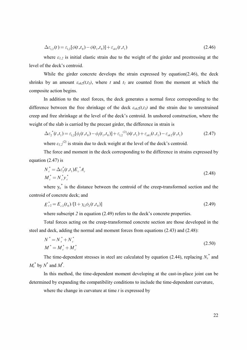
22
1,2 1,2 0 1 0 1 1( ) [ ( , ) ( , )] ( , )sht t t t t t tε ε φ φ ε∆ = − + (2.46)
where ε1,2 is initial elastic strain due to the weight of the girder and prestressing at the
level of the deck’s centroid.
While the girder concrete develops the strain expressed by equation(2.46), the deck
shrinks by an amount εsh2(t,t1), where t and t1 are counted from the moment at which the
composite action begins.
In addition to the steel forces, the deck generates a normal force corresponding to the
difference between the free shrinkage of the deck εsh2(t,t1) and the strain due to unrestrained
creep and free shrinkage at the level of the deck’s centroid. In unshored construction, where the
weight of the slab is carried by the precast girder, the difference in strain is
* (2)
2 1 1,2 1 0 1 1 0 1,2 1 1 1 2 1( , ) [ ( , ) ( , )] ( , ) ( , ) ( , )sh sht t t t t t t t t t t tε ε φ φ ε φ ε ε∆ = − + + − (2.47)
where ε1,2(2) is strain due to deck weight at the level of the deck’s centroid.
The force and moment in the deck corresponding to the difference in strains expressed by
equation (2.47) is
* * *
2 1
* * *
( , )c c c
c c c
N t t E A
M N y
ε=∆
= (2.48)
where yc* is the distance between the centroid of the creep-transformed section and the
centroid of concrete deck; and
*2 2 0 2 2 0( ) /[1 ( , )]c cE t t tE χ φ= + (2.49)
where subscript 2 in equation (2.49) refers to the deck’s concrete properties.
Total forces acting on the creep-transformed concrete section are those developed in the
steel and deck, adding the normal and moment forces from equations (2.43) and (2.48):
* * *
* * *
s c
s c
N N N
M M M
= +
= + (2.50)
The time-dependent stresses in steel are calculated by equation (2.44), replacing Ns* and
Ms* by N
* and M
*.
In this method, the time-dependent moment developing at the cast-in-place joint can be
determined by expanding the compatibility conditions to include the time-dependent curvature,
where the change in curvature at time t is expressed by
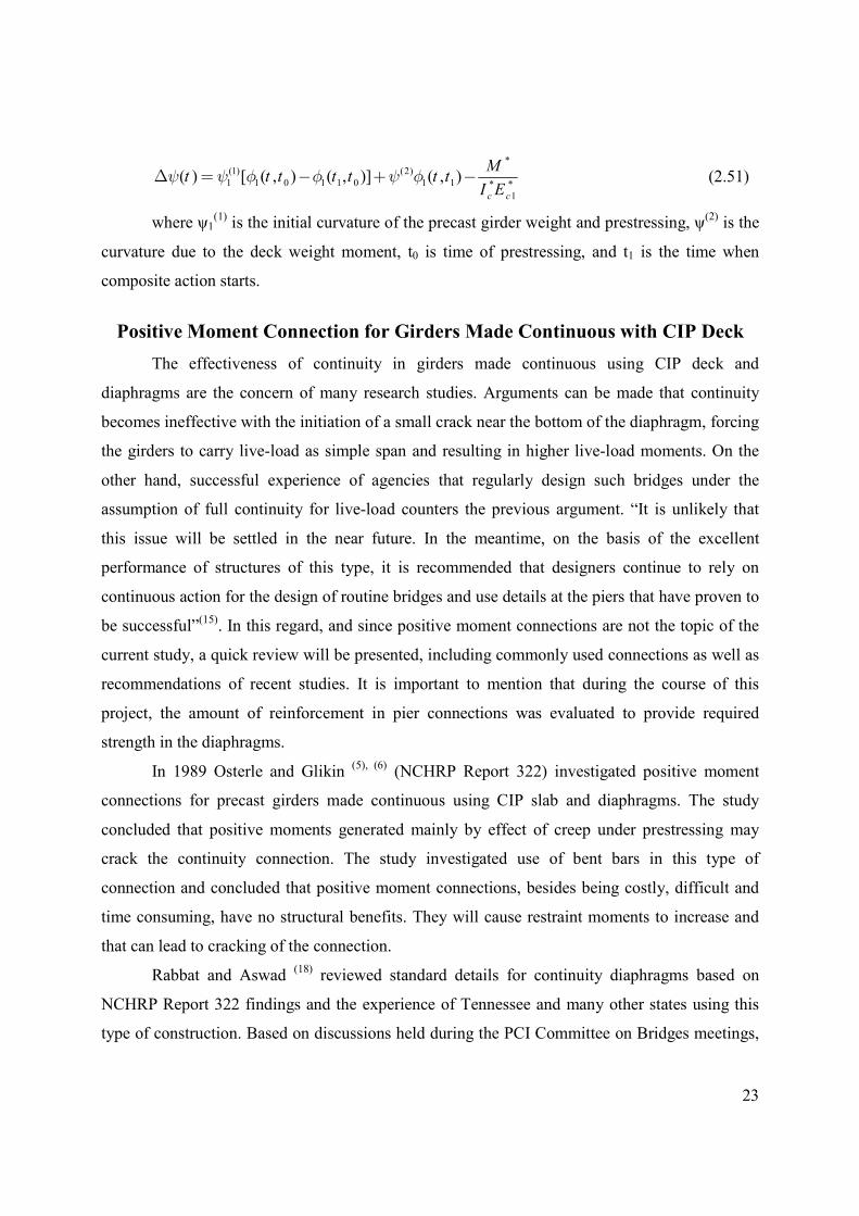
23
*(1) (2)
1 1 0 1 1 0 1 1 * *
1
( ) [ ( , ) ( , )] ( , )c c
Mt t t t t t t
I Eψ ψ φ φ ψ φ∆ = − + − (2.51)
where ψ1(1) is the initial curvature of the precast girder weight and prestressing, ψ
(2) is the
curvature due to the deck weight moment, t0 is time of prestressing, and t1 is the time when
composite action starts.
Positive Moment Connection for Girders Made Continuous with CIP Deck
The effectiveness of continuity in girders made continuous using CIP deck and
diaphragms are the concern of many research studies. Arguments can be made that continuity
becomes ineffective with the initiation of a small crack near the bottom of the diaphragm, forcing
the girders to carry live-load as simple span and resulting in higher live-load moments. On the
other hand, successful experience of agencies that regularly design such bridges under the
assumption of full continuity for live-load counters the previous argument. “It is unlikely that
this issue will be settled in the near future. In the meantime, on the basis of the excellent
performance of structures of this type, it is recommended that designers continue to rely on
continuous action for the design of routine bridges and use details at the piers that have proven to
be successful”(15)
. In this regard, and since positive moment connections are not the topic of the
current study, a quick review will be presented, including commonly used connections as well as
recommendations of recent studies. It is important to mention that during the course of this
project, the amount of reinforcement in pier connections was evaluated to provide required
strength in the diaphragms.
In 1989 Osterle and Glikin (5), (6)
(NCHRP Report 322) investigated positive moment
connections for precast girders made continuous using CIP slab and diaphragms. The study
concluded that positive moments generated mainly by effect of creep under prestressing may
crack the continuity connection. The study investigated use of bent bars in this type of
connection and concluded that positive moment connections, besides being costly, difficult and
time consuming, have no structural benefits. They will cause restraint moments to increase and
that can lead to cracking of the connection.
Rabbat and Aswad (18)
reviewed standard details for continuity diaphragms based on
NCHRP Report 322 findings and the experience of Tennessee and many other states using this
type of construction. Based on discussions held during the PCI Committee on Bridges meetings,
24
the authors recommended the dead load of the girders and the deck as acting on a simple span,
analyzing the structure as continuous for live-load and superimposed loads, and providing a
positive moment connection through reinforcing or prestressing steel to develop a design
strength equal to or greater than 1.2 times the positive cracking moment. In so, no analysis for
restraint moments due to time-dependent effects would be required.
Mirmiran, et al.(19)
carried out an analytical study to investigate the performance of
reinforced continuity connections for precast, prestressed concrete girders with CIP decks. The
study concluded that positive moment reinforcement in the continuity diaphragm has a
significant effect on restraint moments when the continuity is established at early ages. The study
also concluded that continuity behavior of the bridge is generally better when continuity is
established at a later age of the girders. The authors recommended that practicing engineers
should consider providing minimum reinforcement that prevents excessive cracking of the
diaphragm section without crowding the connection.
In 2004, Miller et al.(20)
, under a National Cooperative Highway Research Program,
conducted a survey of state DOTs concerning connections for precast, prestressed concrete
bridge girders. The study concluded that the presence of positive-moment cracking at the
diaphragm doesn’t necessarily reduce continuity. The report proposed revisions to the AASHTO
LRFD bridge design specifications, including details for fabricating positive-moment
connections by either extending the prestressing strands from the end of the girder, bending it at
900 and embedding it in the diaphragm section, or by embedding mild steel at the ends of the
girders with standard hooks at the protruding end of the bar to be embedded in the diaphragms.
In 2004, Saadeghvazini et al. (21)
proposed using flexible CFRP composites to improve
continuity over fixed piers. The study concluded that bond between the concrete and the
composite is the most critical element. It also concluded that wrapping and surface preparation
have a significant effect against debonding the composite.
25
Figure 2. 1 PT-IT bridge system under construction
Figure 2. 2 PT-IT bridge system under construction
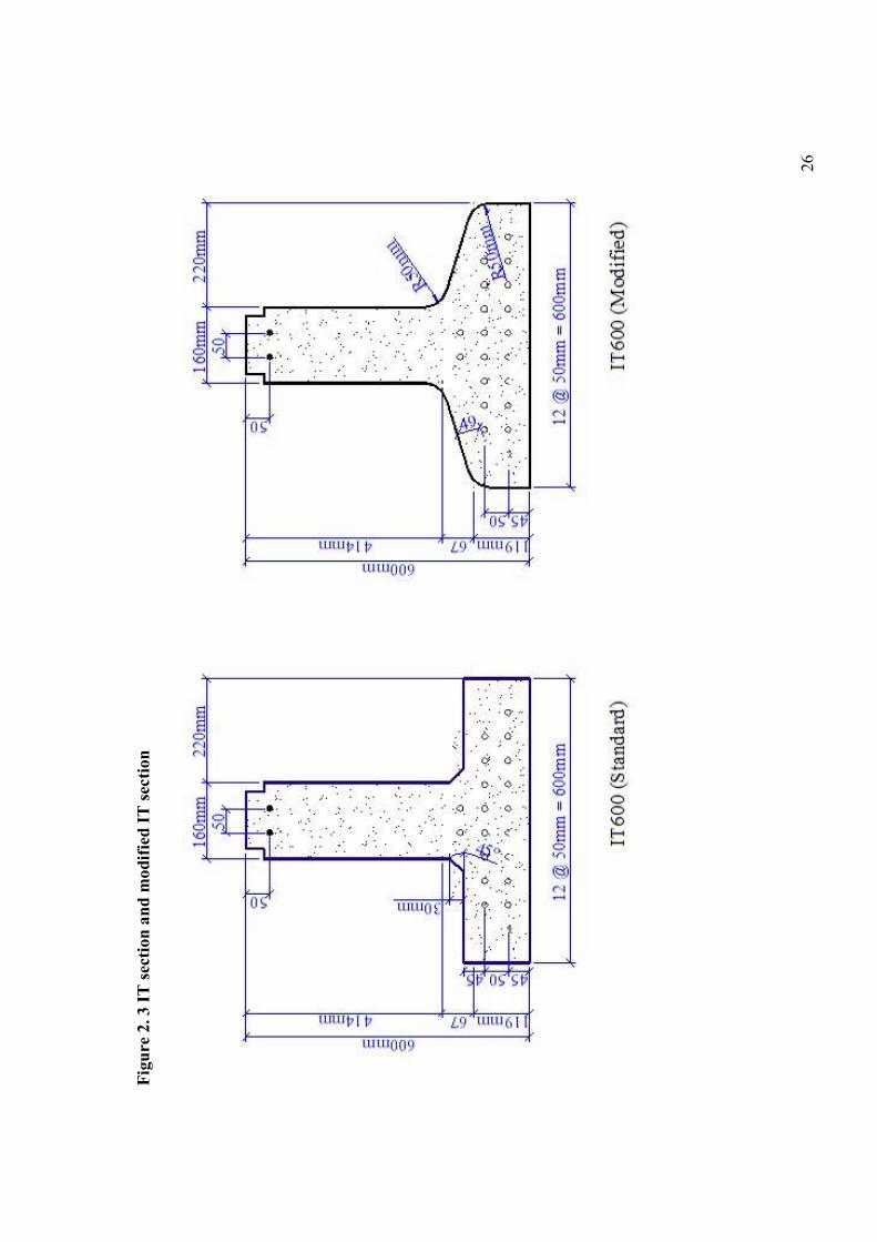
26
Figure 2. 3 IT section and modified IT section

27
Figure 2. 4 PT-IT bridge system
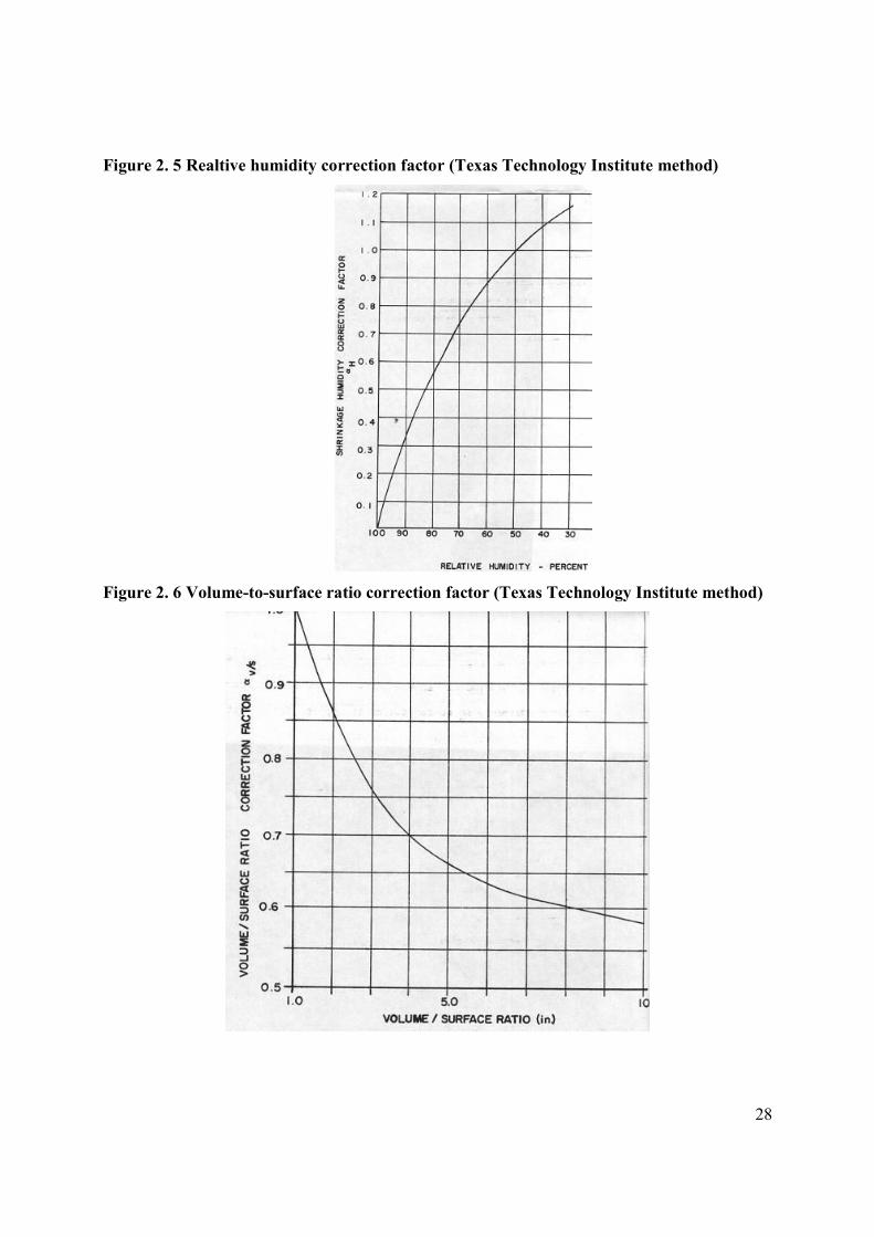
28
Figure 2. 5 Realtive humidity correction factor (Texas Technology Institute method)
Figure 2. 6 Volume-to-surface ratio correction factor (Texas Technology Institute method)
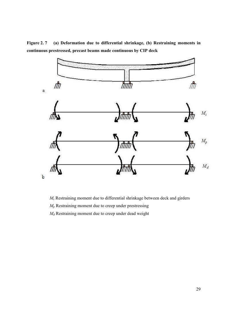
29
Figure 2. 7 (a) Deformation due to differential shrinkage, (b) Restraining moments in
continuous prestressed, precast beams made continuous by CIP deck
Ms Restraining moment due to differential shrinkage between deck and girders
Mp Restraining moment due to creep under prestressing
Md Restraining moment due to creep under dead weight
30
CHAPTER 3 - Analysis of Post-Tensioned Prestressed Inverted T
System
Equation Section 3
The PT-IT program was developed for the purpose of analyzing PT-IT systems. It is used
as a tool to perform parametric study. Parameters varied in the parametric study are discussed in
details in chapter 4. The program is written using C++ object-oriented language. The PT-IT
program performs time-stepping analyses. Structural analysis is performed at each stage during
and after construction. New stage is typically marked by adding structural component or load to
the structure. For example events like casting deck, casting diaphragm, apply post-tensioning,
install barriers, and apply live load mark the beginning of a new stage. Analysis includes
evaluating moments and shears produced by self weight, deck weight, external applied loads,
moment and shear internally produced by prestressing and post-tensioning, as well as time-
dependent moment and shear caused by creep and shrinkage. The program also checks AASHTO
LRFD service and strength limit. A Graphical interface is provided for the program using Visual
Basic 6.
Analysis of moment and shear due to Live-load is performed using the Risa 2D program.
Analysis includes generating influence lines for different moving loads according to AASHTO
LRFD (1), then manually creating the envelope for a maximum of positive moments, negative
moments shear, and live-load deflection. Algorithm used in PT-IT is discussed in details later in
this chapter.
To validate results of the program, results of the PT-IT program are checked versus
Consplice (22)
utilizing major differences between Consplice and PT-IT. Consplice was
developed by LEAP software to analyze spliced girders.
Spliced girders consist of precast prefabricated (usually prestressed) girder, transported to
the construction site and joined together using splices, resulting in a continuous span structure.
Ideally, spliced girders are post-tensioned to maximize span length. Spliced girders are typically
joined within the span, unlike post-tensioned, prestressed IT systems where girders are joined at
the pier.
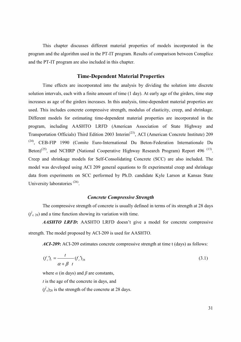
31
This chapter discusses different material properties of models incorporated in the
program and the algorithm used in the PT-IT program. Results of comparison between Consplice
and the PT-IT program are also included in this chapter.
Time-Dependent Material Properties
Time effects are incorporated into the analysis by dividing the solution into discrete
solution intervals, each with a finite amount of time (1 day). At early age of the girders, time step
increases as age of the girders increases. In this analysis, time-dependent material properties are
used. This includes concrete compressive strength, modulus of elasticity, creep, and shrinkage.
Different models for estimating time-dependent material properties are incorporated in the
program, including AASHTO LRFD (American Association of State Highway and
Transportation Officials) Third Edition 2003 Interim(23)
, ACI (American Concrete Institute) 209
(24), CEB-FIP 1990 (Comite Euro-International Du Beton-Federation Internationale Du
Beton)(25), and NCHRP (National Cooperative Highway Research Program) Report 496
(13).
Creep and shrinkage models for Self-Consolidating Concrete (SCC) are also included. The
model was developed using ACI 209 general equations to fit experimental creep and shrinkage
data from experiments on SCC performed by Ph.D. candidate Kyle Larson at Kansas State
University laboratories (26)
.
Concrete Compressive Strength
The compressive strength of concrete is usually defined in terms of its strength at 28 days
(f’c 28) and a time function showing its variation with time.
AASHTO LRFD: AASHTO LRFD doesn’t give a model for concrete compressive
strength. The model proposed by ACI-209 is used for AASHTO.
ACI-209: ACI-209 estimates concrete compressive strength at time t (days) as follows:
28( ) ( )c t c
tf f
ta b=¢ ¢
+ (3.1)
where α (in days) and β are constants,
t is the age of the concrete in days, and
(f’c)28 is the strength of the concrete at 28 days.
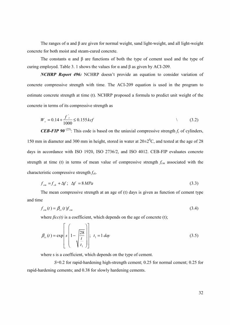
32
The ranges of α and β are given for normal weight, sand light-weight, and all light-weight
concrete for both moist and steam-cured concrete.
The constants α and β are functions of both the type of cement used and the type of
curing employed. Table 3. 1 shows the values for α and β as given by ACI-209.
NCHRP Report 496: NCHRP doesn’t provide an equation to consider variation of
concrete compressive strength with time. The ACI-209 equation is used in the program to
estimate concrete strength at time (t). NCHRP proposed a formula to predict unit weight of the
concrete in terms of its compressive strength as
'
0.14 0.1551000
c
c
fW kcf= + £ \ (3.2)
CEB-FIP 90 (25)
: This code is based on the uniaxial compressive strength fc of cylinders,
150 mm in diameter and 300 mm in height, stored in water at 20±20C, and tested at the age of 28
days in accordance with ISO 1920, ISO 2736/2, and ISO 4012. CEB-FIP evaluates concrete
strength at time (t) in terms of mean value of compressive strength fcm associated with the
characteristic compressive strength fck.
; 8cm ckf f f f MPa= + D D = (3.3)
The mean compressive strength at an age of (t) days is given as function of cement type
and time
( ) ( )cm cc cmf t t fb= (3.4)
where βcc(t) is a coefficient, which depends on the age of concrete (t);
1
1
28( ) exp 1 ; 1cc t s t day
t
t
b
È ˘Ê ˆÍ ˙Á ˜Í ˙= - =Á ˜Í ˙Á ˜Á ˜Í ˙Ë ¯Î ˚
(3.5)
where s is a coefficient, which depends on the type of cement.
S=0.2 for rapid-hardening high-strength cement; 0.25 for normal cement; 0.25 for
rapid-hardening cements; and 0.38 for slowly hardening cements.
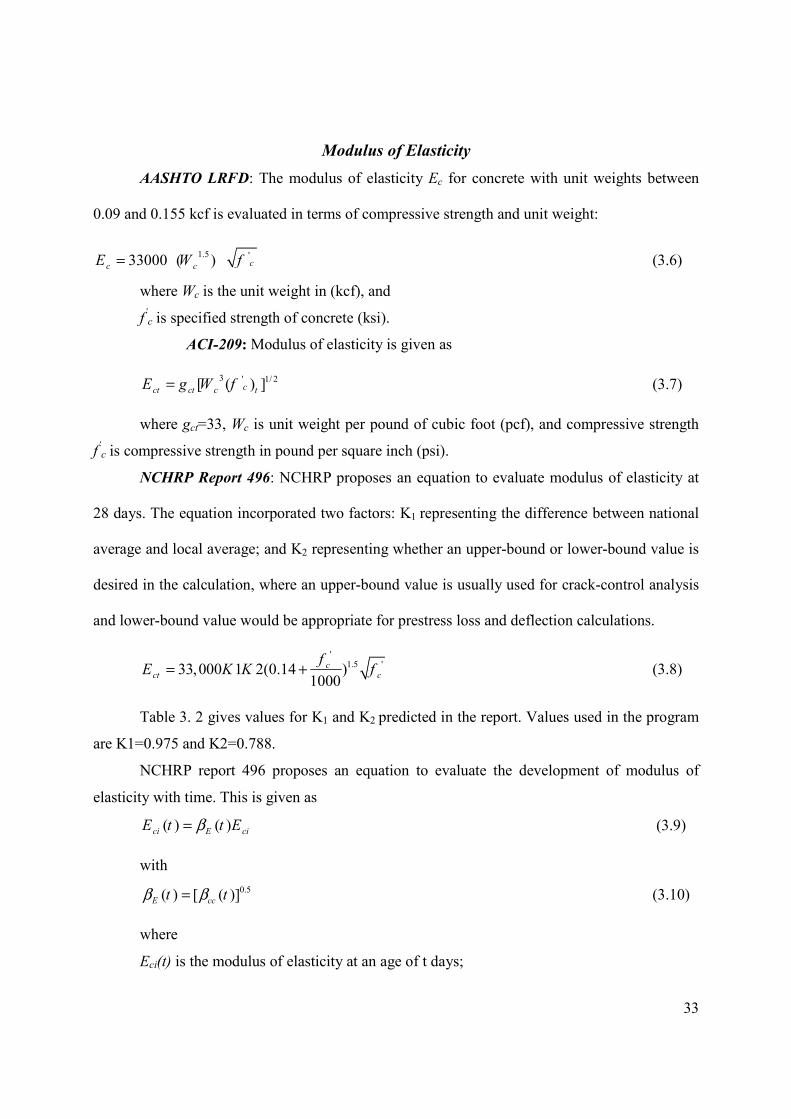
33
Modulus of Elasticity
AASHTO LRFD: The modulus of elasticity Ec for concrete with unit weights between
0.09 and 0.155 kcf is evaluated in terms of compressive strength and unit weight:
1.5 '33000 ( ) cc cE W f= (3.6)
where Wc is the unit weight in (kcf), and
f’c is specified strength of concrete (ksi).
ACI-209: Modulus of elasticity is given as
3 ' 1/ 2[ ( ) ]cct ct c tE g W f= (3.7)
where gct=33, Wc is unit weight per pound of cubic foot (pcf), and compressive strength
f’c is compressive strength in pound per square inch (psi).
NCHRP Report 496: NCHRP proposes an equation to evaluate modulus of elasticity at
28 days. The equation incorporated two factors: K1 representing the difference between national
average and local average; and K2 representing whether an upper-bound or lower-bound value is
desired in the calculation, where an upper-bound value is usually used for crack-control analysis
and lower-bound value would be appropriate for prestress loss and deflection calculations.
'1.5 '33,000 1 2(0.14 )
1000
cct c
fE K K f= + (3.8)
Table 3. 2 gives values for K1 and K2 predicted in the report. Values used in the program
are K1=0.975 and K2=0.788.
NCHRP report 496 proposes an equation to evaluate the development of modulus of
elasticity with time. This is given as
( ) ( )ci E ciE t t Eb= (3.9)
with
0.5( ) [ ( )]E cct tb b= (3.10)
where
Eci(t) is the modulus of elasticity at an age of t days;

34
Eci is the modulus of elasticity at an age of 28 days given as
1
30
0
[ ]cmci c
cm
fE E
f= ; and (3.11)
Ec0=2.15*104 MPa, fcm0 =10 MPa, βcc(t) is given in equation (3.4).
Shrinkage Strain
Shrinkage of concrete is affected by many factors, these factors such as aggregate
characteristics and proportions, average humidity at the bridge site, water-to-cement (W/C) ratio,
type of cure, volume-to-surface area ratio of a member, and duration of drying period. Shrinkage
strain is often defined in terms of ultimate shrinkage and time function to adjust for shrinkage up
to a certain time.
AASHTO LRFD: AASHTO LRFD gives two equations to assess shrinkage strain— one
for moist-cured concrete and the other for steam-cured concrete.
For moist-cured concretes and concrete devoid of shrinkage-prone aggregates, the strain
due to shrinkage εsh at time t, is given by
(3.12)
For steam-cured concrete devoid of shrinkage-prone aggregates
30.56 1055.0
sh s h
tk k
te -Ê ˆ= - ¥Á ˜Ë ¯+
(3.13)
where
t is the drying time (days).
ks is size factor given as
0.36( / ) 1064 94( / )26
923
45
V S
s
t
V Se tkt
t
È ˘Í ˙ -È ˘+= Í ˙ Í ˙Î ˚Í ˙
+Î ˚
(3.14)
kh is humidity factor given as
for H<80%
140
70h
Hk
-= (3.15)
for H>=80%
30.51 1035.0
sh s h
tk k
te -Ê ˆ= - ¥Á ˜Ë ¯+
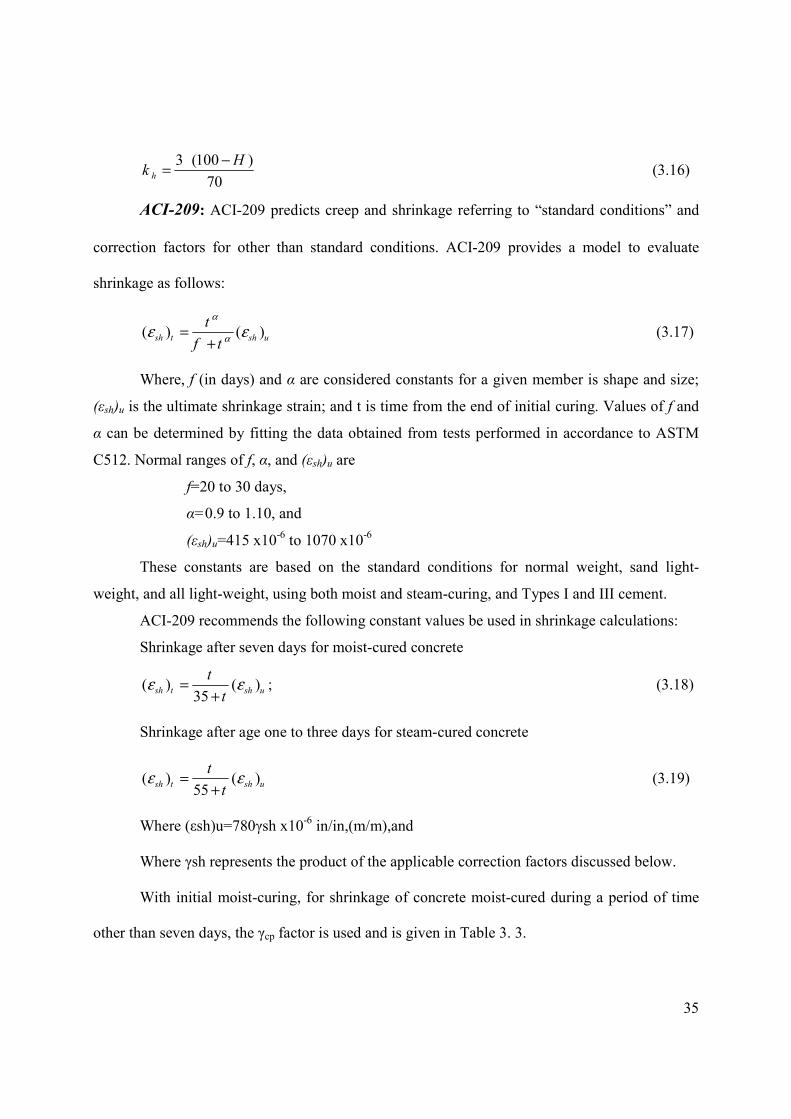
35
3 (100 )
70h
Hk
-= (3.16)
ACI-209: ACI-209 predicts creep and shrinkage referring to “standard conditions” and
correction factors for other than standard conditions. ACI-209 provides a model to evaluate
shrinkage as follows:
( ) ( )sh t sh u
t
f t
a
ae e=+
(3.17)
Where, f (in days) and α are considered constants for a given member is shape and size;
(εsh)u is the ultimate shrinkage strain; and t is time from the end of initial curing. Values of f and
α can be determined by fitting the data obtained from tests performed in accordance to ASTM
C512. Normal ranges of f, α, and (εsh)u are
f=20 to 30 days,
α=0.9 to 1.10, and
(εsh)u=415 x10-6 to 1070 x10
-6
These constants are based on the standard conditions for normal weight, sand light-
weight, and all light-weight, using both moist and steam-curing, and Types I and III cement.
ACI-209 recommends the following constant values be used in shrinkage calculations:
Shrinkage after seven days for moist-cured concrete
( ) ( )35
sh t sh u
t
te e=
+; (3.18)
Shrinkage after age one to three days for steam-cured concrete
( ) ( )55
sh t sh u
t
te e=
+ (3.19)
Where (εsh)u=780γsh x10-6 in/in,(m/m),and
Where γsh represents the product of the applicable correction factors discussed below.
With initial moist-curing, for shrinkage of concrete moist-cured during a period of time
other than seven days, the γcp factor is used and is given in Table 3. 3.
36
With ambient relative humidity, For ambient relative humidity greater than 40 %, the γh
factor should be used, where
1.40 0.010 , for 40 80; and
3.00 0.030 , for 80 100
h
h
g l ll l l
= - £ £= - > £
(3.20)
With average thickness of a member other than 1.5 in. ACI-209 offers two methods to
estimate the effect of member size on shrinkage and creep-the average-thickness method and
volume-surface ratio method. The volume-surface ratio method is discussed here as it was used
in the course of study—
1.2exp( 0.00472 / ) where / ( )vs v s v s mmg = - . (3.21)
ACI-209 included correction factors for temperature and concrete mix other than 70F.
These factors aren’t included in the study. These parameters, however, must be accounted for as
they are used in the final design where the temperature at the construction site is estimated, and
concrete mix is designed.
CEB-FIP-90 (25): Total shrinkage or swelling strains εsc(t,ts) are calculated from
0( , ) ( )cs s cs s st t t te e b= - (3.22)
where εsc0 is the notional shrinkage coefficient given in equation (3.23) below.
βs is the coefficient to describe the development of shrinkage with time;
t is the age of concrete (days); and
ts is the age of concrete (days) at the beginning of shrinkage or swelling.
The notional shrinkage coefficient may be obtained from
0 ( )cs s cm RHfe e b= , and (3.23)
6
0( ) [160 10 (9 / )] 10s cm sc cm cmf f fe b -= + - ¥ , (3.24)
where
fcm is the mean compressive strength of concrete at the age of 28 days (MPa);
fcm0=10 MPa;
βsc is a coefficient which depends on the type of cement: βsc=4 for slowly hardening
cements, βsc=5 for normal or rapid-hardening cements, and βsc=8 for rapid-hardening, high-
strength cements;
37
1.55 for 40% 99%, and
0.25 for 99%
RH sRH
RH
RH
RH
b bb
= - £ <= + ≥
(3.25)
where
3
0
1sRH
RH
RHb
Ê ˆ= - Á ˜Ë ¯
(3.26)
with RH as the relative humidity of the ambient atmosphere (%);
RH0=100%.
The development of shrinkage with time is given by
1
2
0 1
( ) /( ) [ ]
350( / ) ( ) /
ss s
s
t t tt t
h h t t tb
-- =
+ -, and (3.27)
h0=100 mm.
h is the notational size of member (mm) defined as
2 cAhu
= , (3.28)
where Ac is the cross section and u is the perimeter of the member in contact with the
atmosphere.
NCHRP Report 496: Using data collected from experiments on high-strength concrete,
NCHRP Report 496 proposed factors to predict shrinkage in high-strength concrete, where
ultimate shrinkage is assumed to be 0.000480:
6( ) 480 10sh she g-= ¥ ; (3.29)
γsh is given as
sh td s hs fK K K Kg = ; (3.30)
Ktd is the time development factor
'61 4td
c
tK
f t=
- +; (3.31)
Khs is the humidity factor
2.00 0.0143hK H= - ; (3.32)
38
Ks is the size factor
1064 94 /
735s
V SK
-= ; and (3.33)
Kf is the concrete strength factor
'
5
1f
c
Kf
=+
(3.34)
The NCHRP model also suggested factors K1 and K2 to present average, upper, and lower
bound values of shrinkage for local materials. Values for K1 and K2 were not developed in the
project.
Self-Consolidating Concrete Model SCC: As mentioned earlier in this chapter, the
model for predicting shrinkage of self-consolidating concrete is proposed in a study conducted in
the laboratories of Kansas State University by Larson and Peterman (26)
.
The ACI-209 model was used to fit the experimental data and come up with appropriate f
and α factors to best represent shrinkage of SCC; ACI-209 correction factors were also used for
other than standard conditions.
The specimen tested was a “4˝ x 4˝ x 24˝” cube. Material properties of the concrete mix
were as follows: concrete strength at two days was 6280 psi with a modulus of elasticity of 3687
ksi; concrete strength at 29 days was 7878 psi with a modulus of elasticity of 5306 ksi, unit
weight of the mix was 140 pcf.
The specimens were steam-cured over night and left at room temperature for
a day. Readings started two days after curing stopped.
The purpose for including the SCC model in this study was to furnish an estimate of
feasibility of using SCC in fabricating IT members for future research.
The proposed equation to predict shrinkage at time t for SCC is given as:
6( ) 550 10sh t h vs
t
f te g g-= ¥ ¥ ¥
+ (3.35)
Where γh and γvs are given in equations (3.20) and (3.21) above. Figure 3. 1 shows
predicted values versus shrinkage strain from the tested specimen.
39
Creep Coefficient
Creep coefficient is being defined as the creep strain divided by instantaneous (elastic)
strain. The creep coefficient is applied to the instantaneous compressive strain caused by
permanent loads in order to obtain the strain due to creep.
Creep is influenced by the same factors as for shrinkage, and also by magnitude and
duration of the stress, maturity of the concrete at the time of loading, and temperature of
concrete.
Creep shortening of concrete under permanent loads is generally in the range of 1.5 to 4
of the initial elastic shortening, depending primarily on concrete maturity at the time of loading.
Creep prediction models include an ultimate creep coefficient and time function to adjust
for creep at certain times.
AASHTO LRFD: Methods of determining creep and shrinkage in AASHTO LRFD were
taken from Collins and Mitchell (1991) (27)
. These methods are based on the recommendation of
ACI Committee 209, as modified by additional recently published papers.
The creep coefficient is given as
0.60.118
0.6
( )( , ) 3.5 (1.58 )
120 10.0 ( )
ii c f i
i
H t tt t k k t
t ty - -
= -+ -
(3.36)
where
kf is the factor of the effect of concrete strength given as
'
1
0.67 ( )9
f
c
kf
=+
; (3.37)
H is relative humidity; and
kc is the factor for the effect of the volume-to-surface ratio and is given as follows
0.54( / )0.36( / ) 1.80 1.7726
2.587
45
V SV S
c
t
ee tkt
t
-È ˘Í ˙ È ˘++= Í ˙ Í ˙
Î ˚Í ˙+Î ˚
(3.38)
ACI-209: The design approach presented for predicting creep is the same as used for
predicting shrinkage. ACI-209 estimates creep coefficient for standard conditions, then corrects
for non-standard conditions.
40
( )t u
t
d t
y
yn n=+
. (3.39)
where d is days, and ψ are considered constants for a given member shape and size which
define the time-ratio part. Normal ranges of the constants were found to be as follows: d = 6 to
30 days, ψ =0.4 to 0.8, νu=1.3 to 4.15.
This model also allows for fitting experimental data to come up with constants that
mostly fit experimental results. This model will be used for predicting the SCC creep model.
ACI-209 recommended values for d, ψ, and νu be used for predicting creep for normal
weight, sand lightweight, and all lightweight concrete, using both moist and steam-curing, and
Type I and III cement under standard conditions. Creep coefficient νt for a loading age of seven
days for moist-cured concrete and one to three days steam-cured concrete is given by
0.6
0.6( )
10t u
t
tn n=
+ (3.40)
In the absence of specific creep data for local aggregates and conditions, ACI-209
suggested the value of νu=2.35γc, where γc represents the product of the applicable correction
factors.
Correction factors for non-standard conditions are given as follows:
Loading age correction factor γla is applied for loading ages later than seven days for
moist-cured concrete and later than one to three days for steam-cured concrete
0.118
0.094
1.25( ) formoist-cured concrete, and
1.3( ) for steam-cured concrete.
la la
la la
t
t
g
g
-
-
=
= (3.41)
For ambient relative humidity greater than 40%, a correction factor should be estimated
as follows:
1.27 0.00067 , 40forlg l l= - > . (3.42)
To correct for volume-surface ratio, correction factor γvs is given as follows:
2[1 1.13exp( 0.54 / )]
3vs v sg = + - . (3.43)

41
Other correction factors for temperature, concrete composition, and slump are not
considered in the study because their influence is very small, and are they not exactly known
until the construction site and concrete mix design are decided.
CEB-FIP-90 (25): The creep coefficient is given as
0 0 0( , ) ( )ct t t tf f b= - ; (3.44)
where
Φ0 is the notional creep coefficient given as
0 0( ) ( )RH cmf tf f b b= ; (3.45)
with
0
1/3
0
1 /1
0.46( / )RH
RH RH
h hf
-= + , (3.46)
0.5
0
5.3( )
( / )cm
cm cm
ff f
b = , and (3.47)
0 0.2
0 1
1( )
0.1 ( / )t
t tb =
+; (3.48)
where h is defined in equation (3.28)
fcm is the mean compressive strength of concrete at the age of 28 days (MPa);
fcm0 =10 MPa;
RH is the relative humidity of the ambient environment (%);
RH0=100%; and
t1=1 day.
The development of creep with time is given by
0.30 10
0 1
( ) /( ) [ ]
( ) /c
H
t t tt t
t t tb
b-
- =+ -
, (3.49)
with
18
0 0
150[1 (1.2 ) ] 250 1500H
RH h
RH hb = + + £ . (3.50)
42
NCHRP Report 496: NCHRP Report 496 proposed a formula for estimating the creep
coefficient for high-strength concrete. Standard conditions have been defined as R.H.=70%,
V/S=3.5 in, and f’ci=4 ksi; loading age is one day for accelerated curing and seven days for
normal curing. The ultimate creep coefficient for these standard conditions equals 1.90.
( , ) 1.90i crt ty g= ; (3.51)
γcr is the product of the applicable correction factors; and
cr td la s hc fk k k k kg = (3.52)
where
ktd is time-development factor.
'61 4td
c
tk
f t=
- + (3.53)
kla is loading factor:
0.118
lak t -= . (3.54)
khc is the humidity factor for creep:
1.56 0.008hck H= - . (3.55)
ks is the size factor:
1064 94 /
735s
V Sk
-= . (3.56)
kf is the concrete strength factor:
'
5
1f
ci
kf
=+
. (3.57)
Self-Consolidating Concrete (SCC): Experimental data from tests performed by Larson
and Peterman in the laboratories of Kansas State University (26)
are used to predict a model for
SCC creep coefficient.
Two specimens were tested, the first loaded at the age of one day and the second loaded
at the age of 29 days; the second specimen was moist-cured until the day of loading (29 days).
43
Using the ACI-209 model to fit experimental data, constants were found to be d=16 days,
ψ=0.7, and νu=1.75 for specimen loaded at an age of one day. Figure 3. 2 shows actual versus
predicted creep coefficient
0.7
0.71.75
16
t
ty = ¥
+. (3.58)
For specimen loaded at the age of 29 days constants to fit data are d=30 days, ψ=0.74,
and νu=1.6. Figure 3. 3 shows the comparison between experimental versus predicted creep
coefficient.
0.74
0.741.6
30
t
ty = ¥
+. (3.59)
Equation (3.58) is used to predict creep coefficient for specimen loaded at age 29 days by
multiplying with correction factor γla for moist-cured specimen given in equation (3.41). Figure
3.4 shows comparison between measured and predicted creep coefficient
0.7
0.7
0.118
1.75 ,16
: 1.25 ( ) .
la
la la
t
t
where t
y g
g -
= ¥ ¥+
= ¥ (3.60)
Comparison shows that equation (3.58) could be used to predict creep of SCC, noting
appropriate correction factors given by ACI (3.41), (3.42), and (3.43). ACI should be used for
non-standard conditions.
Relaxation of Steel
Relaxation of steel is defined as the change in strand stress due to continued stress.
Prestress losses due to steel relaxation and concrete creep and shrinkage are inter-dependent and
also time-dependent. To account for changes of these effects with time, a step-by-step procedure
in which the time interval increases with age of concrete is recommended (24)
.
AASHTO LRFD: AASHTO LRFD estimates relaxation in two parts, relaxation at
transfer and relaxation after transfer. Relaxation after transfer is calculated in terms of total creep
and shrinkage.
Due to a lack of better estimation of time-dependent steel relaxation in AASHTO LRFD,
relaxation of steel is predicted using a method explained in Consplice software theory (22)
.

44
Consplice software (22)
proposed modifications for these equations. Consplice estimates
relaxation in three parts: ultimate relaxation, change of relaxation with time, and interaction with
creep and shrinkage.
Ultimate relaxation is a function of steel type, elastic shortening, initial stress, and yield
stress, given as ultimate relaxation for stress-relieved strands:
0.5 ( 0.55) 20 0.3( ) 0.4( )u
fpiR fpi Fr Es
fy= ¥ ¥ - < - - ; (3.61)
for low-relaxation strands
0.25 0.5 ( 0.55) 0.3 [20 0.3( ) 0.4( )]u
fpiR fpi Fr Es
fy= ¥ ¥ ¥ - < ¥ - - ; and (3.62)
relaxation variation with time
( ) 0.2 log(24 ) 1F t t= ¥ < , (3.63)
where Ru is the ultimate relaxation,
fpi is the stress in the strands at the beginning of each stage (ksi),
t is time in days from the day the strands were cut,
Fr is friction loss, and
ES is elastic shortening loss.
To account for interaction with creep and shrinkage a reduction factor is applied; steel
relaxation at any time interval is given as
( ) ( ) 0.2 ( )u uR t R fr t Loss CR SH= ¥ - ¥ + . (3.64)
ACI-209: Intrinsic relaxation in ACI-209 is given as follows:
for stress relieved strands:
10
1
( ) 0.1 ( 0.55) log ( )fpi t
R t fpify t
= ¥ ¥ - ¥ ; (3.65)
for low-relaxation strands:
10
1
( ) 0.0222 ( 0.55) log ( )fpi t
R t fpify t
= ¥ ¥ - ¥ ; and (3.66)
where t is estimated in hours, and t1 =1 hour.
CEB-FIP-90 (25): CEB-FIP-90 divides steel into relaxation classes, which refers to the
relaxation at 1000 hours (ρ1000) for initial stresses equal to 0.6, 0.7, and 0.8 of tensile stress.

45
The code defines three relaxation classes:
Class 1: normal relaxation characteristics for wires and strands
Class 2: improved relaxation characteristics for wires and strands
Class 3: Relaxation characteristics for bars
For estimation of relaxation up to 30 years, the following formula may be applied:
1000 ( )1000
k
t
tr r= (3.67)
where k=0.12 for class 1, and 0.19 for class 2.
NCHRP Report 496: The report recommends estimation of steel relaxation at any time t
using a formula based on the work of Magura et al. (28)
2
1
24 1( 0.55) log( )
45 24 1
pi pi
r
py
f f tL
f t
+= -
+ (3.68)
where Lr is intrinsic relaxation loss between t1 and t2 (days);
fpi is stress in prestressing strands as the beginning of the period considered;
fpy is yield strength of the strand;
t2 is age of concrete at the end of the period (days); and
t1 is age of concrete at the beginning of the period (days).
Instantaneous Losses in Post-tensioning
When a tendon is tensioned using a jack, the force produced is not constant along the
length of the tendon due to friction between the tendon and the duct. Typically the friction loss is
estimated in two parts: the wobble curvature and the wobble frictional.
Both AASHTO LRFD and Post-Tensioning Manual (15)
evaluate losses due to friction
between the internal post-tensioned tendon and the duct wall as follows:
( )(1 )k x
pF pjf f e ma- +D = - (3.69)
where
fpj is the stress in the prestressing steel at jacking (ksi);
x is the length of a prestressing tendon from the jacking end to any point under
consideration (ft);
k is wobble friction coefficient (per foot of tendon);
46
µ is the coefficient of friction; and
α is the sum of the absolute values of angular change of the prestressing steel path from the
jacking end, or from the nearest jacked end if tensioning is done equally at both ends, to the point
under investigation (in RAD).
In the course of the study, post-tensioning tendons were assumed to be stressed from the
left side. Tendon profile was assumed to be parabolic.
Both the friction coefficient µ and wobble coefficient k were specified as user input.
Table 3. 4 shows values recommended by the Post-Tensioning Manual for µ and k. These values
are taken into account while performing the parametric study. The effects of anchorage set on
tendon stresses is calculated as recommended by the Post-Tensioning Manual as follows:
3
E Ldf
L
DD = (3.70)
where E is tendon modulus of elasticity (ksi);
∆L is anchor set (in);
d is friction loss in length L (ksi); and
L is length to the point where loss is known (ft).
Length influenced by the anchor set is given as
12
E L Lx
d
¥ D ¥=
¥ (3.71)
where x is measured in (ft).
Design-Limit State
Design-limit stresses are checked according to AASHTO LRFD as follows:
Strength I Limit State
This limit state is related to load combination resulting from normal vehicular use of the
bridge without wind.
Load factors are given as follows:
min maxStrength I :(0.9 1.25 ) ( ) 1.75to DC DW LL¥ + + ¥ , (3.72)
where DC is dead load of structural components and nonstructural attachments, and
47
DW is dead load of wearing surfaces and utilities.
Service I Limit State
Load combination is related to the normal operational use of the bridge with a 55 MPH
wind and all loads taken at their normal values:
Service I :DC DW LL+ + . (3.73)
Service III Limit State
Load combination is related only to tension in prestressed concrete superstructures with
the objective of crack control.
Flexural Design and Capacity Check
Nominal flexural resistance is calculated according to AASHTO LRFD Interim 2006 (23)
.
Factored resistance components shall be based on conditions of equilibrium and strain
compatibility; the resistance factor for flexure is taken as per LRFD 5.5.4.2, as φ=1 for
tensioned-controlled reinforced concrete sections, and φ=0.75 for compression-controlled
reinforced concrete sections, with spirals or ties. For sections in which the net tensile strain in the
extreme tension steel at nominal resistance is between the limits of tension-controlled and
compression-controlled sections, φ is linearly interpolated.
The variation in φ may be computed for prestressed members such that
0.75 0.583 0.25( 1) 1td
cf£ = + - £ (3.74)
where c is the distance from the extreme compression fiber to the neutral axis (in), and
dt is the distance from the extreme compression fiber to the centroid of the extreme
tension steel element (in).
Minimum prestressed and non-prestressed reinforcement should be provided to develop a
factored flexural resistance Mr at least equal to the lesser of 1.2 Mcr or 1.33 Mu where
� 1.2 Mcr: as per LRFD equation 5.7.3.3.2-1 cracking moment Mcr is determined on
the basis of elastic stress distribution and the modulus of rupture fr of the
concrete, where
48
( ) ( 1)ccr c r cpe dnc c r
nc
SM S f f M S f
S= + - - £ ; (3.75)
Where fr is the modulus of rupture, for normal weight concrete given as '0.24 cif (ksi);
fpce is the compression stress in concrete due to effective prestress forces only at the
extreme fiber of the section where tensile stress is caused by externally applied loads (ksi)
Mdnc is the total unfactored dead load moment acting on the monolithic or noncomposite
section.
Sc is the section modulus for the extreme fiber of the composite section where tensile
stress is caused by externally applied loads;
Snc is the section modulus for the extreme fiber of the noncomposite section where tensile
stress is caused by externally applied loads; and
� 1.33 Mu, where Mu is the factored moment required by the applicable strength
combination.
Vertical Shear Design and Capacity Check
According to AASHTO, transverse reinforcement shall be provided where
0.5 ( )u c pV V Vj> + ; (3.76)
where Vu is factored shear force (kip), Vc is nominal shear resistance of the concrete given
in (Kip) as
'0.0316c c v vV f b db= ; (3.77)
β is the factor indicating ability of diagonally cracked concrete to transmit tension; and
Vp is the component of prestressing force in the direction of the shear force (Kip) taken
positive if resisting the applied shear, φ =0.9 for normal weight concrete.
The location for critical shear section is the larger of 0.5dv cot(θ) or dv from the internal
face of the support, where dv and θ are measured at the critical section for shear.
dv is effective shear depth taken as the distance between the resultant of the tensile and
compression forces due to flexure, but not less than the greater of 0.9, the distance between
tension reinforcement and top of the section, or 0.72 of the overall section depth.

49
θ is the angle of inclination of diagonal compressive stresses. The procedure for
determining shear critical section location is iterative, where a value for θ is assumed,
longitudinal strain in web reinforcement εx is calculated, the ratio of shear stress on concrete-to-
concrete compressive strength vu /f’c is obtained, new values for θ and β are obtained from the
table AASHTO-LRFD-5.8.3.4.2-1, and iterations are carried on until the value for θ converges.
For locations other than shear critical section, the value for θ is directly obtained from
AASHTO-LRFD-5.8.3.4.2-1 after determining εx and vu/f’c.
The longitudinal strain in the web reinforcement on the flexural tension side of the
member for sections contains at least the minimum transverse reinforcement given as
0.5 0.5( )cot
0.0012( )
uu u p ps po
vx
s s p ps
MN V V A f
d
E A E A
qe
+ + - -= £
+ (3.78)
where for simplification, 0.5cot(θ)=1 according to the AASHTO 2003 Interim.
If εx is negative, the strain shall be taken as
0.5 0.5( )cot
2( )
uu u p ps po
vx
c c s s p ps
MN V V A f
d
E A E A E A
qe
+ + - -=
+ + (3.79)
where Mu is the factored moment taken as positive quantity but not less than Vudu
(Kip.in), Vu factored shear force is taken as positive quantity (Kip), Nu is factored axial load
(Kip), fpo is taken as 0.7fpu for prestressing and post-tensioned members, and Ac is the area of
concrete on the flexural tension side of the member below the mid-height of the section.
Shear stress on concrete vu is calculated as
u p
u
v v
V Vv
b d
jj-
= (3.80)
where bv is the effective web width.
Required transverse reinforcement shear resistance is calculated to satisfy
. (3.81)
Required stirrups area Av in s inch is obtained as follows:
cot
v s
y v
A V
s f d q= . (3.82)
( )u c s pV V V Vj£ + +
50
Nominal shear resistance Vn is the lesser of
'0.25
n c s p
n c v v p
V V V V
V f b d V
= + +
= + (3.83)
Minimum transverse reinforcement in areas where transverse reinforcement is required is
'0.0316v vc
y
A bf
s f= . (3.84)
If longitudinal reinforcement cannot resist required tension T, transverse shear
reinforcement should be increased but not exceeding the section nominal shear capacity. In the
case where longitudinal reinforcement cannot resist required tension T with maximum transverse
shear reinforcement, longitudinal reinforcement shall be increased.
0.5 ( 0.5 )cotu u us p
v
M N VT V V
dq
j j j= + + - - (3.85)
Allowable Stresses
Stresses in the concrete are checked as specified by AASHTO LRFD per LRFD 5.9.4:
Stresses at transfer: Service load stresses due to beam self weight and prestressing are
computed for precast during release conditions and checked versus allowable stresses. Allowable
stresses are given as follows:
Compression stresses: The compressive stress limit for pretensioned and post-tensioned
concrete components shall be taken as 0.6 f’ci (ksi).
Tension stresses: In areas with bonded reinforcement, the stress is limited to '0.19 cif
(ksi)
-For stresses at service limit state after losses:
Compression stresses: Compression stresses in segmentally constructed bridges
are checked in accordance with LRFD 5.9.4.2.2-1 as follows:
� Stresses due to the sum of effective prestress and permanent loads should be
limited to 0.45 f’ci (ksi); and
� Stresses due to the sum of effective prestress, permanent loads, and transient
loads and during shipping and handling should be limited to 0.4 f’ci (ksi).
Tensile stress: Tensile stresses should be limited to '0.19 cif (ksi).

51
Vehicular Live-load
AASHTO LRFD HL-93 (1) vehicular live-load is considered in design LRFD 3.6.1.2
which is a combination of:
-design truck or design tandem, and
-design lane load.
Application of design live-load is considered as per LRFD 3.6.1.3.
Distribution factors for live-load recommended by Ambare and Peterman(12)
are used in
this study as discussed in chapter two, which is 0.42 for shear and 0.18 for moment.
Live-load deflection is estimated according to 3.6.1.3.2 to be the larger of those
resulting from design truck alone or resulting from 25% of the design truck taken together with
the design lane load.
Analysis of live-load is done separately using Risa 2D software. An envelope of
positive and negative shear, positive and negative moment, as well as upward and downward
deflections is obtained from Risa2D. The values of this envelope are multiplied by the
distribution factors and saved in text file to be read by the PT-IT program.
Algorithm
PT-IT program can be used to analyze various construction sequences and scenarios. The
analysis accounts for construction sequence such as simple span behavior of the girder before
casting of the diaphragm and continuous behavior after that. Casting of the deck and diaphragm,
as well as applying post-tensioning can be done in any sequence and at any age of the girder.
Therefore, the program can be used to investigate behavior under a wide variety of conditions.
The program allows to track cracking of the deck and diaphragm under possible positive
or negative moments, taking into account time-dependent material properties. The program
specifies amounts of reinforcement required in the deck over the pier and in the bottom of the
diaphragm to satisfy strength limit.
Analysis process consists of three main parts: input data, analysis (1-D linear analysis), and
output data.
1. Input data are listed in different categories as follows:
a. Specification of methods and models used in analysis
52
i. Losses calculation method: The user has the option to choose from the
following two methods to calculate losses— AASHTO LRFD (1)
method and creep-transferred section properties method.
ii. Shrinkage and creep models: The program incorporates different creep
and shrinkage models, including AASHTO LRFD(1), ACI-209
(24),
CEB-FIP-90 (25)
, NCHRP (13)
model for high-strength concrete, and
SCC model.
iii. Methods for calculation of time-dependent restraint moment include
PCA, TTI, CTL, P, and “creep-transformed-section properties”
method.
iv. Construction scenario: two main construction scenarios methods are
possible:
1. Using one-step post-tensioning, where post-tensioning is
applied before or after casting the deck
2. Using two-step post-tensioning, where the beam will be
partially tensioned before casting the deck to carry the weight
of the deck. At this point, the duct will remain ungrouted, and
after the deck is cast, another tendon is added and duct is
grouted.
b. Define concrete material models that will be used. This includes material ID,
curing type (steam or moist-curing), cement type (I or III), initial compression
strength (ksi), compression strength at 28 days (ksi), unit weight (pcf), and
humidity %.
c. Define steel properties for pretensioning strands and post-tensioned tendons
that include ID number, ultimate tensile stress (ksi), and yielding stress (ksi).
d. Define layout properties which include number of spans, number of
diaphragms by default is equal to the number of spans -1; define number of
sections in the diaphragm at which stresses and forces will be assessed; define
the following for each span: span ID number, number of section, material ID
(assign one of the materials that are defined earlier), and assign material for
the deck and diaphragm.

53
e. Define nodes properties. Each span or diaphragm will have two nodes. The
diaphragm will share the nodes with the two adjacent spans, and
consequently, the number of nodes to be defined is equal to the number of
spans x 2. Coordinates are defined such as the left bottom corner of the first
span is to be (0,0). For each node a defined node ID number and horizontal
distance to the first node (ft) are specified.
f. Define boundary conditions for each node. Translation (UX or UY) or rotation
(Theta) can be locked.
g. IT section properties are specified giving center of gravity location (distance
from bottom of girders) (in), area of the section (in2), moment of inertia (in
4),
volume-to-surface ratio (in), section height (in), and web width (in)
h. Specify deck’s tributary width and thicknesses.
i. Specify strand properties for each girder including number of pretensioning
rows in the span, diameter, strand type (low-lax or stress-relieved), strand
profile (straight or depressed with one or two depression points), number of
strands, and distance of center of gravity of the strand to the bottom of the
beam.
j. Specify tendon properties: number of tendons (normally one tendon for one-
stage post-tensioning and two strands for two-stage post-tensioning), tendon
profile (parabolic or straight), tendon area (number of strands in the tendon),
anchorage set, friction coefficient, and wobble coefficient. Defining tendon
paths will be discussed later in this chapter.
k. Specify the number of external dead loads applied to the bridge, uniform or
concentrated force. For uniform load, specify the number of spans on which
the load is applied, span IDs on which the load is applied, and magnitude
(kip/ft). For point load, specify span on which load is applied, distance from
the left support of the span (ft), and magnitude (kip/ft)
l. Define construction stages and specify girder age at the beginning of each
stage. Define number of elements forming the structure at this stage (where 1
refers to the girders, 2 refers to girders +diaphragms, 3 to the girders
+diaphragms +deck, 4 to girders +diaphragms +deck +post-tensioning).

54
Define external load ID number if any load is applied at the structure at that
specific stage (0 if no load is applied, load ID for other external loads, number
of external loads+1 for live-load).
2. Live-load analysis is performed using Risa 2D, saved into text file and read by a PT-
IT program. Live-load analysis results include maximum positive and negative shear
envelope, positive and negative concurrent moments, maximum positive and negative
moment envelope, and maximum positive and negative deflection.
3. Figure 3.5 shows the structural analysis model used in analyzing the bridge system.
Each girder and each diaphragm has its own material properties, length, and strand
profiles. Each girder shares its nodes with the adjacent diaphragm.
4. Analysis is performed using the matrix structural analysis approach. For each stage,
stiffness matrices are recalculated depending on concurrent material properties and section
properties. Global stiffness matrix is obtained by assembling element’s stiffness matrices and
applying boundary conditions.
Before establishing continuity (i.e., casting diaphragm), stiffness of diaphragm will be
equal to zero; consequently, each girder will act as simply supported span. After continuity is
established, simultaneous stiffness for the diaphragm is used to obtain the global assembled
stiffness matrix.
Girders weights are carried by simply supported girders. For the one-stage, post-
tensioning scenario, the deck’s weight is carried by the simply supported girders too; while for
the two-stage, post-tensioning scenario, the deck weight is carried by the continuous beam.
External loads are also applied on the continuous beam. Time-dependent restraint moments are
calculated and redistributed on the continuous beam.
The moments due to post-tensioning in continuous beams are not directly proportional to
the tendon eccentricity, because deformations imposed by post-tensioning are resisted by the
continuous member at continuity points. The restraint to post-tensioning deformations modifies
the reactions and hence affects the elastic moments and shears. The restraint to the prestressing
deformations are referred to as secondary moments. Usually secondary moments increase
positive moments within the spans and reduce negative moments at interior supports. Conjugate
beam analogy is used to estimate fixed-end secondary moments. These fixed-end moments are
55
used to calculate moments in interior supports. Moment and shear forces are then evaluated at
each section along girders and diaphragms.
5. Losses in prestressing and post-tensioning stresses are incrementally evaluated for the
duration between each of two consecutive stages. Time increments are considered to
be equal to one day at the beginning and increase as age of the girders increases.
6. Concrete stresses are evaluated at each stage and at each section along the structural
elements; stresses are checked versus allowable stresses.
7. Shear capacity is also checked at each stage and at each section; required vertical
shear reinforcement is evaluated.
8. The program using provisions of AASHTO LRFD calculates required horizontal
shear reinforcement.
9. Area of non-prestressed steel required in the deck to aid in resistance of negative
moment over the pier is determined by the program in order to satisfy strength state
limits in these sections.
10. Area of non-prestressed steel required to resist positive restraint moments in the pier
is evaluated by the program based on strength limit.
Comparison with Consplice
A comparison between Consplice and PT-IT was performed. Consplice results were used
to validate PT-IT results. The comparison highlighted major differences between Consplice and
PT-IT analysis. Two examples for post-tensioned, prestressed, inverted-T beams were designed
using PT-IT and compared with Consplice.
Example 1: IT-700
In considering two-span IT-700; each span is 88 ft long, with two-feet diaphragm
connecting the two spans. Girders were assumed to be prestressed, precast and steam-cured using
(8 ksi) strength concrete. The weight of the girders’ concrete was (140 pcf). Prestressing strands
were placed in two rows. The bottom row consisted of (11-1/2-270K-LL) low-relaxation straight
strands at a distance of (1.77 in) from the bottom of the section. The second row consisted of (6-
1/2-270K-LL) straight strands at a distance of 3.5 in from the bottom of the section. Jacking
stress for the strands was (0.75 fpu ).
56
The construction scenario we considered to be such as deck and diaphragm were cast
simultaneously; the girders were 56 days old when deck was cast, deck thickness was 5.98=6 in,
deck’s concrete strength at 28 days was 3.5 ksi with 140 pcf weight, and the deck was moist-
cured. The diaphragm was assumed to have the same concrete of the deck.
Beams were post-tensioned 17 days after continuity was established, using a 4-0.5''
tendon. The tendon had a parabolic profile. Figure 3. 7and Figure 3. 8 show bridge layout as well
as tendon path along the bridge length. Anchorage set for the post-tensioning tendons was
assumed to be 0.25 in, a friction coefficient of 0.25 was assumed, wobble coefficient was equal
to 0.0002 1/ft, and the tendons were stressed to 0.75 fpu .
Barriers were installed 4 days after post-tensioning. The girder’s age when barriers were
installed was 77 days. Barriers weight was 61 lb/ft. The bridge was assumed to be open for
traffic 10 days after installing the barriers (i.e., girders were 87 days old). Analysis of the system
is performed for 20 years of girder age. Humidity was assumed to be 70%.
Figure 3.6 shows section properties and dimensions, including strands and tendon
locations and numbers. Analysis was performed using AASHTO LRFD specifications. Restraint
moments were calculated using both PCA and P methods.
The PT-IT main screen is shown in Figure 3.9. Main options for analysis are defined in
the main screen. This includes loss calculation method, shrinkage and creep models, restraining
moment calculation method, and construction scenario.
The second step for input data was to define different concrete materials and specify their
properties. These materials will be later assigned to each element in the structure (i.e. each
girder, deck, and diaphragm) to give flexibility in design by allowing use of different material
properties for each girder or span. Figure 3. 10 shows a concrete properties input form. New
material properties are defined in the text boxes. By clicking on the “Add” button, the material is
added to the material list. The user has the option to modify or delete an existing material.
Modifying properties of an existing material is done by clicking on a specified material row in
the list. Properties of this material will be shown in the text boxes. Properties can be modified
and the new properties will be saved by clicking on the Modify” button. An existing material is
simply deleted by pointing to it in the material list and clicking on the “Delete” button. The same
process is followed to add and edit materials and is followed for layout, prestressing, post-
tensioning, loading, and staging.
57
Figure 3. 11 show the“Layout” screen, where girder lengths and diaphragm lengths are
defined and materials are assigned from a dropdown list for each span and diaphragm. Number
of sections along the beam at which analysis is performed is also defined for each span in the
“Layout” screen.
Beam section is defined by clicking on the “Beam Section” button on the “Layout”
screen. This will activate the girder section screen shown in Figure 3. 12 and the user can choose
from the dropoff list different ITs as well as Modified ITs sections discussed in chapter two. By
clicking “Deck Section Button” on the “Girder Section”, the deck section screen appears
allowing user to specify arbitrary width of the deck thickness. Deck material is specified from
the dropdown list. Figure 3. 13 shows the deck properties screen.
Clicking on the “Strands” button on the main screen activates that screen, in Figure 3. 14,
the user has the option of using straight or draped strands. However, for PT-IT, only straight
strands are used as post-tensioning tendons are placed in the stem of the section. Prestressing
strands type is specified by clicking on the list containing available strand diameters.
Figure 3. 15 shows the “Post-Tensioning Tendons Properties” screen, which is activated
by clicking on the “Tendons” button on the main screen. Tendons are combinations of single
strands. A list of commonly used strand combinations is provided on the “Tendon” screen to
choose from. Other properties such as friction and wobble coefficients, jacking stress, and anchor
set are specified by the user. Two options for tendon profile are available— straight and
parabolic. For the PT-IT parabolic profile, tendon path is described using maximum and
minimum eccentricity points along the path, as well as the ratio of the distance between the
contraflexure points and maximum eccentricity points (i.e., points over the pier). Tendon
location along the beam is defined in terms of the distance from the centroid of the tendon to the
bottom of the section.
By clicking on the “Supports” button on the main screen, the “Supports” screen is started.
As default, all nodes are supported in the vertical direction. Figure 3. 16 shows the “Supports”
screen. Clicking on the “Loads” button from the main screen (Figure 3. 17)– activates this
screen. Two types of loads are available for the user— uniform and point loads.
Finally, Figure 3. 18 shows stages defined through the structure’s construction and
lifetime. The “Construction Stages” screen is accessed by clicking on the “Stages” button from
the main screen.
58
It is important to mention that in order to compare results with Consplice, output data
from PT-IT had to be separated into different components to match the Consplice output data
format. For example, Consplice output for forces (shear and moment) due to component weights
includes time-dependent restraining moments resulting from creep under component weights;
moments produced by prestressing include the effect of prestressing force multiplied by the
eccentricity, in addition to the time-dependent restraining moment due to creep under
prestressing; moments produced by post-tensioning include the moment due to the primary and
secondary effect of post-tensioning. Consplice output also contained time-dependent restraint
moments due to differential shrinkage.
Typically, PT-IT output data for forces (moment and shear) contain moment and shear
due to self weight and deck weight separately, as well as time-dependent restraint moment which
includes effect of creep-under-component weight, deck weight, creep under prestressing, and
shrinkage all together. Secondary moments are also reported separately from primary moments
(i.e. PT force multiplied by eccentricity). For the sake of comparison, only different components
for time-dependent restraining moments are evaluated.
Comparison is carried out at a girder’s age of 100 days; at this time, the bridge is
assumed to be in service (open for traffic).
Figure 3. 19 shows stresses in the two layers of prestressing at that stage. A maximum
difference of 3% was obtained. However, Consplice predicts that strands at the end of the girders
are applying tension forces on the girders, while it is known that at the edges, stresses in the
pretensioning strands are equal to zero. It is believed that this was generated in Consplice when
adjusting stresses in the strands for the effect of applying post-tensioning.
Figure 3. 20 shows comparison of stresses in the tendons at the considered stage.
Maximum difference is 0.7%. It is obvious that at the left end of the first span, PT-IT predicts the
same stresses in tendons as Consplice does, However Consplice predicts a sudden increase in
post-tensioning at that same point.
Figure 3. 21 shows a moment diagram resulting from both girder and deck weights acting
on the simple span, along with the time-dependent restraining moments in the pier resulting from
creep-under-component weights. Comparison included restraining moments calculated using
both PCA and P methods. Excellent agreement is achieved especially using the P method, to
estimate restraining moments due to creep under the effect of component weights.
59
Figure 3. 22 includes moments caused by prestressing strands on the structure; this
includes moments caused by prestressing force eccentricity as well as time-dependent restraining
moments due to the effect of creep under prestressing.
Figure 3. 23 show moments introduced by post-tensioning. This effect includes the
primary effect of post-tensioning (due to tendon eccentricity) and secondary effect of post-
tensioning (secondary moments). It is important to mention that post-tensioning doesn’t cause
time-dependent restraining moments due to creep, since it is applied on the structure after
establishing continuity as discussed before.
Figure 3. 24 shows time-dependent restraining moments due to differential shrinkage
between deck and girder. It is obvious that predictions vary using different methods. While PCA
predicts high-restraining moments due to shrinkage, it is believed that the P method predicts
quiet, low-restraining moments.
A discussion about the P method of prediction of moment due to differential shrinkage
will be included at the end of this chapter.
Figure 3. 25 shows moments under barrier weight. Figure 3. 26 through Figure 3. 33
show comparison of live-load positive and negative moments for loading cases required by
AASHTO LRFD. This includes lane load, tandem, truck load, double tandem, and double truck.
Figure 3. 34 andFigure 3. 35 shows maximum positive and negative moments for vehicular live-
loading specified by AASHTO LRFD designated as HL-93 which consists of design truck or
design tandem along with design lane load. Application of design vehicular live-load is
according to LRFD 3.6.1.3.1 for moments and reactions, and LRFD 3.6.1.3.2 for live-load
deflection.
Figure 3. 36 shows factored, required positive and negative moments obtained from
Consplice along with these moments obtained from PT-IT.
Figure 3. 37 compares the amount of 1.2 times cracking moments under positive and
negative moments along the beam. Figure 3. 38 includes a comparison of factored flexural
resistance. Analysis of PT-IT program included analysis of factored resistance according to the
provisions of AASHTO LRFD 3rd Edition (2004)
(1), and provisions of AASHTO LRFD Interim
2006 (23)
using strain compatibility approach. Figure 3. 39 through Figure 3. 42 show a
comparison for time-dependent deflection due to different components. PT-IT has two options to
calculate deflection using PCI factors obtained from the PCI Design Handbook(29)
, Table 4.8.2.

60
The other option was to use the creep-transformed section properties method to calculate
deflection. It is clear from graphs that deflection due to components or loads applied before
continuity compared better with Consplice and PCI factor predictions, while for components and
loads applied after establishing continuity (post-tensioning and barriers), the Creep-transformed
section properties method predicted less deflection.
Example 2: IT-500
The second example is considered to be IT 500. The bridge consisted of two-spans; each
span was (64 ft) in length, with a 2 ft diaphragm connecting the two spans. Girders were
prestressed, precast, and moist-cured using 8 ksi strength concrete. A girder’s concrete unit
weight was considered to be 140 pcf. One layer of prestressing strands used consisted of 6-1/2-
270K-LL low-relaxation straight strands at a distance of 1.77 in from the bottom of the section.
Strands were jacked to a stress of 0.75 fpu.
Deck and diaphragm were cast simultaneously when the girders were 224 days old. The
deck thickness was 5.98=6 in. Figure 3. 43 shows the bridge cross section including the deck.
Concrete of the deck and diaphragms was 3.5 ksi strength at 28 days, with 140 pcf unit weight.
The concrete was moist-cured.
The beams were post-tensioned (17 days) after the deck was cast using 4-0.6'' tendon.
The tendon has a parabolic profile, anchorage set for the tendons is (0.25 in), friction coefficient
of 0.2 was assumed, wobble coefficient is equal to 0.0002 1/ft and the tendons are stressed to
0.75 fpu.
Barriers were installed four 4 days after post-tensioning, the girder’s age when barriers
were installed was 245 days. Barrier weight was assumed to be 61 lb/ft. The bridge was assumed
to be open to traffic (10 days) after installing the barriers (i.e., girders are 255 days old). The
bridge was analyzed for 20 years of girder age. Humidity was assumed to be (70%).
Analysis was performed using AASHTO LRFD specification; restraint moments were
calculated using both PCA and P methods.
Comparison was carried on at girder’s age of 300 days after the bridge was fully constructed and
opened for traffic.
61
Figure 3. 44 and Figure 3. 45 show bridge layout and post-tensioned tendon path. shows stresses
in prestressing strands along the bridge length at this stage. An excellent agreement is achieved,
except for the girders end points, where the stresses in the strands should be equal to zero.
Figure 3. 47 represents comparison of stresses in post-tensioned tendons along the length
of the bridge. Maximum difference between Consplice prediction and PT-IT prediction was
1.9%.
Figure 3. 48 shows moments resulting from girder and deck weights, and restraining
moments in the pier resulting from creep-under-component weights.
Figure 3. 49 and Figure 3. 50 include comparison of moments induced by prestressing
strands and post-tensioned tendons, respectively. For prestressing strands, moments include
moment due to strand eccentricity as well as restraining moments resulting from creep under
prestressing. For post-tensioning, moments included primary and secondary moments produced
by post-tensioning.
Figure 3. 51shows time-dependent restraining moments due to differential shrinkage
between deck and girder.
Figure 3. 52shows moments under barrier weight. Figure 3. 53 and Figure 3. 53show
maximum positive and negative moments for vehicular live-loading (HL-93).
Figure 3. 55 shows factored required positive and negative moments obtained from
Consplice, along with the envelope of maximum positive and negative moments obtained from
PT-IT.
Figure 3. 56 includes comparison of factored flexural resistance. The section is not
overreinforced, but still Consplice predicts less flexural resistance than PT-IT.
Figure 3. 57 through Figure 3. 60 show comparisons for time-dependent deflection due to
different components.
Discussion of P Method and CTL Method
Different methods were presented in chapter two for estimating time-dependent
restraining moments. Comparing results obtained comparing these methods with Consplice
analysis in Figure 3. 21, Figure 3. 22, Figure 3. 24, Figure 3. 48, Figure 3. 49, and Figure 3. 51. It
is obvious that PCA, CTL, and P methods are almost predicting comparable time-dependent
62
restraining moments due to creep effect, while they vary in predicting restraining moments due
to shrinkage.
Derivation of moments due to differential shrinkage was carried out for the purpose of
comparing PCA, CTL, and P methods.
Since the deck and the diaphragm have different concrete properties and different ages,
shrinkage occurred in each one differently. At equilibrium, both deck and girder will have the
same deformation under differential shrinkage. This is Assuming Pd to be force applied at the
center of gravity of the deck due to shrinkage strain in the girder, and Pg to be force applied at
the center of gravity of the girder due to shrinkage strain in the deck. Figure 3. 61 is equivalent to
the case where shrinkage strain in the deck is larger than shrinkage strain in the girder.
For equilibrium, the two forces should be equal:
d gP P P= = (3.86)
Figure 3. 62 illustrates deformations encountered at both deck and girder where δShd and
δShd are deformations due to shrinkage strain in the deck and the girder, respectively, while δPd
and δPg are deformations due to the effect of shrinkage of the deck and the girder on each other.
d d g gSh P Sh Pd d d d- = + (3.87)
Shd Shg
d d g g
P L P LL L
E A E Ae e
¥ ¥¥ - = ¥ + (3.88)
where: εshd and εshg are shrinkage strain in deck and girder, respectively, at time T.
Ed and Eg are modulus of elasticity of deck and girder, respectively.
Ad and Ag are sectional area of deck and girder, respectively.
Shd Shg
d d g g
P P
E A E Ae e- = + (3.89)
where shd shg sh- =e e e
[ ]g g d d
Sh
d d g g
E A E AP
E A E Ade
+= (3.90)
1[ ]
1Sh d d
d d
g g
P E AE A
E A
de=+
(3.91)
63
The moment resulting of that force P is equal to
1( ) [ ]( )
1s g d Sh d d g d
d d
g g
M P C C E A C CE A
E A
de= ¥ - = -+
(3.92)
Where Cg and Cd are distances from the top of the composite section to the center of
gravity of the girder and the deck, respectively.
The centroid of the composite section is at distance Cc from the top of the section, where
;g g d d d
c
g d g
A C nA C EC n
A nA E
+= =
+ (3.93)
g g g d d d
c
g g d d
A E C A E CC
A E A E
+=
+ (3.94)
Rearranging
1( )
1c d g d
d d
g g
C C C CA E
A E
- = -+
, and (3.95)
Substituting in equation (3.92)
( )s Sh d d c dM E A C Cde= - (3.96)
This equation is similar to the equation published by the PCA method to predict moment
due to differential shrinkage, with a difference that in the PCA method, δεsh is the differential
shrinkage between deck and girder as time continuity is established.
CTL method predicts moment due to differential shrinkage as
1[ ]( )
1s Sh d d c d
d d
g g
M E A C CE A
E A
de= -+
(3.97)
Comparing equation (3.92) and equation (3.97), it is clear that the CTL method uses
different expressions in terms of determining the arm of the moment resulting from differential
shrinkage.
P method predicts moment due to differential shrinkage as
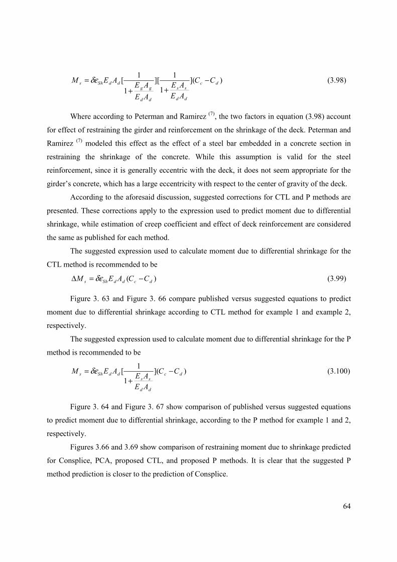
64
1 1[ ][ ]( )
11s Sh d d c d
g g s s
d dd d
M E A C CE A E A
E AE A
de= -++
(3.98)
Where according to Peterman and Ramirez (7), the two factors in equation (3.98) account
for effect of restraining the girder and reinforcement on the shrinkage of the deck. Peterman and
Ramirez (7) modeled this effect as the effect of a steel bar embedded in a concrete section in
restraining the shrinkage of the concrete. While this assumption is valid for the steel
reinforcement, since it is generally eccentric with the deck, it does not seem appropriate for the
girder’s concrete, which has a large eccentricity with respect to the center of gravity of the deck.
According to the aforesaid discussion, suggested corrections for CTL and P methods are
presented. These corrections apply to the expression used to predict moment due to differential
shrinkage, while estimation of creep coefficient and effect of deck reinforcement are considered
the same as published for each method.
The suggested expression used to calculate moment due to differential shrinkage for the
CTL method is recommended to be
( )s Sh d d c dM E A C CdeD = - (3.99)
Figure 3. 63 and Figure 3. 66 compare published versus suggested equations to predict
moment due to differential shrinkage according to CTL method for example 1 and example 2,
respectively.
The suggested expression used to calculate moment due to differential shrinkage for the P
method is recommended to be
1[ ]( )
1s Sh d d c d
s s
d d
M E A C CE A
E A
de= -+
(3.100)
Figure 3. 64 and Figure 3. 67 show comparison of published versus suggested equations
to predict moment due to differential shrinkage, according to the P method for example 1 and 2,
respectively.
Figures 3.66 and 3.69 show comparison of restraining moment due to shrinkage predicted
for Consplice, PCA, proposed CTL, and proposed P methods. It is clear that the suggested P
method prediction is closer to the prediction of Consplice.

65
P method is believed to better estimate creep coefficient used in prediction of restraining
moment due to shrinkage, because it uses creep coefficient for creep effect, initiating when CIP
is cast. On the other hand, CTL uses creep coefficient at each stage, considering creep initiates at
time of prestressing. That explains why for example 1, where continuity was established at age
56 days of girder’s age, suggested CTL and P methods predict comparable shrinkage strain.
While for example 2, where continuity is established at 224 days of girder’s age, CTL noticeably
predicts higher restraining moments due to differential shrinkage.
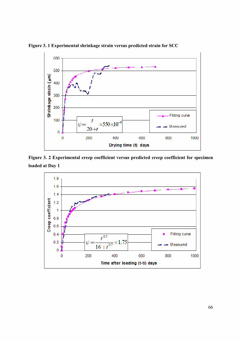
66
Figure 3. 1 Experimental shrinkage strain versus predicted strain for SCC
Figure 3. 2 Experimental creep coefficient versus predicted creep coefficient for specimen
loaded at Day 1
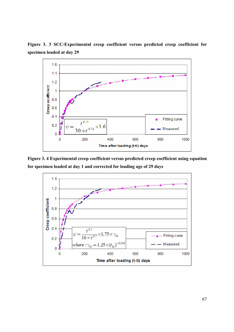
67
Figure 3. 3 SCC-Experimental creep coefficient versus predicted creep coefficient for
specimen loaded at day 29
Figure 3. 4 Experimental creep coefficient versus predicted creep coefficient using equation
for specimen loaded at day 1 and corrected for loading age of 29 days

68
Figure 3. 5 Structural analysis model
Figure 3. 6 Example 1. IT 700 section properties
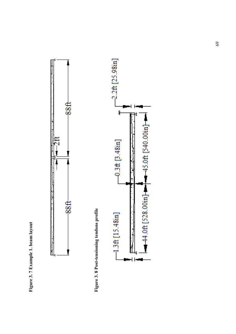
69
Figure 3. 7 Example 1. beam layout
Figure 3. 8 Post-tensioning tendons profile
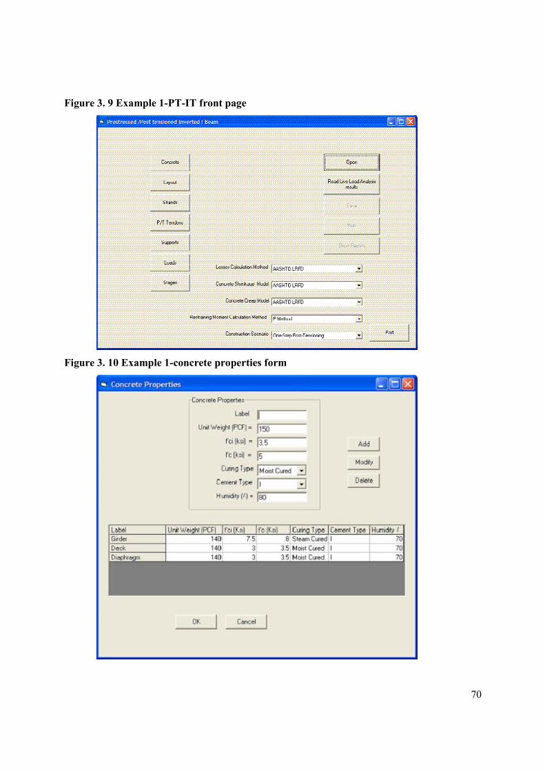
70
Figure 3. 9 Example 1-PT-IT front page
Figure 3. 10 Example 1-concrete properties form
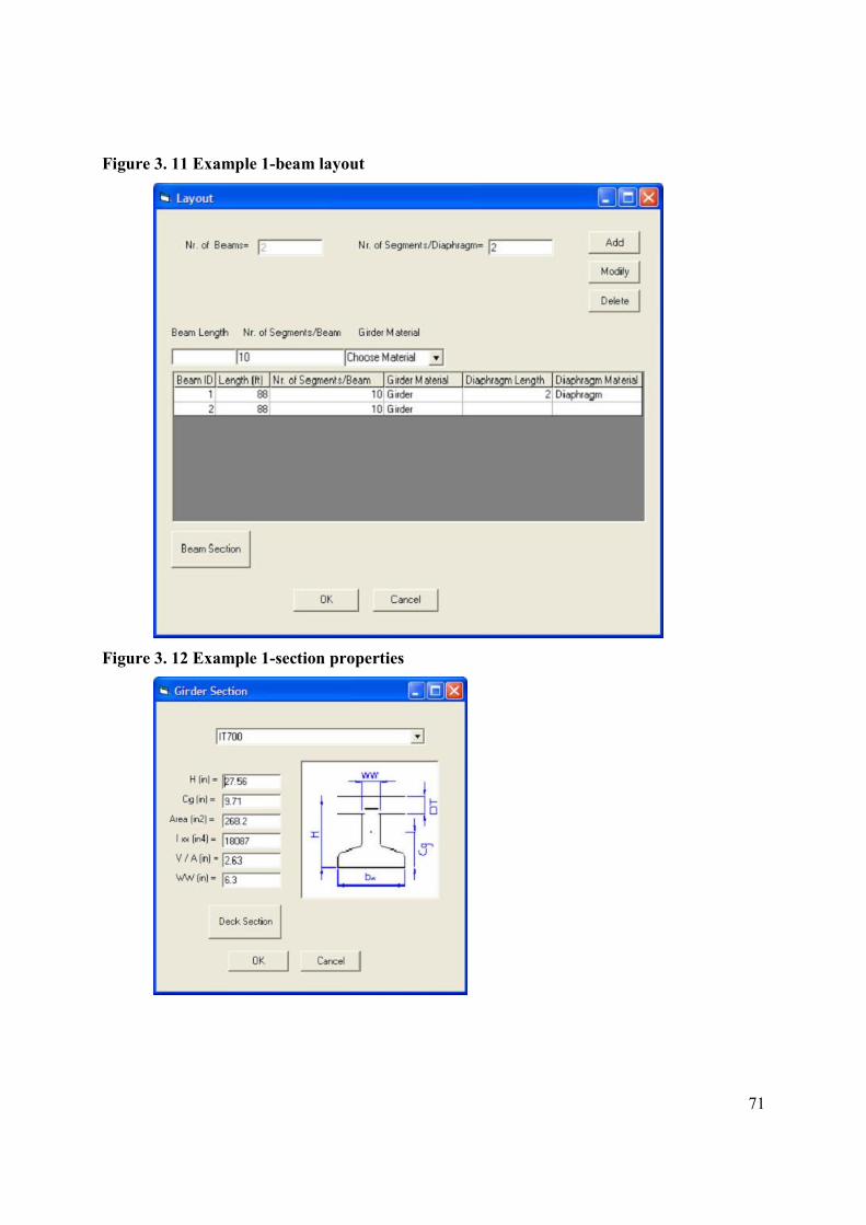
71
Figure 3. 11 Example 1-beam layout
Figure 3. 12 Example 1-section properties
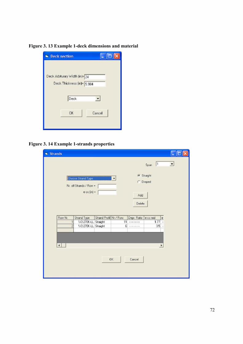
72
Figure 3. 13 Example 1-deck dimensions and material
Figure 3. 14 Example 1-strands properties

73
Figure 3. 15 Example 1-post-tensioned tendons
Figure 3. 16 Example 1-supports
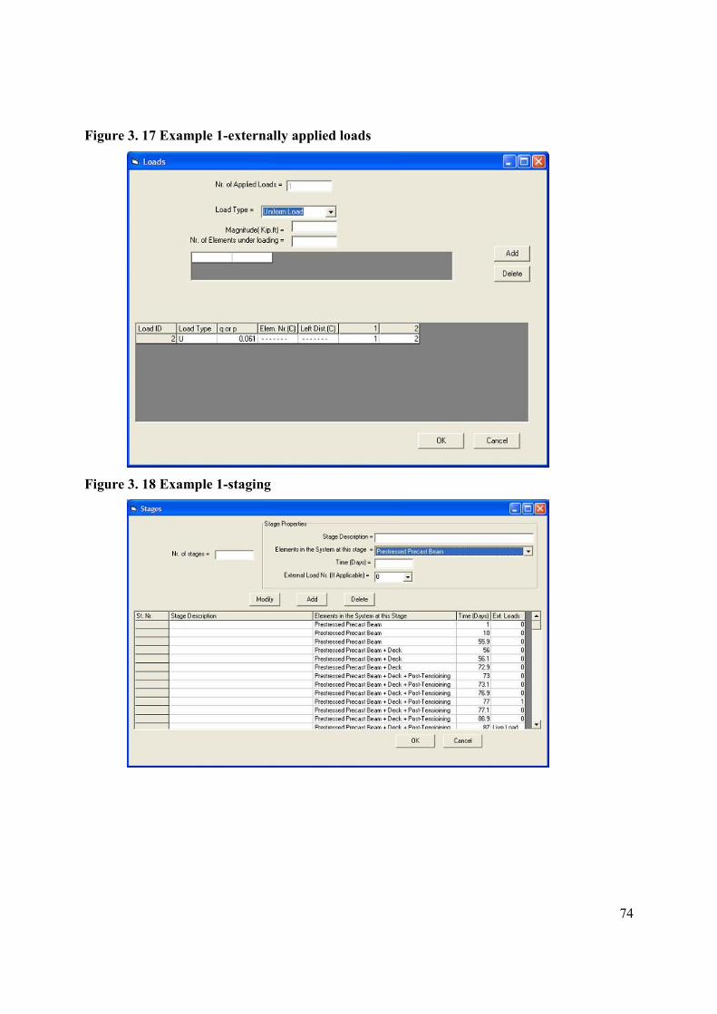
74
Figure 3. 17 Example 1-externally applied loads
Figure 3. 18 Example 1-staging
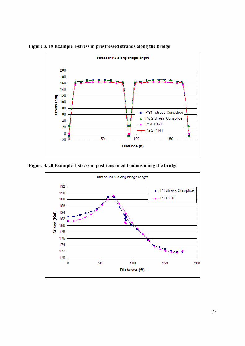
75
Figure 3. 19 Example 1-stress in prestressed strands along the bridge
Figure 3. 20 Example 1-stress in post-tensioned tendons along the bridge
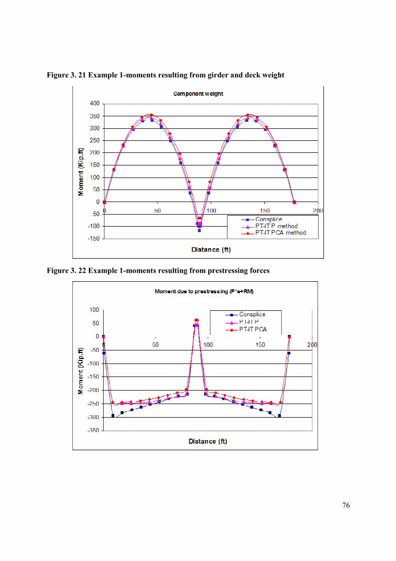
76
Figure 3. 21 Example 1-moments resulting from girder and deck weight
Figure 3. 22 Example 1-moments resulting from prestressing forces
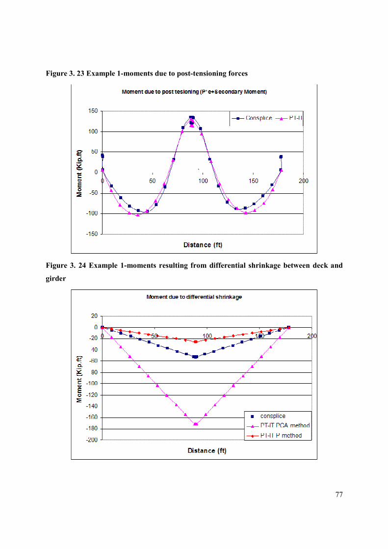
77
Figure 3. 23 Example 1-moments due to post-tensioning forces
Figure 3. 24 Example 1-moments resulting from differential shrinkage between deck and
girder
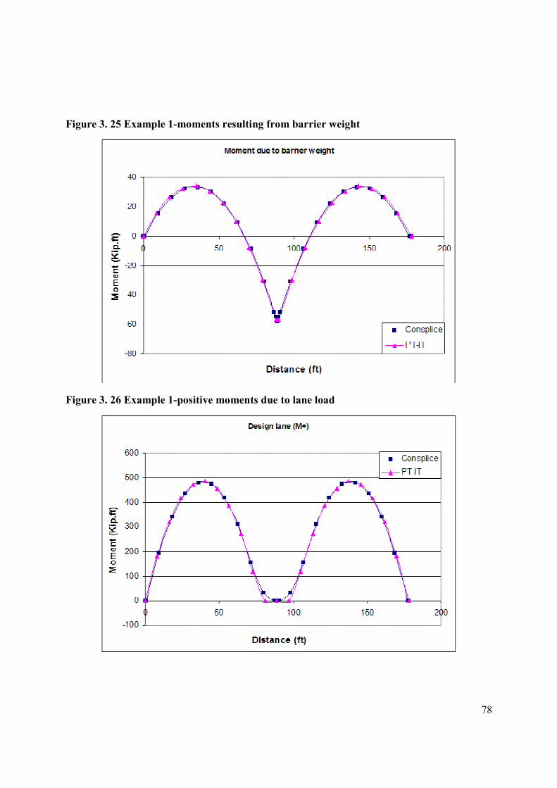
78
Figure 3. 25 Example 1-moments resulting from barrier weight
Figure 3. 26 Example 1-positive moments due to lane load
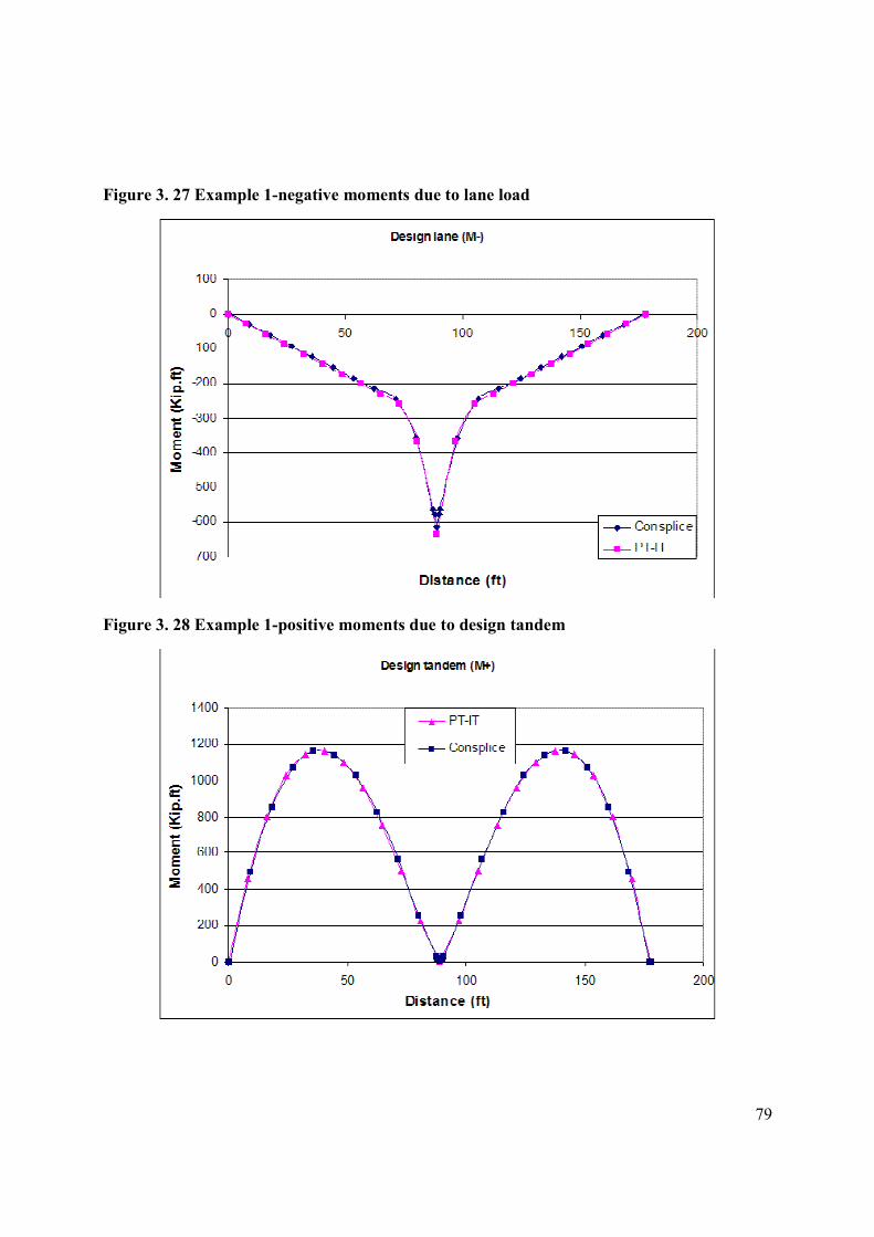
79
Figure 3. 27 Example 1-negative moments due to lane load
Figure 3. 28 Example 1-positive moments due to design tandem
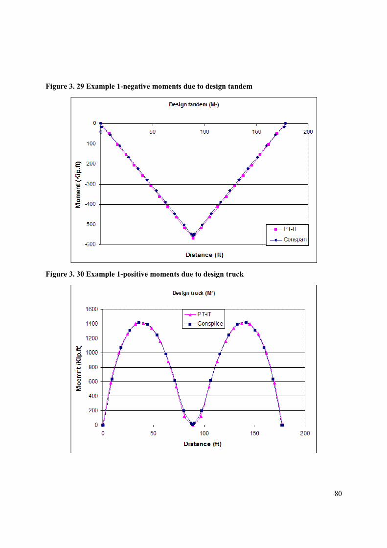
80
Figure 3. 29 Example 1-negative moments due to design tandem
Figure 3. 30 Example 1-positive moments due to design truck
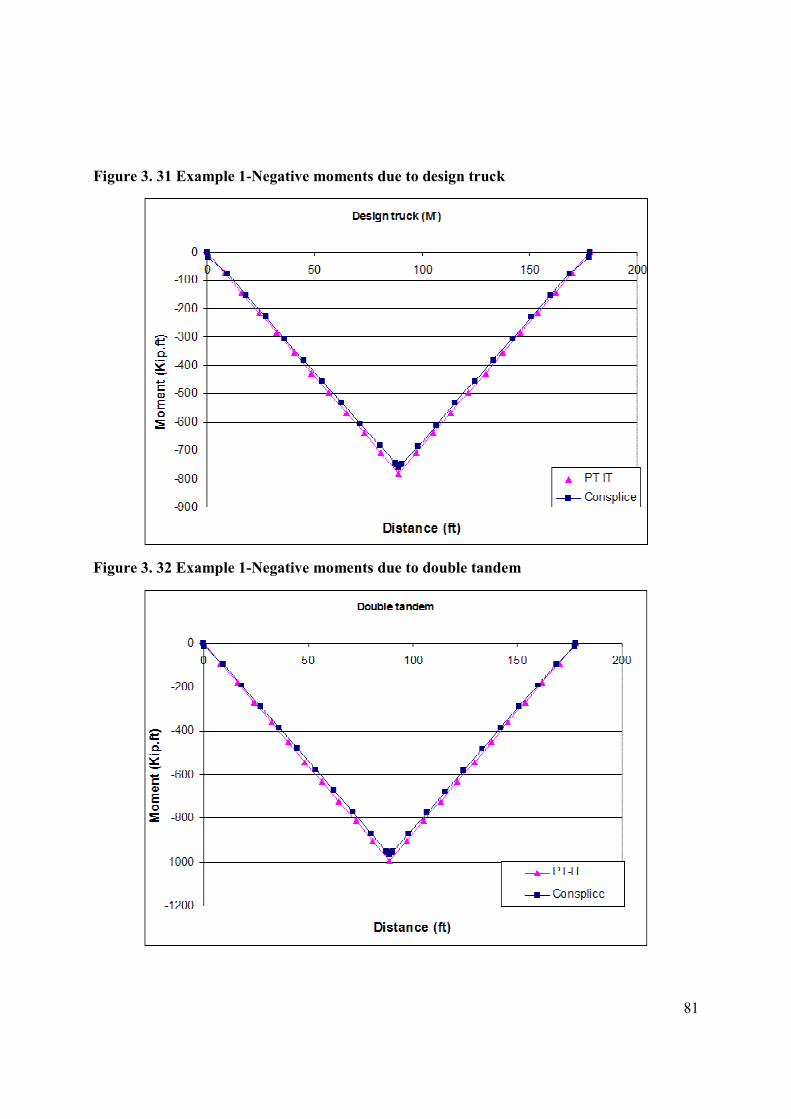
81
Figure 3. 31 Example 1-Negative moments due to design truck
Figure 3. 32 Example 1-Negative moments due to double tandem
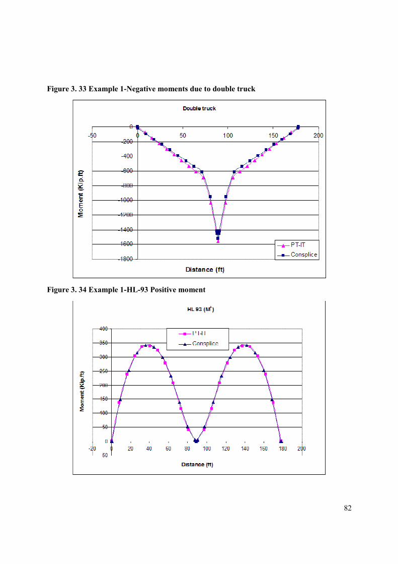
82
Figure 3. 33 Example 1-Negative moments due to double truck
Figure 3. 34 Example 1-HL-93 Positive moment
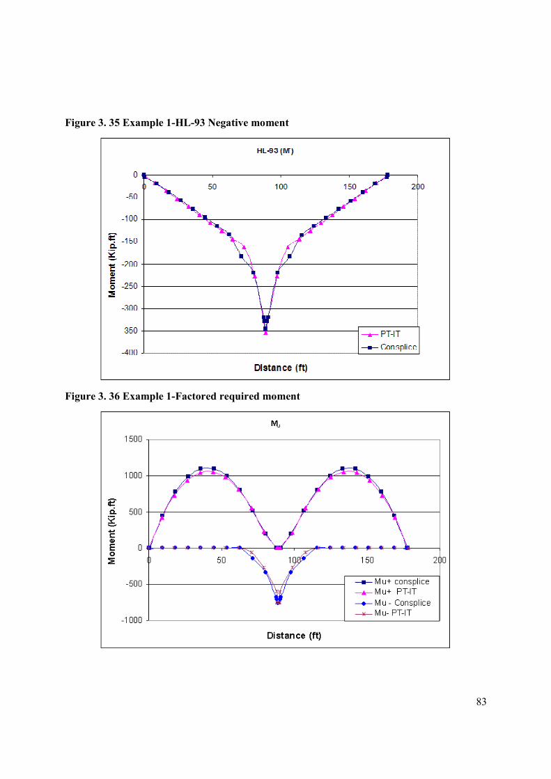
83
Figure 3. 35 Example 1-HL-93 Negative moment
Figure 3. 36 Example 1-Factored required moment
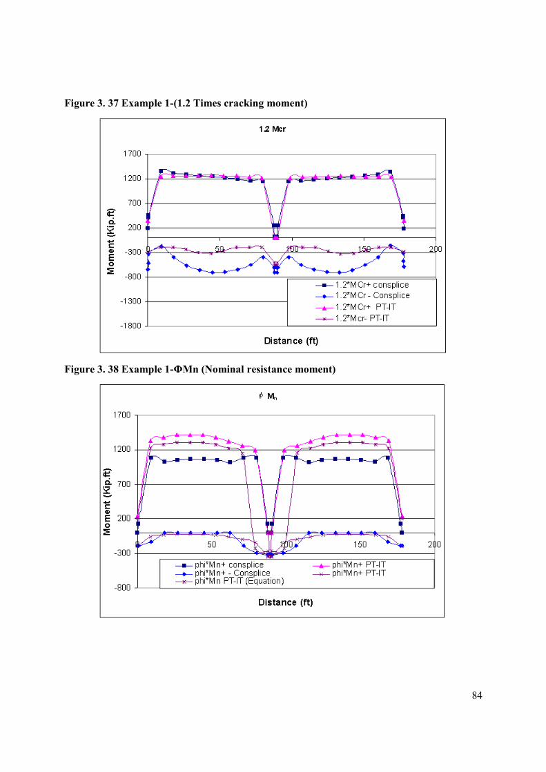
84
Figure 3. 37 Example 1-(1.2 Times cracking moment)
Figure 3. 38 Example 1-ΦMn (Nominal resistance moment)
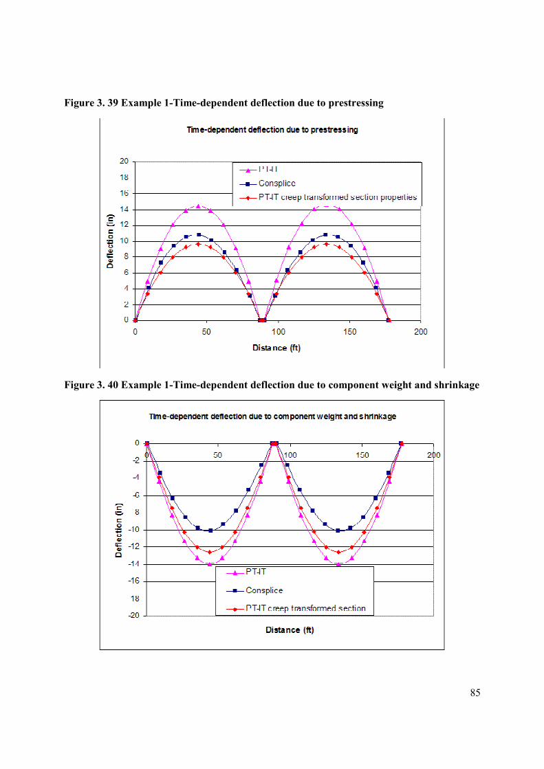
85
Figure 3. 39 Example 1-Time-dependent deflection due to prestressing
Figure 3. 40 Example 1-Time-dependent deflection due to component weight and shrinkage
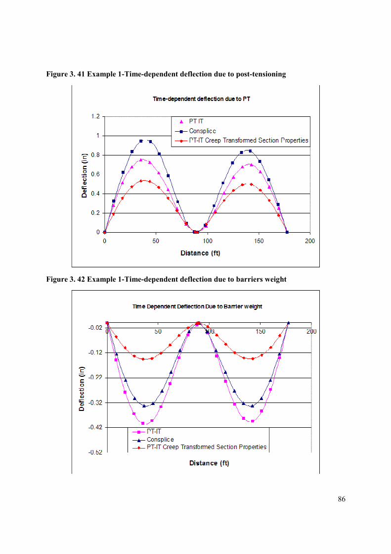
86
Figure 3. 41 Example 1-Time-dependent deflection due to post-tensioning
Figure 3. 42 Example 1-Time-dependent deflection due to barriers weight
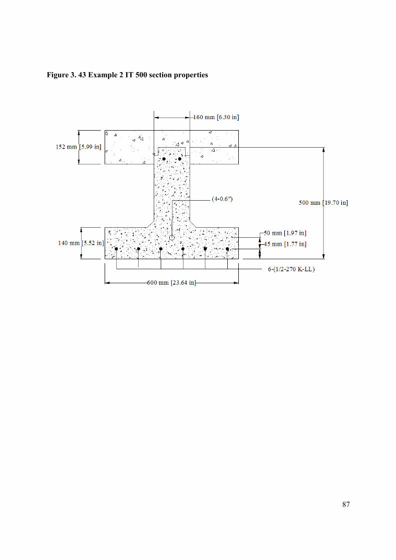
87
Figure 3. 43 Example 2 IT 500 section properties
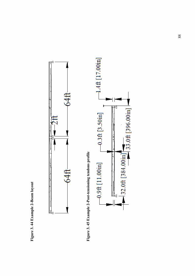
88
Figure 3. 44 Example 2-Beam layout
Figure 3. 45 Example 2-Post-tensioning tendons profile
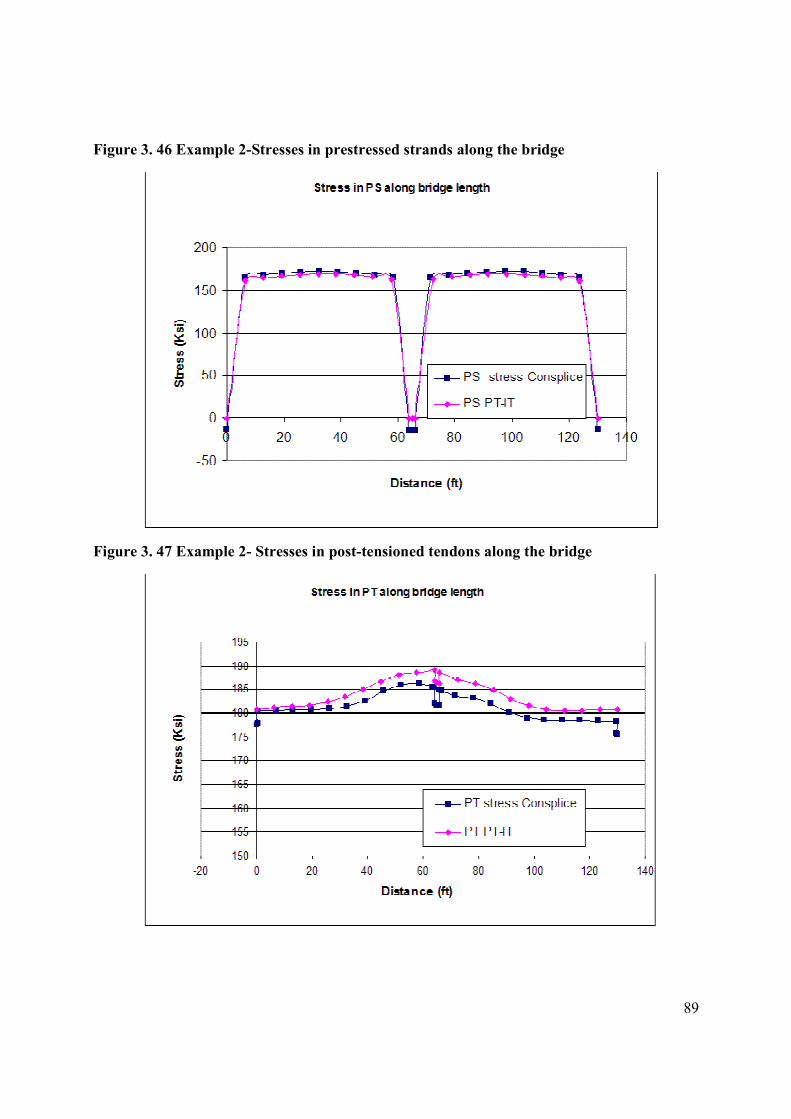
89
Figure 3. 46 Example 2-Stresses in prestressed strands along the bridge
Figure 3. 47 Example 2- Stresses in post-tensioned tendons along the bridge

90
Figure 3. 48 Example 2- Moments resulting from girder and deck weights
Figure 3. 49 Example 2- Moments resulting from prestressing forces
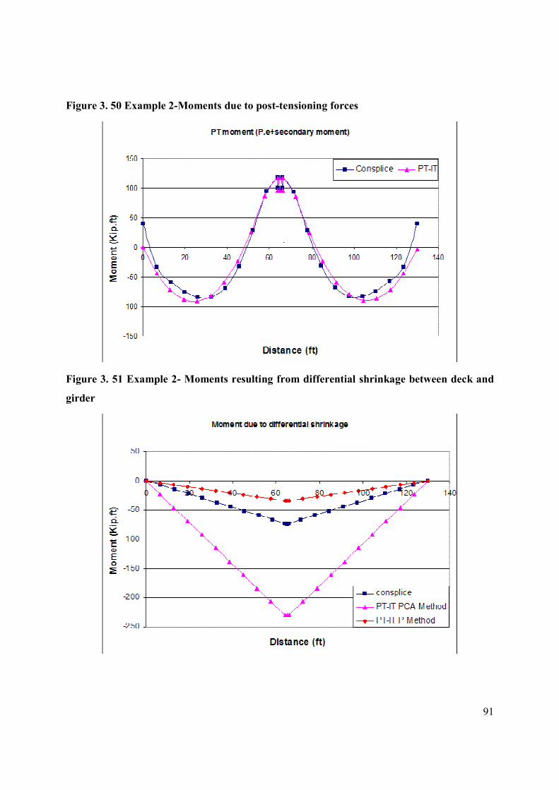
91
Figure 3. 50 Example 2-Moments due to post-tensioning forces
Figure 3. 51 Example 2- Moments resulting from differential shrinkage between deck and
girder
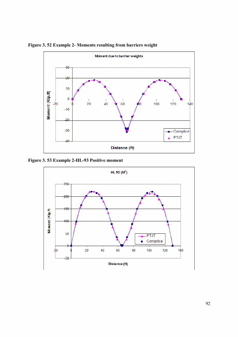
92
Figure 3. 52 Example 2- Moments resulting from barriers weight
Figure 3. 53 Example 2-HL-93 Positive moment
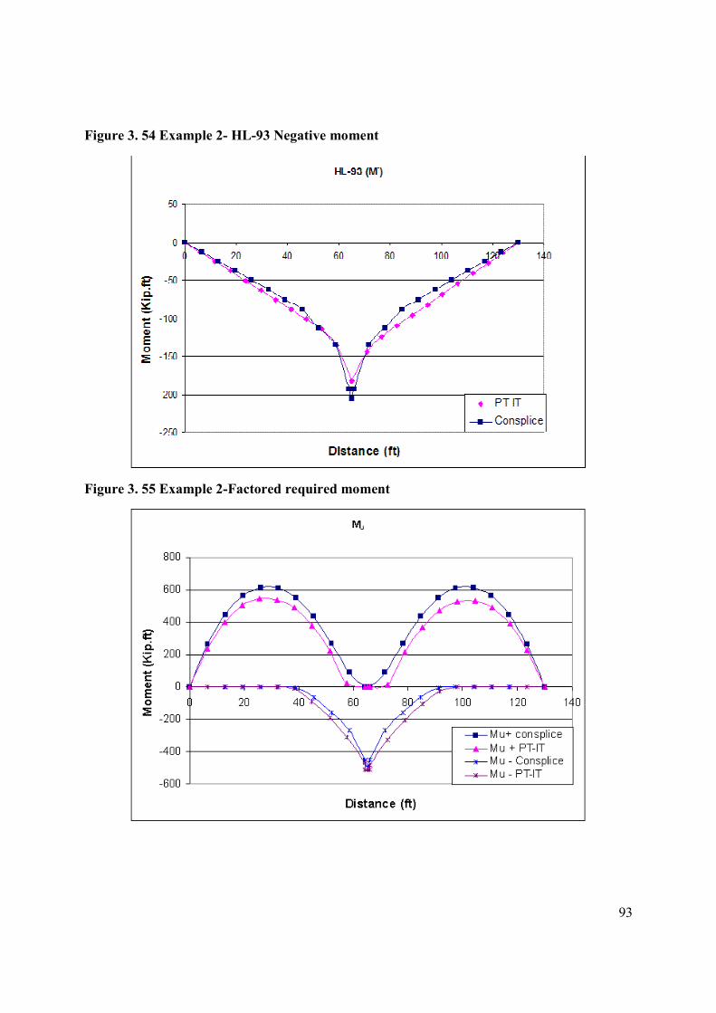
93
Figure 3. 54 Example 2- HL-93 Negative moment
Figure 3. 55 Example 2-Factored required moment
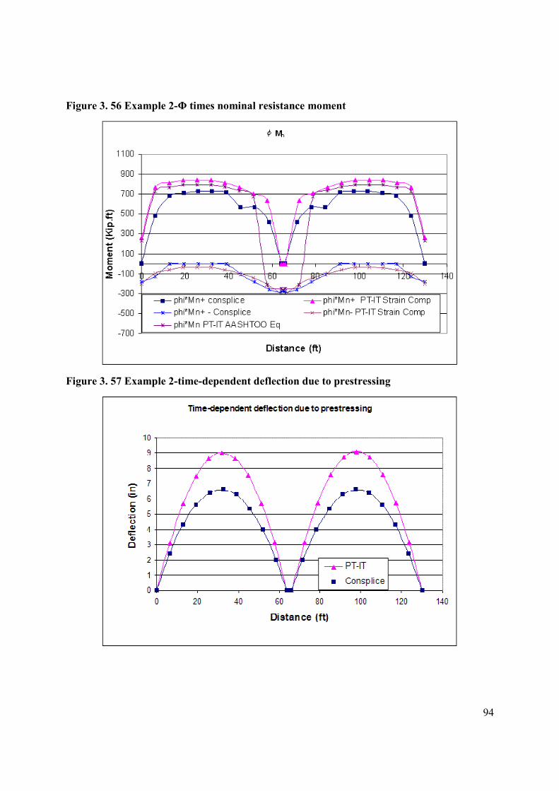
94
Figure 3. 56 Example 2-Φ times nominal resistance moment
Figure 3. 57 Example 2-time-dependent deflection due to prestressing
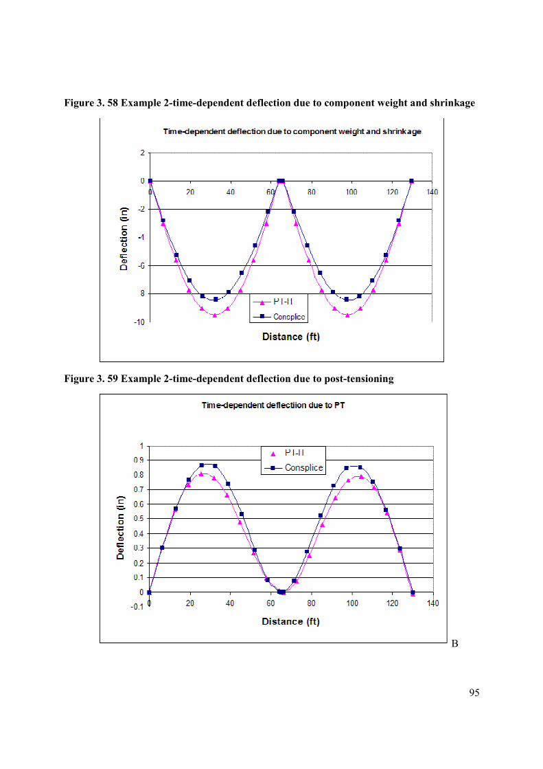
95
Figure 3. 58 Example 2-time-dependent deflection due to component weight and shrinkage
Figure 3. 59 Example 2-time-dependent deflection due to post-tensioning
B
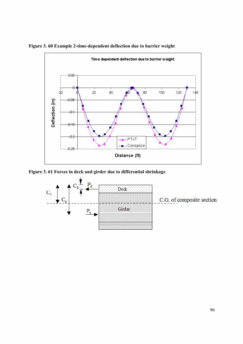
96
Figure 3. 60 Example 2-time-dependent deflection due to barrier weight
Figure 3. 61 Forces in deck and girder due to differential shrinkage
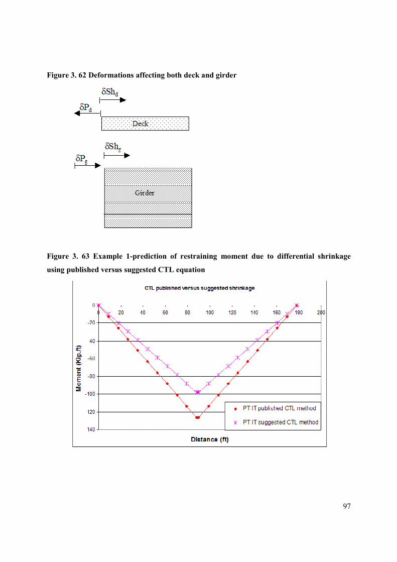
97
Figure 3. 62 Deformations affecting both deck and girder
Figure 3. 63 Example 1-prediction of restraining moment due to differential shrinkage
using published versus suggested CTL equation
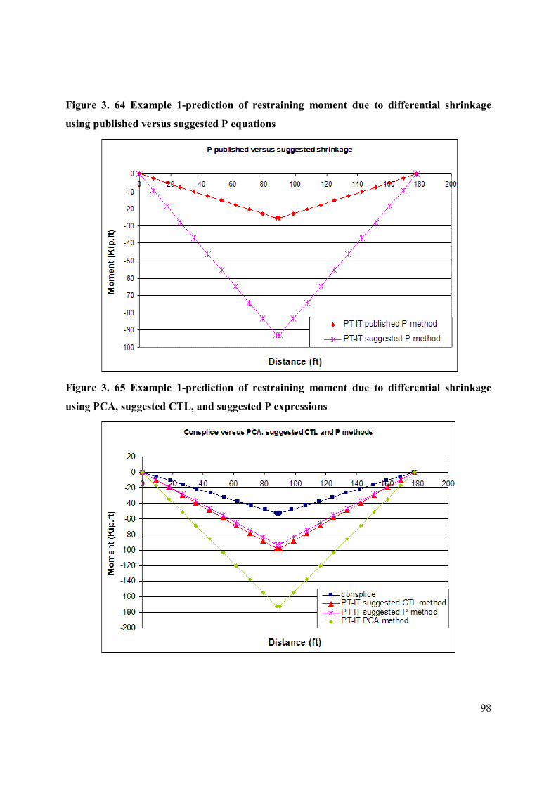
98
Figure 3. 64 Example 1-prediction of restraining moment due to differential shrinkage
using published versus suggested P equations
Figure 3. 65 Example 1-prediction of restraining moment due to differential shrinkage
using PCA, suggested CTL, and suggested P expressions
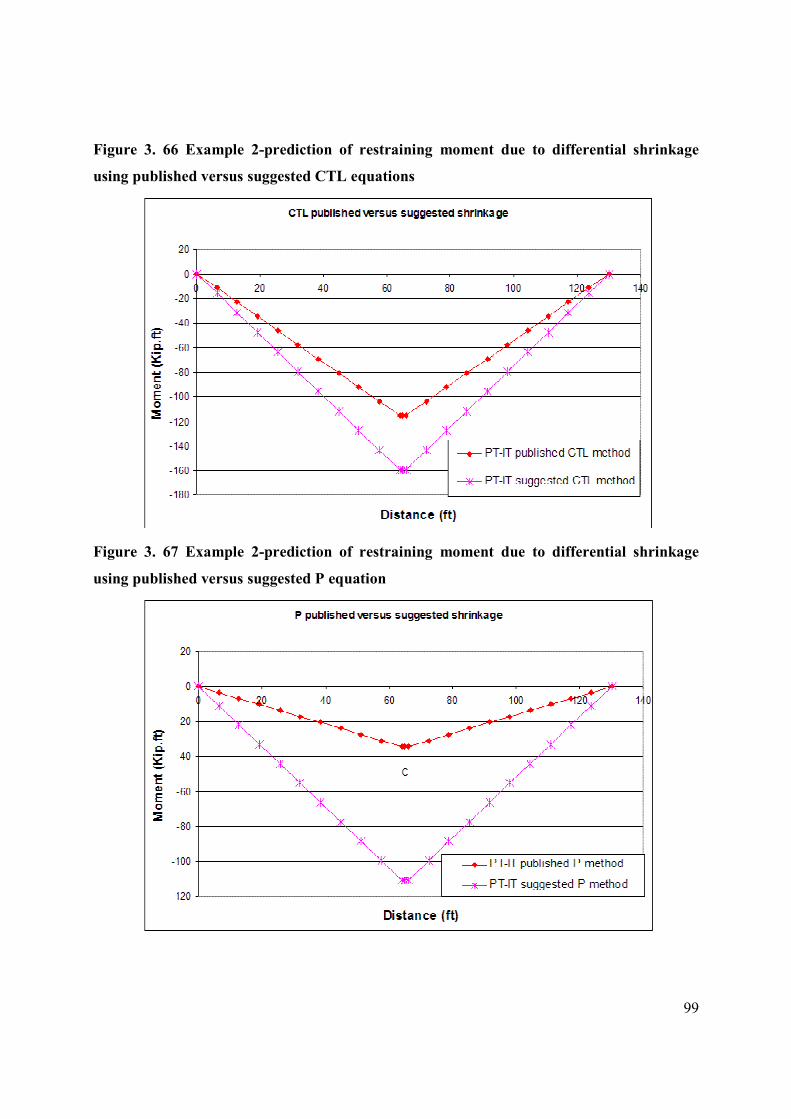
99
Figure 3. 66 Example 2-prediction of restraining moment due to differential shrinkage
using published versus suggested CTL equations
Figure 3. 67 Example 2-prediction of restraining moment due to differential shrinkage
using published versus suggested P equation
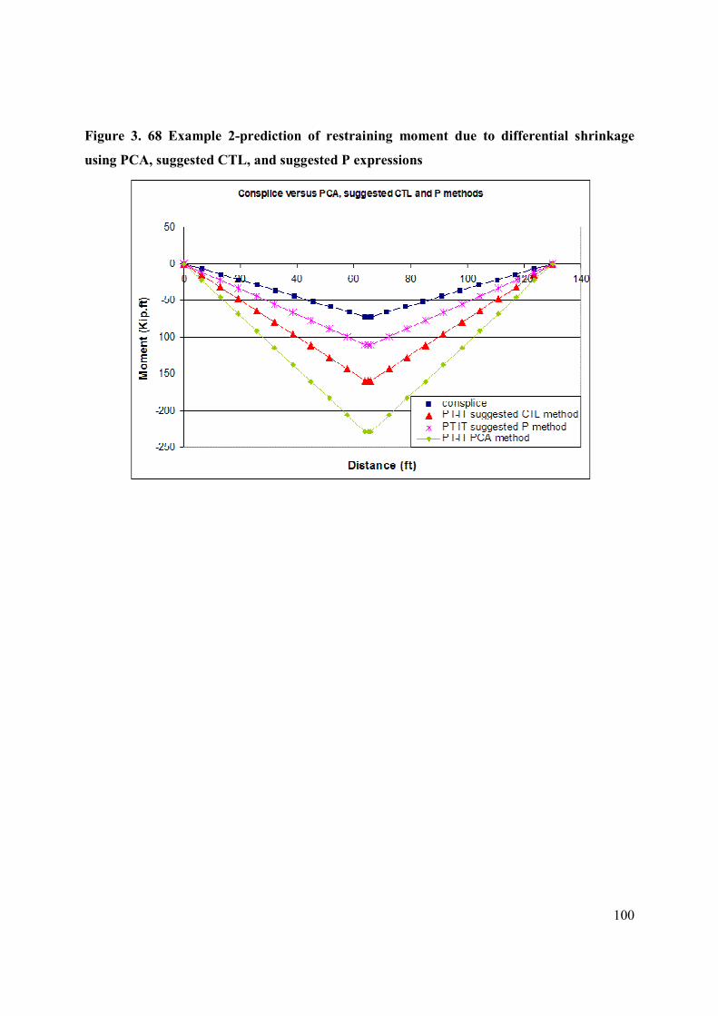
100
Figure 3. 68 Example 2-prediction of restraining moment due to differential shrinkage
using PCA, suggested CTL, and suggested P expressions

101
Table 3. 1 Values of the constants α and β and the time ratio for the concrete compressive strength (24)
Concrete age
Days
Years
Ultim
ate
(in tim
e)
Tim
e ratio
Type of curing
Cem
ent type
Constants
α and β
3
7
14
21
28
56
91
1
10
I α=4.0
β=0.85
0.46 0.7
0.88 0.96 1.0 1.08 1.12 1.16 1.17 1.18
Moist-cured
III
α=2.3
β=0.92
0.59 0.8
0.92 0.97 1.0 1.04 1.06 1.08 1.09 1.09
I α=1.0
β=0.95
0.78 0.91 0.98 1.0
1.0 1.03 1.04 1.05 1.05 1.05
(f’c)t/(f’c)28
Steam
-cured
III
α=0.7
β=0.98
0.82 0.93 0.97 0.99 1.0 1.0
1.01 1.01 1.02 1.02
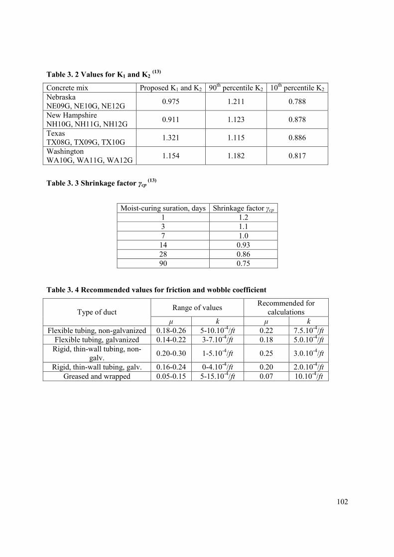
102
Table 3. 2 Values for K1 and K2 (13)
Concrete mix Proposed K1 and K2 90th percentile K2 10
th percentile K2
Nebraska
NE09G, NE10G, NE12G 0.975 1.211 0.788
New Hampshire
NH10G, NH11G, NH12G 0.911 1.123 0.878
Texas
TX08G, TX09G, TX10G 1.321 1.115 0.886
Washington
WA10G, WA11G, WA12G 1.154 1.182 0.817
Table 3. 3 Shrinkage factor γcp (13)
Table 3. 4 Recommended values for friction and wobble coefficient
Range of values Recommended for
calculations Type of duct
µ k µ k
Flexible tubing, non-galvanized 0.18-0.26 5-10.10-4/ft 0.22 7.5.10
-4/ft
Flexible tubing, galvanized 0.14-0.22 3-7.10-4/ft 0.18 5.0.10
-4/ft
Rigid, thin-wall tubing, non-
galv. 0.20-0.30 1-5.10
-4/ft 0.25 3.0.10
-4/ft
Rigid, thin-wall tubing, galv. 0.16-0.24 0-4.10-4/ft 0.20 2.0.10
-4/ft
Greased and wrapped 0.05-0.15 5-15.10-4/ft 0.07 10.10
-4/ft
Moist-curing suration, days Shrinkage factor γcp 1 1.2
3 1.1
7 1.0
14 0.93
28 0.86
90 0.75
103
CHAPTER 4 - RESULTS OF PARAMETRIC STUDY
Scope of Parametric Study
The objective of this parametric study was to examine the behavior of post-tensioned,
prestressed, inverted-T systems (PT-IT) and determine the influence of different parameters on
the design. The parametric study integrated a wide range of parameters, including assessment of
different construction scenarios, effect of timing of each construction stage, and effect of
concrete strength on the design for girder and deck. Different models were considered for
estimating creep and shrinkage of concrete; different methods were examined to evaluate time-
dependent restraint moments due to creep and differential shrinkage. The parametric study
incorporated six different IT sections.
Multiple construction scenarios were considered during the course of this study,
including one and two-step post-tensioning. Different scenarios were considered for one-stage
post-tensioning, including the option of casting the diaphragm and deck simultaneously, then
applying post-tensioning. This scenario will be referred to as Dia & Deck-PT. The second option
was to cast the diaphragm to establish continuity, then cast the deck and apply post-tensioning,
which will be referred to as Dia- Deck-PT. The third option for one-stage post-tensioning was to
cast the diaphragm to establish continuity, apply post-tensioning to the continuous girders, and
then cast the deck. This option will be referred to as Dia-PT-Deck. A two-stage post-tensioning
scenario was also considered, where the diaphragm was first cast to establish continuity, first-
stage post-tensioning was applied, followed by casting the deck, and the last step was applying
second-stage post-tensioning. Comparison of pros and cons of each scenario are discussed later
in this chapter.
Effect of timing on the behavior of the PT-IT system was determined by varying time of
cutting the strands, time of establishing continuity, and time of post-tensioning. The study
included IT500, IT 600, IT 700, IT 800, IT 900, and IT 1000, with concrete strengths of 6, 8, and
10 ksi. Deck concrete strength was considered to be 3, 3.5, and 4 ksi. The effect of different
creep and shrinkage models was investigated, including AASHTO LRFD, ACI 209, SCC, CEB-
FIP 90, and NCHRP report 496 models. Methods to estimate time-dependent restraining
104
moments included PCA, CTL, and P, as well as the creep-transformed section properties method.
Table 4. 1 shows different parameters varied in this study.
Parametric Study Results
Different Construction Scenarios
Construction scenario is considered to be one of the most effective and critical
parameters in design, as it directly affects time-dependent restraining moments due to creep and
differential shrinkage, which in turn affects stress distribution in sections along the beam.
Different construction scenarios were investigated, including the two main options of
applying one or two stages of post-tensioning.
Dia & deck-PT: In this scenario the deck and diaphragm are cast simultaneously, and
then post-tensioning is applied, deck weight is carried by the simply-supported beam. For the
case when continuity is established at early age of the girder, positive restraining moments tend
to develop in the piers. Typically, secondary moments due to post-tensioning are also positive,
causing high-compression stresses in the top of the girders within the spans and consequently,
limiting the maximum span-to-depth ratio of the section to control stresses.
Dia-PT-Deck: For this scenario, the diaphragm is first cast, then post-tensioning is
applied, and finally the deck is cast. The benefit of casting the deck after the diaphragm is cast
and continuity is established, is that the weight of the deck is carried by the continuous structure,
which results in lower positive moments within the span, while negative moments are developing
over the piers. At the same time, the weight of the deck does not cause time-dependent
restraining moments due to creep. This will increase the positive moment or reduce the negative
moment in the pier (depending on whether moments in the pier are positive or negative). It will
help reduce moments in the pier and consequently, reduce the probability of cracking of the
deck.
The disadvantage of this option of construction is that post-tensioning will be applied at
the girder section only, causing high stresses in the bottom of the girder at end adjacent to the
pier. Moreover, for early age of establishing continuity where positive restraining moments are
developed in the diaphragm, these high stresses will be increased.
Dia-Deck-PT: In this scenario continuity is established by casting the diaphragm, and
then after the diaphragm concrete hardens, the deck is cast, post-tensioning is applied to the
105
whole structure, via the scenario. The weight of the deck will be carried by the continuous
structure and will not cause a time dependent effect on moments in the piers. Besides, when post-
tensioning is applied on the continuous structure, primary moments caused by post-tensioning at
the pier will be less if they are to be applied at the girder section (less eccentricity for the post-
tensioning force). This will cause less tension force at the bottom of the girders in the case when
continuity is established at early girder age. The drawback of this type of scenario is that
cracking of the diaphragm over the pier will occur during the period between casting the deck
and post-tensioning. After post-tensioning, the deck will be under compression and
consequently, the cracks will tend to close.
Two-stage post-tensioning: In this scenario, the diaphragm is cast to establish continuity,
post-tensioning is applied enough to balance stresses due to the weight of the deck. Then the
deck is cast, and the final stage of post-tensioning is applied to balance stresses due to the weight
of the barriers and live load. The advantage of this type of construction is that the deck will be
carried by the continuous beam, and less initial prestressing is needed as it controls stresses due
to girder weight only, which results in less initial camber. In addition, the main part of post-
tensioning is to be applied on the composite structure of the girder and the deck, which reduces
the effect of tension caused by post-tensioning on the bottom of the girders at internal piers.
Disadvantages of the two-stage post-tensioning scenario are obviously the extra labor, and the
fact that the post-tensioning ducts have to stay ungrouted between the two stages of post-
tensioning. Under real construction conditions, this time may be long enough that undesired
corrosion could initiate in the tendons applied at the first stage of post-tensioning. If this option
is used, care should be taken to prevent moisture from entering the un-grouted ducts between the
two post-tensioning stages.
As the PCA method did not account for the case when the diaphragm is cast prior to
casting the deck, a modification has been applied to account for these cases. Time-dependent
restraining moments due to creep under prestressing start at the time the diaphragm is cast;
restraining moment due to differential shrinkage doesn’t start until the deck is cast.
Consequently, the creep coefficient in the multiplier (1-e-Φ), which is applied to restraining
moment due to creep under prestressing and dead weight, is based on the increase in the creep
strain from the time when diaphragm is cast. The creep coefficient in the multiplier (1-e-Φ)/Φ,
106
which is applied to the restraining moment due to differential shrinkage, is based on the increase
in the creep strain from the time the deck is cast.
Table 4. 2 shows a comparison of the average maximum span-to-depth ratio for different
construction scenarios, including the case of a continuous IT section reported by Ambare and
Peterman (1)
for girder concrete strength of 8 ksi. The comparison included different IT sections,
considering concrete strengths of 6, 8, and 10 ksi. Values in Table 4. 2 are based on the envelope
of extreme-case scenarios of establishing continuity and the envelope of estimated time-
dependent restraining moments.
Figure 4. 1 shows maximum spans for different IT sections (IT 500 through IT 1000), for
different construction scenarios and different concrete strengths.
Different construction scenarios were investigated for two-span girders with IT 700 cross
sections of 8-ksi concrete strength, taking into account different timing for establishing
continuity along the girder ages. Maximum spans are reported based on worst-case scenarios,
which are earliest and latest age of establishing continuity at 14 and 224 days, respectively.
Table 4. 3 includes section-reinforcement properties for different construction scenarios.
Figure 4. 2 through Figure 4. 5 show time-dependent restraining moments due to creep
and differential shrinkage for different construction scenarios using PCA, CTL, P, and creep-
transformed section properties methods for the case when continuity is established at 14 days. It
is evident that for different methods, estimated restraining moments vary drastically. This shows
the need for experimental investigation on the PT-IT system to determine the actual range of
time-dependent restraining moments, and to determine which of the methods is closer to
evaluating time-dependent effect on this system. The PCA method is believed to overestimate
restraining moment resulting from differential shrinkage as has been noted in other studies (5), (6).
Figure 4. 6 shows secondary moments resulting from post-tensioning for the cases when
continuity is established at 14 days. In cases where post-tensioning is applied to the girder
section, the resulting secondary moment is negative. The secondary moment in its nature
opposes the effect of the primary moment due to post-tensioning, resulting from the resistance of
the continuous member to post-tensioning deformations at the points of continuity. When post-
tensioning is applied to the structure section in a parabolic profile, the primary moment will be
negative when the tendon’s path is under the neutral axis and positive when it is located above
the neutral axis. IT sections for the neutral axis are at 34-38 % of the IT depth measured from the

107
bottom of the section, and maximum eccentricity of the tendon above the neutral axis is almost
twice the maximum eccentricity of the tendon below the neutral axis. This makes the positive
primary moment dominant and the secondary moment negative. On the other hand, when post-
tensioning is applied to the composite section of the girder and the deck, the neutral axis is
located around 60 % of the girder’s depth from the bottom of the section. This makes the
negative primary moment dominant and consequently, the secondary moment is positive. Figure
4. 7 helps illustrates the previous argument by showing the tendon’s location with respect to both
center of gravity of the girder and the composite section.
Figure 4. 8 shows maximum positive restraining moment in the pier, including positive
live-load moment, along with cracking moment of the diaphragm section in the positive
direction. Time-dependent restraining moments are calculated according to the CTL method,
which usually predicts highest positive moment in the pier compared to other methods. It is clear
that cracking of the diaphragm is not a concern in this case. Figure 4. 9 includes maximum
positive restraining moment in the pier where time-dependent restraining moment is calculated
using the P method.
The main purpose of this post-tensioning, besides increasing span-to-depth ratio, is to
come up with a bridge system where top-deck cracks over the piers are greatly reduced or
eliminated. Therefore, discussion of different construction scenarios will be evaluated based on
these two points.
Maximum negative moment in the pier will be evaluated according to the P method, as it
is the only method that accounts for cracking of the diaphragm.
Figure 4. 10 presents the maximum negative moment in the diaphragm for the Dia &
Deck –PT construction scenario, including and excluding maximum negative moment due to live
load. It also shows the cracking moment of the diaphragm section throughout the life of the
structure. It is clear that for this construction scenario, cracking of the deck and diaphragm is not
likely to occur, but in comparing span-to-depth ratios in Table 4. 2, it is evident that other
scenarios provide a higher span-to-depth ratio. In terms of stresses along the girders and
diaphragm, excess tension in the girder bottom ends near the pier (where prestressing doesn’t
apply any compression on the girder) after post-tensioning.
Figure 4. 11 shows development of maximum negative moments including and excluding
live-load moments for the Dia-Deck-PT scenario, along with cracking moment of the diaphragm

108
section. Right after casting the deck, the diaphragm cracks under its weight and moments are
redistributed along the bridge using the cracked-section moment of inertia of the diaphragm. The
diaphragm stays cracked until post-tensioning is applied, where the top of the diaphragm
becomes under compression, closing the cracks and causing the section to behave as uncracked.
Figure 4. 12 shows time-dependent restraining moments developing in the pier. The increase in
time-dependent restraining moments after applying post-tensioning is due to the fact that the
cracks are closed and the section acts as uncracked.
Figure 4. 14 shows restraining moment in the pier for the Dia-PT-Deck scenario. In this
case, post-tensioning is applied to the girder’s section. As discussed previously, this causes
negative secondary moments in the piers, which reduces the effectiveness of compression
applied by the tendon to the top of the diaphragm. Under live load the deck and diaphragm crack
and stay cracked throughout the structure age. Figure 4. 15 shows time-dependent restraining
moments for this construction scenario, and shows that the deck and diaphragm will crack after
applying live load and moments will be redistributed. Consequently, this construction scenario
doesn’t satisfy the criteria of eliminating cracks in the diaphragm.
Figure 4. 17 includes restraining moments in the pier for the case of two-stage PT. In this
scenario, the diaphragm and deck don’t crack at any time; however, tension stresses will exceed
allowable stresses in the top of the diaphragm in the period between casting the deck and second-
stage post-tensioning when it comes under compression.
Figure 4. 18 through Figure 4. 21 show time-dependent restraining moments due to creep
and differential shrinkage for different construction scenarios using PCA, CTL, P, and creep-
transformed section properties methods for the case when continuity is established at 224 days.
Figure 4. 22 shows secondary moments resulting from post-tensioning for this case.
The same discussion regarding the possibility of cracking of the diaphragm and the deck
for all suggested construction scenarios applies for the case when continuity is established at 224
days of girder age. Figure 4. 23 through Figure 4. 30 show Maximum negative moment in the
diaphragm and time-dependent restraining moment for different construction scenarios.
As a result, it is clear that both scenarios of one-stage post-tensioning (Dia-Deck-PT) and
two-stage PT have the highest span-to-depth ratio and satisfy the crack-free deck critirea. Since
the option of Dia-Deck-PT incorporates less labor, it is recommended to be used for construction
of PT-IT systems.
109
Effect of Concrete Strength
Effect of girder concrete strength
From Table 4. 2, it is clear that girder concrete strength plays a major role in maximum
span-to-depth ratio. Increasing girder concrete strength from 6 to 8 ksi helps increase by 15% the
span of 6-ksi girders, while increasing strength from 8 to 10 ksi increases the span by 11% of 8-
ksi girders. In order to determine the effect of girder concrete strength on restraining moments in
the pier, an IT 500 section was considered with deck concrete strength of 4 ksi. Table 4. 4 shows
details for strands and tendons for an IT 500. Figure 4. 39through Figure 4. 42 show time-
dependent restraining moments calculated according to PCA, CTL, P, and creep-transformed
section properties methods.
It is clear that with the increase of concrete strength of the girder, negative restraining
moments increase. Knowing that span lengths of these girders are different, directly affects
moment due to self-weight and consequently, restraining moment due to creep under weight of
the girders. Analysis of different components of time-dependent restraining moment was
conducted to determine the effect of different concrete strengths on time-dependent restraining
moment. From Figure 4. 43, it was found that time-dependent restraining moment due to creep
under prestressing decreases by 12% for 8-ksi concrete compared to that of 6-ksi concrete, and
by 10% when comparing 8-and 10-ksi concrete.
While restraining moment (see Table 4. 5 and Figure 4. 44) due to girder weight
increases at a ratio of 30% for 8-ksi girders compared to 6-ksi, and increases by 21% for 10-ksi
girders compared to 8-ksi girders, time-dependent restraining moment increases by 14 % only for
8-ksi concrete compared to 6-ksi concrete, and increases by 7% for 10-ksi compared to 8-ksi
concrete. The reason for this is that as concrete strength increases, it creeps less under permanent
loads.
As concrete strength increases, it shrinks less and consequently, differential shrinkage
between girders and deck increases. From Figure 4. 45, it was found that time-dependence due to
differential shrinkage increases by 9% for 8-ksi girders compared to 10-ksi, and 7% for 10-ksi
compared to 8-ksi concrete.
110
Effect of concrete strength on losses in prestressing strands and tendons is shown in
Figure 4. 46 and Figure 4. 47. As concrete strength increases, fewer losses in prestressing strands
and post-tensioning tendons occur.
Effect of deck concrete
For the currently used concrete deck strength (3, 3.5, and 4 ksi), concrete strength of the
deck doesn’t affect time-dependent restraint moment under creep and shrinkage, nor losses in
stress of prestressing strands and post-tensioned tendons.
Effect of Different Creep and Shrinkage Models
The effect of using different models to predict creep and shrinkage of concrete was
examined by first investigating the prediction of these models. Figure 4. 50 and Figure 4. 51
compare prediction of shrinkage strain and creep coefficient for a concrete specimen of 6-ksi
strength, 2.77 volume-to-surface ratio, and 70 % humidity for AASHTO LRFD, ACI-209,
NCHRP-496, SCC, and CEB-FIP-90 models. It is clear that all these models closely predict
creep except the CEB-FIP-90 model, which predicts higher creep coefficient and less shrinkage
strain compared to other models. The SCC model predicts less shrinkage to occur after three
months of girder age.
Figure 4. 52 and Figure 4. 53 show prediction for creep and shrinkage for 10-ksi
concrete, 2.77 volume-to-surface ratio, and 70% humidity. It is clear that while NCHRP-496 and
ACI-209 predict close shrinkage strain for 6-ksi concrete, these predict hugely different
shrinkage strain for 10 ksi. At the same time, AASHTO LRFD predicts close creep coefficient to
the NCHRP model which was especially developed for high-strength concrete.
Figure 4. 54 and Figure 4. 55 compare losses in prestressing strands and post-tensioned
tendons using a different model for IT600 with 6-ksi strength. The effect of using different
models for creep and shrinkage affects the prediction of losses within a ratio of 7 %, and post-
tensioning losses within 3 %, since a considerable amount of shrinkage and creep occurs before
post-tensioning.
Figure 4. 56 through Figure 4. 59 show a prediction of time-dependent restraining
moment in the pier using different methods of prediction and different creep-and-shrinkage
models.

111
Effect of Timing
The effect of timing on the behavior of a PT-IT system in general, and the development
of time-dependent restraining moment in particular, were discussed in detail in this section. This
effect is discussed for the Dia-Deck-PT construction scenario, as it was recommended for
construction. Timing effect includes different timing for cutting the strands, timing of
establishing continuity, time of casting the deck, and time of post-tensioning.
Effect of time of cutting prestressing strands
Range of time considered for cutting the strands is between 18 hours and four days. The
latest the strands are cut, the less loss of prestressing occurs. Figure 4. 60 shows that cutting
strands at one day decreases loss by 1%, cutting strands when girders are two days old decreases
loss by 2%, and cutting strands when girders are four days old decreases loss by 3 %. However,
this small difference in stresses doesn’t affect values of time-dependent restraining moments.
Effect of time of establishing continuity and casting the deck
Effect of time of establishing continuity
The effect of time of establishing continuity was studied for the Dia-Deck-PT
construction scenario. It was assumed that the diaphragm is cast first to establish continuity; and
two days after casting the diaphragm, the deck is cast and post-tensioning is applied 15 days after
casting the deck. The effect was investigated for IT 700 with concrete strength of 8 ksi. Table 4.
6 show properties of two-span girders designed in consideration of different times of establishing
continuity. A parametric study showed that the most preferable frame time for establishing
continuity was between 56 and 112 days of girder age, i.e. between almost two and four months
of girder age.
Figure 4. 61 through Figure 4. 65 show time-dependent restraining moment in the pier for
continuity established at 14, 28, 56, 112, and 224 days of girder life. For cases when continuity is
established at an early age of girder life, positive time-dependent restraining moments tend to
develop in the pier. In this case, the design was controlled by positive moments developing
within the span. While for cases when continuity is established after 56 days of girder age,
negative time-dependent restraining moments are developed in the pier. The design is then
controlled by stresses and cracking of the diaphragm and deck. Higher numbers of prestressing
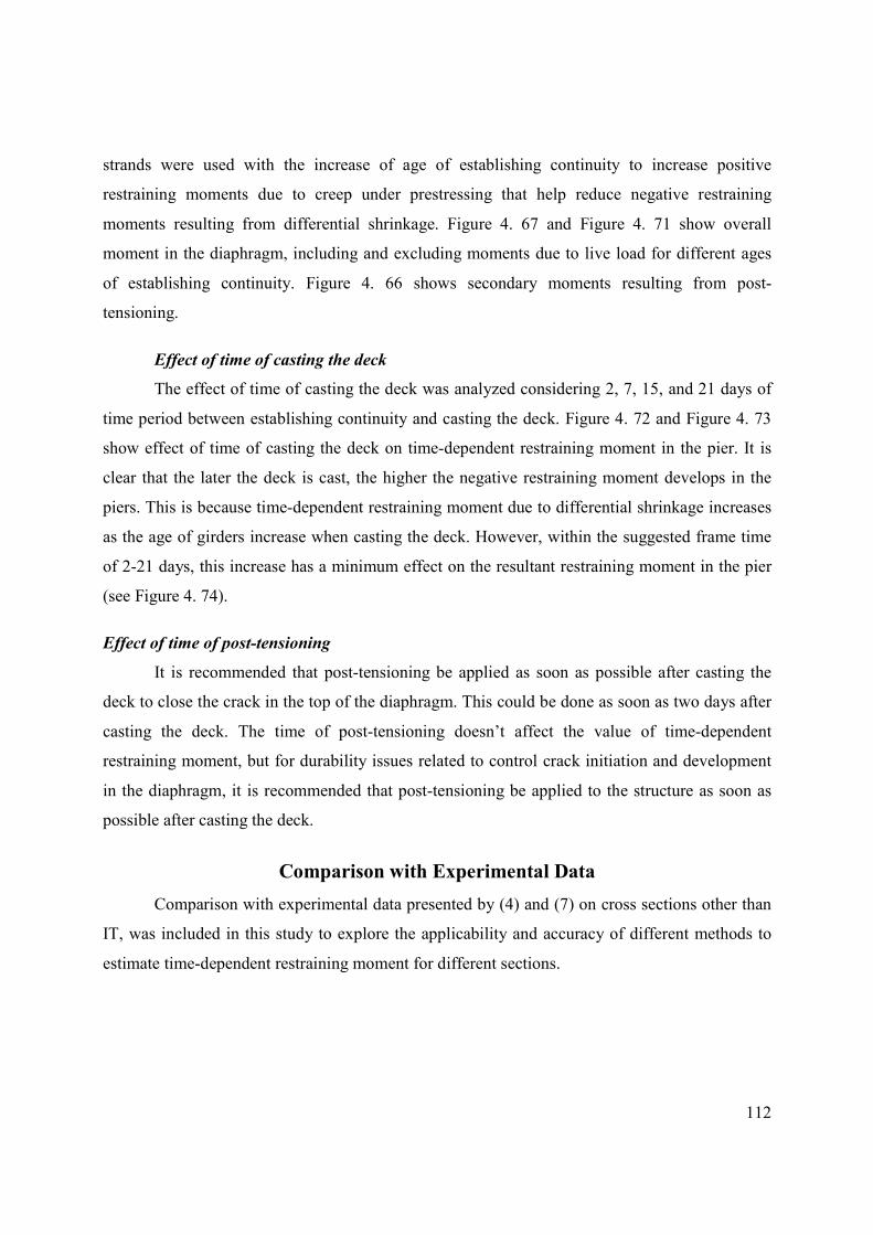
112
strands were used with the increase of age of establishing continuity to increase positive
restraining moments due to creep under prestressing that help reduce negative restraining
moments resulting from differential shrinkage. Figure 4. 67 and Figure 4. 71 show overall
moment in the diaphragm, including and excluding moments due to live load for different ages
of establishing continuity. Figure 4. 66 shows secondary moments resulting from post-
tensioning.
Effect of time of casting the deck
The effect of time of casting the deck was analyzed considering 2, 7, 15, and 21 days of
time period between establishing continuity and casting the deck. Figure 4. 72 and Figure 4. 73
show effect of time of casting the deck on time-dependent restraining moment in the pier. It is
clear that the later the deck is cast, the higher the negative restraining moment develops in the
piers. This is because time-dependent restraining moment due to differential shrinkage increases
as the age of girders increase when casting the deck. However, within the suggested frame time
of 2-21 days, this increase has a minimum effect on the resultant restraining moment in the pier
(see Figure 4. 74).
Effect of time of post-tensioning
It is recommended that post-tensioning be applied as soon as possible after casting the
deck to close the crack in the top of the diaphragm. This could be done as soon as two days after
casting the deck. The time of post-tensioning doesn’t affect the value of time-dependent
restraining moment, but for durability issues related to control crack initiation and development
in the diaphragm, it is recommended that post-tensioning be applied to the structure as soon as
possible after casting the deck.
Comparison with Experimental Data
Comparison with experimental data presented by (4) and (7) on cross sections other than
IT, was included in this study to explore the applicability and accuracy of different methods to
estimate time-dependent restraining moment for different sections.
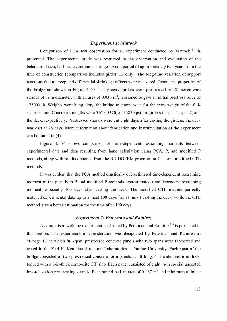
113
Experiment 1: Mattock
Comparison of PCA test observation for an experiment conducted by Mattock (4)
is
presented. The experimental study was restricted to the observation and evaluation of the
behavior of two, half-scale continuous bridges over a period of approximately two years from the
time of construction (comparison included girder 1/2 only). The long-time variation of support
reactions due to creep and differential shrinkage effects were measured. Geometric properties of
the bridge are shown in Figure 4. 75. The precast girders were prestressed by 28, seven-wire
strands of ¼-in diameter, with an area of 0.036 in2, tensioned to give an initial prestress force of
175000 lb. Weights were hung along the bridge to compensate for the extra weight of the full-
scale section. Concrete strengths were 5160, 5370, and 3870 psi for girders in span 1, span 2, and
the deck, respectively. Prestressed strands were cut eight days after casting the girders; the deck
was cast at 28 days. More information about fabrication and instrumentation of the experiment
can be found in (4).
Figure 4. 76 shows comparison of time-dependent restraining moments between
experimental data and data resulting from hand calculation using PCA, P, and modified P
methods, along with results obtained from the BRIDGERM program for CTL and modified CTL
methods.
It was evident that the PCA method drastically overestimated time-dependent restraining
moment in the pier; both P and modified P methods overestimated time-dependent restraining
moment, especially 100 days after casting the deck. The modified CTL method perfectly
matched experimental data up to almost 100 days from time of casting the deck, while the CTL
method give a better estimation for the time after 100 days.
Experiment 2: Peterman and Ramirez
A comparison with the experiment performed by Peterman and Ramirez (7) is presented in
this section. The experiment in consideration was designated by Peterman and Ramirez as
“Bridge 1,” in which full-span, prestressed concrete panels with two spans were fabricated and
tested in the Karl H. Kettelhut Structural Laboratories at Purdue University. Each span of the
bridge consisted of two prestressed concrete form panels, 21 ft long, 4 ft wide, and 6 in thick,
topped with a 6-in-thick composite CIP slab. Each panel consisted of eight ½-in special uncoated
low-relaxation prestressing strands. Each strand had an area of 0.167 in2 and minimum ultimate
114
stress of 270 ksi. Reinforcement in the CIP topping over the pier contained 16 # 4 bars. Figure 4.
77 shows geometric properties of the cross section of the bridge. The four panels for the bridge
were cast simultaneously; the prestress force was transferred to the panels seven days after the
concrete was cast; and the CIP deck was cast when the panels were 147 days old, while stress in
strands was 177 ksi. Reactions at the discontinuous ends of the bridge were monitored
throughout the 50 days following casting of the deck. Restraining moment was then calculated
and reported. Concrete strength of the panels was 7440 psi at 28 days; deck concrete strength
was 5590 psi at 14 days of deck age (when cracks initiated in the deck) and 6150 psi at 28 days.
For more information regarding the experimental procedures, the reader is referred to reference
(7).
Hand calculations using PCA, P, and modified P were conducted and reported along with
analysis results obtained from the BRIDGERM program for both CTL and modified CTL
method.
It is important to mention that for the sake of this comparison, cracking of the deck for
the P and modified P methods was considered, taking into account that it occurred at 14 days of
deck age instead of considering the section cracking-moment criteria.
Figure 4. 78 shows that the PCA method overestimates time-dependent restraining
moment, while CTL and modified CTL methods underestimate negative restraining moment for
the first 14 days after casting the deck, and also underestimate it after 30 days. However,
modified CTL is closer to the experimental results than the CTL method. P method compares
very well with the experimental results; modified P method compares better with the
experimental data at the beginning of the experiment and after cracking of the deck.
As a result, it is believed that P and modified P methods are more capable of capturing
the behavior of shallow sections, while CTL and modified CTL methods are more capable of
predicting the behavior of deeper sections. Nevertheless, the estimation for all these methods is
within the acceptable range of error.
However, the need to conduct experiments on PT-IT sections is imminent to reach a
decision of which method is more capable of capturing the time-dependent effect on restraining
moments for the PT-IT system.
115
Figure 4. 1 Maximum spans for different IT sections for different construction scenarios,
for girder concrete strength of 8 ksi
Figure 4. 2 Time-dependent restraining moments using different methods for Dia & Deck-
PT construction scenario; continuity established @ 14 days of girder's age
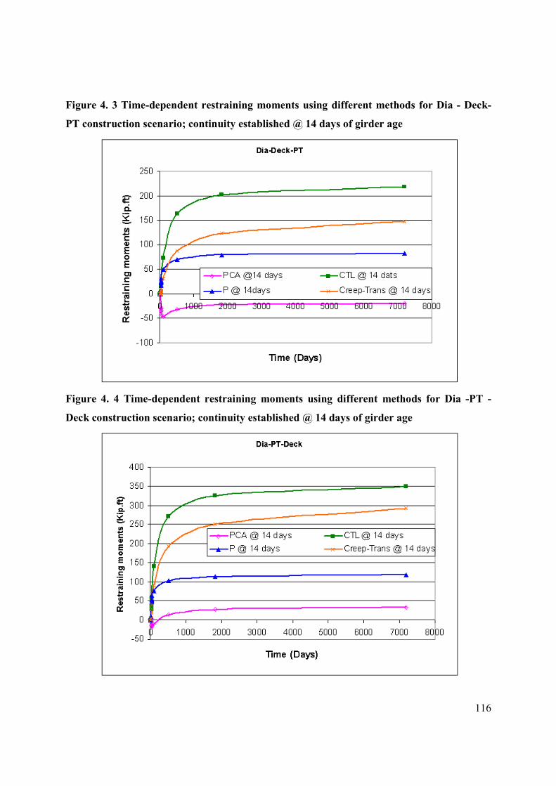
116
Figure 4. 3 Time-dependent restraining moments using different methods for Dia - Deck-
PT construction scenario; continuity established @ 14 days of girder age
Figure 4. 4 Time-dependent restraining moments using different methods for Dia -PT -
Deck construction scenario; continuity established @ 14 days of girder age
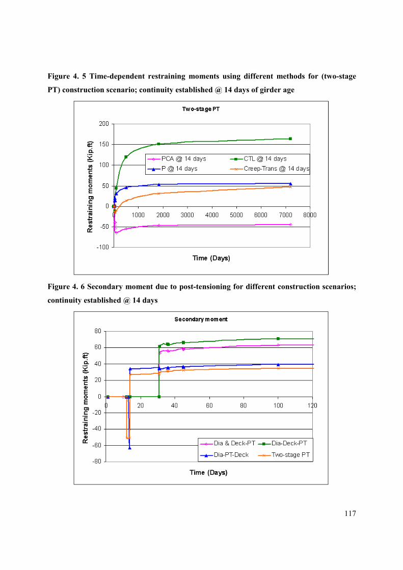
117
Figure 4. 5 Time-dependent restraining moments using different methods for (two-stage
PT) construction scenario; continuity established @ 14 days of girder age
Figure 4. 6 Secondary moment due to post-tensioning for different construction scenarios;
continuity established @ 14 days
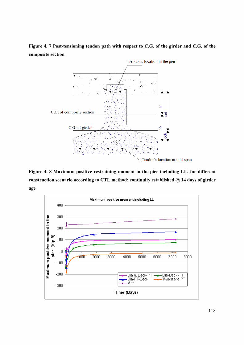
118
Figure 4. 7 Post-tensioning tendon path with respect to C.G. of the girder and C.G. of the
composite section
Figure 4. 8 Maximum positive restraining moment in the pier including LL, for different
construction scenario according to CTL method; continuity established @ 14 days of girder
age
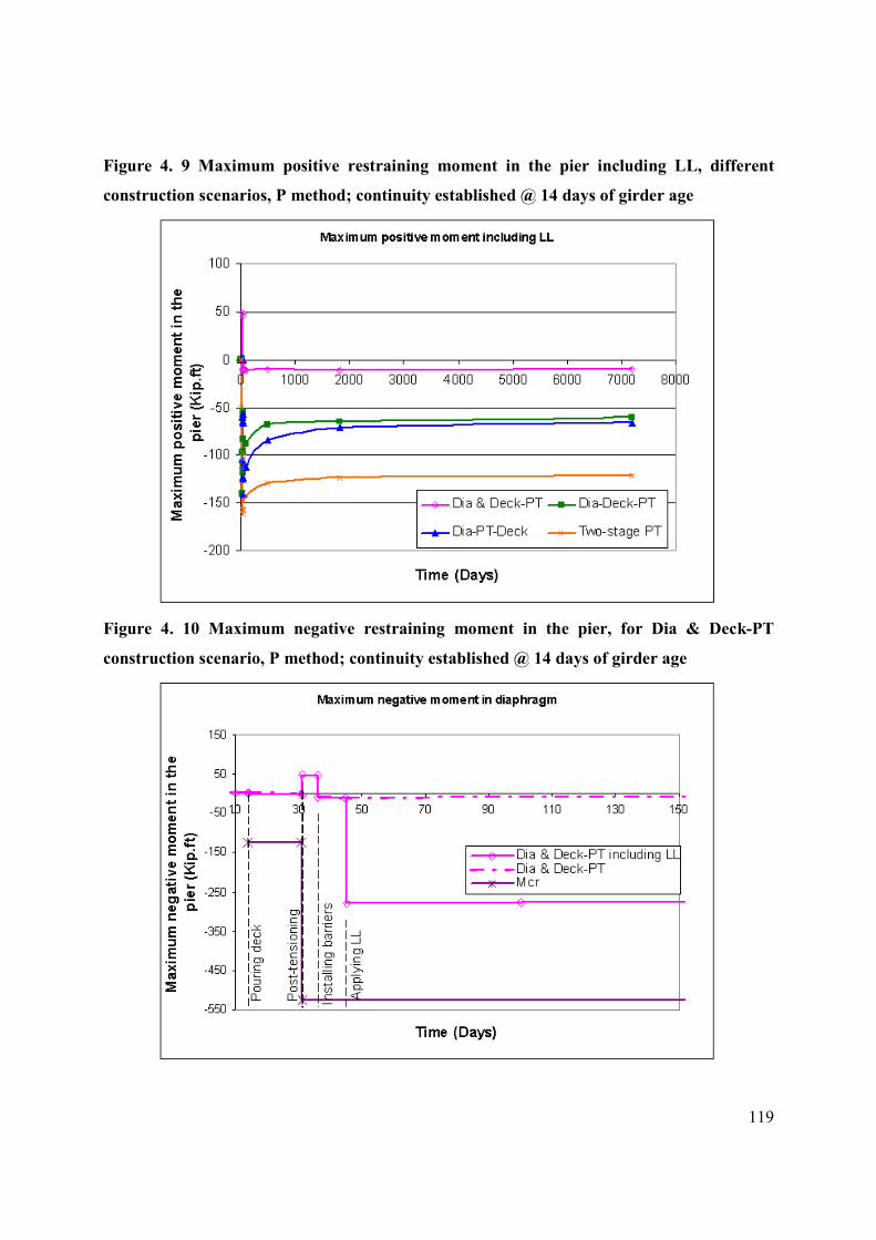
119
Figure 4. 9 Maximum positive restraining moment in the pier including LL, different
construction scenarios, P method; continuity established @ 14 days of girder age
Figure 4. 10 Maximum negative restraining moment in the pier, for Dia & Deck-PT
construction scenario, P method; continuity established @ 14 days of girder age
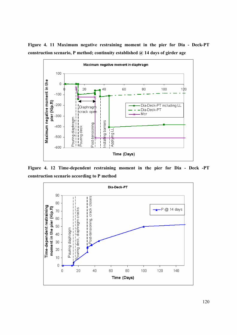
120
Figure 4. 11 Maximum negative restraining moment in the pier for Dia - Deck-PT
construction scenario, P method; continuity established @ 14 days of girder age
Figure 4. 12 Time-dependent restraining moment in the pier for Dia - Deck -PT
construction scenario according to P method
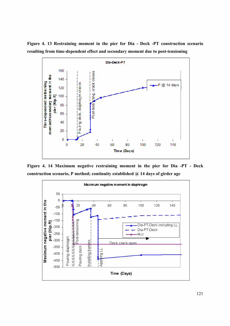
121
Figure 4. 13 Restraining moment in the pier for Dia - Deck -PT construction scenario
resulting from time-dependent effect and secondary moment due to post-tensioning
Figure 4. 14 Maximum negative restraining moment in the pier for Dia -PT - Deck
construction scenario, P method; continuity established @ 14 days of girder age
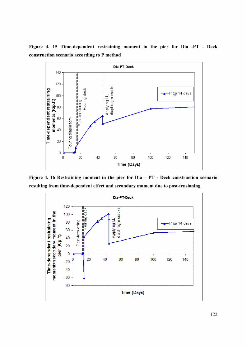
122
Figure 4. 15 Time-dependent restraining moment in the pier for Dia -PT - Deck
construction scenario according to P method
Figure 4. 16 Restraining moment in the pier for Dia – PT - Deck construction scenario
resulting from time-dependent effect and secondary moment due to post-tensioning
123
Figure 4. 17 Maximum negative restraining moment in the pier for two-stage PT
construction scenario, P method; continuity established @ 14 days of girder age
Figure 4. 18 Time-dependent restraining moments using different methods for Dia & Deck-
PT construction scenario; continuity established @ 224 days of girder age
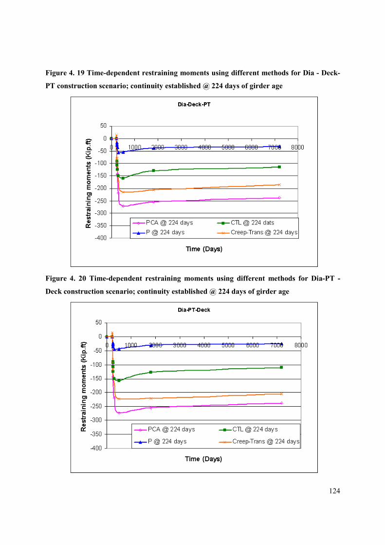
124
Figure 4. 19 Time-dependent restraining moments using different methods for Dia - Deck-
PT construction scenario; continuity established @ 224 days of girder age
Figure 4. 20 Time-dependent restraining moments using different methods for Dia-PT -
Deck construction scenario; continuity established @ 224 days of girder age
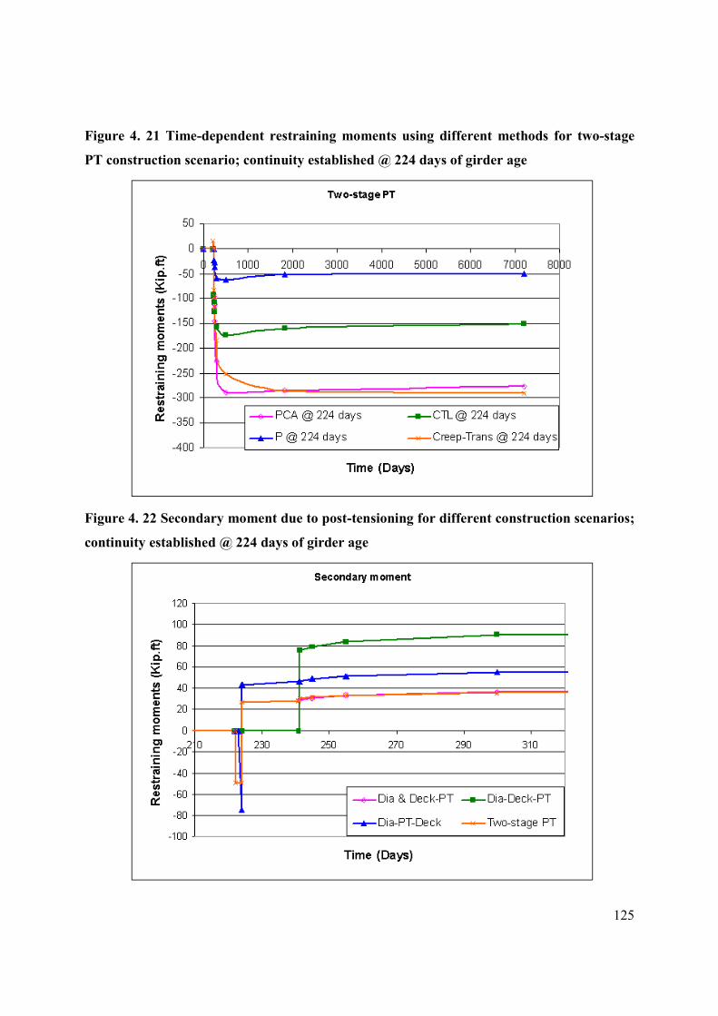
125
Figure 4. 21 Time-dependent restraining moments using different methods for two-stage
PT construction scenario; continuity established @ 224 days of girder age
Figure 4. 22 Secondary moment due to post-tensioning for different construction scenarios;
continuity established @ 224 days of girder age
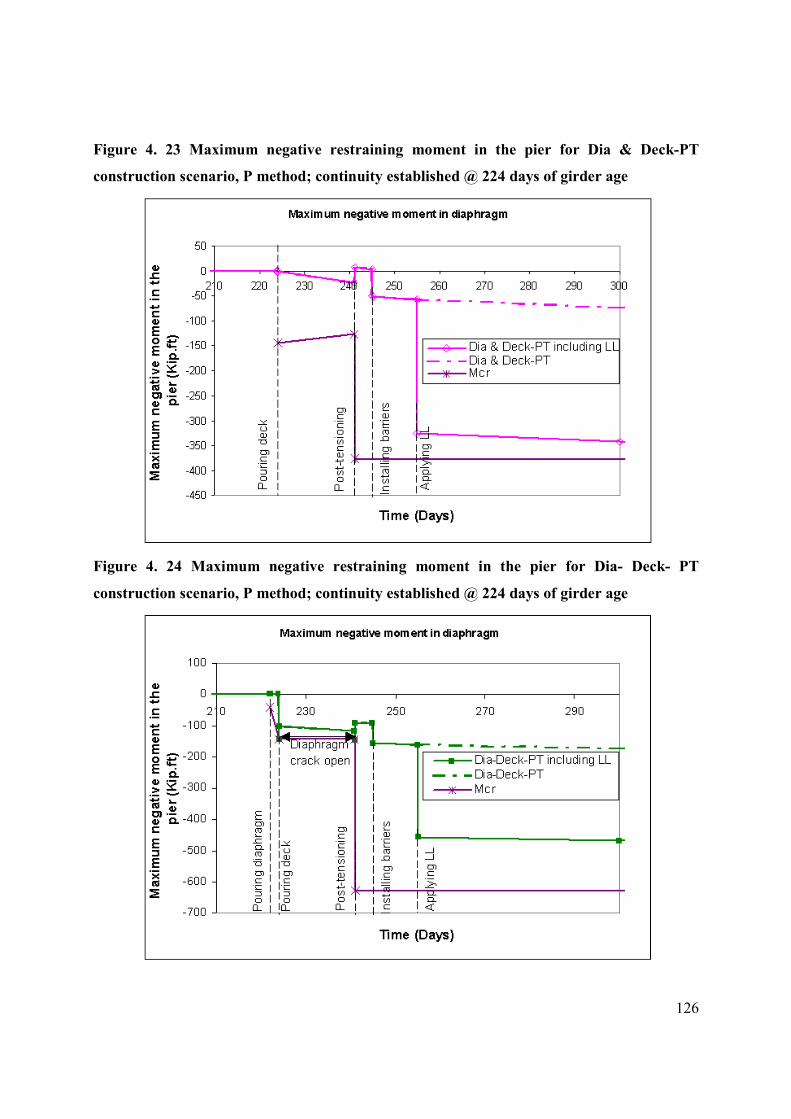
126
Figure 4. 23 Maximum negative restraining moment in the pier for Dia & Deck-PT
construction scenario, P method; continuity established @ 224 days of girder age
Figure 4. 24 Maximum negative restraining moment in the pier for Dia- Deck- PT
construction scenario, P method; continuity established @ 224 days of girder age

127
Figure 4. 25 Time-dependent restraining moment in the pier for Dia - Deck -PT
construction scenario according to P method
Figure 4. 26 Restraining moment in the pier for Dia - Deck -PT construction scenario
resulting from time-dependent effect and secondary moment due to post-tensioning
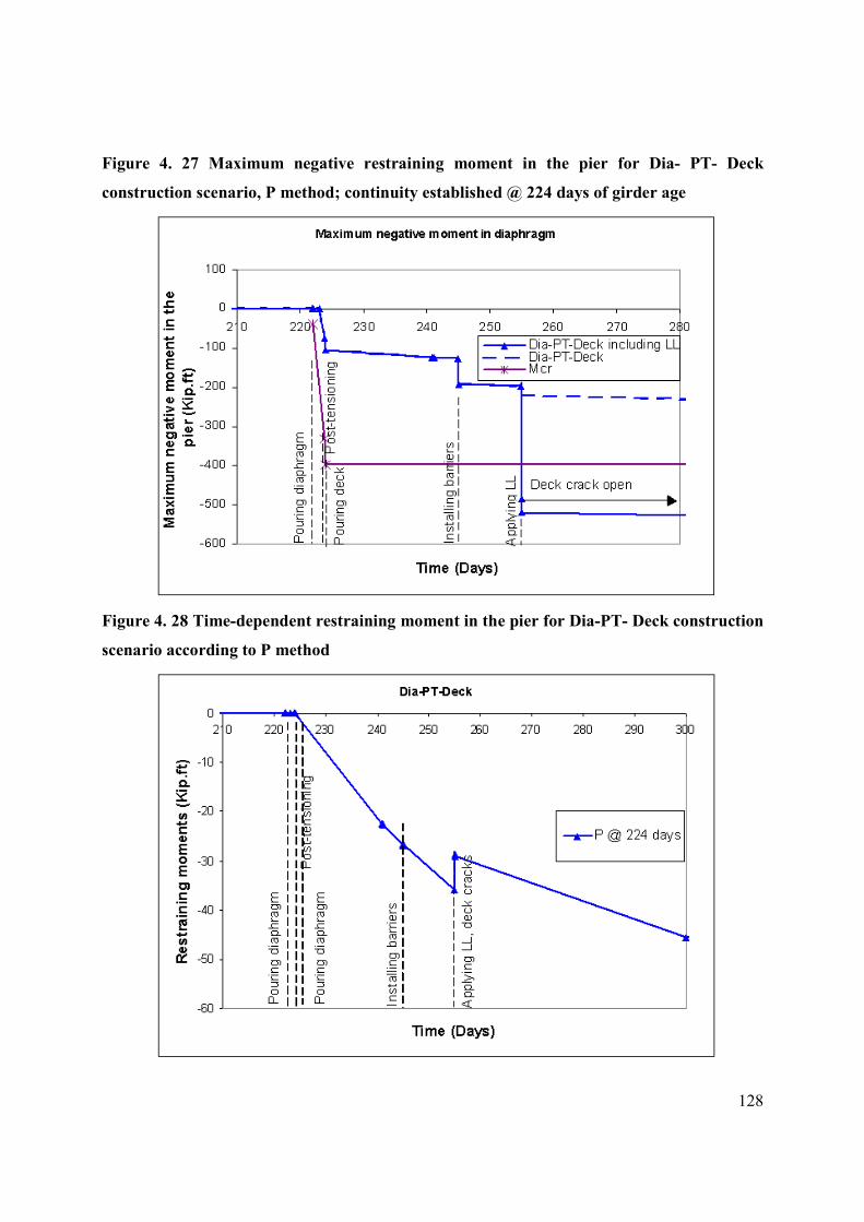
128
Figure 4. 27 Maximum negative restraining moment in the pier for Dia- PT- Deck
construction scenario, P method; continuity established @ 224 days of girder age
Figure 4. 28 Time-dependent restraining moment in the pier for Dia-PT- Deck construction
scenario according to P method
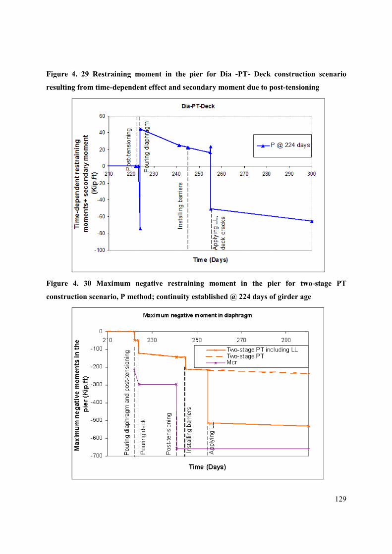
129
Figure 4. 29 Restraining moment in the pier for Dia -PT- Deck construction scenario
resulting from time-dependent effect and secondary moment due to post-tensioning
Figure 4. 30 Maximum negative restraining moment in the pier for two-stage PT
construction scenario, P method; continuity established @ 224 days of girder age
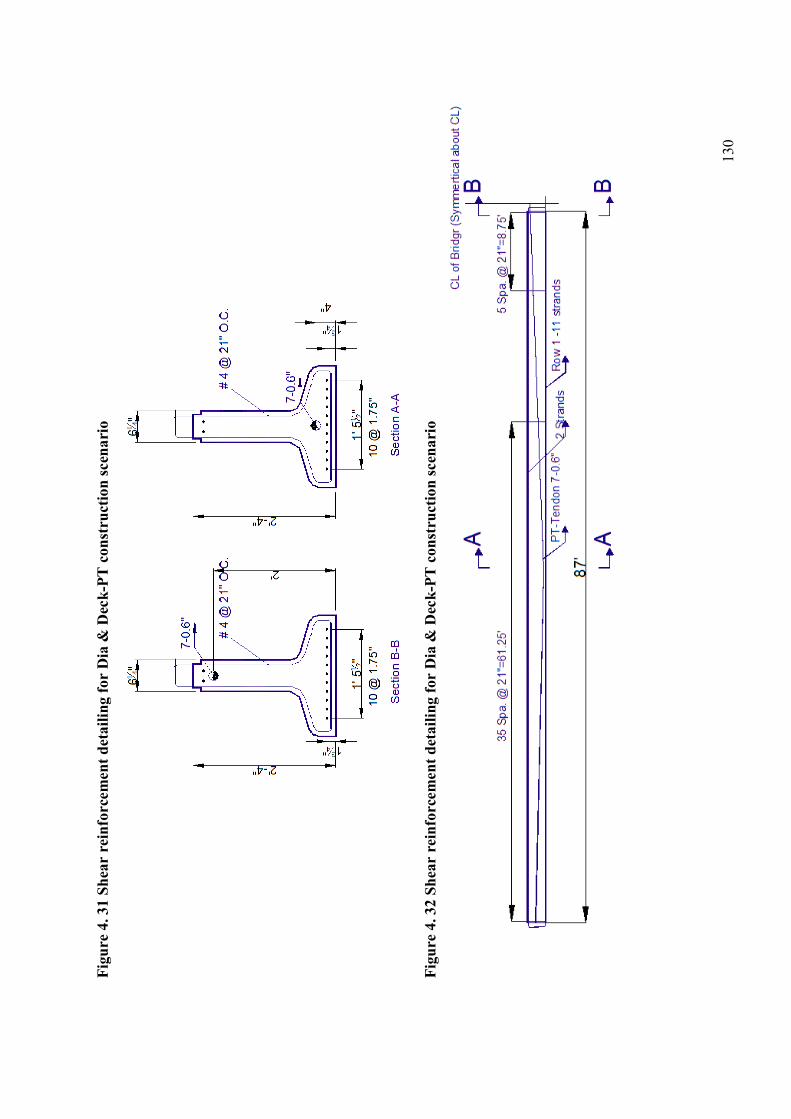
130
Figure 4. 31 Shear reinforcement detailing for Dia & Deck-PT construction scenario
Figure 4. 32 Shear reinforcement detailing for Dia & Deck-PT construction scenario
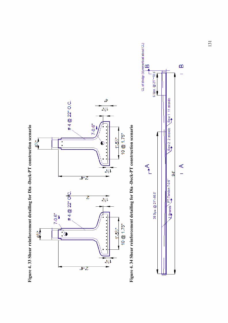
131
Figure 4. 33 Shear reinforcement detailing for Dia -Deck-PT construction scenario
Figure 4. 34 Shear reinforcement detailing for Dia -Deck-PT construction scenario
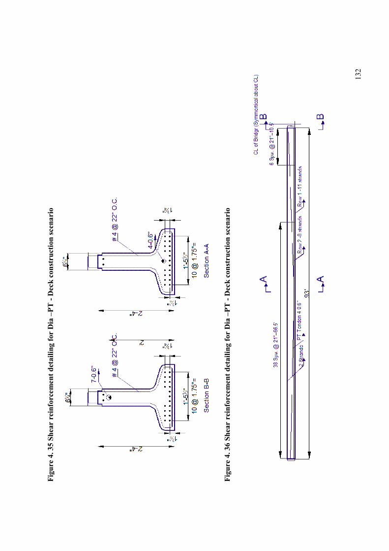
132
Figure 4. 35 Shear reinforcement detailing for Dia –PT - Deck construction scenario
Figure 4. 36 Shear reinforcement detailing for Dia –PT - Deck construction scenario
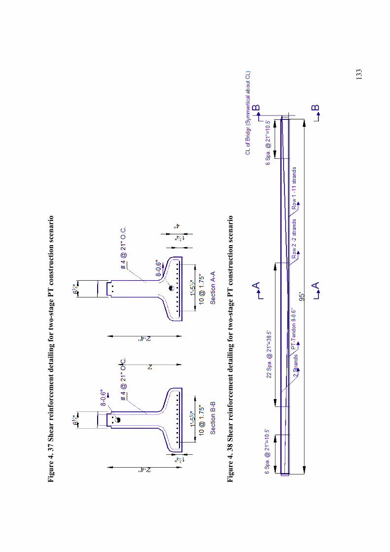
133
Figure 4. 37 Shear reinforcement detailing for two-stage PT construction scenario
Figure 4. 38 Shear reinforcement detailing for two-stage PT construction scenario
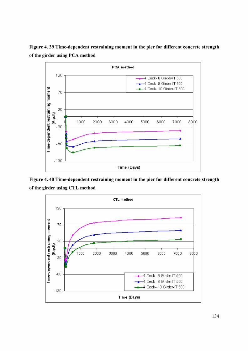
134
Figure 4. 39 Time-dependent restraining moment in the pier for different concrete strength
of the girder using PCA method
Figure 4. 40 Time-dependent restraining moment in the pier for different concrete strength
of the girder using CTL method
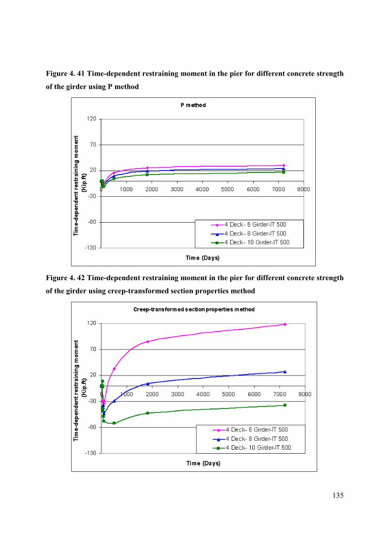
135
Figure 4. 41 Time-dependent restraining moment in the pier for different concrete strength
of the girder using P method
Figure 4. 42 Time-dependent restraining moment in the pier for different concrete strength
of the girder using creep-transformed section properties method
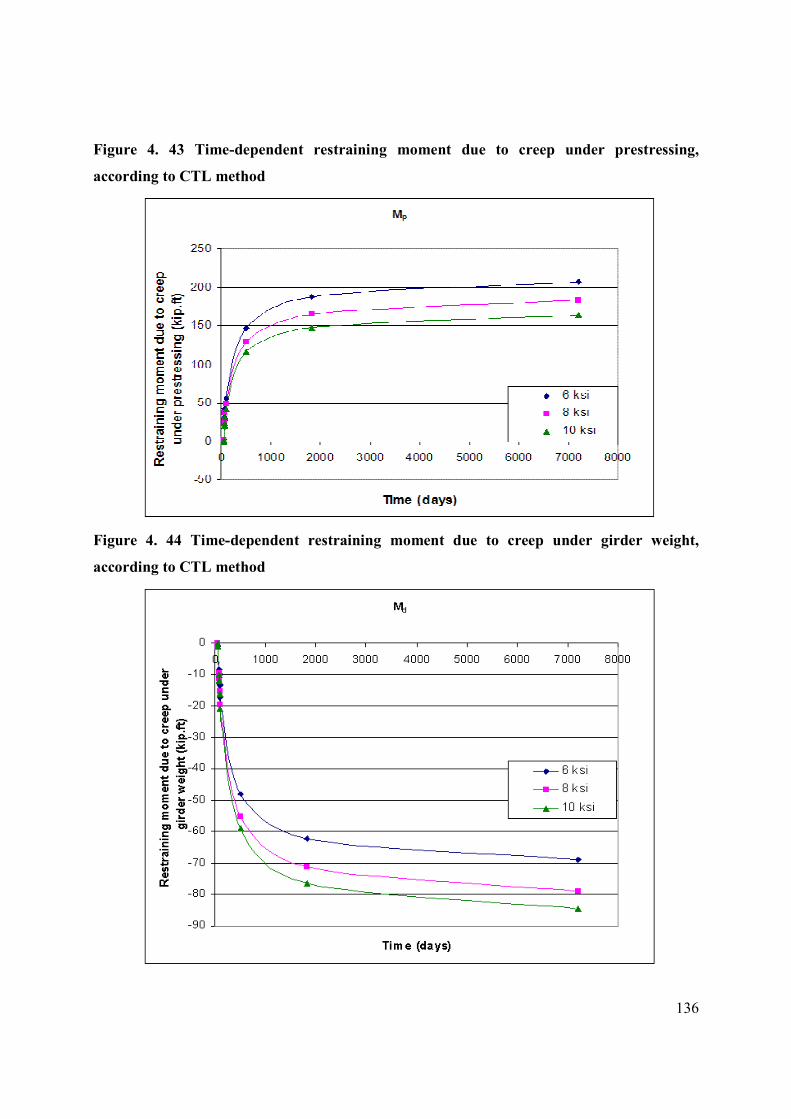
136
Figure 4. 43 Time-dependent restraining moment due to creep under prestressing,
according to CTL method
Figure 4. 44 Time-dependent restraining moment due to creep under girder weight,
according to CTL method
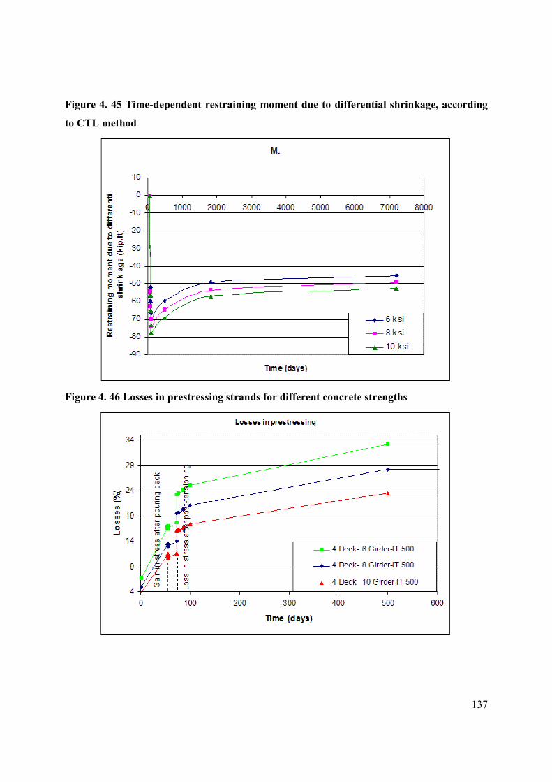
137
Figure 4. 45 Time-dependent restraining moment due to differential shrinkage, according
to CTL method
Figure 4. 46 Losses in prestressing strands for different concrete strengths
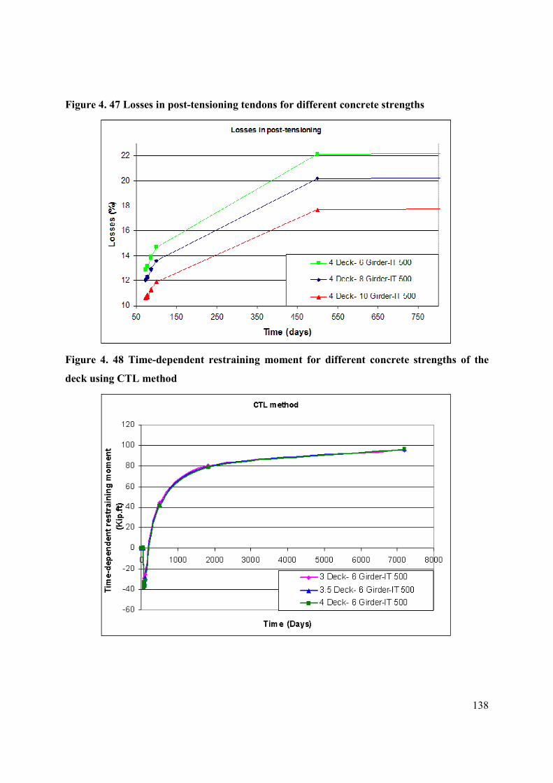
138
Figure 4. 47 Losses in post-tensioning tendons for different concrete strengths
Figure 4. 48 Time-dependent restraining moment for different concrete strengths of the
deck using CTL method
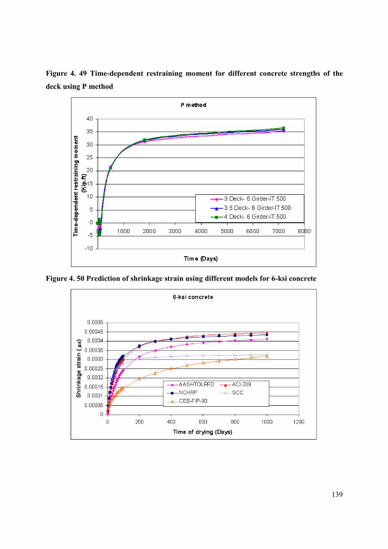
139
Figure 4. 49 Time-dependent restraining moment for different concrete strengths of the
deck using P method
Figure 4. 50 Prediction of shrinkage strain using different models for 6-ksi concrete
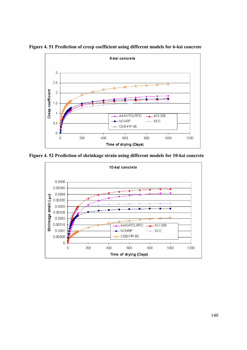
140
Figure 4. 51 Prediction of creep coefficient using different models for 6-ksi concrete
Figure 4. 52 Prediction of shrinkage strain using different models for 10-ksi concrete
141
Figure 4. 53 Prediction of creep coefficient using different models for 10-ksi concrete
Figure 4. 54 Predicted losses in pretensioned strands using different models
142
Figure 4. 55 Predicted losses in post-tensioning using different models
Figure 4. 56 Time-dependent restraining moment for different creep-and-shrinkage models
using PCA method
143
Figure 4. 57 Time-dependent restraining moment for different creep-and-shrinkage models
using CTL method
Figure 4. 58 Time-dependent restraining moment for different creep-and-shrinkage models
using P method

144
Figure 4. 59 Time-dependent restraining moment for different creep-and-shrinkage models
using creep-transformed section properties method
Figure 4. 60 Effect of time of cutting strands on losses in prestressing
145
Figure 4. 61 Time-dependent restraining moment in the pier for continuity established @
14 days of girder age
Figure 4. 62 Time-dependent restraining moment in the pier for continuity established @
28 days of girder age
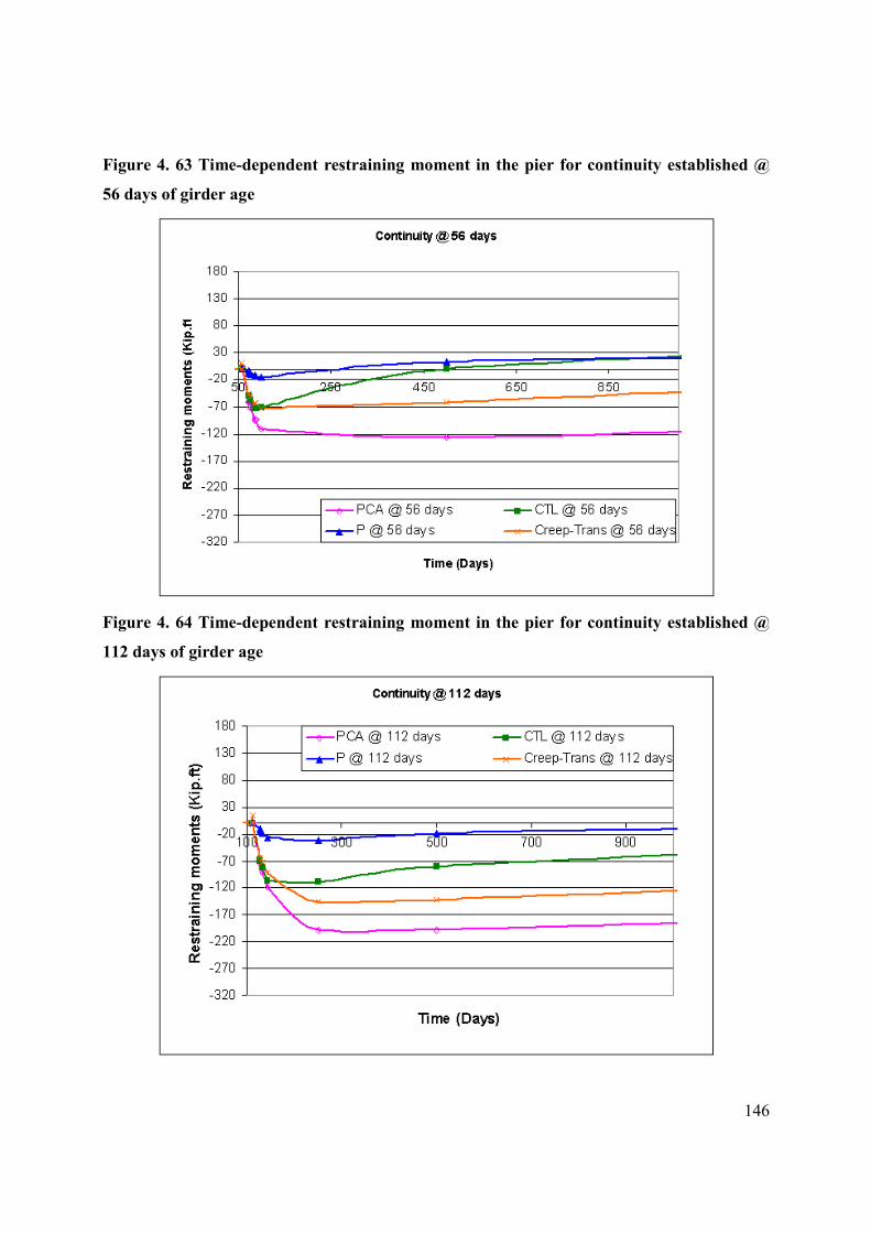
146
Figure 4. 63 Time-dependent restraining moment in the pier for continuity established @
56 days of girder age
Figure 4. 64 Time-dependent restraining moment in the pier for continuity established @
112 days of girder age
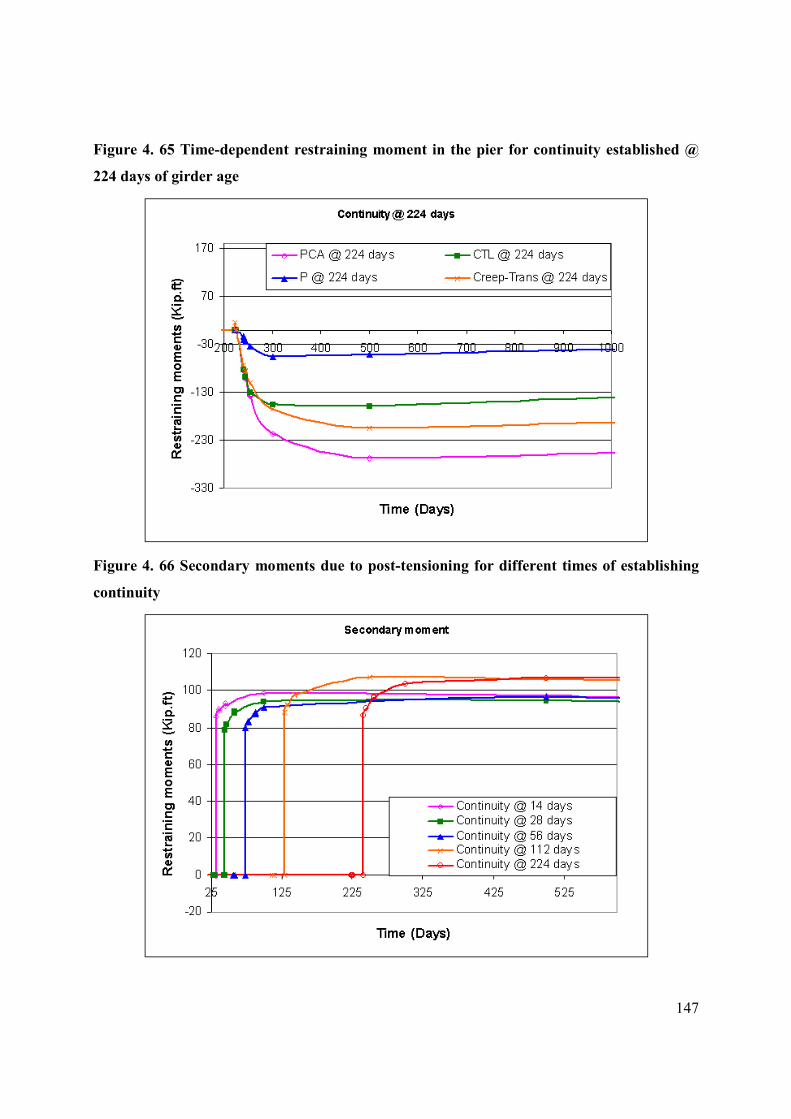
147
Figure 4. 65 Time-dependent restraining moment in the pier for continuity established @
224 days of girder age
Figure 4. 66 Secondary moments due to post-tensioning for different times of establishing
continuity
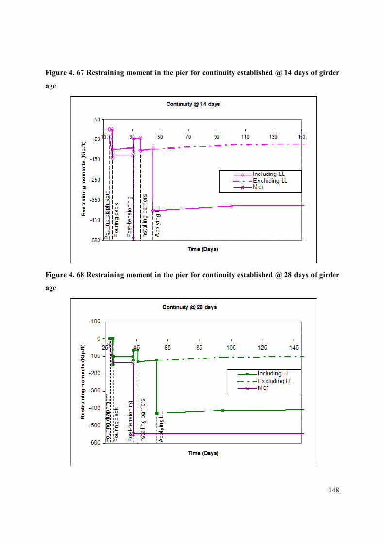
148
Figure 4. 67 Restraining moment in the pier for continuity established @ 14 days of girder
age
Figure 4. 68 Restraining moment in the pier for continuity established @ 28 days of girder
age
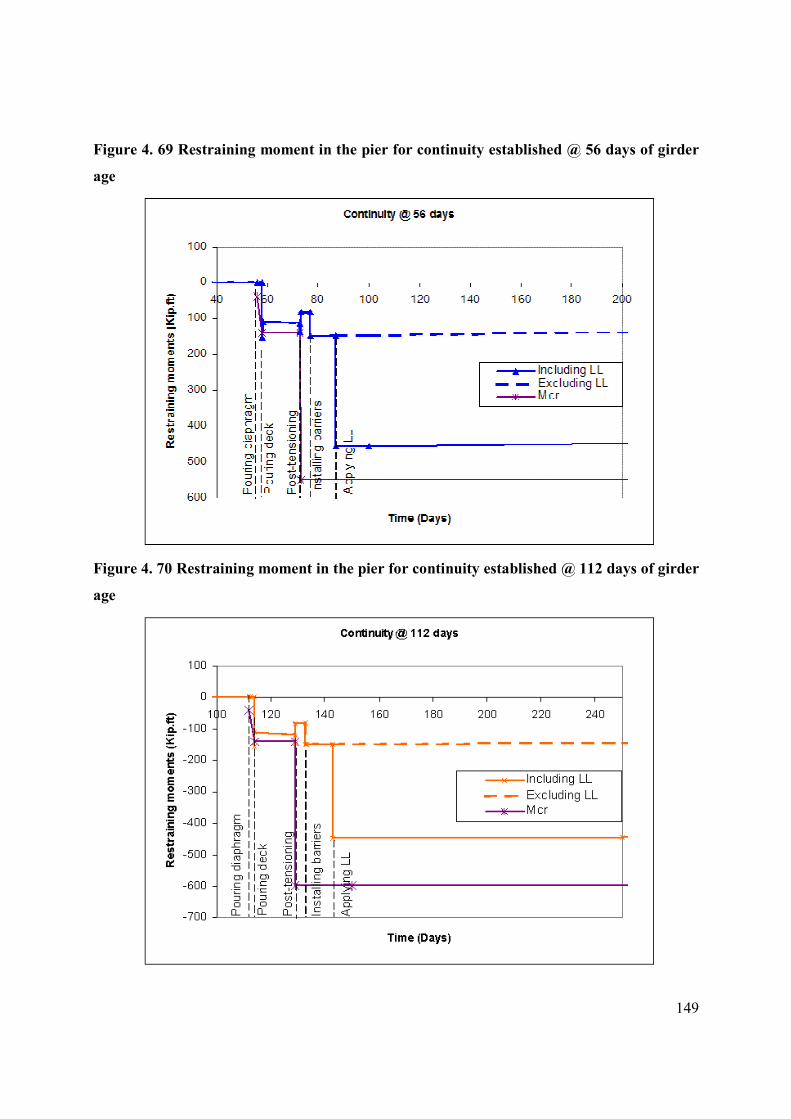
149
Figure 4. 69 Restraining moment in the pier for continuity established @ 56 days of girder
age
Figure 4. 70 Restraining moment in the pier for continuity established @ 112 days of girder
age
150
Figure 4. 71 Restraining moment in the pier for continuity established @ 224 days of girder
age
Figure 4. 72 Effect of time of casting the deck on time-dependent restraining moment using
CTL method
151
Figure 4. 73 Effect of time of casting the deck on time-dependent restraining moment using
P method
Figure 4. 74 Effect of time of casting the deck on the restraining moment in the pier
152
Figure 4. 75 Cross section for experiment conducted by (4)
Figure 4. 76 Comparison with experimental data (4)
153
Figure 4. 77 Cross section of panels tested by (7)
Figure 4. 78 Comparison with experimental data from (7)
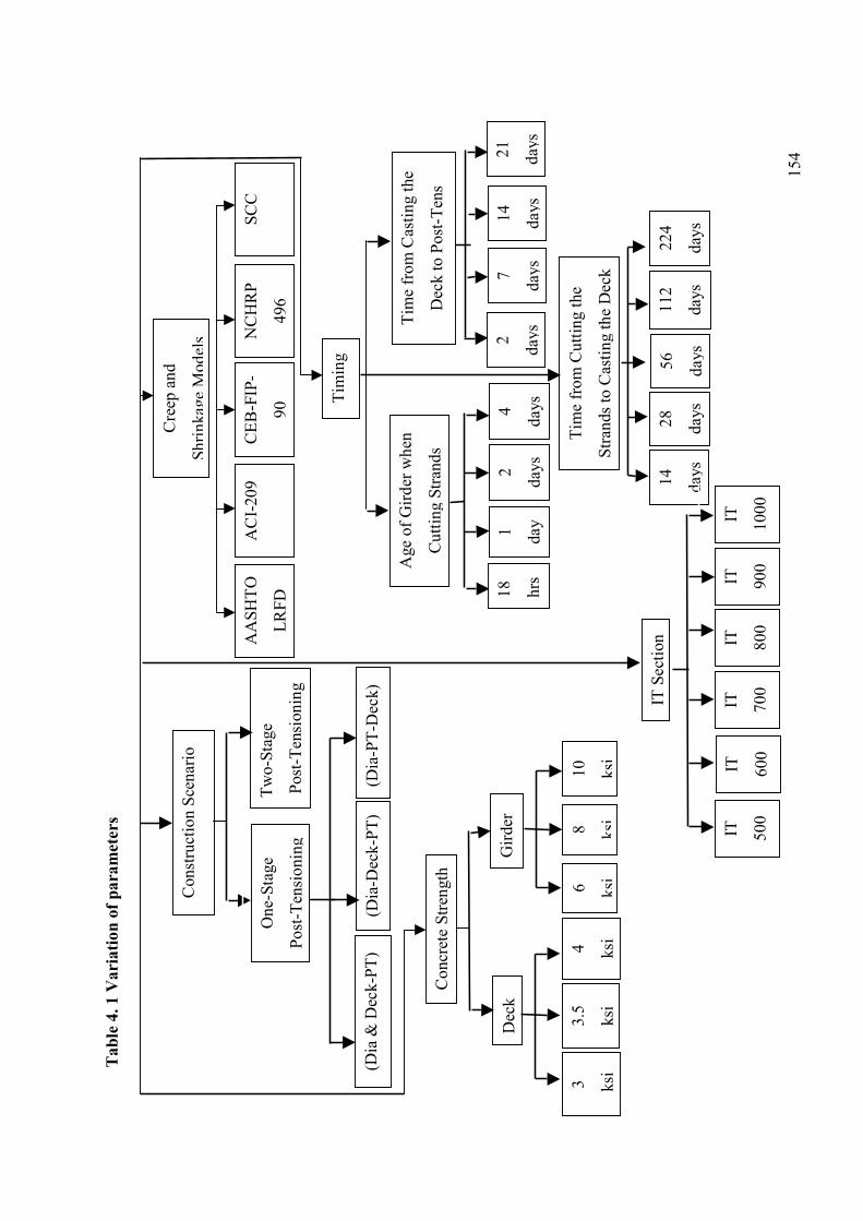
154
Table 4. 1 Variation of parameters
Concrete Strength
3.5
ksi
Girder
Deck
4
ksi
6
ksi
8
ksi
10
ksi
3
ksi
Construction Scenario
Two-Stage
Post-Tensioning
One-Stage
Post-Tensioning
(Dia &
Deck-PT)
(Dia-D
eck-PT)
(Dia-PT-D
eck)
Tim
ing
Age of Girder when
Cutting Strands
18
hrs
2
days
1
day
4
days
Tim
e from Cutting the
Strands to Casting the Deck
14
days
28
days
56
days
112
days
224
days
Tim
e from Casting the
Deck to Post-Tens
2
days
7
days
14
days
21
days
IT Section
IT
1000
IT
900
IT
800
IT
700
IT
600
IT
500
Creep and
Shrinkage Models NCHRP
496
CEB-FIP-
90
ACI-209
AASHTO
LRFD
SCC
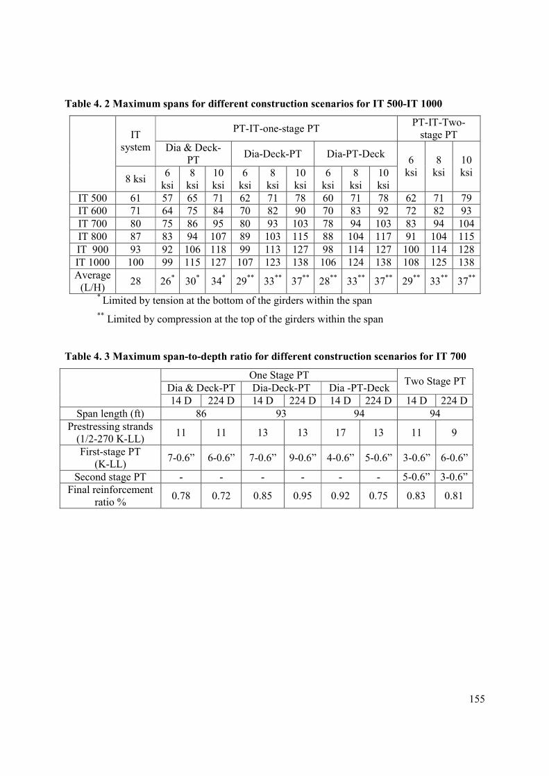
155
Table 4. 2 Maximum spans for different construction scenarios for IT 500-IT 1000
PT-IT-one-stage PT PT-IT-Two-
stage PT IT
system Dia & Deck-
PT Dia-Deck-PT Dia-PT-Deck
8 ksi 6
ksi
8
ksi
10
ksi
6
ksi
8
ksi
10
ksi
6
ksi
8
ksi
10
ksi
6
ksi
8
ksi
10
ksi
IT 500 61 57 65 71 62 71 78 60 71 78 62 71 79
IT 600 71 64 75 84 70 82 90 70 83 92 72 82 93
IT 700 80 75 86 95 80 93 103 78 94 103 83 94 104
IT 800 87 83 94 107 89 103 115 88 104 117 91 104 115
IT 900 93 92 106 118 99 113 127 98 114 127 100 114 128
IT 1000 100 99 115 127 107 123 138 106 124 138 108 125 138
Average
(L/H) 28 26
* 30
* 34
* 29
** 33
** 37
** 28
** 33
** 37
** 29
** 33
** 37
**
* Limited by tension at the bottom of the girders within the span
** Limited by compression at the top of the girders within the span
Table 4. 3 Maximum span-to-depth ratio for different construction scenarios for IT 700
One Stage PT
Dia & Deck-PT Dia-Deck-PT Dia -PT-Deck Two Stage PT
14 D 224 D 14 D 224 D 14 D 224 D 14 D 224 D
Span length (ft) 86 93 94 94
Prestressing strands
(1/2-270 K-LL) 11 11 13 13 17 13 11 9
First-stage PT
(K-LL) 7-0.6” 6-0.6” 7-0.6” 9-0.6” 4-0.6” 5-0.6” 3-0.6” 6-0.6”
Second stage PT - - - - - - 5-0.6” 3-0.6”
Final reinforcement
ratio % 0.78 0.72 0.85 0.95 0.92 0.75 0.83 0.81
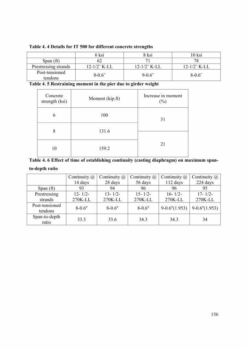
156
Table 4. 4 Details for IT 500 for different concrete strengths
6 ksi 8 ksi 10 ksi
Span (ft) 62 71 78
Prestressing strands 12-1/2˝ K-LL 12-1/2˝ K-LL 12-1/2˝ K-LL
Post-tensioned
tendons 8-0.6˝ 9-0.6˝ 8-0.6˝
Table 4. 5 Restraining moment in the pier due to girder weight
Concrete
strength (ksi) Moment (kip.ft)
Increase in moment
(%)
6 100 31
8 131.6
10 159.2 21
Table 4. 6 Effect of time of establishing continuity (casting diaphragm) on maximum span-
to-depth ratio
Continuity @
14 days
Continuity @
28 days
Continuity @
56 days
Continuity @
112 days
Continuity @
224 days
Span (ft) 93 94 96 96 95
Prestressing
strands
12- 1/2-
270K-LL
13- 1/2-
270K-LL
15- 1/2-
270K-LL
16- 1/2-
270K-LL
17- 1/2-
270K-LL
Post-tensioned
tendons 8-0.6'' 8-0.6'' 8-0.6'' 9-0.6''(1.953) 9-0.6''(1.953)
Span-to-depth
ratio 33.3 33.6 34.3 34.3 34
157
CHAPTER 5 - CONCLUSION AND RECOMMENDATIONS
Conclusion
As considerable numbers of bridges need to be replaced or repaired in Kansas and other
states, it is important to implement a standard method for replacement in which the capacity of
the bridge is maximized and cost is minimized, while durability and safety are not compromised.
Existing replacement methods do not satisfy one or more of these conditions, as previously
discussed in this report.
A post-tensioned, inverted-T bridge system (PT-IT) was implemented in this study,
where pretensioned inverted-T beams are post-tensioned to improve the capacity and durability
of the system, increase span-to-depth ratio of the beam, and eliminate cracks in the deck over the
piers.
A computer program (PT-IT) using C++ object-oriented language was developed to be
used as a tool for the analysis of the PT-IT system. A user-friendly interface was also developed,
using visual basic to help in data input and reading output.
A comparison between analysis results from the PT-IT program and Consplice was
conducted; the comparison proved the capability of the PT-IT program to analyze the system.
An extensive parametric study was conducted to provide guidelines for designing and
constructing a PT-IT system. Different construction scenarios were discussed and evaluated from
maximum capacity and durability points of view. Construction sequence was found to be one of
the most effective and critical parameters in design. Different construction scenarios were
investigated, including two main options of applying one or two stages of post-tensioning. For
one stage post tensioning, many options were evaluated. One of these was casting the deck and
diaphragm simultaneously and then applying post-tensioning. In this case, deck weight was
carried on the simple span beam, along with positive secondary moments due to post-tensioning;
this will cause high positive stresses within the spans of the girders, which will consequently
limit the span-to-depth ratio of the girders.
Another option for one-stage post-tensioning is to cast the diaphragm, then apply post-
tensioning, and then cast the deck. In this scenario, the deck weight is carried by the continuous
structure. This results in lower positive moments within the span, while negative moments
158
develop over the piers. Disadvantage of this option of construction is that post-tensioning will be
applied at the girder section only. This causes high stresses in the bottom of the girder near and
in the pier. Furthermore, as post-tensioning is applied on the girder section only, it will not help
reduce negative stresses in the deck over the piers due to live load.
Another option for one-stage post-tensioning is when continuity is established by casting
the diaphragm, and then after the diaphragm concrete hardens, the deck is cast, and finally post-
tensioning is applied to the whole structure. The advantage of this construction scenario is that
the weight of the deck will be carried by the continuous structure. At the same time, weight of
the deck has no time-dependent effect on moments in the piers. Besides, when post-tensioning is
applied on the continuous structure, primary moments caused by post-tensioning at the pier will
be less, as if they were to be applied at the girder section. This will cause less tension forces at
the bottom of the girders in the case when continuity is established at early girder age. The
drawback of this type of scenario is that cracking of the diaphragm over the pier will occur
during the period between casting the deck and post-tensioning under deck weight. After post-
tensioning, the deck will be under compression and consequently, the cracks will be closed.
In the case of two-stage-post tensioning, the diaphragm is cast to establish continuity,
then the first stage of post-tensioning is enough to balance stresses due to the weight of the deck.
After the deck is cast, the final stage of post-tensioning is applied to balance stresses due to the
weight of the barriers and live load. A disadvantage of two-stage post-tensioning is increased
labor required for construction using this scenario, which reflects on the cost of construction.
Results of parametric study showed that both scenarios of one-stage post-tensioning (Dia-
Deck-PT) and two-stage PT have the highest span-to-depth ratio and satisfy the crack-free deck
critirea. Since the option of Dia-Deck-PT incorporates less labor, it is recommended to be used
for construction of PT-IT systems.
Different methods for estimation of time-dependent restraining moment, and
modifications for both CTL and P methods were suggested in this study. Comparison for CTL, P,
and PCA methods with experimental results showed that the P method better estimates time-
dependent restraining moment for shallow girders, while the CTL method better estimates it for
deeper girders.
While PCA, CTL, P, and creep-transformed section properties methods are considered in
the course of the parametric study to estimate the range in which time-dependent restraining

159
moment will fall, it is recommended that experimental investigations be conducted in order to
determine the method that is capable of providing a better estimation of the effect of time-
dependent forces on restraining moments in the piers.
Girder concrete strength plays a major role in increasing span-to-depth ratio. Increasing
girder concrete strength from 6 to 8 ksi helps increase the span by 15% of 6-ksi girders, while
increasing strength from 8 to 10 ksi increases the span by 11% of the 8-ksi girders.
On the other hand, deck concrete strength doesn’t affect time-dependent restraint moment
under creep and shrinkage, nor losses in stresses of prestressing strands and post-tensioned
tendons.
Different creep-and-shrinkage models were investigated including AASHTO LRFD,
ACI-209, CEB-FIP-90, SCC, and NCHRP 496. It was found that while estimation of losses in
pretensioned strands and post-tensioned tendons is not significantly affected using different
models, variation of time-dependent restraining moment is significant for different models.
The effect of timing on different construction stages was also discussed and addressed in
the parametric study. Establishing continuity was found to be an effective parameter in the
design. For early ages of establishing continuity, positive time-dependent restraining moments
tend to develop in the pier, while for late age of establishing continuity, negative time-dependent
restraining moments tend to form. It is recommended that continuity be established between 56
and 112 days of girder age. Time between establishing continuity and casting the deck was not
found to play a major role in the time-dependent restraining moment.
It is recommended that post-tensioning be applied as soon as possible after casting the
deck to close the crack in the top of the diaphragm. This could be done as soon as two days after
casting the deck. The time of post-tensioning doesn’t affect the value of time-dependent
restraining moment, but for durability issues related to control crack initiation and development
in the diaphragm, it is recommended that post-tensioning be applied to the structure as soon as
possible after casting the deck.
Recommendation
Based on the results of this research, the following recommendations are made for the
post-tensioned inverted-T bridge system:

160
� The need for full or half scale experiments on PT-IT bridge system is imminent to
reach a decision of which method is more capable of capturing the time-
dependent effect on restraining moments for the PT-IT system.
� Use (Dia-Deck-PT) Construction scenario for PT-IT system, this involves casting
diaphragms to establish continuity, then cast the deck, and then apply post-
tensioning
� Using 8 or 10 ksi concrete strength for PT-IT girders enhance span-to-depth ratio
of the system
� It is recommended to cast the diaphragm between 56 and 112 days of girder age.
� Time between establishing continuity and casting the deck was not found to play
a major role on the behavior of the system.
� It is recommended that post-tensioning be applied as soon as possible after casting
the deck to close the crack in the top of the diaphragm. This could be done as
soon as two days after casting the deck.
� The time of post-tensioning doesn’t affect the value of time-dependent restraining
moment, but for durability issues related to control crack initiation and
development in the diaphragm, it is recommended that post-tensioning be applied
to the structure as soon as possible after casting the deck.

161
Notations
Ag = area of the prestressed member
Ad = cross-sectional area of CIP slab
As = steel area
bv = effective web width
dv = effective shear depth taken as the distance between the resultant of the tensile
and compression forces due to flexure
e = base of the Naperian logarithm
ec = distance between the top of the precast member and the centroid of the
composite section
Eci =modulus of elasticity of concrete at transfer
Ed = modulus of elasticity of CIP concrete
Eg = modulus of elasticity of the girder concrete
Ep = modulus of elasticity of prestressing steel
fcgp = sum of concrete stresses at the center of gravity of prestressing tendons
(f’c)28 = strength of the concrete at 28 days
fpce = compression stress in concrete due to effective prestress forces
fpj = initial stress in the tendon at the end of stressing
fpj = stress in the prestressing steel at jacking (ksi)
fpy = specified yield strength of prestressing steel
fr = modulus of rupture
H = average annual ambient relative humidity
h = CIP thickness
Id = moment of inertia of the diaphragm region
Im = moment of inertia of the main span
ks = size factor
kh = humidity factor
kf = factor of the effect of concrete strength
kc = factor for the effect of the volume-to-surface ratio

162
k = wobble friction coefficient
Ld = length of the diaphragm region
Lm = length of the main span
Mu = factored moment
Mdnc = total unfactored dead load moment acting on the monolithic or noncomposite
section
(Md)precast = midspan moment due to dead load of the girders
(Md)CIP = midspan moment due to CIP deck weight
Md =midspan moment due to dead load
PPR = partial prestress ratio
s = girder spacing (in)
sc, snc = section modulus for the extreme fiber of the composite section
t = time estimated in days from stressing to transfer
vp = component of prestressing force in the direction of the shear force (Kip)
vu = factored shear force
x = length of a prestressing tendon from the jacking end to any point under
consideration (ft)
α = fraction of εc, which has occurred when continuity connection is established
∆L = anchor set (in)
∆fpES = loss due to elastic shortening
∆fpR1 = loss due to relaxation of steel at transfer
∆fpR2 = loss due to relaxation of steel after transfer
∆fpT = total loss of prestress
∆fpES = loss due to elastic shortening
∆fpSH = loss due to concrete shrinkage
∆fcdp = change in concrete stress at the center of gravity of prestressing steel
εs = differential shrinkage strain
εc = creep strain at time t due to unit stress
εe = initial strain due to unit stress
εsc0 = notional shrinkage coefficient
ф = creep coefficient

163
Φu = deck’s ultimate shrinkage
Θ = angle of inclination of diagonal compressive stresses
µ = coefficient of friction
χ = aging coefficient

164
References
1. American Association of State Highway and Transportation Officials, “AASHTO-LRFD
bridge design specifications, customary U.S. units,” 3rd Edition, 2004, Washington, DC.
2. Collins, Michael P., Mitchell Denis “Prestressed Concrete Structures” Prentice hall,
Engelwood Cliffs, New Jersey
3. Freyermuth, C., “Design of continuous highway bridges with precast prestressed concrete
girders,” PCI Journal, Vol. 14, No. 2, pp. 14-39, April (1969).
4. Mattock, A., “Precast-prestressed concrete bridges 5: creep and shrinkage studies,”
Journal of the PCA Research, Portland Cement Association, Skokie, IL, pp. 32-66, (May
1961).
5. Oesterle, R., Glikin, J., and Larson, S. “Design of simple-span precast prestressed bridge
girders made continuous (final report)”, Construction Technology Laboratories, Inc. for
National Cooperative Highway Research Program, Transportation Research Board
(NHCRP Project 12-29), Skokie, IL, May (1989).
6. Oesterle, R., Glikin, J., and Larson, S. “Design of precast-prestressed bridge girders made
continuous,” National Cooperative Highway Research Program Report 322,
Transportation Research Board, National Research Council, Washington, DC, pp. 97,
November (1989).
7. Peterman, R., and Ramirez, J. “Restraint moments in bridges with full-span prestressed
concrete form panels,” PCI Journal, pp. 54-73, January-February (1998).
8. Dilger, W. H., “Creep analysis of prestressed concrete structures using creep-transformed
section properties,” PCI Journal, Vol. 27, No. 1, pp. 98-118, January-February (1982).
165
9. Mirza, S. A., and Furlung, R. W., “Design of reinforced and prestressed concrete
inverted-T beams for bridge structures,” Journal of the Prestressed Concrete Institute,
Vol. 30, No. 4, pp. 112-136, July-Aug. (1985).
10. Kamel, Mounir R., and Tadros, Maher K., “The inverted-T, shallow-bridge system for
rural areas,” PCI Journal, Vol. 41, No.5, pp. 28-43, September/October (1996).
11. Kamel, Mounir R., and Derrick, Deb, “A precast alternative for bridge slabs,” Concrete
International, pp. 41-42, August (1997).
12. Ambare, Sameer, and Peterman, Robert J., “Evaluation of the inverted Tee shallow
bridge system for use in Kansas, (final report)” Kansas Department of Transportation (K-
TRAN: KSU-00-1), Topeka, Ks, Oct (2006).
13. National Cooperative Highway Research Program, NCHRP Report 496, “Prestress losses
in pretensioned high-strength concrete bridge girders,” Washington, DC, (2003).
14. American Association of State Highway and Transportation Officials. “AASHTO
standard specifications for highway bridges,” 15th Edition, 1993, Washington, DC.
15. Prestressed Concrete Institute, “PCI bridge design manual,” July (2003), Chicago, IL.
16. Jones, Harry L., and Ingram, Leonard, L. “Automated design of continuous bridges with
precast prestressed concrete beams—Volume I design considerations,” Texas
Transportation Institute and Texas A& M University, Research Report 22-1F, October
(1974).
17. Bazant, Z. P., “Prediction of concrete creep effects using age-adjusted effective modulus
method,” ACI Journal, Proceedings Vol. 69, No. 4, pp. 212-217, April (1972).
18. Rabbat, B.G., and Aswad, A. “Design of precast girders made continuous,” Report to PCI
Committee on Bridges, pp. 4, Oct. (1992).
166
19. Mirmiran, A., Kulkarni, S., Castrodale, R., Miller, R., and Hastak, M. “Nonlinear
continuity analysis of precast, prestressed concrete girders with cast-in-place decks and
diaphragms,” PCI Journal, Sept.-Oct. (2001).
20. Miller, R., Castrodale, R., Mirmiran, A., and Hastak, M., “Connection of simple-span
precast concrete girders for continuity,” National Cooperative Highway Research
Program Report 519, Transportation Research Board, Washington, DC, (2004).
21. Saadeghvaziri, M, A., Spillers, W., and Yin, L. “Improvement of continuity over fixed
piers,” NJDOT Research Project (FHWA-NJ-2004-017).
22. Leap Software, Inc., “Consplice v 1.2.0” Tampa, FL
23. American Association of State Highway and Transportation Officials, “AASHTO LRFD
bridge design specifications, customary U.S. units,” 3rd Edition, 2006 Interim Revisions,
Washington, DC.
24. American Concrete Institute (ACI), ACI Committee 209, “Prediction of creep, shrinkage,
and temperature effects in concrete structures,” Report ACI 209R-92, Detroit, Mich.
(1992).
25. CEB-FIP Model Code 1990, Design Code, “Comite Euro-International du Beton”.
26. Larson, Kyle H., Peterman, Robert J., Esmaeily, Asad, “Evaluating the time-dependent
deformations of pretensioned bridge girders cast with self-consolidating concrete” 2006
Concrete Bridge Conference, Oct 23-25, Grapevine, Tx.
27. Collins, Michael P., and D. Mitchell, “Prestressed concrete structures,” Prentice Hall:
Englewood Cliffs, N. J., (1991).

167
28. Magura, D. D., Sozen, M. A., and Seiss, C. P., “A study of stress relaxation in
prestressing reinforcement,” PCI Journal, Vol. 9, No.2, Chicago, IL, pp. 13-57, April
(1964).
29. Prestressed Concrete Institute, “PCI design handbook,” Fifth Edition (1999), Chicago, IL.
30. Post-Tensioning Institute, “Post-tensioning manual,” Fifth Edition, November (1990),
Phoenix, AZ.
31. Division of Construction Engineering and Management, Purdue University, (2001)
http://www.new-technologies.org/ECT/Civil/itbeam.htm.
32. PCI Committee on Prestress Losses, “Recommendations for estimating prestress losses,”
PCI Journal, Vol. 20, No. 4, pp. 43-75, July-August (1975).
33. Tadros, M., Al-Omaishi, N., Seguirant, S., and Galt, J., “Prestress losses in pretensioned
high-strength concrete bridge girders,” National Cooperative Highway Research Program
(NHCRP Report 496) (2003).

168
Appendix A - Details of Reinforcement
The emphasis of this appendix is on details of Reinforcement
Concrete Cover
Minimum concrete cover shall be specified in AASHTO LRFD 5.12.3 (1). As per LRFD
table 5.12.3-1 concrete cover for “exterior other than above = 2 in” and “interior other than
above for up to No. 11 bar=1.5 in”. as per LRFD 5.12.3 cover of steel should be modified for
water-to-cement ratio (W/C) of concrete. Modification factors for water-to-cement ratio shall be
0.8 for W/C ≤0.4, and 1.2 for W/C ≥0.5. concrete cover for deck surface subject to tire stud or
chain wear=2.5 in
Minimum Spacing of Prestressing Tendons
As per AAHSTO LRFD 5.10.3.3.1 the distance between prestressing strands including
shielded ones, at each end of a member within the transfer length taken as 60 strand diameter, as
specified in Article 5.11.4.1, shall not be less than a clear distance taken as 1.33 times the
maximum size of the aggregate nor less than the center-to-center distance specified in Table 1 as
follows 2 in. for 0.6 in. strand size and 1.75 in. for 0.5 in. Accordingly for IT sections of 23.5 in.
flange width, maximum number of strands in the first row shall be taken as:
� 11 strands size 0.5 in.
� 10 strands size 0.6 in.
Maximum number of strands in the second row is limited to 6 strands to fit the post-
tensioning duct.
Maximum Number of Post-Tensioning Tendons and Duct Size
As per 3.3.3 of Post-Tensioning Manual (30)
“for tendons made up of a plurality of wires,
bars, or strands, duct area should be at least twice the net area of the prestressing steel”. For IT
section of web width of 6.3 in. Duct requires 2 in. concrete cover at each side, that leaves 2.3 in.
maximum diameter for the duct
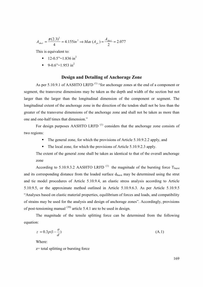
169
22(2.3)
4.155 ( ) 2.0774 2
ductduct ps
AA in Max A
p= = fi = =
This is equivalent to:
� 12-0.5”=1.836 in2
� 9-0.6”=1.953 in2
Design and Detailing of Anchorage Zone
As per 5.10.9.1 of AASHTO LRFD (1) “for anchorage zones at the end of a component or
segment, the transverse dimensions may be taken as the depth and width of the section but not
larger than the larger than the longitudinal dimension of the component or segment. The
longitudinal extent of the anchorage zone in the direction of the tendon shall not be less than the
greater of the transverse dimensions of the anchorage zone and shall not be taken as more than
one and one-half times that dimension.”
For design purposes AASHTO LRFD (1) considers that the anchorage zone consists of
two regions:
� The general zone, for which the provisions of Article 5.10.9.2.2 apply, and
� The local zone, for which the provisions of Article 5.10.9.2.3 apply.
The extent of the general zone shall be taken as identical to that of the overall anchorage
zone
According to 5.10.9.3.2 AASHTO LRFD (1)
the magnitude of the bursting force Tburst
and its corresponding distance from the loaded surface dburst may be determined using the strut
and tie model procedures of Article 5.10.9.4, an elastic stress analysis according to Article
5.10.9.5, or the approximate method outlined in Article 5.10.9.6.3. As per Article 5.10.9.5
“Analyses based on elastic material properties, equilibrium of forces and loads, and compatibility
of strains may be used for the analysis and design of anchorage zones”. Accordingly, provisions
of post-tensioning manual (30)
article 5.4.1 are to be used in design.
The magnitude of the tensile splitting force can be determined from the following
equation:
0.3 (1 )a
z pd
= - (A.1)
Where:
z= total splitting or bursting force

170
P= tendon force
a= depth of the anchor plate
d= depth of the concrete section
Sufficient vertical reinforcement acting at a unit stress of 0.6 of reinforcement yield stress
to resist the computed value of z should be distributed within the distance of d/2 of the anchorage
location.
As per 5.10.9.2.3 AASHTO LRFD (1) “design of local zones shall be either comply with
the reqirments of article 5.10.9.7 or be based on the results of acceptance tests as specified in
Article 5.10.9.7”.
Dimensions of local zone are specified in AASHTP LRFD 5.10.9.7.1 (1) where the
transverse direction of the local zone in each direction should be taken as the greater of:
� The corresponding bearing plate size, plus twice the minimum concrete cover
required for the particular application and environment, and
� The outer dimension of any required confining reinforcement, plus the required
concrete cover over the confining reinforcing steel for the particular application
and environment.
The length of the local zone along the tendon axis shall not be taken less than:
� The maximum width of the local zone;
� The length of the anchorage device confining reinforcement, or
� For anchorage device with multiple bearing surfaces, the distance from the loaded
concrete surface to the bottom of each bearing surface, plus the maximum
dimension of that bearing surface.
The length of the local zone shall not be taken as greater than 1.5 times the width of the
local zone.
Figure A. 1 illustrates locations of local and general zones.
The factored bearing resistance of anchorages shall be taken as:
r n bP f Aj= (A.2)
for which fn is the lesser of:
'0.7 ,andn ci
g
Af f
A= (A.3)
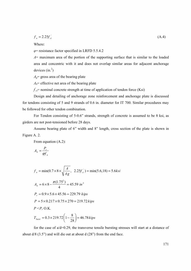
171
'2.25n cif f= (A.4)
Where:
φ= resistance factor specified in LRFD 5.5.4.2
A= maximum area of the portion of the supporting surface that is similar to the loaded
area and concentric with it and does not overlap similar areas for adjacent anchorage
devices (in.2)
Ag= gross area of the bearing plate
Ab= effective net area of the bearing plate
f’ci= nominal concrete strength at time of application of tendon force (Ksi)
Design and detailing of anchorage zone reinforcement and anchorage plate is discussed
for tendons consisting of 5 and 9 strands of 0.6 in. diameter for IT 700. Similar procedures may
be followed for other tendon combination.
For Tendon consisting of 5-0.6” strands, strength of concrete is assumed to be 8 ksi, as
girders are not post-tensioned before 28 days.
Assume bearing plate of 6” width and 8” length, cross section of the plate is shown in
Figure A. 2.
From equation (A.2):
rb
n
PA
fj=
'min(0.7 8 , 2.25 ) min(5.6,18) 5.6n ci
Af f ksi
Ag= ¥ ¥ = =
22(1.75 )
6 8 45.594
bA inp
= ¥ - =
0.9 5.6 45.56 229.79rP kips= ¥ ¥ =
5 0.217 0.75 270 219.72P kips= ¥ ¥ ¥ =
P <Pr O.K.
80.3 219.72 1 46.78
28burstT kips
Ê ˆ= ¥ - =Á ˜Ë ¯
for the case of a/d=0.29, the transverse tensile bursting stresses will start at a distance of
about d/8 (3.5”) and will die out at about d (28”) from the end face.

172
In order to keep the stress in the reinforcement below 0.6 fy=36 ksi
246.781.3
36sA in= =
Hence the number of #3 closed stirrups required is:
1.35.9 6 stirrups
2 0.11= =
¥
we will use 6 stirrups with the first stirrup at 3.5” from the end face and the remaining
stirrups spaced at 5”.
In order to control spalling we will provide reinforcement to resist a tensile force of:
0.02 4.4P kips=
Hence the minimum number of #4 bars working at 36 ksi is:
4.40.61
0.2 36=
¥, Use 2#4. Additionally, we will provide 4#3 U-bars to control potential
vertical splitting cracks on the end face. Assuming VSL-7E15 anchor type use spiral of 10 mm
diameter, 320 mm length, 5 turns. The reinforcing details are summarized in Figure A. 3.
For Tendon consisting of 9-0.6” strands, Assume bearing plate of 6”x14” length, Figure
A. 4 shows cross section of the plate
'min(0.7 8 , 2.25 ) min(5.6,18) 5.6n ci
Af f ksi
Ag= ¥ ¥ = =
22(2.375 )
6 14 79.574
bA inp
= ¥ - =
0.9 5.6 79.57 401.03rP kips= ¥ ¥ =
9 0.217 0.75 270 395.48P kips= ¥ ¥ ¥ =
P <Pr O.K.
140.3 395.48 1 59.32
28burstT kips
Ê ˆ= ¥ - =Á ˜Ë ¯
For the case of a/d=0.5, the transverse tensile bursting stresses will start at a distance of
about d/5 (5.6”) and will die out at about d (28”) from the end face.
In order to keep the stress in the reinforcement below 0.6 fy=36 ksi
259.321.65
36sA in= =

173
Hence the number of #3 closed stirrups required is:
1.657.5 8 stirrups
2 0.11= =
¥
we will use 8 stirrups with the first stirrup at 5” from the end face and the remaining
stirrups spaced at 3”.
In order to control spalling we will provide reinforcement to resist a tensile force of:
0.02 7.91P kips=
Hence the minimum number of #4 bars working at 36 ksi is:
7.911.1
0.2 36=
¥, Use 2#4. We will provide 4#3 U-bars to control potential vertical splitting
cracks on the end face. Assuming VSL-12E15 anchor type use spiral of 15 mm diameter, 600
mm length, 6 turns. The reinforcing details are shown in Figure A. 5
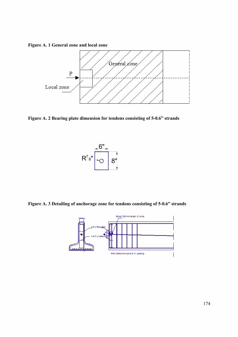
174
Figure A. 1 General zone and local zone
Figure A. 2 Bearing plate dimension for tendons consisting of 5-0.6” strands
Figure A. 3 Detailing of anchorage zone for tendons consisting of 5-0.6” strands
6"
R78" 8"
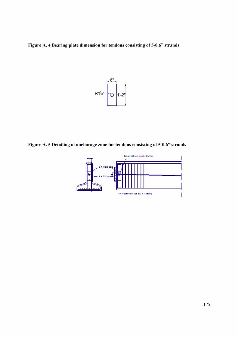
175
Figure A. 4 Bearing plate dimension for tendons consisting of 5-0.6” strands
Figure A. 5 Detailing of anchorage zone for tendons consisting of 5-0.6” strands
6"
1'-2"R118"
176
Appendix B - Program Documentation
The purpose of developing the PT-IT program was for its use as a tool to analyze the
post-tensioned, prestressed, inverted-T system. This includes analysis of shear and moment
forces resulting from girder self-weight, deck weight, time-dependent restraining moments,
secondary moments due to post-tensioning, and external forces. It also includes calculation of
losses in pretensioned strands and post-tensioned tendons. The program also checks girder
capacity and stresses according to AASHTO LRFD. (1)
The PT-IT program is written using C++ language and includes 25 classes. Analysis is
divided into the following major steps:
1. Reading data from the input file (*.inp.txt) may be prepared by the user and saved
as a text file, or prepared using the user-friendly interface, the format of which
will be automatically saved as a text file in the format that the C++ program will
read. The format of the input file is discussed in chapter 3. Input data should
include results of live-load analysis (using Risa or any other program capable of
performing moving load analysis). Live-load data includes maximum shear due to
live load; minimum shear due to live-load; concurrent moments for maximum and
minimum shear, respectively; maximum and minimum moments due to live
loads; and maximum and minimum deflection due to live load as required by
AASHTO LRFD. Live-load data should be saved as a text file with the following
extension: *.LL.txt.
2. For each stage—
a. Calculate element reactions, shear, and moment due to girder self-weight,
deck weight (carried on the simple span or continuous beam), secondary
effect due to post-tensioning, external loads, and time-dependent
restraining moment.
b. Calculate losses in pretensioned strands and post-tensioned tendons during
the time period between each two consecutive stages.

177
3. For each stage, calculate stresses in the concrete according to AASHTO LRFD
requirements.
4. Calculate shear reinforcement required for the girders.
5. Calculate deflection at transfer and at the last stage.
6. Save results as a text file (*.out.txt) that can be read by the interface or directly
from the output file.
Header files for classes forming the PT-IT program are listed below, with a brief
explanation about each class and its functions.
Class “Data”
This class is used for reading input data; creating objects along the way; and saving
output data into objects to be written at the end of analysis, into the output file.
/* Data
The Data class stores all problem data and provides means to access these data.
Design Rationale:
Memory for all data is allocated dynamically after the size of the required storage is
known, during the input-file reading process
Arrays of pointers (double pointers) are used for most objects. */
#ifndef Data_h
#define Data_h
#include <iostream.h>
#include "Node.h"
#include "Element.h"
#include "BCEssential.h"
#include "BCNodalLoad.h"
#include "Matrix.h"
#include "Material.h"
#include <math.h>
#include "Concrete.h"
#include "Steel.h"
#include "PreStrands.h"
#include "LinearPT.h"
#include "MSpanPT.h"
#include "Time.h"
#include "MomentandShear.h"
#include "ConcreteStresses.h"
class Data
{
private:
Node ** nodes; // Array of pointers to node objects

178
Element ** elems; // Array of pointers to element objects (each span is an
// element)
Element ** diaphragm; // Array of pointers to element objects
BCEssential ** essentialBCs; // Array of pointers to essential B.C.
BCNodalLoad ** nodalLoads; // Array of prts to external force The array size is equal to
// the total number of external loads
Concrete ** ConcreteModels; // Array of pointers to user's defined materials
Concrete ** Beammat; // Array of pointers to elements materials
Concrete * Deckmat; // Pointer to deck material
Concrete * Diaphragmmat; // Pointer to diaphragm material
Steel * premat; // Pointer to Prestressing material
teel * postmat; // Pointer to post-tensioning material
PreStrands **prestr; // Array of pointers to prestressing strands (numbre of
// pointers==number of rows)
PostTend ** postten; // Array of pointers to post-tensioning tendons (numbre of
// pointers==number of tendons)
Section **BeamSection; // Array of pointers to element's section (one for each span)
Section *DiaphragmSection; // Pointer to diaphragm's section
ConcreteStresses ** ConStresses; // Array of pointers to save concrete service stresses
Time *time; // Pointer to the matrix which stores stages properties
Matrix * Mcr; // Pointer to the matrix which stores Cracking moments of
// the diaphragms
MomentandShear ** MandV; // Array of pointers to the matrix which stores shear and
// moments
Matrix * MPTSec; // Pointer to array which store secondary moment values
// for all stages
Matrix * VPTSec; // Pointer to array which stores shear due to secondary
// effect of post-tensioning for all stages
Matrix **PreStress; // Array to pointers which store stresses in prestressing
// strands for all stages
Matrix **PostStress; // Array to pointers which store stresses in post-tensioning
// tendons for all stages
Matrix * LiveMoment; // Pointer which stores moment due to live load
Matrix * LiveShear; // Pointer which stores shear due to live load
Matrix * ConMoment; // Pointer which stores moments concurrent to maximum
// and minimum shear
Matrix *Tprov; // Used to store tension force in reinforcement to check
// adequacy of shear reinforcement
Matrix **VerticalShear; // Used to store results of vertical shear analysis
char * title; // Title of input file
char curtype[11]; // Character to store curing type
char name[11];
int nNodes; // Total number of nodes of the model
int nElems; // Total number of elements of the model
int nEssentialBCs; // Total number of essential B.C. of the model
int nNodalLoads; // Total number of external forces.
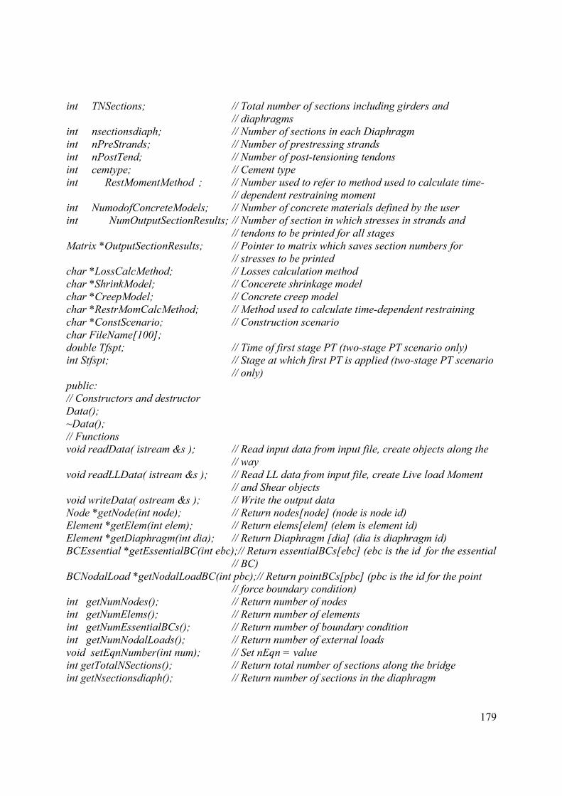
179
int TNSections; // Total number of sections including girders and
// diaphragms
int nsectionsdiaph; // Number of sections in each Diaphragm
int nPreStrands; // Number of prestressing strands
int nPostTend; // Number of post-tensioning tendons
int cemtype; // Cement type
int RestMomentMethod ; // Number used to refer to method used to calculate time-
// dependent restraining moment
int NumodofConcreteModels; // Number of concrete materials defined by the user
int NumOutputSectionResults; // Number of section in which stresses in strands and
// tendons to be printed for all stages
Matrix *OutputSectionResults; // Pointer to matrix which saves section numbers for
// stresses to be printed
char *LossCalcMethod; // Losses calculation method
char *ShrinkModel; // Concerete shrinkage model
char *CreepModel; // Concrete creep model
char *RestrMomCalcMethod; // Method used to calculate time-dependent restraining
char *ConstScenario; // Construction scenario
char FileName[100];
double Tfspt; // Time of first stage PT (two-stage PT scenario only)
int Stfspt; // Stage at which first PT is applied (two-stage PT scenario
// only)
public:
// Constructors and destructor
Data();
~Data();
// Functions
void readData( istream &s ); // Read input data from input file, create objects along the
// way
void readLLData( istream &s ); // Read LL data from input file, create Live load Moment
// and Shear objects
void writeData( ostream &s ); // Write the output data
Node *getNode(int node); // Return nodes[node] (node is node id)
Element *getElem(int elem); // Return elems[elem] (elem is element id)
Element *getDiaphragm(int dia); // Return Diaphragm [dia] (dia is diaphragm id)
BCEssential *getEssentialBC(int ebc);// Return essentialBCs[ebc] (ebc is the id for the essential
// BC)
BCNodalLoad *getNodalLoadBC(int pbc);// Return pointBCs[pbc] (pbc is the id for the point
// force boundary condition)
int getNumNodes(); // Return number of nodes
int getNumElems(); // Return number of elements
int getNumEssentialBCs(); // Return number of boundary condition
int getNumNodalLoads(); // Return number of external loads
void setEqnNumber(int num); // Set nEqn = value
int getTotalNSections(); // Return total number of sections along the bridge
int getNsectionsdiaph(); // Return number of sections in the diaphragm
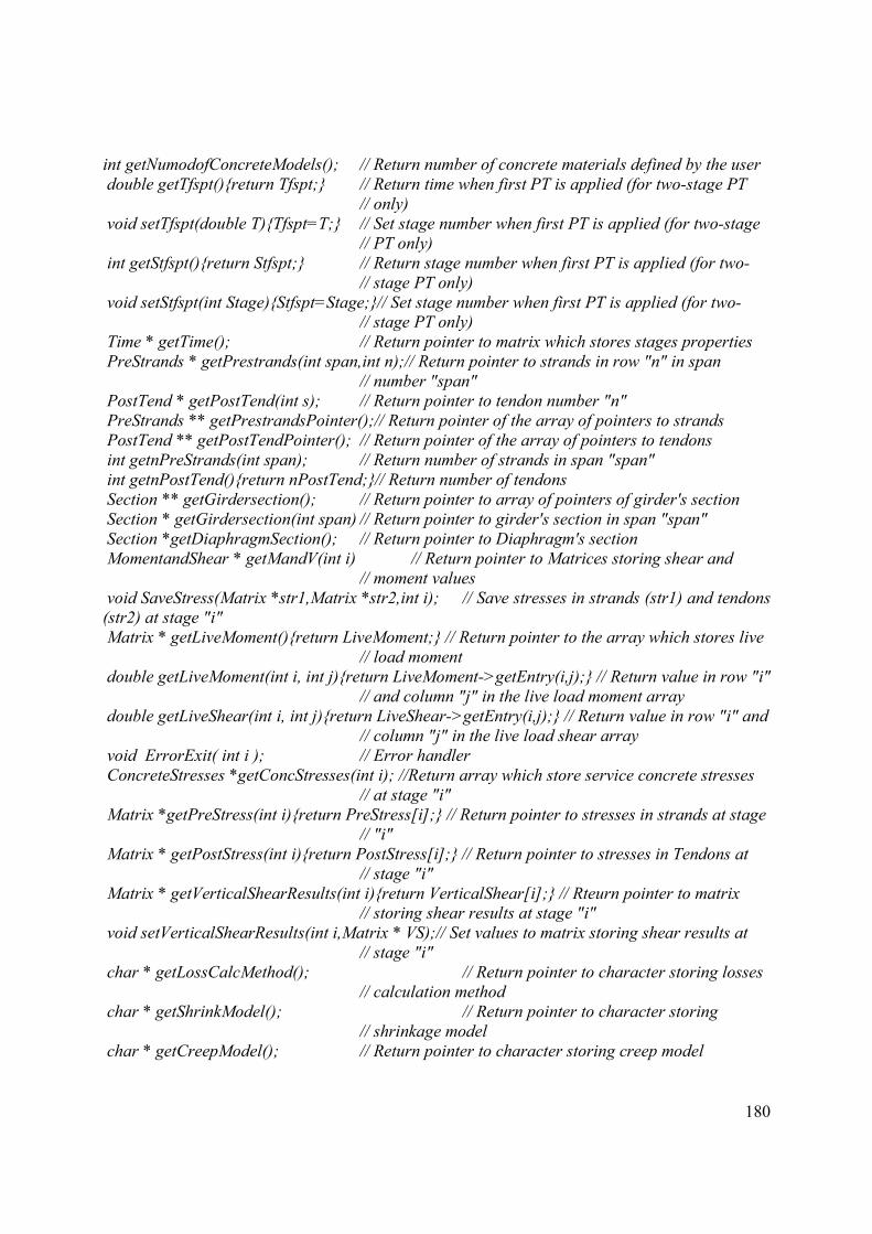
180
int getNumodofConcreteModels(); // Return number of concrete materials defined by the user
double getTfspt(){return Tfspt;} // Return time when first PT is applied (for two-stage PT
// only)
void setTfspt(double T){Tfspt=T;} // Set stage number when first PT is applied (for two-stage
// PT only)
int getStfspt(){return Stfspt;} // Return stage number when first PT is applied (for two-
// stage PT only)
void setStfspt(int Stage){Stfspt=Stage;}// Set stage number when first PT is applied (for two-
// stage PT only)
Time * getTime(); // Return pointer to matrix which stores stages properties
PreStrands * getPrestrands(int span,int n);// Return pointer to strands in row "n" in span
// number "span"
PostTend * getPostTend(int s); // Return pointer to tendon number "n"
PreStrands ** getPrestrandsPointer();// Return pointer of the array of pointers to strands
PostTend ** getPostTendPointer(); // Return pointer of the array of pointers to tendons
int getnPreStrands(int span); // Return number of strands in span "span"
int getnPostTend(){return nPostTend;}// Return number of tendons
Section ** getGirdersection(); // Return pointer to array of pointers of girder's section
Section * getGirdersection(int span) // Return pointer to girder's section in span "span"
Section *getDiaphragmSection(); // Return pointer to Diaphragm's section
MomentandShear * getMandV(int i) // Return pointer to Matrices storing shear and
// moment values
void SaveStress(Matrix *str1,Matrix *str2,int i); // Save stresses in strands (str1) and tendons
(str2) at stage "i"
Matrix * getLiveMoment(){return LiveMoment;} // Return pointer to the array which stores live
// load moment
double getLiveMoment(int i, int j){return LiveMoment->getEntry(i,j);} // Return value in row "i"
// and column "j" in the live load moment array
double getLiveShear(int i, int j){return LiveShear->getEntry(i,j);} // Return value in row "i" and
// column "j" in the live load shear array
void ErrorExit( int i ); // Error handler
ConcreteStresses *getConcStresses(int i); //Return array which store service concrete stresses
// at stage "i"
Matrix *getPreStress(int i){return PreStress[i];} // Return pointer to stresses in strands at stage
// "i"
Matrix * getPostStress(int i){return PostStress[i];} // Return pointer to stresses in Tendons at
// stage "i"
Matrix * getVerticalShearResults(int i){return VerticalShear[i];} // Rteurn pointer to matrix
// storing shear results at stage "i"
void setVerticalShearResults(int i,Matrix * VS);// Set values to matrix storing shear results at
// stage "i"
char * getLossCalcMethod(); // Return pointer to character storing losses
// calculation method
char * getShrinkModel(); // Return pointer to character storing
// shrinkage model
char * getCreepModel(); // Return pointer to character storing creep model
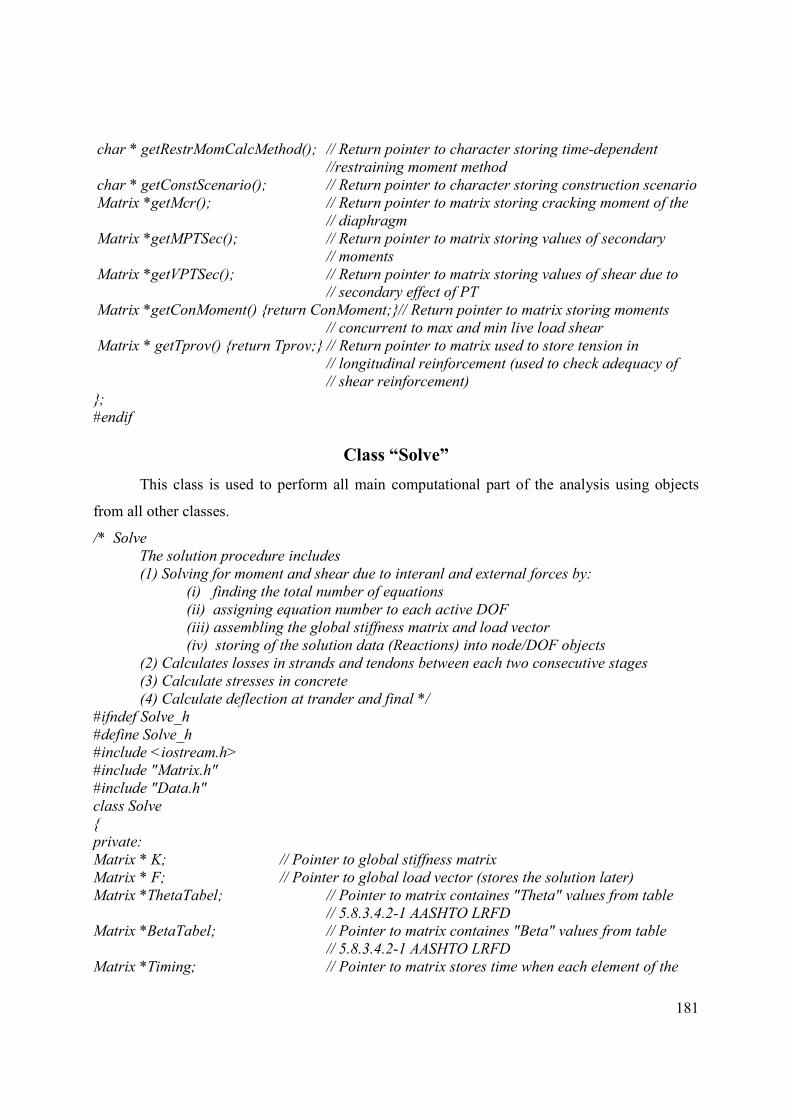
181
char * getRestrMomCalcMethod(); // Return pointer to character storing time-dependent
//restraining moment method
char * getConstScenario(); // Return pointer to character storing construction scenario
Matrix *getMcr(); // Return pointer to matrix storing cracking moment of the
// diaphragm
Matrix *getMPTSec(); // Return pointer to matrix storing values of secondary
// moments
Matrix *getVPTSec(); // Return pointer to matrix storing values of shear due to
// secondary effect of PT
Matrix *getConMoment() {return ConMoment;}// Return pointer to matrix storing moments
// concurrent to max and min live load shear
Matrix * getTprov() {return Tprov;} // Return pointer to matrix used to store tension in
// longitudinal reinforcement (used to check adequacy of
// shear reinforcement)
};
#endif
Class “Solve”
This class is used to perform all main computational part of the analysis using objects
from all other classes.
/* Solve
The solution procedure includes
(1) Solving for moment and shear due to interanl and external forces by:
(i) finding the total number of equations
(ii) assigning equation number to each active DOF
(iii) assembling the global stiffness matrix and load vector
(iv) storing of the solution data (Reactions) into node/DOF objects
(2) Calculates losses in strands and tendons between each two consecutive stages
(3) Calculate stresses in concrete
(4) Calculate deflection at trander and final */
#ifndef Solve_h
#define Solve_h
#include <iostream.h>
#include "Matrix.h"
#include "Data.h"
class Solve
{
private:
Matrix * K; // Pointer to global stiffness matrix
Matrix * F; // Pointer to global load vector (stores the solution later)
Matrix *ThetaTabel; // Pointer to matrix containes "Theta" values from table
// 5.8.3.4.2-1 AASHTO LRFD
Matrix *BetaTabel; // Pointer to matrix containes "Beta" values from table
// 5.8.3.4.2-1 AASHTO LRFD
Matrix *Timing; // Pointer to matrix stores time when each element of the

182
// system and each load is added
double TDiaphragm; // Stores time when diaphragm is cast
int nEqn; // total number of equations (= total number of nodes * 2
// total number of essential BCs)
int setEqnNum( Data &dat); // calculates total number of equations
void assembleRHS(Data &dat,int i,double T); // calculates the global load vector resulting
// external loads considering simply supported spans
void assembleRHSC(Data &dat, int r,double T); // calculates the global load vector resulting
// from external loads considering continious spans
double assembleRHSW(Data &dat,double T,int ind);// calculates the global load vector
// resulting from self weight for deck weight
void assembleRHSCrSH(Data &dat, Matrix & M); // calculates the global load vector
// resulting from effect of creep and differential shrinkage
void assembleK(Data &dat,double t);// assemble the global stiffness matrix. Also modify the
// load vector (for continuous beam)
void assembleKW( Data &dat,double T);// assemble the global stiffness matrix. Also modify the
// load vector (for simply span beam) this is used mainly to
//calculate moments due to self weight of girder and weight
// of the deck when they are carried by the simply supported
// beam
void assembleRHSMPT(double T,Data &dat, Matrix & M); //Calculate load vector resulting
// from secondary effect of PT
void saveSolution(Data &dat); // Save the solution into each active DOF
public:
// Constructors & destructor
Solve();
virtual ~Solve();
//Functions
void solve(Data &dat); // Main function that calls all sub-functions that perform
// analysis
void calcElementReactions(Data &dat,double T,double ind);// Used to calculate element
// reactions
void calcMoment_Shear(Data&dat,int j,int StageNum, double T);//Used to calculate moment
// and shear ate each section along the beam
void calcDeflection(Data&dat); // Used to calculate deflection at transfer and final
void calcShearReinforcement(Data&dat); // Used to calculate amount of shear reinforcement
// needed
double getTheta(double ex, double vu); // Return value of "Theta" corresponding to strain
// ex and shear vu
double getBeta(double ex, double vu);// Return value of "Beta" corresponding to strain ex and
// shear vu
void calcTimeDependentLosses(int StageNum,Data& dat); // Calc losses in stresses in strands
// and tendons between stage "StageNum" and
// “StageNum+1" using AASHTO LRFD method
void calcTimeDependentLosses_Creep_Transformed_Method(int StageNum,Data &dat); // Calc
// losses in stresses in strands and tendons between stage
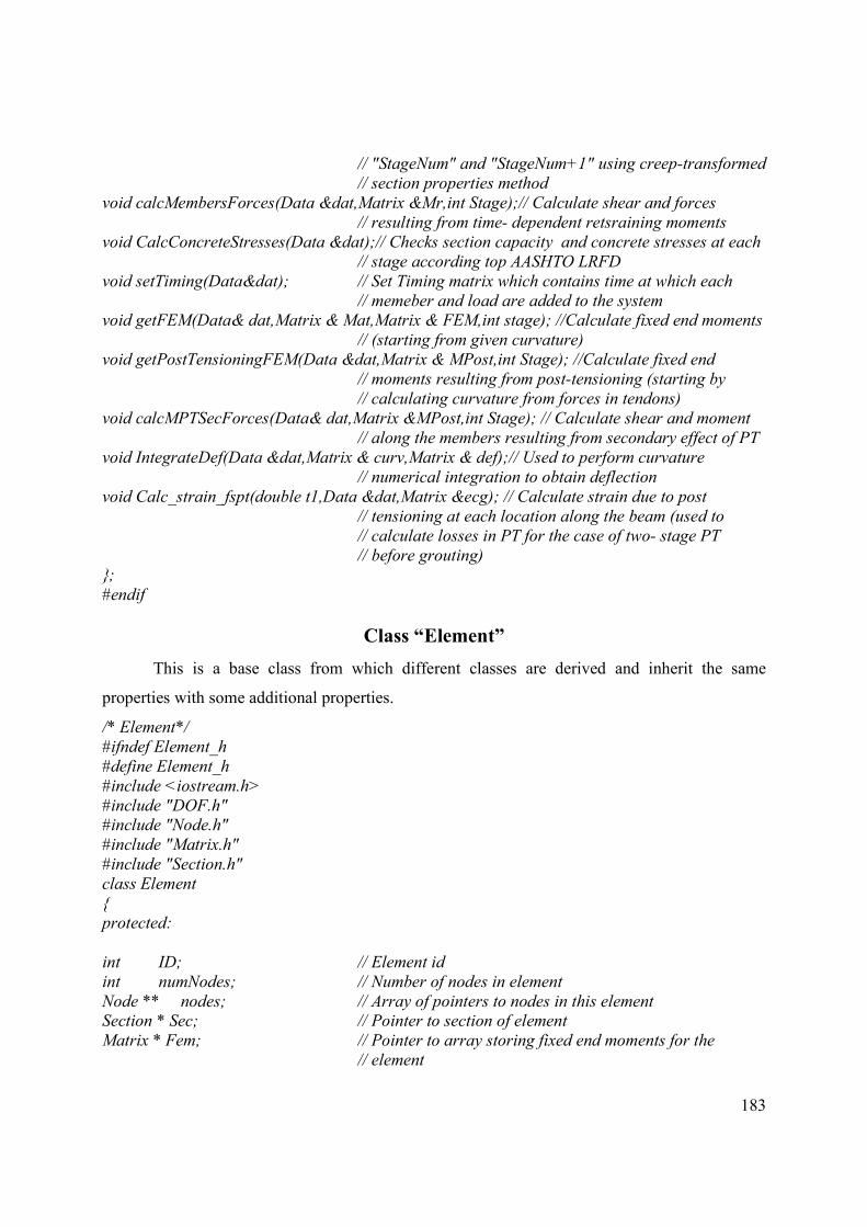
183
// "StageNum" and "StageNum+1" using creep-transformed
// section properties method
void calcMembersForces(Data &dat,Matrix &Mr,int Stage);// Calculate shear and forces
// resulting from time- dependent retsraining moments
void CalcConcreteStresses(Data &dat);// Checks section capacity and concrete stresses at each
// stage according top AASHTO LRFD
void setTiming(Data&dat); // Set Timing matrix which contains time at which each
// memeber and load are added to the system
void getFEM(Data& dat,Matrix & Mat,Matrix & FEM,int stage); //Calculate fixed end moments
// (starting from given curvature)
void getPostTensioningFEM(Data &dat,Matrix & MPost,int Stage); //Calculate fixed end
// moments resulting from post-tensioning (starting by
// calculating curvature from forces in tendons)
void calcMPTSecForces(Data& dat,Matrix &MPost,int Stage); // Calculate shear and moment
// along the members resulting from secondary effect of PT
void IntegrateDef(Data &dat,Matrix & curv,Matrix & def);// Used to perform curvature
// numerical integration to obtain deflection
void Calc_strain_fspt(double t1,Data &dat,Matrix &ecg); // Calculate strain due to post
// tensioning at each location along the beam (used to
// calculate losses in PT for the case of two- stage PT
// before grouting)
};
#endif
Class “Element”
This is a base class from which different classes are derived and inherit the same
properties with some additional properties.
/* Element*/
#ifndef Element_h
#define Element_h
#include <iostream.h>
#include "DOF.h"
#include "Node.h"
#include "Matrix.h"
#include "Section.h"
class Element
{
protected:
int ID; // Element id
int numNodes; // Number of nodes in element
Node ** nodes; // Array of pointers to nodes in this element
Section * Sec; // Pointer to section of element
Matrix * Fem; // Pointer to array storing fixed end moments for the
// element

184
Matrix * R; // Pointer to array storing reactions of the element
Matrix * V; // Pointer to array storing shear forces along the element
Matrix * M; // Pointer to array storing moment values along the element
int nsections; // Number of sections in the element
public:
// Constructors & destructor
Element(int id, Node ** nodes,Section *Sec,int n_sections);
virtual ~Element();
// Functions
int getID() const; // Return ID;
int getNumNodes() const; // Return numNodes;
int getnSections(); // Return number of sections along the element
Node ** getNodeList() const; // Return pointer array of nodes
void setFEM(Matrix &m); // Set values of fixed end mements
vid setR(Matrix &re); // Set values of reactions
void setV(Matrix &v,int j); // Set values of shear forces
void setM(Matrix &m,int j); // Set values of moments
double getV(int i, int j); // Return values of shear forces
double getM(int i, int j); // Return values of moments
double getFEM(int i, int j) // Return values of fixed end moments
double getR(int i, int j); // Return values of reactions
friend ostream & operator<<( ostream &s, const Element & node ); //Function used for output
// data
// Virtual functions have to be implemented in individual element types
virtual int getNumDOFs() const = 0; // Return the total number of DOFs
virtual void getElementK( Node *bn, Node *en,double t, double l, Matrix &esm ) = 0;//Calculate
// and return element stiffness matrix.
virtual void print(ostream &out) const = 0;
virtual Section * getSection()=0; // Return pointer to element's section
virtual double getL()=0; // Return length of the element
};
#endif
Class “Element2”
This class is a derived class from class “Element” it creates girders elements with 2
nodes.
/*Element*/
#ifndef Element2_h
#define Element2_h
#include "Element.h"
#include <iostream.h>
class Element2 : public Element
{
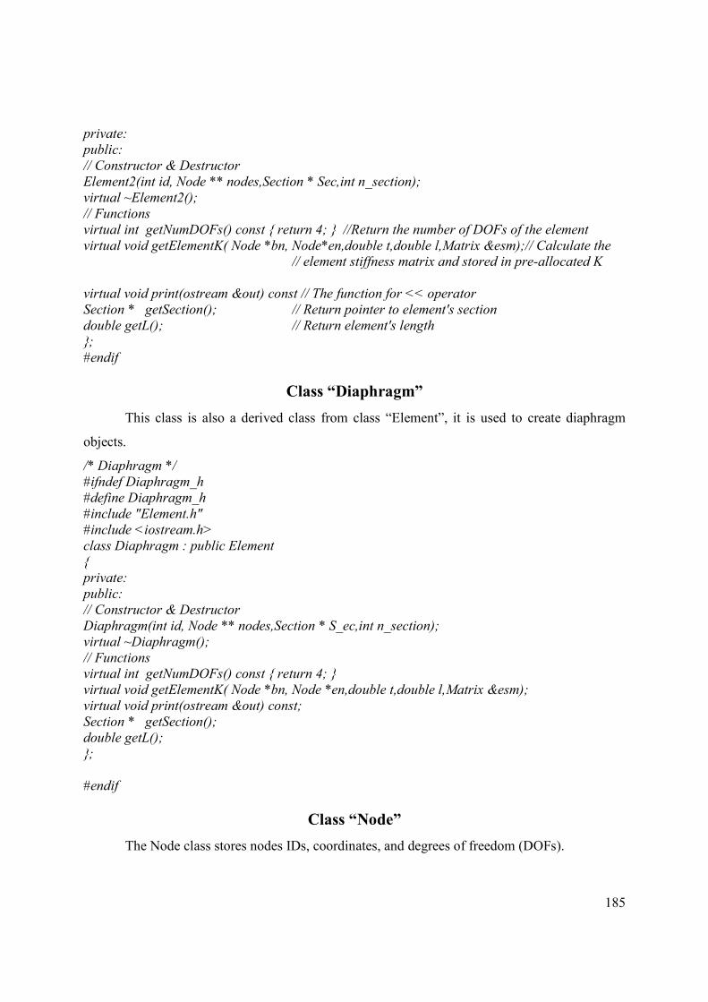
185
private:
public:
// Constructor & Destructor
Element2(int id, Node ** nodes,Section * Sec,int n_section);
virtual ~Element2();
// Functions
virtual int getNumDOFs() const { return 4; } //Return the number of DOFs of the element
virtual void getElementK( Node *bn, Node*en,double t,double l,Matrix &esm);// Calculate the
// element stiffness matrix and stored in pre-allocated K
virtual void print(ostream &out) const // The function for << operator
Section * getSection(); // Return pointer to element's section
double getL(); // Return element's length
};
#endif
Class “Diaphragm”
This class is also a derived class from class “Element”, it is used to create diaphragm
objects.
/* Diaphragm */
#ifndef Diaphragm_h
#define Diaphragm_h
#include "Element.h"
#include <iostream.h>
class Diaphragm : public Element
{
private:
public:
// Constructor & Destructor
Diaphragm(int id, Node ** nodes,Section * S_ec,int n_section);
virtual ~Diaphragm();
// Functions
virtual int getNumDOFs() const { return 4; }
virtual void getElementK( Node *bn, Node *en,double t,double l,Matrix &esm);
virtual void print(ostream &out) const;
Section * getSection();
double getL();
};
#endif
Class “Node”
The Node class stores nodes IDs, coordinates, and degrees of freedom (DOFs).
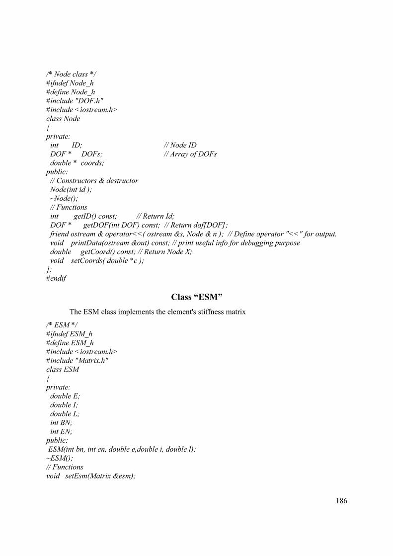
186
/* Node class */
#ifndef Node_h
#define Node_h
#include "DOF.h"
#include <iostream.h>
class Node
{
private:
int ID; // Node ID
DOF * DOFs; // Array of DOFs
double * coords;
public:
// Constructors & destructor
Node(int id );
~Node();
// Functions
int getID() const; // Return Id;
DOF * getDOF(int DOF) const; // Return dof[DOF];
friend ostream & operator<<( ostream &s, Node & n ); // Define operator "<<" for output.
void printData(ostream &out) const; // print useful info for debugging purpose
double getCoord() const; // Return Node X;
void setCoords( double *c );
};
#endif
Class “ESM”
The ESM class implements the element's stiffness matrix
/* ESM */
#ifndef ESM_h
#define ESM_h
#include <iostream.h>
#include "Matrix.h"
class ESM
{
private:
double E;
double I;
double L;
int BN;
int EN;
public:
ESM(int bn, int en, double e,double i, double l);
~ESM();
// Functions
void setEsm(Matrix &esm);
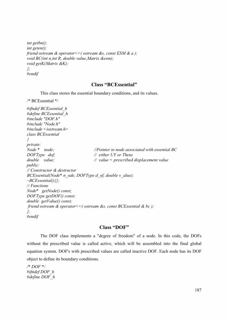
187
int getbn();
int geten();
friend ostream & operator<<( ostream &s, const ESM & a );
void BC(int n,int R, double value,Matrix &esm);
void getK(Matrix &K);
};
#endif
Class “BCEssential”
This class stores the essential boundary conditions, and its values.
/* BCEssential */
#ifndef BCEssential_h
#define BCEssential_h
#include "DOF.h"
#include "Node.h"
#include <iostream.h>
class BCEssential
{
private:
Node * node; //Pointer to node associated with essential BC
DOFType dof; // either UY or Theta
double value; // value = prescribed displacement value
public:
// Constructor & destructor
BCEssential(Node* n_ode, DOFType d_of, double v_alue);
~BCEssential(){};
// Functions
Node* getNode() const;
DOFType getDOF() const;
double getValue() const;
friend ostream & operator<<( ostream &s, const BCEssential & bc );
};
#endif
Class “DOF”
The DOF class implements a "degree of freedom" of a node. In this code, the DOFs
without the prescribed value is called active, which will be assembled into the final global
equation system. DOF's with prescribed values are called inactive DOF. Each node has its DOF
object to define its boundary conditions.
/* DOF */
#ifndef DOF_h
#define DOF_h

188
#include <iostream.h>
enum DOFType{UY=0,Theta};
class DOF
{
private:
double value; // The value of this degree of freedom. For essential BC
// (inactive DOF), it is the prescribed (displacement) value.
// For active DOF, it stores displacement value after system
// equations are solved.
int eqnNum; // equation number of DOF. (-1 indicates an inactive DOF)
public:
// Constructors & Destructors
DOF();
~DOF();
// Functions
bool isActive() const // Return active;
int getEqnNum() const; // Return eqnNum;
double getValue() const; // Return value;
friend ostream & operator<<( ostream &s, const DOF & d );
void setNotActive(); // Set active = false;
void setEqnNum(int n); // For active DOF, set eqnNum = n; for inactive DOF, set
// eqnNum = -1 (or any negative integer)
void setValue(double v); //Set value = value;
};
#endif
Class “FixedEM”
This class calculates fixed end moments resulting from uniform and concentrated loads
/* FixedEM */
#ifndef FixedEM_h
#define FixedEM_h
#include "DOF.h"
#include "Node.h"
#include "Element.h"
#include "Data.h"
#include <iostream.h>
enum LLoadType {UU=0, CC};
class FixedEM
{
private:
Element * elem;
Node *node;
LLoadType ltype;
double bl; //begining location from the right support
double v; //end value

189
public:
// Constructors & Destructor
FixedEM( Element* e_lem, LLoadType l_type, double b_l,double b_v);
FixedEM(Element* e_lem, LLoadType l_type, double b_v);
~FixedEM();
// Functions
void calcFEM(Data& dat);
};
#endif
Class “BCNodalLoad”
The BCNodalLoad class stores properties for uniform and concentrated forces.
/* BCNodalLoad */
#ifndef BCNodalLoad_h
#define BCNodalLoad_h
#include "Node.h"
#include "Element.h"
#include <iostream.h>
enum LoadType {U=0, C};
class BCNodalLoad
{
private:
Element * elem;
Node * node;
LoadType ltype;
Element ** el;
int nelem;
double bl; //begining location from the right support
double v; //end value
public:
// Constructors & Destructor
BCNodalLoad(LoadType l_type, Element* e_lem, double b_l,double b_v);
BCNodalLoad(LoadType l_type,int numelem, Element ** e_lem, double b_v);
BCNodalLoad(LoadType l_type,Element * e_lem, double b_v);
BCNodalLoad(int numelem);
~BCNodalLoad();
// Functions
Element * getElement() const;
LoadType getLoadType() const;
double getValue() const;
int getnelem();
double getbl();
Element * getel(int i);
friend ostream & operator<<( ostream &s, const BCNodalLoad &load );
void calcFEM();

190
};
#endif
Class “MomentandShear”
This class is used to store moment and shear resulting from analysis, due to internal and
external loads applied on the structure.
/* MomentandShear*/
#ifndef MomentandShear_h
#define MomentandShear_h
#include <iostream.h>
#include "Matrix.h"
class MomentandShear
{
private:
Matrix *M;
Matrix *V;
Matrix *Deflection;
int nSections;
int nSpans;
int DianSections;
int nStages;
public:
MomentandShear(int nSections,int nSpans,int DianSections, int nStages);
~MomentandShear();
// Functions
void setM(Matrix &m, int i,int j);
void setV(Matrix &v, int i,int j);
void setDeflection(Matrix &deflection, int i,int j);
double getM(int i, int j);
double getV(int i,int j);
double getDeflection(int i,int j);
void setDeflection(double val,int i,int j);
Matrix * getM();
Matrix * getV();
Matrix * getDeflection();
int MomentandShear:: getNumRows();
int MomentandShear:: getNumCols();
void MomentandShear::addLiveM(int i,int j, double v);
void MomentandShear::addLiveV(int i,int j, double v);
void printMandV();
};
#endif
Class “Concrete Stresses”

191
This class is used to store stresses of the concrete and capacity calculated as required by
AASHTO LRFD
/* Concrete Stresses */
#ifndef ConcreteStresses_h
#define ConcreteStresses_h
#include "Matrix.h"
#include "Concrete.h"
#include "PreStrands.h"
#include "LinearPT.h"
#include "MSpanPT.h"
#include "Time.h"
#include <iostream.h>
class ConcreteStresses
{
private:
int Nrows;
double fi;
Matrix * ReleaseAll_Comp_Stress;
double ReleaseAll_Comp_Stress_Deck;
double ReleaseAll_Tens_Stress;
Matrix * All_Comp_Stress_ServicI_I;
Matrix * All_Comp_Stress_ServicI_II;
Matrix * All_Tens_Stress_ServicIII;
double All_Comp_Stress_ServicI_I_Deck;
double All_Comp_Stress_ServicI_II_Deck;
double All_Comp_Stress_ServicIIII_Deck;
Matrix * StrengthI;
Matrix * ServiceI_I;
Matrix * ServiceI_II;
Matrix * ServiceIII;
public:
//Constructor & Destructor
ConcreteStresses(int i,int nSpans,Concrete ** Beammat,Concrete * Deckmat,PreStrands **
PreStress,PostTend **PostStress,int TNSection,Time * time);
~ConcreteStresses();
void setStrengthI(Matrix & strengthI);
void setServiceI_I(Matrix & serviceI_I);
void setServiceI_II(Matrix & serviceI_III);
void setServiceIII(Matrix & serviceIII);
void setStrengthI (int i, int j,double k);
void setServiceI_I (int i, int j,double k);
void setServiceI_II(int i, int j,double k);
void setServiceIII (int i, int j,double k);
void printConcStresses();
double getReleaseAll_Comp_Stress(int i);

192
double getReleaseAll_Comp_Stress_Deck();
double getReleaseAll_Tens_Stress();
double getAll_Comp_Stress_ServicI_I(int i);
double getAll_Comp_Stress_ServicI_II(int i);
double getAll_Tens_Stress_ServicIII(int i);
double getAll_Comp_Stress_ServicI_I_Deck();
double getAll_Comp_Stress_ServicI_II_Deck();
double getAll_Comp_Stress_ServicIII_Deck();
Matrix * getStrengthI();
Matrix * getServiceI_I();
Matrix * getServiceI_II();
Matrix * getServiceIII();
};
#endif
Class “Meterial”
The material is a base class that provides common interface for materials. Specific
material class is derived from this class and may contain its own additional interface. This is an
abstract class that cannot be directly instantiated. Two classes are derived from this class
“Concrete” and “Steel” classes.
/* Material */
#ifndef Material_h
#define Material_h
#include "Matrix.h"
#include <iostream.h>
class Material
{
protected:
char Name [15];
int ID;
double E;
public:
//Constructor & Destructor
Material(int i);
virtual ~Material();
//Functions
int getID() const; // Return Id;
char *getName();
};
#endif
Class “Steel”

193
/* Steel class */
#ifndef Steel_h
#define Steel_h
#include "Material.h"
#include <iostream.h>
class Steel: public Material
{
private:
double fpu;
double fy;
public:
//Constructor & Destructor
Steel(int i,double fpu, double fy);
virtual ~Steel();
double getfpu();
double getfy();
double getE();
void setfpu(double a);
void setfy(double a);
void setE(int a);
};
#endif
Class “Concrete”
/* Concrete class */
#ifndef Concrete_h
#define Concrete_h
#include "Material.h"
#include "PreStrands.h"
#include "LinearPT.h"
#include "MSpanPT.h"
#include "Matrix.h"
#include <iostream.h>
class Concrete: public Material
{
private:
char Model[20];
char CuringType[11];
char Name[20];
int CementType;
double wc;
double fpct;
double fpc28;
double fpci;
double fr;
double H;

194
double t; //t is time in days
public:
//Constructor & Destructor
Concrete(int i,char * model,char *name,char * CuringType,int CementType,double fpci,double
fpc28,double wc, double h );
virtual ~Concrete();
double getfci(); // Get initial strength
double getfpct(double T); // Get concrete strength at time "T"
double getfpc28(){ return fpc28;} // Get concrete strength at 28 days
double getE(double T); // Get modulus of elasticity time "T"
double getE28(double fpc28) ; // Get modulus of elasticity at 28 days
double getE_Cr(double E1, double X, double fi); // Get creep modified modulus of elasticity at
// 28 days
double getWc(); // Get unit weight
void setWc(double a); // Set unit weight
void setfpc28(double a); // Set concrete strength at 28 days
void setCementType(int a) ; // Set cement type
void setCuringType(char*a); // Set curing type
void setName(char*a); // Set name of the concrete material
char * getCurtype(); // Get curing type
char * getName(); // Get name
int getcemtype(); // Get cement type
double getH(){ return H;} // Get humidity of the enviroment surrounding the concrete
};
#endif
Class “PreStrands”
This class stores properties of pretensioned strands; it allows construction of straight as
well as one and two point depression strands.
/* PrestensionedStrands */
#ifndef PreStrands_h
#define PreStrands_h
#include <iostream.h>
#include "Steel.h"
class PreStrands
{
protected:
char ID[13];
char TenType[10];
char TenProf[10];
int Num;
float ec0;
double jacking;///ratio of the ultimate stress
double d;
double area;

195
float DepressFraction;
float DepressIncrement;
Steel * mat;
Matrix *Stress;
int nSections;
int NSpan;
public:
// Constructors & destructor
PreStrands(Steel *mat,int nspan,char *ID, char *TenType,char *TenProf, int Num, float ecc0);
PreStrands(Steel *mat,int nspan,char *ID, char *TenType, char *TenProf,int Num, float
ecc0,float DepressFraction);
~PreStrands();
int getNum()const;
double getecc(double x);//x is a fraction of the length
double getAngle(double x);//x is a fraction of the length
double getec0();
double getArea();
double getd();
Steel *getmat();
double getJacking();
float getDepFrac();
double CalcElasticShortening(double fcgp, double eci);
void setStress(Matrix * stress);
void setStress(int i,double v);///sets the value of stress v at the row number i
Matrix * getStress();
double getStress(int i);
int getnSections();
int getnElems();
char *getTenType();
char * getTenprof();
char * getID();
void setnSections(int n);
};
#endif
Class “PostTend”
This class is a base class from which two classes are derived, “Straight” and “Parabolic”
/* Post tensioned Tendons */
#ifndef PostTend_h
#define PostTend_h
#include <iostream.h>
#include "Steel.h"
#include "Matrix.h"

196
class PostTend {
protected:
char ID[15];
char TenType[10];
char TenProfile[9];
double D;
double Area;
double AnchSet;
double FricCoeff;
double WobbleCoeff;
double Jacking;
double ecc;
Steel *mat;
Matrix *Stress;
Matrix *stress; //Helps to calaculate the Friction Loss
int NSpan;
int nSections;
double Lset;
double LsetStress;
public:
// Constructors & destructor
PostTend(Steel *mat,int nSpan,char *ID,char *TenProfile,double AnchSet,double FricCoeff,
double WobbleCoeff, double Jacking,int nsections);
virtual ~PostTend();
virtual double getecc(double x)=0;//x is in (inch)
virtual double getAngle(double x)=0;//x is in (inch)
Steel * getmat();
double getArea();
double getJacking();
char * getTendProfile();
char * getTendType();
char * getID();
double returnecc();
virtual double getFrictionAngleChange()=0;
double CalcElasticShortening(int N,double fcgp, double eci);
int getnSections();
void setStress(Matrix * stress);
void setStress(int i,double v);
Matrix * getStress();
double getStress(int i);
void setstress(int i,int j,double v);
double getstress(int i,int j);
double getAnchSet(int i);
double getWobbleCoeff();
double getFricCoeff();
int getNSpans();

197
void setLset(double x) {Lset=x;}
void setLsetStress(double x) {LsetStress=x;}
double getLset() {return Lset;}
double getLsetStress() {return LsetStress;}
virtual int getNRow()=0;
};
#endif
Class “Straight”
/* StraightPT */
#ifndef StraightPT_h
#define StraightPT_h
#include "PostTend.h"
#include <iostream.h>
#include "Matrix.h"
class StraightPT : public PostTend
{
private:
public:
// Constructor & Destructor
StraightPT(Steel *mat,int nSpan,char *ID,char *TenProfile,double AnchSet,double FricCoeff,
double WobbleCoeff, double Jacking,double e_cc,int nsections);
~StraightPT();
// Functions
double getecc(double x);
double getFrictionAngleChange();
int getNRow();
double getAngle(double x);
};
#endif
Class “ParabolicPT”
/* ParabolicPT */
#ifndef ParabolicPT_h
#define ParabolicPT_h
#include "PostTend.h"
#include <iostream.h>
#include "Matrix.h"
class ParabolicPT : public PostTend
{
private:
//
int NSpan;
Matrix *XY;
Matrix *xy;

198
Matrix *xy1; //original xy that is provided by the user
int NRow;
double contraflexure;
public:
// Constructor & Destructor
ParabolicPT(Steel *mat,int NSpan,char *ID,char *TenProfile,double AnchSet,double FricCoeff,
double WobbleCoeff, double Jacking,double contraflexure, Matrix * xy,int nsections);
~ParabolicPT();
// Functions
double getecc(double x);
double getAngle(double x);
double getFrictionAngleChange();
int getNRow(){return NRow;}
};
#endif
Class “Section”
/* Section*/
#ifndef Section_h
#define Section_h
#include <iostream.h>
#include "Material.h"
#include "Concrete.h"
#include "PreStrands.h"
#include "PostTend.h"
class Section {
private:
int CrackingInd; // Used to indicate when the diaphragm has cracked (for P
// Method)
int id; // Used to indicate when the Deck is added to the system
int ipre; /// Used to indicate when the strands is added to the system
int ipost; // Used to indicate when the post-tensioned is added to the system
double Cg; // Distance from the centroid of the section to the bottom of the
// Concrete sectio
double A; // Area of the girder's section
double Ixx; // Moment of Inertia around the X axis for the girder's Section
double VtA; // Volume to Area ratio for the Concrete Section
double H; // Overall Height of the Conceret Section
double WW; // Girder's web width
double hf; // IT flange thickness=5.51 in
double w; // Effective Width of the deck
double hd; // Height of the deck
double CgCompg; // Distance from the centroid of the section to the bottom of
// the (girder and prestressing) Composite section
double Acompg; // Area of the (girder and prestressing) composite section
double IxxCompg; // Moment of inertia around the X axis for the (girder and
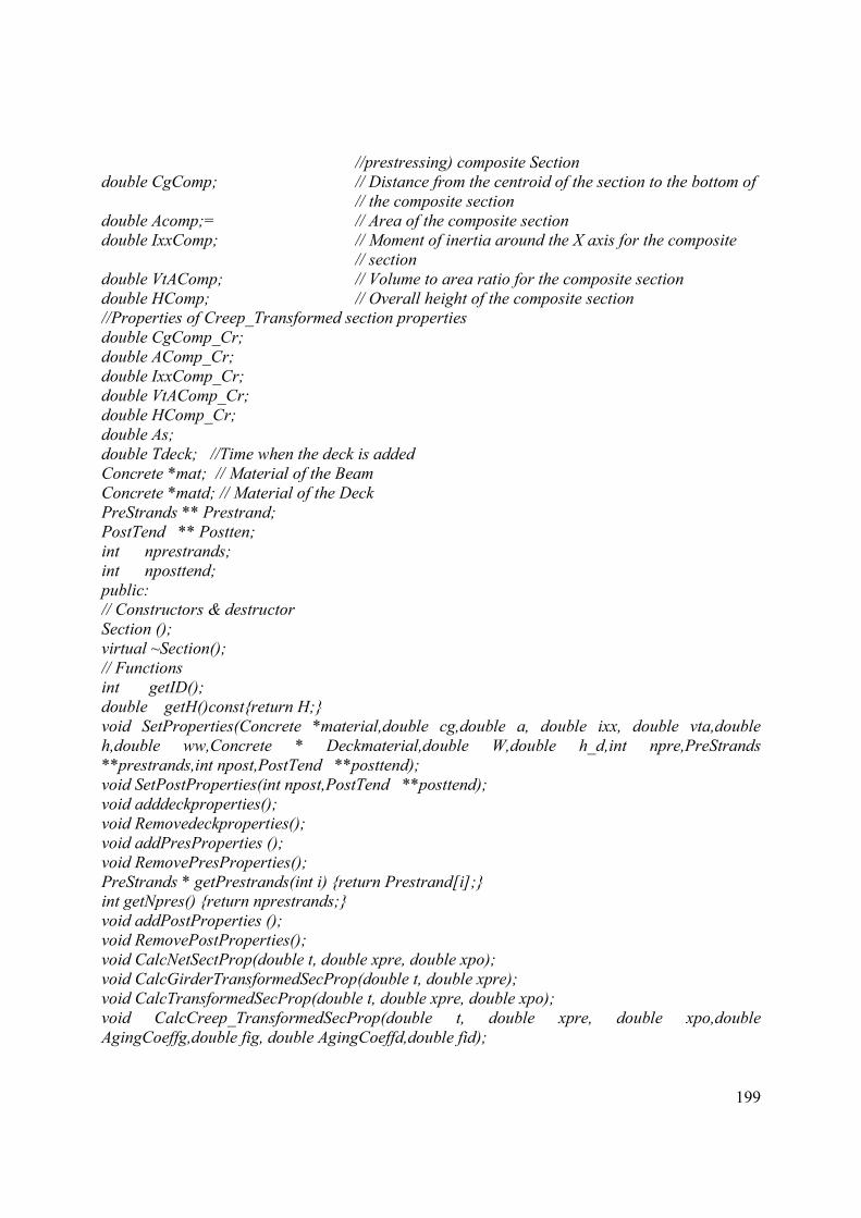
199
//prestressing) composite Section
double CgComp; // Distance from the centroid of the section to the bottom of
// the composite section
double Acomp;= // Area of the composite section
double IxxComp; // Moment of inertia around the X axis for the composite
// section
double VtAComp; // Volume to area ratio for the composite section
double HComp; // Overall height of the composite section
//Properties of Creep_Transformed section properties
double CgComp_Cr;
double AComp_Cr;
double IxxComp_Cr;
double VtAComp_Cr;
double HComp_Cr;
double As;
double Tdeck; //Time when the deck is added
Concrete *mat; // Material of the Beam
Concrete *matd; // Material of the Deck
PreStrands ** Prestrand;
PostTend ** Postten;
int nprestrands;
int nposttend;
public:
// Constructors & destructor
Section ();
virtual ~Section();
// Functions
int getID();
double getH()const{return H;}
void SetProperties(Concrete *material,double cg,double a, double ixx, double vta,double
h,double ww,Concrete * Deckmaterial,double W,double h_d,int npre,PreStrands
**prestrands,int npost,PostTend **posttend);
void SetPostProperties(int npost,PostTend **posttend);
void adddeckproperties();
void Removedeckproperties();
void addPresProperties ();
void RemovePresProperties();
PreStrands * getPrestrands(int i) {return Prestrand[i];}
int getNpres() {return nprestrands;}
void addPostProperties ();
void RemovePostProperties();
void CalcNetSectProp(double t, double xpre, double xpo);
void CalcGirderTransformedSecProp(double t, double xpre);
void CalcTransformedSecProp(double t, double xpre, double xpo);
void CalcCreep_TransformedSecProp(double t, double xpre, double xpo,double
AgingCoeffg,double fig, double AgingCoeffd,double fid);

200
double Section::getCgCompg();
double Section::getIxxCompg();
double Section::getACompg();
double getCgComp();
double getIxxComp();
double getAComp();
double getCgComp_Cr();
double getIxxComp_Cr();
double getAComp_Cr();
double getCg();
double getWW();
double gethf(){return hf;}
double getIxx();
double getA();
Concrete *getmat();
Concrete *getDeckmat();
double getVtAComp();
double getVtA();
double gethdeck();
double getHComp();
double getwdeck();
void setTdeck(double T);
void setCrackingInd(){CrackingInd=1;};
void unsetCrackingInd(){CrackingInd=0;};
int getCrackingInd(){return CrackingInd;};
void setAs(double as) {As=as;}
double getAs() {return As;}
};
#endif
Class “TimeDepLosses”
This class is used to calculate shrinkage and creep properties of the concrete.
/* TimeDep.Losses class */
#ifndef TimeDepLosses_h
#define TimeDepLosses_h
#include <iostream.h>
#include "Matrix.h"
class TimeDepLosses{
private:
double VtS;
double t1;
double t2;
double ti;
double H;
double CR;

201
double SH;
double RE;
char CType[11];//concrete type
char SHModel[20];
char CrModel[20];
Matrix * Aging_Coeff;
public:
TimeDepLosses(char *Shmodel,char *Crmodel,char * cType,double vts, double h);
~TimeDepLosses();
double CalcShrinkage(double Fpc,double Ti,double T1);
double CalcPartialShrinkage(double Fpc,double Ti,double T1,double T2);
double CalcPartialRelaxation(char *TType,double Fpi,double Fy,double T1,double T2);
double CalcPartialfi(double Fpc,double Ti,double T1,double T2);
double Calcfi(double Fpc, double t0,double t);
double Calcfu(double Fpc, double t0);
double getAgingCoeff(double Fpc,double t,double t0);
};
#endif
Class “Time”
This class saves stages properties.
/* Time */
#ifndef Time_h
#define Time_h
#include <iostream.h>
#include "Matrix.h"
class Time
{
private:
int N;
Matrix *time;
public:
// Constructor & destructor
Time(Matrix * ttime);
~Time();
// Functions
int getN();
double gettime(int i, int j);
};
#endif
Class “Matrix”
This class is used to perform manipulation for matrices
/* Matrix */

202
#ifndef Matrix_h
#define Matrix_h
#include <stdio.h>
#include <stdlib.h>
#include <iostream.h>
class Matrix{
private:
double ** entry; // Entries of the matrix. Double point format
int n_row; // Number of rows
int n_column; // Number of columns
public:
// Constructor and destructor
Matrix(int row, int column ); //construct a nr x nc matrix
~Matrix();
// Functions
void zero(); // Initialize all coefficients of the matrix to zero
int getNumRows() const; // Return n_row;
int getNumCols() const; // Return n_column;
friend ostream & operator<<( ostream &s, const Matrix & a );
void setEntry(int i, int j, double value);
void addToEntry(int i, int j, double value);
double getEntry(int i, int j) ;
// Arithmatics
Matrix & operator +=( Matrix &a ); // (*this) = (*this) + a
Matrix & operator *=( double a ); // (*this) = (*this) * a
void mult(Matrix &b, Matrix &c);// c = (*this) * b
void trans(Matrix &a); // a = (*this)^T
// Solver of Gaussian elimination. This is a so-called "Fully Pivoted
// Gaussian Elimination" solver. Solve the equation [*this]{x} = {b}.
// Solution is stored back into b, so the original b is destroyed.
void gauss_solver( Matrix & b );
};
#endif