evaluation of the inverted tee shallow bridge system for use in ...

Report No. K-TRAN: KSU-00-1 FINAL REPORT EVALUATION OF THE INVERTED TEE SHALLOW BRIDGE SYSTEM FOR USE IN KANSAS Sameer Ambare Robert J. Peterman Kansas State University Manhattan, Kansas

DECEMBER 2006 K-TRAN A COOPERATIVE TRANSPORTATION RESEARCH PROGRAM BETWEEN: KANSAS DEPARTMENT OF TRANSPORTATION KANSAS STATE UNIVERSITY THE UNIVERSITY OF KANSAS

1 Report No. K-TRAN: KSU-00-1

2 Government Accession No.

3 Recipient Catalog No.

5 Report Date December 2006

4 Title and Subtitle EVALUATION OF THE INVERTED TEE SHALLOW BRIDGE SYSTEM FOR USE IN KANSAS

6 Performing Organization Code

7 Author(s) Sameer Ambare and Robert J. Peterman

8 Performing Organization Report No.

10 Work Unit No. (TRAIS)

9 Performing Organization Name and Address Kansas State University Department of Civil Engineering 2113 Fiedler Hall Manhattan, Kansas 66506-2905

11 Contract or Grant No. C1161

13 Type of Report and Period Covered Final Report September 1999 – October 2006

12 Sponsoring Agency Name and Address Kansas Department of Transportation Bureau of Materials and Research 700 SW Harrison Street Topeka, Kansas 66603-3754

14 Sponsoring Agency Code RE-0190-01

15 Supplementary Notes For more information write to address in block 9.

16 Abstract With the introduction of the pre-stressed concrete Inverted Tee (IT) girders as an alternative to

the conventional concrete slab bridges, the distribution of live load in this system required considerable investigation. The approximate equations given in AASHTO LRFD can not be used for determining the distribution factors in the IT system because the required girder spacing conditions are not met. Therefore, there was a need for refined methods of analysis.

This report presents the comparison of the AASHTO LRFD and AASHTO Standard Specifications, ignoring the spacing conditions, with the results obtained from 2-dimensional grillage analysis and 3-dimensional finite element analysis. For this purpose, two software packages were used namely, RISA-3D for grillage analysis and GT STRUDL for finite element analysis.

The parameters that were included in this study were span length, superstructure width, skew angle, number of lanes loaded, end support conditions and overhang width. Based on this study, simple equations for determining girder distribution factors in IT bridges have been developed.

Additionally, the effect of using both the KDOT design procedures and AASHTO LRFD design procedures on the required number of strands was investigated.

17 Key Words Bridge Girder, Finite Element, Inverted Tee Girder, LRFD, Load Resistance Factor Design,

18 Distribution Statement No restrictions. This document is available to the public through the National Technical Information Service, Springfield, Virginia 22161

19 Security Classification (of this report)

Unclassified

20 Security Classification (of this page) Unclassified

21 No. of pages 111

22 Price

Form DOT F 1700.7 (8-72)

EVALUATION OF THE INVERTED TEE SHALLOW

BRIDGE SYSTEM FOR USE IN KANSAS

Final Report

Prepared by

Sameer Ambare

And

Robert J. Peterman

A Report on Research Sponsored By

THE KANSAS DEPARTMENT OF TRANSPORTATION TOPEKA, KANSAS

and

KANSAS STATE UNIVERSITY

MANHATTAN, KANSAS

December 2006

© Copyright 2006, Kansas Department of Transportation

ii

PREFACE The Kansas Department of Transportation’s (KDOT) Kansas Transportation Research and New-Developments (K-TRAN) Research Program funded this research project. It is an ongoing, cooperative and comprehensive research program addressing transportation needs of the state of Kansas utilizing academic and research resources from KDOT, Kansas State University and the University of Kansas. Transportation professionals in KDOT and the universities jointly develop the projects included in the research program.

NOTICE The authors and the state of Kansas do not endorse products or manufacturers. Trade and manufacturers names appear herein solely because they are considered essential to the object of this report. This information is available in alternative accessible formats. To obtain an alternative format, contact the Office of Transportation Information, Kansas Department of Transportation, 700 SW Harrison, Topeka, Kansas 66603-3754 or phone (785) 296-3585 (Voice) (TDD).

DISCLAIMER The contents of this report reflect the views of the authors who are responsible for the facts and accuracy of the data presented herein. The contents do not necessarily reflect the views or the policies of the state of Kansas. This report does not constitute a standard, specification or regulation.

iii

Abstract

With the introduction of the pre-stressed concrete Inverted Tee (IT) girders as an

alternative to the conventional concrete slab bridges, the distribution of live load in this

system required considerable investigation. The approximate equations given in

AASHTO LRFD can not be used for determining the distribution factors in the IT system

because the required girder spacing conditions are not met. Therefore, there was a

need for refined methods of analysis.

This report presents the comparison of the AASHTO LRFD and AASHTO Standard

Specifications, ignoring the spacing conditions, with the results obtained from 2-

dimensional grillage analysis and 3-dimensional finite element analysis. For this

purpose, two software packages were used namely, RISA-3D for grillage analysis and

GT STRUDL for finite element analysis.

The parameters that were included in this study were span length,

superstructure width, skew angle, number of lanes loaded, end support conditions and

overhang width. Based on this study, simple equations for determining girder

distribution factors in IT bridges have been developed.

Additionally, the effect of using both the KDOT design procedures and AASHTO

LRFD design procedures on the required number of strands was investigated.

iv

Acknowledgements

The authors would like to acknowledge the contributions of Dr. C.S. Cai, who assisted

with modeling of the IT bridges using GT STRUDL, and Dr. Asad Esmaeily and Ms. Rim

Nayal for their contributions in the preparation of Appendix B. In addition, the authors

would like to thank Dr. Maher Tadros for his guidance at all stages of the research

program. Finally, appreciation is expressed to Mr. Sam Fallaha of NDOR and Ms. Jane

Jordan of Kirkham Michael, and Mr. Kenneth Hurst, Mr. Loren Risch, Mr. Stephen

Burnett, and Mr. Rudy Renolds of the KDOT Bridge Design Section.

v

Table of Contents

ABSTRACT.................................................................................................................................III

ACKNOWLEDGEMENTS ....................................................................................................... IV

TABLE OF CONTENTS .............................................................................................................V

LIST OF TABLES .....................................................................................................................VII

LIST OF FIGURES .................................................................................................................VIII

CHAPTER 1...................................................................................................................................1

INTRODUCTION..........................................................................................................................1 1.1 BACKGROUND ............................................................................................................ 1 1.2 SCOPE OF RESEARCH ................................................................................................ 1

CHAPTER 2...................................................................................................................................3

LITERATURE REVIEW FOR LIVE LOAD DISTRIBUTION FACTOR ............................3 2.1 INTRODUCTION .......................................................................................................... 3 2.2 LITERATURE REVIEW ............................................................................................... 3

2.2.1 Tadros, Kamel and Hennessey................................................................................ 4 2.2.2 Zokaie, Osterkamp, and Imbsen.............................................................................. 4 2.2.3 Bishara, Liu and El-Ali ........................................................................................... 7

CHAPTER 3...................................................................................................................................9

METHODS FOR DETERMINATION OF LIVE LOAD DISTRIBUTION FACTORS.......9 3.1 INTRODUCTION .......................................................................................................... 9 3.2 AASHTO STANDARD SPECIFICATION................................................................. 10

3.2.1 Moment Distribution to Interior Beams and Stringers ......................................... 10 3.2.2 Precast Concrete Beams Used in Multi-Beam Decks........................................... 10

3.3 AASHTO LRFD SPECIFICATION............................................................................. 12 3.3.1 Simplified Method ................................................................................................. 12 3.3.2 Grillage Analogy Method ..................................................................................... 15 3.3.3 Finite Element Analysis ........................................................................................ 16 3.3.4 Rigid Body Effect for Exterior Girders................................................................. 16

CHAPTER 4.................................................................................................................................18

DEVELOPMENT OF LIVE LOAD DISTRIBUTION FACTORS........................................18 4.1 INTRODUCTION ........................................................................................................ 18 4.2 NON-SKEW BRIDGE ................................................................................................. 18

4.2.1 Discretization of Grillage Analogy Model............................................................ 18 4.2.2 Discretization of Finite Element Analysis Model ................................................. 19

vi

4.2.3 Different Bridge Models Analyzed........................................................................ 20 4.2.4 Loading ................................................................................................................. 21

4.3 SKEW BRIDGES ......................................................................................................... 23 4.3.1 Discretization of Grillage Analogy Model............................................................ 23 4.3.2 Discretization of Finite Element Model................................................................ 24 4.3.3 Different Bridge Models Analyzed........................................................................ 24 4.3.4 Loading ................................................................................................................. 25

4.4 RESULTS AND OBSERVATIONS ............................................................................ 25 4.4.1 Non-Skew Bridges................................................................................................. 25 4.4.2 Skew Bridges......................................................................................................... 26

CHAPTER 5.................................................................................................................................49

DESIGN OF INVERTED TEE GIRDERS ...............................................................................49 5.1 INTRODUCTION ........................................................................................................ 49 5.2 PROTOTYPES OF BRIDGES..................................................................................... 49 5.3 LIVE LOAD CASES.................................................................................................... 49 5.4 DESIGN REQUIREMENTS........................................................................................ 50

5.4.1 MS-18 and MS-22.5 Loading Condition............................................................... 50 5.4.2 HL-93 Loading Conditions ................................................................................... 51

5.4 MISCELLANEOUS DATA ......................................................................................... 52 5.5 RESULTS ..................................................................................................................... 52

CHAPTER 6.................................................................................................................................55

CONCLUSION AND RECOMMENDATIONS.......................................................................55 6.1 CONCLUSIONS........................................................................................................... 55 6.2 RECOMMENDATIONS.............................................................................................. 55

REFERENCES.............................................................................................................................60

APPENDIX A...............................................................................................................................61

DEVELOPMENT OF A NEW IT SECTION WITH TAPERED FLANGES.......................61 A1.1 NEED FOR A NEW SHAPE....................................................................................... 61 A1.2 DEVELOPMENT OF NEW CROSS-SECTION ........................................................ 61

APPENDIX B ...............................................................................................................................78

SAMPLE CALCULATIONS FOR THE DESIGN OF A 3-SPAN IT BRIDGE ...................78

vii

List of Tables

Table 4.1: Composite Beam Section Properties of the IT’s studied ..............................................29

Table 4.2: Cross-Sectional Properties of the Transverse Members...............................................29

Table 4.3: Non-Composite Beam Section Properties of the IT’s Studied .....................................29

Table 4.4: Distribution Factor Variation for Change in Girder Spacing for IT 500 on 18.3 m Span ........................................................................................................................................................29

Table 4.5: Comparison between Distribution Factor Depending on the Position of the Truck when Loaded with Single Truck ....................................................................................................30

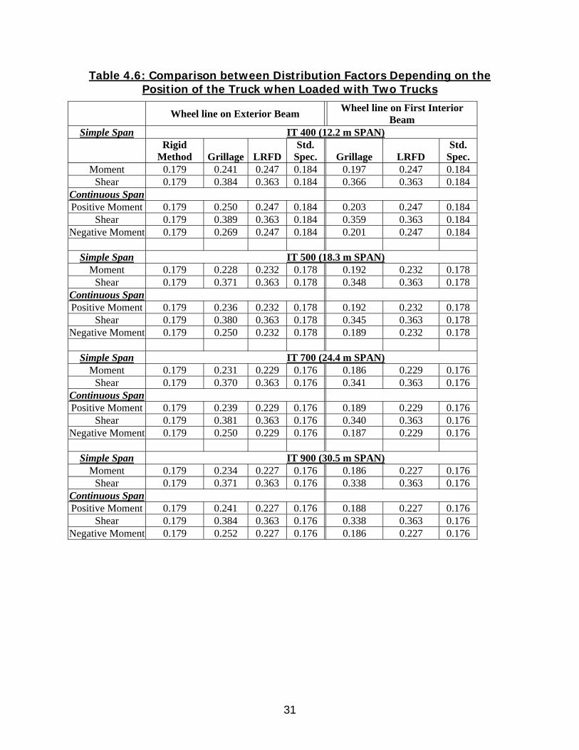
Table 4.6: Comparison between Distribution Factors Depending on the Position of the Truck when Loaded with Two Trucks .....................................................................................................31

Table 4.7: Effect of Multiple Presence of Trucks (with Multiplication Factor)............................32

Table 4.8: Effect of Change in Width of Bridge Model with Two Trucks (no Multiple Presence Factor) ............................................................................................................................................33

Table 4.9 Comparison of Moment Distribution Factors for Skew Bridges (Wheel-Line on the First Interior Girder) ......................................................................................................................33

Table 4.10: Comparison of Shear Distribution Factors for Skew Bridges (Wheel-Line on the First Interior Girder)...............................................................................................................................34

Table 4.11 Variation in Shear Distribution Factor in Exterior Girder for Various Conditions (Wheel-Line on First Interior Girder) ............................................................................................34

Table 4.12 Variation in Shear Distribution Factor in Interior Girder for various Conditions (wheel-line on First Interior Girder) ..............................................................................................35

Table 4.13 Comparison of Maximum Girder Reaction for Finite Element Analysis with Grillage Analogy for Various Boundary Conditions ...................................................................................36

Table 5.1: Strand Requirements for Various Spans for IT Beams ................................................54

viii

List of Figures

Figure 4.1: Member Discretization of 6.7-meter Wide Bridge Model on 18.2-meter Span..........37

Figure 4.2: Idealized Cross-Section...............................................................................................37

Figure 4.3: Cross-Section of IT-500 ..............................................................................................37

Figure 4.4: Typical Grillage Analogy Model of a Non-skew bridge.............................................38

Figure 4.5: Typical Finite Element Analysis Model of a Non Skew bridge..................................38

Figure 4.6: Typical Grillage Analogy Model of a 11-meter wide Bridge with three trucks loaded case.................................................................................................................................................39

Figure 4.7: Typical Grillage Analogy Model of Two Span Continuous Bridge ...........................39

Figure 4.8: Determination of Live Load Shear Distribution Factor for IT 400.............................40

Figure 4.9: Determination of Live Load Moment Distribution Factor for IT 400 ........................40

Figure 4.10: Typical Grillage Analogy Model of a Skew Bridge..................................................41

Figure 4.11: Typical Finite Element Analysis Model of a Skew Bridge.......................................41

Figure 4.12: Truck positions as per NCHRP Report .....................................................................42

Figure 4.13: Actual truck position for Shear in Interior Girder.....................................................43

Figure 4.14: Truck model HS-25...................................................................................................43

Figure 4.15: Shear Variation Along the Span for One Truck Loaded Case ..................................44

Figure 4.16: Shear Variation Along the Span for Two Trucks Loaded Case ................................44

Figure 4.17: Interior Girder Moment Distribution with One Truck, Wheel-Line on Interior Girder45

Figure 4.18: Interior Girder Moment Distribution with Two Trucks, Wheel-Line on Interior Girder .............................................................................................................................................45

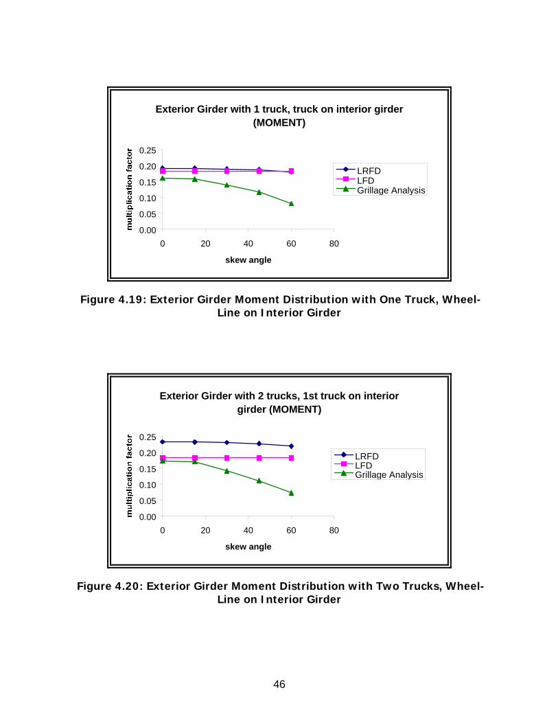
Figure 4.19: Exterior Girder Moment Distribution with One Truck, Wheel-Line on Interior Girder .............................................................................................................................................46

Figure 4.20: Exterior Girder Moment Distribution with Two Trucks, Wheel-Line on Interior Girder .............................................................................................................................................46

Figure 4.21: Interior Girder Shear Distribution with One Truck, Wheel-Line on Interior Girder 47

ix

Figure 4.22: Interior Girder Shear Distribution with Two Trucks, Wheel-Line on Interior Girder47

Figure 4.23: Exterior Girder Shear Distribution with One Truck, Wheel-Line on Interior Girder48

Figure 4.24: Exterior Girder Shear Distribution with Two Trucks, Wheel-Line on Interior Girder48

Figure 5.1: Typical Template for Strands for IT Girder ................................................................53

Figure 5.2: Maximum Spans for Inverted Tee System based on HL-93 Loading.........................53

Figure 6.1: Typical Response for Moment Distribution Factors ...................................................58

Figure 6.2: Recommended Shear Distribution Factor for Interior Girder .....................................58

Figure 6.3: Recommended Shear Distribution Factor for Exterior Girder ....................................59

Figure A1: The New IT Shape has a 17° Slope on the Bottom Flange .........................................62

Figure A2: Comparison of New and Existing IT Shapes ..............................................................62

Figure A3: Comparison of Section Properties for both the Existing (Standard) Section and the New (Modified) Section ................................................................................................................63

1

Chapter 1

Introduction

1.1 Background

The inverted tee (IT) bridge system is a precast composite concrete bridge

superstructure system that was developed by Dr. Maher Tadros and other researchers

at the University of Nebraska. This system uses pretensioned precast concrete members

and has been shown to considerably reduce construction times and is structurally

efficient for short spans. For replacing bridges that cross small streams or storm

ditches, it is often desirable to increase the span lengths in order to minimize pier

obstructions while maintaining the large span to depth ratio. This scenario has resulted

in the use of cast-in-place (CIP) reinforced concrete bridges. The IT system is intended

to provide an alternative to these CIP slab bridges. This system reduces the amount of

formwork in the field and can be installed with relatively small construction equipment.

However, the shallow depth of the IT’s and the absence of a top flange for the base

section could result in excessive deflections when larger spans are bridged with these

members.

1.2 Scope of Research

The current AASHTO bridge codes [1] [2] address the distribution of live loads by

providing equations for determining the fraction of load distributed to individual girders.

However, neither of the codes address systems with adjacent composite precast girders

like the inverted tee bridge system. It is very important to accurately estimate the load

2

distribution factor for each individual girder. This report presents extensive computer

modeling that was performed in order to evaluate the accuracy of current code

equations (when applied to IT bridges) and to develop simplified distribution factors to

be used with the IT system. The results of computer modeling are compared with the

American Association of State Highway and Transportation Officials (AASHTO) Standard

Specifications, 16th Edition and the AASHTO Load and Resistance Factor Design (LRFD)

methods of computing distribution factors.

Both Skew and Non-skew bridges were studied. The research was also aimed at

considering the type and position of barrier rails on the inverted tee bridges. The

position of barrier rail was an important factor, as it affects the placement of the trucks

and therefore the live load distribution factor. Also, preliminary design charts are

developed and presented which illustrate the difference in design using AASHTO

Standard Specification (16th Edition) and AASHTO LRFD (2nd Edition).

3

Chapter 2

Literature Review for Live Load Distribution Factor

2.1 Introduction

In a bridge superstructure, live load distribution factors are used to determine the

fraction of a wheel load that is distributed to individual girders. This load distribution

takes place through complex interactions between the girders and deck. Hence,

different bridge codes have developed simplified methods to compute distribution

factors. If these live load distribution factors are overestimated they may result in

designs requiring larger members. Therefore, accurate distribution factor determination

is critical for the new IT system. The AASHTO LRFD Specification addresses some of the

variability in distribution factors for various bridge types by providing more

comprehensive empirical methods and also by allowing the use of more refined

methods of analyses. The following literature review will discuss the methods used for

determining live load distribution factors and the previous research used to establish

these design methods.

2.2 Literature Review

There are two mathematical idealizations that are frequently used for live load analysis

of prestressed concrete and CIP deck superstructures. The first idealization, Grillage

Analogy, consists of a discrete number of longitudinal and transverse beams.

Longitudinal beam elements represent the prestressed concrete girders while the

transverse beam members represent portions of the cast-in-place deck. In the second

4

idealization, the Finite Element method, the girders are represented by discrete

longitudinal members and the slab is modeled as a continuous transverse medium.

2.2.1 Tadros, Kamel and Hennessey

Tadros, Kamel and Hennessey developed the IT bridge system. They carried out

research to determine the live load distribution factors for non-skew bridges using both

the refined and the simplified methods. They found that the AASHTO Standard

Specification values for moment distribution factors were close to the values obtained

by refined methods, but the shear distribution factor obtained using AASHTO Standard

Specifications were unconservative. There was less than 1 percent difference in the

shear factor computed from grillage analogy and semi-continuum method. It was found

that intermediate diaphragms have a negligible effect on live load distribution factors.

2.2.2 Zokaie, Osterkamp, and Imbsen

Zokaie, Osterkamp and Imbsen performed research on distribution of wheel

loads on highway bridges, whose recommendations have been implemented in the

AASHTO LRFD Specifications. The following formulae were developed for Beam and

Slab bridge types.

Moment distribution to interior girders:

With multiple lanes loaded -

1.0

3

2.06.0

int '315.0 ⎟⎟

⎠

⎞⎜⎜⎝

⎛⎟⎠⎞

⎜⎝⎛

⎟⎠⎞

⎜⎝⎛+=

s

g

LtK

LSSg (Equation 2.1)

where,

gint =distribution factor for interior girder for moment

S =spacing of beams, ft

5

L =span length of beam, ft

ts =depth of concrete slab, in

Kg =longitudinal stiffness parameter =n(I+Aeg2)

where,

n =modular ratio between beam and deck materials

I =moment of inertia of beam, in4

A =cross sectional area of the beam, in2

eg =distance between centers of gravity of basic beam and deck, in

With one lane loaded-

1.0

3

3.04.0

int '41.0 ⎟⎟

⎠

⎞⎜⎜⎝

⎛⎟⎠⎞

⎜⎝⎛

⎟⎠⎞

⎜⎝⎛+=

s

g

LtK

LSSg

(Equation 2.2)

Moment distribution to exterior girders:


intgegext ⋅= (Equation 2.3)

0.1

'1.9'7

≥+

= ede (Equation 2.4)

where,

gext = distribution factor for exterior girder for moment

de =distance from edge of the lane to the center of the exterior web

of the exterior girder, ft

With one lane loaded: It was recommended that simple beam distribution

in transverse direction be used for single lane loading of edge

girders.

Shear distribution to interior girders:


2

int '25'64.0 ⎟

⎠⎞

⎜⎝⎛−⎟

⎠⎞

⎜⎝⎛+=−

SSg V (Equation 2.5)

6

where,

g int-V = distribution factor for interior girder for shear

With one lane loaded -

⎟⎠⎞

⎜⎝⎛+=− '15

6.0intSg V (Equation 2.6)

Shear distribution to exterior girders:


intgeg Vext ⋅=− (Equation 2.7)

'10

'6 ede += (Equation 2.8)

where,

g ext-V = distribution factor for exterior girder for shear

With one lane loaded: It was recommended that simple beam distribution

in transverse direction be used for single lane loading of edge

girders.

Also, correction factors for calculation of interior moment and obtuse

corner girder shear for skewed supports was suggested as follows-

Moment:

( ) 5.11 tan1 θcfactorcorrection −= (Equation 2.9)

where,

θ =skew angle in degrees

5.025.0

31 25.0 ⎟⎠⎞

⎜⎝⎛

⎟⎟⎠

⎞⎜⎜⎝

⎛=

LS

Lt

Kc

s

g (Equation 2.10)

If θ < 30o, c1 = 0.0

If θ > 60o, use θ = 60o

Shear-

( )θtan1 1cfactorcorrection += (Equation 2.11)

7

where,

3.0

3

1

5

1

⎟⎟⎠

⎞⎜⎜⎝

⎛=

s

g

Lt

Kc (Equation 2.12)

The Range of applicability is as follows

0o ≤ θ ≤ 60o

3.5’ ≤ S ≤ 16’

20’ ≤ L ≤ 200’

4.5” ≤ ts ≤ 12”

10,000 ≤ Kg ≤7,000,000 in4

Nb ⟨ 4 (number of girders)

-1’ ≤ de ≤5.5’

The final report of this research also suggested the positioning of the trucks to

find maximum moments and shear values in a bridge. In addition, it also explored the

different ways of generating computer models that can be used for refined method of

analysis. It also suggests that plane grid analysis can produce sufficiently accurate

results if modeled as per the recommendations.

2.2.3 Bishara, Liu and El-Ali

Bishara, Liu and El-Ali (1993) conducted research on developing expression for

wheel load distribution on simply supported skew I-beam composite bridges for interior

and exterior girders. Finite element analyses were carried out on bridges with different

spans, widths and skew angles. The analysis took into account the 3-Dimensional

interaction of all bridge members. They validated the results by testing an actual four

lane skew bridge.

8

Wheel load distribution equations were developed for exterior and interior

girders. These equations gave distribution factors, which were 20-80% of current

AASHTO factor (S/5.5). Live load maximum bending moments in girders of skew

bridges are generally lower than those in right bridges of same span and deck width.

The maximum interior girder bending moment reduction increased with increase in

skew angle. The distribution factor to the interior girders is practically insensitive to the

change in length. The exterior girders become controlling in skew bridges as they are

less affected by the skew angle effect, in case of bending moment. However, this

tendency is only valid when the outer wheel of truck can be placed at 2 ft. from the

centerline of the exterior girder.

9

Chapter 3

Methods for Determination of Live Load Distribution Factors

3.1 Introduction

On bridges, wheel load distribution takes place by interaction between the slab and the

main longitudinal girders. The load is transferred from the deck slab to the longitudinal

girders and then longitudinally to the substructure. Since slabs are typically continuous

in the transverse direction (over the girders), the actual load path and therefore the

amount of load sharing between girders cannot be readily determined. Therefore,

bridge codes address this by providing empirical equations that give approximate values

for transverse distribution of applied wheel loads. In the United States, such codes are

developed by AASHTO. In 1993, the AASHTO subcommittee on bridges adopted a new

set of specifications, known as the Load and Resistance Factor Design (LRFD). These

new specifications changed both the loading magnitudes and the procedures used to

distribute the vehicle loads. The equations given in AASHTO LRFD are believed to be

more accurate for a broader range of bridges than the AASHTO Standard Specifications

and have been checked using finite element analysis [4].

The LRFD Specifications allows the designer to use two different approaches in

determining the Live load distribution factor. These two approaches are listed below-

(a) Use simplified approximate equations.

(b) Use refined methods like finite difference method, finite element method,

grillage analogy, series or harmonic methods, etc.

10

The IT bridge system is unique since the girders are placed adjacent to each

other and therefore do not meet the spacing criterion for the simplified equations in the

codes. As a result a comprehensive analysis and comparison was performed using

AASHTO Standard Specification approximate equations, AASHTO LRFD specifications

approximate equations, and two refined methods of load distribution, namely, Grillage

Analogy method and Finite Element Analysis.

3.2 AASHTO Standard Specification

3.2.1 Moment Distribution to Interior Beams and Stringers

The AASHTO Standard Specification allows for a simplified method of computing

distribution factors. As per Table 3.23.1 (Distribution of Wheel Loads in Longitudinal

Beams), for two or more lanes loaded case, the distribution factor can be calculated as

S/5.5 (per wheel), where S is the beam spacing in feet. This equation applies to bridges

with prestressed concrete girders supporting a concrete slab, with a centerline spacing

of 14 feet or less.

3.2.2 Precast Concrete Beams Used in Multi-Beam Decks

Per section 3.23.4 of the AASHTO Standard Specification, more accurate

distribution factors can be computed for precast concrete beams in multi-beam decks as

actual section properties are used in computation. This section applies to a multi-beam

bridge with prestressed concrete beams placed side by side (as done with the Inverted-

T’s). The conditions for this case to apply are that there has to be continuity developed

between the beams through continuous longitudinal shear keys and transverse bolts

and also that full depth, rigid diaphragms are provided at the ends. The fraction of

11

wheel load that needs to be applied to obtain the live load bending moment is

determined using the following equation

Load Fraction =DS (Equation 3.1)

where,

S = width of precast member;

D = (5.75 – 0.5NL) + 0.7NL(1 – 0.2C)2

when C ≤ 5

D = (5.75 – 0.5NL) when C > 5

NL = number of traffic lanes

C = K(W/L)

where,

W =overall width of the bridge measured perpendicular

to the longitudinal girders in feet;

L =span length measured parallel to longitudinal girders

in feet; for girders with cast-in-place end diaphragms, use the

length between end diaphragms;

K ={(1+μ)I/J}1/2

where,

I =moment of inertia;

J =Saint-Venant torsion constant

μ =Poisson’s ratio for girders.

And

( ) ( ){ }∑ −= btbtJ /63.013/1 3

Note, since there are no shear keys or transverse rods directly connecting the

precast inverted-T’s, this section technically does not apply.

12

3.3 AASHTO LRFD Specification

3.3.1 Simplified Method

The simplified equations in AASHTO LRFD Specification have been verified using

finite element analyses and were found to be more accurate than the AASHTO Standard

Specification equations for a broader range of bridge types [4]. The simplified equations

for lateral load distribution of live loads are given in section 4.6.2.2.2 of the LRFD

Specifications. The equations for live load distribution per lane for different conditions

for concrete deck on concrete beams are as shown below. Note, these are valid only

when the beam spacing, S, is between 1100 and 4900 mm.

Interior Girder Moment, two or more lanes loaded

1.0

3

2.06.0

int 2900075.0 ⎟⎟

⎠

⎞⎜⎜⎝

⎛⎟⎠⎞

⎜⎝⎛

⎟⎠⎞

⎜⎝⎛+=

s

g

LtK

LSSg (Equation 3.2)

where,

g int =distribution factor for interior girder for moment

S =Spacing of beams, mm

L =Span length of beam, mm

ts =depth of concrete slab, mm

Kg =longitudinal stiffness parameter =n(I+Aeg2)

where,

n =modular ratio between beam and deck materials

I =moment of inertia of beam, mm4

A =cross sectional area of the beam, mm2

eg =distance between centers of gravity of basic beam

and deck, mm

13

Interior Girder Moment, one lane loaded

1.0

3

3.04.0

int 430006.0 ⎟⎟

⎠

⎞⎜⎜⎝

⎛⎟⎠⎞

⎜⎝⎛

⎟⎠⎞

⎜⎝⎛+=

s

g

LtK

LSSg (Equation 3.3)

Exterior Girder Moment, two or more lanes loaded

intgeg ext ⋅= (Equation 3.4)

280077.0 ede +=

(Equation 3.5) where,

gext = distribution factor for exterior girder for moment

eg =distance between centers of gravity of basic beam and deck, mm

de =distance from edge of the lane to the center of the exterior web

of the exterior girder, mm

Exterior Girder Moment, one lane loaded

Use Lever Rule

Interior Girder Shear, two or more lanes loaded

0.2

int 1070036002.0 ⎟

⎠⎞

⎜⎝⎛−⎟

⎠⎞

⎜⎝⎛+=−

SSg V (Equation 3.6)

where,

g int-V = distribution factor for interior girder for shear

Interior Girder Shear, one lane loaded

⎟⎠⎞

⎜⎝⎛+=− 7600

36.0intSg V (Equation 3.7)

Exterior Girder Shear, two or more lanes loaded

intgeg Vext ⋅=− (Equation 3.8)

36006.0 ede += (Equation 3.9)

14

where,

g ext-V = distribution factor for exterior girder for shear

Exterior Girder Shear, one lane loaded

Use Lever Rule

Reduction of Load Distribution Factors for Moment in

Longitudinal Beams on Skew Supports

( ) 5.11 tan1 θcfactorcorrection −= (Equation 3.10)

where,

θ = skew angle in degrees

5.025.0

31 25.0 ⎟⎠⎞

⎜⎝⎛

⎟⎟⎠

⎞⎜⎜⎝

⎛=

LS

Lt

Kc

s

g (Equation 3.11)

If θ < 30o, c1 = 0.0

If θ > 60o, use θ = 60o

Correction Factors for Load Distribution Factors for Support

Shear of the Obtuse Corner

θtan2.013.03

⎟⎟⎠

⎞⎜⎜⎝

⎛+

g

s

KLt

(Equation 3.12)

There is a range of applicability for the above equations. This range is as follows:

1100 ≤ S ≤4000

110 ≤ ts ≤ 300

6000 ≤ L ≤ 73000

Nb ⟨ 4 (number of girders)

It can be observed from the range of applicability that the minimum beam

spacing is 1100 mm. This means that these equations are not meant to be used for

beams adjacently placed.

15

3.3.2 Grillage Analogy Method

The grillage analogy method is one of the refined methods allowed by the LRFD

to determine distribution factors for design. This two-dimensional method involves

modeling the bridge superstructures as a planar grid of discrete longitudinal and

transverse members. The number of transverse beam members needed is governed by

the degree of accuracy required and by the position and type of loading applied. The

longitudinal members are placed along the girder centerlines. In order to accurately

model the bridge deck and supporting beams, proper connections are required between

the longitudinal beams and transverse beams at the nodes, which were located at their

intersection. Each of these nodes had three degrees of freedom; vertical translation

perpendicular to the plane of the grid, and rotation about it’s longitudinal and

transverse axes. The boundary conditions at the girder ends were varied to determine

the sensitivity of the model to the type of end restraints.

The moment of inertia of the longitudinal girders was assumed to be the

composite inertia of the girder and with the contributing slab width, while the

transverse girder inertia is taken as only that of the deck slab. The contributing slab

width is taken as half the girder spacing on each side. Care was taken in determining

the correct section properties. The Torsional stiffness of the prototype girders is the

sum of the torsion of the parts that make up the girder. The torsional constant J, is

taken as

PI

AJ0.40

4

= (Equation 3.13)

where,

16

A =cross sectional area of the composite beam, mm2

Ip = polar moment of inertia of the composite beam, Ip=Ix-x+Iy-y,

mm4

3.3.3 Finite Element Analysis

Finite Element Method (FEM) is the other refined method (allowed by the

AASHTO LRFD) that was used to obtain load distribution factors in this study. Although

the 3-Dimensional finite element modeling provides a powerful method of analyzing

simple to complex bridges, it was used primarily to verify the results obtained by the

other 2D analyses.

The program selected (GT STRUDL) was capable of accurately modeling the

bridge elements. The girders were formed from beam elements placed eccentrically

below the deck slab that was formed from plate elements. The mesh density required

depends on the desired accuracy of the results. Several densities were to be explored in

order to determine the sensitivity of the model.

3.3.4 Rigid Body Effect for Exterior Girders

The AASHTO LRFD (Section 4.6.2.2.2d) states, “In a beam-slab bridge cross

sections with diaphragms or cross-frames, the distribution factor for the exterior beam

shall not be less than that which would be obtained by assuming that the cross-section

deflects and rotates as a rigid cross-section”. The recommended procedure for this is

the same as the conventional approximation for loads on piles.

17

∑

∑+=

b

L

N

N

ext

b

L

x

eX

NNR

2

(Equation 3.14)

where,

R =reaction on exterior beams in terms of lanes.

NL =number of loaded lanes under consideration

Nb =number of beams

e =eccentricity of a design truck or a design lane load from the

center of gravity of the pattern of girders, mm

x =horizontal distance from the center of gravity of the pattern of

girders to each girder, mm

Xext = horizontal distance from the center of gravity of the pattern of

girders to the exterior girder, mm

18

Chapter 4

Development of Live Load Distribution Factors

4.1 Introduction

The investigation for the live load distribution factor was broadly classified into two

categories, Non-Skew bridges and Skew bridges. Non-skew bridges were studied

extensively for Moment and Shear distribution factors. In the case of Skew bridges,

more emphasis was given to the determination of shear distribution factors, since these

values increase for skew bridges. The software program used for the Grillage Analogy

method was RISA-3D and for the Finite Element Analysis GT STRUDL was used.

4.2 Non-Skew Bridge

4.2.1 Discretization of Grillage Analogy Model

In Grillage analyses, the Non-skew beam and slab type of bridge is the easiest

and most straight forward to model. The longitudinal members are placed along the

girder centerlines, which represent the inverted tee girders, while the transverse

members represent the stiffness of the slab. Typical discretization of the Non-skew

bridge deck structure is shown in Figures 4.1 and 4.2.

Typically, the inverted tee beams have a spacing of 610 mm, center to center.

Therefore, for both computation of the composite beam section properties and the

transverse slab section properties, a slab width of 610 mm was also used. The

exception to this rule was when the spacing of the beams is more than 610 mm. In this

case, spacing between slab elements was kept at 610 mm.

19

4.2.1.1 Longitudinal Members

Typically, the bridges modeled were 6.7 m wide. Therefore, there were 12

inverted tees placed at 610 mm center to center. The section properties used to model

the longitudinal members were the composite-beam section properties. Details of the

composite beam are shown in Figure 4.3. All of the beams, both interior and exterior,

had same section properties. The effect of the edge stiffening due to curbs was

neglected. Table 4.1 gives the detailed composite section properties of the inverted tees

evaluated in this research program.

4.2.1.2 Transverse Members

As noted above, the spacing of the transverse members was chosen to be

610 mm. The cross sectional properties were calculated for an un-cracked rectangular

concrete section having a width of 610 mm and a height of 152 mm. Torsional

constants were calculated using the equation introduced in chapter 3 {equation (3.13)}.

Table 4.2 gives the cross-sectional properties of a typical transverse member.

4.2.2 Discretization of Finite Element Analysis Model

The finite element analysis more accurately represents a slab-on-girder bridge in

the way it is modeled. In this analysis, the inverted tee girders are modeled as

longitudinal members and deck slab as a continuous transverse medium. The

transverse medium consists of number of plate elements of constant thickness. The

desk slab and girder elements each had a different Young’s moduli; for girder elements

its was based on f’c of 55 MPa and for slab on f’c of 34 MPa and a Poisson ratio of 0.2

20

was used. Other inherent assumptions were that the materials were isotropic and the

structural system followed linear elastic assumptions.

4.2.2.1 Longitudinal members

As previously noted, the bridges modeled were 6.7 m wide. In this case,

all of the 12 longitudinal members, both interior and exterior, had the same section

properties. The effects of concrete railings and the effect of edge stiffening due to curbs

were neglected. The computer program GT STRUDL calculated the composite section

properties from the sectional properties of the girders and deck thickness. The

sectional properties of the girders are shown in Table 4.3.


A standard 4-noded quadrilateral plate element of constant thickness of

152 mm was used in the modeling of the deck slab. An investigation was carried out to

determine the effect, on accuracy, for changes in mesh size. Based on the

investigation, a finite element mesh of 152 mm was selected to model for the slab.

This model typically had more than 11,000 elements.

4.2.3 Different Bridge Models Analyzed

Different bridge models were created so that all objectives of the study were

included. The different models that were created are described below.

(a) Simple span bridges with 610 mm girder spacing – This category

represented the basic bridge type modeled. These bridges were 6.7 m

wide (refer to figures 4.4 and 4.5 for typical models). The different

combinations of simple span lengths and IT types that were modeled with

21

610 mm spacing are shown below.

Inverted tee girders used Span (m)

IT 400 12.2 IT 500 18.3 IT 700 24.4 IT 900 30.5

(b) Simple span bridges with varied girder spacing – Bridge Models with IT

500 girders and 18.2 m spans were studied. The various girder spacing

that were compared were 610 mm, 660 mm, 710 mm and 735 mm.

(c) Simple span bridges with more than two design lane loads – These

bridges were 11 m wide with IT girders at 610 mm center-to-center

spacing. They were compared with two loaded lanes case after applying

the multiple presence factor (0.85) given in AASHTO LRFD section

3.6.1.1.2. Figure 4.6 shows a typical 11 meter wide bridge model.

(d) Two span continuous bridges – The same spans and IT girders used in

model-type (a) were used for this investigation. In addition, a three span

continuous bridges was modeled to verify the results obtained (refer to

Figure 4.7 for a typical bridge model of this type).

4.2.4 Loading

The truck model used for the study was the AASHTO HS-25 as shown in figure

4.14. Determining the position for placement of the truck(s) (to create the maximum

22

effect of moment o shear) was of prime importance since the objective was to

determine the maximum girder response. The number of trucks placed on a bridge to

produce this maximum response was of equal importance.

To determine the exact position of the truck(s) in the longitudinal direction, an

analysis was performed on a single girder line with one truck wheel line. The trucks

were then placed at the same longitudinal positions on the bridge model (where the

maximum shear and moment values were obtained) in order to get the respective

maximized responses on it. This position is near the support for Shear and near the

mid-span for moment as shown in Figure 4.8 and 4.9 [4]. As shown in figure the

maximized responses (shear and flexure) of a single beam line are determined for a

single truck placed on it. The truck is then placed on the bridge model and the

maximized girder responses (shear and flexure) are determined. The ratio of the girder

response (shear or flexure) on a bridge model to that on the single beam line gives the

value of the distribution factor. For example, the maximum girder response on a bridge

model for shear is 108 KN and the maximum shear on a single beam line is 310.5 KN.

Therefore, the ratio of 108 to 310.5 gives the shear distribution factor value as 0.348.

The transverse positions of the trucks also play an important role in determining

the distribution factor. According to AASHTO LRFD, the first truck should be placed 610

mm from the edge of the design lane. The first truck was placed either on the exterior

girder or the first interior girder. When it was placed on the exterior girder, it was

assumed that there was an overhang of 610 mm. When it was placed on the first

interior girder, it was assumed that the inside face of the barrier was at the center-line

23

of the exterior girder. The first wheel line of the second truck was placed at a distance

of 1.22 m from the second wheel line of the first truck [6]. Based on the values thus

obtained a recommendation was made on the position of the barrier rail. Placing the

trucks at 1.83 m from each other was also checked which yielded lower values of

distribution factors. On the recommendation of the sponsors, the 1.22 m spacing was

adhered to in the detailed investigation, since it produced conservative results.

4.3 Skew Bridges

4.3.1 Discretization of Grillage Analogy Model

The skew bridges were modeled according to the recommendations of the

NCHRP report 12-26 [4]. The skewed decks complicate the manner in which the grillage

mesh is laid out. A typical skew bridge model is shown in Figure 4.10. As

recommended in the NCHRP report, spacing of transverse elements was adjusted so

that the elements coincided with the girder ends (i.e. the support locations). Different

support conditions were studied and the details of these supports will be given in a later

section.

4.3.1.1 Longitudinal Members

The longitudinal members were placed coincidental with the girder lines

as in case of Non-skew bridges. All the beams, both interior and exterior, had same

sectional properties. The effect of the edge stiffening was neglected. The cross-

sectional properties in the longitudinal direction were the same as those for the Non-

skew Bridge given in Table 4.3.

24


The members had to be laid out perpendicular to the longitudinal

members (and not parallel to the supports) as recommended in the NCHRP report. The

properties of the transverse members varied depending on the skew angle and position

of the node where the longitudinal and transverse members intersected. Near the

supports, the transverse members properties corresponded to the width of slab which

was less than 610 mm for angles less than 45 degrees and greater for those above 45

degrees. In the middle portion of the bridge span the properties of the transverse

members corresponded to that for a slab of 610 mm in width. To model the case

where flexural cracking of the slab occurs, the transverse member properties were

halved whereas the longitudinal properties were kept the same for simplicity.

4.3.2 Discretization of Finite Element Model

The skew bridge model is similarly modeled as the Non-skew model except for

the fact that the transverse continuous medium, i.e., the slab is modeled parallel to the

support. (See Figure 4.11)

4.3.3 Different Bridge Models Analyzed

The models that were created covered the complete range of skew bridges. The

different skew bridges modeled had skew angles of 15, 30, 45 and 60 degrees.

Different boundary conditions were applied which were as follows

(a) Standard case - No diaphragms, fixed for torsion, pinned for bending

(b) Diaphragm present – A diaphragm of width 914 mm and height 510 mm

was used at the supports and also pinned for bending at the support.

25

(c) Pinned for bending and released for torsion, i.e., Moment Mxx released.

(d) Fixed for bending and Fixed for torsion, i.e., Moment Myy fixed

The effect of changing the transverse member properties to account for cracked

slab section was given consideration wherein the section properties for transverse

members were halved. Along with that the combined effect of cracked slab section

properties and presence of diaphragm were investigated (designated as Ieff).

4.3.4 Loading

Unlike the non-skew bridges, the trucks were moved on the bridge model to

determine the maximized girder response. The first truck was moved along the span

and the positions for maximum girder responses were determined. Then, with this

truck position fixed, the second truck was moved along the span (at a distance of 1.22

m from the first truck in the transverse direction) to find the maximum girder response

for two trucks. This technique is explained by Barker and Puckett [6] and was done for

both shear and moment.

4.4 Results and Observations

4.4.1 Non-Skew Bridges

(a) It can be seen from Table 4.4 that as the spacing is increased the value of

distribution factor for both Shear and Moment increases.

(b) From Grillage analysis, the values of shear and moment distribution

factors when the truck(s) is/are placed on the exterior girder are more

than those obtained when placed on first interior (see Table 4.5).

(c) The values of distribution factors obtained using the AASHTO LRFD

26

approximate equations are typically larger than those obtained using the

refined methods for exterior girder loading and first interior girder loading

(see Table 4.5).

(d) The AASHTO Standard Specification values obtained for Moment, when

compared with refined methods, are conservative for the one lane loaded

case with the wheel-line on the first interior girder. However, these

values may be conservative for the shorter spans when two trucks are

present as well as when there is an overhang (see Table 4.5 and 4.6).

(e) In case of continuous spans grillage analysis, it was observed that the

positive and negative moment distribution factor values were

approximately equal.

(f) From Table 4.7, it can be seen that the two lanes loaded case would be

more critical than the three lanes loaded case on application of the

multiplication factors suggested in the AASHTO LRFD specifications. A

multiplication factor of 0.85 was applied to the values obtained from

placing three trucks on the bridge model.

(g) The change in width of the bridge from 6.7 m to 11 m did not have any

significance on the values of distribution factors when the same number

of trucks are used (see Table 4.8).

4.4.2 Skew Bridges

(a) It was observed that the maximized response for shear would be obtained

in the exterior girder obtuse corner.

27

(b) The position of the trucks to produce maximized effect is very critical. The

NCHRP report suggests that in order to maximize shear response the

trucks be placed close to each other near the supports. It was observed

that the position of the trucks for maximized shear effect is when the

trucks are positioned away from the supports for exterior girder, and one

truck on the support and the other away from the support for the interior

girder (see figures 4.12 and 4.13).

(c) The exterior girder gives greater value of shear distribution factor if the

first wheel-line is placed on the exterior girder.

(d) The moment distribution factors obtained using the refined methods were

always lower than the values obtained by using the AASHTO LRFD and

AASHTO Standard Specifications equations (see Table 4.9). The first

wheel-line was placed on the first interior girder when developing this

table.

(e) The shear distribution factors obtained using the refined methods were

greater than those obtained using the AASHTO Standard specifications.

These same values were less than those obtained using the AASHTO

LRFD equations for all interior girders, and also for exterior girders when

the skew angle was less than 30 degrees. Distribution factors obtained by

grillage analyses and finite element analyses were generally larger than

those obtained by AASHTO LRFD for exterior girders when the skew angle

was 30 degrees or larger (see tables 4.10).

28

(f) For zero skew angle presence of the end diaphragm did not make any

appreciable change in the values obtained. However, for skewed bridges

with skew angles less than 60 degrees, the presence of end diaphragms

may greatly reduce the exterior girder shear near the obtuse corner.

(g) More realistic situations like presence of the end diaphragm and cracking

of slab were also investigated. These typically gave lower values of shear

distribution factors, then the standard condition of pinned for bending and

fixed for torsion (see Tables 4.11 and 4.12).

(h) The values obtained using the two refined methods were usually within

10% of each other and often much closer.

(i) Shear variation was also studied on the bridge along the span. Maximized

shear values were obtained in girders along the span of the bridge at the

support, 0.1L, 0.2L, and 0.3L (where L is the span length) by moving the

truck(s) along the span. It was found that the shear value is highest in

the first one-tenth of the span. This is illustrated in Figures 4.15 and 4.16.

29

Table 4.1: Composite Beam Section Properties of the IT’s studied

Inverted Tee Beams

IT 400 IT 500 IT700 IT 900

Area, A(mm2) 218710 234840 266450 298710

Moment of Inertia, Ix-x(mm4) 7.845x109 12.270x109 24.710x109 42.490x109

Moment of Inertia, Iy-y(mm4) 5.508x109 5.542x109 5.610x109 5.679x109

Torsional constant, J(mm4) 4.284x109 4.270x109 4.156x109 4.132x109

Table 4.2: Cross-Sectional Properties of the Transverse Members

Slab Member

Area, A (mm2) 92903 Moment of Inertia, Ix-x (mm4) 0.180x109 Moment of Inertia, Iy-y (mm4) 2.877x109 Torsional constant, J (mm4) 0.609x109

Table 4.3: Non-Composite Beam Section Properties of the IT’s Studied

Inverted Tee Beams

IT 400 IT 500 IT700 IT 900

Area, A (mm2) 125806 141935 174193 205806

Moment of Inertia, Ix-x (mm4) 1.488x109 2.902x109 7.808x109 16.088x109

Moment of Inertia, Iy-y (mm4) 2.617x109 2.652x109 2.719x109 2.788x109

Torsional constant, J (mm4) 0.687x1099 0.824x109 1.098x109 1.371x109

Table 4.4: Distribution Factor Variation for Change in Girder Spacing for IT 500 on 18.3 m Span

Girder Spacing 610 mm 660 mm 710 mm 735 mm

Shear Distribution Factor 0.348 0.346 0.348 0.363

Moment Distribution Factor 0.187 0.200 0.215 0.218

30

Table 4.5: Comparison between Distribution Factor Depending on the Position of the Truck when Loaded with Single Truck

Wheel line on Exterior Beam Wheel line on First Interior Beam Simple Span IT 400 (12.2 m SPAN)

Rigid

Method Grillage LRFDStd.

Spec. Grillage 1.2*Grillage LRFD Std.

Spec. Moment 0.179 0.202 0.500 0.184 0.158 0.189 0.209 0.184

Shear 0.179 0.369 0.500 0.184 0.348 0.417 0.440 0.184 Continuous Span Positive Moment 0.179 0.217 0.500 0.184 0.167 0.200 0.209 0.184

Shear 0.179 0.385 0.500 0.184 0.342 0.411 0.440 0.184 Negative Moment 0.179 0.261 0.500 0.184 0.170 0.203 0.209 0.184

Simple Span IT 500 (18.3 m SPAN)

Moment 0.179 0.178 0.500 0.178 0.142 0.170 0.191 0.178 Shear 0.179 0.356 0.500 0.178 0.327 0.393 0.440 0.178

Continuous Span Positive Moment 0.179 0.192 0.500 0.178 0.150 0.180 0.191 0.178


Simple Span IT 700 (24.4 m SPAN) Moment 0.179 0.182 0.500 0.176 0.144 0.172 0.184 0.176



Simple Span IT 900 (30.5 m SPAN) Moment 0.179 0.185 0.500 0.176 0.144 0.173 0.180 0.176



31

Table 4.6: Comparison between Distribution Factors Depending on the Position of the Truck when Loaded with Two Trucks

Wheel line on Exterior Beam Wheel line on First Interior Beam


Rigid

Method Grillage LRFDStd.

Spec. Grillage LRFD Std.

Spec. Moment 0.179 0.241 0.247 0.184 0.197 0.247 0.184

Shear 0.179 0.384 0.363 0.184 0.366 0.363 0.184 Continuous Span Positive Moment 0.179 0.250 0.247 0.184 0.203 0.247 0.184

Shear 0.179 0.389 0.363 0.184 0.359 0.363 0.184 Negative Moment 0.179 0.269 0.247 0.184 0.201 0.247 0.184


Moment 0.179 0.228 0.232 0.178 0.192 0.232 0.178 Shear 0.179 0.371 0.363 0.178 0.348 0.363 0.178

Continuous Span Positive Moment 0.179 0.236 0.232 0.178 0.192 0.232 0.178



Moment 0.179 0.231 0.229 0.176 0.186 0.229 0.176 Shear 0.179 0.370 0.363 0.176 0.341 0.363 0.176

Continuous Span Positive Moment 0.179 0.239 0.229 0.176 0.189 0.229 0.176


Simple Span IT 900 (30.5 m SPAN) Moment 0.179 0.234 0.227 0.176 0.186 0.227 0.176

Shear 0.179 0.371 0.363 0.176 0.338 0.363 0.176 Continuous Span Positive Moment 0.179 0.241 0.227 0.176 0.188 0.227 0.176


32

Table 4.7: Effect of Multiple Presence of Trucks (with Multiplication Factor)

IT 400 (12.2 m SPAN) 11 m wide bridge Number of trucks Three Two Three Two

Girder Exterior Exterior First Interior First Interior Grillage Moment 0.208 0.240 0.175 0.191

Shear 0.328 0.385 0.314 0.363 LRFD Moment 0.247 0.247 0.247 0.247

Shear 0.363 0.363 0.363 0.363 Std. Specifications Moment 0.184 0.184 0.184 0.184

Shear 0.184 0.184 0.184 0.184





Shear 0.178 0.178 0.178 0.178





Shear 0.176 0.176 0.176 0.176





Shear 0.176 0.176 0.176 0.176

33

Table 4.8: Effect of Change in Width of Bridge Model with Two Trucks (no Multiple Presence Factor)

Exterior Girder Bridge width 6.7m 11m 6.7m 11m

IT 400 (12.2 m Span) Flexure 0.197 0.191 0.241 0.240 Shear 0.366 0.363 0.384 0.385

IT 500 (18.3 m Span) Flexure 0.192 0.182 0.228 0.225

Shear 0.348 0.345 0.371 0.371

IT 700 (24.4 m Span) Flexure 0.186 0.184 0.231 0.230 Shear 0.341 0.338 0.370 0.369

IT 900 (30.5 m Span) Flexure 0.186 0.185 0.234 0.232

Shear 0.338 0.336 0.371 0.371

Table 4.9 Comparison of Moment Distribution Factors for Skew Bridges (Wheel-Line on the First Interior Girder)

0 15 30 45 60

Grillage 0.170 0.157 0.135 0.117 0.086 LRFD 0.191 0.190 0.189 0.186 0.180 One

trucks Std. Spec. 0.182 0.182 0.182 0.182 0.182 Grillage 0.187 0.171 0.144 0.113 0.079 LRFD 0.232 0.231 0.230 0.226 0.219 Two

trucks Std. Spec. 0.182 0.182 0.182 0.182 0.182 Grillage 0.160 0.157 0.138 0.116 0.081 LRFD 0.191 0.190 0.189 0.186 0.180 One

trucks Std. Spec. 0.182 0.182 0.182 0.182 0.182 Grillage 0.172 0.170 0.141 0.110 0.072 LRFD 0.232 0.231 0.230 0.226 0.219

Interior Girder

One trucks Std. Spec. 0.182 0.182 0.182 0.182 0.182

34

Table 4.10: Comparison of Shear Distribution Factors for Skew Bridges (Wheel-Line on the First Interior Girder)

Skew Angle 0 15 30 45 60

Grillage 0.393 0.403 0.403 0.397 0.387 LRFD 0.440 0.488 0.543 0.618 0.748 One

trucks Std. Spec. 0.182 0.182 0.182 0.182 0.182 Grillage 0.348 0.390 0.400 0.394 0.374 LRFD 0.363 0.403 0.448 0.510 0.618 Two



trucks Std. Spec. 0.182 0.182 0.182 0.182 0.182 Grillage 0.348 0.390 0.400 0.394 0.374 LRFD 0.363 0.403 0.448 0.510 0.618

Exterior Girder

Two trucks Std. Spec. 0.182 0.182 0.182 0.182 0.182

Note- Grillage analyses values contain multiple presence factor where AASHTO LRFD equations

have been directly used, and not for conditions where lever rule is used.

Table 4.11 Variation in Shear Distribution Factor in Exterior Girder for Various Conditions (Wheel-Line on First Interior Girder)

Angle (degrees)

Number of trucks

Without Diaphragm

With Diaphragm

Cracked slab section

Cracked section with diaphragm

0 1 truck 0.087 0.097 0.087 0.101 0 2 trucks 0.082 0.075 0.083 0.060

15 1 truck 0.434 0.330 0.130 0.287 15 2 trucks 0.449 0.154 0.153 0.135 30 1 truck 0.675 0.489 0.529 0.427 30 2 trucks 0.682 0.247 0.536 0.210 45 1 truck 0.785 0.598 0.646 0.581 45 2 trucks 0.750 0.429 0.621 0.355 60 1 truck 0.773 0.840 0.670 0.728 60 2 trucks 0.693 0.673 0.605 0.553

35

Table 4.12 Variation in Shear Distribution Factor in Interior Girder for various Conditions (wheel-line on First Interior Girder)

Angle (degrees)

Number of trucks

Without diaphragm

With diaphragm

Cracked slab section

Cracked section with diaphragm

0 1 truck 0.393 0.398 0.391 0.413 0 2 trucks 0.348 0.354 0.347 0.361

15 1 truck 0.403 0.376 0.403 0.395 15 2 trucks 0.390 0.396 0.381 0.394 30 1 truck 0.403 0.341 0.410 0.369 30 2 trucks 0.400 0.401 0.396 0.401 45 1 truck 0.397 0.295 0.412 0.337 45 2 trucks 0.394 0.363 0.397 0.381 60 1 truck 0.387 0.246 0.407 0.302 60 2 trucks 0.374 0.272 0.382 0.321

Note- No multiplication factor is used in the above comparison.

36

Table 4.13 Comparison of Maximum Girder Reaction for Finite Element Analysis with Grillage Analogy for Various Boundary Conditions

Skew Truck description

2-D Grillage1

Finite Element1

2-D Grillage2

Finite Element2

Finite Element3

Moment Y fixed

EXTERIOR 0 degree Two trucks 126.9 132.3 148.8 148.05 143.55 0 degree One truck 122.0 130.5 159.6 156.15 148.5

15 degree Two trucks 207.9 243.0 150.6 155.25 148.95 15 degree One truck 181.4 204.3 167.2 167.40 158.4 30 degree Two trucks 294.5 318.5 143.7 139.50 127.0 30 degree One truck 239.1 266.7 159.4 156.15 135.9 45 degree Two trucks 334.6 340.3 183.3 174.15 153.0 45 degree One truck 273.2 292.9 192.3 184.95 158.9 60 degree Two trucks 322.2 312.8 237.2 227.25 180.6 60 degree One truck 280.2 279.6 235.7 225.90 184.1

INTERIOR 0 degree Two trucks 119.25 120.2 121.8 121.1 122.0 0 degree One truck 112.1 113.4 112.1 111.6 122.0

15 degree Two trucks 153.45 170.6 53.7 52.2 49.1 15 degree One truck 124.2 145.8 73.9 74.7 59.0 30 degree Two trucks 233.2 239.1 70.4 66.7 63.5 30 degree One truck 192.4 207.6 92.7 90.0 73.8 45 degree Two trucks 256.6 251.1 99.5 93.6 83.0 45 degree One truck 223.7 224.4 116.7 111.6 91.8 60 degree Two trucks 237.1 225.7 144.4 136.8 108.4 60 degree One truck 220.3 208.8 153.0 144.5 114.3

Note:- 1 – Pinned for bending, fixed for torsion 2 – Pinned for bending, released for torsion. 3 – Fixed for bending, fixed for torsion. Trucks are placed in such a manner that one of the wheel-line lied on the particular girder under consideration. All values are in KN. No Multiplication factor is used.

37

Figure 4.1: Member Discretization of 6.7-meter Wide Bridge Model on 18.2-

meter Span

Figure 4.2: Idealized Cross-Section

Figure 4.3: Cross-Section of IT-500 (Note all dimensions are in mm unless noted)

6.7 m

18.2 m

38

Figure 4.4: Typical Grillage Analogy Model of a Non-skew bridge

Figure 4.5: Typical Finite Element Analysis Model of a Non Skew bridge

39

Figure 4.6: Typical Grillage Analogy Model of a 11-meter wide Bridge with three trucks loaded case

Figure 4.7: Typical Grillage Analogy Model of Two Span Continuous Bridge

40

HS-25 Truck position for Maximum Shear

Maximum Shear Diagram for HS-25

Shear Force Diagram of beam b2 when the truck is placed on the first interior girder for one

truck loaded case (Grid Analysis result for IT 400 12.1 m span)

Figure 4.8: Determination of Live Load Shear Distribution Factor for IT 400.

HS-25 Truck position for Maximum Moment

Maximum Moment Diagram for HS-25

Moment Force Diagram of beam b2 when the truck is placed on the first interior girder for one

truck loaded case (Grid Analysis result for IT 400 12.1 m span)

Figure 4.9: Determination of Live Load Moment Distribution Factor for IT 400

41

Figure 4.10: Typical Grillage Analogy Model of a Skew Bridge

Figure 4.11: Typical Finite Element Analysis Model of a Skew Bridge

42

Figure 4.12: Truck positions as per NCHRP Report

43

Figure 4.13: Actual truck position for Shear in Interior Girder

20 K 20 K

4 K 14ft 14ft

Figure 4.14: Truck model HS-25

44

Variation of shear over the bridge for one truck loaded case

0.0

50.0

100.0

150.0

200.0

250.0

0.0 0.1 0.2 0.3 0.4

location on span

Shea

r (K

N) 0 degree skew

15 degree skew30 degree skew45 degree skew60 degree skew

Figure 4.15: Shear Variation Along the Span for One Truck Loaded Case

Variation of Shear over the bridge for two trucks loaded case

0.050.0

100.0150.0200.0250.0300.0

0.0 0.1 0.2 0.3 0.4

location on span

Shea

r (K

N) 0 degree skew

15 degree skew30 degree skew45 degree skew60 degree skew

Figure 4.16: Shear Variation Along the Span for Two Trucks Loaded Case

45

Interior Girder with 1 truck, 1st truck on interior girder (MOMENT)

0.00

0.05

0.10

0.15

0.20

0.25

0 20 40 60 80

skew angle

LRFDLFDGrillage Analysis

Figure 4.17: Interior Girder Moment Distribution with One Truck, Wheel-Line on Interior Girder

Interior Girder with 2 trucks, 1st truck on interior girder (MOMENT)

0.00

0.05

0.10

0.15

0.20

0.25

0 20 40 60 80

skew angle


Figure 4.18: Interior Girder Moment Distribution with Two Trucks, Wheel-Line on Interior Girder

46

Exterior Girder with 1 truck, truck on interior girder (MOMENT)

0.00

0.05

0.10

0.15

0.20

0.25

0 20 40 60 80

skew angle


Figure 4.19: Exterior Girder Moment Distribution with One Truck, Wheel-Line on Interior Girder

Exterior Girder with 2 trucks, 1st truck on interior girder (MOMENT)

0.00

0.05

0.10

0.15

0.20

0.25

0 20 40 60 80

skew angle


Figure 4.20: Exterior Girder Moment Distribution with Two Trucks, Wheel-Line on Interior Girder

47

0.00.10.20.30.40.50.60.70.8

0 20 40 60 80

skew angle

LRFD

LFD

Grillage Analysis without diaphragm

Grillage Analysis w/ diaphragm

Figure 4.21: Interior Girder Shear Distribution with One Truck, Wheel-Line

on Interior Girder

Figure 4.22: Interior Girder Shear Distribution with Two Trucks, Wheel-Line

on Interior Girder

0.00.10.20.30.40.50.60.70.8

0 20 40 60 80

skew angle

LRFD

LFD

Grillage Analysis withoutdiaphragmGrillage Analysis w/ diaphragm

48

Figure 4.23: Exterior Girder Shear Distribution with One Truck, Wheel-Line on Interior Girder

Figure 4.24: Exterior Girder Shear Distribution with Two Trucks, Wheel-Line on Interior Girder

0.00.10.20.30.40.50.60.70.8

0 20 40 60 80

skew angle

LRFD

LFD


0.00.10.20.30.40.50.60.70.8

0 20 40 60 80

skew angle

LRFD

LFD


49

Chapter 5

Design of Inverted Tee Girders

5.1 Introduction

Designing the IT girders was also an important part of the investigation. This process

included the use of the live load distribution factors derived earlier. The designs

involved multiple analyses on bridge models with varying parameters including span

lengths, number of spans, widths and skew angles.

5.2 Prototypes of bridges

There were six prototype bridges that were designed. These are shown below:

Bridge Type Span (m) Width (m) Skew/ Non Skew

Single Span 8 8.5 Both

Single Span 16 11 Both

Single Span 24 12 Non Skew

Continuous Span 21 - 26.25 - 21 8 Non Skew



5.3 Live Load Cases

The above prototype bridges were designed for three different live load conditions. This

was done in order to determine if the loading requirements would result in significantly

different structures, such that the development of separate standards would be

warranted. These load cases were the following…

50

(1) KDOT MS-18 load case – This is similar to the live load provision given in the

AASHTO Standard Specifications which is the HS20-44 Loading. It consisted

of a tractor with a semi-trailer or its corresponding lane load (AASHTO

Standard Specifications Article 3.7.6)

(2) KDOT MS-22.5 load case – This is obtained by increasing the MS-18 Truck

and MS-18 lane loadings by 25% and is often referred to as HS-25.

(3) HL-93 load case – This is the same live load provision given in AASHTO LRFD

which consists of lane loading with a truck (HS20-44) or tandem or a truck

train (with 90% effect, for continuous span), giving maximized effect. This is

given in Article 3.6.1.1 of AASHTO LRFD.

5.4 Design Requirements

The required design conditions are detailed below [7]

5.4.1 MS-18 and MS-22.5 Loading Condition

Temporary allowable concrete Compressive stresses before loss due to

creep and shrinkage is 0.6f’ci MPa

Temporary allowable Tension stresses before loss due to creep and

shrinkage is cif25.0 MPa

Allowable Working Stresses in Prestressed beams due to the prestressing

force service loads and prestress losses shall be limited to

Compression 0.4 f’ci MPa

Tension, precompressed tensile zone:

MS18 Design 0.0 Mpa

Kansas Overload Design (1.25 MS18) cf125.0 MPa

Stresses in the concrete at service load (including the future wearing surface)

after all prestress losses and additional creep and shrinkage losses caused by the

positive moment connection shall be…

51

Compression: 0.40 f’ci MPa

Tension, precompressed tensile zone: cif25.0 MPa **

** (applies to both the MS18 Design and the Kansas Overload Design)

5.4.2 HL-93 Loading Conditions

[2] The various stress limits for concrete were as per Article 5.9.4 of AASHTO

LRFD

For Temporary Stresses before Losses,

Compressive Stress limit in concrete shall be 0.6f’ci MPa.

Tensile Stress limit in concrete in areas other than the precompressed

tensile zones and bonded auxiliary reinforcement shall be cif25.0 MPa [ 1.38 MPa.

For Stresses at Service Limit State after Losses,

Compressive Stress limit in concrete in other than segmentally constructed

bridges due to the sum of effective prestress and permanent loads shall be 0.45f’c MPa.

Compressive Stress limit in concrete in other than segmentally constructed

bridges due to due to live load and one-half the sum of the effective prestress and

permanent loads shall be 0.4f’c MPa.

Compressive Stress limit in concrete due to sum of effective prestress,

permanent loads, and transient loads and during shipping and handling shall be 0.6f’c

MPa.

Tension Stress limit in concrete for components with bonded prestressing

tendons or reinforcement that are subjected to severe corrosive conditions shall be

cf25.0 MPa.

52

5.4 Miscellaneous Data

Concrete Properties

f’c = 55 MPa (girder)

f’ci= 41 MPa (girder)

f’c = 27.5 MPa (deck slab)

Prestressed Strands used – ½”dia. Low Relaxation Strands with Fpu = 270

ksi

Jacking Stress ratio= 0.75

Relative Humidity = 65%

Typical Template for the strands for IT girder - The typical template consists of

two rows of 11 straight stands each in the bottom flange and a row of two strands at

the top (see figure 5.1). The bottom row at 50 mm from the bottom and the second

row at 50 mm on center from the first row. The row with two strands is at a distance of

50 mm for the top of any IT.

5.5 Results

An extensive study was carried out to determine the maximum spans of the inverted

tee system. This was done using the HL-93 loading case for AASHTO LRFD stress limit

conditions for simple-span bridges only. Figure 5.2 shows the maximum span that a

particular IT girder can be used on, based on the stress conditions discussed above.

Table 5.1 shows the strand requirement (for the above bridge prototypes) for

the different loading cases. It also shows the different IT girders used for the different

spans.

From ultimate moment capacity requirement, all three loading cases required

almost the same number of strands.

53

Figure 5.1: Typical Template for Strands for IT Girder

(at ends and mid-span)

Span Vs Inverted T-girder depth

0100200300400500600700800900

39 50 61 71 80 87

Span (ft)

IT g

irder

dep

th (m

m)

Figure 5.2: Maximum Spans for Inverted Tee System based on HL-93 Loading

54

Table 5.1: Strand Requirements for Various Spans for IT Beams

Span Strand Requirement (number) Ultimate Moment Capacity Stress Requirement IT used MS-18 MS-22.5 HL-93 MS-18 MS-22.5 HL-93

8m simple 4 4 4 6 8 8 IT300 8m simple (30 skew) 4 4 4 6 8 8 IT300 6.4m-8m-6.4m cont. 3 3 3 8 11 7 IT300

16m simple 8 8 9 14 16 14 IT500 16m simple (30 skew) 8 8 9 14 16 14 IT500

12.8m-16m-12.8m cont. 6 7 6 14 - 13 IT500 24m simple 11 13 12 20 21 19 IT800

19.2m-24m-19.2m cont. 8 9 9 - - - IT800

55

Chapter 6

Conclusion and Recommendations

6.1 Conclusions

The following main conclusions can be drawn from the investigation of IT bridges

conducted as part of this study.

• The AASHTO Standard Specifications (16th Edition) approximate

equations give moment live load distribution factors that are generally

close to the ones obtained using refined methods, but the shear

distribution factors are usually less than half the values obtained using the

refined methods.

• AASHTO LRFD (2nd Edition) approximate equations gave live load

distribution factor values that were higher than those obtained by refined

methods for moment. For shear, the LRFD equations are generally

conservative but may be un-conservative at large skew angles.

• The two refined methods gave close results and either of them can be

used to model the IT bridges to find the live load distribution.

• The moment and shear distribution factors do not change much when the

girder size is changed.

• Increasing in the width of the bridge will not increase the distribution

factors if the multiple presence factors given in the AASHTO LRFD (2nd

Edition) are used.

6.2 Recommendations

Based on the analyses the following recommendations are made for the inverted tee

girder bridge system.

(1) Moment Distribution Factors - It can be seen from the Figures 4.17 to 4.20

that the moment distribution factors for straight bridges (obtained from

grillage analysis) are always less than the values obtained using the AASHTO

56

LRFD approximate equations and the AASHTO LFD formulae for both the

interior and exterior girders These figures also shows that for bridges with

large skew angles the AASHTO LRFD approximate equations would give over-

conservative results for both the one truck loaded and two or more trucks

loaded cases. Thus, either the AASHTO LRFD Approximate equations or the

AASHTO Standard Specification formula (s/5.5) can be safely used for girders

spaced at 2 ft on center. For simplicity, a moment-distribution factor of 0.2 is

recommended as shown in Figure 6.1.

(2) Shear Distribution Factors – Considerable time was spent investigating the

shear distribution factors for girders in skew bridges. The findings are

summarized in the following recommendations.

Interior Girder Shear Distribution Factor

Shear distribution factors obtained from grillage analyses for interior

girders were always less than that obtained using AASHTO LRFD, but at the same time

greater than those obtained using the AASHTO Standard Specification provisions.

Modeling the IT bridges with different end restraints and slab stiffnesses had a

considerable impact on shear distribution factors in skewed bridges. However, these

values were always less than those computed using the AASHTO LRFD equations.

Therefore, a distribution factor value of 0.42 can be safely used for all interior girders

as shown in Figure 6.2

Exterior Girder Shear Distribution Factor

It can be seen from Figure 4.23 and 4.24 that in the case of straight

bridge (i.e. 0 degree skew) shear distribution factors obtained from grillage analysis (for

the exterior girder) were less than those obtained from using the AASHTO LRFD and

AASHTO Standard Specification expressions. The grillage models without the end

57

diaphragms give shear values higher than those with the diaphragm. Also, the models

with the end diaphragm indicated values comparable to those obtained using AASHTO

LRFD. The AASHTO Standard Specification values were far below the values obtained

using the grillage models. For skew angles below 20 degrees, a distribution factor

value of 0.42 can be used (as per AASHTO LRFD recommendations, exterior girder

distribution factor values cannot be less than the values for interior girder). For skew

angles greater than 20 degrees the following equation may be used

100

2042.0 −+

angleskew, where skew angle is in degrees

(See Figure 6.3)

(3) The barrier rails should be placed directly over the exterior girder so that, by

eliminating the overhang width, a uniform strand pattern for both interior and

exterior beams can be maintained.

58

Recommendation for Moment

0.00

0.05

0.10

0.15

0.20

0.25

0 20 40 60 80

skew angle

mul

tiplic

atio

n fa

ctor

Recommended 1 truck Interior girder2 trucks Interior girder1 truck Exterior girder2 trucks Exterior girder

Figure 6.1: Typical Response for Moment Distribution Factors

Figure 6.2: Recommended Shear Distribution Factor for Interior Girder

Recommendation for Interior Girder Shear

0

0.1

0.2

0.3

0.4

0.5

0 20 40 60 80

skew angle

Recommended1 truck w/ diaphragm2 trucks w/ diaphragm1 truck w/ diaphragm + Ieff2 trucks w/ diaphragm+ Ieff

59

Figure 6.3: Recommended Shear Distribution Factor for Exterior Girder

Recommendation for Exterior Girder Shear

0.00.10.20.30.40.50.60.70.8

0 20 40 60 80

skew angle

Recommended1 truck w/ diaphragm2 trucks w/ diaphragm1 truck w/ diaphragm + Ieff2 trucks w/ diaphragm + Ieff

60

REFERENCES

(1) American Association of State highway and Transportation Officials

(AASHTO). (1996). Standard specifications for highway bridges, Washington,

D.C.

(2) American Association of State highway and Transportation Officials

(AASHTO). (1998). LRFD bridge design specifications, Washington, D.C.

(3) Tadros, M. K., and Kamel, M. R., “The Inverted Tee Shallow Bridge System

for Rural Areas” (September-October 1996), PCI Journal, Vol.41, No.5.

(4) Zokaie, T.,Osterkamp, T.A. and Imbsen, R.A.(1991), “Distribution of wheel

loads on Highway bridges”, NCHRP 12-26/1 Final Rep., National Cooperative

Highway Research Program, Washington, D.C.

(5) Bishara, A. G., Liu, M. C., and Ali, N.D., “Wheel load Distribution on Simply

supported Skew I-beam Composite Bridges”(1992), Journal of Structural

Engineering.

(6) Barker, R. M., and Puckett, J. A., (1997) “Design of Highway Bridges”, A

Wiley-Interscience Publication.

(7) Kansas Department of Transportation Bridge Design Manual.

61

Appendix A

Development of a New IT Section with Tapered Flanges

A1.1 Need for a new shape

The bottom flanges of the inverted tee (IT) shape, developed by Dr. Tadros and

currently used by the Nebraska Department of Roads, have a horizontal (flat) upper

surface. These flat surfaces often trap air pockets during the casting process and result

in large “bug holes” on the finished concrete surface. Therefore, one of the objectives

added during the course of the research program was to investigate the use of a sloped

flange surface to greatly reduce the amount of “bug holes” and to add to the aesthetics

of the current block-like shape.

A1.2 Development of New Cross-Section

In the development of a new cross-section with tapered flanges, the following two

conditions were established were established.

(1) To identify and utilize a top slope similar to girders in other states.

(2) To maintain the same overall height and width of the IT shape(s), and also to

try to match (as close as possible) the section properties of the existing IT

shape(s). This would then allow for Kansas precasters to utilize the tapered

shape as an alternative to the existing IT shape when bidding jobs in other

surrounding states.

An investigation was conducted to determine the bottom-flange slopes currently

used by bridge sections in other states. This investigation found that a slope of

approximately 17 degrees is common for several other bridge girders, including the

Nebraska NU shapes and the Florida Bulb Tee Shape. Thus a slope of 17 degrees was

62

also used for the new Kansas IT Shape. Figures A1 and A2 show the effect of the 17

degree slope on the new shape. The remaining figures show the section properties for

both the new shape and the existing shape.

Figure A1: The New IT Shape has a 17° Slope on the Bottom Flange

Figure A2: Comparison of New and Existing IT Shapes

Modified IT Has

17 Slope

63

Area mm2

Section Std. Modified New/Old

IT300 109,100 113,700 104.2%

IT400 125,100 129,700 103.7%

IT500 141,100 145,700 103.3%

IT600 157,100 161,700 102.9%

IT700 173,100 177,700 102.7%

IT800 189,100 193,700 102.4%

IT900 205,100 209,700 102.2%

Moment of Inertia (I) mm4 x 106

Section Std. Modified New/Old

IT300 590 609 103.3%

IT400 1397 1402 100.4%

IT500 2755 2754 99.9%

IT600 4768 4772 100.1%

IT700 7528 7552 100.3%

IT800 11126 11185 100.5%

IT900 15649 15761 100.7%

Figure A3: Comparison of Section Properties for both the Existing (Standard) Section and the New (Modified) Section

64

Untopped Section Properties Topped Section Properties

A 109056 mm2 = 169.0 in2 A 176012 mm2 = 272.8 in2

yt 197 mm = 7.75 in yt 246 mm = 9.68 in

yb 103 mm = 4.06 in yb 206 mm = 8.11 in

I 589834718 mm4 = 1417 in4 I 3772789056 mm4 = 9064 in4

St 2995265 mm3 = 183 in3 St 15343997 mm3 = 936 in3

Sb 5722237 mm3 = 349 in3 Sb 18303889 mm3 = 1117 in3

300mm

Slabf'c=4000psi

Inverted Teef'c=8000psi

actual width = 610mm

452mm

152mm

300mm

effective width = 431mm

75 mm 9 @ 50mm = 450mm 9 @ 50mm = 450mm75 mm 75 mm 75 mm600mm 600mm

160mm 220mm50mm

IT300 Standard

65


A 125056 mm2 = 193.8 in2 A 192012 mm2 = 297.6 in2

yt 266 mm = 10.49 in yt 300 mm = 11.80 in

yb 134 mm = 5.26 in yb 252 mm = 9.93 in

I 1397019478 mm4 = 3356 in4 I 6590102276 mm4 = 15833 in4

St 5242392 mm3 = 320 in3 St 21983681 mm3 = 1342 in3

Sb 10463400 mm3 = 639 in3 Sb 26127609 mm3 = 1594 in3

400mm

Slabf'c=4000psi



552mm

152mm

400mm


75 mm 9 @ 50mm = 450mm 9 @ 50mm = 450mm75 mm 75 mm 75 mm

600mm 600mm

50mm

160mm 220mm

IT400 Standard

66


A 141056 mm2 = 218.6 in2 A 208012 mm2 = 322.4 in2

yt 332 mm = 13.06 in yt 353 mm = 13.90 in

yb 168 mm = 6.63 in yb 299 mm = 11.77 in

I 2755480535 mm4 = 6620 in4 I 10362553286 mm4 = 24896 in4

St 8309404 mm3 = 507 in3 St 29350209 mm3 = 1791 in3

Sb 16363672 mm3 = 999 in3 Sb 34664991 mm3 = 2115 in3

500mm

Slabf'c=4000psi



652mm

152mm

500mm



600mm 600mm

50mm

160mm 220mm

IT500 Standard

67


A 157056 mm2 = 243.4 in2 A 224012 mm2 = 347.2 in2

yt 394 mm = 15.50 in yt 406 mm = 15.98 in

yb 206 mm = 8.12 in yb 346 mm = 13.63 in

I 4767835160 mm4 = 11455 in4 I 15171196790 mm4 = 36449 in4

St 12111772 mm3 = 739 in3 St 37377738 mm3 = 2281 in3

Sb 23105909 mm3 = 1410 in3 Sb 43833274 mm3 = 2675 in3

600mm

Slabf'c=4000psi



752mm

152mm

600mm



600mm 600mm

50mm

160mm 220mm

IT600 Standard

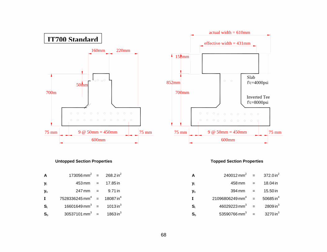
68


A 173056 mm2 = 268.2 in2 A 240012 mm2 = 372.0 in2

yt 453 mm = 17.85 in yt 458 mm = 18.04 in

yb 247 mm = 9.71 in yb 394 mm = 15.50 in

I 7528336245 mm4 = 18087 in4 I 21096806249 mm4 = 50685 in4

St 16601649 mm3 = 1013 in3 St 46029223 mm3 = 2809 in3

Sb 30537101 mm3 = 1863 in3 Sb 53590766 mm3 = 3270 in3

700m

Slabf'c=4000psi



852mm

152mm

700mm



600mm 600mm

50mm

160mm 220mm

IT700 Standard

69


A 189056 mm2 = 293.0 in2 A 256012 mm2 = 396.8 in2

yt 512 mm = 20.14 in yt 510 mm = 20.10 in

yb 288 mm = 11.35 in yb 442 mm = 17.38 in

I 11126411737 mm4 = 26731 in4 I 28219961770 mm4 = 67799 in4

St 21747249 mm3 = 1327 in3 St 55281692 mm3 = 3373 in3

Sb 38582986 mm3 = 2354 in3 Sb 63914859 mm3 = 3900 in3

800mm

Slabf'c=4000psi



952mm

152mm

800mm



600mm 600mm

50mm

160mm 220mm

IT800 Standard

70


A 205056 mm2 = 317.8 in2 A 272012 mm2 = 421.6 in2

yt 569 mm = 22.38 in yt 562 mm = 22.14 in

yb 331 mm = 13.05 in yb 490 mm = 19.28 in

I 15648547029 mm4 = 37596 in4 I 36621106969 mm4 = 87983 in4

St 27525738 mm3 = 1680 in3 St 65119868 mm3 = 3974 in3

Sb 47206123 mm3 = 2881 in3 Sb 74792601 mm3 = 4564 in3

900mm

Slabf'c=4000psi



1052mm

152mm

900mm



600mm 600mm

50mm

160mm 220mm

IT900 Standard

71


A 113656 mm2 = 176.2 in2 A 180612 mm2 = 279.9 in2

yt 194 mm = 7.64 in yt 247 mm = 9.71 in

yb 106 mm = 4.17 in yb 205 mm = 8.08 in

I 609370275 mm4 = 1464 in4 I 3776401722 mm4 = 9073 in4

St 3139059 mm3 = 192 in3 St 15304902 mm3 = 934 in3

Sb 5755570 mm3 = 351 in3 Sb 18398549 mm3 = 1123 in3

300mm 17°

Slabf'c=4000psi

300mm

452mm

17°Inverted Teef'c=8000psi


152mm


75 mm9 @ 50mm = 450mm75 mm 75 mm 9 @ 50mm = 450mm 75 mm

50mm

600mm 600mm

220mm160mm

IT300 Modified

72


A 129656 mm2 = 201.0 in2 A 196612 mm2 = 304.7 in2

yt 265 mm = 10.44 in yt 302 mm = 11.88 in

yb 135 mm = 5.31 in yb 250 mm = 9.86 in

I 1402108477 mm4 = 3369 in4 I 6617332021 mm4 = 15898 in4

St 5288721 mm3 = 323 in3 St 21937480 mm3 = 1339 in3

Sb 10394686 mm3 = 634 in3 Sb 26431799 mm3 = 1613 in3

400mm

17°

Slabf'c=4000psi

400mm

552mm

17°



152mm



50mm

600mm 600mm

220mm160mm

IT400 Modified

73


A 145656 mm2 = 225.8 in2 A 212612 mm2 = 329.5 in2

yt 331 mm = 13.05 in yt 356 mm = 14.01 in

yb 169 mm = 6.63 in yb 296 mm = 11.66 in

I 2753997145 mm4 = 6620 in4 I 10433300550 mm4 = 25066 in4

St 8307938 mm3 = 507 in3 St 29322845 mm3 = 1789 in3

Sb 16343212 mm3 = 997 in3 Sb 35224779 mm3 = 2150 in3

500mm

17°

Slabf'c=4000psi

500mm

652mm

17°



152mm



50mm

600mm 600mm

220mm160mm

IT500 Modified

74


A 161656 mm2 = 250.6 in2 A 228612 mm2 = 354.3 in2

yt 395 mm = 15.54 in yt 409 mm = 16.12 in

yb 205 mm = 8.09 in yb 343 mm = 13.49 in

I 4771501227 mm4 = 11464 in4 I 15305991583 mm4 = 36773 in4

St 12091232 mm3 = 738 in3 St 37387485 mm3 = 2282 in3

Sb 23233107 mm3 = 1418 in3 Sb 44674431 mm3 = 2726 in3

600mm

17°

Slabf'c=4000psi

600mm

752mm

17°



152mm



50mm

600mm 600mm

220mm160mm

IT600 Modified

75


A 177656 mm2 = 275.4 in2 A 244612 mm2 = 379.1 in2

yt 455 mm = 17.93 in yt 462 mm = 18.21 in

yb 245 mm = 9.63 in yb 390 mm = 15.33 in

I 7551551758 mm4 = 18143 in4 I 21316648720 mm4 = 51213 in4

St 16582456 mm3 = 1012 in3 St 46090058 mm3 = 2813 in3

Sb 30872314 mm3 = 1884 in3 Sb 54728229 mm3 = 3340 in3

700mm

17°

Slabf'c=4000psi

700mm

852mm

17°



152mm



50mm

600mm 600mm

220mm160mm

IT700 Modified

76


A 193656 mm2 = 300.2 in2 A 260612 mm2 = 403.9 in2

yt 514 mm = 20.25 in yt 515 mm = 20.28 in

yb 286 mm = 11.24 in yb 437 mm = 17.20 in

I 11185484358 mm4 = 26873 in4 I 28546210166 mm4 = 68583 in4

St 21745411 mm3 = 1327 in3 St 55404826 mm3 = 3381 in3

Sb 39162623 mm3 = 2390 in3 Sb 65357484 mm3 = 3988 in3

800mm

17°

Slabf'c=4000psi

800mm

952mm

17°


152mm

actual width = 610mmeffective width = 431mm


50mm

600mm 600mm

220mm160mm

IT800 Modified

77


A 209656 mm2 = 325.0 in2 A 276612 mm2 = 428.7 in2

yt 572 mm = 22.52 in yt 568 mm = 22.35 in

yb 328 mm = 12.91 in yb 484 mm = 19.07 in

I 15761174309 mm4 = 37866 in4 I 37075397050 mm4 = 89074 in4

St 27554442 mm3 = 1681 in3 St 65314568 mm3 = 3986 in3

Sb 48052538 mm3 = 2932 in3 Sb 76545696 mm3 = 4671 in3

900mm

17°

Slabf'c=4000psi

900mm

1052mm

17°



152mm



50mm

600mm 600mm

220mm160mmIT900 Modified

Appendix B

Sample Calculations for the Design of a 3-Span IT Bridge

78

HW 6.3in=Haunch Width

HT 0.75in=Haunch Thickness

DT 6in=Deck Thickness

ST 0in=Supplementry Thickness

Topping Data

RCurb 2ft=Right Curb

LW 12ft=Lane WidthLCurb 2ft=Left Curb

NL 3=Num of LanesBridgewid 36ft=Overall Bridge Width

Bridge Layout

GeometryInput Data:

IT 500 60 ft 3-Spans"Checking with Conspan"

79

Wlfgr 150pcf= Wlfgf 150pcf= Wlfd 150pcf=

Strength fcgr 5ksi= fcgf 8ksi= fcd 5ksi=

Elasticity Ec fcgr Wlfgr,( ) 4.287 103× ksi= Ec fcgf Wlfgf,( ) 5.422 103× ksi= Ec fcd Wlfd,( ) 4.287 103× ksi=

β1 β1 fcgr( ) 0.8= β1 fcgf( ) 0.65= β1 fcd( ) 0.8=

Poisson Ratio ν 0.2= nEc fcd Wlfd,( )

Ec fcgf Wlfgf,( )= n 0.791=

Span Data

Pier To Pier PTP 60ft=

Precast Length PL 60ft=

Bearing To Bearing BTB 58ft=

Pier CL to Precast PTPR 0ft=

Release Span RS 60ft=

pcflb

ft3

=

Concrete

Formulations Used

Ec fc Wl,( ) 0.001 33× Wl1.5 fc

144

tt=

β1 fc( ) iffc

ksi4< 0.85, if 0.85

fc

ksi4−

0.05−

0.65< 0.65, 0.85fc

ksi4−

0.05−,

,

=

Girder Release Girder Final Deck

Unit Weight

80

Section Properties

Name :IT500

Hight h 19.68in=

Bottom flange width bw 24in=

Stem width ww 6.3in=

Flange Height hf 6in=

81

Ic 2.837 104× in4

=

Ic I A ybc yb−( )2+

bwnDT3

12+ bwnDT hc

DT

2− ybc−

2+

wwnHT3

12+ wwnHT h

HT

2+ ybc−

2+=

ytc 13.912 in=ytc h DT+ HT+ ybc−=

ybc 12.518 in=ybc

A yb DTbwn hcDT

2−

+ HTwwn hHT

2+

+

Ac=

Ac 338.577 in2

=Ac A DTbwn( )+ HTwwn( )+=

hc 26.43 in=hc h DT+ HT+=

Composite Section Properties:

st 538.73 in3

=stI

yt=

sb 1.027 103× in3

=sbI

yb=

yt 12.91 in=yt h yb−=

yb 6.77in=

I 6955in4

=

A 221in2

=

Non Composite Section Properties:

82

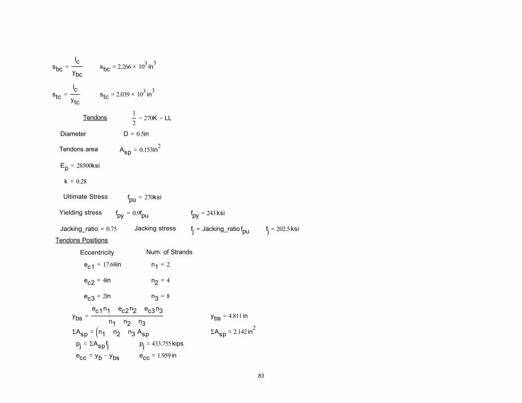
fj Jacking_ratio fpu= fj 202.5ksi=

Tendons Positions

Eccentricity Num. of Strands

ec1 17.68in= n1 2=

ec2 4in= n2 4=

ec3 2in= n3 8=

ybs

ec1n1 ec2n2+ ec3n3+

n1 n2+ n3+= ybs 4.811 in=

ΣAsp n1 n2+ n3+( )Asp= ΣAsp 2.142 in2

=

pj ΣAspfj= pj 433.755kips=

ecc yb ybs−= ecc 1.959 in=

sbc

Ic

ybc= sbc 2.266 103× in

3=

stc

Ic

ytc= stc 2.039 103× in

3=

Tendons1

2270K− LL−

Diameter D 0.5in=

Tendons area Asp 0.153in2

=

Ep 28500ksi=

k 0.28=

Ultimate Stress fpu 270ksi=

Yielding stress fpy 0.9fpu= fpy 243ksi=

Jacking_ratio 0.75= Jacking stress

83

Loss Data

Release Time RT 0.75day=

Relative Humidity RH 75= %

Loads:

SWgirder Wlfgf A=

SWHD Wlfd DTbw HTww+( )=

maintainance 0.02ksf=

SWgirder 230.208lb

ft=

SWHD 154.922lb

ft=

ml maintainanceBridgewid=

ml 720lb

ft=

84

values of shear forces and bending moments are for a simply supported interior beam under self weight weight of slab and haunch, in this case the design span is used.the shear forces and bending moments due to other loadings are calculated based on the continious span length.

85

Distribution factors:

Positive Moment

PMDF 0.2=

Negative Moment

NMDF 0.2=

Shear

VDF 0.42=

Impact Factor:

IM 0.33=

86

Span Data 60 58S.W. 230 154.92 Fy KipsDF 0.2 0.2 0.42 Mz K.ft

Span Node Location Fy Mz Fy Mz Fy Mz Fy Mz+ Mz- Fy Mz+ Mz- Fy Mz+ Mz- Fy Mz+ Mz- 1 1 0 6.68 0 4.49 0 -0.96 0 7.26 0 0 26.75 0 0 32.48 0 0 39.73 0 0

2 5 5.53 30.5 3.72 20.53 -0.72 5.04 5.64 18.4 -2.3 22.65 66.38 -6.356 26.8 78.86 -8.2 32.45 97.29 -10.463 11 4.14 59.51 2.79 40.05 -0.48 8.64 4.03 32.3 -4.61 19.21 113 -12.71 22.12 130.8 -16 26.15 163 -20.924 17 2.76 80.23 1.86 53.99 -0.24 10.8 2.42 41.5 -6.91 15.88 140.8 -19.07 17.68 157.7 -24 20.1 199.2 -31.385 23 1.38 92.66 0.93 62.36 0 11.52 0.81 46.1 -9.21 12.7 151.1 -25.42 13.54 169.1 -33 14.35 215.2 -41.856 29 0 96.8 0 65.14 0.24 10.8 -1.9 46.1 -11.5 -15.7 147.5 -31.78 -16.86 164.7 -41 -17.6 210.7 -52.317 35 -1.4 92.66 -0.9 62.36 0.48 8.641 -3.5 41.5 -13.8 -18.7 132 -38.13 -21.37 147.8 -49 -22.2 189.2 -62.778 41 -2.8 80.23 -1.9 53.99 0.72 5.041 -5.1 32.3 -16.1 -21.4 104.8 -44.49 -25.6 113.6 -57 -26.5 145.9 -73.239 47 -4.1 59.51 -2.8 40.05 0.96 0.001 -6.7 18.4 -18.4 -23.7 69.01 -50.84 -29.48 66.77 -65 -30.5 87.44 -83.6910 53 -5.5 30.5 -3.7 20.53 1.2 -6.48 -8.3 6.9 -27.6 -25.8 28.41 -57.2 -32.94 23.8 -73 -34.1 35.31 -101.111 58 -6.7 6E-14 -4.5 0 1.44 -14.4 -9.9 7.67 -53.7 -27.4 20.34 -81.45 -35.46 26.44 -106 -37.4 34.11 -159.6

2 1 0 6.68 0 4.49 0 -1.2 -14.4 9.41 7.67 -53.7 27.25 20.34 -81.45 33.96 26.44 -106 43.37 34.11 -159.62 5 5.53 30.5 3.72 20.53 -0.96 -7.92 7.79 3.83 -29.2 24.55 33 -71.27 30.09 18.91 -93 37.88 36.84 -121.83 11 4.14 59.51 2.79 40.05 -0.72 -2.88 6.18 13.8 -23 21.81 72.33 -61.09 25.85 71.84 -79 32.03 86.16 -102.44 17 2.76 80.23 1.86 53.99 -0.48 0.722 4.57 25.3 -23 18.78 102.8 -50.91 21.41 109.3 -66 25.98 134.6 -89.215 23 1.38 92.66 0.93 62.36 -0.24 2.882 2.96 32.3 -23 15.59 121.5 -40.73 16.92 132.4 -53 19.88 164.7 -75.986 29 0 96.8 0 65.14 0 3.602 1.34 34.6 -23 -12.9 126.9 -30.55 -13.26 137.1 -40 -11.5 171.6 -62.757 35 -1.4 92.66 -0.9 62.36 0.24 2.882 -3 32.3 -23 -16.1 121.5 -40.73 -17.67 132.4 -53 -19.1 164.7 -75.988 41 -2.8 80.23 -1.9 53.99 0.48 0.722 -4.6 25.3 -23 -19.3 102.8 -50.91 -22.16 109.3 -66 -23.9 134.6 -89.219 47 -4.1 59.51 -2.8 40.05 0.72 -2.88 -6.2 13.8 -23 -22.3 72.33 -61.09 -26.58 71.84 -79 -28.5 86.16 -102.410 53 -5.5 30.5 -3.7 20.53 0.96 -7.92 -7.8 3.83 -29.2 -25 33 -71.27 -30.76 18.91 -93 -32.8 36.84 -121.811 58 -6.7 6E-14 -4.5 0 1.2 -14.4 -9.4 7.67 -53.7 -27.3 20.34 -81.45 -33.96 26.44 -106 -36.7 34.11 -159.6

3 1 0 6.68 0 4.49 0 -1.44 -14.4 9.95 7.67 -53.7 27.45 20.34 -81.45 35.46 26.44 -106 45.41 34.11 -159.62 5 5.53 30.5 3.72 20.53 -1.2 -6.48 8.33 6.9 -27.6 25.48 28.41 -57.2 32.39 23.8 -73 40.73 35.31 -101.13 11 4.14 59.51 2.79 40.05 -0.96 0.001 6.72 18.4 -18.4 23.37 69.01 -50.84 28.86 66.77 -65 35.58 87.44 -83.694 17 2.76 80.23 1.86 53.99 -0.72 5.041 5.11 32.3 -16.1 20.93 104.8 -44.49 24.92 113.6 -57 30.02 145.9 -73.235 23 1.38 92.66 0.93 62.36 -0.48 8.641 3.49 41.5 -13.8 18.2 132 -38.13 20.64 147.8 -49 24.13 189.2 -62.776 29 0 96.8 0 65.14 -0.24 10.8 1.88 46.1 -11.5 15.23 147.5 -31.78 16.08 164.7 -41 17.97 210.7 -52.317 35 -1.4 92.66 -0.9 62.36 0 11.52 0.81 46.1 -9.21 -13.2 151.1 -25.42 -14.21 169.1 -33 -12.4 215.2 -41.858 41 -2.8 80.23 -1.9 53.99 0.24 10.8 -2.4 41.5 -6.91 -16.4 140.8 -19.07 -18.4 157.7 -24 -18.8 199.2 -31.389 47 -4.1 59.51 -2.8 40.05 0.48 8.64 -4 32.3 -4.61 -19.8 113 -12.71 -22.89 130.8 -16 -23.8 163 -20.9210 53 -5.5 30.5 -3.7 20.53 0.72 5.04 -5.6 18.4 -2.3 -23.2 66.38 -6.356 -27.6 78.86 -8.2 -28.9 97.29 -10.4611 58 -6.7 6E-14 -4.5 0 0.96 0 -7.3 0 0 -26.8 0 0 -32.48 0 0 -34 0 0

Tandem*DF*Impact FactorTruck*DF*Impact Factor LL*DF*Impact FactorDead Load Haunch+DeckComposite loadLane*DF*Impact FactorAnalysis Envelop:

87

Bending Moment

-100

-500

50100

150200250

0 10 20 30 40 50 60 70

Dead load moment

Haunch and Deck weight moment

Maintainance load moment

Live load positive moment

Live load negative moment

Prestress Losses:

Pi 0.7fpuΣAsp= Pi 404.838kips=

Elastic Shortening: ∆fpESfcgp= sum of concrete stresses at the center of gravity of prestressing tendons due to prestressing force at transfer and the

self-weight of the member section at section of maximum moment, fcgp will be calculated on Mg using the overall beam length at

release

Mmax1 SWgirderRS

2

8= Mmax1 1.243 103× kips in=

88

∆fpCR 18.949ksi=∆fpCR 12fcgp2 7∆fcdp−=

fcgp2 1.728ksi=fcgp2

Pi

A

Pi ecc2

I

+Mmax2ecc

I

−=

Mmax2 1.162 103× kips in=Mmax2 SWgirderBTB

2

8=

Now for the total final losses fcgp will be conservatively computed on Mg using the design span length

∆fcdp 0.255ksi=∆fcdp MZHD512

ecc

I

MZcomp512

ybc ybs−( )Ic

+

ki=

∆fcdp= Change in concrete stress at center of gravity of prestressing due to pemenant loads except the loads acting at time of

applying prestressing force calculated at the same section as fcgp

∆fpCRCreep:

∆fpSR 5.75ksi=∆fpSR 17 0.15RH−( )ksi=

Shrinkage:

Note: in Conspan 2.1 output file they reported a wrong value for fcgp but the right value for ∆fcgp

∆fpES 11.336ksi=∆fpES

Ep

Ec fcgr Wlfgr,( ) fcgp1=

fcgp1 1.705ksi=fcgp1

Pi

A

Pi ecc( )2

I

+Mmax1ecc

I

−=

89

initial loss% InLoss∆fpi

fj100= InLoss 6.487= %

Total Losses at service load:

∆fpt ∆fpES ∆fpSR+ ∆fpCR+ ∆fpR2+=∆fpt 39.192ksi=

stress in tendons at service load: fpe fj ∆fpt−= fpe 163.308ksi=

total prestressing losses at service load: Ppe fpeΣAsp= Ppe 349.805kips=

total loss% TLoss∆fpt

fj100= TLoss 19.354= %

Relaxation of Prestressing Strands:

Relaxation at Transfer: ∆fPR1

∆fpR1

log 24RT

day

40

fj

fpy0.55−

fj= ∆fpR1 1.801ksi=

Relaxation after Transfer:

∆fpR2 0.3 20ks 0.4∆fpES− 0.2 ∆fpSR ∆fpCR+( )− = ∆fpR2 3.158ksi=

Total Losses at Transfer:

∆fpi ∆fpES ∆fpR1+= ∆fpi 13.136ksi=

stress in tendons after transfer: fpt fj ∆fpi−= fpt 189.364ksi=

total prestressing losses after transfer: Ppi fptΣAsp= Ppi 405.617kips=

90

MDLtrans. 198.555kips in=

MDLtrans. 0.5SWgirderRS TL diff+( ) SWgirder TL diff+( )2

0.5−

=

TL 1.5 ft=TL 60D diff−=

diff 1ft=diff PTP BTB−( )0.5=Transfer length from bearing

Due to the camber of the beam at release, the beam self weight acts on the overall beam length

Check of Stresses at Transfer Length Section:

ftltrans. 0.212ksi=

ftltrans. 0.0948 fcgrks=Tension:

fcltrans. 3ksi=

fcltrans. 0.6fcgr=Compression:

Stress Limits for Concrete:

Ppi 405.617kips=

Check of Concrete Stresses at Transfer:

91

fcld.f.3 2ksi=fcld.f.3 0.4fcd=fclg.f.3 3.2ksi=fclg.f.3 0.4fcgf=

fcld.f.2 2.25ksi=fcld.f.2 0.45fcd=fclg.f.2 3.6ksi=fclg.f.2 0.45fcgf=

fcld.f.1 3ksi=fcld.f.1 0.6fcd=fclg.f.1 4.8ksi=fclg.f.1 0.6fcgf=

DeckBeam

Compression:

Stress Limits for Concrete:

Ppe 349.805kips=Check of Concrete Stresses at Service Load:

fbmspan. 1.399ksi=fbmspan.

Ppi

APpi

ecc

sb+

MDLmspan.

12sb−=

ftmspan. 2.668ksi=ftmspan.

Ppi

APpi

ecc

st−

MDLmspan.

12st+=

MDLmspan. 1.492 104× kips in=

MDLmspan. SWgirderRS

2

812=

Check of Stresses at Mid-span Section:

fttrans. 0.729ksi=fttrans.

Ppi

APpi

ecc

st−

MDLtrans.

st+

=

concrete stress at top fiber of the beam:

92

1. Final I : Under permenant and transit loads:

Concrete stress at the top Fiber of the slab, Service I:

ftsIII.mspan. 2.614ksi=

ftsIII.mspan. 0.5Ppe

APpe

ecc

st−

MZDL512ki

st+

MZHD512ki

st+

MZcomp512 ytc DT− HT−( )ki

Ic+

PMZLL512 ytc DT− HT−( )ki

Ic+=

3. Final III : Under Live loads plus one-half of Dead loads:

ftsII.mspan. 3.951ksi=

ftsII.mspan.Ppe

APpe

ecc

st−

MZDL512ki

st+

MZHD512ki

st+


Ic+=

ftd.s. 0.424ksi=2. Final II : Under permenant loads :

ftsI.mspan. 4.59ksi=

ftsI.mspan.Ppe

APpe

ecc

st−

MZDL512ki

st+

MZHD512ki

st+


Ic+

PMZLL512 ytc DT− HT−( )ki

Ic+=

1. Final I : Under permenant and transit loads:

Service I

Check of Stresses at Mid-span Section:

ftd.s.6

1000fcd1000ks=ftg.s. 0.537ksi=ftg.s.

6

1000fcgf1000ks=

Tension:

93

dp 21.619 in=dp hc ybs−=

PMu 584.716kips in=

PMu 1.25 MZDL5MZHD5

+ MZcomp5+

ki 1.75PMZLL5

ki+=

Total factored bending moment for strength I is:

Positive Moment Section:

Check of Strength limit state:

fbsIII.mspan. 0.592− ksi=

fbsIII.mspan.Ppe

APpe

ecc

sb+

MZDL512ki

sb−

MZHD512ki

sb−

MZcomp512ki

sbc−

0.8PMZLL( )5

12ki

sbc−=

Check of Tension Stress at the bottom fiber of the beam, Service III:

ftsIII.smspan. 1.006ksi=

ftsIII.smspan. ki 0.5

MZcomp512n

stc

PMZLL512( ) n

stc+

=

3. Final III : Under Live loads plus one-half of Dead loads:

ftsII.smspan. 0.05ksi=

ftsII.smspan.

MZcomp512nki

stc=

2. Final II : Under permenant loads:

ftsI.smspan. 1.031ksi=

ftsI.smspan.

MZcomp512nki

stc

PMZLL512( ) nki

stc+=

94

assume the section behave as a rectangular section

crec

ΣAspfpu

0.85fcd β1 fcd( ) bw kΣAsp

fpu

dp+

= crec 6.492 in=

cT

ΣAspfpu 0.85fcd β1 fcd( ) bw ww−( ) hf−

0.85fcd β1 fcd( ) ww kΣAsp

fpu

dp+

= cT 7.515 in=

c if crec hf> cT, crec,( )= c 7.515 in=

Average stress in prestressing steel

fps fpu 1 kc

dp−

= fps 243.72ksi=

a β1 fcd( ) c=

Mn

ΣAspfps dpa

2−

0.85fcd bw ww−( ) β1 fcd( ) hfa

2

hf

2−

+

12=

Mn 809.904kips in=

95

Bridgewid (ft) :Overall bridge widthLCurb (ft) :Left curb widthRCurb (ft) :Right curb widthNL :Number of lanesLW (ft) :Lane widthST (in) :Supplementry thicknessDT (in) :Deck thicknessHT (in) :Haunch thicknessHW (in) :Haunch widthPTP (ft) : Pier to pier lengthPL (ft) :Precast lengthBTB (ft) :Bearing to bearing lengthPTPR (ft) : Pier to centerline lengthRS (ft) :Release span

EC (Ksi) :Modulus of elasticity of the concreteWlfgr (pcf) :Unit length weight for the girder concrete at transferWlfgf (pcf) :Unit length weight for the girder concrete after 28 daysWlfd (pcf) :Unit length weight for the deck after 28 days fcgr (Ksi) :Compression strength for the girder concrete at releasefcgf (Ksi) :Compression strength of the girder after 28 daysfcd (Ksi) :Compression strength of the deck after 28 daysυ :Poisson's ratio

h (in) :Height of the non-composite sectionbw (in) :Bottom flange widthww (in) :Stem widthhf (in) :Flange height

A (in2) :Area of the non-composite section

I (in4) : Moment of inertia of the non-composite sectionyb (in) : Distance between the c.g. of the non-composite section and the bottom of the sectionyt (in) : Distance between the c.g. of the non-composite section and the top of the sectionhc

ksi 1000lb

in2

=

kips lb1000=

ksflb1000

ft2

=

ki kips in=

inkin

kips=

ks ksi=

ttft

5.5ksi

lb2

=

96

hc (in) :Height of the composite section

Ac (in2) :Area of the composite section

Ic (in4) : Moment of inertia of the composite sectionybc (in) : Distance between the c.g. of the composite section and the bottom of the sectionytc (in) : Distance between the c.g. of the composite section and the top of the composite section

D (in) :Tendon Diameter

Asp (in2) :Tendon areaEp (Ksi) :Modulus of elastisity of the tendonsk :Constant defined by AASHTO used in calculating the section's flexural capacityfpu (Ksi) :Tendon's ultimate stressfpy (Ksi) :Tendon's yielding stressfj (Ksi) :jacking stressec1, ec2, ec2 (in) :Eccentricity of the tendons rowsn1, n2, n3 :Number of tendons in a rowybs (in) :Distance between the c.g. of the tendons and the bottom of the section.

ΣAsp (in2) :Tendons areaRT (day) :Release timeRH (%) :Relative humiditySWgirder (kip/ft) :Girder self weight

SWHD (Kip/ft) :Haunch and deck self weight

ml (Kip/ft) :Maintainance loadPMDF :Positive moment distribution factor

NMDF :Negative moment distribution factor

VDF :Shear force distribution factor

IM :Live load impact factorpi (Kips) :Jacking force calculated based on 0.7fpu jacking stress used to calculate elastic shortening loss

97

fcgp1 (Ksi) :sum of concrete stresses at the center of gravity of prestressing tendons due to

prestressing force at transfer and the self-weight of the member section at section of maximum momentMmax1 (Kips-in) :Bending moment calculated at the midspan of a simply supported girder due to self weight

based on the overall beam length∆fpES (Ksi) :Elastic shortening loss

∆fpSR (Ksi) :Shrinkage loss

∆fcdp (Ksi) : Change in concrete stress at center of gravity of prestressing due to pemenant loads except the loads

acting at time of applying prestressing force calculated at the same section as fcgp

Mmax2 (Kips-in) :Bending moment calculated at the midspan of a simply supported girder due to self weight based on

the design span length∆fpcr (Ksi) :Creep loss

∆fPR1 (Ksi) :Relaxation at transfer

∆fPR2 (Ksi) :Relaxation after transfer

∆fPi (Ksi) :Total losses at transfer

fpt (Ksi) :Stress in tendons at transfer

ppi (Ksi) :Prestress force in tendons at transfer

∆fPt (Ksi) :Total losses at service load

fpe (Ksi) :Stress in tendons at service load

ppe (Ksi) :Prestress force in tendons at service load

fcltrans. (Ksi) :Allowable compression stress at transfer

ftltrans. (Ksi) :Allowable tension stress at transfe

98

TL (ft) :Transfer lengthMDLtrans. (Kip-in) :Dead load moment at transfer length

fttrans. (Ksi) :Stress at the top of the section at the transfer length section

MDLmspan. (Kip-in) :Dead load moment at midspan

ftmspan. (Ksi) :Stress at the top of the section at the midspan section

fbmspan. (Ksi) :Stress at the bottom of the section at the midspan section

fclg.f.2, fclg.f.2, fclg.f.2 (Ksi):Allowable compression stresses at service load final 1, 2, 3 respectively

ftg.s. (Ksi) :Allowable tension stresses at service load

ftsI.mspan., ftsII.mspan., ftsIII.mspan. (Ksi):Midspan stresses at the top of the section at service load final 1, 2, 3 respectively

ftsI.smspan., ftsII.smspan., ftsIII.smspan. (Ksi):Midspan stresses at the top of the slab at service load final 1, 2, 3 respectively

99

evaluation of the inverted tee shallow bridge system for use in ...

Documents

Transcript of evaluation of the inverted tee shallow bridge system for use in ...