Journal of Hydraulic ResearchVol. 44, No. 2 (2006), pp. 189–202

© 2006 International Association of Hydraulic Engineering and Research

Flow resistance ofPosidonia oceanicain shallow water

Resistance a l’écoulement dePosidonia oceanicaen eau peu profondeGIUSEPPE CIRAOLO, Researcher,Dipartimento di Ingegneria Idraulica e Applicazioni Ambientali, Università di Palermo,Viale delle Scienze, 90128 Palermo, Italy. Fax: 0039 091 6657749; e-mail: giuseppe@idra.unipa.it

GIOVANNI B. FERRERI, Associated Professor of “Hydraulics”,Dipartimento di Ingegneria Idraulica e Applicazioni Ambientali,Università di Palermo, Viale delle Scienze, 90128 Palermo, Italy. Fax: 0039 091 6657749; e-mail: giofer@idra.unipa.it(author for correspondence)

GOFFREDO LA LOGGIA, Professor of “Hydraulic Constructions”,Dipartimento di Ingegneria Idraulica e Applicazioni Ambientali,Università di Palermo, Viale delle Scienze, 90128 Palermo, Italy. Fax: 0039 091 6657749; e-mail: glal@idra.unipa.it

ABSTRACTManagement of coastal waters and lagoons by mathematical circulation models requires determination of the hydraulic resistance of submergedvegetation. A plant typical of sandy coastal bottoms in the Mediterranean Sea isPosidonia oceanica, which is constituted by very thin and flexibleribbon-like leaves, about 1 cm wide and up to 1.5 m long, and usually covers the bottom with a density of 500–1000 plants/m2. From the hydraulicviewpoint,P. oceanicaconstitutes a particular roughness, because, as the velocity increases, the leaves bend more and more until they lie down on thebottom. AlthoughP. oceanicais widespread, in the technical literature it is difficult to find indications about flow resistance due to this plant. In thispaper, the results of specific experimental research are reported. The runs were carried out in a laboratory flume, where the plants were reproducedassembling plastic strips. In these experiments, the leaf length was larger than the flow depth, reproducing a shallow water situation which is veryfrequent in lagoons. The results allow one to recognize the hydraulic behaviour of the plants with variation in the Reynolds number of flow and theratio between the leaf length and the flow depth. Velocity distribution in the section is also examined and a simple flow resistance law is achieved,which expresses Darcy–Weisbach’s friction factor as a function only of a particular Reynolds number.

RÉSUMÉLa gestion des eaux côtières et des lagunes par les modèles mathématiques de circulation exigent la détermination du frottement dû à la végétationimmergée. Une plante typique des fonds côtiers sableux en Méditerranée est laPosidonia oceanica, qui est constituée de feuilles, en forme de rubans,très minces et flexibles, ayant 1 cm de large environ et jusqu’à 1.5 m de long, et couvre généralement le fond avec une densité de 500 à 1.000 plantespar mètre carré. Du point de vue hydraulique, laPosidonia oceanicaconstitue une rugosité particulière, parce que, à mesure que la vitesse augmente,les feuilles se courbent de plus en plus jusqu’à ce qu’elles se couchent sur le fond. Bien que laPosidonia oceanicasoit très répandue, il est difficilede trouver dans la littérature technique des indications sur la résistance à l’écoulement due à cette plante. Dans le présent article, on rapporte lesrésultats d’une recherche expérimentale spécifique. Les essais ont été effectuées dans un canal de laboratoire, où les plantes ont été reproduites enassemblant les bandes de plastique. Dans ces expériences, la longueur de feuille était plus grande que le tirant d’eau, reproduisant une situation eneau peu profonde qui est très fréquente dans les lagunes. Les résultats permettent d’identifier le comportement hydraulique des plantes en fonctiondu nombre de Reynolds de l’écoulement et du rapport entre la longueur des feuilles et le tirant d’eau. La distribution de vitesse dans la section estégalement examinée et une loi de frottement simple est établie, qui exprime le facteur de frottement de Darcy-Weisbach uniquement comme unefonction d’un nombre de Reynolds particulier.

Keywords: Flow resistance, vegetation, aquatic vegetation, Posidonia oceanica, shallow water, velocity profiles.

1 Introduction

Modern management of coastal waters makes ever-greater useof mathematical circulation models, at present bi- and quasi-tri-dimensional, as research tools on the actual conditions of waterbodies and for prediction of the possible consequences causedby anthropic activities. However, in practice the use of thesemodels has a considerable limit in the user’s difficulty in intro-ducing suitable boundary conditions, both as circulation forcings

Revision received June 23, 2005/Open for discussion until February 28, 2007.

189

(tides, winds, currents, etc.) and as parameters characterizing thesea bottom, in particular the flow resistance (roughness). Thebehaviour of vegetation, which is greatly diversified, is one ofthe elements of uncertainty in the description of the hydrauliccharacteristics of the sea bottom.

In the Mediterranean Sea, close to shore areas,< 40 m deep,Posidonia oceanica(Fig. 1a) is widespread. The latter is a marineplant belonging to the genus ofPotamogetonacees, which is orga-nized (Fig. 1b) in roots, a short stem (called “rhizome”) and

190 Ciraolo et al.

Adult leavesYoung leaves

Root

Intermediate leaves

Rhizome

Bunch

Figure 1 Posidonia oceanica: (a) bottom with the plant; (b) parts ofthe plant.

leaves. The rhizome grows in both the vertical and the horizontaldirections, forming “mattes”, peculiar terrace formations consti-tuted by a weaving of many root beds. The leaves are ribbon-likeand very flexible, about 1 cm wide and up to 1.5 m long. They arearranged in tufts, each usually composed of six leaves, with ageand length decreasing from outside to inside.P. oceanicausuallysettles on sandy bottoms, and covers them for large areas, called“grasslands”. The number of plants per square metre usuallyvaries between 500 and 1000. Because of the peculiar character-istics ofP. oceanica, the latter constitutes a specific roughness,whose effects are considerably marked in lagoon environments,characterized by large expanses and low depths of about 1 m.

Unfortunately, in the technical literature it is not easy to findindications about the hydraulic behaviour of a bottom coveredby P. oceanica. The numerous researches on flow resistance dueto vegetation have traditionally concerned rivers and channels(e.g., see Kouwenet al., 1969; Petryk and Bosmajian, 1975;Chen, 1976; Temple, 1986; Kadlec, 1990; Freemanet al., 1998;Rahmeyeret al., 1999; López and García, 2001; Järvelä, 2002;Stone and Shen, 2002), while applications to coastal sea watersare relatively recent. Moreover, within the latter we find spe-cific studies on vegetable species typical of the particular zonesthat are considered each time (e.g., see Fonsecaet al., 1982;Gambiet al., 1990; Escartin and Aubrey, 1995; Worcester, 1995;Nepf and Vivoni, 2000). Therefore, the roughness coefficientsusually adopted in circulation models for Mediterranean coastalareas, whose bottom is covered byP. oceanica, are actually roughassessments.

In the Department of Hydraulic Engineering and Environ-mental Applications of the University of Palermo (Italy), in thelast few years several field studies have been carried out on themodelling of hydrodynamic circulation in lagoon environments,in particular studying the “Stagnone” at Marsala, near Trapani(West Sicily, Italy). The latter is a lagoon with a surface areaof about 30 km2 and generally under 1 m deep, whose bottomis largely covered byP. oceanica. Within these studies a specialexperimental research on flow resistance ofP. oceanicahas beenstarted (Ferrante, 2000).

This research is being carried out in the laboratory of the afore-said Department, in a flume where the plants were artificiallyreproduced by plastic strips. The research concerns the reciprocal

interference between the plants and the flow, the velocity profilesand the resistance law. The first results of this study, alreadyeffective in applications, were reported by Ciraoloet al. (2001)and Ciraolo and Ferreri (2002).

2 Experimental equipment

The experimental flume (Fig. 2) had an iron bearing structure andit was supplied by a concrete tank that got water from two pipes,of 250 and 100 mm, each equipped with an orifice plate for flowrate measurement. The flume was 14 m long altogether, had a60× 60 cm2 section and consisted of two reaches. The upstreamreach, 4 m long, penetrated into the tank and had iron bottom andwalls, and its function was to straighten pathlines before the flowfaced the second reach, where the experiments were really car-ried out. The second reach, 10 m long, was outside the tank, andhad a marble bottom and glass walls. At the ends of the experi-mental reach, two sharp sluice gates were placed, which allowedflow control. On the bottom of the same reach, 10 piezometricintakes were tapped on the axis, 1 m from one another, for mea-surement of water depths. In the figure, only the two intakes usedin the present research are shown. The flume could tilt around ahorizontal axis, by means of a hinge blocked in a wall of the sup-ply tank. Thanks to an engine, the bottom slope could be variedbetween−5 and+10% (respectively, uphill and downhill), butin the runs reported on here it was kept equal to zero.

On the bottom of the experimental reach 10 panels wereplaced (Fig. 3a), each 1 m long and 59.5 cm wide, over whichthe artificial plants had been arranged (Fig. 3a,b). Each panelwas constituted of a steel plate 1 mm thick, pre-pierced with8 mm diameter holes, fixed by screws to a wooden panel. Thelatter rested on two U-shaped aluminium sections, equippedwith threaded feet to allow its perfect horizontal placing. Thesteel plate was covered by a polyethylene sheet, to eliminate thehydraulic resistance due to the numerous holes in it. The plantswere made by assembling six strips of low density polyethy-lene (Fig. 3c), 1 cm wide and 0.2 mm thick. The outer couple ofleaves was 50 cm long, the middle 25 cm and the inner 12.5 cm.The plants were inserted in the steel plate holes for about 1 cmand blocked by assembling the plate with the wood panel. Theplanimetric distribution of the plants, chosen taking into account

Figure 2 Experimental flume.

Flow resistance ofP. oceanicain shallow water 191

(a) (b) (c)

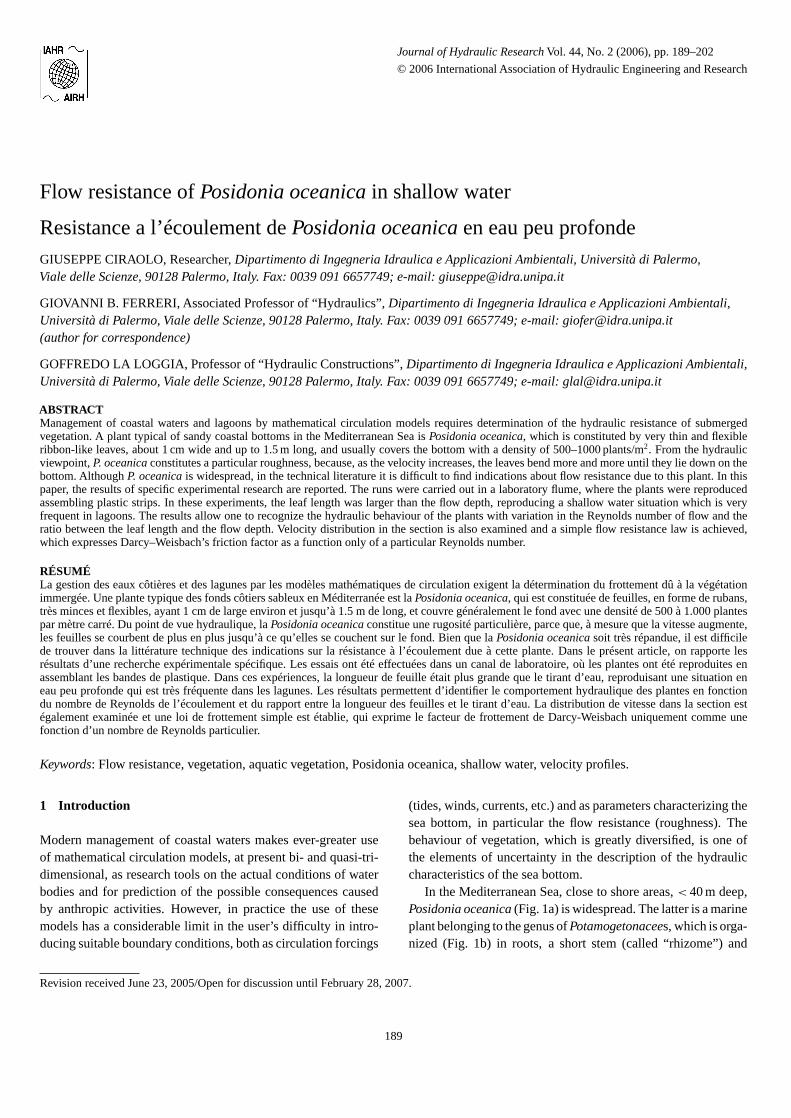
Figure 3 Experimental equipment: (a) flume with artificial plants; (b) flow through the canopy; (c) scheme of artificial plants.

the plate holes, produced an areal density of 682 plants/m2,within the range of the most frequent values met in nature (500–1000 plants/m2). Upstream and downstream, the covered stretchwas linked to the marble bottom of the flume by two concreteslides.

The measurements regarded the depths in two sections, 1 and2, respectively, at 6 and 7 m from the beginning of the coveredstretch, and the velocities in section 1, at the nodes of a gridwith seven vertical threads and, depending on the depth, 9–17horizontal ones. The depths were measured by two piezometerswith diameters of 50 mm, equipped with a water gauge with a1/10 mm nonius, and the velocities by a bi-dimensional ultra-sonic instrument of ADV type (Acoustic Doppler Velocimeter)made by Nortek. The latter was mounted on a truck allowing bothhorizontal and vertical shifts with a precision of 1/10 mm. Thesampling frequency chosen, 25 measurements per second, is themaximum allowed by the instrument. In each node, 1500 instan-taneous velocity values were taken (sampling time of 1 min),which were then averaged in time. Several suitable tests showedthat, over 1500 data, the time mean was practically constant.

With respect to the use of theADV, some points need stressing.The instrument allows a high precision (0.1 mm/s, for velocitieslarger than 2.5 m/s), a measurement error within±0.25% and amaximum sampling frequency of 25 Hz. However, it gauges thevelocity inside a small sampling volume situated laterally to theprobe, at about 5 cm from the latter. This means that, in the flowzone concerned by vegetation, in several cases the measurementswere altered, generally being underestimated, due to the pres-ence of the leaves. This problem proved to be more marked forlow flow velocities, for which the leaves that intervened betweenthe probe and the sampling volume remained almost still, in thesloping position determined by the flow characteristics (Fig. 3b).Despite this, the ADV seemed preferable to other gauges, whichare also intrusive, like the electromagnetic velocity-meter, thecurrent meter and the micro-current meter, also available in ourlaboratory: the first has a low sampling frequency (just a fewdata per second), the current meter is not suitable to operate withvelocities of a few centimetres per second, in shallow depthsand in thick leafage, while the micro-current meter is reliable inclear water only. However, as we shall see afterwards, the reli-ability of the measurements taken by the ADV was checked foreach run.

3 Hydraulic characteristics of the flow

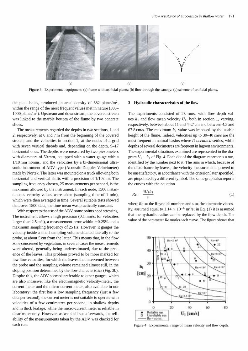
The experiments consisted of 23 runs, with flow depth val-uesh1 and flow mean velocityU1, both in section 1, varying,respectively, between about 11 and 44.7 cm and between 4.3 and67.8 cm/s. The maximumh1 value was imposed by the usableheight of the flume. Indeed, velocities up to 30–40 cm/s are themost frequent in natural basins whereP. oceanicasettles, whiledepths of several decimetres are frequent in lagoon environments.The experimental situations examined are represented in the dia-gramU1 −h1 of Fig. 4. Each dot of the diagram represents a run,identified by the number next to it. The runs in which, because ofthe disturbance by leaves, the velocity measurements proved tobe unsatisfactory, in accordance with the criterion later specified,are pinpointed by a different symbol. The same graph also reportsthe curves with the equation

Re= 4U1h1

ν(1)

whereRe= the Reynolds number, andν = the kinematic viscos-ity, assumed equal to 1.14× 10−6 m2/s; in Eq. (1) it is assumedthat the hydraulic radius can be replaced by the flow depth. Thevalue of the parameterRemarks each curve. The figure shows that

Figure 4 Experimental range of mean velocity and flow depth.

192 Ciraolo et al.

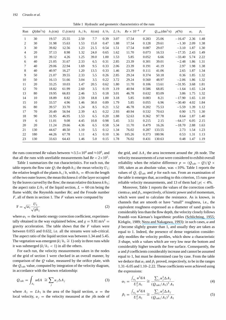
Table 1 Hydraulic and geometric characteristics of the runs

Run Q(dm3/s) h1(cm) U1(cm/s) hv/h1 k(cm) k/h1 L/h1 Re × 10−4 F Qcalc(dm3/s) p(%) α1 β1

1 30 19.57 25.55 2.50 7.7 0.39 3.07 17.54 0.283 25.06 −16.47 2.36 1.482 30 31.98 15.63 1.53 15.0 0.47 1.88 17.54 0.128 29.61 −1.30 2.09 1.383 30 39.82 12.56 1.23 21.5 0.54 1.51 17.54 0.087 29.07 −3.10 1.87 1.304 20 37.13 8.98 1.32 24.0 0.65 1.62 11.70 0.073 16.53 −17.35 2.43 1.495 10 39.12 4.26 1.25 39.0 1.00 1.53 5.85 0.052 6.66 −33.40 5.74 2.226 40 21.05 31.67 2.33 6.5 0.31 2.85 23.39 0.301 39.01 −2.48 1.86 1.317 40 29.06 22.94 1.69 9.5 0.33 2.06 23.39 0.191 41.19 2.97 1.98 1.388 40 40.97 16.27 1.20 13.5 0.33 1.46 23.39 0.111 41.06 2.65 1.87 1.349 50 21.07 39.55 2.33 5.5 0.26 2.85 29.24 0.374 50.18 0.36 1.85 1.32

10 50 16.13 51.66 3.04 3.5 0.22 3.72 29.24 0.560 48.97 −2.06 1.86 1.3211 20 33.25 10.03 1.47 20.5 0.62 1.80 11.70 0.106 13.61 −31.95 3.68 1.8112 70 18.82 61.99 2.60 3.5 0.19 3.19 40.94 0.586 68.85 −1.64 1.65 1.2413 80 19.95 66.83 2.46 3.5 0.18 3.01 46.78 0.632 83.09 3.86 1.75 1.3214 10 18.89 8.82 2.59 18.8 1.00 3.18 5.85 0.083 8.21 −17.90 1.65 1.1015 10 33.57 4.96 1.46 30.0 0.89 1.79 5.85 0.055 6.96 −30.40 4.02 1.8416 80 39.57 33.70 1.24 8.5 0.21 1.52 46.78 0.202 75.53 −5.59 1.39 1.1217 70 20.49 56.94 2.39 4.5 0.22 2.93 40.94 0.532 70.63 0.90 1.75 1.3018 90 31.95 46.95 1.53 6.5 0.20 1.88 52.63 0.362 97.78 8.64 1.87 1.4019 6 11.01 9.08 4.45 10.8 0.98 5.45 3.51 0.215 2.15 −64.17 6.05 2.1520 20 11.24 29.66 4.36 6.5 0.58 5.34 11.70 0.479 16.26 −18.70 2.88 1.6321 130 44.67 48.50 1.10 5.5 0.12 1.34 76.02 0.287 133.55 2.73 1.54 1.2322 180 44.26 67.78 1.11 4.5 0.10 1.36 105.26 0.373 180.96 0.53 1.31 1.1323 130 33.63 64.43 1.46 5.0 0.15 1.78 76.02 0.431 130.63 0.48 1.47 1.19

the runs concernedRevalues between≈3.5×104 and≈106, andthat all the runs with unreliable measurements hadRe< 2×105.

Table 1 summarizes the run characteristics. For each run, thetable reports the flow rateQ; the depthh1; the mean velocityU1;the relative length of the plantshv/h, with hv = 49 cm the lengthof the two outer leaves; the mean thicknessk of the layer occupiedby the leaves curved by the flow; the mean relative thicknessk/h1;the aspect ratioL/h1 of the liquid section,L = 60 cm being theflume width; the Reynolds numberRe; and the Froude numberF , all of them in section 1. TheF values were computed by

F = √α1

U1√gh1

(2)

whereα1 = the kinetic energy correction coefficient, experimen-tally obtained in the way explained below, andg = 9.81 m/s2 =gravity acceleration. The table shows that theF values werebetween 0.055 and 0.632, i.e. all the streams were sub-critical.The aspect ratio of the liquid section was between 1.34 and 5.45.The vegetation was emergent (k/h1

∼= 1) only in three runs whileit was submerged (k/h1 < 1) in all the others.

For each run, the velocity measurements taken in the nodesof the grid of section 1 were checked in an overall manner, bycomparison of theQ value, measured by the orifice plate, withtheQcalc value, computed by integration of the velocity diagram,in accordance with the known relationship:

Qcalc =∫

A1

udA ∼=∑

j

uj�Aj (3)

whereA1 = Lh1 is the area of the liquid section,u = thelocal velocity, uj = the velocity measured at thejth node of

the grid, and�Aj the area increment around thejth node. Thevelocity measurements of a run were considered to exhibit overallreliability when the relative differencep = (Qcalc − Q)/Q ×100, taken as an absolute value, was<10%. Table 1 reports thevalues ofQ, Qcalc andp for each run. From an examination ofthe table it emerges that, according to this criterion, 15 runs gavereliable velocity measurements, and 13 of them had|p| < 4%.

Moreover, Table 1 reports the values of the correction coeffi-cientsα1 andβ1, respectively, of kinetic power and of momentum,which were used to calculate the resistance. As is known, inchannels that are smooth or have “small” roughness, i.e., theequivalent roughness expressed as a diameter of sand grains isconsiderably less than the flow depth, the velocity closely followsPrandtl–von Kàrman’s logarithmic profiles (Schlichting, 1955;Kirkgöz, 1989; Nezu and Nakagawa, 1993): in such cases,α andβ become slightly greater than 1, and usually they are taken asequal to 1. Indeed, the presence of dense vegetation consider-ably modifies the velocity profiles, which show a characteristicS-shape, withu values which are very low near the bottom andconsiderably higher towards the free surface. Consequently, theα andβ coefficients considerably increase and cannot be assumedequal to 1, but must be determined case by case. From the tablewe deduce thatα1 andβ1 proved, respectively, to be in the ranges1.31–6.05 and 1.10–2.22. These coefficients were achieved usingthe expressions:

α1 =∫A1

u3dA

U31A1

∼=∑

j u3j�Aj

(Qcalc/A1)3 A1

(4)

β1 =∫A1

u2dA

U21A1

∼=∑

j u2j�Aj

(Qcalc/A1)2 A1

(5)

Flow resistance ofP. oceanicain shallow water 193

Figure 5 Disposition of vegetation during the runs: (a) waving;(b) prone.

where instead of the actual mean velocityU1 = Q/A1 the valueQcalc/A1 was adopted, considering that the use of the same mea-sured velocity valuesuj (even if affected by measurement errors)both in the numerator and in the denominator is more suitable forgetting information on the particular velocity distribution in therun considered.

Analogously to other experimental studies on long and flex-ible vegetation (Kouwenet al., 1969; Gourlay, 1970; Nepf andVivoni, 2000), during the runs three different dispositions of veg-etation were observed as the velocity increased: (1)erect, withthe plants taking up a position which was steady and slightlyinclined, with respect to the vertical; (2)waving(Fig. 5a), withthe plants being considerably inclined and showing an oscillatorymotion (monami); (3)prone(Fig. 5b), with the plants taking upan inflected, sub-horizontal and quasi-steady position.

4 Velocity distribution in the section

The velocity measurementsuj in the grid nodes were used todraw the velocity profiles along the verticals and the horizontals.Of course, an analysis of such profiles makes sense only for theruns considered reliable (|p| < 10%).

Profiles along a vertical were represented in the plane (u/u∗,y/h), y being the distance from the bottom andu∗ the frictionvelocity, given by

u∗ =√

τ0

ρ(6)

in which ρ = the water density, andτ0 = the shear stress atthe bottom, derived on the basis of the measurements, as will

0

0,2

0,4

0,6

0,8

1

0 2 4 6 8

u/u*

y/h

experimental point

flex point

k/ h

zone I

zone II

zone III

Figure 6 Typical velocity profile, with the three flow zones.

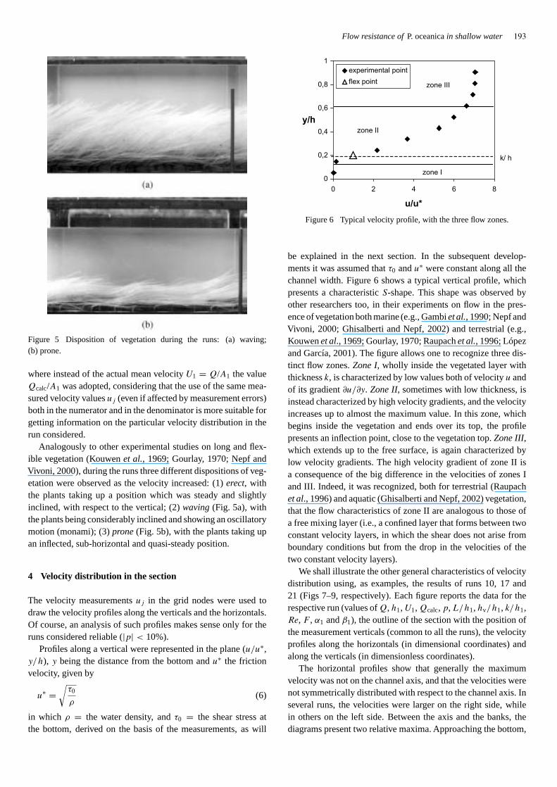
be explained in the next section. In the subsequent develop-ments it was assumed thatτ0 andu∗ were constant along all thechannel width. Figure 6 shows a typical vertical profile, whichpresents a characteristicS-shape. This shape was observed byother researchers too, in their experiments on flow in the pres-ence of vegetation both marine (e.g., Gambiet al., 1990; Nepf andVivoni, 2000; Ghisalberti and Nepf, 2002) and terrestrial (e.g.,Kouwenet al., 1969; Gourlay, 1970; Raupachet al., 1996; Lópezand García, 2001). The figure allows one to recognize three dis-tinct flow zones.Zone I, wholly inside the vegetated layer withthicknessk, is characterized by low values both of velocityu andof its gradient∂u/∂y. Zone II, sometimes with low thickness, isinstead characterized by high velocity gradients, and the velocityincreases up to almost the maximum value. In this zone, whichbegins inside the vegetation and ends over its top, the profilepresents an inflection point, close to the vegetation top.Zone III,which extends up to the free surface, is again characterized bylow velocity gradients. The high velocity gradient of zone II isa consequence of the big difference in the velocities of zones Iand III. Indeed, it was recognized, both for terrestrial (Raupachet al., 1996) and aquatic (Ghisalberti and Nepf, 2002) vegetation,that the flow characteristics of zone II are analogous to those ofa free mixing layer (i.e., a confined layer that forms between twoconstant velocity layers, in which the shear does not arise fromboundary conditions but from the drop in the velocities of thetwo constant velocity layers).

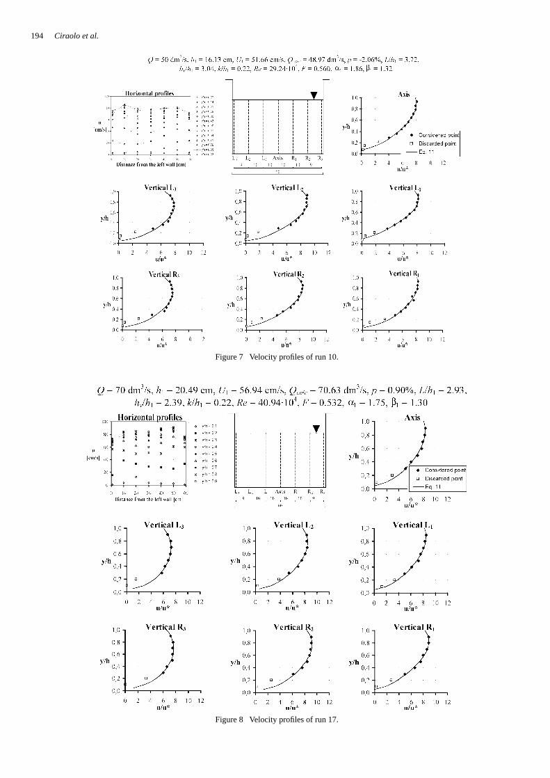
We shall illustrate the other general characteristics of velocitydistribution using, as examples, the results of runs 10, 17 and21 (Figs 7–9, respectively). Each figure reports the data for therespective run (values ofQ, h1, U1, Qcalc, p, L/h1, hv/h1, k/h1,Re, F , α1 andβ1), the outline of the section with the position ofthe measurement verticals (common to all the runs), the velocityprofiles along the horizontals (in dimensional coordinates) andalong the verticals (in dimensionless coordinates).

The horizontal profiles show that generally the maximumvelocity was not on the channel axis, and that the velocities werenot symmetrically distributed with respect to the channel axis. Inseveral runs, the velocities were larger on the right side, whilein others on the left side. Between the axis and the banks, thediagrams present two relative maxima. Approaching the bottom,

194 Ciraolo et al.

Figure 7 Velocity profiles of run 10.

Figure 8 Velocity profiles of run 17.

Flow resistance ofP. oceanicain shallow water 195

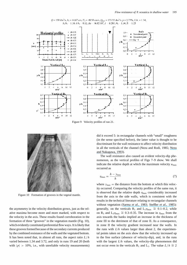
Figure 9 Velocity profiles of run 21.

Figure 10 Formation of grooves in the vegetal mantle.

the asymmetry in the velocity distribution grows, just as the rel-ative maxima become more and more marked, with respect tothe velocity in the axis. These results found corroboration in theformation of three “grooves” in the vegetation mantle (Fig. 10),which evidently constituted preferential flow ways. It is likely thatthese grooves formed because of the secondary currents producedby the combined resistance of the walls and the vegetated bottom.It has been noted that, in almost all runs, the aspect ratioL/h

varied between 1.34 and 3.72, and only in runs 19 and 20 (bothwith |p| > 10%, i.e., with unreliable velocity measurements)

did it exceed 5: in rectangular channels with “small” roughness(in the sense specified before), the latter value is thought to bediscriminant for the wall resistance to affect velocity distributionin all the verticals of the channel (Nezu and Rodi, 1985; Nezuand Nakagawa, 1993).

The wall resistance also caused an evident velocity-dip phe-nomenon, as the vertical profiles of Figs 7–9 show. We shallindicate the relative depth at which the maximum velocityumax

occurred as

ηmax = h − ymax

h(7)

whereymax = the distance from the bottom at which this veloc-ity occurred. Comparing the velocity profiles of the same run, itis observed that the relative depthηmax considerably increasedfrom the axis to the side walls, which is consistent with theresults in the technical literature relating to rectangular channelswithout vegetation (Sarmaet al., 1983; Steffleret al., 1985):generally, on the verticals R1 and L1ηmax

∼= 0.1–0.2, whileon R3 and L3ηmax

∼= 0.3–0.35. The increase inηmax from theaxis towards the banks implied an increase in the thickness ofzone III to the detriment of that of zone II. As a consequence,in zone II the velocity gradient increased near the walls. Inthe runs withL/h values larger than about 2, the experimen-tal points taken on the axis show that the velocity increased upto the free surface (absence of velocity-dip), and, in the runswith the largestL/h values, the velocity-dip phenomenon didnot occur even in the verticals R1 and L1. The valueL/h ∼= 2

196 Ciraolo et al.

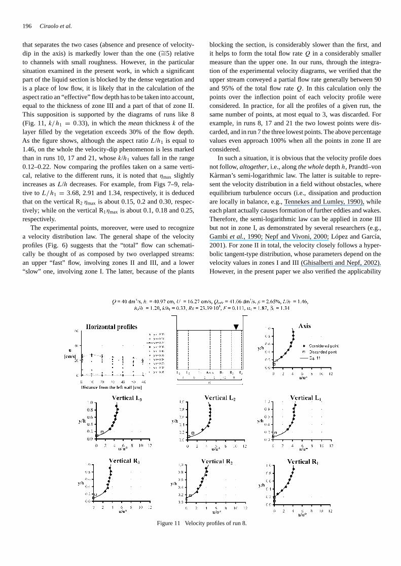
that separates the two cases (absence and presence of velocity-dip in the axis) is markedly lower than the one (∼=5) relativeto channels with small roughness. However, in the particularsituation examined in the present work, in which a significantpart of the liquid section is blocked by the dense vegetation andis a place of low flow, it is likely that in the calculation of theaspect ratio an “effective” flow depth has to be taken into account,equal to the thickness of zone III and a part of that of zone II.This supposition is supported by the diagrams of runs like 8(Fig. 11, k/h1 = 0.33), in which themeanthicknessk of thelayer filled by the vegetation exceeds 30% of the flow depth.As the figure shows, although the aspect ratioL/h1 is equal to1.46, on the whole the velocity-dip phenomenon is less markedthan in runs 10, 17 and 21, whosek/h1 values fall in the range0.12–0.22. Now comparing the profiles taken on a same verti-cal, relative to the different runs, it is noted thatηmax slightlyincreases asL/h decreases. For example, from Figs 7–9, rela-tive to L/h1 = 3.68, 2.91 and 1.34, respectively, it is deducedthat on the vertical R2 ηmax is about 0.15, 0.2 and 0.30, respec-tively; while on the vertical R1ηmax is about 0.1, 0.18 and 0.25,respectively.

The experimental points, moreover, were used to recognizea velocity distribution law. The general shape of the velocityprofiles (Fig. 6) suggests that the “total” flow can schemati-cally be thought of as composed by two overlapped streams:an upper “fast” flow, involving zones II and III, and a lower“slow” one, involving zone I. The latter, because of the plants

Figure 11 Velocity profiles of run 8.

blocking the section, is considerably slower than the first, andit helps to form the total flow rateQ in a considerably smallermeasure than the upper one. In our runs, through the integra-tion of the experimental velocity diagrams, we verified that theupper stream conveyed a partial flow rate generally between 90and 95% of the total flow rateQ. In this calculation only thepoints over the inflection point of each velocity profile wereconsidered. In practice, for all the profiles of a given run, thesame number of points, at most equal to 3, was discarded. Forexample, in runs 8, 17 and 21 the two lowest points were dis-carded, and in run 7 the three lowest points. The above percentagevalues even approach 100% when all the points in zone II areconsidered.

In such a situation, it is obvious that the velocity profile doesnot follow, altogether, i.e., alongthe wholedepthh, Prandtl–vonKàrman’s semi-logarithmic law. The latter is suitable to repre-sent the velocity distribution in a field without obstacles, whereequilibrium turbulence occurs (i.e., dissipation and productionare locally in balance, e.g., Tennekes and Lumley, 1990), whileeach plant actually causes formation of further eddies and wakes.Therefore, the semi-logarithmic law can be applied in zone IIIbut not in zone I, as demonstrated by several researchers (e.g.,Gambiet al., 1990; Nepf and Vivoni, 2000; López and García,2001). For zone II in total, the velocity closely follows a hyper-bolic tangent-type distribution, whose parameters depend on thevelocity values in zones I and III (Ghisalberti and Nepf, 2002).However, in the present paper we also verified the applicability

Flow resistance ofP. oceanicain shallow water 197

of the semi-logarithmic law in the upper part of zone II, abovethe inflection point.

According to Prandtl’s theory, in the turbulent boundary layerthe time-mean velocityu is expressed by

u

u∗ = 1

κln

u∗yν

+ B′ (8)

whereκ ∼= 0.4 is von Kàrman’s constant andB′ = a parameterthat takes into account the effects of the particular characteristicsof the bottom, and has to be experimentally determined. Indeed,in our particular case, it is more correct to speak of anoveralleffect of the lower zone Ithan of aneffect of the bottom. Theformer covers not only the bottom and the waving leaves, butalso the combination of the whirling motions originated by theimpact of water particles on the leaves. In the outer region of theboundary layer, where the “bottom effect” is less felt, numerousexperiences of various researchers have demonstrated that thereare differences, even marked ones, between the measured veloc-ities and the ones given by Eq. (8) (Coleman and Alonso, 1983;Nezu and Rodi, 1986; Cardosoet al., 1989). Therefore, Coles(1956) proposed to correct Eq. (8) by introducing a suitable wakefunctionY(y/h), so that the velocity is expressed by

u

u∗ = 1

κln

u∗ · y

ν+ B′ + Y

(y

h

)(9)

The best known expressions of the wake function are those givenby Coles (1956) and by Finleyet al. (1966). In order to describethe velocity profiles in the present work, we preferred Finleyet al.’s expression, since we considered it more suitable for theparticular shape of the profiles. The expression is the following:

Y = C

(y

h

)2(1 − y

h

)+ D

(y

h

)2(3 − 2

y

h

)(10)

where, according to Finleyet al., C = 1/κ, while D = Y(1)

is a parameter to be determined experimentally; in our case, wealso consideredC a parameter to be determined experimentally.SettingB = B′ + (1/κ) ln(u∗h/ν), Eq. (9) becomes:

u

u∗ = 1

κln

y

h+ B + C

(y

h

)2(1 − y

h

)

+ D

(y

h

)2(3 − 2

y

h

)(11)

with B, C andD parameters to be determined experimentally.The fitting of Eq. (11) to the experimental points of the

upper stream (i.e., over the inflection point) was verified forall the velocity profiles of the runs with reliable measure-ments (|p| < 10%), calculating their coefficients through the leastsquare method. Figures 7–9 and 11 show, for example, the fittingof Eq. (11) to the profiles of the relative runs. The figures showgeneral good fitting of Eq. (11) to the experimental points, even ifthis equation sometimes tends to stress the decrease in the veloc-ity near the free surface(y/h → 1). However, on the whole thefitting proves to be satisfactory, with relative differences betweentheu values measured and given by Eq. (11), which generally area few per cent. Velocity profiles will be better examined closely

by the writers in a subsequent paper. However, the writers thinkthat, in field applications, the aforesaid limit is not decisive, sinceconsiderable uncertainties exist concerning the description of thephysical environment and the flow forcings.

5 Resistance law

The classic methods to determine the flow resistance law areessentially two: (1) application of the momentum equation to acontrol volume, which allows one to calculate the hydraulic resis-tanceT ; (2) application of the energy equation for steady flowsbetween the extreme sections of the same control volume, thatgives the mean friction slopeSf in the stretch. The two quantitiesare linked through the simple relationship

T = γWSf (12)

in which γ = the specific weight of the liquid, andW = thecontrol volume. Indeed, Eq. (12) is rigorous just for uniformflows but it is sufficiently approximate, for practical purposes, forsteady flows. The friction slopeSf can be expressed by Darcy–Weisbach’s formula

Sf = λU2

8Rg(13)

whereλ = the friction factor andR = the hydraulic radius ofthe flow, here assumed to be about equal to the flow depth.

The flow momentum equation applied to the control volumebetween sections 1 and 2 (Fig. 12), projected along the streamdirection, gives:

T = G sinϕ + 1 + M1 − 2 − M2 = γWS + γhG1A1

+ β1ρQU1 − γhG2A2 − β2ρQU2 (14)

in which G = the control volume weight,ϕ = the angle thatthe bottom forms with the horizontal, 1 and 2 = the pres-sure forces in sections, respectively, 1 and 2,M1 andM2 = themomenta in sections, respectively, 1 and 2,S ∼= sinϕ the bot-tom slope, in our case equal to zero,hG1 andhG2 = the depthsof the centroids of the sections, respectively, 1 and 2, under thefree surface,A2 = the area of section 2,β2 = the momentumcorrection coefficient in section 2, andU2 = the mean velocityin section 2.

Figure 12 Control volume between sections 1 and 2, for determinationof flow resistance.

198 Ciraolo et al.

The steady flow energy equation for the same stretch can bewritten:

�E

�x= S − Sf (15)

in which

�E = E2 − E1 =(

h2 + α2U2

2

2g

)−

(h1 + α1

U21

2g

)(16)

is the variation in the specific energyE measured from the bottom,h2 = the flow depth,α2 = the correction coefficient of kineticpower, both in section 2, and�x = 1 m the stretch length; themeanfriction slope in the stretchSf is calculated in the sectionwith mean depth

hm = h1 + h2

2(17)

For each run of the present study (includingthose with|p| >

10%), the friction factorλ was calculated using both methods. Weshall return later to the use of the results of runs with unreliablevelocity measurements. In calculations, it was assumed thatα1 =α2 andβ1 = β2, in the realistic hypothesis that the variations insuch coefficients between the two sections are negligible, withrespect to those of the other quantities involved. Theλ valuesdetermined through the momentum equation(λM) and the energyequation(λE) are compared in Table 2, which shows that thevalues calculated through the two methods practically coincide.In the following processingλ was assumed equal to the meanvalue ofλM andλE. Themeanshear stress at the bottomτ0 (orrather the mean flow resistance per unit bottom area), which by

Table 2 Comparison betweenλ values deter-mined through the momentum equation (λM) andthe energy equation (λE)

Run λM λE

l 0.633 0.6132 1.613 1.6043 2.551 2.5454 3.946 3.9385 11.796 11.7766 0.452 0.4397 0.670 0.6628 6.948 6.9239 0.378 0.360

10 0.294 0.25611 3.592 3.57112 0.226 0.19713 0.231 0.19414 4.098 4.08815 9.568 9.55216 0.421 0.41717 0.264 0.23818 0.303 0.29219 3.434 3.32420 0.469 0.41021 0.263 0.25822 0.145 0.14223 0.154 0.148

Eq. (6) gave themeanfriction velocity u∗ used in the previoussection, was calculated by

τ0 = T

L�x= λ

8ρU2

1 (18)

Theλ values were then used to determine the functional link

λ = f

(Re ; hv

h

)(19)

Among the parameters characteristic of flow and vegetation, inEq. (19) there does not appear the heightk of the inflected plants,because, for fixed shape and stiffness (negligible) of the experi-mental plants,k actually depends on the hydraulic characteristicsof the flow (h, U, ρ andν) and on the plant length (hv), thus inturn it depends onReandhv/h. Indeed, suitable tests carried outby us, also considering the ratiok/h in theλ expression, showedthat the latter actually does not affect theλ value.

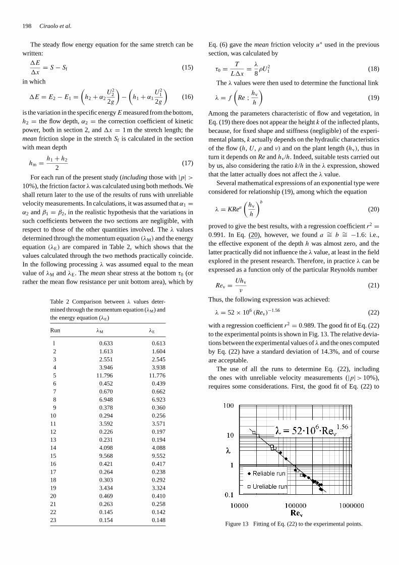
Several mathematical expressions of an exponential type wereconsidered for relationship (19), among which the equation

λ = KRea(

hv

h

)b

(20)

proved to give the best results, with a regression coefficientr2 =0.991. In Eq. (20), however, we founda ∼= b ∼= −1.6: i.e.,the effective exponent of the depthh was almost zero, and thelatter practically did not influence theλ value, at least in the fieldexplored in the present research. Therefore, in practiceλ can beexpressed as a function only of the particular Reynolds number

Rev = Uhv

ν(21)

Thus, the following expression was achieved:

λ = 52× 106 (Rev)−1.56 (22)

with a regression coefficientr2 = 0.989. The good fit of Eq. (22)to the experimental points is shown in Fig. 13. The relative devia-tions between the experimental values ofλand the ones computedby Eq. (22) have a standard deviation of 14.3%, and of courseare acceptable.

The use of all the runs to determine Eq. (22), includingthe ones with unreliable velocity measurements (|p| > 10%),requires some considerations. First, the good fit of Eq. (22) to

Figure 13 Fitting of Eq. (22) to the experimental points.

Flow resistance ofP. oceanicain shallow water 199

the set of experimental points tends to justify this choice. More-over, it must be noted that, in the determination of the resistanceT (Eq. (14)) and of the friction slopeSf (Eq. (15)), the velocitymeasurements are only taken into account through the correc-tion coefficients, respectively,β (Eq. (5)) andα (Eq. (4)). In thecomputation of such coefficients, the errors in the measured localvelocitiesuj intervene with the same exponent, and hence with ananalogous “weight”, in both the numerator and the denominator.Therefore, it is likely that, although the separate velocity valuesuj are incorrect, the correction coefficientsα andβ give accept-able information on the non-uniform distribution of velocityu inthe section considered. Moreover, since all the treated flows aresub-critical, the error in the assessment ofα andβ actually con-cerns two terms, the kinetic headαU2/(2g) and the momentumβρQU, which are minor compared to, respectively, the depthh

and the pressure forceγhGA, which attenuates the consequencesof the measurement errors.

The practical importance of Eq. (22) is evident: it allows one tocalculate the friction factor only knowing the mean flow velocityand maximum leaf length ofP. oceanicain the computing cellconsidered. This simple relationship clearly indicates that, forgiven characteristics of theP. oceanicagrassland (in particularthe leaf lengthhv), the friction factorλ decreases as the flowvelocity U increases (i.e., for a fixedh, asRe increases). Thisdecrease is consistent with the conclusions of other researcherswho have studied the hydraulic resistance of long and flexiblevegetation (Soil Conservation Service, 1954; Kouwenet al.,1969; Kouwen and Unny, 1973; Kouwen and Li, 1980; Tem-ple, 1986; Bakryet al., 1992; Järvelä, 2002). From a physicalviewpoint, this result is attributable to the very considerable flex-ibility of the leaves, which are erect for low velocities but liedown more and more asU increases. This implies that, on theone hand, the flow layer blocked by the vegetation (y < k:zone I, with low velocities, and lower part of zone II, belowthe inflection point) shrinks and, on the other hand, the angleof incidence of the flow with the leaves decreases. It shouldbe noted that, even when the leaves are prone (Fig. 5b), thelayer occupied by the vegetation is actually still thick (in all theruns it wask/h1 > 0.10, see Table 1), involving a large partof the flow. This interpretation is supported by the results ofJärvelä (2002), who made experiments on flexible terrestrial veg-etation, using different combinations of grass, sedge, and willow,the latter both with and without leaves. For leafless willow only,Järvelä found that, because of the slight bending of the stems, thefriction factorλ was practically constant as the Reynolds numberRevaried. By contrast, in the runs with leafy willows,λ con-siderably decreased asReincreased, because of the streamliningof the leaves and the smaller branches, caused by the leaf drag.The latter, on its part, produced a considerable increase (two tothree times) in theλ values, compared to leafless willow. In allthe other runsλ considerably decreased asRe increased. Thisconfirms the basic role of vegetation streamlining in determiningthe resistance law trend.

Equation (22) also allows one to recognize that, for a fixedvelocity U, the friction factorλ decreases as the leaf lengthhv

increases (i.e., for a fixed depthh, as the relative lengthhv/h

increases). The latter result, which was perhaps unexpected, canbe reasonably explained by the fact that the leaves, stretchingdownstream as they are dragged by the flow, in fact hamperdevelopment of eddies within the flow itself. As the lengthhv

increases, the tangle of leaves (inflected and outstretched down-stream) becomes denser and denser (the number of leaves thatintersect a given section increases), more and more hamper-ing the development of local eddies. Besides, it must be takeninto account that, in our experimental situations, the lengthhv

was larger than the flow depth (1.12≤ hv/h1 ≤ 4.83), and thisfavoured the leaves slightly sloping with respect to the horizon-tal. It is likely that the resistance law changes whenhv becomesconsiderably lower than the depthh.

With regard to the use of Eq. (22) in practical applications,some points need to be specified. Although the runs were car-ried out with depthh up to 45 cm, because of the low heightof the flume, the results can also be used for deeper waters.Indeed, the experimental leaf lengthhv was 49 cm, while innature the actual length ofP. oceanicaleaves is usually over 1 m,sometimes reaching 1.5 m. Therefore, the results of the presentresearch can also be extended to shallow natural waters up to1–1.5 m deep. For deeper waters further experimental researchesare needed.

Introducing Eq. (22) into Eq. (13) gives:

Sf = 52× 106ν1.56

8g

U0.44

hh1.56v

= 3.55× 10−4 U0.44

hh1.56v

(23)

in which h also appears, in addition toU andhv. Equation (23)shows that the friction slopeSf increases with the velocityU and decreases with the depthh, as was foreseeable, butdecreases with the leaf lengthhv, for the reasons expoundedabove.

6 Conclusions

We experimentally examined the hydraulic behaviour of theP. oceanica, a plant characteristic of sandy coastal areas in theMediterranean Sea. The experiments, carried out in a labora-tory flume in which the vegetation was artificially reproducedby polyethylene strips, first allowed one to recognize that, asthe flow velocity increases, three different dispositions of plantsoccur:erect, wavingandprone. The velocity diagrams presenteda peculiarS-shape, in which three flow zones are recognizable,with very low velocities in the vegetated layer, and much higherones in the upper flow layer. Through integration of the velocitydiagram, it was recognized that the flow rate in the vegetatedlayer is a small percentage of that of the total flow. This non-uniform velocity distribution along a vertical made it necessary,for the subsequent elaborations, to experimentally determine thecorrection coefficients of kinetic energy and momentum, which,in fact, proved to be considerably higher than one.

The particular experimental conditions, with the leaf lengtheven larger than the flow depth, made it difficult to carry out thevelocity measurements, which in several runs were shown notto be very reliable by comparison of the measured and the cal-culated flow rate. Analysis of the velocity profiles of the runs

200 Ciraolo et al.

considered reliable allowed one to recognize that, along a hori-zontal, generally the velocity presented two relative maxima, noton the axis, ensuing to the formation of three grooves in the veg-etated mantle. Along a vertical, the profile generally presented anevident dip-velocity phenomenon. The latter grew moving fromthe axis towards the walls, and, for aspect ratios of the liquid sec-tion smaller than a certain discriminating value, it also involvedthe flume axis. This discriminating value (about 2) proved to bemarkedly lower than the one (about 5) found in the technicalliterature for smooth channels or ones with an equivalent sandroughness considerably lower than the flow depth. Probably, thisis because an “effective” flow depth lower than the actual oneshould be taken into account. Both the dip-velocity phenomenonand the groove formation with the corresponding relative maximain the horizontal velocity profiles are attributable to wall resis-tance. Further researches would be able to clarify whether andto what extent the results should be rectified for practical fieldapplications, where there is no wall resistance but, on the otherhand, many uncertainties remain on flow forcings and bottomconformation.

Then, using for each vertical profile only the points overhang-ing the flex point of the relativeS, their fitting to Prandtl–vonKàrman’s law, rectified by the wake function of Finleyet al., wasexamined. The fitting proved to be satisfactory from the view-point of the differences between the measured and calculatedvalues, but this mathematical law tends sometimes to reproducea decrease in the velocity near the free surface which is slightlymore stressed than in reality.

Finally, by the application both of the momentum equationand of the energy equation between the outermost sections ofa control volume, for each run the values of the friction fac-tor of the Darcy–Weisbach’s formula were calculated, whichproved to be practically coincident with the two methods. Thesevalues then made it possible to achieve a monomial expres-sion of the friction factor. The latter, for the experimental arealdensity of plants, proves to be a function only of a particu-lar Reynolds number, constructed with the mean flow velocityand theP. oceanicaleaf length. In the light of this relationship,according to which the friction factor decreases as the flow veloc-ity and the leaf length increase, several physical explanationswere given of the role of the individual variables involved in thephenomenon.

The results are immediately applicable, obviously in thedimensionless variable field and for the areal plant density inves-tigated through the experiments. Of course, this field has to beextended, just as the areal plant density, also considering plantsof assorted sizes. The hydraulic behaviour of a bottom coveredby P. oceanicain a bi-dimensional flow field also needs to bestudied.

Notation

A = Area of the liquid sectionA1 andA2 = A values in sections, respectively, 1 and 2

B,B′, C andD = Parameters of velocity distributionE = Specific energy measured from the bottom

E1 andE2 = E values in sections, respectively, 1 and 2F = Froude numberg = Gravity accelerationG = Control volume weighth = Flow depth

h1 andh2 = h values in sections, respectively, 1 and 2hG1 andhG2 = Depths of the centroids of the sections,

respectively, 1 and 2 under the free surfacehm = Mean depth in the control stretchhv = Length of the two outer leavesk = Mean thickness of the layer occupied by the

leaves curved by the flowL = Flume width

M1 andM2 = Momenta in sections, respectively, 1 and 2p = Per cent relative difference betweenQcalc andQ

valuesQ = Flow rate

Qcalc = Flow rate value, computed by integration of thevelocity diagram

R = Hydraulic radiusRe = Reynolds number

Rev = Reynolds number constructed with the mean flowvelocity and the leaf length

S = Bottom slopeSf = Friction slopeT = Hydraulic resistanceu = Local time-mean velocity

uj = Time-mean velocity measured at thejth node ofthe grid

umax = Maximum velocity along a verticalu∗ = Friction velocityU = Flow mean velocity

U1 andU2 = U values in sections, respectively, 1 and 2y = Distance from the bottomY = Wake function

ymax = Value ofy at which the maximum velocityumax

occurredW = Control volumeα = Kinetic power correction coefficient

α1 andα2 = α values in sections, respectively, 1 and 2β = Momentum correction coefficient

β1 andβ2 = β values in sections, respectively, 1 and 2γ = Water specific weight

�Aj = Area increment around thejth node of the grid�x = Control stretch length

ηmax = Relative depth at which the maximum velocityumax occurred

κ = von Kàrman’s constantλ = Friction factor of Darcy–Weisbach’s formula

λE andλM = λ values determined through, respectively, theenergy equation and the momentum equation

ν = Kinematic viscosity 1 and 2 = Pressure forces in sections, respectively, 1 and 2

ρ = Water densityτ0 = Mean flow resistance per unit bottom areaψ = Angle that the bottom forms with the horizontal

Flow resistance ofP. oceanicain shallow water 201

References

1. Bakry, M.F., Gates, T.K. and Khattab, A.F. (1992).“Field-Measured Hydraulic Resistance Characteristics inVegetation-Infested Canals”.J. Irrig. Drain. Engng. ASCE118(2), 256–274.

2. Cardoso, A.H., Graf, W.H. and Gust, G. (1989). “Uni-form Flow in a Smooth Open Channel”.J. Hydraul. Res.27(5), 603–616.

3. Chen, C. (1976). “Flow Resistance in Broad ShallowGrassed Channels”.J. Hydraul. Div. ASCE102(HY3),307–322.

4. Ciraolo, G., Ferrante, F., Ferreri, G.B., Folkard, A.and La Loggia, G. (2001). “Flow Resistance of Ribbon-like Vegetation Long and Very Flexible in Shallow Water”.Proceedings of the 2001 International Symposium on Envi-ronmental Hydraulics, Tempe, Arizona, December 5–8.

5. Ciraolo, G. and Ferreri, G.B. (2002). “Flow ResistanceOver a Bottom Covered byPosidonia oceanica” (in Italian;original title “Resistenza al moto di una corrente su un fondoricoperto daPosidonia oceanica”). Proceedings of the 28thConvegno di Idraulica e Costruzioni Idrauliche (Congressof Hudraulics and Hydraulic Works), Potenza, Italy, Vol. 3,September 16–19, pp. 369–376.

6. Coleman, N.L. and Alonso, C.V. (1983). “Two-dimensional Channel Flows Over Rough Surfaces”.J.Hydraul. Engng. ASCE109(2), 175–188.

7. Coles, D. (1956). “The Law of the Wake in the TurbulentBoundary Layer”.J. Fluid Mech.1, 191–226.

8. Escartin, J. and Aubrey, D.G. (1995). “Flow Structureand Dispersion WithinAlgal Mats”.Estuarine Coastal ShelfSci.40, 451–472.

9. Ferrante, F. (2000). “Experimental Research on FlowResistance of Long and Flexible Ribbon-like Vegetation:the Case ofPosidonia oceanica” (in Italian; original title“ Indagine sperimentale sulla resistenza al moto di vege-tazione nastriforme lunga e flessibile: il caso dellaPosidoniaoceanica”). Graduation Thesis, Dipartimento di Ingegne-ria Idraulica e Applicazioni Ambientali della Università diPalermo, Italy.

10. Finley, P.J., Khoo, C.P. and Chin, J.P. (1966). “VelocityMeasurements in a Thin Turbulent Water Layer”.La HouilleBlanche21(6), 713–721.

11. Fonseca, M.S., Fisher, J.S., Zieman, J.C. and Thayer,G.W. (1982). “Influence of the Seagrass,Zostera marinaL., on Current Flow”. Estuarine Coastal Shelf Sci.15,351–364.

12. Freeman, G.E., Rahmeyer, W., Derrick, D.L. andCopeland, R.R. (1998). “Manning’sValues for Floodplainswith Shrubs andWoodyVegetation”.Proceedings of USCIDConference on Shared Rivers, Park City, UT, October 28–31.U.S. Committee on Irrigation and Drainage, Denver, Coo.

13. Gambi, V.A., Nowell, R.M. and Jumars, P.A. (1990).“Flume Observations on Flow Dynamics inZosteramarina (Eelgrass) Beds”.Mar. Ecol. Prog. Ser. 61,159–169.

14. Ghisalberti, M. and Nepf, H.M. (2002). “Mixing Layersand Coherent Structures in Vegetated Aquatic Flows”.J.Geophys. Res.107(C2), 1–11.

15. Gourlay, M.R. (1970). Discussion of “Flow Retardancein Vegetated Channels” by Kouwen, N., Unny, T.E. andHill, H.M. (1969). J. Irrig. Drain. Div. ASCE 96(IR3),351–357.

16. Järvelä, J. (2002). “Flow Resistance of Flexible and StiffVegetation: a Flume Study with Natural Plants”.J. Hydrol.269, 44–54.

17. Kadlec, R.H. (1990). “Overland Flow in Wetlands: Vege-tation Resistance”.J. Hydraul. Engng.116(5), 691–706.

18. Kirkgöz, M.S. (1989). “Turbulent Velocity Profiles forSmooth and Rough Open Channel Flow”.J. Hydraul.Engng. ASCE115(11), 1543–1561.

19. Kouwen, N., Unny, T. E. and Hill, H.M. (1969). “FlowRetardance in Vegetated Channels”.J. Irrig. Drain. Div.ASCE95(IR2), 329–342.

20. Kouwen, N. and Li, R. (1980). “Biomechanics of Vegeta-tive Channel Linings”.J. Hydraul. Div. ASCE106(HY6),1085–1103.

21. Kouwen, N. and Unny, T.E. (1973). “Flexible Rough-ness in Open Channels”.J. Hydraul. Div. ASCE99(HY5),713–728.

22. López, F. and García, M.H. (2001). “Mean Flow andTurbulence Structure of Open-Channel Flow Through Non-emergent Vegetation”.J. Hydraul. Engng.127(5), 392–402.

23. Nepf, H.M. and Vivoni, E.R. (2000). “Flow Structurein Depth-Limited, Vegetated Flow”.J. Geophys. Res.105(C12), 28,547–28,557.

24. Nezu, I. and Nakagawa, H. (1993).Turbulence in Open-Channel Flows. IAHR Monoghaph Series, A.A. Balkema,Rotterdam.

25. Nezu, I. and Rodi, W. (1985). “Experimental Study on Sec-ondary Currents in Open Channel Flow”.Proceedings of the21st IAHR Congress, Melbourne, Vol. 2, pp. 115–119.

26. Nezu, I. and Rodi, W. (1986). “Open-Channel Flow Mea-surements with a Laser Doppler Anemometer”.J. Hydraul.Engng. ASCE112(5), 335–355.

27. Petryk, S. and Bosmajian, G., III (1975). “Analysisof Flow Through Vegetation”.J. Hydraul. Div. ASCE101(HY7), 871–884.

28. Rahmeyer, W., Werth, D. Jr. and Freeman, G. (1999).“Improved Methods of Determining Vegetative Resistancein Floodplains and Compound Channels”.Proceedings ofASCE Conference on Water Resources, Seattle, WA, August8–12. American Society of Civil Engineers, Reston, VI.

29. Raupach, M.R., Finnigan, J.J. and Brunet, Y. (1996).“Coherent Eddies and Turbulence in Vegetation Canopies:The Mixing LayerAnalogy”.Boundary Layer Meteorol.78,351–382.

30. Sarma, K.V.N., Lakshminarayana, P. and Rao, N.S.L.(1983). “Velocity Distribution in Smooth Rectangular OpenChannels”.J. Hydraul. Engng.109(2), 270–289.

31. Schlichting, H. (1955).Boundary Layer Theory. Perga-mon Press Ltd, London.

202 Ciraolo et al.

32. Soil Conservation Service (1954).Handbook of ChannelDesign for Soil and Water Conservation, SCS-TP-61, USDepartment of Agriculture, Washington, DC.

33. Steffler, P.M., Rajaratnam, N. and Peterson, A.W.(1985). “LDA Measurements in Open Channel”.J. Hydraul.Engng.111(1), 119–130.

34. Stone, B. and Shen, H.T. (2002). “Hydraulic Resistance ofFlow in Channels with Cylindrical Roughness”.J. Hydraul.Engng. ASCE128(5), 500–506.

35. Temple, D.M. (1986). “Velocity Distribution Coefficientsfor Grass-lined Channels”.J. Hydraul. Engng.ASCE112(3), 193–204.

36. Tennekes, H. and Lumley, J.L. (1990).A First Course inTurbulence, MIT Press, Cambridge, MA.

37. Worcester, S.E. (1995). “Effect of Eelgrass Beds onAdvection and Turbulent Mixing in Low Current and LowShoot Density Environments”.Mar. Ecol. Prog. Ser.126,223–232.