This article appeared in a journal published by Elsevier. The attachedcopy is furnished to the author for internal non-commercial researchand education use, including for instruction at the authors institution

and sharing with colleagues.

Other uses, including reproduction and distribution, or selling orlicensing copies, or posting to personal, institutional or third party

websites are prohibited.

In most cases authors are permitted to post their version of thearticle (e.g. in Word or Tex form) to their personal website orinstitutional repository. Authors requiring further information

regarding Elsevier’s archiving and manuscript policies areencouraged to visit:

http://www.elsevier.com/copyright

Author's personal copy

Relationships between multibeam backscatter, sediment grain size andPosidonia oceanica seagrass distribution

Giovanni De Falco a,n, Renato Tonielli b, Gabriella Di Martino b, Sara Innangi b,Simone Simeone c, Iain Michael Parnum d

a Istituto per l’Ambiente Marino Costiero, IAMC-CNR, UO Oristano, Localit �a Sa Mardini, 09072 Torregrande, Oristano, Italyb Istituto per l’Ambiente Marino Costiero, IAMC-CNR Sede, Calata Porta di Massa-Porto di Napoli, 80133 Napoli, Italyc Fondazione IMC, Centro Marino Internazionale ONLUS, Localit �a Sa Mardini, 09072 Torregrande, Oristano, Italyd Centre for Marine Science and Technology, Curtin University, GPO Box U1987, Perth, WA 6845, Australia

a r t i c l e i n f o

Article history:

Received 11 June 2010

Received in revised form

3 September 2010

Accepted 8 September 2010Available online 21 September 2010

Keywords:

Multibeam backscatter

Angular response

Posidonia oceanica seagrass

Sediment grain size

a b s t r a c t

The use of data, including bathymetry, backscatter intensity and the angular response of backscatter

intensity, collected using multibeam sonar (MBS) systems to recognise seabed types was evaluated in

the inner shelf of central western Sardinia (western Mediterranean sea), a site characterised by a

complex seabed including sandy and gravelly sediments, Posidonia oceanica seagrass beds growing on

hardgrounds (i.e. biogenic carbonates) and sedimentary substrates.

A MBS survey was carried out in order to collect bathymetric and acoustic backscatter data. Ground-

truth data in the form of grab samples and diver observations were collected at 57 stations, 41 of which

were in non-vegetated sedimentary substrate and 16 of which were in P. oceanica beds. Sediment

samples were analysed for grain size.

Statistical comparison between MBS backscatter and grain size data showed that backscatter

intensity is strongly affected by sediment grain size, being directly correlated to the weight percent of

the coarse fraction (1–16 mm) and inversely correlated to weight percent of the finer sediments

(0.016–0.5 mm). Factor analysis of grain size and acoustic data identified three sedimentary facies:

sandy gravels (SG), gravelly sands (GS) and slightly gravelly muddy sands (SGMS). Each facies showed

different acoustic responses in terms of backscatter intensity and shape of the angular response curves.

Differences in backscatter intensity among five seabed types, including the three sediment types

identified by factor analysis and P. oceanica beds, growing on hardgrounds and sedimentary substrates,

were tested by analysis of variance. P. oceanica on hardgrounds, P. oceanica on sedimentary substrates

and GS exhibited values of relative backscatter intensity within the same range and, consequently, it

was not possible to distinguish Posidonia beds and gravelly sands only on the basis of backscatter data.

The similarity of backscatter intensity from P. oceanica growing on different substrates suggests that the

acoustic response is mainly linked to the leaf canopy rather than the substrate it is growing on.

A map of seabed classification, including sediment types and seagrass distribution was produced

through a combination of information derived from backscatter data and morphological features

derived from multibeam bathymetry, which were validated by ground-truth data.

& 2010 Elsevier Ltd. All rights reserved.

1. Introduction

Acoustic methods for seafloor mapping have been widelydeveloped over the last decades. In particular, the development ofswath bathymetry has enabled the creation of detailed maps ofseabed topography and acoustic backscatter data; these data havebeen used to predict sediment and habitat types (e.g. Medialdeaet al., 2008; Sutherland et al., 2007, and references therein).

Several studies have compared backscatter responses to ground-truth data (e.g. sediment sampling, video imagery of the seafloor)in order to assess the ability of different acoustic technologies toclassify seafloor types (e.g. Ferrini and Flood, 2006; Goff et al.,2004; Kostylev et al., 2001).

Backscatter intensity, the measurement of sound scatteredback toward the transmitter by acoustic reflection and scattering,has been shown to be related to sediment properties (e.g. Ferriniand Flood, 2006; Goff et al., 2004; Sutherland et al., 2007). Forinstance, backscatter intensity from a muddy seafloor has beenshown to be inversely linearly related to the sediment porosity,percent silt content and percent clay content (e.g. Sutherland

Contents lists available at ScienceDirect

journal homepage: www.elsevier.com/locate/csr

Continental Shelf Research

0278-4343/$ - see front matter & 2010 Elsevier Ltd. All rights reserved.

doi:10.1016/j.csr.2010.09.006

n Corresponding author. Tel.: +39 0783 22027; fax: +39 0783 22002.

E-mail address: giovanni.defalco@cnr.it (G. De Falco).

Continental Shelf Research 30 (2010) 1941–1950

Author's personal copy

et al., 2007; Hamilton et al., 1956). Fine sediments generallyexhibit low backscatter intensity due to low density and soundvelocity (e.g. Ferrini and Flood, 2006; Stewart et al., 1994).

The spatial variability of backscatter intensity along theseafloor characterised by coarse sediments has been shown tobe mainly driven by the weight percent of coarse grains (44 mm)(Goff et al., 2004). Coarse sediments are more likely to result inhigher backscatter intensity due to scattering from coarseparticles, lower porosity, higher density and sound velocity, andgreater roughness of the sediment–water interface (Briggs et al.,2001, 2002; Ferrini and Flood, 2006; Richardson et al., 2001).Furthermore, in sandy sediments backscatter intensity has beenfound to decrease with mean grain size (Ferrini and Flood, 2006).

Exceptions to those relationships can be due to inhomogene-ities, the presence of near-surface gas, or bioturbation in surficialsediments (Borgeld et al., 1999; Fonseca et al., 2002; Urgeles et al.,2002).

In addition to seafloor properties, the incidence angle at whichbackscatter is measured can strongly influence its intensity.Backscatter strength near nadir (i.e. small incidence angles) isgenerally higher than values recorded in the outer swath becauseof differences between reflection (near nadir) and scattering(outer swath) (Ferrini and Flood, 2006; de Moustier andAlexandrou, 1991). The variation of (discrete) measurements ofbackscatter over a range of incidence angles, referred to here as anangular response, has been used as a way to discriminate betweendifferent seafloor types (Hughes Clarke et al., 1997; Parnum et al.,2004). For example, backscatter intensity collected over denseseagrass with the high-frequency Reson Seabat 8125 was found tobe almost independent of the angle of incidence (Siwabessy et al.,2006). In contrast, sandy and muddy sediments exhibit a strongdecrease in backscatter strength toward the outer swaths(Siwabessy et al., 2006). The acoustic response from the seabedalso depends on instrumental characteristics, particularly thefrequency of the signal.

The acoustic response from the seabed can also be related tothe presence of benthic organisms (i.e. macroalgae, seagrass,sessile invertebrates) (Holmes et al., 2008). Consequently, multi-beam bathymetry and related backscatter have been used to mapbenthic habitats (Kostylev et al., 2001). For example, the analysisof backscatter intensity data collected with a MBS (a Reson Seabat8125, operating at 455 kHz) allowed an acoustic classification ofdifferent seafloor habitats along the Australian coastal zone(Siwabessy et al., 2006). Seafloor habitats that were identifiedusing backscatter intensity (validated with ground-truth informa-tion) included: sandy and muddy sediments, coarse sediments(rhodolith, rock and shell debris), rocky outcrops and coral reefs,seagrass and algae (Siwabessy et al., 2006). The backscatterstrength in the presence of Posidonia oceanica seagrass was foundto be higher than compared to sandy and muddy bottom (Parnum,2007), this was also the finding of Lyons and Abrahams (1999).

Compared to rock and sediments, acoustic scattering fromseagrass is poorly understood. Several studies have analysed theacoustic response from different seagrass species in order tounderstand the underlying physical scattering mechanisms.Laboratory experiments have shown the sound speed in a plant-filled resonator to be dependent on plant biomass and tissuecharacteristics, which varies for different seagrass species (Wilsonand Dunton, 2009). The acoustic response from seagrass is alsoinfluenced by photosynthetic activity, which produces free gasbubbles on the plants and in the water column (Hermand et al.,1998). Lyons and Abrahams (1999) also found that the statisticaldescription of variability of backscatter could be used tocharacterise the bottom colonised by P. oceanica seagrass due tothe inhomogeneous distribution of seagrass patches and themotion of leaves due to swell.

The inner shelf of the Mediterranean sea can be characterisedby the presence of the endemic seagrass specie P. oceanica andcoralligenous assemblages. P. oceanica is widely distributed acrossthe whole basin down to a depth of 30–40 m in clear waters(Per�es and Picard, 1964), and can be associated with sedimentarysubstrate and hardgrounds (i.e. rocky or bio-constructed hardsubstrates) with the plant rooted in the troughs. In the inner shelfwhere the depth is greater than maximum limits of P. oceanica,coralligenous assemblages have been found to occur (Ballesteros,2006). These deeper assemblages are calcareous formations ofbiogenic origin and are produced by the accumulation ofencrusting algae growing in dim light conditions (Ballesteros,2006).

In this paper, the capability of MBS data, including bathymetry,backscatter intensity and angular response, to distinguish differ-ent seabed types in a site in the Mediterranean sea is evaluated.The study area has a complex seabed that includes sandy-gravellysediments, P. oceanica seagrass on biogenic hard and sedimentarysubstrate. Acoustic data were statistically correlated to sedimen-tary data and benthic habitat distribution (using ground-truthdata) to evaluate the acoustic variables, which best discriminateseabed typologies in this environment.

2. Material and methods

2.1. Study site

The study area is located in the inner shelf of the central-western coast of Sardinia (Western Mediterranean Sea) from theGulf of Oristano out to the deeper shelf toward the west (Fig. 1).The western Sardinia margin was structured in the Oligoceneearly-Miocene by back-arc transtension processes, and succes-sively segmented under an extensional regime related to theopening of the Tyrrhenian basin from the late Miocene to theQuaternary (Casula et al., 2001; Fais et al., 1996).

The area of the Gulf of Oristano is approximately 150 km2 andhas a maximum depth of 24 m. About 70% (100 km2) of theseabed surface of the gulf is covered by two P. oceanica meadowson sedimentary substrate (Fig. 1). The larger meadow of thecentral sector of the gulf of Oristano was partially included in theacquisition area (Fig. 1). This seagrass meadow was on asedimentary substrate composed of siliciclastic, gravelly sandsand sandy gravels (De Falco et al., 2008).

The non-vegetated area between the two meadows is a widetrough, considered the paleovalley of the Tirso river, the majortributary of the gulf, during the last glaciation (Carboni et al.,1989). Toward the west, this area is characterised by coarsesediments covered in the inner sector by muddy deltaicsediments (De Falco et al., 2008).

A morphological threshold separates the gulf from the opensea (De Falco et al., 2008), which has been interpreted to be theresult of beach rock formations (Carboni et al., 1989). Mappingdata available from the Italian Ministry of Environment show thissector is characterised by the presence of hard substrate (i.e. rockyand biogenic hardgrounds) colonized by P. oceanica (Fig. 1).

The inner shelf outside the gulf toward the west is char-acterised by sands and gravelly sands with variable (siliciclasticand biogenic) mineralogical compositions (Carboni et al., 1989).

2.2. Acoustic data acquisition and processing

A MBS survey was carried out along the central western innershelf of Sardinia (western Mediterranean, Fig. 1) in June 2007. Thesurvey was conducted aboard the R/V Tethis of the Italian National

G. De Falco et al. / Continental Shelf Research 30 (2010) 1941–19501942

Author's personal copy

Research Council (CNR). The depth of the acquisition area wasbetween 15 and 50 m. Data were acquired using the Reson Seabat8111 MBS, which operates at 100 kHz, it has a swath width of1501 whereas the along and across track beam size is 1.51.Following the International Hydrographic Organization standard(IHO, 2008), data acquisition was carried out along parallel trackroutes with at least 50% overlap. Sound speed profiles in the watercolumn were acquired every 8 h. The acoustic footprint varied insize between about 0.5 up to 1.3 m.

The Reson Seabat 8111 MBS also collected backscatter datathrough the so-called ‘snippet’ option. Snippets are fragments ofthe complete signal envelope that aim to contain the seafloorbackscatter from each beam (Parnum, 2007). Backscatter snippetdata were processed using the Centre for Marine Science andTechnology (CMST)’s multibeam sonar processing toolbox, whichwas developed in MATLABs (Parnum, 2007). The MBS processingtoolbox calculates the energy of backscatter pulses by integratingthe squared amplitude of the snippet signals. The resultingnumbers were reduced to the width of the transmitted pulse,giving the pulse-averaged intensity, and also corrected for thetransmit power and receive gain, which makes the backscatterestimates independent of the system settings. In the normaloperation mode, the MBS system applies time variable gain (TVG)to the received signals to compensate for spreading and absorp-tion losses along beams. The CMST algorithm removes the system

TVG correction, as it is not always adequate for the actualconditions of acoustic propagation, and corrects for the actualspreading and absorption loss for each beam. Then the averagebackscatter intensity levels are reduced to the footprint size ofeach beam respectively to obtain estimates of the surfacescattering coefficient, referred to here as the backscatter intensity.This data was collocated with an incidence angle to examine theangular response (AR). To produce a seafloor backscatter imagesfrom parallel overlapping lines, it is necessary to compensate forthe AR of backscatter. The algorithm in the CMST MBS toolboxinvolves calculation of an average AR for backscatter intensitylevel within a spatial window of a programmed length that slidesalong the swath line with a 50% overlap. The average AR wassubtracted from the backscatter intensity level within eachsection of the swath line that spans the central half of theaveraging window. Then the local level of backscatter wasreconstructed by adding the average level measured within theinterval of angle of incidence 30721. As a result, the algorithmremoves artefacts of the angular dependence, minimizes theboundary effects due to angular correction, and, at the same time,tracks gradual variations in backscattering strength over thesurveyed area. Finally, the backscatter intensity data (normalisedfor AR) were gridded using conventional methods using a 2 m-spaced grid. The applied mathematical functions are described inParnum (2007).

Fig. 1. Map of the study area showing location of multibeam sonar survey and the distribution of P. oceanica meadows growing on hardgrounds and sedimentary

substrates.

G. De Falco et al. / Continental Shelf Research 30 (2010) 1941–1950 1943

Author's personal copy

The MBS used for this study was not calibrated to obtainabsolute backscatter levels. Consequently, backscatter data pre-sented are in relative (dB) units and cannot be compared withabsolute values reported in other studies. Backscatter absolutevalues can be obtained from relative values by adding a fixed gain,which is usually unknown for end-users unless the sonar is fullycalibrated (Parnum, 2007). However, for the purpose of evaluatingthe correlation between backscatter strength and ground-truthdata, this study was not affected by the use of relative instead ofabsolute values.

2.3. Ground-truth information

Based on MBS bathymetry and backscatter data, ground-truthobservations were made at 57 stations (Fig. 2b). Sedimentsamples were collected with a Van Veen grab at 41 stations, anddirect observations by divers were made at the remainingstations.

Sediment samples were analysed for grain size distribution. Avariable amount of sediment sample (1–2 kg) was washed a priori

with distilled water in order to remove salt. Different methodol-ogies for grain size measurement were used for the different sizefractions (Lewis and McConchie, 1994). Dry sieving was carriedout for the fraction between 8 and 0.5 mm at half-phi intervals;the finer fraction (o0.5 mm) was analysed using a Galai CIS 1laser system at 5 mm intervals (De Falco et al., 2000). The coarserfraction (48 mm) was analysed by measuring the three axes ofall pebbles with a manual vernier caliper. Data derived fromthe caliper measurements were converted into volume of theequivalent sphere and subsequently into weight, assuming thedensity of quartz (2650 kg m�3) for the pebbles, in considerationof their siliciclastic composition. The final grain size distribution

was obtained by proportional recombination of the individualdata sets.

2.4. Comparison of acoustic data and ground-truth information

For each ground-truth station, relative backscatter intensityvalues were extracted from a radius of 10 m surrounding theposition of the station from the 2 m grid. The radius of 10 m waschosen based on: the error associated with the positioning system(o1 m); the resolution of the grid (2 m) and, the recommenda-tion of Sutherland et al. (2007), who found that a radius between8 and 20 m was required to achieve a strong correlation betweenground-truth information and the acoustic data. Consequently, 70backscatter intensity values from each ground-truth station wereextracted. The mean values and standard deviation of backscatterintensity were then computed for each station.

For each ground-truth station, the AR curves were alsoextracted. An AR curve can be divided into three domains (D1,D2 and D3, Fig. 3), and for each domain different numericalvariables can be calculated in order to describe the shape of theAR curve (Hughes Clarke et al., 1997). In this study, the D1 and D2mean backscatter intensity and the D2 slope values werecalculated.

Factor analysis was used to analyse the relationships betweenacoustic variables and grain size data. Mean backscatter intensityand variables describing the angular response curve (D1 andD2 mean backscatter intensity and D2 slope values) were used asacoustic variables. The weight percent of the grain size classes at1-phi intervals of the gravelly and sandy fractions and weightpercent of the silt+clay content were used as sediment grain sizevariables. A total of 41 cases, including all ground-truth stationswith sedimentary substrate, were used for the analysis.

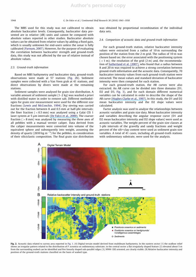
Fig. 2. Acoustic data related to survey area reported in Fig. 1. (A) Digital terrain model derived from multibeam bathymetry. In the eastern sector (1) the seafloor relief

shows an irregular pattern related to the distribution of P. oceanica on sedimentary substrate; in the central sector a flat irregularly shaped feature (2) elevated about 5 m

from the surrounding seabed can be identified and five linearly shaped sub-parallel ridges (3), NNW–SSE oriented, are clearly visible. (B) Relative backscatter intensity and

position of the ground-truth stations classified on the basis of seabed type.

G. De Falco et al. / Continental Shelf Research 30 (2010) 1941–19501944

Author's personal copy

To test the hypothesis that relative backscatter intensity varieswith seabed types, an analysis of variance (ANOVA) wasperformed (Underwood, 1997). Five ground-truth stations foreach seabed type were randomly chosen. At each station,backscatter intensity data were collected in 30 grid cells randomlychosen in a 10 m radius surrounding the ground-truth station.The differences among values of backscatter intensity were testedby ANOVA using five levels of seabed type and five levels ofstations. The first factor was considered orthogonal and fixed,whereas stations were considered random and nested in interac-tion with seabed type.

Prior to analysis, the homogeneity of variance was tested usingCochran’s test and, whenever necessary, data were appropriatelytransformed and retested (Winer et al., 1991). Significantdifferences among seabed typologies detected by ANOVA, werefurther analysed using a posteriori Student–Newman–Keuls (SNK)tests (Underwood, 1997).

3. Results

3.1. Seabed morphology and map of backscatter intensity

The bathymetry of the study site collected using MBS isdisplayed in Fig. 2A. In the eastern sector (1) the seafloor reliefshows an irregular pattern related to the distribution ofP. oceanica on sedimentary substrate as reported from previousmaps (see Fig. 1 for comparison). Several morphological featuresare clearly evident in the central area (20–35 m depth). A flatirregularly shaped feature elevated about 5 m from the surround-ing seabed can be identified (2 in Fig. 2A), while five linearlyshaped sub-parallel ridges, NNW–SSE oriented, are also clearlyvisible (3 in Fig. 2A). This central sector was reported as colonizedby P. oceanica on rocky substrate in previous maps (Fig. 1). Towardthe west the seafloor exhibits more regular morphology withincreasing depth up to about 60 m.

The map of relative backscatter intensity, mapped at 5 dBintervals, is reported in Fig. 2b. Toward the east, sector 1,identified from the multibeam bathymetry, has backscatter valuesbetween �115 and �100 dB. In the central sector the morpho-logical features previously described (2 and 3) are related tovariation in backscatter intensity in the same range as sector 1

(�115 to �100 dB), whereas toward the west, patches of lowerbackscatter from the seabed (o�115 dB) are clearly evident(Fig. 2B).

3.2. Ground-truth data

Ground-truth stations were set up to collect information ondifferent patches detected by backscatter intensity data and ondifferent morphological features. Ground-truth locations andclassifications are shown over the backscatter intensity map inFig. 2B. Particularly, attention was paid to the linearly shapedmorphological features (3 in Fig. 2A), here ground-truth stationswere located to sample both at the top and in the valleys betweenadjacent ridges.

Sediment samples were collected at 41 stations (out of 57)depicted in Fig. 2B. In the remaining stations grab samples ofP. oceanica blades and coralligenous assemblages were collected.Direct observation by divers showed that the stations located inthe eastern sector were characterised by the presence ofP. oceanica on sedimentary substrate, whereas the stations inthe central sector were characterised by biogenic hardgroundscovered by P. oceanica and coralligenous assemblages (Fig. 2B).

Along the linearly shaped ridges (Fig. 2A, sector 3), patches ofP. oceanica were detected on biogenic hardgrounds at the top ofthe ridges alternating with sedimentary substrate in the valleysbetween two adjacent ridges.

Grain size analysis showed that sediments were mainly sandygravel (Table 1). Silt and clay content, with the exception of onesample, did not exceed 20%, whereas 10 samples (out of the 41)showed a gravel content 450% (Table 1).

3.3. Relationships between seabed typology and acoustic response

Backscatter intensity data were compared with weight percentof the individual grain size classes expressed at 1-phi intervals.The correlation coefficient R, which assesses the strength anddirection of the linear relationship between backscatter intensityand grain size classes, is reported in Fig. 4A. Backscatter intensitywas directly correlated with coarse fractions (in the range1–16 mm) and inversely correlated with finer fractions (in therange 0.016–0.5 mm), and the correlations were significant at thepo0.01 level.

The relationship between backscatter intensity and the weightpercent of the 1–16 mm size fraction is depicted in Fig. 4B. As thepercentage of the 1–16 mm fraction increases, so does the relativebackscatter intensity; this increase is linear from around 10% byweight percent of the coarse fraction. The relationship betweenbackscatter intensity and the weight percent of the 0.016–0.5 mmsize fraction is reported in Fig. 4C. Relative backscatter intensitydecreases from �105 to �130 dB with increasing weight percentof the 0.016–0.5 mm size fraction.

Factor analysis identified two factors accounting for 76% of thetotal variance (Table 2). Factor 1 accounts for 44% of the totalvariance. Factor 1 score values increase with relative backscatterintensity, energy variables of the angular response curve (D1 andD2 mean backscatter intensity) and the medium gravel fractions(8–16 mm); and decrease with the medium to fine sand fractions.Factor 2 score values (32% of the total variance) increase withthe slope of the central domain of the angular response curve(D2 slope) and with the coarse sand/very coarse sand/very finegravel fractions (0.5–4 mm); and decrease with the finer fractions(o0.124 mm).

The distribution of ground-truth stations in the plot of Factorscores is reported in Fig. 5. Stations can be arranged in threegroups characterised by different grain sizes and acoustic

Fig. 3. Domains of the angular response of backscatter intensity curve and

variables describing the shape of the curve used for this study (modified from

Hughes Clarke et al., 1997).

G. De Falco et al. / Continental Shelf Research 30 (2010) 1941–1950 1945

Author's personal copy

responses. Stations on the right-hand side of the plot in Fig. 5(positive values of Factor 1 score) are characterised by highbackscatter intensity values. Sediments from those stations aremainly sandy gravels (SG). Factor 2 separates stations charac-terised by a low D2 slope and fine grain size in the lower part ofthe plot (SGMS—slightly gravelly muddy sands) from stationswith a high D2 slope and coarse grain size composed of gravellysands (GS). Factor analysis allowed the identification of groupscharacterised by different sediment grain sizes and acousticresponses, but did not consider the presence of P. oceanica, eithergrowing on sediments or fastened to biogenic hardgrounds.

The differences in relative backscatter intensity between the fiveseabed types, including the three sedimentary seabed typesidentified by factor analysis (GS, SGMS, SG) and P. oceanica growingon sediments (Pos/sed) and hardgrounds (Pos/hg), were tested byanalysis of variance (ANOVA). The ANOVA showed significantdifferences in relative backscatter intensity among the threesedimentary seabed types identified by factor analysis, whereassignificant differences were not found in relative backscatterintensity within sites characterised as P. oceanica growing onsediments (Pos/sed), P. oceanica growing on hardgrounds (Pos/hg),and gravelly sands (SG) (SNK test, Table 3). As a result, highbackscatter values are associated with sandy gravels, intermediatevalues corresponded to gravelly sands and P. oceanica and lowvalues corresponded to slightly gravelly muddy sands (Fig. 6).

4. Discussion

The findings of this study show that the different seabed typesof the Mediterranean inner shelf can be mapped using acombination of data, including backscatter intensity, multibeambathymetry and ground-truth validation. Backscatter intensityalone was not able to distinguish all benthic habitats.

The results presented here show that backscatter intensity isstrongly affected by sediment grain size, thus supporting thefindings of previous studies (Ferrini and Flood, 2006; Goff et al.,2000, 2004; Hamilton et al., 1956; Sutherland et al., 2007). Theresults of this study are in agreement with that of Goff et al. (2000,2004) in that backscatter intensity and the proportion of the coarsefraction in sediments are strongly related. Goff et al. (2004),however, did not find a linear relationship between the weightpercent of the 44 mm size class constituted by shell hash andoccasionally terrigenous gravels, and backscatter intensity. In thisstudy, a relationship was found between backscatter intensity andthe weight percent of the 1–16 mm size class (very coarse sand tomedium gravel); this coarse material was mainly composed ofsiliciclastic grains. The correlation between coarse sediment andbackscatter intensity shows a similar trend in both cases, with alinear relationship for coarse weight percentage greater than 10%.This trend can be explained considering that for sediments with acoarse fraction of less than 10% the variation in backscatter is

Table 1Grain size of sediment samples collected from 41 ground-truth stations with sedimentary seabed.

Sample Latitude (1N) Longitude (1E) Gravel (%) Sand (%) Silt+clay (%) Mean diameter (phi) Sorting (phi) Skewness

1 39.84103 8.46427 48.8 50.2 1.0 �0.90 1.51 0.86

2 39.84105 8.44854 0.0 10.5 89.5 5.70 1.57 0.15

3 39.84093 8.42741 34.8 63.7 1.5 �0.74 2.32 �0.34

4 39.84064 8.42653 82.3 16.9 0.8 �4.06 2.70 1.60

5 39.84078 8.42576 38.9 58.2 2.9 �0.58 2.83 �0.12

6 39.84051 8.41927 84.7 15.2 0.1 �1.85 0.97 0.50

7 39.84039 8.41311 71.1 28.0 0.9 �1.89 2.10 0.74

8 39.84023 8.40208 0.3 81.7 18.0 2.58 1.28 0.48

9 39.84008 8.39765 0.1 78.5 21.4 2.73 1.29 0.40

10 39.84039 8.38565 29.9 68.9 1.2 �0.75 1.94 �0.25

11 39.84004 8.37674 63.7 30.6 5.7 �2.05 3.45 0.71

12 39.84034 8.37707 8.0 77.1 14.9 1.95 2.15 �1.46

13 39.83997 8.36120 28.0 70.1 1.8 �0.44 1.89 �0.07

14 39.83947 8.35125 17.5 80.1 2.5 0.37 1.69 �0.38

15 39.83888 8.33647 4.0 93.6 2.4 0.62 1.31 0.52

16 39.83664 8.45712 76.6 22.7 0.7 �1.87 1.70 0.42

17 39.83613 8.45126 71.9 27.3 0.9 �1.59 1.66 1.15

18 39.83439 8.42921 77.4 20.8 1.8 �3.49 3.04 1.21

19 39.83446 8.42797 0.8 83.0 16.2 2.43 1.35 0.19

20 39.83439 8.42705 36.2 62.9 0.9 �0.54 1.53 0.15

21 39.83205 8.41313 0.1 83.8 16.1 2.34 1.37 0.45

22 39.83247 8.40624 0.1 83.4 16.6 2.48 1.26 0.64

23 39.83238 8.40239 37.3 61.8 1.0 �0.58 1.49 0.31

24 39.83207 8.39900 51.0 48.2 0.9 �0.99 1.63 0.06

25 39.83096 8.38044 41.4 57.0 1.6 �1.46 2.75 �0.22

26 39.82916 8.37143 23.3 75.9 0.8 �0.29 1.49 �0.45

27 39.82927 8.37263 0.6 89.4 10.0 1.93 1.31 0.60

28 39.82972 8.36515 0.1 86.3 13.6 2.25 1.31 0.53

29 39.82864 8.35362 0.5 82.0 17.5 2.49 1.34 0.35

30 39.82832 8.34488 0.1 86.5 13.4 2.31 1.26 0.66

31 39.82216 8.45201 57.9 41.7 0.5 �1.24 1.39 0.47

32 39.81901 8.43205 76.8 21.4 1.8 �3.17 2.67 1.38

33 39.81500 8.40149 0.1 79.7 20.2 2.64 1.31 0.48

34 39.81708 8.39410 0.3 82.9 16.8 2.46 1.31 0.50

35 39.81478 8.38701 28.2 70.5 1.3 �0.22 1.63 �0.16

36 39.81379 8.38042 0.7 82.1 17.2 2.49 1.35 0.30

37 39.81195 8.36460 13.0 85.6 1.4 0.14 1.46 �0.49

38 39.81001 8.35295 33.2 66.0 0.7 �0.60 1.56 �0.37

39 39.80961 8.34096 28.6 70.8 0.6 �0.45 1.24 0.04

40 39.80858 8.33324 0.3 78.7 21.0 2.67 1.32 0.39

41 39.82941 8.45591 11.8 85.7 2.5 0.17 1.40 1.04

G. De Falco et al. / Continental Shelf Research 30 (2010) 1941–19501946

Author's personal copy

mainly driven by the diameter of sand grains, linearly decreasingwith increasing percentage of the 0.016–0.5 mm size fraction(Fig. 4C). This finding agrees with the results of Ferrini and Flood(2006) who found an inverse correlation between backscatter andmean grain size of sandy sediments. In contrast, Goff et al. (2004)did not find a significant relationship between backscatter intensityand the mean grain size of sands, although they found an inverserelationship with finer sediments (o0.063 mm).

Multivariate statistics classified ground-truth stations in threesedimentary seabed typologies: sandy gravels (SG), gravelly sands

(GS) and slightly gravelly muddy sands (SGMS), characterised bydifferent acoustic responses in terms of backscatter intensity andshape of the angular response curves. Factor analysis also showedthat SGMS are separated from GS by the D2 slope of the angularresponse curve. The shape of the angular response curve seems tobe mostly dependent on the grain size of sands (Table 2), with asteepening of D2 domain associated with finer sediments.

The mean angular response curves from different seabedtypologies are shown in Fig. 7. The shape of AR curve forsedimentary seabed is, in general, consistent with previouspublished studies (e.g., Hughes Clarke et al., 1997). However,increase in backscatter intensity between incidence angles of51 and 201 is uncharacteristic, but could be due to non-uniform

Fig. 4. (A) Correlation coefficient between relative backscatter intensity and grain

size classes at 1-phi intervals. Asterisks indicate significant (po0.01) correlations.

(B) Correlation between relative backscatter intensity and the weight percent of

coarse fraction (1–16 mm) in sediments. (C) Correlation between backscatter and

weight percent of the fine fraction (0.016–0.5 mm) in sediments.

Table 2Score coefficients of Factor analysis. Significant coefficients are in bold.

Factor 1 Factor 2

Backscatter intensity (dB) 0.88 0.31

D1 backscatter intensity (dB) 0.84 0.33

D2 backscatter intensity (dB) 0.83 0.30

D2 slope 0.33 0.7332–64 mm—very coarse gravel (%) 0.64 �0.14

16–32 mm—coarse gravel (%) 0.68 0.18

8–16 mm—medium gravel (%) 0.81 0.33

4–8 mm—fine gravel (%) 0.69 0.62

2–4 mm—very fine gravel (%) 0.58 0.751–2 mm—very coarse sand (%) 0.26 0.910.5–1 mm—coarse sand (%) �0.11 0.780.25–0.5 mm—medium sand (%) �0.74 �0.49

0.124–0.25 mm—fine sand (%) �0.69 �0.54

0.062–0.124 mm—very fine sand (%) �0.67 �0.66

o0.062 mm—Silt+clay (%) �0.64 �0.68

Explained variance 44% 32%

Fig. 5. Plot of factor scores deriving from factor analysis (see Table 2 for the

significance of factor scores). Based on their position on the plot stations can be

arranged in three groups characterised by different grain sizes and acoustic

responses.

Table 3Summary results of analysis of variance for backscatter intensity.

Source DF MS F p SNK test

Backscatter

intensity (dB)a

Seabed 4 23.059 17.1 o0.00001 SG4GS¼Pos/sed

¼Pos/hg4SGMS

Station (Seabed) 20 1.348 482.2 o0.00001

Error 725 0.003

a Transformed ln(x+constant); Cochran test NS after transformation.

G. De Falco et al. / Continental Shelf Research 30 (2010) 1941–1950 1947

Author's personal copy

response of the transmit power and receive sensitivity with beamnumber. At incidence angles greater than 201, the curveassociated with SGMS shows a distinct decrease in signal

intensity as a function of angle of incidence (and, consequently,lower values of D2 slope), whereas backscatter intensity seems,for most angles, independent from the angle of incidence for theother seabed types. The acoustic response from P. oceanica,regardless of the meadow substrate, overlaps values recorded forgravelly sands, showing the same values of relative backscatterintensity and similar AR curves (Figs. 6 and 7, Table 4).

High scattering levels from P. oceanica have been reported in aprevious study and were found to be higher than compared tosandy and muddy bottoms (Lyons and Abraham, 1999). Thisfinding agrees with results found for the Australian coastal zonewhere similar scattering differences were found between seagrassand sands (Siwabessy et al., 2006).

The absence of differences in backscattering levels fromP. oceanica growing on sediments and P. oceanica fastened tobiogenic hardgrounds seems to indicate that the acousticresponse is mainly linked to the leaf canopy rather than thebelowground component.

The belowground components of P. oceanica growing onsediments and fastened to biogenic hardgrounds show distinctfeatures. The first is characterised by a net of root rhizomes andsandy-gravelly sediments (De Falco et al., 2008), the second is madeby calcareous formations by the plant’s roots in the troughs. Thehardgrounds are likely stiffer than sediments and different acousticproperties would be expected between those different substrates.

At the leaf canopy level, gas-filled channels in tissues and gasbubbles generated by the plant during photosynthesis controlsthe acoustic behaviour of seagrass (Wilson and Dunton, 2009;Hermand et al., 1998). Laboratory investigation also showed thatthe acoustic response of seagrass tissues depends on biomass andtissue characteristics (i.e. flat leaves exhibited more acousticcontrast than did circular cross-section leaves) (Wilson andDunton, 2009). In this study, the MBS survey was carried outduring the summer, when P. oceanica shows the maximum leafbiomass development (Alcoverro et al., 2001) and leaves can beup to 1 m long. Leaf biomass and gas bubble production linked tophotosynthetic activity could strongly influence the backscatter atleaf canopy level masking the belowground substratum. Futurework could use a MBS capable of collecting backscatter data fromall of the water column to investigate whether the location ofsnippet data collected is centred around the canopy or theseafloor.

In order to obtain a map of seabed types from the acoustic datait was necessary to establish threshold values of backscatterintensity that identified the spatial boundary between seabed type(sedimentary facies and/or benthic habitat). Results frommultivariate statistics and ANOVA showed that this is onlypartially possible for the seabed typologies analysed in this study.Threshold values can be identified as indicated in Fig. 6, and can beused to separate three groups, (i) SG (4�109.5 dB), (ii) SGMS(o�117.5 dB) (iii) GS+P. oceanica beds (both on hard and soft

Fig. 6. Whiskers plot of backscatter intensity for different seabed typologies

(threshold values are indicated on the right side of the plot). High backscatter values

are associated with sandy gravels, intermediate values corresponded to gravelly sands

and P. oceanica, and low values corresponded to slightly gravelly muddy sands.

Fig. 7. Mean angular response of backscatter intensity curves from the different

seabed types. The curve associated to slightly gravelly muddy sands (SGMS) shows

a decrease in signal intensity as a function of angle of incidence, while backscatter

intensity seems almost independent from the angle of incidence for the other

seabed typologies sandy gravels (SG), gravelly sands (GS) and P. oceanica.

Table 4Mean grain size composition and acoustic parameters of seabed types.

Seabed types Gravel (%) Sand (%) Silt+clay (%) Relative backscatter intensity (dB) D2 slope

GS Mean 21.2 77.1 1.7 �113.0 �0.08

SD 12.3 11.6 0.9 2.4 0.06

SGMS Mean 0.9 82.4 16.7 �124.4 �0.23

SD 2.2 3.5 3.2 4.3 0.09

SG Mean 53.0 45.8 1.2 �108.2 �0.10

SD 22.2 22.0 0.7 1.7 0.04

P. oceanica on sediments Mean �112.5 �0.08

SD 1.03 0.05

P. oceanica on hardgrounds Mean �112.2 �0.11

SD 2.89 0.03

G. De Falco et al. / Continental Shelf Research 30 (2010) 1941–19501948

Author's personal copy

substrates, �117.5 to �109.5 dB). A map of backscatter intensitylimited to these three classes is shown in Fig. 8A. Based on this mapit is possible to identify the spatial boundaries of SGMS and SG,whereas P. oceanica beds and GS are represented in the same classes.

A map of seafloor types can be created by combiningbackscatter data, multibeam bathymetry and ground-truth vali-dation (Fig. 8B). Particularly, P. oceanica meadows on sedimentsform reefs with a complex topography of the seabed, includingescarpments, channels, holes and mounds. (Kendrick et al., 2005).This complex topography can be recognised from the digitalterrain model (DTM), which shows an irregular pattern related tothe distribution of P. oceanica on sedimentary substrate. Thebiogenic hardgrounds form ridges and tabular reliefs, which arealso recognisable from the DTM.

The eastern sector (sector 1 in Fig. 2A) was characterised byintermediate backscatter values, and irregular seabed morphol-ogy. In this sector, ground-truth validation showed the presenceof P. oceanica on sedimentary substrate, the deeper, western limitof which can be defined by changes in seabed morphology(Fig. 2A; Fig. 8A and B).

In the central sector, P. oceanica on hardgrounds and coralli-genous assemblages were associated with the top of seafloorridges, whereas in the depression between them, coarse sediments,identified as SG and GS on the basis of backscatter data, werefound. The western sector was well resolved by the backscatterdata, which identified the boundaries between SGMS, GS and SG.

5. Conclusions

MBS data, including bathymetry, backscattering intensity andangular response of backscatter intensity, and ground-truth data

were analysed to distinguish different seabed typologies in asite of the Mediterranean sea characterised by a complex seabedthat includes sandy-gravelly sediments, P. oceanica seagrass onbiogenic hardgrounds and sedimentary substrate.

Based on MBS backscatter, three sediment types werediscriminated: gravelly sands, sandy gravels and slightly gravellymuddy sands. Threshold values of relative backscatter intensitywere established in order to map the spatial distribution of thosesediment types.

The shape of the curve of the angular response was differentfor finer and coarser sediments. The central domain of the curvehas a greater roll off of intensity at steeper angles of incidence forslightly gravelly muddy sands compared with that for gravellysands and sandy gravels, showing a trend consistent withprevious findings (Hughes Clarke et al., 1997).

The relative backscatter intensity and the shape of the curve ofthe angular response from P. oceanica beds were similar to thosefor gravelly sands. Backscatter intensity measured from P. oceanica

beds was found to be independent of the seagrass substratum(sedimentary or biogenic hardgrounds). It was, therefore, proposedby the authors that the acoustic response of seagrass was mainlydue to leaf biomass and gas bubble production linked tophotosynthetic activity masking the belowground substrate, whichis in agreement with other studies (Wilson and Dunton, 2009;Hermand et al., 1998).

The different seabed types analysed in this study—gravelly andsandy sediments and P. oceanica beds—can be mapped using acombination of backscatter intensity, multibeam bathymetry andground-truth data. The boundaries of the non-vegetated sedimen-tary seabed were able to be resolved by backscatter data alone.However, backscatter intensity alone was not an effective para-meter for distinguishing all benthic habitats. Utilising additional

Fig. 8. (A) Map of backscattering using threshold values and (B) seabed map obtained using a combination of data, including backscatter intensity, multibeam bathymetry

and ground-truth validation.

G. De Falco et al. / Continental Shelf Research 30 (2010) 1941–1950 1949

Author's personal copy

information, P. oceanica was recognised from a digital terrainmodel due to the complex topography presumably created by themeadow growing on sediments (Kendrick et al., 2005) and P.

oceanica fastened to the biogenic hardgrounds can be recognisedfrom the ridges and tabular reliefs formed by those features.

Acknowledgment

This work was funded by SIGLA project, from the ItalianMinistry from Scientific Research. We gratefully acknowledge thecaptain and the crew of R/V Thetis for their effort during the dataacquisition. We would like to thank Gianluca Solinas for hiscontribution to grain size analysis and Alexander Gavrilov for thecritic revision of the manuscript. Finally we acknowledgethe reviewers for their useful suggestions which greatly improvedthe manuscript.

References

Alcoverro, T., Manzanera, M., Romero, J., 2001. Annual metabolic carbon balance ofthe seagrass Posidonia oceanica: the importance of carbohydrate reserves.Marine Ecology Progress Series 211, 105–116.

Ballesteros, E., 2006. Mediterranean coralligenous assemblages: a synthesis ofpresent knowledge. Oceanography and Marine Biology: An Annual Review 44,123–195.

Briggs, K.B., Williams, K.L., Richardson, M.D., Jackson, D.R., 2001. Effects ofchanging roughness on acoustic scattering: (1) natural changes. In: Leighton,T.G., Heald, G.J., Griffiths, G., Griffiths, H.D. (Eds.). In: Proceedings of theInstitute of Acoustics, vol. 23, Part 2, pp. 343–390.

Briggs, K.B., Tang, D., Williams, K.L., 2002. Characterization of interface roughnessof rippled sand off Fort Walton Beach, Florida. IEEE Journal of OceanicEngineering 27 (3), 505–514.

Borgeld, J.C., Hughes Clarke, J.E., Goff, J.A., Mayer, L., Curtis, J.A., 1999. Acousticbackscatter of the 1995 flood deposit on the Eel Shelf. Marine Geology 154,197–210.

Carboni, S., Lecca, L., Ferrara, C., 1989. La discordanza versiliana sulla piattaformaoccidentale della Sardegna. Bollettino Societ�a Geologica Italiana 108, 503–519.

Casula, G., Cherchi, A., Montadert, L., Murru, L., Sarria, E., 2001. The Cenozoicgraben system of Sardinia (Italy): geodynamic evolution from new seismic andfield data. Marine Petroleum Geology 18, 863–888.

De Falco, G., Baroli, M., Cucco, A., Simeone, S., 2008. Intrabasinal conditionspromoting the development of a biogenic carbonate sedimentary faciesassociated with the seagrass Posidonia oceanica. Continental Shelf Research28/6, 797–812.

De Falco, G., Ferrari, S., Cancemi, G., Baroli, M., 2000. Relationships between sedimentdistribution and Posidonia oceanica seagrass. Geo-Marine Letters 20, 50–57.

de Moustier, C.P., Alexandrou, D., 1991. Angular dependence of 12-kHz seaflooracoustic backscatter. The Journal of the Acoustical Society of America 90 (1),522–531.

Fais, S., Klingele, E.E., Lecca, L., 1996. Oligo-Miocene half graben structure inWestern Sardinian Shelf (western Mediterranean): reflection seismic andaeromagnetic data comparison. Marine Geology 133 (3-4), 203–222.

Ferrini, V.L., Flood, R.D., 2006. The effects of fine-scale surface roughness and grainsize on 300 kHz multibeam backscatter intensity in sandy marine sedimentaryenvironments. Marine Geology 228, 153–172.

Fonseca, L., Mayer, L., Orange, D., Driscoll, N., 2002. The high frequencybackscattering angular response of gassy sediments: model/data comparisonfrom the Eel River Margin, California. Journal of the Acoustical Society ofAmerica 111 (6), 2621–2631.

Goff, J.A., Kraft, B.J., Mayer, L.A., Schock, S.G., Sommerfield, C.K., Olson, H.C., Gulick,S.P.S., Nordfjord, S., 2004. Seabed characterization on the New Jersey middleand outer shelf: correlatability and spatial variability of seafloor sedimentproperties. Marine Geology 209, 147–172.

Goff, J.A., Olson, H.C., Duncan, C.S., 2000. Correlation of side scan backscatterintensity with grain size distribution of shelf sediments, New Jersey margin.Geo-Marine Letters 20, 43–49.

Hamilton, E.L., Shumway, G., Menard, H.W., Shipek, C.J., 1956. Acoustic andphysical properties of shallow-water sediments off San Diego. Journal ofAcoustical Society of America 28, 1–15.

Hermand, J.P., Nascetti, P., Cinelli, F., 1998. Inversion of acoustic waveguidepropagation features to measure oxygen synthesis by Posidonia oceanica.In: OCEANS ‘98 Conference Proceedings IEEE, Piscataway, NJ, 1998, vol. 2,pp. 919–926.

Holmes, K.W., Van Niel, K.P., Radford, B., Kendrick, G.A., Grove, S.L., 2008.Modelling distribution of marine benthos from hydroacoustics and under-water video. Continental Shelf Research 28, 1800–1810.

Hughes Clarke, J.E., Danforth, B.W., Valentine, P., 1997. Aerial seabed classificationusing backscatter angular response at 95 kHz. Shallow Water, NATOSACLANTCEN, Conference Proceedings Series CP, vol. 45, pp. 243–250.

IHO—International Hydrographic Organization 2008. IHO Standards for Hydro-graphic Surveys. Special Publication no. 44 Published by the InternationalHydrographic Bureau, Monaco, pp. 28.

Kendrick, G.A., Marba, N., Duarte, C.M., 2005. Modelling formation of complextopography by the seagrass Posidonia oceanica. Estuarine, Coastal and ShelfScience 65, 717–725.

Kostylev, V.E., Todd, B.J., Fader, G.B.J., Courtney, R.C., Cameron, G.D.M., Pickrill, R.A.,2001. Benthic habitat mapping on the Scotian Shelf based on multibeambathymetry, surficial geology and seafloor photographs. Marine EcologyProgress Series 219, 121–137.

Lyons, A.P., Abraham, D.A., 1999. Statistical characterization of high-frequencyshallow-water seafloor backscatter. Journal of Acoustical Society of America106 (3), 1307–1315.

Lewis, D.W., McConchie, D., 1994. Analytical Sedimentology. Chapman and Hall,New York 197 pp.

Medialdea, T., Somoza, L., Leon, R., Farran, M., Ercilla, G., Maestro, A., Casas, D.,Llave, E., Hernandez-Molina, F.J., Fernandez-Puga, M.C., Alonso, B., 2008.Multibeam backscatter as a tool for sea-floor characterization and identifica-tion of oil spills in the Galicia Bank. Marine Geology 249, 93–107.

Parnum I.M., 2007. Benthic Habitat Mapping using Multibeam Sonar System. PhDThesis Curtin University of Technology, Department of Imaging and AppliedPhysics, Centre for Marine Science and Technology, pp. 213.

Parnum, I.M., Siwabessy, P.J.W. and Gavrilov, A.N., 2004. Identification of seafloorhabitats in Coastal Shelf waters using a multibeam echosounder. In: Acoustics2004. Gold Coast: Proceedings of the Annual Conference of the AustralianAcoustical Society.

Per�es, J.M., Picard, J., 1964. Nouveau manuel de bionomie benthique de la MerMediterranee. Recueil des Travaux de la Station Marine d’Endoume 31 (47),5–137.

Richardson, M.D., Briggs, K.B., Williams, K.L., Lyons, A.P., Jackson, D.R., 2001. Effectsof changing roughness on acoustic scattering: (2) anthropogenic changes. In:Leighton, T.G., Heald, G.J., Griffiths, G., Griffiths, H.D. (Eds.). In: Proceedings ofthe Institute of Acoustics, vol. 23, Part 2, pp. 343–390.

Siwabessy, P.J.W., Parnum, I., Gavrilov, A., McCauley, R.D., 2006. Overview ofcoastal water habitat mapping research for Coastal CRC. Cooperative ResearchCentre for Coastal Zone, Estuary and Waterway Management. Technical Report86, Australia.

Stewart, W.K., Chu, D., Malik, S., Lerner, S., Singh, H., 1994. Quantitative seafloorcharacterization using a bathymetric sidescan sonar. IEEE Journal of OceanicEngineering 19 (4), 599–610.

Sutherland, T.F., Galloway, J., Loschiavo, R., Levings, C.D., Hare, R., 2007. Calibrationtechniques and sampling resolution requirements for groundtruthing multi-beam acoustic backscatter (EM3000) and QTC VIEW classification technology.Estuarine Coastal and Shelf Science 75, 447–458.

Underwood, A.J. (Ed.), 1997. Experiments in Ecology: Their Logical Design andInterpretation using Analysis of Variance. Cambridge University Press,Cambridge.

Urgeles, R., Locat, J., Schmitt, T., Hughes Clarke, J.E., 2002. The July 1996 flooddeposit in the Sanguenay Fjord, Quebec, Canada: implications for sources ofspatial and temporal backscatter variations. Marine Geology 184, 41–60.

Wilson, P.S., Dunton, K.H., 2009. Laboratory investigation of the acoustic responseof seagrass tissue in the frequency band 0.5–2.5 kHz. Journal of AcousticalSociety of America 125 (4), 1951–1959.

Winer, B.J., Brown, D.R., Michels, K.M. (Eds.), 1991. Statistical Principles inExperimental Design third ed. McGraw Hill, New York.

G. De Falco et al. / Continental Shelf Research 30 (2010) 1941–19501950