www.elsevier.com/locate/rse

Remote Sensing of Environment 88 (2003) 423–441

Effects of seasonal hydrologic patterns in south Florida wetlands on radar

backscatter measured from ERS-2 SAR imagery

Eric S. Kasischkea,*, Kevin B. Smitha,1, Laura L. Bourgeau-Chaveza,2,Edwin A. Romanowiczb,3, Suzy Brunzella,4, Curtis J. Richardsonb

aEnvironmental Research Institute of Michigan, Ann Arbor, MI, USAbNicholas School of the Environment, Duke University, Durham, NC, USA

Received 11 March 2003; received in revised form 29 July 2003; accepted 18 August 2003

Abstract

A multi-year study was carried out to evaluate ERS synthetic aperture radar (SAR) imagery for monitoring surface hydrologic

conditions in wetlands of southern Florida. Surface conditions (water level, aboveground biomass, soil moisture) were measured in 13 study

sites (representing three major wetland types) over a 25-month period. ERS SAR imagery was collected over these sites on 22 different

occasions and correlated with the surface observations. The results show wide variation in ERS backscatter in individual sites when they

were flooded and non-flooded. The range (minimum vs. maximum) in SAR backscatter for the sites when they were flooded was between

2.3 and 8.9 dB, and between 5.0 and 9.0 dB when they were not flooded. Variations in backscatter in the non-flooded sites were consistent

with theoretical scattering models for the most part. Backscatter was positively correlated to field measurements of soil moisture. The

MIchigan MIcrowave Canopy Scattering (MIMICS) model predicts that backscatter should decrease sharply when a site becomes

inundated, but the data show that this drop is only 1–2 dB. This decrease was observed in both non-wooded and wooded sites. The drop in

backscatter as water depth increases predicted by MIMICS was observed in the non-wooded wetland sites, and a similar decrease was

observed in wooded wetlands as well. Finally, the sensitivity of backscatter and attenuation to variations in aboveground biomass predicted

by MIMICS was not observed in the data.

The results show that the inter- and intra-annual variations in ERS SAR image intensity in the study region are the result of changes in

soil moisture and degree of inundation in the sites. The correlation between changes in SAR backscatter and water depth indicates the

potential for using spaceborne SAR systems, such as the ERS for monitoring variations in flooding in south Florida wetlands.

D 2003 Elsevier Inc. All rights reserved.

Keywords: South Florida wetlands; ERS-2 SAR; Backscatter

1. Introduction demonstrated with L-band (24 cm wavelength) data from

The ability of satellite imaging synthetic aperture

radars (SARs) to detect forested wetlands was first

0034-4257/$ - see front matter D 2003 Elsevier Inc. All rights reserved.

doi:10.1016/j.rse.2003.08.016

* Corresponding author. Current address: Department of Geography,

University of Maryland, College Park, MD 20742, USA. Tel.: +1-301-405-

2179.

E-mail address: ekasisch@geog.umd.edu (E.S. Kasischke).1 Currently at Western Regional Office, Ducks Unlimited, 3074 Gold

Canal Drive, Rancho Cordova, CA 95670, USA.2 Currently with Ann Arbor Research and Development Center,

Veridian Systems Division, P.O. Box 134008, Ann Arbor, MI 48113-

4008, USA.3 Currently at Center for Earth and Environmental Sciences, State

University of New York, Plattsburgh, NY, USA.4 Currently at Snohomish County, Public Works, 2731 Wetmore

Avenue, Suite 300, Everett, WA 98201-3581, USA.

the Seasat satellite (Engheta & Elachi, 1982; Hess,

Melack, & Simonett, 1990; Krohn, Milton, & Segal,

1983; Ormsby, Blanchard, & Blanchard, 1985). Since

these initial studies, a number of researchers have shown

that satellite SARs operating at both L-band and C-band

(6-cm wavelength) can be used to map and monitor

wetlands occupying a range of coastal and inland set-

tings. These studies were carried out by using data from

the Shuttle Imaging Radar (Alsdorf et al., 2000; Alsdorf,

Smith, & Melack, 2001; Bourgeau-Chavez et al., 2001;

Hess, Melack, Filoso, & Wang, 1995; Imhoff et al.,

1987; Pope, Rejmankova, & Paris, 2001; Pope, Rejman-

kova, Paris, & Woodruff, 1997), ERS-1 and -2 (Brivio,

Colombo, Maggi, & Tomasoni, 2002; Dwivedi, Rao, &

Bhattacharya, 1999; Kasischke & Bourgeau-Chavez,

E.S. Kasischke et al. / Remote Sensing of Environment 88 (2003) 423–441424

1997; Moreau & Le Toan, 2003; Morrissey, Livingston,

& Durden, 1994, Morrissey, Durden, Livingston, Stearn,

& Guild, 1996; Ramsey, 1995; Ramsey, Nelson, Laine,

Kirkman, & Topham, 1997; Rao et al., 1999; Townsend,

2001), JERS (Ormsby et al., 1985; Rosenqvist & Birkett,

2002; Rosenqvist, Forsberg, Pimentel, Rauste, & Richey,

2002; Townsend & Walsh, 1998), and Radarsat (Kandus

et al., 2001; Parmuchi, Karszenbaum, & Kandus, 2002;

Rio & Lozano-Garcia, 2000; Townsend, 2002; Werle,

Martin, & Hasan, 2000; Zhou, Luo, Yang, Li, & Wang,

2000)]. In addition to mapping natural wetlands, research-

ers have demonstrated that spaceborne SARs can be used

to monitor rice production (Kurosu, Masaharu, & Chiba,

1995; LeToan et al., 1997; Liew et al., 1998; Panigrahy

et al., 1997; Ribbes & Le Toan, 1999; Rosenqvist, 1999;

Shao et al., 2001), with the best results being obtained

using C-band systems (ERS and Radarsat). In rice fields,

growth of new in biomass in flooded rice fields result in

significant increases (on the order of 6–8 dB) in C-band

SAR image intensity (LeToan et al., 1997)).

A unique application for the current generation of imag-

ing radar systems (ERS, JERS, Radarsat, and Envisat) is to

monitor temporal variations in the hydrologic conditions

present in wetlands. Tanis, Bourgeau-Chavez, and Dobson

(1994) and Ramsey (1995) both used the same ERS data set

to map the extent of coastal wetlands in Florida based on

backscatter differences associated with flooded (during high

tides) and non-flooded (during low tides) estuarine vegeta-

tion. Kasischke and Bourgeau-Chavez (1997) noted that

distinct differences in radar backscatter occurred in different

upland and wetland vegetation types in south Florida be-

tween ERS imagery collected during the wet and dry seasons

of this semi-tropical region. Morrissey, Durden, Livingston,

Stearn, and Guild (1996) showed that ERS SAR imagery

could be used to discriminate between flooded and

unflooded tundra on Alaska’s North Slope, and that seasonal

variations in temperature (freezing vs. thawing) strongly

influenced radar backscatter. A number of studies showed

that variations in flood stages along the Brazilian Amazon

influenced the radar backscatter signatures from the SIR-C

instruments (Hess et al., 1995; Alsdorf et al., 2000, 2001).

Pope et al. (1997) noted changes in radar backscatter on SIR-

C imagery based on flooded and non-flooded conditions in

non-wooded wetlands in Central America. Finally, Town-

send and colleagues (Townsend, 2001; Townsend & Foster,

2002; Townsend & Walsh, 1998) used time-series ERS,

JERS, and Radarsat imagery to monitor seasonal patterns

of flooding in wooded wetlands located along rivers.

In this paper, we present the results of a multi-year study

designed to assess the potential for using C-band ERS

synthetic aperture radar (SAR) imagery to monitor wetland

hydrology in south Florida. This study was initiated during

the spring of 1997 to more fully investigate the sources of

backscatter variations observed in the ERS SAR images

collected over south-central Florida wetlands. The overall

goal of this study was to correlate the seasonal responses in

ERS radar backscatter signatures associated with changes in

hydrologic status and vegetation cover in order to develop

approaches to use spaceborne SAR data to monitor regional-

scale hydropatterns in the wetland ecosystems of this region.

2. Previous satellite SAR studies of south Florida

Wetlands

The results presented in this paper extend those from

previous studies of satellite SAR imagery in this region

(Bourgeau-Chavez et al. 1996; Kasischke & Bourgeau-

Chavez, 1997; Kasischke, Bourgeau-Chavez, Smith, Roma-

nowicz, & Richardson, 1997). Kasischke and Bourgeau-

Chavez (1997) initially assessed the utility of ERS SAR

imagery to monitor variations in radar backscatter associat-

ed with changes in soil moisture and surface inundation

during the wet and dry seasons in southwestern Florida.

Relative radar backscatter measurements from 10 different

vegetation types were compared from ERS SAR imagery

collected during the dry (April) and late wet (October)

seasons of 1994. Field observations of water level/soil

moisture were made during October and either directly

observed or inferred for April based on precipitation pat-

terns. The results showed that the radar backscatter either

increased between April and October due to an increase in

soil moisture, or decreased where the ground surface tran-

sitioned from a wet soil to a flooded condition.

During 1995, a more intensive study was carried out using

nine ERS SAR scenes collected betweenMay andNovember,

which spans the typical wet season in this region.Water levels

were measured along several transects in 10 study sites with

different vegetation covers in the same areas studied

(Kasischke & Bourgeau-Chavez, 1997). In the sites domi-

nated by woody vegetation, the changes in water levels did

not result in changes in backscatter because: (a) the sites were

continuously flooded, and therefore changes in water levels

did not result in changes in scattering; or (b) the overstory

canopy was dense enough that the total backscatter signature

changes from flooding were attenuated by the canopy itself.

In sites dominated by non-woody vegetation, there was an

overall decrease in ERS backscatter as water level increased,

with the level of decrease being related to live vegetation

density (Bourgeau-Chavez et al., 1996).

Additional ERS SAR data were collected at roughly

monthly intervals over south-central Florida in 1995 and

1996. The geographic focus was shifted slightly to the east

to encompass sites within the boundaries of the Big Cypress

National Preserve as well as the Everglades National Park

(Fig. 1). These regions contained sites that were quite

similar to those studied by Bourgeau-Chavez et al. (1996)

and Kasischke and Bourgeau-Chavez (1997), but included

additional vegetation cover types characteristic of this

region. Kasischke et al. (1997) showed that not only did

dramatic variations occur throughout all non-woody wet-

lands throughout the wet season/dry season cycle, but that

Fig. 1. ERS SAR image mosaic of the south-central Florida region containing the region investigated in this study and previous research. The white polygon in

the center is the boundary of the Big Cypress National Preserve, while each number represents the location of a site used in the present study.

E.S. Kasischke et al. / Remote Sensing of Environment 88 (2003) 423–441 425

significant differences in radar backscatter occurred between

years because of variations in seasonal precipitation pat-

terns. In addition, this study showed that decreases in radar

backscatter also occurred during the dry season in some

sites, most likely due to decreases in soil moisture.

The results from these studies clearly showed that seasonal

variations in level of water inundation in wetlands during the

wet season, as well as variations in soil moisture in non-

flooded sites during the dry season both have strong influ-

ences on ERS SAR image intensity. As discussed by

Kasischke and Bourgeau-Chavez (1997), additional varia-

tions in radar backscatter in these ecosystems resulted from

differences in the levels of tree cover as well as levels of

aboveground biomass in these ecosystems.

One additional study that relates to the one presented in

this paper is that conducted by Pope et al. (1997), who used

C- and L-band radar imagery from SIR-C to examine varia-

tions in radar backscatter over 11 marshes in Central America

dominated by non-woody (macrophyte) vegetation. These

sites were imaged during the dry and wet seasons, with 10 of

the sites experiencing measurable increases in water depth

during the wet season. In three sites dominated by dense

(>60% vegetation cover) and large-stemmed marsh vegeta-

tion (cattail and saw grass), there was an increase in radar

backscatter associated with flooding. In the seven sites

dominated by lower density (<50%), large-stemmed marsh

vegetation or small-stemmed vegetation (rushes) of variable

density (50 to 80%), there was a decrease in radar backscatter

associated with flooding.

3. Expected influence of seasonal wetland hydrologic

variations on ERS SAR backscatter measurements

The seasonally variable hydrologic conditions occurring

in south Florida’s wetlands should result in a predictable

E.S. Kasischke et al. / Remote Sensing of Environment 88 (2003) 423–441426

trajectory of change in the radar backscatter measurements

obtained from the ERS SAR. Sites exposed to inundation or

flooding during the wet season and no flooding during the

dry season should experience three distinct hydrologic

regimes: (a) a period of increasing soil moisture during

times of increasing precipitation at the beginning of the wet

season; (b) a period where water covers or inundates the

ground surface to various depths during the middle of the

wet season; and (c) a period of decreasing soil moisture in

the middle of the dry season when precipitation levels

decrease sharply.

In terms of radar backscatter or the measured backscatter

coefficient, ro, two wetland types within the study site need

to be considered: those containing only herbaceous vegeta-

tion and those containing shrubs and trees in addition to the

herbaceous vegetation. The total backscatter from wetlands

dominated by herbaceous vegetation (rt-ho ) can be modeled

after Kasischke and Bourgeau-Chavez (1997) as

rot�h ¼ ro

c þ s2cðros þ ro

mÞ ð1Þ

where rco is the backscatter coefficient from the vegetation

canopy, sc is the transmission coefficient of the vegetation

canopy, rso is the backscatter from the ground surface, and

rmo is the backscatter from multiple-path scattering between

the surface and the vegetation canopy. For wetlands con-

taining woody vegetation, the backscattering coefficient

(rt-wo) is modeled as

rot�w ¼ ro

c þ s2cs2t ðro

s þ rot þ ro

d þ romÞ ð2Þ

where, in this case, rco is the scattering from the crown layer of

smaller woody branches and foliage as well as the herbaceous

vegetation, rto is the direct scattering from the tree trunks, st is

the attenuation of microwave energy by the tree trunks, rdo is a

Fig. 2. Variations in ERS backscatter as a function of aboveground biomass and so

MIMICS theoretical microwave scattering model.

double-bounce scattering between the trunks and the ground,

and rmo accounts for multiple-path scattering between the

ground and canopy.

In our study, we used the MIchigan MIcrowave Canopy

Scattering (MIMICS) model (Ulaby, Sarabandi, McDonald,

& Dobson, 1990) to examine the influence of site conditions

(water depth, soil moisture, and canopy cover) on the

expected ERS SAR backscatter measurements from wet-

lands with herbaceous cover (Eq. (1)) following the ap-

proach of Dobson, Ulaby, and Pierce (1995). The MIMICS

model was exercised using soil moisture and biomass levels

that covered the range of site conditions encountered in this

study. The vegetation in the herbaceous wetlands was

assumed to consist primarily of sedges, grasses, and reeds

(rushes), and modeled as vertical dielectric cylinders that

were uniformly distributed.

The MIMICS model was exercised using soil moisture

levels ranging from 0 to 1 cm3 cm�3 and biomass levels

ranging from 0.0 to 1.68 kg m�2. We selected the biomass

levels using data from one of our study sites as a baseline

(Site 4 with average biomass of 0.42 kg m�2, density of 250

stems m�2 and height of 55 cm). We assumed that the

canopy height and weight per stem were constant and

created new biomass levels by varying the stem density

between 0 and 1000 stems m�2 for the different model runs.

For all cases except the no biomass case, we also exercised

MIMICS assuming a flooded ground surface (e.g., standing

water of 5 cm depth). For all model runs, we assumed

system and imaging parameters corresponding to the ERS

SAR, e.g., a 5.6-cm wavelength, VV polarization and

incidence angle of 23j.Fig. 2 presents the MIMICS results consisting of the

backscatter coefficient as a function of soil moisture and

aboveground biomass. These results figure illustrate three

il moisture for marl prairie wetland vegetation based on predictions from the

E.S. Kasischke et al. / Remote Sensing of Environment 88 (2003) 423–441 427

different processes: (a) the response of microwave back-

scatter to increases in soil moisture; (b) the response of

microwave backscatter to changes from a non-flooded to

flooded state; and (c) the response of microwave backscatter

to increases in aboveground, live biomass. In all biomass

level cases, we see an increase in backscatter as soil

moisture increases. In addition, we see a sharp decrease in

backscatter when the site goes from a flooded to a non-

flooded state.

The complex role of vegetation is illustrated in Fig. 2.

When soil is perfectly dry (soil moisture=0), there is little or

no forward and very little backward scattering of incident

microwave energy. In the no soil moisture case (0 cm3

cm�3), as biomass increases, there is an increase in direct

canopy scattering (rco), but there is little or no contribution

from the multiple-interaction scattering (rmo ). This situation

changes when the surface is flooded. In this case, there is no

backscattering of energy from the ground surface, and the

backscattered energy comes entirely from the vegetation

through direct canopy or multi-path scattering. The fact that,

in all biomass cases, the backscatter in the flooded cases is

lower than that in the dry soil cases indicates that MIMICS

predicts there is no multi-path scattering occurring in the

flooded scenario. The decrease in backscatter as a function

of biomass at all soil moisture levels is the result of

vegetation’s role as an attenuator (sc) of direct scattering

from the soil surface.

The results from Fig. 2 are representative of the biomass

levels observed at most of our non-woody study sites. The

results from Pope et al. (1997) indicate that at some point

the size and structure of stems play a role in determining the

degree of multiple-path scattering that occurs in non-woody

wetlands. The study of Pope et al. (1997) contained vege-

tation types (cattail and sawgrass) with much larger stem

Fig. 3. Expected seasonal variations in ERS radar backscatter for marl pra

sizes than the vegetation found in the sites used in the

present study. In sites with high vegetation cover and large-

stem sizes, Pope et al. (1997) observed increases in back-

scatter when sites became flooded, which is identical to the

response that has been observed in wetlands with dense,

woody vegetation.

Based on the MIMICS outputs in Fig. 2 and observations

from other studies, we developed a prediction of how we

expect variations in seasonal flooding and soil moisture to

influence the ERS backscatter signature in the non-wooded

study wetlands in the south Florida. In this prediction, we

assumed that: (a) soil moisture first decreases from 1.0 to

0.10 cm3 cm�3 during the beginning of the dry season and

then increases from 0.10 to 1.0 cm3 cm�3 as the dry season

transitions to the wet season; (b) the site has an average

biomass level of 400 g m�2; (c) the average vegetation

height is 50 cm; and (d) the water depth during the wet

season reaches 25 cm. Fig. 3 shows the expected changes in

backscatter for these conditions. Note that as water level at

the site increases, there is a decrease in backscatter because

the water reduces the amount of vegetation available for

direct backscatter to radar. The results in Fig. 3 represent the

overall trends we expect to observe in the multi-date ERS

SAR imagery collected over south Florida, and may in fact

not exactly match the exact magnitude of change in the

actual data.

The expected changes in the wooded wetland sites are

a little more difficult to predict. In previous studies, radar

backscatter in wooded wetlands has been shown to

increase when they become flooded because of increases

from the multiple-scattering terms in Eq. (2) (rdo, rm

o).

However, the tree density in our sites is quite low, so we

expected the increase in backscatter to be lower than

observed in riparian wetlands, which contain dense forest

iries under different hydrologic patterns in the south Florida region.

E.S. Kasischke et al. / Remote Sensing of Environment 88 (2003) 423–441428

canopies. Because of the low tree density, and overall

low biomass of the underlying herbaceous vegetation in

the wooded sites, we would expect these sites to exhibit

variations associated with variable soil moisture as well.

4. Methods

Field studies were designed to address five hypotheses

on the relationship between radar backscatter and scene

conditions depicted in Fig. 3:

Hypothesis 1. During the dry season, in sites that do not

have standing water, radar backscatter on ERS SAR

imagery will vary in proportion to soil moisture.

Hypothesis 2. As non-wooded wetland sites become

inundated with standing water as the wet season between

Fig. 4. Ground photographs of the different we

May and October progresses, radar backscatter on ERS SAR

imagery will decrease. Wooded wetlands may experience a

decrease or increase in backscatter depending upon the

density of the trees present.

Hypothesis 3. As water depth increases in non-wooded

wetlands, backscatter will decrease.

Hypothesis 4 . In flooded sites, ERS radar backscatter

should increase as biomass increases.

Hypothesis 5 . The sensitivity of ERS radar backscatter

measurements to variations in water level and soil moisture

will decrease as the levels of aboveground live biomass

increases.

To test these hypotheses, we instrumented test sites in

southern Florida with automatic water depth gauges, and

collected additional observations designed to quantify varia-

tland types from sites used in this study.

Fig. 5. Monthly precipitation totals based on data collected at three precipitation gauges operated for this study and data reported from the Tamiami Trail 40

Mile Bend station.

E.S. Kasischke et al. / Remote Sensing of Environment 88 (2003) 423–441 429

tions in vegetation cover, soil moisture, and topography at

each site. Over a 25-month period between June of 1997 and

August of 1999, the instrumented test sites were imaged on

22 different occasions by the C-band (5.6-cm wavelength),

VV polarized SAR system onboard the ERS-2 platform.

Radar backscatter measurements were extracted from the

ERS SAR imagery for each study site and correlated with

the field data.

4.1. Study area characteristics

Several different wetland types found within the Big

Cypress National Preserve (BCNP) and the Everglades

located in south-central Florida were the focus of this study.

The BCNP is an extended system of wetlands interspersed

with drier upland sites, and covers an area of 295,000 ha.

Table 1

Summary of intensive study sites

Site Vegetation type Water monitoring period

1 Marl prairie 6-20-97 to 8-23-99

2 Marl prairie 2-15-98 to 8-23-99

3 Marl prairie 6-21-97 to 7-31-99

4 Marl prairie 6-27-97 to 7-26-99

5 Cypress dome 6-21-97 to 7-31-99

6 Pine flatwood 6-21-97 to 8-2-99

7 Marl prairie 6-21-97 to 8-25-99

8 Marl prairie 6-21-97 to 8-5-99

9 Wet marsh

11 Wet marsh

12 Hatrack cypress 7-7-98 to 8-23-99

14 Marl prairie 7-9-98 to 8-27-99

15 Marl prairie 7-9-98 to 8-27-99

The distribution of wetlands in the study region is controlled

by a combination of physiographic and climatic variables.

The topography of the region is characterized by gently

sloping terrain from mean sea level (MSL) in the south to 6

m above sea level in the northeastern portion of the Preserve

(average slope=0.005 m km�1); however, small variations

in topography have a strong control on site drainage

characteristics. The underlying geology of the region con-

sists of the Tamiami Formation, limestone that was formed

during the Miocene. The soils are mostly entisols, with

layers of very poorly drained marl or peat soils to well-

drained sandy soils all overlying limestone (Brown, Stone,

& Carlilse, 1990).

The climate of the region has been described as sub-

tropical or tropical savanna, with nearly 80% of the annual

precipitation (130 cm) occurring in the wet season (May to

Table 2

Summary of observed precipitation

Long-term

Average

1997 1998 1999

Total precipitation (cm) 128.0 162.2 129.9 160.6

Percent of long-term average 126.7 101.5 125.4

Long-term

Average

1997 1998 1999

Wet season precipitation (cm) 101.9 99.2 89.9 141.4

Percent of long-term average 97.3 88.2 138.8

Long-term

Average

1997/1998 1998/1999

Dry season precipitation (cm) 26.1 51.7 30.7

Percent of long-term average 197.7 117.5

E.S. Kasischke et al. / Remote Sensing of Environment 88 (2003) 423–441430

October) and near drought conditions in the dry season

(November to April) (Duever et al., 1986; Duever, Meeder,

Meeder, & McCollom, 1994). There is also a great deal of

long-term variability in precipitation patterns, resulting in

decadal-scale periods of drier and wetter conditions. The

annual precipitation patterns result in seasonal flooding and

drying of many of the wetlands in this region. In most years,

water levels reach maximum levels by fall (September and

October), and minimum levels during the spring (March and

April) (Gunderson, 1994).

Minor variations in topographic relief and soil drainage

result in a complex spatial distribution of different vegetation

and wetland types. Initial classification of ecosystems in this

region is based upon the hydro-edaphic conditions of a site,

with wetlands having soils that are saturated part of the year

and uplands having soils that are not (Gunderson, 1994).

Fig. 6. Measured water dep

Pine flatwoods and hardwood hammocks can be found in

upland areas of higher relief. In poorly drained areas where

the bedrock is shallow, marl prairies, wet marshes, and

hatrack cypress dominate. Finally, cypress domes and trop-

ical hardwood swamps are the cover types found in the most

poorly drained sites near sloughs or areas with accumulated

peat.

4.2. Study sites and field observations

Since previous studies showed that forested swamps

with dense canopy covers were not amenable to monitoring

using the ERS SAR (Bourgeau-Chavez et al., 1996;

Kasischke et al., 1997), we focused our efforts on two

categories of wetlands: (a) wet marshes and marl prairies

dominated by herbaceous vegetation; and (b) wetlands with

ths at two study sites.

Table 3

Average biomass and canopy height in marl prairie sites

Site 1 2 3 4 7 8 14 15

Average biomass

(kg m�2)

0.20 0.27 0.87 0.42 0.33 0.29 0.36 0.22

Height (cm) 51 33 83 55 44 61 65 55

E.S. Kasischke et al. / Remote Sensing of Environment 88 (2003) 423–441 431

sparse, open tree and shrub canopies including hatrack

cypress, cypress domes, and pine flatwoods (Fig. 4).

Fifteen potential test sites within the BCNP and western

Everglades region were identified during an initial field trip

in early 1997 (Fig. 1). The positions of each site were

determined using a global positioning system (GPS), as

were the locations of easily identifiable features (such as

road intersections) to allow for geometric registration of the

ERS SAR imagery. Subsequently, only 13 of these sites

Fig. 7. ERS SAR images of the stud

were instrumented (Table 1) because it was decided to

reserve instruments as backups in case of equipment break-

downs that were likely to occur over the course of the

study. Eight (8) of these sites were located in marl prairies,

two (2) in wet marshes, and three (3) in sparsely wooded

pine or cypress stands (Fig. 1 and Table 1).

Nine sites were established in June of 1997 (see Table 1),

and equipped with a water monitoring station (a pressure

transducer linked to a data logger that recorded water level

every 30 min). The surface topography for each 200-m2 site

was surveyed to determine if any small-scale topographic

variations were present. No such variations were found in

any of the sites, which were essentially flat. Site 3 was

instrumented in February 1998, while Sites 12, 14, and 15

were instrumented in August 1998. To complement climate

data from existing weather stations, three rain gauges were

y region from 1997 to 1999.

Fig. 8. ERS radar backscatter measurements from 13 different test sites over the entire study period. The unfilled symbols represent the average backscatter

measurements from the unflooded observations, while the solid symbols represent the average backscatter measurements from flooded observations. The error

bars present the minimum and maximum backscatter measurements for each site.

E.S. Kasischke et al. / Remote Sensing of Environment 88 (2003) 423–441432

also installed, and subsequently operated between October

1997 and July 1999.

Field measures of soil type, soil moisture, and vegetation

characteristics (type, biomass, density, height, etc.) were

collected during nine field campaigns spaced at approxi-

mately 3-month intervals throughout the course of the

project. Soil moisture samples were collected coincident

with the satellite overpasses at sites that were road-acces-

sible and non-flooded at selected times throughout the

study. During each collection, soil samples were collected

Fig. 9. ERS radar backscatter as a function of so

with an 11-cm-diameter soil corer to a depth of 10 cm at

five points randomly located in each study site. The samples

were immediately placed in a plastic bag, transported to a

lab, weighed and then dried for 72 h at an oven temperature

of 65 jC, and reweighed. Volumetric soil water (Wv) (in

cm3 of water per cm3 of soil or cm3 cm�3) was computed

as:

Wv ¼ DbWg ð3Þ

il moisture in unflooded marl prairie sites.

E.S. Kasischke et al. / Remote Sensing of Environment 88 (2003) 423–441 433

where Db is the bulk density of the soil and Wg is the

gravimetric moisture content of the soil. Bulk density of the

soil was calculated as

Db ¼ Wd=V ð4Þ

where Dw and V are the dry weight (g) and volume (cm3) of

the soil sample, respectively. Gravimetric moisture was

calculated as

Wg ¼ ðWw �WdÞ=Wd ð5Þ

where Ww is the wet weight of the soil sample.

Fig. 10. ERS radar backscatter and water level measurements mad

Soil moisture and coincident radar imagery were collect-

ed on two dates in 1998 and three dates in 1998. At many of

the sites, the soils were either flooded or saturated with

water, and no samples were collected. From the five data

collections, 12 pairs of soil moisture/backscatter data were

available for analysis.

Vegetation samples were collected at the six marl prairie

sites during each field campaign. Five 0.25�0.25 quadrats

were randomly located in each site, and all aboveground

vegetation harvested and bagged. The heights of 5 stemswere

measured in each sample. Each sample was weighed and then

dried for 72 h at an oven temperature of 65 jC and reweighed.

e at Site 7 and Site 5 between June 1997 and August 1999.

E.S. Kasischke et al. / Remote Sensing of Environment 88 (2003) 423–441434

The dried sample weights were then used to estimate above-

ground biomass.

Finally, the study was designed to begin to investigate

the influence of water control structures (in the form of

raised road beds and adjacent drainage ditches or canals)

on wetland hydrology. Four pairs of sites in similar

vegetation cover types were used, with one site located

up gradient from a water control feature, and the other

down gradient. These paired sites included: Sites 3 and 4;

Sites 5 and 6; Sites 7 and 8; and Sites 14 and 15 (Fig. 1).

In all cases, the water control feature consisted of a raised

roadbed that impeded the natural north to south flow of

water. At three of the paired sites, the roadbed was

approximately 3 m above the surrounding wetlands with

an adjacent drainage canal (2–3 m deep) on the north side

and large, cement drainage structures (located periodically

at a spacing of 500–1000 m) running underneath the road.

At one paired site (Sites 14/15), the roadbed was only 25

cm above the wetlands, and with small (30–40 cm

diameter) metal drainpipes placed under the road.

4.3. ERS SAR imagery

SAR imagery from the ERS-2 satellite for this study was

provided through a data grant from the European Space

Agency (Experiment AO2.USA133). ERS SAR images were

collected on 22 different dates between 24 June 1997 and 3

August 1999. The ERS imagery was collected with a fre-

quency that averaged once every 36 days, although the

shortest time period between images was 6 days and the

longest was 75 days. Ten (10) of these images were collected

during what is considered to be the wet or rainy season (May

to October), while twelve (12) were collected during the dry

season (November to April).

To radiometrically correct the ERS SAR imagery, we used

sensor calibration coefficients provided by the European

Space Agency and image processing software created by

ERIM International. Studies have shown the ERS-2 SAR

Table 4

Summary of variations in average ERS radar backscatter (dB) for flooded and no

Sites Flooded

1997/1998

Flooded

1998/1999

Unflooded

1998

Unflooded

1999

U

v

Marl prairie sites

2 �7.0 �13.3 �3 �10.4 �11.1 �10.1 �14.5 �4 �9.5 �9.5 �8.7 �13.0 �7 �10.1 �10.5 �7.7 �13.0 �8 �8.3 �8.5 �6.6 �11.8 �14 �9.0 �11.0 �7.3 �13.1 �15 �8.8 �10.8 �6.7 �12.4 �Average �9.4 �10.2 �7.7 �13.0 �

Cypress/pine sites

5 �9.3 �9.7 �8.9 �14.4 �6 �9.9 �9.9 �9.0 �15.2 �12 �9.1 �5.7

Average �9.5 �9.8 �7.9 �14.8 �

instrument to be radiometrically stable, allowing for within

scene (relative) calibration to within F0.5 dB and between

scene (absolute) calibration to within F1.5 dB (Meadows,

Laur, & Shattler, 1999). The different images were geo-

referenced using ERDAS-IMAGINE software. Mean back-

scatter values were determined by averaging 16�16 pixels (a

200�200 m2 area) surrounding each study site. This number

of samples results in a 90% confidence interval of F0.7 dB

(Ulaby, Moore, & Fung, 1982).

5. Results

5.1. Hydrologic conditions

Fig. 5 and Table 2 summarize the precipitation patterns

during the study period. The long-term average rainfall for

the region is based on precipitation records collected at the

Tamiami Trail 40Mile Bend station (25j46VN lat., 80j49VWlong.). The observed precipitation is based on the average of

the observations collected for this study and the data collected

at the Tamiami Trail station.

The total annual precipitation during 1998 was near

normal, while precipitation levels for 1997 and 1999 were

above the long-term average by 25% (Table 2). However, the

rainy season (May–October) in 1997 had near normal levels

of precipitation, in 1998 slightly below normal, and in 1999

significantly above normal. Finally, during the dry season

between November 1997 and April 1998, the precipitation

was almost twice the long-term average, while for the same

period in 1998/1999, it was slightly only above normal.

Fig. 6 presents examples of the measured water depths for

two sites, and shows the variations in water depth are related

to seasonal precipitation patterns. Each site experienced

variable water depth levels during the wet season, and non-

flooded conditions during the dry season. However, the

patterns of flooding and non-flooding were different between

sites and between years. The data loggers at the wet marsh

n-flooded conditions in the south Florida study sites

nflooded 1998

s. unflooded 1999

Unflooded 1998

vs. flooded 1997/1998

Unflooded 1999

vs. flooded 1998/1999

6.3

4.4 �0.3 3.4

4.3 �0.8 3.5

5.3 �2.4 2.5

5.2 �1.7 3.3

5.8 �1.7 2.1

5.7 �2.2 1.6

5.3 �1.5 2.7

5.5 �0.4 4.8

6.1 �0.9 5.3

�3.4

5.8 �1.6 5.0

E.S. Kasischke et al. / Remote Sensing of Environment 88 (2003) 423–441 435

sites (Sites 9 and 11) experienced numerous failures due to

insect infestations and higher than expected water levels.

Because of this, limited data from these sites were available.

At no time were the water depths at these sites less than 30 cm

when the sites were visited, and during several visits, they

were >80 cm in depth. These two sites experienced the

deepest levels of inundation of all sites. The maximum levels

of inundation at the other sites were between 25 and 30 cm.

Site 2 experienced very little flooding at all.

The water level data showed that the individual study

sites experienced different hydroperiods, e.g., the length

of time during which a wetland is flooded or inundated.

For sites where water-level data were available through-

out the study period (Sites 1, 3–8), the average water

depth during the 1997 wet season was higher than the

Fig. 11. Variation in ERS radar backscatter as a function of

1998 wet season (average of 8.0 vs. 7.2 cm). Similarly,

the average water depth during the 1997/1998 dry season

was higher than during the 1998/1999 dry season (aver-

age of 4.7 vs. 2.8 cm). These observations are consistent

with the precipitation patterns in Table 2. In two pairs of

sites where water control structures existed, the up-gra-

dient site was drier than the down-gradient site (Sites 3/4

and 14/15), while in the two other pairs of sites, the up-

gradient site was wetter than the down-gradient site (Sites

5/6 and 7/8).

Finally, overall, the soils found within themarl prairie sites

were very poorly drained, and these soils were frequently

saturated even when the sites were not flooded. The lowest

soil moisture measured in these sites was 0.41 cm3 cm�3 in

April of 1999 after a period of low precipitation.

water depth from data collected at Site 7 and Site 5.

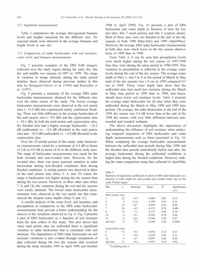
Table 5

Summary of regressions coefficients for plots of ERS radar backscatter as a

function of water depth for non-wooded and wooded study sites in the

south Florida region

Site n Intercept Slope R2 Significance

( p<)

Marl prairie sites

1 22 �8.5 �0.088 0.05 0.32

3 5 �11.6 0.199 0.55 0.15

4 12 �8.7 �0.094 0.32 0.06

7 16 �6.5 �0.333 0.78 0.001

8 15 �7.7 �0.127 0.08 0.34

14 6 �9.1 �0.243 0.70 0.04

15 6 �8.3 �0.146 0.30 0.27

All sitesa 77 �7.9 �0.189 0.28 0.0001

Cypress/pine sites

5 15 �9.2 �0.036 0.12 0.21

6 7 �9.6 �0.194 0.45 0.11

12 9 �8.7 �0.097 0.42 0.06

All sites 31 �9.3 �0.052 0.18 0.02

a Excluding site 3.

ing of Environment 88 (2003) 423–441

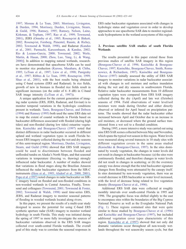
5.2. Vegetation measurements

Table 3 summarizes the average aboveground biomass

levels and heights measured for the different sites. No

seasonal trends were detected in the average biomass and

height levels at any site.

5.3. Comparison of radar backscatter with soil moisture,

water level, and biomass measurements

Fig. 7 presents examples of the ERS SAR imagery

collected over the study region during the early dry, late

dry and middle wet seasons of 1997 to 1999. The range

in variation in image intensity during the study period

matches those observed during previous studies in this

area by Bourgeau-Chavez et al. (1996) and Kasischke et

al. (1997).

Fig. 8 presents a summary of the average ERS radar

backscatter measurements obtained for the different sites

over the entire course of the study. The lowest average

backscatter measurements were observed in the wet marsh

sites (�13.2 dB) that experienced nearly continuous flood-

ing. There was little difference in the average backscatter of

the marl prairie sites (�9.9 dB) and the cypress/pine sites

(�10.1 dB). In both the marl prairie and cypress/pine sites,

the flooded sites had a higher average backscatter: �10.2

dB (unflooded) vs. �9.6 dB (flooded) in the marl prairie

sites and �10.5 dB (unflooded) vs. �9.8 dB (flooded) in the

cypress/pine sites.

Over the 25-month period of this study, radar backscat-

ter measurements varied by a minimum of 4.4 dB (a factor

of 2.8) to 9.0 dB (a factor of 8) in the different study sites.

The range of backscatter measurements was equal for the

both wooded and non-wooded sites. However, for the

wooded sites, there was more seasonal variation in radar

backscatter during non-flooded conditions than during

flooded conditions. A similar pattern was observed in three

of the marl prairie sites (Sites 3, 4, and 15) where the

range is backscatter was higher during the dry season than

during the wet season. However, in three other sites (Sites

7, 8, and 14), the variations during the wet and dry seasons

were nearly identical. The lowest radar backscatter meas-

urements were observed in the wet marsh site that expe-

rienced the deepest water depths (Sites 9 and 11).

A careful analysis of the water level, soil moisture, and

precipitation in comparison to the ERS radar backscatter

measurements does provide a better understanding for the

sources of the variations observed in Fig. 8. Fig. 9 presents

a plot of ERS backscatter as a function of soil moisture

from the data collect in this study. This plot shows that

when marl prairie sites are unflooded there is significant

variation in radar backscatter that is correlated with soil

moisture. The dependence of ERS radar backscatter on soil

moisture variations is also evident through comparison of

data collected during the two dry seasons that occurred

during the study (October 1997 to April 1998 and October

E.S. Kasischke et al. / Remote Sens436

1998 to April 1999). Fig. 10 presents a plot of ERS

backscatter and water depth as function of time for two

test sites: Site 7 (marl prairie) and Site 5 (cypress dome).

Both of these sites were not flooded at the end of the dry

seasons in both 1998 (May/July) and 1999 (April/May).

However, the average ERS radar backscatter measurements

at both sites were much lower in the dry season observa-

tions of 1999 than in 1998.

From Table 2, it can be seen that precipitation levels

were much higher during the wet season of 1997/1998

than they were during the same period in 1998/1999. This

variation in precipitation is reflected in the average water

levels during the end of the dry season. The average water

depth at Sites 1, and 3 to 8 in the period of March to May

(end of the dry season) was 1.9 cm in 1998 compared 0.3

cm in 1999. These water depth data show that the

unflooded sites had much less moisture during the March

to May time period in 1999 than in 1998, and hence,

should have lower soil moisture levels. Table 4 presents

the average radar backscatter for all sites when they were

unflooded during the March to May 1998 and 1999 time

periods. On average, the radar backscatter at the end of the

1999 dry season was 5.4 dB lower than at the end of the

1998 dry season, with very little difference between non-

wooded and wooded wetlands.

The above discussion highlights the importance of

understanding the influence of soil moisture when analyz-

ing temporal sequences of ERS backscatter and water

depth measurements such as those presented in Fig. 10.

When comparing the average backscatter measurements

between the unflooded time periods during May 1998 and

the flooded time periods immediately before and after, the

average backscatter during the unflooded conditions is

higher than during the flooded conditions. However, mak-

ing the same comparison using data collected in April/May

E.S. Kasischke et al. / Remote Sensing of Environment 88 (2003) 423–441 437

of 1999 results in the backscatter during the unflooded

conditions being lower than during the flooded conditions.

This trend was observed in all study sites. In Table 4, we

present the difference in average radar backscatter measure-

ments between flooded and unflooded conditions for the

different study sites. We calculated this difference in two

ways. First, we calculated the average radar backscatter for

Fig. 12. Variation in ERS radar backscatter as a function of water dept

each site when it was flooded during the periods of June

1997 through December 1998 and compared these to the

average backscatter when the site was not flooded in March

to May of 1998. Second, we calculated the average back-

scatter for the period of January 1998 through August of

1999 for each site when it was flooded and compared it to

the average backscatter when the site was not flooded in

h in: (a) all marl prairie sites; and (b) all cypress and pine sites.

E.S. Kasischke et al. / Remote Sensing of Environment 88 (2003) 423–441438

March to May of 1999. A positive difference in Table 4

means that the backscatter in the site increased when they

became flooded, while a negative difference means the

backscatter decreased when the sites became flooded.

The results in Table 4 are consistent in all sites. During

the dry season of 1998 when the sites likely had high soil

moisture, a flooding of the sites resulted in a 1.6-dB

decrease in radar backscatter, with no difference occurring

Fig. 13. Variation in ERS radar backscatter as a function of aboveground biomass:

range in backscatter as a function of biomass in all non-flooded marl prairie sites

between wooded and non-wooded sites. During the dry

season of 1999 (when the sites likely had lower soil

moisture), they experienced a 3.3-dB increase in radar

backscatter when they became flooded, with high increases

being observed in the wooded wetlands. The observations

support Hypothesis 1 of this study and the effects of flood-

ing predicted by MIMICS (Fig. 3). We expect all the sites to

have high soil moisture levels (similar to the conditions

(a) backscatter as a function of biomass in all flooded marl prairie sites; (b)

.

E.S. Kasischke et al. / Remote Sensing of Environment 88 (2003) 423–441 439

observed in March–May 1998) prior to and immediately

after flooding occurs. When flooding does occur, the data

show there is a decrease in radar backscatter.

One clear trend present in the data from Site 7 in Fig. 10

is the strong inverse correlation between changes in water

depth and changes in radar backscatter, e.g., as water depth

increases, radar backscatter decreases. Although not as

evident the same trend is also present in the data for Site

5. Fig. 11 presents a plot of ERS backscatter as a function of

water depth for these two sites showing the correlation

between these variables. Table 5 summarizes the regression

equation of ERS backscatter as function of water depth for

all sites. We can see that there is a positive relationship

between these two variables for all sites except one. The one

case where a positive slope occurs (Site 3) also had the

highest aboveground biomass of any of the marl prairie

sites. Fig. 12 presents a plot of ERS backscatter as function

of water depth for all marl prairie (except Site 3) and all

cypress/pine sites combined. These plots show that overall

there is a statistically significant decrease in radar backscat-

ter as water depth increases, which supports Hypothesis 3.

Finally, our analyses of the data indicate that varia-

tions in biomass had relatively little effect on the radar

backscatter signature, and do not support either Hypoth-

esis 4 or Hypothesis 5. If biomass had a strong influence

on the microwave scattering signature, we would expect:

(a) that radar backscatter in flooded sites would increase

as biomass increases; and (b) the overall range in

backscatter in the unflooded sites to be lowest in those

sites with the highest biomass. Fig. 13a presents a plot of

radar backscatter as a function of biomass for the flooded

sites. In this plot, we reduced the average biomass of a

plot (from Table 3), an amount proportional to the depth

of the water at the time of data collection. In this plot,

there is no apparent relationship between biomass and

radar backscatter. According to theoretical models, the

range in backscatter in unflooded sites should decrease as

biomass increases. Fig. 13b shows this not to be the case

for the sites in this study.

6. Discussion

In this study, we have demonstrated that variations in

hydrologic conditions result in very large variations in radar

backscatter from wetlands in southern Florida. During

unflooded conditions, radar backscatter varies by a factor

of 8 (9 dB) in both wooded and non-wooded wetlands. The

same level of variation is observed in non-wooded wetlands

when they are flooded, with lower levels of variation (5 dB)

occurring in the wooded wetlands.

Variations in radar backscatter associated with changes in

soil moisture and flooding predicted by the theoretical

scattering model (MIMICS) were present in the ERS SAR

data. Large variations in backscatter as a result of changes in

soil moisture were clearly observed in the data. Variations in

soil moisture during the dry seasons between two different

periods were observed in all the study sites. Our interpre-

tation is that all sites, there was a drop in radar backscatter

when the sites became flooded. This reduction in backscat-

ter occurred for all three major vegetation types: marl

prairie, cypress, and pine flatwoods (Table 4). The magni-

tude of this drop for the marl prairie sites (1–2 dB),

however, is much lower than the figure predicted by

MIMICS. Finally, we did see a significant drop in radar

backscatter as a function of increasing water depth, again for

the major vegetation types (Figs. 11 and 12). The sensitivity

to water depth was higher in the marl prairie sites than in the

cypress/pine sites.

Our analyses indicates that variations in biomass had a

relatively little impact on variations in backscatter associat-

ed with changes in soil moisture and water level. The

vegetation of the sites used in this study had relatively short

canopies, low biomass levels and small stem sizes; there-

fore, these should be viewed with certain degree of caution.

In other studies where higher biomass levels occurred in the

flooded sites, there was a strong influence of biomass on

radar backscatter. For example, LeToan et al. (1997) noted a

positive correlation in rice plant biomass and ERS back-

scatter; however, the maximum biomass level in LeToan et

al. (1997) was 3.5 kg m�2, which is 1 order-of-magnitude

higher than the levels present in the sites in this study. Pope

et al. (1997) concluded that wetlands with dense biomass

and large stems experienced an increase in backscatter when

flooded, while those with less dense vegetation and small

stems experienced a decrease in backscatter when flooded

(similar to the conclusion of this study). However, Pope et

al. (1997) did not measure variations in soil moisture in their

unflooded sites. Based on the results of the present study, it

is not possible to attribute the results in Pope et al. (1997)

entirely to differences in vegetation structure and density—

variations in soil moisture likely played a role as well. It is

clear that future studies must include steps to document

vegetation biomass structure, density, and biomass as well

as soil moisture to clearly document the role of each of these

factors on variations in radar backscatter.

Examination of the ERS images in Figs. 1 and 7 show

complex patterns of image intensity within individual

regions not only between wet and dry seasons, but also

between different years. For example, the fact that the

region within Water Conservation Area 3A remains darker

than the surrounding areas throughout the year is consistent

with the fact that water is permanently stored in this basin.

The region that is actually flooded within the Everglades

National Park can clearly be delineated as dark regions in

the ERS-1 SAR imagery. Variations in water levels in the

Everglades are controlled through a combination of the

patterns of water release from the Conservation Areas north

of the Park and seasonal precipitation patterns. The spatially

patchiness of seasonal flooding within the Big Cypress

National is clearly seen on the ERS images. Note that the

more extensive flooding during the wet seasons of 1997 is

E.S. Kasischke et al. / Remote Sensing of Environment 88 (2003) 423–441440

entirely consistent with the higher precipitation experienced

during this time. Finally, the results of this study show that

variations in image intensity during dry periods denotes not

only the switch from a flooded to non-flooded state, but also

variations in soil moisture.

In summary, the results of this study clearly demonstrate

the unique capability for using C-band spaceborne imaging

radar data for monitoring hydrologic conditions within

wetland systems with lower levels of aboveground biomass.

Although variations in aboveground biomass do influence

the radar signature at individual sites, temporal variations in

radar backscatter largely reflect variations in soil moisture

and patterns of flooding in the wetlands of this region.

Correct interpretation of the temporal variations in the radar

signatures requires an understanding of how seasonal pre-

cipitation patterns influence patterns of soil moisture and

inundation. Once these hydrologic patterns are established

for a region, then changes in radar backscatter can be

interpreted in terms of expected changes in soil moisture,

flooding, and water level.

Acknowledgements

Support for this research was provided by the U.S.

Environmental Protection Agency under Grant Number

R825156-01-0. The research presented in this paper has

not been subjected to review by EPA and therefore does

not necessarily reflect their views, and no official

endorsement should be inferred. The authors would like

to thank the anonymous reviewers for their insightful and

helpful comments.

References

Alsdorf, D. E., Melack, J. M., Dunne, T., Mertes, L. A. K., Hess, L. L., &

Smith, L. C. (2000). Interferometric radar measurements of water level

changes on the Amazon flood plain. Nature, 404, 174–177.

Alsdorf, D. E., Smith, L. C., & Melack, J. M. (2001). Amazon floodplain

water level changes measured with interferometric SIR-C radar. IEEE

Transactions on Geoscience and Remote Sensing, 39, 423–431.

Bourgeau-Chavez, L. L., Kasischke, E. S., Brunzell, S. M., Mudd, J. P.,

Smith, K. B., & Frick, A. L. (2001). Analysis of spaceborne SAR data

for wetland mapping and flood monitoring in Virginia riparian ecosys-

tems. International Journal of Remote Sensing, 22, 3665–3687.

Bourgeau-Chavez, L. L., Kasischke, E. S., & Smith, K. B. (1996). Using

satellite radar imagery to monitor flood conditions in wetland ecosys-

tems of southern Florida. In G. Cecchi, G. D’Urso, E. T. Engman, & P.

Gudmandsen (Eds.), Remote sensing of vegetation and sea, vol. 2959

( pp. 139–148). Taormina, Italy: SPIE.

Brivio, P. A., Colombo, R., Maggi, M., & Tomasoni, R. (2002). Integration

Remote sensing data and GIS for accurate mapping of flooded areas.

International Journal of Remote Sensing, 23, 429–441.

Brown, R. B., Stone, E. L., & Carlilse, V. W. (1990). Soils. In R. L. Ewel,

& J. J. Ewel (Eds.), Ecosystems of Florida ( pp. 35–69). Orlando, FL:

University of Central Florida Press.

Dobson, M. C., Ulaby, F. T., & Pierce, L. E. (1995). Land-cover classifi-

cation and estimation of terrain attributes using synthetic-aperture radar.

Remote Sensing of Environment, 51, 199–214.

Duever, M. J., Carlson, J. E., Meeder, J. F., Duever, L. C., Gunderson, L.

H., Riopelle, L. A., Alexander, T. R., Meyers, R. L., & Spangler, D. P.

(1986). The Big Cypress National Preserve. Naples, FL: National Au-

dubon Society.

Duever, M. J., Meeder, J. F., Meeder, L. C., & McCollom, J. M. (1994).

The climate of south Florida and its role in shaping the Everglades. In S.

M. Davis, & J. C. Ogden (Eds.), Everglades—the ecosystem and its

restoration (pp. 225–248). Delray Beach, FL: St. Lucie Press.

Dwivedi, R. S., Rao, B. R. M., & Bhattacharya, S. (1999). Mapping wet-

lands of the Sundaban Delta and its environs using ERS-1 SAR data.

International Journal of Remote Sensing, 20, 2235–2247.

Engheta, N., & Elachi, C. (1982). Radar scattering from a diffuse vegeta-

tion layer over a smooth surface. IEEE Transactions on Geoscience and

Remote Sensing, 20, 212–216.

Gunderson, L. H. (1994). Vegetation of the Everglades: Determinants of

species composition. In S. M. Davis, & J. C. Ogden (Eds.), Ever-

glades—The ecosystem and its restoration ( pp. 323–340). Delray

Beach, FL: St. Lucie Press.

Hess, L. L., Melack, J. M., Filoso, S., & Wang, Y. (1995). Delineation of

inundated area and vegetation along the Amazon floodplain with the

SIR-C synthetic aperture radar. IEEE Transactions on Geoscience and

Remote Sensing, 33, 896–904.

Hess, L. L., Melack, J. M., & Simonett, D. S. (1990). Radar detection of

flooding beneath the forest canopy: A review. International Journal of

Remote Sensing, 11, 1313–1325.

Imhoff, M. L., Vermillion, C., Story, M. H., Choudhury, A. M., Gafoor, A.,

& Polcyn, F. (1987). Monsoon flood boundary delineation and damage

assessment using space borne imaging radar and Landsat data. Photo-

grammetric Engineering and Remote Sensing, 53, 405–413.

Kandus, P., Karszenbaum, H., Pultz, T., Parmuchi, G., & Bava, J. (2001).

Influence of flood conditions and vegetation status on the radar back-

scatter of wetland ecosystems. Canadian Journal of Remote Sensing,

27, 651–662.

Kasischke, E. S., & Bourgeau-Chavez, L. L. (1997). Monitoring south

Florida wetlands using ERS-1 SAR imagery. Photogrammetric Engi-

neering and Remote Sensing, 33, 281–291.

Kasischke, E. S., Bourgeau-Chavez, L. L., Smith, K. B., Romanowicz, E.,

& Richardson, C. J. (1997). Monitoring hydropatterns in southern Flor-

ida ecosystems using ERS SAR data. Proceedings of the 3rd ERS

symposium on space in service of our environment (pp. 71–76). Flor-

ence, Italy: European Space Agency.

Krohn, M. D., Milton, N. M., & Segal, D. B. (1983). Seasat synthetic aper-

ture radar (Sar) response to lowland vegetation types in eastern Maryland

and Virginia. Journal of Geophysical Research, 88, 1937–1952.

Kurosu, T., Masaharu, F., & Chiba, K. (1995). Monitoring of rice crop

growth from space using the ERS-1 C-band SAR. IEEE Transactions

on Geoscience and Remote Sensing, 33, 1092–1096.

LeToan, T., Ribbes, F., Wang, L. F., Floury, N., Ding, K. H., Kong, J. A.,

Fujita, M., & Kurosu, T. (1997). Rice crop mapping and monitoring

using ERS-1 data based on experiment and modeling results. IEEE

Transactions on Geoscience and Remote Sensing, 35, 41–56.

Liew, S. C., Kam, S. P., Tuong, T. P., Chen, P., Minh, V. Q., & Lim, H.

(1998). Application of multitemporal ERS-2 synthetic aperture radar in

delineating rice cropping systems in the Mekong River Delta, Vietnam.

IEEE Transactions on Geoscience and Remote Sensing, 36, 1412–1420.

Meadows, P. J., Laur, H., & Shattler, B. (1999). The calibration of ERS SAR

imagery for land applications. Earth Observation Quarterly, 62, 5–9.

Moreau, S., & Le Toan, T. (2003). Biomass quantification of Andean wet-

land forages using ERS satellite SAR data for optimizing livestock

management. Remote Sensing of Environment, 84, 477–492.

Morrissey, L. A., Durden, S. L., Livingston, G. P., Stearn, J. A., & Guild, L.

S. (1996). Differentiating methane source areas in arctic environments

with multitemporal ERS-1 SAR data. IEEE Transactions on Geoscience

and Remote Sensing, 34, 667–673.

Morrissey, L. A., Livingston, G. P., & Durden, S. L. (1994). Use of SAR in

regional methane exchange studies. International Journal of Remote

Sensing, 15, 1337–1342.

E.S. Kasischke et al. / Remote Sensing of Environment 88 (2003) 423–441 441

Ormsby, J. P., Blanchard, B. J., & Blanchard, A. J. (1985). Detection of

lowland flooding using active microwave systems. Photogrammetric

Engineering and Remote Sensing, 51, 317–328.

Panigrahy, S., Chakraborty, M., Sharma, S. A., Kundu, N., Ghose, S. C., &

Pal, M. (1997). Early estimation of rice area using temporal ERS-1

synthetic aperture radar data—A case study for the Howrah and Hughly

districts of West Bengal, India. International Journal of Remote Sens-

ing, 18, 1827–1833.

Parmuchi, M. G., Karszenbaum, H., & Kandus, P. (2002). Mapping wet-

lands using multi-temporal RADARSAT-1 data and a decision-based

classifier. Canadian Journal of Remote Sensing, 28, 175–186.

Pope, K. O., Rejmankova, E., & Paris, J. F. (2001). Spaceborne imaging

radar-C (SIR-C) observations of groundwater discharge and wetlands

associated with the Chicxulub impact crater, northwestern Yucatan Pen-

insula, Mexico. Geological Society of America Bulletin, 113, 403–416.

Pope, K. O., Rejmankova, E., Paris, J. F., & Woodruff, R. (1997). Detecting

seasonal flooding cycles in marshes of the Yucatan Peninsula with SIR-

C polarimetric radar imagery. Remote Sensing of Environment, 59,

157–166.

Ramsey, E. W. (1995). Monitoring flooding in coastal wetlands by using

radar imagery and ground-based measurements. International Journal

of Remote Sensing, 16, 2495–2502.

Ramsey, E. W., Nelson, G. A., Laine, S. C., Kirkman, R. G., & Topham, W.

(1997). Generation of coastal marsh topography with radar and ground-

based measurements. Journal of Coastal Research, 13, 1335–1342.

Rao, B. R. M., Dwivedi, R. S., Kushwaha, S. P. S., Bhattacharya, S. N.,

Anand, J. B., & Dasgupta, S. (1999). Monitoring the spatial extent of

coastal wetlands using ERS-1 SAR data. International Journal of Re-

mote Sensing, 20, 2509–2517.

Ribbes, F., & Le Toan, T. (1999). Rice field mapping and monitoring

with RADARSAT data. International Journal of Remote Sensing, 20,

745–765.

Rio, J. N. R., & Lozano-Garcia, D. F. (2000). Spatial filtering of radar data

(RADARSAT) for wetlands (brackish marshes) classification. Remote

Sensing of Environment, 73, 143–151.

Rosenqvist, A. (1999). Temporal and spatial characteristics of irrigated rice

in JERS-1 L-band SAR data. International Journal of Remote Sensing,

20, 1567–1587.

Rosenqvist, A., & Birkett, C. M. (2002). Evaluation of JERS-1 SAR mo-

saics for hydrological applications in the Congo River basin. Interna-

tional Journal of Remote Sensing, 23, 1283–1302.

Rosenqvist, A., Forsberg, B. R., Pimentel, T., Rauste, Y. A., & Richey, J. E.

(2002). The use of spaceborne radar data to model inundation patterns

and trace gas emissions in the central Amazon floodplain. International

Journal of Remote Sensing, 23, 1303–1328.

Shao, Y., Fan, X. T., Liu, H., Xiao, J. H., Ross, S., Brisco, B., Brown, R.,

& Staples, G. (2001). Rice monitoring and production estimation us-

ing multitemporal RADARSAT. Remote Sensing of Environment, 76,

310–325.

Tanis, F. J., Bourgeau-Chavez, L. L., & Dobson, M. D. (1994). Application

of ERS-1 SAR for coastal inundation. 1994 IEEE Geosci. Remote Sens.

Society ( pp. 1481–1483). Pasadena, CA: IEEE.

Townsend, P. A. (2001). Mapping seasonal flooding in forested wetlands

using multi-temporal Radarsat SAR. Photogrammetric Engineering and

Remote Sensing, 67, 857–864.

Townsend, P. A. (2002). Relationships between forest structure and the

detection of flood inundation in forested wetlands using C-band SAR.

International Journal of Remote Sensing, 23, 443–460.

Townsend, P. A., & Foster, J. R. (2002). A synthetic aperture radar-based

model to assess historical changes in lowland floodplain hydroperiod.

Water Resources Research, 38 (art. no.-1115).

Townsend, P. A., & Walsh, S. J. (1998). Modeling floodplain inundation

using an integrated GIS with radar and optical remote sensing. Geo-

morphology, 21, 295–312.

Ulaby, F. T., Moore, R. K., & Fung, A. K. (1982). Microwave remote

sensing, active and passive: Volume II. Radar remote sensing and sur-

face scattering and emission theory. Reading, MA: Addison-Wesley

Publishing, 607 pp.

Ulaby, F. T., Sarabandi, K., McDonald, K., & Dobson, M. C. (1990).

Michigan microwave canopy scattering model (MIMICS). International

Journal of Remote Sensing, 11, 1223–1253.

Werle, D., Martin, T. C., & Hasan, K. (2000). Flood and coastal zone

monitoring in Bangladesh with Radarsat ScanSAR: Technical experi-

ence and institutional challenges. Johns Hopkins APL Technical Digest,

21, 148–154.

Zhou, C. H., Luo, J. C., Yang, C. J., Li, B. L., & Wang, S. L. (2000). Flood

monitoring using multi-temporal AVHRR and RADARSAT imagery.

Photogrammetric Engineering and Remote Sensing, 66, 633–638.