Shallow-water tracking in the Sea of Nazare

Submitted to the IEEE Journal of Oceanic Engineering (1998)

Abstract— In the summer of 1996, an experiment was conducted off the coast of Portugal to study the effects of

internal tides on sound propagation. This experiment—called INTIMATE '96 (Internal Tide Investigation by

Means of Acoustic Tomography Experiment)—has provided a great deal of insight about the variability of pulse

transmission over space and time. In contrast to a common view of shallow-water propagation as complicated and

unpredictable, we find a steady pattern of echoes. The echo-pattern stretches and shrinks in a systematic way with

the tides and allows us to infer the components of the first few oceanographic modes. We also used the echo-

pattern to track the source over a period of several days. During this period the isotherms in the ocean wavered by

20 m as a result of the tides, providing a challenge for model-based tracking. We will discuss these acoustic results

with emphasis on the source tracking.

Keywords— tomography, tides, matched-field processing

1 On sabbatical from the Center for Communications and Signal Processing Research and Department of MathematicalSciences, New Jersey Institute of Technology, Newark, NJ 07102.

M.B. Porter*, Y. Stéphan**, X. Démoulin**, S. Jesus+, E. Coelho#,

*Marine Physical Laboratory, Scripps Institution of Oceanography, La Jolla, CA, USA.1

E-mail: [email protected]**EPSHOM/CMO, BP426, F-29275, Brest, FRANCE

+University of the Algarve, Faro, PORTUGAL#Hydrographic Institute, P-1296, Lisbon, PORTUGAL

SHALLOW-WATER TRACKING IN THE SEA OF NAZARÉ


I. INTRODUCTION

The signature of ocean tides has often been seen in ocean acoustic experiments (see Weinberg et al.[1] and references

therein). In the early experiments, the tidal effects were observed in phase rolls of the received signal due to a tonal

source. Later, the tidal signature has been seen clearly in tomography experiments with what are effectively impulsive

sources[2][3].

Tides, as every school child knows, result from the tractive force of the moon and sun; however, this simple mechanism

leads to a complicated effect explained well in Ref. [4]. In the Newtonian equilibrium model, the difference of

gravitational and centrifugal forces creates twin bulges on the earth facing towards and away form the moon. The axis of

rotation of the earth, the orbital planes of the earth around the sun, and of the moon around the earth, are skewed with

respect to each other. Therefore, the daily rhythm of the tides is rather off-beat. Furthermore, this simple Newtonian

model fails to account for the fact that the tides would be traveling so rapidly at the equator that they would break a speed

limit imposed by shallow-water equations. Despite all these complications, the fundamental period associated with the

tides is sharply defined at 12.42 hours for the moon and, naturally, 1 day for the sun.

The most commonly known tidal-effect is the so-called barotropic component that raises and lowers the ocean surface.

The associated tidal current flows over bottom features such as the break from the continental slope to the continental

shelf. At this break, a coupling or scattering process excites a second class of so-called baroclinic or internal-tides.

While the reader may well have no familiarity with these, his intuition has been formed by a day at the beach— the usual

surface waves can be thought of as interfacial waves with the interface is formed by air and water. Similarly, internal

waves propagate between the light and heavy layers within the ocean. However, their scale may surprise. In our

experiment they displace isotherms by about 20 m and are about 10 km long. This is quite typical. When the forcing of the

internal waves is dominated by the tides they are called internal tides.

These enormous waves cause barely a 5-cm ripple on the ocean surface but in the glint of the sun, they are easily seen

from space, as many shuttle astronauts report. In fact, they have also been recently measured precisely by satellite


altimeters. (This requires careful attention to the signal processing exploiting multiple overpasses). These latest results

remind us that barotropic-to-baroclinic coupling also happens over deep-water ridges. Indeed the coupling may be

stronger there since the tidal currents can more easily flow perpendicular to the bottom feature and since their geometry

may be more effective in scattering the energy[7].

From an oceanographic point of view, it is interesting to learn more about this process. It is known from measurements of

the orbit of the moon that the tides are dissipating around 2.5 gigawatts of energy and there is mystery and controversy

over the question of where that energy goes. One envisions a cascade from the large scale (barotropic tides) to medium

scale (baroclinic tides) to small-scale turbulence but the details are not well understood. An interesting discussion of these

issues that provides the basis for our understanding is presented by Munk and Wunsch[7].

Sound provides a way of observing these internal tides and learning more about them. In addition, SONAR systems

operate within the tides so that the tides become a sort of nuisance factor which one would like to understand better. In

this paper, we will discuss the experiment INTIMATE 96 that was designed to address these interests.


II. THE EXPERIMENT

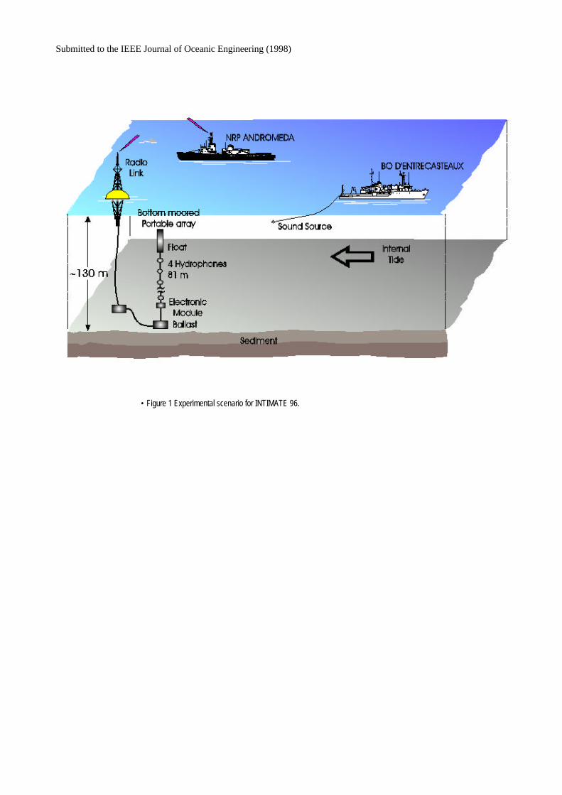
The experimental configuration is shown in Fig. 1. A sound source (Source Pour Tomographie Acoustique) was towed by

the French oceanographic vessel, D'Entrecasteaux. It emitted chirps sweeping from 300-800 Hz over a 2-second period.

The transmissions were repeated every 8 seconds; received on a 4-phone vertical array; and telemetered back to the

Hydrographic Institute's vessel, the Andromeda.

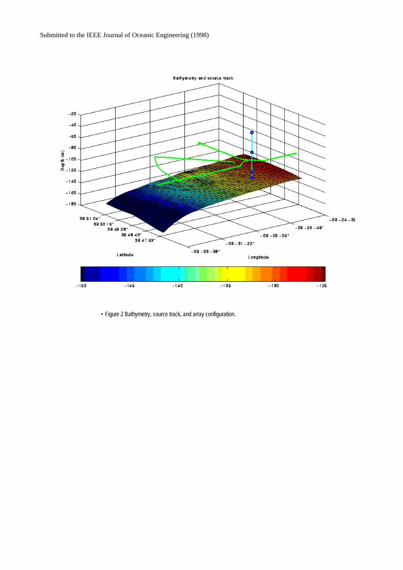
As discussed above, the internal tides are often excited at the break from the continental slope to the shelf. It is at that

break where they tend to have their largest height and this motivated the deployment of the array at that point as shown by

the vertical line in Fig. 2. In the first phase, the source was deployed for 25 hours on a station about 6 km directly north

of the array (and therefore parallel to the crests of the internal tides). That 25 hours provided enough time to observe two

complete tidal cycles.

In the second phase, the source was towed over a sort of bow-tie pattern measured by GPS and shown by the solid line.

This pattern provided several radial slices through the tidal field. In the third and final phase, the source was deployed for

another 25-hour station, this time about 6 km directly west of the array (and therefore perpendicular to the crests of the

internal tides). In the remainder of this paper, we will focus on results from the first station.

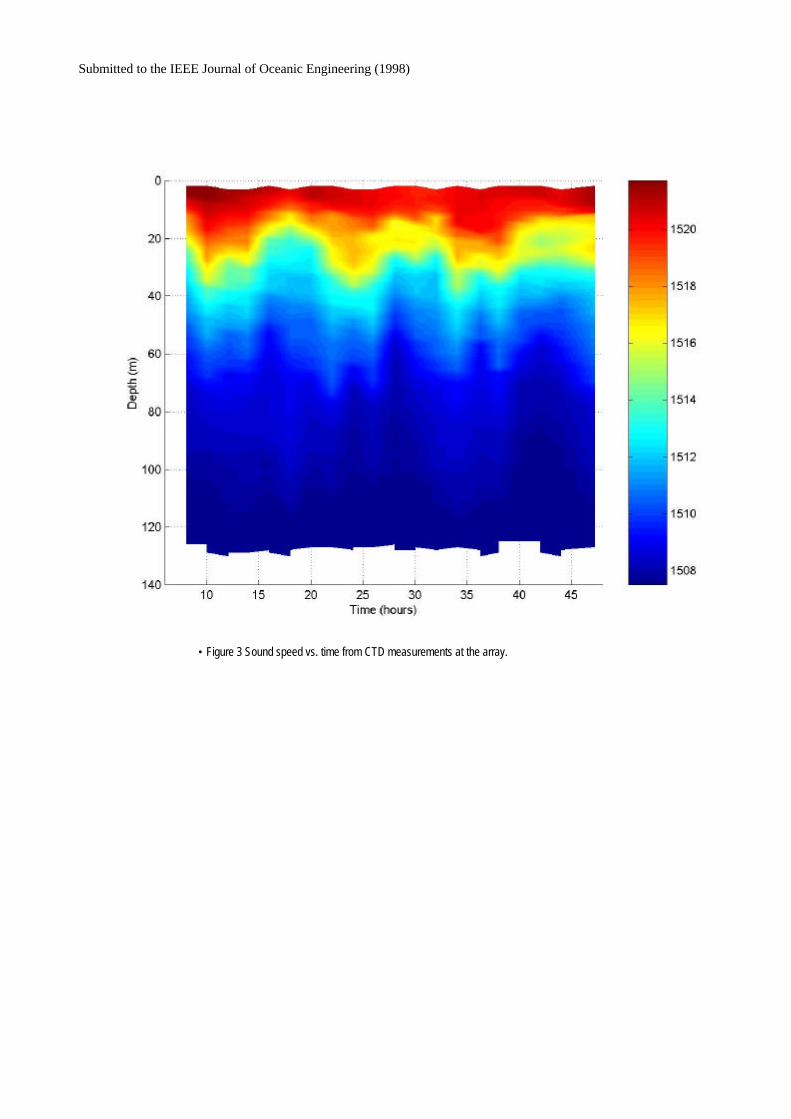
Extensive oceanographic measurements were made during the experiment. A sequence of CTDs taken near the array

shows the evolution of the ocean sound-speed (Fig. 3). Note the 12.5-hour period which is one signature of the internal

tides.


III. ACOUSTICS

The warm temperature near the surface causes a downward refracting profile whose effect is seen on the ray plot in Fig. 4.

We have plotted only the eigenrays (connecting the source at about 90 m, to the deepest phone at about 115 m). We

observe two classes of rays distinguished by whether or not they refract before hitting the surface.

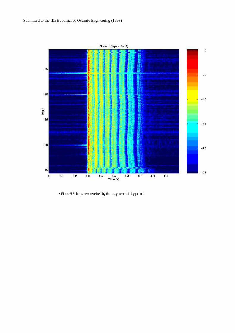
The various rays shown in the previous figure can be associated with the pattern of 40 echoes seen in the data in Fig. 5.

These results were obtained by processing several thousand chirps over the 25-hour period where the source was on the

first station (north of the array). In a standard fashion the received time-series was correlated with a replica of the source

waveform yielding the channel impulse response. The source waveform was not directly measured in the experiment and

therefore was estimated from a laboratory measurement of the sources power spectrum. Next an envelope was formed to

eliminate the wiggles associated with the carrier and aligned by their leading edge. This yields the echo response of the

ocean channel. Groups of 10 echo-responses were summed to reduce noise and then normalized with respect to a peak

value. Finally the results were plotted in dB.

The echoes cut-off at a time determined by the bottom critical-angle (since longer delays would require steeper ray paths).

The overall decay in intensity of the echoes tells us a lot about the bottom reflectivity and confirmed our prior use of a

sandy bottom with a wavespeed of 1750 m/s and attenuation of 0.9 dB per wavelength.

The tidal effect on the sound is quite clear in Fig. 5. Over the 25-hour station, we see a clear sinusoidal variation in the

echo response. (Considering the leading-edge alignment, we are commenting on relative not absolute delay.) This tidal

effect is due to both the barotropic and baroclinic components as has been discussed by Démoulin et al.[8]. During the

first hour of transmission we note a shift in the echo pattern which corresponds to the period when the source ship was

moving to the station.


IV. SOURCE LOCALIZATION

The echo pattern is also a signature of the source position, an idea that forms the basis of matched-field processing for

source localization[9]. We take an acoustic model and predict what the echo-pattern would look like for all plausible

source ranges and depths. Then we compare the actual echo-pattern to the ensemble of predicted echo-patterns and look

for the best match. If we can model the channel response well-enough, the best match will happen for the case where the

model source position is the same as that in the experiment.

Ocean channel-models are now well-developed and there are many suitable choices[10]. Here we have used the

KRAKEN normal-mode program[11] though we have also obtained equally good results with the SCOOTER

wavenumber-integration model and the BELLHOP ray model that was used earlier to produce the eigenray plot.

The way in which one compares the model and data waveforms is important. In the now enormous body of literature

devoted to matched-field processing this has usually been done by forming a covariance or cross-spectral matrix for each

frequency component. Problems of robustness have been widely reported. In an off-handed way one reasons that the

phase of the acoustic signal on the array is extremely sensitive to environmental errors.

It is striking that seen in the time domain the pattern is very stable and with very limited environmental information tells

us the source range and depth. (The further away it is, the more echoes.) However, the tides, which are not usually

considered, cause shifts in the echoes that imply large relative phase changes between phones.

Another significant aspect is that we have plotted the envelope and not the raw time-series. The envelope is insensitive to

pulse inversions that occur when the sound reflects from the ocean surface. More importantly, it is also insensitive to the

more complicated phase changes that occur during bottom reflection. If the bottom were precisely known those phase

changes would be extra useful information in localizing a source. However, this is not the case so the uncertainty just

makes it hard to match model and data.


Finally, there is an image processing question of how best to display the data so as to show features of interest. One well-

known technique is to histogram the intensity in the image and use an intensity scale that assigns the shades in proportion

to the number of levels in each bin. However, as in many other fields, the dB scale has heuristically been found suitable to

best see the interesting features.

These visual considerations are all significant in defining a robust processor. Most of the energy is contained in the

leading 10% of the time series. Thus when we compare the model and data time series by correlation in the original linear

domain, we are effectively trying to find a match in just the first 10% of the data. Unfortunately, this is also the hardest

part to match since it results from a delicate interference of about 5 refracted paths which are sensitive to the ocean

thermal structure. Notice how by covering the last 90% of the echo-pattern you would lose the ability to discern visually

the source range.

One prefers the opposite since by ignoring the first 10% and focusing on the remainder we see an echo-pattern that

fingerprints the source. Doing the correlation in the log domain we further focus on this structure. Thus we measure the

match between model and data using a correlation of logs of envelopes and scanning over the unknown delay time. Only

one phone was used in the correlations. To summarize, for each normalized measured and modeled time series, r(t) and

g(t) respectively, we compute:

( )[ ]( )[ ]

),;(max),(

),;()(),;(

)(log20)(

)(log20)(

zrtczrP

dzrtgrzrtc

atgenvtg

atrenvtr

t

lele

le

le

=

−=

−=

−=

∫ τττ

Here a is set at 30 dB to clip out the noise that would otherwise dominate the correlation. For efficiency the correlation is

implemented in the frequency domain. In an obvious generalization, information from multiple phones can be included;

however, here we present only results using the deepest phone. In theory, the resulting ambiguity surface, P(r,z) then has a

peak at the source location.


Note that this processing assumes that the correlogram, r(t), is available and this in turn assumes a knowledge of the

source spectrum. In many important applications this is known. When it is not, one may correlate the autocorrelations of

each phone with predicted autocorrelations with much weaker assumptions needed about the source spectrum. In a similar

approach, inter-phone cross-correlations have been used by Westwood and Knobles[12]. The reader broadly interested in

correlation-based processing may also find Refs. [13][14]useful.

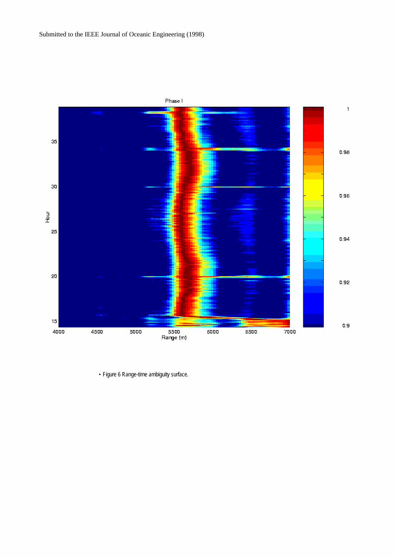
The resulting ambiguity surface showing the range-time plot of the source is presented in Fig. 6. The peak occurs at about

5.6 km, which matches nicely the ship navigational data. However, we see an apparent wander of the source position that

is correlated with the tides. This wander is a sort of mirage that results from using an acoustic model with a static ocean

while the ocean varies under the tidal influence. The effect is essentially the same one that results from errors in bottom-

depth that has been discussed in Refs.[15][16].


V. CONCLUSION

The INTIMATE '96 experiment has proven very interesting in both understanding basic features of shallow-water sound

propagation and learning about the oceanography. Historically, shallow-water has been thought to present great

challenges for acoustic modeling. Ocean variability is often far greater than in deep-water (and is certainly very clear in

this experiment). In addition, the downward-refracting profiles guarantee that all ray paths are bottom interacting and one

therefore worries about problems in characterizing the bottom.

Against this backdrop, it is interesting to see the great stability of the echo response over a 25-hour period. Meanwhile,

the log-envelope correlator yields a very sharp picture of the source position, which has seldom been seen so clearly in

experimental MFP work. Results during the second[17] and third phases and using other phones have been equally

successful but are not reported here for space reasons.

It is noteworthy that the localization algorithm is sufficiently robust that we have been able to track in a spatially and

temporally complicated situation using a range-independent and static environmental model. However, incorporating the

bathymetry and oceanographic variation does improve the results and is certainly important at lower signal-to-noise ratios

or with more limited bandwidth.


VI. ACKNOWLEDGMENTS

This work was supported in part by ONR Grant N00014-95-0558. One of us (M.B.P) gratefully acknowledges support

under the PRAXIS program as a visiting Professor at the Universidade do Algarve. The data was collected on a portable

array lent to us by the SACLANT Undersea Research Centre.


VII. REFERENCES

[1] N.L. Weinberg, J.G. Clark, and R.P. Flanagan, "Internal tidal influence on deep-ocean acoustic ray propagation," J. Acoust. Soc. Amer, vol. 56,

No. 2, 447-458 (1974).

[2] W. Munk, B. Zetler, J. Clark, S. Gill, D. Porter, J. Spiesberger, and R. Spindel, "Tidal effects on long-range sound transmission," J. Geophysical

Research, vol. 86 No. C7, 6399-6410 (1981).

[3] F.R. Martin-Lauzer, Y. Stéphan, and F. Evennou, "Analysis of tomographic signals to retrieve tidal parameters,", Proceedings of the Second

European Conference on Underwater Acoustics, Ed. L. BjØrnØ, European Commission, 1051-1056 (1994).

[4] Open University Course Team, Waves, Tides and Shallow-Water Processes, published by the Open University 1989.

[5] B.D. Dushaw, B.D. Cornuelle, P.F. Worcester, B.M. Howe, and D.S. Luther, "Barotropic and baroclinic tides in the central North Pacific Ocean

determined from long-range reciprocal acoustic transmission," J. Phys. Oceanography, vol. 25, No. 4 631-647 (1995).

[6] R.D. Ray and G.T. Mitchum, "Surface manifestation of internal tides generated near Hawaii," Geophysical Research Letters, vol. 23, No. 16,

2101-2104 (1996).

[7] W. Munk and C. Wunsch, "The Moon, of course …," Oceanography, vol. 10, No. 3 (1997).

[8] X. Démoulin, Y. Stéphan, S. Jesus, E. Coelho, and M. Porter, “INTIMATE96: A shallow-water tomography experiment devoted to the study of

internal tides,'' Proceedings of the Shallow Water Acoustics Conference, Beijing, China (1998) in press.

[9] A. Tolstoy, Matched-Field Processing for Underwater Acoustics, World Scientific, Singapore, (1993).

[10] F. Jensen, W. Kuperman, M. Porter and H. Schmidt, Computational Ocean Acoustics, American Institute of Physics, (1994).

[11] M. B. Porter, The KRAKEN normal mode program, SACLANT Undersea Research Centre Memorandum (SM-245) / Naval Research

Laboratory Mem. Rep. 6920 (1991).

[12] Evan K. Westwood and David P. Knobles, "Source track localization via multipath correlation matching", J. Acoust. Soc. Amer., vol. 102, No. 5,

2645-54 (1997).

[13] L.N. Frazer and P.I. Pecholcs, "Single-hydrophone localization," J. Acoust. Soc. Amer, vol. 88, 995-1002 (1990).

[14] R.K. Brienzo and W.S. Hodgkiss, "Broadband matched-field processing", J. Acoust. Soc. Amer., vol. 94, No. 5, 2821-2831 (1993).

[15] Z.H. Michalopoulou, M.B. Porter, and J. Ianniello, “Broadband source localization in the Gulf of Mexico'', Journal of Computational

Acoustics, Vol. 2(3):361–370 (1996).

[16] G.L. D'Spain, J.J. Murray, W.S. Hodgkiss, N.O. Booth, and P.W. Schey, "Mirages in shallow water matched-field processing," J. Acoust. Soc.

Amer, to appear (1998).

[17] M. Porter, S. Jesus, Y. Stéphan and X. Démoulin, E. Coelho, "Exploiting reliable features of the ocean channel response," Proceedings of the

International Conference on Shallow Water Acoustics held in Beijing, China, April 22-25 (1997) in press.


• Figure 1 Experimental scenario for INTIMATE 96. ............................................................................................... 13• Figure 2 Bathymetry, source track, and array configuration. ................................................................................... 14• Figure 3 Sound speed vs. time from CTD measurements at the array. ..................................................................... 15• Figure 4 Eigenrays connecting the source and the deepest phone. ........................................................................... 16• Figure 5 Echo-pattern received by the array over a 1 day period. ............................................................................ 17• Figure 6 Range-time ambiguity surface.................................................................................................................. 18


• Figure 1 Experimental scenario for INTIMATE 96.


• Figure 2 Bathymetry, source track, and array configuration.


• Figure 3 Sound speed vs. time from CTD measurements at the array.


UNCLASSIFIED• Figure 4 Eigenrays connecting the source and the deepest phone.


• Figure 5 Echo-pattern received by the array over a 1 day period.


• Figure 6 Range-time ambiguity surface.

Shallow-water tracking in the Sea of Nazare

Documents

Transcript of Shallow-water tracking in the Sea of Nazare