Evidence for Spring Loaded Inverted Pendulum Running in a Hexapod Robot
12
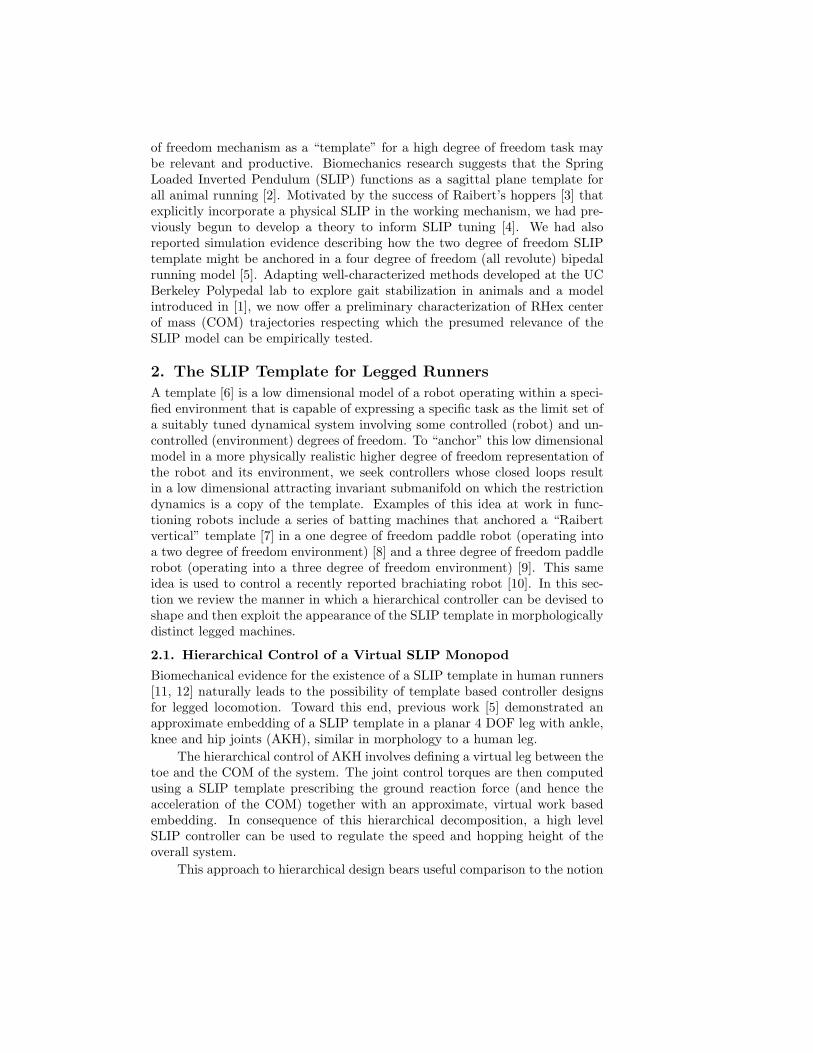
Evidence for Spring Loaded Inverted Pendulum Running in a Hexapod Robot Richard Altendorfer, Uluc . Saranli, Haldun Komsuo¯ glu, Daniel Koditschek Artificial Intelligence Laboratory, University of Michigan Ann Arbor, MI 48109 {altendor, ulucs, hkomsuog, kod}@eecs.umich.edu H. Benjamin Brown Jr. The Robotics Institute, Carnegie Mellon University Pittsburgh, PA 15213 [email protected] Martin Buehler, Ned Moore, Dave McMordie Ambulatory Robotics Laboratory, Dept. of Mech. Engineering, McGill University Montr´ eal, Qu´ ebec, Canada H2A 2A7 {buehler, ned, mcmordie}@cim.mcgill.ca Robert Full Dept. of Integrative Biology, University of California at Berkeley Berkeley, CA 94720 [email protected] Abstract: This paper presents the first evidence that the Spring Loaded Inverted Pendulum (SLIP) may be “anchored” in our recently designed compliant leg hexapod robot, RHex. Experimentally measured RHex center of mass trajectories are fit to the SLIP model and an analysis of the fitting error is performed. The fitting results are corroborated by numerical simulations. The “anchoring” of SLIP dynamics in RHex offers exciting possibilities for hierarchical control of hexapod robots. 1. Introduction We have recently reported on a prototype robot that breaks new ground in artificial legged locomotion [1]. Our shoe-box sized, compliant leg hexapod, RHex, travels at speeds better than one body length per second over terrain that few other robots can negotiate at all. RHex origins and construction are grounded in the interplay between biomechanics, controls, and engineering de- sign that we have come to call “functional biomimesis.” We aim to articulate broad principles with mathematically precise formulations of biomechanically observed fact and then translate these into specific design practices. This pa- per presents the first empirical evidence that our strategy to use a low degree
Transcript of Evidence for Spring Loaded Inverted Pendulum Running in a Hexapod Robot

Evidence for Spring Loaded Inverted
Pendulum Running in a Hexapod
Robot
Richard Altendorfer, Uluc. Saranli, Haldun Komsuoglu, Daniel KoditschekArtificial Intelligence Laboratory, University of Michigan
Ann Arbor, MI 48109{altendor, ulucs, hkomsuog, kod}@eecs.umich.edu
H. Benjamin Brown Jr.The Robotics Institute, Carnegie Mellon University
Pittsburgh, PA [email protected]
Martin Buehler, Ned Moore, Dave McMordieAmbulatory Robotics Laboratory, Dept. of Mech. Engineering, McGill University
Montreal, Quebec, Canada H2A 2A7{buehler, ned, mcmordie}@cim.mcgill.ca
Robert FullDept. of Integrative Biology, University of California at Berkeley
Berkeley, CA [email protected]
Abstract:
This paper presents the first evidence that the Spring Loaded InvertedPendulum (SLIP) may be “anchored” in our recently designed compliantleg hexapod robot, RHex. Experimentally measured RHex center of masstrajectories are fit to the SLIP model and an analysis of the fitting error isperformed. The fitting results are corroborated by numerical simulations.The “anchoring” of SLIP dynamics in RHex offers exciting possibilities forhierarchical control of hexapod robots.
1. IntroductionWe have recently reported on a prototype robot that breaks new ground inartificial legged locomotion [1]. Our shoe-box sized, compliant leg hexapod,RHex, travels at speeds better than one body length per second over terrainthat few other robots can negotiate at all. RHex origins and construction aregrounded in the interplay between biomechanics, controls, and engineering de-sign that we have come to call “functional biomimesis.” We aim to articulatebroad principles with mathematically precise formulations of biomechanicallyobserved fact and then translate these into specific design practices. This pa-per presents the first empirical evidence that our strategy to use a low degree
buehler
in D. Rus and S. Singh, editors, "Experimental Robotics VII," p. 291-302, Springer-Verlag, 2001.
of freedom mechanism as a “template” for a high degree of freedom task maybe relevant and productive. Biomechanics research suggests that the SpringLoaded Inverted Pendulum (SLIP) functions as a sagittal plane template forall animal running [2]. Motivated by the success of Raibert’s hoppers [3] thatexplicitly incorporate a physical SLIP in the working mechanism, we had pre-viously begun to develop a theory to inform SLIP tuning [4]. We had alsoreported simulation evidence describing how the two degree of freedom SLIPtemplate might be anchored in a four degree of freedom (all revolute) bipedalrunning model [5]. Adapting well-characterized methods developed at the UCBerkeley Polypedal lab to explore gait stabilization in animals and a modelintroduced in [1], we now offer a preliminary characterization of RHex centerof mass (COM) trajectories respecting which the presumed relevance of theSLIP model can be empirically tested.
2. The SLIP Template for Legged Runners
A template [6] is a low dimensional model of a robot operating within a speci-fied environment that is capable of expressing a specific task as the limit set ofa suitably tuned dynamical system involving some controlled (robot) and un-controlled (environment) degrees of freedom. To “anchor” this low dimensionalmodel in a more physically realistic higher degree of freedom representation ofthe robot and its environment, we seek controllers whose closed loops resultin a low dimensional attracting invariant submanifold on which the restrictiondynamics is a copy of the template. Examples of this idea at work in func-tioning robots include a series of batting machines that anchored a “Raibertvertical” template [7] in a one degree of freedom paddle robot (operating intoa two degree of freedom environment) [8] and a three degree of freedom paddlerobot (operating into a three degree of freedom environment) [9]. This sameidea is used to control a recently reported brachiating robot [10]. In this sec-tion we review the manner in which a hierarchical controller can be devised toshape and then exploit the appearance of the SLIP template in morphologicallydistinct legged machines.
2.1. Hierarchical Control of a Virtual SLIP Monopod
Biomechanical evidence for the existence of a SLIP template in human runners[11, 12] naturally leads to the possibility of template based controller designsfor legged locomotion. Toward this end, previous work [5] demonstrated anapproximate embedding of a SLIP template in a planar 4 DOF leg with ankle,knee and hip joints (AKH), similar in morphology to a human leg.
The hierarchical control of AKH involves defining a virtual leg between thetoe and the COM of the system. The joint control torques are then computedusing a SLIP template prescribing the ground reaction force (and hence theacceleration of the COM) together with an approximate, virtual work basedembedding. In consequence of this hierarchical decomposition, a high levelSLIP controller can be used to regulate the speed and hopping height of theoverall system.
This approach to hierarchical design bears useful comparison to the notion
of impedance control advanced by Hogan [13] and more recently introduced intothe locomotion literature in the more specific form of “Virtual Model Control”by Pratt and colleagues [14]. This framework allows a user to program therobot’s task in terms of a reference compliance imposed on a targeted partof the body. It is different from our approach in that the allowable referencemodels operate in the quasi-static regime, so, for example, running could not liewithin the formal scope of the method. In contrast, the SLIP template providesan explicitly (hybrid) dynamical specification of the exchange between kineticand potential energy that accomplishes the task at hand after transients in themany degrees of freedom unrelated to the task have died out. In this paper,we are concerned to find a means of effecting this “collapse of dimension” inthe RHex mechanics.
2.2. Hierarchical Control of a Virtual SLIP HexapodWe now describe two alternative approaches to hierarchical control for ourhexapod. Both appeal to the SLIP template for the prescription of COMforces, but incorporate different anchoring mechanisms.
The hexapod model we consider is a rigid body with six massless legs [1].Two of the spherical leg freedoms — the radial length and one of the angles— are driven by passive springs and dampers, whereas the hip angle is torqueactuated. Consequently, there are only six actuated joints, and the overallsystem has six degrees of freedom, all due to the rigid body.
2.2.1. Active ControlIn principle, the force and torque acting on the hexapod rigid body can bedetermined using the equations of motion of the model [1]. Sufficient conditionsfor exact embedding of an arbitrary dynamical template can be developedfrom the invertibility of the dynamics. However, complete input invertibilitygenerally cannot prevail in our system. The morphology of the system, thehybrid nature of the problem and the structure and number of the actuators(especially when not all legs are on the ground) do not yield full control overthe six body degrees of freedom.
A simpler planar model, on the other hand, provides an exactly invertibleplant, except for co-dimension one and two singularities. The model consists ofa three degree of freedom planar rigid body, with six torque actuated masslesslegs, with the assumption that three or more legs are in contact with the groundduring stance.
Preliminary numerical experience with this model suggests that choosinga “reasonable” stance posture affords inverse dynamics controllers that passtransversally through the kinematic singularities and give good SLIP trajecto-ries. Moreover, the planar model is structurally very close to the spatial model.As a consequence, it seems likely that the inverse dynamics anchoring in theplanar model can be readily extended to yield an approximate embedding ofthe SLIP template in the spatial hexapod model.
Nevertheless, realizing the active template through inverse dynamics con-trol suffers the traditional problems of all such approaches based on exactcancellations: the presumption of a perfect model; known parameters; and

noise-free high bandwidth state information. It is not clear how effectively thisexact embedding can be implemented in a physical platform in the face of theinevitable actuator, computational, and sensory limitations.
2.2.2. Passive ControlAn alternative to active control relies on the passive dynamics of the sys-tem combined with low-bandwidth controllers to anchor the SLIP template.Demonstrating that this may be possible represents the chief concern of thepaper as established in §3. Even with a very simple open-loop control strategy,our study reveals the presence of certain “sweet spots” in the RHex parameterspace, wherein the SLIP emerges naturally. It is still unclear whether this re-spects the formal “anchored template” paradigm wherein the lower dimensionaldynamics actually appears as an attracting invariant dynamical submanifold.However, experimental evidence revealing the template behavior in steady statefrom various different initial conditions suggests there are, indeed, operatingregimes where the system trajectories are attracted to the low dimensionalSLIP template dynamics. Further evidence for the SLIP template comes fromnumerical studies using SimSect — a simulation package developed by Saranli[15]. SimSect was devised to approximate the behavior of RHex by numericallyintegrating a set of simplified equations of motion which are expected to governRHex’s hybrid mechanical system. Currently, the same low-level controller asin RHex is implemented in SimSect. This makes SimSect an ideal test-bedfor new control designs for RHex. Although an exact correspondence betweenRHex’s and SimSect’s parameter space has not yet been established, the simu-lation results in §3.4 lend credence to SimSect being a representative numericalapproximation to RHex’s dynamics.
3. Finding the SLIP in RHex’s MotionThe central observations about cockroach locomotion that inform the design ofthe RHex prototype include: (i) that it operates via compliant legs; (ii) that itslimb motions appear to be characterized by a strongly stereotypical “clock”;(iii) that it has a sprawled posture to enhance stability; and (iv) that thestabilizing controller must somehow be embedded in the very morphology itself.The impact of these observations for RHex are, indeed, directly apparent in themorphology and control approach that we have already reported. However, itis not obvious that we will find a SLIP in such a machine.
3.1. Data Collection, Experimental Setup and ProceduresIn order to determine whether RHex passively anchors a SLIP, the groundreaction forces produced by RHex during locomotion were measured during 92trials using two six-component force plates1. The force and torque signals wereamplified2 and each channel was recorded at 1000Hz by an analog to digitalconverter3. Each trial was also recorded by a high speed video camera4.
1Biomechanics Force Platform, Advanced Mechanical Technology, Inc., Newton, MA.2Model SGA, Advanced Mechanical Technology, Inc., Newton, MA.3PCI board, National Instruments, Austin, TX.4MotionScope PCI 1000, Redlake Imaging, Morgan Hill, CA.

In our experiments, the robot started walking approximately two metersaway from the force plates in order to allow the robot to settle into an approx-imate steady state motion upon encountering the plates. While the robot wasin contact with the force plates no directional adjustment was made since thiswould otherwise have broken the open loop symmetry between the right andleft leg motion profiles.
During the trials, four parameters were varied: leg type; ground material;robot mass; and forward speed. For a fixed set of parameters, the experi-ments were repeated between 4 and 8 times. The experiments started off withthe slowest forward speed on the bare force plates with Delrin legs (stiffnessκ ≈ 4300N/m). Then the speed was increased in three steps by choosing dif-ferent cycle times5 (tc ∈ {1.2s, 0.8s, 0.53s, 0.5s}) without changing the physicalstructure. To reduce bounce and slippage, which was observed especially athigh speeds, the surface of the force plates was then covered with an elasticfoam mat, and the same speed sweep with the Delrin legs was performed. Inthe second round of the experiments, a new 4-bar linkage composite leg design(κ ≈ 3100N/m) was used in conjunction with a similar speed sweep on both thebare force plates and the plates covered with the foam mat. Our preliminaryobservations during the first two trial runs suggested that the COM of the bodybehaves more like an inverted pendulum (IP) rather than a spring loaded in-verted pendulum (SLIP). We reasoned that the leg-body system, which definesan overall lumped spring-mass system, has a much higher natural frequencythan the stride frequency achievable by the hip actuators. In order to testthis hypothesis, in the third round of the experiments, the body mass was in-creased, effectively decreasing the natural frequency of the spring-mass system.We ran the robot with composite legs at the highest speed setting on the elasticmat. Its mass was increased incrementally from 7.83kg to 9.47kg to 11.12kgto 11.94kg. In the highest mass regime we observed the transition from IP toSLIP reported below.
3.2. Data Extraction
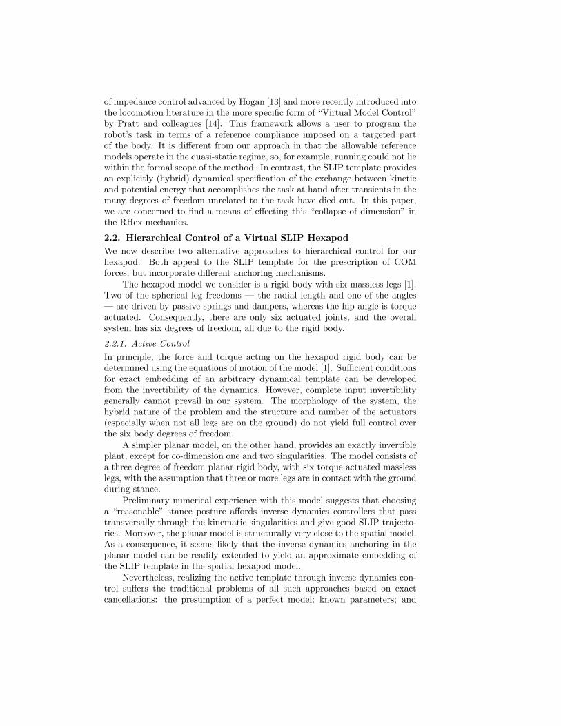
The data plotted in Fig. 1 arise from the summed leg or COM ground reactionforces imparted to the legs by the ground plate while the robot performs analternating tripod gait. To remove noise from the recorded data, the forces werefiltered using a second order Butterworth filter with a cutoff frequency of 50Hz.The minima of the vertical force data were used to isolate single strides. Sincea stride is a complete cycle for all the legs, it contains two steps for each tripodand therefore two minima. Only strides from the middle section of the datafor one force platform — where the force data exhibited oscillatory behavior ofone predominant frequency and roughly constant amplitude — were selected.Only those trials where the maximum of the power spectrum P (f) occursat twice the cycle frequency6 fc = 1/Tc were used, in rough accord with the
5The motion profile utilized by RHex is parametrized by cycle time, sweep angle, leg offsetand flight time (for a detailed description of these parameters see [15]). For each forwardspeed setting a different set of values is assigned to these four parameters.
6During one cycle, two steps are taken.
criterion established in [16] to distinguish walking from running.7 These criteriareduced the number of available trials to be used for SLIP fitting from 92 to 14.
0 1 2 3 4 5 6−100
−50
0
50
100
150
200
250
time [s]
Gro
und
reac
tion
forc
es [N
]
Fore/aft (y)Vertical (z)Step limits
Figure 1. Ground reaction forces fortrial 6 (comp. legs, foam mat, tc = 0.5s,m = 11.94kg). The triangles denote thebeginning and the end points of stepsselected for fitting.
Since the force platform is verynarrow with respect to the widthof RHex and only those trials forwhich RHex stayed on the track wererecorded, the lateral force data arenot used in this investigation.8 Thisrestriction respects the intended lim-itations on our scope of analysis inthis initial study to the saggital planeonly.
Unfortunately, the camera’s res-olution was not good enough to pro-vide integration constants for verti-cal and fore/aft speeds and positionsat the beginning of each stride, re-quired for our fitting study. Instead,the initial vertical speed is indirectlyobtained from the assumption of pe-riodicity – namely, that after onestride, the robot returns to its initial height. Similarly, the fore/aft initialspeed is calculated by matching the average velocity over one stride to the av-erage velocity over both force plates. The initial height is assumed to be atRHex’s static equilibrium with all legs vertical to the ground (0.164m).
3.3. Data AnalysisThe SLIP template imposes a very particular set of relationships — thosespecified by the Lagrangian mechanics of a single point mass prismatic-revolute(i.e., polar coordinate) kinematic chain between the ground reaction forces,motion of the COM, and system energies. Ruina has pointed out [19] that anyconvex curve supports in a neighborhood of its vertical minimum at least onetime varying trajectory generated by some SLIP. RHex’s COM inevitably ridesalong a convex curve: we wish to understand whether its actual time trajectoryalong this curve can be readily generated by some SLIP model.
3.3.1. A Protocol for Fitting SLIP to RHex’s Running DataThe 14 remaining trials that satisfy the criteria in §3.2 are now used to testthe presence of the SLIP template in RHex according to an adaptation of themethodology introduced in [11]. For each of the 136 steps (68 strides) in the14 trials, a SLIP model is fit using ordinary least squares regression. Fitting aSLIP model to these data is not entirely straightforward: since RHex did not
7Specifically, the ratio of the integrated power spectrum around the maximum to the
total integrated power spectrum was required to satisfy (∫ 2fc+ε
2fc−εP (f)df)/(
∫∞0
P (f)df) > 0.8,
where ε was appropriately chosen to include the global maximum alone.8The magnitude of the lateral forces is comparable to the one for the fore/aft forces. A
complete template should incorporate lateral forces, see e. g. [17] or [18].

exhibit any flight phase, the touchdown and lift-off points are not defined. Incontrast, if the anchoring hypothesis has any validity, then the region arounda bottom should be well described by a SLIP stance phase. Absent a specificmodel for determining the limits of this region, we adopt the ad hoc conditiondetermined by the point of zero crossing of the vertical COM force.9
Fitting data to this central force model requires knowledge of the center ofpressure (the pivot point of the virtual SLIP), which could not be determinedwith our experimental equipment. As a reasonable work-around, we assumethat the center of pressure lies directly below the vertical minimum. This inturn, implies that the SLIP model operates at equilibrium on a “neutral orbit”[3, 11] characterized by this symmetry. However, the measured force data arenot perfectly periodic, hence the integrations to yield velocity and position arenecessarily not periodic, either. Notwithstanding this slight conceptual conflict,we see no better method for selecting the nominal center. These assumptionsin force, the data population for SLIP fitting can be restricted to range onlyfrom a vertical minimum to the next zero crossing of the vertical force.
Given a COM trajectory fragment, {b(t), b(t), b(t)}|tN=Tliftoff
t0=Tbottom, the COM
position10 b = (y z)> and acceleration b are fitted to a Hooke spring law withunknown spring length11 qr0 and spring stiffness κ:
b||b|| (κ1 − κ2||b||) = m(b− g) ,
where κ = κ2 and qr0 = κ1κ2
. Note that this model is linear in parameters sothat ordinary least squares applies directly.
The assessment of the quality of the fit proceeds in two steps. First, a SLIPsimulation over the same period of time as the data trajectory is run with thevalues of κ and qr0 obtained in the first step. The initial conditions are taken tobe the positions and velocities of the data trajectory at the minimum. Second,the resulting SLIP trajectories zSLIP, zSLIP, ySLIP, ySLIP are compared to thedata trajectories by L1 and L2 percent errors:
∆XL1 = 100||X −XSLIP||1
Range(X), ∆XL2 = 100
||X −XSLIP||2||X||2 ,
where Range(X) = |max(X) - min(X)|. Here, ||X||p = (∫ t1
t0|X(t)|pdt)
1p and
X ∈ {z, y, z, y}.In an effort to simplify the assessment of the fitting error, the quality of
the fit is reported as a single number — the average Lp percent error ∆Lp=
(∆zLp+ ∆yLp
+ ∆zLp+ ∆yLp
)/4.9Presumably, the phase interval corresponding to flight in the simple SLIP template must
be replaced with an appropriately more complex (but still low dimensional) model. Since wehave not yet developed this model, we rely on the ad hoc termination criterion.
10In this notation, z gives the co-ordinates in the vertical direction and y gives the co-ordinates in the fore/aft direction relative to an inertial frame located at the center of pres-sure.
11Fitting the spring length qr0 alleviates the arbitrariness of selecting the equivalent lift-off point for RHex data, because now the zero crossing of the vertical COM force need notcorrespond to the lift-off point of the fitted SLIP model.

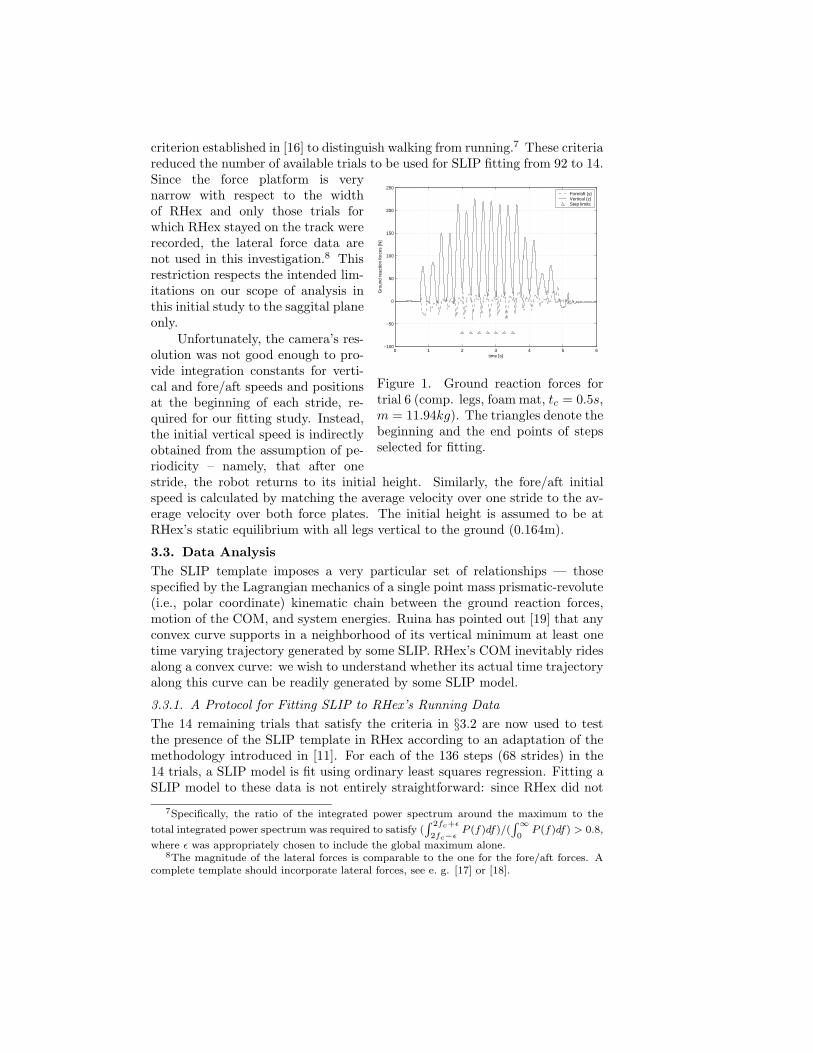
As an illustration of the fitting results, the worst and the best SLIP fitsamongst the 136 steps are presented in the next figure. The data trajectories
0 0.02 0.04 0.06
0
0.01
0.02
0.03
t
y(t)
0 0.02 0.04 0.06
0.13
0.135
0.14
0.145
t
z(t)
hexapodSLIP
0.3
0.4
0.5
y′(t
)
0
0.1
0.2
0.3
z′(t
)
−6
−4
−2
0
2
y′′(t
)
0
5
10
z′′(t
)
0 0.01 0.02 0.03
0.13
0.135
0.14
0.145
y(t)
z(t)
0 0.02 0.04 0.06
0.13
0.135
0.14
0.145
t
q(t)
(a) RHex trial no. 2, 4th stride, 2nd min-
imum (composite legs, foam mat, tc =0.5s, m = 11.12kg) incurs the largestSLIP fitting error of ∆L2 = 21.6%.
0 0.01 0.02 0.03 0.04 0.05
0
0.01
0.02
t
y(t)
0 0.01 0.02 0.03 0.04 0.05
0.144
0.146
0.148
0.15
0.152
t
z(t)
hexapodSLIP
0.5
0.52
0.54
y′(t
)
0
0.1
0.2
z′(t
)
0
0.5
1
1.5
y′′(t
)
0
2
4
6
z′′(t
)
0 0.005 0.01 0.015 0.02 0.0250.144
0.146
0.148
0.15
0.152
y(t)
z(t)
0 0.01 0.02 0.03 0.04 0.050.144
0.146
0.148
0.15
0.152
0.154
t
q(t)
(b) RHex trial no. 10, 5th stride, 1st min-
imum (composite legs, foam mat, tc =0.5s, m = 11.94kg) incurs the smallestSLIP fitting error of ∆L2 = 0.3%.
Figure 2. Worst and best SLIP fits: Dotted lines represent experimental data;solid lines represent SLIP trajectories with fitted values κ and qr0.
of y(t), y(t), y(t), z(y), z(t), z(t), z(t), and q(t) =√
y2(t) + z2(t) (dottedlines) are plotted together with the SLIP predictions computed with the fittedstiffness κ and spring length qr0. The worst SLIP fit with ∆L2 = 21.6% isshown in Fig. 2(a), in contrast to ∆L2 = 0.3% in Fig. 2(b).
As an internal consistency check, we introduce a simple form of cross val-idation: The available COM trajectory components X ∈ {z, y, z, y} each com-prising a time sampled fragment of length N are partitioned by r = bN/20c,sub-sampling them into a fitting population Xi
fit, i ∈ {1, . . . , r} of lengthNfit = bN/rc and its complement Xi
cross = X\Xifit — the cross validation
populations. The fitting procedure is applied to a fitting population Xifit to
yield κi and qir0. The quality of fit is assessed not only on Xi
fit but alsoon the corresponding cross-validation population Xi
cross with κi and qir0 ob-
tained from Xifit. In Table 1 the fitting errors ∆i
Lp,fit and cross valida-tion errors ∆i
Lp,cross are subsumed under ∆Lp,fit = mean{∆iLp,fit}r
i=1 and∆Lp,cross = mean{∆i
Lp,cross}ri=1, and the standard deviations std{∆i
Lp,fit}ri=1
and std{∆iLp,cross}r
i=1.In addition to the L1 and L2 errors that compare the experimental data to
fitted SLIP predictions, experimental measurement errors introduce noise intothe data. To evaluate the quality of fit, one must compare the relative noise

floor, δX/Range(X) to the L1 fitting errors. The noise floor comes from twosources: the measurement error of the ground reaction forces, and the uncer-tainties of the integration constants for the velocity and position trajectories.In Table 1 the estimated relative noise floors for the z, y, z, y trajectories areaveraged over each stride.
3.3.2. Evidence for SLIP in RHex RunningThe fitting protocol outlined in the previous section is now applied to all 136steps12. For the sake of brevity, we refrain from listing the fitted parametersand the fitting errors for each step. Instead, average values over all steps arecalculated together with the standard deviation. The mean fitted stiffness isκ = (6100 ± 940)N/m, and the mean fitted relaxed spring length is qr0 =(0.171± 0.007)m. The results of the error analysis are listed in Table 1.
(%) ∆Lp ∆Lp,fit/∆Lp,cross ∆Lp,cross std(∆Lp,cross)
L2 0.069± 0.054 0.985± 0.013 0.069± 0.054 0.001± 0.001
L1 0.258± 0.197 1.002± 0.012 0.259± 0.199 0.004± 0.006
(%) ∆yL1 ∆zL1 ∆yL1 ∆zL1
L1 0.041± 0.036 0.010± 0.010 0.96± 0.78 0.020± 0.018Noise floor 0.009 0.003 0.38 0.009
Table 1. Error analysis of SLIP fitting to 136 steps.
The average ∆L2 error of ≈ 7% seems to be remarkable for a mechanicaldevice that a priori bears to resemblance to a SLIP model. The L1 averagepercent errors are all similarly low, except for the y fits, which are corrupted inpart by the high noise floor (see discussion at the end of §3.3.1) and in part byreal discrepancies with the putative model, for example, as depicted in Fig. 2.Since the component-wise L1 errors are considerably above the noise floor, andsince the Lp fitting and cross validation errors are comparable, there is littleconcern that we are merely fitting to noise.
The question naturally arises why we only present fitting results for the de-compression phase interval of the COM data instead of the whole compression-decompression phase interval between the zero-crossings of the vertical force.After all, this alternative would serve as a test of our neutral orbit assumption(see §3.3.1). Indeed, the fitting errors for the compression phase interval areof comparable magnitude to the ones for decompression above. However, thefitted spring stiffness is higher and its standard deviation over all 136 stepsis twice as large as compared to the decompression phase interval study re-ported here. An explanation might be the more frequent occurrence of “doublestance” (more than 3 legs on the ground) during compression than decompres-sion. This is in fact observed in sample SimSect simulations. As double stanceevents alter the dynamics of the robot, we single out the decompression phaseinterval of the COM data as the likeliest candidate of the trajectories for the
12In all the selected experiments, RHex operated in the highest speed setting with thecomposite leg design and the elastic foam ground. Moreover, they were mainly experimentswith high body masses: 8 runs with m = 11.94kg, 5 runs with m = 11.12kg and 1 run withm = 9.47kg.

validation of the SLIP model.
3.4. Supporting Numerical Study3.4.1. SLIP Fitting in SimSectThe previous sections suggest that the SLIP model provides a good low dimen-sional approximation to the “stance” dynamics of RHex. In this section, wedescribe a parallel numerical investigation of SimSect simulations to determinethe “sweet spots” wherein the hexapod might actually be presumed to an-chor the SLIP. Specifically, we show that SLIP-like behavior of the mechanicalsystem modeled by SimSect occurs in specific ranges of SimSect’s parameterspace.
In order to compare the SLIP fitting results from SimSect to those fromRHex experiments, the same decompression phase interval as in §3.3.1 is usedfor fitting.13 Only those runs where exactly 3 legs of the same tripod are onthe ground at the vertical minimum were considered to be acceptable; thiswas inspired by the assumption that the jointly controlled three legs, whichconstitute a tripod, can be thought of as a virtual SLIP leg and reflects ourexperimental experience. As an additional filter, only those simulations whichexhibit periodic behavior after a certain amount of time are used for fitting tothe SLIP model.
The simulations are run for a fixed set of physical parameters (e.g. totalmass, moments of inertia, etc.) and initial conditions, whereas the controlparameters sweep angle, cycle time, and leg offset14 are varied in certain rangesdescribed below. The flight time is chosen to be ≈ 0.4 the cycle time in orderto match the highest speed setting for RHex. With force, velocity, and positiondata from SimSect simulations, the fitting procedure is carried out as in §3.3.1.
3.4.2. Fitting ResultsAlthough SimSect is modeled with many simplifications respecting the ac-tual robot, RHex’s main dynamical features are believed to be incorporatedin SimSect. Hence the SimSect simulations were run in parameter regimesthat include the high mass, high speed regimes of RHex where good SLIPfits could be obtained. In particular, with total mass m = 11.9kg, sweepangle= 0.44 . . . 0.76rad, cycle time=0.42 . . . 0.54s, leg offset=0 . . . − 0.15rad,and individual leg stiffnesses κ ≈ 2700N/m, SLIP like behavior could be foundin SimSect, too. This is demonstrated in Fig. 3, which shows — on the leftside — a histogram of the number of simulations from the above listed param-eter range with respect to the average L2 error, ∆L2 . The total number ofsimulations is reported above the histogram. For comparison, a two-parameterexponential distribution is fit to the histogram bins. On the right side a graphshows the average L2 error ∆L2 as a function of two of the four control param-eters: cycle time and sweep angle. The flight time is kept proportional to thecycle time and only a small dependence of ∆L2 on the leg offset was observed.
13In SimSect, information about which legs are on the ground and which are not is, ofcourse, available. A detailed investigation of the quality of the SLIP fitting as a function offootfall patterns will be the subject of a future report.
14For a detailed description of SimSect’s parameter space, see [15].

Instead of a scatter plot, a quadratic surface is fit to the data, and the spreadof the data is characterized by its second moment around the surface, whichis represented by vertical bars at the corners of the surface. For all SimSect
Figure 3. Average errors ∆L2 for SimSect SLIP fits. The left side shows ahistogram of the number of simulations; the right side shows a map of ∆L2 asa function of the (reduced) control parameter space.
simulations the ratio of the average fitting to the average cross validation error∆L2,fit/∆L2,cross did not deviate by more than 10% from unity, thus providinga successful self-consistency check for our fitting procedure. The results in thissection, in particular the low average fitting errors of ≈ 6% in Fig. 3 lendstrong support to the presumption that the SLIP template may be anchoredin SimSect’s dynamics.
4. Conclusion: Implications for More Autonomous Con-trol of RHex
Hierarchy promotes the use of few parameters to control complex systems withmany degrees of freedom. In this light, as we understand matters, the emer-gence of an anchored SLIP in RHex is most fortunate. The pogo-stick canfunction as a useful control guide in developing more complex autonomous lo-comotion behaviors such as registration via visual servoing, local explorationvia visual odometry, obstacle avoidance, and, eventually, global mapping andlocalization. In the longer term, we propose to work with the anchored SLIPin RHex in analogy to the manner in which the simple two-bead template hasbeen exploited in juggling. Namely, as we shape behavior via manipulation ofgains-in-the-loop [20], we hope to develop a formal programming language withsemantics in the world of dynamical attractors [21].
Acknowledgements
This work is supported by DARPA/SPAWAR under contract N66001-00-C-8026. We thank Rodger Kram and Claire Farley for the use of the force plat-form, Irv Scher for collaboration at an early stage of this project and WilliamSchwind for the insight and the analytical tools he provided.

References[1] Saranli U, Buehler M and Koditschek D E 2000 Design, Modeling and Prelimi-
nary Control of a Compliant Hexapod Robot. Proc. IEEE Int. Conf. Rob. Aut.3:2589-2596.
[2] Blickhan R and Full R 1993 Similarity in multilegged locomotion: Bouncing likea monopode. J. J. Comp. Physiol. A 173, 509-517.
[3] Raibert M 1986 Dynamic Robots that Balance, MIT Press, Cambridge.
[4] Schwind W J and Koditschek D E 2000 Approximating the Stance Map of a 2DOF Monoped Runner. Journal of Nonlinear Science 10:533-568.
[5] Saranli U, Schwind W J, and Koditschek D E May 1998 Toward the Controlof Multi-Jointed, Monoped Runner. IEEE Int. Conf. on Rob. and Aut. Leuven,Belgium pp 2676-2682.
[6] Full R J and Koditschek D E 1999 Templates and Anchors: NeuromechanicalHypotheses of Legged Locomotion on Land. J. Exp. Bio. 202:3325-3332.
[7] Koditschek D E and Buhler M Dec 1991 Analysis of a simplified hopping robot.International Journal of Robotics Research 10(6):587-605.
[8] Buhler M, Koditschek D E, and Kindlmann P J 1990 A Family of Robot Con-trol Strategies for Intermittent Dynamical Environments. IEEE Control SystemsMagazine 10(2):16-22.
[9] Rizzi A A, Whitcomb L L, and Koditschek D E 1992 Distributed Real-TimeControl of a Spatial Robot Juggler. IEEE Computer 25(5):12-24.
[10] Nakanishi J, Fukuda T, and Koditschek D E 2000 A Brachiating Robot Con-troller. IEEE Trans. Rob. Aut. 16(2):109-123.
[11] Schwind W J 1998 Spring Loaded Inverted Pendulum Running: A Plant Model.PhD thesis, University of Michigan.
[12] Full R J and Farley C T 2000 Musculoskeletal Dynamics in Rhythmic Systems: AComparative Approach to Legged Locomotion. In: Winter, Crago (eds) Biome-chanics & Neural Control of Posture & Movement Springer Verlag, New York,pp 192-205.
[13] Hogan N Mar 1985 Impedance Control: An Approach to Manipulation. ASMEJournal of Dynamic Systems, Measurement, and Control 107:1-7.
[14] Pratt J and Pratt G May 1998 Intuitive Control of a Planar Bipedal WalkingRobot ICRA Leuven, Belgium pp 2014-2021.
[15] Saranli U 2000 SimSect Hybrid Dynamical Simulation Environment. Universityof Michigan Technical Report CSE-TR-437-00.
[16] Alexander R McN 1992 A Model of Bipedal Locomotion on Compliant LegsPhil. Trans.: Biol. Sc. 338(1284):189-198.
[17] Carver S 2000 The Limits of Deadbeat Control for the Spatial SLIP. in prepa-ration.
[18] Schmitt J and Holmes P 2000 Mechanical models for insect locomotion: Dy-namics and stability in the horizontal plane I: Theory; II: Application. BiologicalCybernetics 83(6):501-515 and 517-527.
[19] Ruina A, personal communication.
[20] Burridge R R, Rizzi A A, and Koditschek D E 1999 Sequential Composition ofDynamically Dexterous Robot Behaviors. Int. J. Rob. Res. 18(6):534 - 555.
[21] Klavins E and Koditschek D E 2000 A formalism for the composition of concur-rent robot behaviors. Proc. IEEE Conf. Rob. and Aut. 4:3395 - 3402.