Online Publication Date: 15th

May, 2012

Publisher: Asian Economic and Social Society

Designing an Electronic System for the Study of Simple

Pendulum at Large Angles

Abdulghefar Kamil Faiq (University of Salahaddin – Erbil. Erbil Iraqi Kurdistan Region Iraq) Muhammad Hamza Abdullah (Fenk Basic Private School. Erbil Iraqi Kurdistan Region Iraq)

Citation: Abdulghefar Kamil Faiq ,Muhammad Hamza Abdullah (2012) “Designing an Electronic

System for the Study of Simple Pendulum at Large Angles”,Journal of Asian Scientific Research,

Vol. 2, No. 5, pp. 281-291.

Journal of Asian Scientific Research, Vol.2, No.5, pp.281-291

281

Author(s)

Abdulghefar Kamil Faiq University of Salahaddin - Erbil

Erbil Iraqi Kurdistan Region Iraq E-mail: ag_kamil@uni-sci.org

abdulghefar1973@yahoo.com

Muhammad Hamza

Abdullah Fenk Basic Private School.

Erbil. Iraqi Kurdistan Region Iraq

E-mail: mhaphy87@gmail.com

Designing an Electronic System for the Study of Simple

Pendulum at Large Angles

Abstract

An electronic system based on a photo gate and an electronic

switching circuit is designed for studying simple pendulum at

large angles. The detailed of the system operation is studied, the

pulse measurements performed on a CRO screen for five

displacement amplitude angles of 5, 10, 15, 20, and 25 degrees,

and the technical problems associated with the measurement

process is treated. Results show that calculated acceleration of

gravity with acceptable magnitudes can be obtained for small

displacement angle of 5o compared with the real value of the local

acceleration of gravity; the relative error is 0.01617 %.

Instantaneous time period, amplitude decay, and maximum

velocities are measured and used for error handling in the

calculation of the acceleration of gravity. In order to overcome the

problem of the operating time of the relays which are used in the

electronic circuit switch, taking 80 periods for manual

measurements have been proved to be useful in decreasing errors

in the calculation of acceleration of gravity.

Key words: Simple Pendulum at Large Angles, Photo Gate, Non Linear Differential Equation,

Electronic Measuring Circuit

Introduction

The study of simple pendulum at large

displacement angles gets great interest in physics

both for undergraduate and graduate levels,

because it is a popular example of treating non-

linear effect at such levels. At undergraduate

level, simple pendulum is used for measuring the

acceleration of gravity (g), however, the

differential equation which governs the

pendulum's motion has no-analytical solution,

hence, either numerical method is used or a

special case of small angle vibration is taken

(Belendez et. al, 2009; Amore et. al., 2007;

Carvalhaes, and Suppes , 2008).

(Aggarwal et. al, 2005) designed an electronic

system for studying simple pendulum which

consists of a microprocessor program controlling

system. In this work, we designed a simpler

electronic circuit, feeds a sophisticated CRO, to

measure the instantaneous time period of

pendulum's oscillatory motion at high level of

accuracy. This work aims at the study of the

amplitude of vibration's effect on the time period,

damping of the pendulum, and the technical

factors that affect the measuring system. All these

are to further investigate the pendulum's problem

at large displacement angles.

Method

Simple pendulum consists of a small bob with a

mass (m) suspended to a certain position by a

light inextensible thread. When we shift the bob

with an angle (), and release it, the oscillatory

motion which takes place in a vertical motion

represents the simple pendulum's motion, it is

governed by the following differential equation

0sin2

2

2

odt

d (1)

Where

L

go (2)

Where L is the length of the pendulum.

The above equation has no analytical solution,

however, for very small , we can use the

approximation sin()= as approach zero (in

radian), and eq. (1) becomes:

Designing an Electronic System for the Study…..

282

02

2

2

odt

d (3)

This is the differential equation of simple

harmonic motion of angular frequency o. The

solution of eq. (3) gives time period (To) of:

g

LTo 2 (4)

Taking into account the large displacement angles

(when the approximation as cannot be used),

the solution of eq. (1) will be (Amrani et. al,

2008):

....

3072

11

16

112

42

oog

LT

(5)

The second order approximation of Bernoulli can

be used (Lima, and Arun, 2006)

2

16

112 o

g

LT (6)

Eq. (6) can be used to calculate g. As a result of

oscillation damping, o must be substituted for

each period, i.e., the calculation of o for each

period is necessary.

The kinetic energy of the pendulum

2

2

1mvEK (7)

v is the linear velocity of the pendulum. The

pendulum's potential energy is:

))cos(1( mgLE p (8)

According to the principle of conservation of

energy, the maximum kinetic energy (at =0) is

equal to the maximum potential energy (=o), the result can be written as:

gL

vo

21cos

max2

1 (9)

Where vmax is the maximum velocity of the bob

at =0.

Oscillation damping follows the following

equation (Nelson, and Olsson, 1986):

n

m

t

mo ee (10)

Where m is the initial displacement angle, is

the damping factor. Its assumed that the

instantaneous time period (t) is slightly changed

with number of period (n), then we can define

as another damping parameter with respect to (n).

Substituting eq.(10) into eq. (6) gives:

2)(

16

112 n

meg

LT (11)

The Procedure

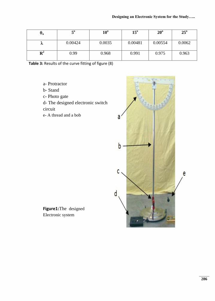
A novel electronic system is designed for the time

period measurements shown in figure (1). The

circuit description is necessary as other researcher

did in their novel circuit designs (Alsadi et. al,

2012). The photo gate consists of a Light

Emitting Diode (LED), and a Light Dependent

Resistor (LDR). The former produces a red light

beam which is detected by the latter. When the

bob intersect the light beam, the LDR resistance

increases rapidly thus it controls the electronic

switch circuit shown in figure (2).

When the bob is shifted with a certain angle, then

release it, simultaneously the LED power switch

turned on. In the light case; when there is no

barrier between the LED and LDR, the LDR

resistance will be very small about 400Ω. In the

dark case, when the bob intersect the light, the

LDR resistance increases to about 1 MΩ, the

timer starts automatically. The voltage divider

circuit, consisting of R1 and the LDR, will derive

the base of T1 and T2 as follows:

LDR

LDR

LDR RRR

VsV

1

(12)

For the light case, we can approximate eq. (12) to:

0LDRV (13)

The above voltage cannot force T1 and T2 to

saturation, while for dark case, eq.(12) can be

approximated to:

21EBLDR VVV (14)

Thus IB=I1, that assures T1 and T2 are both in

saturation, as a result, point (a) will be connected

with point (c). The relays are (ATX201 NAIS

TX2-3V); they have a maximum operating time

equal 4 milliseconds. REL1 is basically at cut off

state as point (a) and point (h) are connected

together. When S2 is at start state i. e., (c)

connects with (d), then (d) will be connected with

(h). With the first disappearance of light, REL2

and REL3 are turned on. In REL2, on one hand,

(h1) will be connected with (h2), on the other

hand, (t0) will be connected with (t1) to start

timing process. In REL3, (f2) will be connected

Journal of Asian Scientific Research, Vol.2, No.5, pp.281-291

283

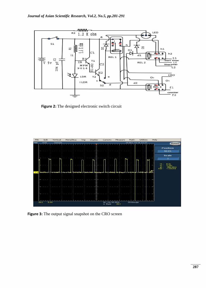
with (f1) to start the counting of the voltage

pulses, while (O0) will be connected with (O1) to

gain pulse amplitude about 9 volts equal to the

source voltage V. This voltage is fed into a digital

phosphorous oscilloscope (1 GHz Tektronix

TDS5104), which has the capability to measure

signal's parameters; maximum pulse voltage,

time duration, and positive time, as its snapshot is

shown in figure(3). The purpose of using Diode

D1 is to prevent Id1 from returning back to point

(d2). With the arrival of the later pulse while S2 is

at stop state, i. e. (c) is connected with (e), REL1

will be turned on, this means that (a) will be

disconnected from (h), at the same time REL2

and REL3 will be turned off. Finally the timer

and the counter are stopped. D2 and D3 are

designed to separate the current passing through

REL1 from that passing through REL2.

Five initial displacement angles o; 5o, 10

o, 15

o,

20o, and 25

o have been chosen, and four different

pendulum lengths 60, 70, 80, and 95 cm were

taken. The larger is the number of oscillation the

less is the error in measuring time period, since

the error is divided by the number of oscillation

(Madrid, 1983). Eighty oscillations have been

taken. The data were taken manually by the timer

and the counter, meanwhile for the case of L=95

cm data were also taken by the CRO. We could

able to measure the time period of each oscillation

with the aid of the snapshot specification of the

CRO, including the measurement of positive

pulse width, time period, and other pulse

parameters. Since the positive pulse widths is

belonging to the dark case, i.e. time spent by the

bob in traversing the LED light, we could able to

measure the maximum velocity of the bob at the

center of the oscillation with the use of the

following equation:

pT

DV max (15)

Where D is the diameter of the bob = 2.45 cm,

and Tp is the positive pulse width time. Vmax is

calculated for each period, substituting them in

eq.(9) to find o for each period and using eq.(6)

we could able to make the second order

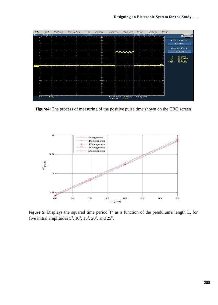
approximation. Figure (4) show how individual

positive pulse time is measured on the CRO

screen.

Results and Discussion

The Manual Method

A matlab software algorithm is used for the whole

results. Figure (5) shows the time periods of four

different lengths and five different initial

displacement angles that are taken manually.

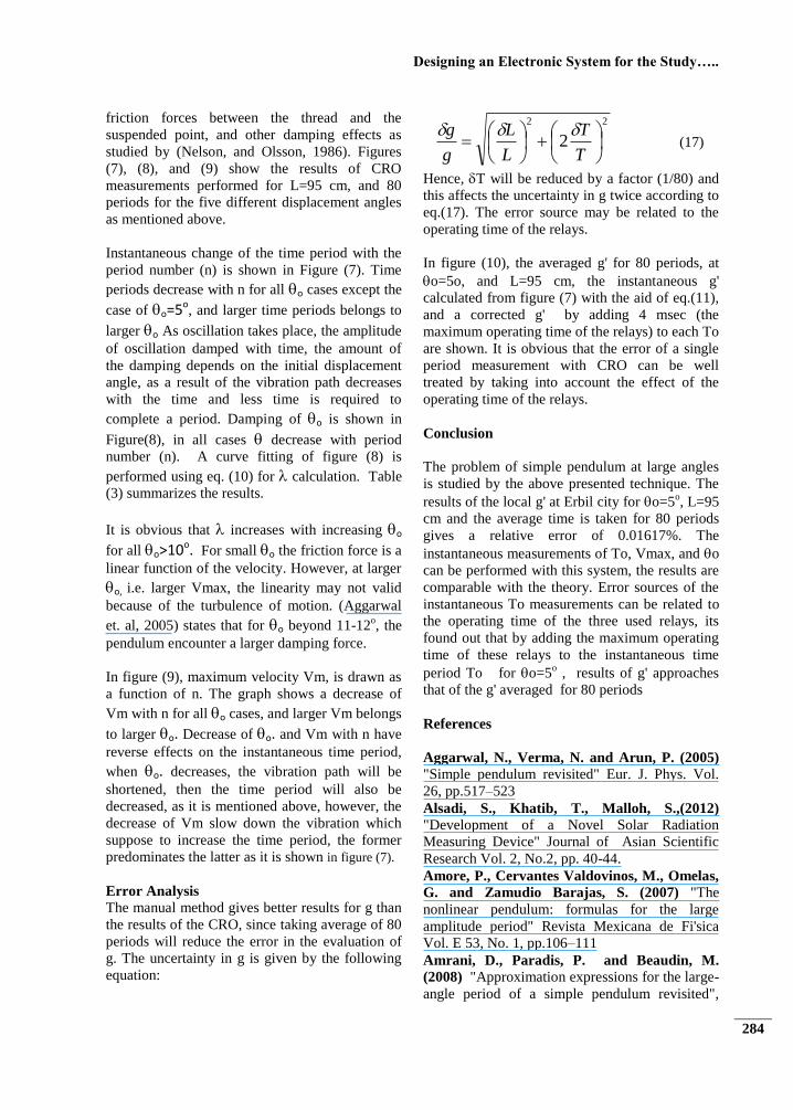
Table (1) summarizes the results which are

deduced from the slopes, g is the acceleration of

gravity calculated by eq. (4), g' is the corrected

acceleration of gravity calculated by eq.(6). While

table (2) summarized g and g' for the case of

o=5o and different lengths L. R2 is the

correlation factor of the fitted curve. The results

show that by increasing L, more accurate g' is

obtained; at L=95 g'=979.863 cm/sec2 is obtained.

The theoretical value of g in Erbil city at College

of science (414 m, Latitude 36o 09' 10'') can be

calculated by using the following equation (Li,

and Gotze, 2001):

(16)

Where:

g= acceleration in cm/sec2, is the latitude, and

h is the high above sea level in meter

The above equation is called the international

gravity formula (1980) with first correction for

high above sea level; the result is 979.705

cm/sec2. If the two results are compared, an

acceptable relative error of 0.01617 % is

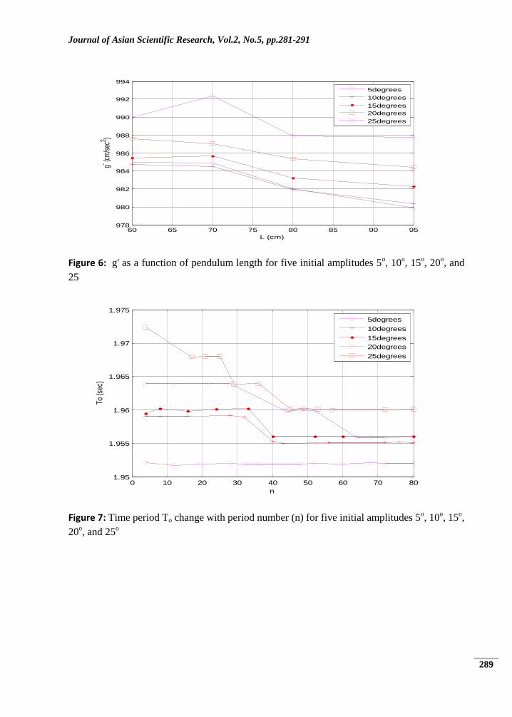
obtained. It is clear from figure (6) that the

calculated g' at L=95 cm approaches the exact

value for all other initial displacement angles.

On the basis of the above results, the pendulum

length of 95 cm for all displacement angles (5o,

10o, 15

o, 20

o, and 25

o) gives adequate g' value,

hence the L=95 cm is chosen for the remainder of

this work.

The CRO Method

Time period changes with number of period as a

result of damping of the motion, which makes

amplitude of vibration decreases after each

period. The maximum displacement angle

represent the total pendulum's energy, at the

initial point, the total energy is a potential , while

at the center of the motion, the total energy

transferred to a kinetic, here, the velocity is

maximum, that can be calculated by using

eq.(15). The pendulum losses its energy with

each period as a result of air resistance, the

Designing an Electronic System for the Study…..

284

friction forces between the thread and the

suspended point, and other damping effects as

studied by (Nelson, and Olsson, 1986). Figures

(7), (8), and (9) show the results of CRO

measurements performed for L=95 cm, and 80

periods for the five different displacement angles

as mentioned above.

Instantaneous change of the time period with the

period number (n) is shown in Figure (7). Time

periods decrease with n for all o cases except the

case of o=5o, and larger time periods belongs to

larger o As oscillation takes place, the amplitude

of oscillation damped with time, the amount of

the damping depends on the initial displacement

angle, as a result of the vibration path decreases

with the time and less time is required to

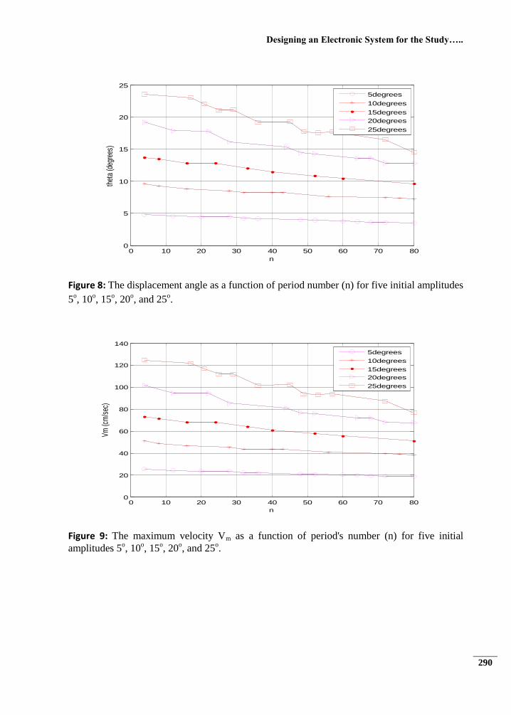
complete a period. Damping of o is shown in

Figure(8), in all cases decrease with period

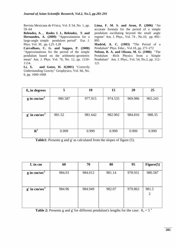
number (n). A curve fitting of figure (8) is

performed using eq. (10) for calculation. Table

(3) summarizes the results.

It is obvious that increases with increasing o

for all o>10o. For small o the friction force is a

linear function of the velocity. However, at larger

o, i.e. larger Vmax, the linearity may not valid

because of the turbulence of motion. (Aggarwal

et. al, 2005) states that for o beyond 11-12o, the

pendulum encounter a larger damping force.

In figure (9), maximum velocity Vm, is drawn as

a function of n. The graph shows a decrease of

Vm with n for all o cases, and larger Vm belongs

to larger o. Decrease of o. and Vm with n have

reverse effects on the instantaneous time period,

when o. decreases, the vibration path will be

shortened, then the time period will also be

decreased, as it is mentioned above, however, the

decrease of Vm slow down the vibration which

suppose to increase the time period, the former

predominates the latter as it is shown in figure (7).

Error Analysis

The manual method gives better results for g than

the results of the CRO, since taking average of 80

periods will reduce the error in the evaluation of

g. The uncertainty in g is given by the following

equation:

22

2

T

T

L

L

g

g (17)

Hence, T will be reduced by a factor (1/80) and

this affects the uncertainty in g twice according to

eq.(17). The error source may be related to the

operating time of the relays.

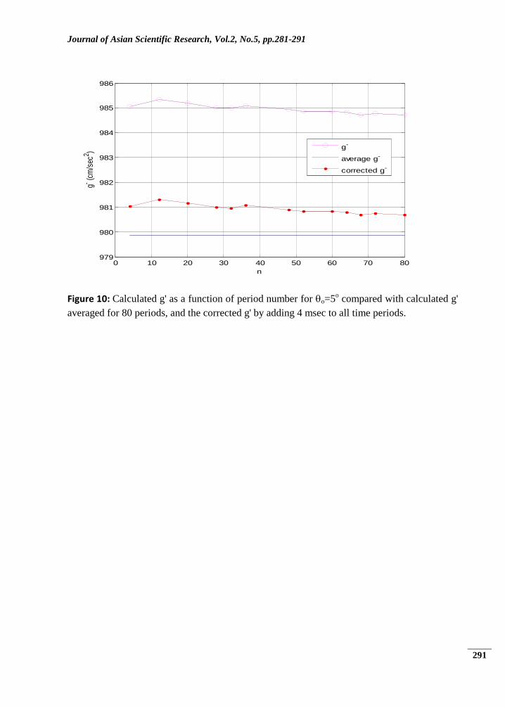
In figure (10), the averaged g' for 80 periods, at

o=5o, and L=95 cm, the instantaneous g'

calculated from figure (7) with the aid of eq.(11),

and a corrected g' by adding 4 msec (the

maximum operating time of the relays) to each To

are shown. It is obvious that the error of a single

period measurement with CRO can be well

treated by taking into account the effect of the

operating time of the relays.

Conclusion

The problem of simple pendulum at large angles

is studied by the above presented technique. The

results of the local g' at Erbil city for o=5o, L=95

cm and the average time is taken for 80 periods

gives a relative error of 0.01617%. The

instantaneous measurements of To, Vmax, and o

can be performed with this system, the results are

comparable with the theory. Error sources of the

instantaneous To measurements can be related to

the operating time of the three used relays, its

found out that by adding the maximum operating

time of these relays to the instantaneous time

period To for o=5o , results of g' approaches

that of the g' averaged for 80 periods

References

Aggarwal, N., Verma, N. and Arun, P. (2005) "Simple pendulum revisited" Eur. J. Phys. Vol.

26, pp.517–523

Alsadi, S., Khatib, T., Malloh, S.,(2012) "Development of a Novel Solar Radiation

Measuring Device" Journal of Asian Scientific

Research Vol. 2, No.2, pp. 40-44.

Amore, P., Cervantes Valdovinos, M., Omelas,

G. and Zamudio Barajas, S. (2007) "The

nonlinear pendulum: formulas for the large

amplitude period" Revista Mexicana de Fi'sica

Vol. E 53, No. 1, pp.106–111

Amrani, D., Paradis, P. and Beaudin, M. (2008) "Approximation expressions for the large-

angle period of a simple pendulum revisited",

Journal of Asian Scientific Research, Vol.2, No.5, pp.281-291

285

Revista Mexicana de Fi'sica, Vol. E 54, No. 1, pp.

59–64

Belendez, A. , Rodes J. J., Belendez, T. and Hernandez, A. (2009) "Approximation for a

large-angle simple pendulum period" Eur. J.

Phys. Vol. 30, pp. L25–L28

Carvalhaes, C. G. and Suppes, P. (2008) "Approximations for the period of the simple

pendulum based on the arithmetic-geometric

mean" Am. J. Phys. Vol. 76, No. 12, pp. 1150-

1154.

Li, X. and Gotze, H. J(2001) "Correctly

Understanding Gravity" Geophysics, Vol. 66, No.

6, pp. 1660-1668

Lima, F. M. S. and Arun, P. (2006) "An

accurate formula for the period of a simple

pendulum oscillating beyond the small angle

regime" Am. J. Phys., Vol. 74 , No.10, pp. 892-

895

Madrid, A. C. (1983) "The Period of a

Pendulum" Phys. Educ., Vol.18, pp. 271-272

Nelson, R. A. and Olsson, M. G. (1986) "The

Pendulum –Rich Physics from a Simple

Pendulum" Am. J. Phys., Vol. 54, No.2, pp. 112-

121

o in degrees 5 10 15 20 25

g in cm/sec2 980.587 977.915 974.535 969.986 965.243

g' in cm/sec2 981.52

981.642

982.902

984.816

988.35

R2 0.999 0.999 0.999 0.999 0.999

Table1: Presents g and g' as calculated from the slopes of figure (5).

L in cm 60 70 80 95 Figure(5)

g in cm/sec2 984.03

984.012

981.14

978.931

980.587

g' in cm/sec2 984.96

984.949 982.07

979.863

981.5

2

Table 2: Presents g and g' for different pendulum's lengths for the case: o = 5 o

Designing an Electronic System for the Study…..

286

o 5o 10

o 15

o 20

o 25

o

0.00424 0.0035 0.00481 0.00554 0.0062

R2 0.99 0.968 0.991 0.975 0.963

Table 3: Results of the curve fitting of figure (8)

a- Protractor

b- Stand

c- Photo gate

d- The designed electronic switch

circuit

e- A thread and a bob

Figure1:The designed

Electronic system

Journal of Asian Scientific Research, Vol.2, No.5, pp.281-291

287

Figure 2: The designed electronic switch circuit

Figure 3: The output signal snapshot on the CRO screen

Designing an Electronic System for the Study…..

288

Figure4: The process of measuring of the positive pulse time shown on the CRO screen

60 65 70 75 80 85 90 95

2.5

3

3.5

4

L (cm)

T2 (s

ec)

5degrees

10degrees

15degrees

20degrees

25degrees

Figure 5: Displays the squared time period T2 as a function of the pendulum's length L, for

five initial amplitudes 5o, 10

o, 15

o, 20

o, and 25

o.

Journal of Asian Scientific Research, Vol.2, No.5, pp.281-291

289

60 65 70 75 80 85 90 95978

980

982

984

986

988

990

992

994

L (cm)

g- (c

m/s

ec2 )

5degrees

10degrees

15degrees

20degrees

25degrees

Figure 6: g' as a function of pendulum length for five initial amplitudes 5o, 10

o, 15

o, 20

o, and

25

0 10 20 30 40 50 60 70 801.95

1.955

1.96

1.965

1.97

1.975

n

To

(sec

)

5degrees

10degrees

15degrees

20degrees

25degrees

Figure 7: Time period To change with period number (n) for five initial amplitudes 5o, 10

o, 15

o,

20o, and 25

o

Designing an Electronic System for the Study…..

290

0 10 20 30 40 50 60 70 800

5

10

15

20

25

n

thet

a (d

egre

es)

5degrees

10degrees

15degrees

20degrees

25degrees

Figure 8: The displacement angle as a function of period number (n) for five initial amplitudes

5o, 10

o, 15

o, 20

o, and 25

o.

0 10 20 30 40 50 60 70 800

20

40

60

80

100

120

140

n

Vm

(cm

/sec

)

5degrees

10degrees

15degrees

20degrees

25degrees

Figure 9: The maximum velocity Vm as a function of period's number (n) for five initial

amplitudes 5o, 10

o, 15

o, 20

o, and 25

o.

Journal of Asian Scientific Research, Vol.2, No.5, pp.281-291

291

0 10 20 30 40 50 60 70 80979

980

981

982

983

984

985

986

n

g- (c

m/s

ec2 )

g-

average g-

corrected g-

Figure 10: Calculated g' as a function of period number for o=5o compared with calculated g'

averaged for 80 periods, and the corrected g' by adding 4 msec to all time periods.