COMPETITION AND INNOVATION:AN INVERTED U RELATIONSHIP

Philippe AghionNicholas Bloom

Richard BlundelRachel Griffith

Peter Howit

THE INSTITUTE FOR FISCAL STUDIESWP02/04

l

t

Competition and Innovation: An Inverted URelationship

Philippe Aghion¤, Nicholas Bloomy, Richard Blundelly,Rachel Gri¢thy, Peter Howittz

February 2002

AbstractThis paper investigates the relationship between product market com-

petition (PMC) and innovation. A Schumpeterian growth model is devel-oped in which …rms innovate ‘step-by-step’, and where both technologicalleaders and their followers engage in R&D activities. In this model, com-petition may increase the incremental pro…t from innovating; on the otherhand, competition may also reduce innovation incentives for laggards. Thismodel generates four main predictions which we test empirically. First, therelationship between product market competition (PMC) and innovation isan inverted U-shape: the escape competition e¤ect dominates for low ini-tial levels of competition, whereas the Schumpeterian e¤ect dominates athigher levels of competition. Second, the equilibrium degree of technologi-cal ‘neck-and-neckness’ among …rms should decrease with PMC. Third, thehigher the average degree of ‘neck-and-neckness’ in an industry, the steeperthe inverted-U relationship between PMC and innovation in that industry.Fourth, …rms may innovate more if subject to higher debt-pressure, espe-cially at lower levels of PMC. We confront these four predictions with anew panel data set on UK …rms’ patenting activity at the US patenting of-…ce. The inverted U relationship, the neck and neck, and the debt pressurepredictions are found to accord well with observed behavior in the data.

¤Harvard University and University College London (p_aghion@harvard.edu)yInstitute for Fiscal Studies and University College London (nbloom@ifs.org.uk,

r.blundell@ucl.ac.uk, rgri¢th@ifs.org.uk)zBrown University (peter_howitt@brown.edu)

1. Introduction1

Economists have long been interested in the relationship between product market

competition (PMC) and innovation. Both the theoretical IO and the more re-

cent endogenous growth literatures tackle the issue. The standard IO literature2

predicts that innovation should decline with competition, as more competition

reduces the monopoly rents that reward entry by new successful innovators. How-

ever, empirical work such as Geroski (1994), Nickell (1996) and Blundell, Gri¢th

and Van Reenen (1999) has pointed to a positive correlation between product

market competition and innovative output. Several theoretical attempts have

been made to reconcile the Schumpeterian paradigm with the evidence provided

in these studies, generating various predictions as to the shape of the relation-

ship between PMC and innovation.3A …rst attempt, in Aghion-Dewatripont-Rey

(1999), introduced the “competition as an incentive mechanism” argument in

Hart (1983) into a Schumpeterian growth framework. This approach would still

predict a monotonic relationship between PMC and innovation. This would be

negative if most …rms are value-maximizing and positive if most …rms are gov-

erned by “satis…cing” managers who mainly care about the …rm remaining in1Acknowledgement: The authors would like to thank Daron Acemoglu, Tim Bresnahan,

Wendy Carlin, Paul David, Janice Eberly, Dennis Ranque, Robert Solow, Manuel Trajtenberg,Alwyn Young, John Van Reenen and participants at the CIAR seminar for their comments.Financial support for this project was provided by the ESRC Centre for the MicroeconomicAnalysis of Fiscal Policy at the IFS. The data was developed with funding from the LeverhulmeTrust.

2See, inter alia, Dasgupta-Stiglitz (1980) and also the …rst generation of Schumpeteriangrowth models (Aghion-Howitt (1992), Caballero-Ja¤e (1993)).

3See Aghion-Howitt (1998), Chapter 7, for a survey of some of these these attempts.

2

business. In addition, this model would predict substitutability between PMC

and debt-…nancing together with hard budget constraints, in the sense that more

debt-…nancing in a hard budget environment could substitute for PMC in inducing

otherwise reluctant managers to innovate more frequently in order to keep their

…rm a‡oat. This latter …nding has been questioned however in recent empirical

work by Grosfeld-Tressel (2001) and Aghion-Carlin-Scha¤er (2002).

An alternative approach, introduced by Aghion-Harris-Vickers (1997) and sub-

sequently analyzed in Aghion-Harris-Howitt-Vickers (2001), extends the basic

Schumpeterian model by allowing incumbent …rms to innovate. In these mod-

els, innovation incentives depend not so much upon post-innovation rents per se,

but more upon the di¤erence between post-innovation and pre-innovation rents

(the latter were equal to zero in the basic model where all innovations were made

by outsiders). In this case, more PMC may end up fostering innovations and

growth as it may reduce a …rm’s pre-innovation rents by more than it reduces its

post-innovation rents. In other words, competition may increase the incremental

pro…ts from innovating, and thereby encourage R&D investments aimed at “es-

caping competition”; and it will do so to a larger extent in more “neck-and-neck”

industries, that is in industries in which oligopolistic …rms face more similar pro-

duction costs; the …rm with lower (resp. higher) unit costs is referred to as the

technological leader (resp. follower) in the corresponding industry.

In this framework …rms innovate in order to reduce production costs, and

they do it “step-by-step”, in the sense that a laggard …rm in any industry must

…rst catch up with the technological leader before becoming itself a leader in the

3

future. In neck-and-neck industries competition is particularly intense and it is

also in those industries that the “escape competition” e¤ect pointed out above

is strongest. On the other hand, in less neck-and-neck, or more “unleveled”, in-

dustries, more competition may also reduce innovation as the laggard’s reward

to catching up with the technological leader may fall (this is a “Schumpeterian

e¤ect” of the kind emphasized in the earlier models). Finally, by increasing in-

novation incentives relatively more in neck-and-neck industries than in unleveled

industries, an increase in product market competition will tend to reduce the

fraction of neck-and-neck industries in the economy; this “composition e¤ect” re-

inforces the Schumpeterian e¤ect in inducing a negative correlation between PMC

and aggregate productivity growth or the aggregate rate of innovations.

The paper begins with the derivation of four main empirical predictions of

this “step-by-step innovation” model, which we then confront with data from a

panel of UK …rms. We argue that the changes in product market competition

and the extensive level of patenting across industries over the last thirty years in

the UK make it a particularly interesting environment to assess these predictions.

The …rst prediction is that the relationship between PMC and innovation is an

inverted-U shape: that is, the escape competition e¤ect tends to dominate for low

initial levels of competition, whereas the Schumpeterian e¤ect tends to dominate

at higher levels of PMC. This prediction is in line with an earlier conjecture by

Scherer (1965). The second prediction is that the equilibrium degree of neck-

and-neckness should decrease with PMC, as more PMC will increase innovation

incentives comparatively more in neck-and-neck sectors, thereby reducing the ex-

4

pected time interval during which an industry remains “neck-and-neck”. Third,

the higher the average degree of neck-and-neckness of an economy, the stronger

the escape competition e¤ect will be on average and therefore the steeper the pos-

itive part of the inverted-U relationship between PMC and innovation. Fourth,

this model predicts that the escape competition e¤ect should also be stronger

in industries where …rms’ managers face harder budget constraints. As a result,

…rms with higher debt/cash-‡ow ratios may innovate more for any level of PMC.

These predictions are examined across a range of industries drawn from a …rm

panel for the UK. The data are on UK listed …rms over the period 1968-1996

and include information on costs, sales, investments and the number of successful

patent applications at the US patent o¢ce. Detailed information on citations are

used to weight our measure of patents granted for each …rm in each year. We derive

a measure of product market competition using a Lerner index. A sequence of

competition policy reforms, that di¤er in their impact across industries, are used

to argue that the Lerner index provides a reliable measure of changes in product

market competition over the period we study. These policy reforms are further

used as instruments to control for the potential endogeneity in the Lerner index.

Within each industry we construct a measure of the size of technology gap (degree

of neck and neckness) based on the dispersion of …rm level technology and cost

indicators. We have matched information at the industry level from the US and

other OECD countries which we use to provide further exogenous instruments for

the technological gap between leaders and followers across industries. Finally, the

long time series on …rms in each industry allow us to control for industry level

5

e¤ects as well as common time e¤ects that plague cross-section and time series

analyses of these relationships.

The theoretical discussion provides a speci…cation for the average arrival rate

of innovations in an industry according to the level of product market compe-

tition and the degree of neck-and-neckness. Our empirical speci…cation starts

with a model for the hazard rate for patenting and uses this to derive a gen-

eralised Poisson model for the count of patents, which is our main measure of

innovative activity. Since we are interested in investigating whether there is a

non-monotonic relationship between innovation and product market competition

we adopt a semiparametric approach and begin our analysis using a hazard rate

speci…cation which is an exponential polynomial spline function in our compe-

tition measure. As part of this empirical investigation we …nd an exponential

quadratic model …ts the data extremely well once industry and time e¤ects are

allowed for.

A striking …nding is of a strong inverted U relationship. This single peaked

relationship is robust to many alternative speci…cations and to the endogeneity

of the Lerner index. Controlling for endogeneity and including time and industry

e¤ects shifts the peak toward the competitive direction but still suggests the

importance of the Schumpeterian e¤ect for a large minority of …rms and industries.

This inverted U relationship continues to hold when we split by the degree of

neck-and-neckness. It is robust to controlling for …rm size and for …xed capital

costs. This inverted U relationship is also found in the data for many individual

industries.

6

The rest of the paper is structured as follows. Section 2 lays out the basic

theoretical framework. Section 3 derives our main predictions analytically in the

special case of a maximum technological gap equal to one. Section 3 simulates the

general model with unbounded gaps. Section 4 concludes the theoretical part by

summarizing our main empirical predictions. Section 5 provides a description of

the data and assesses the degree to which the variables used are likely to provide

good measures of their theoretical counterparts developed in the earlier sections of

the paper. In section 6 we present our main empirical …ndings. We …rst analyze

the robustness of the inverted U relationship and then go on to examine how

this relationship varies with the size of the technology gap between …rms within

the industry (the degree of neck and neckness) and with debt pressure. We …nd

a strong accordance between the main theoretical predictions and the empirical

results. Section 7 provides a short summary and concludes with directions for

further research.

2. A theoretical framework

2.1. Consumers

Suppose that the representative consumer has a utility function of the form:

u =Z 1

0ln xidi; (2.1)

7

where each xi is an aggregate of two goods produced by duopolists in sector i;4

de…ned by the subutility function:

xi = v(xAi; xBi)

where v is homogeneous of degree one and symmetric in its two arguments. We

shall be particularly interested in the case:

xi = (x®iAi + x®iBi)

1®i (2.2)

where a higher ®i 2 (0; 1] re‡ects a higher degree of substitutability between the

two inputs in industry i.

The log-preference assumption made in (2.1) implies that in equilibrium indi-

viduals spend the same amount on each basket xi. We normalize this common

amount to unity by using expenditure as the numeraire for the prices pAi and

pBi at each date. Thus the representative household chooses each xAi and xBi to

maximize v(xAi; xBi) subject to the budget constraint: pAixAi + pBixBi = 1:

In the special case where v(xAi; xBi) = (x®iAi + x®iBi)

1®i , the demand functions

facing the two …rms in industry i are:

xAi =p

1ai¡1Ai

p®iai¡1Ai + p

®iai¡1Bi

and xBi =p

1ai¡1Bi

p®iai¡1Ai + p

®iai¡1Bi

: (2.3)

For notational simplicity we suppress the notation for the industry index i from

here on.4See Aghion-Howitt (2002) for variants of this model with N …rm- industries and free entry.

8

2.2. Technology levels, R&D and innovations

Each …rm produces using labor as the only input,5 according to a constant-returns

production function, and takes the wage rate as given. Thus the unit costs of

production cA and cB of the two …rms in an industry are independent of the

quantities produced. Now, let k denote the technology level of duopoly …rm j in

some industry i; that is, one unit of labor currently employed by …rm j generates

an output ‡ow equal to:

Aj = °kj ; j = A;B; (2.4)

where ° > 1 is a parameter that measures the size of a leading-edge innovation;

(equivalently, it takes °¡kj units of labor for …rm j to produce one unit of output).

An industry is then fully characterized by a pair of integers (l;m), where l is the

leaders technology and m is the technology gap of the leader over the follower. We

de…ne ¼m(respectively ¼¡m) to be the equilibrium pro…t ‡ow of a …rm m steps

ahead of (respectively behind) its rival.6

For expositional simplicity we shall …rst concentrate on the simple case where

knowledge spillovers between leader and follower are such that the maximum sus-

tainable gap is m = 1: That is, if a …rm is one step ahead and it innovates the5In Aghion et al (2001) we argue that the model can be easily extended to the case where

…rms use both capital and labor as inputs according to a CES production technology of theform:

xj = (®k¾¡1

¾j + (1 ¡ ®)(Aj lj)

¾¡1¾ )

¾¾¡1 ;

where Aj measured labor productivity in …rm j and is mutiplied by ° > 1 each time …rm jinnovates.

6The above logarithmic technology along with the cost structure c(x) = x:°¡k implies thatthe pro…t in the industry depends only on the gap m between the leader and follower, and noton absolute levels of technology.

9

follower will automatically copy the leader’s previous technology and so remain

only one step ahead. Therefore, in that case, given that pro…tability is only de-

pendent on the gap between leader and follower, no innovation will be undertaken

by the leader. At any point in time there will therefore be two types of sectors in

the economy: leveled sectors where …rms are neck and neck, that is m = 0, and

unleveled sectors where one …rm is leading the other in the same industry, with

m = 1.

We denote by Ã(n) = 12¯n

2 the R&D cost (in units of labour) of a leader (resp.

follower) …rm moving one technological step ahead with a Poisson hazard rate of

n7. Let nm denote the research intensity put up by each …rm in an industry with

technological gap m, and let n¡m denote the innovation rate or R&D intensity of

the follower in such an industry.

2.3. Bellman equations

Let Vm denote the steady state value of being currently a leader (or follower if

m < 0) in an industry with technology gap m, and let w denote the wage rate,

which we take as given assuming an in…nitely elastic supply of labour. We then

have the following Bellman equations:

rVm = ¼m + nm(Vm+1 ¡ Vm) + n¡m(Vm¡1 ¡ Vm) ¡ w¯(nm)2=2;

rV¡m = ¼¡m + nm(V¡m¡1 ¡ V¡m) + n¡m(V¡m+1 ¡ V¡m) ¡ w¯(n¡m)2=2;7In Aghion et al (2001) we analyze a di¤erent model in which the laggard in an industry

with technological gap m catches up immediately with the technological leader whenever sheinnovates, thereby reducing her unit labor cost by °¡m: This alternative formulation howevertends to exaggerate the importance of the ”escape competition” e¤ect and to downplay theschumpeterian e¤ect of PMC.

10

rV0 = ¼0 + n0(V1 ¡ V0) + n0(V¡1 ¡ V0) ¡w¯(n0)2=2;

In words, the annuity value rVm of currently being a technological leader in an

industry with gap m at date t equals the current pro…t ‡ow ¼m minus the current

R&D cost (w¯nm2=2)dt, plus the discounted expected capital gain nm(Vm+1¡Vm)

from making an innovation and thereby moving one further step ahead of the

follower, minus the discounted expected capital loss n¡m(Vm¡1¡Vm) from having

the follower catch up by one step with the leader. The equation for the annuity

value of a follower is similarly explained. Finally, in the Bellman equation for a

neck-and-neck …rm, note that if each …rm only takes into account its own cost of

R&D, in symmetric Nash equilibrium both R&D e¤orts are equal.

Now, using the fact that each …rm chooses its own R&D e¤ort to maximize its

current value, i.e to maximize the RHS of the corresponding Bellman equation,

we obtain the …rst order conditions:

¯wnm = Vm+1 ¡ Vm; ¯wn¡m = V¡(m¡1) ¡ V¡m;

¯wn0 = V1 ¡ V0:

2.4. Product-market competition

Boone (2001) makes the convincing argument that any parameter increase that

would result in increasing the relative pro…t shares of more advanced …rms; that

is the pro…tability of a greater technological lead, would be a suitable measure of

product market competition. Thus one possible (inverse) measure of competition,

especially in the m · 1 case, would be the pro…t ‡ow of “neck-and-neck” …rms,

11

¼0; with a higher ¼0 resulting from higher collusion among otherwise similar …rms

in the same sector.

Another potential “measure” of competition from Boone’s theoretical stand-

point, is the elasticity of substitution parameter ® in the case:

v(xA; xB) = (x®A + x®B)

1® :

More speci…cally, assume that in any sector the two duopolists in that sector

compete in prices, arriving at a Bertrand equilibrium. According to the de-

mand functions in (2.3), the elasticity of demand faced by each …rm j is ´j =

(1 ¡ ®¸j) = (1 ¡ ®) ; where ¸j = pjxj is the …rm’s revenue:

¸j =p®®¡1j

p®®¡1A + p

®®¡1B

; j = A;B: (2.5)

Thus each …rm’s equilibrium price is:

pj =´j´j ¡ 1

cj =1 ¡ ®¸j® (1 ¡ ¸j)

cj ; j = A;B (2.6)

and its equilibrium pro…t is:

¦j =¸j´j

=¸j (1 ¡ ®)1 ¡ ®¸j

; j = A;B (2.7)

Equations (2.5) » (2.7) can be solved for unique equilibrium revenues, prices

and pro…ts. Given the degree of substitutability ®; the equilibrium pro…t of each

…rm j is determined by its relative cost z = cj=c¡j; an equiproportional reduction

in both cA and cB would induce each …rm to reduce its price in the same propor-

tion, which, because industry demand is unit-elastic, would leave the equilibrium

12

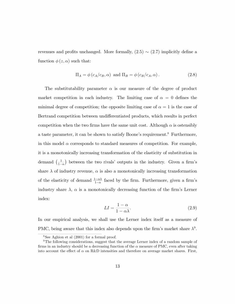
revenues and pro…ts unchanged. More formally, (2.5) » (2.7) implicitly de…ne a

function Á (z; ®) such that:

¦A = Á (cA=cB ; ®) and ¦B = Á (cB=cA; ®) : (2.8)

The substitutability parameter ® is our measure of the degree of product

market competition in each industry. The limiting case of ® = 0 de…nes the

minimal degree of competition; the opposite limiting case of ® = 1 is the case of

Bertrand competition between undi¤erentiated products, which results in perfect

competition when the two …rms have the same unit cost. Although ® is ostensibly

a taste parameter, it can be shown to satisfy Boone’s requirement.8 Furthermore,

in this model ® corresponds to standard measures of competition. For example,

it is a monotonically increasing transformation of the elasticity of substitution in

demand¡

11¡®

¢between the two rivals’ outputs in the industry. Given a …rm’s

share ¸ of industry revenue, ® is also a monotonically increasing transformation

of the elasticity of demand 1¡®¸1¡® faced by the …rm. Furthermore, given a …rm’s

industry share ¸; ® is a monotonically decreasing function of the …rm’s Lerner

index:

LI =1 ¡ ®1 ¡ ®¸: (2.9)

In our empirical analysis, we shall use the Lerner index itself as a measure of

PMC, being aware that this index also depends upon the …rm’s market share ¸9.8See Aghion et al (2001) for a formal proof.9The following considerations, suggest that the average Lerner index of a random sample of

…rms in an industry should be a decreasing function of the ® measure of PMC, even after takinginto account the e¤ect of ® on R&D intensities and therefore on average market shares. First,

13

2.5. The one-step case

In the special case where the maximum technological gap between leaders and

followers is m = 1; assuming for simplicity that w = ¯ = 110, and using the

fact that in that case a technological leader has no incentive to invest in R&D

(n1 = 0); the above Bellman equations become:

rV1 = ¼1 + n¡1(V0 ¡ V1)rV¡1 = ¼¡1 ++n¡1(V0 ¡ V¡1) ¡ (n¡1)2=2

rV0 = ¼0 + n0(V1 ¡ V0) + n0(V¡1 ¡ V0) ¡ (n0)2=2

9>>=>>;

(2.10)

with corresponding …rst order conditions:

n¡1 = V0 ¡ V¡1n0 = V1 ¡ V0

9=; (2.11)

Thus, for example, the annuity value rV1 of being a leader is the current ‡ow

of pro…t ¼1 minus the expected capital loss per unit of time from being caught up

with by the laggard. The expected loss is the loss in value V1 ¡V0 that will occur

if the laggard innovates, multiplied by the ‡ow probability n¡1 of the laggard

innovating.

for ¸ su¢ciently small (which is typically the case in practice), the Lerner index LI is clearlydecreasing in ®; second, we show in the Appendix that for small innovation size ° a …rm’s Lerneris approximately linear in the …rm’s lead size, so that when averaging across the two …rms in thesame industry, we approximately get the Lerner index of a neck-and-neck …rm (with ¸ = 1=2),which itself is decreasing in ®; third, when we calculate the expected Lerner index of a randomlyselected …rm under the steady-state distribution of lead size, using the parameters underlyingour simulations in section 4, we again …nd that the average Lerner index is a decreasing functionof ®:

10We thus take the wage rate as given, with the implicit assumption of an in…nitely elasticsupply of labor at wage w = 1: See Aghion et. al (1997) for a discussion of the case where thesupply of labor is inelastic.

14

2.6. Individual innovation intensities

Equations (2.10) and (2.11) solve for n¡1 and n0: Eliminating the V ’s between

these equations yields the reduced form research equations:

(n0)2

2+ rn0 ¡ (¼1 ¡ ¼0) = 0 (2.12)

(n¡1)2

2+ (r + n0)n¡1 ¡ (¼0 ¡ ¼¡1) ¡ (n0)2

2= 0: (2.13)

This system is recursive, as the …rst quadratic equation solves for n0; and then

given n0 the second quadratic equation solves for n¡1:We obtain:

n0 = ¡r +pr2 + 2(¼1 ¡ ¼0) (2.14)

n¡1 = ¡(r + n0) +q

(r + n0)2 + n20 + 2(¼0 ¡ ¼¡1): (2.15)

Combining (2.14) and (2.15) yields the alternative expression:

n¡1 = ¡(r + n0) +qr2 + (n0)2 + 2(¼1 ¡ ¼¡1): (2.16)

Here, we shall focus on the e¤ects of an increase in product market competition

as represented by a reduction in ¼0 leaving ¼¡1 and ¼1 unchanged. (The analysis

and results in the remaining part of this section can be replicated using the elas-

ticity parameter ® as an alternative way to parametrize PMC). We immediately

see that n0 increases whereas n¡1 can be shown to fall.11 The latter e¤ect (on n¡1)

is the basic Schumpeterian e¤ect that results from reducing the rents that can be11>From (2.14):

@n0

@¼0= ¡ 1p

r2 + 2(¼1 ¡ ¼0)< 0

>From this and (2.16):

15

captured by a follower who succeeds in catching-up with its rival by innovating.12

The former e¤ect (on n0) is what we refer to as an “escape competition e¤ect”,

namely that more competition induces neck-and-neck …rms to innovate in order

to escape competition, as the incremental value of getting ahead is increased with

higher PMC. Thus, if we were to treat the fractions of leveled and unleveled sec-

tors in the economy as an exogenous parameter, we would get the conclusion that

the higher the fraction of neck-and-neck sectors in the economy, the more positive

the e¤ect of product market competition on the average innovation rate. This

complementarity between PMC and neck-and-neckness will appear more clearly

in Section 3 below when we simulate the general model with unbounded gaps.

2.7. Average innovation rate

An increase in product market competition will have an ambiguous e¤ect on

the steady-state aggregate innovation rate because it will induce more frequent

innovations in currently neck-and-neck sectors and slower innovations in currently

unleveled sectors. The overall e¤ect on the average innovation rate and on average

productivity growth will depend on the steady-state fraction of time a sector

@n¡1

@¼0=

@n0

@¼0

24¡1 +

n0qr2 + (n0)

2 + 2(¼1 ¡ ¼¡1)

35 > 0

12As we will see when we allow for m arbitrarily large, this Schumpeterian e¤ect may becounteracted by a “forward looking” escape competition e¤ect. More PMC induces a laggardin a sector with small technological gap (between the leader and that laggard) to increase itsR&D investment in order to enter the race for a large technological lead sooner. This and theSchumpeterian e¤ects together give rise to an inverted U-shape relationship between n¡m andPMC as measured by ® for all m < 0 (see section 3.2 below).

16

spends being neck-and-neck.

More formally, let ¹1 (resp. ¹0) denote the steady-state probability of being

an unleveled (resp. neck-and-neck) industry. During any unit time interval, the

steady-state probability that a sector moves from being unleveled to leveled is

¹1n¡1; and the probability that it moves in the opposite direction is 2¹0n0: In

steady state, these two probabilities must be equal:

¹1n¡1 = 2¹0n0:

This, together with the fact that:

¹1 + ¹0 = 1;

implies that the average ‡ow of innovations is:

I = ¹02n0 + ¹1n¡1 = 2¹1n¡1 =4n0n¡1

2n0 + n¡1: (2.17)

Figure 1 shows a numerical example in which r = :04; ¼¡1 = 0; ¼1 = 10; w =

¯ = 1: As ¼0 decreases from ¼ = ¼1; the innovation rate I follows an inverted-U

shaped pattern.

2.8. The logic of the inverse-U

The reason for the inverted-U shape is that when there is not much product

market competition, ¼0 is close to ¼1; so that there is hardly any incentive for

…rms to innovate when the sector is leveled, and the overall innovation rate will be

highest when the sector is unleveled and there is asymmetric competition. Thus

the industry will be quick to leave the unleveled state (which it does as soon as the

17

laggard innovates) and slow to leave the leveled state (which won’t happen until

one of the neck-and-neck …rms innovates), and as a result the industry will spend

most of the time in the unleveled state. Hence when competition intensi…es, the

e¤ect on the economy-wide average rate of innovation will be determined by what

happens in the leveled state. But we have seen that the e¤ect of more intense

competition on the innovation rate 2n0 in a leveled industry is positive, since the

“escape competition” e¤ect is at work for …rms in that state. In other words, if

the degree of competition is very low to begin with, an increase will result in a

faster average innovation rate.

On the other hand, when competition is very high, ¼0 is close to ¼¡1 and

there is relatively little incentive for the laggard in an unleveled state to innovate,

especially if the rate of interest is high, because the incremental pro…t is very low.

(Of course there is still an incentive for the laggard to innovate even if ¼0 = ¼¡1;

because, although an innovation will not raise current pro…ts, it will take the …rm

one step closer to possibly attaining a leader’s pro…t ¼1:) Thus the industry will be

relatively slow to leave the unleveled state. Meanwhile the large incremental pro…t

¼1 ¡ ¼0 gives …rms in the leveled state a relatively large incentive to innovate, so

that the industry will be relatively quick to leave the leveled state. As a result,

the industry will spend most of the time unleveled, so that when competition

intensi…es the e¤ect on the average rate of innovation may be determined by what

happens in the unleveled state. But we have seen that the e¤ect of more intense

competition on the innovation rate in the unleveled state is negative, since the

Schumpeterian e¤ect is at work on the laggard while the leader never innovates.

18

In other words, if the degree of competition is very high to begin with, an increase

may result in a slower average innovation rate.

Hence the possibility of an inverse-U relationship between competition and

innovation. When competition is low, an increase will raise innovation through

the escape competition e¤ect on neck-and-neck …rms, but when it becomes intense

enough it may lower innovation through the Schumpeterian e¤ect on laggards.

The reason why one e¤ect dominates when competition is low and the other when

competition is intense is the “composition e¤ect” on the steady-state distribution

of technology gaps.

To see this composition e¤ect more clearly note that in the steady state dis-

tribution:

¹0 =n¡1

n¡1 + 2n0and ¹1 =

2n0n¡1 + 2n0

In the limit when there is no competition (¼0 = ¼1), (2.14) implies that n0 = 0;

so that in the steady state the industry is always leveled (¹0 = 1), whereas when

there is the maximum competition (¼0 = ¼¡1), (2.14) and (2.16) imply that

n0 > n¡1; so that the overall rate of innovation in the leveled state is more than

twice that in the unleveled state and as a result the fraction of time ¹0 spent

leveled in steady state is less than 1/3.

2.9. Debt pressure and product market competition

In this subsection we explore the interplay between product market competition

and debt pressure indicators- such as debt-exposure (and the resulting probability

of incurring bankruptcy costs) and the magnitude of default costs (which one

19

could interpret as re‡ecting the hardness of …rms’ budget constraints). We show

the possibility that higher debt pressure and/or higher default costs could induce

…rms to innovate more in order to escape debt pressure.

To formalize the interplay between competition and the exposure to bankruptcy

costs, we consider the following variant of the basic one-step model: (1) neck-and-

neck pro…t ‡ows e¼0 are random, i.i.d over time and uniformly distributed over the

interval [¼0; ¼0+1]; (2) ¼¡1 ´ 0; ¼1 constant with ¼1 >> ¼0+1; (3) …rms …nance

their investments through debt …nancing, which we de…ne here as involving a …xed

‡ow repayment obligation D; a ‡ow default cost f incurred per period of time by

the …rm whenever e¼0 < D:13

Consider …rst the case where exit costs are negligible and where D 2 (¼0; ¼0+

1); then, the Bellman equations for equilibrium R&D investments, can be ex-

pressed as:

rV1 = ¼1 ¡D + n¡1(V0 ¡ V1);

rV0 = Ã(¼0; D; f) + n0(V1 ¡ V0) + n0(V¡1 ¡ V0) ¡ n20=2;

rV¡1 = ¡f + n¡1(V0 ¡ V¡1) ¡ (n¡1)2=2:

where

Ã(¼0; D; f) =Z ¼0+1

D(u¡D)du¡ f

Z D

¼0du;

is the expected ‡ow utility of a manager in a new industry, net of the expected13This formulation is inspired from the costly state veri…cation literature (e.g Townsend

(1979), Gale-Hellwig (1985)) on debt-…nancing, in which …rms’ revenues are assumed to beunveri…able by outside investors, unless they incur a ‡ow veri…cation cost f . For simplicity, weabstract in this section from …rms’ choice over the optimal …nancial contract.

20

veri…cation costs. From these Bellman equations and the corresponding …rst order

conditions, we obtain the following expression for the equilibrium neck-and-neck

…rm’s innovation rate:

n0 = ¡r +pr2 + 2(¼1 ¡D ¡ Ã) = ¡r +

p±; (2.18)

where we re-express à as:

à =12(¼0 + 1 ¡D)2 ¡ f (D¡ ¼0):

Hence:@n0@¼0

= ¡ (¼0 + 1 ¡D+ f ) =p± < 0: (2.19)

Suppose …rst that the default cost f is constant. Then, provided f is large

enough we …nd that the e¤ect of increasing the …rm’s leverage D, will be to raise

innovation. That is:@n0@D

= (¼0 ¡D + f ) =p±

which is positive if f > D¡ ¼0: Thus, for any level of PMC, higher debt pressure

as measured by a higher level of D will result in more R&D by neck and neck

…rms.

Consider next the e¤ect of an increase in the default cost f , which we interpret

as a hardening of the …rm’s budget constraint. We immediately have:

@n0@f> 0;

that is, a higher cost of default induces …rms to innovate more in order to escape

the threat of bankruptcy.

21

3. The general model

In principle, one can solve the general model, but closed form solutions are hard

to derive when m is large, and the best one can do is to solve it numerically.

Figure 2 depicts the values as a function of ®, which we now use to parametrize

PMC, for the case where r = :1; ° = 1:75; w = 1; ¯ = 15: The larger ®; that is the

higher the degree of PMC, the higher the curvature of the logistic Vm function as

a function of m at the neighborhood of m = 0:

3.1. Industry innovation rate

Using the same equations, we can also characterize the relationship between ®

and the individual innovation rates nm and n¡m+h (where h is a help parameter

which re‡ects the fact that it might be easier for laggards than for leaders to go

one technological step forward): Figure 3 depicts the relationship between ® and

total intra-industry innovation rates (nm+ n¡m); for the above parameter values

and for h = 0:025:We see an inverted-U shaped pattern for m 6= 0, which in turn

results from the interplay between the “escape competition” and Schumpeterian

e¤ects of PMC on innovation incentives. We also see that innovation intensities

are higher and also increase more rapidly with ® in the case of neck-and-neck …rms.

Thus, there is complementarity between PMC and the degree of neck-and-neckness

as measured by how small m is. The relationship between PMC and innovation

becomes increasingly steeper as m goes down, i.e as the industry becomes more

neck-and-neck.

22

3.2. Industry structure and steady-state innovation/growth rates

In the equilibrium we de…ne ¹m to be the steady state fraction of time the industry

spends with technological gap m: We obviously have:

X

m

¹m = 1

In addition, the following equations must also hold in steady-state:

¹m(nm + n¡m + h) = ¹m¡1nm¡1 + ¹m+1(n¡(m+1) + h);

for all m ¸ 2: The LHS of this equation represents the ‡ow probability of exit-

ing technological gap (or “state”) m; the RHS represents the ‡ow probability of

entering state m; both, from state (m ¡ 1) with the leader innovating, and from

state (m+ 1) sectors with the follower innovating. For m = 1 we have:

¹1(n1 + n¡1 + h) = 2¹0n0 + ¹2(n¡2 + h);

as two …rms instead of one can turn a neck-and-neck sector into an unleveled

sector with technological gap m = 1:

And for m = 0; we simply have:

2¹0n0 = ¹1(n¡1 + h):

In other words, a neck-and-neck sector becomes unleveled whenever a …rm in that

sector innovates, and only state-1 sectors can become neck-and-neck whenever the

laggard in that sector innovates. Figure 4 depicts ¹ as a function of m and ®.

We see that on average the industry becomes increasingly neck and neck as PMC

increases.

23

Now, we can compute the average rate of productivity growth for the industry.

In the general case where the lead sizem can take any integer value, one can show

that the average growth rate of the industry is equal to:

g = (2¹0x0 +X

k¸1¹kxk) ln °: (G)

Equation (G) states that the growth rate equals the product of the frequency of

“frontier innovations” (innovations by the industry leader or a neck-and-neck …rm,

which advance the industry’s frontier technology) and the (log) size of innovations.

Figure 5 depicts g as a function of ®: We again obtain an inverted U-shape.

4. Summary of theoretical predictions

We now conclude the theoretical part of the paper by stating four main predictions

that came out of our analysis in the previous sections, and which we test in the

empirical part of the paper:

1. The relationship between product market competition and the average in-

novation rate, is an inverted-U shape.

2. The expected technological gap in an industry increases as product mar-

ket competition increases, that is the distribution shifts towards a lower

probability of being neck-and-neck.

3. There is a complementarity between product market competition and the

degree of neck-and-neckness of an industry. The closer …rms are in technol-

ogy space (the more neck-and-neck …rms are in that industry) the steeper

24

the positive e¤ect of product market competition on innovation and the

larger the average number of innovations.

4. Firms with higher debt/cash-‡ow ratios may innovate more for any level of

PMC.

5. Data and Measurement Issues

The empirical investigation that we report in the next section is based on a panel

of UK companies covering the period 1968-1997. The UK over this period pro-

vides an extremely rich environment within which to study the impact of product

market competition on innovation behaviour. Not only is there a long panel of de-

tailed company data but this period also saw a number of signi…cant, and largely

exogenous, changes in product market competition. These changes, which altered

the structure of product market competition across industries, included the im-

plementation of the European Single Market Program, a series of structural and

behavioural reforms imposed on di¤erent industries as a result of investigations

by the Monopolies and Mergers Commission (MMC) under the Fair Trading Act

and large scale privatisations. We document these in more detail below and relate

them carefully to our measure of industry level product market competition. We

will also argue that they provide a powerful set of instrumental variables for our

competitiveness measure.

There are two main data sources used in this study - …rm level accounting

data and administrative data from the US patents o¢ce.14 These allow us to14This data was developed with funding from the Leverhulme Trust. See Bloom and Van

25

combine information on technological performance, revenues, labour costs and

capital costs. The accounting data come from Datastream and include all …rms

quoted on the London Stock Exchange between 1968 and 1997.15 The …rm level

patenting information from the US Patent O¢ce dataset was matched to a subset

of the …rms for which accounting data is available. We have patents data for all

…rms with a name beginning A-L (plus all large R&D …rms) that were listed on

the London Stock Exchange any time between 1983 and 1985. These have been

matched to all of their subsidiaries in 1985.16 This data runs from 1968-1996 and

contains 461 …rms with 236 …rms that patent.

In order to test the predictions detailed in section 5 we need measures of …rms’

innovative output, the degree of product market competition in an industry, the

size of the technology gap between …rms within an industry (how “neck-and-neck”

…rms are) and the extent of bankruptcy threat facing each …rm. We will discuss

these in turn.

5.1. Measuring innovation

There is a large literature on measuring innovation intensity. The most commonly

used measures at the …rm level are research and development spending, patenting

activity, innovation counts and total factor productivity. Although R&D expen-

Reenen (2000) for a more detailed description of the data.15We removed …rms with missing values on sales, capital or employment, …rms with less

than three consecutive observations, observations for …rms with abnormal length accountingperiods (we drop …rms whose accounting period falls outside 300 to 450 days due to changesin accounting year ends) and exclude observations for …rms where there was a jump of greaterthan 150% in any of the key variables (capital, labour, sales).

16This matching has been done by hand in order to achieve a higher match rate than withcomputer matching.

26

diture is available in the UK and we use it to check the robustness of our results,

it is not mandatory for …rms to report it, and prior to 1990 it is frequently not re-

ported. We do not use total factor productivity (TFP) as a measure of innovative

activity either because of the well known problem that commonly used measures

of TFP are themselves biased in the presence of imperfectly competitive product

markets.17 For these reasons our main measure is based on information on patents

taken out by UK …rms in the US patent o¢ce. Our data includes information

on all patents taken out by a randomly selected sample of 461 UK stock market

listed …rms (all …rms with names beginning A-L).18

The US patenting o¢ce is the place where innovations are patented inter-

nationally. These patents can be based on research conducted anywhere in the

world. We also have information on citations to and from these patents. One

concern that is often expressed about using patent counts is that patents may not

be comparable across …rms or industries because their value can vary signi…cantly.

Therefore, we use the number of times a patent has been cited by other patents to

weight the patent and thus provide a measure that is more indicative of the value

of the patent.19 We can extend the interpretation of our results for patents to pro-

ductivity growth as patents are well known to have a strong e¤ect on productivity

growth.20 This has also been demonstrated directly for our dataset by Bloom and17See, inter alia, Hall (1988), Klette and Griliches (1996) and Klette (1999).18As we highlight below the complete set of UK stock market …rms is used to construct the

other industry measures we require.19Hall, Ja¤e and Trajtenberg et al. (2001) use the US Patent O¢ce patenting data set to

examine the e¤ects of patenting on the market value of US …rms.20See for example the survey of the patenting literature in Griliches (1990).

27

Van Reenen (2001) who …nd a highly signi…cant response of productivity to both

patents and patent citations. Figure 5.1 presents a frequency histogram of annual

…rms level patent count. This picture excludes the 37% of zero observations. It

also truncates the distribution at 50 patents per year per …rm. As we note further

below there are a few very large patenting …rms our data. The inclusion of …xed

e¤ects in our empirical model re‡ects the argument that certain …rms and certain

industries may have a higher propensity to patent than others and that this may

not be not causally related to the competitive structure of the …rm or industry.

5.2. Measuring the degree of product market competition

The degree of product market competition is measured at the industry level. We

use the …rm level data to construct these industry level measures. We use in-

formation reported in Datastream which we have for all UK stock market listed

…rms. As discussed in Section 2.3 our main indicator of product market competi-

tion is the Lerner Index or price cost margin. In fact we use 1 minus the Lerner,

so a value of 1 indicates perfect competition (price equals marginal cost) while

values below 1 indicate some degree of market power. This measure has several

advantages over measures such as market shares or a Her…ndahl or concentration

index. In order to measure any of those it is necessary to have a de…nition of

both the geographic and product boundaries of the market in which the …rm op-

erates. This is particularly important in our application as many innovative UK

…rms operate in international markets, so that traditional market concentration

28

measures could be extremely misleading.21

In accordance with our theoretical measure the Lerner index is taken to be

constant within industry. Firms in our data can operate in many industries. We

classify …rms by the 2-digit SIC code in which the …rm had the largest proportion

of its sales in 1995. For 33% of the …rms this represented all of their sales. The

median share of sales accounted for by the largest industry is 90%. We use the

entire sample of Datastream …rms to estimate the industry Lerner Index. We

use accounting data to construct a …rm level measure similar to Nickell (1996)’s

measure of rents over value-added. The Lerner Index is price minus marginal cost

over price. One di¢culty we face is that we do not observe marginal cost. For

the numerator we use operating pro…ts net of depreciation and provisions. This

is more like price minus average cost. We divided this by sales.

liit =operating pro…t (DS137)

sales (DS104):

There are several concerns we might have about this measure. First, in UK

accounts capital depreciation, R&D expenditure and advertising have been de-

ducted. In theory we would like to deduct R&D depreciation (rather than expen-

diture), but this is not available and we note that in steady state investment in the

R&D stock should equal depreciation.22 Second, the assumption that AC ¼MC21One example of the di¢culties in using concentration indexes is provided by the pharma-

ceutical industry, which accounts for about 10% of global R&D. In the UK the pharmaceuticalindustry is dominated by two large players, GlaxoSmithKline and AstraZeneca, whose salesaccounts for about 65% and 30% of the market. But these …rms are global players, competingwith other US and European …rms. In global terms they have market shares of 7% and 4%,with these low market shares re‡ect the …erce competition in the industry. In this case, withoutglobal market sales, concentration measures would be extremely misleading.

22For growing …rms investment will be greater than depreciation so our estimate of Lerner

29

assumes away any signi…cant …xed costs of production.23 We would like to de-

duced the …nancial cost of capital from the numerator, but we do not observe

this. In the empirical analysis we consider the robustness of our results to the

deduction of an estimate of the cost of …nance (cost of capital*capital) from our

measure of pro…ts.24

Our industry measure of product market competition, denoted cjt, is an un-

weighted average across all …rms in the industry,

cjt = 1 ¡ 1Njt

X

i2jliit

where i indexes …rms, j indexes industry, t index time and Njt is the number of

…rms in industry j in year t.

We also use an alternative competition measure ® as described in (2.9). This

strips out the a¤ect of market share on a …rms’ pro…t-margin,

®it =1 ¡ liit

1 ¡msit ¤ liit

We use the …rm’s share of output produced by …rms in the same 2-digit industry

on the London Stock Market to measure market share. This is not our prefered

measure because of our concerns about measuring market shares of …rms operating

in international markets, as discussed above. This adjustment and the results of

it are discussed further in the presentation of the empirical results. They also help

Index will be an underestimate of the true markup.23More precisely, we assume that there is no correlation between signi…cant …xed costs and

innovation in our econometric approach which could lead us to erroneously …nd an inverted Ushape. We are grateful to Robert Barro for pointing this out.

24Where the cost of capital is assumed to be 0.085 for all …rms and time periods and capitalstock is measured using the perpetual inventory method.

30

to back up the analysis in the Appendix which develops a theoretical argument

as to why the Lerner and ® should be inversely related even after allowing for

market share to adjust to changes in the competitive environment.

We are able to measure the Lerner index using information on all UK …rms

in Datastream, not only the sample for which we also observe patents. For …rms

operating in more than one market the Lerner Index will represent a weighted

average of the degree of product market competition across these markets. This

could lead to measurement error and attenuation bias. We discuss this further

in the empirical section below. Figure 5.2 presents the time path of the Lerner

index and our estimate of alpha for six of the manufacturing industries used

in the study.25 This shows a wide variation in the index over time that di¤ers

systematically across industries.

One of our main concerns is that the Lerner may be endogenous to the patent-

ing decision. We address this problem in a number of ways. Our main approach

is to use a number of ‘policy’ instruments that provide exogenous variation in the

degree of industry wide competition. These instruments are described below and

we show that their relationship to the Lerner suggests that the Lerner index is

picking up variation in industry wide product market competition. In the empir-

ical analysis we use the instruments to correct our estimators for endogeneity in

the Lerner index. All instrument sets include industry and time e¤ects. We also

use the lagged value of the Lerner index. Added to these are the set of policy25Extraction of other minerals (23), Chemical industry (25), Manufacture of o¢ce machinery

(33), Electrical and electronic (34), Motor vehicles and parts (35), Food (41).

31

instruments discussed in section 5.2.

Before using the Lerner in our detailed econometric analysis we consider the

extent to with the variation in our Lerner measure re‡ects changes in the degree

of competition. In order to do this we consider a set of major policy event that

a¤ected the degree of competition. These are of three sorts - the EU Single Mar-

ket Programme, Monopoly and Merger Commision investigations that resulted in

structural or behaviours remedies being imposed on the industry, and privatisa-

tions. The table below lists the sic codes and years a¤ect by these policies:

Policy instrumentsSIC Years

SMP high see appendix 1988SMP medium see appendix 1988Cars 351 1984, 1987, 1988Car Parts 353 1982, 1987Periodicals 475 1987Brewing 427 1986Telecoms 344 1981, 1984, 1989Textiles 430 1989Razors and Razor blades 316 1990Steel 220 1987Ordnance 329 1987

In Appendix B we provide more detail on the policies and the industries that

were a¤ected.

5.3. Technology gap

We are also interested in looking at how the size of the technology gap between

…rms within an industry interacts with the degree of product market competition.

We measure this by the proportional distance a …rm is from the technological fron-

32

tier, as measured by total factor productivity. This corresponds to the parameter

m introduced in section 2.2,

mi =TFPF ¡ TFPiTFPF

(5.1)

where F denotes the frontier (the highest TFP) and i denotes non-frontier …rms.

For the frontier …rm (if they are in our sample) our measure is

mF =TFPF ¡ TFPF¡1

TFPF(5.2)

where F¡1 denotes the …rm just behind the frontier. A lower value ofm indicates

that …rms are technologically close (so the industry is more neck and neck) while a

high value ofm indicated a large technology gap, so the industry is more unleveled.

In the empirical application below we use an industry level measure that is the

average across …rms in the industry

mtfpjt =1Njt

X

i2jmit

where Njt is the number …rms in industry j at time t. We measure TFP using

a …rst order approximation (Cobb-Douglas). We using information at on TFP

in the US, Japan and Germany at the industry-year level to capture the foreign

frontier.

5.4. Data description

Table 1 shows the number and proportion of observations where we have both

accounting and patents data and where we have only accounting data. On average

we observe patents data for 34% of the complete Datastream sample. We do not

33

include industries where we have fewer than three …rms or where there were no

patents throughout the period 1968-1996. Our sample contains 330 …rms with

4,500 observations over the period 1971-1994 in seventeen 2-digit industries. Of

these there are 236 patenting …rms, with around 60,000 patents in total which

account for around 200,000 citations.

Table 2 shows the average of the …rm level Lerner Index for the sample of

…rms where we have only accounting data and for the sample where we have both

accounting and patents data. The table shows that the …rms we have in our

sample are similar in terms of their Lerner Index to those not in our sample -

both are used to construct our industry measure of the Lerner. At the industry

level the Lerner averages 8% and ranges from 21% in Extraction of other minerals

in 1976 to 3% in Motor Vehicles in 1981.

Table 3 presents the descriptive statistics on our sample of 330 …rms. >From

this we can see that, …rstly, our patent count is highly skewed with most …rms

taking out no patents in any given year but one …rm (ICI in 1974) taking out

409 patents. Also, the employment …gures give an indicator of the size of our

…rms with about 1,500 employees in the median …rm, while the median of 17

observations per …rm re‡ects the long time series of our data set.

Our measure of the technology gap (neck and neck) also has a large spread

ranging from industries in which leaders and follower …rms all have very similar

levels of TFP (those with measures close to 0) to industries in which the leader

is far ahead of the rest of the industry (those with measures close to 1).

Our …nancial pressure variable is debt payments over operating pro…ts plus

34

depreciation. This also shows a similarly large spread between …rms in which

debt repayments consume all their cash ‡ow (a pressure measure of 1) to those

with little or no debt (a pressure variable of 0).

6. Empirical Support for the Inverted U

Earlier analysis using UK company data (Blundell, Gri¢th and Van Reenen

1995,1999) established two empirical regularities. First, market share is a sig-

ni…cant positive determinant of innovation intensity at the …rm level even after

controlling for …xed e¤ects, for endogeneity of market share and for …rm size.

Second, industry competition measures, including industry concentration and im-

port penetration show positive and signi…cant competition e¤ects. This work also

found that at the industry level the competition e¤ect dominated. This concurs

with other empirical studies based on UK company data, in particular that by

Nickell (1996).

Our aim is to take this research forward by assessing the non-monotonicity of

the relationship between innovation intensity and product market competition.

6.1. A Method of Moments Estimator

The theoretical discussion in sections 2 and 3 generate a relationship between

product market competition and the innovation hazard. Denoting c as our mea-

sure of competition, we can express this as

n = eg(c): (6.1)

35

Suppose the patent process has a Poisson distribution with hazard rate (6.1). The

resulting count of patents in any time interval has the probability distribution

Pr[p = kjc] = eg(c)ke¡eg(c)=k! (6.2)

and the expected number of patents satis…es

E[pjc] = eg(c): (6.3)

Parametric models that study count data processes typically base their speci-

…cation on this Poisson model with a known (linear) form for g(c) but relax the

strong variance assumption underlying (6.2).26 The Poisson MLE is a consistent

estimator in this case but overdispersion, common in innovation and patent data

sets, implies that the estimated variance covariance matrix is incorrect. To cor-

rect for this a heteroscedasticity corrected variance covariance matrix can be used

which adjusts for the presence of overdispersion.27 We follow this approach in our

empirical analysis but, because we are particularly interested in investigating the

shape of relationship between product market competition and patents, we adopt

a semiparametric generalisation.

In our data …rms i = 1; ::::Nt are grouped into J mutually exclusive industries

with i 2 Ij with j = 1; :::; J . We observe …rms for t = 1; ::::; Ti periods. Our

aim is to model average innovation behaviour by industry and relate it to the

competition measure. Our principle competition measure (cjt) is measured at the

industry level while patents (pit) are measured for each …rm. As noted above our26See Griliches, Hall and Hausman(1984).27See Blundell, Gri¢th and Windmeijer (1999).

36

measure cjt is calculated using a larger sample (the population of Stock Market

listed …rms) than is used in estimation. Following from the speci…cation of the

conditional mean (6.3) we write

E[pitjcjt] = eg(cjt) (6.4)

where g(c) is of unknown form. This directly identi…es the innovation hazard

(6.1). Note also that (6.4) is fully nonparametric but will be extended into a

semiparametric speci…cation as we introduce more conditioning variables into the

mean speci…cation.

It is very likely that …rms in di¤erent industries will have observed levels of

patenting activity that have no direct causal relationship with product market

competition but re‡ect other institutional features of the industry. Consequently

industry …xed e¤ects are essential to remove any spurious correlation or ‘endo-

geneity’ of this type. Time e¤ects are also included to remove common macro

shocks. Conditional on industry and time, average patent behaviour is related to

industry competition according to

E[pitjcjt; xjt] = efg(cjt)+x0it¯g (6.5)

where xit represent a complete set of time and industry dummy variables.

The moment condition (6.5) can be used to de…ne an appropriate semipara-

metric estimator and in the analysis below we approximate g(c) with a polynomial

spline function.28 Given this speci…cation, and without introducing any …rm level28See Ai and Chen (2001).

37

covariates, moment condition (6.5) refers speci…cally to an industry level aver-

age relationship. However, we will include certain …rm level covariates in some

speci…cations, for example measures of …rm size and …rm level …xed e¤ects. Con-

sequently we will present all estimations using …rm level regressions.

Finally we note that our actual dependent variable is a citation weighted count

of patents. This is used so as to ‘correct’ the patent measure for the importance

of the innovation. We maintain the same mean speci…cation and same estimation

approach.

6.2. The Basic Inverted U Relationship

As we do not wish to impose any prior restrictions on the shape of g(c) in (6.5)

we begin our analysis using a polynomial spline. The result of this polynomial

spline regression without any conditioning variables is presented in Figure 6.1a.29

The two curves plotted in the …gure represent a quadratic spline30 and a simple

quadratic speci…cation for g(c). It is interesting to note that the simple quadratic

representation of g(c) provides a reasonable approximation and both speci…cations

show a clear inverted U. The underlying distribution of the data is shown by the

intensity of the points on the estimated curves. These indicate that the peak of

the inverted U lies towards the left of the median of the distribution (the median

is 0.92). The estimated coe¢cients for the quadratic model are presented in Table

4. As a further speci…cation check on the overall shape of this relationship we29The relationship between citation weighted patents and 1 - Lerner is evaluated at the median

year and industry.30With four evenly spaced knot points at 0.86, 0.89, 0.92 and 0.95.

38

also present the simple kernel regression of p on c in Figure A6.1(a)31 once again

con…rming an inverted U shape.

[Table 4 ABOUT HERE]

Figure 6.1b uses the same polynomial spline speci…cation as in Figure 6.1a but

includes the time and industry dummies. This displays an inverted U but with the

peak much shifted to the right. It also shows that the basic shape is robust to the

exclusion of these dummy variables. The direction of the shift is to be expected.

Industries that have a higher level of patenting may also be associated with more

concentrated …rms, biasing the results against the competitive story. Once we

condition on industry dummies the competition e¤ect comes in stronger. Figure

A6.1c in Appendix A presents the same curves with 95% con…dence bands. It is

clear that the inclusion of the time and industry e¤ects results in the (exponential)

quadratic providing a very close approximation which is not signi…cantly di¤erent

from the more ‡exible spline representation.

The inclusion of industry and time e¤ects makes the competition e¤ect on

innovation more pronounced. From Figure 6.1b we can see that a simple linear

relationship would yield a positive slope, clearly not the case in Figure 6.1a. This

analysis con…rms the results presented in Nickell (1996) which documents the

positive (linear) impact of industry level competition on innovation in a model

using …rm level UK data and including industry and time e¤ects.31Using a kernel with bandwidth 0.025 and Gaussian weights. We also found a similar U

shape using Epanechnikov weights, which has its entire support lying within a …nite bandwidthunlike the Gaussian Kernel.

39

This inverted U relationship is also persevered when we consider each industry

separately. Figure 6.1c presents the relationship …tted separately for each of the

top four innovating industries in our sample. In each case there is an inverted U

shape with observations on either side of the peak.

In section 6.3 below we consider controlling for endogeneity in the Lerner

index using the instruments described in section 5.5. We show that the inverted

U is robust to endogeneity in the Lerner. In the remainder of this section we

consider a number of further robustness checks. First we control for the size of

the …rm by including beginning of period capital stock in the exponent term of the

conditional mean. Figure 6.2a shows that this does little to impact on the results.

Next we consider the impact of adjusting our Lerner measure of competition for

…xed capital costs. This is done by removing a factor proportional to the observed

value of capital stock in each …rm as described in section 5.2. Figure 6.2b presents

the results for this adjusted measure of industry competition. It shows precisely

the same shape - a clear inverted U. A key point here is that the entire curve

shifts to the right. Accounting for di¤erences in capital intensity does not change

the shape of the curve. As an additional check we consider removing the measure

of …rm market share from the Lerner index using the observed market share data

and the particular expression for ® implicit in the Lerner index (2.9). The results

are presented in Figure 6.2c and again the overall relationship remains in place.

In section 5.1 we noted that in the UK R&D expenditure was not widely

reported in …rms’ accounts before 1990. Nonetheless we use it as a robustness

check. We have 1,162 observations from 1980 - 1994. In 1980 only six …rms in our

40

data reported R&D. From 1990 over 150 …rms report R&D. We estimate a model

of the form

ln(R&D)it = g(cjt) + x0it¯ + uit: (6.6)

Figure 6.2d plots the g (cjt) function as above, and shows that the inverted U

results is preserved.

Together these results seem to substantiate the …rst main prediction from the

theory.

6.3. Technological Gap and Product Market Competition.

The empirical analysis presented so far has studied the impact of product market

competition at the industry level on the level of patenting activity. We now look

at the importance of similarities in technology across …rms in the same industry -

de…ned by the size of the technology gap or the degree of neck and neckness. An

argument derived from the theoretical discussion in section 2 is that in equilibrium

the technology gap should be an increasing function of the overall level of industry

wide competition (so neck and neckness should be a decreasing function). This

constitutes the second of the main theoretical predictions.

To measure the technological gap within any industry at any point in time,

we use a measure the distance of each …rm from the frontier …rm as described in

section 5.3. We label this measure m, a lower value of m indicates that the tech-

nological gap is smaller (so …rms are more neck and neck). Figure 6.3 presents a

kernel smoothed plot ofm for each industry time observation against the industry

41

competition index. This shows a strongly positive relationship as predicted by the

theory.

A further theoretical prediction concerns the form of the inverted U shape

relationship among those industries where the technology gap is small. This is

the third of the predictions listed in section 4. To assess this we split our sample

into those with above median technological gap and those below - these are called

less neck and neckness and more neck and neck respectively. Figure 6.4 presents

a picture of the same quadratic speci…cation as in Figure 6.1b but with this split.

For comparison the quadratic speci…cation in Figure 6.1b is also reproduced and

is represented by the thin line. Two features stand out clearly. First, more

neck and neck industries have a higher level of innovation activity. Second, the

inverted U shape is still pronounced in both groups. It is steeper for the more

neck and neck industries, and we can see that the density lies more to the left

of peak in more neck and neck industries. This accords well with the theoretical

simulations presented in section 3. These di¤erences and the overall shape are

highly signi…cant as can be seen from the con…dence bands presented in Figure

A6.4 in Appendix A.

6.4. Endogeneity

The inclusion of industry and time e¤ects may not be su¢cient to remove all spu-

rious correlation between the competition measure and the average patent count.

These dummies remove unobservable time and industry level e¤ects, so all that

could remain are relative changes in the competition measure across industries

42

in the UK that are indirectly caused by shocks to UK patents. To remove such

temporal correlation we use the policy instruments described in section 5.2. In

addition we include a full set of time and industry e¤ects and also consider the use

of lagged values of the Lerner index. These turn out to be good instruments in

the sense that they are strongly correlated with the UK industry level competing

measure we use.

We adopt a control function approach.32 This di¤ers from standard IV (and

GMM) in nonlinear models.33 The idea is to use functions of the residuals from the

regression of the competition index on the instruments as controls in an extended

version of the moment condition.

Without loss of generality we write our underlying stochastic model for patents

as

pit = efg(cjt)+x0it¯guit: (6.7)

Exogeneity of c and x implies

E[uitjcjt; xjt] = 1 (6.8)

resulting in the moment condition (6.5). Under endogeneity of c this moment

condition on uit no longer holds. However, we assume we have instruments zit

that obey the reduced form

cjt = ¼(zjt) + x0it° + vjt (6.9)32See Newey, Powell and Vella (1998).33See Blundell and Powell (2001).

43

with

E[vitjzit; xjt] = 1 (6.10)

The control function assumption34 states

E[uitjcjt; xjt; vit] = 1 (6.11)

so that controlling for vit in the conditional moment condition is su¢cient to

retrieve the conditional moment assumption. In estimation we use the extended

moment condition (6.4)

E[pitjcjt; xjt; vjt] = efg(cjt)+x0it¯+½(vjt)g (6.12)

The assumption being that inclusion of some function of the reduced form resid-

uals vjt; say just ½vjt; is su¢cient to remove all spurious correlation and recover

the correct structural relationship g(c):35 More precisely, we can integrate over

the distribution of v and recover the ‘average structural function’

efg(cjt)+x0it¯g =

Zefg(cjt)+x

0it¯+½vjtgdFv (6.13)

Empirically this is achieved using the empirical distribution for v.36

For the exponential quadratic speci…cation of g we generalize this slightly by

including the reduced form residuals for the linear and quadratic term in c: Indeed,

if the model were quadratic rather than exponential quadratic this approach would34See Blundell and Powell (2001).35The inclusion of control function terms in a grouped regression model with group and time

dummies as a method of dealing with endogeneity is discussed further in Blundell, Duncan andMeghir (1998).

36See Blundell and Powell (2001).

44

recover exactly the standard instrumental variable estimator for the quadratic

model using the instruments zit. A simple test for endogeneity, conditional on the

time and …xed e¤ects xjt; is given by H0 : ½ = 0:37

6.5. Endogeneity Results

There are two sources of endogeneity we consider. The …rst concerns the Lerner

index itself. For this we use the policy instruments detailed in section 5.5. We also

include measures of R&D intensity in the US and in France matching by industry.

These instruments work well. The p-values for the instruments in the reduced

form regressions for the Lerner index and the Lerner index squared are presented

in Table 4. The policy instruments can be seen to play a direct and signi…cant

role. The impact on our results of controlling for endogeneity in the Lerner index

using the control function approach and these instruments is presented in Figure

6.5a. This is directly comparable with Figure 6.4 but now all lines are adjusted for

endogeneity using this control function approach. If anything the results are now

stronger with a clear inverted U and a much stronger impact of overall competition

for industries where …rms are close in technology space. These di¤erences remain

signi…cant as can be seen from the con…dence bands presented in Figure A6.5a.

A further source of endogeneity may come from the neck and neck split. To

allow for this we follow a similar control function approach. As instruments we use

the following instruments: (i) Imports from the OECD over output in France and

the USA, varies over industry and time, levels and squared terms. (ii) Output37See Blundell and Smith (1986).

45

minus costs over output in France and the USA, varies by industry and time,

levels and squared terms. (iii) Estimate of markup from Martins et al (1996) for

France and the USA, varies by industry, interacted with time trend. (iv) TFP

in France and the USA, varies by industry and time, levels and squared terms.

(v) R&D over output in France and the USA, varies by industry and time, levels

and squared terms.The impact of controlling for the endogeneity of the sample

separation between high and low neck and neck industries is presented in Figure

6.5b. The strong positive impact of high neck and neck industries is further

increased and the inverted U shape remains.

6.6. Financial pressure

Our fourth theoretical prediction is that higher debt pressure should reinforce

the escape competition e¤ect of PMC and thereby enhance innovation incentives

especially at lower levels of PMC. We use a measure of …rms’ debt to cash ‡ow

ratio, as described in section 5.4, to split …rms. We identify the 40% of …rms

with the highest debt payments to cash ‡ow ratio as “high” and compare those

to “low” debt to cash ‡ow …rms. In Figure 6.6a we show the relationship between

product market competition and these two groups, as before the solid line is as

shown in Figure 6.1b. We have allowed the intercept and the coe¢cients on the

Lerner and Lerner squared to vary across the groups. First, we notice that …rms

with higher …nancial pressure innovate more on average than those with lower

…nancial pressure, as predicted by the theory. Secondly, we note that the escape

competition e¤ect dominates over a larger range of values for the Lerner for high

46

…nancial pressure …rms, again, as predicted by the theory.

In Figure 6.6b we control for potential endogeneity of the Lerner as described

above. Our …ndings are robust to these controls.

7. Conclusions

This paper provides a …rst attempt at confronting theory with data on the rela-

tionship between product market competition and the innovation rate. Our em-

pirical results con…rm the existence of an inverted U-shaped relationship between

product market competition and innovations, which in turn indicates that some

kind of an “escape competition” e¤ect should dominate at lower levels of PMC as

measured by the Lerner index, whereas the “Schumpeterian e¤ect” pointed out

in earlier endogenous growth models and before that in the IO literature, should

dominate at high initial levels of PMC. Our results also indicate a similar inverted

U-shaped relationship at the industry level, and that it tends to be steeper for

…rms that are more neck-and-neck and/or that are closer to the leading-edge in

their industry. Finally, we …nd that …rms facing a higher threat of bankruptcy

are subject to a stronger escape competition e¤ect and innovate more on average,

especially at lower levels on competition.

We plan to extend our analysis in two directions. The …rst is to examine

more carefully the timing of the changes in product market competition and their

impact on innovation. This will cover two aspects of dynamics. One is the dy-

namics of the production process of innovations (e.g. incorporating adjustment

costs or an error correction component) and the other to consider the history and

47

institutional aspects of speci…c industries.

The second extension would be to introduce entry and entry threat as alterna-

tive (or complementary) measures of competition. This again would be done using

an extension of the above model with entry and exit in any industry. Preliminary

simulations performed on this extended model suggest: (i) an inverted U-shaped

relationship between potential entry and the innovation rate; (ii) a strategic com-

plementarity between entry and PMC, in the sense that the escape competition

e¤ect of PMC on the aggregate innovation/growth rate, appears to be stronger

the higher the level of entry.

48

8. Appendix A

Here we provide the details of two reasons for believing that, according to thetheory outlined in the …rst part of the paper, the average Lerner index of a randomsample of …rms in an industry should be a decreasing function of the ® measureof competition.

The …rst reason is that for the special case when ° is close to 1 then the averageof the 2 Lerner indexes in an industry with any lead size m is well approximatedby 1¡®

1¡®=2 , which is the Lerner of a neck-and-neck …rm and is strictly decreasing in®: The proof of this proposition goes as follows.

As asserted in the text, the Lerner index of a …rm with lead size m is:

Lm =1 ¡ ®

1 ¡ ®¸ (°¡m; ®) ´ eL¡°¡m; ®

¢

where ¸ (z; ®) is the market share of a …rm with relative cost z, de…ned implicitlyby equations (2.5) and (2.6) of the text. When m = 0 the proposition holdsexactly:

L0 =1 ¡ ®1 ¡ ®=2

because ¸ (1; ®) = 1=2: So suppose m 7 0: Taking a Taylor expansion around° = 1 and de…ning " ´ ° ¡ 1, we have:

Lm = L0 ¡ "m @eL (z; ®)@z

¯̄¯̄¯z=1

+O¡"2

¢

Therefore the average of the two …rms’ Lerner indexes is:

(Lm + L¡m) =2 = L0 +O¡"2

¢=

1 ¡ ®1 ¡ ®=2 +O

¡"2

¢:

So, when gamma is small, whatever the distribution of m, the expected Lernerof a randomly selected …rm is approximately the same decreasing function ofalpha.

The second reason is that even when ° is not small, when you sample …rmswhose lead sizes are distributed according to the steady state distribution ¹ of the

49

theory, numerically the expected value of the randomly selected …rm is a decreas-ing function of ®: This is illustrated below in Figure A1, which plots the expectedvalue of a …rm’s Lerner index under the distribution ¹ against the industry’s ®:The parameter values are the same as those underlying Figures 2 s 5 in the text.Figure A1 also plots the approximate value 1¡®

1¡®=2 analyzed in the preceding para-graphs, which continues to be the actual Lerner index of a neck-and-neck …rm, andwhich continues to approximate the theoretical prediction of the average Lernerfairly closely when ® is small.

9. Appendix B: Policy instruments

9.1. Single Market Program

The EU Single Market Programme (SMP) is used as an exogenous policy in-strument that a¤ected the degree of product market competition. The aims ofthe SMP were to bring down internal barriers to the free movement of goods,services, capital and labour. The European Commission’s White Paper (1985)outlined around three hundred speci…c measures which were designed to achievethis.

Mayes and Hart (1994) summarise these measures into six main areas of ac-tion: (1) uni…ed market in goods and services, (2) uni…ed factor market, (3)promotion of competition, (4) monetary integration, (5) social protection, and(6) united response to external challenges. The measures included harmonisingindirect taxes, standards, border controls, lowering the barriers which enable …rmsto segment markets, thus increasing both the size of the markets and the intensityof competition (e.g. remove nationality requirements, common competition pol-icy, removal of other non-tari¤ barriers); removal of public sector discrimination infavour of its own …rms; reducing the cost of capital and labour by permitting free‡ow across countries and to assist the process of structural change by investing ininfrastructure, technology and human skills (see Burridge and Mayes (1992)).

The measures that were aimed at promoting competition include institutingcommon rules on regulation, takeovers, state assistance to industry, patents andcopyrights, company accounting and disclosure of information, opening up of pub-

50

lic procurement to competitive tender and reducing intervention in agriculture.This wide range of measures impacted upon di¤erent industries di¤erentially. TheCecchini report attempted to quantify the size of non-tari¤ barriers in existencebefore the SMP was implemented. They use a series of surveys and technicalpapers to assign numerical values to the size of non-tari¤ barriers in each indus-try before the SMP. Industries are divided into three categories by the Cecchinireport (the classi…cation used here is from Mayes and Hart (1994, p53) of 3-digitindustries that were likely to be a¤ected by the SMP):

(i) barriers were low pre-SMP so the impact of the SMP was expected to below,

(ii) an intermediate level of barriers pre-SMP and where the measures under-taken as part of the SMP were expected to signi…cantly reduce them:

247 Glass248 Refractory and ceram251 Basic industrial che321 Agricultural machine322 Metal-worked machine323 Textile machinery324 Processing machinery327 Machinery for wood,346 Domestic electric ap347 Electric lamps351 Motor vehicles and e352 Motor vehicle bodies353 Motor vehicle parts427 Brewing and malting428 Soft drinks431 Woollen432 Cotton and silk438 Carpets451 Footwear453 Clothing

51

455 Household textiles481 Rubber(iii) those where there were high level of barriers pre-SMP and the SMP was

expected to signi…cantly reduce them:256 Specialised chemical257 Pharmaceutical produ325 Mining and construct326 Power transmission e328 Other machinery330 O¢ce machinery330 Manufacture of o¢c341 Insulated wires342 Basic electrical equ344 Telecomm equipment345 Other electronic equ361 Shipbuilding362 Railway and tramway371 Precision instrument372 Medical equipment373 Optical instruments421 Ice cream chocolate491 Jewellery494 Toys and gamesThe initial SMP programme was announced in 1986 and implementation was

scheduled to take place starting in 1988 and be completed by 1992 (althoughnot all proposals had been implemented by 1992). Thus three time periods areconsidered:

PRE 1980-1987, pre-SMPDUR 1988-1992, during implementation of SMPAFT 1993-1996, after SMP implementedGri¢th (2001) uses plant level data in the UK to show that the impact of the

SMP was to increase product market competition (bring down the Lerner Index)

52

in those industries that were expected ex ante to be a¤ected. Markups in theintermediate industries came down by around 5% and in the industries with highbarriers they came down by over 10%.

9.2. Cars

MMC (1982) reported on the possible existence of a complex monopoly in thewholesale supply of car parts. The report concluded that car manufacturers andimporters restricted competition by requiring persons to whom they supplied carparts to acquire them exclusively from them or from sources approved by them.This limited the extent to which component manufacturers could compete witheach other and with car manufacturers and importers, restricted price competi-tion, imposed some limitation on the level of services from which the franchisedsector could bene…t, and restricted competition among factors. An Order38 wassubsequently approved making it unlawful for car manufacturers and importersto insist on their franchised dealers buying car parts exclusively from them.

There were four major privatisations in the car industry. Jaquar, a luxury carmaker, was sold in 1984 (…xed price o¤er of 100% of shares). Unipart, a suppiler ofparts and accessories to Rover, was sold in a mangement buyout in 1987. Leyland,a manufacturer of buses, trucks and vans, was sold in 1987 (combination of amanagement buyout and sale to existing …rms). Rover, a vehicle manufacturer,was sold to British Aerospace in 1988.

9.3. Periodicals

MMC (1988) found that publishers of specialist magazines intended for campersclimbers and walkers refused to accept advertisements containing prices and thatthis constituted a complex monopoly. The adverse e¤ects were thought to be:(a) hindering or preventing readers’ informed choice, (b) restriction of competi-tion between specialist retailers and mail order companies, (c) narrowing of price

38HC Hansard 24, 26-May-82, c 314-315 ORDERS SI 1982 : 1146 The Restriction On Agree-ments (Manufacturers And Importers Of Motor Cars) Order

53

ranges and increase of average price level. An Order39 prohibiting such actionswas implemented.

9.4. Brewing

MMC (1989) found a complex monopoly in the brewing industry. The adversee¤ects were identi…ed as: a) inhibition of new entry; b) reduced competition; c)higher or discriminatory prices; d) reduced consumer choice; e) restrictions onthe independence of tenants of pubs; f) pricing structure which adversely a¤ectedwholesalers.

Action taken40 requiring national brewers to free half of their premises inexcess of 2000 from ties. This meant that pubs were able to choose a guest beer.This applied to all brewers ensuring easy exit from loan ties, requiring brewers tosupply beer at maximum published wholesale prices, and stopped brewers sellingpremises with conditions that prevented them from being used as a pub in thefuture. There was a review of the licensing system to see whether magistratesshould in future only take account of whether applicants are ”…t and proper.Following consultation with the EC two Orders were passed. The Tied EstateOrder was concerned with measures applying to national brewers, in particularnational brewers were required to free half of their premises in excess of 2,000from ties by 1.11.92, also, all those tied by national brewers, whether through loanties or tenancies, were to be free to choose a guest beer, low alcohol beer, softdrinks and some other drinks from any source by 1.5.90. The Loan Ties, LicensedPremises and Wholesale Prices Order applied to all brewers and ensured easy exitfrom loan ties, required brewers to supply beer at maximum published wholesaleprices and stopped brewers selling premises with conditions that prevented themfrom being used as pubs in the future. The impact of these orders on …rms pricingbehaviour has subsequently been studied by Slade (2001).

39ORDERS SI 1988 : 1017 The Restriction on Conduct (Specialist Advertising Services)Order

40ORDERS SI 1989 : 2258 The Supply of Beer (Loan Ties, Licensed Premises and WholesalePrices) Order; SI 1989 : 2390 The Supply of Beer (Tied Estate) Order.

54

9.5. Telecoms

Cable and Wireless, a major international telecommunications company, was pri-vatised in 1981. This happened through a …xed price o¤ering of 49.4% of its sharesin 1981, a tender o¤er of an additional 22.3% in 1983 and a further …xed priceo¤er of 22.7% in 1985.

MMC (1989) investigated the the proposed acquisition of The Plessey Com-pany plc by a company jointly owned by The General Electric Company. plc(GEC) and Siemens AG. The MMC allowed the merger but found adverse e¤ectsin the form of a reduction of competition. The MMC recommended that GEC notbe allowed to acquire control of some parts of Plessey’s activities which shouldpass to Siemens only.

GEC and Siemens undertook41 a) that GEC would not acquire any control overPlessey’s radar and military communications business and tra¢c control activities;b) that arrangements for the ownership and management of Plessey’s defence,R&D, and semiconductor businesses would be made to comply with nationalsecurity requirements; c) that access to technologoy and licences for productionof JTDIS equipment would be available to any competitor nominated by theMinistry of Defence.

9.6. Textiles

MMC (1989) investigated two merger situations involving Coats Viyella plc (Coats)and the Tootal Group Plc (Tootal). The …rst involved Coat’s further acquisitionof Tootal equity which raised its holding to 29.9 per cent, the second involved ano¤er for all Tootal’s issued share capital. The impact of these proposed mergerswas found to have adverse e¤ects through: a) reduction in competition; b) higherprices; c) reduced consumer choice. The merger was allowed but Coats under-took42 to dispose of its interest in the UK supply of domestic sewing thread andin Gutermann & Co. Until these disposals Coats undertook to exercise no more

41ORDERS SI 1989 : 27 The Merger Reference (GEC, Siemens and Plessey) Order.42ORDERS SI 1989 : 1054 The Merger Reference (Coats Viyella PLC and Tootal Group

PLC) Order.

55

than 9.9 percent of its voting rights in Tootal.

9.7. Razors

MMC (1991a,b) relate to concurrent references to the Commission concerningthe situation arising from a leveraged buy-out of the Consumer Products (CP)division of Stora, which included the Wilkinson Sword business, using a shelfcompany to be called Swedish Match. Finance for the transaction was to beprovided by a number of Swedish investor institutions together with the Gillettecompany and its subsidiaries. The reports concluded that a monopoly situationexisted in favour of Gillette UK and that the a¤ect of Gillette’s involvement in thetransaction, speci…cally the giving of assistance to and the provision of …nance forSwedish Match in connection with a buy-out, was to weaken the competitivenessof its main competitor in the United Kingdom, to strengthen its competitiveposition, and to reduce competition. This would result in prices being higherthan they would otherwise be and a reduction in consumer choice. The reportsrecommended that Gillette UK should dispose of its equity interests.43

9.8. Steel

British Steel, the largest UK steel producer, was privatised in 1987 through a…xed price o¤er of 100% of its shares.

9.9. Ordnance

Royal Ordnance, manufacturer of artillery, ammunition, explosives, ordnance,small arms and rocket motors, sold to British Aerospace in 1987.

43ORDERS SI 1991 : 750 The Merger Situation (Stora/Swedish Match/Gillette) (InterimProvision) Order SI 1993 : 1703 The Merger Situation (Stora/Swedish Match/Gillette) (InterimProvision) (Revocation) Order.

56

References

Aghion, P, Carlin, W, and M. Scha¤er (2000), ”Competition and Growth inTransition Economies: Exploring the Interactions between Institutions”, mimeoEBRD.

Aghion, P, Dewatripont, M, and P. Rey (1999), ”Competition, Financial Disci-pline, and Growth”, Review of Economic Studies, 66, 825-852.

Aghion, P, Harris, C, and J.Vickers (1997), ”Competition and Growth with Step-by-Step Innovation: An Example”, European Economic Review, Papers and Pro-ceedings, pp. 771-782.

Aghion, P, Harris, C, Howitt, P and J.Vickers (2001), ”Competition, Imitationand Growth with Step-by-Step Innovation”, forthcoming in the Review of Eco-nomic Studies.

Aghion, P and M. Schankerman (1999), ”Competition, Entry, and the SocialReturns to Infrastructure in Transition Economies”, Economics of Transition, 7,pp. 79-101.

Ai, C. and X. Chen (2000),“E¢cient Estimation of Models with ConditionalMoment Restrictions Containing Unknown Functions”, LSE Working Paper inEconometrics, June.

Bloom, N. and Van Reenen, J. (2000), “Real Options, Patents, Productivity andMarket Value: Evidence from a Panel of British Firms”, Institute for Fiscal Studiesworking paper W00/21.

Blundell, R., A. Duncan and C. Meghir (1998), “Estimating Labour Supply Re-sponses using Tax Reforms”, Econometrica, Vol. 66, No.4, July, 827-861.

Blundell, R., Gri¢th, R. and Van Reenen, J. (1999), “Market Share, Market Valueand Innovation in a Panel of British Manufacturing Firms”, Review of EconomicStudies, vol. 66, 529 554.

Blundell, R., Gri¢th, R. and Van Reenen, J. (1995), “Dynamic Count DataModels of Technological Innovation”, Economic Journal, Vol. 105, March 1995,333-344.

Blundell, R., Gri¢th, R. and Windmeijer, F. (1999) “Individual e¤ects and dy-namics in count data models”, IFS working paper W99/3, forthcoming in theJournal of Econometrics.

57

Blundell, R., and J. Powell (2001), “Endogeneity in Nonparametric and Semi-parametric Regression Models”, forthcoming in L. Hansen (ed), Advances inEconometrics, vol. Econometric Monograph Series, Cambridge University Press.http://cemmap.ifs.org.uk/docs/cwp0901.pdf.

Blundell, R., and R.J. Smith (1986), “Endogeneity Tests in Tobit RegressionModels, Econometrica.

Boone, J. (1999): ”Measuring Product Market Competition”, Unpublished, TilburgUniversity.

Cleveland (1979), “Robust Locally Weighted Regression and Smoothing Scatter-plots”, Journal of the American Statistical Association.

Caballero, R and A. Ja¤e (1993), ”How High are the Giants’ Shoulders? An Em-pirical Assessment of Knowledge Spillovers and Creative Destruction in a Modelof Economic Growth”, NBER Macroeconomic Annual, pp. 15-74.

Chirinko, R., Fazzari, S., Meyer, A., 1999. How Responsive is business capitalformation to its user cost? An exploration with micro data. Journal of PublicEconomics 74, 53-80.

Dasgupta, P. and Stiglitz, J. (1980) “Industrial Structure and the Nature of In-novative Activity”, Economic Journal, 90, 266-293.

Geroski, P. (1995) “Market Structure, Corporate Performance and InnovativeActivity”, Oxford: Oxford University Press.

Gri¢th, R (2001) “Product market competition, e¢ciency and agency costs: anempirical analysis”, IFS Working Paper WXX.

Grosfeld, I, and T. Tressel (2001),”Competition, Corporate Governance: Sub-stitutes or Complements? Evidence from the Warsaw Stock Exchange”, CEPRWorking Paper DP2888.

Hall, R (1988) “The relationship between price and marginal cost in U.S. industry”Journal of Political Economy, vol. 96, 921-47

Hall, B., Ja¤e, A. and Trajtenberg, M. (2001), “Market Value and Patent Cita-tions: A First Look”, mimeo UC Berkeley.

Härdle W. (1990) Applied Nonparametric Regression, Cambridge: Cambridge Uni-versity Press.

Hausman, J., B. Hall, and Z. Griliches (1984) ‘Econometric Models for Count

58

Data and an Application to the Patents-R&D Relationship’ Econometrica, 52,909-938.

Hasset, K. and Hubbard, R. (1998), “Are Investment Incentives Blunted byChanges in the Prices of Capital Goods”, NBER Working Paper 6676.

Jacquemin and Sapir (1991) “Competition and imports in European markets”in Winters, L and A Venables (Eds) European Integration: Trade and Industry,Cambridge University Press, Cambridge

Klette, T and Griliches, Z (1996) “The inconsistency of common scale estimatorswhen output prices are unobserved and endogenous” Journal of Applied Econo-metrics 11(4), 343-361

Klette, T.J. (1999) ”Market power, scale economies and productivity: Estimatesfrom a panel of establishment data” Journal of Industrial Economics, Vol. XLVII,No. 4

Levinsohn (1993) “Testing the import-as-market-discipline hypothesis” Journalof International Economics, 35

MMC (1982) “Car parts: a report on the matter of the existence or the possibleexistence of a complex monopoly situation in relation to the wholesale supply ofmotor car parts in the UK” (HC 318 1981-82)

MMC (1988) “Specialised advertising services: a report on the matter of theexistence or possible existence of a monopoly situation in relation to the supplyin the UK of the services of accepting advertisements for publication in specialisedmagazines intended for campers, climbers and walkers” (Cm 280)

MMC (1989) “The supply of beer: a report on the supply of beer for retail salein the UK” (Cm 651)

Martins, J, Scarpetta, S and Pilat, D (1996) ”Markup-up ratios in manufac-turing industries: estimates for 14 OECD countries”, OECD Working Paper No.162

MMC (1989) “The General Electric Co PLC, Siemens AG and the Plessey CoPLC: a report on the proposed mergers” (Cm 676)

MMC (1989) “Coats Viyella PLC and Tootal Group PLC: a report on the mergersituation” (Cm 833)

MMC (1991a) “Stora Kopparbergs Bergslags ABnSwedish Match NV, and StoraKopparbergs Bergslags ABnThe Gillette Company: a report on the merger situ-

59

ations” (Cm 1473)

MMC (1991b) “Razors and razor blades: a report on the supply in the UK ofrazors and razor blades for wet-shaving use” (Cm 1472)

Newey, W. Powell, J. and Vella, F. (1999), “Nonparametric Estimation of Trian-gular Simultaneous Equations Models”, Econometrica, 67, 565-604.

Nickell, S. (1996) “Competition and Corporate Performance”, Journal of PoliticalEconomy, 104, 724-746.

Scherer, F (1965) “Firm size, market structure, opportunity, and the output ofpatented inventions” American Economic Review, 55 (5), 1097-1125

Slade, M. (2001) “Assessing Market Power in UK Brewing” mimeo UBC

Sleuwaegen and Yanawaky (1988) “The formation of European common marketand changes in market structure and performance” European Economic Review,32.

60

0 2 4 6 8 102.9

3

3.1

3.2

3.3

3.4

3.5

Profit-level of neck-and-neck firms

Aver

age

inno

vatio

n ra

te

As competition decreases, the equilibrium profit level π0 of neck-and-neck firms increases, resulting eventually in a fall in the economy-wide rate of growth.

Figure 1

alpha

0

1

lead

20

-20

Figure 2: How a firm's value depends on its technogical lead and on the degree of product market competition

0 alpha 1 gap

0

8

Figure 3: Total Industry R&D as a function of the technological gap between leader and follower and of the degree of product market competition.

0 alpha

1

gap 10 0

Figure 4: The cross-industry distribution of technological gaps for different degrees of product market competition

0 0.5 10

0.01

0.02

0.03

0.04

alpha

grow

th ra

te

Figure 5: The effects of competition on growth

0 0.1 0.2 0.3 0.4 0.5 0.6 0.7 0.8 0.90

0.2

0.4

0.6

0.8

1

Computed averageNeck and Neck firm

Figure A1: The theoretical relation between Alpha and Lerner

alpha

Lern

er In

dex

Frac

tion

Citation weighted patents1 25 50

0

.1

.2

Figure 5.1: Distribution of Patents (0 < p < 50)

Notes: Excluding zeros (37%) and counts over 50 per year.

Figure 5.2: Alpha compared to 1-Lerner

Extraction of other minerals (23)year

(1-Lerner) ALPHA

1975 1980 1985 1990

.8

.85

.9

Chemical industry (25)year

(1-Lerner) ALPHA

1975 1980 1985 1990

.8

.85

.9

.95

Manufacture of office machinery (33)year

(1-Lerner) ALPHA

1975 1980 1985 1990

.8

.85

.9

.95

Electrical and electronic (34)year

(1-Lerner) ALPHA

1975 1980 1985 1990

.86

.88

.9

.92

.94

Motor vehicles and parts (35)year

(1-Lerner) ALPHA

1975 1980 1985 1990

.92

.94

.96

.98

Food (41)year

(1-Lerner) ALPHA

1975 1980 1985 1990

.93

.94

.95

.96

.97

Figure 6.1a: Quadratic and spline with no controls

Cita

tion

wei

ghte

d pa

tent

s

Quadratic and spline with no controls(1-Lerner)

Quadratic Spline

.8 .85 .9 .95 1

0

2

4

6

Figure 6.1b: Quadratic and spline with year and industry effects

Cita

tion

wei

ghte

d pa

tent

s

Quadratic and spline with year and industry effects(1-Lerner)

Quadratic Spline

.8 .85 .9 .95 1

4

6

8

10

Figure 6.1c: Four highest patenting industriesC

itatio

n w

eigh

ted

pate

nts

Motor vehicles(1-Lerner)

.8 .85 .9 .95 1

5

10

15

20

25

Cita

tion

wei

ghte

d pa

tent

s

Chemicals(1-Lerner)

.8 .85 .9 .95 1

15

20

25

Cita

tion

wei

ghte

d pa

tent

s

Electrical and electronics(1-Lerner)

.8 .85 .9 .95 1

7

7.5

8

8.5

9

Cita

tion

wei

ghte

d pa

tent

s

Food and beverages(1-Lerner)

.8 .85 .9 .95 1

12

14

16

Cita

tion

wei

ghte

d pa

tent

s

Exponential Quadratic with firm capital, year and industry effects(1-Lerner)

.8 .85 .9 .95 1

0

5

10

15

Figure 6.2a: Conditioning on firm level capital stock

Figure 6.2b: Quadratic with year and industry effects, with Lerner corrected for fixed costs

Cita

tion

wei

ghte

d pa

tent

s

Quadratic with year and industry effectscontrolling for fixed costs in Lerner

.8 .85 .9 .95 1

5

6

7

8

9

Figure 6.2c: Using alpha rather than 1-Lerner

Cita

tion

wei

ghte

d pa

tent

s

Quadratic with year and industry effectsALPHA

.8 .85 .9 .95 1

6

7

8

9

Figure 6.2d: Using R&D instead of patents (1980-1994; main sample 1990-1994)

R&

D e

xpen

ditu

re

R&D with year and industry effects(1-Lerner)

.8 .85 .9 .95 1

5

10

15

20

Figure 6.3: Composition effect

Notes: Kernel regression, bw = .05, k = 6

Grid points.8 .85 .9 .95 1

.5

.55

.6

(1-Lerner)

tech

nolo

gy g

ap(m

)

Figure 6.4: Neck and neck split (by TFP)

Cita

tion

wei

ghte

d pa

tent

s

Neck and neck split with year and industry effects(1-Lerner)

Quadratic More neck and neck industries Less neck and neck industries

.8 .85 .9 .95 1

4

6

8

10

12

Figure 6.5a: Neck and neck split, controlling for endogeneity of Lerner using control function

Cita

tion

wei

ghte

d pa

tent

s

Neck and neck split with year and industry effectsControl function (Lerner)

Quadratic More neck and neck industries Less neck and neck industries

.8 .85 .9 .95 1

0

5

10

15

Figure 6.5b: Neck and neck split, controlling for endogeneity of Lerner and split using control function

Cita

tion

wei

ghte

d pa

tent

s

Neck and neck split with year and industry effectsControl function (Lerner and split)

Quadratic More neck and neck industries Less neck and neck industries

.8 .85 .9 .95 1

5

10

15

20

1-Lerner

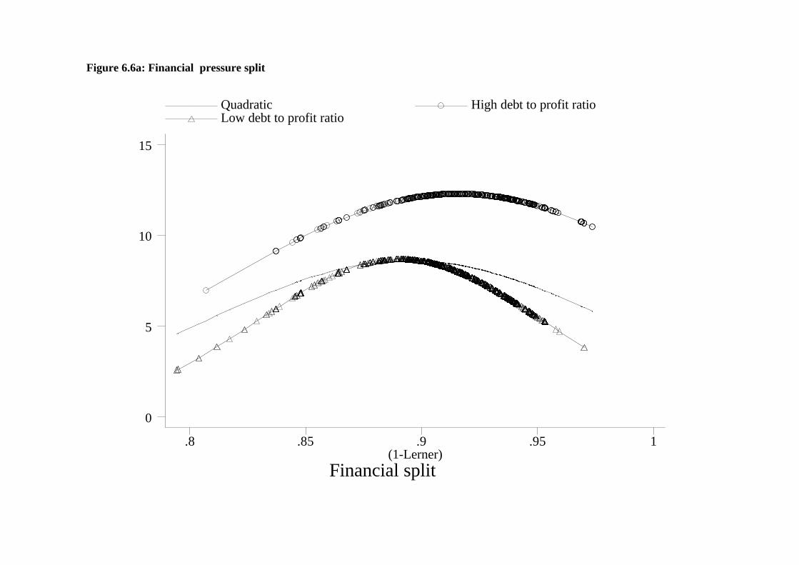
Figure 6.6a: Financial pressure split

Financial split(1-Lerner)

Quadratic High debt to profit ratio Low debt to profit ratio

.8 .85 .9 .95 1

0

5

10

15

Figure 6.6b: Financial pressure split, controlling for endogeneity of Lerner using control function

Financial splitControl function (Lerner)

Quadratic (IV) High debt to profit ratio Low debt to profit ratio

.8 .85 .9 .95 1

0

5

10

Figure A6.1a: Kernel Regression

Kernel regression, bw = .025, k = 6

1-Lerner

.86 .89 .92 .95 1

4

6

8

10

12

CW Patents

Figure A6.1b: Quadratic and spline with no controls

Cita

tion

wei

ghte

d pa

tent

s

Quadratic and spline with no controls(1-Lerner)

Quadratic Spline

.8 .85 .9 .95 1

0

2

4

6

Figure A6.1c: Quadratic and spline with year and industry effects

Cita

tion

wei

ghte

d pa

tent

s

Quadratic and spline with year and industry dummies(1-Lerner)

Quadratic Spline

.8 .85 .9 .95 1

4

6

8

10

Cita

tion

wei

ghte

d pa

tent

s

Quadratic with year and industry effectsBalanced panel

Balanced panel Unbalanced full sample

.8 .85 .9 .95 1

4

6

8

10

Figure A6.2: Balanced and unbalanced panel

Figure A6.3a: Using initial Lerner on sum of patents

Sum

cita

tion

wei

ghte

d pa

tent

s (7

1-92

)

Initial (1-Lerner).8 .85 .9 .95 1

0

500

1000

1500

2000

Figure A6.3b: Using lagged (once) Lerner

Cita

tion

wei

ghte

d pa

tent

s

Quadratic with year and industry effects(1-Lerner(t-1))

.8 .85 .9 .95 1

4

5

6

7

8

Figure A6.4: Neck and neck split (by TFP)

Cita

tion

wei

ghte

d pa

tent

s

Neck and neck split(1-Lerner)

More neck and neck industries Less neck and neck industries

.8 .85 .9 .95 1

0

5

10

15

Figure A6.5a: Neck and neck split, controlling for endogeneity of Lerner using control function

Cita

tion

wei

ghte

d pa

tent

sMore neck and neck industries Less neck and neck industries

.8 .85 .9 .95 1

0

5

10

15

Figure A6.5b: Neck and neck split, controlling for endogeneity of Lerner and split using control function

)C

itatio

n w

eigh

ted

pate

nts

More neck and neck industries Less neck and neck industries

.8 .85 .9 .95 1

0

10

20

30

Table 1: Distribution of observations with patents data by industry

Industry Accounting data only

Accounting and patent data

Total

22 Metal manufacturing 155 123 278 55.76 44.24 100.00 23 Extraction of other 17 34 51 33.33 66.67 100.00 24 Non-Metallic Mineral 320 200 520 61.54 38.46 100.00 25 Chemicals 222 348 570 38.95 61.05 100.00 31 Manufacture of metal 210 273 483 43.48 56.52 100.00 32 Mechanical engineering 917 783 1700 53.94 46.06 100.00 33 Office & Computing 72 31 103 69.90 30.10 100.00 34 Electrical and electronic 554 484 1038 53.37 46.63 100.00 35 Motor vehicles 318 210 528 60.23 39.77 100.00 36 Manufacture of other 133 117 250 53.20 46.80 100.00 37 Instrument engineering 45 48 93 48.39 51.61 100.00 41 Food manufacture 209 112 321 65.11 34.89 100.00 42 Sugar Beverages & 329 259 588 55.95 44.05 100.00 43 Textiles 458 310 768 59.64 40.36 100.00 45 Footwear and cloth 397 0 397 100.00 0.00 100.00 46 Wood Products & Furniture 300 0 300 100.00 0.00 100.00 47 Paper and Paper Products 564 241 805 70.06 29.94 100.00 48 Rubber & Plastic 146 117 263 55.51 44.49 100.00 49 Other manufacturing 227 51 278 81.65 18.35 100.00 Total 9418 4523 13941 67.56 32.44 100.00

Table 2: Lerner index and patent counts by industry

Average firm level Lerner Index Industry Accounting data

only Sample with

accounting and patent data

Average number of annual patents

14 Mineral oil processing 0.074 0 22 Metal manufacturing 0.060 0.053 13 23 Extraction of other minerals 0.153 0.183 9 24 Non-Metallic Mineral Products 0.077 0.114 40 25 Chemicals 0.092 0.100 330 31 Manufacture of metal goods 0.082 0.068 2 32 Mechanical engineering 0.074 0.076 55 33 Office & Computing Machinery 0.133 0.111 8 34 Electrical and electronic engineering

0.090 0.093 145

35 Motor vehicles 0.045 0.061 167 36 Manufacture of other 0.071 0.095 36 37 Instrument engineering 0.106 0.077 4 41 Food manufacture 0.060 0.068 15 42 Sugar Beverages & Tobacco 0.104 0.091 113 43 Textiles 0.062 0.075 3 45 Footwear and clothing 0.078 0 46 Wood Products & Furniture 0.077 0 47 Paper Paper Products & Printing 0.092 0.085 3 48 Rubber & Plastic Products 0.104 0.066 4 49 Other manufacturing 0.080 0.088 14 Total 0.077 0.079

Table 3: Descriptive Statistics

Mean (s.d)

Median Min Max

Patents 7.45 (30.77)

0 0 409

Cite weighted patents 7.45 (30.05)

0 0 392

(1-Lerner) 0.91 (0.025)

0.91 0.79 0.97

Employment (1000s) 11 (28.8)

1.5 0.04 312

Observations per firm 15.7 (5.34)

17 5 22

Technology gap (m) 0.80 (0.189)

0.89 0.004 0.98

Financial pressure 0.066 (2.85)

0.15 0 1

Table 4a: Regression results Figure: Figure

6.1a Figure

6.1b Figure 6.2a

Figure 6.2b

Figure 6.2c

Figure 6.2d

Observations 3248 3248 2662 3248 3248 1162

jtc 232.0 (12.12)

107.5 (16.35)

263.4 (18.31)

156.9 (27.71)

115.7 (18.49)

292.1 (141.5)

2jtc -133.3

(6.75) -60.1 (9.20)

-142.5 (10.28)

-83.6 (14.86)

-64.04 (10.33)

-165.3 (78.4)

Significance of:

2, jtjt cc 0.0000 0.0000 0.0000 0.0000 0.0000 0.0457

Year effects - 0.0000 0.0000 0.0000 0.0000 0.0076 Industry effects

- 0.0000 0.0000 0.0000 0.0000 0.0000

Notes: Significance test shows P-value from 2χ test of joint significance. Figure 6.1a: Quadratic and spline with no controls Figure 6.1b: Quadratic and spline with year and industry effects Figure 6.2a: Conditioning on firm level capital stock Figure 6.2b: Quadratic with year and industry effects, with Lerner corrected for fixed costs Figure 6.2c: Using alpha rather than 1-Lerner Figure 6.2d: Using R&D instead of patents (1980-1994; main sample 1990-1994)

Table 4b: Regression results Figure: Figure 6.4 Figure

6.5a, 6.5b (solid line)

Figure 6.5a Figure 6.5b

high low - high low high low 1288 1960 2491 926 1565 926 1565

jtc 112.0 (25.0)

218.6 (33.94)

159.7 (36.37)

374.7 (82.2)

299.1 (51.1)

453.5 (83.5)

453.6 (40.7)

2jtc -60.6

(14.16) -121.5 (18.71)

-87.41 (20.49)

-211.1 (46.6)

-165.9 (28.6)

-255.9 (47.4)

-257.4 (22.5)

Significance of:

2, jtjt cc 0.0000 0.0000 0.0000 0.0000 0.0000 0.0000 0.0000

year effects 0.0000 0.0000 0.0002 0.0000 0.0000 0.0000 0.0000 industry effects 0.0000 0.0000 0.0000 0.0000 0.0000 0.0000 0.0000 instruments in reduced form for

jtc

0.0000 0.0000 0.0000 0.0000 0.0000

instruments in reduced form for

2jtc

0.0000 0.0000 0.0000

instruments in reduced form for split

- - - - 0.0000

control functions in regression

- 0.0000 0.0000 0.0000 0.0000 0.0000

R2 of reduced form for jtc

0.8649 0.8667 0.8649

R2 of reduced form for 2

jtc 0.8668 0.8685 0.8668

R2 of reduced form - - - - 0.5433 Notes: Significance test shows P-value from 2χ test of joint significance. Excluded variables are: policy instruments discussed in section 5.2, imports over value-added in same industry-year in USA and France, TFP in same industry-year in USA and France, output minus variable costs over output in same industry-year in USA and France, estimate of markup from industry-country regression for USA and France (Martins et al 1996) interacted with time trend. Figure 6.4: Neck and neck split (by TFP) Figure 6.5a: Neck and neck split, controlling for endogeneity of Lerner using control function Figure 6.5b: Neck and neck split, controlling for endogeneity of Lerner and split using control function

Table 4c: Regression results

Figure: Figure 6.6a Figure 6.6b 2662 2662

jtc 253.7 (25.5)

313.1 (44.3)

2jtc -142.9

(14.3) -174.2 (24.9)

jtc *(financial pressure) -157.4 (27.1)

-248.4 (35.7)

2jtc *(financial pressure) 89.6

(15.0) 139.2 (19.8)

Financial pressure 69.3 (12.1)

111.0 (16.1)

Significance of:

2, jtjt cc 0.0000 0.0000

year effects 0.0000 0.0000 industry effects 0.0000 0.0000 instruments in reduced form for jtc 0.0000

instruments in reduced form for 2jtc 0.0000

control functions in regression 0.0000 R2 of reduced form for jtc 0.8550

R2 of reduced form for 2jtc 0.8570

Notes: Significance test shows P-value from 2χ test of joint significance. Excluded variables are: policy instruments discussed in section 5.2, imports over value-added in same industry-year in USA and France, TFP in same industry-year in USA and France, output minus variable costs over output in same industry-year in USA and France, estimate of markup from industry-country regression for USA and France (Martins et al 1996) interacted with time trend. Figure 6.6a: Financial pressure split Figure 6.6b: Financial pressure split, controlling for endogeneity of Lerner using control function