
Essays on Innovation, Strategy and Competition
143
Essays on Innovation, Strategy and Competition Citation Tabakovic, Haris. 2015. Essays on Innovation, Strategy and Competition. Doctoral dissertation, Harvard Business School. Permanent link http://nrs.harvard.edu/urn-3:HUL.InstRepos:25752983 Terms of Use This article was downloaded from Harvard University’s DASH repository, and is made available under the terms and conditions applicable to Other Posted Material, as set forth at http:// nrs.harvard.edu/urn-3:HUL.InstRepos:dash.current.terms-of-use#LAA Share Your Story The Harvard community has made this article openly available. Please share how this access benefits you. Submit a story . Accessibility
-
Upload
khangminh22 -
Category
Documents
-
view
1 -
download
0
Transcript of Essays on Innovation, Strategy and Competition
Essays on Innovation, Strategy and Competition
CitationTabakovic, Haris. 2015. Essays on Innovation, Strategy and Competition. Doctoral dissertation, Harvard Business School.
Permanent linkhttp://nrs.harvard.edu/urn-3:HUL.InstRepos:25752983
Terms of UseThis article was downloaded from Harvard University’s DASH repository, and is made available under the terms and conditions applicable to Other Posted Material, as set forth at http://nrs.harvard.edu/urn-3:HUL.InstRepos:dash.current.terms-of-use#LAA
Share Your StoryThe Harvard community has made this article openly available.Please share how this access benefits you. Submit a story .
Accessibility


Essays on Innovation, Strategy and Competition
A dissertation presented
by
Haris Tabakovic
to
The Strategy Unit at the Harvard Business School
in partial fulfillment of the requirements
for the degree of
Doctor of Business Administration
in the subject of
Strategy
Harvard University
Cambridge, Massachusetts
May 2015

© 2015 Haris Tabakovic
All rights reserved.
Dissertation Committee:Juan Alcácer (Chair)Andrei HagiuJosh Lerner
Author:Haris Tabakovic
Essays on Innovation, Strategy and Competition
Abstract
This dissertation is composed of three essays on innovation, strategy and competition. The
first essay studies how entry of patent intermediaries known as "patent assertion entities"
(PAEs) impacts behavior of other firms in the patent space. It uses deaths of individual
patent owners to exogenously identify PAE patent acquisitions, and estimates its impact
on follow-on citations. Finally, it shows that after being acquired by PAEs, patents lose
a large portion of their follow-on citations. These effects are driven almost entirely by
citing behavior of large entities and are robust to controlling for patent examiner-added
citations. This effect disappears once the acquired patents expire, indicating that large
entities may be acting strategically to reduce the likelihood of patent assertion. The second
essay investigates patent disclosure processes at seven large Standard-Setting Organizations
(SSOs) where participating entities have a choice between specific patent disclosures and
broad generic disclosures. It finds that large, downstream firms who face large technology
search costs prefer to use generic patent disclosures. In addition, it shows that higher quality
patents are more likely to be disclosed in specific disclosures, because they are more likely
to be monetized through licensing. The third essay estimates the causal impact of research
expenditures on scientific output. Unexpected college football outcomes provide exogenous
variation to university funds, and in turn, research expenditures in the subsequent year.
Using this variation, this essay estimates the dollar elasticity of scholarly articles, new patent
applications, and the citations that accrue to each.
iii
Contents
Abstract . . . . . . . . . . . . . . . . . . . . . . . . . . . . . . . . . . . . . . . . . . . . iiiAcknowledgments . . . . . . . . . . . . . . . . . . . . . . . . . . . . . . . . . . . . . viii
Introduction 1
1 Firms and Patent Assertion Entities 51.1 Introduction . . . . . . . . . . . . . . . . . . . . . . . . . . . . . . . . . . . . . . 51.2 Patent Monetization Entities . . . . . . . . . . . . . . . . . . . . . . . . . . . . . 11
1.2.1 Overview . . . . . . . . . . . . . . . . . . . . . . . . . . . . . . . . . . . 111.2.2 Impact on Firm Behavior . . . . . . . . . . . . . . . . . . . . . . . . . . 14
1.3 Patent Citations and Firm Strategy . . . . . . . . . . . . . . . . . . . . . . . . . 161.4 Data . . . . . . . . . . . . . . . . . . . . . . . . . . . . . . . . . . . . . . . . . . . 19
1.4.1 Description . . . . . . . . . . . . . . . . . . . . . . . . . . . . . . . . . . 191.4.2 Summary . . . . . . . . . . . . . . . . . . . . . . . . . . . . . . . . . . . 25
1.5 Empirical Design . . . . . . . . . . . . . . . . . . . . . . . . . . . . . . . . . . . 261.5.1 Overview . . . . . . . . . . . . . . . . . . . . . . . . . . . . . . . . . . . 261.5.2 Patent Owner Deaths . . . . . . . . . . . . . . . . . . . . . . . . . . . . 281.5.3 Specification . . . . . . . . . . . . . . . . . . . . . . . . . . . . . . . . . 321.5.4 Linear IV . . . . . . . . . . . . . . . . . . . . . . . . . . . . . . . . . . . . 331.5.5 Poisson Regression . . . . . . . . . . . . . . . . . . . . . . . . . . . . . . 35
1.6 Results . . . . . . . . . . . . . . . . . . . . . . . . . . . . . . . . . . . . . . . . . 361.6.1 Main Results . . . . . . . . . . . . . . . . . . . . . . . . . . . . . . . . . 361.6.2 Patent Examiner Effects . . . . . . . . . . . . . . . . . . . . . . . . . . . 371.6.3 Active vs. Expired Patents . . . . . . . . . . . . . . . . . . . . . . . . . 391.6.4 Small vs. Large Firms . . . . . . . . . . . . . . . . . . . . . . . . . . . . 40
1.7 Discussion . . . . . . . . . . . . . . . . . . . . . . . . . . . . . . . . . . . . . . . 411.8 Conclusion. . . . . . . . . . . . . . . . . . . . . . . . . . . . . . . . . . . . . . . 44
2 The Standard-Pool Interface 462.1 Introduction . . . . . . . . . . . . . . . . . . . . . . . . . . . . . . . . . . . . . . 462.2 Technical Standards and Disclosure Practices . . . . . . . . . . . . . . . . . . . 49
iv
2.2.1 Background . . . . . . . . . . . . . . . . . . . . . . . . . . . . . . . . . . 492.2.2 Hypotheses . . . . . . . . . . . . . . . . . . . . . . . . . . . . . . . . . . 53
2.3 Empirical Analysis . . . . . . . . . . . . . . . . . . . . . . . . . . . . . . . . . . 542.3.1 Data Sources . . . . . . . . . . . . . . . . . . . . . . . . . . . . . . . . . 542.3.2 Disclosure Preferences Across the Value Chain . . . . . . . . . . . . . 602.3.3 Disclosure Preferences and Patent Value . . . . . . . . . . . . . . . . . 65
2.4 Conclusion . . . . . . . . . . . . . . . . . . . . . . . . . . . . . . . . . . . . . . . 70
3 The Impact of Money on Science: Evidence from Unexpected NCAA FootballOutcomes 733.1 Introduction . . . . . . . . . . . . . . . . . . . . . . . . . . . . . . . . . . . . . . 733.2 US College and University Research . . . . . . . . . . . . . . . . . . . . . . . . 80
3.2.1 How Research is Funded . . . . . . . . . . . . . . . . . . . . . . . . . . 813.3 Data . . . . . . . . . . . . . . . . . . . . . . . . . . . . . . . . . . . . . . . . . . . 86
3.3.1 Sources . . . . . . . . . . . . . . . . . . . . . . . . . . . . . . . . . . . . . 863.3.2 Summary Statistics . . . . . . . . . . . . . . . . . . . . . . . . . . . . . . 90
3.4 Empirical Model . . . . . . . . . . . . . . . . . . . . . . . . . . . . . . . . . . . 923.4.1 Overview . . . . . . . . . . . . . . . . . . . . . . . . . . . . . . . . . . . 923.4.2 Specification . . . . . . . . . . . . . . . . . . . . . . . . . . . . . . . . . . 93
3.5 Results . . . . . . . . . . . . . . . . . . . . . . . . . . . . . . . . . . . . . . . . . 953.5.1 From Football to Money . . . . . . . . . . . . . . . . . . . . . . . . . . . 953.5.2 From Money to Scholarly Articles . . . . . . . . . . . . . . . . . . . . . 973.5.3 From Money to Scholarly Article Citations . . . . . . . . . . . . . . . . 1003.5.4 From Money to Patents . . . . . . . . . . . . . . . . . . . . . . . . . . . 1023.5.5 From Money to Patent Citations . . . . . . . . . . . . . . . . . . . . . . 1033.5.6 Exogeneity Check . . . . . . . . . . . . . . . . . . . . . . . . . . . . . . 1063.5.7 Discussion of Timing . . . . . . . . . . . . . . . . . . . . . . . . . . . . . 108
3.6 Conclusion . . . . . . . . . . . . . . . . . . . . . . . . . . . . . . . . . . . . . . . 111
References 115
Appendix A Appendix to Chapter 3 125A.1 Allocating patent filings to universities . . . . . . . . . . . . . . . . . . . . . . 125
A.1.1 Disaggregating state educational systems . . . . . . . . . . . . . . . . . 128A.2 A brief historical overview of college football . . . . . . . . . . . . . . . . . . . 128
v
List of Tables
1.1 Patent Data Sources . . . . . . . . . . . . . . . . . . . . . . . . . . . . . . . . . . 261.2 Summary Statistics, All Patents (1982-2012) . . . . . . . . . . . . . . . . . . . . 261.3 Summary Statistics, Enforcable Patents (1982-2012) . . . . . . . . . . . . . . . 271.4 Summary Statistics, Expired Patents (1982-2012) . . . . . . . . . . . . . . . . . 281.5 Deaths and Patent Transfers (1981-2012) . . . . . . . . . . . . . . . . . . . . . . 291.6 All Forward Citations, 1981-2012 . . . . . . . . . . . . . . . . . . . . . . . . . . 371.7 Large Entity Examiner-added Citation Effects, 2000-2012 . . . . . . . . . . . . 381.8 Small Entity Examiner-added Citation Effects, 2000-2012 . . . . . . . . . . . . 391.9 Active vs. Expired Patents, Large-Entity-only Citations, 2000-2012 . . . . . . 401.10 Active vs. Expired Patents, Small-Entity-only Citations, 2000-2012 . . . . . . 41
2.1 Summary of Patent Disclosures . . . . . . . . . . . . . . . . . . . . . . . . . . . 572.2 Summary of Patent Disclosures by SSO . . . . . . . . . . . . . . . . . . . . . . 582.3 Disclosure Preference Analysis – Variable Descriptions . . . . . . . . . . . . . 632.4 Disclosure Preference Analysis – Summary Statistics . . . . . . . . . . . . . . 642.5 Correlation Matrix for Firm Size Measures . . . . . . . . . . . . . . . . . . . . 652.6 Disclosure Type Results – Dependent Variable is Specific Disclosure . . . . . . 662.7 Patent Quality Analysis – Summary Statistics . . . . . . . . . . . . . . . . . . 672.8 Patent Quality Results – Dependent Variable is Specific Disclosure . . . . . . . 71
3.1 Football and university finances . . . . . . . . . . . . . . . . . . . . . . . . . . 843.2 The impact of football on non-federal research expenditures . . . . . . . . . . 963.3 The impact of money on scholarly articles . . . . . . . . . . . . . . . . . . . . . 983.4 The impact of money on scholarly articles’ citations . . . . . . . . . . . . . . . 1013.5 The impact of money on patent applications . . . . . . . . . . . . . . . . . . . 1043.6 The impact of money on patents’ citations . . . . . . . . . . . . . . . . . . . . 1053.7 Exogeneity check for instrument . . . . . . . . . . . . . . . . . . . . . . . . . . 1083.8 First stage timing . . . . . . . . . . . . . . . . . . . . . . . . . . . . . . . . . . . 1133.9 Second stage timing: scholarly articles . . . . . . . . . . . . . . . . . . . . . . . 1143.10 Second stage timing: patents . . . . . . . . . . . . . . . . . . . . . . . . . . . . 114
vi
List of Figures
1.1 Patent Expiration (1981-2001) . . . . . . . . . . . . . . . . . . . . . . . . . . . . 201.2 USPTO PAIR Coverage . . . . . . . . . . . . . . . . . . . . . . . . . . . . . . . . 251.3 Temporal Distribution of Patent Citations . . . . . . . . . . . . . . . . . . . . . 34
3.1 Football and scholarly articles . . . . . . . . . . . . . . . . . . . . . . . . . . . . 773.2 Football and scholarly article citations . . . . . . . . . . . . . . . . . . . . . . . 783.3 Football and new patent applications . . . . . . . . . . . . . . . . . . . . . . . 793.4 Football and patent citations . . . . . . . . . . . . . . . . . . . . . . . . . . . . 803.5 Geographic distribution of schools by type . . . . . . . . . . . . . . . . . . . . 893.6 Timing of football, research, and publishing . . . . . . . . . . . . . . . . . . . 933.7 Impact of football on federal vs. non-federal funding . . . . . . . . . . . . . . 107
A.1 Patent applications filed over time . . . . . . . . . . . . . . . . . . . . . . . . . 126
vii

Acknowledgments
I am thankful for the help, support and guidance I received from my advisers: Juan Alcácer,
Josh Lerner and Andrei Hagiu. They took the time to listen to my ideas, challenge and
criticize them, only to see them develop and mature into a finished product worthy of a
doctoral dissertation. Their insights and contributions remolded my thinking and forged a
new lens through which I view the world.
I am grateful for the encouragement and advice of Jean Tirole and Dennis Yao. I am also
thankful for engaging conversations with Anil Doshi, Janet Freilich, Clarence Lee, Jamie
Lee, Cynthia Montgomery, Robert Sitkoff, Kyle Welch and numerous other faculty and
students. Their comments contributed clarity and focus to my academic investigation. I
owe a debt of gratitude to William Lee, Joseph Mueller and George Shuster of WilmerHale.
Their willingness to generously share their time and knowledge of legal practice with me
was an invaluable asset in my research endeavors.
I was blessed to be surrounded by an amazing group of friends. Anoop Menon, Thomas
Wollmann, and many others provided inspiration, support and intellectual stimulation for
which I am immensely grateful. Our, often lengthy discussions did not always converge,
but they always provided food for thought and sparked a glut of provocative ideas.
I would like to thank John Korn, Dianne Le, Janice McCormick, Jennifer Muccarione,
and Marais Young for outstanding administration of the Harvard Business School’s doctoral
program. Their thoughtful deployment of school’s resources always revolved around the
success and wellbeing of doctoral students.
I would also like to thank Chris Allen, Leslie Burmeister, Sarah Eriksen, Barbara Esty,
Kevin Garewal and James Zeitler at the Baker Library and the Baker Research services
for their help with acquiring and deciphering large quantities of data. I am indebted to
Troy Adair, John Galvin, Andrew Marder, Lauren Ross-Miller, John Sheridan and Sarah
Woolverton at the Research Computing Services for ensuring that adequate data processing
and computing resources were always available for my computational struggles.
Finally, I will always be beholden to my family for their unwavering support. To my
viii
amazing wife, Tina Christodouleas for believing in me and standing by my side through all
ups and downs. Without her selfless dedication to our family, the completion of this work
would be all but impossible. To my children Naia, Lejla and Iason for keeping me firmly
grounded, teaching me many invaluable lessons about life, and being a perpetual source of
joy and excitement. To my parents, Ibrahim and Meliha for their unconditional love and the
gift of insatiable curiosity. To my sister, Amra for her kindness and loyalty.
ix

Dedicated to my family.
x
Introduction
How do firms adjust their strategies in response to environmental pressures and competition?
And, more importantly, how do those dynamic processes impact technological innovation?
These are some of the key questions in strategy and economics, and those that have
generated a significant amount of attention over the years. Situated at the intersection of
law, economics, and firm strategy, this dissertation sheds more light on these topics as it
focuses on specific processes that can catalyze or inhibit innovation. In particular, three
such phenomena are examined in detail: 1) entry of patent intermediaries, 2) competition in
standard-setting processes, and 3) productivity of knowledge-generating institutions.
The first essay shows that highly litigious activity of “patent trolls” significantly reduces
subsequent citations of affected technologies, potentially balkanizing the technological space
and reducing follow-on innovation.
Markets for technology are plagued with frictions – high search costs and uncertainty
being the main culprits. An intense policy debate is brewing about the role of market inter-
mediaries in markets for technology and their effects on market efficiency and innovation.
While some specialized intermediaries attempt to foment efficient exchanges of patent rights,
others attempt to capitalize by enforcing patents on a large scale. A drastic rise in activity of
patent assertion entities, commonly referred to as “PAEs” or “patent trolls” is behind the
three-fold increase in the number of US patent assertion cases in the last five years. Rather
than develop new technology themselves, patent trolls specialize in opaquely acquiring
existing patents and strategically asserting them in a very aggressive fashion. Because of
their litigation-optimized organizational form and stealthy operations, patent trolls are
1
particularly interesting as they represent an asymmetric threat for operating firms. Despite
the fact that a prospect of patent litigation can have a significant impact on firms’ behavior,
interrupting knowledge flows and diverting them around technological areas where patent
trolls are present, there is a lack of empirical work on this issue.
This essay uses deaths of individual patent owners as an instrument for patent troll
activity, since estates tend to sell or license out intellectual property assets quickly. It shows
that a highly disproportionate number of recently deceased inventors’ patents is acquired by
patent trolls, and finds that after patent troll acquisitions, large firms strongly avoid citing
these patents. This effect disappears after the focal patent expires. Moreover, I show that
the instrument is a good predictor of patent troll presence in a patent class, and find that
firms avoid these patent classes while the troll-owned patents are legally valid. After being
acquired by patents trolls, patents lose almost 6 citations, or almost 40% of all citations on
average. These effects are driven almost entirely by the citing behavior of large entities and
are robust to controlling for patent examiner-added citations. My results raise two important
issues: the first one is that aggressive patent assertion could potentially have negative effects
on knowledge flows, and the second one is that firms may respond to litigation threats in
patent space by strategically avoiding sourcing of technological knowledge from threatened
domains, thus raising doubts about “inequitable conduct" policy and its effectiveness in
preventing strategic citations of prior art. Both of these have a potential to significantly
impact the performance of the innovation ecosystem and stand out as important areas to be
studied in the future.
The second essay, co-authored with Josh Lerner and Jean Tirole, explores the process
of selection of standard essential patents, their subsequent inclusion in patent pools, and
firm-dependent patent disclosure strategies.
Technological standards determine functionalities, capabilities, interoperability and
evolution of products, services and technologies. A high degree of interdependence and
complexity in modern high-tech product architectures makes technological standards ubiq-
uitous and more important than ever. Standards are usually shaped by standard-setting
2
organizations (SSOs) and participating firms required to disclose all standard-essential
patents in their ownership. An important policy issue in standard setting is that patents
that are ex-ante not important may, by being included into the standard, become standard-
essential patents. In an attempt to curb the monopoly power that they create, most standard
settings organizations require the owners of patents covered by the standard to make a loose
commitment to grant licenses on fair, reasonable and nondiscriminatory terms, even though
such commitments are often conducive to intense and costly litigation activity ex-post.
Commitments made during the standardization process are at the heart of many legal
battles, as some firms have made attempts to “game” the system. SSO-participating entities
usually have a choice between specific patent disclosures and broad generic disclosures.
Little is known about what drives their disclosure strategies and how they may be impacted
by the underlining patent quality.
In this study, a novel dataset is created by linking 21 patent pools with relevant technol-
ogy standards at seven large SSOs and combining standard-disclosed and pooled patent
data with firm financial information. Subsequent analysis finds that, consistent with theory,
large firms with downstream presence face large technology search costs and are more likely
to utilize generic patent disclosures. In addition, it also finds that higher quality patents
are more likely to be disclosed in specific disclosures, because they are more likely to be
monetized through licensing. These results indicate that firms approach standardization
process strategically and closely align patent disclosure decisions with their competitive
advantage.
The third essay, co-authored with Thomas Wollmann, is the first study that derives a
causal estimate of university research funding on scientific output, where that output is
measured in citation-weighted academic publications and citation-weighted patent applica-
tions.
Colleges and universities conduct a gargantuan share of research and development in
the United States, and account for the majority of basic science expenditures. Without any
downstream presence of their own, these institutions act as highly specialized “knowledge
3
generators” in the national innovation economy and help drive economic growth through
scientific discovery. Unfortunately, the high cost of research often makes funding a limiting
factor for scientific advance and represents a policy matter of national importance. At this
point, little is known about the causal impact of money on science, despite its importance
for determining the socially-optimal level of R&D.
This study seeks to inform the debate about the funding of scientific research in the
United States and provide insight into how specialized knowledge producers respond to
unexpected positive shocks in R&D funding. It estimates the dollar elasticity of research
output at American universities by using unexpected NCAA football outcomes to exoge-
nously shift research budgets across schools and time. After presenting a novel dataset of
historic team success, measured by vote tallies from the Associated Press Top 25 Poll, this
essay shows that unexpected within-season changes to this measure are strong predictors
of university-sponsored research funding in the subsequent period. These changes do not
predict university-sponsored funding in the contemporaneous period or federally-sponsored
research in any period, lending further support for the instrument. An elasticity of 1.91 is
found when the outcome is patent applications count and 3.3 when the outcome is patent
citations count; 0.31 when the outcome is scientific publications count, and 0.59 when the
outcome is count of citations that subsequently accrue to those publications. The cost to the
university, at the margin, of additional research funding to generate an idea worth of filing
a patent application is estimated to be between $2.6 and $3 million. For each outcome, the
instrumental variable results contrast sharply with the OLS estimates, which are significant
but near zero and would lead policymakers to underinvest in research. These results imply
that there are constant positive returns to funding of university R&D, and that optimal
policy decision should not seek to reduce funding to R&D.
4
Chapter 1
Firms and Patent Assertion Entities
1.1 Introduction
While spurts in patent enforcement activity have not been an uncommon sight in the past,
over the last five years, patent assertion entities “trolling” the patent space have been a major
contributor to the precipitious rise in the number of patent assertion lawsuits. Without
manufacturing or innovative footprint of their own, these opaque and highly specialized
entities acquire and assert patents en masse. In 2012 alone, the total number of patent lawsuits
rose by 29% over the previous year and almost doubled since 2009 [PricewaterhouseCoopers,
2014]. A portion of new lawsuits were certainly caused by competitive battles of large firms,
especially those in the smartphone arena. However, over 60% of all new lawsuits filed in
2013 originated from PAEs, while the top 10 plaintiffs filing most new cases in 2013 were
all PAEs [Byrd and Howard, 2014, RPX Corporation, 2014]. As the PAE activity intensified,
so did the discourse between the supporters on the one side, and the opponents of patent
assertion business model on the other side.
The main point of contention focuses on the role of PAEs in the technological ecosystem
and whether their net impact on cummulative innovation is positive or negative. Empirical
work on PAEs is scarce for at least two reasons. First, the steep rise in PAE activity is
relatively recent, and data identifying patent portfolios held by PAEs is lacking. Second,
5
PAEs select which patents to acquire and assert, so the relationship between PAE activity
and subsequent firm behavior will be biased away from—or even the wrong sign as—the
true causal impact of PAEs.
In this paper, I construct a new dataset of PAE patent acquisitions and use the death
of individual patent owners as an instrument for PAE patent acquisition activity. When a
patent owner dies, estate trustees tend to sell or license intellectual property assets, which
can be acquired by PAEs. I show that a disproportionate number of these patents ends
us being either acquired or licensed by PAEs, and later used to extract rents from other
firms in the technological space. I show that, subsequent to patents being acquired by
PAEs, large entities strongly avoid citing them to reduce the risk of becoming an assertion
target. This effect disappears after the patent expires. On the other hand, small entities
cite PAE-owned patents more, with this effect increasing in magnitude after the patent
expires. This is consistent with previous studies indicating that large firms are more aware
of their environment and highly strategic in their choices of which patents to cite, and which
technology to build-on [Allison and Lemley, 1998, Ziedonis, 2004, Lampe, 2012]. My results
also indicate that PAE activity could, in fact, boost cumulative innovation amongst small
companies, to the extent that those are proxied by the patent citation patterns.
A subject of an intense debate, the impact of recent spike in PAE activity on firms
and innovation is important for inventors, managers, lawyers, academics, investors, and
policymakers alike1. On one side of the aisle, arguments for innovation-enhancing role of
PAEs underline their importance in reducing technology search costs, increasing liquidity
of market for patents and providing previously scarce patent monetization and enforcement
opportunities for small firms and individual inventors [McDonough, 2006, Geradin et al.,
2011, Risch, 2012]. On the other side, opponents of PAEs underline deadweight loss arising
from unnecessary licensing fees, high litigation costs and skewed incentives to innovate
1See the Federal Trade Commission and the Department of Justice “patent monetization entity ActivitiesWorkshop”:http://www.ftc.gov/news-events/events-calendar/2012/12/patent-assertion-entity-activities-workshop (lastaccessed on 10/10/2014)
6
[Bessen et al., 2011]. This controversy has even attracted the attention of the White House
to make a call for a deeper patent reform and invited remarks by the US President Barack
Obama2:
The folks [PAEs] that you’re talking about are a classic example. They don’tactually produce anything themselves. They’re just trying to essentially leverageand hijack somebody else’s idea and see if they can extort some money out ofthem.
So far, 17 bills dealing with various aspects of patent reform have been introduced by the
US Congress over the last two years to deal with the glut of PAE-intiatied patent assertion
lawsuits.3 It is important to note that while patent enforcement in itself is one of the key
components of a robust intellectual property system, the concern over extensive PAE patent
enforcement arises mainly from the large-scale economic impact and all-too-common lack
of transparency in PAE operations. Assertion of patent rights is a mechanism designed to
protect temporary exclusivity of patent rights. It is intended to compensate patent holders
for their creative endeavors and enhance their incentives to innovate. Not exclusively
reserved for firms’ competitive maneuvers, patent assertion is also a tool for individual
inventors, small and non-profit entites to prevent expropriation and obtain compensation
for their innovative efforts. The effects of patent assertion have been studied extensively
in law, economics and strategy to show that, as a part of firms’ competitive arsenal, it
can be used to reduce competitive pressures and increase barriers to entry. For example,
established, large firms were found to use assert patents disproportionately against smaller
firms, while smaller firms were found to avoid patenting in and entering dense technological
areas, especially those with many litigation-happy firms [Lerner, 1995, Lanjouw and Lerner,
2001, Lanjouw and Schankerman, 2001, Cockburn and MacGarvie, 2011]. Firms were also
2President Barack Obama, “Fireside Hangout,” White House YouTube Channel, February 14, 2013, AccessedMay 5, 2015. https://www.whitehouse.gov/blog/2013/02/14/watch-president-obama-answers-your-questions-google-hangout
3See Patent Progress website for the full list:http://www.patentprogress.org/patent-progress-legislation-guides/patent-progresss-guide-patent-reform-legislation/ (last accessed on 10/07/2014).
7
found to be likely to enforce their patent rights to signal “toughness,” build reputation in
their respective technology and market spaces, and transmit information about the strength
of their patent portfolio to potential entrants and competitors [Choi, 1998, Crampes and
Langinier, 2002].
While there is empirical evidence that firms react to hold-up threats from direct competitors
by agressive patent portfolio building, mergers and acquisitions, joint ventures and patent
pooling [Hall and Ziedonis, 2001, Ziedonis, 2004], the work on how firms react to PAE
activity is scarce. As highly opaque entities without any manufacturing operations of their
own, and with patent holdings divided across many shell companies and subsidiaries they
are difficult to defeat on a legal battlefield. Extensive patenting gives firms rights to exclude
others from utilizing and profiting from patented technologies, while it does not give them
absolute rights to practice those patented technologies themselves. This nuanced legal point
is what keeps patent assertion business model viable. Conventional intellectual property
strategies commonly used to keep competitors at bay are laregly ineffective against PAEs, as
they represent an asymmetric threat, and are optimally organized for informational and
legal arbitrage in the patent space.
PAE-targeted firms usually have a limited set of options. The first one is to face a long,
expensive, and often unpredictable legal battle in order to invalidate PAE-asserted patents
or asserted claims of infringement. The prospects of such a battle can be daunting and can
make a serious dent in the company value sheet. Hence, a promise of a quick settlement
“priced” well below the cost and risk of a protracted patent litigation would look appealing
to any rational firm [Cohen et al., 2014, Feldman and Price, 2014]. Many firms favor this less
costly option, and in order to avoid protracted litigation, reach a quick settlement with PAEs
and pay patent licensing fees to make the threat “go away”. This particular PAE strategy
flavor has a strange resemblance to organized crime extortion rackets, and has incited some
firms to attempt to fight back and counter-sue PAEs under Racketeer Influenced and Corrupt
Organizations (RICO) Act, albeit without much success.4 Firms could also insure themselves
4There were two recent, albeit unsuccesful cases where defendants tried counter-suing PAEs under RICO
8
against patent infringement to cover unexpected litigation costs, but this market is not well
developed and the policies are relatively expensive.5 Firms can also try to pre-empt the
threat and reduce the risk of unwelcome assertion by either basing their products on “open”
technologies [Lerner and Tirole, 2005] and building the chest of prior-art publications [Baker
and Mezzetti, 2005], or signaling that their activities are not related to technological domains
rife with PAE activity. In the similar fashion as the biotech firms with high-litigation costs
who avoid patenting in technological areas crowded with highly litigious entities [Lerner,
1995], firms can strategically avoid drawing on technology and building on knowledge
originating in areas with high PAE activity, if that would decrease their litigation risks.
Most contemporary studies that examine consequences of PAE activity tend to be
focused on PAE business models, their direct costs to the firms and immediate outputs
like R&D spending and patent counts, while overlooking these important strategic choices.
Merges [2009] suggests that extensive patent trolling could result in an overall reduction in
innovation and the number of new products to hit the market and Chien [2014] provides
descriptive evidence that small firms targeted by PAEs are often disrupted, forced to
make operational as well as strategic trade-offs and sometimes even exit product markets.
Relatedly, Bessen and Meurer [2014] estimate the aggregate cost of PAE litigious activity to
be a whopping $29 billion, and suggest that monetary transfer to inventors represents a very
small portion of that amount — sometimes as low as 5% of the direct cost to PAE-targetted
firms. However, while suggesting that the high cost of PAE litigation may force firms to
reallocate funds from R&D to legal activities and reduce innovation, they do not provide
any direct evidence as to what the impact may be on how firms may respond to reduce PAE
exposure and how these responses may play out in the patent space. Several recent studies
Act. The first one was jointly brought by Cisco, Netgear and Motorola against Innovatio IP, while the secondone was filed by FindTheBest against Lumen View. Also, in 2011, Kaspersky Labs sent a letter to FBI requestingthat they investigate RPX Corp for RICO violations because of suspicious, extortion-like behavior related to apending patent lawsuit brought on by IPAT, LLC – a firm who had previously licensed asserted patents to RPX.
5General patent litigation insurance premiums range between 1-5% of the insured amount, which can reachhundreds of millions. (website http://www.hahnlaw.com/references/501.pdf (accessed 10/27/2014)) As adefensive patent aggregator, RPX Corporation does offer a specific PAE insurance policy with premiums ofabout $7,500 for $1 million in coverage. (http://www.rpxcorp.com/rpx-services/rpx-litigation-insurance/)
9
try to address this issue in more detail: Cohen et al. [2014] and Smeets [2014] find that
patent litigation negatively affects corporate R&D spending and output for publically listed
US firms, particularly if initated by a “patent troll”, while Tucker (2014a; 2014b) specifically
addresses trolling effects and finds that PAE activity may reduce venture capital investment,
as well as incremental product innovation and downstream sales. In high-tech industries
that rely on standardization to ensure device interoperability, the risks and potential costs
stemming from PAE-related hold-up can be exceptionally high6 [Shapiro, 2001].
I follow this line of research and examine the effects of increased PAE exposure on
firm behavior and cumulative innovation by focusing not on monetary measures of R&D
spending or direct patent counts, but rather on how firms try to reduce litigation risks
following the entry of PAEs. This paper contributes to a long line of literature on patent
rights, patent assertion, strategy and innovation, and is close in spirit to Lerner [1995],
Lampe [2012] and Galasso and Schankerman [2015]. While Galasso and Schankerman
[2015] show that a growth in cumulative innovation as proxied by patent citations after
invalidations of patents owned by large firms stems from increased participation of small
firms, I show that the negative effect on patent citations after PAE entry is due to strategic
behavior of large firms, i.e. PAE acquisition of a patent causes large firms to cite that patent
less. The effect on small firms is completely opposite. I also contribute to recent set of
studies indicating stricter property rights as a damper for follow-on innovation [Murray and
Stern, 2007, Williams, 2013] and show that a rampant over-enforcement of property rights
forces the firms to respond in a way that could potentially dampen cumulative innovation,
especially for those firms more aware of litigation risks.
The rest of this paper is organized as follows. Section 2 examines the patent assertion
entities in more detail and provides theoretical implications of their activity. Section 3
discusses knowledge flows and their relationship with patent citations, innovation and
6A good example is the case of of Wi-Fi technology and Innovatio IP Ventures. Wi-Fi technology is basedon a IEEE 802.11 standard, and after Innovatio IP Ventures acquired a set of patents declared essential to thisstandard, they proceeded to send patent infringement letters to thousands of Wi-Fi end-users: hotels, coffeeshops, restaurants, grocery stores and many more.
10
firm strategy. Section 4 describes the data sources. Section 5 presents variables, and lays
out empirical strategy. Section 6 gives the descriptive statistics and model robustness
tests. Section 7 provides additional discussion of the results and shortcomings of the study.
Section 8 concludes.
1.2 Patent Monetization Entities
1.2.1 Overview
Although often hailed as a recent phenomenon, the business of purchasing and asserting
patents without clear intention to commercialize them has been around since the early days
of US patent system.7 Patent trade was surprisingly well developed during 19th century and
many specialized intermediaries were participating in the market, including patent assertion
entities [Lamoreaux and Sokoloff, 1999, Khan, 2014]. There are numerous examples of
various non-manufacturing entities engaging in patent assertion practice during industrial
revolution and targeting many different industries: smelting, agriculture, woodworking,
railroads and even automobiles8. Today, PAEs fall in the class of modern intellectual
property intermediaries together with IP brokers, defensive patent aggregators and hybrid
IP intermediaries [Hagiu and Yoffie, 2013]. They do not manufacture any products and
capitalize on information asymmetry in the market by acquiring patents from other entities
only to later assert them against other, usually producing firms. Because of the secrecy
surrounding PAE operations, it is not always immediately clear where acquired patents
originated: some are acquired from large, active operating companies,9 while the significant
portion is acquired from small firms and individual inventors. For example, Risch [2015]
puts the number of PAE patents acquired from individuals and their companies to over 43%,
and Chien [2012] reports that patents acquired from individuals compose almost 30% and
7“Trolling” as a business model is not exclusive to patents only. This phenomenon also impacts otherintellectual property assets classes, like copyrights and trademarks. See Folgers [2007] or Sag [2015], for example.
8See Merges [2009] and Khan [2014] for examples.
9This phenomenon is known as “patent privateering” [Ewing 2012a, 2012b].
11
those acquired from small companies—including individual-inventor-owned companies—
almost 50% of the overall PAE patent acquisitions made in 2010-2011.
These patent acquisitions are often done when original owners are under distress and
have a urgent need to monetize their assets in a “fire sale”: costly divorce proceedings
facing individual inventors10 or financial problems facing a firm, individual inventor or
a start-up are common reasons for patents to be sold11. PAE arbitrage strategy is further
corroborated by PatentFreedom12, a firm that collects and analyzes data related to PAE
activity. According to PatentFreedom, only 19% PAEs are original patent assignees, while
69% are pure patent acquirers.13 Their data also indicates that almost two-thirds of patents
litigated by PAEs in 2011-2012 were patents acquired from someone else.
In these transactions, PAEs effectively utilize frictions in the market for patents: asym-
metric information and the lack of an efficient price discovery mechanism allow them
to “buy low and sell high”. Patents are usually acquired for a fraction of the revenues
generated via subsequent licensing and assertion. This type of market arbitrage is largely
similar to strategies employed by art dealers and brokers.14 In the case of PAEs, information
arbitrage is combined with legal arbitrage to enable them to deliver a maximum punch. For
a manufacturing firm, the strategy of “mutually assured destruction” is a credible detterent
and a very effective response to patent assertion by another manufacturing competitor.
These firms often build large, overlapping patent thickets just so that once a competitor
initiates a patent assertion lawsuit, they can respond with an immediate patent assertion
lawsuit of their own. For example, when Apple sued Samsung for infringement of its
patented designs in the US, Samsung immediately countersued Apple for infringement
of its 3G technology patents. As Hall and Ziedonis [2001] and Ziedonis [2004] point in
10Comment made during in-class discussion by an executive from Intellectual Ventures.
11See McFeely [2008] for an example.
12As of June 2014, PatentFreedom is a part of RPX Corporation, a large defensive patent agregator.
1312 % are a blend of the two. For additional information, see https://www.patentfreedom.com/about-PAEs/background/
14See Wall Street Journal “Why You Can’t Always Trust Art Dealers “ for more detail.
12
their study of patenting in semiconductor industry, this strategy usually results in a mutual
hold-up stalemate and resolves in a settlement involving cross-licensing of each other’s
patents. Kab-tae Han, a senior intellectual property manager of Samsung’s digital media
business reveals this approach as a key part of their IP strategy [Han, Kab-tae, 2004]:
At one time, when we received a patent claim from another company, wedid not have any idea how to deal with the situation. It was quite naturalthat our strategy was focused on how we could pay less. But now we have arelatively good patent portfolio. This means that we can counter-claim againstother companies, which leads us to have more cross-licences. We changed ourstrategy to become more aggressive. We think that having good patents is thebest strategy.
When it comes to competitive interactions between large, operating firms and the PAEs,
“mutually assured destruction” approach is ineffective since PAEs do not have any down-
stream presence. So, while Samsung can respond to Apple’s patent assertion claims by
countersuing Apple and requesting injunction against sales and/or manufacturing of their
products, Samsung cannot do that against a PAE simply because there are no products
or sales to begin with. For the same reason, cross-licensing is also not a viable strategy
against PAEs. In the same interview, Kab-tae Han notes that one of the biggest challenges
for companies like Samsung is dealing with upstream patent owners Han, Kab-tae [2004]:
Another challenge is that many venture companies or individuals who havedone only R&D activities come to the manufacturer asking for higher royalties.This is very tough for companies like us.
Recognizing that PAE litigiousness can have adverse effects on firm’s incentives to build
upon PAE-owned technologies, we can expect a transfer of patent rights to PAEs to lead
to a decrease in observable follow-on innovative activity. Jeruss et al. [2012] point out that
regardless of whether patent intermediaries assert patents themselves and behave as pure
PAEs, or transfer them to other parties to be asserted, the net effect on the market should
be the same. However, given that citing and building upon PAE-owned patents might
increase the probability of an assertion lawsuit, it is hard to believe that market reaction to
PAE-owned patent vs. operating firm-owned patent would be the same. In other words,
13
if a non-practicing entity acquires a patent and transfers it to an operating company for
downstream assertion, the market should react in a different fashion than if that patent was
to be asserted by the non-practing entity itself. For practicing firms in an industry, building
on each-other’s technologies and cross-citing each other’s patents could help delineate
the differences between competing technologies and reduce the probability of a follow-on
lawsuit. On the other hand, the effect for PAE-owned patents would be just the opposite.
1.2.2 Impact on Firm Behavior
Firms learn from their experiences. Productivity improvements arising from firms’ previous
experiences have been documented in various settings: aircraft manufacturing [Alchian, 1963,
Mishina, 1999, Benkard, 2000], ship manufacturing [Rapping, 1965, Thornton and Thompson,
2001] and automobiles [Levitt et al., 2013]. This phenomenon of “learning-by-doing” points
to the existence of an invisible feedback loop that connects knowledge and capabilities
acquired through experience directly to the firm’s production function. Firms learn how to
source, integrate and utilize knowledge in order to improve their performance [Cohen and
Levinthal, 1990]. Experiental learning impacts firm behavior in all aspects of their operations.
Since experience comes with age, and firm age is highly correlated with firm size, I expect
larger firms to be more strategically astute in the patent space [Jovanovic and MacDonald,
1994, Lerner, 1995, Cabral and Mata, 2003, Ziedonis, 2004]. Large firms patent more, patent
more aggressively and have larger patent portfolios [Ziedonis, 2004]. They often have
internal patent review boards and employ internal corporate patent counsel [Lerner, 1995].
They carefully manage prior art during patenting process: Alcácer et al. [2009] show that
large firms receive larger share of examiner-added citations, and Lampe [2012] shows that
they strategically withold prior art to maximize the likelihood of patent issue. Large firms
are likely to be more cognizant of an PAE threat, and act to minimize its exposure. Recent
public actions of large firms like Google all but confirm their awareness of PAE hold-up
risk. For example, in 2014 Google, Cannon, Dropbox and other large companies formed a
License-on-Transfer (LOT) coalition that automatically extends a royalty-free patent license
14
to all members when a member-owned patent is sold to a non participating company.15
This move is largely set to counter a rise in patent privateering and prevent operating
companies from contributing to proliferation of PAE activity. Patents can be transferred
from operating firms to PAEs and have them act as “privateers” to atack direct competitors
with minimal operating firm exposure and without any risk of being counter-sued. Some
operating companies could take this strategy one step further and dissagregate their patent
holdings across many PAEs to inflict even higher damage on their competitors 16[Lemley
and Melamed, 2013].
While there are PAEs who follow the “machine gun” approach and assert their patents
widely against as many firms as possible, requesting modest royalties and licensing fees in
hope to profit from the sheer scale of the operation,17 large companies still represent a juicier
target. According to PatentFreedom, the top 30 companies most pursued by PAEs account
for more than 3300 PAE patent lawsuits between 2009-2014, and are all large, operating
companies ranging from Apple and Samsung to Walmart and Target.18 Many PAEs focus
on acquiring higher value patents to position themselves favorably against large, highly
profitable companies. This approach has a potential to yield large settlement payoffs, and
is further corroborated by Cohen et al. [2014] who find that PAEs opportunistically target
firms flush with cash. Proliferation of sofware and business methods patents, and high
degree of patent right fragmentation in high-tech industries helped make this a profitable
strategy [Lerner, 2010, Feldman and Price, 2014]. A choice of who to pursue in the value
chain can have a significant impact on the final payoff: directly asserting patents against
an upstream provider in some instances can be more costly and yield a lower payoff than
15See http://www.lotnet.com/
16For example, if a single technology is covered by a set of N patents, then the patent owner can divide themaccross N PAEs, thus fragmenting or “disaggregating” that technology. This patent owner would then maintaina backdoor license to each one of the patents, effectively multiplying the returns from this set of patents bysome factor N-k, where N>k>0 . At the same time, any cost for the competitor would be also be multiplied bythe same factor.
17A case of Wi-Fi technology and Innovatio IP Ventures is a great example.
18See https://www.patentfreedom.com/about-npes/pursued/
15
prosecuting all the downstream users [Feldman and Price, 2014]. In addition, asserting
patents against downstream users who may have more elastic demand function and lower
switching costs, may put a great deal of indirect pressure on upstream technology providers
and force them to license asserted patents, especially in the markets with strong network
effects. For example, in his 2013 testimony before the U.S. House of Representatives, Jamie
Richardson, a vice president of the White Castle burger chain called for the patent reform
and highlighted the waste of company’s resources and time caused by frequent PAE patent
assertions as well as the subsequent hesitation in the adoption of the new technologies
related to online and mobile marketing, ordering and payment systems.19
Small firms, on the other hand, have a much more limited arsenal against PAEs at
their disposal. In addition to being less knowledgeable about intricacies of the intellectual
property space than the large firms, they are also more strapped for cash and more likely
to avoid prolonged legal wranglings. Thus a PAE infringement letter is more likely to be
settled with a quick license payment and an non-disclosure agreement. Small firms often
lack funds to employ in-house patent counsel and may abstain from hiring expensive patent
prosecutors. Without added sophistication and experience with patents, these firms are
more likely to rely on more visible or in-licensed patents for prior art. In addition, small
firms also happen to be less diversified and more likely to have their operations concentrated
in a narrow technological domain. Hence, small firms are unlikely to avoid PAE-owned
patents as prior art in a strategic fashion.
1.3 Patent Citations and Firm Strategy
Ever since Jaffe et al. [1993] utilized patent citations to study localization of knowledge
spillovers, the citations have been widely used in economics and management as a mea-
sure of knowledge flows in many different contexts: from academic instutions to firms
19The Impact of Patent Assertion Entities on Innovation and Economy: Hearing Before the House Energy & CommerceSubcommittee on Oversight & Investigation, United States House of Representatives, 113th Congress (2013)(statement of Jamie Richardson, Vice President of Government, Shareholder and Community Relations at WhiteCastle System Inc.)
16
[Henderson et al., 1998, Gittelman and Kogut, 2003], within firms [Zhao, 2006, Alcácer
and Zhao, 2012], between firms [Rosenkopf and Almeida, 2003, Singh and Agrawal, 2011]
and across geographies [Singh, 2005, MacGarvie, 2005]. While patent citations have been
used to map out knowledge flows and follow-on innovation, they have also been shown
to be susceptible to noise. Alcácer and Gittelman [2006] show that patent examiners add a
significant number of patent citations. Roach and Cohen [2013] highlight errors-in-variables
problem when patent citations are used as measures of knowledge flows, and identify
private knowledge flows and strategic citations as two sources of systematic measurement
errors. Other authors have also noted similar issues. For example, firms were found to
cite more prior art to strengthen patent claims, enhance patent validity, and reduce the
risk of invalidity countersuits [Allison and Lemley, 1998, Harhoff et al., 1999]. Large firms
can also cite less prior art to maximize the likelihood of patent issuance [Jaffe et al., 1993,
Lampe, 2012]. However, the problem is not only whether firms simply cite more or less,
but rather how selective they are in who to cite more or less. Whether firms strategically cite
more or less prior art from their direct competitors, scientific literature or technologically
distant small firms can have very different implications. My primary concern is whether
PAE acquired patents are going to elicit a heterogenous response with respect to citing
behavior by small and large firms, especially considering that large firms have been shown
to be strategic in the past.
As a part of patenting process in the United States, inventors are legally obligated
to disclose any known prior art, which is captured in the front end of the patent and
becomes a part of “citations” or “references” section. Disclosure of prior art carries a lot of
weight because it indicates the relationship of the invention to other patented inventions or
published works, and is used in determining the exclusionary scope of the patent. Inventors
have a “duty of candor” to disclose all relevant prior art and any purposeful omissions
can lead to patent being rendered unenforcable due to “inequitable conduct”.20 Since they
signal technological relatedness between cited and citing patents, and imply operational
20See Code of Federal Regulations: Patents, Trademarks, and Copyrights, 37 CFR §1.56
17
technological overlap, citations have been noted as a useful link in detecting potential
licensing partners [Ziedonis, 2004]. Following the same logic, patent citations can be used
as a link to detect potential infringers. One patent attorney’s posting on the Intellectual
Property Networking group forum on LinkedIn21, says:
Forward citations might not be so useful to estimate patent quality but I find themuseful to identify possible, if not likely, defendants in patent infringement suits.Yesterday, I took a look at the forward cites for Adaptix, which was purchasedby Acacia for $161M. Virtually all of the large forward citing companies weresued by Acacia today!
Ziedonis [2004] shows that, in order to mitigate hold-up risk in technological domains
where property rights are fragmented, capital-intensive firms patent and acqire patents
more intensively. However, these strategies do not mitigate PAE threats. Since PAEs are
optimized to extract rents through patent assertion, any possible connection to a patent in
their possession can trigger a legal action. It is not unusual to see more agressive PAEs
filing multiple patent assertion lawsuits every week. For example, one of the few publically
traded PAEs, Acacia Research, filed as many as 239 patent assertion lawsuits in 2013 [RPX
Corporation, 2014]. Given this nature of PAE threat, eliminating any possible connections to
patents in their possesion, and attenuating signals of follow-on innovation while the threat
is active would behove any firm wary of PAE litigation.
While the firms can reduce PAE litigation risk strategically if they conduct thorough
“patent clearance” searches before filing a patent of their own, manufacturing a product,
or providing a service, the search costs in technology space are high, making this option
very expensive and in some cases even impossible to execute [Mulligan and Lee, 2012]. This
is particularly true when it comes to more complex product architectures like integrated
circuits or mobile phones, where patent rights covering product components tend to be
highly fragmented. There is another, perhaps more sinister reason for firms to avoid
21The original post provided the law firm name, the first name and the last initial of the attorney. This attorneywas later identified by the author as Janal M. Kalis, a principal at Schwegman, Lundberg and Woessner, P.A.website: http://www.linkedin.com/groups/Do-you-count-forward-citations-1186457.S.89822516 (last accessed10/28/2014)
18
clearance searches. If a firm conducts a clearance search and finds that its technology may
be infringing on someone else’s patents, yet it decides to ignore these findings and rolls
the dice that the infringement will go undetected, it exposes itself to claims of willfull
infringement. Willfull infringement can be a scary prospect, because it allows the patent
owner to request compensatory damages to be enhanced up to three times the amount.
1.4 Data
1.4.1 Description
To identify citation patterns, I use USPTO patent citation data covering the 1982-2012 time
period. The USPTO grant data identifies patent references for every published patent and
enables us to create backward and forward citation maps. In addition, this data provides
additional bibliographic information like the patent classification, application date and the
grant date. I use patent application and grant dates combined with patent maintenance fee
payment data to determine expected patent term, and examine the effects of PAE activity
pre- and post-patent expiration. I calculate patent expiration dates based on USPTO patent
term rules for utility patents: for utility patents applied for before June 8, 1995, patent term
is set to seventeen years from the grant date, and for utility patents applied for on or after
June 8, 1995, patent term is set to twenty years from the application date. In order to keep
the patent in force, USPTO requires patent owners to pay patent maintenance fees in three
installments: at 3.5, 7.5 and 11.5 years from the date of grant. If any of these installments
are not paid, the patent is set to expire early. As Figure 1.1 shows, majority of US patents
do expire early.
Some patents also get their terms extended, either because of USPTO-related delays, or
because of delays in getting regulatory approvals to release their products to the market.
American Inventors Protection Act of 1999 provides for daily patent term adjustment, if the
grant delay is caused by USPTO. However, in order for adjustment to be viable, the patent
applicant is obligated to continually demonstrate efforts to finalize prosecution. Relatedly,
19
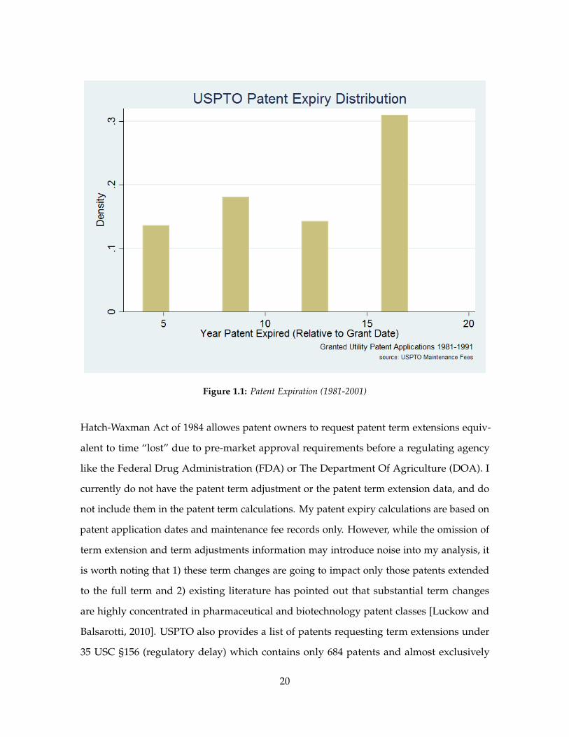
Figure 1.1: Patent Expiration (1981-2001)
Hatch-Waxman Act of 1984 allowes patent owners to request patent term extensions equiv-
alent to time “lost” due to pre-market approval requirements before a regulating agency
like the Federal Drug Administration (FDA) or The Department Of Agriculture (DOA). I
currently do not have the patent term adjustment or the patent term extension data, and do
not include them in the patent term calculations. My patent expiry calculations are based on
patent application dates and maintenance fee records only. However, while the omission of
term extension and term adjustments information may introduce noise into my analysis, it
is worth noting that 1) these term changes are going to impact only those patents extended
to the full term and 2) existing literature has pointed out that substantial term changes
are highly concentrated in pharmaceutical and biotechnology patent classes [Luckow and
Balsarotti, 2010]. USPTO also provides a list of patents requesting term extensions under
35 USC §156 (regulatory delay) which contains only 684 patents and almost exclusively
20
impacts pharmaceutical patents .22
Starting with 2001, USPTO grant data separately identifies patent references made by
the patent applicant from those made by the patent examiner. Examiner-added references
represent a significant share of overall patent references, estimated to be as high as 63% for
an average patent [Jaffe et al., 2000, Alcácer and Gittelman, 2006] Since examiner-added
references can bias my results, I extract examined-added references from USPTO data
2001-2012, and separately classify all references made by patents applied for during that
time period into examiner and non-examiner groups.
Deaths of individual patent owners are identified from the patent re-assignment data
covering 1982-2012 time period. Patent re-assignment data has previously been used to
identify patent trading patterns, but not the singular events affecting patent owners [Serrano,
2010, Galasso et al., 2013]. US patent ownership transfers are recorded in USPTO Patent
Assignment Database and uniquely identified by the reel and frame number. Each re-
assignment record contains patent and application numbers, and the relevant bibligraphic
data: the name of the new patent owner (assignee), the name of the original patent owner
(assignor), the date at which the transfer was recorded at the patent office, the date at which
the transfer of patent rights was executed, the type and the description of the transaction
(conveyance). It is important to note that, while the recordation of the patent ownership
transfer is not mandatory in the United States, patent law provides a strong impetus for
patent owners to ensure that all patent assignments get properly and promptly recorded. If,
for some reason, patent assignment is not recorded with USPTO within three months of
its execution, the assignee “stands at risk of having its rights subordinated to a subsequent
bona fide purchaser or lender acting without notice of the assignment”. This is especially
important if a patent is to be licensed, sold or asserted, since the patent ownership is the first
thing that comes under scrutiny. If, for some reason, a patent transaction is not recorded
with USPTO within three months of its execution, there exists a significant risk of the
22Full lists can be found at http://www.uspto.gov/ip/boards/foia_rr/resources/patents/pte.jsp andhttp://www.uspto.gov/learning-and-resources/ip-policy/foia-reading-room/final-decisions-commissioner-patents
21
transaction being void, if there are any subsequent re-assignements recorded. The Section
261 of the U.S. Patent Act gives this provision:
An assignment, grant, or conveyance shall be void as against any subsequentpurchaser or mortgagee for a valuable consideration, without notice, unless it isrecorded in the Patent and Trademark Office within three months from its dateor prior to the date of such subsequent purchase or mortgage.
Galasso et al. [2013] note that patent professionals and attorneys strongly advocate for
timely recordation of patent ownership transfers [Dykeman and Kopko, 2004, French, 2013].
The direct consequences of unrecorded patent ownership range from unenforceable patent
rights and inability to recover damages for infringement in prior to recordation, to loss
of rights to use patent-related sales as a bargaining chip in legal proceedings.23 In an
instance of patent owner’s death, prompt and proper recordation of patent ownership
transfer is further incentivized by the fiduciary duty bestowed upon the person overseeing
the financial matters. A fiduciary duty legally obligates an executor, trustee, conservator or
person holding the power to act entirely in the best interest of the beneficiaries.24 Under
the US legal system, a fiduciary duty is the strictest recognized standard of care.25 For
example, the Article 8, Section 808 of the Massachussetts Uniform Trust Code holds a trustee
personally liable for any breach of fiduciary duty:
A person who holds a power to direct [a trust] is presumptively a fiduciary whois required to act in good faith with regard to the purposes of the trust and theinterests of the beneficiaries. The holder of a power to direct shall be liable forany loss that results from a breach of a fiduciary duty.
23In compulsory licensing negotiations, for example. For additional details see French [2013].
24Fiduciary duty reaches beyond individual trusts and estates, all the way to corporate boardrooms: theofficers and directors of a firm have a fiduciary duty to act in the best interests of the firm and its shareholdersby pursuing profits and increasing shareholder value. Interestingly enough, in one of its recent decisions, theSuperior Court of Delaware directly linked fiduciary duty and patent monetization by making a statement thatcorporate officers and directors have a fiduciary duty to the corporation and its shareholders to monetize thecorporation’s intellectual property (E.I. Du Pont De Nemours & Co. v Medtronic Vascular, Inc., No. N10C-09-058,2013 WL 1792824, Del. Super., Apr. 24, 2013). This statement, albeit speculative, indicates that courts couldhold corporate officers and directors personally liable for lost profits from any “imprudent” use of intellectualproperty – including a conventional, purely defensive use of patents as a detterent against competitors’ legalactions.
25Fiduciary duty definition at Legal Information Institute (https://www.law.cornell.edu/wex/fiduciary_duty)
22
Since fiduciaries are legally required to act in the best interest of the estate or trust ben-
eficiaries, I can assume that US patent ownership transfers resulting from a death of the
owner are promptly executed and recorded in the USPTO Patent Assignment Database.
This is also noted in a Thomson Reuters FindLaw review on Estate Planning and Intellectual
Property:26
A patent application should be filed with the United States Patent and TrademarkOffice prior to any public use or showing of the invention or sale of the invention.Patents must be transferred in writing. Your will should clearly state who ownsthe patent, who has the right to license it and who has responsibility for makingmaintenance payments. In addition, the estate’s fiduciary must file appropriatedocuments with the United States Patent and Trademark Office to record thetransfer of the patent in order to allow the new owner to administer the patentregistration.
Patent owner deaths are identified from patent assignement records in three steps:
1. Words and phrases associated with a owner-related death are identified in assignor,
assignee and conveyance text fields. A patent transfer record is labelled as death-
related if it contains phrases like “surviving spouse”, “widow”, “deceased”, ”death”,
“testament”, “last will”, etc.
2. Patent transfers that were executed as a part of employment contract are dropped.
These are usually transfers executed before the patent was granted.
3. All patent applications not associated with a granted patent are also dropped.
4. The remaining patent transfers are assumed to be resulting from patent owner death
and are used to instrument for PAE activity.
I dichotomize citing entities from my sample into small and large. This classification comes
directly from the USPTO Patent Application Information Retrieval (PAIR) database, where
a separate entry indicates whether an applicant qualified for discounted patent filing fees
26Beth Silver, Esq. “Estate Planning Issues and Intellectual Property.” Thomson Reuters FindLaw. Lastaccessed April 30, 2015. http://corporate.findlaw.com/law-library/estate-planning-issues-and-intellectual-property.html.
23
based on its size.27 The USPTO assigns patent assignees into small and large according
to Small Business Administration (SBA) criteria. The SBA is a United States government
agency created in 1953 to provides support and assistance to small businesses. While the
size standards for an entity to be classified as small vary accross different industries, the two
widely used size standards are 500 employees or less for most manufacturing and mining
industries, and $7.5 million or less in average annual receipts for many nonmanufacturing
industries.28
Public access section of PAIR displays issued or published application status, including
the classification of the applicant and the status of the patent. Since USPTO PAIR database
dump is not publically available, and USPTO prevents web crawling on PAIR, I use available
parts crawled and provided by Google29 and Reed Tech30. This provides me with patent
application records for more than 3 million granted patents. While both Google and Reed
Tech continuously crawl USPTO PAIR database, there are no intimations that the crawl is
somehow prioritized, or that patent records are acquired in a specific order. Some patent
records are indeed missing from the crawled database, and some are not up-to-date. I
assume these missing points to be completely random since there is nothing about the
crawling process employed by Google and Reed Tech that would indicate a presence of
systematic bias. Figure 1.2 shows coverage of available USPTO PAIR data, and compares
the PAIR data with actual granted US patent counts.31
Table 1.1 summarizes four data sources used to synthesize patent data analyzed in this
27On March 19, 2013, a provision in the America Invents Act added an additional “micro” category.Since all micro entities are a subset of small entities, I group all entries in this category under smallentity status. For more information on entity status determination and filing discounts, see §509.02 athttp://www.uspto.gov/web/offices/pac/mpep/s509.html
28For details, see SBA size standards webpage at https://www.sba.gov/content/summary-size-standards-industry-sector.
29http://www.google.com/googlebooks/uspto-patents-pair.html
30http://patents.reedtech.com/Public-PAIR.php
31Both Google and Reed Tech simply state that they are “crawling the USPTO Public PAIR (Patent ApplicationInformation Retrieval) website and downloading patent documents, including image file wrappers (IFW PDF’s)”,and that the “crawl operates continually and will be retrieving both already-submitted documents and newdocuments as the USPTO makes them publicly available.”
24
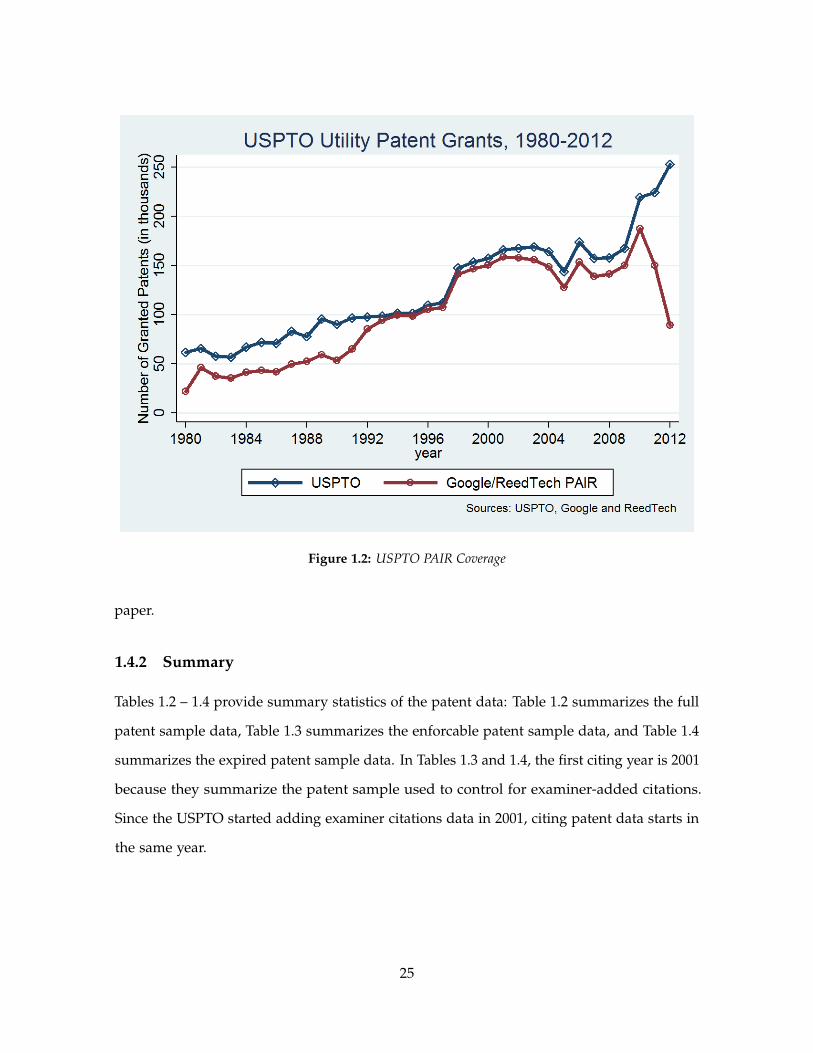
Figure 1.2: USPTO PAIR Coverage
paper.
1.4.2 Summary
Tables 1.2 – 1.4 provide summary statistics of the patent data: Table 1.2 summarizes the full
patent sample data, Table 1.3 summarizes the enforcable patent sample data, and Table 1.4
summarizes the expired patent sample data. In Tables 1.3 and 1.4, the first citing year is 2001
because they summarize the patent sample used to control for examiner-added citations.
Since the USPTO started adding examiner citations data in 2001, citing patent data starts in
the same year.
25
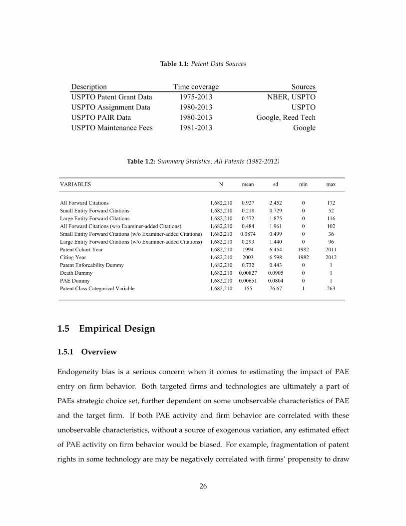
Table 1.1: Patent Data Sources
Description Time coverage SourcesUSPTO Patent Grant Data 1975-2013 NBER, USPTOUSPTO Assignment Data 1980-2013 USPTOUSPTO PAIR Data 1980-2013 Google, Reed TechUSPTO Maintenance Fees 1981-2013 Google
Table 1.2: Summary Statistics, All Patents (1982-2012)
All Forward Citations 1,682,210 0.927 2.452 0 172
Small Entity Forward Citations 1,682,210 0.218 0.729 0 52
Large Entity Forward Citations 1,682,210 0.572 1.875 0 116
All Forward Citations (w/o Examiner-added Citations) 1,682,210 0.484 1.961 0 102
Small Entity Forward Citations (w/o Examiner-added Citations) 1,682,210 0.0874 0.499 0 36
Large Entity Forward Citations (w/o Examiner-added Citations) 1,682,210 0.293 1.440 0 96
Patent Cohort Year 1,682,210 1994 6.454 1982 2011
Citing Year 1,682,210 2003 6.598 1982 2012
Patent Enforcability Dummy 1,682,210 0.732 0.443 0 1
Death Dummy 1,682,210 0.00827 0.0905 0 1
PAE Dummy 1,682,210 0.00651 0.0804 0 1
Patent Class Categorical Variable 1,682,210 155 76.67 1 263
VARIABLES N mean sd min max
1.5 Empirical Design
1.5.1 Overview
Endogeneity bias is a serious concern when it comes to estimating the impact of PAE
entry on firm behavior. Both targeted firms and technologies are ultimately a part of
PAEs strategic choice set, further dependent on some unobservable characteristics of PAE
and the target firm. If both PAE activity and firm behavior are correlated with these
unobservable characteristics, without a source of exogenous variation, any estimated effect
of PAE activity on firm behavior would be biased. For example, fragmentation of patent
rights in some technology are may be negatively correlated with firms’ propensity to draw
26
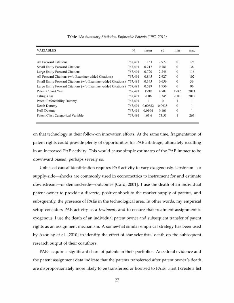
Table 1.3: Summary Statistics, Enforcable Patents (1982-2012)
All Forward Citations 767,491 1.153 2.972 0 128
Small Entity Forward Citations 767,491 0.217 0.781 0 36
Large Entity Forward Citations 767,491 0.720 2.245 0 116
All Forward Citations (w/o Examiner-added Citations) 767,491 0.845 2.627 0 102
Small Entity Forward Citations (w/o Examiner-added Citations) 767,491 0.145 0.656 0 36
Large Entity Forward Citations (w/o Examiner-added Citations) 767,491 0.529 1.956 0 96
Patent Cohort Year 767,491 1999 4.702 1982 2011
Citing Year 767,491 2006 3.345 2001 2012
Patent Enforcability Dummy 767,491 1 0 1 1
Death Dummy 767,491 0.00882 0.0935 0 1
PAE Dummy 767,491 0.0104 0.101 0 1
Patent Class Categorical Variable 767,491 163.6 73.53 1 263
VARIABLES N mean sd min max
on that technology in their follow-on innovation efforts. At the same time, fragmentation of
patent rights could provide plenty of opportunities for PAE arbitrage, ultimately resulting
in an increased PAE activity. This would cause simple estimates of the PAE impact to be
downward biased, perhaps severly so.
Unbiased causal identification requires PAE activity to vary exogenously. Upstream—or
supply-side—shocks are commonly used in econometrics to instrument for and estimate
downstream—or demand-side—outcomes [Card, 2001]. I use the death of an individual
patent owner to provide a discrete, positive shock to the market supply of patents, and
subsquently, the presence of PAEs in the technological area. In other words, my empirical
setup considers PAE activity as a treatment, and to ensure that treatment assignment is
exogenous, I use the death of an individual patent owner and subsequent transfer of patent
rights as an assignment mechanism. A somewhat similar empirical strategy has been used
by Azoulay et al. [2010] to identify the effect of star scientists’ death on the subsequent
research output of their coauthors.
PAEs acquire a significant share of patents in their portfolios. Anecdotal evidence and
the patent assignment data indicate that the patents transferred after patent owner’s death
are disproportionately more likely to be transferred or licensed to PAEs. First I create a list
27
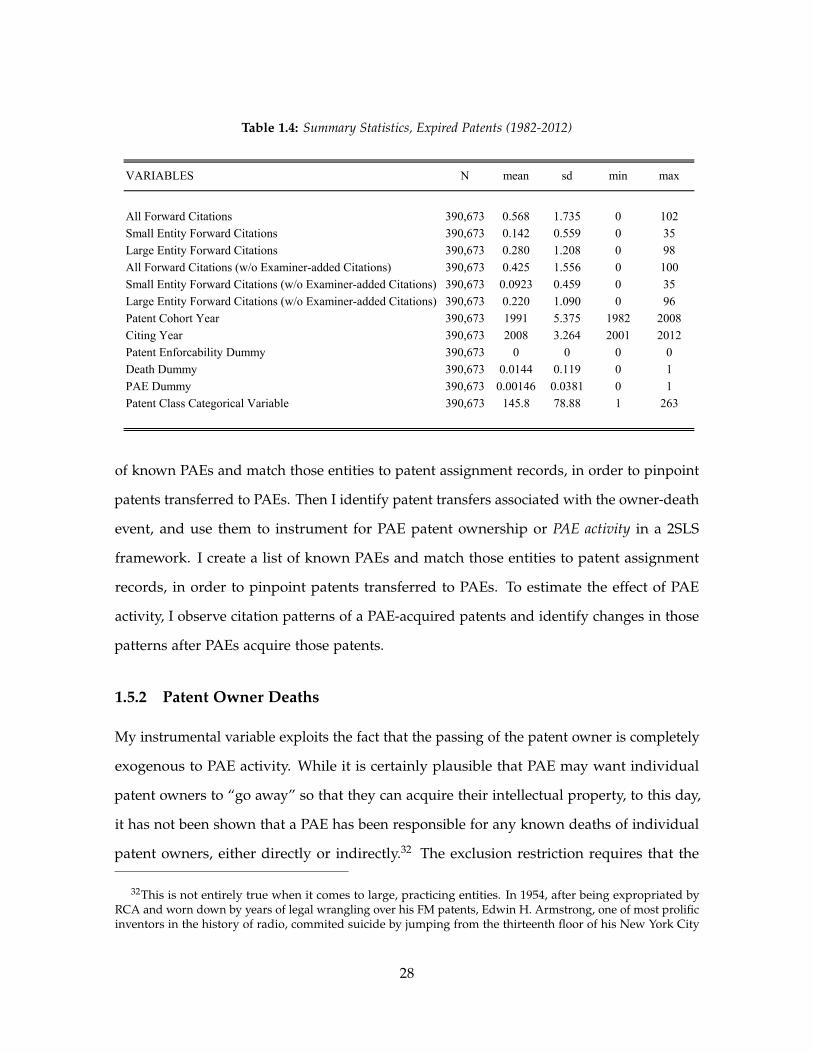
Table 1.4: Summary Statistics, Expired Patents (1982-2012)
All Forward Citations 390,673 0.568 1.735 0 102
Small Entity Forward Citations 390,673 0.142 0.559 0 35
Large Entity Forward Citations 390,673 0.280 1.208 0 98
All Forward Citations (w/o Examiner-added Citations) 390,673 0.425 1.556 0 100
Small Entity Forward Citations (w/o Examiner-added Citations) 390,673 0.0923 0.459 0 35
Large Entity Forward Citations (w/o Examiner-added Citations) 390,673 0.220 1.090 0 96
Patent Cohort Year 390,673 1991 5.375 1982 2008
Citing Year 390,673 2008 3.264 2001 2012
Patent Enforcability Dummy 390,673 0 0 0 0
Death Dummy 390,673 0.0144 0.119 0 1
PAE Dummy 390,673 0.00146 0.0381 0 1
Patent Class Categorical Variable 390,673 145.8 78.88 1 263
VARIABLES N mean sd min max
of known PAEs and match those entities to patent assignment records, in order to pinpoint
patents transferred to PAEs. Then I identify patent transfers associated with the owner-death
event, and use them to instrument for PAE patent ownership or PAE activity in a 2SLS
framework. I create a list of known PAEs and match those entities to patent assignment
records, in order to pinpoint patents transferred to PAEs. To estimate the effect of PAE
activity, I observe citation patterns of a PAE-acquired patents and identify changes in those
patterns after PAEs acquire those patents.
1.5.2 Patent Owner Deaths
My instrumental variable exploits the fact that the passing of the patent owner is completely
exogenous to PAE activity. While it is certainly plausible that PAE may want individual
patent owners to “go away” so that they can acquire their intellectual property, to this day,
it has not been shown that a PAE has been responsible for any known deaths of individual
patent owners, either directly or indirectly.32 The exclusion restriction requires that the
32This is not entirely true when it comes to large, practicing entities. In 1954, after being expropriated byRCA and worn down by years of legal wrangling over his FM patents, Edwin H. Armstrong, one of most prolificinventors in the history of radio, commited suicide by jumping from the thirteenth floor of his New York City
28
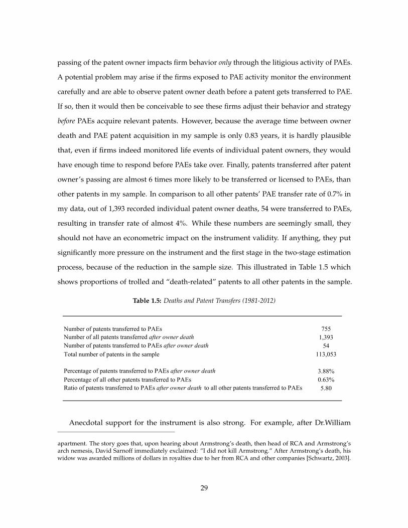
passing of the patent owner impacts firm behavior only through the litigious activity of PAEs.
A potential problem may arise if the firms exposed to PAE activity monitor the environment
carefully and are able to observe patent owner death before a patent gets transferred to PAE.
If so, then it would then be conceivable to see these firms adjust their behavior and strategy
before PAEs acquire relevant patents. However, because the average time between owner
death and PAE patent acquisition in my sample is only 0.83 years, it is hardly plausible
that, even if firms indeed monitored life events of individual patent owners, they would
have enough time to respond before PAEs take over. Finally, patents transferred after patent
owner’s passing are almost 6 times more likely to be transferred or licensed to PAEs, than
other patents in my sample. In comparison to all other patents’ PAE transfer rate of 0.7% in
my data, out of 1,393 recorded individual patent owner deaths, 54 were transferred to PAEs,
resulting in transfer rate of almost 4%. While these numbers are seemingly small, they
should not have an econometric impact on the instrument validity. If anything, they put
significantly more pressure on the instrument and the first stage in the two-stage estimation
process, because of the reduction in the sample size. This illustrated in Table 1.5 which
shows proportions of trolled and “death-related” patents to all other patents in the sample.
Table 1.5: Deaths and Patent Transfers (1981-2012)
Number of patents transferred to PAEs 755Number of all patents transferred after owner death 1,393Number of patents transferred to PAEs after owner death 54Total number of patents in the sample 113,053
Percentage of patents transferred to PAEs after owner death 3.88%Percentage of all other patents transferred to PAEs 0.63%Ratio of patents transferred to PAEs after owner death to all other patents transferred to PAEs 5.80
Anecdotal support for the instrument is also strong. For example, after Dr.William
apartment. The story goes that, upon hearing about Armstrong’s death, then head of RCA and Armstrong’sarch nemesis, David Sarnoff immediately exclaimed: ”I did not kill Armstrong.” After Armstrong’s death, hiswidow was awarded millions of dollars in royalties due to her from RCA and other companies [Schwartz, 2003].
29
Howard Waugh, an accomplished physician, professor, and inventor passed away33, his
estate transferred the rights to two of his patents to the Tawsaura Group LLC.34 These
patents covered the composition and delivery of the L-Citrulline.35 Within two weeks
from acquiring Dr.Waugh’s patents, the Tawsaura Group filed patent infringement lawsuits
against 36 firms in dietary supplement industry. In a little bit over a year, the Tawnsaura
Group has filed 91 lawsuits using these two patents. Similar examples can be found in other
intellectual property classes: in 1842, Henry Wall, often referred to as the first copyright
troll, started collecting fees for unauthorized performances of songs, mostly by acquiring
copyrights from estates of deceased composers [Deazley et al., 2010].
Patent Assertion Entitity Activity
While coming up with a general definition of an PAE is not exceptionally difficult, op-
erationalizing that definition, and identifying PAEs amongst millions of enterprizes in
United States is a much harder task.36 Labelling a business as an PAE can be somewhat
controversial, because of largely negative connotations associated with PAE business models
and their highly litiguous behavior.37 To address the problem so far, the academic literature
has utilized various approaches, from custom databases created via internet and news
searches [Reitzig et al., 2010, Shrestha, 2010, Fischer and Henkel, 2012, Jeruss et al., 2012] to
33Dr. William Howard Waugh’s obituary at the American Physiological Society:http://www.the-aps.org/mm/Membership/Obituaries/Waugh.html (last accessed on 10/10/2014).
34According to the offical State of Nevada business database portal, the Tawnsaura Group was incorporatedin Reno, Nevada only one month before Dr. Waugh’s death. Public records show only one employee listedfor Tawnsaura, the same trial attorney also representing Tawnsaura in every one of its 91 patent infingementlawsuits. To date, there are no records of Tawnsaura doing any type of R&D, no records of it ever manufacturingany products, and no records of it ever patenting any original inventions anywhere in the world.
35L-Citrulline is a naturally occuring amino acid used to improve exercise performance and a widelydistributed dietary supplement
36US Census Bureau puts the number of business in USA at around 30M(http://www.census.gov/compendia/statab/2012/tables/12s0744.pdf)
37During the course of the Lumen View Technology, LLC v Findthebest.com, Inc. legal proceedings, LumenView’s attorney even implied that the Findthebest.com’s CEO committed a hate crime under Ninth Circuit lawby using the term “patent troll”.
30
data dumps from third-party providers38 [Bessen et al., 2011, Cohen et al., 2014, Mazzeo
et al., 2014]. Opacity of most PAEs, hundreds of shell companies under their control, and
lack of readily accessible public data render an agnostic and methodologically consistent
approach to identifying PAEs almost impossible. To get around this, I combine data ac-
quired from internet and news searches with RPX PAE list, Plainsite PAE list39, and 10-K
filings from a handful of publically traded PAEs. From this list, I remove all universities,
university affiliated foundations and entities with a significant number of original patents
(like Qualcomm, for example). My final list consists of 2,776 entities classifed as PAEs.
To identify patents transferred to PAEs, I run a customized version of NBER company
name standardization routines on patent assignors and assignees in USPTO reassignment
records, and on the names of all PAE entities in my list [Hall et al., 2002]. I then match
standardized PAE names to USPTO assignor and assignee names to identify all patents
transferred to PAEs. I use only direct entity name matches in the process, which allows me
to identify a sample of 755 patents transferred to PAEs.
Outcomes
My main dependent variable is the number of forward citations received by the focal patent
in a year t. Some of these citations are made by the patent applicants themselvels and
some are added by the patent examiner during the patent examination process [Alcacer
et al. 2006, 2009]. To account for this dichotomy, and to address potential concerns about
the impact of patent examiners, I separate forward citations in two groups: those made
by patent examiners and those made by patent applicants. In addition, I also split forward
citations in those received by small and large entities to examine the heterogeneity of firm
response to PAE activity.
38Bessen et al. [2011] use RPX PAE database, Cohen et al. [2014] use PatentFreedom PAE database andMazzeo et al. [2014] use PricewaterhouseCoopers data.
39Created through crowdsourced efforts. For more information, see http://www.plainsite.org/tags/patent-trolls/
31
1.5.3 Specification
Estimation of the impact of PAE activity on firm citation patterns presents some interesting
econometric challenges. These stem from two facts: the first being that my ultimate
dependent variable—patent citations—is a non-linear count measure, and the second being
that the endogenous regressor is binary variable. Accounting for endogeneity with the
two-stage instrumental variable estimation becomes quite complex when either the first or
the second stage relationship is non-linear. I use linear 2SLS as the primary specification,
even though the ultimate relationship is non-linear. The use of linear IV framework in this
particular instance can be justified by several arguments. First, the linear IV specification
should capture the treatment effect analogue to LATE for dummy endogenous regressors,
even with the non-linear second-stage relationship [Angrist, 2001, Angrist and Krueger,
2001, Angrist and Pischke, 2009, Cameron and Trivedi, 2013]. Second, using a non-linear
first stage estimation places a lot of weight on getting this functional form just right, and
risks introducting significant bias and making estimates difficult to interpret if the first stage
happens to be incorrectly specified. Finally, a linear 2SLS framework generally results in
estimates that are resonably close to minimum-mean-squared-error linear approximations
of non-linear conditional expectation functions [Angrist and Pischke, 2009]. Because I am
interested in a causal effect of the PAE patent acquisition and would like to know how
citation patterns change over having a precisely estimated parameter, 2SLS framework is
econometrically adequate approach to take. As a robustness check, I also run instrumental
variable Poisson regression using a control-function approach to control for the endogeneity
of PAE patent acquisitions. This approach utilizes Method-of-Moments framework and uses
residuals from the first-stage linear regression of endogenous regressor on instrumental
variable to control for the endogeneity in the second-stage Poisson regression [Newey, 1984,
Wooldridge, 2010].
32
1.5.4 Linear IV
The first stage assesses the relationship between the instrument, in this case being a patent
owner death, and the endogenous regressor, in this case being PAE activity:
PAEp,t = α0 + α1 × Deathp,t + Class′p + Cohort
′p + Year
′p + νp,t (1.1)
where i denotes USPTO main patent class, t denotes citing patent application year, a denotes
cited (focal) patent application year (cohort year), NPE is a binary dummy that denotes an
PAE appearing as an assignee in the USPTO reassignment record, Death is a binary dummy
that denotes the patent owner death-related transfer, Class and Year denote patent class and
citing year fixed effects, and Cohort denotes the patent cohort year fixed effects. While the
temporal lag of patent citations generally follows log-normal distribution (as illustrated
in Figure 1.3), to capture the systematic variations of patenting and patent-citing practices
over time, Cohort and Year control for both the application year of the cited patent and the
application year of the citing patent. The first effect is usually referred to as the “cohort
effect” and was shown to have a significant impact on the citation profile of a patent [Hall
et al., 2002]. Frequent patent policy changes at the USPTO affecting both quantity and
quality of granted patents are the main culprit behind the “cohort effect”. The second effect
is usually referred to as the “calendar effect” and is caused by the systematic increase in the
number of citations per patent over time [Hall et al., 2002]. The patent class fixed effects
Class controls for the heteregeneity in citing practices across technology classes.
I assume errors to be random and orthogonal to other independent variables in the
regression:
E[νp,t|Class, Cohort, Year, Death] = 0 (1.2)
The second stage regresses predicted PAE activity on the patent citation measure to
estimate a causal impact of PAE activity on knowledge flow patterns:
yp,t = β0 + β1 × ˆPAEp,t + Class′′p + Cohort
′′p + Year
′′p + εp,t (1.3)
33
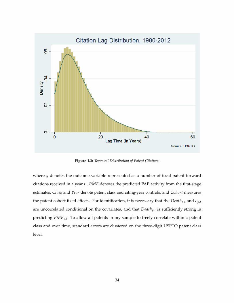
Figure 1.3: Temporal Distribution of Patent Citations
where y denotes the outcome variable represented as a number of focal patent forward
citations received in a year t , ˆPME denotes the predicted PAE activity from the first-stage
estimates, Class and Year denote patent class and citing-year controls, and Cohort measures
the patent cohort fixed effects. For identification, it is necessary that the Deathp,t and εp,t
are uncorrelated conditional on the covariates, and that Deathp,t is sufficiently strong in
predicting PMEp,t. To allow all patents in my sample to freely correlate within a patent
class and over time, standard errors are clustered on the three-digit USPTO patent class
level.
34
1.5.5 Poisson Regression
For robustness check of 2SLS specification, I also run an instrumental variable Poisson
regression with the control function estimator. This estimation strategy maintains the
exponential nature of the dependent variable and relies on the multiplicative error model.
The underlining relationship can be expressed as:
yp,t = exp(β× PAEp,t + Classp + Cohortp + Yearp)εp,t (1.4)
where PMEp,t is an endogenous PAE activity parameter that can be estimated as:
PAEp,t = α× Deathp,t + εp,t (1.5)
The main error term is then decomposed as:
εp,t = exp(ρ× εp,t + kp,t) (1.6)
Finally, the conditional mean model for y is estimated by first estimating ε vector, and
then additing it as additional regressor to control for endogeneity:
E[y|PME, κ, φ, λ, u] = exp(β× PMEp,t + Classp + Cohortp + Yearp + ρ× εp,t) (1.7)
From this, we can define error functions for the endogenous PAE activity and the
dependent variable as:
uPME(PME, Death, α) = PMEi,t − α× Deathp,t (1.8)
uy(y, PME, Class, Cohort, Year, α, β, uPME)
=yp,t
exp(β× PMEp,t + Classp + Cohortp + Yearp + ρ× εp,t)− 1 (1.9)
35
In turn, these give us population mean conditions:
E[Death× uen] = 0 (1.10)
E[(PME, Death, ε̂)× uy] = 0 (1.11)
Which allow us to use GMM to estimate coefficients on PAE activity. However, Poisson
coeffients may be difficult to interpret in this particular context and will be utilized as a
robustness check only.
1.6 Results
1.6.1 Main Results
Tables 1.6-10 present the main results of this study. Table1.6 shows the results on the overall
number of citations for the full sample of US patents 1981-2012: endogenous OLS regression
is in the first column, reduced form regression in the second column, IV 2SLS regression in
the third column and IV Poisson regression in the fourth column.
The sample covers all granted patents from the same patent classes and cohorts as the
patents impacted by the instrument. This set of regressions does not control for examiner-
added citations, since these were added to the data starting in 2001. In addition, these
regressions do not take into account patent expiration dates, and include all patent citations,
regardless of the cited patent enforcability status. Interestingly enough, the PAE activity
coefficient in is positive and significant in the endogenous regressions, and would suggest
that, after being acquired by PAEs, patents would stand to gain about 0.43 citations, or about
3% of all citations on average. However, the same coefficient is negative and signficant in
the instrumented 2SLS regressions, indicating a loss of 2.6 citations, or approximately 17%
of all citations on average . This points to the presence of bias in endogenous regression,
and suggests that, because PAEs endogenously select which patents to acquire and how to
utilize them, simple OLS is not an appropriate analytic tool. This is exactly the shortcoming
36
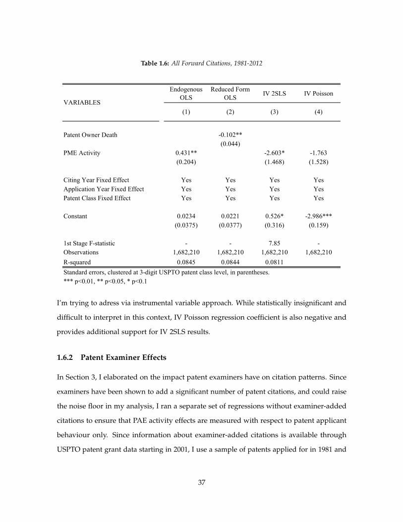
Table 1.6: All Forward Citations, 1981-2012
Endogenous OLS
Reduced Form OLS
IV 2SLS IV Poisson
Patent Owner Death -0.102**(0.044)
PME Activity 0.431** -2.603* -1.763(0.204) (1.468) (1.528)
Citing Year Fixed Effect Yes Yes Yes YesApplication Year Fixed Effect Yes Yes Yes YesPatent Class Fixed Effect Yes Yes Yes Yes
Constant 0.0234 0.0221 0.526* -2.986***(0.0375) (0.0377) (0.316) (0.159)
1st Stage F-statistic - - 7.85 -Observations 1,682,210 1,682,210 1,682,210 1,682,210
R-squared 0.0845 0.0844 0.0811
Standard errors, clustered at 3-digit USPTO patent class level, in parentheses.*** p<0.01, ** p<0.05, * p<0.1
VARIABLES
(1) (2) (3) (4)
I’m trying to adress via instrumental variable approach. While statistically insignificant and
difficult to interpret in this context, IV Poisson regression coefficient is also negative and
provides additional support for IV 2SLS results.
1.6.2 Patent Examiner Effects
In Section 3, I elaborated on the impact patent examiners have on citation patterns. Since
examiners have been shown to add a significant number of patent citations, and could raise
the noise floor in my analysis, I ran a separate set of regressions without examiner-added
citations to ensure that PAE activity effects are measured with respect to patent applicant
behaviour only. Since information about examiner-added citations is available through
USPTO patent grant data starting in 2001, I use a sample of patents applied for in 1981 and
37
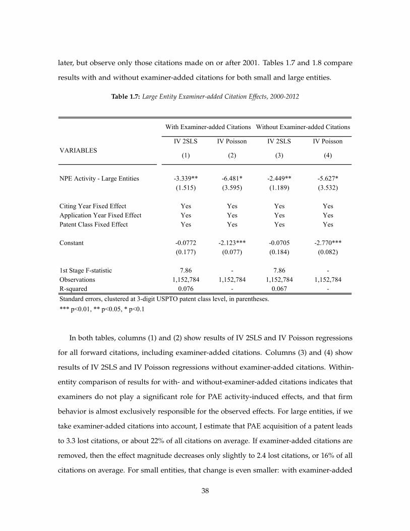
later, but observe only those citations made on or after 2001. Tables 1.7 and 1.8 compare
results with and without examiner-added citations for both small and large entities.
Table 1.7: Large Entity Examiner-added Citation Effects, 2000-2012
IV 2SLS IV Poisson IV 2SLS IV Poisson
NPE Activity - Large Entities -3.339** -6.481* -2.449** -5.627*(1.515) (3.595) (1.189) (3.532)
Citing Year Fixed Effect Yes Yes Yes YesApplication Year Fixed Effect Yes Yes Yes YesPatent Class Fixed Effect Yes Yes Yes Yes
Constant -0.0772 -2.123*** -0.0705 -2.770***(0.177) (0.077) (0.184) (0.082)
1st Stage F-statistic 7.86 - 7.86 -Observations 1,152,784 1,152,784 1,152,784 1,152,784R-squared 0.076 - 0.067 -
Standard errors, clustered at 3-digit USPTO patent class level, in parentheses.
*** p<0.01, ** p<0.05, * p<0.1
With Examiner-added Citations Without Examiner-added Citations
VARIABLES(1) (2) (3) (4)
In both tables, columns (1) and (2) show results of IV 2SLS and IV Poisson regressions
for all forward citations, including examiner-added citations. Columns (3) and (4) show
results of IV 2SLS and IV Poisson regressions without examiner-added citations. Within-
entity comparison of results for with- and without-examiner-added citations indicates that
examiners do not play a significant role for PAE activity-induced effects, and that firm
behavior is almost exclusively responsible for the observed effects. For large entities, if we
take examiner-added citations into account, I estimate that PAE acquisition of a patent leads
to 3.3 lost citations, or about 22% of all citations on average. If examiner-added citations are
removed, then the effect magnitude decreases only slightly to 2.4 lost citations, or 16% of all
citations on average. For small entities, that change is even smaller: with examiner-added
38
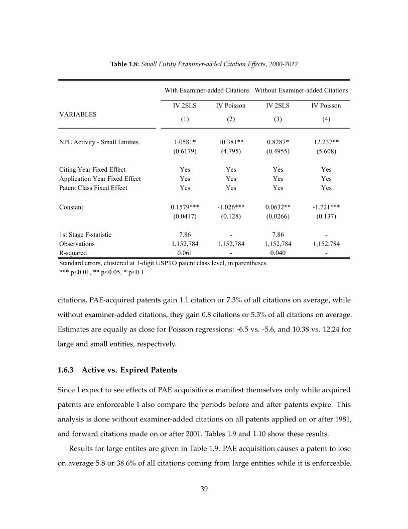
Table 1.8: Small Entity Examiner-added Citation Effects, 2000-2012
IV 2SLS IV Poisson IV 2SLS IV Poisson
NPE Activity - Small Entities 1.0581* 10.381** 0.8287* 12.237**(0.6179) (4.795) (0.4955) (5.608)
Citing Year Fixed Effect Yes Yes Yes YesApplication Year Fixed Effect Yes Yes Yes YesPatent Class Fixed Effect Yes Yes Yes Yes
Constant 0.1579*** -1.026*** 0.0632** -1.721***(0.0417) (0.128) (0.0266) (0.137)
1st Stage F-statistic 7.86 - 7.86 -Observations 1,152,784 1,152,784 1,152,784 1,152,784R-squared 0.061 - 0.040 -
Standard errors, clustered at 3-digit USPTO patent class level, in parentheses.*** p<0.01, ** p<0.05, * p<0.1
With Examiner-added Citations Without Examiner-added Citations
(3) (4)VARIABLES
(1) (2)
citations, PAE-acquired patents gain 1.1 citation or 7.3% of all citations on average, while
without examiner-added citations, they gain 0.8 citations or 5.3% of all citations on average.
Estimates are equally as close for Poisson regressions: -6.5 vs. -5.6, and 10.38 vs. 12.24 for
large and small entities, respectively.
1.6.3 Active vs. Expired Patents
Since I expect to see effects of PAE acquisitions manifest themselves only while acquired
patents are enforceable I also compare the periods before and after patents expire. This
analysis is done without examiner-added citations on all patents applied on or after 1981,
and forward citations made on or after 2001. Tables 1.9 and 1.10 show these results.
Results for large entites are given in Table 1.9. PAE acquisition causes a patent to lose
on average 5.8 or 38.6% of all citations coming from large entities while it is enforceable,
39
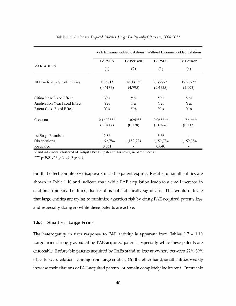
Table 1.9: Active vs. Expired Patents, Large-Entity-only Citations, 2000-2012
IV 2SLS IV Poisson IV 2SLS IV Poisson
NPE Activity - Small Entities 1.0581* 10.381** 0.8287* 12.237**(0.6179) (4.795) (0.4955) (5.608)
Citing Year Fixed Effect Yes Yes Yes YesApplication Year Fixed Effect Yes Yes Yes YesPatent Class Fixed Effect Yes Yes Yes Yes
Constant 0.1579*** -1.026*** 0.0632** -1.721***(0.0417) (0.128) (0.0266) (0.137)
1st Stage F-statistic 7.86 - 7.86 -Observations 1,152,784 1,152,784 1,152,784 1,152,784R-squared 0.061 - 0.040 -
Standard errors, clustered at 3-digit USPTO patent class level, in parentheses.*** p<0.01, ** p<0.05, * p<0.1
With Examiner-added Citations Without Examiner-added Citations
(3) (4)VARIABLES
(1) (2)
but that effect completely disappears once the patent expires. Results for small entities are
shown in Table 1.10 and indicate that, while PAE acquistion leads to a small increase in
citations from small entiries, that result is not statistically significant. This would indicate
that large entities are trying to minimize assertion risk by citing PAE-acquired patents less,
and especially doing so while these patents are active.
1.6.4 Small vs. Large Firms
The heterogenity in firm response to PAE activity is apparent from Tables 1.7 – 1.10.
Large firms strongly avoid citing PAE-acquired patents, especially while these patents are
enforcable. Enforcable patents acquired by PAEs stand to lose anywhere between 22%-39%
of its forward citations coming from large entities. On the other hand, small entities weakly
increase their citations of PAE-acquired patents, or remain completely indifferent. Enforcable
40
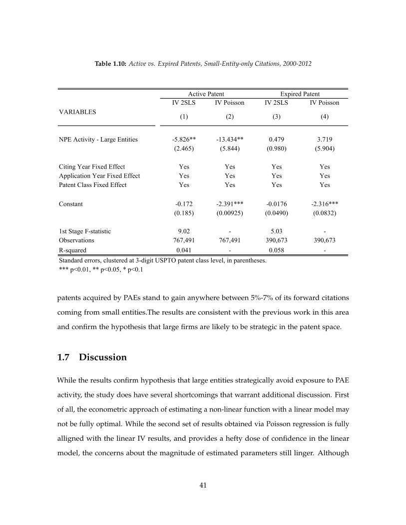
Table 1.10: Active vs. Expired Patents, Small-Entity-only Citations, 2000-2012
IV 2SLS IV Poisson IV 2SLS IV Poisson
NPE Activity - Large Entities -5.826** -13.434** 0.479 3.719(2.465) (5.844) (0.980) (5.904)
Citing Year Fixed Effect Yes Yes Yes YesApplication Year Fixed Effect Yes Yes Yes YesPatent Class Fixed Effect Yes Yes Yes Yes
Constant -0.172 -2.391*** -0.0176 -2.316***(0.185) (0.00925) (0.0490) (0.0832)
1st Stage F-statistic 9.02 - 5.03 -Observations 767,491 767,491 390,673 390,673
R-squared 0.041 - 0.058 -
Standard errors, clustered at 3-digit USPTO patent class level, in parentheses.*** p<0.01, ** p<0.05, * p<0.1
(2) (3) (4)
Active Patent Expired Patent
VARIABLES(1)
patents acquired by PAEs stand to gain anywhere between 5%-7% of its forward citations
coming from small entities.The results are consistent with the previous work in this area
and confirm the hypothesis that large firms are likely to be strategic in the patent space.
1.7 Discussion
While the results confirm hypothesis that large entities strategically avoid exposure to PAE
activity, the study does have several shortcomings that warrant additional discussion. First
of all, the econometric approach of estimating a non-linear function with a linear model may
not be fully optimal. While the second set of results obtained via Poisson regression is fully
alligned with the linear IV results, and provides a hefty dose of confidence in the linear
model, the concerns about the magnitude of estimated parameters still linger. Although
41
there should be no doubt about the direction of the effect, the quest for more precisely
estimated parameters may require additional work, and a custom estimating routine to be
developed. Second, we may be concerned with the fact that patents transferred because of
patent owner death are all individual inventor-owned patents, and may be fundamentally
different from other patents in the sample. USPTO does track and classify intial patent
assignees, but unfortunately leaves a significant number of patents classified as “unassigned”
or “not known”. Thus, running a regression on individual inventor-owned patents only
would 1) introduce a lot of noise into the system and 2) significantly reduce sample size
to the point where statistical power would certainly suffer. Although not reported in this
paper, as a robustness check, I ran 2SLS regressions with an independent variable dummy
for individually owned patents that could be identified from the USPTO data, and noticed
no significant change in PAE effects on follow-on citations.40 If anything, the magnitudes
of estimated parameters showed a slight increase after individually-owned dummy was
included. On a related note, Roach and Cohen [2013] identify private knowledge flows
such as consulting projects, contract work and conferences as a mechanism that could
impact citation counts. While it is certainly possible that a death of an individual inventor
could be a confounding factor, and lead to a subsequent drop in citations caused by the
absence of private knowledge flows, the fact that estimated negative effect of PAE activity
on future citations by large entities dissapears after the patent in question expires, suggests
that private knowledge flows are most likely not the main cause behind the estimated “PAE
effect.” Also, the observed ex-post increase in citations by small entities counters this theory.
A different, but equally as important concern has to do with the broader effects of PAE
activity on cumulative innovation. While I measure direct effects on citation patterns of
PAE-acquired patents, I do not measure effects on broader patent classes, and cannot say
much about possible adjustment in firms’ technology search patterns. Similar to Galasso and
Schankerman [2015], one could create a set of technologically proximate, matching patents
to see if there exists a “substitution effect”, i.e. whether large firms strategically avoid only
40These results are available upon request
42
PAE-owned patents while still citing closely related patents, or they avoid techonologies
plagued with PAEs alltogether. If so, then the advent of PAEs could have more profound
effects on the follow-on innovation. However, because the negative effects on citations
of PAE-owned patents go away after they expire, this lends support for purely strategic
avoidance of these patents by large firms. Lanjouw and Schankerman [2001] find that
litigated patents exibit a “publicity effect”—once they are litigated, they become more
visible to both examiners and applicants, and get cited more as a consequence. While PAEs
litigate many of their patents, I do not observe this “publicity effect” for the large firms.
Citations made to PAE-owned patents by small firms do increase, and publicity effect may
have something to do with that. Because small firms have less options and less resources
to avoid interacting with PAEs, it is likely that either they are being strategic and trying
to signal that PAE-owned patents are different from or inferior to the current invention,
they are already been targeted and are licensing PAE-owned patents, or PAE-owned patents
become more visible and acquire more forward citations by small firms. This state of the
world can have a nefarious undertone: if PAE presence is forcing small firms to focus
their attention on a small set of patents and technologies, that could negatively impact
creativity and overall inovativeness of these firms. Since the propensity of small firms to
cite PAE-owned patents does not change much pre- and post-expiry, it is hard to make an
argument for a clear strategic intent here. If small firms were indeed citing PAE-owned
patents only to minimize their hold-up risk, then after those patents were to expire, citations
by small firms should decrease. However, the coefficients on citations to PAE-owned patents
made by small firms pre- and post- expiry stay remarkably similar.
Finally, while this is one of the first studies to examine the effect of patent term expiration
on forward citations, patent term lengths for those patents maintained through the full
term are only approximated. Patent term adjustments and extensions implemented by the
USPTO are not added to the patent term calculations, and should be included to precisely
estimate these effects in the future. In addition, since the statute of limitations for initiating
patent infringement lawsuits extends for up to 6 years after the patent expires, this could
43
introduce additional lag into the citation patterns.
1.8 Conclusion.
One of the key arguments for a “benevolent troll” hypothesis is that PAEs reduce search
costs and identify technological relationships otherwise difficult to detect. In this world,
potential customers who would benefit from rights to technologies owned by patent trolls
are identified and patents are licensed to them, with or without legal action. Patent license
execution usualy sends a signal about the commercial value of licensed technology to
the market and should lead to increased follow-on research, resulting in higher ex-post
citation rates. Indeed, previous studies have found that citations to licensed patents by
both non–licensees and licensees increased after the licenses were executed [Sampat and
Ziedonis, 2005, Drivas et al., 2014]. Following this line of logic, if the trolling strategy was
truly efficiency-enhancing, we would expect to see citations to troll-acquired patents to
increase after the acquistion, regardless of the citing entity type. While this happens to be
true for the small firms, the trend is completely opposite for the large firms. Since large
firms are more strategic in their behavior, this leads me to conclude that a risk of a PAE
lawsuit drives these firms to reduce citations to PAE acquired patents. Given that this is the
first study that attempts to tease-out the causal effects of PAEs on the firm behavior, even
though the results may not be directly translatable into policy-actionable outcomes, they
undoubtely indicate that firms react to PAE patent acquisitions in the knowledge space. A
more detailed follow-on work is needed to tease out if the changes in citation patterns are
only strategic, or they indeed point to serious disruptions in cumulative innovation patterns.
The results of this study also raise some concerns about “inequitable conduct” policy and
its effectiveness in preventing strategic citations of prior art.
This study also brings attention to empirical strategies we can employ to identify and
answer important questions relevant to the intellectual property policy. While showing a
lot of promise, the use of upstream market shocks in markets for patents as instrumental
variables has gone underutilized for many years. The quest for understanding the intricacies
44

of the value chain in markets for patents could open the doors for causal identification in an
area plagued by endogenous choice bias, and stands out as an important area to be studied
in the future.
45
Chapter 2
The Standard-Pool Interface1
2.1 Introduction
Technological standards have become an unavoidable part of modern life.2 Today, the inter-
operabilty of high-tech devices in complex networks and systems hinges on standardization
of interfaces, communication protocols and processes. The welfare-enhancing effects created
by standardization can be significant, especially in those markets where this interoperability
is important3 and strong network-effects persist [Farrell and Saloner, 1985]. Standardization
can occur through direct market competition to create de facto standards, or via regulatory
intervention.4 Most modern standards, however, are created with assistance of standard-
setting organizations’ (SSOs) driven consensus, and involve voluntary participation and
collaboration of many different entities: firms, government agencies, individuals, academic
institutions and research laboratories. Regardless of whether these entities are downstream
manufacturers and service providers, or are upstream technology developers, their involve-
1Co-authored with Josh Lerner and Jean Tirole
2For example, as far back as one decade ago, in their discussion of Wi-Fi technical standard, the AmericanNational Standards Institute (ANSI) proclaimed that "just about everything associated with a computer, especiallythose connected to the Internet, is based on an industry standard."[ANSI, 2004]
3Mobile communications are a good example.
4An example of de facto standard would be IBM PC, and an example of a standard driven by regulatoryintervention would be HDTV standard. For additional discussion, see Lemley [2002] or Greenstein and [eds.].
46
ment in the standardization process, and in particular their willingness to disclose and
license standard-essential patents (SEPs) are crucial for standard implementation, and its
success later on. SSOs play a pivotal role in this process, act as a consensus-making body
and provide regulatory checks guiding the behavior of participating members. One of the
most important regulatory duties of SSOs is to ensure that concerns about ex-post hold-up
are minimized through proper disclosure of SEPs, and to facilitate reasonable licensing
commitments made by patent owners.
The hold-up in standard-setting usually comes in one of the two flavors. In the first
variant, a firm making a RAND or FRAND licensing commitment ex-ante can decide to
capitalize on the vagueness of the term “reasonable” and attempt to extract unreasonably
high royalty payments ex-post. A recent high-profile legal battle between Microsoft and
Motorola illustrates this issue remarkably well. In this case, Microsoft accused Motorola of
breaching their RAND commitments made when disclosing SEPs to two different standards:
IEEE 802.11 and ITU-T H.264.5 Microsoft has been widely using these standards in many
of their flagship products, including videogame console Xbox 360 and Windows software,
and implicated Motorola in requesting unreasonable royalties for their SEPs. The Federal
District Court sided with Microsoft and reduced royalties due to Motorola to $1.8M per year
from almost $4B per year as originally sought by Motorola. In addition, the court ordered
Motorola to pay $14.5M back to Microsoft in compensatory damages. However, the case
did remain in court for more two years, and was very costly to resolve. While this type
of conduct in standard-setting is not completely uncommon6, it may require a substantial
change in patent disclosure policy and imposition of structured price commitments by
patent owners to improve ex-post outcomes.[Lerner and Tirole, 2015]
In the second variant, ex-post hold-up can arise when patent owners strategically
underdisclose their patents, as to avoid RAND/FRAND provisions. The case of Rambus is
5See Microsoft Corp. v. Motorola Inc., 696 F.3d 872 (9th Cir. 2012)
6See Broadcom Corp. v. Qualcomm Inc., 501 F.3d 297, 310 (3d Cir. 2007)
47
a prime example.7 Rambus failed to disclose its existing DRAM related patents and patent
applications during a standard-setting process at JEDEC SSO, and took care to suspiciously
amend some of its patent applications to read on the standard more closely. This kicked off
a series of lawsuits that plagued the DRAM industry for more than a decade.8
Rapid pace of technological convergence, especially in IT-related fields, allots large
economic value to standards. With a large potential upside and an equally as large potential
downside, it is logical to expect participating firms to be highly strategic. Given the far-
reaching economic impact of standardization, and the potential for strategic gaming and
hold-up by profit-maximizing entities, the setting of optimal disclosure and patent licensing
policies becomes ever increasingly important. Before we can inform policy, we need to
understand exactly how disclosure process works in standard-setting contexts.
This paper analyzes selection mechanisms in technical standards and is focused on the
premise that upstream and downstream patent owners have heterogenous patent disclosure
strategies. We evaluate patent disclosures made to seven large SSOs, and find that, consistent
with theoretical predictions, both downstream and upstream firms act to maximize their
ex-post rents. More specifically, we show that downstream firms are more likely to disclose
lower-quality patents to standard-setting organizations, and prefer to use generic patent
disclosures over specific ones. There are several reasons for such behavior. First of all, large
firms with broad patent portfolios have to contend with costly patent searches when making
specific disclosures. More importantly, firms with large downstream presence usually do not
participate in standard-setting efforts with large licensing revenue in mind. Rather, they are
incentivized in fomenting downstream adoption of their technology, and subsequently do
not have immediate legal concerns that would force them to make specific patent disclosures.
Although it is growing, the quantitative empirical literature about strategic behavior in
standard-setting contexts remains relatively scarce. On a theoretical side, Lerner and Tirole
[2006] use a “forum-shopping” framework to show that technology owners will choose the
7See Complaint, In re Rambus Inc., No. 9302 (F.T.C. June 18, 2002)
8Wikipedia article on Rambus-related lawsuits: http://en.wikipedia.org/wiki/Rambus#Lawsuits
48
friendliest SSO to have their technology adopted by the downstream users. Their model
shows that this particular type of forum-shopping may attenuate distributional conflicts, if
competing firms end up choosing different SSOs. From an empirical side, Simcoe et al. [2009]
investigate the patent disclosure strategies to SSOs, link them to ex-post patent litigation,
and show that they heterogenously impact small and large-firms’ incentives to litigate. In
other related studies, Axelrod et al. [1995] examine firm choices to join standardization
alliances, conditional on the firm size and the presence of close competitors in those alliances,
and Simcoe [2012] shows that strategic rent-seeking behavior of individual participants can
lead to delays in standard-setting process, especially when commercialization pressures are
high.
Our study contributes to several other strands of literature. It directly extends the work
of Lerner and Tirole [2014, 2015], who lay the groundwork for the analysis of standard-
essential patent disclosures made during standardization process. They show that simple
FRAND patent licensing commitments create opportunities for strategic behavior of patent
owners, only to induce outcomes that are ex-post inefficient. When it comes to patent
disclosures, we show that patent owners indeed behave strategically and that asymmetric
information presents a problem that SSOs need to consistently grapple with.
The paper is organized as follows: Section II describes technical standards and firm
disclosure strategies. Section III describes and summarizes the data, presents the hypotheses,
empirical specification and the results. Section IV concludes the paper.
2.2 Technical Standards and Disclosure Practices
2.2.1 Background
As a set of one or more technical specifications, technical standard codifies a collection of
common design rules for a product or a process.9
9According to the National Technology Transfer and Advancement Act (NTTAA), the term “standard” or“technical standard” includes all of the following: (1) Common and repeated use of rules, conditions,guidelinesor characteristics for products or related processes and production methods, and related management systems
49
Standards have many flavors and can emerge in a mulitude of ways. Some are developed
privately by a single entity: a firm or government, for example. However, coordinated
standard development through SSOs is more common these days. SSOs usually combine a
set of very diverse inputs and develop market-driven voluntary standards, which sometimes
get mandated via government intervention. In the course of the standard-setting process,
SSOs play several critical roles: they identify multiple paths towards a technological solution,
they coordinate on one approach among conflicting alternatives and regulate the behavior of
members. One of the most important issues under the aegis of SSOs is ensuring that firms
disclose relevant patents and agree not to price licenses to their patents too aggressively.
Largely due to high coordination costs, sizeable SSOs like ETSI or IEC usually require all
of their members and participants to disclose any patents they believe may be standard-
essential. This disclosure requirement serves multiple purpose: it directs standard-setting
process to take note of disclosed technologies, it forces disclosing parties to make licensing
commitments (usually concurrent with the disclosure), it sends the signal to the market
about the potential implementation cost down the line, and it provides valuable information
for legal authorities in case of a dispute. These disclosure policies vary across different
SSOs, and are usually difficult to change once set.[Bekkers and Updegrove, 2012]
Patent Disclosure Practices
We interviewed nearly one dozen practitioners regarding their organizations’ attitudes
and perspective about the disclosure of intellectual property to standards. These included
lawyers and business development executives at companies specializing in software and
telecommunications, SSO executives, and academic technology transfer officials. The
attitudes of the organizations towards disclosures of intellectual property varied dramatically.
On the one hand, many organizations prefer to undertake generic disclosures, particularly
practices. (2) The definition of terms; classification of components; delineation of procedures; specification ofdimensions, materials, performance, designs, or operations; measurement of quality and quantity in describingmaterials, processes, products, systems, services, or practices; test methods and sampling procedures; ordescriptions of fit and measurements of size or strength. (reference here)
50
if they are not seeking to license standard essential patents, but instead to make money off
downstream products. One of the main reasons for undertaking generic disclosures was
search cost containment: making a generic disclosure avoids the need for a patent search.
This is especially true for firms with large patent portfolios. These firms found the process
of sifting through patents to identify intellectual property relevant to a standard to be an
ardouous and expensive task, which can consume thousands of hours of patent attorney
time. The social dynamics of standard-setting process also impacts these decisions: even if
the SSOs say that the participating firms do not need to engage in a patent search, there is
often informal pressure to do so from other participants.
Since standards and patent applications evolve—sometimes rapidly—time also plays a
major role. An initial disclosure may not be relevant if the standard changes considerably
during the formulation process. Similarly, patents may add or lose claims as they move
through the patent office, and may have a different scope as issued by various national
patent offices. There is often a fear of being exposed from antitrust claims, regardless of
what approach to patent disclosure the firm takes. If the firm does not disclose relevant IP,
it could face antitrust claims, as seen in the litigation around Rambus and the JEDEC SSO.
On the other hand, if the firm is perceived to over-disclose, there can also be accusations
of preemptively discouraging competition. Over-disclosing can have other deleterious
effects for the standard: higher licensing fees and a greater complexity and development
cost immediately come to mind. For instance, to contain over-disclosures, the European
Commission recommends that firms scrub lists of disclosed patents at the end of the
standard-setting process, and include standard-relevant patents only.
The disclosure obligation is seen by firms to be very broad: often, the requirement
by SSOs is that firms must disclose everything that is “likely to be relevant.” In telecom-
munications, many SSOs have adopted the ETSI criterion that patents be disclosed when
deemed “potentially essential.” Licensing obligations are often considerably narrower than
disclosure obligation. As a result of these requirements and the Rambus litigation, firms
tend to feel they need to disclose a considerable number of patents: far more than will ever
51
be included in any patent pool that will eventually form. Again, this concern pushes firms
to lean towards generic disclosures.
Other firms prefer specific disclosures. Companies which are expecting to undertake
licensing programs of SEPs are very careful and chart how different patents map to different
standard functionalities. Thus, they are much more likely to have a good sense of which
patents are relevant to a standardization effort. This observation has two results: first, the
costs of generating the information needed for a disclosure are consequentially lower in
these cases. Second, firms are disproportionately likely to make specific disclosures of their
most important patents. In addition, the nature of the commitment to license with specific
disclosures is more limited. In particular, with a specific disclosure, in many cases, the
firm’s commitment to license only covers the listed patents. Generic disclosure ensures that
all relevant patents will be made available on FRAND terms.
However, specific disclosures help the firm with litigation and licensing negotiations if
one is seeking to monetize SEPs. Even the presence or absence of an SSO disclosure is not
explicitly a criterion used in judicial decisions in patent infringement cases, and the fact that
the firm has undertaken such disclosure looks more favorable in court, particularly in a jury
trial.
Of course, these decisions regarding disclosure may be affected by the rules of the
SSOs themselves. In some cases, like IEC, specific disclosures are strongly encouraged.
Some standard-setting bodies and consortia operate under the ground rules that all relevant
patents will be available under FRAND terms—or royalty-free ones—unless clearly indicated.
Thus, firms must explicitly identify which patents are not covered by these rules, and in
some cases, must explain how these patents are relevant to the standard (normally, there is
not a requirement for such an explanation).
Other relevant observations emerged in the interviews. Several observers suggested that
firms that are active in “downstream” markets submit lower-quality material to SSOs. In
particular, because other participants are eager to lock in their adoption of the standard,
these “downstream” firms felt that their contributions were welcomed, even when not on
52
par with the quality of the others. Another notable observation indicates that while large
downstream firms are frequently eager to participate in SSOs, they are often unenthusiastic
about the formation of an associated pool. They worry that such efforts may attract
numerous smaller players that otherwise would not be able to collect license fees, either
because the patents are not really essential or valid (due to the limited reviews conducted by
patent pooling administrators), or else because the small firms would not be able to mount
effective licensing campaigns. Many of our interviewees underlined that there is a strong
firm heterogeneity in the level of interest and participation in SSOs and standard setting
process, implying that there are many relevant patents never disclosed to SSOs.
2.2.2 Hypotheses
Large, practicing entites with significant downstream presence are more likely to participate
in standard-setting process, as they are more eager not to jeopardize standard’s completeness.
For these entities, the downside of potentially low royalties is offset by the upside of rapid
technology diffusion, favorable to the firm’s downstream operations. In addition, as
confirmed in our interviews, large search costs often prohibit these entities from making
specific disclosures. This logic leads us to our first hypothesis:
H1: Conditional on participating in standard-setting efforts, large downstream firms are
more likely to make a generic disclosure.
Because specific disclosures are much more costly to make, especially for firms with
large portfolios, they will be made only when it is necessary to do so. In addition to
search costs stemming from expensive and time-consuming patent-portfolio examinations,
significant coordination costs are also present. If firms are looking to monetize SEPs, there
must exist close coordination between engineers and scientists participating in SSOs and
intellectual property strategists deciding on patent disclosures. When it comes to active
patent monetization, limited specific disclosures look much more favorable in court if the
owner is seeking to monetize these SEPs through licensing and litigation. Given that active
patent monetization may lead to legal battles, as we’ve seen in Microsoft Corp. v. Motorola Inc.
53
for example, disclosed SEPs may be challenged in court. Hence, it is even more salient for
these patents to read closely on the standard and be of high quality. This line of reasoning
leads us to our second hypothesis:
H2: Conditional on being disclosed to SSOs, higher quality patents are more likely to be
disclosed in a specific disclosure.
2.3 Empirical Analysis
2.3.1 Data Sources
Our analysis is based on a set of patent disclosures made through 2013 to seven large,
modern SSOs:
1. The American National Standards Institute (ANSI), an SSO overseeing the development
of voluntary consensus standards for products, services, processes, systems, and
personnel in the United States covering the wide range of industries. These include
acoustical devices, construction equipment, dairy and livestock production, energy
distribution, and many more. ANSI also coordinates United States standards with
international standards and serves as official representative of United States to the
two major international standards organizations, the International Organization for
Standardization (ISO), and the International Electrotechnical Commission (IEC).
2. The Advanced Television Systems Committee (ATSC), an SSO responsible for develop-
ment of voluntary standards for digital television. The ATSC member organizations
represent the broadcast, broadcast equipment, motion picture, consumer electronics,
computer, cable, satellite, and semiconductor industries. The ATSC is working to
coordinate television standards among different communications media focusing on
digital television, interactive systems, and broadband multimedia communications.
3. The European Telecommunications Standards Institute (ETSI), an SSO operating primarily
in the telecommunications industry, and covering both equipment makers and network
54
providers. ETSI is responsible for standardization of Information and Communication
Technologies (ICT) within Europe. These technologies include telecommunications,
broadcasting and related areas such as intelligent transportation and medical electron-
ics.
4. The International Electrotechnical Comission (IEC), an SSO that creates and publishes
international standards for all electrical, electronic and related technologies: anything
from electromagnetics, electrical power and home appliances to semiconductors, fiber
optics and nanotechnology.
5. The Institute of Electrical and Electronics Engineers (IEEE), an SSO focused on developing
global standards in a wide range of industries covering power and energy, biomedical,
IT, telecommunications, transportation, nanotechnology and many more. Standards
are developed by IEEE Standards Association (IEEE SA), a separate, community
endorsed SSO within IEEE.
6. The International Organization for Standardization (ISO), the world’s largest developer
of voluntary international standards covering a large variety of technologies and
industries: from food safety and computers to energy, agriculture and healthcare.
7. The International Telecommunication Union (ITU), a specialized agency of United Nations
responsible for information and communication technologies. ITU allocates global
radio spectrum and satellite orbits, develops the technical standards that ensure inter-
connection of networks and technologies in the global information and communication
technology sector.
Our analysis starts with an identification of all standards developed by these seven SSOs.
For every standard in our sample, we then identify all specifically disclosed US patents and
patent owners, as well as all entities making generic patent disclosures.10
10While there are many international patents in our sample of disclosed patents, our analysis focuses on theUS patents mainly because of the large size of downstream US markets and the “duty of candor” – a duty todisclose to USPTO all information material to patentability, or potentially deem the patent unenforcable. The
55
This proces results in a dateset covering 1,589 standards. This comprises 7,475 specific
patent-standard disclosures belonging to 313 different entities and 2,883 generic declaration
letters covering 134,800 standard-eligible patents belonging to 353 different entities. Table
2.1 shows the overall numbers of disclosed patents and standards by disclosure type covered
in our dataset.
Table 2.2 summarizes numbers of disclosed patents by disclosure type and SSO.
Since generic declaration letters do not list any specific patents, but rather provide a
general statement of “we believe that we have patents relevant to the implementation of
standard X” type, there is a need to identify all patents that could potentially be disclosed via
such statement. To acomplish this, we first build patent portfolios for all 353 entities making
generic disclosures to standards in our sample. Assembling patent portfolios is a difficult
task. Numerous variants of patent-seeking institution names appear in USPTO records.
These are caused by either the variation in patent-prosecuting law firms or by human
error and incorrectly spelled names. In addition, subsidiary and parent companies often
appear as patent assignees completely independent of one another. For example, we could
have patent A assigned to Philips North America, patent B assigned to Philips Healthcare,
and patent C assigned to Philips Corporation. Since Philips North America and Philips
Healthcare are both subsidiaries of Philips Corporation, all three patents should be grouped
together as a part of Philips Corporation patent portfolio.11 We use a set of special features
available in Thomson Innovation database to aggregate patent portfolios more accurately
than the raw USPTO patent records would allow us to do. We use the browse feature in
Thomson Innovation Assignee/Applicant search field to identify all possible assignee name
variations. This feature is used together with a unique 4-letter Assignee Codes available
large size of the downstream US markets leads us to believe that our results closely mirror the results one wouldfind if the international patents were to be included. In addition, the USPTO “duty of candor” requirementis one of the most stringent, without its equivalent counterpart in other parts of the world like Europe, forexample. As a consenquence, all citation-based patent quality measures calculated over the set of the US patentsshould be more representative of the true patent quality than if calculated over the set of international patents.
11NBER patent dataset corrects this problem, but since it does not cover US patents issued after 2006, wecannot use it [Hall et al., 2002].
56
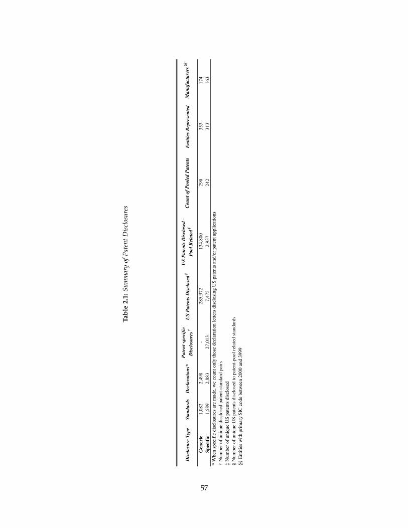
Tabl
e2.
1:Su
mm
ary
ofPa
tent
Dis
clos
ures
Dis
clos
ure
Type
Stan
dard
sD
ecla
ratio
ns*
Ent
ities
Rep
rese
nted
Man
ufac
ture
rs§§
Gen
eric
1,08
22,
498
-28
5,97
213
4,80
029
035
317
4Sp
ecifi
c1,
589
2,88
327
,013
7,47
52,
937
242
313
163
* W
hen
spec
ific
dis
clos
ures
are
mad
e, w
e co
unt o
nly
thos
e de
clar
atio
n le
tters
dis
clos
ing
US
pate
nts
and/
or p
aten
t app
licat
ions
† N
umbe
r of
uni
que
disc
lose
d pa
tent
-sta
ndar
d pa
irs
‡ N
umbe
r of
uni
que
US
pate
nts
disc
lose
d§
Num
ber
of u
niqu
e U
S pa
tent
s di
sclo
sed
to p
aten
t-po
ol r
elat
ed s
tand
ards
§§ E
ntiti
es w
ith p
rim
ary
SIC
cod
e be
twee
n 20
00 a
nd 3
999
Dis
clos
ure
Type
SSO
Dec
lara
tions
*E
ntiti
es R
epre
sent
edM
anuf
actu
rers
§§
AN
SI54
2-
137,
548
397
6294
55A
TSC
36-
45,9
7940
,917
2424
14E
TSI
501
-31
,525
12,5
7327
2311
IEC
420
-19
2,97
453
,816
265
139
77IE
EE
671
-18
1,72
323
,478
9716
079
ISO
313
-12
1,91
074
,692
6175
38IT
U15
-2,
338
1,49
79
43
AN
SI15
044
926
30
174
42A
TSC
2243
240
935
195
1811
ETS
I1,
216
23,6
615,
711
2,32
610
994
46IE
C72
146
529
412
716
6337
IEE
E25
992
163
441
1910
157
ISO
220
475
275
109
1667
39IT
U29
561
035
198
1078
40*
Whe
n sp
ecif
ic d
iscl
osur
es a
re m
ade,
we
coun
t onl
y th
ose
decl
arat
ion
lette
rs d
iscl
osin
g U
S pa
tent
s an
d/or
pat
ent a
pplic
atio
ns†
Num
ber
of u
niqu
e di
sclo
sed
pate
nt-s
tand
ard
pair
s‡
Num
ber
of u
niqu
e U
S pa
tent
s di
sclo
sed
§ N
umbe
r of
uni
que
US
pate
nts
disc
lose
d to
pat
ent-
pool
rel
ated
sta
ndar
ds§§
Ent
ities
with
pri
mar
y SI
C c
ode
betw
een
2000
and
399
9
Spec
ific
US
Pate
nts D
iscl
osed
‡Pa
tent
-spe
cific
D
iscl
osur
es†
Pate
nt-s
peci
fic
Dis
clos
ures
†U
S Pa
tent
s Dis
clos
ed‡
Cou
nt o
f Poo
led
Pate
nts
Cou
nt o
f Poo
led
Pate
nts
US
Pate
nts D
iscl
osed
- Po
ol R
elat
ed§
US
Pate
nts D
iscl
osed
- Po
ol R
elat
ed§
Gen
eric
57
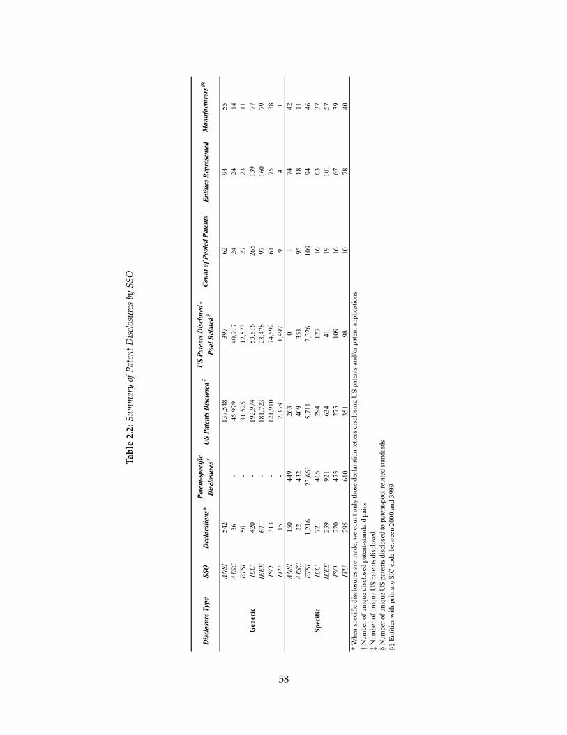
Tabl
e2.
2:Su
mm
ary
ofPa
tent
Dis
clos
ures
bySS
O
Dis
clos
ure
Type
Stan
dard
sD
ecla
ratio
ns*
Ent
ities
Rep
rese
nted
Man
ufac
ture
rs§§
Gen
eric
1,08
22,
498
-28
5,97
213
4,80
029
035
317
4Sp
ecifi
c1,
589
2,88
327
,013
7,47
52,
937
242
313
163
* W
hen
spec
ific
dis
clos
ures
are
mad
e, w
e co
unt o
nly
thos
e de
clar
atio
n le
tters
dis
clos
ing
US
pate
nts
and/
or p
aten
t app
licat
ions
† N
umbe
r of
uni
que
disc
lose
d pa
tent
-sta
ndar
d pa
irs
‡ N
umbe
r of
uni
que
US
pate
nts
disc
lose
d§
Num
ber
of u
niqu
e U
S pa
tent
s di
sclo
sed
to p
aten
t-po
ol r
elat
ed s
tand
ards
§§ E
ntiti
es w
ith p
rim
ary
SIC
cod
e be
twee
n 20
00 a
nd 3
999
Dis
clos
ure
Type
SSO
Dec
lara
tions
*E
ntiti
es R
epre
sent
edM
anuf
actu
rers
§§
AN
SI54
2-
137,
548
397
6294
55A
TSC
36-
45,9
7940
,917
2424
14E
TSI
501
-31
,525
12,5
7327
2311
IEC
420
-19
2,97
453
,816
265
139
77IE
EE
671
-18
1,72
323
,478
9716
079
ISO
313
-12
1,91
074
,692
6175
38IT
U15
-2,
338
1,49
79
43
AN
SI15
044
926
30
174
42A
TSC
2243
240
935
195
1811
ETS
I1,
216
23,6
615,
711
2,32
610
994
46IE
C72
146
529
412
716
6337
IEE
E25
992
163
441
1910
157
ISO
220
475
275
109
1667
39IT
U29
561
035
198
1078
40*
Whe
n sp
ecif
ic d
iscl
osur
es a
re m
ade,
we
coun
t onl
y th
ose
decl
arat
ion
lette
rs d
iscl
osin
g U
S pa
tent
s an
d/or
pat
ent a
pplic
atio
ns†
Num
ber
of u
niqu
e di
sclo
sed
pate
nt-s
tand
ard
pair
s‡
Num
ber
of u
niqu
e U
S pa
tent
s di
sclo
sed
§ N
umbe
r of
uni
que
US
pate
nts
disc
lose
d to
pat
ent-
pool
rel
ated
sta
ndar
ds§§
Ent
ities
with
pri
mar
y SI
C c
ode
betw
een
2000
and
399
9
Spec
ific
US
Pate
nts D
iscl
osed
‡Pa
tent
-spe
cific
D
iscl
osur
es†
Pate
nt-s
peci
fic
Dis
clos
ures
†U
S Pa
tent
s Dis
clos
ed‡
Cou
nt o
f Poo
led
Pate
nts
Cou
nt o
f Poo
led
Pate
nts
US
Pate
nts D
iscl
osed
- Po
ol R
elat
ed§
US
Pate
nts D
iscl
osed
- Po
ol R
elat
ed§
Gen
eric
58
in Thomson Innovation to identify one of approximately 22,300 patenting organizations
worldwide and map them to all subsidiaries listed in Thomson database. This enables us to
count and aggregate US patents and patent applications wherever a firm or its subsidiary
appears as an assignee or applicant on the patent record. Using this approach, we are able
to identify almost 300,000 patents. Since we want to limit our patent sample only to those
patents relevant to standards in question, we use patent International Patent Classification
(IPC) technology codes to accomplish this. First we use specifically disclosed patents to
build libraries of IPC codes associated to every standard with specifically disclosed patents.
Next we compare these libraries with IPC codes assigned to generically disclosed patent
portfolios. All generically disclosed patents having one or more IPC codes equal to one or
more standard-relevant IPC codes are deemed as standard-eligible. All other patents are
dropped. This process yields 134,800 standard-eligible patents.
We obtain additional information about firms disclosing the patents to SSOs from the
Standard & Poor’s Capital IQ and Compustat databases. These databases integrate financial
and operational information on thousands of companies worldwide. We use Capital IQ’s
name-matching feature to match patent owner names to standardized entity names. We then
assign a unique identifier to each entity in our sample and to map it to the parent company.
Similarly to what we do with patents, we also aggregate all patent disclosures on a parent
company level. Mergers and acquistions, as well as company name changes are tracked over
time, and mapped to the patent disclosure date to ensure the most accurate mapping. For
example, if we have separate disclosures from Philips North America and Philips Healthcare,
we map both of these companies to their ultimate parent—Philips Corporation. We use
Capital IQ to obtain time series data on firm size, revenue and earnings, R&D spending,
capital expenditures, primary industry, age, and subsidiary-parent relationships. Since firms
change their activities and industries over time, we also use S&P Compustat to get historical
firm segment information encompassing product and geographical industry segment data.
59
2.3.2 Disclosure Preferences Across the Value Chain
Variables
To test if the large, downstream firms are more likely to use generic disclosures, we first
need to agnostically determine if firms who disclose patents to standards have downstream
presence relative to those standards. For example, if a firm makes a patent disclosure to
3G wireless standard, while it contemporaneously manufactures 3G based products like
cellular phones, then that firm is downstream relative to 3G standard. This requires us to
make a link between industry segments, technical standards and firm activities. To link
standards with relevant industries, we use all specifically disclosed patents to create a list of
standard-relevant IPC codes, and link those to NAICS industry codes. Past studies have
generally linked patent classes to relevant industries by using one of the two publically
available patent-to-industry concordances. The first one is Yale Technology Concordance
(YTC), originally developed by Evenson et al. [1991], and the second one is Brian Silverman’s
Technology Concordance described in Silverman [1999]. Both of these concordances are
probabilistic links of patent technology classes to industry codes based on a set of Canadian
patents which were assigned industry codes in the early 1990s. Unfortunately, because these
concordances are based on 1990s industry codes, some of the important new industries—like
wireless communications—are largelly absent. To get around this problem, we use a newly
developed patent-industry concordance known as Algorithmic Links with Probabilities
(ALP) approach [Lybbert and Zolas, 2014]. This approach exploits recent advances in text
analysis and relies on a keyword extraction from the patents themselves and subsequent
probabilistic matching to textual descriptions of technology, industry or trade classifications.
To generate the concordance, Lybbert and Zolas [2014] use the full PATSTAT database from
the European Patent Office (EPO), and arrive at two-way probability distributions of 1) the
IPC technology classes used within each industry and 2) industries using certain types of
IPC technology classes.12
12Lybbert and Zolas [2014] concordance is available from the World Intellectual Property Organization(WIPO) at: http://www.wipo.int/export/sites/www/econ_stat/en/economics/zip/wp14_concordance.zip
60
Before we apply ALP concordance, we create lists of all 4-digit IPC technology codes
relevant to each individual standard by using specifically disclosed patents. We then match
those IPC codes to NAICS codes obtained from ALP concordance dataset.13 Once we
generate a map of NAICS codes for each standard, we resort to S&P Compustat Historical
Segment data for each firm making a disclosure. Historical segment NAICS codes are
compared to lists of standard-relevant NAICS codes, and those firms whose historical
NAICS codes match any of standard-relevant NAICS codes are labelled as downstream to
that particular standard. For example, if firms 1 and 2 disclose patents to some standard
A, and ALP concordance results in that standard A being associated with NAICS codes X
and Y, then if firm 1’s historical NAICS code is X at the time of its disclosure, and firm 2’s
historical NAICS code is Z at the time of its disclosure, firm 1 will be labelled as downstream
and firm 2 will be labelled as upstream. In addition, since they are not listed in Compustat,
we manually classify all universities and research institutes as upstream entities.
Counting disclosures can also be tricky. For example, a single specific declaration letter
can disclose multiple patents to multiple standards, while a generic declaration can disclose
potentially many patents to one or more standards. To compare disclosure preferences, we
disregard all patents and observe disclosure letters submitted by a firm in a given year only.
So, even if firm 1 was to disclose 10 patents to standard A in 5 different disclosures during
the course of one year, we would count this as a single specific disclosure made by firm 1
to standard A in that year. To reduce sample variability and ensure consistent comparison
across firms, we analyze only those standards receiving both specific and generic disclosures.
Standards receiving only specific or only generic disclosures are dropped from the sample.
This results in a final sample of 840 disclosures.
Since our hypothesis contends that the size of downstream firms will increase the
likelihood of these firms to utilize generic disclosures, we need to account for firm size
[last accessed: 06/10/2015].
13While we generate frequency weights for IPC-standard lists, we do not use them in the final analysis as tonot overcomplicate the process. Rather, we us a simple discrete measure of “match” or “no-match”.
61
in the analysis. Unfortunately, firm size is not a directly measurable quantity, so we are
forced use a set of financial and operational proxies. These include total revenue, R&D
expenditures, property, plant and equipment, number of employees and capital expenditures.
For each one of these proxy variables, we calculate the logarithm of the average over a 3-year
window (from the year of disclosure to two years prior).14 Table 2.3 provides more detailed
descriptions of variables used in this part of the analysis.
Summary statistics are reported in Table 2.4.
Specification
To test if large, downstream firms are more likely to use generic disclosures, we use a logistic
specification:
Pr(Speci,s,t = 1) = F(α + β× Di,s,t + γ× Si,t + δ× Di,s,t × Si,t + Indi + Yeart + SSOs + εi,s,t)
where
F(z) =ez
(1 + ez)
In this specification, the dependent variable Speci,s,t is a dummy equal to 1 if a specific
disclosure was made by the firm i to a standard s in a year t. Di,s,t is a dummy equal to 1 if
the firm i was determined to be downstream to a standard s in a year t. Si,tis a size proxy
for the firm i in a year t. Indi is industry sector fixed effect (4-digit SIC level), Yearm is a
year fixed effect and SSOs is SSO fixed effect. We are particularly interested in the sign of δ
coefficient on the interaction term of the downstream dummy and firm size proxy. Negative
δ would indicate that size makes downstream firms less likely to make specific disclosures.
Given that firm size proxies are highly correlated, we test our specification on each proxy
independently. Correlation coefficients for firm size proxies range between 0.77 and 0.95 as
shown in Table 2.5.
14Our results are robust to changes in time-window length.
62
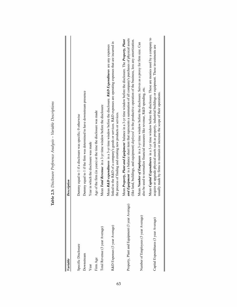
Tabl
e2.
3:D
iscl
osur
ePr
efer
ence
Ana
lysi
s–
Var
iabl
eD
escr
iptio
ns
Var
iabl
eD
escr
iptio
n
Spe
cifi
c D
iscl
osur
eD
umm
y eq
ual t
o 1
if a
dis
clos
ure
was
spe
cifi
c; 0
oth
erw
ise
Dow
nstr
eam
Dum
my
equa
l to
1 if
the
firm
was
det
erm
ined
to h
ave
dow
nstr
eam
pre
senc
e
Yea
rY
ear
in w
hich
the
disc
losu
re w
as m
ade
Fir
m A
geA
ge o
f th
e fi
rm (
in y
ears
) at
the
tim
e th
e di
sclo
sure
was
mad
e
Tot
al R
even
ue (
3 ye
ar A
vera
ge)
Mea
n To
tal R
even
ue in
a 3
-yr
tim
e w
indo
w b
efor
e th
e di
sclo
sure
R&
D E
xpen
ses
(3 y
ear
Ave
rage
)M
ean
R&
D e
xpen
ditu
res
in a
3-y
r ti
me
win
dow
bef
ore
the
disc
losu
re. R
&D
Exp
endi
ture
s ar
e an
y ex
pens
es
link
ed to
the
R&
D o
f a
com
pany
's g
oods
or
serv
ices
. R&
D e
xpen
ses
are
oper
atin
g ex
pens
es th
at a
re in
curr
ed in
th
e pr
oces
s of
fin
ding
and
cre
atin
g ne
w p
rodu
cts
or s
ervi
ces.
Pro
pert
y, P
lant
and
Equ
ipm
ent (
3 ye
ar A
vera
ge)
Mea
n Pr
oper
ty, P
lant
and
Equ
ipm
ent
bala
nce
in a
3-y
r ti
me
win
dow
bef
ore
the
disc
losu
re. T
he P
rope
rty,
Pla
nt
and
Equ
ipm
ent
is a
bal
ance
she
et it
em th
at r
epre
sent
s a
sum
mat
ion
of a
ll c
ompa
ny's
pur
chas
es o
f ph
ysic
al a
sset
s (l
ike
land
, bui
ldin
gs, a
nd e
quip
men
t) d
eplo
yed
in th
e pr
oduc
tive
ope
rati
on o
f th
e bu
sine
ss, l
ess
any
amor
tiza
tion
.
Num
ber
of E
mpl
oyee
s (3
yea
r A
vera
ge)
Mea
n N
umbe
r of E
mpl
oyee
s in
a 3
-yr
tim
e w
indo
w b
efor
e th
e di
sclo
sure
. Ser
ves
as a
pro
xy f
or f
irm
siz
e. C
an
also
be
used
to n
orm
aliz
e fi
nanc
ial m
easu
res
like
rev
enue
, R&
D s
pend
ing,
etc
.
Cap
ital
Exp
endi
ture
s (3
yea
r A
vera
ge)
Mea
n C
apita
l Exp
endi
ture
s in
a 3
-yr
tim
e w
indo
w b
efor
e th
e di
sclo
sure
. The
se a
re m
onie
s us
ed b
y a
com
pany
to
acqu
ire
or u
pgra
de p
hysi
cal a
sset
s su
ch a
s pr
oper
ty, i
ndus
tria
l bui
ldin
gs o
r eq
uipm
ent.
The
se in
vest
men
ts a
re
usua
lly
mad
e by
fir
ms
to m
aint
ain
or in
crea
se th
e sc
ope
of th
eir
oper
atio
ns.
63
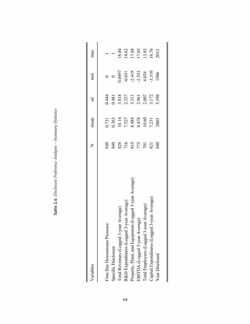
Tabl
e2.
4:D
iscl
osur
ePr
efer
ence
Ana
lysi
s–
Sum
mar
ySt
atis
tics
Var
iabl
esN
mea
nsd
min
max
Fir
m H
as D
owns
trea
m P
rese
nce
840
0.73
10.
444
01
Spe
cifi
c D
iscl
osur
e84
00.
363
0.48
10
1
Tot
al R
even
ues
(Log
ged
3-ye
ar A
vera
ge)
826
10.1
43.
018
0.04
9718
.84
R&
D E
xpen
ditu
res
(Log
ged
3-ye
ar A
vera
ge)
716
7.52
72.
327
-0.6
5114
.62
Pro
pert
y, P
lant
, and
Equ
ipm
ent (
Log
ged
3-ye
ar A
vera
ge)
815
8.48
43.
311
-2.4
1917
.88
EB
ITD
A (
Log
ged
3-ye
ar A
vera
ge)
775
8.47
82.
961
-2.5
5317
.03
Tot
al E
mpl
oyee
s (L
ogge
d 3-
year
Ave
rage
)70
110
.60
2.00
74.
034
13.4
3
Cap
ital
Exp
endi
ture
s (L
ogge
d 3-
year
Ave
rage
)82
17.
231
3.17
2-3
.310
16.7
6
Yea
r D
iscl
osed
840
2003
5.59
819
8620
13
64
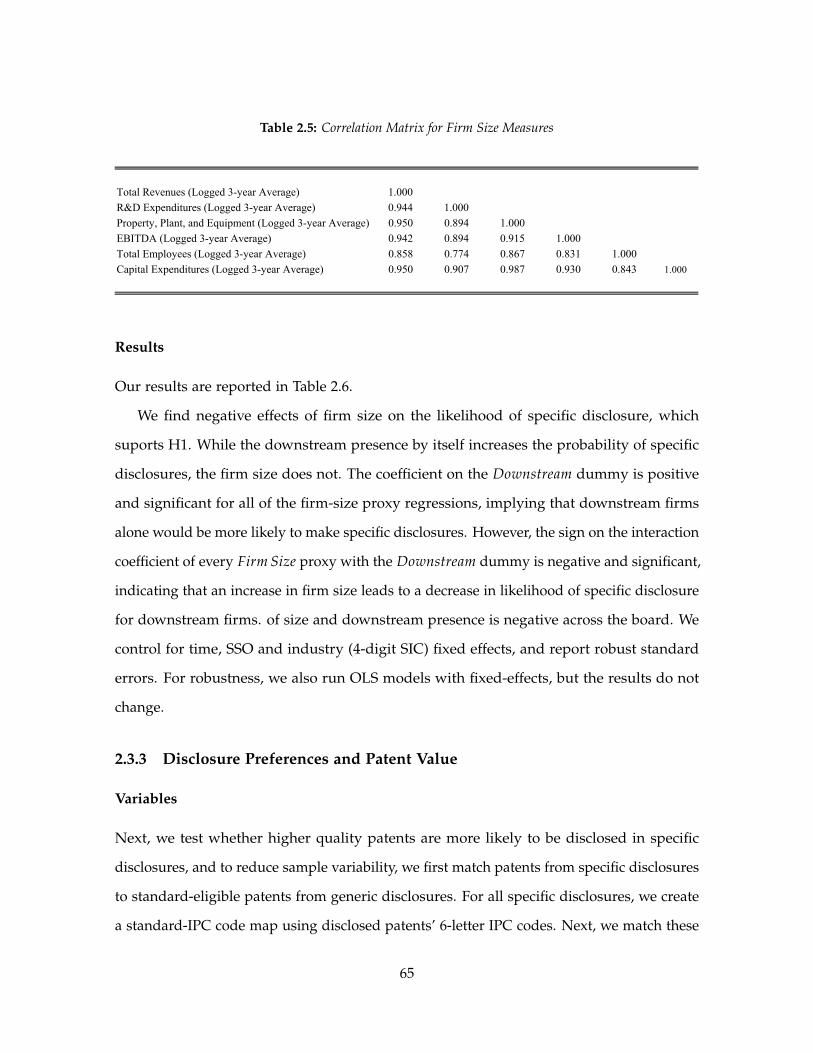
Table 2.5: Correlation Matrix for Firm Size Measures
Total Revenues (Logged 3-year Average) 1.000
R&D Expenditures (Logged 3-year Average) 0.944 1.000
Property, Plant, and Equipment (Logged 3-year Average) 0.950 0.894 1.000
EBITDA (Logged 3-year Average) 0.942 0.894 0.915 1.000
Total Employees (Logged 3-year Average) 0.858 0.774 0.867 0.831 1.000
Capital Expenditures (Logged 3-year Average) 0.950 0.907 0.987 0.930 0.843 1.000
Results
Our results are reported in Table 2.6.
We find negative effects of firm size on the likelihood of specific disclosure, which
suports H1. While the downstream presence by itself increases the probability of specific
disclosures, the firm size does not. The coefficient on the Downstream dummy is positive
and significant for all of the firm-size proxy regressions, implying that downstream firms
alone would be more likely to make specific disclosures. However, the sign on the interaction
coefficient of every Firm Size proxy with the Downstream dummy is negative and significant,
indicating that an increase in firm size leads to a decrease in likelihood of specific disclosure
for downstream firms. of size and downstream presence is negative across the board. We
control for time, SSO and industry (4-digit SIC) fixed effects, and report robust standard
errors. For robustness, we also run OLS models with fixed-effects, but the results do not
change.
2.3.3 Disclosure Preferences and Patent Value
Variables
Next, we test whether higher quality patents are more likely to be disclosed in specific
disclosures, and to reduce sample variability, we first match patents from specific disclosures
to standard-eligible patents from generic disclosures. For all specific disclosures, we create
a standard-IPC code map using disclosed patents’ 6-letter IPC codes. Next, we match these
65
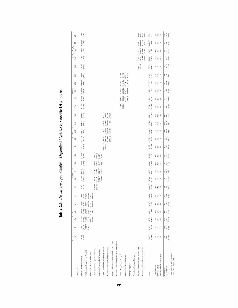
Tabl
e2.
6:D
iscl
osur
eTy
peR
esul
ts–
Dep
ende
ntV
aria
ble
isSp
ecifi
cD
iscl
osur
e
Dow
nstr
eam
(1)
(2)
(3)
(4)
(5)
(6)
(7)
(8)
(9)
(10)
(11)
(12)
(13)
(14)
(15)
(16)
(17)
(18)
(19)
(20)
(21)
(22)
(23)
(24)
(25)
(26)
VA
RIA
BL
ES
Firm
Has
Dow
nstr
eam
Pre
senc
e-0
180
-022
11
611*
**1
420*
*1
585*
*1
400*
-020
71
786*
**1
592*
*1
699*
*2
110*
**-0
273
121
1***
105
0**
118
5**
101
8*-0
324*
197
6***
210
6***
239
0***
209
7***
-025
53
622*
**2
866*
*3
324*
**2
508*
(016
0)(0
166)
(059
4)(0
655)
(069
9)(0
744)
(019
5)(0
616)
(066
3)(0
696)
(080
8)(0
169)
(042
6)(0
466)
(049
4)(0
551)
(017
6)(0
560)
(063
0)(0
655)
(067
2)(0
179)
(101
3)(1
151)
(125
9)(1
398)
Tot
al R
even
ues
(Log
ged
3-ye
ar A
vera
ge)
-009
12**
*0
0280
006
000
0731
000
386
(002
63)
(004
40)
(005
17)
(005
51)
(006
02)
Dow
nstr
eam
Pre
senc
e x
Tot
al R
even
ues
-018
1***
-016
0***
-017
9***
-013
0*(0
0568
)(0
0611
)(0
0647
)(0
0680
)R
&D
Exp
endi
ture
s (L
ogge
d 3-
year
Ave
rage
)-0
206*
**-0
0159
001
450
0313
007
63(0
0379
)(0
0663
)(0
0730
)(0
0761
)(0
0867
)
Dow
nstr
eam
Pre
senc
e x
R&
D E
xpen
ditu
res
-027
4***
-024
5***
-026
4***
-029
2***
(008
09)
(008
62)
(009
01)
(010
1)C
apit
al E
xpen
ditu
res
(Log
ged
3-ye
ar A
vera
ge)
-009
89**
*0
0269
005
260
0657
-001
56(0
0259
)(0
0398
)(0
0461
)(0
0489
)(0
0572
)
Dow
nstr
eam
Pre
senc
e x
Cap
ital
Exp
endi
ture
s-0
205*
**-0
177*
**-0
199*
**-0
131*
(005
51)
(005
81)
(006
10)
(006
68)
Prop
erty
, Pla
nt, a
nd E
quip
men
t (L
ogge
d 3-
year
Ave
rag e
Dow
nstr
eam
Pre
senc
e x
Prop
erty
, Pla
nt, a
nd E
quip
men
EB
ITD
A (
Log
ged
3-ye
ar A
vera
ge)
-011
1***
007
110
125*
*0
146*
*0
0438
(002
86)
(004
88)
(005
62)
(005
91)
(006
84)
Dow
nstr
eam
Pre
senc
e x
EB
ITD
A-0
263*
**-0
268*
**-0
304*
**-0
226*
**(0
0619
)(0
0678
)(0
0706
)(0
0752
)Fi
rm A
ge (
Log
ged)
Dow
nstr
eam
Pre
senc
e x
Firm
Age
Num
ber
of E
mpl
oyee
s (L
ogge
d 3-
year
Ave
rage
)-0
117*
**0
127*
017
9**
022
0**
018
6(0
0393
)(0
0771
)(0
0882
)(0
0985
)(0
126)
Dow
nstr
eam
Pre
senc
e x
Num
ber
of E
mpl
oyee
s-0
358*
**-0
286*
**-0
327*
**-0
232*
(009
08)
(010
3)(0
111)
(012
9)
Con
stan
t-0
431*
**0
503*
-072
3-0
229
034
31
408
111
6***
-026
8-0
971
-050
4-0
0476
032
2-0
632*
-148
0**
-090
3-0
0079
70
528*
-113
6**
-364
9***
-355
2***
-234
2*0
900*
*-1
804*
*-3
859*
**-3
689*
*-2
854*
(013
6)(0
298)
(047
9)(1
844)
(189
6)(1
409)
(032
1)(0
511)
(080
1)(0
908)
(117
9)(0
238)
(033
7)(0
745)
(086
9)(0
876)
(029
4)(0
474)
(116
7)(1
288)
(135
2)(0
455)
(088
1)(1
341)
(148
0)(1
712)
Yea
r Fi
xed
Eff
ect
No
No
No
Yes
Yes
Yes
No
No
Yes
Yes
Yes
No
No
Yes
Yes
Yes
No
No
Yes
Yes
Yes
No
No
Yes
Yes
Yes
SSO
Fix
ed E
ffec
tN
oN
oN
oN
oY
esY
esN
oN
oN
oY
esY
esN
oN
oN
oY
esY
esN
oN
oN
oY
esY
esN
oN
oN
oY
esY
esIn
dust
ry F
ixed
Eff
ect (
4-di
git S
IC)
No
No
No
No
No
Yes
No
No
No
No
Yes
No
No
No
No
Yes
No
No
No
No
Yes
No
No
No
No
Yes
Obs
erva
tion
s84
082
682
681
481
480
871
671
670
870
869
282
182
180
880
880
277
577
576
276
275
970
170
169
369
368
2L
og-L
ikel
ihoo
d-5
497
-532
5-5
266
-477
8-4
667
-433
4-4
501
-444
-403
4-3
943
-354
5-5
265
-518
1-4
714
-459
9-4
287
-490
6-4
807
-431
1-4
214
-396
-458
3-4
496
-407
3-3
97-3
652
Pseu
do R
-squ
ared
000
114
001
410
0249
010
60
127
018
30
0394
005
250
132
015
20
224
001
800
0336
011
10
133
018
50
0194
003
920
129
014
80
197
001
080
0295
011
40
136
018
9
Rob
ust s
tand
ard
erro
rs in
par
enth
eses
***
p<0
01, *
* p<
005
, * p
<0
1
Tot
al R
even
ues
Num
ber
of E
mpl
oyee
sC
apit
al E
xpen
ditu
res
EB
ITD
AR
&D
Exp
endi
ture
s
66
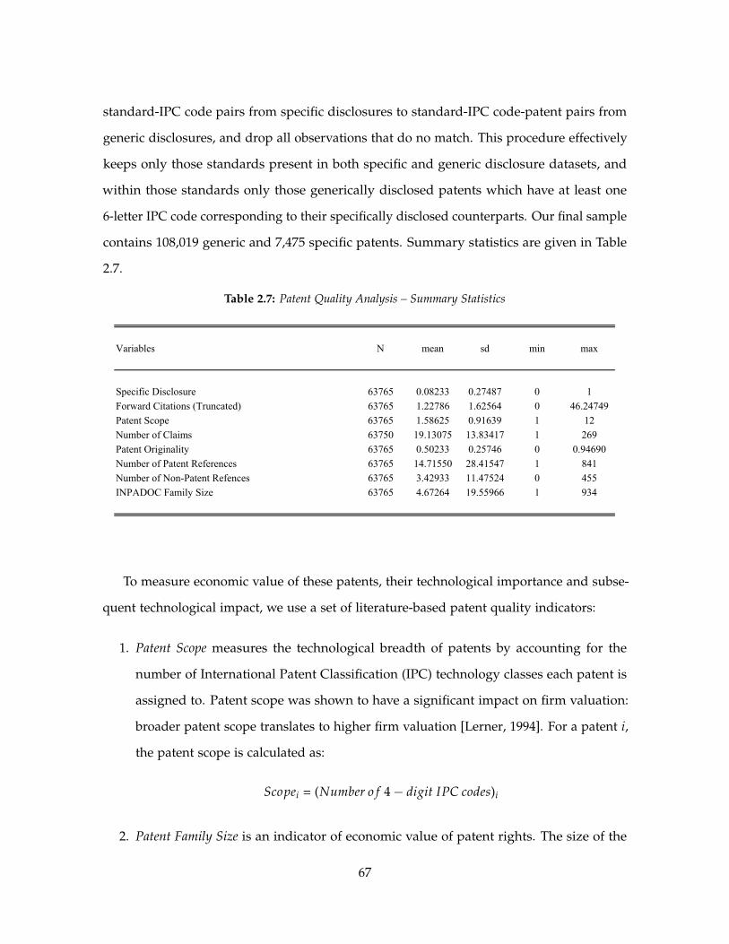
standard-IPC code pairs from specific disclosures to standard-IPC code-patent pairs from
generic disclosures, and drop all observations that do no match. This procedure effectively
keeps only those standards present in both specific and generic disclosure datasets, and
within those standards only those generically disclosed patents which have at least one
6-letter IPC code corresponding to their specifically disclosed counterparts. Our final sample
contains 108,019 generic and 7,475 specific patents. Summary statistics are given in Table
2.7.
Table 2.7: Patent Quality Analysis – Summary Statistics
Variables N mean sd min max
Specific Disclosure 63765 0.08233 0.27487 0 1
Forward Citations (Truncated) 63765 1.22786 1.62564 0 46.24749
Patent Scope 63765 1.58625 0.91639 1 12
Number of Claims 63750 19.13075 13.83417 1 269
Patent Originality 63765 0.50233 0.25746 0 0.94690
Number of Patent References 63765 14.71550 28.41547 1 841
Number of Non-Patent Refences 63765 3.42933 11.47524 0 455
INPADOC Family Size 63765 4.67264 19.55966 1 934
To measure economic value of these patents, their technological importance and subse-
quent technological impact, we use a set of literature-based patent quality indicators:
1. Patent Scope measures the technological breadth of patents by accounting for the
number of International Patent Classification (IPC) technology classes each patent is
assigned to. Patent scope was shown to have a significant impact on firm valuation:
broader patent scope translates to higher firm valuation [Lerner, 1994]. For a patent i,
the patent scope is calculated as:
Scopei = (Number o f 4− digit IPC codes)i
2. Patent Family Size is an indicator of economic value of patent rights. The size of the
67
patent family is highly correlated to the patent ”lifetime”, i.e. the time from the initial
patent application to patent expiration or assignee’s decision not to renew the patent
[Putnam, 1996, Lanjouw et al., 1998]. In addition, large patent families have been
shown to be more valuable [Harhoff et al., 2003]. Patent family size is measured as
the number of different patent jurisdictions (nations) in which patent protection was
sought, excluding European and World patents.15
3. Number of Claims determine the boundary of technology exclusion rights described
in the patent and are associated with technological and economic value of inventions
[Lanjouw and Schankerman, 2001, 2004].
4. Number of Patent References (Backward Citations) was shown to be postively correlated
with the patent value [Harhoff et al., 2003]. The number of patent references is the
number of other patent documents (including patent applications and self-citations)
cited in the patent.
5. Number of Non-Patent References (Backward Citations) is correlated with more significant
knowledge content [Cassiman et al., 2008].The number of non-patent references such
as scientific journals and books is also associated with higher patent quality and
approval rates [Branstetter and Ogura, 2005].
6. Number of Forward Citations is associated with the technological importance and overall
patent quality [Trajtenberg, 1990]. The number of forward citations is the number of
times a patent document is cited in subsequent patents. We correct all forward citation
counts for truncation on a 3-digit US patent class and cohort-year basis [Hall et al.,
2002].
7. Patent Originality measures the technological breadth of patent references. Low
originality score implies that a patent’s backward citation set is technologically narrow
15European and World patents do not give patent protection in individual countries. An applicant stillneeds to request a patent to be granted and comply with national laws in order to gain protection. If so, then anational patent is issued and end-point protection is obtained.
68
(a small and focused number of technology classes), while the high originality score
implies that backward citations belong to a larger and much broader set of technology
classes [Trajtenberg et al., 1997, Hall and Trajtenberg, 2004]. The measure of patent
originality is calculated using 4-digit IPC classes for all identified backward patent
citations as:
Originalityi = 1−Ni
∑j
OS2ij
where OS2ij is a share of citations cited by a patent i that come from a patent class j out
of set of Ni patent classes belonging to a set of all identified patent references cited
by patent i. Originality is calculated using all the references retrieved from Thomson
Innovation database.
Specification
We use simple logistic regression to test if higher quality patents are more likely to be
disclosed in specific disclosures:
Pr(Speci,sso,t = 1) = F(α + β× Patenti + Yeart + SSOsso + εi,s,t)
where
F(z) =ez
(1 + ez)
In this specification, the dependent variable Speci,sso,t is a dummy equal to 1 if a patent
i was disclosed in a specific disclosure to SSO sso in a year t. Patenti is the patent value
measure. Yearm is a year fixed effect and SSOsso is SSO fixed effect. We are particularly
interested in the sign of β coefficient on the patent value measure, and expect it to be
positive.
In this particular case, we aggregate disclosures on SSO level for two reasons. First, our
interviewees have indicated SSO-specific disclosure policies to be a major driver of how
and what firms disclose. Second, because multiple patents are disclosed to many standards
within and across SSOs, aggregating disclosures on the standard level would lead to many
69
duplicate observations, and it would not be entirely appropriate to control for standard-level
fixed effects. Since there are still many patents disclosed to multiple standards within SSOs,
to make sure we’re not overstating the significance of our results, we perform a simple
degree-of-freedom correction and create a dummy for each year and SSO and average over
them before running the regressions. This reduces the number of observations to 63,598.
Results
Table 2.8 reports the results.
We obtain positive and statistically significant effects of patent quality on the likelihood
of those patents being specifically disclosed. This supports H2. The coefficients on the
patent quality measures of scope, family size, number of claims, number of patent references,
number of non-patent-literature references and originality are all positive and significant,
implying that higher quality patents are indeed more likely to be disclosed to SSOs via
specific disclosures. We control for time and SSO, and report robust standard errors. For
robustness, we also run OLS models with fixed-effects, but the results do not change.
2.4 Conclusion
Our goal was to extend the quantitative empirical literature dealing with standard-setting
and illuminate standard-essential patent disclosure mechanisms made during standard-
ization process. In light of opportunities for abuse of standard-setting process, and large
downstream economic impact such abuses may have, this issue is very important. Through
the combination of economic theory and interviews with practicioners and regulators, we de-
veloped two hypotheses which we then tested using a novel dateset of all patent disclosures
made to seven large SSOs. We were able to identify SEP owners who had downstream pres-
ence to relevant standards, and create a binary measure of downstream presence. While our
measures of downstream presence can certainly be further refined, it is unclear if attempts
to refine this measure with somewhat noisy proxies could aggravate errors-in-variables
problem. In addition, we managed to create portfolios of standard-eligible patents using
70
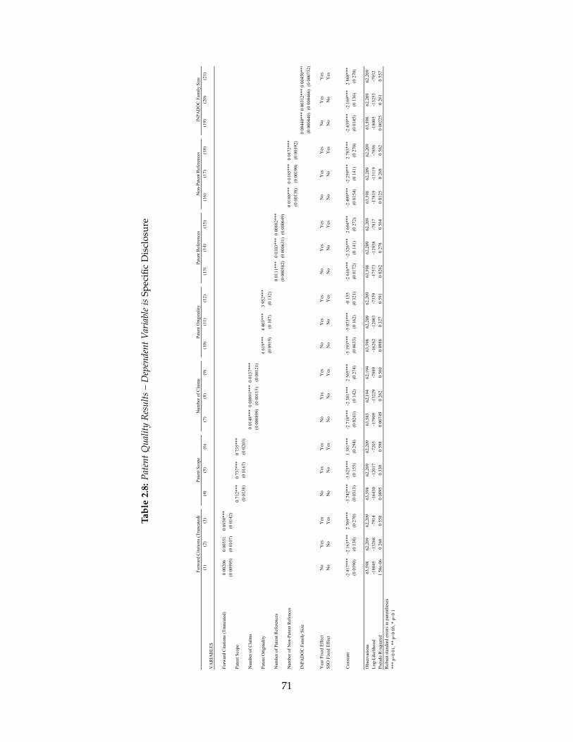
Tabl
e2.
8:Pa
tent
Qua
lity
Res
ults
–D
epen
dent
Var
iabl
eis
Spec
ific
Dis
clos
ure
(1)
(2)
(3)
(4)
(5)
(6)
(7)
(8)
(9)
(10)
(11)
(12)
(13)
(14)
(15)
(16)
(17)
(18)
(19)
(20)
(21)
VA
RIA
BL
ES
For
war
d C
itat
ions
(T
runc
ated
)0
0020
60
0035
10
0930
***
(000
995)
(001
07)
(001
42)
Pat
ent S
cope
071
2***
073
7***
073
5***
(001
38)
(001
67)
(002
03)
Num
ber
of C
laim
s0
0148
***
000
891*
**0
0137
***
(000
0899
)(0
0011
5)(0
0012
1)
Pat
ent O
rigi
nali
ty4
619*
**4
403*
**3
952*
**
(009
19)
(010
7)(0
132)
Num
ber
of P
aten
t Ref
eren
ces
001
11**
*0
0103
***
000
882*
**
(000
0582
)(0
0006
31)
(000
0649
)
Num
ber
of N
on-P
aten
t Ref
ence
s0
0188
***
001
85**
*0
0172
***
(000
138)
(000
190)
(000
192)
INP
AD
OC
Fam
ily
Siz
e0
0044
0***
000
312*
**0
0045
0***
(000
0440
)(0
0004
66)
(000
0732
)
Yea
r F
ixed
Eff
ect
No
Yes
Yes
No
Yes
Yes
No
Yes
Yes
No
Yes
Yes
No
Yes
Yes
No
Yes
Yes
No
Yes
Yes
SS
O F
ixed
Eff
ect
No
No
Yes
No
No
Yes
No
No
Yes
No
No
Yes
No
No
Yes
No
No
Yes
No
No
Yes
Con
stan
t-2
417*
**-2
163*
**2
769*
**-3
742*
**-3
625*
**1
381*
**-2
718*
**-2
381*
**2
565*
**-5
193*
**-5
073*
**-0
155
-261
6***
-232
6***
269
4***
-249
9***
-225
9***
278
3***
-243
9***
-216
9***
286
8***
(001
90)
(013
8)(0
270)
(003
13)
(015
5)(0
294)
(002
41)
(014
2)(0
274)
(006
33)
(016
2)(0
321)
(001
72)
(014
1)(0
272)
(001
54)
(014
1)(0
270)
(001
45)
(013
6)(0
270)
Obs
erva
tion
s63
,598
62,2
0962
,209
63,5
9862
,209
62,2
0963
,583
62,1
9462
,194
63,5
9862
,209
62,2
0963
,598
62,2
0962
,209
63,5
9862
,209
62,2
0963
,598
62,2
0962
,209
Log
-Lik
elih
ood
-180
45-1
3268
-791
4-1
6430
-120
17-7
203
-179
09-1
3229
-788
9-1
6262
-120
63-7
339
-175
73-1
2938
-781
7-1
7819
-131
19-7
856
-180
05-1
3253
-793
2
Pse
udo
R-s
quar
ed1
50e-
060
260
055
80
0895
033
00
598
000
749
026
20
560
009
880
327
059
10
0262
027
80
564
001
250
268
056
20
0022
50
261
055
7
Rob
ust s
tand
ard
erro
rs in
par
enth
eses
***
p<0
01, *
* p<
005
, * p
<0
1
INP
AD
OC
Fam
ily
Siz
eF
orw
ard
Cit
atio
ns (
Tru
ncat
ed)
Pate
nt S
cope
Num
ber
of C
laim
sP
aten
t Ori
gina
lity
Pat
ent R
efer
ence
sN
on-P
aten
t Ref
eren
ces
71
generic disclosures, and link them to patent quality measures.
Two hypotheses we developed are supported by our empirical results. We found strong
support for our first contention that large, downstream firms are more likely to make generic
disclosures to SSOs. The support for our second hypothesis that higher quality patents are
more likely to be disclosed via specific disclosures was equally as strong.
72
Chapter 3
The Impact of Money on Science:
Evidence from Unexpected NCAA
Football Outcomes1
3.1 Introduction
Investments in science can generate large social returns. Scientific discoveries have eradicated
diseases, reduced famine, increased labor productivity, and supported national defense.
However, scientific laboratories and experiments are expensive to run and research funds are
often the key limiting factor in scientific advancement. Together these facts make the level
of R&D investment a central concern of university administrators and public policymakers.
There is urgency about this issue in the United States where the federally-financed share of
university research has fallen over the last forty years and recent recession-induced budget
cuts have slashed states’ investment in academic research. These developments prompted
the America COMPETES Acts of 2007 and 2010 [National Research Council, 2012], which
called for a doubling of funds to basic science, and a potential reauthorization of the Act
in 2014. Despite its salience, the question of whether policymakers fund a socially-optimal
1Co-authored with Thomas Wollmann
73
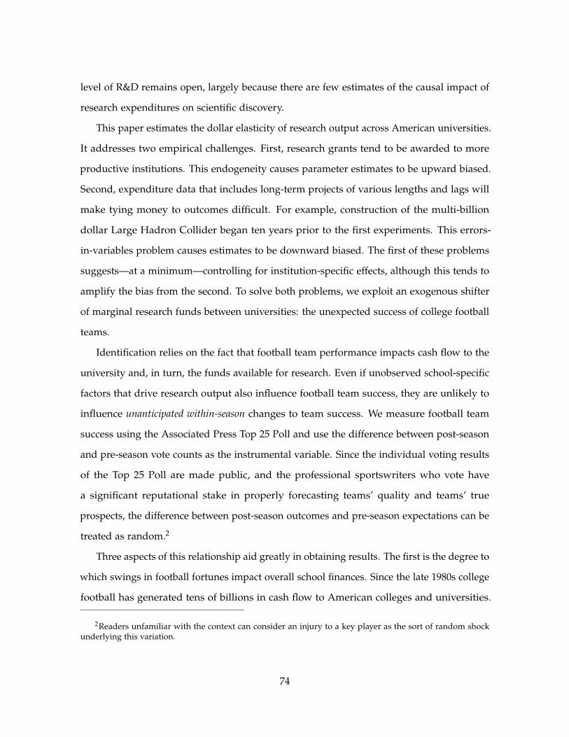
level of R&D remains open, largely because there are few estimates of the causal impact of
research expenditures on scientific discovery.
This paper estimates the dollar elasticity of research output across American universities.
It addresses two empirical challenges. First, research grants tend to be awarded to more
productive institutions. This endogeneity causes parameter estimates to be upward biased.
Second, expenditure data that includes long-term projects of various lengths and lags will
make tying money to outcomes difficult. For example, construction of the multi-billion
dollar Large Hadron Collider began ten years prior to the first experiments. This errors-
in-variables problem causes estimates to be downward biased. The first of these problems
suggests—at a minimum—controlling for institution-specific effects, although this tends to
amplify the bias from the second. To solve both problems, we exploit an exogenous shifter
of marginal research funds between universities: the unexpected success of college football
teams.
Identification relies on the fact that football team performance impacts cash flow to the
university and, in turn, the funds available for research. Even if unobserved school-specific
factors that drive research output also influence football team success, they are unlikely to
influence unanticipated within-season changes to team success. We measure football team
success using the Associated Press Top 25 Poll and use the difference between post-season
and pre-season vote counts as the instrumental variable. Since the individual voting results
of the Top 25 Poll are made public, and the professional sportswriters who vote have
a significant reputational stake in properly forecasting teams’ quality and teams’ true
prospects, the difference between post-season outcomes and pre-season expectations can be
treated as random.2
Three aspects of this relationship aid greatly in obtaining results. The first is the degree to
which swings in football fortunes impact overall school finances. Since the late 1980s college
football has generated tens of billions in cash flow to American colleges and universities.
2Readers unfamiliar with the context can consider an injury to a key player as the sort of random shockunderlying this variation.
74
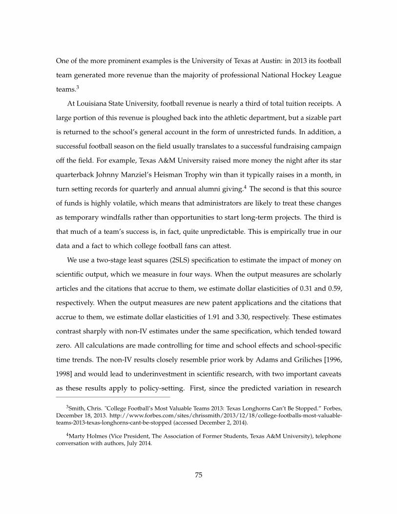
One of the more prominent examples is the University of Texas at Austin: in 2013 its football
team generated more revenue than the majority of professional National Hockey League
teams.3
At Louisiana State University, football revenue is nearly a third of total tuition receipts. A
large portion of this revenue is ploughed back into the athletic department, but a sizable part
is returned to the school’s general account in the form of unrestricted funds. In addition, a
successful football season on the field usually translates to a successful fundraising campaign
off the field. For example, Texas A&M University raised more money the night after its star
quarterback Johnny Manziel’s Heisman Trophy win than it typically raises in a month, in
turn setting records for quarterly and annual alumni giving.4 The second is that this source
of funds is highly volatile, which means that administrators are likely to treat these changes
as temporary windfalls rather than opportunities to start long-term projects. The third is
that much of a team’s success is, in fact, quite unpredictable. This is empirically true in our
data and a fact to which college football fans can attest.
We use a two-stage least squares (2SLS) specification to estimate the impact of money on
scientific output, which we measure in four ways. When the output measures are scholarly
articles and the citations that accrue to them, we estimate dollar elasticities of 0.31 and 0.59,
respectively. When the output measures are new patent applications and the citations that
accrue to them, we estimate dollar elasticities of 1.91 and 3.30, respectively. These estimates
contrast sharply with non-IV estimates under the same specification, which tended toward
zero. All calculations are made controlling for time and school effects and school-specific
time trends. The non-IV results closely resemble prior work by Adams and Griliches [1996,
1998] and would lead to underinvestment in scientific research, with two important caveats
as these results apply to policy-setting. First, since the predicted variation in research
3Smith, Chris. "College Football’s Most Valuable Teams 2013: Texas Longhorns Can’t Be Stopped.” Forbes,December 18, 2013. http://www.forbes.com/sites/chrissmith/2013/12/18/college-footballs-most-valuable-teams-2013-texas-longhorns-cant-be-stopped (accessed December 2, 2014).
4Marty Holmes (Vice President, The Association of Former Students, Texas A&M University), telephoneconversation with authors, July 2014.
75
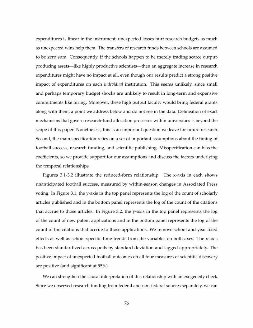
expenditures is linear in the instrument, unexpected losses hurt research budgets as much
as unexpected wins help them. The transfers of research funds between schools are assumed
to be zero sum. Consequently, if the schools happen to be merely trading scarce output-
producing assets—like highly productive scientists—then an aggregate increase in research
expenditures might have no impact at all, even though our results predict a strong positive
impact of expenditures on each individual institution. This seems unlikely, since small
and perhaps temporary budget shocks are unlikely to result in long-term and expensive
commitments like hiring. Moreover, these high output faculty would bring federal grants
along with them, a point we address below and do not see in the data. Delineation of exact
mechanisms that govern research-fund allocation processes within universities is beyond the
scope of this paper. Nonetheless, this is an important question we leave for future research.
Second, the main specification relies on a set of important assumptions about the timing of
football success, research funding, and scientific publishing. Misspecification can bias the
coefficients, so we provide support for our assumptions and discuss the factors underlying
the temporal relationships.
Figures 3.1-3.2 illustrate the reduced-form relationship. The x-axis in each shows
unanticipated football success, measured by within-season changes in Associated Press
voting. In Figure 3.1, the y-axis in the top panel represents the log of the count of scholarly
articles published and in the bottom panel represents the log of the count of the citations
that accrue to those articles. In Figure 3.2, the y-axis in the top panel represents the log
of the count of new patent applications and in the bottom panel represents the log of the
count of the citations that accrue to those applications. We remove school and year fixed
effects as well as school-specific time trends from the variables on both axes. The x-axis
has been standardized across polls by standard deviation and lagged appropriately. The
positive impact of unexpected football outcomes on all four measures of scientific discovery
are positive (and significant at 95%).
We can strengthen the causal interpretation of this relationship with an exogeneity check.
Since we observed research funding from federal and non-federal sources separately, we can
76
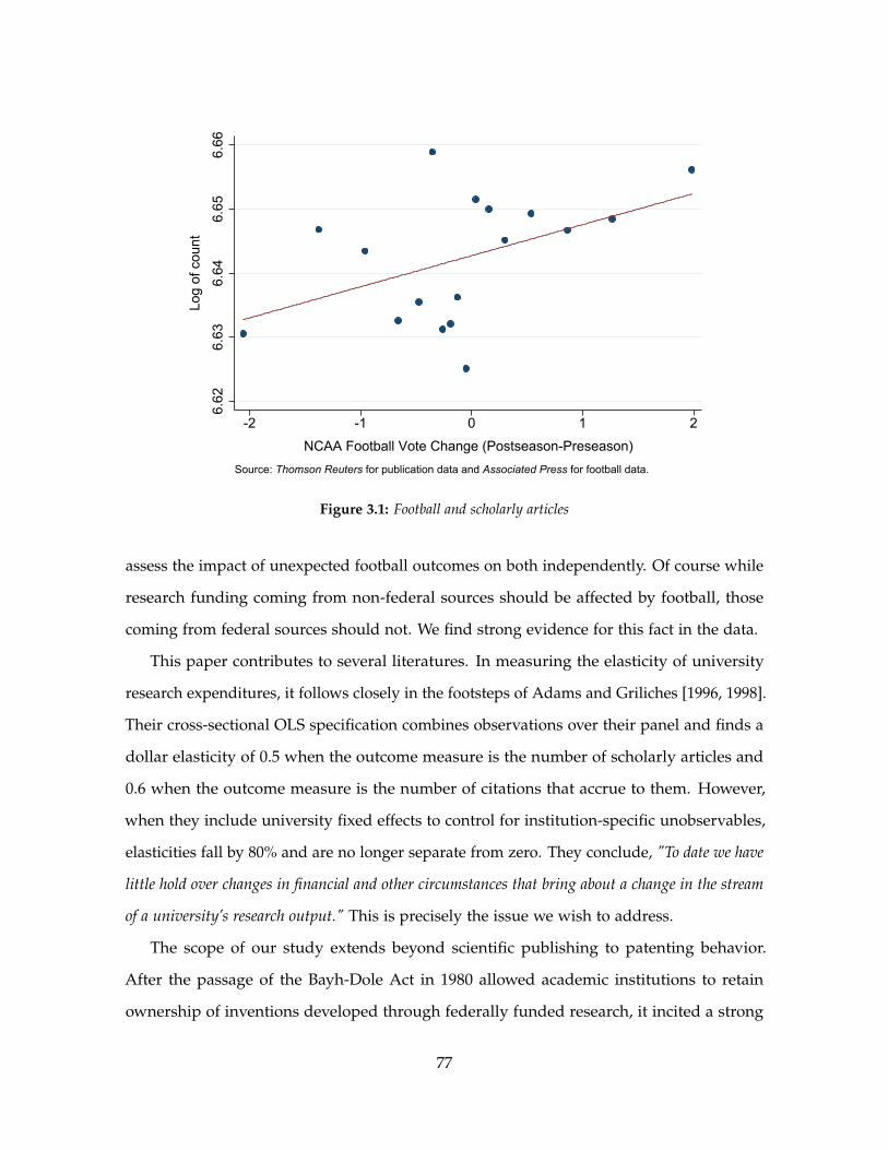
6.62
6.63
6.64
6.65
6.66
Log
of c
ount
-2 -1 0 1 2
NCAA Football Vote Change (Postseason-Preseason)
Source: Thomson Reuters for publication data and Associated Press for football data.
Publications and Football
Figure 3.1: Football and scholarly articles
assess the impact of unexpected football outcomes on both independently. Of course while
research funding coming from non-federal sources should be affected by football, those
coming from federal sources should not. We find strong evidence for this fact in the data.
This paper contributes to several literatures. In measuring the elasticity of university
research expenditures, it follows closely in the footsteps of Adams and Griliches [1996, 1998].
Their cross-sectional OLS specification combines observations over their panel and finds a
dollar elasticity of 0.5 when the outcome measure is the number of scholarly articles and
0.6 when the outcome measure is the number of citations that accrue to them. However,
when they include university fixed effects to control for institution-specific unobservables,
elasticities fall by 80% and are no longer separate from zero. They conclude, "To date we have
little hold over changes in financial and other circumstances that bring about a change in the stream
of a university’s research output." This is precisely the issue we wish to address.
The scope of our study extends beyond scientific publishing to patenting behavior.
After the passage of the Bayh-Dole Act in 1980 allowed academic institutions to retain
ownership of inventions developed through federally funded research, it incited a strong
77
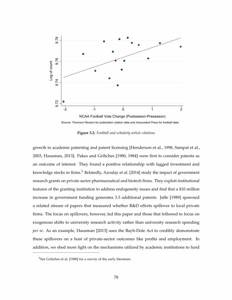
9.72
9.74
9.76
9.78
Log
of c
ount
-2 -1 0 1 2
NCAA Football Vote Change (Postseason-Preseason)
Source: Thomson Reuters for publication citation data and Associated Press for football data.
Publication Citations and Football
Figure 3.2: Football and scholarly article citations
growth in academic patenting and patent licensing [Henderson et al., 1998, Sampat et al.,
2003, Hausman, 2013]. Pakes and Griliches [1980, 1984] were first to consider patents as
an outcome of interest. They found a positive relationship with lagged investment and
knowledge stocks in firms.5 Relatedly, Azoulay et al. [2014] study the impact of government
research grants on private sector pharmaceutical and biotech firms. They exploit institutional
features of the granting institution to address endogeneity issues and find that a $10 million
increase in government funding generates 3.3 additional patents. Jaffe [1989] spawned
a related stream of papers that measured whether R&D efforts spillover to local private
firms. The focus on spillovers, however, led this paper and those that followed to focus on
exogenous shifts to university research activity rather than university research spending
per se. As an example, Hausman [2013] uses the Bayh-Dole Act to credibly demonstrate
these spillovers on a host of private-sector outcomes like profits and employment. In
addition, we shed more light on the mechanisms utilized by academic institutions to fund
5See Griliches et al. [1988] for a survey of the early literature.
78
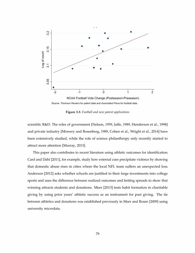
3.05
3.1
3.15
3.2
Log
of c
ount
-2 -1 0 1 2
NCAA Football Vote Change (Postseason-Preseason)
Source: Thomson Reuters for patent data and Associated Press for football data.
New Patent Applications and Football
Figure 3.3: Football and new patent applications
scientific R&D. The roles of government [Nelson, 1959, Jaffe, 1989, Henderson et al., 1998]
and private industry [Mowery and Rosenberg, 1989, Cohen et al., Wright et al., 2014] have
been extensively studied, while the role of science philanthropy only recently started to
attract more attention [Murray, 2013].
This paper also contributes to recent literature using athletic outcomes for identification.
Card and Dahl [2011], for example, study how external cues precipitate violence by showing
that domestic abuse rises in cities where the local NFL team suffers an unexpected loss.
Anderson [2012] asks whether schools are justified in their large investments into college
sports and uses the difference between realized outcomes and betting spreads to show that
winning attracts students and donations. Meer [2013] tests habit formation in charitable
giving by using prior years’ athletic success as an instrument for past giving. The tie
between athletics and donations was established previously in Meer and Rosen [2009] using
university microdata.
79
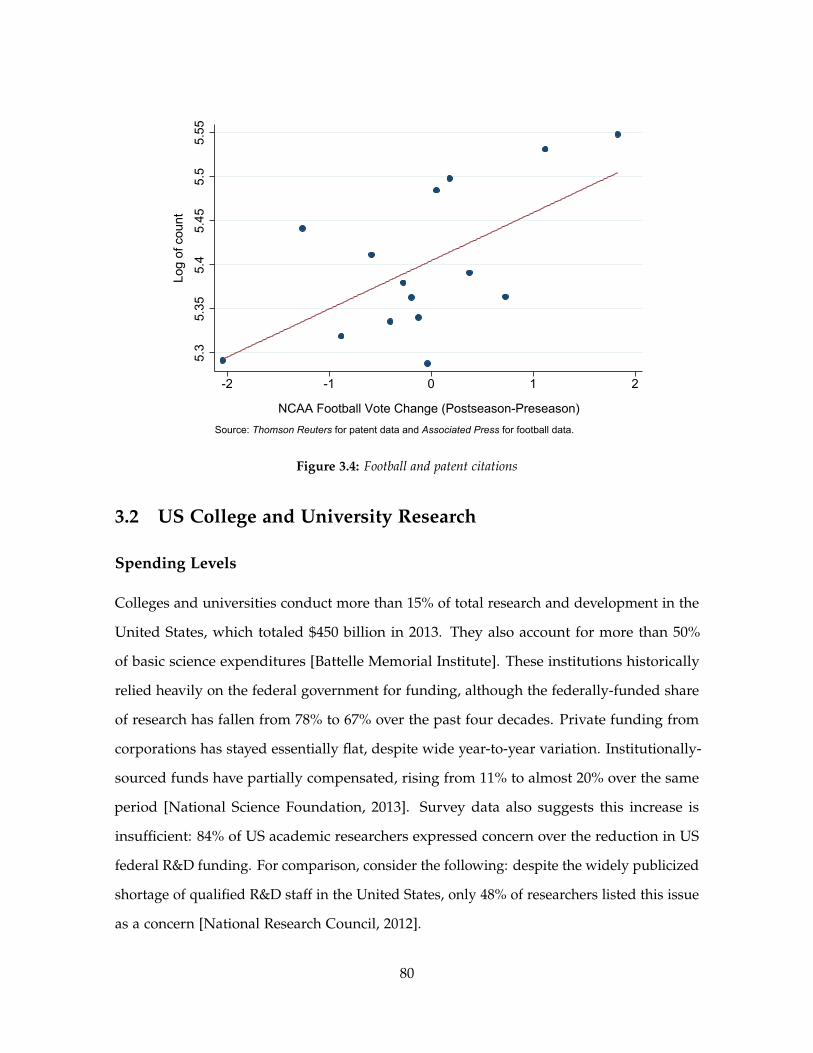
5.3
5.35
5.4
5.45
5.5
5.55
Log
of c
ount
-2 -1 0 1 2
NCAA Football Vote Change (Postseason-Preseason)
Source: Thomson Reuters for patent data and Associated Press for football data.
New Patent Citations and Football
Figure 3.4: Football and patent citations
3.2 US College and University Research
Spending Levels
Colleges and universities conduct more than 15% of total research and development in the
United States, which totaled $450 billion in 2013. They also account for more than 50%
of basic science expenditures [Battelle Memorial Institute]. These institutions historically
relied heavily on the federal government for funding, although the federally-funded share
of research has fallen from 78% to 67% over the past four decades. Private funding from
corporations has stayed essentially flat, despite wide year-to-year variation. Institutionally-
sourced funds have partially compensated, rising from 11% to almost 20% over the same
period [National Science Foundation, 2013]. Survey data also suggests this increase is
insufficient: 84% of US academic researchers expressed concern over the reduction in US
federal R&D funding. For comparison, consider the following: despite the widely publicized
shortage of qualified R&D staff in the United States, only 48% of researchers listed this issue
as a concern [National Research Council, 2012].
80
Congress and the White House have taken notice and begun to act on these concerns. In
2005, Congress asked the National Research Council to prepare a plan that would ensure
American competitiveness in science and technology. Congress then provided bipartisan
support for the America COMPETES Act, which President Bush signed into law in 2007. The
Act emphasizes investment in the science, technology, engineering, and mathematics fields
and authorizes a doubling of National Science Foundation (NSF) grants for many fields by
2011. In 2009, Congress requested a follow-up report. Two years later, President Obama
signed a reauthorization of the bill, the America COMPETES Act of 2010. The budget
sequestration process of 2013 reignited this debate. Ultimately, the authorized funding
increases were not realized. This has prompted the Director of the National Institute of
Health to worry that “we will lose a generation of young scientists” and that “a lot of good
science just won’t be done.”6
As of the time of writing, Congress has proposed but not yet passed another reauthoriza-
tion of the Act. A central driver of this debate is uncertainty about where the funding level
stands in relation to the optimal social level of R&D, which itself turns on the underlying
return on research investment. Measuring this return requires a more detailed examination
of the funding process.
3.2.1 How Research is Funded
Private colleges and universities fund their operations primarily through tuition, federal
grants, philanthropic donations, and auxiliary enterprises (like healthcare and athletics). For
public universities, state appropriations also account for a significant share of incoming cash
flow. Schools then use these funds mainly for student instruction, research, administration,
and running the auxiliary programs. They budget operational expenses on an annual basis7
6Vergano, Dan. “Science Faces Sequestration Cuts.” USAToday, February 25, 2013.http://www.usatoday.com/story/tech/sciencefair/2013/02/25/budget-nih-collins/1947277/ (accessed Decem-ber 2, 2014).
7We use the word “operational” to separate these from capital expenses, like construction projects, whichare likely to be budgeted long ahead of time.
81
and typically follow a June rather than December fiscal year end to synchronize with the
course-year calendar.8 The unused portion of funds are rarely allowed to carry over to the
next year.9
The budgeting process is complicated by widespread earmarks. Strict guidelines on how
funds can be spent are attached to a large portion of incoming cash flow, creating a distinction
between “restricted” and “unrestricted funds.”10 Some earmarks are obvious: an NSF grant
will go directly to the project for which it was awarded and state appropriations will directly
subsidize instruction of in-state residents. Other earmarks are not so straightforward. A
multi-million dollar donation by a wealthy single donor or a foundation could carry with it
the requirement that it be used to extend hours at an art museum or gymnasium, increase a
particular genre of books in the library, or expand the student center. For example, in 2010
Harvard University received a restricted gift of $50 million from the Tata family to fund
two new buildings on the business school campus.11 For both bookkeeping and flexibility
reasons, these unrestricted funds are a precious commodity.
For research, unrestricted funds are often the “source of last resort.” They are needed
when costs run over, other sources fall short, or faculty are too new to have attracted
sufficient grant money. That is, although federal and state funds still account for the
majority of university-led R&D, they are frequently too slow or inflexible to handle the
immediate and diverse needs of academic scholars. In the absence of unrestricted funds to
close the gap, research is often put on hold. Murray [2013] identifies philanthropic donations
as one possible channel for research institutions to fill funding gaps and provides a great
example: in 2008, when the fiscal crisis forced the State of California to reduce funding to
the UC Berkeley’s Radio Astronomy Lab and federal government cut funding for Allen
8There are a few exceptions to the June fiscal year end but these too end in the summer months and areimmaterial for our discussion.
9Carolyn Porter (Director of Development, McDonald Observatory, University of Texas at Austin), telephoneconversation with authors, July 2014.
10We thank Kyle Welch for bringing this to our attention.
11Walsh, Coleen. “Business School Announces Tata Gift; Two Initiatives.” Harvard Gazette, October 14, 2010.http://news.harvard.edu/gazette/story/2010/10/hbs_gift/ (accessed December 2, 2014).
82
Telescope Array, Microsoft’s Paul Allen stepped in and donated funds to ensure continuous
operation of the facility.12 Combined with other, both large and small philanthropic gifts,
unrestricted funds can also allow for scientific research to continue when federal financial
support for science does not deliver. Other sources of unrestricted funds include auxiliary
operations, like athletics and healthcare, housing, and tuition (primarily for out-of-state
residents in the case of public schools). Since it enables us to identify and precisely estimate
the elasticity of research output, football’s contribution is covered in detail below.
How Football Contributes Financially
“We took direct dollars from the athletic budget and put it into academicprograms.”E. Gordon Gee, 11th and 14th President, Ohio State University13
Football contributes to unrestricted university finances in two ways. The first channel
is auxiliary revenues. Since the late 1980s, Division I NCAA football has generated over
$10 billion in sales. For perspective, Table 3.1 provides the top 20 college football teams
in terms of revenue. The sheer size of these programs is staggering, especially in relation
to professional teams. For example, The University of Texas at Austin earns nearly $110
million in revenue. For comparison, this figure is 40% higher than the median professional
hockey team and on par with the median professional basketball team. On a per game basis,
it is 5 times larger than both of these and about 7 times larger than the median baseball
team. Their size relative to total tuition is also quite large. More than half of the schools
on the list have football programs that are more than 20% of the total tuition receipts. At
Louisiana State University and Agricultural and Mechanical College (LSU), the University of
12Murray [2013] emphasizes three key points about science philanthropy: that it is mostly channeled intorestricted funds, that it heavily favors translational science, and that it generally does not strive to fill fundinggaps. However, it is important to note that her study focuses on large philanthropic gifts (>$1M) at top 50research institutions and provides only one part of the funding equation. Some of these large philanthropicgifts happen to be unrestricted, and universities also collect many small philanthropic gifts which are usuallyunrestricted in nature. For example, the Harvard Alumni Association webpage provides opportunities foralumni to donate directly to the various university funds, most of which are unrestricted.
13"Dropping The Ball: The Shady Side Of Big-Time College Sports," The Bob Edwards Show (WashingtonD.C.: Public Radio International, January 4, 2015).
83
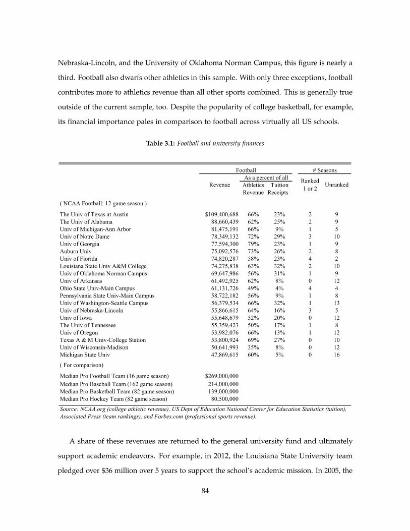
Nebraska-Lincoln, and the University of Oklahoma Norman Campus, this figure is nearly a
third. Football also dwarfs other athletics in this sample. With only three exceptions, football
contributes more to athletics revenue than all other sports combined. This is generally true
outside of the current sample, too. Despite the popularity of college basketball, for example,
its financial importance pales in comparison to football across virtually all US schools.
Table 3.1: Football and university finances
Football # SeasonsAs a percent of all
Athletics TuitionRevenue Receipts
( NCAA Football: 12 game season )
The Univ of Texas at Austin $109,400,688 66% 23% 2 9The Univ of Alabama 88,660,439 62% 25% 2 9Univ of Michigan-Ann Arbor 81,475,191 66% 9% 1 5Univ of Notre Dame 78,349,132 72% 29% 3 10Univ of Georgia 77,594,300 79% 23% 1 9Auburn Univ 75,092,576 73% 26% 2 8Univ of Florida 74,820,287 58% 23% 4 2Louisiana State Univ A&M College 74,275,838 63% 32% 2 10Univ of Oklahoma Norman Campus 69,647,986 56% 31% 1 9Univ of Arkansas 61,492,925 62% 8% 0 12Ohio State Univ-Main Campus 61,131,726 49% 4% 4 4Pennsylvania State Univ-Main Campus 58,722,182 56% 9% 1 8Univ of Washington-Seattle Campus 56,379,534 66% 32% 1 13Univ of Nebraska-Lincoln 55,866,615 64% 16% 3 5Univ of Iowa 55,648,679 52% 20% 0 12The Univ of Tennessee 55,359,423 50% 17% 1 8Univ of Oregon 53,982,076 66% 13% 1 12Texas A & M Univ-College Station 53,800,924 69% 27% 0 10Univ of Wisconsin-Madison 50,641,993 35% 8% 0 12Michigan State Univ 47,869,615 60% 5% 0 16
( For comparison)
Median Pro Football Team (16 game season) $269,000,000Median Pro Baseball Team (162 game season) 214,000,000Median Pro Basketball Team (82 game season) 139,000,000Median Pro Hockey Team (82 game season) 80,500,000
Source: NCAA.org (college athletic revenue), US Dept of Education National Center for Education Statistics (tuition),Associated Press (team rankings), and Forbes.com (professional sports revenue).
RevenueRanked 1 or 2
Unranked
A share of these revenues are returned to the general university fund and ultimately
support academic endeavors. For example, in 2012, the Louisiana State University team
pledged over $36 million over 5 years to support the school’s academic mission. In 2005, the
84
Notre Dame football used $14.5 million of its post-season bowl winnings to fund academic
priorities. From 2011 to 2012, the University of Florida team gave $6 million to cover
shortfalls in university funding [Dosh, 2013]. From 2012 to 2013, the University of Texas -
Austin gave $9.2 million of its $18.9 million back to the university fund while the University
of Nebraska - Lincoln did the same with $2.7 million of its $5.2 million surplus [Lavigne,
2014].
The second channel is alumni contributions. Football success is a major catlyst for
philanthropic fundraising shocks [Meer and Rosen, 2009, Anderson, 2012]. For example,
Texas A&M University raised more money the night after its freshman quarterback, Johnny
Manziel, won the Heisman Trophy than it typically raises in a full month. That year, the
school announced it received a record-setting $740 million in donations14. The university
chancellor John Sharp highlighted the significant role college football played in their fund-
raising efforts, stating, “Football is one heck of a megaphone for us to tell our story”.15
Schools also can directly tie athletic privileges to academic donations. Stinson and Howard
[2010, 2014] document how one large Midwestern school makes donors of academic gifts
over $3,000 eligible to buy season tickets.
Football success, and most likely its financial contribution, are quite volatile. This is
shown in the rightmost two columns of Table I. Sixteen of the twenty schools have competed
for the national championship over the panel 1987 to 2012. On the other hand, every team
was unranked at least twice over the panel, and many were unranked more than ten times.
These reversals of fortune are important because variation in teams’ rank provides the
underlying variation for our identification. For example, a surprising 11-0 record of Boise
State University football team in 2004-2005 resulted in an marked increase in university
donations, a 66% increase in sales of university merchandise at the bookstore, and a 60%
14Marty Holmes (Vice President, The Association of Former Students, Texas A&M University), telephoneconversation with authors, July 2014.
15Troop, Don. “Texas A&M Pulls in $740-Million for Academics and Football.” The Chronicle of HigherEducation, September 16, 2013. http://chronicle.com/blogs/bottomline/texas-am-pulls-in-740-million-for-academics-and-football/ (accessed December 2, 2014).
85
increase in sales of the subsequent year’s seasons tickets [Grant et al., 2008].
3.3 Data
3.3.1 Sources
We draw data from four sources. The first is vote data from the Associated Press (AP) Top
25 Poll, which we use to construct our instrumental variable. The poll surveys sixty-five
sportswriters and sports broadcasters. Each provides a ranking for the top twenty-five teams
from NCAA Division I. Each team receives 25 points for each 1st place vote, 24 points for
each 2nd place vote, and so forth, and the votes are aggregated over survey responses.16
The AP publishes the vote totals of all teams. Ballots are collected weekly through the
season, with results made public and published at the end of the week. We measure the
within-season change in team quality by subtracting pre-season votes from end-of-season
votes. Polls varied slightly in the number of voters and, in 1987 and 1988, the number of
points allocated, so we normalize the measure by standard deviation. This data is widely
disseminated each week of the season and has a special place in college football; unlike
professional sports or other college athletics, which rely on playoffs and divisional rank
and record, polls were the sole source of determining an NCAA football champion until
2013.17 At least three other polls are widely published, although the AP Poll is the best
known. Moreover, although they are closely correlated, the other major polls had obvious
limitations for our setting.18 The relevant time variable for this data is the fiscal year in
which a season is wholly contained. Fiscal years coincide with the academic calendar for
schools in our data.
The second component is academic publishing data. Thomson Reuters Web of Science
16The exception is for 1987 and 1988, where voters ranked only the top 20 teams. For these polls, teamsreceived 20 points for each 1st place vote, 19 points for each 2nd place vote, and so forth.
17In 2014, a playoff system was instituted.
18The BCS Poll, for example, did not cover our full sample. The Coaches Poll could, hypothetically, becontaminated by strategic voting. Other polls were much less widely known and relied upon.
86
collects this for their Incites database product. We extract a count of the scholarly articles
published and a count of the citations that accrue to those articles (up to the date of data
retrieval). Observations are specific to a calendar year, institution, and academic discipline.
Since the instrument only has variation at the institution-year level, we aggregate up to this
level by taking a sum over all science disciplines, excluding social sciences and medicine.19
Although including the latter two categories improves power in our first stage, it can bias
our estimates away from the elasticities of interest.20
The third component is US patent application data. Thomson Reuters collects this for
their Thomson Innovation database. It allows us to identify university patentees better
than the raw USPTO patent records. We use the browse feature in Thomson Innovation
Assignee/Applicant search field to identify all possible university name variations together
with unique 4-letter Assignee Codes identifying one of approximately 22,300 patenting
organizations worldwide. This enables us to count and aggregate patent applications
wherever a college or university appears as an assignee or applicant on the patent record.
Again, we extract a count of new patent applications filed and a count of the citations that
accrue to those patents (up to the date of data retrieval). Although patents are assigned into
technological classes, there is no clear map to academic disciplines. Thus, we aggregate up
to the institution-year level by taking a sum over all classes. We assemble this data on a
fiscal year basis. More details on patent dataset construction are provided in the Appendix.
The final component is university research expenditure data. The National Science
Foundation (NSF) collects this data annually in their Higher Education Research and
Development Survey (prior to 2010, called the Survey of R&D Expenditures at Universities
19For the Incites database, this includes physics, chemistry, mathematics, computer science, biology andbiochemistry, microbiology, plant and animal science, agricultural science, geoscience, environmental science,and ecology.
20Social sciences are not central to the current policy debate. They also tend to have longer and moredispersed publication lags relative to non-social sciences, which will bias our coefficient estimates downward(unless we take a much stronger stand on the timing). In the same vein, medical research will include a largenumber of development applications relative to the other natural sciences. Unrelated to these, we are alsoforced to exclude space science, which includes astronomy but is dominated by aerospace and aeronauticalengineering.
87
and Colleges). Responses are carefully reviewed and verified as needed.21 The survey
is an annual census of all institutions spending at least $150,000 in separately budgeted
R&D. The data is broken down by federal and non-federal sources as well as by disciplines.
Our first expenditure measure is tied to scholarly articles, so as with the Thomson Incites
data, we take a sum over all science disciplines, excluding social sciences and medicine.22
Our second expenditure measure is tied to new patent application filings, which are not
discipline specific, so we take a sum over all non-social science, engineering, and medical
disciplines. This data is on a fiscal year basis.23
Panel Length and Scope
The instrument is based on the difference between post-season and pre-season votes. Since
the median NCAA team receives zero votes, using the universe of teams would result in
a very large number of zero values. So that the schools are selected agnostically and the
instrument has power, we simply order the teams by the sum of the absolute value of their
vote changes and select the top forty schools for our panel. This is exactly 13 of the 120
Division I teams. The only caveat is that if there are heterogeneous treatment effects, our
estimates pertain only to schools with large football programs. The resulting list is very
diverse. It includes private (e.g. Stanford, Notre Dame) and public (e.g. Alabama, Nebraska)
institutions as well as relatively small (e.g. Boise State) and large (e.g. Texas) ones. Figure
21In two cases where we needed clarification, the NSF had also asked for them. This gave us confidence thatthe data was thoroughly reviewed and validated by the NSF. Ronda Britt at the National Center for Science andEngineering Statistics was particularly helpful. Our main issue was missing values for Boise State Universityprior to 1992 and in 2005 and 2006. In the earlier years, the institution was below the survey threshold. Forthe later two years, the NSF followed up with the school and confirmed it made an error in reporting due toa personnel change. We omit these years from our analysis, although the results are robust to dropping thisinstitution entirely.
22For the NSF data, this includes physics, chemistry, and mathematics and statistics, computer science,biological sciences, and other life sciences, agricultural sciences, geosciences, oceanography, atmosphericsciences, and earth sciences.
23This includes all departments from the first measure, as well as medical sciences (including clinical medicine,immunology, pharmacology and toxicology, and molecular biology), engineering (including aerospace, chemical,civil, electrical, materials, mechanical, and other), interdisciplinary and other sciences, and astronomy (which,along with aerospace engineering, would be classified as “space science” in the Incites database).
88
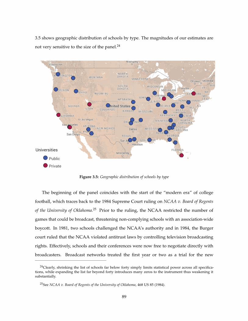
3.5 shows geographic distribution of schools by type. The magnitudes of our estimates are
not very sensitive to the size of the panel.24
Universities
Public
Private
Figure 3.5: Geographic distribution of schools by type
The beginning of the panel coincides with the start of the “modern era” of college
football, which traces back to the 1984 Supreme Court ruling on NCAA v. Board of Regents
of the University of Oklahoma.25 Prior to the ruling, the NCAA restricted the number of
games that could be broadcast, threatening non-complying schools with an association-wide
boycott. In 1981, two schools challenged the NCAA’s authority and in 1984, the Burger
court ruled that the NCAA violated antitrust laws by controlling television broadcasting
rights. Effectively, schools and their conferences were now free to negotiate directly with
broadcasters. Broadcast networks treated the first year or two as a trial for the new
24Clearly, shrinking the list of schools far below forty simply limits statistical power across all specifica-tions, while expanding the list far beyond forty introduces many zeros to the instrument thus weakening itsubstantially.
25See NCAA v. Board of Regents of the University of Oklahoma, 468 US 85 (1984).
89
arrangement, but by 1987 the number of televised games and the exposure of the league
surged, leading to an unprecedented financial gain. That year featured the highly contentious
Fiesta Bowl, which became one of the most watched college games in history, and marks
the start of our panel of football outcomes.26 Data on scholarly articles begin on the same
date, while the patent data begin in 1996. Although we observe data for earlier periods, the
international harmonization of the Unites States patent system in the early 1990’s created a
large spike in the number of filings and seemingly increased the overall level of patenting.
If the response of patenting behavior to research funding was different prior to 1996, and
the goal is to recover parameter estimates that are informative for current policymaking,
then including data on filings prior to 1996 will lead to the wrong parameter estimates. The
dataset ends in 2011. While 2012 data was available for our outcome measures, scholarly
articles and patents have had so little time to attract citations and the resulting drop off
is so steep that these additional points create essentially only noise. Moreover, there is a
chance that patent applications filed in 2012 have not yet been recorded as of the writing of
this paper. This leaves 23 and 16 years of observations for scholarly articles and patents,
respectively.
3.3.2 Summary Statistics
First, we summarize the data by institution. There are forty in total. Texas A&M - Main
Campus spends the highest amount on non-social non-medical science research, at $132
million, followed by the University of Georgia. The mean level is $49 million. Texas A&M
- Main Campus also spends the most in total non-social science and engineering, at $259
million, followed closely by the University of Wisconsin - Madison. The mean level is $98
million.
26The game pitted Penn State against a heavily-favored University of Miami. The pre-game antics of Miami,including dressing in military fatigues for the flight to the game, and controversial remarks by both sides at ajoint team dinner the night before the game contributed to wide-spread media attention. For the first time inhistory, a sitting US President (Ronald Reagan) was interviewed at the halftime show. Penn State won 14-10.The national press coverage of the players, coaches, their backgrounds, and the developments leading up thegame are all common in the “modern era” but were unheard of prior to 1987.
90
The University of Wisconsin-Madison publishes the highest number of scholarly articles,
at an average of over 1,800, followed by the Stanford University and the University of
Michigan, Ann Arbor. The average number is 820. Stanford University also has the highest
average number of related citations, at an average of over 61,000, followed by the University
of Wisconsin-Madison and the University of Washington (main campus). The average
number is 22,336. Stanford University tops the list of new patent application filings and the
citations that accrue to them, at 156 and 3,429, respectively. The University of Texas at Austin
is second, with 117 and 2,205, respectively. The mean levels are 34 and 570, respectively.
Next, we summarize the data by year. The average level of non-social non-medical
science expenditures grows from $24 to $75 million from 1987 to 2011, while the average
level of total non-social science and engineering expenditures grows from $41 to $165 million
over the same period. This is an average compound growth rate of 5% for the former funding
measure and 6% for the latter. The funding measures are monotone increasing over the
panel, with a few exceptions. In 1994, 2004, and 2010, both funding measures drop relative
to the year before (in nominal terms). These years directly follow the peak unemployment
periods of the last three US recessions.27 Over the same period, scholarly articles grow at
3.2% while patent applications grow more than twice as fast, at 7.2%. There is considerable
variation across schools within each year, but both variables tend to increase monotonically
over the panel. The time series of citations is more complicated, since the amount of time
other work has to cite these articles and applications is falling over the panel. Both citations
are monotonically increasing up to and including 1998 and then monotonically decreasing
after and including 2005. In any case, all main empirical specifications below include year
fixed effects, so these issues should not present a problem.
27Peak unemployment hit 7.8% in 1992, 6.3% in 2003, and 10.0% in 2009 for the 1990s recession, 2000srecession, and “Great Recession,” respectively. Source: “Business Cycle Expansions and Contractions.” NBERWebsite. March 5, 2015.
91
3.4 Empirical Model
3.4.1 Overview
We aim to better inform policymakers and administrators about the impact to scientific
output from an additional dollar of investment in university research. Estimating this
requires addressing two empirical issues. The first comes from the fact that high quality
institutions attract big grants as well as big ideas. This causes parameter estimates to be
upward biased and suggests that, at a minimum, removing the institution-specific means
and time trends from the data is required. However, this still leaves open the question of
endogeneity and, as Adams and Griliches [1998] note, probably exacerbates the second issue,
an errors-in-variables problem. When the data include long-term projects with multi-year
payoffs, tying research outcomes to the expenditures that generated them becomes difficult.
Even if a tight causal relationship exists, estimating it can be impossible without information
that the econometrician rarely has access to. In the case of the multi-billion dollar Large
Hadron Collider at CERN, construction began ten years prior to the first experiments. In
the case of the Stanford Linear Accelerator Center, researchers still benefit from portions of
the initial $114 million investment in 1961.
The solution is to find a quantity in the data generating process that shifts only marginal
research funds and yet is not correlated with the time-varying quality of the institution. To
achieve this, we use unexpected NCAA football outcomes. Unexpected wins, for example,
shift out research funds and, in turn, drive scientific discovery. Football presumably has
a negligible effect on the ability of a school to conduct cutting edge research, and so is
excluded from the outcome variables except through funding—especially one or two years
into the future.
Timing
Our assumptions regarding the temporal relationship between the variables are as follows:
football outcomes impact the level of research in the subsequent period and scholarly articles
92
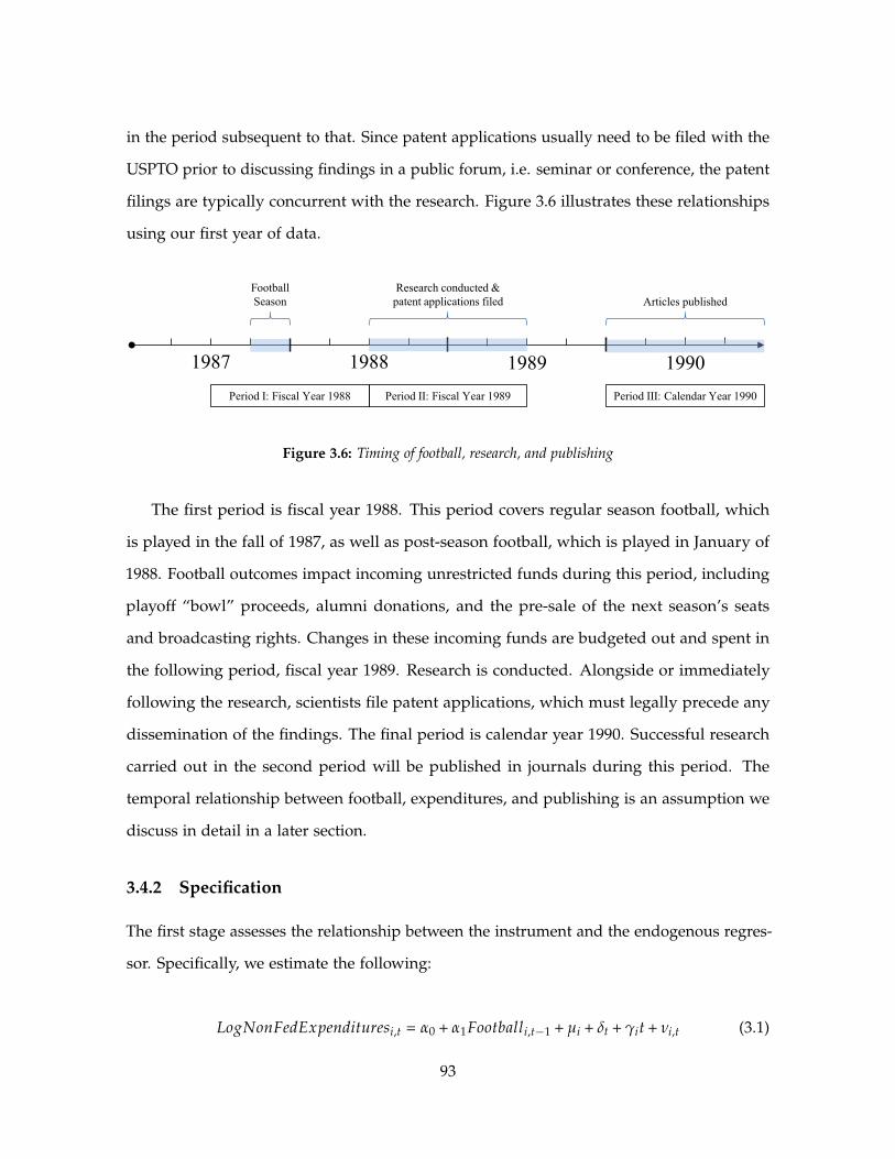
in the period subsequent to that. Since patent applications usually need to be filed with the
USPTO prior to discussing findings in a public forum, i.e. seminar or conference, the patent
filings are typically concurrent with the research. Figure 3.6 illustrates these relationships
using our first year of data.
1987 1988 1989 1990
Period I: Fiscal Year 1988 Period II: Fiscal Year 1989 Period III: Calendar Year 1990
Football
Season
Research conducted &
patent applications filed Articles published
Figure 3.6: Timing of football, research, and publishing
The first period is fiscal year 1988. This period covers regular season football, which
is played in the fall of 1987, as well as post-season football, which is played in January of
1988. Football outcomes impact incoming unrestricted funds during this period, including
playoff “bowl” proceeds, alumni donations, and the pre-sale of the next season’s seats
and broadcasting rights. Changes in these incoming funds are budgeted out and spent in
the following period, fiscal year 1989. Research is conducted. Alongside or immediately
following the research, scientists file patent applications, which must legally precede any
dissemination of the findings. The final period is calendar year 1990. Successful research
carried out in the second period will be published in journals during this period. The
temporal relationship between football, expenditures, and publishing is an assumption we
discuss in detail in a later section.
3.4.2 Specification
The first stage assesses the relationship between the instrument and the endogenous regres-
sor. Specifically, we estimate the following:
LogNonFedExpendituresi,t = α0 + α1Footballi,t−1 + µi + δt + γit + νi,t (3.1)
93
where i denotes institution, t denotes the fiscal year, LogNonFedExpenditures denotes
the log of non-federal research expenditures, Football denotes the difference between
postseason and preseason Associated Press votes (standardized across polls), µ and δ denote
school and time dummies, and γ captures the school-specific time trend (omitting the
superscripts). We use first stage estimates, (α̂0, α̂1, µ̂i, δ̂t, γ̂i), to generate predicted values for
LogNonFedExpendituresi,t, denoted ̂LogNonFedExpendituresi,t.
To estimate the dollar elasticity of scientific output, we regress the log of each of our four
output measures on the predicted values from the first stage. The four estimating equations
are given by the following:
LogArticlesi,t = β10 + β1
1̂LogNonFedExpendituresi,t−1 + κ1
i + φ1t + λ1
i t + ε1i,t (3.2)
LogArticleCitesi,t = β20 + β2
1̂LogNonFedExpendituresi,t−1 + κ2
i + φ2t + λ2
i t + ε2i,t (3.3)
LogPatentsi,t = β30 + β3
1̂LogNonFedExpendituresi,t + κ3
i + φ3t + λ3
i t + ε3i,t (3.4)
LogPatentCitesi,t = β40 + β4
1̂LogNonFedExpendituresi,t + κ4
i + φ4t + λ4
i t + ε4i,t (3.5)
where κ and φ denote school and time controls and λ captures the school-specific time
trend (again, omitting superscripts). (2) and (3) use lagged expenditures while (4) and
(5) use contemporaneous expenditures. For identification, we require that Footballi,t−1 is
uncorrelated with ε1i,t+1, ε2
i,t+1, ε3i,t, and ε4
i,t, and that Footballi,t−1 is a sufficiently strong
predictor of LogNonFedExpendituresi,t. We cluster our standard errors at the university
level, which allows for arbitrary correlation of the unobservables within a university over
time, i.e. the squared sum of regressor and error are required to have the same distribution
across clusters. In theory, we could also allow for arbitrary correlation of the unobservables
within-year in the same specification, as utilized in Petersen [2009], but this is too steep
a requirement of the data. As one of our robustness checks, we tested an alternative
94
specification that clustered at the year level and resulted in smaller standard errors, so we
did not include these results (although they are available on request). β1 is the parameter of
interest.
We also estimate the dollar cost of a patentable idea (or, to be precise, an idea that the
researcher and institution deem worthy of a patent application). To translate the elasticity
estimate into level changes, we multiply the reciprocal of this elasticity—roughly the percent
change in research expenditures required per one percent change in patent applications—by
the average ratio of expenditures to applications. Thus, the cost estimate equals
1N
1T ∑
i∑
tβ̂3
1NonFedExpendituresi,t
Patentsi,t
where N is the number of schools.
There are two potential concerns about the exclusion restriction. Both seem small. One
occurs if unexpected college football outcomes drive research outcomes, whether in the
laboratory or publication process. This includes the case where, for example, football success
may attract researchers that are inherently more productive on average. Previous work like
Anderson [2012] has shown that the undergraduate student body does improve after teams
win. This same argument is unlikely to hold for graduate students and faculty. Another
occurs if a third factor simulatenously improves both football and research outcomes, but
goes unnoticed by the Associated Press voters. Since the reputation and career prospects of
these sports writers and broadcasters depend on the accuracy of their predictions and their
perceived access to information, this also seems unimportant. Nonetheless, evidence in the
“Exogeneity Check” section provides further support for the instrument.
3.5 Results
3.5.1 From Football to Money
Our first stage results assess the relationship between unexpected football outcomes and
research expenditures. Table 3.2 reports these results. Each specification includes university
95
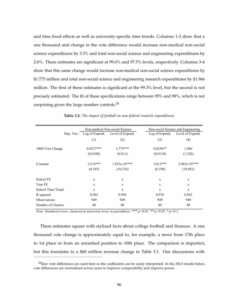
and time fixed effects as well as university-specific time trends. Columns 1-2 show that a
one thousand unit change in the vote difference would increase non-medical non-social
science expenditures by 3.3% and total non-social science and engineering expenditures by
2.6%. These estimates are significant at 99.6% and 97.5% levels, respectively. Columns 3-4
show that this same change would increase non-medical non-social science expenditures by
$1.775 million and total non-social science and engineering research expenditures by $1.966
million. The first of these estimates is significant at the 99.3% level, but the second is not
precisely estimated. The fit of these specifications range between 95% and 98%, which is not
surprising given the large number controls.28
Table 3.2: The impact of football on non-federal research expenditures
Non-medical Non-social Science Non-social Science and EngineeringDep. Var.: Log of Expend. Level of Expend. Log of Expend. Level of Expend.
(1) (2) (3) (4)
1000 Vote Change 0.0327*** 1,775*** 0.0256** 1,966
(0.0108) (618.3) (0.0110) (1,226)
Constant 115.9*** 1.053e+07*** 124.2*** 2.983e+07***
(0.185) (10,376) (0.190) (19,981)
School FE x x x x
Year FE x x x x
School Time Trend x x x x
R-squared 0.965 0.956 0.976 0.963
Observations 949 949 949 949
Number of Clusters 40 40 40 40
Note: Standard errors, clustered at university level, in parenthesis. *** p<0.01, ** p<0.05, * p<0.1.
These estimates square with stylized facts about college football and finances. A one
thousand vote change is approximately equal to, for example, a move from 17th place
to 1st place or from an unranked position to 10th place. The comparison is imperfect,
but this translates to a $60 million revenue change in Table 3.1. Our discussions with
28Raw vote differences are used here so the coefficients can be easily interpreted. In the 2SLS results below,vote differences are normalized across years to improve comparability and improve power.
96
administrators suggest that roughly five to ten percent of cash flow changes find their way
back to university research, and translate into somewhere between $3 million and $6 million
of additional funding. Since funds are shared between social and non-science departments,
and since higher revenues translate to higher costs—for example, hiring more security
guards at games to monitor larger crowds at games—then our estimates are in line with
what one would expect.
3.5.2 From Money to Scholarly Articles
To assess the impact of money on science, we begin with the relationship between research
expenditures and academic publishing behavior. Table 3.3 reports these results. This table,
as well as the three that follow, present the OLS estimates in the first five columns and
the 2SLS estimates in the latter five. Our main findings are in the final column. We find
that the dollar elasticity of scholarly articles is 0.310, after controlling for school and time
fixed effects as well as school-specific time trends. The instrument, lagged unexpected
college football success, provides exogenous variation to science and engineering research
expenditures sourced from the university. The estimate is significant at 99.2%. The F-statistic
of the accompanying first stage is 10.98.
The sharp contrast with the OLS results is striking. Our main elasticity estimate is nearly
ten times what results from an OLS specification with the same level of controls, which
would lead policymakers to underestimate the returns to funding scientific research and
presumably under-invest in it. One potential issue is that the instrument is identifying a
local average treatment affect that is substantially higher than the average elasticity of the
sample schools (or sample school-years). This would happen if the sensitivity of the schools’
budgets to football outcomes are correlated with the schools’ elasticity. If anything, we
would expect this to go in the opposite direction—with schools transforming dollars to
discoveries at the highest rates also being the schools whose budgets are least affected by
football.
More likely the issue is a rather serious errors-in-variables problem for the OLS. The
97

Tabl
e3.
3:Th
eim
pact
ofm
oney
onsc
hola
rly
artic
les
OL
S S
peci
fica
tion
sIV
Spe
cifi
cati
ons
(1)
(2)
(3)
(4)
(5)
(6)
(7)
(8)
(9)
(10)
Lag
ged
Log
Exp
endi
ture
s0.
456*
**0.
438*
**0.
438*
**0.
0658
**0.
0349
**0.
596
0.60
30.
442
0.47
10.
310*
**
(0.0
962)
(0.1
05)
(0.0
419)
(0.0
280)
(0.0
171)
(0.4
86)
(0.5
02)
(0.4
81)
(0.3
26)
(0.1
17)
Con
stan
t1.
930*
2.22
0*0.
719*
*3.
559*
**1.
313*
**0.
485
0.44
91.
158
0.98
11.
233
(1.0
38)
(1.1
68)
(0.2
89)
(0.2
08)
(0.1
89)
(5.0
46)
(5.4
37)
(4.6
90)
(3.3
26)
(1.2
10)
Sch
ool F
Ex
xx
xx
x
Yea
r F
Ex
xx
xx
x
Sch
ool T
ime
Tre
ndx
x
Obs
erva
tion
s86
986
986
986
986
986
986
986
986
986
9
R-s
quar
ed0.
422
0.43
30.
956
0.98
30.
994
0.38
20.
382
0.95
60.
966
0.98
9
Num
ber
of C
lust
ers
4040
4040
4040
4040
4040
F-S
tat:
1st S
tage
2.73
2.45
1.54
5.36
11.1
1
Not
e: S
tand
ard
erro
rs, c
lust
ered
at u
nive
rsit
y le
vel,
in p
aren
thes
is. *
** p
<0.
01, *
* p<
0.05
, * p
<0.
1.
98
difficulty in temporally tying budgets to discoveries is at the heart of the problem. For
example, portions of the $114 million investment in the Stanford Linear Accelerator, built
in 1961, generated research for years afterwards. In projects like this, operating expenses
may precede experiments for many years, weakening the link between research budgets
and articles in the subsequent year and attenuating the elasticity estimates.
To explore this point further, we remove institution specific controls. In fact, removing
the institution-specific time trend alone results in a nearly tenfold increase in the estimated
elasticity (without much relative change in precision). It is, unfortunately, impossible to say
whether the sharp rise is attributable to the mitigation of the errors-in-variables problem or
to the re-introduction of institution specific unobservables that drive both expenditures and
scientific output. Removing the institution or year fixed effects does not further change the
estimates much. It seems that whatever the relative contribution of the errors-in-variables
problem or the omitted variable bias may be, their combined effect varies in a complicated
way—over time and within the institution.
Our pooled OLS estimates are at the bottom end of those found by Adams and Griliches
[1998]. In the presence of only time fixed effects and three high-level institutional controls
(for top ten public university, top ten private university, and other private university), they
find a dollar elasticity of scholarly articles of between 0.4 and 0.7. The school fixed effects
also have the same impact on their OLS results that they have on ours: they find an elasticity
of roughly zero.
There is one important caveat for policymakers who wish to use these numbers to
predict returns to an aggregate national increase in research funding. Since the predicted
variation in expenditures is linear in the instrument, unexpected losses hurt research budgets
as much as unexpected wins help them. Thus, our instrument transfers money between
schools without shifting aggregate annual spending on a national level up or down. If
these money transfers are merely moving scarce assets between institutions, and if these
scarce assets—like highly productive scientists—are inelastically supplied in the short-run,
then our estimates would not be very informative about how scientific output responds
99
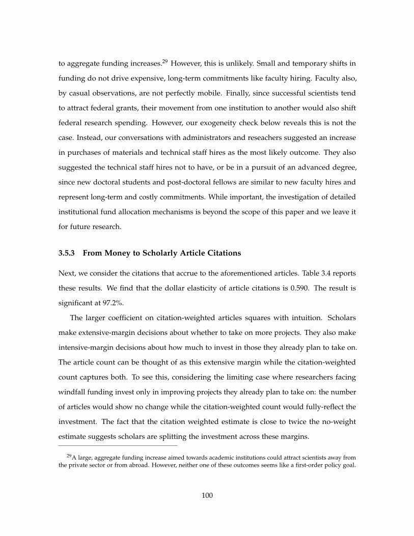
to aggregate funding increases.29 However, this is unlikely. Small and temporary shifts in
funding do not drive expensive, long-term commitments like faculty hiring. Faculty also,
by casual observations, are not perfectly mobile. Finally, since successful scientists tend
to attract federal grants, their movement from one institution to another would also shift
federal research spending. However, our exogeneity check below reveals this is not the
case. Instead, our conversations with administrators and reseachers suggested an increase
in purchases of materials and technical staff hires as the most likely outcome. They also
suggested the technical staff hires not to have, or be in a pursuit of an advanced degree,
since new doctoral students and post-doctoral fellows are similar to new faculty hires and
represent long-term and costly commitments. While important, the investigation of detailed
institutional fund allocation mechanisms is beyond the scope of this paper and we leave it
for future research.
3.5.3 From Money to Scholarly Article Citations
Next, we consider the citations that accrue to the aforementioned articles. Table 3.4 reports
these results. We find that the dollar elasticity of article citations is 0.590. The result is
significant at 97.2%.
The larger coefficient on citation-weighted articles squares with intuition. Scholars
make extensive-margin decisions about whether to take on more projects. They also make
intensive-margin decisions about how much to invest in those they already plan to take on.
The article count can be thought of as this extensive margin while the citation-weighted
count captures both. To see this, considering the limiting case where researchers facing
windfall funding invest only in improving projects they already plan to take on: the number
of articles would show no change while the citation-weighted count would fully-reflect the
investment. The fact that the citation weighted estimate is close to twice the no-weight
estimate suggests scholars are splitting the investment across these margins.
29A large, aggregate funding increase aimed towards academic institutions could attract scientists away fromthe private sector or from abroad. However, neither one of these outcomes seems like a first-order policy goal.
100
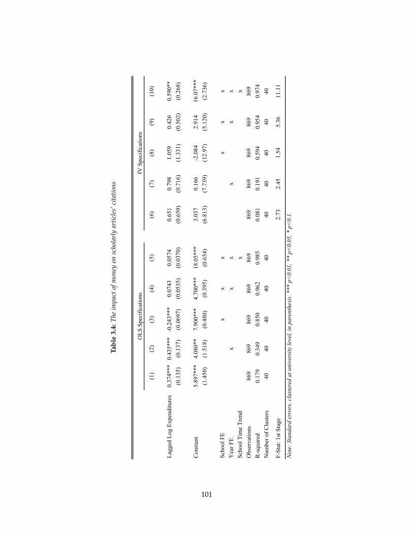
Tabl
e3.
4:Th
eim
pact
ofm
oney
onsc
hola
rly
artic
les’
cita
tions
OL
S S
peci
fica
tion
sIV
Spe
cifi
cati
ons
(1)
(2)
(3)
(4)
(5)
(6)
(7)
(8)
(9)
(10)
Lag
ged
Log
Exp
endi
ture
s0.
374*
**0.
435*
**-0
.243
***
0.07
430.
0574
0.65
10.
798
1.05
90.
426
0.59
0**
(0.1
35)
(0.1
37)
(0.0
697)
(0.0
535)
(0.0
370)
(0.6
59)
(0.7
16)
(1.3
31)
(0.5
02)
(0.2
68)
Con
stan
t5.
897*
**4.
080*
*7.
900*
**4.
700*
**18
.05*
**3.
037
0.16
6-2
.084
2.91
416
.07*
**
(1.4
50)
(1.5
18)
(0.4
80)
(0.3
95)
(0.6
54)
(6.8
13)
(7.7
39)
(12.
97)
(5.1
20)
(2.7
36)
Sch
ool F
Ex
xx
xx
x
Yea
r F
Ex
xx
xx
x
Sch
ool T
ime
Tre
ndx
x
Obs
erva
tion
s86
986
986
986
986
986
986
986
986
986
9
R-s
quar
ed0.
179
0.34
90.
850
0.96
20.
985
0.08
10.
191
0.59
40.
954
0.97
4
Num
ber
of C
lust
ers
4040
4040
4040
4040
4040
F-S
tat:
1st S
tage
2.73
2.45
1.54
5.36
11.1
1
Not
e: S
tand
ard
erro
rs, c
lust
ered
at u
nive
rsit
y le
vel,
in p
aren
thes
is. *
** p
<0.
01, *
* p<
0.05
, * p
<0.
1.
101
This is, of course, only one possible interpretation, and Adams and Griliches [1998]
propose two interesting alternative views. The first is that as Ph.D. students become junior
faculty at smaller schools, papers derived from their doctoral work will be incorrectly
attributed to the school that hired them. However, this problem will be partially corrected if
these papers happen to cite scholars at their degree-granting institution. The second is that
larger programs tend towards basic research, which is more likely to have “hit” papers. We
prefer our interpretation of the relative magnitudes since the ratio of articles to citations is
robust to the inclusion of institution fixed effects and institution-specific time trends.
The errors-in-variables problem discussed in the preceding section again seems an issue
for OLS specifications. Although the pooled OLS specification yields a relatively precise
estimate of 0.374, the addition of the full set of controls yields an imprecise estimate of 0.057.
These results are, again, near the bottom end of the Adams and Griliches [1998] range. They
find a dollar elasticity of article citations of between 0.6 and 0.9 without school fixed effects
but close to zero effect with school fixed effects.
3.5.4 From Money to Patents
To assess the impact of money on translational and applied science output, we assess
the relationship between research expenditures and patenting behavior. Table 3.5 reports
these results. We expand our funding data to encompass total non-social science and
engineering disciplines, rather than non-medical non-social science only.30 We find that
the dollar elasticity of patent applications is 1.91. This result is significant at 96.2% and the
corresponding first stage F-statistic is 11.18. This elasticity is surprisingly high and implies
increasing returns to research spending, i.e. for each proportional increase in research
expenditures, new patent applications will rise by more than 1%. The contrast with the
OLS coefficients are even more striking than in the case of scholarly publications. Here, the
elasticity from the main specification is between two and three times the precisely-estimated
30The University of Oregon was the only school in our sample without an identifiable Assignee/Applicantname or DWPI Assignee code in Thomson Innovation. Since the University of Oregon is also the only school inour sample without the School of Engineering, we drop it from the patent analysis portion of the paper.
102
OLS coefficient. Moreover, it is nearly one hundred times the imprecisely estimated OLS
estimate with a full set of controls and more than twice the upper bound of the 95% percent
confidence interval around that estimate.
We also estimate the dollar cost of generating a patentable idea. This entails dividing
the ratio of non-federal research spending to patents by the elasticity estimated above, and
averaging across schools and, where applicable, time. Using only the most recent years’
spending-to-patent ratios yields a cost of $2.612 million. Using all years’ ratios yields a cost
of $2.975 million. University patenting has increased steadily since the Bayh-Dole Act of
1980, which allowed universities to retain ownership over their publically-funded intellectual
property. Thus, the first figure should better predict the response to a current policy change.
Despite broader coverage in terms of disciplines and a longer panel, these figures are quite
close to—although slightly lower than—the roughly $3.3 million cost estimated in Azoulay
et al. [2014].
3.5.5 From Money to Patent Citations
Finally, we assess the relationship between research expenditures and patent citations. Table
3.6 reports these results. Our main specification yields an elasticity of 3.30, and this result
is significant at 98.8%. This estimate is nearly twice the elasticity on the count of patent
applications, again suggesting researchers are roughly splitting their time between launching
new projects and improving the quality of existing projects. Although the outcome data
comes from an entirely separate source than the scholarly article data, it is reassuring to see
the ratio of documents to their accrued citations be the same for both scholarly articles and
patent applications.
Nonetheless, this suggests strongly increasing returns to research investment at the
margin and may be surprising. However, when one considers the large amount of fixed
investment, both in terms of faculty and facilities, then if the bottleneck for research—as
recent press has indicated—is at the funding level, these elasticities both seem reasonable.
Of course, while one would need to estimate the real returns from academic patents to
103
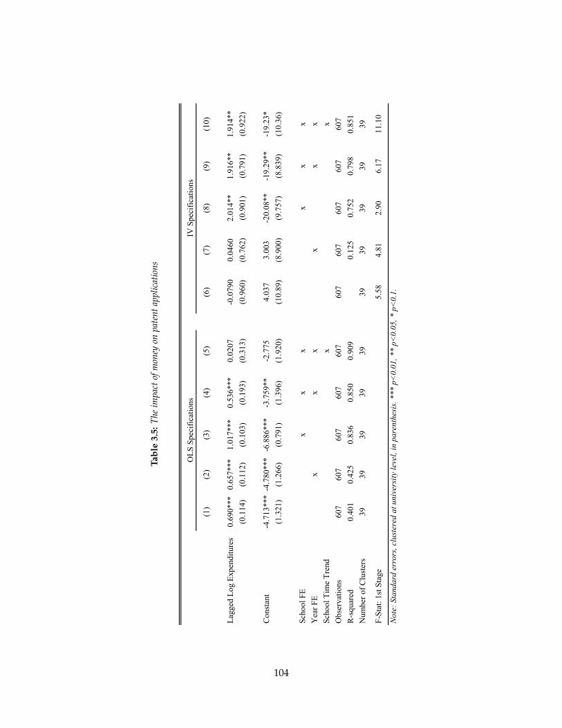
Tabl
e3.
5:Th
eim
pact
ofm
oney
onpa
tent
appl
icat
ions
OL
S S
peci
fica
tion
sIV
Spe
cifi
cati
ons
(1)
(2)
(3)
(4)
(5)
(6)
(7)
(8)
(9)
(10)
Lag
ged
Log
Exp
endi
ture
s0.
690*
**0.
657*
**1.
017*
**0.
536*
**0.
0207
-0.0
790
0.04
602.
014*
*1.
916*
*1.
914*
*
(0.1
14)
(0.1
12)
(0.1
03)
(0.1
93)
(0.3
13)
(0.9
60)
(0.7
62)
(0.9
01)
(0.7
91)
(0.9
22)
Con
stan
t-4
.713
***
-4.7
80**
*-6
.886
***
-3.7
59**
-2.7
754.
037
3.00
3-2
0.08
**-1
9.29
**-1
9.23
*
(1.3
21)
(1.2
66)
(0.7
91)
(1.3
96)
(1.9
20)
(10.
89)
(8.9
00)
(9.7
57)
(8.8
39)
(10.
36)
Sch
ool F
Ex
xx
xx
x
Yea
r F
Ex
xx
xx
x
Sch
ool T
ime
Tre
ndx
x
Obs
erva
tion
s60
760
760
760
760
760
760
760
760
760
7
R-s
quar
ed0.
401
0.42
50.
836
0.85
00.
909
0.12
50.
752
0.79
80.
851
Num
ber
of C
lust
ers
3939
3939
3939
3939
3939
F-S
tat:
1st S
tage
5.58
4.81
2.90
6.17
11.1
0
Not
e: S
tand
ard
erro
rs, c
lust
ered
at u
nive
rsit
y le
vel,
in p
aren
thes
is. *
** p
<0.
01, *
* p<
0.05
, * p
<0.
1.
104

Tabl
e3.
6:Th
eim
pact
ofm
oney
onpa
tent
s’ci
tatio
ns
OL
S S
peci
fica
tion
sIV
Spe
cifi
cati
ons
(1)
(2)
(3)
(4)
(5)
(6)
(7)
(8)
(9)
(10)
Lag
ged
Log
Exp
endi
ture
s0.
609*
**0.
746*
**-0
.872
***
0.81
6***
0.12
9-0
.048
8-0
.110
2.25
12.
539*
*3.
302*
*
(0.0
977)
(0.1
28)
(0.2
58)
(0.2
88)
(0.2
29)
(1.3
74)
(1.2
09)
(1.9
54)
(1.1
20)
(1.3
14)
Con
stan
t-1
.527
-2.0
779.
529*
**-2
.006
1.32
25.
954
5.36
6-2
0.71
-25.
97**
-35.
06**
(1.1
12)
(1.4
10)
(1.9
82)
(1.9
84)
(1.4
60)
(15.
60)
(14.
20)
(21.
15)
(12.
50)
(14.
72)
Sch
ool F
Ex
xx
xx
x
Yea
r F
Ex
xx
xx
x
Sch
ool T
ime
Tre
ndx
x
Obs
erva
tion
s60
460
460
460
460
460
460
460
460
460
4
R-s
quar
ed0.
174
0.39
50.
695
0.80
50.
857
0.06
70.
235
0.76
00.
770
Num
ber
of C
lust
ers
3939
3939
3939
3939
3939
F-S
tat:
1st S
tage
5.58
4.81
2.90
6.17
11.1
0
Not
e: S
tand
ard
erro
rs, c
lust
ered
at u
nive
rsit
y le
vel,
in p
aren
thes
is. *
** p
<0.
01, *
* p<
0.05
, * p
<0.
1.
105
figure out whether the government and universities are funding the right level of research,
our results appear to support arguments for an increase in research spending.
3.5.6 Exogeneity Check
College football should impact only research funds provided by non-federal sources and
have no effect on funds provided by the federal government. We observe the dollars
contributed from these sources independently in the data and use this to strengthen the
exogeneity argument for our instrument. That is, if some unobservable factor that varied
by institution and time was driving unexpected football success, scientific discovery, and
non-federal research funding, then it is likely to show up in federal research funding as
well. Figure 3.7 addresses this potential confound. The y-axis shows research expenditures,
by source, while the x-axis shows the instrument. School and year effects, as well as a
schools-specific time trend, have been removed from both.
The left panel reports the strong, positive relationship between the instrument and
research expenditures sourced from non-federal entities. This is merely the graphical
representation of the first-stage results. The right panel, in contrast, reports the lack of any
relationship between the instrument and federally-sourced research expenditures.
In fact, we can statistically separate the effect on these two sources. To do so, we pool to-
gether federal and non-federal data, so that an observation is university-year-source specific.
We interact the full set of controls with a dummy variable for non-federal expenditures so
that our university and year fixed effects as well as our university-specific time trends are
source specific. The standard errors are clustered at the university-source level. Table 3.7
reports the results of this exercise. In the first column, the left-hand side variable is the log
of non-medical non-social science expenditures. The instrument has a precisely estimated
zero effect on the federally-sourced portion of expenditures. That is, the coefficient is not
significant and the 95% confidence interval spans a relatively narrow range of -0.75% to
0.78%. In contrast, the coefficient on the interaction term—representing the impact of the
instrument on the non-federally-sourced portion of expenditures—is positive and significant
106
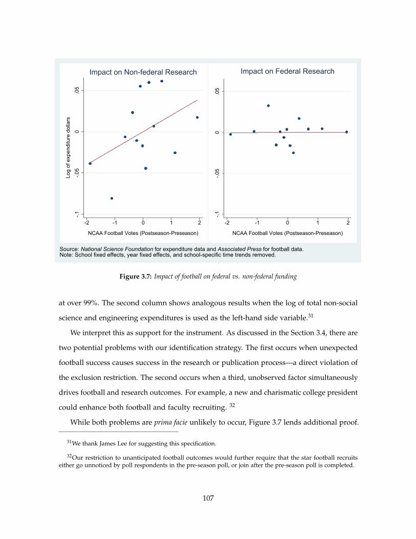
-.1
-.05
0.0
5
Log
of e
xpen
ditu
re d
olla
rs
-2 -1 0 1 2
NCAA Football Votes (Postseason-Preseason)
Impact on Non-federal Research
-.1
-.05
0.0
5-2 -1 0 1 2
NCAA Football Votes (Postseason-Preseason)
Impact on Federal Research
Source: National Science Foundation for expenditure data and Associated Press for football data.Note: School fixed effects, year fixed effects, and school-specific time trends removed.
Figure 3.7: Impact of football on federal vs. non-federal funding
at over 99%. The second column shows analogous results when the log of total non-social
science and engineering expenditures is used as the left-hand side variable.31
We interpret this as support for the instrument. As discussed in the Section 3.4, there are
two potential problems with our identification strategy. The first occurs when unexpected
football success causes success in the research or publication process—a direct violation of
the exclusion restriction. The second occurs when a third, unobserved factor simultaneously
drives football and research outcomes. For example, a new and charismatic college president
could enhance both football and faculty recruiting. 32
While both problems are prima facie unlikely to occur, Figure 3.7 lends additional proof.
31We thank James Lee for suggesting this specification.
32Our restriction to unanticipated football outcomes would further require that the star football recruitseither go unnoticed by poll respondents in the pre-season poll, or join after the pre-season poll is completed.
107
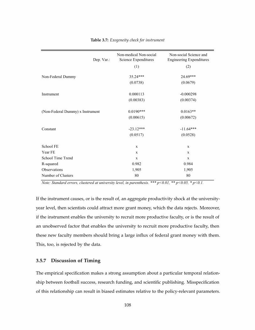
Table 3.7: Exogeneity check for instrument
Non-medical Non-social Non-social Science andDep. Var.: Science Expenditures Engineering Expenditures
(1) (2)
Non-Federal Dummy 35.24*** 24.69***
(0.0738) (0.0679)
Instrument 0.000113 -0.000298
(0.00383) (0.00374)
(Non-Federal Dummy) x Instrument 0.0190*** 0.0163**
(0.00615) (0.00672)
Constant -23.12*** -11.64***
(0.0517) (0.0528)
School FE x x
Year FE x x
School Time Trend x x
R-squared 0.982 0.984
Observations 1,905 1,905
Number of Clusters 80 80
Note: Standard errors, clustered at university level, in parenthesis. *** p<0.01, ** p<0.05, * p<0.1.
If the instrument causes, or is the result of, an aggregate productivity shock at the university-
year level, then scientists could attract more grant money, which the data rejects. Moreover,
if the instrument enables the university to recruit more productive faculty, or is the result of
an unobserved factor that enables the university to recruit more productive faculty, then
these new faculty members should bring a large influx of federal grant money with them.
This, too, is rejected by the data.
3.5.7 Discussion of Timing
The empirical specification makes a strong assumption about a particular temporal relation-
ship between football success, research funding, and scientific publishing. Misspecification
of this relationship can result in biased estimates relative to the policy-relevant parameters.
108
Below we show that although the impact of football extends to periods other than what
the model strictly specifies, the impact of funding does not. This leaves the estimates
unbiased. Lastly, we discuss factors that drive this, seemingly compressed timing of the
expenditures-publications relationship.
We first assess misspecification in the first stage. Our analysis assumes that football
in period t mainly impacts funding in period t + 1. However, football can impact funding
at t if, for example, football inspires some immediate and directed donations to academic
endeavors. It may also impact funding at t + 2 and later if team success at the end of
the season influences the starting point of success for future seasons. It should not, of
course, impact funding at t− 1, a period prior to the football season. Table 3.8 reports the
relationship between funding and the seven prior years’ instrument values as well as the
current year and following year instrument values. A full set of controls are included. The
first column reports the impact on the log of non-medical non-social science expenditures
while the second reports the impact of the log of total non-social science and engineering
expenditures. These results confirm our intuition about the first stage timing. In both
cases, funding is most strongly impacted by one-year lagged instrument values and is not
meaningfully impacted by the future value of the instrument. There is a non-trival impact
from the instrument in the contemporaneous period and the instrument lagged more than
one year. However, the coefficients tend to drop monotonically in terms of both magnitude
and significance.
Expenditures, on the other hand, largely impact output in a single year, so the estimates
are unbiased despite the impact of football being spread out. Table 3.9 reports this result
for academic publishing. The left-hand side variable is the log of scholarly articles. The
right-hand side variables are predicted values of leading, contemporaneous, and one- to
three-year lagged research expenditures. In line with the model, the largest and only
significant coefficient is on once-lagged expenditures. Table 3.10 reports the result for the
case where the publishing measure is new patent applications. In line with the model once
again, the largest and only significant coefficient is on contemporaenous year expenditures.
109
A one-year delay between research fund disbursement and subsequent publication of
scholarly articles may strike readers as too fast, but several factors can explain this. In
Section 3.4 we note that research budgets are reported on a fiscal year basis, while output is
recorded on a calendar year basis, implying an added six month interval between funding
and publishing periods. Also for projects facing funding bottlenecks, budgets will be spent
soon after they are replenished. This results in the actual time lag we measure to be closer
to two years rather than one. Futhermore, non-social non-medical scientific disciplines are
anecdotally faster to produce tangible output than social science research. NSF grant data
provides a direct evidence of this. For example, among all grants given out in 2000, 2005,
and 2010, 26% resulted in the original grant year for physics-related proposals while only
5.4% of economics-related proposals did. Among grants over the same time period that
resulted in at least one publication, 46% resulted in journal publications in the original grant
year for physics-related proposals while only 13% of economics-related proposals did. The
publication process is correspondingly fast. The receipt-to-acceptance time for manuscripts
published in non-social non-medical science journals is around a third of those published
in economics journals. For example, the average time between first submission and final
publication was between 13 and 22 weeks at the five main journals of the American Physics
Society33 but 62 weeks at the American Economic Review (Moffitt [2009]).34 Also, natural
science disciplines in particular tend to rely more on short papers, proceedings, and letters,
which have much shorter review times. For example, “rapid communication” section of the
five main journals of the American Physics Society has an average receipt-to-acceptance
time of between 9 and 15 weeks and a minimum of only two days.
The timing of patent filings is driven by different factors. To ensure intellectual property
protection of an idea, scholars must submit their new patent application to the USPTO
ahead of giving seminars or conference talks. On top of that, patents are generally faster to
33Dr. Thomas Pattard, “How to publish your work in the Physical Review (or Editors are from Mars, Refereesare from Venus, and Authors are from Earth)” (presentation, International Max Planck Research School SummerSeminar, Dresden, Germany, August 11, 2011).
34This comparison is drawn from 2008.
110
write, and are assigned a “publication” date without a formal review process.35
Taken together, it is not surpring that the data indicates scientists file in the same period
that research budgets are replenished. With respect to the timing of patent filings, our
results are in line with earlier work in different settings. For example, in their study of
manufacturing industry investments in R&D from 1972 to 1979, Hall et al. [1986] state that
"R and D and patents appear to be dominated by a contemporaneous relationship."
3.6 Conclusion
Unanticipated within-season football success impacts school-sponsored research, providing
rich exogenous variation that identifies the impact of money on science. An instrumental
variable approach is important to study this relationship for two reasons. First, large grants
are typically awarded to institutions that would otherwise attract big ideas, so any approach
that ignores this endogeneity will recover upwardly biased parameters. Second, funding
data include long-term projects with payoffs to researchers over many years, making it
difficult to tie shifts in spending to shifts in scientific outcomes and creating an errors-
in-variables problem that attenuates estimates toward zero. Our approach yields a dollar
elasticity of scholarly articles at 0.31 and of article citations at 0.59. It also yields a dollar
elasticity of new patent applications at 1.91 and of patent citations at 3.30. If citations are
rough measure of quality, then these results suggest researchers are splitting their time
between launching new projects and improving the quality of existing projects. We find it
costs universities, at the margin, approximately $2.6 million to generate an idea worthy of
filing a patent application. The inclusion of school specific controls, i.e. fixed effects and a
school specific time trend, improved the first stage power but ultimately did not change the
elasticity much for the 2SLS specifications. Their inclusion sharply reduced OLS estimates,
which tended toward zero for all outcome measures. This highlights the importance of
using instruments to “pick out” marginal expenditure shifts that can be tied to scientific
35While patents do not “publish” immediately, their priority date is locked when the application is submitted.
111

outcomes. Without them, this exercise would understate the returns to university R&D and
lead policymakers to under-invest in research.
112
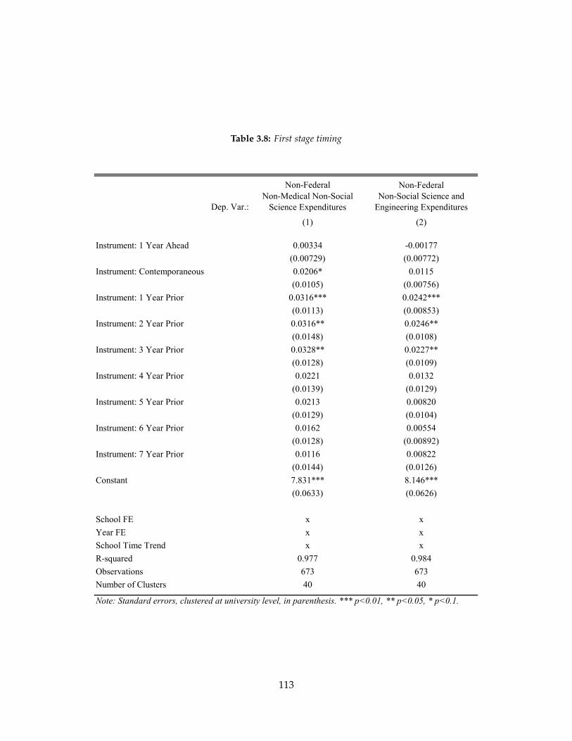
Table 3.8: First stage timing
Non-Federal Non-FederalNon-Medical Non-Social Non-Social Science and
Dep. Var.: Science Expenditures Engineering Expenditures
(1) (2)
Instrument: 1 Year Ahead 0.00334 -0.00177
(0.00729) (0.00772)
Instrument: Contemporaneous 0.0206* 0.0115
(0.0105) (0.00756)
Instrument: 1 Year Prior 0.0316*** 0.0242***
(0.0113) (0.00853)
Instrument: 2 Year Prior 0.0316** 0.0246**
(0.0148) (0.0108)
Instrument: 3 Year Prior 0.0328** 0.0227**
(0.0128) (0.0109)
Instrument: 4 Year Prior 0.0221 0.0132
(0.0139) (0.0129)
Instrument: 5 Year Prior 0.0213 0.00820
(0.0129) (0.0104)
Instrument: 6 Year Prior 0.0162 0.00554
(0.0128) (0.00892)
Instrument: 7 Year Prior 0.0116 0.00822
(0.0144) (0.0126)
Constant 7.831*** 8.146***
(0.0633) (0.0626)
School FE x x
Year FE x x
School Time Trend x x
R-squared 0.977 0.984
Observations 673 673
Number of Clusters 40 40
Note: Standard errors, clustered at university level, in parenthesis. *** p<0.01, ** p<0.05, * p<0.1.
113

Table 3.9: Second stage timing: scholarly articles
(1) (2) (3) (4) (5)
1 Year Leading Expenditures 0.0204
(0.107)
Contemporaneous Expenditures -0.00767
(0.0976)
1 Year Lagged Expenditures 0.310***
(0.117)
2 Year Lagged Expenditures -0.225
(0.249)
3 Year Lagged Expenditures -0.0297
(0.176)
School FE x x x x x
Year FE x x x x x
School Time Trend x x x x x
R-squared 0.993 0.993 0.989 0.990 0.994
Observations 949 909 869 829 789
Number of Clusters 40 40 40 40 41
Note: Standard errors, clustered at university level, in parenthesis. *** p<0.01, ** p<0.05, * p<0.1.
Table 3.10: Second stage timing: patents
(1) (2) (3) (4) (5)
1 Year Leading Expenditures 1.209
(1.999)
Contemporaneous Expenditures 1.914**
(0.922)
1 Year Lagged Expenditures 0.0623
(1.118)
2 Year Lagged Expenditures -1.448
(1.419)
3 Year Lagged Expenditures -0.558
(1.649)
School FE 949 909 869 829 789
Year FE 0.993 0.993 0.989 0.990 0.994
School Time Trend x x x x x
R-squared 0.892 0.851 0.911 0.867 0.904
Observations 609 607 607 607 607
Number of Clusters 39 39 39 39 39
Note: Standard errors, clustered at university level, in parenthesis. *** p<0.01, ** p<0.05, * p<0.1.
114
References
James Adams and Zvi Griliches. Measuring Science: An Exploration. Proceedings of theNational Academy of Sciences, 93(23):12664–12670, 1996.
James Adams and Zvi Griliches. Research Productivity in a System of Universities. Annalesd’Economie et de Statistique, (49-50):127–162, 1998.
Juan Alcácer and Michelle Gittelman. Patent Citations as a Measure of Knowledge Flows:The Influence of Examiner Citations. The Review of Economics and Statistics, 88(4):774–779,2006.
Juan Alcácer and Minyuan Zhao. Local R&D Strategies and Multilocation Firms: The Roleof Internal Linkages. Management Science, 58(4):734–753, 2012.
Juan Alcácer, Michelle Gittelman, and Bhaven N. Sampat. Applicant and Examiner Citationsin U.S. patents: An Overview and Analysis. Research Policy, 38(2):415 – 427, 2009.
Armen Alchian. Reliability of Progress Curves in Airframe Production. Econometrica, 31(4):679–693, 1963.
John R. Allison and Mark A. Lemley. Empirical Evidence on the Validity of Litigated Patents.American Intellectual Property Law Association (AIPLA) Quarterly Journal, 26(3):185–275, 1998.
Michael L. Anderson. The Benefits of College Athletic Success: An Application of thePropensity Score Design with Instrumental Variables. Working paper. June 2012.
Joshua D. Angrist. Estimation of Limited Dependent Variable Models with Dummy Endoge-nous Regressors: Simple Strategies for Empirical Practice. Journal of Business & EconomicStatistics, 19(1):2–16, 2001.
Joshua D. Angrist and Alan B. Krueger. Instrumental Variables and the Search for Identifica-tion: From Supply and Demand to Natural Experiments. Journal of Economic Perspectives,15(4):69–85, 2001.
Joshua D. Angrist and Jorn-Steffen Pischke. Mostly Harmless Econometrics. PrincetonUniversity Press, 2009.
ANSI. Who’s Driving Wi-Fi?, 2004. Accessed March 15, 2015.https://web.archive.org/web/20040327062705/http://www.ansi.org/news_publications/media_tips/wi_fi.aspx.
115
Robert Axelrod, Will Mitchell, Robert E. Thomas, D. Scott Bennett, and Erhard Bruderer.Coalition Formation in Standard-Setting Alliances. Management Science, 41(9):1493–1508,1995.
Pierre Azoulay, Joshua S. Graff Zivin, and Jialan Wang. Superstar Extinction. The QuarterlyJournal of Economics, 125(2):549–589, 2010.
Pierre Azoulay, Joshua S. Graff Zivin, Danielle Li, and Bhaven N. Sampat. Public R&DInvestments and Private Sector Patenting: Evidence from NIH Funding Rules. Workingpaper. August 19 2014.
Scott Baker and Claudio Mezzetti. Disclosure as a Strategy in the Patent Race. Journal ofLaw and Economics, 48(1):173–194, 2005.
Battelle Memorial Institute. 2014 Global R&D Funding Forecast. 2013.
Rudi Bekkers and Andrew Updegrove. A Study of IPR Policies and Practices of a Representa-tive Group of Standards Setting Organizations Worldwide. Technical report, US NationalAcademies of Science, Board of Science, Technology, and Economic Policy (STEP), Projecton Intellectual Property Management in standard-setting processes, 2012.
C. Lanier Benkard. Learning and Forgetting: The Dynamics of Aircraft Production. AmericanEconomic Review, 90(4):1034–1054, 2000.
James Bessen and Michael J. Meurer. The Direct Costs from NPE Disputes. Cornell LawReview, 99(2):387–424, 2014.
James Bessen, Jennifer Ford, and Michael J. Meurer. The Private and Social Costs of PatentTrolls. Regulation, 34(4):26 – 35, 2011.
Lee Branstetter and Yoshiaki Ogura. Is Academic Science Driving a Surge in IndustrialInnovation? Evidence from Patent Citations. Working Paper 11561, National Bureau ofEconomic Research, August 2005.
Owen Byrd and Brian Howard. Lex Machina 2013 Patent LitigationYear in Review. Technical report, 2014. Accessed May 5, 2015.http://pages.lexmachina.com/2013ReviewLandingPage.html.
Luis M. B. Cabral and Jose Mata. On the Evolution of the Firm Size Distribution: Facts andTheory. American Economic Review, 93(4):1075–1090, 2003.
A. Colin Cameron and Pravin K. Trivedi. Regression Analysis of Count Data. CambridgeUniversity Press, 2013.
David Card. Estimating the Return to Schooling: Progress on Some Persistent EconometricProblems. Econometrica, 69(5):1127–1160, 2001.
David Card and Gordon B. Dahl. Family Violence and Football: The Effect of UnexpectedEmotional Cues on Violent Behavior. The Quarterly Journal of Economics, 126(1):103–143,2011.
116
Bruno Cassiman, Reinhilde Veugelers, and Pluvia Zuniga. In Search of Performance Effectsof (In)direct Industry Science Links. Industrial and Corporate Change, 17(4):611–646, 2008.
Colleen Chien. A Race to the Bottom. Intellectual Asset Management, 51:10–17, 2012.
Colleen Chien. Startups and Patent Trolls. Stanford Technology Law Review, 17:461–506, 2014.
Jay Pil Choi. Patent Litigation as an Information-Transmission Mechanism. The AmericanEconomic Review, 88(5):1249–1263, 1998.
Iain M. Cockburn and Megan J. MacGarvie. Entry and Patenting in the Software Industry.Management Science, 57(5):915–933, 2011.
Lauren Cohen, Umit G. Gurun, and Scott Duke Kominers. Patent Trolls: Evidence fromTargeted Firms. Harvard Business School Working Paper. August 2014.
Wesley M. Cohen and Daniel A. Levinthal. Absorptive Capacity: A New Perspective onLearning and Innovation. Administrative Science Quarterly, 35(1):128–152, 1990.
Wesley M. Cohen, Richard Florida, Lucien Randazzese, and John Walsh. Industry and theAcademy: Uneasy Partners in the Cause of Technological Advance. in Roger G. Noll, ed.,Challenges to Research Universities. Brookings Institution Press, 1998.
Claude Crampes and Corinne Langinier. Litigation and Settlement in Patent InfringementCases. The RAND Journal of Economics, 33(2):258–274, 2002.
Ronan Deazley, Martin Kretschmer, and Lionel Bently. Privilege and Property: Essays on theHistory of Copyright. OpenBook Publishers, 2010.
Kristi Dosh. Saturday Millionares. Wiley. New York, 2013.
Kyriakos Drivas, Zhen Lei, and Brian D. Wright. Academic Patent Licenses: Roadblocks orSignposts for Unlicensed Innovators? Working paper. May 2014.
Keith Dunnavant. The Fifty-Year Seduction: How Television Manipulated College Football, fromthe Birth of the Modern NCAA to the Creation of the BCS. St. Martin’s Press. New York., 2004.
David Dykeman and Daniel Kopko. Recording Patent License Agreements in the USPTO.Intellectual Property Today, 11(8):18–19, 2004.
Robert E. Evenson, Jonathan Putnam, and Samuel Kortum. Estimating Patent Counts byIndustry Using the Yale-Canada Concordance. Technical report, The National ScienceFoundation, 1991.
Tom Ewing. Indirect Exploitation of Intellectual Property Rights By Corporations andInvestors. Hastings Science & Technology Law Journal, 4:1–108, 2012a.
Tom Ewing. Practical Considerations in the Indirect Deployment of Intellectual PropertyRights By Corporations and Investors. Hastings Science & Technology Law Journal, 4:110–158,2012b.
117
Joseph Farrell and Garth Saloner. Standardization, Compatibility, and Innovation. TheRAND Journal of Economics, 16(1):70–83, 1985.
Robin Feldman and W. Nicholson Price. Patent Trolling: Why Bio & Pharmaceuticals AreAt Risk. Stanford Technology Law Review, 17:773–808, 2014.
Timo Fischer and Joachim Henkel. Patent Trolls on Markets for Technology – An EmpiricalAnalysis of NPEs’ Patent Acquisitions. Research Policy, 41(9):1519 – 1533, 2012.
Anna B. Folgers. The Seventh Circuit’s Approach to Deterring the Trademark Troll: SayGoodbye to Your Registration and Pay the Costs of Litigation. Seventh Circuit Review, 3(1):452–490, 2007.
Timothy French. Issues of Patent Assignments and Title, September2013. Fish & Richardson Patent Webinar Series. Accessed April 20, 2015.http://www.fr.com/files/Uploads/Documents/(Official)%20Assignments%20and%20Title.pdf.
Alberto Galasso and Mark Schankerman. Patents and Cumulative Innovation: CausalEvidence from the Courts. The Quarterly Journal of Economics, 130(1):317–369, 2015.
Alberto Galasso, Mark Schankerman, and Carlos J. Serrano. Trading and Enforcing PatentRights. The RAND Journal of Economics, 44(2):275–312, 2013.
Damien Geradin, Anne Layne-Farrar, and A. Jorge Padilla. Elves or Trolls? The Role ofNonpracticing Patent Owners in the Innovation Economy. Industrial and Corporate Change,21(1):73–94, 2011.
Michelle Gittelman and Bruce Kogut. Does Good Science Lead to Valuable Knowledge?Biotechnology Firms and the Evolutionary Logic of Citation Patterns. Management Science,49(4):366–382, 2003.
Randy R. Grant, John Leadley, and Zenon Zygmont. The Economics of Intercollegiate Athletics.World Scientific Publishing Company, Singapore, 2008.
Shane Greenstein and Victor Stango (eds.). Standards and Public Policy. Cambridge UniversityPress, 2007.
Zvi Griliches, Ariel Pakes, and Bronwyn H. Hall. The Value of Patents as Indicators ofInventive Activity. NBER Working Paper No. 2083. September 1988.
Andrei Hagiu and David B. Yoffie. The New Patent Intermediaries: Platforms, DefensiveAggregators, and Super-Aggregators. Journal of Economic Perspectives, 27(1):45–66, 2013.
Bronwyn H. Hall and Manuel Trajtenberg. Uncovering GPTs with Patent Data. WorkingPaper 10901, National Bureau of Economic Research, November 2004.
Bronwyn H. Hall and Rosemarie Ham Ziedonis. The Patent Paradox Revisited: An EmpiricalStudy of Patenting in the U.S. Semiconductor Industry, 1979-1995. The RAND Journal ofEconomics, 32(1):101–128, 2001.
118
Bronwyn H. Hall, Zvi Griliches, and Jerry A. Hausman. Patents and R and D: Is There aLag? International Economic Review, 27(2):265–283, 1986.
Bronwyn H. Hall, Adam B. Jaffe, and Manuel Trajtenberg. The NBER Patent Citation DataFile: Lessons, Insights and Methodological Tools, pages 403 – 459. In Patents, Citations andInnovations: A Window on the Knowledge Economy. The MIT Press, 2002.
Han, Kab-tae. Samsung’s Patent Push. Managing Intellectual Property, 2004.
Dietmar Harhoff, Francis Narin, Frederic M. Scherer, and Katrin Vopel. Citation Frequencyand the Value of Patented Inventions. The Review of Economics and Statistics, 81(3):511–515,1999.
Dietmar Harhoff, Frederic M. Scherer, and Katrin Vopel. Citations, Family Size, Oppositionand the Value of Patent Rights. Research Policy, 32(8):1343 – 1363, 2003.
Naomi Hausman. University Innovation, Local Economic Growth, and Entrepreneurship.Working paper. June 2013.
Rebecca Henderson, Adam B. Jaffe, and Manuel Trajtenberg. Universities as a Source ofCommercial Technology: A Detailed Analysis of University Patenting, 1965 - 1988. Reviewof Economics and Statistics, 80(1):119–127, 1998.
Adam B. Jaffe. Real Effects of Academic Research. The American Economic Review, 79(5):957–970, 1989.
Adam B. Jaffe, Manuel Trajtenberg, and Rebecca Henderson. Geographic Localization ofKnowledge Spillovers as Evidenced by Patent Citations. The Quarterly Journal of Economics,108(3):577–598, 1993.
Adam B. Jaffe, Manuel Trajtenberg, and Michael S. Fogarty. Knowledge Spillovers andPatent Citations: Evidence from a Survey of Inventors. The American Economic ReviewPapers and Proceedings, 90(2):215–218, 2000.
Sara Jeruss, Robin Feldman, and Joshua H. Walker. The America Invents Act 500: Effectsof Patent Monetization Entities on US Litigation. Duke Law & Technology Review, 11(2):357–389, 2012.
Boyan Jovanovic and Glenn M. MacDonald. The Life Cycle of a Competitive Industry.Journal of Political Economy, 102(2):322–347, 1994.
B. Zorina Khan. Trolls and Other Patent Inventions: Economic History and the PatentControversy in the Twenty-First Century. George Mason Law Review, 21(4):825–863, 2014.
Naomi R. Lamoreaux and Kenneth L. Sokoloff. Inventors, Firms, and the Market for Technologyin the Late Nineteenth and Early Twentieth Centuries, pages 19 – 57. Learning by Doing inMarkets, Firms and Countries. University of Chicago Press, 1999.
Ryan Lampe. Strategic Citation. The Review of Economics and Statistics, 94(1):320–333, 2012.
119
Jean O. Lanjouw and Josh Lerner. Tilting the Table? The Use of Preliminary Injunctions.Journal of Law and Economics, 44(2):573–603, 2001.
Jean O. Lanjouw and Mark Schankerman. Characteristics of Patent Litigation: A Windowon Competition. The RAND Journal of Economics, 32(1):129–151, 2001.
Jean O. Lanjouw and Mark Schankerman. Patent Quality and Research Productivity:Measuring Innovation with Multiple Indicators. The Economic Journal, 114(495):441–465,2004.
Jean O. Lanjouw, Ariel Pakes, and Jonathan Putnam. How to Count Patents and ValueIntellectual Property: The Uses of Patent Renewal and Application Data. The Journal ofIndustrial Economics, 46(4):405–432, 1998.
Paula Lavigne. College Sports Thrive Amid Downturn. ESPN Outside the Lines, 2014.
Mark A. Lemley. Intellectual Property Rights and Standard-Setting Organizations. CaliforniaLaw Journal, 90(6):1889–1980, December 2002.
Mark A. Lemley and A. Douglas Melamed. Missing the Forest for the Trolls. Columbia LawReview, 113(8):2117–2190, 2013.
Josh Lerner. The Importance of Patent Scope: An Empirical Analysis. The RAND Journal ofEconomics, 25(2):319–333, 1994.
Josh Lerner. Patenting in the Shadow of Competitors. Journal of Law and Economics, 38(2):463–495, 1995.
Josh Lerner. The Litigation of Financial Innovations. Journal of Law and Economics, 53(4):807–831, 2010.
Josh Lerner and Jean Tirole. The Economics of Technology Sharing: Open Source andBeyond. Journal of Economic Perspectives, 19(2):99–120, 2005.
Josh Lerner and Jean Tirole. A Model of Forum Shopping. American Economic Review, 96(4):1091–1113, 2006.
Josh Lerner and Jean Tirole. A Better Route to Tech Standards. Science, 343(6174):972–973,2014.
Josh Lerner and Jean Tirole. Standard-Essential Patents. Journal of Political Economy, 2015.
Steven D. Levitt, John A. List, and Chad Syverson. Toward an Understanding of Learningby Doing: Evidence from an Automobile Assembly Plant. Journal of Political Economy, 121(4):643–681, 2013.
Verne A. Luckow and Steven C. Balsarotti. Statistical Analysis of Federal District CourtCases Seeking Longer Patent Term Adjustments in the Wake of Wyeth v. Kappos. TheJohn Marshall Review of Intellectual Property Law, 10:1–95, 2010.
120
Travis J. Lybbert and Nikolas J. Zolas. Getting Patents and Economic Data to Speak toEach Other: An "Algorithmic Links with Probabilities" Approach for Joint Analyses ofPatenting and Economic Activity. Research Policy, 43(3):530 – 542, 2014.
Megan J. MacGarvie. The Determinants of International Knowledge Diffusion as Measuredby Patent Citations. Economics Letters, 87(1):121 – 126, 2005.
Michael Mazzeo, Jonathan H. Ashtor, and Samantha Zyontz. Patents at Issue: The DataBehind the Patent Troll Debate. George Mason Law Review, 21(4):957–978, 2014.
James F. McDonough. The Myth of the Patent Troll: An Alternative View of the Function ofPatent Dealers in an Idea Economy. Emory Law Journal, 56(1):189–228, 2006.
Daniel J. McFeely. The Giants Among Us. Arizona State Law Journal, 40:289–325, 2008.
Jonathan Meer. The Habit of Giving. Economic Inquiry, 51(4):2002–2017, 2013.
Jonathan Meer and Harvey S. Rosen. The Impact of Athletic Performance on Alumni Giving:An Analysis of Microdata. Economics of Education Review, 28(3):287–294, 2009.
Robert P. Merges. The Trouble with Trolls: Innovation, Rent-Seeking, and Patent LawReform. Berkeley Technology Law Journal, 24(4):1583–1614, 2009.
Kazuhiro Mishina. Learning by New Experiences: Revisiting the Flying Fortress Learning Curve,pages 145 – 184. Learning by Doing in Markets, Firms and Countries. University ofChicago Press, 1999.
Robert A. Moffitt. Report of the Editor: American Economic Review. American EconomicReview, 99(2):660–70, 2009.
David C. Mowery and Nathan Rosenberg. Technology and the Pursuit of Economic Growth.Cambridge University Press, 1989.
Christina Mulligan and Timothy B. Lee. Scaling the Patent System. NYU Annual Survey ofAmerican Law, 68:289–318, 2012.
Fiona Murray. Evaluating the Role of Science Philanthropy in American Research Universities,volume 13 of Innovation Policy and the Economy, pages 23 – 59. National Bureau of EconomicResearch, 2013.
Fiona Murray and Scott Stern. Do Formal Intellectual Property Rights Hinder the Free Flowof Scientific Knowledge?: An Empirical Test of the Anti-Commons Hypothesis. Journal ofEconomic Behavior & Organization, 63(4):648 – 687, 2007.
National Research Council. Research Universities and the Future of America: Ten BreakthroughActions Vital to Our Nation’s Prosperity and Security. The National Academies Press,Washington, D.C., 2012.
National Science Foundation. Higher Education Research and Development Survey (HERD)- 2012 survey cycle. Technical report, 2013.
121
Richard R. Nelson. The Simple Economics of Basic Scientific Research. Journal of PoliticalEconomy, 67(3):297–306, 1959.
Whitney K. Newey. A Method of Moments Interpretation of Sequential Estimators. EconomicsLetters, 14(2-3):201–206, 1984.
Ariel Pakes and Zvi Griliches. Patents and R&D at the Firm Level: A First Report. EconomicsLetters, 5(4):377 – 381, 1980.
Ariel Pakes and Zvi Griliches. Patents and R&D at the Firm Level: A First Look, volume Title:R & D, Patents, and Productivity, pages 55 – 72. University of Chicago Press, 1984.
Mitchell A. Petersen. Estimating Standard Errors in Finance Panel Data Sets: ComparingApproaches. The Review of Financial Studies, 22(1):435–480, 2009.
PricewaterhouseCoopers. 2013 Patent Litigation Study. Technical report, 2014. Accessed May5, 2015. http://www.pwc.com/en_US/us/forensic-services/publications/assets/2013-patent-litigation-study.pdf.
Jonathan Putnam. The Value of International Patent Protection. Phd dissertation, Yale University,1996.
Leonard Rapping. Learning and World War II Production Functions. The Review of Economicsand Statistics, 47(1):81–86, 1965.
Marcus Reitzig, Joachim Henkel, and Ferdinand Schneider. Collateral Damage for R&DManufacturers: How Patent Sharks Operate in Markets for Technology. Industrial andCorporate Change, 19(3):947–967, April 2010.
Michael Risch. Patent Troll Myths. Seton Hall Law Review, 42(2):457–499, 2012.
Michael Risch. The Layered Patent System. Iowa Law Review (forthcoming); VillanovaLaw/Public Policy Research Paper No. 2015-1002., 101, February 2015.
Michael Roach and Wesley M. Cohen. Lens or Prism? Patent Citations as a Measure ofKnowledge Flows from Public Research. Management Science, 59(2):504–525, 2013.
Lori Rosenkopf and Paul Almeida. Overcoming Local Search Through Alliances andMobility. Management Science, 49(6):751–766, 2003.
RPX Corporation. 2013 NPE Litigation Report. Technical report, 2014. AccessedMay 5, 2015. https://www.rpxcorp.com/wp-content/uploads/2014/01/RPX-2013-NPE-Litigation-Report.pdf.
Frederick Rudolph. The American College and University: A History. The University of GeorgiaPress, 1962.
Matthew Sag. Copyright Trolling, An Empirical Study. Iowa Law Review, 100:1105–1147,January 2015.
122
Bhaven N. Sampat and Arvids A. Ziedonis. Patent Citations and the Economic Value of Patents,pages 277–298. In Handbook of Quantitative Science and Technology Research. KluwerAcademic Publishers, Dordrecht, 2005.
Bhaven N. Sampat, David C. Mowery, and Arvids A. Ziedonis. Changes in University PatentQuality After the Bayh-Dole Act: a Re-examination. International Journal of IndustrialOrganization, 21(9):1371 – 1390, 2003.
Evan I. Schwartz. The Last Lone Inventor: A Tale of Genius, Deceit, and the Birth of Television.Harper Perennial, 2003.
Carlos J. Serrano. The Dynamics of the Transfer and Renewal of Patents. The RAND Journalof Economics, 41(4):686–708, 2010.
Carl Shapiro. Navigating the Patent Thicket: Cross Licenses, Patent Pools, and Standard Setting,volume 1 of Innovation Policy and the Economy, pages 119 – 150. National Bureau ofEconomic Research, 2001.
Sannu K. Shrestha. Trolls or Market-Makers? An Empirical Analysis of NonpracticingEntities. Columbia Law Review, 110(2):114–160, 2010.
Brian S. Silverman. Technological Resources and the Direction of Corporate Diversification:Toward an Integration of the Resource-Based View and Transaction Cost Economics.Management Science, 45(8):1109–1124, 1999.
Timothy S. Simcoe. Standard Setting Committees: Consensus Governance for SharedTechnology Platforms. American Economic Review, 102(1):305–36, 2012.
Timothy S. Simcoe, Stuart J. H. Graham, and Maryann P. Feldman. Competing on Standards?Entrepreneurship, Intellectual Property, and Platform Technologies. Journal of Economics &Management Strategy, 18(3):775–816, 2009.
Jasjit Singh. Collaborative Networks as Determinants of Knowledge Diffusion Patterns.Management Science, 51(5):756–770, 2005.
Jasjit Singh and Ajay Agrawal. Recruiting for Ideas: How Firms Exploit the Prior Inventionsof New Hires. Management Science, 57(1):129–150, January 2011.
Roger Smeets. Does Patent Litigation Reduce Corporate R&D? An Analysis of US PublicFirms. Working Paper. April 2014.
Jeffrey L. Stinson and Dennis R. Howard. Athletic Giving and Academic Giving: Exploringthe Value of SPLIT Donors. Journal of Sport Management, 24(6):744–768, 2010.
Jeffrey L. Stinson and Dennis R. Howard. The Value of Split Donors. The NACDA Report 1,National Association of Collegiate Directors of Athletics, February 2014.
Rebecca A. Thornton and Peter Thompson. Learning from Experience and Learning fromOthers: An Exploration of Learning and Spillovers in Wartime Shipbuilding. AmericanEconomic Review, 91(5):1350–1368, 2001.
123
Manuel Trajtenberg. A Penny for Your Quotes: Patent Citations and the Value of Innovations.The RAND Journal of Economics, 21(1):172–187, 1990.
Manuel Trajtenberg, Rebecca Henderson, and Adam B. Jaffe. University Versus CorporatePatents: A Window On The Basicness Of Invention. Economics of Innovation and NewTechnology, 5(1):19–50, 1997.
Catherine Tucker. Patent Trolls and Technology Diffusion: The Case of Medical Imaging.Working Paper. April 2014a.
Catherine Tucker. The Effect of Patent Litigation and Patent Assertion Entities on En-trepreneurial Activity. Working Paper. June 2014b.
Heidi L. Williams. Intellectual Property Rights and Innovation: Evidence from the HumanGenome. Journal of Political Economy, 121(1):1–27, 2013.
Jeffrey M Wooldridge. Econometric Analysis of Cross Section and Panel Data. MIT Press, 2010.
Brian D. Wright, Kyriakos Drivas, Zhen Lei, and Stephen A. Merrill. Technology Transfer:Industry-funded Academic Inventions Boost Innovation. Nature, 507(7492):297–299, 2014.
Minyuan Zhao. Conducting R&D in Countries with Weak Intellectual Property RightsProtection. Management Science, 52(8):1185–1199, 2006.
Rosemarie Ham Ziedonis. Don’t Fence Me In: Fragmented Markets for Technology and thePatent Acquisition Strategies of Firms. Management Science, 50(6):804–820, 2004.
124
Appendix A
Appendix to Chapter 3
A.1 Allocating patent filings to universities
Identifying cohesive patent portfolios and patent applicants and assignees can be a difficult
task. Numerous variations in names of patent-seeking institutions appear in USPTO
records caused by either the variation in patent-prosecuting law firms or human errors and
incorrectly spelled names. For example, there are 157 variations of assignee/applicant names
grouped under the “University of California” umbrella in our Thomson Innovation patent
sample. These names range from “The Regents of the University of California”, “University
of California Berkeley”, “University of California Los Angeles”, “The Regents of the University
of Caliofornia”, to the “The Regents of the University of California”. In addition, to better
identify university owned patents and patent applications, we utilize DWPI assignee
classification available in Thomson Innovation: a unique 4-letter identifying code assigned
to approximately 22,300 international patentees. For example, The University of California
is assigned a unique 4-letter code “REGC”, and in order to retrieve all patent records
assigned to the University of California, we query Thomson database for all variations of
assignee/applicant string grouped under “University of California” and associated with
“REGC” assignee code for earliest patent priority years 1996-2011. It is important to note
that, while we collect patent data starting with 1987, our panel officially starts in 1996. We
125
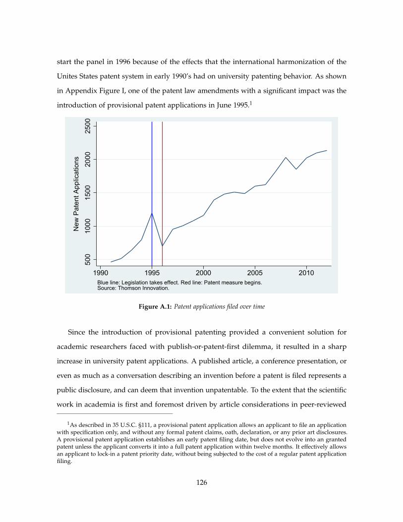
start the panel in 1996 because of the effects that the international harmonization of the
Unites States patent system in early 1990’s had on university patenting behavior. As shown
in Appendix Figure I, one of the patent law amendments with a significant impact was the
introduction of provisional patent applications in June 1995.1
500
1000
1500
2000
2500
New
Pat
ent A
pplic
atio
ns
1990 1995 2000 2005 2010Blue line: Legislation takes effect. Red line: Patent measure begins.Source: Thomson Innovation.
Patent Applications Filed over Time
Figure A.1: Patent applications filed over time
Since the introduction of provisional patenting provided a convenient solution for
academic researchers faced with publish-or-patent-first dilemma, it resulted in a sharp
increase in university patent applications. A published article, a conference presentation, or
even as much as a conversation describing an invention before a patent is filed represents a
public disclosure, and can deem that invention unpatentable. To the extent that the scientific
work in academia is first and foremost driven by article considerations in peer-reviewed
1As described in 35 U.S.C. §111, a provisional patent application allows an applicant to file an applicationwith specification only, and without any formal patent claims, oath, declaration, or any prior art disclosures.A provisional patent application establishes an early patent filing date, but does not evolve into an grantedpatent unless the applicant converts it into a full patent application within twelve months. It effectively allowsan applicant to lock-in a patent priority date, without being subjected to the cost of a regular patent applicationfiling.
126
journals, provisional patent applications are an exceptionally good fit for this environment
as they enable the university to lock an early priority date, while providing additional
12 months for inventors to publish, disseminate and improve the invention. Universities
use provisional patent applications to reduce uncertainty surrounding market value of
inventions and make a more informed decision of whether to prosecute full patents. Indeed,
many university Technology Transfer Offices laud provisional patent applications as the
first order of business after being informed of a new invention.2
Prevalence of provisional patenting in academia was the main reason behind our decision
to stop our panel with patent applications filed in 2011. Since provisional patent applications
take 12 months before they are published, patent application data from 2012 would be
missing all provisional patents applied for in that year, and would result in a truncated
patent count.
We use priority dates rather than application dates to count patent records because
priority years most closely correspond with the date when the invention was first applied for.
While the patent priority date is most often no different than the regular patent application
date, in a case of a converted provisional application, a priority date will be earlier than
the regular application date. This is especially the case when a divisional or a continuation
application was filed. In addition, we use the DWPI Patent Family list available in Thomson
Innovation database to assign all retrieved patent records to unique groups sharing the same
priority application. This enables us to more closely identify patent groups surrounding
the same invention and ensures that we do not overcount patent records in the sample.
Each DWPI Patent Family is counted only once, and all forward patent citation counts are
aggregated on a DWPI Patent Family level.
2For example, see Office of Vice President for Research at Penn Statehttp://www.research.psu.edu/patents/protect-your-invention/what-happens-after-submission), Innovation and New Ventures Office at Northwestern University(http://www.invo.northwestern.edu/process/assessment-patents), Northeastern University Center forResearch Innovation (http://www.northeastern.edu/research/cri/inventors/commercialization-process/), orBoston University Technology Development (http://www.bu.edu/otd/for-researchers/technology-transfer-process/patentapp/).
127
A.1.1 Disaggregating state educational systems
To further exacerbate the problem of allocating patent applications to universities, some
university systems do not specify campus locations where the invention was made when
filing their patents. For example, almost 75% of all patent applications from University of
California System in our sample are assigned to “The Regents of The University of California”
without any additional information about invention-originating campus. Consequently, we
do not know if the invention was made at The University of California at Berkeley, The
University of California at Los Angeles, or any other campus in the system. Since our
instrument works on the individual campus level only, and does not propagate through
the whole system, we need to allocate patent applications to individual campuses within
the university. In other words, unexpected success of The University of California at
Berkeley football team will not impact R&D expenditures at The University of California
at Los Angeles, and vice versa. To rectify this problem, we use the inventor’s home
address information provided on US patent records and use Google Maps API to calculate
the “by car” estimated travel time from inventor’s home address to every campus in the
university system. We then systematically examine the patent portfolio and count a patent
as originating at a specific university campus if at least one inventor lives less than 26
minute drive from that campus.3
A.2 A brief historical overview of college football
The strangely symbiotic relationship between football and national institutions of higher
learning in the United States goes back for almost 200 years, all the way to football’s early
emergence from the English game of Rugby. Initial evolution, cultural assimilation and
standardization of the game of football took place on campuses of colleges and universities
3This distance is based on the 2013 US Census American Community Survey estimate of mean travel timeto work in the United States of 25.8 minutes. Our results are robust to different travel times: travel times of 15,20 and 30 minutes did not cause any significant changes in our outcomes.
128
in Northeastern United States during the mid 19th and early 20th centuries.4 From its
inception, the sport was popular amongst students and alumni, while evoking much more of
a mixed response from the faculty and administrators.5 Because of the faculty indifference
and disinterest during the football’s early years, the games were organized and regulated
mostly by athletes themselves, together with students and alumni. Largely due to the lack
of adequate regulatory oversight, the early college football games were played without any
protective gear, and players regularly sustained physical injuries. The apparent ferocity
of the sport quickly garnered national attention, reaching all the way to the highest level
of the national government.6 In response to public concerns over player safety, university
administrators formed Intercollegiate Athletic Association—a regulatory body which was
renamed the National Collegiate Athletic Association (NCAA) in 1910. Initial role of the
NCAA was limited to formulation of rules and creation of national championships for
a variety of college sports, but as the outside interest in collegiate athletics grew and
the commercialization pressures increased, the NCAA started to ramp up its governance
activities. In the aftermath of World War II, as university enrollments exploded, so did
the numbers of households owning radio boxes and television sets. The potential reach
of college football and the commercialization pressures increased exponentially. Some
universities like Notre Dame and the University of Pennsylvania embraced the advent of
the new medium by crafting contracts with television networks on their own, while other
schools remained cautious and expressed serious concerns that televised games would
undermine their ticket sales [Dunnavant, 2004]. At this point, the NCAA stepped in and,
4The initiation of modern American football is widely regarded to have taken place on November 6th, 1869when Princeton met Rutgers University for the first intercollegiate football game in history [Rudolph, 1962].
5While some saw it as a way to improve physical toughness, build leadership skills and unify student body,others saw it in direct conflict with essential values of higher education. In 1908, Harry Garfield, a president ofWilliams College remarked: “Here, as generally in American Colleges, there is a grave danger of departurefrom the essential idea of a college as distinguished from an institute of physical culture.” [Rudolph, 1962]
6The season of 1905 was particularly brutal—eighteen students died playing football that year. At Harvard,every game but two produced player concussions. After a post-game photo of badly beaten, bloody and bruisedface of Robert “Tiny” Maxwell, a Swarthmore College player was published in a newspaper, then-presidentTheodore Rusevelt made a demand for the colleges to eliminate the brutality and reduce injuries [Rudolph,1962].
129
after comissioning a study of televised college football games and live attendance, imposed
severe restrictions on televised broadcasts of college football games in 1953. For the next
three decades, only one game was to be broadcast every Saturday, and no college team
was to appear in a broadcast game more than once per season. These restrictions were
finally lifted with the 1984 Supreme Court ruling that the NCAA violated antitrust laws by
controlling television broadcasting rights. This decision ushered the college football into the
modern era of unprecented popularity and profitability.
130