Scientific Competition - OAPEN

Conferences onNew Political Economy

25

Scientific Competition

Edited by

Max Albert, Dieter Schmidtchen,and Stefan Voigt

Mohr Siebeck

Manuscripts are to be sent to the editors (see addresses on page 315).

We assume that the manuscripts we receive are originals which have not beensubmitted elsewhere for publication. The editors and the publisher are not liable forloss of or damage to manuscripts which have been submitted.

For bibliographical references please use the style found in this volume.

ISBN 978-3-16-149413-0ISSN 1861-8340 (Conferences on New Political Economy)

The Deutsche Nationalbibliothek lists this publication in the Deutsche National-bibliographie; detailed bibliographic data is available in the Internet at http://dnb.d-nb.de.

� 2008 by Mohr Siebeck, P. O. Box 2040, D-72010 T�bingen.

This book may not be reproduced, in whole or in part, in any form (beyond thatpermitted by copyright law) without the publisher�s written permission. This appliesparticularly to reproductions, translations, microfilms and storage and processing inelectronic systems.

The book was typeset and printed by Konrad Triltsch in Ochsenfurt-Hohestadt on non-aging paper and bound by Großbuchbinderei Spinner in Ottersweier.

e-ISBN PDF 978-3-16-156037-8

Contents

Max Albert: Introduction . . . . . . . . . . . . . . . . . . . . . . . . . . . . . . . . . . . . . . . . . 1

Paula Stephan: Job Market Effects on Scientific Productivity . . . . . . . 11Bernd Fitzenberger: Job Market Effects on Scientific Productivity

(Comment) . . . . . . . . . . . . . . . . . . . . . . . . . . . . . . . . . . . . . . . . . . . . . . . . . . . . . . 31

Gˇnther G. Schulze: Tertiary Education in a Federal System:The Case of Germany . . . . . . . . . . . . . . . . . . . . . . . . . . . . . . . . . . . . . . . . . . . . 35

StefanVoigt: Tertiary Education in a Federal System (Comment) . . . 67

Gustavo Crespi and Aldo Geuna: The Productivity of UKUniversities . . . . . . . . . . . . . . . . . . . . . . . . . . . . . . . . . . . . . . . . . . . . . . . . . . . . . . 71

Christian Pierdzioch: The Productivity of UK Universities(Comment) . . . . . . . . . . . . . . . . . . . . . . . . . . . . . . . . . . . . . . . . . . . . . . . . . . . . . . 97

Michael Rauber and HeinrichW. Ursprung: Evaluation ofResearchers: A Life Cycle Analysis of German AcademicEconomists . . . . . . . . . . . . . . . . . . . . . . . . . . . . . . . . . . . . . . . . . . . . . . . . . . . . . . 101

Werner Gˇth: Evaluation of Researchers (Comment) . . . . . . . . . . . . . . 123

Martin Kolmar: Markets versus Contests for the Provision ofInformation Goods . . . . . . . . . . . . . . . . . . . . . . . . . . . . . . . . . . . . . . . . . . . . . . . 127

Roland Kirstein: Scientific Competition:Beauty Contests or Tournaments? (Comment) . . . . . . . . . . . . . . . . . . . . 147

Christine Godt: The Role of Patents in Scientific Competition:A Closer Look at the Phenomenon of Royalty Stacking . . . . . . . . . . . 151

Christian Koboldt: Royalty Stacking: A Problem, but Why?(Comment) . . . . . . . . . . . . . . . . . . . . . . . . . . . . . . . . . . . . . . . . . . . . . . . . . . . . . . 173

Nicolas Carayol: An Economic Theory of Academic Competition:Dynamic Incentives and Endogenous Cumulative Advantages . . . . . 179

Dominique Demougin: An Economic Theory of AcademicCompetition (Comment) . . . . . . . . . . . . . . . . . . . . . . . . . . . . . . . . . . . . . . . . . 205

Dorothea Jansen: Research Networks – Origins and Consequences:First Evidence from a Study of Astrophysics, Nanotechnology andMicro-economics in Germany . . . . . . . . . . . . . . . . . . . . . . . . . . . . . . . . . . . . 209

Henrik Egbert: Networking in Science and Policy Interventions(Comment) . . . . . . . . . . . . . . . . . . . . . . . . . . . . . . . . . . . . . . . . . . . . . . . . . . . . . . 231

Christian Seidl, Ulrich Schmidt and Peter Gr˛sche:A Beauty Contest of Referee Processes of Economics Journals . . . . 235

Max Albert and JˇrgenMeckl: What Should We Expect from PeerReview? (Comment) . . . . . . . . . . . . . . . . . . . . . . . . . . . . . . . . . . . . . . . . . . . . . 257

Jesu¤ s P. Zamora Bonilla: Methodology and the Constitution ofScience: A Game-theoretic Approach . . . . . . . . . . . . . . . . . . . . . . . . . . . . . 263

Gebhard Kirchg�ssner: Is It a Gang or the Scientific Community?(Comment) . . . . . . . . . . . . . . . . . . . . . . . . . . . . . . . . . . . . . . . . . . . . . . . . . . . . . . 279

Christian List: Distributed Cognition: A Perspective from SocialChoice Theory . . . . . . . . . . . . . . . . . . . . . . . . . . . . . . . . . . . . . . . . . . . . . . . . . . . 285

Siegfried K. Berninghaus: Distributed Cognition (Comment) . . . . . . 309

Contributors and Editors . . . . . . . . . . . . . . . . . . . . . . . . . . . . . . . . . . . . . . . . . . . 315

ContentsVI

Introduction

by

Max Albert

What is scientific competition? When this question is posed by an economist,many people think they already know what the answer must be: science is amarket of ideas, and scientific competition is like market competition. Sur-prisingly, the economics of science1 gives quite a different answer.

Of course, a certain part of science, called commercial or proprietary sci-ence, is a market of ideas. In proprietary science, the results of research areprotected by intellectual property rights, mostly patents or trade secrets; theycan be bought and sold, and their market value derives from the market valueof the goods they help to produce. Moreover, the expected market value of anidea provides the incentives for investments in research.

Competition in proprietary science is not like market competition; it ismarket competition. In contrast, scientific competition means competitionwithin academic or open science and its institutions: learned societies, scien-tific journals, the peer review system, Nobel prizes, and modern research-oriented universities.

In open science, ideas are not protected by intellectual property rights.Contributions to open science are published, and the ideas they contain can beused free of charge by anybody who wishes to do so. Although these ideas arenobody�s property in a legal sense, their use is regulated by moral rights ornorms. Researchers morally “own” results if they were the first to publishthem (the so-called priority rule, see Merton 1973); they have a moral right,then, to be cited by those using their results. The extent to which aresearcher�s ideas are used by others determines the researcher�s status in thescientific community (Merton 1973, Hull 1988). Status is not only a reward onits own (Marmot 2004), but also the key to other, material rewards in openscience. Just like patents in proprietary science, then, the norms of open sci-ence generate incentives to invest in new ideas.

Is open science a market of ideas? There are certainly many similarities. Inopen science as in markets, we observe production, division of labor, spe-cialization, investments, exchange, risk-taking, competition but also cooper-ation, and so forth.2 However, these are aspects of almost all humanendeavors. It is more informative to look for differences. The most importantdifference is that both institutions use different mechanisms of collective

1 For surveys, see Diamond (1996, forthcoming), Stephan (1996, forthcoming).2 On differences and similarities between competition in science and on markets, see

Walstad (2002).

decision making. Markets use the price mechanism. Open science uses asophisticated version of the voluntary contributions mechanism based oncompetition for status.

Many collective decisions are made through voluntary contributions, fromthe cleanliness of public spaces, which is largely determined by voluntaryindividual effort, to the financial volume of private disaster relief. Usually,voluntary contributions determine only the supply of some good. The specialtwist of scientific competition is that the voluntary contributions mechanismregulates both, supply of and demand for research.

Looking at the supply side, we find that researchers in open science are notpaid for each contribution. They receive a lump-sum salary that coversresearch and, possibly, other activities, notably teaching, but in the short runneither this salary nor other possible rewards vary with the number andquality of their contributions. Since, in most cases, nobody demands a specificcontribution, individual contributions are voluntary, unsolicited, and unpaid.

The motives behind volunteering are well-known.3 We can distinguishbetween consumption and investment motives. Consumption motives areenjoyment of one�s work, reciprocity or altruism (which are similar toenjoyment), and the striving for recognition and status, especially amonginsiders. In the case of science, curiosity is often mentioned, which is an aspectof enjoyment. Enjoyment of work usually requires the freedom to chooseone�s tasks and the absence of control, which are characteristics of open sci-ence. Investment aspects are networking, building human capital, and sig-naling one�s ability. In the case of science, signaling one�s ability goes hand inhand with acquiring status among insiders; it does not matter whether oneemphasizes the investment or the consumption aspect.

Looking at the demand side, we see that the scientific community decides,in a decentralized way, about a contribution�s success. Science is cumulative:one researcher�s output is the next researcher�s input. A successful con-tribution is one that is used by other researchers as input for their ownresearch. The more it is used, the higher the success. Citation statistics andimpact factors are relevant because they measure the use of ideas.4

Researchers in open science compete in providing inputs for their peers. Ifthey want to be successful, they must anticipate what kind of input otherresearchers would like to use; their success depends on the decisions of theirpeers. This mechanism should not be confused with peer review. Peer review isused to select among research proposals that compete for funding, or amongpapers that compete for publication in prestigious journals. It is a secondary

3 See the overview in Hackl et al. (2005), partially published in Hackl et al. (2007).4 Though only very approximately: important ideas are used without citation when

they have become textbook knowledge; on the other hand, many citations do not indi-cate use of ideas but only demarcate the contribution of a paper.

Max Albert2

selection mechanism that tries to deal with the scarcity of funds or of atten-tion. The primary selection mechanism – selection of inputs for furtherresearch – could work without peer review, although possibly less efficiently.

Why scientific competition? Traditionally, economists have taken it forgranted that the price mechanism is the only efficient mechanism of collectivedecision making. From this point of view, scientific competition should bereplaced by the price mechanism. However, with the rise of the new institu-tional economics (see Furubotn and Richter 2005) and its integration in theeconomic mainstream, the traditional view has lost its plausibility. Economistshave learned that markets are not always better than hierarchies, and thatmajority voting may be ex ante efficient. Similarly, the economics of sciencestarted with an argument against the price mechanism.

In their pioneering contributions, Nelson (1959) and Arrow (1962) analyzedthe shortcomings of the price mechanism in scientific research: The exclusionof potential users of an idea is inefficient because additional users create noadditional costs. Even with patent protection, the returns on investment inresearch can be appropriated only to some extent. The outcomes of researchare highly unpredictable; thus, researchers will need insurance, but insurancedilutes the researchers� incentives. Consequently, investment in research andutilization of its results will typically be too low. Moreover, results willsometimes be kept secret, which impedes further research. These problemswill be more pronounced for basic than for applied research.

With respect to basic research, Nelson and Arrow considered open, or not-for-profit, science as a solution, without, however, analyzing it in detail. Thiswas done by Dasgupta and David (1994). At the heart of their argument foropen science is a massive delegation problem. In basic research, employers ofresearchers lack the knowledge to judge the quality of research results and,consequently, the achievements of researchers. They cannot effectively mon-itor the efforts of researchers, and they cannot judge the results of theseefforts. Hence, they cannot hire researchers on the basis of incentive contractsthat condition payment on the quality of results. Scientific competition solvesthis delegation problem. It provides incentives to researchers and generatesevaluations of researchers (i.e., scientific reputations) and of research results(i.e., extent of use by the scientific community) that can be observed and usedby employers. Indeed, these achievements of scientific competition mayexplain the existence of open science (David 1998, 2004).

Why care about scientific competition? European science policy seemscurrently to be fixated on the idea that promoting competition between uni-versities is the key to improvements in the European system of scientificresearch (see, e.g., EU Commission 2003, 2005).

Historically, however, university competition has been neither sufficient nornecessary for the flourishing of scientific research. The successes of the 19thcentury Prussian university system were, to a large degree, due to central

Introduction 3

ministerial control – the so-called “System Althoff”, named after theresponsible civil servant. With the help of a network of personal contacts,Althoff extracted the information circulating in the scientific community andused it to hire young scientific high-potentials and to reward renownedresearchers. Thus, the ministry circumvented university competition and,instead, made use of and promoted scientific competition. This central-plan-ning regime was preceded by a very competitive decentralized system whereuniversities competed for student fees. Every employee, from the professor tothe caretaker, got their share: a textbook case of incentive pay. However, inthis system, the scientific standards of university education were very low, anduniversities played no role in research.5

The point of these historical facts is, of course, not that central planningworks better than competition, but that scientific competition is moreimportant than university competition.

Scientific competition provides common pool resources for universities:6

incentives for researchers to do research and to conform to scientific stand-ards; evaluations of research results, which are used by universities for thedevelopment of academic curricula; and evaluations of researchers, which areused by universities for hiring and promotion decisions. These resources areonly available, however, if universities allow their academic staff to participatein scientific competition.

Competition between users of a common pool resource easily leads to over-exploitation. Consider, for instance, the following plausible scenario. Uni-versities compete for the services of renowned researchers, who get contractsthat allow them to do their own research. Less renowned researchers have lessbargaining power, and administrators put them to other uses: teaching,administration, and research that is profitable to the university but of noscientific interest. This is rational from the administration�s point of view.However, scientific competition requires that researchers decide collectivelyabout reputations, by accepting or rejecting new ideas as inputs for their ownresearch. If universities want to employ researchers who have earned a rep-utation in this process, they must collectively bear the costs of letting other,less renowned researchers participate. Yet, each university is better off if itmakes use of scientific competition without bearing its share of the costs. Inthis scenario, university competition will destroy scientific competition.

This is not the place to evaluate current policies. Our concern here is withthe scientific basis of these policies, which fails to take scientific competition

5 See Clark (2006) and, specifically on the “System Althoff”, Vereeck (2001). SeeBurchardt (1988, 185) for an example for the distribution of fees from the university ofBerlin, and this university�s statutes, Statuten der Friedrich-Wilhelms-Universit�t in Berlinv. 31.10.1816, which were typical for the time. I am am obliged to Lydia Buck for bringingthese historical facts and the relevant literature to my attention.

6 On common pool resources and their governance, see Ostrom (1990).

Max Albert4

into account. The EU commission (2003, 2005), for instance, never mentionsscientific competition, under this or a different name. This is like reformingcapitalism and forgetting about the price mechanism. It is hard to believe thatsuccessful policies can be developed on such a basis.

The Contributions to this Volume

The papers in this volume deal with core aspects of the theory and policy ofscientific competition. They have all been presented and extensively discussedat a conference in Saarbr�cken in October 2005. They appear here in revisedform, together with the revised versions of the comments that were alsopresented at the conference.

The economics of science has always been an interdisciplinary undertaking.Economists have learned much from sociology (see esp. Merton 1973).Problems of intellectual property rights are discussed by lawyers and econo-mists. There are also strong connections between the philosophy of science,which has taken an institutionalist turn with the work of Karl Popper, and theeconomics of science (H. Albert 2006). The present volume continues theinterdisciplinary tradition and contains contributions from economics, law,philosophy of science, political science, and sociology.

The first four papers are concerned with supply-side considerations: thesupply of researchers and their productivity. Paula Stephan starts from theobservation that employment conditions in science have changed. Today, theprerequisites for productive research – access to equipment and colleagues, acertain degree of autonomy, job or funding security – are often missing. Anincreasing percentage of young researchers get stuck in laboratory jobs wherethey are not doing their own research. These employment conditions willreduce the future supply of young researchers since the current generation�sexperiences influence the next generation�s expectations. The current systemof research may not be sustainable, then, since it requires a large supply ofyoung researchers motivated by the expectation of getting one of the researchpositions that are becoming increasingly scarce.

G�nther Schulze also looks at the supply of researchers, but from a verydifferent perspective. He analyzes the supply of university professors throughthe states in a federal system. The number of professors is an important part ofeducational services; indeed, Schulze treats this number as a proxy for edu-cational services. He shows that states have an incentive to attract high schoolgraduates from other states by providing capacity in tertiary education,thereby free riding on educational services provided in the primary and sec-ondary education by other states. Optimal tertiary education is less thanproportional to the size of the jurisdiction. For Germany he shows currenttrends in provision of professors and the production of new professors,

Introduction 5

proxied by the number of habilitations. He analyzes the differences in therelative number of professors, their determinants and the resulting crossborder student migration for the German federal states.

The next two papers are concerned with the measurement of productivity inscience. Gustavo Crespi and Aldo Geuna consider the determinants of scienceresearch output (as measured by publications and citations) in the UK. Theyuse an original dataset including information for the 52 “old” UK universities(which account for about 90% of research expenditure) across thirty scientificfields for a period of 18 years, from 1984/85 to 2001/02. On this basis, theyinvestigate the relations between the investment in higher education and theresearch outputs, rejecting the model of a global science production functionfor the UK in favor of four significantly different production functions for themedical sciences, the social sciences, the natural sciences and engineering.

While Geuna and Crespi look at the macroeconomics of scientific pro-ductivity, Michael Rauber and Heinrich Ursprung focus on the micro-economic aspects. They argue that a bibliometric evaluation of researchersshould take life cycle effects and vintage effects into account, and demonstratethe crucial importance of these effects in a bibliometric study of the researchbehavior of German academic economists. On the basis of this study, theydevelop a simple ranking formula that could be used for performance-relatedremuneration and track-record based allocation of research grants. They alsoinvestigate the persistence of individual productivity, which is relevant fortenure decisions, and develop a faculty ranking which is insensitive to thefaculty age structures.

These supply-side considerations are followed by five papers that are con-cerned with specific institutional aspects of open science. Martin Kolmarcompares open and proprietary science from a theoretical perspective. For thepurposes of his paper, proprietary science is identified with research leading topatents. Open science is modeled as a contest for a prize (research grants,tenure, etc.), with the research output becoming a public good. Kolmar con-siders a case where the research results may be used to reduce productioncosts in an oligopolistic downstream market. Thus, the focus is on appliedscience, which is quite often viewed as the natural domain of proprietaryscience. Nevertheless, the patent system turns out to be inefficient, becausethe patent holder has an incentive to restrict the number of licenses too muchand because incentives for research are too weak. Open science, on the otherhand, may be efficient, and even when not, it may be second-best optimal.

Christine Godt is also concerned with problems of the patent system. Shequestions, from a lawyer�s perspective, the view that the possibility of pat-enting actually provides incentives for a better technology transfer fromresearch institutions to industry. The problem is that the accumulation ofroyalties through several stages of a typical innovation process – a phenom-enon called “royalty stacking” – eats up the profit margins on the downstream

Max Albert6

market. Royalty stacking is a result of two distinct mechanisms, one propri-etary, the other contractual. The proprietary mechanism is rooted in theexpansion of patents into the traditional domain of open science. The con-tractual mechanism is primarily due to the transition from sale contracts tolease contracts in the downstream market. In combination, these twomechanisms can impede the technology transfer when the royalty sharebecomes too large.

Nicolas Carayol analyzes the theoretical basis of the so-called Mattheweffect in science. This effect was proposed by Merton as an explanation of thetypical career patterns in science. It assumes that early successes in science leadto a more successful career because successful young researchers get betterjobs with better research opportunities. Thus, an outstanding career in sciencemay be the result not of exceptional ability, but of accidental early success.Carayol explains the Matthew effect in a dynamic model of university com-petition. The basis of the effect is an externality between researchers: suc-cessful old researchers confer an advantage to their younger colleagues. Thisimplies that young researchers who get jobs at high-reputation universities willgo on to be more successful than their peers at low-reputation universities,which perpetuates the reputation differences between universities.

Carayol�s model hints at a further important aspect of academic life.Externalities between researchers can be interpreted as access to researchnetworks. The great practical importance of these networks becomes muchclearer in Dorothea Jansen�s paper, which reviews the results of a largesociological research project under her direction. The project focuses onnetworks in astrophysics, nanotechnology and microeconomics, collectingdata on existing networks and analyzing correlations between networkproperties like size and density on the one hand and success in research on theother hand. The European and German science policies actively promote suchnetworks. Among others, the empirical results show the first consequences ofthese policies.

Christian Seidl, Ulrich Schmidt and Peter Gr�sche present the results of anempirical investigation of the referee processes of economic journals. Peerreview, and especially the referee process of scientific journals, is a centralinstitution of modern open science. Seidl, Schmidt and Gr�sche argue thatpublications in refereed journals today serve mainly as quality signals, influ-encing personal advancement, research opportunities, salaries, grant-funding,promotion, and tenure. For this reason, they consider the validity, impartiality,and fairness of the referee process as very important. The literature, however,casts doubts on the idea that journal referee processes satisfy these require-ments. Their own investigation shows that authors in economics value com-petence and carefulness of the reports more than positive decisions by editors.Competence and carefulness, however, are often missing. Moreover, reportsin economics often fail to help authors improve their manuscripts.

Introduction 7

The volume concludes with two papers devoted to collective decisionmaking in science. Jesu�s Zamorra Bonilla applies the perspective of con-stitutional political economy to methodological rules in science. Combiningphilosophy of science with game theory, he conceives of science as a game ofpersuasion in which competition for status forces scientists to accept meth-odological rules and to acknowledge the contributions of their competitors.On the basis of a specific model, he argues that mutual control in a scientificcommunity ensures that the norms of science are followed frequently, if notperfectly.

Christian List discusses collective decision making in science from a verydifferent, non-competitive perspective, namely, social-choice theory. Drawingon models of judgment aggregation, he addresses the question of how a groupof individuals, acting as a multi-agent cognitive system, can “track the truth”in the outputs it produces. He argues that a group�s performance depends onits “aggregation procedure” – its mechanism for aggregating the groupmembers� inputs into collective outputs; for instance, voting on the truth ofpropositions – and investigates the ways in which aggregation proceduresmatter. These considerations are highly relevant in connection with scientificcommittees that try, against the background of scientific competition with itsdifferences of opinion, to formulate a scientific consensus, as, for instance, inthe case of climate change.

These eleven papers, with accompanying comments, highlight the diverseproblems and questions turning up when we try to understand scientificcompetition. They also illustrate the breadth of contemporary economics ofscience, its many ties with neighboring fields, and its potential to improvescience policies.

Acknowledgements

As organizer of the conference, I am very grateful to the following institutionsfor their financial support: the Fritz Thyssen Stiftung, theMinister f�r Bildung,Kultur und Wissenschaft of the Saarland, the Union Stiftung Saarbr�cken, theVereinigung der Freunde der Universit�t des Saarlandes, and the DeutscheBundesbank.

References

Albert, H. (2006), “Die �konomische Tradition und die Verfassung der Wissenschaft,Perspektiven der Wirtschaftspolitik 7 (special issue), 113 – 131.

Albert, M. (2006), “Product Quality in Scientific Competition”, Papers on StrategicInteraction 6 – 2006, Max Planck Institute of Economics, Jena.

Max Albert8

Arrow, K. J. (1962), “Economic Welfare and the Allocation of Resources for Invention”,609 – 625 in: The Rate and Direction of Inventive Activity: Economic and Social Fac-tors, Princeton University Press: Princeton.

Burchardt, L. (1988), “Naturwissenschaftliche Universit�tslehrer im Kaiserreich”, 151 –214, in: Schwabe, K. (ed.), Deutsche Hochschullehrer als Elite: 1815 – 1945, Boldt:Boppard.

Clark, W. (2006), Academic Charisma and the Origins of the Research University, Uni-versity of Chicago Press: Chicago and London.

Dasgupta, P. and David, P. A. (1994), “Toward a New Economics of Science”, ResearchPolicy 23, 487 – 521.

David, P. A. (1998), “Common Agency Contracting and the Emergence of �Open Sci-ence� Institutions”, American Economic Review 88, 15 – 21.

David, P. A. (2004), “Understanding the Emergence of �Open Science� Institutions.Functionalist Economics in Historical Context”, Industrial and Corporate Change 13,571 – 589.

Diamond, A. M. Jr. (1996), “The Economics of Science”, Knowledge and Policy 9, 6 – 49.Diamond, A. M. Jr. (forthcoming), “Economics of Science”, in: Steven N. Durlauf and

Lawrence E. Blume (eds), The New Palgrave Dictionary of Economics, 2nd ed.,Palgrave Macmillan: Basingstoke and New York (forthcoming).

EU Commission (2003), The Role of the Universities in the Europe of Knowledge,COM(2003) 58 final, Br�ssel.

EU Commission (2005), Recommendation on the European Charter for Researchers andon a Code of Conduct for the Recruitment of Researchers, C(2005) 576 final, Br�ssel.

Furubotn, E. G. and R. Richter (2005), Institutions and Economic Theory. The Con-tribution of the New Institutional Economics, 2nd ed., University of Michigan Press:Ann Arbor.

Hackl, F., M. Halla and G. J. Pruckner (2007), “Volunteering and Income. The Fallacy ofthe Good Samaritan?”, Kyklos 60, 77 – 104 (longer version: Working Paper 415,Department of Economics, Johannes Kepler Universit�t, Linz 2005).

Hull, D. L. (1988), Science as a Process, University of Chicago Press: Chicago andLondon.

Marmot, M. (2004), The Status Syndrome. How Social Standing Affects Our Health andLongevity, Holt and Company: New York.

Merton, R. K. (1973), The Sociology of Science, University of Chicago Press: Chicagoand London.

Nelson, R. R. (1959), “The Simple Economics of Basic Scientific Research”, Journal ofPolitical Economy 67, 297 – 306.

Ostrom, E. (1990), Governing the Commons. The Evolution of Institutions for CollectiveAction, Cambridge University Press: Cambridge.

Statuten der Friedrich-Wilhelms-Universit�t in Berlin v. 31.10.1816, 414 – 428, in: L. vonR�nne, Das Unterrichtswesen des Preussischen Staates Vol. 2, 1855. Reprint. K�ln andWien: B�hlua Verlag, 1990.

Stephan, P. E. (1996), “The Economics of Science”, Journal of Economic Literature 34,1199 – 1235.

Stephan, P. E. (forthcoming), “The Economics of Science”, in: B. H. Hall and N.Rosenberg (eds), Handbook of Economics of Technological Change, North-Holland.

Walstad, A. (2002), “Science as a Market Process”, Independent Review 8, 5 – 45.

Introduction 9

leereseite

Job Market Effects on Scientific Productivity*

by

Paula Stephan

1 Introduction

Much of the discussion in science policy circles today focuses on the questionof whether the production of basic knowledge is threatened by a shift ofemphasis in the public sector towards facilitating technology transfer. Thereare at least two variants of the crowding-out hypothesis. One variant arguesthat in the changing university culture scientists and engineers increasinglychoose to allocate their time to research of a more applied as opposed to basicnature.1 Another variant of the crowding-out hypothesis is that the lure ofeconomic rewards encourages scientists and engineers (and the universitieswhere they work) to seek intellectual property (IP) protection for theirresearch results, eschewing (or postponing) publication, and more generally tobehave more secretively than in the past.2 Much of the work of Blumenthaland his collaborators (1996) focuses on the latter issue in the life sciences,examining the degree to which university researchers receive support fromindustry and how this relates to publication. A related concern is that thegranting of intellectual property can hinder the ability of other researchers tobuild on a given piece of knowledge. This anti-commons hypothesis, articu-lated by Heller and Eisenberg (1998) and David (2001), postulates that theassignment of intellectual property rights discourages the use of knowledge byother researchers.

How changing property rights in science affect the production of newknowledge is clearly of great relevance to the future of scientific productivity.But there are other reasons to be concerned about the production of scientificknowledge. This paper focuses on these. To wit: who will do science? Will theywork in an environment conducive to doing research? The premise of thepaper is that researchers� productivity is affected by the environment in whichthey work and the conditions of their employment. For example, access to

* This paper builds on the presentation that Stephan made at the conference “TheFuture of Science,” Venice, Italy, September 2005. The author would like to thank GrantBlack, Chiara Franzoni, and Daniel Hall for their assistance. The author is indebted toBill Amis, Chiara Franzoni, Bernd Fitzenberger, Christine Musselin, and G�ntherSchulze as well as participants at the conference on Scientific Competition for theiruseful comments. All errors are those of the author.

1 The model examined by Jensen and Thursby (2003) suggests that a changing rewardstructure may not alter the research agenda of faculty specializing in basic research.

2 Clearly, these two variants are not mutually exclusive.

equipment and colleagues clearly affect productivity. Productivity is furtherenhanced by researchers� having a certain amount of autonomy. Moreover, aresearch horizon, facilitated by job security or funding security, encouragesscientists to choose more risky projects than they might otherwise choose.And it doesn�t hurt if scientists work in such environments when they areyoung. Research consistently finds evidence of a relationship between age andproductivity (Levin and Stephan 1991, Stephan and Levin 1992 and 1993,Jones 2005, Turner and Mairesse 2005). For what we might call journeymenscientists, the relationship is not pronounced. But for prize-winning research,there is considerable evidence of a strong relationship (Stephan and Levin1993). While it does not require extraordinary youth to do prize-winningwork, the odds decrease markedly by mid-life. Stephan and Levin (1993)report that the median age that Nobel laureates commenced work on theproblem for which they won the prize is 36.8 in chemistry; 34.5 in physics and39.0 in medicine/physiology for the first 92 years that the prize was awarded.For the more recent period, they find that the median age in chemistry is 38.5;in physics it is 36.0 and in physiology/medicine it is 35.0 (Stephan, Levin andXiao, unpublished data). They conclude (1993, 397) “that regardless of field,the odds of commencing research for which a Nobel Prize is awarded declinedramatically after age 40.” Research opportunities for young scientists affectnot only the productivity of the current generation of scientists. They alsoaffect the scientific enterprise in years to come, since the supply of new sci-entists is responsive to the job opportunities and job outcomes that the currentgeneration experiences.

Historically, scientists and engineers received doctoral training with the goalof achieving a research position either at a university or, depending upon thecountry, a research institute. In some instances, scientists and engineersworked in large industrial research labs, although in the 20th century thispattern was more common in the U.S. than in Europe.

In many western countries today young scientists face problems obtainingresearch positions that have characteristics conducive to doing good research.Here we discuss problems facing young scientists, drawing examples from theUnited States, Italy, and Germany. We also discuss factors contributing to thedismal job outlook faced by young scientists today. We focus on those workingin the fields of the physical, life and mathematical sciences, as well as engi-neers, excluding those working in the social sciences from our discussion.

Paula Stephan12

2 Problems facing young scientists

2.1 The situation in the United States

Public sector research in the United States occurs primarily in the universitysector, although some public research is produced at Federally FundedResearch and Development Centers (FFRDCs) and at national laboratories,such as the National Institutes of Health. Within the university sector, by farthe lion�s share of research is conducted at what are known as Research Oneinstitutions, institutions such as Harvard, MIT, University of Michigan, Uni-versity of Wisconsin, etc., classified by Carnegie as a “one” based on theamount of research funding that they receive and the number of PhD studentsthat they educate. There is also a long tradition in the United States, as notedabove, of scientists and engineers working in large industrial labs. Threenoteworthy examples of such labs that flourished during the 20th century werethose at Bell, DuPont and IBM.

Graduate students in the U.S. have a strong tradition, albeit the tradition isfield dependent, of aspiring to a tenure track position at a research university.A survey of U.S. doctoral students in the fields of chemistry, electrical engi-neering, computer science, microbiology and physics during the academic year1993 – 1994 found that 36% of the respondents aspired to a career at aresearch university; 41% aspired to a career in industry/government (Fox andStephan 2001).3 The preferences vary considerably by field; in microbiologyand in physics more than 50% of the men preferred academic researchpositions as did 40% of the women surveyed. In chemistry and electricalengineering, which have a long tradition in the United States of employmentin industry, a substantially lower percent prefer research positions in academecompared to research positions in industry or government.

The university sector in the United States has been characterized by atenure system that determines, within a period of no more than seven years,whether an individual has the option to remain at the institution or is forced toseek employment elsewhere (Stephan and Levin 2002, 419). If the individualreceives tenure, s/he is promoted to the rank of associate and subsequently fullprofessor if the research record continues to merit promotion. Prior to beinghired as an assistant professor it has become increasingly common to take apostdoctoral position.

The importance of tenure makes it crucial for young scientists to signal toolder colleagues that they have the “right stuff” for doing research. A nec-

3 The mail survey was administered by Fox to a national sample of 3800 doctoralstudents. The response rate was 62%. Respondents were asked “After receipt of yourPhD, do you prefer to pursue an academic or nonacademic (industrial, government)career? The response categories were: (1) “academic with emphasis upon research;” (2)“academic with emphasis upon teaching;” and (3) “nonacademic.”

Job Market Effects on Scientific Productivity 13

essary component of this signal is the ability to establish a lab of one�s own.And while startup capital is generally provided by the institution (Ehrenberg,Rizzo and Jakubson 2003), finding the funds necessary to run the lab (not onlyto buy supplies and equipment but also to hire graduate students, fundpostdoctoral positions, and hire technicians) is the responsibility of theindividual (Stephan and Levin 2002, 419).

Typically the scientist applies to a research institute of the Federal gov-ernment for a research grant, although some resources for research come fromthe private sector (such as the Howard Hughes Medical Institute) and some(and an increasing portion) come from the university itself. In 2001, forexample, 59% of the funds for research in the academic sector came from theFederal government; 7.1% came from state and local governments, 6.8%came from industry, 7.4% came from other places and 20% came from uni-versities themselves (National Science Board 2004, chapter 5).

The field that has grown the most rapidly in the United States is that ofbiomedical sciences. Growth has occurred both in terms of the number ofPhDs produced and the amount of funding available for research. Forexample, PhD production in the slightly broader area of the biological andagricultural sciences grew from 2711 in 1966 to 6798 in 2000 (National ScienceFoundation 2002). Funding from the National Institutes of Health doubledover a recent five-year period, going from $13.648B in 1998 to $27.181B in2003.4 Here we examine the prospects of young PhDs trained in the bio-medical sciences in the United States to be hired into a permanent position ata Research One university, as well as their prospects to get funding.

Figure 1 shows the dramatic increase in the number of PhDs age 35 oryounger trained in the biomedical sciences in the United States. Data for thefigure come from the Survey of Doctorate Recipients (SDR), a biennialsurvey overseen by Sciences Resources Statistics of the National ScienceFoundation and drawn from the sampling frame of the Survey of EarnedDoctorates (SED), a census of all new PhDs in the U.S.5 We see that thenumber of PhDs 35 years of age or younger, trained in biomedical sciences inthe United States, grew by almost 60% during the short interval of eight years,going from 11,715 to 18,671. We also see that the number of tenure-trackpositions has grown by only 7% during the same period, going from 1212 to1294. Thus, the probability that a young person trained in the biomedicalsciences in the United States holds a tenure track position has declined con-

4 http://www.faseb.org/opa/ppp/fed_fund/NIH_funding_trends_4x13x04_files/frame.htm

5 The SED is administered to all PhD recipients. The SDR is administered to a sampledrawn from the SED. The tabulations presented here use weighted data from the SDR.

Paula Stephan14

siderably in recent years, going from 10.3% to 6.9%.6 When we focus onResearch One institutions, we see a similar pattern. We estimate that 618PhDs age 35 or younger trained in the biomedical sciences held tenure trackpositions at Research One institutions in 1993 (5.3% of those 35 or younger).Eight years later, 543 (4.4%) held such positions.

The situation is not limited only to those under 35, as is readily seen inFigure 2 (see p. 16), which shows the number of biomedical PhDs between 36and 40 in tenure track positions to be almost flat during the period. Moregenerally, the number age 55 and under holding tenure track positions hasbeen fairly constant over the eight-year interval; the only growth has been forthose greater than 55 years old.

Not surprisingly, young PhDs trained in the biomedical sciences are havingdifficulty garnering a first award from the National Institutes of Health, asshown in Figure 3 (see p. 17). While in 1979 NIH made awards to almost 1200principal investigators (PI�s) 35 or younger, by 2003 the number had declined toapproximately 200 (National Academies of Science 2005). More generally, theaverage age at first major independent research support has increased from 37

Figure 1 Biomedical PhDs Age 35 or Younger in United States

Source: Computations, SDR (see text).

6 Increasingly faculty are hired into non-tenure track positions that have the title ofassistant, associate or full professor. The number of young individuals holding suchpositions grew from 389 to 527 in 2001. Including this group with the tenure track group,the probability of being in a faculty rank position has declined from 13.7% to 9.7%during the 1993-2001 period for those 35 and younger.


in 1980 to 41.9 in 2002 for PhDs.7 The decline cannot be attributed to a lack ofresources, given the tremendous amount of growth that occurred in the NIHbudget during this period. Nor can it be attributed to a decline in supply ofyoung investigators (see Figure 1 p. 15). Neither can it be attributed to thequality of the proposals submitted by those 35 or younger. NIH data indicatethat the success rates for new funding are highest for those 35 and younger thanfor any age group; the second highest success rate is for those 36 to 40. Rather,the decline reflects the older age at which young researchers obtain a firstpermanent position from which they can apply for funding.8 The funding sit-uation was of sufficient concern for the National Academies of Science (NAS)to appoint a committee, chaired by Nobel laureate Thomas Cech, to study theissue. Their report, entitled “Bridges to Independence,” was issued in 2005.

More generally, the success patterns reflect the changing composition ofPhD employment at U.S. universities. Specifically, universities increasingly arehiring more part-time and non-tenure-track faculty; they employ more andmore post doctorates and staff scientists. For example, the percent of bio-medical PhDs working at universities and employed in non-tenure-trackpositions grew from 26% to 33% in the eight-year period 1993 to 2002. This

Figure 2 Tenure Track Biomedical Faculty by Age: United States

Source: Computations, SDR (see text).

7 First independent research support consists of either an R01 grant or, in earlieryears, an R29 award.

8 Researchers typically hold a position for two or three years before submitting a grantproposal. One reason for this is that the grant application must show evidence relating toprior results.

Paula Stephan16

matches a national trend across disciplines and universities. Figure 4 (seep. 18) shows the ratio of full-time non-tenure-track faculty to full-time faculty atResearch One institutions (Ehrenberg and Zhang 2005, table 3A.1). The dataare displayed for both public and private institutions. In both instances, we seea substantial increase over time. For example, at public institutions, the ratio,which was .245 in 1989, had climbed to .375 by 2001; in private institutions ithad started at .312 and eventually increased to .434 by the year 2001.9

It should be noted that postdoctoral appointments are usually not includedin this data since the postdoctoral position is generally classified as a trainingposition and hence is generally not processed as a hire. During this interval,the number of individuals working in postdoctoral positions has increaseddramatically (Ma and Stephan 2005), going from 23,000 in 1991 to 30,000 in2001.10 Ma and Stephan find the propensity to take a postdoctoral position tobe inversely related to demand for positions in academe. For example, theyfind the probability to be negatively and significantly related to the per centchange in current fund revenue for institutions of higher education.11

Figure 3 National Institute of Health Awards To Those 35 and Under,United States

Source: National Academies of Sciences (2005).

9 The tabulations are based on data from the biennial IPEDS Fall Staff Surveys.10 Richard Freeman (unpublished presentation) estimates that the ratio of post-

doctorates to tenured faculty positions in the life sciences went from .54 in 1987 to .77 in1999, an increase of 43%.

11 They also find the propensity to be positively related to the size of the PhD�s cohort,suggesting that other things equal, as supply of new PhDs increases, recent PhDs aremore likely to take postdoctoral positions.


Several factors explain these hiring trends. First, cutbacks in public fundsand lowered endowment payouts clearly affect hiring. Second, salaries oftenure-track faculty are higher than those of non-tenure-track faculty andresearch shows (Ehrenberg and Zhang 2005) that this leads to a substitutionaway from tenure-track positions. Third, funding for non-permanent positionssuch as staff scientist is available in research grants. The high cost of start-uppackages also plays a role in explaining these trends. A survey of start-uppackages by Ehrenberg, Rizzo and Jakubson (2003) finds that privateResearch One institutions spend on average $403,071 on the start-up packagesfor assistant professors, while public Research One institutions spend onaverage $308,210. Given these sums, when universities do hire in the tenuredranks, they are tempted to recruit senior faculty away from another university,rather than hire an as yet untested junior faculty member. The financial risk isconsiderably lower. While the start-up packages are generally higher at thesenior ranks, the university gets an immediate transfer of grant money,because the senior faculty generally bring existing research grants with themwhen they come.

Despite this situation, many young scientists persist in aspiring to a tradi-tional academic career. Geoff Davis�s (2005) recent survey of postdocs foundthat the overwhelming majority of those looking for a job, were “very inter-ested” in working at a research university.12 While any sample of postdocs is

Figure 4 Full-time Non-tenure-track Faculty/Total Full-time Facultyat Research One Institutions: United States

Source: Ehrenberg and Zhang (2005).

12 Davis reports that 1110 of the 2770 respondents indicated that they were looking fora job. Among these, 72.7% were “very interested” in a job at a research university and23.0% were “somewhat interested.”

Paula Stephan18

inherently biased towards those preferring such employment, as the abovestatistics indicate, the odds that the respondents will achieve a tenure-trackposition are not good.

The academic labor market in the United States has been characterized byStephan and Levin (2002) as building upon a series of implicit contracts.Graduate students and postdocs enter a program and provide some “surplus”for the lab through their work as a research assistant or postdoc, and thenleave the institution to begin a research career. The professor has an incentiveto not cheat on the arrangement. If the student is kept too long, or educatedtoo poorly to be considered employable by a future dean, or provided poorinformation concerning job outcomes, in theory the professor will cease to beable to attract top graduate students and the source of labor, compensatedwell below its opportunity cost, will dry up.

This system, which loosely resembles a pyramid scheme, works reasonablywell as long as there is a growing demand for faculty positions. But for this tooccur, funding for science must not only grow, but must grow sufficiently fastto absorb the growing workforce of scientists. Such a tremendous growth inresources is something that the U.S. system has been unable to provide, par-ticularly in recent years.

But still the system survives and young scientists continue to be recruitedinto PhD programs. Stephan and Levine (2002) argue that three factors haveallowed it to persist: (1) the demand for college education by the babyboomers in the 1960s and 1970s, which provided fuel for the system to expand;(2) the concept of “postdoctoral study” and (3) the eagerness of foreignnationals to study in the U.S. While the first factor is no longer relevant, thesecond and third are. The postdoctoral position provides relief for the systemin several ways. First, by providing employment opportunities for newlyminted PhDs it provides professors an “out” by allowing them to place theirstudents more easily. Second, recipients realize that the postdoctoral positionenhances their research record and thus permits them to signal their researchcapabilities. Finally, and perhaps unwittingly, it diffuses the role that place-ment plays in recruiting students to study. If applicants to graduate schoolinquire about job placements in academe, they can be told that academe nolonger recruits faculty directly from PhD programs, but instead, only considersapplicants with postdoctoral experience. The professor is, so to speak, “off thehook”. The large presence of foreign nationals diffuses even more the rolethat placement plays. Rarely do foreign nationals applying to graduate schoolinquire about job prospects. In an international context, their prospects aresignificantly higher as a result of studying in the U.S. than they would be if


they were not to study in the U.S. Thus, many of the self-correcting mecha-nisms that might otherwise result have failed to take place.13

2.2 The situation in Italy

Public sector research in Italy occurs in the university sector and at publicresearch institutions (PRIs). Within the PRI sector, the National ResearchCouncil (CNR) employs approximately 80% of all PRI researchers.14 Tenuredpositions at universities exist at three levels: researcher, associate professorand full professor. Universities also employ contract researchers as temporaryemployees. Researchers at CNR are hired either into temporary contractpositions or into tenured positions (Ricercatore or Primo Ricercatore).

Figure 5 Age of Tenured Academics in 2004: Italy

Source: MUIR (Ministry of Italy for University and Research):http://www.miur.it/scripts/visione_docenti/vdocenti0.asp

13 U.S. students, as opposed to international students, increasingly find careers inscience and engineering to be not to their liking. Considerable concern has beenexpressed in policy circles regarding this decline in interest.

14 The other public research institutions in Italy are the National Institute of NuclearPhysics (INFN) and the National Institute of Heath (ISS).

Paula Stephan20

The job prospects of young PhDs within the university sector have beenbleak in recent years and in 2003 a “no new permanent position” policy wentinto effect. This has resulted in a situation in which the share of temporaryresearchers at universities has reached 50% in some instances, with youngpeople being heavily concentrated in temporary positions (Avveduto 2005).Figure 5 shows the age distribution for faculty holding tenured positions atItalian universities in 2004. The average age of researchers is 45; those inassociate professor positions is 51.7 and those in full professor positions is 58.What is not shown, but worth noting, is that the average age of researchers hasincreased by more than two years during the seven-year interval from 1997 to2004.

The situation is no better within the CNR, where a “no new permanentposition” went into effect in 2002. The high number of retirements coupledwith the hiring freeze has led to a disproportionate number of young scientistsin temporary positions; the share of temporary researchers has grown to over50% and the average age of the CNR researcher is now above 47. Figure 6shows the age distribution for CNR researchers in tenured positions. The

Figure 6 Age Distribution of CNR Tenured Researchers in 2004: Italy

Source: National Research Council of Italy.


average for those in the position of Ricercatore is 42; for those in the positionof Primo Ricercatore it is 55.15

One response to the poor job prospects for young PhDs in Italy has been foryoung scientists to leave the country to find employment. A 2002 CENSISsurvey of 1996 Italian researchers working abroad found that the commonreason for leaving Italy is lack of access to and progression in a career in theItalian scientific environment.

2.3 The situation in Germany

The article by Schulze (2008) in this book points to the softness of the aca-demic labor market in Germany. For example, figure 1 of his chapter showsthat the number of professors at German universities peaked in 1993 at about23,000 and has been, with few exceptions, steadily declining ever since. In2004, the last year for which he reports data, the number stood at just slightlyover 21,000. The decline is not due to a decline in the number of students. Theauthor shows that during the same period the number of high school gradu-ates increased significantly. He calculates that the ratio of professors per 100high school graduates “has deteriorated significantly from 11.26 in 1996 to9.43 in 2004” (section 3.2).

The decline has come at the same time that the number of Habilitationen, arequirement for obtaining an appointment as a professor at most institutionsand in most fields, has grown dramatically.16 To wit, since 1992, whenapproximately 1300 Habilitationen were produced annually, the number hadgrown by 2004 to approximately 2200 per year. In terms of Habilitationen per100 professors, there has been more than a 66% increase during the period.17

Using a back of the envelope type of calculation, Schulze (2008) estimates thatthe ratio of new applications to job openings rose from roughly 3/2 to 5/2during the 14-year period that he analyzes.

It is not only that the job prospects for individuals who have recentlyreceived their Habilitationen are poor at German universities. It is also thecase that, if and when they do receive a permanent position and the research

15 The average age of tenured new hires at CNR has increased from 30 to 35 since thelate 1980s; the average age of non-tenured new hires is 33.6.

16 The typical academic career path in Germany involves preparing the Habilitation.After completion, and pending availability of a position, one is hired into a C3 or C4(now W2 or W3) position which must be at an institution other than where the Habil-itation was prepared.

17 The situation is reminiscent of that in the U.S. with post docs. While the number oftenure-track faculty positions has grown minimally during the last ten to fifteen years,the ratio of postdocs to faculty has grown dramatically (see footnote 10). The incentive torecruit individuals to prepare the Habilitation is similar to the incentive to recruitgraduates to hold a post doc position. Both are cheap and productive.

Paula Stephan22

autonomy that comes with a permanent position, they are around 42 years ofage (Mayer 2000). Musselin (2005), in her comparison of French, U.S. andGerman academic career paths, notes that among the three countries studiedthe age of obtaining a permanent, tenured, position is oldest in Germany.Moreover, the opportunity to be autonomous has not been possible for youngscientists in Germany, since independent untenured positions have not existedfor young scientists.

Recently Germany has instituted reforms that could have a significanteffect on the academic labor market. Specifically, while heretofore individualscould generally not be appointed to a professorial post until they had obtainedthe Habilitation,18 the reforms mean, depending upon the state, that theHabilitation could disappear and the post of junior assistant professor wouldthen be accessible directly after the doctorate. Contracts for the junior pro-fessor are for three years and renewable one time.19 In certain ways, thissystem resembles that of the United States. However, it will not necessarilyfollow that being hired into a junior position (and renewed) provides forentree into the position of professor. This will depend not only upon thequality of one�s work (as in the U.S.) but also upon availability of posts at theprofessor level. While positions can be cut in the United States, it is uncom-mon for an untenured faculty member who merits promotion to be deniedtenure and promotion because the position no longer exists. Rather, theposition will persist and can be changed from that of an assistant to that of anassociate or full over the course of the scientist�s career.

A second reform measure involves a move from the “C” to the “W” system.Although the reform was ostensibly designed to provide for performance-based salary increases, it arguably may not succeed in accomplishing this goal.A major component of the change is the way in which base salaries arenegotiated. Under the C system, faculty having a competing job offer couldnegotiate a higher salary at their home institution. The resulting raise waspermanent and included in the base used for the computation of pensions.Under the W system, the base salary has been lowered with the idea thatperformance-based supplements would be possible. The supplements are inprinciple for a limited period of time. Only if they have been granted for fiveor more years do they become permanent, although the latter is subject tonegotiation.

The W system has the potential of reducing mobility and penalizing pro-ductive faculty since for C4 professors it is almost impossible to obtain acompetitive W3 job offer. Moreover, not only is the W salary lower, but by

18 There are exceptions to the Habilitation requirement. For example, one couldsubmit equivalent academic achievements, such as publications, and in technical uni-versities many professors do not have a Habilitation.

19 In certain cases junior professors can be tenured if they change universities aftercompleting the Ph.D.


switching to a W position, the professor gives up the moderate increases insalary that accompany the C position. Thus, it is likely that the switch willmake employment at German universities less attractive for productive aca-demics and increase the incentives to go abroad.

2.4 The situation elsewhere

This situation is not unique to Italy, Germany, and the United States. InFrance, for example, restrictions have led to poor job prospects for scientificemployment in the public sector, which makes up half of R&D employment(European Commission 2004, 34). The number of contract researchers dou-bled during the 1990s in the United Kingdom. Most European countries arealso experiencing a brain drain. By way of example, 75% of the 15,158Europeans who received their PhD in the U.S. between 1991 and 2000 indi-cated that they preferred to stay in the U.S. after the PhD to establish theircareer. About 50% indicated that they had a firm offer of employment(Science and Technology Indicators 2003, chapter 3).

To summarize, young scientists today in many western countries have dif-ficulty getting the type of research position – one that provides for autonomyand a sufficient time horizon – that they anticipated getting when they begantheir studies. They end up working for long periods in a postdoctorate fel-lowship or in temporary positions as staff scientist or contract researcher. Ifand when they do get a position that provides for autonomy they are older.

This situation has negative effects on scientific productivity. First, andforemost, is the loss in productivity of what the young could have discovered ifthey had had increased autonomy and a longer horizon. A second effect is theloss in terms of the negative signal such outcomes send to younger people thatscience may not be a choice career. To quote Michael Teitelbaum of theAlfred P. Sloan Foundation (unpublished 2005), “Bad job prospects reinforcelack of interest”. The preface to “Bridges to Independence” makes the case byimagining the year 2029 and a NAS committee assigned to trace the rootcauses of the U.S.�s fall from preeminence in biomedical sciences. “It was notdifficult for the NAS Committee in 2029 to trace the root causes of the U.S.fall from preeminence in biomedical sciences. American college students hadalways paid close attention to what their peers had to say: The stories of adecade-long post-baccalaureate training period characterized by long hoursand low pay were discouraging enough, but when coupled with the slimchance of advancing to an independent research position before the age of 40,few of the most talented American students were enticed” (National Acad-emy of Science 2005, vii – viii). The European Economic and Social Com-mittee observed with regards to the document “Towards a EuropeanResearch Area”: “One reason for the current lack of new recruits in science

Paula Stephan24

and technology is that a few years ago a very large number of young scientists– even those with excellent qualifications – were unemployed” (EuropeanEconomic and Social Committee CES 595/2000, 15).20

3 Shortage

Despite these facts, it is common for policy groups on both sides of theAtlantic to declare an impending shortage of scientists and engineers. A 2003report issued by the National Science Board (2003) concluded that “Analysesof current trends (in U.S. science and engineering workforce) indicate seriousproblems lie ahead that may threaten our long-term prosperity and nationalsecurity.” A 2003 European Commission Communication, “Investing inresearch: an action plan for Europe” concluded that “Increased investment inresearch will raise the demand for researchers: about 1.2 million additionalresearch personnel, including 700,000 additional researchers, are deemednecessary to attain the objectives, on top of the expected replacement of theaging workforce in research.”

Predictions of shortages exacerbate the problem. Encouraging individualsto enter a career when prospects are poor can have serious longer termconsequences. Moreover, such forecasts diminish the credibility of theorganization declaring the shortage, as the National Science Foundationlearned all too painfully in the 1980s.

4 Positions in industry

In recent years the employment of scientists and engineers in industry hasgrown rapidly in the United States, as indicated in Figure 7 (see p. 26). Inchemistry and engineering more than 50% of all PhDs work in industry andhave for a considerable period. Although the percent is considerably lower inmath/computer science and the life sciences, it has grown rapidly in recentyears, tripling in the case of math and computer science and doubling in thecase of the life sciences. Moreover, it would be incorrect to think of these jobsas only concentrated in development work. A considerable amount of funda-mental research is performed in industry in the United States. One manifes-tation of this is that industry authors were listed on approximately 10% of allscientific articles published in the U.S. in 2001 (National Science Board 2004,table 5-40). Many of these articles are coauthored with colleagues in academe.

Employment in industry is a less salient option for European scientists. Thisis partly due to the lower rate of spending on R&D in Europe. For example,

20 Referenced European Commission (2004, 34).


on average the EU spends approximately 2% of GDP on R&D; 55% of this isperformed in industry. By way of contrast, the U.S. spends 2.9% of GDP onR&D; 64% is performed in industry. Japan spends 3.0% on R&D, 74% isperformed in industry. Moreover, the prospects for employment growth inindustrial R&D in the EU are not encouraging. The consequences relating tothe privatization of research labs of state industries is a case in point. Casestudies of labs in Italy and France that have recently been privatized suggestthat privatization has shifted the research focus of these labs away from thegeneration of new knowledge in the national interest to creating value for thecompany and its clients “by emphasizing the assessment and integration ofexternal knowledge” (Munari 2002). Outsourcing of research is also an issuebut the outsourcing is not solely directed towards Asia and countries that havea “cost advantage”. Table 1 presents data on R&D expenditures of Europeanmajority-owned affiliates operating in the United States (Bureau of EconomicAnalysis data). We see that over a short span of five years the amount spentby Europe (current dollars) has grown by more than 67 percent and over the10 year period by 150 percent. A good example of the trend is the recentdecision of Novartis to relocate its research headquarters to Cambridge,Massachusetts, in order to take advantage of the research synergies in thevicinity of MIT and Harvard universities. When it opens, Novartis will employ

Figure 7 Percent of U.S. PhDs Working in Industry, by Field, 1973 – 1999*

* For those five or more years since receipt of PhD and 65 or younger.Source: SDR tabulations (see text).

Paula Stephan26

400 research scientists; its plans call for it to hire an additional 1000researchers in the next five years.

5 Conclusion

Young scientists today have difficulty getting the research positions theyanticipated at the time they began their training. Many end up holdingpostdoctorate positions for long periods or as staff scientists, contractresearchers or adjunct faculty. When they do get a permanent position, theystart out at a considerably older age than did their mentors.

There is much angst in western countries today concerning the prospects foreconomic growth. The role of scientific productivity in economic growth iswidely appreciated. From time to time this angst focuses on problems of thesupply of scientists, with the argument that economic growth will be jeopar-dized if supply fails to keep pace with projected demand. Here we haveargued that the problem is not a lack of supply. Instead it is weakness indemand. Decreasing budgets and increasing relative costs have led the publicsector to hire fewer scientists – especially into permanent positions. Industry,especially in Europe, has been slow to hire scientists and engineers. The futureof science is its ability to attract new generations of scientists and to employthem in a research environment that fosters creativity. Unless fundamentalproblems giving rise to these employment issues are addressed, we risk thepossibility of seriously diminishing scientific productivity in the West.

This risk is occurring in the context of growing competition in an increas-ingly global economy. Non-western nations are aggressively training and hir-ing scientists and engineers. The number of PhDs awarded in China, forexample, increased more than five-fold between 1995 – 2005 (French 2005);that in India and Korea has also grown dramatically. The ability of a countryto innovate and grow relates in part to having a scientific workforce that isgenerating new ideas. Both Europe and the U.S. are educating large numbersof PhDs. Some of these are “native.” Others come as foreign students. UnlessEurope and the U.S. provide work environments in which these scientists and

Table 1 R&D Expenditures of Majority Owned European Affiliates in UnitedStates (Billions U.S. dollars)

1992 1997 2002

Germany 1.8 2.9 5.7U.K. 2.1 3.0 5.5Other 4.4 6.4 9.5Total 8.3 12.3 20.7


engineers can flourish and be productive, they risk losing the scientific edgefrom which they have historically profited. The public sector needs to examineways to enhance the hiring of scientists and engineers into positions thatprovide a productive work environment.21 Temporary, piecemeal jobs, whichhave become increasingly the norm in many countries, are not the solution.Research requires a sufficient time horizon and a degree of autonomy.Countries seeking to enhance productivity need to provide such opportunitiesfor scientists when they are young. Age may not be a fever chill, but prize-winning work is rarely begun when scientists are past the age of 40.

References

Avveduto, S. (2005), “Characteristics and Organization of Research in Italy: A SpecificGlance on Human Resources”, Working Paper IRPPS-CNR, Rome.

Blumenthal, D., N. Causino, E. Campbell, and K. Seashore Louis (1996), “Relationshipsbetween Academic Institutions and Industry in the Life Sciences: An Industry Sur-vey”, New England Journal of Medicine, 334, 368 – 373.

Censis (2002), “Un capitale intellettuale da valorizzare: indagine consoscitiva sul feno-meno della fuga dei cervelli all�estero”, Fondazione Cassia di Risparmio Venezia,CENSIS: Rome.

Davis, G. (2005), “The Sigma XI Postdoc Survey,” http://postdoc.sigmaxi.org.David, P. (2001), “From Keeping �Nature�s Secrets� to the Institutionalization of �Open�

Science”, Working Paper #01-005, Department of Economics, Stanford University:Palo Alto, CA.

Ehrenberg, R. G., M. J. Rizzo and G. H. Jakubson (2003), “Who Bears the Growing Costof Science at Universities?”, NBER Working Paper #9627, Cambridge, MA,

Ehrenberg, R and L. Zhang (2005), “The Changing Nature of Faculty Employment”,32 – 52, in: R. Clark and J. Ma (eds.), Recruitment, Retention and Retirement in HigherEducation: Building and Managing the Faculty of the Future, Edward Elgar: North-ampton, MA.

European Commission, Director-General for Research (2004), Europe Needs MoreScientists: Report by High Level Group on Increasing Human Resources for Scienceand Technology in Europe.

Fox, M. F., and P. Stephan (2001), “Careers of Young Scientists: Preferences, Prospectsand Realities by Gender and Field”, Social Studies of Science, 35, 109 – 122.

French, H. W. (2005), “China Luring Foreign Scholars to Make Its Universities Great”,New York Times, October 26.

Heller M. and R. Eisenberg (1998), “Can Patents Deter Innovation? The Anticommonsin Biomedical Research”, Science, 5364, 698 – 701.

Jensen, R. and M. Thursby (2003), “The Academic Effects of Patentable Research”,NBER Working Paper, #10758, Cambridge, MA.

Jones, B. F. (2005), “Age and Great Invention”, NBER Working Paper #11359, Cam-bridge, MA.

21 By way of example, rather than directing Federal research funds in the U.S. to thesupport of temporary positions such as post docs and staff scientists, ways should beexplored to allocate some of the funds to more permanent positions at universities.

Paula Stephan28

Levin, S. and P. Stephan (1991), “Research Productivity Over the Life Cycle: Evidencefor Academic Scientists”, American Economic Review, 81, 114 – 132.

Ma, J. and P. Stephan (2005), “The Growing Postdoctorate Population,” in: R. Clark andJ. Ma (eds.), Recruitment, Retention and Retirement in Higher Education: Building andManaging the Faculty of the Future, Edward Elgar: Northampton.

Mayer, K.-U. (2000), “Wissenschaft als Beruf oder Karriere?”, presented at “Wissen-schaft zwischen Geld und Geist,” Max-Planck-Institut f�r Wissenschaftsgeschichte,Berlin (November 2000).

Munari, F. (2002), “The Effects of Privatization on Corporate R&D Units: Evidencefrom Italy and France”, R&D Management, 32, 223 – 232.

Musselin, C. (2005), Le Marche des Universitaires, Presses de Sciences Po: Paris.National Academies of Science (2005), Bridges to Independence, National Academies

Press: Washington, D.C.National Science Board (2003), The Science and Engineering Workforce: Realizing

America�s Potential, National Science Foundation: Arlington, VA.National Science Board (2004), Science and Engineering Indicators 2004, National Sci-

ence Foundation: Arlington, VA.National Science Foundation Division of Science and Engineering Resources (2002),

S&E Degrees: 1966-2000, NSF 02-327, National Science Foundation: Arlington, VA.Science and Technology Indicators (2003), “Once They�ve Left, They�re Lost, chapter 3”

ftp://ftp.cordis.lu/pub/rtd2002/docs/3rd_report_snaps3.pdfSchulze, G. (2008), “Tertiary Education in a Federal System. The Case of Germany”, this

volume.Stephan, P. and S. Levin (1992), Striking the Mother Lode in Science: The Importance of

Age, Place and Time, Oxford University Press: New York, NY.Stephan, P. and S. Levin (1993), “Age and the Nobel Prize Revisited”, Scientometrics, 28,

387 – 399.Stephan, P. and S. Levin (2002), “Implicit Contracts in Collaborative Scientific

Research”, 412-430, in: P. Mirowski and E.-M. Sent (eds.), Science Bought and Sold,University of Chicago Press: Chicago, IL.

Turner, L. and J. Mairesse (2005), “Individual Productivity in Public Research”,unpublished paper, CREST: Paris.


Job Market Effects on Scientific Productivity

Comment by

Bernd Fitzenberger*

Stephan analyzes the interaction between job market prospects and scientificproductivity in the sciences.1 She argues that dismal job prospects (will)reduce considerably entry of highly talented young researcher into an aca-demic career. Stephan focusses on the US and she discusses some develop-ments in Italy and Germany.

Being a labor economist, I think this is a very interesting and needed studybecause it discusses the important relationship between scientific progress andindividual job prospects of the researchers. Scientific progress cannot beproduced without suitable incentives (career prospects) for the researchers.This is particularly critical for basic research (nobel prize winning research isonly the tip of the iceberg) typically not involving immediate commercialreturns.

1 Critical Assessment of Analysis for US

Stephan argues that job prospects for PhDs in the sciences have deterioratedtremendously over the recent decade. The implicit contract between PhD andfull professors/research universities, involving remuneration of a successful,hard working PhD/assistant professor by eventual tenure in an academic(university) job has not paid off for an increasing share of the PhDs. Theincreasing supply of completed PhDs in the US has in fact resulted in uni-versities hiring more cheaper postdocs and less more expensive assistantprofessors on tenure-track positions. These changes threaten the viability ofthe implicit contract and, in response, Stephan predicts a severe decline in thewillingness to do a demanding PhD in the future.

Clearly, at face value, this argument relies on irrational behavior of therecent cohorts of PhDs because their expectations regarding the implicitcontract have not been realized on average. Stephan argues that such irra-tional beliefs could have been reinforced by a culture of gift exchange wherepost-docs could be lured into believing for a while that they will eventuallywould get a tenure-track position. Only with delay these postdocs would

* I am grateful for helpful comments by Dominique Demougin, Martin Kolmar, andother conference participants. I thank Marie Waller for excellent research assistance. Allerrors are my sole responsibility.

1 Here, I talk about the sciences when Stephan refers to physical, life, and mathe-matical sciences including engineering.

realize that this expectation will not materialize. As soon as students in thesciences fully realize that these promises are broken, the supply of PhDs willdecline considerably.

I am inclined to investigate potential explanations not relying on irrationalbehavior. For a rational explanation, the difficulty is to explain the strongincrease in supply of new PhDs despite the deterioration of the tenureprospects. I will investigate the following two arguments: (1) Increasing supplyof foreigners obtaining PhDs in the US. (2) Good job prospects in industry forPhDs.

Both arguments are also discussed by Stephan, though under a differentperspective. The first argument is based on the presumption that foreignstudents still find graduate education in the US very attractive, even if chancesfor tenure-track positions have deterioated. Foreign students often preferstaying in the US after completion of their PhD because of better job pros-pects in the US outside of academia compared to job prospects in their homecountries. Postdoc positions are a simple way to extend the stay in the US andto find an attractive job. The huge supply of foreign graduate students is likelyto fuel basic research in the US by filling the labs with highly educated andmotivated postdocs, unless of course incentives to engage in basic researchchange themselves as Stephan indicates.

Turning to the second argument, even in the early 1990s almost 90% ofbiomedical PhDs could not get a tenure-track job (Figure 1 in Stephan�spaper). Thus, the majority of PhDs must eventually end up in industry jobswhich are likely to be quite attractive because these jobs often combineapplied academic research with high salaries.2 This is confirmed by the dis-cussion in section 4 of Stephan�s paper. It seems plausible that a large numberof biomedical PhDs in the US saw only small chances to end up in a tenure-track position. Instead, they view obtaining a PhD and working in a low-paidpostdoc position mainly as an investment for their eventual career in industry.

In the face of an increasing supply of PhDs, it is a rational response ofuniversities to change hiring policies such that young researcher obtain moretempory positions with lower salaries. These changes increase uncertaintyamong young researchers, which Stephan argues to lower research pro-ductivity. This trend is associated with a shift away from basic to more applied(commercialized) research.

A major problem arises nevertheless for the US, as Stephan emphasizes, ifexcellency and creativity (prize winning research) in basic research require

2 It is straight forward to develop an economic model of the decision to obtain a PhDwhere the degree involves two career alternatives: First, PhDs are eligible to apply for atenure-track position in academia. Second, they might obtain a well paid research job inindustry. Ceteris paribus, an increasing number of PhDs can be explained rationally bythe second alternative becoming more attractive, even if the first alternative loses inoption value.

Bernd Fitzenberger32

independence of the researcher at an age below 40. In addition, increasingcompetition for tenure-track position might have an ambiguous effect on theresearch effort of young researchers. On one hand, one might speculate that amore competitive environment might increase incentives to do excellentresearch in order to get one of the rare tenure-track positions. This way thetotal research output increases when competition for tenure-track positionsincreases. On the other hand, the return to research effort declines with thenumber of competitors, as standard tournament theory suggests, becausechances to obtain a tenure-track position (that is, the prize in the tournament)declines at a given level of research effort. In light of the declining returns tothe tournament for the tenure-track positions, the share of PhD studentsengaged in this tournament declines and more of them will focus on appliedresearch enhancing their chances for a well paid position in the industry.

Summing up, the increasing supply of PhDs in the sciences in the US byitself might not reflect irrational behavior but rather the immigration ofexcellent young researchers to the US and the good job prospects of PhDs inindustry. It is not clear that these two effects are going to lose importance inthe near future. Thus the only concern might be that young US citizens enrollto a lesser extent in PhD programs. However, the effect of the increasingsupply of PhDs on total output in basic research (what is the research pro-duction function?) is ambiguous. A related open question is whether the topPhDs still strive and obtain the tenure-track positions allowing them to dobasic research. Thus, I am not convinced that the amount of basic research willdecline dramatically.

2 The situation in Italy and Germany

I think that the situation in Italy and in Germany is very different from the USand therefore, Italy and Germany can not be used as further examples for thearguments put forward for the US. According to Stephan, Italy has turned intoa closed shop with basically no (!) hiring of researchers into tenure-trackpositions in the sciences. Here, the job propects are clearly so bad thatexcellent Italian researchers tend to leave the country (e.g. for the US).

The remainder of this section focusses on the situation in Germany. Stephanaddresses first the fact that the ratio between habilitations3 and the number ofprofessorships increased considerably between 1992 and 2004 from roughly3/2 to 5/2 (referring to the numbers in the paper by Schulze and Warning inthis volume). However, one should be aware that this might be a cohort effectbecause a disproportionately large number of older professors are due to

3 Traditionally, completing a habilitation was a formal requirement to be consideredfor a tenured professorship.


retire between 2000 and 2010. Nevertheless, it is likely that prospects to obtaina tenured position have deteriorated over the last 15 years. In the early 1990s,many professorships had to be refilled in East Germany. Nowadays, budgetsare very tight and a number of professorships are cut or will be cut by thegovernment.

I have run a small exploratory survey about the job prospects among sixyoung researchers in economics and sociology in Germany (for the sake ofbrevity, I can not report the detailed results here – it goes without saying, thatsix responses are not sufficient for statistically valid results).

The following answer in the survey:What I find worrisome is the current “overproduction” of young researchers

due to the promotion of graduate programs and also of post-docs. Combinedwith a probable decrease in tenured positions and an increased net import ofresearchers, this may force many of my generation to drop out of academia ...confirms at first glance Stephan�s point that job prospects have deterioated inGermany in a similar way as in the US. There is, however, a major differencebetween Germany and the US. In Germany, the average age after completionof the habilitation is above 40. At this age, it is much more difficult to start analternative career in industry compared to a postdoc a couple of years aftercompletion of the PhD in the US.

In principle, the introduction of the junior professur without the require-ment of a habilitation as the equivalent of the assistant professur should leadto more independence of young researchers. The time limit imposed by theGerman government should lead to earlier transitions to tenured positions.However, in contrast to the US system, junior professors typically do not havea tenure-track position.

The change of the salary system from the C-system to the W-systeminvolves a considerable decline of the base salary and flexible increases of thesalary based on performance. However, upward salary flexibility is severelylimited by tight budgets, in fact rendering the new pay system less attractive,especially for those who start their academic career under the new system.

In the short run, again as a cohort effect, the introduction of the W-systemmight improve job prospects of young researchers as indicated by the fol-lowing answer in my survey:

Due to the changes in the salary system, the competition from tenured pro-fessors from inside Germany is reduced.

This is because established professors find it less attractive to change jobsunder the new W-system.

Overall, as Stephan concludes, an academic career in Germany is likely tobecome less attractive because of the decline in salaries. The positive incentiveeffects of the new W-system can only work if universities have sufficient re-sources to honor performance and if the junior professor becomes a truetenure-track position.

Bernd Fitzenberger34

Tertiary Education in a Federal System:The Case of Germany*

by

Gˇnther G. Schulze

1 Introduction

In Germany, the responsibility for education rests with the German states, theL�nder. While the primary and secondary education is largely a regional issue– pupils and teachers do not move across state boundaries in order to exploitdifferences in educational quality – this is clearly not so for tertiary education.For many fields students are free to move to universities outside the state inwhich they received their high school diploma. Likewise Ph.D. students seekjobs at universities that best meet their intellectual interests and are conducivefor furthering their career. High mobility of high-school graduates, students,university graduates, and doctoral students across states in the presence ofdecentralized and almost free service provision raises important policy issues.A decentralized education system may well lead to externalities and ineffi-ciencies resulting in suboptimal educational investments by the states, whichmay either be too low or too high.

Students may receive a free education in one state and subsequently moveto a different state where they find employment, pay taxes and increase thelocal GDP thereby free-riding on educational services of the educating state.If this were a random phenomenon, these in kind transfers between stateswould cancel out. However, if students react systematically to differences ineducational capacities (which may translate into different quality levels) intheir choice of university there may be an incentive for states to free-ride onthe educational services provided by other states. This incentive could lead toan underprovision of public education provided that the decision where tolocate after graduating from university was independent from the decisionwhere to study. This assumption, however, is a stark one. There is evidencethat universities produce regional spillovers which create employment in theregion and raise regional human capital and GDP (Stephan 1996).

* I am very grateful to Susanne Warning for her support and to conference partic-ipants and especially my discussant Stefan Voigt for helpful comments. Moreover I amvery much indebted to Hanna Rotarius and Friederike H�lsmann for excellent researchassistance and to Max Albert, Juliane Fliedner, Heinrich Ursprung, and members of thecouncil of the economics of education (Bildungs�konomischer Ausschuß) of the GermanEconomic Association (Verein f�r Socialpolitik) for helpful comments on an earlierdraft.

If these regional spillovers provide an incentive for students to stay in theregion after completion of their studies, states may have an incentive to attractthe most brilliant minds in order to enhance their pool of high-skilled workers.States find themselves in a different situation of strategic interaction that mayresult in an overinvestment in educational capacities as educational quality isthe instrument to attract out of state high school graduates. In that case theattracting states free ride on the primary and secondary education provided bythe home states of migrating students.1

Thus the question suggests itself to what extent a federal system of freetertiary education such as the German one gives rise to external effects andstrategic behavior either through competitive overinvestment or free ridingbehavior. This is the concern of this paper.

I model state governments� decision to provide tertiary education in asimple model of endogenous human capital formation. I consider three factorsof production: Labor is interregionally immobile and inelasticly supplied.Human capital is produced through the education system and thus a con-sequence of a political decision. It is mobile across state boundaries but notinternationally. This dichotomy of mobility reflects in a simple way the wellestablished notion that mobility increases with educational attainment (e.g.,Greenwood 1997, Chiswick 2000, Hunt 2000). Mobility occurs at two stages –after high school individuals decide where to study and after universitygraduation they decide where to work. At both stages there is some inertia –students have a preference to study near home but base their decision also onrelative educational qualities, and university graduates� probability to stay inthe state where they graduated is larger than the share of employment thatthis state provides. Lastly, capital is mobile internationally and thus thedomestically installed capital stock depends on the amount of labor andhuman capital in the state. This reflects the observation that each Germanstate is a small open economy with an endogenous capital stock and that theavailability of labor and human capital is an important location factor forinvestment (Burgess and Venables 2004 for a survey). Thus the decision onhuman capital formation impinges upon interregional capital allocation aswell.

In the empirical section of the paper I look for indications of externalities.In particular, I seek to establish whether there are significant differencesacross states in the level of educational quality as measured by the number ofprofessors per 100 high school graduates and analyze to what extent thesedifferences provide incentives to students to move to a state with bettereducational capacities.

1 Likewise states may seek to free ride on the educational services within the uni-versity system: They could hire new professors and new PhDs that had been trainedelsewhere on a net basis thus saving on education expenses.

G�nther G. Schulze36

The analysis of education provision in the presence of mobility of high-skilled labor dates back to Grubel and Scott (1966) and Bhagwati andHamada (1974) who analyzed the brain drain from developing to developedcountries. Justman and Thisse (1997) show that governments will under-provide education (financed by some immobile factor) if high skilled labor ismobile. Wildasin (2000) shows that the immobile factors have to bear the costsof public education if educated labor becomes mobile, implying a regressivetax system. S�dekum (2005) shows in a core-periphery model that educationalsubsidies in the periphery can miss their regional policy target if increasededucation leads to higher mobility and therefore stronger migration to thecenter. Poutvaara and Kanniainen (2000) demonstrate that in the presence ofeducational spillovers and complementarities between low and high skilledlabor, low skilled labor voluntarily subsidizes education. This result, however,breaks down if high skilled labor becomes mobile and moves across stateboundaries. It evades high taxes that finance education by moving abroad;similarly immobile uneducated labor seeks to free ride on educational effortsof other states and thus avoid taxes – the public education system breaksdown. Poutvaara (2000) analyzes a combination of educational subsidies inthe first period with taxation to finance them in the second period and showsthat this scheme serves as insurance device against uncertainty in educationalproductivity. Interregional mobility may ensure against region-specific shocksand thus increase education, tax competition leads to erosion of taxes –welfare effects can go in either direction. All of these papers allow formobility only after education has been completed; in most papers mobility isassumed to be perfect with the only motivation for mobility being differencesin net returns. In contrast, I do not assume mobility to be perfect in the abovesense, but governed by other considerations as well and I allow mobility ofstudents as well as of high school graduates. B�ttner and Schwager (2004)model mobility of high school graduates in Germany�s federal system andassume local governments care only about the well-being of their high schoolgraduates (wherever they study or work), some research spillover from uni-versities and the costs of their universities. They have thus an incentive to freeride on the education quality provided by neighboring states as their highschool graduates can study there. As a result, investment in universities issuboptimally low. B�ttner and Schwager disregard the effect of universities onthe regional economy (Stephan 1996) and they assume high skilled labor to beperfectly mobile; thus by assumption a state cannot profit from attractingstudents. Contrastingly, I model these effects in a three factor stationary statemodel and show that attracting students increases the remuneration of theimmobile factor, attracts capital and raises regional GDP.

The paper is structured as follows: section 2 presents theoretical consid-erations on the provision of educational services in a federal system. Section 3provides empirical evidence on the provision of professors in Germany – on

Tertiary Education in a Federal System 37

the federal level as well as on state level and demonstrates that differences ineducational capacities influence students� migration flows across state boun-daries. Section 4 provides some concluding remarks.

2 Theoretical Considerations

In a federal system the provision of education may give rise to external effectsat various levels as states may import educational services from other memberstates on a net basis. If states attract high school graduates from other states(for instance by providing a better university infrastructure and quality) andthe attracted people remain in their new states after graduating from uni-versity these states effectively free-ride on primary and secondary educationprovided by other states. If however university graduates locate in a differentstate after completing their education, the receiving state free rides on tertiaryeducation provided by another state (and possibly also on primary and sec-ondary educational services). In other words, interstate mobility of studentsand graduates produce externalities if education is subsidized or even free andthus gives rise to potentially severe inefficiencies.

This situation is described by strategic interaction of states seeking toattract human capital without fully paying for its production at the expense ofother states. They do so by providing a high quality university system thatpromises a good education with high returns. I model the states� calculus toprovide tertiary education in the presence of (limited) mobility of students ina game-theoretic model of two jurisdictions in the steady state, which takesinto account that capital is mobile international and that human capital willnot only attract foreign direct investment. Thereby I am able to modelinternational repercussions of competitive human capital formation in a fed-eral system.

The model proceeds in three steps: In the next subsection optimal humancapital formation in a small open economy is derived; the second subsection isdevoted to modeling the strategic interaction of small open federal states inproviding tertiary education and lastly the properties of the ensuing Nash-equilibrium are described.

2.1 Optimal Human Capital Formation in a Small Open Economy

Assume a small open economy that produces with the help of physical andhuman capital and labor, K, H, L. The neoclassical production functionexhibits constant returns to scale and is described by Yd ¼ FðK;H;LÞ. Yd

denotes the gross domestic product. First partial derivatives are positive,second partial derivatives are negative and cross derivatives are positive (e.g.,


FKH > 0; FKL > 0 etc.). Inada conditions are assumed to hold. Capital ismobile internationally and therefore earns the given world market rate ofreturn rw , which implicitly determines the amount of capital installed in theeconomy (K*), given its human capital and labor endowment:

rw ¼ FKðK�ðH;LÞ;H;LÞ(1)

Implicit in eq. (1) is the notion that a broad human capital and labor base willattract physical capital as it increases its marginal return – K depends on Hand L. Labor is assumed to be immobile. For now I treat human capital asimmobile across boundaries, but will relax this assumption in the next sub-section. Gross national product is given by:

Y ¼ FðK�;H;LÞ þ rwðKS �K�Þ;(2)

where KS denotes the physical capital owned by the society and K* denotesthe physical capital installed in the economy. Thus ðKS �K�Þ denotes the netcapital export.

Optimal human capital formation is analyzed in the steady state becauseeducational investment is long-term by nature. For simplicity I assume laborto be stationary. The steady state condition for capital accumulation requiresthat savings equal depreciation of the capital stock, i.e., s FðK�;H;LÞ½þrw ðKS �K�Þ� ¼ dKS . This determines KS: 2

KS ¼ sd� s rw

FðK�;H;LÞ � rwK�½ �(3)

KS may be larger or smaller than K�.3 Unlike physical capital, which isaccumulated through (private) saving and investment dynamics, human cap-ital is produced through the public education system. Private schools anduniversities, although they exist, play a very minor role in Germany. Thushuman capital accumulation is the result of a political decision. From eq. (2)the effect of increased human capital on steady state national income isderived as:

@ Y@H

¼ @ F@K�

@K�@H

þ @ F@H|fflfflfflfflfflfflfflfflfflfflfflfflfflfflffl{zfflfflfflfflfflfflfflfflfflfflfflfflfflfflffl}

@GDP@H

þ rw@KS

@H� @K�

@H

� �¼ @ F

@Hþ rw

@KS

@H;(4)

2 Note that d > s rw needs to hold, otherwise a non-degenerate steady state does notexist. Realistic parameter constellations always satisfy this condition.

3 Whether the economy exports or imports capital depends on its saving rate relativeto the world saving rate, its production technology and depreciation rate relative to theworld. This is elaborated in detail in appendix 5.1.


where I have made use of the fact that @F=@K� ¼ rw: Differentiating (3) w.r.t.

H and using the same relationship I obtain@KS

@H¼ s

d� s rw@ F@H

> 0. Thus (4)simplifies to

@ Y@H

¼ d

d� s rw@ F@H

> 0:(5)

The accumulation of human capital has three effects: not only does it increaseGDP directly; it also attracts physical capital because it initially raises thereturn to capital (FKH> 0). This portrays the importance of a skilled laborforce as a location factor for foreign direct investment. Lastly, the increase inhuman and physical capital raises the remuneration of the immobile factor:labor. As a consequence GNP and the domestically owned capital stock rise –the society has become more affluent.

The government, however, may not only care about pro growth policies,especially education. The incumbent may want to engage in redistribution, theprovision of public goods, which may not produce growth stimuli, or specialinterest group policies (through transfers or subsidies) in order to maximizepolitical support.4 Spending resources for education or alternative usesdescribed above and denoted by R, is constrained by the size of the budget. AsI want to portray German federal states� optimization calculus I take the taxrate t as given, because it is set by the federal government.5 Taking thealternative uses for the budget as composite commodity R and using it as anumeraire the budget constraint reads as tY ¼ pHHHþR. ph denotes the (rel-ative) price for the production of new human capital HH which in the steadystate replaces exactly the depreciated human capital dH H (retiring skilledpersonnel, obsolete technologies etc.), i.e., HH ¼ dH H. The budget constraintis endogenous as it depends on H.Government�s optimization problem may now be formulated as

maxVðY;RÞ s:t: tY ¼ pH HH þ R,(6)

where V is the objective function of the government. Optimality requires that

@V=@Y@V=@R

¼ pH dH � t @Y=@H@Y=@H

;(7)

4 For a survey of the political economy of redistribution and public goods provisionand special interest rate policy see Drazen (2000).

5 Income and corporate tax rates as well as VATrates are set at the federal level; statesreceive a share of the income taxes roughly according to their share of GNP. In otherfederal systems states have the authority to tax independently of, or in addition to thefederal level, such as Switzerland and the US. In these systems tax rates are additionalpolicy parameters for the state governments.


where @Y=@H is given by eq. (5). The LHS of (7) gives the marginal rate ofsubstitution between Y and R which needs to be equal to the marginal rate oftransformation, the RHS of eq. (7). A marginal increase of steady stateincome through increased human capital stock reduces R by the marginallyincreased expenses for new human capital necessary to balance human capitaldepreciation (pH dH ), minus the increase in budget due to the growth stimulusof enhanced human capital investment (t @Y=@H). Condition (7) determinesimplicitly the optimal value of human capital, H�: Explicit solutions can bederived by specifying functional forms for production and utility functions.

For instance if I specify the utility function as

VðY;RÞ ¼ ð1� qÞ Y þ q R with 0 � q � 1;(8)

eq. (7) may be rewritten by using (5) as

@F�@H

¼ d� s rw

d

q dH pH

1� q ð1� tÞ.

Furthermore, if I specify the production function as

FðK;H;LÞ ¼ KaHbL1�a�b;(9)

the optimal human capital stock is given by

H� ¼ d� s rw

d

q dH pH

1� q ð1� tÞ b�1 K�ðHÞ�a Laþb�1

� � 1b�1

:(10)

Yet, K� is a function ofH. If I use the functional form in eq. (9) I can explicitlyderive the optimal capital stock, given H, from eq. (1):6

K� ¼ a

rwHb L1�a�b

h i 11�a(11)

Plugging (11) into (10) and rearranging yields

H� ¼ d

d� s rw1� q ð1� tÞ

q dH pHb

a

rw

� � a1�a

� � 1�a1�a�b

L:(12)

This result can be summarized in

Proposition 1: In a small open economy with internationally mobile capitalthe optimal amount of human capital is proportional to the labor force; it islower, the higher the political preference for alternative uses of the budget such

6 One can easily show that@K�@H

> 0;@2 K�@H2

< 0.


as redistribution and special interest policies. It rises with the saving rate anddeclines with the price of human capital formation and the price of physicalcapital.

If countries have the same production function and the same depreciationrates of human capital and of physical capital7 the ratio of optimal humancapital stocks in the steady state is given by:

H1�

H2� ¼ d� s2 rw

d� s1 rwð1� q1 ð1� tÞÞ q2

ð1� q2 ð1� tÞÞ q1

� � 1�a1�a�b L1

L2(13)

This gives us

Lemma 1: For two small open economies 1 and 2, not linked by humancapital or labor mobility, the ratio of optimal human capitals,H1

� H2�= , rises with

the ratio of savings rates, s1=s2, and the relative population L1=L2 and declineswith the relative preference for alternative uses of public funds q1=q2. For equalsavings rates and preferences the per capita human capital stock is equal acrossstates, which implies that for identical linear homogenous educational tech-nologies the number of professors per capita is equal across states.

Lemma 1 has been derived for small open economies assuming that there isno strategic interaction in the education market. Yet, in a federal systemhuman capital is formed not by a unitary state, but by many member stateswhich compete for high skilled labor. This situation of strategic interaction isproduced by different degrees of factor mobility – labor is interregionalimmobile and thus its remuneration is determined by the employment of theother factors; capital is internationally mobile making each member state ofthe union a small open economy and a price taker in the international capitalmarket. Human capital is assumed to be interregionally mobile, but interna-tionally immobile; its production is determined by interdependent politicaldecisions of a few state governments to provide university capacities. Statesmay seek to attract human capital formed by other states thereby free-ridingon human capital investments of other member states. Thus states� opti-mization calculus needs to take into account the mobility of individuals withhigh skills and those that seek a higher education.

7 These are very reasonable assumptions for integrated markets as technology transfershould ensure the same – optimal – technology in both countries. Integrated factormarkets for professors and teachers should ensure equal production costs for humancapital. Indeed, in Germany professors� wages have been set on the federal level by law(�Hochschulrahmengesetz�) and through agreements of ministers of science and culture(�Kultusministerkonferenz�).


2.2 Competition for Human Capital in a Federal System

2.2.1 Students� location choiceHigh school pupils reside where their parents locate; this decision is deter-mined by job market and other considerations of the parents but not by dif-ferences in educational quality across states. Interstate mobility of people foreducational purposes occurs only after they have graduated from high school.High school graduates may take up their university studies in their home stateor in a different state, depending on the relative quality of the educationsystem, and they may seek work in the state of their university education, or insome other state. Interstate mobility leads to externalities in provision ofeducation by states and to strategic interaction in the education sector.8

In order to understand the nature of the strategic interaction on the edu-cational market I need to analyze the decision of students where to study aswell as the decision of university graduates where to seek employment. Thesedecision parameters will be taken into account in optimization calculus ofstate governments which produce human capital and compete for it with otherstates.

Since I focus on tertiary education I assume that the number of high schoolgraduates (�Abiturienten�) is given for each state, i.e., HGi ¼ HGi 8i: Withoutloss of generality I assume that each high school graduate wants to study andthat there is no capacity constraint on the federal level.9 I confine our analysisto two states.

High school graduates of state i may either study in their home state or inthe other state. Students have a bias for studying in their home state as thismay reduce costs – they might still live with their parents – and preserves theirestablished social contexts.10 Yet they base their decision also on the relativeeducational capacities of both states, which I proxy by the relative number of

8 If they study and work in a state different from the state in which they received theirprimary and secondary education, the state they work in free rides on the educationalservices provided by the state in which they went to school. If they return to their homestate after graduating from school the home state free rides on the tertiary educationprovided by the state in which they went to university.

9 In reality, not all high school graduates study at the university or technical college(�Fachhochschule�). In 2000 only 78.3% of all high school graduates (�Abiturienten� and�Fachabiturienten�) had enrolled in a university, technical college and similar institutions;most of whom enrolled in the same or the following year after graduation (StatistischesBundesamt, Fachserie 11, Reihe 4.3.1). The analysis could be easily adjusted for atransfer rate smaller than one.

10 About two-thirds of prospective students prefer to study at the university that isclose to their parents home (Kultusministerkonferenz 2002). Therefore, there is a “homebias” which induces students to study in the same state where they graduated from high-school.


professors.11 The number of professors in a state is an indicator for the varietyof subjects offered and the specialities within the subjects and thus for theprobability to study the most preferred subject. Moreover, given the less thanperfect mobility of students, the relative number of professors determines thestudent-professor ratio, which in turn determines the quality of teaching andthe possibility to participate in research.12 Thus the number Pi of professors isthe strategic variable of state governments� to attract students.

The number of new students in state i, Si (i= 1, 2) is given by

S1 ¼ a1 HG1 þ ð1� a2ÞHG2 and S2 ¼ a2 HG2 þ ð1� a1ÞHG1;(14)

where ai � 1 denotes the share of high school residents that study in theirhome state. It is determined by the relative capacity of the state as well as thehome bias bi � 1 of the students in that state:13

a1 ¼ b1P1

P1 þ P2and a2 ¼ b2

P2

P1 þ P2

(15)

If there were no home bias (i.e., b1 ¼ b2 ¼ 1), students would simply allocatethemselves according to relative capacity regardless where they received their

high school diploma: Si ¼Pi

P1 þ P2ðHG1 þHG2Þ. With a home bias they may

trade off better study conditions away from home against being close to home.For that reason also the number of high school graduates in a state matters forthe number of students in that state; without home bias only the relativenumber of professors would matter.

For simplicity, and without loss of generality, I assume that every studentgraduates from university. Upon completion of their studies a share of stu-dents 1 decides to seek a job in the state i where they graduated. Theremainder of the graduates have no regional preference and seek jobs in statei according to the relative prospects of finding a job which is proxied by the

share of state i in the federal GDP: gi ¼Yd

i

Yd1 þ Yd

2

.

11 Of course, temporary staff including post docs and temporary researchers, equip-ment, buildings and student housing are important as well for students� location decision.I assume differences in these factors follow differences in the professor-student ratiowhich I consider the most important factor determining the quality of teaching andresearch.

12 If students were perfectly mobile in the sense that differences in the student-pro-fessor ratios were the only argument for moving, these ratios would be equal in equili-brium. In section 3.4 I provide evidence on students� mobility being influenced by dif-ferences in university capacity and thus in quality. For evidence on student home bias andquality as determinants of migration decision see also B�ttner et al. (2003).

13 Since a � 1;we assume that b is small enough not to violate the restriction that

biPi

P1 þ P2� 1.


The number of new university graduates employed in state i, denoted byUGi , is given by

UGi ¼ 1 Si þ gi ð1� 1Þ ðS1 þ S2Þ ; i ¼ 1; 2:(16)

This formulation portrays a situation where employment of university grad-uates is not completely demand determined (according to the value of gi ), butin which universities can have large spillovers for the regional economy increating high-skilled jobs, a prime example being Stanford University�s impacton the �silicon valley�.14

2.2.2 State governments� optimizationGovernments maximize their utility (eq. 8) subject to the budget constraintwhich is endogenous to the decision how much of the funds to allocate forconsumption and redistributive purposes and how much to invest into humancapital formation. Since I focus on tertiary education the relevant policyinstrument is the number of professors that a state employs in the steady state,Pi.15 As the market for professors is integrated and the salary schemes are thesame for all states the annual price for a professor (including equipment,support staff, and researchers in the research unit), pP , is the same for allstates. State governments� optimization problem can be re-stated as

maxPi

ViðYiðHiÞ;RiÞ s:t: tYiðHiÞ ¼ pP Pi þ Ri :(17)

The gross national product of a state i, Yi , depends on human capital pro-duction as shown in section 2.1, which in turn depends on how many universitygraduates a state is able to attract (eq. 16). In the steady state UGi ¼ dH Hi.The number of university graduates however depends on how many students astate educated – eqs. (14) and (16) – which is a function of the relative numberof professors that a state employs (eq. 15). The utility function can berewritten as

ViðYi;RiÞ ¼ ð1� qiÞYi þ qiRi ¼ ð1� qiÞYi þ qiðtYi � pP PiÞ¼ ½1� qið1� tÞ�Yi � qi pP Pi ,

where I have used the budget constraint. As the policy variable is the absolutenumber of professors the first order condition reads as

@ Vi

@Pi¼ ½1� qið1� tÞ� @Yi

@Hi

@Hi

@UGi

@UGi

@Pi� qi pP ¼ 0:(18)

14 This assumption reflects the availability of high skilled labor as important locationfactor for mobile (high-tech) firms.

15 This implies that the steady state replacement need is given by dPPi, where dP

denotes the average replacement rate for Professors. Since the average age of obtainingthe first tenured job is around 42 and mandatory retirement age is 65, this depreciationrate is about 3 percent per annum.


@Yi=@Hi is given by eq. (5), @Hi=@UGi ¼ 1=dH in the steady state. The term@UGi=@Pi which describes the strategic interaction, still needs to be deter-mined. Plugging eqs. (14) and (15) into (16) and differentiating w.r.t. P1 yields

@UG1

@P1¼ 1 b1 HG1 þ b2 HG2f g P2

ðP1 þ P2Þ2þ ð1� 1Þ

þHG1 þHG2

½Y1 þ Y2�2Y2

@Y1

@P1� Y1

@Y2

@P1

� �:

The terms in the last parenthesis contain the term @[email protected] Solving (18)for @UG1=@P1 gives:

@UG1

@P1¼

1 b1 HG1 þ b2 HG2f g P2

ðP1 þ P2Þ2

1� ð1� 1ÞdH

HG1 þHG2

½Y1 þ Y2�2Y2

@Y1

@H1� Y1

@Y2

@H2

� � ¼ � @UG2

@P1(19)

2.3 Nash-Equilibrium

Now I can derive the first order conditions. Differentiating the state�s utilityfunction with respect to the professors that a state employs and setting thisexpression equal to zero yields the reaction function of that state. From eqs.(18) and (19) I obtain for state 1:

½1� q1ð1� tÞ� @Y1

@H1

1 b1 HG1 þ b2 HG2f g P2

ðP1 þ P2Þ2

dH� ð1� 1Þ ðHG1 þHG2Þ½Y1 þ Y2�2

�Y2

@Y1

@H1� Y1

@Y2

@H2

� ¼ q1 pP

(20)

An analogous expression is obtained for state 2. Solving (20) for P1 anddividing the equation by the analogous equation for state 2 gives us the ratioof professors in both states:

P1

P2¼ q2 ½1� q1ð1� tÞ�

q1 ½1� q2ð1� tÞ�@Y1=@H1

@Y2=@H2¼ q2 ½1� q1ð1� tÞ�

q1 ½1� q2ð1� tÞ�d� s2rw

d� s1rw

L1

H1

� �1�a�b1�a

L2

H2

� �1�a�b1�a

;

(21)

16 The last term in parentheses can be restated as Y2@Y1

@P1� Y1

@Y2

@P1¼

Y2@Y1

@H1

1dH

þ Y1@Y2

@H2

1dH

� �@UG1

@P1, where I have made use of @UG1=@P1 ¼

�@UG2=@P1 .


where for the second equation I have made use of the eq. (5) and the fact thatthe amount of mobile capital installed at home is given by (11).

This gives us

Proposition 2: Assume federal states with identical technology which producewith fixed labor endowments, internationally mobile physical capital (the pricefor which is given) and human capital which is produced by the member statesand is mobile across member states. In the Nash equilibrium states will providethe more capacity for tertiary education relative to their competitors, measuredby the relative number of professors,(I) the larger their political preference for pro-growth policies relative to

consumptive and redistributive use of public funds is relative to that ofother states;

(II) the larger their saving rates are relative to those of the other memberstates;

(III) the larger their relative population.

While effects (i) and (ii) are linear in relative preferences and savings rates,effect (iii) is sub linear; that is, ceteris paribus, larger states have a worse humancapital endowment per capita.

Proof:(I) follows directly from differentiating (21) with respect to (q1/q2). Other

things being equal, the smaller the preference for redistribution andconsumption of public funds (i.e., the smaller q ) the larger the numberof professors relative to its neighbor: Algebraically @ ½ð1� qð1� tÞÞ=q�=@q ¼ � q�2 < 0:

(II) follows directly from differentiating (21) with respect to (s1/s2).(III) follows from differentiating (21) with respect to [(L1/H1)/(L2/H2)].

Higher relative labor to human capital endowment ratios lead to higherrelative numbers of professors and thus to higher numbers of universitygraduates, other things being equal. However this relationship is sub-linear, that is a larger state (in terms of its population) will have a lessthan proportionally larger number of professors. This is seen from theexponent of the last term of eq. (21):

0<1� a� b

1� a< 1.

The last finding starkly contrasts the result of Lemma 1, which states thathuman capital endowment is proportional to the size of the labor force. Inother words, competition between member states for mobile human capitalputs larger states at the receiving end.


3 Empirical Analysis

This section first portrays overall trends in the provision of professors overtime and points out differences between East and West Germany. It thenstudies the distribution of professors across the 16 German �L�nder� in orderto see whether the observed pattern is consistent with the theoretical pre-dictions of the model. Lastly, it provides evidence for one of the model�scentral assumptions that differences in the number of professors translate intomigration flows of students across states.

The tertiary education in Germany has basically three tiers: (1) the uni-versities, (2) technical and other colleges (�Fachhochschulen�)17, (3) vocationaland technical schools (�Fachschulen�) and universities of cooperative educa-tion (�Berufsakademien�) and comparable institutions at each level. I focus onprofessors at the highest level who needed until very recently a habilitation inorder to become a professor.18 This kind of “Super-PhD” required writing abook significantly more comprehensive than a PhD dissertation and passingan oral exam; it typically took at least as long as a normal PhD.19 The customwas that candidates could not get their first tenured position at the universitywhere they had received their habilitation. The second and third tier positionsdo not require a habilitation and are much more applied in their academicapproach.

I thus look at professors of all fields that are employed full time at a uni-versity, a technical university, or a pedagogic university.20 I exclude professorsthat typically required no habilitation (or equivalent scientific output) fortheir appointment; in particular, those at technical and other colleges(�Fachhochschulen�) and colleges of art (�Kunsthochschulen�). The professorsI look at are almost always tenured;21 I exclude assistant professors (�Junior-professoren�) which were introduced only recently and are overwhelminglynon-tenured. All data sources are detailed in appendix 5.2.1.

17 They often refer to themselves as “universities of applied sciences”.18 Habilitation was not an indispensable requirement in order to receive a pro-

fessorship, equivalent scientific achievements could substitute for the habilitation.However the vast majority of university professors held a habilitation. The only notableexception is professors of engineering, many of whom do not have a habilitation.

19 Now Germany moves into the direction of the Anglo-Saxon system with non-ten-ured assistant professors, while the possibility of writing a habilitation and being part of aresearch team under the supervision of a tenured professor still coexists (and arguablystill is the dominant form of preparation for the tenure decision). Recently the cumu-lative habilitation, a collection of papers, has become popular.

20 P�dagogische Hochschule, which existed in Th�ringen and Sachsen-Anhalt until1992, in Schleswig-Holstein until 1993, and still exists only in Baden-W�rttemberg. Mysample includes the Catholic University Eichst�tt and the two universities of the armedforces (“Bundeswehrhochschulen”).

21 These are professors of the salary bracket C2, C3, C4 and after introduction of thenew classification in 2004/5 W2, W3. Very few of these positions are non-tenured.


3.1 Trends in the Number of Professors and Habilitations at the Federal Level

Overall, the number of professors shows a clear downward trend starting in1993, when Germany had 22,892 professors; in 2004 Germany had only 21,323professors. That is a reduction of seven percent in twelve years. This is shownin Figure 1.

The development in the new �L�nder� runs somewhat counter to the overalltrend. Due to the reunification of Germany in 1990 and the ensuing layoff ofEast German professors hired by the GDR and the restructuring of uni-versities in the East, new professors needed to be hired in order to re-createexisting universities. Thus the number of professors rose in the East andleveled off only in 2000 (Figure 2, see p. 50). Yet the overall trend is onlymildly affected by that as the share of Professors in the new �L�nder� is lessthan 20 percent.22

Even though the restructuring of the East German universities may haveopened up a time window of exceptional opportunities for new professorsbetween 1992 and 1995, the overall trend in professorships continued todeteriorate for those seeking a career in academia. This, however, is notreflected in the number of habilitations, which continued to rise from 1311 in

Figure 1 Professors in Germany, 1992 – 2004

22 In Figures 1 and 2 the graphs for West and East Germany both exclude Berlin as itwas reunified as a state as well and thus has two universities of the former West Berlinand one of the former East Berlin. The graph for Germany includes Berlin, of course.


1992 to 2283 in 2004, or by 74 percent (cf. Figure 3)! The drop in habilitationsin the East in 1990 to 1993 is due to the fact that the “Promotion B”, the GDRequivalent to the habilitation is included in that figure. East German scientistssought to finish their “Promotion B” before or shortly after they or their

Figure 2 Professors in East Germany (without Berlin)

Figure 3 Habilitations in Germany, 1990 – 2004


professors were laid off. The low level of habilitations in the East between1993 and 1997 is explained by the fact that a new generation of Ph.D. studentsneeded to be channeled through the system before new habilitations werefinished in larger numbers.

Consequently, the number of habilitations per 100 professors rose verysignificantly during the period from under 6 in 1992 to over 10 in 2004 asshown in Figure 4.

If I assume an average age for first appointment as tenured professor(�Erstberufung�) of 42 years23 and standard retirement at the age of 65 theaverage replacement need would be 4.3 people newly awarded habilitationper 100 professors each year.24 Thus the ratio of new applicants to jobopenings rose from roughly 3/2 to 5/2.

Figure 4 Habilitations per 100 Professors in Germany

23 This number was given by the Deutsche Hochschulverband (the German associa-tion of professors and those awarded habilitation), cf. Hartmer (2001). Berning et al.(2001) find that the average age of habilitation in Bayern was 39.5 years in the period1993 – 98, although with large differences between fields.

24 With the newly increased retirement age of 67 the replacement need is only 4percent p.a. Obviously these are just an illustrative back-of-the-envelope calculations asthe age structure of professors is not uniform in particular due to large expansions ofuniversities in the seventies and the reunification.


3.2 Differences in the Number of Professors across States

I seek to identify differences in the provision of university services acrossstates, measured by the number of professors adjusted for the relevant statesize. I use two variables for size – the number of residents and the number ofhigh school graduates.25 The number of professors divided by number ofresidents does not account for different age and industry structures and socio-economic profiles of the population between states; the number of professorsdivided by number of high school graduates seems the more appropriatenumber as the number of high school graduates measures the demand forprofessors. It would be endogenous if the decision to seek a high schooldiploma was dependent on the university quality in that particular state; whichseems unlikely. However, if there were significant differences between statesin the share of high school graduates that wish to study, a normalization byhigh school graduates could bias results. As number of high school graduates Iuse the average of the last five years as I assume that most students need fiveyears to complete their studies.26

Figure 5 presents the overall trend in the number of professors per 100 highschool graduates. It shows that the ratio has deteriorated significantly from11.26 in 1996 to 9.43 in 2004 (or by 16%) indicating a substantial aggravationof the German university quality.

Hidden behind this overall figure for Germany is a wide disparity in thisindicator. Figure 6 gives an overview of this pattern.

Two stylized facts are evident. First, city states (Hamburg, Berlin, Bremen)have higher ratios of professors to high school graduates than the other states.Cities should be expected to have higher ratios: they draw students from thehinterland because universities tend to be more concentrated in cities orlarger towns (and many towns do not have a university at all) and high schoolgraduates are more evenly distributed. While there are usually no largeexternal effects of this pattern as the hinterland mostly belongs to the samestate as the city, this does not hold for city states, which draw students fromneighboring states. Thus they provide external benefits to the surroundingstates.

Second, the new �L�nder� have smaller ratios than the old �L�nder�. Anapparent combination of these two effects is found in the case of Brandenburgand Berlin where the former is free-riding on the latter�s universities. The

25 I do not use the number of students in that state as control for size as it is endog-enous to the capacity/quality of the universities because students may migrate fromstates with relative low numbers of professors adjusted for size to those with relativelarge numbers. Thus, the professor– student ratio underestimates the high performersand overestimates the low performers.

26 Therefore, if all high school graduates in that state wanted to study and migrationwere absent, the professor-student ratio would be five times lower.


East-West divide may have financial reasons as eastern states are less affluentand they might still be affected by the transition from socialist command andcontrol society and economy to a democratic society and market economy.

Table 1 (see p. 54) provides a more detailed picture for different timeperiods as there is a strong time trend. It also shows that the normalization by

Figure 6 Professors per 100 high school graduates in the states

Figure 5 Professors per 100 high school graduates in Germany, 1996 – 2004


the number of residents produces a somewhat different picture. City statesstill provide a much higher relative number of professors, and Brandenburg isstill the taillight. Yet the ranking is different and there is no longer a clearEast-West difference. The ratio of high school graduates to population obvi-ously differs substantially across states.

Is it possible to shed some light on the reasons behind these stylized facts? Ioffer some very tentative evidence on this issue in the section below.

Table 1 The provision of professors across states in absolute and relative terms

Professors(annual mean)

Professors per100,000Residents(annual mean)

Professors per 100 HighSchool Graduates(annual mean)

Federal State 1992 –1997

1998 –2004

1992 –1997

1998 –2004

1992 –1995

1996 –1999

2000 –2004

Baden-W�rttemberg

3011.17 2693.14 29.27 25.45 13.13 13.46 10.79

Bayern 3092.00 3075.71 25.89 25.02 12.78 13.33 12.17Berlin 1857.83 1511.43 53.66 44.59 27.50 17.08 12.53Brandenburg 297.17 387.29 11.66 14.97 – 4.52 3.69Bremen 347.17 377.29 51.05 56.93 15.36 16.71 18.11Hamburg 1097.17 999.00 64.43 58.04 20.03 19.74 21.09Hessen 1985.50 1812.29 33.15 29.84 12.10 11.66 10.88Mecklenburg-Vorpommern

442.83 501.57 24.21 28.50 – 8.26 8.06

Niedersachsen 1843.33 1708.86 23.86 19.79 9.48 9.64 9.21Nordrhein-Westfalen

4785.33 4562.57 26.82 25.30 9.26 9.43 8.64

Rheinland-Pfalz 913.67 895.14 23.08 22.13 9.76 10.12 9.08Saarland 272.33 257.29 25.13 24.13 11.93 11.88 10.20Sachsen 1136.67 1232.43 24.85 28.08 – 8.50 7.97Sachsen-Anhalt 471.67 585.57 17.17 22.68 – 6.32 6.45Schleswig-Holstein 482.17 509.00 17.74 18.17 7.49 8.74 8.64Th�ringen 532.67 610.86 21.22 25.35 – 7.18 6.54Deutschland 22568.67 21719.43 27.65 25.96 – 10.68 9.61West(without Berlin)

17829.83 16890.29 27.89 25.40 11.11 11.34 10.36

East(without Berlin)

2881.00 3317.71 20.28 24.17 – 7.08 6.55

Data sources: see appendix.


3.3 What Determines the Provision of Professors? – Some Mickey MouseEconometrics

In this section I seek to determine whether there is any pattern in the pro-vision of professors per 100 high school graduates. I thus run an OLSregression with robust standard errors with the number of professors per 100high school graduates as endogenous variable for the sample of 16 Germanstates in 2003. As explanatory variables I use a West dummy, budget percapita and a political index. The West dummy is one if the state is an �old� –Western – state, zero if it is a new state and 0.5 in case of Berlin. The politicalindex is one if the prime minister is from a conservative or liberal party (CDU,CSU, FDP, Schill party) and zero if he or she comes from a left/labor party(SPD, Green Party, PDS).27 As changes in the university system take effectonly gradually I use budget data and political index data for the last ten yearsand discounted the values for past years with 5 percent p.a. Lastly, I used as ameasure for relative size of states the share of state GDP in federal GDP.

The results are given below.

Table 2 Cross-state OLS regression, endogenous variable: number ofprofessors per 100 high school graduates

(1) (2) (3)Variable Coefficient

(t-statistics)Coefficient(t-statistics)

Coefficient(t-statistics)

West-Dummy 7.281299***(5.41)

7.36203***(5.80)

7.252577***(6.30)

Political index .2484231*(1.35)

.2550074(1.43)

.2459507a

(1.46)State share of population � 3.076724

(� 0.26)Share of state GDP � .0052421

(� 0.05)Budget per capita 325.512***

(5.21)318.4054***(4.99)

326.8929***(6.18)

Constant � 4.886064(� 2.02)

� 4.593907*(� 1.80)

� 4.93211**(2.32)

No. obs.: 16 F(4,11) = 13.96Prob > F = 0.0003R2 = 0.836

F(4,11) = 14.06Prob > F = 0.0003R2 = 0.837

F(3,12) = 20.31Prob > F = 0.0001R2 = 0.835

***/**/* indicate significance at the 1/5/10 percent level. a significant at the 17 percentlevel. Data sources and data description are found in appendix 5.2.2.

27 Alternatively I used the party affiliation of the science or education minister, whichaffected results only mildly. Arguably the finance minister and the prime minister havemore influence on the education policy than the education minister.


The preliminary results show a strong East-West divide in the level ofprofessor provision and a strong positive effect of per capita budget, but notan effect of relative size as measured by state GDP as a share of federal GDP.The effect of budget per capita captures some of the city state effect as citystates have larger budget per capita. Lastly, there is some weak indication thatthe level of provision of professors is influenced by the political stance of theincumbent with conservative politicians tending to spend more on professorsin relative terms. The variable never reaches normal significance levels; yetthis may be due to the low degrees of freedom.

These results are only suggestive because of the very small number ofobservations, but they show a direction in which a more profound econometricanalysis could go. There seems to be some supportive evidence for theimportance of different policy stances as expressed in the variable q in themodel as well as the endogenous budget constraint.

3.4 Student Migration across States

Next I seek to determine whether students do in fact react systematically todifferences in university quality across states as measured by the number ofprofessors per 100 high school graduates in that state. This was one of theguiding assumptions in the theoretical part of the paper; it makes the qualityof the educational system a strategic variable in the competition for highskilled people.

I employ a standard gravity equation that has been used widely in empiricalanalyses of international trade and factor movements (Deardorff 1995,Frankel et al. 1996 and many others). It relates positively the gross flows offreshmen from state i to state j (freshmen_ij) to the relevant sizes of the twostates, which are approximated for our problem by the numbers of high schoolgraduates in both states (HS-Grad). Gross flows are negatively influenced bythe distance between states as measured by the distance in kilometersbetween state capitals or, in case a state had two dominant centers, by thepopulation weighted distances between these centers and the correspondingstate�s center.28 As usual, I included a dummy for adjacent states (adjacent)because the variable distance may not capture the relevant distance appro-priately in that case. Because there is a strong East-West difference in Ger-many, separate dummies east were included that took on the value 1 if thehome state or the host state was an East German state, 0.5 in the case of

28 For instance, for a migration from Saxony to the Saarland I used the distancesbetween Leipzig and Saarbr�cken and Dresden and Saarbr�cken weighted by the rel-ative population shares of Leipzig and Dresden. All details on the construction of thevariables including their sources are in appendix 5.2.3.


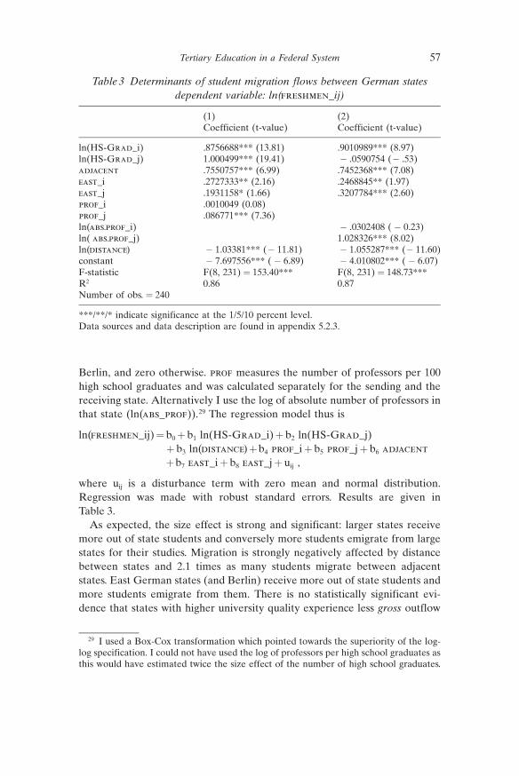
Berlin, and zero otherwise. prof measures the number of professors per 100high school graduates and was calculated separately for the sending and thereceiving state. Alternatively I use the log of absolute number of professors inthat state (ln(abs_prof)).29 The regression model thus is

ln(freshmen_ij)= b0+ b1 ln(HS-Grad_i)+ b2 ln(HS-Grad_j)+ b3 ln(distance)+b4 prof_i+ b5 prof_j+ b6 adjacent+b7 east_i+ b8 east_j+ uij ,

where uij is a disturbance term with zero mean and normal distribution.Regression was made with robust standard errors. Results are given inTable 3.

As expected, the size effect is strong and significant: larger states receivemore out of state students and conversely more students emigrate from largestates for their studies. Migration is strongly negatively affected by distancebetween states and 2.1 times as many students migrate between adjacentstates. East German states (and Berlin) receive more out of state students andmore students emigrate from them. There is no statistically significant evi-dence that states with higher university quality experience less gross outflow

Table 3 Determinants of student migration flows between German statesdependent variable: ln(freshmen_ij)

(1) (2)Coefficient (t-value) Coefficient (t-value)

ln(HS-Grad_i) .8756688*** (13.81) .9010989*** (8.97)ln(HS-Grad_j) 1.000499*** (19.41) � .0590754 (� .53)adjacent .7550757*** (6.99) .7452368*** (7.08)east_i .2727333** (2.16) .2468845** (1.97)east_j .1931158* (1.66) .3207784*** (2.60)prof_i .0010049 (0.08)prof_j .086771*** (7.36)ln(abs_prof_i) � .0302408 ( � 0.23)ln( abs_prof_j) 1.028326*** (8.02)ln(distance) � 1.03381*** (� 11.81) � 1.055287*** (� 11.60)constant � 7.697556*** ( � 6.89) � 4.010802*** ( � 6.07)F-statistic F(8, 231) = 153.40*** F(8, 231) = 148.73***R2 0.86 0.87Number of obs. = 240

***/**/* indicate significance at the 1/5/10 percent level.Data sources and data description are found in appendix 5.2.3.

29 I used a Box-Cox transformation which pointed towards the superiority of the log-log specification. I could not have used the log of professors per high school graduates asthis would have estimated twice the size effect of the number of high school graduates.


of students. However, states with a better ratio of professors per 100 highschool graduates attract out of state students more strongly. That makes netflows strongly respondent to differences in educational quality.30 The secondmodel paints basically the same picture, yet the strong correlation betweenHS-Grad and abs_prof makes an interpretation of the point estimates andsignificance levels of these four variables very difficult (see appendix 5.2.3).Student migration is thus shaped by pull factors rather than push factors: Theresults provide empirical support for my basic hypothesis that universityquality is a strategic variable for the states to attract students and enhancehuman capital endowment.

4 Conclusion

The decentralized provision of free education in a federal system is bound toproduce externalities that give rise to inefficiencies. Because people aremobile within a federation they are free to let one state invest in their humancapital and have another state benefit from the returns to this educationalinvestment. Previous literature has focused on the underprovision of educa-tion because high-skilled labor is mobile: states anticipate that they mayproduce human capital for the benefit of other states (Justman and Thisse1997, Poutvaara and Kanniainen 2000, B�ttner and Schwager 2004, S�dekum2005).

This paper has taken a different perspective: Because mobility occurslargely first at the stage of tertiary education, when prospective students havealready invested significantly in their human capital, states may have anincentive to overprovide tertiary education to attract students, thereby free-riding on the primary and secondary education provided by other states.(They may underprovide primary and secondary education.) Such a strategymakes sense if students are imperfectly mobile after graduating from uni-versity, for example because universities create spillovers for the regionaleconomy and create jobs for high skilled individuals. If this is so, the numberof students influences the human capital endowment of the state.

I have modeled two federal states which produce with immobile labor,internationally mobile capital and interregionally mobile, but internationallyimmobile human capital. The decision to provide educational capacity ispolitical, and it impacts on the market allocation of mobile capital which isattracted by a higher human capital endowment. Mobility of human capitaloccurs at two stages – high school graduates deciding in which state to take up

30 Of course, ideally migration flows and explanatory variables should have been on auniversity level because students go to specific universities rather than to certain states.Unfortunately this data is not available.


their studies and university graduates seeking employment throughout thefederation; it is imperfect at both stages. It turns out that other things beingequal larger states invest relatively less in tertiary education than smallerstates – the latter have a better professor-to-student ratio than the former.This creates a distortion which is due to the strategic interaction states findthemselves in.

The empirical part sought to portray stylized facts of the German situationin tertiary education. First, there is a strong downward trend in the capacity ofuniversities relative to its demand, i.e., the number of high school graduates.This indicates a significant deterioration in the quality of tertiary education.Second, the number of professors per 100 high school graduates differs sig-nificantly across German �L�nder� with city states producing large positiveeffects for their neighboring states. There is a clear East-West gap with thenew �L�nder� providing a lower number of professors per 100 high schoolgraduates. Except for the city states, Bayern, Hessen, Baden-W�rttembergand the Saarland show an above average provision of professors. There aresome indications that this pattern can be explained by differences in budgetconstraints and possibly in political preferences. Third, in their decision tomigrate, students react systematically to differences in relative educationalcapacities.

These inefficiencies obviously call for policy interventions if education is toremain in the authority of the states rather than the center. There are goodreasons to keep education decentralized (and possibly to decentralize evenmore): competition is a revelation procedure for new – better – solutions,serves as a laboratory for better educational policies and (thereby) producesdynamic efficiency gains. Competition enhances educational outcomes, ifexternalities can be adequately internalized. These externalities occur at eachstage of the system at which mobility occurs. One possibility to internalizethese externalities is to privatize the costs of education through user feesthereby eliminating states� incentives to free-ride. This may create other dis-tortions if individuals are credit constrained or risk averse and thus shy awayfrom investing in education. Thus if this solution is ruled out for efficiency ordistributional reasons, a voucher system at the federal level may constitutesuch a solution. Students (and possibly pupils) are given vouchers for theireducation which they can convert into educational services at any institutionwithin the federation. Institutions can redeem them with a central clearinginstitution which is financed at the federal level. Thus, financing and authorityto regulate educational institutions are effectively delinked, thereby ensuringthe advantage of decentralized organization and the efficiency of centralfinancing.

Yet, the current university system may create a third form of externality,which has not been subject of this paper. A state provides external benefits toother states if it exports more educational services in educating and promoting


junior staff that is hired by other states than the educational services that itimports by hiring junior staff or newly appointed professors from out of state.This is the case if junior staff – Ph.D. candidates, assistant professors, orresearch associates seeking a habilitation – are paid more than their marginalvalue product to the university minus the annuity of their educationalinvestment. This issue is left for future research.

5 Appendix

5.1 The determinants of net capital exports

With constant population the steady state condition for capital accumulationrequires that the capital stock owned by a society is constant. In other words,depreciation is exactly replaced by new investment financed out of savings,regardless where the income was generated or the capital installed:s Y ¼ dKS. If the depreciation rate is high, the capital owned by the societywill fall short of the domestically installed capital, KS

1 <K�. As marginalreturns to capital for the domestically owned capital stock exceeds worldreturns (FKðKS

1 ;H;LÞ> rW), the economy attracts foreign capital. This isshown in figure 5.1. Recall that K* is given by the requirement that its mar-ginal rate of return equal the world rate of return, cf. eq. (1).

For low depreciation rates domestically owned capital will exceed domes-tically installed capital. The exported capital earns the world market rate ofreturn; therefore the equilibrium condition is represented by the intersection

Figure 5.1 Steady state capital stock of a small open economy


of the ray from the origin with slope d representing total depreciation and thegraph that depicts total saving which has the slope rw s.

Specifying the production function of the Cobb-Douglass type

Yd ¼ FðK;H;LÞ ¼ KaHbL1�a�b(5.1)

and using eq. (1) I derive the amount of installed capital as

K� ¼ rw

aHb L1�a�b

� � 11�a

:(5.2)

In a closed economy the steady state condition s Y ¼ dKS would read as

d~KS ¼ s ð ~KSÞa Hb L1�a�b

and the steady state capital stock would be

~KS ¼ s

dHb L1�a�b

h i 11�a

:(5.3)

Obviously the closed economy steady state capital stock equals the openeconomy capital stock if it falls short of the domestically installed capital stockK*, but it is smaller if capital is exported as the marginal return to capital is rw

in case of capital export, but lower if the economy is closed. Moreover, if theclosed economy capital stock in the steady state exceeds K* then if thiseconomy is opened it will export capital.

~KS >K� ) KS >K� ^ KS >

~KS

~KS <K� ) KS >K� ^ KS ¼ ~

KS(5.4)

Thus capital export occurs if sa > rw d , where I have made use of eqs. (5.2) –(5.4). Assuming that the world production function is of the same Cobb-Douglass type (but possibly with other parameter values) and noting that

FK ¼ FK

andF~KS

¼ d

sthe small open economy will import capital iff s < sw

d

dw

a

aw

where superscript w indicated world values. For the same technologies thiscondition reduces to ~

KS > K� , s < sw . If the economy�s savings rateexceeds (falls short of) the world savings rate, it will export (import) capital.


5.2 Data Sources

5.2.1 Data for Sections 3.1 – 3.2Data used in section 3.1 and 3.2 were provided by the Federal Office ofStatistics (Statistisches Bundesamt), number of professors and number ofhabilitations by state are based on data in Fachserie 11 Reihe 4.4 and wereprovided as excel files. Data for professors start in 1992 only as the new law onuniversity statistics (Hochschulstatistikgesetz) of 1990 was implementedbeginning 1992. Population was taken online (www.destatis.de); high schoolgraduates by state were provided as files by the Statistisches Bundesamt.31

Professors per 100 high school graduates were averaged over the last fiveyears. Students cross-state migration flows were obtained by the StatistischesBundesamt, Fachserie 11, R 4.1 and refer to the wintersemester 2004/05.

5.2.2 Data and Descriptive Statistics for Section 3.3Budget data for section 3.3 are taken from the following sources: Bundes-ministerium der Finanzen, “Finanzbericht 2005”; K�ln 2004, Bundesministe-rium der Finanzen, “Finanzbericht 2000”; Bonn 1999, and Statistisches Bun-desamt, “Volkswirtschaftliche Gesamtrechnung – Bruttoinlandsprodukt athttp://www.statistik-portal.de/Statistik-Portal/de_jb27_jahrtab65.asp.”

The political index (PI) was based on the political dummy PDi for year iwhich is one if in that year the state prime minister is conservative (or liberal,or from the Schill party) and zero if she or he is socialdemocratic (or green orsocialist) and is aggregated over the last ten years according to followingformula:

PI ¼ P2003i¼1994

PDi ð1:05Þi�2003

An analogous aggregation was made for budget per capita used in theregression. Data for the political index were taken from www.deutschland.deand the pages for the states linked to this page.32

Descriptive statistics and cross correlations are provided below.

31 Earlier data (up to 1992) are also published in Kultusministerkonferenz (http://www.kmk.org/statist, Ver�ffentlichung Sch�ler, Klassen, Lehrer und Absolventen derSchulen 1982 bis 1991, Nr. 121).

32 For instance, http://www.baden-wuerttemberg.de/fm/1899/Regierungen_BW.pdf,http://www.niedersachsen.de/master/C2860930_N1461178_L20_D0_I198.html, http://www.landeshauptarchiv.de/geschichte/kabinette.html. See also Biographisches Hand-buch der deutschen Landesregierungen nach 1945 (2006) M�nchen: K.G. Saur.


5.2.3 Data and Descriptive Statistics for Section 3.4

Data sources are given in appendix 5.2.1. Distance was calculated as thedistance in kilometers between state capitals. Data were compiled by onlinedistance tables and if not available with the help of route planers “Tank &Rast” (http://www.tank.rast.de/services/entfernungstabelle/entfernungen.htm,November 2005) and (http://www.tank.rast.de/services/routenplaner/),respectively. If a state had more than one important metropolitan area, apopulation weighted average of the relevant distances was calculated (cf.fn. 28). In particular, I used for Baden-W�rttemberg, Stuttgart and Karlsruhe,for Bayern, M�nchen and N�rnberg-F�rth-Erlangen, for Hessen, Frankfurt,for Nordrhein-Westfalen, D�sseldorf and K�ln, for Sachsen, Dresden andLeipzig and for all other states the state capital.

Table 5.1 Descriptive statistics for variables used in the regression of Table 2(section 3.3)

Variable; Obs. Mean Std. Dev. Min Max

Professors per 100 highschool graduates

16 10.17341 4.379247 3.610794 20.88965

Budget per capita 16 .0291702 .0101174 .0197562 .0495509Political index 16 3.295331 3.119904 0 7.7217Share of state GDP 16 6.25 6.467188 1.087774 22.07029West-Dummy 16 .65625 .4732424 0 1City state dummy 16 .1875 .4031129 0 1Population 16 5158229 4841514 663129 1.81e + 07

Table 5.2 Cross correlation for variables used in the regression of Table 2(section 3.3)

Profs per 100high schoolgrads

Politicalindex

Share ofstate GDP

West-Dummy

Popula-tion

Budgetpercapita

Profs per 100 highschool grads

1.0000

Political index � 0.0125 1.0000Share of stateGDP

� 0.0092 0.1682 1.0000

West-Dummy 0.5491 � 0.1952 0.4659 1.0000Population � 0.1258 0.1224 0.9851 0.3827 1.0000Budget per capita 0.5392 � 0.0459 � 0.5289 � 0.2654 � 0.5591 1.0000City state dummy 0.8007 � 0.1147 � 0.2671 0.1857 � 0.3310 0.8854


Descriptive statistics are given in Table 5.3 below.

Cross correlations are given in Table 5.4 below.

Table 5.3 Descriptive statistics for the student migration model of section 3.4

Variable Obs Mean Std. Dev. Min Max

freshmen_ij 240 327.525 458.1392 1 2898(HS-Grad_i 240 16153.44 14479.45 2575 57409adjacent 240 .2416667 .428988 0 1east_i 240 .3125 .4644811 0 1prof_i 240 10.17341 4.24905 3.6108 20.8897abs_prof_i 240 1555.245 1406.356 315.8367 4815.697distance 240 409.375 185.5323 33 812


Tab

le5.4

Cross

correlations

forthevariab

lesin

thestud

entmigratio

nmod

elof

section3.4

freshmen

_ij

HS-Grad_

iHS-Grad_j

adjac

ent

east_i

east_j

prof

_ipr

of_j

abs_pro

f_i

abs_p

rof_j

freshmen

_ij

1HS-Grad_

i0.30

411

HS-Grad_j

0.34

35�

0.06

671

adjac

ent

0.65

550.07

350.07

351

east_i

�0.06

05�

0.30

520.02

030.06

041

east_j

�0.14

150.02

03�

0.30

520.06

04�

0.0667

1pr

of_i

�0.16

07�

0.14

380.00

96�

0.14

20�

0.5681

0.03

791

prof

_j�

0.00

070.00

96�

0.14

38�

0.14

200.0379

�0.56

81�

0.06

671

abs_p

rof_i

0.26

840.96

28�

0.06

420.05

22�

0.4368

0.02

910.04

91�

0.00

331

abs_p

rof_j

0.35

03�

0.06

420.96

280.05

220.0291

�0.43

68�

0.00

330.04

91�

0.06

671

distan

ce�

0.40

680.08

240.08

02�

0.55

12�

0.1222

�0.12

220.02

590.02

590.11

460.11

46


References

Berning, E., L. van Harnier, and Y. Hofman (2001), Das Habilitationenwesen an denUniversit�ten in Bayern, Bayrisches Staatsinstitut f�r Hochschulforschung undHochschulplanung: M�nchen.

Bhagwati, J. and K. Hamada (1974), “The Brain-Drain, International Integration ofMarket for Professionals and Unemployment”, Journal of Development Economics, 1,19 – 42.

Burgess, R. and A. Venables (2004), “Toward a Microeconomics of Growth”, WorldBank Policy Research Working Paper 3257, Washington.

B�ttner, T., M. Kraus and J. Rincke (2003), “Hochschulranglisten als Qual-it�tsindikatoren im Wettbewerb der Hochschulen”, Vierteljahreshefte zur Wirt-schaftsforschung, Deutsches Institut f�r Wirtschaftsforschung: Berlin, 72(2), 252 – 270.

B�ttner, T. and R. Schwager (2004), “Regionale Verteilungseffekte der Hochschulfi-nanzierung und ihre Konsequenzen”, 251 – 278, in: W. Franz, H.-J. Ramser and M.Stadler (eds.), Bildung, 33. Wirtschaftswissenschaftliches Seminar Ottobeuren, Mohr-Siebeck: T�bingen.

Chiswick, B. (2000), “Are Migrants Favorably Self-Selected? An Economic Analysis”,61 – 76, in: C. Bretell and J. Hollifield (eds.), Migration Theory, Routledge: London.

Deardorff, A. (1995), “Determinants of Bilateral Trade: Does Gravity Work in a Neo-classical World?”, NBER Working Paper, #5377, Cambridge, MA.

Drazen, A. (2000), Political Economy in Macroeconomics, Princeton University Press:New Jersey.

Frankel, J., E. Stein, and S.-J. Wei (1996), “Regional Trading Arrangements: Natural orSupernatural”, American Economic Review; 86(2), 52 – 56.

Greenwood, M. J. (1997), “Internal Migration in Developed Countries”, 647 – 720, in: M.Rosenzweig and O. Stark (eds.), Handbook of Population and Family Economics,Vol. 1B, Elsevier: Amsterdam.

Grubel, H. and A. Sott (1966), “The International Flow of Human Capital”, AmericanEconomic Review, 56, 268 – 274.

Hartmer, M. (2001), “Professorenbesoldung Einsparungsgesetz (ProfBesEinspG) – Wiedie Bundesregierung die Professorengeh�lter k�rzen will”, Forschung & Lehre 2001,http://www.forschung-und-lehre.de/archiv/07-01/hartmer.html (05-10-11).

Hunt, J. (2000), “Why do People Still Live in East Germany”, NBER Working Paper,#7564, Cambridge, MA.

Justman, M., and J.-F. Thisse (1997), “Implications of the Mobility of Skilled Labor forLocal Public Funding of Higher Education”, Economics Letters, 55, 409 – 412.

Kultusministerkonferenz (2002), “Die Mobilit�t der Studienanf�nger und Studierendenin Deutschland von 1980 bis 2000”, Dokumentation 160, http://www.kmk.org/statist/mobilitaet.html (05-10-11).

Poutvaara, P. (2000), “Education, Mobility of Labour and Tax Competition”, Interna-tional Tax and Public Finance, 7, 699 – 719.

Poutvaara, P., and V. Kanniainen (2000), “Why Invest in Your Neighbor? Social Contracton Educational Investment”, International Tax and Public Finance, 7, 547 – 562.

Stephan, P. (1996), “The Economics of Science”, Journal of Economic Literature, 34,1199 – 1235.

S�dekum, J. (2005), “The Pitfalls of Regional Education Policy”, Finanzarchiv, 61, 327 –352.

Wildasin, D. (2000), “Labor Market Integration, Investment in Risky Human Capital,and Fiscal Competition”, American Economic Review, 90, 73 – 95.


Tertiary Education in a Federal System

Comment by

Stefan Voigt

Schulze�s paper deals with a straightforward question: to what extent dofederal systems of free tertiary education (such as Germany�s) suffer frompositive externalities that give rise to strategic behavior of the states in theprovision of university education? Schulze is definitely not the first to ask thisquestion but he adds an interesting twist to it: previous papers assumed thatstates tried to free ride on the free tertiary education provided elsewhere; inthe aggregate this would lead to an underprovision of university education.Schulze now takes into account that university graduates might have a bias tostay close to where they graduated and that they could produce positiveregional spillovers which might raise GDP regionally. This implies that theremight not be incentives to underprovide tertiary education after all. Indeed,its overprovision is a possibility. But states overproviding tertiary educationmight have an incentive to underprovide both primary and secondary edu-cation.

His model is based on a neoclassical production function and Schulze isinterested in steady states. The model nicely captures that human capitalformation (a consequence of the education budget) does not only increaseGDP directly but also indirectly by attracting physical capital (because thereturn to capital rises initially). Finally, the increase in both physical andhuman capital leads to wage increases (as labor is assumed to be immobile).This means that GNP increases. The Nash-equilibrium in a model with twostates predicts that larger states (in terms of population size) will providemore tertiary education.

The empirical section is interested in identifying differences in the provisionof tertiary education – operationalized as the number of professors per highschool graduate. The provision of professors is endogenized as the next step.The empirical section further deals with the question whether the differencesin the number of professors between the German states are a significantvariable in explaining student mobility. This is implemented by drawing on agravity model. The results show that there is considerable variation in thenumber of professors which can be explained by a dummy for the West (statesin the western part of Germany employing significantly more professors) andthe state�s per capita budget. There is, however, no clear-cut effect of state sizeon the number of professors which means that the theoretically derivedprediction is not confirmed.

The interesting twist in Schulze paper is the possibility that states in afederation might be oversupplying tertiary education while undersupplyingprimary and secondary education. My comment will, hence, focus on thisaspect. Before picking it up, it might, however, be in order to shortly discussthe proxies used in the empirical section.

As a proxy for the provision of tertiary education, Schulze�s uses thenumber of professors employed full time at universities, technical universitiesand pedagogic universities normalized by the number of high school gradu-ates. He thus excludes professors employed at universities of applied sciencesand other more applied organizations. This is one of a number of potentiallypossible quantitative measures. I am not sure, however, whether it is the moststraightforward one. Positive regional spillovers might also be generated bythe more applied universities; their claim to being more applied suggests thatthey aim at such spillovers. Using the number of professors as a proxy impliesthat it is primarily their number that is determining differences in the qualityof tertiary education. A host of other factors might be relevant too: thenumber of assistants, the quality of the library, the laboratories, the computerpools and so forth. I wonder whether simply drawing on a state�s budget fortertiary education would not have been as good a proxy.

Student migration flows across states are conjectured to be influenced bythe number of professors in both the “exporting” as well as the “importing”state. Schulze finds that the number of professors in the importing state ishighly significant whereas the number in the exporting state is insignificant, inother words that there is more of a pull than a push effect. This seems to makeperfect sense, except that students do not seem to choose a state to study inbut rather a university to study at. Schulze is well aware of this problem (seefootnote 30) but it remains a problem. Some German state governments aresaid to consider some universities as their prestige projects whereas othersbarely survive. This will supposedly not be reflected in Schulze�s proxy.

It seems straightforward to assume that student migration flows are at leastpartially determined by differences in the quality of university education. Yet,it would also seem straightforward that students base their decisions onreadily available indicators. It would, hence, be interesting to look at thecorrelation between the Schulze measure and other readily available rankingsthat have been widely publicized and discussed in recent years in Germany.

But let us move to the possibility that tertiary education could be over-provided while primary and secondary education could be underprovided.The paper shows that the professor-per-100-high-school-graduates ratio hasdeteriorated from 11.26 in 1996 to 9.43 in 2004. This is a decline by about onesixth in less than a decade. There certainly does not seem to be any race to thetop with regard to university education in Germany. The recent reform of theGerman payment scheme for professors basically means that salaries weresubstantially reduced. To be a professor has thus become less attractive rel-

Stefan Voigt68

ative to other occupations. It is straightforward to predict that average qualitywill suffer from this reform, another indicator for the absence of a race to thetop.

Schulze might argue that the attempt to free ride on primary and secondaryeducation was the more important part of his argument anyways. Free ridingon others presupposes that high school graduates are highly mobile beforebeginning tertiary education (and substantially less so after having finishedtertiary education). Empirically, we know, however, that around two thirds ofall high school graduates who go on to university remain in the state in whichthey received their high school diplomas. The notion that states could free rideon primary and secondary education implies that basic education could be lowquality whereas university education could be top-notch. Yet, empirically, thecorrelation between states offering high quality basic education and thoseoffering high quality university education seems to be extraordinarily high(e.g. Bavaria, Baden-W�rttemberg). And this seems to make intuitive sensetoo: parents who have graduated from university and stayed in the state wouldsupposedly consider moving out if basic education for their children was nothigh quality too.

In sum, this paper deals with an interesting question and adds a fascinatingnew twist to it. The theoretical model nicely captures the most relevant basicideas. The empirical section presents interesting data – and shows that part ofthe theoretical predictions cannot be confirmed. Yet, there is scope for moredetailed empirics as Schulze terms some of his econometrics “Mickey Mouse”– as the number of observations is very low.


The Productivity of UK Universities

by

Gustavo Cresp i and Aldo Geuna*

1 Introduction

There is increasing recognition in the UK and other OECD countries of theimportance of scientific research in providing the foundations for both inno-vation and competitiveness. This has resulted in increased public funding forresearch in the UK and elsewhere. At the same time, there is a lack of sys-tematic evidence on how such investments can lead to increasing levels ofscientific output and, ultimately, to better economic performance. Much of theavailable literature concentrates on the effects of public funding of basicresearch on either firms� innovative activities (see among others Cohen,Nelson and Walsh 2002; Klevorick et al. 1995; Jaffe 1989; Narin, Hamilton andOlivastro 1997) or firm performance (Adams 1990), bypassing the question ofhow to measure scientific output. The reasons for this are the difficulty ofidentifying a stable causal relationship between the resources spent on thescience budget and �intermediate� scientific outputs. This difficulty originatesfrom the dynamic nature of this relationship. There is a persistent andtherefore recursive feedback between inputs and outputs, which is exacer-bated by lack of appropriate information for analysis. Among the few studiesthat have attempted to address the problem are Adams and Griliches (1996)and Johnes and Johnes (1995). This study is based on and further developsAdams and Griliches�s methodology.

The national science budget comes from several sources. For example, theUK higher education sector received a total of £4,035 millions for researchand development in 2001, financed by the Office of Science and Technology(OST) via the research councils (£942), Higher Education Funding Councils(HEFC) (£1,474), other UK sources such as direct government (£238), highereducation institutions (£166), non-profit organisations (£660) and businessenterprises (£250), and funding from other countries or supranational insti-tutions (£304). These contributions are allocated within the system according

* The authors are grateful to Paul David, David Humphry, Ben Martin, Fabio Mon-tobbio, and Ed Steinmueller, and participants in the Use of Metrics in ResearchAssessment Workshop (Oxford University-Brasenose College, September 2004) andS&T Indicators Conference (Leiden, September 2004), for comments and suggestions.The authors would also like to thank Evidence Ltd for supplying some of the data for theeconometric analysis. This paper is derived from a report commissioned by the Office ofScience and Technology, Department of Trade and Industry. All mistakes, omissions, andviews expressed are the sole responsibility of the authors.

to scientific field and research institution, to provide the resources needed forresearch.

The scientific process produces several research outputs that can be clas-sified into three broadly defined categories: (1) new knowledge; (2) highlyqualified human resources; and (3) new technologies. This paper focuses onthe determinants of the first two types of research output, which are the mostclosely related to the science research budget. There are no direct measures ofnew knowledge, but several proxies have been applied in previous studies. Thetwo that we use in our study, which are also the most commonly used meas-ures are publications and citations. These are incomplete proxies for theproduction of new knowledge and have several shortcomings (Geuna 1999).Highly qualified human resources have been proxied by the total number ofgraduate students that have completed their studies.

In this paper we focus on the determinants of university research output (asmeasured by publications, citations and numbers of graduate students) in theUK. We use an original dataset that includes information for the 52 �old� UKuniversities across 29 scientific fields for a period of 18 years (1984/85 – 2001/02). The paper does not aim to produce exact indicators of the dynamics of thescience system, on the basis of which to draw strong policy conclusions and wefully acknowledge the limitations of the input-output data we use.

The paper is structured as follows. In Section 2 we present the methodologyand the data sources; we depart from the traditional static knowledge pro-duction function model to estimate different dynamic panel data specifica-tions. In Section 3 we present and discuss the results of the estimations. InSection 4 we use the residuals of our fitted knowledge production functions toevaluate the evolution of UK scientific productivity. Finally, in the conclusionwe discuss the limitations of this study and suggest possible further develop-ments.

2 Methodology and data sources

Our methodological approach develops the standard knowledge productionfunction model of Adams and Griliches (1996). They use the expression:

yit ¼ ai þ bWðrÞit þ giXit þ uit; i ¼ 1; ::::::N(1)

where yit is the (log) output of the research �intermediate� output (papers andcitations) by field i and time t. W(r)it is (the log of) a distributed laggedfunction of real past R&D expenditure and Xit is a vector of the controlvariables. The main focus of this analysis is on b, the elasticity of the researchoutput with respect to research input and the measure of local returns to scalein research. Diminishing (constant or increasing) returns predominate whenb< (�1).

Gustavo Crespi and Aldo Geuna72

In order to build a science capital stock we need: the time length over whichthe past investments in university R&D are considered to be relevant for thecurrent research; and a weighting scheme to account for past university R&D.This is where our methodology departs from Adams and Griliches (1996).While they present the results for three and five year distributed lags of R&D,where the weighting pattern is completely ad hoc, we search for a lag struc-ture, and develop a procedure to estimate a flexible and �data driven� lagstructure.

There are two dominant models. First, the Autoregressive Distributed Lag(ADL) model, which assumes a very flexible and unrestricted relationshipbetween (log) R&D inputs and outputs, but at the cost of estimating a largenumber of parameters (see for example, Guellec and van Pottelsberghe 2001and Klette and Johansen 2000). Second, the Polynomial Distributed Lag(PDL) or Almon Model, which specifies the weights as polynomial functionsof a particular estimated degree (Crespi and Geuna 2004). These log linearmodels imply a strong complementarity between the knowledge inputs.1 Inother words, the greater the initial knowledge, the greater will be the amountof knowledge obtained from a given amount of R&D. The more knowledge isproduced, the more it can be recombined to produce new knowledge. For-mally we will assume that:

Kit ¼YJj¼0

rwj

it�j(2)

In this paper we present the results of the PDL Model; we used the ADLmodel in another paper and obtained consistent results. Let us now define thefollowing �finite� distributed lag model:

yit ¼ ai þXqj¼0

bjrit�j þ giXit þ uit; i ¼ 1; ::::::N(3)

Although a model like (3) in theory can be estimated in a straightforwardmanner, there is the potential problem of very long lags in which case themulticollinearity is likely to become quite severe. In such cases it is commonto impose some structure on the lag distribution, reducing the number ofparameters in the model. It is in this context that the PDL model can beuseful. The approach is based on the assumption that the true distribution of

1 By complementarity we mean that marginal productivity of current R&D invest-ment tends to zero if past R&D investment also tends to zero. This assumption is par-ticularly apt in the case of science where we �stand on the shoulders of giants� to buildnew knowledge.

The Productivity of UK Universities 73

the lag coefficients can be very well approximated for by a polynomial of afairly low order:

bj ¼ d0 þ d1jþ d2j2 þ ::::::: þ dpj

p; j ¼ 0; :::::: q > p(4)

The order of the polynomial, p, is usually taken to be quite low, rarelyexceeding 3 or 4. By inserting (4) into (3), one can estimate a transformedmodel where the estimated coefficients are the deltas that can be put backinto (4) in order to recover the original weights. In addition to the p+1parameters of the polynomial, there are two unknowns to be determined: thelength of the lag structure, q, and the degree of the polynomial, p. Here wefollow the non-standard procedure of setting the length of the lags using apriori information and then searching for the degree of the polynomialfunction.

The usual standard procedure is to use the same dataset first to search forthe optimum time lag (using some information criteria) and then, taking thebest lagging as true, to search for the optimum polynomial function. However,this sequential search approach carries the problem that unless the test sta-tistics are overwhelming, the true significance levels in the tests remain to bederived, and the true distribution of the resulting estimator is unknown.Following the evidence in Crespi and Geuna (2004) for a large set of OECDcountries, we set a lag length of 6 years for publications and research students,and 7 years for citations.

Assuming that we know the right lag length we proceed by looking for theright polynomial function. We start by using a fifth degree function andproceed by testing sequential unit reductions in the degree. It is important tonote that in order to retain the appropriate significance level in each step weused a very low individual significance level. The PDL model also implies aset of constraints on the unrestricted model (without a specified functionalform for the lags). For example, if the known lag length is 6 and we use a thirddegree polynomial function, we are implicitly imposing three constraints. Inaddition, we have endpoint constraints, which allow the lag distribution to be�tied down� at its extremes. These endpoint constraints capture the idea thatthere is no effect of R&D on the research outputs before the current periodand also that there is no effect from the research inputs after the maximumlag. That is, we need to impose:

b�1 ¼ 0 and bqþ1 ¼ 0(5)

In total we have five constraints. One way to validate the PDL model is to testwhether these constraints are valid, which can be done by using a simple chi-square test.


Finally, the PDL model also requires exogeneity of R&D. We carried out abivariate Granger causality test. Following Rouvinen (2002), we implementedthe test using a dynamic panel data in differences (DPD-DIF) model, where thefirst differences of the dependent variables are regressed on lags of the firstdifferences of the dependent and independent variables. The findings (notreported here for reasons of space, but available from the authors) would suggestthat there is a two-way causality between R&D, and publications and citations.This may result in a biased estimation of the elasticity coefficients. Given theproblems with available data, and the experimental nature of our work, weacknowledge that our estimations will be biased, and, taking a conservativeapproach, we nevertheless decided to use the PDL model because it allows us touse the level variables and therefore to maintain a high level of information,which is crucial in the case of variables such as ours which are very noisy.

To estimate the model we used the SPRU science field database.2 Thedataset includes information on 52 old universities covering 29 scientific fields,over an 18 year period 1984/85 to 2001/02.3 The 52 old universities consideredprovide a good representation of the scientific research carried out in UKuniversities; in 2001/02 research grant and contract income for these uni-versities accounted for 87% of total UK research grant and contract funding.The dataset has four variables (not including institution and field ids): infor-mation on total research grant and contract income;4 number of publications;number of citations;5 and total number of graduate students.

In the following sections we present the results of the field level estimates ofthe science production function for publications, citations, and graduate stu-dents. Because information about publications and citations is only availableat field level, we cannot estimate a knowledge production function for each ofthe 29 fields. We need to aggregate the micro fields into more broadly definedcategories by mapping the 29 fields into the 4 broad categories in the OECD

2 A detailed description of the procedure used for the development and content of thedatasets can be found in Crespi and Geuna (2004).

3 The 52 old universities do not include the Open University, Cranfield University, theindependent University of Buckingham (not in University Statistical Record statistics) orLancaster University (not in the Higher Education Statistical Agency statistics). Due toproblems with the archiving of the University Statistical Record data, London Universitydata are the sum of all its colleges. Not all the universities are active in every scientificfield, every year.

4 Total research grant and contract income includes all direct research fundingreceived from the research councils, industry, the EC, foundations, etc. Total researchgrant and contract income accounted for 38% of total research income in 1988/89increasing to about 60% in 2000/01 (http://www.ost.gov.uk/setstats/5/t5_1.htm; accessed26/1/2006). We were not able to obtain total research income broken down by scientificfield because this breakdown of HEFC funding by institution and subject area for thewhole period was not available.

5 The source of publication and citation numbers is the Thomson ISI(R) �NationalScience Indicators� (2002) database.


Tab

le1

UK

ResearchOutpu

ts

Yea

rPub

lications

Citations

Gradu

ateStud

ents

NS

ENG

MS

SSNS

ENG

MS

SSNS

ENG

MS

SS

1984

43.3%

13.8%

32.8%

10.1%

44.7%

7.5%

41.1%

6.7%

43.6%

18.8%

9.3%

28.3%

1985

42.1%

13.8%

33.9%

10.2%

42.7%

7.6%

42.4%

7.2%

43.2%

19.5%

9.2%

28.1%

1986

42.2%

14.0%

33.9%

9.9%

42.2%

7.4%

43.2%

7.2%

43.5%

20.1%

8.7%

27.7%

1987

41.7%

14.0%

34.5%

9.8%

41.9%

7.8%

42.9%

7.4%

43.7%

20.5%

9.3%

26.4%

1988

41.3%

14.9%

34.4%

9.3%

41.8%

8.0%

43.2%

7.0%

44.3%

20.3%

8.9%

26.6%

1989

40.6%

14.1%

35.9%

9.4%

40.2%

7.4%

45.2%

7.2%

44.7%

19.3%

8.9%

27.2%

1990

41.1%

14.9%

35.0%

9.1%

41.1%

8.1%

44.2%

6.6%

43.5%

19.0%

9.2%

28.3%

1991

40.6%

15.4%

34.9%

9.1%

41.0%

7.9%

44.6%

6.5%

43.4%

18.8%

9.6%

28.2%

1992

40.5%

16.0%

34.3%

9.1%

40.9%

8.2%

44.6%

6.3%

42.6%

19.1%

9.6%

28.8%

1993

41.1%

15.6%

34.6%

8.7%

41.1%

8.0%

44.7%

6.2%

40.7%

19.0%

10.1%

30.1%

1994

41.0%

16.5%

33.7%

8.8%

40.9%

8.1%

44.6%

6.4%

38.8%

19.1%

10.0%

32.1%

1995

41.2%

16.3%

33.0%

9.5%

42.1%

7.9%

43.9%

6.2%

37.5%

18.8%

10.3%

33.3%

1996

40.8%

16.5%

32.9%

9.8%

41.6%

8.5%

43.2%

6.7%

35.9%

17.9%

12.0%

34.2%

1997

41.2%

15.8%

33.0%

10.0%

41.7%

7.9%

43.8%

6.5%

35.1%

17.4%

12.3%

35.3%

1998

41.1%

16.1%

33.0%

9.9%

42.7%

8.2%

42.6%

6.5%

34.7%

16.9%

13.1%

35.3%

1999

41.1%

16.5%

32.5%

9.8%

42.2%

8.4%

43.0%

6.3%

34.1%

16.9%

13.4%

35.6%

2000

40.6%

16.0%

32.8%

10.6%

42.3%

8.2%

43.4%

6.1%

33.5%

17.3%

13.4%

35.8%

2001

40.9%

16.1%

32.5%

10.5%

43.6%

7.9%

42.6%

5.8%

32.9%

17.7%

13.3%

36.0%

Source:Evide

nce.

NS:

Natural

Sciences;ENG:Eng

inee

ring

;MS:

Med

ical

Sciences,SS

:SocialSciences.


statistics. The four-macro fields analysed were: natural sciences; engineering;medical sciences; and social sciences.

Table 1 summarises the main research outputs used in this section. Acrossthe entire period, there is a remarkable stability in the distribution of researchoutputs by field. Broadly speaking, natural sciences and the medical sciencestogether account for 75% and 85% of total publications and citationsrespectively, in the UK. The remaining percentage is split between engi-neering (15% and 8% respectively) and the social sciences (10% and 6%respectively). The picture changes dramatically when we focus on graduatestudent research output where the importance of the natural sciences declinesto slightly over 30% at the end of the period, while the medical sciencesincreases from 9% to 13%. Taken together, these two macro fields have amuch lower output share (45% at the end of the period). Engineering remainsstable at around 18% for the period, while the social sciences show a sys-tematic growth from 28%, to 36% towards the end of the period.

In order to account for the �truncation problem� in the citations for the mostrecent years, the citations variable was adjusted.6 One way of controlling fortruncation is to use what Hall, Jaffe and Trajtenberg (2001) describe as thefixed effect approach. This involves scaling citations counts by dividing themby the average citation count for a group of publications to which the pub-lication of interest belongs. Thus, a publication that received say 11 citationsand belongs to a group in which the average publication received 10 citations,is equivalent to a publication that received 22 citations, and belongs to a groupwhere the average number of citations is 20. The groups were defined in termsof scientific field and year and the scaling index was computed using the ISIdataset at world level.

On the basis of these data sources we– estimate the science production function for the OECD macro fields

(natural sciences, engineering, the medical sciences, and the social sciences)using information on 29 science fields available for the UK,

– examine the changes in productivity growth across fields.

3 The UK knowledge production function estimates

In this section we present the results of the field level estimates of the scienceproduction function for publications, citations, and graduate students.7 The

6 The citation count is affected by the time span allowed for the papers to be cited: forexample, papers published in 2000 can receive citations in our data only from paperspublished in the period 2000 – 2001; they will be cited by papers in subsequent years, butwe do not observe them.

7 A national level science production function model was statistically rejected infavour of four very broadly defined macro-fields.


four macro fields analysed are: natural sciences, engineering, medical sciences,and social sciences. For each of these macro fields, the aim was to estimate ascience production function as follows:

yFit ¼ aFi þ b

F WðrÞFit þ gFXFit þ uF

it ; i ¼ 1; ::::::N;F ¼ 1; ::: J(6)

where yit is the (log) output of the research �intermediate� output (papers,citations, and graduate students) by scientific micro field i (we have 29 sci-entific micro fields classified into the 4 broad fields listed above) and time t(period 1984 – 2001). W(r)it is (the log of) a distributed lagged function of realpast research grants and contract income by scientific micro fields and Xit is avector of the control variables described below. As explained above, a six-yearlag for publications and graduate students, and a seven-year lag for citationswere applied; then, conditional on them, we tested the shape of the lagfunction using fourth, third and second degree polynomial functions. In allcases we could not reject that the third degree polynomial function was thecorrect one. Also in all cases we tested an unconstrained model and could notreject the constrained model as valid.

The vector Xit refers to a series of control variables included to assess twoimportant phenomena.

– First, we want to control for the way in which time is allocated by theresearchers. One of the most important decisions regarding time for many(but not all) university researchers is how it is allocated between research and(undergraduate) teaching activities. Because we have information about thenumber of undergraduate students by field and year, we can control for theimpact on research output of teaching intensity in the different fields.

– Second, research output can be affected by factors specific to the uni-versity (Geuna 1999). We test for three effects: a) localisation (London baseduniversities); b) research propensity (Russell group universities versus Group94 universities); and c) reputation (when the university was founded).

The control variables are as follows:– Teaching Load: is the ratio of undergraduate students to total staff,

computed by field and year.8

– London: refers to the proportion of research income in each field that isinvested in universities located in London.

8 Information on teaching intensity ratio is only available from 1993. As the estimationsample starts in 1989, we had to reconstruct the �missing� period. The best imputingmechanism was using university level linear interpolation, which respects the hetero-geneity across universities and fields.


– Russell: refers to the proportion of research income in each field that isspent in universities affiliated to the Russell Group (self-selected group ofresearch-led universities).

– Group 94: is the proportion of research income in each field that is spentin universities that belong to the Group 94 (self-selected group of research-leduniversities that are, on average, smaller than the Russell Group, more ori-ented to teaching, and with less prestigious research reputations).

– Medieval Universities: is the proportion of research income in each fieldallocated to universities founded before the 18th century.

– 19th Century Universities: is the proportion of research income in eachfield allocated to universities founded in the 19th century.

– 20th Century Universities: is the proportion of research income in eachfield allocated to universities founded in the first half of the last century.

– Post WWII universities: is the proportion of research income in each fieldspent in universities founded after the Second World War, mostly redbrickuniversities.

The coefficients of these control variables capture, to some extent, the dif-ferences in research productivity of the various institutions. The availableliterature on university research production allows us to hypothesise a neg-ative coefficient for the undergraduate teaching variable: we can expect anegative impact on research production due to the allocation of more time toundergraduate teaching activities. The localisation of universities in theLondon area should create positive externalities for research, which increasesthe productivity of those institutions located in London. We expect a positivevalue for the variable London. With regard to the other control variables noclear a priori expectation can be formulated; to our knowledge this is the firststudy that has attempted to evaluate these effects. A possible hypothesis isthat those universities that are more research-led and more prestigious tend toassign more importance, and therefore more support, to research, whichshould translate into higher research productivity.

We estimate the model for the three research outputs: publications; cita-tions; and number of graduate students.

3.1 Publications

We first show the pattern of weights and then proceed to the results of themodel. As is clear from Figure 1 (see p. 80), a first important result of ourestimation is that the lag structures are significantly different across fields. Thesocial sciences show a relatively important impact in the short run (during thefirst two years) but the effects diminish over time; the situation in the naturaland medical sciences is the reverse, the bulk of the impact being concentrated


towards the end of the lag span. Finally, in the case of engineering we have aclear parabolic function, which suggests a concentration of impact towards themiddle of the time period. These differences in the weighting function arevery important because they point to a differential impact of a given increasein the science budget over time. The research output generated in the socialsciences is much more immediate than in the other sciences, leading to anincrease in the share of socials sciences in total publications in the short run.This situation is reversed over time in favour of the natural and medical sci-ences.

Table 2 presents the results from using the described weighting pattern tocompute the sector knowledge stock and to estimate model (6). The firstinteresting result is that the long run elasticity between knowledge stock andpublications varies widely across broadly defined fields. The highest elasticityis found in the medical sciences (0.46) and the lowest in the natural sciences(0.20). In all four cases elasticities are significant. The year effect, whichcaptures the long run trend in scientific opportunities affecting researchoutput, is always positive. It is important to note that as this model does notinclude a specific variable for spillovers from abroad (an international co-authorship matrix in each science field would be needed) the time trend alsocaptures international spillover effects. The year trend value is highest forengineering, and smallest for the medical sciences.

In terms of the impact distribution of changes in the research budget, thelast two rows of Table 2 show the median lag (the year that accumulated atleast 50% of the impact) and the 90th percentile lag. Consistent with theweight patterns, the most immediate impact is in the social sciences where

Figure 1 Restricted Pattern of Weights (Publications), by fields


90% of the effect is observed after 3 years, compared to the medical scienceswhere it is 5.5 years before 90% of the effect is seen.

We obtained statistically significant and important coefficients for some ofthe control variables. First, the variable capturing teaching load is statisticallysignificant and important for all fields except engineering. The coefficient isalways negative, confirming that large undergraduate teaching loads have adisruptive effect on scientific production. The biggest effect is in the medicalsciences. In this case, an increase of one additional undergraduate student perresearch staff member has the effect of reducing research output by about 5%.Second, and rather surprisingly, a higher allocation of funds to London baseduniversities results in a slightly less productive system in the social sciences.Third, also contrary to expectation, we found some evidence to support theview that a bigger allocation of funds to the Group 94 universities would resultin an overall higher research output in engineering and the medical sciences;

Table 2 UK Levels Estimates, Publications (Method: field fixed effect)

NS ENG MS SS

R&D 0.208 0.216 0.461 0.3400.112* 0.132* 0.145*** 0.086***

Year 0.014 0.036 0.011 0.0330.007* 0.009*** 0.009 0.006***

Undergraduate Teaching � 0.032 � 0.014 � 0.052 � 0.0170.010*** 0.014 0.009*** 0.007**

London 0.001 � 0.012 0.003 � 0.0010.003 0.003 0.004 0.005*

Group94 0.001 0.004 0.003 � 0.0080.004 0.005** 0.003* 0.005

Russell 0.004 � 0.004 0.006 0.0000.003 0.003 0.003 0.005

Medieval 0.002 0.005 � 0.017 0.0130.005 0.004 0.007** 0.004***

19th Century 0.001 0.007 � 0.008 0.0090.004 0.003** 0.004* 0.004**

20th Century 0.008 0.005 � 0.001 0.0180.005 0.007 0.004 0.012

Constant � 21.630 � 67.578 � 19.889 � 64.67712.254* 15.157*** 16.129 11.184***

Observations 108 84 72 84R-squared 0.83 0.78 0.88 0.86Chi(2) 2.97 7.10 7.75 7.44P > Chi(2) 0.71 0.21 0.17 0.1950% Quartile Lag (years) 3.8 2.1 4.0 1.190% Quartile Lag (years) 5.5 4.6 5.6 3.1

Robust standard errors reported below each coefficient. Within R-squared reported.(*) significant at 10%; (**) significant at 5%; (***) significant at 1%


no significant effect was identified for the Russell Group universities.9 Fourth,a larger share of funds to the Medieval universities was shown to result in amore productive system in the social sciences, but has a negative impact onthe medical sciences. A larger share of funds to the 19th Century universitieshad a positive effect on engineering and the social sciences research output,and a negative impact on the medical sciences. The comparator groups foruniversity history is the group of universities founded after WWII. Finally, thetests for validity of the constraints were never rejected.

3.2 Citations

Citation output was analysed following the procedure used for publications.Figure 2 shows the pattern of weights for the different disciplines. The resultsappear similar to those for publications. The citation output tends to respondmore quickly to an increase in R&D investment in the social sciences than theother scientific fields. The medical sciences shows its largest research impactonly at the end of the time period, while the polarisation is less strong for thenatural sciences and engineering. The main difference from the publicationlag structure results is the very similar pattern for engineering and the naturalsciences: engineering has a less symmetric profile and behaves much more likethe natural sciences.

Table 3 (see p. 84) presents the results for the estimation of model (5) in thecase of citations output. In terms of long run science budget elasticity theresults are very similar to the results for publications. The highest elasticity isfound in the medical sciences (0.61), while the lowest is in engineering (0.15),which is non-significant. The time trend variable is always positive and sig-nificant in three of the fields, once again pointing to an increase in scientificopportunities and the existence of international spillovers. Regarding theimpact distribution of changes in the research budget, the earliest impact is inthe social sciences where 90% of the effect is observed after about 4 years,while in the medical sciences 90% of the effect is achieved only after 6 years.

Regarding the remaining control variables, the results tend to be consistentwith those for publications, with the exception of the control variable for theRussell Group universities: a larger allocation to Group 94 universities doesnot have a positive effect on the system output, while a higher share of fundsto Russell Group universities has a positive impact on citations in the medicalsciences, but a negative impact in engineering. The teaching variable is again

9 The higher output could be due to two phenomena: higher productivity of the Group94 universities, or the competition effect from the other universities which received lessfunds. University level micro data would be needed to disentangle these two effects. Thisreasoning applies to the other resource allocation control variables.


negative, with the highest absolute value in the medical sciences. A biggerallocation to London based universities does not provide any positiveadvantage. Larger proportions of direct funding to Medieval universitiesresult in a higher citations output in the social sciences and lower returns inthe medical sciences, similar to the 19th Century universities, with the adjunct

Figure 2 Restricted Pattern of Weights (Citations), by fields

Figure 3 Restricted Pattern of Weights (Graduate Students), by fields


of a positive impact for engineering. Finally, as before, the constraints impliedby the model were not rejected.

3.3 Graduate students

The third science output we examined at the field level for the UK is the�production� of graduate students. Figure 3 (see p. 83) shows the lag structure.The most interesting result of this analysis is that the patterns appear quitedifferent from the patterns for publications and citations. This result might bebecause graduate students are a research output of a completely differentnature to publications and citations. In the case of graduate students, themedical sciences, engineering and the natural sciences show the strongestimpact quite quickly (in the first three years), while the impact in the social

Table 3 UK Levels Estimates, Citations (Method: field fixed effect)

NS ENG MS SS

R&D 0.212 0.146 0.617 0.3530.123* 0.196 0.160*** 0.095***

Year 0.014 0.037 0.005 0.0320.008* 0.009*** 0.011 0.007***

Undergraduate Teaching � 0.031 � 0.018 � 0.059 � 0.0160.010*** 0.014 0.012*** 0.007**

London 0.001 � 0.011 0.007 � 0.0080.003 0.003 0.003 0.005

Group94 0.001 0.004 0.003 0.0010.004 0.003 0.003 0.005

Russell 0.004 � 0.004 0.004 0.0000.003 0.005** 0.004* 0.005

Medieval 0.002 0.005 � 0.018 0.0130.005 0.005 0.007*** 0.005***

19th Century 0.001 0.006 � 0.008 0.0090.004 0.003** 0.004* 0.004**

20th Century 0.008 0.004 0.002 0.0180.005 0.007 0.006 0.012

Constant � 22.493 � 67.690 � 10.691 � 63.94312.946* 16.240*** 18.718 12.118***

Observations 108 84 66 84R-squared 0.68 0.77 0.84 0.67Chi(2) 1.398 2.760 8.635 7.160P > Chi(2) 0.966 0.838 0.195 0.30650% Quartile Lag (years) 4.4 3.3 4.3 1.690% Quartile Lag (years) 5.5 5.3 6.0 3.9



sciences does not become evident until towards the end of the time frame. Wedo not have a definitive explanation for this result, but we incline to the viewthat the combination of a different mix of graduate courses (MSc, Mphil andPhD) across the different fields might be generating these sorts of differentialimpacts.

Table 4 (see p. 86) shows the results of estimating model (6) using field fixedeffects. The largest elasticities regarding this type of research output are foundin the natural and the medical sciences with values of 0.54 and 0.65 respec-tively. The corresponding elasticities for the social sciences (0.21) and engi-neering (0.11 and non-significant) are much lower. The time trend had apositive coefficient in all fields except the natural sciences. This points to anincrease in productivity in the social and the medical sciences and engineeringregarding the �production� of graduate students. In terms of the impact dis-tribution of changes in the research budget, the most immediate impact is inengineering, where 90% of the effect is observed after about 3 years, while themost delayed impact is in the social sciences where it takes 5.3 years for 90%of the effect to be felt.

Regarding the remaining control variables there are some interestingresults. First, the undergraduate teaching variable is negative in the naturalsciences, the medical sciences and engineering, pointing to the fact that inthese fields an increase in the undergraduate teaching load negatively affectsthe time allocated to supervising and guiding graduate students. In contrast, inthe social sciences we have a positive impact from undergraduate teachingtowards graduate teaching, pointing to an apparently different nature ofgraduate studies in this field, a possibility that requires much more analysis forit to be confirmed. Second, as before, there was no evidence of a positivelocalisation effect for a higher allocation of grants and contracts to Londonbased universities. Third, a bigger allocation of funds to the universitiesbelonging to the Group 94 had a positive premium in engineering, while forthose in the Russell Group the biggest premium was in the social sciences.Fourth, in terms of age, a higher share of funds to the Medieval universitieshas a positive effect in the social and the medical sciences, while more fundingto the 19th Century universities induces an increase in the university systemoutput in the medical sciences, but a decrease in the natural sciences. This lastresult also applies to the 20th Century universities, which also showed a pos-itive premium in the social sciences. The comparator group, as in the previoustwo estimations, was the category of the Post WWII universities. Finally, asbefore, in all the models the constraints were not rejected.

Field level estimates provide us with an interesting set of results. Most ofthese are novel to the literature on the economics of science and, thus, shouldbe seen as preliminary and exploratory, to be confirmed by further analyses.First, in the case of the medical science, the social sciences, and the naturalsciences we can identify positive and significant returns for publications,


citations, and graduate students from investment in higher education R&D.Although positive, the effect for engineering is only significant in the case ofpublications, pointing to the fact that the research output from this scientificfield is better captured by measures other than citations and research students.Second, the four scientific fields tend to have different lag structures. This isparticularly noticeable in the case of the social sciences. While investment inR&D in the social sciences affects publications and citations more immedi-ately than in the other three fields, in the case of gradate students most of thereturns to research grant and contract funding are concentrated at the end ofthe period. Third, we found strong evidence that a high undergraduateteaching load negatively affects the research outputs of UK universities. Onlyin the case of graduate students in the social sciences did we find a positiveeffect. Fourth, we constructed a set of control variables to assess the impor-tance of allocation of grants and contracts to different subgroups of uni-

Table 4 UK Levels Estimates, Graduate Students (Method: field fixed effect)

NS ENG MS SS

R&D 0.542 0.107 0.656 0.2140.200*** 0.173 0.158*** 0.091**

year � 0.024 0.027 0.044 0.0640.011** 0.009*** 0.011*** 0.007***

Undergraduate Teaching � 0.062 � 0.044 � 0.024 0.0150.015*** 0.020** 0.010** 0.006***

London 0.002 0.009 � 0.01 � 0.0050.004 0.004 0.004 0.003

Group94 0.003 0.003 0.005 � 0.0050.006 0.005* 0.006 0.002

Russell 0.005 � 0.003 � 0.009 0.0030.004 0.005 0.006 0.002*

Medieval � 0.015 0.004 0.028 0.0060.009 0.005 0.014* 0.004*

19th Century � 0.014 � 0.005 0.017 0.0030.007** 0.004 0.008** 0.004

20th Century � 0.014 0.008 0.002 0.0150.008* 0.007 0.003 0.007**

Constant 47.113 � 48.338 � 93.097 � 124.0818.987** 16.708*** 19.154*** 13.174***

Observations 99 77 66 77R � squared 0.70 0.65 0.87 0.92Chi(2) 3.005 0.635 10.952 9.803P > Chi(2) 0.699 0.986 0.052 0.08150% Quartile Lag (years) 1.3 0.8 1.1 3.890% Quartile Lag (years) 3.5 2.8 3.1 5.3



versities (university specific effects). Some of these were significant andimportant, pointing to the fact that different allocations of funds to uni-versities result in higher or lower university system scientific production. Thehigher or lower output may be due to higher productivity in the institutionsthat received more grants and contracts or a competition effect from theuniversities that received less funds. Micro data at the level of the universitywould be needed to identify which of the two effects is dominant.

4 The UK knowledge productivity analysis

This section focuses on the efficiency with which the domestic stock ofknowledge (science budget and other grants and contracts) is applied in orderto generate the different research outputs. Has this efficiency grown over timeor has it declined across disciplines? Building on the results in section 3 wecomputed field specific total factor productivities (TFPs). These TFPs capturethe evolution of the scientific opportunities in each field, and also the effectsof changes in organisational practices, resources allocation, and management.

For each macro field we computed the residual of the knowledge pro-duction function (6) as:

tfpFit ¼ yFit � b

F WðrÞFit ; i ¼ 1; ::::::N; F ¼ 1; ::: J(6)

where tfpit is the knowledge production function (semi) residual after con-trolling for changes inW(r)it, the distributed lagged function of real past R&Dexpenditures. In order to compute (6) we first need an estimation of theelasticity coefficients by field (the bs). We use the field level results shown inTables 2 (see p. 81) to 4. Given the lags used in the construction of W(r)it wecan only focus on productivity evolution during the 1990s.

Figures 4 (see p. 86), 5 and 6 (see p. 90/ 91) show the evolution of the TFPindex by field over time for each of the research outputs. Two clear patternsemerge. In all macro fields and research outputs there is an upward trend inthe productivity indices, suggesting that there is a clear improvement in theefficiency and technological opportunities of the system. In all four majorscientific fields and for the three traditional outputs of scientific research, theproductivity of UK science has increased along the 1990s. However, from themid 1990s, in all the macro fields, there has been a marked slowdown inproductivity growth rates as highlighted by the less steep slopes of the pro-ductivity indices at the right of the figures.

Across the whole period the TFP growth rate in the case of publications hasfluctuated between 1.2% and 2.4%, with the lowest value in the natural sci-ences and the highest in the social sciences. Taking the cut-off point of 1996(chosen to coincide with the 1996 RAE), the average TFP growth rates during


the first half of the 1990s was compared to the same indicator for the 1990s to2001. The data show a remarkable slowdown in productivity, TFP productivitygrowth rates declined by more than 50% in the natural sciences, engineering(the largest decrease) and the social sciences, but by �only� 22% in the medicalsciences. Numbers of citations show a similar profile. The highest growth rateis in engineering (2.4%) and the lowest in the medical sciences (0.8%). Thereis also a clear slowdown in productivity growth rates, but the degree of thedecline is even greater than in publications. Finally, the results for graduatestudents are similar to those for citations with the exception that the highestgrowth rate occurs in the medical sciences. The slowdown in the second half ofthe 1990s is also remarkable: in engineering and the natural sciences TFPgrowth rates halved, while in the social and the medical sciences TFP growthrates are 60% of their value in the previous period.

It is important to note that the productivity slowdown is not an artefact ofthe increased spending in UK science. The real increase in science andengineering R&D spending in the UK started in 2000 – 01. In our model theimpact on research outputs of an increase of about 7% in 2000 – 01 is spreadacross the succeeding six to seven years; the weight for the first year is small inthe case of publications and citations (lower than 10% for all except the socialsciences) and about 25% in the case of graduate students (again excepting thesocial sciences for which it is near zero). A significant increase in R&Dspending in a particular year can negatively affect the overall productivity ofthe system in that year if a simple productivity measure based on the ratio

Figure 4 TFP Publications


between that year�s inputs and outputs is considered. Our measure of pro-ductivity refers to changes in research output that are not explained bychanges in the stock of scientific knowledge as proxied by current and pastR&D spending. Our estimation of stock of knowledge already controls for the

Figure 5 TFP Citations

Figure 6 TFP Graduate Students


fact that there are some adjustment lags and that a given increase, forexample, in the science budget, is not going to have an immediate impact onresearch outputs. In the case of a traditional productivity measure, such as theratio between papers and HERD, the UK has witnessed a very clear decline inthe 1990s due to the significant increase in the science budget and not to adeterioration in the performance of the system (Evidence 2003). Our measureof productivity controls to some extent for this and tries to capture organ-isational or managerial changes in the system.

The TFP estimations above take account only of the spending on researchgrants and contracts. We now introduce the other control variables to seewhether they explain the productivity slowdown. There are several different,and overlapping, explanations. One is that in the period 1996 – 2001 the dis-tribution of higher education funding led to the system being less productivewithin each scientific field (B and C estimations). Another is that increasedenrolment rates at undergraduate level were not compensated for by anequivalent increase in staff, leading to a reduction in available research time(D estimation). To investigate these two possibilities we re-estimated the TFPindices controlling for how resources are allocated across types of institutionsand for teaching intensity ratio. The results for publications are presented inTables 5 and 6.

Two trends emerge from Tables 5 and 6. First, at field level the process ofresource allocation has no serious impact on productivity growth becausecontrolling (or not) for how resources are distributed across university typesand geographical location (columns B and C compared to column A) onlymarginally affects average productivity growth. The exception is the socialsciences where the distribution of higher education funding in the first periodcompared to the distribution in the second period, which led to the systembeing less productive, reduces the unexplained productivity slowdown (forexample, in column A the difference between the two time periods is 1.6; incolumn C the difference is 1.2).

Table 5 TFP growth rate decompositions for the natural sciences andengineering

Time Natural sciences Engineering

A B C D TOTAL A B C D TOTAL

91 – 96 1.5 1.4 1.4 1.2 1.1 3.0 2.8 3.1 2.8 2.796 – 01 0.7 0.8 0.7 0.6 0.6 1.3 1.2 1.4 1.2 1.3Total 1.1 1.1 1.1 1.0 0.9 2.2 2.1 2.3 2.1 2.1

Note: A controls only for R&D spending; B is A plus controlling for resources allocationby London, Group 94 and Russell Group; C is A plus controlling for University Age; D isA plus controlling for teaching intensity; and Total is A plus (B + C + D).


The results controlling for teaching intensity are similar and, again, arerelatively invariant. The exception is the medical sciences where, after con-trolling for teaching intensity, productivity growth rates reduce from 1.7% to1.2% (row total) and the two sub-periods show no productivity slowdown.Interestingly, after controlling for teaching intensity TFP in the first perioddrops to 1.3, pointing to the fact that the reduction in teaching intensity in thisdiscipline actually contributed to the higher productivity during the first timeperiod.10 For the other research outputs the conclusions are similar to thosefor publications.

Controlling for research allocation and teaching intensity partially explainsthe productivity slowdown in the medical sciences (especially in the case ofpublications), but does not account for the productivity slowdown in thesecond half of the 1990s for the other scientific fields.

There are four possible reasons for this unexplained slowdown. First, theremight have been a deterioration in the organisational efficiency of productionof traditional science outputs within each field (and even within departments)due, for example, to the creation of incentives for the development of thirdstream type activities. Second, there might have been a reduction in humancapital (the quality of labour), i.e., in the research staff. Underlying thishypothesis is the possibility that the lag in the relative compensations paid toresearchers in the universities could have led to some high skilled staff leavingacademia (for positions overseas or for jobs in industry), being replaced by anequivalent number of lower quality personnel. Third, due to the increase inother countries� publishing in English, UK researchers are facing increased

Table 6 TFP growth rate decompositions for the medical and social sciences

Time Medical sciences Social sciences

A B C D TOTAL A B C D TOTAL

91 – 96 2.0 2.0 1.9 1.3 1.2 3.2 3.2 2.7 3.2 2.896 – 01 1.4 1.3 1.3 1.4 1.2 1.6 1.8 1.5 1.7 1.8Total 1.7 1.7 1.6 1.3 1.2 2.4 2.6 2.1 2.5 2.3

Note: A controls only for R&D spending; B is A plus controlling for resources allocationby London, Group 94 and Russell Group; C is A plus controlling for University Age; D isA plus controlling for teaching intensity; and Total is A plus (B + C + D).

10 Student to staff ratios in the medical sciences decreased from 8.4 to 7.4 students perstaff across the whole period. A more detailed inspection shows that any decrease wasmostly during the first sub-period. The ratio of students to staff in 1991 – 95 declinedannually from 8.4 in 1991 to 6.9 in 1995. This variable was more volatile in the secondsub-period oscillating between 6.9 and 7.3.


competition for publication in ISI journals, raising the bar to getting published(a quality effect).11

All of these are pessimistic explanations for the productivity growth slow-down. There is a fourth possibility, which is more optimistic, which is that theRAE has an impact. We can think of the RAE as a sort of institutional shockin the research incentive system for academic units. That is, the introduction ofthe RAE at the end of the 1980s/beginning of the 1990s produced a positiveshock, which induced a productivity increase on the part of UK scientists. Ifthis shock were affecting productivity levels rather than growth rates, after atransition period the system would return to its average growth rate. In otherwords, the effect of the RAE may have been more dramatic in the early 1990s,but subsequently declined. This could explain the productivity slowdown inthe second sub-period considered in our analysis.

It is very difficult to identify which of these potential explanations is themost relevant. Alternative models based on micro data at the university andunit of assessment levels could help to clarify the current dynamics of the UKscience system.

5 Conclusions

This paper has analysed the determinants of the three most common uni-versity research outputs: publications (as a proxy for the production of codi-fied research knowledge); citations (as an impact adjusted proxy for codifiedresearch production); and Masters and PhDs awarded (as a proxy for theproduction of tacit knowledge accumulated in human capital) for the UKcase.

The analysis of the UK science system as represented by the old universities(which account for about 90% of R&D expenditure) points to the existence ofdifferent science production functions. We rejected the model of a globalscience production function for the UK in favour of four very broadly definedmacro-fields: the medical sciences, the social sciences, the natural sciences andengineering. In each of these fields either the weight patterns or the R&Delasticities (and also some of the coefficients of control variables) were sig-nificantly different.

For publications and citations we estimated significantly different lagstructures, with a long lag for the medical sciences before full returns from anincrease in R&D spending were achieved, but the social sciences seeingresults in the first few years. This means that the science system does not

11 There is some evidence of this phenomenon in the discussion in theNew York Times(May 3, 2004) about the loss of dominance of the US in the sciences to non-Englishspeaking countries.


respond uniformly to changes in funds. For example, an increase in the overallscience budget will have a rather sequential impact: first, the changes will befelt mainly in the social sciences, then in engineering and the natural sciencesand finally, in the medical sciences. For graduate student research output theresults are different, with the short term impact being concentrated in engi-neering and the long term impact in the social sciences.

In the case of the medical sciences, the social sciences and the natural sci-ences we identified positive and significant returns for publications, citationsand graduate students from investment in higher education R&D. Althoughpositive the effect in engineering is only significant in the case of publications,pointing to the fact that the research output of this scientific field is bettercaptured by other measures than citations and research students.

We included in the models a set of control variables. We found strongevidence that a large undergraduate teaching load negatively affects theresearch outputs in UK universities. Only in the case of graduate students inthe social sciences did we see a positive effect. Overall, the higher the teachingload the lower the research productivity. This result denies the validity of thepolicy model followed in the 1980s and 1990s, which assumed that the numberof students per lecturer could be increased without a decrease in the overallquality of the HE system.

We also controlled for the impact of different allocations of funding acrosstypes of institutions; the results are mixed and vary according to the differentresearch outputs. Some were significant pointing to the fact that differentallocations of funds to universities result in higher or lower university systemscientific production. Due to the limitations of field level data, the results onuniversity specific factors, though interesting, should be considered as pre-liminary: they require validation through analyses based on micro data.

Finally, we developed an analysis of the productivity of UK science and thechanges in it during the 1990s. UK TFP has grown across the whole period.This result contrasts with the most standard publication per HERD measureof productivity, which presents a remarkable drop in British productivity,mainly due to a combination of increased budget and publication lags.However, we also identified a clear slowdown in TFP growth in the secondhalf of the 1990s compared to the first. This decline is not due to an increase inthe research spending in the later period, nor to the way that resources wereallocated across institutions (although this did have some effect in the medicalsciences and the social sciences), nor to an increase in teaching loads (whichwere fairly static in the second half of the 1990s). We speculate that thisslowdown in productivity is due to mainly unobserved systemic effects (apolicy shock during the first half of the 1990s such as the RAE) or very microfactors related to the (relative) reduction in researchers� rewards, the intro-duction of more transferable research or a �brain drain� of high skilledresearchers. This slowdown can also be ascribed to increased competition for


publication in ISI journals from overseas research. Without more micro data itis not possible to tease out from these alternative explanations their relativeimportance. These results are consistent with the results of internationalanalysis, which point to a decrease in the relative productivity of UK science.Indeed, it is possible to envisage that, during the 1990s, UK science showedpositive productivity growth, but that this growth was less marked than inother countries, especially in the second half of the 1990s.

This paper aimed to test the feasibility of using econometric models toproduce results that could contribute to the development of science policy, theaim being not to produce exact indicators of the dynamics of the sciencesystem, on the basis of which to draw strong policy conclusions. Rather, theinherent shortcomings in the measurement of the output (and ultimately ofthe outcomes) of the scientific activity, and the limitations on the availableinput data call for extreme caution in the interpretations of our results. Theconclusions presented above should be taken as a first and preliminaryattempt to develop a better understanding of the relationship between theallocation of resources and scientific research output.

References

Adams, J., and Z. Griliches (1996), “Research Productivity in a System of Universities”,NBER Working Paper Series, 5833.

Adams, J. (1990), “Fundamental Stocks of Knowledge and Productivity Growth”,Journal of Political Economy, 98, 673 – 702.

Crespi, G. and A. Geuna. (2004), The Productivity of Science. Brighton: SPRU Reportprepared for the Office of Science and Technology (OST), Department of Trade andIndustry (DTI), UK. http://www.sussex.ac.uk/spru/publications/reports/CrespiOST.pdf

Cohen, W., R. Nelson and J. Walsh (2002), “Links and Impacts: The Influence of PublicResearch on Industrial R&D”, Management Science, 48, 1 – 23.

Evidence (2003), PSA Target Metric for the UK Research Base, London: DTI-OST.Geuna, A. (1999), The Economics of Knowledge Production: Funding and the Structure

of University Research, Cheltenham: Edward Elgar.Griliches, Z. (1980), “Returns to Research and Development Expenditures in the Private

Sector”, in: W. Kendrick, and B. Vaccara (ed.), New Developments in ProductivityMeasurement and Analysis, Chicago: University of Chicago Press.

Guellec, D. and B. Van Pottelsberghe (2001), “R&D and Productivity Growth: PanelAnalysis of 16 OECD Countries”, OECD Economic Studies, 33, 103 – 126.

Hall, B., A. Jaffe and M. Trajtenberg (2001), “The NBER Patent Citations Data File:Lessons, Insights and Methodological Tools”, NBER Working Paper Series, 8498.

Jaffe, A. (1989), “Real Effects of Academic Research”, The American Economic Review,79, 957 – 970.

Johnes, J. and G. Johnes (1995), “Research Funding and Performance in the UK Uni-versity Departments of Economics: A Frontier Analysis”, Economics of EducationReview, 14, 301 – 314.

Johnes, G. (1996), “Multi-Product Cost Functions and the Funding of Tuition in the UKUniversities”, Applied Economics Letters 3, 557 – 561.


Klette, T., and F. Johansen (2000), “Accumulation of R&D Capital and Dynamic FirmPerformance: a Not-so-Fixed Effect Model” 367 – 397, in: D. Encaoua, B. Hall, F.Lisney and J. Mairesse (eds.), The Economics and Econometrics of Innovation, Bos-ton/Dordrecht/London: Kluwer Academic Publishers.

Klevorick, A., R. Levin, R. Nelson and S. Winter (1995), On the Sources and the Sig-nificance of Inter-industry Differences in Technological Opportunities”, ResearchPolicy, 26, 185 – 205.

Narin, F., K. Hamilton and D. Olivastro (1997), “The Increasing Linkage between USTechnology and Public Science”, Research Policy, 26, 317 – 330.

Rouvinen, P. (2002), “R&D-Productivity Dynamics: Causality, Lags, and Dry Holes”,Journal of Applied Economics, 5, 123 – 156.


The Productivity of UK Universities

Comment by

Chri st i an P i erdzioch

In an integrating world economy, scientific research leading to the inventionof new products and the development of unconventional ideas forms the basisof the international competitiveness of firms, industries, and entire economies.It is for this reason that it has often been emphasized in academic researchand in policy circles that developing a deeper understanding of the factors thataffect the quantity and quality of research output is of key importance for theprosperity and international competitiveness of economies. One factor thatmay affect research output is the availability of financial funds. But howexactly does the availability of financial funds affect research output? How tomeasure research output? Are the effects of the availability of financial fundson research output different across disciplines? Does the availability offinancial funds affect research output immediately or only with a time lag?These are all important questions, and finding answers to these questions is adifficult task. Gustavo Crespi and Aldo Geuna have used a novel database onthe productivity of scientific research at UK universities to empirically tacklethis task. Their empirical analysis is highly welcome because it yields inter-esting insights into the factors that affect research output, and because it hasbeen competently and thoroughly done.

In order to conduct their empirical analysis, Crespi and Geuna have col-lected data on the productivity of scientific research at 52 UK universities.Their data cover the period 1984 – 2002. They present results for four majorfields of science: engineering, the natural sciences, the medical sciences, andthe social sciences. They have used the number of publications, the number ofcitations, and the number of graduate students to measure research output. Intheir empirical analysis, they have used a production function to link theirmeasures of research output to expenditure on research and development(R&D). In order to capture potential time lags between expenditure on R&Dand research output, Crespi and Geuna have estimated a polynomial dis-tributed lag model. They have estimated this model using techniques availablefor estimating panel data models. Their model contains a number of controlvariables, including a measure of the undergraduate teaching load andmeasures of the localization and reputation of a university.

Crespi and Geuna present a number of interesting arguments and results,and every single argument and result deserves to be discussed in detail. In thefollowing, I shall focus on potential problems that may arise in the meas-urement of research output, the specification of the production function, andthe interpretation of the empirical results.

As concerns the measurement of research output, one problem is thatcounting the numbers of publications is maybe a good indicator of thequantity of research output, but not necessarily of the quality of researchoutput. For example, not all academic journals are highly ranked “top”journals, and getting a paper published in an international “top” journal ismuch more difficult than getting it published in a national journal or a highlyspecialized field journal. For this reason, the scientific community hasdeveloped sophisticated ranking schemes in order to capture the importanceand the impact of academic journals. In consequence, it would be interestingto analyze how the results Gustavo Crespi and Aldo Geuna report wouldchange when rankings of journals were used to weigh publications. Rankingsof journals may also be useful as a weighting scheme for citations because itcould make a difference whether a research paper is mainly cited, forexample, in a specialized field journal or a general interest journal.

As concerns the specification of the production function, it would beinteresting to learn more about potential problems caused by omitted varia-bles and the potential influence of control variables different from those usedby Crespi and Geuna. As concerns potential problems caused by omittedvariables, it could be the case that the positive link between research outputand expenditure on R&D reported in the paper is at least in part due to theinfluence of a third variable not yet included in the empirical model. One suchvariable could be a measure of the stance of the business cycle. For example,in a business cycle boom, tax revenues and, because of a stock market boom,the budgets of private foundations increase. This may lead to an increase inexpenditure on R&D. At the same time, expenditure on R&D by firms islikely to increase, firms may hire researchers, and the salaries paid by firmsmay also increase. This could strengthen the competition between firms anduniversities for researchers, resulting in an increase in research output.

As concerns control variables, it would be interesting to include, forexample, the number of researchers per field, the number of research semi-nars and scientific conferences that took place at a university, and the numberof visiting researchers as control variables in the production function. Thesevariables may give a good account of the reputation of a university. Moreover,these variables may proxy the quality of the research environment at a uni-versity. Of course, collecting data on these variables could turn out to be verydifficult. Given that path dependencies may play an important role for thereputation of a university and the quality of the research environment, it couldbe interesting to use lagged research output as a control variable in the pro-duction function.

As regards the specification of the production function, it would also beinteresting to learn more about the interpretation and the statistical propertiesof the explanatory variables. For example, the authors have included a timetrend in the vector of explanatory variables, and they argue that the time trend

Christian Pierdzioch98

captures spillovers from abroad. It would be interesting to learn more aboutthese spillovers from abroad. Do they represent the international exchange ofideas? Or do they represent the importance of forming international researchteams? One could also ask whether the time trend reflects spillovers fromabroad or rather captures structural breaks or stochastic trends in the data.

As concerns the interpretation of their empirical results, the authors mainlyfocus on the slowdown in productivity of research at UK universities that tookplace at the end of the 1990s. This certainly is an important result thatdeserves a comprehensive and thoughtful analysis. The authors, however,report many more interesting results, and it would be interesting to learn moreabout how these results can be interpreted. For example, Crespi and Geunareport that, regarding the number of publications, the effects of expenditureon R&D are very different across disciplines. Natural questions that arise asregards this result are: Why are there differences across disciplines? Why is itimportant to learn more about differences across disciplines? Are there anypolicy implications? Should we spend more or less money on R&D at uni-versities? Is the allocation of expenditure on R&D across disciplines optimal?It is impossible to answer all these questions in one paper. However, I suggestthat the paper could benefit from considering one or the other of thesequestions.

To sum up, Crespi and Geuna have done very interesting research, and theyhave undertaken their empirical research with care. Their paper is conciselywritten, and I have learnt a lot from reading it. I believe that their paper willstimulate future research.


Evaluation of Researchers:A Life Cycle Analysis of German Academic Economists

by

Michael Rauber and He inr ich W. Ursprung*

1 Introduction

Evaluations compare certain features of a person with the features observedin a group of peers. A worthwhile evaluation needs to explicitly define therelevant comparison group and to make a case for the employed choice. Inmany cases, the contemporaries of the person to be evaluated represent therelevant peer group, the best example being the standard IQ test whose nameeven refers to the fact that intelligence is measured in relation to somedenominator, which is, of course, the respective person�s age. In sports, whereevaluation almost represents the raison d�etre, it is also quite common tocompare contestants of the same age group, but other comparison groups,based, for example, on body weight or professional status, are also widelyemployed.

Research evaluations that are based on scientometric methods are stillsurrounded by a touch of controversy. Nevertheless, it is generally acceptedthat reasonable scientometric evaluations need to focus on narrowly defineddisciplines; how the disciplines should be delineated is, of course, anothermatter. Many scientometric studies are, moreover, restricted to specific geo-graphic regions and types of institutions. Apart from these public-domaincharacteristics, the relevant peer group is also described by personal charac-teristics, arguably the most important one being the researcher�s age.

Age features two distinct dimensions that are relevant in the evaluationcontext: vintage and career age. Both of these dimensions are liable to have astrong impact on research productivity because research production heavilyrelies on human capital that is determined, on the one hand, by the initialendowment (i.e., by ability and initial training) and, on the other hand, byexperience and obsolescence of knowledge. Since initial training (graduateeducation) is related to the age cohort, whereas experience and obsolescenceof knowledge are related to career age, both of these age dimensions representpersonal characteristics that are associated with generally recognized peergroups (class of 2005, assistant professors in their sixth year, etc).

Precisely because life-cycle and vintage effects are liable to influence anyresearcher�s productivity, research evaluations which are undertaken to

* We thank Robert Hofmeister and Philipp St�tzle for valuable research assistance.

implement incentive-compatible managerial reward or penalty schemes needto take these age dimensions into account. In principle, this statement is notcontroversial. Tenure and promotion committees have always compared thetrack records of the applicants with precedents. Alternatively, they havejudged whether the track records are compatible with an established policy orstandard. These standards, however, have evolved over time by investigatingresearch oeuvres of applicants who, by the very fact that they aspired to take acertain career step, constitute a peer group defined by career age. Decisionswith respect to performance-related pay have likewise been based on com-parisons of track records. Since remuneration, unlike tenure and rank, doesnot represent a time-invariant prize, the applicant�s age at the time of theapplication, i.e., his or her cohort or vintage, is always implicitly taken intoaccount by the responsible authorities.

Even though of great importance for management decisions, studies dealingwith the evaluation of economic research have hitherto rather neglected theage dimensions. This neglect applies especially to studies that evaluate entiregroups of researchers, for example university departments or research insti-tutes. An exception is the ranking study by Combes and Linnemer (2003).These authors, who rank 600 economic research institutions from 14 Europeancountries, present, among others, one research productivity index that takesthe respective researcher�s career age into account. Even though theemployed method of normalization with respect to career age is purely ad hoc,and the career age of the economists is estimated by rule of thumb, this studyis groundbreaking because it spells out the demands that high-quality rankingsshould meet.

The available literature on life cycles in research productivity is oddlydisconnected from the evaluation issue. The studies investigating life cyclesare usually motivated by Gary Becker�s human capital theory that predictsthat investment in human capital decreases over the life cycle, thereby gen-erating hump-shaped individual life cycles in labor productivity and earnings.Some scholars have extended the human capital approach to analyze theprocesses which are specific to research production. Others have used thestandard human capital approach in order to guide their attempts to empiri-cally identify the determinants of labor productivity; these scholars focus onresearch production mainly because measuring research productivity is, inmany respects, easier than measuring labor productivity in other fields. TheAER paper by Levin and Stephan (1991) followed both of these routes andwas instrumental in kicking off the field that is now known as the economics ofscience.

Surprisingly few studies on life cycles in research productivity were writtenby economists or investigate the economics profession. This has already beendeplored by Paula Stephan in her (1996) JEL survey. Recent work on theeconomics profession include Kenny and Studley (1996), Oster and Hamer-

Michael Rauber and Heinrich W. Ursprung102

mesh (1998) and Baser and Pema (2004) whose empirical results are com-patible with a hump-shaped progression of individual research productivityover the life cycle as hypothesized by Becker�s human capital theory. Good-win and Sauer (1995), on the other hand, who do not clamp the life cycle inthe Procrustes bed of a quadratic specification, identify a bi-modal life cycle.Hutchinson and Zivney (1995) and Hartley et al. (2001) do not find anyevidence supportive of the standard life cycle hypothesis at all.

Among the many considerable econometric problems that arise whenestimating life-cycles in research productivity, the most challenging onearguably consists of separating career age and cohort effects, an endeavor thatis confounded by the fact that publication behavior has changed over time. Inorder to estimate life cycle and cohort effects separately, an extensive paneldata set comprising many cohorts is indispensable, otherwise the potentiallyconsiderable cohort-specific influences cannot be estimated, and the resultingestimates of the life cycle pattern will be biased.1 It is conceivable that,because of these econometric problems, the empirical evidence with respect tocohort effects is somewhat elusive. Basar and Pema (2004) do not find anycohort effects at all, and Goodwin and Sauer (1995) report only marginallysignificant effects that are tainted since they may well reflect the fact that themembers of the analyzed cohorts differ in age, implying that the older cohortsare composed of academic survivors and thus liable to have been more pro-ductive on the average.

The identification problem becomes even more challenging if oneacknowledges that the publication behavior of economists has changed overtime. Even if these changes have been relatively small, they may becomesignificant in the course of a time period that allows estimating cohort effects.Since, however, career time, historical time and cohort affiliation depend oneach other in a linear manner (career time= historical time� cohort “birth”year), only two out of the three effects can be estimated subject to someassumption about the development of the third one. This is the reason why allestimates of life cycle and cohort effects need to be interpreted with somecaution.2

This paper unfolds as follows. In the next section we present a new data setthat describes the research behavior of German academic economists, and insection 3 we describe the heterogeneity of research production with respect toboth age dimensions (career age and cohort affiliation). Our investigation of

1 Cohort-specific influences are, for example, the knowledge base transmitted duringgraduate education, the rate of obsolescence, access to resources, opportunities providedby the socio-economic environment, and modes of behavior imprinted on the fledglingscientists. See Stephan (1996, 1216-7).

2 For a detailed exposition of the econometric methods that have been proposed toidentify age, cohort, and period effects on individual research productivity, see Hall et al.(2005).

Evaluation of Researchers 103

heterogeneity culminates in the presentation of a simple formula that trans-lates any German economist�s research oeuvre into a ranking vis-a-vis his orher peers. Section 4 describes the results of some life cycle regressions. Sincetenure represents the arguably most important special feature of the academiclabor market, we analyze, in section 5, the persistence of individual researchproductivity in order to assess at what career stage promotion to a tenuredposition is justifiable. In section 6, we turn to evaluations of whole researchunits (German economics departments) and present some rankings that takethe age dimension into account.

2 The data set

Most studies of research productivity over the life cycle employ a sample ofscientists who are relatively active in research. The rationale for this approachis twofold. On the one hand, the behavior of choice researchers is betterdocumented than that of less active ones. On the other hand, the standardeconometric methods are better suited to process steady streams of activitiesthan time series with many periods of inactivity. Since it is our intention todevelop an evaluation scheme for all kinds of scientists, we did not follow thisrestricted approach and compiled a dataset that comprises, in principle, allacademic economists currently working in Germany.

Since we use the EconLit data base we had to restrict ourselves to econo-mists who received their doctoral degree at the earliest in 1969, the first yearcovered by EconLit. Considering that German academic economists receivetheir doctoral degrees when they are about 30 years old, this implies that theoldest economists in our data set were about 65 years old in 2004, the last yearcovered in our study. For these economists, we thus have complete life cycles.For the younger ones, the available life cycle becomes, of course, increasinglyshorter. The shortest life cycles that we decided to consider have a length ofsix years which corresponds to a career age at which promising academiceconomists are granted tenure. We thus only consider scholars who receivedtheir doctoral degrees between 1969 and 1998 and who were employed at aGerman university in the year 2004 or have retired from such a positionshortly before.

On the basis of these restrictions we have analyzed the publication recordsof more than 600 economists. To be more precise, our data set is comprised ofall EconLit-listed journal publications (up to the year 2004) authored or co-authored by the economists included in our sample. Evaluating only the set ofjournals referenced in EconLit excludes journals whose scope is not alignedwith the current mainstream of economic research, new economics journals,and journals that do not meet EconLit�s quality standards. Whereas scope andtimeliness are issues to be considered (scholars with peripheral or inter-


disciplinary specializations and scholars working on emerging fields may beunderrated), exclusion because of insufficient quality does not appear to be anissue since the minimum quality standard set by EconLit is rather soft.

The quality standards set by the journals indexed in EconLit are of coursequite diverse. Any study working with this data base therefore needs tocapture quality differences in one way or another. If a reward scheme does nottake these quality differences into account, the scientists would no longerattempt to produce research output of the highest possible quality but wouldrather shift their efforts towards producing results that are just about pub-lishable in the journals with the softest quality standards. In other words:“Gresham�s law of research evaluation” would see to it that mediocreresearch drives good research out of circulation.

A popular approach to controlling for journal quality is to use a subset ofjournals whose prime quality is uncontested. The ranking study by Kalaitzi-dakis et al. (2003), for example, followed this strategy. Restricting the journalset in this manner comes, however, at a significant cost. First of all, infor-mation especially about less accomplished scientists who do not publish inprime journals is lost with the consequence that reward schemes based onsuch a set of journals would not provide any incentives for this class ofemployees. A second drawback of restricting the journal set is that thisstrategy would prohibit us from investigating changes in research quality overthe life cycle. For these reasons we decided to work with the whole set ofjournals indexed in EconLit, and to explicitly control for journal quality.

The evaluation of journal quality represents a field of its own. From theplethora of weighting schemes we chose the “CLpn” scheme proposed byCombes and Linnemer (2003) because it is based on the journals� relative(subjectively perceived) reputation and (objectively measured) impact, andthus appears to provide a well-balanced rating over the whole quality range.3

The CLpn-scheme converts each journal publication in standardized units ofAER-page equivalents. The quality weight of the five top-tiered journals isnormalized to unity. The sixteen second-tiered journals� imputed weightamounts to two thirds. Weights then decline in discrete steps (one half, onethird, one sixth) down to the minimum weight of one twelfth. Our variablethat measures research productivity of researcher i on an annual basis (year T)is defined as follows:

CLpniðTÞ ¼Xk

pkðiÞwkðiÞnkðiÞ

;(1)

3 One disadvantage of this method is that journal quality is kept constant over theperiod of investigation that covers, after all, a time-span of 36 years.


where pkðiÞ and nkðiÞ denote the number of pages and the number of authors ofresearcher i�s publications k, while wkðiÞ denotes the appropriate journalquality weight. The CLpn-index thus not only controls for quality but also forthe number of authors and the length of the journal articles.4

In order to obtain comparable individual life cycles of research productivity,we merged the annual records of individual research productivity with theyear in which the respective researcher obtained the doctoral degree, i.e., wealign the individual life cycles by this reference year. Our data set also con-tains some coarse information about the included economists� field of spe-cialization, and we also documented the researchers� gender. Only about 7.5%of our academic economists are women. 15% of the economists in our samplespecialize in microeconomics, 26% in macroeconomics, 34% in public eco-nomics and 16% in econometrics. Economists who could not be assigned toany one of these fields were assigned to the field OTHER.

3 Describing the landscape of German academic research in economics

In order to obtain a first impression of the size and distribution of the oeuvresof German academic economists, we cumulate the annual research outputsdefined in equation (1) from career year �5 until career year t, where 0denotes the year in which the economists were granted their doctoral degrees:

RiðtÞ ¼XtT¼�5

CLpniðTÞ;(2)

and then compute for all career ages t the borderline values of R for thefollowing percentiles: 25%, 50%, 80%, and 90%. The resulting information isdepicted in figure 1.

Averaging over all economists in our sample we observe, first of all, that theoeuvre of the median researcher is quite modest. During his whole career themedian German economist does not manage to produce more than 10 AER-equivalent pages. Assuming that all of this research has been published injournals belonging to the lowest quality tier, this implies that the medianeconomist publishes about 6 journal articles (20 pages each) during hisresearch career, i.e., one article every six years. Second, figure 1 reveals thatthe distribution of the individual research oeuvres is skewed to the right andexhibits a large variation. These characteristics do, of course, not come as asurprise. Rather, they constitute stylized facts that have transpired from many

4 We did not, however, take into account that the number of words per page differsacross journals.


related studies.5 More interesting is the fact that the percentile borderlines arenot monotonous and exhibit a marked “overall” concavity. The violation ofmonotonicity of the stock variable R is not as puzzling as it might appear atfirst sight; it simply reflects cohort effects in our unbalanced panel. If researchproductivity increases dramatically across cohorts, the stock of the scientists ata young career age (measured across all cohorts) may well be larger than thestock of the scientists at an older career age (measured across only thosecohorts who have reached this career age). The concavity of the percentileborderlines admits two interpretations: it may either reflect decreasing mar-ginal productivity over the life cycle or it may again represent an artifact ofcohort effects in our unbalanced panel.

In order to discriminate between the decreasing marginal productivityinterpretation and the interpretation that presumes cohort effects, we analyzedthe career-time oeuvres of different cohorts. For that purpose, we divided oursample of economists into five cohorts, each comprising six age groups. Theoldest cohort comprises the age groups 1969 – 1974, and the youngest one theage groups 1993 – 1998. The members of the oldest cohort thus look back on acareer of at least 30 years, while the members of the youngest one have had acareer of at least six years. The percentile borderlines are now monotonous,indicating that vintage effects within the cohorts are relatively small. Figure 2a(see p. 108) presents the percentile borderlines for the oldest cohort.6

Figure 1

5 The highly skewed nature of publication was first observed by Lotka in 1926 in astudy on physics journals (cf. Stephan, 1996, 1203).

6 The working paper version of this article also presents the evidence for the othercohorts.


Two interesting insights transpire. First, eyeballing of the cohort-specificpercentile borderlines does not suggest any pronounced concavity. An S-shaped life cycle productivity pattern supporting the factors portrayed by thestandard human capital model thus cannot be identified, at least not at theaggregate level. To shed some more light on this issue, we will, therefore,further investigate our economists� life cycles with the help of micro-econo-metric methods in section 4. The second feature that emerges is more con-clusive. The German economics profession is characterized by striking cohort

Figure 2a

Figure 2b


effects in research productivity: the percentile borderlines become increas-ingly steeper for younger cohorts. The increase in cohort-specific researchproductivity is illustrated in figure 2b in which the 80%-lines of the fivecohorts are superimposed. This representation shows that it took an econo-mist who tops 80% of his peers in the oldest cohort about 18 years to accu-mulate an oeuvre of 20 AER-equivalent pages, whereas a top-80% economistof the second cohort managed to do so in 12 years. This time span is reducedto 8 and 4.5 years for the two following cohorts, respectively, and the top-80%economist of the youngest cohort only needs 3.5 years to produce 20-AERequivalent pages.

From our data set we can extract information that is directly relevant for theevaluation of individual researchers. In particular, we can assign each econ-omist a peer-specific performance rank at each point of career time. This kindof information is of prime importance for a university management that wantsto pursue a rational performance-related remuneration policy. Informationabout the standing of individual researchers vis-a-vis their peers is, moreover,a prerequisite for department rankings that are insensitive to the age structureof the evaluated faculties. We will turn to this issue in section 6. Whole careerprofiles in terms of relative performance are, finally, of vital importance toassess the persistence of research performance. The crucial question in thiscontext is whether it is possible to forecast a scientist�s research performancefrom his track record, and if so, at which stage of a scientist�s career suchforecasts are sufficiently accurate to serve as a basis for management decisionssuch as granting tenure or awarding substantial research grants. The persis-tence issue will be dealt with in section 5. Here we will follow up the first issueand ask ourselves how the information about the current cohort-specificranking of individual economists can be condensed in such a way that it canserve as a simple management information device.

To do so, we consider the standard situation faced by a university man-agement or a research foundation that would like to assess an economist�srelative research standing in the German academic profession. Usually, theevaluator has only access to this person�s CV including publication list. Withthe help of the publication list it is easy enough to compute via equations (1)and (2) the accumulated research output R at the end of the year 2004.Dividing this output R by the adjusted career age t (t= 2010-Y, where Ydenotes the year in which the evaluated economist received his or her doctoraldegree) yields the average research productivity P.7 How does the averageresearch productivity P of an economist translate into a ranking vis-a-vis his orher peers? Since the relative research standing depends on the average

7 We let the productive time of a researcher start five years before the doctorate. Sincethe doctorate takes place in career year t= 0, the adjusted career age t= 2004-Y+ 6=2010-Y.


research productivity as well as on the cohort age of the person to be eval-uated, we are seeking a formula of the form S= f(P,Y), where S denotes theevaluated economist�s relative research standing in percentiles.8 Regressing Son Y and P yields the following formula:

S ¼ 18:3� 9:21000

� Y þ 0:55 �ffiffiffiffiP3

p:9(3)

For evaluation purposes, the negative residuals of our regression (over-estimation) clearly present the relevant downward risk. Since the distributionof residuals resembles a normal distribution with a standard deviation of0.077, the probability of overestimating a candidate by 10 percentiles is about10%. This appears to be a risk well worth taking in a situation in which thealternative is to rely on peer evaluations and recommendations that arenotoriously biased.

4 A micro-econometric investigation of life cycle productivities

The empirical evidence presented in the previous section suggests that lifecycles in economic research productivity are rather flat. This evidence refers,however, to highly aggregated data. In order to do justice to the heterogeneityin our population of economists we exploited the micro-structure of our dataset by regressing individual research productivity not only on career-time andcohort membership, but also on the field of specialization, on a gender dummyvariable, and on a measure of ability. Following Goodwin and Sauer (1995),we ranked the researchers according to their cohort-specific average life-timeproductivity. We then defined quintile ranks within the distribution for eachthree-year cohort and assigned each researcher the appropriate ability rank.Since about three quarters of our observations of the dependent variable

(research productivity of economist i in year t) are zeroes, one cannot applyOLS. To accommodate this high degree of censoring we used the hurdlemodel, i.e. we allow the decision making process to be more complex than theone captured by a standard Tobit model.10 The first part (being active) isportrayed with a Probit model, whereas the distribution of the positive countsis modeled with the help of a truncated Negative Binomial model since theobserved density distribution of our dependent variable resembles the patternof count data.

8 The relevant peer group always consists of five age groups, namely the age group ofthe person to be evaluated and the four neighboring age groups.

9 Our formula approximates our regression result which explains 93% of the varianceof S.

10 For details and other estimation techniques, see the companion paper: Rauber andUrsprung (2007).


The results of our regressions are shown in the working paper version of thisarticle. Our hurdle model focuses on heterogeneity with respect to ability, i.e.,we include dummy variables for each ability rank and also allow the life-cyclepolynomials to differ across the ability ranks 5 (top researchers), 4 (accom-plished researchers) and 1 – 3 (journeymen researchers).11 Figures 3a and 3b(see p. 112) visualize the fact that the time polynomials differ across abilityranks and that there are significant differences between the time polynomialsof the Probit and NegBin part, thereby suggesting different forces governingthe two respective processes. Our results indicate that the top-researchersmanage to increase their publication incidence over time while their researchproductivity somewhat declines in the second half of their careers. It thusappears that the best researchers in the profession focus in the beginning oftheir careers on fewer research projects (articles) but execute them with moreeffort which gives rise to higher quality (better journals) and more extensiveresults (longer articles), and all this is achieved with fewer co-authors. Lateron in their careers these researchers get involved in more projects that are,however, executed with less effort. The two processes (number of projects andresearch effort put into each project) neutralize each other and, in con-junction, give rise to the flat life cycles in overall research productivity alreadyobserved. Decomposing our measure of research productivity and regressingaverage quality, article length, and number of co-authors on our explainingvariables indeed shows that older economists work together with more col-laborators (co-authors), write shorter articles, and publish in lower qualityjournals. Interestingly, however, top researchers manage to maintain qualitymuch more than their less gifted peers.12

As compared to the top-researchers, the “accomplished” researchers�publication incidence and research productivity declines more sharply overtheir life cycles. These life cycles are thus better in line with the predictions ofthe human capital approach to explaining labor productivity. The “journey-men” researchers, finally, have rather flat and nondescript life cycles.

The coefficients of the cohort dummies, not surprisingly, increase over time.This result is consistent with the joint hypothesis of more productive youngercohorts and a constant historical time effect. We admit, however, that it is notinconceivable that our regressions somewhat overestimate the identifiedvintage effects since the gradual substitution process towards publishingresearch results mainly in journals may still have been at work in the begin-ning of our period of observation. The estimated coefficients of the genderdummy variable indicate that female economists publish significantly less than

11 It was necessary to bundle the first three ranks together because of the high degreeof censoring within these ranks. Nevertheless, we still allow for different intercepts foreach rank.

12 See our companion paper: Rauber and Ursprung (2007).


their male peers. This negative effect, however, arises from the fact thatfemale academic economists seem to be more likely not to engage in researchat all. If female economists decide to be active researchers, then they are justas productive as their male peers. Our field dummies, finally, show thatresearchers specializing in macroeconomics are less likely to be activeresearchers, and active micro-economists publish more than their peers. Even

Figure 3a

Figure 3b


though these effects appear to be relatively small and fragile, it might beworthwhile to bear these field effects in mind when evaluating individualeconomists.

In a second (standard Tobit) regression we focus on heterogeneity withrespect to cohort membership. As in the hurdle model, we allowed the lifecycle polynomials to differ, this time across our six cohorts. Figure 4 visualizes

the cohort specific time polynomials. It can be seen with the naked eye thatthe shape of these life cycles differs across cohorts: younger cohorts have morehump-shaped life cycles than older cohorts. With respect to the otherexplaining variables nothing changes dramatically.

We thus arrive at the result that the life cycles of younger cohorts – as far aswe can tell from the initial phases of these cycles – correspond more closely tothe predictions of the standard human capital approach to explaining changesin labor productivity than the evidence we have for older economists. Varioushypotheses lend themselves to explaining this result. The first and arguablymost plausible one maintains that the academic environment has becomeincreasingly more competitive over the last 35 years. In a more competitivework environment, employees who want to succeed are forced to optimizeunder the pertaining constraints. It is thus not surprising that their behaviormore closely corresponds to the predictions of the human capital model thatnarrowly focuses on labor market incentives. An alternative hypothesis is that

Figure 4


doctoral students of older cohorts have been exposed to different role modelsthan the younger cohorts. This hypothesis relates to the preference formationprocess which works through sociological imprinting. The last hypothesis doesnot assume a change in preference formation but different preferences of thepeople who decide to pursue an academic career. Whether it is possible toempirically discriminate between the three hypotheses (which are, of course,not mutually exclusive), remains to be seen.13

5 Persistence of research productivity

The economics of science literature has clearly demonstrated that an academicscientist�s research productivity has a noticeable influence on his or her labormarket success. First of all, research productivity varies positively with pay (cf.Kenny and Studley 1996 and Moore et al. 2001 for empirical evidence relatingto the economics profession). A strong research record has, moreover, also apositive influence on the obtainable job status in terms of the employinguniversity�s reputation (cf. Grimes and Register 1997 and Coupe et al. 2003),and scientists with strong research records are more likely to be grantedtenure and to be promoted to higher academic ranks (cf. Coupe et al. 2003).Tenure and promotion to the highest level of the academic hierarchy may, onthe other hand, have detrimental effects on research productivity becausethese types of upgrading are irrevocable and thus reduce incentives to workhard. Backes-Gellner and Schlinghoff (2004), for example, have show thatresearch productivity of German (business) economists increases before theonly crucial career step (appointment to a professorship) and is reducedafterwards. An early study on the impact of tenure that arrived at similarresults for the United States is Bell and Seater (1978).14

Precisely because irrevocable career steps are liable to have a certaininfluence on research productivity, it is important to know at what stage of theacademic career the research potential of a scientist can be assessed withreasonable accuracy and to what extent this potential is liable to be used in thepost-tenure period. In other words, it is (from a managerial point of view)important to possess firm information on the persistence of individual researchproductivity. Inspection of our aggregate and individual data has alreadyrevealed that research productivity in our sample of economists is charac-terized by a great deal of persistence. In this section, we focus on the questionwhether the traditional American policy to grant, postpone, or decline tenure

13 See Frank and Schulze (2000) for an experimental design to test a related set ofhypotheses.

14 For a recent theoretical study of tenure and related incentive schemes in academia,see Dnes and Garoupa (2005).


after a review period of six years does make sense in the light of our empiricalevidence. Many knowledgeable observers agree that young scientists have towait too long to be promoted to a professorship in the German universitysystem. On the average, the implicit probation period amounts to eight years(German economists obtain their doctoral degrees when they are about 30years old and are, on the average, appointed to their first professorship at theage of 38). The objective of the investigation presented in this section is toinquire whether the review period could indeed be shortened without greatloss in terms of evaluation accuracy.

As compared to tenure-induced effects on research productivity, the optimaltiming of the tenure decision has not found a great deal of attention in thescientometric literature dealing with the economics profession. A notableexception is the study by Hutchinson and Zivney (1995). These authorsregress the average annual post-tenure productivity (measured in numbers ofjournal articles) on the pre-tenure oeuvre of economists using two hypo-thetical review periods, namely the standard six years and four years. Theirregression analysis leads them to concur with Bell and Seater�s (1978) con-clusion based on cross-sectional data “that granting of tenure seems to havenegative effects on individual publishing performance” (1978, 614). “Yet,because the negative effect is so small numerically, 0.01 articles per year, ourresults indicate that publishers maintain essentially constant pre- and post-sixth-year rates of publication over their post-doctorate years. Moreover,shortening the review period from six years after the doctorate to four, relyingupon our 1969 – 1979 doctorates, only slightly reduces the ability to predictfuture journal publication rates based on existing journal publication infor-mation while also producing almost constant pre- and post-fourth-year ratesof publication” (Hutchinson and Zivney 1995, 74).

In order to check whether the German economists� academic standingreached by their sixth year after the doctorate is a good indicator for theirmid-career reputation (at the approximate age of 42, i.e., in the twelfth yearafter the doctorate), we ranked all economists in our sample at career time t=6 according to the size of their oeuvres in relation to a special five year cohortfor each class.15 We then define quintile ranks and assigned each researcherthe appropriate rank. Repeating this procedure for the career year t= 12, wearrived at the mid-career ranking of the same economists and were then ableto compute the probability of moving from one quintile rank to another withinthe observation period. These transition probabilities are shown separately intable 1 for the older economists in our sample (classes of 1969 to 1980) and forthe younger ones (classes of 1981 to 1992). Due to the inescapable problem of

15 Members of the class of 1981, for example, are ranked in the cohort comprising theclasses of 1979 up to 1983.


research-inactive scholars we had to group the first two quintiles together withthe consequence that the probabilities in the columns do not add up to 100%.

The results summarized in table 1 once more show that research productionis indeed characterized by a great deal of persistence. The probabilities on themain diagonal are substantially larger than the off-diagonal probabilities,implying that marked changes in the academic standing are low probabilityevents. Table 1, in particular, shows that appointing a young professor with ahigh reputation is a relatively safe bet these days. On the other hand,appointing a professor with a bad publication record and hoping (perhapsbased on hearsay) for the best, is not much more than wishful thinking. Theprobability of a bottom group researcher making it in the first six years of hisor her full professorship to the top 40% is nowadays not more than 4 out of100.16 Table 1 also documents that the research track record has become abetter indicator of future research productivity over the years. The transitionprobabilities of the younger economists are more centered on the maindiagonal than those of the older economists.

The evidence summarized in table 1 documents that, currently, a six yearreview period provides ample evidence for an informed tenure decision. Thequestion therefore arises as to whether the German method of appointingprofessors (i.e., after an average review period of eight years) is indeed sig-nificantly superior in terms of avoiding bad appointments to justify the cost(especially the attendant loss of appeal to pursue an academic career). Toinvestigate this question, we have computed the transition probabilities of the

Table 1 Transition probabilities: year 6 – year 12

1&2 3 4 5

1 & 2 Coh. 1Coh. 2

0.800.83

0.140.13

0.040.04

0.020.00

3 Coh. 1Coh. 2

0.300.28

0.410.44

0.240.23

0.050.05

4 Coh. 1Coh. 2

0.020.00

0.370.37

0.470.56

0.140.07

5 Coh. 1Coh. 2

0.000.00

0.000.00

0.190.14

0.810.86

Cohort A: 1969 – 1980Cohort B: 1981 – 1992

16 Notice that the persistence documented in table 1 is, of course, to some extentpredicated by the question we ask, i.e. by the fact that we use stock data that reflectreputation. Using flow data would certainly increase the inter-quintile transition prob-abilities.


younger German economists also for hypothetical review periods of eight andfour years. The results are summarized in table 2. Given that we work withstock variables, it is not surprising that the predictions become somewhatsharper when using an eight instead of a six year review period, and somewhatmore diffuse when using a four year period. More interesting is the fact thatreducing the review period from the German standard of eight years to theAmerican standard of six years does not appear to come at an inordinate lossof information. Research excellence, in particular, can be detected after sixyears just as well as after eight years. In many cases of truly superior youngscientists, a review period of four years may well be sufficiently long to make areasonably safe appointment decision. Our conclusion is thus in line with theresults derived for the United States by Hutchinson and Zivney.

6 Some new rankings for German economics departments

If one agrees that the evaluation of individual researchers should take careerage and cohort affiliation into account, then these age dimensions should alsobe considered when ranking whole departments. After all, meaningfuldepartment rankings are supposed to reflect the research competence of itsmembers and not the age structure of the departments� faculty. In this sectionwe therefore present some rankings of German economics departments thatreflect the life cycle dimension of the evaluated faculties. The objective is todemonstrate how, in principle, such rankings can be conceptualized and toshow how rankings that incorporate life cycle information compare to tradi-tional rankings that do not do so.

Table 2 Transition probabilities of cohort B

1&2 3 4 5

1 & 2 4 – 126 – 128 – 12

0.800.830.88

0.130.120.11

0.050.050.01

0.020.000.00

3 4 – 126 – 128 – 12

0.300.280.24

0.390.440.62

0.260.230.14

0.050.050.00

4 4 – 126 – 128 – 12

0.070.000.00

0.350.370.19

0.450.560.70

0.130.070.11

5 4 – 126 – 128 – 12

0.000.000.00

0.020.000.00

0.190.140.12

0.790.860.88


We decided to produce rankings that are comparable to the researchrankings published by the Centrum f�r Hochschulentwicklung (CHE) becausethe CHE-rankings, even though criticized by an impressive number ofknowledgeable observers of the German research landscape, nevertheless arequite influential. The reference groups of the CHE-rankings are the tenuredprofessors of the respective departments. Whether this reference group con-stitutes a meaningful basis for an evaluation is questionable. Nevertheless weadopt here this approach in order to provide results that are easily comparableto an established German standard.

The rankings that are presented in table 3 refer to 52 economics depart-ments. All of these departments confer degrees in economics and belong to aGerman university; we thus do not consider economics departments of sec-ond-tier universities, the so-called universities of applied sciences. One of themain (but little appreciated) challenges of current potential rankings ascompared to work-done-at rankings consists in the identification of therespective faculty members. Since some of the faculty lists used by the CHEare grossly at variance with a truthful representation, we decided to base ourrankings on a revised set of faculty lists that is reproduced in the appendix ofthe working paper version of this article.

Our first ranking (see column A in table 3) simply represents the mean ofthe individual research standings of the respective faculty members, where theindividual research standing is defined via the percentile value of average life-time research productivity within a three years cohort comprising all econo-mists who received their doctoral degrees in the same year as the evaluatedindividual or in a neighboring year. Since these overlapping three-year cohortsare rather small for some years, we also show a ranking using cohorts of fiveyears (column B). The rankings appear to be quite insensitive to the chosencohort size: only three out the 52 ranked departments move by three ranksand one (L�neburg, one of the two smallest departments with three pro-fessors) by four ranks across the two rankings. The two first rankings are thusvery similar which is confirmed by a rank-correlation coefficient amounting to99.6%.

As far as the top-ranked departments are concerned, the results of the firsttwo rankings confirm, in essence, the results of earlier studies and theassessment of informed observers of the German economics profession (see,e.g., Ursprung 2003). Somewhat surprising is perhaps the fact that the LMUMunich is only placed 9th.17

The first two rankings do not take into account that the research standing ofindividual economists is sensitive to their respective field of specialization. As

17 More important than the rank is of course the numerical value of the variable onwhich the ranking is based (these values are reported in the working paper version of thisarticle). In this respect ratings are more meaningful than rankings.


Table 3

Life Cycle Standard

A B C D E F

FU Berlin 6 6 7 6 9 4HU Berlin 5 5 1 5 8 5HWP Hamburg 49 48 44 48 49 47LMU M�nchen 9 9 6 7 6 3RWTH Aachen 11 12 19 13 4 9TU Berlin 25 24 27 27 23 29TU Chemnitz 43 44 46 45 42 43TU Dresden 18 16 16 14 14 16Uni Augsburg 30 28 37 28 31 37Uni Bamberg 37 37 42 31 35 38Uni Bielefeld 7 7 10 9 11 13Uni Bonn 1 1 2 1 1 1Uni Bremen 46 47 40 50 51 50Uni Dortmund 10 11 8 11 12 12Uni Duisburg-Essen 44 43 45 44 44 42Uni Erfurt 41 41 41 38 25 20Uni Erlangen-N�rnberg 24 25 31 25 24 22Uni Frankfurt/Main 13 13 11 12 10 10Uni Frankfurt/Oder 8 10 12 10 13 18Uni Freiburg 33 33 29 35 32 30Uni Gießen 35 36 43 39 46 49Uni G�ttingen 34 34 34 29 26 28Uni Halle-Wittenberg 40 39 33 41 40 41Uni Hamburg 32 32 26 34 33 31Uni Hannover 20 19 25 23 19 26Uni Heidelberg 23 26 18 16 29 7Uni Hohenheim 26 23 22 24 22 27Uni Jena 52 51 47 49 47 48Uni Karlsruhe 36 35 32 33 37 34Uni Kiel 3 2 5 3 2 8Uni K�ln 27 27 36 26 36 33Uni Konstanz 2 3 3 4 3 6Uni Leipzig 48 49 48 47 48 46Uni L�neburg 12 8 9 8 5 11Uni Magdeburg 19 20 20 21 15 25Uni Mainz 16 18 15 19 21 17Uni Mannheim 4 4 4 2 7 2Uni Marburg 39 40 38 32 30 14Uni M�nster 42 42 35 42 38 36Uni Oldenburg 21 21 21 20 20 15Uni Osnabr�ck 14 14 14 18 28 35Uni Paderborn 50 50 51 51 50 51Uni Passau 31 30 30 36 34 32Uni Potsdam 28 31 24 37 39 39Uni Regensburg 17 17 13 17 18 24Uni Rostock 45 46 49 46 45 40


we have shown in section 4, the field of specialization has a statistically sig-nificant influence on our measure of research productivity. The ranking pre-sented in column C of table 3 therefore adjusts for these field-specific dif-ferences in publication behavior by aligning the field-specific means. Thisranking is still closely correlated to the former ones: the rank-correlationcoefficients amounting to 96.6% and 96.5%, respectively. Now we observehowever quite a few larger deviations in individual rankings. Nevertheless, thegroup of leading departments does not change as compared to the baselinerankings.

Thus far our rankings were based on orderings of individual scientists withinnarrow peer groups. One could argue that relying exclusively on actual data ofrelatively small cohorts may, in some cases, bias the evaluation of individualscientists and thereby give rise to unfair rankings. If, for example, unusuallymany first-rate scientists happen to be of approximately the same age, sci-entists who have the “bad luck” to be their contemporaries appear to bemediocre even when their overall research record is quite good, simplybecause they are compared only to their immediate cohort peers who are,coincidentally, very good. This kind of bias can be avoided by using our for-mula presented in equation (3) – albeit at the cost of losing some information.The ranking presented in column D of table 3 is based on the ranking of therespective faculty members according to our formula. Since the formula-basedranking in some instances does markedly differ from the baseline ranking thatuses actual cohort data we conclude that the identified bias may have anundue effect even in the aggregate.

The last two rankings presented in table 3 do not take the life cycledimension of individual research productivity into account. They are based ona method that is similar to the method used by Combes and Linnemer (2003)

Table 3 (cont.)

Life Cycle Standard

A B C D E F

Uni Siegen 29 29 28 30 27 23Uni Stuttgart 47 45 52 43 43 45Uni Trier 51 52 50 52 52 52Uni T�bingen 15 15 17 15 16 19Uni W�rzburg 22 22 23 22 17 21UniBW Hamburg 38 38 39 40 41 44

A: Life Cycle 3 yearsB: Life Cycle 5 yearsC: Life Cycle 3 years with field correction (mean + 3/ � 3 years)D: FormulaE: Standard Approach: ranking within total DatasetF: Standard Approach: simple average of productivity


in their “career” rankings, i.e., we compute the average research productivityof each department member and then either use the department-average ofthe respective percentile rankings (column E) or the average of the individualproductivities (column F). Comparing these standard rankings with ourbaseline ranking demonstrates that life cycle effects are not only significantfor the evaluation of individual scientists but also for the ranking of wholedepartments (the rank correlations between ranking E and F and the rankingA amount to 94% and 88%). Consider, for example, the department of theLMU. According to the standard ranking E, the LMU is ranked 6th whileaccording to our life-cycle rankings A and B it is ranked only 9th. This drop isapparently due to the fact that the most productive members of the LMUdepartment are relatively young; neglecting the fact that young economistsare in general more productive than older ones thus gives rise to an over-estimation of the department�s research standing. The cases of Frankfurt a.M.,the two small departments of the RWTH Aachen and L�neburg, and Erfurtare similar. The departments of the FU and HU Berlin, Mannheim, Bielefeld,Frankfurt a.O. and Osnabr�ck represent the counterpart category. Thesedepartments do significantly better when life cycle effects are taken intoaccount. In these departments it is thus the old guard that is more productive –at least in relative terms.

The last ranking (F) is more sensitive to outliers than ranking E becausethere is no upper bound for individual productivity. Extremely productivescientists thus give rise to a non-representative department average. Which ofthese two standard rankings is to be preferred depends of course on thecontext of the investigation. In any event, these two standard rankings clearlysupport our main argument: life cycle considerations also matter for researchrankings of whole university departments.

References

Backes-Gellner, U., and A. Schlinghoff (2004), “Careers, Incentives and PublicationPatterns of US and German (Business) Economists,” http://papers.ssrn.com/sol3/papers.cfm?abstract_id= 616822.

Baser, O., and E. Pema (2004), “Publications over the Academic Life-cycle: Evidence forAcademic Economists,” Economics Bulletin 1, 1 – 8.

Bell, J., and J. Seater (1978), “Publishing Performance: Departmental and individual,”Economic Inquiry 16, 599 – 615.

Combes, P., and L. Linnemer (2003), “Where are the economists who publish? Pub-lication Concentration and Rankings in Europe Based on Cumulative Publications,”Journal of the European Economic Association 1, 1250 – 1308.

Coupe, T., V. Smeets, and F. Warzynski (2003), “Incentives, Sorting and Productivityalong the Career: Evidence from a Sample of Top Economists,” Discussion Paper,September 2003.


Dnes, A., and N. Garoupa (2005), “Academic Tenure, Posttenure Effort, and ContractualDamages,” Economic Inquiry 43, 832 – 839.

Goodwin, T. H., and R. D. Sauer (1995), “Life Cycle Productivity in Academic Research:Evidence from Cumulative Publication Histories of Academic Economists,” SouthernEconomic Journal, 728 – 743.

Frank, B., and G. Schulze (2000), “Does Economics Make Citizens Corrupt?,” Journal ofEconomic Behavior and Organization 43, 101 – 113.

Grimes, P. W., and C. A. Register (1997), “Career Publications and Academic Job Rank:Evidence from the Class of 1968,” Journal of Economic Education 28, 82 – 92.

Hall, B., J. Mairesse, and L. Turner (2005), “Identifying Age, Cohort and Period Effectsin Scientific Research Productivity: Discussion and Illustration Using Simulated andActual Data on French Physicists,” NBERWorking Paper No. 11739.

Hartley, J. E., J. W. Monks, and M. D. Robinson (2001), “Economists� Publication Pat-terns,” The American Economist 45, 80 – 85.

Hutchinson, E. B., and T. L. Zivney (1995), “The Publication Profile of Economists,”Journal of Economic Education, 59 – 79.

Kalaitzidakis, P., T. Mamuneas, and T. Stengos (2003), “Ranking of Academic Journalsand Institutions in Economics,” Journal of the European Economic Association 1,1346 – 1366.

Kenny, L., and R. Studley (1996), “Economists� Salaries and Lifetime Productivity,”Southern Economic Journal 65, 382 – 393.

Levin, S., and P. Stephan (1991), “Research Productivity over the Life Cycle: Evidencefor Academic Scientists,” American Economic Review 81, 114 – 132.

Moore, W., R. Newman, and G. Turnbull (2001), “Reputational Capital and AcademicPay,”Economic Inquiry 39, 663 – 671.

Oster, S. M., and D. S. Hamermesh (1998), “Aging and Productivity among Economists,”Review of Economics and Statistics 80, 154 – 156.

Rauber, M., and H. Ursprung (2006), “Evaluation of Researchers: A Life Cycle Analysisof German Academic Economists,” CESifo Working Paper No. 1673.

Rauber, M., and H. Ursprung (2007), “Life Cycle and Cohort Productivity in EconomicResearch: The Case of Germany,” CESifo Working Paper No. 2093.

Stephan, P. (1996), “The Economics of Science,” Journal of Economic Literature 34,1199 – 1235.

Ursprung, H. (2003), “Schneewittchen im Land der Klapperschlangen: Evaluation einesEvaluators,” Perspektiven der Wirtschaftspolitik 2, 177 – 190.


Evaluation of Researchers

Comment by

Werner Gˇth

1 Introduction

My assigned task is to comment in an academic way on the academicexploration of German academic researchers. This may be compared to stu-dents of psychology who study psychology to learn more about themselves.And let us not deny it – the fact that this is about us renders the paper assomething we would not want to miss reading.

Of course, we are all aware of some of the research by some of our col-leagues. So what is new here is the very systematic collection and aggregationof publication success of German academic economists with doctoral degreesfrom 1969 to 1998 who were employed by a German university in 2004. Thesedata are not readily available and, although one may argue that the data arerather selective and possibly even biased, providing such a data basis has to behighly appreciated.

The analysis of the data is impressingly thorough by– distinguishing different cohorts of researchers with probably very dif-

ferent research environments during the various stages of their career,– different types (top, frequent publisher) of economists in each cohort,– following the life cycle regarding publications, and– decomposing publication scores into their components (journal quality,

number of pages, number of coauthors).

Clearly, as demonstrated by the authors, such results can be used for both,evaluating an individual researcher, e.g., by comparing her or him with theaverage researcher in her or his cohort, as well as evaluating faculties, e.g., bydetermining their cohort or age adjusted average quality.

2 Measuring publication record

Like in all empirical work, one might complain about the data which theauthors analyze. Economics is just one of the social sciences which can doboth, gain by importing ideas from neighboring fields and inspire research inneighboring fields. Researchers who engage in such interdisciplinary exchangemight complain about using just economic literature data bases. It wouldprobably not question the main conclusions but it would be comforting to

know that by broadening the data base, e.g., by including law journals (toaccount for a field like “law and economics”) or journals of social, cognitiveand economic psychology, nothing essential changes.

The authors do not consider citation data, presumably since they aremanipulable, e.g., by forming citation cartels. If so, this would not be entirelyconvincing. Editors should soon find out such attempts and take precau-tionary measures. And why are publication scores not at all or at least muchless manipulable? Actually, the share of citations to research reports (mon-ographs, non-economic journals, etc.) outside the economic literature database used by the authors could indicate the selection bias and how repre-sentative the data are for all the scientific work of the included Germanacademic economists. The description: “... that the oeuvre of the medianresearcher is quite modest. During his whole career the median Germaneconomist does not manage to produce more than 10 AER-equivalentpages ...” could be read as a warning that the data source is quite selectiverather than stating that German economists are quite unproductive. Citationdata, job offers, etc. might reveal how the acknowledgement of individualresearchers by their peers and the publication scores, as measured by theauthors, are correlated. So far, this is still questionable.

3 Cohort-specific life cycles

Not only industrial but also scientific production experienced quite dramaticchanges in the impressingly large time span covered by the data. We now useanalytical and statistical software, much improved computing hardware, betterdata, text systems, etc. and the academic labor markets are, of course, nowmuch more competitive. So comparing a young and a senior researcher�spublication score would not be fair. The authors avoid this by distinguishingquality types (top, frequent, ... publishers) only within a given cohort and bycohort weights for individual researchers when comparing faculties. This isentirely convincing. Estimating the life cycle not only for different cohorts butalso for different quality types of each cohort renders the analysis even moreconvincing.

The explorative analysis via time polynomials up to the fourth degree yieldsconvincing results which could be checked for robustness by piecewise linearlife cycles or dummies for time intervals of one�s career. Due to the manyresearchers with 0-publication score, the overall estimation (table I of theworking paper version) first estimates the probability of publishing at all andonly then how much one publishes where this, furthermore, can depend on thefield (micro-, macro-, public economics, econometrics).

From the perspective of an individual researcher, the idea of a life cyclesuggests, of course, a strong path dependence, e.g., in the sense that past

Werner G�th124

publications reflect human capital or habit formation as, for instance, capturedby a (possibly weighted) previous publication score as an aspiration level forfuture research. The authors analyze this by the transition probabilities of“quintile” persistence (tables II and III of the working paper version) for twotime points (career years 6 and 12) and confirm quite some persistence ofpublication habits.

4 Faculty ranking

When publication activity is cohort and career age specific, as convincinglyillustrated by the authors, evaluating faculties by just comparing per capitapublication scores is usually done but appears quite arbitrary by favoringfaculties whose members predominantly belong to more productive (the later)cohorts and/or are in their most productive career stage. The authors use theirmethod to correct this, i.e., by assessing for each faculty member the pub-lication type by her or his percentile ranking in view of her or his total life-time publication score in the respective cohort (varying the length of cohortsto check for robustness). The fact that the authors rely partly on field-specific(micro-, macro-, public economics, econometrics) adjustments suggests thatfaculties nowadays specialize by trying to focus on specific fields.

This, naturally, changes the ranking of faculties with some losing in rank(e.g., the University of Munich (LMU) whose faculty members were mainlyyoung but not necessarily overproductive) whereas others gain (e.g., the fac-ulties in Berlin (FUB, HUB) whose “old-timers” are relatively productive).Given the authors� affiliation, members of the losing faculties might suspect aself-serving attitude. But even they should concede that it would be a rathersophisticated and intuitive way of evaluating in a self-serving way. One alsowould like to ask: if one accounts for the age composition of a faculty, whydoes one not account for heterogeneity in other aspects like number of stu-dents, PhDs, habilitations, type of graduate education, etc.?

5 Suggestions

The authors motivate their study by the apparent need to assess the promiseof individual scholars as well as of faculties when deciding academic promo-tion and when designing funding schemes for faculties and universities. Dothey really believe that we do it only just for the money? Did not old Germanacademic economists without any monetary incentive to publish prove theopposite?

It definitely is interesting to explore the best reward and funding schemeswhen money rules the academic world. But one should not forget that aca-


demic life leaves us a lot of freedom what to research – as the authors illus-trate, research can be even self-reflective –, with whom we cooperate andoffers a lot of exciting experiences by attending workshops and conferencesand spending sabbaticals abroad. For many of us this seems to be quiteimportant. In this sense, the study is very informative and inspiring but oneshould refrain from policy recommendations before having discussed howdecisive some of its shortcomings are. The authors selectively measure(publication) success, neglect habit formation and intrinsic interest in aca-demic research, and do not pay attention to other success measures likecitation impact, external funding, external offers, etc.

On the other hand, the data basis offers several chances to answer newquestions (Are American coauthors more helpful than German ones inimproving one�s life cycle?) or old ones anew (Are scholars with names earlyin the alphabet more successful? Are there especially good faculties for cer-tain fields?) to mention just a few.

Werner G�th126

Markets versus Contests for the Provision of InformationGoods

by

Martin Kolmar*

1 Introduction

“It appears that patent policy is a very blunt instrument trying to solve a very delicateproblem. Its bluntness derives largely from the narrowness of what patent breadth candepend on, namely the realized values of the technologies. As a consequence, theprospects for fine-tuning the patent system seem limited, which may be an argument formore public sponsorship of basic research.”

(S. Scotchmer, Journal of Economic Perspectives, 1991).

“In the field of industrial patents in particular we shall have seriously to examinewhether the award of a monopoly privilege is really the most appropriate form of rewardfor the kind of risk bearing which investment in scientific research involves.”

(Friedrich Hayek, Individualism and Economic Order, 1948).

The classical justification for patents emphasizes the positive effects of patentson the incentives to invest in innovation. Granting a temporally restrictedmonopoly right increases the incentives to invest in research; however, ifperfect price discrimination were not possible there would exist a tradeoff dueto the welfare loss associated with the monopoly right. These welfare lossesrestrict the optimal term of the patent.

Recent research has challenged this orthodoxy by focussing on com-plementarities in environments where production requires the use of multiplepatents. The analysis of a complementary-goods oligopoly dates back toCournot (1838) who found that prices tend to be higher and quantities tend tobe lower than in a monopoly. For obvious reasons this result is also called thetragedy of the anti-commons because it is exactly the existence of propertyrights that leads to an inefficiency (Buchanan and Yoon 2000, Depoorter,Parisi, and Schulz 2001).

In addition to the anti-commons problem that is based on a negativeexternality between different patent holders (contrary to the negative exter-nality in the case of a substitutive-goods oligopoly), a number of other patent-system related problems are being discussed, ranging from holds-ups whenpatents are complementary, excessive information costs due to an excessivenumber of potential patent infringements, inefficient designing-around effortsthat raise costs and/or reduce product quality, etc. (Shapiro 2001, 2004).

* I thank Salvatore Barbaro, Roland Kirstein, Dorothee Schmidt, and Dana Sisak forhelpful comments.

Shapiro (2001) has coined the term �patent thicket� to focus attention on thetransaction costs that are associated with highly fragmented property rights.

The inefficiency of a specific mechanism, however, cannot be considered tobe problematic as long as it has not been demonstrated that alternativemechanisms exist that support equilibria that – given a normative criterion –dominate the equilibrium of the patent mechanism. The literature mentionsalternative mechanisms, however, without explicitly analyzing their specificproperties.

One obvious class of alternative mechanisms is a contest (see Tullock 1980)or tournament where researchers compete for a prize, for example, researchgrants, tenure positions, etc. Contests award the price according to a relative-performance measure, for example, scientific publications. Each researchercan influence his probability of winning the prize by increasing his researchactivities. There is a large literature on contests and tournaments that analyzesthe properties of this type of mechanism, mostly for the case of private goods(see Lazear 1997).

There is one specific feature of research or information goods, namely, thatthey are non-rivalrous in nature (see Che and Gale 2003, Kolmar andWagener 2004, Morgan 2000). Similar to the tournament literature, invest-ments in a contest are socially productive. The specific feature of the pro-duction process of information goods is, however, that the resulting goods arenon-rival. Basically, the idea is to introduce a compensating (i.e., negative)externality to resolve the under-provision dilemma present in voluntary-contribution games in the provision of public goods. Information goods aretransformed into public goods if the exclusion mechanism is not applied. Theidea of a compensating externality to promote the production of public goodscan already be found in Cornes and Sandler (1984, 1994).

One of the novel aspects of this paper is to understand exclusion as a socialagreement and not an exogenous property of the specific good. If the societydecides to grant patent rights on innovations, the exclusion mechanism isapplied. If, on the other hand, the society decides not to grant patent rights, aninformation good becomes public property. The decision whether to grantproperty rights or not should therefore depend on the economic costs andbenefits of the alternative mechanism.

In a transaction-costs free world one would assume that both types ofmechanisms turn out to be equally efficient. It is therefore of crucial impor-tance to understand the idiosyncratic transaction costs of both types ofmechanisms. In this paper we identify a new potential problem of the patentmechanism, namely, that the holder of a patent may have an incentive toinefficiently restrict the number of licenses sold. We restrict attention toinformation goods that have the character of a process innovation that – ifapplied – reduces the production costs of firms in a downstream market.Hence, a patent holder can influence the competitive structure on the

Martin Kolmar128

downstream market with his license-policy. We show that for the case of anoligopolistic downstream market with Cournot-competition the innovator willinefficiently restrict the number of licences if the cost-differential associatedwith the application of the innovation is relatively large. Under these cir-cumstances the patent system has welfare costs in terms of a reduced sum ofrents on the market.

However, these welfare costs may be unavoidable as long as it is not pos-sible to characterize an alternative mechanism that avoids these inefficiencieswithout creating new types of welfare losses that are even worse. For thespecial case of risk-neutral innovators we show that under a mild restrictionthe contest mechanism in fact dominates the patent mechanism. However, ifone allows for risk-averse innovators the introduction of a contest increasesthe individually perceived risk. No clear-cut results concerning the optimalbalance of both types of mechanisms have been derived for this case. How-ever, we show for a special case that both types of �corner solutions� may turnout to be second-best optimal. Depending on the specific structure of themodel it can turn out that the patent mechanism dominates the contestmechanism and vice versa.

The paper proceeds as follows. The model is introduced and solved inSection 2. The model has three stages and is solved by backwards induction.Therefore, the equilibrium on the downstream market is analyzed in Sec-tion 2.1. The optimal license policy of a patent holder is analyzed in Sec-tion 2.2. Section 2.3 analyzes the incentives to innovate and the optimal bal-ance of incentive schemes. In Section 2.3.1 the analysis is restricted to risk-neutral innovators. It is extended to risk aversion in Section 2.3.2. Finally, theoptimal balance of incentive schemes with risk-averse innovators is derivedfor a specific functional specification in Section 2.3.3. Section 3 concludes.

2 The model

We assume an economy with one representative innovator from a set of npotential innovators (researchers) with generic index i. Every innovator candevote li> 0 units of time and effort to the production of innovations. Hederives utility out of monetary income, yi, (positive) and time and effort spentfor research (negative). All innovators have identical utility functions that arelinear in li and concave in yi, and that are consistent with the von-Neumann-Morgenstern axioms for expected utility,

ui(yi, li)= v(yi)� li.(1)

For simplicity we assume that there is a measure of scientific output, forexample, published research papers, that is perfectly correlated with li. Hence,we will use li as a measure for scientific output directly in the following

Markets versus Contents for the Provision of Information Goods 129

analysis. Scientific output is an information good, which means that it isnonrivalrous in a sense that will be exactly defined below.

We assume that scientific output has the character of a process innovation:if an innovation occurs it has the potential to reduce production costs in adownstream product market. To be more specific, there are m potential firmswith generic index j who produce quantities x= {x1, ..., xm} of a consumptiongood by means of a linear cost function CðxjÞ ¼ c � xj. Without scientificinnovation the unit costs are equal to ch> 0. If an innovation occurs, any firmthat uses this innovation is able to reduce its unit costs to cl 2 ½0; chÞ. Theinnovation is nonrival because the use of it by firm j does not preclude firm kfrom using it and the costs of an additional user are equal to zero. The marketexists for a span of time T, and for simplicity we abstain from discounting.

An innovation is called indispensable or perfectly complementary to theproduction process, if ch!1 . This notation allows it to refer to other resultsin the literature that focus on the role of complementarities between differentinputs. We assume that all firms supply a homogenous good and engage inCournot competition.

The incentives to devote time and effort to the production of scientificoutput are given by means of two basic mechanisms.

– First, there may exist a tournament-type incentive scheme that can bethought of as a contest among scientists for research grants or for lecturer ortenure positions at research institutes or universities. This contest maps anyvector of individual scientific output l= {l1, ..., ln} into a vector of probabilitiesg= {g1, ..., gn} for getting a fixed prize z� 0. To be more specific we assumethat this contest is of the Tullock-type

giðlÞ ¼liPnj lj

:(2)

– Second, there exists a patent system that protects the innovation fort 2 ½0;T� periods of time. We assume that the time and effort spent forresearch influences the probability of generating a patentable idea. Let1iðliÞ 2 ½0; 1�, 10ð:Þ > 0, 10ð0Þ ! 1, 100ð:Þ< 0 be the probability of generating apatentable idea. For simplicity we assume that the direct and opportunitycosts of getting a patent are zero. If researcher i has a patent on an innovation,he can sell it to s 2 ð0; 1; . . .mÞ in the downstream market. For simplicity weassume that there is no discounting of future payoffs.

Both incentive schemes can be summarized by a vector {z, t}. Denote by s · rithe sum of royalties paid by s firms using the innovation. Taken together,innovator i has the following modified utility function:

Martin Kolmar130

E [u(li)]= 1(li)g(l)u(z+ s · ri)+ (1� 1(li))g(l)u(s · ri)+ 1(li)(1� g(l))u(z)� li,

(3)

where we have w.l.o.g. normalized the utility of yi= 0 to zero. For the specialcase of risk neutrality, the underlying preferences can be represented by autility function

ui(li)= gi(l)z+ 1i(li)s · ri� li.(4)

If neither incentive system exists, it follows from (1) that li= 0 for everyresearcher i. If society decides to use only the contest mechanism and not toprotect the innovation by a patent system, t= 0, the innovation falls intopublic domain, and every firm j can use it for free. If society decides toincrease incentives by means of the patent system, every firm that uses theinnovation within the first t periods has to pay royalties n to the innovator.Afterwards the innovation again falls into public domain and can be used forfree.

The sequence of the game is as follows:1. At stage 1 the potential innovators simultaneously and non-coopera-

tively choose li and the prize is awarded according to (2). Because we areultimately interested in the optimal design of an incentive scheme {z, t}, thecomparative-static behavior of this equilibrium would have to be taken intoconsideration.

2. At stage 2 an innovator who has been successful in developing a patentbargains with the potential users of the innovation, firms 1, ..., m about theroyalties paid. The outcome of the bargaining determines the number andidentity of low-cost firms on the downstream market during the time span tthat is protected by the patent.

3. At stage 3 the firms at the downstream market determine their optimalproduction plan.

The game is solved by backwards induction.

2.1 Stage 3

There are two possible scenarios on the downstream market. During theperiod of patent protection, only those firms that have paid royalties to theinnovator have access to the low-cost technology, whereas afterwards all firmshave access to it. Fortunately the first case is a special case of the second andwe can therefore restrict attention to the solution of the following game:assume that s�m is the number of low-cost firms in the market. Marketdemand is given by the function pðxÞ ¼ a� b

Pmj¼1 xj

� �. The maximization

problem of both types of firms is given by


phðxÞ ¼ tðpðxÞ � chÞxj;(5)

if it is a high-cost firm, and by

plðxÞ ¼ tðpðxÞ � clÞxj � ri;(6)

if it is a low-cost firm. It is straightforward to show that a Cournot-Nashequilibrium of this game has the following structure: all low-cost firms pro-duce the same quantity and all high-cost firms produce the same quantity thatis given by

x�hðsÞ ¼a� ð1þ sÞch þ scl

ð1þmÞb ,(7)

x�l ðsÞ ¼a� ð1þm� sÞcl þ ðm� sÞch

ð1þmÞb(8)

for an interior solution. The associated profit levels are equal to

p�hðsÞ ¼ t

ða� ð1þ sÞch þ sclÞ2ð1þmÞ2b ,

(9)

p�l ðsÞ ¼ t

ða� ð1þm� sÞcl þ ðm� sÞchÞ2ð1þmÞ2b � ri:(10)

Total output is therefore

X�ðsÞ ¼ sa� ð1þm� sÞcl þ ðm� sÞch

ð1þmÞb þ ðm� sÞ a� ð1þ sÞch þ sclð1þmÞb

¼ am� ðm� sÞch � sclð1þmÞb ;

(11)

and the equilibrium price is equal to

p�ðsÞ ¼ ðaþ chðm� sÞ þ clsÞð1þmÞ(12)

In an efficient solution, only the s low-cost firms would produce until price isequal to marginal costs. Hence, we can calculate the deadweight loss as

DL�ðsÞ ¼ tðp� � clÞðða� clÞ=b�X�Þ

2;

which is equal to

DL�ðsÞ ¼ tðaþ chðm� sÞ � clðm� sþ 1ÞÞ2

2bð1þmÞ2 :(13)

Martin Kolmar132

We can use the expression for the excess burden to establish a first result.Differentiating (13) with respect to s yields for all s<m and t> 0

@DL�ðsÞ@s

¼ tðcl � chÞðða� clÞ þ ðm� sÞðch � clÞÞ

bð1þmÞ2 < 0;(14)

which impliesProposition 1: The deadweight loss is decreasing in the number of licences s.It is useful to refer to two special cases before we turn to a discussion of the

general solution.All firms use the low-cost technology. In the case where all firms have free

access to the innovation, quantities, profits, and the deadweight loss are equalto:

x�ðmÞ ¼ a� clð1þmÞb ;

(15)

p�ðmÞ ¼ ða� clÞ2ð1þmÞ2b ;

(16)

DL�ðmÞ ¼ ða� clÞðaþmclÞ2bð1þmÞ2 :(17)

High-cost firms drop out of the market. According to (7), the supply of thehigh-cost firms is equal to zero if and only if ch � �cchðsÞ :¼ ðaþ clsÞ=ð1þ sÞ. Inthis case, s firms remain active in the market, and quantities, profits, and thedeadweight loss are equal to:

x�ðs;�cchðsÞÞ ¼a� cl

ð1þ sÞb ;(18)

p�ðs;�cchðsÞÞ ¼ tða� clÞ2ð1þ sÞ2b ;

(19)

DL�ðs;�cchðsÞÞ ¼ða� clÞðaþ sclÞ

2bð1þ sÞ2 :(20)

2.2 Stage 2

At stage 2 an innovator who has been successful in patenting his innovationhas to determine the royalties he charges the firms who buy a license of theinnovation as well as the number and identity of the firms to whom a license issold. From the point of view of a single firm j that assumes that s� 1 firms payroyalties, paying royalties is rational if and only if


plðsÞ � phðs� 1Þ|fflfflfflfflfflfflfflfflfflfflfflfflffl{zfflfflfflfflfflfflfflfflfflfflfflfflffl}:¼DpðsÞ

�ri � 0:(21)

For simplicity we assume that the innovator can extract a fraction a 2 ð0; 1� ofthe additional profit Dp(s) as royalty from each firm buying a license. Hence,the only problem of the innovator is to determine the optimal number oflicenses s. His optimization problem is

maxs

asDpðsÞ:(22)

Indispensable innovation. We start to analyze the solution of this optimizationproblem for the special case that the innovation is indispensable/perfectlycomplementary. With this we can concentrate on a potential efficiency problemof the patent system for the case of non-rival goods in the most focused way.In fact we can relax the assumption of indispensability by assuming thatch� ch(m). In this situation, Dp(s)=pl(s). Treating s as a continuous variable, it

follows that

@ðsDpðsÞÞ@s

¼ �tða� clÞ2ðs� 1Þ

bð1þ sÞ3 ;(23)

which is equal to zero if and only if s= l.1

Proposition 2: If the innovation is indispensable, the innovator will sell onlyone license.

In the light of Proposition 1 this solution demonstrates that the patentsystem as an incentive mechanism may be problematic from the point of viewof economic welfare. At least in the case of an indispensable innovation theinnovator has an incentive to restrict access to its innovation and to create amonopoly in the downstream market. The economic intuition for this result isstraightforward: It is a standard result from oligopoly theory that aggregateprofits in a Cournot-market are decreasing in the number of competitors.

The general case. In the general case, setting the partial of (22) equal tozero and solving for s yields:2

s� ¼ min14

2ða� clÞðch � clÞ

þm� �

;m �

(24)

It is easy to check that s* is increasing in cl, m, and decreasing in cl. Thisimplies that the optimal number of licences is decreasing in the cost difference

1 It is straightforward to check that this solution constitutes the global maximum ofthe optimization problem.

2 Again, it is straightforward to check that the second-order conditions are fulfilled.

Martin Kolmar134

(ch� cl) that can be realized by buying the licence. An analysis of (24) showsthat the optimal number of s� is equal tom if and only if ch� ch(s�=m) :=cl +2(a� cl)/(3m). This condition is illustrated in Figure 1.

In the figure above, the area below the solid line defines all parametervalues for which the optimal number of licences is equal to the number offirms operating in the market. The area above the solid line gives allparameter values for which the optimal number of licences is smaller than thenumber of firms. Both areas are divided by ch(s�=m), which crosses the 458-line at cl= ch= a, the point where unit costs are equal to the maximum will-ingness to pay in this market. Hence, we get a generalization of Proposition 2.

Proposition 3: If the innovation reduces unit costs by less than ch(s�=m)�cl, the innovator will sell m licences. If unit costs are reduced by more thanch(s�=m)� cl, the innovator will sell less than m licences.

What is the economic rationale for this result? Selling a licence to anadditional firm has two opposing effects. First it increases the profit of theinnovator directly because an additional licence is sold. Second it changes thecompetitiveness on the Cournot-market because the number of low-cost firmsincreases. This reduces the profits of the other firms using the licence. If thepotential for cost savings of the innovation is relatively small, the secondeffect is dominated by the first, whereas the opposite occurs for large costsavings.

The result establishes an additional explanation for the inefficiency of thepatent mechanism as a means to shape incentives for research. The standardliterature on patents has focused on the deadweight loss created by themonopolistic holder of a patent if he is not able to perfectly discriminate

Figure 1 Equilibrium number of licenses


prices between users of the patent. This source of inefficiency is absent in ourmodel because the royalties paid by the firms using the innovation are sunkwhen they operate on the downstream market. The second argument datesback to Cournot (1838) and emphasizes the “anti-commons” problem if dif-ferent patents are complementary from the point of view of the potential users(see Buchanan and Yoon 2000, Depoorter, Parisi, and Schulz 2001, Shapiro2001, 2004). In this case, equilibrium prices tend to be higher than those set bya monopoly holder of the whole set of complementary patents. Our argumentrests on the observation that (i) a number of innovations are process inno-vations that influence the competitive structure in a downstream market and(ii) innovations are non-rivalrous. Non-rivalry and efficient marginal-costpricing imply that the innovation should be used as widely as possible fromthe point of view of economic efficiency. However, the patent holder mayhave an incentive to suppress access to his innovation in order to maximizeprofits.

We conclude this section with an analysis of the optimal regulation of thepatent system ceteris paribus that an innovation has occurred. If the normativecriterion is to minimize the deadweight loss in the downstream market, twocases have to be distinguished.

1. If s�=m, the duration of a patent t is irrelevant with respect to theassociated deadweight loss. t has, however, an impact on the distribution ofrents between the innovator and the downstream firms. Hence, if the innovatorvoluntarily sells m licences (the innovation reduces unit costs by less thanch(s�=m)� cl), the patent system has only an impact on the distribution ofrents. It is therefore possible to vary t in order to shape incentives for inno-vation at Stage 1 of the game without efficiency costs in the downstreammarket. This observation has important consequences for a comparison withthe alternative contest mechanism. If both, patent as well as contest mecha-nisms, have in principle the same incentive effects and impacts on individualutility, the choice of a specific type of mechanism is irrelevant with respect toeconomic welfare. However, if a contest mechanism has idiosyncratic welfarecosts or if individual incentives cannot be adequately shaped by this class ofmechanisms, the patent system turns out to be superior. Hence, for innovationsimplying “small” cost reductions the burden of proof rests on the contestmechanism.

2. If s�<m, the duration of a patent t has an impact on the associateddeadweight loss: the longer t, the higher DL. Hence, if the innovation reducesunit costs by more than ch(s�=m)� cl, patents ceteris paribus reduce eco-nomic welfare. Extending t in order to improve incentives for innovation atStage 1 therefore has efficiency costs. Hence, if the incentive and utilityconsequences of the contest as well as the patent mechanisms are identical forthe class of innovators, we have an argument in favor of a contest mechanismif the cost reductions of an innovation are sufficiently big.

Martin Kolmar136

2.3 Stage 1

By (10), the innovator�s profit from the royalties is equal to

s�ri ¼ atmð2ða� clÞ þmðch � clÞÞ2

8bð1þmÞ2 ¼: Vi:(25)

Note that these profits are independent on the innovator�s investments li atstage 1.

2.3.1 Risk neutralityIf the innovator is risk neutral, we can use yi as a measure of utility. At Stage 1,every potential innovator anticipates the potential profit Vi that results if hisresearch leads to an innovation that can be patented. Hence, his optimizationproblem (4) becomes

uiðliÞ ¼ giðliÞzþ 1iðliÞVi � li:(26)

The derivative with respect to li is equal to

@ui

@li¼ @gi

@lizþ @1i

@liVi � 1 ¼ 0:(27)

First note that li= 0 if z= 0 and Vi= 0, which means that incentives forinnovations are neither provided by the patent system nor by a contestmechanism. In order to see whether it is possible to provide optimal incentivesby an adequate design of both mechanisms, we first have to specify optimality.

Optimality. In order to determine the optimal incentive scheme to promoteinnovations, it is necessary to characterize the conditions for an optimal sol-ution. We define optimality by the maximization of the expected sum ofconsumer and producer surpluses plus the sum of utilities of the innovatorsand start with a characterization of the first-best.

Given that an innovation takes place, it is obvious that all m downstreamfirms shall have access to it for the whole time T. The sum of consumer andproducer surpluses is therefore Sm=T(a� cl)2/(2b)�DL*(m). Utility ofresearcher i is equal to ui(yi, li)= yt� li=� li. In addition and to close themodel we assume that z can be financed by a lump-sum tax imposed on thedownstream market, which implies that z � �zz :¼Pn

i¼1 Sm. Given risk neu-

trality and additivity, this tax cancels from the equation that characterizesaggregate welfare:

WðlÞ ¼Xni¼1

1iðliÞðSmÞ �Xni¼1

li:(28)

The first-best investments in innovation are therefore characterized by thefollowing first-order conditions:


W@li

ðloÞ ¼ @1i

@liðloÞSm � 1 ¼ 0; i ¼ 1; . . . ; n;(29)

where we denote the optimal values of l by the superscript “o”.A comparison of (27) and (29) shows that it is necessary to induce optimal

research incentives for researcher i to have

@gi

@liðloÞzþ @1i

@liðloÞVi ¼

@1i

@liðloÞSm:(30)

Assume first that z= 0. In this case, (30) becomes

Vi= Sm.(31)

However, Sm is the maximum surplus that results from the innovation and istherefore always strictly larger than Vi, the maximum profit of the innovatorfrom licensing his innovation, even if the patent span is extended to itsmaximum T.

Proposition 4: It is impossible to provide first-best optimal incentives toinnovate by the patent system alone.

Next assume that t= 0. In this case, (30) becomes

@gi

@liðloÞz ¼ @1i

@liðloÞSm:(32)

For the case of the Tullock CSF and in a symmetric equilibrium, the conditionbecomes

z ¼@1i

@liðloÞSm

ðn� 1Þn2lo

(33)

The right-hand side of (33) is a positive finite number. The feasibility con-straint z� z imposes the additional condition loð@1=@lðloÞÞ � ðn� 1Þ=n. Thisleads to the following conclusion.

Proposition 5: There exists exactly one positive and finite prize z for whichefficient research incentives can be induced. A contest mechanism can be usedto induce efficient incentives if loð@1=@lðloÞÞ � ðn� 1Þ=n.

This in principle positive result depends crucially on the assumption of riskneutrality of the researchers. Any degree of risk aversion would make itimpossible to implement the optimal allocation because individuals would beexposed to additional risk which would ceteris paribus decrease their expectedutility.

Martin Kolmar138

2.3.2 Risk aversionIn this section we will focus attention on the behavior of a single innovatorwho treats the other innovator�s choice of effort as exogenous. We set thecomplete analysis of the comparative static behavior of the Nash-equilibriumchoices of li aside with the associated technical complexity. For the case of riskaversion, the expected utility of an innovator is given in (3). Given incentivescheme {z, t}, the innovator will set li(z, t) such that

@E½uðliÞ�@li

¼ 0:(34)

Due to the strict concavity of 1(.) and g(.) in li and the boundary behavior ofboth functions, a unique solution exists. Inserting this solution into theexpected utility function yields an optimal-value function F(z, t).

For every incentive scheme {z, t} and li (z, t), the expected total welfare onthe downstream market is equal to

Wðz; tÞ ¼ 1ðliðz; tÞÞ � ðð1� aÞ � t � psl þ ð1� aÞ � ðm� sÞ � t � ps

h

þðT � tÞ �m � pml þ 1ðliðz; tÞÞðt � CSs þ ðT � tÞCSmÞ

þ ð1� 1ðz; tÞÞðT �m � ~ppþ T � ~CCSÞ � ðgðliðz; tÞÞþ lð1� gðliðz; tÞÞÞz:

(35)

Given our focus on a representative researcher, z can have two differentinterpretations from the point of view of society. First, and this is the inter-pretation consistent with the idea of a contest, society has to pay z withprobability 1 because it is only the relatively most successful researcher whowill win the prize. In this case, l= 1. Given that we restrict attention to arepresentative researcher in this section, it can also be interpreted as thecontingent payment to researcher i that occurs with probability g(li) from thepoint of view of society. In this case, l= 0. We will differentiate between bothinterpretations in the following analysis because the results turn out to besensitive with respect to the specific interpretation. CSS and CSm denoteconsumer surplus if s,m firms use the innovation, and p, CS denote profits andconsumer surplus if no innovation occurs. Furthermore it is assumed that thePrize z can be financed by means of a lump-sum tax.

An optimal solution is again assumed to be characterized by the max-imization of the sum of the expected utility of the innovator and the welfareon the downstream market, F (z, t)+W(z, t). If an interior solution exists, it ischaracterized by the following first-order conditions:

@F

@zþW@z

¼ 0;@F

@tþW

@t¼ 0:(36)


In order to better understand the structure of the optimal solution, we start bydefining the set of {z, t} for which the innovator is indifferent. Totally differ-entiatingF(z, t) and applying the Envelope theorem it follows that this set canbe described by the condition

dtdz

¼ � @F=@z@F=@t

¼ � @E½u�=@z@E½u�=@t :(37)

The total differential of W with respect to z, t can be written as

dWdz

¼ W@li

dlidz

þW@t

dtdz

þW@z

:(38)

The term dli /dz can be approximated by

@li@z

¼ � @2E½u�=@li@z@2E½u�=@l2i

:(39)

Using (37), we can write

dWdz

¼ � @W@li

@2E½u�=@li@z@2E½u�=@l2i

� �� @W

@t@E½u�=@z@E½u�=@t

� �þ @W

@z:(40)

(40) has the following interpretation: Considering only pairs {z, t} for whichthe expected utility of an innovator is constant, total welfare increases in z if(40) is positive. We will discuss the sign of all terms in turn.

– The sign of @W/@li is positive if the net-welfare on the downstreammarket in the presence of the innovation exceeds the welfare without inno-vation. Whether this is the case depends on the fraction of the profits that canbe extracted by the innovator and the welfare without innovation. The con-dition is unambiguously positive if the innovation is indispensable.

– The sign of (@2E[u]/@li@z)/(@2E[u}/@l2i ) is ambiguous in general. Thedenominator is negative because li characterizes a maximum of the innova-tor�s optimization problem. It can be shown, however, that the numerator ispositive for the class of probability functions 1= li /(li+D), g= li /(li+E),D,E> 0, and the class of exponential utility functions, u(x)= xq, q2 (0,1).

– The sign of @W/@t is negative if the net-welfare on the downstreammarket in the presence of the innovation exceeds the welfare without inno-vation. Again, whether this is the case depends on the fraction of the profitsthat can be extracted by the innovator and the welfare without innovation.The condition is unambiguously negative if the innovation is indispensable.

– The sign of (@E[u]/@z)/(@E[u]/@t) is unambiguously positive because@E[u]/@z= 1((1� g)u’(z)+gu’(astpl+ z)) and @E[u]/@t= asgpl((1� 1)u’(ast pl)+pu’(ast pl+ z)).

Martin Kolmar140

– Finally, the sign of @W/@z=� (g+ l(1� g)) is unambiguously negative.

Given the level of generality of the model, it is impossible to derive moreconstructive results. We will therefore continue with a functional specificationof the model that allows us to better understand the tradeoffs of the model.

2.3.3 Functional specificationIn order to get a better intuition for the implications of the general tradeoff,we will use a functional specification of the model in the following. W.l.o.g. wespecify the oligopoly market as follows: innovation is indispensable, and theparameters that characterize market demand and cost functions are a= 100,b= 1, cl = 0, T= 1. Recall that these specifications imply that for the time-span [0, t] the innovator sells one licence and that the resulting monopolyprofit and consumer surplus is equal to ps¼1

l ¼ a2=4b, CSs=1= a2/8b. For thetime-span (t, 1] the oligopoly profit is equal to ps¼m

l ¼ ðm� 1Þa2=ð1þmÞ2b,and consumer surplus is equal to CSs=m=m2a2/(1+m)22b.

In addition, we assume that the potential innovator has a utility functionuð:Þ ¼ ffiffiffiffiffiffið:Þp

. Furthermore, the probabilities to win the contest and to generatea patentable idea are perfectly and positively correlated, (1� 1(.))g(.)=1(.)(1� g(.))= 0. For convenience we denote the joint distribution by 1(.) inthe following analysis and assume the functional form 1(li)= li/(li+ 1). Theinnovator�s expected utility simplifies to

E½uðli; z; tÞ� ¼ 1ðliÞuðzþ staplÞ � li ¼li

li þ 1

ffiffiffiffiffiffiffiffiffiffiffiffiffiffiffiffiffiffiffiffiffiffiffizþ taa2=4b

p� li:

Welfare on the downstream market, (36), becomes:

Wðli; z; tÞ ¼ 1ðliÞ � ðð1� aÞ � t � a2=4bþ ð1� tÞ �m � ðm� 1Þa2=ð1þmÞ2bÞþ 1ðliÞðt � CSs¼1 þ ð1� tÞCSs¼mÞ � ð1ðliÞz� lð1� 1ðliÞÞzÞ;

¼ lili þ 1

� ðð1� aÞ � t � ps¼1l þ ð1� tÞ �m � ps¼m

l Þ

þ lili þ 1

t � a2

8bþ ð1� tÞ m2a2

ð1þmÞ22b

!

� lili þ 1

zþ l 1� lili þ 1

� �z

� �:

The maximization of the innovator�s expected utility with respect to li resultsin an effort level of

li=t; z;mÞ ¼ maxf0; ð250000t þ zÞ1=4 � 1g:(41)


It is straightforward to check that the second-order conditions hold true. Theexpression demonstrates two things: first, the marginal expected revenue(measured in marginal utility) must exceed 1, the marginal loss of utility froman additional unit of effort. Second, patent rights and prizes are perfectsubstitutes from the point of view of the researcher. This latter finding is adirect consequence of the assumption that both risks are perfectly correlated.

Inserting (41) into the expected utility function and the function measuringwelfare on the downstream market gives rise to optimal value functionsF{z, t), W{z, t). We assume again that an optimal solution is characterized bythe maximization of the sum, of both terms, W(z, t)=F(z, t)+W(z, t).

Contingent payment, l= 0: In this case we get

Wðz; tÞ ¼ � ð250000t þ zÞ1=4ðð250000 t þ zÞ1=4 � 1Þ

� ð5000 ð3m� 2Þð1� tÞ=ð1þmÞ2 � 246250 t � zÞðð250000 t þ zÞ1=4 � 1Þð250000 t þ zÞ1=4

þ1� ð250000 t þ zÞ1=4:

(42)

An analysis of (42) yields the following result.Proposition 6: (1) For z=0, the optimal duration of a patent is positive, t>0.

(2) Without patent protection (t= 0) the optimal prize is positive, z> 0. (3)Numerical simulations show that the optimal prize-patent mix leads to z> 0and t= 0.Proof:ad 1: differentiating (42) with respect to t, setting z= 0 and evaluating the

resulting equation at t= 0 yields

signW@t

� �z¼0;t¼0

¼ �sign1125

ð2� 3mÞm� �

;

which is unambiguously positive because m� 1.ad 2: Differentiating (42) with respect to z, and setting t= 0, we get from

(41) that li=max{0, z1/4� 1}, which is positive only if z> 1. Hence, for all z� 1an increase in z has no impact on incentives while increasing costs. However,for z> 1 we get

signW@z

� �z¼0;t¼0

¼ sign �1þmð�10002þ 14999mÞ½ �;

which is unambiguously positive because m> 1. Obviously, W(0, 0)= 0.Hence, it remains to be shown thatW does not converge to r< 0 for increasingz, which is straightforward to prove.

Martin Kolmar142

ad 3: Figure 2 provides the intuition behind this result.In the figure, t is plotted along the abscissa and z is plotted along the

ordinate for m= 100. Each graph represents the locus of welfare-indifferencecurves. It can be seen for �small� values of z, there exists an interior localmaximum for t, whereas the local maximum for t is equal to 0 for larger valuesof z. The global optimum is at a point {z, 0},z> 0. Unfortunately it has beenimpossible to derive a closed proof of this result, but it turns out to be robustfor all values m= 1, 2, ..., 200 for which a simulation has been run.3

Part 3 of the proposition highlights that even in the presence of risk aver-sion the economic costs of the contest mechanism can be dominated by thewelfare costs of an inefficient licensing-policy that exists with a patent system.

Non-contingent payment, l= 1: In this case we get

Figure 2 Welfare-indifference curves for different levels of (z, t) with proba-bilistic costs (darker shades= lower level of welfare).

3 Details of the simulation will be provided by the author upon request.


Wðz; tÞ ¼ � ð250000 t þ zÞ1=4ðð250000 t þ zÞ1=4 � 1Þð1250 ð197 t þmÞð8þ 386 t þm ð209 t � 12ÞÞÞð1� ð250000 t þ zÞ1=4Þ

ð1þmÞ2ð250000 t þ zÞ1=4þ1� z� ð250000 t þ zÞ1=4:

(43)

An analysis of (43) yields the following result.Proposition 7: (1) For z= 0, the optimal duration of a patent is positive,

t> 0. (2) Without patent protection (t= 0) the optimal prize is positive, z> 0.(3) Numerical simulations show that the optimal prize-patent mix leads to z=0 and t> 0.Proof: The proof of parts (1) and (2) are similar to parts (1) and (2) in

Proposition 6. Figure 3 provides the intuition behind part 3.

Figure 3 Welfare-indifference curves for different levels of (z, t) with definitecosts (darker shades= lower level of welfare).

Martin Kolmar144

As in Figure 2, t is plotted along the abscissa and z is plotted along theordinate for m= 100. Each graph represents the locus of welfare-indifferencecurves. It can be seen that for �small� values of t, there exists an interior localmaximum for z, whereas the local maximum for z is equal to 0 for largervalues of t. The global optimum is at a point {0, t}, t> 0. As before, it has beenimpossible to derive a closed proof of this result, but it turns out to be robustfor all values m= 1, 2, ..., 200 for which a simulation has been run.4

Part 3 of this proposition highlights that there exists no clear evidence infavor of or against a contest mechanism or a patent mechanism. The sig-nificance of the idiosyncratic transaction costs differ dependent on the allo-cation problem at hand.

3 Conclusions

In this paper we have focused attention on the tradeoff between two types ofmechanisms that can be used to induce incentives for scientific research, thepatent and the contest mechanism. The relative transaction-costs of both typesof mechanisms are a result of (a) the incentives of a patent holder to selllicences and thereby influence incentives on a downstream market and (b) theadditional innovator-specific risk generated by a contest. It has been shownthat the optimal licensing policy of an innovator tends to be suboptimal if thecost-reduction of the innovation is relatively large. In this case, reducingaccess to the innovation is profit maximizing for the innovator. If the costreduction of the innovation is, however, relatively small, the innovator has anincentive to sell the optimal number of licences. In the latter case, an increasein the term of the patent merely shifts rents from the firms on the downstreammarket to the patent holders.

A comparison of the patent and the contest mechanism as means to induceoptimal incentives to invest in research must identify the transaction costs ofboth types of mechanisms. In the case of risk neutrality of the innovators itfollows that optimal research incentives can be induced by an adequatelydesigned contest as long as the necessary prize does not exceed the budget. Itis, however, impossible to induce optimal incentives by the use of the patentmechanism because the patent holder can only participate in the surplus thelicence generates for a firm. This surplus marginally (which is relevant forincentive design) differs from the social surplus generated by the innovation.

The optimal incentive structure is very complicated when risk aversion ofthe innovators is taken into consideration, and no clear-cut results can bederived. This result is not very surprising, given the anything-goes results fromthe literature on contest behavior with risk-averse bidders (see for example

4 Details of the simulation will be provided by the author upon request.


Cornes and Hartley 2003, Konrad and Schlesinger 1997, Skaperdas and Li1995). However, we have shown for a specific example that in a second-bestworld with inefficient licensing incentives, extreme solutions can be second-best optimal. Depending on the specific structure of the model it can turn outthat the patent mechanism dominates the contest mechanism and vice versa.The results of this section therefore raise more questions than answers aregiven.

References

Buchanan, J., and Y. J. Yoon (2000), “Symmetric Tragedies: Commons and AnticommonsProperty”, Journal of Law and Economics, 43, 1 – 13.

Che, Y.-K., and I. Gale (2003), “Optimal Design of Research Contests”, AmericanEconomic Review, 93, 646 – 671.

Cornes, R., and T. Sandler (1984), “Easy Riders, Joint Production, and Public Goods”,Economic Journal, 94, 580 – 598.

Cornes, R., and T. Sandler (1994), “The Comparative Static Properties of the ImpurePublic Good Model”, Journal of Public Economics, 54, 403 – 421.

Cornes, R., and R. Hartley (2003), “Risk Aversion, Heterogeneity and Contests”, PublicChoice, 117, 1 – 25.

Cournot, A. (1838), “Recherches sur les Principes Mathmatiques de la Theorie desRichesses”, Paris: Hatchette. English translation by N. T. Bacon, Researches into theMathematical Principles of the Theory of Wealth, New York: MacMillan

Depoorter, B., F. Parisi, and N. Schulz (2001), “Duality in Property: Commons andAnticommons”, University of Virginia Public Law Working Paper Series, 00 – 8.

Kolmar, M., and A. Wagener (2004), “Tenure Contests”, Mimeo, University of Mainz.Konrad, K., and H. Schlesinger (1997), “Risk Aversion in Rent-Seeking and Rent-

Augmenting Games”, Economic Journal, 107, 1671 – 1683.Lazear, E. P. (1997), “Incentives in Basic Research”, Journal of Labor Economics, 15,

167 – 197.Lerner, J., and J. Tirole (2002), “Efficient Patent Pools”, NBER Working Paper, 9175.Maurer, S. M., and S. Scotchmer (2003), “Procuring Knowledge”, NBERWorking Paper,

9903.Morgan, J. (2000), “Financing Public Goods by Means of Lotteries”, Review of Economic

Studies, 67, 761 – 784.Shapiro, C. (2001), “Navigating the Patent Thicket: Cross-Licenses, Patent Pools, and

Standard Setting”, University of California, Berkeley Working Paper.Shapiro, C. (2004), “Patent System Reform: Economic Analysis and Critique”, Berkeley

Technology Law Journal, 19, 1017 – 1047.Skaperdas, S., and G. Li (1995), “Risk Aversion in Contests”, Economic Journal, 105,

951 – 62.Tullock, G. (1980), “Efficient Rent-Seeking” 3 – 15, in: Buchanan, J., Tollison, R., Tul-

lock, G. (eds.), Toward a Theory of the Rent-Seeking Society, College Station: TexasA&M University Press.

Martin Kolmar146

Scientific Competition:Beauty Contests or Tournaments?

Comment by

Roland Kirste in

1 Basic idea of the paper

Pure public goods are characterized by non-rivalness in consumption (themarginal costs of serving additional consumers are zero) and by non-exclusion(consumers who do not pay for the good may also have access). While non-rivalness is a natural and unavoidable property of information goods, this isnot necessarily true with regard to the exclusion principle. In his paper, MartinKolmar points out that it is a matter of choice whether the exclusion principleapplies to information goods. This is the case if society establishes patent rightprotection. Thereby, society decides whether information goods are purepublic goods or club goods. This decision should take into account therespective welfare outcome in a positive transaction cost world. From aproperty rights point of view the question could be restated: Should theproperty rights to a specific information good be in the hands of a singledecision maker (this would establish a club good), or should it be in the handsof all members of society (this would turn it into a pure public good)?

Society faces two stylized types of mechanism to provide incentives forpotential innovators: the contest and the patent. A contest of the Tullock typeinduces the players to compete for a prize which is awarded according to theirrelative effort. If innovations are generated, they can be used for free (noexclusion). In a patent system, on the other hand, a patent right and thelicense fees generated thereof are introduced as the prize for the successfulinnovator. To University researchers, contests appear to be very familiar. Itseems to be the archetype of scientific competition. Researchers are less inter-ested in filing for patents, as their main interest is directed towards prestigiouspublications, well paid chairs, and the access to research funds. If, however, aninnovation has been published in a scientific journal, it cannot be patentedanymore (according to German patent law), as it is already publicly available.

2 Political relevance

Kolmar�s paper contributes to an ongoing debate in Germany on the abol-ishment of the “professorial privilege” in the German patent law. A few yearsago, the federal government initiated a reform of the Employees� Inventions

Act to abolish the “professors� privilege”. Until then, the choice betweencontest and patent, as described by Kolmar, was left to the professors them-selves. Having made an invention, a professor could choose whether to file fora patent (and collect 100% of the royalties) or to publish his results imme-diately, thereby forgoing the patent. The federal government, however,claimed that the number of patents filed by German universities was “toosmall”, and therefore deprived the university researchers of their privilege.From now on, an invention belongs to the researcher�s university (unless theemployer rejects it). The university is supposed to install a professional patentmanagement and may file for a patent; the researcher is eligible for only 30%of the royalties.1

Kolmar�s model provides an explanation why it may have been beneficialnot only for the professors, but also for society not to employ the patentsystem. The researchers were compensated with a scientific career, whilesociety gained free access to their inventions (only the universities were leftempty-handed). The federal government seems to have completely over-looked this. To the contrary, it considered the existence of a functioning patentrights system a prerequisite for inventions to have economic value. Moreover,the former German government seems to have been unaware of the fact thatprices and value are different economic concepts. A patent right system maybe a prerequisite for an invention to have a positive market price. Withoutexclusion, the market price will be zero, but the invention can still bear value.Even worse, a positive price for a non-rival good would create an ex postinefficiency.

3 Discussion of Kolmar�s results

By choosing patent right protection, the exclusion principle applies and apatent holder may charge a license fee from other users of the right. Kolmarshows that a patent holder has an incentive to restrict the oligopolistic com-petition by selling a smaller than efficient number of licenses if three con-ditions are met:– the patent holder competes in a Cournot oligopoly,– the innovation in question is one that decreases marginal costs,– and this cost differential is relatively large.

The resulting welfare loss, however, has to be compared with the one gen-erated by the best alternative incentive mechanism. When comparing contests

Roland Kirstein148

1 The economic analysis demonstrates that the new law may miss its goal to increasethe number of filed patents; see Kirstein and Will (2006) and Will and Kirstein (2004)with an overview of the relevant literature.

and patents, society should not condemn one mechanism on the grounds thatit fails to implement a first-best outcome, but rather look for a second-bestsolution. For risk-neutral inventors, Kolmar derives that the contest mecha-nism dominates the patent system. With risk-averse inventors, the results arenot as clear cut.

Kolmars paper highlights incentive and welfare aspects of the scientificproduction process which prove relevant for the recent political debate inGermany. However, some objections deserve to be discussed. The firstobjection relates to the idea that only “contest” is a tournament, but not“patent”. Kolmar models unrelated inventions. In reality, however, the patentsystem may also be characterized as a rank-order tournament if severalresearchers explore products or technologies which are substitutes. Theextreme case would be a patent race between researchers pursuing the samegoal. In such a situation the prize is only awarded to the first inventor. Severalpatent race models exist,2 but the Tullock formula may also serve this purpose.The common wisdom is that patent races lead to overinvestment and, there-fore, are inefficient.

The second objection may question whether the “contest” betweenresearchers is actually a rank-order tournament. It is a typical property of atournament that only one prize is used to motivate a group of agents. How-ever, researchers face the prospect of more than one chair or research fund. Itmay well be the case that several competing candidates all receive a prize.Moreover, it can pay to heterogenize, i.e., to deviate from a strict competitionand specialize into an idiosyncratic direction. This may put a researcher into abetter position, compared to his competitors, when pursuing a specific prize.In other words, equilibria can be asymmetric. If, however, “patent” may alsobe a tournament and “contest” is perhaps a much more complicated tour-nament with multiple prizes and asymmetric specialization, then the com-parison of the two mechanisms becomes more complex.

A last objection may challenge the author�s view that the Tullock model ofrent-seeking actually provides a realistic and correct description of the com-petition for research funds or tenured positions. What happens in reality isthat competitors present their research agendas, and evaluation committeeschoose the most impressing or promising one. Previous effort may play a rolein convincing search committees or referees who decide upon research funds.But the main criterion for its decision is not the past achievements, but theprospects of the candidate or his ideas.

These three objections try to make clear that the difference between“contest” and “patent” is not as clear cut as it was described by Kolmar�smodel. So what are the differences between the two systems? One differencelies in the respective system�s ability to discover decision errors.

Scientific Competition: Beauty Contests or Tournaments? 149

2 One example is found in chapter 14 of the textbook by Rasmusen (2001).

Scientific competition is characterized to a large extent by ex-ante evalu-ation, i.e., they are multiple “beauty contests”. Candidates may present theirplans to several committees or single referees, who decide about awarding oneof the available prizes, e.g., a chair or a research grant. For the successfulcandidate, being awarded a prize implies the access to resources which can beused for either the production of scientific output (research grants, chairs), orfor its presentation (publication space, conference slots). In both cases, it mayturn out only later whether the winner has actually produced somethingvaluable, either because the production of knowledge only takes place later,or because the published work will be cited.

Ex-ante, the decision-makers are uncertain about the respective merits.Normally, such an evaluation system is characterized by alpha- and beta-errors: the selected candidate may perform worse than expected, and arejected candidate might have produced a more valuable invention. Inextreme cases, when the loser receives no opportunity to pursue his researchagenda at all, society will never learn whether the losing candidates wouldhave produced something more valuable. In such a system, an alpha error (theselected candidate has failed to produce anything valuable) can be detectedlater on, while it would be impossible to discover a beta error.

In the patent system, an ex post evaluation of achieved innovations takesplace. The task of the evaluation authority is limited to determining which oneof the contestants is the actual winner (the first, the best, the most original),and thereby is granted a monopoly right to use the innovation/invention. Thisdecision can even be made subject to judicial review. It is not excluded thatunsuccessful projects, which are not awarded the patent right, may later turnout to be actually superior. Both alpha- and beta-errors can be discoveredlater, and therefore the quality of the system can be controlled better.

References

Kirstein, R. and B. Will (2006), “Efficient Compensation for Employees� Inventions”,European Journal of Law and Economics, 21 (1), 129 – 148.

Rasmusen, E. (2001), Games and Information, 3rd edition, Blackwell: Oxford.Will, B. and R. Kirstein (2004), Effiziente Verg�tung von Arbeitnehmererfindungen. Eine

�konomische Analyse einer deutschen Gesetzesreform, Zeitschrift f�r Betriebswirt-schaft, Erg�nzungsheft 4/2004, 25 – 49.

Roland Kirstein150

The Role of Patents in Scientific Competition:A Closer Look at the Phenomenon of Royalty Stacking

by

Chri st ine Godt

1 Introduction

Recently, patents have become both, a product of scientific research and ameasure of performance and excellency. Prior to this, patents were confined toindustrial development within the market vicinity – aimed at keeping the ideasecret inside the corporation as long as possible until the commercialisation ofthe end product begins. In contrast, basic science was perceived as a separatecounterpart to applied science and defended as a patent-free zone. Scientificperformance in basic science was conceived as reputation measured by pub-lications. Today, in the field of natural sciences, patents have supplementedpublications and citations as an indicator of reputation not only of individualresearchers but also of scientific institutions. This development is highlycontested in respect to its impact on basic science. Do patents impede orpromote science, and in which ways? Will they accelerate research or slow itdown? What kind of incentives do they provide for researchers and theirhome institutions? When patents found their way into the scientific realm inthe 1980s, opponents raised concerns that researchers would hold back theirresults, publish less or later and refuse the exchange of knowledge andmaterial. In the 1990s, concerns were raised that patents would proliferate,thus stifling research and development.1 Proponents would claim that patentsfoster scientific competition,2 that they set an incentive for individuals toinvent and for institutions to invest, thus resulting in more innovation.

In the meantime, the debate has become more sophisticated. There is evi-dence that scientists in private and in public research do both, patent andpublish (Stokes 1997, Agrawal and Henderson 2002, Murray and Stern 2005).The long-perceived tension between patenting and publishing does not seemto exist, at least not sharp and measureable. Empirical evidence suggests thataccess is more willingly granted to patented knowledge than to material(Walsh, Cho and Cohen 2005). Access problems persist in research on clinical

1 This discussion is known as the “anticommons debate” – an inversed reference to thefamous article “Tradegy of the Commons” by Hardin (1968). The parallel was first drawnby Heller (1998). The debate of how to evalute the process is still ongoing: Is patentprotection “too strong” (inter alia Eisenberg 1996a, David 2004) or “too weak” (Heller1999)?

2 For the US see, e.g., Nelson (1998), Walsh, Arora and Cohen (2003); for Germany,e.g., Hoeren (2005).

diagnostics, suggesting that problems occur when research is closely related to(or being itself) a commercial activity.3 Overlapping claims, e.g. related toDNA, make it difficult to know one�s own rights and those of others (Ver-beure, Mattijs and Overwalle 2005). Special attention is paid to the problem ofpatented research tools.4 Consent is growing that patents in science do notfunction in their traditional sense as incentives for the individual researcher toinvent. Researchers respond stronger to other incentives (Agrawal andHenderson 2002). Former high-income expectations of research institutionsthrough patenting and licensing have not been fulfilled, at least not for theaverage university. Instead, it has become evident that patents play differentroles for different actors. In industry, beyond the traditional function ofcompetitive exclusion, patent protection for scientific research results servestwo different functions. First, patents commodify information and thus securethe transfer of information between internationally decentralised entities.Second, as patents can be purchased, formally intramural research can beoutsourced and re-aquired in a contract-based transaction. In other words,patents are essential for the transfer of knowledge between contractors andthe firm. For research intensive, small biotech companies, patents serve toattract venture capitel. For universities, other functions prevail: Patents pro-vide benchmarks for ingenuity and high performance, thus enhancing publi-city and profile. Increased international cooperation in every form, betweenscientists and industry5 and between scientists across borders,6 has instigatedthe claiming of intellectual property rights.7 Patents can help to establish start-up companies, thus providing career opportunities for graduates.8 For policymakers in industrialised countries, two functions are important: First, a high

Christine Godt152

3 Merz, Kriss amd Leonard et al. (2002), Walsh, Cho and Cohen (2005) – then, patentholders are more likely to assert and researchers are more likely to abandon infringingactivities.

4 The public discussion about research tools (see for the US: National ResearchCouncil 2005, Gewin 2005; for the UK: Nuffield Council on Bioethics 2002) has givenrise to much research (legal, economic and econometric), see Eisenberg (2000), Holmanand Munzer (2000) on the one hand highlighting problems, and Walsh, Arora and Cohen(2003) on the other hand aiming at appreasing and structuring the debate.

5 See the rationale of the 6th EU Framework Research Programme (recital 1 of theDecision No. 1513/2002/EG from 27 July 2002, Off. J. l 232/1) and the rationale of thefunding policies of the German Research Ministry in: Richtlinien f�r Zuwendungsan-tr�ge (BMBF-Formular 0027/01.03, available at http://www.bmbf.de).

6 See the contributions in Edler, Kuhlmann and Behrens (2003), see also thedescriptions of Knorr-Cetina (1999).

7 In the case of science-industry collaboration, it is the industrial partner who usuallyhas an interest in proprietarily secured knowledge; empirical evidence for the correlationbetween industry involvement and patent applications of research institutions is pro-vided by Carayol (July 2005, 5 and 13). In the case of science-science collaboration, it isthe scientists themselves who are interested in securing their rights to material andknowledge in order to protect their own future research opportunities.

8 Or can provide additional pension payments – as suggested by Carayol (2005, 14).

patent standard serves as an instrument in global regulatory competition toattract industry, because innovative, high technology firms tend to prefercountries with a high patent standard. Second, patents are meant to enhancethe transfer of knowledge from science to industry, thus securing long-terminnovation and growth. Therefore, public policy has fostered the collaborationof science and industry, most prominently by funding schemes, and supportedthe move of patent protection into basic science.9

The following article focuses on the patent function of technology transferand will only cover the technology transfer from basic science to industry. Atits center is the question whether there is a causal link between patents inbasic research and technology transfer to industry – as often claimed. Thus, itwill neither analyse the much debated impact of patents on scientific researchbehaviour per se,10 nor will the incentive for the individual researcher bediscussed. The article is less interested in the behavioural incentive of patentsto invent than in the institutional effect of patents on technology transfer.Thus, it complements the broad debate about the effects of patents in scienceby providing an additional perspective. It takes patents on scientific results ofpublic research institutions as a given fact, but asks about the commerciallogic underlying the assumption of the causal link. It contributes to a betterunderstanding of the functions and different roles fulfilled by research insti-tutions. The modern university systems, especially in Europe, is characterisedby a mixture of competition and cooperation which conventional economicapproaches are not easily applied to.11 The article raises the question if apatent is a decisive sine qua non condition or just one enhancing factor amongmany others that instigate technology transfer. Are they important in somesectors, less important in others? Are they beneficial in some, but detrimentalin others?

The article focuses on the counterintuitive phenomenon of “royalty stack-ing”. This expression describes the problem of accumulating royalty promisesin the research process which results in an ever decreasing profit margin untilthe research result is “ready” to be transferred to the process of product

The Role of Patents in Scientific Competition 153

9 Funding rules require researchers to secure intellectual property rights in theirresearch results. Technology transfer offices are fostered, in Germany as an integral partof the patent reform that abolished the so-called professor�s privilege in 2002. Thisprovision had assigned their inventions to them personally. By now, all inventions can beclaimed by the university or research institution.

10 A lot of research has been done in respect of how scientific research has changedunder the influence of the hybrid incentive structure of traditional norms and com-mercial incentives, see only Godt (2007, Chap. 3), v. Overwalle (2006), v. d. Belt (2004),Rai and Eisenberg (2003), Heller and Eisenberg (1998), Blumenthal et al. (1997). Untiltoday, the legal discussion has revolved around the question how science can be shieldedand whether the given instruments are sufficient, especially the so-called researchexemption in patent law Galama (2000), Holzapfel (2003), Godt (2007, Chap. 6).

11 Mowery and Sampat (2005, 233) describe this analytical lacuna.

development. Therefore, the phenomenon threatens the very idea of tech-nology transfer from science to industry. It is counterintuitive because itcontradicts the very assumption that property rights result into the mostefficient distribution of ressources. Therefore, the analysis of the phenomenonof “royalty stacking” may help to understand the conditions required fortechnology transfer to happen, but may also improve our understanding of theboundaries beyond which the dynamics of the patent system are more detri-mental than beneficial to basic science – and in the long run to industrialprosperity and to society as a whole.

The article proceeds as follows. First it describes the phenomenon and itsgeneration (2). It then puts the phenomenon into the broader context oftechnology transfer in the information society (3). Taking these considerationsinto account, it portrays some possible policies for the various actors involved(4) before drawing some final conclusions (5).

2 “Stacking Royalties”

The expression “Stacking Royalties” describes the “problematique” of accu-mulated negotiated royalties by researchers in the subsequent researchprocess. If the profit margins for the commercial developer have already beenused up before the developer comes into play, technology transfer from sci-ence to industry will not happen. The patent attorney Philip Grubb estimatedthat a royalty accumulation of 20% is the limit for transfering the researchresult to the industrial process of product development.12

There are two causes for the accumulation of royalty claims, one beingproprietary, the other being contractual. The proprietary cause is at the heartof the patent system. Problems with this type of accumulation are in built and,until today, dealt with either statutorily or in corporatist ways. However,problems occur in the modern science system because these practicalmechanisms are not available to research institutions and because the everbroadening scope of patent protection affects science in particular. The con-tractual cause is the one that gives rise to yet unresolved challenges for sci-ence. Both are mutually reinforcing.

Christine Godt154

12 Oral presentation during the workshop on “Genetic Inventions, Intellectual Prop-erty and Licensing Practises”, organised by the German Federal Government (BMBF)and the OECD, 24/25 January 2002 in Berlin.

2.1 Property

For the sake of analytic precision, “proprietary royalty stacking”, first, needsto be distinguished from “stacking patents”. The latter, technically calleddependency, is the central patent mechanism.

2.1.1 Linear dependency distinguishedDependency describes the “stacking of patents” (not royalties). It is the key tothe patent system as it upholds the incentive to invent during the process ofcontinuous progress. It makes the patent the strongest form of intellectualproperty in comparison with copyright or plant varieties. First of all, thepatent provides an incentive to any innovator by granting him/her a time-limited monopoly.13 However, any further improvement, in principle, has thepotential to destroy the economic value of the former innovation before thepatent expires. This is what Schumpeter (1942) called “the process of creativedestruction”. Therefore, in order to uphold the incentive to innovate in thepursuit of progress, the system links initial patents to subsequent patents offollow-on innovators. The idea is that although the subsequent invention is“novel”, “non-obvious” and “inventive” and thus patentable on its own, thispatent is still covered by the scope of the basic patent.14 The legal con-sequence is that neither the base patent holder nor the improver are allowedto use the invention of the other unless authorised by a negotiated license.This mechanism creates mutual blocking rights15 and enables the pioneerinventor to reap some of the benefits of subsequent improvements.Dependency provides the balance between the incentive for the pioneer andthe incentive for improvers.16 In principle, dependency does not result inroyalty stacking. If one patent builds on a previous one (linear dependency),any follower can promise a share of his/her own profits when using a formerinvention. Privious royalty promises can only be for shares of this promise;thus they do not accumulate over time.

For applied industrial research, linear dependency has not yet causedinsurmountable problems (Kowalski and Smolizza 2000). Although history


13 However, time limits differ considerably. Patents have a maximum livespan oftwenty years after first application (although less than half are prolonged after 10 yearsby their owners). Copyrights usually last seventy years after the death of the creator.

14 For the dogmatic distinction between “novelty” of the inventive idea and “breadthof a patent scope” which form the basis of dependency in patent law, see Godt (2003, 11),Godt (2007, Chap. 7).

15 Merges (1994); for an economic description of the equilibrium between sufficientlystrong incentives for the pioneer and the improvers, see Scotchmer (2004).

16 Although, unsurprisingly, the definition of the „right balance“ is highly contested.On the quest for a broad patent scope for the pioneer see, e.g., Kitch (1977), on the questfor sufficiently large incentives for the innovators see, e.g., Nelson (2000), Merges (1996),Scotchmer (1991).

has witnessed situations of blockage in the optics and the aviation industry(Merges 1994, 1996), choosing between the exclusion of competitors andgranting a license is a business decision geared by strategic considerations.17

The hightened concern about rising transaction costs in patent litigation(Fischermann 2005, Kanellos 2005) led economists and lawyers to advise thetightening of patentability requirements (e.g., Merges and Nelson 1990, Bar-ton 2001, 881) by the internal reorganisation of patent offices (Moufang 2003,Straus 2001b, Barton 2000) or by third party review.18 Besides, ignoringinfringements is as widely known19 as (non-infringing) parallel developments(Scotchmer 2004, 140ff.). Under the threat of compulsory licenses and anti-trust motions, industry has usually been willing to find arrangements, pref-erably via cross-licensing. As a consequence, dependency has until recentlyattracted little academic attention beyond the field of self-reproductivematerial.20

Problems occur, however, when a patent depends on too many previousindependent patents (“property rights complex”) (2.1.2) and when too manyfurther developments depend on one basic patent (2.1.3).

2.1.2 Dependency on too many patents: The “property rights complex”The problem of dependency of one patent on too many parallel patents andthe resulting royalty stacking is not a new one for industry and is dealt withunder the heading of “property rights complex”. The profitable developmentof an end product is put at risk when too many employees of different firmsections claim a share of the profits from a new (typically assembled) product.In Europe, this problem is explicitly dealt with in remuneration rules foremployee inventions in private firms and in public service.21 As an annex tothe law governing employee inventions (German: Arbeitnehmer-

Christine Godt156

17 Although the strategic use of patents puts some pressure on the system, see Barton(2000, 2002), European Commission (2003).

18 Either envisioned as an administrative (Jaffe and Lerner 2004, 22) or a judicialprocedure (Lemley 2001).

19 Schmidtchen (1994, 37), notes two examples: the un-licensed production of lightbulbs by Philips and the un-licensed production of plant-oil based butter (margarine) byJurgens and van den Bergh (later Unilever), both resulting in a market-dominatingproduction.

20 The classic example is the sui generis system of plant varieties, for a concise historicaccount with an outlook on modern biotechnology see Winter (1992) and Straus (1987).

21 In Germany: “Richtlinien f�r die Verg�tung von Arbeitnehmererfindungen imprivaten Dienst” (RLArbnErfprivD) 20 July 1959 (Bundesanzeiger Nr. 156 v. 18. Aug.1959), version 1 Sept. 1983 (Bundesanzeiger 1983, 9994). Pertaining to inventions ofemployees in public service according to “Richtlinien f�r die Verg�tung von Arbeit-nehmererfindungen im �ffentlichen Dienst” of 1 Dec. 1960 (Bundesanzeiger Nr. 237from 8 Dec. 1960), enacted as Executive Order of the Minister of Labour after con-sultation with representatives of employers and employees, based on § 11 ArbnErfG;printed in Bartenbach and Volz (1999, 2002).

erfindergesetz, ArbNErfG), No. 19 of the German remuneration guidelinesholds that the value of the whole complex shall be evaluated if a process or aproduct uses a number of prior inventions.22 This value (in practice usually 1to 3% of expected profits) is to be shared by all previous inventors – takingeach contribution to the whole into account. Disputes are settled by anarbitral body (“Schiedsstelle”) (§ 29 ArbnErfG).

This rule builds on the concepts that each employee is entitled to his/herinvention although he/she is paid for making inventions. Technically, only theemployer has the right to claim the invention. If the invention is claimed,compensation is due to the employee. This system, installed in Germany in the1930s, has come under pressure due to the bureaucratic burden for theemployer and the risk to miss the four-months deadline (§ 6 sec. 2 ArbnErfG).A national draft reform proposal aims at making the system easier. It proposesthe removal of the deadline and of the instrument of the employer to claim theemployee�s invention (“Inanspruchnahme”). Also the remuneration system isto be simplified. Instead of a share in profits, the employee shall only be entitledto lump sums, with additional royalty promises remaining optional.23

In the scientific environment, things differ in three aspects. First, as onesingle innovative development is usually not confined to one institution, thecorporatist mechanism of evaluating “the whole” is not available to a researchinstitution. Typically, dominant patents are owned by a plurality of researchinstitutions. Second, the problem is exacerbated especially in molecularbiology by the necessity of using a large array of research tools. Third,according to German law, university scientists are entitled to 30% royalties(§ 42 No. 4 German ArbNErfG).

2.1.3 Too many dependant patents: The inverse “property rights complex”Problems also occur when too many patents depend on one base patent. Thisis the problem that has prompted the lively debate about anticommons.24 Base


22 “Schutzrechtskomplexe” Nr. 19 RLArbnErfprivD: “Werden bei einem Verfahrenoder Erzeugnis mehrere Erfindungen benutzt, so soll, wenn es sich hierbei um eineneinheitlich zu wertenden Gesamtkomplex handelt, zun�chst der Wert des Gesamtkom-plexes, gegebenenfalls einschließlich nicht benutzter Sperrschutzrechte, bestimmt wer-den. Der so bestimmte Gesamterfindungswert ist auf die einzelnen Erfindungen auf-zuteilen. Dabei ist zu ber�cksichtigen, welchen Einfluss die einzelnen Erfindungen aufdie Gesamtgestaltung des mit dem Schutzrechtskomplex belasteten Gegenstandeshaben.”

23 For a critical economic analysis see Will and Kirstein (2004). Kirstein and Will(2004), arguing that the profit share is less efficient than a bonus contingent on theproject value.

24 The anticommons debate as a discussion about “the right patent scope” has dis-placed the formerly more popular questions with economists about the optimal timelength of patents (Merges and Nelson 1990, Scotchmer 1999 and the differentiation ofpatent protection between industries Lemley 1997).

patents which are too broad might block research and competing develop-ments, following (dependent) patents might be too narrow to be economicallyuseful and therefore poison the system by increasing transaction costs andmake research more expensive. However, at first glance, the growing numberof dependent patents does not instigate the stacking of royalties – the focus ofthis article. On the contrary, the smaller the scope of patents becomes, thesmaller is the chance that other patents will depend on them.

A closer look reveals something else: Not only does the broadening of thepatent scope increase the amount of improvements covered by the scope of aprior patent. The growing scope creates the often deplored “patent thicket”(Shapiro 2001) of overlapping claims. This problem is most virulent in mo-lecular science when a nucleotid sequence or a gene sequence is covered bymore than one patent (Jensen and Murray 2005, 240), but it also troubles theinformation industry (David 2000). It was originally dealt with by the outrightexclusion of discoveries and theories. With the move of the patent system tocover research results and information, especially in the fields of bio-technology and information technology, this “easy solution” has beenblocked.25 Problems, formerly crowded out by the discovery/invention dis-tinction, seriously threaten the functioning of the patent system.26 And theyalso instigate dependencies which result in the accumulation of royalties.27

The discussion about the right definition of patentable subject matter(technically the distinction between invention and discovery), in principle, isan old debate about the proper balance between a sufficiently strong incentivefor the inventor and the sufficiently broad leeway for improvers. The conceptswere transposed to modern science by the economist Suzanne Scotchmer(1991) in her seminal paper.28 She holds that “sequential innovation” is aspecific characteristic of the modern science system. She re-defines modernscientific progress in ways that were formerly enshrined in considerations onthe exclusion of discoveries and theories from patentability. Thereby, sheinspired the modern debate about the right scope of patents and problemswhich are due to patents being either too numerous and too narrow or beingtoo broad and thus impeding subsequent developments.29

Yet, this discussion is dominated by a discourse about access rights toresearch results for scientists. The perceived problem is the exercise of

Christine Godt158

25 Bearing in mind that the distinction between discovery (theories) and invention hasalways been conceived as an “entry” qualification to the patent system rather than asemantic definition. See for the historic example of the chemical dye industry v. d. Belt(1992); for modern biotechnology Straus (2001a), Godt (2007, Chap. 2).

26 For a considered analysis of scientists not known as radical critics of the patentsystem see Cornish (2004); also the contributions in Dreyfuss, Zimmerman and First(2001).

27 Seriously considered as a problem also recently by Jensen and Murray (2005, 240).28 Scotchmer (1991), later finetuned in Green and Scotchmer (1995).29 See the “anticommons debate” (Will and Kirstein 2004, Kirstein and Will 2004).

exclusion and the rising costs of research. Therefore, reflections aim atshielding science from the exercise of patents via a broad research exemption(Eisenberg 1987, Barton 2000, Gold, Joly and Caulfield 2005) or via access-securing compulsory license type mechanisms.30 These solutions would alsoease the problem of stacking royalty promises that follow from licensing.However, with research institutions becoming normal commercial partnersand scientific patenting becoming an everyday phenomenon, researchexemptions and compulsory schemes will continue to be narrow and rare.31

Therefore, the problem of royalty stacking will also remain unresolved.

2.2 Contracts

2.2.1 The beast of the knowledge societyThe second mechanism for royalty accumulation are contracts. Contractualarrangements can even be more intricate than the property mechanism. Thelatter only functions when a patent is technically dependent on a plurality ofprior patents. Thus, only “using” a patented method in research withoutmaking it part of the new patented invention will seldomly result in a vetoright or in a claim to royalties. However, contract clauses might “reachthrough” the use of the patent to future patents to be created (or futurecontracts) by stipulating that the owner of the patented reseach tool is entitledto royalties from those patents that will only result from using this researchtool.32 This can result in stacking royalties.

There are various reasons for the owner of an intellectual property tonegotiate such clauses. Evidently, it helps to keep track of the market.Tracking future dependent patents is difficult. More important is that infor-mation goods are licenced instead of sold. In contrast to the industrial era,property of a patented product is not simply or necessarily transferred – like ahigh-tech microscope. In the information era, only the use of the technology isconsented – i.e. licensed. The transfer of property is not at the center ofinterest. Important is the control of use. For copyright, contractual clauses


30 Such as the newly discussed clearing-house mechanism for patented diagnostics; seecontributions to the Conference “Patents and Public Health”, organised by Overwalleunder the umbrella of the CIPR, Leuven, Belgium on May 27, 2005, http://www.law.kuleuven.ac.be/cir/conference_27may.htm (visited 7/05).

31 The Supreme Court of the US upheld a decision of the CAFC in Duke University v.John Madey which narrowly interpreted the experimental use exemption as not coveringacademic non-commercial use per se; for a commentary see Eisenberg (2003).

32 To be clear: These do not necessarily depend on the previous patent.

allow the restriction of duplication33 In science, these contracts not onlyinclude use restrictions which evidently impede scientific freedom34, they alsopromote the stacking of royalties.

2.2.2 Information contracts in scienceThe public debate about “reach through contracts” as a problem for scientificresearch was first lauched by an expert advisory committee of the USNational Institutes of Health in 1998 (National Institutes of Health (NIH)1998). It was embedded in the broad discussion about research tool patenting.This committee was the first to frame it as a problem for scientists and labeledit “royalty stacking”: When scientists do research, they depend on a variety ofresearch tools (material, methodologies, know-how) which need to belicensed.35 However, in contrast to industry, additional drivers are in place inscience when stipulating the contract fostering the accumulation of royaltypromises:

When negotiating a license, the typical remuneration are royalties. Inprinciple, royalties are in the interest of both parties. The uncertain value ofthe information good is captured by a percentage of profits earned later in thedevelopment instead of a fixed price. Payment is postponed until the com-mercial value materialises. The licensee does not have to procure moneyimmediately. The licensor hopes that the share in profits will be higher than anactual payment.

The effects of these basic principles are reinforced in the scientific envi-ronment. For the licensor of a patented research tool, science is the onlymarket and the only source of income. Research tools do not usually give riseto “dependency” of subsequent patents because mostly they enable researchbut do not necessarily form part of the subsequent invention.36 Therefore, asthe chances of future proprietary profit participation are small, the immediateselling prize must be high – but this high price is difficult to realize. In fact, atthis early stage the value often seems to be low – a point in favor of royalties.Also, the licensee will normally not be the one to develop the final productready to be commercialized. Therefore, it is in the interest of the licensor tosecure some profit from the value enhancing chain by “reaching through” thecontract. The license permits the broadening of the group of people obligatedto the original licensor. The contract can not only obligate the licensee to pay

Christine Godt160

33 This issue has been intensively discussed as a problem of private legislationundercutting publically secured access rights, see Reichman and Franklin (1999, 964),Samuelson and Opsahl (1999).

34 This problem was analysed in Godt (2007, Chap. 6).35 Type 2 of the three types of cumulativeness of Scotchmer (2004, 144); also coined as

“stacking licenses”, see Runge (2004, 821).36 A big exemption from this rule are gen patents. Both diagnostics and therapeutics

will typically be dependent on isolation patents.

a share of his/her profits made when he/she succeeds in improving, patentingand licensing. It can also require him/her to transfer the royalty obligation infavor of the old licensor to the next scientists taking up the research.37

Assuming that a final research result builds on a broad range of “in-licensed”technologies (apart from previous dominant technologies), such promisesaccumulate over time.

For scientists as licensees, the royalty promise is of no concern with regardto the problem of the unknown market value of the information good. Fromtheir perspective, future royalties will not be debited to their current researchbudget, but will be borne by the research institution or future aquirers.Therefore, they as well have an incentive to negotiate royalties.38 In addition,the royalty promise reduces the time investment in negotiations and providesthem with quick access to the research tool.39

Consequentually, contractual promisses contribute to royalty stacking.

2.3 Discussion

Summing up, with patents being registered in science long before a productbecomes reality, two mutually reinforcing factors contribute to the risk ofroyalty accumulation, a proprietary and a contractual mechanism. The pro-prietary mechanism touches on the sensitive question of the science/marketdistinction that was once captured by the invention/discovery distinction.Academically new and challenging, however, is the contractual mechanism.This reason for royalty accumulation deserves more attention. Up to now,patent lawyers and economists have focused on the exclusionary function ofproperty rights and on contracts only as far as the concern the right to exclude.The tectonic shift from sales to lease in information goods has as yet attractedlittle theoretical analysis.40

Under both mechanisms research patents run the risk of accumulatingroyalty promises before they are finally ready to be commercialised (“royaltystacking”). Thus, the causal link between patents and technology transfer isnot as compelling as is often claimed. Patents are one, but not the only con-dition for technology transfer to happen. Industry will not be interested inaquiring research patents if substantial profit shares have already beenassigned to others. Therefore, stacked royalties ultimately threaten thetransfer of (patented) knowledge from science to industry.


37 Type 3 of the three types of cumulativeness of Scotchmer (2004, 145).38 Not taking into account institutional long-term interests (like the problem of

stacking royalties).39 Patience is a decisive factor that influences the “efficient” prize, see G�th, Kr�ger

and Normann (2004).40 For a first account see Godt (2007).

3 Technology transfer in the context of the information society

Before addressing policies of how to deal with the stacking of royalties, a briefhistorical note seems appropriate. The shift of paradigms in research policiescame about in the 1980�s. In the late 1970s, policy makers had identified aslowing down of innovation in Western economies whereas global techno-logical change was accelerating. Thus, they turned to intellectual property as aclassical incentive for innovation and strove for reform, both in the US and inEurope. In the US, the initial idea was to strengthen small and medium sizedcompanies. This was the approach of the celebrious Bayh-Dole Act of 1980.The Act transferred the property of patents resulting from governmentallysponsored reseach to the inventor. Prior to this, those inventions had generallybeen assigned to the government. However, it came as a surprise that it wasthe universities and research institutions which primarily profited from theAct. By patenting, they attracted large amounts of investments, gave spin-offsan economic base to start with, and thus not only nurtured, but provided theemerging New Economy with the essential knowledge base. Shortly after itsfirst enactment, the Bayh-Dole Act was adapted to this realization.41 Even ifinitial expectations of high revenue only materialised for few universities, theactivities of the newly established technology transfer offices strengthened theregional knowledge base of the economy and the reputation of researchinstitutions.

In Europe, the process developed differently. Although driven by the sameconcern, the legal set-up was fundamentally different. Legally, patents werealways assigned to the inventor. In universities, the so-called “Professor�sPrivilege” safeguarded the inventor�s ownership of the invention as part of theacademic freedom.42 Public laws provided for equitable licences granted toeverybody when an invention was publicly funded. This mandatory require-ment came under pressure, first inside the EU member states,43 later in EUresearch policies.44 Publicly funded research results were diagnosed as notbeing turned into “useful products”, and the mentioned restrictions on theexclusivity of property rights were identified as the reason (Ullrich 1997).By now, public access rights have been either abolished or relegated toadministrative regulations.45 The owner only has the obligation to use the

Christine Godt162

41 A short history of the Bayh-Dole Act is provided by Eisenberg (1996b).42 Formerly Art. 42 German Employee Inventions Act (Arbeitnehmererfindungs-

gesetz, ArbNERfG).43 See for Germany the advice of the expert group to the Ministry of Science and

Technology, Ullrich (1997).44 6th EU Framework Programme, Art. 23 Reg. (EC) No. 2321/2002, Off. J. L 355/23.45 E.g. No. 8.1 Internal Regulations of the German Ministry for Education and

Research (“Besondere Nebenbestimmungen f�r Zuwendungen auf Ausgabenbasis”)(funding for public research institutions), BNBest-BMBF Juni 2002): Free access has tobe provided for other academic research institutions.

results.46 Patent owners have almost unrestricted power of their intellectualproperty rights and are even allowed to license them exclusively. Also, the“Professor�s Privilege” has been abolished in major EU countries.47 Like anyother employer, the university can claim the intellectual property right withdue compensation to the personnel.48 This reform provided the technologyoffices with the proper base for professional management of the universities�patent portfolios. Thus, in contrast to the US and in contrast to popular policyperception,49 the patent was not deployed in its classical way as an initialincentive to invent. The fact that universities come up with innovative ideas istaken for granted.50 The regulatory core idea was that scientific researchpatents would instigate technology transfer from research institutions toindustry because the knowledge is proprietarily secured. Thereby, the designof scientific research became less geared towards questions valued by theepistemic scientific community but more towards industrial interests. Thisredefinition of science policies became known as a paradigm shift from sci-ence being a “push partner for industry” to industry becoming a “pull partnerfor science”.51 In other words, it turns the old perspective of science as“producer driven” vis-a-vis the consumers (the colleagues)52 towards a closerscience/industry relation. These motivations of industry and economic policymakers coincided with expectations of policy makers and scientists alike thatresearch institutions could do both, attract additional private funding forresearch prior to an invention and, after the invention is made, could sell theirresearch results, thus contributing to their funding themselves. Although theseexpectations have not materialised (not for most US universities, even less inthe EU), the effects to improve the knowledge base of the overall economy


46 For the EC: Art. 23 Reg. (EC) No. 2321/2002, Off. J. L 355/23; for Germany: Nr. 4. 2BNBest-BMBF June 2002 (ibid); German Research Foundation (DFG): No 13 and 14“Verwendungsrichtlinie Sachbeihilfe; Vordruck 2.02”.

47 European Commission – Expert Group (2004, 15). In Germany “Gesetz zur�nderung des Gesetzes �ber Arbeitnehmererfindungen vom 18. Januar 2002”, in forcesince 2 July 2002, BGBl. Part I/2002, p. 414. (Jurisdictions that still adhere to the Pro-fessor�s Privilege are Finland, Sweden, Norway, and recently installed by Italy).

48 Although some restrictions apply: e.g. the academic scientist retains the right topublish freely (§ 42 sec. 1 ArbNErfG).

49 Portraying patents also in the academic sphere as behavioral incentives to invent.50 The driving force for academic innovation has been attributed to the scientific norm

of esteem in the scientific community, first described in depth by Merton (1938/1973,1942/1973).

51 In the EU lauched with the 5th Framework Programme in 1998; in the US throughdevelopments instigated by the Bayh-Dole Act 1980, see Godt (2007, Chap. 3); Moweryand Sampat (2005, 224ff).

52 For an economic behavioral analysis of this relation see Albert (2006).

have been acknowledged. A cooperative system between science and industryhas emerged.53

From the patent systems� and the behavioural perspective, the key questionis whether innovation has become causally stimulated by these reforms fos-tering technology transfer. As far as preliminary results go, the evidenceseems to be mixed. There are other factors that influence the cooperationbetween science and industry as much as the availablity of patent protection.Beyond institutional and intrafirm organisational arrangements (Owen-Smithand Powell 2001, Bercovitz et al. 2001), there are other legal aspects thatfoster or impede technology transfer. For instance, in contrast to the US,European provisions on joint ownership do not allow one-sided licensingwithout the consent of all co-owners, thus slowing down technology transfer(European Commission – Expert Group 2004, 16 – 17). Property laws inEurope are fragmented. Technology Transfer Offices are still in the process ofbeing built up. Also, the majority of scientists still adhere to classical researchnorms like instant publishing and cooperative exchange. Both are potentiallydetrimental to the claim of patents. Where an adaptation to financial incen-tives in science has occurred, the repercussions of patents on research54 as wellas the repercussions of scientific patenting on the patent system itself (Nelson2000) have been criticised.

Therefore, it is safe to say that the “problematique” of “royalty stacking” isone facet of the changing environment of the science/industry interface.However, if there is neither technology transfer, nor financial gain for theresearch institutions, then the suspension of classical research norms cannotbe justified. The phenomenon of “royalty stacking” re-traces the profoundstructural differences of research in academic and industrial settings. It pointsat problems that were formerly delt with by the exclusion of “discoveries” and“theories” from the patent system. Those problems re-surface and are rein-forced by contractual “reach through” arrangements. Stacked royaltiesundermine both, the policy of why the patents were installed in the realm ofscience, and the traditional norms of science (as described by Robert Merton).Impeding both patent mechanisms and mechanisms of science will hamper theoverall pace of innovation in the long run.

However, it is illusionary to expect that the former invention/discoverydistinction can be reinstalled. The convergence is due to the fading distinctionbetween basic science and applied science that is part of the informationsociety. Therefore, other policies must be devised to deal with occurringproblems.

Christine Godt164

53 Coined by the EU as “innovation system”, European Commission – Expert Group(2004, 32).

54 See only critics like v. d. Belt (2004) and Krimsky (1999).

4 How to catch the beast?

How can the various actors deal with the problem of stacking royalties? In thefollowing, the capacities of industry (1), research institutions (2) and gov-ernmental public policy (3) will be considered.

4.1 Industry

As a first reaction, industry could consider the acquisition of research resultsearly in the process. However, this motion contradicts contemporary indus-trial philosophy to reduce R&D costs by acquiring research results at a fixedprice later in the process when commerciability becomes a probable option.

Therefore, strategies must be more effectively geared towards avoidingroyalty stacking in scientific institutions. A first step, especially for IP managersin industry and lawyers in private practice negotiating these contracts, is tounderstand the functional differences of how research results emerge in a publicand in a private research setting. Although the difference between basic scienceand applied science in respect of marketability has largely vanished, the processof how research results are produced is still different. This realization shouldcaution against the transposition of contract clauses that may be common toindustry, but may have different effects and be ultimately detrimental in sci-ence. Whereas industry has its own ways of dealing with burgeoning patents andlicenses (mergers and acquisition, closed or open patent pools) (Scotchmer2004, 157), science is not in the position to apply these strategies.

A starting point for industry involves two aspects. On the one hand, it canacknowledge that proprietarily secured technology transfer is perceived associally valuable by both public policy and research institutions. On the otherhand, it should understand that the dichotomy of the private and publicresearch realm is ultimately favorable to economic evolution. Taking both intoconsideration, industry has at least two options to prevent the accumulation ofroyalties in research institutions. First, it can refrain from negotiating royalties.This seems to be a cooperative (information) problem inside industry thatneeds to be resolved. Any licensor of a research tool has an interest innegotiating as high a percentage as possible irrespective of the danger that theprofit margin is used up before any end product has reached the market. Thebottom line is, however, that everybody loses out because no product at allwill be developed. This consideration might induce industrial associations todraw up a code of conduct aimed at reducing use restrictions and favoringone-time payments instead of royalties when licensing research tools to publicresearch institutions. Second, industry can finance research tools, promotetheir pooling and open access, either by putting them into the public domainor by pooling them via “one-stop” (clearinghouse) arrangements.


4.2 Research institutions

The most eminent goal for research institutions is to formulate a patentstrategy that articulates the profile of the research institution and adoptscorresponding rules. These policies will position the institution somewhere onthe line between a merely publicly funded institution driven by researchinterests formerly labeled as basic science (with no obvious commerciability)and an applied science institution aiming at revenue generated by the sale ofresearch results to industry. Such policies will include the duties and freedomsof scientists, principles of their remuneration and publication rules55 (espe-cially rules on publication if research is funded directly by private companies).

These policies translate into patent policies: If a research institution aims atbeing a basic science institution, not interested in technology transfer, then itshould be easy to convince a licensor of patent tools to sell a tool instead oflicensing it. This strategy can be complemented by the recommendations ofthe Dutch Advisory Council for Science and Technology Policy (AWT) whichadvises research institutions not to patent very basic and broad inventions(Dutch Advisory Council for Science and Technology Policy (AWT) 2001).From the perspective of the licensor, the revenue in these institutions isuncertain anyway. This might help institutions such as Max Planck Institutesto avoid royalty promises altogether. On the other hand, for institutionsworking very closely with industry, royalty promises will be unproblematic.Industry is used to the royalty quarrels. The challenge lies with the “middlerange” institutions, i.e. most universities. They have to devise proceduralstrategies to avoid royalties as far as possible. One policy principle might be tooblige their researchers to avoid royalties by first trying to buy the tool. If thisis economically unreasonable, they must negotiate the smallest possible roy-alty. Also, a form of recordkeeping needs to be installed, in order to staybelow the 20% margin that impedes later commercialisation.56

4.3. Government public policy

Stacking Royalties has to do with the newly emerging commodification ofinformation, with the patenting of research tools and “reach through” con-tracts. Governments should approach the emerging problems more coura-geously. Mechanisms need to be devised for the financing of research tools.Administrations can pool them, provide public access, or help industry to find

Christine Godt166

55 In respect to clauses relating to publication freedoms, a variety of model contractsare already available, an overview is provided by Peter and Runge (2004).

56 The record is also important for use restrictions.

“one-stop” solutions, devise policies promoting free access of non-commercialresearch institutions to research tools.

One important instrument is the regulation of public funding. The licensingof research tools can be limited by obliging recipients of public funding toprovide free access to emanating research results. Here, more economicresearch needs to be done.57

5 Conclusion

The phenomenon of “royalty stacking” threatens the very goal of technologytransfer from science to industry. In this respect, it is a challenge to researchpolicy. It is a result of two distinct mechanisms, one proprietary, the othercontractual. The proprietary mechanism is rooted in the expansion of patentsinto areas traditionally defined as “discovery” or “theory” and formerlyexcluded from the patent system. The contractual mechanism is primarily dueto the transition from sale contracts to lease contracts in the user market. Incombination, these two mechanisms can have detrimental effects on thetransfer of technology from science to industry when the royalty sharebecomes “too large”. Two lessons can be learnt: First, the claim of patentsdoes not per se secure the transfer of knowledge. A patent is only a conditiosine qua non, but other conditions have to be met as well. Second, the phe-nomenon of “stacking royalties” sheds light on the diverse nature of the sci-entific process. There are areas which are suited to commercialization, thereare others which are not. The latter seem insusceptible to market mechanisms.Patenting in the field of basic science which was formerly classified as amarket failure (justifying public funding) gives rise to problems that wereonce delt with by its exclusion from the patent system. With the fading dis-tinction between basic and applied science, new mechanisms have to bedevised in order to conserve scientific norms if science is to continue to serveas an incubator for “fresh knowledge”.

Thus, the phenomenon of “stacking royalties” helps to understand changesand continuities in science. Even if the concept of science and the market asopposites seems outmoded, differences persist. Science as a system hasbecome diverse, integrating areas which can be modeled on market mecha-nisms. Other areas continue to function differently. These differences must betaken into account if research policies want to exploit the potential of bothrealms, the realm of “intentionless” science with long lasting processes and therealm of science with high susceptibility for economic innovation.


57 See Scotchmer�s (2004, 152) idea of research exemptions counterintuitivelyfavouring the pioneer.

References

Agrawal, A., and R. Henderson (2002), “Putting Patents in Context: ExploringKnowledge Transfer from MIT”, Management Science, 48, 44 – 60.

Albert, M. (2006), “Product Quality in Scientific Competition”, Papers on StrategicInteraction 6-2006, Jena: Max Planck Institute of Economics.

Bartenbach, K., and F. E. Volz (1999), Arbeitnehmererfinderverg�tung – Kommentar, 2.Ed., K�ln: Heymanns.

Bartenbach, K., and F. E. Volz (2002), Arbeitnehmererfindungsgesetz – Kommentar, C.,K�ln: Heymanns.

Barton, J. H. (2002),United States Law of Genomic and Post-Genomic-Patents, M�nchen:VCH Verlagsgesellschaft.

Barton, J. H. (2000), “Policy Forum: Intellectual Property Rights. Reforming the PatentSystem”, Science, 287, 1933 – 1934.

Barton, J. H. (2001), “Antitrust Treatment of Oligopolies with Mutually Blocking PatentPortfolios”, Antitrust Law Journal, 69, 851 – 882.

Belt, H. v. d. (1992), “Why Monopoly Failed: The Rise and Fall of Societe La Fuchsine”,British Journal of the History of Science, 25, 45 – 63.

Belt, H. v. d. (2004), “A New Constellation of Knowledge and Power: Gene Patents inthe Information Society – Mag ik uw genen even patenteren?” Philosophy Journal ofthe Netherlands, ndl.: Krisis, 5, 22 – 37.

Bercovitz, J., M. Feldman, I. Feller, and R. Burton (2001), “Organizational Structure as aDeterminant of Academic Patent and Licensing Behavior: An Explanatory Study ofDuke, John Hopkins, and Pennsylvania State Universities”, Journal of TechnologyTransfer, 26, 21 – 35.

Blumenthal, D., E. G. Campbell, M. S. Anderson, N. Causino, and K. S. Louis (1997),“Withholding Research Results in Academic Life Sciences: Evidence From a NationalSurvey of Faculty”, Journal of the American Medical Association, 277, 1224.

Carayol, N. (July 2005), “Academic Incentives, Research Organization and Patenting at aLarge French University”, http://cournot2.u-strasbg.fr/EEAAS/carayol/research.htm.

Cornish, W. (2004), Intellectual Property: Omnipotent, Distracting, Irrelevant, Oxford:Oxford University Press.

David, P. A. (2000), “A Tragedy of the ”Public Knowledge“ Commons: Global Science,Intellectual Property and Digital Technology Boomerang”, http://www.oiprc.ox.ac.uk/EJWP0400.pdf.

David, P. A. (2004), “Can �Open Science� be Protected from the Evolving Regime of IPRProtection?” Journal of Institutional and Theoretical Economics, 160; 1, 9 – 34.

Dreyfuss, R., D. L. Zimmerman, and H. First (eds) (2001), Expanding the Boundaries ofIntellectual Property: Innovation Policy for the Knowledge Society, Oxford and NewYork: Oxford University Press.

Dutch Advisory Council for Science and Technology Policy (AWT) (2001), “Trading inKnowledge. University Patenting Policy for the Benefit of Utilising Knowledge”,Advisory Council for Science and Technology Policy, Den Haag.

Edler, J., S. Kuhlmann, and M. Behrens (eds) (2003), Changing Governance of Researchand Technology Policy: The European Research Area, Cheltenham, UK; North-ampton, MA: Edward Elgar.

Eisenberg, R. (1987), “Proprietary Rights and the Norms of Science in BiotechnologyResearch”, Yale Law Journal, 97, 177 – 231.

Eisenberg, R. (1996a), “Patents: Help or Hindrance to Technology Transfer”, 161 – 171in: F. B. Rudolph and L. V. McIntire (eds), Biotechnology: Science, Engineering, andEthical Challenges for the Twenty-First Century, Washington: Joseph Henry Press.

Christine Godt168

Eisenberg, R. (1996b), “Public Research and Private Development: Patents and Tech-nology Transfer in Government-sponsored Research”, Virginia Law Review, 82,1663 – 1752.

Eisenberg, R. (2000), “Re-Examining the Role of Patents in Appropriating the Value ofDNA Sequences”, Emory Law Journal, 49, 783 – 800.

Eisenberg, R. (2003), “Patent Swords and Shields”, Science, 299, 1018 – 1019.European Commission (2003), “Strategic Use and Adaptation of Intellectual Property

Rights Systems in Information and Communications Technologies-based Research”,Working Paper EUR 20734 EN, http://europa.eu.int/comm/research/rtdinfo/index_en.html.

European Commission – Expert Group (2004), “Management of Intellectual Property inPublicly-Funded Research Organisations: Towards European Guidelines”, WorkingPaper EUR 20915 EN, http://europa.eu.int.

Fischermann, T. (2005), „In der Grauzone: Trickreiche Patentj�ger pressen ameri-kanischen Unternehmen Millionensummen ab. Jetzt kommen sie nach Europa“, DIEZEIT (24.02.2005), 31.

Galama, J. E. M. (2000), “Expert Opinion on the Case For and Against the Introductionof a Grace Period in European Patent Law”, http://www.european-patent-office.org/news/pressrel/2000_07_25_e.htm.

Gewin, V. (2005), “Locked in the Lab: Intellectual Property Disputes Make it Hard forResearch to Escape”, Nature, 437, 948 – 949.

Godt, C. (2003), Streit um den Biopatentschutz: Stoffschutz, Patente auf Leben und OrdrePublic – nationaler Gestaltungsspielraum bei der Umsetzung der Europ�ischen Bio-patentrichtlinie, ZERP-Diskussionspapier 1/2003, ZERP: Bremen.

Godt, C. (2007), Eigentum an Information: Der Funktionswandel des Patentschutzes inder Wissensgesellschaft: Die genetische Information als Beispiel, T�bingen: MohrSiebeck.

Gold, E. R., Y. Joly, and T. Caulfield (2005), “Genetic Research Tools, the ResearchExeption and Open Science”, GenEdit, 3, 1 – 11.

Green, J., and S. Scotchmer (1995), “On the Devision of Profit in Sequential Innova-tion”, RAND Journal of Economics, 26, 20 – 33.

G�th, W., S. Kr�ger, and H.-T. Normann (2004), “Durable-Goods Monopoly with Pri-vately Known Impatience: ATheoretical and Empirical Study”, Economic Inquiry, 42,413 – 424.

Hardin, G. (1968), “The Tragedy of the Commons”, Science, 162, 1243 – 1248.Heller, M. (1998), “The Tragedy of the Anticommons: Property in the Transition from

Marx to Markets”, Harvard Law Review, 111, 621 – 688.Heller, M. (1999), “Boundaries to Private Property”, Yale Law Journal, 108, 1163 – 1223.Heller, M., and R. Eisenberg (1998), “Can Patents Deter Innovation? The Anticommons

in Biomedical Research”, Science, 280, 698 – 701.Hoeren, T. (2005), “Zur Patentkultur an Hochschulen: auf neuen Wegen zum Ziel”,

Wissenschaftsrecht, 38, 131 – 156.Holman, M. A., and S. R. Munzer (2000), “Intellectual Property Rights in Genes and

Gene Fragments: A Registration Solution for Expressed Sequence Tags”, Iowa LawReview, 85, 735 – 748.

Holzapfel, H. (2003), Das Versuchsprivileg im Patentrecht und der Schutz bio-technologischer Forschungsinstrumente, Baden-Baden: Nomos.

Jaffe, A. B., and J. Lerner (2004), Innovation and Its Discontents: How Our Broken PatentSystem is Endangering Innovation and Progress, and What to Do about it. Princeton:Princeton University Press.

Jensen, K., and F. Murray (2005), “Intellectual Property Landscape of the HumanGenome”, Science, 310, 239 – 240.


Kanellos, M. (2005), “Stacking Patent Claims – for Gold Mines”, ZDNet News: http://news.zdnet.com/2100 – 9589_22 – 5796531 – 2.html.

Kitch, E. W. (1977), “The Nature and Function of the Patent System”, Journal of Lawand Economics, 20, 265 – 290.

Kirstein, R., and B. Will (2004), “Efficient Compensation for Employees� Inventions”,Manuscript, 30. Sept. 2004.

Knorr-Cetina, K. (1999), Epistemic Cultures, Cambridge, MA: Harvard Univ. Press.Kowalski, T. J., and C. M. Smolizza (2000), “Reach-through Licensing: A US Per-

spective”, www.Pharmalicensing.com /features/disp/963567614_398edffe132c5.Krimsky, S. (1999), “The Profit of Scientific Discovery and its Normative Implications”,

Chicago-Kent Law Review, 75, 15 – 39.Lemley, M. (1997), “The Economics of Improvement in Intellectual Property Law”,

Texas Law Review, 75, 989.Lemley, M. (2001), “Rational Ignorance at the Patent Office”, Northwestern University

Law Review, 95, 1495 – 1532.Merges, R. P. (1994), “Intellectual Property Rights and Bargaining Breakdown: The Case

of Blocking Patents”, Tennessee Law Review, 62, 75 – 106.Merges, R. P. (1996), “Contracting into Liability Rules: Intellectual Property and Col-

lective Rights Organizations”, California Law Review, 84, 1293 – 1393.Merges, R. P., and R. R. Nelson (1990), “On the Complex Economics of Patent Scope”,

Columbia Law Review, 90, 839 – 916.Merton, R. K. (1938/1973), “Science and the Social Order”, 254 – 266 in: N. W. Storer

(ed.), The Sociology of Science, Chicago: University of Chicago Press.Merton, R. K. (1942/1973), “The Normative Structure of Science”, 267 – 285 in: N. W.

Storer (ed.), The Sociology of Science, Chicago: University of Chicago Press.Merz, J. F., A. G. Kriss, and D. G. B. Leonard et al. (2002), “Diagnostic Testing Fails the

Test”, Nature, 415, 577 – 579.Moufang, R. (2003), Vortrag vor dem Deutschen Nationalen Ethikrat am 23. April 2003,

http://www.nationalerethikrat.de/texte/pdf/Forum_Patent_03-04-23_Protokoll.pdf (11/03).

Mowery, D. C., and B. N. Sampat (2005), “Universities in National Innovation Systems”,209 – 239 in: J. Fagerberg, D. C. Mowery and R. R. Nelson (eds), The Oxford Hand-book of Innovation, Oxford: Oxford University Press.

Murray, F., and S. Stern (2005), “Do Formal Intellectual Property Rights Hinder the FreeFlow of Scientific Knowledge? A Test of the Ant-Commons Hypothesis”, Paperprepared for NBER Academic Science and Entrepreneurship Conference, June 2005.

National Institutes of Health (NIH) (1998), “Report of the National Institutes of Health(NIH) Working Group on Research Tools” (June 4), www.nih.gov/news/researchtools/index.htm.

National Research Council (2005), A Patent System for the 21th Century, www.nap.edu.Nelson, L. (1998), “The Rise of Intellectual Property Protection in the American Uni-

versity”, Science, 279, 1460 – 1461.Nelson, R. R. (2000), “Observations on the Post-Bayh-Dole Rise of Patenting at

American Universities”, Manuscript.Nuffield Council on Bioethics (2002), “The Ethics of Patenting DNA”, Nuffield Council

on Bioethics, http:www. nuffieldbioethics.org, London.Owen-Smith, J., and W. W. Powell (2001), “To Patent or Not: Faculty Decisions and

Institutional Success at Technology Transfer”, Journal of Technology Transfer, 26, 99 –114.

Peter, M., and P. Runge (2004), “Leitfaden zur Gestaltung von Drittmittelvertr�genzwischen Hochschulen und der Industrie”, http://www.gewrs.de/files/leitfaden_duesseldorfer_vertragswerkstatt.pdf.

Christine Godt170

Rai, A. K., and R. Eisenberg (2003), “Bayh-Dole Reform and the Progress of Bio-medicine”, Law and Contemporary Problems, 66, 289 – 314.

Reichman, J. H., and J. A. Franklin (1999), “Privately Legislated Intellectual PropertyRights: Reconciling Freedom of Contracts with Public Good Uses of Information”,Univ Penn L R, 875 – 950, 875 – 970.

Runge, C. F. (2004), “Enclosure, Intellectual Property and Life-Science Research”,Journal of World Intellectual Property, 7, 807 – 827.

Samuelson, P., and K. Opsahl (1999), “Licensing Information in the Global InformationMarket: Freedom of Contract Meets Public Policy”, European Intellectual PropertyReview, 386 – 393.

Schmidtchen, D. (1994), “Kommentar zu Erich Kaufer: Innovationspolitik als Ord-nungspolitik”, 33 – 39 in: C. Ott and H.-B. Sch�fer (eds), �konomische Analyse derrechtlichen Organisation von Innovationen, T�bingen: Mohr-Siebeck.

Schumpeter, J. (1942), Capitalism, Socialism and Democracy, New York: Harper & Row.Scotchmer, S. (1991), “Standing on the Shoulders of Giants: Cumulative Research and

the Patent Law”, Journal of Economic Perspectives, 5, 29 – 41.Scotchmer, S. (1999), “On the Optimality of the Patent Renewal System”, RAND

Journal of Economics, 30, 181 – 196.Scotchmer, S. (2004), “Standing on the Shoulders of Giants: Protecting Cumulative

Research”, in: S. Scotchmer (ed.), Innovation and Incentives, Cambridge, Mass: MITPress.

Shapiro, C. (2001), “Navigating the Patent Thicket: Cross Licenses, Patent Pools, andStandard-Setting”, http://faculty.haas.berkeley.edu/shapiro/thicket.pdf.

Stokes, D. (1997), Pasteur�s Quadrant: Basic Science and Technological Innovation,Washington D. C.: Brookings Institution.

Straus, J. (1987), “The Principle of ”Dependence“ under Patents and Plant Breeders�Rights”, Industrial Property, 26, 433 – 443.

Straus, J. (2001a), “Produktpatente auf DNA-Sequenzen: Eine aktuelle Herausforderungdes Patentrechts”, Gewerblicher Rechtsschutz und Urheberrecht, 1016 – 1021.

Straus, J. (2001b), “Elemente eines �nderungsprozesses zur ggf. erforderlichen Ver-besserung und Pr�zisierung der Richtlinie 98/44 des Europ�ischen Parlaments und desRates vom 6. Juli 1998 �ber den rechtlichen Schutz biotechnologischer Erfindungen inFolge der technischen und gesellschaftlichen Entwicklung der letzten Zeit unterBer�cksichtigung der Aspekte des internationalen Rechtsrahmens: Stellungnahmeerstellt im Auftrage des Bundesministeriums der Justiz”, M�nchen: Bundesministe-rium der Justiz.

Ullrich, H. (1997), “Mehr Initiative, mehr Innovation”, Mitteilungen der deutschen Pa-tentanw�lte, 80 – 86.

v. Overwalle, G. (2006), “Reconciling Patent Policies with the University Mission”,Ethical Perspectives: Journal of the European Ethics Network 13 (No. 2), 231 – 247.

Verbeure, B., G. Mattijs, and G. v. Overwalle (2005), “Analysing DNA Patents inRelation with Diagnostic Genetic Testing”, European Journal of Human Genetics,1 – 8.

Walsh, J. P., A. Arora, and W. M. Cohen (2003), “Research Tool Patenting and Licensingand Biomedical Innovation”, www.merit.unimaas.nl/epip/papers/walsh_paper.pdf.

Walsh, J. P., C. Cho, and W. M. Cohen (2005), “View from the Bench: Patents andMaterial Transfer”, Science, 309, 2002 – 2003.

Will, B., and R. Kirstein (2004), “Effiziente Verg�tung von Arbeitnehmererfindungen”,Zeitschrift f�r Betriebswirtschaft, 25 – 49.

Winter, G. (1992), “Patent Law Policy in Biotechnology”, Journal for EnvironmentalLaw, 4, 167 – 187 (republished in P. Drahos, Intellectual Property, Ashgate, Dart-mouth, 181 – 201).


Royalty Stacking: A Problem, but Why?

Comment by

Chri st i an Koboldt

Christine Godt�s paper in this volume describes a problem that, in her words,“threatens the very idea of technology transfer from science to industry”.Because scientific research increasingly relies on a multitude of inputs that areprotected by patents, and because the holders of these patents individuallywish to negotiate royalties which link their remuneration to the commercialvalue of the output of such research, there is a risk that, by the time researchresults can be commercially exploited, the accumulated royalties havereduced the potential margin to such an extent that the investment that wouldbe needed for successful cross-over has become unattractive.1 Put differently,royalty stacking is a problem because it leads to research outputs being soencumbered with royalty promises that they become commercially unat-tractive and will not be exploited. The paper deals with this problem mainlyfrom a legal perspective, discussing it in the context of the general feature ofpatent dependency, which supports incremental innovation, but which alsocreates the risk of accumulated royalties that may eventually stymie com-mercial success.

In this comment, I will try to draw out more clearly the economic issues thatare of interest with regard to the problem of royalty stacking. In particular, Iwill address the question whether accumulated royalties may indeed exceedthe level that would be optimal for all the parties involved in cumulativeresearch (which, in turn, may or may not be socially optimal – a questionwhich I do not discuss), and if this is the case, why patent holders do not solvethis problem by using different terms in licensing their intellectual property.Given the scope of this comment, I will raise mainly questions rather thanprovide answers, but I hope that this (unencumbered by royalties) will lead tofurther research. I will begin by assuming that patent holders wish to negotiateroyalties in order to examine the impact on the overall royalty level, and thendiscuss whether this assumption is justified.

From an economic perspective, royalty stacking seems to be a clear problemof externalities. By trying to increase their individual share of the prospectivecake, patent holders put at risk the commercial success of the research project

1 It is worth pointing out that the problem is not limited to technology transfer, butcould arise with regard to any investment made in advancing a particular researchproject. Accumulated royalties affect the likely return that such an investment can beexpected to earn, and thus royalty stacking may lead to research projects being aban-doned at any stage whenever the burden of accumulated royalties has reduced theexpected return to a prohibitive level.

– without which there is no cake that could be shared. The basic mechanism iseasy to demonstrate.

Assume there are n patent holders whose intellectual property is a neces-sary input into a research project. The project, if successful, generates a valueof 1. For the sake of simplicity, assume further that all of these licensors areidentical in terms of the contribution that their patents make to the success ofthe research project, and with regard to their requirement for compensation,and that licensors make a take-it-or-leave it offer, i.e. set the royalty level.2

Consider that the probability p of the research project being completed andsuccessfully exploited decreases with the level of accumulated royaltiesr ¼Pn

i¼1 ri, where ri denotes the royalty negotiated by licensor i. Thus, theexpected value of the research project is pðrÞ with p0 < 0. For simplicity, assumethat the probability decreases linearly with the accumulated royalty level, i.e.pðrÞ ¼ 1� r.Individually, each licensor wishes to maximise its share of the commercial

value, i.e. set ri so as to maximise riðp�P riÞ. Using the assumption ofsymmetry of licensors, solving the first order conditions in a model ofsimultaneous royalty setting3 gives an individually optimal royalty level ofr*i¼ 1=ðnþ 1Þ for all i ¼ 1 ::: n. Cumulative royalties are thereforer*¼ n=ðnþ 1Þ: Whenever there are multiple licensors, this is in excess of thelevel of cumulative royalties �rr that would be optimal from the perspective ofall licensors together. The collectively optimal royalty level is obtained bymaximising rð1� rÞ, which gives �rr ¼ 1=2. Unsurprisingly, the problem is worsethe larger the number of licensors – and it also is worse (and progressively so)if royalties are being set sequentially.4

Thus, it is indeed the case that individual attempts to maximise royaltyrevenues lead to a collectively sub-optimal outcome. Each licensor enjoys thefull benefits from increasing its royalty level, whereas the negative impact onthe probability of the research project�s success is socialised. This wouldsuggest that collective negotiations of royalties (or the use of one-stopclearinghouse arrangements as suggested by Godt) is one way to reduce theproblem, although not one that is guaranteed to succeed. As we know fromthe economic literature, the existence of gains from co-operation is by nomeans sufficient for co-operation to succeed.

2 This assumption obviously has a bearing on the level of royalties, but not on thegeneral result that individually set royalties are cumulatively higher than collectivelynegotiated ones.

3 Royalties are being set simultaneously in the sense that no individual licensor pos-sesses information about the royalty levels set by the other licensors.

4 Where the k-th licensor sets its royalty level knowing the royalties set by all licensorsj< k, and anticipating the royalties set by licensors l> k, it is easy to show that theoptimal royalty for the k-th licensor is r*k¼ 1=2k, and therefore the cumulative royaltylevel is 1� 1=2n. It pays to be first in the licensing queue.

Christian Koboldt174

Having a clear view of the problem associated with individually negotiatedroyalties, however, puts the focus on the second part of the question. Why, ifthe encumbrance of profit opportunities through (accumulated) royaltiesreduces the likelihood of commercial success, are licensors interested inroyalty arrangements in the first place? Would it not be better to negotiateother forms of remuneration, such as an outright sale of, or a fixed licence feefor the use of intellectual property? Indeed, it is easy to demonstrate that boththe licensee and the licensor could benefit from negotiating a fixed licence feewhenever royalty promises reduce the probability of successful commercialexploitation of research.

Assume again that a research project generates a value of 1 if its results canbe successfully exploited commercially, and that the probability of successdepends on the level of (accumulated) royalties. The licensee would prefer topay a royalty rather than a fixed licence fee l for an input protected by apatent if ð1� rÞpðrÞ > pð0Þ � l, i.e. if the licence fee is l > pð0Þ � pðrÞ½ �þrðpðrÞÞ. As the second term on the right hand side of this equation gives theexpected payment to the licensor under a royalty arrangement, this impliesthat as long as pð0Þ > pðrÞ, for any royalty level there must exist a licence feewhich is preferred by both the licensee and the licensor. In very simple terms,if a royalty arrangement reduces the chance of success, the gains fromavoiding the encumbrance with royalty promises can be split between thelicensee and the licensor through a fixed licence fee instead of a royalty. Thislogic applies to multiple licensors, and suggests that negotiating a licence fee isbetter for each individual licensor and the licensee regardless of what theother licensees have done, or will do.

Again, the existence of such gains from co-operation is not a sufficientcondition for co-operation to occur, but the fact that patent holders andresearch institution can do better by agreeing to a fixed licence fee rather thana royalty arrangement in cases where encumbrance with royalty promisesreduces the potential commercial value of the research raises the questionwhy royalty arrangements are observed in such a context. It certainly suggeststhat further analysis would be required with regard to the claim by Godt that,in principle, royalties are in the interest of both parties.

In this regard, it is worth pointing out that the fact that research increasinglyrelies on intellectual property rather than physical capital or labour is not, initself, a reason for the use of royalties. Although it is true that it may not at allbe in the patent holder�s interest to �sell� the patent rights, there should benothing stopping her from licensing her intellectual property for a fixed feethat is payable irrespective of whether or not the research ultimately hascommercial success. Thus, we must look elsewhere for an explanation as towhy royalty agreements are entered into even in cases where they reduce theexpected value of the research project (and in particular where the problemmay be exacerbated through royalty stacking).

Royalty Stacking: A Problem, but Why? 175

From an economic perspective, a number of potential explanations spring tomind:

– There could be a problem of asymmetric information. If the licensee hasbetter information about the likely commercial value of the project, licensorsmay fear that they do not receive their fair share when negotiating a fixedlicence fee. The licensee may understate the likelihood of success or thecommercial value of the project, and rather than agreeing to a fixed licencefee based on the value predicted on the basis of information provided by thelicensee, the patent holder may wish to negotiate a royalty which links pay-ments to the value that will actually be realised.

– Licensors may also simply be myopic or unaware of the detrimentalimpact that a royalty arrangement can have on the likelihood of commercialsuccess, although in this case the licensee should find it easy to alert licensorsto the potential downside.

– Conversely, there may be principal-agent issues involved on the part ofthe licensee in the sense that those agreeing to royalty payments (e.g.indvidual researchers) are not the residual claimants of the commercial valueof the research. As Godt points out, they are not the ones who pay futureroyalties, whereas fixed payments now would have to come out of theirresearch budgets. Thus, researchers motivated by scientific rather than com-mercial success may well prefer to agree to royalties, as this may allow them toachieve their objective at a lower cost, even though the overall impact isdetrimental.

– Licensee and licensor may have different preferences with regard to therisk associated with the research project, or may have different discount ratesand therefore attach different relative weights to future royalty payments/receipts and current fixed payments/receipts.

– There may be capital market imperfections that limit the ability of thelicensee to fund current payments of a fixed licence fee against future rev-enues from successful commercialisation.

– There may be other constraints in play which affect the choice oflicensing arrangements. For example, it may be the case that royalty agree-ments perform better in some cases, and that licensors may be worried aboutallegations of discriminatory treatment that might lead to complaints or pri-vate litigation under competition law.5

5 This would obviously be an issue only in cases where the licensor may be deemed tohave market power. It is worth pointing out that the reason why licensors may preferroyalties to fixed payments in other settings may have to do with the effect on com-petition of cross-licensing arrangements where licensor and licensee compete in adownstream market. In such cases, royalty payments have the effect of profit-sharingarrangements, which may affect the intensity of competition downstream.

Christian Koboldt176

It would certainly be worthwhile to investigate in greater detail which of thesereasons is mainly responsible for the choice of royalties over fixed licencepayments, and to what extent their relative importance varies between�industry� and �science�.

This would not only provide a better insight into the differences betweenthese two areas, and suggest why the problem of royalty stacking is one thatparticularly affects licensing of intellectual property in the context of scientificresearch. More importantly, a better understanding of the underlying causesfor using royalty agreements in cases where they reduce the expected value ofresearch is indispensable for identifying potential solutions to the problem ofroyalty stacking. A �simply say no� approach to royalty arrangements, thepromotion of collective negotiations, or a cross-over to industry before theroyalty burden becomes too large, as suggested by Godt, may not be the onlyresponses, and may not necessarily be the best ones.

Royalty Stacking: A Problem, but Why? 177

An Economic Theory of Academic Competition:Dynamic Incentives and Endogenous Cumulative Advantages

by

Nicolas Carayol

1 Introduction

The implicit and explicit rules of academic research stress a specific rewardsystem in which priority is essential (Merton 1957). The recognition of ascholar as the intellectual proprietor of the knowledge she produced increasesher credit within the peer community. In turn scientific reputation translatesinto increased wages, more prestigious positions and other non-monetaryrewards (Dasgupta and David 1994). The academic reward system appears tobe fundamentally reputation-based, which has two main implications on theprovision of incentives across time (for a given scholar) and across scholars.First, reputation-based incentives tend to distort the distribution of incentivesduring researchers� careers since the returns of research activity are usuallydelayed and spread over the remaining professional cycle. Scientists are thusessentially facing dynamic incentives (career concern). Because the expectedreturns of efforts are decreasing with the remaining activity period, the sharpdecline of incentives in the late career is likely to overbalance the experienceeffect. Thus, an inverse-U shape of scientific production distribution over thecareer cycle is predicted. Several empirical studies using panel data of pub-lication profiles have corroborated this statement (Weiss and Lillard 1982,Levin and Stephan 1991).1,2 The second consequence of such a reputation-based reward system is that resources and means are not uniformly distributedacross agents but tend to be concentrated in the hands of those who havemore credit. Cumulative processes bias the academic competition, providingsome competitive advantage to the agents who have experienced the best

1 Stephan and Levin (1997) show that the peak is often attained between ages 35 and50 in biochemistry and physiology. Diamond (1986) finds that the publication profiles ofBerkeley University mathematicians decrease over the whole career. This specificity maybe explained by the low experience effect in this discipline.

2 Such results suggested improvements of human capital theory. Two technical sol-utions may be used. The first one consists in introducing human capital depreciation.Since it also generates a counter-factual decrease in wages, another solution has beensuggested by Levin and Stephan (1991), who introduced a “puzzle solving” argument inacademics objective function, namely, the agents do not value only wages but also sci-entific production itself (or get other satisfactions from it but the wage).

early career accomplishments.3 Analyses of the distribution of publicationrecords among scholars4 and time series analysis (Allison and Stewart 1974))support the cumulative advantage hypothesis.

This paper presents an original model of academic competition5 which en-compasses the two stylized facts exposed above. It relies upon the followingsimple mechanism. We suggest that academic positions differ both in theirassociated productivity and in the utility they provide to scholars (both due todifferent wages and other non-monetary satisfactions). At the different stagesof their career path, agents compete to get the best positions. In equilibrium,universities� hiring and promotion decisions are taken according to the sci-entific production (or credit) ranking at the previous stage. Therefore, thescientists most productive in their early careers are favored in the next stages.

Empirical evidence supports the idea that a mechanism of this kind is atplay in academia. The universities, as well as the research positions they offer,are quite heterogeneous in terms of their associated productivity. Stephan(1996) argues that prestigious institutions are endowed with heavy instru-mentation equipment that less established ones cannot afford. Cole (1970)shows that the reputation of the hosting institution generally signals

3 R. K. Merton (1968, 1988) gives the label ofMatthew effect to the various cumulativeadvantages affecting the academic sphere. He refers to the quotation of the Gospelaccording to Saint Matthew: “for unto every one that hath shall be given, and he shallhave abundance: but from him that hath not shall be taken away even that which hehath”. The first evidence of cumulative advantages in academia is due to H. Zuckerman�sPh.D. thesis defended in 1965 (with Merton as a supervisor), which was dedicated tostudying Nobel laureates career paths. In their early work, both Merton and Zuckermantend to limit the application of the notion to the symbolic mechanism according to whichalready reputed scholars gain more credit than less reputed ones from a co-authoredpaper or from a simultaneous discovery. The extension to various cumulative advantagescomes later (e.g., in Merton 1988).

4 This distribution is known to be highly skewed: few researchers publish many articlesand many researchers publishing only a few papers each. The shape of the distributioncan be well approximated by an inverse power distribution (power law) given by thefunction f(n)= an�k, with f(n) as the number of authors having published n papers and aand k as parameters of the law. When k=2, this expression is identical to the one initiallyproposed by Lotka (1926). Many empirical studies have confirmed the relevance of thisdistribution for different scientific domains, see, e.g., Murphy (1973) for the humanities,Radhakrishnan and Kernizan (1979) for computer science, Chung and Cox (1990) forfinance, Cox and Chung (1991) for economics, Newman (2000) for physics and medicine,Barabasi et al. (2001) for mathematics and neuroscience, etc.

5 Several modelling attempts have considered other dimensions of academia. Car-michael (1988) intends to explain the tenure system. Merton and Merton (1989) describethe optimal timing scheme for solving a set of scientific problems. Lazear (1997) modelsfunding agencies. Brock and Durlauf (1999) propose a model of discrete choice of sci-entific theories when agents have an incentive to conform to the opinion of the com-munity. Lach and Schankerman (2003) model the licensing of scientific discoveries.Carayol and Dalle (2004) propose a model of scientific knowledge accumulation over anincreasing set of scientific areas.

Nicolas Carayol180

researchers� abilities, enabling them both to more efficiently raise funds and tomore quickly and widely diffuse their results in the scientific community.Hansen et al. (1978) showed that the quality of the researchers� universities isthe critical variable for explaining future production. Cole and Cole (1973)found a university department quality effect on the productivity of physicists.Some empirical evidence also suggests that the allocation of the best positions,either through internal promotions or through hiring decisions (Garner 1979),is mainly based on past scientific production. Zivney and Bertin (1992)showed that the researchers “tenured” in the twenty five most reputed financedepartments of US universities previously published perceptibly more thanthe average tenured researcher. Having studied the mobility of more than3,800 economists, Ault, Rutman and Stevenson (1978, 1982) showed that themain determinant of the quality of the first position hosting institution is thequality of the training university (both at undergraduate and graduate levels)and the quality of the university where the Ph.D. has been defended. More-over, they showed that further “upward mobility” (mobility associated with anincrease in the quality of the institution) is mainly explained by past pub-lications (even if the effect is limited). The most productive agents will benefitfrom better research positions and are in turn likely to publish more. In thisway, the academic competition is dynamically biased in the sense of Merton�scumulative advantage, because the initial successes tend to further improveproductivity and, in turn, favor late successes. Thus, in the very nature of theacademic employment relationship lies one of the sources of the cumulativeadvantage process.

More precisely, we model two employers (we refer to universities, but itcould be departments or research labs) which offer at each period researchpositions at all career stages – Ph.D., junior and senior levels – to overlappinggenerations of two researchers. While taking promotion and hiring decisions,universities cannot (or just do not) observe both agents� efforts and cardinalvalues of past productions: such decisions are taken on the basis of agents�past production ranking.6 At each stage of the career, positions differ both interms of their remuneration and their associated productivity. There is aproductive premium due to both, the accumulated reputation of the hostinstitution and positive spillovers from first-ranked colleagues of other gen-erations within the university. At the junior and senior stages, the previouslymost productive agents will select the positions they prefer, while others willaccept the remaining academic positions or even choose the outside option

6 The structure of the model has much in common with the biased contests literatureinitially applied to sequential auctioning (Laffont and Tirole 1988), imperfect meas-urement of agents� production within firms (Milgrom and Roberts 1988, Prendergast andTopel 1996), and, lastly, career paths within firms that are either autoregressive (“late-beginner effect”, Chiappori et al. 1999) or dynamically correlated (“fast track”, Meyer1991, 1992).

An Economic Theory of Academic Competition 181

(i.e., leave academia). Getting the most productive position improves thechances to win the next competition round, that is, to get again more pro-ductive positions and higher wages. This is the way cumulative advantage inresearchers� competition is captured in the model. In this paper, we alsoexplicitly introduce competition between universities, which also compete ateach period to hire the best researchers at junior and senior stages. Therefore,hiring decisions according to agents� ranking, wages, and cumulative advan-tages are endogenously determined in a dynamic setting.

Our main results are the following. We derive researchers� equilibriumefforts and show that, as highlighted by several empirical contributions(Zuckerman and Merton 1972, Allison and Stewart 1974), the anticipatedcumulative advantage improves early career efforts (because it generatesdynamic incentives) while it deters late career efforts. However, the effect ofthe cumulative advantage on scientific production over the whole careerremains ambiguous.7 As regards universities competition, we derive Markovperfect equilibria of the game under non-restrictive assumptions. The equili-brium is stationary in the long run: a fixed cumulative advantage endoge-nously arises that the leading university confers to its researchers. We pre-cisely compute the equilibrium and the optimal wages and show that theequilibrium wages offered to second-ranked agents are optimal and that thewages offered by the leading university to the first-ranked agents may belarger or lower than their optimal counterparts. This is because leading uni-versities do not internalize the positive incentive effect of the wages they offeron scholars hired by other institutions at previous stages.

The paper is organized as follows. The model is presented in the next sec-tion. The third section is dedicated to agents� behaviors under such a biasedcompetition. The fourth section introduces universities competition. The fifthsection compares optimal to equilibrium wages. The last section concludes.

2 The model

2.1 Main features

Let us define the population of academic researchers as overlapping gen-erations of agents whose career lasts three periods. Let p2 {1, 2, 3} denote theperiods at which the agents can be, respectively, Ph.D., junior researchers, andsenior researchers. At each period t of discrete time, a fixed cohort Ct arrives,

7 In a previous contribution (Carayol 2003), which introduces a more specific model(only one cohort), I specifically studied and found an optimal level of cumulativeadvantage, i.e., the second stage competitive bias given to the first stage winner thatoptimally balances early career incentive effect and late career disincentive effect.

Nicolas Carayol182

composed of two researchers. There are two research institutions, say, uni-versities {i, j}, which offer a position of each stage.

The outcome of scholars� work is assumed to result in some aggregatedoutput which can be called research production (that is, papers properlyweighted to account for quality differences or, equivalently, credit in the peerscientific community). Research production is supposed to be additivelyseparable in efforts over the two first periods of activity. At period t, theresearch output of the agent employed in university i at stage p of her career isgiven by

yp; ti � f p ep; tið Þ þ bp; ti þ epi :(1)

It is a function of effort spent at time t by the agent being at stage p of hercareer ep; ti , with fp a positive and increasing function whose derivative gives theproductivity of effort at the different stages of the career (Ph.D., junior andsenior: p2 {1, 2, 3}). fp is assumed to be strictly increasing, concave, and nullwhen the agents exerts zero efforts: f p0 > 0; f p00 � 0 and f p (0)= 0. The term epiis the specific random shock that affects agent z�s production at stage p, whereE [ep]= 0. Let us assume these shocks are iid across agents and periods. Wedefine Dep as the difference between the individual random shocks at stage p:Dep � epi � epj . The distribution function of this random variable is denoted Gp

and its density function is gp. The latter is assumed to be unimodal, con-tinuously differentiable, strictly positive over �1;1½ �, and symmetric aroundits unique maximum attained at 0 (which implies that gp’(0)= 0). The term bp; t

i

gives the surplus of credit which is due to the agents� context of work: it is anattribute of the university in which the agent is working. This position specificcomponent is formed as follows:

bp; ti � at

i þ bp; ti ;(2)

with ati as the effect of the accumulated reputation of the institution on agents�

production. For simplicity, we assume that it is independent of the stage p. Thevector at ¼ ðat

i; atjÞ synthesizes the reputational advantages of the two uni-

versities at t. The term bp; ti is the potential production premium due to the

previous period ranking of co-workers in the academic institution. It is apositive externality which can be seen as a reputation effect. Alternatively itmight also be thought as a spillover due to costless interactions (like goodadvisers or next-door office colleagues). It can be computed as

bp; ti � b 1 i p0j jt ranks first with p0=pf g(3)

for p,p’= 2, 3, with b a positive parameter and 1 { · } the indicator functionwhich is equal to 1 if the condition in brackets holds. The expression “i p0j jt


ranks first” simply means that university i employs at t a researcher who is atstage p’ of her carrier and who was ranked first at the end of the precedingperiod (period t� 1 and stage p’� 1). This assumption formalizes the idea thatjunior and senior scientists gain some production premium b to be workingwith high-ranking scientists of the other generation. Ph.D. students (firststage) are assumed to gain equally from the ranks of the two older gen-erations: b1;t

i ¼ 12 b

2;ti þ b

3;ti

� . The term at

i is simply constituted of the accumu-lation of the past premia as follows:

ati �

Pp¼2;3

Pt¼1:::T

gtbp; t�t

i(4)

with some discount factor g over a given relevant period of time T. If g tendsto 1, then past and present advantages have nearly equal weights in presentproduction. When g tends to 0, then at

i also tends to zero and the productionpremium bp; t

i tends to be restricted to the present spillover bp; ti .

Agents� instantaneous net utility is given by the function W sp; ti ; bp; ti ; ep; tið Þ,

which is assumed to be additively separable between disutility of efforts andutility as follows:

Wp; ti � U sp; tið Þ þ f 1 bp; t

i > bp; tj

� �� V ep; tið Þ(5)

where f> 0 represents the surplus of satisfaction derived from being in themost prestigious institution. Agents value not only wages but also the prestigeof their host institution.8 U is an instantaneous utility function that assumesagents to be intra-periods risk averse: U : 0;1ð Þ ! �1;1ð Þ such that U’> 0;U’’� 0, lims!0 U(s) = �1 . The instantaneous disutility of efforts functionV : 0;1ð Þ ! 0;1ð Þ is assumed to satisfy V(0)=V’(0)= 0, V’> 0, V’’� 0, andline!1 V’(e)=1 .The whole career net utility function is assumed to be additively separable

between the three periods of the career. We also assume that agents do nothave access to the financial market; so they can neither save nor borrow and,thus, consume their whole revenue received at each period. Thus, the total netutility of agent i of cohort Ct actualized at the initial period t is given by

Wt

i ¼P

p¼1;2;3dp�1a Wp; tþp�1

i ;(6)

with da the agents� discount factor.

8 Levin and Stephan (1991) assume that scholars� objective function has a “puzzlesolving” argument, that is, scholars also directly like publishing papers. Our assumption isslightly different in that we rather assume that scholars like being in a distinguished andprestigious institution.

Nicolas Carayol184

2.2 Information and timing

At each period, universities offer a position at each of the three stages. At thefirst stage, wages are uniform and exogenously fixed and agents are assignedto Ph.D. research positions. At the junior and senior stages, the universitiescompete in wage offers. Universities cannot adapt wages to cardinal infor-mation on past production: they only compare the scientific production of thetwo candidates at the previous stage.9 At both levels, the positions they offerhave distinct associated productivities. The universities play simultaneouslyand have an infinite time horizon. This game is called the Universities Game.

Agents have a life cycle point of view and face intra-cohort competition.They compete during the first round when they are Ph.D. At the end of thefirst period, they can access junior positions offered by universities. Positionsare characterized by an associated utility and a production premium. Givenuniversities competition, the most productive agent chooses the universitythat offers the preferred junior position. The other agent accepts theremaining junior position offered by the other university or defects and takesthe outside option. If not, the two agents compete in the following stage.Again, the most productive chooses the senior position he prefers. There is acumulative advantage because the first winner can choose the junior positionthat provides an advantage to get the best senior position. At the end of thethird period, they retire.

Agents competition is analyzed in the following section while section 4deals specifically with universities competition. Time consistency between thetwo interrelated competitions is due to the fact that efforts are not observableand that cardinal information on production is not available. Previous-stagecontest ranking is the only information available. Therefore, scholars careonly about future wages and productive advantages that they consistentlybelieve to be stationary. As we shall show, universities care only about pre-vious period ranking, the other university�s strategy, and the present efforts ofits current employees at previous stages when setting their wage offers.

3 Researcher behavior

We now concentrate on the computation of scientists� equilibrium behavior,leaving aside the issue of universities competition that will be treated in thenext section. Important for us now, we shall show there that, at each stage, theagent who wins the competition occupies (as expected) at the next period the

9 Thereby, we also assume that universities do not consider the ranking of the Ph.D.stage to hire a senior researcher. This information is either neglected, irrelevant, or justlost.


position that provides the highest satisfaction, which also provides the highestproductivity. Let the difference in productive advantages bp at each stage p=1, 2, 3 be denoted Dbp.10 We shall also define Pp

i as the expected utility of theagent employed at university i11 from stage p to the end of the career given itslevel of information so far. Formally, we have

Ppi ¼ E

P3q¼p

dq�1a Wq; tþq�1

i ;(7)

with E as the expectation operator.At each stage, agents maximize expected utility over their remaining career

cycle. We use standard backward induction reasoning. Since there is no motivefor any competition in the last stage of the career, we have e3k ¼ 0; k ¼ i; j andthird stage production thus is equal to the shock and the potential productionpremium.12 We thus concentrate on the two first stages of the career: we firststudy the second stage Nash equilibrium and then the first stage subgameperfect Nash equilibrium.

3.1 Second stage Nash equilibrium

At the second stage, agent i chooses her effort level e2i given j�s (e2j ) in order tomaximize her expected net utility from then. Agents believe that they will getmore utility if they win than if they loose such that DU3 > 0, a belief which isconsistent with universities� behaviors as we shall show in the next section.Thus, i�s program at the beginning of stage 2 consists in

~ee2i � argmax

P y2i > y2j� �

da U3 þ f

� �þ 1� P y2i > y2j

� �h i daU

3 � V e2i� n o

:

(8)

U3is the utility derived from the wage if the second contest is won and U3 if it

is lost. The Nash equilibrium effort level (~ee2i ) maximizes the expected netutility actualized at the second career stage. It is equal to the probability ofwinning the second contest times the utility he will receive if he wins thecontest, plus the probability to loose that contest times the utility received ifhe looses it, net of the disutility of efforts.13 An identical program could be

10 Since the analysis in this section will be limited to only one cohort�s behavior, wewill remove time superscript and uniquely refer to career periods (given by p).

11 In this section “agent i” and “the agent employed by university i” have the samemeaning.

12 Clearly, senior researchers do exert efforts in real life. Nevertheless, this behaviorseems not to respond to the kind of motives that are considered in this model.

13 We omit second stage utility since it is independent of second stage efforts.

Nicolas Carayol186

written for j. The simultaneous solution of the two programs, detailed in theappendix, leads to a unique Nash equilibrium which is symmetric and given by

~ee2 ¼ V�12 da DU3 þ fð Þg2 Db2ð Þð Þ;(9)

with functionV2 defined as V2 (x)=V’ (x)/f 2’ (x). This function is null at 0 andstrictly increasing from then (and, thus, so is its inverse function V�1

2 ).Therefore, second period efforts are increasing with agents� actualizationfactor, and the differences in third stage differences in utility whatever theycome from, difference in wages (DU3) or in satisfaction derived from being ina prestigious institution (f). The cumulative advantage (Db2) effects arenegative (for details, see the appendix).

3.2 First stage subgame perfect Nash equilibrium

We now turn to agents� first period behaviors. Agent i�s objective is todetermine her first period effort level in order to maximize expected netutility, that is,

~ee1i ¼ argmax P1i

� �:(10)

This maximization program is different from the second period one since thefirst period success influences the second stage competition. The unique andsymmetric subgame perfect Nash equilibrium (again, detailed computationsare in the appendix) is given by

~ee1 ¼ V�11 g1 Db1ð Þda DU2 þ fþ da 2G2 Db2ð Þ � 1ð Þ DU3 þ fð Þ½ �ð Þ(11)

with V1 defined as V1 (x)=V’ (x)/ f1’ (x) and V�11 increasing. Moreover, since

Db2> 0 and g2 is symmetric around its unique extremum at 0, G2 (Db2)� 1/2and, thus, 2G2 (Db2)� 1� 0. Thus, first stage equilibrium efforts e1 areincreasing with the discount factor and with the differences in utilities at thejunior and the senior stages (DU2 and DU3) whatever they come from, thedifferences in wages or the differences in satisfaction to be in the mostprestigious institution. The cumulative advantage effects (Db2) are positivewhile the effects of the initial advantage (Db1) are negative (for details, see theappendix).

These results are summed up in proposition 1 below. It confirms the resultsof several empirical studies according to which the cumulative advantagestimulates early career efforts while it diminishes late career efforts.


Proposition 1. Agents� equilibrium efforts are unique and symmetric at eachstage of the career cycle. Equilibrium efforts decrease with the differences inutility provided by positions at the remaining stages of the career. The cumu-lative advantage which favors in the second stage the winner of the firstcompetition increases first period equilibrium efforts while it decreases thesecond period efforts. The first stage advantage decreases first period efforts.

4 Universities competition

In this section, we shall focus on the Universities Game. At the end of eachperiod, the scholars� ranking is public knowledge. At the beginning of the nextperiod, the universities offer one position at each stage p=1, 2, 3. To fill theiravailable junior and senior positions (agents are assigned exogenously toPh.D. positions at the beginning of the career), universities compete to hirethe best researchers. Neither do the universities care about the institutionswhere the researchers were previously employed, nor is relevant cardinalinformation on past production available (or relevant with regard to theinstitutional constraints). The universities compete simultaneously in wages.The competition is asymmetric with respect to their respective reputations.Universities consider the game as lasting infinitely.

Let us denote by Qj the objective function of university i at some timeperiod t0. Without loss of generality, we will consider t0= 0 in order to avoidcumbersome notation. The objective of university i is its discounted net sur-plus over an infinite period of time:

Wi ¼P1t¼0

P3p¼1

dtyyp;ti � sp;tið Þ(12)

The parameter y> 0 gives the per-unit value of scientific knowledge capturedor just considered14 by the university. It is assumed to be homogeneous ornormalized. Parameter d is the discount factor.

Let now Dyp; ti denote the net surplus of production university i gets fromemploying at stage p and period t the scientist who won her preceding aca-demic contest (as compared to hiring the one who did not). It directly derivesfrom the preceding section that this surplus is only composed of the directproductive complement a first-ranked agent provides to other researchersemployed by i (at other stages). It is independent of i and can directly be

14 If the university is controlled by any external institution or body having its owngoals (e.g., a state), the rate ip in the objective function might be higher than the effectiverate of returns of scientific knowledge on the university budget. It would become closerto its social value. For a comparison between ip and the real social value of scientificknowledge, see section 5.

Nicolas Carayol188

computed from agents� production function (1) and from the equation whichsets the direct externality:

Dyp; ti ¼ Dyp ¼ 32 b:(13)

We denote by yp; t the expected production only due an agent�s efforts(without considering the premium). It is only affected by her equilibriumefforts (which are unique at each stage as shown in section 3).

The universities� payoffs at period t can be written as a function of thewages offered by the two universities at the two last stages summed up invector st ¼ sp; tkð Þk¼i; j;p¼2;3:

pi stð Þ ¼P3p¼1 yyp; t � sp; ti

� � 1 Pp

i � bWWpn o

(14)

þyP3

p¼232b 1 Pp

i > Ppj and Pp

i � bWWpn o

University i must offer agents a wage that provides a higher expected utilitythan their reserve utility level outside the university system Pp

i < bWW� �.

Otherwise, agents always defect and the university gets a null payoff. Thesecond component of the right hand side of the equation indicates that, ateach stage p= 2, 3, if university i provides the highest expected utility giventhe level of information of agents so far Pp

i > Ppj

� �, it hires the researcher

ranked first and captures the surplus of production as given in (13). Otherwise,the university hires the other researcher and cannot capture the surplus inrevenues associated with the production premia given in (13).

At each period, an action of university k= i, ‚ j in the Universities Game is avector stk ¼ s2;tk ; s3;tk

� of the two wages offered at t. The history of the game so

far, denoted ht 2 Ht, where Ht is the set of all possible histories in period t, isthe collection of all previous actions such that ht ¼ ht�1 [ st�1ð Þ. H is the set ofall possible histories over time, that is,H ¼ [1

t¼0Ht. A pure behavioral strategy

at t is a function 1ti : H

t Rþ2 ! Rþ2, which gives a couple of wages at t (anaction sti) for each possible history at t and each possible wage simultaneouslyoffered by the other university (stj).

We are interested in Markov Perfect Equilibria (MPE, see Maskin and Ti-role 2001) of the Universities Game. So we restrict considerations to Markovstrategies, that is, strategies that are not functions of the whole history of thegame but only of the state of the system. The vector at 2 Rþ2, which syn-thesizes the reputational premia of the two universities at t, is the payoff-relevant state of the system because no other past variable does consistentlyinfluence present actions. We consider only strategies of the formsti : R

þ2 Rþ2 ! Rþ2. Such strategies give, for each action of the opponentand for each given reputation levels, a couple of wages sti. They are of the form


sti ¼ st

iðstj;atÞ. An MPE is a couple of strategies sst ¼ ðssti ; ss

tjÞ such that bsst

i and bsstj

are best responses to each other and are Markov strategies.The MPE notion relies much on the idea that small causes have minor

effects. In the dynamic programming spirit, agents are assumed to simulta-neously maximize their continuation equations which in the context of theUniversities Game can be set as follows:

qi st;atð Þ ¼P3p¼1 yyp; t � sp; ti

� � 1 Pp

i � bWWpn o

(15)

þP3p¼2 B 1 Pp

i > Ppj and Pp

i � bWWpn o

:

This expression is similar to the payoff function (14), except that now hiringthe first-ranked scientist at the junior and senior levels brings some delayedproductive surplus due to the increase of reputation to the host university itcauses. The increment of reputation depreciates over years at rate g and isdiscounted by factor d over an infinite horizon. The payoff surplus is thus32by

P1t¼1 d

tgt. When one adds to this term the direct spillovers 3

2by alreadypresent in (14), it becomes equal to B � 3

2byP1

t¼0 dtlt ¼ 3

2by 1� dgð Þ�1.

The simultaneous maximization, at each period, of the two universities�continuation equations leads to the MPE. The intuitions for the equilibria arethe following. By convention, and without loss of generality, let i be theleading university at the period considered, t, while j is the other university,that is: at

i > atj. University i can attract the best scientist with a lower salary at

stages 2 and 3 because agents value being in the most reputed university and,if they are about to enter the junior stage of the career, they also know thatworking in this university will increase their probability to win the next con-test. Since both institutions value equally recruiting the best researcher, suchasymmetry provides university i a decisive advantage. Indeed, university i canoffer a wage such that university j cannot set a wage that might attract a first-ranked researcher without having a lower return than when just hiring thesecond-ranked agent. The best rate at which university j can attract the sec-ond-ranked agent is by setting the minimal wage which saturates agents�participation constraints. Theorem 2 states this more rigorously.

Theorem 2. Given assumptions 3, at any period t>0 of the UniversitiesGame, the MPE sst ¼ ðsst

i ; sstjÞ is such that, if at

i > atj, the equilibrium wages sst ¼

ðssti; sstjÞ are ssti ¼ �ssp; tð Þp¼2;3 and sstj ¼ sp; tð Þp¼2;3 that i) Pp

j ¼ bWWp for all p= 2, 3, andii) ssti ¼ argmaxsp; ti ;p¼2;3

P3p¼1 ðyyp; t � sp; ti Þ subject to the incentive constraints (9)

and (11), subject to the participation constraints and subject to competitionconstraints that ensure i attracts the first-ranked agents. The competition con-straints are given by the following condition. For any vector of wages s’t thatdiffers from sst only in wages offered by j (possibly, both) sp; tj ¼ sp0= sp; t such

Nicolas Carayol190

that Ppj � Pp

i , then qj s0 t;atð Þ<qj ss

t;atð Þ (any move allowing j to hire first-rankedagent(s) would be detrimental to j).

Proof. See appendix.

Assumptions 3. A3.1) For all vectors of wages s’’t identical to st with theexception that, at any given stage p (possibly, both), sp; tj is equal to 0 instead ofsp, t, we have qi s00t;atð Þ � qi st;atð Þ. A3.2) For all vectors of wages s’’’t identical tost with the exception that at any given stage p (possibly both), sp; ti is equal to sp, t

instead of s p, t, we have qi (s’’’t, at)� qi (st, at).

Assumption 3 simply rules out trivial and uninteresting scenarios. It statesthat, at the equilibrium and at both stages, the university which has not thereputational advantage prefers to hire the second-ranked worker rather thanhiring no-one (A3.1); and the university which has the reputational advantageprefers to hire the first-ranked worker at the equilibrium wage at both stagesrather than hiring the second-ranked worker at the wage where this agentachieves her outside option utility (A3.2).

Theorem 2 shows how the rivalry with the other university places a com-petition constraint on the leading university. The competition equilibrium issaid to arise when the leading university saturates the competition constraint.In this scenario, the leading university sets its third stage wage s3,t such that

U s3;t þ Bð Þ ¼ U �ss3;tð Þ þ f;(16)

that is, the first-ranked agent, at the beginning of the senior stage, would havean equal satisfaction whether being hired by the less reputed university, whichwould offer (in addition to the wage that saturates the participation constraints3,t) to the agent all the value of the productive (direct and delayed) premiumthis agent would bring in15, or being hired by the leading university.

The leading university sets its second stage wage s2 such that

U s2;t þ Bð Þ ¼ U �ss2;tð Þ þ fþ da 2G bð Þ � 1½ � U �ss3;tð Þ þ f�U s3;tð Þð Þ:(17)

At the beginning of the junior stage, the first-ranked agent would again havethe same expected utility whether being hired by the less reputed university,which would offer the value of its productive premium (B), or being hired bythe leading university and benefiting from both the direct satisfaction ofworking there (f) and the discounted surplus of expected utility due to theincreased chance to win the next contest.

Nevertheless, the incentive constraint is still effective because the uni-versities� employees consistently anticipate that the wage offers are constant

15 B is the maximal amount the non-leading university is ready to offer to the first-ranked agent on top of the wage that it would give to the second-ranked agent.


in time. The leading university knows that the second period wage it offers hasan incentive effect on the agent who is currently employed by the university atPh.D. stage. Similarly, the leading university knows that the senior wage itoffers has an incentive effect on both the Ph.D. and the junior who areemployed in this university. Thus, there is no reason to exclude a priori ascenario in which the competition constraint is not saturated due to pureincentive purposes. The leading university wages might differ depending onwhether the competition constraints are saturated or not.

Let us define (sp, t*)p=2,3 as the full incentive maximizing wages of the leadinguniversity i, which are solutions of the optimization program of theorem 2 butnow irrespective of the competition condition. If �ssp; t� > �ssp; t; 8p ¼ 2; 3, thenthe competition constraint is not effective and the full incentive maximizingequilibrium is said to arise (none of the incentive constraints is saturated). If�ss2;t�<�ss2;t and�ss3;t� > �ss3;t, themixed equilibrium arises. The incentive effect is thenprevalent only for the senior wage16 while the junior wage offered by theleading university saturates the competition constraints.

Corollary 4. Theorem 2 leads to three possible Markov Perfect Equilibriawhich differ only in the wages offered by the leading university depending onwhether the competition constraints are saturated: i) the competition equili-brium, where sp, t> sp, t*= 2, 3; ii) the mixed incentive equilibrium, where s2,t*<s2,t and s3,* > s3,t; and iii) the full incentive maximizing equilibrium, where sp, t*>sp, t, p= 2, 3.

Now we investigate the long run implications of theorem 2, which showsthat the leading university always attracts the first-ranked scholars. There is,thus, a path-dependent process since the equilibrium of the university com-petition game preserves the competitive advantage of the leading universitywhich tends to some fixed value as stated in corollary 5 below.

Corollary 5. The MPE of the Universities Game preserves the competitiveadvantage of the leading university over time: the most reputed university hiresthe winning agents at junior and senior stages and thus conserves full advantageover time. In the long run t ! 1ð Þ the endogenous competition advantages theleading university confers to its employees tend to b � b 1þ gð Þ= 1� gð Þ for aninfinite reputation relevant period T.

Proof. According to theorem 2, the leading institution hires at both stagesthe first-ranked agents and thus preserves its advantage for ever. When t tends

16 Senior wages have a higher incentive effect because they affect positively both thePh.D. and the junior stages efforts, while the junior wages only affects agents holding aPh.D. position.

Nicolas Carayol192

to infinity, any productive premia the non-leading university might have had(by any kind of accident) tends to zero (due to discounting). Then, the pro-ductive advantage (Dbp,t) of any agent employed by the leading university isstrictly equal to the productive premium (bp,t). In the long run, when t ! 1, italso becomes invariant in time and is computed as follows:bp; t ¼ bþPp¼2;3

Pt¼1;:::;T g

tb, which tends to b � b 1þ gð Þ= 1� gð Þ when therelevant period T tends to infinity.

5 Welfare analysis

This section is dedicated to the welfare analysis. Optimal wages are computedin the first subsection under some simple specifications of the utility, disutilityand production functions. In the second subsection, we compute the equili-brium wages given these specifications and study how they relate to optimalones.

5.1 Optimal wages

We assume that the social surplus created by the academic activity is simplyobtained, through function F, as the actualized sum of the individual pro-ductions times a given parameter (f> 0 which gives the per-unit social valueof scientific knowledge, which is assumed to be homogeneous (or normal-ized).17 Thus, the total surplus generated, actualized at period t0= 0, is givenby

F �P1t¼0

Pk¼i

P3p¼1

dt �yp;tk � sp;tkð Þ;(18)

with d the social discount factor.The program of the central planner is to set the optimal recruitment scheme

at each period and stage. We assume that the central planner has exactly thesame level of information as universities: at each period, it can only useordinal information on the previous period ranking.18 The planner naturallyoffers the best positions to the first-ranked agents (as universities competitiondoes) in order to fully preserve the career incentives. It sets the optimal wagesas follows: SSt ¼ ðss2;�ss2; ss3;�ss3Þ ¼ argmaxStF StÞð under the incentive constraints

17 Notice that we do not assume that the social value of knowledge f and the valueconsidered by the universities y are identical.

18 Therefore, our analysis can be seen as a second-best approach relative to anapproach assuming omniscient central planner.


given in (8) and (10) and the participation constraints. By convention, wages ssp

are offered to the first-ranked agents and wages ssp are offered to second-ranked ones.

We now specify the functions U, Vand f p according to their properties givenin section 2. The utility function is simply assumed to be U (s)= ln s. Thedisutility function is assumed to be quadratic in efforts: V (e)= 1

2 ce2. The

production functions of scientific knowledge are assumed to be linear inefforts: f 2 (e)= (mf 1 (e)= mae. The strictly positive parameter m, gives theincrease in agents� productivity between the two first periods of their career. Ifwe have m> 1, then agents� productivity increases through the career path. Letalso the Ded be identically distributed across the different periods of thecareer, that is gd ¼ g; 8d.We focus on the long run wages t ! 1ð Þ, for which we know that

Dbp; t ! b; p ¼ 1; 2; 3. Again, the long term wages are consistently expectedto be stationary by agents. They anticipate that the next period wages will bethe same they observe in the current period. Given such anticipations, thecentral planner has no reason to modify the long run wages in time.

The central planner sets the lowest optimal wages at junior and seniorstages so as to saturate agents� participation constraints. Thus, the wages of thesecond-ranked agents at both stages are �ss2 ¼ exp ð bWW2Þ19 and �ss3 ¼ exp ð bWW3Þ.The wages offered to the first-ranked agents are simply derived from the twoFOCs of the central planner program solved for s2 and s3 (detailed compu-tations are in the appendix):

ss2 ¼ 2�a2

cdag bð Þ(19)

ss3 ¼ 2�a2

cdag bð Þ da 2G bð Þ � 1ð Þ þ m2

� (20)

The optimal first-ranked junior wages decrease with the cumulative advantageb. The effect of b on ss3 is ambiguous. The optimal wages also increase with theproductivity of agents� efforts (a), the per-unit social value of scientificknowledge (f), and agents� discount factor (da). They decrease with the per-unit cost of efforts (c).

19 We assume here, so as to simplify the notations, that agents compare the secondstage outside option with the current period utility (and not with the whole careerexpected utility flow). In short, agents compare bWW2 with U2 instead of P2.

Nicolas Carayol194

5.2 Comparing optimal and equilibrium wages

Let us compute the equilibrium wages given the specifications introduced inthe previous subsection. As stated in theorem 2, i), the lowest equilibriumwages saturate the participation constraints: s2 ¼ exp ð bWW2Þ; s3 ¼ exp ð bWW3Þ.These wages are strictly identical to their optimal counterparts. Let us nowfocus on the competition equilibrium. The equilibrium wages of the leadinguniversity are simply obtained by using equations (16) and (17) and intro-ducing the specifications:

�ss2 ¼ exp ln ebW3 þ B� �

1� da 2G bð Þ � 1ð Þ½ � � f� da 2G bð Þ � 1ð Þ f� bWW3� �n o

(21)�ss3 ¼ ebW3 þ B

� �e�f

(22)

These wages saturate the constraint that the leading university attracts the twofirst-ranked agents for any profitable offer of the opponent university. The otheruniversity is ready to offer a wage to a first-ranked researcher up to the totalityof the spillovers and reputation premia he would bring in. The first-rankedresearcher accepts the position if such a wage provides her a higher utility thanthe satisfaction to be in the most reputed university and (at the junior stage only)the surplus of expected utility due to the higher probability to win the nextcontest. Thus the leading university offers a wage to the first-ranked agent sothat the wages the other university should offer to attract her are sufficientlyhigh so that it prefers to hire the second-ranked agent at the best rate.

If the leading university prefers to pay more to its employees just becausethis increases its payoffs due to the incentive effects of higher wages on itscurrent employees at previous stages, we are in the full incentive maximizingequilibrium. It can easily be shown that the wages offered by the leadinguniversity in this case (set irrespectively of the competition constraints) can besimply derived from the optimal wages as follows:

�ssp� ¼ y

2�ssp; p ¼ 2; 3

(23)

Universities value scientific knowledge production at rate y instead of f, andthey only take into account the incentive effect of wages on their own

employees. Ify

2�ssp > �ssp; p ¼ 2; 3 and if the university�s associated returns are

higher, then the university sets the wage offer so as to maximize the incentivesprovided to its currently employed Ph.D. agents. Notice that the equilibriumwages will be lower than their optimal counterparts only if y > 2�, that is, ifthe universities value knowledge at least twice its social value.20

20 For space constraints, we do not examine the mixed equilibrium here, the analysis ofwhich does not bring much.


Proposition 6. Optimal and equilibrium wages of the second-ranked agentsat junior and senior career stages are equally set so as to saturate agents� par-ticipation constraints. The competition and full incentive equilibria wagesoffered to the first-ranked agents can be either greater or lower than the optimalones depending on the values of the parameters.

Proof. The proof results trivially from a comparison of (21) and (22) with(19) and (20), respectively, and from considering (23) for the full incentivemaximizing equilibrium.

6 Conclusion

In this paper, we have introduced a model of academic competition whichintends to capture both the life-cycle effect and the cumulative advantageseffect of the academic reputation-based reward system on individual incen-tives. We have suggested a mechanism according to which such an effect isrooted in the employment relationship. Research positions are intrinsicallyunequally productive, and the allocation of the best positions is based on aranking of past scientific productivity. Unequal productivity is essentially dueto some positive externality high-ranking agents have on the scholarsemployed by their university and to a positive effect of the accumulatedreputation of the employing university, which is endogenously determined bypast successes in the recruitment of the most reputed scholars.

Our results highlight that the cumulative advantage has negative effects onincentives at each stage of the career but the first, at which the effect isambiguous. The most important results of this paper concern the other side ofthe coin, namely, competition between universities. In equilibrium, the leadinguniversity always hires the first-ranked agents at junior and senior stages. Thecumulative advantage the leading university confers to its employees isendogenously generated in the long run and is stationary. The wages offeredby the non-leading university are optimal. There are three possible equili-brium wage offers by the leading university. In the competition equilibrium,the leading university sets the wages so as to saturate the competition con-straint which ensure it hires the first-ranked scholars. In the full incentiveequilibrium, the leading university sets wage offers so as to maximize theincentives provided to the agents it currently employs at previous stages. Inthe mixed equilibrium, only the junior wage saturates the competition con-straint.

In all cases, there is no reason why the equilibrium wages offered to first-ranked agents should correspond to the optimal ones. In the competitionequilibrium, the leading university cares only about the capacity of theopponent university to attract first-ranked agents. If competition between

Nicolas Carayol196

universities is very low, the full incentive equilibrium is likely to arise. Then,the leading university may not consider the competition constraint and ratherfocus on the provision of incentives to agents (as in the optimal scenario) butin a very specific and partial manner. The leading university does not take intoaccount the incentives its wages have on the other university�s employees.Moreover, since universities can control neither efforts nor production at anystage, no incentive can be provided to their seniors, and junior wages impactonly on the Ph.D. they hire. It is only if the leading university values knowl-edge twice more than its social value (which is rather unlikely) that the fullincentive equilibrium wages of the leading university are higher than theiroptimal counterparts.

Appendix

Computation of the second stage Nash equilibrium

The first order condition of program (8) is

da DU3 þ fð Þ @P ðy2i > y2j Þ=@e2i ¼ @V e2i�

=@e2i :(24)

Notice that the probability that i wins the second contest is given by

P ðy2i > y2j Þ ¼P ðf 2 ðe2i Þ þ Db2 þ De2 > f 2 ðe2j ÞÞ ¼ ½1�G2 ðf 2 ðe2j Þ � f 2 ðe2i Þ � Db2Þ�:

When differentiating that expression with respect to j�s efforts, one obtains

@P ðy2i > y2j Þ=@e2i ¼ f 20 ðe2i Þ g2 ðf 2 ðe2j Þ � f 2 ðe2i Þ � Db2Þ:

Introducing this expressions in the first order condition (24), one gets

f 20 ðe2i Þ g2 ðf 2 ðe2j Þ � f 2 ðe2i Þ � Db2Þda ðDU3 þ fÞ ¼ V 0 ðe2i Þ:

Let us define the function V2 by V2 (x)=V’ (x)/f 2’ (x). This function is definedon Rþ;V2 : ð0;1Þ ! ð0;1Þ. Since V’ (0)= 0, this function is null at0 (V2 (0)= 0). Moreover, since V’> 0, V’’> 0, f 2’> 0, f 2’’ � 0, it can easily be

shown that this function is strictly increasing: V2 > 0. Thus, its inverse function

V�12 : ð0;1Þ ! ð0;1Þ is also increasing. Then, one can rewrite the two first

order conditions using these new notations:

V2 ðe2i Þ ¼ da ðDU3 þ fÞg2 ðf 2 ðe2j Þ � f 2 ðe2i Þ � Db2Þ;


V2 ðe2j Þ ¼ da ðDU3 þ fÞg2 ðf 2 ðe2i Þ � f 2 ðe2j Þ � Db2Þ:

Given the assumptions formulated so far, these two equations are of the forme2i ¼ h ðe2j Þ and e2j ¼ h ðe2i Þ with h a strictly increasing and continuous functionon Rþ. Therefore, if an equilibrium exists, it is necessarily symmetric of theform e2i ¼ e2j ¼ e2. This equilibrium then satisfies the following expression:

V2 ðe2Þ ¼ da ðDU3 þ fÞg2 ðDb2ÞSince V2 is strictly positive, null at 0, and strictly increasing, this equationadmits a unique solution. Moreover, since g2 > 0, DU3> 0 and f 2’> 0, thissolution is strictly positive. The unique symmetric second stage Nash equili-brium is thus given by

~ee2 ¼ V�12 ðda ðDU3 þ fÞg2 ðDb2ÞÞ:

Computation of the first stage subgame perfect Nash equilibrium

Let pi denote the probability that, if the agent employed by university i haswon the first stage contest, he will also win the second stage contest. Since thesecond contest is influenced by the results of the first, pi is a conditionalprobability. Since the second stage equilibrium efforts (9) are identical, thatconditional probability is independent of agents� identity {p= pi= pj). It canbe computed as follows:

p=P(e2+ei+Db2> e2+ ej) = 1�P(De<�Db2) = 1�G2 (�Db2).

Referring to the assumption that g is symmetric around 0, one can write:p=G2(Db2).

We denote by DPp the surplus of expected utility received from stage p,inclusively, over the remaining career cycle that results from winning thecontest at stage p; formally,

DPp ¼ Ppi ypi >ypj

�Ppi

��ypi < ypj

;

where Ppi ypi >ypj

�� is the expected utility of agent i at stage p conditionally on iwinning period p�s contest.

Using these notations and definitions, we can rewrite DP1 as follows:

DP1 ¼ da ð �UU2 þ fÞ þ d2a ½p2 ð �UU3 þ fÞ þ ð1� p2ÞU3� � daU

2 � d2a

þ½ ð1� p2Þ ð �UU3 þ fÞ þ p2U3�

After a few simplifications, we get

DP1 ¼ da ðDU2 þ fÞ þ d2a ð2G2 ðDb2Þ � 1Þ ðDU3 þ fÞ;

Nicolas Carayol198

with DU2 the difference in utility between having won the first contest andhaving lost it. Introducing that expression in the first order condition of thefirst period maximization program (10), we get:21

V�11 ðe1Þ ¼ g1 ðDb1Þda ½DU2 þ da ð2G2 ðDb2Þ � 1ÞDU3�,

with V1 defined analogously to V2, that is, V1 (x)=V’ (x)/f 1’ (x). The equili-brium is symmetric and unique for the same reason given in case of the secondperiod. The final expression of the equilibrium efforts (11) follows.

The incentive properties of the cumulative advantage

Here, we study the effects of the competitive advantages at the first two stagesof the career (Db1 and Db2) on the equilibrium efforts (e1 and e2).

The second period efforts are independent of the first period advantage. Inorder to characterize how the cumulative advantage Db2 affects the secondperiod equilibrium efforts, we differentiate both sides of (11) with respect toDb2:

@~ee2=@Db2 ¼ g20 ½Db2�da ðDU3 þ fÞ V�1

1 ðg2 ðDb2Þda ðDU3 þ fÞÞ ð� 0Þ

We know that V�11 is an increasing function. Moreover, since Db2> 0, and

since g2 has its unique extremum at 0, g2’ (Db2) is strictly negative. Thus, wecan conclude that @~ee2=@Db2 � 0.

The first period equilibrium efforts are functions of both the first and sec-ond stages cumulative advantages. From (9), we obviously have @~ee1=@Db1 < 0,sinceV�1

1 is increasing, Db1> 0, and g1 (x) decreases for all x> 0 and, thus, 2G2

(Db2)� 1� 0 (g1 is symmetric around its unique extremum at 0). As regardsthe effect of the second stage advantage on the first stage efforts, we differ-entiate both sides of (9) with respect to Db2. We get

@~ee1=@Db2 ¼ 2g1 ðDb1Þg2 ðDb2Þd2a ðDU3 þ fÞ

V�10

1 ðg1 ðDb1Þda ½DU2 þ fþ da ð2G2 ðDb2Þ � 1Þ ðDU3 þ fÞ�Þ ð> 0Þ:

The second period bias has a disincentive effect on the second period effortswhile it increases first period efforts.

21 The symmetry of the density function around 0 preserves the symmetry of theequilibrium since gpðDbpÞ ¼ gpð�DbpÞ, p= 1, 2.


Proof of theorem 2

The proof has two parts.a) It is an MPE. Let us show that university j has no incentive to deviate. If

j offers a higher wage at any stage, two cases may arise. This increase is notsufficient to attract the first-ranked agent. Then j has higher costs but returnsremain unchanged. If the increase is sufficiently high, university j attracts thefirst-ranked agent but, according to ii), j�s expected payoffs are lower. If jdecreases any wage offer, then the second-ranked agent has an incentive todeviate and leave the university system. The university does not fill theposition and gets a lower return according to A3.1. Thus, j has no incentives tomove. Let us show now that university i has also no incentive to deviate. If iincreases any wage, revenues remain the same while costs increase. If idecreases wages by any increment, then j reacts by setting a wage which allowsit to hire the first-ranked agent and increase its returns. This would of coursesharply decrease i�s payoffs. Thus, i has no incentive to move either.

b) No other MPE exists. Excluding the above mentioned MPE equilibrium,there are four possible situations for any given stage p (which can be treatedindependently) that can be categorized by comparing the wages offered by iand j to those offered at st. 1) Both universities offer higher wages at stage p:If j�s offer is not sufficient to attract the first-ranked agent, then it has aincentive to reduce its offer. If it is sufficient to attract the first-ranked agent,then j has an incentive to reduce its offer because its payoffs are then lowerthan the payoffs from just setting its offer to sp, t and hiring the second-rankedagent. This would already be true if i were setting its wage offer at sp, t (con-dition ii). Now that i makes an even higher offer, it is clearly also true, and jhas an incentive to deviate. 2) University j offers a higher wage at stage p and ia lower wage: If j�s offer is not sufficient to attract the best scientist, j clearlyhas an incentive to deviate. If it is sufficient, then i has an incentive to increaseits offer so that it will reach the threshold given in ii), that is, where j willprefer reducing its offer and aim at hiring the second-ranked agent. 3) Bothuniversities offer lower wages at p: Then j certainly cannot hire any agent andgets lower payoffs according to A3.2. University j deviates. 4) University joffers a lower and i a higher wage at p: Then j certainly cannot hire any agentand gets lower payoffs according to A3.2 and i pays a higher salary withoutcompensation. University j deviates. In all situations which differ from theMPE, at least one university deviates. Then, there is no other equilibrium.

Nicolas Carayol200

Computation of the optimal wages

The program of the central planner can be rewritten as follows:

maxSSt ;8t>0

F ¼P1t¼0

dt ð2� ½f 1 ð~eet1Þ þ f 2 ð~eet2Þ þ f 3 ð~eet3Þ þ 3e�

þ3�Dbp;t � ½2s1;t þ ss2;t þ ss2;t þ ss3;t þ ss3;t�Þ

Given the specifications introduced in section 4, we have V1ðeÞ ¼cae and

V2ðeÞ ¼cma

e. Moreover, one obtains f 1 V�11 ðxÞ ¼ a2

cx and

f 2 V�12 ðxÞ ¼ ðmaÞ2

cx. Then F becomes

F ¼P1r¼0

dt

2�

a2

cdagðDbp;tÞðln ss2;t � ln�ss2;t þ fþ da½2GðDbp;tÞ � 1�

�þðln ss3;t � ln�ss3;t þ fÞÞ:þ a2m2

cdagðDbp;tÞðln ss3;t � ln�ss3;t þ fÞ þ 3e

�þ3�Dbp;t � ½2s1;t þ ss2;t þ �ss2;t þ ss3;t þ �ss3;t�

!:

In the long run, when t ! 1, the cumulative advantage becomes stationaryDbp;t ¼ b, as shown in corollary 5. Then, the optimal wages also becomestationary: ssp;t ¼ ssp and �ssp;t ¼ �ssp, p= 2,3. The first order conditions of thecentral planner�s program, solved with respect to the lowest wages, lead tonegative values. Then, the central planner saturates the participation con-straint of the second-ranked agents at the two stages considered: s2 ¼ expð bWW2Þand s3 ¼ expð bWW3Þ. After some computations and simplifications, the firstorder conditions computed with respect to the highest wages lead to theequilibrium wages given in (19) and (20).

References

Ault D., Rutman G. and Stevenson T. (1978), “Mobility in the Labor Market for Aca-demic Economists”, American Economic Review 69, 148 – 153.

Ault D., Rutman G. and Stevenson T. (1982), “Some Factors Affecting Mobility in theLabor Market for Academic Economists”, Economic Inquiry 20, 104 – 133.

Allison, P. D., and J. A. Stewart (1974), “Productivity Differences among Scientists:Evidence for Accumulative Advantage”, American Sociological Review 39, 596 – 606.

Barabasi, A. L., H. Jeong, Z. Neda, E. Ravasz, A. Schubert, and T. Visek (2001),“Evolution of the Social Network of Scientific Collaborations”, working paper, cond-mat/0104162.

Brock, W. A., and S. N. Durlauf (1999), “A Formal Model of Theory Choice in Science”,Economic Theory, 14, 113 – 130.


Carmichael, H. L. (1988), “Incentives in Academics: Why is there Tenure?”, Journal ofPolitical Economy 96, 453 – 472.

Carayol, N. (2003), “Optimal Academic Competition in the Presence of DynamicIncentives and Cumulative Advantages”, mimeo, BETA, University Louis Pasteur,Strasbourg.

Carayol, N., and J-M. Dalle (2004), “Sequential Problem Choice and the Reward Systemin the Open Science”, mimeo, BETA, Universite Louis Pasteur, Strasbourg.

Chiappori, P-A., Salanie, B., and J. Valentin (1999), “Early Starters Versus LateBeginners”, Journal of Political Economy 107, 731 – 760.

Chung, K. H., and R. A. Cox (1990), “Patterns of Productivity in the Finance Literature:A Study of the Bibliometrics Distribution”, Journal of Finance 45, 301 – 309.

Cole, S. (1970), “Professional Standing and the Reception of Scientific Discoveries”,American Journal of Sociology 76, 286 – 306.

Cole, J. R., and S. Cole (1973), Social Stratification in Science, University of ChicagoPress: Chicago.

Cox, R. A., and K. H. Chung (1991), “Patterns of Research Output and Author Con-centration in the Economic Literature”, Review of Economics and Statistics 73, 740 –747.

Dasgupta, P. and David, P. A. (1994), “Toward a New Economics of Science”, ResearchPolicy 23, 487 – 521.

Diamond, A. M. (1986), “The Life-Cycle Research Productivity of Mathematicians andScientists”, The Journal of Gerontology 41, 520 – 525.

Garner, C. A. (1979), “Academic Publication, Market Signaling, and Scientific ResearchDecisions”, Economic Inquiry 17, 575 – 584.

Hansen, W. L., Weisbrod B. A., and R. P. Strauss (1978), “Modeling the Earnings andResearch Productivity of Academic Economists”, Journal of Political Economy 86,729 – 741.

Lach, S., and M. Schankerman (2003), “Incentives and Invention in Universities”, NBERWorking Paper #9267.

Laffont, J. J., and J. Tirole (1988), “Repeated Auctions of Incentive Contracts, Invest-ment, and Bidding Parity with an Application to Takeovers”, RAND Journal ofEconomics 19, 516 – 537.

Lazear, E. P. (1997), “Incentives in Basic Research”, Journal of Labor Economics 15,167 – 197.

Levin, S. G., and P. E. Stephan (1991), “Research Productivity over the Life Cycle:Evidence for Academic Scientists”, American Economic Review 81, 114 – 132.

Lotka, A. (1926), “The Frequency Distribution of Scientific Productivity”, Journal of theWashington Academy of Science 16, 317 – 323.

Maskin, E., and J. Tirole (2001), “Markov Perfect Equilibrium, I: Observable Actions”,Journal of Economic Theory 100, 191 – 219.

Merton, R. K. (1957), “Priorities in Scientific Discovery: A Chapter in the Sociology ofScience”, American Sociological Review 22, 635 – 659.

Merton, R. K. (1968), “The Matthew Effect in Science”, Science 159, 56 – 63.Merton, R. K. (1988), “The Matthew Effect in Science, II: Cumulative Advantage and

the Symbolism of Intellectual Property”, ISIS 79, 606 – 623.Merton, R. C., and R. K. Merton (1989), “Unanticipated Consequences of the Reward

System in Science: A Model of the Sequencing of Problem Choices”, unpublishedmanuscript.

Meyer, M. A. (1992), “Biased Contests and Moral Hazard: Implications for CareerProfiles”, Annales d�Economie et de Statistique 25/26, 165 – 187.

Meyer, M. A. (1991), “Learning from Coarse Information: Biased Contests and CareerProfiles”, Review of Economic Studies 58, 15 – 41.

Nicolas Carayol202

Milgrom, P., and J. Roberts (1988), “An Economic Approach to Influence Activities inOrganizations”, American Journal of Sociology 94, 154 – 179.

Murphy, L. (1973), “Lotka�s Law in the Humanities”, Journal of the American Society forInformation Science 24, 461 – 462.

Newman, M. E. J. (2001), “The Structure of Scientific Collaborations”, Proceedings ofthe National Academy of Science 98, 404 – 409.

Prendergast, C, and R. E. Topel (1996), “Favoritism in Organizations”, Journal ofPolitical Economy 104, 958 – 78.

Radhakrishnan, T., and R. Kernizan (1979), “Lotka�s Law and Computer Science Lit-erature”, Journal of the American Society for Information Science 30, 51 – 54.

Stephan, P. E. (1996), “The Economics of Science”, Journal of Economic Literature 34,1199 – 1235.

Stephan, P. E., and S. G. Levin (1997), “The Critical Importance of Careers in Collab-orative Scientific Research”, Revue d�Economic Industrielle 79, 45 – 61.

Weiss, Y., and L. A. Lillard (1982), “Output Variability, Academic Labor Contracts, andWaiting Times for Promotion”, 157 – 188, in: R. G. Ehren-burg (ed.), Research inLabor Economics Vol. 5, JAI Press: Green-which, CT.

Zivney, T. L., and W. J. Bertin (1992), “Publish or Perish: What the Competition is ReallyDoing”, The Journal of Finance 47, 295 – 329.

Zuckerman, H. A., and R. K. Merton (1972), “Age, Aging, and Age Structure in Sci-ence”, 497 – 559, in: R. K. Merton (1973), The Sociology of Science, University Chi-cago Press: Chicago.


An Economic Theory of Academic Competition

Comment by

Domin ique Demougin

Economists and organizational theorists have long overlooked the study oftheir own institution, the university. What precisely do universities produce?What is their objective function? Why are they structured the way there are?What is the best way to organize them? Align incentives? The enormousincrease in higher education together with budgetary restrictions, increasedsystems competition, the importance of human capital, in particular, inresearch and development, brain drain, and more, all of these things shouldinduce organizational researchers to analyze the institutions of higher edu-cation. Nicolas Carayol�s paper is a welcome step in that direction.

Carayol aims at explaining two phenomena observed in the universitysystems of most countries and referred to in his paper as the life cycle and thecumulative advantage effects. The first effect simply recognizes that for mostprofessors, the early phase of their career is usually also the more productivein terms of research. This observation seems to be true independently of thecountry examined despite very different university systems. The second effectrefers to the impact of reputation which seems to afford a durable advantageto institutions endowed with it. The paper shows that both effects can beexplained as resulting from an optimal mechanism problem in the face ofmoral hazard difficulties.

Intuitively, suppose universities benefit from the research output of theirresearchers and researchers benefit from the reputation of their respectiveinstitution. At the end of their doctorate, more reputed universities will beable to attract the best young professors. In addition, due to the moral hazardproblem on the side of professors, universities will offer them an incentivescheme. Here the paper imposes a very strong restriction assuming that uni-versities cannot offer incentive schemes based on output. Rather each periodthe universities make competitive wage offers to their academic staff. Giventhe competition between the universities, researchers are faced with a form oftournament. However, given that the universities do not have the same rep-utation the tournament is biased, favoring last period�s winner.

The setup provides a straightforward explanation for the inverse U-shapedproductivity. Naturally, in the three periods framework analyzed by themodel, the winner in the doctoral phase goes to the better institution.Therefore, due to the positive externality of reputation, his next period�sproductivity increases. However, in the third period the researcher does nothave any incentive to work since the wage scheme only rewards last period�s

output. Altogether, it guarantees the inverse U-shaped result. More generally,the reputation effect would allow us to generalize the conclusion to a modelwhere academics live longer than three periods. Intuitively, the effect wouldobtain because reputation is important to the academic in the early phase ofhis career, but evidently becomes less important over time. The cumulativeadvantage effect is also very intuitive; better institutions can more easilyattract promising academics. They in turn have higher productivity (also dueto the reputation effect). On average and over time, the mechanism onlyreinforces the reputation on the institution.

The paper suggests a few interesting conclusions. For the remaining dis-cussion, we will need to keep in mind that universities produce more than justresearch, e.g., teaching and administrative tasks. These other tasks are not allas difficult to measure. For example under the old German university system,professors received a bonus related to the number of students participating intheir class. In such a context, the foregoing analysis suggests that universitiesshould provide incentives for older colleagues to shift the emphasis of theirwork away from research and more towards those more easily measurableactivities. For example, in the current German system faculties often nominaterelatively young professors to become chairman while some of the oldercolleagues are free from administrative work. Given the inversed U-shapedeffect described above, this is most certainly a waist of human capital. Fromthe point of view of the German university system and according to Carayol�smodel, this should have two negative effects. First, it reduces the accumulatedreputation since some of the human capital is wasted. Moreover, it suggests tothe better German academics that they would be better of starting outside ofthe German system, for example by spending the early part of their career inthe US. Again from the point of view of the overall system, this effect isnegative reducing their current reputation and through the inter-temporalfeedback also future reputation.

In addition, the paper makes clear that universities may have an advantageproviding tournament contracts, instead of solely creating incentives by theuse of outside offers. As discussed earlier, the outside offer scheme distortsincentives, particularly in the latter part of the career.1 A tournament schemebetween academics of single institutions would require for many countries asignificant departure from current practice. Since output is not easily verifi-able from the outside (e.g., how would an economist be able to judge theresearch output of colleagues in a medical faculty and vice et versa), it wouldrequire either a complicated mechanism with outside referees or delegatingdecisions to a “powerful” chairman. The later mechanism only functions as

1 It is likely that distortions are not only found in the latter part of the career. Withoutsolving for the first best solution, I would presume that in the early phase researchersmay, under some conditions, get involved in a rat race contest.

Dominique Demougin206

part of a reputational equilibrium. In that respect, it is interesting to note thatNorth American universities (i.e., Canadian included) have been doing thisfor quite a while. In practice, it seems to require both a powerful chairman andoutside referees.

The paper also emphasizes that an intelligent emeritus policy may beadvantageous. It would allow universities to increase research incentives evenin the last years of a colleague�s career. For example, granting privilegedaccess to research facilities and libraries, office space, secretarial work etc. areall important ways to reward colleagues for their commitment to the lastperiod.

To conclude, I would like to discuss a few critical aspects of Carayol�s paper,thereby suggesting future avenues of research. First and foremost, the paperintroduces a very ad hoc objective function for universities and for professors.Not withstanding the importance of research, universities are also focused onteaching and require a management structure. Due to particularities of highereducation, universities are usually managed by academics themselves. Whatwould be important is to create a link between “teaching and research” outputand revenues, or, alternatively, directly with society�s welfare.2 Regarding thedescription of researchers, an extension including multiple tasks would appearessential and promising. Finally, considering alternative hypotheses may alsobe useful. Suppose, for example, that the incentive problem for research canbe easily solved, either because research output is more easily verified thanoften assumed or because of intrinsic motivation. Moreover, suppose thatacademics decide on their specialization during their doctoral phase and thatchanging specialization later on is too costly. Finally, assume that the “hot”topics follow some random drift and that better universities have betterinformation on the drift.3 First, this would explain why doctoral candidateswant to go to top universities and why graduates from top institutions dobetter on the job market. It would also explain the inversed U-shapedresearch output. Intuitively, over time “hot” topics shift away therebyreducing the output of researchers. For example, the benefits of having done aPh.D. with Debreu vanished in the early 80s. Last but not least, it also explainswhy the reputational advantageous are long lasting.

2 To emphasize the importance of this point, consider the case of French faculties ineconomics. Clearly outside of France most would agree that Toulouse is currently thebest French research faculty. Nevertheless, recent decisions by the French ministry ofeducation seem to favor institutions in Paris for the development of a top Ph.D. Program.

3 For example, because the editorial boards of the top journals are selected fromrenowned universities. These assumptions would also explain why universities oftensubsidize journals by allowing their researchers to take editorial position and often evenrewarding them for doing so.


Research Networks – Origins and Consequences:First Evidence from a Study of Astrophysics,

Nanotechnology and Micro-economics in Germany

by

Dorothea Jansen*

1 Introduction

There is a fast growing discourse on the potential benefits of networks for theresearch process in sociology, business administration and economics.Important concepts are the idea of the emergence of a new mode of knowl-edge production, the concept of social capital and its role for the production ofknowledge or the idea of creating critical mass in research. These ideas havefound their way into science policy recommendations and programs such asnetworks of excellence or the promotion of interdisciplinarity and of uni-versity-industry-cooperation by research funding organizations in Germanyand abroad.

This paper presents concurring hypotheses on why networks might have apositive impact on research performance. Preliminary evidence from aquantitative and qualitative study of three subfields, astrophysics, nano-technology and micro-economics, is presented. These fields are characterizedby input and output indicators with a special focus on the structure of net-works and on strategic network behavior. Next to a bivariate analysis, fourpreliminary models relating input, networks and output are presented. Thedata were collected in a research project which is part of a larger researchgroup dealing with the changing governance of the German research system.

2 The role of networks in scientific production

2.1 Networks and a new mode of knowledge production

The information society, the knowledge society and the network society aremetaphors trying to catch important characteristics and changes in modernsocieties. One of these metaphors is the idea of a new mode of knowledge

* The members of the project team are Dorothea Jansen (principal investigator andspeaker of the research group), Andreas Wald and Karola Franke at the GermanInstitute for Public Administration. Information on the project and the larger researchgroup is available at www.foev-speyer.de/governance/. Funding by the German ResearchAssociation is acknowledged (DFG FOR 517: Ja 548/4-1, Ja 548/5-1, Ja 548/5-2).

production (Gibbons et al. 1995, Nowotny et al. 2001). Scholars from thesociology of science postulate that scientific knowledge today is no longer thedomain of scientific disciplines and academic actors. Instead it arises fromdistributed production connecting producers and users from different societalsubsystems. Transdisciplinarity and an orientation toward application, col-laboration and networking between these actors are supposed to become vitalfor the production of knowledge and for its legitimacy. The proponents ofthese contested theses (for a critique c.f. Weingart 1997, Kr�cken 2001,Slaughter and Rhoades 2004, Trute 2005) expect that users instead of aca-demic disciplines will have a larger say in the definition and evaluation ofresearch programs. The trend for this new mode of knowledge production issupposed to be particularly strong within fields such as biotechnology ornanotechnology while traditional fields such as astrophysics are seen to holdon to disciplinary lines.

Although there is still little systematic empirical evidence of a positiveeffect of a mode-2 type of research and collaboration profile on academicperformance,1 the mode-2 ideas soon became topics in the political debates onreforming the German research system. Shortcomings in quality and quantityof research output, in competitiveness and innovativeness of the system wereattributed to a deficit in collaboration and networking between disciplines,between different types of research organizations, between academic andindustrial actors and between basic and applied research. More collaborationand heterogeneous collaboration and networking are asked for by more andmore funding agencies and programs (DFG 2003, Wissenschaftsrat 2003). Iwill try to give a tentative answer to the question of whether enforcement ofheterogeneous networks or of an applied research strategy actually doesenhance scientific productivity. In the next paragraph, I argue that networkscan be an asset and deliver social capital, but can be a social liability as well.

2.2 Social capital and social liability from research networks

The main producers of new knowledge today are not individual researchers orentrepreneurial inventors but research groups collaborating within and acrossorganizations. These groups are embedded in different types of organizations(academic, government, industry), disciplines and industry sectors. Newknowledge and especially basic innovation and new paradigms emerge mostlyat the margins of disciplines, organizations and sectors (cf. Hippel 1988,Blackler et al. 1998, Nahapiet and Ghoshal (1998). It is produced by combi-nation and exchange. This is why embeddedness into research networks via

Dorothea Jansen210

1 Negative effects found by Evans (2004); no effects found by Gulbrandson andSmeby (2005) and Heinze (2004).

research contacts, the flow of information, knowledge pieces, materials,instrumentation and people can be treated as a kind of social capital.

I define those aspects of a network structure2 that open or constrainopportunities of action for individual or corporate actors as social capital.Social capital can be converted into other forms of capital. In the socialnetwork literature, five types of benefits from social capital are distinguished(Jansen 2002, Lin et al. 2001): information and (tacit) knowledge, trust intoand enforcement of norms, structural autonomy, entrepreneurial profits fromarbitrage, and finally social influence coming from legitimacy and reputationattributed by other relevant actors. The benefits accrue to individual andcorporate actors, or to groups of actors within a social structure.3

The different benefits from social capital are supposed to be based ondifferent types of ties and structural configurations. Structures or positions,which are beneficial in one regard can be detrimental for some other goal. Themain structural differentiation is between so called strong and trusted ties(solid lines) in densely knit networks and so called weak ties (dotted lines) insparse extended networks. A sparse network yields information and structural

Research Networks – Origins and Consequences 211

Figure 1 The bases of social capital:weak ties vs. strong ties, structural holes vs. dense clusters3

2 Networks in a methodological sense consist of a set of nodes (actors, events, ideas)and the edges/ relations that are defined on them (e.g. information flow, influence,membership). This concept is related to but not identical to the governance focused useof the term in transaction cost economics (Williamson 1991) or in neoinstitutionalsociological approaches (Powell 1990, Podolny 2001, Jansen 2002).

3 Adapted from Burt (1992, 27).

autonomy for a broker. Brokers can bridge “structural holes” (e.g. betweenEGO and the three dense clusters) and thereby combine diverse information/knowledge, transfer knowledge or extract arbitrages from otherwise uncon-nected ties. While Burt (1992) in his theory of structural holes claims thatdense networks mean constraints and inefficiency for an actor, other scholarsunderline the positive effects of dense networks with easy going collaborationand knowledge flow, high trust and low transaction costs (Coleman 1990,Powell 1990).

Empirical studies show strong tendencies of interorganizational and personalnetworks towards homophily and stability. In-depth studies of collaborationpatterns (Uzzi 1997) as well as longitudinal quantitative studies of allianceformation (Gulati and Gargiulo 1999, Todeva and Knoke 2002) report thatnetwork formation is guided by previous experience with partners or partnersof partners. Strong and embedded ties tend to go together with high returns toan actor in the form of stability, profitability, successful innovations, access totacit knowledge and to finance (Uzzi 1997, Talmud and Mesch 1997, Ingramand Roberts 2000, Hansen 1999, Ahuja 2000, for a review see Jansen 2002). Butthere is also evidence that an overdose of embeddedness into networks canhamper innovation and produce too much confidence into established routinesand products (Burt 1999, Kern 1998, Henderson and Clark 1990).

Studies of academic research networks at the micro level are mostly basedon bibliometric data, i.e. copublication analysis. They confirm a positive effectof network embeddedness, particularly of top level and international ties onscientific output and impact (Frenken et al. 2005, Adams et al. 2005). Struc-tural information (clustering, density, brokerage positions) are seldomreported in bibliometric analysis.

Thus the central question is which type of tie and which type of network ismore successful in knowledge production in the long run. Will trust breedingcliquish networks bring about stability at the cost of innovation and learningcapacities? What is the effect of brokerage between cliques? Since networkstructures and ties that work in the exchange of codified and public knowledgemay not work in the transfer and creation of implicit or proprietary knowl-edge, the ultimate question will probably be how to balance both types of tiesand stability and openness of networks.

2.3 Learning and network strategies as governance mechanisms in networks

There are two important cognitive variables which can explain the effect thatnetworks will have in the long run. The capacity for the production of newknowledge depends on the absorptive capacity (Cohen and Levinthal 1990) ofa group. Only those working close to new knowledge can grasp its relevance.This means that a wise learning strategy must invest into the monitoring of

Dorothea Jansen212

research areas other than the current ones. Whether a research group is ableto do this depends on its size and organizational slack.

Next, a wise network strategy should try to avoid the ossification of net-works. Open and strategic choice of complementary skills and synergy ofresearch capacities should be an important argument in network formation.But such a strategy rests on the provision of a functional equivalent for per-sonal trust as the heretofore prominent governance mechanism in networks.Systems trust into more abstract role structures and positions must be built upendogenously by the network actors.

Centrality and prestige of actors might be able to substitute for personalexperience (cf. Powell et al. 1999, Stuart 1998, Podolny et al. 1996). Actors incentral positions tend to attract collaboration offers without such previousexperience. In particular, actors in the center of role structures succeed incombining high centrality and prestige with a broker position that attracts newties (cf. Jansen 2000 and 2004, Darr and Talmund 2003, Obstfeld 2005). Theyare the ones that connect heterogeneous partners. But their position does not– as Burt would have it – support unconstraint brokerage and arbitrage. Onthe contrary, they are caught between two or more groups or cliques(Krackhardt 1999). They have to integrate divergent demands, research cul-tures, and disciplinary views. At the same time they are highly visible. Rep-utation effects are strong for them and they have a lot to loose. Transitive rolestructures and actors in between several cliques might very well work asgovernance mechanisms that support trust in an open social structure withchanging actors. Those with high influence and prestige act as trustees whocan prevent opportunistic behavior in networks by informal more or lesshorizontal control and sanctioning (cf. Wittek 1999, Lazega 2000).

This idea of stable transitivity and changing actors within an open socialstructure can only work if actors build their network not only on past expe-rience but on a forward looking calculation of potential trustworthiness(Buskens and Raub 2002). Since ossification of networks could thus beavoided the strategic attitude towards networks should have a positiveinfluence on the absorptive capacity for new ideas and on research per-formance.

2.4 The role of funding organizations and research policy

The political quest for building networks comes along with another reformissue: the idea of strategic concentration of funds on selected research pro-grams. At the meso-level, organizations are advised to concentrate on corecompetencies and sharpen their profiles. At the micro level research groupsare advised to assemble critical mass by becoming part of a larger researchnetwork. However, it is not at all clear how an increase in networking, con-


centration of internal resources and concentration of external funding willinfluence innovativeness and competitiveness of the research system.

One of these problems is the choice between generalist and specialiststrategies by the research groups. What will research groups do when they areconfronted with a highly volatile research area and concentrated resources?Focused funding programs establish a monopolistic demand structure. Fromthe point of view of organizational ecology, they constitute a coarse grainedenvironmental niche (Hannan and Freeman 1977). Science and engineeringare characterized by a so-called concave fitness structure, i.e. large differencesbetween the demands of different research lines and methods. Concave fitnessstructures ideally should lead to high profits from specialization. In interactionwith a coarse-grained environment and high volatility, population ecologyinstead predicts a more generalist strategy as a hedge against long periods oflow fit to the demand structure. De-differentiation and a loss of returns oninvestments in specialization could be the consequence. Generalist strategieswould also lower the need for external collaboration and networking.

Another question is how the strategy of research groups depends on its sizeand on resources of the larger organization (Wernerfelt 1984). It might verywell be that under conditions of resource concentration only large andestablished research organizations are able to profit from specialization byinternal differentiation and the management of resources and portfolios.Networks ideally allow for the bundling of resources. Thus, networks might beable to solve the critical mass problem of the smaller research groups. Opennetworks might be able to profit from their heterogeneity and innovativeness.On the other hand networks combined with the concentration of resources onlarge programs might lead to lock-in effects. They might undermine theemergence of new research lines, which happen to fall outside of focusedprograms and profiles. Enforcing network building and critical mass mightcome to the disadvantage of smaller university groups, who cannot build onthe support of large and established research institutions.

2.5 Concurring hypotheses on determinants of research productivity and therole of networks

According to all approaches discussed above the size of networks is expectedto enhance research performance (H1). Disciplinary heterogeneity of researchgroups (H2), an applied research orientation (H3), and industry collaboration(H4) increase research performance in the perspective of the mode-2 theory.The structural holes approach in social network analysis posits that hetero-geneity of networks and low social control/ constraints in networks have apositive impact on performance. Thus it is expected that a large amount ofindustry ties (H4) as well as of international ties (H5) enhance performance.

Dorothea Jansen214

Low network density in ego-networks (H6) is an indicator of efficient net-works and low control/ constraints. Sparse networks therefore could supporthigh performance. On the other hand, the concurring view on the mostimportant asset from networks holds that dense networks will support fruitfulscientific exchange and knowledge transfer (H6 reversed). From an actor-centered learning perspective on networks, the strategic relevance of net-works, an open choice of partners and the intake of new ties into networks areseen as indicators for a governance mechanism that might avoid the pitfalls ofclosed ossified networks. Open networks are expected to have a positiveimpact on performance (H7). Next, arguments from organizational ecologyand management posit that specialization and differentiation of researchprofiles lead to higher performance (H8) as well as to larger networks (H9).Organizational ecology draws attention to a possible negative effect of acoarse grained environment – here a concentration of funding in focusedprograms – on specialization and performance (H10). Finally, from a resourcebased view on organizations we expect that groups from large establishedresearch institutions such as the Max Planck Society or the National ResearchCenters are in a better position to attract large networks (H11) and to investin specialization (H12). This in turn yields a higher performance (H13).

3 Networks and scientific performance – preliminary evidence

3.1 Sampling procedure and data collection

Three disciplinary subfields were chosen for this study. One of them is atypical mode-2 field – nanotechnology – while another one is a typical mode-1field – astrophysics. To represent the social sciences disciplines micro-economics was chosen. The population includes all German institutions whichpublished at least one article in the selected fields according to the ScienceCitation Index (SCI) respectively ECONLIT in 2002 or 2003. Fields weretechnically described by experts from the central data project. The relevantresearch groups affiliated to the institutions listed were identified with thehelp of directories and other information available at the web. The researchgroup is defined here as the smallest unit in an organization which conducts amore long-term research program.

The web search resulted in 122 astrophysics groups, 225 nanotechnologygroups, and 56 microeconomics groups. After a validation with the help ofexperts from academia and funding institutions, samples of size n= 25 weredrawn for each field. Expert interviews with the leaders of these researchgroups were conducted in 2004 and 2005. The interview consisted of a semistructured qualitative part and a network inventory for the collection of socalled ego-networks (JANSEN 2003, 79 – 85). In addition the interviewee was


asked to fill in a standardized questionnaire on input and output data of hisgroup.

Bibliometric data on publications, citations and co-publications at the levelof the members of each research group were collected and aggregated to abibliometric profile of each group.4 For astrophysics and nanotechnology theSCI database, for microeconomics SCOPUS with better journal coverage wasused.

3.2 Research input and output and disciplinary differences

The most important resource for research are researchers. Table 1 shows somestriking differences in the size, composition and funding of research groupsbetween the fields. Both fields from the natural sciences by far exceed the sizeof the typical research group in microeconomics. Dispersion of size is high inall fields and particularly in the natural sciences. Groups from universitiestend to be smaller than those from non-university research institutes. Inmicroeconomics, professors account for about one third of the manpower of agroup, while in nanotechnology they represent just 7%.

In line with the idea of a mode-2 field, nanotechnology groups fund 64% ofthe group�s manpower by external funds. The difference to astrophysics as anatural science mode-1 field is not that high (52%), only on the edge of beingsignificant. The funding structure of the microeconomics groups is completely

Dorothea Jansen216

Table 1 Structure of staff

Astrophysics Nanotechnology Microeconomics

Mean Std Mean Std Mean Std

# researchers 13.4 11.5 13.8 13.5 4.1 2.4% internally funded 48.1% 5.8 31.5% 4.2 85.1% 1.9% funded by third stream 51.5% 9.1 63.6% 8.9 14.4% 0.8% of postdocs 67.9% 7.5 48.8% 8.9 43.4% 1.7% of C3/C4 9.4% 0.8 6.9% 0.6 30.8% 1.0% of doctoral students 51.7% 6.6 50.6% 6.8 67.9% 2.0% of research students funded 9.3% 2.7 4.3% 1.0 13.9% 0.9# technicians 2.2 2.8 2.9 2.4 0.3 0.5# disciplines in group 1.4 0.6 2.1 1.1 1.6 0.7Valid cases listwise 22 22 22

4 The data on the population institutions and the bibliometric data on the researchgroups studied in depth were provided by the central data project, ISI Karlsruhe. Thanksto Ulrich Schmoch, Sybille Hinze and Torben Schubert.

different. With almost one third of manpower at the professorial level thedegree of internal funding is much higher (p< 0.01). Disciplinary hetero-geneity in the groups is highest in nanotechnology.

Time for research is lowest in microeconomics with a large amount ofprofessorial group members who devote a lot of time to teaching duties.Percentage of time for research is much higher in both natural science fieldswith a higher amount of externally funded personnel explicitly hired forresearch projects. Percentage of time for project acquisition is largest innanotechnology (13.4%) with the largest amount of externally fundedresearchers. Time for research is getting scarcer and time for teaching andadministrative duties increased in all fields.

In all fields groups invest by far most of their research time into basicresearch projects. Astrophysics qualifies as a typical mode-1 field with veryfew applied research, nanotechnology groups devote a fifth of their capacityto applied research. The high amount of applied research in microeconomics(25%) reflects the work of groups applying microeconomic analysis to envi-ronmental, innovation and agricultural problems. It comes at some surprisethat there is hardly a difference between nanotechnology and astrophysicsconcerning the amount of development work (13 – 15%). Interview data showthat this work in both fields deals mostly with the building of new researchequipment.

Output indicators show a large amount of dispersion. This is partly due tothe large differences in group size. The large standard deviations reflect thetypical evidence of highly skewed distributions of research output (Lotka1926, Price 1976). While publications in national journals still have somerelevance for microeconomics, astrophysics and nanotechnology groupsexclusively publish in international journal. For all fields publication in


Table 2 Allocation of work time of the group



% time for research 60.4% 17.6 55.9% 17.6 40.5% 17.0% time for teaching 19.8% 11.9 18.6% 10.6 34.1% 15.0% time for project acquisition 10.2% 5.7 13.4% 8.4 7.9% 5.6% time for other work 9.5% 9.8 12.0% 7.8 17.0% 10.7Change in time for research 2.7 0.8 2.7 0.8 2.6 0.8Change in time for teaching 3.3 0.8 3.7 0.6 3.6 0.7Change in time for project acquisition 3.3 0.8 3.5 0.8 3.0 0.8Change in time for other work 3.6 0.8 4.1 0.8 3.8 1.0Valid cases listwise 23 20 21

Change: 1 = much reduced, 5 = much increased

international journals is the most important output. Even in nanotechnologypatents are not of countable relevance.

The differences between the fields shrink a lot when we control for numberof researchers. The number of international journal papers per researcher andconference papers per researcher is about twice as large in astrophysicscompared to microeconomics. Nanotechnology is in between with regard tointernational papers and at the same level as microeconomics in conferencepapers. The lower productivity of microeconomics is probably due to the factthat these groups devote less of their time to (externally funded) research thanboth natural science fields.

In table 5 self reported data from the standardized questionnaire and theself assessment data from the interviews are compared to bibliometric data.Nanotechnology groups are slightly more productive according to biblio-metric data, the profile of astrophysics is slightly lower. Microeconomics ranksthird both in bibliometric indicators, self reports and assessments.

Dorothea Jansen218

Table 3 Research orientation and type of funding



% basic research 84.4% 19.1 63.9% 26.3 74.3% 31.0% applied research 2.5% 5.3 21.1% 21.8 25.7% 31.0% development 13.1% 16.9 15.0% 12.4% of third stream funded research 59.6% 23.5 70.7% 30.6 20.2% 27.0out of this% funded by science foundations 57.2% 33.2 58.2% 31.3 76.8% 36.5% funded by public/ state institutions 37.0% 33.6 26.6% 23.6 18.2% 33.6% funded by industry 0.6% 2.2 8.6% 11.4 5.0% 9.2% other funding 5.2% 14.7 7.1% 18.0 0.0% 0.0Valid cases listwise 23 21 23

Table 4 Output indicators – self report

Time period 2002 – 2003 Astrophysics Nanotechnology Microeconomics


Papers in international refereedjournals

44.3 43.0 39.0 64.6 7.0 8.5

Papers in national refereed journals 0.0 0.0 0.2 0.7 1.4 1.7Conference papers 48.0 62.3 34.8 48.4 9.3 14.7Papers international/ researcher 3.8 2.3 2.8 1.6 2.0 3.0Papers national/ researcher 0.0 0.0 0.0 0.1 0.4 0.5Conference papers/ researcher 4.0 3.1 2.1 1.3 2.3 2.9Valid cases listwise 23 20 22

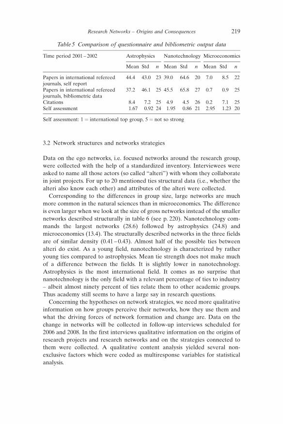
3.2 Network structures and networks strategies

Data on the ego networks, i.e. focused networks around the research group,were collected with the help of a standardized inventory. Interviewees wereasked to name all those actors (so called “alteri”) with whom they collaboratein joint projects. For up to 20 mentioned ties structural data (i.e., whether thealteri also know each other) and attributes of the alteri were collected.

Corresponding to the differences in group size, large networks are muchmore common in the natural sciences than in microeconomics. The differenceis even larger when we look at the size of gross networks instead of the smallernetworks described structurally in table 6 (see p. 220). Nanotechnology com-mands the largest networks (28.6) followed by astrophysics (24.8) andmicroeconomics (13.4). The structurally described networks in the three fieldsare of similar density (0.41 – 0.43). Almost half of the possible ties betweenalteri do exist. As a young field, nanotechnology is characterized by ratheryoung ties compared to astrophysics. Mean tie strength does not make muchof a difference between the fields. It is slightly lower in nanotechnology.Astrophysics is the most international field. It comes as no surprise thatnanotechnology is the only field with a relevant percentage of ties to industry– albeit almost ninety percent of ties relate them to other academic groups.Thus academy still seems to have a large say in research questions.

Concerning the hypotheses on network strategies, we need more qualitativeinformation on how groups perceive their networks, how they use them andwhat the driving forces of network formation and change are. Data on thechange in networks will be collected in follow-up interviews scheduled for2006 and 2008. In the first interviews qualitative information on the origins ofresearch projects and research networks and on the strategies connected tothem were collected. A qualitative content analysis yielded several non-exclusive factors which were coded as multiresponse variables for statisticalanalysis.


Table 5 Comparison of questionnaire and bibliometric output data

Time period 2001 – 2002 Astrophysics Nanotechnology Microeconomics

Mean Std n Mean Std n Mean Std n

Papers in international refereedjournals, self report

44.4 43.0 23 39.0 64.6 20 7.0 8.5 22

Papers in international refereedjournals, bibliometric data

37.2 46.1 25 45.5 65.8 27 0.7 0.9 25

Citations 8.4 7.2 25 4.9 4.5 26 0.2 7.1 25Self assessment 1.67 0.92 24 1.95 0.86 21 2.95 1.23 20

Self assessment: 1 = international top group, 5 = not so strong

The most frequent motivation given for a project is that it emerged frompath dependence naturally. More than three quarters of the respondents inastrophysics and microeconomics and more than half of the nanotechnologistsattributed the origin of their projects to path dependency. Scientific relevanceoften goes together with path dependence reasoning. It is much moreimportant for astrophysics and microeconomics than for nanotechnologists.On the other hand application options are relevant only for nanotechnologists.More than a third of them reported that projects are strategically fitted toexternal funding programs. This was reported by a fifth of astrophysics groupsand only by one in eight microeconomics groups.

The differences between the fields concerning the reasoning on the emer-gence of networks are quite similar. Path dependence is less important fornanotechnology groups. They are more prone than astrophysics groups tochoose new partners with a strategic and open perspective. Microeconomicsgroups make hardly use of an open strategic choice of new partners. They also

Dorothea Jansen220

Table 6 Structure of research networks



Size* 10.080 3.174 25 11.300 4.027 27 7.240 5.797 25Network density* 0.427 0.235 25 0.412 0.236 27 0.430 0.226 23Mean duration of ties* 9.674 4.076 21 6.811 3.487 20 7.742 4.379 22Mean tie strength* ** 1.533 0.226 25 1.466 0.231 27 1.533 0.284 23% of international ties* 0.614 0.233 25 0.381 0.249 27 0.398 0.302 23% of industry ties* 0.000 0.000 25 0.107 0.154 27 0.032 0.088 23

* Detailed ego-network data** 1 = weak, 2 = strong

Table 7 Origins of research projects and of networks



% Projects: path dependent 0.84 0.28 25 0.52 0.51 25 0.76 0.44 25% Projects: scientific relevance 0.32 0.48 25 0.04 0.20 25 0.28 0.46 25% Projects: application relevance 0.00 0.00 25 0.40 0.50 25 0.04 0.20 25% Projects: external incentives 0.20 0.41 25 0.36 0.49 25 0.12 0.33 25% NW: path dependent 0.92 0.28 25 0.72 0.46 25 0.96 0.20 25% NW: strategic open choice ofpartners

0.68 0.46 25 0.80 0.41 25 0.16 0.37 25

% NW: effect of external incentives 0.24 0.44 25 0.20 0.41 25 0.08 0.28 25

refer very seldom to external incentives for the establishment of their net-works. External incentives for the establishment of their networks do havesome effect in both natural science fields.

There is a striking difference in the role of external funds for the researchopportunities between the fields. External resources were not a subject at allin many interviews in microeconomics. Obviously the much lower infra-structural and personnel requirements of microeconomic research makeexternal resources and group size not a problem for this field. On the otherhand, for more than two thirds of the natural science groups external fundingis a condition sine qua non for doing research.

Networks are a strategic asset for the research capacity of most of thenatural science groups. Instead, microeconomics has a lower but more dividedview on networks. The function of networks is to provide for complementaryresources, skills and knowledge. Critical mass reasoning is less important,most common in nanotechnology. Specialization is strongest in astrophysics.More than half of astrophysics groups specialize in both, subject and methods.Modular arrangements of projects or conduction of several unconnectedprojects are the most common strategies for nanotechnologists. Micro-economics seems to be divided between the two ends of the scale. A largegroup specializes in subject and methods, and another one conducts diverseunconnected projects.


Table 8 Relevance of external resources, networks and types of specialization



% research capacity depends onexternal resources

0.72 0.48 25 0.68 0.48 25 0.12 0.33 25

% external resources provide niceadds

0.28 0.58 25 0.16 0.37 25 0.16 0.37 25

% smallness of group is a problem 0.16 0.37 25 0.08 0.28 25 0.00 0.00 25NW importance* 2.72 0.46 25 2.88 0.33 25 2.24 0.83 25% NW function: complementaryresources

0.84 0.37 25 1.00 0.00 25 0.76 0.44 25

% NW function: assemblingcritical mass

0.12 0.33 25 0.16 0.37 25 0.08 0.28 25

% low specialization, hetero-genous projects

0.12 0.33 25 0.24 0.44 25 0.40 0.50 25

% modular arrangement ofprojects and capacities

0.20 0.41 25 0.36 0.49 25 0.08 0.28 25

% specialization in methods 0.16 0.37 25 0.20 0.41 25 0.36 0.49 25% specialization in subject andmethod

0.52 0.51 25 0.20 0.41 25 0.24 0.44 25

* Importance of networks: 1 = low, 3 = essential

4 Evaluation of hypotheses

4.1 Bivariate correlation analysis

As an indicator of performance the self reports on the number of internationalpapers in refereed journals are used here. Correlation with the bibliometricindicator is r= 0.897 (p= 0.000). Since a split of the data for a disciplinespecific analysis is not possible, in the bivariate analysis the dependent vari-able is transformed to z-values using discipline specific means and standarddeviations.

Despite small sample size, some hypotheses from chapter 2.5 can be cor-roborated by the data (see table 9). The size of the network – the overall grosssize (r= 0.40, p< 0.01) and the size of the structurally described network (r=0.34, p< 0.01) – correlates strongly with discipline specific performance (H1).Some of the central variables of the mode-2 thesis, the percentage of industry

Dorothea Jansen222

Table 9 Correlation matrix: Bivariate analysis and regression variables

Bivariate pearson correlations

1 2 3 4 5 6 7 8

1 Ln (paper intern. journals)

2 Z-transformation per discipline .65***

3 # researchers .59*** .58***

4 % externally funded research .31** � .20

5 % applied research � .29** � .08 � .08

6 # of disciplines .24** .23** .35** .22*

7 Size of gross network .50*** .40*** .69*** .21* � .13 .42***

8 Size of described network .48** .34*** .33** .26** � .03 .35** .65*** .13

9 % industry ties .25** .26** .38** .12 .30* .46** .30*** .30***

10 (% industry ties)2 .22* .22* .32** .09 .27* .43** .31*** .13

11 % international ties .14 0.08 � .16 � .02 � .44** � .09 � .00 .22

12 Density of network .03 .05 .24* � .04 � .25* � .04 0.18 � .41**

13 Strength of ties .06 .14 .10 � .06 .02 � .21 � .10 � .00

14 Duration of ties .04 � .06 .14 .06 � .25 � .04 .23* .16

15 Importance of networks .38*** .18 .20 .49*** � .01 .27* .25** .34**

16 NW origin: path dependent � .24** � .18* � .21* � .17 � .21* � .07 � .32*** � .20*

17 NW origin: open choice of partners .38*** .08 .31** .51*** .06 .11 .22* .30**

18 % low specialization � .07 .09 .11 .10 .10 .14 � .08 � .22

19 % specialization subject & methods .11 .09 � .04 � .16 � .16 .05 .14 .16

20 field 1 astrophysics .38*** .00 .08 .19 � .42** � .30** .08 .07

21 field 2 nanotechnology .30*** .00 .22 .43*** .14 .42** .24** .27*

22 Non-university group .44*** .37*** .31*** � 0.18 � 0.12 0.17 .32*** .24**

* p = 0.10 2-sided

** p = 0.05 2-sided

*** p = 0.01 2-sided

n pairwise between 72 and 76, except duration of ties: n = 62

ties (H4: r= 0.26, p< 0.05) and the number of disciplines in the group(r=0.23, p< 0.05) are positively correlated to performance. However, apositive effect of the amount of applied research cannot be corroborated (H3:r=0.08).

Concerning indicators of network structure, the only significant effect is thepercentage of industry ties (see above, H4). Neither density of networks norstrength or duration of ties displays a significant relation to performance. Thissheds some doubts on a purely structural approach to networks (chapter 2.2)and underlines the necessity to look at the learning and network strategies ofthe actors (chapter 2.3).

Concerning the qualitative aspect of network strategies (H7) we find arelevant negative correlation of a path dependent “non-strategy” in networkformation with performance (H7: r=� 0.18, p< 0.10), but no effect of astrategic open choice of network partners or of young ties. Albeit openpartner choice does correlate with the size of collaboration networks (gross


Table 9 (cont.)

Bivariate pearson correlations

9 10 11 12 13 14 15 16 17 18 19 20 21

.97**

� .28* � .25*

� .02 .02 � .05

� .17 � .17 .17 � .19

� .18 � .14 .18 .30* � .02

.11 .11 .12 .06 � .03 � .02

� .13 .29** � .13 � .05 .04 � .01 � .18

� .06 � .14 � .04 � .01 .04 .02 .38** � .20*

.26* .22 � .25* .19 � .02 � .23 � .23 � .13 � .09

� .19 � .11 .08 � .08 � .16 .29* .06 .27*** .15 � .33**

� .30** � .25* .38** .01 .07 .27* .12 .11 .19 � .22 .30**

.39** .35** � .22 � .03 � .13 � .21 .30** � .31*** .36** � .02 � .18 � .51**

.09 .12 .18 � .02 .03 .06 .15 � .15 .26** � 0.11 .28** .25** 0.08

networks: r=0.22, p< 0.10; detailed networks: r=0.30, p< 0.05). On the otherhand, a path dependent choice is correlated negatively with both measures ofnetwork size. Strategic network behavior in turn is correlated positively withthe size of a group (r=0.31, p< 0.05) and the amount of externally fundedresearch (r=0.51, p< 0.05).

Concerning hypotheses 8 to 10, they are only partly corroborated bybivariate analysis. Neither specialization nor heterogeneity of project strategyhas a significant effect on performance (H8). Specialization leads to largernetworks, but the effect is not significant. We observe a relevant negativecorrelation between the percentage of applied projects and specialization(r=� 0.16), albeit again not significant. A heterogeneous project strategyleads to a larger amount of industry ties (r=0.26, p< 0.10) and to smallernetworks (H9: r=� 0.22, p< 0.10).

Of greater statistical relevance are the hypotheses on potential advantagesof groups from their embeddedness into larger established non-universityresearch organizations. Non-university groups tend to be significantly larger(23.78 vs. 9.41). Most of them come from astrophysics, only few from micro-economics. Non-university groups perform significantly better (H13: r=0.37,p= 0.001). They command larger networks (H11: r=0.32, p= 0.005) and theyare more often specialized than university groups (H11: r=0.28, p= 0.014). Atthe same time they are less dependent on external funding (r=� 0.18, p=0.124).

As a preliminary conclusion, I hold that networks and particularly networksize have a strong effect on scientific performance. Heterogeneity of networks,particularly industry ties, can have a positive effect on performance. However,applied research and a heterogeneous research strategy do not have positiveeffects on performance. A strategic attitude to networks in contrast to a pathdependent attitude has a positive effect on the size of networks. Strategicnetwork behavior leads to and/ or tends to be supported by group size andlarger amounts of external research money. It comes at some surprise thatspecialization is not correlated with performance. The options for special-ization seem to be better in the context of non-university research organ-izations. Groups in these contexts perform significantly better. They are largerand can attract larger networks. At the same time, they are less dependent onexternal funding. Focused funding is acknowledged as relevant for projectchoice in the two natural science fields, mostly from university groups.Whether such resource constraints indeed do lead to less specialization ofuniversity groups is a research question that needs further attention.

Dorothea Jansen224

4.2 Preliminary regression models

Small numbers and skewed distributions such as performance data posesevere problems for a thorough regression analysis. The current data filetherefore will be enlarged soon in order to come to better founded con-clusions. The large differences between the disciplines and their productionlogics ask for a discipline specific analysis, which unfortunately is impossiblewith the small data set available now.

What is presented here is a linear regression analysis on the dependentvariable self reported number of papers in international refereed journals. Forreasons of improved fit to assumptions on the distribution of residuals, thenumbers have been transformed to their natural logarithm. Two dummyvariables are introduced to represent the field differences. I start from abaseline model with the two field variables and the number of researchers.Packages of variables concerning the hypotheses from the four theory strands(see chapter 2) are introduced then.

In table 10 (see p. 226), beta coefficients (left column) and respective p-values (right column) are reported (see table 9 for a correlation matrix).Because of the small case numbers, strong significance cannot be expectedeven for sizable beta coefficients.

Model 1 is the baseline model. The differences between the fields are highlysignificant. Performance compared to the baseline field (microeconomics) ishigher for astrophysics (beta= 0.613) and nanotechnology (0.529). Differencein group size (# of researchers, beta= 0.430) also accounts for a sizable part ofthe adjusted explained variance of 0.627.

Some of the strong effects of size and fields can be captured by othervariables. However, given the high percentage of explained variance reachedby the basic model, R2 increases only very modestly. Model 2 tests for theeffects of the mode-2 variables. The number of disciplines is not a relevantfactor, but the percentage of industry ties and the percentage of appliedresearch seem to have some effect, despite a lack of significance. As on thebivariate analysis, the percentage of industry ties increases the productivity ofthe group (beta= 0.125) as long as it only maintains a small work time budgetto applied research (beta=�0.135). This could imply that industry ties areonly scientifically productive if the group keeps a strong footing in basicresearch.

Model 3 introduces the structural network variables (H4 to H6). This is themodel with the highest percentage of explained variance (R2 adjusted= 0.672,p= 0.000). Field differences seem partly to be captured by network variablessuch as size of network (beta= 0.17, p= 0.102), the percentage of industry ties(beta= 0.201, p= 0.552) and of international ties (beta= 0.128, p= 0.161).Since the quadratic term of industry ties is (not significantly) negative, thequestion whether there is a curvilinear relation to performance needs further


observation. Structural variables (density, tie strength, and duration) are againirrelevant.

Model 4 retains the variables size of network and industry ties from model 3and adds some variables on network and research strategies of the groups. Themodel explains 69,6% of the variance, R2 adjusted is 0.648. Size of network isthe only variable with a significant effect. Obviously some of the group size�seffect is taken up by it. Thus, while small groups might need networks themost, it is the larger groups who command large networks. Strategic networkorientation and importance of networks, which are strongly correlated withperformance as well, display no effect when introduced together with networksize and size of research group.

In order to be aware of the drawbacks of a joint analysis of the fields, acomparison of the correlations of the two types of performance variable, thediscipline specific transformation and the logarithmic transformation, is ofsome help (see table 9 p. 222/223). There are some striking differences: the

Dorothea Jansen226

Table 10 Regressions analysis: Dependent variable = Natural logarithm of selfreported number of publications in international journals (OLS regression)

Regression Analysis: Dependent variable LN (# papers international journals)

Model 1 Model 2 Model 3 Model 4

n = 72 n = 68 n = 59 n = 68

constant 0.000 0.000 0.841 0.393# researchers 0.430 0.000 0.393 0.000 0.408 0.000 0.370 0.000% applied research –0.135 0.130# of disciplines 0.046 0.619Size of network 0.170 0.102 0.246 0.006% industry ties 0.125 0.194 0.201 0.556 0.080 0.411(% industry ties)**2 –0.100 0.759% international ties 0.128 0.161Density of network 0.046 0.643Strength of ties 0.057 0.499Duration of ties –0.069 0.434Importance of networks 0.056 0.510NW strategic open choice ofpartners

–0.090 0.353

% low specialization 0.047 0.588% specialization subject &methods

0.046 0.576

field 1 astrophysics 0.613 0.000 0.590 0.000 0.498 0.000 0.597 0.000field 2 nanotechnology 0.529 0.000 0.439 0.000 0.394 0.000 0.405 0.001R2 0.643 0.655 0.729 0.696R2 adjusted 0.627 0.621 0.672 0.648p 0.000 0.000 0.000 0.000

amount of external funding changes sign when we regard the discipline spe-cific standardization. The effect of network size stays positive and significant,but is reduced. The negative effect of a path dependent network strategy holdsfor both indicators. However, indicators of networks� strategic importance andstrategic network building loose much of their positive effect. This could meanthat research resources such as external research money and large networkstake on a very different role in the three fields studied here. Further analysison the basis of a larger data set and longitudinal data will have to disentanglethese effects in detail.

5 Conclusion

The preliminary analysis presented here makes clear that networks are animportant factor in scientific performance. In particular, the size of networkshas a relevant and significant effect on performance. On the basis of this smalland heterogeneous sample, a relevant effect of structural network attributes,which are focused by the different strands of social capital theory, could not befound. Instead, an actor oriented approach focusing on the network strategiesof a research group seems to be promising. A path-dependent “non-strategy”in network formation not only prevents groups from attracting sizable net-works but also has a negative effect on scientific performance. Small groupshave a tendency to build their networks in a path dependent way, while largergroups tend to choose a more strategic view on networks. What is cause andeffect here is hard to say from cross-sectional data. Follow-up interviews areplanned to disentangle these relations.

While networks are important, they seem to have quite a different role inthe subfields studied. They may have a strong role in attracting externalresearch money, which can be used to enlarge one�s group. But there aredisciplines such as microeconomics which are not really dependent on exter-nal money and large group sizes. A disciplinary split of model 1 – despite thevery small numbers – yielded no effect of group size on performance inmicroeconomics, but strong significant effects in the natural science fields. Athorough analysis of the economies of group size, network size and amount ofexternal funding is scheduled for the next year when the larger data sets forthe fields are available.

As for the mode-2 thesis, it can be stated that nanotechnology indeed dis-plays some of the mode-2 attributes. But except for the stronger orientationtowards applied projects the differences to the other fields are not reallystriking. Nanotechnology groups have on average 10% industry ties, but still90% academic ties in their networks. Concerning the relation to performance,the picture is still ambivalent. A large amount of applied research and het-erogeneous projects seem to hamper research performance, while industry ties


as such have a positive effect. Here we need to follow up the question ofwhether there is an upper threshold of the amount of industry ties, whichmight lead to an inverted u-shape of its effect on performance.

References

Adams, J. D., G. C. Black, J. R. Clemmons, and P. E. Stephan (2005), “Scientific Teamsand Institutional Collaborations: Evidence from U. S. universities, 1981 – 1999,”Research Policy, 34, 259 – 285.

Ahuja, G. (2000), “Collaboration Networks, Structural Holes, and Innovation. A Lon-gitudinal Study,” Administrative Science Quarterly, 45, 425 – 455.

Blackler, F., N. Crump, and S. McDonald (1998), “Knowledge, Organizations and com-petition,” 67 – 86 in: G. von Krogh, J. Roos, and D. Kleine (eds.), Knowing in Firms,Sage: London.

Burt, R. S. (1992), Structural Holes, Harvard University Press: Cambridge MA.– (1999), “Entrepreneurs, Distrust, and Third Parties: A Strategic Look at the Dark Side

of Dense Networks,” 213 – 243 in: L. L. Thompson, J. M. Levine, and D. M. Messick(eds.), Shared Cognition in Organizations. The Management of Knowledge, LawrenceEarlbaum: Mahwah, NJ.

Buskens, V., Ch. Snijders, and W. Raub (2002), “Embedded Trust: Control and Learn-ing,” 167 – 202 in: S. R. Thye, and E. J. Lawler (eds.), Group Cohesion, Trust andSolidarity. Advances in Group Processes, Vol. 19, JAI, Elsevier Press: Amsterdamet al.

Cohen, W., and D. A. Levinthal (1990), “Absorptive Capacity. A New Perspective onLearning and Innovation,” Administrative Science Quarterly, 35, 128 – 152.

Coleman, J. S. (1990), Foundations of Social Theory, The Belknap Press: Cambridge,MA.

Darr, A., and I. Talmud (2003), “The Structure of Knowledge and Seller-Buyer Networksin Markets for Emergent Technologies”, Organization Studies, 24, 443 – 461.

Deutsche Forschungsgemeinschaft (DFG), 2003: F�rder-Ranking 2003: Institutionen –Regionen – Netzwerke. Bonn.

Evans, J. A. (2004), “Sharing the Harvest: The Uncertain Fruits of Public/Private Col-laboration in Plant Biotechnology,” Unpublished Dissertation, Department of Soci-ology, University of Stanford.

Frenken, K., W. H�lzl, and F. de Vor (2005), “The Citation Impact of Research Col-laborations: the Case of European Biotechnolgy and Applied Microbiology (1988 –2002),” Journal of Engineering and Technology Management, 22, 9 – 30.

Gibbons, M., C. Limoges, H. Nowotny, S. Schwartzman, P. Scott, and M. Trow (1995),The New Production of Knowledge, Sage: London u. a.

Gulati, R., and M. Gargiulo (1999), “Where Do Interorganizational Networks ComeFrom?” American Journal of Sociology, 104, 1439 – 1493.

Gulbrandson, M., and J.-Chr. Smeby (2005), “Industry Funding and University Pro-fessors� Research Performance,” Research Policy, 34, 932 – 950.

Hannan, M. T., and J. Freeman (1977), “The Population Ecology of Organizations,”American Journal of Sociology, 82, 929 – 964.

Hansen, M. T. (1999), “The Search-Transfer Problem: The Role of Weak Ties in SharingKnowledge across Organization Subunits,” Administrative Science Quarterly, 44, 82 –111.

Heinze, Th. (2004), „Wissensbasierte Technologien, Organisationen und Netzwerke.Eine Untersuchung der Kopplung von Wissenschaft und Wirtschaft am Beispiel der

Dorothea Jansen228

Nanotechnologie in Deutschland,“ Deutsche Hochschule f�r Verwaltungswissen-schaften: Speyer.

Henderson, R., and K. B. Clark (1999), “Architectural Innovation: The Reconfigurationof Existing Products Technology and the Failure of Established Firms,” AdministrativeScience Quarterly, 35, 9 – 30.

Hippel, E. von (1988), The Sources of Innovation, Oxford University Press: New York/Oxford.

Ingram, P., and P. W. Roberts (2000), “Friendships among Competitors in the SydneyHotel Industry,” American Journal of Sociology, 106, 387 – 423.

Jansen, D. (2000), “Netzwerke und soziales Kapital. Methoden zur Analyse strukturellerEinbettung,” 35 – 62 in: J. Weyer (Hrsg.), Soziale Netzwerke. Konzepte und Methodender sozialwissenschaftlichen Netzwerkforschung, Oldenbourg: M�nchen.

– (2002), “Netzwerkans�tze in der Organisationsforschung,” 88 – 118 in: J. Allmendinger,and Th. Hinz (eds.), Organisationssoziologie. Sonderheft 42/2002, K�lner Zeitschriftf�r Soziologie und Sozialpsychologie.

– (2003), Einf�hrung in die Netzwerkanalyse, 2nd ed., Leske und Budrich: Opladen.– (2004), “Networks, Social Capital and Knowledge Production,” F�V Discussion papers

No. 8, Forschungsinstitut f�r �ffentliche Verwaltung: Speyer.Kern, H. (1998), “Lack of Trust, Surveit of Trust. Some Causes of the Innovation Crisis in

German Industry,” 201 – 215 in: Chr. Lane, and R. Bachmann (eds.), Trust Within AndBetween Organizations, Oxford University Press: Oxford.

Krackhardt, D. (1999), “The Ties that Torture: Simmelian Tie Analysis in Organ-izations,” 183 – 210 in: St. B. Andrews, and D. Knoke (eds.), Networks in and aroundOrganizations. Research in the Sociology of Organizations, Vol. 16, JAI Press: Stam-ford, Co.

Kr�cken, G. (2001), “Jenseits von Einsamkeit und Freiheit? Zur Verortung von Uni-versit�ten in der Wissensgesellschaft”, Soziologische Revue 25, 15 – 21.

Lazega, E. (2000), “Enforcing Rules among Peers: A Lateral Control Regime,”Organizations Studies, 21, 193 – 214.

Lin, N., K. S. Cook, and R. S. Burt (eds.) (2001) Social Capital. Theory and Research, deGruyter: New York.

Lotka, A. J. (1926), “The Frequency Distribution of Scientific Productivity,” Journal ofthe Washington Academy of Science, 16, 317 – 232.

Nahapiet, J., and S. Ghoshal (1998), “Social Capital, Intellectual Capital, and theOrganizational Advantage”, Academy of Management Review, 23, 242 – 266.

Nowotny, H., P. Scott, and M. Gibbons (2001), Re-thinking Science: Knowledge and thePublic in an Age of Uncertainty, Polity Press: Cambridge.

Obstfeld, D. (2005), “Social Networks, the Tertius Lungens Orientation, and Involve-ment in Innovation,” Administrative Science Quarterly, 50, 100 – 130.

Podolny, J. M. (2001), “Networks as Pipes and Prisms of the Market,” American Journalof Sociology, 107, 33 – 60.

–, T. E. Stuart, and M. T. Hannan (1996), “Networks, Knowledge, and Niches: Com-petition in the Worldwide Semiconductor Industry, 1984 – 1991”, The AmericanJournal of Sociology 102, 659 – 689.

–, K. W. Koput, L. Smith-Doerr, and J. Owen-Smith (1999), “Network Position and FirmPerformance: Organizational Returns to Collaboration in the Biotechnology Indus-try,” 129 – 160 in: St. B. Andrews, and D. Knoke (eds.), Research in the Sociology ofOrganizations, Vol. 16, JAI Press: Stamford, Connecticut.

Price, D. J. de Solla (1976), “A general Theory of Bibliometric and other CumulativeAdvantage Processes,” Journal of the American Society for Information Science, 27,292 – 306.


Slaughter, S., and G. Rhoades (2004), Academic Capitalism and the New Economy.Markets, State, and Higher Education, The John Hopkins University Press: Baltimore/London.

Stuart, T. E. (1998), “Networks Positions and Propensities to Collaborate: An Inves-tigation of Strategic Alliance Formation in a High-technology Industry,” Admin-istrative Science Quarterly, 43, 668 – 698.

Talmud, I., and G. S. Mesch (1997), “Market Embeddedness and Corporate Instability:the Ecology of Inter-industrial Networks,” Social Science Research, 26, 419 – 441.

Todeva, E., and D. Knoke (2002), “Strategische Allianzen und das Sozialkapital vonUnternehmen,” 345 – 380 in: J. Allmendinger, and Th. Hinz (eds.), Organ-isationssoziologie. Sonderheft 42/ 2002, K�lner Zeitschrift f�r Soziologie und Sozial-psychologie.

Trute, H.-H. (2005), “Comment from a Legal Perspective,” 53 – 61 in: H. Nowotny, D.Pestre, E. Schmidt-Aßmann, H. Schulze-Fielitz, and H.-H. Trute (eds.), The PublicNature of Science under Assault. Politics, Markets, Science and the Law, Springer:Berlin/Heidelberg.

Uzzi, B. (1997), “Social Structure and Competition in Interfirm networks: The Paradoxof Embeddedness,” Adminstrative Science Quarterly, 42, 35 – 67.

Weingart, P. (1997), “From �Finalization� to �Mode 2�: Old Wine in New Bottles”, SocialScience Information, 36, 591 – 613.

Wernerfelt, B. (1984), “A Resource-based View of the Firm,” Strategic ManagementJournal, 5, 171 – 180.

Williamson, O. E. (1991), “Comparative Economic Organization: The analysis of Dis-crete Structural Alternatives,” Administrative Science Quarterly, 36, 269 – 296.

Wissenschaftsrat: Strategische Forschungsf�rderung. Empfehlungen zu Kommunikation,Kooperation und Wettbewerb im Wissenschaftssystem. Essen.

Wittek, R. (1999), “Closed Structures, Open Structures, Stable Structures: ExplainingStructural Form and Temporal Stability of Informal Social Networks in Organ-izations,” Bulletin de Methodologique Sociologique, 63, 5 – 28.

Dorothea Jansen230

Networking in Science and Policy Interventions

Comment by

Henrik Egbert

Dorothea Jansen�s paper deals with the influence of networking and socialcapital on the production of knowledge. Jansen investigates this topic forGermany, where reforms of the mainly publicly financed science sector pro-mote network building among scientists. The major questions are related tothe effects of ego-centred networks of scientists and the output scientistsproduce (chiefly publications). The study is part of a larger research programon scientific networks in Germany. The focus is on three disciplines, i.e.,astrophysics, nanotechnology and microeconomics. The paper combinessociological theory and empirical data, addressing topics that are of relevancebecause the results may allow an evaluation of some of the reforms in theGerman scientific system.

The paper consists of two parts. In the first part, theories about the role ofnetworks in science together with the research hypotheses are outlined. In thesecond part, Jansen presents preliminary results from an investigation of ego-centred networks. Data include 25 research groups from each of the threefields. Jansen tries to answer two questions. The first focuses on the effects ofheterogeneous networks on output and the second addresses the effects of anapplied research strategy on output. She analyzes existing networks with thestandard and well established sociological toolkit and tests several hypothesesthat may explain positive network effects.

The prevalent assumptions throughout the paper suggest that networking(and social capital) generally yields positive effects. The idea is that networkstructures have inherent resources; if individuals collaborate, positive networkeffects come into existence. These may then foster the production and thespread of knowledge. The idea of the positive network effects has been takenup by politics. Politicians and research funding institutions nowadays imple-ment reforms which favor a high degree of networking (e.g., the SixthFramework Programme of the EU). One consequence is that resources areredistributed in favor of scientists who are active in networking. It seems thatpoliticians tend to think that networks can cure the shortcomings in theGerman science system. Thus, the well-known statement of Portes (1998, 2)that “social capital has evolved into something of a cure-all for the maladiesaffecting societies” seems to apply also for network approaches.

For this reason, I deal with an aspect left out in the paper, the influence ofpolicy reforms on scientists� decisions and science output. I assume thatindividuals are �embedded�, i.e., institutions matter, and that they behave

rationally, i.e., they adjust their behavior to changing incentives. I start with anenvironment for scientists where no externally-set incentives for networkingexist. After that I consider the political interventions in this environment.Within these scenarios, I point out some aspects that could be of interest in thecontext of Jansen�s research.1

Let us imagine an environment for scientists in which there is no externalintervention that promotes or punishes collaboration in research. Let us fur-ther assume that scientists behave rationally by publishing in recognizedjournals. The more they publish, the better. For the production of publications,they rely on inputs from other scientists. For instance, scientists use publishedarticles from other scientists to develop their own research ideas. However,using published articles or patented ideas is not cost-free. Scientists can reducetransaction costs if they decide to collaborate with each other in the exchangeof knowledge so that information can flow faster. Therefore, collaboratingunits – we may also call them networks – come into existence. Moreover, eachscientist within a network can specialize.2 The gains from such a division oflabor are shared among network members (see, e.g., Beaver 2001) and ascientist participates in the collaboration as long as individual gains are pos-itive. In this kind of “self-organising networks” (Wagner and Leydesdorff2005, 1608), the exchange of knowledge is faster and cheaper than betweennetworks. Transaction costs are low because low entry and exit barriers exist.Presumably such networks have a rather informal character. Assuming thatscientists are free to choose with whom and with what intensity to collaborate,it can be argued that for scientists networks are a means of achievingindividual objectives.3 Therefore, networks will have the structure, the densityof ties and the size that suit their members best. Obviously, networks prove tobe rather heterogeneous with respect to these variables, as the data fromdifferent networks and research fields show.

Now let us assume that the environment changes through a policy inter-vention which rewards scientists who work in networks. I assume further thatthe total budget for science remains constant. Thus, the policy interventionleads to a redistribution of public resources in favor of those scientists whowork in networks (or claim to do so). This change in the institutional settingprovides incentives to react to. In order to look at the effects, I distinguish twotypes of scientists.

The first type does not engage in networking before the policy changes.These scientists now may need to become members of networks otherwise

Henrik Egbert232

1 This comment can be understood as a contribution to the ongoing discussion amongsociologists and economists on networks. For a recent debate, see Rauch and Casella(2001) and Zuckerman (2003); for a criticism of social capital and network concepts in aspecific context see Egbert (2006).

2 Cf. Walstad (2002, 14 – 15) for specialization and exchange in science.3 Cf. Melin (2000, 34) for reasons to collaborate.

they lose resources. In extreme cases, collaboration is not anymore a questionof whether it is useful for the production of output; it is a precondition forreceiving funds. Scientists of this type have to devote more time to networkingactivities. They may either try to enter existing networks or decide to set upnew ones. In both cases, individual efforts are spent on network buildinginstead of the production of output. Consequently, the policy intervention ismost likely to have negative effects on output.

The second type is actively engaged in collaborations before the policyintervention. One effect of the new incentive could be that collaborationsbecome more formalized because of two reasons. First, other scientists wish toenter the networks in order to get part of the available budget. For thosescientists who are already in the network, it could be reasonable to set upentry barriers for newcomers. Second, funding is related to formality; it isdifficult for informal networks to receive funds. With formalization, trans-action costs rise.4 This may cause efficiency losses as compared to a situationof informal collaboration. Another effect is that an increase in the networksize also increases the probability of conflicts among members, thus leading toefficiency losses. It is not at all clear whether a policy intervention whichpromotes networking increases the production of knowledge. There areplausible reasons to believe that the opposite effect is possible.5

To sum up, collaboration among scientists evolves naturally. Networks showdifferent structures reflecting the aims of the participants. As long as thesecollaborations are voluntary, they can be considered as efficient arrangementsfor the production of scientific output. If the incentives for collaborationchange, then the structures of networks (size, density, structure, etc.) change aswell. Networks that were efficient before the policy intervention are unlikelyto be efficient after the policy intervention. For this reason, it cannot beargued that the observation of a correlation between network variables andoutput measures provides a justification for a policy that influences thesevariables. Such a policy can only be justified if it can be shown that, without it,network formation is inefficient.

Jansen certainly contributes to the knowledge on networks in the Germanscience sector by describing particular networks. Her case study providesdetailed information on ego-centred network structures. However, it is diffi-cult to understand how descriptions of existing networks will help to evaluatepolicy interventions in science. Networks are constantly formed and reshapedby individual decisions. If one aims at an evaluation of policy reforms thatfavor networking in science, one needs a theory on network formation. SinceJansen does not refer to such a theory, important questions remain unan-

Networking in Science and Policy Interventions 233

4 The transaction costs of formal networks may even be so high that scientists decidenot to collaborate.

5 See also Cowan and Jonard (2003) for negative effects of growing networks.

swered. To mention but some of the prominent ones: What are the generalpatterns (according to the optimal size and optimal density) of efficient net-works? How do size, density, and structure of networks fluctuate when theresources available for the network increase or decrease?6 What is the optimaldistribution of resources within a network? A more thorough insight into thematter would make it necessary to combine the descriptive material presentedby Jansen with a theory that allows predictions about individual behaviorupon changes in the environment.

References

Beaver, D. (2001), “Reflections on Scientific Collaboration (and its Study): Past, Presentand Future”, Scientometrics, 52, 365 – 377.

Cesaroni, F., and A. Gambardella (2003), “Research Productivity and the Allocation ofResources in Publicly Funded Research Programmes”, 202 – 233 in: A. Geuna, A. J.Salter, and W. E. Steinmueller (eds.), Science and Innovation, Cheltenham andNorthampton: Edward Elgar.

Cowan, R., and N. Jonard (2003), “On the Workings of Scientific Communities”, 309 –334 in: A. Geuna, A. J. Salter, and W. E. Steinmueller (eds.), Science and Innovation,Cheltenham and Northampton: Edward Elgar.

Egbert, H. (2006), “Cross-border Small-scale Trading in South-Eastern Europe: DoEmbeddedness and Social Capital Explain Enough?”, International Journal of Urbanand Regional Research, 30, 346 – 361.

Melin, G. (2000), “Pragmatism and Self-organization: Research Collaboration on theIndividual Level”, Research Policy, 29, 31 – 40.

Portes, A. (1998), “Social Capital: Its Origins and Applications in Modern Sociology,”American Journal of Sociology, 24, 1 – 24.

Rauch, J. E., and A. Casella (eds.) (2001), Networks and Markets, New York: Russel SageFoundation.

Wagner, C. S., and L. Leydesdorff (2005), “Network Structure, Self-organization, and theGrowth of International Collaboration in Science,” Research Policy, 34, 1608 – 1618.

Walstad, A. (2002), “Science as a Market Process”, Independent Review, 7, 5 – 45.Zuckerman, E. W. (2003), “On Networks and Markets by Rauch and Casella, eds.”,

Journal of Economic Literature, 41, 545 – 565.

Henrik Egbert234

6 Cf. the attempt of Cesaroni and Gambardella (2003) in this respect.

A Beauty Contest of Referee Processes of EconomicsJournals

by

Christ i an Se idl, Ulr ich Schmidt and Peter Gr˛sche*

This paper is a concise report on an internet survey of economists to ascertaintheir satisfaction with peer review processes of publishing in economicsjournals. Other problems of peer review processes are not addressed in thispaper. Instead we refer to the starred footnote.

1 The Survey

At the end of 2001 and at the beginning of 2002 we addressed some twentythousands persons twice by e-mail asking them for their online responses toseven questions concerning their experience with referee processes of eco-nomics journals. Some 6,000 persons in total had a look at our questionnaire,but only a bit more than 10% of these individuals started to respond to it.

As the professional institutions in the Anglo-Saxon world did not evenrespond to our inquiry, let alone did offer their cooperation, we used as manysources of mail addresses as possible in the hope of capturing many econo-mists. We had the mail addresses of the members of the European EconomicAssociation, Verein f�r Socialpolitik, Economics Bulletin, IZA (For-schungsinstitut zur Zukunft der Arbeit – Institute for the Study of Labor), andInomics. Hence, we could rely on some 4,500 academic economists. Manyother addresses were those of professional people who had never published.Thus, an overall response rate of 3% may seem to be small, but it increases tosome 13% if we count the “certain” academic economists only.

* This paper was presented at the ESA/Public Choice Conference 2003 in Nashvilleand at the PET 04 Conference 2004 in Bejing. Helpful comments were received fromS�hnke Albers, Ted Bergstrom, John Conley, Leigh Hobson, Alan Kirman, Stefan Traub,and Joachim Wolf. The usual disclaimer applies. A more comprehensive version of thispaper was published in Estudios de Econom�a Aplicada, 23/3 (2005), 505 – 551. We referto this source as EEA. We are indebted to the editors of Estudios de Econom�a Aplicadafor their permission to reprint part of the earlier article in this volume. An even morecomprehensive study on The Performance of Peer Review: An Interdisciplinary Report, ispresently under elaboration.

2 The journals

In our survey we used two groups of journals. We call them invited andcontributed journals, respectively. The invited journals centred on the famousDiamond (1989) list (see Table 1 in EEA), which comprises 27 economicsjournals. We enlarged this list by 49 journals taken from the A and B categ-ories of the VSNU (Vereniging van Samenwerkende Nederlandse Uni-versiteiten – Association of Universities in the Netherlands) economicsjournals ranking list, which we considered as important enough to be included.This makes 76 invited journals. Furthermore, we solicited our respondents forcontributing journals to their short list at their own discretion.

This procedure yielded a total of 359 journals. Space does not permit toinclude a list of all journals in this article.1 However, the structure of responsesshows that our choice of the 76 invited journals provided a good match withrespondents� experience: Among the 73 journals showing at least 10 responsesto Question 1, only four were not listed among the invited journals. All tenjournals which attracted one hundred or more responses are also members ofthe Diamond list. All journals of the Diamond list, with the exception of theBrooking Papers on Economic Activity, elicited at least 11 responses to thefirst question. Moreover, the responses show that the Diamond list ignoressome renowned (mostly non-American) journals, which existed well before1989.

For the presentation of the results of our study, the data were broken downas follows: For the analysis of relationships between respondents� attitudes, weemployed all data irrespective of how many responses per journal we had. Fordescriptive documentations with respects to particular journals we arbitrarilysettled on at least five valid responses for the respective journals. To report onjournals with less than five valid responses would probably convey a distortedpicture. As some respondents had chosen to drop out during the survey, theset of journals decreases somewhat for later posed questions. For Questions 1and 2, 110 journals had at least five valid responses, for Question 3 we had 107journals, and for Questions 4 – 7 we had 106 journals.

For the purpose of this paper we prepared, moreover, a concise summarydocumentation of subjects� responses. We narrowed down the set of papers toa cut-off benchmark of at least twenty valid responses to Question 7 (the last

1 The list of all 359 journals can be downloaded from our homepage http://www.wiso.uni-kiel.de/vwlinstitute/ifs/chair/peerreview.php as Table 1*. It contains all journals forwhich the first question was answered (respondents could answer subsequent questionsonly by passing Question 1 first). In this table, the invited journals are marked with anasterisk, the journals of the Diamond list among them with a diamond, and the con-tributed journals are unmarked.

Christian Seidl, Ulrich Schmidt and Peter Gr�sche236

question).2 51 journals satisfy this condition. Table 1 (see p. 241) shows themordered according to the ranking of the journals with respect to Question 7asking for subjects� general satisfaction with the journals� referee processes.All rank numbers are, however, taken from the more comprehensive tables.

3 Respondents

A survey of researchers� experience with referee processes can follow severalroutes. One possibility is to address successful authors who managed to gettheir papers published in a journal. The other way is to address economists atlarge and thus collect also the experience of the less lucky ones which is,however, crucial for a valid picture of the performance of referee processes.Although this approach might be in danger of attracting mainly frustratedauthors who wish to take revenge on allegedly unfair refereeing, we shalldemonstrate below that our data do not suffer from such biases. Rather theyare biased in the opposite direction.

Taking the second route, we asked several institutions for e-mail addressesof economists. We received help from the European Economic Association,the Verein f�r Socialpolitik, the editorial board of the Economics Bulletin,from IZA and from Inomics. Our faculty colleagues S�nke Albers and Joa-chim Wolf also provided good advice. Some e-mail addresses of economistswere collected by us. Several institutions, mostly from the Anglo-Saxon world,did not even reply to our inquiries, let alone offer us their cooperation. Thesewere, in particular, The American Economic Association, The EconometricSociety, and The Royal Economic Society, as well as some less well-knownAsian economic associations. This refusal of cooperation implies that Amer-ican, Asian and Pacific economists are unfortunately underrepresented in oursurvey (see Table 2 in EEA). We had only the choice to work with the dataavailable or dispensing with our endeavour at all. We decided to continue ouranalysis.

The data of all respondents underwent a plausibility test. This led to theelimination of the data of 9 respondents, representing their joint responses to22 journals, for various reasons.3 As these were typing errors, jokes, orattempts at manipulation,4 the data of these subjects had to be eliminated.

2 The documentation of the results based on a benchmark of at least five validresponses can be downloaded from our homepage http://www.wiso.uni-kiel.de/vwlinstitute/ifs/chair/peerreview.php as Tables 3* – 8*.

3 The elimination criteria were: Response time exceeding 250 weeks (3 respondents),having received more than 10 referee reports (5 respondents), and having receivedreferee reports without having submitted a paper (1 respondent).

4 We checked also computer IP addresses for similar evaluations, but did not observesuspicious similarities of responses in the cases of multiple uses of the same computers.

A Beauty Contest of Referee Processes of Economics Journals 237

Concerning the descriptive results for the particular journals (at least fiveusable responses), we were left with 630 respondents to the first question, ofwhich 551 participated in the survey through to the seventh question. In theaggregate5, we could dispose of between 4538 (for Question 1) and 3791 dataper question (for the entries to Questions 2 – 7 cf. the number of entries inTable 4, see p. 248).

4 Reactions

In addition to responses to our questions, many subjects sent us comments andsuggestions. The tenor of their reactions was helpful, sympathetic, or critical.

Numerous sympathetic, some of them even enthusiastic, reactions camefrom all strata of respondents. Many commentators argued that we shouldhave posed more and more detailed questions. Yet, it is true that we startedoriginally with a far more comprehensive list of questions, but decided toconfine the questionnaire to but seven questions for fear of too many drop-outs. Our experience with this survey showed ample evidence that we wereright in doing so: Only about eight per cent out of all persons originallyinterested in our survey embarked on responding to all questions. Othersympathetic scholars took the occasion of our survey to broach their ownuneasiness with the current referee situation.

Critical comments were received from only a few prominent economists.For instance, a renowned economist urged us: “Please stop sending mereminders about this research. Such research projects are dangerous andmisleading!” Comments like this suggest that research directed at refereeprocesses of learned journals seems not to be favored among some of theprofession�s most prestigious scholars.

5 The questionnaire

When a responded connected to our server, (s)he was first presented with ageneral plea to participate in the survey. Then the respondent was shown a listof our 76 invited journals and asked to select those journals with which (s)hehad experience as an author. Furthermore, the respondent was prompted toadd further economics journals of his or her choice. Both sets together formedthe particular respondent�s journal set.

Then the respondent was asked the first question and asked to respond tosubsequent items for the selected journals. For the Questions 1, 2, 3, and 7,(s)he was urged to respond to the respective question for all journals in his or

5 Counting all journals irrespective of how many responses we had per journal.


her set. As to the first three questions (s)he could proceed only after therespective question had been answered for all journals in the set.6 Questions4 – 6 could only be answered if the respondent had actually received a refereereport. As some journals reject manuscripts without having solicited refereereports, a respondent may not have had experience with referee reports of alljournals to which (s)he had submitted manuscripts. Therefore, for Questions4 – 6 we allowed for passing to the next question without having responded tothe respective question for all journals. Moreover, during the response proc-ess, a respondent could also opt to eliminate some journals altogether from hisor her journal set. While the questions answered up to this point were kept inour data, these journals were then dropped for the subsequent questions. Thisdevice was intended to encourage respondents to complete the questionnaireeven if s(he) realized that (s)he had initially proposed a larger set of journalsthan s(he) was able or willing to evaluate.7

The questionnaire consisted of the following seven questions per journal.8

Question 1: “After submission of your paper, how long did it take on average to get areply other than just a confirmation that your paper had been received?”9

Question 2: “How many referee reports did you receive on average?”Question 3: “How many papers did you submit to this journal and how many paperswere accepted?”Question 4: “Were the referee reports competent?”Question 5: “Did the decision of the editor match the referee report?”Question 6: “Were the referee reports carefully done?”Question 7: “How was your overall satisfaction with the procedure of paper submissionto the respective journal?”

Note that the responses to Questions 1 – 3 are numbers such as the spell to geta first reply, numbers of referee reports received, and numbers of paperssubmitted and accepted. In contrast to that, the responses to Questions 4 – 7result from mouse click to one out of seven fields on Likert scales. In ourresults, the worst value is coded with a 0, and the best with a 6, so that 3 formsthe mean coded value of each Likert scale if all values were clicked with equalfrequency. Notice, of course, that data from Likert scales are necessarilysubjective data. An economist told us that he did not participate in our surveybecause he would have to have consulted all his files. However, authors ofmanuscripts usually decide to send a manuscript to a journal according to theperceptions in their memory without having consulted their files first. Mim-icking this behaviour, we were interested in the immediate opinions of our

6 This method warrants that subjects could concentrate on meaningful comparisonsamong the journals of their set for the same aspect of evaluation.

7 The elimination of journals was easily accomplished. The respondent had only toerase a little hook after the journal.

8 The screenshots of all seven questions can be downloaded from our homepage http://www.wiso.uni-kiel.de/vwlinstitute/ifs/chair/peerreview.php.

9 In the respective cell subjects were asked to indicate the response time in weeks.


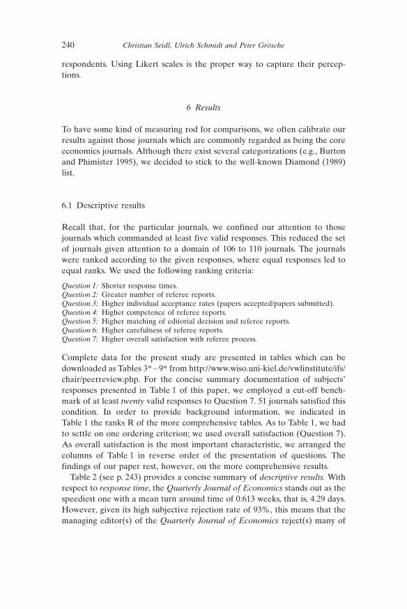
respondents. Using Likert scales is the proper way to capture their percep-tions.

6 Results

To have some kind of measuring rod for comparisons, we often calibrate ourresults against those journals which are commonly regarded as being the coreeconomics journals. Although there exist several categorizations (e.g., Burtonand Phimister 1995), we decided to stick to the well-known Diamond (1989)list.

6.1 Descriptive results

Recall that, for the particular journals, we confined our attention to thosejournals which commanded at least five valid responses. This reduced the setof journals given attention to a domain of 106 to 110 journals. The journalswere ranked according to the given responses, where equal responses led toequal ranks. We used the following ranking criteria:

Question 1: Shorter response times.Question 2: Greater number of referee reports.Question 3: Higher individual acceptance rates (papers accepted/papers submitted).Question 4: Higher competence of referee reports.Question 5: Higher matching of editorial decision and referee reports.Question 6: Higher carefulness of referee reports.Question 7: Higher overall satisfaction with referee process.

Complete data for the present study are presented in tables which can bedownloaded as Tables 3* – 9* from http://www.wiso.uni-kiel.de/vwlinstitute/ifs/chair/peerreview.php. For the concise summary documentation of subjects�responses presented in Table 1 of this paper, we employed a cut-off bench-mark of at least twenty valid responses to Question 7. 51 journals satisfied thiscondition. In order to provide background information, we indicated inTable 1 the ranks R of the more comprehensive tables. As to Table 1, we hadto settle on one ordering criterion; we used overall satisfaction (Question 7).As overall satisfaction is the most important characteristic, we arranged thecolumns of Table 1 in reverse order of the presentation of questions. Thefindings of our paper rest, however, on the more comprehensive results.

Table 2 (see p. 243) provides a concise summary of descriptive results. Withrespect to response time, the Quarterly Journal of Economics stands out as thespeediest one with a mean turn around time of 0.613 weeks, that is, 4.29 days.However, given its high subjective rejection rate of 93%, this means that themanaging editor(s) of the Quarterly Journal of Economics reject(s) many of


Tab

le1

Journa

lSa

tisfactionRan

king

(Atleast20

valid

respon

ses)

Journa

ln

Satisfaction

(7)

Carefulne

ss(6)

Match

(5)

Com

petence

(4)

Accep

tanceRate

(3)

Num

ber

(2)

Spell

(1)

R˘

STD

R˘

STD

R˘

STD

R˘

STD

R˘

STD

R˘

STD

R˘

STD

Finan

zarchiv

386

4.53

1.43

204.16

1.39

284.97

1.20

293.82

1.43

160.73

0.38

571.63

0.49

1413.26

7.26

Math.

Soc.

Sc.

308

4.47

1.81

124.35

1.52

255.03

1.55

94.39

1.50

330.62

0.45

501.69

0.73

3917.56

11.18

J.Econo

mics/ZfN

7012

4.33

1.67

254.09

1.41

215.12

1.38

323.76

1.47

270.66

0.43

301.88

0.64

2014.58

11.58

J.Math.

Econo

mics^

2413

4.25

1.76

114.36

1.53

75.39

1.31

154.26

1.36

260.87

0.33

611.59

0.83

9729.07

29.70

Scott.J.Po

lit.Ec.

2015

4.20

1.91

513.62

1.91

344.91

1.64

673.23

1.80

530.47

0.50

671.48

0.65

3216.33

11.49

Soc.

Cho

iceWelfare

3216

4.19

1.71

144.29

1.58

165.22

1.18

104.36

1.32

170.72

0.41

341.82

0.71

8023.71

16.50

J.Inst.The

or.Ec./ZfgStW

4917

4.18

1.50

194.16

1.46

334.94

1.28

303.78

1.39

280.66

0.44

371.81

0.71

3616.76

10.20

Econo

mic

Inqu

iry^

2419

4.13

1.90

304.00

1.83

294.96

1.75

114.30

1.55

240.68

0.39

172.04

0.43

4518.57

13.37

J.Ec.

Dyn

amicsCon

trol

3320

4.09

2.07

313.97

1.82

314.94

1.61

243.94

1.59

390.58

0.46

162.08

0.88

6922.07

18.25

J.Econo

metrics

^23

214.09

2.04

234.09

1.66

544.64

1.40

144.29

1.43

310.64

0.44

201.94

0.74

8224.44

16.79

J.Pub

licEc.

The

ory

2923

4.03

1.57

134.31

1.29

175.20

0.85

184.13

1.14

500.48

0.49

381.81

0.48

7423.14

12.37

J.Po

pulation

Econo

mics

2425

3.92

1.74

254.09

1.44

205.13

1.10

413.65

1.53

140.74

0.40

241.89

0.63

7022.10

12.90

Ec.

The

ory

5127

3.84

1.96

284.04

1.70

185.17

1.42

233.98

1.52

440.54

0.45

711.42

0.62

5821.22

19.65

Eur.J.Po

litical

Ec.

7628

3.84

1.67

453.68

1.61

464.73

1.54

473.56

1.62

350.61

0.47

251.89

0.60

5520.65

17.26

Econo

metrica

^98

293.82

1.91

174.23

1.88

374.88

1.36

124.30

1.91

880.20

0.31

132.12

0.80

6822.04

14.57

Weltw

irtsch.Archiv

6230

3.81

1.77

244.09

1.23

245.05

1.37

373.69

1.50

470.51

0.41

801.25

0.56

2114.71

13.73

Can

ad.J.Econo

mics^

3733

3.73

1.84

363.81

1.47

275.00

1.33

503.51

1.43

540.45

0.48

441.74

0.55

5420.58

11.89

Gam

esEc.

Beh

av.

6634

3.73

1.76

353.81

1.83

105.35

0.97

214.06

1.69

580.43

0.43

471.71

0.56

9026.22

16.23

Man

agem

entScience

3136

3.68

2.04

403.71

1.70

444.81

1.58

433.64

1.73

560.44

0.46

72.36

0.88

5120.03

17.14

Scan

d.J.Eccon

omics

7437

3.66

1.93

493.64

1.73

534.64

1.51

693.21

1.68

600.43

0.46

191.95

0.51

5019.98

12.41

Econo

micsLetters

^154

383.63

1.99

713.27

1.88

95.36

1.13

493.55

1.81

490.50

0.44

860.86

0.55

2214.77

10.70

J.Pub

licEccon

omics^

112

393.59

1.81

343.83

1.68

684.45

1.52

423.64

1.57

740.34

0.40

271.88

0.54

6721.66

11.91

J.Econo

mic

The

ory^

9441

3.56

1.93

393.73

1.91

235.09

1.16

343.76

1.77

760.32

0.37

481.70

0.72

8925.86

17.00

J.Develop

men

tEc.

^42

423.52

1.94

373.78

1.72

514.67

1.43

733.16

1.73

670.38

0.44

351.82

0.56

100

32.47

24.29

EmpiricalEcono

mics

4443

3.50

1.85

323.91

1.61

424.83

1.41

443.61

1.62

200.69

0.44

391.80

0.53

7623.22

17.82

Pub

licCho

ice

5747

3.39

2.10

733.16

1.87

265.02

1.23

643.28

1.68

450.54

0.46

691.42

0.61

3116.19

14.33

American

Ec.

Review

^171

483.37

1.83

553.55

1.86

654.49

1.61

273.86

1.71

910.17

0.33

331.85

0.75

6621.64

15.83

J.Ec.

Beh

.Org.

6749

3.37

1.91

613.51

1.86

584.61

1.60

603.39

1.64

400.56

0.47

601.60

0.73

8525.11

19.30

Review

Ec.

Stud

ies^

8450

3.37

1.73

294.03

1.53

474.72

1.58

204.08

1.42

870.22

0.38

291.88

0.66

9528.33

17.72

J.Indu

str.Ec.

4651

3.35

1.69

274.04

1.38

434.83

1.14

403.66

1.40

800.30

0.39

321.86

0.59

6321.50

16.10

J.Mon

.CreditBan

king

2952

3.35

1.72

443.69

1.97

275.00

1.23

792.97

1.70

720.34

0.46

491.69

0.60

4718.67

11.88


Tab

le1

(con

t.)

Journa

ln

Satisfaction

(7)

Carefulne

ss(6)

Match

(5)

Com

petence

(4)

Accep

tanceRate

(3)

Num

ber

(2)

Spell

(1)

R˘

STD

R˘

STD

R˘

STD

R˘

STD

R˘

STD

R˘

STD

R˘

STD

Rev.Ec.

Statistics^

7153

3.34

1.93

543.55

1.82

674.46

1.60

313.78

1.56

690.36

0.44

451.73

0.70

6021.36

13.99

Internationa

lEc.

Rev.^

7654

3.33

1.87

413.70

1.59

384.87

1.41

393.67

1.64

750.32

0.44

261.89

0.88

9327.78

15.20

J.Internationa

lEc.

^60

553.32

1.73

573.54

1.58

614.56

1.38

523.48

1.55

840.26

0.38

211.91

0.48

8625.14

13.20

The

oryan

dDecision

2656

3.31

1.87

483.64

1.60

364.88

1.64

553.44

1.58

250.67

0.43

721.41

0.73

7723.25

19.43

Int.J.Gam

eThe

ory

3060

3.17

2.04

433.96

1.83

145.24

1.12

363.73

1.70

610.43

0.44

561.64

0.64

101

33.76

30.35

OxfordEc.

Pap

ers^

5162

3.10

1.96

703.28

1.93

744.31

1.80

763.06

1.82

780.31

0.43

431.75

0.66

6221.48

14.00

Kyk

los

5363

3.09

2.11

563.55

1.74

195.14

1.22

543.44

1.55

700.36

0.46

851.11

0.76

410.07

8.32

J.App

liedEcono

mics

2366

3.04

2.23

513.62

1.69

275.00

1.05

563.43

1.69

220.69

0.45

661.48

0.80

104

38.48

28.35

Ran

dJ.Econo

mics^

6067

3.03

1.97

473.66

1.92

604.59

1.37

373.69

1.67

850.23

0.38

511.67

0.70

8324.49

16.14

Cam

bridge

J.Ec.

2069

2.95

1.73

503.63

1.80

564.63

1.89

773.05

1.57

510.47

0.48

152.10

0.88

7923.50

16.58

Europ

eanEc.

Review

^187

702.95

1.83

693.32

1.73

504.68

1.40

653.26

1.56

770.31

0.41

281.88

0.61

8425.08

16.66

Econo

mica^

5271

2.94

1.92

763.08

1.91

574.63

1.48

753.11

1.76

630.42

0.47

421.75

0.60

7523.21

14.21

Southe

rnEcono

mic

J.22

722.91

2.11

773.05

1.96

394.86

1.36

783.00

1.95

620.42

0.49

641.56

0.64

4618.65

14.53

Qua

rterly

J.Econo

mics^

106

732.90

2.05

753.08

2.03

794.86

2.02

573.42

1.90

940.07

0.21

791.25

0.82

10.61

3.70

J.Lab

orEcono

mics^

3274

2.88

1.90

633.43

1.81

554.63

1.65

333.77

1.38

900.19

0.35

591.61

0.60

8825.79

17.66

J.Hum

anResou

rces

3075

2.87

2.11

683.36

1.87

784.08

2.20

383.68

1.60

640.42

0.49

521.66

0.87

4819.29

14.06

Oxf.Bull.Ec.

Statistics

2976

2.86

2.18

533.57

1.83

304.96

1.19

683.22

1.76

730.34

0.45

831.19

0.86

5220.11

11.08

Econo

mic

J.^

115

772.86

2.01

623.50

1.86

714.38

1.72

593.40

1.71

820.27

0.41

231.90

0.78

6521.58

13.54

J.Mon

etaryEcono

mics^

3480

2.79

2.03

663.39

2.12

324.94

1.41

633.29

1.92

810.29

0.41

681.46

0.72

102

36.65

30.81

J.Finan

c.Ec.

^28

812.79

1.85

583.54

1.62

634.54

1.67

663.24

1.70

930.10

0.31

731.40

0.55

1012.44

8.04

J.Po

litical

Econo

my^

8885

2.13

1.92

812.61

1.96

664.47

1.72

802.89

1.91

920.15

0.33

701.42

0.59

9126.77

21.28


the submitted manuscripts without ever having consulted a single referee as torejection or acceptance of a paper. Indeed we registered n= 91, 89, 88responses to Questions 4, 5, 6, but n= 106 responses to Question 7 whichmeans that several subjects did not receive a referee report at all. These valuesresemble those obtained for Economics Letters, for which we registered n=129, 125, 123 responses to Questions 4, 5, 6, but n= 154 responses to Question7. Given a mean response time of 14.77 weeks and a meager mean of 0.86referee reports, this leads us to conjecture that the decision to reject a paperwithout having sent it to a referee takes the editor of Economics Lettersconsiderable time. Moreover, we cannot exclude that some authors counted aletter from the editor only as a true referee report.

As compared to other disciplines, e.g., the natural sciences, economicsjournals seem to take a particularly long time to reach a decision. Hardly anyjournals decide in fewer than 10 weeks, and more than half of them need 20weeks and more to take a decision. 20 journals of the Diamond list (out of the26 remaining ones) need more than 20 weeks to make a decision.

A mean of more than two referee reports is the exception rather than therule. Among the Diamond journals, only Econometrica and Economic Inquiryreach a mean number of referee reports above two. These are the only Dia-mond journals which rank among the first twenty ranks with respect to themean number of referee reports. Economics Letters ranks last among thejournals from the Diamond list (0.86 referee reports per respondent). Recallthat respondents might have considered the managing editors� rejection as avalid referee report.

We used subjects� reports on total numbers accepted by and submitted to arespective journal to compute the journal�s individual acceptance rates. Thedata show that the more reputed journals have lower acceptance rates, whichwas to be expected. Indeed, 17 journals out of the Diamond list figure among

Table 2 Concise Summary of Descriptive Results

Item Remarks

Response time Median: 20.5 weeks; QJE: 0.613 weeks; 20 journals of the 26DIAMOND journals need more than 20 weeks.

Number of refereereports

Median: 1.75; only 24 out of 110 journals provided at least 2 refereereports.

Acceptance rates Median: 0.5; 23 DIAMOND journals below 0.5.Competence Median: 3.641; even distribution of DIAMOND journals; only 12

below 3.Matching Median: 4.826; only 7 below 4.Carefulness Median: 3.69; even distribution of DIAMOND journals; only 10

below 3.Satisfaction Median: 3.524; 36 score 4 or better, 23 worse than 3.

The median values are the medians of the mean values for the individual journals.


the last 25 ranks.10 Cross-disciplinary comparisons show that manuscriptrejection rates are much higher in the humanities than in the natural scien-ces.11 By and large a rejection rate of more than 80% in the humanitiescontrasts with an acceptance rate of some 80% in the natural sciences.

Competence of the referee reports is, on the whole, judged rather favorably.Only twelve out of 106 journals were rated below 3.0 (out of a maximum 6.0),among them only two Diamond journals, viz. the Journal of Political Economyand the Journal of Financial Economics. Seven out of the journals of theDiamond list (recall that the Brooking Papers dropped out) score at 4.0 orbetter. Competence of referee reports seems to be not positively correlatedwith the reputation of a journal. Neither the journals of the Diamond list norof the invited journals bunch at the upper or at the lower end; they appear tobe rather evenly distributed among the ranks. For instance, 14 journals of theDiamond list rank ahead of, and 12 rank behind the mean rank of 44.

Our results show that most journals score rather well with respect tomatching of the managing editors� decisions with the recommendations of thereferee reports. However, this signals a good performance of peer review ifand only if referees� judgements are valid. If they are just reliable,12 and themanaging editor decides blindly in accordance with them, this need not be aproxy for good refereeing because referee hostility or incompetence may bebut insufficiently monitored by the editor.13 Attentive editors should interferein the latter case, which would be reflected in lower matching scores.Accompanying letters to the editors may also be harsher than the referee

10 However, there are some exceptions to this regularity. For instance, four journals ofthe Diamond list rank below 50 (out of 94 ranks).

11 Cf., e.g., Zuckerman and Merton (1971), Lazarus (1982), Adair (1982), Hargens(1988; 1990).

12 For a discussion of the concepts of validity and reliability see EEA.13 With respect to the editorial decision to accept or reject a manuscript, voices have

been aired which encourage editors to use their discretionary powers wisely and – ifnecessary – should not shy at overriding referees� recommendations (Bailar 1991, 138).Stricker (1991, 164) disputes that good editors should behave like psychometric clerkswho simply add up the scores that a manuscript gets from the referees. He argues that“good editors are not clerks. They read the manuscript, appraise the reasons reviewersgive for their recommendations, and weigh all the information about it ...” He is paral-leled in this view by Glenn (1982, 212), Rodman (1970, 355 – 356), and Goodstein (1982,213). Crandall (1991) pleads along the same lines that editors should be super referees.He deplores that too many editors do not behave in this way. He suspects “that manyeditors do not even read the papers for which they are supposed to have editorialresponsibility.” Scarr (1982, 54), editor of Developmental Psychology and the AmericanPsychologist, has made a case for editorial responsibility. She refers editors who shirktheir duties to one of Harry Truman�s wise insights: “If you can�t stand the heat, get outof the kitchen.” Yalow (1982, 244) blamed reviewer and editorial incompetence for in-stances as revealed by the Peters and Ceci (1982a, 1982b) experiment. Simon et al. (1986,270) report that only between 13 and 19% of authors� complaints against referee reportswere successful.


reports for the authors. Editorial deviation from referee recommendationsmay also be prompted by high backlogs of manuscripts which may goadeditors� zeal to curb the growth of the queues of papers agreed to be pub-lished. Such independent decisions by editors may help explain the lowerrankings of some prestigious journals, such as the American Economic Review,the Journal of Political Economy, the Review of Economics and Statistics, theJournal of Public Economics, the Economic Journal, and the Quarterly Jour-nal of Economics. When an editor, because of space limits, is forced to rejectmanuscripts furnished with good referee reports, (s)he may well give in tofavoritism.

Concerning carefulness of the referee reports, journals scores were similarto their scores on competence of the referee reports. Only 10 out of 106journals scored less than 3, among them again the two notorious DiamondJournals, the Journal of Political Economy and the Journal of FinancialEconomics. Only 6 out of the 26 journals of the Diamond list (after droppingthe Brooking Papers) scored at 4 or better than 4. As compared to com-petence, we observe a minor shift of the reputed journals to lower ranks: 11journals of the Diamond list were rated above and 15 below the mean rank.Some reputed journals rank among the bottom 20 of carefully done refereereports, viz. the European Economic Review, the Oxford Economic Papers,Economics Letters, the Quarterly Journal of Economics, Economica, theJournal of Political Economy, and the Journal of Financial Economics.

Overall satisfaction with the whole procedure of paper submission provedas disappointing for the prestigious journals. Out of 106 journals, 36 scored at4 or better; among them only five journals were from the Diamond list. Out ofthe 106 journals, 23 scored worse than 3; among them eight journals were fromthe Diamond list, to wit, the European Economic Review, Economica, theQuarterly Journal of Economics, the Journal of Labor Economics, the Eco-nomic Journal, the Journal of Monetary Economics, the Journal of FinancialEconomics, and the Journal of Political Economy.

6.2 Statistical Results

6.2.1 Response BiasesAll data obtained from the subjects are, of course, subjective data. However,the data collected for Questions 1 – 3 have “objective” counterparts. In anattempt to correct for subjective biases, we sent a mail to the editors of all 110journals for which we had received at least five valid responses to Question 1and asked them for editorial data on the average response time to authors, theaverage number of referee reports solicited, and the average acceptance rateof manuscripts. Replies to these questions seemed to be easy, as editors ofmost journals are wont to keep regular statistics on these figures. Indeed, a


few journals do even publish them (see, for instance, The Economic JournalManaging Editors� Report 2005). Editors who did not respond to our mailwere sent a reminder. We received responses from the editors of 52 journals(response rate: 47.3%), among them 7 responses from the 26 Diamond jour-nals (response rate: 26.9%). Note that we could not check whether wereceived the true “objective” data, biased data or mere conjectures of theeditors, but they represent an independent alternative data source whichallowed inferences on possible biases. For the sake of a shorthand expressionwe address them as the objective data in this paper.

Table 3 gives a concise summary of our results. Their entries are the means(taken over all journals for which we had data) of the ratios of the meanresponses of the subjects and the responses of the editorial board. Table 3shows us that the subjective response time exceeds the objective one by some50%, that the subjective number of referee reports is slightly lower than theobjective number of referee reports, and that the subjective acceptance rateexceeds the objective one by some 150%.

The most spectacular upward bias is noticed for the subjective acceptancerates. We may offer several explanations for that (all of which may havecontributed to produce this result):

1. Self-selection effect: It seems that the more successful scholars felt moreattracted by our survey.14

2. Survey-selection effect: As our survey was directed to investigate authors�experience with referee processes, we had asked subjects to respond only forthose journals with which they had experienced at least one referee process.This rules out manuscript submissions which were rejected immediately by the

Table 3 Response Biases: Statistics

Subjective value divided by objective value N Min. Max. Mean STD

Response Time 52 0.61* 4.73 1.49 0.69No. of Reports 52 0.53 1.40 0.90 0.16Accept. Rate 50 0.42** 8.89 2.50 1.34

All means significant at the 1% level (two-sided).* Only 8 values smaller than 1.** Only 4 values smaller than 1.

14 Similar effects were observed by Sweitzer and Cullen (1994). They polled 209authors for their satisfaction with peer review processes. 67% of the AR (accept withrevision) authors, 43% of the RR (reject but may resubmit) authors, and only 30% of theRO (reject outright) authors responded to their questionnaires sent to unsolicitedauthors of the Journal of Clinical Anesthesia. Higher response rates of authors whosepapers were accepted were also observed by Garfunkel et al. (1990) for the Journal ofPediatrics.


editors without soliciting referee reports. Of course, manuscripts which wereinfused into the referee process have positive chances of being accepted,whereas the crude (objective) rejection rate includes also purely editorialrejections.

3. Cognitive-dissonance effect: Successful events are memorized, failuresare mentally suppressed.

4. Trend effect: True acceptance rates fell with the lapse of time.Respondents who remember their submission history of papers amalgamatepast with present experience, which, due to the influence of higher pastacceptance rates, biased their perception of acceptance rates upwards.

The upward bias of the response time is most probably associated with theupward bias of the acceptance rates. Awell-established result says that it takesjournals shorter times to reject a paper than to offer a revision of the paper.15

This is reinforced when many papers are rejected immediately by the editorswithout having been infused into referee processes. Given that the moresuccessful authors were over-represented in our survey, this implies longerspells of response time.

Note, therefore, that our data are biased in favor of the more successfulauthors. However, as we did not pre-select our respondents a priori from theset of the successful ones, this upward bias is certainly less than it would havebeen, had we addressed only people whose papers were actually accepted forpublication. On the other hand, a survey such as ours is endangered ofattracting frustrated respondents who wish to deal a blow to those journalswhich they consider to have treated them unfairly. The entries in Table 3 showthat this was certainly not the case.

6.2.2 FavoritismFavoritism can manifest itself in three ways, to wit, personal, institutional, andregional favoritism. Personal favoritism means that certain persons enjoypreferential treatment with respect to refereeing and/or editorial decisions.The literature abounds with gossip about personal favoritism, yet, in order todemonstrate its presence, one needs inside data on referee processes andeditorial decisions, to which we had no access. Hence we could not studypersonal favoritism. Likewise, we could not study institutional favoritismbecause, for reasons of respondents� anonymity, we have only a regional, notan institutional breakdown of data. Yet our investigation of regional favori-tism does not allow sensible results. Indeed, favoritism seems to manifest

15 Cf., e.g., Ellison (2002, 955, Table 2); Omerod (2002) remonstrated the longresponse time of decision processes of the Economic Journal: In the year 2000, it tookthis journal 18 weeks to reject a paper and 28 weeks to offer a revision of a paper. Seealso The Economic Journal Managing Editors� Report (2005, 6, Table 4).


itself, first and foremost, as institutional favoritism, followed by personalfavoritism. The Coupe data (2000a; 2000b) convey some flavor of institutionalfavoritism; alas, these data rest on published manuscripts rather than onsubmitted manuscripts, as asked for by Hodgson and Rothman (1999). Formore information see EEA.

6.2.3 Correlation AnalysesTo identify relationships among the responses to our questions, we pooled thedata for all journals (irrespective of the number of responses per journal), andcombined them into a correlation matrix, Table 4.

When considering response time, we find that it is negatively correlatedwith all responses. Although longer response times may also be caused bymore and better referee reports, the negative correlation with all responsessuggests that longer response times seem to be more associated with editorialinefficiency than with more or better referee reports.

When considering the number of referee reports, we observe a moderate,but positive correlation with the acceptance rate and with the qualitativeresponses. The positive correlation of the number of referee reports with theacceptance rates seems to be influenced by the occurrence of manuscriptrejection without referee reports. These manuscripts have no chance of beingaccepted. Thus, whenever referee reports are solicited, the chance of

Table 4 Correlation Matrix of Responses to Questions

ResponseTime

Number Accept.Rate

Compe-tence

EditorialMatch

Care-fulness

Number � .0214333

Accept. Rate � .0294049

.147**4049

Competence � .112**3974

.279**3974

.322**3974

EditorialMatch

� .056**3858

.032*3858

.177**3858

.265**3858

Carefulness � .099**3817

.276**3817

.314**3817

.722**3817

.281**3817

Satisfaction � .256**3791

.199**3791

.467**3791

.682**3791

.312**3791

.684**3791

** Significance of correlation at the 1% level (two-sided).* Significance of correlation at the 5% level (two-sided).The lower lines in the cells denote the number of cases.


acceptance becomes greater than nought. The small correlation between thenumber of referee reports and the editorial match shows that referee reli-ability becomes a problem in case of multiple referee reports. As editors ofeconomics journals are wont to reject a paper whenever a single one amongseveral referee reports is somewhat critical, irrespective of how positive theother reviews are,16 authors perceive an editorial mismatch with refereesuggestions. This perception seems to have caused the small correlation.Concerning the rest, more referee reports are associated with the perceptionof higher competence and higher carefulness, and, by that way, with higheroverall satisfaction.

Prima facie one might have expected that the manuscript acceptance rateexhibits the paramount correlation with overall satisfaction. However, whilethat correlation is substantial, it is much lower than the correlation betweencompetence and overall satisfaction, and between carefulness and overallsatisfaction. The perceptions of higher carefulness and higher competence ofthe referee reports are associated with higher acceptance rates. Concerningthe correlation of editorial match with referees� recommendations and sat-isfaction, one would, however, have expected a higher correlation.

The highest correlation reported in Table 4 is the one between competenceand carefulness of the referee reports. Obviously, our respondents hold that areferee who does competent work also does it carefully and vice versa.17 Bothqualitative responses have at the same time the paramount positive correla-tions with overall satisfaction with the referee process. Thus, competence andcarefulness emerge as the most important positive features of referee proc-esses in authors� perceptions. They are even more meaningful for overallsatisfaction than the acceptance rate itself.18 This gives rise to the conjecturethat authors accept rejection of their manuscripts more easily when it is basedon competent and careful referee reports. And, conversely, they seem to be

16 Cf., e.g., Zuckerman and Merton (1971, 78), Bakanic et al. (1990, 378), Hargens andHerting (1990, 97), Kupfersmid and Wonderly (1994, 56). In a similar sense cf. alsoIngelfinger (1974, 687), Crandall (1982; 1991), Cole (1991), Coleman (1991, 142), andEckberg (1982).

17 In our instructions for response to Question 6 we used the following remark to alertrespondents that competence and carefulness need not coincide: “Concerning question 4,please note that competence and carefulness may be independent.” The full set ofquestions inclusive of instructions can be downloaded from our homepage http://www.wiso.uni-kiel.de/vwlinstitute/ifs/chair/peerreview.php.

18 This result accords with the results of Garfunkel et al. (1990), who did not findmajor differences in review evaluation among authors whose papers were accepted orrejected by the Journal of Pediatrics. However, our result for economics authors stands inremarkable contrast to the findings of Weber et al. (2002), who observed for authors ofthe Annals of Emergency Medicine that author satisfaction is associated with acceptancebut not with review quality.


but moderately happy with the acceptance of their paper when it was based onincompetent and sloppy referee reports.

Finally, to make use of similarities among responses, we applied a factoranalysis. We employed a principal-component analysis using a varimax rota-tion with Kaiser Normalization.19 This produced a factor composed of the twocomponents: carefulness and competence, each with a factor weight of 0.539,which means that their marginal rate of substitution is equal to �1. We callthis factor quality. It explains 86.114% of the variance among the two char-acteristics competence and carefulness. Competence and carefulness are,therefore, good proxies for the factor “quality”. Our analysis yielded 48 factorlevels, which we found to be arranged in terms of 13 distinct groups. Repre-senting each group by its median allowed us to focus on 13 representativefactor levels. A negative (positive) factor value means that a subject exhibits aless (better)-than-average evaluation of the respective journal. A factor valueof zero corresponds to the average evaluation.

Associating these 13 factor levels with the seven levels of overall sat-isfaction shows a characteristic distributional pattern: For low quality weobserve a positively skewed distribution of satisfaction. As quality increases,the distribution of satisfaction becomes symmetrical, and gradually becomesnegatively skewed as quality approaches its peak. Note that, although thispattern is in a way due to bunching effects inherent in categorical measure-ment, it is, nevertheless, rather distinctive in this case. Figure 1 shows therespective graph, which arranges normalized quality at the abscissa, sat-

Figure 1 Distribution of Satisfaction for Factor Levels

19 For the ease of calculation we shifted the Likert scales of questions 4 – 7 by 1 toLikert scales from 1 to 7. For the presentation in the figures, we stick to the scale rangefrom 0 to 6.


isfaction at the ordinate. The vertical axis indicates the absolute frequency ofour 3817 data points.

Low levels of satisfaction are caused by a positively skewed distribution offactor values having their peak at the lowest factor level for the lowest level ofsatisfaction. For higher satisfaction levels the distribution of factor levelsconverges first to a symmetric distribution which is reached at the mediumsatisfaction level. For still higher satisfaction levels the distribution of factorlevels assumes the shape of negatively skewed distributions. The factor dis-tribution for the highest satisfaction level has its peak at the highest factorlevel.

Figure 1 depicts a mountain extending across the figure from the (�2.16, 0)coordinate point to the (1.48, 6) coordinate point. The steepness of thismountain on both sides of its ridge is captured by the correlation coefficientbetween the quality factor and overall satisfaction. Its value is 0.735. It issignificant (two-sided) at the 1% level. This illustrates a good explanation ofoverall satisfaction with the referee process by competence and carefulness ofthe referee reports.

Finally, we have a look at the joint distribution of overall satisfaction andsubjective acceptance rates. Figure 2 shows the respective graph. We observenegatively skewed distributions for all intervals of acceptance rates except thelowest acceptance rates (virtually rejections). Subjects whose papers are often

Figure 2 Distribution of Satisfaction with Referee Reports in Terms ofAcceptance Rates


rejected are not distinctly dissatisfied. Although they are not extremelyenthusiastic about rejection, we encounter in this pattern a reflection of theappreciation of careful and competent referee reports. Good-quality refereereports may, thus, indeed cause authors to understand rejection of theirmanuscripts.

Figure 3 repeats this exercise for the 13 representative factor levels. Forhigher acceptance rates we observe negatively skewed distributions, while forthe lowest acceptance rates satisfaction is rather evenly distributed with theexception of extreme happiness.

3 Conclusions

Peer review in science is a tribunal of sorts. It influences decisively personaladvancement, research opportunities, salaries, grant-funding, promotion, andtenure. Peer review claims to exert quality control of manuscripts, to improvemanuscripts, to promote innovative research, to foster dissemination of newresearch, to select projects for grant funding, to screen papers for conferencepresentation, and to serve as a means to rank researchers, journals, andinstitutions.

Figure 3 Distribution of Satisfaction with Referee Reports in Terms ofAcceptance Rates for Factor Levels


Yet journals no longer serve the function of disseminating new research.About three and a half decade ago, Garvey and Griffith (1971) had alreadydemonstrated that the bulk of communication and dissemination of currentresearch runs over informal outlets such as personal communications, tech-nical reports, discussion papers, and preprints. Eventual publication of a papermeans that it had entered the archives of science, while its author had long agostarted new research. This applies even more so in the electronic age. Themain purpose of journal publication nowadays is to imprint a signal of qualityon a scholar�s research. However, this requires an excellent performance ofpeer review. When peer review lacks validity, impartiality, and fairness, theimprint of manuscript excellence becomes dubious.

These limitations induced us to conduct an internet questionnaire inves-tigation of authors of economics journals. We found much longer responsetimes than what is customary in the natural sciences. The top journals had onaverage high rejection rates. While the top journals did not show particulardifferences from other journals with respects to the distribution of com-petence and carefulness of referee reports, they perform somewhat worse foroverall satisfaction. Moreover, it is always the same group of some eight topeconomics journals which populate the bottom rungs in the respective rank-ings.

We observed response biases among our respondents: the subjectiveresponse time exceeds the objective one by some 50% and the subjectiveacceptance rate exceeds the objective one by some 150%. This may beexplained by several effects (self-selection, survey-selection, cognitive dis-sonance, and trend).

A correlation analysis showed that competence and carefulness are highlycorrelated, and showed the paramount correlation with overall satisfaction,while the acceptance rate exhibited a smaller correlation with overall sat-isfaction. This suggests that the authors of economics journals have a higheresteem for good referee reports in comparison to a mere focus on theacceptance rate. In other words, they will understand a rejection of their paperif it is backed by well-founded reports.

Combining competence and carefulness into a factor “quality” showed that,as quality increases, the distribution of satisfaction follows, first, a positivelyskewed distribution, becomes, for higher levels of quality, a symmetrical dis-tribution, and approaches a negatively skewed distribution for the highestlevel of quality. When juxtaposing overall satisfaction (quality) and accept-ance rates, we found negatively skewed distributions for all acceptance rateswith the exception of the very lowest acceptance rates, for which the dis-tribution is largely uniform. This confirms that manuscript rejection is tol-erated provided that the referee reports are competent and carefully done.


References

Adair, R. K. (1982), “A Physics Editor Comments on Peters and Ceci�s Peer-ReviewStudy,” Behavioral and Brain Sciences, 5, 196.

Bailar, J. C. (1991), “Reliability, Fairness, Objectivity and other Inappropriate Goals ofPeer Review,” Behavioral and Brain Sciences, 14, 137 – 138.

Bakanic, V., C. McPhail, and R. J. Simon (1990), “If at First You Don�t Succeed: ReviewProcedures for Revised and Resubmitted Manuscripts,” The American Sociologist, 21,373 – 391.

Burton, M. P., and E. Phimister (1995), “Core Journals: A Reappraisal of the DiamondList,” The Economic Journal, 105, 361 – 373.

Cole, S. (1991), “Consensus and the Reliability of Peer-Review Evaluations,” Behavioraland Brain Sciences, 14, 140 – 141.

Colman, A. M. (1991), “Unreliable Peer Review: Causes and Cures of Human Misery,”Behavioral and Brain Sciences, 14, 141 – 142.

Coupe, T. (2000a), “Revealed Performances: World Wide Rankings of Economists andEconomic Departments,” unpublished manuscript, Free University of Brussels.

– (2000b), ECARES/Universite Libre de Bruxelles. Data on the main regions of journalcontributors: homepages.ulb.ac.be/~tcoupe/update/journreg.html. Data on the maininstitutions of journal contributors: hompages.ulb.ac.be/~tcoupe/update/journuni.html.

Crandall, R. (1982), “Editorial Responsibilities in Manuscript Review,” Behavioral andBrain Sciences, 5, 207 – 208.

– (1991), “What Should Be Done to Improve Reviewing?” Behavioral and Brain Sci-ences, 14, 143.

Diamond, A. M. Jr. (1989), “The Core Journals of Economics,” Current Contents, 1, 4 –11.

Eckberg, D. L. (1982), “Theoretical Implications of Failure to Detect PrepublishedSubmissions,” Behavioral and Brain Sciences, 5, 209 – 210.

Ellison G. (2002), “The Slowdown of the Economics Publishing Process,” Journal ofPolitical Economy, 110, 947 – 993.

Garfunkel, J. M., E. E. Lawson, H. J. Hamrick, and M. H. Ulshen (1990), “Effect ofAcceptance or Rejection on the Author�s Evaluation of Peer Review of MedicalManuscripts,” Journal of the American Medical Association, 263, 1376 – 1378.

Garvey, W. D., and B. C. Griffith (1971), “Scientific Communication: Its Role in theConduct of Research and Creation of Knowledge,” American Psychologist, 26, 349 –362.

Glenn, N. D. (1982), “The Journal Article Review Process as a Game of Chance,”Behavioral and Brain Sciences, 5, 211 – 212.

Goodstein, L. D. (1982), “When Will the Editors Start to Edit?” Behavioral and BrainSciences, 5, 212 – 213.

Hargens, L. L. (1988), “Scholarly Consensus and Journal Rejection Rates,” AmericanSociological Review, 53, 139 – 151.

– (1990), “Variation in Journal Peer Review Systems: Possible Causes and Con-sequences,” Journal of the American Medical Association, 263, 1348 – 1352.

– and J. R. Herting (1990), “Neglected Considerations in the Analysis of AgreementAmong Journal Referees,” Scientometrics, 19, 91 – 106.

Hodgson, G. M., and H.Rothman (1999), “The Editors and Authors of EconomicsJournals: A Case of Institutional Oligopoly?” The Economic Journal, 109, F165-F186.

Ingelfinger, F. J. (1974), “Peer Review in Biomedical Publications,” The AmericanJournal of Medicine, 56, 686 – 692.


Kupfersmid, J., and D. M. Wonderly (1994), An Author�s Guide to Publishing BetterArticles in Better Journals in the Behavioral Sciences, Clinical Psychology PublishingCo.: Brandon VT.

Lazarus, D. (1982), “Interreferee Agreement and Acceptance Rates in Physics,”Behavioral and Brain Sciences, 5, 219.

Omerod, P. (2002), “Dealing With Journal Submissions,” Royal Economic SocietyNewsletter, No. 117, 18.

Peters, D. P., and S. J. Ceci (1982a), “Peer-Review Practices of Psychology Journals: TheFate of Published Articles, Submitted Again,” Behavioral and Brain Sciences, 5, 187 –195.

– (1982b), “Peer-Review Research: Objections and Obligations,” Behavioral and BrainSciences, 5, 246 – 252.

Rodman, H. (1970), “The Moral Responsibility of Journal Editors and Referees,” TheAmerican Sociologist, 5, 351 – 357.

Scarr, S. (1982), “Anosmic Peer Review: A Rose by Another Name is Evidently not aRose,” Behavioral and Brain Sciences, 5, 237 – 238.

Simon, R. J., V. Bakanic, and C. McPhail (1986), “Who Complains to Journal Editors andWhat Happens,” Sociological Inquiry, 56, 259 – 271.

Stricker, L. J. (1991), “Disagreement Among Journal Reviewers: No Cause for UndueAlarm,” Behavioral and Brain Sciences, 14, 163 – 164.

Sweitzer, B. J., and D. J. Cullen (1994), “HowWell Does a Journal�s Peer Review ProcessFunction? A Survey of Authors� Opinions,” Journal of the American Medical Asso-ciation, 272, 152 – 153.

The Economic Journal Managing Editors� Report (2005), Royal Economic SocietyNewsletter No. 128, 3 – 7.

Weber, E. J., P. P. Katz, J. F. Waeckerle, and M. L. Callaham (2002), “Author Perceptionof Peer Review. Impact of Review Quality and Acceptance on Satisfaction,” Journalof the American Medical Association, 287, 2790 – 2793.

Yalow, R. S. (1982), “Competency Testing for Reviewers and Editors,” Behavioral andBrain Sciences, 5, 244 – 245.

Zuckerman, H., and R. K. Merton (1971), “Patterns of Evaluation in Science: Institu-tionalisation, Structure and Functions of the Referee System,” Minerva, 9, 66 – 100.


What Should We Expect from Peer Review?

Comment by

Max Albert and Jˇrgen Meckl

Seidl, Schmidt and Gr�sche (henceforth, SSG) report on an internet ques-tionnaire study that asked economists about their experiences and satisfactionwith the referee process in economics journals. In this comment, we put thepaper in the context of scientific competition and ask whether we should beworried by its results.

1 Scientific competition and scientific quality standards

Scientific competition is mainly driven by the quest for status or reputation.Researchers earn status when their contributions are used – and not just cited– by other researchers (see Hull 1988, 283). Status-seeking researchers shoulduse the products of previous research (contained mainly in research papers) ifthey believe that it will help them to produce output that will, in turn, be usedas an input in future research.

In a nutshell, then, research is the production of papers by means of papers.In order to use the results of a paper, researchers must, of course, be aware ofthe paper and believe it to be relevant to the problems they are working on.Even if these conditions are satisfied, however, they will not use a paper if theyconsider it (i.e., the results and ideas contained in it) to be of too low a quality.

Scarcity of attention and quality concerns explain the peer review system.Journals try to collect high-quality papers that have something in common,either a specific topic or, in the case of general journals, a potential to interesteven off-topic researchers. Some journals are more successful than others inpublishing high-quality work, get more attention, and, in turn, attract moresubmissions of high-quality work. This positive-feedback effect leads toquality rankings among journals.

Ultimately, publishers compete, with the help of their journals, for theattention of the scientific community. There is a hierarchy of delegation,where all agents pursue their own interests. Publishers select and controleditors, who, in turn, select and control referees. On each stage, there iscompetition and moral hazard. Moreover, some deviations from the appli-cation of quality standards, like promoting papers sympathetic to an editor�sor referee�s research, can be viewed as payment in kind for editorial or ref-ereeing services. For this reason and others, we should expect some amount ofpersonal, institutional, or regional favoritism, as well as inner-scientific par-tisanship, in the selection of papers for publication.

The explanations so far assume given quality standards used by researchersin selecting input for their own research. It is, however, not at all clear howdecision-relevant quality standards can become established in the productionprocess we have described above. Even if everybody expects everybody elseto use only inputs that satisfy certain standards of high quality, this expect-ation is not self-fulfilling – unless using high-quality inputs increases one�schances to produce high-quality output. However, the last assumption is quitereasonable for the quality criteria used in science.1

Quality standards in science, then, are the outcome of an intertemporalcoordination problem among self-interested and forward-looking researchers.As explained above, we expect these quality standards to spill over, ifimperfectly, into the peer review process. With perfect coordination, thereexists a single quality standard. However, there are several factors workingagainst perfect coordination. First, new methodological arguments can shiftthe focal point of the coordination game. Second, at a given time, there mayexist several candidates for a focal point. Third, researchers have differentinformation about current debates and different reaction speeds. Thus, thecoordination process is slow and subject to shocks, working – despite theforward-looking attitude of researchers – like an evolutionary process ofshort-sighted adaption to one�s perception of the current trends, with severalstandards competing during adjustment. Fourth, quality standards in differentresearch areas (which are defined by relatively low probabilities of use acrossboundaries) differ, which leads to grey areas where standards are uncertain ordisputed. Fifth, quality in science has many dimensions, and weighing thesedimensions may be a problem even if there is broad agreement about thedimensions themselves.

Thus, scientific competition involves competition between quality stand-ards. There exists pressure in the direction of harmonizing the standards, butone should not expect perfect harmony, especially with respect to the finepoints and when new ideas threaten existing standards. Moreover, quality maybe difficult to detect. Even on the basis of common standards, different editorsor referees may still come to different conclusions because they prefer dif-ferent trade-offs between errors of the first and second kind.

2 Quality standards for peer review

SSG suggest that journals only archive papers and hand out quality signals. Intheir conclusions, they write that peer review in science is a tribunal withdecisive influence on individual careers. They then list the claims made in

1 See Albert (2006) for a model explaining quality standards in scientific competitionalong these lines.

Max Albert and J�rgen Meckl258

favor of peer review, which, as far as the journal referee process is concerned,are: quality control, improvement of manuscripts, promotion of innovativeresearch, fostering dissemination of new research, and serving as a means torank researchers. They note that, due to the publication lag, journals no longerdisseminate new research; instead, their main purpose is “to imprint a signalof quality on a scholar�s research”. This, in their view, requires excellentperformance of peer review, especially validity, impartiality, and fairness.

Reliability of the referee process means that different referees come to thesame conclusion. Validity of the referee process means that quality judgmentsreport the true quality of the paper. For instance, stories about highly suc-cessful papers that were frequently rejected before their eventual publicationare often viewed as anecdotal evidence of low validity. Typically, the degree ofreliability and validity is measured in terms of correlations between differentreferee conclusions or between quality judgments and quality.

Validity is ill-defined, however, and reliability is not to be expected whenseveral quality standards compete. Only with (almost) perfect coordination onquality standards, low validity and reliability must be due to imperfections inthe peer review process. We do not believe that perfect coordination has beenreached in economics.

Impartiality and fairness mean absence of favoritism and, instead, relianceon quality standards, which is of course possible even with competing stand-ards. SSG report regional favoritism. However, consider the case of theQuarterly Journal of Economics. This journal rejects most papers withoutreferee reports but (not mentioned by SSG) publishes many previous NBERworking papers. Since NBER papers are already subject to quality control,selecting from them might lower the cost of refereeing without loweringquality. Hence, it may be a sign of efficiency if some journals tap such pools ofhigh-quality papers. Due to the nature of the NBER, this leads to regionalfavoritism.

However, there is no prima facie case that such practices lead to an unfairand partisan publication system. A combination of journals with differentbiases can lead to a fair system. Moreover, in judging the quality signalsproduced by journals, it is easy to adjust for known biases: If you publish apaper at a journal biased against you, it just means that the quality of yourpaper is probably higher than the journal�s average.

Editors usually want the referee to point out possible improvements of thepaper. Within limits, this is reasonable since the editor would like to be thepaper as good as possible and the referee can produce at least some relevanthints as a by-product of quality control at almost no additional cost. However,referees should not invest much in improving a paper. If they did, this wouldcreate incentives for an author to abuse referees as unpaid ghostwriters orconscripted audiences. It is unlikely that this would result in an efficient teameffort. Hence, it is perfectly alright if bad papers get sloppy and short reports.

What Should We Expect from Peer Review? 259

This sets incentives to authors to invest more into their papers (and seek forcoauthors by themselves) and makes a better use of the scarce time of thereferees, who can concentrate on good papers. It also implies, however, thateditors and referees should not necessarily aim at the satisfaction of authors.

Nevertheless, trying to measure imperfections is certainly an excellent idea.The question is whether the data of SSG actually point to imperfections, andhence whether we should be worried about the relatively poor performance oftop journals.

We both admit that, independently of each other, we started filling in SSG�squestionnaire but gave up since, due to lack of time or access, we could notconsult our files. We both were resolved to get to it later, but as these thingsgo, we never did. In line with our experience, SSG admit that those whopersevered may have answered the questions from memory, which, as theyrecognize, may lead to systematic biases. They argue, however, that authors�memory is probably what counts in submission decisions and with respect toauthor satisfaction. We agree. However, we cannot quite see why authorsatisfaction should be important, especially if, as SSG find, it depends stronglyon the competence and care invested in the reports.

SSG note that top journals receive lower-than-average ratings for theirreferee processes. Even if this indicated lower-than-average quality, this neednot be problematic. Authors submitting a paper face costs in terms of sub-mission fees, rejection risks and decision times, which may be more or lessmitigated by the quality of the reports. Top journals overwhelmed by sub-missions should offer worse terms to authors; they could do this by urgingtheir referees not to waste time on any but the most excellent papers.

However, we can think of two plausible explanations for lower-than-aver-age ratings for top journals� referee processes even if these journals offeraverage quality. First, authors may just expect more from higher-rankedjournals and judge referee processes not in comparison with each other but incomparison with their expectations. Second, authors can make two errorswhen submitting their papers: aiming too high or aiming too low. If they preferthe first error to the second, papers will on average be submitted too high,which, in the worst case, leads to a rejection based on a single sloppy and shortnegative report. Papers then trickle down to lower-ranked journals until paperquality matches journal rank. If referee reports get more careful as the gapbetween journal rank and paper quality shrinks, the trickle-down effectimplies that author satisfaction with the referee process increases with fallingjournal ranks, even if journal policies are all the same. In this context, sig-nalling a large gap between journal rank and paper quality by a sloppy reportsoffers a further advantage: authors may adjust their self-assessment morequickly, which reduces the number of wasted submissions in the trickle-downprocess.

Max Albert and J�rgen Meckl260

References

Albert, M. (2006), “Product Quality in Scientific Competition”, Papers on StrategicInteraction 6-2006, Max Planck Institute of Economics, Jena.

Hull, D. L. (1988), Science as a Process, University of Chicago Press: Chicago andLondon.

What Should We Expect from Peer Review? 261

Methodology and the Constitution of Science:A Game-theoretic Approach

by

Je su¤ s P. Zamora Bonilla

1 Science as a game

Competition is an essential element of the scientific process as it is usuallycarried out. Nevertheless, its competitive aspects have been much more fre-quently studied from a sociological point of view than from a philosophical orepistemological one, and (perhaps with the main exception of Popperianfalsificationism and Mertonian institutionalism), the effects of competitionand rivalry on the cognitive value of scientific discoveries have tended to begiven an anti-objectivist interpretation. Furthermore, although competition isa phenomenon clearly under the scope of game-theoretic analysis (or, ingeneral, of micro-economic analysis), very few attempts have been made untilnow of formally describing scientific research as a kind of �game�. Taking allthis into account, the aim of this paper is to sketch some guidelines of aphilosophical understanding of scientific research as a competitive, game-likeprocess, a point of view which, in the end, will try to provide some analyticaltools with which to assess the rationality and objectivity of scientific knowl-edge.

An underlying idea of this approach will be the notion that scientificresearch can be described as a game which is played according to some rules.This idea can be traced back to Karl Popper�s Logik der Forschung, where thenotion of scientific method is explicated as something more alike to �the logicof chess� than to the rules of formal logic.1 In this sense, methodological rulesare conventions, as long as they can conceivably be as different as they are(actually, many of them are not equal in different scientific fields or schools,and also vary with time). Popper�s attempt was to justify his own preferredrules by somehow deriving them from the goal of maximising the �criticiz-ability� of every scientific item, although he offered few convincing justifica-tions of why this epistemic value, criticizability, had to be taken as the mostimportant one in science. I will not attempt to determine here what the valuesof scientific research �must� or �should� be: I rather think that most of theanswer has better to be left to scientists themselves, as well as to people usingthe outcomes of science or suffering from them; but I shall neverthelessexplore this idea of scientific norms as conventions derived in some way from

1 As will become clearer below, I suggest that the rules of science resemble even morethe rules of sports, like football or tennis, than of �logical� games like chess.

the goals �we� want science to fulfil (the question, of course, is who �we� are?).From a game-theoretic perspective, two different but interrelated sets ofquestions emerge once we interpret scientific norms as the rules of a game:First, what will scientists� behaviour be once certain norms have been estab-lished? And second, what norms would they prefer to have if they were giventhe choice? Obviously, a rational answer to the second question can only begiven after making some prediction about how people will react under somenorms, i.e., after having given some answer to the first question. The theoryabout how do people choose the norms under which they have to interact isknown as �constitutional political economy� (cf. Brennan and Buchanan 1985),and one particular goal of this paper is, then, to outline a �constitutional –economic� approach to methodological rules (see Jarvie 2001) for a non-economic, but also �constitutional� interpretation of Popper�s view of scientificnorms).

The main elements in the description of a game are the options (or �strat-egies�) of each player (or agent), the rules (i.e., an indication of which outcomeobtains for every feasible combination of strategies, one for each player), andthe preferences of the agents (i.e., an indication of how each player evaluateseach possible outcome). Once this description has been given, the analysis of agame typically proceeds by trying to determine its �solutions� or equilibria.Technically, an equilibrium of a game is a combination of individual choicessuch that no player can make a decision better for her than the one she hasmade, given the decisions made by the other players (Nash equilibrium). Ingeneral, the goal of a game theoretic analysis of a social fact is to show howsome relevant features of the situation can be explained as an equilibriumemerging from the interaction of the agents. As readers familiar with thedevelopments of game theory will know, one typical problem is that manygames have more than one possible equilibrium, and in this case, either theoutcome of the game remains indeterminate, or some stronger conditionsmust be added to justify why some specific solution is attained. It is alsopossible that no equilibrium exists, but it can be proved that, under a wide setof circumstances, there always are some equilibria if agents have the option ofchoosing, not directly an option, but a determinate probability of choosingevery possible option.2 Further mathematical complications result from theanalysis of repeated or dynamic games (when players have to take a sequenceof decisions, perhaps in a changing environment), of stochastic games (whenthe outcomes of the players� decisions are not known with certainty), or ofgames of incomplete or asymmetrical information (when players do not knowwith certainty some possible states of nature, or some of them know more

2 This is traditionally called a �mixed strategy�, whereas a �mixed equilibrium� is onethat obtains by a combination of mixed strategies; nevertheless, the analysis presented inthis paper will always stay at the level of �pure�, i.e., deterministic, equilibria.

Jesus P. Zamora Bonilla264

than others). The application of these models will surely be extremely inter-esting and even unavoidable for understanding many features of science, butthis paper will again offer only the most simple analysis.

2 Scorekeeping in the game of science

I proceed now to a description of the basic elements in the game of scientificresearch, which will essentially be conceived as a game of persuasion. Thatlanguage is extremely important to science can hardly be denied. Authors asdifferent as the logical positivist Rudolf Carnap and the post-modernanthropologist Bruno Latour would agree at least on this point, thoughobviously for very different reasons. The perspective I am going to take here iscloser to Latour�s in the sense that I will assume that interaction betweenresearchers mostly takes place through a continuous mutual examination ofwhat each other says or writes, although I would guess that scientists can agreeto evaluate their colleagues� �inscriptions� (to use Latour�s word) by means ofrules which a Carnapian would not dislike too much. This does not mean,however, that other things besides language are unimportant; scientists alsoperform non-verbal actions, they experiment, observe, earn and spend money,draw diagrams, organise meetings, and so on, though it is true as well that a bigpart of these things is made by speaking, and, on the other hand, that whatpeople say (and specially what they write) is usually more public than whatthey do, and so it is easier for other people to scrutinise. So, it can beinstructive to describe the game scientists play as if their main decisionsrelated to what assertions to make (probably before or after performing someother actions), and as if their rewards would essentially depend on what otherpeople is asserting. This vision of the process of scientific communication ascentral to the strategies of researchers is not only consistent with a big part ofthe work on sociology of science of the last two or three decades, but is alsoclose in spirit to some recent proposals in the philosophy of language. I amreferring particularly to Robert Brandom�s inferentialism (Brandom 1994).According to Brandom, what makes a series of noises to count as an assertionis the chain of inferences the speech community takes as appropriate to makeregarding that assertion, inferences which essentially relate to the normativestatus that each participant in a conversation attributes to the others (i.e., thethings participants are allowed or committed to do by the rules of the languagegame). For example, my saying �there is a cat on my roof� can be taken as anassertion by my hearers if and only if we share a set of normative inferentialpractices which allow them to attribute to me, under specified circumstances,the �obligation� of presenting some relevant evidence from which that sen-tence can be derived, as well as that of accepting the linguistic or practicalconsequences which, together with other commitments I have made, follow

Methodology and the Constitution of Science 265

from it. Using a metaphor suggested by Wilfried Sellars, understanding anexpression would amount to mastering its role �in the game of giving andasking for reasons�. It is important to mention that Brandom�s concept of�inference� does not only cover moves from sentences to sentences, but alsofrom �inputs� of the language game (e.g. observations) to sentences, as well asmoves from sentences to �outputs� of the game (e.g., actions).

The aspect of Brandom�s theory I want to emphasise is that linguisticpractice proceeds by each speaker �keeping score� of the commitments madeby the others and of the actions commanded by those commitments, accordingto some inferential rules which define the language games which are possiblewithin their speech community. It is this idea of �scorekeeping� that will be putinto use here in order to analyse the game of science. I propose to consider the�inscriptions� produced by a researcher as her set or �book� of commitments(her �book�, for short). There is no need that every such commitment amountsto the bare acceptance of a certain proposition (say, A), for it is possible tomake a variety of qualified (or �modalised�) commitments, as �it seems likelythat A�, �there is some evidence that A�, �A deserves some attention�, and soon. The game theoretic nature of scientific research arises because each scien-tist�s payoff depends on what is �written� not only on her own book, but on thebook of each other member of her community. This payoff is generated bythree interacting factors: an internal score, an external score, and a resourceallocation mechanism, all of which are determined by several types of norms.In the first place, any scientific community will have adopted a set of meth-odological norms with which to assess the scientific value of any set of com-mitments; the coherence of a researcher�s book with these norms (or, moreprecisely, the coherence her colleagues say it has) will determine the internalscore associated to that book. Second, and in contrast to the case of everydaylanguage games, in science many propositions are attached to the name of aparticular scientist, usually the first who advanced them; one fundamentalreward a scientist may receive is associated with the fate that the theses (laws,models, experimental results...) proposed by her have in the books of hercolleagues. This �fame� is what I call here her external score. The combinationof the internal and the external score associated to a book is its global score.Third, the community will work with a set of rules for the allocation of re-sources which will determine how much money, what facilities, what workconditions, what assistants, and so on, will be allotted to each scientist,depending on her global score.

So viewed, the game of scientific research proceeds as follows. The meth-odological norms of a discipline tell each researcher what things can she do(or must she do) in order to write a book with a high internal score; this willmake her count as a more or less �competent� researcher. These norms indi-cate how to perform and report experiments, what formal methods to employand how, what types of inductive inferences are appropriate, what styles of


writing are acceptable, and so on. By following these norms, she will end upcommitting herself to the acceptance of some propositions advanced by othercolleagues, hence contributing to their having a high external score. She willalso have to comment on the coherence of her colleagues� commitments withthe methodological norms of the discipline, contributing to rising or loweringtheir internal score. On the other hand, in order to reach a high external score,she has to take advantage of her colleagues� struggle for attaining a highinternal score: she has to be able to devise experiments, hypotheses, or modelswhich her colleagues, given their previous commitments, and given theaccepted methodological norms, cannot refuse to accept without running therisk of high losses in their internal scores.

3 An example: the first gravity wave experiments

To exemplify the applicability of a game theoretic approach to the analysis ofscientific research processes, I shall take H. M. Collins� classic narration of thedispute about gravity waves which followed the experiments of the physicistJoseph Weber (Collins 1985). According to Collins, Weber�s results stronglyconflicted with accepted cosmological theories (for his experiments indicatedan amount of gravitational energy too big for our nearby universe to be stable),and nearly all attempts of replication failed to show the same results (althoughno one of them was indisputably negative taken in isolation). Under thesecircumstances, the other members of the scientific community chose to rejectWeber�s results, and decided that presumed �gravity wave detectors� detectednothing at all because there was no signal strong enough to be detectable; thismeans that the community did not assign a high score to Weber, neither anexternal score (for his presumed results were not accepted), nor an internal one(because deficiencies in his methods were pointed out). In spite of this, Weberwent on defending his experiments and trying to improve them. From a gametheoretical point of view, the first relevant question is whether all those deci-sions (both Weber�s and those of his critics) were rational and mutually con-sistent, i.e., whether they constituted a Nash equilibrium. For example, couldWeber have made a better decision at some point of the process? It is verylikely that he could have forecasted the negative reaction of the community;furthermore, he might have acknowledged that he was wrong when non-con-firmatory results begun to appear in the experiments of some colleagues. Thathe did not take this decision seems to indicate that he severely misrepresentedthe chances of his �discovery� being recognised; then, though his decisions mighthave been �optimal� given his own (over-) estimation of success, this estimationhad to be very wrong, and so in a sense he was acting �irrationally�, at least fromthe cognitive point of view. If we did not want to accuse Weber of irrationality,we would have to look more deeply into his view of the situation.


On the other hand, what about the decisions of his colleagues? Given thatmost experiments were inconclusive, that the acceptance of Weber�s resultsmight have forced a toilsome reformulation of much accepted knowledge, andthat this reformulation would demand the cooperation of many theoreticiansand experimenters, the decision of waiting till a �significant� number of col-leagues had made a decision seems logical for a majority of researchers.Nevertheless, for those who had more to loose or to win if Weber was right(for example, because their prestige strongly depended on the theories whichnegated the existence of detectable gravity waves, or because they expected tocontribute with new discoveries in the line of Weber�s if he happened to win)it seemed rational to attempt to replicate the experiments soon, as many did.In conclusion, the resolution of the debate looks like a Nash equilibrium, sinceeverybody chose her best option, given what the other people were doing,although perhaps Weber himself suffered from a strong confirmatory bias (i.e.,his decision was rational according to the beliefs he actually had about theprobability of successful replications, but these probability judgements weresomehow defective).

The situation, however, is not so simple once we consider more deeply thestrategies available to each researcher. For example, imagine you are one ofthose who are waiting for more information from your colleagues beforedeciding what to do with Weber�s assertions. Your options are not just �accept�and �reject�, but rather �accept if at least ten percent of the community accept;reject otherwise�, �accept if at least fifty percent accept; reject otherwise�, andso on, or even something more complicated, because you will surely take alsointo account your own degree of belief in the validity of the disputedhypothesis. The scientific community must be in an equilibrium also withrespect to the decisions about when there are �enough� reasons in favour of aproposition for it to become acceptable.3 On the other hand, what aboutpeople trying to replicate Weber�s experiments? If it is true that the �com-munity leaders� have so much prestige that their own conclusions would�trigger� a consensus around them, they had at least a choice between per-forming the experiment as carefully as possible or not, as well as a choicebetween describing the results in the most neutral way or in a way which isfavourable to their preferred theories. As long as they suspect that theirdeclarations will virtually close the debate, they will be strongly tempted tochoose the second option in both cases, especially when there is only oneleader (according to Collins, in the dispute about gravity waves this role wasplayed by Richard Garwin). A full analysis of the episode in game-theoreticalterms should indicate, hence, what the reasons of the leaders were for

3 See also Zamora Bonilla (2002) for an analysis of a possible agreement amongresearchers about how much �corroborated� a hypothesis must be for making itsacceptance compulsory.


behaving �honestly� (if they did it), and also what reasons the remaining sci-entists had for accepting the leaders� assertions, especially if it was not clearwhich strategy the leaders were to use. The mathematical model I present insection 5 allows to explain why scientists may choose to behave �honestly� veryfrequently (though not always).

The next question is whether other possible equilibria could have existed.Collins himself strongly sympathises with this possibility, for he repeatedlyasserts that every scientific controversy might have been �closed� in a differentway. For example, in the case of Weber, the community might have acceptedthe existence of gravity waves, since (according to Collins) the experimentsdid not point too much clearly in the opposite direction. In that case, Weberwould have been recognised as an important contributor to the advancementof knowledge. But what about the other members of the scientific commun-ity? Would all of them necessarily have found it profitable to accept gravitywaves given that the others had accepted them? Probably not, because,lacking a powerful theory to explain why these waves are as they wereaccepted to be (under these counterfactual circumstances), some researcherscould still have opted for defending the old theory and rejecting Weber�sresults. This simply means that, if other equilibria exist, some of them can inprinciple correspond not to a full consensus around the new result, but to adivision of the community into two or more rival �schools�. Nevertheless, evenif a unanimous acceptance of Weber�s results were a Nash equilibrium, it isvery likely that it would be judged by most scientists as worse than an almostunanimous rejection. This is again because of the absence of a theory whichcan accommodate those results: with the help of the old theory they expect tobe able of solving still many problems, whereas the prospects for scientificmerit under the other scenario are much more uncertain. In a nutshell, had allof Weber�s colleagues accepted his results, they would surely have got, onaverage, a payoff below the payoff from almost unanimous rejection.

4 Scientific norms as the constitution of science

Although nearly all the choices individual scientists have to make refer todecisions whose outcome will depend on their coherence with the normsprevailing within their scientific community, the norms themselves must alsobe selected, for they are, after all, social conventions. As I said in the firstsection, the perspective advocated in this paper is that of constitutionalpolitical economy; so I assume that the norms governing scientists� inter-actions are to be chosen by those scientists themselves, and I will ask whatproperties the norms can be expected to have according to that assumption.After all, though it is true that a single scientist can do little or nothing tosubstantially change the norms of her community, these can be easily changed


by means of a collective agreement. A unanimous or almost unanimousagreement about a norm can sometimes derive from its adoption by only apart of the community, for, if enough colleagues accept it (both in theirpractice and in their public assessment of the others� internal scores), prob-ably many others will find it profitable to do the same. On the other hand,since most norms are better understood as regular practices than as explicit,well-defined precepts, these practices can also change smoothly by smallindividual adaptations to changing circumstances. In any case, if the normshave to be collectively accepted, it is absurd to assume, as constructivistssometimes claim (e.g., Latour and Woolgar 1979, Latour 1987), that they canbe �imposed� on the whole community by a small group of researchers, save,perhaps, when these have a monopoly over the material resources which arenecessary for the rest. For example, a norm designed just to favour a particulartheory or model would be rejected by those scientists who are proposingdifferent ideas.

Another relevant aspect of norms is that they tend to be in force for a longtime (usually, more than the mean life of most theoretical models, forexample). This has two important consequences regarding the epistemicproperties of the norms. First, it is hard for researchers to guess what modelsthey will be proposing in the future, when the norms which they are choosingtoday will still be in force; so, under a more or less thick �veil of ignorance�,and assuming that no monopoly over material resources exists, impartial (and,in particular, epistemic) criteria will preferably be employed in order to dis-cuss the acceptability of a norm. Second, at any moment in the evolution of ascientific discipline, prevailing norms will probably have evolved in order tohelp the community members in their striving to find acceptable results. Thisentails that methods, models, laws, and even styles of research, which had beenaccepted after being evaluated with impartial norms, may become a normthemselves (for example, your paper can be rejected in a physics journal if itcontains a model which contradicts Maxwell�s equations, even if it is meth-odologically sound in any other respect). As a result, the methodologicalnorms a community has at a given moment can be an obstacle for theadoption of new ideas; scientists will only take seriously the possibility ofabandoning the old norms when the prospects of finding out new results whichare acceptable according to those norms begin to decrease, as compared to thenew norms. Although the last two points seem mutually contradictory, it ispossible to accommodate them in the following way: after all, the argumentsemployed to defend the new norms must be based on some methodologicalcriteria of a higher level; this means that these criteria are thought to be inforce during a longer period, and in a wider field; so, these �metanorms� willvery probably be impartial and epistemically sound, or at least, more so thanthe �lower level� norms which are assessed with their help.


With respect to the norms which serve to determine the value of internalscores, we can distinguish three different kinds. In the first place, there mustbe some norms about the disclosure of information, i.e., rules indicating whichof your commitments have to be inscribed in your book; they can alsodetermine who is entitled to access each part of another�s book, for not all itsparts need be equally public. Obviously, the interests of the scientists inestablishing some rules of disclosure of information instead of others candepend on the existing technical and institutional possibilities for getting re-sources or other benefits by using that information in a non public way.4

Second, some norms (which I shall call inferential norms) must establish whatkinds of inferences from a set of actual or hypothetical commitments toanother are mandatory, discretionary, or forbidden; these are the norms whosefulfilment within a book is easier to check, for usually they only demand toanalyse the �inscriptions� contained in the book (Zamora Bonilla 2002). Third,further norms must refer to the coherence of a book�s �inscriptions� withsomething external; these norms serve to introduce in the books �inputs� whichare not just inferred from other commitments already contained in them.Usually, norms of this type establish the conditions under which a researcheror group of researchers are entitled to introduce a new inscription in such away that their colleagues are committed to accept it by default, i.e., unless theymanage to present a justifiable chain of commitments which lead to a differentconclusion. Norms governing laboratory protocols and demanding repli-cability are of this kind. The most important point about these norms ofobservation is that they do not need to refer to an �indubitable empirical basis�,or something like that, for it is enough that scientists find it advantageous toplay the game defined by these norms (amongst others). However, as long asthe results of a discipline have some practical consequences, on which scien-tists� payoffs may depend, it is sensible to assume that a discipline whose rulesof inference and of observation lead systematically to mistaken practicalconclusions will cease to get the resources it needs. So, the members of ascientific discipline will have an interest, if only for this reason, in collectivelyadopting a system of rules which is efficient in the production of (approx-imately) true statements.

5 The effectiveness of the scientific constitution

The status of norms is one of the most fiercely debated points in the sociologyand the philosophy of science. Without assuming that the game theoreticapproach can offer a definitive solution to all the problems related with sci-entific norms, it can be useful, at least, to illuminate some deficiencies of other

4 Dasgupta and David (1994) is the main reference on this topic.


approaches. For example, functionalists, such as Robert Merton, tend to argueas if indicating the virtues of a norm from a �collective� point of view wereenough for explaining why this norm is accepted and obeyed by the individualsforming that collective. Obviously, those cases where the interests of theindividual and those of the �group�, whatever this means, are in conflict pose aproblem for this approach, for it leaves unexplained just why an individualdecides, in the first place, to approve the rule, and, in the second place, to actaccording to it. Constructivists, in their turn, tend to talk about norms as ifthey were either mere rhetorical devices, or mechanisms for benefiting someprivileged group. In this case, the problem is that, although this approach canexplain why some people may have an interest in proposing or using somenorms, it does not explain why others (knowing that the norms are just rhet-orical strategies for defending the interests of some) actually behave as if theyalso accepted these norms. In contrast, from a game theoretic point of view,individuals �obey� the norms just because it is in their own interest to do it(though social influences on individual preferences are not discarded a priori).This means that a system of norms will be stable if and only if it constitutes aNash equilibrium, i.e., if, under the assumption that the others obey the norms,anyone�s best option is also to obey. For example, given that most peoplespeak a certain language in a country, it will be in my interest to do the same;given that firms and public administrations hire people according to theiracademic certificates, it will be in my interest to try to get some; given thatjudges and policemen do efficiently their work according to the prevailingcivil and criminal laws, it will be in my interest to obey these. As it is clearlyshown in these examples, when �obeying certain norms� includes �punishingthose who do not obey�, general compliance with the rules is to be expected(Axelrod 1984, Elster 1989). In the case of science, this is reflected in the factthat a researcher�s book is permanently evaluated by other colleagues,whose evaluations are contained in their respective books, which are eval-uated by other scientists, and so on. For example, I will be punished if mymodel violates the law of energy conservation, but also if I fail to criticise acolleague whose model makes this mistake. So, the fact that a certain norm isfollowed by a high proportion of my colleagues makes not obeying very costlyfor me.

Nevertheless, it is clear that disobedience may sometimes provide greatadvantages, particularly if the chances of not being discovered are high. I canmanipulate experimental results, or fail to put enough effort in my work, orfail to disclose some information that the norms command to publish, and soon. The sociological literature is full with case studies showing how scientists�misbehave�, at least according to the rules they (scientists) preach, not tospeak of the rules preached by the philosophers. Even some institutionalmechanisms (which are norms themselves) may have the perverse effect ofrewarding this type of misbehaviour (for example, the �publish – or-perish�


practice).5 The persistence and the spread of an institution like science, wheremost fundamental things depend on the trust people put on other people�sassertions, demands, however, that misconduct is severely limited, particularlyin those cases where the fate of a discipline is at stake. Actually, science seemsto attain this goal rather well even in the absence of something like a �police�or �courts of justice�. The question is, hence, whether the mechanism of mutualchecks described in the last sections is strong enough for deterring researchersfrom systematically disobeying the prevailing rules. If the answer were �no�,then either the public trust in scientific results should be much more fragilethan what is usually presumed by the scientistic rhetoric, or the apparentstability of so many portions of scientific knowledge would just be based onscientists� exceptional honesty. I hope, however, that the following toy modelmay allow to avoid this dilemma.

Let f be the frequency with which a researcher disobeys the norms, andsuppose, for simplicity, that all infringements are equally important (if this isnot the case, then f can be alternatively interpreted as a normalised average ofan individual�s infringements). Let u( f ) (>0) be the utility received by ascientist if she is not discovered and disobeys the norms with frequency f, andlet �v( f ) (<0) her disutility if she is discovered and hence punished. In thismodel, punishment basically consists in reducing a researcher�s internal score,e.g., by not accepting her papers for prestigious journals or congresses. Theprobability of being discovered, p( f ), is an increasing function of f. I willassume that the functions u, v and p are equal for all the community members.Given these assumptions, an individual�s expected utility from disobeying thenorms with frequency f is EU( f )= (1� p( f ))u( f )� p( f )v( f )= u( f )�p( f ) (u( f )+ v( f )), and the optimum infringement frequency for her corre-sponds to that value of f which maximises EU( f ). On the other hand, it isreasonable to assume that an individual�s utility depends on the frequencywith which the norms are disobeyed by other researchers: the more frequentlynorms are infringed by your colleagues, the less utility will you get from thesame actions (for example, because by producing outputs of a lower quality,the scientific community obtains less resources from society). Hence, a sit-uation where f were low for all, would also be better for everyone than asituation where f were high for all. The essential question is, of course,whether in a situation of equilibrium the f �s will be �high� or �low�. In order toanswer this question, I will add some more simplifications: first, suppose thatp( f ) is just equal to f (i.e., the probability of being discovered is the same asthe frequency of infringement); second, assume that u( f ) and v( f ) are linearfunctions of f, in particular, u( f )= a+ bf, and v( f )= cf (with a, b, c> 0); thisentails that u(0) is positive (you get a positive payoff by not disobeying thenorms) and v(0)= 0 (you are not punished if you obey the norms); lastly, your

5 See Wible (1998) for a good rational choice approach to the study of scientific fraud.


utility will also depend on the average frequency of infringement within therest of your community, f, so that u( f,f)= (1� f) (a+ bf ) (i.e., even if yourinfringements are not discovered, you get a null utility if norms are alwaysdisobeyed), whereas v( f ) does not depend on f (i.e., you will be punished byyour infringements independently of how frequently your colleagues disobeythe norms).

Under these assumptions, a researcher�s expected utility is given by

EU( f, f)= (1� f ) (a+ bf ) (1� f)� f (cf )=� f 2(b(1� f )+ c)+ f (b� a) (1� f )+ a(1� f )(1)

Individual maximisation of (1) is reached when qEU/qf= 0, which yields theoptimal frequency

f *(f)= [(b� a) (1� f )] /2(b(1� f)+ c).(2)

Some useful consequences are the following:

a) f *(f)< 1/2 if a< b(3)

b) f *(f)= 0 if a� b

c) df*/df =� (b� a) c / [(2(b(1� f)+ c))2]< 0 if a< b

d) j df*/df j< 1 if a< b

Thus, (3a) says that your optimal frequency of infringement is less than fiftypercent. Furthermore, the bigger the reward a from always obeying the norms,and the stronger the punishing reaction c to your infringements, the smallerwill this optimum frequency be. For example, if punishment is at least asstrong as the benefits you get from disobeying (i.e., if c� b), then f * will besmaller than 1/4. Note also that, if a� b, then f* will be 0 according to (3b), forin that case EU is decreasing within the interval [0,1]. On the other hand, (3c)says that your optimum frequency of infringement decreases as the averagefrequency of your colleagues rises. This result essentially derives from theassumption that you are not less punished for your transgressions when yourcolleagues commit more infringements in the aggregate. Regarding othertypes of social norms, this need not be true; for example, when the policeworks less efficiently, it is more probable that you will not be punishedbecause of your crimes (although you can be �punished� even if you do notcommit any crime), and this provides a reason to commit more crimes.However, in the case of science, researchers want essentially to have a globalscore higher than their colleagues�, and this entails that they will hardly missthe opportunity of denouncing your infringements, even when they commitmany. So, our assumption that f affects u but not v simply means that, thehigher is f, the less willing will your colleagues be to recognise your merits,though they will always be prone to punish you. Lastly, (3d) will be useful in


proving the next theorem; it can be derived from (3c) by taking into accountthat f is according to (3a) necessarily less than 1/2 if each researcher takes arational decision.

The main result of this simple model is the following:There is only one Nash equilibrium, which corresponds to the case where allresearchers disobey the norms with a frequency f such that f *(f)= f.

Proof: In figure 1a (see p. 276), this equilibrium corresponds to the pointwhere the function f *(f) crosses the line of 45 degrees (the identity line); let dbe the frequency associated to that point. In the first place, it is easy to seethat all scientists disobeying the norms just with frequency d is a sufficientcondition for a Nash equilibrium, because in that case the best option forevery researcher is choosing exactly f= d. To see that it is also a necessarycondition, suppose first that all researchers chose another frequency, as d1 infigure 1a; this can not be an equilibrium, because the optimum responsewould not be d1, but e, and hence, researchers would not be acting rationally.Suppose next that there were an equilibrium in which not all researcherschose the same frequency. In this case, the average frequency could be equalto d, higher (e.g., d2), or lower (e.g., d3). Suppose first that it were d (figure 1b,see p. 276), and take one of the scientists which disobey the norms with thehighest frequency, h; if h is the frequency chosen by her, this means that theaverage of the rest of the community (i.e., of every member save i) must be g,if her decision is rational; hence, the average of the full community is at most(h+ g)/2, which is necessarily less than d, because j df*/df j< 1, and so thecommunity average can not be d. In the second place, suppose that thecommunity average were d2< d (figure 1c, see p. 276); in this case, again, ascientist selecting the highest of the chosen frequencies (h) will be responding,if rational, to an average of the rest of the community equal to g, but then thecommunity average is at most (h+ g)/2, which is again less that d2 becauseof the same reason. In the third place, suppose that the average is d3< d(figure 1d, see p. 276); in this case, a rational scientist which chooses the lowestof the selected frequencies (k) will be responding to an average of the rest ofher community equal to g’, and the average of the full community will behigher than (k+ g’)/2, which is higher than d3. Hence, the assumption that inequilibrium not all researchers choose frequency d leads necessarily to con-tradictions.

In conclusion, given the type of mutual control the members of a scientificcommunity exert over themselves, we can expect that an equilibrium arises inwhich the norms are followed with a �high� frequency. Perhaps this situation isnot ideal for scientists, nor for citizens, all of which could get a higher utility ifthe norms where always obeyed; but surely other situations are possible thatwould be much worse. In fact, the picture which derives from our model seemsto be more realistic than that offered by the �deconstructionists� referred to at


the beginning of this section, since according to them methodological normsare not designed to be �obeyed� at all, but just to be used as weapons in sci-entists� rhetorical tournaments. In contrast to this, researchers seem to followmethodological norms in a very systematic way, though not perfectly, and thisis what makes their infringements so salient when they are discovered (eitherby their colleagues, or by the social students of science). The model presentedin this section makes this type of behaviour understandable in the case ofpeople who, as most social studies show, are not exclusively motivated by analtruistic desire for truth.

Figure 1 Determination of the equilibrium rate of compliance with norms

Figure 1a Figure 1b

Figure 1c Figure 1d


References

Axelrod, R. (1984), The Evolution of Cooperation, New York: Basic Books.Brandom, R. B. (1994), Making It Explicit. Reasoning, Representing, and Discursive

Commitment, Cambridge, MA: Harvard University Press.Brennan, G., and J. Buchanan (1985), The Reason of Rules. Constitutional Political

Economy, Cambridge: Cambridge University Press.Collins, H. M. (1985), Changing Order: Replication and Induction in Scientific Practice,

Chicago: University of Chicago Press.Dasgupta, P., and P. A. David (1994), “Toward a New Economics of Science”. Research

Policy, 23, 487 – 521.Elster, J. (1989), The Cement of Society: A Study of Social Order, Cambridge: Cambridge

University Press.Jarvie, I. (2001), The Constitution of Science, Amsterdam and Atlanta: Rodopi.Latour, B. (1987), Science in Action. How to Follow Scientists and Engineers through

Society, Cambridge, MA: Harvard University Press.Latour, B., and S. Woolgar (1979), Laboratory Life. The Social Construction of Scientific

Facts, London: Sage.Wible, J. R. (1998), The Economics of Science: Methodology and Epistemology as if

Economics Really Mattered, London: Routledge.Zamora Bonilla, J. P. (2002), “Scientific Inference and the Pursuit of Fame: A Con-

tractarian Approach”, Philosophy of Science, 69, 300 – 323.


Is It a Gang or the Scientific Community?

Comment by

Gebhard Kirchg�s sner

The paper by Zamora Bonilla intends to show that a game theoretic approachis helpful and perhaps even “unavoidable for understanding many features ofscience” (p. 263). He interprets science as a game and the outcome of thescientific process as a Nash-equilibrium. To underline his point, he constructsa model of this process and he shows that the equilibrium outcome of thisprocess is unique. Thus, his approach might be seen as being an additionalversion of economic imperialism. While this was in the past mainly directedtowards other social sciences, it is now also directed towards philosophy(sociology) of science.

Despite the fact that this paper is very interesting to read as it providesmany interesting historical details which might be interpreted in a gametheoretic framework, it is not clear whether this paper reaches its objective (oris at least an important step in this direction). In particular, there are threequestions I want to raise:

(i) Does the model really represent the characteristics of the scientificprocess, or is it just the behaviour of some (special) groups, like criminalgangs? Should it be modified to account more for specific aspects of thisprocess?

(ii) Does the game theoretic approach (the model) add anything to ourunderstanding of the scientific process? Is this approach really �unavoidable�?Or is it just a new language game?

(iii) Can this paper convince somebody who is not familiar with the gametheoretic approach that this approach can add something to our understandingof the scientific process?

In the following, I will mainly discuss the model, its limitations and someextensions. In doing so, I take on the traditional economic perspective and tryto give an answer to the first question. Finally, however, I will take on theperspective of a social scientist who is not an economist and try to giveanswers to the other two questions. As far as I can see, despite some inter-esting insights in this paper, the model is neither very specific for the scientificprocess (community) nor will this paper convince other social scientists whodo not already follow the rational choice approach that the game theoreticperspective leads to new insights. To reach this, we would need �new� results,i.e. insights about the scientific process derived by applying the game theoreticapproach which at least partially contradict traditional beliefs but are sup-ported by empirical observations.

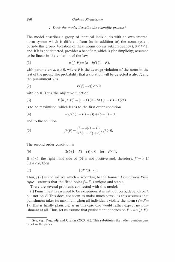
1 Does the model describe the scientific process?

The model describes a group of identical individuals with an own internalnorm system which is different from (or in addition to) the norm systemoutside this group. Violation of these norms occurs with frequency f, 0� f� 1,and, if it is not detected, provides a benefit u, which is (for simplicity) assumedto be linear in the violation of the law,

u ( f, F )= (a+ bf ) (1�F ),(1)

with parameters a, b> 0, where F is the average violation of the norm in therest of the group. The probability that a violation will be detected is also F, andthe punishment v is

v ( f )= cf, c> 0(2)

with c> 0. Thus, the objective function

E [u ( f, F)]= (1� f ) (a+ bf ) (1�F )� f (cf )(3)

is to be maximised, which leads to the first order condition

�2f (b(1�F )+ c))+ (b� a)= 0,(4)

and to the solution

f*(F)=ðb� aÞð1� FÞ2ðbð1� FÞ þ cÞ , f*� 0.(5)

The second order condition is

�2(b (1�F)+ c))< 0 for F� 1.(6)

If a� b, the right hand side of (5) is not positive and, therefore, f*= 0. If0� a< b, then

j df*/dF j< 1(7)

Thus, f ( · ) is contractive which – according to the Banach Contraction Prin-ciple – ensures that the fixed point f=F is unique and stable.1

There are several problems connected with this model:(i) Punishment is assumed to be exogenous, it is without costs, depends on f,

but not on F. This does not seem to make much sense, as this assumes thatpunishment takes its maximum when all individuals violate the norm ( f=F=

1). This is hardly plausible, as in this case one would rather expect no pun-ishment at all. Thus, let us assume that punishment depends on F, v= v ( f, F ).

1 See, e.g., Dugundji and Granas (2003, 9f.). This substitutes the rather cumbersomeproof in the paper.

Gebhard Kirchg�ssner280

The more a law is violated, the smaller is usually punishment, @v( f, F)/@F< 0.There are many cases where behaviour, which originally was strictly forbiddenand, if detected, severely punished, was legalised when it became common.This holds, e.g., for abortion, but in some cases also for consumption of illegaldrugs. Thus, a reasonable assumption is v( f, 1)= 0, i.e. if all members of agroup violate the norm, there is no punishment at all. Assuming a similarrelation as in the utility function, the punishment function might be written as

v ( f, F)= cf · (1�F),(8)

with c� 0. The solution of this model is

f*=b� a

2 ðbþ cÞ ,(9)

which makes the optimal norm-violating behaviour independent of thebehaviour of the rest of the group. The reason for this is that the utility as wellas the punishment depend in the same way on the frequency with which theothers violate the norm. To come to a solution where the norm violatingbehaviour depends on the behaviour of others, we would need two different(plausible) functional forms of how the utility from violating the norm as wellas the punishment if such a behaviour is detected depend on the averagefrequency of violation.2

(ii) Punishment has costs and benefits. Pointing to the norm violation ofothers might increase the own reputation, but also demands resources and,what may be more important, can produce enemies. But if it reduces theirutility, why should people punish others? This, at least, is not consistent withthe primitives of neo-classical theory which are the basis of this model.

On the other hand, modern behavioural economics has shown that there arepeople who take the costs and punish others, even if it is costly.3 Theirbehaviour is essential to ensure that norms are observed within a societywhich are not sanctioned in a formal way (e.g., by penalties through thejudicial system). However, not all individuals behave in this way. There are�altruists�, who behave in this way, but also �egoists� who follow the classicaleconomic assumptions. Thus, to describe the equilibrium outcome of thisgame we have to distinguish (at least) two kinds of individuals; a modelassuming identical individuals is hardly able to correctly describe the scientificgame.

2 One might also question why the utility from strictly following the norm, a, dependson the behaviour of others and is zero whenever all violate the law. However, makingthis utility independent which implies setting a= 0 and including a constant into theutility function (3) would not change the character of the solution.

3 See, e.g., Fehr and G�chter (2002).

Is It a Gang or the Scientific Community? 281

(iii) Finally, which are the norms or rules to be observed? And howautonomous are scientists in setting these rules? We can distinguish threekinds of rules:a) Basic rules, like the rules of logic, or the norm that experimental results

should be reported correctly.b) Rules which constitute the hard core of the paradigm (or of a scientific

research programme).c) Rules which belong to the security belt of the research programme.

The model applies only to the basic rules (a). These are the ones whereindividuals try to hide their violations and where punishment is to be expectedif these violations become public. Rules which belong to the security (c) beltmay, on the other hand, be suspended at any time without major con-sequences. The perhaps most interesting rules are those which constitute thehard core (b). In neoclassical economics, these rules, e.g., demand basingtheoretical models on the primitives of this theory. Violations of these rulesare punished, but the violators do not try to hide them. Just the contrary is thecase: to reach the benefit of the violation it is necessary that the violationsbecome public. If the violators are successful, this might lead to a change ofthe paradigm in the long-run and to scientific reputation. These violationsmight be seen as risky investments into the own future scientific reputation.

Though the model in the paper does not apply to these rules, the paper alsodeals with them. And this is reasonable, as violations of these rules are often aprecondition for scientific progress. But this aspect is not discussed in thepaper.

Thus, this model covers only part of the norms of the scientific process,perhaps not even the most relevant ones. It is just a model of norm-violatingbehaviour which could be applied in the same way (or perhaps even better) toany other group with an internal norm system and, therefore, also to a gang ofcriminals. Insofar, it is of very limited value for understanding the scientificprocess, and it is at least debatable whether it really covers the essentials ofthis process. From a perhaps somewhat nave point of view, the objective ofscience is the generation of true statements about reality. This holds, despitethe fact that we can never be sure that a scientific statement is true. A modelwhich describes the scientific process should – at least in my opinion – givereference to it. This would also distinguish it from a model of a criminal gang.

2 Is game theory unavoidable to understand the scientific process?

Even if this model does meet the essentials of the scientific process, it can beasked whether the game theoretic approach is really “unavoidable forunderstanding many features of science” (p. 265). Obviously, science is an

Gebhard Kirchg�ssner282

interactive game played in a community which has a set of rules which theactors more or less obey. Thus, the language of game theory can be used fordescribing this process. It is true, that the system of rules of the scientificcommunity “will be stable if and only if it constitutes a Nash equilibrium, i.e. ifunder the assumption that the others obey the norms, anyone�s best option isalso to obey” (p. 272). But is this sufficient to proof that there is an addedvalue in applying game theory? Is then, therefore, each application of theeconomic model of behaviour to human interaction an application of gametheory?

According to my opinion, to be justified, the application of game theoreticconcepts should give more and new insights in addition to what we alreadyknow. The idea which is behind the definition of an equilibrium given above ismuch older than the formal treatment by Nash (1950), and has been appliedlong before by economists.4 Moreover, one of the basic characteristics of thescientific process is that it is never in equilibrium and that its rules are per-manently changed. This raises the question whether the concept of a Nash-equilibrium is well suited to describe the core characteristics of the scientificprocess. Would not (at least) a model of a dynamic game be necessary?

As mentioned in the introduction, in the first parts the paper provides manyinteresting details of and insights into the scientific process. However, this isquite independent of the use of the language of game theory. It is to hope thatgame theory, when used for analysing the scientific process, can provide newinsights in the future, and taking this paper as a first attempt, we shouldperhaps not be too critical. Nevertheless, this paper does not provide suchinsights; it presents game theory as a new rhetoric or language game of con-cepts we have known before. Consequently, this paper will hardly convinceany non-economist (or non-game-theorist) of the usefulness of the gametheoretic language game.

References

Fehr, E., and S. G�chter (2002), “Altruistic Punishment in Humans”, Nature, 415, 137 –140.

Dugundji, J., and A. Granas (2003), Fixed Point Theory, New York: Springer.Keynes , J. M. (1936), The General Theory of Employment, Interest, and Money, London:

Macmillan.Nash, J. F. (1950), “The Bargaining Problem”, Econometrica, 18, 155 – 162.Tobin, J. (1997), “An Overview of the General Theory”, 3 – 40, in: G. C. Harcourt and

P. A. Riach (eds), A �Second Edition� of the General Theory, Vol. II, London and NewYork: Routledge.

4 This concept has, e.g., been applied in the first book of theGeneral Theory of Keynes(1936). See for this Tobin (1997, 17).

Is It a Gang or the Scientific Community? 283

Distributed Cognition:A Perspective from Social Choice Theory

by

Christ i an List*

1 Introduction

�Distributed cognition� refers to processes with two properties. First, they arecognitive, i.e. they involve forming certain representations of the world. Sec-ond, they are not performed by a single (human) agent, but are distributedacross multiple (human) agents or (technical) devices. Distributed cognitionhas attracted interest in several fields, ranging from law (e.g., jury decisionmaking) and sociology (e.g. information processing in organizations) tocomputer science (e.g., GRID computing) and the philosophy of science (e.g.,expert panels).

An influential account of distributed cognition is Hutchins�s (1995) study ofnavigation on a US Navy ship. Hutchins describes the ship�s navigation as aprocess of distributed cognition. It is a cognitive process in that it leads torepresentations of the ship�s position and movements in its environment. It isdistributed in that there is no single individual on the ship who performs thecomplex navigational task alone, but the task is performed through theinteraction of many individuals, together with technical instruments. At anygiven time, no single individual may be fully aware of the navigational processin its entirety. Thus, on Hutchins�s account, the ship�s navigation is performednot at the level of a single individual – a �chief navigator� – but at the level of alarger system.

In the philosophy of science, Giere (2002) argues that many scientificpractices, especially large-scale collaborative research practices, involve dis-tributed cognition, as these practices are “situation[s] in which one or moreindividuals reach a cognitive outcome either by combining individualknowledge not initially shared with the others or by interacting with artefactsorganized in an appropriate way (or both)” (2002, 641). He distinguishesbetween �distributed� and �collective� cognition, where the first is more gen-

* Although earlier versions of this paper were presented at seminars at the AustralianNational University, the London School of Economics and the University of Liverpool in2003, this revised version draws substantially on related technical material in List(2005b), but offers a different interpretation of this material. I am grateful to the seminarparticipants at these occasions and particularly the organizers and participants of the 24th

Conference on New Political Economy in Saarbr�cken, October 2005, for comments andsuggestions. I especially thank Max Albert and Siegfried Berninghaus for their helpfulcomments.

eral than the second. Distributed cognition includes not only cases of col-lective cognition, where a cognitive task is distributed across multipleindividuals, but also cases where such a task is distributed between a singleindividual and an artifact, such as a technical instrument.1 While researchersoften compete with one another, collectively distributed cognition is a phe-nomenon associated with more cooperative practices within research groupsor communities.

Knorr Cetina (1999) provides a case study of distributed cognition in sci-ence. Studying high-energy physics research at the European Center forNuclear Research (CERN), she observes that experiments, which lead tocognitive outcomes, involve many researchers and technicians, using complextechnical devices, with a substantial division of labour, expertise, andauthority. She describes this research practice as “something like distributedcognition” (25, cited in Giere 2002).2

Other instances of distributed cognition in science can be found in multi-member expert committees. For example, in 2000, the National AssessmentSynthesis Team, an expert committee commissioned by the US GlobalChange Research Program with members from governments, universities,industry and non-governmental organizations, presented a report on climatechange.3 Such a committee�s work is cognitive in that it involves the repre-sentation of certain facts about the world; and it is distributed in that itinvolves a division of labour between multiple committee members and apooling of different expertise and judgments. Here it may be more plausible toascribe authorship of the report to the committee as a whole rather than anyparticular committee member.

In this paper, I discuss collectively distributed cognition from the per-spective of social choice theory. Social choice theory can provide a generaltheory of the aggregation of multiple (individual) inputs into single (collec-tive) outputs, although it is usually applied to the aggregation of preferences.Drawing on social-choice-theoretic models from the emerging theory ofjudgment aggregation (e.g., List and Pettit 2002, 2004; Pauly and van Hees2005; Dietrich 2005; Bovens and Rabinowicz 2005; List 2005a, 2005b, 2006), Iaddress two questions. First, how can we model a group of individuals as a

1 Collective cognition is “[a] special case of distributed cognition, in which two ormore individuals reach a cognitive outcome simply by combining individual knowledgenot initially shared with others” (Giere 2002, 641).

2 Knorr Cetina also studies research practices in molecular biology, but argues thathere research is more individualized than in high energy physics and “the person remainsthe epistemic subject” (217, cited in Giere 2002). Giere (2002, especially 643) respondsthat, while there may be less collective cognition in molecular biology than in high energyphysics, there may still be distributed cognition, “where the cognition is distributedbetween an individual person and an instrument”.

3 The title of the report is “Climate Change Impacts on the United States: ThePotential Consequences of Climate Variability and Change”. See http://www.usgcrp.gov/.

Christian List286

distributed cognitive system? And, second, can a group acting as a distributedcognitive system be rational and track the truth in its cognitive outputs?

I argue that a group�s performance as a distributed cognitive systemdepends crucially on its organizational structure, and a key part of thatorganizational structure is the group�s �aggregation procedure�, as defined insocial choice theory. An �aggregation procedure� is a mechanism a multi-member group can use to combine (�aggregate�) the judgments or repre-sentations held by the individual group members into judgments or repre-sentations endorsed by the group as a whole. I investigate the ways in which agroup�s aggregation procedure affects its capacity to be rational and to trackthe truth in the outputs it produces as a distributed cognitive system.

My discussion is structured as follows. I begin with some introductoryremarks about modelling a group as a distributed cognitive system in section 2and introduce the concept of an aggregation procedure in section 3. The coreof my discussion consists of sections 4 and 5, in which I discuss a group�scapacity to be rational and to track the truth in its cognitive outputs,respectively. In section 6, I draw some conclusions.

2 Modelling a group as a distributed cognitive system

When does it make sense to consider a group of individuals as a distributedcognitive system rather than a mere collection of individuals? First, the groupmust count as a well-demarcated system, and, second, it must count as asystem that produces cognitive outputs.

The first condition is met if and only if the group�s collective behaviour issufficiently integrated. A well organized expert panel, a group of scientificcollaborators or the monetary policy committee of a central bank, forexample, may have this property, whereas a random crowd of people atLondon�s Leicester Square lacks the required level of integration. And thesecond condition is met if and only if the group is capable of producingoutputs that have representational content; let me call these outputs �collec-tive judgments�. If a group�s organizational structure – e.g. its procedures forgenerating a joint report – allows the group to make certain joint declarationsthat count as collective judgments, then the group has this property, whereas agroup without any formal or informal organization, such as a random crowd atLeicester Square, lacks the required capacity.

At first sight, we may be reluctant to attribute judgments to groups over andabove their individual members. But, as Goldman (2004, 12) has noted, inordinary language, groups or collective organizations are often treated assubjects for the attribution of judgments. Goldman�s example is the recentdebate on what the FBI as a collective organization did or did not “know”prior to the terrorist attacks of 9/11. In addition to the literature on distributed

Distributed Cognition 287

cognition, there is now a growing literature in philosophy that considersconditions under which groups are sufficiently integrated to produce outputsthat we normally associate with rational agency (e.g., Rovane 1998; Pettit2003; List and Pettit 2005a, 2005b). Roughly, a sufficient level of integration isgiven in those cases in which it is pragmatically and explanatorily useful todescribe the group�s outputs in intentional terms (Dennett 1987), namely asthe group�s �beliefs�, �judgments�, �commitments� or �knowledge�. Arguably,this condition is satisfied by those groups that Hutchins, Giere, Knorr-Cetinaand others have described as distributed cognitive systems.

In short, a necessary condition for distributed cognition in a group is thepresence of an organizational structure that allows the group to producecollective judgments, i.e., collective outputs with representational content.Once this necessary condition is met, the group�s performance as a distributedcognitive system depends on the nature of that organizational structure.

Consequently, to construct a model of a group as a distributed cognitivesystem, we need to represent not only the individual group members, but alsothe group�s organizational structure. In the next section, I illustrate how wecan think about this organizational structure in terms of a simple social-choice-theoretic model.

3 The concept of an aggregation procedure

How can we think about a group�s organizational structure? Let me introducethe concept of an �aggregation procedure� to represent (a key part of) agroup�s organizational structure. As defined in the theory of judgmentaggregation (List and Pettit 2002, 2004; List 2006), an aggregation procedureis a mechanism by which a group can generate collective judgments on thebasis of the group members� individual judgments (illustrated in table 1).Formally, an aggregation procedure is a function which assigns to each com-bination of individual judgments across the group members a correspondingset of collective judgments. A simple example is �majority voting�, whereby agroup judges a given proposition to be true whenever a majority of groupmembers judges it to be true. Below I discuss several other aggregationprocedures.

Of course, an aggregation procedure captures only part of a group�sorganizational structure (which may be quite complex), and there are alsomultiple ways (both formal and informal ones) in which a group mightimplement such a procedure. Nonetheless, as argued below, aggregationprocedures are key factors in determining a group�s performance as a dis-tributed cognitive system.

In the next section, I ask what properties a group�s aggregation proceduremust have for the group to be rational as a distributed cognitive system –

Christian List288

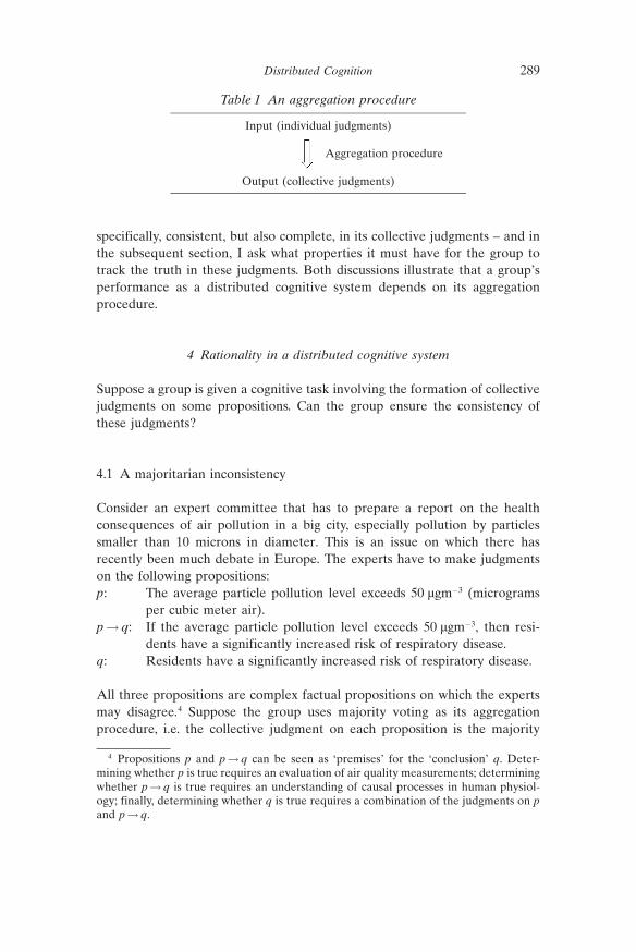
specifically, consistent, but also complete, in its collective judgments – and inthe subsequent section, I ask what properties it must have for the group totrack the truth in these judgments. Both discussions illustrate that a group�sperformance as a distributed cognitive system depends on its aggregationprocedure.

4 Rationality in a distributed cognitive system

Suppose a group is given a cognitive task involving the formation of collectivejudgments on some propositions. Can the group ensure the consistency ofthese judgments?

4.1 A majoritarian inconsistency

Consider an expert committee that has to prepare a report on the healthconsequences of air pollution in a big city, especially pollution by particlessmaller than 10 microns in diameter. This is an issue on which there hasrecently been much debate in Europe. The experts have to make judgmentson the following propositions:p: The average particle pollution level exceeds 50 mgm�3 (micrograms

per cubic meter air).p! q: If the average particle pollution level exceeds 50 mgm�3, then resi-

dents have a significantly increased risk of respiratory disease.q: Residents have a significantly increased risk of respiratory disease.

All three propositions are complex factual propositions on which the expertsmay disagree.4 Suppose the group uses majority voting as its aggregationprocedure, i.e. the collective judgment on each proposition is the majority

Table 1 An aggregation procedure

Input (individual judgments)

Aggregation procedure

Output (collective judgments)

4 Propositions p and p!q can be seen as �premises� for the �conclusion� q. Deter-mining whether p is true requires an evaluation of air quality measurements; determiningwhether p! q is true requires an understanding of causal processes in human physiol-ogy; finally, determining whether q is true requires a combination of the judgments on pand p!q.


judgment on that proposition, as defined above. Now suppose the experts�individual judgments are as shown in table 2.

Then a majority of experts judges p to be true, a majority judges p! q to betrue, and yet a majority judges q to be false, an inconsistent collective set ofjudgments. The expert committee fails to be rational in the collective judg-ments it produces as a distributed cognitive system.

This problem – sometimes called a �discursive dilemma� – illustrates that,under the initially plausible aggregation procedure of majority voting, a groupacting as a distributed cognitive system may not achieve consistent collectivejudgments even when all group members hold individually consistent judg-ments (Pettit 2001; List and Pettit 2002, 2004; List 2006; the problem originallygoes back to the so-called �doctrinal paradox� first identified by Kornhauserand Sager 1986).

Is the present example just an isolated artefact, or can we learn somethingmore general from it?

4.2 An impossibility theorem

Consider again any group of two or more individuals that is given the cog-nitive task to form collective judgments on a set of non-trivially inter-connected propositions, as in the expert committee example.5 Call an agent�sjudgments on these propositions �complete� if, for each proposition-negationpair, the agent judges either the proposition or its negation to be true; and call

Table 2 A majoritarian inconsistency

p p! q q

Individual 1 True True TrueIndividual 2 True False FalseIndividual 3 False True FalseMajority True True False

5 Following List [2006], a set of propositions is �non – trivially interconnected� if it is ofone of the following forms (or a superset thereof): (i) it includes k> 1 propositions p1, ...,pk and either their conjunction �p1 and ... and pk� or their disjunction �p1 or p2 or ... or pk�or both (and the negations of all these propositions); (ii) it includes k> 1 propositions p1,..., pk, another proposition q and either the proposition �q if and only if (p1 and ... and pk)�or the proposition �q if and only if (p1 or p2 or ... or pk)� or both (and negations); (iii) itincludes propositions p, q and p!q (and negations).

Christian List290

these judgments �consistent� if the set of propositions judged to be true by theagent is a consistent set in the standard sense of propositional logic.6

Suppose now that each individual holds complete and consistent judgmentson these propositions, and that the collective judgments are also required tobe complete and consistent. One can then prove the following impossibilityresult (for a discussion of parallels and disanalogies between this result andArrow�s (1951) classical theorem, see List and Pettit 2004 and Dietrich andList 2005a).

Theorem (List and Pettit 2002). There exists no aggregation proceduregenerating complete and consistent collective judgments that satisfies thefollowing three conditions simultaneously:

Universal domain. The procedure accepts as admissible input any logicallypossible combinations of complete and consistent individual judgments on thepropositions.

Anonymity. The judgments of all individuals have equal weight in deter-mining the collective judgments.

Systematicity. The collective judgment on each proposition depends only onthe individual judgments on that proposition, and the same pattern ofdependence holds for all propositions.

In short, majority voting is not the only aggregation procedure that runsinto problems like the one illustrated in table 2 above. Any procedure sat-isfying universal domain, anonymity and systematicity does so. If these con-ditions are regarded as indispensable requirements on an aggregation pro-cedure, then one has to conclude that a multi-member group acting as adistributed cognitive system cannot ensure the rationality of its collectivejudgments. But this conclusion would be too quick. The impossibility theoremshould be seen as characterizing the logical space of aggregation procedures(List and Pettit 2002; List 2006). In particular, we can characterize differentaggregation procedures in terms of which conditions they meet and whichthey violate.

If a group acting as a distributed cognitive system seeks to ensure therationality of its collective judgments, the group must use an aggregationprocedure that violates at least one of the conditions of the theorem.

4.3 First solution: relaxing universal domain

If the amount of disagreement in a particular group is limited or if the grouphas mechanisms in place for reducing disagreement – such as mechanisms ofgroup deliberation – the group might use an aggregation procedure that

6 This consistency notion is stronger than that in List and Pettit (2002). But when thepresent consistency notion is used, no deductive closure requirement needs to be added.


violates universal domain. For example, a deliberating group that successfullyavoids combinations of individual judgments of the kind in table 2 might usemajority voting as its aggregation procedure and yet generate rational col-lective judgments.

But this solution does not work in general. Even in an expert committeewhose task is to make judgments on factual matters without conflicts ofinterest, disagreement may still be significant and pervasive. Although onecan study conditions that make the occurrence of judgment combinations ofthe kind in table 2 less likely (Dryzek and List 2003; List 2002), I set this issueaside here and assume that groups that are faced with primarily cognitivetasks (as opposed to primarily political ones, for example) should normallyuse aggregation procedures satisfying universal domain.

4.4 Second solution: relaxing anonymity

It can be shown that, if anonymity is relaxed but the other two conditions areretained, the only possible aggregation procedure is a �dictatorial procedure�,whereby the collective judgments are always those of some antecedently fixedgroup member (the �dictator�) (Pauly and van Hees 2005). Some groups mightput one individual – say a committee chair – in charge of forming its collectivejudgments. But this solution clearly conflicts with the idea of collectivelydistributed cognition, and as discussed below, a group organized in this dic-tatorial way loses out on the epistemic advantages of distributed cognition.

However, below I also suggest that a group acting as a distributed cognitivesystem may sometimes benefit from relaxing anonymity together with sys-tematicity and implementing a division of cognitive labour whereby differentcomponents of a complex cognitive task are allocated to different subgroups.

4.5 Third solution: relaxing systematicity

A potentially promising solution lies in relaxing systematicity, i.e., treatingdifferent propositions differently in the process of forming collective judg-ments. For the purposes of a given cognitive task, a group may designate somepropositions as �premises� and others as �conclusions� and assign epistemicpriority either to the premises or to the conclusions (for a more extensivediscussion of this process, see List 2006).

If the group assigns priority to the premises, it may use the so-called�premise – based procedure�, whereby the group first makes a collectivejudgment on each premise by taking a majority vote on that premise and thenderives its collective judgments on the conclusions from these collectivejudgments on the premises. In the expert committee example, propositions p

Christian List292

and p! qmight be designated as premises (perhaps on the grounds that p andp! q are more basic than q), and proposition q might be designated as aconclusion. The committee might then take majority votes on p and p! q andderive its judgment on q from its judgments on p and p! q.7

Alternatively, if the group assigns priority to the conclusions, it may use theso-called �conclusion – based procedure�, whereby the group takes a majorityvote only on each conclusion and makes no collective judgments on thepremises. In addition to violating systematicity, this aggregation procedurefails to produce complete collective judgments. But sometimes a group isrequired to make judgments only on conclusions, but not on premises, and insuch cases incompleteness in the collective judgments on the premises may bedefensible.

The premise- and conclusion-based procedures are not the only aggregationprocedures violating systematicity. Further important possibilities arise whenboth systematicity and anonymity are relaxed. The group can then use anaggregation procedure that not only assigns priority to the premises, but alsoassigns different such premises to different subgroups and thereby implementsa particularly clear form of distributed cognition. Specifically, the group mayuse the so-called �distributed premise-based procedure�. Here differentindividuals specialize on different premises and give their individual judg-ments only on these premises. Now the group makes a collective judgment oneach premise by taking a majority vote on that premise among the relevant�specialists�, and then the group derives its collective judgments on the con-clusions from these collective judgments on the premises. This procedure isdiscussed in greater detail below.

For many cognitive tasks performed by groups, giving up systematicity andusing a (regular or distributed) premise-based or conclusion-based proceduremay be an attractive way to avoid the impossibility result explained above.Each of these procedures allows a group to produce rational collectivejudgments. Arguably, a premise-based or distributed premise-based proceduremakes the group�s performance as a unified cognitive system particularlyvisible. A group using such a procedure acts as a reason-driven system when itderives its collective judgments on conclusions from its collective judgmentson relevant premises.

However, giving up systematicity comes with a price. Aggregation proce-dures that violate systematicity may be vulnerable to manipulation by pri-oritizing propositions strategically, and strategic agents with agenda-settinginfluence over the group might exploit these strategic vulnerabilities.

7 In the present example, the truth-value of q is not always settled by the truth-valuesof p and p!q; so the group may need to stengthen its premises in order to make themsufficient to determine its judgment on the conclusion.


For example, in the case of a regular premise-based procedure, the collec-tive judgments may be sensitive to the choice of premises. In the example oftable 2, if p and p! q are designated as premises, then all three propositions,p, p!q and q, are collectively judged to be true. If p and q are designated aspremises, then p is judged to be true and both q and p! q are judged to befalse; finally, if q and p! q are designated as premises, then p! q is judged tobe true, and both p and q are judged to be false. Although there seems to be anatural choice of premises in the present example, namely p and p! q, thismay not generally be the case, and the outcome of a premise-based proceduremay therefore depend as much on the choice of premises as it depends on theindividual judgments to be aggregated. In the present example, an environ-mental activist may prefer to prioritize the propositions in such a way as tobring about the collective judgment that proposition q is true, while a trans-port lobbyist may prefer to prioritize them in such a way as to bring about theopposite judgment on q.

Under the distributed premise-based procedure, an additional sensitivity tothe choice of �specialists� on each premise arises. Likewise, in the case of theconclusion-based procedure, the choice of conclusions obviously matters,since the group makes collective judgments only on these conclusions and onno other propositions.8

4.6 Fourth solution: permitting incomplete collective judgments

The first three solutions proposed in response to the impossibility theoremabove have required relaxing one of the three minimal conditions on howindividual judgments are aggregated into collective judgments. The presentsolution preserves these minimal conditions, but weakens the requirements onthe collective judgments themselves by permitting incompleteness in thesejudgments (see also List 2006).

If a group acting as an overall cognitive system is prepared to refrain frommaking a collective judgment on some propositions – namely on those onwhich there is too much disagreement between the group members – then itmay use an aggregation procedure such as the �unanimity procedure�, wherebythe group makes a judgment on a proposition if and only if the group mem-bers unanimously endorse that judgment. Propositions judged to be true by allmembers are collectively judged to be true; and ones judged to be false by allmembers are collectively judged to be false; no collective judgment is madeon any other propositions. (Instead of the unanimity procedure, the group

8 It can be shown that in some important respects, the premise-based procedure ismore vulnerable to strategic manipulation than the conclusion-based procedure. SeeDietrich and List (2005b).

Christian List294

might also use �supermajority voting� with a sufficiently large supermajoritythreshold.)

Groups operating in a strongly consensual manner may well opt for thissolution, but in many cases making no judgment on some propositions issimply not an option. For example, when an expert committee is asked to giveadvice on a particular issue, it is usually expected to take a determinate stanceon that issue.

4.7 Lessons to be drawn

I have shown that a group�s capacity to form rational collective judgmentsdepends on the group�s aggregation procedure: a group acting as a distributedcognitive system can ensure the rationality of its collective judgments on somenon-trivially interconnected propositions only if it uses a procedure thatviolates one of universal domain, anonymity or systematicity or that producesincomplete collective judgments. Moreover, different aggregation proceduresmay lead to different collective judgments for the same combination ofindividual judgments. As an illustration, table 3 shows the collective judg-ments for the individual judgments in table 2 under different aggregationprocedures.

If we were to assess a group�s performance as a distributed cognitive systemsolely on the basis of whether the group�s collective judgments are rational,this would give us insufficient grounds for selecting a unique aggregationprocedure. As I have illustrated, many different aggregation proceduresgenerate consistent collective judgments, and even if we require completenessin addition to consistency, several possible aggregation procedures remain. To

Table 3 Different aggregation procedures applied to the individual judgmentsin table 2

p p! q q

Majority voting* True True FalsePremise-based procedure with p,p! q as premises

True True True

Conclusion-based procedure with qas conclusion

No judgment No judgment False

Distributed premise-based procedurewith individual 1 specializing on pand individual 2 specializing on p! q

True False False

Unanimity procedure No judgment No judgment No judgmentDictatorship of individual 3 False True False

* inconsistent


recommend a suitable aggregation procedure that a group can use for a givencognitive task, the question of whether the group produces rational collectivejudgments is, by itself, not a sufficient criterion.

5 Truth-tracking in a distributed cognitive system

Can a group acting as a distributed cognitive system generate collectivejudgments that track the truth? Following Nozick (1981), a system �tracks thetruth� on some proposition p if two conditions are met. First, if – actually orcounterfactually – p were true, the system would judge p to be true. Second, if– actually or counterfactually – p were not true, the system would not judge pto be true. These conditions can be applied to any cognitive system, whether itconsists just of a single agent or of multiple agents acting together. In par-ticular, if a group�s organizational structure allows the group to form collec-tive judgments, then one can ask whether these judgments satisfy Nozick�s twoconditions.

As a simple measure of how well a system satisfies Nozick�s two conditions,I consider two conditional probabilities (List 2006): the probability that thesystem judges p to be true given that p is true, and the probability that thesystem does not judge p to be true given that p is false. Call these two con-ditional probabilities the system�s �positive� and �negative reliability� on p,respectively.

By considering a group�s positive and negative reliability on various prop-ositions under different aggregation procedures and different scenarios, I nowshow that it is possible for a group acting as a distributed cognitive system totrack the truth, but that, once again, the aggregation procedure affects thegroup�s success.

5.1 The first scenario and its lesson: epistemic gains from democratization

Suppose that a group is given the cognitive task of making a collectivejudgment on a single factual proposition, such as proposition p in the expertcommittee example above. As a baseline scenario (e.g., Grofman, Owen andFeld 1983), suppose that the group members hold individual judgments onproposition p, where two conditions are met. First, each group member hasthe same positive and negative reliability r on proposition p, where 1> r> 1/2(the �competence� condition); so individual judgments are noisy but biasedtowards the truth. Second, the judgments of different group members aremutually independent (the �independence� condition). (Obviously, it is also

Christian List296

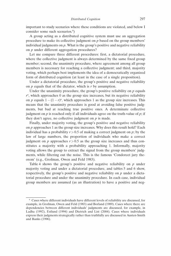
important to study scenarios where these conditions are violated, and below Iconsider some such scenarios.9)

A group acting as a distributed cognitive system must use an aggregationprocedure to make its collective judgment on p based on the group members�individual judgments on p. What is the group�s positive and negative reliabilityon p under different aggregation procedures?

Let me compare three different procedures: first, a dictatorial procedure,where the collective judgment is always determined by the same fixed groupmember; second, the unanimity procedure, where agreement among all groupmembers is necessary for reaching a collective judgment; and third, majorityvoting, which perhaps best implements the idea of a democratically organizedform of distributed cognition (at least in the case of a single proposition).

Under a dictatorial procedure, the group�s positive and negative reliabilityon p equals that of the dictator, which is r by assumption.Under the unanimity procedure, the group�s positive reliability on p equals

rn, which approaches 0 as the group size increases, but its negative reliabilityon p equals 1� (1� r)n, which approaches 1 as the group size increases. Thismeans that the unanimity procedure is good at avoiding false positive judg-ments, but bad at reaching true positive ones. A determinate collectivejudgment on p is reached only if all individuals agree on the truth-value of p; ifthey don�t agree, no collective judgment on p is made.

Finally, under majority voting, the group�s positive and negative reliabilityon p approaches 1 as the group size increases. Why does this result hold? Eachindividual has a probability r> 0.5 of making a correct judgment on p; by thelaw of large numbers, the proportion of individuals who make a correctjudgment on p approaches r> 0.5 as the group size increases and thus con-stitutes a majority with a probability approaching 1. Informally, majorityvoting allows the group to extract the signal from the group members� judg-ments, while filtering out the noise. This is the famous �Condorcet jury the-orem� (e.g., Grofman, Owen and Feld 1983).

Table 4 shows the group�s positive and negative reliability on p undermajority voting and under a dictatorial procedure, and tables 5 and 6 show,respectively, the group�s positive and negative reliability on p under a dicta-torial procedure and under the unanimity procedure. In each case, individualgroup members are assumed (as an illustration) to have a positive and neg-

9 Cases where different individuals have different levels of reliability are discussed, forexample, in Grofman, Owen and Feld (1983) and Borland (1989). Cases where there aredependencies between different individuals� judgments are discussed, for example, inLadha (1992), Estlund (1994) and Dietrich and List (2004). Cases where individualsexpress their judgments strategically rather than truthfully are discussed in Austen-Smithand Banks (1996).


Table 4 The group�s positive and negative reliability on p: majority voting (topcurve); dictatorship (bottom curve) (setting r = 0.54 as an illustration)

Table 5 The group�s positive reliability on p: dictatorship (top curve);unanimity procedure (bottom curve) (setting r = 0.54 as an illustration)

Christian List298

ative reliability of r= 0.54 on p. In all tables, the group size is on the horizontalaxis and the group�s reliability on the vertical axis.10

What lessons can be drawn from this first scenario? If individuals areindependent, fallible, but biased towards the truth, majority voting outper-forms both dictatorial and unanimity procedures in terms of maximizing thegroup�s positive and negative reliability on p. The unanimity procedure isattractive only in those special cases where the group seeks to minimize therisk of making false positive judgments, such as in some jury decisions. Adictatorial procedure fails to pool the information held by different individ-uals.

Hence, when a group acting as a distributed cognitive system seeks to trackthe truth, there may be �epistemic gains from democratization�, i.e. frommaking a collective judgment on a given proposition democratically by usingmajority voting. More generally, even when individual reliability differsbetween individuals, a weighted form of majority voting still outperforms adictatorship by the most reliable individual: each individual�s vote simply

Table 6 The group�s negative reliability on p: unanimity procedure (top curve);dictatorship (bottom curve) (setting r = 0.54 as an illustration)

10 The present curves are the result of averaging between two separate curves foreven- and odd-numbered group sizes. When the group size is an even number, thegroup�s reliability may be lower because of the possibility of majority ties.


needs to have a weight proportional to log(r/(1� r)), where r is the individ-ual�s reliability on the proposition in question (Ben-Yashar and Nitzan 1997).

5.2 The second scenario and its lesson: epistemic gains from disaggregation

Suppose now that a group is given the cognitive task of making a collectivejudgment not only on a single factual proposition, but on a set of inter-connected factual propositions. As an illustration, suppose that there are k> 1premises p1, ..., pk and a conclusion q, where q is true if and only if the con-junction of p1, ..., pk is true. This structure also allows representing a variant ofthe expert committee example above. For extensive discussions of the presentscenario and other related scenarios, see Bovens and Rabinowicz (2005) andList (2005a, 2006). Analogous points apply to the case where q is true if andonly if the disjunction of p1, ..., pk is true.

In this case of multiple interconnected propositions, individuals cannotgenerally have the same reliability on all propositions. Suppose, as an illus-tration, that each individual has the same positive and negative reliability r oneach premise p1, ..., pk and makes independent judgments on differentpremises. Then each individual�s positive reliability on the conclusion q is rk,which is below r and often below 0.5 (whenever r< k-th root of 0.5), while hisor her negative reliability on q is above r. Here individuals are much worse atdetecting the truth of the conclusion than the truth of each premise, but muchbetter at detecting the falsehood of the conclusion than the falsehood of eachpremise. In the expert committee example, it might be easier to make correctjudgments on propositions p and p! q than on proposition q. Of course, otherscenarios can also be constructed, but the point remains that individualstypically have different levels of reliability on different propositions (List2006).

What is the group�s positive and negative reliability on the various propo-sitions under different aggregation procedures? As before, suppose thejudgments of different group members are mutually independent.

Majority voting performs well only on those propositions on whichindividuals have a positive and negative reliability above 0.5. As just argued,individuals may not meet this condition on all propositions. Moreover,majority voting does not generally produce consistent collective judgments(on the probability of majority inconsistencies, see List 2005a). Let me nowcompare dictatorial, conclusion-based and premise-based procedures.

Under a dictatorial procedure, the group�s positive and negative reliabilityon each proposition equals that of the dictator; in particular, the probabilitythat all propositions are judged correctly is rk, which may be very low, espe-cially when the number of premises k is large.

Christian List300

Under the conclusion-based procedure, unless individuals have a highreliability on each premise, namely r> k-th root of 0.5 (e.g. 0.71 when k= 2, or0.79 when k= 3), the group�s positive reliability on the conclusion qapproaches 0 as the group size increases. Its negative reliability on qapproaches 1. Like the unanimity procedure in the single-proposition case, theconclusion-based procedure is good at avoiding false positive judgments onthe conclusion, but (typically) bad at reaching true positive ones (see alsoBovens and Rabinowicz 2005).

Under the premise-based procedure, the group�s positive and negativereliability on every proposition approaches 1 as the group size increases. Thisresult holds because, by the Condorcet jury theorem as stated above, thegroup�s positive and negative reliability on each premise p1, ..., pk approaches1 with increasing group size, and therefore the probability that the groupderives a correct judgment on the conclusion also approaches 1 withincreasing group size.

As illustration, suppose that there are k= 2 premises and individuals have apositive and negative reliability of r= 0.54 on each premise. Table 7 shows thegroup�s probability of judging all propositions correctly under the premise-based procedure and under a dictatorial procedure. Tables 8 and 9 show,respectively, the group�s positive and negative reliability on the conclusion qunder a dictatorial procedure and under the conclusion-based procedure.

Table 7 The group�s probability of judging all propositions correctly: premise-based procedure (top curve); dictatorship (bottom curve) (setting r = 0.54 as an

illustration)


Table 8 The group�s positive reliability on the conclusion q: dictatorship (topcurve); conclusion-based procedure (bottom curve) (setting r = 0.54 as an

illustration)

Table 9 The group�s negative reliability on the conclusion q: conclusion-basedprocedure (top curve); dictatorship (bottom curve) (setting r = 0.54 as an

illustration)

Christian List302

What lessons can be drawn from this second scenario? Under the presentassumptions, the premise-based procedure outperforms both dictatorial andconclusion-based procedures in terms of simultaneously maximizing thegroup�s positive and negative reliability on every proposition. Like the una-nimity procedure before, the conclusion-based procedure is attractive onlywhen the group seeks to minimize the risk of making false positive judgmentson the conclusion; again, a dictatorial procedure is bad at information pooling.

Hence, if a larger cognitive task such as making a judgment on some con-clusion can be disaggregated into several smaller cognitive tasks such asmaking judgments on relevant premises, then there may be �epistemic gainsfrom disaggregation�, i.e. from making collective judgments on that conclusionon the basis of separate collective judgments on those premises. (For furtherresults and a discussion of different scenarios, see Bovens and Rabinowicz2005 and List 2006.)

5.3 The third scenario and its lesson: epistemic gains from distribution

When a group is faced with a complex cognitive task that requires makingjudgments on several propositions, different members of the group may havedifferent levels of expertise on different propositions. This is an importantcharacteristic of many committees, groups of scientific collaborators, largeorganizations, and so on. Moreover, each individual may lack the temporal,computational and informational resources to become sufficiently reliable onevery proposition. If we take this problem into account, can we improve onthe premise-based procedure?

Suppose, as before, that a group has to make collective judgments on k> 1premises p1, ..., pk and a conclusion q, where q is true if and only if the con-junction of p1, ..., pk is true. Instead of requiring every group member to makea judgment on every premise, we might partition the group into k subgroups(for simplicity, of approximately equal size), where the members of eachsubgroup specialize on one premise and make a judgment on that premisealone. Instead of a using a regular premise-based procedure as in the previousscenario, the group might now use a distributed premise-based procedure: thecollective judgment on each premise is made by taking a majority vote withinthe subgroup specializing on that premise, and the collective judgment on theconclusion is then derived from these collective judgments on the premises.

When does the distributed premise-based procedure outperform the regularpremise-based procedure at maximizing the group�s probability of makingcorrect judgments on the propositions?

Intuitively, there are two effects here that pull in opposite directions. First,there may be �epistemic gains from specialization�: individuals may becomemore reliable on the proposition on which they specialize. But, second, there


may also be �epistemic losses from lower numbers�: each subgroup voting on aparticular proposition is smaller than the original group (it is only approx-imately 1/k the size of the original group when there are k premises), whichmay reduce the benefits from majoritarian judgment aggregation on thatproposition.

Whether or not the distributed premise-based procedure outperforms theregular premise-based procedure depends on which of these two oppositeeffects is stronger. Obviously, if there were no epistemic gains from special-ization, then the distributed premise-based procedure would suffer only fromlosses from lower numbers on each premise and would therefore performworse than the regular premise-based procedure. On the other hand, if theepistemic losses from lower numbers were relatively small compared to theepistemic gains from specialization, then the distributed premise-based pro-cedure would outperform the regular one. The following result holds:

Theorem. For any group size n (divisible by k), there exists an individual(positive and negative) reliability level r*> r such that the following holds: if,by specializing on some proposition p, individuals achieve a reliability abover* on p, then the majority judgment on p in a subgroup of n/k specialists (eachwith reliability r* on p) is more reliable than the majority judgment on p in theoriginal group of n non-specialists (each with reliability r on p).Hence, if by specializing on one premise, individuals achieve a reliability

above r* on that premise, then the distributed premise-based procedureoutperforms the regular premise-based procedure. How great must the reli-ability increase from r to r* be to have this effect? Strikingly, a small reliabilityincrease typically suffices. Table 10 shows some sample calculations. Forexample, when there are k= 2 premises, if the original individual reliabilitywas r= 0.52, then a reliability above r*= 0.5281 after specialization suffices; itwas r= 0.6, then a reliability above r*= 0.6393 after specialization suffices.

Table 11 shows the group�s probability of judging all propositions correctlyunder regular and distributed premise-based procedures, where there are k=2 premises and where individuals have positive and negative reliabilities of r=0.54 and r*= 0.58 before and after specialization, respectively.

Table 10 Reliability increase from r to r* required to outweigh the loss fromlower numbers

k = 2, n = 50 k = 3, n = 51 k = 4, n = 52

r = 0.52 0.6 0.75 0.52 0.6 0.75 0.52 0.6 0.75r* = 0.5281 0.6393 0.8315 0.5343 0.6682 0.8776 0.5394 0.6915 0.9098

Christian List304

What lessons can be drawn from this third scenario? Even when there areonly relatively modest gains from specialization, the distributed premise-based procedure may outperform the regular premise-based procedure interms of maximizing the group�s positive and negative reliability on everyproposition.

Hence there may be �epistemic gains from distribution�: if a group has toperform a complex cognitive task, the group may benefit from subdividing thetask into several smaller tasks and distributing these smaller tasks acrossmultiple subgroups. Plausibly, such division of cognitive labour is the mech-anism underlying the successes of collectively distributed cognition in science,as investigated by Knorr Cetina (1999), Giere (2002) and others. The researchpractices in large-scale collaborative research projects, such as those in high-energy physics or in other large expert teams as mentioned above, rely onmechanisms similar to those represented, in a stylized form, by the distributedpremise-based procedure.

In conclusion, a group acting as a distributed cognitive system can succeedat tracking the truth, but the group�s aggregation procedure plays an impor-tant role in determining the group�s success.

Table 11 The group�s probability of judging all propositions correctly: dis-tributed (top curve) and regular premise-based procedure (bottom curve)

(setting r = 0.54 and r* = 0.58 as an illustration)


6 Concluding remarks

I have discussed collectively distributed cognition from a social-choice-theo-retic perspective. In particular, I have introduced the emerging theory ofjudgment aggregation to propose a way of modelling a group as a distributedcognitive system, i.e. as a system that can generate collective judgments.Within this framework, I have asked whether such a group can be rational andtrack the truth in its collective judgments. My main finding is that a group�sperformance as a distributed cognitive system depends crucially on itsaggregation procedure, and I have investigated how the aggregation proce-dure matters.

With regard to a group�s rationality as a distributed cognitive system, I havediscussed an impossibility theorem by which we can characterize the logicalspace of aggregation procedures that a group can use to generate rationalcollective judgments. No aggregation procedure generating consistent andcomplete collective judgments can simultaneously satisfy universal domain,anonymity and systematicity. To find an aggregation procedure that producesrational collective judgments, it is therefore necessary to relax one of universaldomain, anonymity or systematicity, or to weaken the requirement of ration-ality itself by permitting incomplete collective judgments. Which relaxation ismost defensible depends on the group and cognitive task in question.

With regard to a group�s capacity to track the truth as a distributed cog-nitive system, I have identified three effects that are relevant to the design of agood aggregation procedure: there may be epistemic gains from democra-tization, disaggregation and distribution. Again, the applicability and magni-tude of each effect depends on the group and cognitive task in question, andthere may not be a �one size fits all� aggregation procedure that is best for allgroups and all cognitive tasks. But the fact that a group may sometimesbenefit from the identified effects reinforces the potential of epistemic gainsthrough collectively distributed cognition.

The present results give a fairly optimistic picture of a group�s capacity toperform as a distributed cognitive system. I have thereby focused on coop-erative rather than competitive practices within groups or communities. It isan important empirical question how pervasive such cooperative practices areand how often the favourable conditions such practices require are met.Clearly, scientific communities are characterized by both competitive andcooperative practices. Much research in the sociology and economics of sci-ence has focused on competitive practices (as evidenced by the theme of the2005 Conference on New Political Economy). There has also been muchresearch on rationality failures and inefficiencies that can arise in groupstrying to perform certain tasks at a collective level. Public choice theorists, inparticular, have highlighted the impossibility results on democratic aggrega-

Christian List306

tion and the pervasiveness of suboptimal equilibria in various collectiveinteractions.

Clearly, the details of my rather more optimistic results depend on variousassumptions and may change with changes in these assumptions. But my aimhas not been to argue that all groups acting as distributed cognitive systemsperform well; indeed, this claim is likely to be false. Rather, my aim has beento show that successful distributed cognition in a group is possible and toillustrate the usefulness of the theory of judgment aggregation for inves-tigating how it is possible and under what conditions.

References

Arrow, Kenneth J. (1951), Social Choice and Individual Values, Wiley: New York.Austen-Smith, David, and Jeffrey Banks (1996), “Information Aggregation, Rationality

and the Condorcet Jury Theorem,” American Political Science Review, 90, 34 – 45.Ben-Yashar, Ruth, and Shmuel Nitzan (1997), “The optimal decision rule for fixed-size

committees in dichotomous choice situations: the general result,” International Eco-nomic Review, 38, 175 – 186.

Borland, Philip (1989), “Majority systems and the Condorcet jury theorem,” Statistician,38, 181 – 189.

Bovens, Luc, and Wlodek Rabinowicz (2005), “Democratic Answers to ComplexQuestions: an Epistemic Perspective,” Synthese, forthcoming.

Dennett, Daniel (1987), The Intentional Stance, MIT Press: Cambridge, MA.Dietrich, Franz (2005), “Judgment aggregation: (im)possibility theorems,” Journal of

Economic Theory, forthcoming.Dietrich, Franz, and Christian List (2004), “A model of jury decisions where all jurors

have the same evidence,” Synthese, 142, 175 – 202.Dietrich, Franz, and Christian List (2005a), “Arrow�s theorem in judgment aggregation,”

Working paper, London School of Economics, London.Dietrich, Franz, and Christian List (2005b), “Strategy-proof judgment aggregation,”

Working paper, London School of Economics, London.Dryzek, John, and Christian List (2003), “Social Choice Theory and Deliberative

Democracy: A Reconciliation,” British Journal of Political Science, 33(1), 1 – 28.Estlund, David (1994), “Opinion leaders, independence and Condorcet�s jury theorem,”

Theory and Decision, 36, 131 – 162.Giere, Ronald (2002), “Distributed Cognition in Epistemic Cultures,” Philosophy of

Science, 69, 637 – 644.Goldman, Alvin (1999), Knowledge in a Social World, Oxford University Press: Oxford.Goldman, Alvin (2004), “Group Knowledge versus Group Rationality: Two Approaches

to Social Epistemology,” Episteme: A Journal of Social Epistemology, 1(1), 11 – 22.Goodin, Robert E. (ed.) (1996), The Theory of Institutional Design, Cambridge Uni-

versity Press: Cambridge.Grofman, Bernard, Guillermo Owen, and Scott Feld (1983), “Thirteen theorems in

search of the truth,” Theory and Decision, 15, 261 – 278.Hutchins, Edwin (1995), Cognition in the Wild, MIT Press: Cambridge, MA.Knorr Cetina, Karin (1999), Epistemic Cultures: How the Sciences Make Knowledge,

Harvard University Press: Cambridge, MA.


Kornhauser, Lewis A., and Lawrence G. Sager (1986), “Unpacking the Court,” Yale LawJournal, 96(1), 82 – 117.

Ladha, Krishna (1992), “The Condorcet jury theorem, free speech and correlated votes,”American Journal of Political Science, 36, 617 – 634.

List, Christian (2002), “Two Concepts of Agreement,” The Good Society, 11(1), 72 – 79.List, Christian (2005a), “The Probability of Inconsistencies in Complex Collective

Decisions,” Social Choice and Welfare, 24(1), 3 – 32.List, Christian (2005b), “Group Knowledge and Group Rationality: A Judgment

Aggregation Perspective,” Episteme: A Journal of Social Epistemology, 2(1), 25 – 38.List, Christian (2006), “The Discursive Dilemma and Public Reason,” Ethics, forth-

coming.List, Christian, and Philip Pettit (2002), “Aggregating Sets of Judgments: An Impossi-

bility Result,” Economics and Philosophy, 18, 89 – 110.List, Christian, and Philip Pettit (2004), “Aggregating Sets of Judgments: Two Impossi-

bility Results Compared,” Synthese, 140(1 – 2), 207 – 235.List, Christian, and Philip Pettit (2005a), “On the Many as One,” Philosophy and Public

Affairs, 33(4), 377 – 390.List, Christian, and Philip Pettit (2005b), “Group Agency and Supervenience,” Southern

Journal of Philosophy, forthcoming.Nozick, Robert (1981), Philosophical Explanations, Harvard University Press: Cam-

bridge, MA.Pauly, Marc, and Martin van Hees (2005), “Logical Constraints on Judgment Aggrega-

tion,” Journal of Philosophical Logic, forthcoming.Pettit, Philip (2001), “Deliberative Democracy and the Discursive Dilemma,” Philo-

sophical Issues (supplement to Nous), 11, 268 – 99.Pettit, Philip (2003), “Groups with Minds of their Own,” in: Fred Schmitt (ed.), Social-

izing Metaphysics, Rowan and Littlefield: New York.Rovane, Carol (1998), The Bounds of Agency: An essay in Revisionary Metaphysics,

Princeton University Press: Princeton.

Christian List308

Distributed Cognition

Comment by

Si egfr i ed K. Berninghaus

1 Brief summary of List�s contribution

From a general point of view the contribution by Christian List is concernedwith such types of social processes which can be called cognitive and dis-tributed. Distributed cognition is not a new field which is applied for the firsttime to problems in social science in this paper. However, more often weobserve ideas of distributed cognition in various and different fields ofresearch, for example in the field of artificial intelligence or distributedcomputing.

To learn some basic facts about distributed cognition, we need not even godeeply into the artificial intelligence literature. In a nutshell, we can observemost aspects and problems of distributed cognition in our university systemitself. In some sense the numerous committees established in universities, forexample, committees on allocating the university budget, or committees onestablishing new studies, can be regarded as expert panels representing dis-tributive intelligence. There is a strong connection of List�s theoretical paperwith practical problems of scientific competition which is the main topic ofthis conference.

In his paper, Christian List discusses distributed cognition from the par-ticular perspective of Social Choice Theory. He basically refers to results ongroup aggregation procedures in judgement aggregation. Such procedures areused to combine individual beliefs and judgements of the members of a groupinto collective beliefs and judgements. We know from the pioneering work byChristian List himself and other authors (see, for example, List and Pettit(2002), List and Pettit (2004), Dietrich and List (2004) that judgementaggregation procedures may suffer from serious inconsistencies in the col-lective decisions, i.e., that a group may not achieve consistent judgementsalthough all group members individually hold consistent beliefs. A famousimpossibility result shows that consistent collective judgements are not pos-sible provided the aggregation procedure satisfies some mild conditions.1

These conditions are universal domain (any logically possible combination ofpersonal sets of judgements is admissible as aggregation input), anonymity(collective set of judgements are invariant under any permutation of theindividuals) and systematicity (collective judgement depends exclusively on

1 There exist some analogies to Arrow�s famous impossibility theorem on the aggre-gation of individual preferences (for details see List and Pettit 2004).

the pattern of individual judgements). In the literature on judgement aggre-gation one can find various strategies to escape from this impossibility result.One strategy could be to give up some of the basic requirements on theaggregation rule or to consider incomplete judgements.

In his paper, List deals with the problem whether collective beliefs orjudgements constitute group knowledge. He considers the positive and neg-ative reliability on propositions under various different aggregation proce-dures and scenarios. Suppose that each group member has a certain degree ofreliability on a factual proposition p.1. In scenario 1, the effect of three different aggregation rules on the groups

reliability on the same factual proposition is investigated.2. In scenario 2, the focus is on the collective judgement on a collection of

interconnected factual propositions.3. Scenario 3 is concerned with gains from specialization which may arise

from splitting up the original group into expert panels who are responsiblefor making judgements only on a small subset of interconnected proposi-tions.

2 Questions and comments

List�s approach to judgement aggregation is an interesting and innovativecontribution to Social Choice. Compared with most papers presented at thisconference, this contribution is rather abstract. However, this may not be adisadvantage at all. Quite to the contrary, this paper contributes substantiallyto basic research in group rationality and, therefore, to basic research in thetheory of scientific competition, too.

2.1 General comments

1. In the paper, institutional design is more or less identified with the judge-ment aggregation rule. I think this is a rather narrow interpretation of theprocesses taking place in institutions. Of course, aggregation rules are the corepart of institutional design but important strategic aspects are missing. Whydon�t group members try to manipulate either the aggregation procedure byitself or why don�t they communicate with other group members to makebargained arrangements?

2. In the logical framework of List and Pettit, the individuals do not expresspreferences (like in Arrow�s Social Choice framework) but make statementsabout their beliefs in the truth of propositions. Can we interpret the individualreliability probabilities p as degrees of confirmation (in the sense of Carnap�s

Siegfried K. Berninghaus310

Inductive Logic2)? Then the p�s could differ even in a group of homogenousindividuals because of different individually accumulated empirical evidence(for the truth of a proposition). Therefore, the judgement aggregation prob-lem could be transformed into a belief aggregation problem.

Belief aggregation problems were considered, for example, by DeGroot(1974), who proved in an elegant approach (via Markovian process argu-ments) that the weights, which each group member attaches to the subjectivebeliefs of the remaining group members converge to a common weightscheme which may generate common subjective beliefs in the group.

2.2 Specific comments

1. First comment on scenario 1: The most important conclusion of this sce-nario is that there exist highest epistemic gains from democratization(majority voting) when compared with two alternative aggregation proce-dures (dictatorial and unanimity).

Is a set of (two) alternatives really large enough to draw definitive con-clusions on the superiority of majority voting? Don�t there exist many morevoting procedures?

2. Second comment on scenario 1: Results in this scenario are derived fromrather restrictive formal assumptions on the majority voting aggregationprocedure. More concretely, group members must have identical reliability injudging the truth of a proposition and, moreover, they should act independ-ently from each other.

The results on majority voting are based on the simple relation

rgroup :¼ Prob�X

i

Xi � ðmþ 1Þ��

where Xi 2 f0; 1g denotes the random variable that group member i judgesthe proposition in question as being true and n= 2m+1 is the group sizewhich is supposed to be odd. The group�s reliability rgroup on a proposition canthen be calculated explicitly when the Xi are stochastically independent andits limit can be determined when the group size increases.

List himself mentions that these restrictive assumptions on judgementaggregation can be relaxed without changing his results. Boland (1989), forexample, shows that the aggregation results on group reliability still hold whenthe group members� independence assumption is substituted by a lessrestrictive assumption postulating the existence of an opinion leader in the

2 That is, we define the reliability p of group member to judge a proposition to be trueas the degree of confirmation c(h j e) of proposition h supported by accumulatedempirical evidence e (see Carnap and Jeffrey 1971).


group. There is not a unique way to escape from the independence assump-tion. Many alternative assumptions modelling dependence between groupmember in judgement aggregation exist. Some may be more and some may beless reasonably be applied to this particular Social Choice framework. In thefollowing, I would like to suggest two interesting extensions of the inde-pendence assumptions.

a) Suppose the {Xi}i are exchangeable random variables, i.e.

Prob ðfX1 ¼ x1; :::;Xn ¼ xngÞ ¼ Prob ðfXpð1Þ ¼ xð1Þ; :::;XpðnÞgÞfor any permutation p : f1; :::; ng ! f1; :::; ng and xi 2 f0; 1g.

Exchangeability has an interesting interpretation: According to De Finetti�stheorem (combined with Aldous�s results 1985) on finite exchangeable ran-dom variables the reliability of the judgements of the group members

Prob ({X1=x1, ..., Xn= xn})

can be (approximately) regarded as a “mixture” of the judgements of inde-pendently judging group members, where the weights are determined by“collective events” which concern the whole group. In other words, we stillassume some type of independence in judgement making on the individuallevel which, however, has to be conditioned on collective events.3

I am not sure how the results of majority voting in the modified model withexchangeable agents will change. Because of the equivalence of exchange-ability and conditional independence, I would conjecture that List�s resultswill remain valid conditionally on the occurrence of specific collective events.

b) It is reasonable to assume that all human groups are composed ofindividuals having many social interactions with their neighbors. In otherwords, each group can be characterized by a social network structure which hasan important impact on individual judgements. As an illustrative example of asimple network structure see Figure 1, where each group member is connectedto 4 other group members (one neighbor on the right, one on the left, oneabove, and one below).

Being connected to some group members can be interpreted in thisframework as being influenced by the judgement of the neighbors.

Formally, a group�s judgement configuration in period t can be defined as amapping

ht : S ! f0; 1g;

where S denotes the sites of a graph which represents the local interactionstructure imposed on the whole group.4 There exist many models in the lit-

3 In technical terms, collective events are elements of the terminal s-algebra generatedby the random variables {Xi}i

4 In the example presented in Figure 1, sites of the interaction graph are the points 1 –9.


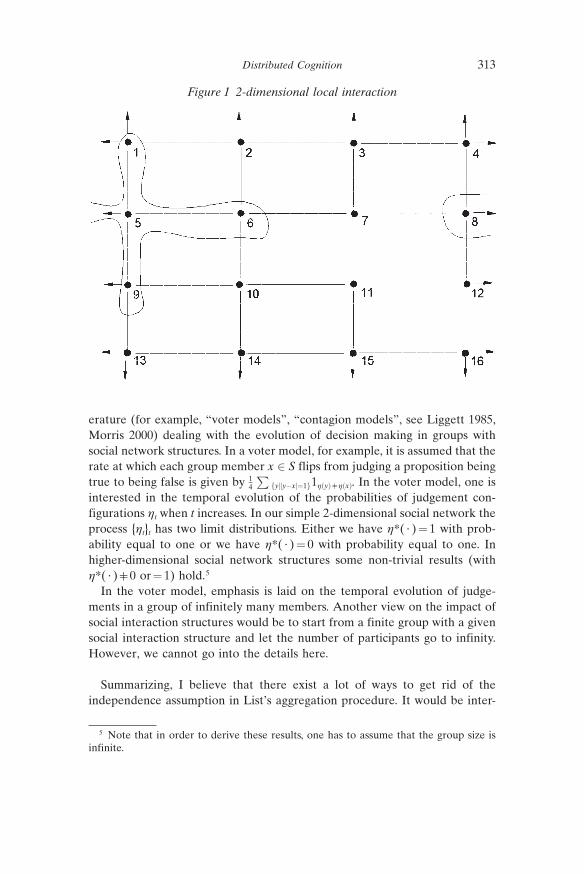
erature (for example, “voter models”, “contagion models”, see Liggett 1985,Morris 2000) dealing with the evolution of decision making in groups withsocial network structures. In a voter model, for example, it is assumed that therate at which each group member x 2 S flips from judging a proposition beingtrue to being false is given by 1

4

Pfy y�x ¼1gjk 1hðyÞ=hðxÞ. In the voter model, one is

interested in the temporal evolution of the probabilities of judgement con-figurations ht when t increases. In our simple 2-dimensional social network theprocess {ht}t has two limit distributions. Either we have h*( · )= 1 with prob-ability equal to one or we have h*( · )= 0 with probability equal to one. Inhigher-dimensional social network structures some non-trivial results (withh*( · )=0 or= 1) hold.5

In the voter model, emphasis is laid on the temporal evolution of judge-ments in a group of infinitely many members. Another view on the impact ofsocial interaction structures would be to start from a finite group with a givensocial interaction structure and let the number of participants go to infinity.However, we cannot go into the details here.

Summarizing, I believe that there exist a lot of ways to get rid of theindependence assumption in List�s aggregation procedure. It would be inter-

Figure 1 2-dimensional local interaction

5 Note that in order to derive these results, one has to assume that the group size isinfinite.


esting to see how these alternative assumptions would change the results inList�s paper.

References

Aldous, D. J. (1985), “Exchangeability and related topics,” Lecture Notes in Mathematics1117, Springer New York, 298 – 409.

Boland, P. (1989), “Majority systems and the Condorcet jury theorem,” Statistician, 38,181 – 189.

Carnap, R., and R. C. Jeffrey (1971), Studies in Inductive Logic and Probability Vol. I,Berkeley

DeGroot, M. H. (1974), “Reaching a consensus,” Journal of the American StatisticalAssociation, 69, 118 – 121.

Dietrich F., and C. List (2004), “A model of jury decisions where all jurors have the sameevidence,” Synthese, 142, 175 – 202.

List C., and P. Pettit (2002), “Aggregating sets of judgements: An impossibility result,”Economics and Philosophy, 18, 89 – 110.

List C., and P. Pettit (2004), “Aggregating sets of judgements: Two impossibility resultscompared,” Synthese, 140, 207 – 235.

Liggett, T. M. (1985), Interacting particle systems, Springer New-York.Morris, S. (2000), “Contagion,” Review of Economic Studies, 67, 57 – 78.


Contributors and Editors

Albert, Max – Justus Liebig University Giessen, Behavioral and InstitutionalEconomics, Licher Str. 66, 35394 Giessen, Germany,Email: [email protected]

Berninghaus, Siegfried K. – Universit�t Karlsruhe, Institut f�r Wirtschafts-theorie und Operations Research, Lehrstuhl f�r Volkswirtschaftslehre III,Postfach 6980, 76128 Karlsruhe, Germany,Email: [email protected]

Carayol, Nicolas – BETA, CNRS & Universite Louis Pasteur (Strasbourg 1),61, avenue de la Foret Noire, 67085 Strasbourg Cedex, France, and ADIS,Universite Paris Sud Orsay (Paris 11) & Faculte Jean Monnet, 54 BvdDesgranges, 92331 Sceaux Cedex, France,Email: [email protected]

Crespi, Gustavo – International Development Research Center, Canada

Demougin, Dominique – European Business School International University,Schloss Reichartshausen, Department of Law, Governance & Economics,65375 Oestrich-Winkel, Germany,Email: [email protected]

Egbert, Henrik – Justus Liebig University Giessen, Behavioraland Institutional Economics, Licher Str. 66, 35394 Giessen, Germany,Email: [email protected]

Fitzenberger, Bernd – Universit�t Freiburg, Abteilung f�r EmpirischeWirtschaftsforschung und kometrie, Platz der Alten Synagoge,79085 Freiburg, Germany,Email: [email protected]

Geuna, Aldo – University of Sussex, Science and Technology Policy Research,Freeman Centre, Brighton, East Sussex BN19QE, United Kingdom,Email: [email protected]

Godt, Christine – Universit�t Bremen, Zentrum f�r Europ�ischeRechtspolitik, Fachbereich Rechtswissenschaft, Universit�tsallee GW 1,28359 Bremen, Germany,Email: [email protected]

Gr�sche, Peter – Rheinisch-Westf�lisches Institut f�r Wirtschaftsforschung,Kompetenzbereich Umwelt und Ressourcen, Hohenzollernstr. 1 – 3,45128 Essen, Germany,Email: [email protected]

G�th, Werner – Max-Planck-Institut f�r konomik, Strategic InteractionGroup, Kahlaische Str. 10, 07745 Jena, Germany,Email: [email protected]

Jansen, Dorothea – German University of Administrative Sciences Speyer,Chair of Sociology of Organization, Freiherr-vom-Stein-Str. 2,67346 Speyer, Germany,Email: [email protected]

Kirchg�ssner, Gebhard – University of St. Gallen, SIAW-HSG,Bodanstr. 8, 9000 St. Gallen, Switzerland,Email: [email protected]

Kirstein, Roland – Economics of Business and Law, Faculty of Economicsand Management, Otto-von-Guericke University, Universit�tsplatz 2,39106 Magdeburg, Germany,Email: [email protected]

Koboldt, Christian – DotEcon Ltd, 17 Welbeck Street, London, W1G9XJ,United Kingdom,Email: [email protected]

Kolmar, Martin – University of St. Gallen, Chair forApplied Microeconomics, Varnb�elstr. 14, 9000 St. Gallen, Switzerland,Email: [email protected]

List, Christian – Department of Government, London School of Economics,London WC2A2AE, United Kingdom,Email: [email protected]

Meckl, J�rgen – Justus Liebig University Giessen, International Economics,Licher Str. 66, 35394 Giessen, Germany,Email: [email protected]

Pierdzioch, Christian – Saarland University, Department of Economics,Macroeconomics and International Economics, PO Box 151150,66041 Saarbruecken, Germany,Email: [email protected]

Rauber, Michael – Department of Economics, University of Konstanz,PO Box D-138, 78457 Konstanz, Germany,Email: [email protected]

Schmidt, Ulrich – Christian-Albrechts-Universit�t zu Kiel,Olshausenstr. 40, 24098 Kiel, Germany,Email: [email protected]

Contributors and Editors316

Schmidtchen, Dieter – Center for the Study of Law and Economics,University of the Saarland, PO Box 15 11 50, 66041 Saarbr�cken, Germany,Email: [email protected]

Schulze, G�nther G. – University of Freiburg, Department of Economics,Platz der Alten Synagoge, 79085 Freiburg i. Br., Germany,Email: [email protected]

Seidl, Christian – Christian-Albrechts-Universit�t zu Kiel, Olshausenstr. 40,24098 Kiel, Germany,Email: [email protected]

Stephan, Paula – Georgia State University and Research Associate, NationalBureau of Economic Research, Georgia State University, Department ofEconomics, PO Box 3992, Atlanta, GA 30302-3992, United States,Email: [email protected]

Ursprung, Heinrich W. – Department of Economics, University of Konstanz,PO Box D-138, 78457 Konstanz, Germany,Email: [email protected]

Voigt, Stefan – Chair for Institutional and International Economics, Dept. ofEconomics and Business Administration, University of Marburg, Barf�s-sertor 2, 35032 Marburg, Germany,Email: [email protected]

Zamora Bonilla, Jesus P. – Universidad Nacional de Educacion a Distancia,Faculdad de Filosofia, 28040 Madrid, Spain,Email: [email protected]

Contributors and Editors 317

Scientific Competition - OAPEN

Documents

Transcript of Scientific Competition - OAPEN