arX

iv:1

101.

0062

v1 [

mat

h-ph

] 3

0 D

ec 2

010

On rotational solutions for elliptically excited

pendulum

Anton O. Belyakov

Institute of Mechanics, Moscow State Lomonosov UniversityMichurinsky pr. 1, Moscow 119192, Russia;

ORCOS, Institute of Mathematical Methods in Economics,Vienna University of Technology

Argentinierstrasse 8/105-4, A-1040 Vienna, Austria

Abstract

The author considers the planar rotational motion of the mathematical pendulumwith its pivot oscillating both vertically and horizontally, so the trajectory of thepivot is an ellipse close to a circle. The analysis is based on the exact rotationalsolutions in the case of circular pivot trajectory and zero gravity. The conditions forexistence and stability of such solutions are derived. Assuming that the amplitudesof excitations are not small while the pivot trajectory has small ellipticity the ap-proximate solutions are found both for high and small linear damping. Comparisonbetween approximate and numerical solutions is made for different values of thedamping parameter.

1 Introduction

Elliptically excited pendulum (EEP) is a mathematical pendulum in the ver-tical plane whose pivot oscillates not only vertically but also horizontally withπ/2 phase shift, so that the pivot has elliptical trajectory, see Fig. 1. EEP isa natural generalization of pendulum with vertically vibrating pivot that isone of the most studied classical systems with parametric excitation, so it isoften referred to simply as parametric pendulum, see for example [1–4] andreferences therein.

Dynamics of EEP has been studied numerically and analytically in [5]. Ap-proximate oscillatory and rotational solutions for EEP are the common exam-

Email address: a belyakov@inbox.ru

(Anton O. Belyakov).

Preprint submitted to Elsevier 4 January 2011

ples in literature [6–9] on asymptotic methods. Sometimes EEP is presentedin a slightly more general model of unbalanced rotor [6–8], where the phaseshift between vertical and horizontal oscillations of the pivot can differ fromπ/2. EEP is also a special case of generally excited pendulum in [10].

The usual assumption for approximate solution in the literature is the small-ness of dimensionless damping and pivot oscillation amplitudes in the EEP’sequation of motion. The author could find only one paper [11], where os-cillations of EEP with high damping and yet small relative excitation werestudied.

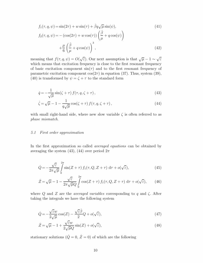
In the present paper we study rotations of EEP with not small excitationamplitudes and with both small and not small linear damping. Our analy-sis uses the exact solutions for EEP with the absence of gravity and withequal excitation amplitudes, when elliptical trajectory of the pivot becomescircular. 1

The paper is organized as follows. In Section 2 the dimensionless equationof EEP motion is derived. In Section 3 the exact rotational solutions andtheir stability conditions are obtained in the case, with no gravity and thecircular trajectory of the pivot. In Section 4 first and second order approximatesolutions are obtained by multiple scale method [13] for the close to circletrajectory of the pivot and high damping, where we assume that gravity issmall or the frequency of excitation is high. In Section 5 for the same excitationand small damping second order approximate solutions are obtained with theuse of averaging method [3,14]. In Section 6 both solutions in Sections 4 and 5are compared with the numerical solutions for different values of the dampingparameter.

2 Main relations

Equation of EEP’s motion can be derived with the use of angular momentumalteration theorem (e. g. [5])

ml2d2θ

dt2+ c

dθ

dt+ml

(

g − d2y(t)

dt2

)

sin(θ)−mld2x(t)

dt2cos(θ) = 0, (1)

where l is the distance between the pivot and the concentrated mass m; c isthe viscous damping coefficient; θ is the angle of the pendulum deviation fromthe vertical position; t is time; g is gravitational acceleration.

1 When there is no gravity the model of EEP coincides with that of hula-hoop, see[12] and references therein.

2

Fig. 1. Scheme of the elliptically excited mathematical pendulum of length l. Thepivot of the pendulummoves along the elliptic trajectory (dashed line) with semiaxisX and Y .

It is assumed that the pivot of the pendulum moves according to the periodiclaw

x = X sin(Ωt), y = Y cos(Ωt), (2)

where X , Y , and Ω are the amplitudes and frequency of the excitation.

We introduce the following dimensionless parameters and new time

Ω0 =

√

g

l, ε =

Y −X

2 l, µ =

Y +X

2 l> 0,

ω =Ω0

Ω, β =

c

m l2Ω, τ = Ωt, (3)

in which equation (1) with substituted (2) in it takes the following form

θ + βθ + µ sin(τ + θ) = ε sin(τ − θ)− ω2 sin(θ), (4)

were we use formula Y cos(Ω t) sin(θ)+X sin(Ω t) cos(θ) = Y+X2

sin(Ω t + θ)−Y−X

2sin(Ω t− θ). Here the upper dot denotes differentiation with respect to

new time τ .

3 Exact rotational solution when ε = 0 and ω = 0

Conditions ε = ω = 0 mean that we find the mode of rotation for the circularexcitation X = Y with absence of gravity g = 0. In this case, we call equation

3

(4) the unperturbed equation

θ + βθ + µ sin(τ + θ) = 0 (5)

which has exact solutions

θ = θ0 − τ, (6)

where constants θ0 are defined by the following equality

sin(θ0) =β

µ, (7)

provided that |β| ≤ µ.

To investigate the stability of these solutions we present the angle θ as θ =θ0−τ+η, where η = η(τ) is a small addition, and substitute it in equation (5).Then linearizing in (5) and using equality (7), we obtain the linear equation

η + βη + µ cos(θ0)η = 0, (8)

According to the Lyapunov stability theorem, solution (6) is asymptoticallystable according to the linear approximation if all eigenvalues of linearizedequation (8) have negative real parts. Which happens when the followinginequalities are satisfied

β > 0, µ cos(θ0) > 0, (9)

obtained from the Routh–Hurwitz conditions. From conditions (9), assump-tion µ > 0 in (3), and equality (7), it follows for β > 0 that the solutions

θ = θ0 − τ, θ0 = arcsin

(

β

µ

)

+ 2πk (10)

are asymptotically stable, while the solutions

θ = θ0 − τ, θ0 = π − arcsin

(

β

µ

)

+ 2πk (11)

are unstable, where k is any integer number. For negative damping, β <0, both these solutions are unstable. From now on we will assume that thefollowing conditions are satisfied

0 < β < µ, (12)

4

which ensure the existence of stable rotational solution (10) as it is seen from(7) and (9). Indeed, in order to guarantee asymptotic stability β should benot only positive, but also strictly less than µ because of the second conditionin (9), which can be transformed to inequality µ cos(θ0) =

√µ2 − β2 > 0 with

the use of the positive root for µ cos(θ0) from (7).

4 Approximate rotational solutions when ε ≈ 0 and ω ∼ √ε

We assume that values of ε and ω2 are small of the same order of smallness,i.e. ε ∼ ω2 ≪ 1, so we can introduce new parameter w = ω2/ε.

One can deduct from (3) and current assumptions that either gravity g issmall or the frequency of excitation Ω is high with such damping c and massm so that damping coefficient β ∼ 1.

All small terms are in the right-hand side of equation (4). To solve equation(4) we will use multiple scale method [13]. In this method general solution ofequation (4) is assumed to be of the following form

θ = −τ + θ0 + εθ1 + ε2θ2 + . . . (13)

A series of time scales (independent variables), T0, T1, . . ., is introduced, whereT0 = τ , T1 = ετ , . . .. So that θ is a function of these time scales, θ(T0, T1, . . .).Using the chain rule, the time derivatives become

d

dτ=D0 + εD1 + ε2D2 + . . . (14)

d2

dτ 2=D2

0 + 2εD0D1 + ε2(D0D2 +D21) + . . . (15)

where Dmn = ∂m/∂Tm

n . Next the general solution and the time derivatives aresubstituted into equation (4), where sines are expended into the Taylor serieswith respect to ε. By grouping together the terms with the same powers of εand equating to zero, a set of differential equations is obtained,

D20θ0 + βD0(θ0 − T0) + µ sin(θ0) = 0, (16)

D20θ1 + βD0θ1 + µ cos(θ0)θ1 = −(2D0D1 + βD1)(θ0 − T0)

+ sin(2T0 − θ0) + w sin(T0 − θ0), (17)

D20θ2 + βD0θ2 + µ cos(θ0)θ2 = µ sin(θ0)θ

21/2− (2D0D1 + βD1)θ1

− (D0D2 +D21 + βD2)(θ0 − T0)

− (cos(2T0 − θ0) + w cos(T0 − θ0)) θ1, (18)

5

. . .

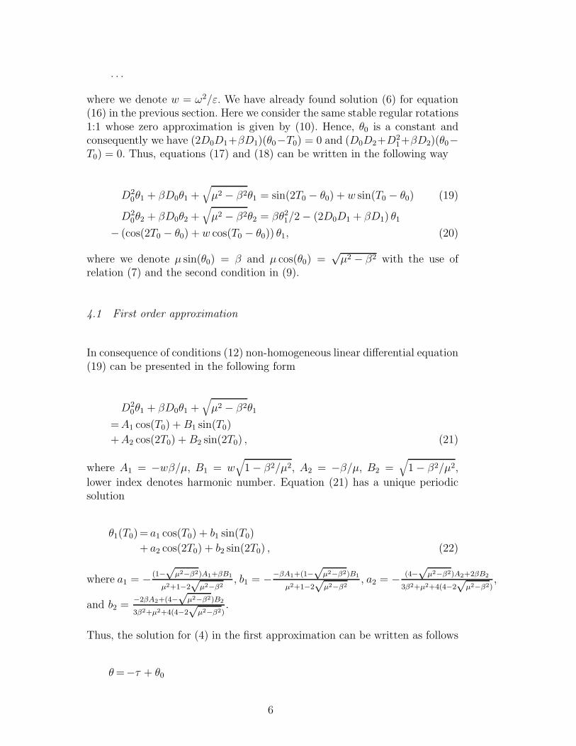
where we denote w = ω2/ε. We have already found solution (6) for equation(16) in the previous section. Here we consider the same stable regular rotations1:1 whose zero approximation is given by (10). Hence, θ0 is a constant andconsequently we have (2D0D1+βD1)(θ0−T0) = 0 and (D0D2+D

21+βD2)(θ0−

T0) = 0. Thus, equations (17) and (18) can be written in the following way

D20θ1 + βD0θ1 +

√

µ2 − β2θ1 = sin(2T0 − θ0) + w sin(T0 − θ0) (19)

D20θ2 + βD0θ2 +

√

µ2 − β2θ2 = βθ21/2− (2D0D1 + βD1) θ1

− (cos(2T0 − θ0) + w cos(T0 − θ0)) θ1, (20)

where we denote µ sin(θ0) = β and µ cos(θ0) =√µ2 − β2 with the use of

relation (7) and the second condition in (9).

4.1 First order approximation

In consequence of conditions (12) non-homogeneous linear differential equation(19) can be presented in the following form

D20θ1 + βD0θ1 +

√

µ2 − β2θ1

=A1 cos(T0) +B1 sin(T0)

+A2 cos(2T0) +B2 sin(2T0) , (21)

where A1 = −wβ/µ, B1 = w√

1− β2/µ2, A2 = −β/µ, B2 =√

1− β2/µ2,

lower index denotes harmonic number. Equation (21) has a unique periodicsolution

θ1(T0)= a1 cos(T0) + b1 sin(T0)

+ a2 cos(2T0) + b2 sin(2T0) , (22)

where a1 = − (1−√

µ2−β2)A1+βB1

µ2+1−2√

µ2−β2

, b1 = −−βA1+(1−√

µ2−β2)B1

µ2+1−2√

µ2−β2

, a2 = − (4−√

µ2−β2)A2+2βB2

3β2+µ2+4(4−2√

µ2−β2)

,

and b2 =−2βA2+(4−

õ2

−β2)B2

3β2+µ2+4(4−2√

µ2−β2)

.

Thus, the solution for (4) in the first approximation can be written as follows

θ=−τ + θ0

6

−ε2 β cos(2T0 − θ0) +

(

4−√µ2 − β2

)

sin(2T0 − θ0)

3β2 + µ2 + 8(2−√µ2 − β2)

−ω2β cos(T0 − θ0) +

(

1−√µ2 − β2

)

sin(T0 − θ0)

µ2 + 1− 2√µ2 − β2

, (23)

where constant θ0 is defined in (10).

4.2 Second order approximation

Since (22) does not contain any constant of integration we set (2D0D1 +βD1)θ1 = 0 in equation (20) and substitute in it an expression cos(2T0 − θ0)+w cos(T0 − θ0) = B1 cos(T0)− A1 sin(T0) + B2 cos(2T0)− A2 sin(2T0) with co-efficients defined in (21). Thus, equation (21) takes the following form

D20θ2 + βD0θ2 +

√

µ2 − β2θ2 =A′

0

2+

4∑

n=1

(A′

n cos(nT0) +B′

n sin(nT0)) ,(24)

where coefficients in the right-hand side are the following

A′

0=(

b22 + b1

2 + a22 + a1

2)

β + (A1b1 + A2b2 −B2a2 −B1a1) (25)

A′

1= (a1a2 + b1b2) β + (A1b2 + A2b1 − B1a2 − B2a1)/2 (26)

A′

2=(

a21 − b21)

β/2− (A1b1 +B1a1)/2 (27)

A′

3= (a1a2 − b1b2)β − (A2b1 + A1b2 +B1a2 +B2a1)/2 (28)

A′

4=(

a22 − b22)

β/2− (A2b2 +B2a2)/2 (29)

B′

1= (a1b2 − b1a2)β − (A1a2 −A2a1 +B1b2 − B2b1)/2 (30)

B′

2= β a1b1 + (A1a1 − B1b1)/2 (31)

B′

3= (a1b2 + b1a2) β + (A1a2 + A2a1 − B1b2 − B2b1)/2 (32)

B′

4= β a2b2 + (A2a2 − B2b2)/2. (33)

Periodic solution for equation (24) has the following form which is obtainedfrom (59) in Appendix

θ2(T0) =A′

0

2√µ2 − β2

−4∑

n=1

(n2 −√µ2 − β2)A′

n + nβB′

n

(n2 − 1)β2 + µ2 + n2(n2 − 2√µ2 − β2)

cos(nT0)

−4∑

n=1

−nβA′

n + (n2 −√µ2 − β2)B′

n

(n2 − 1)β2 + µ2 + n2(n2 − 2√µ2 − β2)

sin(nT0) , (34)

7

0 2*pi

−1.2

−1.1

−1

−0.9

−0.8

−0.7

time τ

angu

lar

velo

city

dθ

/ dτ

µ =1, ω =0.3, ε =0.2, β =0.5, Q =−0.34993, Z =−6.9004

numericalfirst approx.second approx.

Fig. 2. Angular velocities θ calculated from the first order approximate solution(23), second order approximate solution (35), and results of numerical simulation,when damping coefficient β is not small.

where constant term is derived from (60) taking A0 = A′

0/2. Thus, secondorder approximate solution can be shortly written in the following form

θ=−τ + θ0 + εθ1(τ) + ε2θ2(τ), (35)

where constant θ0 is defined in (10), function θ1 in (22), and function θ2 in(34). In Fig. 2 it is shown how first and second order approximate solutionsapproach the numerical solution.

In this section we have used the fact that all solutions in each time scalemust converge to corresponding unique periodic solutions because dampingβ is not small. If it is not the case the multiple scale analysis becomes morecomplicated. In the next section we will tackle the problem of small dampingβ ∼ √

ε with the use of classical averaging technique.

8

5 Approximate rotational solutions when ε ≈ 0, ω ∼ √ε, and β ∼ √

ε

One can see in (3) that assumptions ω ∼ β ∼ √ε are valid for the high

frequency of excitation Ω ∼ 1/√ε with other parameters being of order 1.

Another option is small gravity g ∼ ε along with small ratio c/m ∼ √ε.

After change of variable θ = −τ +√εϑ equation (4) takes the following form

ϑ+ µϑ− β = µ

(

ϑ− sin(√εϑ)√ε

)

−√εβϑ

+√ε sin

(

2τ −√εϑ)

+√εw sin(τ −

√εϑ), (36)

with small right-hand side, where we denote β = β/√ε and as in the previous

section w = ω2/ε. With zero right-hand side equation (36) ϑ + µϑ − β = 0would describe harmonic oscillations about β/µ value with frequency

õ.

After Taylor’s expansion of sines in the right-hand side of (36) about ϑ = 0we obtain the following equation

ϑ+ (µ+ ε cos(2τ) + εw cos(τ))ϑ− β

=√ε sin(2τ) +

√εw sin(τ)−

√εβϑ+ εµ

ϑ3

6+ o(ε), (37)

which describes oscillator with both basic and parametric excitations. To solveequation (37) we will use averaging method [3,14]. For that purpose we willwrite (37) in the standard form of first order differential equations with smallright-hand sides. First, we use Poincare variables q and ψ defined via thefollowing solution of generating system ϑ + µϑ − β = 0 which is (37) withε = 0

ϑ =β

µ+ q cos(ψ), ϑ = −√

µq sin(ψ). (38)

In Poincare variables equation (37) becomes a system of first order differentialequations

q=−sinψ√µf(τ, q, ψ), (39)

ψ=√µ− cosψ

q√µf(τ, q, ψ), (40)

where small function f(τ, q, ψ) =√εf1(τ, q, ψ)+ εf2(τ, q, ψ)+ o(ε) is the right

hand side of (36), where

9

f1(τ, q, ψ)= sin(2τ) + w sin(τ) + βq√µ sin(ψ), (41)

f2(τ, q, ψ)=− (cos(2τ) + w cos(τ))

(

β

µ+ q cos(ψ)

)

+µ

6

(

β

µ+ q cos(ψ)

)3

, (42)

meaning that f(τ, q, ψ) = O(√ε). Our next assumption is that

√µ− 1 ∼ √

εwhich means that excitation frequency is close to the first resonant frequencyof basic excitation component sin(τ) and to the first resonant frequency ofparametric excitation component cos(2τ) in equation (37). Thus, system (39),(40) is transformed by ψ = ζ + τ to the standard form

q=− 1√µsin(ζ + τ) f(τ, q, ζ + τ) , (43)

ζ =√µ− 1− 1

q√µcos(ζ + τ) f(τ, q, ζ + τ) , (44)

with small right-hand side, where new slow variable ζ is often referred to asphase mismatch.

5.1 First order approximation

In the first approximation so called averaged equations can be obtained byaveraging the system (43), (44) over period 2π

Q=−√ε

2π√µ

2π∫

0

sin(Z + τ) f1(τ, Q, Z + τ) dτ + o(√ε), (45)

Z =√µ− 1−

√ε

2π√µQ

2π∫

0

cos(Z + τ) f1(τ, Q, Z + τ) dτ + o(√ε), (46)

where Q and Z are the averaged variables corresponding to q and ζ . Aftertaking the integrals we have the following system

Q=−√εw

2√µcos(Z)−

√εβ

2Q+ o(

√ε), (47)

Z =√µ− 1 +

√εw

2õQ

sin(Z) + o(√ε), (48)

stationary solutions (Q = 0, Z = 0) of which are the following

10

Q2=ω2/ε

µ (4(√µ− 1)2 + β2)

+ o(1), (49)

Z =arctan

(

2(µ− 1)

β

)

+ 2πk + o(1), (50)

where we have substituted back w = ω2/ε and β = β/√ε. Symbol arctan

stands for the principal value of the function on the interval from 0 to π. Notethat the phase Z is determined to within 2π rather than π, since the functionssin(Z) and cos(Z) obtained from equations (47) and (48) determine Z up toan additive term 2πk. Solution of system (43-44) in the first approximation isq = Q+ o(1), ζ = Z + o(1) so the solution of (4) is the following

θ = −τ + β

µ+√εQ cos(Z + τ) + o(

√ε),

which does not contain higher harmonics observed numerically. That is whywe need to proceed to the second order approximation.

5.2 Second order approximation

In the second approximation averaged equations can be obtained as follows

Q=

(

−√ε cos(Z) +

εβ

4

(

4

µ− 1

)

sin(Z)

)

w

2õ

+

(

−√εβ

2+

ε

4õsin(2Z)

)

Q + o(ε), (51)

Z =√µ− 1 +

(√ε sin(Z) +

εβ

4

(

4

µ− 1

)

cos(Z)

)

w

2õQ

−εβ2

8

(

2

µ√µ+ 1

)

+ε

4√µcos(2Z)− ε

õ

16Q2 + o(ε), (52)

stationary solutions (Q = 0, Z = 0) can be found numerically or with ab-sence of gravity (ω = 0) analytically. Solution of system (43-44) in the secondapproximation is the following

q=Q +

√ε

2õ

(

− sin(τ − Z) +w

2sin(2τ + Z) +

1

3sin(3τ + Z)

)

+√εβ Q

4sin (2τ + 2Z) + o(

√ε), (53)

11

ζ =Z +

√ε

2õQ

(

cos(τ − Z) +w

2cos(2τ + Z) +

1

3cos(3τ + Z)

)

+√εβ

4cos (2τ + 2Z) + o(

√ε), (54)

Substitution of these expressions into (38) yields the second order approximatesolution of (36) in the following form

ϑ=β

µ+Q cos(Z + τ) +

√εβ Q

4sin(Z) (55)

+

√εw sin(τ)

4õ

−√ε sin(2τ)

3õ

+ o(√ε) (56)

which after changes of variable θ = −τ +√εϑ and parameters w = ω2/ε,

β = β/√ε results in the approximate solution of the original equation (4)

θ=−τ + β

µ+√εQ cos(Z + τ) +

√εβ Q

4sin(Z)

+ω2 sin(τ)

4õ

− ε sin(2τ)

3õ

+ o(ε). (57)

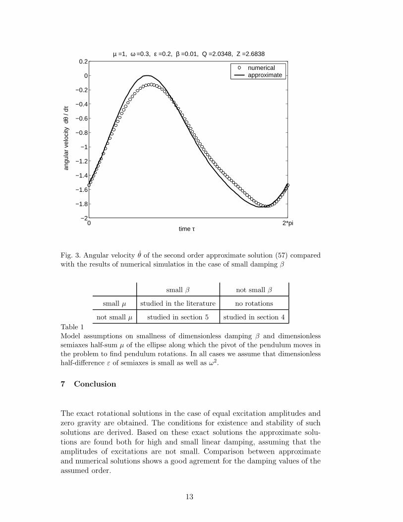
Agreement of solution (57) with the numerical experiment is shown in Fig. 3.We see that the amplitude of angular velocity oscillations is much higher thanthat for not small β in Fig. 2.

6 Domains of applicability

For asymptotic solutions in the previous two sections the parameter con-straints are more strict than those for the existence of stable exact solution in(12). Thus, for our analysis in Section 4 to be valid we must exclude cases whenβ = o(1) or/and

√µ2 − β2 = o(1). The case when β = o(1) and µ = O(1) is

studied in Section 4. Note that the case when both β = o(1) and µ = o(1)meaning

√µ2 − β2 = o(1) has already been studied in the literature, for ex-

ample in the more general model of unbalanced rotor in [6]. The case whenβ = O(1) and µ = o(1) is not feasible for asymptotic rotational solution.Indeed, with such assumptions the generating system θ + βθ = 0 has onlyconstant solutions. These different cases are presented in the Table 1.

To show quantitatively the limits of applicability of the assumptions in Sec-tions 4 and 5 we plot the absolute and relative angular velocity errors depend-ing on parameter β while excitation was constant µ = 1, see Fig. 4.

12

0 2*pi−2

−1.8

−1.6

−1.4

−1.2

−1

−0.8

−0.6

−0.4

−0.2

0

0.2

time τ

angu

lar

velo

city

dθ

/ dτ

µ =1, ω =0.3, ε =0.2, β =0.01, Q =2.0348, Z =2.6838

numericalapproximate

Fig. 3. Angular velocity θ of the second order approximate solution (57) comparedwith the results of numerical simulatios in the case of small damping β

small β not small β

small µ studied in the literature no rotations

not small µ studied in section 5 studied in section 4

Table 1Model assumptions on smallness of dimensionless damping β and dimensionlesssemiaxes half-sum µ of the ellipse along which the pivot of the pendulum moves inthe problem to find pendulum rotations. In all cases we assume that dimensionlesshalf-difference ε of semiaxes is small as well as ω2.

7 Conclusion

The exact rotational solutions in the case of equal excitation amplitudes andzero gravity are obtained. The conditions for existence and stability of suchsolutions are derived. Based on these exact solutions the approximate solu-tions are found both for high and small linear damping, assuming that theamplitudes of excitations are not small. Comparison between approximateand numerical solutions shows a good agrement for the damping values of theassumed order.

13

0 0.2 0.4 0.6 0.8 10

0.05

0.1

0.15

0.2

0.25

0.3

0.35

0.4

0.45

0.5

damping β

abso

lute

err

or o

f ang

ular

vel

ocity

dθ

/ dτ

µ =1, ω =0.3, ε =0.2

first approx.second approx.second approx. for small β

0 0.2 0.4 0.6 0.8 10

0.05

0.1

0.15

0.2

0.25

0.3

0.35

0.4

0.45

0.5

damping β

rela

tive

erro

r of

ang

ular

vel

ocity

dθ

/ dτ

µ =1, ω =0.3, ε =0.2

first approx.second approx.second approx. for small β

Fig. 4. Maximal absolute (left) and relative (right) deviation of analytically obtainedangular velocities θ in (23), (35), and (57) from the numerically obtained θ. Solution(57) specially obtained for better approximation at small damping β. Error in theright graph is calculated relative to the oscillation amplitude of angular velocity θ.

Acknowledgement

The author would like to thank Professor Alexander P. Seyranian from LomonosovMoscow State University for his valuable comments on the text of the paper.

Appendix

Non-uniform second order linear differential equation

ϑ+ βϑ+√

µ2 − β2ϑ = An cos(nτ) +Bn sin(nτ), (58)

has solutions which obey the principle of superposition and contain only har-monics of the right-hand side in (58)

ϑ[n] =− (n2 −√µ2 − β2)An + nβBn

(n2 − 1)β2 + µ2 + n2(n2 − 2√µ2 − β2)

cos(nτ)

− −nβAn + (n2 −√µ2 − β2)Bn

(n2 − 1)β2 + µ2 + n2(n2 − 2√µ2 − β2)

sin(nτ) (59)

where n = 0, 1, 2, . . .. Thus, solution with n = 0 is the following

ϑ[0] =A0√µ2 − β2

, (60)

14

when n = 1

ϑ[1] =−(1 −√µ2 − β2)A1 + βB1

µ2 + 1− 2√µ2 − β2

cos(τ)

− −βA1 + (1−√µ2 − β2)B1

µ2 + 1− 2√µ2 − β2

sin(τ) (61)

when n = 2

ϑ[2] =− (4−√µ2 − β2)A2 + 2βB2

3β2 + µ2 + 4(4− 2√µ2 − β2)

cos(2τ)

− −2βA2 + (4−√µ2 − β2)B2

3β2 + µ2 + 4(4− 2√µ2 − β2)

sin(2τ) (62)

References

[1] Lenci, S., Pavlovskaia, E., Rega, G., and Wiercigroch, M. Rotating solutions andstability of parametric pendulum by perturbation method. Journal of Sound andVibration 310, 2008, pp. 243–259.

[2] Xu, X., Wiercigroch, M. Approximate analytical solutions for oscillatory androtational motion of a parametric pendulum. Nonlinear Dyn. 47, 2007, pp. 311–320.

[3] Bogolyubov, N. N., Mitropol’skii, Yu. A. Asymptotic Methods in the Theory ofNonlinear Oscillations. Gordon and Breach, New York, 1961.

[4] Seyranian, A. P., Yabuno, H., Tsumoto, K. Instability and periodic motionof a physical pendulum with a vibrating suspension point (theoretical andexperimental approach). Doklady Physics, 50(9), 2005, pp. 467–472.

[5] Horton B., Sieber J., Thompson, J. M. T., Wiercigroch, M. Dynamics of theelliptically excited pendulum. arXiv:0803.1662v1 [math.DS] 11 Mar 2008.

[6] Blekhman, I. I. Rotation of an unbalanced rotor caused by harmonic oscillationsof its axis. Izv. AN SSSR, OTN, 8, 1954, pp. 79–94. (in Russian)

[7] Blekhman, I. I.: Vibrations in Engineering. A Handbook. Vol. 2. Vibrations ofNonlinear Mechanical Systems, Mashinostroenie, Moscow, 1979. (in Russian)

[8] Blekhman, I. I. Vibrational Mechanics. Nonlinear Dynamic Effects, GeneralApproach, Applications, World Scientific, Singapore 2000, 509 pp.

[9] Akulenko, L. D. Higher-order averaging schemes in the theory of non-linearoscillations. J. Appl. Mafhs Mechs, 65(5), 2001, pp. 817–826.

15

[10] Trueba, J. L., Baltanaas, J. P., Sanjuaan, M. A. F. A generalized perturbedpendulum. Chaos, Solitons and Fractals. 15, 2003, pp. 911-924.

[11] Fidlin, A., Thomsen, J. J. Non-trivial effects of high-frequency excitationfor strongly damped mechanical systems. International Journal of Non-LinearMechanics, 43, Issue 7, 2008, pp. 569–578.

[12] Belyakov, A. O., Seyranian, A. P. The Hula-Hoop Problem. Doklady Physics,55(2), 2010, pp. 99–104.

[13] Nayfeh, A. H. Perturbation Methods. Wiley-Interscience, New York, 1973,425 pp.

[14] Volosov, V. M., Morgunov, B. I. Averaging Method in the Theory of NonlinearOscillatoratory Systems. MSU, Moscow, 1971.

16