Super-resolved spatial light interference microscopy

Kaiqin Chu,1,* Zachary J. Smith,1 Sebastian Wachsmann-Hogiu,1,2 and Stephen Lane1,3

1Center for Biophotonics Science and Technology, University of California, Davis, California, 95817, USA2Department of Pathology and Laboratory Medicine, University of California at Davis, California 95817, USA

3Department of Neurological Surgery, University of California at Davis, California 95817, USA*Corresponding author: kqchu@ucdavis.edu

Received November 10, 2011; accepted November 14, 2011;posted November 21, 2011 (Doc. ID 157295); published February 22, 2012

We report a scheme to achieve resolution beyond the diffraction limit in spatial light interference microscopy(SLIM). By adding a grating to the optical path, the structured illumination technique can be used to improvethe resolution by a factor of 2.We show that a direct application of the structured illumination technique, however,has proved to be unsuccessful. Through two crucial modifications, namely, one to the pupil plane of the objec-tive and the other to the demodulation procedure, faithful phase information of the object is recovered and theresolution is improved by a factor of 2. © 2012 Optical Society of America

OCIS Codes: 110.0180, 110.3175, 110.4980, 120.3890, 120.5050, 180.3170.

1. INTRODUCTIONSince the invention of phase contrast microscopy by Zernike[1], imaging with intrinsic signals from transparent biologicalsamples such as cells has become possible. The recorded im-age is an interference pattern between the unscattered illumi-nation light and the light scattered by the sample. The phasedifference between unscattered and scattered light reveals in-formation about the changes in the refractive index in the bio-logical sample. However, efforts to quantitatively extract thisphase difference from the interference pattern have only re-cently been demonstrated [2–8]. The spatial light interferencemicroscopy (SLIM) proposed by Wang et al. utilizes a four-step phase stepping method to obtain the phase difference be-tween the unscattered and scattered light and thus obtain thephase of the object field as well [8]. One advantage of the SLIMis the clean background compared to some other quantitativephase microscopy techniques [3–7]. The reason for this is thatspectrally broad and spatially incoherent illumination is ap-plied so speckle is greatly reduced. The unscattered and scat-tered light travel a common path before they interfere at theimage plane, making the system relatively immune to vibra-tions. The conversion from an existing phase contrast micro-scope is also convenient requiring only the addition of amodule with the phase modulating ability. Many applicationsof SLIM have been previously reported [9–11]. Even thoughthe phase information obtained from SLIM reveals the heightof the sample with nanometer sensitivity, the lateral resolu-tion is still diffraction-limited.

Many techniques have been developed for imaging beyondthe diffraction limit [12–14] for fluorescence microscopy, buttheir translation to nonfluorescent microscopies is not appar-ent. One technique, however, structured illumination micro-scopy [15], can be extended to phase microscopies as wewill detail below. The image formation process in the caseof fluorescence microscopy is intensity-based and linear whilein the phase contrast microscopy the recorded image and ob-ject are bilinear [16,17]. Direct application of the structuredillumination in the phase microscopy will result in artifacts

and low-contrast phase images (as shown in the paper). Wepropose a method to modify the SLIM system to accommodatethe structured illumination and to modify the demodulationprocedure of the structured illumination microscopy to ac-commodate the SLIM. The reconstructed phase images arehigh contrast with few artifacts.

The paper is organized in the following fashion. First wedescribe how to estimate the object field from the SLIM setupand establish a linear relationship between the estimate andthe original object field (Section. 2). Analysis and imagingresults of the direct and modified application of the structuredillumination technique to the SLIM setup are shown inSubsections 3.A and 3.B with the conclusion that modificationis necessary to achieve faithful and high contrast phaseimages. The performance of the modified system, in termsof the resolution, effects of noise, and the contrast of thestructured illumination are studied in Sections 4 and 5. Finally,summary comments are given in Section 6.

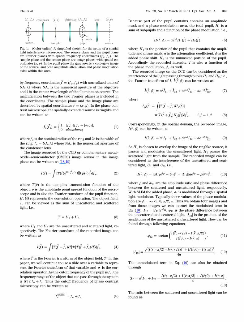
2. FOURIER ANALYSIS OF THE IMAGEFORMATION OF SLIM AND ITS CUTOFFFREQUENCYA typical SLIM setup is sketched in Fig. 1 where a ringlikesource is followed by a condenser lens, the sample plane,the objective lens, the pupil plane, the imaging lens, and thesensor array downstream. In this simplified sketch, the phasemodulation element has been included in the pupil planewhile in demonstrated setups it is a separate element placedin a plane conjugate to the objective’s pupil plane. Thus in thepupil plane shown in Fig. 1 there are two overlapping masks.One is a fixed amplitude attenuation mask and the other is avariable phase modulation mask, with both masks acting onthe unscattered light. The illumination is of Köhler type. As thesystem is made achromatic, i.e., the imaging properties andphase modulation are uniform for all wavelengths of thesource, we can consider the image formation for just the cen-ter wavelength. The source plane and the back focal planeof the objective are the Fourier planes, they are described

344 J. Opt. Soc. Am. A / Vol. 29, No. 3 / March 2012 Chu et al.

1084-7529/12/030344-08$15.00/0 © 2012 Optical Society of America

by frequency coordinates ~f � �f x; f y�with normalized units ofNAo∕λ where NAo is the numerical aperture of the objectiveand λ is the center wavelength of the illumination source. Themagnification between the two Fourier planes is included inthe coordinates. The sample plane and the image plane aredescribed by spatial coordinates ~r � �x; y�. In the phase con-trast microscope, the spatially-extended source is ringlike andcan be written as

Is� ~f s� ��1 j ~f sj ∈ f s � �−ε; ε�;0 elsewhere;

(1)

where f s is the nominal radius of the ring and 2ε is the width ofthe ring. f s � NAc∕λ where NAc is the numerical aperture ofthe condenser lens.

The image recorded by the CCD or complementary metal–oxide–semiconductor (CMOS) image sensor in the imageplane can be written as [18,19]

I�~r� �Z

jT�~r�ei2π� ~f s ·~r� ⊗ p�~r�j2d ~f s; (2)

where T�~r� is the complex transmission function of theobject, p is the amplitude point spread function of the micro-scope and is also the Fourier transform of the pupil function,H. ⊗ represents the convolution operation. The object field,T , can be viewed as the sum of unscattered and scatteredlight, i.e.,

T � U1 � U2; �3�

where U1 and U2 are the unscattered and scattered light, re-spectively. The Fourier transform of the recorded image canbe written as

~I�~f � �Z

�~T�~f � ~f s�H �⋆�~T�~f � ~f s�H �d ~f s; (4)

where ~T is the Fourier transform of the object field, T . In thispaper, we will continue to use a tilde over a variable to repre-sent the Fourier transform of that variable and ⋆ is the cor-relation operator. As the cutoff frequency of the pupil is f o, thefrequency range of the object that can pass through the systemis j~f j ≤ f o � f s. Thus the cutoff frequency of phase contrastmicroscopy can be written as

f�SLIM�c � f o � f s: (5)

Because part of the pupil contains contains an amplitudemask and a phase modulation area, the total pupil, H, is asum of subpupils and a function of the phase modulation, i.e.,

H�~f ;ϕ� � aeiϕH1�~f � �H2�~f �; (6)

where H1 is the portion of the pupil that contains the ampli-tude and phase mask, a is the attenuation coefficient, ϕ is theadded phase shift. H2 is the unmasked portion of the pupil.Accordingly the recorded intensity, I is also a function ofthe phase modulation, ϕ, as well.

The recorded image on the CCD can be considered as theinterference of the light passing through pupilsH1 andH2, i.e.,the Fourier transform of I, ~I�~f ;ϕ� can be written as

~I�~f ;ϕ� � a2~I11 � ~I22 � aeiϕ~I12 � ae−iϕ~I�12; (7)

where

~Iij�~f � �Z�~T�~f � ~f s�Hi�~f ��

⋆�~T�~f � ~f s�Hj�~f ��d ~f s; i; j � 1; 2. (8)

Correspondingly, in the spatial domain, the recorded image,I�~r;ϕ� can be written as

I�~r;ϕ� � a2I11 � I22 � aeiϕI12 � ae−iϕI�12: (9)

As H1 is chosen to overlap the image of the ringlike source, itpasses and modulates the unscattered light. H2 passes thescattered light from the sample. The recorded image can beconsidered as the interference of the unscattered and scat-tered light, U1 and U2, i.e.,

I�~r;ϕ� � jaU1eiϕ � U2j2 � jU1jjaeiϕ � βeϕ12 j2; (10)

where β and ϕ12 are the amplitude ratio and phase differencebetween the scattered and unscattered light, respectively.With SLIM the added phase, ϕ, is modulated through a spatiallight modulator. Typically those values of the phase modula-tion are ϕ � −π∕2, 0, π∕2, π. Thus we obtain four images andfrom those images we can extract the modulated term inEq. (10), I12 � jI12jeiϕ12 . ϕ12 is the phase difference betweenthe unscattered and scattered light. jI12j is the product of theamplitudes of the unscattered and scattered light. They can befound through following equations,

ϕ12 � arctan�I�~r;−π∕2� − I�~r; π∕2�

I�~r; 0� − I�~r; π�

�; (11)

jI12j����������������������������������������������������������������������������������������������I�~r;−π∕2�− I�~r;π∕2��2��I�~r;0�− I�~r;π��2

p4a

: (12)

The unmodulated term in Eq. (10) can also be obtainedthrough

hIi � a2I11 � I22 �I�~r;−π∕2� � I�~r; π∕2� � I�~r; 0� � I�~r; π�

4:

(13)

The ratio between the scattered and unscattered light can befound as

Fig. 1. (Color online) A simplified sketch for the setup of a spatiallight interference microscope. The source plane and the pupil planeare Fourier planes with spatial frequency coordinates (f x, f y). Thesample plane and the sensor plane are image planes with spatial co-ordinates (x, y). In the pupil plane the gray area is a conjugate imageof the source, and both amplitude attenuation and phase modulationexist within this area.

Chu et al. Vol. 29, No. 3 / March 2012 / J. Opt. Soc. Am. A 345

β�~r� �����U2

U1

���� � hIi −��������������������������������hIi2 − 4a2jI12j2

p2jI12j

: (14)

Thus the estimated field in the sample plane can be writtenas

U �SLIM��~r� ��������I11

p�1� βeiϕ12�; (15)

where I11 � hIia2�β2. The estimated phase information about the

object can be directly obtained through

ϕ�SLIM��~r� � arctan�imag�U �SLIM��real�U �SLIM��

�: (16)

This is the imaging result of the spatial light interference mi-croscope (SLIM). Note that the estimated object field inEq. (15) and the phase information about the sample inEq. (16) are approximations to their originals because the ima-ging system, SLIM, is bandlimited. The cutoff frequency isdecided by Eq. (5) and the lateral resolution can be estimatedas [20,21]

d�SLIM� � 1.22λ

NAo � NAc

� 1.22

f�SLIM�c

: (17)

An example image is shown in Fig. 2(a), where the phaseobject is a resolution chart. The numerical aperture of the ob-jective is 0.6, and 0.54 of the condenser. The width of thesource is 1% of the pupil radius. The attenuation to the unscat-tered light is 0.1. The center wavelength of the illuminationsource is 0.5 μm. The cutoff frequency of this system is thus2.28 μm−1. Because of the limited bandwidth of the imaging

system, we can see that details smaller than element 5 ofGroup 1 are lost.

Next we consider a way to extend the cutoff frequency ofthe imaging system by providing a structured illumination forthe sample, thus improving the spatial resolution.

3. SUPER-RESOLUTION IN SLIM WITHSTRUCTURED ILLUMINATIONThe structured illumination is typically used in fluorescencemicroscopy to achieve a factor of 2 improvement in resolution[15]. In order to see how structured illumination can be ap-plied to the SLIM setup, we will give two examples here. Oneis a direct application where we add a grating or project animage of the grating to the sample plane and then followthe same demodulation procedure and reconstruction de-scribed in [15,22]. The second is a modified version whichgives phase images of fewer artifacts and higher contrast.

A. Direct Application of Structured IlluminationTechnique in SLIM: SLIM+SI, DirectAs in the case of fluorescence microscopy, the structured il-lumination in the SLIM setup can be generated by adding agrating in front of the sample plane to the original setup shownin Fig. 1. In this case, the object field becomes

T 0�~r� � T�~r��1�m cos�2π~f g · ~r � θ��; (18)

where ~f g and θ are the spatial frequency and phase of the grat-ing respectively,m is the contrast of the sinusoidal pattern onthe grating. In the Fourier domain, the spectrum of theobject field becomes

(a) SLIM (b) SLIM+SI, direct (c) SLIM+SI, adapted

µ

(d) Cross-sectionofthebarsinthedashedboxesin(a)-(c)

Fig. 2. (Color online) Imaging results by (a) SLIM, (b) SLIM+SI, direct (c) SLIM+SI, adapted. (d) Cross-sections of the image in the dashed boxes(corresponding to element 6 in Group 1) in (a)–(c) show that the contrast of the adapted SLIM+SI is better than the direct SI+SLIM.

346 J. Opt. Soc. Am. A / Vol. 29, No. 3 / March 2012 Chu et al.

~T 0�f � � ~T�f � �m

2eiθ ~T�f � f g� �

m

2e−iθ ~T�f − f g�. (19)

The Fourier transform of the recorded intensity can be foundby using ~T 0 in Eq. (4) and can be written as

~I 0�~f ; θ� �Z

� ~T 0�~f � ~f s�H �⋆� ~T 0�~f � ~f s�H �d ~f s;

� ~I0�f � �m

2eiθ~I�1 �

m

2e−iθ~I−1 �

m2

4ei2θ~I�2

�m2

4e−i2θ~I−2; (20)

where

~I0 �Z �X1

i�−1

�~T�~f � i~f g � ~f s�H �

⋆�~T�~f � i~f g � ~f s�H��d ~f s; (21)

~I�1 �Zf�~T�~f � ~f g � ~f s�H �⋆�~T�~f � ~f s�H�

� �~T�~f � ~f s�H�⋆�~T�~f − ~f g � ~f s�H �gd ~f s; (22)

~I−1 �Zf�~T�~f − ~f g � ~f s�H�⋆�~T�~f � ~f s�H �

� �~T�~f � ~f s�H �⋆�~T�~f � ~f g � ~f s�H �gd ~f s; (23)

~I�2 �Z�~T�~f � ~f g � ~f s�H�

⋆�~T�~f − ~f g � ~f s�H�d ~f s; (24)

~I−2 �Z�~T�~f − ~f g � ~f s�H �

⋆�~T�~f � ~f g � ~f s�H �d ~f s. (25)

Equation (20) demonstrates that the output is a linear combi-nation of five components, I0, I�1, I�2. With the same phase-shifting technique as described in [22] we can construct acomposite image spectrum

~I�~f � � ~I0�~f � � ~I�1�~f − ~f g� � ~I−1�~f � ~f g� � ~I�2�~f − 2~f g�� ~I−2�~f � 2~f g�: (26)

We see that five images are needed to subtract ~I0, ~I�1, ~I�2

from ~I 0 and construct a composite image spectrum with cutofffrequency extended in the direction of ~f g. In order to achieveisotropic improvement in resolution, we can rotate the grating0, 120°, 240°, as detailed in [15]. Thus each image with cutofffrequency extended isotropically requires 15 frames. By chan-ging the phase value of the aperture H1 four times, we canestimate the phase difference of the light passing throughH1 and H2 following the procedures described in Section 2.Thus one super-resolved phase image requires 60 frames.

However in reconstructing the object field, we cannot as-sume the light passing through H2 is purely the scattered light

because the grating will bend some of the unscattered lighttoward the aperture H2. This will cause a phase bias in thereconstructed phase information of the sample, thus reducingthe image contrast.

In order to see the image performance of the SLIM withstructured illumination, we used the same SLIM setup as de-scribed in Section 2, a grating with frequency 1.8 μm−1 isadded to the sample plane to create the structured illumina-tion. The contrast of the structured illumination in the sampleplane is assumed to be 1. Then we use the procedure de-scribed in this section to reconstruct the phase informationof the same phase object used in Section 2. The imaging resultis shown in Fig. 2(b). We see that more details are resolvedcompared to the results from the original SLIM setup as ex-pected. However there are significant artifacts and the imagecontrast is low. The fundamental reason for this can be ex-plained as follows: the standard demodulation for structuredillumination microscopy expects that ~I0 (shown in Eq. (20))represents only the unshifted frequency spectrum collectedby the system while ~I�1;�2 (shown in Eq. (20)) represent upor down shifted version of the spectrum collected by the sys-tem. As can be seen in their definitions shown in Eq. (21–25),~I0;�1;�2 are all mixtures of both shifted and unshifted contri-butions. Therefore the demodulation procedure does not ac-curately reconstruct the true object spectrum. This is a directconsequence of a lack of a linear relationship between the ob-ject and the measured image intensity in the phase micro-scope and is the reason why we derived the estimate of thefield in Section 2. As we will show below, performing the de-modulation in terms of the field, where a linear imaging rela-tionship exists, produces clean images with the expectedfactor of 2 improvement in resolution.

B. Modifying both SLIM and the DemodulationProcedure: SLIM+SI, AdaptedAs we have mentioned above, the unscattered light travelsalong three directions after the sample plane and has threecomponent center frequencies at 0, �~f g separately (shownin Eq. (19). In order to modulate all the unscattered light, thepupil function should have three ringlike areas for thispurpose. Thus the new pupil can be written as

H 0 � aeiϕH 01 �H 0

2; (27)

where

H 01 �

�1 where j~f � �0;�~f g�j � j ~f sj;0 elsewhere;

�28�

and H 02 is the unmodulated area of the pupil. Thus the light

passing through apertures H 01 and H 0

2 can be considered asbeing the unscattered and scattered light, respectively.

Through the same four phase steps of the phase modulationin the pupil plane, we can estimate the object field as de-scribed in Section 2. Because of the presence of the grating,the estimated object field, U 0, can be thought as a product ofthe grating function and the original object field, i.e., the newestimated object field can be written as

U 0�~r; θ� � U�1�m cos�2π~f g · ~r � θ��; (29)

and its Fourier transform as

Chu et al. Vol. 29, No. 3 / March 2012 / J. Opt. Soc. Am. A 347

~U 0�~f ; θ� � ~U�~f � �m

2eiθ ~U�~f � ~f g� �

m

2e−iθ ~U�~f − ~f g�: (30)

We see that the Fourier transform of the new estimated ob-ject field is a linear combination of three terms, one unshiftedand two shifted terms of the object field. Thus with threevalues of the phase of the grating, θ, we have three estimatedobject fields. Their Fourier transforms, ~U 0�~f ; θi�; i � 1; 2; 3,are related to ~U�~f � and ~U�~f � ~f g� in the form of a matrix:

24

~U 0�~f ; θ1�~U 0�~f ; θ2�~U 0�~f ; θ3�

35 �

24 e−iθ1 1 eiθ1

e−iθ2 1 eiθ2

e−iθ3 1 eiθ3

3524

m2~U�~f − ~f g�~U�~f �

m2~U�~f � ~f g�

35: (31)

Inverting the above matrix gives the three terms~U�~f � �0;�~f g��. Shifting ~U�~f � ~f g� back to the (f x, f y) coordi-nates, they become ~U��~f �. By combining them with U�~f �, weobtain a composite object spectrum which can be written as

~U �xSLIM� � ~U−�~f � � ~U�~f � � ~U��~f �: (32)

The cutoff frequency of U �xSLIM� becomes f�slim�c � f g. As

j~f gj ≤ f o � f s, the maximum cutoff frequency of I�xSLIM� is

max�f �xSLIM�c � � 2�f o � f s� � 2f �SLIM�

c : (33)

Thus we conclude that through the Moiré effect (produced byadding a grating), the cutoff frequency of xSLIM can beextended to be twice of that of SLIM. Accordingly, the resolu-tion is improved by a factor of 2.

The composite image in the spatial domain is an inverseFourier transform of ~U �xSLIM�, i.e.,

U �xSLIM��~r� � F−1f~U �xSLIM�g: (34)

The phase of the object field in this case can be obtaineddirectly through

ϕ�xSLIM��~r� � arctan�imag�U �xSLIM��real�U �xSLIM��

�; (35)

For the same SLIM setup and the same grating used to gen-erate the imaging results shown in Figs. 2(a) and 2(b), we

modified the pupil plane of the objective and the demodula-tion procedures as described in this section. The imaging re-sult is shown in Fig. 2(c). We see that not only are more detailsresolved compared to the results from the original SLIM setup,but also the image is of high contrast with few artifacts. Cross-sections of the images of element 6 in Group 1 are plotted inFig. 2(d). Note also that the direct SLIM+SI needs 60 frames toreconstruct phase images (four phase steps to reconstructϕ12, each phase steps requires three directions of the grating,each direction of the grating requires five phase-shifts) whilethe adapted application needs only 36 frames (each gratingdirection with only three phase-shifts). Comparing the ima-ging results by both the direct and adapted application ofthe structured illumination technique to the SLIM setup, weconclude that the imaging performance of the adaptedapplication is much better than the direct application. Thekey to the success of our proposed reconstruction techniqueis performing the demodulation on estimates of the fieldrather than the recorded intensity. The estimation of the ob-ject from the SLIM intensity images is a key new result ofthis paper.

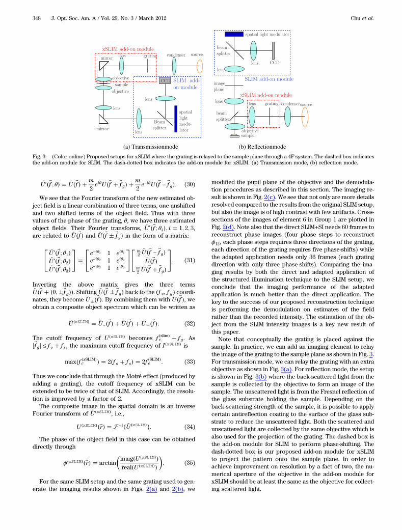
Note that conceptually the grating is placed against thesample. In practice, we can add an imaging element to relaythe image of the grating to the sample plane as shown in Fig. 3.For transmission mode, we can relay the grating with an extraobjective as shown in Fig. 3(a). For reflection mode, the setupis shown in Fig. 3(b) where the back-scattered light from thesample is collected by the objective to form an image of thesample. The unscattered light is from the Fresnel reflection ofthe glass substrate holding the sample. Depending on theback-scattering strength of the sample, it is possible to applycertain antireflection coating to the surface of the glass sub-strate to reduce the unscattered light. Both the scattered andunscattered light are collected by the same objective which isalso used for the projection of the grating. The dashed box isthe add-on module for SLIM to perform phase-shifting. Thedash-dotted box is our proposed add-on module for xSLIMto project the pattern onto the sample plane. In order toachieve improvement on resolution by a fact of two, the nu-merical aperture of the objective in the add-on module forxSLIM should be at least the same as the objective for collect-ing scattered light.

Fig. 3. (Color online) Proposed setups for xSLIM where the grating is relayed to the sample plane through a 4F system. The dashed box indicatesthe add-on module for SLIM. The dash-dotted box indicates the add-on module for xSLIM. (a) Transmission mode, (b) reflection mode.

348 J. Opt. Soc. Am. A / Vol. 29, No. 3 / March 2012 Chu et al.

4. SIMULATED IMAGING OF RANDOMLYPOSITIONED BEADSIn order to test the resolution of the modified SLIM setup, wegenerated a sample of randomly positioned bead pairs wherewe have two beads separated by a distance of 0.25 μm whichis smaller than the resolution limit, which in this case is0.5 μm. The beads themselves are represented by Gaussianfunctions with width 0.125 μm. The random beads are imagedby both SLIM and xSLIM. For the SLIM setup, we assume thecenter wavelength of the illumination is 0.5 μm. The numericalaperture of the objective is 0.8 and 0.55 of the condenser. Thewidth of the source is 1% of the pupil radius. The overall cutofffrequency of the SLIM system is f �SLIM�

c � 2.48 μm−1 accordingto Eq. (5) and the resolution is 0.5 μm according to Eq. (17).The parameters for SLIM will remain the same through therest of the simulation work in this paper. For the xSLIM setup,we can insert a grating with a period f

�SLIM�g � 2.464 μm−1 to

the SLIM setup as shown in Fig. 3. The imaging results areshown in Fig. 4(a) and (b), respectively. First we note that

the images of single beads are smaller in the xSLIM image thanin the SLIM. This means that the point spread function forxSLIM is narrower than that for SLIM. For two close beads,for example, those pointed out by the white arrow, theyare well resolved in xSLIM but not in SLIM. The cross-sectionsof those two beads are shown in Fig. 4(c) together with thecross-section of the original object. The distance between thecenter of those two beads is about 0.25 μm. This example de-monstrates that the resolution for xSLIM is 0.25 μm demon-strating resolution doubling for xSLIM.

5. EFFECTS OF NOISE IN THE DETECTORARRAY AND THE CONTRAST OF THEGRATING ON IMAGING QUALITYNext we are going to study the effect of noise in the image sen-sor. Because the object field ismodulated by a grating function,the intensity in the image plane has significant spatial varia-tions. The noise in the sensor array will affect the phase esti-mation just as in a phase-shifting interferometer [23]. In the

(a) SLIM (b) xSLIM

−0.6 −0.4 −0.2 0 0.2 0.4 0.6

0

0.2

0.4

0.6

0.8

1

distance (µ m)

ph

ase

(a.u

.)

(c) Cross−sections of two beads

SLIMxSLIMoriginal

Fig. 4. (Color online) Images of randomly positioned bead pairs by (a) SLIM and (b) xSLIM. The two beads denoted by white arrows are 0.5 μmapart. The cross-sections of the images of these two beads by SLIM, xSLIM, and the original sample are shown in (c).

(a) SNR: 104 (b) SNR: 103 (c) SNR:102

(d) (e) (f)

Fig. 5. (Color online) Imaging results of xSLIM when the signal-to-noise ratio in the image plane is (a) 104, (b) 103, and (c) 102. The zoomed-inversion of the two beads denoted by the white arrows in (a)–(c) are shown in (d)–(f), respectively. The scale bars in (a) and (d) represent 2.5 μmand 0.25 μm, respectively.

Chu et al. Vol. 29, No. 3 / March 2012 / J. Opt. Soc. Am. A 349

next simulation, the signal-to-noise ratios in the intermediateimages I�~r;ϕ� are assumed to be 104, 103, 102, respectively.The contrast of the grating is assumed to be 0.01. The originalobject consists of randomly positioned beads.

The estimated images from xSLIM for those cases areshown in Figs. 5(a)–(c), where we see that good imagescan be obtained even though the signal-to-noise ratio is aslow as 102, which is a common level for most scientific imagesensors. Zoomed-in versions of the two beads, which arepointed to by the white arrows in Figs. 5(a)–(c), are shownin (d)–(f), respectively. We see that two beads with a separa-tion distance of 0.25 μm are well resolved in all three cases.This means that even with signal-to-noise ratios as low as 102,the resolution of xSLIM is kept at twice that of SLIM.

Depending on the numerical aperture of the objective andimaging quality in the relaying element, the contrast of theprojected sinusoidal pattern in the sample plane may vary.In the next simulation the original object is composed of therat hippocampal neurons [24]. The original image is a fluores-cence image, and the intensity of the image is converted toheight to create a phase-type object for testing xSLIM. Westudy two cases where in one case the contrast of the sinusoi-dal pattern is 0.01 and in the other 0.001. The spatial frequencyof the grating is the same as in Sections 4 and 5. The imagingresults are shown in Figs. 6(a)–(d), respectively. Here we have

assumed that the signal-to-noise ratios are 1000 and 100. Com-paring (a) with (c) or (b) with (d) in Fig. 6, we can see thatwith lower contrast of the grating, the imaging result is morenoisy and of lower contrast.

Note that all the imaging results shown are without any de-noising or optical transfer function (OTF) compensation. Weexpect that with a simple weighted Wiener–Helstrom-like fil-ter [15,22,25], we can remove some of the noise and artifacts,thus improving the contrast of those images. Further, with arecently developed nonlinear algorithm to deconvolve acomplex field, where the resolution is shown to improve bya factor of 2.3 [26], we expect that the resolution of xSLIMcan be further improved.

6. SUMMARYIn this paper we have shown that super-resolution is madepossible in SLIM by applying structured illumination to thesample plane. In this way we can obtain images which notonly are label-free but also contain details beyond the diffrac-tion limit, thus expanding the ability of quantitative phase con-trast microscopy. We first apply the structured illuminationtechnique directly in the SLIM setup, with imaging resultsshowing improved resolution but with substantial artifactsand low contrast. Then we modified both the SLIM systemand the demodulation procedure using the field estimation

10µm

(a) xSLIM, m=0.01, SNR=1000 (b) xSLIM, m=0.01, SNR=100

(c) xSLIM, m=0.001, SNR=1000 (d) xSLIM, m=0.001, SNR=100

Fig. 6. Imaging results of a neuron-cell by xSLIM where contrast of the grating and the signal-to-noise ratio are (a) m � 0.01, SNR � 1000;(b) m � 0.01, SNR � 100; (c) m � 0.001, SNR � 1000; (d) m � 0.001, SNR � 100, respectively. Scale bar in (a) represents 10 μm.

350 J. Opt. Soc. Am. A / Vol. 29, No. 3 / March 2012 Chu et al.

derived in Section 2. These modifications produce imagingresults with high contrast and few artifacts and improved re-solution. The performance of the adapted spatial light interfer-ence microscope with structured illumination is demonstratedthrough numerical examples. First, random bead pairs wereused to show the resolution improvement by a factor of 2.Then effect of noise and contrast of the sinusoidal patternare also studied with the conclusion that super-resolution isstill possible even in the presence of high noise and low grat-ing contrast. Note that all imaging results shown in this paperare without denoising and deconvolution. The fundamentalreason for the improvement in resolution is that informationbeyond the cutoff frequency is passed and recorded physicallyin the modified imaging system. Through simple or advancedprocessing, the image contrast and resolution can be furtherimproved. This will stimulate more interest and open up moreapplications for the emerging field of quantitative phasemicroscopy.

ACKNOWLEDGMENTSThis work was funded by the Center for Biophotonics Scienceand Technology, a designated NSF Science and TechnologyCenter managed by the University of California, Davis, underCooperative Agreement No. PHY0120999.

REFERENCES1. F. Zernike, “How I discovered phase contrast,” Science 121,

345–349 (1955).2. R. Liang, J. K. Erwin, and M. Mansuripur, “Variation on Zernike’s

phase-contrast microscope,” Appl. Opt. 39, 2152–2158 (2000).3. C. J. Schwarz, Y. Kuznetsova, and S. Brueck, “Imaging interfero-

metric microscopy,” Opt. Lett. 28, 1424–1426 (2003).4. M. K. Kim, “Principles and techniques of digital holographic

microscopy,” SPIE Rev. 1, 1–50 (2010).5. G. Popesu, L. P. Deflores, and J. C. Vaughan, “Fourier phase

microscopy for investigation of biological structures and dy-namics,” Opt. Lett. 29, 2503–2505 (2004).

6. T. Ikeda, G. Popescu, R. R. Dasari, and M. S. Feld, “Hilbert phasemicroscopy for investigating fast dynamics in transparentsystems,” Opt. Lett. 30, 1165–1167 (2005).

7. G. Popescu, T. Ikeda, R. R. Dasari, and M. S. Feld, “Diffractionphase microscopy for quantifying cell structure and dynamics,”Opt. Lett. 31, 775–777 (2006).

8. Z. Wang, L. Millet, M. Mir, H. Ding, S. Unarunotai, J. Rogers,M. U. Gillette, and G. Popescu, “Spatial light interference micro-scopy (SLIM),” Opt. Express 19, 1016–1026 (2011).

9. H. Ding and G. Popescu, “Instantaneous spatial light interfer-ence microscopy,” Opt. Express 18, 1569–1575 (2010).

10. H. Ding, Z. Wang, X. Liang, S. A. Boppart, K. Tangella, and G.Popescu, “Measuring the scattering parameters of tissues fromquantitative phase imaging of thin slices,” Opt. Lett. 36, 2281–2283 (2011).

11. Z. Wang, L. Millet, V. Chan, H. Ding, M. U. Gillette, R. Bashir, andG. Popescu, “Label-free intracellular transport measured by spa-tial light interference microscopy,” J. Biomed. Opt. 16, 026019(2011).

12. B. Huang, M. Bates, and X. Zhuang, “Super-resolutionfluorescence microscopy,” Ann. Rev. Biochem. 78, 993–1016(2009).

13. G. Patterson, M. Davidson, S. Manley, and J. Lippincott-Schwartz, “Superresolution imaging using single-moleculelocalization,” Ann. Rev. Phys. Chem. 61, 345–367 (2010).

14. S. W. Hell, “Far-field optical nanoscopy,” Science 316, 1153–1158 (2007).

15. M. G. L. Gustafsson, “Surpassing the lateral resolution limitby a factor of two using structured illumination microscopy,”J. Microsc. 198, 82–87 (2000).

16. H. H. Hopkins, “On the diffraction theory of optical images,”Proc. R. Soc. A 217, 408–432 (1953).

17. C. J. R. Sheppard and A. Choudhury, “Image formation in thescanning microscope,” J. Mod. Opt. 24, 1051–1073 (1977).

18. M. Born and E. Wolf, Principles of Optics: Electromagnetic

Theory of Propagation, Interference and Diffraction of Light,7th ed. (Cambridge University, 1999), pp. 554–618.

19. P. Mondal, “Phase contrast microscopy in partially coherentlight,” Opt. Acta 15, 65–82 (1968).

20. L. Rayleigh, “On the accuracy of focus necessary for sensiblyperfect definition,” in Scientific Papers, Vol. 1 (CambridgeUniversity, 1899), pp. 430–432.

21. J. Haldar, Z. Wang, G. Popescu, and Z.-P. Liang, “Label-free high-resolution imaging of live cells with deconvolved spatial lightinterference microscopy,” in Engineering in Medicine and

Biology Society (EMBC), 2010 Annual International Confer-

ence of the IEEE (2010), pp. 3382–3385.22. S. A. Shroff, J. R. Fienup, and D. R. Williams, “OTF compensa-

tion in structured illumination superresolution images” (InvitedPaper), Proc. SPIE 7094, 709402 (2008).

23. P. Hariharan, Basics of Interferometry, 2nd ed. (Academic,2007), pp. 49–56.

24. D. Brandner and G. Withers, http://cellimagelibrary.org/images/8735.

25. L. P. Yaroslavsky and H. J. Caulfield, “Deconvolution ofmultiple images of the same object,” Appl. Opt. 33, 2157–2162(1994).

26. S. D. Babacan, Z. Wang, M. Do, and G. Popescu, “Cell imagingbeyond the diffraction limit using sparse deconvolution spa-tial light interference microscopy,” Biomed. Opt. Express 2,1815–1827 (2011).

Chu et al. Vol. 29, No. 3 / March 2012 / J. Opt. Soc. Am. A 351