
Precision spectroscopy with trapped Ca and Al ions
127
Precision spectroscopy with trapped 40 Ca + and 27 Al + ions Dissertation, submitted to the Faculty of Mathematics, Computer Science and Physics of the Leopold-Franzens University of Innsbruck in partial fulfillment of the requirements for the degree of Doctor of Philosophy (Physics) by Dipl.-Phys. Michael Guggemos Innsbruck, February 2017
-
Upload
khangminh22 -
Category
Documents
-
view
0 -
download
0
Transcript of Precision spectroscopy with trapped Ca and Al ions

Precision spectroscopy with trapped40Ca+ and 27Al+ ions
Dissertation, submitted to theFaculty of Mathematics, Computer Science and Physics
of the Leopold-Franzens University of Innsbruckin partial fulfillment
of the requirements for the degree of
Doctor of Philosophy(Physics)
by
Dipl.-Phys. Michael Guggemos
Innsbruck, February 2017

Abstract
This thesis reports on setting up from scratch a new experimental apparatus with trapped27Al+ and 40Ca+ ions, including the ion trap and all relevant laser systems for precisionspectroscopy. Laser ablation loading of both ion species was implemented and in additiontheir sympathetic cooling dynamics were investigated. Second, systematic frequency shifts,especially the electric quadrupole shift along 40Ca+ ion strings were calibrated with sub-Hertzresolution by carrying out Ramsey experiments with Ramsey times orders of magnitude longerthan the single ion coherence time, correlating the results and evaluating the obtained parityoscillations. Third, the absolute frequency of the 1S0 ↔ 3P1, F = 7/2 transition in 27Al+
and the Landé g-factor of the excited state g 3P1 F=7/2 were measured using Ramsey‘s methodof separated fields by quantum logic spectroscopy with a 40Ca+ ion whose S1/2 ↔ D5/2
electric quadrupole transition was used as a frequency reference. Finally the 1S0 ↔ 3P0 clocktransition in 27Al+ was observed.
i

Zusammenfassung
Diese Arbeit berichtet vom Aufbau eines neuen Ionenfallenexperiments inklusive aller relevatenLasersysteme für die Präzisionsspektroskopie an gespeicherten 27Al+ und 40Ca+ Ionen. Ionenbeider Spezies wurden mittels Laser-Ablation geladen und deren mitfühlendes Kühlverhal-ten wurde untersucht. Des Weiteren wurden systematische Frequenzverschiebungen, spezielldie elektrische Quadrupolverschiebung entlang einer Kette von gefangenen 40Ca+ Ionen mitsub-Hertz Auflösung gemessen. Dazu wurden Ramsey Experimente mit um Größenordnungenlängeren Wechselwirkungszeiten als die Kohärenzzeit des einzelnen Ions durchgeführt. Oszilla-tionen des Paritätssignals geben Aufschluss über den Unterschied in den Übergangsfrequenzender einzelnen Ionen. Darüber hinaus wurde die absolute Frequenz des 1S0 ↔ 3P1, F = 7/2Übergangs in 27Al+ Ionen sowie der Landé g-Faktor des oberen Zustands g 3P1 F=7/2 mittelsRamsey Spektroskopie bestimmt. Die elektronische Besetzung im Aluminiumion wurde durchQuantenlogik mit einem 40Ca+ Ion nachgewiesen, dessen S1/2 ↔ D5/2 Quadrupolübergangals Frequenzreferenz diente. Schließlich wurde der 1S0 ↔ 3P0 Uhrenübergang im 27Al+ Ionbeobachtet.
ii

Contents
Abstract i
Zusammenfassung ii
1 Introduction 1
2 Ion trapping fundamentals & theoretical framework 42.1 Operation principle of a linear ion trap . . . . . . . . . . . . . . . . . . . . . . . 42.2 Mixed Coulomb ion crystals . . . . . . . . . . . . . . . . . . . . . . . . . . . . . 62.3 Interaction of trapped ions with lasers . . . . . . . . . . . . . . . . . . . . . . . 10
2.3.1 Interaction of a free two level atom with monochromatic light . . . . . . 102.3.2 Quantum mechanical harmonic oscillator . . . . . . . . . . . . . . . . . 112.3.3 Combined system . . . . . . . . . . . . . . . . . . . . . . . . . . . . . . . 112.3.4 Off-resonant light field . . . . . . . . . . . . . . . . . . . . . . . . . . . . 132.3.5 Dissipation & decoherence . . . . . . . . . . . . . . . . . . . . . . . . . . 142.3.6 The Bloch sphere . . . . . . . . . . . . . . . . . . . . . . . . . . . . . . . 152.3.7 Ramsey experiment . . . . . . . . . . . . . . . . . . . . . . . . . . . . . 16
3 Level structure and radiative transitions in 40Ca+ and 27Al+ ions 183.1 Level structure and radiative transitions of 40Ca+ . . . . . . . . . . . . . . . . . 18
3.1.1 Dipole transitions . . . . . . . . . . . . . . . . . . . . . . . . . . . . . . 193.1.2 Quadrupole transitions . . . . . . . . . . . . . . . . . . . . . . . . . . . . 20
3.2 Level structure and radiative transitions of 27Al+ . . . . . . . . . . . . . . . . . 223.2.1 The 1S0↔ 3P1 intercombination line . . . . . . . . . . . . . . . . . . . 233.2.2 The hyperfine induced 1S0↔ 3P0 clock transition . . . . . . . . . . . . 253.2.3 Nuclear spin flips . . . . . . . . . . . . . . . . . . . . . . . . . . . . . . . 27
4 Experimental setup 294.1 Ion trap setup . . . . . . . . . . . . . . . . . . . . . . . . . . . . . . . . . . . . . 29
4.1.1 Linear Paul trap . . . . . . . . . . . . . . . . . . . . . . . . . . . . . . . 304.1.2 Vacuum vessel . . . . . . . . . . . . . . . . . . . . . . . . . . . . . . . . 344.1.3 Magnetic field shielding . . . . . . . . . . . . . . . . . . . . . . . . . . . 37
iii

Contents
4.1.4 Imaging system & state detection . . . . . . . . . . . . . . . . . . . . . . 384.2 Laser systems . . . . . . . . . . . . . . . . . . . . . . . . . . . . . . . . . . . . . 40
4.2.1 Lasers for Doppler-cooling, repumping, and photo-ionization . . . . . . 404.2.2 Wavelength meter & wavelength control . . . . . . . . . . . . . . . . . . 454.2.3 Ultra-stable lasers . . . . . . . . . . . . . . . . . . . . . . . . . . . . . . 474.2.4 Frequency comb . . . . . . . . . . . . . . . . . . . . . . . . . . . . . . . 61
4.3 Experimental control . . . . . . . . . . . . . . . . . . . . . . . . . . . . . . . . . 68
5 Experimental techniques 705.1 Laser ablation loading of ions . . . . . . . . . . . . . . . . . . . . . . . . . . . . 705.2 Experimental sequence . . . . . . . . . . . . . . . . . . . . . . . . . . . . . . . . 755.3 Locking the 729 nm Laser to the S-D transition . . . . . . . . . . . . . . . . . . 815.4 Micromotion compensation . . . . . . . . . . . . . . . . . . . . . . . . . . . . . 815.5 Quantum logic spectroscopy . . . . . . . . . . . . . . . . . . . . . . . . . . . . . 84
6 Measurements 866.1 Sympathetic cooling . . . . . . . . . . . . . . . . . . . . . . . . . . . . . . . . . 866.2 Ramsey correlation spectroscopy . . . . . . . . . . . . . . . . . . . . . . . . . . 916.3 Precision spectroscopy on the 1S0↔ 3P1, F = 7/2 transition . . . . . . . . . . 996.4 Observation of the 1S0↔ 3P0 clock transition . . . . . . . . . . . . . . . . . . 107
7 Summary and outlook 109
A Appendix 111
B Journal publications 112
Acknowledgements 120
iv

1 Introduction
Thousands of years ago mankind started to observe time based on regular periodic phenomenain nature. Monuments like Stonehenge and devices like the sky disk of Nebra allowed for theobservation and prediction of equinoxes and solstices, respectively which was important forearly agriculture.The progression of civilization and the need of synchronizing social events required the
observation of time on shorter scales. This led to the development of sundials [1]. Thefrequency ratio of the earth‘s orbit and the phases of the moon led to the division of thedaylight into twelve parts [1]. However, there are some impractical characteristics of sundials.The length of one hour changes with the latitude of the observer and depends on the season.Moreover sundials simply don‘t work at night and cloudy days. Other approaches to measuretime like water clocks and sandglasses overcame this problem by tracking time based on aconstant flow rate.Development in metal processing led to the invention of pendulum clocks by Christiaan
Huygens in 1656, which were the first clocks containing an intrinsic oscillator. Each oscillationperiod of these pendula corresponds to a temporal period of one second. However, sincetheir oscillation frequency depends on the acceleration, acting on the pendulum, which is notconstant on a wavering ship, these clocks turned out to be not accurate enough for nauticalnavigation. The use of a spring-based oscillator solved this problem.With the development of electronics and the discovery of the piezo-electric effect [2] at the
end of the 19th century quartz clocks came up. With a higher clock speed and independencefrom external perturbations quartz clocks led to an improvement of one order of magnitudein time keeping with respect to the best pendulum clocks [1]. However, quartz crystals havenever identical natural frequencies and in addition they age, resulting in long term frequencydrifts.The idea of using atomic systems for time keeping was conceived in the middle of the 20th
century. The first concept of an atomic clock was devised in 1945 by I. I. Rabi [3,4]. It makesuse of two atomic energy levels that are coupled by electromagnetic radiation at their resonancefrequency which denotes the oscillator. Atoms of the same kind have identical properties (tothe current status of knowledge), allowing identical atomic clocks to be built anywhere. Thecurrent definition of the second is based on cesium fountain clocks using Ramsey‘s method ofseparated fields [5]:
1

Chapter 1. Introduction
The second is the duration of 9 192 631 770 periods of radiation corresponding to the transitionbetween the two hyperfine levels of the ground state of the cesium 133 atom.
The performance of a clock is characterized by two properties, accuracy and stability. Ac-curacy is the degree of conformity of the measured time to its definition, which is related to anoffset from the ideal value. It depends on the perturbability of the clock. Stability indicateshow well an oscillator can produce the same frequency over a given period of time τ and ischaracterized by the Allan deviation. The instability of a shot-noise limited atomic clock isexpressed by [6]
σy(τ) ∼ 1πQ
√TcNτ
(1.1)
where Tc is the interrogation time, Q = ν0/∆νFWHM the quality factor as the ratio betweenoscillation frequency and the spectral width of the atomic transition, N the number of atoms(shot noise) and τ the measurement time. Reduction of Doppler-shifts by laser cooling enablecurrent cesium fountain clocks [7] to reach fractional frequency instabilities in the low 10−16
range. From equation 1.1 it can be seen that this can be improved using spectrally narrowtransitions with higher frequency.The invention of optical frequency combs [8] facilitated direct frequency measurements in
the optical domain substantially and so optical atomic clocks became a logical consequence.The frequency comb down-converts optical frequencies to the radio frequency domain wherethey can be handled and distributed by common electronics. Over the last years huge progresswas made with optical clocks based on trapped ions [9] and neutral atoms captured in opticallattices [10], which nowadays outperform the cesium fountain clocks by two orders of magnitudein terms of stability and accuracy [9, 10]. Currently the most stable clock is based on neutralstrontium atoms in an optical lattice [10]. The stability of these clocks benefits from a highnumber of atoms that can be investigated simultaneously. However, the accuracy of theseclocks suffers from drifting systematic shifts, especially the AC Stark shift resulting fromblack-body radiation.Contrary to that, aluminium ions feature a clock transition around 1.121 PHz that is ex-
tremely robust to external perturbations which makes it well suited for time keeping, especiallyin noisy environments. Single ion aluminium clocks already reached amazing stability and ac-curacy almost a decade ago. The fractional inaccuracy of 8.6 · 10−18 measured in ref. [9] islimited primarily by uncertainties in the second order Doppler-shift, which could be recentlyreduced by a factor of 50 [11]. It was proposed that a quantum network of clocks basedon aluminium ions has the potential to reach the 10−20 level [12]. The only drawback ofaluminium ions is that they lack a practical closed transition for Doppler-cooling and statedetection. This problem can be overcome by simultaneously trapping another species that
2

can be directly cooled. So far beryllium and magnesium ions were used as logic ions [9]. Theuse of 40Ca+ ions as logic ions is advantageous as better cooling results due to a narrowerlinewidth of the cooling transition and its similar mass to 27Al+can be achieved [13], reducingthe uncertainty in the second order Doppler-shift. A detailed comparison of advantages anddisadvantages of relevant atomic and ionic species under investigation for an optical frequencystandard can be found in [14].There are plenty of useful applications for ultra precise clocks. Besides for time keeping,
frequency measurements can be used for a more accurate definition of other physical units.Furthermore the resolution of positioning systems like GPS and GALILEO rely on the perfor-mance of atomic clocks. Research in the field of general relativity benefited from that progresssince a gravitational red-shift from an elevation difference of only 30 cm could be observedby recent clock comparisons [15] and also relativistic time dilatation of ions experiencing dif-ferent excess micromotion was investigated [15]. The test of fundamental theories and theinvestigation of the variation of fundamental constants like the fine structure constant [16] areprobed by comparing transition frequencies of different atomic species over a long period oftime. Furthermore, more precise synchronization of radio telescopes increases the resolutionof telescope arrays and interferometric measurements on large baselines which opens up newpossibilities in astrophysics.All these interesting applications and a collaboration with the European Space Agency
(ESA) initiated the work on an optical frequency standard in the group of Rainer Blatt inInnsbruck. The key focus of research in the group is on quantum computation and quantuminformation processing with trapped 40Ca+ ions. Key techniques developed in that context al-low one to detect the internal state of the 27Al+ ion via quantum logic spectroscopy (QLS) andcan enhance the performance of trapped-ion clocks by deterministic creation of entanglement.This work lays the foundation of a frequency standard based on trapped 27Al+ and 40Ca+
ions. The thesis is structured as follows. Chapter 2 gives a short theoretical description ofall relevant phenomena of trapped ions interacting with light fields. Chapter 3 focuses on theatomic properties of both ion species and the relevant transitions used in this work. A detaileddescription of the experimental setup that was built can be found in chapter 4. Chapter 5presents fundamental experimental techniques in ion trapping experiments. The experimentalresults of this work are presented in chapter 6. Chapter seven concludes the thesis.
3
2 Ion trapping fundamentals & theoreticalframework
This section describes the confinement generated by a linear Paul trap and the resultingclassical motion of a charged particle in the potential [17]. Later, the discussion will beextended to describe the collective motion of ions in a mixed ion crystal [18].
2.1 Operation principle of a linear ion trap
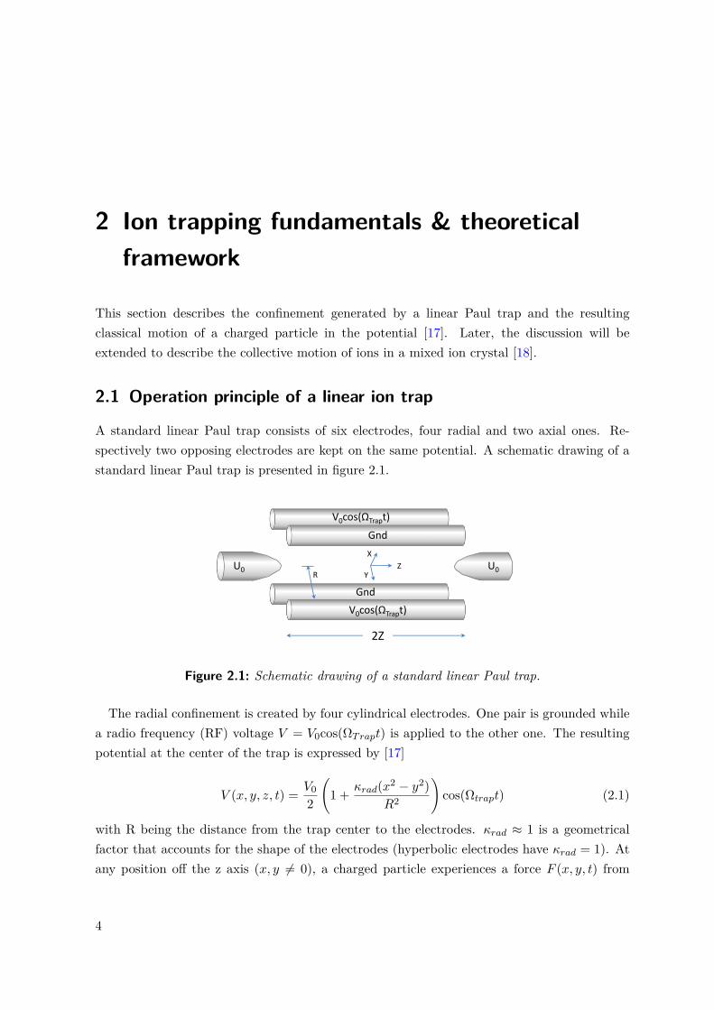
A standard linear Paul trap consists of six electrodes, four radial and two axial ones. Re-spectively two opposing electrodes are kept on the same potential. A schematic drawing of astandard linear Paul trap is presented in figure 2.1.
U0U0
V0cos(ΩTrapt)
V0cos(ΩTrapt)
Gnd
Gnd
X
YZ
2Z
R
Figure 2.1: Schematic drawing of a standard linear Paul trap.
The radial confinement is created by four cylindrical electrodes. One pair is grounded whilea radio frequency (RF) voltage V = V0cos(ΩTrapt) is applied to the other one. The resultingpotential at the center of the trap is expressed by [17]
V (x, y, z, t) = V02
(1 + κrad(x2 − y2)
R2
)cos(Ωtrapt) (2.1)
with R being the distance from the trap center to the electrodes. κrad ≈ 1 is a geometricalfactor that accounts for the shape of the electrodes (hyperbolic electrodes have κrad = 1). Atany position off the z axis (x, y 6= 0), a charged particle experiences a force F (x, y, t) from
4

2.1. Operation principle of a linear ion trap
the corresponding electric field. Over one radio frequency period the mean ion position hardlychanges and the force averages to 〈F (x, y)〉. The related pseudopotential well [17] can becalculated by integration Φps = −
∫〈F (x, y)〉 to
Φps = QV 20
4MR2Ω2trap
, (2.2)
where M is the mass and Q the charge of the particle. The axial confinement is created bytwo endcap electrodes on the trap axis which are kept on a static voltage U0. The distancebetween the endcaps (2Z) is the same as the length of the radial electrodes. The resultingstatic potential is given by
U(x, y, z) = κaxU0Z2
(z2 − 1
2(x2 + y2)). (2.3)
A further geometrical factor κax < 1 accounts for the shape of the endcap electrodes. Themotion of a trapped particle in the combined static and RF potential is described by theMathieu equations
d2xidt2
+Ω2Trap
4 (ai + 2qicos(ΩTrapt))xi = 0 (2.4)
using the dimensionless parameters ai and qi which are defined as ax,y = −az/2 = − 4QκaxU0MZ2Ω2
trap
and qx = −qy = 2QκradV0MR2Ω2
trap, qz = 0. Stable ion trapping is possible, if the trajectories in all three
directions are confined. Parameters that lead to stable solutions are depicted in a stabilitydiagram [17,19]. Finally the equation of motion can be approximated by
xi(t) ≈ Aicos(ωit+ ϕi)(
1 + qi2 cos(ΩTrapt)
)(2.5)
with the amplitude Ai and phase ϕi depending on the initial conditions. The motion of theparticle can be separated in two parts. A harmonic oscillation at frequencies
ωx,y = 12ΩTrap
√ai + 1
2q2i and ωz =
√κaxQU08MZ2 (2.6)
which is called secular motion and the driven motion due to the trapping field at frequencyΩtrap, called micromotion. Additional electric stray fields at the trap can shift the static partof the potential. As a consequence RF and DC null do not necessarily overlap which gives riseto excess micromotion.
5

Chapter 2. Ion trapping fundamentals & theoretical framework
2.2 Mixed Coulomb ion crystals
As soon as more ions are confined in the trap, the Coulomb repulsion between the ions needs tobe considered. When the kinetic energy of the ions becomes small compared to the Coulombenergy, regular structures are formed which are known as ion crystals. The ions align them-selves such that their potential energy is minimum [20]. For sufficiently cold temperatures theions‘ motion can be described as a set of collective motional modes around their equilibriumpositions [20]. A detailed description of the problem for ions of the same kind can be foundin [20]. In order to determine the equilibrium positions and mode frequencies of a mixed ionstring the equations derived in [20] need to be generalized for different ion masses. Accordingto [18,21] this can be done in the following way.
The potential energy of a mixed N-ion string in a static harmonic potential is given by
V =N∑i=1
∑α=x,y,z
12miω
2i,αr
2i,α +
N∑n=1
∑m 6=n
12Z2e2
4πε01
|rm − rn|(2.7)
where mn is the mass of the nth ion and ωn,α its oscillation frequency along the direction α.All ions are assumed to have the same charge Z. Introducing the length scale l3 = Z2e2
4πε0m0ω20
with the mass m0 and the oscillation frequency ω0 of a reference ion (40Ca+ in this work),allows one to rewrite the potential energy in a dimensionless form
V = 12m0l
2
∑i,α
µiω2i,αρ
2i,α + ω2
0∑n,mn6=m
1|ρm − ρn|
(2.8)
with ρi = ri/l and µi = mim0
. In the case of a linear ion string the coordinates in the transversedirections are zero (ρi,x = ρi,y = 0). With the definition ui ≡ ρi,z the expression for theequilibrium positions u0
i of the ions is given by
∂V
∂ui
∣∣∣∣ui=u0
i
= 0 ⇐⇒ ciu0i + d
dui
∑nn6=i
1|ui − un|
∣∣∣∣ui=u0
i
= 0
⇐⇒ ciui −∑nn<i
1(u0i − u0
n)2 +∑nn>i
1(u0i − u0
n)2 = 0 (2.9)
with ci = µi(ωizω0
)2. This expression can be solved by numerical solvers for nonlinear equations.For two singly charged ions in a static harmonic potential the equilibrium positions are u2 =−u1 = 2− 2
3 and the equilibrium distance is
6

2.2. Mixed Coulomb ion crystals
d =(
e2
2πε0m0ω20
) 13
. (2.10)
The calculation of the motional modes of a mixed ion crystal starts with the Lagrangian, whichcontains the kinetic and potential energy terms L = T − V , and is given by
L = 12∑i,α
mi·r
2i − V (ri,α) = 1
2m0l2
∑i,α
µi·ρ
2i,α − ω2
0
∑i,α
ci,αρ2i,α +
∑n,mn6=m
1|ρm − ρn|
. (2.11)
Approximating the Lagrangian to second order around the equilibrium positions ρ0m = (0, 0, u0
m)determined above, and rewriting the ion positions as ρm = (qmx, qmy, u0
m+qmz) the Lagrangiancan be decomposed as L = Lx + Ly + Lz where
Lz = 12m0l
2
∑i
µi·q
2i,z −
∑i
µiω2i,zq
2i,z −
ω20
2∑i,j
qi,zqj,z∂
∂qi,z
∂
∂qj,z
∑n,mn6=m
1|ρm − ρn|
∣∣∣∣qi=0
. (2.12)
The expressions for Lx and Ly are similar. Note that a constant offset was subtracted from
L. The term S = 12∑i,j qi,zqj,z
∂∂qi,z
∂∂qj,z
∑n,m
n6=m
1|ρm−ρn|
∣∣∣∣qi=0
can be split into two parts for i = j
and i 6= j and yields
S = 12∑i
q2i,z
∑n,mn 6=m
2|u0m − u0
n|3(δn,i + δm,i) + 1
2∑i,ji 6=j
qi,zqj,z∑n,mn 6=m
2|u0m − u0
n|3(δn,iδm,j + δn,jδm,i)
=∑n
q2n,z
∑n6=m
2|u0m − u0
n|3
+∑n,mn6=m
qn,zqm,z
( −2|u0m − u0
n|3). (2.13)
The Lagrangian can be rewritten as [18,21]
Lz = 12m0l
2
∑i
µi·q
2i,z −
∑i,j
Azi,jqi,zqj,z
(2.14)
7
Chapter 2. Ion trapping fundamentals & theoretical framework
where Azi,j is the coupling matrix (Hessian matrix)
Azi,j =
µiω
2i,z + 2ω2
0∑n6=i
1|u0
i−u0n|3
i = j
−2ω20∑n6=i
1|u0
i−u0n|3
i 6= j .(2.15)
Using mass weighted coordinates q′ = Mq with Mij = δij√
mim0
the Lagrangian becomes
Lz = 12m0l
2[(·q′z)t
·q′z − (q′z)tM−1AzM−1q′z
](2.16)
Inserting the Lagrangian into the Lagrangian equation of motion
d
dt
∂L
∂·qi− ∂L
∂qi= 0 (2.17)
leads to the axial modes
··q′z +M−1AzM−1q′z = 0 (2.18)
For ions with the same mass the expression reduces to the formula given in [20]. Introducingthe symmetric matrix Az = M−1AzM−1 with its elements
Azij = 1√µiµj
Azij =
ω2i,z + 2ω2
0µi
∑n6=i
1|u0
i−u0n|3
i = j
− 2ω20√
µiµj
∑n6=i
1|u0
i−u0n|3
i 6= j(2.19)
the equations of motion become
··q′z + Azq′z = 0. (2.20)
Solving the eigenvalue problem Azq′z = (λz)2q′z leads to the eigenfrequencies λz of the col-lective modes of motion. The transverse mode frequencies can be calculated by the same ap-proach. The only difference is the second order derivative of the term describing the Coulombinteraction. The corresponding matrix elements are
Axi,j =
µiω
2i,x − ω2
0∑n 6=i
1|u0
i−u0n|3
i = j
+ω20∑n6=i
1|u0
i−u0n|3
i 6= j(2.21)
that enter into the eigenvalue problem for the transverse mode frequencies λx and analogouslyfor λy. A comprehensive description of mixed ion crystals can be found in [18].The motion of a mixed two-ion crystal is described by six motional modes, one in-pase and
one out-of-phase mode along the three trap axis. A detailed description of the normal modes
8

2.2. Mixed Coulomb ion crystals
of a Ca+/Al+ion crystal can be found in [13].
9

Chapter 2. Ion trapping fundamentals & theoretical framework
2.3 Interaction of trapped ions with lasers
The following section describes the interaction of an ion, confined in a trap, with laser radiation.First a free two-level atom is considered. Second, the confinement is taken into account by thedescription of the quantum mechanical harmonic oscillator. Subsequently, both Hamiltoniansare added up to describe the combined system. Furthermore, carrier and sideband transitionsare described as well as off-resonant laser-ion interactions. Next, a change to the densitymatrix formalism is made which allows one to account for dissipation and decoherence. Last,Ramsey‘s method of separate oscillatory fields is described.
2.3.1 Interaction of a free two level atom with monochromatic light
To describe the interaction of an atom with a laser field simplifications need to be made. Incases where the driving field is close to resonance to the transition between two atomic levelswhile other transitions are far detuned, the so called two-level atom is a good approximationto real systems. The Hamiltonian describing the bare atom is
Ha = ~ω02 σz (2.22)
where ~ω0 denotes the energy difference between ground |g〉=|↓〉 and excited |e〉=|↑〉 state andσz is a Pauli spin operator. The perturbation by a classical light field close to resonance withfrequency ωl and phase φl is described by the Hamiltonian
Hl = ~Ωσxcos(ωlt+ φl). (2.23)
Resonant light leads to population oscillations between ground and excited state at a frequencyΩ, known as the Rabi frequency whose strength is set by the electric field strength of the lightfield and the coupling matrix element of the atomic levels coupled by the light field (see section3). The combined Hamiltonian H = Ha + Hl is transferred to the interaction picture withrespect to Ha via Hint = U†0HaU0 using the time evolution operator U0 = e−iHat/~ [22]. Aftera rotating wave approximation, neglecting sum frequency terms, the interaction Hamiltoniandenotes
Hint = ~Ω2 (cos((ωl − ω0)t+ φl)σx + sin((ωl − ω0)t+ φl)σy) . (2.24)
After introducing the electronic raising and lowering operators σ± = (σx ± iσy)/2 and substi-tuting the detuning (ωl − ω0) = δ , the Hamiltonian can be rewritten as:
Hint = ~Ω2(e−i(δt+φl)σ+ + ei(δt+φl)σ−
)(2.25)
10

2.3. Interaction of trapped ions with lasers
This is the final expression for the interaction of a two-level atom with a laser.
2.3.2 Quantum mechanical harmonic oscillator
So far the position of the particle, interacting with a laser was assumed to be fixed. To accountfor the influence of the ion motion in the trap, the Hamiltonian for a quantum mechanicalharmonic oscillator has to be added. For the sake of simplicity, a one dimensional quadraticpotential is assumed.
Htr = p2
2m + 12mω
2trx
2 (2.26)
The Hamiltonian describes the total energy of a particle with mass m oscillating at a frequencyωtr/2π, where x and p denote position and momentum operators. It is useful to introduce thecreation and annihilation operators [23]
a† =√
mωtr2~
(x− i
mωtrp)
and a =√
mωtr2~
(x+ i
mωtrp). (2.27)
Hence the position and momentum operators can be represented as
x = (a+ a†)x0 and p = i(a† − a) ~2x0
(2.28)
where x0 =√~/(2mωtr) denotes the spatial extent of the ground state wave function. In
terms of the creation and annihilation operators the Hamiltonian can be expressed as
Htr = ~ωtr(a†a+ 12) = ~ωtr(n+ 1
2). (2.29)
The number operator n has eigenstates |n〉 that correspond to the number of motional quanta(phonons) contained in the oscillator.
2.3.3 Combined system
In order to describe the interaction of a trapped two-level atom with a laser field equation(2.25) has to be modified with an additional term eikx = eiη(a+a†) that accounts for the ion‘sposition. The resulting Hamiltonian yields [24]
H1 = ~Ω2 (σ+ + σ−)(eiη(a+a†)e−i(δt−φl) + e−iη(a+a†)ei(δt−φl)) (2.30)
with η being the Lamb-Dicke parameter. It is the product of the angular wavenumber of thelaser field k with the spatial extent of the ion‘s ground state wave function and the anglebetween the laser and the direction of motion.
11

Chapter 2. Ion trapping fundamentals & theoretical framework
η = kx0cos(Θ) = k
√~
2mωtrcos(Θ) (2.31)
In the case of a mixed ion crystal (see section 2.2) the Lamb-Dicke parameter is given by
ηiα = k
√~
2miωαVi,α (2.32)
where Vi,α is the matrix element of the matrix V diagonalizing the matrix A = V DV † (withD = Azor D = Ax). The elements Vi,α, i = 1, ..., N are the normal mode contributions tothe mass weighted coordinate vector q′ normalized to 1. A rotating wave approximation andtransforming the Hamiltonian to the interaction picture with respect to the Hamiltonian ofthe unperturbed system H0 = ~ω0
2 σz + ~ωtr(a†a+ 12) leads to:
Hint = ~Ω(σ+eiη(ae−iωlt+a†eiωlt)e−i(δt−φl) + h.c.) (2.33)
If the extension of the wave function is small compared to the laser wavelength, the inequalityη2(2n+1) 1 holds, which is known as the Lamb-Dicke regime. In this regime the Hamiltoniancan be Taylor-expanded to first order to
Hint(t) = ~Ωσ+(1 + iη(ae−iωt + a†eiωt))e−i(δt−φl) + h.c.. (2.34)
The approximation holds for transitions that change the motional state by zero or one quanta.The ion motion in the trap leads to an oscillating Doppler shift of the laser frequency. From theion‘s point of view this translates into a frequency modulation of the laser. As a consequencesideband transitions show up that allow for manipulation of the ion‘s internal and motionalstate. Three different types of resonant transitions can be identified. The carrier transitiononly couples the internal states and leaves the motional state unchanged. Its Hamiltonian isgiven by:
Hcar = ~Ωn,n
2(eiφl σ+ + e−iφl σ−
). (2.35)
Deep within the Lamb-Dicke regime, the coupling strength of the carrier transition is indepen-dent from its motional state. When considering up to second order in η the coupling strengthscales as Ωn,n = (1−η2n)Ω. A process that changes the internal state and lowers the motionalstate by one quantum is called red sideband transition with the corresponding Hamiltonian
Hrsb = i~ηΩn,n−1
2(eiφl aσ+ − e−iφl a†σ−
). (2.36)
12

2.3. Interaction of trapped ions with lasers
The opposite process adds a phonon to the system and is called blue sideband transition anddescribed by
Hbsb = i~ηΩn,n+1
2(eiφl a†σ+ − e−iφl aσ−
). (2.37)
The coupling strengths on red and blue sideband transitions are Ωn−1,n = η√nΩ and Ωn,n+1 =
η√n+ 1Ω respectively. Comparing Rabi frequencies on carrier and sideband transitions allows
one to extract the Lamb-Dicke parameter. Sideband transitions allow one to couple internaland external degrees of freedom and therefore enable:
1. Coupling of internal and external degrees of freedom
2. Frequency-resolved sideband cooling (see section 5.2)
3. Quantum logic spectroscopy (see section 5.5).
The mean phonon number can be determined by comparing the relative coupling strengths ofred and blue sideband. Typically the ion‘s motional state after laser cooling is described by athermal state with Fock state populations pn(n) = 1
n+1( nn+1)n. Thus carrier Rabi oscillations
contain frequency components weighted by the thermal distribution.
|c↑|2 =∞∑n=0
pn(n)sin2(Ωn,n
2 t
)(2.38)
Consequently Rabi oscillations damp faster with increasing n and the oscillation period be-comes longer.
2.3.4 Off-resonant light field
As the light is tuned away from the atomic resonance Rabi oscillations become faster witha decreasing amplitude. The upper state population |c↑|2 can be calculated by solving theoptical Bloch equations [25]
|c↑|2 = Ω2
Ω2 + δ2 sin2(1
2√
Ω2 + δ2t
). (2.39)
For a large detuning δ Ω the population transfer is greatly suppressed, but the presence ofthe light field shifts the atomic energy levels, which is known as the AC-Stark effect. The per-turbation causes new eigenenergies of the two-level atom. The AC-Stark shift of the transitionis given by
4Stark = Ω2
2δ (2.40)
while the lower level is shifted by −Ω2/4δ and the upper level by Ω2/4δ.
13

Chapter 2. Ion trapping fundamentals & theoretical framework
2.3.5 Dissipation & decoherence
So far the coherent interaction of a trapped two-level atom with a laser field was consid-ered. In real quantum systems dissipation and decoherence are always present. Such effectsstochastically change the quantum state. In the case of spontaneous emission the populationschange due to a stochastic decay of the atom from the excited state to the ground state.Since the quantum system exchanges energy with the environment, it is said to be open. Aquantitative treatment of open quantum systems is possible by the use of the density ma-trix formalism [25, 26]. The generalized form of the Schrödinger equation, the Von Neumannequation, is
d
dtρ = − i
~
[H, ρ
](2.41)
where ρ = ∑ipi |ψi〉 〈ψi| is the density matrix with probabilities pi. Including dissipative
processes described by a Liouvillian L that takes into account system-environment interactions,the master equation becomes
d
dtρ = − i
~
[H, ρ
]+ Lρ. (2.42)
Using the Lindblad notation [27], the Liouvillian describing spontaneous emission can be re-expressed in terms of the electronic raising and lowering operators as
d
dtρ = − i
~
[H, ρ
]− Γ
2 [ρσ+σ− + σ+σ−ρ− 2σ−ρσ+] (2.43)
with the decay rate Γ of the excited state. The master equation of a coherently driven twolevel system including spontaneous emission can be explicitly written where energy conservingand dissipative terms are separated. The time dynamics of the density matrix elements for atwo-level system (|g〉 , |e〉) is given by the optical Bloch equations:
·ρee = + i
2Ω(ρeg − ρge)− Γρee (2.44)
·ρgg = − i2Ω(ρeg − ρge) + Γρee (2.45)
·ρeg = + i
2Ω(ρee − ρgg) + iδρeg − (Γ/2)ρeg (2.46)
·ρge = − i2Ω(ρee − ρgg)− iδρge − (Γ/2)ρge. (2.47)
14

2.3. Interaction of trapped ions with lasers
An analytical expression describing the upper state population (with |ρee(t = 0)|2 = 0) of aresonantly driven two level atom including dissipation is given by [26]
|ρee(t)|2 = Γ2
Γ2 + 2Ω2
[1− 2Ω2
Γ e−(3Γ/4)tcosh(ζt) + (3Γ/4)
ζsinh(ζt)
](2.48)
where ζ =√
(Γ/4)2 − Ω2.
2.3.6 The Bloch sphere
To gain a graphical understanding of coherent operations on a two-level atom it is useful tointroduce the Bloch sphere representation of the two-level system which is depicted in figure2.2.
|ψ
1
2(|↓ +|↑ )
|↓ = |1
θ
φ
Z
X Y
|↑ = |0
1
2(|↓ -|↑ )
1
2(|↓ −i|↑ )
1
2(|↓ +i|↑ )
Figure 2.2: Bloch sphere representation of a two-level system. Any pure quantum state |ψ〉 =α |↓〉 + β |↑〉 with α2 + β2 = 1 can be represented as a vector (Bloch vector), pointing on thesurface of a three dimensional unit sphere. Ground and excited state correspond to north andsouth pole of the sphere, respectively. Two pairs of orthogonal superposition states lie in theequatorial plane. Interior points correspond to mixed states.
Ground and excited state of the two-level system correspond to the north and the southpole of the sphere, respectively. Superposition states lie in the equatorial plane. Coherentmanipulations of the two-level system are described by the Pauli matrices (σx, σy, σz) [23, 25]and correspond to rotations of the Bloch vector around the corresponding coordinate axis. Alaser pulse with Ωt = π is called π pulse and rotates the Bloch vector by 180° and thereforeinverts the population of ground and excited state. Decoherence of the quantum state can beseen as a decay of the Bloch vector along the z-axis towards the ground state. More detailedinformation can be found in numerous textbooks and theses [23,25,28–30].
15

Chapter 2. Ion trapping fundamentals & theoretical framework
2.3.7 Ramsey experiment
So far the interaction of an atom with a contineous laser field was considered. In practice, theinteraction time between the laser field and the atom is limited to a duration τ . For a set ofdifferent frequency detunings of the laser field from the atomic resonance, an excitation profilecan be observed which corresponds to the Fourier transform of the excitation pulse [25]. Thisis known as Rabi spectroscopy. The spectral line width is limited by the interaction time τ .Ramsey‘s method of separate oscillatory fields [5] is an alternative method to interrogate an
atomic transition. Contrary to simple Rabi spectroscopy the interrogation consists of two laserpulses, separated by a waiting time τR. Starting in the electronic ground state |0〉, a resonantπ/2 - pulse on the transition creates the superposition state |ψ〉 = 1√
2(|↓〉 + |↑〉). Duringthe waiting time τR the state vector evolves freely |ψ〉 = 1√
2(|↓〉 + ie−iω0τR |↑〉) at the opticalfrequency (ω0/2π ≈ 1015 Hz), that corresponds to the energy separation of both involvedatomic states. It is useful to change into a co-rotating frame in order to see the influenceof the second pulse. The state vector now becomes |ψ′〉 = 1√
2(|↓〉 + ie−i(ωl−ω0)τR |↑〉), whichremains unchanged for a resonant laser field. Depending on its optical phase with respect tothe first pulse, the second π/2 - pulse rotates the Bloch vector either up to the excited state|1〉 for 4ϕ = 0° or back to the ground state |1〉 for 4ϕ = 180°. A detuning of the laser fromthe atomic resonance causes the Bloch vector to rotate around the z axis by φ = (ωl − ω0)τR,which gets mapped onto the observable σz by the second π/2 pulse. Precise knowledge of τRallows one to infer the detuning of the laser from the transition. This calculation is valid, if theduration of the π/2 - pulses is negligibly short compared to τR, otherwise an effective Ramseytime has to be considered. If the experiment is repeated for different laser detunings, a fringepattern is observed (Ramsey pattern [5]). The spectral width of the fringes scales as 1/τR infrequency. If the spectral resolution is limited by the finite interaction time between the laserand the ion, this method outperforms Rabi spectroscopy by roughly a factor of two in termsof frequency resolution [31].If more than one ion is interrogated simultaneously, their transition frequencies can be
slightly different due to external perturbations (see section 6.2). As already mentioned, dis-sipation and decoherence are always present in real quantum systems which are the limitingfactors for the lifetime of the atom‘s quantum state (coherence time) [25]. Therefore the fre-quency resolution limit of the Ramsey experiment described above is set by the single ioncoherence time which makes it hard to resolve transition frequency differences on the Hz scaleor below. From Ramsey experiments with Ramsey times well beyond the single ion coher-ence time no useful information can be directly obtained from the excited state populations,but there are still correlations between the ions, which are known as quantum discord [32].These correlations can be observed in the time evolution of the parity signal between two ions.The parity signal P is the product of the Pauli σz operators obtained by the excited state
16

2.3. Interaction of trapped ions with lasers
populations pj .
P =n∑j=0
(−1)jpj (2.49)
The parity rescales the co- or anti-aligned z-components of the Bloch vectors to the interval[−1, 1]. Time-dependent oscillations in the parity signal represent a relative transition fre-quency difference between the ions. More information about this method can be found insection 6.2.
17

3 Level structure and radiative transitions in40Ca+ and 27Al+ ions
This chapter describes the relevant energy levels of 40Ca+ and 27Al+ and the radiative tran-sitions between them. The calcium ion has been used for a long time and its properties aredescribed in detail in various theses [19,29,33–35]. However, for 27Al+, there is no thesis con-taining a summary of its relevant properties. The available information is spread over variouspublications and theses. In terms of completeness a summary of the most important factson 40Ca+ is presented. Since this thesis is the first that reports on 27Al+ in this group, adetailed description of the level structure and the relevant radiative transitions between themis presented. Furthermore a condensed version of a theoretical calculation of the decay ratesof both relevant optical transitions according to [36] is given.
3.1 Level structure and radiative transitions of 40Ca+
Singly charged Ca+ has a single electron in the 4s shell. Therefore, its electronic structure issimilar to hydrogen. A detailed level diagram of its lowest energy levels is presented in figure3.1. The next orbital higher in energy than the ground state is the metastable 3d state thatconsists of two fine structure components, the D3/2 and D5/2 states with lifetimes of ∼ 1.2 sand 1.149(4) s [37] respectively. They are linked to the ground state via an electric quadrupoletransitions. The S1/2 ↔ D5/2 transition is of interest as a frequency standard at a transitionfrequency of 411 042 129 776 393.2(1.0) Hz [38], which was measured by our group. There arethree other absolute frequency measurements of this transition where one value agrees with thevalue above [39], while the other two are about 5 Hz [40] and 8 Hz [41] higher in frequency. Theg-factors of ground and excited states are gS1/2 = 2.002 256 64(9) [42] and gD5/2 = 1.200 3340(3)[38]. For the purpose of quantum computation and quantum simulation [28–30,32,33] a qubit/ pseudo-spin can be encoded in the S1/2 and D5/2 Zeeman sub-states in a non-zero magneticfield. The frequency deviations from the line center of the ten possible transitions within theZeeman manifolds can be calculated from the linear Zeeman effect
4νS↔D = µBh
(gD5/2 ·mf − gS1/2 ·mi
)·B (3.1)
18

3.1. Level structure and radiative transitions of 40Ca+
where µB is the Bohr magneton, mi and mf are the magnetic quantum numbers of initial andfinal state and B is the amplitude of the magnetic field defining the quantization axis1.Again higher in energy is the short lived P orbital that consists of two fine structure com-
ponents, the P1/2 and P3/2 state. Both levels are connected to the ground state and the Dstates via strong dipole transitions.
729nm
2D5/2mj=5/2
τ=1,15s
2S1/2
2D3/2
2P3/2
2P1/2
τ=1,2s
τ=7,1ns
τ=6,9ns
732nm
854nm
866nm397nm
393nm
mj=1/2
850nm
Figure 3.1: Detailed level diagram showing all relevant orbitals including the Zeeman sub-levels of 40Ca+. Laser light at 397 nm is used for Doppler-cooling, state detection and opticalpumping. The S-D electric quadrupole transition is driven by an ultra-stable laser at 729 nm.Since the P levels can decay to the D states, repumping lasers at 854 nm and 866 nm arerequired.
The S1/2 ↔ P1/2 transition is used for Doppler-cooling and state detection. Because ofa probability of 6.435(7) % [43] to decay to the D3/2 state, a laser at 866 nm is used forrepumping. For the purpose of repumping from the D5/2 states after each experiment as wellas for quenching while sideband-cooling [44,45] a laser at 854 nm is used. A detailed overviewof natural abundances of calcium isotopes, branching ratios of the transitions in figure 3.1 andtransition wavelengths can be found in [29] and references therein.
3.1.1 Dipole transitions
The Rabi frequency Ω of an electric dipole transition is related to the dipole matrix element
Ω = 1~〈S| ~d · ~E |P 〉 (3.2)
1µB/h ≈ 1.3996385 MHz/G
19
Chapter 3. Level structure and radiative transitions in 40Ca+ and 27Al+ ions
with the maximum electric field amplitude ~E at the position of the ion and the electric dipolemoment ~d = e · ~r. The decay rate of the excited state is given by
Γ = ω3| 〈S| ~d · ~Evac |P 〉 |2
3πε0~c3 (3.3)
where ~Evac is the vacuum electric field amplitude at the position of the ion, ε0 is the vacuumpermittivity and c the speed of light.
3.1.2 Quadrupole transitions
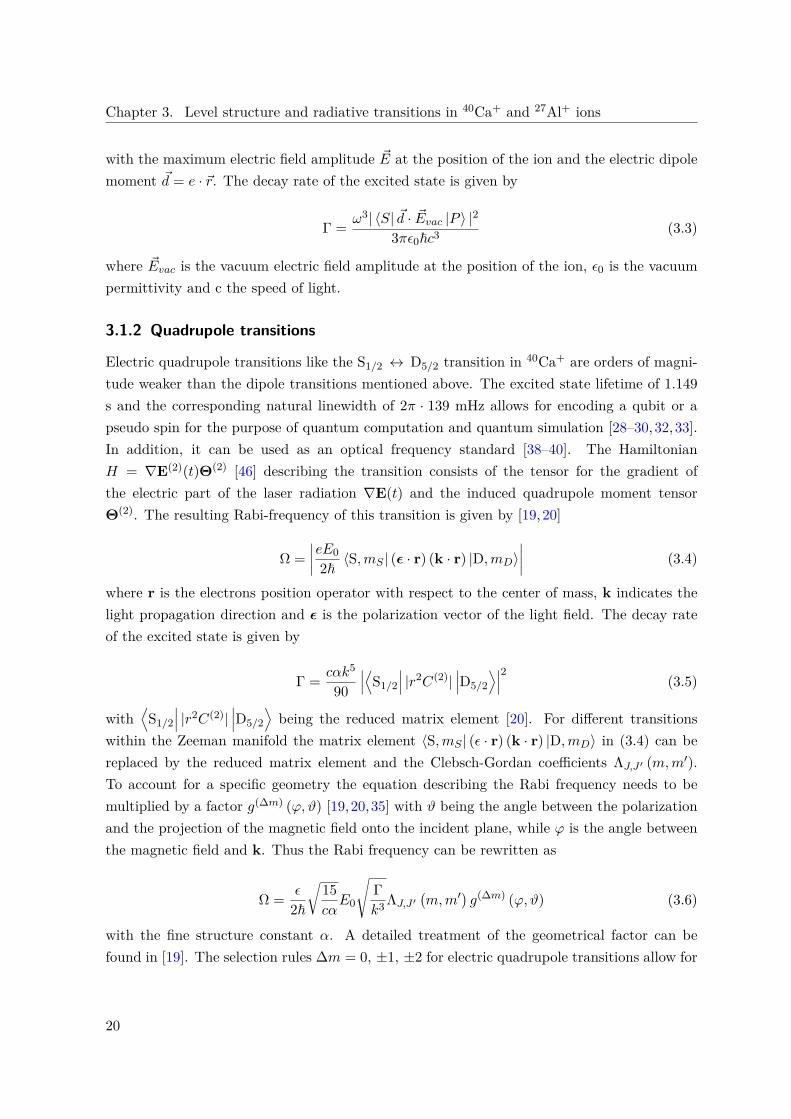
Electric quadrupole transitions like the S1/2 ↔ D5/2 transition in 40Ca+ are orders of magni-tude weaker than the dipole transitions mentioned above. The excited state lifetime of 1.149s and the corresponding natural linewidth of 2π · 139 mHz allows for encoding a qubit or apseudo spin for the purpose of quantum computation and quantum simulation [28–30,32,33].In addition, it can be used as an optical frequency standard [38–40]. The HamiltonianH = ∇E(2)(t)Θ(2) [46] describing the transition consists of the tensor for the gradient ofthe electric part of the laser radiation ∇E(t) and the induced quadrupole moment tensorΘ(2). The resulting Rabi-frequency of this transition is given by [19,20]
Ω =∣∣∣∣eE0
2~ 〈S,mS | (ε · r) (k · r) |D,mD〉∣∣∣∣ (3.4)
where r is the electrons position operator with respect to the center of mass, k indicates thelight propagation direction and ε is the polarization vector of the light field. The decay rateof the excited state is given by
Γ = cαk5
90∣∣∣⟨S1/2
∣∣∣ |r2C(2)|∣∣∣D5/2
⟩∣∣∣2 (3.5)
with⟨
S1/2∣∣∣ |r2C(2)|
∣∣∣D5/2⟩
being the reduced matrix element [20]. For different transitionswithin the Zeeman manifold the matrix element 〈S,mS | (ε · r) (k · r) |D,mD〉 in (3.4) can bereplaced by the reduced matrix element and the Clebsch-Gordan coefficients ΛJ,J ′ (m,m′).To account for a specific geometry the equation describing the Rabi frequency needs to bemultiplied by a factor g(∆m) (ϕ, ϑ) [19,20,35] with ϑ being the angle between the polarizationand the projection of the magnetic field onto the incident plane, while ϕ is the angle betweenthe magnetic field and k. Thus the Rabi frequency can be rewritten as
Ω = ε
2~
√15cαE0
√Γk3 ΛJ,J ′
(m,m′
)g(∆m) (ϕ, ϑ) (3.6)
with the fine structure constant α. A detailed treatment of the geometrical factor can befound in [19]. The selection rules ∆m = 0, ±1, ±2 for electric quadrupole transitions allow for
20

3.1. Level structure and radiative transitions of 40Ca+
five different transitions starting in a particular Zeeman level of the S1/2 ground state. Thecorresponding Clebsch-Gordan coefficients are listed in table 3.1.
m′ −32 −1
212
32
52
Λ(1/2,m′)√
15
√25
√35
√45 1
Table 3.1: Clebsch-Gordan coefficients Λ(m,m′) for S1/2, mj = 1/2 ↔ D5/2, m′ transitions.
In the case of starting in S1/2, mj = −1/2 the sign of the target states m′ is inverted.
21

Chapter 3. Level structure and radiative transitions in 40Ca+ and 27Al+ ions
3.2 Level structure and radiative transitions of 27Al+
27Al is the only stable aluminium isotope. With two valence electrons in the 3s shell, theelectronic structure of 27Al+ is similar to Helium. It has a nuclear spin of I = 5/2 andtherefore shows hyperfine structure. A detailed overview of the level structure is presented infigure 3.2. The magnetic dipole moment of the nucleus is 3.6415069(7) µN [47] (µN = e~
2mp)
and its electric quadrupole moment is 0.1466(10) · 10−28 em2 [47]. The next orbital above theground state is the 3p level, which consists of three fine-structure components. The lowest oneis the 3P0 state with a natural lifetime of 20.6(1.4) s [48] which results in a natural linewidthof 2π ·7.6 mHz. It is linked to the ground state via a hyperfine-induced [36] transition at 267.4nm. This transition is doubly forbidden with respect to dipole transition selection rules sincethe spin state changes and the angular momentum state does not. Because of its low sensitivityto magnetic field fluctuations, electric field gradients [49,50] and black body radiation [51], itis well suited for an optical frequency standard. The exact transition frequency was measuredto be 1 121 015 393 207 857.4(7) Hz [52] and the g-factors are g1S0 = −0.00079248(14) andg3P0 = −0.00197686(21) [48].
3P0
3P1
3P2
1S0
1P1
HPF 267.4nm
IC 267.0 nm
M2 266.1 nm
167.1nm
3P1
3P0
1S0
F=7/2
5/2
5/2
mf=7/2
τ=20.6s
τ=305µsF=5/2
F=3/2
Figure 3.2: Left: Overview of the energy levels of 27Al+ and transitions indicated by coloredarrows. See main text for further information. Right: Detailed level diagram of the relevantorbitals and their Zeeman sub-levels. An ultra-stable laser at 267.0 nm is used to drive theintercombination transition for optical pumping to the stretched Zeeman states and for quantumlogic state mapping. Another ultra-stable laser at 267.4 nm is used to drive the hyperfine-induced clock transition.
This results in a relatively small sensitivity with respect to the magnetic field of only afew kHz/G. The line center shifts because of the quadratic Zeeman shift by −0.71988(48)Hz/G2 [48]. A detailed discussion of systematic frequency shifts of a single aluminium ion
22

3.2. Level structure and radiative transitions of 27Al+
clock can be found in [14, 48]. The 3P1 level can be reached from the ground state via a spinforbidden intercombination [36] transition at 267.0 nm. The upper state lifetime is 305 µs [53]and the corresponding natural linewidth is 2π · 520 Hz. It can be used for optical pumpingand state mapping but is not strong enough for efficient Doppler-cooling. Again higher inenergy is the 3P2 state that can be reached from the ground state via a magnetic quadrupoletransition at 266.1 nm [54]. The natural lifetime of the 3P2 state is about 5 min [54]. Thestrong 1S0 ↔ 1P1 dipole transition at 167.1 nm [54] lies in the vacuum ultraviolet (VUV)range. Even though current laser technology makes excitation of this transition possible, itsspectral width of 2π·224 MHz [54] prevents efficient Doppler-cooling to the Lamb-Dicke regime.Nevertheless it could be used for fluorescence detection, but has the disadvantage that the lightsource and the detection unit need to be in vacuum because of the low transmissivity of airat this wavelength. In contrast to the case of 40Ca+ there is no strong transition that can beused for repumping from the long lived states.Since both transitions used in this work behave like dipole transitions, the corresponding
Rabi frequencies can be estimated by using the expression for dipole transitions with a lowerdecay rate. Calculations of the level energies and decay rates for the 3P0 and 3P1 states arequite sophisticated. Nevertheless a short guideline of the mathematical treatment accordingto [36] is given. Since this is only a brief summary, showing the main results of an extensivetheory the reader is referred to [55–58] where a detailed treatment of the problem is presented.The mathematical approach is the same for both transitions. The P states are not considered
to be pure electronic states anymore but are constructed as mixed electronic states with mixingcoefficients ci, i.e.
|”γJIF”〉 =∑i
ci |γiJiIF 〉 (3.7)
with quantum numbers for the nuclear spin I and the total angular momentum F = J + I.The notation ”γJIF” represents the dominant part of the eigen-vectors that construct thestate. γ represents the mean quantum numbers to fully specify the state. Thus the state”γJIF” contains admixtures from other states γiJiIF and their properties like a finite tran-sition probability to the ground state. The coupling mechanisms that introduce the mixing ofthe wave-functions can have different origins like relativistic interaction or hyperfine interac-tion. The cases of the intercombination line 1S0 ↔ 3P1 and the hyperfine induced transition1S0 ↔ 3P0 will be considered in the following.
3.2.1 The 1S0↔ 3P1 intercombination line
The intercombination transition in 27Al+ is spin-forbidden with respect to dipole transitionselection rules (∆S = 0). It‘s finite probability to decay to the ground state via a single photon
23

Chapter 3. Level structure and radiative transitions in 40Ca+ and 27Al+ ions
process is induced by relativistic interaction between 1P1 and 3P1 states which is describedby the Breit-Pauli Hamiltonian [36, 55, 58]. Since the Breit-Pauli Hamiltonian ist extremelycomplex, the reader is referred to the corresponding references for more detailed information.A first order expression of the transition moment S1/2(3s3p 3P1 → ns2 1S0), which is de-
fined as the square root of the line strength S, is expressed by the dipole matrix element⟨3s3p 3P1
∣∣ |D(1)|∣∣3s2 1S0
⟩[36]
S1/2(3s3p 3P1 → ns2 1S0) =⟨
3s3p 3P1∣∣∣ |D(1)|
∣∣∣3s2 1S0⟩
∝ 4EFS4Eterm
⟨3s3p 1P1
∣∣∣ |D(1)|∣∣∣3s2 1S0
⟩(3.8)
where D(1) = d ·E is the electric dipole operator [55,58], 4EFS is the fine-structure splittingbetween 3P1 and 3P0 levels and 4Eterm is the energy separation of the 1P −3 P terms. Thedecay rate can be calculated from the transition moment [36] to
Γ(3s3p 3P1 → ns2 1S0) = e2a20ω
3
9πε0~c3
∣∣∣S1/2(3s3p 3P1 → 3s2 1S0)∣∣∣2 . (3.9)
The intercombination transition is induced by the strong 1S0 ↔ 1P1 dipole transition. Con-sequently, possible transitions between the Zeeman manfifolds of ground and excited stateare subject to selection rules for electric dipole transitions (∆mf = 0,±1). The transitionmanifold is depicted in figure 3.3.
1S0,mf5/2
-1/2
3P1,F=7/2,mf
7/2
3/21/2
-3/2-5/2
-7/2
5/2
3/21/2-1/2-3/2-5/2
πσ-
Figure 3.3: A finite magnetic field lifts the degeneracy of the 1S0 and 3P1, F = 7/2 Zeemanstates. Consequently six π (∆mf = 0) and twelve σ (∆mf = ±1) transitions are possible.
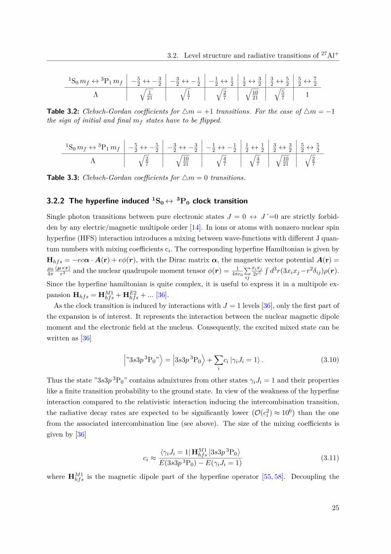
Clebsch-Gordan coefficients for specific transitions within the Zeeman manifolds are listedin tables 3.2 and 3.3.
24
3.2. Level structure and radiative transitions of 27Al+
1S0mf ↔ 3P1mf −52 ↔ −
32 −3
2 ↔ −12 −1
2 ↔12
12 ↔
32
32 ↔
52
52 ↔
72
Λ√
121
√17
√27
√1021
√57 1
Table 3.2: Clebsch-Gordan coefficients for 4m = +1 transitions. For the case of 4m = −1the sign of initial and final mf states have to be flipped.
1S0mf ↔ 3P1mf −52 ↔ −
52 −3
2 ↔ −32 −1
2 ↔ −12
12 ↔
12
32 ↔
32
52 ↔
52
Λ√
27
√1021
√47
√47
√1021
√27
Table 3.3: Clebsch-Gordan coefficients for 4m = 0 transitions.
3.2.2 The hyperfine induced 1S0↔ 3P0 clock transition
Single photon transitions between pure electronic states J = 0 ↔ J´=0 are strictly forbid-den by any electric/magnetic multipole order [14]. In ions or atoms with nonzero nuclear spinhyperfine (HFS) interaction introduces a mixing between wave-functions with different J quan-tum numbers with mixing coefficients ci. The corresponding hyperfine Hamiltonian is given byHhfs = −ecα ·A(r) + eφ(r), with the Dirac matrix α, the magnetic vector potential A(r) =µ04π
(µ×r)r3 and the nuclear quadrupole moment tensor φ(r) = 1
4πε0∑ij
xixj
2r5∫d3r(3xixj−r2δij)ρ(r).
Since the hyperfine hamiltonian is quite complex, it is useful to express it in a multipole ex-pansion Hhfs = HM1
hfs + HE2hfs + ... [36].
As the clock transition is induced by interactions with J = 1 levels [36], only the first part ofthe expansion is of interest. It represents the interaction between the nuclear magnetic dipolemoment and the electronic field at the nucleus. Consequently, the excited mixed state can bewritten as [36]
∣∣∣”3s3p 3P0”⟩
=∣∣∣3s3p 3P0
⟩+∑i
ci |γiJi = 1〉 . (3.10)
Thus the state ”3s3p 3P0” contains admixtures from other states γiJi = 1 and their propertieslike a finite transition probability to the ground state. In view of the weakness of the hyperfineinteraction compared to the relativistic interaction inducing the intercombination transition,the radiative decay rates are expected to be significantly lower
(O(c2
i ) ≈ 106) than the onefrom the associated intercombination line (see above). The size of the mixing coefficients isgiven by [36]
ci ≈〈γiJi = 1|HM1
hfs
∣∣3s3p 3P0⟩
E(3s3p 3P0)− E(γiJi = 1) (3.11)
where HM1hfs is the magnetic dipole part of the hyperfine operator [55, 58]. Decoupling the
25
Chapter 3. Level structure and radiative transitions in 40Ca+ and 27Al+ ions
nuclear and electronic part of HM1hfs = T(1) ·M(1) by using the spherical electronic and nu-
clear tensor operators T(1) and M(1) [55,58], respectively followed by a lengthy mathematicaltransformation yields [36]
ci ≈µI(1 + I−1)1/2
√3
〈γiJi = 1| |T(1)|∣∣3s3p 3P0
⟩E(3s3p 3P0)− E(γiJi = 1) (3.12)
where µI is the nuclear magnetic moment and I the nuclear spin. This is the final result forthe mixing coefficient to first order in the presence of hyperfine interaction. For the calculationof the transition rate only the electric dipole contribution needs to be considered [36] sincethe decay rate of the 1S0 ↔ 3P2 magnetic quadrupole transition is at least 4-5 orders ofmagnitude lower than the decay rate of the intercombination line. The decay rate of the 3P0
state is given by
Γ(3s3p 3P0 → 3s2 1S0) = e2a20ω
3
9πε0~c3
(∑i
ci 〈γiJi = 1| |D(1)| | 3s2 1S0〉)2
(3.13)
with the electric dipole operator D(1). Inserting the mixing coefficients leads to the finalexpression for the decay rate of the 3P0 level [36].
Γ(3s3p 3P0 → 3s2 1S0) ≈
µ2I(1 + I−1) e2a2
0ω3
27πε0~c3
∣∣∣∣∣∑i
〈γiJi = 1| |T(1)|∣∣3s3p 3P0
⟩E(3s3p 3P0)− E(γiJi = 1) 〈γiJi = 1| |D(1)| | 3s2 1S0〉
∣∣∣∣∣2
. (3.14)
The transition is induced by the 1S0 ↔ 3P1 intercombination transition which is representedas the reduced matrix element of the electric dipole operator D(1). This is weighted by theratio of the rduced matrix element of the hyperfine T(1) operator and the energy separationof the atomic levels involved. The complete nuclear contribution to the decay rate is governedby the term µ2
I(1 + I−1).Possible transitions according to the selection rules for dipole transitions between the Zeeman
manfifolds of ground and excited state are depicted in figure 3.4. Clebsch-Gordan coefficientsfor the transition manifold are listed in tables 3.4 and 3.5.
26

3.2. Level structure and radiative transitions of 27Al+
1S0,mf
5/23/21/2-1/2-3/2-5/2
3P0,mf 5/23/21/2-1/2-3/2-5/2
σ+ σ-
π
Figure 3.4: The degeneracy of the 1S0 and 3P0 Zeeman states is lifted by a finite magneticfield. Consequently six π - and ten σ - transitions can be driven.
1S0mf ↔ 3P0mf −52 ↔ −
52 −3
2 ↔ −32 −1
2 ↔ −12
12 ↔
12
32 ↔
32
52 ↔
52
Λ −√
57 −
√935 −
√135
√135
√935
√57
Table 3.4: Clebsch-Gordan coefficients for 4m = 0 transitions.
1S0mf ↔ 3P0mf −52 ↔ −
32 −3
2 ↔ −12 −1
2 ↔12
12 ↔
32
32 ↔
52
Λ −√
621 -
√1635 -
√1835 -
√1635 -
√621
Table 3.5: Clebsch-Gordan coefficients for 4m = +1 transitions. For the case of 4m = −1flip the sign of initial and final mf states.
3.2.3 Nuclear spin flips
Transitions between the hyperfine ground state levels can be induced by an AC magnetic fieldperpendicular to the quantization axis, that couples to the magnetic dipole moment of thenucleus. The coupling strength is given by:
Ω =∣∣∣∣ 12~⟨
1S0, mF
∣∣∣µI · B ∣∣∣1S0, mF ‘⟩∣∣∣∣ (3.15)
where µI is the nuclear magnetic moment and
B the AC magnetic field. The transition
wavelength is on the order of 100 km for laboratory conditions and the resulting Lamb-Dickeparameter is on the order of 10−12. Consequently only carrier transitions can be driven.Nuclear transitions within the Zeeman manifold of the electronic ground state are depicted infigure 3.5. The Clebsch-Gordan coefficients for transitions between the six ground state levelsof 27Al+ are listed in table 3.6.These nuclear spin flips can be used to characterize the efficiency of optically pumping
(see section 5.2) the aluminium ion to the outermost Zeeman states (stretched states). At a
27

Chapter 3. Level structure and radiative transitions in 40Ca+ and 27Al+ ions
finite magnetic field the degeneracy of the six ground state levels is lifted. This results in sixequidistantly spaced energy levels with Zeeman splittings of ~ 1.1 kHz/G. The same approachcan be used to drive transitions between the two ground state levels of 40Ca+. In this case,the magnetic field couples to the spin of the valence electron [35].
1S0,mf
5/23/21/2-1/2-3/2-5/2
Figure 3.5: Zeeman structure of the 1S0 ground state of 27Al+ in a finite magnetic field. Sixequally spaced Zeeman levels emerge due to a nuclear spin of I = 5/2 which can be coupled byan AC magnetic field.
1S0mf ↔ 1S0mf −52 ↔ −
32 −3
2 ↔ −12 −1
2 ↔12
12 ↔
32
32 ↔
52
Λ√
27
√1635
√1835
√1635
√27
Table 3.6: Clebsch-Gordan coefficients for 4m = ±1 transitions.
28

4 Experimental setup
The main part of the experiments presented in this work was carried out in a newly setup laboratory (lab 2) located at the Institute of Quantum Optics and Quantum information(IQOQI) in Innsbruck. It hosts a new vacuum chamber including the ion trap, designed for thepurposes of a semi-portable optical frequency standard and all required laser systems. The iontrap and most of the lasers were set up on a non-magnetic optical table and on breadboardsmounted below the table. The high-finesse resonators for all three stable light sources arelocated in the basement of the building and are linked to the lasers via optical fibers.
4.1 Ion trap setup
For the new setup a modified version of the standard Innsbruck blade-shaped linear Paultrap [29, 33] was designed. A sectional view of the vacuum chamber, which contains the iontrap, and the optical beam paths is presented in figure 4.1.
PMT / EMCCDside view top view
B-field
N
S
EW
729 nm
423, 394, 375 & 397 nm
397, 866 & 854 nm
267.4 nm
267.0 & 729 nm
Figure 4.1: Sectional view of the octagon showing optical access and the imaging path. Thecoils that provide the quantization magnetic field along the trap axis are indicated in orange.Laser beams are presented as colored arrows. The compass indicates the orientation of thechamber in the laboratory.
A technical drawing, which shows the trap electrodes, the isolating parts and the compensa-tion electrodes is presented in figure 4.2. In figure 4.7 a more detailed drawing of the chamberis presented, which also shows the parts attached to the vacuum chamber like the helical res-onator, magnetic field coils, the vacuum pumps and so on. The vacuum chamber is mounted
29

Chapter 4. Experimental setup
to an optical breadboard which rests on electrically isolated posts, that are mounted to theoptical table.
To optimize the new trap setup for the operation as a frequency standard, the main focuswas to keep the influence of external perturbations and the corresponding systematic frequencyshifts as small as possible. A crucial point is the stability of the magnetic field, which isimproved by a magnetic shielding enclosure. In view of the AC-Stark shift caused by black-body-radiation, the trap temperature should be kept low, which required a different choice ofmaterials compared to other traps in our group. With regard to portability, the compactnessof the vacuum chamber played a role. During this work two nearly identical ion trap setupswere built.
4.1.1 Linear Paul trap
The new linear Paul trap consists of four blade-shaped electrodes that are symmetricallyaligned within the radial plane. Pairs of opposite blades are kept on the same potential, withone pair connected to RF and the other pair grounded or kept on a low DC voltage (1.5Vbattery) to break the symmetry of the resulting trap potential. This creates the pseudopoten-tial in the radial direction. To confine the ions along the axis, two endcap electrodes are heldat a positive voltage. To allow for the compensation of stray fields two stainless steel pairs ofelectrodes parallel to the trap axis are attached. The radial electrode to ion distance is about555 µm, the endcap separation is 4.5 mm. The radius of curvature at the end of the bladesis 135 µm. Holes in the endcaps with a diameter of 0.5 mm provide optical access along thetrap axis.Former traps which were made of stainless steel and Macor reached temperatures up to 150
°C during their operation [34]. This is a drawback for optical frequency standards becauseof the increased AC Stark shift caused by black-body radiation at elevated temperatures. Toreduce the heating of the new trap significantly, different materials were chosen. In the newsetup sapphire is used as the electrically isolating part (see figure 4.2). Its heat conductivityof about 24 W/mK is a factor of ~ 17 higher1 and its RF loss tangent of about 5 · 10−5
an order of magnitude smaller2 compared to Macor. In order to directly measure the traptemperature a resistor3 was attached to the sapphire. Figure 4.3 diplays the dependance ofthe trap temperature on the RF power that is sent into the helical resonator. To match thethermal expansion coefficient of sapphire, gold-plated titanium electrodes were used. Sincetitanium has a native oxide on its surface, which reduces electrical conductivity especiallyin the radio frequency domain, the titanium was coated with a 10 µm thick layer of gold by
1Comparison of mean values found on websites of different manufacturers in the World Wide Web2Comparison of mean values found on websites of different manufacturers in the World Wide Web3Allectra PT 100-C2
30
4.1. Ion trap setup
electroplating4. Consequently less electrical power gets dissipated in the trap electrodes, whichreduces the trap temperature and makes it insensitive against RF power changes. Furthermore,low power consumption5 is for instance important for satellite applications.
A A
B
B
Secon A-A Secon B-B
Blade
Endcap
Compensaon
electrode
R=135µm
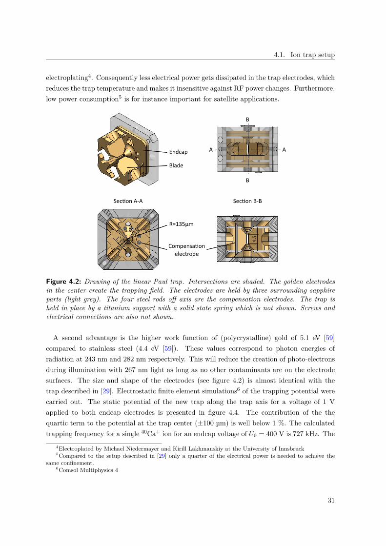
Figure 4.2: Drawing of the linear Paul trap. Intersections are shaded. The golden electrodesin the center create the trapping field. The electrodes are held by three surrounding sapphireparts (light grey). The four steel rods off axis are the compensation electrodes. The trap isheld in place by a titanium support with a solid state spring which is not shown. Screws andelectrical connections are also not shown.
A second advantage is the higher work function of (polycrystalline) gold of 5.1 eV [59]compared to stainless steel (4.4 eV [59]). These values correspond to photon energies ofradiation at 243 nm and 282 nm respectively. This will reduce the creation of photo-electronsduring illumination with 267 nm light as long as no other contaminants are on the electrodesurfaces. The size and shape of the electrodes (see figure 4.2) is almost identical with thetrap described in [29]. Electrostatic finite element simulations6 of the trapping potential werecarried out. The static potential of the new trap along the trap axis for a voltage of 1 Vapplied to both endcap electrodes is presented in figure 4.4. The contribution of the thequartic term to the potential at the trap center (±100 µm) is well below 1 %. The calculatedtrapping frequency for a single 40Ca+ ion for an endcap voltage of U0 = 400 V is 727 kHz. The
4Electroplated by Michael Niedermayer and Kirill Lakhmanskiy at the University of Innsbruck5Compared to the setup described in [29] only a quarter of the electrical power is needed to achieve the
same confinement.6Comsol Multiphysics 4
31

Chapter 4. Experimental setup
experimentally observed value is 819 kHz. The mismatch is most likely due to an asymmetryof the trap with respect to the radial plane. All four blades were shifted by a few ten µmtowards one endcap during the assembling.
RF power (W)
Trap
tem
per
atu
re (
°C)
Figure 4.3: Equilibrium trap temperature depending on the RF power sent into the helical res-onator. The resistance was measured with the 4-point method. Since the trap RF disturbedthe measurement, the displayed values represent the temperature directly after switching offthe RF. Since the trap already started to cool down, conservative error bars are given. Thetemperature increases linearly by 1.4 K/W. The room temperature in the lab is 22 °C. Dur-ing experiments with the mixed ion crystal, the trap is operated at 1 W which increases itsequilibrium temperature by 1.4 degrees.
The pseudopotential in the radial plane, which is displayed in figure 4.5, is derived fromthe simulated static potentials in a second step. The radial oscillation frequency for a singlecalcium ion at a RF voltage of V0 = 1000 V is 3.2 MHz. Since there is no direct way tomeasure the voltage on the radial blades in this setup, there are no experimental values tocompare to. For more information the reader is referred to [29]. There, a voltage divider onthe helical resonator was used to estimate the blade voltage and consequently a comparisonbetween theoretical and experimental results was possible. A setup for a stabilization of theRF voltage on the blade electrodes can be found in [32].To avoid thermal stress during the bake-out, the trap holder with a solid-state spring (see
figure 4.7) at one side was also made of titanium. Two targets, one of pure aluminium andone of an alloy7 (30% Ca, 70% Al) were attached 26 mm above the trap for laser ablation.
7Konik industries
32

4.1. Ion trap setup
Axial distance from trap center (mm)
Vo
ltag
e (m
V)
-2 -10
1 20
100
200
300
400
500
600
700
800
-0.1 0.10.0
2.80
2.84
2.88
Figure 4.4: Finite element simulation of the axial trapping confinement for a voltage of +1 Von both endcaps. The resulting potential is displayed by the blue curve in the main plot. Theinset plot shows the potential at the trap center (±100 µm) and a fourth degree polynomial fit(red line). The orange line in the main plot represents the harmonic part of the potential. Theanharmonicities at the trap center are well below 1 %.
Pse
ud
op
ote
nti
al [
eV] 60
0
10
20
30
40
50
70
80
0 0
x [mm]
y [mm] -0.5 -0.5 0.5
0.5
Figure 4.5: Pseudopotential for a 40Ca+ion at a trap drive frequency of 32 MHz and V0 = 1000V inferred from electrostatic FEM simulations. The blade electrodes are aligned along the xand y axis.
33

Chapter 4. Experimental setup
An important property of ion traps is the heating rate. It determines the rate at which acold trapped ion gains kinetic energy. The first trap that was built during this work has aaxial heating rate of 1.3(2) phonons per second at an axial confinement of 1 MHz. The secondtrap, which was used during the measurements presented in this work, has a heating rate of37(2) phonons per second at the same axial confinement. The heating rate measurements areshown in figure 4.6. The reasons for the difference in the heating rate of the two traps areunknown. Different surface contamination due to a different treatment during the gold platingprocess could be responsible.
Waiting time (ms)
0.0
0.1
0.2
0.3
0.4
Waiting time (ms)
0.0
0.4
0.8
1.2
Figure 4.6: Axial heating rates of both traps at an axial confinement of 1 MHz. Trap 1 showsa heating rate of 1.3(2) phonons per second. The heating rate of trap 2 of 37(2) phononsper second is more than an order of magnitude higher. The heating rate was determined bycomparing excitation of red and blue sideband for a given waiting time after ground statecooling.
4.1.2 Vacuum vessel
The main part of the ultra high vacuum (UHV) chamber containing the trap (see figure 4.7) isa stainless steel spherical octagon8. It has two big 100 mm and eight smaller 40 mm confocalflanges (CF). The mechanical connection between the trap holder and the octagon is done witha groove grabber9. Both CF100 and four of the CF40 flanges are equipped with fused silicaviewports10,11 with an anti-reflective coating12 for 267 nm, 397 nm and 729 nm to avoid lossesand reflections inside the chamber. The reflectivity depending on the wavelength is presentedin figure 4.8.
8Kimball physics MCF600-SphOct-F2C89Kimball physics MCF275-GrvGrb-CYL1000
10VACOM VPCF40DUVQ-L-NM11VACOM VPCF100DUVQ-L-NM12Tafelmaier X/UIMCS6
34

4.1. Ion trap setup
Helical resonatorIon geer +
NEG pump
Valve
Coils
Feedthroughs
NEG pump
Solid state spring
Ablaon targets
RF connecon
DC connecon Ablaon laser
Opcal access
Figure 4.7: Drawing of the UHV chamber containing the trap. Electrical feedthroughs areattached at the top and bottom for the helical resonator providing the high voltage RF and thestable DC voltages respectively. To the bottom right and the top left two pumps are connectedas well as a valve. Three coil pairs orthogonal to each other allow one to apply a quantizationmagnetic field and to compensate for magnetic stray fields perpendicular to the quantizationaxis. The remaining flanges have fused silica viewports with anti-reflective coatings.
Top and bottom flanges are used for RF13 and DC14 feedthroughs. All electrical connec-tions inside the vacuum are done with oxygen free high conductivity copper (OFHC) wires,electrically isolated with aluminium oxide ceramic beads. The RF source for the trap driveis a frequency generator15 at 32.3 MHz, whose output is amplified16 to 1-2 W and coupledinto the quarter wave helical resonator which amplifies the voltage by a factor of ∼ 60. Thecoupling is done via a sliding contact that is attached to a threaded teflon bar, that is screwedinto the resonator coil. This has the advantage over the usual clip contact, that the impedancematching can be done while the grounding shield is closed. A reflectometer17 between ampli-
13VACOM CF40-HV25S-2-CE-CU6414VACOM W-HV6-4-CE-CU1315Rohde & Schwarz SML0116Minicircuits LZY-22+17Rohde & Schwarz power reflection meter NRT
35

Chapter 4. Experimental setup
fier and helical resonator shows the reflected power and therefore allows one to adjust the RFfrequency to the resonance. The DC voltages for the endcap and compensation electrodes areprovided from a stable high voltage source18 (∆V/V ≈ 10−5). Low pass filters with a cut-offfrequency of 4 Hz directly at the feedthroughs suppress noise that is picked up on the cables.
Wavelength (nm)
Ref
lect
ivit
yat
0°
angl
eo
fin
cid
ence
200 4000.00
800 1000600
0.02
0.04
0.06
0.08
0.10
0.12
0.14
0.16
1200
Figure 4.8: Reflectivity of viewport coatings at 0° angle of incidence depending on the wave-length. The reflectivities for the spectroscopy laser wavelengths around 267 nm and 729 nm aswell as the Doppler cooling laser at 397 nm are well below 1 %.
An ION/NEG pump19 is attached to the CF40 tee-piece at the top west viewport as well asan all-metal angle valve. The remaining bottom east flange is used for a NEG pump20, that isnext to the trap. Before assembling the setup the in-vacuum steel parts and the gold-platedelectrodes were air baked at 350 °C for one day. This passivates the steel surfaces by creation ofan oxide layer and therefore reduces outgassing of hydrogen. After that all parts were carefullycleaned with acetone (except copper), isopropanol and methanol in an ultrasonic bath. Afterassembling the chamber it was baked for 1 week at 180 °C. Next, the NEGs were activatedand the valve was closed. Finally the pressure settled down to 10−11 mbar. The pressure ismeasured with the ion pump current ~ 1 nA. A single ion collision rate of ≈ 0.3/min withthe background gas was observed by analyzing the fluorescence counts while Doppler-cooling.This indicates, that the pressure at the trap is about 5 · 10−11 mbar.Three big and one small coil pair (see figure 4.7) provide the quantization axis and the
compensation magnetic field. The three big pairs are designed to create a field of 5 G at the
18ISEG EHS8020x-K219SAES NEXTorr D 100-520SAES Capacitorr D 100
36

4.1. Ion trap setup
ion‘s position at a current of 1 A. Due to practical reasons none of the coil pairs fulfills theHelmholtz criteria. The coils attached to the big viewports have 100 turns, the other oneshave 220. An additional small pair of coils (see figure 4.1) in anti-parallel configuration alongthe trap axis allows one to compensate for a magnetic field gradient along an ion string. Thecurrent which is sent through the quantization coils is stabilized by a home-built PID regulatorthat contains a reference resistor21.
4.1.3 Magnetic field shielding
Fluctuating magnetic fields in the lab shift atomic energy levels and therefore affect coherentqubit operations as well as the stability of an optical atomic clock. In order to improve themagnetic field stability at the ion‘s position the vacuum chamber is enclosed in a magneticshield22. It consists of a welded aluminium case lined with a double layer of a magnetic nickel-iron alloy23. The box has a big front door and two smaller inspection doors on the sidesthat are usually closed. Several small holes in the back provide access for optical fibers andelectrical cables. Four holes in the base serve to attach the trap setup directly to the opticaltable via electrically isolating posts.
. .
Figure 4.9: AC magnetic field attenuation in the center of the chamber measured by the man-ufacterer. Magnetic fields with frequencies below 1 Hz are attenuated by 35 dB. At a frequencyof 50 Hz, which is the strongest component in the lab, an attenuation of more than 65 dB isobtained.
21Vishay VCS 30222IMEDCO AG23Magnifer by ThyssenKrupp
37

Chapter 4. Experimental setup
AC magnetic fields with frequencies ranging from 10 mHz to 1Hz are attenuated in the centerof the box by 35 dB. For frequencies beyond 1Hz the screening effect increases linearly, reaching65 dB at 50 Hz. The shielding effectiveness of the enclosure depending on the AC magneticfield frequency along all three directions is presented in figure 4.9. With this shield, magneticfield deviations within on line cycle could be reduced from 1 mG to 40 µG peak to peak. Thiswas measured with Ramsey experiments that were synchronized to the AC power line andrepeated for different delays with respect to the power line phase [29]. The currently limitingfactors for the short term stability of the magnetic field of ∆B50Hz/B ≈ 10−5 are electricalcables running into the shielding. The long term magnetic field stability was measured withthe clock script (see section 5.3) which was not synchronized to the AC power line. Thereforethe line cycle induced fluctuations are averaded out. The progression of the magnetic fieldover a period of 100 minutes is shown in figure 4.10. The long term stability of the magneticfield of ∆B/B ≈ 3 · 10−6 is limited by the temperature stability of the PID regulator whichstabilizes the current that is sent through the coils.
t (min)
-10
Magnetic field - 4.04601 G (µG)
0
20
40
60
80
100
120
Co
un
ts
Mag
net
ic f
ield
-4
.04
60
1 G
(µ
G)
-5
0
5
10
15
0-6 6 12-124020 60 800 100
Figure 4.10: Left: Magnetic field at the ion measured with a Ramsey experiment with a Ramseytime of 3 ms. Short term fluctuations of 5-10 µG peak to peak are visible. The red line isFourier smoothed to highlight periodicities. The 10 µG modulation with a cycle time of ∼ 30min is caused by the air conditioning of the lab, which modulates the temperature of the currentdriver and therefore the temperature of the reference resistor inside [29]. Right: Histogram ofthe magnetic field with a bin size of 2 µG. The orange line is a Gaussian fit with 10 µG FWHM.
4.1.4 Imaging system & state detection
The optical setup for imaging and fluorescence detection is identical with the one describedin [29], where a detailed description of the detection method and the detection efficiencies ispresented. In short, the discrimination between the internal S1/2 and D5/2 states in 40Ca+ isdone by electron shelving [49]. As long as the calcium ion is in the S1/2 state, illuminatingthe ion with the 397 nm and 866 nm lasers will cause the ion to scatter 397 nm photons
38

4.1. Ion trap setup
which are detected by a photomultiplier or a camera. The ion is detected as “bright”. Inthe case of the ion being in the D5/2 state no 397 nm photons will be scattered and theion is detected as “dark”. Repeating the experiment n times leads to two different photoncount distributions. These distributions correspond to the two cases described above and canbe related to peaks in a histogram. The photon count distributions can be expressed by aPoisson distribution [60]. Typically the fluorescence counts are accumulated for a duration of 5ms after each single experiment. For experiments with up to 4 calcium ions the internal statescan be well discriminated but for longer ion strings a clear discrimination is no longer possiblebecause of overlapping peaks in the histogram [29]. This problem is overcome by detection ofspatially resolved fluorescence of individual ions on an EMCCD camera.The collection of the ion‘s fluorescence is done with a custom-made objective24. The photons
are guided to a PMT25 and an EMCCD26 camera. An optical band-pass filter27 (transmissionbetween 381 nm and 399 nm) and a variable slit28 block stray light, entering the imaging path.Since the camera pixel size (8 µm) and the equilibrium distance of two ions at a certain
trapping confinement (see equation 2.10) are known, the magnification factor of the objectivecan be calibrated by determining the the pixel-to-pixel distance of two fluorescing 40Ca+ ionson the EMCCD camera image. The axial oscillation frequency of the ions was determindedby modulating the axial confinement. If the modulation hits the resonance frequency of thecenter-of-mass mode, the ions oscillate around their equilibrium positions which can be seenon the EMCCD camera. The corresponding images are shown in figure 4.11. At an oscillationfrequency of 199.1(1) kHz the calculated equilibrium distance yields 16.435(6) µm. The pixel-to-pixel distance of the ions is 56(0.5). Consequently the imaging system covers an area of 330µm · 330 µm at the trap center with a magnification factor of ~ 27.
a) b)
Figure 4.11: Average of 100 EMCCD camera images each of two trapped calcium ions. a)two calcium ions resting at their equilibrium positions. b) modulation of the axial trappingconfinement at the resonance frequency of 199.1(1) kHz. The calculated equilibrium distancefor this confinement is 16.435(6) µm. The ion to ion distance in pixels which yields 56(0.5).
24Silloptics f = 66.8 mm, d = 34 mm25Sens-Tech P25PC, quantum efficiency of ~27% at 397 nm26Andor iXon DV885JCs-VP, pixel size 8 x 8 µm, quantum efficiency of 37% at 397 nm.27Semrock SEM-FF01-390/18-2528Owis Spalt 40
39

Chapter 4. Experimental setup
4.2 Laser systems
A total of eleven different laser systems were used in this work. Each of them has its specifictask and therefore the requirements in terms of spectral properties, power, etc differ. A listwith all the laser systems and a short description of their application is presented in table 4.1.All of them are commercially available diode, fiber or solid state lasers. A description of alllasers setups is presented in the following section. Setting up laser systems for experiments withtrapped calcium ions is now standard and described in detail in various theses [19,29,33–35,61].For this reason the main focus of this section was laid on describing the laser systems, relevantfor aluminium ions, as well as technical innovations.
Laser wavelength Application
397 nm Doppler cooling of 40Ca+
854 nm Repumping from the D5/2 levels in 40Ca+
866 nm Repumping from the D3/2 levels in 40Ca+
423 nm Photo-ionization of 40Ca
394 nm Photo-ionization of 27Al
375 nm Photo-ionization of 40Ca
532 nm pulsed Ablation of Ca and Al atoms
729 nm Excitation of the S1/2 ↔ D5/2 clock transition in 40Ca+
267.0 nm Excitation of the 1S0 ↔ 3P1 intercombination transition in 27Al+
267.4 nm Excitation of the 1S0 ↔ 3P0 clock transition in 27Al+
Frequency comb Frequency measurement of both clock lasers
Table 4.1: Listing of all laser systems implemented in the experimental setup as well as theirapplication.
4.2.1 Lasers for Doppler-cooling, repumping, and photo-ionization
All laser systems for Doppler-cooling, repumping and photo-ionization are mounted on a bread-board, hanging under the optical table. A second breadboard accommodates the acousto-opticmodulators for switching the light on and off within the experimental sequence. The lasersare stabilized to the wavelength-meter (see section 4.2.2) which is situated between the twobreadboards.
40

4.2. Laser systems
397 nm cooling laser
The S1/2 ↔ P1/2 dipole transition in 40Ca+ at a wavelength of 397 nm is used for Doppler-cooling, optical pumping and state detection by fluorescence (electron shelving). The cor-responding light source is a frequency-doubled external cavity diode laser29 (ECDL) at afundamental wavelength of 793 nm which is subsequently amplified by a tapered amplifier(TA). A schematic drawing of the 397 nm laser setup is presented in figure 4.12. Even thoughlaser diodes at 397 nm are commercially available, their handling is more difficult and so thestandard approach to produce this wavelength was chosen to have a low-maintainance systemalthough it is more expensive. Furthermore these systems have the advantage of having a nicerbeam profile and less amplified spontaneous emission (ASE). A few ten µW of the infrared lightare sent via a single mode fiber to the Wavelength meter30, to which the laser is stabilized to(see section 4.2.2). Approximately 12 mW of 397 nm light is guided to the AOM breadboard.It is frequency up-shifted by 160 MHz by the double-pass AOM31 1 and subsequently splitinto two parts. A mechanical shutter that blocks the 0th diffraction order can be opened andthe far red detuned light helps to recrystallize the ions after a collision with the backgroundgas. The first path contains the main part of the light and passes the single-pass AOM32 2 at80 MHz, which enhances the attenuation when the light is supposed to be turned off and iscoupled into a photonic crystal fiber together with the repumping lasers (see below).
AOM1
Wavelength meter
TA
SHG397 nm AOM2
AOM3
2 x 80 MHz 1 x 80 MHz
1 x 80 MHz
Shutter for 0th order
feedback
top-east
east
DP +1st SP +1st
SP +1st
PCF
PMF
FC
PMFPCF FC SP DP +1st
Polarization maintaining fiberPhotonic crystal fiberFiber couplerAOM single-pass configurationAOM double-pass configurationAOM diffraction order
ECDL793 nm
PMF
PMF
Figure 4.12: Schematic drawing of the 397 nm laser setup. Fundamental light at 793 nm,created by an ECDL, is amplified by a tapered amplifier and subsequently frequency doubled. Asmall fraction of it is sent to the wavelength meter for frequency drift compensation. The 397nm light is split into two paths for Doppler-cooling and optical pumping. Black lines representoptical fibers, colored lines indicate free-space beam paths.
Light from this path is used for Doppler-cooling and state detection and has overlap withall three normal modes of an ion in the trap (see figure 4.1 top-east viewport). The beamis focused to a Gaussian beam waist of 100 µm FWHM at the ion. About 500 µW optical
29Toptica TA-SHG pro30High Finesse WSU-231Crystal Technology Inc. 3080-12032Crystal Technology Inc. 3080-120
41
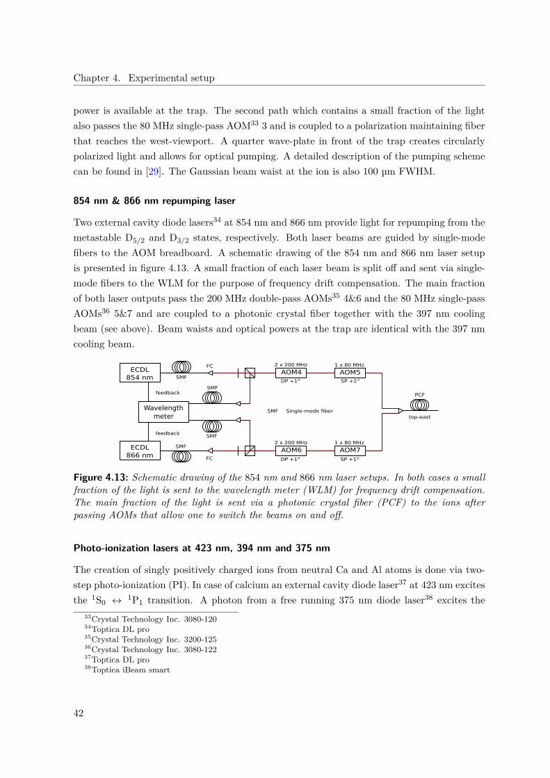
Chapter 4. Experimental setup
power is available at the trap. The second path which contains a small fraction of the lightalso passes the 80 MHz single-pass AOM33 3 and is coupled to a polarization maintaining fiberthat reaches the west-viewport. A quarter wave-plate in front of the trap creates circularlypolarized light and allows for optical pumping. A detailed description of the pumping schemecan be found in [29]. The Gaussian beam waist at the ion is also 100 µm FWHM.
854 nm & 866 nm repumping laser
Two external cavity diode lasers34 at 854 nm and 866 nm provide light for repumping from themetastable D5/2 and D3/2 states, respectively. Both laser beams are guided by single-modefibers to the AOM breadboard. A schematic drawing of the 854 nm and 866 nm laser setupis presented in figure 4.13. A small fraction of each laser beam is split off and sent via single-mode fibers to the WLM for the purpose of frequency drift compensation. The main fractionof both laser outputs pass the 200 MHz double-pass AOMs35 4&6 and the 80 MHz single-passAOMs36 5&7 and are coupled to a photonic crystal fiber together with the 397 nm coolingbeam (see above). Beam waists and optical powers at the trap are identical with the 397 nmcooling beam.
AOM4
Wavelength meter
AOM52 x 200 MHz 1 x 80 MHz
feedback
top-east
ECDL854 nm
AOM6 AOM72 x 200 MHz 1 x 80 MHz
feedback
SMF
SMF
SMF
SMF
PCF
DP +1st
DP +1st
SP +1st
SP +1st
SMF Single-mode fiber
ECDL866 nm
FC
FC
Figure 4.13: Schematic drawing of the 854 nm and 866 nm laser setups. In both cases a smallfraction of the light is sent to the wavelength meter (WLM) for frequency drift compensation.The main fraction of the light is sent via a photonic crystal fiber (PCF) to the ions afterpassing AOMs that allow one to switch the beams on and off.
Photo-ionization lasers at 423 nm, 394 nm and 375 nm
The creation of singly positively charged ions from neutral Ca and Al atoms is done via two-step photo-ionization (PI). In case of calcium an external cavity diode laser37 at 423 nm excitesthe 1S0 ↔ 1P1 transition. A photon from a free running 375 nm diode laser38 excites the
33Crystal Technology Inc. 3080-12034Toptica DL pro35Crystal Technology Inc. 3200-12536Crystal Technology Inc. 3080-12237Toptica DL pro38Toptica iBeam smart
42

4.2. Laser systems
atom to an energy above the ionization threshold of 6.1 eV [54]. In the case of aluminiuman ECDL39 at 394 nm excites the 2P1/2 ↔ 2S1/2 transition (See also section 5.1). Another394 nm photon is sufficient to reach the ionization threshold of 6 eV [54]. The laser can bealso tuned to the 2P3/2 ↔ 2S1/2 transition at 396 nm. A level scheme of neutral aluminiumcontaining the relevant levels for photo-ionization is presented in figure 4.14. More detailedinformation about the level structure of neutral aluminium, including the hyperfine structure,can be found in [62] .
394 nm
2S1/2
continuum
2P1/22P3/2
394 nm 396 nm
396 nm
Figure 4.14: Level structure of neutral aluminium containing the relevant levels for photo-ionization. The hyperfine structure is not shown. Starting in the electronic ground state 2P1/2a 394 nm photon excites the atom to the 2S1/2 intermediate state. Another 394 nm photon issufficient to reach the ionization threshold of 6 eV. However, at temperatures that are requiredto evaporate aluminium atoms from bulk material the 2P3/2 state is also populated [63]. Thisenables a second way of photo-ionization via two 396 nm photons.
A schematic drawing of the PI laser setup is presented in figure 4.15. The light from bothECDLs (423 nm and 394 nm) is guided to the AOM breadboard via single mode fibers. There,a small fraction of both beams is split off and sent to the WLM via single mode fibers forthe purpose of frequency drift compensation. The 80 MHz single-pass AOM40 8 in the 394nm path allows for a precise temporal delay of the PI laser with respect to the ablation pulse(see section 5.1). 375 nm light, wich is produced by a free running laser diode, is guidedvia a multi-mode fiber to the AOM breadboard. Finally, all three beams are coupled into asingle-mode fiber that goes to the trap. The beams have Gaussian beam waists of about 100µm FWHM at the trap center. Typically 500 µW optical power of each laser is available atthe trap. A mechanical shutter in front of the fiber allows us to switch all beams on and off.
39Toptica DL pro40Crystal Technology Inc. 3080-120
43

Chapter 4. Experimental setup
AOM8
Wavelength meter
ECDL423 nm
1 x 80 MHz
feedback
top-east
ECDL394 nm
feedback
DL375 nm
SP +1st
FC
FC
SMF
SMF
SMF
SMF
SMFMMF
MMF Multi-mode fiber Shutter
Figure 4.15: Schematic drawing of the photo-ionization laser setup. In the cases of the 394 nmand 423 nm lasers a small fraction of the light is sent to the wavelength meter for frequencydrift compensation. The main fraction of both laser outputs is combined with the 375 nm lightand sent to the trap. An AOM in the 394 nm path allows for switching the light on and off onthe µs timescale.
Ablation laser
In this work laser ablation loading of calcium and aluminium ions was implemented (see section5.1). Therefore neutral atoms of both species are evaporated from ablation targets by singlelaser pulses. The atoms are subsequently photo-ionized in the center of the trap. A schematicdrawing of the ablation laser setup is presented in figure 4.16.
Beam dump
DPSS1064 nm
SHG532 nm
Calcite beam
displacer
HWP HWP
Ablation targets
PBS
Figure 4.16: Schematic drawing of the ablation laser setup. The energy of the laser pulses isadjusted by a half-wave plate and a polarizing beam splitter. A calcite beam displacer sendsthe laser pulses along two different paths depending on their polarization, which allows one toaddress the two ablation targets individually.
The laser system is a frequency-doubled diode-pumped solid state laser (DPSS)41, whichemits laser pulses at a wavelength of 532 nm. The pulses have a fixed pulse energy of 400µJ and a temporal duration of 2 ns. Single pulses are triggered via transistor-transistor logic(TTL). For optimizing the probability of creating one ion per ablation pulse, the energy of theablation pulses, sent to the targets, needs to be adjusted. This can be achieved by a half-waveplate followed by a polarizing beam splitter in the beam path. Furthermore two differenttargets for the two atomic species, respectiveley are mounted above the trap, which have to
41Coherent flare 532
44
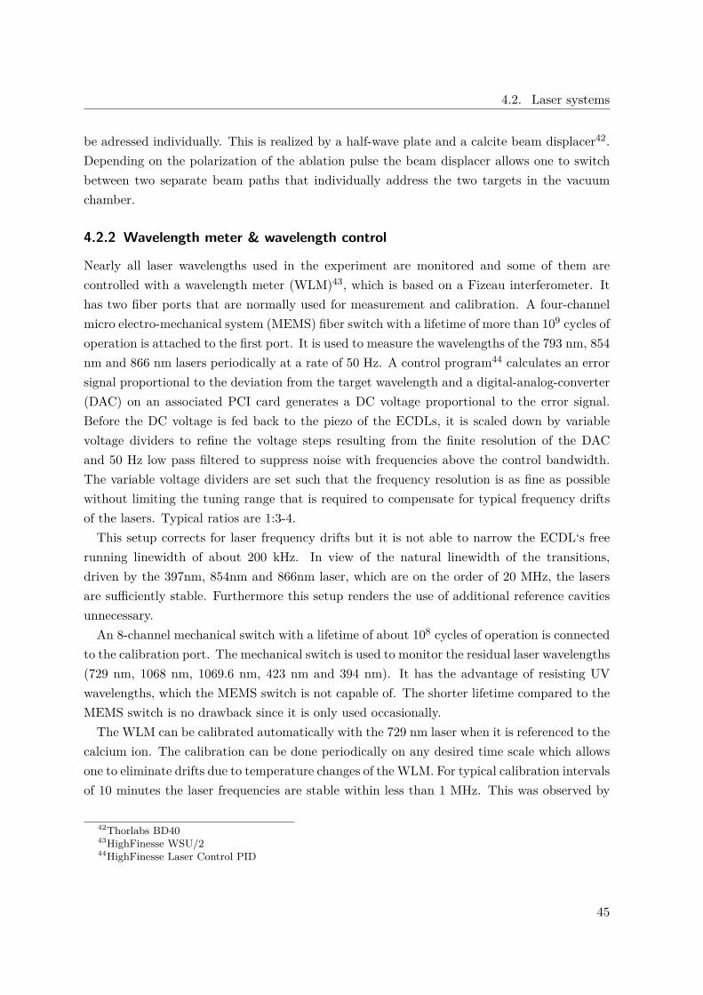
4.2. Laser systems
be adressed individually. This is realized by a half-wave plate and a calcite beam displacer42.Depending on the polarization of the ablation pulse the beam displacer allows one to switchbetween two separate beam paths that individually address the two targets in the vacuumchamber.
4.2.2 Wavelength meter & wavelength control
Nearly all laser wavelengths used in the experiment are monitored and some of them arecontrolled with a wavelength meter (WLM)43, which is based on a Fizeau interferometer. Ithas two fiber ports that are normally used for measurement and calibration. A four-channelmicro electro-mechanical system (MEMS) fiber switch with a lifetime of more than 109 cycles ofoperation is attached to the first port. It is used to measure the wavelengths of the 793 nm, 854nm and 866 nm lasers periodically at a rate of 50 Hz. A control program44 calculates an errorsignal proportional to the deviation from the target wavelength and a digital-analog-converter(DAC) on an associated PCI card generates a DC voltage proportional to the error signal.Before the DC voltage is fed back to the piezo of the ECDLs, it is scaled down by variablevoltage dividers to refine the voltage steps resulting from the finite resolution of the DACand 50 Hz low pass filtered to suppress noise with frequencies above the control bandwidth.The variable voltage dividers are set such that the frequency resolution is as fine as possiblewithout limiting the tuning range that is required to compensate for typical frequency driftsof the lasers. Typical ratios are 1:3-4.This setup corrects for laser frequency drifts but it is not able to narrow the ECDL‘s free
running linewidth of about 200 kHz. In view of the natural linewidth of the transitions,driven by the 397nm, 854nm and 866nm laser, which are on the order of 20 MHz, the lasersare sufficiently stable. Furthermore this setup renders the use of additional reference cavitiesunnecessary.An 8-channel mechanical switch with a lifetime of about 108 cycles of operation is connected
to the calibration port. The mechanical switch is used to monitor the residual laser wavelengths(729 nm, 1068 nm, 1069.6 nm, 423 nm and 394 nm). It has the advantage of resisting UVwavelengths, which the MEMS switch is not capable of. The shorter lifetime compared to theMEMS switch is no drawback since it is only used occasionally.The WLM can be calibrated automatically with the 729 nm laser when it is referenced to the
calcium ion. The calibration can be done periodically on any desired time scale which allowsone to eliminate drifts due to temperature changes of the WLM. For typical calibration intervalsof 10 minutes the laser frequencies are stable within less than 1 MHz. This was observed by
42Thorlabs BD4043HighFinesse WSU/244HighFinesse Laser Control PID
45

Chapter 4. Experimental setup
monitoring the frequency of the stable 1068 nm laser. Consequently the frequencies of thecooling and repumping lasers only need to be adjusted to the corresponding transitions onceper day.
46

4.2. Laser systems
4.2.3 Ultra-stable lasers
Driving narrow transitions coherently requires light sources with a linewidth on the order ofthe natural linewidth of the transition. The clock transitions of 27Al+ and 40Ca+ have naturallinewidths of 2π ·7.6 mHz and 2π ·139 mHz, respectively. Therefore, the 267.4 nm and 729 nmlasers are stabilized to optical resonators with high finesse, which are temperature-stabilizedand vibration-isolated from the environment. In practice, the limiting factor for narrowingthe linewidth of a laser is the thermal noise floor of the reference cavity (typically ∼ 10−15).Consequently, spectral laser linewidths on the order of 1 Hz are achieveable.The intercombination transition of the 27Al+ ion has a natural linewidth of 2π · 520 Hz.
Driving this transition coherently does not require a 1 Hz laser, but it is advantagous to haveanother ultra-stable laser at 267 nm which the 267.4 nm clock laser can be compared to. Thelaser systems are located in the labs, the three high-finesse cavities are placed inside a woodenbox in the basement due to a lack of space in the lab.In the following the three ultra-stable lasers at 729nm, 267.0 nm and 267.4 nm are described.
This subsection is structured as follows: First, an overview of the optical setup of each lasersystem is given which includes schematical drawings of those. Second, the method of Pound-Drever-Hall (PDH) laser stabilization is introduced and a description of the PDH setup is given.Furthermore the spectral properties of both 267 nm lasers are characterized. A characterizationof the 729 nm laser can be found in [61].
729 nm laser
An ultra-stable titanium-sapphire laser (Ti:Sa) with a short term linewidth of 1 Hz [61], whichis located in lab 1 is used to coherently drive transitions between the S1/2 and D5/2 manifolds.It can be used to manipulate the ion‘s internal and motional state with high fidelity [29,32,35]using carrier and sideband transitions. A detailed description of the current setup in lab 1 canbe found in [29] and references therein.A 10 m long polarization maintaining fiber (APC end), whose optical path length is stabi-
lized, guides 15 mW of the light to lab 2. A schematic drawing of the 729 nm laser setup ispresented in figure 4.17. The light is sent through the 80 MHz AOM45 12 (+1st order) followedby a wedge, which is used to reflect 4 % of the light back into the fiber. An interferometerin lab 1 is used for fiber noise cancellation (FNC). The stable light is used to seed a taperedamplifier46 with a maximum output power of 560 mW. The 80 MHz AOM47 13 (-1st order)cancels the frequency offset and can be used for intensity stabilization (PD 5) and locking the
45Crystal Technology Inc. 3080-12046Toptica TA 10047Crystal Technology Inc. 3080-120
47

Chapter 4. Experimental setup
laser to the spherical cavity48, located in the basement.
Verdi V-10
AOM9
AOM10AOM11
FI GTP EOM
CCD
430mWTi:Sa 729nm Lab1 trap
west/southviewport
bottom-westviewport
AOM12AOM13
AOM14 AOM15
AOM16
WLM Lab1
WLM Lab2
AOM Acustio-optic modulatorEOM Electro-optic modulatorFI Faraday IsolatorGTP Glan Thompson polarizerWLM Wavelength meterPD PhotodiodePMF Polarization maintaining fiberVCO Voltage controlled oscillatorTA Tapered amplifierCCD Charge coupled device camera
SP AOM single pass configurationDP AOM double pass configuration
~18MHz
~18MHz
Intensity
stabilization
50:50
10%
FI GTP EOM
CCD
12MHz
30:70
TA10mW
430mW
560mW
Intensity stabilization AOM13
1 x 80 MHz
1 x 80 MHz
2 x 270 MHz
1 x 80 MHz
1 x 80 MHz
2 x 1,5 GHz
1 x 80 MHz
Fiber noise cancellation
Fiber noise cancellation
Ti:Saerror signal
Error signalvia VCO to
AOM13
LAB1
LAB2
Basement
AOM17 AOM182 x 270 MHz 1 x 80 MHz
Intensity stabilization
Intensity stabilization
Acoustic shielding
+ vibration isolation
Vacuum vessel
Acoustic & RF shielding
+ vibration isolation
Vacuum vessel to frequency comb
SP +1st
SP -1st
SP +1st
SP +1st
DP +1st
DP +1st SP +1st
SP 0th
DP +1st
SP +1st
30:70
PD 1
PD 2
PD 3
PD 4
PD 5
PD 6
PD 7
PD 8
Figure 4.17: Schematic overview of the 729 nm laser setup. It is spread over three differentlocations. The laser itself and the PDH locking setup (vertical cavity) is located in lab 1. Apart of the light is split off and sent to lab 2 where a tapered amplifier provides 560 mW ofpower. Afterwards the light is distributed among different paths that go to the experiment,the wavelength meter, intensity stabilization and the Pound-Drever-Hall setup located in thebasement.
The main fraction of the light is going into the 270 MHz double-pass AOM49 14, which isused to bring the laser frequency into resonance with the Zeeman transition to be excited.The 80 MHz single pass AOMs50 15&16 in a row allow one to send the light to different portsat the trap and two 2 m long PM fibers guide the light to the ions.
48ATF 6300 spherical cavity49Brimrose TEF 270-100-72950Crystal Technology Inc. 3080-120
48

4.2. Laser systems
The fraction of the light, which is not going into AOM 14, is used for an optical beat notewith the frequency comb (see section 4.2.4), for the PDH locking setup in the basement, forlaser intensity stabilization (PD 5) and calibrating the wavelength meter. The main part ofthe light passes the 270 MHz double pass AOM51 17, which is used to compensate for thecavity drift, an interferometer (FNC) and the 80 MHz single pass AOM52 18 for laser intensitystabilization (PD 8) and fiber noise cancellation. The rest of the light is sent to the wavelengthmeter and to a photo diode (PD 5) for laser intensity stabilization.The spherical cavity has a finesse of F ≈ 200.000 which was measured by cavity ring-down
spectroscopy and shows a drift rate of 50 mHz/s. Since the Ti:Sa is already phase-stabilizedby the PDH setup in lab 1, the PDH setup in the basement is currently not used to lock the729 nm laser to the spherical cavity. Nevertheless it provides the ability to be independent ofthe 729 nm laser in lab 1.
267.0 nm laser
To drive the 1S0 ↔3 P1 intercombination line in 27Al+ an ultra stable laser at 267.0 nm with amaximum output power of 18 mW is used. The laser setup consists of a frequency quadrupledECDL53, which is locked to an external high finesse cavity54 at its fundamental wavelengthof 1068 nm. The spherical cavity has a finesse of F ≈ 300.000 and shows a drift rate of 46mHz/s. A schematic drawing of the 267.0 nm laser setup is presented in figure 4.18. Coarsewavelength tuning is done via manually aligning the grating of the ECDL. A piezo actuatingon the grating is used for fine tuning of the wavelength and for compensation of drifts and lowfrequency noise. Frequency stabilization with high bandwidth is done by a commercial PIDcontroller55 that feeds back to the laser diode current. The lock setup consists of the doublepass AOM56 19 for frequency mode matching and cavity drift compensation and the 80 MHzAOM57 20 for fiber noise cancellation (PD 9) and laser intensity stabilization (PD 10). A 10m long fiber guides the light to the PDH setup in the basement, which is described later. Theerror signal (PD 11) is fed into the fast analog linewidth control (FALC) with a slow and afast locking branch. The slow part feeds back onto the piezo, the fast part on the laser diodecurrent.A linewidth of less than 1.63 Hz FWHM at 4 s was observed (see figure 4.24) by an optical
beat note with the stable fiber laser (see below). However, there is broad-band high frequencynoise that can not be fully compensated due to a relatively low control loop bandwidth of about
51Brimrose TEF 270-100-72952Crystal Technology Inc. 3080-12053Toptica DL TA FHG pro54ATF 6300 spherical cavity55Toptica FALC56Brimrose TEF 270-100-106857Crystal Technology Inc. 3080-197
49

Chapter 4. Experimental setup
500 kHz. The locking bandwidth is limited by the modulation input or the diode current driverof the laser. This is proved by a phase delay measurement.
ECDL1068 nm
TA
SHG534 nm
SHG267 nm
eastviewport
westviewport
AOM22
AOM231 x 200 MHz
1 x 200 MHz
~18MHzFI GTP EOM
CCD
12MHz Error signalBasement
AOM19 AOM202 x 270 MHz 1 x 80 MHz
Intensity stabilization
Acoustic shielding
+ vibration isolation
Vacuum vessel
AOM212 x 200 MHz
Wavelength meter
Beat with frequency comb
30:70
Fiber noise cancellation
LAB2
DP +1st SP +1st
DP +1st SP +1st
SP +1st
PD 10
PD 11
PD 9
Figure 4.18: Schematic overview of the 267.0 nm lasers setup. An external cavity diode laseremits radiation at 1068 nm which is sent to a tapered amplifier. A fraction of the infrared lightis split off and sent to the wavelength meter and the Pound-Drever-Hall setup located in thebasement. The main part of the light is frequency-quadrupled and guided to the experiment.
The laser diode current was amplitude-modulated, which leads to a frequency modulation ofthe laser, and the laser light was sent through a low-finesse cavity58. At a wavelength of 1068nm the reflectivity of the cavity mirrors is ≤50 %, which leads to a finesse of F .10. Whilesitting on the slope of the cavity resonance the transmitted light gets amplitude modulatedwhich is detected with a photo diode. The relative phase between the diode current modulationand the photodiode signal is presented in figure 4.19. At a modulation frequency of 300 kHzthe phase delay is already 90° and reaches 180° around 1 MHz. Additional phase delays fromthe PID controller and finite cable lengths are expected. Consequently, the control bandwidthis expected to be substantially smaller than 1 MHz. However, an additional 50 µF capacitorin parallel to the laser diode current reduced the high-frequency noise without decreasingthe control bandwidth notably. The stable light at 1068 nm gets subsequently frequency-quadrupled.The light at 267 nm passes the 200 MHz double-pass AOM59 21, which is used to adjust the
laser frequency to the Zeeman transition to be excited and is sent to the 200 MHz single-pass
58Toptica FPI 100-0750-159Crystal Technology Inc. 3200-1220
50

4.2. Laser systems
AOMs60 22&23 in a row, that split the light into two paths.
Modulation frequency (Hz)
Phasedelay
(°)
Figure 4.19: Phase delay of the laser diode response with respect to the modulation signal. Thegreen line is a Bezier interpolation. A phase delay of 90° is already reached at a frequency of300 kHz and reaches 180° around 1 MHz. From this measurement servo bumps around 1 MHzare expected. Additional phase delays result from finite cable lengths in the lock setup and thePID circuit itself which further decrease the control bandwidth.
Solid-core photonic crystal fibers guide the light to the east and west viewport. These fibershave low losses in the UV due to a modification of the color centers in the material [64]. Thisis achieved by loading the fiber with hydrogen gas under pressure and illuminating it with UVlight afterwards. Typically 1.5 mW optical power is available at the trap. The beam is focusedto a Gaussian beam waist of 65 µm FWHM at the ion.
267.4 nm laser
The ultra-stable 267.4 nm laser setup, which is used to drive the 1S0 ↔ 3P0 transition in27Al+, consists of a frequency-quadrupled61 fiber laser62, which is locked to an external highfinesse cavity63 at its fundamental wavelength of 1069.6 nm. The cylindrical cavity has afinesse of F ≈ 405.000 and shows a drift rate of 100 mHz/s. The optical setup is almostidentical with the one described above. A schematic drawing of the 267.4 nm laser setupis presented in figure 4.20. Typically the laser provides 30 mW of 267.4 nm light. Coarse
60Crystal Technology Inc. 3200-122061Toptica FHG standalone62Menlo Systems orange one63ATF6020 notched cavity
51
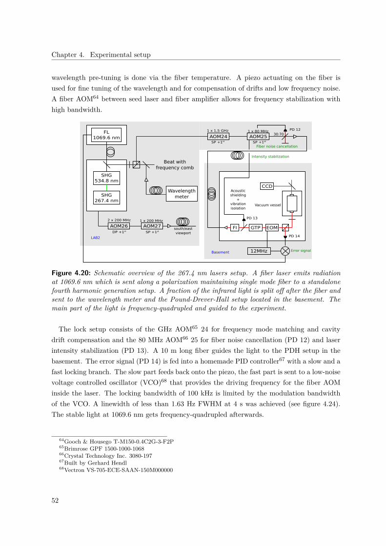
Chapter 4. Experimental setup
wavelength pre-tuning is done via the fiber temperature. A piezo actuating on the fiber isused for fine tuning of the wavelength and for compensation of drifts and low frequency noise.A fiber AOM64 between seed laser and fiber amplifier allows for frequency stabilization withhigh bandwidth.
FL1069.6 nm
SHG534.8 nm
SHG267.4 nm
south/eastviewport
AOM271 x 200 MHz
FI GTP EOM
CCD
12MHz Error signalBasement
AOM24 AOM251 x 1,5 GHz 1 x 80 MHz
Intensity stabilization
Acoustic shielding
+ vibration isolation
Vacuum vessel
AOM262 x 200 MHz
Wavelength meter
Beat with frequency comb
30:70
Fiber noise cancellation
LAB2
SP +1st SP +1st
SP +1stDP +1st
PD 13
PD 12
PD 14
Figure 4.20: Schematic overview of the 267.4 nm lasers setup. A fiber laser emits radiationat 1069.6 nm which is sent along a polarization maintaining single mode fiber to a standalonefourth harmonic generation setup. A fraction of the infrared light is split off after the fiber andsent to the wavelength meter and the Pound-Drever-Hall setup located in the basement. Themain part of the light is frequency-quadrupled and guided to the experiment.
The lock setup consists of the GHz AOM65 24 for frequency mode matching and cavitydrift compensation and the 80 MHz AOM66 25 for fiber noise cancellation (PD 12) and laserintensity stabilization (PD 13). A 10 m long fiber guides the light to the PDH setup in thebasement. The error signal (PD 14) is fed into a homemade PID controller67 with a slow and afast locking branch. The slow part feeds back onto the piezo, the fast part is sent to a low-noisevoltage controlled oscillator (VCO)68 that provides the driving frequency for the fiber AOMinside the laser. The locking bandwidth of 100 kHz is limited by the modulation bandwidthof the VCO. A linewidth of less than 1.63 Hz FWHM at 4 s was achieved (see figure 4.24).The stable light at 1069.6 nm gets frequency-quadrupled afterwards.
64Gooch & Housego T-M150-0.4C2G-3-F2P65Brimrose GPF 1500-1000-106866Crystal Technology Inc. 3080-19767Built by Gerhard Hendl68Vectron VS-705-ECE-SAAN-150M000000
52

4.2. Laser systems
The 267.4 nm light is sent to the 200 MHz double-pass AOM69 26, which is used to bringthe laser frequency into resonance with the Zeeman transition to be excited, and subsequentlypasses the 200 MHz single-pass AOM70 27. A solid-core photonic crystal fiber guides the lightto the south or east viewport. Laser power and beam waist at the trap are identical with theone described above.
Pound-Drever-Hall locking setup
All three spectroscopy lasers (729 nm, 267.0 nm and 267.4 nm) are phase-stabilized to externalhigh-finesse resonators via the Pound-Drever-Hall (PDH) method [65, 66] which became astandard technique in the field of quantum optics and precision spectroscopy. The methodand the required optical setup is described in numerous theses and articles i.e. [33, 34, 61, 67]just to name a few. Therefore the following description is restricted to a short summary.The optical setup is identical for the three lasers mentioned above. Faraday isolators71 avoid
disturbing back-reflections of the laser beam to the light source and Glan-Thompson polariz-ers72 keep the linear polarization as pure as possible. Next, electro-optic modulators73 (EOM)phase-modulate the laser at the drive frequency (∼12 MHz). The light passes a polarizingbeam splitter and a quarter wave-plate before it enters the cavity. The polarization of thelaser light in front of the EOM needs to be aligned to its crystal axis in order to minimize po-larization modulation (at the drive frequency), which results in amplitude modulation after thePBS. Significant residual amplitude modulation leads to an unwanted frequency modulation ofthe laser due to the intensity modulation of the light on the PDH photo diode. Approximately50 % of the light is coupled into the cavity (TEM00 mode). The reflected part of the lightpasses the quarter wave plate again and is reflected by the PBS to fast photo diodes (PD 774
in figure 4.17, PD 1175 in figure 4.18 & PD 1476 in figure 4.20).To obtain the PDH error signal [65,66] when the laser frequency is scanned over the cavity
resonance, the photo diode signal is mixed with the EOM drive frequency. The steepest slopeof the error signal at the zero point is achieved with a modulation depth of 42% [65].The error signal is fed into a PID controller which acts on different feedback elements
depending on the laser. About 30% of the incident beam power gets transmitted through thecavity for optimized PID parameters.A small fraction of the light inside the cavity is absorbed by the mirror coatings which
69Crystal Technology Inc. 3200-122070Crystal Technology Inc. 3200-122071Isolation > 35 dB72B. Halle, 10−8extinction ratio73Linos PM-C-BB74Thorlabs DET10A/M75Thorlabs PDA10CF-EC76Thorlabs PDA10CF-EC
53

Chapter 4. Experimental setup
leads to local heating of those. The resulting thermal expansion of the coatings decreases theeffective cavity length and thus changes the resonance frequency of the cavity. This responsedepending on the incident beam power is presented in figure 4.21 for the two infrared cavities.
Incident beam power (µW)
Laserfreq
uen
cyshift(kHz)
Figure 4.21: Laser frequency shift depending on the optical power of the incident beam for bothinfrared high-finesse cavities. The frequency shift is presented with respect to the lowest pointin power. The difference in the slope can be partially explained by a factor of 2 in cavity lengthas well as a slightly smaller spot size of the cavity mode at the planar mirror of the sphericalcavity (116 µm and 138 µm at 1/e2 intensity).
Therefore the laser intensity inside the cavity has to be stabilized77. In the case of the 729nm laser a photo diode (PD 878) in transmission is used. Due to the relatively low sensitivityof the photo diodes (PD 1079 & PD 1380) at the infrared wavelengths compared to 729 nm, thestabilization is done right after the Faraday Isolators for both aluminium lasers. Fractionalintensity instabilities of 10−4 are achieved.Another important point in order to achieve the ultimate laser stability is the temperature
stabilization of the reference cavities. The target temperature is given by the so called zerocrossing temperature (TC) of the Ultra-Low Expansion glass (ULE), which the cavity spaceris made of. This is the point where the thermal expansion coefficient changes its sign and thelinear part vanishes. The zero crossing temperatures of all three cavities are shown in figure4.22.
77SRS SIM96078Thorlabs PD10A79Hamamatsu G12180-010A80Hamamatsu G12180-010A
54

4.2. Laser systems
Cavity temperature (°C) Cavity temperature (°C) Cavity temperature (°C)
Do
ub
le-p
ass
AO
M f
req
uen
cy (
MH
z)
Lase
r fr
equ
ency
–2
80
.71
09
80
TH
z (M
Hz)
Lase
r fr
equ
ency
–2
80
.25
36
83
TH
z (M
Hz)
0
5
10
15
1.5
2.0
2.5
1.0
0.5
8.0 10.58.5 9.0 9.5 10.0 11.0
262.1
262.4
262.5
262.6
262.3
262.2
3.0 5.53.5 4.0 4.5 5.0 6.0 24 3426 28 30 32 36 380
Figure 4.22: Measurements of the zero crossing temperatures for the three high finesse cavities.The data represents the cavity length depending on its temperature. At the point where thecoefficient of thermal expansion changes its sign, the linear part vanishes. At this point laserfrequency changes due to temperature changes of the cavity are minimal. In the case of the 729nm cavity the laser was locked to the ion and the double pass AOM was adjusted to resonance.The positive curvature arises from the fact that the −1st diffraction order of the AOM was used.In the case of the two infrared cavities the laser frequency was measured with the frequencycomb.
A further important point is the isolation from acoustic noise present in the lab. The cavityspacer slightly changes its shape when it experiences accelerations which results in a change ofthe cavity length and therefore influences the laser frequency. For acoustic shielding a woodenbox was built which rests on Sorbothane81 sheets in the basement. To avoid electromagneticpick up, the outside of the box was lined with copper-wallpaper. The inside of the box is linedwith lead rubber to increase its weight and therefore lower its natural frequency and acousticfoam to break sound waves. The box is filled with 10 cm quartz sand (grain size 1 mm) todamp acoustic vibrations. Two active vibration isolation platforms82 rest on the sand. One ofthem carries both spherical cavities for 729 nm and 1068 nm, the other one accomodates thecylindrical cavity for 1069.6 nm.The temperature stabilization of the spherical cavities is done with a commercial temper-
ature controller83 that acts on Peltier elements inside the vacuum vessels. The cylindricalcavity is temperature-stabilized with a commercial temperature controller84 that is connectedto a resistive heater outside the vacuum can but within the heat shield. Typical temperaturestabilities of ± 200 µK (in loop) are achieved for all three cavities.During the optimization of the laser locks it is necessary to identify noise sources by their
characteristic frequencies. Typically this is done via a beat note with a laser that is known tobe stable. If there is only one noise source modulating the phase of one laser at a particular
81Visco-elastic polymer, used for vibration isolation (http://www.sorbothane.com/)82ACCURION halcyonics micro6083SRS PTC1084Wavelength Electronics LFI 3751
55

Chapter 4. Experimental setup
frequency, a sideband at the modulation frequency shows up on the beat signal spectrum.Depending on the modulation depth also higher order sidebands at harmonic frequencies canappear. As soon as both lasers are affected by several noise sources, this method breaks downsince only a broad peak will be visible on the beat spectrum. Therefore it is useful to extractthe phase noise spectrum of the beat. This can be done by detecting the beat note (212 MHzin this case) with a fast photo diode and mixing it down to about 10 kHz with two identicalRF signals while one is phase shifted with respect to the other one by 90° (quadrature term).Consequently two beat signals at 10 kHz with a relative phase of 90° emerge, which are recordedby a fast oscilloscope. The quadrature term is needed to get the complete information aboutthe phase evolution and to isolate amplitude noise. Subsequently the linear term in the phaseevolution, which results from the non-zero beat frequency, is subtracted and a fast Fouriertransform (FFT) leads to the phase noise Sϕ(f). More detailed information about the methodcan be found in reference [68]. The phase noise power spectral density of both aluminiumlasers is presented in figure 4.23.
Frequency (Hz)
Ph
ase
no
ise
PSD
(d
B/H
z)
100 101 102 103 104 105
-60
0
-40
-20
-80
-100
-120
-140
Figure 4.23: Phase noise power spectral density of both aluminium lasers at 1069.6 nm. Thediode laser was locked to the TEM00 mode of the spherical cavity which is closest to the fiberlaser frequency. The down-mixed beat signal was recorded for one second and the phase noisePSD was derived as described in the main text. The peaks from 10 Hz to 30 Hz result fromvibrations affecting the cylindrical cavity. The spikes at 50 Hz and harmonic frequencies upto 500 Hz are not real since they were not observed on the optical beat note. The spikesemerge from electromagnetic pick up resulting from a ground loop with the oscilloscope. Thebroad-band phase noise at frequencies of about 5 kHz and higher is attributed to the diodelaser. The increased high-frequency noise is the limiting factor for coherent operations on theintercombination transition in 27Al+ (see section 5.5) but could not be compensated for.
56

4.2. Laser systems
At frequencies ranging from 1 Hz to 1 kHz the phase noise power spectral density decreaseslinearly (20 dB/decade). At frequencies of 5 kHz and higher two phase noise bumps can beobtained in the spectrum, which can be attributed to the diode laser (see section 5.5). Assoon as the locks were optimized, the combined spectral width of both lasers was analyzed.Therefore the beat signal at 212 MHz was Fourier analyzed with a high resolution spectrumanalyzer85 with an acquisition time of 4 s and a resolution bandwidth of 1 Hz. The resultsare presented in figure 4.24. A lorentzian fit of the beat spectrum yields a spectral width of4ν = 1.63(3) Hz FWHM. In the case of both lasers contributing equally to the signal eachlaser is assumed to have a linewidth of 4ν/2 = 0.82(2) Hz. Servo bumps and characteristicnoise sources can be identified in the logarithmic plot.
Beat frequency – 212 MHz (Hz)
Lin
ear
bea
t si
gnal
po
wer
(a.
u.)
60
40
20
-20 -10 0 10 200
Beat frequency – 212 MHz (Hz)
Loga
rith
mic
bea
t si
gnal
po
wer
(a.
u.)
-60
-40
-20
-80
-100-1.0 -0.5 0 0.5 1.0
a) b)
Δν = 1.63(3) Hz
Figure 4.24: Optical beat note detection between both stable aluminium lasers at 1069.6 nm.The diode laser was locked to the TEM00 mode of the spherical cavity which is closest to thefiber laser frequency. The beat at 212 MHz was detected with a fast photodiode. a) linear powerspectrum of the beat signal. The data consists of two consecutive sweeps (centered afterwards)at a resolution bandwidth of 1 Hz with an acquisition time of 4 s each. A lorentzian fit yieldsa spectral width of 4ν = 1.63(3) Hz FWHM. If both lasers contribute equally to to the signal,a spectral width of 4ν/2 = 0.82(2) Hz each can be assumed. Note, that the data representsthe two best shots out of five. The other data sets suffered from the long-term instability of thediode laser (see figure 4.25 and main text for more information) b) logarithmic power spectrumof the beat signal taken with a resolution bandwidth of 10 Hz. The small shoulders around 10kHz correspond to noise of the diode laser. Servo bumps of the fiber laser lock are slightlyvisible at 100 kHz. The broad peaks around 500 kHz are servo bumps of the diode laser lock.The spikes at 250 kHz and 1.1 MHz are most likely due to electromagnetic pick up.
The frequency stability of the lasers over longer time scales is typically characterized by theAllan deviation. It denotes the fractional frequency uncertainty for different averaging times
85Rohde & Schwarz FSP 13
57

Chapter 4. Experimental setup
and is expressed by
σy(τ) =
√√√√ 12(m− 1)
m−1∑i=1
(yi+1 − yi)2 (4.1)
where yi are the fractional frequencies averaged over a temporal period τ and m is the numberof yi values. An optical beat note detection between two lasers contains the instabilities of bothlasers. The combined Allan variance of two oscillators is σ2
A,B(τ) = σ2A(τ) + σ2
B(τ). As soonas a third oscillator C comes into play the variances can be decomposed into the variances ofeach oscillator by the three-cornered hat method σ2
A(τ) = 12(σ2
A,B(τ) +σ2C,A(τ)−σ2
C,B(τ)). Toextract the instability of each laser, both laser frequencies were simultaneously measured withthe frequency comb (see section 4.2.4). The Allan deviations of both lasers and the frequencycomb are presented in figure 4.25.
Averaging time τ (s)
Alla
n d
evia
tio
n σ
(τ)
100010010110-15
10-14
10-13
10-12
Figure 4.25: Allan deviations of the frequency comb (locked to the GPS disciplined OCXO)and both aluminium lasers at their fundamental wavelength. The laser frequencies were simul-taneously measured with the frequency comb. The Allan deviations were calculated afterwards(see main text). The short-term stability of the 1069 nm laser of 3 · 10−15 at 1 s is close tothe thermal noise floor of the cylindrical reference cavity (7.4 · 10−16 at 1 s). The long-termbehaviour is dominated by the cavity drift rate. The short-term stability of the 1068 nm laserof 5.5 · 10−15 at 1 s is also close to the thermal noise floor of the spherical reference cavity(1.7 · 10−15 at 1 s). The drift rate is significantly smaller compared to the cylindrical cavity.On time scales from 10 s to 100 s the stability suffers from the cavity response to its temper-ature stabilization (see main text). Note that each optical path contained a 2 m long opticalfiber whose optical path length was not stabilized. Therefore the short term stabilities of bothlasers should be considered as upper bounds. The direct linewidth measurement in figure 4.24indicates a combined instability of 5.8 · 10−15 at 4 s. The instability of the comb (OCXO) isquite constantly 2 · 10−13.
58

4.2. Laser systems
The inferred short term stabilities of both lasers are close to the thermal noise limit ofthe corresponding reference cavities. Each optical path contained a 2 m long fiber, whoseoptical pathlength was not actively stabilized. Therefore the short term stabilities should beseen as an upper bound. The long term behaviour is dominated by the aging of the cavities,resulting in frequency drifts. Linear drifts can be compensated for by sweeping the frequencyof an AOM in the optical path. The stability of the 1068 nm laser on time scales between10 s and 100 s suffers from the temperature stabilization of the spherical cavity. The digitaltemperature stabilization has a low pass filter of 10 s. Therefore the current, sent throughthe Peltier-element inside the cavity housing is changed on this time scale. Whenever thecurrent is changed an instantaneous increase of the laser frequency of about 10 Hz is observed,which then relaxes during the next seconds, leading to a saw-tooth-like signal. The mechanismleading to the frequency excursions of the laser is not clear. A possible explanation could bethat the cavity is held in place by a clamp which is mounted to a base-plate to which thePeltier-element is attached. When the Peltier cools (TC=5.514°C) the housing the base-platecontracts, resulting in an increased force on the cavity spacer.The laser stabilization is done on a best effort basis. In view of the acoustic and electro-
magnetic noise at the location of the cavities as well as the spatial separation of lasers andcavities, the short term stability is quite remarkable since it is close to its theoretical limit.Further improvements of the laser stability would require major changes on the setup in termsof acoustic and electromagnetic shielding.
Fiber noise cancellation
Light that travels along an optical fiber acquires frequency noise due to changes of the opticalpath length caused by acoustic vibrations, thermally and air pressure induced stress [69].These effects broaden the laser linewidth, depending on the fiber length and the noise that itis exposed to. For precision experiments that rely on a narrow laser line, this fiber noise is nottolerable and it has to be compensated for [69].The optical setup for fiber noise cancellation (FNC) consists of a non-polarizing beam splitter
with 30% reflection. The transmitted light passes an 80 MHz AOM and the +1st diffractionorder is coupled into a fiber. Typically 4% of the light is reflected at the 0° angle-polishedfiber end and acquires the noise twice while travelling backwards along the fiber. The lightpasses the AOM a second time and the +1st order is overlapped with the incident beam atthe beam splitter in front of the AOM. A fiber noise modulated beat note at twice the AOMfrequency can be detected with a fast photodiode. The beat signal is mixed down with astable 160 MHz signal from a referenced RF synthesizer. The error signal represents the phasedifference between the beat signal and the RF signal. It is sent to a PI controller whose
59

Chapter 4. Experimental setup
output is connected to a voltage-controlled oscillator (VCO). The VCO86 provides the drivingfrequency for the AOM and therefore closes the control loop. The fiber noise is compensatedby a phase locked loop (PLL).
Beat frequency – 160 MHz (Hz)
Lin
ear
bea
t si
gnal
po
wer
(a.
u.)
60
80
100
40
20
-20 -10 0 10 200
Beat frequency – 160 MHz (Hz)Lo
gari
thm
ic b
eat
sign
al p
ow
er (
a.u
.)
-60
-40
-20
-80
-100
-1.0 -0.5 0 0.5 1.0
a) b)
Δν = 0.879(1) Hz
Figure 4.26: Optical beat note detection of a 10 m long noise-cancelled fiber. a) Linear powerspectrum of the beat signal. The data is taken with a resolution bandwidth of 1 Hz. The spectralwidth of the peak is close to the resolution limit of the spectrum analyzer. For 1/f noise inthe lab a Gaussian-like line shape is expected [70]. A Gaussian fit gives a spectral width of0.879(1) Hz FWHM. b) Logarithmic power spectrum of the beat signal taken with a resolutionbandwidth of 10 Hz. The peaks around 200 kHz correspond to servo bumps of the control loop.
Typically locking bandwidths of more than 100 kHz are achieved. A Fourier spectrum ofthe beat signal for a 10 m long noise cancelled fiber is presented in figure 4.26. The spectralwidth of the beat is 0.879(1) Hz FWHM, which is close to the resolution limit of the spectrumanalyzer.
UV fiber noise
Like all optical fibers also the fused silica solid core photonic crystal fibers [64], which guidethe 267 nm light to the trap, modulate noise onto the laser light. These fibers are moreexposed to acoustic noise present in the lab since only the bare fiber without any cord isused. At this point in the beam path the noise cannot be cancelled in the usual way sinceit is not continuous wave (CW) any more. Therefore the spectral broadening of the lighttravelling through 1.5 m long fibers for typical noise conditions in the lab were investigated.The spectral broadening is measured by a self-heterodyne linewidth measurement with a fastphoto diode. A constant frequency offset of 150 MHz was induced by an AOM. The spectrumof the beat was observed with a high resolution spectrum analyzer87, which is presented infigure 4.27. The laser used in this experiment was a free-running frequency-quadrupled fiber
86Micronetics MW500-153187Rohde & Schwarz FSP 13
60

4.2. Laser systems
laser with a short term linewidth of ≤ 8 kHz. Since the beam paths of the interferometerare nearly equally long the observed spectral width of the beat results only from fiber noise.The presented spectrum consists of 100 acquisitions with a resolution band width of 1 Hz.The total measurement time was about 5 min. A spectral width of 4.02(3) Hz FWHM wasobserved. Probably the spectral broadening of the light can be further suppressed by betteracoustic shielding and vibration damping.
Beat frequency – 150 MHz (Hz)
Lin
ear
bea
t si
gnal
po
wer
(a.
u.)
60
40
20
-40 -20 0 20 400
Beat frequency – 150 MHz (kHz)
Loga
rith
mic
bea
t si
gnal
po
wer
(a.
u.)
-60
-40
-20
-80
-1004 2 0 2 4
80
100
a) b)
Δν = 4.02(3) Hz
Figure 4.27: Optical beat note detection of frequency noise induced by a 1.5 m long fiber. a)linear power spectrum of the beat signal. The data consists of an average of 100 consecutivemeasurements with a resolution bandwidth of 1 Hz with a total measurement time of ∼ 5 min.The spectral width of the peak is not limited by the bandwidth of the spectrum analyzer. AGaussian fit gives a spectral width of 4.02(3) Hz FWHM. b) logarithmic power spectrum of thebeat signal taken with a resolution bandwidth of 10 Hz. The peaks between 600 Hz and 1.5 kHzcorrespond to acoustic noise and mechanical vibrations on the optical table.
4.2.4 Frequency comb
One of the centerpieces of an optical frequency standard is the frequency comb, used formeasuring frequencies in the optical domain. It acts as a clockwork and down-converts thefrequency of a laser that is locked to an atomic transition to the radio-frequency (RF) domain.The RF frequencies can then be handled and distributed by commercial electronics. In thefollowing, the setup and working principle of the femto-second fiber laser frequency comb88
used in this work is described.
Operating principle
A fiber ring emits a train of ultra-short laser pulses which result from a coherent superpositionof many equally spaced optical frequencies fn = n ·frep. The temporal separation of the pulsesis set by the round trip time within the fiber ring. The output of a frequency comb in the
88Menlo Systems FC1500
61
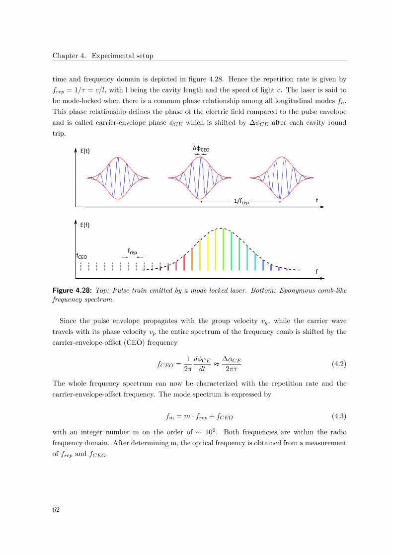
Chapter 4. Experimental setup
time and frequency domain is depicted in figure 4.28. Hence the repetition rate is given byfrep = 1/τ = c/l, with l being the cavity length and the speed of light c. The laser is said tobe mode-locked when there is a common phase relationship among all longitudinal modes fn.This phase relationship defines the phase of the electric field compared to the pulse envelopeand is called carrier-envelope phase φCE which is shifted by ∆φCE after each cavity roundtrip.
ΔφCEOE(t)
f
t
E(f)
frep
1/frep
fCEO
Figure 4.28: Top: Pulse train emitted by a mode locked laser. Bottom: Eponymous comb-likefrequency spectrum.
Since the pulse envelope propagates with the group velocity vg, while the carrier wavetravels with its phase velocity vp the entire spectrum of the frequency comb is shifted by thecarrier-envelope-offset (CEO) frequency
fCEO = 12π
dφCEdt
≈∆φCE2πτ (4.2)
The whole frequency spectrum can now be characterized with the repetition rate and thecarrier-envelope-offset frequency. The mode spectrum is expressed by
fm = m · frep + fCEO (4.3)
with an integer number m on the order of ∼ 106. Both frequencies are within the radiofrequency domain. After determining m, the optical frequency is obtained from a measurementof frep and fCEO.
62

4.2. Laser systems
Femtosecond fiber laser
The centerpiece of the comb is an Erbium doped fiber ring laser. The repetition rate isadjustable via an intra-cavity EOM and a mirror piezo by adjusting the optical path lengthof the laser resonator. Variable pump power and a moveable intra-cavity wedge providescontrol over the carrier envelope offset frequency. The pump light is coupled into the fiberring via a wavelength division multiplexer (WDM). A Faraday isolator (FI) pretends thepredominant direction for the light. Wave plates before and after the fiber provide controlover the laser polarization. A schematic overview of the comb setup is presented in figure 4.29.Usually the repetition rate and the offset frequency are locked to the 10 MHz reference (GPSdisciplined oven controlled quartz oscillator (OCXO)89) with a fractional frequency instabilityof ∼ 2 · 10−13.
WDM
CTR
GPS 10MHzReference
M-VIS EDFASHG 780
EDFAHMP1068
Repetition rate lock Offset frequency lock
PCF redEOM
FI
Pump
1:4
M-Phase EDFAXPS1500-WG
Phasedetector PID HV Amp
DRO 980MHz DDS 20MHz
CTR
Phasedetector PID
x2 DDS 20MHz
Er3+
PBS
wedgeMirror
WPs QWP
WPs
to short pulse exp.
Beat with 729 Laser
Beat with 1068 / 1069,6 Laser
GPS DRO HV Amp CTR
EDFA HMP SHG PCF HNLF DDS WDM
repetition rate 4th harmonic.
Global Positioning SystemDielectric Resonator OscillatorHigh Voltage AmplifierRadio frequency counter
Erbium Doped Fiber AmplifierHigh-power Measurement PortSecond Harmonic Generation Photonic Crystal Fiber Highly Non-linear Fiber Direct Digital Synthesis Wavelength division multiplexer
Figure 4.29: Schematic drawing of the frequency comb locked to the 10 MHz GPS signal (greenlines). The centerpiece of the comb is the Erbium doped fiber ring at the bottom left. Red andblue lines represent the measured repetition rate and offset frequency, respectively as well astheir control signals. The EOM in the fiber ring is only in use when the comb is locked to anoptical reference. See main text for more information.
89Menlo systems GPS 6-12
63

Chapter 4. Experimental setup
Within the M-VIS EDFA SHG 780 unit, the light from the fiber ring is amplified, frequency-doubled and sent to a highly non-linear fiber for spectral broadening. The outcome is usedto measure the frequency of the 729 nm laser via an optical beat note (see below). TheEDFA HMP1068 unit amplifies the comb light and creates a comb spectrum around 1068 nmwhich is used for the frequency measurement of both aluminium lasers at their fundamentalwavelengths of 1068 nm and 1069.6 nm. The frequency shift of the comb spectrum is achievedby the soliton self-frequency Raman shift [71], which depends on the pump power. Typicalcomb spectra are presented in figure 4.30.
-40
-35
-30
-25
-20
-15
-10
-5
0
5
500 700 900 1100 1300 1500
Inte
nsi
ty (
dB
)
Wavelenth (nm)
1550 nm
729 nm port
1068 nm port
Figure 4.30: Frequency comb spectra at the fundamental wavelength around 1550 nm (red) andthe two measurements ports around 729 nm (green) and 1068 nm (orange). The optical powerat the two measurement ports are 132 mW and 79 mW, respectively. With kind permissionfrom Menlo Systems.
Optical beat note detection
There are several ways to characterize a laser‘s spectral properties and its frequency. In thecase of a second laser being the reference, this is done via an optical beat note detection.Therefore both lasers with similar frequencies are overlapped on a fast photodiode via a non-polarizing beam splitter (BS). The resulting photo-current is frequency-modulated by thedifference frequency of the lasers and can be expressed as:
I(t) ∼ |E1(t) + E2(t)|2 = |E1(t)|2 + |E2(t)|2 + 2Re E∗1(t) · E2(t) (4.4)
The power spectrum observed on a spectrum analyzer is a convolution of both laser spectra:
SE∗1 ·E2(f) = SE1(f)⊗ SE2(f) (4.5)
64

4.2. Laser systems
The contribution of each laser to the convoluted spectrum depends on their noise spectra.In the case of white noise the line shape of the lasers are lorentzian and the spectral width(full width at half maximum ) of the convoluted signal is ∆beat = 4f1 +4f2. Gaussian laserspectra lead to ∆beat =
√4f2
1 +4f22 .
Repetition rate lock
To stabilize the repetition rate (250 MHz in this case) to the GPS reference a small part ofthe comb light is sent to a fast photodiode where the fourth harmonic of the repetition rateis detected. This signal around 1 GHz is mixed down with a 980 MHz signal derived from areferenced dielectric resonator oscillator (DRO) and a signal around 20 MHz is generated. Tocreate an error signal at DC it is once more mixed down with a 20 MHz signal derived from areferenced direct digital sythesizer (DDS). The error signal is fed into a PID controller, ampli-fied afterwards and applied to the mirror piezo that controls the cavity length and thereforethe repetition rate. The repetition rate can be also locked to a stable laser when the comb isused to down-convert a optical frequency to RF. Therefore the beat signal between the comband the laser is kept fixed by feeding back onto the intra-cavity EOM and the piezo mirror.
Offeset frequency lock
The CEO frequency is generated in the M-Phase EDFA XPS1500-WG unit. There the lightat a center wavelength 1.56 µm is amplified and spectrally broadened by a highly non-linearfiber to more than an octave (1 µm - 2.1 µm). A non-linear interferometer, which doubles thefrequency of the long-wavelength part of the spectrum and compares it with the near infraredpart via a beat note. The beat frequency is the CEO frequency, which is usually set to 20MHz.
|2(nfrep + fCEO)− (2nfrep + fCEO)| = fCEO (4.6)
To lock the CEO frequency to 20 MHz it is mixed with a frequency doubled GPS signal. Theresulting signal is put into a phase detector together with the target frequency derived froma referenced DDS. The error signal is sent to a PID controller and its output is connected tothe pump current control.
Frequency measurement
The frequency of a continuous wave (CW) laser can be measured via an optical beat note withthe light of the frequency comb. Therefore the two laser beams with the same polarizationare spatially overlapped. To select only comb modes with a frequency similar to the CW laserthe beams are sent onto a grating. The CW laser and the nearest comb modes are diffracted
65

Chapter 4. Experimental setup
under the same angle and sent to a fast photodiode. A beat note (typically∼ 40 kHz FWHMif limited by the comb stability) between the laser and the nearest comb modes is visible ona spectrum analyzer. The signal to noise ratio (SNR) of the beat signal has to be optimizedby improving the spatial alignment and the spectral output of the comb. The latter is donevia translation stages that vary the amount of comb light which is coupled into the nonlinearfibers by moving objectives. The output spectra depend on the pump power. Depending onthe RF counters used in the measurement the beat signal has to be amplified and the signal-to-noise ratio should reach 30 dB or more at a resolution bandwidth of 50 kHz to guaranteefor correct frequency counting. It is useful to use band pass filters to enhance the SNR. Ideallythe beat signal is split and counted by two separate counters while one path is attenuated by3 dB or more. For precision measurements on the Hz scale both counter values should fullyagree within the resolution limit. If both counters disagree by more than ∼10 mHz for beatfrequencies in the 10 MHz range and a gate time of 1 s, the SNR is too low.Before the absolute frequency measurement can start, the signs of the beat frequencies and
the absolute mode number n have to be determined.
fCW = nfrep ± fCEO ± fbeat (4.7)
The sign of the beat frequency can be determined by changing the repetition rate slightly. Ifthe sign is positive, the beat frequency decreases while the repetition rate increases and viceversa. The sign of the offset-beat can be determined in a similar way. The sign is positive whenthe beat frequency decreases with increasing offset frequency. In the case of the visible combport, the offset frequency is added twice since the comb light was frequency-doubled. The modenumber can be calculated by two frequency measurements with significantly different repetitionrates. The repetition rates should differ by about 10 kHz or more, otherwise mistakes in thedetermination become more likely due to a lower signal-to-noise ratio. This is not necessaryin this setup since the wavelength meter is accurate enough to identify the mode number.The optical power density of the comb output spectra around 729 nm and 1068 nm is
typically ∼ 2 mW/nm which results in ∼ 1.4 µW per comb mode for optimized parameters.As soon as the measurement starts, the repetition rate, the offset frequency and the beatfrequency are simultaneously recorded by dead-time free RF counters 90 and are added up tothe optical frequency. Usually the repetition rate and the offset frequency are locked to the 10MHz reference (GPS disciplined OCXO91) with a fractional frequency instability of ∼ 2 ·10−13
at time scales of from seconds to hours (see figure 4.25). There is the possibility to lock therepetition rate directly to a stable laser (for example 729 nm laser) which should improve thestability of the comb. Unfortunately the translation stage, which is responsible for the 729 nm
90FXM50 K&K Messtechnik91Menlo systems GPS 6-12
66

4.2. Laser systems
spectrum, is mechanically not stable enough and therefore requires high maintainance to keepa sufficient SNR which makes it laborious to work with.
67

Chapter 4. Experimental setup
4.3 Experimental control
Several different hardware components are involved in the electronic control of the experiment.A schematic drawing of the experimental control is presented in figure 4.31. Its centerpiece isthe Control PC on which a C++ program (TrICS = trapped ion control system) coordinatesthe tasks of multiple devices and provides a graphical user interface (GUI). It compiles thepulse sequences that are written in python for a given set of parameters in the TrICS GUI andsends it via a Ethernet connection to the “Pulse Box”. The latter is FPGA-based and contains8 direct digital synthesizers (DDS) which allow for precise timing, frequency and phase controlof the generated RF pulses that are sent to AOMs in the stable laser setup. All frequencysources that are crucial in terms of accuracy are referenced to the 10 MHz GPS signal.
Control PC
Pulse Box
AOM breadboard
EMCCD
TrICSLabVIEWMatlab
NI DIO-32HS
python server
NI 6733
DDS rack
Diode lasers
8 RF outputs32 logic outputs
8logic inputs
WLM PC
python server
USB
WLM
PCUSB
ISEG Box
Linetrigger
Archive server
Stable Laser AOM network
PMT
RF
RF+TTL
TTL
TCP/IP
TTL
TTLDCDC
USB
CAN Bus
Andor Bus
Bus
RS 232
TTL
TCP/IP
TCP/IP
TCP/IP
Figure 4.31: Schematic overview of the experimental control. Devices are represented as boxesand their links by arrows. All control signals emanate from the control PC in the center. Itis connected to two auxilary PCs that are responsible for the control of the high-voltage source(ISEG), which provides the voltage for the endcap electrodes and the wavelength meter (WLM)which is involved in the stabilization of the diode lasers. The Pulse box and the DDS rackprovide the RF signals for the AOMs. The fluorescence data is acquired by a photomultipliertube or by an electron multiplying charge coupled device camera.
All other AOMs on the breadboard are driven by homebuilt DDSs whose output power andfrequency are controlled by TrICS via the bus system. The WLM PC on which the wavelengthmeter software is running is connected to the Control PC via Ethernet. It receives the setpointfrequencies of the diode lasers from TrICS. The high finesse wavelength control translates theminto DC voltages which are applied to the piezos. A further PC is used to control the stablehigh voltage source (ISEG) and other devices. The state detection is done by recording the
68

4.3. Experimental control
fluorescence counts for a given time window after each experiment. For experiments withonly one calcium ion the photomultiplier tube (PMT) was used. For experiments with longion strings a LabVIEW based program [72] communicating with the EMCCD camera can beused. The experimental data is displayed on the TrICS GUI or automatically post-processedto feed back on the laser lock and the calculation of the magnetic field.
69

5 Experimental techniques
In this chapter important experimental techniques for experiments with trapped ions are pre-sented. The first part presents an investigation of the laser ablation loading of 40Ca+ and27Al+ ions, which was published in New Journal of Physics [73]. The second part describesthe procedures of setting up a typical experimental sequence involving laser cooling, opticalpumping as well as the calibration of sideband frequencies and AC-Stark shifts. The thirdand fourth parts present how a stable laser is referenced to a narrow atomic transition anddetail the method of compensating micromotion using the narrow-band laser. In the last part,the method of quantum logic spectroscopy is introduced which is used to detect the electronicstate of an aluminium ion.
5.1 Laser ablation loading of ions
The standard approach of loading ions into a trap is to evaporate neutral atoms of a particularelement from a resistively heated oven and to photo-ionize them at the trap center. In thecase of calcium ions this is a well-proven technique, which has been used for more than adecade. Evaporating neutral aluminium atoms from a thermal source requires considerablyhigher temperatures to create a sufficient atom flux. In the first trap setup an alumina ceramicoven with a piece of pure aluminium in the center was resistively heated by a tantalum wire. Totrap an aluminium ion the oven was operated at 12 W for several minutes. The dissipated heatled to thermal expansion of the ion trap holder of tens of microns and outgassing problems.Another drawback was the short lifetime of the oven since the tantalum wire burnt throughafter a few attempts.An alternative approach, which was used in the secon setup, is to evaporate neutral atoms
by single ablation laser pulses. For this purpose, single laser pulses at 532 nm with a durationof 2 ns and a pulse energy of 100 µJ were fired onto ablation targes. The trap potentialwas set such that a single calcium ion oscillated with frequencies of 400 kHz axially and 2MHz radially. To load calcium ions the alloy target (see section 4.1) was used on which theablation laser was focused to a Gaussian beam waist of 200 µm FWHM. Aluminium atomswere ablated from the pure aluminium target with a spot size of 50 µm FWHM. Initially theintention was to load both species from the alloy target. However, loading aluminium ionsfrom the alloy target was only possible with a substantially higher pulse energy which directly
70

5.1. Laser ablation loading of ions
created unwanted calcium ions. Both targets are hit by the ablation pulse under an incidentangle of 30°. Simultaneously the photo-ionization lasers were sent along the trap axis withGaussian beam waists of 100 µm FWHM and laser powers of 500 µW each.For experiments with a mixed ion crystal a calcium ion is loaded first, since aluminium
ions can only be sympathetically cooled. Typically a single calcium ion is loaded after a fewablation pulses. The probability of creating a single aluminium ion with one ablation pulseis similar. At the first attempts to load aluminiums ions, relatively long cooling times on theorder of several minutes were observed until the ions crystallize. In order to understand theselong sympathetic cooling times, time-resolved neutral atom fluorescence measurements werecarried out to characterize the velocity distribution of ablated atoms.
Arrival time (µs)
Lase
r fr
equ
en
cy –
75
9 T
Hz
(GH
z)
Atomic velocity (km/s)
Arrival time (µs)
Figure 5.1: Time-resolved fluorescence spectroscopy on the 2P1/2 ↔ 2S1/2 transition. a)Time-resolved fluorescence of Al atoms crossing the trap center versus laser detuning. Thenumber of detected photons is colour-coded in the image. The vertical line at τ ≈ 0 resultsfrom photons produced by the ablation pulse. The white lines indicate expected resonancesbetween the motion of the atoms and the laser beam of 87.7°. b) Hyperfine structure of thetransition with hyperfine shifts [62] in units of MHz. c) Histogram of atomic arrival times. d)Histogram of atomic velocities (see main text). The distribution peaks at velocities around 4.5km/s.
Towards this end, single ablation pulses with an energy of 200 µJ were fired onto the targetswhile the photo-ionization laser was turned on. The atoms crossing the 394 nm laser beam
71

Chapter 5. Experimental techniques
scatter photons (see figure 5.1 b) which were detected by the PMT and recorded by a fastoscilloscope1. Since atomic motion and laser beams were not perfectly perpendicular to eachother a Doppler shift was observed. Each horizontal trace is the average of five laser ablationpulses. A fraction of the ablation pulse light was sent to a fast photodiode which provided thetrigger signal for the oscilloscope. Because of the hyperfine structure of the ground and excitedstate four individual transitions are observed which are spread over about 3 GHz in frequency.To get rid of Doppler shifts the detected photon counts were summed up in frequency spacewhich yields the arrival time distribution of the atoms on which a background was subtracted.To derive the atomic velocity distribution assumptions have to made. The probability ofdetecting a scattered photon is inversely proportional to the atomic velocity. In the case ofaluminium it is assumed that each atom only scatters one photon before it gets pumped to adifferent state. The fluorescence data and the inferred distributions are shown in figure 5.1.Finally, atomic velocities ranging from 1.5 up to 15 km/s are observed. The distribution peaksat atomic velocities of 4.5 km/s.In order to detect the presence of an Al+ ion before the Ca+ and the Al+ ions crystallize
into a 2-ion crystal, a new detection method was developed. A hot ion orbiting in the trapcreates time-varying electric fields that act as a source of motional heating for the cold Ca+
ion. Small heating effects are easily detectable with Rabi spectroscopy on a motional sidebandtransition. In this case the heating effect is big enough that it is detectable on the carriertransition since their coupling strength depends on the motional state outside the Lamb-Dickeregime. The experimental sequence is the following:
• Doppler-cooling the calcium ion to the Lamb-Dicke regime and optical pumping to theS1/2 ground state.
• During a waiting time τ , the ion is heated if an aluminium ion is present in the trap.
• A π - pulse carried out on the S1/2 ↔ D5/2 transition. In the presence of an aluminiumion a reduced transfer probability is observed.
• State detection via electron shelving.
Figure 5.2 illustrates this detection technique. The recorded reduced transfer probability canbe used to calculate the mean number of transferred motional quanta during the the waitingtime τ . By integration over time the initial energy of the hot ion can be calculated. Moreinformation about the sympathetic cooling dynamics can be found in section 6.1.
The velocity distribution of ablated calcium atoms can be also derived from neutral atom flu-orescence. Since the 1S0 ↔ 1P1 transition in calcium is closed, contrary to the 2P1/2 ↔ 2S1/2
transition in aluminium, a calcium atom can scatter more than one photon while crossing the1LeCroy SDA 11000
72

5.1. Laser ablation loading of ions
laser beam. Corresponding data as well as the inferred arrival time and velocity distributionsare presented in figure 5.3.
0 50 150100 250200 350300 4000
10
0.2
20
1.0
0.0
0.4
0.6
0.8
Time (s)
D5
/2st
ate
pro
bab
ility
Co
un
ts (
kHz)
Figure 5.2: Detecting the loading of a hot aluminium ion by a cold calcium ion. A π - pulseon the S1/2 ↔ D5/2 transition transfers the population to the excited state of the calciumion. After 10 s an ablation pulse is triggered and a hot 27Al+ ion gets captured in the trap.It transfers kinetic energy to the present calcium ion which results in a reduced state transferprobability towards the excited state. Over the next 340 s the aluminium ion is sympatheticallycooled until the ions crystallize. The presence of the hot ion does not show up in the fluorescencecounts. The EMCCD camera images above show the equilibrium position of a single calciumion and the two-ion crystal later on. The rightmost picture shows motional excitation of themixed crystal by modulation of the axial confinement at the in-phase mode frequency for ameasurement of the mass of the dark ion.
Atomic velocities between 600 m/s and 4.2 km/s are observed. The main fraction of theablated calcium atoms have velocities around 1.6 km/s which is almost a factor of 3 slowercompared to ablated aluminium atoms.A way to reduce the sympathetic cooling times of hot aluminium ions is to select relatively
slow atoms by introducing a temporal delay τd between ablation pulse and the time when thephoto-ionization laser is turned on for a duration τ . This also allows one to investigate whichvelocity classes of aluminium ions can be trapped. It turns out that only ions with velocitiesbetween 800 m/s and 3700 m/s can be trapped. The lower limit is given by the low densityof slow atoms while the upper limit is set by the trap depth.
73
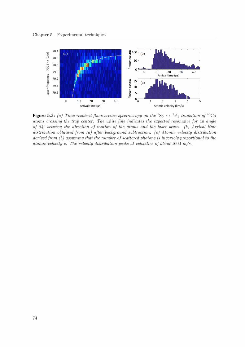
Chapter 5. Experimental techniques
Arrival time (µs)
Lase
rfr
equ
ency
–7
09
TH
z(G
Hz)
78.4
78.6
78.8
79.0
79.2
79.4
79.6
Atomic velocity (km/s)
Arrival time (µs)
Figure 5.3: (a) Time-resolved fluorescence spectroscopy on the 1S0 ↔ 1P1 transition of 40Caatoms crossing the trap center. The white line indicates the expected resonance for an angleof 84° between the direction of motion of the atoms and the laser beam. (b) Arrival timedistribution obtained from (a) after background subtraction. (c) Atomic velocity distributionderived from (b) assuming that the number of scattered photons is inversely proportional to theatomic velocity v. The velocity distribution peaks at velocities of about 1600 m/s.
74

5.2. Experimental sequence
5.2 Experimental sequence
Every single experiment with trapped ions consists of a series of different steps.A schematic overview of a typical sequence is depicted in figure 5.4. Before thedesired experiment can be carried out, the ions are prepared in a well-definedinternal and motional state by laser cooling and optical pumping. After thatcoherent operations on the narrow transitions can be carried out with high fidelity.At the end of each experiment a quantum state measurement is performed. In thefollowing each experimental step for experiments with an Al+- / Ca+- mixed ioncrystal is described. Thereby the focus is laid on the part describing the aluminiumion. The experimental sequences containing all relevant experimental parametersare encoded in a python file that is interpreted by the experiment control program.A detailed description can be found in [29].
267.0σ
267.4
PMT
EMCCD
397
729
854
866
397σ
t0 tLT
I II III IV V VI VII VIII
20ms
IX
Ca+
Al+
Figure 5.4: Schematic of a typical pulse sequence with a mixed ion crystal. Doppler-cooling(I) followed by optical pumping of Ca+ (II). Optical pumping on the aluminium ion (III).Continuous sideband cooling (IV). Frequency-resolved optical pumping (V). The particularexperiment (VI). Quantum logic state transfer (VII) & (VIII). State detection (IX).
(I) Doppler-cooling
Every experimental sequence starts with Doppler-cooling the ions. A 397 nm beam adressingthe S1/2 ↔ P1/2 transition is applied for a period of 5 ms. The beam has overlap with allthree normal modes of an ion in the trap. Since the transition is not closed, the 866 nmlaser is used simultaneously for repumping population from the D3/2 states. The intensity ofthe cooling laser is chosen to be half the saturation intensity of the transition and the laserfrequency is red-detuned by half the spectral width of the transition 4 = −γ/2. To avoidadditional line broadening from the 866 nm laser its power is set close to saturation. Slightlyblue-detuning the frequency of the 866 nm laser prevents coherent state trapping. The settingsfor sympathetic Doppler-cooling when working with mixed ion crystals are identical to the ones
75

Chapter 5. Experimental techniques
chosen for cooling a single Ca+ ion. The fluorescence counts registered during Doppler-coolingcan be used to monitor the crystalline order of the ions. In the case of a melting event due to acollision with background gas an additional 160 MHz red-detuned beam is used to recrystallizethe ions and the corrupted data is taken again.
(II) Optical pumping of 40Ca+
After Doppler-cooling the calcium ion is prepared in the mj = +1/2 ground state using theweak circularly polarized beam at 397 nm for about 20µs. The achieved pumping fidelity istypically 99%.
(III) Frequency-resolved optical pumping of 27Al+
If an aluminium ion is involved in the experiment a series of π - pulses on the 1S0 ↔3 P1
transition manifold is applied with 4m = ±1 , depending on the desired target state. Each π- pulse is followed by a 300 µs waiting time to allow the excited state to decay.
t (ms)
0 2 4 6 80
0.2
0.4
0.6
0.8
1
Zeem
an s
ub
stat
ep
op
ula
tio
n
10 12
Figure 5.5: Calculated time evolution of the resonantly driven six-level system starting inthe mf = 5/2 Zeeman substate. The calculation assumes a level splitting of 4.4 kHz and aRabi frequency of 200 Hz. The small modulation from the fast rotating term indicates thata rotating-wave approximation would still be justified. Since the inner levels couple in bothdirections, only the stretched Zeeman states are fully populated at a certain point in time.
A frequency measurement of the outermost transitions and precise knowledge of the magneticfield, calibrated with the S1/2 ↔ D5/2 transition in calcium, allows one to calculate thefrequencies of the inner transitions. Since the Rabi frequency on the outermost transition isknown, the length of the π - pulses on the inner transitions can be calculated by the inverseratio of the corresponding Clebsch-Gordan coefficients. The whole procedure is repeated fivetimes.
76

5.2. Experimental sequence
The pumping efficiency is characterized by inducing nuclear spin flips by an AC magneticfield. With this the ion can be prepared in the other stretched Zeeman substate. The timeevolution of the Zeeman substate populations for a given coupling strength is presented infigure 5.5. Frequency-resolved optical pumping as described above is carried out afterwardsfollowed by a detection whether the ion has reached its target Zeeman state or not. Thecorresponding data is presented in figure 5.6.
AC pulse length (ms)
D5/2stateexcitation
Pump repetitions
D5/2stateexcitation
0.4
0.6
0.8
0.2
00.0
20 40 60 80
a) b)
1.0
100 1200 40 80 120 160 200 240
0.4
0.6
0.8
0.2
0.0
1.0
Figure 5.6: a) Nuclear spin rotation induced by an AC magnetic field at 4.452 kHz, detectedvia quantum logic spectroscopy with a calcium ion. At the beginning of the experiment the ionis prepared in the mF = 5/2 Zeeman state via 100 pump repetitions. An AC magnetic field(~15 mGpeak) induces a full spin rotation within 150 ms. Since the initialization is not perfect,the data was postselected depending on the outcome of the previous experiment. The contrast islimited by imperfect state detection, the Rabi frequency is limited by the inductance of the coilpair (~6.5 mH) and the current driver, respectively as well as the magnetic field attenuation bythe vacuum chamber (~15 dB). b) Pump efficiency characterization. The ion is transferred tothe opposite stretched state mF = −5/2 via a 75 ms long AC pulse and optical pumping towardsthe mF = 5/2 state is carried out subsequently. The baseline at 0.15 arises from imperfectstate detection. The red line is an exponential fit to the data. After about 40 repetitions half ofthe population is brought back to the target state. The probability of transferring the populationfrom one stretched state to the other one is about 2% per pump repetition.
After about 40 pump repetitions half the population is brought back from one stretchedZeeman state to the target Zeeman state. Therefore the probability of transferring the popu-lation from one outermost Zeeman state to the other using a single pumping step is about 2 %.One limiting factor for the pump efficiency are imperfect π - pulses due to laser noise. Anotherreason could be a quadratic Zeeman shift of the inner 3P1 Zeeman substates, resulting froma coupling to other 3P1 hyperfine states, which would lead to off-resonant pump pulses, butneeds further investigation.
77

Chapter 5. Experimental techniques
(IV) Sideband cooling
For experiments that require the ions to be prepared in the ground state of a particularmotional mode, continuous sideband-cooling is applied to the motional mode of interest fora duration of 7 ms. The 729 nm laser frequency is addressed to the red sideband of thecorresponding mode of the S1/2, mj = 1/2 ↔ D5/2, mj = 5/2 transition. To speed up theprocess the 854 nm laser is used to reduce the lifetime of the excited state (quenching). Eachof these cycles reduces the mean phonon number of the thermal state after Doppler-coolingby one. Since there is also a finite probability to decay from the P3/2 into the D3/2 state the866 nm laser is used for repumping via the P1/2 state. Additional optical pumping with the397 nm laser ensures a closed cooling cycle.
(V) Frequency-resolved optical pumping of 40Ca+
The optical pumping efficiency can be improved by using the 729 nm laser. Its frequency ismade resonant with the S1/2, mj = −1/2 ↔ D5/2, mj = 3/2 transition. Together with the854 nm and 866 nm laser this leads to a population transfer to the desired S1/2, mj = 1/2state. Pumping efficiencies after 200 µs of 99.9 % can be achieved.
(VI) Coherent state manipulation
Now the ions are prepared in a particular electronic and motional state and the actual experi-ment can start. During the experiment the ion‘s internal and external states are manipulatedusing different accessible carrier and sideband transitions. While the carrier transition fre-quencies of 40Ca+ are calibrated with the clock script (see section 5.3), sideband transitionfrequencies are calibrated manually. Symmetrically to carrier transitions motional sidebandsappear. The sidebands can be identified by their response to changes of the trap potential. Afraction of a typical excitation spectrum is presented in figure 5.7. The confinement and thequantization magnetic field have to be chosen in a way that sideband and carrier transitionsare well separated in frequency. The linear Zeeman shift of transition frequencies dependingon the quantization magnetic field is depicted in figure 5.8. Here only the electric quadrupoletransition in 40Ca+ and the intercombination line in 27Al+ are considered.At typical quantization magnetic fields of about 4 G and secular frequencies on the order of
1 MHz the linear Zeeman effect on the aluminium clock transition is too small to cause anyoverlap of sideband and carrier transitions.Once the trapping confinement is chosen, excess micromotion has to be compensated (see
section 5.5). As soon as micromotion is compensated for, Rabi frequencies on the transitionsof interest as well as AC-Stark shifts of those have to be calibrated manually.
78

5.2. Experimental sequence
Frequency offset near 411 THz (MHz)
D5/2stateexcitation
-2.0 -1.5 -1.0 -0.5 0.0 0.5 1.0 1.5 2.00.0
0.1
0.2
0.3
0.4
0.5
0.6
Figure 5.7: Fraction of an excitation spectrum of on the calcium S1/2 ↔ D5/2 transition witha mixed Al-/Ca- ion crystal at typical trapping conditions, taken with the diagonal 729 nmbeam. The center peak represents the S1/2, mj = 1/2 ↔ D5/2, mj = 5/2 carrier transitionand symmetric to it red and blue motional sidebands of the mixed crystal appear. The axialin- and out-of-phase modes are visible at ± 888 kHz and ± 1.596 MHz respectively. The radialmodes are not degenerate. Calcium-like modes are observed at ± 0.9 MHz and ± 1.1 MHz, thealuminium-like modes show up at ± 1.9 MHz and ± 2.1 MHz. Other peaks appearing correspondto second order sidebands or combination of those.
-2 0 42 8 6 1210
Linear Zeeman shift (MHz)
Mag
net
ic fi
eld
(G
)
-20 -15 -5-10 0 5 1510
1
5
0
2
3
4
1
5
0
2
3
4
Linear Zeeman shift (MHz)
a)
b)
Mag
net
ic fi
eld
(G
)
Figure 5.8: Calculated Zeeman-splitting of the S1/2, mj = 1/2 ↔ D5/2 transition manifold in40Ca+ (top) and the 1S0, F = 5/2, mf = 5/2 ↔ 3P1, F = 7/2, mf = 3/2, 5/2, 7/2 transitionmanifold in 27Al+ (bottom) including red and blue motional sidebands. Carrier transitionfrequencies are depicted as black lines. The green lines are micromotion sidebands. For thecase of 1S0, F = 5/2, mf = −5/2 ↔ 3P1, F = 7/2, mf = −3/2, −5/2, −7/2 flip the sign onthe x-axis. The Zeeman splitting of the ground state is negligible. For most of the experimentsa quantization field of 4 G was applied.
79

Chapter 5. Experimental techniques
(VII) & (VIII) Quantum logic state mapping
In the case of experiments with a mixed-ion crystal, the internal state of the aluminium ion hasto be mapped to the internal state of the calcium ion before the fluorescence detection on thecalcium ions happens. This is done in the quantum logic way by transferring the aluminiumion‘s internal state onto the motional state of a common motional mode and subsequently tothe internal state of the calcium ion by the means of sideband pulses (see section 5.4).
(IX) Fluorescence detection
To discriminate between the S1/2 and D5/2 state of the calcium ions the 397 nm beam isturned on. In the case of the calcium ion being in the S1/2 state photons are scattered onthe S1/2 ↔ P1/2 transition. The fluorescence photons are collected by a PMT or an EMCCDcamera. To reach a high fluorescence rate the intensity of the 397 nm laser is set to thesaturation intensity of the transition (on resonance). The laser frequency is still red-detunedby 4 = −γ/2 from resonance. Detection efficiencies are well above 99% when collectingfluorescence photons for about 5 ms.
80

5.3. Locking the 729 nm Laser to the S-D transition
5.3 Locking the 729 nm Laser to the S-D transition
In order to carry out coherent operations with high fidelity precise knowledge of the laserfrequency and the magnetic field is required. Therefore two symmetric transitions (±1/2 ↔±3/2) with respect to the line center that suffer least from the quadrupole shift are probed bya Ramsey experiment. The duration of the π/2 - pulses is set to 100 µs to avoid significant ACStark shifts. Each transition is probed twice with the phase of the second pulse shifted withrespect to the first one by (φ1 = π
2 , φ2 = 3π2 ). The pulses are separated by a waiting time τR.
Taking the average over a hundred experiments each provides an estimate of the excited stateprobabilities pφ1and pφ2 . The difference between the laser frequency and the atomic transitionfrequency is expressed by
∆ν = 12π(τR + 2τπ/π)arcsin
pφ1 − pφ2
pφ1 + pφ2
. (5.1)
The line center at zero magnetic field can be calculated from the two measured frequencydifferences ∆ν1 and ∆ν2. The line center is the arithmetic mean of both frequencies sincesymmetric transitions were chosen. The magnetic field can be derived from the frequencydifference of both transitions resulting from the linear Zeeman effect. The measurements areautomatically executed every few minutes by the experiment control program which raises orlowers the waiting time between 10 µs and 4 ms depending on the outcome of the previousmeasurement. The laser frequency and the magnetic field are fitted by a polynomial of a chosenorder (typically 1 for the frequency and 0 for the magnetic field) and the extrapolated values areused in the next experiment. It is useful to weigh the data contributing to the fit by the timewhen they were taken, which is implemented by an exponential loss of memory at a timescaleof 10 min. Error bars are calculated from quantum projection noise [60] σ =
√p(1− p)/N
where N is the number of measurements and p is the excitation probability.
5.4 Micromotion compensation
Electric stray fields that shift the ion from the RF nodal point cause excess micromotion, i.e. adriven motion at the trap‘s driving frequency ΩT . Analogous to the case of secular motion thelaser seems frequency modulated in the ion‘s reference frame due to resulting Doppler shifts.Consequently, the effective electric field can be expressed as [74]
E(t) = E0e−iωlteikxa
q2sin(ΩT t) (5.2)
where ωl is the laser frequency, k is the wavevector of the laser beam, xa is the ion‘s dis-tance from the nodal point and the q-parameter q (see section 2.1). The second exponen-
81

Chapter 5. Experimental techniques
tial in equation 5.2 can be expanded in terms of Bessel functions Jn(β) as eikxaq2sin(ΩT t) =∑∞
n=−∞ Jn(β)einΩT t with the modulation index β = kxaq2 . In the limit of small modulation,
the modulation index β can be expressed in terms of the coupling strength ratios betweencarrier and micromotion sideband as β/2 ≈ J1(β)
J2(β) = ΩMMSBΩCarrier
.The distance of the ion from the RF nodal point can be determined by d = 2β
qk . The strengthof a static electric stray field that shifts the ion‘s equilibrium position by d can be calculatedby Es = mω2
rde where ωr is the secular frequency. Excess micromotion first of all causes a loss
in coupling strength on the carrier transitions and can prevent the ion from being efficientlycooled. Furthermore, it induces a systematic frequency shift in frequency standards and there-fore has to be minimized by micromotion compensation techniques. The compensation is doneby changing the DC voltages on the compensation electrodes and comparing the Rabi frequen-cies on carrier and micromotion sideband transitions. The relative coupling strength of thefirst micromotion sideband depending on the compensation voltage is presented in figure 5.9.
Horizontal compensation voltage (V) Vertical compensation voltage (V) Z-axis ion position (µm)
ΩMMSB/Ω
Carrier
58 60 62 64 660.00
0.03
0.04
0.05
0.02
0.01
79 8480 81 82 83 85 -15 10-10 -5 0 5 1586
0.06
ΩMMSB/Ω
Carrier
0.00
0.03
0.04
0.05
0.02
0.01
0.06
0.07
ΩMMSB/Ω
Carrier
0.000
0.015
0.020
0.010
0.005
a) b) c)
Figure 5.9: Micromotion compensation in vertical a), horizontal b) and axial direction c).The data shows the coupling strength ratios of the first micromotion sideband to the carrierdepending on the horizontal a) and vertical b) compensation voltages as well as the positionalong the trap axis c). The data was taken at an axial and radial confinement of 820 kHz and1.35 MHz, respectively for a single 40Ca+ ion. Minimal modulation indices of β ≈ 1/250 aremeasured along the radial directions. Along the axial direction a minimal modulation index ofβ ≈ 1/2000 is observed.
For the current trap, typical compensation voltages are on the order of 60 - 80 V which leadto electric fields of 150 - 200 V/m at the position of the ion. In standard linear Paul traps(with endcap electrodes), driven by quarter wave resonators, also axial micromotion is present.To compensate for this, the endcap voltages are imbalanced such that the ion is placed to theRF nodal point. Optimized coupling strength ratios for all three directions of micromotion ofΩcarΩmm & 500 are achieved. The uncompensated stray field in radial direction is therefore 120mV/m.The homogeneity of radial micromotion along the trap axis was investigated by shifting the
ion by 20 µm along the axis and optimizing the radial compensation voltages. Only a slightchange of 0.5 V of the compensation voltage was necessary to reach optimal parameters again.
82

5.4. Micromotion compensation
Some field lines from the RF blade electrodes point to the endcap electrodes which causesa shallow confinement along the axis. By comparing the q parameters in axial and radialdirection using the relations q = 2β
dk and q =√
8ωrΩT
respectively, the ratio of the quadrupolepotentials can be calculated. This result shows that the trap creates nearly an ideal 2Dquadrupole potential with 99.6% of the RF potential curvature in the radial plane.
83

Chapter 5. Experimental techniques
5.5 Quantum logic spectroscopy
Quantum logic spectroscopy [75] is a technique that provides the ability to carry out experi-ments with ions that lack suitable transitions for cooling and state detection. With the helpof a co-trapped “logic ion” (40Ca+ ) the “spectroscopy ion” (27Al+ ) can be sympatheticallylaser-cooled. Furthermore the internal state of the spectroscopy ion can be transferred to theinternal state of the logic ion by coherent operations. The method uses coherent sidebandpulses that map an internal state to a motional state of a common motional mode and viceversa.At the beginning of the experiment both ions are prepared in the electronic and motional
ground state of a joint motional mode |0, gS , gL〉. Spectroscopy on the clock transition of thespectroscopy ion creates a coherent superposition of the two clock states |0, gL〉 ⊗ α |gS〉 +β |eS(3P0)〉. A π - pulse on the blue sideband of the intercombination transition maps theground state population to a phonon of a joint motional mode β |0〉+ α |1〉 ⊗ β |eS(3P0)〉+α |eS(3P1)〉⊗ |gL〉. A π- pulse on the red sideband of the clock transition of the logic ion mapsthe motional state to the logic ions internal state |0〉 ⊗ β |eS(3P0)〉 + α |eS(3P1)〉 ⊗ α |gL〉 +β |eL〉. The electronic state of the logic ion α |gL〉 + β |eL〉 is detected via electron shelving.The sequence described above is illustrated in figure 5.10.
S L S LS LS LS L
Spectroscopy BSB (S) Detection (L)RSB (L)
|0⟩n |S⟩
|D⟩
|1S0⟩
|3P0⟩|3P1⟩
|1⟩n
|0⟩n|1⟩n
|0⟩n
I II III IV V
Figure 5.10: Quantum logic spectroscopy with an Al+−/Ca+− ion crystal. (I) The experimentstarts with both ions in the electronic and motional ground state of a joint motional mode. (II)Spectroscopy on the clock transition of the spectroscopy ion. (III) Mapping of the ground statepopulation to a phonon of a joint motional mode. (IV) Mapping the motional state to the logicions internal state. (V) State detection via electron shelving.
During the measurements carried out in this work the out-of-phase axial mode at 1.596 MHzwas chosen for the state transfer since it is further away in frequency from the carrier and hasa much lower heating rate of only ∼ 0.8 phonons/s compared to the axial in-phase mode with∼ 70 phonons/s .The limit for the overall detection fidelity is given by the sum of different imperfect opera-
tions like state preparation, ground state cooling and the fidelity of the mapping pulses. The
84

5.5. Quantum logic spectroscopy
biggest contribution comes from the imperfect blue sideband pulse on the intercombinationtransition. The highest transfer probability for this π - pulse was ∼ 95%, mainly limited byhigh frequency noise of the laser (see figure 4.23 & 4.24). Rabi oscillations on the blue sidebandand the carrier are presented in figure 5.11.
Pulse length (µs)
D5
/2st
ate
exci
tati
on
0.6
0.8
1.0
0.4
0.2
0 25 50 75 1000.0
Pulse length (µs)
D5
/2st
ate
exci
tati
on
0.6
0.8
1.0
0.4
0.2
0 50 100 150 200
a) b)
125 1500.0
250 300
Figure 5.11: a) Rabi oscillations on the blue out-of-phase mode sideband of the 1S0, mf =5/2 ↔ 3P1, F = 7/2, mf = 7/2 transition measured by quantum logic spectroscopy. After15 µs approximately 95% of the population is transferred to the excited state, which gives riseto the baseline in the Ramsey patterns in chapter 6. The main limitation therefore is highfrequency noise of the probe laser (see main text). The error bars are calculated by quantumprojection noise for 50 experiments per data point. b) Rabi oscillations on the 1S0, mf =5/2 ↔ 3P1, F = 7/2, mf = 7/2 carrier transition measured by quantum logic spectroscopy.In this experiment, a laser pulse, resonant with the carrier transition, was applied prior to thesideband pulse on the out-of-phase mode.
This assumption is justified by the fact that the contrast decreases further with higherRabi frequency. Therefore the Rabi frequency was chosen such that the maximum transferprobability is achieved. The quantum logic experiments that were carried out, start withthe 40Ca+ ion being in the excited state. A blue sideband pulse followed by a fluorescencedetection provided a check if sideband cooling to the ground state was successful. For thisreason the QLS measurements show an inverted signal that starts at an excitation of 1.
85

6 Measurements
The experimental results achieved in this work are presented in this chapter. It is structuredas follows: The first part (section 6.1) describes the experimental investigation of the sympa-thetic cooling dynamics of aluminium and calcium ions which was published in New Journal ofPhysics [73]. Theoretical modelling and numerical simulations of the sympathetic cooling dy-namics can be found in the publication. In the next section (section 6.2) collective Ramsey ex-periments with long ion strings were used to investigate the electrical quadrupole shift in a cal-cium ion string. In section 6.3 an absolute frequency measurement of the 1S0 ↔ 3P1, F = 7/2transition in 27Al+ via quantum logic spectroscopy with a 40Ca+ ion is described. Furthermorethe Landé g-factor of the 3P1, F = 7/2 state was determined. Section 6.4 concludes with afirst spectroscopic signal from the 1S0 ↔ 3P0 clock transition.
6.1 Sympathetic cooling
The method for detecting the presence of a hot ion in the trap (see section 5.1) providesdetailed information about the sympathetic cooling process. The experiments start with aDoppler-cooled 40Ca+ ion with trapping frequencies of 2 MHz radially and 0.4 MHz axially.After a waiting time of 10 ms two π - pulses on the S1/2, mj = −1/2 ↔ D5/2, mj = −3/2and S1/2, mj = 1/2 ↔ D, mj = 3/2 transitions were carried out. The internal state of the40Ca+ ion was detected by electron shelving. The sequence was repeated continuously with50 experimental cycles per data point. In one experimental cycle an ablation pulse was firedonto the target and the 394 nm photo-ionization laser was turned on with the goal of creatinga 27Al+ ion in the trap. As soon as a hot aluminium ion gets trapped it manifests itself as adrop in excitation probability. Over time a trend to lower and lower excitation probabilities isobserved which results from the increasing heating rate the calcium ion experiences. Finallythe ions crystallize and the excitation probability recovers. The temporal evolution of theexcitation probability during the sympathetic cooling process is presented in figure 6.1.The coupling strength Ωnn on a carrier transition outside the Lamb-Dicke regime depends
on the motional state of a vibrational mode and is given by Ωnn = Ω0 〈n| eiη(a+a†) |n〉. Theexcitation probability of a laser pulse that corresponds to a π - pulse for an ion in the Lamb-Dicke regime allows for inferences on the transferred motional quanta during the waiting time.
86

6.1. Sympathetic cooling
The mean squared Rabi frequency can be approximated by
〈Ω2〉n ≈ Ω20e
(−2η2n)I0(2η2n) (6.1)
with I0 being the modified Bessel-function of the first kind.
0 400 6002000.0
0.2
D5/
2st
ate
exci
tati
on
Time (s)
(a)
800
0.4
0.6
1000
0.8
1.0
0 400 6002000.0
0.1
Exce
ss e
ner
gy (
eV)
Time (s)
(a)
800
0.2
0.3
1000 0 40 60200.0
0.5
Exce
ss e
ner
gy (
meV
)
Time (s)
(a)
80
1.5
2.0
1.0
0.0
0.2
D5/
2st
ate
exci
tati
on
Time (s)
(a)
0.4
0.6
0.8
1.0
0 40 6020 80
a) c)
d)b)
Figure 6.1: Sympathetic cooling dynamics of a 27Al+ ion cooled by one 40Ca+ ion. a) D5/2state excitation probability after a π - pulse on the S - D carrier transition. After a few seconds(left dashed vertical line) a hot 27Al+ ion is created by an ablation pulse. The ions crystallizeafter 1000 s of sympathetic cooling (right dashed vertical line). The D5/2 state populationshown as red (pink) dots results from binning 250 (50) experimental cycles. b) Energy of the27Al+ ion calculated from the binned data in a). The dashed-dotted black line is the temporalenergy loss predicted by equation (6.3) with initial energy and cooling time adjusted to fit theexperimental data. c) and d) show the same type of signal as a) and b) respectively for a 27Al+ion that was trapped for about 40 s before getting lost again.
The excitation probability of a laser pulse with a duration Ω0τ = π applied to an ion in athermal state is approximated by [73]
pn =⟨sin(Ωnnτ/2)2
⟩≈ 1
Ω0sin2
(π
2
√〈Ω2〉
n
). (6.2)
Thus the phonons transferred to the calcium ion during the waiting time and furthermore theinitial energy of the hot ion can be tracked back. To infer the initial energy of the aluminiumion assumptions have to be made. The heating rate is expected to be spatially isotropic andit is assumed that laser cooling dissipates all the transferred energy such that the calcium ion
87

Chapter 6. Measurements
stays close to the Lamb-Dicke regime until the final stage of the cooling process. The latteris confirmed by experiments with and without the waiting time before the π - pulses andcomparing the excitation probabilities. The excitation without the waiting time (grey datapoints in figure 6.2 a) is largely close to one but drops at the end of the cooling process. Forthe conversion of the excitation probability to a heating rate 250 experiment were binned toreduce the influence of quantum projection noise. Sometimes it happened that a hot trappedaluminium ion got lost after seconds to minutes. A possible explanation therefore are collisionswith the cooling ion that repartition the kinetic energy among the three spatial directions andthe ion escapes along a direction where the trap is not deep enough to confine it. Ions withhigh kinetic energy might also explore unstable trapping regions.
(a) (a)
0 400 6002000.0
D5/
2st
ate
exci
tati
on
Time (s)
800
0.5
1000
1.0
0 400 6002000.0
0.5
Exce
ss e
ner
gy (
eV)
Time (s)
800
1.0
1.5
1000
Figure 6.2: Sympathetic cooling dynamics of a 27Al+ ion cooled by one 40Ca+ ion with thesame type of curves as in figure 6.1. In this experiment the waiting time for every seconddata point (grey dots in (a)) was omitted. It ensures that the transfer probability is still highuntil the end of the cooling process. The error made by assuming that the calcium has zerotemperature at the beginning of each experiment is negligibly small (grey line in (b)).
According to a simple sypathetic cooling model, derived in [73] the temporal energy loss ofthe hot ion is given by
E(t) = 3
√E(0)3 −
(t
τ
) 24mh
mcE3d , (6.3)
where E(0) is the initial energy of the hot ion, τ = 2π/ω is the oscillation period of the hotion and mh and mc are the masses of the hot and the cold ion, respectively. Ed = 1
2mhω2d2 =
e2/4πε0d is an energy scale with d = (e2/2πε0mhω2)1/3. The time that is needed to extract
all energy is expressed by [73]
τcool = mc
24mh
(E(0)Ed
)3τ. (6.4)
The cooling time τcool shows a strong dependence on the initial energy of the hot ion. For ahot aluminium ion with an initial energy of 1 eV and an oscillation frequency of ω = (2π) 1MHz a cooling time of 5000 s is predicted, which is of the same order of magnitude as thecooling time observed in figuere 6.2.
88

6.1. Sympathetic cooling
Similar measurements were carried out to investigate the sympathetic cooling dynamics ofhot 40Ca+ ions as a function of the number of Doppler-cooled 40Ca+ ions present in the trap.In the regime where the Doppler shift is much bigger than the detuning of the cooling laserfrom resonance, simple models [76] predict cooling rates that scale only weakly with the energyof the ion dE/dt ∼ 1/
√E. Numerical estimates based on [76] predict cooling times of many
seconds to minutes for E0 = 0.1...1 eV for Doppler-cooling settings optimized for achieving lowtemperatures. These predictions are confirmed by the experimental observations presented infigure 6.3. A mean cooling time of 100 s is found for cooling one hot 40Ca+ ion by a coldone, which is shorter than the cooling times for a hot 27Al+ ion but considerably longer thanwhat is expected from numerical simulations [73]. Shorter cooling times can be achieved byadjusting the laser frequency to the Doppler shift during the cooling process.
100 500 700300
1
2
Number
ofeven
ts
Cooling time (s)
900
3
4
11000
100
Coolingtime(s)
(a)
300
400
200
1 3 42
Refrigerant ion number
5
b)a)
Figure 6.3: a) Distribution of sympathetic cooling times of a hot 27Al+ ion cooled by a 40Ca+
ion. The histogram shows 19 loading events at a bin size of 200 s. A mean cooling time of 600s is observed. b) Distribution of the sympathetic cooling times of a 40Ca+ ions as function ofthe number of refrigerant ions (also 40Ca+ ). The red circles indicate the individual coolingtimes for each experiment. The black lines show the mean value for each data series withcalculated standard deviation error bars in grey. Assuming that the initial energy of the hotion is identical on average the average cooling time is expected to decrease inversely with thenumber of ions (due the increased refrigeration power of the string).
The long sympathetic cooling times observed in these experiments are ascribed to the highinitial energy of the ions. One part of it is the kinetic energy of laser-ablated atoms. Analuminium atom at a velocity of 1000 m/s has a kinetic energy of 0.14 eV. Since the sympatheticcooling times scale as τ ∼ E3
0 , the initial energy E0 of ions loaded into the trap has to be keptas low as possible. To a certain extent this can be done by a delay between ablation pulseand the photo-ionization beam and therefore selecting the low velocity tail of the distribution.Another contribution is the potential energy of an ion created off-center. An ion created at
89

Chapter 6. Measurements
z = 500 µm in a conservative harmonic potential with an oscillation frequency of ωz/2π = 500kHz exhibits a potential energy of Epot = 0.35 eV. It is currently not clear if the sympatheticcooling times can be shortened by restricting the ion creation volume to a region aroundthe trap center. In the case of calcium this could be realized by two tightly focused PI beamscrossing at the trap center instead of co-propagating beams along the trap axis. For the slowestaluminium atoms a cooling time of a few seconds is predicted [73] but cooling times shorterthan a minute were never observed experimentally. In this setup the ions can be created overa rather long distance along the trap axis, which is assumed to be the limiting factor for thecooling times.
90

6.2. Ramsey correlation spectroscopy
6.2 Ramsey correlation spectroscopy
The future of trapped ion optical frequency standards lies in spectroscopy of multi-ion entan-gled states [12,34]. Contrary to the single ion case the spatial extension of an ion string is onthe order of 100 µm along the trap axis for typical trapping conditions.
Figure 6.4: EMCCD camera image of a string of eleven trapped calcium ions. The ions areseparated by ~ 4.4-6.5 µm.
Inhomogeneous magnetic and electric fields at the trap as well as the presence of otherions lead to different systematic frequency shifts along the ion string. In the case of 40Ca+
ions the most dominant part is the electric quadrupole shift which can lead to a difference intransition frequency up to 100 Hz from the inner to the outermost ions depending on the axialconfinement and the transition to be excited.The shift arises from a non-spherical charge distribution of the D states that couples to
electric field gradients at the position of the ions. These electric field gradients are created bythe DC potential along the trap axis and the electric field from other ions present in the trap.Detailed information about the electric quadrupole shift in 40Ca+ can be found in [34, 46, 77]and references therein. The electric quadrupole moment of an atom in the electronic state|γ, J 6= 0〉 is given by
Θ(γ, J) = −e 〈γ, J,mJ = J | |N∑i=1
r2iC
(2)0 (θi, ϕi)| |γ, J,mJ = J〉 (6.5)
It consists of the sum over all electrons with coordinates ri, θi and ϕi and the normalizedspherical harmonic C(2)
0 (θi, ϕi) =√
4π5 Y2,0(θi, ϕi). The Hamiltonian describing the interaction
of the electric quadrupole moment with the gradient of an external electric field denotes H =∇E · Θ. The electric quadrupole moment of the D5/2 state of 40Ca+ was measured to beΘ(3d, 5/2) = 1.82(1)ea2
0 [38] where a0 is the Bohr radius. The resulting frequency shift to firstorder for a magnetic sub-level mj is given by [78,79]
∆νQ = 14h∇E ·Θ(γ, J)
J(J + 1)− 3m2j
J(2J − 1) (3cos2β − 1) (6.6)
where β is the angle between the quantization axis and the electric field gradient. A calculationof the electric quadrupole shift for a string of 40Ca+ ions is presented in figure 6.5. The ionsin the center of the ion string experience the strongest electric field gradients. Therefore theelectric quadrupole shift is biggest for the center ions.
91

Chapter 6. Measurements
Ion position (µm)
Quadrupoleshift(Hz)
Figure 6.5: Calculated quadrupole shift of the D5/2,mj = 1/2, 3/2, 5/2 levels for a string of 20ions at an axial confinement of 219 kHz and β = 0. The calculation uses equilibrium positionsat zero temperature. The electric field gradient from the presence of neighboring ions as wellas the static field gradient from a harmonic trapping potential was taken into account.
As long as these frequency shifts are well calibrated this does not form an obstacle to builda multi-ion frequency standard. A way to measure the differences in transition frequency isto perform collective Ramsey experiments with Ramsey times beyond the single ion coherencetime. During the Ramsey time the Bloch vectors rotate in the equatorial plane. Correlatednoise influences the rotation speed and thus washes out the average Bloch vector. A projectionof the Bloch vector onto the z-axis of the Bloch sphere leads to a time-dependent parity signalbetween two ions. The parity signal arises from a measurement whether the z-components ofthe two Bloch vectors are co- or anti-aligned. One of the outermost ions of the ion string isused as a reference. Oscillations in the parity signal in time correspond to relative transitionfrequency differences. Typical parity oscillations observed with this method are presented infigure 6.6. The data was taken with the apparatus described in [29] since it is optimized towork with long ion strings.To separate the influence of an inhomogeneous magnetic field and the electric quadrupole
shift, different Zeeman transitions within the S1/2 ↔ D5/2 manifold as well as the RF transitionbetween the two S1/2 ground states were investigated. The experiments were carried out witha string of 20 ions at an axial and radial confinement of 219 kHz and 2.7 MHz for a singlecalcium ion respectively. The quantization magnetic field was about 4 G. The inhomogenitiesin the magnetic field measured with the S1/2, mj = −1/2 ↔ S1/2, mj = +1/2 RF transition
92

6.2. Ramsey correlation spectroscopy
are presented in figure 6.7. The magnetic field gradient along the trap axis was compensatedwith an anti-parallel coil pair.
Ramsey time (ms)
Pari
tyo
scill
atio
ns
corr
elat
edw
ith
ion
1
Ion 2
Ion 3
Ion 4
Ion 5
Ion 6
Ion 7
Ion 8
Ion 9
Ion 10
Ion 11
Ion 12
Figure 6.6: Parity oscillations of ions 2-12 correlated with ion 1 (blue curves) inferred fromRamsey experiments on the S1/2, mj = +1/2 ↔ D5/2, mj = +5/2 transition with Ramseytimes up to 250 ms. The data consists of 4 individual scans with 50 cycles per data point.The transition frequency differences with respect to ion 1 can be determined by a sinusoidal fit(red lines). The data indicates a magnetic field gradient along the ion string since the electricquadrupole shift is expected to be symmetric.
A curvature of the magnetic field, which arises from the non-Helmholtz configuration ofthe magnetic field coils, is observed which leads to a parabolic distribution of the transitionfrequency differences. The transition frequency differences along the ion string were fitted witha second order polynomial and the residual frequency offsets from the fit were calculated (seefigure 6.7). The W-shaped distribution of the residuals could lead to the assumption that the
93

Chapter 6. Measurements
origin of the residuals result from higher order terms in the quantization magnetic field.
Ion number
Freq
uen
cy d
iffe
ren
ce (
Hz)
Res
idu
als
(Hz)
Figure 6.7: Frequency differences of ion 2-20 with respect to ion 1 (blue circles) inferredfrom Ramsey experiments on the S1/2, mj = −1/2 ↔ S1/2, mj = +1/2 RF transition. Themagnetic field gradient was compensated with an anti-parallel coil pair. The parabolic shapearises from a curvature of the magnetic field. The difference in the effective magnetic fieldfrom the inner to the outermost ions is about 3 µG according to the linear Zeeman shift of about2.8 MHz/G. The data is fitted by a second order polynomial (green circles) and the residualfrequency differences between the data points and the parabolic fit are presented in the lowerplot (red circles). Residuals of 1 Hz peak to peak are observed.
To investigate this, two approaches were made. First, the endcap voltages were imbalancedwhich shifted the ion string by about 38 µm along the trap axis and the experiment wasrepeated. The outcome was identical with the data taken at symmetric endcap voltages. Afurther experiment was carried out at a higher quantization field of 5 G. Again no notablechanges with respect to the data presented in figure 6.7 were observed and therefore higherorder magnetic field terms could be ruled out.A possible explanation for the residual transition frequency shifts can be the AC magnetic
field at 25 MHz generated by the trap drive [29]. The AC magnetic field off-resonantly couplesthe Zeeman levels of ground S1/2, m↔ S1/2, m+ 1 and excited D5/2, m↔ D5/2, m+ 1 stateswhich leads to a shift in energy, analogously to the AC Stark shift. This effect is about anorder of magnitude stronger compared to the trap in lab 2 for identical radial confinements.
94

6.2. Ramsey correlation spectroscopy
The lower AC-magnetic field-induced shift in the lab 2 setup can be explained by a higher trapdrive frequency of 32 MHz (larger detuning), a more symmetric wiring of the trap electrodesand differences in the magnetic susceptibilities of the trap materials.To investigate the electric quadrupole shift of the D states, Ramsey experiments on the 729
nm transition were carried out in the same way.
Ion number
Freq
uen
cy d
iffe
ren
ce (
Hz)
Res
idu
als
(Hz)
Figure 6.8: Frequency differences of ion 2-20 with respect to ion 1 (blue circles) inferred fromRamsey experiments on the S1/2, mj = 1/2 ↔ D5/2, mj = 5/2 transition. The observedfrequency shifts are in good agreement with the calculated quadrupole shifts (green circles).The amplitude of the residuals of about 2 Hz is two times higher compared to the Zeemanground state data. The linear Zeeman shift of the transition frequency is approximately 2MHz/G which is a factor of 1.4 smaller than the RF transition.
The contribution of the magnetic field curvature was scaled according to the Landé g-factors and subtracted from the signal. The transition frequency differences inferred fromRamsey experiments on the S1/2, mj = +1/2 ↔ D5/2, mj = 5/2, −3/2, −1/2 transitions arepresented in figures 6.8-6.10. The electric quadrupole shift observed in the experiments is ingood agreement with the calculated values. Slight errors in the calculation can arise fromthe ion motion around the equilibrium positions. Since the electric field gradient around theequilibrium positions is not constant, the mean electric field gradient experienced by the ionsdiffers from the case where the ions are at rest. Expected corrections therefore are on theorder of 10−2 of the total shift. Uncertainties in the angle between the quantization magnetic
95
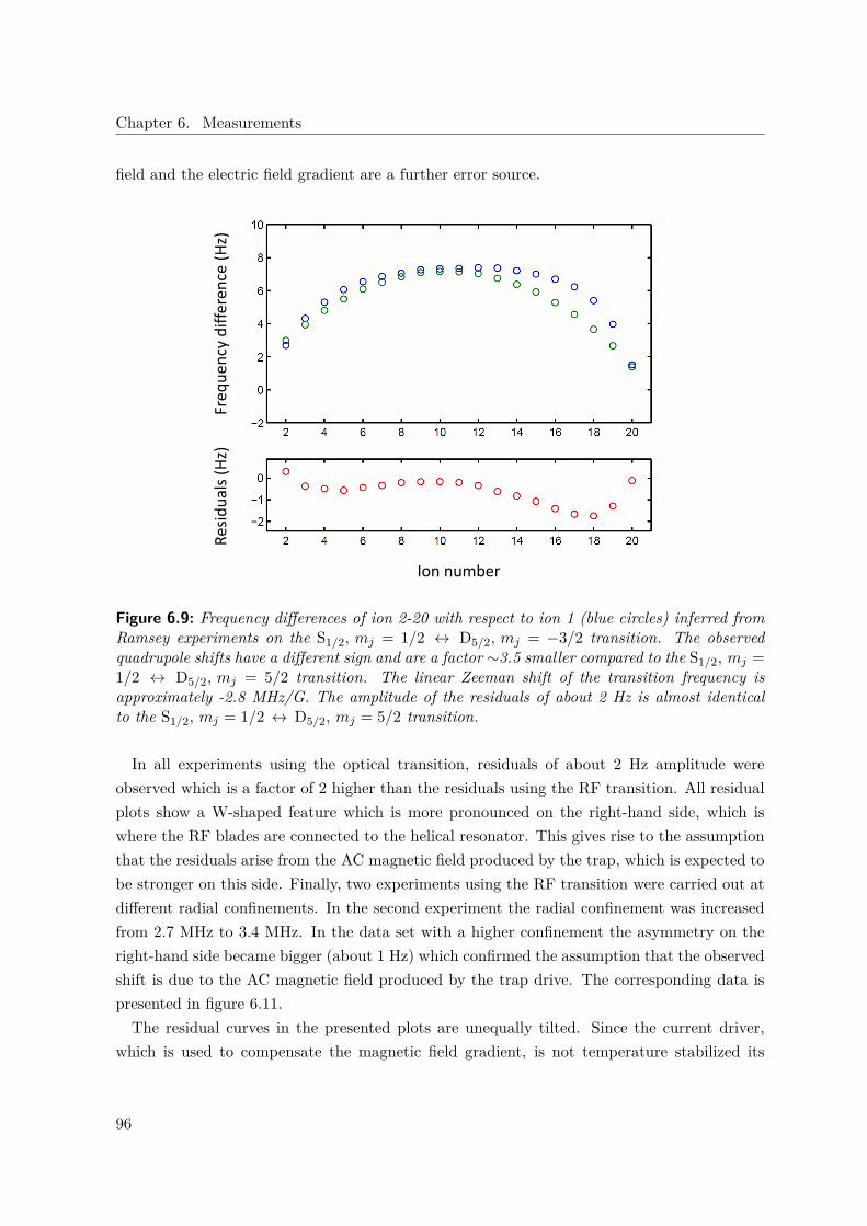
Chapter 6. Measurements
field and the electric field gradient are a further error source.
Ion number
Freq
uen
cy d
iffe
ren
ce (
Hz)
Res
idu
als
(Hz)
Figure 6.9: Frequency differences of ion 2-20 with respect to ion 1 (blue circles) inferred fromRamsey experiments on the S1/2, mj = 1/2 ↔ D5/2, mj = −3/2 transition. The observedquadrupole shifts have a different sign and are a factor ∼3.5 smaller compared to the S1/2, mj =1/2 ↔ D5/2, mj = 5/2 transition. The linear Zeeman shift of the transition frequency isapproximately -2.8 MHz/G. The amplitude of the residuals of about 2 Hz is almost identicalto the S1/2, mj = 1/2 ↔ D5/2, mj = 5/2 transition.
In all experiments using the optical transition, residuals of about 2 Hz amplitude wereobserved which is a factor of 2 higher than the residuals using the RF transition. All residualplots show a W-shaped feature which is more pronounced on the right-hand side, which iswhere the RF blades are connected to the helical resonator. This gives rise to the assumptionthat the residuals arise from the AC magnetic field produced by the trap, which is expected tobe stronger on this side. Finally, two experiments using the RF transition were carried out atdifferent radial confinements. In the second experiment the radial confinement was increasedfrom 2.7 MHz to 3.4 MHz. In the data set with a higher confinement the asymmetry on theright-hand side became bigger (about 1 Hz) which confirmed the assumption that the observedshift is due to the AC magnetic field produced by the trap drive. The corresponding data ispresented in figure 6.11.The residual curves in the presented plots are unequally tilted. Since the current driver,
which is used to compensate the magnetic field gradient, is not temperature stabilized its
96

6.2. Ramsey correlation spectroscopy
current output can vary according to changes in the room temperature and therefore can leadto improper compensation of the field gradient.
Ion number
Freq
uen
cy d
iffe
ren
ce (
Hz)
Res
idu
als
(Hz)
Figure 6.10: Frequency differences of ion 2-20 with respect to ion 1 (blue circles) inferred fromRamsey experiments on the S1/2, mj = 1/2 ↔ D5/2, mj = −1/2 transition. The observedquadrupole shifts are a factor ∼3 bigger compared to the S1/2, mj = 1/2 ↔ D5/2, mj = −3/2transition. The linear Zeeman shift of the transition frequency is with -1.6 MHz/G the smallestof all optical transitions interrogated. The amplitude of the residuals of about 1.5 Hz is slightlysmaller compared to the other two optical transitions.
In summary the method of correlated Ramsey experiments describes a relatively simplebut powerful method to investigate systematic frequency shifts in ion strings. The frequencyresolution depends on the number of data points taken and the maximum Ramsey time. Bothparameters have influence on the accuracy of the fits to the parity oscillations. While thenumber of data points is just a matter of time, the maximum Ramsey time is set by the collisionrate with the background gas that leads to melting events of the crystal. For experiments withmixed crystals where one species can be directly cooled during the interrogation, the upperbound is given by the finite lifetime of the excited state. For the complete understanding of allsystematic effects more work is needed. Finite element simulations of the AC magnetic fieldin the trap center with different electrode materials could lead to a more complete picture.Furthermore, a calculation of the mean electric field gradient experienced by ions in an ionstring at a finite temperature would be instructive.
97

Chapter 6. Measurements
With regard to a multi-ion frequency standard the inhomogeneous systematic frequencyshifts as well as the observed residual frequency offsets, point out the need of using ionicspecies that are less sensitive to these kinds of systematic frequency shifts. In the case ofaluminium ions these effects are expected to be orders of magnitude smaller and could betherefore disregarded.
Ion number
Freq
ue
ncy
dif
fere
nce
(Hz)
Figure 6.11: Frequency differences of ion 2-20 with respect to ion 1 at different RF confine-ments inferred from Ramsey experiments on the S1/2, mj = −1/2 ↔ S1/2, mj = +1/2 RFtransition at radial confinements of 2.7 MHz (blue) and 3.4 MHz (red). Frequency differencesof up to 2 Hz are obtained.
98

6.3. Precision spectroscopy on the 1S0↔ 3P1, F = 7/2 transition
6.3 Precision spectroscopy on the 1S0↔ 3P1, F = 7/2 transition
To perform coherent operations with high fidelity on the 1S0 ↔ 3P0 clock transition in 27Al+
the ion has to be prepared in a certain mF ground state. This can be achieved by frequency-resolved optical pumping via the 1S0 ↔ 3P1, F = 7/2 transition. In order to do this withhigh efficiency it is necessary to have precise knowledge of the Zeeman transition frequenciesand therefore the Landé g-factors of ground and excited state. The g-factor of the groundstate is known very accurately [48] but for the excited state only the calculated value ofg3P1 F=7/2 ≈ 3/7, which neglects relativistic and nuclear corrections, is known. Expectedcorrections from the nuclear contribution are on the order of ∼ 10−3. For typical magneticfields of ∼4 G this results in a frequency deviation of several 10 kHz between the two outermosttransitions. In order to derive the g-factor of the excited state, frequency measurements of the1S0, mf = ±5/2 ↔ 3P1, F = 7/2, mf = ±7/2 transitions were carried out in the quantumlogic way. Using Ramsey‘s method of separated fields [5], the transition linewidth, which waslimited by the interaction time of the laser with the ion, could be reduced by a factor of ~ 2compared to Rabi spectroscopy.
Frequency offset near 1.122 PHz (kHz)
-20 0 20 -10 00
0.2
0.4
0.6
0.8
D5
/2st
ate
exci
tati
on
10 20
D5
/2st
ate
exci
tati
on
0
0.2
0.4
0.6
0.8
-20
Frequency offset near 1.122 PHz (kHz)
a) b)
Figure 6.12: Ramsey frequency scans on the 1S0, mf = 5/2 ↔ 3P1, F = 7/2, mf = 7/2transition with 50 µs long π/2 - pulses and Ramsey times of a) 100 µs and b) 200 µs. The redline is a simulation based on solving the optical Bloch equations. The simulation results arerescaled to take into account the finite efficiency of the state-mapping procedure. Each datapoint is the average of the results of 50 experimental cycles.
The 729 nm clock transition in 40Ca+ was used as a frequency reference and allowed one tocalibrate the magnetic field at the position of the ions (see section 5.3). Therefore Ramsey ex-periments with a Ramsey time of 2 ms were performed on the S1/2, mj = ±1/2 ↔ D5/2, mj =±3/2 transitions. To speed up the measurements, only Doppler-cooling was performed for thecalcium interrogation. On each of the two calcium transitions two data points were taken withphases of the second Ramsey pulse of ±π, respectively. Each data point consists of 100 experi-
99
Chapter 6. Measurements
mental cycle. With this, the frequency offset between 729 nm laser and the transition as well asthe magnetic field can be determined. With precise knowledge of the 729 nm laser frequency,the repetition rate of the frequency comb, which was referenced to the GPS disciplined OCXOduring the measurements, can be recalculated and therefore allows one to calculate the 267 nmlaser frequency from its fundamental frequency at 1068 nm. In order to measure the frequencyoffset between the 267 nm laser and the probed atomic transition, Ramsey experiments onthe 1S0, mf = ±5/2 ↔ 3P1, F = 7/2, mf = ±7/2 transitions were carried out subsequently.Each transition was interrogated with four measurements with phases of the second pulse of0, π/2, π and −π/2. Each data point consists of 100 experimental cycles. The four phasesof the second pulse enable a reconstruction of the Bloch vector, which is important when thelaser drifts and the transitions are not probed on the slopes of the center fringe any more. Themeasurements were carried out in the following order:
1. Al 1S0, mf = ±5/2 ↔ 3P1, F = 7/2, mf = ±7/2 φ = 0
2. Al 1S0, mf = ±5/2 ↔ 3P1, F = 7/2, mf = ±7/2 φ = π/2
3. Al 1S0, mf = ±5/2 ↔ 3P1, F = 7/2, mf = ±7/2 φ = π
4. Al 1S0, mf = ±5/2 ↔ 3P1, F = 7/2, mf = ±7/2 φ = −π/2
5. Ca S1/2, mj = +1/2 ↔ D5/2, mj = +3/2 φ = π/2
6. Ca S1/2, mj = −1/2 ↔ D5/2, mj = −3/2 φ = −π/2
7. Ca S1/2, mj = −1/2 ↔ D5/2, mj = −3/2 φ = π/2
8. Ca S1/2, mj = +1/2 ↔ D5/2, mj = +3/2 φ = −π/2
In total, one set of measurements consists of 50 repetitions of the sequence described above.For each stretched Zeeman transition on the aluminium 4 data sets were taken (8 in total)with Ramsey times on the aluminium of either 100 µs or 200 µs. The latter increases the slopeby a factor of 1.6 compared to the 100 µs data. The spectroscopy laser intensities for bothspecies were adjusted to π/2 - times of 50 µs in order to keep AC Stark shifts from the probelaser low. Ramsey frequency scans on the aluminium transition and numerical fits of those forboth Ramsey times are presented in figure 6.12. The visibility of the fringes is mainly limitedby imperfect state detection. The Ramsey contrast on the intercombination transition as afunction of the Ramsey time is presented in figure 6.13. For Ramsey times up to 100 µs thecontrast is mainly limited by high frequency noise of the laser. For longer Ramsey times thecontrast is at its theoretical limit which is given by the natural lifetime of the excited state(305 µs).
100

6.3. Precision spectroscopy on the 1S0↔ 3P1, F = 7/2 transition
Ramsey time (µs)
1S 0
-3P
1R
amse
y co
ntr
ast
(%)
Figure 6.13: Ramsey contrast on the 1S0, mf = 5/2 ↔ 3P1, F = 7/2, mf = 7/2 carriertransition measured by quantum logic spectroscopy (blue data points). An overall contrastreduction of 10% results from imperfect mapping pulses. For Ramsey times between 1 µs and100 µs the contrast suffers from high frequency noise of the laser (see also figure 5.11). ForRamsey times beyond 100 µs the contrast is at the theoretical limit, set by the natural lifetimeof the excited state. The red line indicates an ideal Ramsey contrast, only limited by the naturallifetime of the excited state and imperfect state detection.
- 2 0 0 0 0 2 0 0 0 4 0 0 0- 1 0 0- 8 0- 6 0- 4 0- 2 0
02 04 06 08 0
1 0 0
Resid
ual fre
quenc
y diffe
rence
[Hz]
F r e q u e n c y o f f s e t c o r r e c t i o n [ H z ]
Figure 6.14: Residual frequency differences. The y axis presents the residuals of the 8 frequencydata sets, extrapolated to B = 0. The inferred frequency offset between laser and transitionis shown on the x axis. The scatter of the data points leads to a statistical uncertainty of 30Hz (1σ) according to the standard deviation. Laser frequency variations during the experimentcould lead to an error of up to 12 Hz. Therefore a total uncertainty of 42 Hz is assumed.
101

Chapter 6. Measurements
For the evaluation the Ramsey experiments on both ions and the comb measurements wereaveraged separately and the errors were summed up. Data points where the comb measurementwas not reliable were omitted. The error bars of each data set are calculated from the scatterof the 50 reconstructed transition frequencies. The error bars are slightly bigger than whatis expected from quantum projection noise. Plotting the 8 mean transition frequencies versusthe mean magnetic field and interpolating the data linearly to B = 0 leads to the transitionfrequency. The residual frequency differences of the 8 data sets are presented in figure 6.14.
Systematic frequency shifts
In the following section a summary of the relevant frequency shifts of both transitions is given.In view of the spectral width of the transition, only significant frequency shifts are considered.Systematic effects with shifts and uncertainties that are expected to be substantially smallerthan 1 Hz are briefly mentioned at the end for the sake of completeness. A detailed evaluationof all relevant frequency shifts of the 729 nm transition can be found in [34] and referencestherein.
729 nm reference
There are three absolute frequency measurements of the S1/2 ↔ D5/2 transition in 40Ca+
mentioned in literature. The mean frequency with a conservative estimate of its uncertaintyis 411 042 129 776 396.6(8.7) Hz. In order to ensure that there is no overlooked systematicfrequency shift on the 729 nm transition which would distort the results, a transition frequencycomparison between single calcium ions in lab 1, lab 2 and the university was made. For thispurpose Ramsey experiments on the S1/2, mj = ±1/2 ↔ D5/2, mj = ±3/2 transitions with aRamsey time of 3 ms were carried out in each experiment to measure the frequency differencebetween the 729 nm laser and the ions. The frequency difference between the two 729 nm lasersin lab 1 and the university was recorded with an optical beat note between them. Thereforethe 729 nm light from the university was sent via a noise-cancelled, 400 m long optical fiberto lab 1. The transition frequency difference between the labs for a measurement duration of6 hours is presented in figure 6.15. Putting everything together the S1/2 ↔ D5/2 transitionfrequencies in all three experiments agreed well within 1 Hz. Consequently an additionaluncertainty of 1 Hz of the S-D transition frequency is taken into account for the evaluation ofthe 1S0 ↔ 3P1, F = 7/2 transition frequency in in 27Al+.
102
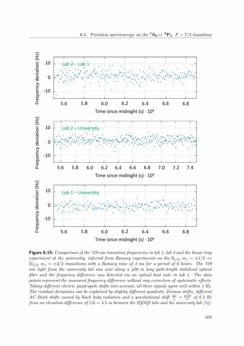
6.3. Precision spectroscopy on the 1S0↔ 3P1, F = 7/2 transition
Lab 2 – University
Freq
uen
cy d
evia
tio
n (
Hz)
0
-10
10
0
-10
10
0
-10
10
Freq
uen
cy d
evia
tio
n (
Hz)
Freq
uen
cy d
evia
tio
n (
Hz)
Lab 2 – Lab 1
Lab 1 – University
Time since midnight (s) · 104
5.6 5.8 6.0 6.2 6.4 6.6 6.8
Time since midnight (s) · 104
5.6 5.8 6.0 6.2 6.4 6.6 6.8
Time since midnight (s) · 104
5.6 5.8 6.0 6.2 6.4 6.6 6.8 7.0 7.2 7.4
Figure 6.15: Comparison of the 729 nm transition frequencies in lab 1, lab 2 and the linear trapexperiment at the university, inferred from Ramsey experiments on the S1/2, mj = ±1/2 ↔D5/2, mj = ±3/2 transitions with a Ramsey time of 3 ms for a period of 6 hours. The 729nm light from the university lab was sent along a 400 m long path-length stabilized opticalfiber and the frequency difference was detected via an optical beat note in lab 1. The datapoints represent the measured frequency difference without any correction of systematic effects.Taking different electric quadrupole shifts into account, all three signals agree well within 1 Hz.The residual deviations can be explained by slightly different quadratic Zeeman shifts, differentAC Stark shifts caused by black body radiation and a gravitational shift ∆ν
ν = g4hc2 of 0.2 Hz
from an elevation difference of 4h = 4.5 m between the IQOQI labs and the university lab [34].
103

Chapter 6. Measurements
Electric quadrupole shift
The electric quadrupole shift has two contributions. First the electric field gradient resultingfrom the axial confinement and second an additional electric field gradient resulting from thepresence of the second ion. The combined first- and second-order shift on the S1/2, mj =±1/2 ↔ D5/2, mj = ±3/2 transition is calculated to be 2.7(0.003) Hz for the confinementused during the experiments. The error is dominated by the uncertainty of the ion to iondistance.Since electronic states with J > 1/2 can have a finite electric quadrupole moment [14], the
3P1 state in 27Al+ can be also shifted in energy. The electric quadrupole moment of the 3P1
state is not known. Although it is expected to be small, a conservative estimate of <1.5ea20
is made. An upper bound of the shift can be calculated by using equation 6.4 and assumingelectronic states 3P1, J = 1, mj = ±1 and therefore ignoring the nuclear spin. This would leadto frequency shifts < 11.25 Hz. Even though the sign of the shift (-) is known, a symmetricerror is given.
Second order Zeeman shift
Coupling of the D5/2, mj = ±3/2 levels in 40Ca+ with the corresponding sublevels of the D3/2
state introduces a small quadratic frequency shift, which can be calculated by second orderperturbation theory to [80]
4ν = κ(µBB)2
h2νFS(6.7)
where νFS is the fine structure splitting, Jm is the larger one of the J numbers and a constantκ = (Jm−L+S)(Jm+L−S)(L+S+1+Jm)(L+S+1−Jm)
4J2m(2Jm−1)(2Jm+1) (J2
m −m2j ) depending on the magnetic sublevel
mj . For an average magnetic field of 4.0464(1) G during the measurements the mj = ±3/2levels (κ = 4/25) were up-shifted by 2.821(0.005) Hz.
The quadratic Zeeman shift of the 3P1, F = 7/2, mf = ±7/2 levels in 27Al+ can be de-termined in a similar way. All levels besides the 3P0 and 3P2 states are separated by opticalfrequencies and therefore do not contribute significantly. Since the 3P0 does not have anyF = 7/2 components, only the coupling to the 3P2 state needs to be considered. With a finestructure splitting of 3.71(1) THz [54] the 3P1, F = 7/2, mf = ±7/2 levels (κ = 1/4) weredown-shifted by 2.16(1) Hz. The error is due to the uncertainty in the hyperfine splittingwhich is expected to be less than 10 GHz.
Minor Frequency shifts
There are several systematic effects which shift both transition frequencies by negligible amounts.For the sake of completeness they are briefly mentioned. During the Ramsey experiments all
104
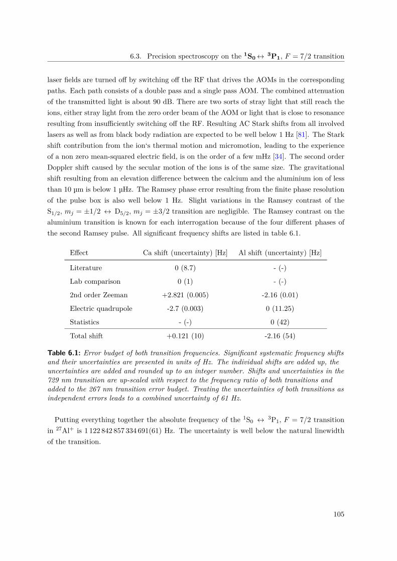
6.3. Precision spectroscopy on the 1S0↔ 3P1, F = 7/2 transition
laser fields are turned off by switching off the RF that drives the AOMs in the correspondingpaths. Each path consists of a double pass and a single pass AOM. The combined attenuationof the transmitted light is about 90 dB. There are two sorts of stray light that still reach theions, either stray light from the zero order beam of the AOM or light that is close to resonanceresulting from insufficiently switching off the RF. Resulting AC Stark shifts from all involvedlasers as well as from black body radiation are expected to be well below 1 Hz [81]. The Starkshift contribution from the ion‘s thermal motion and micromotion, leading to the experienceof a non zero mean-squared electric field, is on the order of a few mHz [34]. The second orderDoppler shift caused by the secular motion of the ions is of the same size. The gravitationalshift resulting from an elevation difference between the calcium and the aluminium ion of lessthan 10 µm is below 1 µHz. The Ramsey phase error resulting from the finite phase resolutionof the pulse box is also well below 1 Hz. Slight variations in the Ramsey contrast of theS1/2, mj = ±1/2 ↔ D5/2, mj = ±3/2 transition are negligible. The Ramsey contrast on thealuminium transition is known for each interrogation because of the four different phases ofthe second Ramsey pulse. All significant frequency shifts are listed in table 6.1.
Effect Ca shift (uncertainty) [Hz] Al shift (uncertainty) [Hz]
Literature 0 (8.7) - (-)
Lab comparison 0 (1) - (-)
2nd order Zeeman +2.821 (0.005) -2.16 (0.01)
Electric quadrupole -2.7 (0.003) 0 (11.25)
Statistics - (-) 0 (42)
Total shift +0.121 (10) -2.16 (54)
Table 6.1: Error budget of both transition frequencies. Significant systematic frequency shiftsand their uncertainties are presented in units of Hz. The individual shifts are added up, theuncertainties are added and rounded up to an integer number. Shifts and uncertainties in the729 nm transition are up-scaled with respect to the frequency ratio of both transitions andadded to the 267 nm transition error budget. Treating the uncertainties of both transitions asindependent errors leads to a combined uncertainty of 61 Hz.
Putting everything together the absolute frequency of the 1S0 ↔ 3P1, F = 7/2 transitionin 27Al+ is 1 122 842 857 334 691(61) Hz. The uncertainty is well below the natural linewidthof the transition.
105

Chapter 6. Measurements
Determination of the Landé g-factor
The set of 8 frequency measurements provides four frequency values for each of the 1S0, mf =±5/2 ↔ 3P1, F = 7/2, mf = ±7/2 transitions. From this, the mean values for each transitionfrequency are calculated. The statistical error bars are calculated by the standard deviation.The Landé g-factor of the excited state is inferred from the frequency difference of the twotransitions, and the magnetic field which was calibrated with 729 nm transition.The ion trap creates an AC magnetic field at 32 MHz at the position of the ions. The
magnetic field, calibrated by the Zeeman splitting of the S1/2, mj = ±1/2 ↔ D5/2, mj = ±3/2transitions in 40Ca+, increases by 9.7(1.2) µG/W when increasing the RF power, going intothe helical resonator. This effect is expected to be smaller for aluminium since the Zeemansplitting of ground and excited state is smaller compared to the case of calcium. During theexperiments the trap was operated at 1 W. Since this effect is rather small (∼ 10−6), it is nottaken into account. Consequently a conservative error is given. The magnetic field gradientalong the trap axis of 29(8) mG/m, which was calibrated by Ramsey correlation spectroscopywith a string of calcium ions, is also negligibly small. Finally the Landé g-factor yields tog3P1,F=7/2 = 0.42884(1). The measured value is 0.06 % bigger than the calculated value of3/7.
106

6.4. Observation of the 1S0↔ 3P0 clock transition
6.4 Observation of the 1S0↔ 3P0 clock transition
At the end of this work a first signal of the clock transition in 27Al+ was observed. To detectthe electronic excitation of the 1S0 ↔ 3P0 clock transition, a 1 ms long excitation pulse wasintroduced into the experimental sequence directly before the quantum logic state mappinghappens. In the case of no excitation on the clock transition the blue sideband pulse onthe intercombination transition can be carried out and the resulting phonon gets mapped tothe internal state of the calcium which is detected by electron shelving. In the case of thealuminium ion being in the excited clock state, the blue sideband pulse on the intercombinationtransition will remain without consequences.
Frequency offset near 1.121 PHz (kHz)
Statetransfer
probability
1.0
0.8
0.6
0.4
0.2
0.0
-5 -4 -3 -2 -1 0 1 2 3 4 5
Figure 6.16: Excitation spectrum on the 27Al+ 1S0, mf = −5/2 ↔ 3P0, mf = −3/2 clocktransition observed via quantum logic spectroscopy with a co-trapped 40Ca+ ion. With 1 ms longexcitation pulses a state change probability of ~ 0.9 was achieved on resonance. Consequentlythe pulse area on resonance was about π. Each data point consists of 20 experimental cycles.The error bars are calculated from quantum projection noise. The spike at -2.5 kHz arisesfrom a collision of one of the ions with the background gas (observed on the EMCCD camera).The small spikes can be explained by poor statistics. The red line is a Fourier transform of theexcitation pulse.
Since no method to initialize the aluminium ion in the ground state was used so far, thealuminium ion is either in the ground or the excited state at the beginning of each experimentalcycle. Therefore it is useful to look at the state change probability from shot to shot. Anexcitation spectrum is presented in figure 6.16. The 1S0, mf = −5/2 ↔ 3P0, mf = −3/2transition was driven with a sigma polarized beam along the quantization axis. In order toget rid of false detections where ground state cooling was not successful, each experiment was
107

Chapter 6. Measurements
repeated twice while during the second run the clock laser was turned off. Only experimentswith the same outcome contribute to the signal. However, collision events with the backgroundgas can lead to false counts since the outcome of the state detection is random if the ions are notcrystallized. The spectral width of the peak of about 800 Hz FWHM is Fourier-limited. Thelaser beam with a power of 1.5 mW was focused to a Gaussian beam waist of 65 µm FWHMat the ion. The corresponding Rabi frequency in the center of the beam was estimated to afew kHz. During the experiments involving the clock transition the formation of AlH+ ionswas observed after 15 minutes on average. At experiments only using the intercombinationtransition this was rarely a problem. A possible explanation therefore is that the chemistryonly occurs when the ion is in the excited state. The time which the ion spends in the excitedstate is about 50% for the clock transition and about 0.1% for the intercombination transition.The AlH+ionic molecule can be photo-dissociated with two pulsed lasers at 360 nm and 266nm [82] but not with the lasers available, which requires to release the ions and reload a mixedion crystal.
108

7 Summary and outlook
The work presented in this thesis covers a large amount of technical work as well as threepublications in the field of precision spectroscopy and atomic physics.The technical part describes the construction of a new ion trap which was optimized for
precision spectroscopy. Furthermore, a total of eleven laser systems were set up for the meansof precision spectroscopy with trapped aluminium and calcium ions.The main scientific results of this work cover three major topics: During the implementation
of laser ablation loading of ions a technique to detect the presence of a hot ion in the trap wasdeveloped. This method provides information of the sympathetic cooling dynamics and allowsus to trace back the initial energy of the hot ion. Statistical analysis of the sympathetic coolingtimes were carried out. Furthermore the limitations for the cooling times were discussed anddifferent strategies to decrease the cooling times were pointed out.Moreover, a method to investigate systematic frequency shifts in an ion string was developed.
With ion strings containing up to 20 40Ca+ ions, Ramsey experiments with Ramsey timesup to 300 ms were carried out. Oscillations in the parity signal between two ions give someindication about their difference in transition frequency. Thereby relative systematic frequencyshifts between the ions could be determined with sub-Hertz resolution. This method allowsone to investigate the homogeneity of the quantization magnetic field along the ion string withhigh resolution which is important for multi-ion frequency standards. The main focus wasto investigate the electric quadrupole shift, which is the biggest systematic frequency shiftin calcium ion strings for typical experimental parameters. Meanwhile another systematiceffect, the AC Zeeman effect, emerged, which caused frequency shifts up to 2 Hz among thecalcium ions and needs further investigation for a complete understanding. Finite elementsimulations of the AC magnetic field, produced by the trap drive, at the position of the ionswould be useful. In conclusion a powerful method to investigate systematic frequency shiftsin ion strings was presented.Once a mixed crystal could be loaded, the two optical transitions in 27Al+ were observed
via quantum logic spectroscopy with a co-trapped 40Ca+ ion. The frequency of the 1S0 ↔3P1, F = 7/2 transition was measured and the g-factor of the excited (g3P1 F=7/2) state wasdetermined using the clock transition in 40Ca+ as a frequency reference and a magnetic fieldsensor. The transition frequency was measured with an accuracy well below the naturallinewidth of the transition, using Ramsey‘s method of separate oscillatory fields.
109

Chapter 7. Summary and outlook
Finally the 1S0 ↔ 3P0 clock transition in 27Al+ was observed via quantum logic spec-troscopy, which was the second time worldwide to my knowledge.During experiments using the clock transition the formation of AlH+ molecular ions, which
can not be photo-dissociated with the lasers present in the lab, became an obstacle since it istime consuming to load another mixed ion crystal. This molecular ion can be photo-dissociatedwith two pulsed lasers at 360 nm and 266 nm [82] which would make the work much moreefficient. The 266 nm light could be produced by frequency doubling of the ablation laser at532 nm.So far, the internal state of the 27Al+ ion was detected via quantum logic spectroscopy via
the intercombination transition. The detection fidelity is limited by high frequency noise ofthe diode laser which drives the transition and should be replaced by either a laser diode thatallows for a faster feedback or a fiber laser which is intrinsically more stable. This would alsoimprove the fidelity of the pump pulses and therefore make optical pumping more efficient.Other detection methods like [83] that do not rely on sideband cooling and could speed up
the measurements and enhance the detection fidelity. Sympathetic cooling of the aluminiumion during longer interrogations could reduce melting events of the ion crystal caused bycollisions with the background gas. Faster recrystallization can be achieved by lowering thetrapping confinement for a short amount of time after a collision.Efficient cooling of the radial modes is crucial for coherent operations on the 4m = 0
transitions in 27Al+ in this setup. Sympathetic Raman [11] or EIT cooling could help to coolthe ion crystal to a near 3D ground state. Furthermore these cooling techniques allow oneto reduce uncertainties in motional frequency shifts and therefore make aluminium ion clocksoperating at the 10−19 level possible [11].
110

A Appendix
Table of fundamental constants according to CODATA [84].
Quantity Symbol Numerical value Unit
speed of light in vacuum c 299792458 m/s
magnetic constant µ0 4π · 10−7 N/A2
electric constant 1/µ0c2 ε0 8.854187817...× 10−12 F/M
Newtonian constant of gravitation G 6.67408(31)×10−11 m3/kg · s
Planck constant h 6.626070040(81)× 10−34 J · s
h/2π ~ 1.054571800(13)× 10−34 J · s
elementary charge e 1.6021766208(98)× 10−19 C
magnetic flux quantum h/2e Φ0 2.067833831(13)× 10−15 Wb
conductance quantum 2e2/h G0 7.7480917310(18)× 10−5 S
electron mass me 9.10938356(11)× 10−31 kg
proton mass mp 1.672621898(21)× 10−27 kg
proton-electron mass ratio mp/me 1836.15267389(17)
fine-structure constant e2/4πε0~c α 7.2973525664(17)×10−3
inverse fine-structure constant α−1 137.035999139(31)
Rydberg constant α2mec/2h R∞ 10973731.568508(65) 1/m
Avogadro constant NA 6.022140857(74)× 1023 1/mol
molar gas constant R 8.3144598(48) J/mol ·K
Boltzmann constant R/NA kB 1.38064852(79)× 10−23 J/K
Stefan-Boltzmann constant (π2/60)k4/~3c2 σ 5.670367(13)× 10−8 W/m2 ·K4
electron volt (e/C) J eV 1.6021766208(98)× 10−19 J
(unified) atomic mass unit 112m(12C) u 1.660539040(20)× 10−27 kg
111

B Journal publications
• M. Guggemos, D. Heinrich, O. A. Herrera-Sancho, R. Blatt, and C. Roos. Sympatheticcooling and detection of a hot trapped ion by a cold one. New Journal of Physics,17(10):103001, 2015.
• M. Guggemos, D. Heinrich, O. A. Herrera-Sancho, R. Blatt, and C. F. Roos. Quantumlogic spectroscopy with a 27Al+ / 40Ca+ ion crystal (to be submitted to NJP)
• M. Guggemos, C. Hempel, R. Blatt, and C. F. Roos. Ramsey correlation spectroscopywith long ion strings (to be published)
112
Bibliography
[1] J. Jespersen and J. Fitz-Randolph. From Sundials to Atomic Clocks: understanding Timeand Frequency. Dover Publications Inc., 2003.
[2] J. Curie and P. Curie. Development, via compression, of electric polarization in hemihedralcrystals with inclined faces. Bulletin de la Societe de Mineralogique de France, 3:90–93,1880.
[3] I. I. Rabi, J. R. Zacharias, S. Millman, and P. Kusch. A New Method of MeasuringNuclear Magnetic Moment. Phys. Rev., 53:318, 1938.
[4] N. F. Ramsey. History of atomic clocks. JOURNAL OF RESEARCH of the NationalBureau of Standards, 88:301–320, 1983.
[5] N. F. Ramsey. A molecular beam resonance method with separated oscillatory fields.Phys. Rev., 78:695–699, 1950.
[6] G. Santarelli, P. Laurent, and P. Lemonde. Quantum projection noise in an atomicfountain: A high stability cesium frequency standard. Physical Review Letters, 82:4619–4622, 1999.
[7] A. Clairon, C. Salomon, S. Guellati, and W. D. Phillips. Ramsey Resonance in a ZachariasFountain. Europhysics Letters (EPL), 16(2):165–170, 1991.
[8] Th. Udem, R. Holzwarth, and T. W. Hänsch. Optical frequency metrology. Nature,416:233–237, 2002.
[9] C. W. Chou, D. Hume, and J. Koelemeij. Frequency comparison of two high-accuracyAl+ optical clocks. Phys. Rev. Lett., 104:070802, 2010.
[10] B. J. Bloom, T. L. Nicholson, and J. R. Williams. An optical lattice clock with accuracyand stability at the 10−18 level. Nature, 506:71–75, 2014.
[11] J.-S. Chen, S. M. Brewer, and C. W. Chou. Sympathetic Ground State Cooling andTime-dilation Shifts in an 27Al+ Optical Clock. Phys. Rev. Lett., 118:053002, 2017.
113

Bibliography
[12] P. Kómár, E. M. Kessler, and M. Bishof. A quantum network of clocks. Nature Physics,10:582–587, 2014.
[13] J. Wübbena, S. Amairi, O. Mandel, and P.O. Schmidt. Sympathetic cooling of mixed-species two-ion crystals for precision spectroscopy. Phys. Rev. A - Atomic, Molecular,and Optical Physics, 85:043412, 2012.
[14] A. Ludlow, M. Boyd, and J. Ye. Optical atomic clocks. Rev. Mod. Phys., 87:637–701,2015.
[15] C. W. Chou, D. Hume, T. Rosenband, and D. Wineland. Optical clocks and relativity.Science, 329:1630–1633, 2010.
[16] T. Rosenband, D. Hume, and C. W. Chou. Alpha-Dot or Not: Comparison of TwoSingle Atom Optical Clocks. Proceedings of the 7th Symposium Frequency Standards andMetrology, pages 20–33, 2012.
[17] P. K. Ghosh. Ion Traps. Oxford University Press, 1996.
[18] J. P. Home. Quantum Science and Metrology with Mixed-Species Ion Chains. Advancesin Atomic, Molecular and Optical Physics, 62:231–277, 2013.
[19] C. Roos. Controlling the quantum state of trapped ions. PhD thesis, University of Inns-bruck, 2000.
[20] D. James. Quantum dynamics of cold trapped ions with application to quantum compu-tation. Applied Physics B-Lasers and Optics, 66:181–190, 1998.
[21] C. Roos. Personal communication, 2016.
[22] D. Leibfried, R. Blatt, C. Monroe, and D. Wineland. Quantum dynamics of single trappedions. Rev. Mod. Phys., 75:281–324, 2003.
[23] Claude Cohen-Tannoudji, Bernard Diu and Frank Laloe. Quantum mechanics. JohnWiley and Sons, 2006.
[24] C. A. Blockley, D. F. Walls, and H. Risken. Quantum collapses and revivals in a quantizedtrap. EPL (Europhysics Letters), 17(6):509–514, 1992.
[25] Mark Fox. Quantum Optics: An Introduction. Oxford University Press, 2006.
[26] H. J. Carmichael. Statistical Methods in Quantum Optics 1: Master Equations and Fokker-Planck Equations. Springer, 2002.
114

Bibliography
[27] G. Lindblad. On the generators of quantum dynamical semigroups. Comm. Math. Phys.,48:119–130, 1976.
[28] T. Monz. Quantum information processing beyond ten ion-qubits. PhD thesis, Universityof Innsbruck, 2011.
[29] C. Hempel. Digital quantum simulation, Schroedinger cat state spectroscopy and settingup a linear ion trap. PhD thesis, University of Innsbruck, 2014.
[30] P. Schindler. Quantum computation and simulation with trapped ions using dissipation.PhD thesis, University of Innsbruck, 2013.
[31] D. Kleppner. Norman Ramsey and his method. Phys. Today, 66(1):25, 2013.
[32] P. Jurcevic. Quantum Computation and Many-body Physics with Trapped Ions. PhDthesis, University of Innsbruck, 2016.
[33] J. Benhelm. Precision spectroscopy and quantum information processing with trappedcalcium ions. PhD thesis, University of Innsbruck, 2008.
[34] M. Chwalla. Precision spectroscopy with Ca+ ions in a Paul trap. PhD thesis, Universityof Innsbruck, 2009.
[35] G. Kirchmair. Quantum non-demolition measurements and quantum simulation. PhDthesis, University of Innsbruck, 2010.
[36] T. Brage, P. Judge, and A. Aboussaïd. Hyperfine Induced Transitions as Diagnostics ofIsotopic Composition and Densities of Low-Density Plasmas. The Astrophysical Journal,500:507, 1998.
[37] P. Staanum, I. Jensen, and R. Martinussen. Lifetime measurement of the metastable 3d2D5/2 state in the 40Ca+ ion using the shelving technique on a few-ion string. Phys. Rev.A, 69:032503, 2004.
[38] M. Chwalla, J. Benhelm, and K. Kim. Absolute Frequency Measurement of the 40Ca+ 4s2S1/2 - 3d 2D5/2 Clock Transition. Phys. Rev. Lett., 102:023002, 2009.
[39] Y. Huang, J. Cao, and P. Liu. Hertz-level measurement of the 40Ca+ 4s 2S1/2 - 3d 2D5/2
clock transition frequency with respect to the SI second through the Global PositioningSystem. Phys. Rev. A, 85:030503, 2012.
[40] K. Matsubara, H. Hachisu, and Yi. Li. Direct comparison of a Ca+ single-ion clockagainst a Sr lattice clock to verify the absolute frequency measurement. Optics Express,20:22034–22041, 2012.
115
Bibliography
[41] Y. Huang, H. Guan, and P. Liu. Frequency comparison of two 40Ca+ Optical Clocks withan uncertainty at the 10−17 Level. Phys. Rev. Lett., 116:013001, 2016.
[42] G. Tommaseo, T. Pfeil, and G. Revalde. The gj-factor in the ground state of Ca+.European Physical Journal D, 25:113–121, 2003.
[43] M. Ramm, T. Pruttivarasin, and M. Kokish. Precision measurement method for branchingfractions of excited P1/2 states applied to 40Ca+. Phys. Rev. Lett., 111:023004, 2013.
[44] F. Diedrich, J. C. Bergquist, W. M. Itano, and D. J. Wineland. Laser cooling to thezero-point energy of motion. Phys. Rev. Lett., 62:403–406, 1989.
[45] C. Roos, Th. Zeiger, and H. Rohde. Quantum state engineering on an optical transitionand decoherence in a paul trap. Phys. Rev. Lett., 83:4713–4716, 1999.
[46] W. Itano. External-Field Shifts of the 199Hg+ Optical Frequency Standard. Journal ofResearch of the National Institute of Standards and Technology, 105(6):829–837, 2000.
[47] N. J. Stone. Nuclear Magnetic Dipole and Electric Quadrupole Moments: Their Mea-surement and Tabulation as Accessible Data. Journal of Physical and Chemical ReferenceData, 44:031215, 2015.
[48] T. Rosenband, P.O. Schmidt, and D. Hume. Observation of the 1S0 - 3P0 clock transitionin 27Al+. Phys. Rev. Lett., 98:220801, 2007.
[49] H. Dehmelt. Mono-Ion oscillator as potential ultimate laser frequency standard. IEEETransactions on Instrumentation and Measurement, 31:83–87, 1982.
[50] N. Yu, H. Dehmelt, and W. Nagourney. The 3 1S0 - 3 3P0 transition in the aluminumisotope ion 26Al+. Proceedings of the National Academy of Sciences, 89:7289, 1992.
[51] T. Rosenband, W. Itano, and P. O. Schmidt. Blackbody radiation shift of the 27Al+ 1S0
- 3P0 transition. in Proceedings of the 20th European Time and Frequency Forum, pages289–291, 2006.
[52] T. Rosenband, D. Hume, and P.O. Schmidt. Frequency Ratio of Al+ and Hg+ Single-IonOptical Clocks; Metrology at the 17th Decimal Place. Science, 319:1808–1812, 2008.
[53] E. Träbert and A. Wolf. Measurement of the B+ and Al+ intercombination and Sc12+
forbidden transition rates at a heavy-ion storage ring. J.Phys. B.: At. Mol. Opt. Phys.,32(2):537, 1999.
[54] NIST. Atomic Spectra Database.
116
Bibliography
[55] P. Jönsson. Multi-configuration Hartree- and Dirac-Fock Calculations of Atomic HyperfineStructures. Physica Scripta, 48:678–687, 1993.
[56] P. Jönsson and C. Froese Fischer. Large-scale multiconfiguration Hartree-Fock calcu-lations of hyperfine-interaction constants for low-lying states in beryllium, boron, andcarbon. Phys. Rev. A, 48(6):4113–4123, 1993.
[57] P. Jönsson, C. G. Wahlström, and C. Froese Fischer. A program for computing magneticdipole and electric quadrupole hyperfine constants from MCHF wavefunctions. ComputerPhysics Communications, 74:399–414, 1993.
[58] P. Jönsson, F. A. Parpia, and C. Froese Fischer. HFS92: A program for relativistic atomichyperfine structure calculations. Computer Physics communications, 96:301–310, 1996.
[59] William M. Haynes. CRC Handbook of Chemistry and Physics 96th Edition. CRC, NewYork, 2015.
[60] W. Itano, J. Bergquist, J. J. Bollinger, and D. Wineland. Quantum projection noise:Population fluctuations in two-level systems. Phys. Rev. A, 47:3554–3570, 1993.
[61] G. Kirchmair. Frequency stabilization of a Titanium-Sapphire laser for precision spec-troscopy on Calcium ions. Diploma thesis, University of Innsbruck, 2006.
[62] H. Nakai, W. Jin, and M. Kawamura. Hyperfine Structure of 27Al by High-ResolutionUltraviolet Laser Spectroscopy. Jpn. J. Appl. Phys., 46(2):815–816, 2007.
[63] D. Hume. Two-Species Ion Arrays for Quantum Logic Spectroscopy. PhD thesis, Univer-sity of Colorado, 2010.
[64] Y. Colombe, D. Slichter, and A. Wilson. Single-mode optical fiber for high-power, low-lossUV transmission. Optics Express, 22:19783–19793, 2014.
[65] R. Drever and J. Hall. Laser Phase and Frequency Stabilization Using an Optical Res-onator. Applied Physics B, 31:97–105, 1983.
[66] J. L. Hall, M. Taubman, and J. Ye. Laser Stabilization. in Optics Handbook, OpticalSociety of America, pp. 27.1-27.24., 2000.
[67] J. Alnis, A. Matveev, and N. Kolachevsky. Subhertz linewidth diode lasers by stabilizationto vibrationally and thermally compensated ultralow-expansion glass Fabry-Perot cavities.Phys. Rev. A, 77:053809, 2008.
[68] M. Schiemangk, S. Spießberger, and A. Wicht. Accurate frequency noise measurement offree-running lasers. Applied Optics, 53:7138–7143, 2014.
117

Bibliography
[69] L. S. Ma, P. Jungner, J. Ye, and J. L. Hall. Delivering the same optical frequency attwo places: accurate cancellation of phase noise introduced by an optical fiber or othertime-varying path. Optics Letters, 19:1777–1779, 1994.
[70] G. Domenico, S. Schilt, and P. Thomann. Simple approach to the relation between laserfrequency noise and laser line shape. Applied Optics, 49:4801–4807, 2010.
[71] F . M. Mitschke and L. F. Mollenauer. Discovery of the soliton self-frequency shift. OpticsLetters, 11:659–661, 1986.
[72] B. Casabone. Two Ions Coupled to an Optical Cavity : from an Enhanced QuantumComputer Interface towards Distributed Quantum Computing Dissertation. PhD thesis,University of Innsbruck, 2015.
[73] M. Guggemos, D. Heinrich, O. A. Herrera-Sancho, R. Blatt, and C. Roos. Sympatheticcooling and detection of a hot trapped ion by a cold one. New Journal of Physics,17(10):103001, 2015.
[74] D. Berkeland, J . Miller, and J. Bergquist. Minimization of ion micromotion in a Paultrap. Journal of Applied Physics, 83(10):5025–5033, 1998.
[75] P.O. Schmidt, T. Rosenband, and C. Langer. Spectroscopy Using Quantum Logic. Sci-ence, 309:749–752, 2005.
[76] J. H. Wesenberg, R. J. Epstein, and D. Leibfried. Fluorescence during Doppler cooling ofa single trapped atom. Phys. Rev. A - Atomic, Molecular, and Optical Physics, 76:053416,2007.
[77] A. A. Madej, J. E. Bernard, and P. Dubé. Absolute frequency of the 88Sr+ 5s 2S1/2 - 4d2D5/2 reference transition at 445 THz and evaluation of systematic shifts. Phys. Rev. A- Atomic, Molecular, and Optical Physics, 70:012507, 2004.
[78] G. P. Barwood, H. S. Margolis, and G. Huang. Measurement of the Electric QuadrupoleMoment of the 4d 2D5/2 Level in 88Sr+. Phys. Rev. Lett., 93:133001, 2004.
[79] P. Dube, A. Madej, Z. Zhou, and J. Bernard. Evaluation of systematic shifts of the88Sr+ single-ion optical frequency standard at the 10−17 level. Phys. Rev. A - Atomic,Molecular, and Optical Physics, 87:023806, 2013.
[80] I. I. Sobelman. Atomic spectra and radiative transitions. Springer Series on Atoms andPlasmas, 1992.
[81] Y. Yu, B. Suo, and H. Fan. Finite-field calculation of the polarizabilities and hyperpolar-izabilities of Al+. Phys. Rev. A, 88:052518, 2013.
118

Bibliography
[82] C. Seck, E. Hohenstein, and C. Lien. Rotational state analysis of AlH+ by two-photondissociation. Journal of Molecular Spectroscopy, 300:108–111, 2014.
[83] D. Hume, C. W. Chou, and D. R. Leibrandt. Trapped-ion state detection through coherentmotion. Phys. Rev. Lett., 107:243902, 2011.
[84] Peter J. Mohr, David B. Newell, and Barry N. Taylor. CODATA Recommended Valuesof the Fundamental Physical Constants: 2014. Rev. Mod. Phys, 88:1527–1605, 2016.
119

Acknowledgements
Setting up a new ion trapping experiment with two ion species in a formerly empty laboratoryis certainly an uncomfortable way to do a PhD. Retrospectively I can say that it was oncemore worth going down the more difficult road. As my PhD comes to its end the foundationfor an optical frequency standard in Innsbruck based on aluminium and calcium ions was laid.Since this work would not have been possible without the help of many people inside andoutside the institute I will take the opportunity to thank all of them for their contribution.
First, I want to thank Rainer Blatt for receiving me in his group and for his confidence inmy work. He let me free in setting up the experiment according to my perceptions, which wasan enriching experience for me.Second, I want to thank Christian Roos for co-supervising this work. Many interesting dis-
cussions and especially his theoretical support greatly contributed to the experimental results.Moreover I want to thank all my colleagues in the group who helped with words and deeds.
Especially i want to thank Daniel Heinrich for many important contributions, primarily on theexperimental control. I also want to thank the people from the quantum simulation experimentin lab 1 for providing stable 729 nm light. My successor Milena Guevara-Bertsch, who joinedthe group at the end of my PhD, has already made useful contributions to the last achievementsof this work.Furthermore I want to thank Piet Schmidt for all the friendly communication and for sharing
a lot of useful information about the aluminium ion. In addition i want to thank Jook Walravenfor improving my understanding in atomic physics.Moreover I want to thank my office mate Ben Lanyon for many funny and interesting
conversations as well as for improving my English skills.Building the experimental setup involved the guys from the fine-mechanical and electrical
workshops, namely Stefan Haslwanter, Gerhard Hendl, Andreas Strasser and Bernhard Öttl.The collaboration with them brightened everyday life.I also want to thank the people responsible for the administrative tasks namely Markus
Knabl, Doris Corona, Elisabeth Huck, Patricia Moser, Nikolaus Falschlunger, Valentin Staub-mann and David Jorda.Furthermore I want to thank the guys who joined me stopping by at a pub for many funny
and interesting conversations.Very important to me is to balance work and recreation. Alpinism is not only a hobby for
120

me but more a way of life. Big up to my friends for many unforgettable adventures in themountains.Finally, I want to express my gratitude to my parents for all their support and encourage-
ment.
“The struggle itself (towards the heights) is enough to fill a man‘s heart. One must imagineSisyphus happy.” - Albert Camus
121