
Maximum and Comparison Principles for Convex Functions on the Heisenberg Group
Upload
calpolypomonaCategory
view
0download
0
A Heisenberg Picture Mean Field Model for
Magneto-association of a Quantum Degenerate
Bose Gas Close to a Feshbach Resonance
Andrew Carmichael, Ph.D.University of Connecticut, 2008
We construct a simple quantum optics style mean field model to investigate thebehaviour of a zero-temperature untrapped quantum degenerate Bose gas close toa Feshbach resonance. The model allows for both atomic and molecular conden-sates as well as correlated zero-momentum “BCS” pairs whose provenance wouldbe dissociated zero momentum molecules. Beginning with a second quantized(momentum representation) Hamiltonian and equations conserving total (free andbound) atom number and enforcing an assumption that atoms only appear eitherin the condensates or pairs and the usual Bogoliubov approximation, the systemis numerically and in certain limits, analytically, soluble in the steady state andexhibits a second order phase transition to a pure atomic condensate when thecontrollable parameters of the coupling Rabi frequency and detuning are variedacross an (analytically determined) transition line. Analysis of the thermodynam-ics of the zero-entropy system shows a negative pressure and hence mechanicalinstability on both sides of the resonance. A mathematical difficulty arising froman ultra-violet divergence due to the assumption of a zero range interaction isresolved with the help of a simpler, exactly analytically soluble two atom versionof the problem.
A Heisenberg Picture Mean Field Model for
Magneto-association of a Quantum Degenerate
Bose Gas Close to a Feshbach Resonance
Andrew Carmichael
MPhys. Physics, University of Sussex, Brighton, Sussex, UK, 1994M.Sc. Physics, University of Connecticut, Storrs, CT, USA, 2003
A DissertationSubmitted in Partial Fullfilment of the
Requirements for the Degree ofDoctor of Philosophy
at theUniversity of Connecticut
2008

Copyright by
Andrew Carmichael
2008
APPROVAL PAGE
Doctor of Philosophy Dissertation
A Heisenberg Picture Mean Field Model for
Magneto-association of a Quantum Degenerate
Bose Gas Close to a Feshbach Resonance
Presented byAndrew Carmichael, MPhys., MSc.
Major Advisor
Juha JavanainenAssociate Advisor
Robin CoteAssociate Advisor
Reinhold BlumelAssociate Advisor
University of Connecticut2008
ii

Dedicated to the memory of my great uncle John Crossand to my American cousin Dave Liebler
who both sadly passed away during my time here,and to the memory my grandfather Ronald Goldsworthy
who had a profound impact on my life, probably more than he ever knew.They all live on in memory.
iii
ACKNOWLEDGEMENTS
First and foremost I would like to thank my advisor, Juha Javanainen forhis advice, patience and most of all, his humour. Many other members of facultyhave helped me in various ways throughout courses, research and teaching. Inparticular I would like to acknowledge Robin Cote, Suzanne Yelin, Phil Gould,Ronald Mallett, the late Kurt Haller, Barrett Wells, Doug Hamilton, GayanethFernando, George Gibson, Phil Best, Boris Sinkovic, Bill Hines and most especiallyPhillip Mannheim.
For extremely helpful discussions on some of the mathematics discussed inthis thesis I would like to offer my thanks to Stuart Sidney, Joe McKenna, KeithConrad and Yung-Sze Choi from the UCONN Mathematics Department, my ad-visor Juha Javanainen. Additionally, I gratefully acknowledge Paulina Chin fromMaplesoft and others in the Mapleprimes discussion group, particularly RobertIsrael for useful discussions and suggestions on the message board on Maple pro-gramming, including on the code in the appendices.
The current and former members of our group, our various collaboratorsand sympathizers including Marijan Kostrun, Matt Mackie, Uttam Shrestha, YiZheng, Jerome Sanders, and Artur Ishkhanyan have been invaluable for theiradvice and input.
From my undergraduate days at the University of Sussex both for teachingme physics and helping me towards my graduate career I would like to thank BarryGarraway, “Iron” Mike Hardiman, Gabriel Barton, Ed Hinds, David Bailin, ColinFinn, Norman Dombey, David Waxman and Ed Copeland.
Many members of staff at UCONN have helped me enormously. Theseinclude Cecile Stanzione, Kim Giard, Dawn Rawlinson, Nicole Hryvniak, LindaKruse and Danielle Fowler, Christine, Nicole and the other student workers in themain office. Gloria Ramos, Carol Guerra and Dave Perry with undergrad labs,Michael Rozman with computers and Mihwa Lee, Bob Chudy and the rest of thestaff at the international house who have striven to keep me legal.
I owe a special thank you to Reinhold Blumel who helped me enormouslyboth during my undergraduate time when we worked together in Freiburg andas an external advisor during my work here at UCONN. I consider myself veryfortunate to have known you and I sincerely hope that our professional relationshipand friendship will continue for many years.
It was propitious that I landed so close to the American branch of my familywho helped make my stay here much more pleaseant. To Mark, Anne, Chris, Paul,Mike, Yolande, Larry, Alan and the late Dave Liebler, Wilbur and Karen Hence,Steph Haapala and Dave Masiukiewicz. Thank you all so much for your hospitality
iv
and friendship. It never seemed like I was so far from home after all.To my friends and comrades in arms in the programme and elsewhere who
have made these years enjoyable as well as educational, many thanks. I’d like tomention in particular (in random order) Derick Becker, Dave Cox, Phil Gee, ZsoltNyiri, Julian Klinner, Thomas Clausen, Richard White, Max Allsworth, AndrewBradbury, John “The Great JC” Chu, Ilona Westram, Alex “KGB” Razumny,Marwan Rasumny, Marin Pichler, Anguel Nikolov, Tank Bragdon, Naim Maj-dalani, Kandra Painter, the digital Jedi master Ionel Simbotin, Javier Peressutti,Jason Byrd, Jo & Hyewon Pechkis, Erin Seder, Ken Miller, James O’Brien, SamEmery, Yifei Huang, Jim Marie, Jo Consiglio, Andrea Tully, Aurelien Carlier,John Haga, Mihajlo Kornicer, the Loglisci’s, Don Telesca, and Chris Verzani.
There are a few people for whose impact on my world the label friendshipseems insufficient. I know of no words to express to any of you how deeply Iappreciate you and how much it costs me to leave you. I shall think fondly uponour time together. They include my girlfriend Cynthia Zocca, Andriy Kurilov,Beth Taylor-Juarros, the “gang”; Philippe Pellegrini, Jim Lin, Illa Sivarajah,Marko Gacesa and, of course, Pete Benzi.
For high quality beer and companionship, the crew at John Harvard’s havebeen immeasurably wonderful. To Jenn K., Lauren, Leah, Greg, Scioscio, Na-talie, Erin, Erika, Annie, Jeff, Kaitlin, Dean, Brandan, Heather and Jamie, manythanks. I may even miss drinking at JH more than solving equations at UCONN.Ryan and the crew at Ted’s also have my appreciation for a friendly place tounwind.
To my family, in particular my parents, who have given me more love, sup-port and affection than I ever deserved, I hope this thesis evidences that all theseyears spent thousands of miles from home have been spent somehow wisely. Toyou more than anyone else I owe my gratitude.
v
TABLE OF CONTENTS
1. Introduction . . . . . . . . . . . . . . . . . . . . . . . . . . . . . . . . 11.1 Backgound and motivation . . . . . . . . . . . . . . . . . . . . . . . . 11.2 Thesis Overview . . . . . . . . . . . . . . . . . . . . . . . . . . . . . 7
2. Background Physics . . . . . . . . . . . . . . . . . . . . . . . . . . . 92.1 Introduction to Quantum Field Theory . . . . . . . . . . . . . . . . . 92.2 Bose-Einstein Statistics . . . . . . . . . . . . . . . . . . . . . . . . . . 112.3 Fermi-Dirac Statistics . . . . . . . . . . . . . . . . . . . . . . . . . . 122.4 Bose-Einstein Condensation . . . . . . . . . . . . . . . . . . . . . . . 132.4.1 Statistical Arguments . . . . . . . . . . . . . . . . . . . . . . . . . 132.4.2 General Definition of BEC . . . . . . . . . . . . . . . . . . . . . . . 152.5 Second Quantisation . . . . . . . . . . . . . . . . . . . . . . . . . . . 152.6 Atom-atom Interactions and the Scattering Length . . . . . . . . . . 182.7 Feshbach Resonances . . . . . . . . . . . . . . . . . . . . . . . . . . . 232.8 Interactions in Second Quantization . . . . . . . . . . . . . . . . . . . 242.9 Quantum Field Theory for Constructing Molecules . . . . . . . . . . 272.10 Traditional Mean Field Theories . . . . . . . . . . . . . . . . . . . . . 312.10.1 Bogoliubov Approximation and Gross Pitaevskii Equation . . . . . 312.10.2 Bogoliubov Approach to Bose and Fermi Gases . . . . . . . . . . . 34
3. Two-Atom System & Dressed Molecules . . . . . . . . . . . . . . 373.1 General Formulation . . . . . . . . . . . . . . . . . . . . . . . . . . . 373.1.1 Constants of the Motion . . . . . . . . . . . . . . . . . . . . . . . . 383.2 Two Atom Problem and Dressed Molecules . . . . . . . . . . . . . . . 393.3 Renormalization . . . . . . . . . . . . . . . . . . . . . . . . . . . . . 463.4 Fano Theory . . . . . . . . . . . . . . . . . . . . . . . . . . . . . . . 483.4.1 Bound State . . . . . . . . . . . . . . . . . . . . . . . . . . . . . . 513.4.2 Continuum States . . . . . . . . . . . . . . . . . . . . . . . . . . . 53
4. Many Atom Mean Field Model . . . . . . . . . . . . . . . . . . . . 554.1 The Many Atom Model . . . . . . . . . . . . . . . . . . . . . . . . . 554.1.1 Equations of Motion . . . . . . . . . . . . . . . . . . . . . . . . . . 554.1.2 Mean Field Approximation . . . . . . . . . . . . . . . . . . . . . . 574.1.3 Atom-Molecule Coupling . . . . . . . . . . . . . . . . . . . . . . . . 574.1.4 Equations Defining the Mean-Field Model . . . . . . . . . . . . . . 584.1.5 Constants of the Time Dependent System . . . . . . . . . . . . . . 604.1.6 Steady State Equations . . . . . . . . . . . . . . . . . . . . . . . . 614.2 Pairing Approximation for the Steady State . . . . . . . . . . . . . . 624.3 Renormalization . . . . . . . . . . . . . . . . . . . . . . . . . . . . . 674.3.1 Steps in renormalization of the energy per particle. . . . . . . . . . 71
vi
4.4 Equations of the Mean-Field Model . . . . . . . . . . . . . . . . . . . 724.5 Behaviour of the Integrals . . . . . . . . . . . . . . . . . . . . . . . . 734.5.1 Asymptotic Behaviour of Integral A1/2(m) . . . . . . . . . . . . . . 764.5.2 Asymptotic Behaviour of Integral P1/2(m) . . . . . . . . . . . . . . 774.5.3 Asymptotic Behaviour of Integral P3/2(m) . . . . . . . . . . . . . . 77
5. Solution of the Model . . . . . . . . . . . . . . . . . . . . . . . . . . 855.1 Solutions: Atomic Condensate Present . . . . . . . . . . . . . . . . . 855.2 Solutions: No Atomic Condensate Present . . . . . . . . . . . . . . . 875.3 Numerical Solutions . . . . . . . . . . . . . . . . . . . . . . . . . . . 885.4 Phase Transition Line . . . . . . . . . . . . . . . . . . . . . . . . . . 905.5 Features of the Theory . . . . . . . . . . . . . . . . . . . . . . . . . . 915.5.1 Regimes . . . . . . . . . . . . . . . . . . . . . . . . . . . . . . . . . 915.5.2 Energy Scales . . . . . . . . . . . . . . . . . . . . . . . . . . . . . . 925.5.3 Unitarity Limit . . . . . . . . . . . . . . . . . . . . . . . . . . . . . 93
6. Thermodynamics of the Atom-Molecule System . . . . . . . . . 1016.1 Thermodynamic Analysis . . . . . . . . . . . . . . . . . . . . . . . . 101
7. Concluding Remarks . . . . . . . . . . . . . . . . . . . . . . . . . . 108
Appendices . . . . . . . . . . . . . . . . . . . . . . . . . . . . . . . . . . 112
A. Maple Code . . . . . . . . . . . . . . . . . . . . . . . . . . . . . . . . 112A.1 Maple Code for Asymptotic Expansions . . . . . . . . . . . . . . . . 112A.2 Maple Code for Numerical Solutions . . . . . . . . . . . . . . . . . . 115A.3 Maple Code for Pressure . . . . . . . . . . . . . . . . . . . . . . . . . 120
Bibliography 124
vii

LIST OF FIGURES
2.1 Schematic Illustration of a Feshbach Resonance . . . . . . . . . . . . 252.2 Scattering Length as a Function of Magnetic Field for 7Li . . . . . . 26
4.1 Bosonic pairing approximation for the paired state. . . . . . . . . . . 684.2 Integral A1/2(m) plotted numerically with Maple . . . . . . . . . . . 824.3 Integral P1/2(m) plotted numerically with Maple . . . . . . . . . . . . 834.4 Integral P3/2(m) plotted numerically with Maple . . . . . . . . . . . . 84
5.1 α as a function of Ω and δ . . . . . . . . . . . . . . . . . . . . . . . . 955.2 Chemical Potential µ as a function of Ω and δ . . . . . . . . . . . . . 965.3 β as a function of δ and Ω . . . . . . . . . . . . . . . . . . . . . . . . 975.4 Ω as a function of β when both α = 0 and m = 1. . . . . . . . . . . . 985.5 Numerically determined detuning δ as a function of Ω when α = 0 and
m = 1 . . . . . . . . . . . . . . . . . . . . . . . . . . . . . . . . . 995.6 Analytically determined detuning δ as a function of Ω when α = 0 and
m = 1 . . . . . . . . . . . . . . . . . . . . . . . . . . . . . . . . . 100
6.1 Specific Thermodynamic Pressure as a function of Ω and δ . . . . . . 107
viii
LIST OF TABLES
4.1 Accuracy of asymptotic form (4.5.24) of A1/2(m). . . . . . . . . . . . 794.2 Accuracy of asymptotic form (4.5.28) of P1/2(m). . . . . . . . . . . . 804.3 Accuracy of asymptotic form (4.5.33) of P3/2(m). . . . . . . . . . . . 81
ix

Chapter 1
Introduction
1.1 Backgound and motivation
Precipitated by rapidly improving experimental techniques, ultracold physics hasbecome one of the most fascinating areas of contemporary research in physics.Heretofore unattainable regimes in the nanokelvin range are now readily reachedin the laboratory; fragile samples of dilute gases can be confined in traps fashionedof combinations of laser beams and magnetic fields. Many species of atoms andmolecules can now be held at low temperature for long enough to be experimentedupon. Such clouds of cold particles have the interesting distinction of being thecoldest ‘objects’ in the universe; even deep space has the higher temperature of the3K microwave echo of the big bang [1] (this argument of course ignores the pos-sibility of extraterrestrial physicists performing similar experiments). The field ofultra-cold physics is already sufficiently developed and well populated (in terms ofboth scientists and species of particle involved) to encompass a variety of avenueswith a plethora of initial motivating factors and putative future applications. Al-though in the present thesis we do not appeal to such motivations save generalscientific curiosity of how accurately the type of model to be presented describesthe result of (some ostensible future) experiment along with the interesting math-ematical features (and challenges) which the model entails, it perhaps is worthmentioning some of the motivating factors which have driven and which continueto drive the development of the field. It is perhaps logical, however, to brieflydiscuss what is being done before mentioning some of the reasons why.
The physics outlined here will be explored more rigorously in chapter 2; here weprovide a simple overview. The essential starting point of the discussion is toremark that in a quantum mechanical description identical particles are funda-mentally indistinguishable, a fact which makes their collective statistics differentfrom those of classical (always distinguishable) particles. Moreover all knownparticles in the universe, composite or elementary, fall into two categories prede-termined by their quantum spin and with radically different collective behaviour(different many-body wavefunctions). Those with integral spin obey Bose-Einstein
1

Ph.D. Thesis Chapter 1 Andrew Carmichael 2008
statistics, first written down by Albert Einstein ( [2], [3], reprinted in [4]) in theextension to massive particles of fixed number of an argument due to Satyen-dra Nath Bose [5] which considered the statistics of a thermal field of (massless)photons), and all share the significant characteristic that any number of themmay occupy a given quantum state. Conversely, those with fractional spin obeyFermi-Dirac (after Enrico Fermi and Paul Dirac) statistics, are known as Fermionsand are forbidden by the Pauli exclusion principle from multiply occupying anyquantum state unless they be individually distinguishable in some way as are,for example, different spin states of the same fermionic (the adjective naturallyextends from the noun and is generally used in the community although it doesnot yet appear in the Oxford English dictionary while the noun does; likewise forBoson and bosonic) atom.
Furthermore, an important consequence stems from the quantum statistics forbosons. Although a collection of identical bosons may multiply occupy any givenquantum state, whether they do so depends upon the thermodynamics of thesystem. In the argument originally given by Einstein, identical, non-interactingbosons are considered in free space in which case the available states of transla-tional motion are plane waves, the lowest in energy being that with zero momen-tum. The result of the calculation, which can be found in the original publicationsreferenced above and is replicated in most standard texts on statistical mechanics(see, for example, [6], [7], [8] and reviews such as [9]) is dependent on the dimen-sion of the system. In three dimensions it turns out that at finite temperaturesthe capacity of excited states is limited while that of the ground state is not. Asthe gas (neglecting the consideration of interactions necessitates the discussioncentering around a dilute gas) is cooled below a critical temperature which is onthe order of a few nano-Kelvin (and dependent on the system and interactions; afew nano-Kelvin in the non-interacting case), a macroscopic fraction of the bosonsenters this zero momentum state and becomes the so-called Bose Einstein con-densate (BEC). As one typically thinks of the term condensation being appliedto the fusion of a vapour into a liquid, it is perhaps worth remarking that this isa condensation in momentum space rather than in coordinate space; the bosonsconfine themselves to a narrow (indeed infinitesimal) region along the momen-tum rather than coordinate axis of phase space [10]. In a real system, one mayhave weak interactions but the bosons must be confined in some way (methodsof trapping will be discussed a little later) usually in a magnetic field which canbe described by a trapping potential (although not always, optical traps can alsobe used [11]). In this case, where one allows for weak inter-boson interactionsand a trapping potential, one approach is to invoke the mean-field approximation.This will be elucidated in chapter 2, but the essential idea is to treat the cumu-lative affect of all the interactions affecting an individual atom due to all of theothers by a single so-called mean-field. One can then solve the nonlinear version
University of Connecticut 2

Ph.D. Thesis Chapter 1 Andrew Carmichael 2008
of the Schrodinger equation with the eponymous name Gross-Pitaevskii equationwhich makes use of this mean field approximation and contains a term cubic inthe wavefunction and Bose-Einstein condensation is nonetheless observed to occurin its lowest eigenstate. One is not condemned to use this approach; the linearSchrodinger equation works as well although is computationally challenging. Itmay be worth remarking here that in the untrapped case with which we shall bedealing, condensates (any macroscopic occupation of a quantum state) need notoccur only in the zero momentum state, but indeed in any momentum state; anystate with a given momentum has zero momentum in a different Galilean referenceframe. In the case of a trapped gas, the trap frame is of course privileged.
Papers discussing the experimental feasibility of Bose-Einstein condensation ini-tially focussed on spin polarized hydrogen [12] but condensation was actuallyrealized in 1995 by independent groups at JILA and at NIST in Colorado [13] ina 87Rb vapour, at MIT in Na [14] and in 7Li [15] at Rice University in Texas.Bose-Einstein condensation was finally observed in hydrogen in 1998 [16] and ex-periments continue expanding the class of atoms which have been Bose condensed.The fact that condensation is possible in real systems is quite remarkable; therewas skepticism about whether the phenomenon predicted for the non-interactinggas could be observed in the presence of particle interactions, however weak (see[17], section 2.4; [18]).
In addition to fascinating new atomic physics, the study of Bose Einstein con-densation has in and of itself other interesting features; studies of condensatesin the laboratory may prove useful in analysis of astrophysical systems includingour universe [19], [20], [21]. Moreover, hitherto separate areas of physics such asatomic and condensed matter physics find common ground in their study. Thenew field of atom optics has developed [22] which essentially combines classicaland quantum optics with atomic and condensed matter physics; one can use theBEC as an atom laser and construct a parallel body of theory and experiment tothat which exists for light such as interference and diffraction [23], [24], [25], [26],[27], [28], [29], [30]. The fact that condensates exhibit the high degree of coherenceevidenced by these experiments while containing a large number of atoms (around104) indicates that here, in addition to those listed above, is an instance of quan-tum behaviour of a macroscopic object. Because the print media has a relativelylong response time to new developments in this rapidly expanding field, one isdirected to the websites of the various research groups as well as sites dedicatedto Bose-Einstein condensation and ultra-cold physics such as [31], [32], [33], [34],[35] for up to date developments in the field.
Direct practical applications include the new and rapidly expanding field of quan-tum computing; the field whose goal is to construct a computer which uses those
University of Connecticut 3
Ph.D. Thesis Chapter 1 Andrew Carmichael 2008
aspects of quantum mechanics in which it differs from classical mechanics, par-ticularly the ability of quantum systems to assume superposition states, advanta-geously. A quantum computer would replace classical ‘bits’ with ‘qubits’; quantumbits physically constituted of systems in superpositions of two (or possibly more)states and is predicted to be vastly superior to its classical counterpart. The needto enable the qubits to interact sufficiently with the environment to be accessedbut not enough to suffer decoherence (the destruction of superpositions) has ledresearchers to consider ultra-cold systems as a candiate [36].
We turn now to a brief discussion of how cold and quantum degenerate samples areachieved in the laboratory where the currently popular techniques include lasercooling and evaporative cooling. For an excellent discussion see the book [37] orgeneral articles such as [38] and [39]. The idea of laser cooling is not a new one; seefor example pioneering papers such as [40] and [41] and even from 1950 the article[42]. The method of cooling using lasers is, however, limited in its realm of appli-cability to those atoms with the appropriate internal structure, i.e. those whosestructure has a closed circular path of absorption and emission in the range of cur-rently available laser frequencies. The group of atoms susceptible to the methodis currently mainly alkali metals, alkali-earth metals and metastable noble gases.Many ions too can be trapped and cooled [43]. Those atoms which are sufficientlycomplicated, around 90% of the periodic table, allow many decay channels of anexcited electron, each of which must be pumped with a different laser and so are ex-cluded from this group, along with all (even simple) molecules whose rich internalstructure makes laser cooling experimentally difficult (although not prohibitive);many more lasers (order of magnitude a hundred) are required to apply the samemethod to molecules as is used for atoms. Alternative schemes exist, however,including a scheme for molecules which proposes to cool the rotational, transla-tional and vibrational degrees of freedom of molecules using sequential transitionsfor each degree of freedom; sequential transitions for successively lower values ofJ (rotational cooling), simultaneously exciting ro-vibrational levels while chirping(because of the changing Doppler shifts of the decelerating atoms) (translationalcooling) and finally optical pumping to the lowest vibrational level (vibrationalcooling) [44]; a method applicable to polarizable atoms, molecules or ions usingnon-resonant transitions induced by coherent scattering of the particles coupledto an off-resoant light field in a cavity which results in a velocity dependent forcesimilar to the Doppler cooling result [45]; cooling (for atoms and molecules) ontwo-photon transitions using ultrafast pulse trains [46]; an atomic coil-gun [47]which decelerates anything with a magnetic dipole moment passing through aseries of pulsed electromagnetic coils in a process analagous to that of Stark de-celeration which similarly works on anything with an electric dipole moment andhas been used on several species of neutral, ground state polar molecules [48];evaporative cooling, the process of lowering the potential walls of a trap to allow
University of Connecticut 4
Ph.D. Thesis Chapter 1 Andrew Carmichael 2008
the most energetic atoms or molecules to escape has been used successfully toreach quantum degeneracy; see, for example, [49]; a novel and ingenious methodwhich uses an asymmetric potential barrier, a one-way ‘wall of light’, to transferatoms or molecules from a magnetic into an optical trap [50], [51], [52], [53], [54],[55], [56].
In this thesis, we are interested in another route towards the molecular quantumdegenerate regime; that of photo-association (atomic association via laser photonabsorption) and magneto-association via a Feshbach resonance. Both processesare expounded upon with mathematical details in chapter 2, but we remark herethat both processes concern association of two atoms into a dimer molecule en-abled by an external field; a laser field in the case of photo-association and anexternal magnetic field in the vicinity of a Feshbach resonance in the case ofmagneto-association. Further, the formulation of these processes in terms of sec-ond quantized fields makes it manifest that they are mathematically equivalent(see chapter 2). The literature of photo-association is rich, but a few resources are[37], initial papers such as [57], [58] and reviews such as [59], [60], [61]. Similarly,Feshbach resonances have been widely explored since their inception in the fieldof nuclear physics [62], [63], and the literature is also rather extensive. Some goodgeneral treatments, particularly concerning their relevance in degenerate gases canbe found in books such as [64], [65], [66], [67], [37] and in review articles such as[68]. An overview includes pioneering papers such as [69] to more recent paperssuch as [70]. Postponing a detailed discussion until chapter 2, we remark here thata Feshbach resonance occurs when the scattering length, the parameter with thedimensions of length which determines the scattering cross section at low energies,diverges to ±∞ at a particular (resonant) value of an external applied magneticfield. It occurs when the energy of two colliding (in our case) atoms interacting viaa given potential (the open channel) is resonant with a bound state in a differentpotential (closed channel) which could describe, for example, their interaction indifferent spin states.
Recent uses of both processes include the combination of the two [71], [72], theobservation of Feshbach resonances in Bose-Einstein condensates [73], two-photonphoto-association in Bose-Einstein condensates [74] , measurement of the inten-sity dependence of photo-association in condensates [75], achievement of a Bose-Einstein condensate of molecules by ramping an atomic condensate across a Fesh-bach resonance [76], [77], [78], collapse of condensates (Bosenova) when the inter-action is changed from repulsive to attractive via a Feshbach resonance (furtherdiscussion in chapter 2) [79], [80].
We focus here primarily on magneto-association, although as mentioned we con-sider this process to be essentially the same as photoassociation and so the dis-
University of Connecticut 5
Ph.D. Thesis Chapter 1 Andrew Carmichael 2008
cussion can be considered applicable to both processes. The case where fermionicatoms are converted into bosonic molecules has been of interest for a while; onehas the ability to switch a gas from BCS Cooper pairs (see chapter 2 for a dis-cussion of the backgound physics) to a BEC of molecules; the so-called BEC-BCScrossover. Molecules formed through this process are in highly excited vibrationalstates and are thus prone to collisional quenching. In a Bose gas they tend tobe short lived (τ ∼ 10 ms). Experiments have been reported [81], [82] whichcreated 40K2 bosons by reversible magneto-association from 40K fermions with asubsequent lifetime of τ ∼ 1 ms. A 2003 paper [83] reported efficient (∼ 50%)conversion of an ultracold Fermi gas of 6Li atoms into an ultracold gas of 6Li2bosonic molecules. The neophyte molecular gas in this case had a lifetime ofτ ∼ 1 s. Molecular condensates are now routinely prepared in this way; for ex-ample [77] and [84] also report success with 6Li2. The publication [85] reports ameasurement via optical spectroscopy of the equilibrium fraction of molecules asa function of magnetic field again for the 6Li2 system performed using a laser toproject pairs of atoms onto a vibrational level of an excited molecule. Creation ofstate-selected 87Rb2 bosonic molecules from a BEC of 87Rb atoms was reportedin [74] in an experiment using coherent free-bound stimulated Raman transitions.
The advent of thermal equilibrium experiments in Fermi systems has inspiredtheoretical work wielding the equilibrium-oriented approach of condensed mat-ter physics as in, for example, [86], [87], [88]. Our group at the University ofConnecticut has previously explored a system of fermions close to a Feshbachresonance using a time-dependent Heisenberg picture model [89], [90]. The sta-tionary solution to the time dependent model is not unique, but can be made soby a constraint which assumes that all fermions in the system exist in correlatedBCS pairs with zero net spin and momentum, as though their provenance werethe dissociation of zero momentum bosonic molecules. The model is essentially aversion of the standard BCS theory for paired atoms rather than paired electrons(see, for example, [7] for general treatment of the BCS theory and more specifi-cally [64] and references therein for the atom-molecule version). Comparison withexperiment [85] of our model and similar work by others [88], [91] looks auspicious.
The goal of the present thesis is to solve the analogous all-boson system; a Heisen-berg picture model allowing for a molecular condensate, “BCS” style pairs ofatoms with equal and opposite momenta whose provenance would be dissociationof zero momentum molecules from the condensate and, because the atoms arenow bosonic, an atomic BEC. Previous publications by our group developing thetheory of atom-molecule condensates undergoing magneto-association in Feshbachresonances or photoassociation in laser fields sometimes allowing only atomic andmolecular condensates and no atom-pairs (what we call the two-mode approxima-tion) are [92], [93], [94], [95], [96], [97] (also in recent PhD theses; [98], [99]) and
University of Connecticut 6
Ph.D. Thesis Chapter 1 Andrew Carmichael 2008
by others [100] and the goal here is to solve for the stationary state of the timedependent system. As with fermions the stationary solution may only be renderedunique with a constraint which entails the assumption that all atoms are paired.However, because bosons obey no exclusion principle, they need not only comein pairs of two and so a more sophisticated argument must be employed whichis explicated in section 4.2. The fractions of atomic and molecular condensatesand chemical potential for atoms are solved for in a parameter space of the atom-molecule coupling and the detuning (the energy difference between two stationaryatoms and a stationary molecule).
The model is numerically and in some limits analytically solved and the salient re-sult is a phase transition in which the atomic condensate emerges in a non-analyticfashion as the parameters are varied across an analytically and numerically deter-mined transition line. In the limit of weak atom-molecule coupling (as in a verydilute gas) the phase transition is at the position of the two-body resonance. Forstronger coupling, however, the transition line moves over to the molecule (nega-tive detuning) side of the resonance. The two mode version of the problem, thatadmitting atomic and molecular condensates but no “BCS” style atomic pairsand which is detailed in the aforementioned publications of our group exhibitsthe same feature. Moreover, some work by others shows a similar feature in finitetemperature studies of the problem [101], [102], [103]. Finally, we analyze thethermodynamics of the system and discover negative energy and pressure in thewhole parameter space indicating mechanical instability. The two mode modelwas itself already dynamically unstable in the presence of the atomic condensate(see the above cited publications, particularly [97]).
1.2 Thesis Overview
Chapter 2 gives an outline of the background physics including the necessaryelements from quantum optics, quantum field theory and atomic physics, partic-ularly Feshbach physics, accessible hopefully to any reader with a background inelementary physics. Chapter 3 describes a simple non-degenerate version of theproblem which consists of only two atoms or a molecule and the associating field.This discussion proves useful as a mathematically more tractable special case ofthe central model, and also serves to introduce a renormalization to resolve anultraviolet divergence which will prove necessary in the many-body case. Chapter4 introduces the Hamiltonian of the many body problem, leads to the equationsto be solved and discusses the mathematical details of the system, including thenature of the integrals which arise in the model whose provenance is a summationover momenta in the Hamiltonian. Chapter 5 describes the numerical solution ofthe model, discusses more of the mathematical details and exhibits the plots of thesolutions. Chapter 6 discusses the thermodynamics of the system including the
University of Connecticut 7
Ph.D. Thesis Chapter 1 Andrew Carmichael 2008
result of negative pressure and energy and exhibits plots of the atomic chemicalpotential and the specific pressure. Chapter 7 makes some concluding remarksand the appendices contain the Maple code used in the project.
Lastly, the project described in this thesis is detailed primarily in a publication at[104], also available in the Cornell archive [105]. A digital version of this thesis,with minor corrections, can be accessed from the University of Connecticut PhysicsDepartment athttp://www.phys.uconn.edu/~cmichael/ACarmichaelThesis.pdf
This version with minor corrections was typeset on Thursday 15th April, 2010.
University of Connecticut 8
Chapter 2
Background Physics
2.1 Introduction to Quantum Field Theory
An excellent discussion introducing quantum field theory and explaining its ne-cessity is given in texts such as [106], [107] and we expound the topic here becauseof its import for this thesis. Further useful references are [108], [109], [110], [111]and particularly for the application of quantum field theory to condensed matterphysics [112].The starting point is to notice that a, even the, crucial differencebetween quantum and classical mechanics is that in the former case, particles ofthe same species and (if they be composite particles) in the same internal statecannot be distinguished from one another, whereas in classical mechanics theycan. It has been argued [106] section 61, that the origin of this distinction liesin the uncertainty principle; if particles are localised at some instant, at a laterinstant one cannot determine which particle has moved to a selected point. In theclassical case it is always in principle possible to follow the exact path of any par-ticle. Notice also that single particle quantum mechanics also does not suffer fromthis difficulty as there is no possibility of confusion even in light of the uncertaintyprinciple. From this point it follows that the wavefunction of the system of manyidentical particles can change only by a sign under the interchange of the particlelabels, a point empirically confirmed. There are then two possibilities; that of awavefunction symmetric under particle interchange and its anti-symmetric coun-terpart. Superpositions of states of symmetric and antisymmetric character wouldhave mixed character and are forbidden. The procedure, then, is to construct amany-body wavefunction which has the desired symmetry from any complete ba-sis of single particle wavefunctions.
It turns out (due to relativistic considerations) that the spin of the particles pre-scribes the character of their collective wavefunction. Those with half integral spinare named fermions and possess antisymmetric many-body wavefunctions whilethose with integral spin possess symmetric many-body wavefunction and are des-ignated bosons. These particles are said to obey Fermi-Dirac and Bose-Einsteinstatistics respectively. The statistics refer to the ability of identical particles topopulate quantum states; more than one identical fermions are precluded from
9
Ph.D. Thesis Chapter 2 Andrew Carmichael 2008
occupying any given state (a statement known as the Pauli exclusion principle)while any state can be occupied by any number of identical bosons.
Although the present discussion is couched it terms of generic particles, the presentthesis will centre around a discussion of atoms and molecules and so a word aboutcomposite particles at this juncture is perhaps warranted. In a simple argumentdue to Landau ( [106], section 61), one can readily suppose that the interchangeof two composite particles is equivalent to the interchange of many pairs of identi-cal elementary particles. All massive elementary particles are fermions (one couldconsider the photon and other massless gauge bosons to be elementary) and so theinterchange corresponds to that of pairs of fermions each of which, by the abovediscussion, results in a sign flip for the many-body wavefunction. Consequentlythe question hinges on the parity of the number of pairs of fermions. An oddnumber of fermions leaves an overall sign flip of the many-body wavefunction andthe composite particles can be declared to obey Fermi-Dirac statistics and thus befermions. Similarly, an even number of fermions produces no overall sign changein the many-body wavefunction and such a composite body can be consideredto obey Bose-Einstein statistics and thus be a boson. For an atom, where in allcases electrons and protons pair off to yield an even number, the statistics areclearly determined by the number of neutrons which is the difference between theatomic weight and the atomic number. In cases where this is even, the atom isbosonic while in those where this is odd the atom is fermionic. For example 3Heis a fermion while 4He a boson.
A useful approach to deal with many particle systems is to invoke the method ofsecond quantisation, developed by Dirac for bosons but later extended to fermions.To begin, consider a Hilbert space in which the operator measuring the number ofquanta in a given state is diagonal. In this case the eigenvalues of such an operator,here denoted ni, play the role of independent variables, their specification denotingentirely the state of the system. Moreover, if the system consists of free and non-interacting particles described by a plane wave basis of states for which conservedmomentum and spin indices are good quantum numbers, occupation numbers foreach state remain constant over time. In an interacting system, these occupationnumbers need not be conserved. A many body wavefunction, symmetric in thecase of bosons, antisymmetric in that of fermions, can be constructed by writingan appropriately normalised summation over all permutations of the product ofall states in the chosen basis. However, our approach is to write as the statecorresponding to such a many-body wavefunction the eigenstate of the numberoperator ni, in Dirac notation labelled by its eigenvalue as follows
ni|ni〉 = ni|ni〉 (2.1.1)
where i represents the set of quantum numbers designating the given state in the
University of Connecticut 10
Ph.D. Thesis Chapter 2 Andrew Carmichael 2008
basis, momentum (and possibly spin) in a basis of plane waves for example. Thestate |ni〉 is an abbreviation for the true many-particle state
|n1, n2...., ni, ..., np〉 = |n1〉|n2〉...|ni〉...|np〉 (2.1.2)
but the operator ni is transparent to all of the states except the one designated bythe specific set of quantum numbers i. The operators used to describe the statesare different for bosons and fermions, as well as for different species of each andso we shall present these separately.
2.2 Bose-Einstein Statistics
We now introduce the operators ai which are defined by the following operationon the many-body state
ai|ni〉 =√ni|ni − 1〉 (2.2.1)
or equivalently as a matrix whose only nonzero element (up to an optional phasefactor) is
〈ni − 1|ai|ni〉 =√ni (2.2.2)
The operator ai is known as an annihilation or destruction operator as it removes aparticle from the state i, returning a state whose eigenvalue to the number operatorni has been reduced by one. As with the number operator, it is transparent to allstates except the state i, hence the use of the abbreviated form of the state. TheHermitian adjoint of the destruction operator, a†i , is defined by the operation
a†i |ni〉 =√ni + 1|ni + 1〉 (2.2.3)
and similarly has the nonzero matrix element
〈ni + 1|a†i |ni〉 =√ni + 1 (2.2.4)
It follows from this discussion that
a†i ai|ni〉 = ni|ni〉 (2.2.5)
which when compared with (2.1.1) shows that this particular product of creationand annihilation operators acts as the number operator, returning as an eigenvaluethe number of particles in the state i.
ni = a†i ai (2.2.6)
To discuss, as will become necessary, how pairs of operators other than that justseen act on a particular number state, we need to elucidate multiplication rules
University of Connecticut 11
Ph.D. Thesis Chapter 2 Andrew Carmichael 2008
for them. The salient aspect of operators which distinguishes them from functionsis that they do not necessarily commute; the order of their application becomesimportant. It is then necessary to define commutation relations. This is done asfollows. Two kinds of commutation relation are particularly pertinent, one definesthe class of particles called bosons and the other the class called fermions. Allfree particles belong to one of these families and so both will be discussed eventhough this thesis is primarily concerned with bosons. A commutator is definedin general by
[A,B] = AB −BA (2.2.7)
while the anti-commutator is defined to be
[A,B]+ = AB +BA (2.2.8)
sometimes denoted by curly braces. For the bosons, the commutator for thecreations and annihilation operators is defined to be
[ai, a†j] = 1δij (2.2.9)
with all other commutators, e.g. those with operators pertaining to different statesi, equal to zero. The result follows that for bosons
aia†i |ni〉 = (1 + ni) |ni〉 (2.2.10)
Operators for different bosons commute with one another. Bosons in different in-ternal states are represented by different operators and in this sense are considereddifferent particles.
2.3 Fermi-Dirac Statistics
In the corresponding Fermi case we define operators obeying an anti-commutatorrule given by
[ai, a†j]+ = 1δij (2.3.1)
ai|ni〉 = (−1)Pi−1
s=1 nsni|ni − 1〉 (2.3.2)
anda†i |ni〉 = (1− ni) |ni + 1〉 (2.3.3)
We can see here the Pauli exclusion principle at work. If one acts on an unoccupiedstate with the creation operator a particle is added to the state just as in the Bosecase. If one, however, acts on an occupied state, the right hand side of (2.3.3)becomes zero. Fermion creation and annihilation operators are therefore nilpotentoperators.
a†i a†i |ni〉 = aiai|ni〉 = 0 (2.3.4)
University of Connecticut 12
Ph.D. Thesis Chapter 2 Andrew Carmichael 2008
The operators have the following nonzero matrix elements
〈0i|ai|1i〉 = 〈1i|a†i |0i〉 = (−1)Pi−1
s=1 ns (2.3.5)
As with the Bose case, the number operator is given by the bilinear combination
ni = a†i ai (2.3.6)
with the same effect upon the number states as before (2.1.1). This operator hasthe nonzero matrix element
〈1i|a†i ai|1i〉 = 〈1i|ni|1i〉 = 1 (2.3.7)
and is known as a projector operator, having only 0 and 1 as eigenvalues andbeing equal to its own square
n2i = ni (2.3.8)
ni = 0, 1 (2.3.9)
2.4 Bose-Einstein Condensation
2.4.1 Statistical Arguments
In the previous section the different quantum statistics have been introduced. Thesalient difference between the two is the Pauli exclusion principle for fermions andno corresponding principle for bosons. It follows, therefore, that a large, macro-scopic (meaning comparable to Avogadro’s number), occupation number of a givensingle particle state is possible for an ensemble of bosons. Such a system was pre-dicted by Einstein for a non-interacting system of bosons and has become knownas a Bose-Einstein conensate (BEC). Some care is needed first, however, becausethe occupancies of states at finite temperature are determined by the thermody-namics and extreme states, while permitted, may be entropically suppressed inthat their occurrence is astronomically improbable.
To outline a simple argument given, for example, in [64], consider a system of nparticles with m states open to them. In the classical, distinguishable case, thetotal number of states of the whole system is mn with the number of ways ofarranging each state with ri particles in box i is given by the multinomial formula
W (n, ri) =n!∏mi=1 ri
(2.4.1)
The probability of the system assuming each state is then
P (N, r) =W (n, r)
mn(2.4.2)
University of Connecticut 13
Ph.D. Thesis Chapter 2 Andrew Carmichael 2008
For a simple illustration, consider the case where m = 2 (2 states available). Inthis case, the multinomial formula reduces to
W (n, r) =n Cr =n!
r!(n− r)!(2.4.3)
and the number of states reduces to 2n. The probability then becomes
P (n, r) =W (n, r)
2n(2.4.4)
which is strongly peaked around r = n/2. The extreme cases, with close to Nparticles in one state and close to zero in the other are realizable in fewer waysand so are less probable.
In the indistinguishable quantum case, however, a given set of values of ri canrepresent only one state of the system since the particles are in this case onlydistinguishable by the box they inhabit. Interchange of any two doesn’t producea new arrangement and so finding the number of states becomes the problem ofdistributing n identical objects among m boxes. One can consider the problemas n objects separated by m − 1 walls, and the number of combinations is thenumber of ways we can arrange n+m−1 objects m−1 at a time i.e. the numberof ways of arranging the walls. The standard combinatorics formula is then usedwith n→ n+m− 1 and r → m− 1. This yields
W (n,m) =(n+m− 1)!
(m− 1)!n!(2.4.5)
In the case m = 2 this reduces to
W (n, 2) = n+ 1 (2.4.6)
i.e. we have only n+ 1 states corresponding to each value of r from 0 to N . Thenumber of ways each state can be arranged is then simply,
W (r) = 1 ∀r (2.4.7)
since as long as the number in one box (and therefore the other because theirtotal is fixed) is specified, the system is defined and any interchange of identicalparticles does not produce a different state. The corresponding probability is then
P (r) =1
n+ 1(2.4.8)
The crucial point here is that in the quantum case, the probability is independentof r and so the extreme states with close to n particles in one well and closeto zero in the other are equally likely to be assumed. For the case where morethan two wells are present, the argument proceeds along the same lines using themultinomial formula for the classical case and that given above for the quantumcase. We conclude that macroscopic occupation of one state is not entropicallyforbidden and expect BEC to be an observable phenomenon.
University of Connecticut 14
Ph.D. Thesis Chapter 2 Andrew Carmichael 2008
2.4.2 General Definition of BEC
A general definition of BEC in a system which allows for the possibility of inter-particle interactions and an external, even time dependent potential is given byLandau and Lifschitz [7] section 133 and by Penrose and Onsager [113] who defineBEC in terms of the one-particle density matrix. This is an operator which playsthe role of the classical phase space density in quantum statistical mechanics(whence its name). It is defined by
ρ(r, r′) = 〈ψ†(r′)ψ(r)〉 (2.4.9)
and the system is Bose condensed if the any of the eigenvalues of the densitymatrix are of order N rather than on the order of one. To be more precise, in thethermodynamic limit, namely where V → ∞ and N → ∞ while N/V = const.,one or more of the eigenvalues of the density matrix (which denote occupancies ofthe given eigenstates) obeys limni/N = const. while the rest obey limnj/N = 0.As one can see in treatments of condensation in the simple non-interacting bosoncase, one has the result that,
limN0/N →(
1− (T/Tc)3/2)
= const. (2.4.10)
where N0 represents the occupancy of the zero momentum state k = 0. Thecases where two or more eigenvalues of the density matrix remain finite in thethermodynamic limit are referred to as fragmented condensates. One should notfeel obliged to rethink of the concept of BEC; a state with any momentum k isthe same as k = 0 in a different Galilean reference frame. As remarked earlier,this point applies to the homogeneous, untrapped gas. In the case of a trappedgas which is not in a plane wave state, the trap frame is privileged.
2.5 Second Quantisation
Consider now the Schrodinger equation
i~∂
∂tψ(r, t) =
[− ~2
2m∇2 + V (r, t)
]ψ(r, t) (2.5.1)
The wavefunction ψ(r, t) can be written as an expansion in some (at least com-plete) basis of states, familiar from standard quantum mechanics.
ψ(r, t) =∑n
an(t) |n〉 (2.5.2)
If the basis is indeed orthonormal, the time dependent Schrodinger equation forthe amplitudes becomes
id
dtak(t) =
∑n
an(t)〈k|H|n〉 (2.5.3)
University of Connecticut 15
Ph.D. Thesis Chapter 2 Andrew Carmichael 2008
In the case that the states |n〉 are eigenstates of the Hamiltonian,
H|n〉 = En|n〉 (2.5.4)
then the substitution of (2.5.2) into (2.5.1) yields the time dependent Schrodingerequation for the amplitudes an
i~d
dtan(t) = Enan (2.5.5)
leading immediately toan(t) = an(0)e−iEnt/~ (2.5.6)
In light of the quantisation procedure which takes the time dependent Maxwellequations to the QED description involving a field with photons which can beadded or removed by applications of their creation and annihilation operators, onesuspects that a similar approach can be used for the wavefunction of a particle ψ,seen here as a “classical” field, with the aforementioned operators performing thesame task for the particles (be they elementary or composite). In this sense, theparticles are seen as quanta of the wave-field ψ in the same way that photons arequanta of the Maxwell field. The quantised many-body wavefunction, known asa field operator, is written in analogy to (2.5.2) as
ψ(r, t) =∑n
an(t)un(r) (2.5.7)
with the adjoint
ψ†(r, t) =∑n
a†n(t)u∗n(r) (2.5.8)
where the operator an and its adjoint a†n are the creation and annihilation opera-tors introduced above.
A great deal of freedom exists in the choice of the basis functions un in that it isnot necessary for them to be orthogonal or normalizable, only that they at leastbe complete, i.e. that they at least span the space. They may even be over-complete, such as coherent states, although we shall not make use of such basesin the present discussion. It is also irrelevant that the basis functions may not beeigenfunctions of the wave equation of the interacting particles. Indeed, one mayexpand, for example, in a basis of states characterized by the relative momentumk which may not be conserved and thus not be a good quantum number of thesystem. Any complete basis will do. Because of this fact, any basis convenient
University of Connecticut 16
Ph.D. Thesis Chapter 2 Andrew Carmichael 2008
for the calculation can be chosen and so we frequently make use of a basis whichsatisfies the following convenient orthonormality integral
〈ui|uj〉 =
∫u∗i (r)uj(r)d3x = δij (2.5.9)
One such basis is that of plane waves sharp in momentum and confined to a largebut finite volume L3
uk(r) =1
L3/2eik·r (2.5.10)
so that the normalization condition reads∫d3x
L3ei(ki−kj)·r = δij (2.5.11)
Here we have opted to use the quasi-continuum approach, in which the system isconsidered to be confined in a box with standard periodic boundary conditions.The volume can be taken to infinity at the end of the calculation. This has theimmediate effect that summations remain summations for the moment. Were weto remove the artifice of the boundary, the calculation would have to be carriedout differently, normalising the basis functions to delta functions in momentumrather than their discrete counterparts the Kronecker deltas.The field operators themselves have commutations relations consistent with theirdefinition (2.5.7) and the commutators for the relevant particles. In the bosoncase, the (equal time) commutator is[
ψ(r, t), ψ(r′, t)]
= δ(r− r′) (2.5.12)
while for fermions, anticommutators are used[ψ(r, t), ψ(r′, t)
]+
= δ(r− r′) (2.5.13)
The Hamiltonian for non-interacting particles is written in analogy with its “clas-sical” (first quantised) counterpart as
H =
∫d3x ψ†(r, t)H0ψ(r, t) (2.5.14)
looking very much like a classical expectation value, the integrand representingthe energy density H(r).
H =
∫d3rH(r) (2.5.15)
University of Connecticut 17

Ph.D. Thesis Chapter 2 Andrew Carmichael 2008
H0 is the Hamiltonian from the Schrodinger equation. If one substitutes an ex-pansion for the field operator (2.5.7) and employs the orthonormality conditionsone easily obtains
H =∑i
Eia†i ai (2.5.16)
known as the kinetic part of the Hamiltonian. Since the combination a†i ai denotesthe number operator and Ei denotes the free single particle energies, this Hamilto-nian can be thought of as the total energy of the field of free particles; the energyof each one particle state multiplied by the occupancy of that state summed overthe states. Were we to use, as we shall, plane waves for the basis, each labelledby the momentum ki of the individual state.
uki = eiki·r (2.5.17)
then the single particle energies are (in frequency units)
εki=
~k2i
2m(2.5.18)
εkiis written with a suffix ki rather than as a function of ki implying that the
system is confined in a (large) box with only discrete values of ki allowed (theso-called quasi-continuum approach). The Hamiltonian is then
H
~=∑i
εkia†kiaki
(2.5.19)
sometimes to be writtenH
~=∑k
εka†kak (2.5.20)
In future discussions the ~ on the left hand side will be omitted, thus casting theHamiltonian and its eigenvalues in frequency rather than energy units (a practicecommon in quantum optics literature).
H =∑k
εka†kak (2.5.21)
εk =~k2
2m(2.5.22)
2.6 Atom-atom Interactions and the Scattering Length
Treatments of quantum scattering theory are discussed at varying lengths in manystandard texts on quantum mechanics. Examples pertinent to this section are[114], [67], [64], [115], [67], [64], [106], [116]. The salient elements of the theory for
University of Connecticut 18
Ph.D. Thesis Chapter 2 Andrew Carmichael 2008
the study of degenerate quantum gases are presented in this section.
In the quantum mechanical treatment of two interacting atoms, one must solvethe Schrodinger equation. This task is usually undertaken in the centre of massframe, one we can easily transform into using standard Galilean transformationrule; the relative velocities involved in typical cold atom experiments being toosmall to necessitate its Lorentz counterpart. An accurate description of the in-teraction potential is needed, and such are obtained from ab initio calculationsor from accurate spectroscopy experiments. The interaction potentials dependin a complicated way upon the types of colliding atoms and on their respectiveinternal states. They all, however, have a qualitatively similar shape with a hardsphere repulsion (and therefore a steep slope of V (r) with V (r) > 0) at shortdistances and an attractive tail at large distances V (r) < 0 which, dependingupon the atoms and their internal states could, for example, be a Van der Waals1/r6 term, and with all interaction falling to zero at infinity corresponding to anasymptotically vanishing slope of V (r). In between, a well exists and states withenergy lower than the top of the well correspond to bound (molecular) states,while those with energies above form an unbound continuum. For atoms collidingwith positive energy, the unbound states are those which are relevant.
The Schrodinger equation for the relative motion of the atoms can be written inspherical polar coordinates, and for collisions in which the total angular momen-tum is conserved, the radial part separated from the angular part. The wave-function can be written ψ(r, θ, φ) = ψ(r)Yl,m(θ, φ) where the Yl,m are sphericalharmonics, eigenfunctions of the square of the angular momentum operator. Theradial equation can be written more conveniently in terms of the function ul,k(r)where rψ(r) = ul,k(r) and the Schrodinger equation becomes[
− ~2
2µ
d2
dr2+
~2
2µ
l(l + 1)
r2+ V (r)
]ul,k(r)−
~2k2
2µul,k(r) = 0 (2.6.1)
where~2k2
2µ= E (2.6.2)
the energy of the stationary state, and µ is the reduced mass
1
µ=
1
m1
+1
m2
(2.6.3)
At low temperatures, s-wave (l = 0) collisions dominate, and so the scatteredwavefunction has an angular part proportional to Y0,0, regardless the nature ofthe potential.
University of Connecticut 19

Ph.D. Thesis Chapter 2 Andrew Carmichael 2008
Consider for the moment the hard sphere potential defined by
U =
0 r > a
∞ r ≤ a(2.6.4)
The radial Schrodinger equation for s-wave (l = 0) becomes(d2
dr2+ k2
)ul,k(r) = 0 (r > a) (2.6.5)
ul,k(r) = 0 (r ≤ a) (2.6.6)
For low energies k → 0 these become
d2
dr2ul,k(r) = 0 (r > r0) (2.6.7)
ul,k(r) = 0 (r ≤ r0) (2.6.8)
The solution for the exterior region is
ul,k(r) = α + βr (2.6.9)
For later convenience we redefine the constants of integration to be A and a, whereβ = A and α = −Aa so that the solution is written in a slightly unconventionalway
ul,k(r) = A (r − a) (2.6.10)
This form will make satisfaction of the boundary condition manifest. The radialwavefunction ψ(r) = ul,k(r)/r then becomes
ψ(r) =ul,k(r)
r= A
(1− a
r
)(2.6.11)
which cleary satisfies the boundary condition, ψ(a) = 0.Moreover, the general form of the solution to (2.6.1) for any central potential
U(r) = U(r) (2.6.12)
can be written, in mixed coordinates, in the form
ψ(r) ∝ eikz + fk(θ, ϕ)eikr
r(2.6.13)
where the first term represents an incoming plane wave along the z directionand the second represents and outgoing spherical wave with an amplitude whichhas (possibly) angular dependence fk(θ, φ). This amplitude depends upon thepotential describing the interaction. For low energies, l = 0 or s-wave scattering
University of Connecticut 20
Ph.D. Thesis Chapter 2 Andrew Carmichael 2008
dominates and kz 1 and kr 1 and it turns out that the scattering amplitudebecomes a constant. The general solution is then
ψ(r) ∝ 1 +f
r(2.6.14)
and the constant scattering amplitude is by definition denoted f = −a, so thatthe form of the solution becomes
ψ(r) = A(
1− a
r
)(2.6.15)
and a, known as the s-wave scattering length, can be thought of as the radiusof the hard sphere which has the same low energy wavefunction as the potentialin question. Moreover, if one finds the solution to the l = 0, k → 0 radial waveequation, [
d2
dr2− U(r)
]u(r) = 0 (2.6.16)
to find u(r) and hence ψ(r) = u(r)/r, the scattering length a will be the interceptof the asymptotic form radial wavefunction on the r axis.
The scattering length can be positive (repulsive interactions) or negative (attrac-tive interactions) and depends sensitively on the details of U(r). It can varyanywhere between +∞ and −∞ and is very difficult to calculate and so must inpractice be measured by, for example, measuring photoassociation spectra whichare sensitive to its value.
To gain another angle on the scattering length, consider now the radial Schrodingerequation for large distances r, so large that the effects of the radial part of thepotential U(r) can be neglected, leaving the centrifugal term, but not necessarilyfor low energies k. The Schrodinger equation becomes[
d2
dr2− 1
r2l(l + 1) + k2
]ul,k(r) = 0 (2.6.17)
which has the solution in terms of Bessel functions
ul,k(r) = krjl(kr) (2.6.18)
which has the asymptotic form
ul,k(r)∣∣∣r→∞
= A sin
(kr − lπ
2
)(2.6.19)
In the case where U(r) 6= 0, the solution is expected to have the same asymptoticform with a phase shift relative to the U(r) = 0 case.
ul,k(r)∣∣∣r→∞
= A sin(kr − lπ
2+ δl
)(2.6.20)
University of Connecticut 21
Ph.D. Thesis Chapter 2 Andrew Carmichael 2008
In the s-wave l = 0, low energy kr0 0 with r0 the order of magnitude extent ofthe potential, it turns out that the scattering amplitude fk,l=0(θ, φ) obeys
fk,l=0(θ, φ) ≈ δl=0
k(2.6.21)
while the differential cross section, in general given by
σ =4π
k2
∞∑l=0
(2l + 1) sin2 δl (2.6.22)
becomesσ = 4πa2 (2.6.23)
where a is related to the scattering amplitude by
a = −f = − limk→0
δ0
k(2.6.24)
The scattering length can then be thought of as the quantity with the dimensionsof length which dictates the scattering cross section.
In the first Born approximation, the scattering amplitude is given by
fk(θ, ϕ) = − µ
2π~2
∫d3r e−K·rU(r) (2.6.25)
where K is the difference in scattered and initial momenta (positive for momentumgain). For low energies this becomes
fk(θ, ϕ) = − µ
2π~2
∫d3r U(r) (2.6.26)
Given the above relation between a and f , and with the definition
U0 =
∫d3r U(r) (2.6.27)
we have
U0 =4π~2a
m(2.6.28)
where m is the mass for identical particles µ = m/2. The method we shall use isto replace U(r) with a pseudopotential which will obey the above equation andhave the same scattering length as the actual potential. The pseudopotential canbe written
U(r) =4πa~2
mδ(r) (2.6.29)
This potential is particularly useful in describing two-body inter-particle interac-tions in degenerate gases and is one to which we shall appeal. That such compli-cated interactions can be described by a single parameter, the scattering length a,is propitious for many problems in atomic physics particularly in the degenerateregime.
University of Connecticut 22
Ph.D. Thesis Chapter 2 Andrew Carmichael 2008
2.7 Feshbach Resonances
Two-particle interactions, which dominate in the ultracold vapours of contempo-rary experiments, are described in terms of the aforementioned s-wave scatteringlength a, which for typical alkali atoms in the absence of external fields is around100a0 where a0 is the Bohr radius. The scattering length depends upon the statesof the colliding atoms, and so can also depend on external conditions such asapplied magnetic field such that by changing the field one can arbitrarily changethe scattering length in both sign and magnitude. At particular values of the fieldthe scattering length can diverge to ±∞, a point known as a Feshbach resonance.
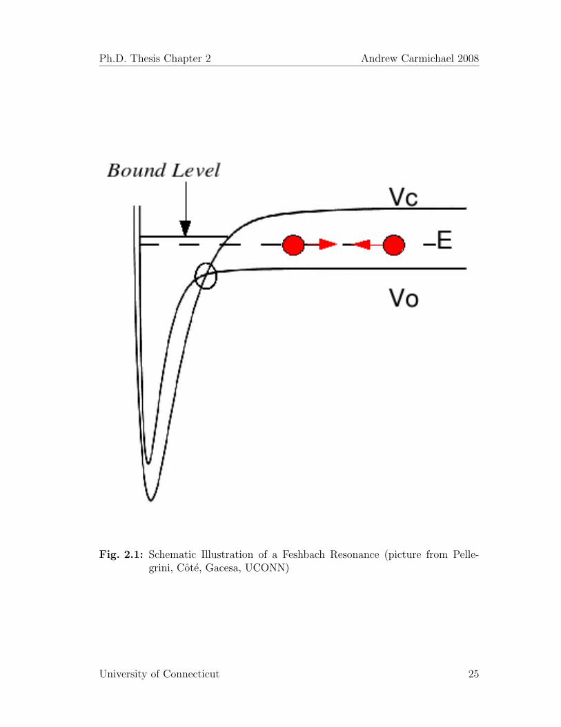
Excellent discussions on Feshbach resonances can be found in graduate level textssuch as [66], [67] and [64] and also in recent PhD theses such as [117]. First inves-tigated in nuclear physics [62], [63], but seen more recently in ultracold systems[73] [118], Feshbach resonances enable one to directly control the scattering lengthof atomic systems. The first point to note is that the interaction potential curve ofthe two interacting atoms as a function of internuclear separation depends uponthe states of the atoms. The asymptotes of the potential curve are called collisionchannels and are labelled by the hyperfine quantum numbers for the collidingatoms |F,mf〉. With the atoms in different spin states their interaction is de-scribed by a different potential curve. It is possible in a collision for atoms toenter one channel and leave in another, provided that energy is conserved. Chan-nels which are energetically unattainable are referred to as closed, while thoseattainable are open. The Feshbach resonance (figure 2.1) occurs when the energyof an incoming open channel (two atoms) is close to the energy of a bound state(molecule) in another, closed channel. The closed channel may describe the in-teraction of the atoms in different spin states, in which case the atoms in eachchannel will have different magnetic moments. They will then respond differentlyto external magnetic fields so that it becomes possible to tune the separation be-tween the states until a resonance occurs [68]. The coupling between the openand closed channels is provided by the Coulomb interaction which overpowers thehyperfine interaction allowing a spin flip to occur putting the atoms into the otherpotential. It should be remarked, however, that in real systems one must allowfor coupling to multiple closed channels rather than just one. The result of thisis that the scattering length becomes dependent on the magnetic field, with thedependence having the form
a(B) = abg
(1− ∆
B −B0
)(2.7.1)
where abg is the background scattering length which dominates far from the reso-nance, B0 is the position of the resonance; the value of the magnetic field at whichthe scattering length diverges and ∆ is known as the width of the resonance; the
University of Connecticut 23
Ph.D. Thesis Chapter 2 Andrew Carmichael 2008
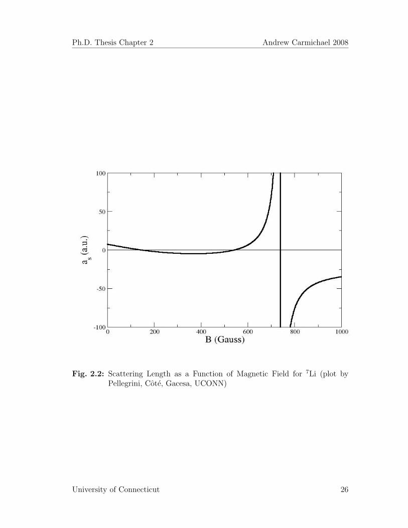
separation along the B axis of the resonance and the point at which a = 0. Closeto the resonance, the scattering length can easily be changed to any value on thereal axis, and interactions can even be switched off by tuning to a = 0. Figure 2.2shows a typical plot of the scattering length for 7Li from a calculation done by ourcollaborators at the University of Connecticut; Robin Cote, Philippe Pellegrini,Marko Gacesa et. al. In this thesis we shall introduce a quite general model whichis not restricted to a specific system. This plot is given simply to illustrate typicaldependence of the scattering length on the magnetic field.
One can even induce a collapse (Bosenova) by crossing the resonance from positiveto negative scattering length [119]. Moreover, experiments have probed the ‘BEC-BCS crossover’ regime; switching a system from BCS pairs of fermionic atoms (weshall discuss paring of this nature a little later on) to a condensate of moleculesby crossing a Feshbach resonance [120], [121], [122], [123], [124].
Photo-association [125] is a similar process, where a light field rather than amagnetic field induces the association of atoms to excited molecules. The toolsof quantum field theory in momentum representation which we shall employ inthis thesis treat both photo-association and magneto-associaiton as equivalentand so we treat them as such albeit primarily couching the discussion in terms ofmagneto-association.
2.8 Interactions in Second Quantization
Now that the nature of two-particle interactions has been explicated, we turn toconsider how such an interaction enters into the formalism of quantum field theory.We have already seen how to construct the kinetic part of both the Hamiltonianand the Hamiltonian density and the analysis for the interactions proceeds asfollows. We write the Hamiltonian density to include three terms; the kineticpart we are already familiar with and a term which describes the inter-particleinteraction.
H(r) = Ψ†(r)
[− ~2
2m∇2
]Ψ(r) +
1
2
∫d3r′Ψ†(r)Ψ†(r′)U(r, r′)Ψ(r′)Ψ(r) (2.8.1)
In the expression (2.8.1) r′ is merely a running integration variable, rather thanthe relative coordinate. Following the spirit of section 2.1, we can substitute anexpansion for the field operator of the form (2.5.7) to find the more commonlyencountered (at least in the literature of quantum optics and atomic physics), andperhaps more intuitive momentum representation form
H =∑k
εka†kak +
1
2V
∑p,p′,q
U(q,p,p′)a†p+qa†p′−qap′ ap (2.8.2)
University of Connecticut 24
Ph.D. Thesis Chapter 2 Andrew Carmichael 2008
Fig. 2.1: Schematic Illustration of a Feshbach Resonance (picture from Pelle-grini, Cote, Gacesa, UCONN)
University of Connecticut 25
Ph.D. Thesis Chapter 2 Andrew Carmichael 2008
Fig. 2.2: Scattering Length as a Function of Magnetic Field for 7Li (plot byPellegrini, Cote, Gacesa, UCONN)
University of Connecticut 26

Ph.D. Thesis Chapter 2 Andrew Carmichael 2008
As in the discussion involving non-interacting particles, εk represents the singleparticle energy for momentum k. The interaction term here can be seen to destroytwo particles and create them back in different momentum states, conservingmomentum for the whole process, an amount q being transferred from one to theother. The factor of 1/2 is necessary to avoid double counting when one sums overall incoming and transferred momenta, and V is the volume in which the gas isconfined. It will prove pertinent to us to discuss the particular case of zero rangecontact interactions of the form (2.6.29) and the analysis proceeds as follows
H = −Ψ†(r)~2
2m∇2Ψ(r) +
1
2
∫d3r′Ψ†(r)Ψ†(r′)U0δ(r− r′)Ψ(r′)Ψ(r) (2.8.3)
= −Ψ†(r)~2
2m∇2Ψ(r) +
1
2U0Ψ†(r)Ψ†(r)Ψ(r)Ψ(r) (2.8.4)
with the Hamiltonian becoming
H =∑k
εpa†pap +
U0
2V
∑p,p′,q
a†p+qa†p′−qap′ ap (2.8.5)
We shall make use of this Hamiltonian at a later stage.
2.9 Quantum Field Theory for Constructing Molecules
We write the interaction part of the Hamiltonian density Hint analogously tothe interparticle scattering term in traditional field theoretical descriptions ofquantum gases discussed in section 2.10. See previous work of our group such as[95].
Hint(r) = −1
2
∫ψ†(r)U(r, r′)ϕ(r + 1
2r′)ϕ(r− 1
2r′)d3r′ + h.c.
= −1
2ψ†(r)
∫U(r, r′)ϕ(r + 1
2r′)ϕ(r− 1
2r′)d3r′ + h.c. (2.9.1)
where the field of atoms is represented by ϕ and that of molecules by ψ. Thoughit may be apparent, in notation common to treatments of classical mechanics, thevector r represents the position of the centre of mass of the two atoms, while thevector r′ represents the relative vector r1 − r2, i.e. the vector going to atom 1from atom 2. The Hamiltonian density (2.9.1) is for the moment an Ansatz. Weshall see that, when written in momentum representation, its meaning becomesapparent.
University of Connecticut 27
Ph.D. Thesis Chapter 2 Andrew Carmichael 2008
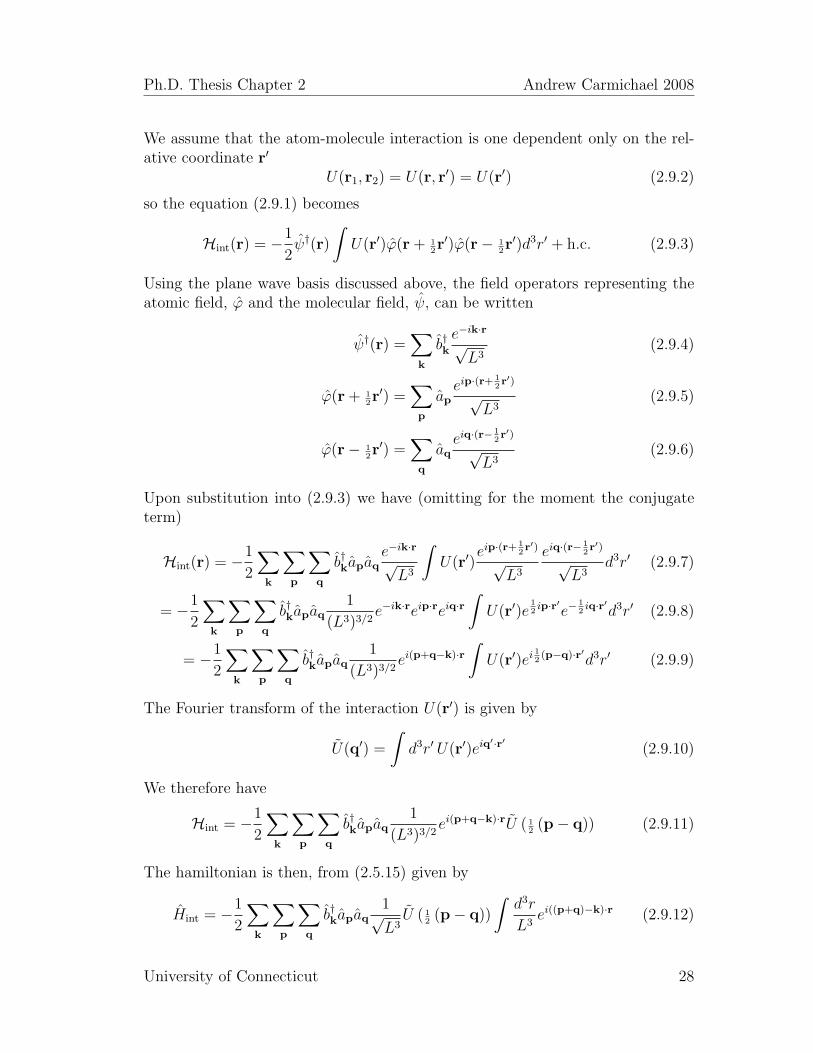
We assume that the atom-molecule interaction is one dependent only on the rel-ative coordinate r′
U(r1, r2) = U(r, r′) = U(r′) (2.9.2)
so the equation (2.9.1) becomes
Hint(r) = −1
2ψ†(r)
∫U(r′)ϕ(r + 1
2r′)ϕ(r− 1
2r′)d3r′ + h.c. (2.9.3)
Using the plane wave basis discussed above, the field operators representing theatomic field, ϕ and the molecular field, ψ, can be written
ψ†(r) =∑k
b†ke−ik·r√L3
(2.9.4)
ϕ(r + 12r′) =
∑p
apeip·(r+ 1
2r′)
√L3
(2.9.5)
ϕ(r− 12r′) =
∑q
aqeiq·(r−
12r′)
√L3
(2.9.6)
Upon substitution into (2.9.3) we have (omitting for the moment the conjugateterm)
Hint(r) = −1
2
∑k
∑p
∑q
b†kapaqe−ik·r√L3
∫U(r′)
eip·(r+ 12r′)
√L3
eiq·(r−12r′)
√L3
d3r′ (2.9.7)
= −1
2
∑k
∑p
∑q
b†kapaq1
(L3)3/2e−ik·reip·reiq·r
∫U(r′)e
12ip·r′e−
12iq·r′d3r′ (2.9.8)
= −1
2
∑k
∑p
∑q
b†kapaq1
(L3)3/2ei(p+q−k)·r
∫U(r′)ei
12
(p−q)·r′d3r′ (2.9.9)
The Fourier transform of the interaction U(r′) is given by
U(q′) =
∫d3r′ U(r′)eiq
′·r′ (2.9.10)
We therefore have
Hint = −1
2
∑k
∑p
∑q
b†kapaq1
(L3)3/2ei(p+q−k)·rU ( 1
2(p− q)) (2.9.11)
The hamiltonian is then, from (2.5.15) given by
Hint = −1
2
∑k
∑p
∑q
b†kapaq1√L3U ( 1
2(p− q))
∫d3r
L3ei((p+q)−k)·r (2.9.12)
University of Connecticut 28
Ph.D. Thesis Chapter 2 Andrew Carmichael 2008
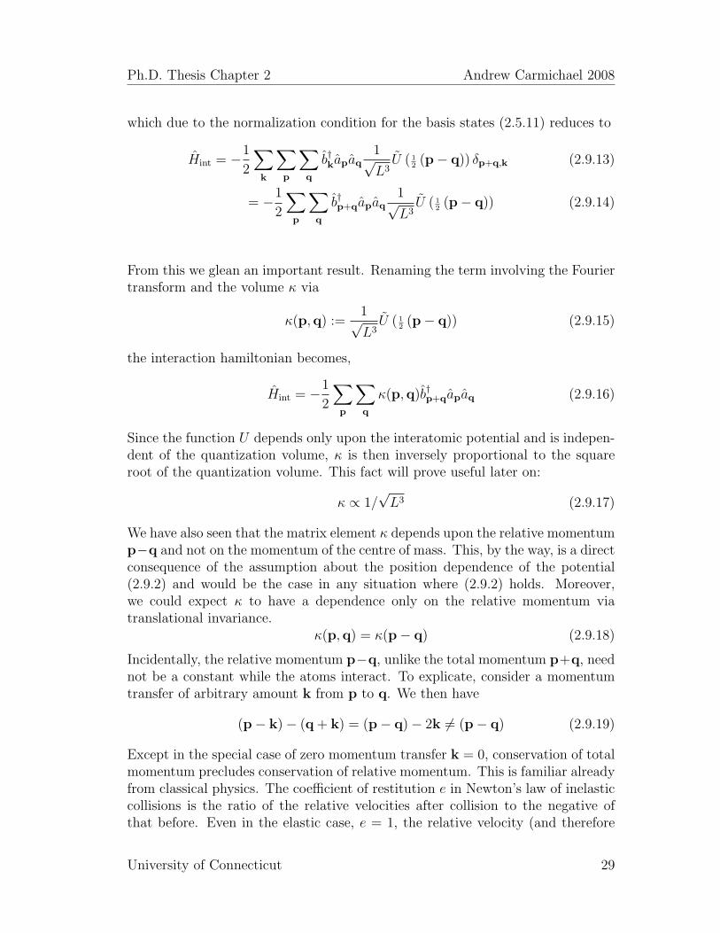
which due to the normalization condition for the basis states (2.5.11) reduces to
Hint = −1
2
∑k
∑p
∑q
b†kapaq1√L3U ( 1
2(p− q)) δp+q,k (2.9.13)
= −1
2
∑p
∑q
b†p+qapaq1√L3U ( 1
2(p− q)) (2.9.14)
From this we glean an important result. Renaming the term involving the Fouriertransform and the volume κ via
κ(p,q) :=1√L3U ( 1
2(p− q)) (2.9.15)
the interaction hamiltonian becomes,
Hint = −1
2
∑p
∑q
κ(p,q)b†p+qapaq (2.9.16)
Since the function U depends only upon the interatomic potential and is indepen-dent of the quantization volume, κ is then inversely proportional to the squareroot of the quantization volume. This fact will prove useful later on:
κ ∝ 1/√L3 (2.9.17)
We have also seen that the matrix element κ depends upon the relative momentump−q and not on the momentum of the centre of mass. This, by the way, is a directconsequence of the assumption about the position dependence of the potential(2.9.2) and would be the case in any situation where (2.9.2) holds. Moreover,we could expect κ to have a dependence only on the relative momentum viatranslational invariance.
κ(p,q) = κ(p− q) (2.9.18)
Incidentally, the relative momentum p−q, unlike the total momentum p+q, neednot be a constant while the atoms interact. To explicate, consider a momentumtransfer of arbitrary amount k from p to q. We then have
(p− k)− (q + k) = (p− q)− 2k 6= (p− q) (2.9.19)
Except in the special case of zero momentum transfer k = 0, conservation of totalmomentum precludes conservation of relative momentum. This is familiar alreadyfrom classical physics. The coefficient of restitution e in Newton’s law of inelasticcollisions is the ratio of the relative velocities after collision to the negative ofthat before. Even in the elastic case, e = 1, the relative velocity (and therefore
University of Connecticut 29
Ph.D. Thesis Chapter 2 Andrew Carmichael 2008
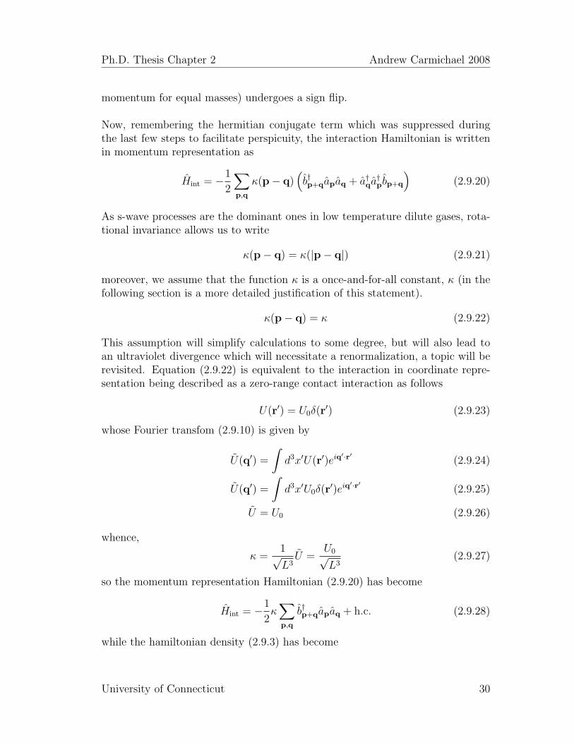
momentum for equal masses) undergoes a sign flip.
Now, remembering the hermitian conjugate term which was suppressed duringthe last few steps to facilitate perspicuity, the interaction Hamiltonian is writtenin momentum representation as
Hint = −1
2
∑p,q
κ(p− q)(b†p+qapaq + a†qa
†pbp+q
)(2.9.20)
As s-wave processes are the dominant ones in low temperature dilute gases, rota-tional invariance allows us to write
κ(p− q) = κ(|p− q|) (2.9.21)
moreover, we assume that the function κ is a once-and-for-all constant, κ (in thefollowing section is a more detailed justification of this statement).
κ(p− q) = κ (2.9.22)
This assumption will simplify calculations to some degree, but will also lead toan ultraviolet divergence which will necessitate a renormalization, a topic will berevisited. Equation (2.9.22) is equivalent to the interaction in coordinate repre-sentation being described as a zero-range contact interaction as follows
U(r′) = U0δ(r′) (2.9.23)
whose Fourier transfom (2.9.10) is given by
U(q′) =
∫d3x′U(r′)eiq
′·r′ (2.9.24)
U(q′) =
∫d3x′U0δ(r
′)eiq′·r′ (2.9.25)
U = U0 (2.9.26)
whence,
κ =1√L3U =
U0√L3
(2.9.27)
so the momentum representation Hamiltonian (2.9.20) has become
Hint = −1
2κ∑p,q
b†p+qapaq + h.c. (2.9.28)
while the hamiltonian density (2.9.3) has become
University of Connecticut 30
Ph.D. Thesis Chapter 2 Andrew Carmichael 2008
Hint(r) = −1
2
∫ψ†(r)U0δ(r
′)ϕ(r + 12r′)ϕ(r− 1
2r′)d3r′ + h.c. (2.9.29)
= −1
2U0ψ
†(r)
∫δ(r′)ϕ(r + 1
2r′)ϕ(r− 1
2r′)d3r′ + h.c. (2.9.30)
= −1
2U0ψ
†(r)ϕ(r)ϕ(r) + h.c. (2.9.31)
In the tradition in quantum optics literature, and in keeping with the remarksat the end of section 2.5, we proceed to state the terms in the Hamiltonian infrequency rather than energy units (dividing through by ~), thus
Hint
~= −1
2κ∑p,q
b†p+qapaq + h.c. (2.9.32)
κ is now written in frequency units. The ~ in the denominator on the left handside will be suppressed.
Hint = −1
2κ∑p,q
b†p+qapaq + h.c. (2.9.33)
This Hamiltonian can be seen to describe the processes by which two atoms ofmomenta p and q are destroyed creating a molecule of momentum p + q, andthe conjugate process (necessary to preserve hermiticity of the Hamiltonian) de-stroying a molecule of momentum p + q and producing two atoms of momenta pand q. The summation then includes a continuum of values of both p and q; weconsider the particles to be effectively in (box normalized) free space.
Physically, the processes described by this interaction Hamiltonian, where moleculesare destroyed producing atoms and atom pairs destroyed producing molecules, areattainable via tunable interactions in Feshbach resonances (magneto-association)and by laser assisted association and dissociation, a process known as photo-association. In quantum field theory, these two processes are mathematicallyequivalent and the conclusions we draw from analysis of a Hamiltonian contain-ing terms like (2.9.28) (or, equivalently, a Hamiltonian density with terms like(2.9.31)) shall be considered applicable to both types of process in the laboratory.The physics behind both processes will be elucidated in the following sections.
2.10 Traditional Mean Field Theories
2.10.1 Bogoliubov Approximation and Gross Pitaevskii Equation
The mean field approximation one can apply to macroscopically condensed bosonswas first broached by Bogoliubov [18]. See standard texts on statistical mechanics
University of Connecticut 31

Ph.D. Thesis Chapter 2 Andrew Carmichael 2008
or condensed matter physics such as [7], [126], [127], or specialized texts such as[66], [67], [64], [128], [129]. If the operator a0 destroys particles in a macroscopicallyoccupied state, then we can make the approximation
〈a†0a0〉 = N0 ≈ N 1 (2.10.1)
where N represents the total number of atoms in the system, and N0 representsthose in the zero momentum state. This means
〈a†0a0〉 ± 1 ≈ 〈a†0a0〉 (2.10.2)
The commutator can then be approximated viz.
[a0, a†0] = a0a
†0 − a
†0a0 = 1 (2.10.3)
[a0, a†0]− 1 = a0a
†0 − a
†0a0 − 1 = 0 (2.10.4)
= a0a†0 − (a†0a0 + 1) = 0 (2.10.5)
≈ a0a†0 − a
†0a0 = [a0, a
†0] (2.10.6)
and so the commutator is functionally equivalent to
[a0, a†0] = a0a
†0 − a
†0a0 = 0 (2.10.7)
enabling one to replace the operator a0 with a simple complex number such as(making the simplest branch choice)
a0 → a0 =√N0 ,
a†0 → a∗0 =√N0
(2.10.8)
the non-commutivity of the operators having been neglected. This is what we,and many other authors, refer to as the mean field approximation with a0 beingthe mean or “classical” field.
This should be contrasted with the field operator Ψ which, for a free gas (with pe-riodic boundary conditions) with its single zero momentum state macroscopically
University of Connecticut 32
Ph.D. Thesis Chapter 2 Andrew Carmichael 2008
occupied, would, using a plane wave basis, read
Ψ(r) =∑k
akuk(r) (2.10.9)
=∑k
akeik·r√V
(2.10.10)
=a0√V
+∑k 6=0
akeik·r√V
(2.10.11)
=a0√V
+∑k 6=0
akeik·r√V
(2.10.12)
=
√N0
V+∑k 6=0
akeik·r√V
(2.10.13)
where in the last two steps the Bogoliubov substitution (2.10.8) has been made.Many authors refer to the first term
Ψ0 =
√N0
V(2.10.14)
as the condensate wavefunction and note that it also is a classical field followingthe same argument as with a0 concerning the commutator. If we consider nowthe equation of motion of (2.10.14) by using the Heisenberg equation (equivalentto the Schrodinger picture for the classical quantity Ψ0)
i~∂
∂tΨ(r) = [Ψ(r, t), H] (2.10.15)
where the Hamiltonian is obtained from the Hamiltonian density (2.8.4) via (2.5.15),we obtain
i~∂
∂tΨ0 =
(−~2∇2
2m+ Vext(r, t) + U0|Ψ0(r, t)|2
)Ψ0(r, t) (2.10.16)
which is known as the Gross-Pitaevskii equation (GPE), the nonlinear Schrodingerequation which governs the macroscopic condensate wavefunction (also referred toas the condensate order parameter). Equation, (2.10.16) valid in the zero temper-ature limit and neglecting all correlations between the atoms, is the centrepiece ofmuch theoretical research on condensates. The Vext(r, t) part of course describesthe external trapping potential. The nonlinear part of (2.10.16) describes theinteratomic interaction; important in condensates despite their being very dilute.The magnitude of this term is fixed by
U0 =4π~2a
m(2.10.17)
University of Connecticut 33
Ph.D. Thesis Chapter 2 Andrew Carmichael 2008
where a is the s-wave scattering length previously introduced. Clearly the signof a determines the sign of the interactions likewise the magnitude of a deter-mines the magnitude of the interactions. One would like to have the ability toarbitrarily change the scattering length and it turns out that one can via a Fesh-bach resonance which was discussed in section 2.7. Since we deal with analysisin Heisenberg picture quantum mechanics, we shall couch future discussions interms of quantities like a0 rather than Ψ0 and refer the these as the mean field.Indeed, since we shall not be solving the GPE but rather Heisenberg equations ofmotion, one might consider introduction of (2.10.16) to be unnecessary. However,the importance of this equation in much of the research on condensates (and inmany of the papers cited in the bibliography) implies to us that any work such asthe present thesis which entails Bose-Einstein condensation at all would be quiteremiss, indeed incomplete, not to discuss (2.10.16).
2.10.2 Bogoliubov Approach to Bose and Fermi Gases
To analyse the Bose gas in the weakly interacting regime we follow Bogoliubovand begin with the Hamiltonian (2.8.5),
H =∑k
εka†kak +
1
2V
∑p,p′,q
U(q,p,p′)a†p+qa†p′−qap′ ap (2.10.18)
The Bogoliubov approach is to expand the above Hamiltonian using the classicalfield approximation described above. Keeping terms no more than quadratic inap and a†p for the bosons outside the condensate, i.e. those with p 6= 0, one endsup with
H =N2
0U0
2V+∑p6=0
(εp + 2
N0
VU0
)a†pap +
N0U0
2V
∑p6=0
(a†pa
†−p + apa−p
)(2.10.19)
We note the appearance of the particular combinations of operators apa−p and
a†pa†−p. These create and destroy pairs of bosons of zero total momentum. We
shall have use for operators such as these later on, but let us first turn to theanalysis of the Fermi gas.
Fermions, in contrast to bosons, have a maximum occupancy in any given spinand momentum state of one. This means that the Bogoliubov approximation isnot remotely applicable. It is, however, possible to make an analogous approxima-tion via BCS theory. This construction, named after its creators Bardeen, Cooperand Schrieffer, describes the phenomenon of superfluidity through the formationof Cooper pairs of fermions of opposite (about the origin in k-space) momentaand spin. These quasi-particles are bosons and can thus Bose condense. The
University of Connecticut 34
Ph.D. Thesis Chapter 2 Andrew Carmichael 2008
formation of Cooper pairs is a many-body effect and separate from the formationof bosonic molecules which can take place against a vacuum background.
We begin an introductory analysis with the aforementioned Hamiltonian;
H =∑p
εp
(a†pap + b†pbp
)+
1
V
∑p,p′,q
U(q,p,p′)a†p+qb†p′−qbp′ ap (2.10.20)
different only in that two species of equally massive fermions are considered. Thesecould, for example, be the same atoms in two different spin states. The factor of1/2, necessary in the Bose case, is absent here as double counting is precluded bythe fact that the species are distinguishable. As in the Bose case, it is convenientto fix the particle number by introducing a Lagrange multiplier, the chemicalpotential, whence the Kamiltonian,
K =∑p
(εp − µ)(a†pap + b†pbp
)+
1
V
∑p,p′,q
U(q,p,p′)a†p+qb†p′−qbp′ ap (2.10.21)
The Bogoliubov approximation cannot be used here for the creation and annihila-tion operators for individual fermions, as the Pauli exclusion principle proscribesthe presence of even two fermions in the same state. If, however, a condensate ofpairs is present, we can describe the operators which create and destroy zero mo-mentum pairs of fermions as simple complex numbers. The only requirements arethat the members of a pair lie on opposite sides of the Fermi sphere and that theirspin states be different. Let us introduce the operator b−pap and its expectationvalue, which we henceforth denote
C(p) = 〈b−pap〉 (2.10.22)
and is simply a complex number. With the substitution of
b−pap = C(p) + b−pap − C (p) (2.10.23)
into (2.10.21) keeping only terms which are at most quadratic in operators a andb, we are led to
K =∑p
(εp − µ)(a†pap + b†−pb−p
)+
1
V
∑k
∆∗(k)b−kak +1
V
∑k
∆(k)akb−k (2.10.24)
where∆(k) =
∑p
U(k,p)C(p) (2.10.25)
University of Connecticut 35

Ph.D. Thesis Chapter 2 Andrew Carmichael 2008
is the called the gap function. The function C(p), known as the anomalous pairingamplitude describes a pair of fermions with opposite momenta and is significantin that it defines the gap function ∆ which sets the binding energy of the Cooperpairs. We shall have use for quantities like the pairing amplitude (2.10.22) in theboson system approached in this thesis.
University of Connecticut 36
Chapter 3
Two-Atom System & Dressed Molecules
3.1 General Formulation
The system we wish to analyse is a collection of bosonic atoms in the presenceof either a photo-associating laser field or a magneto-associating Feshbach reso-nance such that states for the free atoms are coupled to a bound molecular state.Without restricting the generality, we also assume that the conserved center-of-mass momentum equals zero. We approach the problem in the Heisenberg pictureand write down a second quantised momentum representation Hamiltonian (all infrequency units) following (2.5.21) and (2.9.33) as follows
H =∑k
[εka
†kak +
(1
2εk + δ
)b†kbk
]− 1
2κ∑k,p
(b†k+pakap + a†pa
†kbk+p
)(3.1.1)
The operator a†k creates an atom in momentum state k while b†k creates a moleculein momentum state k. εk represents the single particle energy in frequency units.
εk =~k2
2m(3.1.2)
where m is the atomic mass. The first summation represents the kinetic energy ofatoms and molecules. The factor of 1/2 in the second term under the summationis because the molecule has double the mass of an atom.
The quantity δ is known in quantum optics as the detuning and represents theenergy difference between zero momentum atoms and zero momentum molecules.This depends in the photo-association case upon the frequency of the laser(s) whilein the magneto-association case depends upon the dot product of the difference inthe dipole moments of the free and bound states with the magnetic field measuredfrom resonance
~δ = ∆µ · (B −B0) (3.1.3)
where B0 is the location of the Feshbach resonance; the value of B for which thescattering length diverges. In both cases δ = 0 corresponds to the position of the
37

Ph.D. Thesis Chapter 3 Andrew Carmichael 2008
resonance.
The second summation is over terms which describe the creation of a moleculevia the destruction of two atoms and the conjugate process (necessary to preservehermiticity of the Hamiltonian) of the destruction of a molecule and the creationof two atoms. The amplitude for this coupling κ has been presumed momentumindependent (corresponding to a zero range interaction in position representation)pursuant to the discussion in section 2.6.
With the exception of occasional comments which apply to both the photo-association and magneto-association processes, we have opted to couch the dis-cussion from now on purely in terms of the latter case although, as stated before,the two processes in second quantised notation are the same as long as one bearsin mind that a time dependent laser field carries momentum into and out of thesystem (system being just the atoms and molecules) while the static B field inthe Feshbach resonance case does not; the atom molecule conversion process out-lined in this chapter therefore has constant momentum but not energy. Otherpublications of our group have explored explicitly the case of photo-association[95], [97], [96], [94], [93] using essentially the same Hamiltonian as (3.1.1) with anextra momentum index on the coupling κ to deal with momentum transfer by thephoton.
Sign of the Atom-Molecule Coupling κ
Considering the atom-molecule system in the centre of mass frame, a single molec-ular bound state is coupled to the continuum of the relative motion of the atoms.We can choose the phases of the free (continuum) states such that the matrixelements satisfy,
κ ∈ R (3.1.4)
andκ ≥ 0 (3.1.5)
If the physics is time-reversal invariant, the stationary wavefunctions may bechosen real, the time dependence always being the only non-hermitian part of awavefunction.
3.1.1 Constants of the Motion
The Hamiltonian has as a constant of the motion anything which commutes withit. We can see that the total atom number operator (including those atoms insidea molecule) defined by
N =∑k
(a†kak + 2b†kbk
)(3.1.6)
University of Connecticut 38
Ph.D. Thesis Chapter 3 Andrew Carmichael 2008
is a constant of the motion as[N , H] = 0 (3.1.7)
The factor of 2 is inserted into the definition of N because it takes two atoms tomake a molecule. We shall refer to the eigenvalue of this operator as the invariantatom number in future.
In addition, the total momentum, defined by,
P =∑k
k(a†kak + b†kbk
)(3.1.8)
commutes with H and is likewise, as previously mentioned, a constant of the mo-tion. This we could also expect on physical grounds for a translationally invariantsystem.
3.2 Two Atom Problem and Dressed Molecules
For the present chapter we shall focus on the special exactly soluble case of onlytwo atoms combining to form a single molecule. In this case, the eigenvalue of(3.1.6) reduces to
2 =∑k
(〈a†kak〉+ 2〈b†kbk〉
)(3.2.1)
The Hilbert space is spanned by vectors of the form
|ψ〉 =
[1
2
∑k
Aka†ka†−k + βb†0
]|0〉 (3.2.2)
where Ak and β are complex numbers, and |0〉 is the particle vacuum. a†k is the
creation operator for a single atom in state k while b†k is that for a molecule. Theamplitude Ak is considered invariant under a inversion of the axes (inverting theaxes (x → −x, y → −y and z → −z) to change the sign of momentum) so thatAk = A−k. We abbreviate the atom pair states by
|Ak〉 = a†ka†−k|0〉 (3.2.3)
and the molecular state by
|B〉 = b†0|0〉 (3.2.4)
The statevector (3.2.2) then takes the form
|ψ〉 =1
2
∑k
Ak|Ak〉+ β|B〉 (3.2.5)
University of Connecticut 39

Ph.D. Thesis Chapter 3 Andrew Carmichael 2008
The factor of 1/2 in in front of the summation is because of the fact that, due tobosonic commutation, the states |Ak〉 and |A−k〉 are the same, and so one needonly sum over half of this basis to obtain a state vector spanning the space.
The time dependent Schrodinger equation for the amplitudes of a general wave-function expressed as an expansion in an orthogonal basis of states |n〉
|ψ〉 =∑n
an(t)|n〉 (3.2.6)
is given by
id
dtak =
∑n
an〈k|H|n〉 (3.2.7)
In the case of the statevector (3.2.5), the Schrodinger equation becomes
id
dt〈B|ψ〉 = β〈B|H|B〉+
1
2
∑k
Ak〈B|H|Ak〉 (3.2.8)
id
dt〈Ak|ψ〉 = β〈Ak|H|B〉+
1
2
∑k′
Ak′〈Ak|H|Ak′〉 (3.2.9)
We are now to determine the matrix elements for which we first require the innerproducts of the basis sates. Some care must be taken due to the fact that since|Ak〉 = |A−k〉 the inner product of two states each occupied with an atom pair ofgenerally different momenta is not simply a single Kronecker delta, but rather acombination of them.
We begin by finding the inner product for a rather more general state than thatcurrently required, identified by the symbol analogous to that already employedas |Ak,p〉 = a†ka
†p|0〉 along with its inner product denoted by 〈Ap′,k′ |Ak,p〉 and
defined in the first line below. The states already referred to are special cases ofthose just mentioned with p = −k and the symbol used was an abbreviation viz.|Ak,−k〉 = |Ak〉.
We proceed to arrange the operators in normal order as follows
〈Ap′,k′ |Ak,p〉 = 〈0|ap′ ak′ a†ka†p|0〉
= 〈0|ap′(δk,k′ + a†ka′k)a†p|0〉
= δk,k′〈0|ap′ a†p|0〉+ 〈0|ap′ a
†kak′ a
†p|0〉
= δk,k′〈0|(δp,p′ + a†pap′)|0〉+ 〈0|ap′ a†k(δk′,p + a†pak′)|0〉
= δk,k′δp,p′〈0|0〉+ δk,k′〈0|a†pap′|0〉+ δk′,p〈0|ap′ a†k|0〉+ 〈0|ap′ a
†ka†pak′|0〉
University of Connecticut 40
Ph.D. Thesis Chapter 3 Andrew Carmichael 2008
noting that
〈0|ap′ a†ka†pak′|0〉 = 0 (3.2.10)
〈0|a†pap′ |0〉 = 0 (3.2.11)
〈0|0〉 = 1 (3.2.12)
we end up with
〈Ap′,k′ |Ak,p〉 = δk,k′δp,p′ + δk′,p〈0|ap′ a†k|0〉
= δk,k′δp,p′ + δk′,p〈0|(δk,p′ − a†kap′)|0〉= δk,k′δp,p′ + δk′,pδk,p′〈0|0〉 − δk′,p〈0|a†kap′|0〉= δk,k′δp,p′ + δk′,pδk,p′ − δk′,p〈0|a†kap′ |0〉
again, noting that
〈0|a†kap′|0〉 = 0 (3.2.13)
we are left with the result
〈0|ap′ ak′ a†ka†p|0〉 = δk,k′δp,p′ + δk′,pδk,p′ (3.2.14)
For the case at hand, we are dealing with zero momentum pairs and thereforehave the condition that p = −k and p′ = −k′ and so the general result becomes
〈A−k′,k′|Ak,−k〉 = 〈0|a−k′ ak′ a†ka†−k|0〉
= δk,k′δ−k,−k′ + δk′,−kδk,−k′ (3.2.15)
Of course, only one of the Kronecker delta symbols in each term used in the lastexpression are necessary and the others are redundant. Retaining them, however,keeps an air of symmetry in the expression.
We are now enabled to easily perform summations over the matrix elements asfollows ∑
k′
Ak′〈A−k,k|Ak′,−k′〉 =∑k′
Ak′(δk,k′δ−k,−k′ + δk′,−kδ−k′,k) (3.2.16)
= Ak + A−k (3.2.17)
= 2Ak (3.2.18)
where in last step we have made use of the previously stipulated property of theamplitude A that A−k = Ak. Furthermore, we can find other inner products suchas
〈B|B〉 = 1 〈Ak|B〉 = 〈B|Ak〉 = 0 (3.2.19)
University of Connecticut 41

Ph.D. Thesis Chapter 3 Andrew Carmichael 2008
We are now in a position to see that, remembering the factor of 1/2 in the definitionof |ψ〉, the inner products on the left hand side of equations (3.2.8) and (3.2.9)are
〈B|ψ〉 = β 〈Ak|ψ〉 = Ak (3.2.20)
From the Hamiltonian (3.1.1) one can now obtain the diagonal matrix elements
〈B|H|B〉 = δ (3.2.21)
and
〈Ak′ |H|Ak〉 = εk(δk,k′δ−k,−k′ + δk′,−kδk,−k′)
+ ε−k(δk,−k′δ−k,k′ + δk′,kδ−k,−k′) (3.2.22)
Equation (3.2.9) requires us to evaluate the term∑k
Ak〈Ak′ |H|Ak〉
=∑k
Akεk(δk,k′δ−k,−k′ + δk′,−kδk,−k′)
+∑k
Akε−k(δk,−k′δ−k,k′ + δk′,kδ−k,−k′) (3.2.23)
= Ak′εk′ + A−k′ε−k′ + A−k′εk′ + Ak′ε−k′ (3.2.24)
= 4εk′Ak′ (3.2.25)
where in the last step the property of the single particle energy εk = ε−k and theaforementioned symmetry of the amplitude Ak under parity inversion have beenused.
We also need to evaluate the off-diagonal matrix element 〈B|H|Ak〉. Observingthat the only nonvanishing term of the Hamiltonian between these two states isthat which creates a zero-momentum molecule from two atoms, we proceed asfollows
〈B|H|Ak〉 = −κ2
∑p
〈B|b†0apa−p|Ak〉 (3.2.26)
= −κ2
∑p
〈0|b0b†0apa−pa
†ka†−k|0〉 (3.2.27)
University of Connecticut 42
Ph.D. Thesis Chapter 3 Andrew Carmichael 2008
making use of the fact that〈0|b0b
†0 = 〈0| (3.2.28)
we have
〈B|H|Ak〉 = −κ2
∑p
〈0|apa−pa†ka†−k|0〉 (3.2.29)
= −κ2
∑p
(δk,pδ−k,−p + δp,−kδk,−p) (3.2.30)
= −κ2
(2) = −κ (3.2.31)
Since the Hamiltonian is Hermitian, 〈B|H|Ak〉 = 〈Ak|H†|B〉∗ = 〈Ak|H|B〉∗ musthold, and since the matrix element is real, 〈B|H|Ak〉 = 〈Ak|H|B〉.
We can now write the Schrodinger equations for the amplitudes as follows
id
dtβ = βδ − κ
2
∑k
Ak (3.2.32)
id
dtAk = −βκ+ 2εkAk (3.2.33)
We can also find the Eigenenergy of H
〈ψ|H|ψ〉 = E〈ψ|ψ〉 (3.2.34)
〈ψ|H|ψ〉 =1
2β∗∑k′
Ak′〈B|H|Ak′〉+1
4
∑k
A∗k∑k′
Ak′〈Ak|H|Ak′〉
+ β∗β〈B|H|B〉+1
2β∑k
A∗k〈Ak|H|B〉 (3.2.35)
which using the matrix elements above becomes
〈ψ|H|ψ〉 = −κ2β∗∑k
Ak +∑k
A∗kAkεk + β∗βδ − κ
2β∑k
A∗k (3.2.36)
Assuming that β∗ = β and A∗k = Ak, this further reduces to
〈ψ|H|ψ〉 = −κβ∑k
Ak +∑k
A2kεk + β2δ (3.2.37)
University of Connecticut 43
Ph.D. Thesis Chapter 3 Andrew Carmichael 2008
we can also evaluate the norm
〈ψ|ψ〉 = β2〈B|B〉+1
4
∑k
A∗k∑k′
Ak′〈Ak|Ak′〉
+1
2β∑k′
Ak′〈B|Ak′〉+1
2β∑k
Ak〈Ak|B〉 (3.2.38)
〈ψ|ψ〉 = β2 +1
4
∑k
A∗k(2Ak) (3.2.39)
= β2 +1
2
∑k
A∗kAk (3.2.40)
If rotational invariance prevails at the initial time so that Ak is only a functionof |k|, or equivalently, a function of εk ≡ ε, the same symmetry holds at all latertimes. Moreover, in a two-atom system we may replace the sum over k by acontinuum approximation without running into problems with the atomic BEC.We write the continuum approximation as∑
k
f(ε(k))→ V
(2π)3
∫d3k f(ε(k))→ 3N
2ε3/2f
∫ ∞0
dε√εf(ε) (3.2.41)
We prefer quantities with the dimension of frequency over ~ times the same quan-tities with the dimension of energy, so that the integral runs over frequencies. Wedefine the energy ~εf with
εf =~
2m
(6πN
V
)2/3
(3.2.42)
The factor N is retained even though here N = 2 at all times to make the equa-tions commensurate with those which will appear in the many atom mean-fieldtheoretical version of the problem. The equation (3.2.42), then, equals the Fermienergy for a single-component gas with density N/V , but obviously has nothingto do with any physical Fermi energy. Instead, εf is a measure of the density ofthe gas; the essentially unique frequency that can be constructed out of density(N/V ) for a quantum mechanical (~) gas of atoms (m).
Lastly, we define the parameter characterizing the atom-molecule coupling
Ω =√Nκ (3.2.43)
University of Connecticut 44
Ph.D. Thesis Chapter 3 Andrew Carmichael 2008
As we have freedom to chooseκ ≥ 0 (3.2.44)
we can also chooseΩ ≥ 0 (3.2.45)
The time dependent Schrodinger equation for the coefficients β and A(ε(k)) finallyreads
id
dtβ(t) = δβ(t)− 3
4
√2 · Ω
ε3/2f
∫ ∞0
dε√εA(ε, t) (3.2.46)
id
dtA(ε, t) = 2εA(ε, t)− Ω√
2β(t) (3.2.47)
Similarly, the matrix element (3.2.34) becomes
〈ψ|H|ψ〉 = − Ω√Nβ
3N
2ε3/2f
∫ ∞0
dε√εA(ε) +
3N
2ε3/2f
∫ ∞0
dεA2(ε)ε3/2 + β2δ (3.2.48)
which for N = 2 reduces to
〈ψ|H|ψ〉 = −β 3Ω√
2
2ε3/2f
∫ ∞0
dε√εA(ε) +
3
ε3/2f
∫ ∞0
dεA2(ε)ε3/2 + β2δ (3.2.49)
The norm now becomes
〈ψ|ψ〉 = β2 +1
2
3N
2ε3/2f
∫ ∞0
dε√εA2(ε) (3.2.50)
N = 2 =⇒ 〈ψ|ψ〉 = β2 +3
2ε3/2f
∫ ∞0
dε√εA2(ε) (3.2.51)
The essense of the two-channel theory is to regard atoms and molecules as distinctthough coupled degrees of freedom. The boson operators in Hamiltonian (3.1.1)create and annihilate atoms and molecules that would be observed if there wereno atom-molecule coupling. As such, they would represent the observable atomsand molecules immediately after the atom-molecule coupling were switched off.In the case of photoassociation this could be achieved literally by switching off thelasers. For the Feshbach resonance an equivalent decomposition could be effected(in principle) by suddenly switching the magnetic field so far off resonance thatthe atoms and the molecules effectively decouple. There are also experimentalprobes that directly see the bare molecules, for instance, by making use of opticaltransitions in the bare molecules.
University of Connecticut 45
Ph.D. Thesis Chapter 3 Andrew Carmichael 2008
However, standard radio frequency spectroscopy at a Feshbach resonance probestransitions between energy eigenstates of the system in the presence of the atom-molecule coupling, i.e., stationary states of Eqs. (3.2.46) and (3.2.47). These aresupepositions of a bare molecule and pairs of bare atoms, and so we refer to thecoupled system as the dressed molecule.
3.3 Renormalization
The energy eigenstates are obtained by inserting an Ansatz of the form
β(t) = e−iωtβ(0) (3.3.1)
A(k, t) = e−iωtA(k, 0) (3.3.2)
into Eqs. (3.2.46) and (3.2.47), (assuming effectively that ωk = ω for all modes k)which gives
(ω − δ)β(0) = −3
4
√2 · Ω
ε3/2f
∫ ∞0
dε√εA(ε, 0) (3.3.3)
(ω − 2ε)A(ε, 0) = − Ω√2β(0) (3.3.4)
Simple elimination of A(ε) from Eq. (3.3.3) using Eq. (3.3.4) gives a relation todetermine the eigenfrequency ω in
ω − δ =3Ω2
4ε3/2f
∫ ∞0
dε
√ε
ω − iη − 2ε(3.3.5)
Here −η, with η = 0+, is an imaginary part in the energy that needs to be addedto handle the divergence of the integrand at 2ε = ω. This practice is the same asif we took Fourier transformations of the time dependent equations and used themto study the evolution of the system forward in time. Such an asymmetry in thedirection of time is not desirable if we are looking for true stationary states of theatom-molecule system. We outline in section 3.4 a method, following [130], to findthe true stationary states, but here our main issue is the ultraviolet divergence.
Physically, Eqs. (3.2.46) and (3.2.47) descibe the coupling of the bare-moleculestate to many (actually, a continuum) of atom-pair states. The coupling of thebound molecular state to the continuum of atom pair states is analogous to thecoupling of an excited state to the continuum of unoccupied vacuum modes whichintroduces a Lamb shift (see [131] for a general discussion of the Lamb shift). Theconsequence here is that if there still is a bound state corresponding to the baremolecule in the system, it is shifted (and broadened) in energy from the original
University of Connecticut 46
Ph.D. Thesis Chapter 3 Andrew Carmichael 2008
bare molecular state [132]. In the contact-interaction model for the shape of thecoupling to the continuum, the momentum representation coupling κ is a constantand the shift simply is infinite. Mathematically, the integral in (3.3.5) diverges.
We renomalize as follows. We adopt an upper limit of the integral M . This isequivalent to stating that the coupling κ is really given by κθ(M − ε), essentiallyan upper momentum cut-off in the spirit of Bethe’s approach to the self-energyof the electron. In essence, the electrons in Bethe’s case, the atoms in ours, areassumed not to be point-like but to acquire spatial dimension equal to 1/M (~/Mcin natural units where ~ = c = 1). The Fourier transform of any coupling with thisdependence corresponds to a momentum cut-off of M (Mc/~). See, for example,[133]. With this in mind, we write Eq. (3.3.5) as
ω −
(δ − 3Ω2
4ε3/2f
∫ M
0
√ε
2ε
)
=3Ω2
4ε3/2f
∫ M
0
dε
( √ε
ω − iη − 2ε+
√ε
2ε
)(3.3.6)
and let M →∞ at the end of the calculation. The right-hand side then convergesnicely, but ostensibly not so the left-hand side; the detuning δ gets modified bythe infinite level shift. The idea of the renormalization is to incorporate the levelshift in the definition of the energies, and take the renormalized detuning
δ − limM→∞
[3Ω2
8ε3/2f
∫ M
0
1√εdε
]= δ (3.3.7)
to have a finite value.
In this way Eq. (3.3.5) turns into a well-behaved equation
ω − δ =3Ω2
4ε3/2f
∫ ∞0
dε1√ε
ω
ω + iη − 2ε(3.3.8)
The integral can be shown to give∫ ∞0
ω√ε (ω − 2 ε+ iη)
dε = −csgn
((√−2ω − 2 iη
)∗)π ω
√−2ω − 2 iη
(3.3.9)
where the star denotes the complex conjugate and the function csgn is the complexsign function, defined to be +1 when its argument lies in the right half plane and-1 when the argument lies in the left half plane (the assignment of points along
University of Connecticut 47
Ph.D. Thesis Chapter 3 Andrew Carmichael 2008
the imaginary axis is a matter of choice, but it doesn’t concern us here anyway).We’ve now to take the limit η → 0
limη→0
RHS = −csgn
(√−2ω
)π ω
√−2ω
(3.3.10)
Clearly for ω > 0 no real solution exists. However, for ω = −|ω|, the equationbecomes
−|ω| − δ =
[3Ω2
4ε3/2f
]π|ω|√
2|ω|(3.3.11)
The salient point is that when ω < 0 and δ < 0 the equation has precisely one realsolution whereas for ω < 0 and δ > 0, no real solution exists. The system has atrue stationary state that does not evolve in time only for δ < 0. In the section 3.4below we replace this statement with the more precise observation that our systemhas a normalizable stationary state if and only if δ < 0. A bound state exists forthe dressed molecule for δ < 0, otherwise the dressed molecule only exists in adissociated form as a pair of bare atoms with a component of the bare moleculemixed in. We take it to mean that the renomalized detuning δ = 0 denotes theposition of the Feshbach resonance in the two-atom system.
3.4 Fano Theory
Following the classic reference [130], we study the steady state of the two-atommodel as a bound-continuum problem paying careful attention to the renormal-ization of the ultraviolet divergence.
To begin, consider a bound molecular state |b〉 and a continuum of unbound statesdenoted |ε〉 normalized such that
〈ε′|ε〉 = δ(ε′ − ε) (3.4.1)
〈ε|b〉 = 0 (3.4.2)
with the states coupled by a photo-associative or magneto-associtive couplingwritten in the general form K(ε). The Hamiltonian without coupling can bewritten in general form as
H =∑i
Ei|i〉〈i| (3.4.3)
which for our chosen basis and including the coupling becomes
H = |b〉δ〈b|+∫dε|ε〉δ〈ε|+
∫dεK(ε) [|b〉〈ε|+ |ε〉〈b|] (3.4.4)
University of Connecticut 48

Ph.D. Thesis Chapter 3 Andrew Carmichael 2008
with matrix elements
〈b|H|b〉 = δ (3.4.5)
〈ε|H|ε〉 = δ (3.4.6)
〈ε|H|b〉 = 〈b|H|ε〉 = K(ε) (3.4.7)
〈ε′′|H|ε′〉 = δ δ(ε′ − ε′′) (3.4.8)
For the purpose of comparison with the paper [130], we list the notation equiv-alents with our notation on the left (some notation we shall meet further down,they are all listed here for convenience)
|b〉 −→ |ϕ〉 (3.4.9)
|ε〉 −→ |ψE′〉 (3.4.10)
ω −→ E (3.4.11)
ω′ −→ E (3.4.12)
ε −→ E ′ (3.4.13)
δ −→ Eϕ (3.4.14)
b(t) −→ a (3.4.15)
a(ε; t) −→ bE′ (3.4.16)
K(ε) −→ VE′ f(ε) −→ f(E ′) (3.4.17)
K(ω) −→ VE f(ω) −→ z(E) (3.4.18)
K(ω′) −→ VE f(ω′) −→ z(E) (3.4.19)
K(ε) can be written
K(ε) =1
84
√4
π24√κε (3.4.20)
the essential feature being the constant κ which has the dimensions of frequency(as the κ already introduced) and the quartic root of ε. The other constantsmerely simplify the appearance of some later results. The state vector can bewritten
|ψ〉 = b(t)|b〉+
∫dεa(ε; t)|ε〉 (3.4.21)
The time-dependent Schrodinger equation becomes
i∂
∂tb(t) = δb(t) +
∫dεK(ε)a(ε; t) (3.4.22)
i∂
∂ta(ε; t) = εa(ε; t) +K(ε)b(t) (3.4.23)
University of Connecticut 49
Ph.D. Thesis Chapter 3 Andrew Carmichael 2008
To find the time-independent Schrodinger equation we insert the ansatz
a(ε; t) = a(ε)e−iωt (3.4.24)
b(t) = be−iωt (3.4.25)
to obtain
(ω − δ)b =
∫dεK(ε)a(ε) (3.4.26)
(ω − ε)a(ε) = K(ε)b (3.4.27)
These equations can be converted into equations (3.3.3) and (3.3.4) by the sub-stitutions
b −→ β (3.4.28)
a(ε) = − 3√π 4√εΩ
√2 4√κε
3/2f
A(ε
2
)(3.4.29)
κ =π2Ω4
512 ε3f
(3.4.30)
along with (3.4.20) The present Hamiltonian simply solves the dilute-gas (single-molecule) limit of the mean-mean field degenerate gas theory to be presentedin the ensuing chapters, but with the advantage that the amplitudes b and a(ε)also have the normalization conditions that follow from the orthonormality of thestates |b〉 and |ε〉 and the manifest hermiticity of equations (3.4.22) and (3.4.23).In the steady state the amplitudes become functions of the eigenvalue ω, a depen-dence we shall write down below.
Equation (3.4.27) immediately has the solution for a(ε, ω)
a(ε, ω) =K(ε)b(ω)
ω − ε(3.4.31)
It is clear, however, that this equation possesses a singularity at ε = ω that rendersthe right hand side of (3.4.26) ambiguous. The simple approach of substituting
ω −→ ω − iη (3.4.32)
where η = 0+ removes the ambiguity but gives at most one stationary state. Wefollow Fano [130] following Dirac [134] and attempt a solution of the form
a(ε, ω) = K(ε)b(ω)
[P 1
ω − ε+ f(ω)δ(ε− ω)
](3.4.33)
University of Connecticut 50
Ph.D. Thesis Chapter 3 Andrew Carmichael 2008
where P denotes the principal value integral and f(ω) is yet to be determined.The case
f(ω) = iπ (3.4.34)
would give the forward in time solutions which have previously been mentioned.This solution for a(ε, ω) in equation (3.4.26) gives
ω − δ = P∫dεK2(ε)
ω − ε+ θ(ω)f(ω)K2(ω) (3.4.35)
θ is the usual Heaviside step function
θ(x) =
0 x < 0
1 x ≥ 0(3.4.36)
The integral on the right hand side of (3.4.35) has the same ultraviolet divergenceas does (3.3.6) and the resolution is the same; add the infinite quantity∫ ∞
0
dεK2(ε)
ε(3.4.37)
to both sides. Remembering that
K2(ε) ∼√ε (3.4.38)
this leads us to a convergent integral with a renormalized detuning
ω −[δ −
∫ ∞0
dεK2(ε)
ε
]=
θ(ω)f(ω)K2(ω) + P[∫ ∞
0
dεK2(ε)
ω − ε+
∫ ∞0
dεK2(ε)
ε
](3.4.39)
ω − δ = θ(ω)f(ω)K2(ω) + P∫ ∞
0
dεK2(ε)ω
ε(ω − ε)(3.4.40)
where
δ = δ − P∫ ∞
0
dεK2(ε)
ε(3.4.41)
3.4.1 Bound State
Let us consider first the case where
ω < 0 (3.4.42)
University of Connecticut 51

Ph.D. Thesis Chapter 3 Andrew Carmichael 2008
Then equation (3.4.40) gives
ω − δ = P∫ ∞
0
dεK2(ε)ω
ε(ω − ε)(3.4.43)
The principal value integral is standard and gives
ω − δ = 2√−κω (3.4.44)
This equation has a real root only if
ω = −|ω| (3.4.45)
so it can be written−|ω| − δ = 2
√κ|ω| (3.4.46)
which clearly only has a real solution if
δ < 0 (3.4.47)
The unique solution is then
ωb = δ − 2κ+ 2√κ2 − κδ (3.4.48)
The point here is that there is one, and only one, negative energy solution if, andonly if, the detuning is negative.
We can see if the state is bounded, i.e. normalizable to unity, by integrating(3.4.31) ∫ ∞
0
|a(ε, ωb)|2dε = |b(ωb)|2√
κ
|ωb|(3.4.49)
Normalization implies ∫ ∞0
|a(ε, ωb)|2dε+ |b(ωb)|2 = 1 (3.4.50)
(3.4.49) and (3.4.50) =⇒
|b(ωb)| =
√ √|ωb|√
κ+√|ωb|
(3.4.51)
(3.4.31) and (3.4.20) =⇒
a(ε, ωb) = 4
√κε
π2
b(ωb)
ωb − ε(3.4.52)
Equations (3.4.51) and (3.4.52) are the bound and continuum amplitudes in thewavefunction normalized to unity.
University of Connecticut 52

Ph.D. Thesis Chapter 3 Andrew Carmichael 2008
3.4.2 Continuum States
For the caseω > 0 (3.4.53)
and equation (3.4.40) becomes
ω − δ = f(ω)K2(ω) + P∫ ∞
0
dεK2(ε)ω
ε(ω − ε)(3.4.54)
It turns out that
P∫ ∞
0
dεK2(ε)ω
ε(ω − ε)= 0 (3.4.55)
and so we are left withω − δ = f(ω)K2(ω) (3.4.56)
which leads to
f(ω) =ω − δK2(ω)
(3.4.57)
For positive energies, states are in the continuum and so we expect them to benormalized to delta functions
b∗(ω)b(ω′) +
∫ ∞0
a∗(ε, ω)a(ε, ω′)dε = δ(ω − ω′) (3.4.58)
using the expression for a, (3.4.33), in (3.4.58) we end up with several terms whichare dealt with as in [130]. The first is
P 1
ω − εP 1
ω′ − ε
=1
ω′ − ω
(P 1
ω − ε− P 1
ω′ − ε
)+ π2δ(ω − ω′)δ(ε− ω) (3.4.59)
which upon insertion into (3.4.58) gives
b∗(ω)b(ω′)
[π2δ(ω − ω′)K2(ω) +
1
ω′ − ωP∫K2(ε)
ω − εdε
− 1
ω′ − ωP∫
K2(ε)
ω′ − εdε
](3.4.60)
The two principal value integrals here can be seen to vanish as in (3.4.55) if K(ε)has the dependence we took in (3.4.20), however, these terms will be seen to cancellater on regardless of K(ε) as argued in the reference [130]. The next term is
b∗(ω)b(ω′)
∫f 2(ω)δ(ε− ω)δ(ε− ω′)K2(ε)dε
= b∗(ω)b(ω′)K2(ω)f 2(ω)δ(ω − ω′) (3.4.61)
University of Connecticut 53
Ph.D. Thesis Chapter 3 Andrew Carmichael 2008
and the next
b∗(ω)b(ω′)
[P∫
1
ω − εf(ω)δ(ε− ω′)K2(ε)dε
+ P∫
1
ω′ − εf(ω)δ(ε− ω)K2(ε)dε
](3.4.62)
= b∗(ω)b(ω′)
[1
ω − ω′f(ω′)K2(ω′) +
1
ω′ − ωf(ω)K2(ω)
](3.4.63)
The left hand side of equation (3.4.58) has now become
b∗(ω)b(ω′) + b∗(ω)b(ω′)[π2δ(ω − ω′)K2(ω) +K2(ω)f 2(ω)δ(ω − ω′)
+1
ω′ − ω
[P∫K2(ε)
ω − εdε− P
∫K2(ε)
ω′ − εdε
+f(ω)K2(ω)− f(ω′)K2(ω′)]]
(3.4.64)
The term in the inner brackets can be simplified using (3.4.54), as follows
ω − δ = P∫K2(ε)
ω − εdε+ f(ω)K2(ω) (3.4.65)
ω′ − δ = P∫
K2(ε)
ω′ − εdε+ f(ω′)K2(ω′) (3.4.66)
(3.4.64) becomes
b∗(ω)b(ω′)[π2δ(ω − ω′)K2(ω) +K2(ω)f 2(ω)δ(ω − ω′)
]= δ(ω − ω′) (3.4.67)
which tells us nothing when ω 6= ω′, but when ω = ω′ implies
|b(ω)|2[π2K2(ω) +K2(ω)f 2(ω)
]= 1 (3.4.68)
or
|b(ω)|2[π2K2(ω) +
(ω − δ)2
K2(ω)
]= 1 (3.4.69)
which gives
b(ω) =
√2√π−1 4√kω√
4 kω + (ω − δ)2
(3.4.70)
and
a(ε, ω) =
(4√
4kε4√π2P 1
(ω − ε)+
1
4
(ω − δ
)δ (ε− ω)
43/4 4√π2 4√ε
4√k√ω
)b (ω) (3.4.71)
These amplitudes completely specify the continuum state vectors for ω > 0.
University of Connecticut 54

Chapter 4
Many Atom Mean Field Model
4.1 The Many Atom Model
The Hamiltonian for the many atom problem in which we consider a collection ofbosonic atoms in the presence of a magneto-associating Feshbach resonance is thesame as that for the two atom problem; (3.1.1) recapitulated here
H =∑k
[εka
†kak +
(1
2εk + δ
)b†kbk
]− 1
2κ∑k,p
(b†k+pakap + a†pa
†kbk+p
)(4.1.1)
with the symbols having the same meaning; a†k creates atoms in state k, b†k createsmolecules in state k, δ is the detuning, εk the single particle energy and κ theatom molecule coupling. The scheme here is to solve the system in the Heisenbergpicture allowing for atomic and molecular condensates (obviously absent from thetwo atom system discussed in chapter 3) and to allow for the dissociation ofcondensate molecules into BCS style atom pairs with momenta k and −k.
4.1.1 Equations of Motion
We now proceed with the Hamiltonian (3.1.1), which we simplfy by making theapproximation that molecules only come in a molecular condensate. The onlymolecule operator to remain after summation is then that for zero momentummolecules; b0. The last two terms in the Hamiltonian (3.1.1) then describe theprocesses whereby two atoms with momenta k and −k are destroyed creating azero momentum molecule and the conjugate process, in which the zero momentummolecule is destroyed creating two atoms of equal and opposite momenta. Thedouble summation in the Hamiltonian is then restricted by the condition
k + p = 0 (4.1.2)
and is thus reduced to a single summation over one of the indices, say k. Whence
H =∑k
εka†kak + δb†0b0 −
1
2κ∑k 6=0
(b†0aka−k + a†−ka
†kb0
)− 1
2κ(b†0a0a0 + a†0a
†0b0
)(4.1.3)
55
Ph.D. Thesis Chapter 4 Andrew Carmichael 2008
At this point we also decide to track the operator for zero momentum atoms a0
separately to accommodate the corresponding atomic condensate. The Hamil-tonian then leads immediately to the following equations for the single particleoperators a0 and b0 with the summation now excluding the k = 0 term which hasbeen written separately
id
dta0 = −κb0a
†0 (4.1.4)
id
dtb0 = δb0 −
1
2κa2
0 −1
2κ∑k 6=0
a−kak (4.1.5)
and for the annihilation operator for the atoms of nonzero momentum we end upwith
id
dtak = εkak − κb0a
†−k (4.1.6)
equation (4.1.6) can be easily seen to be the special case of (4.1.4) for k = 0. How-ever, macroscopic occupation of the zero momentum state means that a significantfraction, or all of the atoms in the system could be in the atomic condensate andso the a0 operator is worth tracking separately.These equations have the adjoints
id
dta†0 = κ∗a0b
†0 (4.1.7)
id
dtb†0 = −δb†0 +
1
2κ∗(a†0
)2
+1
2κ∗∑k 6=0
a†ka†−k (4.1.8)
and,
id
dta†k = −εka†k + κa−kb
†0 (4.1.9)
These can be combined to find the Heisenberg equations of motion for the followingquadratic operator products
id
dta†kak = κk
(b†0a−kak − a†ka
†−kb0
)(4.1.10)
id
dta−kak = 2εka−kak − κk
(1 + a†kak + a†−ka−k
)b0 (4.1.11)
The first of these, a†kak, is the occupancy for atoms in state k, while a−kak is theannihilation operator for a state containing anomalous pairs of atoms with equaland opposite momenta whose provenance would be dissociation of molecules fromthe molecular condensate.
University of Connecticut 56

Ph.D. Thesis Chapter 4 Andrew Carmichael 2008
4.1.2 Mean Field Approximation
The equations at this point contain cubic operator products such as a†−ka†kb0 which
we factorize by use of the (Bogoliubov) mean field approximation [18], (recall thediscussion in section 2.10). The operators a0 and b0 both represent macroscopicallyoccupied states, and so we can replace both with simple complex numbers.
a0 −→ a0 a†0 −→ a∗0 (4.1.12)
b0 −→ b0 b†0 −→ b∗0 (4.1.13)
For our system, the expectation values of the cubic operator products can thenbe factorized as in the following
〈a†kakb0〉 = 〈a†kak〉〈b0〉 (4.1.14)
Application of this factorization to equations (4.1.4)-(4.1.6),(4.1.8) and (4.1.9)produces a closed set of equations of motion in the now classical quantities b0, a0,〈a†kak〉 and 〈a−kak〉.For the convenience of the formulation we assume that the problem is effectivelyrotationally symmeric, so that, for example, the expectation value 〈aka−k〉 de-pends only on the magnitude of k or equivalently the energy ε := εk. We write
P (ε) = 〈a†kak〉 A(ε) = 〈aka−k〉 (4.1.15)
It should be noted carefully that P (ε) stands for the expectation value of thenumber of atoms in a one-particle state with the energy ~ε, not for a quantitysuch as the number of atoms per unit energy interval (which could be written assomething proportional to ε1/2P (ε)). We also define the amplitudes for atomicand molecular condensates
α =
√1
Na0 β =
√2
Nb0 (4.1.16)
so that |α|2 and |β|2 stand for the fractions of the atoms that are in the systemas part of the atomic or the molecular condensates respectively. As the atomicBEC has already been taken into account separately, the continuum approxima-tion (3.2.41) should work as before.
4.1.3 Atom-Molecule Coupling
Lastly, we define the atom-molecule Rabi frequency as in the two atom case(3.2.43)
Ω =√Nκ (4.1.17)
University of Connecticut 57

Ph.D. Thesis Chapter 4 Andrew Carmichael 2008
recalling that κ is inversely proportional to volume (2.9.17), then
Ω ∝√N
V(4.1.18)
and so Ω, the quantity analogous to the Rabi frequency in traditional quantumoptics (see, for example, [135], [131], [136]), is one which behaves itself in thethermodynamic limit, and the reason for its inclusion along with N in the twoatom discussion in chapter 3 has become clear. As we have freedom to choose
κ ≥ 0 (4.1.19)
we can also chooseΩ ≥ 0 (4.1.20)
as in the two atom case. The exercise has thus been cast one in the calculationof the purely classical quantities α(t), β(t), A(ε, t) and P (ε, t).
Physics Missing from the Model
At this point, an important element missing from the model is the backgroundscattering length. As explained in chapter 2, around the atom-molecule resonancethe scattering length diverges to values very large in magnitude due to cause otherthan the atom-molecule coupling we are interested in. Far away from the reso-nance, however, a background scattering length dominates. We keep the compli-cating factors to a minimum by focussing our attention on the region around theresonance (δ = 0).
Furthermore, the Hamiltonian (4.1.1) neglects atom-atom and molecule-moleculescattering, which involve quartic rather than cubic operator products. In addition,we have also neglected all non-condensate molecules.
4.1.4 Equations Defining the Mean-Field Model
We finally have the equations of motion of our mean-field theory for atom-moleculeconversion in a boson system,
iα(t) = − Ω√2β(t)α∗(t) (4.1.21)
iβ(t) = δβ(t)− Ω√2α2(t)− 3Ω
2√
2ε3/2f
∫ ∞0
dε√εA(ε, t) (4.1.22)
iA(ε, t) = 2εA(ε, t)− Ω√2
[1 + 2P (ε, t)]β(t) (4.1.23)
iP (ε, t) =Ω√2
[β∗(t)A(ε, t)− β(t)A∗(ε, t)] (4.1.24)
University of Connecticut 58
Ph.D. Thesis Chapter 4 Andrew Carmichael 2008
The similarity to the notation we employed in the discussion of the two-atomproblem in section 3 is no coincidence. In fact, in the absence of a BEC ofatoms (α = 0), and assuming that the occupation numbers of the atomic statesare small enough that the factor [1 + 2P (ε)] can be considered approximatelyunity, eqs. (4.1.21) and (4.1.22) coincide with the two-atom theory Eqs. (3.2.46)and (3.2.47). We thus have cause to view the mean-field theory as a many particleextension of the two-atom theory amended to include the possibility of an atomicBEC and a Bose enhanchement factor for the atoms. It is further worth mention-ing that previous work by our group concerning the analogous fermion problem[89], [90] yielded similar equations with the factor [1− 2P (ε)] in the counterpartto (4.1.23). In that case, the factor rather than being an expression of Bose en-hancement, we interpret as being an expression of the Pauli exclusion principle.To explicate further, in the Bose case P (ε) can assume any value from 0 up tothe total atom number N and so the factor [1 + 2P (ε)] could be very large +ve.In the Fermi case, however, we can have a state such as
|ψ〉 = c0|0k↑〉+ c1|1k↑〉 (4.1.25)
The population P (ε) is then defined in analogy to its Bose counterpart by
P (ε) = 〈c†k↑ck↑〉 (4.1.26)
where c†k↑ creates a fermion in state k, ↑. For the above state this turns out tobe
P (ε) = 〈c†k↑ck↑〉 (4.1.27)
= |c1|2 (4.1.28)
which can take only the values between zero and one.
Writing the expectation value of the invariant atom number (3.1.6) in terms ofthe mean-field variables gives the equation
|α|2 + |β|2 +3
2ε3/2f
∫ ∞0
dε√ε P (ε) = 1 , (4.1.29)
and the left-hand side is indeed a constant of the motion by virtue of Eqs. (4.1.21)–(4.1.24). Finally, one may write the expectation value of the Hamiltonian in themean-field approximation as
e =〈H〉~N
=1
2δ|β|2 +
3
2ε3/2f
∫ ∞0
dε ε3/2P (ε)
− Ω
2√
2
(α2β∗ +
3β
2ε3/2f
∫ ∞0
dε√εA(ε) + c.c.
). (4.1.30)
University of Connecticut 59
Ph.D. Thesis Chapter 4 Andrew Carmichael 2008
Using Eqs. (4.1.21)–(4.1.24) it may be shown straightforwardly that, providedone is willing to subtract formally equal diverging integrals to obtain a zero, theenergy per particle ~e from Eq. (4.1.30) is also a constant of the motion. Thedivergent integrals are part of the issue of renormalization, which was alreadydiscussed above and will be revisited again shortly.
4.1.5 Constants of the Time Dependent System
From the equations (4.1.21)-(4.1.24) we can deduce a further conserved quantityto add to the list of those given in section 3.1.1 as follows
id
dtA∗(ε, t)A(ε, t) = iA∗(ε, t)A(ε, t) + iA∗(ε, t)A(ε, t) (4.1.31)
and recalling (4.1.23) along with its complex conjugate we have
id
dtA∗(ε, t)A(ε, t) =
[−2εA∗(ε, t) +
Ω∗√2β∗(t) (1 + 2P (ε, t))
]A(ε, t)
+ A∗(ε, t)
[2εA(ε, t)− Ω√
2β(t) (1 + 2P (ε, t))
](4.1.32)
=1√2
(1 + 2P (ε, t)) (Ω∗β∗(t)A(ε, t)− Ωβ(t)A∗(ε, t)) (4.1.33)
Remembering that Ω = Ω∗, we have
id
dtA∗(ε, t)A(ε, t) =
1√2
Ω(1 + 2P (ε, t))(β∗(t)A(ε, t)− β(t)A∗(ε, t)) (4.1.34)
= (1 + 2P (ε, t))
[1√2
Ω(β∗(t)A(ε, t)− β(t)A∗(ε, t))
](4.1.35)
The term in the square brackets can be replaced with the LHS of (4.1.24), and so
id
dtA∗(ε, t)A(ε, t) = (1 + 2P (ε, t))
[idP (ε, t)
dt
](4.1.36)
= i
(dP (ε, t)
dt+ 2P (ε, t)
dP (ε, t)
dt
)(4.1.37)
= id
dt
[P (ε, t) + P 2(ε, t)
](4.1.38)
We now have
id
dtA∗(ε, t)A(ε, t) = i
d
dt
(P (ε, t) + P 2(ε, t)
)(4.1.39)
which can be rearranged to give,
d
dt
[A∗(ε, t)A(ε, t)−
(P (ε, t) + P 2(ε, t)
)]= 0 (4.1.40)
So the quantity in brackets is a conserved quantity of the time dependent system.
University of Connecticut 60
Ph.D. Thesis Chapter 4 Andrew Carmichael 2008
4.1.6 Steady State Equations
In the mean field approximation, the target quantities P (ε, t), A(ε, t), α(t) andβ(t) are simply complex numbers. Barring probes such as interference of theatomic BEC component of the atom-molecule system with another reference BEC,a multiplicative complex phase factor in the quantities α, β and A(ε) is not ob-servable. Besides, it is obvious from the equations of motion (4.1.21)–(4.1.24) thatthey are consistently satisfied by a certain combination of exponentially evolvingphases. Specifically, we will search for a stationary solution in the form
α(t) = α(0)e−iµt = αe−iµt
β(t) = β(0)e−2iµt = βe−2iµt
A(ε, t) = A(ε, 0)e−2iµt = A(ε)e−2iµt
P (ε, t) = P (ε, 0) = P (ε)
(4.1.41)
where µ is a real frequency. It will turn out that ~µ is the chemical potential forthe atoms in this system (and half of the chemical potential for the molecules),but such an interpretation is not a given at this stage.
Now, by a suitable choice of the zero of time we may always make the coefficientβ in Eqs. (4.1.41) real and non-negative, β ≥ 0; let us assume so from now on.To render Eq. (4.1.24) valid with an Ansatz of the form (4.1.41) at all times isonly possible if (β = 0 or if) A(ε) is real. Likewise, by Eq. (4.1.21), the amplitudeα must be real. With these restrictions, the time independent coefficients mustsatisfy
α
(µ+
β Ω√2
)= 0 (4.1.42)
(2µ− δ) β = −√
2
2Ω
[α2 +
3
2ε3/2f
∫ ∞0
dε√εA(ε)
](4.1.43)
(µ− ε)A(ε) = −√
2
4Ω β (1 + 2P (ε)) (4.1.44)
and, of course, the norm condition (4.1.29).
The unknowns in the steady state are µ, α, β, A(ε), and P (ε). Thinking abouta numerical solution with a discrete set of values for ε, it is clear that there aremany more unknowns than equations. The problem is the original Eq. (4.1.24),which, despite of its appearance, will not lead to any useful relation between A(ε)and P (ε) in the steady state. Additional conditions are needed to constrain thesolution.
University of Connecticut 61
Ph.D. Thesis Chapter 4 Andrew Carmichael 2008
4.2 Pairing Approximation for the Steady State
The need for another equation came up in a similar model which considered asso-ciation of fermions into bosons [89], [90]. We resolved it by the assumption thatthe fermions only come in pairs with opposite momenta and spins, as though theirprovenance were the dissociation of zero momentum spinless molecules.
For simplicity, consider a system with only two momentum states open to it; ±,short for ±k, with the occupation numbers n+ and n− and the state vector to bedenoted by |n−, n+〉. The most general state is then
|ψ〉 =∑n,m
cn,m|n−,m+〉 , (4.2.1)
which keeps total momentum constant under changes of n and m simply by ob-serving
P = n(−k) +mk = const. (4.2.2)
For the total momentum to be zero,
−n+m = 0 =⇒ n = m (4.2.3)
this case being the most general completely paired state with a statevector of theform
|ψ〉 =∑n
cn|n−, n+〉 , (4.2.4)
which with the sum truncated by the Pauli exclusion principle, becomes
|ψ〉 = c0|0, 0〉+ c1|1, 1〉 (4.2.5)
From this it follows that
ck↑c−k↓|ψ〉 = c1|0, 0〉 (4.2.6)
c†k↑ck↑|ψ〉 = c1|1, 1〉 (4.2.7)
which in turn gives
〈ψ|ck↑c−k↓|ψ〉 = c0c1 (4.2.8)
〈ψ|c†k↑ck↑|ψ〉 = c21 (4.2.9)
〈ψ|c†k↑ck↑|ψ〉2 = c4
1 (4.2.10)
If the state |ψ〉 is normalized, it follows that
〈ψ|ψ〉 = c20 + c2
1 = 1 (4.2.11)
University of Connecticut 62
Ph.D. Thesis Chapter 4 Andrew Carmichael 2008
using (4.2.8) to (4.2.10) and (4.2.11) we obtain
〈ψ|c†k↑ck↑|ψ〉 − 〈ψ|c†k↑ck↑|ψ〉
2 = c21 − c4
1 (4.2.12)
= c21(1− c2
1) (4.2.13)
= c21c
20 (4.2.14)
= 〈ψ|ck↑c−k↓|ψ〉2 (4.2.15)
Leaving us with the the relation between pairing amplitudes and occupation num-bers
|〈ck↑c−k↓〉|2 = 〈c†k↑ck↑〉 − 〈c†k↑ck↑〉
2 , (4.2.16)
or, in the notation of the mean-field theory in [90], [89]
|C(ε)|2 − [P (ε)− P 2(ε)] = 0 (4.2.17)
C(ε) is the fermion pairing amplitude analogous to A(ε) of the present discussionand P (ε) = 〈c†k,↑ck,↑〉. With Eq. (4.2.17), the number of equations was sufficientfor a (presumably) unique solution. Moreveor, the left-hand side of Eq. (4.2.17)turned out to be a constant of the motion in the BCS style mean-field theory forfermions in an argument parallel to that of section 4.1.5.
In the two atom case of chapter 3, we adopted the state vector (3.2.2) whichrequired the two atoms to either be in a pair or a zero momentum molecule. Inthis case of a system with only two atoms and zero total momentum no otherstate need be considered; states like
a†ka†k|0〉 = |0−k, 2k〉 (4.2.18)
would violate conservation of momentum and so an assumption of pairing becomesa statement.
In the many boson case, however, we could indeed have states like
a†ka†ka†−ka
†−k|0〉 = |2−k, 2k〉 (4.2.19)
without any violation and so the corresponding allowed statevector should havethe form
|ψ〉 =∑n
cn|n, n〉 , (4.2.20)
without the Pauli truncation and with∑n
|cn|2 = 1. (4.2.21)
University of Connecticut 63
Ph.D. Thesis Chapter 4 Andrew Carmichael 2008
One should indeed consider this a pairing Ansatz; states like
|3−k, 13k〉 (4.2.22)
which conserve momentum but could not exist in either the fermion case or thetwo boson case but could in principle exist in the many boson case have beenexcluded by considering only two available states. Because the system allowsfor only zero momentum molecules, this condition is enforced. A zero momen-tum molecule cannot dissociate into two atoms with anything other than equaland opposite momenta. Any model which considered trimers or molecules withnonzero momentum (non-condensate molecules) would have to re-examine thisassumption.
Given the propensity of bosons to favour Poissonian statistics, we take
cn = e−12|α|2 α
n
√n!, (4.2.23)
where α is a complex number. In the limit |α| 1 this is a general description fora situation when only the states |00〉 and |11〉 are occupied, and the latter witha much smaller probability. Similarly, in the limit of a real α ≡ x 1 we havea generic description of the state in which |cn| peak around n ' x2, and cn varyslowly as a function of n around the maximum. In fact, we cover the case |α| 1,too, if we just use a real and positive x in our argument, so that is how we proceed.
Given the model, we can calculate the expectation value
P = 〈a†+a+〉 (4.2.24)
= 〈ψ|a†+a+|ψ〉 (4.2.25)
with which we use the state (4.2.20)
P =∞∑m=0
∞∑n=0
cncm〈m+,m−|a†+a+|n+, n−〉 (4.2.26)
=∞∑m=0
∞∑n=0
cncm√n√n〈m+,m−|n+, n−〉 (4.2.27)
=∞∑m=0
∞∑n=0
cncmnδn,mδn,m (4.2.28)
=∞∑n=0
c2nn (4.2.29)
University of Connecticut 64
Ph.D. Thesis Chapter 4 Andrew Carmichael 2008
=∞∑n=0
ne−|α|2α2n
n!(4.2.30)
= e−|α|2∞∑n=0
nα2n
n!(4.2.31)
because the first term is zero, we can change the lower limit of the sum.
= e−|α|2∞∑n=1
nα2n
n!(4.2.32)
= e−|α|2∞∑n=1
n(α2)n
n(n− 1)!(4.2.33)
= e−|α|2∞∑n=1
(α2)n
(n− 1)!(4.2.34)
replacing n with m where m = n− 1
= e−|α|2∞∑m=0
(α2)m+1
(m)!(4.2.35)
= e−|α|2
α2
∞∑m=0
(α2)m
(m)!(4.2.36)
the summation is nothing other than the exponential function
= e−|α|2
α2eα2
(4.2.37)
= α2 = x2 (4.2.38)
Similarly, we can evaluate
A = 〈a+a−〉 (4.2.39)
= 〈ψ|a+a−|ψ〉 (4.2.40)
=∞∑n=0
∞∑m=0
cncm〈m,m|a+a−|n, n〉 (4.2.41)
=∞∑n=0
∞∑m=0
cncm√n√n〈m,m|n− 1, n− 1〉 (4.2.42)
=∞∑n=0
∞∑m=0
cncmnδm,n−1 (4.2.43)
University of Connecticut 65
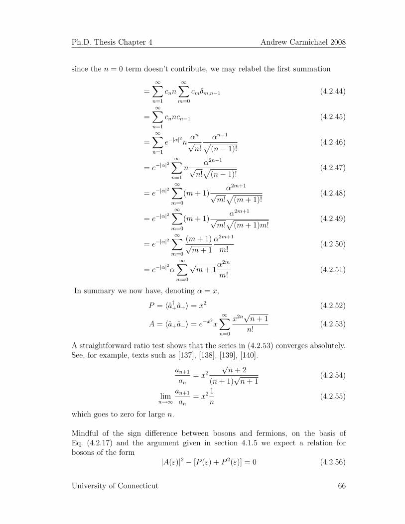
Ph.D. Thesis Chapter 4 Andrew Carmichael 2008
since the n = 0 term doesn’t contribute, we may relabel the first summation
=∞∑n=1
cnn∞∑m=0
cmδm,n−1 (4.2.44)
=∞∑n=1
cnncn−1 (4.2.45)
=∞∑n=1
e−|α|2
nαn√n!
αn−1√(n− 1)!
(4.2.46)
= e−|α|2∞∑n=1
nα2n−1
√n!√
(n− 1)!(4.2.47)
= e−|α|2∞∑m=0
(m+ 1)α2m+1
√m!√
(m+ 1)!(4.2.48)
= e−|α|2∞∑m=0
(m+ 1)α2m+1
√m!√
(m+ 1)m!(4.2.49)
= e−|α|2∞∑m=0
(m+ 1)√m+ 1
α2m+1
m!(4.2.50)
= e−|α|2
α∞∑m=0
√m+ 1
α2m
m!(4.2.51)
In summary we now have, denoting α = x,
P = 〈a†+a+〉 = x2 (4.2.52)
A = 〈a+a−〉 = e−x2
x∞∑n=0
x2n√n+ 1
n!(4.2.53)
A straightforward ratio test shows that the series in (4.2.53) converges absolutely.See, for example, texts such as [137], [138], [139], [140].
an+1
an= x2
√n+ 2
(n+ 1)√n+ 1
(4.2.54)
limn→∞
an+1
an= x2 1
n(4.2.55)
which goes to zero for large n.
Mindful of the sign difference between bosons and fermions, on the basis ofEq. (4.2.17) and the argument given in section 4.1.5 we expect a relation forbosons of the form
|A(ε)|2 − [P (ε) + P 2(ε)] = 0 (4.2.56)
University of Connecticut 66

Ph.D. Thesis Chapter 4 Andrew Carmichael 2008
To find out if it works, we define the function
f(x) :=A(x)√
P (x) + P 2(x)(4.2.57)
where A(x) and P (x) are evaluated using (4.2.52) and (4.2.53). This functionwould identically equal unity were the pairing Ansatz (4.2.56) exact. We plot thefunction f(x) in figure 4.1. One can see that the maximum deviation of this ratiofrom unity is about three per cent. We surmise that (4.2.56) is a reasonable ap-proximation between pairing amplitudes and occupation numbers for boson statesof the form (4.2.20). Moreover, heuristically, it is applicable whenever we expectatoms to emerge only in opposite momentum pairs as though from the dissocia-tion of molecules, as we do in this case.
The pairing assumption for bosons is further cemented by the observation that,fully analogously to the fermion theory, in our mean-field theory for bosons theleft-hand side of (4.2.56) is a constant of the motion, as elucidated in section4.1.5. This also gives an interesting piece of insight into the problem of findingthe steady state: There is a large (infinite) number of constants of the motion, sothat time evolution cannot possibly lead to a unique steady state.
Given that A(ε) is real and that it must be positive in the limit ε→∞ by virtueof equation (4.1.44), equations (4.2.56) may be solved for the pairing amplitudeand occupation numbers,
A(ε) =βΩ
2√
2(ε− µ)2 − β2Ω2(4.2.58)
P (ε) =1
2
[√[β2Ω2
2(ε− µ)2 − β2Ω2+ 1
]− 1
](4.2.59)
Hence, given the chemical potential ~µ and the amplitude of the molecular con-densate β, both the occupation numbers P (ε) and pairing amplitudes A(ε) areuniquely determined. The inequality
µ ≤ −βΩ√2
(4.2.60)
must hold, else complex occupation numbers would result. The equality presentsno problem, since the ensuing singularities in the occupation numbers and pairingamplitudes are sufficiently mild not to hamper the analysis.
4.3 Renormalization
Equations (4.1.42), (4.1.43) and (4.1.29) suffice to determine the remaining un-knowns α, β and µ, although a few issues remain. Next we discuss renormalization.
University of Connecticut 67

Ph.D. Thesis Chapter 4 Andrew Carmichael 2008
Fig. 4.1: The function f(x) for the poissonian paired state plotted with Maple.If the pairing approximation (4.2.56) were exact, this function wouldbe identically unity.
University of Connecticut 68
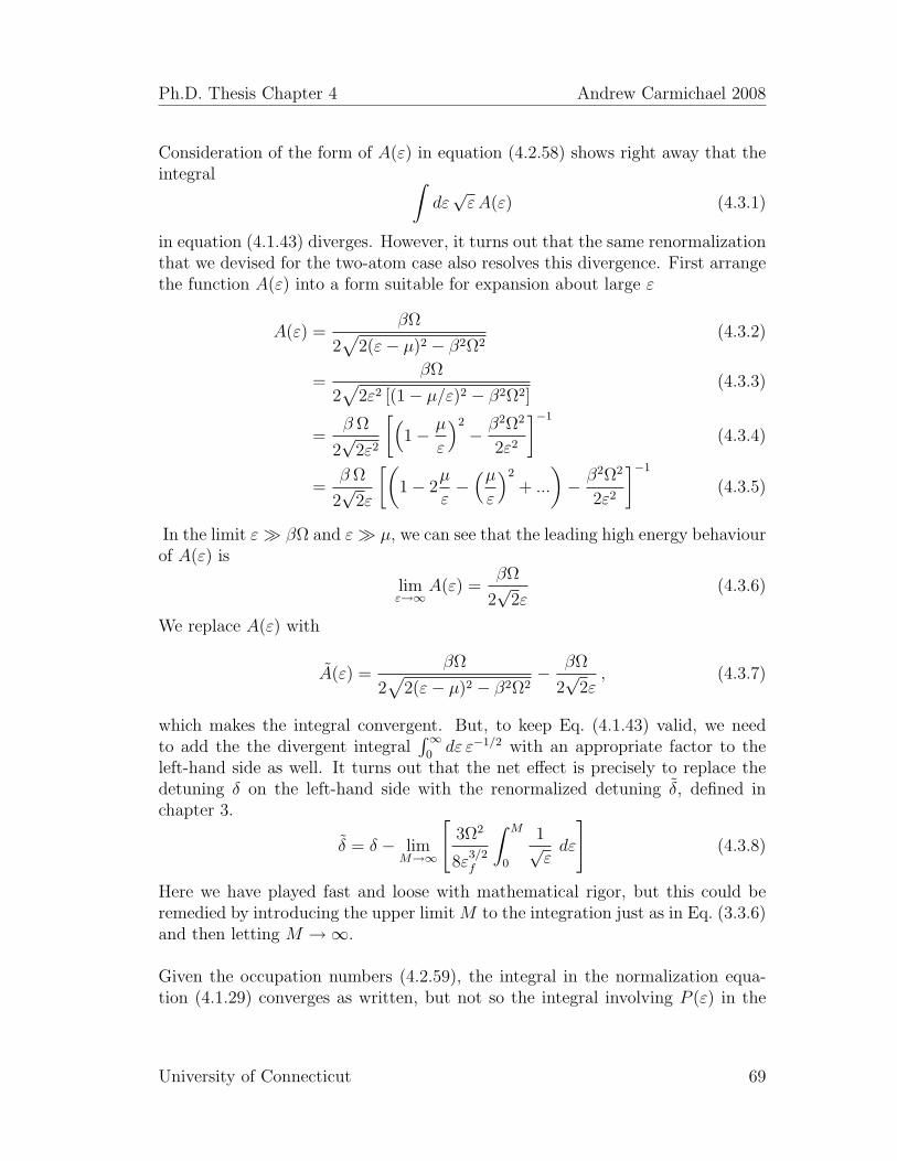
Ph.D. Thesis Chapter 4 Andrew Carmichael 2008
Consideration of the form of A(ε) in equation (4.2.58) shows right away that theintegral ∫
dε√εA(ε) (4.3.1)
in equation (4.1.43) diverges. However, it turns out that the same renormalizationthat we devised for the two-atom case also resolves this divergence. First arrangethe function A(ε) into a form suitable for expansion about large ε
A(ε) =βΩ
2√
2(ε− µ)2 − β2Ω2(4.3.2)
=βΩ
2√
2ε2 [(1− µ/ε)2 − β2Ω2](4.3.3)
=β Ω
2√
2ε2
[(1− µ
ε
)2
− β2Ω2
2ε2
]−1
(4.3.4)
=β Ω
2√
2ε
[(1− 2
µ
ε−(µε
)2
+ ...
)− β2Ω2
2ε2
]−1
(4.3.5)
In the limit ε βΩ and ε µ, we can see that the leading high energy behaviourof A(ε) is
limε→∞
A(ε) =βΩ
2√
2ε(4.3.6)
We replace A(ε) with
A(ε) =βΩ
2√
2(ε− µ)2 − β2Ω2− βΩ
2√
2ε, (4.3.7)
which makes the integral convergent. But, to keep Eq. (4.1.43) valid, we needto add the the divergent integral
∫∞0dε ε−1/2 with an appropriate factor to the
left-hand side as well. It turns out that the net effect is precisely to replace thedetuning δ on the left-hand side with the renormalized detuning δ, defined inchapter 3.
δ = δ − limM→∞
[3Ω2
8ε3/2f
∫ M
0
1√εdε
](4.3.8)
Here we have played fast and loose with mathematical rigor, but this could beremedied by introducing the upper limit M to the integration just as in Eq. (3.3.6)and then letting M →∞.
Given the occupation numbers (4.2.59), the integral in the normalization equa-tion (4.1.29) converges as written, but not so the integral involving P (ε) in the
University of Connecticut 69
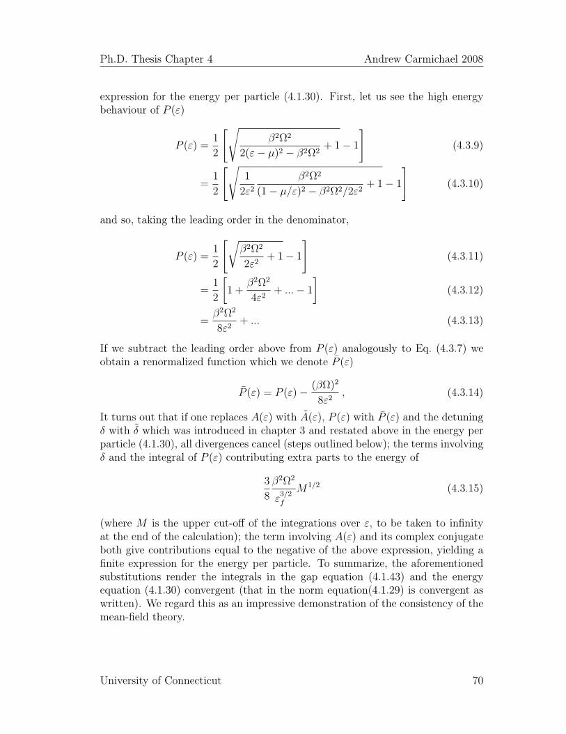
Ph.D. Thesis Chapter 4 Andrew Carmichael 2008
expression for the energy per particle (4.1.30). First, let us see the high energybehaviour of P (ε)
P (ε) =1
2
[√β2Ω2
2(ε− µ)2 − β2Ω2+ 1− 1
](4.3.9)
=1
2
[√1
2ε2
β2Ω2
(1− µ/ε)2 − β2Ω2/2ε2+ 1− 1
](4.3.10)
and so, taking the leading order in the denominator,
P (ε) =1
2
[√β2Ω2
2ε2+ 1− 1
](4.3.11)
=1
2
[1 +
β2Ω2
4ε2+ ...− 1
](4.3.12)
=β2Ω2
8ε2+ ... (4.3.13)
If we subtract the leading order above from P (ε) analogously to Eq. (4.3.7) weobtain a renormalized function which we denote P (ε)
P (ε) = P (ε)− (βΩ)2
8ε2, (4.3.14)
It turns out that if one replaces A(ε) with A(ε), P (ε) with P (ε) and the detuningδ with δ which was introduced in chapter 3 and restated above in the energy perparticle (4.1.30), all divergences cancel (steps outlined below); the terms involvingδ and the integral of P (ε) contributing extra parts to the energy of
3
8
β2Ω2
ε3/2f
M1/2 (4.3.15)
(where M is the upper cut-off of the integrations over ε, to be taken to infinityat the end of the calculation); the term involving A(ε) and its complex conjugateboth give contributions equal to the negative of the above expression, yielding afinite expression for the energy per particle. To summarize, the aforementionedsubstitutions render the integrals in the gap equation (4.1.43) and the energyequation (4.1.30) convergent (that in the norm equation(4.1.29) is convergent aswritten). We regard this as an impressive demonstration of the consistency of themean-field theory.
University of Connecticut 70
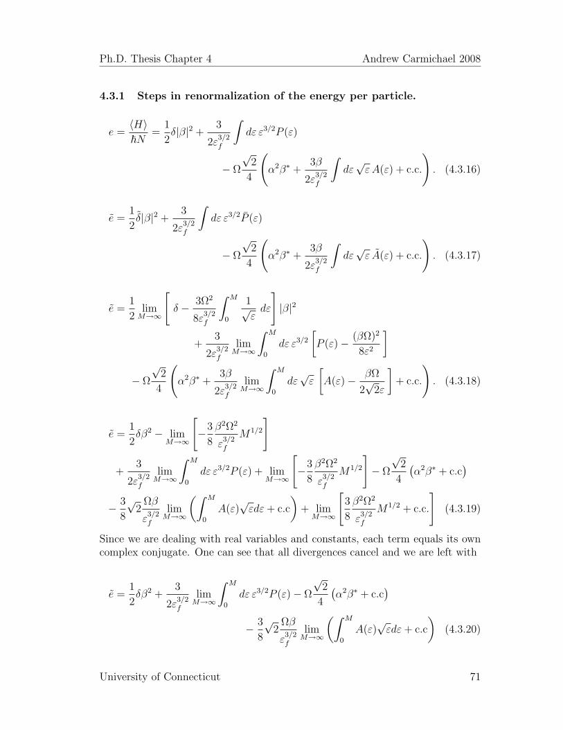
Ph.D. Thesis Chapter 4 Andrew Carmichael 2008
4.3.1 Steps in renormalization of the energy per particle.
e =〈H〉~N
=1
2δ|β|2 +
3
2ε3/2f
∫dε ε3/2P (ε)
− Ω
√2
4
(α2β∗ +
3β
2ε3/2f
∫dε√εA(ε) + c.c.
). (4.3.16)
e =1
2δ|β|2 +
3
2ε3/2f
∫dε ε3/2P (ε)
− Ω
√2
4
(α2β∗ +
3β
2ε3/2f
∫dε√ε A(ε) + c.c.
). (4.3.17)
e =1
2limM→∞
[δ − 3Ω2
8ε3/2f
∫ M
0
1√εdε
]|β|2
+3
2ε3/2f
limM→∞
∫ M
0
dε ε3/2
[P (ε)− (βΩ)2
8ε2
]
− Ω
√2
4
(α2β∗ +
3β
2ε3/2f
limM→∞
∫ M
0
dε√ε
[A(ε)− βΩ
2√
2ε
]+ c.c.
). (4.3.18)
e =1
2δβ2 − lim
M→∞
[−3
8
β2Ω2
ε3/2f
M1/2
]
+3
2ε3/2f
limM→∞
∫ M
0
dε ε3/2P (ε) + limM→∞
[−3
8
β2Ω2
ε3/2f
M1/2
]− Ω
√2
4
(α2β∗ + c.c
)− 3
8
√2
Ωβ
ε3/2f
limM→∞
(∫ M
0
A(ε)√εdε+ c.c
)+ lim
M→∞
[3
8
β2Ω2
ε3/2f
M1/2 + c.c.
](4.3.19)
Since we are dealing with real variables and constants, each term equals its owncomplex conjugate. One can see that all divergences cancel and we are left with
e =1
2δβ2 +
3
2ε3/2f
limM→∞
∫ M
0
dε ε3/2P (ε)− Ω
√2
4
(α2β∗ + c.c
)− 3
8
√2
Ωβ
ε3/2f
limM→∞
(∫ M
0
A(ε)√εdε+ c.c
)(4.3.20)
University of Connecticut 71

Ph.D. Thesis Chapter 4 Andrew Carmichael 2008
e =1
2δβ2 +
3
2ε3/2f
∫ ∞0
dε ε3/2P (ε)− Ω
√2
4
(α2β∗ + c.c
)− 3
8
√2
Ωβ
ε3/2f
(∫ ∞0
A(ε)√εdε+ c.c
)(4.3.21)
which equals the energy e.
4.4 Equations of the Mean-Field Model
We are now to deal with the equations
α
(µ+
βΩ√2
)= 0 (4.4.1)
(2µ− δ
)β +
1
2
√2 Ω
[α2 +
3
84√
2(β Ω)3/2
εf 3/2A1/2(m)
]= 0 (4.4.2)
α2 + β2 +3
84√
2(β Ω)3/2
εf 3/2P1/2(m)− 1 = 0 (4.4.3)
where m is a dimensionless variable defined on the interval m ∈ [0,∞) by
m := −√
2µ
βΩ(4.4.4)
Equation (4.4.2) is analogous to the usual gap equation in BCS theory (see, forexample [129], [64], [67], [66], [126], [128] for good general treatments at differentlevels) while (4.4.3) is the original norm equation coming from conservation ofparticles, and they shall henceforth be referred to as such.The energy per particle is found from the substitution for P (ε) from (4.2.59) and(4.3.14), for A(ε) from (4.2.58) and (4.3.7) into (4.1.30) (or (4.3.16)) and aftersome manipulation can be shown to be given by
e =1
2β2δ − 1
2
√2β Ω
[α2 +
3
84√
2(β Ω)3/2
εf 3/2
(A1/2(m)− P3/2(m)
)](4.4.5)
The functions A1/2(m), P1/2(m) and P3/2(m) are the integrals whose provenanceis the summation over k in the norm and in the mean field equations (ultimately
University of Connecticut 72
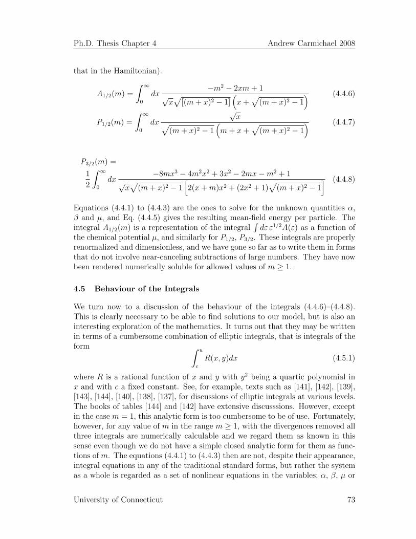
Ph.D. Thesis Chapter 4 Andrew Carmichael 2008
that in the Hamiltonian).
A1/2(m) =
∫ ∞0
dx−m2 − 2xm+ 1
√x√
[(m+ x)2 − 1](x+
√(m+ x)2 − 1
) (4.4.6)
P1/2(m) =
∫ ∞0
dx
√x√
(m+ x)2 − 1(m+ x+
√(m+ x)2 − 1
) (4.4.7)
P3/2(m) =
1
2
∫ ∞0
dx−8mx3 − 4m2x2 + 3x2 − 2mx−m2 + 1
√x√
(m+ x)2 − 1[2(x+m)x2 + (2x2 + 1)
√(m+ x)2 − 1
] (4.4.8)
Equations (4.4.1) to (4.4.3) are the ones to solve for the unknown quantities α,β and µ, and Eq. (4.4.5) gives the resulting mean-field energy per particle. Theintegral A1/2(m) is a representation of the integral
∫dε ε1/2A(ε) as a function of
the chemical potential µ, and similarly for P1/2, P3/2. These integrals are properlyrenormalized and dimensionless, and we have gone so far as to write them in formsthat do not involve near-canceling subtractions of large numbers. They have nowbeen rendered numerically soluble for allowed values of m ≥ 1.
4.5 Behaviour of the Integrals
We turn now to a discussion of the behaviour of the integrals (4.4.6)–(4.4.8).This is clearly necessary to be able to find solutions to our model, but is also aninteresting exploration of the mathematics. It turns out that they may be writtenin terms of a cumbersome combination of elliptic integrals, that is integrals of theform ∫ u
c
R(x, y)dx (4.5.1)
where R is a rational function of x and y with y2 being a quartic polynomial inx and with c a fixed constant. See, for example, texts such as [141], [142], [139],[143], [144], [140], [138], [137], for discussions of elliptic integrals at various levels.The books of tables [144] and [142] have extensive discusssions. However, exceptin the case m = 1, this analytic form is too cumbersome to be of use. Fortunately,however, for any value of m in the range m ≥ 1, with the divergences removed allthree integrals are numerically calculable and we regard them as known in thissense even though we do not have a simple closed analytic form for them as func-tions of m. The equations (4.4.1) to (4.4.3) then are not, despite their appearance,integral equations in any of the traditional standard forms, but rather the systemas a whole is regarded as a set of nonlinear equations in the variables; α, β, µ or
University of Connecticut 73

Ph.D. Thesis Chapter 4 Andrew Carmichael 2008
m with the parameters Ω and δ.
In the case where m = 1, the integrals simplify to
A1/2(1) = 2
∫ ∞0
√x√
2x+ x2(x+√
2x+ x2) (4.5.2)
P1/2(1) =
∫ ∞0
√x√
x2 + 2x(x+ 1 +
√x2 + 2x
)dx (4.5.3)
P3/2(1) = −1
2
∫ ∞0
x+ 8x2 + 2√x+ 2
√x(2x2√x+ 2 +
√x+ 2 + 2x5/2 + 2x3/2
)dx (4.5.4)
The integral A1/2(1) turns out to be writeable in terms of the Meijer G function.This function is defined as the Laplace transform of a combination of productsof Gamma functions. In standard form it has as parameters four vectors and oneargument. One can equivalently write two vectors a and b with extra parametersn and m delimiting the products which should belong to the numerator from thosewhich belong in the denominator. The standard definition is then
Gm,np,q
(x
∣∣∣∣a1, . . . , an, an+1, . . . , apb1, . . . , bm, bm+1, . . . , bq
)=
1
2πi
∫Πmj=1Γ(bj − s)Πn
j=1Γ(1− aj + s)
Πpj=n+1Γ(aj − s)Πq
j=m+1Γ(1− bj + s)xsds (4.5.5)
In our case, the integral A1/2(1) reduces to a Meijer G function with a multiplica-tive constant
A1/2(1) = − 1
2π
√2G3,2
3,3
(1
∣∣∣∣ 1, 1, 2
1, 1/2, 1/2,
)(4.5.6)
In Maple [145] notation the MeijerG function is written
MeijerG([[1,1], [2]], [[1,1/2,1/2], []],1) (4.5.7)
The MeijerG function is defined by the a and b vectors given by;
(a1, ...., an) = (a1, a2) = (1, 1) (4.5.8)
(an+1, ......., ap) = (a1) = (2) (4.5.9)
(b1, ....., bm) = (b1, b2, b3) = (1, 1/2, 1/2) (4.5.10)
(bm+1, ....., bq) = () = () (4.5.11)
which means that n = 2, p = 3, m = 3 and q = 3 while x = 1. Moreover, it turnsout that
G3,23,3
(1
∣∣∣∣ 1, 1, 2
1, 1/2, 1/2,
)= 4π (4.5.12)
University of Connecticut 74
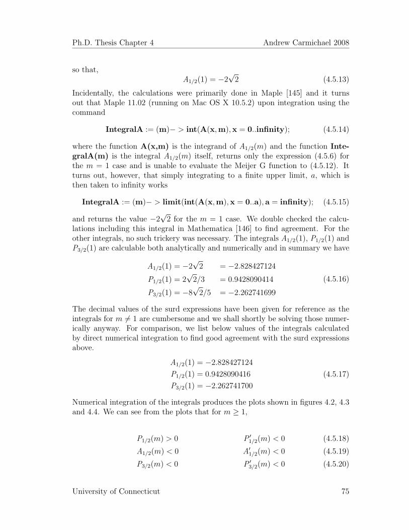
Ph.D. Thesis Chapter 4 Andrew Carmichael 2008
so that,A1/2(1) = −2
√2 (4.5.13)
Incidentally, the calculations were primarily done in Maple [145] and it turnsout that Maple 11.02 (running on Mac OS X 10.5.2) upon integration using thecommand
IntegralA := (m)− > int(A(x,m),x = 0..infinity); (4.5.14)
where the function A(x,m) is the integrand of A1/2(m) and the function Inte-gralA(m) is the integral A1/2(m) itself, returns only the expression (4.5.6) forthe m = 1 case and is unable to evaluate the Meijer G function to (4.5.12). Itturns out, however, that simply integrating to a finite upper limit, a, which isthen taken to infinity works
IntegralA := (m)− > limit(int(A(x,m),x = 0..a), a = infinity); (4.5.15)
and returns the value −2√
2 for the m = 1 case. We double checked the calcu-lations including this integral in Mathematica [146] to find agreement. For theother integrals, no such trickery was necessary. The integrals A1/2(1), P1/2(1) andP3/2(1) are calculable both analytically and numerically and in summary we have
A1/2(1) = −2√
2 = −2.828427124
P1/2(1) = 2√
2/3 = 0.9428090414
P3/2(1) = −8√
2/5 = −2.262741699
(4.5.16)
The decimal values of the surd expressions have been given for reference as theintegrals for m 6= 1 are cumbersome and we shall shortly be solving those numer-ically anyway. For comparison, we list below values of the integrals calculatedby direct numerical integration to find good agreement with the surd expressionsabove.
A1/2(1) = −2.828427124
P1/2(1) = 0.9428090416
P3/2(1) = −2.262741700
(4.5.17)
Numerical integration of the integrals produces the plots shown in figures 4.2, 4.3and 4.4. We can see from the plots that for m ≥ 1,
P1/2(m) > 0 P ′1/2(m) < 0 (4.5.18)
A1/2(m) < 0 A′1/2(m) < 0 (4.5.19)
P3/2(m) < 0 P ′3/2(m) < 0 (4.5.20)
University of Connecticut 75
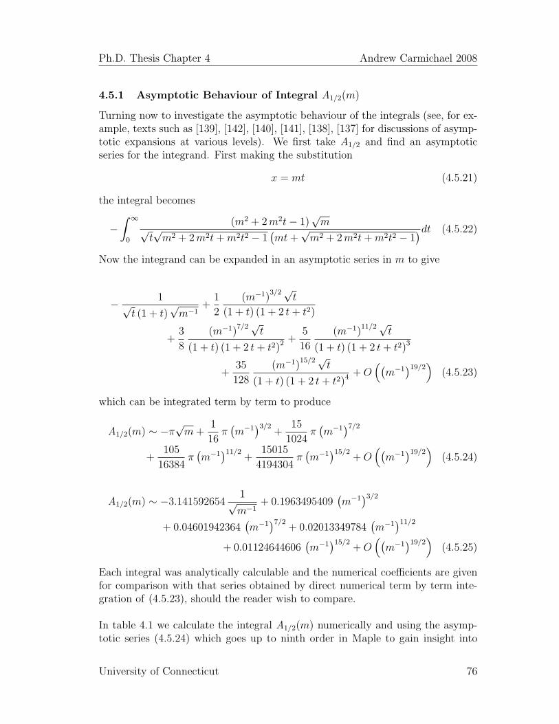
Ph.D. Thesis Chapter 4 Andrew Carmichael 2008
4.5.1 Asymptotic Behaviour of Integral A1/2(m)
Turning now to investigate the asymptotic behaviour of the integrals (see, for ex-ample, texts such as [139], [142], [140], [141], [138], [137] for discussions of asymp-totic expansions at various levels). We first take A1/2 and find an asymptoticseries for the integrand. First making the substitution
x = mt (4.5.21)
the integral becomes
−∫ ∞
0
(m2 + 2m2t− 1)√m√
t√m2 + 2m2t+m2t2 − 1
(mt+
√m2 + 2m2t+m2t2 − 1
)dt (4.5.22)
Now the integrand can be expanded in an asymptotic series in m to give
− 1√t (1 + t)
√m−1
+1
2
(m−1)3/2√
t
(1 + t) (1 + 2 t+ t2)
+3
8
(m−1)7/2√
t
(1 + t) (1 + 2 t+ t2)2 +5
16
(m−1)11/2√
t
(1 + t) (1 + 2 t+ t2)3
+35
128
(m−1)15/2√
t
(1 + t) (1 + 2 t+ t2)4 +O((m−1
)19/2)
(4.5.23)
which can be integrated term by term to produce
A1/2(m) ∼ −π√m+
1
16π(m−1
)3/2+
15
1024π(m−1
)7/2
+105
16384π(m−1
)11/2+
15015
4194304π(m−1
)15/2+O
((m−1
)19/2)
(4.5.24)
A1/2(m) ∼ −3.1415926541√m−1
+ 0.1963495409(m−1
)3/2
+ 0.04601942364(m−1
)7/2+ 0.02013349784
(m−1
)11/2
+ 0.01124644606(m−1
)15/2+O
((m−1
)19/2)
(4.5.25)
Each integral was analytically calculable and the numerical coefficients are givenfor comparison with that series obtained by direct numerical term by term inte-gration of (4.5.23), should the reader wish to compare.
In table 4.1 we calculate the integral A1/2(m) numerically and using the asymp-totic series (4.5.24) which goes up to ninth order in Maple to gain insight into
University of Connecticut 76

Ph.D. Thesis Chapter 4 Andrew Carmichael 2008
the accuracy of the expansion. Of course, an asymptotic expansion would not bevalid for small values of the argument m and the first entry for m = 1 is purelyfor comparison. For higher values of m we can see that the expansion becomesquite valid for any m higher than around 20.
4.5.2 Asymptotic Behaviour of Integral P1/2(m)
The same procedure can be applied to the integral (4.4.7). Making the samesubstitution (4.5.21) the integrand becomes
m3/2√t√
m2t2 + 2m2t+m2 − 1(mt+m+
√m2t2 + 2m2t+m2 − 1
) (4.5.26)
and an asymptotic expansion of the integrand can be obtained, viz.
1
2
√t√m−1
(1 + t)2 +3
8
√t (m−1)
5/2
(1 + t)2 (t2 + 2 t+ 1)
+5
16
√t (m−1)
9/2
(1 + t)2 (t2 + 2 t+ 1)2 +35
128
√t (m−1)
13/2
(1 + t)2 (t2 + 2 t+ 1)3
+63
256
√t (m−1)
17/2
(1 + t)2 (t2 + 2 t+ 1)4 +O((m−1
)21/2)
(4.5.27)
which can be integrated term by term to produce
P1/2(m) ∼ 1
4π√m−1 +
3
128π(m−1
)5/2+
35
4096π(m−1
)9/2
+1155
262144π(m−1
)13/2+
45045
16777216π(m−1
)17/2+O
((m−1
)21/2)
(4.5.28)
P1/2(m) ∼ 0.7853981635√m−1 + 0.07363107783
(m−1
)5/2
+ 0.02684466379(m−1
)9/2+ 0.01384177977
(m−1
)13/2
+ 0.008434834546(m−1
)17/2+O
((m−1
)21/2)
(4.5.29)
In table 4.2 we again list values for the integral (4.4.7) found via direct numericalintegration and via the series 4.5.28 to show good agreement.
4.5.3 Asymptotic Behaviour of Integral P3/2(m)
For the integral (4.4.8) we use the same procedure. Firstly, the integrand can berecast using substitution (4.5.21). The result is cumbersome, and so we state the
University of Connecticut 77
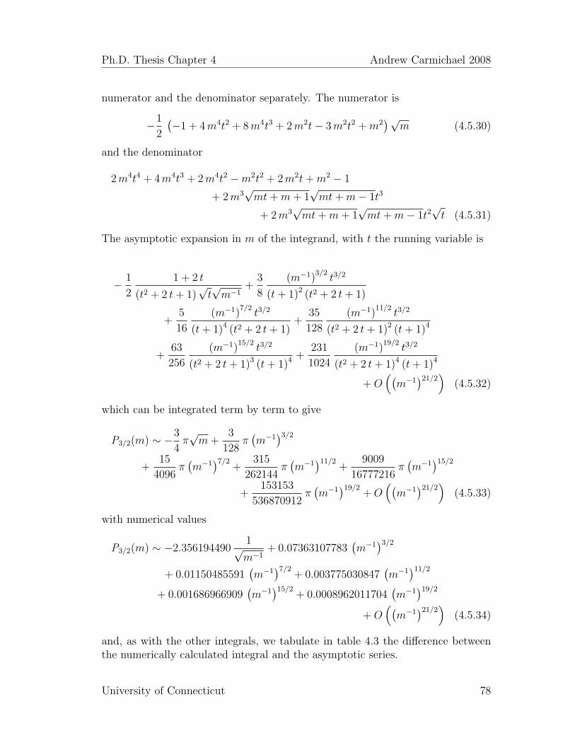
Ph.D. Thesis Chapter 4 Andrew Carmichael 2008
numerator and the denominator separately. The numerator is
−1
2
(−1 + 4m4t2 + 8m4t3 + 2m2t− 3m2t2 +m2
)√m (4.5.30)
and the denominator
2m4t4 + 4m4t3 + 2m4t2 −m2t2 + 2m2t+m2 − 1
+ 2m3√mt+m+ 1
√mt+m− 1t3
+ 2m3√mt+m+ 1
√mt+m− 1t2
√t (4.5.31)
The asymptotic expansion in m of the integrand, with t the running variable is
− 1
2
1 + 2 t
(t2 + 2 t+ 1)√t√m−1
+3
8
(m−1)3/2t3/2
(t+ 1)2 (t2 + 2 t+ 1)
+5
16
(m−1)7/2t3/2
(t+ 1)4 (t2 + 2 t+ 1)+
35
128
(m−1)11/2
t3/2
(t2 + 2 t+ 1)2 (t+ 1)4
+63
256
(m−1)15/2
t3/2
(t2 + 2 t+ 1)3 (t+ 1)4 +231
1024
(m−1)19/2
t3/2
(t2 + 2 t+ 1)4 (t+ 1)4
+O((m−1
)21/2)
(4.5.32)
which can be integrated term by term to give
P3/2(m) ∼ −3
4π√m+
3
128π(m−1
)3/2
+15
4096π(m−1
)7/2+
315
262144π(m−1
)11/2+
9009
16777216π(m−1
)15/2
+153153
536870912π(m−1
)19/2+O
((m−1
)21/2)
(4.5.33)
with numerical values
P3/2(m) ∼ −2.3561944901√m−1
+ 0.07363107783(m−1
)3/2
+ 0.01150485591(m−1
)7/2+ 0.003775030847
(m−1
)11/2
+ 0.001686966909(m−1
)15/2+ 0.0008962011704
(m−1
)19/2
+O((m−1
)21/2)
(4.5.34)
and, as with the other integrals, we tabulate in table 4.3 the difference betweenthe numerically calculated integral and the asymptotic series.
University of Connecticut 78

Ph.D. Thesis Chapter 4 Andrew Carmichael 2008
mIn
tegr
alA
1/2(m
)A
sym
pto
tic
seri
es(4
.5.2
4)D
iffer
ence
1-2
.828
4271
2474
6190
0976
0337
7-2
.867
8437
4520
3242
3248
9031
13.
94×
10−
2
20-1
4.04
7432
9197
8716
9609
1277
6-1
4.04
7432
9197
8717
2745
7582
73.
14×
10−
15
30-1
7.20
6016
3720
4941
7524
4776
9-1
7.20
6016
3720
4941
7591
0322
86.
66×
10−
17
40-1
9.86
8400
2781
6049
8463
5750
2-1
9.86
8400
2781
6049
8467
9012
94.
33×
10−
18
50-2
2.21
3859
2783
5041
3590
3861
8-2
2.21
3859
2783
5041
3590
9054
55.
19×
10−
19
100
-31.
4157
3018
1754
9393
1266
653
-31.
4157
3018
1754
9393
1266
725
7.17×
10−
22
Tab
le4.1
:A
ccura
cyof
asym
pto
tic
form
(4.5
.24)
ofA
1/2(m
).
University of Connecticut 79
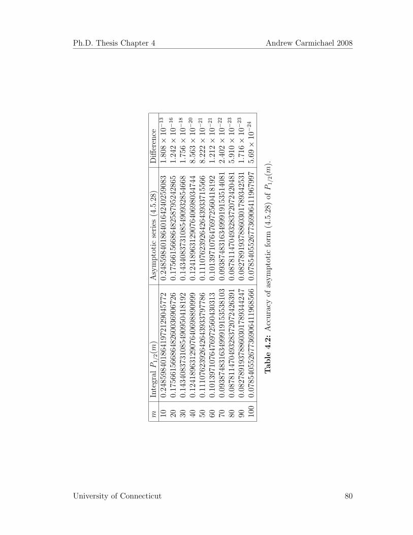
Ph.D. Thesis Chapter 4 Andrew Carmichael 2008
mIn
tegr
alP
1/2(m
)A
sym
pto
tic
seri
es(4
.5.2
8)D
iffer
ence
100.
2485
9840
1864
1972
1290
4577
20.
2485
9840
1864
0164
2402
5908
31.
808×
10−
13
200.
1756
6156
6864
8260
0369
0672
60.
1756
6156
6864
8258
7952
4286
51.
242×
10−
16
300.
1434
0837
3108
5490
9504
1819
20.
1434
0837
3108
5490
9328
5466
81.
756×
10−
18
400.
1241
8963
1290
7640
6988
9099
90.
1241
8963
1290
7640
6980
3474
48.
563×
10−
20
500.
1110
7623
9264
2643
9337
9778
60.
1110
7623
9264
2643
9337
1556
68.
222×
10−
21
600.
1013
9710
7647
6972
5604
3031
30.
1013
9710
7647
6972
5604
1819
21.
212×
10−
21
700.
0938
7483
1634
9991
9153
5381
030.
0938
7483
1634
9991
9153
5140
812.
402×
10−
22
800.
0878
1147
0493
2837
2072
4263
910.
0878
1147
0493
2837
2072
4204
815.
910×
10−
23
900.
0827
8919
3788
6030
1789
3442
470.
0827
8919
3788
6030
1789
3425
311.
716×
10−
23
100
0.07
8540
5526
7736
9064
1196
8566
0.07
8540
5526
7736
9064
1196
7997
5.69×
10−
24
Table
4.2
:A
ccura
cyof
asym
pto
tic
form
(4.5
.28)
ofP
1/2(m
).
University of Connecticut 80

Ph.D. Thesis Chapter 4 Andrew Carmichael 2008
mIn
tegr
alP
3/2(m
)A
sym
pto
tic
seri
es(4
.5.3
3)D
iffer
ence
10-
7.44
8609
1300
7607
0087
7545
64-
7.44
8609
1300
7607
1781
3365
571.
6935
820×
10−
15
20-
10.5
3639
8554
2502
1380
9764
73-
10.5
3639
8554
2502
1381
0346
655.
8192×
10−
19
30-
12.9
0496
0539
1835
3422
5439
36-
12.9
0496
0539
1835
3422
5444
855.
49×
10−
21
40-
14.9
0159
1317
8746
3675
5483
41-
14.9
0159
1317
8746
3675
5483
612.
00×
10−
22
50-
16.6
6060
2744
9381
7995
5625
06-
16.6
6060
2744
9381
7995
5625
082.
0×
10−
23
60-
18.2
5084
5606
1498
4413
0748
28-
18.2
5084
5606
1498
4413
0748
280.
070
-19
.713
2117
2001
3062
6042
5551
-19
.713
2117
2001
3062
6042
5551
0.0
80-
21.0
7434
1288
0502
4411
8263
95-
21.0
7434
1288
0502
4411
8263
950.
090
-22
.352
7373
5863
2260
8170
5308
-22
.352
7373
5863
2260
8170
5307
1.0×
10−
23
100
-23
.561
8712
6969
5107
4347
8106
-23
.561
8712
6969
5107
4347
8106
0.0
Table
4.3
:A
ccura
cyof
asym
pto
tic
form
(4.5
.33)
ofP
3/2(m
).
University of Connecticut 81

Ph.D. Thesis Chapter 4 Andrew Carmichael 2008
m1 2 3 4 5 6 7 8 9 10
A12
(m)
K9
K8
K7
K6
K5
K4
K3
Fig. 4.2: Integral A1/2(m) plotted numerically with Maple
University of Connecticut 82

Ph.D. Thesis Chapter 4 Andrew Carmichael 2008
m10 20 30 40 50
P12
m
0.2
0.3
0.4
0.5
0.6
0.7
0.8
0.9
Fig. 4.3: Integral P1/2(m) plotted numerically with Maple
University of Connecticut 83
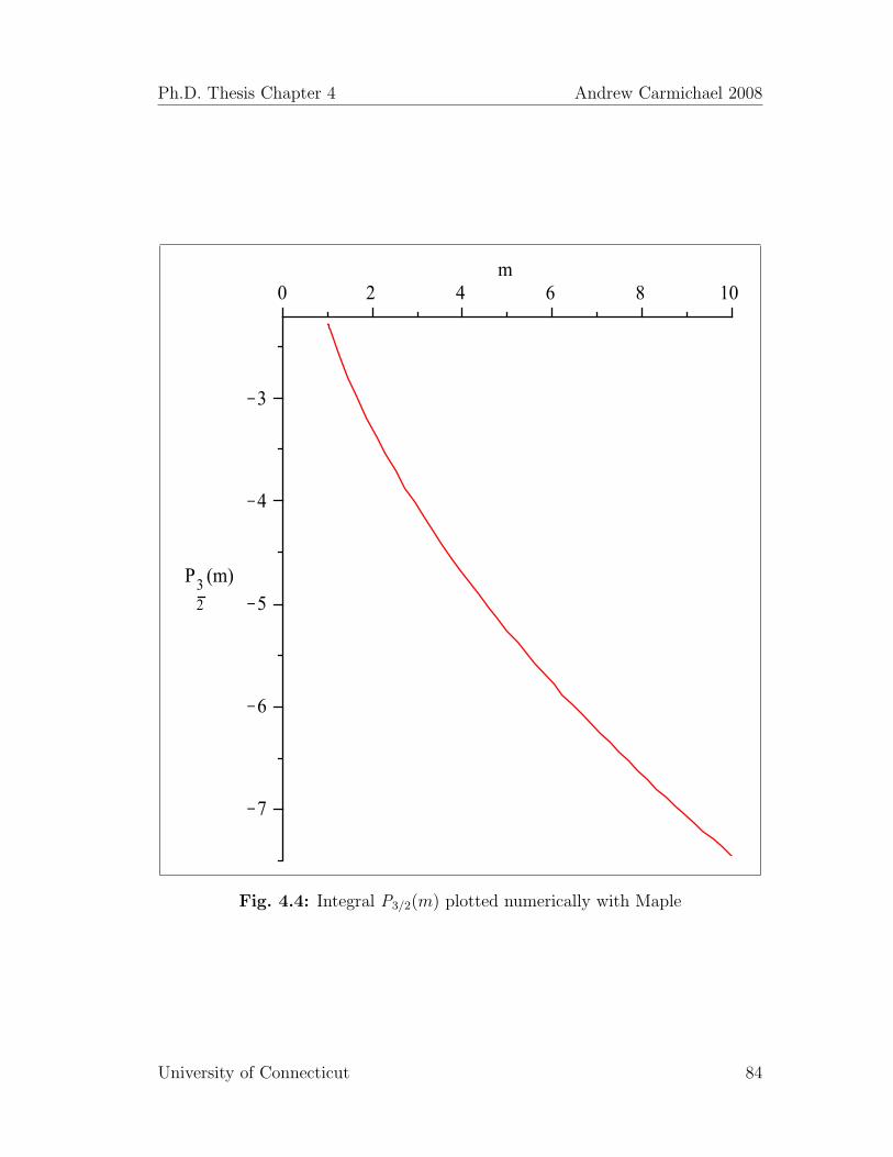
Ph.D. Thesis Chapter 4 Andrew Carmichael 2008
m0 2 4 6 8 10
P32
(m)
K7
K6
K5
K4
K3
Fig. 4.4: Integral P3/2(m) plotted numerically with Maple
University of Connecticut 84
Chapter 5
Solution of the Model
5.1 Solutions: Atomic Condensate Present
Equation (4.4.1) can clearly be satisfied by choosing either
α = 0 (5.1.1)
(no atomic condensate present) or
(µ+ βΩ/√
2) = 0 (5.1.2)
which is equivalent to
m = 1 (5.1.3)
In this section we examine the latter case, where m = 1 and the atomic condensateamplitude need not be zero. The integrals in the equations then take the valueslisted in (4.5.16). The equations have now become
µ = −βΩ√2
(5.1.4)
(2µ− δ
)β +
1
2
√2 Ω
[α2 +
3
84√
2(β Ω)3/2
εf 3/2A1/2(1)
]= 0 (5.1.5)
α2 + β2 +3
84√
2(β Ω)3/2
εf 3/2P1/2(1)− 1 = 0 (5.1.6)
With the values of the integrals for m = 1 (4.5.16), the equations become
µ = −βΩ√2
(5.1.7)
(2µ− δ
)β +
1
2Ω√
2
[α2 − 3
423/4 (β Ω)3/2
εf 3/2
]= 0 (5.1.8)
α2 + β2 + 23/4 1
4
1
εf 3/2(β Ω)3/2 − 1 = 0 (5.1.9)
85
Ph.D. Thesis Chapter 5 Andrew Carmichael 2008
The expression for the single particle energy (4.4.5) in this case becomes
e(α, β,Ω, δ) =1
2β2δ
− 1
2
√2β Ω
[α2 +
3
84√
2(β Ω)3/2
εf 3/2
(A1/2(1)− P3/2(1)
)](5.1.10)
which with the values of the integrals for m = 1 (4.5.16) becomes
e(α, β,Ω, δ) =1
2β2δ − 1
2
√2 β Ω
[α2 − 3
2023/4 (β Ω)3/2
εf 3/2
](5.1.11)
We can eliminate δ, β and Ω from the expression for the single particle energyby utilising the equations (5.1.7) to (5.1.9). The procedure is to eliminate δ fromthe energy equation using (5.1.8), then eliminate the terms in βΩ from the energyand norm equations using (5.1.7), and finally use the new norm equation (whichis in only α, β2, µ to eliminate β2 from the energy equation yielding
e(µ, α) = µ− 1
2µα2 −
√2
1
20
µ (−µ)3/2
εf 3/2(5.1.12)
which can also be expressed in terms of β with the slightly more cumbersome formin terms of β and Ω as
e (β,Ω) = −1
4β Ω√
2− 1
104√
2β2Ω2
√β Ω
εf 3/2− 1
4β3Ω√
2 (5.1.13)
From the gap (5.1.8) and norm (5.1.9) equations come the following expressions foralpha squared which must be real positive and thus constrain the other variables.
α2 (β, µ,Ω, δ) = −2√
2β µ
Ω+√
2β δ
Ω+ 23/4 3
4
(β Ω)3/2
εf 3/2≥ 0 (5.1.14)
α2 (β,Ω) = 1− β2 − 23/4 1
4
(β Ω)3/2
εf 3/2≥ 0 (5.1.15)
We can eliminate α and µ from the equations (5.1.7), (5.1.8) and (5.1.9) (oralternatively by equating the above equations (5.1.15) and (5.1.14) and using(5.1.7)) to find an equation relating β to the parameters Ω, δ and εf .
β2 + 2β +√
2δ
Ω+ 23/4
(β
Ω
εf
)3/2
− 1 = 0 (5.1.16)
University of Connecticut 86
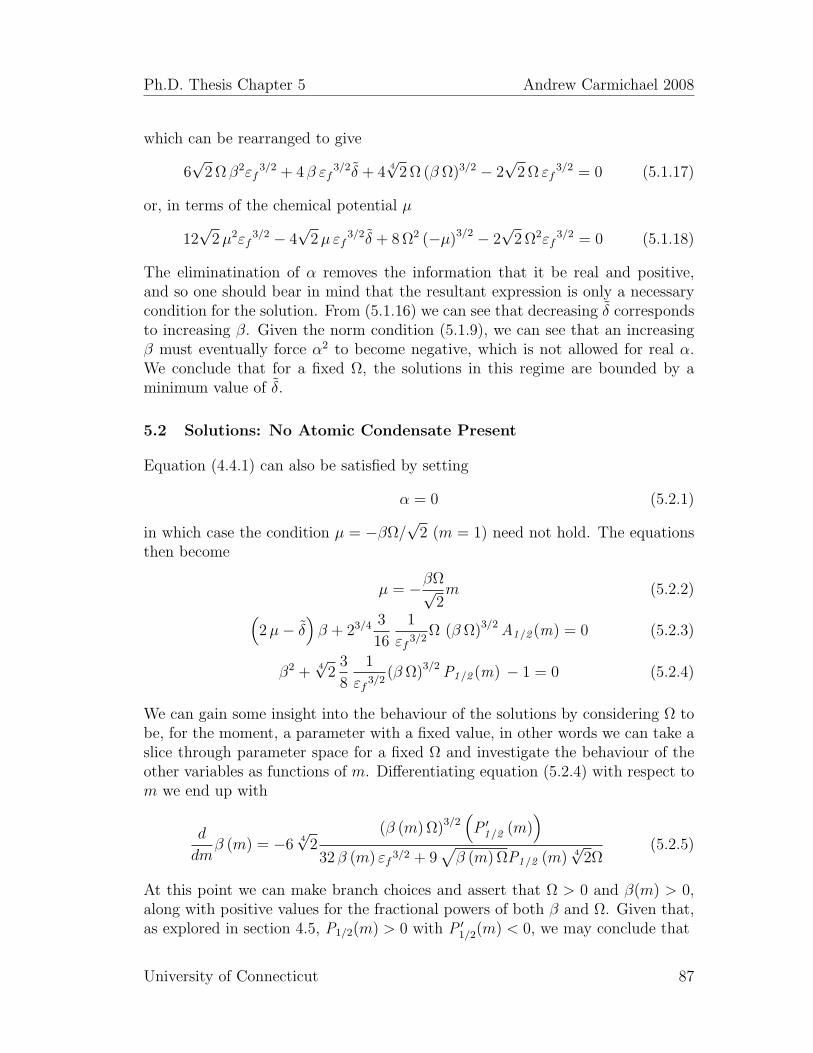
Ph.D. Thesis Chapter 5 Andrew Carmichael 2008
which can be rearranged to give
6√
2 Ω β2εf3/2 + 4 β εf
3/2δ + 44√
2 Ω (β Ω)3/2 − 2√
2 Ω εf3/2 = 0 (5.1.17)
or, in terms of the chemical potential µ
12√
2µ2εf3/2 − 4
√2µ εf
3/2δ + 8 Ω2 (−µ)3/2 − 2√
2 Ω2εf3/2 = 0 (5.1.18)
The eliminatination of α removes the information that it be real and positive,and so one should bear in mind that the resultant expression is only a necessarycondition for the solution. From (5.1.16) we can see that decreasing δ correspondsto increasing β. Given the norm condition (5.1.9), we can see that an increasingβ must eventually force α2 to become negative, which is not allowed for real α.We conclude that for a fixed Ω, the solutions in this regime are bounded by aminimum value of δ.
5.2 Solutions: No Atomic Condensate Present
Equation (4.4.1) can also be satisfied by setting
α = 0 (5.2.1)
in which case the condition µ = −βΩ/√
2 (m = 1) need not hold. The equationsthen become
µ = −βΩ√2m (5.2.2)(
2µ− δ)β + 23/4 3
16
1
εf 3/2Ω (β Ω)3/2 A1/2 (m) = 0 (5.2.3)
β2 +4√
23
8
1
εf 3/2(β Ω)3/2 P1/2 (m) − 1 = 0 (5.2.4)
We can gain some insight into the behaviour of the solutions by considering Ω tobe, for the moment, a parameter with a fixed value, in other words we can take aslice through parameter space for a fixed Ω and investigate the behaviour of theother variables as functions of m. Differentiating equation (5.2.4) with respect tom we end up with
d
dmβ (m) = −6
4√
2(β (m) Ω)3/2
(P ′1/2 (m)
)32 β (m) εf 3/2 + 9
√β (m) ΩP1/2 (m) 4
√2Ω
(5.2.5)
At this point we can make branch choices and assert that Ω > 0 and β(m) > 0,along with positive values for the fractional powers of both β and Ω. Given that,as explored in section 4.5, P1/2(m) > 0 with P ′1/2(m) < 0, we may conclude that
University of Connecticut 87
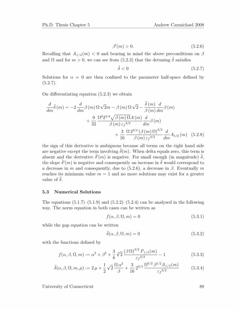
Ph.D. Thesis Chapter 5 Andrew Carmichael 2008
β′(m) > 0. (5.2.6)
Recalling that A1/2 (m) < 0 and bearing in mind the above preconditions on β
and Ω and for m > 0, we can see from (5.2.3) that the detuning δ satisfies
δ < 0 (5.2.7)
Solutions for α = 0 are then confined to the parameter half-space defined by(5.2.7).
On differentiating equation (5.2.3) we obtain
d
dmδ (m) = −2
d
dmβ (m) Ω
√2m− β (m) Ω
√2− δ (m)
β (m)
d
dmβ (m)
+9
32
Ω223/4√β (m) ΩA (m)
β (m) εf 3/2
d
dmβ (m)
+3
16
Ω 23/4 (β (m) Ω)3/2
β (m) εf 3/2
d
dmA1/2 (m) (5.2.8)
the sign of this derivative is ambiguous because all terms on the right hand sideare negative except the term involving δ(m). When delta equals zero, this term isabsent and the derivative δ′(m) is negative. For small enough (in magnitude) δ,the slope δ′(m) is negative and consequently an increase in δ would correspond toa decrease in m and consequently, due to (5.2.6), a decrease in β. Eventually mreaches its minimum value m = 1 and no more solutions may exist for a greatervalue of δ.
5.3 Numerical Solutions
The equations (5.1.7)–(5.1.9) and (5.2.2)–(5.2.4) can be analysed in the followingway. The norm equation in both cases can be written as
f(α, β,Ω,m) = 0 (5.3.1)
while the gap equation can be written
δ(α, β,Ω,m) = 0 (5.3.2)
with the functions defined by
f(α, β,Ω,m) := α2 + β2 +3
84√
2(β Ω)3/2 P1/2 (m)
εf 3/2− 1 (5.3.3)
δ(α, β,Ω,m, µ) := 2µ+1
2
√2
Ωα2
β+
3
1623/4 Ω5/2 β1/2A1/2 (m)
εf 3/2(5.3.4)
University of Connecticut 88
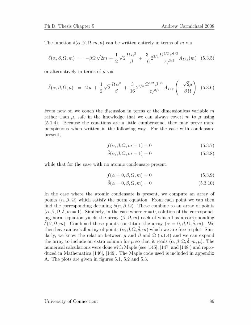
Ph.D. Thesis Chapter 5 Andrew Carmichael 2008
The function δ(α, β,Ω,m, µ) can be written entirely in terms of m via
δ(α, β,Ω,m) = −βΩ√
2m +1
2
√2
Ωα2
β+
3
1623/4 Ω5/2 β1/2
εf 3/2A1/2 (m) (5.3.5)
or alternatively in terms of µ via
δ(α, β,Ω, µ) = 2µ +1
2
√2
Ωα2
β+
3
1623/4 Ω5/2 β1/2
εf 3/2A1/2
(−√
2µ
β Ω
)(5.3.6)
From now on we couch the discussion in terms of the dimensionless variable mrather than µ, safe in the knowledge that we can always covert m to µ using(5.1.4). Because the equations are a little cumbersome, they may prove moreperspicuous when written in the following way. For the case with condensatepresent,
f(α, β,Ω,m = 1) = 0 (5.3.7)
δ(α, β,Ω,m = 1) = 0 (5.3.8)
while that for the case with no atomic condensate present,
f(α = 0, β,Ω,m) = 0 (5.3.9)
δ(α = 0, β,Ω,m) = 0 (5.3.10)
In the case where the atomic condensate is present, we compute an array ofpoints (α, β,Ω) which satisfy the norm equation. From each point we can thenfind the corresponding detuning δ(α, β,Ω). These combine to an array of points(α, β,Ω, δ,m = 1). Similarly, in the case where α = 0, solution of the correspond-ing norm equation yields the array (β,Ω,m) each of which has a correspondingδ(β,Ω,m). Combined these points constitute the array (α = 0, β,Ω, δ,m). Wethen have an overall array of points (α, β,Ω, δ,m) which we are free to plot. Sim-ilarly, we know the relation between µ and β and Ω (5.1.4) and we can expandthe array to include an extra column for µ so that it reads (α, β,Ω, δ,m, µ). Thenumerical calculations were done with Maple (see [145], [147] and [148]) and repro-duced in Mathematica [146], [149]. The Maple code used is included in appendixA. The plots are given in figures 5.1, 5.2 and 5.3.
University of Connecticut 89
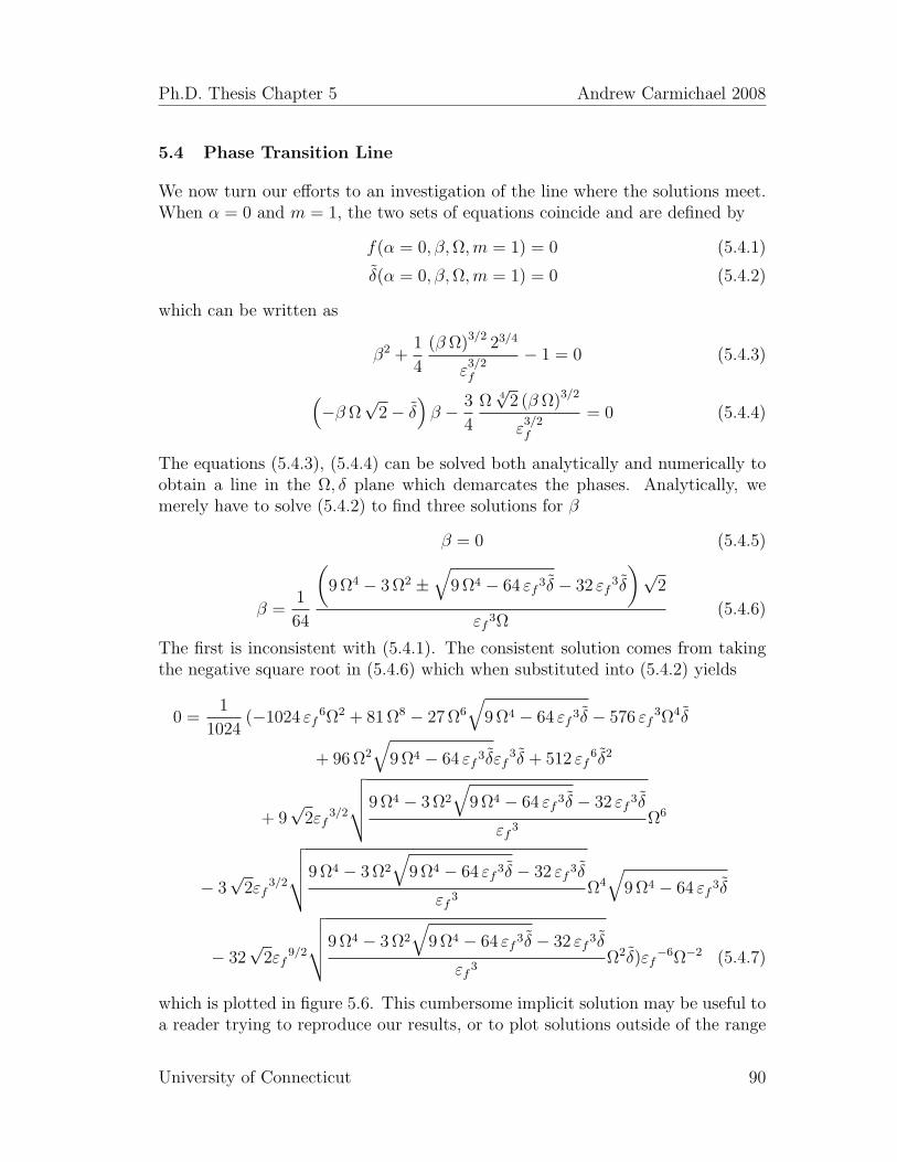
Ph.D. Thesis Chapter 5 Andrew Carmichael 2008
5.4 Phase Transition Line
We now turn our efforts to an investigation of the line where the solutions meet.When α = 0 and m = 1, the two sets of equations coincide and are defined by
f(α = 0, β,Ω,m = 1) = 0 (5.4.1)
δ(α = 0, β,Ω,m = 1) = 0 (5.4.2)
which can be written as
β2 +1
4
(β Ω)3/2 23/4
ε3/2f
− 1 = 0 (5.4.3)
(−β Ω
√2− δ
)β − 3
4
Ω 4√
2 (β Ω)3/2
ε3/2f
= 0 (5.4.4)
The equations (5.4.3), (5.4.4) can be solved both analytically and numerically toobtain a line in the Ω, δ plane which demarcates the phases. Analytically, wemerely have to solve (5.4.2) to find three solutions for β
β = 0 (5.4.5)
β =1
64
(9 Ω4 − 3 Ω2 ±
√9 Ω4 − 64 εf 3δ − 32 εf
3δ
)√2
εf 3Ω(5.4.6)
The first is inconsistent with (5.4.1). The consistent solution comes from takingthe negative square root in (5.4.6) which when substituted into (5.4.2) yields
0 =1
1024(−1024 εf
6Ω2 + 81 Ω8 − 27 Ω6
√9 Ω4 − 64 εf 3δ − 576 εf
3Ω4δ
+ 96 Ω2
√9 Ω4 − 64 εf 3δεf
3δ + 512 εf6δ2
+ 9√
2εf3/2
√√√√9 Ω4 − 3 Ω2
√9 Ω4 − 64 εf 3δ − 32 εf 3δ
εf 3Ω6
− 3√
2εf3/2
√√√√9 Ω4 − 3 Ω2
√9 Ω4 − 64 εf 3δ − 32 εf 3δ
εf 3Ω4
√9 Ω4 − 64 εf 3δ
− 32√
2εf9/2
√√√√9 Ω4 − 3 Ω2
√9 Ω4 − 64 εf 3δ − 32 εf 3δ
εf 3Ω2δ)εf
−6Ω−2 (5.4.7)
which is plotted in figure 5.6. This cumbersome implicit solution may be useful toa reader trying to reproduce our results, or to plot solutions outside of the range
University of Connecticut 90

Ph.D. Thesis Chapter 5 Andrew Carmichael 2008
presented here. It can be cut and pasted into Maple [145] or some equivalentsystem and plotted in any range using, for example, the implicitplot command.
The equations (5.4.3) and (5.4.4) can also be solved numerically using the fol-lowing prescription: we find solutions for the equation (5.4.1) producing an arrayof points (β,Ω) which is plotted in figure 5.4. Each point has a correspondingδ(β,Ω) and so we can plot the corresponding values of (Ω, δ) shown in figure 5.5.This line demarcates the regions which the two solutions inhabit, as indicated.The plots obtained by the numerical and analytic methods clearly agree.
The two classes of solution, α = 0 and α > 0 corresponding to the presence andabsence of the atomic condensate join continuously and on the phase transitionline plotted in figure 5.5 both
m = 1 (5.4.8)
andα = 0 (5.4.9)
hold simultaneously. Furthermore, along the border between the two regions, thesingle particle energy becomes
e(β, δ,Ω, α = 0,m = 1) =1
2β2δ +
3
104√
2β Ω (β Ω)3/2
ε3/2f
(5.4.10)
5.5 Features of the Theory
5.5.1 Regimes
In summary, the numerical analysis of the equations (4.4.1)-(4.4.3) shows thatsolutions for µ, α and β exist in two regimes in a parameter space of Ω and δcharacterized by the following conditions, with the equality signs holding on theborder.Atomic Condensate Allowed:
m = 1 (5.5.1)
α ≥ 0 (5.5.2)
Atomic Condensate Absent:
α = 0 (5.5.3)
m ≥ 1 (5.5.4)
Borderline:
m = 1 (5.5.5)
α = 0 (5.5.6)
University of Connecticut 91
Ph.D. Thesis Chapter 5 Andrew Carmichael 2008
The numerical analysis shows the solutions to be unique; for any given (δ,Ω),only one of the solutions exists. On the borderline, both solutions exist and agree,so that one moves continuously from one to the other when crossing the borderwhose analytic form, while cumbersome, can be determined from the equations.We recall here assumptions made on the range of the variables
Ω > 0 (5.5.7)
α ≥ 0 (5.5.8)
β > 0 (5.5.9)
while delta exists everywhere
−∞ < δ <∞ (5.5.10)
The first three are a matter of convenience and can always be made, while δ is atunable parameter can take any real value.
5.5.2 Energy Scales
The model has three parameters with the dimensions of frequency; Ω, δ and εf .In present day dilute quantum degenerate gases the representative value
εf ∼ 2π × 10KHz (5.5.11)
In the classic Feshbach resonances with bosons Rabi frequencies of
Ω ∼ 10εf (5.5.12)
are typical [94] but a much narrower Feshbach resonance could have a much dif-ferent ratio, and this quantity can’t be tuned but is fixed for a given Feshbachresonance in a given system. In photo-association, the ratio Ω/εf may be con-trolled by changing the intensity (intensities) of the lasers. In magneto-associationthe detuning δ depends on the product of the magnetic field with the differencein the dipole moments of the free atom state and the bound molecular state.Roughly,
δ ∼ εf (5.5.13)
corresponds to a change in the magnetic field of
∆B ∼ 10 mG (5.5.14)
In photo-association, as remarked before, changing δ is directly a matter of chang-ing the frequency/ frequencies of the laser(s).
University of Connecticut 92
Ph.D. Thesis Chapter 5 Andrew Carmichael 2008
It might prove illuminating to review salient aspects of the one-channel theoryfor a BEC [150], [151]. Such modelling allows for no explicit molecules, but thatthe atoms interact with one-another via a scattering length a that may be tunedby varying the detuning, i.e. the magnetic field. At positive detunings the scat-tering length is negative which indicates attractive interaction and collapse of an(untrapped) condensate. At negative detunings (at least close to the resonance;the scattering length can cross the axis further away) the scattering length islarge and positive and here one would expect a weak molecular bound state whichthe one-channel theory does not explicitly include. Thermodynamics implies thatsuch molecules would make the thermal equilibrium state. We conclude that pos-itive detunings represent the atom side of the resonance while negative detuningsrepresent the molecule side of the resonance. The numerical results for our modelshow that the region where the atomic condensate disappears is indeed in theregion of negative detuning. The transition line moves away from the line δ = 0with increasing coupling Ω, however, and we regard this as the shifting of theresonance by many-body effects.
5.5.3 Unitarity Limit
Unitarity (discussed in the case of Fermi gases in [152], [153]) is the name given tothe regime where in the limit of very strong interaction (unitary limit) the inter-action strength itself vanishes from the system of equations (leaving the system ina universal state), leaving only other parameters with the dimensions of energy, inour case εf , which is set by the density of the gas and was defined by (3.2.42). Inour notation, the coupling was given by the atom-molecule Rabi frequency and sowe look or solutions in the regime where this becomes large. One can see from thenumerical solution 5.1 that this is the regime with the atomic condensate presentand so we are in the regime
Ω→∞m = 1
α 6= 0
(5.5.15)
The numerical solution seems to flatten out as Ω becomes larger, and so it seemsthe result should be the same for any δ. We can then for simplicity set
δ = 0 (5.5.16)
We expect α(Ω) and µ(Ω) to be even functions of Ω and remembering that α > 0,while µ < 0 we can make an ansatz asymptotic expansion like
α = A0 + A−2Ω−2 + A−4Ω−4 + ... (5.5.17)
−µ = M0 +M−2Ω−2 +M−4Ω−4 + ... (5.5.18)
University of Connecticut 93
Ph.D. Thesis Chapter 5 Andrew Carmichael 2008
which can be substituted along with (5.5.16) into equations (5.1.7)-(5.1.9) and thepowers of Ω compared to give soluble equations for the coefficients. The result is
A0 =
√3
2(5.5.19)
M0 =1
2εf (5.5.20)
which in turn means that in this regime (5.5.15), (5.5.16)
|α|2 =3
4(5.5.21)
µ = −1
2εf (5.5.22)
It is interesting to look at the energy in the unitary regime. Using the aboveexpressions in the equation we previously derived for e(α, µ) in the m = 1 regime,(5.1.12), we obtain
limΩ→∞
e(α, µ) = − 3
10εf (5.5.23)
University of Connecticut 94
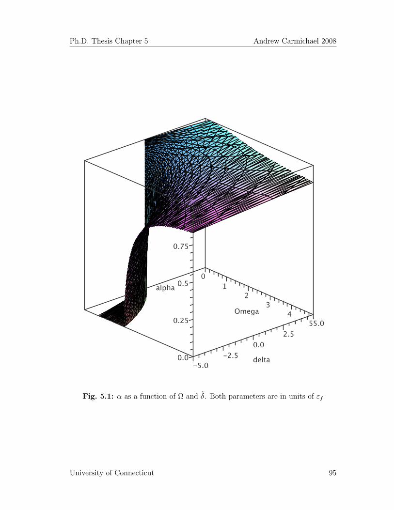
Ph.D. Thesis Chapter 5 Andrew Carmichael 2008
01
2
Omega3
45.05
2.5
delta
0.0
-2.5-5.0
0.0
0.25
0.5alpha
0.75
1.0
Fig. 5.1: α as a function of Ω and δ. Both parameters are in units of εf
University of Connecticut 95
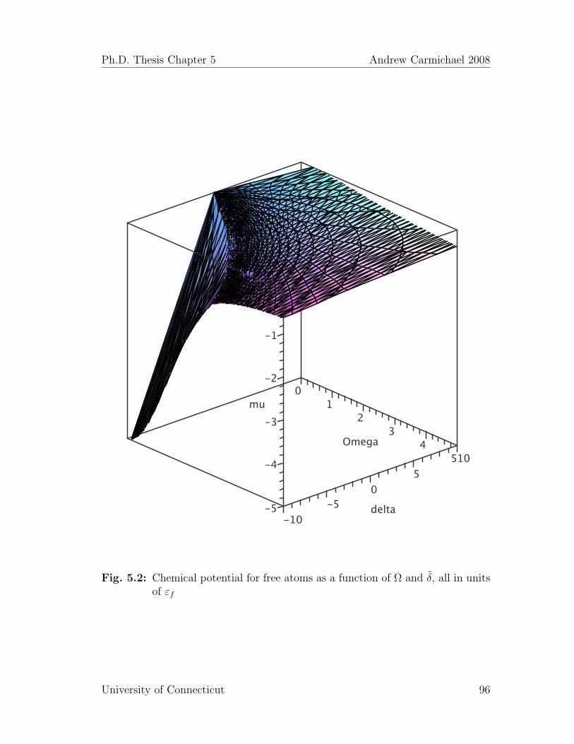
Ph.D. Thesis Chapter 5 Andrew Carmichael 2008
Fig. 5.2: Chemical potential for free atoms as a function of Ω and δ, all in unitsof εf
University of Connecticut 96

Ph.D. Thesis Chapter 5 Andrew Carmichael 2008
-5.0
-2.5
0.0 delta2.5
50.0
4
Omega
3 2
0.25
1 0
beta
5.0
0.5
0.75
1.0
Fig. 5.3: Dependence of scaled molecular condensate fraction β on δ and Ω, bothin units of εf .
University of Connecticut 97
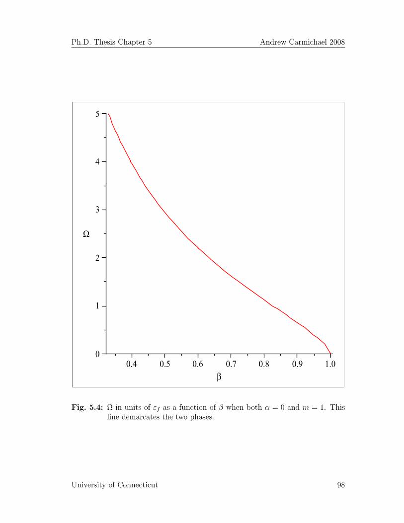
Ph.D. Thesis Chapter 5 Andrew Carmichael 2008
b0.4 0.5 0.6 0.7 0.8 0.9 1.0
W
0
1
2
3
4
5
Fig. 5.4: Ω in units of εf as a function of β when both α = 0 and m = 1. Thisline demarcates the two phases.
University of Connecticut 98
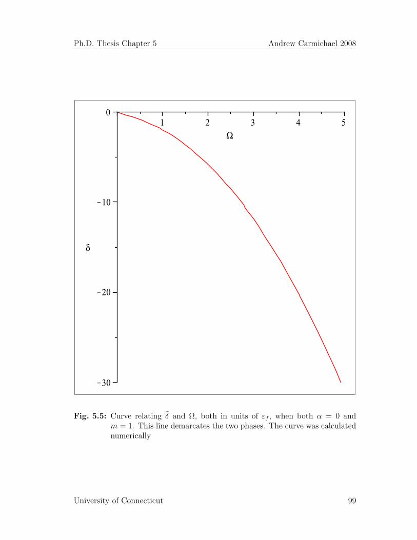
Ph.D. Thesis Chapter 5 Andrew Carmichael 2008
W1 2 3 4 5
d
K30
K20
K10
0
Fig. 5.5: Curve relating δ and Ω, both in units of εf , when both α = 0 andm = 1. This line demarcates the two phases. The curve was calculatednumerically
University of Connecticut 99

Ph.D. Thesis Chapter 5 Andrew Carmichael 2008
Fig. 5.6: Analytically determined curve relating δ and Ω, both in units of εf ,when both α = 0 and m = 1. This line demarcates the two phases.
University of Connecticut 100

Chapter 6
Thermodynamics of the Atom-Molecule System
6.1 Thermodynamic Analysis
Turning now to the thermodynamics of the system, we must first recall the cen-tral equation of thermodynamics and identify the appropriate variables from thecoupled atom molecule system. The central equation, in a common notation,reads
dU = TdS +∑
µdN −XdY (6.1.1)
See, for example, [127], [6], [7], [154] and [155]. The term on the left represents thetotal differential of internal energy which is equated to the sum of contributionsfrom heat flow (and therefore entropy change), addition or subtraction of particles(the relevant energy contribution being the chemical potential; the summation isover species of particles) and the last term representing mechanical or electro-magnetic coupling to the environment through work which could be (as in ourcase) pressure-volume work −PdV , coupling through external fields (for exampleB · dM or E · dP) etc.
The central equation becomes
dU = TdS − PdV +∑
µdN (6.1.2)
Recalling the condition for equilibrium, consider two systems a and b in thermal,mechanical and chemical contact so that they can exchange volume, energy andparticles. If they are isolated from every source or sink of these except each other,then it must hold that
dUa = −dUbdVa = −dVbdNa = −dNb
(6.1.3)
For equilibrium, the total entropy must be at a minimum
dS = dSa + dSb = 0 (6.1.4)
101

Ph.D. Thesis Chapter 6 Andrew Carmichael 2008
Writing the central equation for system a as
dSa =1
Ta[dUa + PadVa − µadNa] (6.1.5)
and the corresponding form for b. Inserting (6.1.5) and its b counterpart alongwith (6.1.3) into (6.1.4) yields(
1
Ta− 1
Tb
)dUa +
(PaTa− PbTb
)dVa +
(−µaTa
+µbTb
)dNa = 0 (6.1.6)
The above expression must hold for all values of dUa, dVa and dNa and so thecoefficients must vanish. These three relations constitute the condition for equi-librium.
Ta = Tb Thermal equilibrium (6.1.7)
Pa = Pb Mechanical equilibrium (6.1.8)
µa = µb Chemical equilibrium (6.1.9)
To apply this to our atom-molecule system, consider the cloud of atoms and thecloud of molecules to be two systems capable of communicating only with oneanother thermally, mechanically and chemically via association and dissociationand to be at equilibrium. The above discussion holds but we must modify therelation concerning particle exchange. The invariant total number of atoms, boundand unbound is
N = Na + 2Nm (6.1.10)
dN = dNa + 2dNm (6.1.11)
dN = 0 =⇒ 0 = dNa + 2dNm (6.1.12)
dNa = −2dNm (6.1.13)
which alters the condition for chemical equilibrium to give(1
Ta− 1
Tm
)dUa +
(PaTa− PmTm
)dVa +
(−µaTa
+1
2
µmTm
)dNa = 0
whenceµm = 2µa (6.1.14)
University of Connecticut 102
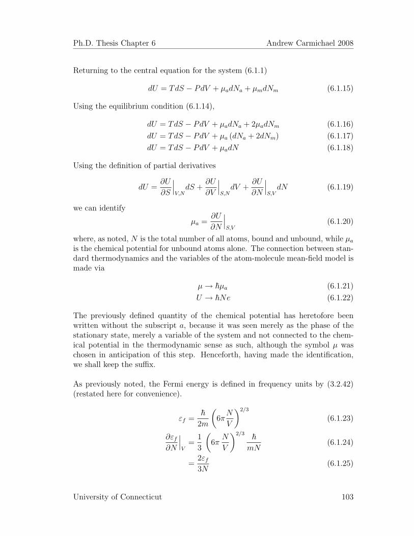
Ph.D. Thesis Chapter 6 Andrew Carmichael 2008
Returning to the central equation for the system (6.1.1)
dU = TdS − PdV + µadNa + µmdNm (6.1.15)
Using the equilibrium condition (6.1.14),
dU = TdS − PdV + µadNa + 2µadNm (6.1.16)
dU = TdS − PdV + µa (dNa + 2dNm) (6.1.17)
dU = TdS − PdV + µadN (6.1.18)
Using the definition of partial derivatives
dU =∂U
∂S
∣∣∣V,N
dS +∂U
∂V
∣∣∣S,N
dV +∂U
∂N
∣∣∣S,VdN (6.1.19)
we can identify
µa =∂U
∂N
∣∣∣S,V
(6.1.20)
where, as noted, N is the total number of all atoms, bound and unbound, while µais the chemical potential for unbound atoms alone. The connection between stan-dard thermodynamics and the variables of the atom-molecule mean-field model ismade via
µ→ ~µa (6.1.21)
U → ~Ne (6.1.22)
The previously defined quantity of the chemical potential has heretofore beenwritten without the subscript a, because it was seen merely as the phase of thestationary state, merely a variable of the system and not connected to the chem-ical potential in the thermodynamic sense as such, although the symbol µ waschosen in anticipation of this step. Henceforth, having made the identification,we shall keep the suffix.
As previously noted, the Fermi energy is defined in frequency units by (3.2.42)(restated here for convenience).
εf =~
2m
(6πN
V
)2/3
(6.1.23)
∂εf∂N
∣∣∣V
=1
3
(6π
N
V
)2/3 ~mN
(6.1.24)
=2εf3N
(6.1.25)
University of Connecticut 103
Ph.D. Thesis Chapter 6 Andrew Carmichael 2008
Using the definition of Ω (3.2.43) and remembering that κ depends upon V , butnot N , we have
Ω =√Nκ (6.1.26)
∂Ω
∂N
∣∣∣V
=1
2
κ√N
(6.1.27)
=Ω
2N(6.1.28)
Both εf and Ω depend upon invariant atom number N and on density N/V .Since the system is at zero temperature, we expect S = 0 (one expects zero entropyfor a system of zero total momentum anyway, [67]) and so the central equationreduces to
dU = −PdV + µadN (6.1.29)
which in terms of the variables of the model is
d(~Ne) = −PdV + ~µadN (6.1.30)
identifying the pressure as
P = −∂U∂V
∣∣∣N
= −∂(~Ne)∂V
∣∣∣N
(6.1.31)
and the corresponding Gibbs-Duhem relation (the “integrated” form of the centralequation) is then
U = −PV +∑
µN (6.1.32)
U = −PV + µaNa + µmNm (6.1.33)
U = −PV + µaNa + 2µaNm (6.1.34)
U = −PV + µa(Na + 2Nm) (6.1.35)
U = −PV + µaN (6.1.36)
which in the variables of the model is
~Ne = −PV + ~µaN (6.1.37)
e = −PV~N
+ µa (6.1.38)
e = − P~ρ
+ µa (6.1.39)
P
~ρ= µa − e (6.1.40)
University of Connecticut 104
Ph.D. Thesis Chapter 6 Andrew Carmichael 2008
In figure 5.2, we plot with Maple the atomic chemical potential (referred to in thissection as µa and actually in frequency units) in the parameter space of the model.The phase transition line is clearly noticeable and corresponds to that on the plotof atomic condensate fraction α, fig. 5.1. Incidentally, we have plotted the singleparticle energy e in the same parameter space as the chemical potential 5.2 andfound that the plots are so similar as to render the printing of the energy plothere redundant. One can see why this is so from equation (6.1.40); the differencebetween the e and µ is the specific pressure which one can see in figure 6.1 neverpushes much past 0.2εf and so the difference between the two is hard to discernon a plot with µ/εf going up to 5.
We also concern ourselves with the pressure in the unitary limit. In the previouschapter it was shown that in the regime
α 6= 0
m = 1
Ω→∞δ = 0
(6.1.41)
the chemical potential and energy approach the following limits
µ→ −1
2εf
e(α, µ)→ − 3
10εf
(6.1.42)
Given equation (6.1.40), this means that the specific pressure becomes
P
~ρ→ −1
5εf (6.1.43)
From the figure one can see that the pressure is negative throughout the whole ofthe parameter space plotted, in addition to being negative in the unitary limit.Thermodynamically this implies a mechanical instability. If we consider the phasetransition line evidenced in figures 5.5 and 5.6 to be the line of the Feshbach res-onance shifted by many-body effects, then on the atom condensate side of theresonance the standard single-channel picture has a negative interatomic scat-tering length and the atomic BEC is likely to collapse, commensurate with thenegative pressure depicted in the figure 6.1 and in the unitary limit.
However, what the figure also shows is that even on the side of the resonancewhere no atomic condensate exists (we refer to this side of the condensate as the
University of Connecticut 105
Ph.D. Thesis Chapter 6 Andrew Carmichael 2008
‘molecule’ side, even though figure 5.3 shows that the molecular condensate existseverywhere; it would be the molecule side of the two-body resonance) the pressureremains negative. This contrasts with the analogous fermion mean field theory[89], [90] which shows positive pressure everywhere. Moreover, there is no ques-tion about the experimental stability of the Fermi gas near a Feshbach resonance.
For the Bose gas, the negative pressure and implied instability are a somewhatsurprising prediction. We remarked earlier that one of the original motivations forthis endeavour was to compare the results of the all-boson theory with the fermionversion to see whether and to what degree the different quantum statistics affectthe outcome of an otherwise identical theory. That question appears to have ananswer; the results are really quite different. No negative pressure develops in thefermion system. We post-pone reflection on this matter until the next chapter.
University of Connecticut 106
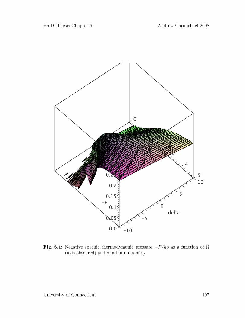
Ph.D. Thesis Chapter 6 Andrew Carmichael 2008
Fig. 6.1: Negative specific thermodynamic pressure −P/~ρ as a function of Ω(axis obscured) and δ, all in units of εf
University of Connecticut 107

Chapter 7
Concluding Remarks
The purpose of this exercise was to consider atomic condensate in the presence of amagnetic field close to one of the Feshbach resonances for the system, thus allowingfor magneto-association from an atomic into a molecular condensate. We analysedthe system in the Heisenberg picture and solved for operators for the atomic andmolecular condensates with parameters being the detuning and atom-moleculecoupling. We expect molecules formed in this way to be prone to dissociationinto atom-atom pairs of equal and opposite momentum and included this in themodel by solving for those operators, whose expectation values are analogous tothe anomalous pairing amplitudes in traditional BCS theory, which create suchpairs. The system was solved in the steady state, using a classical (mean-field)approximation where appropriate. The model was essentially an all-boson versionof a system our group analysed previously to describe magneto-association of atwo-component (spin up and down) gas of fermionic atoms into bosonic molecules[90], [89] and a comparison of the two systems was one of the motivating factorshere.
The salient result of the all-boson model is the prediction of a phase transitionwith one side characterised by the complete absence of any atomic condensatefraction while on the other there exist both atomic and molecular condensates.Furthermore, a curious feature was the negative pressure and energy throughoutthe parameter space. The corresponding fermion case exhibited positive pres-sure and a phase transition line which stayed close to the two-body resonance.In the boson case, the phase transition line was shifted to the molecule side ofthe resonance further and further as the coupling is increased (figures 5.1, 5.5, 5.6).
The first question for any theoretical prediction is how it fares in comparison withexperiment. At the moment, unfortunately, molecular lifetimes have been pro-hibitively short and atom-molecule equilibration in a Bose gas near a Feshbachresonance has not, to our knowledge, been achieved. This particular field is de-veloping with such celerity, however, that it soon may be. Progress continues onfronts such as two-photon (two-colour) photo-association in a Raman scheme [74]and production of superpositions of atomic and molecular condensates [156]. In
108
Ph.D. Thesis Chapter 7 Andrew Carmichael 2008
a heteronuclear system direct one-photon photo-association from the dissociationcontinuum to a low lying vibrational level is possible in principle [157]. We are ofthe opinion that photo-association to a stable molecular state will eventually beachieved in a BEC.
We see this as the appropriate juncture to discuss the exact meaning of the term‘mean-field theory’, a point alluded to in chapter 2. Many authors link the phrase‘mean field approach’ with analysis of the condensate in terms of the Gross-Pitaevskii equation (2.10.16). The comparable analysis for an atom moleculesystem could centre on an equivalent equation in a model which admitted onlyatomic and molecular condensates and no non-condensate atoms and moleculesat all. Our group has studied such systems in what we call the two-mode approx-imation [158], as have others [159]. As discussed before, however, the process ofmagneto-association in free space which we have considered here obeys momen-tum conservation (no time dependent EM field to carry momentum) and so anasymmetry is present; two zero momentum condensate atoms may only combineto become a zero momentum condensate molecule whereas in the reverse processa zero momentum condensate molecule can disintegrate into two atoms with ar-bitrary equal and opposite momenta. Dealing with such ‘rogue’ dissociation [94]was the original reason for our including zero momentum atom-atom pairs in themodel. One could regard this as an extension of the mean-field approach, but thefact that the atom-atom pairs introduced in the fermion version of the problemand applied here are treated in the same way as electron pairs in BCS theory, oneof the most traditional mean-field theories (discussed to some extent in section2.10), leads us to use the phrase mean-field theory here as well.
Mean-field theories, despite swallowing potentially complicated inter-particle in-teractions into scalar constants, have a history of vast success in a variety offields of physics [160], [126]. In the field of dilute, degenerate quantum gases weknow of no occasion where great trouble has resulted from a properly formulatedmean-field theory. Indeed, only recently has it become possible to empiricallydistinguish between a mean-field theory and a strongly correlated approach [161],[86].
Such considerations cast an interesting light upon one feature of our model; theprediction of negative pressure and hence instability, even on the molecule side ofthe resonance where the standard picture is that the scattering length be large andpositive indicating a stable condensate. Our model has limitations, in particularthat we have ignored the background scattering length that dominates far fromthe resonance, that we have been perfunctory about the details of the molecularbound state and that we have neglected atom-atom, atom-molecule and molecule-molecule collisions. It is possible that inclusion of factors such as collisions could
University of Connecticut 109
Ph.D. Thesis Chapter 7 Andrew Carmichael 2008
stabilize the gas against the predicted instability. The model also provides notimescale for the instability, meaning that perhaps it may be undetectable even ifit existed. After all, the fact that at sub Kelvin temperatures the ground state ofalkali metals is a solid rather than a gas has not precluded innumerable successfulexperiments in Bose-Einstein condensation.
Moreover, if the instability is not extant in this system, it would be a false predic-tion of a mean-field theory, a startling but interesting result in and of itself. Onthe other hand, as we do not have a timescale associated with the collapse due tothe negative pressure, it may not be short either. Indeed, it could contribute toor even dominate the loss of atoms from a condensate observed to occur on bothsides of a resonance.
The quite different results for the boson case presented in this thesis and thefermion case presented in the aforementioned publications brings to mind anotherpoint. A while ago we noticed [162] that in a simple model for quantum motionof two trapped ions in one dimension that the thermodynamics is irrespectiveof the quantum statistics. Our interpretation was that the Coulomb interactionbetween the ions kept them sufficiently far apart that they became distinguish-able and that quantum statistics was moot. Calculations [163] in which stronglyinteracting bosons crystallize in a trap just as ions do led to the idea of ‘super-universality’; if sufficiently strong interactions keep the particles apart, then statesare not only independent of the strength of interactions (standard universality)but also of the quantum statistics. The analysis of our boson and fermion sys-tems however, throws a spanner in the works; we’ve seen quite different behaviourof bosons versus fermions in a strongly interacting regime. Super-universality inmean field theories of this kind is neither a necessary nor sufficient condition forsuperuniversality in nature. Nonetheless, super-universality did not pass this par-ticular test.
As with any toy model such as ours, a future direction could always be to dothe same thing again with the inclusion of those elements which were neglected inthe present analysis; the background scattering length, non-condensate molecules,interparticle scattering and so on. The inclusion of such things might stabilize thegas on the molecule side of the resonance. Moreover, a more realistic momen-tum dependence of the coupling matrix elements from a more realistic interactionpotential than the contact interaction used would be an interesting avenue. Thecontact interaction, which becomes a constant in momentum space, is the sourceof the ultra-violet divergence seen in our model. A realistic interaction potentialwould give different integrals (maybe not in need of renormalization) which couldbe a blessing or not. More interesting, perhaps, could be an attempt to integratethe full time-dependent equations of motion in imaginary time to see if the sys-
University of Connecticut 110

Ph.D. Thesis Chapter 7 Andrew Carmichael 2008
tem evolves from some given initial condition to the stationary state we found.If so, this could provide us with the timescale for the collapse due to the ther-modynamic instability from the negative pressure to compare with some putativefuture experiment.
University of Connecticut 111
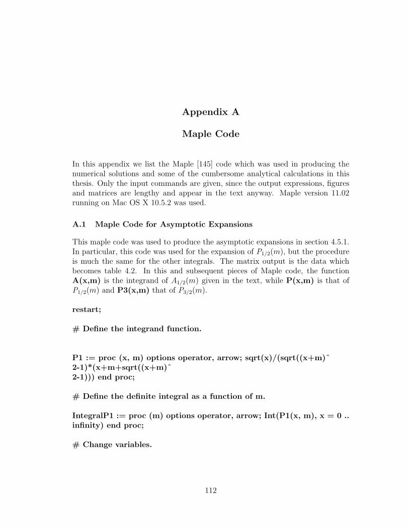
Appendix A
Maple Code
In this appendix we list the Maple [145] code which was used in producing thenumerical solutions and some of the cumbersome analytical calculations in thisthesis. Only the input commands are given, since the output expressions, figuresand matrices are lengthy and appear in the text anyway. Maple version 11.02running on Mac OS X 10.5.2 was used.
A.1 Maple Code for Asymptotic Expansions
This maple code was used to produce the asymptotic expansions in section 4.5.1.In particular, this code was used for the expansion of P1/2(m), but the procedureis much the same for the other integrals. The matrix output is the data whichbecomes table 4.2. In this and subsequent pieces of Maple code, the functionA(x,m) is the integrand of A1/2(m) given in the text, while P(x,m) is that ofP1/2(m) and P3(x,m) that of P3/2(m).
restart;
# Define the integrand function.
P1 := proc (x, m) options operator, arrow; sqrt(x)/(sqrt((x+m)ˆ2-1)*(x+m+sqrt((x+m)ˆ2-1))) end proc;
# Define the definite integral as a function of m.
IntegralP1 := proc (m) options operator, arrow; Int(P1(x, m), x = 0 ..infinity) end proc;
# Change variables.
112

IntegralP1A := ‘assuming‘([IntegrationTools[Change](IntegralP1(m), x= m*t, t)], [m > 1]);
# Extract the integrand
IntegrandP1A := op(1, IntegralP1A);
# Find the asymptotic series
‘assuming‘([map(normal, asympt(IntegrandP1A, m, 10))], [t > 0]);
# Integrate term by term
ASeries := map(int, convert(%, polynom), t = 0 .. infinity);
# Find the numerical coefficients
evalf(%);
# Define the function NUMINTP(m) as the numerical integral of P
NUMINTP:=(m)->evalf(Int(P1(x, m), x = 0 .. infinity), 25);
# Check that it works for a random value of m.
NUMINTP(1.3);
# Define the function NUMASERIES(m) as the numerical value givenby the series for a given m.
NUMASERIES:=(n)->evalf(eval(ASeries,m=n), 25);
# Check that it works for a given m.
NUMASERIES(1.3);
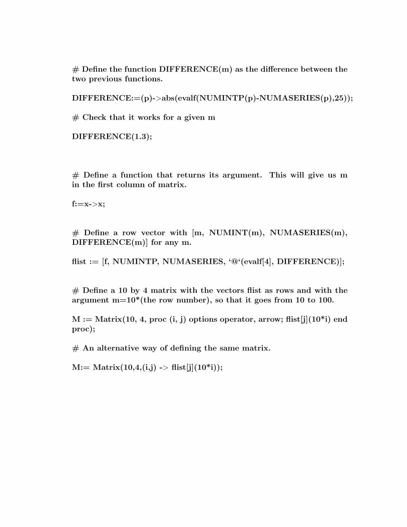
# Define the function DIFFERENCE(m) as the difference between thetwo previous functions.
DIFFERENCE:=(p)->abs(evalf(NUMINTP(p)-NUMASERIES(p),25));
# Check that it works for a given m
DIFFERENCE(1.3);
# Define a function that returns its argument. This will give us min the first column of matrix.
f:=x->x;
# Define a row vector with [m, NUMINT(m), NUMASERIES(m),DIFFERENCE(m)] for any m.
flist := [f, NUMINTP, NUMASERIES, ‘@‘(evalf[4], DIFFERENCE)];
# Define a 10 by 4 matrix with the vectors flist as rows and with theargument m=10*(the row number), so that it goes from 10 to 100.
M := Matrix(10, 4, proc (i, j) options operator, arrow; flist[j](10*i) endproc);
# An alternative way of defining the same matrix.
M:= Matrix(10,4,(i,j) -> flist[j](10*i));
A.2 Maple Code for Numerical Solutions
This Maple code was used to produce the plots in chapters 5 and 6.
# Define the integrand A(x,m)
A := proc (x, m) options operator, arrow; (-mˆ2-2*x*m+1)/(sqrt(x)*sqrt((x+m)ˆ2-1)*(x+sqrt((x+m)ˆ2-1))) end proc;
# Define the integral
IntegralA:=(m)->Int(A(x,m),x=0..infinity);
# Check it works for a given m
IntegralA(1);
# Find the numerical value
evalf(IntegralA(1));
# Define the next integrand
P:=(x,m)->sqrt(x)/(sqrt((x+m)ˆ2-1)*(x+m+sqrt((x+m)ˆ2-1)));
# and the integral
IntegralP:=(m)->Int(P(x,m),x=0..infinity);
# Test it for m=1.
IntegralP(1);
# Find the integrals for m=1.
int(P(x, 1), x = 0 .. infinity);
int(A(x, 1), x = 0 .. infinity);
# Find the numerical value to see if all is defined correctly.

evalf(IntegralP(1));
# Define the function f3; the gap equation with zero RHS.
f3:=(alpha,beta,Omega,delta,m)->(2*(-beta*Omega*m/sqrt(2))-delta)*beta+Omega/sqrt(2)*(alphaˆ2+(3*(beta*Omega)ˆ(3/2)*evalf(IntegralA(m)))/(4*2ˆ(3/4)));
# Define the function f4; the norm equation with zero RHS.
f4:=(alpha,beta,Omega,m)->alphaˆ2+betaˆ2+(3*(beta*Omega)ˆ(3/2)*evalf(IntegralP(m)))/(4*2ˆ(3/4))-1;
# Test the function for some random values of its arguments.
f4(0, 1, 1, 2);
evalf(f4(0, 1, 1, 2));
# Activate plots package.
with(plots):
# Define plotB as an array of points which satisfy the norm equation.Get an array of points (alpha,beta,Omega).
plotB := implicitplot3d(f4(alpha, beta, Omega, 1) = 0, alpha = 0 .. 1,beta = 0 .. 1, Omega = 0 .. 5, grid = [40, 40, 40]);
# Activate plottools package
with(plottools):
# Define del(alpha,beta,Omega,m) from the gap equation solved fordelta.
del := proc (alpha, beta, Omega, m) options operator, arrow;-2*beta*Omega*m/sqrt(2)+Omega*(alphaˆ2+(3/8)*abs(beta*Omega)ˆ(3/2)*IntegralA(m)*2ˆ(1/4))/(sqrt(2)*beta)end proc;
# Test it for m=1.
del(alpha, beta, Omega, 1);
# Define plotBTrans as the array that results from changing the arrayplotB from (alpha,beta,Omega) to (Omega,delta,alpha) all in the m=1region..
plotBTrans := (transform(proc (alpha, beta, Omega) options operator,arrow; [Omega, del(alpha, beta, Omega, 1), alpha] end proc))(plotB);
# Define the array plotBTrans1 as the array that results from changingthe array plotB from (alpha,beta,Omega) to (Omega,delta,beta).
plotBTrans1 := (transform(proc (alpha, beta, Omega) options opera-tor, arrow; [Omega, del(alpha, beta, Omega, 1), beta] end proc))(plotB);
# Define the array plotC in the same way as plotB but for the alpha=0region (where m is not necessarily 1) to get (beta,Omega,m).
plotC := implicitplot3d(f4(0, beta, Omega, m) = 0, beta = 0 .. 1,Omega = 0 .. 5, m = 1 .. 50, grid = [30, 30, 30]); # TransformplotC in the same way as plot B to get plotCTrans which is the array(Omega,delta,beta) and plotCTrans2 which is (Omega,delta,alpha=0).
plotCTrans := (transform(proc (beta, Omega, m) options operator, ar-row; [Omega, del(0, beta, Omega, m), beta] end proc))(plotC);
plotCTrans2 := (transform(proc (Omega, del, beta) options operator,arrow; [Omega, del, 0] end proc))(plotCTrans);
# Display plotBTrans1 which is (Omega,delta,beta) when m=1 andplotCTrans which is (Omega,delta,beta) when alpha=0 on the sameaxes.
display(plotCTrans, plotBTrans1, labels = [Omega, delta, beta], ori-entation = [99, 69], axes = box, view = [0 .. 5, -5 .. 5, 0 .. 1]);
# Display plotBTrans which is (Omega,delta,alpha) for the region wherem=1 and plotCTrans2 which is (Omega,delta,alpha=0) for the regionalpha=0 on the same axes.

display(plotBTrans, plotCTrans2, labels = [Omega, delta, alpha], ori-entation = [-42, 67], axes = box, view = [0 .. 5, -5 .. 5, 0 .. 1]);
# Plot the numerically calculated integral A(m).
plot(evalf(IntegralA(m)), m = 1 .. 5, labels = [m, ”A(m)”]);
# Plot the numerically calculated integral P(m).
plot(evalf(IntegralP(m)), m = 1 .. 50, labels = [m, ”P(m)”]);
# Plot the phase transition line by solving the norm equation whenboth alpha=0 and m=1.
p := implicitplot(f4(0, beta, Omega, 1), beta = 0 .. 1, Omega = 0 ..5);
display(p);
# Transform the previous plot to (Omega,delta).
pTrans := (transform(proc (beta, Omega) options operator, arrow;[Omega, del(0, beta, Omega, 1)] end proc))(p);
#display(pTrans, labels = [Omega, delta], view = [0 .. 5, 0 .. -30]);
# Define the chemical potential.
mu := proc (beta, Omega, m) options operator, arrow;-beta*Omega*m/sqrt(2) end proc;
# Define plotCTrans1 as the array which tranforms plotC which is(beta,Omega,m) in the region alpha=0 into (Omega,delta,mu) in thesame region alpha=0.
plotCTrans1 := (transform(proc (beta, Omega, m) options operator,arrow; [Omega, del(0, beta, Omega, m), mu(beta, Omega, m)] endproc))(plotC);
# Define plotBTrans2 as the array which results when plotB which is(alpha,beta,Omega) in the region m=1 is transformed into
(Omega,delta,mu) also in the region m=1.
plotBTrans2 := (transform(proc (alpha, beta, Omega) options opera-tor, arrow; [Omega, del(alpha, beta, Omega, 1), mu(beta, Omega, 1)]end proc))(plotB);
# Now display both of the arrays just defined on the same axes.
display(plotCTrans1, plotBTrans2, labels = [Omega, delta, mu], ori-entation = [-42, 67], axes = box, view = [0 .. 5, -10 .. 10, 0 .. -5]);
A.3 Maple Code for Pressure
This Maple code was used to produce the pressure plot 6.1.
restart;
# Define the integrand in integral A.
A := proc (x, m) options operator, arrow; (-mˆ2-2*x*m+1)/(sqrt(x)*sqrt((m+x)ˆ2-1)*(x+sqrt((m+x)ˆ2-1))) end proc;
IntegralA := proc (m) options operator, arrow; Int(A(x, m), x = 0 ..infinity) end proc;
# Test it for m=1.
IntegralA(1);
# Just to prove the integral is numerically doable
evalf(IntegralA(1));
evalf(IntegralA(1.6));
P := proc (x, m) options operator, arrow; sqrt(x)/(sqrt((m+x)ˆ2-1)*(x+m+sqrt((m+x)ˆ2-1))) end proc;
IntegralP := proc (m) options operator, arrow; Int(P(x, m), x = 0 ..infinity) end proc;
IntegralP(1);int(P(x, 1), x = 0 .. infinity);
int(A(x, 1), x = 0 .. infinity);
# Just to show the integral is numerically doable
evalf(IntegralP(1));
evalf(IntegralP(1.6));
# f3 is the function that is really the gap equation arranged with zeroRHS
f3 := proc (alpha, beta, Omega, delta, m) options operator, arrow; (-2*beta*Omega*m/sqrt(2)-delta)*beta+Omega*(alphaˆ2+(3/8)*(beta*Omega)ˆ(3/2)*evalf(IntegralA(m))*2ˆ(1/4))/sqrt(2) endproc;
# f4 is the function that is really the norm arranged with zero RHS.
f4 := proc (alpha, beta, Omega, m) options operator, arrow; alphaˆ2+betaˆ2+(3/8)*(beta*Omega)ˆ(3/2)*evalf(IntegralP(m))*2ˆ(1/4)-1 end proc;
# del(alpha,beta,Omega,m) is the function delta, obtained from thegap equation.
del := proc (alpha, beta, Omega, m) options operator, arrow;-2*beta*Omega*m/sqrt(2) +Omega*(alphaˆ2 +(3/8)*abs(beta*Omega)ˆ(3/2)*evalf(IntegralA(m))*2ˆ(1/4))/(sqrt(2)*beta) end proc;
# P3 is really the function under the integral P 3/2(m)
P3 := proc (x, m) options operator, arrow; -(1/2)*(-1+4*xˆ2*mˆ2+8*xˆ3*m+2*x*m-3*xˆ2+mˆ2)/((2*xˆ2+1+2*sqrt((x+m)ˆ2/((x+m+1)*(x+m-1)))*xˆ2)*(x+m+1)*(x+m-1)*sqrt(x)) end proc;
# IntegralP3 is really the function P 3/2(m)
IntegralP3 := proc (m) options operator, arrow; Int(P3(x, m), x = 0 ..infinity) end proc;
# Just to prove the integral is numerically doable.
evalf(IntegralP3(1));
evalf(IntegralP3(1.6));
# e is the energy per particle taken from file equations.mw
e := proc (alpha, beta, Omega, m) options operator, arrow; (1/2)
*betaˆ2*del(alpha, beta, Omega, m)-beta*Omega*(alphaˆ2+(3/8)*(beta*Omega)ˆ(3/2)*2ˆ(1/4)*(evalf(IntegralA(m))-evalf(IntegralP3(m))))/sqrt(2) end proc;
# To show e is numerically evaluateable.
evalf(e(1.2, 1.2, 1.2, 1.9));
mu := proc (beta, Omega, m) options operator, arrow;-beta*Omega*m/sqrt(2) end proc;
# Define negative pressure (actually P/“hbar“rho))
negpressure := proc (alpha, beta, Omega, m) options operator, arrow;e(alpha, beta, Omega, m)-mu(beta, Omega, m) end proc;
# Test it for rnadom values of the arguments.
evalf(negpressure(0, 1.1, 1.1, 1.1));
with(plots);
with(plottools);
# plotB is an implicit plot of all solutions in the range to the normequation alone, in the nonzero alpha, m=1.
# plotC is an implicit plot of all solutions in the range to the normequation alone, in the alpha=0 zone.
plotB := implicitplot3d(f4(alpha, beta, Omega, 1) = 0, alpha = 0 .. 1,beta = 0 .. 1, Omega = 0 .. 5, grid = [40, 40, 40]);
plotC := implicitplot3d(f4(0, beta, Omega, m) = 0, beta = 0 .. 1,Omega = 0 .. 5, m = 1 .. 50, grid = [45, 45, 45]);
#pressureplot1 := (transform(proc (beta, Omega, m) options operator,arrow; [Omega, del(0, beta, Omega, m), negpressure(0, beta, Omega,m)] end proc))(plotC);
pressureplot2 := (transform(proc (alpha, beta, Omega) options oper-ator, arrow; [Omega, del(alpha, beta, Omega, 1), negpressure(alpha,beta, Omega, 1)] end proc))(plotB);
# Display both plots on the sam axes.
display(pressureplot2, pressureplot1, labels = [Omega, delta, -P], ori-entation = [-42, 67], axes = box, view = [0 .. 5, -10 .. 10, 0 .. .3]);
#
Bibliography
[1] B. W. Carroll, Introduction to Modern Astrophysics. Benjamin Cummings,second ed., 2006.
[2] A. Einstein Sitzber. Pr. Akad. Wiss., vol. 22, p. 261, 1924.
[3] A. Einstein, “Quantentheorie des Einatomigen Idealen Gasen/ Quantumtheory of the monatomic ideal gas,” Sitz. Ber. Preuss. Akad. Wiss. (Berlin),vol. 3, 1925.
[4] A. Einstein, The collected papers of Albert Einstein. Princeton UniversityPress, 1989.
[5] S. Bose, “Planck Gesetz und Lichtquantenhypothese,” Zeit. Phys., vol. 26,p. 178, 1924.
[6] W. Greiner, L. Neise, and H. Stocker, Thermodynamics and Statistical Me-chanics. Springer, first ed., 2001.
[7] L. D. Landau and E. M. Lifshitz, Statistical Physics Part 1, vol. 5 of Courseof Theoretical Physics. Pergamon Press, 1958.
[8] R. K. Pathria, Statistical Mechanics. Butterworth-Heinemann, second ed.,1996.
[9] E. A. Cornell and C. E. Wieman, “Nobel lecture: Bose-Einstein condensa-tion in a dilute gas, the first 70 years and some recent experiments,” Rev.Mod. Phys., vol. 74, pp. 875–893, Aug 2002.
[10] C. Kittel, Elementary Staistical Physics. Dover, first dover edition ed., 2004.
[11] M. D. Barrett, J. A. Sauer, and M. S. Chapman, “All-optical formation ofan atomic Bose-Einstein condensate,” Phys. Rev. Lett., vol. 87, p. 010404,Jun 2001, http://dx.doi.org/10.1103/PhysRevLett.87.010404.
[12] W. C. Stwalley and L. H. Nosanow, “Possible ‘new’ quantum systems,”Phys. Rev. Lett., vol. 36, pp. 910–913, Apr 1976.
124
[13] M. H. Anderson, J. R. Ensher, M. R. Matthews, C. E. Wieman, andE. A. Cornell, “Observation of Bose-Einstein Condensation in a Di-lute Atomic Vapor,” Science, vol. 269, no. 5221, pp. 198–201, 1995,http://www.sciencemag.org/cgi/reprint/269/5221/198.pdf.
[14] K. B. Davis, M. O. Mewes, M. R. Andrews, N. J. van Druten, D. S. Dur-fee, D. M. Kurn, and W. Ketterle, “Bose-Einstein condensation in a gas ofsodium atoms,” Phys. Rev. Lett., vol. 75, pp. 3969–3973, Nov 1995.
[15] C. C. Bradley, C. A. Sackett, J. J. Tollett, and R. G. Hulet, “Evidence ofBose-Einstein condensation in an atomic gas with attractive interactions,”Phys. Rev. Lett., vol. 75, pp. 1687–1690, Aug 1995.
[16] D. G. Fried, T. C. Killian, L. Willmann, D. Landhuis, S. C. Moss, D. Klepp-ner, and T. J. Greytak, “Bose-Einstein condensation of atomic hydrogen,”Phys. Rev. Lett., vol. 81, pp. 3811–3814, Nov 1998.
[17] J. I. Kapusta, Finite Temperature Field Theory. Cambridge UniversityPress, first paperback edition ed., 1993.
[18] N. N. Bogoliubov J. Phys. (USSR), vol. 11, p. 23, 1947.
[19] M. Uhlmann, Y. Xu, and R. Schutzhold, “Aspects of cosmic inflation in ex-panding Bose Einstein condensates,” New Journal of Physics, vol. 7, p. 248,2005.
[20] J. E. Lidsey, “Cosmic dynamics of Bose Einstein condensates,” Classicaland Quantum Gravity, vol. 21, no. 4, pp. 777–785, 2004.
[21] C. G. Bohmer and T. Harko, “Can dark matter be a Bose Einstein conden-sate?,” Journal of Cosmology and Astroparticle Physics, vol. 2007, no. 06,p. 025, 2007.
[22] P. Meystre, Atom Optics. Springer, first ed., 2001.
[23] M. R. Andrews, C. G. Townsend, H.-J. Miesner, D. S. Durfee, D. M.Kurn, and W. Ketterle, “Observation of Interference Between TwoBose Condensates,” Science, vol. 275, no. 5300, pp. 637–641, 1997,http://www.sciencemag.org/cgi/reprint/275/5300/637.pdf.
[24] J. Javanainen and M. Wilkens, “Phase and phase diffusion of a split Bose-Einstein condensate,” Phys. Rev. Lett., vol. 78, pp. 4675–4678, Jun 1997.
[25] M. Naraschewski, H. Wallis, A. Schenzle, J. I. Cirac, and P. Zoller, “In-terference of Bose condensates,” Phys. Rev. A, vol. 54, pp. 2185–2196, Sep1996.
[26] J. I. Cirac, C. W. Gardiner, M. Naraschewski, and P. Zoller, “Continuousobservation of interference fringes from Bose condensates,” Phys. Rev. A,vol. 54, pp. R3714–R3717, Nov 1996.
[27] Z. Hadzibabic, S. Stock, B. Battelier, V. Bretin, and J. Dalibard, “Inter-ference of an array of independent Bose-Einstein condensates,” Phys. Rev.Lett., vol. 93, p. 180403, Oct 2004.
[28] J. Ruostekoski, S. M. Yoo, and J. Javanainen, “Interference of two Bose-Einstein condensates,” Journal of Modern Optics, vol. 44, no. 10, pp. 1763– 1774, 1997.
[29] E. M. Wright, T. Wong, M. J. Collett, S. M. Tan, and D. F. Walls, “Col-lapses and revivals in the interference between two Bose-Einstein conden-sates formed in small atomic samples,” Phys. Rev. A, vol. 56, pp. 591–602,Jul 1997.
[30] J. Ruostekoski, B. Kneer, W. P. Schleich, and G. Rempe, “Interference ofa Bose-Einstein condensate in a hard-wall trap: From the nonlinear Talboteffect to the formation of vorticity,” Phys. Rev. A, vol. 63, p. 043613, Mar2001.
[31] “BEC Matters.” http://www.iop.org/EJ/ejs_extra/-coll=becm.
[32] “University of Toronto Ultracold Atom News.” http://ucan.physics.
utoronto.ca/.
[33] “The Cold Molecule Portal, Laboratoire Aime Cotton.” http://www.lac.
u-psud.fr/coldmolecules/network/index.html.
[34] “Boulder Centre for Theoretical Atomic, Molecular and Optical Physics.”http://condon.colorado.edu/~leland/CTAMOP/.
[35] “Chapman Labs, Georgia Tech.” http://www.physics.gatech.edu/
ultracool/base.htm.
[36] H. J. Briegel, T. Calarco, D. Jaksch, J. Cirac, and P. Zoller, “Quantumcomputing with neutral atoms,” Journal of Modern Optics, vol. 47, pp. 415–451(37), February 2000.
[37] H. J. Metcalf and P. van der Straten, Laser cooling and trapping. Springer,first ed., 1999.
[38] A. Aspect, R. Kaiser, N. Vansteenkiste, and C. I. Westbrook, “Laser ma-nipulation of neutral atoms,” Physica Scripta, vol. T58, pp. 69–77, 1995,http://stacks.iop.org/1402-4896/T58/69.

[39] W. D. Phillips, “Nobel lecture: Laser cooling and trapping of neutralatoms,” Rev. Mod. Phys., vol. 70, pp. 721–741, Jul 1998.
[40] T. W. Hansch and A. L. Schawlow, “Cooling of gases by laser radiation,”Optics Communications, vol. 13, no. 1, pp. 68–69, 1975.
[41] D. J. Wineland and W. M. Itano, “Laser cooling of atoms,” Phys. Rev. A,vol. 20, pp. 1521–1540, Oct 1979.
[42] Kastler, “Quelques suggestions concernant la production optique et ladetection optique d’une inegalite de population des niveaux de quantifi-gation spatiale des atomes. Application a l’experience de stern et gerlachet a la resonance magnetique,” Journal de physique et le Radium, vol. 11,no. 6, pp. 255–265, 1950.
[43] D. E. Pritchard and M. P. Bradley, “Atom traps compared with ion traps,”Physica Scripta, vol. T59, pp. 131–133, 1995.
[44] J. T. Bahns, W. C. Stwalley, and P. L. Gould, “Laser cooling ofmolecules: A sequential scheme for rotation, translation, and vibration,”The Journal of Chemical Physics, vol. 104, no. 24, pp. 9689–9697, 1996,http://link.aip.org/link/?JCP/104/9689/1.
[45] V. Vuletic and S. Chu, “Laser cooling of atoms, ions, or molecules by co-herent scattering,” Phys. Rev. Lett., vol. 84, pp. 3787–3790, Apr 2000.
[46] D. Kielpinski, “Laser cooling of atoms and molecules with ultrafast pulses,”Physical Review A (Atomic, Molecular, and Optical Physics), vol. 73, no. 6,p. 063407, 2006.
[47] E. Narevicius, A. Libson, C. G. Parthey, I. Chavez, J. Narevicius, U. Even,and M. G. Raizen, “Stopping supersonic beams with a series of pulsed elec-tromagnetic coils: An atomic coilgun,” Physical Review Letters, vol. 100,no. 9, p. 093003, 2008.
[48] E. R. Hudson, J. R. Bochinski, H. J. Lewandowski, B. C. Sawyer, and J. Ye,“Efficient stark deceleration of cold polar molecules,” The European PhysicalJournal D - Atomic, Molecular, Optical and Plasma Physics, vol. 31, no. 2,pp. 351–358, 2004.
[49] W. Ketterle, Evaporative Cooling, vol. 37 of Advances in Atomic, Molecularand Optical Physics. Academic Press, Oct 1996.
[50] G. N. Price, S. T. Bannerman, K. Viering, E. Narevicius, and M. G. Raizen,“Single-photon atomic cooling,” Physical Review Letters, vol. 100, no. 9,p. 093004, 2008.

[51] J. J. Thorn, E. A. Schoene, T. Li, and D. A. Steck, “Experimental realizationof an optical one-way barrier for neutral atoms,” 2008, arXiv:0802.1585v1[physics.atom-ph].
[52] M. G. Raizen, A. M. Dudarev, Q. Niu, and N. J. Fisch, “Compression ofatomic phase space using an asymmetric one-way barrier,” Physical ReviewLetters, vol. 94, no. 5, p. 053003, 2005.
[53] A. Ruschhaupt and J. G. Muga, “Atom diode: A laser device for a unidirec-tional transmission of ground-state atoms,” Phys. Rev. A, vol. 70, p. 061604,Dec 2004.
[54] A. M. Dudarev, M. Marder, Q. Niu, N. J. Fisch, and M. G. Raizen, “Sta-tistical mechanics of an optical phase space compressor,” EPL (EurophysicsLetters), vol. 70, no. 6, pp. 761–767, 2005.
[55] S. W. Kim and M.-S. Choi, “Decoherence-driven quantum transport,” Phys-ical Review Letters, vol. 95, no. 22, p. 226802, 2005.
[56] A. Ruschhaupt and J. G. Muga, “Adiabatic interpretation of a two-levelatom diode, a laser device for unidirectional transmission of ground-stateatoms,” Physical Review A (Atomic, Molecular, and Optical Physics),vol. 73, no. 1, p. 013608, 2006.
[57] H. R. Thorsheim, J. Weiner, and P. S. Julienne, “Laser-induced photoasso-ciation of ultracold sodium atoms,” Phys. Rev. Lett., vol. 58, pp. 2420–2423,Jun 1987.
[58] R. Napolitano, J. Weiner, C. J. Williams, and P. S. Julienne, “Line shapesof high resolution photoassociation spectra of optically cooled atoms,” Phys.Rev. Lett., vol. 73, pp. 1352–1355, Sep 1994.
[59] W. C. Stwalley and H. Wang, “Photoassociation of ultracold atoms: A newspectroscopic technique,” Journal of Molecular Spectroscopy, vol. 195, no. 2,pp. 194–228, 1999.
[60] J. Weiner, V. S. Bagnato, S. Zilio, and P. S. Julienne, “Experiments andtheory in cold and ultracold collisions,” Rev. Mod. Phys., vol. 71, pp. 1–85,Jan 1999.
[61] K. M. Jones, E. Tiesinga, P. D. Lett, and P. S. Julienne, “Ultracold pho-toassociation spectroscopy: Long-range molecules and atomic scattering,”Reviews of Modern Physics, vol. 78, no. 2, p. 483, 2006.
[62] H. Feshbach, “Unified theory of nuclear reactions,” Annals of Physics, vol. 5,no. 4, pp. 357–390, 1958.
[63] H. Feshbach, “A unified theory of nuclear reactions. ii,” Annals of Physics,vol. 19, no. 2, pp. 287–313, 1962.
[64] A. J. Leggett, Quantum Liquids: Bose Condensation and Cooper Pairing inCondensed Matter Systems. Oxford University Press, first ed., 2006.
[65] H. Friedrich, Theoretical Atomic Physics. Berlin, Heidelberg: Springer, sec-ond ed., 1998.
[66] L. Pitaevskii and S. Stringari, Bose-Einstein Condensation. Oxford, UK:Oxford University Press, first ed., 2003.
[67] C. Pethick and H. Smith, Bose-Einstein Condensation in Dilute Gases.Cambridge, U.K.: Cambridge, first ed., 2002.
[68] T. Kohler, K. Goral, and P. S. Julienne, “Production of cold molecules viamagnetically tunable Feshbach resonances,” Reviews of Modern Physics,vol. 78, no. 4, p. 1311, 2006.
[69] W. C. Stwalley, “Stability of spin-aligned hydrogen at low temperaturesand high magnetic fields: New field-dependent scattering resonances andpredissociations,” Phys. Rev. Lett., vol. 37, pp. 1628–1631, Dec 1976.
[70] E. Tiesinga, B. J. Verhaar, and H. T. C. Stoof, “Threshold and resonancephenomena in ultracold ground-state collisions,” Phys. Rev. A, vol. 47,pp. 4114–4122, May 1993.
[71] M. Gacesa, P. Pellegrini, and R. Cote, “Feshbach resonances and photoas-sociation in heteronuclear systems,” APS Meeting Abstracts, pp. 4004P–+,June 2007.
[72] P. Pellegrini, M. Gacesa, and R. Cote, “Production of ultracold molecules viaphotoassociation through a Feshbach resonance,” APS Meeting Abstracts,pp. C1010+, Oct. 2007.
[73] S. Inouye, M. R. Andrews, J. Stenger, H. J. Miesner, D. M. Stamper-Kurn,and W. Ketterle, “Observation of Feshbach resonances in a Bose-Einsteincondensate,” Nature, vol. 392, no. 6672, pp. 151–154, 1998.
[74] R. Wynar, R. S. Freeland, D. J. Han, C. Ryu, and D. J. Heinzen, “Moleculesin a Bose-Einstein Condensate,” Science, vol. 287, no. 5455, pp. 1016–1019,2000, http://www.sciencemag.org/cgi/reprint/287/5455/1016.pdf.
[75] I. D. Prodan, M. Pichler, M. Junker, R. G. Hulet, and J. L. Bohn, “Intensitydependence of photoassociation in a quantum degenerate atomic gas,” Phys.Rev. Lett., vol. 91, p. 080402, Aug 2003.

[76] J. Herbig, T. Kraemer, M. Mark, T. Weber, C. Chin, H.-C.Nagerl, and R. Grimm, “Preparation of a Pure Molecular Quan-tum Gas,” Science, vol. 301, no. 5639, pp. 1510–1513, 2003,http://www.sciencemag.org/cgi/reprint/301/5639/1510.pdf.
[77] S. Jochim, M. Bartenstein, A. Altmeyer, G. Hendl, S. Riedl, C. Chin,J. Hecker Denschlag, and R. Grimm, “Bose-Einstein Condensationof Molecules,” Science, vol. 302, no. 5653, pp. 2101–2103, 2003,http://www.sciencemag.org/cgi/reprint/302/5653/2101.pdf.
[78] K. Xu, T. Mukaiyama, J. R. Abo-Shaeer, J. K. Chin, D. E. Miller, andW. Ketterle, “Formation of quantum-degenerate sodium molecules,” Phys.Rev. Lett., vol. 91, p. 210402, Nov 2003.
[79] E. A. Donley, N. R. Claussen, S. L. Cornish, J. L. Roberts, E. A. Cornell,and C. E. Wieman, “Dynamics of collapsing and exploding Bose-Einsteincondensates,” Nature, vol. 412, no. 6844, pp. 295–299, 2001.
[80] S. Wuster, B. J. Dabrowska-Wuster, A. S. Bradley, M. J. Davis, P. B. Blakie,J. J. Hope, and C. M. Savage, “Quantum depletion of collapsing Bose-Einstein condensates,” Physical Review A (Atomic, Molecular, and OpticalPhysics), vol. 75, no. 4, p. 043611, 2007.
[81] C. A. Regal, C. Ticknor, J. L. Bohn, and D. S. Jin, “Creation of ultracoldmolecules from a Fermi gas of atoms,” Nature, vol. 424, no. 6944, pp. 47–50,2003.
[82] M. Greiner, C. A. Regal, and D. S. Jin, “Emergence of a molecular Bose-Einstein condensate from a Fermi gas,” Nature, vol. 426, no. 6966, pp. 537–540, 2003.
[83] K. E. Strecker, G. B. Partridge, and R. G. Hulet, “Conversion of an atomicFermi gas to a long-lived molecular Bose gas,” Phys. Rev. Lett., vol. 91,p. 080406, Aug 2003.
[84] M. W. Zwierlein, C. A. Stan, C. H. Schunck, S. M. F. Raupach, S. Gupta,Z. Hadzibabic, and W. Ketterle, “Observation of Bose-Einstein condensationof molecules,” Phys. Rev. Lett., vol. 91, p. 250401, Dec 2003.
[85] G. B. Partridge, K. E. Strecker, R. I. Kamar, M. W. Jack, and R. G. Hulet,“Molecular probe of pairing in the bec-bcs crossover,” Physical Review Let-ters, vol. 95, no. 2, p. 020404, 2005.
[86] A. Bulgac, J. E. Drut, and P. Magierski, “Thermodynamics of a trappedunitary Fermi gas,” Physical Review Letters, vol. 99, no. 12, p. 120401, 2007.

[87] J. Carlson, S.-Y. Chang, V. R. Pandharipande, and K. E. Schmidt, “Su-perfluid Fermi gases with large scattering length,” Phys. Rev. Lett., vol. 91,p. 050401, Jul 2003.
[88] Q. Chen and K. Levin, “Population of closed-channel molecules in trappedFermi gases with broad Feshbach resonances,” Physical Review Letters,vol. 95, no. 26, p. 260406, 2005.
[89] J. Javanainen, M. Kostrun, M. Mackie, and A. Carmichael, “Simple mean-field theory for a zero-temperature fermionic gas at a Feshbach resonance,”Phys. Rev. Lett., vol. 95, p. 110408, Sep 2005.
[90] J. Javanainen, M. Kostrun, Y. Zheng, A. Carmichael, U. Shrestha, P. J.Meinel, M. Mackie, O. Dannenberg, and K.-A. Suominen, “Collectivemolecule formation in a degenerate Fermi gas via a Feshbach resonance,”Phys. Rev. Lett., vol. 92, p. 200402, May 2004.
[91] M. W. J. Romans and H. T. C. Stoof, “Bogoliubov theory of Feshbachmolecules in the BEC-BCS crossover,” Physical Review A (Atomic, Molec-ular, and Optical Physics), vol. 74, no. 5, p. 053618, 2006.
[92] M. Mackie, K.-A. Suominen, and J. Javanainen, “Mean-field theory ofFeshbach-resonant interactions in 85Rb condensates,” Phys. Rev. Lett.,vol. 89, p. 180403, Oct 2002.
[93] M. Mackie, A. Carmichael, M. Kostrun, R. J. Perkins, C. Xu, Y. Zhen, K.-A.Suominen, and J. Javanainen, “Rapid adiabatic passage from an atomic toa molecular condensate,” 2002, arXiv:physics/0210131v2 [physics.atom-ph].
[94] J. Javanainen and M. Mackie, “Rate limit for photoassociation of a Bose-Einstein condensate,” Phys. Rev. Lett., vol. 88, p. 090403, Feb 2002.
[95] M. Kostrun, M. Mackie, R. Cote, and J. Javanainen, “Theory of coher-ent photoassociation of a Bose-Einstein condensate,” Phys. Rev. A, vol. 62,p. 063616, Nov 2000.
[96] J. Javanainen and M. Mackie, “Probability of photoassociation from a qua-sicontinuum approach,” Phys. Rev. A, vol. 58, pp. R789–R792, Aug 1998.
[97] J. Javanainen and M. Kostrun, “Instability of a mixed atom-molecule con-densate underphotoassociation,” Opt. Express, vol. 5, no. 9, pp. 188–195,1999.
[98] M. Kostrun, Theory of Atom-Molecule Bose-Einstein Condensate. PhD the-sis, University of Connecticut, 2002.
[99] M. A. Mackie, Photoassociation: From a quasicontinuum model to coherentmatter optics. PhD thesis, University of Connecticut, 1999.
[100] R. A. Duine and H. T. C. Stoof, “Microscopic many-body theory of atomicBose gases near a Feshbach resonance,” Journal of Optics B: Quantum andSemiclassical Optics, vol. 5, no. 2, pp. S212–S218, 2003.
[101] L. Radzihovsky, J. Park, and P. B. Weichman, “Superfluid transitions inbosonic atom-molecule mixtures near a Feshbach resonance,” Phys. Rev.Lett., vol. 92, p. 160402, Apr 2004.
[102] M. W. J. Romans, R. A. Duine, S. Sachdev, and H. T. C. Stoof, “Quantumphase transition in an atomic Bose gas with a Feshbach resonance,” Phys.Rev. Lett., vol. 93, p. 020405, Jul 2004.
[103] L. Radzihovsky, P. B. Weichman, and J. I. Park, “Superfluidity and phasetransitions in a resonant Bose gas,” 2007, arXiv:0711.0425v1.
[104] A. Carmichael and J. Javanainen, “Mean-field stationary state of a Bosegas at a Feshbach resonance,” Physical Review A (Atomic, Molecular, andOptical Physics), vol. 77, no. 4, p. 043616, 2008.
[105] A. Carmichael and J. Javanainen, “Mean-field stationary state of a Bose gasat a Feshbach resonance,” 2008, arXiv:0801.2580v1 [cond-mat.other].
[106] L. D. Landau and E. M. Lifshitz, Quantum Mechanics: Non-RelativisticTheory, vol. 3 of Course of Theoretical Physics. Pergamon Press, 1956.
[107] W. Greiner, Quantum Mechanics, Special Chapters. Springer, second ed.,2004.
[108] X.-G. Wen, Quantum Field Theory of Many Body Systems. Oxford GraduateTexts, Oxford University Press, 2004.
[109] A. L. Fetter and J. D. Walecka, Quantum Theory of Many Particle Systems.Dover, 2003.
[110] E. K. U. Gross, E. Runge, and O. Heinonen, Many-Particle Theory. AdamHilger, 1991.
[111] A. M. Zagoskin, Quantum Theory of Many-Body Systems. Springer, 1998.
[112] H. Bruus and K. Flensberg, Many Body Quantum Theory in CondensedMatter Physics. Oxford University Press, first ed., 2004.
[113] O. Penrose and L. Onsager, “Bose-Einstein condensation and liquid helium,”Phys. Rev., vol. 104, pp. 576–584, Nov 1956.
[114] C. J. Foot, Atomic Physics, vol. 7 of Oxford Master Series in Physics. OxfordUniversity Press, first ed., 2007.
[115] K. Gottfried and T.-M. Yan, Quantum Mechanics: Fundamentals. Springer,second ed., 2004.
[116] E. Merzbacher, Quantum Mechanics. Wiley, third ed., 1998.
[117] N. R. Claussen, Dynamics of Bose-Einstein condensates near a Feshbachresonance in 85Rb. PhD thesis, University of Colorado, 2003.
[118] P. G. Kevrekidis, G. Theocharis, D. J. Frantzeskakis, and B. A. Malomed,“Feshbach resonance management for bose-einstein condensates,” Phys.Rev. Lett., vol. 90, p. 230401, Jun 2003.
[119] J. L. Roberts, N. R. Claussen, J. P. Burke, C. H. Greene, E. A. Cornell,and C. E. Wieman, “Resonant magnetic field control of elastic scattering incold 85Rb,” Phys. Rev. Lett., vol. 81, pp. 5109–5112, Dec 1998.
[120] Y. Ohashi and A. Griffin, “Bcs-bec crossover in a gas of Fermi atoms witha feshbach resonance,” Phys. Rev. Lett., vol. 89, p. 130402, Sep 2002.
[121] M. W. Zwierlein, C. A. Stan, C. H. Schunck, S. M. F. Raupach, A. J.Kerman, and W. Ketterle, “Condensation of pairs of fermionic atoms neara feshbach resonance,” Phys. Rev. Lett., vol. 92, p. 120403, Mar 2004.
[122] T. Bourdel, L. Khaykovich, J. Cubizolles, J. Zhang, F. Chevy, M. Teich-mann, L. Tarruell, S. J. J. M. F. Kokkelmans, and C. Salomon, “Experimen-tal study of the BEC-BCS crossover region in lithium 6,” Phys. Rev. Lett.,vol. 93, p. 050401, Jul 2004, http://dx.doi.org/10.1103/PhysRevLett.93.050401.
[123] C. A. Regal, M. Greiner, and D. S. Jin, “Observation of resonance conden-sation of fermionic atom pairs,” Phys. Rev. Lett., vol. 92, p. 040403, Jan2004.
[124] M. Theis, G. Thalhammer, K. Winkler, M. Hellwig, G. Ruff, R. Grimm, andJ. H. Denschlag, “Tuning the scattering length with an optically inducedfeshbach resonance,” Phys. Rev. Lett., vol. 93, p. 123001, Sep 2004.
[125] K. M. Jones, E. Tiesinga, P. D. Lett, and P. S. Julienne, “Ultracold pho-toassociation spectroscopy: Long-range molecules and atomic scattering,”Reviews of Modern Physics, vol. 78, no. 2, p. 483, 2006.
[126] E. M. Lifshitz and L. P. Pitaevskii, Statistical Physics Part 2: Theory ofthe Condensed State, vol. 9 of Course of Theoretical Physics. Oxford, U.K.:Butterworth Heinemann, 1996.
[127] L. E. Reichl, A Modern Course in Statistical Physics. Wiley, second ed.,1998.
[128] J. F. Annett, Superconductivity, Superfluids and condensates. No. 5 in Ox-ford Master Series in Physics, United Kingdom: Oxford University Press,first ed., 2004.
[129] M. Tinkham, Introduction to Superconductivity. Dover, second ed., 2004.
[130] U. Fano, “Effects of configuration interaction on intensities and phaseshifts,” Phys. Rev., vol. 124, pp. 1866–1878, Dec 1961.
[131] M. O. Scully and M. S. Zubairy, Quantum Optics. Cambridge UniversityPress, first ed., 2001.
[132] M. Holland, J. Park, and R. Walser, “Formation of pairing fields in res-onantly coupled atomic and molecular Bose-Einstein condensates,” Phys.Rev. Lett., vol. 86, pp. 1915–1918, Mar 2001.
[133] A. Messiah, Quantum Mechanics. Dover, first ed., 1999.
[134] P. Dirac, “Uber die Quantenmechanik der Stossvorgange,” Zeitschrift furPhysik A Hadrons and Nuclei, vol. 44, no. 8, pp. 585–595, 1927.
[135] P. Meystre and M. Sargent, Elements of Quantum Optics. Springer,fourth ed., 2007.
[136] D. F. Walls and G. J. Milburn, Quantum Optics. Springer, first ed., 1995.
[137] G. B. Arfken and H. J. Weber, Mathematical Methods for Physicists. Aca-demic Press, fourth ed., 1995.
[138] M. L. Boas, Mathematical Methods in the Physical Sciences. Wiley, sec-ond ed., 1983.
[139] D. Zwillinger, ed., Standard Mathematical Tables and Formule. CRC Press,thirtieth ed., 1996.
[140] L. Rade and B. Westergren, Mathematics Handbook. Sweden: Studentliter-atur, Lund, fifth ed., 2004.
[141] E. J. Borowski and J. M. Borwein, Web-linked Dictionary of Mathematics.Harper Collins Publishers, 2005.
[142] M. Abramowitz, I. A. Stegun, M. Danos, and J. Rafelski, eds., Pocketbookof Mathemtaical Functions. Verlag Harri Deutsch, first ed., 1984.
[143] A. Jeffrey, Handbook of Mathematical Formulas and Integrals. AcademicPress, second ed., 1995.
[144] E. Ziedler and B. Hunt, eds., Oxford Users’ Guide to Mathematics. OxfordUniversity Press, first ed., 2004.
[145] “Maple.” http://www.maplesoft.com/.
[146] “Mathematica.” http://www.wolfram.com/.
[147] A. Heck, Introduction to Maple. Springer, third ed., 2003.
[148] D. Richards, Advanced Mathematical Methods with Maple. Cambridge Uni-versity Press, first ed., 2001.
[149] S. Wolfram, The Mathematica Book. Cambridge University Press, fourth ed.,1999.
[150] M. Bhattacharya and C. Raman, “Detecting level crossings without solvingthe hamiltonian. (ii). Applications to atoms and molecules,” Physical ReviewA (Atomic, Molecular, and Optical Physics), vol. 75, no. 3, p. 033406, 2007,http://dx.doi.org/10.1103/PhysRevA.75.033406.
[151] F. Dalfovo, S. Giorgini, L. P. Pitaevskii, and S. Stringari, “Theory of bose-einstein condensation in trapped gases,” Rev. Mod. Phys., vol. 71, pp. 463–512, Apr 1999.
[152] R. B. Diener and T.-L. Ho, “The condition for universality at resonanceand direct measurement of pair wavefunctions using rf spectroscopy,” 2004,arXiv:cond-mat/0405174v2.
[153] G. M. Bruun, “Universality of a two-component Fermi gas with a resonantinteraction,” Phys. Rev. A, vol. 70, p. 053602, Nov 2004.
[154] F. Reif, Fundamentals of Statistical and Thermal Physics. McGraw-HillSeries in Fundamentals of Physics, McGraw-Hill, first ed., 1965.
[155] C. Finn, Thermal Physics. Chapman & Hall, second ed., 1993.
[156] K. Winkler, G. Thalhammer, M. Theis, H. Ritsch, R. Grimm, and J. H. Den-schlag, “Atom-molecule dark states in a bose-einstein condensate,” PhysicalReview Letters, vol. 95, no. 6, p. 063202, 2005.
[157] C. Ospelkaus, S. Ospelkaus, L. Humbert, P. Ernst, K. Sengstock, andK. Bongs, “Ultracold heteronuclear molecules in a 3d optical lattice,” Phys-ical Review Letters, vol. 97, no. 12, p. 120402, 2006.
[158] J. Javanainen and M. Mackie, “Coherent photoassociation of a Bose-Einstein condensate,” Phys. Rev. A, vol. 59, pp. R3186–R3189, May 1999.
[159] P. Tommasini, E. Timmermans, M. Hussein, and A. Kerman, “Feshbachresonance and hybrid atomic/molecular BEC-systems,” 1998, arXiv:cond-mat/9804015v1.
[160] P. M. Chaikin and T. C. Lubensky, Principles of Condensed Matter Physics.Cambridge University Press, first ed., 2000.
[161] L. Luo, B. Clancy, J. Joseph, J. Kinast, and J. E. Thomas, “Measurementof the entropy and critical temperature of a strongly interacting Fermi gas,”Physical Review Letters, vol. 98, no. 8, p. 080402, 2007.
[162] J. Yin and J. Javanainen, “Quantum motion of two trapped ions in onedimension,” Phys. Rev. A, vol. 51, pp. 3959–3966, May 1995.
[163] I. Romanovsky, C. Yannouleas, and U. Landman, “Crystalline boson phasesin harmonic traps: Beyond the Gross-Pitaevskii mean field,” Phys. Rev.Lett., vol. 93, p. 230405, Dec 2004.
Copyright © 2022 FDOKUMEN