coupling Lyα line and multi-wavelength continuum radiative ...
18
Mon. Not. R. Astron. Soc. 424, 884–901 (2012) doi:10.1111/j.1365-2966.2012.21228.x ART 2 : coupling Lyα line and multi-wavelength continuum radiative transfer Hidenobu Yajima, 1,2 Yuexing Li, 1,2 Qirong Zhu 1,2 and Tom Abel 3 1 Department of Astronomy and Astrophysics, Pennsylvania State University, 525 Davey Lab, University Park, PA 16802, USA 2 Institute for Gravitation and the Cosmos, The Pennsylvania State University, University Park, PA 16802, USA 3 Kavli Institute for Particle Astrophysics and Cosmology, SLAC National Accelerator Laboratory, Stanford University, 2575 Sand Hill Road, Menlo Park, CA 94025, USA Accepted 2012 May 2. Received 2012 April 30; in original form 2011 September 21 ABSTRACT Narrow-band Lyα line and broad-band continuum have played important roles in the discovery of high-redshift galaxies in recent years. Hence, it is crucial to study the radiative transfer of both Lyα and continuum photons in the context of galaxy formation and evolution in order to understand the nature of distant galaxies. Here, we present a three-dimensional Monte Carlo radiative transfer code, All-wavelength Radiative Transfer with Adaptive Refinement Tree (ART 2 ), which couples Lyα line and multi-wavelength continuum, for the study of panchromatic properties of galaxies and interstellar medium. This code is based on the original version of Li et al., and features three essential modules: continuum emission from X-ray to radio, Lyα emission from both recombination and collisional excitation, and ionization of neutral hydrogen. The coupling of these three modules, together with an adaptive refinement grid, enables a self-consistent and accurate calculation of the Lyα properties, which depend strongly on the UV continuum, ionization structure and dust content of the object. Moreover, it efficiently produces multi-wavelength properties, such as the spectral energy distribution and images, for direct comparison with multi-band observations. As an example, we apply ART 2 to a cosmological simulation that includes both star formation and black hole growth, and study in detail a sample of massive galaxies at redshifts z = 3.1– 10.2. We find that these galaxies are Lyα emitters (LAEs), whose Lyα emission traces the dense gas region, and that their Lyα lines show a shape characteristic of gas inflow. Furthermore, the Lyα properties, including photon escape fraction, emergent luminosity and equivalent width, change with time and environment. Our results suggest that LAEs evolve with redshift, and that early LAEs such as the most distant one detected at z ∼ 8.6 may be dwarf galaxies with a high star formation rate fuelled by infall of cold gas, and a low Lyα escape fraction. Key words: line: profiles – radiative transfer – dust, extinction – galaxies: evolution – galaxies: formation – galaxies: high-redshift. 1 INTRODUCTION The hydrogen Lyα emission is one of the strongest lines in the UV band. It provides a unique and powerful tool to search for distant galaxies, as first suggested by Partridge & Peebles (1967), and evidenced by the successful detection of hundreds of Lyα emitting galaxies, or Lyα emitters (LAEs), at redshifts z > 3 over the past decade (e.g. Hu & McMahon 1996; Cowie & Hu 1998; Hu, Cowie & McMahon 1998; Rhoads et al. 2000, 2003; Steidel et al. 2000; Fynbo, M ¨ oller & Thomsen 2001; Hu et al. 2002, 2004, 2010; Fynbo E-mail: [email protected] et al. 2003; Kodaira et al. 2003; Maier et al. 2003; Ouchi et al. 2003, 2008, 2010; Dawson et al. 2004; Horton et al. 2004; Malhotra & Rhoads 2004; Stern et al. 2005; Taniguchi et al. 2005; Hu & Cowie 2006; Iye et al. 2006; Kashikawa et al. 2006; Shimasaku et al. 2006; Cuby et al. 2007; Gronwall et al. 2007; Nilsson et al. 2007; Stark et al. 2007; Ota et al. 2008; Willis, Courbin, Kneib & Minniti 2008). More recently, Lehnert et al. (2010) have discovered the most distant galaxy at z = 8.6 using the Lyα line. To obtain a full picture of the physical properties of the high- redshift LAEs, efforts have been made recently to observe these objects in broad-band continuum (e.g. Gawiser et al. 2006; Gronwall et al. 2007; Lai et al. 2007, 2008; Nilsson et al. 2007; Pirzkal et al. 2007; Ouchi et al. 2008; Pentericci et al. 2009; Hayes et al. C 2012 The Authors Monthly Notices of the Royal Astronomical Society C 2012 RAS Downloaded from https://academic.oup.com/mnras/article/424/2/884/1004516 by KIM Hohenheim user on 20 April 2022
-
Upload
khangminh22 -
Category
Documents
-
view
1 -
download
0
Transcript of coupling Lyα line and multi-wavelength continuum radiative ...

Mon. Not. R. Astron. Soc. 424, 884–901 (2012) doi:10.1111/j.1365-2966.2012.21228.x
ART2 : coupling Lyα line and multi-wavelength continuumradiative transfer
Hidenobu Yajima,1,2� Yuexing Li,1,2 Qirong Zhu1,2 and Tom Abel31Department of Astronomy and Astrophysics, Pennsylvania State University, 525 Davey Lab, University Park, PA 16802, USA2Institute for Gravitation and the Cosmos, The Pennsylvania State University, University Park, PA 16802, USA3Kavli Institute for Particle Astrophysics and Cosmology, SLAC National Accelerator Laboratory, Stanford University, 2575 Sand Hill Road,Menlo Park, CA 94025, USA
Accepted 2012 May 2. Received 2012 April 30; in original form 2011 September 21
ABSTRACTNarrow-band Lyα line and broad-band continuum have played important roles in the discoveryof high-redshift galaxies in recent years. Hence, it is crucial to study the radiative transfer ofboth Lyα and continuum photons in the context of galaxy formation and evolution in orderto understand the nature of distant galaxies. Here, we present a three-dimensional MonteCarlo radiative transfer code, All-wavelength Radiative Transfer with Adaptive RefinementTree (ART2), which couples Lyα line and multi-wavelength continuum, for the study ofpanchromatic properties of galaxies and interstellar medium. This code is based on the originalversion of Li et al., and features three essential modules: continuum emission from X-ray toradio, Lyα emission from both recombination and collisional excitation, and ionization ofneutral hydrogen. The coupling of these three modules, together with an adaptive refinementgrid, enables a self-consistent and accurate calculation of the Lyα properties, which dependstrongly on the UV continuum, ionization structure and dust content of the object. Moreover,it efficiently produces multi-wavelength properties, such as the spectral energy distributionand images, for direct comparison with multi-band observations.
As an example, we apply ART2 to a cosmological simulation that includes both star formationand black hole growth, and study in detail a sample of massive galaxies at redshifts z = 3.1–10.2. We find that these galaxies are Lyα emitters (LAEs), whose Lyα emission traces the densegas region, and that their Lyα lines show a shape characteristic of gas inflow. Furthermore, theLyα properties, including photon escape fraction, emergent luminosity and equivalent width,change with time and environment. Our results suggest that LAEs evolve with redshift, andthat early LAEs such as the most distant one detected at z ∼ 8.6 may be dwarf galaxies with ahigh star formation rate fuelled by infall of cold gas, and a low Lyα escape fraction.
Key words: line: profiles – radiative transfer – dust, extinction – galaxies: evolution – galaxies:formation – galaxies: high-redshift.
1 I N T RO D U C T I O N
The hydrogen Lyα emission is one of the strongest lines in the UVband. It provides a unique and powerful tool to search for distantgalaxies, as first suggested by Partridge & Peebles (1967), andevidenced by the successful detection of hundreds of Lyα emittinggalaxies, or Lyα emitters (LAEs), at redshifts z > 3 over the pastdecade (e.g. Hu & McMahon 1996; Cowie & Hu 1998; Hu, Cowie& McMahon 1998; Rhoads et al. 2000, 2003; Steidel et al. 2000;Fynbo, Moller & Thomsen 2001; Hu et al. 2002, 2004, 2010; Fynbo
�E-mail: [email protected]
et al. 2003; Kodaira et al. 2003; Maier et al. 2003; Ouchi et al. 2003,2008, 2010; Dawson et al. 2004; Horton et al. 2004; Malhotra &Rhoads 2004; Stern et al. 2005; Taniguchi et al. 2005; Hu & Cowie2006; Iye et al. 2006; Kashikawa et al. 2006; Shimasaku et al. 2006;Cuby et al. 2007; Gronwall et al. 2007; Nilsson et al. 2007; Starket al. 2007; Ota et al. 2008; Willis, Courbin, Kneib & Minniti 2008).More recently, Lehnert et al. (2010) have discovered the most distantgalaxy at z = 8.6 using the Lyα line.
To obtain a full picture of the physical properties of the high-redshift LAEs, efforts have been made recently to observe theseobjects in broad-band continuum (e.g. Gawiser et al. 2006; Gronwallet al. 2007; Lai et al. 2007, 2008; Nilsson et al. 2007; Pirzkalet al. 2007; Ouchi et al. 2008; Pentericci et al. 2009; Hayes et al.
C© 2012 The AuthorsMonthly Notices of the Royal Astronomical Society C© 2012 RAS
Dow
nloaded from https://academ
ic.oup.com/m
nras/article/424/2/884/1004516 by KIM H
ohenheim user on 20 April 2022

ART2: coupling Lyα line and continuum 885
2010; Ono et al. 2010a,b; Finkelstein et al. 2011; Nilsson & Møller2011). One remarkable result from these multi-wavelength surveysis that LAEs appear to evolve with cosmic time: the LAEs at highredshifts z > 5 tend to be smaller and younger galaxies, and haveless dust extinction and higher equivalent widths (EWs) than theircounterparts at lower redshifts z ∼ 3.
Despite the rapid progress in the Lyα detections, the origin andnature of these distant LAEs, however, remain largely unknown,because the radiative transfer (RT) of Lyα line is a complicatedprocess. It depends on the geometry, kinematics, ionization stateand dust content of the surrounding medium, as well as the stellarpopulation and other ionizing sources of the galaxy. To date, therehave been a number of theoretical studies on the resonant scatter-ing of Lyα photons, analytically in simple geometry (e.g. Hummer1962; Adams 1972; Harrington 1973, 1974; Neufeld 1990, 1991;Loeb & Rybicki 1999), and numerically (e.g. Auer 1968; Avery &House 1968; Ahn, Lee & Lee 2000, 2001, 2002; Zheng & Miralda-Escude 2002; Dijkstra, Haiman & Spaans 2006; Hansen & Oh 2006;Tasitsiomi 2006; Verhamme, Schaerer & Maselli 2006; Laursen& Sommer-Larsen 2007; Laursen, Razoumov & Sommer-Larsen2009a; Pierleoni, Maselli & Ciardi 2009; Faucher-Giguere et al.2010; Zheng et al. 2010, 2011; Schaerer et al. 2011). Among the nu-merical codes, Monte Carlo method is widely employed to solve theLyα RT, owing to the irregular geometry and inhomogeneous distri-bution of the interstellar medium (ISM), and the slow convergenceof the numerical techniques at high optical depths. By applying Lyα
RT codes to cosmological simulations, several aspects of the LAEshave been investigated by various groups, including observed prop-erties of LAEs at z ∼ 5.7 (Zheng et al. 2010, 2011), escape fractionof Lyα photons from high-z galaxies (Laursen, Sommer-Larsen &Andersen 2009b), effects of ionization on the emergent Lyα spectra(Pierleoni et al. 2009) and the mechanism of high EWs in dustymulti-phase ISM (Hansen & Oh 2006). However, most of these pre-vious works have focused only on the Lyα line, and were thereforelimited to some aspect of the Lyα properties, such as flux and lineprofile.
On the other hand, there has been an array of RT codes in con-tinuum over the last several decades, using either ray-tracing meth-ods (e.g. Rowan-Robinson 1980; Efstathiou & Rowan-Robinson1990; Folini et al. 2003; Steinacker et al. 2003; Steinacker, Bac-mann & Henning 2006), or Monte Carlo methods (e.g. Witt 1977;Lefevre, Bergeat & Daniel 1982; Lefevre, Daniel & Bergeat 1983;Whitney & Hartmann 1992; Witt, Thronson & Capuano 1992; Code& Whitney 1995; Lopez, Mekarnia & Lefevre 1995; Lucy 1999;Wolf, Henning & Stecklum 1999; Bianchi, Davies & Alton 2000;Bjorkman & Wood 2001; Whitney et al. 2003; Harries et al. 2004;Jonsson 2006; Pinte et al. 2006; Li et al. 2008; Chakrabarti &Whitney 2009). In particular, Li et al. (2008) developed a multi-wavelength RT code that employs radiative equilibrium and anadaptive refinement grid, which reproduced the observed dust prop-erties of the most distant quasars detected at z ∼ 6 when applied tothe hydrodynamic quasar simulations of Li et al. (2007).
However, most of these developments focused mainly on radi-ation transport in dusty environments, in particular the absorptionand re-emission by dust, of local star-forming regions. In order toexplain the diverse properties of LAEs and their evolution with red-shift, it is critical to couple Lyα with continuum, in the context ofgalaxy formation and evolution. Several aspects of such an approachhave been attempted in previous studies. For examples, Pierleoniet al. (2009) incorporated pre-computed grid of Lyα RT into ion-ization calculations; Tasitsiomi (2006) considered a combination ofLyα and ionization RT; Laursen et al. (2009b) studied the effect
of ionization and dust on transfer of Lyα photons; while Schaereret al. (2011) included dust and non-ionizing UV continuum in theLyα RT calculations. An ultimate goal would be to tackle the ion-ization of hydrogen, non-ionizing continuum, interstellar dust andLyα propagation and scattering simultaneously.
Furthermore, the implementation of Lyα emission should includetwo major generation mechanisms: the recombination of ionizingphotons and collisional excitation of hydrogen gas. In addition, rel-evant ionizing sources such as stars, active galactic nucleus (AGN)and UV background radiation should be included. Last, but not theleast, the RT code should incorporate an adaptive refinement gridin order to cover a large dynamical range and resolve dense gas re-gions where star formation takes place and prominent Lyα emissioncomes from (Laursen et al. 2009a).
In this work, we present a new, three-dimensional (3D) MonteCarlo RT code, All-wavelength Radiative Transfer with Adap-tive Refinement Tree (ART2), which couples Lyα line and multi-wavelength continuum, for the study of panchromatic properties ofgalaxies and ISM. (Note that the ‘coupling’ in this paper meansthe RT of Lyα with other continuum photons, not the couplingbetween RT and hydrodynamics.) Our code improves over the orig-inal continuum-only version of Li et al. (2008), and features threeessential modules: continuum emission from X-ray to radio; Lyα
emission from both recombination and collisional excitation; andionization of neutral hydrogen. The coupling of these three mod-ules enables a self-consistent and accurate calculation of the Lyα
and multi-wavelength properties of galaxies, as the EW of the Lyα
line depends on the UV continuum, and the escape fraction ofLyα photons strongly depends on the ionization structure and thedust content of the object. Moreover, the adaptive refinement gridhandles arbitrary geometry and efficiently traces inhomogeneousdensity distribution in galaxies and ISM. Furthermore, this codetakes into account radiation from both stars and accreting blackholes (BHs), so it can be used to study both galaxies and AGNs.ART2 can produce a number of observables, including spectralenergy distribution (SED) from X-ray to radio, multi-band fluxesand images, Lyα emission line and its EW, which can be directlycompared to real observations. It has a wide range of applications,and can be easily applied to simulations using either grid-basedor smoothed particle hydrodynamic (SPH) codes by converting thesimulation snapshot to the grid structure of ART2.
This paper is organized as follows. In Section 2, we describethe ART2 code, which includes implementation of three modulesof Continuum, Lyα line and Ionization of hydrogen, the adaptiverefinement grid and the dust model. In Section 3, we present the ap-plication of ART2 to an SPH cosmological simulation, and study indetails the Lyα emission and multi-band properties from individualgalaxies at redshifts z = 8.5, 6.2 and 3.1 from the simulation. Wediscuss in Section 4 contribution to Lyα emission from AGNs, starsand excitation cooling from gas accretion in our model, and effectsof numerical resolutions on the RT calculations, and summarize inSection 5.
2 A RT 2: A L L - WAV E L E N G T H R A D I AT I V ETRANSFER WI TH ADAPTI VEREFI NEMENT TREE
ART2 is a 3D, Monte Carlo RT code based on the original versionof Li et al. (2008), which included the continuum emission fromX-ray to radio, and an adaptive refinement grid. We have added twomore modules, Lyα emission from both recombination and colli-sional excitation, and ionization of neutral hydrogen, to the current
C© 2012 The Authors, MNRAS 424, 884–901Monthly Notices of the Royal Astronomical Society C© 2012 RAS
Dow
nloaded from https://academ
ic.oup.com/m
nras/article/424/2/884/1004516 by KIM H
ohenheim user on 20 April 2022

886 H. Yajima et al.
version and couple them self-consistently. The continuum part wasdescribed in details in Li et al. (2008). Here we briefly outline theContinuum procedure, and focus on the new implementations ofLyα line and Ionization.
2.1 Continuum radiative transfer
The Continuum module in ART2 was developed in Li et al. (2008),which adopted the radiative equilibrium algorithm of Bjorkman &Wood (2001). In dusty environments, absorbed radiation energyby dust is re-emitted as thermal emission. The re-emitted spec-trum depends on the temperature of the dust, which is assumedto be in thermal equilibrium with the radiation field. The radiativeequilibrium is ensured by performing the Monte Carlo transfer iter-atively until the dust temperature distribution converges, which canbe computationally expensive. To accelerate the calculation, ART2
uses the ‘immediate reemission’ scheme (Bjorkman & Wood 2001),in which the dust temperature is immediately updated on absorp-tion of a photon packet, and the frequency of re-emitted photons issampled from a spectrum that takes into account the modified tem-perature. The temperature is determined by the balance between thestacked energy absorbed by dust in the cell and the thermal emissionfrom them. The emitted energy in a cell in the time interval �t is
Eemi = 4π�t
∫dVi
∫ρκνBν(T ) dν
= 4π�tκP(Ti)B(Ti)mi , (1)
where κP = ∫κνBν dν/B is the Planck mean opacity, B = σT4/π is
the frequency integrated Planck function and mi is the dust mass inthe cell, the subscript i indicates the ith cell.
Solving the balance between the absorbed and emitted energy, weobtain the dust temperature as follows after absorbing Ni packets,
σT 4i = NiL
4Nγ κP(Ti)mi
, (2)
where Nγ is the total number of photon packets in the simula-tion, and L is the total source luminosity. Note that because thedust opacity is temperature-independent, the product κP(Ti)σT 4
i in-creases monotonically with temperature. Consequently, Ti alwaysincreases when the cell absorbs an additional packet.
The added energy to be radiated owing to the temperature increase�T is determined by a temperature-corrected emissivity �jν in thefollowing approximation when the temperature increase, �T , issmall:
�jν ≈ κνρ�TdBν(T )
dT. (3)
The re-emitted packets, which comprise the diffuse radiationfield, then continue to be scattered, absorbed and re-emitted untilthey finally escape from the system. This method conserves the totalenergy exactly, and does not require any iteration as the emergentSED, νLν = κνBν(T), corresponds to the equilibrium temperaturedistribution.
2.2 Lyα line transfer
Hydrogen Lyα photon corresponds to the transition between then = 2 and n = 1 levels of a hydrogen atom. It is the strongestH I transition. The RT of Lyα photons is determined by Lyα reso-nant scattering, dust absorption and scattering, and ionization stateof the medium. The process is highly complicated in galaxies owingto the complex geometry and gas distribution. In order to acceler-ate the numerical convergence of the RT process, the Monte Carlo
method has been commonly used in a number of Lyα codes (e.g.Zheng & Miralda-Escude 2002; Dijkstra et al. 2006; Tasitsiomi2006; Verhamme et al. 2006; Laursen et al. 2009a; Pierleoni et al.2009; Faucher-Giguere et al. 2010). Our implementation of Lyα
line transfer adopts the Monte Carlo method, and the major im-provements over many of these codes are that it is coupled withionization and multi-wavelength continuum which enables a self-consistent and accurate calculation of the Lyα properties, and isincorporated with a 3D adaptive-mesh refinement grid which ef-ficiently handles arbitrary geometry and inhomogeneous densitydistribution. Moreover, we treat both recombination and collisionalexcitation for Lyα emission.
2.2.1 Propagation and scattering of Lyα photons
The optical depth τ ν(s) of a Lyα photon with frequency ν travellinga path of length s is determined by
τν(s) =∫ s
0
∫ +∞
−∞n(V‖)σν dV‖ dl, (4)
where n(u‖) is the number density of neutral hydrogen gas withparallel velocity component V‖, and σ ν is the scattering cross-section as a function of frequency. In the rest frame of the hydrogenatom, σ ν takes the form
σν = f12πe2
mec
�νL/2π
(ν − ν0)2 + (�νL/2)2, (5)
where f 12 = 0.4162 is the Lyα oscillator strength, ν0 = 2.466 ×10¹⁵ Hz is the line-centre frequency, �νL = 9.936 × 10⁷ Hz is thenatural line width, and the other symbols have their usual meaning.Assuming a Maxwellian distribution for the thermal velocity of theencountering atoms, the resulting average cross-section is
σx = f12
√πe2
mec�νDH (a, x), (6)
where
H (a, x) = a
π
∫ +∞
−∞
e−y2
(x − y)2 + a2dy (7)
is the Voigt function, �νD = [2kBT/(mpc2)]1/2ν0 is the Dopplerwidth, x = (ν − ν0)/�νD is the relative frequency of the incidentphoton in the laboratory frame and a = �νL/(2�νD) is the relativeline width.
Some previous work approximated the Voigt function with aGaussian fitting in the core and a power-law fitting in the wing.However, since this approximation causes a relative error of afew tens per cent at the transit region, we use the analytical fit ofTasitsiomi (2006),
H (a, x) = q√
π + e−x2, (8)
where
q ={
0 for ζ ≤ 0(1 + 21
x2
)a
π(x2+1)
∏(ζ ) for ζ > 0,
(9)
with ζ = (x2 − 0.855)/(x2 + 3.42) and �(ζ ) = 5.674ζ 4 − 9.207ζ 3 +4.421ζ 2 + 0.1117ζ .
This approximation fits the Voigt function well for all frequen-cies, and the relative error is always less than 1 per cent above atemperature of 2K.
The optical depth of dust absorption and scattering is estimatedas
dτ = nH Iσ (ν) ds + mdαd(ν) ds, (10)
C© 2012 The Authors, MNRAS 424, 884–901Monthly Notices of the Royal Astronomical Society C© 2012 RAS
Dow
nloaded from https://academ
ic.oup.com/m
nras/article/424/2/884/1004516 by KIM H
ohenheim user on 20 April 2022

ART2: coupling Lyα line and continuum 887
where md is the dust mass and αd = αd,abs + αd,sca is themass opacity coefficient of absorption and scattering. When thestacked optical depth through passing cells achieves an opticaldepth determined by equation (10), the encountering medium ischosen using a random number by comparing with the fractionnH Iσ (ν)/ [nH Iσ (ν) + mdαd(ν)].
When Lyα photons are scattered by neutral hydrogen atoms, thefrequency in laboratory frame is changed depending on the velocitycomponents of the atoms and the direction of the incidence and thescattering. Then, the velocity components of the directions perpen-dicular to the incident direction will follow a Gaussian distribution,and can be generated by a simple Box–Muller method (Press et al.1992). However, the parallel component of the velocity depends onrelative frequency x of the incident photon owing to the resonancenature of the scattering. The probability distribution of the parallelcomponent is drawn from
f (u‖) = a
πH (a, x)
e−u2‖
(x − u‖)2 + a2, (11)
where u‖ = V‖/vth is velocity of the parallel component normalizedby thermal velocity vth (hereafter u means normalized velocity byvth). To follow this distribution, we use the method of Zheng &Miralda-Escude (2002).
When a photon has a frequency x < xcw in the optically thickcell, where xcw is the boundary between the core and the wing ofthe Voigt profile, i.e. where e−x2
/√
π = a/πx2, it cannot travel longdistance and is confined in the cell with numerous scattering. Onlywhen it has a large x from scattering by high-velocity atoms can itescape from the cell and travel long distance. The photon usuallyexperiences many scatterings (N � 103) before it moves into thewing; it is therefore extremely computation costly to trace this pro-cess for all photon packets. In order to speed up the calculation, inparticular to avoid the huge number of scatterings in the core, we usea core skipping method developed by Ahn et al. (2002) and followthe procedure of Dijkstra et al. (2006) and Laursen et al. (2009a). Itartificially pushes the photon in the wing by scattering with atomswhich have high velocity in the direction perpendicular to the inci-dent direction. The velocity of the perpendicular component u⊥ isgenerated from a truncated Gaussian,
u⊥,1 = (x2crit − lnR1)1/2cos2πR2
u⊥,2 = (x2crit − lnR1)1/2sin2πR2, (12)
where R1 and R2 are two univariates, and we use the criticalfrequency xcrit introduced in Laursen et al. (2009a), i.e. xcrit =0.02eξ (lnaτ0)χ where (ξ , χ ) = (0.6, 1.2) for aτ 0 ≤ 60, or (ξ , χ ) =(1.4, 0.6) for aτ 0 > 60. This acceleration scheme can reduce thecalculation time by several orders of magnitude, and can producea line profile which agrees well with analytical solutions in a staticslab.
The frequency after scattering depends on the direction in whichthe photon is scattered. The direction is given by the phase function,W (θ ) ∝ 1 + R
Qcos2θ , where θ is the angle between the incident
direction ni and the outgoing direction nf , and R/Q is the degree ofpolarization. The ratio R/Q becomes 3/7 for the 2P3/2 state in x <
xcw (Hamilton 1940), and 1 for the scattering in the wing (Stenflo1980). The transition from 2P1/2 in the core, together with the coreskipping scheme, results in isotropic scattering.
The difference in the phase function does not affect the Lyα
properties such as the escape fraction f esc, the emergent line profileand luminosity, even if a single phase function is used for all scat-terings (e.g. Laursen et al. 2009a). Therefore, we simply assume
an isotropic scattering for all the scattering processes in this work.We should point out, however, that the phase function becomes im-portant in the polarization effect of Lyα line (e.g. Dijkstra & Loeb2008), and so care must be taken in dealing with that.
In the scattering process, the final frequency in the laboratoryframe is then
xf = xi − u‖ + nf · u − g(1 − ni · nf ) (13)
where the factor g = hPν0/mHcvth takes into account the recoileffect (Field 1959; Zheng & Miralda-Escude 2002) with hP beingthe Planck constant. We trace the Lyα photon packet until it isabsorbed by dust or escapes from a galaxy (e.g. when the photonsmove out of the calculation box typically 10 times larger than thevirial radius of a galaxy).
2.2.2 Lyα emissivity
Lyα emission is generated by two major mechanisms: recombi-nation of ionizing photons and collisional excitation of hydrogengas.
(i) Recombination. Ionizing radiation from stars, AGNs andultra-violet background (UVB) can ionize the hydrogen gas ingalaxies. The collision by high-temperature gas can also ionize thehydrogen. The ionized hydrogen atoms then recombine and createLyα photons via the state transition 2P → 1S. The Lyα emissivityby the recombination is
εrecα = fααBhναnenH II, (14)
where αB is the Case B recombination coefficient, and f α is theaverage number of Lyα photons produced per Case B recombina-tion. Here we use αB derived in Hui & Gnedin (1997). Since thetemperature dependence of f α is not strong, f α = 0.68 is assumedeverywhere (Osterbrock & Ferland 2006). The product hνα is theenergy of a Lyα photon, 10.2 eV.
(ii) Collisional excitation. High-temperature electrons can excitethe quantum state of hydrogen gas by the collision. Due to thelarge Einstein A coefficient, the hydrogen gas can quickly emitthe Lyα photon with de-excitation process. The Lyα emissivity bythe collisional excitation is estimated by
εcollα = CLyαnenH I, (15)
where CLyα is the collisional excitation coefficient, and CLyα =3.7 × 10⁻¹⁷exp( − hνα/kT)T−1/2 erg s−1 cm3 (Osterbrock & Ferland2006).
Once the ionization structure is determined (see Section 2.3), weestimate the intrinsic Lyα emissivity in each cell by the sum of aboveLyα emissivity, εα = εrec
α + εcollα . The excitation cooling dominates
at Tgas ∼ 104−5K, but becomes smaller than the recombinationcooling at Tgas � 106 K (e.g. Faucher-Giguere et al. 2010).
There is a large ambiguity in the estimation of the excitationcooling from multi-component ISM in SPH simulations (Faucher-Giguere et al. 2010). However, in the present work, we find that thepower from stars and AGNs is always larger than or comparablewith the excitation cooling. Hence, even the largest possible coolingrate is still sub-dominant to the nebular Lyα emission (i.e. comingfrom H II regions around young hot stars). In this paper, we estimatethe ionization rate and Lyα emissivity for each cell by using themixed physical quantities of multi-component ISM at first, andthen reduce it by weighting with the mass fraction of cold gas f cold,i.e. εcoll
α = εcollα,0 × (1 − fcold), where f cold can reach ∼0.9 depending
on the situation.
C© 2012 The Authors, MNRAS 424, 884–901Monthly Notices of the Royal Astronomical Society C© 2012 RAS
Dow
nloaded from https://academ
ic.oup.com/m
nras/article/424/2/884/1004516 by KIM H
ohenheim user on 20 April 2022

888 H. Yajima et al.
Figure 1. The Neufield test of emergent Lyα profiles of monochromaticline radiation emitted from a dust-free uniform slab. The black lines areour simulation results, and the colour lines represent analytical solutions byNeufeld (1990) for different optical depths: red, τ 0 = 104; blue, τ 0 = 105;and green, τ 0 = 107. The temperature of gas is 10 K.
2.2.3 Test calculations
To test our implementation of the Lyα RT, we perform some stan-dard tests against analytical solutions, as well as other numericalresults in the literature.
1. Neufield test
As the first test, we carry out the RT calculation in a dust-freeslab of uniform gas. The uniform slab was analytically studied byNeufeld (1990) in the optically thick limit. In this case, the emergentLyα line profile is given by
J (±τ0, x) =√
6
24
x2
√πaτ0
1
cosh[√
π3/54(x3 − x3inj)/aτ0]
, (16)
where τ 0 is the optical depth at the line centre from mid-plane tothe boundary of the slab and xinj is the injection frequency x.
Fig. 1 shows our test result of emergent spectra from a dust-freegas slab with a temperature of T = 10 K and a central plane source,in comparison with analytical solutions for optical depths τ 0 = 104,105 and 106, respectively. The width of the peaks becomes largerwith larger τ 0, in agreement with the dependence of the opticaldepth on frequency. Our simulation results agree very well with theanalytical solutions, and the agreement becomes better with higherτ 0.
The dust absorption is crucial in the study of escape fraction,flux, image and profile of Lyα from galaxies. Neufeld (1990) hasderived an approximate expression for the escape fraction of Lyα
photons in a static dusty slab,
fesc = 1
cosh[ζ
′√(aτ0)1/3τa
] , (17)
where τ a is the absorption optical depth of dust, and ζ′ ≡√
3/ζπ5/12, with ζ � 0.525 being a fitting parameter. This solu-tion is valid for extremely optically thick media (aτ 0 ≥ 103), andin the limit of (aτ 0)1/3 � τ a. It suggests that the escape fractiondecreases rapidly with increasing (aτ 0)1/3τ a.
Figure 2. The Neufield test of escape fraction of Lyα photons in a dusty slabas a function of (aτ 0)1/3 τ abs. The solid line is an approximate analyticalsolution of Neufeld (1990), and the open circles are our simulation results.
In Fig. 2, we compare our simulation results of Lyα escape frac-tion in a dusty slab with the analytical solutions of Neufeld (1990).As is shown, our results agree with the analytical curve very well.
2. Loeb & Rybicki test
Loeb & Rybicki (1999) analytically derived the intensity fieldin a spherically symmetric, uniform, radially expanding neutralhydrogen cloud surrounding a central point source of Lyα photons.No thermal motion is included (T = 0 K). In the diffusion limit, themean intensity J (r , ν) as a function of distance from the source r
and frequency shift ν is given by
J = 1
4π
(9
4πν3
)3/2
exp
(− 9r2
4ν3
), (18)
with ν = (ν0 − ν)/ν�, where ν� is the comoving frequency shiftof Lyα at which the optical depth to infinity is unity, and r = r/r�
is the scaled distance, where r� is the physical distance at whichthe Doppler shift from the source due to the Hubble-like expansionequals ν�.
We use a simulation setup similar to that of Semelin, Combes& Baek (2007) for the test. The results are presented in Fig. 3 incomparison with the analytical solutions of Loeb & Rybicki (1999).Our simulation results are very close to those from previous tests(e.g. Tasitsiomi 2006; Semelin et al. 2007), and are in good agree-ment with the analytical solutions in regimes where the diffusionlimit is valid. However, the simulations diverge from the analyticsolutions at larger r , where the assumption of optically thick is nolonger valid.
3. Bulk motion test
The bulk motion of gas affects the escape of Lyα photons as itdecreases the effective optical depth (Dijkstra et al. 2006; Laursenet al. 2009a). In practice, the bulk speed of the gas to the cen-tre can be ∼10–1000 km s−1 for inflow caused by gravitation, oroutflow by supernovae (SNe). The relative velocity can decreasethe optical depth significantly. Unfortunately, there is no analyticalsolution of emergent spectrum for moving medium of T �= 0 K.
C© 2012 The Authors, MNRAS 424, 884–901Monthly Notices of the Royal Astronomical Society C© 2012 RAS
Dow
nloaded from https://academ
ic.oup.com/m
nras/article/424/2/884/1004516 by KIM H
ohenheim user on 20 April 2022

ART2: coupling Lyα line and continuum 889
Figure 3. The Loeb & Rybicki test of mean intensity profiles of a monochro-matic Lyα source in a uniformly expanding medium at various frequencies.The dotted lines are analytical solutions by Loeb & Rybicki (1999) in thediffusion limit, and the colour lines are our simulation results.
However, Laursen et al. (2009a) calculated the emergent spectra ofan isothermal and homogeneous sphere undergoing isotropic ex-pansion or contraction. Here, we follow the procedure of Laursenet al. (2009a) to set up the test. The velocity vbulk(r) of a fluidelement at a distance r from the centre is set to be
vbulk(r) = Hr, (19)
where the Hubble-like parameter H is fixed such that the velocityincreases linearly from 0 in the centre to a maximal absolute velocityvmax at the edge of the sphere (r = R):
H = vmax
R, (20)
with vmax positive for an expanding sphere, or negative for a col-lapsing one.
Fig. 4 shows the our test results of the emergent spectrum from anisothermal and homogeneous sphere undergoing isotropic expan-sion with different maximal velocities vmax at the edge of the sphere.As vmax increases, the blue wing is suppressed while the red wing isbroadened. This is because in an outflowing sphere, the photons inthe blue wing have a higher probability of encountering hydrogenatoms and being scattered than those in the red wind, which canescape more easily. This plot suggests that the peak of the profile ispushed further away from the line centre for increasing vmax. How-ever, above a certain threshold value, the peak moves back towardsthe centre again owing to the decrease of optical depth caused bythe fast bulk motion. Our results show a good agreement with theprevious simulations by Laursen et al. (2009a).
2.3 Ionization radiative transfer
Ionizing photons from young stars play an important role in galaxyevolution and the cosmic reionization of the intergalactic medium(IGM) in the early universe. Stellar radiation can ionize interstellargas, and a fraction of them can escape from galaxies, and reionizethe neutral hydrogen (e.g. Iliev et al. 2007; Gnedin, Kravtsov &Chen 2008; Yajima et al. 2009; Razoumov & Sommer-Larsen 2010;
Figure 4. Bulk motion test of emergent Lyα spectrum from an isothermaland homogeneous sphere undergoing isotropic expansion with differentmaximal velocities at the edge of the sphere. The initial conditions are thesame as those used for fig. 8 in Laursen et al. (2009a), with a temperatureof the sphere T = 104 K, and the hydrogen column density NH I = 2 ×1022 cm−2.
Yajima, Choi & Nagamine 2011a). The ionization structure in IGMis highly relevant to the detectability of high-z LAEs (e.g. McQuinnet al. 2007; Dayal, Maselli & Ferrara 2011). In particular, ionizationsignificantly affects the properties of distant LAEs, as the emissivity,scattering and escaping of Lyα photons depend sensitively on theionization state of the ISM.
The existing algorithms of ionization RT can be broadly dividedinto three categories: moments, Monte Carlo and ray-tracing meth-ods (see Trac & Gnedin 2011 for a recent review). Recently, Ilievet al. (2006, 2009) conducted a comparison of various cosmologicalionization codes. It was shown that the ray-tracing method providesthe most accurate solution but is computationally expensive (e.g.Gnedin & Ostriker 1997; Abel, Norman & Madau 1999; Umemura,Nakamoto & Susa 1999; Abel & Wandelt 2002; Razoumov et al.2002; Mellema et al. 2006; Susa 2006; Hasegawa & Umemura2010), the moments method is usually diffusive (e.g. Gnedin &Abel 2001) and the Monte Carlo method is efficient and flexible butrequires a large number of photon packets (e.g. Ciardi et al. 2001;Maselli, Ferrara & Ciardi 2003; Pierleoni et al. 2009).
Our implementation of the ionization RT in ART2 code is basedon the Monte Carlo method, which is also used in CRASH (Maselliet al. 2003).
2.3.1 Basic equations and methods
The RT of ionizing photons in our code also includes absorp-tion and scattering process by hydrogen gas and interstellar dust.The optical depth is estimated similar to equation (10), dτ =nH IσH0 (ν)ds + mdαd(ν)ds, where σH0 (ν) = 6.3 × 10⁻¹⁸(ν/νL)−3 isthe ionizing cross-section of hydrogen with Lyman limit frequencyνL (Osterbrock 1989). The time evolution of ionization degree ofhydrogen gas is estimated by
nHdX
dt= k
γstarnH I + k
γUVBnH I + kCnH Ine − αrecnH IIne, (21)
C© 2012 The Authors, MNRAS 424, 884–901Monthly Notices of the Royal Astronomical Society C© 2012 RAS
Dow
nloaded from https://academ
ic.oup.com/m
nras/article/424/2/884/1004516 by KIM H
ohenheim user on 20 April 2022

890 H. Yajima et al.
where kγstar, k
γUVB are the photoionization efficiency by star and
UVB, respectively, kC is the collisional-ionization efficiency andαrec is the recombination coefficient. Both kC and αrec are takenfrom Cen (1992). The kγ by UVB is estimated by self-shieldingmodel, in which UVB is optically thin at nH < ncrit, zero intensityat nH ≥ ncrit. We set the critical density to be ncrit = 0.0063 cm−3
based on the observational data of the column density distributionof neutral hydrogen gas (Nagamine, Choi & Yajima 2010).
The photoionization rate by stars and AGNs is estimated byabsorbed-photon number in a cell N ion
abs , i.e. kγstarnH I = N ion
abs . Wetreat the time integration with an adaptive time-step introduced inBaek et al. (2009) by using three time-steps, �tevo, �tRT and �trec,where �tevo is an evolution time-step to renew the ionization state. Itis determined by splitting the recombination time-scale of volume-mean density by ∼100, which is close to that of the low-densityregion. In each �tevo, the photon-budget of Nph is traced and theionization rate is estimated. The evolution of ionization degree isrenewed with �tevo, which is divided by �trec, a time-step estimatedfrom recombination time-scale in each cell such that the ionizationrate is constant. However, when the ratio of the absorbed photonnumber to that of neutral hydrogen in a cell exceeds a pre-set limit(=0.25 in this work), the ionization fraction is renewed with �tRT.
In addition, the frequency of the photon is sampled from thesource spectrum, similar to that in the continuum RT calculation.We use the stellar population synthesis model of GALAXEV (Bruzual& Charlot 2003) to produce intrinsic SEDs of stars for a grid ofmetallicity and age, and use a simple, broken power law for theAGN (Li et al. 2008). A Salpeter (1955) initial mass function isused in our calculations.
2.3.2 Test calculations
To test our code, we simulate an H II bubble by a central point sourcein a hydrogen sphere with uniform density, i.e. the Stromgren sphere(Stromgren 1939). The radius of the H II bubble, rs, is estimated
by the balance between the ionization rate of the source and therecombination rate of the gas
rs =(
3Nion
4παBn2H
) 13
, (22)
where N ion is the number of ionizing photons from the source persecond, and αB is the recombination coefficient to all excitationstates.
The position of the ionizing front of the H II bubble, ri, is analyt-ically derived by Spitzer (1978),
ri = rs
(1 − e− t
trec
) 13, (23)
where trec is the recombination time-scale. When t � trec, ri ap-proaches to rs.
In the presence of dust, the size of H II bubble decreases due todust extinction. Spitzer (1978) has also analytically derived the sizeof the H II bubble ri in a dusty medium:
3∫ yi
0y2eyτSd dy = 1, (24)
where y = r/rS, yi = ri/rS and τ Sd is the optical depth of dust fromthe source to the distance of the Stromgren sphere.
In the tests, we calculate the ionization structure of a uniformdensity field. The source is placed at the corner of the simulation boxwith N ion = 5 × 1048 s−1. The number density is nH = 10−3 cm−3,and the recombination coefficient αB = 2.59 × 10⁻¹³ cm3 s−1 (T =104 K).
Fig. 5 shows the neutral fraction of hydrogen gas at mid-plane att = 3trec, in a dust-free (left-hand panel) and a dusty medium (right-hand panel). The H II bubble becomes significantly smaller than thatin dust-free medium. Fig. 6 shows the corresponding neutral fractionof hydrogen gas as a function of the distance from the source forboth dust-free and dusty tests, and Fig. 7 shows the position of theionization front of the dust-free medium. All our results are in goodagreements with the analytical solutions of Spitzer (1978).
Figure 5. Ionization structure by a point source in a uniform density field. The colour bar indicates the neutral fraction of the hydrogen gas in log scale.Left-hand panel: dust-free medium with nH = 10−3 cm−3; and right-hand panel: dusty medium with nH = 10−3 cm−3 and τSd = 4.0, where τSd is a opticaldepth of dust absorption from source to the radius of the Stromgrem sphere. The source is placed at the corner of the simulation box with Nion = 5 × 1048 s−1,and the cell size is 66.7 pc.
C© 2012 The Authors, MNRAS 424, 884–901Monthly Notices of the Royal Astronomical Society C© 2012 RAS
Dow
nloaded from https://academ
ic.oup.com/m
nras/article/424/2/884/1004516 by KIM H
ohenheim user on 20 April 2022

ART2: coupling Lyα line and continuum 891
Figure 6. Neutral fraction of hydrogen gas in log scale as a function ofdistance from source in a dust-free uniform medium. The distance is nor-malized by the radius of Stromgrem sphere. The colour lines represent oursimulation results for a dust-free (blue line) and a dusty medium with τSd =4.0 (red line), and the dotted lines are the analytical solutions by Spitzer(1978).
Figure 7. Time evolution of the H II region radius in a dust-free uniformmedium. The dotted line is the analytical solution by Spitzer (1978), andthe red filled circles are our simulation results. The error bars indicate theradius of neutral fraction of 0.3–0.7.
2.4 Adaptive refinement grid
Our RT calculation is done on a grid. In order to handle arbitrarygeometry, and cover a large dynamical range while resolving small-scale, high-density gas regions in galaxies and ISM, we use anadaptive-mesh refinement grid in 3D Cartesian coordinates. Thedetailed description of the adaptive grid is given in Li et al. (2008).Here we briefly summarize the basic method and procedures.
We typically start with a base grid of 43 box covering the entiresimulation volume. Each cell is then adaptively refined by dividing
Figure 8. An example of the adaptive grid applied to a snapshot at redshiftz = 3.1 from the cosmological simulation on top of the gas density distribu-tion of the system. The box size is 1 Mpc in comoving scale. The maximumRL is 11, and the size of the finest cell is 59.5 pc in physical scale.
it into 23 sub-cells. The refinement is stopped if a predefined max-imum refinement level (RL) is reached, or if the total number ofparticles in the cell becomes less than a certain threshold (typicallyset to be 32 for SPH simulations), whichever criterion is satisfiedfirst. The resolution of the finest level is therefore Lmin = Lbox/2RL+1,where Lbox is the box length, and RL is again the maximum RL.
The ART2 code can be easily applied to either grid- or particle-based simulations, once the snapshot is converted to the format ofour grid, which is an effective octo-tree. For particle-based simu-lations, the physical quantities of particles are interpolated on to agrid. For example, the gas properties at the centre of each grid cell,such as density, temperature and metallicity, are calculated usingthe SPH smoothing kernel of the original simulation. All physicalquantities are assumed to be uniform across a single cell.
Fig. 8 shows an example of the adaptive grid applied to a snapshotredshift z = 3.1 from the cosmological simulation used in thiswork (see Section 3.1 for details). For the parameters used in thisapplication, Lbox = 1 Mpc, RL = 11, we use a total grid numberof only ∼58 300 and reach a minimum cell size of Lmin = 59.5 pcin physical scale, which corresponds to the spatial resolution of244 pc in comoving scale of the hydrodynamic simulation. Thisgrid resolution is equivalent to a ∼40963 uniform grid, which isprohibitive with current computational capabilities.
2.5 ISM model
ART2 implements a multi-phase model of the ISM (McKee &Ostriker 1977), as adopted in the hydrodynamic simulations(Springel & Hernquist 2003a,b). It consists of a ‘hot-phase’ (dif-fuse) and a ‘cold-phase’ (dense molecular and H I core) compo-nent, which co-exist under pressure equilibrium but have differentmass fractions and volume filling factors (i.e. the hot-phase gas is≤0.1 in mass but �0.99 in volume). The cold gas is assumed to
C© 2012 The Authors, MNRAS 424, 884–901Monthly Notices of the Royal Astronomical Society C© 2012 RAS
Dow
nloaded from https://academ
ic.oup.com/m
nras/article/424/2/884/1004516 by KIM H
ohenheim user on 20 April 2022
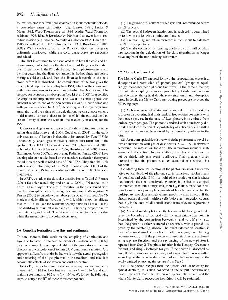
892 H. Yajima et al.
follow two empirical relations observed in giant molecular clouds:a power-law mass distribution (e.g. Larson 1981; Fuller &Myers 1992; Ward-Thompson et al. 1994; Andre, Ward-Thompson& Motte 1996; Blitz & Rosolowsky 2006), and a power-law mass–radius relation (e.g. Sanders, Scoville & Solomon 1985; Dame et al.1986; Scoville et al. 1987; Solomon et al. 1987; Rosolowsky 2005,2007). Within each grid cell in the RT calculation, the hot gas isuniformly distributed, while the cold, dense cores are randomlyembedded.
The dust is assumed to be associated with both the cold and hotphase gases, and it follows the distribution of the gas with certaindust-to-gas ratio. In the RT calculation, when a photon enters a cell,we first determine the distance it travels in the hot phase gas beforehitting a cold cloud, and then the distance it travels in the coldcloud before it is absorbed. The combination of the two gives thetotal optical depth in the multi-phase ISM, which is then comparedwith a random number to determine whether the photon should bestopped for scattering or absorption (see Li et al. 2008 for a detaileddescription and implementation). The Lyα RT in a multi-phase ISMand dust model is one of the new features in our RT code comparedwith previous works. In ART2, depending on the hydrodynamicsimulation and the nature of the calculation, we can choose either amulti-phase or a single-phase model, in which the gas and the dustare uniformly distributed with the mean density in a cell, for theISM.
Galaxies and quasars at high redshifts show extinction by inter-stellar dust (Maiolino et al. 2004; Ouchi et al. 2004). In the earlyuniverse, most of the dust is thought to be created by Type II SNe.Theoretically, several groups have calculated dust formation in theejecta of Type II SNe (Todini & Ferrara 2001; Nozawa et al. 2003;Schneider, Ferrara & Salvaterra 2004; Hirashita et al. 2005; Dwek,Galliano & Jones 2007). In particular, Todini & Ferrara (2001) havedeveloped a dust model based on the standard nucleation theory andtested it on the well-studied case of SN1987A. They find that SNewith masses in the range of 12–35 M� produce about 0.01 of themass in dust per SN for primordial metallicity, and ∼0.03 for solarmetallicity.
In ART2, we adopt the dust size distribution of Todini & Ferrara(2001) for solar metallicity and an M = 22 M� SN model, as infig. 5 in their paper. The size distribution is then combined withthe dust absorption and scattering cross-section of Weingartner &Draine (2001) to calculate dust absorption opacity curves. The SNmodels include silicate fractions f s = 0.1, which show the silicatefeature ∼9.7 μm (see the resultant opacity curve in Li et al. 2008).The dust-to-gas mass ratio in each cell is linearly proportional tothe metallicity in the cell. The ratio is normalized to Galactic valuewhen the metallicity is the solar abundance.
2.6 Coupling ionization, Lyα line and continuum
To date, there is little work on the coupling of continuum andLyα line transfer. In the seminar work of Pierleoni et al. (2009),they incorporated pre-computed tables of the properties of the Lyα
photons in the calculation of ionizing UV continuum radiation. Ourapproach differs from theirs in that we follow the actual propagationand scattering of the Lyα photons in the medium, and take intoaccount the effects of ionization and dust absorption.
In ART2, the photons are treated in three regimes: ionizing con-tinuum at λ ≤ 912 Å, Lyα line with centre λ = 1216 Å and non-ionizing continuum at 912 Å < λ ≤ 107 Å. We follow the followingsteps to couple the RT of these three components.
(1) The gas and dust content of each grid cell is determined beforethe RT process.
(2) The neutral hydrogen fraction nH I in each cell is determinedby following the ionizing continuum photons.
(3) The resulting ionization structure is then input to calculatethe RT of Lyα photons.
(4) The absorption of the ionizing photons by dust will be takeninto account in the calculation of the dust re-emission in longerwavelengths of the non-ionizing continuum.
2.7 Monte Carlo method
The Monte Carlo RT method follows the propagation, scattering,absorption and reemission of ‘photon packets’ (groups of equal-energy, monochromatic photons that travel in the same direction)by randomly sampling the various probability distribution functionsthat determine the optical depth, scattering angle and absorptionrates. In detail, the Monte Carlo ray-tracing procedure involves thefollowing steps.
(1) A photon packet of continuum is emitted from either a stellarsource or an accreting BH with random frequencies consistent withthe source spectra. In the case of Lyα photon, it is emitted fromionized hydrogen gas. The photon is emitted with a uniformly dis-tributed random direction. The probability of a photon being emittedby any given source is determined by its luminosity relative to thetotal.
(2) A random optical depth over which the photon must travel be-fore an interaction with gas or dust occurs, τ i = −lnξ , is drawn todetermine the interaction location. The interaction includes scat-tering and absorption. In our method, the photon energies arenot weighted, only one event is allowed. That is, at any giveninteraction site, the photon is either scattered or absorbed, butnot both.
(3) Starting from the location of the photon emission, the cumu-lative optical depth of the photon, τ tot, is calculated stochasticallyfor both hot and cold ISM in a multi-phase model, or single-phasemedium with the mean density along the ray. If the photon is stoppedfor interaction within a single cell, then τ tot is the sum of contribu-tions from possibly multiple segments of both hot and cold for themulti-phase model, or a single-phase gas/dust within this cell. If thephoton passes through multiple cells before an interaction occurs,then τ tot is the sum of all contributions from relevant segments inthese cells.
(4) At each boundary between the hot and cold phase gas clouds,or at the boundary of the grid cell, the next interaction point isdetermined by the comparison between τ i and τ tot. If τ i ≤ τ tot,then the photon is either scattered or absorbed, with a probabilitygiven by the scattering albedo. The exact interaction location isthen determined inside either hot or cold phase gas, such that τ tot
becomes exactly τ i. If the photon is scattered, its direction is alteredusing a phase function, and the ray tracing of the new photon isrepeated from Step 2. The phase function is the Henyey–Greensteinfor dust, and simply isotropic for gas. If the photon is absorbed bydust, the dust temperature is raised, and a new photon is re-emittedaccording to the scheme described below. The ray tracing of thenewly emitted photon again restarts from Step 2.
(5) If the photon escapes from the system without reaching theoptical depth τ i, it is then collected in the output spectrum andimage. The next photon will be picked up from the source, and thewhole Monte Carlo procedure from Step 1 will be restarted.
C© 2012 The Authors, MNRAS 424, 884–901Monthly Notices of the Royal Astronomical Society C© 2012 RAS
Dow
nloaded from https://academ
ic.oup.com/m
nras/article/424/2/884/1004516 by KIM H
ohenheim user on 20 April 2022

ART2: coupling Lyα line and continuum 893
2.8 Making images
In ART2, we incorporate a ‘peeling off’ procedure using weightedphotons to obtain high-resolution images from a particular viewingdirection. From a particular viewing direction, the contribution fromdirect (radiation source or thermal dust emission) and scatteredphotons is tracked separately with different weight.
At each location of emission, the contribution from direct photonsto the image is computed as
Idirec(x, y) = I0e−τ1
4πd2, (25)
where I0 is the energy of each photon packet, x and y are the positionof the emission site projected on to the image plane, and τ 1 and dare the total optical depth and distance from the emission site to theobserver, respectively.
At each scattering site, the contribution from scattered photonsto the image is
Iscatt(x, y) = I0e−τ2f (θ )
d2, (26)
where τ 2 is the optical depth from the scattering location to theobserver, and f (θ ) is the scattering phase function.
The total intensity of the image is the sum of Idirect and Iscatt, and isaccumulated as each photon packet is emitted and scattered duringthe course of the Monte Carlo simulation. To obtain an image fora given telescope at a given waveband, a specific filter function isthen applied to convolve the image.
3 A P P L I C AT I O N TO C O S M O L O G I C A LSIMULATIONS
3.1 The simulations
The cosmological simulation presented here follows the formationand evolution of a Milky Way sized galaxy and its substructures. Thesimulation includes dark matter, gasdynamics, star formation, BHgrowth and feedback processes. The initial condition is originallyfrom the Aquarius Project (Springel et al. 2008), which produced thelargest ever particle simulation of a Milky Way sized dark matterhalo. The hydrodynamical initial condition is reconstructed fromthe original collisionless one by splitting each original particle intoa dark matter and gas particle pair, displaced slightly with respectto each other (at fixed centre of mass) for a regular distribution ofthe mean particle separation, and with a mass ratio correspondingto a baryon fraction of 0.16 (Wadepuhl & Springel 2011).
The whole simulation falls in a periodic box of 100 h−1 Mpc oneach side with a zoom-in region of size 5 × 5 × 5 h−3 Mpc3. Thespatial resolution is ∼250 h−1 pc in the zoom-in region. The massresolution of this zoom-in region is ∼2 × 10⁵ h−1 M� for darkmatter particles, and ∼1.9 × 10⁴ h−1 M� for gas and star particles.The cosmological parameters used in the simulation are �m = 0.25,�� = 0.75, σ 8 = 0.9 and h = 0.73, consistent with the 5-yr results ofthe Wilkinson Microwave Anisotropy Probe (Komatsu et al. 2009).The simulation evolves from z = 127 to z = 0.
The simulation was performed using the parallel, N-body/SPHcode GADGET-3, which is an improved version of that described inSpringel, Yoshida & White (2001) and Springel (2005). For the com-putation of gravitational forces, the code uses the ‘TREEPM’ method(Xu 1995) that combines a ‘tree’ algorithm (Barnes & Hut 1986)for short-range forces and a Fourier transform particle mesh method(Hockney & Eastwood 1981) for long-range forces. GADGET im-plements the entropy-conserving formulation of SPH (Springel &
Hernquist 2002) with adaptive particle smoothing, as in Hernquist &Katz (1989). Radiative cooling and heating processes are calculatedassuming collisional ionization equilibrium (Katz et al. 1996; Daveet al. 1999). Star formation is modelled in a multi-phase ISM, witha rate that follows the Schmidt–Kennicutt law (Schmidt 1959; Ken-nicutt 1998). Feedback from SNe is captured through a multi-phasemodel of the ISM by an effective equation of state for star-forminggas (Springel & Hernquist 2003a). The UV background model ofHaardt & Madau (1996) is used.
BH growth and feedback are also included in our simulationbased on the model of Springel, Di Matteo & Hernquist (2005b), DiMatteo, Springel & Hernquist (2005), where BHs are represented bycollisionless ‘sink’ particles that interact gravitationally with othercomponents and accrete gas from their surroundings. The accretionrate is estimated from the local gas density and sound speed usinga spherical Bondi–Hoyle (Hoyle & Lyttleton 1941; Bondi & Hoyle1944; Bondi 1952) model that is limited by the Eddington rate.Feedback from BH accretion is modelled as thermal energy, ∼5 percent of the radiation, injected into surrounding gas isotropically, asdescribed in Springel et al. (2005b) and Di Matteo et al. (2005). Thisfeedback scheme self-regulates the growth of the BH and has beendemonstrated to successfully reproduce many observed propertiesof local elliptical galaxies (e.g. Springel, Di Matteo & Hernquist2005a; Hopkins et al. 2006) and the most distant quasars at z ∼6 (Li et al. 2007). We follow the BH seeding scheme of Li et al.(2007) and Di Matteo et al. (2008) in the simulation: a seed BH ofmass MBH = 105 h−1 M� was planted in the gravitational poten-tial minimum of each new halo identified by the friends-of-friends(FOF) group finding algorithms with a total mass greater than1010 h−1 M�.
Each snapshot is processed by an on-flying FOF group findingalgorithm with a dark matter linking length less than 20 per centof their mean spacing. Other types of particles are then linked tothe nearest dark matter particle. A substructure detection algorithmSUBFIND (Dolag et al. 2009) is then applied to each group to searchsatellite haloes. In the simulation, each FOF group with its substruc-ture is identified as a galaxy (a detailed description of the simulationis presented in Zhu et al., in preparation).
In this work, we apply the ART2 code to the 10 most massivegalaxies in each snapshot at six redshift bins from z = 3.1 to 10.2 andfocus on the Lyα and multi-band properties. In our post-processingprocedure, we first calculate the RT of ionizing photons (λ ≤ 912 Å)and estimate the ionization fraction of the ISM. The resulting ioniza-tion structure is then used to run the Lyα RT to derive the emissivity,followed by the calculation of non-ionizing continuum photons (λ> 912 Å) in each cell. Our fiducial run is done with Nph = 105 pho-ton packets for each ionizing, Lyα and non-ionizing components.Because the spatial resolution of the cosmological simulation is notadequate to resolve the multiple phase of the ISM, we assume asingle-phase medium in each density grid. The highest refinementof the grid is RL = 11.
3.2 Multi-wavelength properties of high-redshift galaxies
3.2.1 Flux images
The galaxies in our sample are the 10 most massive ones from thecosmological simulation at six snapshots from z = 3.1 to 10.2. Notethat because our simulation focuses on a Milky Way sized galaxy,our sample represents the progenitors of the Milky Way at differentcosmic time; they are not the typical ‘massive’ galaxies one expectsfrom a general cosmological simulation with a mean overdensity.
C© 2012 The Authors, MNRAS 424, 884–901Monthly Notices of the Royal Astronomical Society C© 2012 RAS
Dow
nloaded from https://academ
ic.oup.com/m
nras/article/424/2/884/1004516 by KIM H
ohenheim user on 20 April 2022

894 H. Yajima et al.
Figure 9. Evolution of galaxies in different wavebands. The left-hand panels show the distribution of gas and stars from the cosmological simulation. Middlepanels show the surface brightness of Lyα, and right-hand panels are the flux images in NIR IRAC-1 (3.6 μm) on board of Spitzer telescope. The box size is1 Mpc in comoving scale. Note the middle and right-hand panels show only images of the most massive galaxies corresponding to the redshifts labelled in theleft-hand column.
The total and stellar masses of these galaxies become larger withtime (decreasing redshift) due to gas accretion and merging process.For example, the total mass of the most massive galaxy is ∼2.6 ×10¹⁰ M�, 5.8 × 10¹⁰ M�, 1.6 × 10¹¹ M� and 5.4 × 10¹¹ M� atz = 10.2, 8.5, 6.2 and 3.1 respectively, and the corresponding stellarmass is ∼8.5 × 10⁸ M�, 4.3 × 10⁹ M�, 9.3 × 10⁹ M� and 4.1 ×10¹⁰ M�.
Fig. 9 (left-hand panels) shows the projected density of gas andstars of each snapshot at the mentioned redshift. Filamentary struc-ture is clearly seen, and the most massive galaxy resides in theintersection of the filaments. The resulting Lyα and near-infrared(NIR) fluxes of the most massive galaxy from our RT calculationsare shown in the middle and right-hand panels of Fig. 9, respectively.The NIR band corresponds to IRAC-1 (3.6 μm) of the Spitzer tele-scope. The flux image is generated from a ‘peeling off’ techniquein the RT calculation as described in Section 2.8.
The Lyα emission appears to follow the distribution of gas andstars of the galaxy. Its surface brightness and size increase withtime (decreasing redshift), while those of the NIR show a differentpattern. The Lyα emission depends on the star formation rate (SFR)of the galaxy and the photon escape fraction. Although SFR de-creases at lower redshift, the escape fraction increases as the galaxygrows larger, resulting in an increase in Lyα luminosity. In addi-tion, the Lyα emission is bright over extended region, owing tomany scattering processes.
On the other hand, the observed IRAC-1 in these redshifts cor-responds to wavelengths ∼3200–9000 Å in the rest frame, henceit depends on both SFR and stellar mass of the galaxy. The cross-section of dust decreases steeply with increasing wavelength; itbecomes very small at these wavelengths. Therefore, a significantfraction of photons emitted by the stars in this wavelength range canescape without being scattered or absorbed by dust. Thus, unlike
C© 2012 The Authors, MNRAS 424, 884–901Monthly Notices of the Royal Astronomical Society C© 2012 RAS
Dow
nloaded from https://academ
ic.oup.com/m
nras/article/424/2/884/1004516 by KIM H
ohenheim user on 20 April 2022

ART2: coupling Lyα line and continuum 895
Lyα, the IRAC-1 image is more compact, and it concentrates onthe high-density peak of stars. We note that the infrared fluxes arehigher than those of the LAE sample at z = 3.1 by Gronwall et al.(2007), but comparable with those of the IRAC-detected LAEs inLai et al. (2008). This may be due to high SFR in these galaxies.
The NIR wavelength shown here is similar to the F356W fil-ter of the next generation telescope, the James Webb Space Tele-scope (JWST). The detection limit of the filter in AB magnitude canachieve mAB = 28.1 with 1 h exposure time (e.g. Zackrisson et al.2011). Our calculations show that the model galaxies have mAB =24.3 (z = 3.1), 25.1 (z = 6.2), 28.5 (z = 8.5) and 29.8 (z = 10.2) atthis wavelength. Hence, the JWST will be able to detect the infraredemission from galaxies such as the progenitor of the Milky Way at z∼ 6 with an ∼1 min exposure time. Even at higher redshifts, thesegalaxies may be detected with an integration of ∼2 h for z = 8.5,and ∼23 h for z = 10.2.
3.2.2 Evolution of spectral energy distribution
The corresponding multi-wavelength SEDs of the most massivegalaxy at selected redshift are shown in Fig. 10. The shape of theSED changes significantly from z = 10.2 to z = 3.1, as a resultof changes in radiation from stars, absorption of ionizing photonsby gas and dust, and re-emission by dust in the infrared. The Lyα
line appears to be strong in all cases. The deep decline of UVcontinuum at z > 8 is caused by strong absorption of ionizingphotons by the dense gas. Galaxy at lower redshift has a higherfloor of continuum emission from stars and accreting BHs, a higherionization fraction of the gas, and a higher infrared bump owingto increasing amount of dust and absorption. Moreover, due to theeffect of negative k-correction, the flux at �500 μm stays close indifferent redshifts. Our calculations show that the model galaxieshave a flux of f ν = 0.043 (z = 3.1), 0.057 (z = 6.2), 0.02 (z = 8.5) and0.004 (z = 10.2) mJy at 850 μm in observed frame. The new radiotelescope Atacama Large Millimetre/Submillimetre Array (ALMA)may be able to detect such galaxies at z ∼ 6 with ∼2 h integration,and at z ∼ 8.5 for ∼20 h with 16 antennas. Even with ALMA, it
Figure 10. SED of model galaxies at redshifts z = 10.2 (green), 8.5 (orange),7.2 (blue), 6.2 (purple) and 3.1 (black), respectively.
may be very difficult to detect such a galaxy at z = 10.2 (more than70 d integration).
From the SEDs, it is interesting to compare the emergent Lyα lu-minosity and that of the infrared integrated from 8 to 1000 μmin the rest frame. A simple relation between infrared and Lyα
luminosity has been suggested by Kennicutt (1998) through starformation, namely SFR(M� yr−1) = 4.5 × 10−44 LIR(erg s−1) andSFR(M� yr−1) = 0.91 × 10−42Lα(erg s−1) with the assumption ofLα /LHα = 8.7 (Case B). However, our calculation suggests a morecomplex relation between Lyα and infrared luminosity, as inferredfrom Fig. 10. This is because Lα depends on f Lyα
esc , while the LIR de-pends on f UV
esc , and the two escape fractions differ from each other.In our simulations, the f UV
esc mostly decreases with redshift, and isbelow 0.5 at z � 6. Hence, the UV continuum may serve as a goodtracer of SFR at z � 6, while at z � 6 the infrared flux may be one.In addition, since the modelled galaxies at z � 6 show a smallervalue of f Lyα
esc than 0.5 (see the next subsection), Lyα flux also maynot be a good indicator of SFR.
3.2.3 The Lyα properties
The derived properties of Lyα emission from these modelled galax-ies are shown in Fig. 11, in comparison with their correspondingSFR. The most massive galaxies at very high redshift (z > 6) main-tain a high SFR of ∼10–30 M� yr−1 fuelled by accretion of cold gasand merging process. The SFR decreases to ∼3 M� yr−1 at z ∼ 3owing to depletion of star-forming gas and suppression by radiationfeedback from both stars and accreting BHs. The resulting emergentLyα luminosity from recombination of ionizing photons and fromexcitation cooling increases from ∼1.0 × 1042 erg s−1 at z = 8.5 to
Figure 11. Lyα properties of modelled galaxies at different redshifts, inclockwise direction: SFR, emergent Lyα luminosity, EW of Lyα line in restframe, and photon escape fraction of Lyα (open circles) and UV continuum(1300–1600 Å, crosses). Red and blue filled circles are the values of themost massive galaxies and the median in our sample at each snapshot,respectively. Filled and open red circles in the panel of escape fraction showthe Lyα and UV continuum escape fraction of the most massive galaxies;filled and open blue circles are the median values of Lyα and UV continuum,respectively.
C© 2012 The Authors, MNRAS 424, 884–901Monthly Notices of the Royal Astronomical Society C© 2012 RAS
Dow
nloaded from https://academ
ic.oup.com/m
nras/article/424/2/884/1004516 by KIM H
ohenheim user on 20 April 2022

896 H. Yajima et al.
∼2.3 × 1042 erg s−1 at z = 3.1. The observed LAE luminosity func-tions show a characteristic luminosity L∗
Lyα ∼ 4.4 × 1042 erg s−1 atz = 6.6 (Ouchi et al. 2010), and L∗
Lyα ∼ 6 × 1042 erg s−1 at z = 3.1(Gronwall et al. 2007; Ouchi et al. 2008; Blanc et al. 2011), whichare comparable to the luminosity range of our modelled galaxies.The median values of SFR moderately decrease with increasingredshift, and show ∼0.5–3 M� yr−1. However, the Lα does not de-crease largely by the redshift evolution of f esc. In addition, a fewgalaxies in each snap shot are Lyα bright, and have Lyα luminosityof Lα ≥ 1042erg s−1, which is detectable with recent observationalstudies (e.g. Ouchi et al. 2008).
The lower-left panel of Fig. 11 shows the photon escape fractionof Lyα, f Lyα
esc and UV continuum f UVesc , where f UV
esc is calculated atλrest = 1300–1600 Å. Both escape fractions appear to increasewith time (decreasing redshift), with f Lyα
esc ∼ 0.18 at z = 8.5 to∼0.5 at z = 3.1, while f UV
esc ∼ 0.09 at z = 8.5 to ∼0.6 at z = 3.1.In the early evolution phase, the most massive galaxies are compactand gas-rich. They grow rapidly from accretion of cold gas whichfuelled intense star formation. The highly concentrated gas anddust efficiently absorb the Lyα and UV photons, and suppress theirescape. At a later time, the gas and stars distribute to a more extendedregion, and a large fraction of gas is converted to stars. Hence, thephoton may easily escape from the galaxy, contributing to a higherphoton escape fraction.
On the other hand, the median value of f esc of Lyα and UVincreases monotonically with redshift, e.g. f Lyα
esc ∼ 0.75 at z = 8.5to ∼0.29 at z = 3.1, while f UV
esc ∼ 0.81 at z = 8.5 to ∼0.38 at z =3.1. Such a trend is consistent with observations by Hayes et al.(2011).
Unlike the most massive galaxies, the low-mass ones have lowerSFR and lower dust content, the ISM is less dense and less clumpy,and the metallicity is lower. As a result, the escape fractions arehigher in small galaxies than the massive ones.
The EW of Lyα line is defined by the ratio between the Lyα fluxand the UV flux density f UV in rest frame, where the mean fluxdensity of λ = 1300–1600 Å in rest frame is used. In practice, the
EW is estimated by EW = EWintf Lyαescf UVesc
, where EWint is the intrinsicEW. The EWint depends on the stellar SED and the excitation Lyα
cooling: the younger SED (or top-heavy IMF) and the more efficientLyα cooling, the higher EWint.
The resulting Lyα EWs of the most massive galaxies are shownin the lower-right panel of Fig. 11. Since the photon escape fractionof Lyα is close to that of the UV continuum, the EW shown isbasically EWint. All three modelled galaxies have EW > 20 Å;they are therefore classified as LAEs (e.g. Gronwall et al. 2007).The EW evolves gradually with redshift. At z > 6, the EWs are high,EW ∼ 60 Å, owing to strong Lyα emission from excitation coolingand AGN activity, while at z = 3.1, it drops to ∼21 Å as the Lyα
emission is mainly produced by stellar radiation. The median valueincreases more steeply with redshift, from ∼14 Å at z = 3.1 Å to∼164 at z = 8.5. These EWs are within the observed range, andthe trend is in broad agreement with observations that galaxies athigher redshifts appear to have higher EW than their counterparts atlower redshifts (e.g. Gronwall et al. 2007; Ouchi et al. 2008). Somegalaxies at higher redshift z � 8 show very high EW because theexcitation Lyα cooling becomes dominant (Yajima et al. 2011b).However, it will be suppressed significantly by IGM at such a highredshift.
The recent discovery of the most distant LAE, UDFy-38135539,at z = 8.6 by Lehnert et al. (2010) marks a milestone in observationalcosmology that galaxies formed less than 600 million years after
the big bang. The detected Lyα line flux of this object is ∼6 ×10⁻¹⁸ erg cm−2 s−1, which implies a Lyα luminosity of ∼5.5 ×1042 erg s−1. This is close to that of our galaxy at z = 8.5. Our modelsuggests that this LAE may have a total mass of ∼1010−11 M�, astellar mass of ∼109 M�, a SFR of the order of 10 M� yr−1 andf Lyα
esc ∼ 0.18. We note that Dayal et al. (2011) suggested a lowerSFR of 2.7 − 3.7 M� yr−1 for this galaxy by assuming a Lyα escapefraction of 100 per cent. However, our detailed RT calculations showthat the escape fraction is much smaller than unity, which meansthat it would require a higher SFR in order to produce the observedLyα flux.
3.2.4 The Lyα line profiles
Fig. 12 shows the profiles of Lyα line of the modelled galaxies. Thefrequency of the intrinsic Lyα photon is sampled from a Maxwelliandistribution with the gas temperature at the emission location in therest flame of the gas. We collect all escaped Lyα photons and esti-mate the line profile. In practice, the inhomogeneous gas structurecan cause the change of flux depending on the viewing angle. Al-though the Lyα flux can change by some factors (Yajima et al.2011b), we focus on only the mean value in this paper.
The Lyα lines of our galaxies show mostly a single peak, acommon profile of LAEs at high redshifts (e.g. Ouchi et al. 2010).In a static and optically thick medium, the profile can be doublepeaked, but when the effective optical depth is small due to highrelative gas speed or ionization state, there might be only a singlepeak (Zheng & Miralda-Escude 2002). In our case, the flow speedof gas is up to ∼300 km s−1, and the gas is highly ionized by stellarand AGN radiation, which results in a single peak.
In addition, the profile at higher redshift shifts to shorter wave-length, and it shows the characteristic shape of gas inflow (Zheng &Miralda-Escude 2002). Although our simulation includes feedbackof stellar wind similar to that of Springel et al. (2005b), the Lyα
line profile shows a gas-inflow feature or a symmetric one indicatesgas inflow or symmetric in these galaxies. Our result suggests that
Figure 12. Emergent Lyα profile. Dot and solid lines are the profiles ofintrinsically emitted and escaped photons, respectively.
C© 2012 The Authors, MNRAS 424, 884–901Monthly Notices of the Royal Astronomical Society C© 2012 RAS
Dow
nloaded from https://academ
ic.oup.com/m
nras/article/424/2/884/1004516 by KIM H
ohenheim user on 20 April 2022

ART2: coupling Lyα line and continuum 897
high-redshift star-forming galaxies may be fuelled by efficient in-flow of cold gas from the filaments. We will address this issue indetail in a forthcoming paper (Yajima et al., in preparation).
We note that there is a number of studies on inflow and outflow inLyα lines, both observationally (Kunth et al. 1998) and theoretically(e.g. Verhamme et al. 2006; Dijkstra & Wyithe 2010; Barnes et al.2011; Dijkstra, Mesinger & Wyithe 2011). It has been suggestedthat the IGM correction of Lyα emission may be enhanced due toinflow (e.g. Dijkstra, Lidz & Wyithe 2007) or decreased via outflows(e.g. Verhamme et al. 2006). However, there is a large uncertainty inthe prescription of wind feedback in current simulations. To inves-tigate the velocity field of ISM in high-redshift galaxies, one needssimulations with a realistic wind model and a high spatial resolu-tion comparable to that of line observations, which are currentlyunavailable and are beyond the scope of this paper.
In addition, the line profile may be highly suppressed and changedby scattering in the IGM (e.g. Santos 2004; Dijkstra et al. 2007;Zheng et al. 2010; Laursen, Sommer-Larsen & Razoumov 2011).The IGM effectively absorbs the Lyα photons at the line centreand at shorter wavelengths by the Hubble flow (e.g. Laursen et al.2011). Therefore, the inflow feature in our profiles may disappearand the shape may change to an asymmetric single peak with onlyphotons at red wing. We will investigate the IGM correction infuture work that includes propagation and scattering of Lyα andionizing photons in the IGM.
3.2.5 The properties of ionizing photons
Fig. 13 shows the escape fraction of ionizing photons, f Ionesc , and
the resulting emissivity from both stars and AGNs of the modelledgalaxies. The escape fraction of the most massive galaxies has arange of f Ion
esc ∼ 0.03–0.37, consistent with the results of Dijkstraet al. (2011) and Yajima et al. (2011a). In addition, f Ion
esc decreaseswith increasing redshift. Unlike the Lyα and non-ionizing UV pho-tons, the ionizing photons can be absorbed by hydrogen gas anddust. At high redshift, the star formation efficiency is small, so alarge fraction of hydrogen gas remains neutral and prevents the es-
Figure 13. The escape fraction of ionizing photons (top panel) and theresulting emissivity (bottom panel) of modelled galaxies at redshifts z =3.1–10.2. Red and blue filled circles are the values of the most massivegalaxies and the median in our sample at each snapshot, respectively.
cape of ionizing photons. The median values do not decrease withredshift due to lower dust mass.
The emissivity of the ionizing photons roughly increases withdecreasing redshift, reaching ∼5 × 1053 s−1 at z = 3.1. In thiswork, we do not calculate the RT in the IGM, but the size of theH II bubble around the galaxy may be estimated by a modifiedStromgrem sphere. Assuming a clumpiness factor of C = 5 (Ilievet al. 2007; Pawlik, Schaye & van Scherpenzeel 2009), the radiusof the H II bubble is estimated to be r = 554, 198, 47 and 28 kpcat z = 3.1, 6.2, 8.5 and 10.2, respectively. The Lyα photons maypass through the H II bubbles, resulting in a correlation betweenhigh-redshift LAEs and H II regions, as suggested by McQuinnet al. (2007). In addition, the median value of ionizing photonsemissivity is smaller due to lower SFR, and hence the H II bubblebecomes smaller than that of the most massive galaxy by a factorof ∼2–6.
4 DI SCUSSI ON
In observations of Lyα emission from high-redshift galaxies, thereare a number of uncertainties regarding the contributions fromAGNs (e.g. Wang et al. 2004; Ouchi et al. 2008; Nilsson & Møller2011), stars and excitation cooling from cold accretion. With ourmodel, we can separate the radiation components and disentanglethe contribution from different sources. Also, in numerical simu-lations, resolution plays an important role in the robustness of theresults. So we discuss these physical and numerical effects on Lyα
emission in this section.
4.1 Effects of AGN and stellar radiation on Lyα emission
The effects of AGN and stars on the Lyα emission is shown inFig. 14. It appears that the presence of AGN does not change sig-nificantly the Lyα escape fraction. It is because AGNs are usuallylocated in Galactic Centre where the gas density peaks, most of theionizing photons near Lyman-limit (∼13.6 eV) are trapped there(e.g. Nagamine et al. 2010; Yajima et al. 2011a) and cannot escape.
Figure 14. Effects of AGN on escape fraction of Lyα photons (top panel)and the emergent luminosity (bottom panel). The ionization and Lyα lumi-nosity are estimated with radiation from the following sources: UVB only(triangles), UVB + star (squares) and UVB + AGN + star (circles).
C© 2012 The Authors, MNRAS 424, 884–901Monthly Notices of the Royal Astronomical Society C© 2012 RAS
Dow
nloaded from https://academ
ic.oup.com/m
nras/article/424/2/884/1004516 by KIM H
ohenheim user on 20 April 2022

898 H. Yajima et al.
On the other hand, a fraction of high-energy photons can escapefrom the galaxy without ionizing interstellar gas due to small cross-section of gas and dust. Therefore, AGN radiation has little effecton the f esc of Lyα photons. There is no change in f esc in the casewhere there is no stellar and AGN radiation.
In addition, the AGN does not affect the Lyα luminosity, asshown in the bottom panel of Fig. 14. This may be because theBHs in these galaxies are still quite small and the accretion ratesare quite low. On the other hand, the presence of stars appears tochange the escape fraction and emergent luminosity of Lyα, be-cause the stellar radiation is much stronger than that of AGN inthe model galaxies, and the effect becomes stronger at lower red-shift. Because Lyα emissivity is produced by the recombination ofionizing photons and collisional excitation from hydrogen gas, theinterplay between these two mechanisms determines the outcome.At redshifts z > 6, excitation cooling from cold accretion of densegas becomes comparable to recombination cooling, while at z ∼ 3,the number of Lyα photons by recombination in H II regions by starsand AGNs outnumbers that from excitation cooling. Therefore, thecontribution from stars to the Lyα emission changes with cosmictime and environment. The Lyα emissivity from excitation coolingcan be reduced due to the stellar ionization (e.g. Faucher-Giguereet al. 2010). Moreover, the distribution of excitation Lyα coolingcan be more extended than star-forming regions, resulting in higherescape fraction. Thus, the escape fraction and emergent luminosityof Lyα somewhat increase in the case without stellar radiation.
4.2 Resolution effect
Fig. 15 demonstrates effects of photon number on the escape fractionof Lyα photons, with different number of photon packets, Nph =102, 103, 104 and 105. It appears that the results converge once thephoton number is above 104, which is an order of magnitude lowerthan the fiducial Nph = 105 in our general RT calculations. Therelative difference between Nph = 104 and 105 is 1–6 per cent. Ofcourse, the photon number should increase with galaxy mass, butfor our modelled galaxies, Nph = 105 should be sufficient.
Figure 15. Effects of photon number on the escape fraction of Lyα photons.Open triangles, squares and circles indicate photon packet number Nph =102, 103, 104 and 105, respectively. The fiducial number used in our generalRT calculations is Nph = 105.
Figure 16. Effect of grid resolution on the escape fraction of Lyα photons.Different colour indicates different maximum RL: purple – RL = 4, blue– RL = 6, green – RL = 8, orange – RL = 10, and red – RL = 11. Thefiducial RL used in our general RT calculations is 11. The cell size of thehighest RL is 1/2RL +1 Mpc in comoving scale.
The effects of grid resolution on the escape fraction of Lyα pho-tons is presented in Fig. 16, where results from different maximumRL are compared. It appears that f esc changes dramatically with RL,but it converges at RL ≥ 10. Grids with poor resolution can produceartificially high f esc by a factor of more than 20. Because most ofthe Lyα photons are created in high-density gas clumps, where theyare also effectively absorbed by numerous scatterings, sufficientlyresolving the gas density field is important in the calculation of Lyα
RT. If we follow the resolution of RL = 10 with uniform grids,it would require a number of cells of ∼20483, too expensive forRT simulations with the current computational facility. In fact, thecurrent limit is ∼5003, as demonstrated by recent work on 3D RTcalculations using uniform grid (e.g. Iliev et al. 2007; Yajima et al.2011a). Therefore, adaptive refinement grid is critical in the RTcalculation of Lyα emission.
5 SU M M A RY
We have presented an improved, 3D, Monte Carlo RT code ART2 tostudy multi-wavelength properties of galaxies. It has the followingessential features.
(i) It couples Lyα line, ionization of neutral hydrogen and multi-wavelength continuum RT. The Lyα module includes emission fromboth recombination and collisional excitation, and the continuumincludes emission from X-ray to radio.
(ii) It employs an adaptive grid scheme in 3D Cartesian coor-dinates, which handles an arbitrary geometry and covers a largedynamic range over several orders of magnitude. Such a grid is crit-ical in resolving the clumpy, highly inhomogeneous density field inthe RT calculations.
(iii) It adopts a two-phase ISM model in which the cold, denseclouds are embedded in a hot, diffuse medium in pressure equilib-rium. In the case where hydrodynamic simulations have sufficientresolution to resolve the multi-phase ISM, this model ensures anappropriate prescription of the ISM physics, which is important forstudying dust properties in galaxies.
C© 2012 The Authors, MNRAS 424, 884–901Monthly Notices of the Royal Astronomical Society C© 2012 RAS
Dow
nloaded from https://academ
ic.oup.com/m
nras/article/424/2/884/1004516 by KIM H
ohenheim user on 20 April 2022

ART2: coupling Lyα line and continuum 899
(iv) It includes an SN-origin dust model in which the dust isproduced by Type II SNe, which is especially relevant for dustin high-redshift, young objects, because there are insufficient low-mass, old AGB stars in these systems to produce the observedamount of dust from the classical dust models.
(v) It follows the radiation from stars and AGNs, and calcu-lates the scattering, absorption and re-emission of the surroundingmedium. It efficiently and self-consistently produces SEDs and im-ages in a full spectrum, including Lyα emission line and continuumfrom X-ray to millimetre, as well as ionization structures of themedium, for direct comparison with multi-band observations.
(vi) It can be easily applied to either grid- or particle-based hy-drodynamical simulations and has broad applications in cosmology.
We have tested the new ART2 extensively, and found that thecoupling of Lyα line and continuum enables a self-consistent andaccurate calculation of the Lyα properties of galaxies, as the EW ofthe Lyα line depends on the UV continuum, and the escape fractionof Lyα photons strongly depends on the ionization structure and thedust content of the object.
We applied the code to a cosmological SPH simulation of a MilkyWay like galaxy, and studied in details a sample of massive galax-ies at redshift z = 3.1–10.2. We find that most of these galaxiesare LAEs. The escape fraction of Lyα photons of the most mas-sive galaxy in each snap shot increases with decreasing redshift,from about 0.18 at redshift z ∼ 8.5 to 0.6 at z ∼ 3. The emergentLyα luminosity shows similar trend, increasing from Lα = 1.0 ×1042 erg s−1 at z ∼ 8.5 to Lα = 2.3 × 1042 erg s−1 at z ∼ 3. TheEWs of these galaxies change with redshift as well, from ∼67 Åat z ∼ 8.5 to ∼21 Å at z ∼ 3. The profiles of the resulting Lyα
lines commonly show single peak, and the peak of the profile atz � 6 is shifted to shorter wavelength, implying gas inflow fromsurrounding filaments. On the other hand, the median values in ourgalaxy sample shows somewhat different trend from that of themost massive ones. The escape fraction monotonically increaseswith redshift, while the Lyα luminosity shows a weak evolution, asa result of the interplay between SFR and escape fraction.
Our results suggest that the LAEs and their properties evolvewith cosmic time, and that the first LAEs in the early universe, suchas currently the most distant one detected at z ∼ 8.6 (Lehnert et al.2010), may be dwarf galaxies with a total mass of ∼1010−11 M�fuelled by cold gas accretion. They may have a SFR of the order of10 M� yr−1, and a Lyα escape fraction of ∼20 per cent.
AC K N OW L E D G M E N T S
We thank Mark Dijkstra, Claude-Andre Faucher-Giguere, CarylGronwall, Robin Ciardullo, Lars Hernquist and Avi Loeb for stim-ulating discussions and helpful comments, as well as the refereefor an insightful and constructive report which has helped us inimproving the manuscript significantly. Support from NSF grantsAST-0965694, AST-1009867 (to YL) and AST-0807075 (to TA)is gratefully acknowledged. YL thanks the Institute for Theoryand Computation (ITC) at Harvard University where the projectwas started for warm hospitality. We acknowledge the ResearchComputing and Cyberinfrastructure unit of Information Technol-ogy Services at The Pennsylvania State University for providingcomputational resources and services that have contributed to theresearch results reported in this paper (URL: http://rcc.its.psu.edu).The Institute for Gravitation and the Cosmos is supported by theEberly College of Science and the Office of the Senior Vice Presi-dent for Research at the Pennsylvania State University.
R E F E R E N C E S
Abel T., Wandelt B. D., 2002, MNRAS, 330, L53Abel T., Norman M. L., Madau P., 1999, ApJ, 523, 66Adams T. F., 1972, ApJ, 174, 439Ahn S., Lee H., Lee H. M., 2000, J. Korean Astron. Soc., 33, 29Ahn S.-H., Lee H.-W., Lee H. M., 2001, ApJ, 554, 604Ahn S.-H., Lee H.-W., Lee H. M., 2002, ApJ, 567, 922Andre P., Ward-Thompson D., Motte F., 1996, A&A, 314, 625Auer L. H., 1968, ApJ, 153, 783Avery L. W., House L. L., 1968, ApJ, 152, 493Baek S., Di Matteo P., Semelin B., Combes F., Revaz Y., 2009, A&A, 495,
389Barnes J., Hut P., 1986, Nat, 324, 446Barnes L. A., Haehnelt M. G., Tescari E., Viel M., 2011, MNRAS, 416,
1723Bianchi S., Davies J. I., Alton P. B., 2000, A&A, 359, 65Bjorkman J. E., Wood K., 2001, ApJ, 554, 615Blanc G. A. et al., 2011, ApJ, 736, 31Blitz L., Rosolowsky E., 2006, ApJ, 650, 933Bondi H., 1952, MNRAS, 112, 195Bondi H., Hoyle F., 1944, MNRAS, 104, 273Bruzual G., Charlot S., 2003, MNRAS, 344, 1000Cen R., 1992, ApJS, 78, 341Chakrabarti S., Whitney B. A., 2009, ApJ, 690, 1432Ciardi B., Ferrara A., Marri S., Raimondo G., 2001, MNRAS, 324, 381Code A. D., Whitney B. A., 1995, ApJ, 441, 400Cowie L. L., Hu E. M., 1998, AJ, 115, 1319Cuby J.-G., Hibon P., Lidman C., Le Fevre O., Gilmozzi R., Moorwood A.,
van der Werf P., 2007, A&A, 461, 911Dame T. M., Elmegreen B. G., Cohen R. S., Thaddeus P., 1986, ApJ, 305,
892Dave R., Hernquist L., Katz N., Weinberg D. H., 1999, ApJ, 511, 521Dawson S. et al., 2004, ApJ, 617, 707Dayal P., Maselli A., Ferrara A., 2011, MNRAS, 410, 830Di Matteo T., Springel V., Hernquist L., 2005, Nat, 433, 604Di Matteo T., Colberg J., Springel V., Hernquist L., Sijacki D., 2008, ApJ,
676, 33Dijkstra M., Loeb A., 2008, MNRAS, 386, 492Dijkstra M., Wyithe J. S. B., 2010, MNRAS, 408, 352Dijkstra M., Haiman Z., Spaans M., 2006, ApJ, 649, 14Dijkstra M., Lidz A., Wyithe J. S. B., 2007, MNRAS, 377, 1175Dijkstra M., Mesinger A., Wyithe J. S. B., 2011, MNRAS, 414, 2139Dolag K., Borgani S., Murante G., Springel V., 2009, MNRAS, 399, 497Dwek E., Galliano F., Jones A. P., 2007, ApJ, 662, 927Efstathiou A., Rowan-Robinson M., 1990, MNRAS, 245, 275Faucher-Giguere C., Keres D., Dijkstra M., Hernquist L., Zaldarriaga M.,
2010, ApJ, 725, 633Field G. B., 1959, ApJ, 129, 551Finkelstein S. L. et al., 2011, ApJ, 729, 140Folini D., Walder R., Psarros M., Desboeufs A., 2003, in Hubeny I., Mi-
halas D., Werner K., eds, ASP Conf. Ser. Vol. 288, Stellar AtmosphereModelling. Astron. Soc. Pac., San Francisco, p. 433
Fuller G. A., Myers P. C., 1992, ApJ, 384, 523Fynbo J. U., Moller P., Thomsen B., 2001, A&A, 374, 443Fynbo J. P. U., Ledoux C., Moller P., Thomsen B., Burud I., 2003, A&A,
407, 147Gawiser E. et al., 2006, ApJ, 642, L13Gnedin N. Y., Abel T., 2001, New Astron., 6, 437Gnedin N. Y., Ostriker J. P., 1997, ApJ, 486, 581Gnedin N. Y., Kravtsov A. V., Chen H. W., 2008, ApJ, 672, 765Gronwall C. et al., 2007, ApJ, 667, 79Haardt F., Madau P., 1996, ApJ, 461, 20Hamilton D. R., 1940, Phys. Rev., 58, 122Hansen M., Oh S. P., 2006, MNRAS, 367, 979Harries T. J., Monnier J. D., Symington N. H., Kurosawa R., 2004, MNRAS,
350, 565Harrington J. P., 1973, MNRAS, 162, 43
C© 2012 The Authors, MNRAS 424, 884–901Monthly Notices of the Royal Astronomical Society C© 2012 RAS
Dow
nloaded from https://academ
ic.oup.com/m
nras/article/424/2/884/1004516 by KIM H
ohenheim user on 20 April 2022

900 H. Yajima et al.
Harrington J. P., 1974, MNRAS, 166, 373Hasegawa K., Umemura M., 2010, MNRAS, 407, 2632Hayes M. et al., 2010, Nat, 464, 562Hayes M., Schaerer D., Ostlin G., Mas-Hesse J. M., Atek H., Kunth D.,
2011, ApJ, 730, 8Hernquist L., Katz N., 1989, ApJS, 70, 419Hirashita H., Nozawa T., Kozasa T., Ishii T. T., Takeuchi T. T., 2005, MN-
RAS, 357, 1077Hockney R. W., Eastwood J. W., 1981, in Hockney R. W., Eastwood J. W.,
eds, Computer Simulation Using Particles. McGraw-Hill, New YorkHopkins P. F., Hernquist L., Cox T. J., Di Matteo T., Robertson B., Springel
V., 2006, ApJS, 163, 1Horton A., Parry I., Bland-Hawthorn J., Cianci S., King D., McMahon
R., Medlen S., 2004, in Moorwood A. F. M., Iye M., eds, SPIE Conf.Ser. Vol. 5492. Ground-based Instrumentation for Astronomy. SPIE,Bellingham, p. 1022
Hoyle F., Lyttleton R. A., 1941, MNRAS, 101, 227Hu E. M., Cowie L. L., 2006, Nat, 440, 1145Hu E. M., McMahon R. G., 1996, Nat, 382, 231Hu E. M., Cowie L. L., McMahon R. G., 1998, ApJ, 502, L99Hu E. M., Cowie L. L., McMahon R. G., Capak P., Iwamuro F., Kneib J.-P.,
Maihara T., Motohara K., 2002, ApJ, 568, L75Hu E. M., Cowie L. L., Capak P., McMahon R. G., Hayashino T., Komiyama
Y., 2004, AJ, 127, 563Hu E. M., Cowie L. L., Barger A. J., Capak P., Kakazu Y., Trouille L., 2010,
ApJ, 725, 394Hui L., Gnedin N. Y., 1997, MNRAS, 292, 27Hummer D. G., 1962, MNRAS, 125, 21Iliev I. T. et al., 2006, MNRAS, 371, 1057Iliev I. T., Mellema G., Shapiro P. R., Pen U., 2007, MNRAS, 376, 534Iliev I. T. et al., 2009, MNRAS, 400, 1283Iye M. et al., 2006, Nat, 443, 186Jonsson P., 2006, MNRAS, 372, 2Kashikawa N. et al., 2006, ApJ, 648, 7Katz N., Weinberg D. H., Hernquist L., Miralda-Escude J., 1996, ApJ, 457,
L57Kennicutt R. C., Jr, 1998, ARA&A, 36, 189Kodaira K. et al., 2003, PASJ, 55, L17Komatsu E. et al., 2009, ApJS, 180, 330Kunth D., Mas-Hesse J. M., Terlevich E., Terlevich R., Lequeux J., Fall S.
M., 1998, A&A, 334, 11Lai K., Huang J.-S., Fazio G., Cowie L. L., Hu E. M., Kakazu Y., 2007, ApJ,
655, 704Lai K. et al., 2008, ApJ, 674, 70Larson R. B., 1981, MNRAS, 194, 809Laursen P., Sommer-Larsen J., 2007, ApJ, 657, L69Laursen P., Razoumov A. O., Sommer-Larsen J., 2009a, ApJ, 696, 853Laursen P., Sommer-Larsen J., Andersen A. C., 2009b, ApJ, 704, 1640Laursen P., Sommer-Larsen J., Razoumov A. O., 2011, ApJ, 728, 52Lefevre J., Bergeat J., Daniel J.-Y., 1982, A&A, 114, 341Lefevre J., Daniel J.-Y., Bergeat J., 1983, A&A, 121, 51Lehnert M. D. et al., 2010, Nat, 467, 940Li Y. et al., 2007, ApJ, 665, 187Li Y. et al., 2008, ApJ, 678, 41Loeb A., Rybicki G. B., 1999, ApJ, 524, 527Lopez B., Mekarnia D., Lefevre J., 1995, A&A, 296, 752Lucy L. B., 1999, A&A, 344, 282McKee C. F., Ostriker J. P., 1977, ApJ, 218, 148McQuinn M., Hernquist L., Zaldarriaga M., Dutta S., 2007, MNRAS, 381,
75Maier C. et al., 2003, A&A, 402, 79Maiolino R., Schneider R., Oliva E., Bianchi S., Ferrara A., Mannucci F.,
Pedani M., Roca Sogorb M., 2004, Nat, 431, 533Malhotra S., Rhoads J. E., 2004, ApJ, 617, L5Maselli A., Ferrara A., Ciardi B., 2003, MNRAS, 345, 379Mellema G., Iliev I. T., Alvarez M. A., Shapiro P. R., 2006, New Astron.,
11, 374Nagamine K., Choi J., Yajima H., 2010, ApJ, 725, L219
Neufeld D. A., 1990, ApJ, 350, 216Neufeld D. A., 1991, ApJ, 370, L85Nilsson K. K., Møller P., 2011, A&A, 527, L7Nilsson K. K. et al., 2007, A&A, 471, 71Nozawa T., Kozasa T., Umeda H., Maeda K., Nomoto K., 2003, ApJ, 598,
785Ono Y. et al., 2010a, MNRAS, 402, 1580Ono Y., Ouchi M., Shimasaku K., Dunlop J., Farrah D., McLure R., Okamura
S., 2010b, ApJ, 724, 1524Osterbrock D. E., 1989, Astrophysics of Gaseous Nebulae and Active Galac-
tic Nuclei, University Science Books, Mill ValleyOsterbrock D. E., Ferland G. J., 2006, in Osterbrock D. E., Ferland G.
J., eds, Astrophysics of Gaseous Nebulae and Active Galactic Nuclei.University Science Books, Mill Valley
Ota K. et al., 2008, ApJ, 677, 12Ouchi M. et al., 2003, ApJ, 582, 60Ouchi M. et al., 2004, ApJ, 611, 660Ouchi M. et al., 2008, ApJS, 176, 301Ouchi M. et al., 2010, ApJ, 723, 869Partridge R. B., Peebles P. J. E., 1967, ApJ, 147, 868Pawlik A. H., Schaye J., van Scherpenzeel E., 2009, MNRAS, 394, 1812Pentericci L., Grazian A., Fontana A., Castellano M., Giallongo E., Salim-
beni S., Santini P., 2009, A&A, 494, 553Pierleoni M., Maselli A., Ciardi B., 2009, MNRAS, 393, 872Pinte C., Menard F., Duchene G., Bastien P., 2006, A&A, 459, 797Pirzkal N., Malhotra S., Rhoads J. E., Xu C., 2007, ApJ, 667, 49Press W. H., Teukolsky S. A., Vetterling W. T., Flannery B. P., 1992, in Press
W. H., Teukolsky S. A., Vetterling W. T., Flannery B. P., eds, NumericalRecipes in FORTRAN. The Art of Scientific Computing. CambridgeUniv. Press, Cambridge
Razoumov A. O., Sommer-Larsen J., 2010, ApJ, 710, 1239Razoumov A. O., Norman M. L., Abel T., Scott D., 2002, ApJ, 572, 695Rhoads J. E., Malhotra S., Dey A., Stern D., Spinrad H., Jannuzi B. T., 2000,
ApJ, 545, L85Rhoads J. E. et al., 2003, AJ, 125, 1006Rosolowsky E., 2005, PASP, 117, 1403Rosolowsky E., 2007, ApJ, 654, 240Rowan-Robinson M., 1980, ApJS, 44, 403Salpeter E. E., 1955, ApJ, 121, 161Sanders D. B., Scoville N. Z., Solomon P. M., 1985, ApJ, 289, 373Santos M. R., 2004, MNRAS, 349, 1137Schaerer D., Hayes M., Verhamme A., Teyssier R., 2011, A&A, 531, 12Schmidt M., 1959, ApJ, 129, 243Schneider R., Ferrara A., Salvaterra R., 2004, MNRAS, 351, 1379Scoville N. Z., Yun M. S., Sanders D. B., Clemens D. P., Waller W. H., 1987,
ApJS, 63, 821Semelin B., Combes F., Baek S., 2007, A&A, 474, 365Shimasaku K. et al., 2006, PASJ, 58, 313Solomon P. M., Rivolo A. R., Barrett J., Yahil A., 1987, ApJ, 319, 730Spitzer L., 1978, in Spitzer L., ed., Physical Processes in the Interstellar
Medium. Wiley, New YorkSpringel V., 2005, MNRAS, 364, 1105Springel V., Hernquist L., 2002, MNRAS, 333, 649Springel V., Hernquist L., 2003a, MNRAS, 339, 289Springel V., Hernquist L., 2003b, MNRAS, 339, 312Springel V., Yoshida N., White S. D. M., 2001, New Astron., 6, 79Springel V., Di Matteo T., Hernquist L., 2005a, ApJ, 620, L79Springel V., Di Matteo T., Hernquist L., 2005b, MNRAS, 361, 776Springel V. et al., 2008, MNRAS, 391, 1685Stark D. P., Ellis R. S., Richard J., Kneib J.-P., Smith G. P., Santos M. R.,
2007, ApJ, 663, 10Steidel C. C., Adelberger K. L., Shapley A. E., Pettini M., Dickinson M.,
Giavalisco M., 2000, ApJ, 532, 170Steinacker J., Henning T., Bacmann A., Semenov D., 2003, A&A, 401, 405Steinacker J., Bacmann A., Henning T., 2006, ApJ, 645, 920Stenflo J. O., 1980, A&A, 84, 68Stern D., Yost S. A., Eckart M. E., Harrison F. A., Helfand D. J., Djorgovski
S. G., Malhotra S., Rhoads J. E., 2005, ApJ, 619, 12
C© 2012 The Authors, MNRAS 424, 884–901Monthly Notices of the Royal Astronomical Society C© 2012 RAS
Dow
nloaded from https://academ
ic.oup.com/m
nras/article/424/2/884/1004516 by KIM H
ohenheim user on 20 April 2022

ART2: coupling Lyα line and continuum 901
Stromgren B., 1939, ApJ, 89, 526Susa H., 2006, PASJ, 58, 445Taniguchi Y. et al., 2005, PASJ, 57, 165Tasitsiomi A., 2006, ApJ, 648, 762Todini P., Ferrara A., 2001, MNRAS, 325, 726Trac H., Gnedin N. Y., 2011, Adv. Sci. Lett., 4, 228Umemura M., Nakamoto T., Susa H., 1999, in Miyama S. M., Tomisaka
K., Hanawa T., eds, Astrophysics and Space Science Library, Vol. 240.Numerical Astrophysics. Kluwer, Boston, p. 43
Verhamme A., Schaerer D., Maselli A., 2006, A&A, 460, 397Wadepuhl M., Springel V., 2011, MNRAS, 410, 1975Wang J. X. et al., 2004, ApJ, 608, L21Ward-Thompson D., Scott P. F., Hills R. E., Andre P., 1994, MNRAS, 268,
276Weingartner J. C., Draine B. T., 2001, ApJ, 548, 296Whitney B. A., Hartmann L., 1992, ApJ, 395, 529Whitney B. A., Wood K., Bjorkman J. E., Wolff M. J., 2003, ApJ, 591,
1049
Willis J. P., Courbin F., Kneib J.-P., Minniti D., 2008, MNRAS, 384, 1039Witt A. N., 1977, ApJS, 35, 1Witt A. N., Thronson H. A., Jr, Capuano J. M., Jr, 1992, ApJ, 393, 611Wolf S., Henning T., Stecklum B., 1999, A&A, 349, 839Xu G., 1995, ApJS, 98, 355Yajima H., Umemura M., Mori M., Nakamoto T., 2009, MNRAS, 398, 715Yajima H., Choi J.-H., Nagamine K., 2011a, MNRAS, 412, 411Yajima H., Li Y., Zhu Q., Abel T., Gronwall C., Ciardullo R., 2011b, preprint
(arXiv:1112.1031)Zackrisson E., Rydberg C., Schaerer D., Ostlin G., Tuli M., 2011, ApJ, 740,
13Zheng Z., Miralda-Escude J., 2002, ApJ, 578, 33Zheng Z., Cen R., Trac H., Miralda-Escude J., 2010, ApJ, 716, 574Zheng Z., Cen R., Trac H., Miralda-Escude J., 2011, ApJ, 726, 38
This paper has been typeset from a TEX/LATEX file prepared by the author.
C© 2012 The Authors, MNRAS 424, 884–901Monthly Notices of the Royal Astronomical Society C© 2012 RAS
Dow
nloaded from https://academ
ic.oup.com/m
nras/article/424/2/884/1004516 by KIM H
ohenheim user on 20 April 2022